arX

iv:s

ubm

it/10

8724

6 [

mat

h.N

A]

11

Oct

201

4 On the distance from a weakly normal matrix polynomial to

matrix polynomials with a prescribed multiple eigenvalue

E. Kokabifar∗, G.B. Loghmani∗ and P.J. Psarrakos†

October 11, 2014

Abstract

Consider an n× n matrix polynomial P (λ). An upper bound for a spectral normdistance from P (λ) to the set of n×nmatrix polynomials that have a given scalar µ ∈ C

as a multiple eigenvalue was recently obtained by Papathanasiou and Psarrakos (2008).This paper concerns a refinement of this result for the case of weakly normal matrixpolynomials. A modification method is implemented and its efficiency is verified byan illustrative example.

Keywords: Matrix polynomial, Eigenvalue, Normality, Perturbation, Singular value.

AMS Classification: 15A18, 65F35.

1 Introduction

Let A be an n × n complex matrix and µ be a complex number, and denote by Mµ theset of n × n complex matrices that have µ ∈ C as a multiple eigenvalue. Malyshev [10]obtained the following formula for the spectral norm distance from A to Mµ:

minB∈Mµ

‖A−B‖2 = maxγ≥0

s2n−1

([

A− µI γIn0 A− µI

])

,

where ‖·‖2 denotes the spectral matrix norm (i.e., that norm subordinate to the euclideanvector norm) and s1(·) ≥ s2(·) ≥ s3(·) ≥ · · · are the singular values of the correspondingmatrix in nonincreasing order. Malyshev’s work can be considered as a theoretical solutionto Wilkinson’s problem, that is, the calculation of the distance from a matrix A ∈ C

n×n

∗Department of Mathematics, Faculty of Science, Yazd University, Yazd, Iran (e.kokabifar@yahoo.com,loghmani@yazd.ac.ir).

†Department of Mathematics, National Technical University of Athens, Zografou Campus, 15780Athens, Greece (ppsarr@math.ntua.gr).

1

that has all its eigenvalues simple to the n×n matrices with multiple eigenvalues. Wilkin-son introduced this distance in [17], and some bounds for it were computed by Ruhe [15],Wilkinson [18–21] and Demmel [1].

However, in the non-generic case where A is a normal matrix, Malyshev’s formula isnot directly applicable. In 2004, Ikramov and Nazari [4] showed this point and obtainedan extension of Malyshev’s method for normal matrices. Moreover, Malyshev’s resultswere extended by Lippert [9] and Gracia [3]; in particular, they computed a spectral normdistance from A to the set of matrices that have two prescribed eigenvalues and studieda nearest matrix with the two desired eigenvalues. Nazari and Rajabi [12] refined themethod obtained by Lippert and Gracia for the case of normal matrices.

In 2008, Papathanasiou and Psarrakos [14] introduced and studied a spectral normdistance from a n × n matrix polynomial P (λ) to the set of n × n matrix polynomialsthat have a scalar µ ∈ C as a multiple eigenvalue. In particular, generalizing Malyshev’smethodology, they computed lower and upper bounds for this distance, constructing anassociated perturbation of P (λ) for the upper bound. Motivated by the above, in this note,we study the case of weakly normal matrix polynomials. In the next section, we give somedefinitions and present briefly some of the results of [13,14]. We also give an example of anormal matrix polynomial where the method described in [14] for the computation of theupper bound is not directly applicable. In Section 3, we prove that the methodology of [14]for the computation of the upper bound is indeed not directly applicable to weakly normalmatrix polynomials, and in Section 4, we obtain a modified procedure for weakly normalmatrix polynomials to improve the method. The same numerical example is consideredto illustrate the validity of the proposed technique.

2 Preliminaries

For A0, A1, . . . , Am ∈ Cn×n, with det(Am) 6= 0, and a complex variable λ, we define the

matrix polynomial

P (λ) = Amλm +Am−1λm−1 + · · ·+A1λ+A0. (1)

The study of matrix polynomials, especially with regard to their spectral analysis, hasreceived a great deal of attention and has been used in several applications [2,6,7,11,16].Standard references for the theory of matrix polynomials are [2,11]. Here, some definitionsof matrix polynomials are briefly reviewed.

If for a scalar λ0 ∈ C and some nonzero vector x0 ∈ Cn, it holds that P (λ0)x0 = 0,

then the scalar λ0 is called an eigenvalue of P (λ) and the vector x0 is known as a (right)eigenvector of P (λ) corresponding to λ0. The spectrum of P (λ), denoted by σ(P ), isthe set of all eigenvalues of P (λ). Since the leading matrix-coefficient Am is nonsingular,

2

the spectrum σ(P ) contains at most mn distinct finite elements. The multiplicity of aneigenvalue λ0 ∈ σ(P ) as a root of the scalar polynomial detP (λ) is said to be the algebraicmultiplicity of λ0, and the dimension of the null space of the (constant) matrix P (λ0) isknown as the geometric multiplicity of λ0. Algebraic multiplicity of an eigenvalue is alwaysgreater than or equal to its geometric multiplicity. An eigenvalue is called semisimple ifits algebraic and geometric multiplicities are equal; otherwise, it is known as defective.

Definition 2.1. Let P (λ) be a matrix polynomial as in (1). If there exists a unitarymatrix U ∈ C

n×n such that U∗P (λ)U is a diagonal matrix polynomial, then P (λ) is saidto be weakly normal. If, in addition, all the eigenvalues of P (λ) are semisimple, then P (λ)is called normal.

The suggested references on weakly normal and normal matrix polynomials, and theirproperties are [8, 13]. Some of the results of [13] are summarized in the next proposition.

Proposition 2.2. [13] Let P (λ) = Amλm+ · · ·+A1λ+A0 be a matrix polynomial as in(1). Then P (λ) is weakly normal if and only if one of the following (equivalent) conditionsholds.

(i) For every µ ∈ C, the matrix P (µ) is normal.

(ii) A0, A1, . . . , Am are normal and mutually commuting (i.e., AiAj = AjAi for i 6= j).

(iii) All the linear combinations of A0, A1, . . . , Am are normal matrices.

(iv) There exists a unitary matrix U ∈ Cn×n such that U∗AjU is diagonal for every

j = 0, 1, . . . ,m.

As mentioned, Papathanasiou and Psarrakos [14] introduced a spectral norm distancefrom a matrix polynomial P (λ) to the matrix polynomials that have µ as a multipleeigenvalue, and computed lower and upper bounds for this distance. Consider (additive)perturbations of P (λ) of the form

Q(λ) = P (λ) + ∆(λ) = (Am +∆m)λm + · · · + (A1 +∆1)λ+A0 +∆0, (2)

where the matrices ∆0,∆1, . . . ,∆m ∈ Cn×n are arbitrary. For a given parameter ǫ > 0

and a given set of nonnegative weights w = {w0, w1, . . . , wm} with w0 > 0, define the classof admissible perturbed matrix polynomials

B(P, ǫ,w) = {Q(λ) as in (2) : ‖∆j‖2 ≤ ǫwj, j = 0, 1, . . . ,m}

and the scalar polynomial w(λ) = wmλm + wm−1λm−1 + · · · + w1λ + w0. Note that the

weights w0, w1, . . . , wm allow freedom in how perturbations are measured.

3

For any real number γ ∈ [0,+∞), we define the 2n× 2n matrix polynomial

F [P (λ); γ] =

[

P (λ) 0γP ′(λ) P (λ)

]

,

where P ′(λ) denotes the derivative of P (λ) with respect to λ.

Lemma 2.3. [14, Lemma 17] Let µ ∈ C and γ∗ > 0 be a point where the singular values2n−1(F [P (µ); γ]) attains its maximum value, and denote s∗ = s2n−1(F [P (µ); γ∗]) > 0.

Then there exists a pair

[

u1(γ∗)u2(γ∗)

]

,

[

v1(γ∗)v2(γ∗)

]

∈ C2n (uk(γ∗), vk(γ∗) ∈ C

n, k = 1, 2) of

left and right singular vectors of F [P (µ); γ∗] corresponding to s∗, respectively, such that

(1) u∗2(γ∗)P′(µ)v1(γ∗) = 0, and

(2) the n × 2 matrices U(γ∗) = [u1(γ∗) u2(γ∗)] and V (γ∗) = [v1(γ∗) v2(γ∗)] satisfyU∗(γ∗)U(γ∗) = V ∗(γ∗)V (γ∗).

Moreover, it is remarkable that (1) implies (2) (see the proof of Lemma 17 in [14]).

Consider the quantity φ = w′(|µ|)w(|µ|)

µ|µ| , where, by convention, we set µ

|µ| = 0 whenever

µ = 0. Let also V (γ∗)† be the Moore-Penrose pseudoinverse of V (γ∗). For the pair of

singular vectors

[

u1(γ∗)u2(γ∗)

]

,

[

v1(γ∗)v2(γ∗)

]

∈ C2n of Lemma 2.3, define the n× n matrix

∆γ∗ = −s∗U(γ∗)

[

1 −γ∗φ

0 1

]

V (γ∗)†.

Theorem 2.4. [14, Theorem 19] Let P (λ) be a matrix polynomial as in (1), and letw = {w0, w1, . . . , wm}, with w0 > 0, be a set of nonnegative weights. Suppose thatµ ∈ C\σ(P ′), γ∗ > 0 is a point where the singular value s2n−1(F [P (µ); γ]) attains itsmaximum value, and s∗ = s2n−1(F [P (µ); γ∗]) > 0. Then, for the pair of singular vectors[

u1(γ∗)u2(γ∗)

]

,

[

v1(γ∗)v2(γ∗)

]

∈ C2n of Lemma 2.3, we have

min {ǫ ≥ 0 : ∃ Q(λ) ∈ B(P, ǫ,w) with µ as a multiple eigenvalue}

≤s∗

w(|µ|)

∥

∥

∥

∥

V (γ∗)

[

1 −γ∗ φ

0 1

]

V (γ∗)†

∥

∥

∥

∥

.

Moreover, the perturbed matrix polynomial

Qγ∗(λ) = P (λ) + ∆γ∗(λ) = P (λ) +

m∑

j=0

wj

w(|µ|)

(

µ

|µ|

)j

∆γ∗ λj, (3)

4

lies on the boundary of the set B

(

P, s∗w(|µ|)

∥

∥

∥

∥

V (γ∗)

[

1 −γ∗ φ

0 1

]

V (γ∗)†

∥

∥

∥

∥

,w

)

and has µ

as a (multiple) defective eigenvalue.

Some numerical examples in Section 8 of [14] illustrate the effectiveness of the upperbound of Theorem 2.4. In all these examples, s∗ is a simple singular value, and con-

sequently, the singular vectors

[

u1(γ∗)u2(γ∗)

]

,

[

v1(γ∗)v2(γ∗)

]

∈ C2n of Lemma 2.3 are directly

computable (due to their essential uniqueness). Let us now consider the normal (in par-ticular, diagonal) matrix polynomial

P (λ) =

1 0 00 1 00 0 1

λ2 +

−3 0 00 −1 00 0 3

λ+

2 0 00 0 00 0 2

(4)

that is borrowed from [13, Section 3]. Let also the set of weights w = {1, 1, 1} and the scalarµ = −4. The singular value s5(F [P (−4); γ]) attains its maximum value at γ∗ = 2.0180,and at this point, we have s∗ = s5(F [P (−4); 2.0180]) = s4(F [P (−4); 2.0180]) = 12.8841;i.e., s∗ is a multiple singular value of matrix F [P (−4); 2.0180]. A left and a right singularvectors of F [P (−4); 2.0180] corresponding to s∗ are

[

u1(γ∗)u2(γ∗)

]

=

00.8407

00

0.54160

and

[

v1(γ∗)v2(γ∗)

]

=

00.5416

00

0.84070

,

respectively, and they yield the perturbed matrix polynomial (see (3))

Qγ∗(λ) =

1 0 00 0.0664 00 0 1

λ2 +

−3 0 00 −0.0664 00 0 3

λ+

2 0 00 −0.9336 00 0 2

.

One can see that µ = −4 is not a multiple eigenvalue of Qγ∗(λ). Moreover, proper-ties (1) and (2) of Lemma 2.3 do not hold since u∗2(γ∗)P

′(µ)v1(γ∗) = −2.6396 6= 0 and‖U∗(γ∗)U(γ∗)− V ∗(γ∗)V (γ∗)‖2 = 0.4134 6= 0.

Clearly, this example verifies that the computation of appropriate singular vectorswhich satisfy (1) and (2) of Lemma 2.3 is still an open problem when s∗ is a multiplesingular value. In the next section, we obtain that for weakly normal matrix polynomials,s∗ is always a multiple singular value, and in Section 4, we solve the problem of calculationof the desired singular vectors of Lemma 2.3.

5

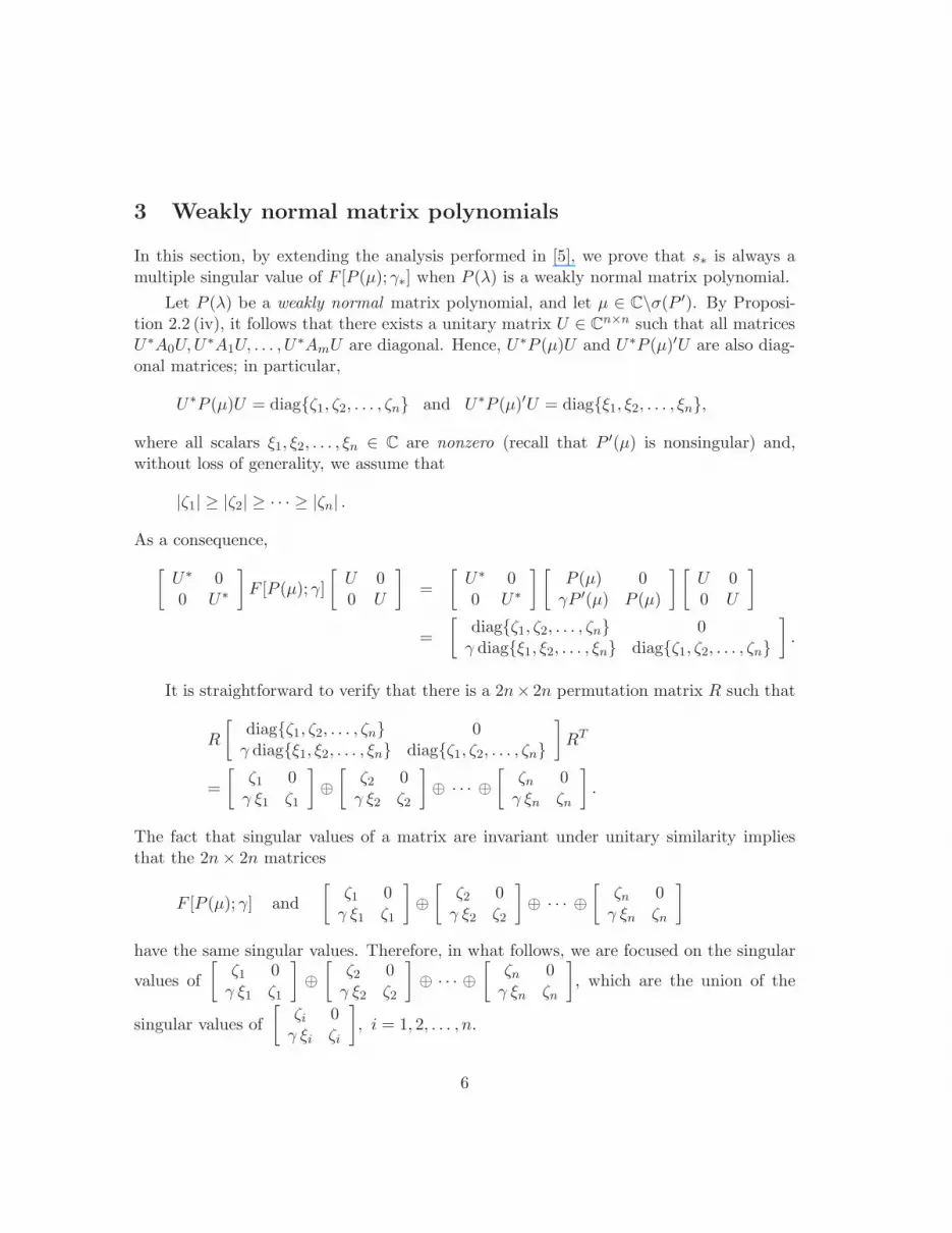
3 Weakly normal matrix polynomials

In this section, by extending the analysis performed in [5], we prove that s∗ is always amultiple singular value of F [P (µ); γ∗] when P (λ) is a weakly normal matrix polynomial.

Let P (λ) be a weakly normal matrix polynomial, and let µ ∈ C\σ(P ′). By Proposi-tion 2.2 (iv), it follows that there exists a unitary matrix U ∈ C

n×n such that all matricesU∗A0U,U

∗A1U, . . . , U∗AmU are diagonal. Hence, U∗P (µ)U and U∗P (µ)′U are also diag-

onal matrices; in particular,

U∗P (µ)U = diag{ζ1, ζ2, . . . , ζn} and U∗P (µ)′U = diag{ξ1, ξ2, . . . , ξn},

where all scalars ξ1, ξ2, . . . , ξn ∈ C are nonzero (recall that P ′(µ) is nonsingular) and,without loss of generality, we assume that

|ζ1| ≥ |ζ2| ≥ · · · ≥ |ζn| .

As a consequence,

[

U∗ 00 U∗

]

F [P (µ); γ]

[

U 00 U

]

=

[

U∗ 00 U∗

] [

P (µ) 0γP ′(µ) P (µ)

] [

U 00 U

]

=

[

diag{ζ1, ζ2, . . . , ζn} 0γ diag{ξ1, ξ2, . . . , ξn} diag{ζ1, ζ2, . . . , ζn}

]

.

It is straightforward to verify that there is a 2n× 2n permutation matrix R such that

R

[

diag{ζ1, ζ2, . . . , ζn} 0γ diag{ξ1, ξ2, . . . , ξn} diag{ζ1, ζ2, . . . , ζn}

]

RT

=

[

ζ1 0γ ξ1 ζ1

]

⊕

[

ζ2 0γ ξ2 ζ2

]

⊕ · · · ⊕

[

ζn 0γ ξn ζn

]

.

The fact that singular values of a matrix are invariant under unitary similarity impliesthat the 2n× 2n matrices

F [P (µ); γ] and

[

ζ1 0γ ξ1 ζ1

]

⊕

[

ζ2 0γ ξ2 ζ2

]

⊕ · · · ⊕

[

ζn 0γ ξn ζn

]

have the same singular values. Therefore, in what follows, we are focused on the singular

values of

[

ζ1 0γ ξ1 ζ1

]

⊕

[

ζ2 0γ ξ2 ζ2

]

⊕ · · · ⊕

[

ζn 0γ ξn ζn

]

, which are the union of the

singular values of

[

ζi 0γ ξi ζi

]

, i = 1, 2, . . . , n.

6

For any i = 1, 2, . . . , n, let si,1(γ) ≥ si,2(γ) be the singular values of

[

ζi 0γ ξi ζi

]

, and

consider the characteristic polynomial of matrix

[

ζi 0γ ξi ζi

]∗ [ζi 0γ ξi ζi

]

=

[

|ζi|2 + γ2 |ξi|

2 γ ξi ζiγ ξi ζi |ζi|

2

]

,

that is,

det

(

tI −

[

|ζi|2 + γ2 |ξi|

2 γ ξi ζiγ ξi ζi |ζi|

2

])

= t2 −(

2 |ζi|2 + γ2 |ξi|

2)

t+ |ζi|4 .

The positive square roots of the eigenvalues of matrix

[

|ζi|2 + γ |ξi|

2 γ ξi ζiγ ξi ζ i |ζi|

2

]

are the

singular values of matrix

[

ζi 0γ ξi ζi

]

, namely,

si,1(γ) =

√

√

√

√

|ζi|2 +

γ2 |ξi|2

2+ γ |ξi|

√

|ζi|2 +

γ2 |ξi|2

4,

and

si,2(γ) =

√

√

√

√

|ζi|2 +

γ2 |ξi|2

2− γ |ξi|

√

|ζi|2 +

γ2 |ξi|2

4.

As γ ≥ 0 increases, si,1(γ) increases and limγ→+∞

si,1(γ) = +∞, while si,2(γ) decreases and

limγ→+∞

si,2(γ) = 0 (recall that |ξi| > 0, i = 1, 2, . . . , n). Also, it is apparent that

si,2(γ) ≤ |ζi| ≤ si,1(γ), and si,1(0) = si,2(0) = |ζi| .

Next we consider two cases with respect to |ζn−1| and |ζn|.

Case 1. Suppose |ζn| < |ζn−1|. At γ = 0, it holds that sn,1(0) = |ζn| < |ζn−1| =sn−1,2(0). According to the above discussion, as the nonnegative variable γ increases fromzero, the functions

s1,1(γ), s2,1(γ), . . . , sn−1,1(γ), sn,1(γ)

increase to +∞, whereas the functions

s1,2(γ), s2,2(γ), . . . , sn−1,2(γ), sn,2(γ)

7

decrease to 0. Let (γ0, s0) be the first point in R2 where the graph of the increasing function

sn,1(γ) intersects the graph of one of the n−1 decreasing functions s1,2(γ), s2,2(γ), . . . , sn−1,2(γ),say sκ,2(γ) (for some κ ∈ {1, 2, . . . , n − 1}). Note that by the definition of si,1(γ) andsi,2(γ) (i = 1, 2, . . . , n), s0 lies in the open interval (0, |ζn−1|) and the graph of sn,1(γ)cannot intersect the graph of one of the increasing functions s1,1(γ), s2,1(γ), . . . , sn−1,1(γ)for γ ≤ γ0.

Since sn,2(γ) and sκ,2(γ) are both decreasing functions in γ ≥ 0, it follows that (seeFig. 1 below, where κ = n− 1 = 2)

γ∗ = γ0 and s∗ = s0 = s2n−1(F [P (µ); γ∗]) = sn,1(γ∗) = sκ,2(γ∗) = s2n−2(F [P (µ); γ∗]).

Hence, when |ζn| < |ζn−1|, γ∗ is the minimum positive root of one of the equations

sn,1(γ) = sn−1,2(γ), sn,1(γ) = sn−2,2(γ), . . . , sn,1(γ) = s1,2(γ)

and s∗ is a multiple singular value of F [P (µ); γ∗].

Case 2. Suppose |ζn| = |ζn−1|. Then, it follows that sn,1(γ) = sn−1,1(γ) and sn,2(γ) =sn−1,2(γ). Moreover, one can see that at γ = 0,

sn,1(0) = sn,2(0) = sn−1,1(0) = sn−1,2(0) = |ζn| = |ζn−1| ,

i.e.,

s2n(F [P (µ); 0]) = s2n−1(F [P (µ); 0]) = s2n−2(F [P (µ); 0]) = s2n−3(F [P (µ); 0]) = |ζn| = |ζn−1| .

Since sn,2(γ) and sn−1,2(γ)) are decreasing functions in γ ≥ 0, s2n−1(F [P (µ); γ]) attainsits maximum value s∗ at γ = 0 = γ∗, and s∗ is a multiple singular value of F [P (µ); 0]. Inthis non-generic case, an upper bound and an associate perturbed matrix polynomial canbe computed by the method described in Section 6 of [14].

Hence, we have the following result.

Theorem 3.1. Let P (λ) in (1) be a weakly normal matrix polynomial, and let µ ∈C\σ(P ′). If γ∗ > 0 is a point where the singular value s2n−1(F [P (µ); γ]) attains its maxi-mum value, then s∗ = s2n−1(F [P (µ); γ∗]) > 0 is a multiple singular value of F [P (µ); γ∗].

4 Computing the desired singular vectors

In this section, we apply a technique proposed in [5] (see also the proof of Lemma 5in [10]) to compute suitable singular vectors of F [P (µ); γ∗] corresponding to the singularvalue s∗, which satisfy (1) and (2) of Lemma 2.3. It is remarkable that the proposedtechnique can be applied to general matrix polynomials and not only to weakly normalmatrix polynomials.

8

4.1 The case of multiplicity 2

First we consider the case where γ∗ > 0 and the multiplicity of the singular value s∗ > 0is equal to 2, and we work on the example of Section 2.

Recall that for the normal matrix polynomial P (λ) in (4) and for µ = −4, the singularvalue s2n−1(F [P (µ); γ]) = s5(F [P (−4); γ]) attains its maximum value at γ∗ = 2.0180and s∗ = s5(F [P (−4); 2.0180]) = s4(F [P (−4); 2.0180]) = 12.8841 (i.e., s∗ is a doublesingular value of F [P (−4); 2.0180]). Two pairs of left and a right singular vectors ofF [P (−4); 2.0180] corresponding to s∗, which do not satisfy properties (1) and (2) of Lemma2.3 are

[

u1(γ∗)u2(γ∗)

]

=

00.8407

00

0.54160

,

[

v1(γ∗)v2(γ∗)

]

=

00.5416

00

0.84070

,

and

[

u1(γ∗)u2(γ∗)

]

=

00

−0.422200

0.9065

,

[

v1(γ∗)v2(γ∗)

]

=

00

−0.906500

0.4222

.

In particular, we have

u2(γ∗)∗P ′(−4)v1(γ∗) = −2.6396 6= 0 and u2(γ∗)

∗P ′(−4)v1(γ∗) = 4.1089 6= 0.

In Figure 1, the graphs of

s2n−1(F [P (µ); γ]) = s5(F [P (−4); γ]) and s2n−2(F [P (µ); γ]) = s4(F [P (−4); γ])

are plotted for γ ∈ [0, 10], and their common point (γ∗, s∗) = (2.0180, 12.8841) is markedwith “◦”. With respect to the discussion in the previous section, it is worth noting thatin this example, the graph of s2,2(γ) (that is, sn−1,2(γ)) is the graph of the decreasingfunctions s1,2(γ) and s2,2(γ) that intersects first the graph of the increasing function s3,1(γ)(that is, sn,1(γ)). Moreover, it is apparent that s2n−1(F [P (µ); γ]) and s2n−2(F [P (µ); γ])are non-differentiable functions at γ∗.

9

0 1 2 3 4 5 6 7 8 9 104

6

8

10

12

14

16

18

20

γ

s

2n−1(γ)

s2n−2

(γ)

o

(γ*,s

*)

Fig 1: The singular values s2n−1(F [P (µ); γ]) (solid line) and s2n−2(F [P (µ); γ]) (dashed line).

Since s∗ = s5(F [P (−4); 2.0180]) = s4(F [P (−4); 2.0180]) = 12.8841 is a double sin-

gular value, the pairs of unit vectors

[

u1(γ∗)u2(γ∗)

]

,

[

u1(γ∗)u2(γ∗)

]

and

[

v1(γ∗)v2(γ∗)

]

,

[

v1(γ∗)v2(γ∗)

]

form orthonormal bases of the left and right singular subspaces corresponding to s∗, re-spectively. So, recalling that in Lemma 2.3, assertion (1) yields assertion (2), henceforthwe are looking for a pair of unit vectors

[

u1(γ∗)u2(γ∗)

]

= α

[

u1(γ∗)u2(γ∗)

]

+β

[

u1(γ∗)u2(γ∗)

]

,

[

v1(γ∗)v2(γ∗)

]

= α

[

v1(γ∗)v2(γ∗)

]

+β

[

v1(γ∗)v2(γ∗)

]

(5)

such that

u2(γ∗)∗P ′(µ)v1(γ∗) = 0, (6)

where the scalars α, β ∈ C satisfy |α|2 + |β|2 = 1. By substituting the unknown singularvectors of (5) into (6), we obtain

[

α β]

M

[

α

β

]

= 0, (7)

where

M =

[

u2(γ∗)∗P ′(µ)v1(γ∗) u2(γ∗)

∗P ′(µ)v1(γ∗)u2(γ∗)

∗P ′(µ)v1(γ∗) u2(γ∗)∗P ′(µ)v1(γ∗)

]

. (8)

Lemma 4.1. The matrix M in (8) is always hermitian.

10

Proof. Recall that γ∗ and s∗ are positive. By the proof of Lemma 17 in [14], it followsthat the diagonal entries of matrix M are real.

By the definition of the pairs of singular vectors

[

u1(γ∗)u2(γ∗)

]

,

[

v1(γ∗)v2(γ∗)

]

and

[

u1(γ∗)u2(γ∗)

]

,

[

v1(γ∗)v2(γ∗)

]

of F [P (µ); γ∗] corresponding to s∗, we have

[

P (µ) 0γ∗P

′(µ) P (µ)

] [

v1(γ∗)v2(γ∗)

]

= s∗

[

u1(γ∗)u2(γ∗)

]

,[

P (µ) 0γ∗P

′(µ) P (µ)

] [

v1(γ∗)v2(γ∗)

]

= s∗

[

u1(γ∗)u2(γ∗)

]

,

or equivalently,

P (µ)v1(γ∗) = s∗u1(γ∗),γ∗P

′(µ)v1(γ∗) + P (µ)v2(γ∗) = s∗u2(γ∗),P (µ)v1(γ∗) = s∗u1(γ∗),γ∗P

′(µ)v1(γ∗) + P (µ)v2(γ∗) = s∗u2(γ∗),

(9)

and

[

u1(γ∗)∗ u2(γ∗)

∗]

[

P (µ) 0γ∗P

′(µ) P (µ)

]

= s∗[

v1(γ∗)∗ v2(γ∗)

∗]

,

[

u1(γ∗)∗ u2(γ∗)

∗]

[

P (µ) 0γ∗P

′(µ) P (µ)

]

= s∗[

v1(γ∗)∗ v2(γ∗)

∗]

,

or equivalently,

u1(γ∗)∗P (µ) + γ∗u2(γ∗)

∗P ′(µ) = s∗v1(γ∗)∗,

u2(γ∗)∗P (µ) = s∗v2(γ∗)

∗,

u1(γ∗)∗P (µ) + γ∗u2(γ∗)

∗P ′(µ) = s∗v1(γ∗)∗,

u2(γ∗)∗P (µ) = s∗v2(γ∗)

∗,

(10)

By multiplying the fourth equation in (9) by u2(γ∗)∗ from the left, and the second

equation of (10) by v2(γ∗) from the right, we obtain

γ∗u2(γ∗)∗P ′(µ)v1(γ∗) + u2(γ∗)

∗P (µ)v2(γ∗) = s∗u2(γ∗)∗u2(γ∗), (11)

and

u2(γ∗)∗P (µ)v2(γ∗) = s∗v2(γ∗)

∗v2(γ∗), (12)

11

respectively. As a consequence,

γ∗u2(γ∗)∗P ′(µ)v1(γ∗) = s∗ (u2(γ∗)

∗u2(γ∗)− v2(γ∗)∗v2(γ∗)) . (13)

Performing similar calculations, one can verify that

γ∗u2(γ∗)∗P ′(µ)v1(γ∗) = s∗ (u2(γ∗)

∗u2(γ∗)− v2(γ∗)∗v2(γ∗)) . (14)

Clearly, equations (13) and (14) imply that the non-diagonal entries of matrix M arecomplex conjugate.

By Lemma 2.3 (1), equation (7) has always a nontrivial (i.e., nonzero) solution, andhence, the hermitian matrix M in (8) cannot be (positive or negative) definite. In ournumerical example, M has a negative and a positive diagonal entries (namely, −2.6396and 4.1089), and thus, it is an indefinite hermitian matrix.

To derive an explicit solution of (7), suppose that η1, η2 ∈ C are the (real) eigenvaluesof matrix M , with η1 > 0 > η2, and let w1, w2 ∈ C

2 be unit eigenvectors of M corre-sponding to η1 and η2, respectively. Then, it is straightforward to see (keeping in mindthe orthogonality of the eigenvectors) that the unit vector

[

α

β

]

=

√

|η2|

|η1|+ |η2|w1 +

√

|η1|

|η1|+ |η2|w2

satisfies

[

α β]

M

[

α

β

]

=|η1| η2

|η1|+ |η2|+

|η2| η1|η1|+ |η2|

= 0.

Finally, in order to verify the validity of this refinement, we return again to thenormal matrix polynomial P (λ) in (4), and by applying the above methodology, we obtainα = 0.6254 and β = 0.7803. Consequently, the desired vectors in (5) are (approximately)

[

u1(γ∗)u2(γ∗)

]

=

00.6560−0.2640

00.42260.5669

and

[

v1(γ∗)v2(γ∗)

]

=

00.4226−0.5669

00.65600.2640

.

In particular, it holds that

u∗2(γ∗)P′(−4)v1(γ∗) = −4.4409 · 10−16,

12

and for the n× 2 matrices U(γ∗) = [u1(γ∗) u2(γ∗)] and V (γ∗) = [v1(γ∗) v2(γ∗)], we have

∥

∥

∥U∗(γ∗)U(γ∗)− V ∗(γ∗)V (γ∗)

∥

∥

∥

2= 1.1383 · 10−6.

Thus, Lemma 2.3 is verified.

Moreover, using the matrices U(γ∗) and V (γ∗), Theorem 2.4 yields the upper bound0.9465 for the distance from P (λ) to the set of 3 × 3 quadratic matrix polynomials thathave µ = −4 as a multiple eigenvalue, and the perturbed matrix polynomial

Qγ∗(λ) =

1 0 00 0.0680 0.01520 −0.1552 0.5986

λ2+

−3 0 00 −0.0680 −0.01520 0.1552 3.4014

λ+

2 0 00 −0.9320 0.01520 −0.1552 1.5986

that lies on the boundary of B (P, 0.9465,w) and has spectrum

σ(

Qγ∗(λ))

= {1, 2, 4.1982, −0.5140, −4.0000 + i 0.0031, −4.0000 − i 0.0031} .

In addition, the lower bound 0.4031 of the distance is given by Theorem 11 in [14]. (Allcomputations were performed in Matlab with 16 significant digits.)

4.2 The case of multiplicity greater that 2

Suppose that γ∗ > 0, and the multiplicity of the singular value s∗ > 0 is r ≥ 3. Forweakly normal matrix polynomials this means that the graph of the increasing func-tion sn,1(γ) intersects the graphs of more than one of the n − 1 decreasing functionss1,2(γ), s2,2(γ), . . . , sn−1,2(γ), at the point (γ∗, s∗). Let also

[

u(1)1 (γ∗)

u(1)2 (γ∗)

]

,

[

u(2)1 (γ∗)

u(2)2 (γ∗)

]

, . . . ,

[

u(r)1 (γ∗)

u(r)2 (γ∗)

]

and[

v(1)1 (γ∗)

v(1)2 (γ∗)

]

,

[

v(2)1 (γ∗)

v(2)2 (γ∗)

]

, . . . ,

[

v(r)1 (γ∗)

v(r)2 (γ∗)

]

be orthonormal bases of the left and right singular subspaces of F [P (µ); γ∗] correspondingto s∗, respectively. Then, we are looking for a pair of unit vectors

[

u1(γ∗)u2(γ∗)

]

=r

∑

j=1

αj

[

u(j)1 (γ∗)

u(j)2 (γ∗)

]

,

[

v1(γ∗)v2(γ∗)

]

=r

∑

j=1

αj

[

v(j)1 (γ∗)

v(j)2 (γ∗)

]

(15)

13

such that

u2(γ∗)∗P ′(µ)v1(γ∗) = 0, (16)

where the scalars α1, α2, . . . , αr ∈ C satisfy |α1|2 + |α2|

2 + · · ·+ |αr|2 = 1.

Following the arguments of the methodology described in the previous subsection, wecan compute the desired vectors in (15) that satisfy (16). In particular, we need to find asolution of the equation

[

α1 α2 · · · αr

]

Mr

α1

α2...αr

= 0, (17)

where the r × r matrix

Mr =

u(1)2 (γ∗)

∗P ′(µ)v(1)1 (γ∗) u

(1)2 (γ∗)

∗P ′(µ)v(2)1 (γ∗) · · · u

(1)2 (γ∗)

∗P ′(µ)v(r)1 (γ∗)

u(2)2 (γ∗)

∗P ′(µ)v(1)1 (γ∗) u

(2)2 (γ∗)

∗P ′(µ)v(2)1 (γ∗) · · · u

(2)2 (γ∗)

∗P ′(µ)v(r)1 (γ∗)

......

. . ....

u(r)2 (γ∗)

∗P ′(µ)v(1)1 (γ∗) u

(r)2 (γ∗)

∗P ′(µ)v(2)1 (γ∗) · · · u

(r)2 (γ∗)

∗P ′(µ)v(r)1 (γ∗)

is hermitian and not definite. Considering a unit eigenvector wmax ∈ Cr of Mr corre-

sponding to the maximum eigenvalue ηmax > 0 of Mr and a unit eigenvector wmin ∈ Cr

corresponding to the minimum eigenvalue ηmin < 0 of Mr, it is straightforward to verifythat the unit vector

√

|ηmin|

|ηmax|+ |ηmin|wmax +

√

|ηmax|

|ηmax|+ |ηmin|wmin

satisfies (17).

References

[1] J.W. Demmel, On condition numbers and the distance to the nearest ill-posed prob-lem, Numer. Math., 51 (1987), 251–289.

[2] I. Gohberg, P. Lancaster and L. Rodman, Matrix Polynomials, Academic Press, NewYork, 1982.

[3] J.M. Gracia, Nearest matrix with two prescribed eigenvalues, Linear Algebra Appl.,401 (2005), 277–294.

14

[4] Kh.D. Ikramov and A.M. Nazari, Computational aspects of the use of Malyshev’sformula, Comput. Math. Math. Phys., 44(1) (2004), 1–5.

[5] Kh.D. Ikramov and A.M. Nazari, On a remarkable implication of the Malyshev for-mula, Dokl. Akad. Nauk., 385 (2002), 599–600.

[6] T. Kaczorek, Polynomial and Rational Matrices: Applications in Dynamical SystemsTheory, Springer-Verlag, London, 2007.

[7] P. Lancaster, Lambda-Matrices and Vibrating Systems, Dover Publications, 2002.

[8] P. Lancaster and P. Psarrakos, Normal and seminormal eigenvalues of matrixp oly-nomials. Integral Equations Operator Theory, 41 (2001), 331–342.

[9] R.A. Lippert, Fixing two eigenvalues by a minimal perturbation, Linear AlgebraAppl., 406 (2005), 177–200.

[10] A.N. Malyshev, A formula for the 2-norm distance from a matrix to the set of matriceswith a multiple eigenvalue, Numer. Math., 83 (1999), 443–454.

[11] A.S. Markus, Introduction to the Spectral Theory of Polynomial Operator Pencils,Amer. Math. Society, Providence, RI, Translations of Mathematical Monographs,Vol. 71, 1988.

[12] A.M. Nazari and D. Rajabi, Computational aspect to the nearest matrix with twoprescribed eigenvalues, Linear Algebra Appl., 432 (2010), 1–4.

[13] N. Papathanasiou and P. Psarrakos, Normal matrix polynomials with nonsingularleading coefficients, Electron. J. Linear Algebra, 17 (2008), 458–472.

[14] N. Papathanasiou and P. Psarrakos, The distance from a matrix polynomial to matrixpolynomials with a prescribed multiple eigenvalue, Linear Algebra Appl., 429 (2008),1453–1477.

[15] A. Ruhe, Properties of a matrix with a very ill-conditioned eigenproblem, Numer.Math., 15 (1970), 57–60.

[16] F. Tisseur and K. Meerbergen, The quadratic eigenvalue problem, SIAM Rev., 43(2001), 235–286.

[17] J.H. Wilkinson, The Algebraic Eigenvalue Problem, Claredon Press, Oxford, 1965.

[18] J.H. Wilkinson, Note on matrices with a very ill-conditioned eigenproblem, Numer.Math., 19 (1972), 175–178.

15

[19] J.H. Wilkinson, On neighbouring matrices with quadratic elementary divisors, Nu-mer. Math., 44 (1984), 1–21.

[20] J.H. Wilkinson, Sensitivity of eigenvalues, Util. Math., 25 (1984), 5–76.

[21] J.H. Wilkinson, Sensitivity of eigenvalues II, Util. Math., 30 (1986), 243–286.

16