Abstract— This paper presents a detailed analysis of the two most well-known hill-climbing MPPT algorithms, the Perturb-and-Observe (P&O) and Incremental Conductance (INC). The purpose of the analysis is to clarify some common misconceptions in the literature regarding these two trackers, therefore helping the selection process for a suitable MPPT for both researchers and industry. The two methods are thoroughly analyzed both from mathematical and practical implementation point of view. Their mathematical analysis reveals that there is no difference between the two. This has been confirmed by experimental tests according to the EN 50530 standard, resulting in a deviation between their efficiencies of 0.13% in dynamic, and as low as 0.02% in static conditions.

The results show that despite the common opinion in the literature, the P&O and INC are equivalent.

Index Terms— MPPT, Perturb and Observe, Incremental Conductance, Discrete implementation, Photovoltaic systems

I. INTRODUCTION

aximum Power Point Tracking (MPPT) is one of the key functions that every grid-connected PV inverter should

have. There is a large amount of publications dealing with MPPT, and trackers in the majority of the commercial PV inverters are able to extract around 99% of the available power from the PV plant, over a wide irradiance and temperature range - at least in steady state [1]. An extensive overview of modern MPPT techniques has been presented in [2].

The two most frequently discussed MPPT algorithms are the P&O and the INC. These methods are based on the fact that, on the voltage-power characteristic, the variation of the power w.r.t. voltage is positive (dP/dV > 0) in the left-hand side of the Maximum Power Point (MPP), while it is negative (dP/dV < 0) on the right-hand side of MPP.

The main advantages of these methods are that they are generic, e.g. suitable for any PV array, they do not require any information about the PV array, they work reasonably well in most conditions, and they are simple to implement on a digital controller.

A detailed literature review today would lead to the conclusion that although the INC is slightly more complicated to implement, it provides better performance than P&O in both static and dynamic conditions. The two main problems of the P&O frequently mentioned in the literature, are the oscillations around the MPP in steady state conditions, and the poor tracking (possibly in the wrong direction, away from D. Sera, L. Mathe, T. Kerekes, S. Spataru and R. Teodorescu are with the Department of Energy Technology, Aalborg University, Aalborg, DK-9220, Denmark (e-mail: des@et.aau.dk, lam@et.aau.dk, tak@et.aau.dk; ssp@et.aau.dk, ret@et.aau.dk)

MPP) under changing irradiance [3]–[14]. Methods to improve the dynamic behavior of the P&O, including variable step size and perturbation frequency have been reported in the literature [4], [5], [8], [15]–[18].

On the other hand, it is often stated in the literature that the INC can determine the position of the actual operating point relative to the MPP, and it can find the distance to it; it can also stop perturbing when the MPP has been reached, thus offering a superior performance to the P&O. It is also often stated that INC can track fast changing irradiance better than P&O, e.g. [2], [5], [12], [14], [17], [19]–[30].

Typical statements include “The [INC] method […] has been proposed to improve the tracking accuracy and dynamic performance under rapidly varying conditions” [7], “The disadvantage of the P&O method can be improved by comparing the instantaneous panel conductance with the incremental panel conductance” [11], “[INC] gives a good performance under rapidly changing conditions”[11], “Incremental conductance can determine that the MPPT has reached the MPP and stop perturbing the operating point”, “[INC] can track rapidly increasing and decreasing irradiance conditions with higher accuracy than P&O”[10].

In a recent work [31], both the P&O and INC have been implemented on a commercial PV inverter, challenging the common belief of higher INC performance. The performance of these two methods using various perturbation amplitudes and frequencies has been compared. The results “suggest that the two algorithms are similar”[31]; however, the author does not provide mathematical explanation of why the two methods perform so similarly.

The aim of this work is to provide theoretical and experimental proof that P&O and INC are equivalent, and to clarify some of the common misconceptions in the literature regarding these two trackers. Furthermore, this paper provides a thorough analysis of these two that can help the industry and researchers in choosing the right tracker for a given application. In Section II it is mathematically proven that the P&O and INC are equivalent both in static and dynamic conditions, and in Section III this is confirmed by experimental tests according to the EN 50530 [32] standard.

II. ANALYSIS OF P&O AND INC

A. Operating principle of P&O and INC

The P&O is probably the most often used MPPT algorithm today, due to its simplicity and generic nature [33]–[35].

It is based on the fact that on the derivative of power in

On the Perturb-and-Observe and Incremental Conductance MPPT methods for PV systems

Dezso Sera, Member, IEEE, Laszlo Mathe, Member, IEEE, Tamas Kerekes, Member, IEEE, Sergiu Spataru, Student Member, IEEE, Remus Teodorescu, Fellow, IEEE

M

function of voltage is zero at MPP. At an operating point on the P-V curve, if the operating voltage of the PV array is perturbed in a given direction and dP > 0, it is known that the perturbation moved the array's operating point towards the MPP. The P&O algorithm would then continue to perturb the PV array voltage in the same direction. If dP < 0, then the change in operating point moved the PV array away from the MPP, and the P&O algorithm reverses the direction of the perturbation. In this paper the nonlinear characteristic of the PV array is reproduced using the single-diode 5-parameter model, in accordance with the requirements of the EN 50530. A detailed description of this model can be found in [36].

The second well-known MPPT algorithm, the INC [37] claims to improve the P&O by replacing the derivative of the power versus voltage dP/dV used by the P&O with comparing the PV array instantaneous (I/V) and incremental (dI/dV) conductance. These terms are obtained by manipulating the dP/dV equation, as shown in equations (1) and (2).

The derivative of power in function of voltage at MPP can be expressed in mathematical form as:

0mp

mp

P PV V

P

V

(1)

Rewriting (1) by replacing P with VI, results in (2):

0 0mpmpmpmp

mp mpI II IV VV V

VI IV I

V V

(2)

In the above equations, Vmp is the voltage at MPP, and Imp is the current at MPP.

The first incremental conductance – based algorithm was proposed in [38], where an analogue implementation was presented. In [38], the term dI/dV has been calculated based on a harmonic component in the PV array voltage and current, which is independent from the perturbation of the MPPT, and is not affected by changing irradiance.

However, the discrete implementation that became the well-known INC algorithm proposed in [37], has an essential difference from the analogue implementation proposed in [38]. In [37], dI/dV is identified based on the tracker’s own perturbations; therefore it is not immune to the changing irradiance.

B. Mathematical comparison in continuous time

From equations (1) and (2) can be seen that dividing equation (2) by Vmp will not change its value at MPP (since ⁄ is zero at MPP). However, it has a scaling effect

everywhere else on the IV curve. Considering an arbitrary point on the IV curve, one can

write the mathematical expression based on which the P&O decides the next perturbation direction: PO P V (3)

While P&O decides the direction of the next perturbation based on the sign of δPO, INC decides based on δINC, as shown below: INC I V I V (4)

From (2), (3), and (4), it is obvious that:

INC PO V (5)

From mathematical point of view (in continuous time), this factor of 1/V is the only difference between the two methods, which - considering that the PV array voltage is always positive - will not change the sign of compared to δPO at any point on the IV curve. Therefore, two trackers that base their tracking on δPO,, and δINC respectively will have perfectly identical behavior.

C. Discrete implementation of P&O and INC

In practice, both P&O and INC are implemented in discrete time, with various update frequencies, usually between 1-20Hz [31], [39], [40].

The discrete form of equation (3) becomes:

1

1

k

k

kPO

k

P P

V V

P

V

(6)

Where is the discrete form of δPO, ,and .The other notations have the following

meaning: , , – the power, voltage, and current at the k-th (actual) sampling instance; , , – the power, voltage, and current at the previous sampling instance.

Looking at the case of INC, the discrete implementation of (4) usually takes the form below:

1

1

kk k

k k

kINC

k k

I I II

V V V V

I

V

(7)

Where is the discrete version of δINC. Other discrete implementations of (4) can be done by using forward or central differences. In this paper, the discrete implementation according to [37], which is shown in eq.(7), will be analyzed.

In order to compare the P&O and INC in discrete, the differences between eq. (6) and (7) are calculated, analogously to (5), defined as: INC PO kV (8)

From the above, ε can be calculated as:

00k I

I V

(9)

Eq. (9) shows that the equality in (5) is no longer fulfilled in discrete. This difference is due to the fact that the discrete implementation of INC ignores the last term in the backward difference of P, which can be expressed as:

k kP I V I V V I I V (10)

As a result, the discrete counterpart of (5) becomes:

PO POINC

k k k

I

V V V

(11)

The extra checks (ΔV=0?, ΔI =0?,) performed by the INC will not be analyzed here, since in one hand they can be equally applied to both the P&O and INC, and on the other hand these conditions are met extremely rarely in a practical application [37]. In the following, the effects of the discretization error will be investigated.

D. Effects of the discretization error in static conditions

Equation (9) shows that the discrete implementation of INC introduces an error in addition to the P&O. This means that theoretically a situation can exist, where the sign of is different from the sign of , leading to a different direction of the next perturbation. It can be easily seen that the relative

size of the error compared to is maximum in the vicinity of the MPP, where both and tend to zero.

It will be shown below that as long as and are on the same side of the MPP (the last perturbation did not move the operating point from one side of the MPP to the other), the error will not affect the next perturbation direction. (The situation where the perturbation moves the operating point from one side to the other of the MPP will be discussed in the next subsection II.D.2).

1) Vk>Vmp and Vk-1>Vmp, or Vk<Vmp and Vk-1<Vmp In order to evaluate the effect of ε on the tracking of INC,

first an ‘ideal’ ∗ is defined, which assumes that (5) is valid also in discrete: * *

INC PO k INC INCV (12)

Secondly, the worst case scenario – where the relative size of ε compared to ∗ is the maximum – should be determined. On a given IV curve, the relative size of ε is the maximum at the MPP, since ∗ tends to zero at this point. A worst case scenario for a given IV curve can then be considered:

1 1

,k mp k mp

k mp k mp

V V V V Vor

V V V V V

(13)

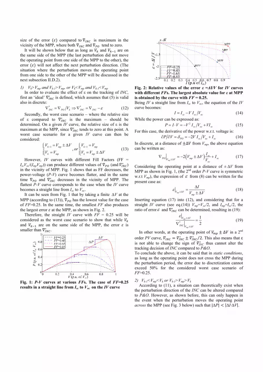
However, IV curves with different Fill Factors (FF = IscVoc/(ImpVmp)) can produce different values of (and ∗ ) in the vicinity of MPP. Fig. 1 shows that as FF decreases, the power-voltage (P-V) curve becomes flatter, and in the same time and ∗ decreases in the vicinity of MPP. The flattest P-V curve corresponds to the case when the IV curve becomes a straight line from Isc to Voc.

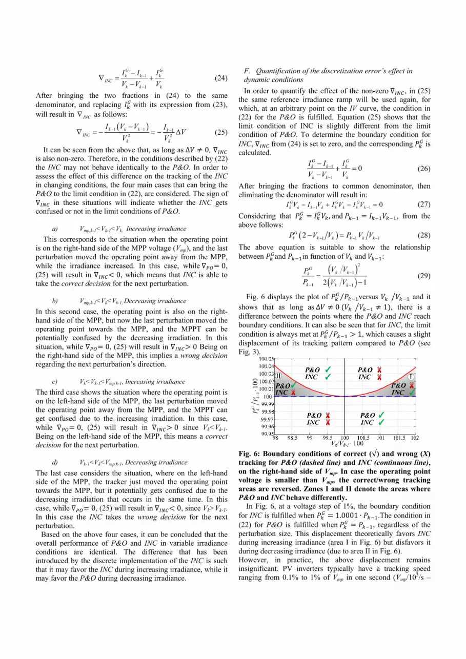
It can be seen from Fig. 1 that by taking a finite V at the MPP (according to (13)), has the lowest value for the case of FF=0.25. In the same time, the smallest FF also produces the largest error at the MPP, as shown in Fig. 2.

Therefore, the straight IV curve with FF = 0.25 will be considered as the worst case scenario to show that while and are on the same side of the MPP, the error is smaller than ∗ .

PV

Fig. 1: P-V curves at various FFs. The case of FF=0.25 results in a straight line from Isc to Voc on the IV curve

I /

V

Fig. 2: Relative values of the error ε =ΔI/V for IV curves with different FFs. The largest absolute value for ε at MPP is obtained by the curve with FF = 0.25. Being IV a straight line from Isc to Voc, the equation of the IV curve becomes: sc sc ocI I V I V (14)

While the power can be expressed as: 2

sc oc scP I V V I V VI (15)

For this case, the derivative of the power w.r.t. voltage is: 2PO sc oc scP V V I V I (16)

In discrete, at a distance of ∆ from Vmp, the above equation can be written as:

2mp

scPO mp scV V

oc

IV V I

V (17)

Considering the operating point at a distance of ±∆V from MPP as shown in Fig. 1, (the 2nd order P-V curve is symmetric w.r.t Vmp), the expression of from (8) can be written for the present case as:

mpV V

mp

I

V V

(18)

Inserting equation (17) into (12), and considering that for a straight IV curve (see eq.(14)) Vmp=Voc/2, and Imp=Isc/2, the ratio of error and ∗ can be determined, resulting in (19):

*

1

2mp

mp

V V

INC V V

(19)

In other words, at the operating point of ∆ in a 2nd order PV curve, ∗ ∗ 2⁄ . This also means that ε is not able to change the sign of INC

∗ thus cannot alter the tracking decision of INC compared to P&O. To conclude the above, it can be said that in static conditions, as long as the operating point does not cross the MPP during the perturbation period, the error due to discretization cannot exceed 50% for the considered worst case scenario of FF=0.25.

2) Vk-1<Vmp<Vk or Vk-1>Vmp>Vk According to (11), a situation can theoretically exist when

the perturbation direction of the INC can be altered compared to P&O. However, as shown before, this can only happen in the event when the perturbation moves the operating point across the MPP (see Fig. 3 below) such that |∆P| |∆I·∆V|.

Fig. 3: Movement of the operating point around the MPP for P&O and INC, for the case when | | | ∗ |.

The above figure shows an interesting consequence of the imperfect discrete differentiation on which the INC is based (see equations (10) and (11)). A situation can exist, where the INC is ‘stuck’ to the MPP, and stays within one perturbation distance ΔV from Vmp. That is due to the fact that the sign of

is determined by the sign of ΔI, which forces the INC to change direction at each perturbation and hence oscillate between A and B. However, this is not related to its credited capability that it can determine when the MPPT has reached the MPP [10], [37] it is merely a consequence of the discrete differentiation error and can only occur in specific circumstances.

It is worth noting that the effect of ε on the tracking of INC is masked in practical cases, when measurement error, noise and ripple are present, as shown by the experimental tests.

E. Dynamic behavior of P&O and INC

Fig. 4 shows the situation when an increase in irradiance occurs during the MPPT update period. If the MPPT takes a sample of the measured power at the instance (k-1), i.e. Pk-1, then takes the next sample at the sampling instance k, the calculated ∆ will contain the power change due to the perturbation (ΔPPO), but also the change due to the increased irradiance (ΔPG).

GP

GkP1kP

kPPOP

VV

P

GP

GkP

1kP

kPPOP

VVpkT 1 pk T

P

pkT 1 pk T

Fig. 4: Effect of the irradiance change during a perturbation period for the P&O. In case of slow irradiance changes, P&O is able to determine the right tracking direction (a), while a fast changing irradiance can cause it to track in the wrong direction (b). [41]

In the above figure, the notations have the following meaning: Tp – the sampling period of the MPPT; – the power value at the k-th sampling instance when irradiance change occurred; ∆ – the change in power caused by the MPPT action alone; ∆ – the change in power caused by the increase in irradiation alone; ∆ – the voltage increment of the MPPT.

The overall change of power during the MPPT sampling period can be expressed as: 1

G PO Gk kP P P P P (20)

Therefore, in case of opposite signs for ∆ and∆ the sign of P will be determined by the larger one.

In case of INC, the above situation is illustrated in Fig. 5:

GkI

GIINCI

1kI

kI

pkT 1 pk TVV

I

GkI

kI

GIINCI

1kI

V

I

VpkT 1 pk T

Fig. 5: Illustration of the effect of irradiance change during a perturbation period for the INC. Equally to the P&O, fast changing irradiance can cause the INC to track in wrong direction.

In the above figure, the notations have the following meaning: , – the current values measured at the k-1-th and the k-th sampling instances; – the current at sampling instance k when no change in irradiance occurred; ∆

– the change in current caused by the perturbation of the MPPT; ∆ – the change in current caused by the increased irradiation.

Similarly to the case of P&O, if ∆ and ∆ have different signs, the sign of I will be determined by the larger one (see Fig. 5): 1

G Ck

IN GkI I I I I (21)

1) Boundary conditions of correct tracking for P&O For both the P&O and INC in changing irradiance, one can

write the boundary conditions for correct tracking. In case of the P&O, this is met when the amplitude of ∆ becomes larger and with opposite direction compared to ∆ .

In order to compare the behavior of the P&O and INC in changing conditions, a reference irradiance ramp is considered, for which, at a given point on the IV curve, the following condition for the P&O is fulfilled: 0 0 PO G

PO P P P (22)

where ΔP is the total change of power within an MPPT sampling period, according to (20). This is the limit condition for which the P&O can decide the correct tracking direction. The condition in (22) can be written as: 1 1 1 1 1

G G Gk k k k k k k k k kP P I V I V I I V V (23)

In the following, it is verified whether for the same irradiance ramp, at the same point on the IV curve, the INC is able to track in the correct direction, or gets confused.

2) Boundary conditions for correct tracking for INC Considering the same conditions as in (22), INC will take

the form:

1

1

G Gk k k

INCk k k

I I I

V V V

(24)

After bringing the two fractions in (24) to the same denominator, and replacing with its expression from (23), will result in INC as follows:

1 1 1

2 2k k k k

INCk k

I V V IV

V V

(25)

It can be seen from the above that, as long as∆ 0, is also non-zero. Therefore, in the conditions described by (22) the INC may not behave identically to the P&O. In order to assess the effect of this difference on the tracking of the INC in changing conditions, the four main cases that can bring the P&O to the limit condition in (22), are considered. The sign of

in these situations will indicate whether the INC gets confused or not in the limit conditions of P&O.

a) Vmp,k-1<Vk-1<Vk, Increasing irradiance

This corresponds to the situation when the operating point is on the right-hand side of the MPP voltage (Vmp), and the last perturbation moved the operating point away from the MPP, while the irradiance increased. In this case, while 0, (25) will result in 0, which means that INC is able to take the correct decision for the next perturbation.

b) Vmp,k-1<Vk<Vk-1, Decreasing irradiance

In this second case, the operating point is also on the right-hand side of the MPP, but now the last perturbation moved the operating point towards the MPP, and the MPPT can be potentially confused by the decreasing irradiation. In this situation, while 0, (25) will result in 0 Being on the right-hand side of the MPP, this implies a wrong decision regarding the next perturbation’s direction.

c) Vk<Vk-1<Vmp,k-1, Increasing irradiance

The third case shows the situation where the operating point is on the left-hand side of the MPP, the last perturbation moved the operating point away from the MPP, and the MPPT can get confused due to the increasing irradiation. In this case, while 0, (25) will result in 0 since Vk<Vk-1. Being on the left-hand side of the MPP, this means a correct decision for the next perturbation.

d) Vk-1<Vk<Vmp,k-1, Decreasing irradiance

The last case considers the situation, where on the left-hand side of the MPP, the tracker just moved the operating point towards the MPP, but it potentially gets confused due to the decreasing irradiation that occurs in the same time. In this case, while 0, (25) will result in 0, since Vk>Vk-1. In this case the INC takes the wrong decision for the next perturbation.

Based on the above four cases, it can be concluded that the overall performance of P&O and INC in variable irradiance conditions are identical. The difference that has been introduced by the discrete implementation of the INC is such that it may favor the INC during increasing irradiance, while it may favor the P&O during decreasing irradiance.

F. Quantification of the discretization error’s effect in dynamic conditions

In order to quantify the effect of the non-zero , in (25) the same reference irradiance ramp will be used again, for which, at an arbitrary point on the IV curve, the condition in (22) for the P&O is fulfilled. Equation (25) shows that the limit condition of INC is slightly different from the limit condition of P&O. To determine the boundary condition for INC, from (24) is set to zero, and the corresponding is calculated.

1

1

0G Gk k k

k k k

I I I

V V V

(26)

After bringing the fractions to common denominator, then eliminating the denominator will result in: 1 1 0G G G

k k k k k k k kI V I V I V I V (27)

Considering that ,and , from the above follows: 1 1 12G

k k k k k kP V V P V V (28)

The above equation is suitable to show the relationship between and in function of and :

2

1

1 12 1

Gk kk

k k k

V VP

P V V

(29)

Fig. 6 displays the plot of ⁄ versus and it shows that as long as∆ 0 1 , there is a difference between the points where the P&O and INC reach boundary conditions. It can also be seen that for INC, the limit condition is always met at ⁄ 1, which causes a slight displacement of its tracking pattern compared to P&O (see Fig. 3).

110

0G k

kP

P

Fig. 6: Boundary conditions of correct (√) and wrong (X) tracking for P&O (dashed line) and INC (continuous line), on the right-hand side of Vmp. In case the operating point voltage is smaller than Vmp, the correct/wrong tracking areas are reversed. Zones I and II denote the areas where P&O and INC behave differently.

In Fig. 6, at a voltage step of 1%, the boundary condition for INC is fulfilled when 1.0001 ∙ .The condition in (22) for P&O is fulfilled when , regardless of the perturbation size. This displacement theoretically favors INC during increasing irradiance (area I in Fig. 6) but disfavors it during decreasing irradiance (due to area II in Fig. 6). However, in practice, the above displacement remains insignificant. PV inverters typically have a tracking speed ranging from 0.1% to 1% of Vmp in one second (Vmp/103/s –

Vmp/102/s) [42], but can be as fast as 2% of nominal Vmp per second [1].

Modern MPPTs have update frequencies of 10Hz or above [40], which correspond to voltage steps of V<0.5% of nominal Vmp resulting in about 0.0025% difference between

and in Fig. 6. This is an order below the basic power accuracy of the high precision power analyzer in [43], which is 0.02% of the reading value, and it is not realistic for a commercial PV inverter to match this power measurement accuracy, especially when measurement noise, ripple etc. are taken into account.

III. EXPERIMENTAL TESTS AND RESULTS

A. Test setup

The test setup consists of the following components: 1000V/40A high bandwidth PV simulator (Regatron TopCon Quadro with a linear post-processing unit TC.LIN), a custom-

built 800W DC/DC boost converter connected to a 2.2kW Danfoss VLT-FC302 inverter, which is then connected to the grid through an LC filter and a 1:1 transformer (Fig. 7). The PV simulator emulates a preloaded I-V curve of the PV array as given in II.A, corresponding to the EN 50530 standard’s requirements for the PV simulator specifications.

The control structure has been implemented in Simulink, and using the dSPACE Real-Time Interface, it has been compiled and downloaded to the dSpace 1103 controller board. The control structure for the grid connected converter is a classical one based on resonant controller. The DC/DC boost converter unit has its own voltage and current sensing (Vpv and Ipv), as well as the voltage control implemented on a Texas Instruments TMS320F335 controller board. The MPPT unit, implemented in the dSpace controller, receives Vpv and Ipv, and sends the reference, Vpv ref, back to the converter through CAN bus.

s in

Fig. 7: Simplified diagram of the experimental setup, including the main control structure

B. Test conditions

The considered PV array is crystalline Si with Pmp = 700W and Vmp = 300V in STC1. The DC link voltage (Vdc in Fig. 7) was kept constant at 450V by the inverter’s DC link voltage controller.

The MPPT methods have been implemented with the following sets of identical perturbation frequencies ( ) and perturbation amplitudes (∆ ): 1: 10 , ∆1 ; 2: 10 , ∆ 2 , and 3: 5 , ∆ 1 . These values have been chosen according to common MPPT voltage adjustment speeds [42]. All tests have been carried out according to the EN 50530 standard: “Overall efficiency of grid connected photovoltaic inverters” [32]. In the following, a brief description of the EN 50530 requirements is given.

1) EN 50530 requirements in static conditions EN 50530 requires the measurement of static MPPT

efficiency at a series of well-defined power levels according to the European Efficiency (ηEUR) and Californian Efficiency (ηCEC). The formulae for the ηEUR and ηCEC are given below:

1 Standard Test Conditions - test conditions to measure PV cells/modules

nominal output power. Irradiance is 1000W/m2, solar spectral distribution corresponds to air mass 1.5 and cell/module junction temperature is 25°C.

5% 10% 20%

30% 50% 100%

0.03 0.06 0.13

0.1 0.48 0.2EUR

(30)

10% 20% 30%

50% 75% 100%

0.04 0.05 0.12

0.21 0.53 0.05CEC

(31)

The indices of 5%, 10% etc. in the above equations refer to power levels of corresponding fractions of STC, i.e. %refers to MPPT efficiency at 5% of STC (rated) power, and so on. The corresponding static efficiencies are calculated as:

,

,

PV meask

stat kmp M

P T

P T

(32)

In (32), Pmp is provided by the PV simulator, ΔT is the sampling period, k refers to the actual power level, e.g. 5%, 10%, etc., and TM is the total measurement period for the given power level (10 min). The ηEUR and ηCEC must be calculated at three different voltage levels, corresponding to the rated (Vmp rtd), minimum (Vmp min) and maximum (Vmp max) MPP voltages of the PV inverter.

2) EN 50530 requirements in dynamic conditions In order to evaluate their dynamic performance, the MPP

trackers are subjected to variable irradiance conditions, in a trapezoidal shape, from 10 to 50% of STC irradiance, as

shown in Fig. 8. The times t1, t2, t3 and t4 determine the speed of irradiance change, and N defines the number of repetition for each profile, which forms a sequence. EN 50530 requires the use of 11 sequences, with well-defined t1, t2, t3, t4, and N, with increasing steepness of the trapezoidal irradiance profiles.

In the next step a second series of sequences, similar to the above described, are applied, from 30% to 100% of STC irradiance. Finally, the dynamic MPPT efficiency is calculated as:

,

, ,1

1,

PV measKi

dyn dyn i dyn ii

mpi

P Twhere

KP T

(32)

In the above equations, ΔT is the sampling period, and Pmp is provided by the PV simulator.

11t

12t

13t

14t

21t

22t

23t

24t

2N1N kN

1Kt ...

...

Fig. 8: Trapezoidal irradiance profiles for testing the dynamic performance of MPPTs, according to EN 50530.

C. Experimental results

1) Static conditions Table 1 below summarizes the measured EN 50530 EUR

and CEC efficiencies for P&O and INC, calculated with a resolution of two decimals. MPPT efficiencies for PV inverters are normally given with one [40] or no decimals [1]. Table 1: Experimental results: ηEUR and ηCEC

/∆ P&O INC P&O-INC

10Hz/1V

ηEUR at Vmp min 99.80 % 99.80 % 0.00 % ηCEC at Vmp min 99.85 % 99.85 % 0.00 % ηEUR at Vmp rtd 99.77 % 99.78 % 0.01 % ηCEC at Vmp rtd 99.83 % 99.83 % 0.00 % ηEUR at Vmp max 99.59 % 99.61 % 0.02 % ηCEC at Vmp max 99.82 % 99.81 % 0.01 % ηEUR average 99.72 % 99.73 % 0.01 % ηCEC average 99.83 % 99.83 % 0.00 %

10Hz/2V

ηEUR at Vmp min 99.79% 99.79% 0.00% ηCEC at Vmp min 99.83% 99.83% 0.00% ηEUR at Vmp rtd 99.74% 99.74% 0.00% ηCEC at Vmp rtd 99.81% 99.80% 0.01% ηEUR at Vmp max 99.72% 99.72% 0.00% ηCEC at Vmp max 99.79% 99.79% 0.00% ηEUR average 99.75% 99.75% 0.00% ηCEC average 99.81% 99.81% 0.00%

Vmp min = 250V, Vmp rtd = 300V, Vmp max = 350V It can be seen from the above that P&O and INC perform

extremely close, in most cases showing the same efficiencies, with a maximum deviation of 0.02%, which is well within the

statistical variations between successive tests of the same tracker. In static conditions only two different ∆ –s have been considered, as it is not expected that to have a significant effect on the tracking performance, as long as it does not approach the converter’s bandwidth [4].

2) Dynamic conditions In order to verify the repeatability of the results, similarly to

the cases of static EUR and CEC efficiencies where the same tests were carried out at three different voltage levels, the EN 50530 dynamic tests have been also repeated three times. The results are summarized in Table 2, below: Table 2: Experimental results: dynamic efficiencies

/∆ P&O INC P&O-INC

10Hz/1V

test 1 98.26 % 97.51 % 0.75 % test 2 97.78 % 98.17 % 0.39 % test 3 97.72 % 97.69 % 0.03 % avg. 97.92 % 97.79 % 0.13 %

5Hz/1V

test 1 95.64% 95.62% 0.02% test 2 95.38% 94.90% 0.48% test 3 95.45% 95.61% 0.16% avg. 95.49% 95.38% 0.11%

10Hz/2V

test 1 98.86% 98.77% 0.09% test 2 98.67% 98.80% 0.13% test 3 98.82% 98.83% 0.01% avg. 98.78% 98.80% 0.02%

As can be seen in Table 2, the dynamic performances are again very close. Their efficiencies, averaged over the three test runs, show a deviation well below the statistical variations between successive tests of the same tracker, for all .and ∆ combinations. These results are in good agreement with the outdoor results reported in [31].

IV. CONCLUSIONS

The results of the analysis show that the tracking performances of P&O and INC are largely identical in both static and dynamic conditions. They are both based on the same mathematical relation of the derivative of power with voltage, and it has been shown that the only difference between them is that the INC neglects the second order term in the discrete differentiation of the power. Detailed experimental tests have been carried out according to the EN 50530 standard and the resulting efficiency deviations in static conditions are below 0.02% in and below 0.01 in . In dynamic conditions, this deviation is below 0.15%. In both static and dynamic conditions, the differences between the two trackers are within the statistical variations among successive tests of the same method.

Considering that they share the same principle, show equal behavior and equal performance, it can be concluded that the two methods are equivalent.

It is hoped that this analysis will be useful for researchers and industry alike when selecting a suitable hill-climbing MPPT for their application.

Finally, the recommendation of the authors is that INC is not treated as a separate MPPT, but a specific implementation of the P&O algorithm.

V. REFERENCES

[1] PHOTON International, “An all-round success,” PHOTON International, pp. 159–169, Jun-2010.

[2] N. Femia, G. Petrone, G. Spagnuolo, and M. Vitelli, Power Electronics and Control Techniques for Maximum Energy Harvesting in Photovoltaic Systems. Boca Raton, FL: CRC PressISBN:978-1-4665-0690-9, 2013.

[3] L. Egiziano, N. Femia, D. Granozio, G. Petrone, G. Spagnuolo, and M. Vitelli, “Photovoltaic inverters with Perturb & Observe MPPT technique and one-cycle control,” Proc of IEEE ISCAS, 2006.

[4] N. Femia, G. Petrone, G. Spagnuolo, and M. Vitelli, “Optimization of Perturb and Observe maximum power point tracking method,” IEEE T. Power. Electr., vol. 20, no. 4, pp. 963–973, 2005.

[5] X. Liu and L. A. C. Lopes, “An improved perturbation and observation maximum power point tracking algorithm for PV arrays,” Proc. of IEEE PESC, pp. 2005–2010, 2004.

[6] N. Femia, G. Petrone, G. Spagnuolo, and M. Vitelli, “Optimizing duty-cycle perturbation of P&O MPPT technique,” Proc of IEEE PESC, 2004, vol. 3, no. 1, pp. 1939–1944.

[7] K.-H. Chao and C.-J. Li, “An intelligent maximum power point tracking method based on extension theory for PV systems,” Expert Syst. Appl., vol. 37, no. 2, pp. 1050–1055, Mar. 2010.

[8] F. Zhang, K. Thanapalan, J. Maddy, and A. Guwy, “Development of a novel hybrid maximum power point tracking methodology for photovoltaic systems,” Proc of IEEE ICAC, 2012, no. September.

[9] N. Kasa, T. Iida, and G. Majumdar, “Robust control for maximum power point tracking in photovoltaic power system,” Proc of IEEE PCC, 2002, vol. 2, pp. 827–832.

[10] D. P. Hohm and M. E. Ropp, “Comparative study of maximum power point tracking algorithms using an experimental, programmable, maximum power point tracking test,” Proc of IEEE PVSC, 2000, pp. 1699–1702.

[11] K. Tse, M. Ho, H. S. H. Chung, and S. Hui, “A novel maximum power point tracker for PV panels using switching frequency modulation,” IEEE T. Power. Electr., vol. 17, no. 6, 2002.

[12] W. Wu, N. Pongratananukul, W. Qiu, K. Rustom, T. Kasparis, and I. Batarseh, “DSP-based multiple peak power tracking for expandable power system,” Proc of IEEE APEC, 2003, vol. 1, no. C, pp. 525–530.

[13] T. Esram and P. L. Chapman, “Comparison of Photovoltaic Array Maximum Power Point Tracking Techniques,” IEEE T. Energy. Conver., vol. 22, no. 2, pp. 439–449, 2007.

[14] V. Salas, E. Olías, A. Barrado, and A. Lázaro, “Review of the maximum power point tracking algorithms for stand-alone photovoltaic systems,” Sol. Energy Mater. Sol. Cells, vol. 90, no. 11, pp. 1555–1578, Jul. 2006.

[15] N. Femia, D. Granozio, G. Petrone, G. Spagnuolo, M. Vitelli, I. Introduction, and A. S. I. Conditions, “Predictive & Adaptive MPPT Perturb and Observe Method,” IEEE T. Aero. Elec. Sys., vol. 43, no. 3, pp. 934–950, 2007.

[16] N. Femia, G. Petrone, G. Spagnuolo, and M. Vitelli, “Perturb and Observe MPPT technique robustness improved,” Proc of IEEE PESC, 2004, vol. 3, no. 1, pp. 845–850 o. 2.

[17] C. W. Tan, T. C. Green, and C. A. Hernandez-Aramburo, “An improved maximum power point tracking algorithm with current-mode control for photovoltaic applications,” Proc of IEEE PEDS, 2005, vol. 1, no. 2, pp. 489–494.

[18] D. Sera, R. Teodorescu, J. Hantschel, and M. Knoll, “Optimized maximum power point tracker for fast changing environmental conditions,” IEEE T. Ind. Electron., vol. 55, no. 7, 2008.

[19] I. S. Kim, M. B. Kim, and M. J. Youn, “New maximum power point tracker using sliding-mode observer for estimation of solar array current in the grid-connected photovoltaic system,” IEEE T. Ind. Electron., vol. 53, no. 4, pp. 1027–1035, 2006.

[20] J.-M. Kwon, K.-H. Nam, and B.-H. Kwon, “Photovoltaic power conditioning system with line connection,” IEEE T. Ind. Electron., vol. 53, no. 4, pp. 1048–1054, 2006.

[21] F. A. Inthamoussou, H. De Battista, and R. J. Mantz, “New concept in maximum power tracking for the control of a photovoltaic/hydrogen system,” Int. J. Hydrogen Energy, vol. 37, no. 19, pp. 14951–14958, Oct. 2012.

[22] C. Hua and C. Shen, “Comparative study of peak power tracking techniques for solar storage system,” Proc of IEEE APEC, 1998, vol. 2, no. 1, pp. 679–685.

[23] T. Y. Kim, H. G. Ahn, S. K. Park, and Y. K. Lee, “A novel maximum power point tracking control for photovoltaic power system under rapidly changing solar radiation,” Proc of IEEE ISIE, 2001, vol. 2, pp. 1011–1014.

[24] C. T. Pan, J. Y. Chen, C. P. Chu, and Y. S. Huang, “A fast maximum power point tracker for photovoltaic power systems,” Proc of IEEE IECON, 1999, vol. 1, pp. 390–393.

[25] C. Hua, J. Lin, and C. Shen, “Implementation of a DSP-controlled photovoltaic system with peak power tracking,” IEEE T. Ind. Electron., vol. 45, no. 1, pp. 99–107, 1998.

[26] G. J. Yu, Y. S. Jung, J. Y. Choi, and G. S. Kim, “A novel two-mode MPPT control algorithm based on comparative study of existing algorithms,” Solar Energy, vol. 76, no. 4, pp. 455–463, Apr. 2004.

[27] A. Zegaoui, M. Aillerie, P. Petit, J. P. Sawicki, A. Jaafar, C. Salame, and J. P. Charles, “Comparison of Two Common Maximum Power Point Trackers by Simulating of PV Generators,” Energy Procedia, vol. 6, pp. 678–687, Jan. 2011.

[28] T. Tafticht, K. Agbossou, and M. L. Doumbia, “A new MPPT method for photovoltaic systems used for hydrogen production,” COMPEL, vol. 26, no. 1, pp. 62–74, 2007.

[29] H. Koizumi, “A novel maximum power point tracking method for PV module integrated converter using square root functions,” Proc of IEEE IECON, 2005.

[30] B. M. Wilamowski and X. Li, “Fuzzy system based maximum power point tracking for PV system,” Proc of IEEE IECON, 2002, vol. 4, no. I, pp. 3280–3284.

[31] S. B. Kjaer, “Evaluation of the ‘Hill Climbing’and the ‘Incremental Conductance’ Maximum Power Point Trackers for Photovoltaic Power Systems,” IEEE T. Energy. Conver., vol. 27, no. 4, pp. 922–929, 2012.

[32] European Committee of Electrotechnical Standardization, European Standard EN 50530 - Overall efficiency of grid connected photovoltaic inverters. 2010.

[33] J. A. Gow and C. D. Manning, “Development of a photovoltaic array model for use in power-electronics simulation studies,” IET Electr. Power Appl., vol. 146, no. 2, pp. 193–200, 1999.

[34] H. Haeberlin and L. Borgna, “A new approach for semi-automated measurement of PV inverters, especially MPP tracking efficiency, using a linear PV array simulator with high stability,” Proc of EUPVSEC, 2004, no. June, pp. 7–11.

[35] G. Petrone, G. Spagnuolo, and M. Vitelli, “Analytical model of mismatched photovoltaic fields by means of Lambert W-function,” Sol. Energy Mater. Sol. Cells, vol. 91, no. 18, pp. 1652–1657, Nov. 2007.

[36] D. Sera, R. Teodorescu, and P. Rodriguez, “PV panel model based on datasheet values,” Proc of IEEE ISIE, 2007, no. 4.

[37] K. H. Hussein, I. Muta, T. Hoshino, and M. Osakada, “Maximum photovoltaic power tracking: an algorithm for rapidly changing atmospheric conditions,” IEE Proc. Gen., Transm. & Distr., vol. 142, no. 1, pp. 59–64, 1995.

[38] O. Wasynezuk, “Dynamic behavior of a class of photovoltaic power systems,” IEEE T. Power. Ap. Syst., vol. PAS-102, no. 9, 1983.

[39] K. Lee, Y. Fujii, T. Sumiya, and E. Ikawa, “Development of a 250kW PV PCS and Adaptive MPPT Method,” Proc of Int Pow Electr Conf, 2010, pp. 2598–2602.

[40] Danfoss Solar Inverters, “Supreme Maximum Power Point Tracking efficiency,” 2011. [Online]. Available: http://www.danfoss.com/NewsAndEvents/Archive/Solar+Energy+News/Supreme-Maximum-Power-Point-Tracking-efficiency/62E02010-F50C-4AE3-845D-7A5B73F6F6AE.html. [Accessed: 29-Oct-2012].

[41] D. Sera, T. Kerekes, R. Teodorescu, and F. Blaabjerg, “Improved MPPT algorithms for rapidly changing environmental conditions,” Proc of EPE-PEMC, 2006, pp. 1420–1425.

[42] H. Schmidt, B. Burger, U. Bussemas, and S. Elies, “How fast does an MPP tracker really need to be?,” Proc of EUPVSEC, 2009, no. September, pp. 3273–3276.

[43] Yokogawa Electric Corporation, “WT3000 Precision Power Analyzer User’s Manual,” 2008.

Dezso Sera (S’05-M’08 ) received his B.Sc. and M.Sc. degrees in Electrical Engineering from the Technical University of Cluj, Romania in 2001 and 2002, respectively. In 2005, he graduated from the M.Sc. program at Aalborg University, Denmark, in the Department of Energy Technology (DET) and in 2008 he received his PhD degree from the same department, where he currently works as Associate Professor. Since 2009 he has been the coordinator of the Photovoltaic Systems

Research Programme at DET. His current research activities are in photovoltaic power systems, specifically in the modelling, characterisation, diagnostics and maximum power point tracking (MPPT) of PV systems, grid integration of PV power, power electronics.

Laszlo Mathe (S’07–M’10) received the B.Sc. degree in electrical engineering and the M.Sc. degree from the Technical University of Cluj-Napoca, Cluj-Napoca, Romania, in 2000 and 2002, respectively. Between 2002 and 2007 he was working as a Control Development Engineer. In 2007 he was enrolled in as a PhD fellow at the Department of Energy Technology, Aalborg University, Denmark, and in 2010 he received his Ph.D. degree in electrical engineering. He is currently an

Assistant Professor with Aalborg University. His current research activities are in PV systems, modulation techniques (MMC, two level inverters), motor control, electric vehicle, SiC based inverter design.

Tamas Kerekes (S’05-M’10) obtained his Electrical Engineer diploma in 2002 from Technical University of Cluj, Romania, with specialization in Electric Drives and Robots. In 2005, he graduated the Master of Science program at Aalborg University, Department of Energy Technology in the field of Power Electronics and Drives. In 2009 he received his PhD degree from Aalborg University. Currently he is working as an Associate Professor at the same Department. Since he started his

PhD at the Department of Energy Technology his main interest is on PV inverter modelling, control and topologies as well as modulation techniques with focus on transformerless PV inverter systems.

Sergiu Viorel Spataru (S’10) was born in Arad, Romania, in 1985.He received his B.Sc. degree in electrical engineering, in 2009, from the “Politehnica” University of Timisoara (UPT), Romania. In 2011 he received his M.Sc. degree in wind power systems from Aalborg University (AAU), Denmark, where he is currently working towards his Ph.D. degree. His current research interests include characterization methods for photovoltaic modules, data analysis,

modelling and machine learning methods applied to diagnostic and condition monitoring of photovoltaic power systems

Remus Teodorescu (S’96–A’97–M’99–SM’02-F’12) received the Dipl. Ing. degree in electrical engineering from Polytechnic University of Bucharest, Romania in 1989, and PhD degree in power electronics from University of Galati, Romania, in 1994. In 1998, he joined Aalborg University, Department of Energy Technology, power electronics section where he currently works as a professor. He has more than 200 papers published, 1 book (“Grid Converters for

Photovoltaic and Wind Power Systems”, ISBN-10: 0-470-05751-3 – Wiley) and 5 patents. He is an IEEE Fellow, Past Associate Editor for IEEE Transactions on Power Electronics Letters and chair of IEEE Danish joint IES/PELS/IAS chapter. He is the founder and coordinator of the Green Power Laboratory at Aalborg University focusing on the development and testing of grid converters for renewable energy systems. He is the coordinator of Vestas Power Program, involving 10 PhD students and guest professors in the areas of power electronics, power systems and energy storage. His areas of interests are: design and control of power converters used in photovoltaics and wind power systems, grid integration with wind power, medium-voltage converters, HVDC/FACTS, energy storage.