Embed Size (px)
Citation preview

Nguyen Thi Hong Nhung/ ICYREB 2017 Proceedings
International Conference For Young Researchers In Economics And Business, ICYREB 2017, October 30th 2017 Da Nang, Vietnam
Online Dispute Resolution – Experience for Vietnam
Dr. Nguyen Thi Hong Nhung Faculty of Law, University of Economics and Law, VNU-HCM
Linh Xuan Ward, Thu Duc District, Ho Chi Minh City, Viet Nam
1. Introduction
At present, the whole world is in the early stages of the Industrial Revolution 4.0 and this has been identified as a hinge strategy for developing countries to keep pace with world trends and open a new turning point for human development. Basically, the Industrial Revolution 4.0 will be based on three main areas including: Digital Field (Big Data, Internet Connected Objects, Artificial Intelligence); Field of Biotechnology (Applications in agriculture, fisheries, medicine, food processing, environmental protection, renewable energy, chemistry and materials); and Physics (Next-generation robotics, 3D printing, self-driving, new materials (graphene, skyrmions ...), nanotechnology) [1].
In fact, billions of people are being connected through mobile phones, through social networks. Today's computer generations have an unprecedented processing power with significantly increased storage capacity allowing people to easily access unlimited knowledge. These capabilities are multiplied by breakthrough technologies in areas such as artificial intelligence, robotics, Internet, auto driving, 3D printing, nanotechnology, biotechnology, materials science, energy storage and quantum computers. Like the previous industrial revolution, this Industrial Revolution 4.0 will increase income and improve the quality of life for the people of the world. So far, the most beneficiaries of this revolution are consumers. They have easy access to the digital world. In reality, when the Internet connects people from all over the world to become consumers, the world seems to be closer although it is still far in the physical aspect. Of course, the development in trade also raises disputes.
Facing to this Industrial Revolution, the dispute resolution must be also changed to adapt with the new trend of economics and society. The parties to a dispute need a resolution process quicker, cheaper, as well as efficient. Online Dispute Resolution is a recommended solution to resolve disputes when parties are far apart, to save money and save time. The Online Dispute Resolution is not too unfamiliar with developed countries, such as European countries, United-States, etc, but it is still a very new thing for Vietnam. Such procedures are an alternative to resolving disputes before a court and are hence called Alternative Dispute Resolution (ADR). When they are carried out online, they are called Online Dispute Resolution (ODR).
Usually considered as a cyber-court, the ODR use technology to support the settlement of civil and commercial disputes arising from an online, e-commerce transaction, or even from an issue not involving the Internet, called an “offline” dispute. It is known as an alternative to the traditional legal process, which usually involves a court, judge, and possibly a jury to decide the dispute [2]. It means that the parties may use the Internet and web-based technology in a variety of ways. The ODR can be done entirely on the Internet, through email, chat rooms, conferencing software, etc. Parties may never meet face to face when participating in the ODR. They might communicate solely online.
Tel: +84.902895518
Email address: [email protected]
A B S T R A C T
When the Internet connects people from all over the world to become consumers, the world seems to be closer although it is still far in the physical aspect. The development in trade also raises disputes. Facing to the Industrial Revolution 4.0, the dispute resolution must be also changed to adapt with the new trend of economics and society. The parties to a dispute need a resolution process quicker, cheaper and efficient. This paper introduces an method of Alternative Dispute Resolution (ADR) which is carried out online and so called Online Dispute Resolution (ODR), to make some recommendations for Vietnam. The Online Dispute Resolution is not too unfamiliar with developed countries, such as European countries, United-States, etc, but it is still a very new thing for Vietnam.
Keywords: Industrial Revolution; dispute; Online Dispute Resolution; platform; consumers.
334

Nguyen Thi Hong Nhung/ ICYREB 2017 Proceedings
Some e-commerce companies provide the ODR as a service to customers to resolve the claims of customers toward their goods or services. Some other organizations specialize in providing ODR services for consumers and e-commerce businesses. These organizations are called Online Dispute Resolution Providers. We can find some ODR Provider websites at OnlineDisputeResolution.com, OnlineMediators.com, OnlineArbitrators.com, ec.europa.eu.odr, etc.
2. Advantages and disadvantages of the ODR
Only basing on the Internet where parties as well as handlers can access any time at any places, the ODR can help the parties to cut cost in resolution of dispute. In fact, the ODR is often less expensive than the traditional. Except for a very small service fee for the businesses (most of the ODR service is free to consumers), the ODR can allow parties in different locations or countries to avoid the costs and inconveniences of travel. It also helps parties to save the time efficiently. Moreover, parties using ODR must work with each other to resolve the dispute and often have more control of the outcome of the dispute. The procedure of resolution is more simple and flexible than the traditional legal process.
However, this method of resolution need for the party consent to resolve the dispute online. In other words, like other alternative resolution, the parties must agree to choose the ODR for their disputes to bind themselves to the process. Further, the lack of face-to-face contact can cause limitations for mutual understanding to reach mutual agreement. Moreover, the loss of public access and pressure can be the disadvantage of this ODR. For traditional legal procedure, public pressure is considered one of the factors making the case successful in the sense that the public will give to the judge their objective opinions so that the judge has more basis to define the equity to bring into the case. However, for the ODR, no one knows about the conflict, except for the parties and the handlers. The result therefore may be a little subjective. Another disadvantage is the lack of enforcement of ODR outcomes for some jurisdictions. This is a very important reason to discourage the ODR. If the outcomes are not respected by the parties, no one will choose the ODR for the next time conflict.
3. Different types of ODR
The ODR can take a number of different forms. It can be negotiation, mediation and arbitration.
3.1. Negotiation
Negotiation is a voluntary, usually informal process used by disputing parties to reach an agreement. In negotiation, attorneys are not very important but they may represent the disputing parties. Negotiation is different from mediation and arbitration in the sense that there is usually no third- party neutral. It is the first method chosen by the parties to the dispute. And in practice, the majority of business and commercial disputes are resolved by this method.
The ODR uses Internet technology for negotiation, such as email, chat rooms or videoconferencing. Some Online Dispute Resolution Providers help parties negotiate online through a process called “blind bidding.” Blind bidding involves each party making a settlement bid unknown to the other party to a computer system. At certain times, the computer system combines each party’s suggestion and announces a settlement amount to both parties [2].
3.2. Mediation
It is the parties' negotiation of a dispute resolution with the assistance of a third party, a mediator. However, the outcome of the mediation depends on the goodwill of the parties to the dispute and the prestige, experience and skills of the mediator. The final decision of the settlement is belong to the parties to the dispute. This means that the mediator does not have the right to make a binding decision or impose any matter on the parties to the dispute. If the parties reach agreement, they complete a written agreement that contains the specific details of the settlement. In most jurisdictions, this agreement can be enforced by a court.
This method of settlement has many advantages: mediation procedures are conducted quickly and at low cost. The parties have the right to decide, choose any mediator as well as the place to proceed solution. They are not constrained in time as in court proceedings. It is considered as a friendly method to preserve and develop business relationships for the benefit of both parties. Moreover, the mediation is the desire of the parties to settle the case so that no party loses, not leading to a confrontation, win or loss as the process of litigation in court.
This form of settlement is especially effective when dealing with business and technical disputes (construction, finance...) [3]. Because the parties to the dispute have full authority to seek a knowledgeable mediator to participate in the dispute. But in the practice of litigation in court, the parties have no right to choose judges to resolve except in some cases to change the trial panel in accordance with the law (Article 52 Viet Nam Civil Procedure Code of 2015). Another important thing making business people interested in mediation is the possibility for parties to control the relevant evidence (business secrets). These requirements are not guaranteed in a public court.
For the ODR, the parties have the opportunity to present their issues, present evidence, and argue for their desired
335

Nguyen Thi Hong Nhung/ ICYREB 2017 Proceedings
resolution. This process can be done entirely online with Internet technology such as email or videoconferencing, or the parties can physically meet in the same room. Some ODR methods involve a combination of these methods.
3.3. Arbitration
Arbitration is a private process where a third party has power to make a decision about the dispute after hearing arguments and looking at evidence. Arbitration is different from mediation because the neutral arbitrator has the authority to make a decision about the dispute. Compared to traditional litigation, arbitration is less formal, has fewer rules of evidence, and can usually be completed more quickly.
The advantage of this mode of dispute resolution is that it has the flexibility to create the initiative for the parties. Speed, time saving can shorten the arbitration process and ensure confidentiality. Arbitrators shall settle disputes according to the principle of arbitration and arbitral awards shall not be publicized widely. According to this principle, the parties can keep the business secret as well as honor and prestige. Dispute resolution is not limited in terms of territory as the parties have the option of selecting arbitration centers to settle their disputes. Judgment of the arbitrator is final. It means that after the arbitrator makes a ruling, the parties have no right to appeal to any organization or court. Furthermore, arbitrator’s award does not require the court recognition to bind the parties to enforcement. This is a superior advantage over the form of negotiation or conciliation. For the ODR, this process can be done entirely online with Internet technology such as email or videoconferencing.
Briefly, except for the arbitration, participation in a non-binding ODR process (including online negotiation or online mediation) does not prevent parties from later pursuing their case in court. It means that for these cases, parties can use dispute resolution before, or even after they have filed a case in court.
4. Recommendation for Vietnam
Currently, the use of smart mobile phones or computer has become very popular in Vietnam. With a phone or a computer connected to the Internet, we can be updated with social news in Vietnam as well as in the world. We can also book airline tickets, call taxi, chat with friends, or do online shopping. In reality, Vietnam is also enjoying the latest technology in the world of information. This is also the initial basis for Vietnam to participate in the Industrial Revolution 4.0.
Furthermore, online shopping forums is not a new trend in Vietnam. However, up to now, most of the forums have only function as the information exchange channel between the sellers and the buyers and do not have the dispute resolution mechanism.
Under the influence of the Industrial Revolution 4.0, the need to set up platforms to resolve online disputes is real in Vietnam. The ODR Providers should be encouraged to set up in Vietnam in order to meet the need of dispute resolution between Vietnamese or between Vietnamese and foreigner. This is considered as an alternative dispute resolution offering to the parties in business due to its advantages.
Among the disputes should be resolved online, the dispute relating to online trading is one of the urgent reason to establish an official platform for resolution online complaints. The fact that buyers make money transfer but do not receive goods, receive poor quality goods, not enough quantity or sellers use many virtual nicknames to sell counterfeit goods to many people, etc are still popular scams on online trading. Therfore, for the protection of consumers, we can take the model of EU Online Dispute Resolution Platform. This platform offers a single point of entry that allows EU consumers and traders to settle their disputes for both domestic and cross-border online purchases [4], as follows:
From the 15 February 2016, the European Commission released a new online platform to assist consumers to resolve disputes against online retailers. The platform is an online tool that will allow consumers to make a complaint against a trader where goods or services have been bought online.
To make the platform efficient, businesses established in the EU that sell goods or services to consumers online are required to comply with the ADR/ODR legislation. In this way, online traders that commit or are obliged to use ADR must inform consumers of the dispute resolution bodies by which they are covered. They should do this on their websites and in the general terms and conditions of sales or service contracts. Moreover, they are required to provide consumers with a link on their website to the ODR platform, irrespective of whether they currently market their products or services to consumers in other member states; an email address on their website so that consumers have a first point of contact. This could be the email address of an individual or a shared mailbox that has been set up to deal with the complaints.
For the procedure, consumers should first try to resolve the dispute directly with the trader. If this fails, the consumer can submit their complaint via the electronic complaint form on the ODR platform. When this is completed, the ODR platform will send the details of the complaint to the trader. The trader has 10 days to state if they are obliged by a trade membership or statute to use a particular ADR provider to assist in resolving the complaint. If there is no obligation on the trader, they can decide in 10 day period if they would like to offer the choice of ADR provider to assist in resolving the complaint. If consumers agree to one of the ADR bodies suggested by the trader, consumers can confirm this on the platform. The complaint details get sent to the ADR provider for consideration.
336

Nguyen Thi Hong Nhung/ ICYREB 2017 Proceedings
But if consumers do not agree on the choices, consumers have the chance to provide a suitable alternative to the trader. Unless both parties can agree on an ADR provider, the case will be closed within 30 days of the initial submission to the platform [5]. When this happens, parties are free to access litigation procedure to bind obligations between them. It is insisted again that at any stage the parties are free to exit the procedure and to take independent advice.
Under legal aspect, in Vietnam, when the ODR is a mediation procedure, the result of mediation can be recognized by the court. According to the Article 416 Civil Procedure Code of 2015, the Court shall consider issuing the decision to recognize the result of an out-of-Court mediation in a dispute between agencies, organizations and individuals that is conducted by a competent agency, organization or individual according to law regulations on mediation to be a successful mediation result.
However, to be recognized by the court, the successful out-of-Court mediation result must satisfy many conditions, such as: parties of the mediation agreement have sufficient civil act capacity; parties of the mediation agreement are persons who have rights and obligations relating to the dispute (if the successful mediation contents are related to rights and obligations of a third party, such mediation must be agreed by such party); either or both parties must file application to the Court for recognition of the mediation; the mediation result is totally voluntary and is not contrary to law, not contrary to social ethics nor for evasion of obligations towards the State or the third party (Article 417 Civil Procedure Code of 2015). In other words, the Judge shall make decisions to not recognize the successful out-of-Court mediation result when conditions mentioned above are not fully satisfied. However, the refusal to recognize the successful out-of-Court mediation result shall not affect the contents and legal value of such out-of-Court mediation result (Clause 6, Article 419 Civil Procedure Code of 2015). The decision to recognize or to not recognize a successful out-of-Court mediation result shall immediately take effect and shall not be appealed against according to appellate procedures. When the successful out-of-Court mediation result is recognized, it shall be enforced according to law regulations on enforcement of civil judgments (Clause 9, Article 419 Civil Procedure Code of 2015).
For summary, beside the online arbitration with the enforced award, Vietnam now has the basis for establishing and developing the ODR mediation due to the new rule of recognition of the mediation result. With the new trend in living and trading that the Industrial Revolution brings to us, the hope to have an effective ODR in Vietnam is not so far.
References
[1] Đăng Khoa (2017), “Cách mạng công nghiệp lần thứ tư: Việt Nam đang đứng đâu?”, http://viettimes.vn/cach-mang-cong-nghiep-lan-thu-tu-viet-nam-dang-dung-dau-118838.html.
[2] American Bar (2002), “ABA Task Force on Electronic Commerce and Alternative Dispute Resolution Task Force”, https://www.americanbar.org/content/dam/aba/migrated/2011_build/dispute_resolution/consumerodr.authcheckdam.pdf.
[3] Minh Khuê Law Firm (2011), “Phương thức giải quyết tranh chấp trong kinh doanh, thương mại”, https://luatminhkhue.vn/kien-thuc-luat-doanh-nghiep/phuong-thuc-giai-quyet-tranh-chap-trong-kinh-doanh--thuong-mai.aspx.
[4] European Consumer Centre Ireland, “Solving disputes online: new online dispute resolution (ODR) platform for consumers and traders”, http://www.eccireland.ie/popular-consumer-topics/online-dispute-resolution-odr/.
[5] UK European Consumer Centre, http://www.ukecc.net/consumer-topics/online-dispute-resolution.cfm
337

International Conference For Young Researchers In Economics And Business, ICYREB 2017, October 30th 2017 Da Nang, Vietnam
The Impact of State Ownership on Profitability of Vietnamese
Commercial Banks
Vo Hoang Diem Trinha, Le Thi To Nhub
a The University of Danang, The University of Economics,71 Ngu Hanh Sơn, Da Nang, Viet Nam b 23 My An 5, Da Nang, Viet Nam
1. Statement of the Problem
The restructuring of the banking system has undergone significant changes to be able to integrate into the international banking system. Besides the development of scale and quality of operations, one of the most prominent aspects of the banking system is the diversification of ownership. In the process of renovation, the percentage of the state-ownership in the banking system has been gradually reduced through the transformation of rural banks into joint stock commercial banks as well as the equitization of large state owned banks. However, Vietnamese’s banking sector is still dominated by state-owned banks. According to studies on the role of state ownership in many countries around the world, state ownership tends to reduce operational efficiencies, increase risk (Micco et al., 2004; La Porta et al., 2002). The reality in Vietnam shows that banks with large state ownership, for example Agribank, Vietcombank, BIDV and Vietinbank, have better performance than the other banks. However, there are no clear evidences about the performance of the other state owned banks. Moreover, according to qualitative researches of some economic analysts suppose that these big state banks already have efficient operation but they can have the better performance if they reduce the extent of state ownership.
The relation between state-ownership and bank profitability has been the topic of debates. There are many current studies investigating whether state-ownership plays a significant role in bank performance. However, in Vietnam, there are a few officially studies that clarify the role of state-ownership structure in bank performance. Therefore, to fill this gap, this study analyzes the impact of degree of state-ownership on banks’ profitability in Vietnam.
2. Literature Review
There have been numerous studies examining the impact of state ownership on profitability in the banking industry.
Stiglitz (1993) researched the role of the state in some major financial markets noted that state ownership banks play a important role in the financial and economic development, improve general welfare and often hold the majority of total assets in a country’s banking system. However, the state ownership affects negatively on the performance of the banks as state owners are concerned more with social and political targets rather than bank’s value maximization (Vining, Boardman, 1992). La Porta et al (2002) provided further support through analyzing data of state owned banks from 92 countries in 1970, showed the negative relationship between state ownership and an average growth rate.
A B S T R A C T
By using the data collected from the whole 39 commercial banks in the banking system in Vietnam from 2007-2014, the researcher try to investigate the impacts of state ownership on bank profitability in Vietnamese commercial banks. This paper employs pooled OLS model, FEM and REM to investigate the relationship between state ownership and bank profitability. And then the GMM model is used as a robustness check. As indicated by previous literature about bank profitability, two measures of profitability are used namely return on assets and on equity and the influence that ownership as the percentage of the state ownership has on them, this paper also used some control variables such as bank size, leverage, loans, liquidity and non-performing loans. The study finds that state ownership has negative relationship with bank profitability.
Keywords: state ownership; bank profitability
338

Author also mentioned state-owned banks operating in developing countries tend to have lower profitability than their private counterparts and this lower profitability is due to lower net interest margin, higher overhead, and higher non-performing loans.
Micco et al. (2004) examined the relationship between bank ownership and bank performance for banks by covering approximately 50,000 observations for 119 countries over the 1995-2002 period, providing separated estimations for developing and industrial countries. They found that in developing countries, state owned banks have lower profitability, higher costs, higher employment ratios, and poorer asset quality than their domestic counterparts. Ana Isabel Fernández et al. (2005) analyzes the influence of bank ownership on non-risk and risk-adjusted bank profitability in 8 countries using country-level panel data from 1987 to 1997. Net interest income, net income and profits before taxes divided by total bank assets were used as yardsticks of bank profitability. The result indicates that state-owned banks have higher interest margins than private banks.
Cornett et al. (2009) examined how state ownership and its involvement in a banking system affect bank performance between 1989 and 2004. They indicated that state-owned banks were less profitable, held less core capital, and had greater credit risk than their privately owned peers. In addition, higher degree of government involvement in the banking sectors, was also found to be associated with lower bank efficiency, less saving and borrowing, lower productivity, slower growth and positively related with corruption.
Bo Xu et al. (2013) used unbalanced panel data from Chinese banks from 2000 to 2011 to analyze the impact of government ownership on bank performance. The empirical results show that virtually all the state owned banks have seen significant improvement in ROA and ROE ratios after they went public, and regression results show that there is positive correlation between government ownership change and performance of state owned banks.
Using generalised method of moments (GMM) estimation technique to analyze an unbalanced panel data, Faizul Haque et al. (2015) examined the effect of ownership structure on bank risk-taking and performance in India covering 217 bank-year observations from 2008 to 2011. Their study results suggest that government ownership is positively associated with default risk and negatively related to bank profitability.
Regarding the performance studies on Vietnam banking system in particular, there are a limited number of them. Ali Malik et al. (2014) observed 23 Vietnamese banks in total, from 2007 to 2012, to examine the effects of state
ownership on bank performance in Vietnam. The panel data shows that state ownership negatively effects bank performance. By using the data collected from the whole 44 banks in the banking system in Vietnam from 2010-2012 Nguyen Hong Son et al. (2015) showed that the increase in privatization through privatization of Vietnamese commercial banks would facilitate the profitability of banks.
According to the study of Kieu Huu Thien et al. (2014) collected the data of 24 Vietnamese banks for the period 2005 to 2013, including 216 observations. They used the ratio of ROA, ROE, COI and NPL presenting to bank performance to investigate the relationship between ownership structure and bank performance. The results indicate that 100% state owned banks, the state holds dominant shares and the state holds shares but not dominate have the significantly negative effect on bank performance, higher non-performing loans to total loans than private banks.
Some researches in Vietnam show a negative correlation between state ownership and bank profitability. However, these studies were based on relatively small samples and quantitative models have not been robustness check, so the results may not be sufficiently reliable. In this study, authors used a sample of 39 commercial banks and used the GMM model to verify the sustainability of the model, increasing the reliability of the study results as a basis for some implications.
In addition, the most recent research of Nguyen Thi Minh Hue and Dang Tung Lam (2017) analyzed the data with all the companies listed on two stock exchange of Viet Nam (included commercial banks) in the period 2007-2014. The empirical results of this study show that the higher the state ownership is, the lower the performance of listed companies are. However, this result is based on all listed companies in all sectors. Our study focuses on the impact of state ownership on the profitability of Vietnamese commercial banks (both listed and unlisted).
3. Model and Methodology
3.1. The sample
Data employed for the purpose of this study were elicited from financial statements of 39 commercial banks that operated in the Vietnam banking industry during the years 2007-2014. The raw data are provided by Stoxplus.
The Stata v12 software is applied in this study to analyse the data. Descriptive statistics are used to describe the basic features of the data in this study. They provide simple summaries about the sample and the measures and assist in exploring the data and identifying any potential data errors. The clear scenes from descriptive statistics will somehow provide the probable answers to the results of regression analysis (Jiang, 2007). In addition, correlation analysis is a measure of linear association between state ownership and bank profitability. This step along with the variance inflation factor (VIF) quantifies the severity of multi-collinearity in an ordinary least squares regression analysis. Finally, multiple regression analysis on the panel data is conducted to investigate the degree and direction of the variables’ relationships.
339

Especially, the paper has applied an outlier rule to the variables which allows to drop some variables that are either not available or contain extreme values for certain indicators. Outlier detection is very important in many fields of study, since an outlier indicates the bad behavior of the dataset (Alwadi, 2015). The variables are winsorized at the 1st and 99th percentiles to eliminate outliers so they are closer to within the normal distribution curve. Furthermore, the multivariate panel regression analysis framework based on the Ordinary Least Square (OLS), the Fixed Effect (FE), the Random Effect (RE) models adopted to examine the determinants of banks profitability. Then some tests are conducted to approach the panel data modeling and choose which model is better.
Generalized method of moments (GMM) model is performed in order to validate the results and fix some disadvantages of FE model. The study uses a two-step GMM panel estimator with heteroskedasticity-robust standard errors introduced by Hansen (1982). Baum et al. (2003) suggest that GMM makes use of the orthogonality conditions to produce consistent and efficient estimates in the presence of heteroskedasticity. Two-step GMM results in more asymptotic efficient estimates than one step. The GMM techniques are designed for small T large N samples (in this study T=8 year, N= 39 banks) (Ommeren,2011).
To address endogeneity, following among others, Faizul Haque et al. (2015) in using heteroskedasticity-robust version of Hausman test for every profitability variables. This has led to identify NPL as potentially endogenous variable. And it is easy to see that SIZE variable is the second endogenous variable because it has a two-way relationship with dependent variables. Therefore, I use (first) lags of these endogenous variables. The validity of the instruments is tested (test of over identifying restrictions) using the Sargan and Hansen J statistic. And the exogenous variable is used in this research is State ownership (SO).
3.2. Empirical model
Based on the conceptual framework which was presented in the literature review, the empirical models below are estimated to test the hypotheses about the impact of state-ownership on bank profitability:
Model (1) for the hypothesis H1: Profit it = α + β1SOit + β2 LEV it + β3 SIZE it + β4 NPLit + β5 LIQ it + β6 LOAN it + β7 D_YEARt + εit (1)
Where: Profitit as measured by ROA, ROE for 39 firms (i = 1,……, 39) over the period 2007-2014 (t = 1,……, 8). Independent variables consist of SOit is percentage of state ownership of commercial banks i in year t. This study controls for the effect of variables on profitability which are leverage (LEV), bank size (SIZE), non-
performing loan (NPL), liquidity (LIQ) and loan to asset (LOAN) (all of them are explained in the next section). D_YEARt is year dummy variables employed to control for the year effect. Finally, is the error term.
Following the proposed hypothesis H1 in the literature review, it is expected that β1 will be negative in model (1).
3.3. The variables
Return on Asset (ROA) is included in the model as a proxy for the profitability of banks which calculated as net income divided by average total assets. The ROA ratio is generally widely used by analysts across the globe to conduct financial analysis and evaluate a company’s ability to generate profits from its available total assets. In most cases, higher ROA ratio indicates that a bank has better performance (La Porta et al, 2002; Cornett et al., 2008; Bo Xu et al., 2013).
Return on Equity (ROE) is calculated as net income divided by total average total equity. The ROE ratio is used to measure how efficiently a bank can generate profits from its shareholder’s equity.
State ownership variable(SO): The traditional approach of including the effect of state ownership is with the use of a dummy variable (Ana Isabel Fernández, 2005). However, state ownership (SO) in this study is measured by percentage of equity shares held by state owners in a bank, consistently with prior studies (Cornett, 2010; Antoniadis, 2010; La Porta, 2002; Ali Malik, 2015; Nguyen Hong Son, 2015). In this research, the proportion of state ownership includes direct ownership by the government, state ownership of enterprises (SOEs) and the representatives of the State.
In accordance with previous studies, this research includes several bank-specific control variables representing for: size, leverage, non-performing loan, loan to asset and liquidity.
Bank size (SIZE) is measured as natural logarithm of bank’s total assets. There is still an unsure effect of this variable on bank profitability. The study of Bo Xu et al. (2013), Ali Malik et al. (2015), Faizul Haque (2015) indicate that bank size has a significant positive impact on bank profitability. Meanwhile, with the same measurement of profitability, Cornett et al. (2010) find that there is a negative significant effect of bank size on bank profitability. These mixed results may be explained that bank size is a main variable which is positively correlated to the bank performance to certain degree, and when bank size passes certain level its impact on bank performance will not be as significant as before, according to Shleifer (1998).
Leverage (LEV) is calculated as equity divided by total assets indicating the degree of capital adequacy of the bank and its ability to resist financial distress, for example, meet liability and other risks such as credit risk. A positive influence on profitability is expected for this variable. Empirically, the positive relationship is often found in prior
340

studies (Antoniadis et al., 2010; Ana Isabel Fernández et al., 2000; Cornett et al., 2008) Non-performing loans (NPL): The ratio of non-performing loans to total loans to measure a bank's loan quality.
Because non-performing loans cause losses for banks, higher non-performing loans are associated with lower profitability of banks (Simion Kirui, 2013). Many studies indicated that there are negative effects of non-performing loans on bank profitability (Cornett, 2008; Nguyen Hong Son et al, 2015)
LOAN is the ratio of loans to total assets. Loans might be the main business operating activity that have more profitable than other, such as securities trading. The research of Faizul Haque (2015), Ali Malik et al. (2015), revealed the positive relationship between loans to total assets and bank profitability.
Liquidity (LIQ) is another control variable that determines bank profitability. It is measured as bank’s liquid assets to total assets. Das and Ghosh (2009) observe that higher liquid assets indicate poor cash management and lower interest incomes, leading to a decline in bank profiability.The net impact of liquidity on profit is expected to be negative.
The year dummy variable represents the influence of each year during the 2007-2014 periods on the profitability of banks. The effects of each year on the performance of banks are different, can have a positive or negative impact on the profitability of banks. This variable was used in the prior studies (Cornett et al., 2008; La Porta et al., 2002; Micco et al. 2004)
Some recent studies of bank profitability have shown macroeconomic outcomes such as economic growth or inflation in explanatory variables, but the level of explanation is not high. Moreover, as the main objective of this research is the impact of state ownership on commercial bank profitability in Vietnam, the macroeconomic variables have the same impact on all banks, the study does not include the macroeconomic index in explaining the model .
Table 3-1 Description of the variables used in the empirical analysis
No. Variables Symbol for the variable
Description of the variable Expected sign
Dependent variables 1 Return on assets ROA The ratio of net income to total average assets 2 Return on equity ROE The ratio of net income to total average equity Independent variables
1 State ownership SO Percentage of equity shares held by government or government’s companies in bank. -
Control variables 1 Size SIZE Natural logarithm of total assets + 2 Leverage LEV The ratio of equity to total assets + 3 Non-performing loan NPL The ratio of non-performing loans to total loans - 4 Loans LOANS The ratio of loans to total assets + 5 Liquid to asset LIQ The ratio of liquid assets to total assets -
6 Year dummy D_YEAR Influence of each year on the profitability of banks.
+/-
Source: Author’s calculation
4. Analysis of Results
4.1. Descriptive statistics of data
The descriptive statistics is adopted first to investigate the situations and characteristics of Vietnamese commercial banks with state ownership. The purpose of descriptive statistics is to help the study in achieving solid understanding and insights about state ownership of commercial banks before doing further regression analysis.
Table 4-2 Statistical summary of variables
Variable mean min max sd sum median ROA .0118978 -.0148487 .0632271 .0102141 3.426564 .0106942 ROE .1073943 .0006794 .4449051 .0750037 30.92956 .0965659 SO .2625617 0 1 .3178533 73.51729 .1476 LEV .1244277 .0290511 .505691 .0840565 35.83518 .0997887 SIZE 31.37767 28.31809 34.10852 1.289406 9036.77 31.28176 NPL .0182769 0 .1673265 .0226992 5.263745 .0160872 LOAN .5138757 .1560969 .8516832 .1458331 147.9962 .5066817 LIQ .0185987 .0001017 .1235943 .0238319 5.356437 .0097234
Source: Research findings
341

As mentioned before, bank profitability indicators are presented by ROA, ROE. The profitability variables reveal a wide range of average values across banks ROA varied from -1.48% to 6.32%, whereas for ROE the range is from 0.67% to 44.49%. The average value of ROA of the Vietnamese commercial banks during the period is quite low, only 1.18%. This shows that effective use of assets and management quality in the banks did poorly. However, the average value of ROE is rather high (10.73%) in comparison to ROA. State ownership (the average of 26.25%) showed the contribution of the state ownership is quite lower than non-state ownership in the banking industry, but still higher than the state ownership in different countries.
4.2. Correlation analysis
Table 4-2 outlines the correlation matrix of all sample variables. The function of correlation analysis is used to determine whether a relationship between two variables is present, and how strong it might be. Simultaneously, correlation matrix is also employed to test the ability of multi-collinearity appearing between two independent variables in research model.
In general, most correlation coefficients among variables are quite low. Analysis of Table 3.3 indicates that bank profitability in term of ROA is negatively correlated with state ownership. Specifically, the correlation coefficient between ROA and state ownership is -0.1355, while ROE has positive correlation with state ownership which is 0.0630.
Table 4-2 Correlation matrix of variables
ROA ROE SO LEV SIZE NPL LOAN LIQ ROA 1.0000 ROE 0.4472 1.0000 SO -0.1355 0.0630 1.0000 LEV 0.5323 -0.1959 -0.2606 1.0000 SIZE -0.3717 0.1936 0.4060 -0.6913 1.0000 NPL -0.2783 0.0951 -0.0273 -0.0927 0.0995 1.0000 LOAN 0.0330 0.0160 0.2914 0.0345 0.0548 0.0913 1.0000 LIQ 0.0523 0.1259 -0.2015 -0.0593 0.0535 -0.0234 0.2013 1.0000
Source: Research findings
The study conducts the VIF test for panel data to consider the extent of multicollinearity in model. The results show the VIF values of all independent variables are less than 10 thereby suggesting that a little multicollinearity is present between variables (Hair et al., 2006). In addition, according to Gujarati (2003), correlation coefficients are smaller than 0.8 is insignificant and acceptable.
4.3. Empirical results
Table 4-3 Pooled OLS, FEM, REM regression results of model (1)
OLS FEM REM
VARIABLES ROA ROE ROA ROE ROA ROE
state -0.0000 0.0082 -0.0168* -0.0845 -0.0046* -0.0438* (-0.00) (0.48) (-1.72) (-1.10) (-1.78) (-1.82) LEV 0.0630*** -0.0953 0.0594*** -0.0942 0.0699*** -0.0618 (7.55) (-1.31) (5.24) (-1.06) (8.17) (-0.87) SIZE 0.0000 0.0054 0.0002 0.0307* 0.0019** 0.0249*** (0.05) (1.07) (0.12) (1.82) (2.35) (3.37) NPL -0.1045*** 0.2739 -0.0506** 0.7804*** -0.0512** 0.7785*** (-4.62) (1.39) (-2.25) (4.43) (-2.46) (4.70) LOAN 0.0015 -0.0152 0.0063 0.0591 0.0047 0.0249 (0.39) (-0.45) (1.14) (1.36) (1.16) (0.74) LIQ 0.0312 0.4051** -0.0085 0.0249 -0.0122 -0.0610 (1.37) (2.04) (-0.25) (0.09) (-0.48) (-0.28) Constant 0.0038 -0.0543 0.0071 -0.7753 -0.0475* -0.5956*** (0.21) (-0.33) (0.10) (-1.46) (-1.87) (-2.58)
Observations 280 280 280 280 280 280 R-squared 0.3426 0.0647 0.4752 0.3487 Year dummies NO NO YES YES YES YES
342

Overall F-test Pro > F
23.71 0.0000
3.15 0.0053
15.88 0.0000
9.39 0.0000
Wald (Chi2) Pro > Chi2
247.31 0.0000
137.92 0.0000
Hausman test Chi2 Pro > Chi2
5.73 0.0167
4.92 0.0266
F-test that u_i=0 Pro > F
2.26 0.0001
3.36 0.0000
t-statistics in parentheses *** p<0.01, ** p<0.05, * p<0.1 Dummy variables are not shown
Source: Research findings
The result overall indicates mixed findings. Pooled OLS regression is applied to analyze the link between state ownership and bank profitability variables while controlling other determinants of leverage, size, non-performing loan, loan and liquidity without year dummy variable. There exists a negative effect of state-ownership percentage on profitability variable but not statistically significant.
The Hausman test is conducted to choose FEM versus REM. As shown in Table 4-3, the Hausman test statistics with dependent variables have Prob > Chi2 lower than 0.05, which indicates that the unobserved individual effects are correlated with the observed regressors. Thus, the REM may give biased and inconsistent estimators. The FEM model allows controls for unobserved heterogeneity across banks and all time-invariant differences between the banks (Micco & Panizza, 2006; Berrospide & Edge, 2010; Carlson et al., 2013). Therefore, the estimated coefficients of the FE models can be unbiased and consistent.
Besides, pooled OLS estimator does not consider that data has different individuals across time periods and so it ignores the panel structure of the data and simply estimates the coefficients. More importantly, the usual standard errors of the pooled OLS estimator are incorrect and tests based on them are not valid (Schmidheiny and Basel, 2011). Therefore, pooled OLS estimator is not efficient. Also, the F-test statistic (Pro > F = 0.0000) shows that the FEM is better than pooled OLS model.
Overall, in this research, FEM is better than pooled OLS and REM to indicate the effect of state ownership on bank profitability.
FEM model also points out the coefficient of state ownership and profitability in term of ROA is negative and it is statistically significant (10% level). State ownership has negative effect on ROE but it is insignificant. The statistical result and findings above tend to agree with existing literature on effects of state ownership on bank performance (La Porta et al., 2002; Ali Malik et al., 2015; Cornett, 2008).
The beta of ROA is -0.0168 which implying that 1% increase in percentage of state ownership is supposed to decrease ROA by 1.68%. The R-squared of ROA is around 47.53% implying that about 47.53% variance of profitability variable in term of ROA can be explained by variance of independent variables in regression model. Whereas, the R-squared of regression model of ROE is relatively lower at 34.87%.
In order to increase the efficiency of the FEM, the study conducts a test of Wald which checks up the presence of heteroskedasticity between individuals and a Lagram-Multiplier test for serial correlation, of which advantage is that it is not essential to specify if the model includes fixed or random effects (Camille et al., 2012). Table 4-4 presents the test results of heteroskedasticity and autocorrelation. The result of the Wald test shows that heteroskedasticity exists in the FEM. Similarly, the Wooldridge test revealed the presence of autocorrelation in FEM models. Therefore, to deal with these issues, the GMM is employed to deal with the problem.
Table 4-4 Results for heteroskedasticity and autocorrelation tests
ROA ROE Wald test for heteroskedasticity
Chi2 Prob > Chi2
9933.87 0.0000
696.63 0.0000
Wooldridge test for autocorrelation F statistics
Pro > F 21.797 0.0000
37.314 0.0000
Source: Research findings
The GMM model is adopted with NPL and SIZE as potentially endogenous variables. Therefore, I use (first) lags of these endogenous variables as instrument variables. And the exogenous variable is used in this research is state ownership (SO).
343

Table 4-5 GMM regression results of model (1)
GMM VARIABLES ROA ROE state -0.0147* -0.0441 (-1.79) (-0.50) LEV 0.0474** -0.0012 (2.17) (-0.01) SIZE 0.0065** 0.0237 (2.05) (0.56) NPL -0.0535* 0.2686 (-1.76) (0.61) LOAN 0.0005 0.0390 (0.04) (0.40) LIQ -0.0874 -0.1613 (-1.23) (-0.16) Constant -0.1774* -0.5817 (-1.91) (-0.47) Observations 280 280 Year dummies YES YES Number of banks 39 39 Number of instruments 30 30 Arellano-Bond test for AR(2) Pr > z
0.535
0.729 Sargan test chi2(15) Prob > chi2 22.25
0.101 52.46 0.000
Hansen test chi2(14) Prob > chi2
18.79 0.223
26.90 0.030
t-statistics in parentheses
*** p<0.01, ** p<0.05, * p<0.1
Dummy variables are not shown
As can be seen in above table, Robust check with static two step GMM indicates that the key results are consistent with the FEM model, state ownership consistently has a negative and statistically significant effect on the profitability variables in term of ROA (at 10% level). However, the result for ROE variable fails to support this.
In GMM model with ROA variable, Hansen test and Sargan test show that the P value was greater than 0.1, meaning that the hypothesis H0 (the instrument variable is exogenous) was rejected, so the instrument variables used in the model are appropriate. In addition, the model has a variable number of instruments (30) smaller than the number of banks (39) that the result of GMM model is reliable. In addition, the AR (2) test results in a value of P value greater than 0.1, meaning that the model has no autocorrelation. Robust is included in the command to fix autocorrelation and heteroskedasticity. Therefore, all the results in the GMM system are meaningful.
5. Conclusion
This paper sheds some light on the relation between state ownership and bank profitability in Viet Nam. The pooled OLS model, FEM, REM and GMM are conducted to analyse a balanced panel data set covering 39 banks for the period 2007 to 2014. Although state ownership percentage in bank have gone down recently, it is considered as an important part of the bank ownership structure in emerging markets, should not be ignored when analysing performance determinants. Theoretically, a negative association between state ownership and bank profitability is existed because of a number of reasons. The main reason is that state ownership banks commonly function as government agents to full-fill national development plans and pursue non-economic goals of maintaining social stability and employment rather than profit maximization (Zhao Shi-Yong et al., 2013).
The study results suggest implication that following globally privatization, the theoretical studies in Section 1, the results from the empirical model in Section 3, together with the State's orientation of restructuring ownership in the Vietnamese banking system, and some examples from countries in the same area, like Indonesia before, the extent state ownership in banks were pretty high but now they reduce to 40%, in Thailand, the state ownership percentages is approximate 21%, and in Philippine, this figure is only 13%, therefore, the reduction in the percentage of State ownership is an indispensable trend.
344

However, it cannot be immediately eliminated or minimized to the maximum extent of state ownership in banks. The rapid privatization of banks in transitional countries is unlikely to succeed, but decreasing state ownership at a certain degree may be necessary. Privatization of banks should be accompanied by improvements in corporate governance, regulatory environment. Quick privatization can lead to the loss of state property to some private or foreign capital, which can lead to failure.
References
[1] Aidan Vining and Anthony Boardman (1992), “Ownership versus Competition: Efficiency in Public Enterprise”, Public Choice, vol. 73, issue 2, 205-39
[2] Alejandro Micco, Ugo Panizza, Mónica Yañez (2004); “Bank Ownership and Performance”; Inter -American Development Bank Banco Interamericano de Desarrollo
[3] Ali Malik, Ngyen Minh Thanh and Haider Shah (2015); “Effects of Ownership Structure on Bank Performance: Evidence from Vietnamese Banking Sector”; Journal of Banking & Finance. 33(1), 1000–010
[4] Alwadi, S. (2015), “Existing outlier values in financial data via wavelet transform”, European Scientific Journal, 11(22).
[5] Ana Isabel Fernández, Ana Rosa Fonseca, Francisco González (2000); “Does ownership affect banks profitability? Some international evidence”; Spanish Ministry of Science and Technology, project BEC 2000-0982
[6] Antoniadis, Lazarides, Sarrianides (2010); “Ownership and performance in the greek banking sector”; International Conference On Applied Economics – ICOAE 2010
[7] Associate Prof. Kieu Huu Thien el al. (2014); “Mối Liên Hệ Giữa Cấu Trúc Sở Hữu Và Hiệu Quả Hoạt Động Của Các Ngân Hàng Thương Mại Nhà Nước Và Ngân Hàng Thương Mại Do Nhà Nước Giữ Cổ Phần Chi Phối (Thực Trạng, Xu Hướng Và Định Hướng Điều Chỉnh)”
[8] Bo Xu, Haiyi Hu (2013); “The impact of government ownership on performance: Evidence from major Chinese banks”
[9] Damodar N Gujarati (2003), Basic econometrics, 4th edition, McGraw Hill Higher Education [10] Faizul Haque Rehnuma Shahid (2016); "Ownership, risk-taking and performance of banks in emerging economies
Evidence from India"; Journal of Financial Economic Policy, Vol. 8 Iss 3 pp. 282- 297. [11] J.F. Hair Jr., R. Anderson, R. Tatham, W. Black(2006), “Multivariate data analysis”, Pearson Education, USA [12] Jiang, J. (2007), “A study on the relationship between foreign ownership and the performance of Chinese listed
companies”, Bangkok, China: Bangkok University. [13] [14] Lars Hansen (1982), “Large Sample Properties of Generalized Method of Moments Estimators”, Econometrica,
vol. 50, issue 4, 1029-54 [15] Marcia Millon Cornett, Lin Guo, Shahriar Khaksari, Hassan Tehranian (2008); “The impact of state ownership on
performance differences in privately-owned versus state-owned banks: An international comparison”; J. Finan. Intermediation 19 (2010) 74–94.
[16] Nguyen Hong Son, Tran Thi Thanh Tu, Dinh Xuan Cuong, Lai Anh Ngoc & Pham Bao Khanh (2015); “Impact of Ownership Structure and Bank Performance – An Empirical Test in Vietnamese Banks”; International Journal of Financial Research Vol. 6, No. 4; 2015.
[17] Nguyen Thi Minh Hue, Dang Tung Lam “Impacts of Ownership Structure on Firm profitability among listed firms in Vietnamese Securities Exchange”; Journal of Science Vol. 33, No 1 (2017), p23-33.
[18] Rafael La Porta, Florencio Lopez-de-Silanes, Andrei Shleifer (2002); “Government Ownership Of Banks”; National Bureau Of Economic Research 1050 Massachusetts Avenue Cambridge, Ma 02138.
[19] Stiglitz, Joseph E.. (1994), “The role of the state in financial markets.” Washington, D.C. : The World Bank. [20] http://stoxplus.com/ [21] http://www.sbv.gov.vn/ [22] http://www.stata.com/ [23] http://www.cophieu68.vn/ [24] http://cafef.vn/ [25] http://vietstock.vn/ [26] http://vitv.vn/tin-video/07-11-2016/giam-ty-le-so-huu-nha-nuoc-tai-cac-ngan-hang/44769
345

Doan Thi Lien Huong/ ICYREB 2017 Proceedings
International Conference For Young Researchers In Economics And Business, ICYREB 2017, October 30th 2017 Da Nang, Vietnam
Does Quantity Matter? The Role of Perceived Critical Mass on
OTT Acceptance in Vietnam
Doan Thi Lien Huonga
a University of Economics- University of Danang, 71 Ngu Hanh Son, Danang
1. Introduction
Over the past few years, Vietnam has become a promising market for instant messaging apps with the success of WhatsApp, Facebook Messenger, or iMessage, offering an alternative to costly traditional SMS messages. Other Internet services like Skype, Viber, Apple’s Facetime, Youtube and so on enable consumers to make free voice calls, text, see and share image, share video, facilitate real-time online communication, private chat room, music/video sharing, games playing, online sales etc. Those products are defined as Over the Top (OTT) which are ““the distribution of voice, video and data services via the public Internet without the controlling management of a mobile nestwork, fixed network, or Internet service provider..”[1]. Compared to the conventional communication tools, such as email, OTT has several unique communication features that are especially suitable for work as well as for entertainment.
A number of researches have been devoted to adoption and diffusion of technologies in recent years using technology acceptance model (TAM) [2] [3] [4], yet researches on OTT are still limited. In addition, none of OTT researches have taken into consideration the unique characteristics of OTT applications as a communication technology. Unlike traditional information technology, the purpose of communication technology is to facilitate collaboration and cooperation. Therefore, benefits of using a communication technology can be achieved only when the majority of the users accept and use the system [5].
Consequently, in this study, the author started with the technology acceptance model (TAM) and motivational theories, then incorporated the concept of perceived critical mass as a prominent factor to explain the acceptance of OTT. We aimed to answer the question “How does critical mass affect the adoption of OTT?” and “What are other factors leading to the adoption of OTT?”
The rest of the article is organized as follows: The theoretical background of this study is described in the next section. The third section introduces our research model of OTT user acceptance. Research methodology follows in the fourth section. Statistical results and the findings are then presented in fifth section. The article is concluded with a discussion of implications of the findings and limitations of the study.
2. Theoretical background
2.1. Technology Acceptance Model (TAM)
TAM (Technology Acceptance Model) is one of the most popular theories focusing on technology adoption. TAM [6] posits that an individual’s behavioral intention to use an technology is determined by two beliefs: perceived usefulness (PU), defined as the extent to which a person believes that using a technology will improve his or her job
A B S T R A C T
In the era of Industrial Revolution 4.0, OTT (Over-The-Top) services have become more and more important as for both work and entertainment purposes. Drawing upon the TAM, motivational theory and theory of critical mass, this study aims to examine the role of critical mass and other drivers toward the adoption of OTTs among the young users. The results confirmed the impact of perceived critical mass on (1) OTT intention to use (2) perceived usefulness and (3) perceived enjoyment. Perceived enjoyment was also found to have impact on OTT behavioral intention while the influence of perceived usefulness, perceived ease of use and perceived risk were found insignificant.
Keywords: TAM, Motivational Theory, Perceived Critical Mass, Perceived Enjoyment, OTT Acceptance
346

Doan Thi Lien Huong/ ICYREB 2017 Proceedings
performance, and perceived ease of use (PEU), defined as the degree to which a person believes that using a technology will be free of effort. And these beliefs will affect a user’s attitude which in turn determines user intention and user behavior.
2.2. Motivation Theories
From the motivation approach, motivational models [4] suggest that individuals can be extrinsically and intrinsically motivated in adopting technology. Extrinsic motivation refers to an individual’s engagement in an activity as something that is perceived to be instrumental in achieving some valuable outcomes and goals [4]. Intrinsic motivation indicates that an individual conducts an activity for its own sake, such as fun, enjoyment, and pleasure [4]. In the technology adoption literature, it is generally agreed that perceived usefulness is an typical example of extrinsic motivation, while perceived enjoyment is an intrinsic motivation [4][7][8][9]. Enjoyment may be derived from the interactions with other partners or conveyed from materials provided by peer-users.
2.3. Critical Mass Theory
The Theory of Critical Mass was first proposed by [10] in social science, indicating that a small segment of the population chooses to make big contributions to the collective action. When applied in the technology area, the theory implies that the success of a communication technology does not only depend on an individual’s use of the technology but also on their peers’ responses to this use. Consequently, technology become more attractive as more users adopt the technology.
3. Research Model and Hypothesis
3.1. Perceived Usefulness
Perceived Usefulness (PU) is a key variable of TAM research, which is defined as “the degree to which a person believes that using a particular system would enhance his or her job performance”[4]. TAM literature suggests that for users to adopt OTT, they need first find OTT as useful tool for improving their communication efficiency, helping them to communicate more conveniently with partners especially for work related purposes. Hence when people believe that the OTT application will enhance their working productivity and communication efficiency, they will be more likely to accept this technology. Thus the first hypothesis is:
H1: Perceived usefulness is positively associated with OTT intention to use
3.2. Perceived Ease of Use
In TAM research, perceived ease of use (PEU) is defined as “the degree to which a person believes that using a particular system would be free from effort” [6]. As noted earlier, TAM research ([6], [4] [9]) indicates that PEU is a significant determinant of intention to use. It also claims that PEU exerts an impact on perceived usefulness (PU) [9]. These arguments have been also empirically supported by many earlier studies [11] [12], we therefore hypothesize:
H2: Perceived ease of use is positively associated with OTT intention to use H3: Perceived ease of use is positively associated with perceived usefulness
3.3. Perceived Enjoyment
According to [4], perceived enjoyment is defined as “the extent to which the activity of using a specific system is perceived to be enjoyable in its own right, aside from any performance consequences resulting from system use”. A lot of studies ([4] [13]) have found that perceived enjoyment, as an intrinsic motivation, has an important influence on a user’s technology acceptance, especially for hedonic systems. As OTT often has rich entertainment functions and users can obtain great enjoyment while using it, we expect that users will be intrinsically motivated to adopt an OTT technology. Thus perceived enjoyment is expected to promote users’ intention of accepting OTT. Hence we suggest:
H4: Perceived enjoyment is positively associated with OTT intention to use
3.4. Perceived Risk
As defined by [14], perceived risk is an assessment of the possibility of an event taking place that may impact the achievement of its objectives. Such events that may increase the risk regarding the misuse of information or failure to safeguard information by receivers. Earlier research have found that perceived risk is related to intention to use technology such as mobile commerce and online transactions [15][16]. In this paper, the perceived risk pertains to the probability that the transmitted information may be compromised by the information receiver. If the perceived risk is
347

Doan Thi Lien Huong/ ICYREB 2017 Proceedings
high, the users may not be willing to use OTT. Hence the following hypothesis is proposed: H5: Perceived risk is negatively associated with OTT intention to use
3.5. Perceived Critical Mass
In social science, critical mass refers to “the idea that some threshold of participants or actions has to be crossed before a social movement explodes into being” [17]. Although the actual critical mass is difficult to measure, an individual may have a perception of whether an innovation reaches the threshold of critical mass and such perception is termed “perceived critical mass” in prior studies [5]. In this study, perceived critical mass is defined as the degree to which a person believed that most of his or her peers are using the system. As noted earlier, communication technology like OTT is different from traditional information technologies because it requires collective efforts and interdependence between two or more people. A large number base of users would encourage more participation into OTT. These influences have been tested and found to be significant in several empirical studies (e.g. [18][5]). Thus we propose:
H6: Perceived critical mass is positively associated with OTT intention to use
Figure 1: Research Model
The impact of perceived critical mass on an individual’s acceptance of a particular technology may be explained
by concepts of information role of the group [17]. Informational influence occurs when a group member considers information from other members as trustworthy evidence about reality and create his/her perception or behavior based on this source. Regarding OTT, potential users may have witnessed other peers using OTT for various purposes and learned about the features and functionalities of technology through word of mouth, demonstrations, etc. Such information exchange and the perception that most of their peers are using the technology may persuade people to believe that the OTT is indeed useful. Therefore, perceived critical mass can affect the perception of potential users about the technology’s usefulness. These arguments lead us to the hypothesis:
H7: Perceived critical mass is positively associated with perceived usefulness The Critical Mass Theory has also pointed out that there are some individuals who have “the personal
characteristics of being sought after” by others ([19],p.503). These individuals may gain pleasure and enjoyment from being sought after, and this may create an enjoyable atmosphere for using the communication technology. On the other hand, if an individual perceives that many of his or her friends and partners use OTT, the perception of having fun collectively or being present with each other via OTT may be higher. Thus, we hypothesize:
H8: Perceived critical mass is positively associated with perceived enjoyment
4. Methodology
To answer the research questions, the author conducted an online survey via Google Doc. in February-March 2016 with 254 respondents from Danang. The sample was conveniently selected, composed of students, fresh graduates,
H
H7
H3
H5
H2
H1
H6
Perceived
enjoyment
Perceived
critical mass
Perceived
usefulness
OTT Intention
to use
Perceived
ease of use
Perceived
risk
H4
348

Doan Thi Lien Huong/ ICYREB 2017 Proceedings
entry-level employees or employees in the age range from 18 to 35. This group seems perfectly appropriate respondents for the study as they live in an urban environment, trendy to the technology and take services and apps like OTT for granted in their daily life.
The author measured all research variables using Likert 5 point scales adapted from prior studies, making minor modifications to tailor them to the Vietnamese context. The author adopted items for intention to use from [9]; items for perceived critical mass from [18], items for perceived enjoyment from [20] and [4]; items for perceived usefulness from [4], items for perceived ease of use from [9], and items for perceived risk from [21]. Description of items and their sources are provided in Appendix 1.
5. Data Analysis and Results
Regarding the sample, 83.5% of respondents were between 18 and 25 years old. 12% of them held a postgraduate degree, the rest were undergraduate level.
Data was analysed in Partial Least Squares (PLS) via the SmartPLS.2.0.M3. As a structural equation modeling technique, PLS model is able to specify the relationships among the underlying conceptual constructs (structural model) as well as the one between measures and constructs (measurement model). This method provides more accurate estimates of the paths among constructs which are typically biased downward by measurement error when using techniques such as multiple regression [22] [23]. Furthermore, partial least squares structural equation modeling (PLS-SEM) was found to outperform covariance-based structural equation modeling (CB-SEM) (eg. LISREL, AMOS) in its ability to deal with nonnormality and small-to-medium sample sizes [22] [23].
Following the two-step analytical procedures recommended by [24], we first examined the measurement model and then the structural model.
Table 1: Sample Characteristics
Characteristics Criteria Number (N=254) Percentage
Gender Male 76 29.9 Female 178 70.1
Age Between 18 – 25 212 83.5 Between 26 - 30 36 14.1 Between 30 – 35 5 2.0
Above 35 1 0.4 Education High school 2 0.8
College-University 238 93.7 Postgraduate 12 4.7
Other 2 0.8 OTT Experience Under 6 months 42 16.5
Between 0.5-1 year 81 31.9 Between 1-2 years 71 28.0
Above 2 years 60 23.6 Average time per use Under 30 minutes 24 9.4
Between 30- 60 minutes 31 12.2 Between 1-2 hours 37 14.6
Above 2 hours 162 63.8
5.1. The Measurement Model
The measurement model was assessed on its convergent validity and discriminant validity. Convergent validity indicates the correlation among the items of a scale that are theoretically related via two indices: composite reliability (CR) and average variance extracted (AVE). CR of a construct is a commonly used measure to check whether the scale items measure the construct in question or other (related) constructs. AVE reflects the overall amount of variance in the indicators accounted for by the latent construct. CR and AVE should be more than 0.7 and 0.5 respectively to be acceptable [25]. Table 2 summarizes the factor loadings, CR, and AVE of measures of the research model. All factors fulfill the recommended levels of the CR and AVE. The factor loadings of all items also exceed the required level of 0.4 [26].
Table 2: Constructs and their convergent validity indicators
Construct AVE CR Items Factor Loading
Perceived enjoyment (PE) 0.7432 0.8967 EN1 0.8614
EN2 0.8390
349

Doan Thi Lien Huong/ ICYREB 2017 Proceedings
EN3 0.8853
Intention to use (IB) 0.8551 0.9219 IB1 0.9296
IB2 0.9198
Perceived critical mass (PCM) 0.5727 0.8427
PCM1 0.7534
PCM2 0.7286
PCM3 0.7669
PCM4 0.7776
Perceived ease of use (PEU) 0.7519 0.9008
PE1 0.8814
PE2 0.8983
PE3 0.8199
Perceived risk (PR) 0.5901 0.8073
PR1 0.7545
PR2 0.5946
PR3 0.9206
Perceive usefulness (PU) 0.8101 0.9275
PU1 0.9161
PU2 0.8811
PU3 0.9025
Note: CR: composite reliability, AVE: average variance extracted
Discriminant validity is the extent to which the measure is not a reflection of other variables. As shown in Table 3, discriminant validity of the model is validated as the square root of the average variance extracted for each construct is higher than the correlations between it and all other constructs [25], showing that that items of same construct share greater variance than with the items from other constructs.
Table 3: AVE and Correlation between Constructs
IB PCM PE PEU PR PU
Intention to use (IB) 0.9247 0.0000 0.0000 0.0000 0.0000 0.0000
Perceived critical mass (PCM) 0.5366 0.7567 0.0000 0.0000 0.0000 0.0000
Perceived enjoyment (PE) 0.4911 0.3642 0.8629 0.0000 0.0000 0.0000
Perceived ease of use (PEU) 0.4439 0.4475 0.4766 0.8671 0.0000 0.0000
Perceived risk (PR) 0.2398 0.3676 0.1286 0.2342 0.7681 0.0000
Perceive usefulness (PU) 0.3280 0.3888 0.4271 0.4312 0.0912 0.900
Notes: Square root of AVEs are showed on the diagonal.
The author also examined item loadings and cross-loadings to check whether the measurements satisfy the two criteria for discriminant validity [26]: “an indicator loads higher on the construct it is intended to measure rather than other constructs; and each block of indicators loads higher for its respective constructs than indicators for other constructs”. As shown in Table 4, on the same columns, item loadings of the respective construct are all higher than loadings of the other items used to measure other constructs. Furthermore, on the same rows, the item loadings are shown higher for their corresponding constructs than for others.
Table 4: Loading and cross loadings of items
IB PCM PE PEU PR PU
EN1 0.4472 0.2787 0.8614 0.4385 0.1141 0.3935
EN2 0.3508 0.2696 0.8306 0.3814 0.1215 0.3732
EN3 0.4589 0.3805 0.8786 0.4110 0.1008 0.3444
IB1 0.9292 0.5203 0.4467 0.4415 0.2412 0.3119
IB2 0.9201 0.4709 0.4658 0.3778 0.2011 0.2943
PCM1 0.4100 0.7519 0.2084 0.3085 0.3073 0.2457
PCM2 0.3538 0.7272 0.2386 0.3468 0.2180 0.3729
PCM3 0.3504 0.7671 0.3011 0.3130 0.2794 0.2827
PCM4 0.4965 0.7799 0.3046 0.3783 0.3070 0.2755
PE1 0.4405 0.4218 0.3885 0.8814 0.2180 0.3939
350

Doan Thi Lien Huong/ ICYREB 2017 Proceedings
PE2 0.3692 0.3468 0.4162 0.8983 0.1413 0.4121
PE3 0.3358 0.3983 0.4414 0.8199 0.2609 0.3054
PR1 0.1536 0.3588 0.0886 0.2110 0.7545 0.1650
PR2 0.0282 0.1417 -0.0383 0.0145 0.5945 -0.0435
PR3 0.2504 0.2971 0.1085 0.2086 0.9206 0.0360
PU1 0.3030 0.3929 0.3820 0.3528 0.1017 0.9161
PU2 0.2354 0.3051 0.3069 0.3116 0.0870 0.8810
PU3 0.3328 0.3455 0.3966 0.4765 0.0614 0.9026
Note: Intention to use (IB), Perceived critical mass (PCM), Perceived enjoyment (PE), Perceived ease of use (PEU), Perceived risk (PR), Perceive usefulness (PU).
5.2. The Structural Model
The results of PLS analysis with estimated path coefficients and associated t-values are shown in Error! Not a valid bookmark self-reference. and summarized in Table 5. T-values were calculated by using the bootstrap resampling procedure in PLS. Six out of eight paths exhibited a p-value less than 0.05. The R2 value shows that 40.4 % of the variance in OTT intention to use was explained by perceived critical mass and perceived enjoyment. Furthermore, the 13.3% of the variance in perceived enjoyment, 23.4% in perceived usefulness were accounted in the model. Among the two beliefs, perceived critical mass revealed the stronger impact on intention to use (b=0.353, t =5.279) than perceived enjoyment did (b=0.291, t=4.293).
Figure 2: Results of PLS analysis (*p<0.05, **p<0.1)
Notes: * significant at 0.05, ** significant at 0.1
Table 5: Results of hypothesis testing
Hypothesis Results H1: Perceived usefulness is positively associated with OTT intention to use Not Supported H2: Perceived ease of use is positively associated with OTT intention to use Not Supported H3: Perceived ease of use is positively associated with perceived usefulness Supported
Perceived
enjoyment
R2=0.133
Perceived
critical mass
Perceived
usefulness
R2=0
intention to use
R2=0.404
Perceived
ease of use
Perceived
risk
0.291* (t=4.293)
0.353* (t=5.279)
0.1363** (t=1.905)
0.0404 (t=0.749)
0.322* (t=3.965)
0.245* (t=3.227)
0.364* (t=5.438)
0.004 (t=0.058)
351

Doan Thi Lien Huong/ ICYREB 2017 Proceedings
H4: Perceived enjoyment is positively associated with OTT intention to use Supported H5: Perceived risk is negatively associated with OTT intention to use perceived Not Supported H6: Critical mass is positively associated with OTT intention to use Supported H7: Perceived critical mass is positively associated with perceived usefulness Supported H8: Perceived critical mass is positively associated with perceived enjoyment Supported
6. Discussion and Implications
Drawing upon the critical mass theory, the study shows that perceived critical mass has substantial impacts on intention to use, perceived usefulness and perceived enjoyment. The study also finds that perceived enjoyment, as an intrinsic motivation, is an important determinant of OTT intentional usage, while the effect of extrinsic motivators such as perceived usefulness, perceived ease of use has not been found. Also, perceived risk is not revealed to influence OTT intentional usage.
The most interesting finding of this study is the effects of perceived critical mass on OTT intention to use. This finding indicates that a user’s decision to use OTT is influenced by the number of their peers/friends/family using the application, in line with [18][5]. This role of critical mass may be explained by the impact of informational and normative influence on group behavior [17]. Since the use of OTT is mostly voluntary, the author believes that perceived critical mass does not significantly relate to normative norm but to informational influence.
The study also reveals that the critical mass affects the OTT users’ perceived usefulness and enjoyment. The positive impact of perceived critical mass on perceived usefulness may be derived first by network externality impact [27] which means that OTT benefits that can be gained as the number of people use the technology increases. Furthermore, as more peers use the technology, potential users observe more examples of using the technology, they may perceive that the technology is more useful. The positive correlation between perceived critical mass and perceived usefulness is expected. Regarding the enjoyment, the perceived widespread use of an OTT may persuade potential users to believe that experiencing technology is probably fun, enjoyable and collectively pleasant.
However, this study does not find support for the effect of perceived ease of use, conflicting with [18] [5], but in line with [6] [28]. One explanation is that as users are more experienced and technologies are more user-friendly, ease of use has become less of a factor in technology acceptance decisions [29] [30] [31].
Regarding the insignificant perceived usefulness, our finding is inconsistent with most of prior TAM studies [6][9]. This intriguing result can be explained by the fact that OTT applications are used primarily for entertainment or leisure activities. Consequently, their usefulness is not as important as work-based applications, which were the focus of earlier studies.
Surprisingly, the author detects no significant influence from perceived risk to behavioral intention, conflicting with prior studies [32]. Here the leisure nature of OTT may interfere. While OTTs are used mainly for entertainment purposes, they create almost no risk, especially ones related to informational aspect.
The findings have several practical as well as theoretical implications. The study’s results suggest that OTT providers should pay intensive attention to the achievement of a critical mass of users in early stages of OTTs. Selecting appropriate individuals and groups to participate in the initial introduction is crucial to this purpose. For instance, OTT provider may first target well-established groups whose members have close relationships, because members of such groups are more likely to be influenced by their peers.
Secondly, since perceived enjoyment is found to have a significant impact on users’ OTT intention to use, practitioners should focus on OTT features which create fun and enjoyment to maximize prospective users’ likelihood to adopt OTT. Then again, perceived enjoyment is significantly determined by perceived critical mass. OTT users expect a large number of their peers to enjoy the technology.
From a theoretical point of view, the results empirically confirm the prevalence of perceived critical mass in OTT acceptance. The study also confirms the importance of perceived enjoyment as an intrinsic motivation of OTT adoption. The proposed model provides a foundation for further study of the perceived critical mass and enjoyment constructs. More attention should be paid to the strategies to create a fun, pleasant collective environment for OTT users.
The results of this research should be interpreted while taking into account the study’s limitations. The first limitation might be the omission of important variables. The theoretical model accounts for 40.4 % of the variance in intention to use, which suggests that some important predictors may be missing such as individual factors, including gender, age, experience, voluntariness [33] [9], cultural background [34]. The second limitation regards the fact that the data were mostly collected from university students. Although the recruitment of university students as research participants in this study is justified as they are major OTT adopters, replication of this study with other age groups and in other countries will ensure the generalization of the results.
352
Doan Thi Lien Huong/ ICYREB 2017 Proceedings
References
[1] Detecon Consulting, “OTTs- Value Killers for Telcos? Focus on African Operators,” 2014. [2] E. M. Rogers, DIFFUSION OF INNOVATIONS, Third Edition. Library of Congress Cataloging in Publication
Data , 1983. [3] I. Ajzen and M. Fishbein, Understanding attitudes and predicting social behavior . Prentice-Hall, 1980. [4] F. D. Davis, R. P. Bagozzi, and P. R. Warshaw, “Extrinsic and Intrinsic Motivation to Use Computers in the
Workplace,” J. Appl. Soc. Psychol., vol. 22, no. 14, pp. 1111–1132, 1992. [5] H. Lou, W. Luo, and D. Strong, “Perceived critical mass effect on groupware acceptance,” Eur. J. Inf. Syst., vol.
9, no. 2, pp. 91–103, Jun. 2000. [6] F. D. Davis, R. P. Bagozzi, and P. R. Warshaw, “User Acceptance of Computer Technology: A Comparison of
Two Theoretical Models,” Manage. Sci., vol. 35, no. 8, pp. 982–1003, Aug. 1989. [7] M. Igbaria, S. Parasuraman, and J. J. Baroudi, “A Motivational Model of Microcomputer Usage,” Journal of
Management Information Systems, vol. 13. Taylor & Francis, Ltd., pp. 127–143. [8] T. S. . Teo, V. K. . Lim, and R. Y. . Lai, “Intrinsic and extrinsic motivation in Internet usage,” Omega, vol. 27, no.
1, pp. 25–37, Feb. 1999. [9] V. Venkatesh, M. G. Morris, G. B. Davis, and F. D. Davis, “User Acceptance of Information Technology: Toward
a Unified View,” MIS Quarterly, vol. 27. Management Information Systems Research Center, University of Minnesota, pp. 425–478.
[10] P. Oliver, G. Marwell, and R. Teixeira, “A Theory of the Critical Mass. I. Interdependence, Group Heterogeneity, and the Production of Collective Action,” American Journal of Sociology, vol. 91. The University of Chicago Press, pp. 522–556, 1985.
[11] I.-L. Wu and J.-L. Chen, “An extension of Trust and TAM model with TPB in the initial adoption of on-line tax: An empirical study,” Int. J. Hum. Comput. Stud., vol. 62, no. 6, pp. 784–808, Jun. 2005.
[12] B. Wixom and P. Todd, “A theoretical integration of user satisfaction and technology acceptance,” Inf. Syst. Res., 2005.
[13] H. van der Heijden, “User Acceptance of Hedonic Information Systems,” MIS Quarterly, vol. 28. Management Information Systems Research Center, University of Minnesota, pp. 695–704, 2014.
[14] M. Sumner, “Information Security Threats: A Comparative Analysis of Impact, Probability, and Preparedness,” Inf. Syst. Manag., vol. 26, no. 1, pp. 2–12, Jan. 2009.
[15] J. Cho, “Likelihood to abort an online transaction: influences from cognitive evaluations, attitudes, and behavioral variables,” Inf. Manag., vol. 41, no. 7, pp. 827–838, Sep. 2004.
[16] J.-H. Wu and S.-C. Wang, “What drives mobile commerce?,” Inf. Manag., vol. 42, no. 5, pp. 719–729, Jul. 2005. [17] M. DEUTSCH and H. B. GERARD, “A study of normative and informational social influences upon individual
judgement.,” J. Abnorm. Psychol., vol. 51, no. 3, pp. 629–36, Nov. 1955. [18] H. Lou, P. Chau, and D. Li, “Understanding Individual Adoption of Instant Messaging: An Empirical
Investigation,” J. Assoc. Inf. Syst., vol. 6, no. 4, Apr. 2000. [19] M. L. Markus, “Toward a "Critical Mass" Theory of Interactive Media: Universal Access,
Interdependence and Diffusion.,” Commun. Res. An Int. Q., vol. 14, no. 5, pp. 491–511, 1987. [20] R. Agarwal and E. Karahanna, “Time Flies When You’re Having Fun: Cognitive Absorption and Beliefs About
Information Technology Usage,” Manag. Inf. Syst. Q., vol. 24, no. 4, Dec. 2000. [21] M. S. Featherman and P. A. Pavlou, “Predicting e-services adoption: a perceived risk facets perspective,” Int. J.
Hum. Comput. Stud., vol. 59, no. 4, pp. 451–474, Oct. 2003. [22] W. W. Chin and P. A. Todd, “On the Use, Usefulness, and Ease of Use of Structural Equation Modeling in MIS
Research: A Note of Caution,” MIS Q., vol. 19, no. 2, p. 237, Jun. 1995. [23] J. F. Hair, C. M. Ringle, and M. Sarstedt, “PLS-SEM: Indeed a Silver Bullet,” J. Mark. Theory Pract., vol. 19, no.
2, pp. 139–152, Apr. 2011. [24] J. F. Hair Jr, M. Sarstedt, L. Hopkins, and V. G. Kuppelwieser, “Partial least squares structural equation modeling
(PLS-SEM),” Eur. Bus. Rev., vol. 26, no. 2, pp. 106–121, Mar. 2014. [25] C. Fornell and D. Larcker, “A second generation of multivariate analysis: Classification of methods and
implications for marketing research. Review of marketing, 51, 407-450.,” Rev. Mark., vol. 51, pp. 407–450, 1987. [26] C. WW, “The Partial Least Squares Approach for Structural Equation Modeling.” In (ed.), , pp.. , London.,” in
Modern Methods for Business Research, GA Marcoul., London: Lawrence Erlbaum Associates, 1998, pp. 295–336.
[27] M. L. Katz and C. Shapiro, “Technology Adoption in the Presence of Network Externalities,” J. Polit. Econ., vol. 94, no. 4, pp. 822–841, 1986.
[28] M. Igbaria, J. Iivari, and H. Maragahh, “Why do individuals use computer technology? A Finnish case study,” Inf. Manag., vol. 29, no. 5, pp. 227–238, Nov. 1995.
[29] P. Y. K. Chau, “An Empirical Assessment of a Modified Technology Acceptance Model,” J. Manag. Inf. Syst., vol. 13, no. 2, pp. 185–204, 1996.
[30] L. Liu and Q. Ma, “Perceived system performance: A test of an extended technology acceptance model,” ACM
353

Doan Thi Lien Huong/ ICYREB 2017 Proceedings
SIGMIS Database, vol. 37, no. 2–3, p. 51, Sep. 2006. [31] D. Gefen, D. Straub, J. Mack, and R. Distinguished, “The Relative Importance of Perceived Ease of Use in IS
Adoption: A Study of E-Commerce Adoption,” J. Assoc. Inf. Syst., vol. 1, no. 1, 2000. [32] M. Cocosila, N. Archer, and Y. Yuan, “Early Investigation of New Information Technology Acceptance: A
Perceived Risk - Motivation Model,” Commun. Assoc. Inf. Syst., vol. 25, no. 30, pp. 339–358, 2009. [33] V. Venkatesh and H. Bala, “Technology Acceptance Model 3 and a Research Agenda on Interventions,” Decis.
Sci., vol. 39, no. 2, pp. 273–315, May 2008. [34] J. Choi and L. V. Geistfeld, “A cross-cultural investigation of consumer e-shopping adoption,” J. Econ. Psychol.,
vol. 25, no. 6, pp. 821–838, Dec. 2004.
Appendix 1: Items and sources
Construct
Code Items Source
Perceived enjoyment
EN1 I would find using OTT to be enjoyable [4]
EN2 Using OTT would be pleasant EN3 I like using OTT
Perceived usefulness
PU1 Using OTT in work helps me to accomplish more quickly [6] PU2 Using OTT would increase my work productivity PU3 Using OTT makes my job easier
Perceived ease of use
PE1 Learning to use OTT is easy for me [6] PE2 OTT’s interface is simple and easy for use PE3 It would be easy for me to be skilful at using OTT
Perceived critical mass
PCM1 Most of my colleges use OTT [18]
PCM2 Most of my family and friends use OTT PCM3 Most of the people I communicate with use OTT PCM4 In my opinion, a large number of people use OTT
Perceived risk PR1 I would not feel secured providing personal details in using OTT [21]
PR2 I am worried to use OTT because others may access to my user account
PR3 I would not feel secured in sending sensitive information via OTT
Intention of use IB1 I intend to continue to use OTT in future [20] [9] IB2 I would use OTT in my daily life
IB3 I plan to use OTT frequently
354
Le Thi Minh Hang, Bao Quoc Truong Dinh/ ICYREB 2017 Proceedings
International Conference For Young Researchers In Economics And Business, ICYREB 2017, October 30th 2017 Da Nang, Vietnam
Developing Brand Personality Scale in A Vietnamese Context
Le Thi Minh Hang a, Bao Quoc Truong-Dinhb*
aFaculty of Business Administration, University of Economics, The University of DaNang bFaculty of Marketing, University of Economics, The University of DaNang
1. Introduction
Consumer behavior is a complicated area and takes many attentions from the academy and practice in marketing. Consumers buy a product or brand is not simply based on the utility of itself, but on so base on the “invisible” values from them. Following the development of science and technology in recent years, the difference in product physical attributes is no more a competitive advantage. Thus, the symbolic values of brand prove their important role in the success of brands. Brand personality that is considered as an important factor in creating symbolic values (added-value) for brands need to be concentrated.
Although the topic of building the brand personality scales has emerged in recent years, however, the result showed the inconsistency, particularly in the replicability of the factors among different cultures. In addition to that, Vietnam after the implementation of the ‘opening and reform’ policy in 1991 has become a fast-growing economy in the last 20 years. With the increase in the spending of the consumer, Vietnam welcomes more and more foreign companies to have business in Vietnam market lead to the advertising activities also consequently growth. Thus, these brands increase their marketing activities, particularly in building a brand personality for their brands. However, lack of research in Vietnam concentrates on testing or building a brand personality for Vietnam culture perspective.
Since Aaker’s [1] seminal paper, the field of brand personality has rapidly grown in various sectors, such as tangible products, service, company, retail channel, etc. The criticisms around Aker’s definition of brand personality still raise a big question about the ability to replicate her scale of brand personality in many different countries and product categories [2, 3]. The main concern is the debate among academics about should or should not involve other characteristics beyond the personality traits in brand personality scales. In this paper, we agree with the pure brand personality definition of psychologists that is the “set of personality traits” only [4] without other characteristics. Previous studies about brand personality scale in Asia countries (Japan, South Korea, and China) showed the inconsistency result in the dimensions of scales [5-7]. Thus, a total replication these scales that majority used Aaker’s model is not convinced.
In sum, this paper aims to return to the basic of brand personality and develop a personality scale for Vietnamese context based on the rigorous definition of brand personality that excludes all non-personality items. In our knowledge, this study is the first study in Vietnam tries to build a brand personality scales in the Vietnamese context.
* Corresponding author. Tel.: +84905915510.
E-mail address: [email protected]
A B S T R A C T
Although a considerable amount of research has been conducted to conceptualize brand personality, no study yet developed a brand personality scale in Vietnam. This study responds to criticism of Aaker’s brand personality measures that embrace other aspects of besides brand personality, we applied the pure definition of personality and developed a brand personality scales in Vietnamese context consisting of brand personality items only. Vietnamese (n=2465) participated in a study with 16 brands. The scale consists of five dimensions (Extraversion, Agreeableness, Conscientiousness, Neuroticism, Openness) that show an affinity with the Big-Five human personality dimensions. The findings suggest that the scale can be applied in Vietnam in future research and managerial implications regarding the use of brands are discussed.
Keywords: brand personality, brand personality scale, brand personality measure, scale development, Vietnamese.
355

Le Thi Minh Hang, Bao Quoc Truong Dinh/ ICYREB 2017 Proceedings
2. Literature Review
This section developed two points. The first aims to define the concept of brand personality and the importance of measuring brand personality by means of personality items only. The second is to review the different versions of brand personality scales in recent years.
2.1. Brand personality definition
Aaker’s [1] definition of brand personality is “the set of human characteristics associated with the brand.” Aaker’s definition is the first definition of brand personality. However, it is subject to many criticisms, particularly in regard to its overly vague and “catch-all” character [3]. Aaker defined personality in terms of characteristics instead of traits; this definition is opposite with the psychologist definition of personality that purely contains trait only. Psychologist defines the substance of personality as “the systematic description of traits” [4], where traits are “relatively enduring styles of thinking, feeling, and acting” [8]. The significant achievement of researchers on the taxonomy of human personality, consensus rests upon the five dimension of the Big-Five model that provides a competence of personality: Extraversion or Surgency, Agreeableness, Conscientiousness, Emotional Stability versus Neuroticism, and Openness or Intellect [9].
Aaker started from Big-Five items, but completed them with, amongst other things, social-demographic characteristics [10]. Whereas Big-Five researchers deliberately exclude gender and social class [8], Aaker [1] includes feminine, upper class, young, etc. in her scale. Other researchers adopted Aaker’s definition also prove that not all their items are real personality traits and came up with the items such as good-looking, healthy, old, new, heavy, and big [11], or cost-effective and financially stable [12].
Besides the criticisms on “too wide and loose” definition, brand personality definition of Aaker still contains a validity problems and leaves researchers and practitioners uncertain of what they actually measured: the perceived brand personality (a sender aspect) or perceived users characteristics (receiver aspects) [10]. Brand personality forms a major component of brand identity. Kapferer [13] developed a brand identity prism that considers brand as a speech following from a sender to a receiver. Kapferer [13] argues that the brand identity dimensions of physique (i.e., physical features, and qualities) and personality (i.e., human personality traits) picture the sender. The identity dimensions of reflection (i.e., image of the target group) and self-image (i.e., how the brand makes consumer feel) depict the receiver. The dimension of culture (i.e., values) and relationship (i.e., mode of conduct) from a bridge between the sender and receiver. Konecnik and Go [14] prove that most researchers agree the opinion that brand identity (and brand personality) is best understood from the sender-side and brand image from the receiver-side perspective. For example, user imagery often is not often the same with brand personality [15]. Plummer [16] found that consumers perceive the stereotypical user of Oil of Olay as “a pretty, down-to-earth, solid, female citizen,” whereas the brand personality of Oil of Olay is more upscale and aspirational. Aaker’s scale mixes up sender and receiver aspects and embraces a mix of the different identity concepts. For instance, Aaker and Joachimsthaler [17]’s model showed that the mixing up ‘the brand as a product’ with ‘the brand as a symbol.'
Azoulay and Kapferer [3] argues that it is important to make a distinction between sender and receiver and each of composing elements of brand identity in both theoretical and practical measurement instruments. Consider to Kapferer’s identity prism [13], Aaker scales also pertains to inner values (culture), physical traits (physique), and typical user characteristics (reflection) [3]. The researcher of this study accept the definition of brand personality is “the unique set of human personality traits both applicable and relevant to brands” [3].
2.2. Brand personality dimensions
Aaker [1] developed a theoretical framework of brand personality dimensions including Sincerity, Excitement, Competence, Sophistication, and Ruggedness presents an important step for marketing researchers to examine symbolic meanings of brands. Comparing with five dimensions of Big-Five model, there are three dimensions in Aaker [1] five-factor structure of brand personality. Sincerity taps into traits of Agreeableness and Conscientiousness. Excitement includes items like Extraversion such as sociability, energy, and activity. Competence contains the trait items that can find in Conscientiousness and Extraversion. The other two dimensions, Sophistication, and Ruggedness, do not relate to any Big-Five dimensions.
After Aaker, many empirical studies replicate her framework across cultures. However, the result showed inconsistency in the result, particularly in Asia countries that appear many new dimensions (table 1). In addition, the majority showed they fail to replicate all five dimensions of Big-Five model. This result is not too surprising since most of them use Aaker’s broad definition of brand personality. However, Caprara, Barbaranelli [18] and Ferrandi and Valette-Florence [19] are some few researchers try to build a brand personality scale that can replicate the Big-Five model of human personality. Only Ferrandi and Valette-Florence [19] successfully replicate a Big-Five model in building brand personality scale in the French context.
Considering the all the factor structures in table 1, it is marked that some of the dimensions that related to Big-Five model appear more often than other dimensions. Extraversion or Introversion appears 6 times as a pure dimension
356

Le Thi Minh Hang, Bao Quoc Truong Dinh/ ICYREB 2017 Proceedings
and Conscientiousness 9 times. Agreeableness shows up in eight studies and Openness emerge as a pure dimension in 6 studies, and Emotional stability two studies. In majority studies, the dimensions emerge that consist of a mix of items belong to two Big-Five dimensions or split from one Big-Five dimension. The dimensions (Sophistication, Ruggedness, White collar, Western and Androgyny) that do not show an affinity with the Big Five dimension do not contain any trait.
In sum, the loose brand personality definition includes a construct validity problem and leads to brand personality dimensions that do not cover the personality traits. This studies develop a brand personality based on the personality traits only and take the definition of Azoulay and Kapferer [3] as a foundation. We expected to find a scale could replicate all five dimension of Big-Five model.
Table 1. Resemblance of brand dimensions to Big Five dimensions (modified from [10])
Author(s) Country Big Five-like dimensions Other dimensions Aaker [1] USA
(brands) Sincerity (A-C), Excitement (E), Competence (A-E)
Sophistication, Ruggedness
Aaker [20] Japan (brands)
Sincerity (A-C), Excitement (E), Competence (A-E) Peacefulness (E-A)
Sophistication
Aaker [5] Japan (brands)
Sincerity (A-C), Excitement (E), Competence (A-E) Peacefulness (E-A)
Sophistication
Spain (brands)
Sincerity (A-C), Excitement (E), Peacefulness (E-A) Passion (ES-O)
Sophistication
Caprara, Barbaranelli [18]
Italy (brands) Markers of 1 (A-E), and 2 (E-O)
Ferrandi and Valette-Florence [19]
France (brands)
Introversion (opposite E), Agreeableness, Conscientiousness, Emotional Stability, Openness
Sung and Tinkham [11] USA (brands)
Likeableness (A), Trendiness (O), Competence (C), Traditionalism (O)
Sophistication, Ruggedness, White collar, Androgyny
Korea (brands)
Likeableness (A), Trendiness (O), Competence (C), Traditionalism (O)
Sophistication, Ruggedness, Western, Ascendancy
Chu and Sung [6] China (brands)
Competence (C), Traditionalism (O), Excitement (E), Trendiness (O),
Joyfulness, Sophistication,
Note: Letters between parentheses in the third column refer to the Big Five dimensions: E=Extraversion, A=Agreeableness, C=Conscientiousness, ES=Emotional Stability, and O=Openness.
3. Methodology
3.1. Selection of brand personality items
This study agrees with the definition of brand personality is “the set of human personality traits both applicable and relevant to brands” [3] and exclude all characteristics related to social, functional attributes, demographic characteristics user imagery, brand attitudes, etc. We begin to build a scale for brand personality based on the selection
357

Le Thi Minh Hang, Bao Quoc Truong Dinh/ ICYREB 2017 Proceedings
of personality traits from the human personality. Thus, this research chooses the human personality Mini-Makers (short version of Big-Five) scales of Saucier [21] to develop the brand personality scale in the Vietnamese context. We chose the Mini-Marker scale because (1) this scale was developed from the original scale of Goldberg [22] and (2) original scale with 100 items is too long and creates respondent fatigue. The Mini-Marker scales showed the consisting with original scale in gathering the traits into 5 dimensions and was verified in other studies [23, 24]. In addition, the shorter version supports the respondent to answer the questionnaire faster, reduce their tiredness. Next, we translated the Mini-Maker scale by using back translation approach. Two English experts individually translated 40 items from English to Vietnamese and worked together to deliver a final Vietnamese version. The same process was applied to translate back from Vietnamese to English. We compared two versions and consulted with English experts to have a final version of Vietnamese Mini-Marker scale. Human personality has naturally both positive and negative traits. Thus, the Mini-Makers scale also contains 20 positive and 20 negative personality traits.
After that, we ask 16 marketing experts to help us evaluate 40 items in the ability to apply for a brand base on the 9-point Likert scales (from totally cannot apply for a brand to totally can apply for the brand). The result (table 2) showed that majority negative traits and positive traits divide into two groups. These positive traits have the higher mean score than negative traits (with the highest mean score of a negative trait is 3.25). However, there are two traits exchange their position, “quite” move to the positive group and “talkative” move to negative group. This happens is resulted from the changing in the meaning of these traits when translating to Vietnamese. In Vietnamese culture, “quite” means “diệu dàng, trầm tĩnh” is a prefer personality trait of human, and talkative means “ba hoa, nói nhiều” is the opposite one. Finally, we chose 20 positive items that had a higher evaluation from the experts to use in our study. This result is not surprising because companies often build their brand with positive traits rather than negative [1, 25].
Table 2. The result of selection personality traits (items)
No. Items Mean S.D No. Items Mean S.D 1 Creative 6.8125 0.54391 21 Talkative 3.25 1.73205 2 Imaginative 5.8667 1.55226 22 Cold 3.1875 1.86971 3 Deep 5.75 1.69312 23 Uncreative 3.0667 2.25093 4 Energetic 5.75 1.43759 24 Inefficient 2.5625 2.3085 5 Warm 5.6667 1.23443 25 Withdrawn 2.5333 1.76743 6 Bold 5.5 1.36626 26 Temperamental 2.4375 1.31498 7 Quiet 5.375 1.62788 27 Moody 2.375 1.08781 8 Relaxed 5.1875 2.04022 28 Shy 2.375 1.5864 9 Sympathetic 5.1875 2.10456 29 Bashful 2.3333 1.39728 10 Intellectual 5.125 2.15639 30 Touchy 2.3333 1.67616 11 Kind 5.0625 1.91377 31 Unsympathetic 2.2667 1.57963 12 Practical 4.8667 1.45733 32 Disorganized 2.1333 1.64172 13 Extraverted 4.75 1.84391 33 Unintellectual 2.0667 1.43759 14 Efficient 4.6875 2.18232 34 Jealous 2.0 0.89443 15 Cooperative 4.5625 2.18994 35 Envious 1.8 0.94112 16 Philosophical 4.0667 1.94447 36 Fretful 1.7857 1.3114 17 Systematic 3.8125 1.93972 37 Careless 1.75 0.93095 18 Organized 3.625 1.66833 38 Rude 1.6875 1.19548 19 Unenvious 3.5333 1.50555 39 Harsh 1.5625 0.72744 20 Complex 3.3125 2.02382 40 Sloppy 1.5625 0.62915
3.2. Selection of brands
Previous authors on brand personality argued that brand personality scale need to test in the group of brands with the various product category. These brands need to represent for all brands in the market and gain knowledge from respondents. Customers evaluate brand through consumption situation. Therefore, we selected products for this study following the consumption situations [26], include products belong to private consumption situation, brands belong to public consumption situation and brand can use for both situations.
We ran a small research to ask respondents rate their opinion about 40 different products, give a brand for each product, and divide it into three groups of consumption situation. Respondents answer three questions: which product are you using now? Give a brand for each product, and which situation do you use this product? The third question used 9-points Likert scale from ‘totally use in private situation’ to ‘totally use in public situation.' We chose two products for each privacy and public situation, and four products for both situations. With each product, we chose two brands; therefore, there are totally 16 brands in this study (table 3).
358

Le Thi Minh Hang, Bao Quoc Truong Dinh/ ICYREB 2017 Proceedings
Table 3. List of selected brands
Consumption situation Product category Brands Private situation Personal cleaning Close up, PS
Washing Omo, Tide Public situation Automobile Honda, Yamaha
Mobile phone Sonny, Sam Sung mobile Both private and public situation
Non-alcohol drinking Pepsi, Coca Cola Household electronic Sony TV, Sam Sung TV Alcohol drinking Beer Sai Gon, Heineken Laptop Dell, Lenovo
3.3. Participants and procedure
We delivered 3200 questionnaires for 16 different brands (200 questionnaires for each) that involved in this study. We used convenience sampling to collect the data from the student of Danang University. The sample after the data collection is 2465 students (undergraduate, graduate, and part-time students, 49.7 % male, and 50.3 female) from 17 to 47 years old. The questionnaire includes 2 main parts: respondents evaluate the personality of one brand, and some demographic data will be collected. Each respondent rated one brand on each of the 20 items using 9-point Likert scales (1= totally agree, 7= totally disagree). Only the participants who indicated knowledge of the brand qualified to proceed with the questionnaire.
4. Result
Exploratory Factor Analysis We first employed exploratory factor analysis (EFA) to purify scale because (1) the main focus of this stage to
identify the underlying structure of brand personality dimensions and (2) the analysis of this stage is truly exploratory procedure. We purposed to find a replicate Big-Five scale; thus, we fixed the factors to extract in five. Each item with the factor loading lower than .4 [1] was removed respectively, the result showed four items were removed (i.e., complex, extroverted, philosophical, unenvious) and the EFA was rerun (table 4).
Table 4. EFA result for brand personality dimensions (promax rotation)
Five dimensions of brand personality scale Items 1 2 3 4 5 Bold .759 -.059 .281 .111 .158 Cooperative .742 .273 .283 .301 .332 Creative .653 .184 .696 .008 .379 Deep .590 .373 .597 .258 .215 Efficient .597 .091 .458 .303 .546 Energetic .623 -.093 .362 .438 .388 Imaginative .292 .074 .841 .188 .232 Intellectual .375 .115 .757 .380 .544 Kind .295 .340 .276 .793 .187 Organized .207 .213 .290 .689 .578 Warm .189 .433 .116 .657 .294 Practical .351 .193 .265 .388 .708 Quiet .065 .845 .117 .324 .169 Relaxed .104 .860 .114 .364 .168 Sympathetic .287 .586 .229 .562 .153 Systematic .252 .121 .324 .186 .813 Confirmatory factor analysis (CFA) In the next step, we performed a confirmatory factor analysis to compare with the pervious framework of brand
personality and find a suitable scale with the high reliability and validity for Vietnamese context. We used the framework of Ferrandi and Valette-Florence [19] that used Big-Five model to build a brand personality scale for French context to make a comparison. We begin the CFA test with the original framework from the result of EFA in the previous step and the framework of Ferrandi and Valette-Florence [19]. Then, we performed three adjustment frameworks based on the adjustment with the framework of Ferrandi and Valette-Florence. The result in table 5 showed the second adjustment is the best version with the CFA yielded adequate model fit (X²=824.224, p=.000, GFI =.950, AGFI=.917, RMSEA=.076). Thus, we chose the framework of the second adjustment to develop a brand personality for Vietnam. The brand personality scale contains 13 items of personality traits in five dimensions.
359

Le Thi Minh Hang, Bao Quoc Truong Dinh/ ICYREB 2017 Proceedings
Table 5. CFA result for brand personality scale
Factor EFA’s original result
Frist adjustment Second adjustment
Third adjustment
Ferrandi and Valette-Florence scale
Extraversion F1
Bold Energetic Cooperative Efficient
Bold Energetic
Bold Energetic
Bold Energetic
Bold Talkative Extraverted
Agreeableness F2
Philosophical Sympathetic Kind
Warm Sympathetic Kind
Warm Sympathetic Kind
Warm Sympathetic Kind
Warm Sympathetic Kind
Conscientiousness F3
Practical Organized Systematic
Efficient Organized Systematic
Practical Efficient Systematic
Practical Organized Systematic
Efficient Organized Systematic
Neuroticism F4
Quite Relaxed
Quite Relaxed
Quite Relaxed
Quite Relaxed
Quite Relaxed
Openness F5
Imaginative Creative Deep Intellectual
Imaginative Creative Deep
Imaginative Creative Deep
Imaginative Creative Deep
Imaginative Creative Deep
ddl 94 55 55 55 67 X² 1418.932 756.706 824.224 836.001 1090.63 p .000 .000 .000 .000 .000 GFI .933 0.950 .950 .946 .937 AGFI .903 0.917 .917 .911 .902 RMSEA .076 0.072 .076 .076 .079 Alpha Cronbach
F1 .689 .554 .554 .554 .305 F2 .645 .556 .556 .556 .556 F3 .603 .573 .586 .603 .573 F4 .788 .788 .788 .788 .788 F5 .726 .657 .657 .657 .657
Jöreskog's rho
F1 .689 .568 .569 .565 .305 F2 .648 .584 .585 .584 .584 F3 .602 .565 .577 .601 .569 F4 .791 .791 .791 .791 .791 F5 .728 .668 .668 .668 .671
Rho vc F1 .375 .400 .401 .395 .108 F2 .380 .332 .332 .332 .334 F3 .336 .307 .317 .336 .308 F4 .654 .654 .654 .654 .654 F5 .402 .404 .405 .404 .407
Reliability and Validity We used the partial least-squares (PLS) technique to check the scale reliability and validity. The result in table 6
showed these items in each dimension have a high correlation with each other (>.5) and have a low correlation with other items belonging to other dimensions. Next, the Cronbach’s alpha and Jöreskog's rho calculated for each of five dimensions indicated a high level of internal reliability and discriminant validity. The bootstrap result showed the measurement model demonstrated acceptable, fit to the data (RMSEA=0.095, AGFI=0.817, GFI=0.922, Gamma=0.929, Adjusted Gamma=0.883, Khi²/ddl=975.899/55) (table 7).
360
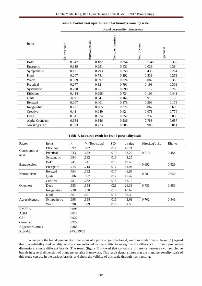
Le Thi Minh Hang, Bao Quoc Truong Dinh/ ICYREB 2017 Proceedings
Table 6. Partial least squares result for brand personality scale
Items
Brand personality dimensions
Ext
rave
rsio
n
Ag
ree
able
nes
s
Co
nsc
ien
tiou
snes
s
Neu
rotic
ism
Op
enn
ess
Bold 0.847 0.182 0.254 -0.048 0.352 Energetic 0.819 0.291 0.431 0.029 0.38 Sympathetic 0.12 0.793 0.258 0.433 0.264 Kind 0.207 0.781 0.292 0.339 0.262 Warm 0.309 0.597 0.324 0.082 0.353 Practical 0.277 0.32 0.791 0.193 0.301 Systematic 0.208 0.251 0.698 0.112 0.265 Efficient 0.414 0.298 0.724 0.103 0.441 Quite -0.031 0.34 0.166 0.91 0.15 Relaxed 0.007 0.401 0.178 0.908 0.173 Imaginative 0.271 0.265 0.277 0.067 0.699 Creative 0.41 0.249 0.42 0.071 0.776 Deep 0.34 0.374 0.357 0.232 0.83 Alpha Cronbach 0.554 0.556 0.586 0.788 0.657 Jöreskog's rho 0.823 0.773 0.785 0.905 0.814
Table 7. Bootstrap result for brand personality scale
Factor Items (Bootstrap) S.D t-value Jöreskog's rho Rho vc
Conscientious-ness
Efficient .692 .692 .017 40.71 0.713 0.454 Practical .633 .632 .019 33.26
Systematic .694 .692 .016 43.25
Extraversion Bold .741 .741 .015 49.40
0.692 0.529 Energetic .714 .713 .017 41.94
Neuroticism Relaxed .794 .793 .017 46.65
0.781 0.640 Quite .806 .807 .017 47.47
Openness Creative .781 .782 .015 52.13
0.733 0.483 Deep .553 .554 .021 26.38 Imaginative .730 .730 .015 48.67
Agreeableness Kind .691 .691 .018 38.39
0.702 0.441 Sympathetic .698 .698 .016 43.63 Warm .598 .599 .019 31.53
RMSEA AGFI GFI Gamma Adjusted Gamma Khi²/ddl
0.095 0.817 0.922 0.929 0.883 975.899/55
To compare the brand personality dimensions of a pair competitive brand, we draw spider maps. Aaker [1] argued
that the reliability and validity of scale are reflected in the ability to recognize the difference in brand personality dimensions among different brands. The result (figure 1) showed that contains a difference between two completive brands in several dimension of brand personality framework. This result demonstrates that the brand personality scale of this study can use in the various brands, and show the validity of this scale through many testing.
361

Le Thi Minh Hang, Bao Quoc Truong Dinh/ ICYREB 2017 Proceedings
Figure 1. Comparison of five dimensions of brand personality scale between two competitive brands
362

Le Thi Minh Hang, Bao Quoc Truong Dinh/ ICYREB 2017 Proceedings
5. Discussion
This study attempt to build a brand personality scales for Vietnam. Starting from a definition that confines brand personality to human personality traits that are relevant for and applicable to brands, we developed a new brand personality for Vietnamese context. The Vietnamese version scale contains thirteen items and five factors (Extraversion, Agreeableness, Conscientiousness, Neuroticism, Openness) (figure 2). The brand personality scale of this study, in our knowledge, is the first ones in Vietnamese context and try to test in diversity consumption situation and a large number of brands. Thus, this scales promises to be a practical instrument for branding research and is important for both academics and practitioners. For academics, future branding researchers in Vietnam can apply this scale like a recommendation to develop more research related to this one. For practitioners, it is very important that the scale can be used on diversified product categories. Moreover, companies can use this study to test their brand personality and assess what degree their brands have a true brand personality.
Figure 2. Brand personality measure in Vietnamese context
By adopting a restricted definition of brand personality and develop a scale from human personality traits. We developed a brand personality scale in Vietnamese context that replicates a Big-Five model and showed the consistency with human personality scale. This study creates a foundation and opens the opportunities for more research in measurement the congruency between human and brand.
However, this study is not without limitations. Frist, we apply a Mini-markers scale with 20 items to support our data collection. Thus it is possible that we missed useful and meaningful items because they were not associated with one of the dimensions. Future research can apply a full scale of Goldberg [22] and to retest a validity of the scale. Second, although we tested the scale on a large number of brands (16 brands) and several product types, this is not all the brand in Vietnam market, future research may try to extend sample of brands. Future research may test the scale in different areas of Vietnam, not just in Danang city of this study and use other characteristics of specific target groups (demographic, culture, goals, genders, etc.)
References
[1] Aaker, J. (1997). Dimensions of brand personality. Journal of Marketing Research, 34(3), 347-356. [2] Ambroise, L. and P. Valette-Florence. (2010). Métaphore de la personnalité de la marque et stabilité inter-produits
d'un baromètre spécifique. Recherche et Applications en Marketing (French Edition), 25(2), 3-29. [3] Azoulay, A. and J.-N. Kapferer. (2003). Do brand personality scales really measure brand personality? The
Journal of Brand Management, 11(2), 143-155. [4] McCrae, R.R. and P.T. Costa. (1987). Validation of the five-factor model of personality across instruments and
observers. Journal of personality and social psychology, 52(1), 81. [5] Aaker, J., V. Benet-Martinez, and J. Garolera. (2001). Consumption symbols as carriers of culture: A study of
Japanese and Spanish brand personality constructs. Journal of Personality and Social Psychology, 81(3), 492. [6] Chu, S.-C. and Y. Sung. (2011). Brand personality dimensions in China. Journal of Marketing Communications,
17(3), 163-181. [7] Kim, C.K., D. Han, and S.B. Park. (2001). The effect of brand personality and brand identification on brand
loyalty: Applying the theory of social identification. Japanese Psychological Research, 43(4), 195-206. [8] McCrae, R.R. and P.T. Costa. (1997). Personality trait structure as a human universal. American psychologist,
52(5), 509. [9] John, O.P. and S. Srivastava. (1999). The Big Five trait taxonomy: History, measurement, and theoretical
perspectives. Handbook of personality: Theory and research, 2(1999), 102-138. [10] Geuens, M., B. Weijters, and K. De Wulf. (2009). A new measure of brand personality. International Journal of
Research in Marketing, 26(2), 97-107. [11] Sung, Y. and S.F. Tinkham. (2005). Brand personality structures in the United States and Korea: Common and
363

Le Thi Minh Hang, Bao Quoc Truong Dinh/ ICYREB 2017 Proceedings
culture-specific factors. Journal of Consumer Psychology, 15(4), 334-350. [12] Venable, B.T., et al. (2005). The role of brand personality in charitable giving: An assessment and validation.
Journal of the Academy of Marketing Science, 33(3), 295-312. [13] Kapferer, J.-N. (2008). The new strategic brand management (Trans. Ed.^Eds. 4th ed. Vol.). London: Kogan page
publishers. [14] Konecnik, M. and F. Go. (2008). Tourism destination brand identity: The case of Slovenia. Journal of Brand
Management, 15(3), 177-189. [15] Keller, K.L. (2008). Strategic brand management: Building, measuring, and managing brand equity (Trans.
Ed.^Eds. 3rd ed. Vol.). Upper Saddle River, NJ: Prentice Hall. [16] Plummer, J. (2000). How personality makes a difference. Journal of Advertising Research, 40(6), 79-83. [17] Aaker, D. and E. Joachimsthaler. (2012). Brand Leadership (Trans. Ed.^Eds. ed. Vol.). Simon and Schuster. [18] Caprara, G.V., C. Barbaranelli, and G. Guido. (2001). Brand personality: How to make the metaphor fit? Journal
of Economic Psychology, 22(3), 377-395. [19] Ferrandi, J.-M. and P. Valette-Florence. (2002). Premiers test et validation de la transposition d'une échelle de
personnalité humaine aux marques. Recherche et Applications en Marketing (French Edition), 17(3), 21-40. [20] Aaker, J. (2000). Accessibility or diagnosticity? Disentangling the influence of culture on persuasion processes
and attitudes. Journal of Consumer Research, 26(4), 340-357. [21] Saucier, G. (1994). Mini-Markers: A brief version of Goldberg's unipolar Big-Five markers. Journal of Personality
Assessment, 63(3), 506-516. [22] 22. Goldberg, L.R. (1992). The development of markers for the Big-Five factor structure. Psychological
Assessment, 4(1), 26. [23] Dwight, S.A., K.M. Cummings, and J.L. Glenar. (1998). Comparison of criterion-related validity coefficients for
the Mini-Markers and Goldberg's Markers of the Big Five Personality Factors. Journal of Personality Assessment, 70(3), 541-550.
[24] Palmer, J.K. and J.M. Loveland. (2004). Further Investigation of the Psychometric Properties of Saucier's Big Five" Mini-Markers:" Evidence for Criterion and Construct Validity. Individual Differences Research, 2(3).
[25] Aaker, J. and S. Fournier. (1995). A brand as a character, a partner and a person: Three perspectives on the question of brand personality. ACR North American Advances, 22, 391-395.
[26] Graeff, T.R. (1997). Consumption situations and the effects of brand image on consumers' brand evaluations. Psychology & Marketing, 14(1), 49-70.
364

Tran Thi Thanh Huyen, Nguyen Duc Hoang Tho / ICYREB 2017 Proceedings
International Conference For Young Researchers In Economics And Business, ICYREB 2017, October 30th 2017 Da Nang, Vietnam
Enhancing The Social Efficiency of Hanoi’s Foreign Direct Investment in The Context of The Industrial Revolution 4.0
Tran Thi Thanh Huy ena*, Nguyen Duc Hoang Thob
aBanking Academy of Vietnam, 12 Chua Boc Street, Dong Da District, Hanoi bPolitical Academy, 124 Ngo Quyen Street, Ha Dong District, Hanoi
1. Introduction
Hanoi’s socio-economic development shows that FDI is considered as one of the "pillars" of economic growth, which contributed to modern - oriented economic restructure, helped to increase the state budget. Besides FDI’s important economic contribution, its social contribution is also specially cared for. Nowadays, in the context of the Industrial Revolution 4.0, when all aspects of socio-economic are impacted, the social efficiency of FDI has becomed increasingly important.
This paper investigates Hanoi’s data since the extension of administrative boundaries under Decision No 15/2008/QH12 dated 29/5/2008. The main method used in this paper is descriptive statistics. In order to make policy implications to enhance the social efficiency of FDI, which contributes to improving the living standard of Hanoi’s citizens, the paper focuses on clarifying: (i) The situation of Hanoi’s FDI attraction; and its main contributions to economic development; (ii) The socical efficiency evoluation of FDI in the period of 2008-2016; (iii) Issues needed to be solved to increase the social efficiency of FDI in the context of the Industrial Revolution 4.0.
2. Literature review
Up to now, there have been many researches about FDI in Vietnam, however, the number of studies about effectiveness of FDI is minor. Current studies about FDI’s effectiveness are mainly limited in national scope, such as Nguyen Thi Tue Anh and Tran Toan Thang (2015), Nguyen Van Giao (2016); Duong Manh Hai (2003) and Vu Chi Loc (1995)... At local scope, representative researches which can be listed here include Duong Thi Binh Minh and Phung Thi Cam Tu (2009), Phung Xuan Nha and Vu Thanh Huong (2010), Pham Thi Thuy (2014)... It can be clearly seen that these works have clarified the theoretical and practical issues related to the economic, social and environmental efficiency of FDI on different scopes of research. Yet, the social efficiency of FDI in Hanoi has never
* Corresponding author. Tel: +84983830104
E-mail address: [email protected]
A B S T R A C T
Foreign direct investment (FDI) is an important factor, which contributed significantly to economic growth and modern - oriented economic restructure of Hanoi. It also helped to increase the state budget, promote export ability. Besides economic aspect, FDI has also made social contributions, helping to improve the living standard of Hanoi’s citizens. Through surveying Hanoi’s data since the extension of administrative boundaries and by descriptive statistic method, this paper focuses on the social efficiency of FDI through considering employment issues, wages and corporate social responsibility (CSR). FDI is proved to have contributed positively to job creation and labour restructrure in the direction of industrialization, boosted wage increase, reduced income inequality. Besides, this article also points out the downward trend in the contribution of FDI to the wage increase. The implementation of CSR by FDI enterprises in Hanoi is mainly obligatory. The assessment of the social performance of the FDI sector, together with new requirements of the Industrial Revolution 4.0 reveal that policy adjustment is really necessary in order to improve the effectiveness of FDI inflows.
Keywords: Social efficiency; FDI; the Industrial Revolution 4.0; Hanoi .
365
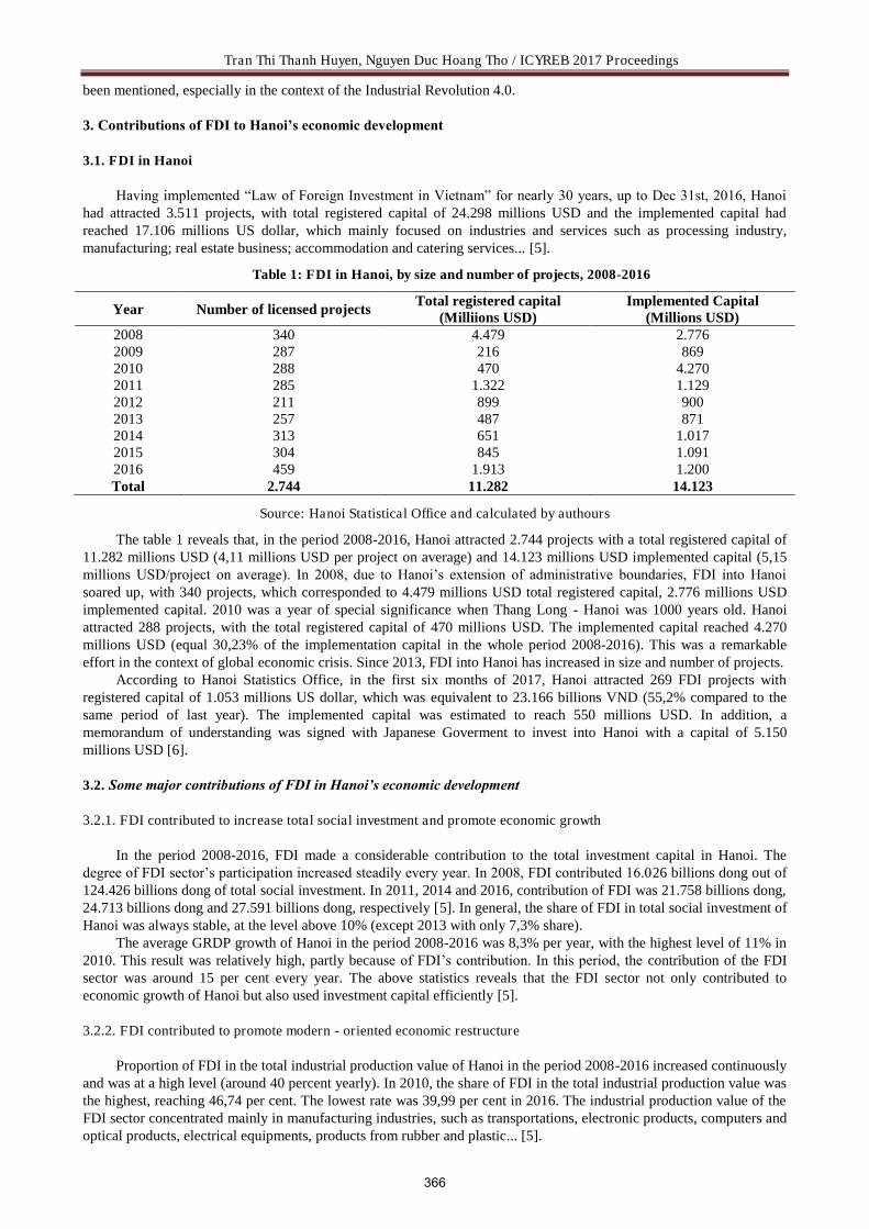
Tran Thi Thanh Huyen, Nguyen Duc Hoang Tho / ICYREB 2017 Proceedings
been mentioned, especially in the context of the Industrial Revolution 4.0.
3. Contributions of FDI to Hanoi’s economic development
3.1. FDI in Hanoi
Having implemented “Law of Foreign Investment in Vietnam” for nearly 30 years, up to Dec 31st, 2016, Hanoi had attracted 3.511 projects, with total registered capital of 24.298 millions USD and the implemented capital had reached 17.106 millions US dollar, which mainly focused on industries and services such as processing industry, manufacturing; real estate business; accommodation and catering services... [5].
Table 1: FDI in Hanoi, by size and number of projects, 2008-2016
Year Number of licensed projects Total registered capital
(Milliions USD) Implemented Capital
(Millions USD) 2008 340 4.479 2.776 2009 287 216 869 2010 288 470 4.270 2011 285 1.322 1.129 2012 211 899 900 2013 257 487 871 2014 313 651 1.017 2015 304 845 1.091 2016 459 1.913 1.200 Total 2.744 11.282 14.123
Source: Hanoi Statistical Office and calculated by authours
The table 1 reveals that, in the period 2008-2016, Hanoi attracted 2.744 projects with a total registered capital of 11.282 millions USD (4,11 millions USD per project on average) and 14.123 millions USD implemented capital (5,15 millions USD/project on average). In 2008, due to Hanoi’s extension of administrative boundaries, FDI into Hanoi soared up, with 340 projects, which corresponded to 4.479 millions USD total registered capital, 2.776 millions USD implemented capital. 2010 was a year of special significance when Thang Long - Hanoi was 1000 years old. Hanoi attracted 288 projects, with the total registered capital of 470 millions USD. The implemented capital reached 4.270 millions USD (equal 30,23% of the implementation capital in the whole period 2008-2016). This was a remarkable effort in the context of global economic crisis. Since 2013, FDI into Hanoi has increased in size and number of projects.
According to Hanoi Statistics Office, in the first six months of 2017, Hanoi attracted 269 FDI projects with registered capital of 1.053 millions US dollar, which was equivalent to 23.166 billions VND (55,2% compared to the same period of last year). The implemented capital was estimated to reach 550 millions USD. In addition, a memorandum of understanding was signed with Japanese Goverment to invest into Hanoi with a capital of 5.150 millions USD [6].
3.2. Some major contributions of FDI in Hanoi’s economic development
3.2.1. FDI contributed to increase total social investment and promote economic growth
In the period 2008-2016, FDI made a considerable contribution to the total investment capital in Hanoi. The degree of FDI sector’s participation increased steadily every year. In 2008, FDI contributed 16.026 billions dong out of 124.426 billions dong of total social investment. In 2011, 2014 and 2016, contribution of FDI was 21.758 billions dong, 24.713 billions dong and 27.591 billions dong, respectively [5]. In general, the share of FDI in total social investment of Hanoi was always stable, at the level above 10% (except 2013 with only 7,3% share).
The average GRDP growth of Hanoi in the period 2008-2016 was 8,3% per year, with the highest level of 11% in 2010. This result was relatively high, partly because of FDI’s contribution. In this period, the contribution of the FDI sector was around 15 per cent every year. The above statistics reveals that the FDI sector not only contributed to economic growth of Hanoi but also used investment capital efficiently [5].
3.2.2. FDI contributed to promote modern - oriented economic restructure
Proportion of FDI in the total industrial production value of Hanoi in the period 2008-2016 increased continuously and was at a high level (around 40 percent yearly). In 2010, the share of FDI in the total industrial production value was the highest, reaching 46,74 per cent. The lowest rate was 39,99 per cent in 2016. The industrial production value of the FDI sector concentrated mainly in manufacturing industries, such as transportations, electronic products, computers and optical products, electrical equipments, products from rubber and plastic... [5].
366

Tran Thi Thanh Huyen, Nguyen Duc Hoang Tho / ICYREB 2017 Proceedings
Table 2. FDI’s contribution to total turnover of trade and services
Year Total turnover of trade and services
(bil. dong) Share of FDI
(bil. dong) Contributon proportion
(%) 2008 580.107 21.042 3,6 2009 678.262 31.864 4,7 2010 972.890 49.182 5,1 2011 1.316.407 74.041 5,6 2012 1.408.165 72.868 5,2 2013 1.578.892 84.222 5,3 2014 1.480.587 99.758 6,7 2015 1.754.002 105.013 6,0 2016 1.892.604 111.970 5,9
Source: Hanoi Statistical Office and calculated by authours
In the period 2008-2016, share of FDI to Hanoi’s total turnover of trade and services increased stably both in terms of volume and contribution (see Table 2). In 2014, proportion of FDI to total trade and services turnover was the highest, reaching 6,7%.
FDI contributed to modern – oriented economic restructure of Hanoi. Hanoi’s economic structure in the period 2008-2016 shifted towards a gradual reduction of agriculture, forestry and fisheries proportion (4% in 2010, 3,7% in 2013 and 3,2% in 2016), gradual increase of industry and services proportion, especially services (56,8% in 2010; 57,1% and 57,3% in 2013 and 2016, respectively) [5].
3.2.3. FDI contributed to increase the state budget
8.016 8.229 11.315 13.619 14.908 16.809 16.404 17.614 18.962
72.40785.448
108.301121.919
145.701164.05 165.403
225.528
177.837
2008 2009 2010 2011 2012 2013 2014 2015 2016
Unit: Bil. Dong
Share of FDI Total state budget collection (Bil. Dong)
Fig 1. Contribution of FDI to Hanoi’s total state budget collection
Source: Hanoi Statistical Office and calculated by authours
One of important contributions of FDI to the socio-economic development of Hanoi was that FDI helped to increase the state budget collection through taxes (including corporate income tax, natural resources tax, value added tax…). The Fig. 1 shows that from 2008 to 2016, the contribution of FDI to Hanoi's total annual state budget collection increased year by year, was relatively stable at above 10% (except 2009 and 2015 when the contribution of FDI was only 9,6% and 7,8%). The increase trend of the FDI sector’s contribution to Hanoi’s state budget was the result of Vietnam's deepening integration process, the improvement of the investment environment and especially the FDI management efficiency of Hanoi in this period.
3.2.4. FDI contributed to promote export
Table 3. Contribution of FDI to Hanoi’s total export value
Year Total export value
(mil. USD) Share of FDI (mil. USD)
Contributon proportion (%)
2008 6.904 2.754 39,89 2009 6.328 2.592 40,96
367

Tran Thi Thanh Huyen, Nguyen Duc Hoang Tho / ICYREB 2017 Proceedings
2010 8.109 3.630 44,79 2011 9.782 3.919 40,06 2012 9.813 4.743 48,33 2013 9.913 4.908 49,51 2014 11.069 5.357 48,39 2015 10.475 5.221 49,84 2016 10.683 5.226 48,92
Source: Hanoi Statistical Office and calculated by authours
The FDI sector helped to improve the quality, efficiency as well as the competitiveness of export products in some areas. It also contributed to accelerate the growth of Hanoi’s export turnover. In the period 2008-2016, the value export turnover of Hanoi as well as the FDI sector increased rapidly and continuously over the years. The share of the FDI sector in the total value of export turnover increased regularly. The respective statistic data in 2008, 2012 and 2016 was 39.89%, 48,33% and 48,92%. On the other hand, the development index of FDI sector’s export value was always higher than that of Hanoi, which proved that FDI sector pushed export (see Table 3).
Alonging with export promotion impact, FDI activities also contributed to promoting Hanoi's international economic integration in the direction of multilateralization and diversification. Hanoi has not only established economic, cultural, investment and trade cooperation with more than 100 capitals and cities of other countries but also been a member of many prestigious international organizations.
4. Social efficiency of FDI in Hanoi
4.1. Social efficiency of FDI through job creation and labour restructure
In the period 2010-2016, the number as well as percentage of employees (above 15 years old) who worked in the FDI sector increased significantly. In 2010, there were 175.000 labours in the FDI sector, accounting for 4,9% of the total labour force in Hanoi. In 2016, the respective numbers were 231.000 labours and 6,2%. In addition to creating jobs through directly employing labours, FDI also indirectly generated many jobs, especially in the manufacturing sector supplying goods and services for FDI enterprises.
Table 4. The ratio of implemented capital to the number of employees working directly
Year
Labours working at July 1st every year
(1.000 people)
Implemented capital (bil. dong)
Implemented capital/ direct working labour
(%) Total FDI sector Total FDI sector Total FDI sector
Labours Proportion (%) 2010 3.546 175 4,9 148.112 20.328 4,177 11,616 2011 3.544 210 5,9 170.749 21.758 4,818 10,361 2012 3.631 214 5,9 249.287 27.055 6,866 12,643 2013 3.681 222 6,0 279.352 20.036 7,589 9,172 2014 3.702 228 6,1 230.381 24.713 6,223 10,839 2015 3.747 229 6,1 252.685 26.945 6,744 11,766 2016 3.749 231 6,2 277.950 27.519 7,414 11,913
Source: Hanoi Statistical Office and calculated by authours
The social efficience of FDI was not only reflected in creating many jobs, but also in the implemented investment capital per direct worker in the FDI sector. Table 4 shows that the ratio of implemented capital to direct working labour of the FDI sector was always higher than that of the entire Hanoi. This is reasonable because FDI is usually only allowed in areas where other sectors are ineffective.
In the period 2010-2016, the proportion of implemented invested capital compared to the number of working labour in Hanoi increased continuously, which revealed that the economic efficiency of Hanoi in terms of job creation tended to decrease. However, this rate in the FDI sector was relatively stable. This proves that, compared to other economic sectors, the FDI sector contributed positively in solving jobs for workers in Hanoi.
In stead of its contribution to job creation, the FDI sector also played an important role in shifting Hanoi’s labour structure towards industrialization, especially helped to increase proportion of industrial labour. According to Hanoi Statistical Office, in 2010, the number of industrial workers in FDI sector was 129.848, accounting for 19,5 per cent of the total labour force in Hanoi. By 2016, corresponding figures were 168.234 and 22,22%, respectively.
368

Tran Thi Thanh Huyen, Nguyen Duc Hoang Tho / ICYREB 2017 Proceedings
4.2. Social efficiency of FDI through wage trend and income inequality
In 2012, the monthly average wage of labours in FDI enterprises was 6.648.780 VND/person, 3.32 times higher than the minimum wage which was regulated by Decree 70/2011/ND-CP dated 22/8/2011 of the Government (according to the General Statistic Office of Vietnam). In 2016, the monthly average salary was 7.675.500 VND per person, which was 2,19 times higher than the general minimum salary which was regulated by Decree 122/2015/ND-CP dated 14/11/2015 by the Government [3].
2012 2013 2014 2015 2016
General 6648.78 6716.48 6838.75 6927.23 7675.5
Male 7117.43 7647.03 7530 7946.15 8047.5
Female 6322.2 6074.45 6380.5 6356.85 7450.5
0
1000
2000
3000
4000
5000
6000
7000
8000
9000
Unit: 1000 VND/labour
Fig. 2: Monthly average wage of labours in FDI enterprises
Source: GSO and calculated by authors
In the period 2012-2016, nominal wages increased averagely 3,73% per year. Especially, in the last two years of this period, wage growth rate reached 6,05% per year. After removing inflation, real wages increased 4,18% per year in 2012-2016 and 4,48% per year in the last two years. Alonging with inflation rate, FDI sectors’s continuous growth was also considered one of main factors which enhance the above increasing wage trend.
Comparing the monthly average wages of male and female labours in FDI enterprises in the period 2012-2016 reveals that male labours had higher wage than female labours. However wage growth rate of men was lower than that of women, especially in the last two years (3,41% per year for males versus 8.42% for females). As a result, the wage gap between male and female workers in FDI enterprises tended to decrease so that income inequality was reduced.
Table 5. The monthly average wage of labours in FDI enterprises in comparison with other economic types in Hanoi
Economic types Monthly average wage
(1.000 VND/labour) Growth rates (%/labour)
2012 2014 2016 2012-2016 2014-2016 Individual/ individual production and business households
3.113,73 3.568,00 4.344,50 8,63 10,35
Group 2.757,08 3.264,50 2.968,00 2,31 - 4,19 Private 5.089,85 5.772,25 6.762,25 7,57 8,36 State 5.342,68 6.396,50 7.182,75 7,88 6,10 FDI 6.648,78 6.716,48 6.838,75 3,73 6,05 Total 4.783,25 5601,75 6.381,50 7,65 6,86
Source: GSO and calculated by authors
As we can see in Table 5, in the period 2012-2016, the monthly average wage of labours in FDI enterprises was rather higher than that of other types of workers. However, the wage growth rates of labours in FDI enterprises was low, only higher than the rate of group type.
If in 2012, the monthly average wage of workers in FDI enterprises was the highest, in 2016, the highest position belonged to the state type. The process of economic restructuring, which caused the increase in labour productivity, the dynamic development of the private sector and the reform of wage, was considered as the key factor leading to changes in the monthly average wage correlation among types of economy in Hanoi. Applying the common minimum wage in domestic and FDI enterprises has speeded the process of narrowing the wage gap of labours in economic types.
369

Tran Thi Thanh Huyen, Nguyen Duc Hoang Tho / ICYREB 2017 Proceedings
4.3. Social efficiency of FDI through CSR implementation
Corporate social responsibility (CSR) is a criterion to assess the social efficiency of FDI enterprises. CSR is the whole responsibility of an enterprise for the social impact of its decisions and operations. In order to implement CSR, first of all, FDI enterprises must respect laws and commitments with related parties. Besides, they must be capable of linking production and business with solving social, ethical issues, protecting environment and human rights, responsing customer concerns in order to maximize utilities of business owners, stakeholders and the whole society. In addition, FDI enterprises should identify, prevent and minimize the potential negative impacts of business operations. Empirically, in the world, enterprise which is well-regarded CSR often have high economy efficiency and performance.
Similar to FDI enterprises of Vietnam in general, FDI enterprises of Hanoi have only implemented CRS obligatorily, especially in applying regulations about responsibilties for employees (including providing formal contracts, paying health and social insurance). Only very few FDI enterprises carry out CRS as well as sign to enhance social responsibility.
According to the Central Institute for Economic Management and Research (CIEM), the proportion of FDI enterprises implementing CSR for workers is very high (79% to 99%) [2]. However, currently, many labours of FDI enterprises are being dismissed when they are over 35 years old [8]. The proportion of FDI enterprises participating in social activities with the community is very low, even lower than that of domestic private enterprises, which shows that FDI enterprises have less interaction with the community. The two highest proportions in CSR groups of FDI enterprises, which are environmental protection and poverty reduction, reaches only 19% and 9% respectively. In particular, these factors tend to decrease [2]. This fact also raises question about the sustainability of FDI enterprises’ strategies in Vietnam. A long – term business usually has a strategy which engages nearer with the society and community of the receiving country. Therefore, it is time for us to recognize the role of CSR and to consider CSR as a criterion to select investors and foreign direct investment capital [1].
5. The context of the Industrial Revolution 4.0 and related issues
The Industrial Revolution 4.0 has been bringing people into the era of science and technology development, changing the world economy day by day. Making profound and systematic changes is the main characteristic of this revolution. The Industrial Revolution 4.0 is based on digital technology, which integrates all smart technologies in order to optimize processes and production methods. This revolution also emphasizes the technologies which have impacted greatly, including 3D printing technology, biotechnology, new material technology, automation technology, robots... This revolution is now giving some problems:
* For the world economy For manufactures, the Industrial Revolution 4.0 witnesses the releases of many technologies, which help to create
new products and services, increase production efficiency, promote the industry’s innovation and development in long run. In addition, cost of transportation, communication and trade are being reduced, supply chains are expected to be more and more efficient.
For consumers, the 4th industry revolution promises to change the consumption model and the time to approach products. Activities such as consumption, basic service usage can be performed remotely. Besides, consumers are able to access information of products more transparently and adequately due to the pressure to maintain competitive advantages among manufacturers.
For legislative branch, technology and digital infrastructure facilities not only allow two-way interaction between people and the government but also enhance supervising and leading ability, so that accelerate transparency and integration. The Industrial Revolution 4.0 will help strengthen national security in case the state's regulatory system is flexible enough to manage and cooperate closely with enterprises and citizens.
In addition to the above advantages, this revolution is also expected to break the labour market balance as well as widen the income gap between people who provide financial capital (investors), knowledge capital (inventors) and those who depend on labour (workers). As a result, the 4th Industrial Revolution may lead to the income decline of major citizens in developed countries when the demand for high-skilled labours increases while the demand for basis labours decreases drammatically.
Another scenario is that organizations and businesses may not have enough abilties to acquire new technologies or law enforcement agencies have difficulties in ecruiting staff for managing new technologies. This would be more difficult as national security issues become more complex with a combination of traditional elements and non-traditional elements (such as cyber war, biological weapons). It is necessary for businesses and the government to make innovation, improve the structure or enhance high - quality human resources training.
* For the development of enterprises in the economy The Industrial Revolution 4.0 provides good development opportunities for domestic enterprises if they can take
advantage of digital technology and transform the business model in time. Moreover, this revolution also brings opportunities for domestic consumers to have closer access to diverse goods and services at more reasonable prices.
However, Vietnamese enterprises have to face the challenge of adjusting flexibly their products to meet consumer
370
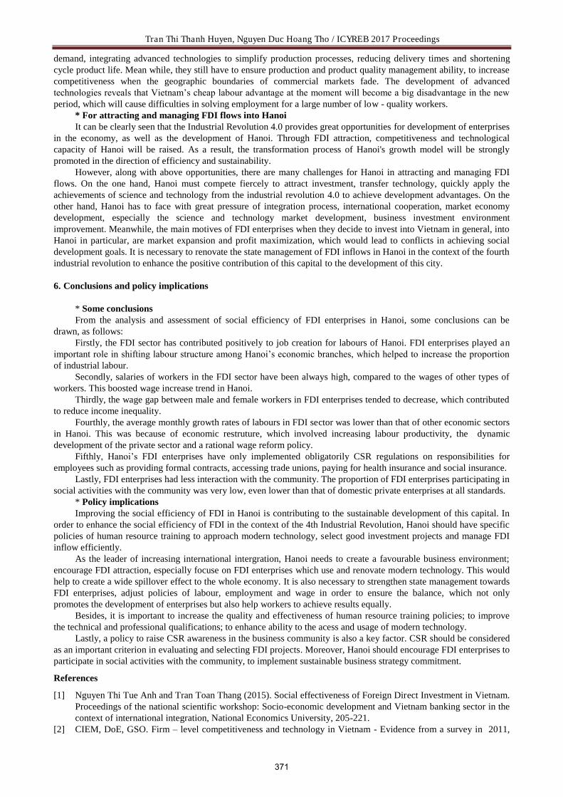
Tran Thi Thanh Huyen, Nguyen Duc Hoang Tho / ICYREB 2017 Proceedings
demand, integrating advanced technologies to simplify production processes, reducing delivery times and shortening cycle product life. Mean while, they still have to ensure production and product quality management ability, to increase competitiveness when the geographic boundaries of commercial markets fade. The development of advanced technologies reveals that Vietnam’s cheap labour advantage at the moment will become a big disadvantage in the new period, which will cause difficulties in solving employment for a large number of low - quality workers.
* For attracting and managing FDI flows into Hanoi It can be clearly seen that the Industrial Revolution 4.0 provides great opportunities for development of enterprises
in the economy, as well as the development of Hanoi. Through FDI attraction, competitiveness and technological capacity of Hanoi will be raised. As a result, the transformation process of Hanoi's growth model will be strongly promoted in the direction of efficiency and sustainability.
However, along with above opportunities, there are many challenges for Hanoi in attracting and managing FDI flows. On the one hand, Hanoi must compete fiercely to attract investment, transfer technology, quickly apply the achievements of science and technology from the industrial revolution 4.0 to achieve development advantages. On the other hand, Hanoi has to face with great pressure of integration process, international cooperation, market economy development, especially the science and technology market development, business investment environment improvement. Meanwhile, the main motives of FDI enterprises when they decide to invest into Vietnam in general, into Hanoi in particular, are market expansion and profit maximization, which would lead to conflicts in achieving social development goals. It is necessary to renovate the state management of FDI inflows in Hanoi in the context of the fourth industrial revolution to enhance the positive contribution of this capital to the development of this city.
6. Conclusions and policy implications
* Some conclusions From the analysis and assessment of social efficiency of FDI enterprises in Hanoi, some conclusions can be
drawn, as follows: Firstly, the FDI sector has contributed positively to job creation for labours of Hanoi. FDI enterprises played an
important role in shifting labour structure among Hanoi’s economic branches, which helped to increase the proportion of industrial labour.
Secondly, salaries of workers in the FDI sector have been always high, compared to the wages of other types of workers. This boosted wage increase trend in Hanoi.
Thirdly, the wage gap between male and female workers in FDI enterprises tended to decrease, which contributed to reduce income inequality.
Fourthly, the average monthly growth rates of labours in FDI sector was lower than that of other economic sectors in Hanoi. This was because of economic restruture, which involved increasing labour productivity, the dynamic development of the private sector and a rational wage reform policy.
Fifthly, Hanoi’s FDI enterprises have only implemented obligatorily CSR regulations on responsibilities for employees such as providing formal contracts, accessing trade unions, paying for health insurance and social insurance.
Lastly, FDI enterprises had less interaction with the community. The proportion of FDI enterprises participating in social activities with the community was very low, even lower than that of domestic private enterprises at all standards.
* Policy implications Improving the social efficiency of FDI in Hanoi is contributing to the sustainable development of this capital. In
order to enhance the social efficiency of FDI in the context of the 4th Industrial Revolution, Hanoi should have specific policies of human resource training to approach modern technology, select good investment projects and manage FDI inflow efficiently.
As the leader of increasing international intergration, Hanoi needs to create a favourable business environment; encourage FDI attraction, especially focuse on FDI enterprises which use and renovate modern technology. This would help to create a wide spillover effect to the whole economy. It is also necessary to strengthen state management towards FDI enterprises, adjust policies of labour, employment and wage in order to ensure the balance, which not only promotes the development of enterprises but also help workers to achieve results equally.
Besides, it is important to increase the quality and effectiveness of human resource training policies; to improve the technical and professional qualifications; to enhance ability to the acess and usage of modern technology.
Lastly, a policy to raise CSR awareness in the business community is also a key factor. CSR should be considered as an important criterion in evaluating and selecting FDI projects. Moreover, Hanoi should encourage FDI enterprises to participate in social activities with the community, to implement sustainable business strategy commitment.
References
[1] Nguyen Thi Tue Anh and Tran Toan Thang (2015). Social effectiveness of Foreign Direct Investment in Vietnam. Proceedings of the national scientific workshop: Socio-economic development and Vietnam banking sector in the context of international integration, National Economics University, 205-221.
[2] CIEM, DoE, GSO. Firm – level competitiveness and technology in Vietnam - Evidence from a survey in 2011,
371

Tran Thi Thanh Huyen, Nguyen Duc Hoang Tho / ICYREB 2017 Proceedings
2012 and 2013. [3] General Statistics Office of Vietnam. Report of Survey about Labour and Jobs 2012, 2013, 2014, 2015, 2016. [4] Nguyen Van Giao (2016). The socio – economic efficience of foreign direct investment projects in Vietnam
nowadays, PhD thesis on economics, Thuongmai University. [5] Hanoi Statistical Office. Hanoi Statistical Yearbook 2008, 2009, 2010, 2011, 2012, 2013, 2014, 2015, 2016. [6] Hanoi Statistical Office. Report of socio-economic situation in June and estimate of the first 6 months of 2017. [7] Duong Manh Hai (2003). Scientific basis and solutions to improve the socio-economic efficiency of attracting and
using foreign direct investment capital in the process of implementing the export-oriented strategy. PhD thesis on economics, Institue of world economics.
[8] Van Khanh (2017). More burden for socila security, [http://baodansinh.vn/doanh-nghiep-sa-thai-lao-dong-tren-35-tuoi-d60972.html].
[9] Vu Chi Loc (1995). The socio – economic efficience of foreign direct investment in Vietnam. Deputy PhD thesis on economics, Foreign Trade University.
[10] Duong Thi Binh Minh, Phung Thi Cam Tu (2009). Solutions to improve the socio – economic efficiency of foreign direct investment usage in Ho Chi Minh City. Journal of Economic Development, Ausgust Issue, 34-42.
[11] Phung Xuan Nha, Vu Thanh Huong (2010). Foreign direct investment with the development of Hanoi in the period of innovation and international integration. Proceedings of the international scientific conference on the 1000th anniversary of Thang Long - Hanoi: "Sustainable development of Hanoi Capital: Culture, heroic, for peace”.
[12] Pham Thi Thuy (2014). Evaluation of Foreign Direct Investment Effectiveness in Vinh Phuc. Economy and Forecast Review, No 11 (June), 62-64.
372

Le Thi Khanh Ly/ ICYREB 2017 Proceedings
International Conference For Young Researchers In Economics And Business, ICYREB 2017, October 30th 2017 Da Nang, Vietnam
KPI in Evaluat ing Organization’s Recruitment and Selection
Practices
Le Thi Khanh Ly *
Duy Tan University, 254 Nguyen Van Linh, Da Nang, Viet Nam
1. In troduction
Human resource management is also known as effective labor force management process in the workplace. Human Resource Management studies what can and should be done to make employees work more productively and feel more satisfied with their work. One of the most important activities in human resource management is recruitment and selection. Recruitment refers to attracting applicants to vacancies, while selection includes using tools to find out who is best suited for vacancies. So, this process is very importance for any organization. One of the newer approaches refer on measuring the efficience of recruitment and selection activities via KPI.
Key Performance Indicators, also known as KPI or Key Success Indicators, help managers and employees shape and monitor the effectiveness of activities and functions that are important in achieving organizational goals. Due to that fact in first part of this paper will be explained what are KPI, recruitment and selection pratices; the characteristics of KPI and importance of organization performances measurement. In second part of this paper will showed the reseach methodology for this paper. In third part of the paper will proposed a set of KPIs used for assessing the effectiveness of recruitment and selection and indicated the notes in using this set of KPIs in any organizations
2. Literature Review
2.1. KPI
2.1.1. What are KPI
KPI stands for Key Performance Indicator (Carol Talor, 1990), a measure of productivity that helps organizations shape and track growth relative to their goals. KPI was introduced in the United States from the 80s of the 20th century and is now widely used in the world including Vietnam. The application of KPI is seen as a solution to help organizations evaluate their success in the management of business operations. Once the business has formed a mission,
* Corresponding author. Tel.: +84979161711. E-mail address: [email protected]
A B S T R A C T
Nowadays, human resource is a critical factor that make the organization’s success. So, most of organization is well cared for choosing organization members. These decisions have a critical impact on the organization’s ability to complete, as well as each and every job applicant’s life. These decisions are too importance because this is not only unfair to applicants who are wrongly denied jobs, but it is also a questionable business practice because it hurts the firm’s ability to complete. This mean, evaluating the efficience of hiring process is nessesary for all organizations. There are many tools to manage and measure the efficiency of business operation, one of them is the KPI which stand for Key Performance Indicator – those performance measures that will make a profound difference.
This paper was undertaken to address some issues related to the KPI and apply to create the KPI for evaluating organization’s recruitment and selection activities.
Keywords: Key Performance Indicator, performance, recruitment, selection.
373

Le Thi Khanh Ly/ ICYREB 2017 Proceedings
identifying the factors that influence and set goals, the business needs to measure growth against the set goals. KPI is a measure of this growth.
However, the first thing we need to consider is the difference between a performance metric and a result metric. Performance indicators (Dean, 2007) represent the results of previous actions, while the result indicator is a measure of direction of the results achieved in the performance indicators. In a simple way, according to Nguyen Thanh Hoi, Phan Thang, 2001, performance indicators are quantifiable measures. These measures have been agreed by all members and they reflect the critical success factors of the business. Therefore, the KPI requires reflecting the goals and mission of the business.
However, in practice there are many measurable indicators. This does not mean they are the keys to the success of the business. Therefore, when selecting the KPIs, it is important to carefully select the indicators that are needed and can help the business achieves its objectives. KPIs, on the other hand, give the staff an overall picture of the key factors and what they need to prioritize in their jobs. Thus, it is important to ensure that all employees are focused on achieving the goals in the KPIs for performance measurement.
2.1.2. Seven Characteristics of KPIs
David Parmenter (2010) define seven characteristics of KPIs: Are non financial measures (e.g., not expressed in dollars, yen, pounds, euros, etc.) Are measured frequently (e.g., 24/7, daily, orweekly) Are acted on by the CEO and senior management team (e.g., CEO calls relevant staff to enquire what is going on) Clearly indicate what action is required by staff (e.g., staff can understand the measures and know what to fix) Are measures that tie responsibility down to a team(e.g., CEO can call a team leader who can take the necessary
action) Have a significant impact (e.g., affect one or more of the critical success factors [CSFs] and more than one BSC
perspective) They encourage appropriate action (e.g., have been tested to ensure they have a positive impact on performance,
whereas poorly thought-through measures can lead to dys-functionalbehavior)
2.1.3. The role and importance of measuring oraganization performance with KPI
The system of standardized activities such as KPI allows good measurement of the activities of the business. The magnitude of the measurement is enormous. Continuous measurement is the basis for continuous improvement of organizational activities and is one of the most important management principles (Besic & Djordjevic, 2007).
If the organization do not have enough information about the process, product or service, they can not control them. There are a lot of values measured during the operation of a business. Lord Kelvin, 1891, said, "When you can measure what you are doing, you really understand it."
Measuring performance means qualitative or quantitative the results by selected indicators. Choosing the suitable indicators is important in measuring the organization performance. The performance indicators have two functions:
Developing and guiding function - because they are the basis for developing and implementing organizational strategy.
Motivating function - promotes to completion of goals and motivates all employees to achieve that goal (Pesalj, 2006; Stamatovic Zakic, 2010).
All employees know that there are the important activities for the managers. Accordingly, the manager must identify a set of indicators that represent the main activities in a business. Key Performance Indicators (KPIs) are the financial and non-financial indicators that the organization uses to demonstrate how successful in the long-term.
2.2. Recruitment and selection
2.2.1. What is Recruitment and selection practices
There are many definitions of recruitment and selection. However, all contain common elements: focus on attracting, identifying and retaining employees. Dragons are often considered as a term, but there are differences. In different situations, the recruitment sources could be external sources or internal sources (Searle, 2003). The key purpose of recruitment is the identification and attraction of the competent applicant for a vacancy, while the selection is the assessment and determination of the suitability of the candidate.
Recruitment and selection provide the key opportunities for an organization to change the type of employee, but those changes may need to be considered in the context of attrition levels and accurate investigation of who is leaving and why (Schneider, 1998). Therefore, an organization might determine the need for separate and distinct configurations in new hires, such as when technology has advanced and lack of skills, the organization also needs to be aware that the introduction and retention of their new employees also need attention.
374

Le Thi Khanh Ly/ ICYREB 2017 Proceedings
Raymond A. Noe et al (2010) indicated that the source from which a company recruits potential employees are a critical aspect of it overall recruitment strategy. The total labor market is expansive; any single organization needs to draw from only a fraction of that total. The size and nature of the fraction that applies for an organization’s vacancies will be affected by how (and to whom) the organization communicates its vacancies. We have some recruitment sources, including:
Direct applicants and Referrals Advertisements in newspapers Electronic recruiting Puplic and private employment agencies Colleges and universities Recruitment and selection might be just one stage in the human resources cycle for a company, but it can have a
huge impact on productivity and survival in the future. While it is central to the beginning of employment it can also have wide implications for other HR processes, such as organizational development and change. Evaluating the effectiveness of recruitment and selection involves assessing not only the number of new recruit, but also their effective integration and retention, and their impact on existing employees and on the organization’s performance.
2.2.2. Evaluating the effectiveness of recruitment and selection
During the recruitment and selection process, there are four possibilities for each candidate (Dung, 2003).
Table 1: Four possibilities for each candidate
Ability’ candidate to complete the job
Hiring decisions Eliminating Hiring
Good Mistake (Due to underestimation) (2)
Accuracy (1)
Not good Accuracy (3) Mistake (Due to overestimation) (4)
In boxes 1 and 3: Candidates have the ability to complete a job well and get rid of unqualified applicants. In box 2, the recruiters evaluated the candidate as being less than practical, thus ignoring good candidates. In contrast, in box 4, recruiters evaluated the candidates too hight, hiring of inappropriate employees, performed poorly on the job. And all of this directly affects the effectiveness of recruiting. In addition, when evaluating the effectiveness of recruitment and selection, managers also pay attention to some factors (Carrell et al, 1995)
Cost for recruitment and selection activities and costs for each recruitment. This cost includes recruitment service costs, advertising
The number and quality of applications. The coefficient between the new employees and the proposed employees. Number of applicants accepting and refusing to jobs at a certain salary. The new employee’ performance. The number of new employees voluntary turnover. Methodology In oder to address the set of KPI used in evaluating the effectiveness of recruitment and selection pratices, the
quanlitative reseach methodology was used. The research was conducted in two steps as outlined below: Designing a research questionnaire from selective information of many books and magazines, including: Dung, 2003 said that when analyzing the effectiveness of recruiting activities, it is necessary to collect
information on candidates' competencies. Carrell et al, 1995 proposed several criteria for assessing the effectiveness of recruitment and selection, including:
cost for recruitment and selection activities, the number and quality of applications, the new employee’ performance …. Searle, 2003 and Schneider, 1998 defined recruitment and selection that focus on attracting, identifying and
retaining employees. David Pamenter, 2010 argued building a KPI set should be based on business strategy. Dean, 2007 said that performance indicators represent the results of previous actions and Hoi et al, 2001, argued
that performance indicators are quantifiable measures. ………… Conducting interviews with 25 human resource managers of 14 companies in Danang. The interview questions
focused on the following issues: Hiring’s strategy The criteria for evaluating the organization’s recruitment and selection practices How to evaluate the efficience of recruitment and selection practices
375

Le Thi Khanh Ly/ ICYREB 2017 Proceedings
3. Discussion
3.1. Propose a set of KPIs used for assessing the effectiveness of recruitment and selection.
Based on the knowledge of recruitment and selection and KPIs, the author develops KPIs to evaluate the effectiveness of recruitment and selection activities.
3.1.1. KPIs use for evaluating the effectiveness of recruitment.
As you know, the recruiting performance can be seen through the activities, results, performance and fairness, so we will rely on here to developing KPIs in the table below:
Table 2: KPIs use for evaluating the effectiveness of recruitment
KPIs Formulation Notes Number of applications submitted by each recruitment source
Direct applicants
The total number of candidates from each recruitment source/The total number of candidates.
The organization have data capture of the number of candidates from each recruitment source.
Internal sources Newspaper advertising Electronic Recruiting – Internet Public & Private Employment Agencies Job fairs Colleges& Universities- campus placement services
Number of eligible candidates by recruitment source
Direct applicants
Number of eligible candidates by recruitment source/ The total number of candidates.
Used to evaluate the quality of candidates by each recruitment source. It is necessary to store the specific data the candidate comes from.
Internal sources Newspaper advertising Electronic Recruiting – Internet Public & Private Employment Agencies Job fairs Colleges& Universities- campus placement services.
Cost per candidate by each recruitment source
Direct applicants
Total cost for each recruitment source/The number of candidates come that recruitment source
Used to calculate the cost effectiveness for each recruitment source.
Internal sources Newspaper advertising Electronic Recruiting – Internet Public & Private Employment Agencies Job fairs Colleges& Universities- campus placement services
3.1.2. KPIs use for evaluating the effectiveness of selection.
As you kow, hiring decisions affect on the productivity and professional qualification of the workforce. Table 3 is a list of criteria for assessing the effectiveness of selection activities.
376

Le Thi Khanh Ly/ ICYREB 2017 Proceedings
Table 3: KPIs use for evaluating the effectiveness of selection
KPIs Formulation Notes Cost per new employee. The total cost of hiring process/the
number of candidates.
This indicator shows the cost of hiring per candidate, so that effectiveness of this hiring process might compare with one another.
The number of new employees. The number of new employees/The number of candidates.
This indicator can show the cadidates’s qualification.
The number of employees who work over five years.
The number of employees who work over five years/The number of new employees.
This indicator shows the willingness for jobs and loyalty of new employees.
Average working time of new employees at organization.
Total working time of new employees at organization/The number of new employees.
This indicator shows the average working time of new employees.
New employees’s qualification.
Base on the result of performance appraisal.
This indicator shows the new employees’s qualification
The rate of good new employees
Base on the result of performance appraisal.
This indicator show the rate of good new employees on each hiring process.
New employees’s promotion. Base on the result of performance appraisal.
This indicator shows the new employee’s career path.
Cadidates’ awareness: satisfaction with hiring process, knowledge of the organization, satisfaction with organization.
Base on the result of the recruitment interviews.
This indicator indicates whether the candidates are satisfied with the organization's hiring program, which can be considered as the information to improve hiring practices.
3.2. Some notes when using KPI in evaluating organization’s recruitment and selection practices
3.2.1. Perfecting in data system
In order to use a set of indicators to assess the effectiveness of recruitment and selection, it is important to build a specific data system. This can be performed by software or hand depending on the size of each organization, but it must ensure some data as follows:
Table 4: Data system
Name of hiring’s programe Date: Human Resource Recruitment Sources
Direct applicants
Internal sources
Newspaper advertising
Electronic Recruiting Internet
Public & Private Employment Agencies
Job fairs
Colleges& Universities- campus placement services.
The total number of candidates.
… … … … … … …
The number of eligible candidates
… … … … … … …
Total cost … … … … … … … The number of new employees
… … … … … … …
Cost per a new employee
… … … … … … …
The number of employees who
… … … … … … …
377

Le Thi Khanh Ly/ ICYREB 2017 Proceedings
work over five years. Average working time of new employees at organization
… … … … … … …
New employees’s qualification
… … … … … … …
New employees’s promotion.
… … … … … … …
The number of cadidates who is satisfaction with hiring process
… … … … … … …
All of the above data is easy to get, but the clerks need to note some of the following: The information about the candidate's recruitment sources should be added to the recruitment form. The hiring cost should be accumulated from all costs incurred during the hiring process, including recruitment
advertising costs, travel and accommodation costs, training for new employees costs
3.2.2. Some notes in using the KPI results to evaluating organization’s recruitment and selection
After collecting and calculating KPIs, the executives use these data to evaluating the efficiency of the recruitment and selection activities in the organization, which depends on each indicator in the KPI set. However, whether these indicators reflect the effectiveness of these activities, it depends on the organization’s strategy in specific hiring program.
In the hiring strategy, organizations need to determine the number of cadidates who are attracted in each vacancy. During the hiring pocess, some applicants do not qualify or do not accept jobs, the organization needs to attract more applicants than they need to hire. The selection rates help organizations determine this. The selection ratios show the relationship between the number of candidates who are chose in each step and the number of people who will be accepted into the next step.
In the hiring plan, organizations must determine the appropriate selection rates. The selection rates affect on the organization’s finance and candidate’s psychology and candidate's expectations. The selection rates are mostly determined by job’s characteristics and the candidate’s psychology. Therefore, the determination of selection rates should be based on the following factors:
The diversity of labor market (labor supply and demand) The quality of labor force The complexity of the work The candidate’s psychology The organization's experience in recruitment.
4. Conclusion
Continuing to measure business performance via Key Performance Indicators is a new concept used by many organizations today. KPI is a financial or non-financial indicator that helps businesses test their business success. One of the prerequisites for using KPIs is the clarity of the goals and business process.
This paper gives explanation of the KPI, the recruitment and selection activities that are used in organizations. Then it proposes a set of KPIs used for assessing the effectiveness of recruitment and selection. Tables show simplicity of measuring and explanation of a given results, what is one of the most important advantage of using such indicators.
This article offers a set of KPIs used for assessing the effectiveness of recruitment and selection. However, depending on the type of business and the different types of vacancies, the managers should choose the KPI to suit each situation.
378

Le Thi Khanh Ly/ ICYREB 2017 Proceedings
References
[1] David Pamenter (2010), Developing, Implementing, and using winning KPIs, Jonh Wiley & Sons Inc. [2] Nguyen Thanh Hoi, Phan Thang (2011), Management, Hong Duc Co, Ltd [3] Raymond A. Noe, John R. Hollenbeck, Barry Gerhart, Patrick M. Wright (2010), Human Resource Management:
Gaining a Competitive Advantage, McGraw-Hill [4] Tran Kim Dung (2003), Human Resource Management, Statistic Publishing House. [5] Carrell, Elbert, Hatfield (1995), Human Resource Management: Global strategies for Managing a Diverse Work
Force, Prentice Hall. London [6] Spitzer, Dean (2007), Transforming Performance Measurement: Rethinking the Way We Measure and Drive
Organizational Success. Amazon Div American Mgmt Assn, p.288. ISBN 9780814408919 [7] Stefanović, I., Damnjanović, P., & Jaško, O. (2010) The analysis of the contemporary environsment impact upon
organizational operations, Serbian Journal of Management 5 (1): 97 - 109 [8] Carol Taylor Fitz-Gibbon (1990), Performance indicators, BERA Dialogues (2), ISBN 978-1-85359-092-4 [9] Besic, C., Djordjevic, D. (2007) Benchmarking, Technical Faculty - Cacak, Cacak. [10] Searle, R. H, Ball, B. S (2003), Supporting Innovation Through HR Policy: Evidence from the UK. Published in
Creativity and Innovation Management volume 12. Issue 1, pp 50-62
379

International Conference For Young Researchers In Economics And Business, ICYREB 2017, October 30th 2017 Da Nang, Vietnam
The Impact of FDI on Quality of Environment – Empirical
Analysis For Six Asean Countries
Le Thi Hong Minh a, Hoang Thi Phuong Anhb, Tran Nguyen Danc, Tran Thi Anh Thu d*
a,b,c University of Economics Hochiminhcity, 59c Nguyen Dinh Chieu Str, 3rd District, Hochiminh city
Ph.D candidate of University of Economics Hochiminhcity d University of Economics Hochiminhcity, 59c Nguyen Dinh Chieu Str, 3rd District, Hochiminh city
BS of University of Economics Hochiminhcity
A B S T R A C T
The objective of this paper is to examine the impact of FDI on CO2 emissions for six ASEAN countries. By using annual data from 1971 to 2013 and the ARDL model, empirical result shows that FDI has an impact on both short-term and long-term CO2 emission. Specifically, in the long run, only the regression result in Vietnam is statistically significant. Accordingly, FDI has a positive impact on environment that reducing CO2 emissions. In the short term, FDI was found to have negative and statistically significant effects in Thailand and Vietnam that means FDI can help improve environment in concerned countries.
Keywords: FDI; economic growth; energy consumption; CO2 emissions
1. Introduction
Over the past few decades, the world is facing the challenges of global warming and climate change. CO2 emissions (Carbon Dioxide) is one of the causes of climate change and the greenhouse effect. Climate change, rare animals are declining, resource depletion and over all human lives are under threat. In particular, FDI inflows are one of the factors that increase pollution and degradation of the environment. FDI can increase environmental pollution and degradation when it is invested in polluting industries.
The hypothesis of the PHH-Pollution Haven Hypothesis assumes that strict environmental laws in developed countries will drive polluting industries from these countries to developing countries. In the form of FDI outflow investment (Aliyu Mohammed, 2005). At the same time, lax environmental laws in developing countries will attract polluting industries through inflows of FDI. This is going to happen with trade and capital liberalization.
Responding to CO2 emissions, the concept of "low carbon city" and "green economy" are gaining popularity in developing countries in global and Southeast Asia economy in particular. Finding out how FDI affects the quality of the environment is essential for energy and environmental policy makers.
Therefore, in this paper, we will study the impact of FDI on living environment quality for six ASEAN countries (Indonesia, Malaysia, Philippines, Singapore, Thailand and Vietnam) in the period 1971-2013 aims to provide one more empirical evidence of the impact of FDI on CO2 emissions, thus helping policymakers develop more effective economic and environmental growth policies.
* Le Thi Hong Minh. Tel:+84 919 045 446
E-mail address: [email protected]
Hoang Thi Phuong Anh. Tel: +84 973 607 230
E-mail address: [email protected]
Tran Nguyen Dan. Tel: +84 906 645 851
E-mail address: [email protected]
Tran Thi Anh Thu
E-mail address: anhthu1508gmail.com
380

2. Literature review
2.1. Environmental Kuznets Curve (EKC) hypothesis
The inverted U relationship was first found by Kuznets (1955) on the relationship between income and income inequality. As a result, inequality will increase with growth in the early stages of development, due to the large amount of displacement made by low-income agricultural workers to higher-industrial field but unfair income distribution. However, in the later stages of development, as a large population moves to urban areas, there will be an increase in wages for the poor workers in both urban and rural areas. There will be many policy measures taken to reduce inequalities within and between sectors. Thus, overall income inequality in the economy will decline in the later stages of development. Nowadays, many studies on the relationship between environmental quality and economic development focused on approaching the EKC hypothesis. Accordingly, environmental degradation begins to decline as the nation grows. The relationship between environmental quality and economic growth is assumed to be shaped like the relationship between income and income inequality proposed by Kuznets, which is inverted U.
Grossman and Kruger (1991) are the first authors to explain the relationship between environment and income. The author argues that economic growth affects the environment through three different channels: scale effect, component effect and technical effect. The scale effect confirms that even if the structure of the economy and technology does not change, increasing output will increase emissions and degrade the environment. Therefore, economic growth through scale effect will have a negative impact on the environment. However, Grossman and Krueger argue that component effect have a positive impact on the environment. In the early stages of economic development, when the structure of the economy shifted from agriculture to heavy industry, environmental pollution increased, but the environment would be improved at a later stage when the economic structure moving from heavy industry to service, information technology and light industry. Therefore, component effect can lessen the detrimental effects of economic growth on the environment. In terms of technical effect, the author argues that economic growth, thanks to improvements in productivity and the application of clean technology, enhances the quality of the environment. In summary, the author argues that in the inverted - U the relationship between environmental quality and economic growth, at the upward regions of environmental degradation there is the appearance of scale effect, component and technical effects appear at the reduced area of environmental degradation.
The shape of the Kuznets curve for the environment can be explained as follows: as GDP per capita rises, it leads to a degraded environment; However, when it reaches a certain point, increasing per capita GDP reduces environmental degradation.
Figure 1: Environmental EKC curve
López (1994) concluded that the demand for a clean environment was increased by income per capita. Andreoni and Levinson (2001) argue that the existence of scale effects is very important for EKC, since EKC is initiated by technology if pollution increases with scale. Suri and Chapman (1998) suggest that the import-export industry forms the EKC, where low level of pollution reflect the growth of the import industry, while high level of pollution reflect growth of export industry.
2.2. Impact of FDI on CO2 emissions
There are two schools of thought that explain the relationship between FDI and the quality of the living environment, namely the classical trade point of Ricardian comparative advantage theory and the point of neo-technological trade (Mihci et al. 2005). From the classical trade point of view of comparative advantage theory, the environment is considered a factor in the production process, in which strict environmental legislation increases production costs. Accordingly, developed countries will not specialize in polluting industries due to the costs incurred. On the other hand, developing countries with weak environmental laws will specialize in polluting industries due to their relatively low cost in these countries. At the same time, lax environmental laws in developing countries will attract polluting industries through FDI inflows into these countries. An empirical finding for this hypothesis is that FDI
381

inflows could increase CO2 emissions in developing countries. In contrast to this school, the neo-technology school's viewpoint has argued that is a positive effect of FDI on the
environment. According to the Pollution Haloes Hypothesis, FDI can have a positive impact on the environment through the transfer of environmentally friendly production technology from developed to developing countries. Accordingly, some empirical results of this hypothesis suggest that FDI may inflows decrease CO2 emissions in developing countries.
2.2.1. FDI has a negative impact on CO2 emissions and degrades environmental quality
At the experimental level, the debate on FDI and the environment is still present. Copeland and Taylor (2004) state that the PHH hypothesis is valid rather than a hypothesis. Co et al. (2004) conducted a study on US FDI inflows to developed and developing countries in the 1982-1992 period. The author finds that environmental regulations affect the investment decisions of companies in the United States. The author also suggests that there is a negative correlation between the environmental standards and FDI inflows in developing countries, particularly the loose environmental law, which will attract FDI inflows from polluting industries. However, the author adds that this negative relationship is not the case for all developing countries.
Javorcik and Wei (2004) also found evidence supporting the PHH hypothesis when conducting enterprise-level data research in place of national data to describe the investment decisions of 143 multinational companies from 25 countries of eastern Europe and the former Soviet Union, concluded that countries with higher environmental standards are less likely to attract FDI inflows. Mihci et al. (2005) found a relationship between environmental legislation and FDI outflow. Specifically, the author studies the impact of stringent environmental standards on foreign trade in general and the FDI inflows in particular for some OECD countries, the results of which have shown that FDI outflows are increasing if laws of environment are more stringent in developed countries. Aliyu (2005) also confirmed similar results with the study using split data including FDI inflows for 14 developing countries and FDI outflows for 11 developed countries at the period 1990-2000.
In 2011, Zhang conducted a study on the impact of financial market development on CO2 emissions in China by approaching the VAR model and the Granger causality test, which transforms FDI into the regression equation as control variable and found evidence of FDI that has a negative impact on CO2 emissions. Xing and Kolstad (2002) also found similar results when using cross-sectional data for 22 economies including seven developing countries and 15 developed countries to examine whether countries with weak environmental laws attract FDI inflows. Perkins and Neumayer (2009) also point out that FDI inflows have a negative impact on environmental quality through research paper for some developing countries in the 1980-2005 period by approaching the GMM model. Mielnik and Goldemberg (2002) in a study of FDI and the separation of energy and GDP for 20 developing countries in the period 1970-1998 showed that FDI has a negative impact on energy use and this results in increased CO2 emissions. Sadorsky (2010) also showed similar results when doing research on the impact of financial market development on energy consumption for 22 emerging market in the period 1990-2006 by using the GMM model for panel data. In a paper on the impact of FDI on environmental quality in Turkey in the period 1974-2010. Seker et al. (2015) used the ARDL model and the ECM model to estimate the long-term and short-term coefficients of FDI. The authors also used the Granger causality test based on the VECM model to examine Granger causality whether exist a relationship between FDI and CO2. The results show that FDI has a negative impact on CO2 emissions but is low in both short and long term. Similarly, Merican et al. (2007) conducted a study on FDI and environmental pollution in five Southeast Asian countries in the period 1970-2001 using the ARDL model, which found that FDI increased CO2 emissions in the long term in Malaysia, Philippines and Thailand. Lau et al. (2014) in a study for Malaysia from 1970 to 2008, the author uses FDI variables and foreign trade turnovers in models, the result shows that increasing in FDI and foreign trade reduce environmental quality. Elliott and Shimamoto (2008) also found that FDI had a significant impact on CO2 emissions in Indonesia and Malaysia in the period 1986-1998 but was not statistically significant.
2.2.2. FDI has a positive impact on CO2 emissions and improves environmental quality
List and Co (2000) argue that the neo-technology viewpoint is appropriate and that impression-pollution theory is valuable. The study used conditional logit model to examine how US environmental regulations affect the decision to place the plant site of foreign multinationals in the period 1986-1993. The authors find that FDI inflows help promote local energy use and cut CO2 emissions to help improve the quality of the environment.
In Levinson's paper that published in 1996, author conducted a statistic review of previous studies and showed that after 20 years of evidence supporting PHH hypothesis was weak. In 2009, Acharyya undertook a study looking at the effects of FDI growth and FDI-induced growth on CO2 emissions in India in the 1980s, the results of the study showed that PHH hypothesis can not explain the increase in FDI inflows in the 1990s. However, the results may change if other pollutants are considered.
Tamazian et al. (2009) conducted a study to see whether economic and financial developments would lead to deterioration of the quality of the environment. Authors used panel data for countries in BRIC(Brazil Russia, India and
382

China) during the period 1992-2004 by approaching the fixed effects model, the result is that FDI will help businesses promote technology innovation and applying new technology to production, thereby increasing energy efficiency and boosting low-carbon economy. Pao and Tsai (2011) also conducted research for the countries BRIC in the period 1980-2007 (except Russia from 1992-2007). The author also noted that FDI inflows from developed countries helped energy use in host countries has been effective, thereby reducing CO2 emissions.
Merican et al. (2007) conducted research for the five ASEAN countries (Indonesia, Malaysia, Philippines, Singapore, Thailand) during 1976-2001 by approaching the ARDL model for time series data. Authors find that FDI seems to reduce CO2 emissions in Indonesia. In the case of Singapore, the authors also find that the FDI's coefficient is negative but not statistically significant. Hitam and Borhan (2012) used Johansen's co-integration method and found that FDI had negative effects on CO2 emissions in the research conducted in Malaysia in the period 1965-2010. Also studied for some ASEAN countries (Malaysia, Indonesia, Philippines), Elliott et al. (2008) used panel data with 10 specific industries per country for the period 1986-1998 and FDI is the Japanese FDI inflows were invested in the three countries to see whether the three ASEAN countries would be a hiding place for polluting industries in Japan. The author applies the GLS regression method and finds the negative coefficient FDI for the case in the Philippines, indicating that Japanese FDI inflows help improve the environmental quality in the country and the Philippines is not a place to hide pollution for polluting industries in Japan. In a study on the effects of energy consumption, income and FDI on CO2 emissions in Viet Nam during the period 1976-2009 using the VECM model, Tang and Tan (2015) also found low CO2 emission reductions both short and long term.
Atici (2012) conducted a study examining the relationship between trade liberalization, FDI and CO2 emissions for 10 ASEAN countries during the 1970-2006 period. The author uses the panel data divided into 3 groups: 10 countries, 4 countries (Indonesia, Malaysia, Philippines and Thai Lan) and two countries (Brunei and Singapore) ) and random effects (REM) were used. Regression results show that FDI has a negative impact on CO2 for the 10-nation sample, which implies that ASEAN countries benefit from FDI inflows, helping to reduce environmental pollution. However, the results for the four-country table, the author found no evidence of the impact of FDI on CO2. For the panel for the two developing countries of Brunei and Singapore, the regression coefficient for FDI has a negative sign, suggesting that FDI reduces CO2 emissions.
3. Research Methodology
3.1. Data analysis
The study uses variables such as: CO2 emissions per capita, GDP per capita, energy consumption per capita, average foreign direct investment per capita (FDI). Data were collected for six ASEAN countries (Indonesia, Malaysia, Philippines, Singapore, Thailand and Vietnam) from 1971 to 2013. All data of the variables are taken from the World Development Indicators (WDI-reported by the World Bank) and UNCTAD (United Nations Conference on Trade and Development).
3.2. Research model
According to the empirical model proposed by Pao and Tsai (2011), Chandran and Tang (2013) and Seker et al. (2015), this paper examines the impact of FDI on CO2 emissions for six regional countries ASEAN period 1971-2013 as follows:
LCO2 = 0 + 1LGDP + 2LGDPsq + 3LEN + 4LFDI + � (1)
Because the LGDPsq variable is the quadratic function of the LGDP variable, in order to avoid multi-collinearity, when entering the regression model, we divide equation (1) into two equations:
LCO2 = 0 + 1LGDP + 3LEN + 4LFDI + � (2)
LCO2 = 0 + 2LGDPsq + 3LEN + 4LFDI + � (3)
where: • CO2 denotes CO2 emissions per capita is calculated by divide CO2 emissions to total population of the country
(tons per capita). • GDP represents the real GDP per capita calculated by divide real GDP data to total population of the country
(USD per capita). • EN is the energy consumption per capita. Energy consumption refers to the use of primary energy before it is
converted to final consumption, equivalent to the volume of domestic production plus imports, minus exports and fuel supplies to ships, aircraft involved in international transport. Energy consumption is measured in kg of oil per capita (kg per capita)
• Foreign direct investment (FDI) is calculated by dividing the FDI inflows to the total population of the country
383

(USD per capita). • β� with � = 1, 2, 3, 4 is the long-term elastic coefficient of the variables The variables are measured in many different units so before analysis it is necessary to convert all variables into a
uniform measure. Converting data sequences to natural logarithms avoids issues related to the distributed nature of the data series. So all the variables of the six data series in this article are converted to self-logarithm.
Table 1: Variable description
Variable Sign CO2 emissions per capita LCO2 GDP per capita LGDP Squared GDP per capita LGDPsq Energy consumption per capita LEN Foreign direct investment per capita LFDI
Equation (1) is used to estimate the impact of GDP, EN and FDI on CO2, equation (2) is regressed to determine the existence of the EKC hypothesis whereby LGDPsq is the major variable in the equation, the remaining variables are control variables.
Under the EKC hypothesis, as rising incomes increase CO2 emissions to a certain level, CO2 emissions will decrease. Thus, the sign of β1 of the coefficient is expected to be positive, while the sign of β2 is expected to bear a negative sign, implying an U inverse -relationship between CO2 emissions and income (Dinda, 2004; Stern, 2004). On the other hand, increased energy consumption increases CO2 emissions from energy used in production activities to produce output, so the sign of β3 is expected to be positive (Ang, 2007; Halicioglu, 2009). Finally, the sign of β4 can be either negative or positive depending on the assumption of the contamination of the impression or the hidden of pollution hypothesis.
In this paper we use the ARDL model (Autoregressive-Distributed Lag) proposed by Pesaran, Shin & Smith (2001) to determine the impact of FDI, economic growth And consume energy on CO2 consumption. According to the author, the ARDL method has many advantages over other co-integrated methods:
• First, unlike conventional methods for finding long-term relationships, the ARDL method does not estimate the system of equations; instead, it only estimates a single equation (Hamuda et al., 2013). .
• Secondly, the ARDL method requires an integrated dependent variable at level I (1), the explanatory variables can be integral at level I (0) or level I (1) or mixed medium I(0) and I (1) While other co-ordinate techniques such as Johansen (1991), Johansen and Juselius (1990) require that the variables included must be of the same degree of integration (Hamuda et al., 2013). In addition, the ARDL model allows to tolerate different latencies for each variable, while other co-linking methods require variables to have the same latency (Shrestha and Chowdhury, 2005).
• Third, the Error Correction Model (ECM) allows for short-term and long-term equilibrium effects to be considered without losing information in the long run.
4. Empirical Result
4.1. Unit root tests
Table 2: Unit root test results (without trend)
Variable Level of statistical significance
Country
Indonesia Malaysia Philippines Singapore Thailand Vietnam
LCO2
(τ–s
tatis
tic)
-1.3141 -0.7105 1.1476 -2.3271 -0.8868 0.4946
LGDP -0.9849 -1.5780 0.5729 -2.7080 -1.2104 1.2865
LGDP sq -0.9849 -1.5780 0.5729 -2.7080 -1.2104 1.2865
LEN -1.1241 -1.0059 -2.7025 -1.9748 -0.0165 1.6628
LFDI -1.8755 -2.5822 -3.3697 -2.1306 -1.6645 -2.4169
ADF critical 1% -3.8867 -3.5966 -3.6104 -3.6210 -3.6463 -3.5966
5% -3.0521 -2.9331 -2.9389 -2.9434 -2.9540 -2.9331
DLCO2
(τ–s
tatis
tic) -5.7532 -7.8338 -5.7063 -1.9638 -4.3272 -6.6200
DLGDP -4.7666 -5.5674 -3.3635 -5.0145 -3.9112 -3.8372
DLGPDsq -4.7666 -5.5674 -3.3635 -5.0145 -3.9112 -3.8372
DLEN -6.3640 -6.7054 -8.9023 -7.1404 -4.8234 -5.3207
384

DLFDI -5.6832 -2.9891 -9.3904 -6.0825 -8.7110 -7.7388
ADF critical 1% -3.8867 -3.6009 -3.6009 -3.6210 -3.6009 -3.6009
5% -3.0521 -2.9571 -2.9350 -1.9498 -2.9350 -2.9350
Source: Calculated by the author.
Table 3: Unit root test results (with trend)
Variable Level of statistical significance
Country
Indonesia Malaysia Philippines Singapore Thailand Vietnam
LCO2
(τ-s
tatis
tic) -3.3198 -2.1831 -3.1578 -2.6041 -1.4424 -2.3866
LGDP -2.3315 -2.4692 -0.6709 -1.8399 -1.8001 -2.2434
LGDP sq -2.3315 -2.4692 0.6709 -1.8399 -1.8001 -2.2434
LEN -1.0345 -2.0432 -2.6874 -1.5571 -2.6928 -1.7418
LFDI -2.8955 -2.8538 -4.6072 -4.7520 1.4597 -3.0258
ADF critical
1% -4.6162 -4.2627 -4.2268 4.2191 -4.1985 -4.1985
5% -3.7104 -3.5529 -3.5366 -3.5308 -3.5236 -3.5236
DLCO2
(τ-s
tatis
tic)
-5.7612 -7.7521 -5.6681 -8.3263 -4.3371 -7.5156
DLGDP -4.7643 -5.6455 -3.7771 -5.6073 -3.9895 -3.9019
DLGDPsq -4.7643 -5.6455 -3.2990 -5.6073 -3.9895 -3.8372
DLEN -6.4594 -6.7845 -9.0239 -7.3000 -4.7833 -5.3207
DLFDI -6.1498 -2.8184 -9.4265 -6.5592 -8.5988 -7.567
ADF critical
1% -4.2845 -4.1985 -4.2191 -4.2732 -3.6009 -4.2967
5% -3.5628 -3.5236 -3.5366 -3.5577 -2.9350 -3.5683
Source: Calculated by the author.
The results of stationary test of the time series data in Table 2 and Table 3 show that: In the case of Indonesia, Malaysia, Singapore, Thailand and Vietnam, the variables are not stationary at the root of I (0), after taking the first difference, all variables are stationary at I (1) with a significance level of 1% and 5%. In Philippines case, except that the FDI variable is stationary at level I (0) in both test cases, the remaining variables after the first differences are stationary at 1% significance level (LCO2, LEN) and 5% significance level (LGDP, LGDPsq).
According to Pesaran et al. (2001), the appropriate ARDL method for time series data has the integrated dependent variable at level I (1), the integrated explanatory variables at level I (0) or I (1). With the stationary test results for 6 data series, applying the ARDL model is suitable.
4.2. The impact of FDI on CO2 emissions
Table 4: Long-term impact
Variable Coefficient
Indonesia Malaysia Philippines Singapore Thailand Vietnam LGDP -0.012 -3.110 -1.389 0.763 -1.282 1.475* LEN 1.175 3.889 -2.021 0.478 1.645 0.190 LFDI 0.056 -0.160 0.251 -0.494 0.374 -0.060**
Source: Calculated by authors; ***, **, and *, respectively, denote significance at the 1%, 5%, and 10% level.
Table 5: Short-term impact
Variable Coefficient
Indonesia Malaysia Philippines Singapore Thailand Vietnam DLGDP -0.064 0.763*** 0.957* 1.923** 1.051* 0.011* DLEN 0.071 0.562** 0.540* 0.481** 0.259 1.393* DLFDI -0.013 -0.0004 0.005 -0.0075 -0.043** -0.062* ECM (-1) -0.345** -0.203* -0.096* -0.085 0.201** -1.06*
385

Source: Calculated by authors; ***, **, and *, respectively, denote significance at the 1%, 5%, and 10% level.
The paper uses the ARDL model to estimate the effects of LGDP, LEN and LFDI on CO2 in the short and long run, as shown in Tables 4 and 5.
As a result, in the long term, GDP reduces CO2 emissions in Indonesia, Malaysia, the Philippines and Thailand, but has a increasing effect on Singapore and Vietnam. Except for the Philippines, energy consumption has a positive effect on CO2 in the rest of sample. FDI has positive impact in Indonesia, Philippines, Thailand and negative impact in Malaysia, Singapore and Vietnam. However, except for Vietnam, these impacts in the long run were not statistically significant for the five time-series data of the five studied countries. In Vietnam, in the long run, GDP has a positive impact on the 1% significance level on CO2. At a 5% level of significance, FDI reduces CO2 emissions, but not significantly. This result is also found to be similar to that reported in Tang and Tan (2015) when studying for Vietnam in the period 1976-2009. Energy consumption also increases CO2 emissions but is not statistically significant in the case of the remaining five country.
As a result, in the long term, GDP reduces CO2 emissions in Indonesia, Malaysia, the Philippines and Thailand, but has a increasing effect on Singapore and Vietnam. Except for the Philippines, energy consumption has a positive effect on CO2 in the rest of sample. FDI has positive impact in Indonesia, Philippines, Thailand and negative impact in Malaysia, Singapore and Vietnam. However, except for Vietnam, these impacts in the long run were not statistically significant for the five time series data of the five studied countries. In Vietnam, in the long run, GDP has a positive impact on the 1% significance level on CO2. At a 5% level of significance, FDI reduces CO2 emissions, but not significantly. This result is also found to be similar to that reported in Tang and Tan (2015) when studying for Vietnam in the period 1976-2009. Energy consumption also increases CO2 emissions but is not statistically significant in the case of the remaining five countries.
To analyze the effect of short-term change trends on long-term equilibrium, the study used the ECM (error correction model) based on the ARDL model. Table 6 presents the results of estimating the short-term coefficients from the ARDL model. Accordingly, in the short term, GDP has a statistically significant positive effect, increasing CO2 emissions for Malaysia, the Philippines, Singapore, Thailand and Vietnam. Meanwhile, GDP has a negative impact on CO2 emissions in the case of Indonesia but not statistically significant. Energy consumption was found to have a positive effect, increasing CO2 emissions for all six time series data but only significant for Malaysia, the Philippines, Singapore and Vietnam. This result is similar to the study by Chadran and Tang (2013) for 5 ASEAN countries, Tang and Tan (2015), Shahbaz et al. (2013). Regarding FDI, except for the Philippines, the FDI coefficient was found to be negative for all rest five time series data, but only statistically significant for Thailand and Vietnam.
4.3. The test results of the existence of the EKC hypothesis
Table 6: Results of examination of the existence of the EKC hypothesis
Country LGDPsq’s coefficient
Shor-term Exist EKC Long-term Exist EKC Indonesia 0.222 - -0.001 - Malaysia -0.401* yes -0.129 - Philippines 0.478* no -0.694 - Singapore -0.298* yes 1.790 - Thailand 0.564* no 0.552** no Vietnam 0.006* no 0.721* no
Source: Calculated by authors; ***, **, and *, respectively, denote significance at the 1%, 5%, and 10% level.
To test for the existence of the EKC hypothesis, the U inversed-relationship between economic growth and environmental quality, regression equation (3) to estimate the sign of LGDPsq's coefficient. If the coefficient of the LGDPsq variable is negative and statistically significant, the EKC hypothesis exists; in other cases not satisfied, the EKC hypothesis does not exist. Results of regression analysis show that:
- In the short term, the EKC hypothesis exists only in the case of Malaysia and Singapore with a significance level of 1%. This finding also exists in the study by Saboori et al. (2012), Shahbaz et al. (2013), Lau et al. (2014). While in the Philippines, Thailand and Vietnam, CO2 emissions increase with economic growth, suggesting the EKC hypothesis does not exist.
- In the long term, in Thailand and Vietnam, the LGDPsq coefficient is similar to that in the short term, that means the EKC hypothesis does not exist at 5% and 1%, respectively. The regression coefficient of LGDPsq for the remaining countries is not statistically significant, so it is impossible to conclude on the existence of EKC. The absence of the EKC hypothesis cause by LGDPsq has a positive effect on CO2 in both short and long term in Vietnam is also found in the results of Al-Mulali et al. (2015). The case of the Philippines and Thailand is also found in Chandran and Tang (2013), Narayan and Narayan (2010), Lean and Smyth (2010).
386

5. Conclusion
The paper examines the impact of FDI on CO2 emissions for the six ASEAN countries, 1971-2013, using the ARDL model. The results show that in the long run, only the regression results in Vietnam are statistically significant. Accordingly, GDP poses a negative impact on CO2 emissions, FDI has a positive impact and reduces CO2 emissions. In the short run, except for Indonesia, GDP was found to have a positive and statistically significant impact (increase pollution) on the remaining five countries. Energy consumption was also found to have a negative impact, increasing CO2 emissions for the six ASEAN countries but only significant for Malaysia, Philippines, Singapore and Vietnam.
Except for the Philippines, FDI was found to have a positive impact, reducing CO2 emissions for the remaining 5 countries but only significant in Thailand and Vietnam. The logical explanation for the regression coefficient is not statistically meaning that countries that are invested in FDI inflows are difficult or near impossible to learn and adapt to advanced technology and new production techniques. It takes time to catch up (Tang and Tan, 2015).
Therefore, it is not surprising that the effects are not statistically significant. To determine the value of the EKC hypothesis that the U inverse-relationship between economic growth and environmental quality for the six ASEAN economies, the regression coefficient of GDPs q is considered. The results only found that EKC existed in the short term in the case of Malaysia and Singapore, while EKC did not exist in the rest of group in this period.
In the long run, EKC does not exist in Thailand and Vietnam, and the rest have no evidence to conclude. This sample includes developing countries (except Singapore), should not be too surprised that the EKC does not exist, as developing countries are unlikely to succeed in achieving desired growth that the environment is improved. The EKC that exists in Malaysia represents efforts to improve the quality of the environment in the course of economic development in this country. Malaysia has pledged to reduce its CO2 emissions by 40% by 2020 and its current efforts to move to a green economy is a viable option for the EKC.
The results of this empirical study show that the higher economic growth leads to higher CO2 emissions, the more developed economies will attract FDI and FDI inflows will stimulate economic growth. The estimation of short and long term effects showed that FDI plays an important role for developing countries, which increases GDP and reduces CO2 in developing countries.
From this empirical evidence, we recommend that policy maker should create an attractive business environment to attract FDI inflows, especially quality FDI flows to achieve green economies. High-quality FDI will help developing countries to access environmentally friendly technologies and thus play an important and effective role in the transfer of clean technology. In addition, the government should also improve the legal framework and stricter environmental standards for investing-countries to avoid polluting industries from developed countries taking advantage of legal loopholes to access developing countries.
References
[1] Acharyya, J. (2009). FDI, growth and the environment: Evidence from India on CO2 emission during the last two decades. Journal of Economic Development, 34(1), 43-58.
[2] Aliyu, M. A. (2005). Foreign direct investment and the environment: Pollution haven hypothesis revisited. Eight Annual Conference on Global Economic Analysis, (pp. 9-11). Lübeck, Germany.
[3] Al -Mulali, U., Saboori, B., & Ozturk, I. (2015). Investigating the environmental Kuznets curve hypothesis in Vietnam. Energy Policy, 76, 123-131.
[4] Andreoni, J., & Levinson, A. (2001). The simple analytics of the environmental Kuznets curve. Journal of Public Economics, 80, 269-286.
[5] Ang, J. B. (2007). CO2 emissions, energy consumption, and output in France. Energy Policy, 35(10), 4772-4778. [6] Atici, C. (2012). Carbon emissions, trade liberalization, and the Japan–ASEAN interaction: a group-wise
examination. Journal of the Japanese and International Economies, 26(1), 167-178. [7] Chandran, V., & Tang, C. F. (2013). The impacts of transport energy consumption, foreign direct investment and
income on CO2 emissions in ASEAN-5 economies. Renewable and Sustainable Energy Reviews, 24, 445-453. [8] Co, C. Y., List, J., & Qui, L. (2004). Intellectual property rights, environmental regulations and FDI. Land
Economics, 80, 153-173. [9] Copeland, B. R., & Taylor, M. S. (2004). Trade, Growth, and the Environment. Journal of Economic Literature,
42(1), 7-71. [10] Dinda, S. (2004). Environmental Kuznets Curve Hypothesis: A Survey. Ecological Economics, 49(4), 431-455. [11] Elliott, R. J., & Shimamoto, K. (2008). Are ASEAN Countries Havens for Japanese Pollution-Intensive Industry?
The World Economy, 31(2), 236-254. [12] Grossman, G. M., & Krueger, A. B. (1991). Environmental Impacts of a North American Free Trade Agreement.
National Bureau of Economics research working paper 3914, 1-57. [13] Halicioglu, F. (2009). An econometric study of CO2 emissions, energy consumption, income and foreign trade in
Turkey. Energy Policy, 37(3), 1156-1164. [14] Hamuda, A., Sulikova, V., Gazda, V., & Horvath, D. (2013). ARDL Investment Model of Tunisia. Theoretical
387

and Applied Economics, 2(579), 57-68. [15] Hitam, M. B., & Borhan, H. B. (2012). FDI, Growth and the Environment: Impact on Quality of Life in Malaysia.
Procedia - Social and Behavioral Sciences, 50, 333-342. [16] Javorcik, B. S., & Wei, S.-J. (2004). Pollution Havens and Foreign Direct Investment: Dirty Secret or Popular
Myth? Contributions to Economic Analysis & Policy, 3(2). [17] Johansen, S. (1991). Estimation and Hypothesis Testing of Cointegration Vectors in Gaussian Vector
Autoregressive Models. Econometrica, 59(6), 1551-1580. [18] Johansen, S., & Juselius, K. (1990). Maximum Likelihood Estimation and Inference on Cointegration with
Applications to Demand for Money. Oxford Bulletin of Economics and Statistics, 52, 169-210. [19] Kuznets, S. (1955). Economic Growth and Income Inequality. The American Economic Review, 45(1), 1-28. [20] Lau, L.-S., Choong, C.-K., & Eng, Y.-K. (2014). Investigation of the environmental Kuznets curve for carbon
emissions in Malaysia: Do foreign direct investment and trade matter? Energy Policy, 68, 490-497. [21] Lean, H. H., & Smyth, R. (2010). Multivariate Granger causality between electricity generation, exports, prices
and GDP in Malaysia. Energy, 35(9), 3640-3648. [22] Levinson, A. (1996). Environmental regulations and manufacturers' location choices: Evidence from the Census
of Manufactures. Journal of public Economics, 62(1), 5-29. [23] List, J. A., & Co, C. Y. (2000). The Effects of Environmental Regulations on Foreign Direct Investment. Journal
of Environmental Economics and Management, 40(1), 1-20. [24] López, R. (1994). The Environment as a Factor of Production: The Effects of Economic Growth and Trade
Liberalization. Journal of Environmental Economics and Management, 27(2), 163-184. [25] Merican, Y., Yusop, Z., Mohd Noor, Z., & Siong Hook, L. (2007). Foreign direct investment and the pollution in
Five ASEAN nations. International Journal of Economics and Management, 1(2), 245-261. [26] Mielnik, O., & Goldemberg, J. (2002). Foreign direct investment and decoupling between energy and gross
domestic product in developing countries. Energy Policy, 30(2), 87-89. [27] Mihci, H., Cagatay, S., & Koska, O. (2005). The impact of environmental stringency on the foreign direct
investments of the OECD countries. Journal of Environmental Assessment Policy and Management, 7(4), 679-704.
[28] Narayan, P. K., & Narayan, S. (2010). Carbon dioxide emissions and economic growth: Panel data evidence from developing countries. Energy Policy, 38(1), 661-666.
[29] Pao, H.-T., & Tsai, C.-M. (2011). Multivariate Granger causality between CO2 emissions, energy consumption, FDI (foreign direct investment) and GDP (gross domestic product): Evidence from a panel of BRIC (Brazil, Russian Federation, India, and China) countries. Energy, 36(1), 685-693.
[30] Perkins, R., & Neumayer, E. (2009). Transnational linkages and the spillover of environment-efficiency into developing countries. Global Environmental Change, 19(3), 375-383.
[31] Pesaran, M. H., Shin, Y., & Smith, R. J. (2001). Bounds testing approaches to the analysis of level relationships. Journal of Applied Econometrics, 16(3), 289-326.
[32] Saboori, B., Sulaiman, J. B., & Mohd, S. (2012). An Empirical Analysis of the Environmental Kuznets Curve for CO2 Emissions in Indonesia: The Role of Energy Consumption and Foreign Trade. International Journal of Economics and Finance, 4(2), 243-251.
[33] Sadorsky, P. (2010). The impact of financial development on energy consumption in emerging economies. Energy Policy, 38(5), 2528-2535.
[34] Seker, F., Ertugrul, H. M., & Cetin, M. (2015). The impact of foreign direct investment on environmental quality: A bounds testing and causality analysis for Turkey. Renewable and Sustainable Energy Reviews, 52, 347-356.
[35] Shahbaz, M., Kharief, N., Uddin, G. S., & Ozturk, I. (2014). Environmental Kuznets curve in an open economy: A bounds testing and causality analysis for Tunisia. Renewable and Sustainable Energy Reviews, 34, 325-336.
[36] Shrestha, M., & Chowdhury, K. (2005). ARDL modelling approach to testing the financial liberalization hypothesis. Economics Working Paper Series 2005 (WP 05-15). Australia: University of Wollongong.
[37] Stern, D. I. (2004). The Rise and Fall of the Environmental Kuznets Curve. World Development, 32(8), 1419-1439.
[38] Suri, V., & Chapman, D. (1998). Economic growth, trade and energy: implications for the environmental Kuznets curve. Ecological Economics, 25(2), 195-208.
[39] Tamazian, A., Chousa, J. P., & Vadlamannati, K. C. (2009). Does higher economic and financial development lead to environmental degradation: Evidence from BRIC countries. Energy Policy, 37, 246-253.
[40] Tang, C. F., & Tan, B. W. (2015). The impact of energy consumption, income and foreign direct investment on carbon dioxide emissions in Vietnam. Energy, 79(1), 447-454.
[41] Xing, Y., & Kolstad, C. (2002). Do Lax Environmental Regulations Attract Foreign Investment? Environmental and Resource Economics, 21, 1-22.
[42] Zhang, Y.-J. (2011). The impact of financial development on carbon emissions: An empirical analysis in China. Energy Policy, 39(4), 2197-2203.
388

Duong Thi Lien Ha, Vo Quang Tri/ ICYREB 2017 Proceedings
International Conference For Young Researchers In Economics And Business, ICYREB 2017, October 30th 2017 Da Nang, Vietnam
Determinants of Relationship Quality in The Context of The
Industrial Zones in The Central Vietnam Key Economic Region
Duong Thi Lien Ha*, Vo Quang Tri †
University of Economics – The University of Danang, 71 Ngu Hanh Son, Danang city
1. Introduction
The Central Vietnam key economic region (CVKER) present an important role in the overall growth of the Vietnamese economy but tends to slow down in recent years due to regional competition. In fact, the policy development and economic network between provinces in the CVKER are not effective (Le The Gioi, 2009). One of the representative example for this phenomenon is that the cooperation between Industrial Zones (IZs) in the CVKER is especially dispersed and hightly internal competitive. The development of the IZs is being defragmented by the localization point of view, which leads to the competition and pressure for all the economics participants in this region. Therefore, improving the relationship quality between enterprises in the IZs, focalized in the context of B2B, is becoming a hight interet of policy makers as well as enterprises participating in IZs.
Relation quality is relatively new concept, developed in less than 30 years, in comparison with the theorical principle marketing. Many marketing research and marketing strategies, for long time, have considered, buying exchanges as independent transaction for short-term relationships. In Vietnam, the research related to the relationship quality between suppliers and customers is very limited. However, the results from a small number of studies have shown that the relationship quality significantly influences the business performance. Based on this, the objective of this study is to determine and evaluate the factors that directly impact the relationship quality, in the context of the IZs in the CVKER, it will to provide and valid a theoretical model of the relationship quality, with high recommendations for enhancing the relationship quality between enterprises in this Region.
2. Review Literature & Empirical evidences of the CVKER
2.1. Relationship marketing
In today's hight competitive environment, losing customers is considered an important failure for businesses. Recent studies have shown that the cost of acquiring a new customer is five times higher than the cost of maintaining an
Corresponding author * Email: [email protected] , 0983 218 458 Email : [email protected], 097 978 0858
A B S T R A C T
The Industrial Zones (IZs) in the Central Vietnam key economic region (CVKER) play an important role for the development of the local economy. This research aims to identify the determinant factors that directly affect the relationship quality between enterprises in the IZs in the CVKER. The results of a survey with 180 questionnaire responders, analyzed by SPSS software, show that the relationship quality with three main components (trust, satisfaction and commitment) is strongly influenced by the communication factor, followed by service quality and barriers to change factors. That so, the study proposes to the authority’s region as well as macroeconomic policy makers some policy implications to enhance and consolidate the relationship between enterprises located in the IZs of the CVKER.
Keywords: Commitment, Satisfaction, Trust, Relationship Quality, The Central Vietnam key economic region, Industrial zone
389

Duong Thi Lien Ha, Vo Quang Tri/ ICYREB 2017 Proceedings
existing customer (Athanasopoulou, 2008). One of the business solutions is to build and to implement relationship marketing (RM). According to Berry (1983), RM is a strategy of engaging, maintaining, and enhancing relationships with customers. Crosby and al. (1990) shows that the incongruance between expericen of the seller and buying behavior of the customer lead to establish and to maintain a long-term relationship between the partners – a form of reward for both parties. In other words, the main purpose of relationship marketing is to promote customer loyalty. Shirazi & Som's (2011) study has confirmed that relationship marketing is one of two key factors that help businesses gain competitive advantages.
2.2. Relationship quality
From the 1980s to the 20th century, the concept of relationship quality (RQ) in relationship marketing filed has been discussed by researchers, for the first time by Dwyer and Oh (1987) and developed a theoretical model of relationship quality by Crosby and al. (1990), in which all authors agree that the quality of relations is the core factor of relationship-oriented marketing strategies. If the definitions of service quality have long been consistent by researchers, (Gronroos, 2007), the relationship quality is not having a common definition. Table 1 below summarizes some of the relationship quality that researchers have studied over the past 30 years.
Table 1: Recapticulatif table of the definitions of Relationship Quality (RQ)
Author/ Year Definitions of RQ
1 Dwyer and Oh (1987) RQ is the customer's perception about three key dimensions of the relationship: satisfaction, minimization of opportunism and trust.
2 Crosby & al. (1990),
Luethesser (1997), Parson RQ is the customer's perception of trust and satisfaction about the seller
3 Parasuraman & al. (1994),
Huntley (2006) RQ reflects a set of evaluation customer about the deals/ transaction they have experienced. Customer satisfaction is a prerequisite for RQ awareness.
4
Heining Thurau & Klee (1997),
Smith (1998), Walter & al.
(2003), Iven (2004)
RQ is viewed as the relevance of a relationship to satisfy the customer's need for this relationship. The RQ concept consists of three components: customer satisfaction with the service or product, trust and commitment in the relationship with the partner
5 Dorch & al. (1998) RQ is a concept that includes: trust, satisfaction, commitment, minimizing opportunism, customer orientation, and ethical profiles established by the customer.
6 Jonhson (1999) RQ covers important dimensions of relationships such as trust, honesty, and non-opportunisme.
7 Naudé & Buttle (2000) RQ has five attributes: trust, unity, need understanding, capacities and benefits of exchange.
8 Lang & Colgate (2003) RQ includes commitment, trust, satisfaction, social network and conflict.
Source: Holmlund (2008, p36-38). Cited by Hoàng Lệ Chi (2013)
From the Table 1, we constate that there are different ways to define the RQ, however this concept get following common points: (1) RQ is to recognize and appreciate the perceptions of the partners; (2) RQ is a multi-dimension concept, (3) three key aspects of the RQ concept are satisfaction, trust and commitment. Other aspects of RQ are also highlighted by researchers such as opportunistic behavior, information sharing, customer orientation, long-term orientation, and so on.
2.3. Determinants of the Relationship quality
Previous studies have a consensus opinion on the importance of RQ for sustaining and developing business relationship. However, the fact to identify factors that affect the relationships quality is considered as a challenge for researcher due to the wide variability range. Hoang Le Chi (2013) has synthesized the determinants factors of RQ into the following four main groups: (1) Factors that characterize the partners (buyers - sellers), that includes variables such as the similarity between buyers and sellers (Crosby et al., 1990); (2) Factor group expressing relationship attributes such as communication efficiency, information sharing; cost of relationship transformation (Bowen & Shoemaker, 1998); (3) Group of factors that characterize a product/service such as service quality (Athanasopoulou, 2008; Liu et al.,
390

Duong Thi Lien Ha, Vo Quang Tri/ ICYREB 2017 Proceedings
2011); (4) Factors reflecting the business environment such as Market orientation (Nguyen, 2007; Nguyen and al., 2010) , the uncertainty of the business environment (Mysen & Svensson, 2010) .... The factors that affect the RQ vary greatly in different sectors (Finn, 2013).
2.4. Situation of economics development and relationship quality in the IZs of the CVKER
The CVKER is the name of the dynamic economic zone in Central Vietnam, includes five provinces and cities: Thua Thien-Hue, Da Nang, Quang Nam, Quang Ngai and Binh Dinh provinces. This is the third largest economic region in Vietnam, characterised by integrated seaport economic zones with the potential of developing shipbuilding and maritime services. The Industrial zones in this Region play an important role in the economic development of the province in particular and in the Central in general. The total number of IZs is 31, namely: 4 IZs in Hue, 6 IZs in Da Nang, 8 IZs in Quang Nam, 6 IZs in Quang Ngai and 7 IZs in Binh Dinh‡. The province with the most active industrial zones is Da Nang and Quang Nam, especially Da Nang has 100% of industrial zones in operation. It is also the city with the highest industrial surperficie. In terms of industrial production value, Da Nang city has the highest IZs value (VND 13,352 billion), Quang Nam province is second (VND 7,073 billion). Danang city has the highest value, double the second place§. This evidence proves that the development and performance of the IZs is not stable, based only on the strengths of each local without cooperation. The activities of enterprises in IZs are diversified, focusing mainly on seafood processing, animal food processing, wood processing and agricultural product processing. The size of the enterprise in the IZs is mostly small and medium. The capital enterprises are from 5 to 50 billion (for 61.8%). Corresponding to the workforce, the majority of enterprises in the Region has a workforce of 50-300 people present 42.5%, enterprises with 10-50 employees present 30.1% and enterprises employing more than 1000 people are only 6.2%.
Situation of relationship quality in the IZs of the CVKER Although the specific governmental policy in favour of developing the CVKER has been implemented since 2003,
the results of implication policies related to investment capital, sectors to develop in IZs rest delocalized and limited. There is a lack of cooperation between IZs in particular and between locals of the region in general. Many surveys show that 5 provinces of the Region are competing for promotion policy related to investment supports, to reduction of income tax, to reduction of land rent and land use tax ... All the policies present a lack to synchronize a whole regional development plan, an overlapping phenomen between the diferent sectors to invest, also the movement of human resources from the IZs. The forecasting of the development in the IZs is impossible for the Central Region. Especially, the 31 industrial zones have almost the same action planning and investment activities: emphazy to traditional industries (such as textiles and garments, agro-forestry-fishery processing) but the enterprises for the new industrie that creates higher added value and enhances the dynamic of the IZ occupy a very small proportion (Le The Gioi, 2009).
The common characteristics of the IZs in the region are that they are spontaneous and disconnected to attract foreign and local investment. Almost the investment activities lack the mutual support and cooperation in the base of relationship between the IZs, between IZs and economic partner outside of the IZs; between IZs in the same province, and between provinces in the CVKER. This results is such a duplication, overlap but lack of association to exchange information, materials, technology, seeking export markets as well as competitive inadequacies. The industrial products the CVKER are considered low productivity, low quality and high price, so the competitiveness is low.
3. Research Model and Methodology
3.1. Research Model
The IZs in the CVKER contribute significantly to the economic development of the region and of Vietnam. However, for many reasons, the competitive pressure between industrial zones within the region and between different regions has been increasing. That means improving the relationship quality between enterprises of the IZs in the CVKER becomes a main concern. As we mentioned in Section 2.4 above, the determinants of the relationship quality vary greatly across sectors, therefore we have conducted a qualitative study aimed to identify the initial factors considered fundamental for this relationship. The research team conducted an in-depth interview with one representative from the management board of Hoa Cam IZ (Danang city) and one enterprise manager in Thang Binh IZ (Quang Nam provice) in 8th May 2017. Based on the results of the qualitative research, the authors identified three initial factors that often directly affect the relationship quality. They are Communication effectiveness, Barriers to change, and perceived service quality. These factors have also been cited in a numerous number of previous studies (section 2.3). The relationship quality variable is used based on Cosby's (1990) point of view, with three basic dimensions of satisfaction, trust and commitment. Specifically:
Independent variables:
‡ http://viipip.com/homevn/?module=listip § http://vietccr.vn/xem-tin-tuc/lien-ket-phat-trien-cac-khu-cong-nghiep-vung-duyen-hai-mien-trung-default.html
391

Duong Thi Lien Ha, Vo Quang Tri/ ICYREB 2017 Proceedings
“Communication Effectiveness” is defined as the sharing of meaningful and timely information using both formal and informal channels between customers and enterprises for a mutual understanding (Sharma & Patterson, 1999). In order to attain effective communication, the enterprise provides a variety of communication mediums to assist customers in the decision making process. This allows customers to fully enjoy all features of goods and services that makes their consumption goods and services much better. The "Communication Effectiveness" scale with four items tested by Anderson & Weitz (1992), Sharma & Patterson (1999), Lages et al. (2005) and Jena et al. (2011), will be used for this study (Appendix 1).
“Barriers to change” is any factor that makes it difficult or expensive to change a supplier for the enterprises (Jones et al., 2002). In particular, barriers to change tend to be higher for service enterprises (Grembler & Brown, 1996). The measurement scale of barriers to change of Liu & Xi (2011) and Jena et al. (2011) with four observational variables is selected for this study (Appendix 1).
“Service Quality” reflects the feeling of customers when experiencing the services such as contract processing, problem solving, customer support, information provision, etc. The measurement scale of service quality in previous studies (Gronroos, 2007, Sharma & Patterson, 1999, Palaima & Auruskeviciene, 2010) is adopted in this study (Appendix 1).
Dependent variable: “Relationship Quality” is defined as the customer's perception of trust and satisfaction and commitment to the
seller (Crosby et al., 1990). Based on studies by Crosby et al. (1990) and Hoang Le Chi (2013), the RQ scale is developed with 3 observational variables RQ1: We satisfy with the goods and services of company A; RQ2. We fully trust company A; RQ3. Our relationship with company A deserves to be maintained with utmost effort. A theoretical model of factors affecting the quality of relationships among enterprises in the IZs in the CVKER is constructed as shown in Figure 2 below.
Figure 2. Determinants of the relationship quality among enterprises in IZs in the CVKER
Research hypothesis Many studies found a positive relation between barriers to change and the quality of the buyer-seller relationship.
For example, Liu et al. (2011) conclude that barriers to change have a direct and positive effect on individual customer loyalty in the mobile market in Taiwan. Ping's study (1999) shows the direct and positive impact of barriers to change on commitment in the relationship between service provider and customer. Julander & Soderlun (2003) discovers the indirect effect of barriers to change in loyalty through satisfaction. The hypothesis H1 is constructed as follows:
H1: Barriers to change have a positive impact on the quality of relationships among enterprises in the IZs. Many studies in B2C context (ex. Shemwell et al., 1998; Sharma & Patterson, 1999; Wong & Shohal, 2006;
Caceres et al., 2007; Ou et al., 2011, Heinning-Thurau & Klee,1997) pointed out that there is a positive relation between the service qualtiy and the communication effectiveness to the relationship quality buyer-seller. Therefore, in the B2B context, the hypotheses H2 and H3 are formed:
H2: Service quality have a positive impact on the quality of the relationship among enterprises in the IZs. H3: Communication Effectiveness have a positive impact on the quality of the relationship among enterprises
in the IZs.
3.2. Methodology
This study uses a combination of qualitative and quantitative study. The qualitative phase (in - deep interview, presented in section 3.1) is designed and conducted to identify key elements of the research model and to adopt the measurement scales in the context of B2B and in Vietnam. In quantitative study, the primary data is collected by questionnaire. We used non-probability sampling method with the population of the enterprises in the IZs in Da Nang city and Quang Nam province. The respondents were customer care representatives (sales staff, warehouse keeper, accountant ...), managers, member of the Board of Directors of enterprises in the IZs in Da Nang city and Quang Nam
Communication Effectiveness
Barriers to change
Service Quality
Relationship Quality
392

Duong Thi Lien Ha, Vo Quang Tri/ ICYREB 2017 Proceedings
province (Hoa Khanh IZ, Lien Chieu IZ, Dien Nam - Dien Ngoc IZ, Tam Hiep IZ, Chu Lai IZ). The respondents are selected if they participate in exchange transactions, directly monitoring sales contracts and keeping information about key clients. There are only 180 questionaires out of 186 questionaires sent back that are eligible for data analysis.
4. Findings research & Discussions
4.1. Descriptive Statistics
The analysis of the data reveals some important characteristics of the survey sample as follow: the respondents were mostly male (Figure 3.1), with the average age of 41-50 years (Figure 3.2), about one third of them are senior managers or at least group leader (Figure 3.3) and have more than 10 years of working experience (Figure 3.4).
Fig. 3.1: Respondents by gender (%) Fig. 3.2: By age group (%)
Fig. 3.3: By job position (%) Fig. 3.4: By job seniority (%)
According to the results of the survey, almost all respondents are working in textile, and garment, and leather manufacturing companies; steel production enterprises, wood products and plastic products; logistic services, and information and data service suppliers. Those who work for wood and steel production enterprises accounts for the largest share of 49.4% (Figure 4). Most surveyed companies have 50 to 100 employees (48.9%), followed by companies with 20 to 50 employees (32.8%). The level of commercial transactions with the companies in the IZs over the past 3 to 6 months accounts for the highest proportion of 44.4%. The types of transactions vary including buying - selling products or materials; construction, installation and repair of infrastructure. Of which the main transaction is purchase of materials (accounting for 46.1%).
Figure 4: Business activities in the IZs of the CVKER
4.2. Research hypotheses testing
Before testing the three hypotheses presented in Section 3.1, the authors conducted an EFA (exploratory factor analysis) to determine the key factors affecting the relationship quality between enterprises in the IZs of the CVKER. All items of independent variables were included in the first EFA. The results show that the coefficient KMO = 0.727, sig. = 0.000, Chi-Square's Bartlett test value = 1491,144 with Sig. = 0.000 <0.05 – that assure the relevance of the EFA and the quality of the data used to perform the factor analysis. The extraction sums of squared loading with 74.302% means that those three factors could contribute to 74.302% of the variance (Appendix 2a). Based on this result, the EFA results permit the identification of the following three factors: Communication Effectiveness (CE), Barrier to change (BC), perceived Service quality (SQ). Similarly, the authors also performed another EFA for the Relationship Quality.
393

Duong Thi Lien Ha, Vo Quang Tri/ ICYREB 2017 Proceedings
The result again is satisfactory. Given the factors obtained from the first EFA, the team conducted the Alpha Cronbach Coefficient Analysis to
evaluate the reliability of the 4 scales. With 14 variables (both dependent and independent) included in the alpha Chrobach’ analysis, all explanatory variables are significant except CE4 (Communication Effectiveness Factor), BC4 (Barrier to change factor), SQ2 (perceived service quality factor) due to the coefficient <0.3. Thus, the remaining variables (11 items) are included for the next analysis (Appendix 2b).
To test the hypotheses, the authors carry out a multivariate regression between the three independent variables and the dependent variable. The results of the analysis (Appendix 3) showed that the three independent variables Communication Effectiveness, Barriers to change and Service Quality were positively correlated with Relationship quality (pearson coefficients are sequentially 0.646; 0.554, 0.184 with sig <0.05). The mean values of the variables were 3.61, 3.79 and 2.61, 3.76 / 5, respectively. The linear regression analysis showed that the model had R2 = 0.543 and R2 corrected (adjusted?) = 0.536. In other words 54.3% of the variance of the Relationship quality are explained by the three determinants. The coefficients F= 69.808 and sig 0.00 in the analysis of variance show that there is no multicollinearity in the Regression models (Table 2 below).
Table 2: Resutls of linear regression analysis
Models/Variable
Non-standardized
Coefficient
Standardized
Coefficient t Sig. Co-lineatiry
B Std. Error Beta Tolerance VIF
(Constant) .209 .299 .700 .485
Communication Eff. .419 .048 .494 8.724 .000 .810 1.235
Barriers to change .335 .055 .343 6.061 .000 .809 1.236
Service quality .293 .081 .186 3.640 .000 .999 1.001
a. Dependent Variable: Relationship quality The regression results (unstandardized) show the following relationship between the independent and dependent
variables: RQ = 0,209 + 0,419*CE + 0,335*BC + 0,293*SQ Note RQ: Relationship quality, CE: Communication Effectiveness; BC: Barriers to change; SQ: service quality
perceived. The highest impact factor was the Communication Effectiveness (beta coef. = 0.494 with positive effect),
followed by the barrier to change factor (beta coef. = 0.343 with positive effect), and finally the Service quality (beta coef. = 0.186 with positive effect). These results allow us to conclude that the three hypotheses H1, H2, and H3 are accepted at statistically significant level of 0.000.
In addition to the regression analysis above, the authors have also done the ANOVA analysis to find the differences of level of relationship quality following the different groups by sex, age, position, and seniority. The results of the ANOVA analysis show that the relationship quality depend on age (Appendix 2) - younger managers tend to be more satisfied, more committed as they are newly promoted, and always full of enthusiasm in new jobs, new positions.
5. Conclusions & recommendations
This research identifies the key factors that influence the relationship quality in the context of the IZs in the CVKER, namely, communication effectiveness, barriers to change and service quality. We draw some conclusions and recommandation following this three factors determinants as follows:
Communication Effectiveness: The results of this research model show that the factor is the strongest factor that influence the RQ. Currently, businesses are very interested in enhancing interaction, mutually supporting the process of doing business. The long-term cooperation and communication is the most essential and obvious method. In the context of B2B, direct marketing plays an important role in maintaining and establishing meaningful ongoing dialogues with stakeholders (email, phone, brochures, etc.). Furthermore, Internet communications constitute the main trend of the Industrial revolution 4.0, and present a strong power communication (website, social network toolkits…). In addition, businesses need to recruit and train professional staff, who are knowledgeable and have the skills to negotiate and convince potential and existing customers. Any incident occurring during the process of delivering goods and services should be quickly communicated to customers and enterprise need to provide the best customer support.
Barriers to change: In the study, this factor has the positive impact on the relationship quality between enterprises located in the IZs of the CVKER. Due to the specificity of using goods and services on a large scale, industrial clients have to deal with many important barriers if they want to switch suppliers. Creating high conversion costs (providing business solutions, technical solutions, multiple promotions and one-to-one customer policies), creating technical
394

Duong Thi Lien Ha, Vo Quang Tri/ ICYREB 2017 Proceedings
barriers (by adding technological content to each attribute of product/service) or creating psychological barriers (customer care centre, hotline, consultancy, …) are ways to retain customers with higher attachment and loyalty.
Service Quality is the third factor that has the greatest impact on the relationship quality. In reality, the level of the perceived service quality depends on the human factor, particulary in the context of B2B. In order to enhance the relationship quality with customers, enterprises need to ensure that their core personnel has the same commitment to customer service, always ready to satisfy all requirements of the customer and is willing to solve customer problems incurring. In addition, business organizations need to build a friendly, trust worthy and customer-friendly service environment. For example, clean, well-stocked office, clear, comprehensible, recognizable, and easy to implement procedures and instructions. In particular, the elements of the service provider’s logo should be reflected in the design of the office so that customers can always easily associate with the brand.
6. Appedix
6.1. Appedix 1 - Measurement scales of the main variables
Items Likert scale
I COMMUNICATION EFFECTIVENE SS 1 2 3 4 5
1 Company A always informs us immediately when something goes wrong and supports us in the best way in those situations.
2 Company A's sales representative often discusses with us about their services and goods
3 Employees of Company A always explain clearly the features of the goods and services they are providing to us
4 There is always a good deal of formal and informal communication between our company and Company A
II BARRIERS TO CHANGE
1 2 3 4 5
5 Switching to a new supplier will lead to economic loss for our company
6 Changing to a new supplier will lead to the risk of losing the business relationships of our company with our customers
7 It is difficult to find suppliers that meet the needs of our company as Company A
8 Company A has made certain changes in its service process to meet the specific needs of our company.
III PERCEIVED SERVICE QUALITY
1 2 3 4 5
9 Employee’s company A are able to solve all the problems arising in our goods and services
10 I always have a great experience when interacting with Company A
11 Company A responds very promptly to complaints about our goods and services
IV RELATIONSHIP QUALITY
1 2 3 4 5
12 We satisfy with the goods and services of company A
13 We fully trust company A
14 Our relationship with company A deserves to be maintained with utmost effort.
6.2. Appendix 2: EFA analysis & Cronbach’s Alpha
6.2.1. EFA Analysis
Table 3: KMO & Bartlett's test
Kaiser-Meyer-Olkin Measure of sampling adequacy .727
Bartlett's Test of Sphericity Approx. Chi-Square 491.144
df 28
395

Duong Thi Lien Ha, Vo Quang Tri/ ICYREB 2017 Proceedings
Kaiser-Meyer-Olkin Measure of sampling adequacy .727
Bartlett's Test of Sphericity Approx. Chi-Square 491.144
df 28
Sig. .000
Table 4: Total variance explained
Factor Initial Eigenvalues
Extraction sums of squared loading
Extraction sums of squared loading
Total % of
Variance Cumulative% Total
% of Variance
Cumulative% Total % of
Variance Cumulative%
1 3.065 38.308 38.308 3.065 38.308 38.308 2.424 30.305 30.305
2 1.655 20.686 58.994 1.655 20.686 58.994 1.864 23.304 53.609
3 1.225 15.309 74.302 1.225 15.309 74.302 1.655 20.694 74.302
4 .630 7.873 82.175
5 .407 5.092 87.268
6 .376 4.696 91.964
7 .362 4.521 96.485
8 .281 3.515 100.000
Extraction Method: Principal Component Analysis.
Table 5: Rotated Component Matrix
Components
1 2 3
CE1 .889
CE3 .863
CE2 .828
BC2 .871
BC1 .839
BC3 .557
SQ3 .887
SQ1 .875
Extraction Method: Principal Component Analysis.
Rotation Method: Varimax with Kaiser Normalization.
a. Rotation converged in 4 iterations.
6.2.2. Alpha Chronbach’s analysis
Table 5: Alpha Cronbach’s analysis
Factors Before Cronbach’s Alpha analysis
After Cronbach’s Alpha analysis
Number Cronbach’s Alpha Number CE: Communication Effectiveness 4 0,854 3 BC: Barriers to change 4 0,711 3 SQ: Servive quality 3 0,732 2 RQ: Relationship quality 3 0,822 3
396

Duong Thi Lien Ha, Vo Quang Tri/ ICYREB 2017 Proceedings
6.3. Appendix 3 – Means test
Table 7: Means Test
Means Std Deviation N
Relationship quality 3.7632 .78694 180
Communication Effectiveness 3.6129 .92780 180
Barrier to change 3.7979 .80557 180
Service quality 2.6142 .49764 180
6.4. Appendix 4 – Linear regression analysis
Table 8: Model summery
Model R R square Adjusted R
square F df1 df2
Sig F
Durbin Watson
1 0,737 0,543 0,536 69,808 3 176 0,000 1,826
Table 9: ANOVA
Model Sum of square df Mean square F Sig.
1 Regression 60,231 3 20,077 69,8
08 0,000
Residual 50,618 176 0,288 Total 110,849 179
References
[1] Athanasopoulou, P., 2008. Relationship quality: a critical literature review and research agenda. European Journal of Marketing.
[2] Berry, L., Shostack, G.L. & Upah, G.D., 1983. Relationship marketing in emerging perspectives on services marketing, 25-28. American Marketing Association, Chicago.
[3] Crosby, L.A., Evans, K. R., & Cowless, D., 1990. Relationship quality in services selling: an interpersonal influence perspective. Journal of marketing, pp 68-81.
[4] Dwyer, F. R., and Oh, S., 1987. Developing Buyer-seller relationship. Journal of Marketing, Apr., Vol. 51. pp11-27.
[5] Hoang Le Chi, 2013. The relationship quality between the service provider and the customer: a case study of the telecommunication services industry client, PhD thesis. University of Economics Ho Chi Minh City.
[6] Holmlund, M., 2008. A definition, model, and empirical analysis of business- to-business relationship quality. International Journal of Service Industry Management, vol 19, pp 32-62.
[7] Le The Gioi, 2009. Attract investment and improve the performance of industrial zones in the Central Vietnam key economic region - policies and solutions for development (2003-2005), Research projects No. B2003-III -TD (Main researcher).
[8] Liu, Chung-Tzer, Guo, Yi Maggie, Lee, Chia-Hui, 2011. The effects of relationship quality and switching barriers on customer loyalty, International Journal of Information Management, vol 31(1), 71-78.
[9] Nguyen T.T.M., Nguyen, T. D., & Barret N.J., 2007. The role of market and learning orientations in relationship quality: evidence from Vietnamese exporters and their foreign importers. International Marketing Research: Opportunities and Challenges in the 21st Century. Advances in International Marketing, pp 107-133.
[10] Nguyen T.T.M., Nguyen, T. D., 2010. Learning to build quality business relationships in export markets: evidence from Vietnamese exporters. Asia Pacific Business Review, Vol 16(1-2), pp 203-220.
397

International Conference For Young Researchers In Economics And Business, ICYREB 2017, October 30th 2017 Da Nang, Vietnam
Antecedents and Consequences of The Initial Consumer Trust in
The Context of Mobile Payment in Vietnam
DANG Thi Thu Trang
Commerce Department, University of Economics, University of Danang
A B S T R A C T
Vietnam, like the rest of the world, is now standing on the brink of a technological revolution that will fundamentally change the way we live, work. For this revolution, the technologies such as virtual reality, Internet of Things, 3D printing, big data, and artificial intelligence are applied to all areas of socio-economic life, including the banking industry in general as well as the mobile payments in particular. This article aims to explore the antecedents and consequences of the initial trust in the context of mobile payment in Vietnam. Establishing four focus group sessions and twenty semi-structured individual interviews collected the empirical data for this explorative study. The results show that the reputation of service provider of mobile payment, the reputation of mobile payment vendor, structural assurance, service quality, perceived ease of use and perceived risk influence the initial consumer trust. Results also suggest that initial trust and perceived usefulness affect the intention to use mobile payment. We believe that this paper will have implications for banks managers, policymakers and consumers. Therefore, this subject not only offers interesting perspectives in terms of development strategies of mobile payment in Vietnam but also offers suggestions for future research.
Keywords: mobile payment; initial trust; intention to use; Vietnam
1. Introduction
Mobile payments are generally defined as the process of the exchange of money for goods and services between two parties using all kinds of mobile devices and wireless communication technologies (mobile telecommunication networks, Internet), in return for goods and services. The mobile devices help users to connect to a server through which transactions are made and confirmed [1]. Mobile payment (m-payment) can be broadly classified into two categories: point of sale (POS) contactless payments and mobile remote payments [2]. Besides, a mobile payment is carried out with a mobile instrument such as mobile credit card or a mobile wallet. Therefore, mobile payments were distinguished from any specific type of electronic or mobile money, the use of mobile devices to access electronic payment services, and electronic banking.
According to a recent study by Appota and Google, the Internet penetration rate in Vietnam stands at 52 percent. Mobile subscriptions have increased to 131.9 million with the smartphone ownership reaching 72 percent and 53 percent in urban and rural areas respectively. In urban areas, smartphone ownership has almost quadrupled from 20 percent in 2013 to 72 percent in 2016. The rapid growth of Internet usage and smartphone penetration driven by cheap smartphones and low service costs will continue to act as enablers and provide the necessary means for m-payment services. Furthermore, there have been 50 banks in the market and participating in Vietnam’s retail banking. In addition, there are seven suppliers of mobile telecommunications service in action, which have extensive coverage all over the country. Therefore, Vietnam is a huge potential market to harness the mobile payment service.
In Vietnam today, transaction value in the “Mobile Payments” segment amounts to US$18m in 2017, and transaction value is expected to show an annual growth rate (CAGR 2017-2021) of 75.4 % resulting in the total amount of US$170m in 2021. In the “Mobile Payments” segment, the number of users is expected to amount to 4.6m by 2021. The average transaction value per user in the “Mobile Payments” segment amounts to US$10.34 in 2017* . There are three models, which deploy the mobile payment service in Vietnam. The first model is mobile company as the leading model, which is called operate-led model. The second model is bank as the leading model. The last model is
* https://www.statista.com/outlook/331/127/mobile-payments/vietnam#takeaway
398

cooperative bank-telecommunication model. However, Vietnam has one of the highest cash dominated economy in the world, with almost 90 percent of all transactions conducted in cash. According to Christian König, a fintech consultant and founder of Finanzpro, which operates several sites on the topic focusing on Europe and Southeast Asia, trust is a major issue among Vietnamese customers in regards to digital payments as well as m-payment.
In addition, several researchers showed that m-payment was destined to become an unavoidable means for commercial and financial transactions. However, the adoption of m-payment remains relatively weak and the market has not yet matured. These researchers suggested that m-payment was still in its infancy [3]. This gap between what m-payment can become and the current stage has led to increasing interest among researchers in understanding consumer concerns and studying the acceptance of this means of payment. The slow progress of m-payment is explained by a lack of standardized standards, as well as concerns about security and confidentiality [4]. These problems arising from trust concerns can be explained by a lack of understanding of the factors that influence customer trust in m-payment [3], [5], [6]. It is therefore crucial to understand how consumers develop their trust. At the literature level, there is a limited understanding of the antecedents of trust in the context of m-payment. Most previous studies on the adoption of mobile payment have treated consumer trust as a general concept without specifying how this trust was induced and what are the explanatory factors. Especially in Vietnam, no study has attempted to develop a model of factors explaining the initial consumer trust of mobile payment. The objective of this research is to examine the explanatory factors of initial trust and to describe its effect on the intention to use m-payment among Vietnamese consumers. This research helps to examine how the characteristics of the m-payment service provider and mobile payment vendor, structural assurance and mobile technology shape the development of consumer trust in m-payment and identify barriers to adoption of this service.
2. Literature review and hypotheses proposal
Lots of research has been done about initial trust in diverse fields such as economics, organizational behavior, psychology and sociology. In an intergrated view, initial trust is a form of trust developed without agreement or prior experience. Initial trust assumes that the individual has the will to rely on a third party for the first interaction [7]. It reflects the willingness of individuals to take risks to meet a need [8]. Customers that have a high confidence level for the mobile payment services will feel the honesty and reliability of the service providers, and it will make customer inscrease the intention to use this service [9]. Indeed, trust is an important factor in the context of technology such as e-commerce [9], mobile commerce [10][11], and mobile banking [12]. Examining initial trust in mobile banking, several researchers show that structural insurance is one of the primary determinants of initial trust [10] and that initial trust affects the use of mobile banking [13]. Besides, [14] show that perceived security, perceived ubiquity and perceived ease of use have significant effects on initial trust, which in turn determines perceived usefulness and intention to use. [15] suggest that the willingness of consumers to adopt mobile payment depends on their trustworthiness assessment of mobile service provider and vendor, their evaluation of functional reliability of mobile payment systems as well as their general disposition to trust and their cultural background, in particular, uncertainty avoidance. With the above rationale, this study establishes a research model consisting of following variables: reputation of mobile service provider; reputation of mobile payment vendor; structural assurance; service quality; perceived ease of use; perceived risk, perceived usefulness and intention to use.
2.1. Initial trust and reputation of mobile service provider, reputation of mobile payment vendor
The perceived reputation of mobile service provider is defined as the extent to which the consumers believe in the mobile service provider’s competence, honesty and benevolence [16], [17]. Similarly, the perceived reputation of mobile payment vendor is defined as the extent to which consumers feel in the mobile payment vendor’s competency, honesty, and benevolence (adapted from [5]). It has been identified as a determinant of initial trust. When consumers do not have previous experience with a firm, they rely on its reputation to evaluate its trustworthiness [17]. In a mobile banking study, [11] also find a positive relationship between the reputation of a mobile banking provider and consumer trust [11]. By extension to the mobile payment services, several researchers find a positive relationship between the reputation of the service provider and consumer trust [3], [5]. Accordingly, this study proposes reputation of the mobile service provider and reputation of the mobile payment vendor can affect initial consumer trust.
H1: Perceived reputation of the mobile service provider is positively asscociated with the level of consumer initial trust in mobile payment.
H2: Perceived reputation of the mobile payment vendor is positively asscociated with the level of consumer initial trust in mobile payment.
2.2. Initial trust and structural assurance
The perceived structural assurance is defined as “consumers’ perception about the institutional environment that all structures like guarantees, regulations and promises are operational for safe, secure and reliable transactions” [5].
399

Besides, [18] point out that structural insurance is a important antecedent of initial trust because it discourage possible opportunistic behavior of the trustee parties, such as non-compliance, fraud, data leakage, etc. Previous research in e-commerce and m-commerce supports the positive relationship between consumer trust in mobile banking and structural insurance [3]. Indeed, m-payment services can be vulnerable to fraud, piracy and interception of information. These problems incur the users’ concern about the security and reliability of payment. To strengthen their initial trust in m-payment, users can rely on structural guarantees. Based on these empirical findings, we propose the following hypothese.
H3. Perceived structural assurance is positively asscociated with the level of consumer initial trust in mobile payment.
2.3. Initial trust and service quality
Service quality reflects service reliability, speed, and personalization [9]. Each person evaluates the service quality offered according to his or her own perception, opinions and expectations. Due to the lack of prior experience, individuals will rely on their perception of service quality to build initial trust [19]. Ensuring good service quality is a process that requires time and investment. If consumers can not get reliable, fast, and personalized services, they may think that service providers do not have the capacity and integrity to deliver quality services that meet their expectations [5]. A perceived service quality as bad will have a negative impact on the evaluation of credibility, honesty and benevolence of service providers. The effect of service quality on trust has been validated in e-commerce [9] and mobile banking [14]. In the m-payment context, good service quality requires continuous resources and investments to ensure a stable, secure and permanent connection to mobile networks as well as instant technical assistance. Due to lack of previous experience, consumers can rely on their own perception of the information quality and system quality to form their initial trust in mobile services [14]. Communicated information that is inaccurate, erroneous or not updated will reduce consumers’ expectation to achieve positive results in the future. This can lead to a lack of trust in m-payment services. Thus, we propose the following hypothese.
H4. Perceived service quality is positively asscociated with the level of consumer initial trust in mobile payment
2.4. Initial trust and perceived ease of use
Perceived ease of use is defined as the degree to which a person believes that using a particular system would be free from effort [20]. According to [21], perceived ease of use is explained by the complexity of a system, which is a barrier that discourages consumers from adopting an innovation. Perceived ease of use is closely linked to initial trust. Various researchers find the significant relationship between initial consumer trust and perceived ease of use in the context of online transactions [9], [22]–[24]. In the mobile payment context, perceived ease of use reflects the difficulty of using this service. The complexity of the technology and the discomfort with the use of the mobile interface, because of its small size, can represent obstacles for the use of m-payment and may be the cause of an unfavorable attitude amongs consumers [25]. A clear interface, with easy navigation reduces the consumer’s need to control the system. Consumer will spend less time and effort, which is likely to increase his level of initial trust [14]. Hence the following hypothese is proposed.
H5. Perceived ease of use is positively asscociated with the level of consumer initial trust in mobile payment
2.5. Initial trust and perceived risk
Perceived risk is defined as the overall uncertainty perceived by the consumer in a vulnerable situation [26]. Previous research show that perceived risk is one of the main drivers of consumer resistance to mobile finance services [27, p. 20], [28, p. 201]. For mobile payment systems, which is focused on virtual transactions via a wireless network, it involves many risks that can hinder consumer trust in this service, such as the risks of fraud and the hacking of personal data [5, p. 20]. In addition, [6] identified four types of risk in this context: financial risks, technical risks, security risks and risks of confidentiality. The financial risks concern the sum to be paid, for example the delays in the payment transaction, only one product can be purchased several times. Technical risks are linked to mobile networks and technology. The reliability of the payment system and the mobile phone device is a major concern because they can lead to transaction errors. These errors could be caused by the payment system or by misuse of the system. Other risks are technical, such as the phone battery that may be missing or the network connection that may fail in the middle of a payment transaction. Perceived security risks include piracy, fraud, and the theft of credit card numbers. The problem of privacy is perceived as a risk because consumers are not willing to disclose their personal information to payment service providers. They think that their purchases will be recorded, and their personal information will be misused for commercial purposes. Some consumers may feel in a vulnerable position because they have no control over transactions and their privacy may be jeopardized by opportunistic trading partner behavior [5]. All of these studies indicate that consumers take into account the risks, which they face before developing their initial trust in m-payment. Therefore, we propose the following hypothese.
400

H6. Perceived risk is positively asscociated with the level of consumer initial trust in mobile payment
2.6. Initial trust and perceived usefulness
Perceived usefulness is defined as the degree to which a person believes that using a particular system would enhance his or her job performance [20, p. 198]. Indeed, an individual will be more likely to adopt a technology when it derives an economic, informational, or social benefit as a result of that use. In addition, perceived usefulness was frequently cited as a cognitive variable [9, p. 2], [24, p. 2]. In the context of m-payment, perceived usefulness means the benefits derived from the use of this technology, such as time saving, access to payment at any time, convenience, etc. Besides, initial trust provides a guarantee that users will achieve the expected positive results [9], [14]. Thus, the following hypothese is proposed.
H7. Initial trust is positively asscociated with perceived usefulness in mobile payment
2.7. Initial trust and intention to use mobile payment
Behavioral intention is defined by Rogers (1995) as the mental pattern followed by an individual since the first information that he receives concern an innovation until he adopts it definitively [29, p. 1]. Trust can influence consumer’s intention to adopt technology [30, p. 199]. Previous studies on e-commerce and m-commerce show that trust has a positive relationship with the intention to adopt technology [5], [9], [11], [28, p. 201], [31, p. 200]. By extension to the m-payment context, the level of consumer trust indicates the probability of adopt m-payment [3], [5, p. 20]. Consequently, consumer trust plays a crucial role in the decision to adopt m-payment. Lack of trust is considered as an obstacle to the adoption of m-payment, which is a relatively new innovation. Thus,
H8. Initial trust is positively asscociated with intention to use mobile payment
2.8. Perceived usefulness and intention to use mobile payment
Several studies confirmed that perceived usefulness has a significant effect on the explanation of attitude, behavioral intention and consumer behavior. [20] show that perceived usefulness is an important determinant of intention to adopt. Numerous studies confirm that perceived usfulness plays a significant role in explaining consumer attitudes and behavioral intention [10, p. 20], [20, p. 198]. Besides, [14] demonstrate that perceived usefulness is an important determinant of intention to adopt m-payment. Therefore,
H9. Perceived usefulness is positively asscociated with intention to use mobile payment
3. Methodology
Data collection: A qualitative approach through focus groups and individual interviews was chosen to explore initial trust in the
context of m-payment. First, we will conduct group interviews that prepare the ground for individual interviews. The combination of two methods aims to limit the bias that may be due to subjectivity of data analysis, and to enhance data richness and depth of inquiry [32, p. 20]. This exploratory phase will elicit the research hypotheses.
Four groups were formed: students (9), young workers (8), officers and employees (9), and middle-aged people (8). The total number of participants was 34. Theses meetings lasted approximately two hours.
Semi-structured interviews were conducted in order to gain a deeper understanding of the research problem. The data are then obtained from 20 individuals without representativeness [32, p. 200].
All interviews were written to meet the research objectives. They cover the following topics: initial trust in m-payment, reputation of service provider, reputation of mobile payment vendor, structural insurance, service quality, perceived ease of use, perceived risk, perceived usefulness and intention to use m-payment.
Data analysis: All recorded interviews were transcribed for content analysis. We constructed an encoding grid, which organized
around the themes to be studied. We counted the frequency of appearance of the extracts having a similar meaning for each theme. We will present the main results analysis.
4. Results analysis and discussion
First, participants were asked about their use of the mobile phone. Then they were asked about m-payment, their perception of this service, the factors that influence their initial trust and intention to adopt this service.
The objective of this research is to determine the factors explaining the initial consumer trust and its effect on the intention to use m-payment. Results analysis from the thematic analysis will allow us, through a comparison with the literature and advanced research proposals, to generate the research hypotheses.
401

4.1. Initial trust and reputation of mobile service provider, reputation of mobile payment vendor
Reputation may be considered as a decisive factor among respondents (100%) “This is the first factor that positively influences trust”. They highlighted some service provider characteristics and mobile payment vendor characteristics that are related to reputation, such as the number of years in business, the size of a business, and notoriety. To speak about reputation, participants used terms such as image, positive feedback, expertise, competence and communication. Some participants discussed about the psychological influence of the service provider’s communication and reputation on consumer trust. The results indicate that a good reputation of the m-payment service provider/mobile payment vendors reduces the perceived risks and contributes to the formation of initial trust among consumers. Respondents are more willing to conduct mobile transactions if service providers and mobile payment vendors are reliable, with a good brand image and expertise in the field “A firm with a reputation for service quality is trustworthy”. The results show that the reputation of mobile service provider/reputation of mobile payment vendor is crucial antecedents of initial trust. These results are in agreement with the literature [5] and support the hypothese H1, H2.
4.2. Initial trust and structural assurance
100% of respondents said that they would be more confident to use m-payment if the regulations are in line with the digital reality in order to safeguard the interests of the consumer and ensure the commitment of the service provider “If a service has a well-defined legal framework that protects the rights of users, we will have more confidence and will be encouraged to use it”. Several participants suggested that legislation has an impact on trust as it governs consumer protection “Traceability is an important factor in piracy”. Others mentioned the need for m-payment service providers to have certification and authorization to operate such a service “I will choose the service that meets the law the most to avoid the risk of fraud”. These results are in agreement with the literature [5] and support the hypothese H3.
4.3. Initial trust and service quality
100% of respondents said that the m-payment service should be safe, fast, and reliable. The parties involved in the m-payment process must ensure a stable, secure and permanent connection to mobile networks and offer instant technical assistance in the event of a failure. A good service quality must be “easy to use, compatible with many operators and several mobile devices, reduce costs, or no cost and high security”. Some participants said that they would have confidence in the experiences of those around them. In addition, they insisted on having a certification by the service provider to prove the quality of service offered. A high quality of m-payment service is likely to generate a positive attitude among consumers and cause initial consumer trust. These results are in agreement with the literature [14] and support the hypothese H4.
4.4. Initial trust and perceived ease of use
82% of respondents said that the characteristics of the device could influence their confidence, such as mobile design, service interface, application ergonomics, etc. If service interface were clear and easy to use, they would have more confidence in m-payment service. “I feel safer when the application is easy to use”. They also say that the brand of the mobile device has an influence on their trust, and that some mobile devices are safer and less vulnerable than other operating systems. The rest of the participants argued that these features could affect the use and adoption of m-payment instead of their trust in this service. They find that ease of use is not tied to trust. The rest of the respondents supported the hypothese H5.
4.5. Initial trust and perceived risk
5% of respondents said that m-payment was safe. For the rest, their concerns with m-payment relate to the risks of fraud and piracy, as well as misuse of data or theft and spoofing of credit card numbers, personal data, etc. The results show that the perceived risks closely influence consumer trust. Four types of risks have been identified. Security risk is the biggest cause (80%). Participants mentioned the possibility of attacks, fraud, and fake credit card numbers. They talked about scam, risk of hacking, security breach. Participants are also concerned about cases of theft or loss of telephone “The biggest risk is losing the phone and being charged does not match my usage”. The confidentiality is considered as the second biggest risk (35%). Some respondents mention their concerns about privacy, and disclosure of personal data “The major risk of this service would be the insecurity of the data exchanged during the various operations”. The technical risks occupy the third position (16%). They are linked to several factors: The interface used, the compatibility of the technology with the operating system of the phone, the method of payment, connection, network coverage, phone battery, or technical bugs. Participants were less concerned about financial risks (8%). Micro-payments involve less risk in case of error or delay that occurs in payment transactions. Moreover, the lack of
402
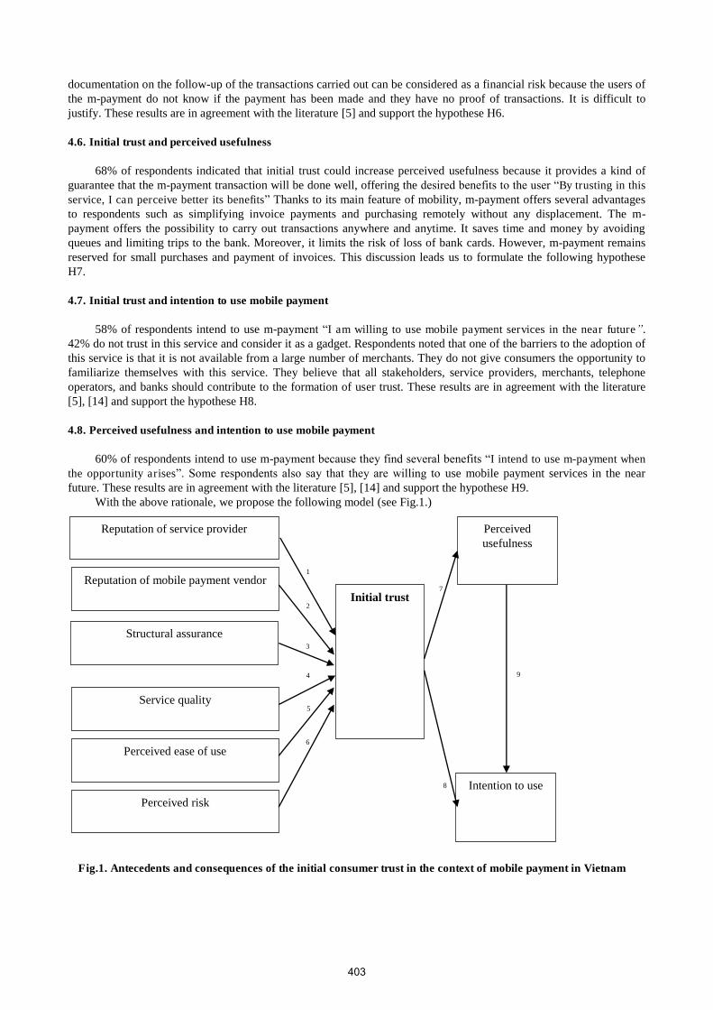
documentation on the follow-up of the transactions carried out can be considered as a financial risk because the users of the m-payment do not know if the payment has been made and they have no proof of transactions. It is difficult to justify. These results are in agreement with the literature [5] and support the hypothese H6.
4.6. Initial trust and perceived usefulness
68% of respondents indicated that initial trust could increase perceived usefulness because it provides a kind of guarantee that the m-payment transaction will be done well, offering the desired benefits to the user “By trusting in this service, I can perceive better its benefits” Thanks to its main feature of mobility, m-payment offers several advantages to respondents such as simplifying invoice payments and purchasing remotely without any displacement. The m-payment offers the possibility to carry out transactions anywhere and anytime. It saves time and money by avoiding queues and limiting trips to the bank. Moreover, it limits the risk of loss of bank cards. However, m-payment remains reserved for small purchases and payment of invoices. This discussion leads us to formulate the following hypothese H7.
4.7. Initial trust and intention to use mobile payment
58% of respondents intend to use m-payment “I am willing to use mobile payment services in the near future”. 42% do not trust in this service and consider it as a gadget. Respondents noted that one of the barriers to the adoption of this service is that it is not available from a large number of merchants. They do not give consumers the opportunity to familiarize themselves with this service. They believe that all stakeholders, service providers, merchants, telephone operators, and banks should contribute to the formation of user trust. These results are in agreement with the literature [5], [14] and support the hypothese H8.
4.8. Perceived usefulness and intention to use mobile payment
60% of respondents intend to use m-payment because they find several benefits “I intend to use m-payment when the opportunity arises”. Some respondents also say that they are willing to use mobile payment services in the near future. These results are in agreement with the literature [5], [14] and support the hypothese H9.
With the above rationale, we propose the following model (see Fig.1.)
Initial trust
Intention to use
Perceived usefulness
Reputation of service provider
Reputation of mobile payment vendor
Structural assurance
Service quality
Perceived ease of use
Perceived risk
1
2
3
4
5
6
7
8
9
Fig.1. Antecedents and consequences of the initial consumer trust in the context of mobile payment in Vietnam
403

5. Managerial implications
Consumer trust is essential to the development of m-payment. Trust is a continuous process that involves both technological and commercial efforts. To build initial trust in m-payment among potential customers, the service providers can cultivate their interest and convince them that their expected benefits will be realized. Various solutions can be considered to create initial consumer trust in the mobile payment context. It is possible to communicate about the measures taken to prevent fraud and ensure the security of payment and the confidentiality of personal data. These measures concern regulatory compliance and control and authentication policies, including electronic signature, anti-virus use, biometric identification, etc. To ensure greater transparency and security, each mobile payment service provider can ensure that an independent body certifies it. Although mobile payment service is easy to use and has high usefulness, but if it is not safe, the customers will not accept it as an alternative service to the traditional payment methods in Vietnam.
One of barriers to consumer trust in m-payment is the lack of traceability. In addition, the proposed applications should be technologically reliable, and accessible at all times. Each mobile transaction carried out should be followed by a confirmation SMS for more transparency. The reputation of service provider/mobile payment vendor strongly affected initial consumer trust. It reflects the company’s history, and suggests its development. Consumers in Vietnam can be familiarized with the m-payment service provider, by providing repeat contact with the company. The operators in the field of payment can encourage the establishment of a community using payments to share experiences with potential customers. Moreover, the ergonomics and practicality of the application make it possible to judge the competence level of service provider. Having an easy to use m-payment application would help to create initial trust. On the other hand, the results of this research have identified many perceived benefits of the use of m-payment such as ubiquity of service, decreased shifts to outlets, no queues, replacement of bank card. Therefore, to develop m-payment service amongs potential customers, the relate service providers in Vietnam can offer free trials and provide attractive premiums to users. They can also encourage the adoption of this service among many merchants, need to partner more proactively with merchants in improving the entire customer experience, both before and after the payment transaction. Other barriers to m-payment adoption are mainly economic, social, cultural and technological contexts in Vietnam.
6. Conclusions and future research
This research enriches the existing literature and contributes to a deeper understanding of consumer behavior in the context of m-payment in Vietnam. The results show that initial consumer trust is explained by factors different from [14] (perceived ubiquity, perceived safety, perceived ease of use, perceived usefulness, and perceived cost). The results also indicate that the reputation of service provider, reputation of mobile payment vendor, and structural insurance, service quality of m-payment, perceived ease of use, and perceived risk are antecedents of initial consumer trust in the mobile payment context. Besides, the results show that initial trust affects perceived usefulness and both have an impact on the intention to use.
However, this research has some limitations that can lead to future research pathways. Due to the exploratory nature of this research, the results cannot be generalized. They were used to explore the factors of initial trust in the m-payment context in Vietnam. In the light of this research, a quantitative study can be carried out to study the hypotheses issued by measuring the impact of each antecedent identified in the explanation of initial trust, as well as the relationship between initial trust and intention to use. In addition, the cultural context as well as the technological context can be integrated in order to better understand the link between initial trust and the intention to use m-payment. Moreover, several theories such as the innovation diffusion theory or the TAM can be examined to explain the adoption of m-payment. Finally, this research can be supplemented by a longitudinal study to observe the evolution of respondents’ attitudes to m-payment in Vietnam.
References
[1] L. Antovski and M. Gusev, “M-payments, Proceedings of The 25th International Conference on Information Technology Interfaces,” Cavtat, Croatia, pp. 16-19 June, 95–100, 2003.
[2] OECD, “Report on Consumer Protection in Online and Mobile Payments,” OECD Digital Economy Papers 204, Aug. 2012.
[3] H. Xin, A. A. Techatassanasoontorn, and F. B. Tan, “Exploring the Influence of Trust on Mobile Payment Adoption,” Pacific Asia Conference on Information Systems, 2013.
[4] Y. A. Au and R. J. Kauffman, “The economics of mobile payments: Understanding stakeholder issues for an emerging financial technology application,” Electronic Commerce Research and Applications, vol. 7, no. 2, pp. 141–164, Jun. 2008.
[5] S. Chandra, S. . Srivastava, and Y. . Theng, “Evaluating the Role of Trust in Consumer Adoption of Mobile Payment Systems: An Empirical Analysis,” Communications of the Association for Information System, p. 1 (27), 561-588., 2010.
[6] A. Shuhaiber and H. Lehmann, “Exploring Customer Trust in B2C Mobile Payments – A Qualitative Study,”
404

International Conference on Mobile Business and Commerce, 2013. [7] K. Marios and H.-S. William, “The development of initial trust in an online company by new customers,”
Information and Management, p. 377–397., 2004. [8] K. K. Kim and B. Prabhakar, “Initial trust and the adoption of B2C e-commerce,” Database for Advances in
Information Systems, p. 50–64., 2004. [9] D. Gefen, E. Karahanna, and D. W. Sraub, “Trust and TAM in online shopping: An integrated model,” MIS
quarterly, p. 51–90., 2003. [10] C. Kim, M. Mirusmonov, and I. Lee, “An empirical examination of factors influencing the intention to use mobile
payment,” Computers in Human Behavior, vol. 26, no. 3, pp. 310–322, May 2010. [11] Z. Liu, Q. Min, and S. Ji, “An Empirical Study on Mobile Banking Adoption: The Role of Trust,” in 2009 Second
International Symposium on Electronic Commerce and Security, 2009, vol. 2, pp. 7–13. [12] B. Sun, C. Sun, C. Liu, and C. Gui, “Research on Initial Trust Model of Mobile Banking Users,” 2017. [13] X. Luo, H. Li, J. Zhang, and J. P. Shim, “Examining multi-dimensional trust and multi-faceted risk in initial
acceptance of emerging technologies: An empirical study of mobile banking services,” Decision Support Systems, vol. 49, no. 2, pp. 222–234, May 2010.
[14] T. Zhou, “The effect of initial trust on user adoption of mobile payment,” Information Development, vol. 27, no. 4, pp. 290–300, Nov. 2011.
[15] H. Xin, A. A. Techatassanasoontorn, and F. B. Tan, “Antecedents of Consumer Trust in Mobile Payment Adoption,” Journal of Computer Information Systems, vol. 55, no. 4, pp. 1–10, Jun. 2015.
[16] P. M. Doney and J. P. Cannon, “An Examination of the Nature of Trust in Buyer-Seller Relationships on JSTOR,” Journal of Marketing, pp. 5–51, 1997.
[17] D. H. McKnight, L. L. Cummings, and N. L. Chervany, “Initial Trust Formation in New Organizational Relationships,” The Academy of Management Review, vol. 23, no. 3, pp. 473–490, 1998.
[18] D. H. McKnight, V. Choudhury, and C. Kacmar, “Developing and Validating Trust Measures for e-Commerce,” Information Systems Research, pp. 334–359, 2002.
[19] P. B. Lowry, A. Vance, G. Moody, B. Beckman, and A. Read, “Explaining and Predicting the Impact of Branding Alliances and Web Site Quality on Initial Consumer Trust of E-Commerce Web Sites,” Journal of Management Information Systems, vol. 24, no. 4, pp. 199–224, Apr. 2008.
[20] F. D. Davis, “Perceived Usefulness, Perceived Ease of Use, and User Acceptance of Information Technology,” MIS Quarterly, vol. 13, no. 3, pp. 319–340, 1989.
[21] E. M. Rogers, Diffusion of Innovations, Fourth Edition, 4th ed. Free Press, 1995. [22] J. S. Benamati, M. Fuller, M. Serva, and J. Baroudi, “Clarifying the Integration of Trust and TAM in E-Commerce
Environments: Implications for Systems Design and Management - IEEE Xplore Document,” IEEE Transactions on Engineering Management 57(3), no. 380–393, 2010.
[23] Y.-H. Chen and S. Barnes, “Initial trust and online buyer behaviour,” Industrial management & data systems, vol. 107, no. 1, pp. 21–36, 2007.
[24] W. Hampton-Sosa and M. Koufaris, “The effect of web site perceptions on initial trust in the owner company,” International Journal of Electronic Commerce, vol. 10, no. 1, pp. 55–81, 2005.
[25] Y. E. Lee and I. Benbasat, “A framework for the study of customer interface design for mobile commerce,” International Journal of Electronic Commerce, vol. 8, no. 3, pp. 79–102, 2004.
[26] D. F. Cox and S. U. Rich, “Perceived Risk and Consumer Decision-Making: The Case of Telephone Shopping,” Journal of Marketing Research, vol. 1, no. 4, p. 32, Nov. 1964.
[27] P. Luarn and H.-H. Lin, “Toward an understanding of the behavioral intention to use mobile banking,” Computers in human behavior, vol. 21, no. 6, pp. 873–891, 2005.
[28] Y. Guangming and M. Yuzhong, “A research on the model of factors influencing consumer trust in mobile business,” in E-Business and E-Government (ICEE), 2011 International Conference on, 2011, pp. 1–5.
[29] E. . Rogers, “Diffusion of innovations,” fourth edition, free Press, 1995. [30] S. L. Jarvenpaa, N. Tractinsky, and L. Saarinen, “Consumer trust in an internet store: a cross-cultural validation,”
Journal of Computer-Mediated Communication, vol. 5, no. 2, pp. 0–0, 1999. [31] B. Suh and I. Han, “Effect of trust on customer acceptance of Internet banking,” Electronic Commerce Research
and Applications, vol. 1, no. 3–4, pp. 247–263, Autumn 2002. [32] Y. Evrard, B. Pras, and E. Roux, MARKET, 4ème édition. Paris, Dunord, 2009.
405
Tran Duc Tuan/ ICYREB 2017 Proceedings
International Conference For Young Researchers In Economics And Business, ICYREB 2017, October 30th 2017 Da Nang, Vietnam
Interface Between Competition Law and Intellectual Property
Law in The Enforcement of Intellectual Property Right in
Vietnam
Tran Duc Tuan *
University of Economics and Law, Vietnam National University HCMC, Vietnam
1. Introduction
Trademarks have vital value to businesses. The survival or prosperity of many businesses depends on trademarks. Therefore, the protection of trademarks against violations is the matter of great importance. Although Vietnam has had the Law on Intellectual property of 2005 (amended and supplemented in 2009) and many legal documents guiding the implementation of this Law. However, the resolution of disputes concerning the protection of trademarks in practice meets difficulties in complex and long lasting procedures, which take a lot of time and efforts; and in different interpretations of problem evaluating approach to the law by contents and its application. Consequently, the resolution of disputes is ineffective. No normative precedent has been created accordingly for entities to follow. Trademark infringements occur frequently.
First of all, this paper generalizes the basic provisions of laws and regulations concerning trademark protection, particularly to some limitations with the comparison to the United States’ provisions. Afterwards, this paper introduces some considerations and solutions regarding legal framework improvement for more efficient trademark protection.
In Vietnam, there are a number of legislation regulating on intellectual propery, namely Constitution 2013, Civil Code 2015, especially Vietnam’s Law on Intellectual property of 2005 (amended and supplemented in 2009) and many guiding documents. The Law on Intellectual Property regulates copyright, copyright related rights, industrial property rights and rights to plant varieties; and the protection of such rights.
Relating to trademark protection, the Lanham Act that was enacted July 5, 1946 is seen as the primary federal trademark statute of law in the United State of America. The Act prohibits a number of activities, namely trademark infringement, trademark dilution and false advertising.
* Tel.: +84 961 807155.
E-mail address: [email protected]
A B S T R A C T
Trademarks generate from creations, are vital “properties” of many businesses. The protection of trademarks with legal provisions not only helps businesses secure their rights and legitimate interests, it also helps consumers get easy to find their desired goods. In our country, although there are a number of legal documents that aim to protect intellectual properties in general and trademarks in particular, however, there are many limitations and weaknesses, especially in legal procedures, solving experience and remedies, compensations that are not sufficient for deterrence.
With the comparison to the United States’ provisions, this paper will give an objective approach to the change of the limitations in protecting intellectual property in Vietnam. Besides, the paper will introduce some recommendations for perfecting Vietnam’s current legal framework in the protection of intellectual property, protecting trademarks accordingly.
Keywords: Trademarks; protection; intellectual properties; Vietnam; the United States.
406

Tran Duc Tuan/ ICYREB 2017 Proceedings
2. Overview of Vietnamese provisions of laws concerning conditions for trademark protection
As above mentioned, in the field of intellectual property protection, Vietnam has a number of legislation, namely Constitution 2013, Civil Code 2015, especially Vietnam’s Law on Intellectual property of 2005 (amended and supplemented in 2009) enacted by the National Assembly; and many guiding documents issued by the Government and Ministries. The Law on Intellectual Property regulates copyright, copyright related rights, industrial property rights and rights to plant varieties; and the protection of such rights.
The Law also express the State’s policies on intellectual property in order to recognize and protect intellectual property rights of organizations and individuals on the basis of harmonizing the interests of intellectual property right holders and the public interest; and to encourage and promote activities of creation and utilization of intellectual assets aimed at contributing to socio-economic development and improving the people’s material and spritual life.
Provisions of laws and regulations on trademark protection is to protect the prestige and reputation of businesses and to help the consumers to recognize the origin of bought goods and services.
2.1. Why it is so important to protect trademarks by provisions of laws
Owing to the prevention of trademark copying, consumers reduce the cost and time in shopping and become potential consumers of companies. Trademarks also distinguish goods and services of businesses from those of their competitors. Hence, businesses shall focus on the investment an innovation to offer high quality products and create well-known trademarks and improve their competitiveness to other business rivals.
2.2. General regulations on trademarks and trademark protection
Clause 16 Article 3 of Law on Intellectual property introduces the definition of trademarks. Accordingly, a trademark means any sign used to distinguish goods and/or services of different organizations or individuals. Those signs are understood as words or images or logos to distinguish goods and services.
However, only trademarks that fulfil the following conditions shall be protected: (i) a sign in visible form of letters, words, pictures, images, including holograms or a combination of such elements, is represented by one or more colors;† (ii) Being capable of distinguishing goods or services of the mark owner from those of other subjects.‡
To be considered as capable of distinguishing the goods or services of other businesses, trademarks must be made up of one or more recognizable, memorable elements or combination of multiple recognizable and memorable elements except for cases specified in Clause 2 Article 74§. Laws and regulations on trademarks are limited to qualitative provisions and could not do otherwise. There are discretions in laws and regulations in order that the applicants, particularly judges, shall make judgment case by case and base on justice without favoritism.
3. Some limitations of trademark protection
3.1. Limitations from the protection of only registered trademarks
In Vietnam, only trademarks with Certificate of Registered trademarks are protected within 10 years (could be renewed). Businesses shall be considered owners of trademarks by the grant of a protection title by the authority or the recognition of the international registration of trademarks by the authority or the ownership of well-known trademarks.
For unregistered trademarks, only well-known and “widely used and recognized” trademarks are protected by law, meanwhile, unregistered trademarks in general are not protected despite of their practical uses. Besides, there are different interpretations of criteria to determine well-known trademarks and widely used and recognized trademarks. Consequently, the illegal copies of trademarks occur frequently, for example, the illegal copies of “5 Cua” trademark in Vung Tau or “Lac Ba Van” trademark in Pho Hue, Ha Noi. Due to those infringements, the most important goal of laws and regulations concerning business and trade, which is to protect interests of consumers, is not achieved. Consumers
† Article 1127 of Lanham Act of the United States provides that: “The term "trademark" includes any word, name, symbol, or device, or any
combination thereof used by a person, or which a person has a bona fide intention to use in commerce and applies to register on the principal
register established by this chapter, to identify and distinguish his or her goods, including a unique product, from those ma nufactured or sold by
others and to indicate the source of the goods, even if that source is unknown.”.
Although this article does not give direct definition, according to the interpretations of the Supreme Court of the United States and the United
States Patent and Trademark Office, trademarks also include sounds and colors (Reference: Find law, U.S. Supreme Court Decides Colors Alone May
be Registered as a Trademark, corporate.findlaw.com; Lynda Zadra-Symes, Sounds, Smells, Shapes and Colors Protection and Enforcement of
Nontraditional Trademarks in the U.S., knobbe.com). ‡ Article 72 of Law on Intellectual property (Integrated document No. 19/VBHN-VPQH dated December 18, 2013). § Article 74 of Law on Intellectual property (Integrated document No. 19/VBHN-VPQH dated December 18, 2013)
407

Tran Duc Tuan/ ICYREB 2017 Proceedings
cannot distinguish the genuine “5 Cua” or “Lac Ba Van” and the first owners of those trademarks. Hence, there are many stores on the roads of our countries with similar trademarks, which makes the consumers difficult to distinguish the “genuine” one. As businesses who create the genuine trademarks are not protected, the creativity of prestigious trademarks shall gradually disappear.
The goal of our country’s current law is that businesses who need protection have the obligation of registration; without registration, they shall take their own responsibility for others’ infringements.
On the other hand, in the United States, to secure and encourage the creativity, the first person/organization who creates or uses the trademarks shall be automatically protected. Particularly, from this protection, the first mentioned person/organization who creates or uses the trademarks shall be entitle to file a lawsuit against those who infringe the trademarks. Hence, in business, people are aware that once a trademark has been used by another, then they are not allowed to use it. With this regulation, consumers are assured that they shall buy their desired goods and services. This is the ultimate goal of law in oder to create standards in the conduct of businesses according to plausibility.
In addition, registered trademarks and unregistered trademarks shall be distinguished by precise signs on goods and products (® for registered trademarks, while sign for unregistered trademarks is ™ and uses ® sign for unregistered goods and products are illegal).
3.2. Registered trademark is just an advantage
In the United States, a trademark could be registered since it came into use. Lanham Act of the United States provides that owner of trademark shall have full rights in the trademark registration and prevention of other uses of his/her trademark.** The protection of trademark does not depend on its registration, but depends on its uses in practical business. To be more detailed, it is whether or not the use of this trademark affixed to the products or services in operational processes and production.†† Both registered trademarks and unregistered trademarks are protected.‡‡
However, registration of trademark shall bring certain advantages including: (i) rights to the national trademark; (ii) automatic recognition as legitimate trademark; (iii) owner are considered genuine owner; (iv) not considered a waiver of protection in case of unused; (v) right to ask the Federal Court in settling disputes concerning infringement of trademark; (vi) “incontestability”. After 05 years of registration without disputes, a trademark shall be considered incontestable (absolutely protected); (vii) warnings to others who could not adduce that they have no idea the trademark has been registered for uses; (viii) strict sanctions are applied in case of violations, including penalties of up to 3 times and criminal sanctions possibly applied to the counterfeit of trademarks for goods and services; (ix) right to ask the United States Customs to prevent importation of violating trademarks.§§
As analyzed above, Vietnamese law only protects registered trademarks and grants protection titles or international registration or well-know trademarks. However, almost protected trademarks are registered trademarks in practice. The authorities are reserved in considering well-known trademarks despite of the precise regulations on well-known trademarks.*** For example, Hao Hao instant noodle trademark has not been recognized as well-known trademark.
Our laws and regulations only focus on violated trademarks without specific provisions and effective enforcement mechanisms to prevent the violations of intellectual properties early. For example, it is difficult for the owner of trademark to ask the customs authorities to prevent others from importing goods with trademark infringement, etc. In addition, criminal sanctions are applicable to the trademark infringement for business purposes (infringed party must prove that the violating goods are used for business purposes)†††. The frequent violations also take roots from the lenient sanctions and complex and complicated procedures.
4. Some recommendations on the improvement of laws on trademark protection
Law regulates principles for all members of society to adhere to and its goal is to maintain the social order and protect the rights and legitimate interests of citizens and create incentives production, business and trade. Provisions of laws on trademarks aim at protecting trademark owners from infringements, thereby promoting innovation, improving quality of goods and products; and helping consumers get easy to find their desired goods.
Trademarks are considered vital to many businesses. Therefore, regulations and “strict enough” measures and sanctions or quick and effective procedures shall make efficient protection to infringed businesses on their rights and legitimate interests.
** Article 1052 and Article 1114 of Lanham Act. †† For more information: Alan S. Gutterman, The Law of Domestic and International Strategic Alliance, page 62. ‡‡ For more information: Section 43 of Lanham Act §§ Subchapter 1 – The principle register, Lanham (Trademark) Act (15 U.S.C. (last undated in November 2005) (source:
http://www.bitlaw.com/source/15usc/). *** Clause 20 Article 4; Article 75 of Law on Intellectual Property ††† Article 171 of Criminal Code
408
Tran Duc Tuan/ ICYREB 2017 Proceedings
With the protection of both registered and unregistered trademarks and appropriate provisions of law on trademark protection of the United States, businesses and trademark owners shall be "secured" in the prevention and handling of violations of intellectual properties. At the same time, this shall create standards in respecting the conduct not to use “what is neither of our ownership, nor from our creativity”.
The provisions of laws and regulations on intellectual property protection in Vietnam is still seen as a starting progress in the country’s legal structure. In addition, experiences in the prevention, protection, handling of violations of intellectual properties in general, and in particular to trademarks of businesses of the competent authorities are limited. The study of regulations and practical experiences other countries, especially those who focus on the importance of protection of intellectual properties secure the creativity such as the United States is necessary in order to improve the legal framework of the home country to meet the international integration, especially with the commitments in the FTAs./.
Preferences
[1] Vietnam’s Constitution 2013 [2] Vietnam’s Civil Code 2015 [3] Vietnam’s Law on Intellectual property of 2005 (amended and supplemented in 2009). [4] Vietnam’s Criminal Code of 1999 (amended and supplemented in 2009). [5] Vietnamese Government’s Decree No. 103/2006/ND-CP detailing and guiding the implementation of a number of
articles of the Law on Intellectual property regarding industrial property. [6] Vietnamese Government’s Decree No. 99/2013/ND-CP on sanctioning of administrative violations in industrial
property (Vietnam). [7] Lanham (Trademark) Act (United States). [8] Brian T. Yeh, Intellectual Property Rights Violations: Federal Civil Remedies and Criminal Penalties Related to
Copyrights, Trademarks, and Patents, https://www.fas.org. [9] Cathleen Flahardy (2012), Gucci win trademark infringement cases against Guess, IC Inside Counsel Website. [10] Kevin G. Cain, The McDonald’s Coffee Lawsuit, http://www.jtexconsumerlaw.com/.
409

Le Hoang Phong, Ho Hoang Gia Bao, Dang Thi Bach Van/ ICYREB 2017 Proceedings
International Conference For Young Researchers In Economics And Business, ICYREB 2017, October 30th 2017 Da Nang, Vietnam
The Impact of Real Exchange Rate and Some Macroeconomic
Factors on Vietnam's Trade Balance: An ARDL Approach
Le Hoang Phonga, * , Ho Hoang Gia Baob, Dang Thi Bach Vanc
aPhD Candidate, School of Public Finance, HoChiMinh University of Economics, HoChiMinh city, Vietnam;
Vice Head of Division and Lecturer at the School of Management, HoChiMinh University of Law, HoChiMinh city, Vietnam. bMaster, Lecturer at the School of Management, HoChiMinh University of Law, HoChiMinh city, Vietnam. cPhD Candidate and Lecturer at the School of Public Finance, HoChiMinh University of Economics, HoChiMinh city, Vietnam.
1. Introduction and literature review
Many governments prefer trade balance surplus as they try to use policies to encourage trade balance. In order for such policies to be effective, it is necessary to examine the factors that can affect trade balance.
The first factor, and presumably the most common one, is exchange rate. Magee (1973) proposed the term “J-curve” relating to the reaction of trade balance when local currency is devaluated: downward in the short-run and upward in the long-run. A famous condition for J-curve existence is the Marshall-Lerner condition, saying that the elasticities of demand of export and import in the long run in absolute values altogether must exceed one. When the Marshall-Lerner condition is satisfied, devaluation of local currency can help a country enjoy surplus trade balance in the long-run (see Wei, 1999). If the Marshall-Lerner condition is not satisfied, devaluation does not result in better trade balance, which is clearly analyzed in Rose (1990) when examining 30 countries with the findings of insignificant or even negative effects of devaluation on trade balance for the majority of the cases.
Many studies in the world have examined the J-curve phenomenon and generated different outcomes. These researches are mainly classified as “elasticity approach” because they treat exchange rate as the main determinant of trade balance as well as try to find the existence of J-curve under the Marshall-Lerner condition. For instance, Bahmani-Oskooee (1985) found that J-curve appeared in Greece, India and South Korea. Similarly, Bahmani-Oskooee and Malixi (1992) also detected the J-curve appearance in Greece, India and South Korea, along with Brazil. Bahmani-Oskooee and Goswami (2003) witnessed J-curve in the trade between Japan and two countries (Germany and Italy). Bahmani-Oskooee, Economidou and Goswami (2006) identified J-curve in the trade between the United Kingdom and two countries including Canada and the United States. Tsen (2011) found the evidence of J-curve in Malaysia. Bahmani-Oskooee and Hegerty (2011) surveyed the export and import of goods between Mexico and the United States and spotted J-curve effects in 7 industries. Almost no trace of J-curve was reported in Wang, Lin and Yang (2012) for the case of China. The sign of J-curve in Australia was discovered in Wijeweera and Dollery (2013). Harvey (2013)
* Corresponding author. Tel.: +84932060629.
E-mail address: [email protected]
A B S T R A C T
This study analyzes the influence of real effective exchange rate, domestic GDP and money supply on Vietnam’s trade balance in both short-run and long-run. We apply Autoregressive Distributed Lag (ARDL) approach on time series data under quarterly basis between the year 2000 and 2015. Money supply positively impacts trade balance in the short-run. In the long-run, however, it has negative and negligible effects. On the contrary, real exchange rate, together with domestic GDP, considerably influences trade balance in the long-run. Real exchange rate causes trade balance to improve in the long-run whilst it worsens trade balance in the short-run. By utilizing impulse response functions, we are able to observe the J-curve occurrence in Vietnam. Besides, we use Cumulative Sum of Recursive Residuals (CUSUM) and Cumulative Sum of Squares of Recursive Residuals (CUSUMSQ) tests to inspect the stability of the trade balance equations.
Keywords: trade balance, real exchange rate, macroeconomic factors, bound test, ARDL model
410

Le Hoang Phong, Ho Hoang Gia Bao, Dang Thi Bach Van/ ICYREB 2017 Proceedings
noticed J-curve in the Philippines. Umoru and Eboreime (2013) provided proof of J-curve in Nigeria whilst Abd-El-Kader (2013) reported similar result for the case of Egypt. Sulaiman and Abdul-Rahim (2014), by analyzing the export and import of forest products, recognized no J-curve in Thailand. Prakash and Maiti (2016) found no sign of J-curve in Fiji. Bahmani-Oskooee, Halicioglu and Hegerty (2016) found no trace of J-curve in Mexico. Bahmani-Oskooee Harvey and Hegerty (2017) discovered the occurrence of J-curve in Japan in the trade between this country and Canada.
Besides exchange rate, there are several other factors influencing trade balance. They are, for example, money supply, domestic GDP (also known as Gross Domestic Product or income or output) and foreign GDP (Waliullah, et al., 2010). There are studies including exchange rate along with money supply, domestic GDP and other factors in their analyses of trade balance. For instance, Duasa (2007) used exchange rate, domestic GDP and money supply to study trade balance of Malaysia and reported obvious positive effect of domestic GDP on trade balance in contrast to the negative effect of money supply on trade balance. Also, the findings of Duasa (2007) showed negligible influence of exchange rate on trade balance as well as unsatisfied Marshall-Lerner condition in Malaysia. This outcome encouraged the utilization of “absorption approach” and “monetary approach” in analyzing trade balance. The absorption approach focuses on domestic GDP, along with foreign GDP, with the explanation that if domestic GDP increases relatively to foreign GDP, domestic residents tend to purchase more foreign goods, which increases import and thus reduces trade balance (Buluswar et al., 1996). Rivera-Batiz and Rivera-Batiz (1989), for an example of the absorption approach, used exchange rate, domestic GDP and foreign GDP as variables to judge their impacts on the trade balance. The monetary approach focuses on money supply and states that when money supply expands, trade balance will decrease (Buluswar et al., 1996). Liew et al. (2003), for instance, reported that nominal exchange rate did not significantly affect trade balance in ASEAN-5 countries. The money supply influenced the trade balance instead.
2. Estimation Methodology
Our empirical model is based on the research of Miles (1979), Krugman and Baldwin (1987), Rivera-Batiz and Rivera-Batiz (1989), Rose (1991), Bahmani-Oskooee and Pourheydarian (1992), Wei (1999), and Duasa (2007). The empirical formula is as follows:
1 2 3 . t t t t tTB REER GDP M
(1)
In formula (1), TB is trade balance. REER stands for real effective exchange rate and shows the relationship between the value of VND and the currencies of main trading partners of Vietnam. REER is used for testing J-curve and Marshall-Lerner condition (elasticity approach). GDP is the Gross Domestic Product, and M is the money supply (M2) of Vietnam. With the use of GDP and M, the formula implies absorption and monetary approaches in analyzing the trade balance.
There are some methods for examining the cointegration. Among them, Engle and Granger provided a method focusing on residuals (Engle and Granger, 1987), while Johansen proposed a technique using maximum likelihood (Johansen, 1988). However, both of them demanded that the order of integration of variables is the same. To overcome this restriction, Pesaran et al. and Pesaran and Shin introduced and developed an approach called Autoregressive Distributed Lag (ARDL) (see Pesaran et al., 1996; Pesaran and Shin, 1998). Namely, ARDL approach can deal with I(0), I(1) or mutually cointegrated variables. Although ARDL does not need unit root test, it should be used to check for the cointegration of variables at I(2) (Nkoro and Uko, 2016). In addition, ARDL method can bring some benefits. For instance, it is suitable for small sample size with excellent properties (Al-Malkawi et al., 2012; Pesaran and Shin, 1998). Furthermore, when endogenous variables are in the model, the long-term estimates will be free from bias (Pesaran, Smith, and Shin, 2001). Additionally, both short-run and long-run effects can be measured from only one equation (Pesaran and Shin, 1998).
We take the advantage of the above benefits when using ARDL method in this research to evaluate the determinants of trade balance of Vietnam. The formula (1) is transformed into:
1
1,1
2 3 4
2, 3, 4,0 0 0
1 1 2 1 3 1 4 1 .
p
t i t ii
p p p
j t j k t k l t lj k l
t t t t t
TB TB
REER GDP M
TB REER GDP M
(2)
The first step of the ARDL procedure is checking the occurrence of cointegration among the variables in the model, which is also known as bound test. The hypotheses are H0:
1 2 3 4 0 (no cointegration) and H1:
1 2 3 4 0 . We base on the calculated F-statistics and the critical values under I(0) and I(1) assumptions provided in Pesaran (1997) to test these hypotheses. Particularly, H0 is rejected in case the F-statistics exceeds the upper bound of the critical value, implying that there is long-term relationship among variables. H0 cannot be rejected when the F-statistics is smaller than the lower bound of the critical value. The conclusion regarding H0 is not clear if
411

Le Hoang Phong, Ho Hoang Gia Bao, Dang Thi Bach Van/ ICYREB 2017 Proceedings
the F-statistics lies between the lower and the upper bounds of the critical values. Next, we apply Schwarz Bayesian Criteria (SBC) to select the optimal lag orders of the regressors in equation (2).
We also run diagnostic tests including serial correlation, functional form, normality, and heteroscedasticity to find out whether there are issues with our model or not. Another essential test implemented to evaluate the stability of residuals in the model is Cumulative Sum (CUSUM) and Cumulative Sum of Squares (CUSUMSQ).
Additionally, we run the impulse response function, a tool of ECM, to observe how trade balance changes in connection with the exchange rate movement.
3. Estimation Sample and Data
The data we use in this paper is retrieved from Direction of Trade Statistics (DOTS) and International Financial Statistics (IFS) of IMF. The time series data is on quarterly basis from the first quarter of the year 2000 to the fourth quarter of the year 2015. Every variable takes the form of index with the value of the base period 2000(1) set to 100 and then transformed into natural logarithm. Namely, the variable REER is the natural logarithm of real effective exchange rate index calculated from taking geometric average of the nominal exchange rates between VND and each of the currencies of 22 countries accounting for nearly 90% of Vietnam’s total trade with the respective weights as the percentage of trade volume of each country in the trade with Vietnam. The real exchange rates are achieved from the bilateral exchange rates between VND and each of the foreign currencies and then adjusted by the respective consumer price indices of relevant countries. GDP is the natural logarithm of the real GDP index of Vietnam. M is the natural logarithm the money supply index of Vietnam. TB is the natural logarithm of Vietnam’s trade balance index where trade balance is measured by the export value divided by the import value.
4. The empirical results
Although ARDL approach does not need unit root test, it should be used to check the cointegration of variables at I(2) to ensure the validity of F-test because F-test may be misleading in case the variables are I(2) (Nkoro and Uko, 2016).
The results of Augmented Dickey-Fuller (ADF) test (proposed by Phillips and Perron (1988)) and the Phillips-Perron (PP) test (proposed by Phillips and Perron (1988)) are shown in table 1, which is used to find out the order of integration of variables.
Table 1.Results of unit root test using ADF and PP tests
Variable ADF test statistic PP test statistic
TB ‒6.003339*** ‒5.904744***
REER ‒1.982632 ‒2.270239
GDP ‒8.307229*** ‒8.315656***
M 1.547039 8.026318
D(TB) ‒17.52242*** ‒28.91540***
D(REER) ‒5.395644*** ‒5.364851***
D(GDP) ‒15.70245*** ‒26.84714***
D(M) ‒7.081134*** ‒7.172602***
Note: ***, ** and * represent the significance levels 1%, 5% and 10%.
D is the first difference of variables.
The results of ADF and PP tests indicate that TB and GDP are I(0), whilst REER and M are I(1). For cointegration test, bound tests (with F-statistics) are utilized to look for the cointegration among variables in
the model. The calculated F-statistics are compared with the critical values of upper and lower bounds at 3 levels including 1%, 5%, 10% which are provided by Pesaran and Pesaran (1997, p.478).
Table 2.The results of bound tests
Lag order 1 2 3 4 5 6
F- 4.78911 3.19838 4.36373 1.9851 1.35562 1.29381
412

Le Hoang Phong, Ho Hoang Gia Bao, Dang Thi Bach Van/ ICYREB 2017 Proceedings
statistics 4** 4 1* 70 0 6
Note: ** and * represent the significance levels 5% and 10%.
From table 2, we observe that 2 F-statistics values are larger than the upper bounds critical values. We, therefore, reject the hypothesis H0. This indicates that cointegration occurs among variables in our model. In other words, there is long-term relationship among variables in our model.
Concerning ARDL model estimation, we calculate the optimal lag length for all variables by employing Schwartz Bayesian Criterion (SBC). The outcome is ARDL(1,2,2,1) and it is shown in table 3.
Table 3.Estimation results of ARDL model (ARDL(1,2,2,1); dependent variable is TB)
Variable Coefficient t-statistic
1tTB 0.24827** 2.3373
tREER 0.41049 0.72584
1tREER ‒1.2293 ‒1.4069
2tREER 1.3966** 2.5340
tGDP ‒0.46434*** ‒5.9987
1tGDP ‒0.095818 ‒1.0976
2tGDP ‒0.45490*** ‒6.3201
tM 0.87706* 1.9542
1tM ‒0.92044** ‒2.0341
constant 5.8645*** 4.1592
2R
0.61224
DW - statistics
1.7878
SE of Regression
0.079393
Diagnostic tests
:A Serial Correlation : F(1,51)= 1.0919 [0.301]
B : Functional Form : F(1, 51)= 0.66053 [0.420]
C : Normality : ChiSQ(2)= 2.3961 [0.302]
: F(1, 60)= 0.51695 [0.475]D : Heteroscedasticity
Note: ***, ** and * represent the significance levels 1%, 5% and 10%.
A: Lagrange multiplier test of residual serial correlation
B: Ramsey's RESET test using the square of the fitted values
C: Based on a test of skewness and kurtosis of residuals
D: Based on the regression of squared residuals on squared fitted values.
Table 3 indicates that the overall goodness of fits (Adjusted R-squared) is 0.61224. The diagnostic tests are as we expected. Specifically, there are no problems with our model relating to serial correlation, functional form, normality, and heteroscedasticity.
To examine the stability of residuals of ARDL model, we use the Cumulative Sum of Recursive Residuals
413

Le Hoang Phong, Ho Hoang Gia Bao, Dang Thi Bach Van/ ICYREB 2017 Proceedings
(CUSUM) and Cumulative Sum of Squares of Recursive Residuals (CUSUMSQ) tests. The results of CUSUM and CUSUMSQ statistics are illustrated in Figure 1 and 2. We can observe that the residuals are stable at 5% significance level. Residuals
The straight lines represent critical bounds at 5% significance level
-5
-10
-15
-20
-25
0
5
10
15
20
25
3 13 23 33 43 53 63 64
Fig. 1.The CUSUM graph of Recursive Residuals
The straight lines represent critical bounds at 5% significance level
-0.5
0.0
0.5
1.0
1.5
3 13 23 33 43 53 63 64
Fig. 2.The CUSUMSQ graph
The results of diagnostic tests and residuals tests show that our ARDL model are valid for estimating short-run and long-run coefficients.
Concerning the short-run impacts, current money supply and the real GDP of the previous quarter positively affect the current trade balance. Also, current real GDP and the real exchange rate of the previous quarter negatively affect the current trade balance. We can say that the decrease of VND value compared to foreign currencies leads to the decline of trade balance in short-run.
Table 4.The result of Error Correction derived from ARDL(1,2,2,1) with the dependent variable TB
Variable Coefficient t-statistic
tREER 0.41049 0.72584
1 tREER ‒1.3966** ‒2.5340
tGDP ‒0.46434*** ‒5.9987
1 tGDP 0.45490*** 6.3201
tM 0.87706* 1.9542
constant 5.8645*** 4.1592
1tEC
‒0.75173*** ‒7.0768
2R
0.74006
6867 3503
57702 7 8014
t -1 t -1 t -1 t -1
t -1
EC TB= 0.7 × REER + 1. × GDP
+ 0. × M . × constant
414

Le Hoang Phong, Ho Hoang Gia Bao, Dang Thi Bach Van/ ICYREB 2017 Proceedings
Note: ***, ** and * represent the significance levels 1%, 5% and 10%.
The result from table 4 shows that the coefficient of 1tEC is negative and significant at 1% significance level,
which gives another proof of cointegration relationship of variables. 1 0.75173 t
EC indicates that 75% of the short-run disequilibrium is adjusted to the equilibrium state in the long-run.
Concerning the long-run impacts, the coefficients of variables are given in table 5. It can be observed that real GDP and money supply negatively influence trade balance. On the contrary, real exchange rate positively influence trade balance. In other words, in the long-run, devaluation of VND enhances trade balance.
Table 5.The estimation results in the long-run based on ARDL approach with dependent variable TB
Variable Coefficient t-statistic
tREER 0.76867** 2.0917
tGDP ‒1.3503*** ‒5.8005
tM ‒0.057702** ‒2.2462
Constant 7.8014*** 5.5578
Note: ***, ** and * represent the significance levels 1%, 5% and 10%.
In addition, to observe how devaluation affects trade balance of Vietnam as time passes, or, in other words, to judge the J-curve effect in Vietnam, we employ impulse response function formed on the ECM model.
14
-.05
.00
.05
.10
2 4 6 8 10 12 14
Response of LTB to LREER
Response of LREER to LREER
Source: Authors’ computation.
Fig. 3.Response of TB to REER (Response to Cholesky One S.D. Innovations).
It can be witnessed from figure 3 that the trade balance goes down when devaluation happens. Particularly, trade balance reaches its lowest value after 2 quarters from the devaluation. As time passes, the trade balance tends to increase. About 5 quarters from the devaluation, real exchange rate positively impacts the trade balance. The trade balance is stable from the 9th quarter. From the above graph in figure 3, we can detect the occurrence of J-curve in Vietnam.
5. Conclusion
There are several factors that can have impacts on trade balance. Different studies focus on different variables. In our research, we examine the effects of GDP, real exchange rate and money supply on the trade balance of Vietnam. We find that the effect of money supply on trade balance is positive in short-run but negative in long-run. Although, in the long run, the impact of money supply on trade balance is insignificant, the impact of Vietnam’s GDP on trade balance is significant.
Regarding the impacts of real exchange rate on the trade balance of Vietnam, there are considerable short-term and long-term influences. The short-term influence causes the trade balance to fall in the first 2 quarters and then rise from that time onward the 5th quarter. Between the 5th and 9th quarter, despite some minor fluctuations, the trade balance continues on the upward trend. The long-term influence of real exchange rate is favorable.
Our findings show that the trade balance deteriorates in the short-run and improves in the long-run. This movement of trade balance resembles the “J-curve effect”. Furthermore, our findings confirm the usefulness of devaluation in case of Vietnam. In other words, devaluation is a possible choice for Vietnam’s macroeconomic policy maker to encourage trade balance in the long-run. Along with devaluating VND, Vietnam government should pay attention to the impacts of money supply, GDP and other determinants of trade balance so as to increase the effectiveness of the overall policy in supporting the trade balance.
415

Le Hoang Phong, Ho Hoang Gia Bao, Dang Thi Bach Van/ ICYREB 2017 Proceedings
References
[1] Abd-El-Kader, E.S.M. (2013). Is the J-Curve Effect observable for Egypt economy?. Journal of Economic Cooperation and Development, 34, 91-118.
[2] Al -Malkawi, H.A.N., Marashdeh, H.A. and Abdullah, N. (2012). Financial Development and Economic Growth in the UAE: Empirical Assessment Using ARDL Approach to Co-integration. International Journal of Economics and Finance, 4(5), 105-115.
[3] Bahmani-Oskooee, M. (1985). Devaluation and the J-curve: some evidence from LDCs. The Review of Economics and Statistics, 67, 500-504.
[4] Bahmani-Oskooee, M., Economidou, C. & Goswami, G. (2006). Bilateral J-curve between the UK vis-à-vis her major trading partners. Applied Economics, 38(8), 879-888.
[5] Bahmani-Oskooee, M., Halicioglu, F. & Hegerty, S. W. (2016). Mexican bilateral trade and the J-curve: An application of the nonlinear ARDL model. Economic Analysis and Policy, 50, 23-40.
[6] Bahmani-Oskooee, M., Harvey, H., & Hegerty, S. W. (2017). The Japanese trade balance and asymmetric effects of yen fluctuations: Evidence using nonlinear methods. Economic Modelling, 55, 382-393.
[7] Bahmani-Oskooee, M. & Hegerty, S. W. (2011). The J-curve and NAFTA: evidence from commodity trade between the US and Mexico. Applied Economics, 43(13), 1579-1593.
[8] Bahmani-Oskooee, M. & Goswami, G. (2003). A disaggregated approach to test the J-Curve phenomenon: Japan versus her major trading partners. Journal of Economics and Finance, 27(1), 102-113.
[9] Bahmani-Oskooee, M., & Malixi, M. (1992). More evidence on the J curve from LDCs. Journal Of Policy Modeling, 14(5), 641-653.
[10] Bahmani-Oskooee, M. and Pourheydarian, M. (1992). What are the long-run determinants of the U.S. trade balance. Journal of Post Keynesian Economics, 15, 85–97.
[11] Buluswar, M.D., Thompson, H. & Upadhyaya, K. P. (1996). Devaluation and the Trade Balance in India: Stationarity and Cointegration. Applied Economics, 28, 429-432.
[12] Dickey, D. A., and Fuller, W. A. (1979). Distribution of the Estimators for Autoregressive Time Series with a Unit Root. Journal of the American Statistical Association, 74, 427–31.
[13] Duasa, J. (2007). Determinants of Malaysian Trade Balance: An ARDL Bound Testing Approach. Global Economic Review, 36(1), 89 -102.
[14] Engle, R. F., and C. W. J. Granger. (1987). Co-Integration and Error Correction: Representation, Estimation, and Testing. Econometrica 55, 251-276.
[15] Harvey, H. (2013). Exchange rate sensitivity in the Philippines: Does the J-curve exist?. Asian Journal of Business and Management Sciences, 2(10), 51-61.
[16] Johansen, S. (1988). Statistical Analysis of Cointegration Vectors. Journal of Economic Dynamic and Control, 12, 231-254.
[17] Krugman, P. R., and Baldwin, R. E. (1987). The persistence of the U.S. trade deficit. Brookings Papers on Economic Activity, 18(1), 1–55.
[18] Liew, K. S., Lim, K. P., and Hussain, H. (2003). Exchange Rates and Trade Balance Relationship: The Experience of ASEAN Countries. International Trade. 0307003, Econ WPA.
[19] Magee, S. P. (1973). Currency contracts, pass through and devaluation. Brooking Papers on Economic Activity, 1, 303–325.
[20] Miles, M.A. (1979). The effects of devaluation on the trade balance and the balance of payments: some new results. Journal of Political Economy, 87(3), 600–620.
[21] Nkoro, E., and Uko, A. K. (2016). Autoregressive Distributed Lag (ARDL) cointegration technique: application and interpretation. Journal of Statistical and Econometric Methods, 5(4), 63-91.
[22] Pesaran, M. H., and Pesaran, B. (1997). Microfit 4.0 (Window Version). New York: Oxford University Press. [23] Pesaran, H. M., & Shin, Y. (1998). An Autoregressive Distributed Lag Modeling Approach to Cointegration
analysis. In: Storm, S. Editor, Econometrics and Economic Theory in the 20th Century, The Ragnar Frisch Centennial Symposium, UK, Cambridge University Press.
[24] Pesaran, M. H., Shin, Y., and Smith, R. J. (1996). Bounds Testing Approaches to the Analysis of Level Relationships. DEA Working Paper 9622, Department of Applied Economics, University of Cambridge.
[25] Pesaran, M.H., Smith, R.J., and Shin, Y. (2001). Bounds Testing Approaches to the Analysis of Level Relationships. Journal of Applied Econometrics, 16, 289-326
[26] Phillips, Peter C., and Perron, P. (1988). Testing for a Unit Root in Time Series Regression. Biometrika 75, 335–346.
[27] Prakash, K., & Maiti, D. (2016). Does devaluation improve trade balance in small island economies?. The case of Fiji. Economic Modelling, 55, 382-393.
[28] Rivera-Batiz, K. L., and Rivera-Batiz, L. (1989). International finance and open economy macroeconomics. New York: Macmillan Publishing.
[29] Rose, A. K. (1991). The role of exchange rates in a popular model of international trade: Does the ‘Marshall-
416

Le Hoang Phong, Ho Hoang Gia Bao, Dang Thi Bach Van/ ICYREB 2017 Proceedings
Lermer’ condition hold?. Journal of International Economics, 30(3–4), 301-316. [30] Rose, A. K. (1990). Exchange Rates and the Trade Balance: Some Evidence from Developing Countries.
Economics Letters, 34, 271-75. [31] Sulaiman, C. & Abdul-Rahim, A.S. (2014). J-curve Effect and Thailand’s Trade in Forest Products: ARDL
Bounds Testing. World Applied Sciences Journal, 29(1), 150-155. [32] Tsen, W. (2011). Bilateral Trade Balances: Evidence from Malaysia. Asian Economic Journal, 25(2), 227-244. [33] Umoru, D. and Eboreime, M.I. (2013). The J-curve hypothesis and the Nigerian oil sector: The ARDL bounds
testing approach. European Scientific Journal, 9(4), 314-327. [34] Waliullah, M. K, Kakar, R. and Khan, W. (2010). The Determinants of Pakistan’s Trade Balance: An ARDL
Cointegration Approach. The Lahore Journal of Economics, 15(1), 1-26. [35] Wang, C., Lin, C., & Yang, C. (2012). Short-run and long-run effects of exchange rate change on trade balance:
Evidence from China and its trading partners. Japan And The World Economy, 24(4), 266-273. [36] Wei, W.X. (1999). An empirical study of the foreign trade balance in China. Applied Economics Letters, 6(8),
485-490. [37] Wijeweera, A. & Dollery, B., (2013). J-curve disparity between the goods sector and the services sector: evidence
from Australia. Applied Economics Letters, 20, 452-456.
417

Vo Thi Phuong/ ICYREB 2017 Proceedings
International Conference For Young Researchers In Economics And Business, ICYREB 2017, October 30th 2017 Da Nang, Vietnam
Customer Behaviour of Using Internet Banking in The Fourth
Industrial Revolution: A Study of Vietnam
Vo Thi Phuong*
Faculty of economics, Da Nang University – Campus in Kon Tum, Vietnam
A B S T R A C T
The primary purpose of the paper is to investigate customer behaviour of using internet banking in Vietnam with application of digital technology to support comprehensive financial promotion in the fourth industrial revolution. Customers are aware of the benefits of internet banking but we still concerned about safety and security of internet banking. Therefore, decide to use internet banking services, customers have to go through the analysis process of choice. The study of consumer behavior with internet banking services will be significant for both banks as well as for consumers. This research model is based on using the orginal beliefs of Technology acceptance model (TAM) perceived usefulness and perceived ease of use and introducing new variables such as: security risk, financial risk, privacy risk, awareness, computer self-efficacy and resistance to change. Final, author give some conclusion and implication. This article helps commercial banks to adjust customer-oriented policies and improve the efficiency of internet banking services.
Keywords: customer behaviour; internet banking; technology acceptance model
1. Introduction
The significant role of banks in the economics development is undeniable. The economic health nowadays depends more than ever, on the soundness of the banking system. In most countries, banking is an important area for the economy of each country and governments interest particularly. It is one of the most closely monitored sectors in the economy, especially in developing countries.
IB is a service provided early in the world. In 1980 this service was provided by a bank in Scotland (Tait, Fand Davis, 1989). However, this service was officially provided by banks in 1990 (Daniel, 1998). The advent of internet banking has completely changed the relationship between customers and banks. Developing alongside traditional channel to carry out transactions, thanks to modern distribution channels, through automated teller machines (ATM), internet, telephone. Bank and customer do not face to face with transactions. Internet banking services are growing rapidly. Recognizing the importance of IB services, banks are constantly diversifying their services, increasing customer convenience, reducing transaction time, improving employee productivity, reducing transaction costs. Improve the quality of service to best satisfy the diverse needs of our customers.
Consumer behavior is a complex study field that includes: studies of attitudes, actions, consumer reactions. Consumer behavior research helps business managers to predict and identify trends in consumer behaviors that build business strategies, develop products, distribute products and services. in line with customer needs.
Internet banking (IB) provides a very convenient method of managing personal finances since it is easily accessible 24 hour/seven days/week. For corporate, sophisticated cash management packages offered via IB. It provides real time information, enabling timely fund management decisions. Simultaneously, banks can more easily retain existing customers as well as providing services to customers without constraints of time and place. The aggressive competition among banks operating in Vietnam will ultimately lead to a race to improve service in order to attract customers. This race will make the launch of online banking services inevitable. In fact, some banks in Vietnam are already providing online banking. However, online banking remains immature in Vietnam, and is little utilized. This study thus examines the drivers of intention to use online banking among bank customers in Vietnam. Because
* Tel.: +84904009038
E-mail address: [email protected]
418

Vo Thi Phuong/ ICYREB 2017 Proceedings
customers only use online banking once they develop intentions to do so the question becomes one of identifying what motivates customers to intend to use online banking.
2. Research model and hypotheses
Internet banking means any user with a personal computer and a browser can get connected to his bank -s website to perform any of the virtual banking functions. In internet banking system the bank has a centralized database that is web-enabled. All the services that the bank has permitted on the internet are displayed in menu. Any service can be selected and further interaction is dictated by the nature of service. The traditional branch model of bank is now giving place to an alternative delivery channels with ATM network. Once the branch offices of bank are interconnected through terrestrial or satellite links, there would be no physical identity for any branch. It would a borderless entity permitting anytime, anywhere and anyhow banking. The services provided by banks that only exist on the internet.
This model is a combination of variable factors that affect the acceptance of technology use, it analyzes beliefs, attitudes, behaviors, intentions, etc. Many studies have applied TAM model to analyze the customer behaviour, especially in the applications of different types of information systems. Therefore, author used the TAM model to explain users’ intention to use IB and the following hypothesis is proposed.
Studies [9;4,11] indicated that the greater the perceived usefulness of using IB services and greater the utility to the customer. Moreover the studies done in Egypt reinforced the importance of perceived usefulness as a significant variable in the use of IB [13]. Reference [23] examined the perceived ease of use, perceived usefulness and trust as factors affecting IB adoption in Egypt for a sample of 103 respondents. The results revealed that perceived usefulness, perceived ease of use and trust are significant factors for using IB. Moreover, in the study [1] they are concerned with an empirical investigation of factors that could affect a successful internet banking services adoption such as perceived ease of use, perceived usefulness, compatibility, trust, awareness on internet banking adoption in Jordan. 517 data is used for structural equation modeling analysis and confirmatory factor analysis. The results revealed that perceived usefulness, perceived ease of use as and trust were found to have significant positive effect on internet banking adoption.
Perceived usefulness is defined as the extent to which an individual believes that using IB will enhance their benefit. The important of perceived usefulness has been widely recognized in the field of electronic banking [3,2,10]. Previous researches have consistently argued that there is a positive relationship between perceived usefulness of mobile banking intention and attitude toward mobile banking and mobile banking usage [3;8]. For example, Chau and Lai's (2003) examined the contributing factors towards the consumers' adoption of IB and determined that perceived usefulness was found as an important factor in fostering a positive attitude towards accepting the IB services. Moreover, many researches reaffirmed that the perceived usefulness is an important factor to refine the technology acceptance model (TAM) [3;8]. Therefore, Perceived usefulness will influence their intention to accept and use e-banking services, this complies with Chau and Lai's (2003) study, in which they examined the contributing factors towards consumer's adoption of IB and found that perceived usefulness (PU) has a positive effect on the attitude towards accepting the IB services. Alsamydai (2014) found that the perceived usefulness (PU) has a positive effect on the attitude, intention and usage of mobile banking services. Accordingly the following hypothesis is proposed.
H1: Perceived usefulness has a significant positive impact on user’ intention to use internet banking Several studies indicated the impact of perceived ease of use on intention to use IB and pointed out that the ease of
use is significantly positive impact on user’ intention to use IB. A experimental study in Saudi to examine the different variables that may impact to use IB include: demographic variables (gender, age, academic specialty, number of years in organization), service quality, security, loyalty, relative advantage, complexity trialability and observability compatibility. The results showed that complexity and privacy are the highest impact variables on user’ intention to use IB [2].
Perceived ease of use is one aspect of the technology acceptance model. It is defined as the degree to which an individual beliveds that using a particular information technology system would be free of effort.
Davis (1989) argued that perceived ease of use also influences, in a significant way, the attitude of the individual through two main mechanisms: self-efficacy and instrumentality. The Self- efficacy term, which was introduced by Lee (2009), explains that the more the system is easy to use, the greater should be the user's sense of efficacy.
Perceived ease of use is one of the two key variables in the technology acceptance model. Perceived ease of use will lead to attitude toward use, behavioral intention to use and actual use. PEOU also influences the second key variable, perceived usefulness. According to references [4;9] have studied the relationship between perceived ease of use and perceived usefulness. Perceived ease of use can also contribute in an instrumental way in improving a person's performance. Due to the fact that the user will have to deploy less effort with a tool which is easy to use, they will be able to spare efforts to accomplish other tasks [4]. Accordingly, the following hypothesis is proposed.
H2: Perceived ease of use has a significant positive impact on user’ intention to use internet banking
419

Vo Thi Phuong/ ICYREB 2017 Proceedings
2.1. Risk determinants and perceived usefulness
Security is one of the most discussed issues around e-banking. Security has been a major barrer that affects customer to turnover from traditional banking to IB in most of country. The lack of security is one of the factors that have been identified in most studies as affecting the growth and development of IB. Security risks against IB can be through network and data transaction attacks and unauthorized account access. Both fraud and hacker attack could lead to users’ monetary loss and violate users’ privacy [24; 25].
A study in Tunisia using a sample of 253 respondents for responding: 95 were internet bank users, 158 were internet bank non users. Factor analyses and regression technique are employed to study the relationship. The model tested the demographic characteristic, convenience, prior internet knowledge, security perceived risk, information on online banking. The result indicate that use of IB is influenced most strongly by convenience perceived risk, security and prior internet knowledge [22].
Reference [16] measure service quality of IB in Saudi Arabia with a list comprising 64 variables influence quality of IB users’perception. The three factorial groups were named in accordance with the appropriate criterial: efficiency and security, fulfilment and responsiveness. The results of the factor analysis in terms of factor name reveals that efficiency and security is the most influencing factor in users evaluation of service quality. Security, which involves protecting users from the risk of fraud and financial loss.
In a study used quantitative method to measure users’ risk perception in Chinese. The paper classified eight risk dimensions impact on intention to use IB such as: security, financial, privacy, time, psychological, social, physical and performance. A total of 510 participants agreed to participate in this study with 504 valid questionnaires. The results show that security, performance, privacy and financial risks are considered the most important in delaying Chinese’s usge from traditional banking to IB. The security is perceived as the most important dimensions [11]. Accordingly the following hypothesis is proposed.
H3: Security risk has a significant negative impact on the perceived usefulness Privacy refers to the protection of data that are collected either with or without the knowledge of the users
throught their communication with the IB system [23]. Reference [11] clarified that the privacy risk is the risk of losing personal control. Users are concerned that their personal information may be manipulated or misused without their knowledge. Further, reference [19,22] studied users adoption of e-banking services in Malaysia in the light of ten determinants derived from extant literature, namely convenience, accesssibility, feature availability, bank management and image, security, privacy, design, content, speed, and fees and charges. The survey results indicate privacy and recurity are the major sources of dissatisfaction. Results also reveal that privacy; security and convenience factors play an important role in determining the users’ acceptance of e-banking services with respect to different segmentation of age group, education level and income level.
Reference [21] pointed out that if customers belief that the banks protect their personal information, detect fraud and transactions are secure, they are more likely to using IB for their transaction.
Reference [12; 17] stressed that privacy issues relating to IB have created significant barriers to the up-take of IB. That as a mojor concern of most IB users, fraud and hacking not only cause the losses of their money, but also violate their privacy. Rotchanakitumnuai and Speece (2003) pointed out that it creates a negative effect if customers’ personal information is unsecured and there is the possibility that their privacy can be revealed in the virtual environment. Therefore, it is important for IB service providers to ensure that IB activities are safe and their customers’ privacy are well-protected. In addition, perceived worries of revealing personal information may produce adverse feelings that could negatively affect users perceived usefulness of using IB [11,21]. Accordingly the following hypothesis is proposed.
H4: Privacy risk has a significant negavtive impact on the perceived usefulness Financial risk is the potential for monetary loss due to transaction error or bank account misuse is considered a
financial risk. Reference [16;18] showed that many users have concerns of losing money while performing transactions or transferring money over the internet. For that reason, customers prefer to trade directly at a bank.
Reference [11] indicated that there is a positive relationship between privacy concerns and financial risk lead to conclude that the more users worry about losing their privacy data, the more they are concerned about financial loss. Moreover, reference [6] indicated that privacy risk vegatively affect users’ perceived usefulness of using IB therefore, the same could apply for financial risk and the following hypothesis is proposed.
H5: Financial risk has a significant negavtive impact on the perceived usefulness
2.2. Behavioral determinants and perceived ease of use
A study indicated that awareness of IB services is important through effective use of flyers, brochures, web pages. If users have enough information about IB services, how to use IB services, they awareness of IB site web user friendly and easy to access, they can use this service more. The adoption of IB are determined by the level of awareness that a user has about IB and its possible benefits [14].
Reference [4] study adopt TAM and difference variables to test IB acceptance in Saudi Arabia with a sample of
420
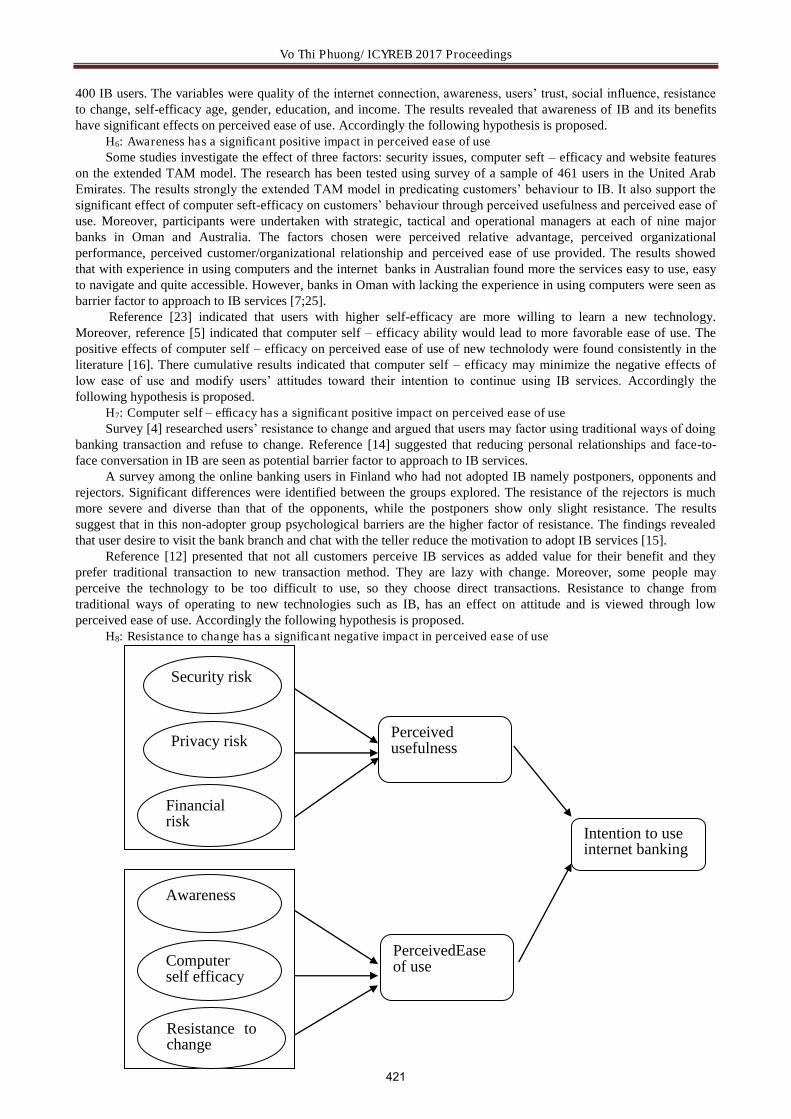
Vo Thi Phuong/ ICYREB 2017 Proceedings
400 IB users. The variables were quality of the internet connection, awareness, users’ trust, social influence, resistance to change, self-efficacy age, gender, education, and income. The results revealed that awareness of IB and its benefits have significant effects on perceived ease of use. Accordingly the following hypothesis is proposed.
H6: Awareness has a significant positive impact in perceived ease of use Some studies investigate the effect of three factors: security issues, computer seft – efficacy and website features
on the extended TAM model. The research has been tested using survey of a sample of 461 users in the United Arab Emirates. The results strongly the extended TAM model in predicating customers’ behaviour to IB. It also support the significant effect of computer seft-efficacy on customers’ behaviour through perceived usefulness and perceived ease of use. Moreover, participants were undertaken with strategic, tactical and operational managers at each of nine major banks in Oman and Australia. The factors chosen were perceived relative advantage, perceived organizational performance, perceived customer/organizational relationship and perceived ease of use provided. The results showed that with experience in using computers and the internet banks in Australian found more the services easy to use, easy to navigate and quite accessible. However, banks in Oman with lacking the experience in using computers were seen as barrier factor to approach to IB services [7;25].
Reference [23] indicated that users with higher self-efficacy are more willing to learn a new technology. Moreover, reference [5] indicated that computer self – efficacy ability would lead to more favorable ease of use. The positive effects of computer self – efficacy on perceived ease of use of new technolody were found consistently in the literature [16]. There cumulative results indicated that computer self – efficacy may minimize the negative effects of low ease of use and modify users’ attitudes toward their intention to continue using IB services. Accordingly the following hypothesis is proposed.
H7: Computer self – efficacy has a significant positive impact on perceived ease of use Survey [4] researched users’ resistance to change and argued that users may factor using traditional ways of doing
banking transaction and refuse to change. Reference [14] suggested that reducing personal relationships and face-to-face conversation in IB are seen as potential barrier factor to approach to IB services.
A survey among the online banking users in Finland who had not adopted IB namely postponers, opponents and rejectors. Significant differences were identified between the groups explored. The resistance of the rejectors is much more severe and diverse than that of the opponents, while the postponers show only slight resistance. The results suggest that in this non-adopter group psychological barriers are the higher factor of resistance. The findings revealed that user desire to visit the bank branch and chat with the teller reduce the motivation to adopt IB services [15].
Reference [12] presented that not all customers perceive IB services as added value for their benefit and they prefer traditional transaction to new transaction method. They are lazy with change. Moreover, some people may perceive the technology to be too difficult to use, so they choose direct transactions. Resistance to change from traditional ways of operating to new technologies such as IB, has an effect on attitude and is viewed through low perceived ease of use. Accordingly the following hypothesis is proposed.
H8: Resistance to change has a significant negative impact in perceived ease of use
Security risk
Privacy risk
Financial risk
Awareness
Computer self efficacy
Resistance to change
Perceived usefulness
PerceivedEase of use
Intention to use internet banking
421

Vo Thi Phuong/ ICYREB 2017 Proceedings
Figure 1. Research framework
Research model is shown in Figure 1. It is a simple TAM model, testing perceived usefulness and perceived ease of use impact in intention to use internet banking without external variables.
3. Research methodology
The author uses qualitative and quantitative methods, interviews to analyze some of the relevant content in the article. Assessing the reliability of the scales employed and a structured equation modeling (SEM) and statistical package analysis moment of structures (AMOS version 22) are used.
3.1. Sample
A reliable sample frame representing all bank users in Vietnam, is not easily abtainable and cost-effective to be done in this research. Therefore, questionnaires are distributed at 3 city areas: Hanoi capital, Danang city and Hochiminh city. At the end of the investigation with 560 bank customers agreed to participate in the study. After removing 11 invalid questionnaires, I had a usable sample of 536 qualified questionnaires with a reasonably high response rate of about 95.71%. Therefore the sample size is consistent with this recommendation (Hair & ect, 2013). Before distributing the questionnaire, all participants were assured that their participation was voluntary and anonymity was guaranteed. The age of them ranged from 18 up.
Figure 2. The age of participant
3.2. Measures
The questionnaire design based on the model and qualitative research. Participants surveyed through the questionnaire marked the most appropriate option in 5-point likert scale. Answers ranged from 1 “strongly disagree” to 5 “strongly agree”. The scale of variables in the model from the overview of studies, in-depth interviews and corrected to the conditions in Vietnam. The questionnaire used in this research consistend of three parts: first part, description of IB services provided by commercial banks. The second part, demographic information from each respondent. Third, questions to assess the research variables. Table 1 show the variables used and their sources.
Table 1. The research variables used and their sources
Variables Encoding Items
1 Intention to use internet banking ITUIB 4
2 Perceived usefulness PU 5
3 Perceived ease of use PEOU 3
4 Security risk SR 3
422

Vo Thi Phuong/ ICYREB 2017 Proceedings
5 Privacy risk PR 3
6 Financial risk FR 3
7 Awareness AW 3
8 Computer self – efficacy CSE 4
9 Resistance to change RTC 3
Table 2. Descriptive statistics and reliability coefficients
Variables Mean Standard deviation Cronbach’s alpha
ITUIB 15.62 2.71 .814
PU 11.96 2.85 .715
PEOU 11.25 3.04 .791
SR 16.23 3.49 .711
PR 9.42 3.71 .701
FR 10.64 3.91 .762
AW 10.67 4.63 .812
CSE 13.91 2.62 .701
RTC 20.76 3.96 .815
Evaluating the reliability of the scale via Cronbach’s alpha coefficients it satisfied three conditions: Cronbach’s alpha coefficients > 0.6; Corrected Item-Total Correlation > 0.3 but < Cronbach’s alpha coefficients (Hair & ect, 2013). Table 2 present descriptive statistics and reliability coefficients.
4. Data analysis and results
To investigate the relationships between different possible explanatory variables to intention to use IB, Pearson correlation coefficients were calculated (shown in Table 3). To test the theoretical model a structures equation modeling (SEM) and the statistical package analysis momemt of structures (AMOS version 22) are used in this study.
Table 3. Correlation matrix for varibles
Variable 1 2 3 4 5 6 7 8 9
ITUIB 1
PU .408** 1
PEOU .319** .649** 1
SR -.413** -.679** -.604** 1
PR -.489** -.587** -.394** .853** 1
FR -.319** -.845** -.634** .584** .674** 1
AW 431** .609** .717** -.456** -.319** -.331** 1
CSE .395** .586** .729** -.497** -.313** -.324** -.342** 1
RTC -.518** -671** -.674** .685** .608** .531** .531** -.598** 1
SEM models indicated the relationships among variables using one or more regression equation. A collection of such equations is referred to as a structural equation model. All of them are significant. The table show that perceived usefulness and perceived ease of use have a positive and significant effect on intention to use. However, perceived ease of use has slight higher impact than perceived usefulness. Moreover, financial risk has the highest negative significant impact among all factors on user’s perceived usefulness (β = -0.625, SE = .078, t-value = 5.24). Furthermore, computer self-efficacy has the highest significant impact on the perceived ease of use (β = -0.307, SE = .065, t-value = 4.18).
423

Vo Thi Phuong/ ICYREB 2017 Proceedings
Table 4. Goodness of fit indices
Indices Research results
Adjusted goodness of fit (AGFI) 0.96
Comparative fit index (CFI) 0.94
Normed fit index (NFI) 0.91
Goodness of fit (GFI) 0.97
Root mean square error of approximation (RMSEA) 0.065
Table 4 show goodness of fit indices compatible with the recommended values. As follows: AGFI, CFI, NFI, GFI indices with 1 indicating maximum fit and RMSEA indices with values 0.08 indicating good fit (Hair & ect, 2013). Therefore, the model is suitable for the market.
5. Conclusion and implication
IB offers a lot of advantage over traditional banking services for banks and customers. For banks, save costs, reach new market segments, improve operational efficiency, reputation and competitiveness of banks. Intention to use the consumer is a very important factor in the success of the bank. So, banks should study appropriate solutions to improve the use of IB services.
First, when IB was born, there will be 3 customer groups. The first group will adapt and use service immediately because they appreciate the time and want to save them. The second group of clients has a slower adaptation because they are concerned about the safety of the service. For this customer group, we have to make sure they understand the safety and reliability of this service and at the same time use a number of promotions and incentives to encourage them to try out the product. The final customer group will have the slowest adaptation. These customers, after seeing the other two groups, will use them gradually. It is important for banks to guide and create trust for customers with these services. The key here is to change the habits of customers so they realize that IB is very convenient. The bank should carry out the campaign introduces the characteristics of the IB system, its benefits and how to use it. Increased awareness of IB benefits, diversified service offering, service improvement.
Second, enhancing awareness about benefits of IB through different marketing and advertising strategies. It should take advantage of the media, social networking and marketing transmitted to raise awareness of the usefulness of the IB service. Banks can launch brand communities through different social media platforms where they can post detailed information about IB or customers who are satisfied with IB can share their positive experiences with other less experienced users. The bank should carry out the campaign introduces the characteristics of the IB system, its benefits and how to use it. Increased awareness of IB benefits, diversified service offering, service improvement. Banks should make their customer more aware of their service quality and the regulations governing IB. This can be achieved by having seminars and exhibitions to allow customers to evaluate their new innovation. Next, the customers’ level of trust in IB was found to have a significant effect on the customer’s decision to adopt this innovation and for the continued use of this innovation. So, banks should try to earn customers’ trust.
Third, banks need to build easy-to-see, easy-to-use interfaces including users not proficient in technology. The interface has a role to interact directly with the user, so it should be designed to be compatible and suitable for each type of device. There are specific instructions on the level the security level, rules and regulation related to security and things to note when using IB service. Hot line guide using service 24 hour.
Four, a important feature in any IB solution is to ensure the authenticity and security of the transaction. Decrease security, privacy and financial risk banks have and build secure firewalls to avoid hacker attack, developing methods for strengthening encryption, and authenticating websites. Work with one online security firms to support and handle any security problems. Application identification solution and access management system in online banking security; Application of blockchain technology in improving the efficiency of banking operations. Currently, banks can apply a variety of methods to solve security such as: virtual keyboards, one time password, two-factor authentication or hardware token, smart card with digital signature. Major banks around the world often use secure and transactional solutions based on a public key infrastructure, with the participation of hardware lockers, digital signature cards or smart cards. Compared with other solutions, e-signature security solution can solve simultaneously four important issues: (i) user authentication; (ii) confidentiality of transaction information, (iii) data integrity; (iv) refusal. In addition, banks need to invest in infrastructure development to create favorable conditions for clients, train qualified staff have got good skill to handle customer's problems.
Outside, administrators to build and completion the legal directories systems as to follow work at the business on the network and be used to solve the solution between bank with customer when happen attempt to transaction on the internet bank service. Building the rules and logical rule for the electronic writer, electronic signature and certificate certificate.
424

Vo Thi Phuong/ ICYREB 2017 Proceedings
References
[1] Al -Majali, M., & Nik Kamariah Nik Mat. (2001). Modeling the antecedents of internet banking service adoption (IBSA) in Jordan: A structural equation modeling (SEM) approach. Journal of internet banking and commerce, 16(1), 1.
[2] Al -Ghaith, W., Sanzogni, L., & Sandhu, K. (2010). Factors influencing the adoption and usage of online services in Saudi Arabia. The electronic journal on information systems in development countries, 40(1).
[3] Alsamydai, M. J., Doma, M., Dojani, Saad, G., & Yaseen. (2014). Factors influence the use of e-promotion means in Jordanian business organization. International journal of management science, Vol 13, No 16, 433-445.
[4] Al -Somali, S. A., Gholami, R., & Clegg, B. (2009). An investigation into the acceptance of online banking in Saudi Arabia. Technovation, 130-141.
[5] Ariff, M. S., Min, Y. S., Zakuan, N., Ishak, N., & Ismail, K. (2013). The impact of computer seft eficacy and technology acceptance model on behavioral intention in internet banking system. Review of integrative business and economics research, 2(2), 587-595.
[6] Bashir, I., & Madhavaiah, C. (2015). Consumer attitude and behavioural intention towards internet banking adoption in India. Journal of Indian business research, 7(1), 67-102.
[7] Chau, P. Y., & Lai, V. S. (2003). An empirical investigation of the determinants of user acceptance of internet banking. Journal of organizational computing, 13920, 123-145.
[8] Davis, F. D. (1989). Perceived usefulness perceived ease of use and user acceptance of information technology. MIS Quarterly, Vol 13, No 13, 319-340.
[9] Ezzi, S. W. (2014). A theoretical model for internet banking: beyond perceived usefulness and ease. Archives of business research, 2 (2), 31-46.
[10] Hair, J. F., Ringle, C. M., & Sarstedt, M. (2013). Edittorial - partial least squares structural equation modeling: Rigorous applications, better results and higher acceptance. Long Range Planning 46(1-2), 1-12.
[11] Harridge-March, S., Lifen Zhao, A., Hanmer-Lloy, S., Ward, P., & Goode, M. M. (2008). Perceived risk and Chinese consumers' internet banking services adoption. International journal of bank marketing, 26(7), 505-525.
[12] Hemandez, J., Mazzon, J. (2007). Adoption of internet banking: Proposition and implementation of an integrated methodology approach. International journal of bank marketing, 25, 72 – 88.
[13] Kamel, S. & Hassan, A. (2003). Assessing the introduction of electronic banking in Egypt using the technology acceptance model. Annals of cases on information technology, 5, 1-26.
[14] Jaruwachirathanakul, B., & Fink, D. (2005). Internet banking adoption strategies for a developing country: the case of Thailand. Internet research, 295-311.
[15] Laukkanen, P., Sinkkonen, S., & Laukkanen, T. (2008). Consumer resistance to internet banking: postponers, opponents and rejectors. International journal of bank marketing, 26(6), 440-455.
[16] Lee, M. C. (2009). Factors influencing the adoption of internet banking: An integration of TAM and TPB with perceived risk and perceived benefit. Electronic commerce research and applications, 8(3), 130-141.
[17] Littler, D., Melanthiou, D. (2006). Customer perceptions of risk and uncertainty and the implications for behavior towards innovative retail services: The case of internet banking. Journal of retailing and consumer services, 13, 431 – 443.
[18] Maditinos, D., Chatzoudes, D., & Sarigiannidis, L. (2013). An examination of the critical factors affecting consumer acceptance of online banking: A focus on the dimensions of risk. Journal of systems and information technology, 15(1), 97-116.
[19] Maditinos, D., Chatzoudes, D., & Sarigiannidis, L. (2013). An examination of the critical factors affecting consumer acceptance of online banking: A focus on the dimensions of risk. Journal of systems and information technology, 15(1), 97 - 116.
[20] Rotchanakitummuai, S., Speece, M. (2003). Barriers to internet banking adoption: A qualitative study among corporate customers in Thailand. International journal of bank marketing, 21(6/7), 312 – 323.
[21] Riffai, M., Grant, K., & Edgar, D. (2012). Big TAM in Oman: Exploring the promise of online banking, its adoption by customers and the challeges of banking in Oman, international journal of information management, 32(3), 239 – 250.
[22] Sohail, M. S., & Khaikh, N. (2008). Internet banking and quality of service perspectives from a developing nation in the Middle East. Sohail, Sadiq M and Shaikh, 58 - 72.
[23] Sum Chau, V., & Ngai, L. W. (2010). The youth market for internet banking services: perceptions, attitude and behaviour. Journal of services marketing, 24 (1), 42-60.
[24] Wang, Y. S., Wang, Y. M., Lin, H., & Tang, T. (2003). Determinants of user acceptance of internet banking: an empirical study. International journal of service industry management, 14(5), 501 - 519.
[25] Yavas.U, & Benkenstein.M. (2001). An assessment of SERVQUAL in Germany. J. Int. Sell. Sales Mange 7 (1), 15 - 23.
425

Hoang Thi Mai Khanh, Nguyen Anh Tuan/ ICYREB 2017 Proceedings
International Conference For Young Researchers In Economics And Business, ICYREB 2017, October 30th 2017 Da Nang, Vietnam
Determinants of Sustainability Reporting Quality: An Empirical
Research on Vietnamese Listed Companies
Hoang Thi Mai Khanh*, Nguyen Anh Tuan
University of Economics and Law, National University Ho Chi Minh City 3 Quarter, Linh Xuan Ward, Thu Duc Dist. Ho Chi Minh City,
700000 Vietnam
1. Introduction
Sustainability reporting is increasingly popular on a global scale due to broader awareness of sustainable development in terms of environment and business. Sustainability reporting benefits greatly companies by building trust with stakeholders which helps reduce reputational risks, improving internal management and decision-making process as well as information system, progressing vision and strategy that helps companies address strengths and weaknesses, reducing compliance costs and creating competitive advantages (GRI, The benefits of sustainability reporting, 2014).
A research conducted by Nielsen Vietnam in 2015 revealed that 86% of Vietnamese consumers would be willing to pay a premium to buy products or services from sustainable development companies which was the highest percentage among South East Asia countries (Nielsen Vietnam, 2015). This suggests the enhancement of customers’ attention regarding sustainable issues, which encourages corporations to engage in sustainability practices. As a results, sustainability reporting is expected to enjoy the widespread popularity among businesses, given increasing demands of stakeholders in corporate responsibilities information and efforts towards economic, environmental and social developments.
Since there has been very limited amount of empirical research on sustainability reporting practices in Vietnam, this study is undertaken with the purpose of providing some preliminary empirical evidence on which factors influence sustainability reporting quality.
2. Literature review and developed hypotheses
2.1. Sustainability
The World Commission on Environment and Development (often known as Brudtland committee) held by United Nations in the 1980s published its reports – Our common future (the Brudtland report) in 1987 which provides a widely-known definition of sustainability. Sustainability is defined as ‘ensuring that development meets the needs of the present without compromising the ability of future generation to meet their own needs’ (United Nations, 1987).
* Hoang Thi Mai Khanh. Tel.: +84982464279.
E-mail address: [email protected]
A B S T R A C T
This research aims at providing some empirical evidence on determinants of sustainability reporting quality in Vietnam. A sample of 99 sustainability reports published by listed companies for the year of 2016 was obtained and further analysed by employing content analysis method to construct sustainability reporting index for each company. The study used a wide range of variables to examine hypotheses developed. Proportion of female non-executive directors, gross profit margin, financial services and utilities sector dummy variable, export status are found to significantly positively associate with sustainability reporting quality whereas chairwoman characteristic and profit before tax margin strongly associate in the opposite direction.
Keywords: Sustainability; sustainability reporting quality; GRI; gender diversity; financial performance
426

Hoang Thi Mai Khanh, Nguyen Anh Tuan/ ICYREB 2017 Proceedings
However, this definition has been criticised to be vague (Szekely & Knirsch, 2005). International Institute for sustainable development (IISD, 1992) suggested a more comprehensive definition of sustainability as “adopting business strategy and activities that meet the needs of the enterprise and its stakeholders today while protecting, sustaining and enhancing the human and natural resources that will be needed in the future”. Szekely and Knirsch (2005) also proposed a more detailed explanation of sustainability as achieving and sustaining “economic growth, shareholder value, prestige, corporate reputation, customer relationships, quality of products and services” while pursuing business ethics and maintaining accountabilities with other stakeholders. Despite the differences of various definitions, they share the same view in emphasising the responsibilities of organisations in all three pillars: economic, social and environmental, rather than focusing on economic aspect only.
2.2. The Global Reporting Initiatives (GRI)
To report voluntarily on sustainability practices, companies can adopt numerous approaches, among which GRI is the most widely used. Despite not a mandatory reporting framework, over 75% of G250 companies applied GRI guidelines to prepare their sustainability reports (Sherman & DiGuilio, 2010).
‘GRI is an international independent organization that helps businesses, governments and other organizations understand and communicate the impact of business on critical sustainability issues such as climate change, human rights, corruption and many others’ (GRI, About GRI, 2017).
With the vision of creating a future which sustainability is integrated into organisational decision-making process, GRI aims at developing a reporting framework that sustainability reports become regular and comparable as financial reporting. The principles for defining reporting quality include: balance, comparability, accuracy, timeliness, clarity and reliability (GRI, 2015).
In general, a sustainability report consists of two parts: general standards disclosure and specific standards disclosure. The former includes disclosure relating to strategy and analysis, organisational profile, identified material aspects and boundaries, stakeholder engagement, report profile, governance, ethics and integrity. The latter includes disclosure relating to 6 categories: economic, environmental, labour practices and decent work, human rights, society and product responsibility.
2.3. Theoretical framework
2.3.1. Legitimacy theory
Unsurprisingly, legitimacy theory has been extensively used to explain organisational behaviours in relation to social and environmental accounting areas (Matthew, 2004). The term ‘legitimacy’ is defined by Suchman (1995) as “a generalized perception or assumption that the actions of an entity are desirable, proper, or appropriate within some socially constructed system of norms, values, beliefs, and definitions’.
General speaking, organisations in their existence receive supports from surrounding stakeholders, hence in turn they should benefit the society where they base or at least do not threaten or destroy the existence of the society and natural environment (Adriana & Ion, 2013). Between the organisations and society, there is a ‘social contract’ that constrains organisations’ activities within boundaries set by society. Legitimacy theory suggests that organisations will always want to ensure that their operation is within society’s boundaries and perceived as legitimate by outsiders.
Organisation’s activities perceived by the society will have to be reported in the way that meets social expectations. Failing to do so or having activities that counter social and moral standards would result in organisation being punished and criticised by the whole society even end up in close-down (Adriana & Ion, 2013).
2.3.2. Stakeholder theory
The term “stakeholder” was first used officially as “all groups on which an organisation is dependent for its survival” at a conference held by Stanford Research Institute in 1963 (Maria B-Boucher; Jacob D. Rendtorff, 2016). From that time, stakeholder was used frequently in management area with varying definitions. However, the most all-inclusive definition was defined by Freeman (1984) as “an individual or group of individuals which can affect or be affected by the achievement of organizational objectives”.
In general, stakeholder theory suggests that organisations are accountable to a wide range of stakeholders due to their (potential) significant impacts on the society that cannot be only responsible to shareholders. With regard to corporate social responsibility, the interest of shareholders or some stakeholders should not be attained at the sacrifice of other stakeholders’ interest, however, it would be unlikely that the organisation can satisfy all legitimate stakeholders simultaneously, therefore it will have to manage all stakeholders appropriately and effectively (Becker-Olsen & Moynihan, 2013).
427

Hoang Thi Mai Khanh, Nguyen Anh Tuan/ ICYREB 2017 Proceedings
2.3.3. Agency theory
Agency theory concerns the agency problem arising from the separation between ownership and management of a company, which management (the agent) may act in their own interests rather than the ones of shareholders (the principals).
In Encyclopaedia of Corporate Social Responsibility, Menyah (2013) stated that “Agency theory provides a framework for determining the appropriate contractual arrangement (implicit or explicit) that aligns the interests of a principal and an agent who are engaged in a cooperative activity in the presence of hidden action and hidden information which the principal cannot observe or can do so at a cost, but may still not be able to prevent opportunistic behaviour by the agent”.
The agency problem resulted from the separation between the ownership and management was first officially identified by Berle & Means (1932) that the achievement of organisational objective of maximising shareholders’ value may be deteriorated by self-interested managers who make decisions that may conflict with owners’ interests.
Regarding corporate social responsibility, Friedman (1970) suggested that managers following socially responsible activities by using organisational resources were acting on their own interests at the expense of shareholders’ benefits. Nonetheless, Baron (2001) proposed that shareholders could motivate their managers by providing some incentives to embark on CSR activities, which may create competitive advantages for the company hence benefit shareholders in long-term prospective.
2.4. Literature review and hypothesis development
Previous studies have indicated that sustainability reporting quality may be influenced by various determinants which can be grouped as follows:
Industrial characteristics The legitimacy theory has been deployed substantially to examine and explain the relationship between industry
affiliation and sustainability practices. Dissanayakea et al.(2016) found that banking and finance industry had considerably higher disclosure than other industries in Sri Lanka, hence being in sensitive industry sectors (such as chemical, pharmaceutical, oil and gas industry) would not be a determinant of sustainability reporting. Similarly, Chena et al.(2015) stated that CSR reporting may be general and relevant across industries since there was no evidence on significant difference in CSR disclosure of automotive, chemical, forest and paper, metal products and health care industry.
In contrast, Dilling (2010) found that corporations in high-profile sectors would actively publish sustainability reports, especially companies in energy and production industry. Similarly, Legendre & Coderre (2013) pointed out that high-risk industry sector firms were more likely to provide sustainability reports with higher GRI application level and independent assurance to ease pressures from their stakeholders and media concerns. In their study, Kansala et al. (2014) discovered that companies operating in steel and metal-non ferruos industry had the highest sustainability reporting scores while the ones belonging to construction and constracting and pharmaceutical industry had the lowest scores. Kuzeya & Uyarb (2016) suggested that firms operating in manufacturing industry had tendency to engage more actively in sustainability reporting than service-industry firms due to the fact that environmental impacts and health issues would be more significant to manufacturing corporations. Wuttichindanon (2017) concluded that firms in property industry appeared to provide less sustainability reports than the ones in other industries.
Therefore, the first hypothesis is examined to address whether sustainability reporting quality varies among different industry sectors in Vietnam:
H1: There are variations in sustainability reporting quality across industry sectors. Financial performance Financial performance of an organisation can be assessed through various measures: return on assets, return on
equity, profitability margin, sales growth, liquidity ratios, leverage, etc. Whether sustainability performance is associated with corporate financial status and vice versa is controversial issue which is subject to concern of not only management, investors but also academic researchers and governments.
Some studies suggest that there is no or weak obvious links between financial performance and sustainability practices. Kuzeya & Uyarb (2017) discovered irrelevant relationship between profitability, free cash flows, growth opportunities and sustainability reporting practices although they found weak negative association of leverage and significant negative association of current ratio with sustainability reporting practices. Financial performance (profitability, leverage) is not a significant determinant of CSR disclosure, since stakeholders (including shareholders) can exert their power over the firms to force them to engage in and report on CSR activities regardless their economic status (Wuttichindanon, 2017).
On the other hand, some studies found significant correlation between financial performance and sustainability reporting practices. Better financial performance firms can invest excessive capital in sustainable development hence enhance sustainability performance (Ziegler & Schröder, 2010). Profitable companies may have extra resources to conduct and report on CSR activities which in turn potentially creates competitive advantages and facilitates short-term
428
Hoang Thi Mai Khanh, Nguyen Anh Tuan/ ICYREB 2017 Proceedings
economic targets achievement (particularly ROE) (Chena, Feldmannb, & Tang, 2015). McGuinnessa et al. (2017) revealed significant negative association between leverage and CSR ratings, they also identified contrary relationship between social ratings and lagged financial performance. Dilling (2010) confirmed the connection between higher profit margin and G3 sustainability reports while Kansala et al. (2014) concluded that profitability determined CSR disclosure in a positive way. Similarly, Lourenço & Branco (2013) suggested that corporations with higher sustainability reporting performance had larger return on equity than lower ones.
Due to debatable results on the relationship between financial performance and CSR, sustainability reporting practices, this research does not predict the direction but speculate the existence of the association in Vietnam. This brings to the second hypothesis tested:
H2: There is an association between financial performance and sustainability reporting quality Board gender diversity The report on Women in decision-making highlighted the relationship between corporate ethical behaviour and
number of female directors (European Commission, 2012). Davies Report (2011) argued that larger proportion of female directors on boards would enhance board’s
performance through more active contributions of female NED compared to their male counterparts, conscientious preparation for board meetings and willingness to challenge strategies. Moreover, greater female representation could help the board achieve better corporate governance by monitoring strategy, committing to ethical standards and concerning more on stakeholder issues such as employee, customer satisfaction, sustainable development and corporate social responsibility.
The representation of women on boards could bring diversity due to distinctive values of female directors compared to male directors, they are more stakeholder-oriented than their male counterparts (Adams, 2015). Furthermore, greater number of women on boards can positively associate with ethical and social compliance because of female sensitivity towards these matters (Isidro & Sobral, 2014). Thus creating a legitimate expectation that there would be a relationship between board gender diversity and sustainability reporting practice since diverse boards could increase the transparency and accuracy of financial reports, hence reduce information asymmetry and improve stakeholder engagements (Gul, Hutchinson, & Lai, 2013).
Al -Shaer & Zaman (2016) found a significant positive relationship between sustainability reporting quality and board gender diversity measured by five alternatives: number of female directors on boards, percentage of boards’ female directors, number of independent female directors, Shannon index of diversity and Blau index of diversity. By categorising into two groups: small and large sized companies, the paper also discovered that while all board gender diversity measures of the small sized companies were significantly associated with sustainability reporting quality, two measures (number of female directors and number of independent female directors) were significantly associated for large sized firms (although all of them had positive associations with sustainability reporting quality).
The presence of women on boards could help firms become socially responsible by encouraging the adoption of environmentally friendliness and good corporate governance practices (Nadeem, Zaman, & Saleem, 2017). The research also found that gender diversity positively associated with corporate sustainability practices in Australia.
Non-executive female directors The UK’s Higgs report on the role and effectiveness of non-executive directors highlighted the importance of non-
executive directors who have no managerial responsibility in assuring boards’ balancing influence and reducing conflicts of interest between principals (shareholders) and their agents (management). Arguably, non-executive directors are believed to play a key role in challenging and scrutinising the strategy implemented by executive directors due to their wider perspectives. Besides the positive relation of women’s proportion on boards to board’s effectiveness, female directors are likely to have similar impact possessing by independent directors (Adamsa & Ferreira, 2009). Al -Shaer & Zaman (2016) found a significant positive association of number of independent female directors with sustainability reporting quality. As a result, it is worth to expect that independent and non-executive female directors may require more effort on sustainability practices which eventually benefits shareholders in long-term and in a sustainable way.
Female leadership While the chairman is responsible for leading the board of directors, the chief executive director (CEO) leads the
management team. The UK’s Higgs report emphasised the vital role of chairman in ensuring the effectiveness of the whole board as well as individual directors by directing boards’ operation to strategic matters, actively engaging with shareholders, allocating sufficient time for controversial issues discussions. On the other hand, CEO’s roles are more likely to involve in running the business, implementing board’s resolutions, assuring organisational objectives achievement and liaison with stakeholders. Due to these characteristics, it would be a mistake not to address the influence of corporate leadership on companies’ strategies and policies on sustainable development including related public disclosures. McGuinnessa et al. (2017) found that companies led by chairwoman and female CEO tend to have higher corporate social responsibility rating. Furthermore, the effect of female leadership still significantly remained after board gender diversity measures had been controlled.
This research is to examine whether board gender diversity influences the quality of sustainability reporting among Vietnamese listed firms. Therefore, the following hypotheses will be tested:
429
Hoang Thi Mai Khanh, Nguyen Anh Tuan/ ICYREB 2017 Proceedings
H3a: There is a positive association between board gender diversity and sustainability repor ting quality H3b: Non-executive female directors have a positive association with sustainability reporting quality. H3c: Female leadership has a positive relationship with sustainability reporting quality.
3. Research methodology
3.1. Sample and data collection
The primary objective of this study is to identity whether factors hypothesised have any association with quality of sustainability reports. As a result, only reports exclusively named ‘sustainability report’ or ‘sustainable development report’ are subject to the assessment. Since sustainability reporting is relatively new in Vietnam, there is no database or statistics about the quantity of published reports nor list of publishing organisations. In order to gather all available sustainability reports, websites and annual reports of all companies listed on two domestic stock exchanges were scanned with relevant key words. The reporting period is for the financial year ended 31 December 2016 (or earlier but not prior to 1 January 2016). Finally, there were 99 companies meeting the requirements. These reports were subsequently analysed through a scoring scheme.
All financial data was retrieved from data stream of Thomson Reuters EIKON, while non-financial one was collected manually from annual reports, corporate governance reports, corporations’ website, Vietstock.com and data stream.
3.2. Sustainability reporting scoring scheme and sustainability reporting index
Content analysis has been extensively employed in this research to assess the quality of sustainability reporting. Clarkson et al. (2008) adopted GRI guidelines to construct an index to assess environmental disclosures in related reports. Similarly, in this research the construction of a sustainability reporting index is implemented which eventually generates indices facilitating the comparability of sustainability reporting quality across companies. However, before that, a scoring scheme must be applied to calculate scores (which represents quality and completeness) of sustainability reports.
Both Clarkson et al. (2008) and Dissanayakea et al. (2016) adopted GRI guidelines for their scoring framework due to its superior characteristics such as international standardised guidelines that can be flexibly applied to various types of organisation through the usage of each reporting indicator; improving the transparency, relevance, completeness, accuracy of sustainability reports; ensuring reports representing a balanced picture regarding different dimensions, etc. Because of these benefits, this study adopts G4 sustainability reporting guidelines as scoring scheme based on reporting indicators to measure reporting practices in Vietnam. Furthermore, some adaptions were brought in to make scoring scheme suitable to Vietnamese corporate reporting practices. The scoring scheme is demonstrated in appendix 1.
Generally, most of companies in the population have sustainability reports included in their annual reports, which are subject to scoring scheme. However, companies who publish stand-alone sustainability reports will have their separate reports marked individually not the ones included in annual reports or integrated reports (as they are often in brief and referred to stand-alone ones). To maintain the comparability and fairness, only information disclosed in sustainability reports is subject to this scoring scheme, which means information referred to elsewhere in annual reports or other reports will be not taken into account even it is mentioned in G4 reference.
In Vietnam, circular 155/2015/TT-BTC issued by Ministry of Finance has its section 6 in appendix 2 guiding the preparation of report on related impact of the company on the environment and society, which is used by many firms (especially SMEs) as a framework to produce sustainability reports. With the purpose of enabling the comparability of sustainability reporting indices across companies’ practices, this research prescribes a minimum disclosure based on reporting requirement of section 6 appendix 2 with the addition of some indicators (G4-1, G4-18, G4-24, G4-25, G4-26, G4-27, G4-DMAs) that is similar to the way used by Dissanayakea et al. (2016). The purpose of the prescription is to provide a fixed number of weights towards the total score in arriving at the index which would established comparable standards. For example, if a company fulfil fully all prescribed indicators and other indicators (that company chose to disclose), its sustainability reporting index will be 1 (the absolute index); however, if the firm fails to disclose prescribed indicator although it fulfils fully other indicators, its index will be lower than 1. It would be inappropriate to force all companies to disclose all indicators because of the principle-based nature of guidelines with comply or explain practice. That adaption seems to be fit with Vietnamese current circumstances since it is still necessary to have a threshold to evaluate the quality of sustainability reports. These prescribed indicators are present in appendix 2.
Reporting indicators not prescribed in appendix 2 will be treated as ‘voluntary’ or ‘additional’ disclosure which is subject to scoring scheme accordingly with corresponding weights when the company includes them in their reports.
The scoring scheme does differentiate between the important indicators and unimportant ones. Except for prescribed indicators, the ones belonging organisational profile, report’s profile, G4-22 and G4-23 are treated as unimportant since they are usually included in annual reports. The important indicators individually have maximum
430

Hoang Thi Mai Khanh, Nguyen Anh Tuan/ ICYREB 2017 Proceedings
Hypo-thesis
Variable group
Variable Measurement
H1 Industry ch_ph Dummy variable, which: 1: company belongs to chemical, pharmaceutical industry sector 0: otherwise
const Dummy variable, which: 1: company belongs to construction industry sector 0: otherwise
condis Dummy variable, which: 1: company belongs to consumer discretionary industry sector 0: otherwise
energy Dummy variable, which: 1: company belongs to energy industry sector 0: otherwise
fin Dummy variable, which: 1: company belongs to financial services industry sector 0: otherwise
real Dummy variable, which: 1: company belongs real estate industry sector 0: otherwise
trans Dummy variable, which: 1: company belongs transportation industry sector 0: otherwise
uti Dummy variable, which: 1: company belongs utilities industry sector 0: otherwise others Dummy variable, which: 1: company does not belong to any above
industry sector 0: otherwise H2 Financial
performance roa Return on assets roe Return on equity pbt_margin Profit before tax margin gross_margin Gross profit margin eps Earnings per share current Current ratio quick Quick ratio lev Leverage (debt to equity) ocf_ts Operating cashflows to net sales
Hypo-thesis
Variable group
Variable Measurement
H3a Board gender diversity
no_fmb Number of female directors (members) on boards (including chairwoman)
p_fmb Percentage of female directors (members) on boards (members)
H3b Female NED no_fned Number of female non-executive directors on boards
p_fned Percentage of female non-executive directors on boards
H3c Female leadership
chairwoman Dummy variable which: 1: lead of the board is a woman (chairwoman) 0: lead of the board is a man (chairman)
f_ceo Dummy variable which: 1: CEO is a woman 0: CEO is a man f_mgt Number of female senior manager (CEO
and vice-CEO) Corporate
governance bodsize Number of directors (members) on boards no_ned Number of non-executive directors on
boards p_ned Percentage of non-executive directors on
boards duality Dummy variable, which: 1: there is duality of chairman and CEO 0: otherwise
Size lnta Natural logarithm of total assets at year end lnrev Natural logarithm of net sales for relevant
period export Dummy variable, which: 1: company has its goods/services trade
internationally 0: otherwise
score of 1 with corresponding weight of 1, while the ones of unimportant indicators are 0.5. Additionally, each indicator is scored differently based on whether it is fully disclosed or partly disclosed or not disclosed with the score of 1, 0.5 and 0 respectively. For example, an indicator is required by guidelines to disclose approach, supporting statistics of each components but the company decided to disclose only its approach or partly necessary figures, the indicator would only receive a score of 0.5 or even 0 if information provided is judged to be irrelevant or not meaningful. The criteria applied would be G4 detailed guidelines and judgement would be used to evaluate the information. This method would reflect the quality and completeness of disclosure.
Following that the sustainability reporting index is determined as below:
Where: I represents sustainability reporting index of assessing company Total score is the score of sustainability report marked by using scoring scheme Number of fixed weights is the number of weights fixed to prescribed indicators (15 for financial services related
organisations and 25 for others) Number of variable weights is the total of weights of additional indicators disclosed (not prescribed indicators) These indices represent the quality of sustainability reports and will be used as dependent variable in research
models to identify which factors have influence on them. This approach was utilised widely by many studies involving the assessment of reports’ quality ( (Kansala, Joshib, & Batra, 2014), (Mohammad Badrul Muttakin, 2014)), which would ensure the comparability across companies and industries (for example financial services related corporations are not required to disclose environmental impact while manufacturers do have to) without significant deviations if absolute scores were used.
3.3. Measurement of independent variables
Table 1: List of independent variables
431

Hoang Thi Mai Khanh, Nguyen Anh Tuan/ ICYREB 2017 Proceedings
4. Research results and discussions
Table 2: Regression analysis results
Table 2 represents results produced by regression analysis, which indicates all variables having meaningful associations with sustainability reporting quality (indices).
Industrial characteristic First of all, H1 is substantiated by moderate positive associations of the indices with financial services and utilities
industry variable. This indicates that these industries are likely to perform better in reporting sustainable development activities than the average. Unlike others, companies operating in financial services sector are not subject to disclosures relating to environmental perspectives (the most lengthy, complicated section and difficult to collect all relevant data) and they are also the ones who actively seek to build strong legitimacy in the public eyes. Utility corporations are owned substantially or partly by the government, hence may be under pressure from the government to develop sustainably (recently, the government has encouraged all companies to follow the sustainable development initiatives). Furthermore, as state-owned firms, they are usually subject to greater scrutiny from the public due to their relatively significance in size and considerably political contribution backed, as a result, they must disclose more environmental and social information to maintain their accountability to society at large (Cormier & Gordon, 2001).
Financial performance The results discovered opposite associations with sustainability reporting quality with regard to gross profit
margin and profit before tax margin, which confirms H2. While gross profit margin significantly positively associates with the indices, the profit before tax margin correlates in the contradictory direction (negatively). The former relationship is in line with previous studies such as Chena et al. (2015), Dilling (2010), Lourenço & Branco (2013), Kansala et al. (2014). It would be sensible to expect that higher gross profit margin could allow companies to have extra resources to undertake and report on sustainability practices without considerable detriments to the bottom lines. The latter association seems to conflict with the former and is difficult to rationalise by usual justifications. However, using statistical analysis, the common characteristic for poor performers in sustainability reporting but having high profit before tax margin is that most of them have trouble with cash-flows (negative operating cash-flows, negative net cash-flows), which indicates the remote likelihood for them to engage and report intensively on sustainability practices (lack of financial resources).
432

Hoang Thi Mai Khanh, Nguyen Anh Tuan/ ICYREB 2017 Proceedings
In addition, the findings suggest a weak negative association between leverage and sustainability reporting quality which is similar to previous studies such as Kuzeya & Uyarb (2017), McGuinnessa et al. (2017).
Board gender diversity In line with Al-Shaer & Zaman (2016), this research found a significant positive association between percentage
of female non-executive directors and sustainability reporting quality, which confirms H3b. Surprisingly, the result indicates that chairwoman significantly associates with the indices in a negative manner
which contrasts to McGuinnessa et al. (2017). Together with the absence of H3a’s confirmation in the results, this may partly reflect gender inequality in Vietnam where women’s involvement in business is still largely restricted. Using descriptive analysis, there are only 12 and 14 companies have their chair of board and CEO are women respectively in a total population of 99. Moreover, except for some large companies (VNM, REE), most of these companies are small and medium enterprises. Considering tight constraint of capital, technical and human resources, these companies may have many other urgent priorities in order to survive in the competition with larger ones, which frustrates the efforts in sustainability or CSR reporting. In addition, given their size, their potential impacts on the society may be judged to be little than large companies. As a results, they also receive less scrutiny and expectation from the public compared to large ones, which allows them to fulfil only minimum requirements in voluntary disclosure as prevailing requirements (annual reports regulated by circular 155/TT-BTC).
Although number of female senior managers variable has a meaningful positive correlation with the indices, its magnitude is insignificant due to small co-efficient. The opposition of direction between chairwoman variable and number of female management variable can be explained by agency theory and their roles in companies. While the chairman or chairwoman is accountable to shareholders and responsible for monitoring the management team to make sure they act on shareholders’ interests, one of management’s responsibility is dealing with various stakeholders who may highly concern in corporate sustainability practices. Furthermore, by involving in firm’s daily operation, management team may understand more about the company’s circumstances and actively contribute to boards’ strategies. Under their role of executive manager, if they perceive sustainability practice as strategic CSR which can benefit economically and financially companies in long-term as well as enhance the ‘corporate citizen’ image and hence reputation, they may be encouraged to engage in sustainability activities and reporting as an instrument to signal the public, even when company is not as good as what they state. Therefore, it would be arguably that companies with larger proportion of female management may have higher sustainability reporting quality. Another reason for this paradox is that large companies who have sufficient resources for CSR or sustainability reporting tends to be balanced in management’s gender with the purpose of seeking best practice.
Finally, the study also found positive associations between sustainability reporting quality with duality, logarithm of total assets and export variables but the magnitudes are varying that only export variable has strong impact. The influence of export status is in line with Mohammad (2014). The international customers especially developed countries’ ones pay considerable attention towards environmental and social issues relating to manufacturers producing products they buy. Failing to address these issues may make exporting companies being boycotted or losing contracts. One indicator in G4 sustainability framework is choosing suppliers based on environmental and social behaviours, moreover G4 guidelines are intensively used in foreign countries, thus encouraging Vietnamese export-oriented companies to engage more in sustainability reporting.
5. Conclusion
This research aims at providing some empirical evidence on determinants of sustainability reporting quality in Vietnam. A sample of 99 sustainability reports published by listed companies for the year of 2016 was obtained and further analysed by employing content analysis method to construct sustainability reporting index for each company. The study used a wide range of variables to examine hypotheses developed.
In general, the quality of sustainability reports published by Vietnamese listed corporations is relatively low with limited amount of disclosure. The results point out that sustainability reporting quality does vary across industry sectors with better than average performers operating in financial services and utilities sector.
With regard to financial performance, the research found out a mix of relationship directions. While gross profit margin significantly positively associates with sustainability reporting quality, profit before tax margin associates with the reporting quality in a negative manner. A weak negative association with leverage is also discovered which is in line with previous studies.
The findings suggest that proportion of female non-executive directors positively associates with sustainability reporting quality whereas chairwoman characteristic correlates in a negative manner would point out some issues relating to gender inequality and some unique traits belonging to Vietnamese business practices. In addition, there is a significant positive association between export status and sustainability reporting quality.
The limitation of this study is that it was undertaken exclusively for sustainability reports issued for the year of 2016 not a period of time which may result in the findings only reflecting ‘snapshots’ not trends in time. A longitudinal research may reveal more significantly meaningful trends.
433

Hoang Thi Mai Khanh, Nguyen Anh Tuan/ ICYREB 2017 Proceedings
Reference
[1] Samuel O. Idowu, Nicholas Capaldi • Liangrong Zu Ananda Das Gupta (2013), Encyclopedia of Corporate Social Responsibility, Springer
[2] Maria Bonnafous-Boucher; Jacob Dahl Rendtorff (2016), Stakeholder Theory: A Model for Strategic Management, Springer.
[3] Freeman R.E. (1984), Strategic Management: A Stakeholder Approach, Boston, Pitman. [4] [5] Adams, R. B. (2015). Myths and Facts about Female Directors. Washington: International Finance Corporation. [6] Adamsa, R. B., & Ferreira, D. (2009). Women in the boardroom and their impact on governance and performance.
Journal of Financial Economics Vol 94, 291-309. [7] Adriana, S. B., & Ion, P. (2013). Legitimacy Theory. In S. O. Idowu, N. Capaldi, L. Zu, & A. D. Gupta,
Encyclopedia of Corporate Social Responsibility (pp. 1579-1584). Springer Berlin Heidelberg. [8] Al -Shaer, H., & Zaman, M. (2016). Board gender diversity and sustainability reporting quality. Journal of
Contemporary Accounting & Economics, 210-222. [9] Becker-Olsen, K., & Moynihan, K. (2013). Stakeholders. In S. O. Idowu, N. Capaldi, L. Zu, & A. D. Gupta,
Encyclopedia of Corporate Social Responsibility (pp. 2316-2321). Springer Berlin Heidelberg. [10] Baron, D.P. (2001), “Private Politics, Corporate Social Responsibility, and Integrated Strategy”, Journal of
Economics & Management Strategy, Vol. 10 (1), Spring, pp. 7-45. [11] [12] Chena, L., Feldmannb, A., & Tang, O. (2015). The relationship between disclosures of corporate social
performance and financial performance: Evidences from GRI reports in manufacturing industry. International Journal of Production Economics, Volume 170, 445-456.
[13] Chih, H., Chih, H., & Chen, T. (2010). On the determinants of corporate social responsibility. International evidence on the financial industry. Journal of Business Ethics, 115-135.
[14] Clarkson, P. M., Lic, Y., Richardson, G. D., & Vasvari, F. P. (2008). Revisiting the relation between environmental performance and environmental disclosure: An empirical analysis. Accounting, Organizations and Society vol 33, 303-327.
[15] Cormier, D., & Gordon, I. M. (2001). An examination of social and environmental reporting strategies. Accounting, Auditing & Accountability Journal, 14 (5) , 587-616.
[16] Davies Report. (2011). Women on boards: An independent review into women on boards. London: Department for Business Innovation and Skills (BIS).
[17] Dilling, P. F. (2010). Sustainability Reporting In A Global Context: What Are The Characteristics Of Corporations That Provide High Quality Sustainability Reports An Empirical Analysis. International Journal of Economics and Business Research, 19-30.
[18] Dissanayakea, D., Tilta, C., & Xydias-Lobob, M. (2016). Sustainability reporting by publicly listed companies in Sri Lanka. Journal of Cleaner Production, Volume 129, 169-182.
[19] European Commission. (2012). Women in Decision-Making in the EU. Brussels: European Union. [20] Friedman, M. 1970. The social responsibility of business is to increase its profits. New York Times Magazine,
September 13: 32-33, 122-124. [21] [22] Global Reporting Initiative. (2015). G4 Sustainability Reporting Guidelines. Amsterdam: Global Reporting
Initiative. [23] GRI. (2014). The benefits of sustainability reporting. Amsterdam: GRI. [24] GRI. (2017, May 22). About GRI. Retrieved from Global Reporting Initiatives:
https://www.globalreporting.org/Information/about-gri/Pages/default.aspx [25] Gul, F., Hutchinson, M., & Lai, K. (2013). Gender-diverse boards and properties of analyst earnings forecasts.
Accounting Horizons, 511-538. [26] Higgs report. (2003). Review of the Role and Effectiveness of Non-Executive Directors. London: Department for
Trade and Industry. [27] Isidro, H. O., & Sobral, M. (2014). The Effects of Women on Corporate Boards on Firm Value, Financial
Performance, and Ethical and Social Compliance. Journal of Business Ethics 132(1), 1-19. [28] International Institute for sustainable development (IISD), 1992. Business strategy for sustainable
development: Leadership and accountability for the '90s. https://www.iisd.org/business/pdf/business_strategy.pdf [29] [30] Kansala, M., Joshib, M., & Batra, G. S. (2014). Determinants of corporate social responsibility disclosures:
Evidence from India. Advances in Accounting, Volume 30, 217-229. [31] Kuzeya, C., & Uyarb, A. (2017). Determinants of sustainability reporting and its impact on firm value: Evidence
from the emerging market of Turkey. Journal of Cleaner Production vol 143, 27-39. [32] Legendre, S., & Coderre, F. (2013). Determinants of GRI G3 Application Levels: The Case of the Fortune Global
434

Hoang Thi Mai Khanh, Nguyen Anh Tuan/ ICYREB 2017 Proceedings
500. Corporate Social Responsibility and Environmental Management vol 20, 182-192. [33] Lourenço, I. C., & Branco, M. C. (2013). Determinants of corporate sustainability performance in emerging
markets: the Brazilian case. Journal of Cleaner Production, 134–141. [34] Matthew, T. V. (2004). Refinements to Legitimacy Theory in Social and Environmental Accounting.
COMMERCE RESEARCH PAPER SERIES NO. 04-6. [35] McGuinnessa, P. B., Vieito, J. P., & Wang, M. (2017). The role of board gender and foreign ownership in the
CSR performance of Chinese listed firms. Journal of Corporate Finance Vol 42, 75-99. [36] Michelon, G., & Parbonetti, A. (2012). The effect of corporate governance on sustainability disclosure. Journal of
Management & Governance vol 16, 477-509. [37] Michelona, G., Pilonatob, S., & Ricceri, F. (2015). CSR reporting practices and the quality of disclosure: An
empirical analysis. Critical Perspectives on Accounting vol 33, 59-78. [38] Mohammad Badrul Muttakin, A. K. (2014). Determinants of corporate social disclosure: Empirical evidence from
Bangladesh. Advances in Accounting, Volume 30, 168-175. [39] Nadeem, M., Zaman, R., & Saleem, I. (2017). Boardroom gender diversity and corporate sustainability practices:
Evidence from Australian Securities Exchange listed firms. Journal of Cleaner Production Vol 149, 874f-885. [40] Nielsen Vietnam. (2015). SUSTAINABILITY INFLUENCES PURCHASE INTENT OF VIETNAMESE
CONSUMERS. Ho Chi Minh city: Nielsen Vietnam. [41] Sherman, W., & DiGuilio, L. (2010). The second round of G3 reports: is triple bottom line reporting becoming
more comparable? Journal of Bussiness and Economic Responsibility, 59-78. [42] Szekely, F., Knirsch, 2005. Responsible leadership and corporate social respnsibility : metrics for sustainable
development, European Management Journal Vol. 23, No. 6, pp. 628–647, 2005 [43] United Nations. (1987). Our Common Future - Brundtland Report. Oxford: Oxford University Press. [44] Wikigender. (2012). Gender Equality in Corporate Boards. Retrieved from Wikigender:
http://www.wikigender.org/wiki/gender-equality-in-corporate-boards/ [45] Wuttichindanon, S. (2017). Corporate social responsibility disclosure—choices of report and its determinants:
Empirical evidence from firms listed on the Stock Exchange of Thailand. Kasetsart Journal of Social Sciences. [46] Ziegler, A., & Schröder, M. (2010). What determines the inclusion in a sustainability stock index? A panel data
analysis for European firms. Ecological Economics, 848-856.
Appendices
1. Appendix 1: Summary of scoring scheme
Category Aspect No. of indicators
Score and weight for
each
Note
General disclosure Strategy and Analysis 2 1 Organizational Profile 14 0.5 Identified Material Aspects and Boundaries 7 1 Stakeholder Engagement 4 1 Report Profile 6 0.5 Governance 22 1 Ethics and Integrity 3 1 G4- DMA 1 Economic category Economic Performance 4 1 Market Presence 2 1 Indirect Economic Impacts 2 1 Procurement Practices 1 1 Environmental category
Materials 2 1 [1]
Energy 5 1 [1] Water 3 1 [1] Biodiversity 4 1 [1] Emissions 7 1 [1] Effluents and Waste 6 1 [1] Materials 1 1 [1] Environmental Compliance 1 1 [1] Overall 2 1 [1] Supplier Environmental Assessment 2 1 [1] Management Approach 1 1 [1]
435

Hoang Thi Mai Khanh, Nguyen Anh Tuan/ ICYREB 2017 Proceedings
Labour practices and decent work
Employment 3 1
Labour/Management Relations 1 1 Occupational Health and Safety 4 1 Training and Education 3 1 Diversity and Equal Opportunity 2 1 Supplier Social Assessment 2 1 Management Approach 1 1 Human rights Human Rights Assessment 2 1 Non-discrimination 1 1 Freedom of Association and Collective
Bargaining 1 1
Child Labour 1 1 Forced or Compulsory Labour 1 1 Security Practices 1 1 Rights of Indigenous Peoples 1 1 Human Rights Assessment 1 1 Supplier Social Assessment 2 1 Management Approach 1 1 Society Local Communities 2 1 Anti-corruption 3 1 Public Policy 1 1 Anti-competitive Behaviour 1 1 Socioeconomic Compliance 1 1 Supplier Social Assessment 2 1 Management Approach 1 1 Product responsibility Customer Health and Safety 2 1 Marketing and Labelling 2 1 General Disclosures 2 1 Marketing and Labelling 1 1 Customer Privacy 1 1 Socioeconomic Compliance 1 1 Transparency and General view
Reliability and Transparency in overall 1 1 [2]
Reliability specifically in the Environmental Dimension
1 [2]
Reliability specifically in the Social Dimension
1 [2]
Accessibility and Structure 1 [2] Layout and Language 1 [2] Not required for companies operating in banking, financial, insurance, securities sector These indicators are used to assess the transparency and reliability of the report and its components. Judgement would
be employed to derive appropriate evaluation. These indicators were used additionally to assess sustainability reporting practices by Dissanayakea et al (2016)
2. Appendix 2: Minimum required disclosing indicators
Category G4 Ref Indicator Note General disclosure G4-1 Statement from senior decision-maker G4-10 Information on employees and other workers Identified Material Aspects and Boundaries
G4-18 Defining report content and topic Boundaries
Stakeholder Engagement
G4-24 List of stakeholder groups
G4-25 Identifying and selecting stakeholders G4-26 Approach to stakeholder engagement G4-27 Key topics and concerns raised Economic category G4-EC5 Ratios of standard entry level wage by gender compared to local
436

Hoang Thi Mai Khanh, Nguyen Anh Tuan/ ICYREB 2017 Proceedings
minimum wage Environmental category
G4-EN1 Materials used by weight or volume [1]
G4-EN2 Recycled input materials used [1] G4-EN3 Energy consumption within the organization [1] G4-EN4 Energy consumption outside of the organization [1] G4-EN6 Reduction of energy consumption [1] G4-EN7 Reductions in energy requirements of products and services [1] G4-EN8 Water withdrawal by source [1] G4-EN10 Water recycled and reused [1] G4-EN29 Non-compliance with environmental laws and regulations [1] G4-DMA The management approach and its components [1] Labour practices and decent work
G4-LA2 Benefits provided to full-time employees that are not provided to temporary or part-time employees
G4-LA8 Health and safety topics covered in formal agreements with trade unions
G4-LA9 Average hours of training per year per employee G4-LA10 Programs for upgrading employee skills and transition assistance
programs
G4-DMA The management approach and its components Society G4-SO1 Operations with local community engagement, impact assessments,
and development programs
G4-DMA The management approach and its components Not required for companies operating in banking, financial, insurance, securities sector
437

Le Thai Phong, Le Do Thien Truc / ICYREB 2017 Proceedings
International Conference For Young Researchers In Economics And Business, ICYREB 2017, October 30th 2017 Da Nang, Vietnam
Risk Management at Mobile World Corporation
Le Thai Phonga, Le Do Thien Trucb*
a Foreign Trade University, 91 Chua Lang, Dong Da, Hanoi, Vietnam b Foreign Trade University, 15 D5 street, Ward 25, Binh Thanh District, Ho Chi Minh City, Vietnam
A B S T R A C T
The study applies the financial risk measurement by using financial ratios and Default risk model (Edward I.Altman’s Z-Score model) and operational risk measurement by measuring the quantity of operational risks and quality of risk management. The results are consistent with the explanations of the measurement by financial ratios and default risk model and quantity method of operational risks and quality of risk management that there is Good comment for financial status of Mobile World Corporation and Operational risk figured out as Event risk. As a result, TOWS method is used to reach the solutions for the risk found out.
Keywords: Risk assessment, financial risk, Operational risk, Risk management assessment, Mobile World Corporation.
1. Introduction
Risks can come from various sources including uncertainty in financial markets, threats from project failures (at any phase in design, development, production, or sustainment life-cycles), legal liabilities, credit risk, accidents, natural causes and disasters, deliberate attack from an adversary, or events of uncertain or unpredictable root-cause. Risk management is the identification, assessment, and prioritization of risks (defined in ISO 31000:2009 as the effect of uncertainty on objectives) followed by coordinated and economical application of resources to minimize, monitor, and control the probability and/or impact of unfortunate events or to maximize the realization of opportunities. Risk management’s objective is to assure uncertainty does not deflect the endeavour from the business goals.It is important in an organization because without it, a firm cannot possibly define its objectives for the future. If a company defines objectives without taking the risks into consideration, chances are that they will lose direction once any of these risks hit home.
Mobile World Investment Corporation operates under two distribution formats: the thegioididong.com which means Mobile World, and “dienmay” which means Consumer Electronics. Over the past years the Company has been continuously growing despite the not favourable macroeconomic conditions. Mobile World has been awarded with several international prizes by prestigious organizations, including The Global Growth Enterprise by the World Economic Forum, the Top 5 Fastest Growth Retailer in Asia – Pacific 2010 by Euro monitor International, and the Top 500 Retailers in Asia-Pacific by Retail Asia magazine for 6 consecutive years (2010-2015). Besides, Mobile World’s success story has been taught in many leading American business schools such as Harvard University, UC Berkeley, and Tuck School of Business..
As a result, the risk assessment and management of Mobile World Corporation shall be an important part for writer to understand the big success story of the big company.
2. Literature review
2.1. Concept of risk and risk management
Risk, according to ISO 31000:2009 is defined as the “effect of uncertainty on objectives”. There are two types of risk as financial risk (risks associated with financing, including financial transactions and loans in risk of default) and operational risk (the risk of indirect or indirect loss due to inadequate or failed internal processes, people, and systems or from external events).
* E-mail address: [email protected]
438

Le Thai Phong, Le Do Thien Truc / ICYREB 2017 Proceedings
Risk management is the identification, assessment, and prioritization of risks (defined in ISO 31000 as the effect of uncertainty on objectives) followed by coordinated and economical application of resources to minimize, monitor, and control the probability and/or impact of unfortunate events or to maximize the realization of opportunities. Risk management’s objective is to assure uncertainty does not deflect the endeavor from the business goals.
2.2. Risk measurement
2.2.1. Financial risk measurement
Activity ratios: Measure the efficiency of a company’s operations. Major activity ratios include inventory turnover, days of inventory on hand, receivables turnover, days of sales outstanding, payables turnover, number of days payables, working capital turnover.
Liquidity ratios: Measure the ability of a company to meet short-term obligations. Major liquidity ratios include the current ratio, quick ratio.
Solvency Ratio: Assess a company’s ability to fulfill its long-term obligations. Major solvency ratios include debt ratios and coverage ratios.
Profitability ratios: Net profit margin, ROA, ROE Cash flow analysis (CFO,CFI,CFF): Cash flow to revenue, Cash to income, Debt coverage. Default risk model: Edward I.Altman’s Z-Score model
Z=1.2x1+1.4x2+3.3x3+0.6x4+1.0x5 Where: x1=Working capital/Total assets (%); x2= Retained earnings/Total assets (%); x3= Earnings before
interest and taxes/ Total assets (%); x4=Market value of equity/Total liabilities (%); x5=Sales/Total assets (number of times).
Scores below 1.81 signify serious credit problems, where as a score above 3.0 indicates a healthy firm. Scores in the ranges between 1.81 and 3.0 signify firm’s conditions needed to be investigated.
2.2.2. Operational risk measurement
Quantity of risk: According to “Sound Practices for the Management & Supervision of Operational Risk”, Basel, operational risk could be defined as “the risk of direct or indirect loss due to inadequate or failed internal processes, people, and systems, or from external events”
Quantity of risks could be measured based on People, Process, Systems, Events and Overall. Based on World Bank assessment criteria, these risks could be assessed at HIGH, MODERATE and LOW
degree. Quality of risk management: Based on recent researches such as ISO 31000 for SME, Risk Management Standard
from Institute of Risk management (IRM) and other updates, risk management process has a process as follow.
Throughout this guide, the term risk is used describe an uncertainty that has positive or negative consequences; or both positive and negative consequences. Many risks have both positive and negative consequences. The term “risk treatment” is defined as “a process to modify risk”. The standard includes the following note: risk treatments that deal with negative consequences are sometimes referred to as ‚risk mitigation”, “risk elimination‛, “risk prevention‛ or ‚risk reduction”. The definition of ‚risk attitude‛ is defined as ‚an organization’s approach to assess, and eventually pursue, retain, take or turn away from risk‛. When a risk has a positive consequence the ‚pursuit‛ of
439

Le Thai Phong, Le Do Thien Truc / ICYREB 2017 Proceedings
the risk is a logical course of action in order to enhance the achievement of objectives. Based on World Bank assessment criteria, the Quality of Risk Management is assessed based on:
Board and Senior Management Oversight .Policies, Procedures and Limits Measurement, Monitoring, and MIS Internal Controls and Internal Audit. Degree of quality of risk management could be assessed as STRONG, ACCEPTABLE, WEAK scale.
A combination of quantity of risk and quality of ri sk management
High Quantity – Weak Management High Quantity – Strong Management Confirm risk assessment Low reliance internal measures Full on-site procedures
Confirm risk assessment Rely on internal measures Modified on-site procedures targeting specific areas
Low Quantity – Weak Management Low Quantity – Strong Management Confirm risk assessment Low reliance internal measures Target “Management” section of on-site procedures
Confirm risk assessment Rely on internal measures Minimal on-site procedures
Examination Scope Based on Hypothesis
Source: World Bank
2.2.3. Whole reflection of every risk occurrence and assessment
Source: Corporate Risk Management Course
OR4
OR3
FR
Negligible Marginal Significant Critical Catastrophic CONSEQUENCES
Improbable
Remote
Occasional
Possible
Frequent
PROBABILI TY
High Quantity Weak RM Process
High Quantity Strong RM Process
Low Quantity Weak RM Process
Low Quantity Strong RM Process
High Exposure
Strong RM Process
Low Exposure
Weak RM Process
440

Le Thai Phong, Le Do Thien Truc / ICYREB 2017 Proceedings
Acceptable Risks
Conditionally acceptable Risks
Risks not acceptable
2.3. Managing Risks
Based on the effects of risk factors to possible outcomes, the writer selects the most concerned risk to find the solution by using TOWS analysis of the company.
3. Risk Management at Mobile World Corp.
3.1. Company introduction
Mobile World Corporation has its full name as Mobile World Investment Corporation with the stock code like MWG. The company was established under Business Registration License No.4103012275 issued by Planning and Investment Department in Ho Chi Minh City as of the date of 16 January 2009 and other documents with chartered capital at 1,119,567,790,000 VND and invested capital is 1,474,956,147,637 VND.
In 2004, thegioididong.com was established and now become the top No.1 retailer in Vietnam with 960 supermarkets (each has area from 100-200 m2) nationwide.
In May, 2015, dienmay.com (created in the end of 2010) was officially changed into Dien may Xanh Supermarket, which specializes in electrical appliances and digital products and have 250 supermarkets nationwide in 2016.
In the end of 2015, the very first store named Bach Hoa Xanh appeared. Till the end of 2016, Bach hoa Xanh has completed the first trial period with more than 40 supermarkets majoring in Tan Phu, Binh Tan, Ho Chi Minh City areas and achieved positive revenue and good feedbacks from customers.
Vuivui.com – the first B2C electronic commercial website was built in the beginning of 2016 and official went into work in delivery in Ho Chi Minh City in Oct, 2016.
3.2. Company’s risk status
3.2.1. Financial risk measurement
Firstly, it is about activity ratios. Receivables (Debtor) turnover in 2016 is 278.51 times; shorter than in 2015 with 416.07 times. As a result, Days
of Sales outstanding in 2016 is 1.31 days and in 2015 is 0.88 day, with 1.07 days in 2014 and 1.2 days in 2013 (quite constant during years). This proves a stable maintenance of ability to collect receivables. Besides, the number of sales outstanding of MWG is lower than its average peers indeed. (with 15 days in 2016 and 14 days in 2015). This comparison could lead to the implications that MWG is applying strict credit policy which may hamper sales.
Inventory (Stock) turnover in 2016 is 5.23 times lower than in 2015 with 5.98 times. Consequently, numbers of day inventory on hand in 2016 is 69.8 days higher than 60.99 days in 2015. (low development in inventory management system). However, the average inventory turnover of industry peers in 2016 is 5 times and 6 times higher than the figure of MWG; as a result, the average number of inventory on hand of industry peers in 2016 is 69 days lower than 69.8 days. In respect of numbers of day inventory on hand, MWG’s operation is quite good and inventory management system of MWG is at good rate.
Payables (Creditor) turnover in 2016 is 11.25 times shorter than in 2015 with 14.45 times. As a consequence, number of day payables in 2016 is 32.46 days higher than 25.27 days of 2015. This trend proves the improvement in cash flow management of MWG and better financial condition. Besides, in comparison with the average figures of industry peers (38 days in 2016 and 31 days in 2015), MWG’s working capital management is in good condition.
Cash Conversion Cycle= Days of sales outstanding + Days of inventory on hand – Number of days of payables. As a result, cash conversion cycle of MWG in 2016 is 38.65 days, higher than 36.6 days in 2015. This shows a
downturn in the speed that MWG could convert its products into cash through sales. Moreover, in comparison with the average industry peers (46 days in 2016 and in 2015 with 44 days), cash conversion cycle of MWG is in good condition as well.
Working capital turnover of MWG in 2016 is 35 times, higher than 18.1 times in 2015, which shows an improvement in working capital management system of MWG. Besides, in comparison with average industry peers (at
441

Le Thai Phong, Le Do Thien Truc / ICYREB 2017 Proceedings
17.86 days in 2016 and 24.42 days in 2015), working capital management system of MWG is still far beyond the expectation.
Overall, activity ratios of MWG implies that the credit policy MWG applying is quite strict, which may hamper sales. Besides, although numbers of day inventory on hand of the company is quite good, and inventory management system of MWG is at good rate. MWG’s working capital management is in good condition. As a result, cash conversion cycle of MWG is in good condition as well. Furthermore, working capital management of MWG is superior.
Secondly, it is liquidity ratio. Current Ratio of MWG in 2016 is 1.12 times; lower than in 2015 with 1.29 times. This trend proves the
downturn in the firm’s market liquidity and ability to meet creditor’s demands although the ratios are quite good. (higher than 1).However, compared with the average industry peers ( with 1.13 times in 2016 and 1.26 times in 2015), the short-term liquidity condition of MWG is good and acceptable, which proves a healthy business.
Quick ratio of MWG in 2016 is 0.26 times, same as in 2015 with 0.26 times. A stability in liquidity was marked from 2015 to 2016. Moreover, in comparison with the average industry peers (with 0.47 times in 2016 and 0.47 times in 2015), liquidity situation of MWG is still far below; however; it could be acceptable albeit for lower than 1 values.
In general, liquidity ratios of the company reflect the good and acceptable liquidity condition of MWG which proves a healthy business.
Third is solvency ratios. Debt-to-equity ratio in 2016 of MWG is 124.67% strongly higher than in 2015 with 82.66%; which signifies
that in 2015, large majority of debt used to finance its assets mostly occupied 124.67% of the shareholders’ equity, higher than in 2015. The figure is extremely as same as the average industry peers ( at 130% in 2016), which may implies a normal solvency status for MWG.
Interest coverage in 2016 of MWG is 17.77 times; lower than 36.63 times in 2015, which show a decrease in debt management system of MWG. However, in comparison with the average industry peer figures in 2016 (at 9.85 times) and 17.33 times in 2015, the debt management system of MWG is still at good condition.
Overall, MWG could have the potential solvency risk albeit for the current good debt management system. Fourth is profitability ratios. Net profit margin of MWG in 2016 is 3.54%, lower than 4.26% in 2015. Compared with the average industry
peers ( at 3.707% in 2015 and 3.53% in 2016), the MWG’s figures are positive, which marks a strong profitability of MWG in the industry.
ROA of MWG in 2016 is 14.26%, lower than 20.09% in 2015. However, when compared with the peers (at -10.02% in 2016 and -7.83% in 2015), the MWG’s figures are still very high.
Return on Equity of MWG in 2016 is 49.88%, lower than 54.16% in 2015. However, when compared with the peers (at 25.27% in 2016 and 26.9% in 2015), the MWG’s figures are still very high, which marks a substantial profitability condition of the company.
Above all, MWG’s profitability ratios are still very high, which marks a substantial profitability condition of the company.
Final assessment is cash flow analysis. Cash Flow to revenue of MWG in 2016 -1.31%; lower than 2015 with -2.54%, which indicates that operating cash
flow generated from revenue in 2016 is negative. From this fact, we could understand that MWG lacks money for operations per revenue received. However, in comparison with average industry peers (at 2.22% in 2016 and -0.72% in 2015), the figures of MWG is quite not good and below the industry requirements.
Cash to income in 2016 is -29.22%, higher than in 2015 with -47.09%. As well as cash flow to revenue, the ratio of cash to income in 2016 of MWG is still negative albeit for the strong improvement from the previous year, which indicates that the cash generating ability of operations is low. Besides, when compared with peers ( at -111% in 2016 and -181.71% in 2015), the cash generating ability of operations of MWG is quite acceptable.
Debt coverage in 2016 is -5.33%, higher than in 2015 with -13.41%, which shows an improvement on debt situation of the company. However, in comparison with the peer figures (2.52% in 2016 and -6.583% in 2015), the figure in 2016 shows that the company is in the rear of financial risk and financial leverage for the cash flow from operations per total debt.
To sum up, cash generating ability of operations of MWG is currently in the problem. Having a look on the cash flow statement of MWG in 2016, we could easily recognize the negative value of cash flow from operations and the positive net cash flow due to the appearance of positive financing cash flow, which majorly comes from money from loans (at approximately 19,961.551billion VND) ( an increase than 8,129.262 billion VND in 2015).
Based on the financial analysis of MWG as above, we could figure out the company is still under the investigation of financial risk and financial leverage owing to the cash flow from operations per total debt value and should be investigated more clearly.
Default risk model: As a result, the writer goes deeper by measuring the health of the firm. And it is recommended to apply Edward I.
442

Le Thai Phong, Le Do Thien Truc / ICYREB 2017 Proceedings
Altman’s Z-score model. Z = 1.2X1+1.4X2+3.3X3+0.6X4+1.0X5
Based on the figure calculation from financial statement, X1 (Working Captial /Total assets) is at 0.09; X2 (Retained Earnings/Total assets) is at 0.15; X3 (EBIT/Total assets) is at 0.14; X4(Market value of equity/Total liabilities) is at 3.00 and X5 (Sales/Total assets) is at 3.00. As a result, total Z-score is at 5.56.
With the final Z-score result at 5.56 scores (>3.0 scores), we could infer from the value that the firm is currently at healthy status, albeit it is in the question of financial risk and financial leverage of the operating cash flows.
3.2.2. Operational risk measurement
a, Quantity of Risk
People: The number of staff by the end of 2016 is more than 26,000 employees, higher than in 2015 with 15183 persons.
Among that, the number of staffs in supermarkets accounts for the largest percentage (88%). Stood second is the staffs of Business Development department with 1183 in 2016 versus 336 in 2015. Third is of Logistics – Supply chain with more than 500 persons during 2 years.
Bonus or rewarding system: Apart from contractual salary, MWG implements a wide range of salary and bonus policies to recognize and motivate employees to stay engaged and work more productively. Finally, MWG is committed to providing employees with a FRIENDLY, ENGAGING, PROFESSIONAL, STABLE working environment and a fair opportunity for advancement.
Training: MWG regularly organizes training courses such as the New Staff Training Program, Combined Field Training, Professional Development, Soft Skills Training for Call Centers, Customer Care, TCC, E-learning as well as special courses training for the management team, the office block.
Processes (Execution, Delivery & Process Management) Store Openings: Area Managers shall cooperate with Ground Development Department to look for a potential
place to open a store. Based on detailed analysis, Ground Development Department shall decide to select the place and continue on the upcoming procedures and transfer the place to Sales Department ( handled by Area managers) to inform and work with Brand Department ( in charge of goods selection, purchasing, and dealing at best prices..) and other related parties such as Human resources (training staffs), Marketing ( in charge of shop image management, incentive programs), Accounting ( in charge of cashier), Administration to complete all necessary processes to open a store at an agreed/fixed date.
The core store supervising department: Sales Department (with the structure as: 1.Lowest: Store manager/ 2. Area Manager/ 3. Regional Sales Manager/ 4. Highest: Senior Regional Sales Manager)
All departments work collaboratively in mutual supports. Delivery system: Brand department shall appoint its inferior named Logistics dept. to do the timely calculations.
Central warehouses shall delivery goods nationwide. Inventory is managed and handled within 30 days dictated by ERP system.
Sales and marketing campaigns: MWG apply the same campaigns (banners, loudspeakers, standees, TVs, newspaper, online advertisings, etc) nationwide for every shop at agreed time.
Systems ( Business Disruption & Systems Failure) Modern IT system is used to control the business systems such as ERP system for controlling inventory
management system (Accounting). For fresh products, the system is being built, Goods – prices - incentives ( Marketing), Employee Appraisal Program for Sale point ticking after work hours (Human resources); Hotline for receiving prompt feedbacks from customers ( Sales & Customer services).
External events (Clients, Products, and Business Practices; Damage to Physical Assets) There are macroeconomics risk, competitive rivalry, loss of goods at the supermarket and risk of inventory price
decrease. Risk assessment People There are currently 26000 people in MWG at the end of 2016. Personnel in the store system are suitably recruited,
well-trained and familiar with job requirements. Besides, they are well-supported, got promotion or considered for rotation every 6 months by the human resource and reward policy of the company.
Quantity of risk: low Processes (Execution, Delivery & Process Management) The activity consists of few control points; simple, easy to understand activities and a relatively non-specialized
knowledge base. Moreover, extensive use of straight-through processing with little or no manual intervention.( ERP system). Besides, branches, operation centers and personnel operate smoothly within a local geographic area (nationwide in Vietnam).
Quantity of risk: low
443

Le Thai Phong, Le Do Thien Truc / ICYREB 2017 Proceedings
Systems (Business Disruption & Systems Failure) The organization’s business operations utilize industry standard networks. Moreover, MWG retains a non-stop
level of technological innovation, and selectively implements emerging technologies that are consistent with its business plan.
Quantity of risk: moderate External events (Clients, Products, and Business Practices; Damage to Physical Assets) MWG is facing the macroeconomics risk of unstable exchange rate, high unemployment rate, high inflation rate, a
decrease of consumer trust in the future. Besides, strong competitions with other retailers are very fiercely. Furthermore, risk of inventory price decrease has been hampered the operation process of the company quite far. Apart from that, the fear of losing goods at supermarket has been another issue of MWG.
Quantity of risk: high
b, Company’s risk management status
Board & Senior Management Oversight & Policies, Procedures and Limits Based on the Annual report of MWG 2016, Boards of Directors and Managers are strictly controlled and
supervised by Supervisory Board. Year 2016 is the year MWG finishes expanding dienmayxanh chain throughout 63/63 provinces, completes the trial of mini grocery supermarket model “Bach hoa Xanh” and with the plan as above, Boards of Directors and Managers have performed all the rules and requirements of the company’s business plans and regulations.
Monitoring and Management Information System & Internal Control, Audit Assumptions, data resources, and procedures used for monitoring are appropriate, adequately documented, and
tested for reliability. Operational risk is systematically identified and assessed, impeded at least annually by supervisory board. Supervising and evaluating commitments of all departments to the supermarkets/stores are conducted (including promotional expense management procedures, business cost management procedures, store management procedures, business process management at supermarkets, inventory and cash control at supermarkets, cost of renting business premises control process, procedure to control the use of loans). Supporting and consulting in building up IT and monitoring systems of the company are implemented. Besides, External Audit Company’s team has already been assessed for education levels, skills and resources and effectiveness to be chosen as Ernst & Young Vietnam Co., Ltd by Supervisory Board.
Quantity of risk: strong
3.2.3. Whole reflection of every risk occurrence and assessment
Based on the different risk measurement results as above, the writer would like to put them into the one table with different measurement levels for every risk measured.
OR4
OR3
FR;OR2;OR1
Negligible Marginal Significant Critical Catastrophic
CONSEQUENCES
Improbable
Remote
Occasional
Possible
Frequent
PROBABILITY
444

Le Thai Phong, Le Do Thien Truc / ICYREB 2017 Proceedings
Note: FR: Financial Risk (Credit Risk) OR1: Operational Risk 1 – People Risk OR2: Operational Risk 2 – Process Risk OR3: Operational Risk 3 – System Risk OR4: Operational Risk 4 – Event Risk
Acceptable Risks Conditionally acceptable Risks
Risks not acceptable
Based on the analysis above of Financial Risk and Operational Risks, the writer assesses and selects Operational Risk 4 – Event Risk for impact of macroeconomics on the current operation of MWG and its competitive rivalry to go deeper and look for recommendations to soften this issue.
3.3. Solutions and suggestions to improve risk management at the firm
Since the risk is assessed as high exposure but under the controlling status of strong risk management, the
strategies to suggest recommendations should be as follows. Confirm risk assessment Rely on internal measures Modified on-site procedures targeting specific areas Due to the fact that we have already realised the risk of the economy’s macroeconomics (unstable exchange risk,
high unemployment rate, high inflation rate, a decrease of consumer trust in the future), fierce competitions with other retailers, fear of inventory price decrease, losing goods at supermarket, it is a must that MWG should follow the above recommendations. More apparently, MWG should set up its strategies by maintaining the current growth of thegioididong.com chain, focusing on Dienmayxanh.com in 2017 -2018 and switching to Bach hoa xanh from 2018 and developing Vuivui.com in the long-term.
Maintaining the current growth of thegioididong.com chain Reasonable strategy has generated strong growth over the past period. By the end of 2016, the thegioididong.com
chain has reached 951 stores, increasing its market share in mobile phones from 31% in 2015 to 36% in 2016, the market share in the laptop segment has increased sharply from 9.1% in 2015 to 23.3% in 2016. It can be seen that the strategy of MWG to gain market share from small retailers is completely reasonable, market share of MWG continues to increase year by year. While the market share of small shops has been shrinking.
However, growth began to slow down. Revenue per store of thegioididong is on the downward trend, which results in lower revenue growth compared to the growth of the number of stores. In 2016, thegioididong's sales increased 49% while the number of stores increased to 69%.
Focusing on Dienmayxanh.com in 2017 -2018 The electronics market now has many similarities with the mobile market about three years ago, with retail stores
accounting for more than 50%. At present, the market share of the electronics retail sector is still largely in traditional stores with the habit of buying traditional electronic appliances of Vietnamese people, so MWG continues its strategy to exploit the market share of electrical appliances from the traditional stores with Dien May Xanh chain.
Dien May Xanh.com steps into the thriving phase with a strategy of gaining market share from traditional retail stores. The chain started operating in 2011, but it is not until 2015 that this supermarket chain will really begin to focus on development investment. A Dien May Xanh shop is smaller than other electronics centres (800-1,000 m2 per store) because the MWG's strategy is to break down and distribute the entire market instead of focusing on super Big market. With the presence of the mini green line (300-400m2 / store), the MWG wants to penetrate more deeply into residential areas and expand to other areas outside the centres.
High Exposure
Strong RM Process
Low Exposure
Weak RM Process
High Quantity Weak RM Process
Low Quantity Weak RM Process
Low Quantity Weak RM Process
OPERATIONAL RISK (EVENTS)
High Quantity Strong RM Process
445

Le Thai Phong, Le Do Thien Truc / ICYREB 2017 Proceedings
Dien May Xanh is more advantageous than the main competitors are traditional stores for reasonable price , service quality and scale advantages. In the long run this strategy will create a brand in consumer perception and change the habit of buying traditional electronics and currently replace thegioididong.com to become the head of growth for 2017-2018.
Foster Bach hoa xanh from 2018 Bach Hoa Xanh is developed under the model of the successful Alfamart supermarket chain in Indonesia. The
segment that the model targets is the acquisition of market share from traditional markets and grocery stores (including large and small retailers), which account for 76% of Vietnam's $ 70 billion retail market share.This is a smart and reasonable choice because this segment has no major competitors yet. As a result, Bach hoa xanh is compatible with the MWG's small business and extensive business intelligence capabilities.
Bach Hoa Xanh model is being tested and showing initial results. According to the plan, the MWG will only open 20 stores in 2016, but by November 2016 the number of stores has opened up to 40 stores. The average monthly revenue per store has reached $ 1.2 billion by November 2016, exceeding the average revenue plan. By 2017, plans to develop Bach Hoa Xanh will continue as planned. MWG will build a warehouse system to manage the goods flow with the management system to manage the cost of the chain. Profit margins along with EBITDA will be the key indicators MWG needs to assess with Bach Hoa Xanh in 2017. By 2018, the model will be replicated and deployed across the country.
Long-term prospect – develop Vuivui.com Vuivui.com is an online shopping / shopping site developed entirely by MWG to direct access to the online sales
segment. Accordingly, Vuivui.com is being further developed in parallel with the current operation. This will be the next strategy of MWG following the development of Bach Hoa Xanh. Accordingly, it will take at least 2 or 3 years for the new online trading segment to really see significant changes and gradually shape into the MWG business model. However, when compared to other service websites, MWG is also in a similar position, firmly with 16 million hits per month for Thegioididong, second only to Lazada in terms of traffic. Therefore, MWG is fully experienced in the field of online sales as well as web site development and operation and logistical development for these activities.
4. Conclusion
The study has shown the operational risk (event risk), which reveals the current difficulties of MWG. MWG is now facing the downturn of macroeconomics, competitive rivalry, a decrease in inventory price and loss of goods in supermarkets. As a result, the writer proposes the suggested solutions for the risk above as:
Maintaining the current growth of thegioididong.com chain Focusing on Dienmayxanh.com in 2017 -2018 Foster Bach hoa xanh from 2018 Long-term prospect – develop Vuivui.com To sum up, although Mobile World Corporation has big risks, methods to solve the issues of the company always
prove its outstanding operations and performances to make preparations for handling unexpected events in the short-term and long-term future. And this story should be learned for any companies from now on.
Acknowledgements
From the beginning to the end of this long and challenging journey, I have been motivated by inspiring number of people surrounding. It is such a pleasure to express my warm and heartfelt gratitude to them all in my humble acknowledgement.
In the first place I would like to record my deep gratitude to Professors and colleagues from Foreign Trade University both in Hanoi and Ho Chi Minh City campus. Additionally, I sincerely would like to express my respect to the members of the reading and examination committee who would give valuable comments on my scientific research.
Second appreciation goes to my Supervisor, Professor Dr. Le Thai Phong, Dean of Faculty of Business Administration of Foreign Trade University, for his guidance, supervision and tactical advice throughout the entire process of writing this research. I am deeply proud of being his follower for paving me the way to do research on my own first and receive his assistance later on. Supervisor, who believes in my potentials, provided me with thousands of encouragement and support in various ways.
Third are my thanks to all members of Mobile World Corporation for their support in providing data for my thesis.
Last but not least, I would like to express my warm sentiment to my parents, my Father, Mother and Brother and family members for their continuous moral and financial support in pursuing my education in this program. They are my source of energy and my will to carry on.
446
Le Thai Phong, Le Do Thien Truc / ICYREB 2017 Proceedings
Reference
[1] Bao Viet Securities, 2017, MWG Stock Report [2] Basel Committee on Banking Supervision, February 2003, ,”Sound Practices for the Management & Supervision
of Operational Risk” [3] Gallagher, Timothy, 2003, Financial Management, Englewood Cliffs: Prentice Hall, page 94–95 [4] Hua Chia Yee, 2011, CFA Level 1 – Dec 2011 exam – Vol 1, Ethics, Financial Reporting & Analysis, FMTM
Global ,page 44,45,46 [5] Hua Chia Yee, 2011, CFA Level 1 – Dec 2011 exam – Vol 1, Ethics, Financial Reporting & Analysis, FMTM
Global ,page 51 [6] Hua Chia Yee, 2011, CFA Level 1 – Dec 2011 exam – Vol 1, Ethics, Financial Reporting & Analysis, FMTM
Global ,page 52,53 [7] Investopedia, 2016, Debt/Equity ratio. Available online at:
http://www.investopedia.com/terms/d/debtequityratio.asp [8] Investopedia, 2016, Interest coverage. Available online at:
http://www.investopedia.com/terms/i/interestcoverageratio.asp [9] Martin Fridson and Fernando Alvarez, 2002, Financial Statement Analysis – A Practitioner’s Guide, John Wiley
& Sons, Inc., page 327 [10] Mobile World Corporation, 2016, Annual Report [11] Tracy, John A, 2004, How to Read a Financial Report: Wringing Vital Signs Out of the Numbers, John Wiley and
Sons, page 173 [12] Wikipedia, 2016, Current ratio. Available online at:
https://en.wikipedia.org/wiki/Current_ratio [13] Wikipedia, 2016, Quick ratio. Available online at:
https://en.wikipedia.org/wiki/Quick_ratio [14] Rong Viet Securities, 2017, MWG Stock Report [15] World Bank, Operational Risk Assessment – Fulton
447

Ngoc Huong Vu, Ha Thu Le / ICYREB 2017 Proceedings
International Conference For Young Researchers In Economics And Business, ICYREB 2017, October 30th 2017 Da Nang, Vietnam
Monetary Policy and Inequality in Vietnam: Implications for The
Industrial Revolution 4.0
Ngoc Huong Vu*, Ha Thu Le
Banking Academy of Vietnam, 12 Chua Boc Str, Hanoi, Vietnam
A B S T R A C T
This paper mainly concentrates on examining the impact of monetary policy on income inequality in Vietnam from 1995 to 2014. In our study, monetary policy is represented by the growth rates of money supply and policy rates of the State Bank of Vietnam (SBV), while income inequality is measured by Gini coefficients. The results of VAR model show that monetary policy has a small and lagged effect on income inequality. Besides monetary policy, inflation is also found to have a significant impact on income inequality, while economic growth and unemployment have insignificant effect on this variable. Based on these findings, we suggest that the SBV should pay more attention at the inequality consequences caused by its monetary policy as well as opportunities and challenges arised from the Industrial Renovation when implementing monetary policy.
Keywords: income inequality, industrial innovation, monetary policy
1. Introduction
1.1. The trend of inequality in Vietnam
Vietnam has experienced rapid economic growth in the last 30 years, characterized by rising average incomes and a significant fall in the number of people living in poverty. However, there is now a growing gap between rich and poor in Vietnam. According to the Standardized World Income Inequality Database (SWIID), the Gini coefficient (ratio of the area between the actual income distribution curve and the line of perfect income equality over the total area under the line of perfect income equality) increased from 40.1 to 42.2 in the 22-year period from 1992 to 2014, indicating that income inequality rose in that period.
(a) (b)
Fig. 1. (a) Changes in Income Inequality in Vietnam, 1992 to 2012; (b) Per Capita Income, by Income Quintiles, 2004 to 2014 Source: Oxfam (2017)
* Corresponding author. Tel.: +84974999938.
E-mail address: [email protected]
448

Ngoc Huong Vu, Ha Thu Le / ICYREB 2017 Proceedings
Moreover, as Oxfam (2017) reported, between 1992 and 2012, the Palma ratio (which measures the ratio between the income share of the top 10 percent to the bottom 40 percent) increased by 17 percent, mostly driven by a decline in the income share of the bottom 40 percent of the population (Figure 1). This indicated that the poorest sections of the population have not benefited as much as the rest. Furthermore, the distribution of the benefits of growth has become more unequal in recent years. In other words, income distribution has been increasingly polarizing over time. While there are small income differences between the first four quintiles of the distribution (the bottom 80 percent), there is a large gap between these and the richest quintile (the top 20 percent), and this gap has been widening since 2004 (Figure 2).
1.2. Monetary policy and inequality in Vietnam
Monetary policy involves the use of monetary instruments to regulate or control the volume, the cost, the availability and the direction of money and credit in an economy to achieve some macroeconomic objectives such as price stability, full employment and sustainable economic growth (Mishkin, 2013). In Vietnam, monetary policy is implemented by the State Bank of Vietnam (SBV). According to the 2010 Law on the SBV, its monetary policy aims at “currency value stability which is denoted by the inflation rate and decisions on the use of tools and measures to obtain the set objective”. In other words, the main objective of the SBV’s monetary policy is to stabilize currency’s value and control inflation rate. Furthermore, the SBV announces annual targets for total liquidity (M2) and credit to the economy and uses monetary instruments including direct instruments (i.e. setting credit growth limitation, applying ceilling interest rates, and stipulating lending rates in prioritized areas) and indirect instruments (i.e. reserve requirements, refinancing policy and open market operations) to achieve this target.
Based on the Law, it can be seen that addressing inequality is not a direct objective of the SBV’s monetary policy. However, in pursuing its macroeconomic objectives, the instruments used by the SBV might potentially affect inequality. According to Furceri et al (2016), the effect of monetary policy on inequality is ambiguous as the quantitative importance of different transmission channels can result in its increase or decrease. For example, expansionary monetary policy can increase inequality by boosting inflation as lower-income households tend to hold more liquid assets and thus tend to be influenced more by inflation. On the other hand, expansionary monetary policy lowers interest rates which will benefit borrowers – generally those less wealthy, therefore it can reduce inequality.
1.3. The Industrial Revolution 4.0
The Industrial Revolution 4.0 is a name for the current trend of automation and data exchange in manufacturing technologies including cyber-physical systems, the Internet of things, cloud computing and cognitive computing. It is characterized by a fusion of technologies that is blurring the lines between the physical, digital, and biological spheres. With the power of changing the whole world, the Industrial Revolution 4.0 is expected to significantly affect inequality and monetary policy in different countries, including Vietnam.
Firstly, the Industrial Revolution 4.0 raises a concern associated with inequality. According to Schwab (2016), the largest beneficiaries of innovation tend to be the providers of intellectual and physical capital – the innovators, shareholders, and investors – which explains the rising gap in wealth and income between them and others who depend on capital versus labor. Technology is therefore one of the main reasons why incomes have stagnated, or even decreased, for a majority of the population in high-income countries: the demand for highly skilled workers has increased while the demand for workers with less education and lower skills has decreased.
Secondly, new financial technologies (FinTech) like electronic money, digital banking, crowd funding platforms, or distributed ledger technology are reshaping the financial sector by changing the types of financial services available, including who can access them, and how. Furthermore, financial innovations might also influence the ability of central banks to implement monetary policy effectively and safeguard financial stability. In particular, financial innovations may reduce the demand for banknotes and banks’ deposits and thus, require a review of monetary policy transmission methods. FinTech applications also raise new issues for the measurement of monetary aggregates, since an increasing portion of financial transactions are counted outside established banks.
To summarize, inequality in Vietnam has been increasing for the last two decades, while the SBV’s monetary policy is expected to potentially impact inequality. Moreover, Vietnam is now at the gate of the Industrial Revolution 4.0 which considerably affects both variables. Therefore, it is important to analyze the relationship between monetary policy and inequality with the consideration of the revolution. In this paper, we first review some research on the link between monetary policy and inequality in different countries. After that, we describe our data, model and results on this issue. We then discuss these results and finally come up with some implications for Vietnam in the context of the Industrial Revolution.
449

Ngoc Huong Vu, Ha Thu Le / ICYREB 2017 Proceedings
2. Literature Review
2.1. The relationship between monetary policy and inequality
Monetary policy usually refers to central banks’ actions to achieve specified targets, for example maximum employment, stable prices, and moderate long-term interest rates. A number of theoretical channels have been proposed by which monetary policy might influence inequality. However, none of them provides a clear answer of the relationship because each depends on the distribution of population characteristics and the association with different types of income as well as assets and liabilities.
Nakajima (2015) and Amaral (2017) analyzed the relationship between monetary policy and inequality in theory and suggested relatively similar channels through which monetary policy might affect inequality. These channels could be described as following:
(i) Inflation tax channel: Expected inflation acts as a regressive consumption tax which disproportionately erode the purchasing power of lower-income households who hold a larger fraction of their assets in cash, thereby increasing inequality.
(ii) Savings redistribution channel: Increases in unexpected inflation reduce the real value of nominal assets and liabilities, making borrowers better off at the expense of lenders, because the real value of nominal debts declines. Therefore, the effect of monetary policy on inequality depends on how these assets are distributed across the population.
(iii) Interest rate exposure channel: Declines in real interest rates increases financial asset prices because the interest rate used to discount future cash flows reduces. Net savers whose wealth is concentrated in short-duration assets (like CDs or T-bills) and net borrowers whose liabilities are of relatively long-duration (like fixed-rate mortgages) benefit from expansionary monetary policy, since it decreases real interest rates. On the contrary, net savers whose wealth is concentrated in long-duration assets (like Treasure bonds) and of net borrowers whose liabilities are of relatively short-duration (like adjustable-rate mortgages) lose as real interest rates reduce. However, the effect of monetary policy on inequality also depends on the distribution of these assets and liablities across the population.
(iv) Earnings heterogeneity channel: Changes in monetary policy might differently affect labor earnings, depending on where a household is in the earnings distribution. While earnings at the bottom of the distribution are mainly influenced by changes in working hours and unemployment rate, earnings at the top are mainly influenced by changes in hourly wages. Therefore, monetary policy which affects these variables differently might produce redistributive income effects.
(v) Income composition channel: Households’ incomes are contributed by different sources, e.g. business and capital income, labor income and transfer income (like unemployment benefits). Each of these sources might respond differently to changes in monetary policy. Therefore, monetary policy might create different impacts on different class of population, or inequality.
2.2. Empirical evidence
Since there is no clear implication on the effects of monetary policy in theory, empirical evidence on these effects is still limited and inconclusive.
With the focus on labor market, Carpenter and Rodgers (2004) identified the effects of monetary policy on the labor market outcomes of several population groups including teenagers, minorities, out-of-school youth, and less-skilled individuals in the United States from 1948 to 2002. By using VAR and ADL models, the authors indicated that the employment-population ratios of minorities and less-skilled are more sensitive to contractionary monetary policy which increases unemployment rate. Furthermore, contractionary monetary policy also has a disproportionate effect on the unemployment rate of teenagers, especially out-of-school and African American teenagers. These findings imply that monetary policy has a considerable effect on inequality through labor market in the United States.
Focusing on inflation and the redistribution of nominal wealth, Doepke and Schneider (2006) investigated the effects of inflation through changes in the value of nominal assets. By documenting nominal asset positions in the United States across population groups, as well as estimating the wealth redistribution caused by moderate inflation episode, the authors found that the main losers from inflation are rich, old households and the major bondholders, while the main winners are young, middle-class households with fixed-rate mortgage debt. Besides transferring resources from the old to the young, the authors suggested even moderate inflation may lead to significant redistribution of wealth in the economy. Although this study did not mention the effects of monetary policy on inequality, but it contributed to the literature by assessing the effect of inflation on redistributing nominal wealth, which is later considered as inflation tax channel.
Based on the difference between income and wealth, empirical research on inequality might focus on income inequality, wealth inequality, or both.
Coinbion et al (2016) studied the effects and historical contribution of monetary policy shocks to consumption and income inequality in the United States since 1980. In this paper, they used the method developed by Romer and Romer (2004), which measures monetary policy shocks by changes in the target Federal Funds rate at each FOMC meeting
450

Ngoc Huong Vu, Ha Thu Le / ICYREB 2017 Proceedings
from 1969 to 1996, and extended the dataset until 2008. To measure inequality, the authors used Gini coefficients of levels, cross-sectional standard deviations of log levels, and differences between individual percentiles of the cross-sectional distribution of log levels. They found that monetary shocks might significantly affect cyclical variation in income and consumption inequality. Moreover, contractionary monetary policy systematically increases inequality in labor earnings, total income, consumption and total expenditures. This point of view is similar to Furceri et al (2016). They also used Gini coefficients as the measure of income inequality, but followed Auerbach and Gorodnichenko (2013) to measure monetary policy shocks. In particular, they computed the forecast error of the policy rates (i.e. the difference between the actual policy rate and the rate expected by analysts of the same year), and then regressed for each country the forecast errors of the policy rates on similarly computed forecast errors of inflation and output growth to get the residual which captures exogenous monetary policy shocks. By using the dataset of 32 advanced and emerging market countries over the period 1990-2013, the authors also found that contractionary monetary policy increases income inequality. However, their new finding is the effect depends on the type of shocks, the state of the business cycle, the share of labor income and redistribution policies. In particular, the effect is larger for positive monetary policy shocks, especially during expansions and for countries with higher labor share of income and smaller redistribution policies. Furthermore, the authors contributed to the literature by suggesting that unexpected increases in policy rates increase inequality, while the oposite is true for changes in policy rates driven by economic growth.
Choosing another type of inequality, Domanski et al (2016) analyzed the potential effect of monetary policy on wealth inequality through its impact on interest rates and asset prices. In this paper, wealth inequality is measured as the ratio of the net wealth of richer to poorer households, while monetary policy is represented by changes in interest rates and asset prices. By exploring the recent evolution of household wealth inequality in advanced economies, particularly valuation effects on household assets and liabilities, the authors found that rising equity prices are the key driver of wealth inequality, while low interest rates and rising bond prices have a neglibible impact on this variable. Therefore, expansionary monetary policy which boosted equity prices is suggested to increase wealth inequality.
Other research conducted by Bivens (2015) and O’Farrell et al (2016) targets inequality in general. By comparing the distributional consequences of Fed monetary policy, Bivens (2015) argued that the Fed’s very low interest rates and large-scale asset purchases attempt to push the economy closer to full employment, and thus reduce inequality. In other word, the Fed’s expansionary monetary policy can lower inequality by moving the economy to potential output.
With a larger dataset of selected advanced economies, O’Farrell et al (2016) studied the effects of monetary policy on inequality through its impacts on returns on assets, the cost of debt servicing and asset prices. The authors found that expansionary monetary policy has a priori ambigous and small effects on inequality, which is explained by cross-country differences in the size and distribution of income and net wealth. Increases in house prices generally reduce net wealth inequality, while increases in equity and bond prices have the oposite effect. In this paper, the authors also analyzed the influence of inequality on monetary policy, i.e. higher inequality may slightly reduce the effectiveness of expansionary monetary policy in boosting private consumption. Furthermore, cross-country differences in the size and composition of household financial assets rather than in their distribution are more relevant to the effectiveness of monetary policy.
To summarize, the literature suggests that there is a relationship between monetary policy and inequality. However, this area is still under-researched as the direction and magnitude of the effect is inconclusive, and papers mostly focus on advanced economies, particularly the United States. Therefore, to contribute to the literature, we conduct a research on the effect of monetary policy on income inequality in Vietnam from 1995 to 2014.
3. Empirical Evidence of Vietnam
3.1. Data
For the measurement of inequality, this paper uses Gini coefficient, following the previous studies including Coibion et al. (2012) and others. For the measurement of SBV’s monetary policy, because the impact of the SBV’s monetary policy on the domestic economy is through both quantity and price channels, both money aggregate and interest rates play important roles in monetary policy implementation of SBV. Therefore, this paper employs two measurements of monetary policy, including policy rate and money supply, which is the intermediate target in the monetary policy conduction of the SBV. Moreover, other relevant macroeconomic variables including real GDP, inflation rate and unemployment rate are also employed.
The time-series data of real GDP (GDP) and unemployment rate (UNEMP) is collected from the International Financial Statistics - IFS database of IMF, while the World Development Indicators - WDI database of World Bank provides the data of broad money as a proxy of money supply (MS) and Vietnam’s inflation rate (INF) is collected from Vietnam’s General Statistics Office – GSO. Another monetary policy’s variable is policy rate, therefore the re-discount interest rate data which is collected from the SBV’s website is used for policy rate (PR) variable. Besides, Gini coefficient (GINI) measures the inequality in equivalized household disposable income; and this data is collected from the Standardized World Income Inequality Database (SWIID). Due to the availability of the time-series data about Vietnam from those databases, the data of these variables is collected from 1995 to 2014.
451

Ngoc Huong Vu, Ha Thu Le / ICYREB 2017 Proceedings
For the purpose that all input variables in VAR model are stationary, the growth rates of these variables which are GMS, GPR, GINF, GGDP, GUNEMP, and GGINI are generated and proved to be stationary at their own levels through unit root tests.
Table 1. Statistic summary of variables
GMS GPR GINF GGDP GUNEMP GGINI
Mean 0.06 0.01 0.02 0.05 0.00 0.001
Median 0.06 -0.00 0.11 0.02 -0.00 0.001
Maximum 0.37 0.65 5.79 2.95 0.55 0.005
Minimum -0.07 -0.33 -5.84 -0.03 -0.26 -0.004
Std. Dev. 0.05 0.12 1.39 0.33 0.09 0.001
Skewness 3.73 1.99 0.69 8.67 2.70 -0.55
Source: EVIEWS’s calculation
3.2. Model
To assess the effect of monetary policy on inequality in Vietnam, this paper applies the Vector Autoregression (VAR) model. The regressed variables includes the growth rates of broad money, policy rate, inflation rate, real GDP, and Gini coefficient, as they are proved to be stationary. The Cholesky ordering in VAR model is GMS, GPR, GINF, GGDP, GUNEMP and GGINI, as the impact of monetary policy on macroeconomic variables and then inequality which can be affected by the changes in the economy. For two measurements of monetary policy, since the intermediate target of SBV’s monetary policy is money supply, it has some explanatory power over policy rate of SBV. Therefore, in the Cholesky ordering, GMS is placed at the first variable, which is followed by GPR and the rest of the input variables.
The lag of four periods is chosen, as recommended by the sequential modified LR test and Akaike Information Criterion (AIC) (Table 2)
Table 2. Lag Specification
Lag LogL LR FPE AIC SC HQ
0 369.1588 NA 1.92e-12* -9.949557 -9.761300* -9.874533*
1 383.6146 26.13925 3.48e-12 -9.359304 -8.041506 -8.834139
2 386.8864 5.378313 8.71e-12 -8.462642 -6.015301 -7.487334
3 394.2613 10.91080 2.01e-11 -7.678392 -4.101510 -6.252943
4 515.0817 158.8871* 2.17e-12 -10.00224* -5.295816 -8.126648
5 540.8311 29.62939 3.41e-12 -9.721400 -3.885435 -7.395667
6 545.7847 4.885787 1.05e-11 -8.870815 -1.905308 -6.094940
* indicates lag order selected by the criterion
All inverse roots of Autoregressive (AR) characteristic polynomial are less than 1 (see Figure 2), proving that the VAR model is stationary and the estimated output is considered to be reliable. The validity of this VAR model is also proved through the VAR Residual Portmanteau Tests for autocorrelations and Heteroskedasticity Tests for cross terms between residuals. According to these two tests, the null hypotheses presenting no autocorrelation and no cross terms can not be rejected, proving that there is no significant relationship between residuals in this VAR model (see Table 3 and Table 4).
452

Ngoc Huong Vu, Ha Thu Le / ICYREB 2017 Proceedings
Fig. 2. Inverse roots of Autoregressive Characteristic Polynomial
Table 3. VAR Residual Portmanteau Tests for Autocorrelations
Lags Q-Stat Prob. Adj Q-Stat Prob. df
1 11.79530 NA* 11.95470 NA* NA*
2 14.72839 NA* 14.96814 NA* NA*
3 22.11115 NA* 22.65852 NA* NA*
4 63.22040 NA* 66.08379 NA* NA*
5 87.02113 0.0000 91.58456 0.0000 36
6 99.59595 0.0173 105.2529 0.0065 72
7 113.6083 0.3371 120.7077 0.1900 108
8 207.7158 0.0004 226.0518 0.0000 144
9 227.0619 0.0100 248.0360 0.0006 180
10 238.2398 0.1429 260.9336 0.0197 216
11 251.7887 0.4919 276.8113 0.1356 252
*The test is valid only for lags larger than the VAR lag order.
Table 4. VAR Residual Heteroskedasticity Tests
Joint test:
Chi-sq Df Prob.
1015.252 1008 0.4302
3.3. Limitations
453

Ngoc Huong Vu, Ha Thu Le / ICYREB 2017 Proceedings
Although the necessary tests are conducted and prove the validity of this VAR model, this empirical model has some limitations due to some difficulties regarding to data availability. Foremost, for VAR model, the applied time-series data is required to be long time-series data which contain many observations. Moreover, due to the Vietnam’s annual data availability from 1995 to 2014, the total number of observations is 20, which is not enough to assure the validity of the VAR model. Therefore, to handle with these difficulties, the data is re-estimated and rearranged into quarterly data. Besides, the Census X12 seasonal adjustment method is also applied to support for the smoothness of regressed time-series data. Despite of the mentioned limitations related to data, the validity of this VAR model has been proved through various tests and the results which are produced by this VAR model is considered to be reliable and ready to be used for further discussions.
3.4. Discussion
Fig. 3. Reponses of GINI to the shocks of other variables
Table 5. Variance Decomposition of GGINI
Period S.E. GMS GPR GINF GGDP GUNEMP GGINI
1 0.001152 8.570176 3.303716 6.642606 0.153031 14.97357 66.35690
2 0.001196 9.000650 4.903410 6.663271 0.611450 13.99352 64.82770
3 0.001217 9.506789 5.191245 6.485867 0.843330 13.77615 64.19662
4 0.001255 9.741209 8.711422 6.133549 1.154502 12.96761 61.29171
5 0.001404 13.62650 10.64537 7.784165 0.980481 13.41591 53.54757
6 0.001423 14.27244 10.62529 7.724471 0.955465 13.13294 53.28940
7 0.001430 14.68455 10.53055 7.649701 0.960090 13.09956 53.07555
8 0.001433 14.65776 10.48231 7.812993 0.958665 13.21968 52.86858
9 0.001457 15.05630 10.14284 7.582225 0.927822 14.52238 51.76843
10 0.001461 15.19834 10.09992 7.595636 0.967327 14.51227 51.62652
First of all, we found the impact of monetary policy on inequality in Vietnam. Specifically, the impulse response
function of GGINI to GMS is always above zero-line while the impulse response function of GGINI to GPR is fluctuated around the zero-line, showing a relatively weak effect of policy rate on inequality than money supply’s on
-.0008
-.0004
.0000
.0004
.0008
.0012
1 2 3 4 5 6 7 8 9 10
Response of GGINI to GMS
-.0008
-.0004
.0000
.0004
.0008
.0012
1 2 3 4 5 6 7 8 9 10
Response of GGINI to GPR
-.0008
-.0004
.0000
.0004
.0008
.0012
1 2 3 4 5 6 7 8 9 10
Response of GGINI to GINF
-.0008
-.0004
.0000
.0004
.0008
.0012
1 2 3 4 5 6 7 8 9 10
Response of GGINI to GGDP
-.0008
-.0004
.0000
.0004
.0008
.0012
1 2 3 4 5 6 7 8 9 10
Response of GGINI to GUNEMP
-.0008
-.0004
.0000
.0004
.0008
.0012
1 2 3 4 5 6 7 8 9 10
Response of GGINI to GGINI
Response to Cholesky One S.D. Innovations ± 2 S.E.
454

Ngoc Huong Vu, Ha Thu Le / ICYREB 2017 Proceedings
this social issue. Indeed, while GMS is responsible for about 15% of the change in GGINI, GPR explains only about 10% of the change of this variable, according to Table 5. Both Variance Decomposition Computation and Impulse Response which are produced from the VAR model show the lagged effect of monetary policy on inequality, as the proportion of the GGINI’s fluctuation which is due to the shocks of two monetary policy measurements is greater for further periods. Moreover, the positive impact of money supply on inequality, which can be observed through the impulse response of GGINI to GMS, can be explained by the inflation tax channel presenting the impact of monetary policy on inequality. In particular, as the intermediate target in monetary policy implementation of SBV, the increase of money supply generally announces an expansionary monetary policy in Vietnam’s economy. This action of expanding money supply enhances inflation in the domestic economy. Thus, the inequality is increased, as the negative effect of inflation is relatively stronger on poor people. Therefore, the impact of monetary policy on inequality is shown significantly through inflation.
Secondly, the impact of inflation on inequality in Vietnam is stable and quite significant, as shown by the evidence from the Variance Decomposition. According to this table, the inflation rate of Vietnam’s economy always explain around 6% and 7% of the change in income inequality of Vietnamese people. According to the Impulse Response of GGINI to GINF, the increase in inflation rate promotes the increase in income inequality of Vietnam which is presented by the Gini coefficient, as the impulse response graph is always above the zero-line. Practically, inflation decreases the real incomes of all individuals in the economy through increasing the prices of consumption goods and services. However, it can also be seen that the poor people spend relatively larger proportion of their incomes in consumption and hold a relatively larger fraction of their assets in cash than the richer people do. This fact shows that the dampening effect of inflation is stronger on the poorer people’s real income compared to the real incomes of richer people, which increases the income inequality in society. This result confirms the importance of inflation tax channel in the impact of monetary policy on inequality in Vietnam.
Thirdly, we do not found the strong evidence on the effect of economic growth (GDP growth rate) on inequality. Specifically, according to Variance Decomposition analysis, GGDP is responsible for only approximately 1% of the change of income inequality in Vietnam. The growth of global economy throughout these years is along with the development of technology, in which the industrial innovation 4.0 is the most noticed. The rapid development of the high technology increases the inequality in the society, as the people who are able to access these technology and also the middle income class or higher will get more benefit, while the low income class who usually do not have many chances to approach the high technology will get less benefit. Therefore, in general, there is a positive relationship between economic growth and inequality. However, the rapid economic growth that Vietnam’s economy has been experiencing throughout these years is mainly based on the growth of invested capital. One of the main capital sources in Vietnam is foreign direct investment (FDI) which promotes the employment of low income people and thus increase the income of this class. In short, the economic growth in Vietnam is found not to have strong effect on the income inequality.
Fourthly, GUNEMP is responsible for about 14% of the change in GGINI, showing the significant impact of unemployment rate on the income inequality in Vietnam. Indeed, when the economy experiences an increased unemployment rate, the less skilled-labor who are also the poorer people in society will be unemployed first and suffer more than the skilled-labor who are usually the richer people. This fact makes the gap between the rich and poor people in society greater. Therefore, both practical fact and empirical evidence show the importance of unemployment in causing inequality. Indeed, according to the VAR model’s results, the explanatory power of GUNEMP over GGINI is only less than the impact of GGINI on itself, which is estimated to be roughly 66% in the first period and gradually decreased in the following periods.
4. Conclusion and implications
This paper has revealed the relationship between monetary policy and income inequality in Vietnam from 1992 to 2014 and found that monetary policy has a small and lagged effect on income inequality. This finding is consistent with the majority of previous studies including Coinbion et al (2016), Furceri et al (2016), and O’Farrell et al (2016). Besides monetary policy, inflation is also found to have a significant impact on income inequality, while economic growth and unemployment have insignificant effect on this variable.
From these findings, some implications have been made. Firstly, since monetary policy is found to have a potential effect on income inequality, the SBV should pay more attention at the inequality consequences caused by its monetary policy. Decisions regarding the redistribution of income or income inequality are usually considered to be the province of fiscal policy. However, it might be impossible to avoid these consequences of monetary policy. If these effects are relatively small compared with the ways in which monetary policy affects all segments of the population equally, these consequences might be less of a concern. Nevertheless, monetary policymakers should consider these effects carefully so that their policy will not exacerbate income inequality further. Secondly, since the Industrial Renovation 4.0 might have potential effects on monetary policy and income inequality in Vietnam, it might also change the way monetary policy affects income inequality. Therefore, the SBV should carefully assess opportunities and challenges arised from the Industrial Renovation when implementing monetary policy.
455

Ngoc Huong Vu, Ha Thu Le / ICYREB 2017 Proceedings
References
[1] Amaral, P., 2017, Monetary Policy and Inequality, Economic Commentary, No 2017-01, Federal Reserve Bank of Cleveland
[2] Auerbach, A., and Y. Gorodnichenko, 2013, Fiscal Multipliers in Recession and Expansion, in Fiscal Policy After the Financial Crisis, eds. Alberto Alesina and Francesco Giavazzi, NBER Books, National Bureau of Economic Research, Inc,, Cambridge, Massachusetts
[3] Bivens, J., 2015, Gauging the Impact of the Fed on Inequality during the Great Recession, Hutchins Center on Fiscal and Monetary Policy at Brookings, WP12
[4] Carpenter, S., and W. Rodgers III, 2004, The Disparate Labor Market Impacts of Monetary Policy, Journal of Policy Analysis and Management, 23(4): 813-30
[5] Coibion, O., Y. Gorodnichenko, L. Kueng, and J. Silvia, 2016, Innocent Bystanders? Monetary Policy and Inequality in the U.S., unpublished manuscript, University of Texas-Austin
[6] Doepke, M., and M. Schneider, 2006, Inflation and the Redistribution of Wealth, Journal of Political Economy, 114(6): 1069-97
[7] Furceri, D., P. Loungani, and A. Zdzienicka, 2016, The Effects of Monetary Policy Shocks on Inequality, IMF Working Paper 16/245
[8] Mishkin, F.S., 2013, The Economics of money, banking, and financial markets, 10th edn, Pearson Education, New York
[9] Nakajima, M., 2015, The Redistributive Consequences of Monetary Policy, Business Review, Second Quarter 2015, Federal Reserve Bank of Philadelphia Research Department
[10] O’Farrell, R., L. Rawdanowicz, and K. Inaba, 2016, Monetary Policy and Inequality, OECD Working Papers No. 1281, February 2016
[11] Oxfam, 2017, Even It Up: How to Tackle Inequality in Vietnam, Oxfam briefing paper, January 2017 [12] Romer, C. D., and D. H. Romer, 2004, A New Measure of Monetary Shocks: Derivation and Implications, The
American Economic Review, September 2004 [13] Schwab, K., 2016, The Fourth Industrial Revolution: What It Means, How to Respond, World Economic Forum,
available at < https://www.weforum.org/agenda/2016/01/the-fourth-industrial-revolution-what-it-means-and-how-to-respond/>, retried on 28 August 2017
[14] Solt, F., 2016, The Standardized World Income Inequality Database, Social Science Quarterly 97, SWIID Version 6.0, July 2017
456

Nguyen Thanh Liem, Nguyen Thi Canh, Nguyen Thi Ngoc Diep/ ICYREB 2017 Proceedings
International Conference For Young Researchers In Economics And Business, ICYREB 2017, October 30th 2017 Da Nang, Vietnam
Corporate Debt Maturity Structure: Quantile Regression and
Oaxaca-Blinder Decomposition Approaches
Nguyen Thanh Liem*, Nguyen Thi Canh*, Nguyen Thi Ngoc Diep**
**University of Economics and Law, Hochiminh City, Vietnam
**Lac Hong University, Dong Nai Province, Vietnam
1. Introduction
Several studies on DM structure have analyzed the impact of firm-level factors (see, for example, Barclay and Smith (1995) and Costa et al. (2014)) and macroeconomic factors (Cai et al. (2008) and Lemma and Negash (2012)), using static models. Other studies focus on the dynamic dimension, dissecting the process of adjusting the DM structure to its optimal level (Deesomsak et al., 2009; Matues and Terra, 2013). However, compared to capital structure decisions DM structure choices have received less attention.
Vietnamese firms in general employ short DM structure (high ratios of short term debt to total debt) (Tran & Nguyen, 2017; Ngo & Pham, 2015). Natural questions are raised: Is this due to the high liquidity risk, thus low creditworthiness, or other reasons? Is it always advisable to increase long-term debt usage as stated in Tran and Nguyen (2017)? Those questions may have general implications in emerging markets.
Almost all extant researches rely on the assumption of constant impact of determinants on the DM across the regressant distribution. Zhao (2014), however, suggests that at short and low DM structures, the impact of determinants differ due to dissimilar influences of liquidity risk and agency cost. With high ratios of short-term debt to total debt firms are exposed to high liquidity risk, while with long DM agency costs tend to be more severe. With high liquidity risk, firms with abundant investment opportunities may have to resort to long-term debt rather than short-term debt as Myers (1977) predicted. The same argument applies in case of high agency costs caused by long DM structure. So, it is not always desirable to increase long-term debt, especially when firms already have long DM structure.
With Zhao (2014)’s approach, we can empirically verify which friction firms do concern more: liquidity risk or agency cost. Following Zhao (2014)’s approach we can test which motive remains persistent in deciding DM structure, even at high liquidity risk/agency cost. These two frictions are more likely to manifest in developing countries, whereas Zhao (2014) only investigate US firms. Besides, a firm’s DM structure is not always at its average value, and at times can be extremely short or long. Therefore, studies of determinants considering the short or long DM structure in emerging markets are guaranteed.
Moreover, firms in developing countries are prone to financial constraints due to fledgling financial markets and * Nguyen Thanh Liem . Tel: +84.969.328.466 E-mail address: [email protected], Nguyen Thi Canh. Tel: +8490382483 E-mail address:
A B S T R A C T
This study focuses on how firms decide debt maturity (DM) structure given certain levels of financial constraints in Vietnamese context. Our findings provide strong evidence showing that constrained firms suffer more from liquidity risk and information asymmetry, while unconstrained firms with stronger financial profiles are better equipped to withstand both of these frictions effectively. Both groups demonstrate strong interest in reducing agency cost associated with high ratios of long-term debt. Our evidence is therefore quite consistent with Stephan et al. (2011) for Ukrainian firms, but indicates a major divergence from Zhao (2014) for US firms. Our findings imply that for an emerging market like Vietnam, firms with more constraints act more appropriately to take advantage of the benefits of DM structure.
Keywords: DM structure, quantile regression, Oaxaca-Blinder decomposition
457

Nguyen Thanh Liem, Nguyen Thi Canh, Nguyen Thi Ngoc Diep/ ICYREB 2017 Proceedings
inadequate institutions. The financial constraints lead to firms having different DM strategies (Stephan et al., 2011; Ngo and Pham, 2015). The difference in two firms’ groups classsified based on level of financial constraints could be due to the difference in the value of characteristics or the “explained” part (such as size, growth opportunities), or due to the difference in awareness of the importance of characteristics (the “unexplained” part). Previous studies only show that firms with different levels of constraints use different DM, but none decided to decompose the differentials to see in more detail the contribution of each characteristic (in terms of both average value and coefficient) in explaining the variance of DM.
This study will first employ quantile regression to analyze the varying impacts of determinants across DM distribution of listed firms in Vietnam. In adopting this approach, we investigate whether financial constraints exacerbate the concern over liquidity risk and/or agency costs, thus deterring firms from actively pursuing various motives in deciding DM. We then apply Oaxaca Blinder to analyze the possible causes of the changing impacts of determinants across DM distribution. According to the literature that we are aware of, we are the first to employ quantile regression to analyze DM structure for emerging markets and first to apply a decomposition technique to evaluate the contributors towards the difference in DM structure between two firm groups.
2. Literature review
2.1. Theoretical background
2.1.1. Theories on DM structure
Agency cost theory predicts that firms use more short-term debt to mitigate agency costs (Myers, 1977). This is because short-term debt facilitates lenders to observe more frequently, thus reducing the information asymmetry between firms and lenders.
Stohs and Mauer (1996) show that firms are at risk without proper cash provision to pay debt when the maturities of debt and asset are mismatched, necessitating maturity matching in reducing the mentioned risk.
If the interest curve is sloping upwards, firms can enhance their value by increasing the amount of long-term debt and vice versa (Brick and Ravid, 1985). Kane et al. (1985) suggest that firms should increase DM following lower corporate tax rates, higher debt issuance cost and/or lower volatility of firm value. As for signalling hypothesis, Flannery (1986) argue that firms with high credit quality are more willing to borrow more short-term debt due to severe information asymmetry.
Firms with low credit quality are prone to borrow short-term loans due to their high bankruptcy risk and too low firm value (Diamond, 1991), and firms with high quality prefer to borrow on a short-term basis due to very low liquidity risk and the benefits of short-term debts. Graham and Harvey (2001) suggest that CEOs admit to borrow more short-term debt when its rates are lower than those of long-term debt, or when they are waiting for the rates of long-term debt to fall (market timing theory).
2.1.2. The impact of determinants across DM structure’s distribution
Theories have suggested that high (low) ratios of short-term debt to total debt (equivalent to short (long) DM structure) are associated with different levels of liquidity risk and agency cost (Zhao, 2014). When firms have short DM structure, even though firms wish to borrow more short-term debt when its rate is low or to signal their high credit quality, they may not issue more short-term debt to avoid high liquidity risk.
On the other hand, too much long-term debt can lead to high agency cost that is associated with debt overhang and asset substitution. Therefore, even though firms have needs for long-term debt to utilize debt tax shield or to avoid liquidity risk, they may not borrow more long-term debt to lower agency cost.
The above arguments suggest that the response of firms may not be like what is expected by maturity debt theory, especially at extremely high or low ratios of short/long-term debts. The impacts of traditional determinants are expected to vary in terms of size or even direction, rather than being constant at all levels of short/long-term debt to total debt.
2.2. Empirical studies
The empirical studies so far are inconclusive about the impact of determinants of DM structure. Long-term debt is negatively associated with growth opportunities (Barclay and Smith, 1995; Guedes and Opler, 1996; Ozkan, 2002; Demirguc Kunt and Maksimovic, 1999; Cai et al., 2008). However, this variable is not significant as in Antoniou et al. (2006) and Shah and Khan (2009). Size is mostly found to have positive impaact on long-term debt to total debt (Barclay and Smith, 1995; Demirguc Kunt and Maksimovic, 1999; Shah and Khan, 2009), but negative in Guedes and Opler (1996). These two variables show some inconsistence of the validity of agency theory in the literature.
The signalling theory is weak and not supported empirically in Barclay and Smith (1995), Ozkan (2002) and Antoniou et al. (2006) and Arslan and Karan (2006). Similarly, tax theory receives least support as this theory is
458

Nguyen Thanh Liem, Nguyen Thi Canh, Nguyen Thi Ngoc Diep/ ICYREB 2017 Proceedings
rejected in most studies (Barclay and Smith, 1995; Ozkan, 2002; Antoniou et al., 2006, Arslan and Karan, 2006). On the other hand, maturity matching theory is highly supported in both developing and developed markets (Shah and Khan, 2009; Stephan et al., 2011, Antoniou et al., 2006). Likewise, liquidity risk theory is strongly advocated (Antoniou et al., 2006; Cai et al., 2008; Orman and Koksal, 2015).
The above studies are based on the assumption that the impact of the determinants remains the same across the DM distribution. However, as mentioned earlier as firms have different concerns about agency cost and liquidity risk at different quantiles of DM structure, the impacts of determinants are not likely to be constant but change depending on whether firms possess short or long DM structure. Zhao (2014) has substantiated this argument by showing empirically the positive impact of some determinants to increase DM dwindles as DM structure switches from short to long one, and vice versa. Up to now, only Zhao (2014) focuses on this aspect for the sample of US firms.
3. Hypotheses and research methodology
3.1. Hypotheses
The determinants that are expected to be positively associated with long-term debt as size, asset maturity... have stronger impact as firms move from long DM to short one. On the contrary, as the ratio of long-term debt is high and agency cost is on the rise when firms switch from long DM to short one, the impact of size and asset maturity etc. supposedly weakens. Consistent with Zhao (2014), we propose the following hypotheses:
Hypothesis 1: determinants that are expected to be positively associated with short-term debt have stronger impacts as firms have higher long-term debt proportions.
Hypothesis 2: determinants that are expected to be positively associated with long-term debt have decreasing impacts as firms have higher and higher long-term debt proportions.
Stephan et al. (2011) find that financial constraints have firms opt for different DM strategies on average. The constraints may be more destructive at high or low ratios of long-term debt, as they may interact with high levels of agency cost or liquidity risk, respectively. Considering the impact of financial constraints, we propose the below hypothesis:
Hypothesis 3: financial constraints change the pattern of the impact of determinants on DM structure.
3.2. Data
This study’s sample includes all the non-financial firms listed on both HOSE and HNX. The period of research is from 2007-2016.
3.3. Research model
Our aim is to examine the impacts of the conventional determinants on the ratio of long term debt to total debt. Inheriting from similar studies such as Stephan et al. (2011), Cai et al. (2006) and Zhao (2014), we retrieve regressors to use as in the following model:
Q (Long_debtit) = sizeit + growthit + asset_matit + taxit + turnoverit + tangit + leverageit-1 + termt + bankdevt + stockdevt + εit
Where, long_debt is the ratio of long-term debt to total debt, the main proxy for DM structure (Stephan et al., 2011, Cai et al., 2006). Long-term debt is defined as debt that has the maturity longer than 1 year. Q (Long_debtit) indicates that this model aims to analyze the impact of regressors on long_debt depending on the quantile of the dependent variable.
Size is measured by the logarithm of total assets, and Tang represents collateralizable assets, measured by the ratio of fixed assets to total assets. Asset_mat is the asset maturity, measured by the ratio of fixed assets to depreciation expenses. Growth is measured by the ratio of sales growth to total assets’ growth. Tax represents tax rates, measured by the ratio of tax due in the period to the taxable income. Leverage represents financial leverage, measured by the total debt to total assets. Lagged leverage is employed to reduce the endogeneity between leverage and DM. Term represents the term structure of interest rates, measured by the difference of the rates of long-term debt (here 10-year treasury bond) and those of short-term debt (two-year treasury bond). Bankdev is bank development, measured by the ratio of private credit supplied by banks to GDP and Stockdev is stock development, measured by the ratio of stock market capitalization.
To test hypothesis 3, we run quantile regression for model (1) for both samples that are divided based on financial constraints. Avoiding the criticisms of the use of single indicators to reflect constraints, we adopt the approaches from Musso & Schiavo (2007) and Mulier et al. (2014), selecting six financial indicators (size, profitability, liquidity, solvency, dividend payout indicator, cash flow) to create indexes. Each indicator is compared against median value of the sample in each year, and if it is higher than median then receives 1, and 0 otherwise. Then, we add the value of all indicators for each firm for each year and form the index (FC6_index), with highest value being 6 and
459
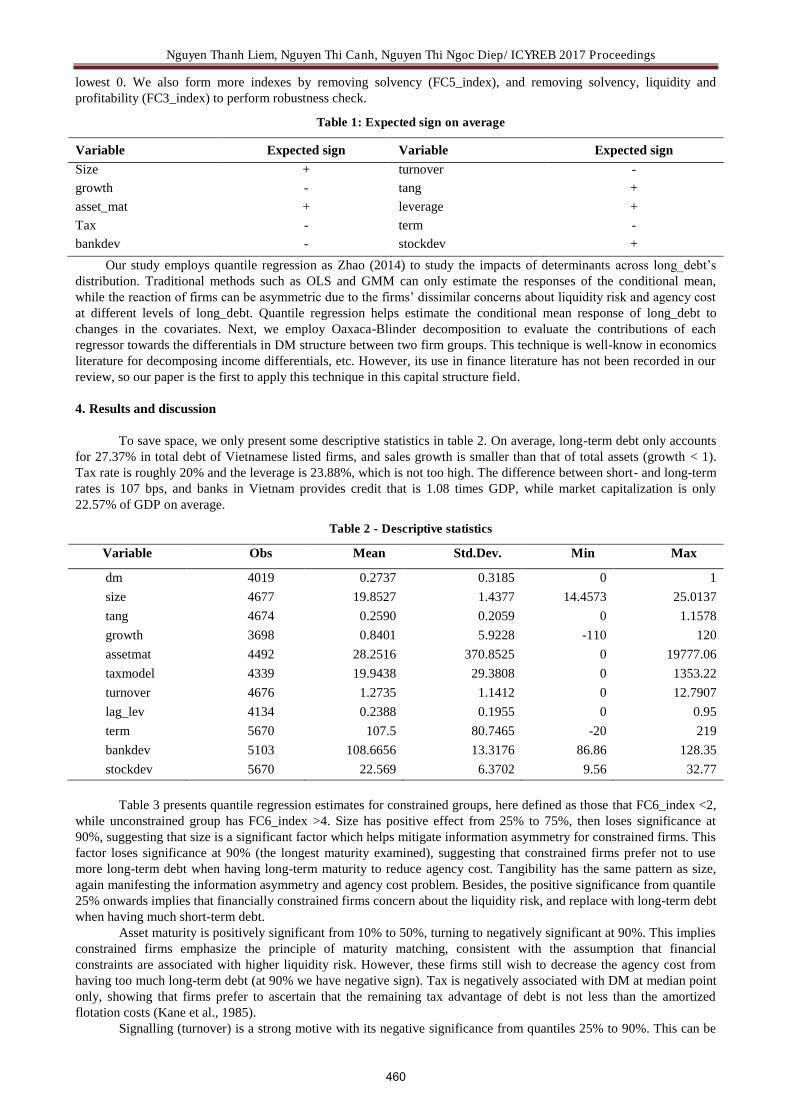
Nguyen Thanh Liem, Nguyen Thi Canh, Nguyen Thi Ngoc Diep/ ICYREB 2017 Proceedings
lowest 0. We also form more indexes by removing solvency (FC5_index), and removing solvency, liquidity and profitability (FC3_index) to perform robustness check.
Table 1: Expected sign on average
Variable Expected sign Variable Expected sign
Size + turnover -
growth - tang +
asset_mat + leverage +
Tax - term -
bankdev - stockdev +
Our study employs quantile regression as Zhao (2014) to study the impacts of determinants across long_debt’s distribution. Traditional methods such as OLS and GMM can only estimate the responses of the conditional mean, while the reaction of firms can be asymmetric due to the firms’ dissimilar concerns about liquidity risk and agency cost at different levels of long_debt. Quantile regression helps estimate the conditional mean response of long_debt to changes in the covariates. Next, we employ Oaxaca-Blinder decomposition to evaluate the contributions of each regressor towards the differentials in DM structure between two firm groups. This technique is well-know in economics literature for decomposing income differentials, etc. However, its use in finance literature has not been recorded in our review, so our paper is the first to apply this technique in this capital structure field.
4. Results and discussion
To save space, we only present some descriptive statistics in table 2. On average, long-term debt only accounts for 27.37% in total debt of Vietnamese listed firms, and sales growth is smaller than that of total assets (growth < 1). Tax rate is roughly 20% and the leverage is 23.88%, which is not too high. The difference between short- and long-term rates is 107 bps, and banks in Vietnam provides credit that is 1.08 times GDP, while market capitalization is only 22.57% of GDP on average.
Table 2 - Descriptive statistics
Variable Obs Mean Std.Dev. Min Max
dm 4019 0.2737 0.3185 0 1
size 4677 19.8527 1.4377 14.4573 25.0137
tang 4674 0.2590 0.2059 0 1.1578
growth 3698 0.8401 5.9228 -110 120
assetmat 4492 28.2516 370.8525 0 19777.06
taxmodel 4339 19.9438 29.3808 0 1353.22
turnover 4676 1.2735 1.1412 0 12.7907
lag_lev 4134 0.2388 0.1955 0 0.95
term 5670 107.5 80.7465 -20 219
bankdev 5103 108.6656 13.3176 86.86 128.35
stockdev 5670 22.569 6.3702 9.56 32.77
Table 3 presents quantile regression estimates for constrained groups, here defined as those that FC6_index <2,
while unconstrained group has FC6_index >4. Size has positive effect from 25% to 75%, then loses significance at 90%, suggesting that size is a significant factor which helps mitigate information asymmetry for constrained firms. This factor loses significance at 90% (the longest maturity examined), suggesting that constrained firms prefer not to use more long-term debt when having long-term maturity to reduce agency cost. Tangibility has the same pattern as size, again manifesting the information asymmetry and agency cost problem. Besides, the positive significance from quantile 25% onwards implies that financially constrained firms concern about the liquidity risk, and replace with long-term debt when having much short-term debt.
Asset maturity is positively significant from 10% to 50%, turning to negatively significant at 90%. This implies constrained firms emphasize the principle of maturity matching, consistent with the assumption that financial constraints are associated with higher liquidity risk. However, these firms still wish to decrease the agency cost from having too much long-term debt (at 90% we have negative sign). Tax is negatively associated with DM at median point only, showing that firms prefer to ascertain that the remaining tax advantage of debt is not less than the amortized flotation costs (Kane et al., 1985).
Signalling (turnover) is a strong motive with its negative significance from quantiles 25% to 90%. This can be
460

Nguyen Thanh Liem, Nguyen Thi Canh, Nguyen Thi Ngoc Diep/ ICYREB 2017 Proceedings
explained by the fact that constrained firms are those suffering from information asymmetry, thus signalling the credit quality is imperative for those firms. Another strong motive is the desire to reduce the cost of capital, i.e. by using more short-term debt when it is cheaper than long-term financing. This factor is negatively significant from 25% to 90%, not at 10% where liquidity risk is of higher concern. For leverage it seems that even for constrained firms, too high agency cost is not preferrable and those firms are willing to shift to short-term debt (negative signs at 75% and 90%). Finally, bank and stock development and growth factor are not significant at any quantile.
Table 4 shows the case for financially unconstrained firms (FC6_index >4). Size has negative effect but only at 90%, showing that unconstrained firms do not suffer much from information asymmetry (size is not significant at most quantiles). However, unconstrained firms also wish to decrease agency cost from having too much long-term debt (size turns negative here). Tangibility follows closely the pattern of size, so the same justification applies.
Interestingly, growth is positively associated with long DM structure, rather than negatively. This implies that for unconstrained firms, growth is not associated with asymmetric information.
Unconstrained firms do not seem to prioritize maturity matching, which is manifested by wrong negative sign at quantiles 75% and 90% (in fact this is where firms have long DM). Tax rate is negatively related to DM structure only at 50%.
Importantly, turnover is negatively related to DM only at 90% quantile, suggesting that firms only care for signalling when they have too much long-term debt. Besides, this move is also to reduce the agency cost arising from high agency cost from high ratios of long-term debt. Term is negatively associated to DM at 75% only, suggesting that the timing of debt issue to minimize the cost is not a concern to unconstrained firms. These firms only try to substitute long-term debt with short-term borrowing when they owe too much long-term debt (so high agency cost). Again, as in the case of constrained firms, bank and stock development do not have impact on firm DM choices.
Table 3. Quantile regression estimates for constrained firms (FC6_index <2)
10 25 50 75 90
Coef. Std.Err Coef. Std.Err Coef. Std.Err Coef. Std.Err Coef. Std.Err
size 0.0015 0.0033 0.0146
***
0.0043 0.0293
***
0.0071 0.036
***
0.0135 0.0193 0.194
tang 0.0017 0.0234 0.2441
***
0.0701 0.7099
***
0.0633 0.8884
***
0.857 0.6615
***
0.1285
growth -0.0002 0.0002 -0.0012 0.0008 -0.0005 0.0005 -0.0006 0.0004 -0.0008 0.0007
assetmat 0.000054
***
0.0000 0.0000401
***
0.0000 0.0000148
***
0.0000 0.000 0.000 -0.0000118
**
0.000
taxmodel 0.0000 0.0001 0.000 0.0000 -0.0001 0.0000 -0.000147
***
0.000 0.001 0.0039
turnover -0.0013 0.0016 -0.0191
***
0.0047 -0.0349
***
0.0069 -0.0558
***
0.0088 -0.10392
***
0.0175
lag_lev 0.0055 0.0181 0.0384 0.0234 -0.0322 0.0411 -0.2511
***
0.0733 -0.7427
***
0.1441
term 0.0000 0.0000 -0.0001271
**
0.0001 -0.00042
***
0.0001 -0.0003
*
0.0002 -0.001
*
0.0006
bankdev -0.0001 0.0005 -0.0002 0.0007 -0.0007 0.0012 0.000 0.0024 0.0024 0.0066
stockdev 0.0002 0.0011 0.0015 0.0016 0.0041 0.0030 0.0002 0.0046 0.0209 0.0151
R-sq 0.0108 0.1875 0.2047 0.2104 0.1500
No of obs 672
Table 4. Quantile regression estimates for unconstrained firms (FC6_index >4)
10 25 50 75 90
dm Coef.
Std.
Err. Coef.
Std.
Err. Coef.
Std.
Err. Coef.
Std.
Err. Coef. Std. Err.
size
0.000
0 0.0168 0.0152 0.0146 0.0222 0.0274 -0.0139 0.0451 -0.0583612* 0.0317
tang
0.000
0 0.1953 0.2200 0.1734
0.9226966**
* 0.2814 0.6817295** 0.3474 0.2039 0.2261
growth
0.000
0 0.0095 0.0073 0.0086 0.0149718** 0.0074 0.0162078** 0.0079 0.0229 0.0170
assetmat1
0.000
0 0.0011 0.0001 0.0002 -0.0001 0.0002
-
0.0006286*** 0.0002
-
0.0008502*** 0.0001
461

Nguyen Thanh Liem, Nguyen Thi Canh, Nguyen Thi Ngoc Diep/ ICYREB 2017 Proceedings
taxmodel
0.000
0 0.0033 -0.0012 0.0025 -0.0083164** 0.0041 -0.0066 0.0105 -0.0021 0.0061
turnover
0.000
0 0.0243 -0.0156 0.0457 -0.1194 0.0869 -0.2095 0.1328 -0.1089136* 0.0588
lag_lev
0.000
0 0.2467
0.3862771**
* 0.2160 0.4269 0.3561 -0.4931 0.3263
-
0.7106285*** 0.2647
term
0.000
0 0.0003 -0.0002 0.0002 -0.0005 0.0004
-
0.0014963*** 0.0005 -0.0006 0.0005
bankdev
0.000
0 0.0040 -0.0024 0.0035 -0.0053 0.0058 -0.0052 0.0087 0.0024 0.0067
stockdev
0.000
0 0.0089 0.0050 0.0073 0.0148 0.0123 0.0238 0.0170 0.0054 0.0118
R-
squared 0.0835 0.1476 0.1527 0.0640
No 192
Our results are in line with Zhao (2014), which indicates intensified refinancing risk and liquidity risk in the
lower tail of the DM distribution (when firms have too much short-term debt) and the more severe agency cost in the upper tail. Zhao (2014) states that firms with access to public credit market tend to perform closer to the prediction by hypotheses 1 and 2, thanks to being more financially flexible. However, our paper suggests the opposite, and this can be ascribed to the constrained firms in Vietnam being more concerned about liquidity risk and information risk than their unconstrained peers, thus behaving closely to the prediction of hypotheses 1 and 2. Meanwhile, unconstrained firms do not have such concern and behave in a more unpredictable manner.
In summary, the above analysis shows that firms with and without financial constraints react differently to liquidity risk and agency cost. However, in general constrained firms tend to appreciate liquidity risk and information asymmetry more than unconstrained firms; meanwhile, firms without financial constraints show more concern about agency cost stemming from owing too much long-term debt. We perform similar analysis using different measures of financial constraints as FC5_index and FC3_index; and the results remain relatively the same, solidifying our findings. The results related to FC5_index and FC3_index are not reported for the brevity sake, but can be provided upon requested.
4.1. Oaxaca – Blinder decomposition results
We perform the decomposition of the differential in DM structure between the two groups of firms divided by financial constraints (FC6_index). Here we only discuss differences that are significantly different from zero. Table 5 shows that the unconstrained firms have longer DM than constrained counterparts, at 34.12% and 21.76% respectively. The difference is therefore 12.36% which is significantly different from zero, and is decomposed into 2 parts due to the differences in the average values and the coefficients of the variables. It is clear that difference in average value only account for 41% of the differences (the explained part) while the varying coefficients of the variables account for the majority of the difference (the unexplained part).
Table 5. Oaxaca Blinder decomposition – General comparison
Coef. Std. Err. z P>z
unconstrained 0.341178 0.0275109 12.4 0
constrained 0.2175656 0.0108338 20.08 0
Difference 0.1236125 0.0295673 4.18 0
Decomposition
Explained 0.051018 0.0163893 3.11 0.002
Unexplained 0.0725944 0.0320121 2.27 0.023 Table 6 shows the differences in the average values of factors between the two groups (or the breakdown of
explained differences), but we only focus on the differences that are significantly different from zero (p_value smaller than 10%). These include size (accounting for about 20% of the explained difference), tangibility (20%) and leverage (40%), whose values are larger for unconstrained group versus the other group. The superiority of unconstrained firms in terms of these factors implies that these firms tend to be larger and have more fixed assets, so suffer less from information asymmetry, and be more able to access long-term financing. Unconstrained firms have higher leverage, and according to liquidity risk theory higher leverage neccessitates longer maturity, even though with strong financial profiles (fc6_index is larger than 4) those firms can shoulder high leverage.
462

Nguyen Thanh Liem, Nguyen Thi Canh, Nguyen Thi Ngoc Diep/ ICYREB 2017 Proceedings
Table 6. Oaxaca-Blinder decomposition - detail
Dm_explained Coef. Std.Err z P>z
Size 0.01541 0.00587 2.62 0.009
Tang 0.01231 0.00695 1.77 0.077
growth -0.00003 0.00043 -0.88 0.935
assetmat -0.00029 0.00031 -0.96 0.335
taxmodel -0.00083 0.00123 -0.67 0.501
turnover -0.00377 0.00433 -0.87 0.383
lag_lev 0.02197 0.01068 2.06 0.04
Term 0.00761 0.00475 1.6 0.109
bankdev -0.00208 0.00249 -0.84 0.404
stockdev 0.00719 0.00345 0.21 0.835
Total 0.05101 0.01638 3.11 0.002
The unexplained difference is again analyzed for the differences in the coefficents that are not zero (table 7):
size, growth, asset maturity. Interestingly, an unconstrained firm tend to borrow more long-term debt to finance the investment (when having more growth opportunities) than their constrained counterparts. For unconstrained firms, having a larger scale seems to be more involved in agency cost from “empire building” issue, so shortening DM as a measure to tackle this issue is needed. Finally, constrained firms tend to be careful with the maturity matching of their assets and debt probably due to their weaker financial conditions.
In summary, the Oaxaca-Blinder decomposition adds robust check to our findings that financially unconstrained firms care more about agency cost from high ratios of long-term debt. Meanwhile, constrained firms are more prone to both agency cost, liquidity risk and information asymmetry. These findings are in line with Stephan et al. (2011) for Ukrainian firms since the authors claim that smaller firms (more constrained firms) are influenced by information asymmetry and liquidity risk (so matching asset-DM, size and signalling are critical for these firms).
Table 7. Oaxaca-Blinder decomposition – detail
Dm_unexplained Coef. Std.Err z P>z
Size -0.8366 0.4333 -1.93 0.054
Tang 0.0168 0.0489 0.34 0.731
growth 0.0164 0.0066 2.47 0.013
assetmat -0.0063 0.0030 -2.07 0.039
taxmodel -0.0819 0.0593 -1.49 0.137
turnover -0.0597 0.0469 -1.27 0.203
lag_lev 0.0312 0.0235 1.32 0.185
Term -0.0270 0.0326 -0.83 0.407
bankdev -0.1389 0.5403 -0.26 0.797
stockdev 0.1800 0.2256 0.8 0.425
_cons 0.9850 0.6391 1.54 0.123
Total 0.0725 0.0320 2.27 0.023
5. Conclusion
This paper analyzes the different behavior of financially constrained and unconstrained firms in terms of DM choices in Vietnam. Our approaches include two methods: quantile regression to find out how firms react to the differing levels of liquidity risk and agency cost across the DM distribution and Oaxaca Blinder decomposition to dissect the contributors of the difference in the average DM of constrained and unconstrained firms.
Our findings from both methods provide strong evidence showing that constrained firms suffer more from liquidity risk and information asymmetry, while unconstrained firms with stronger financial profiles are better equipped to withstand both of these frictions effectively. Both groups also show strong interest in reducing agency cost associated with high ratios of long-term debt. Our evidence is therefore quite consistent with Stephan et al. (2011) for Ukrainian firms, but shows a major divergence from Zhao (2014) for US firms. Our findings suggest that for an emerging market like Vietnam, firms with more constraints act more appropriately to take advantage of the benefits of DM structure.
463

Nguyen Thanh Liem, Nguyen Thi Canh, Nguyen Thi Ngoc Diep/ ICYREB 2017 Proceedings
References
[1] Antoniou, A., Guney, Y., Paudyal, K., (2006). The determinants of DM structure: Evidence from France, Germany and the UK. European Financial Management, 12(2), 161-194.
[2] Arslan, O; Karan, M. B., (2006). Ownership and control structure as determiannts of corporate DM: a panel study of an emerging market. Corporate Governance: An International Review, 14(1), 312-324.
[3] Barclay, M. J.; Smith, C. W., (1995). The maturity structure of corporate debt. The Journal of Finance, 50(2), 609-631
[4] Brick, I. E., Ravid, S. A., (1985). On the relevance of DM structure. Journal of Finance, 40, 1423-1437. [5] Cai, K., Fairchild, R., Guney, Y.,(2008). DM structure of Chinese companies. Pacific-Basic Finance Journal,
16(3), 268-297. [6] Deemsomsak, R., Paudyal, K., Pescetto, G., (2009). DM structure and the 1997 Asian financial crisis. Journal of
Multinational Financial Management, 19, pp. 26-42. [7] Demirguc-Kunt, A.; Maksimovic, V., (1999). Institutions, financial markets and firm DM. Journal of Financial
Economics, 54, 295-336 [8] Diamond, D. W., (1991). DM structure and liquidity risk. Quarterly Journal of Economics (August) [9] Flannery, E. F. (1986), Asymmetric information and risky DM choice, Journal of Finance, 41(1), 18-38. [10] Graham, J. R., Harvey, C. R., (2001). The theory and practice of corporate finance: evidence from the field.
Journal of Financial Economics, 60, 187-243. [11] Guedes, J.; Opler, T., (1996). The determinants of the maturity of corporate debt issues. The Journal of Finance,
11 (1), 1809-1833. [12] Kane, A., Marcus, A. J., McDonald, R. L., (1985). Debt policy and the rate of return premium to leverage. Journal
of Financial and Quantitative analysis, 20, 479-499. [13] Koenker, R.; Bassett, G., (1978). Regression quantiles. Econometrica, 46(1), pp. 33-50 [14] Marchica, MT & Mura, R (2007), Financial Flexibility and Investment Decisions: Evidence from Low-Leverage
Firms. in Eastern Finance Association, New Orleans, USA. [15] Mulier, L.; Schoors, K.; Merlevede, B, (2014). Investment-cash flow sensitivity and the cost of external finance.
Universiteit Gent Working Paper D/2014/7012/19 [16] Myers, (1977). Determinants of corporate borrowing. Journal of Financial Economics, 1977. 147-175. [17] Ngô Văn Toàn, Phạm Thị Thu Hồng, (2015). Các yếu tố ảnh hưởng đến quyết định lựa chọn kỳ hạn nợ của các
công ty niêm yết trên thị trường chứng khoán Việt Nam. Tạp chí Công nghệ Ngân hàng, 115, pp. 27-41 [18] Orman, C., Koksal, B., (2015). Structure of DM across firm types. Central Bank of the Public of Turkey Working
Paper No 15/21. [19] Ozkan, A., (2002). The determinants of corporate DM: Evidence from UK firms. Applied Financial Economics,
12(1), 19-24 [20] Shah, A., Khan, S. A., (2009). Empirical investigation of debt-maturity structure: Evidence from Pakistan. The
Pakistan Development Review, 48(4), 565-578. [21] Stohs, M. H., Mauer, D. C., (1996). The determinants of corporate DM structure. The Journal of Business, 69(3),
279-312 [22] Trần Thị Thùy Linh, Nguyễn Thanh Nhã, (2017). Nghiên cứu cấu trúc kỳ hạn nợ của công ty tại Vi ệt Nam. Tạp
chí Phát triển Kinh tế, 28(2), pp. 20-43 [23] Zhao, S., (2014). Three essays in empirical finance. Universite de Grenoble, 2014. PhD thesis.
464

Cao Thi Hong Vinh, Trinh Quynh Linh, Nguyen Thi An Ly / ICYREB 2017 Proceedings
International Conference For Young Researchers In Economics And Business, ICYREB 2017, October 30th 2017 Da Nang, Vietnam
The Effect of FDI on Inequality-Adjusted HDI (IHDI) in Asian
Countries
CAO Thi Hong Vinh *, TRINH Quynh Linh, NGUYEN Thi An Ly
Foreign Trade University
A B S T R A C T
Inequality-adjusted Human development index (IHDI) is a new measurement of countries’ human development with the big advantages of considering human development with the control of inequality – a big concern of countries. Despite the fact that the impact of Foreign direct investment on human development has drawn much attention of economists, we have not found any researches using IHDI as a proxy for human development, especially for Asian countries. From the hope to narrow this gap, we have carried out this empirical research and we found that FDI did not significantly affect human development in Asian countries in general and even in each of the three groups of very high, high and medium human development countries. Moreover, FDI did raise the inequality in income, but it helped to reduce the inequality in education. In addition, the higher institutional quality in general did raise the countries’ human development, and among sub-indices of institutional quality, better political situation and law did also lift up the human development levels of countries.
Keywords: Foreign Direct Investment, Inequality-adjusted Human Development Index
1. Introduction
In the context that countries worldwide make lots of efforts to fulfill the targets of sustainable development, human development (measured by human development index - HDI) is considered as a more and more important factor which countries care about. HDI is calculated with regards to three aspects of education, longevity and income. Until now, the index is still the most popular, widely used measurement of human development. However, despite these facts, HDI has its own weakness that there is no consideration of inequality included in human development across regions of countries though the matter of unequal distribution gradually becomes a big social concern these days. As a result, a new measurement which is Inequality-adjusted Human Development Index (IHDI) has been set up and calculated by United Nations Development Program (UNDP). The new variable is a better proxy for sustainable development as it covers not only the human development in general, but also the equality in human development as well.
Foreign direct investment (FDI) is a kind of foreign flows which have played a considerably significant role to host countries’s economic growth and social development in a certain aspects. Nevertheless, on the contrary of its positive effects, FDI on its own cause negative consequences to the recipients for both human development and inequality (mainly about income inequality) of countries. As a result, the final impact of FDI on human development with the control of inequality of countries is still in doubt.
However, in our perception, there have been no studies that have looked into Inequality-adjusted human development (meaning that human development is taken into consideration as inequality problem has been controlled for). To narrow the gap, the paper did a research on the effect of FDI inflows on IHDI in 23 Asian countries for the period from 2013 to 2015. We have found that FDI did not significantly affect human development in Asian countries in general and even in each of the three groups of very high, high and medium human development countries. Moreover, FDI did raise the inequality in income, but it helped to reduce the inequality in education. In addition, the higher institutional quality in general did raise the countries‘ human development, and among subindices of institutional quality, better political situation and law did also lift up the human development levels of countries.
The remainder of the paper is organized as follows. Section 2 presents the literature review, while Section 3 looks into the theoretical effect of FDI on IHDI and Section 4 is about the data. Next section is about the empirical strategies.
* Corresponding author. Email: [email protected]
465

Cao Thi Hong Vinh, Trinh Quynh Linh, Nguyen Thi An Ly / ICYREB 2017 Proceedings
Section 6 shows the main results. The final section is the conclusion.
2. Literature review
In our perception, there have been no recent researches about the impact of FDI on Inequality-adjusted Human development index (IHDI) in the world. Most researches do just focus on the impact of that financial flow on either HDI (not IHDI) or inequality (mostly on income inequality).
Regarding the impact of FDI on HDI, Santosa (2014) in the paper of “Analysis of the impact of Foreign direct investment on Social development in Indonesia and other ASEAN countries” did a research with a stress on Indonesia and other ASEAN countries after the financial crisis during the period of 1999-2012. The paper figured out the unclear influence of FDI in 7 ASEAN countries of Singapore, Malaysia, Brunei Darusalam, Thailand, Indonesia, Lao và Campuchia, but the positive one of FDI on human development in Vietnam and Myanmar, and negative on that in Philippines. Colen et. al. (2009) supported the idea that FDI could make a positive contribution to human development of host countries given appropriate conditions. The positive effect of FDI on HDI was also proved in the research of Makki and Somwaru (2004). In contrast, Sharma and Gani (2004) as looking into Latin American countries didn’t find any evidence for a significant impact of FDI on HDI.
Relating to the effect of FDI on income inequality, this is a topic which has drawn much attentions of economists, epecially after the release of Human development report in 1999. According to the report, the gap between rich and poor countries tended to widen in this modern era with the fast technological development. Basu et. al. (2007) in the paper of “FDI, Inequality and Growth” did carry out an empirical research about if FDI raised inequality in 119 developing countries from 1970 to 1999. The results presented a clear evidence about the existence of this effect. Vietnam Industrial Investment Report in 2011 of UNIDO (2012) also showed that FDI leaded to rise of income inequality in the country due to the fact that FDI created a big gap in the wage between FDI and non-FDI enterprises. This point was also supported by Pham Hoang Mai (2004) in "FDI and Development: Policy implication”. Meanwhile, in their research, Figini (2011) showed two opposite outcomes for two groups of countries. For the group of OECD countries, FDI did not raise the inequality, while for the one of non-OECD, the income inequality rose considerably. In contrast, other researches such Feenstra and Hanson (2001) did find the negative effect, meaning that FDI helped to reduce the inequality.
3. Theoretical effects of FDI on IHDI
In theory, the effects of FDI on different variables are based on two main perspectives of capital widening and capital deepening. As a capital flow, FDI could help host countries to accumulate more capital (that direct effect is called capital widening). In addition to that, FDI with its advantages of pushing technology transfer, improving labor skills, expanding the linkages of domestic firms with global networks, etc., could also have spillover effects which raise host countries’ productivity (this impact is called capital deepening).
Inequality-adjusted Human development index (IHDI) is developed by United Nations Development Program (UNDP). This index is better than the previous one of Human development index (HDI), because besides considering the 3 sub-indices of health (measured by life-expectancy), education (measured by adult literacy index and gross enrollment combined index) and income (measured by GDP per capita), IHDI also adjusts the inequality among regions for each above sub-index. Inequality for sure is also a serious problem that countries care about as human development is considered.
The impact that FDI has on IHDI is based on its effect on IHDI’s aspects (including income, health, education, and inequality). As a consequence, the following section illustrates the theoretical impacts of FDI on IHDI’s components via either capital widening or capital deepening.
3.1. Positive impacts
3.1.1. The positive impacts of FDI on income
FDI can help to raise the income of labors mostly by creating jobs and developing local skills. Since investment from other countries is used to promote businesses in a developing country, it can generate several jobs for local people. Karlsson (2007) stated in “FDI and Job Creation in China” that FDI did positively impact employment growth, which added more income to households and strengthening spending power for local residents. To be more specific, foreign direct investment flows into the country through many channels, including multinational companies which bring advanced technologies and managerial experience. Those skills have not yet developed properly in less developed countries. According to Kurtishi -Kastrati (2013), the foreign firms have high quality training given to their employees. Some of those skills are taken with the workers when they enter domestic firms. Consequently, the host countries can benefit from “managerial superiority” of multinational companies by learning and imitating. Simultaneously, employees can have higher income as they upgrade their skills and apply for their later jobs.
466

Cao Thi Hong Vinh, Trinh Quynh Linh, Nguyen Thi An Ly / ICYREB 2017 Proceedings
The income also rises as FDI flows raise the countries’ economic growth, which indirectly boosts the income. Tran Trong Hung (2005) stated in “Impact of Foreign Direct Investment on Poverty Reduction in Vietnam” that FDI, through economic growth and employment rate, can reduce poverty rate and improve quality of local people. The increase in economic growth and demand for employment is certainly contributed by the increase in disposable income of households overall, which means the number of people living below the poverty line is reduced.
3.1.2. The positive impacts of FDI on health
FDI can affect health of people in a country through several channels as follows: The first channel is self – consciousness of people on health issues as their income increases. When people earn
more money and they are aware of the importance of health, they are willing to spend more share of their disposable income on health service. Furthermore, they can also use that extra income to buy more high quality consumption necessities such as organic food. Higher spending on healthcare and high quality goods will make people’s become better, which then gradually increase life expectancy.
FDI could also help improve health conditions in recipient countries by not only paying higher salary than the domestic firms but also providing safe working places and better social services. Safe workplace is one of compulsory criteria for operation in developed countries and expected to be exercised by the company all the time. When foreign firms set up business in the host country, it also pays attention to working condition of the employees than the domestic ones.
3.1.3. The positive impacts of FDI on education
Education is always an essential part of a country’s development, which FDI certainly creates a significant impact on.
Nowadays, more and more foreign investors consider education is a good way to invest in a country. They usually seek for countries that have high demand for global standard education or desire to send people to study abroad. By investing a system of education from elementary schools to universities in the host countries, foreign investors create a win – win situation: they could make money and eventually utilize the human resource while local residents can receive high quality education standard at a much lower price. Therefore, the school enrollment rate in the host countries will increase since now people will remain in their countries while study in world – standard classes.
What’s more, FDI inflows make education become more diversified, creating more options for people in host countries to choose when deciding future careers. After finishing university, some people will choose to pursue master degree immediately. In the other way, some will choose to work for foreign companies and those companies will fund them to pursue certificates relevant to their jobs rather than higher education.
3.1.4. The positive impacts of FDI on inequality
Working for foreign enterprises might associate with higher income on national scale. However, it does not address the inequality in income distribution which result in the remaining of poverty. Inequality in income distribution is typically discussed with the context of North – South models. The availability of cheap labor in poor countries (the South) encourages richer countries (the North) to undertake efficiency – seeking FDI by offshoring labors intensive parts of production process. This may increase skills to the South but also the inequality. As the foreign firms are usually larger, more productive and more skills intensive, they can put pressure on wages in domestic counterparts. Foreign investors are able to use their technological advantage to increase the efficiency of companies taken over. If such efficiency increase are achieved through automation, the primary employees to suffer from that are the low-paid (low-skilled), who may be more easily replaced than the higher paid (skilled) employees.
3.2. Negative impacts
3.2.1. The negative impacts of FDI on income
Most negative impacts of FDI on income come from the impact of FDI on the rise of income inequality as mentioned in the previous section.
3.2.2. The negative impacts of FDI on health
Although it is argued that FDI can have positive impact on health, there are some evidences which support the contrast argument.
First, given the concern of income, it is well known that increases in income may lead to higher life expectancy in poor countries; however, as income rises, the relationship becomes weaker or even absent among the richest countries.
467

Cao Thi Hong Vinh, Trinh Quynh Linh, Nguyen Thi An Ly / ICYREB 2017 Proceedings
In other words, health is affected by standard of living in low income countries, while an increase in income has little or even no effect on health in high income countries. Indeed, if higher income associates with longer working hours leading to less social contact, more stress, less sleep, and increase in unhealthy food consumption, it could be that income – health relationship become negative. Moreover, multinational corporations (MNCs) have been often criticized due to discriminative and exploitative practices toward local employees and other resources of the host country. Regarding to the local employees, the working conditions of them in firms sponsored by FDI have been alarming. The presence of sweatshops in some countries, which subject laborers, who are sometimes child laborers, to dangerous, sub-human working conditions, often in violation of local workplace regulations, is a serious issue. According to Brown et. al. (2004), although multinationals pay their workers more than their domestic competitors, many people have complained that multinationals abuse their workers in sweatshop conditions, and have demanded that products from these sweatshops be banned from US markets.
Second, there are many studies on the effect of environmental pollution on health. Eskeland and Harrison (2003) stated that the so – called pollution of intensive goods tends to migrate from countries with high standard of environment (typically developed countries) to countries where this standard is low (developing countries). Indeed, in order to cut cost, foreign companies usually released unprocessed waste to the environment in domestic countries, causing dramatic environment damage and eventually negatively affect health of local people.
The other effect of FDI on health may be reflected by people travelling for business, which result in the spread of infectious diseases.
In summary, FDI can have both positive, as discussed in the previous section, and negative effects on health. The net effect will vary with level of income.
3.2.3. The negative impacts of FDI on education
According to De Groot (2014), the increases in FDI are associated with decreases in HDI as a result of deteriorating government policy. Due to the attractiveness of FDI, one government may have two possibilities: invest in FDI promotion policies or invest in other public projects. This implies that such FDI promotion policies by definition reduce other public expenditures which is not optimal for the social welfare. For example, foreign investor may ask for the expansion of infrastructure which government must pay for by cutting down the expenditures in education, which would have negative effect on HDI.
The negative effect of FDI on education also depends on type of foreign investment. For example, horizontal foreign investors tend to seek potential market and they must support development of the host country’s market. Meanwhile, efficiency – seeking investors tend to look for cheap labor only. Therefore, they usually offer lower wages and in consequence, low motivation for the local to pursue tertiary education.
In short, FDI can have both positive and negative impacts on HDI. Understanding those impacts and analyzing in the case of Vietnam will help to generate suitable orientations and policies to further reinforce the positive influences and hinder the negative ones in order to improve HDI in Vietnam.
3.2.4. The negative impacts of FDI on inequality
The explanation for these impacts clarified in the paper of Im and McLaren (2015) is that inward FDI could compete with domestic capital for domestic workers, as a result, the income of domestic investors will reduce while that of domestic workers will rise. That helps to narrow the income gap. The idea is withdrawn from political argument of Pandya (2014) that the normal people are in favor of FDI.
4. Empirical strategies
Along with FDI, Institution is also an important factor which could affect human development of a country. The role of Institutional quality is also widely acknowledged in the development fields. As a result, in addition to FDI, the Institutional quality is also considered as a factor affecting human development. From those points, the main empirical specification for Fixed effect model† for panel data is as follows:
(1)
Moreover, to further look into the impact of FDI inflow on particular aspects of inequality, the additional specification is:
(2)
The final specification that focuses on the effect of specific sub-indices of institutional quality on IHDI is: (3)
† As Fixed effect could help control for all countries’ time-invariant characteristics, it is considered a good model
for panel data.
468

Cao Thi Hong Vinh, Trinh Quynh Linh, Nguyen Thi An Ly / ICYREB 2017 Proceedings
where i denotes country i, t is year t, k is specific aspect of Inequality (comprising of Inequality in life expectancy, education and income), l is particular sub-index of Institutional quality (mentioned below).
LogIHDI it is the natural logarithm of Inequality-adjusted Human development index of country i in year t; LogFDI it is the natural logarithm of FDI inflow of country i in year t; LogPRSit is the natural logarithm of index calculated from sub-indices taken from International Country Risk
Guide data provided by PRS group. This variable is a proxy for institutional quality of countries. Sub-indices are comprised of:
Prsvait/Prsvavnt is the index of Voice and Accountability of country i/Vietnam in year t; Prsgeit/Prsgevnt is the index of Government Effectiveness of country i/Vietnam in year t; Prsccit/Prsccvnt is the index of Control of Corruption of country i/Vietnam in year t; Prsrqit/Prsrqvnt is the index of Regulatory Quality of country i/Vietnam in year t; Prspvit/Prspvvnt is the index of Political Stability and Absence of Violence of country i/Vietnam in year t; Prsrl it/Prsrl vnt is the index of Rule of Law of country i/Vietnam in year t.
is the value of Inequality in different aspects of human development (life expectancy,
education and income) of country i in year t (in percentage); denotes time dummies;
The coefficient of interest in the previous equation is α, which measures the effect of FDI inflows on Inequality-adjusted Human development index (equations 1 and 3) and on Inequality (equation 2) for countries in Asia. If FDI does help these Asian countries improve their human development (equations 1 and 3) or raise the inequality (equation 2), this coefficient will be positive.
Table 1 and 2 present the summary statistics and correlation of the main variables.
Table 1: Summary Statistics of Variables
Variable Obs Mean Std. Dev. Min Max
LogIHDI 66 -.5255024 .1944514 -.9808292 -.2319321
LogHDI 66 -.3217014 .1292291 -.6217572 -.10425
LogFDI 66 2.213.566 1.368.926 183.622 2.496.054
LogFDI*LogPRS 66 -132.753 4.285.111 -2.308.237 -3.616.929
inequalityinlifeexpectancy 66 1.356.667 6.797.722 3.2 32.8
inequalityineducation 66 1.897.273 1.247.959 2.1 45.2
inequalityinincome 66 2.074.545 8.933.415 4.5 46.6
Logadjustedlifeexpectancy 66 .7149091 .1159188 .479 .947
Logadjustededucation 66 .5485909 .159726 .204 .798
Logadjustedincome 66 .5717727 .1025646 .357 .773
LogPRS 66 -.6016369 .1922187 -1.035.637 -.1566538
LogPRSva 66 -.5680081 .2700943 -1.108.663 -.0833816
LogPRSpv 66 -.4718358 .1669532 -.8209805 -.198451
LogPRSge 66 -.6634073 .3792136 -1.386.294 0
LogPRSrq 66 -.4941704 .2082775 -1.139.434 -.0512933
LogPRScc 66 -.604363 .3021572 -1.386.294 -.1863296
Table 2: Correlations of Variables
LogIHDI LogHDI LogFDI Inequality in
life expectancy Inequality in
education Inequality in income
LogPRS
LogIHDI 1
LogHDI 0.9388 1
LogFDI 0.0562 0.1135 1
Inequality in life expectancy
-0.7962 -0.8587 -0.1051 1
Inequality in education -0.7765 -0.5699 0.1310 0.4590 1
Inequality in income -0.1818 0.0609 0.0185 -0.2858 0.2157 1
LogPRS 0.3876 0.4602 0.1634 -0.4343 -0.0752 0.0155 1
469

Cao Thi Hong Vinh, Trinh Quynh Linh, Nguyen Thi An Ly / ICYREB 2017 Proceedings
5. Data
This section discusses briefly about the data to construct the sample with the range from 2013 to 2015. Inequality-adjusted Human development index (IHDI) data: The data is taken from the official website of
United Nations Development Programme (UNDP). The data for the other variables of Inequalityinlifeexpectancy, Inequalityineducation, Inequalityinincome, Inequalityadjustedexpectancy, and Inequalityadjustededucation, Inequalityadjustedincome are also supplied by UNDP. Figure 1 describes steps to calculate IHDI which is considered to be a more efficient measurement of Human development as the problem of inequality across sections is dealt with.
Figure 1: Steps to calculate Inequality-adjusted Human development index
Source: The official website of United Nations Development Programme (UNDP)
http://hdr.undp.org/en/content/inequality-adjusted-human-development-index-ihdi
FDI data: The authors collect the data of net FDI inflows to country i (in current USD) from the online database of World Development Indicator on the website of World Bank.
PRS (Institution) data: Indices for countries' institution such as Political Stability and Absence of Violence (Prspvit and Prspvvnt), Regulatory Quality (Prsrqit and Prsrqvnt), Control of Corruption (Prsccit and Prsccvnt), Voice and Accountability (Prsvait and Prsvavnt), Government Effectiveness (Prsgeit and Prsgevnt) and Rule of Law (Prsrlit and Prsrlvnt) are from the International Country Risk Guide (ICRG) database provided by PRS Group. The final index of PRS is calculated by taking the simple average of these above six sub-indices. According to World Bank‡, ICRG is a good institutional data and it is widely used in published studies.
6. Results
6.1. Baseline results for the effect of FDI on human development
The baseline results for the impact of FDI inflows on human development are shown on Table 3, Columns (1)-(3). Since the data for IHDI from UNDP and those for other variables of FDI and PRS are not available for all Asian countries, the sample just covers 66 observations of Asian countries during the period of 2013-2015. The estimators for Fixed effect (FE) model are displayed with time-dummies controlled. From Columns (1)-(3), it could be seen that FDI consistently has no statistically significant effects on IHDI of Asian countries, meaning that in fact, FDI inflows do not really help host countries improve their human development as inequality problem is considered. Even as FDI of the previous year is controlled for in Column 2, the effect still remains insignificant. Regarding institutional quality , Column (1) illustrates the significant positive impact of PRS, showing that on the contrary of FDI’s effect, institutional quality plays an important role to the enhancement of human development.
For checking if the above impacts stay the same as HDI rather than IHDI is considered, the authors run the regression with the results presented in Column (4). The evidence proves the consistent insignificant effect of FDI and positive one of institutional quality on Human development in both cases with and without controlling for the problem of inequality. Column (5) demonstrates the influences of independent variables on the difference between IHDI and HDI. Again, the insignificant coefficient of FDI supports that FDI does not really help Asian countries in the sample to be better in human development.
‡ http://siteresources.worldbank.org/INTLAWJUSTINST/Resources/IndicatorsGovernanceandInstitutionalQuality.pdf)
470

Cao Thi Hong Vinh, Trinh Quynh Linh, Nguyen Thi An Ly / ICYREB 2017 Proceedings
Table 3: Baseline results for the effects of FDI on human development
LogIHDI LogHDI Loss (1) (2) (3) (4) (5) LogFDI -0.00316 0.0171 0.00755 -0.00381 -0.00894 (0.00389) (0.0155) (0.00632) (0.00349) (0.389) LogPRS 0.103** -0.645 0.00957 0.0750* -1.905 (0.0482) (0.532) (0.0642) (0.0385) (3.569) _Iyear_2014 0.0153*** 0.0153*** -0.0134*** 0.0143*** -0.0775 (0.00358) (0.00348) (0.00339) (0.00299) (0.295) _Iyear_2015 0.0265*** 0.0267*** 0.0235*** -0.255 (0.00551) (0.00552) (0.00452) (0.360) LogFDI*LogPRS 0.0342 (0.0247) LaglogFDI -0.00161 (0.00584) Observations 66 66 43 66 66 R-squared 0.567 0.589 0.509 0.620 0.029 Countries 23 23 22 23 23 Type FE FE FE FE FE Regression Xtreg Xtreg Xtreg Xtreg Xtreg Timedummies Yes Yes Yes Yes Yes (Loss (in percentage) is the percentage difference between IHDI and HDI due to the controlling inequality. The panel technique of Fixed effect is applied. ***/**/* present significant level of t-statistics at %/5%/10% level.)
6.2. Results for the effect of FDI on IHDI by groups
To discover if the above effect of FDI on IHDI could change across groups of Asian countries, the authors categorize the sample into 3 groups. The classification of groups is based on the value of HDI with the reference from UNDP website (See Appendix for the list of countries included in the sample). Group 1 includes countries with very high human development ( ); Group 2 contains countries with high human development ( ; Group 3 comprises of countries with medium human development (0 (the rest group of low human development countries ( ) includes just 1 country in the sample, hence it is not considered here). The results from the Table present consistent insignificant effects of FDI on IHDI across all groups of countries from very high to medium human development.
Table 4: Results for the effects of FDI on IHDI by groups
LogIHDI HDIgroup1 HDIgroup2 HDIgroup3 (1) (2) (3) LogFDI 0.0247 -0.00529 0.0469 (0.0268) (0.0104) (0.0250) LogPRS -4.243 0.0685 0.0575 (2.294) (0.0642) (0.0898) _Iyear_2014 -0.0219 0.0157** 0.0124** (0.0216) (0.00571) (0.00359) _Iyear_2015 -0.00175 0.0269*** 0.0270*** (0.00504) (0.00794) (0.00586) Observations 9 30 18 R-squared 0.415 0.592 0.834 Countries 4 10 6 Type FE FE FE Regression Xtreg Xtreg Xtreg Timedummies Yes Yes Yes (The classification of groups is based on the value of HDI. Group1: Countries with very high human development ( ); Group 2: Countries with high human development ( ; Group 3: Countries with medium human development (0 . The panel technique of Fixed effect is applied. ***/**/* present significant level of t-statistics at %/5%/10% level.)
471

Cao Thi Hong Vinh, Trinh Quynh Linh, Nguyen Thi An Ly / ICYREB 2017 Proceedings
6.3. Further analyses
6.3.1. Effects of FDI on equality in specific aspects
Beside the effect of FDI on human development in general, that on inequality is also of the authors‘ interest. Rather than looking into inequality generally, we consider the effects on inequality in specific aspects (life expectancy, education and income) of host countries. Results from Table 5 show the entirely different effects of FDI on distinguished dependent variables. It could be seen that while FDI inflows have no significant impacts on the inequality in life expectancy, they lead to the reduction in inequality in education, but the rise in the inequality in income. That means FDI inflows help to reduce the differences in education among regions, but make the gaps broader in income.
Table 6 explains further for these points in the way that FDI raise the education level of host countries, but reduce the income as these education and income levels have been adjusted for the inequality.
Table 5: Results for the effects of FDI on inequality in specific aspects
inequalityinlifeexpectancy inequalityineducation inequalityinincome (1) (2) (3) LogFDI 0.0102 -1.140** 1.042* (0.251) (0.413) (0.598) LogPRS -0.480 -3.416 -3.945 (5.371) (4.204) (6.393) _Iyear_2014 -0.000466 -0.728* 0.501 (0.0430) (0.409) (0.610) _Iyear_2015 -0.237 -1.211*** 0.730 (0.439) (0.401) (0.581) Observations 66 66 66 Countries 23 23 23 Type FE FE FE Regression Xtreg Xtreg Xtreg Timedummies Yes Yes Yes (The dependent variables of Inequalityinlifeexpentancy, Inequalityineducation, Inequalityinincome are in percentage. The panel technique of Fixed effect is applied. ***/**/* present significant level of t-statistics at %/5%/10% level.)
Table 6: Results for the effects of FDI on specific aspects of IHDI
Logadjustedlifeexpectancy Logadjustededucation Logadjustedincome (1) (2) (3) LogFDI -0.0107** 0.0140** -0.0138** (0.00468) (0.00637) (0.00545) LogPRS 0.120 0.0777 0.119 (0.104) (0.0981) (0.114) _Iyear_2014 0.00874* 0.0297*** 0.00679 (0.00433) (0.00761) (0.00837) _Iyear_2015 0.0119 0.0611*** 0.00592 (0.00931) (0.0105) (0.00918) Observations 66 66 66 Countries 23 23 23 Type FE FE FE Regression Xtreg Xtreg Xtreg Timedummies Yes Yes Yes (The panel technique of Fixed effect is applied. ***/**/* present significant level of t-statistics at %/5%/10% level.)
6.3.2. Effects of FDI on IHDI controlling for particular subindex of institutional quality
Institutional quality is also important for human development. In addition to the index of PRS, we would like to have a careful look into the effect of sub-indices of institutional quality on human development. The results illustrated in Table 7 also present consistent insignificant effect of FDI on IHDI regardless of sub-indices of institutional quality. The only two indices the coefficients of which are significant at 5% as controlling separately are PRSva (Voice and Accountability) and PRSrl (Rule of Law). PRSva is measured on the basis of Military in politics and Democratic accountability, while PRSrl is calculated with regard to Law and Order. The significant positive effects of these two variables on IHDI support that the political situation and law of host countries play an important role to their countries’ development.
472

Cao Thi Hong Vinh, Trinh Quynh Linh, Nguyen Thi An Ly / ICYREB 2017 Proceedings
Table 7: Results for the effects of FDI on IHDI controlling for the particular subindex of institution al quality
LogIHDI (1) (2) (3) (4) (5) (6) (7) LogFDI -0.00129 -0.00242 -0.00302 -0.00209 -0.00251 -0.00181 -0.00180 (0.00459) (0.00420) (0.00414) (0.00422) (0.00409) (0.00412) (0.00432) LogPRSva -0.00831 0.0364*** (0.0274) (0.0109) LogPRSpv -0.0248 0.0551 (0.0528) (0.0386) LogPRSrq 0.0201* 0.0199 (0.0102) (0.0121) LogPRSrl 0.0847** 0.0761** (0.0405) (0.0311) LogPRScc -0.0269 -0.0187 (0.0451) (0.0412) _Iyear_2014 0.0163*** 0.0156*** 0.0150*** 0.0150*** 0.0147*** 0.0160*** 0.0154*** (0.00433) (0.00384) (0.00363) (0.00375) (0.00370) (0.00378) (0.00408) _Iyear_2015 0.0287*** 0.0274*** 0.0267*** 0.0274*** 0.0269*** 0.0276*** 0.0283*** (0.00633) (0.00605) (0.00597) (0.00609) (0.00580) (0.00556) (0.00671) Observations 66 66 66 66 66 66 66 R-squared 0.597 0.546 0.549 0.535 0.550 0.580 0.538 Number of id 23 23 23 23 23 23 23 Type FE FE FE FE FE FE FE Regression Xtreg Xtreg Xtreg Xtreg Xtreg Xtreg Xtreg Timedummies Yes Yes Yes Yes Yes Yes Yes PRScompo Yes Yes Yes Yes Yes Yes Yes (The panel technique of Fixed effect is applied. ***/**/* present significant level of t-statistics at %/5%/10% level.)
7. Conclusions
Using the data of 23 Asian countries during the duration of 2013-2015 and applying fixed-effect for the above panel data, our paper tried to clarrify the impact of FDI inflows on Inequality-adjusted human development index (IHDI) of these countries. The findings prove for the insignificant effect of these financial flows on human development as inequality is controlled for. As a result, Asian countries do need to take a careful look into opposite effects (both positive and negative ones) of FDI as mentioned in the theoretical section on their human development. Especially from the perspective of inequality, FDI does raise the income inequality in these countries, and it even helps to reduce the inequality in education.
A further look into the role of institutional quality has shown that different from the impact of FDI, that of institution on human development is significantly positive. This means Asian countries should base more on their own institutional quality improvement rather than FDI attraction to raise the human development. Moreover, the aspects of institutional quality which they should think about first could be Political situation and Law.
Reference
[1] BASU, P., GUARIGLIA, A. & HY, D. 2007. FDI, Inequality and Growth. Journal of Macroeconomics, 29. [2] BROWN, D. K., DEARDORFF, A. & STERN, R. 2004. The effects of multinational production on wages and
working conditions in developing countries. Challenges to globalization: Analyzing the economics. University of Chicago Press.
[3] COLEN, L., MAERTENS, M. & SWINNEN, J. 2009. Foreign direct investment as an engine for economic growth and human development: a review of the arguments and empirical evidence. Hum. Rts. & Int'l Legal Discourse, 3, 177.
[4] DE GROOT, O. 2014. Foreign direct investment and welfare. [5] ESKELAND, G. S. & HARRISON, A. E. 2003. Moving to greener pastures? Multinationals and the pollution
haven hypothesis. Journal of development economics, 70, 1-23. [6] FEENSTRA, R. & HANSON, G. 2001. Global production sharing and rising inequality: A survey of trade and
wages. National Bureau of Economic Research. [7] FIGINI, P. 2011. Does foreign direct investment affect wage inequality? An empirical investigation. The World
Economy, 34, 1455-1475. [8] IM, H. & MCLAREN, J. 2015. Does Foreign Direct Investment raise income inequality in developing countries?
473

Cao Thi Hong Vinh, Trinh Quynh Linh, Nguyen Thi An Ly / ICYREB 2017 Proceedings
A new Instrumental variables. [9] KARLSSON, S., LUNDIN, N., SJÖHOLM, F. & HE, P. 2007. FDI and Job Creation in China. IFN Working
Paper. [10] KURTISHI-KASTRATI, S. 2013. The effects of foreign direct investments for host country's economy. European
Journal of Interdisciplinary Studies, 5, 26. [11] MAKKI, S. S. & SOMWARU, A. 2004. Impact of foreign direct investment and trade on economic growth:
Evidence from developing countries. American Journal of Agricultural Economics, 86, 795-801. [12] PANDYA, S. 2014. Trading Spaces: Foreign Direct Investment Regulation, 1970-2000. Cambridge University
Press. [13] PHAM, H. M. 2004. FDI and development in Vietnam: policy implications, Institute of Southeast Asian Studies. [14] SANTOSA, W. 2014. Analysis of the impact of Foreign direct investment on Social development in Indonesia
and other ASEAN countries. In: UNIVERSITY, T. (ed.). [15] SHARMA, B. & GANI, A. 2004. The effects of foreign direct investment on human development. Global
economy journal, 4. [16] TRAN, T. H. 2005. Impacts of foreign direct investment on poverty reduction in Vietnam. Discussed paper,
GRIPS, Vietnam. [17] UNITED NATIONS INDUSTRIAL DEVELOPMENT ORGANIZATION 2012. Vietnam Industrial Investment
Report in 2011
APPENDIX
Countries in the samples ARMENIA KAZAKHSTAN AZERBAIJAN KOREA, REP. BANGLADESH LEBANON CYPRUS MONGOLIA INDIA PAKISTAN INDONESIA PHILIPPINES IRAN, ISLAMIC REP. RUSSIAN FEDERATION IRAQ SRI LANKA ISRAEL THAILAND JAMAICA TURKEY JAPAN VIETNAM JORDAN
474

International Conference For Young Researchers In Economics And Business, ICYREB 2017, October 30th 2017 Da Nang, Vietnam
Developing Government Bond Portfolios at Commercial Banks by
Barbell Strategy: A Case study in VPBank
Do Hoai Linh, Dr. *, Nguyen Thanh Trung, M.A., Le Phong Chau, M.Sc.
National Economics University, 207 Giai Phong street, Hanoi 100000, Vietnam
A B S T R A C T
In the field of fix income investment, Barbell strategy is one of the most popular securities investment strategies, focusing on short-term and long-term bonds and ignoring medium-term bonds, with a view to balance between liquidity and profit. Barbell strategy was based on the methodology initiated by the economic professor Harry Markowitz in a "portfolio theory" (Markowitz, 1952). This strategy is often used by big investment size institutions to cope with the volatilation of market interest rate with the purpose of diversifying their portfolio and increasing the probability of higher return. In Vietnam, especially, in the context of an international integration, Barbell strategy performs a suitable tool with commercial banks; that help banks to build up their bond portfolios in not only managing liquidity assets but also ensuring sustainable profit. Besides researching contents of Barbell strategy, to demonstrate the feasibility of this strategy investment in real-life, the authors also tested the strategy with VPBank’s Portfolio in Vietnam Government Bonds in 2017.
Keywords: Barbell Strategy, Portfolio, Government Bonds.
1. Introduction
Barbell Strategy is one of portfolio diversification strategies that aim to minimize interest rate risk on a profit-maximizing basis, primarily for large and fixed income investors, who consider the portfolio mixed by short-term and long-term securities. Such portfolios have few or even zero investments in medium-term securities (Markowitz, 1959). The article applies Barbell Strategy with the Government Bond in Vietnamese Dong specifically to the Vietnam Prosperity Commercial Joint Stock Bank (VPBank) in 2017.
2. Theoretical basis
A portfolio is a grouping of securities, commodities, real estate, cash equivalents or other assets held by an individual or an organization (Schultz, 2008). Forming a portfolio is putting money into securities with various risk levels by different investment shares in the market, building a reasonable asset structure to diversify or minimize risks (HSBC, 2009).
Government bond is a debt instrument issued by the government of a country, with a term, face value, interest rate, and the Government's debt repayment obligation to bondholders. Government bonds are generally considered risk-free because the government may raise taxes or print more money to pay for bonds at maturity. Government bonds include: i) Treasury-bill (T-bill), a type of bond issued by the State Treasury with less-than-one-year term in the form of discount or interest payment at maturity; ii) Treasury Bonds (T-bond), a type of bond issued by the State Treasury with more-than-one-year term, usually with interest paid periodically (Kapoor, 2015).
Barbell Strategy Barbell strategy was based on the methodology initiated by the economic professor Harry Markowitz in a
"portfolio theory" (Markowitz, 1952), which was later developed into "portfolio choices" (Markowitz, 1959), stating that the overall risk of a portfolio drops significantly when a proper mix of investments is achieved. Based on Markowitz's theory, William Sharpe, and Jan Mossin later on, established the modern financial modeling with the
* Corresponding author. Tel.: +84912797782. E-mail address: [email protected]
475

CAPM model (Sharpe, 2007), (Mossin, 1968) as the first quantitative model forming the correlation between risk and profit. According to the theory, investors target at maximizing their expected return of a portfolio at an acceptable level of risk. Having assumptions of investment holding period and risk attitude of investors, risks can be measured by the variance or standard deviation of the portfolio’s rate of return. William Sharpe, among other scientists, found a way to simplify the input processing and data arrangement to determine the correlation of investments (Sharpe, 2007). Mitigating risks through diversification in the portfolio measured by its variance and the covariance in pairs of all assets, the Barbell strategy is a model that satisfies the balance between the rate of return and the risk for all assets. In the portfolio optimization model, it was found that the return on any asset was linearly related to its market beta. A negative beta represents the securities unlinear by market and removed as soon as the investment option is chosen. Similarly, the securities that earn a return lower than the risk-free rate is also removed from the portfolio because the risks inherent to the investment are not adequately compensated by profitability (Sharpe, 2007). The model results show a relatively high (approximately 1) correlation between return and risk. This means that short-term securities, providing "liquidity" and long-term investments with higher profitability are closely correlated. It is important to consider the ratio of short-term and long-term securities in the selected portfolio.
Dt = ∑Wsi x Dsi + ∑Wlj x Dlj (4) where: Dt: targeted duration Wsi: proportion of short-term bond i compared to the whole portfolio Dsi: duration of short-term bond i Wlj: proportion of long-term bond j compared to the whole portfolio Dlj: duration of long-term bond j To calculate Wsi and Wlj, the following steps should be taken: Step 1: Determine how long the portfolio is held; Step 2: Predict the yield curve of the selected bond; and Step 3: Based on the budget limit and expected return for the bond portfolio, determine the targeted duration for
the bond portfolio. Balancing the reasonable rates of risk and return in a portfolio is extremely important. It is essential to have a
portfolio that balances short-term and long-term securities at an appropriate timing (Frank, 1991). To form a bond portfolio that follows the Barbell Strategy, two factors that investors need to determine are yield curve and bond duration.
Yield curve The yield curve represents the interest rates at different maturities of the same debt, showing the relationship
between the borrowing cost and the time to maturity (Estrell, 2005a). The yield curve is a graph that reflects the relationship between interest rate and maturity of a debt instrument (at the same credit and quality), which plays an important role in generating a reference for issuance, trading and investment in the bond market, informing the market management and operation, and enabling transparency and liquidity for the exchange market.
To effectively manage a portfolio, the yield curve is a prerequisite for investors to decide which bonds to invest and how long they should be held. The yield curve is useful for a variety of purposes, namely: i) investors use it to decide the expected interest rate by adding a risk premium to cover liquidity risk, credit risk, and profit (Estrell, 2005a); ii) it is also a parameter for the investors or financial managers to estimate profit/loss of bonds in their portfolio; iii) risk managers need the yield curve to measure the portfolio's risk, especially market risk, and then sets limits based on an acceptable risk appetite (Estrell, 2005b).
An incorrectly constructed yield curve will mislead the valuation of profit/loss as well as the measurement of risks in a portfolio, thereby the fund allocation and management by investors.
Bond duration Duration is considered the key to most innovations in the modern management of bond portfolio. Macaulay
(1938) was the first to mention the concept of duration and scope of its application. Having found different incomes generated from securities with the same maturity, Macaulay (1938) introduced the concept of duration to explicitly account for the relative holding period of bonds, and applied in asset management of insurance companies. Duration is introduced as a weighted average maturity of bonds. Consider a set of fixed cash flows generated from a bond, the present value of the ith cash flow is:
(1)
The Macaulay duration is defined as: MacD= (2)
where: i is indexes the cash flows, PVi is the present value of the ith cash payment from the bond, ti is the time in years until the ith payment will be received, r is the expected rate of return.
476

In the second expression the fractional term is the ratio of the cash flow PVi to the total PV. These terms add to 1.0 and serve as weights for a weighted average. Thus the overall expression is a weighted average of time until cash flow payments, with weight , being the proportion of the asset's present value due to cash flow i.
Duration is measured in years. The duration of a bond increases in the same direction as the bond maturity, but shorter than it. In the case of a zero-coupon bond, the bond’s remaining time to its maturity date is equal to its duration. The higher the coupon rate of a particular bond, the shorter its duration will be. In other words, the more money coming in now (because of a higher rate), the faster the cost of the bond will be recovered, and investors would need to wait a shorter period to receive the coupon payments and principal.
Duration is an elasticity measure, i.e., the sensitivity of the price level (PV) of an asset when there is a change in the discount factor (1 + r). This property was pointed out by Rhys and Huw (1974) for active strategies in bond portfolio management and used to calculate "VaR" in the worst case scenario. Bonds with long maturities and low coupons have the longest durations. These bonds are more sensitive to a change in market interest rates and thus are more volatile in a changing rate environment.
Thus, duration is the weighted average maturity of fixed income securities, reflecting the volatility of bond prices when interest rates change. It helps assess the change in bond value when there is a change in interest rates.
3. Research methodology
3.1. Data source and processing methods
The secondary data used in research includes: i) government bond yields from May 1, 2011, to December 31, 2016 with various maturities of 1 year, 2 years, 3 years, 5 years, 10 years and 15 years collected by Bloomberg, used to forecast the interest rate of government bonds maturing in 2017; and ii) VPBank Annual Report used to apply the Barbell Strategy for 2017 Government Bond Portfolio in VPBank.
Most of government bonds invested by Vietnamese commercial banks have maturities of 1 year, 2 years, 3 years, 5 years, 10 years and 15 years. The ARIMA model is applied to forecast interest rates on government bonds. To simulate the yield curve, the study forecasts interest rates corresponding to each term for subsequent periods, using the ARIMA model. In particular, the technique chosen is to automatically predict the model's suitability standards. For each data series, EVIEWS software automatically selects the format of the predictor variable (initial or differential) and the corresponding lag length of AR and MA by running all models within the lag limit. The software will select the model with the best AIC criteria as the forecasting model.
3.2. Methodology is specified in the research framework
Figure 1: Research Framework
(Source: Synthesized by the authors)
The determinants for applying the Barbell Strategy to the bond portfolio at VPBank in 2017 include: i) forecasted volatility of government bond yields used to establish the yield curve in 2017; ii) duration of the government bond portfolio (calculated by the first derivative of the regression formula of the present values of cash flows); iii) the share Wi and Wj for each bond term.
Desk review Review and consolidation of materials related to investment management theories and investment
Barbell Strategy + Content
+ Implications
Barbell Strategy is applied to VPB’s government bond portfolio in 2017
Quantitative methodology ARIMA model is used to forecast the interest rates of government bonds in 2017
Case study Barbell Strategy is applied to VPB’s government bond portfolio in 2017
477

4. Test results
4.1. Projection of government bonds in 2017
To forecast the yield curves, the interest rates for next periods are predicted by the ARIMA forecasting model. In particular, the technique chosen is to automatically predict by the model's suitability standards. For each data series, EVIEWS software automatically selects the format of the predictor variable (initial or differential) and the corresponding lag length of AR and MA. By running all models within the lag limit, the software will select the model with the best AIC criteria as the forecasting model.
Estimate equation of ARIMA model (p, q) with the dependent variables in the form of first order differential equations and criterion of model selection
2 21 1 2 1 2( )(1 ... ) (1 ... )p q
t t p t qY Y c L L L u L L L
of which: 1. t tL X X and
kt t kL X X
where: c is intercept coefficient in regression results
1 2, ,..., p are corresponding coefficients of AR(1), AR(2),…,AR(p)
1 2, ,..., q are corresponding coefficients of MA(1), MA(2), …, MA(q)
The estimate equation is: 1 1 1 1 2 1 1 1 1... ... 1 ... ...t t p t p t t p t p p t t q t qY Y Y Y Y Y c u u u or: 1 1 1 2 1 2 1 1 1 11 ... (1 ) ( ) ... ( ) ...t p t t p p t p p t p t q t qY c Y Y Y Y u u
Then:
- If t q , then 0tu
- If t q , then 1 1t t t t tu Y Y Y Y With the time series model, one of the criteria for choosing models is the rationality criterion, of which the
commonly used one is Akaike Information Criterion (AIC). In particular, AIC with the maximum rational estimates is estimated by the formula:
2log 2AIC L k LogL is the logarithm of the rational function of model estimation and k is the number of coefficients present in
the model. This criterion evaluates the trade-off between the regression rationality and the model complexity, whereby a smaller AIC indicates a better model.
Forecast of interest rates by different terms Based on the selected forecasting model, the generated sequences are in first-order differential form. Then, an
Augmented Dickey-Fuller Test is used for the time series of interest rate differential with results presented as follows:
Table 1: ADF Test for the time series of interest rate differential
Series form Testing form Series feature P-value
15-year term First-order differential ADF With intercept coefficient 0.0001 PP With intercept coefficient 0.0001
10-year term First-order differential ADF With intercept coefficient 0.0000 PP With intercept coefficient 0.0000
5-year term First-order differential ADF With intercept coefficient 0.0000 PP With intercept coefficient 0.0000
3-year term First-order differential ADF With intercept coefficient 0.0000 PP With intercept coefficient 0.0000
2-year term First-order differential ADF With intercept coefficient 0.0000 PP With intercept coefficient 0.0000
1-year term First-order differential ADF With intercept coefficient 0.0000 PP With intercept coefficient 0.0000
(Source: Forecast of interest rate for 2017 government bonds by the authors)
Both the ADF and the PP tests indicate that the series of first-order differential form are those with even intercept
478
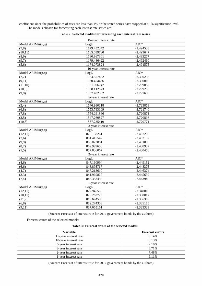
coefficient since the probabilities of tests are less than 1% or the tested series have stopped at a 1% significance level. The models chosen for forecasting each interest rate series are:
Table 2: Selected models for forecasting each interest rate series
15-year interest rate Model ARIMA(p,q) LogL AIC* (7,8) 1179.452342 -2.494533 (10,11) 1185.039730 -2.493647 (8,9) 1180.867301 -2.493277 (9,7) 1179.486422 -2.492460 (5,6) 1174.073824 -2.491575
10-year interest rate Model ARIMA(p,q) LogL AIC* (7,7) 1054.557432 -2.300238 (9,11) 1060.454456 -2.300010 (11,10) 1061.396747 -2.299882 (10,8) 1058.112873 -2.299253 (9,9) 1057.402332 -2.297680
5-year interest rate Model ARIMA(p,q) LogL AIC* (2,4) 1546.980118 -2.723859 (6,8) 1553.783109 -2.721740 (7,8) 1554.291866 -2.720871 (3,5) 1547.260827 -2.720816 (10,8) 1557.235410 -2.720771
3-year interest rate Model ARIMA(p,q) LogL AIC* (12,11) 873.138261 -2.487209 (7,6) 861.415542 -2.482157 (9,9) 866.023881 -2.481008 (8,7) 862.999656 -2.480937 (5,5) 857.836067 -2.480458
2-year interest rate Model ARIMA(p,q) LogL AIC* (4,6) 847.160994 -2.449152 (6,6) 848.895767 -2.448375 (4,7) 847.213610 -2.446374 (3,3) 841.969827 -2.445659 (7,4) 846.383453 -2.443940
1-year interest rate Model ARIMA(p,q) LogL AIC* (12,11) 822.945500 -2.340016 (10,11) 820.263725 -2.338017 (11,9) 818.694538 -2.336348 (6,8) 812.274309 -2.335115 (9,11) 817.665161 -2.333329
(Source: Forecast of interest rate for 2017 government bonds by the authors)
Forecast errors of the selected models:
Table 3: Forecast errors of the selected models
Variable Forecast errors 15-year interest rate 5.14% 10-year interest rate 8.13% 5-year interest rate 9.10% 3-year interest rate 6.71% 2-year interest rate 7.48% 1-year interest rate 9.11%
(Source: Forecast of interest rate for 2017 government bonds by the authors)
479

Simulation of the yield curve at selected dates in 2017 The yield curve is forecasted, using the ARIMA model, at selected dates in 2017:
Figure 1: Forecasted yield curve of government bonds in 2017
(Source: Forecast of interest rate for 2017 government bonds by the authors)
As a result, the forecasts show that the Government bond yield curve for 2017 with various terms is a normal yield curve with upward-sloping (i.e., lower interest rates for short terms and higher interest rates for long terms). This shows a relatively stable evolution of Vietnam's economy in 2017, and the use of conservative strategies in short-term and aggressive in long-term by banks is perfectly fit.
4.2. Application of Barbell Strategy for Government Bond Portfolio of VPBank in 2017
In 2017 VPBank plans to invest VND 40 trillion to target a profit of VND 1,900 billion (VPBank, 2016). Having these targets, a Barbell portfolio of government bonds is formulated, consisting of short-term bonds (50%)
and long-term bonds (50%). Adopting the Macauley formulas (Macauley, 1938), the study assumes the share of bonds in the portfolio, the
reinvestment effect on cash flows and the capitalization effect of bond prices, combined with the yield to maturity of investors (VPB in this case), and the maturity of bond portfolio as follows:
VPBank invests in bonds of 1-year, 3-year, 10-year and 15-year maturities. The bank's budget for bond investment is M. Time: The bank is assumed to hold this portfolio in n (years). The maturity of TP1 is n1 years The maturity of TP2 is n2 years The maturity of TP3 is n3 years The maturity of TP4 is n4 years Interest rate: The yield to maturity that the bank determines for this portfolio is r; The market interest rate of TP1 at the portfolio starting time is y1; The market interest rate of TP2 at the portfolio starting time is y2; The market interest rate of TP3 at the portfolio starting time is y3; The market interest rate of TP4 at the portfolio starting time is y4. To have this portfolio, the following conditions must be met: - According to Macaulay (1938), Biewarg and Kaufman (1977):
480

w1*D 1 + w2*D 2 + w3*D 3 + w4*D 4 = n (1) Where: Di is the duration of TP1, TP2, TP3 and TP4. wi is the weight of each bond on the portfolio. For example, w1 = with P1 is the bank’s investment in TP1. The Barbell portfolio requires: w1 + w2 = 0.5 w3 + w4 = 0.5 In order to satisfy the holding period, the coupons are reinvested and the bond principals are capitalized. The total
value of the portfolio at maturity date is equal to the expected profitability of the initial investment by the bank. In other words, the following equation must be satisfied:
M*(1+r)n = (P1+ F1)* + F2 * + P2* + F3 + P3* + F4 + P4*
It is assumed that VPBank invests VND 40,000 billion in government bonds in 2017, with an expected rate of return 5% for this portfolio in a 5-year holding period. Applying the Barbell Strategy, the bank chooses to contain 1-year, 3-year, 10-year and 15-year bonds in their portfolio. These bonds have coupon rates of 3%, 4.5%, 6% and 7%, respectively. The discount rates valid at the purchase date of these bonds (February 13, 2017) are shown in Table 4:
Table 4: Assumptions of the bond portfolio
No. 1-year 3-year 10-year 15-year 1 Purchase date 13/02/17 13/02/17 13/02/17 13/02/17 2 Maturity date 13/02/18 13/02/20 13/02/27 13/02/32 3 Coupon rate 3% 4.50% 6% 7% 4 Market interest rate 3.16% 4.55% 6.34% 7.36% 5 Number of annual coupons 1 1 1 1 6 Day count convention code 1 1 1 1 Duration 1 2.872573363 7.770677565 9.654996132
(Source: Bloomberg)
Applying the stated conditions, the investments distributed to four classes of bond are as follows: 1-year bonds: VND 7,391.3 billion; 3-year bonds: VND 12,608.7 billion; 10-year bonds: VND 19,456.5 billion; and 15-year bonds: VND 543.5 billion.
4.3. Conditions for the application of Barbell Strategy in bond portfolio management of Vietnamese commercial banks
First, the yield curve is in normal shape (i.e., the longer the maturity, the higher the interest rate), and the difference between short, medium and long-term interest rates is modest (i.e., upward-sloping yield curve). This is a prerequisite for an effective Barbell Strategy, as if the yield curve diverts from these conditions, the use of Barbell Strategy will not be appropriate.
Second, the yield curves of government bonds should be built, which reflect market references for investors. Third, the forecasts of interest rates are correct and sufficient, which accommodate all macroeconomic
fluctuations, and external shocks, if any. Having changes in the economy, interest rates will be immediately affected, which lead to changes in bond prices and expected portfolio performance as a consequence.
Fourth, the investment in government bonds must be significantly large, which is easily satisfied by commercial banks because their size of bond investment is often a multiple of that by common investors. Especially, in the current context, the majority of Vietnamese commercial banks choose government bonds as the key securities in their portfolio for the purposes of both liquidity and profitability.
5. Conclusion
In addition to its achievements, the research has some limitations such as: i) the macroeconomic forecasts should cover a broader scope and details; ii) only government bonds portfolio is considered in the study, but the two common categories of bond portfolio in commercial banks (including trading book and bank book); iii) transaction costs payable to form the bond portfolio have not been taken into consideration.
Thus, the focus on two extremes (short-term and long-term securities) to balance liquidity and profitability of the portfolio, the Barbell Strategy enables Vietnamese commercial banks in the current economic context to achieve both targets.
481

References
[1] ADB (Asian Development Bank), 2016, Asian Bond Monitor, 11/2016. [2] Arturo Estrella (2005a), “Why does yield curve predict output and inflation?”, The Economics Journal, Vol 115, p
722 – 744 [3] Arturo Estrella (2005b), “The yield curve and recessions”, The International Economy, Vol 19, p 8 – 11. [4] Berk, Jonathan and DeMarko, Peter (2014), Corporate Finance, 3rd edition, Pearson, Boston, pp. 169-205 [5] Ministry of Finance, Circular No. 11/2016/TT-BTC issued on January 19, 2016 guiding a number of articles of
the Government's Decree No. 42/2015/ND-CP [6] Government (2012), Decree 42/2015/ND-CP on derivatives and derivatives market, visited on December 12, 2016
at: http://thuvienphapluat.vn/van-ban/Chung-khoan/Nghi-dinh-42-2015-ND-CP-chung-khoan-phat-sinh-thi-truong-chung-khoan-phai-sinh-273248.aspx
[7] Frank J. Jones (1991), “Yield curve strategies”, The Journal of Fixed Income, Vol 1(2), pp. 43-48. [8] Frederick Robertson Macaulay (1938), Some theoretical problems suggested by the movements of interest rates,:
bond yields and stock prices in the United States since 1856; New York, National Bureau of Economic Research [9] G. P. E. Box & G. M. Jenkins (1978), Time Series Analysis: Forecasting and Control, Holden Day, San Francisco. [10] HNX (2012), Annual Report. [11] Harry M Markowitz (1959), Portfolio selection: Effective diversification of investments, Research in Economic at
Yale University, visited on March 10, 2015 at http://cowles.yale.edu/sites/default/files/files/pub/mon/m16-all.pdf [12] Ha Van Hoi (2013), "Viet Nam with progress of trade liberalization towards the establishment of ASEAN
Economic Community", Journal of Southeast Asian Studies, May 2014 [13] HSBC (2009), Diversification of Portfolio, visited on October 28, 2016 at http://tinnhanhchungkhoan.vn/chung-
khoan/da-dang-hoa-danh-muc-dau-tu-60702.html [14] Jack R. Kapoor (2015), Personal financial planning and Insurance, Mc Graw Hill, Chapter 4. [15] Jan Mossin (1968), Optimal Multi-period Portfolio Policies, The Journal of Business, Vol 41, No 2, p 215-229. [16] Kristina Levišauskaite (2010), Investment Analysis and Portfolio Management, Vytautas Magnus University,
visited on March 5, 2016 at http://www.bcci.bg/projects/latvia/pdf/8_IAPM_final.pdf [17] State Bank of Vietnam, 2011, Decree No. 01/2011/ND-CP issued by the Government dated 5 January 2011 on the
issuance of Government Bonds, visited on December 15, 2016 at: http://www.chinhphu.vn/portal/page/portal/chinhphu/hethongvanban?class_id=1&mode=detail&document_id=98535
[18] Nguyễn Duy, ARIMA forecasting model, visited on February 22, 2017 at http://nghiencuudinhluong.com/mo-hinh-du-bao-arima/
[19] Assoc. Prof. Nguyen Thi Kim Yen (2009), Securities Analysis and Portfolio Management, Chapter 1, Statistical Publishing House.
[20] Rhys, Huw (1974), Duration and interest rate risk for uncertain cash flow streams, Journal of Business Finance and Accounting, Vol 1
[21] Schultz Collins Lawson Chambers (2008), Portfolio management: Theory and Practice, Schultz Collins Lawson Chambers INC, page 58.
[22] General Statistics Office (2016), Socio-economic situation in 2016, visited on February 20, 2017 at https://www.gso.gov.vn/default.aspx?tabid=621&ItemID=16174
[23] Institute of Informatics and Applied Economics (2008), Financial Management – Investment: Theory and Applications, Chapter 1, Labor and Social Publishing House
[24] VPBank (2016), Annual Report 2016. [25] William F Sharpe (2007), Investors and markets: Portfolio choices, asset prices and investment advice, Princeton
N.J.: Princeton University Press [26] World Bank (2016), Vietnam Report 2035, retrieved at
http://dsi.mpi.gov.vn/Includes/NewsDetail/12_2016/dt_11220161028_vn2035english.pdf [27] Vuong Quan Hoang, Pham Minh Chinh (2009), Vietnam's Economy: The Rise, Fall, and Breakthrough, National
Political Publishing House.
482

Do Ngoc Lan/ ICYREB 2017 Proceedings
International Conference For Young Researchers In Economics And Business, ICYREB 2017, October 30th 2017 Da Nang, Vietnam
Impact of ODA on Poverty Reduction in Viet Nam
Do Ngoc Lan*
1. Introduction
Reducing poverty has become a great concern to most governments, international organizations and people of all regions given its consequences to their well-being. As a way of reducing poverty, different strategies have been applied at one time or other (Narayan, et al. 2000a, 2000b).
One of the international strategies that have appeared more prominent in recent times is foreign aid which if properly used would spur economic growth as well as reduce poverty. As Killick (1991) put it “aid that comes in a form of technical co-operation would affect the quality of a nation’s labour force through the provision of training and imported skills which is essentially for economic growth and poverty reduction, if an enabling environment is allowed to exist”.
ODA over the past 20 years has helped Vietnam achieve impressive development results, not only in terms of infrastructure, but also in training, human resources and poverty reduction. According to statistics, from 1993 to 2014, the total value of committed ODA for Vietnam has reached 89.5 billion USD, the total signed capital reached 73.68 billion USD, an average of 3.5 billion USD per year , ODA and preferential loans disbursed nearly $ 54 billion, accounting for over 73.2% of total signed ODA.Nearly $ 80 billion committed by donors to Vietnam has not only provided Vietnam with significant additional funding for economic development but also poverty reduction.
Official development assistance (ODA) has been delivered over the years with the basic assumption that it works for poverty reduction. The outcomes however have varied substantially across different contexts. While some recipients have excelled in reducing poverty and sometimes even enhancing economic growth, others have failed to produce tangible outcomes (Collier and Dollar, 2001; Collier, 2008). It is critical for development actors to understand the threshold of ODA capable of delivering meaningful results, and the sectors most efficient and effective in utilizing ODA allocations in order to alleviate poverty (Collier and Dollar, 2001). This paper presents a summary of the outcomes of analysis of the impact of ODA on poverty in VietNam.
2. Literature review
To date, decades of research have failed to provide conclusive evidence for the direct relationship between foreign aid and economic growth or poverty reduction. There are those who argue that it is not possible to reach consensus with selected research methods, among other factors. Dependence on national analysis of case studies at the national level as well as the failure of economists to focus on foreign aid as a means, not just Economic growth but also poverty reduction are considered contributing factors to debate (Cassen 1986, Ayers 1999, Burnside and Dollar 2000, Moreira and Bayraktar 2008). Some economists study the impact of foreign aid on economic growth or poverty reduction ending their research by calling for further analysis in this area to gain better understanding or Remove ambiguity around the
* Hanoi University of Industry, 298 Cau Dien, North Tu Liem District, Ha Noi, Viet Nam
A B S T R A C T
The paper analyzes the impact of ODA on poverty reduction in Viet Nam's provinces using secondary data from GSO from 2006 to 2015. The empirical results show that ODA has the opposite effect on poverty reduction, which means that the increase in ODA will result in the decrease of poverty rate in the provinces of Vietnam. The empirical results are important evidence for economic managers and policymakers, helping them to find specific solutions to attract increasing ODA to Vietnam as well as to use ODA effectively in order to best achieve the goal of growth and poverty reduction for the country.
Keywords: ODA, poverty reduction, Vietnam
483

Do Ngoc Lan/ ICYREB 2017 Proceedings
subject (Barro 1991, 2000, Durbarry, Gemmell and Greenaway 1998, Hansen and Tarp 2001, Veiderpass 2001, Easterly, Levine and Roodman 2003). The profoundly debated discussion on this increase in development aid was enhanced by the publication of Craig Burnside's Aid, Growth and and Policies, and David Dollar's Dollar Aid in 2000.
Burnside and Dollar (1997a, 1998) argue that foreign aid in some underdeveloped countries with good policy has contributed significantly to government spending including regular spending on health and education, rescuing Social assistance, defense and industrialization, in the long run, have improved social welfare and reduced poverty. Killick (1991) mentions foreign aid in some countries due to financial constraints by increasing local taxes and other revenues and increasing the ability to sustain economic services and capital formation. Causing inflationary pressures and / or balance of payments, boosting growth especially if they are in the form of stimulating private sector activities.
The discussion surrounding the relationship between foreign aid and economic growth and poverty reduction has been controversial. Many empirical assessments have failed to yield the final result, whether foreign aid has a major impact on growth or poverty, and to what extent.
3. Data Source and methodology
3.1. Data source
The paper uses secondary data from the General Statistical Office, in which, ODA data, poverty reduction and institutional data are collected at provincial level from 1993 to 2015. Particularly, institutional data are collected from 2006 to 2015
3.2. The model
In specifying the model emphasis is placed on whether foreign aid has a significant impact on poverty reduction in Vietnam (Gafa, T. and Muftau, A., 2004)
(PROVERTY REDUCTION)it = + ODAit +STITUTIONALit + Uit
Dependent variable: Poverty reduction. There are many different proxies to measure poverty. However, this article uses the poverty rate among households as the best measurement of poverty reduction in Viet Nam.
Independent variable: ODA that flows into the provinces of Vietnam from 1993 to 2015. The author takes the logarithm of ODA when introducing the variable into the model.
Institutions are measured by the compositeprovincial competitiveness indices of Vietnam for the period from 2006 to 2015. Acompositeprovincial competitiveness index is calculated following a 3-step sequence: 1) collect enterprise survey data using questionnaires and data from published sources; 2) calculate 10 sub-indices and standardize the results to a 10-point scale; and 3) calibrate the composite PCIas the weighted mean of the 10 sub-indices with a maximum score of 100.
3.3. Statistical description and correlation of variables
The actual situation of ODA and the average rate of poor households in Vietnam over the past 2 decades are shown in Figure 1. Accordingly, ODA to Vietnam tends to increase over the years, whereas the rate of poor households decreases sharply over the years. . Thus, Vietnam has benefited from the impressive results of poverty reduction, right at the time when donors are focusing more on hunger eradication and poverty alleviation and willing to aid those who use the source better.
Statistical descriptions of variables are shown in Table 1 below
Table 1: Statistical summary
Variable Obs Mean Std. Dev. Min Max
Poverty reduction 1343 31.0928 20.9343 0.01 105.52
ODA 1343 868.439 2121.19 10.02 24372
Institution 554 56.7909 6.31233 36.39 77.2
Source: The author calculated from the GSO data
484

Do Ngoc Lan/ ICYREB 2017 Proceedings
Unit: billion VND Unit: %
Figure 1: ODA and the rate of poor households in Vietnam on average over the years
Source: The author calculated from the GSO data
Description of the correlation between the variables is shown in Table 2 below. Accordingly, variables ODA
and institutions are negatively correlated with poverty reduction, and the correlation between OAD and poverty
reduction is relatively strong (31.3%). In addition, the correlation between OAD and Institution variables is low (5.7%);
so the explanatory variables do not have a high linear relationship.
Table 2: Correlation Matrix
Variable Poverty reduction ODA Institution Poverty reduction 1 ODA -0.3125 1 Institution -0.241 0.0568 1
Source: The author calculated from the GSO data
3.4. Results of estimation and discussion
The result of Lagrange Test indicates that the POLS model is inappropriate. The result of Hausman Test shows that the FE model is more efficient than the RE model. However, the FE model violates the assumptions of heteroskedasticity, autocorelation, and cross section. We need a model that can overcome the above violations. Thus, the final model chosen for analysis is the Regression with Driscoll-Kraay standard errors model.
Table 3: Estimation result
Variable RE FE
Regression with Driscoll-Kraay standard
errors
LnODA -2.7542*** -2.4135*** -4.8221*** (0.4018) (0.4367) (0.3563) Institution -0.1439*** -0.1379*** -0.2803* (0.0419) (0.0420) (0.1338) _cons 41.0815*** 38.9643*** 61.9214*** (3.3382) (3.3257) (5.8454)
Lagrang Test chibar2(01) = 954.880 P-value =0.0000
Hausman test chibar2(02) = 12.19 P-value =0.0023
Cross - section chi2(1953) = 2730.957
485

Do Ngoc Lan/ ICYREB 2017 Proceedings
P-value =0.0000
Heterokedasticity chibar2(63) = 13360.34 P-value =0.0000
Autocorelation F( 1, 61) = 76.708 P-value =0.0000
N 554 554 554 r2 0.28 0.08 0.29
Note: The values in parentheses are standard errors, *, **, *** mean the significance at 10%, 5% and 1% respectively.
Source: The author calculated entirely from data obtained from GSO and the help of STATA software.
According to the estimation results,ODA and institutional variables are significant at 10%, which implies that both ODA and institutions have an impact on poverty reduction in Vietnam. In particular, OAD has the opposite effect on reducing poverty in Vietnam. This result is consistent with economic theory, meaning that the increase in international aid will reduce the rate of poor households in the provinces of Vietnam. Poverty reduction is one of the first principles given by international donors in formulating formal development assistance. This goal demonstrates the humanitarian nature of ODA. According to the empirical results, 1% increase in ODA results in the decrease in the poverty rate of the provinces in Vietnam by 2.75% on average.
On the other hand, institutional improvements also help to reduce the incidence of poverty in the provinces of Vietnam. There are many studies in the world suggesting that differences in economic institutions are the underlying cause of different patterns in economic growth. The core of these studies is based on the argument that the way people organize their society determines whether or not the society is prosperous. A social organization that encourages people to innovate, take risks, save for the future, study, solve common problems, and provide public goods ... is a society that reaches higher levels of revenue. On the contrary, the society that goes against this organization will fall into poverty. The empirical result of this research does support the rule, emphasizing that for provinces in Vietnam, improving the quality of economic institutions would help reduce poverty. This result is consistent with the general theory of institutional economics.
4. Conclusion
The article analyzes the impact of ODA on poverty reduction in Viet Nam, studies for provinces using secondary data from the General Statistics Office. Results of quantitative research indicate that ODA has the opposite effect on poverty reduction in Vietnam. Specifically, 1% increase in ODA will result in the decrease of the poverty rate among households in the provinces in Vietnam by 2.75% on average. This result is consistent with economic theory. The study confirms the important role of ODA in growth and poverty reduction. The research results are important empirical evidence for economic managers and policymakers to find specific solutions to attract and increase ODA to Vietnam as well as to use ODA effectively to best achieve the goal of growth and poverty reduction of the country.
References
[1] Akhand, Hafiz, and Kanhaya L. Gupta. “Zero Foreign Aid?: Policy Implications for Donor and Recipient Countries”. Regina, Sask.: Saskatchewan Institute of Public Policy, 2006.
[2] Angeles, Luis, and Kyriako C. Neanidis. "Aid Effectiveness: the Role of the Local Elite."Journal of Development Economics 90 (2009): 120-34.
[3] Ayres, Robert L.” Foreign Aid and Poverty Reduction” Foreign Aid and Poverty Reduction. Finance and Development, Sep 1990, Vol. 27, 3
[4] Baliamourne-Lutz, Mina and George Mavrotas. 2009.“Aid Effectiveness: Looking at the Aid-Social Capital-Growth Nexus”.Review of Developmental Economics, 13 (3), pp. 510-525
[5] Barro, Robert. 1991. “Economic Growth in a Cross Section of Countries”. The Quarterly Journal of Economics, Vol. 106, No. 2, pp. 407-443
[6] Barro, Robert. 2000. “Inequality and Growth in a Panel of Countries”. Journal of Economic Growth; Vol. 5, 1, pp 5-32
[7] Betances, Emelio. State and Society in the Dominican Republic.Boulder, Colo.: Westview, 1995. [8] Boone, Peter, 1996. "Politics and the effectiveness of foreign aid".European Economic Review, Elsevier, Vol.
40(2), pages 289-329, February. [9] Bornschier, Volker, Christopher Chase-Dunn , and Richard Rubinson. 1978. “Cross-National Evidence of the
Effects of Foreign Investment and Aid on Economic Growth and Inequality: A Survey of Findings and a Reanalysis.” The American Journal of Sociology, Vol. 84, No. 3, pp. 651-683
[10] Brautigam, Deborah A. and Stephen Knack. “Foreign Aid, Institutions, and Governance in SubSaharan Africa”.Economic Development and Cultural Change; Jan 2004; 52, 2; 255-286
[11] Burnside, Craig and David Dollar. ” Aid, Policies, and Growth.” The American Economic Review. Vol. 90, No. 4
486

Do Ngoc Lan/ ICYREB 2017 Proceedings
(Sep., 2000), pp. 847-868. [12] Burnside, Craig. and David. Dollar. 2004. “Aid, Policies and Growth: Revisiting the Evidence”, World Bank
Policy Research Paper O-2834, World Bank, Washington. [13] Collier, P., Dollar, D., 2001. Can the world cut poverty in half? How policy reform and effective aid can meet the
international development goals?,World Development29 (11), 1787-1802. [14] Collier, Paul, and David Dollar, 2002, “Aid Allocation and Poverty Reduction” European Economic Review, Vol.
46, No. 8, pp. 1475–1500 [15] Cassen, Robert “The Effectiveness of Aid.”Finance and Development, Vol.23, Issue. 1. March 1985. [16] Clemens, Michael, Steven Radelet, and Rikhil Bhavnani. “Counting Chickens When They Hatch:The short term
effect of aid on growth”. Center for Global Development. Working Paper Number. 44, November 2004. [17] Dollar, David and Victoria Levin. “The Increasing Selectivity of Foreign Aid, 1984-2002”.World Bank Policy
Research Working Paper 3299, May 2004 [18] Hansen, Henrik and Finn Tarp. 2001. "Aid and Growth Regressions”. Journal of Development Economics. 64:2,
pp. 547-70. [19] Gafa, T. and Muftau, A. 2004. ‘Foreign aid and poverty reduction in sub – Saharan africa”. Sajems ns 7, no3. 542
- 552 [20] Krauss, Melvyn. 1983. Development Without Aid: Growth, Poverty and Government. New York. McGraw-Hill [21] Kryzanek, Michael J., and Howard J. Wiarda. The Politics of External Influence in the Dominican Republic. New
York: Praeger, 1988. [22] Tandon. Yash. “Aid without Dependence: An alternative conceptual model for development cooperation”.
Development. 2009, Vol. 52, No. 3. pp. 356-362 [23] Schwalbenberg, Henry. 1998. “Does Foreign Aid Cause the Adoption of harmful Economic Policies?”, Journal of
Policy Modeling. 20(5), pp. 669-675 [24] Schulz, Nils-Sjard. "Implementing Paris and Accra: Towards a Regional Agenda inLatin America and the
Caribbean”.Fundación Para Las Relaciones Internacionales Y El Diálogo Exterior (FRIDE) January (2009): 1-24.
487

Nguyen Thi Ngan, Nguyen Thị Diem Hien, Hoang Trung Nghia / ICYREB 2017 Proceedings
International Conference For Young Researchers In Economics And Business, ICYREB 2017, October 30th 2017 Da Nang, Vietnam
The Effects from The U.S. and Japan to Emerging Stock Markets
in Asia and Vietnam
Nguyen Thi Ngan, Nguyen Thi Diem Hien, Hoang Trung Nghia*
University of Economics and Law – Vietnam National University - HCMC
A B S T R A C T
The subprime mortgage crisis in the U.S. in mid-2008 suggests that stock prices volatility do spillover from one market to another after international stock markets downturn. The purpose of this paper is to examine the magnitude of return and volatility spillovers from developed markets (the U.S. and Japan) to eight emerging equity markets (India, China, Indonesia, Korea, Malaysia, the Philippines, Taiwan, Thailand) and Vietnam. Employing a mean and volatility spillover model that deals with the U.S. and Japan shocks and day effects as exogenous variables in ARMA(1,1), GARCH(1,1) for Asian emerging markets, the study finds some interesting findings. Firstly, the day effect is present on six out of nine studied markets, except for the Indian, Taiwanese and Philippine. Secondly, the results of return spillover confirm significant spillover effects across the markets with different magnitudes. Specifically, the U.S. exerts a stronger influence on the Malaysian, Philippine and Vietnamese market compared with Japan. In contrast, Japan has a higher spillover effect on the Chinese, Indian, Korea, and Thailand than the U.S. For the Indonesian market, the the return effect is equal. Finally, there is no evidence of a volatility effect of the U.S. and Japanese markets on the Asian emerging markets in this study.
Keywords: Spillover; emerging markets; volatility effect; day effect
1. Introduction
In recent years, the world – especially developing countries – experienced a strong capital liberalization, financial market reform and advances in information technology. Consequently, information transmits across global financial markets more freely than ever, resulting in an increased linkage between stock markets. It has been found that the deeper the level of global financial integration, the more likely it is that financial markets of developing countries are affected by volatility spillover effects from mature financial markets. The latest financial turmoil began from U.S. in 2007 and spread to Asian markets in the early of 2008 through different mechanisms, such as increasing market volatility or market and funding illiquidity (Frank, Gonzalez-Hermosillo and Heese 2008). Following that crisis, Asian financial markets became highly volatile and shook violently. Due to its size and economic importance in the world, the U.S. potential impact on emerging markets cannot be denied. Likewise, Japan as a major investor and trading partner of many Asian countries is expected to exert its influenced on these markets. Japan is the world’s fourth largest stock exchange in terms of aggregate market capitalization of listed companies, and the largest in Asia. Japanese investors also hold a large amount of Asian assets (Fornari and Levy, 2000).
The volatility transmissions between stock markets have been the object of study of both practitioners and academia over the years. Understanding the level of correlations between stock markets would be a great help to investors and hedgers in their international portfolio diversification and optimization. A plenty of studies provided evidence for the spillover effects from the U.S. and Japan to other stock markets. This paper attempts to empirically examine the level of spillover effects from these two large mature markets on eight Asian emerging and Vietnamese stock markets. The ARMA(1,1)-GARCH(1,1) is utilized. In particular, the return spillover are modelled using ARMA(1,1), volatility spillover is estimated using a two-step GARCH (1,1) model. The data of this study is from 2000 to 2017, covering the period prior, during, and after the global financial crisis in 2007. This extensive coverage lends credibility to the results of this analysis. The empirical results in this research may be helpful for academics, domestic
* Corresponding author. Tel.: +84962001284
E-mail address: [email protected]
488

Nguyen Thi Ngan, Nguyen Thị Diem Hien, Hoang Trung Nghia / ICYREB 2017 Proceedings
policy makers and professionals in understanding the magnitude of volatility spillover effects of the U.S. and Japanese stock markets on the Asian emerging stock markets. Moreover, this study contributes to the growing literature on the spillover effects and volatility transmission of equity returns.
The remainder of the paper is organized as follows. A literature review on the study of return and volatility spillover across markets is presented in the next section. Section 3 gives details about the financial model for estimating volatility transmissions and spillover effects and as well as estimation procedure. Research data and the descriptive statistics are provided in Section 4. The empirical results are given in section 5 and finally, in the last chapter, the paper closes with concluding comments.
2. Literature Review
The study of market integration through analyzing both returns and volatility spillover has important implications for the modern portfolio theory. Several empirical literature provides strong evidence of market interdependence and integration among among national stock markets.
Mervyn and Wadhwani (1990) applied correlation coefficients to stock market returns in order to examine how the market crash in the U.S. influenced the stock markets in Japan and the U.K. by using the GARCH model, co-integration tests, and the probability of specific events. The results show that the U.S. stock market crash significantly increased the correlation coefficients between multiple markets. Pan and Hsueh (1998) examined the nature of transmission of stock returns and volatility between the U.S. and Japanese stock markets employing a two-step GARCH approach. By using futures prices on the S&P500 and Nikkei225 stock indexes, they found that there are unidirectional contemporaneous return and volatility spillovers from the U.S. to Japan. In particular, the U.S. influence on Japan in returns is approximately four times as large as the other way around. There are also no significant lagged spillover effects in both returns and volatility from the Japan to the U.S. while a significant lagged volatility spillover is observed from the U.S. to Japan.
Cha and Oh (2000) studied weekly stock indices of the U.S., Japan and four Asian NIEs from 1980 to 1998. They reported that the stock market crash the U.S. market began to have a significant impact on the Hong Kong and Singapore after the October 1987, yet its influence on Taiwan and South Korea remained unchanged. Employing a multivariate GARCH in Mean, Zaid (2011) investigated the international transmission of daily stock index volatility movements from the U.S. and U.K. to selected Middle Eastern and North African emerging markets, namely Egypt, Israel, and Turkey. The study finds that Egypt and Israel are significantly influenced by the U.S. stock market while Turkey is not.
Batareddy et al. (2012) investigated the stability of the long‐run relationships between emerging (India, China, South Korea, and Taiwan) and developed stock markets (the U.S. and Japan) using use time varying cointegration tests with the sample data from mid 1998 to 2008. Their empirical findings support the presence of one long‐ run relationship (cointegration vector) between emerging and developed stock markets and the individual Asian emerging stock markets tend to display stronger linkages with the U.S. rather than with their neighbors.
Dhanaraj et al. (2013) using FEVD analysis in researching on the dynamic interdependence between the U.S. and Asian markets revealed the dominance of the U.S. stock market on Asian markets and that Asian stock markets are not immune to the shocks originating in the USA though the effects of shocks vary considerably across markets.
For the Vietnamese stock market, Farber et al. (2006) show that there exist anomalies stock returns through clusters of limit-hits and limit-hit sequences in HSC. Besides, there is a strong herd effect toward the extreme positive returns in market portfolios. Moreover, the specification of ARMA- GARCH can help capture issues such as serial correlations and fat-tails for a stabilized period, and policy decisions on the technicalities of trading can influence movements in risk level through the conditional variance behavior of HSC stock returns.
Using the correlation contagion test and Dungey et al.’s (2005) contagion test by EGARCH model, Wang and Lai (2011) find contagion effects between the Vietnamese and Japanese, Singaporean, Chinese, and the U.S. stock markets. They also show that the Japanese stock market causes stronger contagion risk in the Vietnamese stock market compared to China, Singapore, and the U.S. The stronger interdependence effects of Chinese and U.S. stock markets causes weaker contagion effects in the Vietnamese.
In summary, we have seen that most empirical studies have focused on the effects of developed markets both across the world and in the U.S., Japan to stock markets of other emerging countries. However, empirical examination of stock markets in Asia and Vietnam are limited, which necesitate further studies.
3. Methodology
Fama (1965) and others have documented that stock returns exhibit mild serial correlations. In particular, large changes in daily stock prices tend to be followed by large changes and small price changes tend to be followed by small changes (see Mandelbrot, 1963; and Fama, 1965). The generalized autoregressive conditionally heteroscedastic (GARCH) family is designed to model the conditional mean and volatility of stock returns by taking into account the above properties. Since its introduction, the GARCH model has been generalized and extended in various directions.
489

Nguyen Thi Ngan, Nguyen Thị Diem Hien, Hoang Trung Nghia / ICYREB 2017 Proceedings
According to Akgriray (1989) and Brooks (2008), the GARCH(1,1) model is sufficient to capture the volatility clustering in the data, and rarely is any higher order model estimated or even entertained in the academic finance literature. The (1,1) in parentheses is a standard notation in which the first number refers to how many autoregressive lags, or ARCH terms, appear in the equation, while the second number refers to how many moving average lags are specified, which is often called the number of GARCH terms. The conditional variance is a linear function of 1 lag of the squares of the error terms () (also referred to as the “news” from the past) and 1 lag of the past values of the conditional variances ( ) or the GARCH terms, and a constant ω.
Following Liu and Pan (1997), this paper allows innovations in the U.S. and Japan to influence the equity return of Asian emerging markets through the error term. The importance of modelling the volatility effect in financial markets during the financial turmoil has increased significantly and there has been a correspondingly large amount of literature over time to address the issue. Currently, the GARCH models are amongst the most popular econometric models used in academic studies.
The model used in our research is the ARMA(1,1)-GARCH(1,1) and can be summarized as below.
3.1. Developed markets: the U.S. and Japan
We begin by specifying an appropriate ARMA-GARCH model, daily returns of the U.S. and Japan. We assume that the U.S. and Japan stock market returns are not affected by other markets and those returns are estimated through the following ARMA(1)-GARCH(1,1) model with the mean and variance equations:
4
, 0, 1 1, 2 1, , , ,1
t i i t i t i j j t i t ij
r r d D (1)
2, ,(0, )t i t iN
2 2 2, 0, 1 1, 2 1,t i i t i t i (2)
where tr is the daily stock index return; i represents the U.S. and Japan; tjD , is dummy variable for Monday, Tuesday, Wednesday and Thursday respectively; and t is the residual.
The residual t is the short-term fluctuation which expresses the unexpected events, new information or innovation in the U.S. and Japanese stock markets and spreads to eight Asian emerging markets and Vietnam. The larger the residuals are, the more likely they spread to Asian markets. Therefore, the residuals are employed to capture to the spillover effects from the U.S. and Japan to Asian markets.
3.2. Emerging markets and Vietnam
On the assumption that Asian markets could be affected by both the U.S. and Japanese markets, we consider the case where the international transmission from the U.S. and Japanese market could exist in terms of the mean and volatility effects. We construct a mean and volatility spillover model that deals with the shocks from the U.S. and japan as an exogenous variable in a ARMA-GARCH to the Asian markets by substituting the residual derived from equations (1) and its square from equations (2) of the U.S. and Japan market into the following ARMA-GARCH model.
Due to different trading time, a shock in the U.S. stock market during day t will not be reflected in the Asian emerging stock markets until day t+1. As a result, the appropriate pairing is time t–1 for the U.S. and time t for the Asian markets. Furthermore, as shown in Table 1, the Japanese market is closed earlier than other Asian stock markets, except for Taiwan. Therefore, the appropriate pairing is time t–1 for Japan and time t for Taiwan, and it is time t for Japan and time t for Hong Kong, Singapore, and Thailand.
That is, our model is given by: For the Taiwanese market:
4
0 1 1 2 1 , , 1 , 11
t t t j j t US US t JP JP t tj
r r d D e e
2(0, )t tN
2 2 2 2 20 1 1 2 1 , 1 , 1t t t US US t JP JP te e
For others:
4
, 0 1 1, 2 1, , , , 1 , ,1
t i t i t i j j t i US US t JP JP t t ij
r r d D e e
490

Nguyen Thi Ngan, Nguyen Thị Diem Hien, Hoang Trung Nghia / ICYREB 2017 Proceedings
2, ,(0, )t i t iN
2 2 2 2 2, 0 1 1, 2 1, , 1 ,t i t i t i US US t JP JP te e
Where 1, tUSe and 2
1, tUSe are the residual and the square of the residual for the U.S. market estimated in equation (1) and (2). The model allows us to model the volatility transmission spillovers between markets, with the data generating processes for the time-varying covariances across markets, rather than an unconditional consistent shock. We allow for mean spillover effects by including residual of S&P500 and Nikkei225 retrieved from the equation (1) and include the residual squares obtained from Equation 2 for S&P500 and Nikkei225 in variance equation, to capture the volatility spillover effects. The coefficient US , JP captures the mean spillover effect (cross-mean spillover) and the coefficient US , JP captures the volatility spillover effect (cross- volatility spillover) from the US and Japan . Statistically significant values for 1 and 2 respectively, indicate the influence of own-mean and own-volatility spillovers from previous returns of Asian markets returns. Notice that the lag of the residuals of the U.S. and Japan is used due to different time zones between the US and Japan.
4. Data
Fuelled by an increase of capital in recent years, the stock markets of the emerging markets in the Asian region have experienced a rapid growth. Data employed in the thesis are daily adjusted closing for 8 indexes of emerging markets in Asia, namely Taiwan, Korea, Indonesia, Philippines, China, Thailand, Malaysia, Indian (as classified by Morgan Stanley Capital International (MSCI) 2015). In addition, Vietnam's market is also considered. As a result, stock indices used are TSEC weighted index TWII (Taiwan), Kospi Index KS11 (Korea), Jakarta Composite Index JKSE (Indonesia), PSEi-Index PSEI.PS (Philippines), SET Index (Thailand), KLSE (Malaysia), S&P BSE SENSEX Index (Indian), Shanghai Composite Index (China), and VN-Index (Vietnam). The data are retrieved from Yahoo Finance and Datastream. The sample period spans from January 2, 2000, to May 31, 2017. Daily returns data is able to capture most of the possible interactions.
For the U.S. stock market, we used the Standard and Poor 500 (S&P 500) Index, which is a market value weighted index and one of the common benchmarks for the U.S. stock market. The index includes 500 leading companies and captures approximately 80% coverage of available market capitalization. For the Japanese stock market, we employed the Nikkei225 Index, the leading and most-respected index of Japanese stocks. It is a price-weighted index comprised of Japan's top 225 blue-chip companies traded on the Tokyo Stock Exchange. the Nikkei is the most widely quoted average of Japanese equities, represents roughly 50% of the total market capitalization for the Tokyo Stock Exchange.
The number of observations is approximately 4300 for each country. The data for the whole period are illustrated in the Appendix A. The data of stock price exhibit large fluctuations during the whole period. The paper analyzes the exogenous effects of the U.S. and Japanese returns and volatilities on Asian countries.
Table 1: Emerging Markets as Classified by MSCI
https://www.msci.com/emerging-markets
The stock indices and their home countries are presented in Table 2. Also presented are their trading hours in both local and UT time for the purpose of studying the same effects. As can be seen from the table (Trading-UTC column), the U.S. market closes later than the other Asian stock markets; therefore, a shock in the U.S. stock market during day t will not be reflected in the Asian emerging stock markets until day t+1. Thus, the appropriate pairing is time t–1 for the
491

Nguyen Thi Ngan, Nguyen Thị Diem Hien, Hoang Trung Nghia / ICYREB 2017 Proceedings
U.S. and time t for the Asia markets. Furthermore, as Table 2 shows, the Japanese market is closed earlier than the other Asian stock markets, except Taiwan. Therefore, the appropriate pairing is time t–1 for Japan and time t for Taiwan, and it is time t for Japan and time t for Hong Kong, Singapore, and Thailand.
The indices are transformed to a daily rate of return as below, which are defined as the natural logarithmic returns in two consecutive trading days:
)
Where is the daily log return, and are the daily adjusted closing price of each stock indices at time t and t-1.
Table 1: Indices, home countries, time-zones and trading hours in local and GMT time
The plots for the daily log returns fluctuate around a zero mean (see Figure 1). Each of all series appears to show
the signs of ARCH effects in that the amplitude of the returns varies over time. Volatility clustering – the periods of high volatility alternate periods of low volatility – can be observed (large and
small swings tend to cluster, see Figure 1. Abusing the terminology slightly, it could be started that “volatility is autocorrelated”. Observing the time series data set of returns, we see that there exists heteroskedasticity in the model. However, we cannot determine whether this is enough to warrant consideration.
Descriptive characteristics for the daily stock index returns of emerging markets are given in Table 3. It can be seen that the average daily returns are positive (except for TWII with negative mean returns) but
negligibly small compared to the sample standard deviation. Six out of eight Asian markets (with the exception of China and Taiwan) have a higher return than the the U.S. and Japan. This is why the mean is often set at zero when modelling daily portfolio returns (Figlewsky,1994), which reduces the uncertainty and imprecision of the estimates. PSEI shows the most extreme values of daily market returns compared to the rest. China has the highest standard deviation whereas Malaysia has lowest.
The returns series display similar statistical properties as far as the third and fourth moments are concerned. More specifically, the returns series are skewed (either negatively or positively) and the large returns (either positive or negative) lead to a large degree of kurtosis. Excess kurtosis is a measure of peakedness or flatness of data in comparison to normal distribution. Both the indices show evidence of fat tails (leptokurtic) since the kurtosis exceeds 3 (the normal value), implying that the distribution of these returns has a much thicker tail than the normal distribution. As we know, skewness is a measure of symmetry, which is equal to zero for normal distribution. The skewnesses of all markets (except PSEI.PS) are also negative, indicating that the distribution has an asymmetric tail extending out to the left and is referred to as “skewed to the left”. This leads the standard deviation of all markets which presents the “risk” is underestimated when kurtosis is higher and skewness is negative.
The Ljung-Box (LB) Q statistics for daily stock returns of both assets are highly significant at five-percent level indicate the presence of serial correlations. Furthermore, the Ljung-Box Q statistics for squared returns are much higher than that of raw returns indicate the time-varying volatility. The p-value of ArchTest shown in the last row are all zero to both places, resoundingly rejecting the “no ARCH” hypothesis.
Furthermore, the presence of serial correlations and time-varying volatility make the traditional OLS regression inefficient. These features of the data lead us to consider the GARCH type models that can accommodate time-varying
Index Country Time-zone Trading - local time Trading - UTC
Open Close Open Close
S&P 500 The U.S. UTC-5 9:30 16:00 14:30 21:00
Nikkei 225 Japan UTC+9 9:00 15:00 0:00 6:00
TWII Taiwan UTC+8 9:00 13:30 1:00 5:30
KS11 Korea UTC+9 9:00 15:30 0:00 6:30
JKSE Indonesia UTC+8 9:30 16:00 1:30 8:00
PSEi Philippines UTC+8 9:30 15:30 1:30 7:30
SET Thailand UTC+7 10:00 16:30 3:00 9:30
KLSE Malaysia UTC+8 9:00 17:00 1:00 9:00
S&P BSE SENSEX Indian UTC+05:30 9:15 15:30 3:45 10:00
Shanghai China UTC+8 9:30 15:00 1:30 7:00
VN Vietnam UTC+7 9:00 15:00 2:00 8:00
492

Nguyen Thi Ngan, Nguyen Thị Diem Hien, Hoang Trung Nghia / ICYREB 2017 Proceedings
and persistent behavior of volatility of returns. We start modeling with ARMA(1,1)- GARCH(1,1).
Figure 1: The daily returns of stock indices
Table 2: Descriptive statistics of indices
z US N225 BSE China JKSE KLSE KS11 PSEI SET TWII VNI
Mean 0.0001 0.0000 0.0004 0.0001 0.0005 0.0002 0.0001 0.0003 0.0003 -0.0001
0.0004
Min -0.0947
-0.1211
-0.1181
-0.0926
-0.1131
-0.0998 -0.1237
-0.1309 -0.1606 -0.1013
-0.0766
Max 0.1096 0.1323 0.1599 0.0940 0.0762 0.0450 0.1128 0.1618 0.1058 0.0700 0.0664
Std.dev 0.0124 0.0154 0.0151 0.0162 0.0137 0.0081 0.0154 0.0131 0.0135 0.0139 0.0155
493

Nguyen Thi Ngan, Nguyen Thị Diem Hien, Hoang Trung Nghia / ICYREB 2017 Proceedings
Skewness -0.2659
-0.4113
-0.2082
-0.3140
-0.6214
-0.8163 -0.5326
0.3595 -0.7567 -0.4060
-0.3062
Kurtosis 8.6710 6.1992 7.7607 4.8561 6.0801 10.6911 6.0148 16.0136 10.1317 4.2050 2.9301
LB Q-statistics
Daily Returns
LB (12) 83 32 46 22 69 99 21 64 63 42 400
0.0 0.0 0.0 0.0 0.0 0.0 0.05 0.0. 0.0 0.0 0.0
LB (24) 150 52 61 57 81 110 37 90 78 50 450
0.0 0.0 0.0 0.0 0.0 0.0 0.05 0.0 0.0 0.001 0.0
Squared Daily Returns
LB (12) 4200 2800 1100 820 1200 400 1800 180 690 1100 9300
0.0 0.0 0.0 0.0 0.0 0.0 0.0 0.0 0.0 0.0 0.0
LB (24) 6500 3400 1500 1400 1500 490 2800 210 740 1800
14000
0.0 0.0 0.0 0.0 0.0 0.0 0.0 0.0 0.0 0.0 0.0
ArchTest (12)
1200 930 420 350 530
210 640 130 450 430 1700
0.0 0.0 0.0 0.0 0.0 0.0 0.0 0.0 0.0 0.0 0.0
5. Empirical Results
Empirical models for these Asian markets are as below: 4
0 1 1 2 1 , , 1 ,1
t t t j j t US US t JP JP t tj
r r d D e e
2(0, )t tN 2 2 2 2 2
0 1 1 2 1 , 1 ,t t t US US t JP JP te e
The dummy variable for day effect is insignificant in most countries in mean equation, indicating there is no weekday effect in mean returns. It is worth noting that markets where day effect is present, the dummy variable has a negative sign and most falls on Monday. This result implies there is a difference between stock returns on Monday and Friday on these markets which is consistent with prior studies. Accordingly, the average stock return on Monday is negative and lower than the other weekdays. The Monday effect is a form of inefficient market when the Monday average return is affected by return of the other weekdays, especially the last Friday. Reactions of investors on Monday are normally unfavorable, resulting in a negative average return. This effect is related to financial behavior of investors.
Coefficients 1 in the U.S., Japan, Malaysia, Korea, Taiwain and Vietnam are positive and significant, suggesting that stock returns on Asian markets today are affected by stock returns of the previous day. The negative and significant coefficient 1 for Indian, Indonesian, Philippine and Thai markets indicates that there is no impact of return on the previous day on the today return.
The statistically significant values of US , JP suggest that returns on the U.S. and Japanese affect the conditional mean of the considered Asian markets returns (e.g. cross-mean spillover). The results for the conditional mean equations show statistically significant positive mean spillover effect from the U.S. and Japan returns, indicating that a high return in the two those mature markets are followed by high returns in the Asian markets. Global financial markets display a higher degree of correlation owing to globalization and more efficient dissemination of information. Stocks are more likely to be affected by developments in overseas markets.
Another noticeable finding is Japan has a stronger influence on Korea than the U.S. (0.370 versus 0.210) while the U.S. has a stronger influence on Taiwan than Japan (0.436 versus 0.009). These effects are likely due to the strong economic relationship between Japan – Korea and the U.S. – Taiwan. However, these effects cannot be so easily explained and and require further study for explanation. Vietnam’s stock market exhibits the lowest influence from the U.S. compared with other examined markets. This is perhaps due to the tight capital control by the Vietnamese Government.
On the other hand, in terms of the volatility spillover, the estimates of GARCH parameters 1 , 2 for for Asian markets are significant and the sum of these two coefficients which measures the persistence of volatility is close to unity. The parameter estimates for the conditional variance 1 , 2 are highly significant, indicating that the conditional variance process of the Asian markets returns is indeed time-varying. The own-volatility spillover effect
494

Nguyen Thi Ngan, Nguyen Thị Diem Hien, Hoang Trung Nghia / ICYREB 2017 Proceedings
from the previous volatility 2 is highly significant whereas the cross-volatility spillover effect from the U.S. and Japan is insignificant. The statistically insignificant values for US , JP indicate there is no influence of volatility spillovers from the U.S. and Japan to the Asian markets. Possible reason is that their volatility is mainly explained by the Asian own volatility.
These diagnostics show that the residuals of the models are reasonably well-behaved. The portmanteau LB statistics in Panel B of Table 4 evaluate the serial correlations in the raw and squared standardized residuals of the model up to lags 7 and 9 and find that most of the conditional dependence in the return has been modeled reasonably well.
6. Conclusions
This paper focuses on investigating the transmission volatility and spillover effects from the U.S. and Japan to eight Asian and Vietnamese stock markets by exploring the level of conditional correlations between markets from January 1st, 2000 to May 31st, 2017 using ARMA(1,1)-GARCH(1,1) models. The results provided interesting findings which contribute to the understanding of the time-varying nature of mean and volatility spillover effects between developed and Asian emerging stock markets. We allow for mean spillover effects by including residual of S&P500 and Nikkei225 obtained from the equation (1) and including the residual squares obtained from equation (2) for S&P500 and Nikkei225 in variance equation to capture the volatility transmission effects. The results do not support the evidence of the day effect on all markets. For markets where the day effect, dummy variable has a negative sign and most fall on Monday. We also found clear evidence that the returns of the U.S. and Japan exert a positive influence on the returns on Asian markets. In addition, the cross-volatility spillover effect from the U.S. and Japan returns is insignificant whereas the own-volatility spillover effect from Asian returns itself are highly significant.
These results are important for economic policy makers in order to safeguard the financial sector from international financial shocks. The investors can use this information for constructing efficient portfolios to reduce risks and enhance returns.
The majority of recent studies of international prices and volatility focus on the developed markets. Thus the present paper also contributes to the literature by broadening the focus of the existing evidence. Further research is necessary for investigating the mean and volatility transmission through multivariate GARCH (M-GARCH) models. The ability of capturing cross-market spillovers increases with MARCH specification because of its advantages.
Table 3: Empirical Results
US N225 BSE China JKSE KLSE KS11 PSEI SET TWII VNI
0
1
2
1d
2d
3d
4d
US
JP
0
1
2
US
JP
LB Q-Statistic Standardized Residuals LB(5)
0.0001 0.9***
-0.93**
* 0.001 0.0003 0.0005 0.0004
0.000**
0.104***
0.88***
2.957353
0.4989 6.8866
67 0.1393 5.979 0.0910
0.0003 0.934*
** -
0.944*** -
0.0004 0.0001 0.000 0.001
0.000* 0.11**
* 0.869*
**
3.163 0.3733 5.219 0.4053 0.7458
1 0.9140
0.001** -
0.982***
0.979***
0.000 0.000 0.0000 0.000 0.133*
** 0.220*
** 0.000 0.102*
** 0.886*
** 0.000 0.000 1.5328 0.9974 4.3075 0.6177 8.668
0.001 0.988*
** -
0.986***
-0.001 0.000 0.000
-0.002*
** 0.058*
** 0.147*
** 0.00
0.076***
0.92***
0.00 0.00 3.532 0.1933 7.110 0.1178
0.002*** -0.288*** 0.378*** -0.003*** -0.001 0.001 -0.001 0.206*** 0.205*** 0.000*** 0.123*** 0.852*** 0.000 0.000 2.728
0.001***
0330** -
0.200* -
0.001**
-0.000 -0.000 -0.000 0.141*
** 0.122*
** 0.000 0.140*
* 0.819*
** 0.006 0.004 5.165 0.186 7.478 0.884
0.000 0.560*
-0.579* -0.000 0.001 0.000 0.001*
* 0.210*
** 0.370*
** 0.000 0.075* 0.920*
** 0.000 0.000 2.7868
4 0.6082 5.0880
0 0.4339 6.642
0.001** -
0.034* 0.137* -0.001 -0.001 -0.000 0.000 0.336*
** 0.143*
** 0.000 0.120*
** 0.860*
** 0.000 0.000 2.352 0.8504 4.674 0.5295 1.2462
4 0.8019
0.002*** -
0.971***
0.979*** -
0.002** -
0.001***
-0.001 -
0.001**
0.142***
0.200***
0.000***
0.138***
0.807***
0.0002 0.626*
** -
0.66***
0.000 0.000
0.0005 0.0002 0.436*
** 0.009 0.000 0.063*
** 0.93**
* 0.000 0.000 1.7710 0.9870 3.2231 0.8540 2.8823
9
0.001**
0.100* 0.120*
-0.001*
** -
0.002***
-0.001 -0.001 0.082*
** 0.051*
** 0.000*
** 0.257*
** 0.742*
** 0.000 0.000 2.948 0.675 4.491
495

Nguyen Thi Ngan, Nguyen Thị Diem Hien, Hoang Trung Nghia / ICYREB 2017 Proceedings
LB(9) Squared Standardized Residuals LB(5) LB(9)
8.296 0.1127
1.46850
0.9581
0.0200 1.2322 0.1531 8.668 0.200
2.79812
0.4452 3.9467
9 0.5979
0.6452 3.622 0.7758 6.232 0.07926 7.960 0.13124
1.3845 0.7683 3.3876 0.6936
0.06328
8.616 0.0973
1
2.45672
0.8441
0.000 0.000 5.269 0.175 6.302 0.153 0.2310 0.9902 0.3395 0.9996
0.4290 4.8002
4 0.4593
0.5123 5.825 0.100 7.432 0.166
Parentheses include the p-value. *, ** and *** indicate significance at 10, 5 and 1% levels, respectively
References
[1] Ahmed S Abou-Zaid (2011), Volatility Spillover Effects in Emerging MENA Stock Markets, International Review of Applied Economics 7(1-2):107-127
[2] Batareddy, M., Gopalaswamy, K. A., & Huang, C. (2012). The stability of long-run relationships: a study on Asian emerging and developed stock markets (Japan and US). International Journal of Emerging Markets, 7(1), 31-48.
[3] Cha, B. and Oh, S. (2000), “The relationship between developed equity markets and the pacific basin’s emerging equity markets”, International Review of Economics Finance, Vol. 9, pp. 299-322.
[4] Dungey, Mardi, Renée Fry, Brenda González-Hermosillo, and Vance L. Martin. (2005), “Empirical Modelling of Contagion: A Review of Methodologies.” Quantitative Finance, 5(1), pp. 9-24.
[5] Farber, André, Van Nam Nguyen, and Quan-Hoang Vuong. (2006). “Policy Impacts on Vietnam Stock Market: A Case of Anomalies and Disequilibria 2000–2006.” Centre Emile Bernheim Working Paper 06/005.
[6] Kuan-Min Wang and Hung-Cheng Lai. (2014), Which Global Stock Indices Trigger Stronger Contagion Risk in the Vietnamese Stock Market? Evidence Using a Bivariate Analysis, Panoeconomicus, 2013, 4, pp. 473-497
[7] King, Mervyn A., and Sushil Wadhwani. (1990), “Transmission of Volatility between Stock Markets.” Review of Financial Studies, 3(1), pp. 5-33.
[8] Mervyn A King and Sushil Wadhwani (1990), Transmission of Volatility between Stock Markets, Review of Financial Studies, vol. 3, issue 1, 5-33.
[9] Ming-Shiun PanL. Paul Hsueh (1998), Transmission of Stock Returns and Volatility between the U.S. and Japan: Evidence from the Stock Index Futures Markets, Asia-Pacific Financial Markets, Volume 5, Issue 3, pp 211–225
[10] Sowmya Dhanaraj and Arun Kumar Gopalaswamy, Suresh Babu M (2013), Dynamic interdependence between US and Asian markets: an empirical study, Journal of Financial Economic Policy, Vol. 5 No. 2, 2013, pp. 220-237
496

International Conference For Young Researchers In Economics And Business, ICYREB 2017, October 30th 2017 Da Nang, Vietnam
Vietnamese Enterprises with Technological Challenges When
Integrate into The International Market
Nguyen Anh Tuana*, Nguyen Minh Thanhb, Tran Thi Loc c
aUniversity of Economics and Law, Quarter 3, Linh Xuan Ward, Thu Duc District, HCM city, Vietnam b University of Economics and Law, Quarter 3, Linh Xuan Ward, Thu Duc District, HCM city, Vietnam c University of Economics and Law, Quarter 3, Linh Xuan Ward, Thu Duc District, HCM city, Vietnam
1. Introduction
The enterprises are the subject of the national economy and have an important role in supplying products, goods and services to meet the requirements of socio-economic development of a country and "the standard of living of a country depends on its ability to produce goods and services" [4]. In Vietnam, the role of all economic sectors has been identified by the Party and State at the XI National Party Congress: "To develop diversified forms of ownership, economic sectors, types of enterprises; To protect the legitimate rights and interests of owners of assets under ownership forms and types of enterprises in the economy."
Over the past 30 years of implementing the reform policy, Vietnam has joined in regional and international organizations such as ASEAN, APEC, WTO, AEC, EAEU, EEA and Asia-European Economic Agreement, and been completing all procedures for participation in the Trans-Pacific Partnership (TPP) Agreement. Deepening our engagement with international financial institutions, countries in the region and the world brings many opportunities and challenges for us, in which, under the enterprise’s angle, the increasing of the competitive capacity is very urgent.
Vietnam's enterprises have gone through a period of “the closed economy" "subsidized by the state" and the playground has now expanded both in the width and the depth. In the width, it is the size of the regional market (AEC) with more than 600 million inhabitants, the average annual GDP is about $ 2 trillion USD [17]. In the depth, we have to compete with a lot of businesses in the region on many different aspects.
In terms of potentials, our businesses are mainly small scale, lack of financial resources, human resource quality, labor productivity is still low; the application of technological advances is limited, there are not many innovative ideas to increase labor productivity and increase the competitiveness of enterprises in the market; If this situation is not being
* Nguyen Anh Tuan. Tel + 84912017367 Email: [email protected]
A B S T R A C T
This research aims to evaluate the current state of technology of enterprises in Vietnam in comparison with several countries in the AEC economic community, thereby to propose several recommendations to Vietnamese enterprises in order able to promote technology innovation activities, create competitiveness with enterprises in the region.
Qualitative research methods are used through statistics and comparative descriptions from data collected from various sources: WEF, World Bank, CIEM, General Statistic Office. The study results show that Vietnamese enterprises still have many limitations in technology, originated from their small business scale (capital and labor), the current research capacity is still low, the funding for this activity is not high and the accessibility of the capital is still difficult.
According to the Global Competitiveness Index, Vietnam's science and technology indexes are low compared to other AEC-developed countries, which shall be a major barrier for Vietnamese enterprises to have to overcome to be able to create the competitiveness when entering the global market. From then on, the authors proposed solutions for two subjects, enterprises and government, to help Vietnamese enterprises to overcome this barrier.
Keywords: enterprise; innovation; technology; transfer; integration
497

improved, Vietnamese enterprises will not be able to compete with large corporations in the region, which will make the economy to be dependent on stronger countries such as Singapore, Malaysia, Thailand, etc.
This is undesirable as we have been deeply integrating into the regional and global economy. In order to avoid this challenge, enterprises are required to be aware of and enhance their competitiveness, in particular to pay a serious attention to the application of technology innovation in a responsible and responsible manner.
The study looks at the current state of enterprise development in Vietnam and assesses the current state of technology, thus providing a number of recommendations to speed up the process of technological innovation in Vietnam, to contribute to enhance competitiveness in the enterprise perspective. The structure of the study, in addition to the introduction and concluding paragraphs, there are (1) theoretical basis; (2) technology innovation at the enterprise level in Vietnam; (3) the causes of technological limitations of enterprises in Vietnam.
2. Theoretical basis
2.1. Enterprises
The 5th economic principle clearly states: Market is the best way to organize economic activities [5]. Thus, if the market itself operates, each person providing different products, it will also solve the problem of supply and demand in the economy. However, considering the car production, this is a process that requires a deep specialization and coordination between production processes.
Why a car cannot be produced by a group of individuals working independently and contracting when appropriate, rather than hiring a particular automobile manufacturing company? Each person can take on different tasks: the designer, the iron purchaser, the steering wheel producer, the radiator producer... and so on, the work is carried out, coordinated with one another at an agreed fee level.
In principle, a car can be manufactured by independent laborers, upon completion it can be assembled and operated. However, this mode of production is extremely inefficient and costly. With this method, who will be responsible for assigning tasks to each person: who designs, who manufactures the assembly, who assembles etc. and the cost of each job?
When there is any change in design, then it has to change all the processes and processes, re-negotiate the price etc. Therefore, the enterprise appeared with the role of direction and there is a way of coordinating between departments and individuals to ensure the goal of maintaining the production and creating the products and using the inputs in a most effective way. Thus, the emergence of the form of business is the inevitable rule and the true function of the business is to save costs by turning the transaction relationship in the market into the assigned relationships, the collaboration within an organization [4].
In addition, in order to explain the reason for the formation of the business, the economic management curriculum (2005) [8] outlined 3 reasons for forming corporate entities:
Firstly, the economic efficiency of specialized production, mass production. Secondly, an enterprise as a particular, socially independent, economic entity is a form of demonstration of the
principle of centralized democracy in the organization of social production. The independence of enterprises, especially in terms of finance, creates the direct ability to exploit investment resources for production according to market principles.
Thirdly, enterprises are formed to perform the function of managing, organizing, coordinating and supervising inputs to ensure that they are used effectively to meet the expectations of the production owners. In order to perform this function, enterprises must be independent with each other, compete against each other, and rely on appropriate management philosophy to achieve their objectives in the most effective way.
According to the approach of economics, enterprises are first and foremost an economic organization with the function of organizing and using input factors to produce appropriate outputs [4]. Demonstrating its active role, by definition, is an independent business unit that decides on income (or turnover) and is entirely responsible for any losses in business.
The Law on Enterprises of Vietnam also stipulates that enterprises are economic organizations which have their own transactional names, assets and transaction offices and have registered their business according to the provisions of law [10]; continuously performing one, several or all stages of the investment process, from production to marketing of goods or provision of services on the market for profit-making purposes. Forms of enterprises as prescribed include: limited liability companies, joint-stock companies, partnerships and private enterprises.
Thus, in essence, the criteria for identifying enterprises include [8]: An enterprise is an economic unit which has the legal person status and has independent rights and obligations,
has the legal capacity and act capacity to engage in relevant economic and legal activities. The business must register the business, is licensed to operate and conduct its business activities in accordance
with the regime and procedures of the particular country. The purpose of the enterprise is to maximize profit (for business enterprise) or to achieve the highest socio-
economic efficiency (for some special enterprises in the form of public utility or particular Government regulations).
498
2.2. The role of technology and technological innovation in the development of enterprises
2.2.1. The concept of technology
According to UNIDO (United Nations Industrial Development Organization), technology is the application of science to technology by using research results and processing it in a systematic and methodical way. According to the Economics and Social Commission for Asia – Pacific – ESCAP, technology is the knowledge system of process and technology of processing materials and information.
In addition, the Vietnamese Dictionary of Science has approached and gathered into six concepts of technology in different approaches: (1) science; (2) technical means; (3) a set of product formulations; (4) parts to ensure production and service; (5) approach from a production perspective to transform inputs into outputs; (6) High-tech is the latest scientific material and organizational structure.
Although approaching from a variety of perspectives, it is possible to generalize that technology is the synthesis of methods, tools, and means based on the application of scientific knowledge to production and life to create the products and services to meet the material and spiritual needs of people14.
2.2.2. Technology transfer and improvement
Production technology contributes to creating products, improving the material and spiritual life of people. However, human needs are always infinite, so in order to meet human needs, technology also needs to be renewed. Technological innovation is understood as the process of inventing, developing and marketing new products, processes and new technologies.
Technology innovation is the result of three successive stages: invention- innovation - spreading (commercialization) [9]. At present, in the modern world, "technology innovation is the replacement of existing obsolete equipment with modern equipment, replacing the old production process with newer and more modern production process, more advanced than the processes are being applied, and at the same time, that process is the process of qualitative changes of other elements in technology such as improving the production capacity of employees, innovating the organizational measures to manage the technology elements, processing information to improve or produce new products to meet the increasing demands of consumers"[9].
Therefore, technological innovation consists of two main forms: (1) advanced innovation: improving existing technologies, making it more perfect, while (2) radical innovation is to create truly revolutionary new technologies. Advanced innovation aims to improve and perfect the existing technologies, so it takes less time, cost and risk for the enterprises.
At the same time, radical innovation is about creating new technologies, so to some extent it can be said that it creates a new trend, creates a real competitive edge for the enterprises holding it.
While advanced innovation enhances the perfection of old technology, enhances the productivity of laborers, radical innovation can create a new trend in consumption, increase demand for business development and affirm its position in the market. Therefore, if the enterprise has the programs to invest, innovate in technology, it will make the production technology more and more perfect, contribute to improve the product quality.
With variety and high-quality products, enterprises can enhance the attention and appreciation of customers. Since then, technological innovation can help businesses expand their markets not only domestically but internationally. In summary, technology and technological innovation increasingly play an important role in the development of the enterprise, which (1) improves product quality; (2) expand the market share so that it (3) creates competitive advantage over other enterprises in the market.
In order to obtain the innovation and advancement in the technology of enterprises, while the enterprises themselves need the investment and innovation, the improvement can also be derived from the spreading impacts of industry organizations. In particular, technology transfer activities are considered as factors that have a decisive influence on the prosperity, speed and efficiency of socio-economic development as well as the quality of life of many countries in the world [14].
From a business perspective, it is possible to understand that technology transfer is an activity aimed at introducing advanced technology into production through the application of scientific research results to production or the application of a technology. Finished from one enterprise to another. It is a technology purchase and an education and training process for the use of acquired technology [9].
Although there are many approaches to technology transfer, there are two following basic contents: (1) There are two parties involved: the transferee and the transferor. Objects are new technologies. (2) Transfer is not just the delivery of tangible assets; it also includes intangibles such as management, education, training of the laborers to capture, use the imported technology proficiently and even adapt, improve its
Technology transfer can take two forms: vertical transfer and horizontal transfer. Longitudinal technology transfer is the result of scientific research (which has been completed in the trial production stage, not just in the laboratory) into production. Horizontal technology transfer is the transfer of a piece of technology (from which only well-established
499

products are marketed) from place to place, from one country to another, from one to another enterprises [15]. The objects, as well as the mode of technology transfer are also very plentiful, which can be expressed in many
forms: (1) license trading; (2) production cooperation; (3) technology transfer with basic investment; (4) trade clearing; (5) consulting services; (6) import the technology talent. In addition, technology transfer is carried out at various levels depending on the level of the transferee and the intentions of the parties such as: (1) knowledge transfer; (2) give the key; (3) product delivery; (4) transfer the market.
So, in order to get technological advances, besides the need for businesses to invest and improve internally, they can receive the transfers from outside. These are two basic activities that contribute to the competitiveness of the technology that businesses always need to pay attention to invest in improving their competitiveness, especially in an open economy today.
3. The technology status of Vietnamese enterprises
3.1. Overview of the development of Vietnamese enterprises
By December 31, 2014, Vietnam has more than 402 thousand active enterprises, increasing more than 1,4 times in 2010. On average, this year the number of enterprises increased by 9.5%.
According to the type of enterprises, there has been a gradual shift towards reducing the share of state-owned enterprises and increasing the share of non-state and foreign-invested enterprises (FDI), as shown in the following table.
Figure 1: The number and growth rate of Vietnamese enterprises in the period 2010-2014
Source: General Statistics Office, Production and business results of Vietnamese enterprises in the period 2010-2014 (page 9)
Table 1: Number of enterprises in Vietnam for the period 2009-2014
Type Number Proportion (%)
2009 2010 2011 2012 2013 2014 2009 2010 2011 2012 2013 2014
State owned enterprises 3360 3281 3265 3239 3199 3048 1,42 1,17 1,01 0,93 0,86 0,75
Centers 1806 1779 1798 1792 1790 1703 0,76 0,64 0,55 0,52 0,48 0,42
Provinces 1554 1502 1467 1447 1409 1345 0,66 0,54 0,45 0,42 0,38 0,33
Non-state owner enterprises 226676 268831 312416 334562 359794 388232 95,81 96,23 96,22 96,48 96,40 96,50
Private companies
47840 48007 48913 48159 49203 49222 20,22 17,18 15,06 13,89 13,18 12,23
Partnerships 69 79 179 312 502 507 0,03 0,03 0,06 0,09 0,13 0,13
Limited liability companies
134407 163978 193281 211069 230640 254952 56,81 58,70 59,53 60,87 61,80 63,37
500

Joint stock company with the state’s capital
1738 1710 1751 1761 1614 1536 0,73 0,61 0,54 0,51 0,43 0,38
Joint Stock Company without the State’s capital
42622 55057 68292 73261 77835 82015 18,02 19,71 21,03 21,13 20,86 20,39
Foreign-invested enterprises (FDI)
6548 7248 9010 8976 10220 11046 2,77 2,59 2,77 2,59 2,74 2,75
100% foreign owned enterprises
5414 5989 7516 7523 8632 9383 2,29 2,14 2,31 2,17 2,31 2,33
Joint ventures with foreign companies
1134 1259 1494 1453 1588 1663 0,48 0,45 0,46 0,42 0,43 0,42
Total 236584 279360 324691 346777 373213 402326 100 100 100 100 100
Source: General Statistics Office, Statistical Yearbook 2014, 2015
About the capital scale of enterprises, mainly small and medium enterprises, with the proportion of enterprises with the capital of under 50 billion VND or more, accounting for 93.8% by 2010 and falling to 92.9% by 2014. Enterprises with a capital of more than VND50 billion occupied a small proportion, in which the types of state-owned enterprises and FDI enterprises occupied a high proportion.
Table 2: Scales of Vietnamese enterprises by source of capital
Type
Year 2010 Year 2014
Under 5 billion VND
From 5 to 10 billion VND
From 10 to 50 billion VND
Over 50 billion VND
Under 5 billion VND
From 5 to 10 billion VND
From 10 to 50 billion VND
Over 50 billion VND
Total
55,2 19 19,6 6,2 53 18,3 21,6 7,1
1. 1. Classified by the types of enterprises
State owned enterprises
6,1 7,1 27,1 59,7 4,6 5 24,1 66,2
Non-state owned enterprise
56,8 19,4 19,2 4,7 54,3 18,7 21,3 5,7
FDI enterprises 19,4 10,4 31,2 39 20,1 9,6 29,6 40,7
2. Classified by the production sectors
Agriculture and fisheries
60,8 12,2 16,2 10,7 53 14,4 20,3 12.4
Industry and construction
48,4 18,7 24 9 43,4 19,5 26,1 11
Services 58,5 19,3 17,4 4,8 57,3 17,9 19,6 5,2
Source: General Statistics Office, Business results of Vietnamese enterprises in the period 2010-2014 (page 19)
On the scale of labor, mainly under 50 employees (accounting for 90.9% in 2010 and up to 92.4% in 2014); Remarkably, SOEs and FDI often have a large scale of employment (over 200 people); manufacturing and service industries with over 200 employees occupy a small proportion to use the following table:
501

Table 3: Scales of Vietnamese enterprises by laborers
Type
Year 2010 Year 2014
Less than 10 employees
From 10 to 49 employees
From 50 to 199 employees
Over 200 employees
Less than 10 employees
From 10 to 49 employees
From 50 to 199 employees
Over 200 employees
Total 62 28,9 6,5 2,6 67,5 24,9 5,5 2,1
1. Classified by the types of enterprises
State owned enterprises 2,7 18,7 36,3 42,2 3,2 20,7 36,4 39,7
Non-state owed enterprise 64 29 5,5 1,5 69,3 24,8 4,7 1,2
FDI enterprises 17,5 28,9 28,1 25,5 23,7 29,1 23,5 23,8
2. Classified by the production sectors
Agriculture and fisheries 29,7 47,9 15,8 6,7 49,2 34,8 11,2 4,8
Industry and construction 42,1 38,8 12,9 6,2 50,3 33,3 11,2 5,2
Services 72,5 23,6 3,2 0,8 75,5 21 2,8 0,7
Source: GSO, Production and business results of Vietnamese enterprises in the period 2010-2014 (pages 15-16)
3.2. The state of technology of enterprises in Vietnam
According to the General Statistics Office survey on the obstacles to business operation of enterprises, the criterion of machinery and equipment is considered as the obstacles ranked second and third only after the financial problem. This shows that technology as well as operation of Vietnamese enterprises are problems that enterprises are facing.
Figure 2: Obstacles to business activities of Vietnamese enterprises
Source: CIEM, DOE, GSO, Competitiveness and Enterprise-Level Technologies in Vietnam through the 2013 Survey results (page 18)
502

3.2.1. Regarding technology transfer: According to CIEM survey, the origin of technology transfer of enterprises is mainly from domestic enterprises, not from foreign enterprises, as shown in the following table:
Table 4: Main technology source
Source transfer Total Rate
Vietnamese enterprises, same industry 857 10,87
Vietnamese enterprises, other sectors 4355 55,26
Foreign businesses, the same industry 1270 16,12
Foreign enterprises, other sectors 1399 17,75
Total 7881 100
Source: CIEM, DOE, GSO, Competitiveness and Enterprise-Level Technologies in Vietnam through the 2013 Survey results (page 23)
This data table shows that among the surveyed enterprises, the main source of technology supply is from domestic and other enterprises, which shows a low degree of internal spreading. In addition to the technology level of Vietnamese enterprises, they are often lower than foreign ones, so the restrictions on technology transfer from foreign firms will likely affect the technology level of the Vietnamese enterprises.
In addition, in the form of technology transfer, enterprises also give the most important assessment of the type of transfer attached to the equipment. In addition, enterprises also pay attention to the role of new employees in the process of technology transfer of their units. The surveyed enterprises assessed the level of transfer with the equipment at 4.2/5 followed by the newly recruited labor force at the level of 3.88/5. This shows the level of high expectations of enterprises in terms of labor qualification, especially quality labor.
Figure 3: Assessment of technology transfer channel by scales of enterprise
Source: CIEM, DOE, GSO, Competitiveness and Enterprise-Level Technologies in Vietnam through the 2013 Survey results (page 21)
3.2.2. About technological innovation.
This is an important activity to help enterprises to improve their research capacity. Based on available resources, enterprises can invest in research, improvement and development of technologies that are not yet available in the market.
In the CIEM’s survey, among the 8,010 surveyed enterprises, only 514 enterprises (accounting for 6.4%) invested in some form of research and development. Among these activities, enterprises rated only 4% of these activities as new ones to the world, while 53.2% rated as new ones to the market, while 42.9% considered that the product research as new ones to the enterprise. Thus, the level of technological innovation of Vietnamese enterprises has mostly stopped at the level of technological innovation available in the product or market, investing in innovation to create innovative activities, or the radical renovation is still being limited, shown in the following figure:
503

Figure 4: The novelty of innovative research products in Vietnamese enterprises
Source: CIEM, DOE, GSO, Competitiveness and Enterprise-Level Technologies in Vietnam through the 2013 Survey results (page 41)
Meanwhile, the forms of innovation that enterprises perform mainly only at the research level (with the enterprises that conducted the research). While the level of implementation of both research and innovation activities of enterprises only accounts for a very small proportion of about 1%. Up to 90% of enterprises do not perform these activities.
Figure 5: Percentage of enterprises implementing technology research and innovation in Vietnam.
Source: CIEM, DOE, GSO, Competitiveness and Enterprise-Level Technologies in Vietnam through the 2013 Survey results (page 44)
4. Technological constraints of Vietnam in correlation with some AEC countries
To illustrate the competitiveness of Vietnamese enterprises in comparison with several AEC countries, the authors used data on WEF's Global Competitiveness Index (World Economic Forum: World Economic Forum), shown in the following table.
Table 5. Global Competitiveness Index of Vietnam's Technology Compared to Several AEC Countries
Criteria
Vietnam Malaysia Singapore Thailand Indonesia
o i n n k i o i n n k i o i n n k i o i n n k i o i n n k i
GCI index of 2015-2016 (total 140 countries)
4,3 56 5,23 18 5,68 2 4,64 32 4,52 37
GCI index of 2014-2015 (total 144 countries)
4,2 68 5,2 20 5,6 2 4,7 31 4,6 34
2013-2014 (total 148 countries) 4,2 70 5 24 5,6 2 4,5 37 4,5 38
504

2012-2013 (total 144 countries) 4,1 75 5,1 25 5,7 3 4,5 38 4,4 50
2011-2012 ( total 142 countries) 4,2 65 5,1 25 5,6 2 4,5 39 4,4 46
Criteria for technological availability
Availability of the latest technology
4 112 5,7 30 6,2 13 4,7 70 4,8 68
Acquisition of technology at the enterprise level
3,9 121 5,6 23 5,7 16 4,9 53 5,1 41
FDI and technology transfer 4,2 81 5,5 5 6 2 4,9 28 4,6 54
Rate of internet users 48,3 73 67,5 45 82 24 34,9 93 17,1 113
Internet bandwidth / 100 people 6,5 79 10,1 68 27,8 23 8,2 73 1,2 106
International internet bandwidth per user
20,7 86 27,2 77 616,5 4 46,8 55 6,2 111
Mobile subscriber bandwidth 31 83 58,3 48 156,1 1 79,9 23 34,7 76
Criteria for improvement
Capacity of improvement 3,8 81 5,5 7 5,1 19 4,1 54 4,7 30
Quality of scientific research organizations
3,3 95 5,3 20 5,6 12 4 53 4,3 41
Companies invested in R & D 3,3 57 5,3 8 5 11 3,5 45 4,2 24
Cooperation between universities and enterprises in technology transfer
3,3 92 5,3 12 5,6 5 4 45 4,5 30
The level of government procurement of new technology
3,9 28 5,3 3 5 4 3,1 90 4,2 13
Availability of scientists and engineers
3,9 75 5,4 5 5,1 11 4,3 47 4,6 34
Inventions, patents, technical applications / million people
0,2 91 11,6 33 127 14 1,3 66 0,1 102
Source: Compiled from WEF global competitiveness report in 2015-2016
Among the AEC countries, the index of competitiveness related to technology and innovation of Vietnam is only in medium rate. Vietnam is slightly larger than several other countries such as Cambodia, Laos, East Timor, Myanmar, in the group close to the Philippines but far away from Singapore, Malaysia, Thailand and Indonesia (in this report Brunei does not have enough data to evaluate). In this report, the criteria related to Vietnam's science and technology are almost alarming at the enterprise level, typical of the following criteria:
Firstly, the availability of technology in Vietnamese enterprises was only 4 points, ranking 112th in 140 countries, lower than that of Laos and Cambodia. This shows that the application of technology at the enterprise level is still very limited, we almost still use the backward technology.
Secondly, the acquisition of technology at the enterprise level of Vietnam was 3.9 points, ranking 121st in the world. At AEC only was more than Myanmar and East Timor. This shows that the technology barrier for Vietnamese enterprises is huge and our acquisition capacity derives from the quality of human resources and the available technological resources are not good enough to able to apply the new technology.
Thirdly, Vietnam's capacity for improvement is only 3.8 points, ranking 81st in the world, just above East Timor, Cambodia and Myanmar.
In addition, other indicators of Vietnam such as (1) the quality of scientific organizations; (2) level of investment in R & D; (3) cooperation between enterprises and universities, research organizations; (4) the level of availability of scientists and engineers; (5) The number of inventions, patents and usefulness of Vietnam in relation to other countries in the region are still limited. Our scores on these criteria are average, with almost no superiority to correlation, while high quality human resources have not yet met the enterprises’ needs and technological premises. Therefore, it is necessary to put Vietnamese enterprises in correlative relations with enterprises and corporations in the same region in front of many challenges and difficulties.
505

5. The cause of technology limitations of Vietnamese enterprises
It can be said that Vietnam's entry into the world market, in the immediate future AEC will face a lot of competition, in which the technology factor is becoming a huge barrier to the development, directly affects the competitiveness of enterprises. Main causes of major limitations are:
Firstly, Vietnamese enterprises are mainly small (in terms of capital and labor), low labor productivity (handicraft production), limited technology (compared to other countries in the region and the world - in 2014 is 50.84 million VND/ per person, much lower than other countries in the region such as Thailand, Malaysia ...).
In addition, investment in technology of enterprises is limited. This comes from the enterprises’ financial problems that have many difficulties; Equity capital is limited to access to high technology; while the accessing with Government incentives is very limited. In addition, businesses are facing many risks when investing in new technology, so they are also very cautious when mobilizing venture capital for this activity.
Figure 6. Reasons to improve technology instead of buying technology
Figure 7. Mobilizing capital for technological innovation
Source: CIEM, DOE, GSO, Competitiveness and Enterprise-Level Technologies in Vietnam through the 2013 Survey results (pp 46.47)
Secondly, the elements outside the business. The average annual bankruptcy rate in Vietnam is high, accounting for 60% of the total number of new enterprises. This shows that Vietnamese enterprises are not oriented towards sustainable development and also show difficulties from (1) competition from competitors in international integration process, (2) Domestic businesses are facing many difficulties. The percentage of bankruptcy enterprises is shown in the table below.
506

Table 6. Number and percentage of bankruptcy enterprises compared to newly registered enterprises
Criteria Year
2011 2012 2013 2014 2015
Bankruptcy enterprises 52739 54261 60767 67823 80858
Newly-established enterprises 77552 69874 76955 74842 94754
The rate of bankruptcy enterprises / newly-established enterprises
68,00 77,66 78,96 90,62 85,33
Source: http://cafebiz.vn/thi-truong/gan-81-000-doanh-nghiep-chet-trong-nam-2015-2015122612514818.chn and an overview report on business situation and Socio-economic development tasks in 2014-2015
Among the components of the GCI, our institution rated at 3.7 / 7; infrastructure rated at 3.8 / 7 and the development of financial markets also rated 3.7 / 7. These are very difficult constraints, inhibiting the development of enterprises. In addition, the ease of doing business index provided by the World Bank in 2016 highlighted the difficulties in doing business in Vietnam: the start-up of business (ranked 119/189), the protection of investors (ranked 122/189), tax (ranked 168/189); international trade (ranked 99/189); bankruptcy proceedings (ranked 123/189)20. The administrative and managerial difficulties have reduced the competitiveness of the economy which made the business of Vietnamese enterprises meet many difficulties.
In addition, although Vietnam has made great efforts in institutional reforms on innovation and technology transfer, it is still slow and not synchronous, which does not create conditions for enterprises to access the capital, finance, greatly influencing the development of the business.
6. Conclusions and recommendations
After more than 30 years of reform performance and the international competition is more and more serious, Vietnamese enterprises are under a lot of pressure in the process of international economic integration from developed countries. Although the development of enterprises has improved in recent years, however, as an emerging market, the majority of Vietnamese enterprises are still being limited in comparison with foreign firms. In terms of scale, technology, access to capital; particularly technological factor that becomes a major barrier to the development of enterprises, because now that it becomes a common market in the region, we will have to compete with very strong corporations from top countries such as Singapore, Malaysia, Thailand etc.
These enterprises are not only strong in financial potential but also very strong in terms of technological ability and creativity. In this stage, technology as well as creativity is a decisive factor in the market's ability to develop. Therefore, in order not to be weak in the process of the globalization, the regionalization that is going on very strong as now, Vietnamese enterprises need to overcome this barrier to create strengths, to compete with other enterprises in the same region. To do this, according to the authors, a number of solutions and recommendations proposed to enterprises and management agencies as follows:
For the enterprises. It is important to focus on the enterprises’ sustainable development, not just the wave of start-ups that are happening nowadays. In order to achieve sustainable development, enterprises must emerge from the technological potential, the scientific basis, the advancement and focus on the management matters. Therefore, it is necessary to identify technology as a key factor in determining the competitiveness and development of enterprises in the integration process.
Enterprises need to invest properly in research and development and carried out at the enterprises. In addition to radical innovations, which require abundant financial resources and high risk, enterprises can focus on continuous improvement and incrementally improve production efficiency, improve the product, improve the process, renovate models to enhance their competitiveness.
Within the enterprises, attention should be paid to improving the level of staff, especially managers and investment in R & D staff, and encourage employees to contribute to the development of the enterprises through competitions, advocacy programs to mobilize them to improve the quality of activities in the areas of the production process.
The current international economic integration process is both a challenge but also an opportunity for Vietnamese enterprises to expand their market. However, to take advantage of opportunities, enterprises need to capture information to be more dynamic in competition with foreign businesses. To do this, enterprises need to focus on marketing, research and market development; collaborate with strategic partners to proactively access technology transfer and improve competitiveness.
In addition, the financial problem, especially the funding for research implementation should be focused and expanded by the enterprises. This funding can be extended in many different forms, not just from the owner's equity. However, taking advantage of the support from the Government or investors, enterprises must also have the capacity
507

shown through their research and development results. For the Government. Together with defining that the enterprises as a driving force for economic development, it
should be accompanied by the implementation of supporting policies. Enterprises have difficulty in mobilizing capital in production and accessing new technological advances. Therefore, the Government, besides promulgating support policies, also needs to show concrete activities, closely monitor the implementation of policies to create an equal environment for the enterprises to access capital and disseminate information on new technologies in the world.
With the role of directing and creating the working environment, the Government should first create an equal "playing field" on the basis of clear, strict and transparent regulations. To intensify administrative procedures and policies related to business and investment. In addition, as a function of direction, the Government should also provide the necessary support to businesses operating in sectors that need to be encouraged.
Improving the quality of research by scientific organizations as well as training high quality human resources is always the policy and direction of the Government. In recent years, the Government has concretized these policies with specific policies such as autonomy of science and technology organizations, encouraging autonomous and research-oriented universities.
However, this policy also needs time to transform, along with the development of resources to ensure that these institutions are strong enough to be autonomous, so in the first period, the government still needs to have appropriate supportive policies, such as focused investments in nationwide high-level scientific organizations, high-tech centers, and the expansion of attracting the research talent from foreign countries (or overseas Vietnamese) to be back to work at universities and research institutions. In addition, it is necessary to build bridges between enterprises and scientific and technological organizations through programs such as the fairs introducing new technology, dissemination of scientific knowledge, etc.
Finally, the Government needs to continue to reform its institutions, perform its macroeconomic management functions: control the inflation, stabilize the exchange rate and interest rates, thus create a favorable environment for enterprises to focus on the production and business, perform well their role in the economic development of the country.
References
[1] According to the Ministry of Planning and Investment (2014), An overview report on business situation and socio-economic development tasks for 2014-2015, report to the conference of the Prime Minister with the enterprises in 2014.
[2] CIEM, DOE, GSO (2014), Competitiveness and Enterprise-Level Technologies in Vietnam through the Survey results in 2013, Finance Publishing house.
[3] Nguyen Tien Dung, Nguyen Anh Tuan (2016), Developing the enterprises as a Driving Force for Economic Development in Vietnam, Proceedings of the National Scientific Seminar: Dynamics of Vietnam's Economic Development. Period 2006-2020, vision to 2035, National Economics University Publishing House.
[4] Phi Manh Hong (2013), Microeconomics textbook, VNU Publishing House. [5] .N. Gregory ManKiw (2014), Macroeconomics Textbook, Cengage Learning Publishing House (the 6th edition,
translated by HCMC University of Economics) [6] Phung Xuan Nha, Le Quan (2013), Innovation of Vietnamese Enterprises, Journal of Science, VNU, Economics
and Business, Volume 29, No. 4 (2013) (1-11). [7] Nguyen Dinh Phan, Nguyen Ke Tuan (2007), Economics and Industrial Management Textbook, Publisher of
National Economics University. [8] Nguyen Van Sau (editor), (2005), Economic Management Textbook, Political Theory Publisher. [9] Le Van Tam, Ngo Kim Thanh (2008), Business Administration textbook, Publisher of National Economics
University. [10] Law No. 68/2014 / QH13, Enterprise Law [11] General Statistics Office (2014), Statistical Yearbook 2014, Statistics Publishing House. [12] General Statistics Office (2015), Statistical Yearbook 2015, Statistics Publishing House. [13] General Statistics Office (2016), Business results of Vietnamese enterprises in the period of 2010-2014, Statistics
Publishing House [14] Shoi Chi Yamashita (1994), Transfer of technology and management of Japan to ASEAN countries; National
Political Publishing House, Hanoi, pp. 150-151 English documents
[15] World Bank (2016), Doing Business 2016: Measuring Regulatory Quality and Efficiency. Washington, DC: World Bank.
[16] World economic forum (2016), The Global Competitiveness Report 2015-2016, World Economic forum Websites
[17] http://cafebiz.vn/thi-truong/gan-81-000-doanh-nghiep-chet-trong-nam-2015-2015122612514818.chn, accessed on September 23rd 2016
[18] http://www.moit.gov.vn/vn/tin-tuc/4771/aec--co-hoi-lon--thach-thuc-nhieu-(ky-1--viet-nam-huong-toi-mot-thi-truong-chung-aec).aspx, , accessed on September 23rd 2016.
508

Hoang Thi Phuong Anh, Pham Duc Anh, Nguyen Ngoc Hong Trang/ ICYREB 2017 Proceedings
International Conference For Young Researchers In Economics And Business, ICYREB 2017, October 30th 2017 Da Nang, Vietnam
The Impact of Board Gender Diversity on Firm Performance:
Evidence from Vietnamese listed firms
Hoang Thi Phuong Anha, Pham Duc Anhb*, Nguyen Ngoc Hong Trangc
a,cUniversity of Economics Ho Chi Minh City, 59C Nguyen Dinh Chieu, Dist.3, Ho Chi Minh City, Vietnam bBanking Academy of Vietnam, 12 Chua Boc, Dong Da, Hanoi, Vietnam
A B S T R A C T
This paper evaluates the impact of board gender diversity on the performance of 170 non-financial corporations listed on the Vietnamese stock market over the period 2010-2015. Research findings show that gender diversity measured by the proportion of female directors on board and the number of female directors on board has a positive influence on firm performance. Besides, we found robust evidence that the boards of directors with three or more female members may exert a stronger positive effect on firm performance than board with two or fewer female members.
Keywords: Board Gender Diversity; Firm Performance; Listed Firm; Vietnam.
1. Introduction
In Asian cultures including Vietnam, there have been long held misconceptions about the role of women in society. People in these countries tend to have preconceived notions such as gender prejudice and point out that the duty of women is only in their homes, taking care of families and doing the housework. Nevertheless, in recent years, the position of women in families in particular and in society in general has been strengthened a great deal. Women have been engaging in as many professions as men have, particularly in the business area. According to a report by the Vietnam Chamber of Commerce and Industry (VCCI) in 2014, one in every four businesses would have female directors on board. Alongside the ownership role in small and medium enterprises, business women have assisted major corporations, step by step, in coping with difficulties, growing and striving for success, either at domestic or international level.
Although Vietnam was successful in realising the goal of gender equality, today’s women have still encountered countless difficulties and limitations in different areas, notably in the political and economic aspects. A range of empirical studies suggest that, unlike males, females supposedly fall far short of requisite qualities and talents to be successful as they tend to associate themselves with friendliness and sharing mind (social service-oriented model), rather than rewardingness (performance-oriented model), and the latter is firmly believed to be a must-have quality of a commander (Eagly and Johannesen-Schmidt, 2001). In addition, Kanter (1977) argues that observers are inclined to distort the image of female executives by closely relating their image with femininity rather than the distinct qualities of a leader. Indeed, in this regard, the role of women in Vietnamese society has not received adequate attention from the government. According to the World Bank statistics, in 2014, there were merely 23% of household businesses headed by women, up to 71% of small and medium enterprises (SMEs) owned by female, and the proportion of female to male employed stands at 88.7%. As shown from the World Bank survey, there still exist doubts and prejudices in Vietnam about whether the capacity and quality of women could contribute significantly to the development of enterprise community in particular and the economy as a whole.
Unlike Norway, Italy or any other European nations where regulations governing the number of women on the board of directors appear explicit, there has been a lack of government intervention in this regard in Asian countries, including Vietnam. Hence, along with the increasing social recognition of the women’s role, this study aims to clarify the impact of board gender diversity on firm performance in Vietnam during the period from 2010 to 2015.
* Corresponding author: Tel.: +84 1699557815.
E-mail address: [email protected]
509

Hoang Thi Phuong Anh, Pham Duc Anh, Nguyen Ngoc Hong Trang/ ICYREB 2017 Proceedings
2. Literature Review
2.1. Theoretical Background
2.1.1. Agency Theory
Agency problems arise in businesses when the managers act not in the best interests of the shareholders. A solution to this issue is to extend the supervision by the board of directors. Fama and Jensen (1983) argue that the efficient guidance and monitoring from the board is the key to minimising such conflicts of interest. Gender diversity is believed to help enhance board oversight since hiring members with different backgrounds might help fortify diversity in multiple aspects of supervision, and as a result, a wide range of questions could be raised in the board to illuminate the status quo. Since women tend to assume their responsibility on board in earnest, this might lead to more civilized behaviors, and thereby strengthen the quality of corporate governance (Singh and Vinnicombe, 2004). There is ample evidence that female members appear more proactive in monitoring activities, for instance, Gul et al. (2008) found that boards with greater gender diversity would require a higher degree of control and management effort, thence firm performance could be improved.
2.1.2. Resource Dependence Theory
Pfeffer and Salancik’s (1978) resource dependence theory acknowledges that businesses are contingent upon external resources to survive and this could pose a risk to them. In order to minimise such dependency and uncertainty, firms could establish relationship with external entities who possess these resources. According to Pfeffer and Salancik (1978), advice and counseling, legitimacy and communication channels are deemed to be the three most important benefits to corporate board linkages. As regards the issue of advice and counseling, existing literature suggests that gender-diverse boards have higher-quality board meetings on complex issues, some of which might be difficult for all-male boards (Huse and Solberg, 2006; Kravitz, 2003). As regards legitimacy, business activities could be legitimated by accepting societal values and norms. "Value in diversity" assumption by Cox et al. (1991) points out that, as women's equality has become a major tendency in society, businesses could acquire legitimacy when appointing female members to their board of directors. Concerning communication channels, female leaders with their real-world experiences and perspectives could perform better in connecting their businesses to female clients, female workers and to society as a whole (Campbell and Minguez-Vera, 2008).
2.1.3. Critical Mass Theory
As pointed out by Kramer et al. (2007), the critical mass theory refers to the fact that a subgroup must reach a certain size in order to affect the overall group. As indicated in Asch (1951, 1955) studies, the efficiency derived from a subgroup's pressure could be markedly improved when the group size equals three, yet the increase in group size might contribute only a small fraction to the overall effect. Accordingly, it is proposed in a majoirity of related literature that three be generally the starting point (critical mass level) that has an impact on group formation (Bond, 2005; Nemeth, 1987). Based on previous arguments, recent studies on board gender diversity (Erkut et al., 2008; Konrad et al., 2008) suggest that if there are at least three female directors on board, then the critical mass level for female members is met. Based on in-depth inverviews and group discussion among 50 female directors, research findings reveal that the board with at least three women could alter the general working style and thus influence the boardroom’s dynamics. Under the circumstances, the women’s voices and opinions may gain more weight and thus the dynamics of the board would improve significantly (Erkut et al., 2008; Konrad et al., 2008).
2.2. Empirical Evidence
Corporate governance is a subject that has openly been discussed across nations. The rationale behind these discussions, as indicated by Carter et al. (2010), is the tendency for gender diversity being disregarded in both management and board of directors of major corporations. Due to this, 16 countries are demanding a quota with higher number of women directors on board, and concurrently, many others set voluntary quotas in their corporate governance laws (Rhode and Packel, 2014). Norway has been among the leading countries in this regard – From 2003 to 2008, the Norwegian government pushed through legislation requiring at least 40% of board members to be women (Boren and Strom, 2010). Although no regulation has yet been introduced in Sweden, the issue of women executives on board has still received considerable attention, along with greater political pressure on businesses to either demand improvements in the current status or consider taking legal actions from the government (Lindén, 2014). Anders Borg - the former Swedish Finance Minister - claimed that 24% of women are currently refused to participate in the board in Sweden. He continued to highlight, if the proportion of female directors on board did not increase, Sweden would seek to introduce legislation on quotas. The state of legal intervention seems to be the result of the fact that, leaders of listed companies
510

Hoang Thi Phuong Anh, Pham Duc Anh, Nguyen Ngoc Hong Trang/ ICYREB 2017 Proceedings
are not always easy to convince of the positive association between gender diversity and firm performance. For example, Herman Bulls, former CEO of Bulls Advisory Group and director of Comfort Systems USA, claimed that "When I was on the board of directors, my ultimate responsibility was to act in the best interests of the shareholders, rather than of the entire society. I could discuss about gender diversity, however, it is not a business problem" (Dvorak, 2008). Although it is not always possible to persuade decision-makers and business leaders, the general view in such debate and legitimate argument acknowledge that gender diversity would bring greater financial benefits to the board with just single-gender.
Attempts at empirical investigation into the impact of board gender diversity on firm performance have yielded mixed results. An enormous number of scholars have admitted the positive influence of board gender diversity on firm financial performance. For instance, Carter et al. (2003) found a positive association between proportion of female directors in the boardroom and firm value using Tobin's Q measurement on a sample of Fortune 1000 public companies. This finding is reinforced by the study by Erhard, Werbel and Shrader (2003), who witnessed that gender diversity on board in American firms has helped enhance surveillance effectiveness and corporate performance as measured by ROA and ROI. Positive relationship between the percentage of female directors on board and Tobin’s Q of Spanish enterprises was also revealed in a study by Campell and Minquez-Vera (2008). Liu et al. (2014) have documented the robust positive impact of female participation on board on the ROA and ROE of selected firms in China. Mahadeo, Soobaroyen and Hanuman (2012) examined enterprises in Mauritius and pointed out a marked difference in impact on corporate performance of between gender-diverse boards and all-male boards. Other studies have also indicated a favourable relation between board gender diversity and business performance, including studies in France by Sabatier (2015), or Spain by Martin-Ugedo and Minquez-Vera (2014). Unlike the vast majority of empirical literature on listed companies, Martin-Ugedo and Minquez-Vera (2014) focused their study on a sample of small and medium enterprises. Outside the positive relationship as aforementioned, some have shown that in case gender diversity in the boardroom is enhanced, there would be a gradual decline in firm performance (Adams and Ferreira, 2008). This study admits that female directors involvement makes the monitoring process more positive, yet, as for countries with strong shareholder defense, higher degree of gender diversity on board might possibly lead to over-supervision which in turn has a negative impact on the business performance.
In addition to positive and negative results, a number of studies found no evidence of the impact of board gender diversity on firm performance. Applying Tobin’s Q measurement, Rose’s (2007) study did not find a significant association between board gender diversity and corporate performance. This result is reinforced by Carter et al. (2010). Although female participation in the boardrooms is deemed to deliver a stronger business performance, there still remain studies showing no evidence that gender diversity in the boardroom helps boost business value (Farrell and Hersch, 2005). Francoeur et al. (2008) examined women participation in senior management and governance boards of Canadian enterprises and concluded that incremental income gained from board gender diversity appears sufficient to catch up with ordinary stock returns, yet not greater than from alternative models of boards. Moreover, during financial crisis period, board gender diversity was proved to have no impact on corporate performance (Engelen, van den Berg and van der Laan, 2012).
3. Data and Methodology
3.1. Data
The study obtains data from 170 non-financial corporations listed on Hanoi Stock Exchange (HNX) and Ho Chi Minh Stock Exchange (HOSE) between 2010 and 2015. In this article, we exclude firms in financial and public utility areas from our sample. The removal of public utility firms is due to the fact that these firms often receive subsidies from the government to bring welfare to society, hence their operations are deemed economically inefficient. Meanwhile, the motive for the exclusion of financial firms is that, the capital structure of these firms completely differs from that of ordinary businesses, furthermore, it could not reflect accurately the objective of this research. Data on the characteristics and structure of the board as well as financial performance of these firms are collected from their annual reports published on Vietstock.vn.
3.2. Econometric Model
To investigate the effect of board gender diversity on firm performance, we follow the regression model developed by Liu et al. (2014). Our model is constructed as follows: Firm_Performanceit = Board_Gender_Diversityit + β1 Board_Charit + β2 Firm_Char it
+ αi + λt + εit where: Firm_Performance: To measure firm performance, two proxies are employed: (1) return on sales (ROS),
calculated as the ratio of net income to sales; (2) return on assets (ROA), calculated as the ratio of net income to total
511

Hoang Thi Phuong Anh, Pham Duc Anh, Nguyen Ngoc Hong Trang/ ICYREB 2017 Proceedings
assets. Board_Gender_Diversity: is a measure of gender diversity. A diverse range of studies employed the percentage
of female directors on board to measure board gender diversity (Adams and Ferreira, 2009; Ahern and Dittmar, 2012). Others have used the number of female executives on board, or a dummy based on the critical mass threshold to be met before female directors involvement takes effect (Simpson et al., 2010). In this article, we use both the percentage of female directors on board (%_Women) and the number of female directors on board as measures of board gender diversity. The number of female directors is specified under a set of three dummies defined as follows: the dummy D_1Woman equals 1 when the board has one female director and 0 otherwise; the dummy D_2Women equals 1 when the board has two female directors and 0 otherwise; the dummy D_3Women equals 1 when the board has greater than or equal three female directors and 0 otherwise.
Aside from that, Board_Char, and Firm_Char are control variables related to the characteristics of the Board and the characteristics of the firm:
Board_Char (board characteristics) consists of the percentage of independent board directors (%_Independent), the natural log of the board size (Ln_BoardSize), and the dummy Duality (equals 1 if the CEO is also the board chair, and 0 otherwise).
Firm_Char (firm characteristics) includes the dummy Woman_CEO (equals 1 if the CEO is female, and 0 otherwise), the natural log of the number of employees (Ln_Employee), financial leverage (debt ratio) and the natural log of the number of years for which a firm is listed on exchange (Ln_FirmAge).
To estimate panel data, we may use either pooled OLS, fixed effect or random effect model. Nevertheless, the view proposed by Hermalin and Weisbach (1998) that the board of directors is determined to be endogenous seems theoretically and empirically reasonable. Clearly, firm performance is not only the consequence of actions from the prior directors on board, but a key criterion for selecting board members in the future. These authors also indicate that poor performance could possibly lead to higher degree of independence, which is measured by the number of independent directors on board. Therefore, like De Andres and Vallelado (2008), the study employs system GMM (Generalized Method of Moments) estimation to address endogeneity issue.
4. Estimation Results
4.1. Impact of the percent of women directors on board on firm performance
First, the study explores if the proportion of female directors on board (%_Women) has a significant impact on firm financial performance. Table 1 presents the results of the main regression model, where board gender diversity is measured by %Women and firm performance is measured by either ROS or ROA. It is evident from statistical summary for the GMM estimates (at the bottom of Table 1) that Hansen’s over-identification and AR(2) testing conditions are satisfactorily met. This implies estimation results from our models are reliable.
Our results show that female directors (%_Women) have a positive influence on the firm performance measured by both ROA and ROS. This finding is consistent with the resource dependence theory, which claims that firms assemble benefits through three channels: advice and counseling, legitimacy and communication (Pfeffer and Salancik, 1978). The gender-diverse board could help reinforce the three channels. For example, businesses may supplement female entrepreneurs to their board to sustain relationships with their female trade partners and consumers. Some firms regard their female leaders as fresh inspiration and connections with their female workers. Other businesses desire to incorporate female views in every key decisions of the board. Hence, gender diversity on board helps strengthen the board’s reputation and the quality of their decisions, thereby benefiting businesses as a whole.
The percentage of independent directors (%_Independent) has an inverse influence on the performance of the business. The reason for this finding might primarily be due to the fact that, a majority of Vietnamese listed companies fail to meet the required rate of 20% for independent directors on board, as stipulated in the Circular number 121/2012/TT-BTC of the Vietnam’s Ministry of Finance. Later on, the Law on Enterprises 2014 has redefined the criteria and conditions of independent board member under Article 5, Clause 2; nevertheless, in the current situation of Vietnam, entrepreneurs argue that it is not an easy task to hunt for members considered eligible for independence, academic qualifications, real-world experience and social status on duty. Since a majority of firms in Vietnam fail to meet the required number of independent members, the role of independent members seems negligible in the decision-making process of the board. Hence, it is understandable why independence is limited to the fulfilment of its role.
Table 1. Impact of the percent of women directors on board on firm performance
ROS (Net income/Sales) ROA (Net income/Assets)
(1) (2)
%_Women 0.0605 0.0636** [0.220] [0.022]
%_Independent -0.0485** -0.0591***
512

Hoang Thi Phuong Anh, Pham Duc Anh, Nguyen Ngoc Hong Trang/ ICYREB 2017 Proceedings
ROS (Net income/Sales) ROA (Net income/Assets)
(1) (2)
[0.013] [0.001] Ln_BoardSize 0.1934*** 0.0141
[0.000] [0.434] Duality 0.0249*** 0.0179*
[0.000] [0.051] [0.234] [0.234]
Woman_Ceo 0.1231 0.0163*** [0.600] [0.002]
Ln_Employee 0.1231*** 0.0071 [0.000] [0.143]
Leverage -0.2633*** -0.1358*** [0.000] [0.000]
Ln_FirmAge 0.0018 -0.0205*** [0.747] [0.000]
Obs 847 847
AR(1) 0.001 0.006 AR(2) 0.948 0.239 Hansen test 0.385 0.512
***,**,* indicate significance at 1%, 5% and 10%, respectively
4.2. Impact of the number of women on board on firm performance
Liu et al. (2014) study suggests that three female directors among a total of 15 members on board could exert a stronger impact than only one female member among five board members, although both cases have similar proportions of women. According to Kramer et al. (2006), the critical mass theory highlights that a subgroup must reach a threshold in order to affect the overall population. Thus, female directors must also attain a certain scale in order to have influence on the board, and hence rule over the firm performance.
There are an enormous number of arguments on how many female members should be in a boardroom (Burke, 1997, Carver and Oliver, 2002; Cassell, 2000; Huse, 2005; Singh et al., 2007), yet, in several countries, female directors on board appear to be a ‘token’ representation (Daily and Dalton, 2003; Kanter, 1977; Singh et al., 2004; Terjesen et al., 2008). Manifold research on female entrepreneurs has endeavoured to work out the threshold number of women members on board, beyond which the influence of women on firm value could genuinely be perceived, yet no specific conclusions is drawn for this matter. Hence, in this paper, we intend to unveil the critical mass theory using a set of three female director dummies (D_1Woman, D_2Women, D_3Women) as measures of board gender diversity in regression model (1). Specifically, the paper tests the relationship between different groups (one female, two females and at least three females) and the firm performance. The results are presented in Table 2. As can be seen, the Hansen and AR(2) tests in both models come up with p-values in excess of 10% significance level. Hence, the reliability of our GMM estimation models is ensured.
Table 2. Impact of the number of women on board on firm performance
ROS (Net income/Sales) ROA (Net income/Assets)
(1) (2)
D1_Woman -0.1545** -0.0071* [0.016] [0.084]
D2_Women 0.1614* 0.0098** [0.064] [0.036]
D3_Women 0.1767* 0.0558*** [0.096] [0.000]
Obs 847 847
AR(1) 0.001 0.005 AR(2) 0.562 0.265 Hansen test 0.975 0.574
D_1Woman = 1 when the board has 1 female director, = 0 otherwise
513

Hoang Thi Phuong Anh, Pham Duc Anh, Nguyen Ngoc Hong Trang/ ICYREB 2017 Proceedings
D_2Women = 1 when the board has 2 female directors, = 0 otherwise D_3Women = 1 when the board has 3 or more female directors, = 0 otherwise
***,**,* indicate significance at 1%, 5% and 10%, respectively We first focuses on the impact of D_1Woman and D_2Women on financial performance measured by ROS and
ROA. Table 2 reveals that a board with a lone female director (D_1Woman) has an inverse influence on firm performance. Nevertheless, as the number of females rises, empirical findings reveal that a board with two (D_2Women) or three (D_3Women) female members will have a positive impact on the performance of the business. These results support the critical mass theory, that “one female on board is just like a ‘token’, two females only show their presence, and three females on board will have a say in the decision-making” (Kristie, 2011).
5. Conclusion
The objective of this study is to investigate board gender diversity, viz. the influence of female directors on the financial performance of 170 companies listed on the Vietnamese stock market between 2010 and 2015. Our results show that board gender diversity made a positive contribution to business performance, as measured by ROS and ROA. Another striking finding is that boards with at least three female directors seem to have stronger impact on the firm performance than boards with two or fewer female members.
As proved empirically, board gender diversity seems, to certain extent, useful in the case of Vietnamese publicly listed companies. Such judgement would likely open up several policy implications to government regulators, for example, in terms of legislation, until the present time, there has been no specific regulation on the number of women required to achieve. Accordingly, the article could provide policymakers with compelling arguments in setting minimum standards for the number of women directors on board in Vietnamese listed companies. In addition, it is universally accepted in existing literature that good corporate governance could help reduce agency issues, thanks to which firm performance would be enhanced. Empirical evidence also indicates that gender-diverse board might probably improve corporate governance shortcomings (Gul et al., 2011). Typically, female directors can enhance corporate governance through improved monitoring and supervision in management activities (Adams and Ferreira, 2009; Gul et al., 2008). Furthermore, their involvement in board meetings could greatly enhance the quality of discussion on complicated issues, and thanks to this, the probability of error in making key decisions is mitigated (Huse and Solberg, 2006; Kravitz, 2003). Based on the aforementioned argument, it is concluded that board gender diversity seems to be an effective solution to poor governance of Vietnamese businesses for the time being.
This research is expected to provide readers with a profound insight into the role of women in the context of economic development and restructuring in Vietnam. In fostering this role, the government, business community and society as a whole should offer favorable conditions for female entrepreneurs to maximise their potentials and capacities, thereby contributing actively to the overall development process.
References
[1] Adams, R.B. and Ferreira, D. (2009). Women in the boardroom and their impact on governance and performance. J. Financ. Econ. 94, 291–309.
[2] Ahern, K. and Dittmar, A. (2012).The changing of the boards: the impact on firm valuation of mandated female board representation. Q. J. Econ. 127 (1), 137–197.
[3] Asch, S.E. (1951). Effects of group pressure on the modification and distortion of judgments. In H. Guetzkow (Ed.), Groups, leadership and men (pp. 177-190). Pittsburgh, PA: Carnegie Press
[4] Asch, S.E. (1955). Opinions and social pressure . Scientific American, 193, 33-35 [5] Bohren, O. and Strom, R.O. (2010). Governance and politics: Regulating independence and diversity in the board
room. Journal of Business Finance & Accounting, 37(9‐ 10), 1281-1308. [6] Bond, R. (2005). Group size and conformity. Group processes & intergroup relations, 8(4), 331-354. [7] Burke, R. and Mattis, M. (2000). Women on corporate boards of directors: where do we go from here? In: Burke,
R., Mattis, M. (Eds.), Women on Corporate Boards of Directors. Kluwer Academic, Netherlands, pp. 3–10. [8] Campbell, K. and Minguez-Vera, A. (2008).Gender diversity in the boardroom and firm financial performance. J.
Bus. Ethics 83, 435–451. [9] Carter, D.A., D'Souza, F., Simkins, B.J. and Simpson, W. (2010). The gender and ethnic diversity of US boards
and board committees and firm financial performance. Corp. Gov. 18, 396–414. [10] Carter, D.A., Simkins, B.J. and Simpson, W.G. (2003). Corporate governance, board diversity, and firm value.
Finan. Rev. 38, 33–53. [11] Carver, J. and Oliver, C. (2002). Corporate boards that create value: Governing company performance from the
boardroom. John Wiley & Sons. [12] Cox, T., Lobel, S. and McLeod, P. (1991). Effects of ethnic group cultural differences on cooperative and
competitive behavior on a group task. Acad. Manage. J. 34 (4), 827–847. [13] Daily, C.M. and Dalton, D.R. (2003). Women in the boardroom: A business imperative. Journal of Business
514

Hoang Thi Phuong Anh, Pham Duc Anh, Nguyen Ngoc Hong Trang/ ICYREB 2017 Proceedings
Strategy, 24(5). [14] De Andres, P. and Vallelado, E. (2008). Corporate governance in banking: The role of the board of directors.
Journal of banking & finance, 32(12), 2570-2580. [15] Dvorak, P. (2008). Some things don’t change. Wall Street Journal, R4. [16] Eagly, A.H. and Johannesen-Schmidt, M.C. (2001). The leadership styles of women and men. J. Soc. Issues 57,
781–797. [17] Engelen, P. J., van den Berg, A. and van der Laan, G. (2012). Board Diversity as a Shield During the Financial
Crisis. In Corporate Governance, 259-285. Springer Berlin Heidelberg. [18] Erhardt, N.L., Werbel, J.D. and Shrader, C.B. (2003). Board of Director diversity and firm financial performance.
Corporate governance: An international review, 11(2), 102-111. [19] Erkut, S., Kramer, V.W. and Konrad, A.M. (2008). Critical mass: Does the number of women on a corporate
board make a difference. Women on corporate boards of directors: International research and practice, 350-366. [20] Fama, E.F. and Jensen, M.C., (1983). Separation of ownership and control. J. Law Econ. 26, 301–325. [21] Farrell, K.A. and Hersch, P.L. (2005). Additions to corporate boards: the effect of gender. J. Corp. Financ. 11, 85–
106. [22] Francoeur, C., Labelle, R. and Sinclair-Desgagne, B. (2008). Gender diversity in corporate governance and top
management. Journal of Business Ethics, 81(1), 83–95. [23] Gul, F.A., Srinidhi, B. and Ng, A.C. (2011). Does board gender diversity improve the informativeness of stock
prices? J. Account. Econ. 51 (3), 314–338. [24] Gul, F.A., Srinidhi, B. and Tsui, J.S.L. (2008). Board diversity and the demand for higher audit effort. Working
Paper. [25] Hermalin, B. E. and Weisbach, M. S. (1998). Endogenously chosen boards of directors and their monitoring of the
CEO. American Economic Review, 96-118. [26] Huse, M. and Solberg, A. (2006). How Scandinavian women make and can make contributions on corporate
boards. Women Manage. Rev. 21, 113–130. [27] Kanter, R.M. (1977). Men and Women of the Corporation. Basic Books, New York. [28] Konrad, A. M., Kramer, V. and Erkut, S. (2008). Critical Mass:: The Impact of Three or More Women on
Corporate Boards. Organizational dynamics, 37(2), 145-164. [29] Kramer, V.W., Konrad, A.M., Erkut, S. and Hooper, M.J., (2007). Critical mass on corporate boards: why three or
more women enhance governance. Dir. Mon. 31 (2), 19–22. [30] Kravitz, D.A. (2003). More women in the workplace: is there a payoff in firm performance? Acad. Manage. Exec.
17 (3), 148-148. [31] Kristie, J., (2011). The power of three. Dir. Boards 35 (5), 22–32. [32] Lindén, C.G. (2014). The threat of quotas. Nordic Labour Journal [33] Liu, Y., Wei, Z. and Xie, F. (2014). Do Women Directors Improve Firm Performance in China? Journal of
Corporate Finance 28 (2014) 169-184. [34] Mahadeo, J.D., Soobaroyen, T. and Hanuman, V.O. (2012). Board composition and financial performance:
Uncovering the effects of diversity in an emerging economy. Journal of Business Ethics, 105(3), 375-388. [35] Martín-Ugedo, J. F. and Minguez-Vera, A. (2014). Firm Performance and Women on the Board: Evidence from
Spanish Small and Medium-Sized Enterprises. Feminist Economics, 20(3), 136-162. [36] Nemeth, C.J. and Kwan, J.L. (1987). Minority influence, divergent thinking and detection of correct solutions.
Journal of Applied Social Psychology, 17(9), 788-799. [37] Pfeffer, J. and Salancik, G.R. (1978). The External Control of Organizations: a Resource Dependence Perspective.
Harper & Row, New York. [38] Rhode, D.L. and Packel, A.K. (2014). Diversity on corporate boards: How much difference does difference make.
Del. J. Corp. L., 39, 377. [39] Rose, C. (2007). Does female board representation influence firm performance? The Danish evidence. Corp. Gov.
15, 404–413. [40] Sabatier, M. (2015). A women’s boom in the boardroom: Effects on performance?. Applied Economics, 47(26),
2717-2727. [41] Simpson, W., Carter, D. and D'Souza, F., (2010). What do we know about women on boards? J. Appl. Financ. 20,
27–39. [42] Singh, V. and Vinnicombe, S., (2004). Why so few women directors in top UK boardrooms? Evidence and
theoretical explanations. Corp. Gov. Int. Rev. 12, 479–489. [43] Singh, V., Vinnicombe, S. and Terjesen, S. (2007). Women advancing onto the corporate board. In: Bilimoria, D.,
Piderit, S.K. (Eds.), Handbook on Women in Business and Management. Edward Elgar, Cheltenham, pp. 304–329.
[44] Terjesen, S. and Singh, V. (2008). Female presence on corporate boards: a multi-country study of environmental context. J. Bus. Ethics 83, 55–63.
515

Dang Thi Huyen Huong, Pham Thi Ngoc Thu, Ngo Thi Hong Tham/ ICYREB 2017 Proceedings
International Conference For Young Researchers In Economics And Business, ICYREB 2017, October 30th 2017 Da Nang, Vietnam
Cost Stickiness of Selling and Administration Expense: The Case
of Vietnam
Dang Thi Huyen Huonga, Pham Thi Ngoc Thub, Ngo Thi Hong Thamc*
a,b,cForeign Trade University, Vietnam
1. Introduction
Cost management is one of the most important issues of firm performance and financial management. Cost management - the process of effectively planning and controlling the costs involved in a business - is considered one of the more challenging tasks in business management. Effective cost management creates value for firms and leads to a firm's success.
The traditional cost behavior postulates that activity costs change proportionately with activity volume change and treats costs as fixed or variable, which assume that variable costs automatically change symmetrically with change in the activity driver (Noreen, 1991). However, recent researches (Anderson et al., 2003; 2009; Weiss, 2010; Cannon, 2011; Roodzant, 2012, Via & Perego, 2013; Serdaneh, 2014) document that an asymmetric response of cost to increase and decrease in activity. They label that, stick cost is the phenomenon that the costs increase more rapidly with an activity increase than they decrease with an activity decrease. In 2003, Anderson et al (2003) found an evidence for the first time that, for 7,629 US firms over 20 years, that SGA costs increase on average 0.55% per a one percent increase in sales but decrease only 0.35% per one percent decrease in sale. After a decade, Roodzant (2012) found, for 39,738 US – listed firms over the recent 14 years, that US firms still exhibit significant asymmetrical SGA cost behavior, SGA cost increase with 0.46% following a one percent increase in activity and decrease with 0.32% follow a one percent decrease in activity.
Many subsequent researches have applied the model developed by Anderson et al., (2003) to test the cost stickiness of firms in OECD countries (Banker and Chen, 2006), UK, French and German (Callejia et al., 2006), Japan (He et al., 2010), Korea (Rhee et al., 2012), Thailand (Dezie et al., 2014), Jordan (Serdaneh, 2014), Iran (Fasarani, 2015). However, it is not expected that all costs to be sticky in all circumstances. On the contrary, based on the economic foundations of cost stickiness, the degree of cost stickiness could vary systematically across different cost accounts, firms, industries and countries (Anderson et al., 2009).
Recent researchers also find the impacts of sticky cost on firm performance. A firm with sticky costs shows a greater decline in earnings when activity level falls than a firm with less sticky costs. Because sticky costs result in a smaller cost adjustment when activity level declines and therefore lower cost saving. Lower cost savings result in greater decrease in earnings. Weiss (2010) also states that cost stickiness influences the magnitude of analyst’s earning forecast errors, particularly when market condition takes a turn for the worse. Sticky cost behavior would influence analysts’ coverage priorities if they recognize the relationship between cost sticky and accuracy of earning forecast.
* Corresponding author. Tel.: +84.0985020379
E-mail address: [email protected]
A B S T R A C T
The purposes of the paper is to test the cost stickiness of selling and administration expense in Vietnam and compare with its in the case of Japan in He et al.(2010). The empirical results found that, the stickiness of selling and administration cost in Vietnam is less likely to be adjusted due to temporary changes in their performance while there is a significant decrease in the magnitude of stickiness in Japan after the asset bubble burst. The paper also suggests some recommendations for managers to avoid the negative effects of sticky cost on business performance.
Keywords: Sticky cost, selling and administration expense, asymmetric cost, Japan, listed companies in Vietnam
516

Dang Thi Huyen Huong, Pham Thi Ngoc Thu, Ngo Thi Hong Tham/ ICYREB 2017 Proceedings
Applying the model from Weiss (2010), Dezie (2014) tested the impact of sticky cost on the future performance of business in Indonesia and found that the cost stickiness threatened the earning per share of companies. Banker et al (2014) suggest that managers should adjust sticky cost before revenue reduction, however in the case of revenue increase, sticky cost are useful.
To find out the reasons causing sticky costs, Anderson et al (2003) argues that firms experience these sticky costs because managers increase resources when sales rise but make a deliberate decision to maintain slack resources when there is uncertainty about future demand and they expect a current drop in sales to be temporary. In this way, they seek to minimize both current and future adjustment costs (e.g., disposal costs of existing equipment and installation costs of new equipment when demand bounces back). Managers may purposely delay reductions to committed resources until they are more certain about the permanence of a decline in demand. Another justification for sticky cost behavior is based on managerial empire building and the manager’s tendencies to grow the firm beyond its optimal size or to maintain unutilized recourses with the purpose of increasing utility from status, power, and prestige (Medeiros and Costa, 2004). Another important drive of sticky cost is manager’s incentives when their compensation is linked to profit or stock prices that are related to reported profit. Agency issues may diminish or reinforce cost stickiness (Chen et al., 2008; Weiss, 2013). Other factors of sticky cost behavior associated with firm specific characteristics such as asset intensity, employee intensity and debt intensity (Anderson et al., 2003; Banker, 2006; Chen et al., 2012, Via & Perego, 2013).
Recently, due to the increasing of competition, selling and administration play significant roles in listed companies in Vietnam, SGA costs are increasing, much higher than other costs. To investigate sticky cost behavior in the listed companies, the first part of the paper compares the variation of SGA costs with sales revenue increase with the variation of SGA cost with sales revenue in periods when revenue decreases. It also analyzes the variation in degree of sticky cost whether the stickiness of SGA cost changed with the aggregation of periods and less pronounced when revenue declined in the preceding period. The second part of the paper is to measure the stickiness of each company and tests the argument that whether the phenomenon of sticky cost affects the profitability of those companies. The result shows that, the stickiness of selling and administration expense affects the earning per share recently. Hence, to maintain the profitability a firm manager should take concern on the cost asymmetry to avoid the negative impact on the firm stability.
2. Hypothesis development
By labeling the definition of sticky cost is the phenomenon that the costs increase more rapidly with an activity increase than they decrease with an activity decrease (Anderson et al., 2003). The first objective of the paper to detect whether the SGA costs are sticky, the paper will compare the variation of SGA costs with sales revenue in the periods when revenue increases with the variation of SGA cost with sales revenue in the periods when revenue decrease. The first hypothesis considers how the managerial intervention affects the process of resource adjustment. Managers make discrete changes in committed resources because some corresponding costs cannot be added or reduced fast enough to combine changes in resources with small changes in demand.
H1: The relative magnitude of an increase in SGA for an increase in sales revenue is greater than the relative magnitude of a decrease in SGA cost for a decrease in sales revenue.
Observing cost stickiness in one - time period only reflects the costs of maintaining unused resources in a period when a revenue decline occurred. When the observation window includes several time periods, more complete adjustment cycles are captured. During longer time intervals, the managerial assessment about permanence of a change in revenues become more precise and the the adjustment costs become lower relative to the cost of keeping unused resources. Therefore, it is likely that cost stickiness is less pronounced when time periods are aggregated into two, three or four year periods, instead of one year periods. Besides, the cost adjustment to revenue changes can occur not only contemporaneously but also in a lagged way.
H2: Cost stickiness declines with the aggregation of periods. Changes in sale revenues can reflect short term market conditions or structural shifts in demand for products and
service. Managers, when observing a sales drop can wait for information which will allow them to assess the permanence of the demand fall before taking decisions on cutting resources. Such delays provoke cost stickiness, since unused resources are kept during the period between the reduction in volume and the adjustment decision. A time interval between the decision of cutting resources and the effective cost reduction can also occur, since contractual commitments take time to be undone. A consequence of the delay in taking decision and undoing contractual arrangements is that the asymmetric change observed in one - time period might be reverted in subsequent periods. In order to test this possibility, two hypotheses are established.
H3: There is a lagged adjustment of costs relative to revenue changes (3>0) H4: Cost stickiness is reverted in subsequent periods. (4>0 and 4 < | 2|).
517
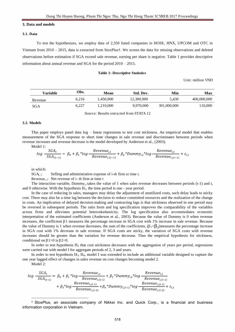
Dang Thi Huyen Huong, Pham Thi Ngoc Thu, Ngo Thi Hong Tham/ ICYREB 2017 Proceedings
3. Data and models
3.1. Data
To test the hypothesizes, we employ data of 2,350 listed companies in HOSE, HNX, UPCOM and OTC in
Vietnam from 2010 – 2015, data is extracted from StoxPlus†. We screen the data for missing observations and deleted
observations before estimation if SGA exceed sale revenue, earning per share is negative. Table 1 provides descriptive
information about annual revenue and SGA for the period 2010 – 2015.
Table 1: Descriptive Statistics
Unit: million VND
Source: Results extracted from STATA 12
3.2. Models
This paper employs panel data log – linear regressions to test cost stickiness. An empirical model that enables measurement of the SGA response to short time changes in sale revenue and discriminates between periods when revenue increases and revenue decrease is the model developed by Anderson et al., (2003).
Model 1:
in which: SGAt, i: Selling and administration expense of i-th firm at time t. Revenuet, i: Net revenue of i- th firm at time t The interaction variable, Dummyi,t takes the value of 1 when sales revenue decreases between periods (t-1) and t,
and 0 otherwise. With the hypothesis H1, the time period is one - year period. In the case of reducing in sales, managers may delay the adjustment of unutilized costs, such delay leads to sticky
cost. There may also be a time lag between the decision to reduce committed resources and the realization of the change in costs. An implication of delayed decision-making and contracting lags is that stickiness observed in one period may be reversed in subsequent periods. The ratio form and log specification improves the comparability of the variables across firms and alleviates potential heteroskedasticity. The log specification also accommodates economic interpretation of the estimated coefficients (Anderson et al., 2003). Because the value of Dummy is 0 when revenue increases, the coefficient 1 measures the percentage increase in SGA cost with 1% increase in sale revenue. Because the value of Dummy is 1 when revenue decreases, the sum of the coefficients, (1+ )measures the percentage increase in SGA cost with 1% decrease in sale revenue. If SGA costs are sticky, the variation of SGA costs with revenue increases should be greater than the variation for revenue decrease. Thus the empirical hypothesis for stickiness, conditional on 1>0 is 2<0.
In order to test hypothesis H2 that cost stickiness decreases with the aggregation of years per period, regressions were carried out with model I for aggregate periods of 2, 3 and years.
In order to test hypothesis H3, H4, model I was extended to include an additional variable designed to capture the one year lagged effect of changes in sales revenue on cost changes becoming model 2.
Model 2:
† StoxPlus, an associate company of Nikkei Inc. and Quick Corp., is a financial and business
information corporation in Vietnam.
Variable Obs. Mean Std. Dev. Min Max
Revenue 6,216 1,450,000 12,300,000 5,430 406,000,000
SGA 6,227 1,210,000 9,970,000 301,000,000 110,000
518

Dang Thi Huyen Huong, Pham Thi Ngoc Thu, Ngo Thi Hong Tham/ ICYREB 2017 Proceedings
In the model 2, the interaction variable, Dummy i,( t-1) takes the value of 1 when sales revenue decreases between periods (t-2) and (t-1), and 0 otherwise.
Condition for acceptance H3: 3>0; H4: 4>0, 4 < in absolute value. Model 1 was estimated for one year periods and for aggregate periods of 2, 3 and 4 years, whereas model 2 was
estimated for one-year periods only. The results are presented as follow:
Table 2: Coefficient estimates of model 1 and model 2
Model 1 Model 2
t= 1 year t=2 years t=3 years t=4 years t=1 year
0.0473 (0.000)
0.1322 (0.000)
0.1142 (0.000)
0.1822 (0.000)
0.00682525 (0.6642)
0.3176 (0.000)
0.3535 (0.000)
0.4391 (0.000)
0.3106 (0.0072)
0.2790 (0.000)
-0.1499 (0.0052)
-0.2645 (0.001)
-0.3310 (0.0006)
- 0,2393 (0.0985)
-0.1598 (0.0510)
0.0635
(0.0236)
-0.0594
(0.1001)
+ 0.1677 0.089 0.1081 0.0713 0.1192
N 7,523 5,720 4,067 2,558 5,658
r2 0.116 0.109 0.174 0.132 0.056
Source: Results extracted from STATA 12
Table 3: Coefficient estimates comparison between the case of Vietnam and Japan
Model 1 Model 2
t= 1 year t=2 year t=3 years t=4 years t= 1 year
Vietnam Japan Vietnam Japan Vietnam Japan Vietnam Japan Vietnam Japan
0.047 0.020 0.132 0.041 0.114 0.059 0.182 0.073 0.006 0.016
0.317 0.593*** 0.353 0.649*** 0.439 0.692*** 0.310 0.734*** 0.279*** 0.548***
-0.149 -0.139*** -0.264 -0.114*** -0.331 -0.100*** - 0,239 -0.086*** -0.159* -0.129***
0.063** 0.130***
-0.059* 0.037**
+ 0.167 0.454 0.089 0.535 0.108 0.592 0.071 0.648 0.119 0.419
Source: The author (2017) and He et al.(2010)
Note: ***, **, *: Indicate significance at 1, 5, 10 % levels respectively.
Results from regression model 1 for one-year periods, show that: The coefficient 1 measures the percentage rise in costs with respect to a 1% rise in revenue, 1 = 0.317 means when revenue increases 1%, cost will increase 0,317%. The estimated value 2 = -0.149 provides strong support to hypothesis H1 of cost stickiness. The combined value (1 +2) = 0.168 shows that costs fell by 0.16% in response to a 1% drop in revenues. The fact that both 1 and (1 + 2) are significantly smaller than 1 show that cost changes are not proportional to revenue changes, despite the relevance of this cost driver. With this result, the cost stickiness hypothesis H1, accepted for the case of Vietnam. Comparing from our study with those of He et al., (2010) (in table 3), we can see that 2 = -0.139 is negative so that cost stickiness also exist in the case of Japan.
It can also be seen from table 2 that, hypothesis H2 that cost stickiness falls with the aggregation of years per period, which is accepted in He et al. (2010), is rejected for model 1 in our study with common intercept. In the estimation results, 2 increases in absolute value, showing the cost stickiness gets worse as aggregation of years per period increases, whereas 2 in model 1 decreases in absolute value as the number of years per period increases in He et al., (2010). Comparing (1 + 2) from our study with those in Japan (He et al., 2010), when we aggregate the time t =2; t=3; t=4, the coefficients’ sum (1 + 2) in He et al. (2010) is increasing, this tells us that the stickiness is reducing. However, the coefficients’ sum (1 + 2) for Vietnam firms is reducing, meaning that the stickiness become continuous
519

Dang Thi Huyen Huong, Pham Thi Ngoc Thu, Ngo Thi Hong Tham/ ICYREB 2017 Proceedings
and more serious. This is an indication that firms’ cost stickiness is higher in Vietnam relative to the case of Japan. Model 2, which includes revenue changes lagged by one period, was used to test hypothesis H3 that cost stickiness
is reversed in subsequent periods. In this estimation of model 2 with common intercept, we found 1 = 0.279, which is somewhat smaller than that obtained for model 1. Coefficient 2 = - 0.1598 confirms cost stickiness in model 2. However, in model 2, 3 = 0.0635 is significant, which leads to the accept of H3, it means change in revenue from the previous years affects change of SGA cost, there is a lag-effect of revenue on sticky cost. A significant and negative 4= -0.0594 confirms the sticky cost in the period subsequent to a revenue drop, which leads to reject H4.
In the case of Japan (He et al., 2010), coefficient 2 = - 0.129, and (1 + 2) = 0.419 confirms cost stickiness in model 2. However, in model 2, 3 = 0.130 is significant, which leads to the accept of H3, it means change in revenue from the previous years affects change of SGA cost, there is a lag-effect of revenue on sticky cost, so that we the accept H3 hypothesis, it is the same as the case of Vietnam above. However, coefficient 4 = 0.037 is significant and positive in He et al.(2010) so we accept H4.
4. Empirical results
From the results of estimation above, we have an empirical evidence that SGA sticky cost happened in both Japan industrial companies (1975-2000) and listed companies in Vietnam (2010-2015) and sticky cost is affected by lag revenue change. He et al. (2010) found that the stickiness of selling, general and administrative cost in Japan is less likely to be adjusted due to temporary changes in their performance. It was said that Japanese managers tended to focus more on long – term measures such as market share, rather than short term measures (Porter, 1992). Temporary reductions in sales were less likely to influence their long term goals. They might have ignored those revenue fluctuation, thus making the cost behavior stickier. In addition, lifetime employment is common and it is unusual in Japan for firms to lay off employees (McAlinn, 1996). This distinct feature of Japan’s labor market is likely to enhance the cost stickiness.
However, the phenomenon of sticky cost is less serious in the case of Japan when sticky cost is reverted after two years. He et al. also found that there is a significant decrease in the magnitude of stickiness in Japan after the asset bubble burst in 1990, showing that Japanese managers adjusted their cost behavior in the post –bubble era. They explained that, Japanese corporate governance mechanisms are quite different from those in other countries. Agency problems are mitigated in Japanese firms, Japanese financial institutions hold significant debt and equity of firms and are therefore able to maintain effective control of the behavior of managers of these firms. Thus the mechanisms mitigate the agency problem for Japanese firms in comparison to their US counterparts and may therefore reduce the stickiness of SGA costs. It affirms that Japanese managers are quite cautious however they response very quickly when they realize sticky cost.
While SGA sticky cost in Japan was found to be reverted, it is more serious in the case of Vietnam according to my estimation results. It seems that, the Vietnamese managers may not realize the sticky cost, otherwise they are optimistic about the increasing demand or they may intentionally maintain the slack resources to to grow the firm beyond its optimal size or to maintain unutilized recourses with the purpose of increasing utility from status, power, and prestige. To affirm the determination of sticky cost in Vietnam, we need to do further researches in this field.
5. Conclusion and recommendations
The results in this paper show that, for Vietnamese listed companies, SGA stickiness has existed and it is stickier compared to that in Japan. This phenomenon was found to have impacts on firm probability. To to limit the effects of cost stickiness in the context of demand reduction, the paper recommends:
Firstly, managers should evaluate the demand of market annually and make the decision on how to adjust the cost structures. If there is a short term reduction, the manager may consider the adjustment cost and the lost of cost stickiness before making a decision to change the cost structure. In the circumstance of long term reduction of market demand, managers need to reallocate the resources, contracts should be flexible and adjustable in order to cut off the adjustment cost.
Secondly, firms need to build up a flexible cost structure in order to explore market advantages in case of growth and restrain the effect of revenue reduction. The paper suggests the following two ways: (1) Change the portion of fixed cost to variable cost by creating a contingent labor pool, outsourcing of activities, and deployment of software as a service; (2) Increase the productivity via economies of scale or extended working hours.
Thirdly, firms should apply modern management method such as JIT (Just In Time) to minimize the inventory cost, ABC method (Activity Based Costing) to determine the valuable activities and eliminate non valuable activities and allocated the cost more precisely.
Lastly, together with those solutions, firms should choose a flexible selling mechanism with the combination between internal selling staff and outsource selling forces to maximize the efficiency and effectiveness.
Acknowledgement This paper is a result of the Research group on “Corporate Restructuring”, Foreign Trade University.
520

Dang Thi Huyen Huong, Pham Thi Ngoc Thu, Ngo Thi Hong Tham/ ICYREB 2017 Proceedings
References
[1] Anderson, R. Banker, and S. Janakiraman. (2003). Are selling, general and administrative costs sticky?, Journal of Accounting Research, vol. 41, 2003, pp. 47–63.
[2] Banker.R, D. Byzalovy, and J. Plehn-Dujowichz. (2011). Sticky cost behavior: theory and evidence, working paper, Temple University.
[3] R.Banker, and L.Chen. (2006). Predicting earnings using a model based on cost variability and cost stickiness, the Accounting Review, vol. 81, 2006, pp. 285 – 307.
[4] Calleja, K., Steliaros, M., & Thomas, D. (2006). A note on cost stickiness: Some international comparisons, Management Accounting Research, 17, 127–140. http://dx.doi.org/ 10.1016/j.mar.2006.02.001.
[5] Chen.E, and W. Dixon. (1972). Estimates of parameters of a censored regression sample, Journal of the American Statistical Association, vol 67, pp. 664-71.
[6] Cooper.R, and J. Haltiwanger. (2006). On the nature of capital adjustment costs, Review of Economic Studies, vol. 73, pp. 611-633.
[7] Dierynck, B., & Renders, A. (2009). Earnings management incentives and the asymmetric behavior of labor costs. Working paper, Tilburg University. http://dx.doi.org/10.2139/ssrn.1441250.
[8] He, D., Teruya, J., & Shimizu, T.(2010). Sticky Selling, General, and Administrative Cost Behavior and its Changes in Japan, Global Journal of Business Research, 4(4), 1–10. Retrieved from http://ssrn.com/abstract=1871276.
[9] Masulis, R. W., Wang, C., & Xie, F. (2007). Corporate governance and acquirer returns. The Journal of Finance, 62(4), 1851–89. http://dx.doi.org/10.2139/ssrn.697501.
[10] Medeiros and Costa. (2004). Cost Stickiness in Brazilian Firms, paper presented at the 4th USP Congress of Managerial Control and Accounting, held in Sao Paulo, Brazil, October 7-8, 2004.
[11] Noreen, E., & Soderstrom, N. (1997). The accuracy of proportional cost models: Evidence from hospital service departments. Review of Accounting Studies, 2, 89–114. http://dx.doi.org/10.1023/A:1018325711417
[12] Özkaya, H., & Yükcü, S. (2011). Cost Behavior in Turkish Firms: Are Selling, General and Administrative Costs and Total Operating Costs “Sticky”? World of Accounting Science, 13(3), 1–27.
[13] Rhee, C. S., Kim, J., & Lee, S. (2012). Sticky Cost Behavior: Quantity Based Approach, AAA 2012 Management Accounting Section (MAS) Meeting Paper. Retrieved from http://aaahq.org/AM2012/abstract.cfm?submissionID=846
[14] Warganegara và Tamara. (2014). The Impacts of Cost Stickiness on the Profitability of Indonesian Firms, International Journal of Social, Behavioral, Educational, Economic, Business and Industrial Engineering Vol:8, No:11, 2014.
[15] Weiss, D, Cost behavior and analysts’ earnings forecasts, The Accounting Review, 85(4), 2010, pp. 1441-1471.
521

Nguyen Thi Thu Ha, Lam Ba Hoa/ ICYREB 2017 Proceedings
International Conference For Young Researchers In Economics And Business, ICYREB 2017, October 30th 2017 Da Nang, Vietnam
Evaluating The Entrepreneurship Performance in Vietnam
Through The GEDI (The Global Entrepreneurship Development
Index) Approach
Nguyen Thi Thu Haa*, Lam Ba Hoab
a The University of Danang, University of Economics, Danang city 550000, Vietnam
PhD Candidate in University of Pecs, Pecs city 7622, Hungary
b The University of Danang, University of Economics, Danang city 550000, Vietnam
A B S T R A C T
The study mainly aims to measure entrepreneurship performance in Vietnam at the national level through a new approach - the GEDI (the Global Entrepreneurship Development Index). The GEDI index consists of three sub-indices, including Entrepreneurial Attitudes, Entrepreneurial Abilities and Entrepreneurial Aspiration, which are divided into 14 pillars and can be further subdivided into 28 subdivided variables. By analyzing these pillars and variables in comparison to two Southeast Asia developing economies Thailand and Indonesia, which have similar cultural, economic and social characteristics, the study can identify the best and worst performing variables of the GEDI index. The results indicate that in Vietnam, nine bottlenecks of 14 pillars are poorly performing with very low scores, in which the highest policy priority is given for four pillars, including risk acceptance, opportunity perception, internationalization and technology absorption. Finally, the Penalty for Bottleneck methodology, which is considered as the policy application of the GEDI methodology and a simulation of “optimal” policy allocation are suggested to alleviate the weakest performing pillars aiming to achieve the greatest improvement of entrepreneurship performance as well as reach the desired five-point increase in the Vietnam’s GEDI.
Keywords: Entrepreneurship; performance; the GEDI; the Penalty for Bottleneck methodology; Vietnam.
1. Introduction
Entrepreneurship has formally accepted in Vietnam since the 1990s and known as the simple view such as business activities, individual or firm levels, thus traditional approach is usually used by researchers and policy-makers when analyzing Vietnam’s entrepreneurship [28]. However, in fact, entrepreneurship is the complex view basing on the multidimensional measure in a country [16]. When discussing entrepreneurship in countries, recent studies follow National Systems of Entrepreneurship introduced by Acs, Autio and Szeb (2014), which are fundamentally resource allocation systems and driven by both the individual and country-specific institutional characteristics in evaluating the entrepreneurship performance of a country [1].
The main purpose of this paper is to measure entrepreneurship in Vietnam at the national level. This study first uses the GEDI (the Global Entrepreneurship Development Index) methodology to analyze Vietnam’s entrepreneurship performance through the GEDI index, three GEDI sub-indices, and its relative position at the pillar and variable levels. More specifically, the GEDI index consists of three sub-indices, which is divided into 14 pillars and can be further subdivided into 28 variables. To have more detailed and deeper understanding of the entrepreneurial performance of Vietnam, this study chooses two developing Southeast Asia countries: Thailand and Indonesia to compare and identify the best and worst performing pillars. The Penalty for Bottleneck (PFB) methodology, which is considered as the policy application of the GEDI methodology, is then applied to alleviate the weakest performing pillars or the bottlenecks
* Corresponding author. Tel.: +841688212888.
E-mail address: [email protected]; [email protected]
522

Nguyen Thi Thu Ha, Lam Ba Hoa/ ICYREB 2017 Proceedings
aiming to achieve the greatest improvement of GEDI. Finally, we suggest a simulation of “optimal” policy allocation to reach the desired five-point increase in the Vietnam’s GEDI.
2. The basic description of new approach - The GEDI methodology
While entrepreneurship is known as the complex and multidimensional view, most of recent empirical researches base on one-dimensional measures of entrepreneurship in a country [16]. Some popular indicators are used to identify the level and/or dynamics of entrepreneurship such as self-employment, the rate of new business start-up or established business, the Total Early-stage Entrepreneurship Activity Index (TEA) which is calculated by the percentage of the working age population engaging in or willing to engage in entrepreneurial activity. Nonetheless, the problematic of one-dimensional measures are that it is hard to distinguish between the quality and the quantity aspects of entrepreneurship [2, 21] and it does not include the impact of national and contextual factors in analyzing entrepreneurship of a country in the different stages of economic development [18]. Indeed, the one-dimensional measures does not indentify differences in the quality of entrepreneurial activity, thus leads to only providing policy recommendations concerning the quantity of entrepreneurship, not its quality.
Due to problems of the one-dimensional measures, it is necessary to adopt a system approach to considering the entrepreneurial performance of countries that helps researchers and policy-makers think in system and take a broad view when considering both individual and country level indicators, but also is helpful in designing policies to nurture and enhance entrepreneurship for sustainable economic development. Therefore, Acs, Autio and Szeb (2014) introduce a National Systems of Entrepreneurship perspective that emphasizes the dynamic interactions between entrepreneurial attitudes, abilities, and aspiration by individuals within the institutional context in producing entrepreneurial action and regulating the quality and outcome of this action. At the country level, they also mentioned that the Global Entrepreneurship Development Index (GEDI) is the most widely used approach for measuring the output of multi-faced character of country-level entrepreneurship in countries [1].
Also, according to Acs, Szerb and Autio (2013), the GEDI is the first complex index, which concentrates on the multidimensional quality rather than the quantity aspects of country-level entrepreneurship and provides a useful platform for policy analysis [4]. The GEDI is similar to other indexes having a complex structure with 28 individual and institutional variables that create 14 pillars and then is divided into three sub-indices: Attitudes (ATT), Abilities (ABT), and Aspiration (ASP). ABT and ASP sub-indices show the quality of actual entrepreneurship activities through nascent and start-up businesses, while attitudes sub-index determines the attitudes of population in a country regarding entrepreneurship. Individual variables are collected from the Adult Population Survey of 79 countries participating in the Global Entrepreneurship Monitor (GEM), while institutional variables are interaction variables, which are considered as country-specific weighting factors and taken from various surveys of the Global Competitiveness Index, the Doing Business Index or the Index of Economic, or from multinational organizations such as the United Nations and the OECD [5].
However, the GEDI methodology differs from others in two important respects, which are that GEDI index includes both individual and institutional variables and this methodology examines interdependencies of the system by developing a Penalty for Bottleneck (PFB) methodology. The key principles of the PFB are that the system performance depends on the weakest link and because of having the bottlenecks the higher scores of pillars cannot show its full influence on the system performance [3].
3. Vietnam’s entrepreneurial performance
The consideration of policymakers is how to identify the most important issues affecting the entrepreneurship in a country. The GEDI approach can identify the best and the worst components of the GEDI of a country before policy priorities are given for this country. The data in this study is collected from the World Development Indicators of the World Bank and The Global Entrepreneurship and Development Index from 2011 to 2015 in the entrepreneurship projects of Acs, Autio and Szerb. Based on the scores of the Global Entrepreneurship and Development Index of countries in the world, the authors use the average calculation and statistical methods to compute the data for the study’s purposes.
The first part of this paper is to determine the overall entrepreneurial performance by analyzing Vietnam’s entrepreneurial position through its rankings in the GEDI Index and three GEDI sub-indices.
523
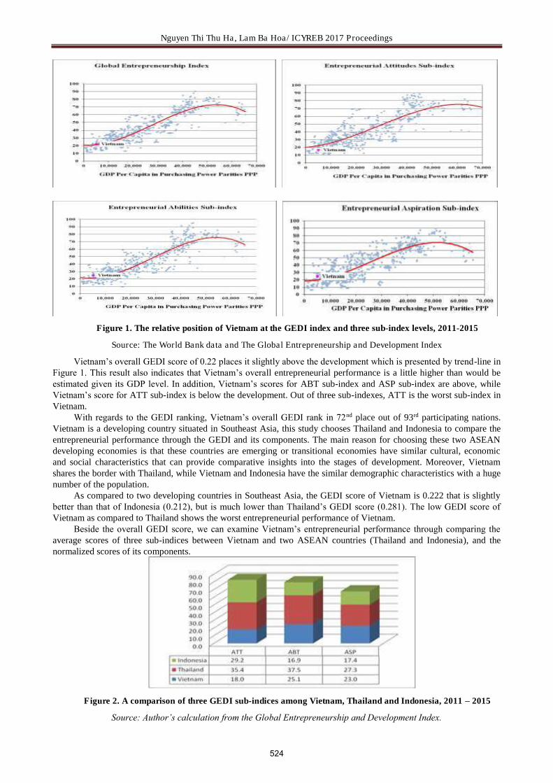
Nguyen Thi Thu Ha, Lam Ba Hoa/ ICYREB 2017 Proceedings
Figure 1. The relative position of Vietnam at the GEDI index and three sub-index levels, 2011-2015
Source: The World Bank data and The Global Entrepreneurship and Development Index
Vietnam’s overall GEDI score of 0.22 places it slightly above the development which is presented by trend-line in Figure 1. This result also indicates that Vietnam’s overall entrepreneurial performance is a little higher than would be estimated given its GDP level. In addition, Vietnam’s scores for ABT sub-index and ASP sub-index are above, while Vietnam’s score for ATT sub-index is below the development. Out of three sub-indexes, ATT is the worst sub-index in Vietnam.
With regards to the GEDI ranking, Vietnam’s overall GEDI rank in 72nd place out of 93rd participating nations. Vietnam is a developing country situated in Southeast Asia, this study chooses Thailand and Indonesia to compare the entrepreneurial performance through the GEDI and its components. The main reason for choosing these two ASEAN developing economies is that these countries are emerging or transitional economies have similar cultural, economic and social characteristics that can provide comparative insights into the stages of development. Moreover, Vietnam shares the border with Thailand, while Vietnam and Indonesia have the similar demographic characteristics with a huge number of the population.
As compared to two developing countries in Southeast Asia, the GEDI score of Vietnam is 0.222 that is slightly better than that of Indonesia (0.212), but is much lower than Thailand’s GEDI score (0.281). The low GEDI score of Vietnam as compared to Thailand shows the worst entrepreneurial performance of Vietnam.
Beside the overall GEDI score, we can examine Vietnam’s entrepreneurial performance through comparing the average scores of three sub-indices between Vietnam and two ASEAN countries (Thailand and Indonesia), and the normalized scores of its components.
Figure 2. A comparison of three GEDI sub-indices among Vietnam, Thailand and Indonesia, 2011 – 2015
Source: Author’s calculation from the Global Entrepreneurship and Development Index.
524

Nguyen Thi Thu Ha, Lam Ba Hoa/ ICYREB 2017 Proceedings
As compared to Thailand and Indonesia, out of three GEDI sub-indices, ATT is the worst sub-index in Vietnam with the lowest score (0.18) that is resulted from a small and poor income level of Vietnam economy in the past leading to low perceived opportunities and capabilities of Vietnamese people to start a business and big fear of business failure [28], followed by ASP sub-index and the last is Vietnam’s ABT sub-index.
Table 1. The normalized scores of components of three sub-indices in Vietnam in 2015
The normalized scores of components of Entrepreneurial Attitudes Sub-index
Vietnam Opportunity perception Start-up skills Risk acceptance Networking Cultural support
0.16 0.24 0.07 0.21 0.21
33% percentile 0.32 0.31 0.27 0.36 0.29
67% percentile 0.54 0.58 0.63 0.53 0.57
The normalized scores of components of Entrepreneurial Abilities Sub-index
Vietnam Opportunity startup Technology absorption Human capital Competition
0.21 0.17 0.50 0.22
33% percentile 0.29 0.30 0.33 0.31
67% percentile 0.59 0.60 0.54 0.56
The normalized scores of components of Entrepreneurial Aspirations Sub-index
Vietnam Product innovation Process innovation High growth Internationalization Risk capital
0.33 0.19 0.22 0.16 0.46
33% percentile 0.31 0.29 0.27 0.34 0.28
67% percentile 0.56 0.60 0.61 0.57 0.60
Source: Author’s calculation from the Global Entrepreneurship and Development Index.
Most components of three sub-indices of Vietnam are not good with its normalized scores are under 0.24, which are presented in red lines in Table 1. For each sub-index, along with the worst score of Vietnam’s ATT sub-index, RISK ACCEPTANCE is the weakest pillar with only 0.07 normalized score. The second weakest pillars are OPPORTUNITY PERCEPTION of ATT sub-index and INTERNATIONALIZATION of ASP sub-index having the same normalized score (0.16). The last weakest pillar is TECHNOLOGY ABSORPTION of ASP sub-index (0.17).
The low score of OPPORTUNITY PERCEPTION pillar can be explained that Vietnam has experienced a long history of centrally-planned economy in which private businesses were restricted or even prohibited for decades. Indeed, the history of Vietnam was closely tied with the struggles for national independency, leading to its low income level economy and Vietnam only has transformed to a market driven economy since 1986. The consequence of wars, the lack of or the limitation of enterprises to access resources and capital in the economy resulted in the low perception level of entrepreneurs regarding opportunities in business and big fear of entrepreneurs of business failure, which causing the low level of RISK ACCEPTANCE pillar [8]. Besides, Vietnam has just been a member of the WTO since 2007, while most enterprises in Vietnam have small and medium sizes with a weak competitiveness. Therefore, economic activities such as exporting and trading by small and medium enterprises (SMEs) in Vietnam are reality low and below the international average. So it is not surprised that the score of INTERNATIONALIZATION is low [7] . The low score of TECHNOLOGY ABSORPTION pillar indicates the low level of new technology absorption of firms that is true for Vietnam because in emerging economies - especially in stages of transition, entrepreneurs face the same problem of lacking innovation, thus the ability of firms to absorb new technologies is limited [11].
By contrast, the three best pillars of Vietnam’s entrepreneurship are HUMAN CAPITAL, RISK CAPITAL and PRODUCT INNOVATION with its normalized scores of 0.5, 0.46 and 0.33 respectively. The first pillar with the highest normalized score (0.5) is a component of Vietnam’s ABT sub-index, while the two remaining pillars are components of Vietnam’s ASP sub-index. The highest level of HUMAN CAPITAL pillar can be explained through a higher rate of Vietnamese entrepreneurs receiving higher education as well as a large investment of the government in education system in recent years [28]. Besides, the high RISK CAPITAL pillar level for Vietnam is resulted from the larger informal investment in start-ups that is measured by the liquidity of debt and credit markets and development of stock market in Vietnam in this period. Lastly, PRODUCT INNOVATION means the introduction of any improvements in functional characteristics, technical abilities or ease of use to the existing goods or services of the firm. In Vietnam, investment more in R&D of private sector, the appearance of high quality research institutions, technology transfer and the attention of government on the intellectual property protection in the period of economic transition has encouraged the enterprises to add value to its products as well as enhance the innovation in production [12].
525

Nguyen Thi Thu Ha, Lam Ba Hoa/ ICYREB 2017 Proceedings
Figure 3. The relative position of Vietnam at the pillar level, 2011 – 2015
In order to have more detailed and deeper understanding of the entrepreneurial performance of Vietnam, we continue to analyze the relative position of Vietnam at the pillar level and compare the scores of Vietnam’ pillars (which is shown in blue) to that of 93 participating countries in top third (67% percentile) and bottom third (33% percentile).
All scores of Vietnam’s pillars in Figure 3 are below the scores of 93 countries’ corresponding pillars in the top third. Also, most of Vietnam’s pillar scores are below the scores of 93 countries’ pillars in the bottom third, except for two pillars: HUMAN CAPITAL from ABT sub-index and RISK CAPITAL from ASP sub-index. For the remaining twelve pillars, Vietnam ranks in the bottom third out of 93 countries, in which four pillars having the lowest scores are RISK ACCEPTANCE, TECHNOLOGY ABSORPTION, INTERNATIONLIZATION and OPPORTUNITY PERCEPTION.
Figure 4. The pillar scores of Vietnam, Thailand and Indonesia, 2011 - 2015
As shown in Figure 4, the performances of Thailand’s pillars are the best as compared to the pillar’s performances of Vietnam and of Indonesia. Taken alone, Thailand has five strongest pillars out of 14 GEDI pillars, including OPPORTUNITY PERCEPTION, HUMAN CAPITAL, PRODUCT INNOVATION, OPPORTUNITY STARTUP, and HIGH GROWTH. In Vietnam, there are three best pillars are mentioned above, including HUMAN CAPITAL, RISK CAPITAL and PRODUCT INNOVATION, while three strongest pillars of Indonesia are NETWORKING, PRODUCT INNOVATION and STARTUP SKILLS.
It is not surprised that the pillar scores of Thailand are higher than those scores of Vietnam and of Indonesia because Thailand now is an upper-middle income economy (GDP per capita PPP in 2015 is 15346.6 USD), which also has made a remarkable socio-economic development progress with a sustained and strong growth in Southeast Asia [29]. Furthermore, Indonesia’s pillars are performed better than Vietnam’s pillars that are explained by the higher economic development of Indonesia as compared to Vietnam. In fact, although Indonesia is the world’s fourth most
526

Nguyen Thi Thu Ha, Lam Ba Hoa/ ICYREB 2017 Proceedings
populous nation, GDP per capita has steadily increased and now Indonesia is an emerging middle-income country [30]. In Vietnam, the population has reached 100 million people, but its economy transferred from a poor income level to enter the low-medium income country in 2008 [7].
Al l three countries Thailand, Indonesia and Vietnam pay more attention on PRODUCT INNOVATION in their entrepreneurship development. According to Hoi et al (2016), the same issue of emerging economies, especial in transition stages, is that entrepreneurs often lack innovation, resulting in their weak foundations of entrepreneurship. Thus, in order to develop the entrepreneurial performance, it is easy to understand that the first priority is given to PRODUCT INNOVATION pillar for three countries. Interestingly, the score of HUMAN CAPITAL pillar is high and the same between Thailand and Vietnam [14]. Many studies such as Jens et al. (2011), Thomas and Dung (2014) in Vietnam and Chuthamas et al. (2011) in Thailand argued that human capital plays an important role in entrepreneurial success and the entrepreneur’s education leads to the business success of small and medium enterprises (SMEs) [17,26,10]. More specific, in Vietnam, due to the important of human capital for its economic development, the government invests more in education system, resulting in the higher rate of entrepreneurs who had higher education [28].
On the other hand, as mentioned above, the four Vietnam’s worst pillars are RISK ACCEPTANCE, INTERNATIONALIZATION, OPPORTUNITY PERCEPTION and TECHNOLOGY ABSORPTION. Similarly, Indonesia has three worst pillars: INTERNATIONALIZATION, TECHNOLOGY ABSORPTION and HIGH GROWTH. Two of the three weakest pillars in Indonesia are the same in Vietnam that is because of the similar demographic, cultural, economic and social characteristics between two countries. With regards to the weakest pillar of Thailand, only INTERNATIONALIZATION pillar is not good, which is similar to Vietnam and Indonesia and is the main issue not only three countries but also most ASEAN countries have to face in the global integration process [19].
The 14 pillars that create three entrepreneurial sub-indices (ATT, ABT and ASP) of the GEDI index can be further subdivided into 28 variables. Each pillar is formed from an institutional variable and an individual variable. Deeper researching on the basic variable is necessary for analyzing Vietnam’s entrepreneurial performance.
Table 2.The relative position of Vietnam at the variable level, 2011 - 2015
PILLARS INSTITUTIONAL VARIABLES INDIVIDUAL VARIABLES
Ent
repr
eneu
rial
Atti
tude
s
Opportunity Perception 0.16 Freedom and Property 0.20 Opportunity Recognition 0.67
Start-up skills 0.24 Education 0.36 Skill Perception 0.67
Risk Acceptance 0.07 Business Risk 0.18 Risk Perception 0.27
Networking 0.21 Connectivity 0.21 Know Entrepreneurs 0.90
Cultural Support 0.21 Corruption 0.35 Career Status 0.71
Entrepreneurial Attitudes 16.9
Ent
repr
eneu
rial
Abi
litie
s
Opportunity Startup 0.21 Tax and government 0.36 Opportunity Motivation 0.55 Technology Absorption 0.17 Tech Absorption 0.27 Technology Level 0.40 Human Capital 0.50 Labor Market 0.57 Educational Level 0.71
Competition 0.22
Competitiveness and Regulation
0.47 Competitors
0.32
Entrepreneurial Abilities 24.9
Ent
repr
eneu
rial
Asp
iratio
ns
Product Innovation 0.33 Technology Transfer 0.46 New Product 0.63 Process Innovation 0.19 Science 0.34 New Tech 0.79 High Growth 0.22 Finance and strategy 0.45 Gazelle 0.42 Internationalization 0.16 Economic complexity 0.32 Export 0.38
Risk Capital 0.46
Depth of Capital Market
0.66 Informal Investment
0.61
Entrepreneurial Aspirations 24.8
GEDI 22.2 Institutional 0.37 Individual 0.57
Source: Author’s calculation from the Global Entrepreneurship and Development Index.
Table 2 presents the relative position of Vietnam at the variable level, in which Vietnam’s scores belong to the upper 33%, the middle 33% and the bottom 33% of participating countries are shown by green colored, yellow colored and red colored groups respectively. The last row in bold shows the GEDI level and its institutional and individual variable scores.
The overall score of individual variable is 0.57, which places Vietnam in the middle third of the GEDI countries, is better than the overall level of institutional variable (0.37). This result also indicates that the individual environment
527

Nguyen Thi Thu Ha, Lam Ba Hoa/ ICYREB 2017 Proceedings
of Vietnam is relatively well developed for entrepreneurial development than the institutional environment. As can be seen in Table 2, most of individual variables have the high scores and six individual variables, which receive a score of over 0.65: OPPORTUNITY RECOGNITION, SKILL PERCEPTION, KNOW ENTREPRENEURS, CARRER STATUS, EDUCATIONAL LEVEL, and NEW TECH play a key role contributing to Vietnam’s entrepreneurial performance. However, there also exist five individual variables with a low score of below 0.5: GAZELLE, TECHNOLOGY LEVEL, EXPORT, COMPETITORS, and RISK PERCEPTION place Vietnam in the lowest third of the GEDI countries need to be considered.
Moreover, the best performing individual variables of Vietnam is KNOW ENTREPRENEURS (0.90), followed by NEW TECH (0.79), EDUCATION LEVEL and CARRER STATUS (with the same score of 0.71), and the last are OPPORTUNITY RECOGNITION and SKILL PERCEPTION (with the same score of 0.67). According to Acs, Autio and Szeb (2014), the high score of KNOW ENTREPRENEURS variable is explained by a better knowledge or understanding of entrepreneurs on entrepreneurship [1]. The high score of NEW TECH variable is as a result of an increase in using new technologies in business of entrepreneurs. For EDUCATION LEVEL and CARRER STATUS variables, these high scores are resulted from the development of education system in providing a good preparation for start-up in the population. And SKILL PERCEPTION is known as the percentage of working age population having enough knowledge and skills to start a new business. Lastly, the high score of OPPORTUNITY RECOGNITION shows a higher percentage of working age population recognizing better opportunities to startup the business in the area.
On the other hand, the scores of Vietnam’s institutional variables are not good and very low. Only LABOR MARKET variable is green colored, showing that it belongs to the top level (33% of the GEDI countries). It is not surprising for the highest score of LABOR MARKET among institutional variables because in recent times Vietnam have an abundance of young population and cheap labor, which has become the competitive advantage in attracting business start-ups, [22]. Besides, nine institutional variables: FREEDOM AND PROPERTY, EDUCATION, BUSINESS RISK, CONNECTIVITY, CORRUPTION, TAX AND GOVERNMENT, TECH ABSORPTION, SCIENCE, and ECONOMIC COMPLEXITY are coded red showing that the scores of these variables are in the lowest third of GEDI countries, in which five out of nine institutional variables with the lowest scores are from the ATT sub-index.
Out of the nine worst institutional variables, BUSINESS RISK has the lowest performing score (0.18), followed by FREEDOM AND PROPERTY, CONNECTIVITY with the performing scores are 0.20 and 0.21 respectively, and then TECH ABSORPTION with the score of 0.27. Also, according to Acs, Autio and Szeb (2014), BUSINESS RISK is referred as the overall quality of business environment in a country. FREEDOM AND PROPERTY are identified by the efficiency of government in the regulatory process relating to starting, operating and closing a business of entrepreneurs and the ability to access the capital and resources. CONNECTIVITY is mentioned as the connection activities among entrepreneurs in the entrepreneurial network. TECH ABSORPTION is the new technology absorption capability of firms in a country [1].
Table 3. The four worst pillars and the corresponding institutional and individual variables of Vietnam in 2015
PILLARS INSTITUTIONAL VARIABLES INDIVIDUAL VARIABLES
Opportunity Perception 0.16 Freedom and Property 0.20 Opportunity Recognition 0.67
Risk Acceptance 0.07 Business Risk 0.18 Risk Perception 0.27
Technology Absorption 0.17 Tech Absorption 0.27 Technology Level 0.40
Internationalization 0.16 Economic complexity 0.32 Export 0.38
Source: Collecting the data from Table 2
Table 3 shows the four worst pillars and the corresponding influenced individual and institutional variables of Vietnam, which is collected from Table 2. More specific, the lowest level of RISK ACCEPTANCE in Vietnam is caused by the low levels of institutional variable, BUSINESS RISK and of individual variable, RISK PERCEPTION. In other words, the lowest level of RISK ACCEPTANCE pillar can be explained by the low quality of business environment in Vietnam and the fear of failure of Vietnamese that prevent them from starting a business [6; 28]. The second lowest score of INTERNATIONALIZATION pillar are affected by the low levels of ECONOMIC COMPLEXITY representing by the high position of Vietnam in Economic Complexity Index relative to its low GDP per capita and the limited exporting and trading activities in Vietnam economy [20; 7]. The worst performance of TECHNOLOGY ABSORPTION pillar are because of the limitation of Vietnam firms in new technology absorption [11], Vietnam enterprises mainly rely on low-medium technologies and only 2% of Vietnam enterprises have high technology [28] (which is showed by TECHNOLOGY LEVEL variable). And the low score of OPPORTUNITY PERCEPTION pillar is mainly explained by the low level of FREEDOM AND PROPERTY variable or the low efficiency of Vietnam government in the regulatory process and the limitation of Vietnamese enterprises in accessing to capitals and resources in the economy [13].
528

Nguyen Thi Thu Ha, Lam Ba Hoa/ ICYREB 2017 Proceedings
4. The Penalty for Bottleneck (PFB) methodology
The GEDI methodology is considered as a better policy tool, not an optimal tool to identify the weakness inhibiting entrepreneurship development in a country, but it can provide little guidance for policy design. The uniqueness is that this methodology provides a comprehensive analysis of individual and institutional aspects of entrepreneurship derived from the perspective of system. It helps contextualize national level entrepreneurial process, thus making it consistent with the study of country-specific features. Indeed, this methodology identifies bottleneck factors, which constitute the weakest link amongst the pillars and constrain system performance, thereby helping set tangible goals for policies and support initiatives designed to improve the bottleneck identified. In practice, in the GEDI methodology, the higher pillars values are adjusted to the weakest performing pillar value of the particular sub-index, thus eliminating full, one-to-one substitutability across pillars. However, this methodology does not guide how to measure exactly the penalty, therefore, the solution is not optimal, and it only provides a better solution [24].
Besides, there are some limitations of the GEDI methodology that need focus on a better methodology. Firstly, although the GEDI is a complex measure of entrepreneurship, we only select 28 variables and 14 pillars representing the GEDI index that are available in the data reports of countries, thus leads to an imperfect or incomplete selection, and then the policy recommendations do not generalized so well. Moreover, the fourteen pillars of the GEDI only particular reflect a national system of entrepreneurship. Therefore, maximizing the GEDI of one country does not mean maximizing the entire national system of entrepreneurship of this country. Secondly, the GEDI analysis is not flexible because there do not exist a perfect configuration suitable with all countries and contexts. More important, the GEDI methodology is the best method that can increase the overall GEDI as well as to reduce the disparities between the pillars by improving the weakest GEDI pillar. Nevertheless, due to the dynamic of the system, the other pillar may become the weakest pillar and restrict an entrepreneurship performance of a country, thus the issue of GEDI methodology is related to how to allocate additional resources to achieve the optimal outcome of GEDI [9].
Due to the limitations of the GEDI methodology, and because all pillars are formed as interactions between individual and institutional aspects, the PFB methodology is considered as the policy application of the GEDI methodology will be utilized, which provide a more realistic analysis of overall entrepreneurial performance of a country, contributing to more insightful policy development and cross country comparison [24].
According to Acs, Autio and Szeb (2014), a bottleneck is defined as the weakest link or the binding constrain in the national entrepreneurial performance. In other words, within a given set of normalized pillars, a bottleneck is a factor with the lowest value. From the policy perspective, the PBF methodology focuses on the weakest pillar that is the starting point where policy is generated to achieve the greatest enhancement of system. The principle of this methodology is that the pillar scores should be adjusted regarding this concept of balance. After equalizing the scores of all pillars, the value of each pillar is “penalized” by linking it to the value of the weakest performing indicator (that is called the bottleneck) in a given nation. If the bottleneck is improved, the overall GEDI index will be enhanced significantly [1].
The PFB methodology also implies that a stable and efficient configuration will be reached if all pillars are the same level. Traditional methods assume full substitutability between indicators of the system, but this assumption is not realistic because the value of substitutability between different components of the system may differ. Based on the approach proposed by Tarabusi and Palazzi (2004) that if the difference between the particular pillar and the corresponding pillar is larger, there requires a higher compensation for the loss of one pillar [25], Acs, Autio and Szeb (2014) create the penalty function reflecting compensation for the loss of one pillar with an improvement in another pillar [1]. The penalty function is written as follows:
h(i),j = miny(i),j + (1 – e - y(i),j) - miny(i),j) ) Where h(i),j is the modified, post-penalty score of pillar j in country i; y(i),j is the normalized score of pillar j in
country i; miny(i),j) is the lowest score of y(i),j for country i. i = 1, 2, . . ., n = the number of countries; j = 1, 2, . . ., m = the number of index components. In this above function, by adding one minus the base of the natural logarithm of the negative difference between a
particular pillar’s value and the lowest normalized value of any pillar in country i, we can identify the modified, post-penalty score of pillar in a country. Therefore, improving the value of the weakest pillar will bring a greater impact on the GEDI index than improving the stronger pillar’s value.
For policy section, this study will present a policy portfolio analysis aims to increase the GEDI score by five points. TNhe principle of PFB approach is that the greatest improvement can be reached by lessening the weakest performing pillar. Once the weakest pillar has been eliminated, we add the available resources to improve the next binding pillar and only stop if the additional resources are exhausted.
In order to increase the average GEDI score by five points, the first stage of PFB methodology is that we increase the score of weakest pillar until reaching the next bottleneck pillar. We assume that the cost of reaching the improvement is the same for all pillars. After that, we continue to add the available resources to improve the next weakest pillar score and so on. Once we achieve the desired five-point increase in GEDI, we will stop to add further resources.
529

Nguyen Thi Thu Ha, Lam Ba Hoa/ ICYREB 2017 Proceedings
Table 3. A simulation of “Optimal” Policy Allocation to increase the GEDI score by five points
Source: Author’s calculation
Table 3 represents the required increase in the particular in absolute values and the percentage of total new effort. Vietnam has a relatively low GEDI score and several bottlenecks. Nine Vietnam’s bottlenecks are RISK ACCEPTANCE with a 0.07 pillar score, followed by OPPORTUNITY PERCEPTION (0.16), INTERNATIONALIZATION (0.16), TECHNOLOGY ABSORPTION (0.17), PROCESS INNOVATION (0.19), NETWORKING, CULTURAL SUPPORT and OPPORTUNITY STARTUP with the same 0.21 pillar score, and COMPETITION (0.22). Vietnam should allocate the additional resources reasonably among different pillars as well as increase nine poor performing pillars to 0.24 (up to the level of START-UP SKILLS) to achieve the desired five-point GEDI increase.
More specific, RISK ACCEPTANCE is the weakest performing pillar with the lowest score and is much lower than the scores of other pillars, thus policy priority is given for RISK ACCEPTANCE pillar. We increase this pillar for Vietnam by 0.17 units to reach the value 0.24 of START-UP SKILLS. The reason of high required increase in this pillar is that a risk acceptance emphasis is necessary to start up SMEs in a turbulent business environment in the transitional economy in Vietnam as well as increase the firm’s performance [23]. More important, the rate of fear of business failure of Vietnam - a developing country in the first stage of development is higher than that of other developing countries in the third stage of development that is because of a decline in economic growth in Vietnam in recent period, the difficulties of businesses in mobilizing capital and output market, leading to the dissolution of many firms in recent years. The high rate of fear of Vietnamese business failure is one of the most important factors blocking an individuals’ engagement in entrepreneurship as well resulting in a low percentage of entrepreneurship in Vietnam [15].
Once the weakest RISK ACCEPTANCE pillar has eliminated, OPPORTUNITY PERCEPTION, INTERNATIONALIZATION and TECHNOLOGY ABSORPTION become the next weakest pillars. We also add the available resources to improve these next binding pillars. More specific, we also increase a high value for three pillars in the lowest bottom third group by 0.08, 0.05 and 0.07 respectively, which based on the level of improved requirement in the context of Vietnam. The policy priority order is explained through some reasons. Firstly, due to a long history of the struggles for national independency of Vietnam, the consequence of socialist economy and now the slow recovery of the economy after the global financial crisis occurred leading to the limitation of economic opportunities to start a business in Vietnam, the percentage of people who perceive an opportunity to start a new business in Vietnam is much lower and that of countries having the similar economic development level of factor-driven economies. As compared to other ASEAN countries in the same stage of development (Malaysia, Thailand, Indonesia and Philippines), the percentage of Vietnamese who perceive an opportunity to start a new business is also lower than that of all four countries. Thus, the second policy priority is given for OPPORTUNITY PERCEPTION, which will receive 16% of total new effort when allocating to this pillar a 0.08 point increase [15]. Secondly, TECHNOLOGY ABSORPTION is the next important pillar needs to be enhanced because like emerging economies especially in stages of transition, Vietnam firms now face the big problem of lacking innovation and its ability to absorb new technologies is limited, resulting in a low competitive capability of enterprises [11]. We allocate 0.07 points to TECHNOLOGY ABSORPTION to reach 14% of total new effort. After that, a 0.05 point increase is given for the binding pillar INTERNATIONALIZATION. The allocation of additional resources for INTERNATIONALIZATION pillar is
Original averaged pillar scores
Required Increase in Pillars Percentage of total new
effort
Opportunity Perception 0.16 0.08 16%
Start-up Skills 0.24 0.00 0%
Risk Acceptance 0.07 0.17 35%
Networking 0.21 0.03 6%
Cultural Support 0.21 0.02 4%
Opportunity Startup 0.21 0.01 2%
Technology Absorption 0.17 0.07 14%
Human Capital 0.50 0.00 0%
Competition 0.22 0.03 6%
Product Innovation 0.33 0.00 0%
Process Innovation 0.19 0.03 6%
High Growth 0.22 0.00 0%
Internationalisation 0.16 0.05 10%
Risk Capital 0.46 0.00 0%
Sum of Changes 0.49 14.6%
530

Nguyen Thi Thu Ha, Lam Ba Hoa/ ICYREB 2017 Proceedings
necessary because of the low level of economic complexity of Vietnam and the low level of Vietnam enterprises’ exporting potential [20,7].
After INTERNATIONALIZATION pillar has eliminated, PROCESS INNOVATION becomes the next binding pillar with the score of 0.19. In this case, we only allocate 0.03 points to this pillar. The low required increase of this pillar is resulted from higher startups’ use of new technologies and higher expenditure of Vietnam on Research and Development (R&D) activities as well as higher potential to conduct applied research of Vietnam in recent years. Businesses in Vietnam make active efforts for process innovation [7].
NETWORKING and COMPETITION are the next binding pillars having the same score that we should add the same value of 0.03 to these pillars. The important role of NETWORKING is that it helps entrepreneurs access and mobilize opportunities and resources as well as provides entrepreneurs’ ease in reaching each other. COMPETITION refers as the market uniqueness of start-ups, the market power of existing enterprises and business groups and the effectiveness of competitive regulation [1]. Therefore, in order to improve the performance of COMPETITION pillar, Vietnam need focus on the market uniqueness of start-ups, control the market power of existing businesses as well as increase the effectiveness of competitive regulation.
Lastly, we increase a value for two next binding pillars in Vietnam: CULTURAL SUPPORT and OPPORTUNITY STARTUP by 0.02 and 0.01 units respectively. To increase the value of CULTURAL SUPPORT pillar, Vietnam should highly appreciate entrepreneurial career as well as reduce the level of corruption in Vietnam. As for OPPORTUNITY STARTUP pillar, in order to improve this pillar, a country needs to reduce taxes as well as lessen its bureaucracy, and should encourage the consistency of regulations and taxation [1].
Then, we stop to add further resources because the desired five-point GEDI increase is achieved. Altogether, a sum of changes (0.49) or 14.6% of the existing resources is needed to alleviate the nine binding constraints in Vietnam to improve its GEDI score by five from 22.2 to 27.1. The percentage of additional resources in Vietnam is relatively high, so this entrepreneurship improvement is probably an expensive and time-consuming task for Vietnam.
5. Summary
This paper analyzes Vietnam’s entrepreneurship performance based on the GEDI Index and its sub-indices at the pillar and variable levels, and then utilizes the PBF methodology to rank policy priorities for entrepreneurship development aiming to improve the GEDI score by five points for Vietnam.
This study, firstly, applies the GEDI methodology in analyzing Vietnam’s entrepreneurship performance. In order to have deeper understanding of Vietnam’s relative position at the GEDI and sub-index levels, Thailand and Indonesia are choosen to compare with Vietnam regarding the entrepreneurial performance. The main reason for choosing these two Southeast Asia developing economies is that these countries are transitional economies have similar cultural, economic and social characteristics that can provide comparative insights into the stages of development. Moreover, Vietnam shares the border with Thailand, while Vietnam and Indonesia have the similar demographic characteristics with a huge number of the population. As compared to the overall GEDI values of 93 participating countries, Vietnam’s overall GEDI is only ranks in 72nd place out of 93 participating countries with a low value of 0.22. This GEDI score of Vietnam is slightly better than that of Indonesia, but is much lower than Thailand’s GEDI score, showing the Vietnam’s worst entrepreneurial performance.
With regards to three GEDI sub-indices, Vietnam received the lowest value for ATT and the highest value for ABT. For fourteen components of three GEDI sub-indices, most of these pillars are not good with its low normalized scores under 0.24. In particular, RISK ACCEPTANCE, OPPORTUNITY PERCEPTION, INTERNATIONALIZATION and TECHNOLOGY ABSORPTION are the four weakest pillars with very low normalized scores. The weakest scores of four pillars are due to a long history of the struggles for national independency, the low starting point of Vietnam economy, while most of Vietnam enterprises have small and medium sizes (SMEs) with a low competitive capability in the world market, and the limitation of new technology absorption of enterprises. By contrast, the three best pillars of Vietnam’s entrepreneurship are HUMAN CAPITAL, RISK CAPITAL and PRODUCT INNOVATION.
It is interestingly that there is a similar picture regarding the best and the worst GEDI pillars in Vietnam, Thailand and Indonesia. As for the best GEDI pillars, all three countries now pay more attention on PRODUCT INNOVATION in their entrepreneurship development. The score of HUMAN CAPITAL pillar is high and the same between Thailand and Vietnam. On the other hand, as for the worst GEDI pillars, INTERNATIONALIZATION is the main issue not only three countries but also most ASEAN countries have to face in the global integration process. Indeed, two of the three weakest pillars in Indonesia are the same in Vietnam, including INTERNATIONALIZATION and TECHNOLOGY ABSORPTION.
Next, the 14 GEDI pillars can be further subdivided into 28 institutional and individual variables. In Vietnam, individual variables represent better outcomes than institutional variable. Six out of fourteen individual variables of Vietnam have the high scores: OPPORTUNITY RECOGNITION, SKILL PERCEPTION, KNOW ENTREPRENEURS, CARRER STATUS, EDUCATIONAL LEVEL, and NEW TECH, which play a key role contributing to Vietnam’s entrepreneurial performance. However, there also exist the five worst individual variables:
531

Nguyen Thi Thu Ha, Lam Ba Hoa/ ICYREB 2017 Proceedings
GAZELLE, TECHNOLOGY LEVEL, EXPORT, COMPETITORS, and RISK PERCEPTION. Besides, as for Vietnam’s institutional variables, only LABOR MARKET has a good score, while nine out of 14 institutional variables: FREEDOM AND PROPERTY, EDUCATION, BUSINESS RISK, CONNECTIVITY, CORRUPTION, TAX AND GOVERNMENT, TECH ABSORPTION, SCIENCE, and ECONOMIC COMPLEXITY, in which five variables with the lowest scores are from the ATT sub-index, which are main factors explaining the four above weakest performing pillars of the GEDI Index.
The GEDI methodology is considered as a better policy tool, not an optimal tool to identify the weakness inhibiting entrepreneurship development in a country. Indeed, this methodology relies on fourteen GEDI pillars that reflect a national system of entrepreneurship. Thus, maximizing the GEDI of one country does not mean maximizing the entire national system of entrepreneurship of this country. The Penalty for Bottleneck (PFB) methodology is then employed, which is considered as the policy application of GEDI methodology providing a more realistic analysis of overall entrepreneurial performance of a country, contributing to more insightful policy development and cross country comparison. The principle of the PFB method is that the greatest improvement can be achieved by alleviating the weakest performing pillars or the bottlenecks.
Lastly, we suggest a simulation of “optimal” policy allocation to increase Vietnam’s GEDI score by five points. More specific, we increase the score of weakest pillar until reaching the next bottleneck pillar. Then, we continue to add the available resources to improve the next binding pillar and so on, and only stop to add further resources once we have achieved the desired five-point increase in the GEDI. In Vietnam, nine bottlenecks with the lowest scores are RISK ACCEPTANCE, OPPORTUNITY PERCEPTION, INTERNATIONALIZATION, TECHNOLOGY ABSORPTION, PROCESS INNOVATION, NETWORKING, CULTURAL SUPPORT, OPPORTUNITY STARTUP and COMPETITION, which will be allocated the additional resources reasonably to reach the desired five-point GEDI increase. Policy priority order in Vietnam bases on the scores of GEDI pillars. In which the highest priority is given for RISK ACCEPTANCE pillar, followed by policy priorities for OPPORTUNITY PERCEPTION, INTERNATIONALIZATION and TECHNOLOGY ABSORPTION. The second policy priority group focuses on the improvement of PROCESS INNOVATION, NETWORKING and COMPETITION pillars. And the last policy priority group aims to enhance the scores of CULTURAL SUPPORT and OPPORTUNITY STARTUP. Additional resources allocation is stopped because we reach the desired five-point GEDI increase in this step. However, entrepreneurship improvement is an expensive and time-consuming task for Vietnam because we need a high percentage (14.6%) of the existing resources to alleviate nine binding constraints.
References
[1] Acs, Z.J., Autio, E.,Szeb, L., (2014). National Systems of Entrepreneurship: Measurement issues and policy implications. Research Policy, 43(2014), 476-494.
[2] Acs, Z.J., Szerb.L., (2009). The Global Entrepreneurship Index (GEINDEX). Foundations and Trends in Entrepreneurship, 5(5), 341-435.
[3] Acs, Z.J. & Szerb, L. (2011). Global Entrepreneurship and Development Index 2011. Cheltenham, UK: Edward Elgar Publishing.
[4] Acs, Z., Szerb, L. & Autio, E. (2013). Global Entrepreneurship and Development Index 2013. Edward Elgar, London.
[5] Acs, Z. J., Varga, A., (2005). Entrepreneurship, Agglomeration and Technological Change. Small Business Economics, 24(3), 323–334.
[6] Anh, D.D., (2010). Trade liberalization and institutional quality: evidence from Vietnam. MPRA Paper No. 31485, Munich Personal RePEc Archive. Accessed 22 May 2017 at: https://mpra.ub.uni-muenchen.de/31485/1/MPRA_paper_31485.pdf
[7] Anh, N.Q., Sullivan, M.G., Clare, D., (2015). Vietnam in transition: SMEs and the necessitating environment for entrepreneurship development. Entrepreneurship & Regional Development, 27(3), 154-180.
[8] Anh, N.Q. & Sullivan, M.G. (2016). Economic Reform and Entrepreneurship in Vietnam: A Policy Perspective, in J. Ateljević and J. Trivić (Eds.), Economic Development and Entrepreneurship in Transition Economies: Issues, Obstacles and Perspectives (pp. 109-125), Spring International Publishing Switzerland.
[9] Autio, E., Cleevely, M., Hart, M., Levie, J., Acs, Z. J., Szerb, L., (2012). Entrepreneurial Profile of the UK in the Light of the Global Entrepreneurship and Development Index. Access 23 May 2017 at: https://papers.ssrn.com/sol3/papers2.cfm?abstract_id=2070320
[10] Chuthamas, C. et al, (2011). Factors Affecting Business Success of Small & Medium Enterprises (SMEs) in Thailand. Asian Social Science, 7(5), 180-190.
[11] Dabić, M., Daim, T.U., Aralica, Z., Bayraktaroglu, A.E., (2012). Exploring relationships among internationalization, choice for research and development approach and technology source and resulting innovation intensity: Case of a transition country Croatia. The Journal of High Technology Management Research, 23(1), 15-25.
[12] Enrico, S., Hien, T.T., (2013). The interplay of human and social capital in shaping entrepreneurial performance:
532

Nguyen Thi Thu Ha, Lam Ba Hoa/ ICYREB 2017 Proceedings
the case of Vietnam. Small Business Economics, 40(2), 435-458. [13] Hai, T.T.T., (2015). Challenges of Small and Medium-Sized Enterprises (SMEs) in Vietnam during the Process of
Integration into the ASEAN Economic Community (AEC). International Journal of Accounting and Financial Reporting, 5(2), 133-143.
[14] Hoi, V.Q, Trang, V.T., Hoang, V.Q., (2016). Relationship between past experience, social network participation and creative capacity: Vietnamese entrepreneurship survey. CEB Working Paper No.16/032, Centre Emile Bernheim, Solvay Brussels School of Economics and Management, Belgium.
[15] Huan, L.M., Tuan, N.P., (2014). Understanding Entrepreneurial Perception and Business Conditions in Vietnam Through the Approach of the Global Entrepreneurship Monitor. VNU Journal of Science: Economics and Business, 30(2), 13-27.
[16] Iversen, J., Jorgensen, R., Malchow-Moller, N., (2008): Defining and Measuring Entrepreneurship. Foundations and Trends in Entrepreneurship, 4(1), 1–63.
[17] Jens, M.U. et al, (2011). Human capital and entrepreneurial success: A meta-analytical review. Journal of Business Venturing, 26(3), 341–358.
[18] OECD (2007). OECD Framework for the Evaluation of SME and Entrepreneurship Policies and Programmes. Paris: OECD Publishing.
[19] Pempel, T.J. (2005). Remapping East Asia: The construction of a region. Ithaca and London: Cornell University Press.
[20] Ricardo, H. et al., (2013). The Atlas of Economic Complexity: Mapping Paths to Prosperity. Cambridge, England: The MIT Press.
[21] Shane, S., Venkataraman, S., (2000). The promise of entrepreneurship as a field of research. Academy of Management Review, 25(1), 217–226.
[22] Stephanie, J., Rafael, M., (2016). Opening up to International Investment and Diversification: A case study of Vietnam. Working Paper No. 2016/7, The Maastricht School of Management.
[23] Swierczek, F.W., Ha, T.T., (2003). Entrepreneurial orientation, uncertainty avoidance and firm performance: An analysis of Thai and Vietnamese SMEs. ENTREPRENEURSHIP AND INNOVATION, February 2003, 46-58.
[24] Szerb, L., Aidis, R. & Ács, Z.J. (2012). A comparative analysis of Hungary’s entrepreneurial performance in the 2006 - 2010 time period based on the Global Entrepreneurship Monitor and the Global Entrepreneurship and Development Index methodologies. University of Pécs, Faculty of Business and Economics. Carbocomp Ltd. Pécs, Hungary.
[25] Tarabusi, C.E., Palazzi, P., (2004). An index for sustainable development. BNL Quarterly Review, 229, 185-206. [26] Thomas, G., Dung, H.V., (2014).Institutional environment, human capital, and firm growth: Evidence from
Vietnam. Working Papers No.83, CIE Center for International Economics, Paderborn University, [27] Thu, P., Thuy, T. (2016). Only 2% of enterprises have high technology. Access 23 May 2017 at:
http://customsnews.vn/only-2-of-enterprises-have-high-technology-2068.html [28] VCCI (2014). Global Entrepreneurship Monitor Vietnam Report 2013. Ha Noi: Vietnam News Agency Publishing
House. [29] World Bank (2016). Thailand overview. Accessed 22 May 2017 at:
http://www.worldbank.org/en/country/thailand/overview [30] World Bank (2016). Indonesia overview. Accessed 22 May 2017 at:
https://www.worldbank.org/en/country/indonesia/overview
533

Thai Duy Tung/ ICYREB 2017 Proceedings
International Conference For Young Researchers In Economics And Business, ICYREB 2017, October 30th 2017 Da Nang, Vietnam
Corporate Financial Strength and Sovereign Default Risk in
Vietnam: Cross-sector Evidence from Vietnamese Public
Companies
Thai Duy Tung*
Industrial University of Ho Chi Minh City, Vietnam
1. Introduction
It is widely viewed that financial crises and debt crises have become severe during the first decade of this century with worldwide spill-over effects, particularly, the sub-prime crisis in the United States in 2008 and the recent debt crisis in the Euro zone. Mink and de Haan (2013) found a cause-and-effect relationship between news about Greek bailouts and sovereign bond prices in Portugal, Ireland and Spain. As discussed by Allen and Moessner (2012), the Eurozone debt crisis generated negative impacts on international liquidity. Earlier, Reinhart and Rogoff (2009) listed some consequences of a default crisis including high inflation, collapses of exchange rates, banking crises and currency devaluation. According to Borensztein and Panizza (2009), a sovereign default crisis results in even more serious political consequences. Therefore, sovereign debt and sovereign default risk have received great attention internationally from lawmakers and scholars.
Sovereign default risk is often determined by macroeconomic variables such as the inflation rate, GDP growth, the level of foreign debt, the exchange rate, etc. For instance, the impact of a procyclical fiscal policy on default risk in emerging markets was discussed through a dynamic stochastic model by Cuadra et al. (2010). Bi (2012) employed the fiscal limits and sovereign debt level to explain the movement of a country’s default risk premium. Accordingly, long-term risk premia can be considered as early warnings for the rising sovereign default probabilities. Macroeconomic variables like general output and foreign debt also interact with sovereign default risk (Arellano, 2008). This “top-down” approach treats the national economy as an independent entity characterized by its macroeconomic figures among which the level of debt as percentage of GDP is one of the most common measures. According to The Economist, Vietnam’s sovereign debt to GDP ratio was 46.9 percent in 2015, which is lower than the public debt to GDP ratio of many developed nations. However, the perspective of default is visible, especially when income from oil exporting - one of the main budget’s inflows - keeps declining. Experience has also showed that a relatively low debt to GDP ratio cannot assure a low probability of sovereign default. In 2010, sovereign debt to GDP in Greece was 130
* Email address: [email protected]
A B S T R A C T
The warning signals of sovereign default risk are the changes of credit ratings granted by credit rating agencies. In attempts of determining the factors affecting sovereign default risk, some previous researches focused on macroeconomic variable, whereas Altman, the author of Z-score model, proposed a new “bottom-up approach” using microeconomic data. Following the “bottom-up” perspective, this paper aims at discovering the relationship between sovereign default risk and financial strength of public companies in Vietnam. In order to achieve the objective, a cross-sector analysis of financial ratio measuring financial distress has been performed. The study found that among financial ratios used to calculate the Z-score, only less than half of the examined ratios showed a clear trend in the distressed period. Therefore, these ratios can act as warning indicators for potential increase in average borrowing cost as well as the change of sovereign credit rating. Furthermore, the country Z-score proposed by Altman and Rjiken (2011) may not work effectively with financial data of Vietnamese public companies.
Keywords: financial distress, default risk, credit rating, cross-sector analysis, Vietnamese public companies.
534
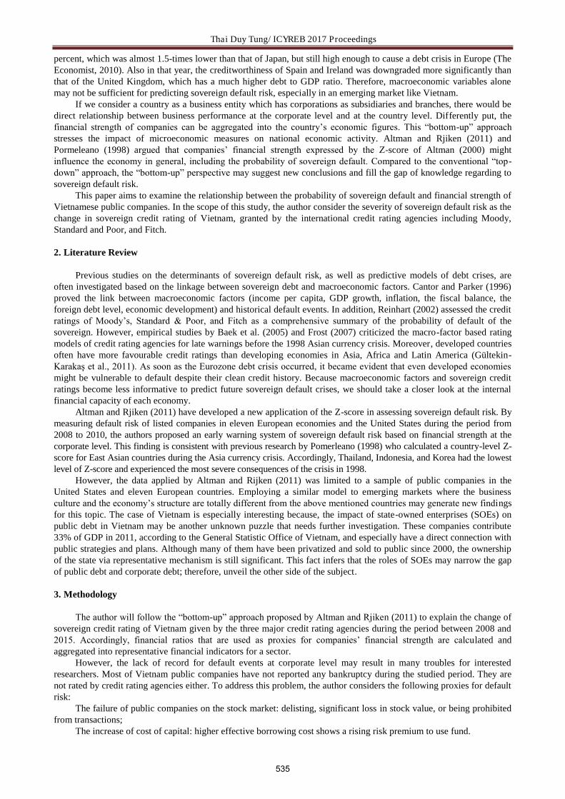
Thai Duy Tung/ ICYREB 2017 Proceedings
percent, which was almost 1.5-times lower than that of Japan, but still high enough to cause a debt crisis in Europe (The Economist, 2010). Also in that year, the creditworthiness of Spain and Ireland was downgraded more significantly than that of the United Kingdom, which has a much higher debt to GDP ratio. Therefore, macroeconomic variables alone may not be sufficient for predicting sovereign default risk, especially in an emerging market like Vietnam.
If we consider a country as a business entity which has corporations as subsidiaries and branches, there would be direct relationship between business performance at the corporate level and at the country level. Differently put, the financial strength of companies can be aggregated into the country’s economic figures. This “bottom-up” approach stresses the impact of microeconomic measures on national economic activity. Altman and Rjiken (2011) and Pormeleano (1998) argued that companies’ financial strength expressed by the Z-score of Altman (2000) might influence the economy in general, including the probability of sovereign default. Compared to the conventional “top-down” approach, the “bottom-up” perspective may suggest new conclusions and fill the gap of knowledge regarding to sovereign default risk.
This paper aims to examine the relationship between the probability of sovereign default and financial strength of Vietnamese public companies. In the scope of this study, the author consider the severity of sovereign default risk as the change in sovereign credit rating of Vietnam, granted by the international credit rating agencies including Moody, Standard and Poor, and Fitch.
2. Literature Review
Previous studies on the determinants of sovereign default risk, as well as predictive models of debt crises, are often investigated based on the linkage between sovereign debt and macroeconomic factors. Cantor and Parker (1996) proved the link between macroeconomic factors (income per capita, GDP growth, inflation, the fiscal balance, the foreign debt level, economic development) and historical default events. In addition, Reinhart (2002) assessed the credit ratings of Moody’s, Standard & Poor, and Fitch as a comprehensive summary of the probability of default of the sovereign. However, empirical studies by Baek et al. (2005) and Frost (2007) criticized the macro-factor based rating models of credit rating agencies for late warnings before the 1998 Asian currency crisis. Moreover, developed countries often have more favourable credit ratings than developing economies in Asia, Africa and Latin America (Gültekin-Karakaş et al., 2011). As soon as the Eurozone debt crisis occurred, it became evident that even developed economies might be vulnerable to default despite their clean credit history. Because macroeconomic factors and sovereign credit ratings become less informative to predict future sovereign default crises, we should take a closer look at the internal financial capacity of each economy.
Altman and Rjiken (2011) have developed a new application of the Z-score in assessing sovereign default risk. By measuring default risk of listed companies in eleven European economies and the United States during the period from 2008 to 2010, the authors proposed an early warning system of sovereign default risk based on financial strength at the corporate level. This finding is consistent with previous research by Pomerleano (1998) who calculated a country-level Z-score for East Asian countries during the Asia currency crisis. Accordingly, Thailand, Indonesia, and Korea had the lowest level of Z-score and experienced the most severe consequences of the crisis in 1998.
However, the data applied by Altman and Rijken (2011) was limited to a sample of public companies in the United States and eleven European countries. Employing a similar model to emerging markets where the business culture and the economy’s structure are totally different from the above mentioned countries may generate new findings for this topic. The case of Vietnam is especially interesting because, the impact of state-owned enterprises (SOEs) on public debt in Vietnam may be another unknown puzzle that needs further investigation. These companies contribute 33% of GDP in 2011, according to the General Statistic Office of Vietnam, and especially have a direct connection with public strategies and plans. Although many of them have been privatized and sold to public since 2000, the ownership of the state via representative mechanism is still significant. This fact infers that the roles of SOEs may narrow the gap of public debt and corporate debt; therefore, unveil the other side of the subject.
3. Methodology
The author will follow the “bottom-up” approach proposed by Altman and Rjiken (2011) to explain the change of sovereign credit rating of Vietnam given by the three major credit rating agencies during the period between 2008 and 2015. Accordingly, financial ratios that are used as proxies for companies’ financial strength are calculated and aggregated into representative financial indicators for a sector.
However, the lack of record for default events at corporate level may result in many troubles for interested researchers. Most of Vietnam public companies have not reported any bankruptcy during the studied period. They are not rated by credit rating agencies either. To address this problem, the author considers the following proxies for default risk:
The failure of public companies on the stock market: delisting, significant loss in stock value, or being prohibited from transactions;
The increase of cost of capital: higher effective borrowing cost shows a rising risk premium to use fund.
535

Thai Duy Tung/ ICYREB 2017 Proceedings
The latter measure is more straightforward because the change of borrowing cost can be obtained directly from companies’ financial data. Hence, the author uses borrowing cost of company to determine the default risk in this study.
Altman (2000) suggested that there would be four factors having impact on financial strength of company: (1) short-term liquidity, measured by the ratio of Net working capital to Total asset, (2) the level of retention, measured by the ratio of Accumulated retained earnings to Total asset, (3) the asset’s productivity, measured by Total asset turnover and the ratio of Earning Before Interest and Taxes (EBIT) to Total asset, and (4) the maximum loss in market value of the company before insolvency, determined by the ratio of market value of equity over book value of total liabilities.
In addition, the debt level, expressed by the ratio of Total liabilities to Total asset, and long-term debt ratio (long-term borrowings to total long-term capital) can be considered as the proxies for company’s leverage, thus, affect the financial risk.
4. Data handling and description
4.1. Data handling
The financial data of Vietnamese public companies is obtained from a data service provider with full information from 2000 to 2016. Currently, there are 325 companies listed in Hochiminh City Stock Exchange (HOSE) and 381 stocks traded in Hanoi Stock Exchange (HNX). However, most of the companies became public only after 2008, as shown in Table 1.
Table 1. Public and Non-public companies on HOSE and HSX
Year
HOSE HNX
Public Non-public Public Non-public
2000 1 324 0 381
2001 1 324 0 381
2002 5 320 2 379
2003 18 307 5 376
2004 32 293 10 371
2005 128 197 92 289
2006 179 146 145 236
2007 259 66 247 134
2008 287 38 318 63
2009 293 32 335 46
2010 298 27 343 38
2011 304 21 351 30
2012 314 11 362 19
2013 320 5 375 6
2014 321 4 380 1
2015 321 4 380 1
Source: summarized by the author
Therefore, the study is conducted using data from 2008 to 2015 to avoid too many missing data. More than 700 Vietnamese public companies are grouped into 10 sectors according to the Global Industry
Classification Standard (GICS®) of MSCI Inc. and Standard & Poor’s, except the Telecommunication Services sector. The Financial sector is also excluded from the research because of its unique characteristic. The companies listed on HOSE have already classified by the stock exchange, while the ones on HNX are put in another category system. In attempt to make a better comparable data set, the author has converted the HNX category system into GICS®. The 9 sectors are Consumer Discretionary, Consumer Staples, Energy, Health Care, Industrials, Information Technology, Materials, Real Estate, and Utilities.
Financial ratios of the sector are the means of those for component companies. In order to avoid negative influence of extreme outliers, the author removed all data points lying out of the 3-σ confidence estimates, in accordance with the method conducted by Van Gestel et al (2006).
536

Thai Duy Tung/ ICYREB 2017 Proceedings
4.2. Data description
The data of financial ratios in each sector shows relatively clear trends during the studied period; however, when being compared to each other, the financial ratios for each sector go in different patterns as they can been seen figures in Part 5. Therefore, a cross-sector analysis will be conducted instead of a comprehensive perspective. The author will analyze and explain the co-movement of sectors regarding to the same financial ratio, rather than attempting to consider a common figure for the whole Vietnamese economy.
5. Cross sector analysis of corporate’s financial strength in Vietnam
5.1. Short-term liquidity
The short-term liquidity is measured by the ratio of net working capital to total asset, while net working capital (NWC) is the difference of total current asset and total current liabilities. There are also some other financial ratios which are the proxies for short-term liquidity, such as current ratio and quick ratio. Nevertheless, these ratios are less effective to predict the company’s financial distress (Altman, 2000).
The pattern of NWC to Total Asset ratio in each sector is shown in Figure 1. Although short-term liquidity is often used to assess potential financial risk, this may not the case in Vietnam. Most of sectors experienced fairly stable movement of NWC to Total Asset over time. Furthermore, each sector has its own level of liquidity ratio based on its unique features. For example, Information Technology provides service packages that are paid in instalments; therefore, the account receivables of IT companies are often greater than firms in other sectors.
Figure 1. Net Working Capital to Total Asset ratio
5.2. The size of retained earnings
Accumulated retained earnings give the information of how much the company saves for reinvestment. It is also the same as a “saving account” of the company. The common logic is that the more money the company saves the less default risk it exposed to, i.e. “more money is safer”. In addition, the assessment of financial strength based on the size of retained earnings may lead to a discrimination against young companies which are not aging enough to build up sufficient capital base. This measure also gives a favourable consideration towards traditional sectors and long-term established companies.
Figure 2. Retained Earnings to Total Asset ratio
The average retained earnings as a percentage of total assets is lower than 10% in most of sectors, as shown in
537
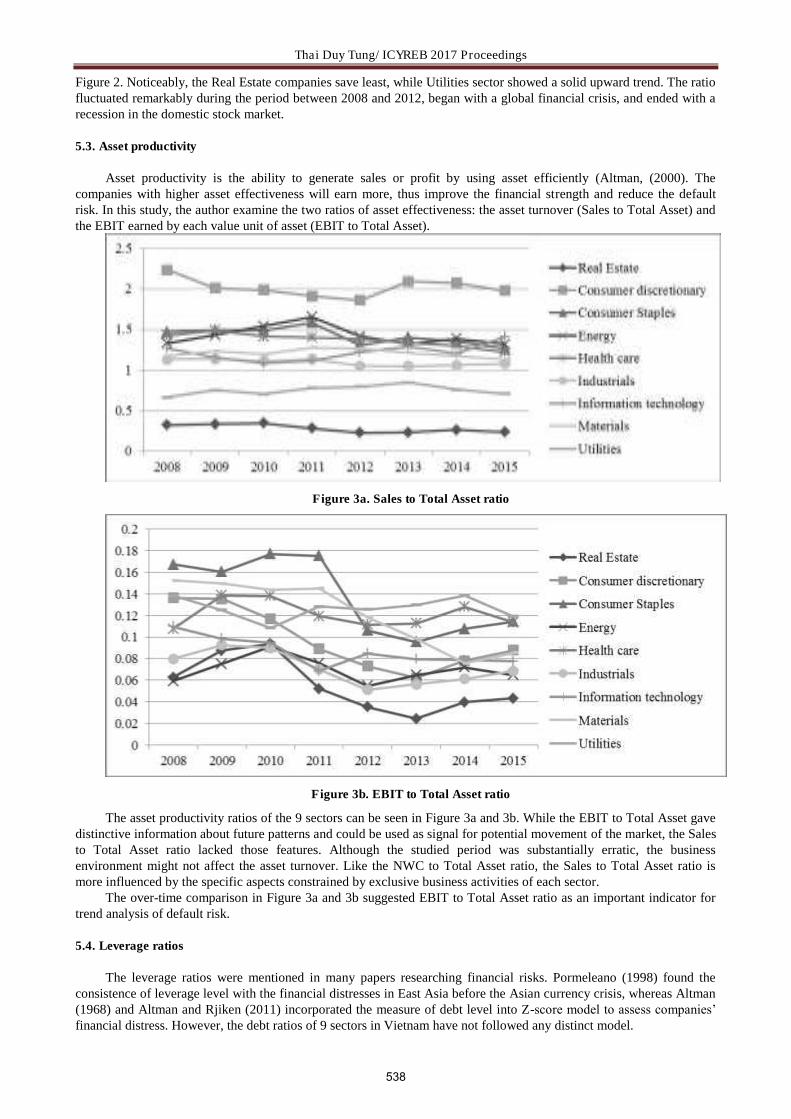
Thai Duy Tung/ ICYREB 2017 Proceedings
Figure 2. Noticeably, the Real Estate companies save least, while Utilities sector showed a solid upward trend. The ratio fluctuated remarkably during the period between 2008 and 2012, began with a global financial crisis, and ended with a recession in the domestic stock market.
5.3. Asset productivity
Asset productivity is the ability to generate sales or profit by using asset efficiently (Altman, (2000). The companies with higher asset effectiveness will earn more, thus improve the financial strength and reduce the default risk. In this study, the author examine the two ratios of asset effectiveness: the asset turnover (Sales to Total Asset) and the EBIT earned by each value unit of asset (EBIT to Total Asset).
Figure 3a. Sales to Total Asset ratio
Figure 3b. EBIT to Total Asset ratio
The asset productivity ratios of the 9 sectors can be seen in Figure 3a and 3b. While the EBIT to Total Asset gave distinctive information about future patterns and could be used as signal for potential movement of the market, the Sales to Total Asset ratio lacked those features. Although the studied period was substantially erratic, the business environment might not affect the asset turnover. Like the NWC to Total Asset ratio, the Sales to Total Asset ratio is more influenced by the specific aspects constrained by exclusive business activities of each sector.
The over-time comparison in Figure 3a and 3b suggested EBIT to Total Asset ratio as an important indicator for trend analysis of default risk.
5.4. Leverage ratios
The leverage ratios were mentioned in many papers researching financial risks. Pormeleano (1998) found the consistence of leverage level with the financial distresses in East Asia before the Asian currency crisis, whereas Altman (1968) and Altman and Rjiken (2011) incorporated the measure of debt level into Z-score model to assess companies’ financial distress. However, the debt ratios of 9 sectors in Vietnam have not followed any distinct model.
538

Thai Duy Tung/ ICYREB 2017 Proceedings
Figure 4a. Total debt ratio
Figure 4b. Long-term debt ratio
Figure 4a illustrated the stability of total debt ratio in all 9 studied sectors, while Figure 4b made a definite separation of long-term capital structure in these groups. Both total debt ratio and long-term debt ratio did not change significantly during the period under the study in spite of the volatility featured in that time. Additionally, Figure 4b revealed the long-term capital structure of different industries in Vietnam. Industrials sector can be considered the “boundary” stabilized at 0.2; while the upper side includes Real Estate, Energy, and Utilities, the capital-intensive groups, and the lower side contains less investment-concentrated sectors.
6. Sector borrowing cost and sovereign default risk in Vietnam
The integrated sector ratios to assess financial strength of Vietnamese public companies need to be evaluated by putting them aside the potential default risk of the sectors. In this paper, the author use sector’s average borrowing cost as a measure of credit risk. The lenders will ask for extra risk premium to provide funds to distressed organizations; therefore, increased credit spreads or borrowing costs will definitely reflect the information of risk in financial market. At country level, we can use the sovereign credit ratings or the spread of Credit Default Swap (CDS) to measure default risk (Altman and Rjiken, 2011); however, the similar assessment is not appropriate at corporate and sector level because the corporate bond market in Vietnam is not popular.
Figure 5. Sector average borrowing cost
539
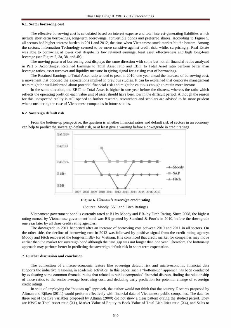
Thai Duy Tung/ ICYREB 2017 Proceedings
6.1. Sector borrowing cost
The effective borrowing cost is calculated based on interest expense and total interest-generating liabilities which include short-term borrowings, long-term borrowings, convertible bonds and preferred shares. According to Figure 5, all sectors had higher interest burden in 2011 and 2012, the time when Vietnamese stock market hit the bottom. Among the sectors, Information Technology seemed to be more sensitive against credit risk, while, surprisingly, Real Estate was able to borrowing at lower cost despite its low retained earnings, least asset effectiveness and high long-term leverage (see Figure 2, 3a, 3b, and 4b).
The moving pattern of borrowing cost displays the same direction with some but not all financial ratios analyzed in Part 5. Accordingly, Retained Earnings to Total Asset ratio and EBIT to Total Asset ratio perform better than leverage ratios, asset turnover and liquidity measure in giving signal for a rising cost of borrowings.
The Retained Earnings to Total Asset ratio tended to peak in 2010, one year ahead the increase of borrowing cost, a movement that opposed the expectations implied in previous studies. It can be explained that corporate management team might be well-informed about potential financial risk and might be cautious enough to retain more income.
In the same direction, the EBIT to Total Asset is higher in one year before the distress, whereas the ratio which reflects the operating profit on each value unit of asset should have been low in the difficult period. Although the reason for this unexpected reality is still opened to further research, researchers and scholars are advised to be more prudent when considering the case of Vietnamese companies in future studies.
6.2. Sovereign default risk
From the bottom-up perspective, the question is whether financial ratios and default risk of sectors in an economy can help to predict the sovereign default risk, or at least give a warning before a downgrade in credit ratings.
Figure 6. Vietnam’s sovereign credit rating
(Source: Moody, S&P and Fitch Ratings)
Vietnamese government bond is currently rated at B1 by Moody and BB- by Fitch Rating. Since 2008, the highest rating earned by Vietnamese government bond was BB granted by Standard & Poor’s in 2010, before the downgrade one year later by all three credit rating agencies.
The downgrade in 2011 happened after an increase of borrowing cost between 2010 and 2011 in all sectors. On the other side, the decline of borrowing cost in 2013 was followed by positive signal from the credit rating agency: Moody and Fitch recovered the long-term BB- for Vietnam. It is convinced that credit market for companies may move earlier than the market for sovereign bond although the time gap was not longer than one year. Therefore, the bottom-up approach may perform better in predicting the sovereign default risk in short-term expectation.
7. Further discussion and conclusion
The connection of a macro-economic feature like sovereign default risk and micro-economic financial data supports the inductive reasoning in academic activities. In this paper, such a “bottom-up” approach has been conducted by evaluating some common financial ratios that related to public companies’ financial distress, finding the relationship of those ratios to the sector average borrowing cost, and deducing early prediction for potential change of sovereign credit ratings.
In spite of employing the “bottom-up” approach, the author would not think that the country Z-scores proposed by Altman and Rjiken (2011) would perform effectively with financial data of Vietnamese public companies. The data for three out of the five variables proposed by Altman (2000) did not show a clear pattern during the studied period. They are NWC to Total Asset ratio (X1), Market Value of Equity to Book Value of Total Liabilities ratio (X4), and Sales to
540

Thai Duy Tung/ ICYREB 2017 Proceedings
Total Asset (X5). In addition, an attempt to calculate the representative of sector Z-score has been done. However, the Z-scores for four out of the nine sectors are in grey area, as Altman (2000) defined the cut-off scores for unclassified cases, i.e. the grey area, were 1.81 and 2.675. The figure of Z-scores of 9 sectors is shown in the Appendix.
In future researches regarding sovereign default risk and financial distress, the author will refrain from using Z-score and other linear regression because linear (panel) models have been highlighted to perform poorly in predicting sovereign default risk (Amstad and Packer, 2015). Instead, non-parametric machine learning models will be considered to predict emerging market’s sovereign default. The development of computer science raises the motivation for researchers to explore new techniques to rediscover and refine the study in finance. Contributions of Van Gestel et al (2006) with the applications of Support Vector Machine method, and Ozturk et al (2016) with the random forest decision tree method suggest more improved papers regarding to this topic in the future.
Appendix. Z-scores of sectors
Although there are some versions of Z-score calculation suggested by Altman and other researchers, the function and weights presented by Altman (2000) were employed because of the appropriation between the data set and Altman’s research.
The formula of Z-score is given as follows:
Where: = Net Working Capital / Total Asset = Retained Earnings / Total Asset = Earnings Before Interest and Taxes / Total Asset = Market Value of Equity / Book Value of Total Liabilities = Sales / Total Asset
Figure 7. Z-score of sectors
References
[1] Reinhart, C. M., & Rogoff, K. (2009). This Time is Different. Eight Centuries of Financial Folly, Princeton University, Princeton and Oxford.
[2] Allen, W. A., & Moessner, R. (2012). The Liquidity Consequences of the Euro Area Sovereign Debt Crisis. BIS Working Paper No. 390
[3] Altman, E. I. (2000). Predicting Financial Distress of Companies: Revisiting the Z-score and ZETA Models. Stern School of Business, New York University, 9-12.
[4] Altman, E. I., & Rijken, H. A. (2011). Toward a Bottom‐Up Approach to Assessing Sovereign Default Risk. Journal of Applied Corporate Finance, 23(1), 20-31.
[5] Amstad, M. and Packer, F (2015). Sovereign Ratings of Advanced and Emerging Economies after the Crisis. BIS Quarterly Review.
[6] Arellano, C. (2008). Default Risk and Income Fluctuations in Emerging Economies. The American Economic Review, 98(3), 690-712.
[7] Baek, I. M., Bandopadhyaya, A., & Du, C. (2005). Determinants of Market-Assessed Sovereign Risk: Economic Fundamentals or Market Risk Appetite?. Journal of International Money and Finance, 24(4), 533-548.
[8] Bi, H. (2012). Sovereign Default Risk Premia, Fiscal Limits, and Fiscal Policy. European Economic Review, 56(3), 389-410.
[9] Borensztein, E., & Panizza, U. (2009). The Costs of Sovereign Default. IMF Economic Review, 56(4), 683-741 [10] Cantor, R., & Packer, F. (1996). Determinants and Impact of Sovereign Credit Ratings. Economic Policy Review,
541

Thai Duy Tung/ ICYREB 2017 Proceedings
2(2). [11] Cuadra, G., Sanchez, J. M., & Sapriza, H. (2010). Fiscal Policy and Default Risk in Emerging Markets. Review of
Economic Dynamics, 13(2), 452-469. [12] Frost, C. A. (2007). Credit Rating Agencies in Capital Markets: A Review of Research Evidence on Selected
Criticisms of the Agencies. Journal of Accounting, Auditing & Finance, 22(3), 469-492. [13] Gültekin-Karakaş, D., Hisarcıklılar, M., & Öztürk, H. (2011). Sovereign Risk Ratings: Biased toward Developed
Countries?. Emerging Markets Finance and Trade, 47(sup2), 69-87. [14] Mink, M., & de Haan, J. (2013). Contagion During the Greek Sovereign Debt Crisis. Journal of International
Money and Finance, 34, 102-113. DOI: 10.1016/j.jimonfin.2012.11.006 [15] Ozturk, H., Namli, E. and Erdal, H.I. (2016). Modelling Sovereign Credit Ratings: The Accuracy of Models in a
Heterogeneous Sample. Economic Modelling, 54, 469-478. [16] Pomerleano, M. (1998). Corporate Finance Lessons from the East Asian Crisis. Available at:
https://openknowledge.worldbank.org/handle/10986/11531. [17] Reinhart, C. M. (2002). Default, Currency Crises, and Sovereign Credit Ratings. The World Bank Economic
Review, 16(2), 151-170. [18] Van Gestel, T, Baesens, B., Van Dijcke, P. Garcia, J., Suykens, A.K. and Vanthienen, J. (2006). A process model
to develop an internal rating system: Sovereign credit ratings. Decision Support Systems, 42(2), 1131-1151. [19] The Economist (2015). The Global Debt Clock. Available at:
http://www.economist.com/content/global_debt_clock.
542

Le Thai Phong, Nguyen Thi Hanh/ ICYREB 2017 Proceedings
International Conference For Young Researchers In Economics And Business, ICYREB 2017, October 30th 2017 Da Nang, Vietnam
Determinants of Fund Raising for Vietnamese Startups
Le Thai Phonga*, Nguyen Thi Hanhb
aPhD, Foreign Trade University, Vietnam bPhD candidate, Foreign Trade University, Vietnam
A B S T R A C T
The purpose of this paper is to identify the factors that influence the fund raising ability of innovative new ventures/startups. We investigate a data set composed of 42 Vietnamese innovative new ventures. Specifically, the authors run a Tobit regression model linking the amount of equity raised by the company to the human capital of the company and firm’s characteristics and focused the analysis on the Chief Executive Officer (CEO) of the new company, who usually is a founder and, in the early stages, the most charismatic figure. The paper sheds light on the factors affecting the fund raising process of innovative new ventures in the early stage of the company’s life cycle.
Keywords: CEO; Entrepreneurship; New venturers; Fund raising
1. Introduction
Entrepreneurial activity fosters the innovation and technological change of a nation (Schumpeter, 1943). It is widely acknowledging the fact that places with high numbers of enterprises usually have high economic growth. The cause of this relationship is by starting a business does not only create value for the economy but also create many job opportunities, thereby improving the quality of life of people (Park and Taher, 2010). Shane (1995) demonstrates entrepreneurship is key for the economic growth by investigating contribution of entrepreneurial firms to the US economic growth in the period 1947-1990. Moreover, new ventures are responsible for job creation (Vesper, 1996). Recent studies (Stangler and Kedrosky, 2010; Kane, 2010) show that startups are accountable for almost all the new jobs created in the USA (about 63 percent). A research by Haltiwanger et al. (2013) on the US economy in the period 1992-2005 confirms that existing firms are net job destroyers, losing one million jobs net combined per year. By contrast, in their first year, new firms add an average of three million jobs. During recessionary years, job creation at startups remains stable. For all these reasons, entrepreneurship has attracted the attention of scholars since many decades and startups are becoming a growing area of interest. The success of start-ups has an impact on the economy, so that governments in developed and developing countries have adopted a variety of supportive policies and efforts, creating a favourable business environment to promote startups growth.
Entrepreneurship is a very complex category that involves many activities, such as identifying and evaluating opportunities and motives; search and allocate resources; corporate governance; fundraising. As pointed out by Clarysse et al. (2011), the growth paths of young technology-based firms result from structuring resource portfolios. Resources embrace human, technology, and financial resources. More specifically, this entrepreneurial model is usually associated to a need for capital exceeding the founders’ ability to self-fund and the company’s capability to self-sustain. Consequently, new ventures (also referred as “startups” or “young and new technology-based companies/NTBF” [1]) in the early stages base their development on the resources collected through external financing, which comes from investors specialized on equity (seed and venture capital, as well as business angels, incubators, accelerators, recently also crowdfunding). Equity capital acquisition is one of the most critical factors in the growth path of a startup/new venture (Hustedde and Pulver, 1992; Colombo and Grilli, 2010; Colombo et al., 2010). The lack of adequate funds hinders firms’ growth and even threatens survival because it is strong correlated to resources acquisition (Carpenter and Petersen, 2002).
Therefore, it is critical to understand the variables affecting the ability of new ventures – specifically in the early-stage phase – to access to financial resources. This paper concentrate on new ventures in the early stage phrase in terms of company’s life cycle combine with venture capital life cycle. This mean, at this early stage, the company has a
* Corresponding author. Tel.: + 84886226688
E-mail address: [email protected]
543

Le Thai Phong, Nguyen Thi Hanh/ ICYREB 2017 Proceedings
product or service that it is testing or still developing, but it isn’t completely ready to go to market. In some cases, the product may be commercially available in a limited manner but not yet generating revenue. Typically, a company that receives early stage financing has been in business for less than three years. Insofar, only a few studies have focused on the influence of human capital and firm’s characteristics on fund raising. Cressy (1996) suggests that human capital determines the ability of a company to access to financial resources, while others affirm that capital raised by a startup is positively related to the entrepreneurs’ level of education (Bates, 1990). By contrast, Storey and Wynarczyk, 1996 find that company-specific factors also have a great explanatory power as fund raising is involved.
While the importance of equity capital on future new venture performance has been deeply investigated, access to equity capital for start-ups at an early stage and the existing linkages with human capital and firms’ characteristics still remain an open research problem. In particular, the study of factors affecting the successful fundraising of startups is quite new. However, research in the world often focuses on developed country contexts, where business environment is more advanced, and probably completely different from emergent contexts, such as in Vietnam. The research in Vietnam is very new, and it focuses mainly on the first issue (studying the factors that influence the entrepreneurial intention of the business).
Our analysis aims at filling this gap by linking the founders’ background (education) and firm characteristic to the ability to raise new capital. This study contributes to the entrepreneurship literature and provide important implications for researchers and practitioners who are more and more interested in startup companies in general and, specifically, in the funding process of early-stage companies (with a focus on qualitative and quantitative evaluation criteria).
The paper is structured as follows. The first section is an introduction to the main topic of paper, i.e. the relationship between entrepreneurship, firm age, firm size and capital raising process. The second one introduces the theoretical framework and includes a comprehensive literature review on human capital, firm characteristics and new ventures/startups. In this section we also introduce the conceptual framework we adopted to run the analysis. Then, the methodology is discussed and the main features of the sample are presented. In the final section, results are described and discussed. Some managerial and research implications complete the paper.
2. Literature review
Although the idea of considering a company as a set of resources was already addressed by Penrose (1959), it was only during the 1980s that academic researchers began to consider resources as a key aspect for strategic management. Until that time in fact, attention was focused mostly on the industry and on the company positioning within a specific strategic group. Wernerfelt (1984) introduces the concept of resource position barriers in analogy to entry barriers and shifts the focus of analysis from the product/business side to the resource side. The resource approach offers a theory able to explain the linkages between diversification and economies of scope, as defined by Panzar and Willig (1981). In fact, the tangible and intangible assets owned by a firm are supposed to drive its diversification process, the choice of the markets to address and the types of firms to acquire or partner with. In this perspective, mergers and acquisitions as well as alliances can be seen as a way of obtaining a set of resources in an imperfect market.
Starting from the five competitive forces model (Porter, 1980), Wernerfelt examines the concept of resource position barriers, considering them as a competitive advantage against competitors, able to give the company higher returns. As opposed to entry barriers, resource position barriers are able to protect an incumbent not only from potential entrants, but also from other companies operating in the same industry or strategic group. Another key aspect of resource position barriers is that the resources behind them could be utilized in other markets. It is worth noting that to be valuable, a resource position barrier should be transformed into an entry barrier in at least one market.
The importance of resources is particularly true for small firms that rely on owner(s) skills (Lerner and Almor, 2002). Therefore, management skills can be considered part of human capital resources and are able to lead competitive advantages. According to Alvarez and Busenitz (2001), also opportunity identification can be considered as a resource. Consistently, many authors (Shane, 2000; Eckhardt and Shane, 2003) have focused their work on the motivations, methods, and circumstances underlying the ability to identify opportunities that only certain individuals seem to have access to.
This paper focusses on company internal resources, with a specific attention to early-stage innovative companies. Specifically, our research aims at shedding light on the relation between human capital, firm characteristics and organizational capital resources and physical ones, with a focus on financial resources (equity capital acquired by the company through fund raising).
2.1. Firm characteristics: size and age
As regards the size of firms, already Schumpeter (1942) emphasised the positive influence of size on innovative firm performance, while a number of theoretical studies have claimed that larger companies have potential factors such as economies of scale, lower risk, a larger market and greater opportunities for appropriation (Fernández, 1996), which enables them to undertake innovative projects and difficult to reach the fund. Organizations perform differently due to their size-specific characteristics. Small firms are viewed as more flexible and innovative (Acs and Audretsch, 1990;
544

Le Thai Phong, Nguyen Thi Hanh/ ICYREB 2017 Proceedings
Winters and Stam, 2007), whilst larger firms have more resources and capabilities arising from their economies of scale (Winters and Stam, 2007). Thus, organizational size can be seen to convey both advantages and disadvantages to fundraising behavior. Accordingly, this study proposes the hypothesis:
H1: Firm with a lager size are more successful in equity fund raising. Organizational age can have both a negative and positive effect on organizations. Older firms have more
experience, and have established relationship networks, technical competencies and new product development processes and routines (Bierly and Daly, 2007). On the other hand, older firms can be more bureaucratic (Bierly and Daly, 2007). Meanwhile, younger firms are often more flexible and are more likely to raise fund.
H2: Firm with a longer age are more successful in equity fund raising.
2.2. Human capital
Several studies on entrepreneurship have focused on the person of the entrepreneur (human capital). According to this stream of research, different variables have been considered as predictors of entrepreneurial propensity and firm’s performance.
Entrepreneurs’ age and gender are common variables scholars study when focusing on entrepreneurs’ basic demographic factors (Roberts, 1991; Bates, 2002; Levesque and Minniti, 2006). Scholars argue that entrepreneurial propensity and ability to identify opportunities decreases with age. Empirical research demonstrates that young adults have a stronger focus on opportunities than older adults (Zacher and Frese, 2011). By contrast, to recognize an opportunity, a certain degree of domain-specific knowledge is required. Recent contributions ascribable to the field of study related to “young entrepreneurship” (Lewis and Massey, 2003; Schoof, 2006) state that young entrepreneurs face major challenges by trying to raise capital to start-ups their business (Stevenson, 1987). First, they typically do not own real assets that can be used as a collateral security for a bank loan; second they lack of credibility from banks and financial actors.
As regards entrepreneur’s gender, extensive research investigates on the existence of a gap between male and female entrepreneurs. Scholars outlined the difficulties that female entrepreneurs face in fund raising especially in the early-stage phases of a start-up (Rosa et al., 1996).
Experience and education are other human capital characteristics that have been studied in relation to company’s performance (Rauch and Rijsdijk, 2013; Colombo and Grilli, 2005, 2010). Specifically, entrepreneurs’ high educational levels/years of schooling can be considered as a proxy of the knowledge acquired by the entrepreneur before initiating a start-up (Rauch and Rijsdijk, 2013). Education provides the necessary cognitive skills to adapt to environmental changes (Hatch and Dyer, 2004).
As previously mentioned, studies on entrepreneurship show how experience and education have a strong impact on company’s performance. Specifically, education is a source of knowledge, skills, discipline, motivation, and self-confidence (Cooper et al., 1994). Entrepreneurs may also leverage their knowledge and the social contacts generated through the education system to acquire resources and access to business networks (Shane and Khurana, 2003; Arenius and De Clercq, 2005). This is particularly true when taking into consideration higher level of education. The network of contacts that a person may acquire through an MBA course could be crucial for the growth of the new venture. Therefore, we expect that entrepreneurs who have broader business experience, solid background in business and management and are older should have more chance of succeeding in their business ventures. Actually, they could leverage their prior experience and exploit their network, develop more sounding business plans and be more effective in raising capital (Hustedde and Pulver, 1992). In summary, we hypothesize that:
H3. Entrepreneurs with a more solid academic education are more successful in equity fund raising. H4. Entrepreneurs with business education are more successful in equity fund raising.
3. Data and methodology
Base on the proposed issue we used a data set composed of 42 Vietnamese innovative new ventures that was announced in Daily Street Asia online magazine. In addition, drawing the sample from this source provides several advantages, i.e.: identify teams engaged in the early stages of the entrepreneurial process; scout firms and founder’s characteristics and perform longitudinal studies, monitoring the phenomenon in a specific area or region.
Data, that are crossection, gathered contain information about the new ventures, such as the year of incorporation and place of establishment, sector, number of founders, business description and available market data, company investment profile (capital raised and investors’ typology), financials. Moreover, demographic information on the founders and management team have been collected, such as date and place of birth, gender, education background, role played in the new venture, prior working experience (detailed information on the prior positions in companies/universities/research centers) and prior entrepreneurial experience (detailed information for each previous startup the founders have been involved).
As a proxy for the individual specific variables of the investigated startups, we decided to focus on the Chief Executive Officer (CEO), who is usually the founder of the new venture and, in the early stages, the key figure and
545

Le Thai Phong, Nguyen Thi Hanh/ ICYREB 2017 Proceedings
decision maker for the company (Papadakis and Barwise, 2002). Therefore, we analyzed the CEOs of the above-mentioned 42 new ventures. The other people composing the founding team are considered as part of the company-specific variables.
3.1. Dependent variable: capital raised
Equity capital acquisition is one of the most critical factors in the growth path of a startup/new venture (Hustedde and Pulver, 1992), in particular for the most innovative ones (Venturelli and Gualandri, 2009) that operate in high-tech industries (Colombo et al., 2010). Scholars argue that access to financial capital provides the necessary resources to foster exploration, pursue new opportunities (March and Simon, 1958; Bourgeois, 1981; Zahra, 1991; Stevenson and Jarillo, 1990) and sustain the new venture over the long term. In particular, securing early-stage equity financing is a key factor for the survival, growth and future performance of the new venture (Cassar, 2004; Wetzel, 1986; Mason and Harrison, 2000). Raising capital from outside investors represents a further validation for the new venture business plan and, implicitly, determines a sort of acceptance of the new venture by the environment (Alsos et al., 2006). In this case, the data gathered amount of fund raising in the early stage of venture capital, that is combine of seed funding, first round, second round and third round.
3.2. Control variables
We include some company-specific characteristics referring to the size of the company and to the age of the company. McMahon (2001) found that the size of the company – measured in terms of headcount – positively impacts its performance. Furthermore, the number of employees can be considered as a proxy of the stage of development of the company and the level of risk associated to the company (Lee and Zhang, 2011). In this respect, investors typically prefer to invest in younger ventures. This specific issue creates problem to researchers because they need to include in their research samples.
The table 1 show the statics of the variables related to the sample we analysed.
Table 1: Descriptive statics of the sample
Variables Obs Type Mean Std. Dev. Min Max
Capital raised 42 Continuous 1.25e+07 2.86e+07 0 1.37e+08
CEO Age 42 Continuous 34.14286 5.532923 22 46
Firm Age 42 Continuous 4.095238 2.611509 1 11
No. of employees 42 Continuous 437.119 1457.695 5 9000
Frequency (%)
83.3 Male
97.6 Uni degree
38.1 MBA
CEO gender 42 Dummy
CEO academic education 42 Dummy
CEO MBA 42 Dummy The CEOs are on average 34-year old (ranging from a minimum of 22 to a maximum of 46); 83 percent are male
and 17 percent female. 97.6 percent of the CEO have a university degree, 38.1 percent also an MBA. As regards the field of activity of the companies, Web and ICT represent the more prevalent areas of business (85 percent). A minor role is played by companies specialized in Financial Technologies (10 percent) and in Biotech/Agricultural Sciences (5 percent). Ventures capital is the common source of funding (57 percent) for the 42 new ventures, 17 percent companies were also able to raise seed capital, while 26 percent were zero.
In our research, we decided to investigate the characteristics of both the CEOs and new ventures with the ability of a start-up in fund raising (measured by the amount of the capital raised since inception). We adopted a Tobit model. The variable is therefore zero for a part of the sample and is continuously distributed over positive values (Wooldridge, 2009). In fact, capital raised is zero for about 26 percent of our sample, while for the remaining 74 percent it assumes values ranging between 5000 dollars and 137.000.000 dollars. We performed a Tobit modelling using Stata, testing the relationship between the amount of capital raised and the variables indicated in the table above.
Analyzing the correlation matrix, we did not find any significant correlation (> 0.70) among the independent variables, as shown by Table 2.
We developed Tobit model, analyzing the influence of education, age, gender and firms’ size, firm’s age on the ability to raise capital.
Furthermore, in Table 4 we developed a Probit model, to show the variables influencing the ability of the start-up to raise capital.
546

Le Thai Phong, Nguyen Thi Hanh/ ICYREB 2017 Proceedings
4. Discussion and implication
Our results show that the age of CEO positively affects the fund raising process. We assume that more experienced individuals are more successful in fund raising given the experience accrued during their working life and the larger network of contacts they can leverage (Hustedde and Pulver, 1992; Eesley and Roberts, 2012). This result is confirmed by our model.
Table 2: Correlation Matrix
CEO Age CEO gender CEO education
CEO MBA Firm Age No. of Employees
CEO Age 1.0000
CEO Gender -0.0000 1.0000
CEO Education 0.2041 -0.0698 1.0000
CEO MBA 0.2217 0.0877 0.1225 1.0000
Firm Age 0.3839 -0.1073 0.1268 -0.2380 1.0000
No. of Employees 0.2339 -0.4029 0.0465 -0.0815 0.1068 1.0000
Table 3: Tobit Model
Capital raised Coef. Std. Err. t P>|t| [95% Conf. Interval]
Firm’s Age -1727770 2241689 -0.77 0.446 -6274125 2818585
No. of Employees 938.6078 3804.28 0.25 0.807 -6776.829 8654.045
CEO Age 3257766 1116789 2.92 0.006 992812.8 5522718
CEO Gender -2451901 1.60e+07 -0.15 0.879 -3.49e+07 3.00e+07
CEO Education -2.10e+07 3.14e+07 -0.67 0.509 -8.47e+07 4.28e+07
CEO MBA 1.48e+07 1.11e+07 1.33 0.191 -7678485 3.72e+07
_cons -8.18e+07 4.31e+07 -1.90 0.066 -1.69e+08 5528720
/sigma 2.97e+07 3988149 2.16e+07 3.78e+07
Table 4: Probit Model
Capital raised Coef.
Firm’ Age .0258583
No. of Employees .0002303
CEO Age -.0078367
CEO gender 1.446796
CEO Education 0 (omitted)
CEO MBA 1.524252
_cons -.8868154 The level of education can be considered a good proxy of the fund raising process. Entrepreneurs with stronger
education background are better able to develop and communicate a business plan. Specifically, managerial and finance competences are required ability to properly identify and explain the value proposition, strategy and business model of the new venture as well as the target market and customers. Entrepreneurs with an MBA also may benefit of higher credibility potential investors.
Company-specific factors are also important to explain the ability of new ventures to secure investments. Dimensional factors – measured in terms of number of employees – can be considered a proxy of the stage of development of the company (Lee and Zhang, 2011). Our data support the thesis that investors prefer to invest in more structured companies rather than early-stage projects.
The Probit model provides further insights on the results by showing that the CEO gender and the CEO MBA are the only two significant variables. On the other hand, the CEO age seems not to affect the dependent variable.
547

Le Thai Phong, Nguyen Thi Hanh/ ICYREB 2017 Proceedings
5. Conclusion and limitation
The Probit model provides further insights on the results by showing that the CEO gender and the CEO MBA are the only two significant variables. On the other hand, the CEO age seems not to affect the dependent variable.
Our analysis focusses the factors that influence the fundraising ability of innovative new ventures/startups. The literature review highlights a lack of empirical studies dealing with the ability of new ventures to raise capital specifically in the early stage of development. The innovativeness of this study lies in the choice of the sample, since it is composed mainly by young and innovative startups. Our findings show a significant link between the amount of capital raised and the age of entrepreneurs. Beside that, the higher the education, the higher is the amount of capital raised by the startups by positive effect of MBA degree on ability to raising fund. Consistently with previous studies carried out on the topic (Colombo and Grilli, 2005; Hustedde and Pulver, 1992), we found that “MBA-like” and – in general – post-graduate education on management/business topics facilitates the ability of entrepreneurs to attract outside investments. Our data do not seem to support the role played by academic education. As regards firm-specific characteristics, the model reveals a significant relation between the CEO gender and the ability in fund raising.
In conclusion, the results of our empirical study provide further insights about the relationship between the human capital and the amount of capital raised by the startups. Moreover, we provide insights about the valuation criteria seed and venture capital investors as well as business angels adopt while approaching an investment in a startup company.
The focus on startups founded by Vietnamese entrepreneurs (although some of them are incorporated abroad) may impact on the generalization of the results. Therefore, a cross-country study will represent the natural prosecution of our research. An additional major limitation consists in the impossibility to test the endogeneity of education inasmuch as we do not have any strong and convincing instrumental variables to test the endogeneity. This aspect need to be further investigated.
Note
We define “start-ups” as new entrepreneurial initiatives focussed on innovation and growth. The proposed definition is in line with the definition of “young and new technology based companies,” adopted by the most widespread literature on entrepreneurship (see also Gilbert et al., 2006; Onetti et al., 2012) and also with the one proposed by Ries (2001): “A start-up is a human institution designed to deliver a new product or service under conditions of extreme uncertainty.”
References
[1] Alsos, G.A., Isaksen, E.J. and Ljunggren, E. (2006), “New venture financing and subsequent business growth in men- and women-led business”, Entrepreneurship Theory and Practice, Vol. 30 No. 5, pp. 667-686.
[2] Alvarez, S. and Busenitz, L. (2001), “The entrepreneurship of resource-based theory”, Journal of Management, Vol. 27 No. 6, pp. 755-775.
[3] Arenius, P. and De Clercq, D. (2005), “A network-based approach on opportunity recognition”, [4] Small Business Economics, Vol. 24 No. 3, pp. 249-265. [5] Bates, T. (1990), “Entrepreneur human capital inputs and small business longevity”, Review of Economics and
Statistics, Vol. 72 No. 4, pp. 551-559. [6] Bates, T. (2002), “Restricted access to markets characterizes women-owned businesses”, Journal of Business
Venturing, Vol. 17 No. 4, pp. 313-324. [7] Baum, J.R. and Bird, B.J. (2010), “The successful intelligence of high-growth entrepreneurs: links to new venture
growth”, Organization Science, Vol. 21 No. 2, pp. 397-412. [8] Beckman, C.M. (2006), “The influence of founding team company affiliations on firm behaviour”, [9] Academy of Management Journal, Vol. 49 No. 4, pp. 741-758. [10] Blanchflower, D.G. and Oswald, A.J. (1998), “What makes and entrepreneur?”, Journal of Labor Economics, Vol.
16 No. 1, pp. 26-60. [11] Bosma, H.A., Graafsma, T.L.G., Grotevant, H.D. and de Levita, D.J. (Eds) (1994), Identity and Development: An
Interdisciplinary Approach, SAGE Publications, Thousand Oaks, CA. [12] Bourgeois, L.J. (1981), “On the measurement of organizational slack”, The Academy of Management Review,
Vol. 6 No. 1, pp. 29-39. [13] Brinckmann, J., Salomo, S. and Gemuenden, H.G. (2009), “Financial management competence of founding teams
and growth of new technology-based firms”, Entrepreneurship Theory and Practice, Vol. 35 No. 2, pp. 217-243. [14] Brüderl, J., Preisendörfer, P. and Ziegler, R. (1992), “Survival chances for newly founded business organizations”,
American Sociological Review, Vol. 57 No. 2, pp. 227-242. [15] Brush, C.G., Greene, P.G. and Hart, M.M. (2001), “From initial idea to unique advantage: the entrepreneurial
challenge of constructing a resource base”, Academy of Management Executive, Vol. 15 No. 1, pp. 64-78. [16] Carpenter, R.E. and Petersen, B.C. (2002), “Capital market imperfections, high-tech investment, and new equity
548

Le Thai Phong, Nguyen Thi Hanh/ ICYREB 2017 Proceedings
financing”, The Economic Journal, Vol. 112 No. 447, pp. F54-F72. [17] Cassar, G. (2004), “The financing of business start-ups”, Journal of Business Venturing, Vol. 19 No. 2, pp. 261-
284. [18] Clarysse, B., Bruneel, J. and Wright, M. (2011), “Explaining growth path of young technology- based firms:
structuring resource portfolios in different competitive environments”, Strategic Entrepreneurship Journal, Vol. 5 No. 2, pp. 137-157.
[19] Colombo, M.G. and Grilli, L. (2005), “Founders’ human capital and the growth of new technology- based firms: a competence-based view”, Research Policy, Vol. 34 No. 6, pp. 795-816.
[20] Colombo, M.G. and Grilli, L. (2010), “On growth drivers of high-tech start-ups: exploring the role of founders’ human capital and venture capital”, Journal of Business Venturing, Vol. 25 No. 6, pp. 610-626.
[21] Colombo, M.G., Luukkonen, T., Mustar, P. and Wright, M. (2010), “Venture capital and high-tech startups”, Ventrue Capital: An International Journal of Entrepreneurial Finance, Vol. 12 No. 4, pp. 261-266.
[22] Cooper, A.C. and Gimeno-Gascon, F.J. (1992), “Entrepreneurs, processes of founding and new firm performance”, in Sexton, D. and Kasarda, J. (Eds), The State of the Art in Entrepreneurship, PWS Publishing Co., Boston, MA, pp. 301-340.
[23] Cooper, A.C., Gimeno-Gascon, F.J. and Woo, C.Y. (1994), “Initial human and financial capital as predictors of new venture performance”, Journal of Business Venturing, Vol. 9 No. 5, pp. 371-395.
[24] Cressy, R. (1996), “Are business startups debt-rationed?”, Economic Journal, Vol. 106 No. 438, pp. 1253-1270. [25] Dahl, M.S. and Reichstein, T. (2007), “Are you experienced? Prior experience and the survival of new
organizations”, Industry & Innovation, Vol. 14 No. 5, pp. 497-511. [26] Delmar, F.D.R. and Shane, S. (2006), “Does experience matter? The effect of founding team experience on the
survival and sales of newly founded ventures”, Strategic Organization, Vol. 4 No. 3, pp. 215-247. [27] Doutriaux, J. and Simyar, F. (1987), “Duration of comparative advantage accruing from some start-up factors in
high-tech entrepreneurial firms”, in Churchill, N.C., Hornaday, J.A., Kirchhoff, B.A., Krasner, O.J. and Vesper, K.H. (Eds), Frontiers of Entrepreneurship Research, Babson College, Wellesley, MA, pp. 436-450.
[28] Dyke, L.S., Fisher, E.M. and Reuber, A.R. (1992), “An inter-industry examination of the impact of owner experience on firm performance”, Journal of Small Business Management, Vol. 30 No. 4, pp. 73-86.
[29] Eckhardt, J. and Shane, S. (2003), “Opportunities and entrepreneurship”, Journal of Management, Vol. 29 No. 3, pp. 333-349.
[30] Eesley, C.E. and Roberts, E.B. (2012), “Are you experienced: when does talent vs experience drive entrepreneurial performance”, Strategic Entrepreneurship Journal, Vol. 6 No. 3, pp. 207-219.
[31] European Commission (2013), “Enterprise and industry – SBA 2013 fact sheet Italy”, European Commission, Brussels.
[32] Foltz, J., Barham, B., Chavas, J.-P. and Kim, K. (2012), “Efficiency and technological change at US research universities”, Journal of Productivity Analysis, Vol. 37 No. 2, pp. 171-186.
[33] Foo, M., Wong, P.K. and Ong, A. (2005), “Do others think you have a viable business idea? Team diversity and judges’ evaluation of ideas in a business plan competition”, Journal of Business Venturing, Vol. 20 No. 3, pp. 385-402.
[34] Gilbert, B.A., McDougall, P.P. and Audretsch, D.B. (2006), “New venture growth: a review and extension”, Journal of Management, Vol. 32 No. 6, pp. 926-950.
[35] Gimeno, J., Folta, T.B., Cooper, A.C. and Woo, C.Y. (1997), “Survival of the fittest? Entrepreneurial human capital and the persistence of underperforming firms”, Administrative Science Quarterly, Vol. 42 No. 4, pp. 750-783.
[36] Haltiwanger, J., Jarmin, R.S. and Miranda, J. (2013), “Who creates jobs? Small vs large vs young”, [37] The Review of Economics and Statistics, Vol. XCV No. 2, pp. 347-361. [38] Hatch, N.W. and Dyer, J.H. (2004), “Human capital and learning as a source of sustainable competitive
advantage”, Strategic Management Journal, Vol. 25 No. 12, pp. 1155-1178. [39] Hustedde, R.J. and Pulver, G.C. (1992), “Factors affecting equity capital acquisition: the demand side”, Journal of
Business Venturing, Vol. 7 No. 5, pp. 363-374. [40] Kane, T. (2010), “The importance of startups in job creation and job destruction”, Kauffman Foundation Research
Series: Firm Formation and Economic Growth, Ewing Marion Kauffman Foundation, Kansas City, MO. [41] Kauffman – The Foundation of Entrepreneurship (2008), “The Kauffman firm survey – the capital structure
decisions of new firms”, Ewing Marion Kauffman Foundation, Kansas City, MO. [42] Kisfalvi, V. (2002), “The entrepreneur’s character, life issues, and strategy making: a field study”, [43] Journal of Business Venturing, Vol. 17 No. 5, pp. 489-518. [44] Lazear, E.P. (2004), “Balanced skills and entrepreneurship”, The American Economic Review, Vol. 94 No. 2, pp.
208-211. [45] Lee, J.J. and Zhang, W. (2011), “Financial capital and startup survival”, paper presented at the annual meeting of
the Academy of Management, San Antonio, TX, August 12-16. [46] Lerner, M. and Almor, T. (2002), “Relationships among strategic capabilities and the performance of women-
549

Le Thai Phong, Nguyen Thi Hanh/ ICYREB 2017 Proceedings
owned small ventures”, Journal of Small Business Management, Vol. 40 No. 2, pp. 109-125. [47] Levesque, M. and Minniti, M. (2006), “The effect of aging on entrepreneurial behavior”, Journal of Business
Venturing, Vol. 21 No. 2, pp. 177-194. [48] Lewis, K. and Massey, C. (2003), “Youth entrepreneurship and government policy”, paper presented at the ICSB
Conference 2003, Belfast, June 15-18. [49] Littunen, H. and Niittykangas, H. (2010), “The rapid growth of young firms during various stages of
entrepreneurship”, Journal of Small Business and Enterprise Development, Vol. 17 No. 1, pp. 8-31. [50] McMahon, R.G.P. (2001), “Growth and performance of manufacturing SMEs: the influence of financial
management characteristics”, International Small Business Journal, Vol. 19 No. 3, pp. 10-28. [51] Mai, Y. and Zheng, Y. (2013), “How on-the-job embeddedness influences new venture creation and growth”,
Journal of Small Business Management, Vol. 51 No. 4, pp. 508-524. [52] March, J. and Simon, H. (1958), Organizations, Wiley, New York, NY. [53] March, J.G. (1991), “Exploration and exploitation in organization learning”, Organization Science, Vol. 2 No. 1,
pp. 71-87. [54] Mason, C.M. and Harrison, R.T. (2000), “Investing in technology ventures: what do business angels look for at
the initial screening stage?”, in Reynolds, P.D., Autio, E., Brush, C.G., Bygrave, W.D., Manigart, S., Sapienza, H.J. and Shaver, K.G. (Eds), Frontiers of Entrepreneurship Research, Babson College, Babson Park, MA, pp. 293-304.
[55] Miller, D. and Toulouse, J.M. (1986), “Strategy, structure, CEO personality and performance in small firms”, American Journal of Small Business, Vol. 10 No. 3, pp. 47-62.
[56] Onetti, A., Zucchella, A., Jones, M.V. and McDougall, P. (2012), “Internationalization, innovation and entrepreneurship: business models for new technology-based firms”, Journal of Management and Governance, Vol. 16 No. 3, pp. 337-368.
[57] Panzar, J.C. and Willig, R.D. (1981), “Economies of scope”, The American Economic Review, Vol. 71 No. 2, pp. 268-272.
[58] Papadakis, V.M. and Barwise, P. (2002), “How much do CEO and top managers matter in strategic decision-making?”, British Journal of Management, Vol. 13 No. 1, pp. 83-95.
[59] Penrose, E.G. (1959), The Theory of the Growth of the Firm, John Wiley & Sons, New York, NY. [60] Politis, D. (2008), “Does prior startup experience matter for entrepreneurs’ learning? A comparison between
novice and habitual entrepreneurs”, Journal of Small Business and Enterprise Development, Vol. 15 No. 3, pp. 472-489.
[61] Porter, M.E. (1980), Competitive Strategy: Techniques for Analyzing Industries and Competitors, Free Press, New York, NY.
[62] Rauch, A. and Rijsdijk, S.A. (2013), “The effects of general and specific human capital on long- term growth and failure of newly founded businesses”, Entrepreneurship Theory and Practice, Vol. 37 No. 4, pp. 923-994.
[63] Ries, E. (2001), The Lean Startup: How Today’s Entrepreneurs Use Continuous Innovation to Create Radically Successful Businesses, Crown Publishing Group, New York, NY.
[64] Roberts, E.B. (1991), Entrepreneurs in High Technology: Lessons from MIT and Beyond, Oxford University Press, New York, NY.
[65] Rosa, P., Carter, S. and Hamilton, D. (1996), “Gender as a determinant of small business performance: insights from a British study”, Business Economics, Vol. 8 No. 6, pp. 463-478.
[66] Schoof, U. (2006), “Stimulating youth entrepreneurship: barriers and incentives to enterprise start-ups by young people”, Series on Youth and Entrepreneurship, International Labour Organization, SEED Working Paper No. 76, Geneva.
[67] Schumpeter, J.A. (1943), Capitalism Socialism and Democracy, Harper and Row, New York, NY. [68] Shane, S. (1995), “Is the independent entrepreneurial firm a valuable organizational form?”, Best paper
proceedings of the Academy of Management 1985 Annual Meeting, Vancouver. [69] Shane, S. (2000), “Prior knowledge and the discovery of entrepreneurial opportunities”, [70] Organization Science, Vol. 11 No. 4, pp. 448-469. [71] Shane, S. (2001), “Technology regimes and new firm formation”, Management Science, Vol. 47 No. 9, pp. 1173-
1190. [72] Shane, S. and Khurana, R. (2003), “Bringing individuals back in: the effects of career experience on new firm
founding”, Industrial and Corporate Change, Vol. 12 No. 3, pp. 519-543. [73] Siegel, D.S. and Wessner, C. (2012), “Universities and the success of entrepreneurial ventures: evidence from the
small business innovation research program”, Journal of Technology Transfer, Vol. 37 No. 4, pp. 404-415. [74] Sorensen, J.B. (2007), “Closure vs exposure: mechanisms in the intergenerational transmission of self-
employment”, in Ruef, M. and Lounsbury, M. (Eds), Research in the Sociology of Organizations, Vol. 25, Emerald Group Publishing Limited, pp. 83-124.
[75] Stangler, D. and Kedrosky, P. (2010), “Neutralism and entrepreneurship: the structural dynamics of startups, young firms, and job creation”, Kauffman Foundation Research Series: Firm Formation and Economic Growth,
550

Le Thai Phong, Nguyen Thi Hanh/ ICYREB 2017 Proceedings
Ewing Marion Kauffman Foundation, Kansas City, MO. [76] Stevenson, H.H. and Jarillo, J.C. (1990), “A paradigm of entrepreneurship: entrepreneurial management”,
Strategic Management Journal, Vol. 11 No. 5, pp. 17-27. [77] Stevenson, H.H. and Sahlman, W.A. (1989), “The entrepreneurial process”, in Burns, P. and Dewhurst, J. (Eds),
Small Business and Entrepreneurship, Macmillan, Basingstoke, pp. 94-157. [78] Stevenson, L. (1987), “Toward understanding young founders”, in Churchill, N.C., Hornaday, J.A., Kirchhoff,
B.A., Krasner, O.J. and Vesper, K.H. (Eds), Frontiers of Entrepreneurship Research, Babson College, Wellesley, MA.
[79] Storey, D.J. and Wynarczyk, P. (1996), “The survival and non-survival of micro firms in the UK”, [80] Review of Industrial Organization, Vol. 11 No. 2, pp. 211-229. [81] Venturelli, V. and Gualandri, E. (2009), “The determinants of equity needs: size, youth or innovation?”, Journal of
Small Business and Enterprise Development, Vol. 16 No. 4, pp. 599-614. [82] Vesper, K. (1996), New Venture Experience, Vector Books, Seattle, WA. [83] Wernerfelt, B. (1984), “A resource-based view of the firm”, Strategic Management Journal, Vol. 5 No. 2, pp. 171-
180. [84] Wetzel, W.E. (1986), “Informal risk capital: knowns and unknowns”, in Sexton, D. and Smilor, R. (Eds), The Art
and Science of Entrepreneurship, Ballittger Publishing Company, Cambridge, MA, pp. 85-108. [85] Wooldridge, J.M. (2009), Introduction Econometrics. A Modern Approach, Cengage Learning and South-
Western, Mason, OH. [86] Zacher, H. and Frese, M. (2011), “Maintaining a focus on opportunities at work: the interplay between age, job
complexity, and the use of selection, optimization, and compensation strategies”, Journal of Organizational Behavior, Vol. 32 No. 2, pp. 291-318.
[87] Zahra, S. (1991), “Predictors and financial outcomes of corporate entrepreneurship: an explorative study”, Journal of Business Venturing, Vol. 6 No. 4, pp. 259-285.
551

Nguyen Thi Ngoc Diep/ ICYREB 2017 Proceedings
International Conference For Young Researchers In Economics And Business, ICYREB 2017, October 30th 2017 Da Nang, Vietnam
The Timing of Financial Statement Publication and Stock Return:
The Case of Vietnam
Nguyen Thi Ngoc Diep*
Lac Hong University, Bien Hoa City, Viet Nam
A B S T R A C T
This study investigates the impact of the timeliness of the financial statement publication on stock returns for listedfirms of different industries in Vietnam from 2010 to 2016. Our findings show that the timing of financial statement publication does have impact on stock returns: the earlier the publication is, the better the stock returns; the later the announcement is, the worse the stock returns. Also, it is content that even when firms may try to publish their statements early, there still remains negative influence of bad news on stock returns.
Keywords: stock returns, timeliness, financial statement, announcement
1. Introduction
Information published through financial statements contains details used to evaluate investment opportunities in stocks, and is shown to influence investor behavior (Mousa, 2015). Therefore, firms do have campaign strategies that aim to consolidate their image through financial statement publication (Bagnoli, 2002; Vinh & Phuong, 2014; Nguyen, 2010). Ball and Brown (1968) show that there is a link between stock price volatility and information from accounting reports since almost all the information on reports is utilized by investors. FASB (1980) circulates the definition regarding the reliability and relevancy of financial information. Accordingly, the relevancy relies on the predictability, feedback value and the timeliness of the reports. Indeed, one of the prerequisites is to assure the timeliness of the publication to maintain the reliability and the relevancy of the published information.
The macro-stability and the effort from Securities State Commission have spurred the growth of Vietnamese stock market. Firms in Vietnam have amassed greatest amount of equity ever since, and the market capitalization has reached its most recent 6-year peak. Furthermore, Vietnamese stock market is evaluated as one of the fastestgrowing ones and has the largest returns in Quarter II/2016 in South East Asia.
Studies regarding stock market in Vietnam are numerous, yet until now there have not been any empirical papers on the impact of the timeliness of the financial statement publication on stock returns for all firms and for firms of different industries in Vietnam. We study the impact of the timeliness of the publication on stock return, then evaluate the efficiency level of Vietnamese stock market. This is the first study for an emerging market using the approaches from Bagnoli (2002) and Nguyen (2010) conducted for developed markets. Our research is warranteed since Vietnam is an emerging market whose institutional level and financial development are not similar to that of developed countries. Therefore, the results obtained in a developing economy may not be the same as in Bagnoli (2002) for US and Nguyen (2010) for the UK, US and France.
2. Related studies
2.1. Background theories
Information asymmetry theory: This friction stems from the situation when one side of the transaction has more information than the other side. Easley and Ohara (2004) suggest that uninformed traders lose to informed counterparts, so they require a risk premium to purchase/hold stocks with higher levels of information asymmetry.
* Corresponding author. Tel.: +84942664879
E-mail address: [email protected]
552

Nguyen Thi Ngoc Diep/ ICYREB 2017 Proceedings
Efficient market theory: Perfect market is a market that achieves efficiency in distribution, operation and information flow. Among the three factors, information efficiency is the dominating factor to ensure the market efficiency in general. Market efficiency is evaluated into three levels: weak, semi-strong and strong. The level of market efficiency is important as it determines how investors price the information flows in the market when purchasing stocks.
2.2. Empirical studies
Most extant studies show that there is connection between the timing of report publication and the good and bad news delivered. Firms tend to publish good news faster than bad news (Chambers and Penman, 1984; Kross and Schroeder, 1984). Moradi et al. (2013) show that there is positive relationship between bad news and the number of delays in publishing yearly reports for Iranian firms. On average, these studies show evidence supporting market efficiency theory, while Begley and Fischer (1998), Bagnoli et al. (2002) and Haw et al. (2006) do not.
However, Chen and Mohan (1994) and Skinner (1994) suggest that firms can also report bad news early to avoid litigation risk. Aubert (2009) also supports the same argument for French listed, for there is a negative relationship between bad news and the delay in publishing reports. Chen and Mohan (1994)’s survey shows that managers tend to concern about the timing of publishing, while 50% of the managers hold that firms do have a fixed schedule for publishing reports. Chen and Mohan find that only firms that change the schedule are those whose abnormal earnings have impact on the timeliness of publication. Lower-than-expected earnings (bad news) are more likely to cause changes in the publication timing than higher-than-expected earnings (good news).
3. Object and scope of research and methodology
The object of this study is the link between the timeliness of financial report publication, the news from the financial reports and the stock returns of firms listed on both HOSE and HNX in Vietnam. The sample in this study comprises firms listed in Vietnamese stock markets from 2010 to 2016, and financial firms are excluded due to their different operating nature. Besides, firms should have their reports published periodically as required by Securities State Commission and the exchanges (HOSE and HNX), so that the data are sufficient to analyze.
Variables included in the paper are: ue (difference between the current year’s EPS and that of last year), and if ue > 0 then it is good news (positive change in EPS) and if ue < 0 then it is regarded as bad news. Neg_ue is a dummy variable that receives 1 if ue < 0, and 0 otherwise; Days-late and days-early are the difference in days between the publication date of the current year and last year, for late and early announcers respectively. Negue_ue is the interaction term between neg_ue and ue; late_negue is the interaction term between late_dummy and neg_ue. Late_ue, early_ue, late_negue_ue and early_negue_ue are the interaction terms formed by the multiplication of late_dummy, ue, early dummy and negative ue.
4. Findings
4.1. General statistics
Table 1. Statistics regarding the dates of financial report publications
No. of dates Late (+)
Full sample 2011 2012 2013 2014 2015
Early (-) N % N % N % N % N % N % <= - 35 47 2.09 8 2.00 11 2.48 4 0.87 18 3.88 6 1.26
- 29 - 34 24 1.07 6 1.50 2 0.45 8 1.74 4 0.86 4 0.84 - 22 - 28 73 3.25 22 5.49 7 1.58 18 3.90 17 3.66 9 1.89 -15 - 21 98 4.36 17 4.24 18 4.05 23 4.99 21 4.53 19 3.98
-14 23 1.02 8 2.00 3 0.68 4 0.87 6 1.29 2 0.42 -13 25 1.11 7 1.75 3 0.68 6 1.30 4 0.86 5 1.05 -12 29 1.29 8 2.00 7 1.58 8 1.74 4 0.86 2 0.42 -11 28 1.25 1 0.25 4 0.90 5 1.08 11 2.37 7 1.47 -10 50 2.23 12 2.99 7 1.58 12 2.60 8 1.72 11 2.31 -9 44 1.96 9 2.24 9 2.03 12 2.60 6 1.29 8 1.68 -8 55 2.45 6 1.50 11 2.48 17 3.69 13 2.80 8 1.68 -7 41 1.82 10 2.49 9 2.03 11 2.39 6 1.29 5 1.05 -6 60 2.67 15 3.74 7 1.58 14 3.04 11 2.37 13 2.73 -5 71 3.16 11 2.74 12 2.70 19 4.12 16 3.45 13 2.73
553

Nguyen Thi Ngoc Diep/ ICYREB 2017 Proceedings
-4 65 2.89 7 1.75 14 3.15 15 3.25 16 3.45 13 2.73 -3 68 3.03 11 2.74 9 2.03 16 3.47 20 4.31 12 2.52 -2 85 3.78 9 2.24 18 4.05 17 3.69 16 3.45 25 5.24 -1 119 5.30 20 4.99 20 4.50 20 4.34 30 6.47 29 6.08 0 161 7.17 31 7.73 28 6.31 31 6.72 35 7.54 36 7.55 1 116 5.16 22 5.49 17 3.83 26 5.64 22 4.74 29 6.08 2 87 3.87 13 3.24 10 2.25 24 5.21 20 4.31 20 4.19 3 78 3.47 9 2.24 10 2.25 15 3.25 25 5.39 19 3.98 4 66 2.94 15 3.74 13 2.93 13 2.82 9 1.94 16 3.35 5 65 2.89 9 2.24 17 3.83 11 2.39 10 2.16 18 3.77 6 70 3.12 7 1.75 17 3.83 16 3.47 14 3.02 16 3.35 7 45 2.00 5 1.25 6 1.35 15 3.25 12 2.59 7 1.47 8 46 2.05 11 2.74 7 1.58 7 1.52 10 2.16 11 2.31 9 48 2.14 6 1.50 8 1.80 7 1.52 7 1.51 20 4.19 10 59 2.63 10 2.49 14 3.15 8 1.74 13 2.80 14 2.94 11 25 1.11 3 0.75 5 1.13 6 1.30 3 0.65 8 1.68 12 32 1.42 4 1.00 8 1.80 4 0.87 7 1.51 9 1.89 13 33 1.47 10 2.49 7 1.58 3 0.65 2 0.43 11 2.31 14 24 1.07 6 1.50 5 1.13 1 0.22 5 1.08 7 1.47
1521 122 5.43 17 4.24 38 8.56 18 3.90 28 6.03 21 4.40 2228 63 2.80 20 4.99 27 6.08 7 1.52 2 0.43 7 1.47 2934 38 1.69 3 0.75 15 3.38 10 2.17 6 1.29 4 0.84 >=35 64 2.85 13 3.24 21 4.73 10 2.17 7 1.51 13 2.73 Sum 2247 100 401 100 444 100 461 100 464 100 477 100
(Source: author’s calculation)
From 1/2010 to 6/2016, we collected in total 2,730 observations regarding the publication dates. The dates are then categorised into late, early and on-time announcements, based on the dates of publication in year t and year t – 1. If in year t firms publish reports on a date that is later than that in year t – 1, we recognize it as late announcement, and early if vice versa. If it reports on the same date, then we deem it as on-time announcement (Bagnoli, 2002).
Table 1 shows that there are 1,005 observations with early publications and 161 on-time ones, accounting for 44.73% and 7.17% of the total sample, respectively. The number of late announcement observations is 1,081, accounting for 48.11% of the total sample. This suggests that the numbers of late and early announcements are quite similar.
Fig.1. Year-on-year differences in days of firms publishing financial statements from 1/2010 to 6/2016
(Source: author’s calculation)
554

Nguyen Thi Ngoc Diep/ ICYREB 2017 Proceedings
This result is consistent with Champers and Penman (1984) for US firms (the publication window is within 14 days). Haw (2006) shows that for Chinese listed firms, managers tend to have their financial reports circulated within [-90,9] days compared to the date of publication the year before. For Vietnamese firms, the findings show that the number of days later than the publication date of previous year tends to increase. This could be that since Vietnam is an emerging market, the regulations on financial statement publication are being developed. Indeed, in our study period, there have been 3 circulars issued, causing much problem for accounting staff as well as firm management in financial statement preparation. The next reason could be the incompetent accounting staff and management team who do not possess thorough experience in composing financial reports, thus leading to delays. Whittred (1980) and Keller (1986) show that accounting employees are plagued with difficulties in finalizing financial statements and/or being required to redo the statements, causing further delay.
4.2. The link between bad and good news and the timing of financial statement publication.
In order to evaluate the impact of the timing of the publication of financial statements on CAAR, this study adopts the approach from Bagnoli (2002) to conduct several regressions for the total sample and different industries. Specifically, this paper analyzes the above relationship for groups divided based on whether firms published their financial reports late, early or on time compared to the date of previous year (Bagnoli, 2002).
4.2.1. Regression results on the impact of publication date on CAAR for firms that publish financial statements late
Table 2 shows that for late announcers, the news does have impact on CAAR at 5% level and the impact is positive (ue=0.0972). Meanwhile bad news has negative influence on CAAR at 5% level (neg_ue = -0.0944). Specifically, the later the firms publish, the harsher the market responses (days_late is -0.1816). Moreover, firms that publish late and have bad news at the same time receive even worse response, but this is insignificant.
I use the same approach for industries to remove the industry effect when examining the same relationship. The results show that for industries like Basic Materials, Healthcare, Industrials and others the sign of the late announcement is also negative and significant. However, for industries like Oil and Gas, this effect does not have significant impact on CAAR. In summary, for firms that publish late, the later the announcement,the more severe the market responses, even with or without industry effect.
Table 2. The link between good news, bad news and the publication date of firms that publish late
CAAR ue Days _late
neg _ue
late_ue negue_ue late
_negue
late _negue
_ue _cons
Full sample
Coef. 0.09724 -0.1816 -0.0944 0.0000 5.21E-06 -0.0139 -0.00001 0.2836 t 2.05 -4.29 -2.48 1.39 0.46 -0.23 -0.65 5.59 P>|t| 0.041 0.000 0.013 0.166 0.645 0.819 0.514 0.000 Obs 1081 R2 0.1337 P > F 0.000
Basic Materials
Coef. -0.0192 -0.4153 -0.0562 0.00002 -1.45E-05 0.14316 0.00001 0.4155 t -0.1 -2.83 -0.37 0.51 -0.23 0.64 0.13 2.1 P>|t| 0.918 0.005 0.71 0.613 0.822 0.524 0.897 0.037 Obs 131 R2 0.1777 P > F 0.0225
Consumer Goods
Coef. 0.0939 -0.154 -1.231 -1.139 5.21E-06 -0.0409 7.4E-06 1.4240 t 1.98 -4.04 -1.93 -1.79 0.46 -0.7 0.38 2.23 P>|t| 0.048 0.000 0.053 0.074 0.645 0.482 0.704 0.026 Obs 153 R2 0.1343 P > F 0.000
Consumer Services
Coef. 0.10522 -0.5357 -0.4598 0.00001 2.01E-06 0.3512 -0.51560 0.6383 t 2.26 -9.77 -8.69 1.31 0.2 4.97 -9.59 10.31 P>|t| 0.024 0.000 0.000 0.19 0.841 0.000 0.000 0.000 Obs 72 R2 0.1712 P > F 0.000
Health Care Coef. 0.08642 -0.2133 -0.1771 0.00005 6.17E-06 0.05118 -0.00004 0.3447 t 1.22 -3.21 -2.82 1.64 0.19 0.52 -0.86 4.57 P>|t| 0.223 0.001 0.005 0.100 0.852 0.605 0.392 0.000
555

Nguyen Thi Ngoc Diep/ ICYREB 2017 Proceedings
Obs 32 R2 0.1394 P > F 0.00
Industrials
Coef. 0.19364 -0.3063 -0.1427 0.00012 -0.00011 0.05682 -0.00002 0.2120 t 1.26 -1.95 -0.93 1.11 -0.82 0.26 -0.14 1.24 P>|t| 0.209 0.054 0.354 0.269 0.412 0.796 0.888 0.217 Obs 595 R2 0.1089 P > F 0.0402
Oil & Gas
Coef. 0.01948 0.1225 -0.2504 -0.0001 -0.00009 0.43340 0.00045 0.31134 t 0.06 0.39 -0.96 -0.44 -0.91 0.96 1.46 0.99 P>|t| 0.952 0.698 0.341 0.662 0.366 0.344 0.15 0.33 Obs 23 R2 0.0965 P > F 0.6951
Technology
Coef. 0.06378 0.0291 0.1246 -0.0008 -0.00014 -0.0826 0.00127 0.1147 t 0.25 0.07 0.3 -0.45 -0.45 -0.14 0.63 0.42 P>|t| 0.808 0.943 0.762 0.655 0.655 0.892 0.531 0.678 Obs 28 R2 0.1308 P > F 0.6127
Others
Coef. 0.09547 -0.1743 -0.0993 0.00001 3.88E-06 -0.0095 -2.32E-06 0.28694 t 2.01 -4.28 -2.58 1.13 0.29 -0.16 -0.22 5.57 P>|t| 0.044 0.000 0.01 0.257 0.770 0.876 0.830 0.000 Obs 47 R2 0.1336 P > F 0.000
(Source: author’s calculation)
4.2.2. Regression results on the date of publication and CAAR for firms that publish financial statements early
Table 3 shows that for early-announcing firms, the sign of the impact of the news is positive (ue=0.1141) but the news itself does manifest its importance. Negative news imposes negative impact on stock returns (-0.1528), and for early-announcing firms negue_ue is significantly negative (-0.1381), suggesting that bad news does have destructive influence on the returns.
Similar to the above section, I also analyze the same link with industry effect removed (by running the same regression for separate industries). Table 1 maintains that the sooner firms announce their statements, the more positive response awarded, at least for industries such as Basic Materials (ue = 0.2327), Consumer Services (ue = 0.1142), Healthcare (ue = 0.1194). Besides, consistent with the findings for the total sample, bad news renders firms subject to punishment from the market for almost all industries (coefficients of neg_ue and negue_ue are negative and significant for most industries, except for Oil and Gas and Others).
Table 3.The link between good news, bad news and the publication date of firms that publish early
CAAR ue early _dum
neg _ue
early _ue
negue _ue
early _negue
early _negue
_ue _cons
Full sample
Coef. 0.1141 0.00001 -0.1528 -6.1E-06 -0.1381 -0.07485 -5.2E-07 0.2588
t 2.39 0.89 -3.98 -0.49 -3.37 1.23 -0.02 5.15
P>|t| 0.017 0.374 0.00 0.627 0.001 0.218 0.982 0.000
Obs 571
R2 0.1203
P > F 0.00
Basic Materials
Coef. 0.2327 0.00004 -0.0040 -4.5E-06 -0.2162 -0.11244 -5.3E-05 0.0365
t 1.82 1.16 -0.04 -0.1 -1.84 -0.64 -0.61 0.26
556
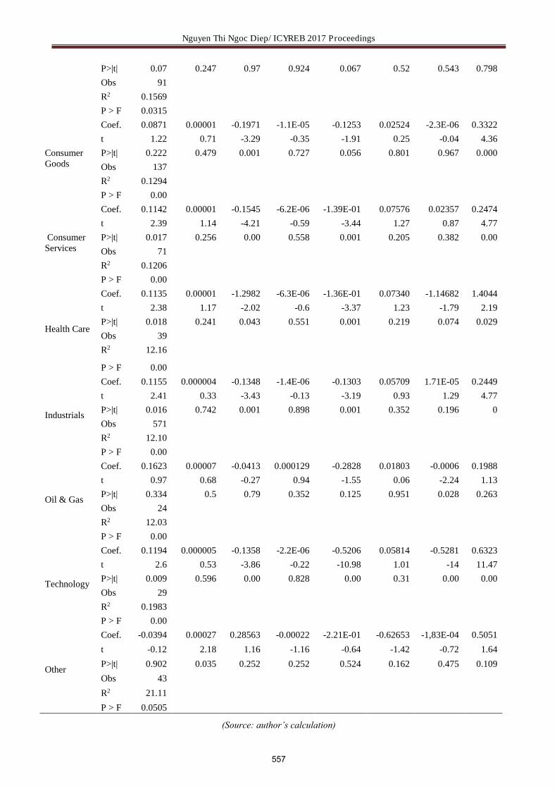
Nguyen Thi Ngoc Diep/ ICYREB 2017 Proceedings
P>|t| 0.07 0.247 0.97 0.924 0.067 0.52 0.543 0.798
Obs 91
R2 0.1569
P > F 0.0315
Consumer Goods
Coef. 0.0871 0.00001 -0.1971 -1.1E-05 -0.1253 0.02524 -2.3E-06 0.3322
t 1.22 0.71 -3.29 -0.35 -1.91 0.25 -0.04 4.36
P>|t| 0.222 0.479 0.001 0.727 0.056 0.801 0.967 0.000
Obs 137
R2 0.1294
P > F 0.00
Consumer Services
Coef. 0.1142 0.00001 -0.1545 -6.2E-06 -1.39E-01 0.07576 0.02357 0.2474
t 2.39 1.14 -4.21 -0.59 -3.44 1.27 0.87 4.77
P>|t| 0.017 0.256 0.00 0.558 0.001 0.205 0.382 0.00
Obs 71
R2 0.1206
P > F 0.00
Health Care
Coef. 0.1135 0.00001 -1.2982 -6.3E-06 -1.36E-01 0.07340 -1.14682 1.4044
t 2.38 1.17 -2.02 -0.6 -3.37 1.23 -1.79 2.19
P>|t| 0.018 0.241 0.043 0.551 0.001 0.219 0.074 0.029
Obs 39
R2 12.16
P > F 0.00
Industrials
Coef. 0.1155 0.000004 -0.1348 -1.4E-06 -0.1303 0.05709 1.71E-05 0.2449
t 2.41 0.33 -3.43 -0.13 -3.19 0.93 1.29 4.77
P>|t| 0.016 0.742 0.001 0.898 0.001 0.352 0.196 0
Obs 571
R2 12.10
P > F 0.00
Oil & Gas
Coef. 0.1623 0.00007 -0.0413 0.000129 -0.2828 0.01803 -0.0006 0.1988
t 0.97 0.68 -0.27 0.94 -1.55 0.06 -2.24 1.13
P>|t| 0.334 0.5 0.79 0.352 0.125 0.951 0.028 0.263
Obs 24
R2 12.03
P > F 0.00
Technology
Coef. 0.1194 0.000005 -0.1358 -2.2E-06 -0.5206 0.05814 -0.5281 0.6323
t 2.6 0.53 -3.86 -0.22 -10.98 1.01 -14 11.47
P>|t| 0.009 0.596 0.00 0.828 0.00 0.31 0.00 0.00
Obs 29
R2 0.1983
P > F 0.00
Other
Coef. -0.0394 0.00027 0.28563 -0.00022 -2.21E-01 -0.62653 -1,83E-04 0.5051
t -0.12 2.18 1.16 -1.16 -0.64 -1.42 -0.72 1.64
P>|t| 0.902 0.035 0.252 0.252 0.524 0.162 0.475 0.109
Obs 43
R2 21.11
P > F 0.0505
(Source: author’s calculation)
557

Nguyen Thi Ngoc Diep/ ICYREB 2017 Proceedings
4.2.2. Regression results for the link between publication date and CAAR for firms publishing financial statements on the same date between the current and previous years
For firms that have their statements published on time (or on the same date between the current and previous years as defined by Bagnoli (2002)), I find that the observations are quite limited in terms of quantity: Basic materials (16 observations), Consumer Services (14 observations), Healthcare (4), Oil and Gas (6), Technology (3) and Other (4). Therefore, this section only investigates the relationship for the total sample and for Consumer Goods (31 observations) and Industrials (83 observations).
The results from table 4 show that for the total sample, change in earnings has positive relation with the stock return (ue = 0.1197 and is significant at 1% level). For firms that have bad news, the impact on CAAR is negative (neg_ue = -0.13597 and negue_ue = -0.10706). Therefore, these results show that even though firms try to publish early, bad news contained in the statements still solicits negative feedback from the market.
With regards to industries, Consumer Goods firms show that change in earnings and bad news do have impat on CAAR significantly. Positive change in earnings is positively associated with CAAR, and negative news has negative impact on CAAR (neg_ue = -0.1128 and significant at 1% level and negue_ue=-0.0559). For Industrials firms, neg_ue = -0.2161 and negue_ue = -0.00019 and both are significant at 1%, again confirming that even if firms may strive to deliver their statements on time, bad news still imposes negative impacts on stock returns.
Table 4. Link between publication date and CAAR, for firms publishing reports on time
CAAR ue neg_ue negue_ue _cons
Total sample
Coef. 0.11970 -0.13597 -0.10706 0.24073 t 2.53 -5.11 -3.91 4.99 P>|t| 0.011 0.00 0.00 0.00 obs 161 R-squared 0.1197 Prob > F 0.00
Comsumer Goods
Coef. 0.11425 -0.11288 -0.05599 0.20357 t 2.41 -3.7 -1.42 4.27 P>|t| 0.016 0.00 0.157 0.00 R-squared 0.1142 obs 31 Prob > F 0.00 Prob > F 0.00
Industrials
Coef. 0.21850 -0.21618 -0.00019 0.13713 t 1.43 -2.11 -2.23 0.87 P>|t| 0.154 0.036 0.028 0,385 obs 83 R-squared 0.164 Prob > F 0.0357
(Source: author’s calculation)
In summary, this section provides consistent evidence showing that the information contained on the statements does have influence on stock returns for all three samples: early, late and on time announcers. Interestingly, for early firms the more early they are, the higher stock return and for late counterparts the later the more negative stock returns.
5. Conclusion
This study investigates the impact of the timeliness of the financial statement publication on stock returns for all firms and for firms of different industries in Vietnam from 2010 to 2016. Our findings show that the timing of financial statement publication does have impact on the stock returns: the earlier the publication, the better the stock returns; and the later the announcement, the worse the stock returns. Also, it is content that even the firms may try to publish their statements early, the negative influence of bad news on stock returns persists.
This paper brings new evidence in Vietnamese context that the timing and the content of the financial statements pose influence on stock returns. One critical implication from this study is that if firms wish to receive positive market response, accounting staff and management play an important role. The staff need to be well-trained on financial statement preparation and management team need to facilitate the process of making statements in order for these reports to be issued as early as possible. Certainly, the early publication should not compromise the quality of statements as sources of information about firms’ prospects and current well-being. Besides, the regulatory bodies should not introduce many changes in the requirements for financial statement preparation if unneccessary, since it requires time for the staff and management to be well-acquainted with the new regulation.
558

Nguyen Thi Ngoc Diep/ ICYREB 2017 Proceedings
References
[1] Aubert, F., (2009). Determinants of corporate financial disclosure tim-ing: the French empirical evidence, Journal of Accounting and Taxation. 1(3), 053-060. Available at http://www.academic-journals.org/jat
[2] Bagnoli, Mark, K.William, and Susan G. Watts., (2002). The information in manag ement expected earnings report date A day late, a penny short. Journal of Accounting Research 40, 1275-1296
[3] Begley, J. and P. E. Fischer., (1998). Is there Information in an Earnings Announcement Delay. Review of Accounting Studies, 3 pp. 347-363.
[4] Ball, R. B., P.,(1968). An Empirical Evaluation of Accounting Income Numbers. Journal of Accounting Research 6: 159-178.
[5] Chambers, A.E. and S.H. Penman., (1984) Timeliness of Reporting and Stock Price Reaction to Earnings Announcements. Journal of Accounting Research 22 (Spring 1984),pp. 21–47.
[6] Chen, C. R. & Mohan, N. J., (1994). Timing the Disclosure of Information: Management’s View of Earnings Announcements. Financial Management, 23(3), 63.
[7] Easley and Ohara., (2004). Information and the Cost of Capital. The Journal of Finance, Volume 59, Issue 4. Pages 1447–1950. DOI: 10.1111/j.1540-6261.2004.00672.
[8] Kross, W. & Schroeder, D. A., (1984). An empirical investigation of the effect of quarterly earnings announcement timing on stock returns. Journal of Accounting Research, 22 (1), 153-176, http:// dx.doi.org/10.2307%2F2490706
[9] Haw, I. M., K. J. Park, D. Qi, W. Wu., (2006). Securities Regulation, the Timing of Annual Report Release, and Market Implications Evidence from China. Journal of International Financial Management and Accounting 17, 111-139
[10] Mahdi Moradi, Mahdi Salehi1, Seyyed Saeed Mehrdad Ayask., (2013). The Relationship between Delay in Announcing Quarterly Forecasts of Annual Earnings and the Type of Earnings News. Research papers- Organizacija, Volume 46- Number 2, March-April 2013
[11] Nguyen, N. D., (2010). Post earnings announcement drift and stock liquidity in the US, the UK and French equity markets. Brunel University Research Archive (BURA). Doctor of Philosophy: 1-206.
[12] Skinner D., (1994). Why Firms Voluntarily Disclose Bad News. Journal of Accounting Research, 32(1), 38–60, http://dx.doi. org/10.2307%2F2491386
[13] Shukairi Nori Mousa, (2015). The effect of financial statement disclosure on stock prices on industrial shareholding companies. European Journal of Business and Social Sciences, ISSN : 2235-767X
[14] Võ Xuân Vinh, Lê Thị Kim Phượng, (2014). Biến động thu nhập bất thường, tính thanh khoản và tỷ suất sinh lời cổ phiếu khi công bố báo cáo tài chính trên thị trường chứng khoán Việt Nam. Tạp chí Kinh tế và Phát triển, số 199, tr. 31-39
559

Tran Minh Thu/ ICYREB 2017 Proceedings
International Conference For Young Researchers In Economics And Business, ICYREB 2017, October 30th 2017 Da Nang, Vietnam
Factors Affecting The Ability of Foreign Trade University
Students from Three Campuses to Start Their Own Business
Tran Minh Thu MA
Foreign Trade University, 91 Chua Lang, Dong Da, Hanoi, Hà Nội
A B S T R A C T
The research was conducted to identify the factors influencing the ability to start a new business of Business Administration students. The results of the study were based on a survey of 132 students from June 2017 to September 2017. Methods used in the study included Cronbach's Alpha, EFA, and multi regression linear. The results show that there are four main factors influencing the ability to start a new business of the students: attitudes and passion, starting up readiness, impact of relatives and knowledge from the school.
Keywords: Entrepreneur, business start-up, business administration, student, Foreign Trade University
1. Introduction
Vietnam is a country with a fast-growing economy and a large population, especially the working-age population, which accounts for a high percentage. This is a good environment for new enterprises. Foreign Trade University students in general and especially students in the business administration faculty are the ones with the greatest potential for start-up. They have youth, intellect, enthusiasm as well as in-depth knowledge. However, in practice, the number of students after graduation who want to start their own business is relatively small, whereas there is a large number of students who apply for jobs to be the employees of a specific company. The research question of this study is: Which factors affect the ability to start a new business of Foreign Trade University students? Identify these factors to encourage start-up business of Foreign Trade students. There are many research gaps in Vietnamese entrepreneurship field. Major researches usually focus on entrepreneur such as their specific characteristic i.e. Youth, gender. There is not much studies on entrepreneurship of students while the students are the ones who are best equipped with the knowledge and enthusiasm conditions to start a business. In addition, there have been quite a few debates about the impact of school knowledge and practical experience on students' ability to start a business. This research was conducted to identify which factors influence, which do not, quantifying and verifying these impacts on students' ability to start their own business. With the objective of identifying the factors affecting the start-up potential of business administration faculty students from Foreign Trade University, the authors used the quantitative method to analyse the survey results, which evaluate approximately 132 students’ answers from June 2017 to September 2017 to accomplish the goal of this study. Therefore, this study has both practical and theoretical implications.
2. Research Methodology
2.1. Study design
Previous researches in the world have shown that environmental factors and individual characteristics have a great impact on students' potential for starting-up. According to Sexton (2001) and Smith (2000), qualities, attitudes and entrepreneurial spirit are the main factors that influence the ability to start a successful business. In addition, financial resources play an important role in increasing the rate of start-ups (Pennings 1982). Only a few students after graduation have sufficient fund to start a business, while most are short of capital, having difficulty raising external fund when starting a business. Studies by Zahariah Mohd Zain (2010), Wenjun Wang (2011) explores the entrepreneurs’ potential of Malaysian, Pakistani, Chinese and American students, pointing to family traditions, characteristic traits, educational background, desire, willingness to do business, experience directly impact on students' starting-up intentions in these countries. A set of studies focused on students from wide range of majors of Kolvereid (1999), Peterman and Kennedy
560

Tran Minh Thu/ ICYREB 2017 Proceedings
(2003), Autio (2001) show that students from Entrepreneurship major has more desire and self-esteem to start their own business than other business group students (Nguyễn Thu Thủy, 2013). The practical experience also plays an important role, relatively large impact on the potential of starting a new business of the students. Previously, large-scale research by Kim and Hunter (1993) confirmed that university education had an effect on the possibility of students who want to start their own business. More than 50% of people have a positive attitude, wanting to do business and 30% of which actually start their own business. In addition, studies by Perera KH (2011), Francisco Linan (2011) conclude that social, psychological factors, political and legal factors are major factor that affect the ability to start a new business of students in Sri Lanka and Spain. After conducting the study of domestic and foreign studies, the model proposed in the study of factors affecting the potential of starting up business of the students. The facilities of FTU include the following factors:
1. The attitude toward entrepreneurship 2. Impact of relatives 3. Knowledge from the school 4. Practical experience from life 5. Passion to do business 6. Starting up readiness 7. Source of capital
Entrepreneurs’ potential
The attitude toward entrepreneurship
Impact of relatives
Knowledge from the school
Practical experience from life
Passion to do business
Starting up readiness
Source of capital
Fig.1. Recommended research model
With these seven factors, the author proposes 25 variable observations with a 5-point Linkert scale: Scale Score Level 1: Absolutely not agree 1 Level 2: Disagree 2 Level 3: Neutral 3 Level 4: Agree 4 Level 5: Absolutely agree 5
561

Tran Minh Thu/ ICYREB 2017 Proceedings
Table 1: Scale of factors influencing the potential of starting a new business of students from business faculties of Foreign Trade University
Factors Symbol Observation variable
The attitude toward entrepreneurship
TC TC1 I will start doing business after graduation TC2 I will start doing business if there is enough capital and opportunity TC3 I will start a business if I do not get a job after graduation
Impact of relatives NT NT1 Friends support my decision of starting a business NT2 Family support my decision of starting a business NT3 Family tradition and value affect my decision of starting a business
Knowledge from the school
KT KT1 Study at the school provides practical knowledge and practical skills KT2 The school organizes orientation activities toward entrepreneurship KT3 You has attended a seminar about entrepreneur before
Practical experience from life
KN KN1 Experience of being an employees KN2 Experience of being a manager KN3 Experience of doing business
Passion to do business DM
DM1 I like doing business DM2 I do not like to work for a salary DM3 The goal is to become a business owner DM4 I have many plans on starting a business
Starting up readiness SS
SS1 Sufficient understanding of the potential market to start a business SS2 Skills and knowledge to start a business start SS3 Not afraid of taking risk in business SS4 There are many relationships helped starting a business
Source of capital NV NV1 Can raise capital from family, friends NV2 Saving to create capital NV3 Can raise capital from other sources (banks, credit)
The model has a scale of seven independent factors (23 variables observed). Potential entrepreneur = f (TC, NT, KT, KM, DM, SS, NV)
2.2. Analytical methods
To determine the factors affecting the potential of starting a new business of Business Administration students from Foreign Trade University, the author carried out the process of this research in the following order. Step 1: Verify scale quality using Cronbach's Alpha method. Step 2: Use the Exploratory Factor Analysis (EFA) model: factor determination. Step 3: Using the Multiple Regression Analysis model: Identifying the factors affecting the potential of
562

Tran Minh Thu/ ICYREB 2017 Proceedings
starting a new business of Business Administration students and the role of each factor.
2.3. Method of data collection
Specify Sample Size According to Hair (2006), the sample size of the exploratory factor analysis model was determined on the basis of
two conditions: Minimum (1) and number of variables included in the analysis of the model (2). Whereas: (1) Minimum (Min) = 50 (2) The number of factors taken into the analysis of the model. If the model has m scale, Mi: Number of
observations of i scale. We have 1
m
ii
n mM
The ratio of sample size to analytical variable k is 5 / 1. If n <minimum level, sample size is set to minimum. Thus, applying the two conditions above, we have the sample size for the model is 115. In fact, the author has surveyed 132 students in the business administration faculty. Thus, data collection can ensure good performance of the research model.
3. Result of the research
3.1. Test the reliability of the scale
In order to determine the factors that impact to the entrepreneurship potential of business administration students in the Foreign Trade University and the impact of each factor, the author uses SPSS 22 software to perform the analysis according to the theoretical which shown in part 2. Scales that are well accepted and accepted result must meet two conditions:
• Cronbach's Alpha coefficient of overall> 0.6 • Total variable correlation coefficient> 0.3 The results are shown in Table 2. The Cronbach's Alpha value is 0.836. In the process of the four variables TD1,
NT3, KT3, DM2 were eliminated due to a total variable coefficient of less than 0.3. So the other 19 variables will be used for the next step - exploratory factor analysis.
Table 2: Results of testing scale
Symbol Scale The correlation
coefficient of total variation
Cronbach’s Alpha if item
deleted
TD2 I will start doing business if there is enough capital and
opportunity 0.432 0.841
TD3 I will start a business if I do not get a job after graduation 0.498 0.838 NT1 Friends support my decision of starting a business 0.380 0.843 NT2 Family support my decision of starting a business 0.376 0.846
KT1 Study at the school provides practical knowledge and
practical skills 0.342 0.842
KT2 The school organizes orientation activities toward
entrepreneurship 0.356 0.839
KN1 Experience of being an employees 0.375 0.844 KN2 Experience of being a manager 0.377 0.839 KN3 Experience of doing business 0.370 0.846 DM1 I like doing business 0.518 0.836 DM3 The goal is to become a business owner 0.520 0.832 DM4 I have many plans on starting a business 0.588 0.821
SS1 Sufficient understanding of the potential market to start a
business 0.491 0.838
SS2 Skills and knowledge to start a business start 0.579 0.834 SS3 Not afraid of taking risk in business 0.493 0.837 SS4 There are many relationships helped starting a business 0.482 0.832 NV1 Can raise capital from family, friends 0.485 0.784 NV2 Saving to create capital 0.421 0.792 NV3 Can raise capital from other sources (banks, credit) 0.391 0.802 Cronbach’s Alpha = 0.836
563
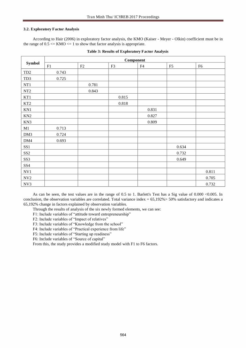
Tran Minh Thu/ ICYREB 2017 Proceedings
3.2. Exploratory Factor Analysis
According to Hair (2006) in exploratory factor analysis, the KMO (Kaiser - Meyer - Olkin) coefficient must be in the range of 0.5 <= KMO <= 1 to show that factor analysis is appropriate.
Table 3: Results of Exploratory Factor Analysis
Symbol Component
F1 F2 F3 F4 F5 F6
TD2 0.743
TD3 0.725
NT1 0.781
NT2 0.843
KT1 0.815
KT2 0.818
KN1 0.831
KN2 0.827
KN3 0.809
M1 0.713
DM3 0.724
DM4 0.693
SS1 0.634
SS2 0.732
SS3 0.649
SS4
NV1 0.811
NV2 0.705
NV3 0.732 As can be seen, the test values are in the range of 0.5 to 1. Barlett's Test has a Sig value of 0.000 <0.005. In
conclusion, the observation variables are correlated. Total variance index = 65,192%> 50% satisfactory and indicates a 65,192% change in factors explained by observation variables.
Through the results of analysis of the six newly formed elements, we can see: F1: Include variables of “attitude toward entrepreneurship” F2: Include variables of “Impact of relatives” F3: Include variables of “Knowledge from the school” F4: Include variables of “Practical experience from life” F5: Include variables of “Starting up readiness” F6: Include variables of “Source of capital” From this, the study provides a modified study model with F1 to F6 factors.
564
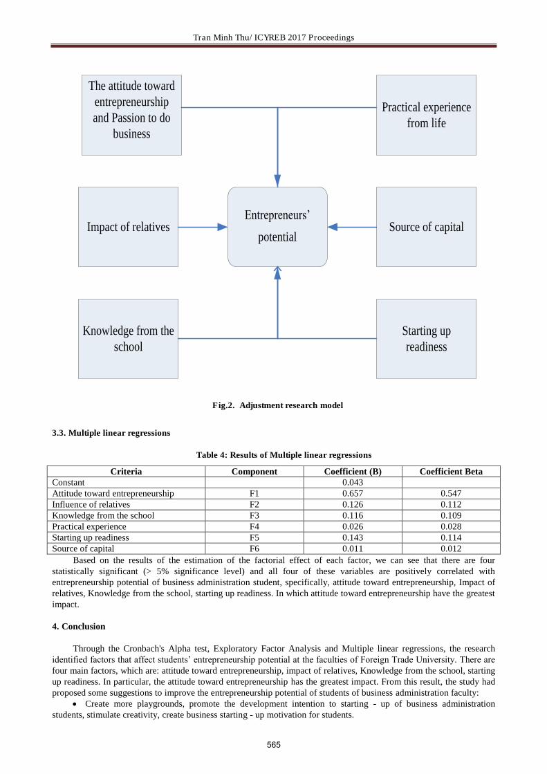
Tran Minh Thu/ ICYREB 2017 Proceedings
Entrepreneurs’ potential
The attitude toward entrepreneurship and Passion to do
business
Impact of relatives
Knowledge from the school
Practical experience from life
Starting up readiness
Source of capital
Fig.2. Adjustment research model
3.3. Multiple linear regressions
Table 4: Results of Multiple linear regressions
Criteria Component Coefficient (B) Coefficient Beta Constant 0.043 Attitude toward entrepreneurship F1 0.657 0.547 Influence of relatives F2 0.126 0.112 Knowledge from the school F3 0.116 0.109 Practical experience F4 0.026 0.028 Starting up readiness F5 0.143 0.114 Source of capital F6 0.011 0.012
Based on the results of the estimation of the factorial effect of each factor, we can see that there are four statistically significant (> 5% significance level) and all four of these variables are positively correlated with entrepreneurship potential of business administration student, specifically, attitude toward entrepreneurship, Impact of relatives, Knowledge from the school, starting up readiness. In which attitude toward entrepreneurship have the greatest impact.
4. Conclusion
Through the Cronbach's Alpha test, Exploratory Factor Analysis and Multiple linear regressions, the research identified factors that affect students’ entrepreneurship potential at the faculties of Foreign Trade University. There are four main factors, which are: attitude toward entrepreneurship, impact of relatives, Knowledge from the school, starting up readiness. In particular, the attitude toward entrepreneurship has the greatest impact. From this result, the study had proposed some suggestions to improve the entrepreneurship potential of students of business administration faculty: Create more playgrounds, promote the development intention to starting - up of business administration students, stimulate creativity, create business starting - up motivation for students.
565

Tran Minh Thu/ ICYREB 2017 Proceedings
The family and society should encourage student when they want to start up a business. Entrepreneurship is not an easy job therefore; all the encouragement and help are all the necessary help for future entrepreneurs. Knowledge in the school must be updated regularly, closer to reality in order to better equip students in business start up. Every business administration student must self-training, and must be willing to take part in entrepreneurship and accept the risks of starting up.
References
[1] Hair, J. F., Black, W. C., Babin, B. J., Anderson, R. E. & Tatham, R. L., (2006).Multivariate data analysis.6th ed, Pearson Prentice Hall. Journals:
[2] Autio, E. Keeley, R.H., Klofsen, M., Parker, G.G.C and Hay, M.(2001), Entrepreneurial intention among students in Scadinavia and in the USA, Enterprise and Innovation Management Studies, 2(2), Pp.145 - 160
[3] Francisco Liñán, Juan Carlos Rodríguez-Cohard, José M. Rueda-Cantuche, (2011). Factors affecting entrepreneurial intention levels: a role for education. International Entrepreneurship and Management Journal, Volume 7, Issue 2, pp195-218.
[4] Kim, M.S. and Hunter,J.E. (1993), Relationships among attitudes, behavioural intentions and behaviour. A meta-analysis of past research” part 2, Communication Research, pp.331
[5] Kolvereid, L. (1996) Organizational employment versus self-employment: Reasons for career intension, Entrepreneurship Theory and Practice, 20(3), 23-31
[6] Nguyễn Thu Thủy,(2013), Study on factors impact to university students’ entrepreneurship, doctoral thesis [7] Perera K. H., Jayarathna L.C.H., Gunarathna R.R.P.K., (2011), The Entrepreneurial Intention of Undergraduates
in Sri Lankan Universities, Faculty of Commerce and Management Studies, University of Kelaniya, Sri Lanka. [8] Peterman, N.E & Kennedy, J.(2003) Enterprise Education: Influencing Students‘s Perceptions of
Entrepreneurship, Entrepreneurship Theory and Practice, 28, pp 129 -144 [9] Sexton, D.L. (2001). Wayne Huizenga: Entrepreneur and wealth creator. Academy of
Management Executive, 1, 40-48. [10] Smith, J.K., & Smith, R. L. (2000). Entrepreneurial finance. New York: Wiley.
The State of Small Business: A report to the President. Washington, DC: U.S. Government Printing Office.
[11] Wenjun Wang, Wei Lu, John Kent Millington, (2011), Determinants of Entrepreneurial Intention among College Students in China and USA, Journal of Global Entrepreneurship Research, Winter & Spring, 2011, Vol.1, No.1, pp.35-44.
[12] Zahariah Mohd Zain, Amalina Mohd Akram, Erlane K Ghani, (2010), Entrepreneurship Intention Among Malaysian Business Students, Canadian Social Science,Vol.6, No.3, 2010, pp.34-44.
566

Dao Gia Phuc/ ICYREB 2017 Proceedings
International Conference For Young Researchers In Economics And Business, ICYREB 2017, October 30th 2017
Da Nang, Vietnam
Carbon Leakage and The Legality of Border Carbon Adjustment:
a Possible Approach through The Active Participation of
Domestic Industries
Dao Gia Phuc1
Lecturer - Faculty of Economic Law, Vice-Director - American Law Center, University of Economics and Law, VNU-HCM, Viet Nam
PhD Candidate, Transnational Doctoral Program for Leading Professionals in Asian Countries, Nagoya University, Japan
A B S T R A C T
National climate measure or Border Carbon Adjustment is one of the best solutions to combat carbon leakage, and the issue of climate change since international cooperation has not reached any significant movement in decades. However, the adoption of such measures can be faced with legal uncertainties under the legal framework of the World Trade Organization (WTO) with its principles of trade liberalizations. Particularly, Border Carbon Adjustment might violate the market access, non-discrimination principles, disciplines of technical regulations and the regulations on subsidies. This paper focuses on the legal hurdles of the issue and discusses a possible approach to enhance the capacities of the domestic industries itself to offset the disadvantages of competitiveness especially within the fourth industrial evolution rather than strict measures imposing on imports that may violate the international trade law.
Keywords: the fourth industrial evolution, climate change, border carbon adjustment, carbon leakage, WTO law, non-discrimination, general exceptions, technical regulations, subsidies, domestic industries
1. Climate change mitigation and carbon leakage
According to Intergovernmental Panel on Climate Change (IPCC), greenhouse gas (GHG) emissions from 2000–2010 were even larger than in the previous three decades. As a results, the average global temperature rose by 0.85°C from 1880–2012 and the global sea level also rose by 19 cm (1901–2000)2. The impact of climate changes are not only limited to extreme weather events (e.g. floods, drought, typhoons, etc.) but also affects to agricultural trade sectors, foods security, diseases, and extinctions of plants and animals3. Therefore, it undoubtedly needs to have significant contributions from lawmakers, policies and international organizations if we wish to avoid irreversible damage with catastrophic consequences.
The connection between the international trade and the climate change is an undeniable and very complex issue. Every business activity conducts an environmental consequence, and the collective impact of those activities affects the climate of the whole planet. Especially, there are much of the world’s energy needs are likely mainly depend on fossil fuels, together with an increase in global population, will lead to a higher level of GHG emissions. In another hand, free
* Corresponding author. Tel.: +84 909 473 184
E-mail address: [email protected] 2 IPCC, “Fifth Assessment Report - Climate Change 2013: The Physical Science Basis,” 5–6, accessed February 8,
2017 https://www.ipcc.ch/report/ar5/wg1/. 3 Margareta Tîmbur, “International Trade Development - Risks for the Environment?,” Economy
Transdisciplinarity Cognition; Bacau 13, no. 2 (2010): 6–22.
567

Dao Gia Phuc/ ICYREB 2017 Proceedings
trade can take part in the climate change mitigation’s process by encouraging the development of climate-friendly technologies and the efficiency of resource use4. Moreover, the well-known environmental Kuznets curve5 (Figure 1.1) has shown that the environmental degradation worsens as per capita GDP increases until the curve reaches a turning point, after which the environment improves shall occur.
Source: http://alturi.com/kexsi Figure 1.1 The environmental Kuznets curve
Since the relationship between climate change and trade becomes obvious and no country can take effective action to control such issue alone, there is a demand for international collective action. States and regulators working in disciplines that have long been free-standing now have to engage with the realities of cross-regime coherence that can only be realized through collaborative action6.
As part of multilateral efforts to combat climate change, countries during the Rio and Kyoto UN Conferences on Environment & Development agreed to set pollution control targets for developed countries while still leaving the developing countries with easier conditions for compliance. This is a great effort by the international community to limit the negative impact of pollution. However, the pollution targets for the production of particular goods and services of a particular country is not specified. Even within the 21st annual Conference of Parties (COP21, also known as 2015 Paris Climate Conference), the commitments of countries are still founded on a voluntary basis without any legally binding caps7. In addition, the levels of reduction between developed and developing countries varies considerably. These arrangements have led to unequal competition conditions between domestic and foreign producers. While countries with strict emissions reduction targets may be well intentioned, it is generally the case that domestic produces bear a significant portion of the emissions reduction costs. The unequal application of such policies between nations consequently incentivize companies to relocate their carbon-intensive production to countries with no carbon or lax constraint regime to balance the competition condition. As a result, a strict climate policy in one country may, in fact, lead to an increase of GHG emissions in countries low or no carbon emissions restrictions The result of such inconsistent application of emissions reduction policies may result in the fight against climate change being meaningless. This phenomenon has been called as 'carbon leakage'8.
This issue can be overcome by also putting the price on emissions of foreign products through border adjustment measures. The measures could balance the playing field between domestic and foreign products in this context and help domestic industries be less hesitant to take part in national emissions reduction schemes. The foreign producers could also be encouraged to reduce the carbon footprint of their products for lower taxes and lax regulations from importing
4 Ibid. 5 Rachel S. Franklin and Matthias Ruth, “Growing up and Cleaning up: The Environmental Kuznets Curve Redux,”
Applied Geography, Environmental Kuznets Curves and Environment-Development Research, 32, no. 1 (January
2012): 29–39. 6 “Trade and Climate Change,” in World Development Report 2010, 0 vols., World Development Report (The
World Bank, 2009), 251–55; Nicholas Herbert Stern and Great Britain Treasury, The Economics of Climate Change:
The Stern Review (Cambridge University Press, 2007). 7 Sushanta Kumar Mahapatra and Keshab Chandra Ratha, “Paris Climate Accord: Miles to Go,” J. Int. Dev. 29, no.
1 (January 1, 2017): 147–54. 8 Harro van Asselt and Thomas Brewer, “Addressing Competitiveness and Leakage Concerns in Climate Policy: An
Analysis of Border Adjustment Measures in the US and the EU,” Energy Policy 38, no. 1 (January 2010): 42.
568
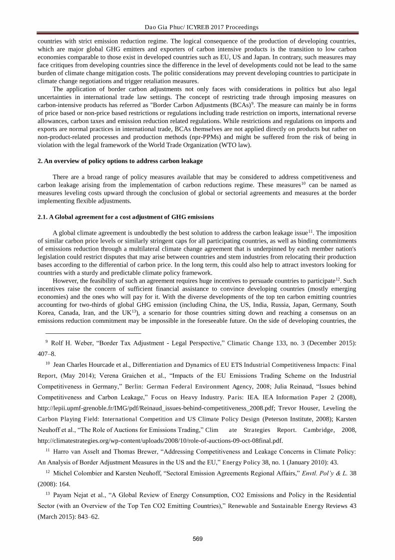
Dao Gia Phuc/ ICYREB 2017 Proceedings
countries with strict emission reduction regime. The logical consequence of the production of developing countries, which are major global GHG emitters and exporters of carbon intensive products is the transition to low carbon economies comparable to those exist in developed countries such as EU, US and Japan. In contrary, such measures may face critiques from developing countries since the difference in the level of developments could not be lead to the same burden of climate change mitigation costs. The politic considerations may prevent developing countries to participate in climate change negotiations and trigger retaliation measures.
The application of border carbon adjustments not only faces with considerations in politics but also legal uncertainties in international trade law settings. The concept of restricting trade through imposing measures on carbon-intensive products has referred as "Border Carbon Adjustments (BCAs)9. The measure can mainly be in forms of price based or non-price based restrictions or regulations including trade restriction on imports, international reverse allowances, carbon taxes and emission reduction related regulations. While restrictions and regulations on imports and exports are normal practices in international trade, BCAs themselves are not applied directly on products but rather on non-product-related processes and production methods (npr-PPMs) and might be suffered from the risk of being in violation with the legal framework of the World Trade Organization (WTO law).
2. An overview of policy options to address carbon leakage
There are a broad range of policy measures available that may be considered to address competitiveness and carbon leakage arising from the implementation of carbon reductions regime. These measures10 can be named as measures leveling costs upward through the conclusion of global or sectorial agreements and measures at the border implementing flexible adjustments.
2.1. A Global agreement for a cost adjustment of GHG emissions
A global climate agreement is undoubtedly the best solution to address the carbon leakage issue11. The imposition of similar carbon price levels or similarly stringent caps for all participating countries, as well as binding commitments of emissions reduction through a multilateral climate change agreement that is underpinned by each member nation's legislation could restrict disputes that may arise between countries and stem industries from relocating their production bases according to the differential of carbon price. In the long term, this could also help to attract investors looking for countries with a sturdy and predictable climate policy framework.
However, the feasibility of such an agreement requires huge incentives to persuade countries to participate12. Such incentives raise the concern of sufficient financial assistance to convince developing countries (mostly emerging economies) and the ones who will pay for it. With the diverse developments of the top ten carbon emitting countries accounting for two-thirds of global GHG emission (including China, the US, India, Russia, Japan, Germany, South Korea, Canada, Iran, and the UK13), a scenario for those countries sitting down and reaching a consensus on an emissions reduction commitment may be impossible in the foreseeable future. On the side of developing countries, the
9 Rolf H. Weber, “Border Tax Adjustment - Legal Perspective,” Climatic Change 133, no. 3 (December 2015):
407–8. 10 Jean Charles Hourcade et al., Differentiation and Dynamics of EU ETS Industrial Competitiveness Impacts: Final
Report, (May 2014); Verena Graichen et al., “Impacts of the EU Emissions Trading Scheme on the Industrial
Competitiveness in Germany,” Berlin: German Federal Environment Agency, 2008; Julia Reinaud, “Issues behind Competitiveness and Carbon Leakage,” Focus on Heavy Industry. Paris: IEA. IEA Information Paper 2 (2008),
http://lepii.upmf-grenoble.fr/IMG/pdf/Reinaud_issues-behind-competitiveness_2008.pdf; Trevor Houser, Leveling the
Carbon Playing Field: International Competition and US Climate Policy Design (Peterson Institute, 2008); Karsten
Neuhoff et al., “The Role of Auctions for Emissions Trading,” Clim ate Strategies Report. Cambridge, 2008,
http://climatestrategies.org/wp-content/uploads/2008/10/role-of-auctions-09-oct-08final.pdf. 11 Harro van Asselt and Thomas Brewer, “Addressing Competitiveness and Leakage Concerns in Climate Policy:
An Analysis of Border Adjustment Measures in the US and the EU,” Energy Policy 38, no. 1 (January 2010): 43. 12 Michel Colombier and Karsten Neuhoff, “Sectoral Emission Agreements Regional Affairs,” Envtl. Pol’y & L. 38
(2008): 164. 13 Payam Nejat et al., “A Global Review of Energy Consumption, CO2 Emissions and Policy in the Residential
Sector (with an Overview of the Top Ten CO2 Emitting Countries),” Renewable and Sustainable Energy Reviews 43
(March 2015): 843–62.
569

Dao Gia Phuc/ ICYREB 2017 Proceedings
question of how to balance the autonomy of national legislatures on one hand and the influence of supra-national authorities to fiscal policy matter on the other continues to be controversial14.
2.3 Flexible Adjustments through Border Adjustments
Instead of measures supporting domestic producers or efforts to conclude a global agreement, a State could address carbon leakage by imposing border adjustments that target imports and exports that originate from or are destined for countries that have no comparable GHG emissions reductions system. The key difference between this approach and the other two types of measures mentioned above is that adjusting GHG emissions costs at the border could provide a mechanism to immediately address the issue of carbon leakage15. Such border carbon adjustments (BCAs) include tariffs, taxes, quotas, subsidies or technical regulations that can level GHG emissions costs both upward and downward. In other words, BCAs address the risk of carbon leakage by imposing trade restrictions on carbon-intensive imports and compensate emissions costs for domestic exporters. The proposal of a national climate policy with BCAs provisions has recently gained the support not only from policymakers but also from scholars in the field16 as a more feasible solution to offset carbon leakage than a multilateral approach.
2.3.1. Measures targeting imports
Trade restriction on imports Being inspired by strict regulations in the Montreal Protocol17, which achieved the success of a ban on import of
CFCs and CFC-related products with non-parties, some proposals suggested that the Kyoto Member States should apply embargoes to products from non-Kyoto countries or from countries that refuse to take part in the Kyoto process18. However, unlike Montreal Protocol aiming to prevent certain harmful chemical substances (mainly used in some industries as refrigerants, solvents, foam blowing substances, aerosols, and fire extinguishers) from damaging ozone layer, the targets of Kyoto Protocol are the reduction of GHG emissions that are produced by most industries, thus impacting a broad range of products and human activities. Another approach of this type of measure is to put a ban on products manufactured using high emissions processes. This requires the importing countries to have details on the production process of imported products. Similar to requirements associated with genetically modified organisms (GMOs), the measure may face the challenge of traceability given the complex production chains of today19.
International Reverse Allowances An International Reserve Allowances (IRAs) or emission allowances on imports would be regulated under a
cap-and-trade scheme20. Under this measure, in order to gain access to a specific market, a product would either originate from a country that has a program equivalent to the emissions control program in the destination country, or it would be required to submit allowances sufficient to cover the attributable GHG emissions. Such allowances might be acquired by purchasing carbon credits from an established emissions trading scheme on the market or from a special international reserve. Failure to submit such allowances would bar entry of imported products.
14 Gary Clyde Hufbauer and Jisun Kim, “Climate Change and Trade: Searching for Ways to Avoid a Train Wreck,”
TAIT second conference “Climate Change, Trade and Competitiveness: Issues for the WTO”, Geneva, June 2010, 24,
http://www.wto.int/english/res_e/reser_e/climate_jun10_e/background_paper7_e.pdf. 15 The analysis of energy-intensive sectors subject to carbon pricing points out that trade flows are the significant
cause of emission leakage in the short term, whereas capital flows supplement in the mid to long term. See Susanne
Dröge et al., “Tackling Leakage in a World of Unequal Carbon Prices,” Climate Strategies 1 (2009),
http://climatestrategies.org/wp-content/uploads/2009/10/cs-leakage-final-230909.pdf. 16 van Asselt and Brewer, “Addressing Competitiveness and Leakage Concerns in Climate Policy,” January 2010,
42. 17 Montreal Protocol on Substances that Deplete the Ozone Layer, done at Montreal, 16 September 1987. 18 Jagdish Bhagwati and Petros C. Mavroidis, “Is Action against US Exports for Failure to Sign Kyoto Protocol
WTO-Legal?,” World Trade Review; Cambridge 6, no. 2 (July 2007): 300. 19 Thomas Cottier, Olga Nartova, and Sadeq Z. Bigdeli, International Trade Regulation and the Mitigation of
Climate Change: World Trade Forum (Cambridge University Press, 2009), 59. 20 A prime example of this type of measure is the proposal of the International Brotherhood of Electrical Workers
and American Electric Power that IRAs should be included in the US climate change policy.
570

Dao Gia Phuc/ ICYREB 2017 Proceedings
Border Tax Adjustments A measure to address carbon leakage may also take the form of a price-based measure such as a duty, charge or
tax on carbon-intensive products on the release of GHG emissions into the atmosphere21. This type of ‘carbon tax' or Border Tax Adjustment (BTA) which applies both to domestic and foreign products, is calculated according to the GHG emissions emitted by products during their manufacture. A BTA can thus be applied both to consumers and producers; however, many countries directly apply this ‘carbon tax’ on consumers through a duty on fuel consumption22.
Regulatory measures A government can include in its climate change policy a set of standards or technical regulations relating to the
GHG emissions generated during a product's use or the production process. Such measures, although intended to be applied equally to domestic and imported products, may still cause an adverse effect on the competitive condition in the market for imports. Failing to do so, the producers could be required to surrender allowances for the price differential between the cost of production and the carbon footprint to offset lower standards pertinent to imported goods, or otherwise have their products banned from entering the market23.
A standard could also be a labeling requirement indicating the carbon footprint of a product. The original idea of this measure is for consumers preferences on low GHG emissions products, but in fact, carbon labeling requirements can be used to implement or facilitate an ETS or carbon tax system24.
2.3.2 Measures targeting export
Besides measures targeting imports to ensure a level playing field in a country's domestic market, a government could also issue measures targeting exports to offset the competitive disadvantages of its products in foreign markets. The aim of such measures is to reduce the costs of production for exports, such as by imposing an export side border adjustment of charges incurred under an ETS. For instance, in the case of admission allowance rebates on exporters, a certain amount of emissions allowance issued under cap-and-trade system could be forgone. However, these types of measures may produce negative consequences for the effectiveness of the national GHG emissions reduction system25.
3. The legality of Border Carbon Adjustments under WTO law
3.1 Market access and non-discrimination principles
National climate measures in forms of BTAs and emission allowances usually referred as price-based border adjustments26 which introduce a domestic carbon tax or domestic allowances requirements that apply to both domestic products and imported product usually based on the GHG emissions rate produced during the production and process methods (PPMs) of products. In particular, if imported products produced with low efficiency or carbon intense energy sources, coal-produced steel, for example, would be, on an equal basis, taxed or treated at a higher, less favorable rate than domestic products made with a more efficient production-methods or greener energy resources.
In general, GATT provisions distinguish governmental measures into border measures and internal measures, and depending on how a price-based border adjustment will be classified, it will be allocated by a certain set of rules. As a result, the threshold issue of WTO laws compliance is to determine whether the a price-based border adjustment at
21 A proposal to introduce BTAs of carbon taxes was made in Europe as early as at the beginning of the 1990s.
They were linked to the efforts initiated by Finland to establish an EC-wide carbon tax system. 22 Ludivine Tamiotti et al., Trade and Climate Change: A Report by the United Nations Environment Programme
and the World Trade Organization (UNEP/Earthprint, 2009), 90. 23 For an example, see Climate Change Legislation Design White Paper: Competitiveness Concerns/Engaging
Developing Countries, U.S. House of Representatives Committee on Energy and Commerce, (2008), 10–11. 24 There is a proposal of “carbon passport” indicating the carbon footprint of a product in order to provide necessary
information to calculate the level of border adjustment in ETS or carbon tax system. See Gary Clyde Hufbauer, Steve
Charnovitz, and Jisun Kim, Global Warming and the World Trading System (Columbia University Press, 2009), 68. 25 A proposal from French government suggested that 2% of the total number of the GHG emissions allowances
under the EU ETS third phrase would be rebated for EU exporters. See Kateryna Holzer, Carbon-Related Border
Adjustment and WTO Law (Edward Elgar Publishing, 2014), 53. 26 Donald Regan, “How to Think About PPMs (and Climate Change),” In International Trade Regulation and the
Mitigation of Climate Change: World Trade Forum, , Edited by T. Cottier, O. Nartova, and S. Z. Bigdeli, Cambridge:
Cambridge Univ. Press, 2009, 104.
571

Dao Gia Phuc/ ICYREB 2017 Proceedings
issue is a ‘border measure’ or an ‘internal measure’. Some scholars have argued that such adjustment especially in price-based form should fall within the broad allocation of Article III while the others consider them as ‘occulte taxes’ which are defined in report of the GATT Working Party on Border Tax Adjustment but have not been decided yet by the Members whether such taxes can be justified27. Therefore, at the current development of WTO law, this issue is still uncertain.
If the measure at issue is not considered as an internal tax in fact but rather be an import duty – a border measure, such measure could violate Article II of the GATT 1994 to the extent that they exceed the tariff bindings28. On the other hand, if GHG price-based adjustments are tax adjustments on imports, there are two relevant principles that must be compliant. First, the National Treatment under Article III of the GATT 1994 which requires that imported products shall accord treatment ‘no less favorable’ than ‘like’ domestic products. And the second principle is the Most-Favored-Treatment under Article I of the GATT 199429.
The concept ‘like product’ is not defined in the GATT, and it needs to be determined on a case-by-case basis. The Appellate Body in Japan – Alcoholic Beverages II (1996)30 clarified that the degree of likeness is considered by comparing products on (i) products characteristics, (ii) end uses, (iii) consumer’s tastes and habits and (iv) tariff classification. In EC-Asbestos31 the Appellate Body implied that likeness under Article III:4 of GATT is determined by, among other factors, the extent and nature of the competitive relationship between imported and domestic products. In a climate change context, the term ‘like product’ may be controversial as in determining whether steel made with power from a coal plant and steel made with power from a hydropower plant are ‘like products’. Thus, the key determination of likeness relies on the distinction between product characteristics and the way in which they are produced (PPMs). Traditional GATT case law did not seem to accept the possibility of applying PPMs as criteria to consider the likeness of products as illustrated by the un-adopted US-Tuna32 panel report. So, if products that are considered ‘like’ based on traditional criteria of GATT case laws can be treated differently (and somehow discriminated) by a national climate measure based on their production and process methods, such measure could be deemed in violation of Article III and Article I of GATT.
3.2 Article XX of the GATT 1994
When a price-based adjustment violates Article I, II, or III, it may still be permitted if it satisfies the conditions set forth in Article XX of the GATT. The Appellate Body in US – Gasoline33 provides the two-tier test to determine whether a violated measure can justify under Article XX. First, the measure at issue must fall within one of the exceptions from sub-paragraphs from (a) to (j). Second, that measure must also satisfy the chapeau of the article. Among exceptions listed in Article XX, the two paragraphs (b) and (g) could play an important role in justifying the violation of such national climate measure. Paragraph (b) allows exceptions for measures that are ‘necessary’ to protect human, animal, or plant life, or health while paragraph (g) allows exceptions for measures relating to the conservation of exhaustible natural resources.
In order to determine whether the measure at issue is ‘necessary’ to achieve a public policy goal in paragraph (b),
27 Joel P. Trachtman, WTO Law Constraints on Border Tax Adjustment and Tax Credit Mechanisms to Reduce the
Competitive Effects of Carbon Taxes, Rochester, NY, SSRN Scholarly Paper ID 2738752 (Social Science Research
Network, January 25, 2016), 6–10; Deok-Young Park, Legal Issues on Climate Change and International Trade Law
(Springer, 2016), 5–8. 28 Art II:1(b) of GATT: “The products described in Part I of the Schedule … shall …be exempt from ordinary
customs duties in excess of those set forth and provided therein …” 29 according to the language of Article I:1 of the GATT, in order to determine a measure both border and internal
measure be compliant with MFN principle, ‘any benefit’ confers by a Member to products destined in any countries shall be treat ‘no less favourable’ than ‘like products’ from other Members immediately and unconditionally.
30 Appellate Body report, Japan – Taxes on Alcoholic Beverages, WT/DS8/AB/R, WT/DS10/AB/R,
WT/DS11/AB/R, adopted 1 November 1996, para. 117 31 Appellate Body report, European Communities – Measures Affecting Asbestos and Asbestos Containing
Products, WT/DS135/AB/R, adopted 5 April 2001, para. 93 32 GATT Panel report, United States – Restrictions on Imports of Tuna (US – Tuna), DS21/R, 3 September 1991,
unadopted, BISD 29S/155, para. 155 33 Appellate Body report, United States – Standards for Reformulated and Conventional Gasoline (US-Gasoline),
WT/DS2/AB/R, adopted 20 May 1996, p. 22
572

Dao Gia Phuc/ ICYREB 2017 Proceedings
the Appellate Body, firstly, in Korea – Various Measures on Beef (2001)34 developed a necessity test involving a ‘weighing and balancing’ of the values at issue. Then in Brazil – Retreated Tyres (2007)35, the Appellate Body shifted to the existence of a material contribution of a measure to the achievement of its objectives. The existence of less-trade-restrictive alternatives thus plays an important role to justify a measure successfully under paragraph (b). This means that a WTO Member challenging the legality of a GHG price-based adjustment against Article XX defense would have to prove that there were other less-trade-restrictive possibilities to combat the climate change other than the original measure36. Therefore, the main purpose of the measures must be defined by their impact in reducing global emissions rather than for their role in reducing competitiveness concerns for domestic industries. Many scholars argued that with this inference from paragraph (b), GHG climate measure that rebate the cost of a carbon tax on exports from countries without climate change regulations may fail the consistent test of the paragraph37.
Unlike paragraph (b), which allows for exceptions ‘necessary to protect human, animal or plant life or health’, paragraph (g) applies to measures ‘relating to the conservation of exhaustible natural resources’. Panel and Appellate Body have been clarified the term ‘exhaustible resources’, so far, as tuna38, sea turtles39, dolphins40, salmon and herring41 and clean air42. Some scholars believed that, in the climate change context, the levels of carbon and GHG in the atmosphere could also be viewed as a exhaustible natural resource like clean air in US – Gasoline (1996)43. However, this issue is still be unclear and it should be further clarified in future climate change – related WTO cases as well as be supported by multilateral environmental agreements. Another element must be qualified in paragraph (g) relates to the term ‘relating to’. This requirement asks for a close and real relationship of ends and means44 such as a close and genuine relationship between the structure of the GHG price-based adjustment and the carbon emissions reduction goals in the context of climate change. This clause also contains an unambiguous requirement that even-handed domestic policies are also undertaken to obtain the public policy objective but does not ask for an identical treatment of domestic and imported products45. It is then uncertain whether a different treatment based on products’ impact on climate change could qualify this requirement.
These exception provisions in paragraph (b) and (g) must be interpreted alongside the Chapeau of Article XX, which requires that a measure must not be applied in a manner that constitutes ‘a means of arbitrary or unjustifiable discrimination’ or ‘a disguised restriction on international trade’. In climate change context, these good-faith criteria would require that the implementing country demonstrates its serious efforts to seek international agreement on climate
34 See Appellate Body report, Korea – Measures Affecting Imports of Fresh, Chilled and Frozen Beef,
WT/DS161/AB/R, WT/DS169/AB/R adopted 10 January 2001, para. 161-164 35 See Appellate Body report, Brazil – Measures Affecting Imports of Retreaded Tyres, WT/DS332/AB/R, adopted
3 December 2007, para. 151 36 the Appellate Body at first required the country invoking the exception would have to prove the absence of
alternatives, but then conclude that such country only needs to show the necessity of the measure. The burden of proof
is then on the side of the complaining country. See Appellate Body Report, United States – Measures Affecting the
Cross Border Supply of Gambling and Betting Services, WT/DS285/AB/R, adopted 20 April 2005, para. 309 37 Stéphanie Monjon and Philippe Quirion, “A Border Adjustment for the EU ETS: Reconciling WTO Rules and
Capacity to Tackle Carbon Leakage,” Climate Policy 11, no. 5 (September 1, 2011): 1212–25. 38 GATT Panel Report, United States – Prohibition of Imports of Tuna and Tuna products from Canada,
L/5198-29S/91, adopted 22 February 1982 39 Appellate Body Report, United States – Import Prohibition of Certain Shrimp and Shrimp Products (US –
Shrimp (1998)), WT/DS58/AB/R, adopted 6 November 1998 40 GATT Panel report, US-Tuna, supra note 10 41 GATT Panel report, Canada – Measures Affecting Exports of Unprocessed Salmon and Herring, L/6268-35S/98,
adopted 22 March 1988 42 Appellate Body report, United States – Standards for Reformulated and Conventional Gasoline (US – Gasoline
(1996)), WT/DS2/AB/R, adopted 20 May 1996 43 Bradly J. Condon, “Climate Change and Unresolved Issues in WTO Law,” J Int Economic Law 12, no. 4
(December 1, 2009): 895–926. 44 Appellate Body report, US – Shrimp (1998), para. 128-131 45 Condon, “Climate Change and Unresolved Issues in WTO Law,” 920–26.
573

Dao Gia Phuc/ ICYREB 2017 Proceedings
change prior to enacting a GHG price-based adjustment46. From this point of view, some scholars believed that, in the case of an international agreement like the Kyoto Protocol, which sets emissions-reduction targets for certain period, may lead to an outcome that parties have only met their goals at the end of the evaluation period. Then, whether it could be considered arbitrary or unjustified discrimination, or otherwise disguised restrictions on trade to impose a national climate measure against certain countries that have not committed GHG emission targets and not others during this period is still an open question47.
3.3 TBT Agreement
For a national climate measure to fall within the application scope of the TBT Agreement as a ‘technical regulation’48, it must (i) lay down product characteristics, (ii) be mandatory, and (iii) apply to an identifiable product or group of products. The definition of a technical regulation in the first sentence of Annex 1.1 of the TBT Agreement indicates ‘product characteristics for products or related process and production methods’ while in the last sentence of the article, measures that are concerned with ‘terminology, symbols, packaging, marking or labeling requirements as they apply to a product, process or production method’ can be considered as technical regulations. In other words, a non-product-related national climate measure, prima facie, may not fall within the scope of application of TBT, since it requires the ‘related’ element, but if such a measure is adopted in the form of a labeling requirement, it may be covered by the agreement. To date, the complained measures in US – Tuna II (Mexico) (2012)49 and US – COOL (2012)50 were labeling requirements relating to non-product-related PPMs. The United States, in both cases, did not question the scope of application of the TBT Agreement for these measures. Some commenters agreed that, in case the TBT Agreement does not regulate non-product-related national climate measures, such measures cannot be prohibited by the agreement and thus, would be examined under Article III and Article XI and may find justification under Article XX51.
The TBT Agreement encourages Members to harmonize internal measures with international standards by providing that a technical regulation based on an existing international standard shall be deem consistent with the TBT Agreement. This regulation in Article 2.4 is very helpful in the context of international cooperation and governance; however there is no comprehensive definition of the term ‘international standards’ within the agreement. The Appellate Body ruled the matter as a standard that is adopted by an international organization or body and made available to all WTO Members in a non-discrimination manner52 without a requirement that such international standard must be adopted by consensus53. It remains unclear whether a climate change standard could be considered as an ‘international standard’ especially standards developed by a group of WTO Members which may not be appropriate for the development objectives of developing countries.
3.4 Subsidies
Article 1.1 of the SCM Agreement rules the term 'subsidy' as a ‘financial contribution’ by a ‘government or any public body’ that confers a ‘benefit’. Besides, a subsidy must be deemed ‘specific’. In climate change context, a free allocation of GHG permits, for an example, may constitute a subsidy within the meaning of SCM Agreement. Because it can be a ‘financial contribution’ in the form of a ‘revenue … foregone’ by the government, and thus, bring the ‘benefit’ to the ‘specific’ companies or industry receiving an allocation. Support from the government for its domestic industry to combat climate change therefore could be considered a ‘subsidy’ within the SCM Agreement. However,
46 The Appellate Body in US – Shrimp (1998) ruled the issue of good faith in relation to international efforts from
US to address the environmental objective – turtle conservation in the context of the Chapeau leading to ‘unjustifiable discrimination’. See Appellate Body report, US – Shrimp, para. 168
47 Jochem Wiers, “French Ideas on Climate and Trade Policies,” Carbon and Climate Law Review 2(1), 2008,
18–32. 48 See Annex 1.1 of TBT Agreement 49 Appellate Body report, United States – Measures Concerning the Importation, Marketing and Sale of Tuna and
Tuna Product (US – Tuna II), WT/DS381/AB/R, adopted 16 May 2012 50 Appellate Body report , United States – Certain Country of Origin Labelling (COOL) Requirements,
WT/DS384/AB/R, adopted 23 July 2012 51 Park, Legal Issues on Climate Change and International Trade Law, 22–23. 52 Appellate Body report, US – Tuna II, para. 374-375 53 Appellate Body report, European Communities – Trade Description of Sardines, WT/DS231/AB/R, adopted 26
September 2002, para. 222
574

Dao Gia Phuc/ ICYREB 2017 Proceedings
such measures prima facie are not prohibited; it depends on the content of the subsidy per se. If a subsidy is classified as a ‘prohibited subsidy’54, it is deemed specific and may be challenged by another Member in a WTO dispute settlement mechanism. An ‘actionable subsidy’55, on the other hand, can only be challenged in a dispute settlement when the complaining Member can show its ‘adverse effect’56 to international trade. Nonetheless, an importing Member can also use a unilateral solution by imposing countervailing measures when its domestic industry has suffered from injury by those subsidies.
4. A possible approach to address carbon leakage through the active participation of domestic industries
Carbon leakage, competitive concerns are main drivers that have led countries to consider the adoption of national climate measures such as border carbon adjustment. Such measures can have an effect on international trade and thus violating WTO rules. Using carbon leakage as the rationale for a national climate measure can support characterizing the measures as an environmental measure - mitigating climate change. However, with the drivers from competitiveness concerns, it will be more likely an economic measure with the protection of jobs and secure of economic development by leveling the playing field States between strict and less climate standard.
It should also be noted that national measures to address the competitiveness loss can only arrive at limited findings as it deals only with the price element of competitiveness. Whereas carbon policy is only one part of the broader industry picture, there are still many non-price elements influence companies’ decisions on production levels and investment. Looking at production and investment decisions only through the lens of climate policy certainly, maintains the negative image of asymmetric action and could oversimplify the picture on industry’s location choices. Studies on competitiveness under asymmetric carbon constraints do not consider the possible positive effects of ETS on companies’ competitiveness if they are the first to develop low-carbon technologies (i.e., the first-mover advantage). Delivering ambitious targets will require actions across a range of playing fields: rapidly conducting and implementing new approaches to promote investment flows towards low-carbon developmental production and removing barriers to trade and investment to support and facilitate large-scale distribution of climate-friendly goods, services and technologies are just two. Gaining political support for these kinds of actions may be challenging, even impossible, without a further eyesight of the potential benefits rather than costs of the low-carbon transition. Investments in energy-efficient technologies will help improve the productivity of companies and strengthen their competitive position and are expected to become more important as the global price of energy increases. Another aspect of competitiveness and leakage that is not studied enough in the literature is the possibility for non-participating countries to benefit from technological developments taking place in those countries with ETS. In the longer run, these so-called spillover effects may help non-participating countries reduce their GHG emissions – not to mention making their industries more efficient and competitive.
Finally, it is important to remember that there is a discrepancy between how policy-makers look at competitiveness and how companies themselves see it. Growth in investment in an emerging country may enhance the competitiveness of firms in a developed country that established plants in the country, even though from a European perspective it is perceived as a loss of competitiveness. Further, plant closures sometimes result from a decision to focus activity on higher value added parts of the production chain – an odd proposition regarding profitability, even if the result is increased imports of energy-intensive goods, sometimes akin to carbon leakage.
Reference
[1] Montreal Protocol on Substances that Deplete the Ozone Layer, done at Montreal, 16 September 1987. [2] Bhagwati, Jagdish, and Petros C. Mavroidis. “Is Action against US Exports for Failure to Sign Kyoto Protocol
WTO-Legal?” World Trade Review; Cambridge 6, no. 2 (July 2007): 299–310. [3] Colombier, Michel, and Karsten Neuhoff. “Sectoral Emission Agreements Regional Affairs.” Envtl. Pol’y & L. 38
(2008): 161–67. [4] Condon, Bradly J. “Climate Change and Unresolved Issues in WTO Law.” J Int Economic Law 12, no. 4
(December 1, 2009): 895–926. [5] Cottier, Thomas, Olga Nartova, and Sadeq Z. Bigdeli. International Trade Regulation and the Mitigation of
Climate Change: World Trade Forum. Cambridge University Press. 2009. [6] Dröge, Susanne, Harro van Asselt, Thomas Brewer, Michael Grubb, Roland Ismer, Yasuko Kameyama, Michael
Mehling, et al. “Tackling Leakage in a World of Unequal Carbon Prices.” Climate Strategies 1 (2009). http://climatestrategies.org/wp-content/uploads/2009/10/cs-leakage-final-230909.pdf.
[7] Franklin, Rachel S., and Matthias Ruth. “Growing up and Cleaning up: The Environmental Kuznets Curve
54 Part II of the SCM Agreement 55 Part III of the SCM Agreement 56 Article 5 of the SCM Agreement
575

Dao Gia Phuc/ ICYREB 2017 Proceedings
Redux.” Applied Geography, Environmental Kuznets Curves and Environment-Development Research, 32, no. 1 (January 2012): 29–39.
[8] Graichen, Verena, Katja Schumacher, F.-Chr Matthes, Lennart Mohr, Vicky Duscha, Joachim Schleich, and Jochen Diekmann. “Impacts of the EU Emissions Trading Scheme on the Industrial Competitiveness in Germany.” Berlin: German Federal Environment Agency, 2008.
[9] Holzer, Kateryna. Carbon-Related Border Adjustment and WTO Law. Edward Elgar Publishing. 2014. [10] Hourcade, Jean Charles, D Demailly, K Neuhoff, and S Sato. Differentiation and Dynamics of EU ETS Industrial
Competitiveness Impacts: Final Report, May 2014. [11] Houser, Trevor. Leveling the Carbon Playing Field: International Competition and US Climate Policy Design.
Peterson Institute. 2008. [12] Hufbauer, Gary Clyde, Steve Charnovitz, and Jisun Kim. Global Warming and the World Trading System.
Columbia University Press. 2009. [13] Hufbauer, Gary Clyde, and Jisun Kim. “Climate Change and Trade: Searching for Ways to Avoid a Train Wreck.”
TAIT second conference “Climate Change, Trade and Competitiveness: Issues for the WTO”, Geneva, June 2010. http://www.wto.int/english/res_e/reser_e/climate_jun10_e/background_paper7_e.pdf.
[14] IPCC. “Fifth Assessment Report - Climate Change 2013: The Physical Science Basis.” Accessed February 8, 2017. https://www.ipcc.ch/report/ar5/wg1/.
[15] Mahapatra, Sushanta Kumar, and Keshab Chandra Ratha. “Paris Climate Accord: Miles to Go.” J. Int. Dev. 29, no. 1 (January 1, 2017): 147–54.
[16] Monjon, Stéphanie, and Philippe Quirion. “A Border Adjustment for the EU ETS: Reconciling WTO Rules and Capacity to Tackle Carbon Leakage.” Climate Policy 11, no. 5 (September 1, 2011): 1212–25.
[17] Nejat, Payam, Fatemeh Jomehzadeh, Mohammad Mahdi Taheri, Mohammad Gohari, and Muhd Zaimi Abd. Majid. “A Global Review of Energy Consumption, CO2 Emissions and Policy in the Residential Sector (with an Overview of the Top Ten CO2 Emitting Countries).” Renewable and Sustainable Energy Reviews 43 (March 2015): 843–62.
[18] Neuhoff, Karsten, F. Chr Matthes, Regina Betz, Susanne Dröge, Angus Johnston, Mariusz Kudelko, Andreas Löschel, et al. “The Role of Auctions for Emissions Trading.” Climate Strategies Report. Cambridge, 2008. http://climatestrategies.org/wp-content/uploads/2008/10/role-of-auctions-09-oct-08final.pdf.
[19] Park, Deok-Young. Legal Issues on Climate Change and International Trade Law. Springer. 2016. [20] Regan, Donald. “How to Think About PPMs (and Climate Change).” In International Trade Regulation and the
Mitigation of Climate Change: World Trade Forum, , Edited by T. Cottier, O. Nartova, and S. Z. Bigdeli, Cambridge: Cambridge Univ. Press, 2009, 97–123.
[21] Reinaud, Julia. “Issues behind Competitiveness and Carbon Leakage.” Focus on Heavy Industry. Paris: IEA. IEA Information Paper 2 (2008). http://lepii.upmf-grenoble.fr/IMG/pdf/Reinaud_issues-behind-competitiveness_2008.pdf.
[22] Stern, Nicholas Herbert, and Great Britain Treasury. The Economics of Climate Change: The Stern Review. Cambridge University Press. 2007.
[23] Tamiotti, Ludivine, Anne Olhoff, Robert Teh, Veslie Kulacoglu, and Hussein Abaza. Trade and Climate Change: A Report by the United Nations Environment Programme and the World Trade Organization. UNEP/Earthprint. 2009.
[24] Tîmbur, Margareta. “International Trade Development - Risks for the Environment?” Economy Transdisciplinarity Cognition; Bacau 13, no. 2 (2010): 6–22.
[25] Trachtman, Joel P. WTO Law Constraints on Border Tax Adjustment and Tax Credit Mechanisms to Reduce the Competitive Effects of Carbon Taxes. Rochester, NY, SSRN Scholarly Paper ID 2738752. Social Science Research Network. January 25, 2016.
[26] van Asselt, Harro, and Thomas Brewer. “Addressing Competitiveness and Leakage Concerns in Climate Policy: An Analysis of Border Adjustment Measures in the US and the EU.” Energy Policy 38, no. 1 (January 2010): 42–51.
[27] ———. “Addressing Competitiveness and Leakage Concerns in Climate Policy: An Analysis of Border Adjustment Measures in the US and the EU.” Energy Policy 38, no. 1 (January 2010): 42–51.
[28] Weber, Rolf H. “Border Tax Adjustment - Legal Perspective.” Climatic Change 133, no. 3 (December 2015): 407–17.
[29] Wiers, Jochem. “French Ideas on Climate and Trade Policies.” Carbon and Climate Law Review 2(1), 2008, 18–32.
[30] Climate Change Legislation Design White Paper: Competitiveness Concerns/Engaging Developing Countries. U.S. House of Representatives Committee on Energy and Commerce, 2008.
[31] “Trade and Climate Change.” In World Development Report 2010, 251–55. World Development Report. The World Bank. 2009.
576

Huynh Thi Dieu Linh / ICYREB 2017 Proceedings
International Conference For Young Researchers In Economics And Business, ICYREB 2017, October 30th 2017 Da Nang, Vietnam
Exchange Rate Uncertainty and Export Flows: Evidence from 30
Countries
Huynh, Thi Dieu Linh *
School of Economics, The University of Da Nang, Viet Nam
A B S T R A C T
The main purpose of this paper is to examine to what extent exchange rate volatility affects export trade performance at 30 selected countries. A dynamic generalized method of moments (GMM) is employed on panel data over a ten-year period, and four measures of the exchange rate volatility are used. The main findings confirm that exchange rate volatility has statistically significant impacts on export trade flows in the majority of the estimated equations, and the magnitude of the impact appears to be fairly large. Apart from population variable, all other remaining independent variables show expected signs as income have positive impact on exports whereas relative price’s impact is negative.
Keywords: exchange rate volatility, trade, exports, generalized method of moments, panel data.
1. Introduction
As an important macro variable, the exchange rate has a significant influence on the whole economy, especially on the international trade. Exchange rates became more unstable after the collapse of Bretton Woods in 1971 as the international exchange rate system switched from fixed to floated system of exchange rates. Since understanding the effect of exchange rate fluctuations on export trade is crucial for policy makers issuing exchange rate and trade policy, the research area has attracted many theoretical and empirical studies
From a theoretical point of view, the impact of exchange rate risk on international trade is not unambiguous. The general presumption is that an increase in exchange rate volatility will have an adverse effect on trade flows. If exchange rate variations become unpredictable, the risks of exchange rate increase uncertainty of international trade, which lead to risk-averse and risk-neutral traders reduce or leave their trading activities in contracts denominated in a foreign currency which ultimately decrease the trade flows. In contrast to this, it can be argued that positive trade flow impacts stemming from instability in the exchange rate due to higher risk represent a greater opportunity for profit and may increase trade (Égert & Morales-Zumaquero, 2008).
From an empirical point of view, a large number of literatures have evaluated the relationship between exchange rate variability and trade performance. It is, however, still difficult to give a general definitive conclusion on whether there is any effect of exchange rate change on international trade flows because the results among those studies are inconsistent. The sign of this relationship vary with the choices of sampling period, methodology, exchange rate volatility measure and countries considered, as well as by the contexts of their examinations.
Briefly, neither theoretical studies nor empirical models provide us with a consistent answer, leaving estimated results unclear (Baum & Caglayan, 2010). There exists an ambiguity about the link between exchange rate uncertainty and foreign trade performance that requires more studies with recent data and methods.
This study focuses on the impact of exchange rate variability on export flows in 30 selected countries given the evidence from the two-step system generalized method of moments (GMM). A panel dataset of 30 cross-sectional annually observations for the period from 2003 to 2012 are used. This paper also generates volatilities of exchange rate by different methods to see whether or not a different method of volatility measurements cause a different trade impact. Specifically, this study applies the two most popular methods in measuring exchange rate volatility namely moving average standard deviation (MOVSD) and the GARCH models for each nominal and real effective exchange rate.
The rest of the paper is constructed as follows. Section 2 briefly reviews previous studies on the impact of
* Corresponding author. Tel.: +84 236 836935.
E-mail address: [email protected]
577

Huynh Thi Dieu Linh / ICYREB 2017 Proceedings
exchange rate uncertainty on trade performance, focusing on exports. Section 3 discusses the methodology and descripts data used in this study. Then, section 4 documents and discusses the estimation results. Finally, section 5 presents the conclusions and policy implication of this study.
2. Literature Review
Early economic theory states a negative effect of exchange rate variability on international trade as presented by Clark (1973), Ethier (1973), Hooper and Kohlhagen (1978) and Gagnon (1993). Exchange rate volatility can have a harmful effect on trade performance either directly or indirectly, the former through uncertainty and adjustment costs while the latter through its effect on the allocation of resources and government policies. A risk growth resulting from increase in exchange rate uncertainty will lead risk-averse traders to reduce their trading activities and to reallocate their business toward domestic markets.
In contrast, other theoretical studies suggest a positive impact of exchange rate risk on export flows as argued by De Grauwe (1988) Franke (1991), Secru and Vanhulle (1992), and Broll and Eckwert (1999), among these studies, the majority of exporters are risk-lovers. Interestingly, De Grauwe (1988) also indicates that “when exporters are sufficiently risk-averse, a positive relationship may still arise. Very risk-averse firms will worry about the worst possible scenario. When risk increases, the way to avoid a drastic decline in export revenues is by increasing the export volume”.
Besides that, theoretical developments stress that exchange rate uncertainty can influence on trade either positively or negatively as studies of Baldwin and Krugman (1989) and Dixit (1989). Interestingly, Willett (1986) suggest that exchange rate volatility have no impact on trade flows. As theory alone cannot determine the sign and significance of the relationship between exchange rate uncertainty and foreign trade, empirical research has studied the relationship between exchange rate change and international trade.
A huge volume of empirical research has been conducted within and across the countries to investigate whether exchange rate instability results in changes in trade volumes. These researches evaluate this issue from the view of aggregate as well as disaggregate trade. However, from an empirical point of view, the relation between exchange rate risk and international trade levels is still mixed. The sign of this relationship varies with the choices of different methods to measure of exchange rate variability, data sets and estimation techniques used in these studies. The majority of empirical studies indicate that there is an adverse relationship between exchange rate uncertainty and foreign trade (McKenzie, 1999; Ozturk, 2006). In contrast, there are works proving exchange rate volatility have a positive impact on international trade flows, such as studies undertaken by Brada and Mendez (1988), McKenzie and Brooks (1997), Choudhry (2008), Baum and Caglayan (2010), and Shehu and Zhang (2012). Interestingly, there are studies suggesting that the exchange rate risk – trade relationship is not significant as argued by Hooper and Kohlhagen (1978), Bailey, Tavlas and Ulan (1986, 1987), McKenzie (1998), and Tenreyro (2007). Notably, some studies conclude that there may have both negative and positive impact of exchange rate variability on trade, namely research of Koray and Lastrapes (1989), Klein (1990), Kroner and Lastrapes (1993), and Chou (2000).
3. Model and Data Specification
3.1. Model Specification
In this study, the equation for export volume is estimated using Arellano-Bond (1991) estimation method. The models estimated are as follow:
(1)
represents export volume of country to the rest of the world, denotes export volume of country to the rest of the world lagged one period, denotes income of country ’s trading partners nations (foreign income of country ), denotes relative prices of country to those of its trading partners, denotes population of country ’s trading partners (foreign population of country ), denotes exchange rate variability, is error term of
export equation, include 17 developed countries and 13 developing countries, denotes time. The foreign income and relative price variables were drawn from the analytic framework proposed by Bailey,
Tavlas and Ulan (1986). The population variable was derived from the gravity model of Brada and Mendez (1988). In the export equation, the economic theory suggests that income of country’s trading partners is an important
factor to determine country’s trade performance. The demand for country ’s exports will increase if foreign income increases, so it is expected that will take positive values. If relative price increases the demand for country ’s exports will decrease, so it is expected that will be negative. It is expected that if population of country ’s trading partners increase, the demand for country ’s exports will increase, so it is expected that will be positive.
However, the effect of exchange rate volatility on exports cannot be determined a priori, and the sign of those are
578

Huynh Thi Dieu Linh / ICYREB 2017 Proceedings
theoretically ambiguous (Siregar & Rajan, 2002; Kasman & Kasman, 2005; Todani & Munyama, 2005), and they are the focus of this empirical study.
3.2. Data Specification
The dataset includes 30 countries, namely: Australia, Austria, Belgium, Brazil, Cambodia, Canada, China, Czech Republic, France, Germany, HongKong, India, Italy, Japan, Malaysia, Mexico, Netherland, Philippines, Poland, Russia, Singapore, South Africa, South Korea, Spain, Sweden, Switzerland, Thailand, United Kingdom, United States and Vietnam. For example, aggregate dataset of country 1 as follow: country 1’s aggregate exports volume (EXPORT1), foreign income (GDPF
1) which is constructed by taking the sum of the GDP volume series of country 1’s nine most important trading partners, terms of trade serving as relative price (RP1), foreign population (POPF
1) which is constructed by taking the sum of the population of country 1’s nine most important trading partners and four exchange rate volatilities ( ) generated from nominal effective exchange rate (NEER) and real effective exchange rate (REER) through the moving standard deviation of the change of effective exchange rate (MOVSD) in logarithm and the conditional variance from the generalised autoregressive conditional heteroscedasticity (GARCH) model for the effective exchange rate in logarithm.
The data used in the export equations were collected annually from 2003 to 2012. The export volume of thirty countries (Year 2000 = 100) was collected from United Nations Conference on Trade and Development (UNCTAD). The GDP volume data series is used as a proxy of foreign income of thirty sample countries was collected from the World Bank database (WB). The foreign income is the sum of GDP of top nine important trading partners. In order to aggregate trading partners GDP series, it was necessary to convert them to a common currency (the U.S. dollar is chosen) at constant price. The population data series as a proxy of foreign population of thirty sample countries are also collected from the WB. The foreign population is sum of population of top nine important trading partners. Terms of trade serving as relative price, NEER and REER of thirty countries (Year 2000 = 100) are also collected from UNCTAD.
There are eight data series used in the econometric estimation of export demand equation in analysing 30 sample countries: export volume (EXPORT), foreign income (GDPF), relative price (RP), foreign population (PopF), real effective exchange rate volatility derived from the moving standard deviation method (REERMOVSD), nominal effective exchange rate volatility derived from the moving standard deviation method (NEERMOVSD), real effective exchange rate volatility derived from the GARCH method (GARCHREER), and nominal effective exchange rate volatility derived from the GARCH method (GARCHNEER).
3.3. Exchange rate volatility measures
Exchange rate volatility captures the uncertainty faced by the international traders due to the unpredictable exchange rate risk (Todani & Munyama, 2005). There are many methods to measure exchange rate variability. Currently, the two most popular measures used are the Moving Standard Deviation (MOVSD) model, and General Autoregressive Conditional Heteroskedasticity (GARCH) model. This study will apply both these models to calculate exchange rate volatility.
3.3.1. The moving standard deviation
This measure used the standard deviation of the first difference of logarithms of the exchange rate as a proxy to the exchange rate uncertainty based on assumption that a constant trend would not impact volatility and would be perfectly predictable. Exchange rate volatility is defined as:
where is the first difference of natural logarithms of exchange rate of country at time ,which could be nominal or real, depending on the exchange rate used, is the order of moving average. In this paper, will be set to six to stress the importance of medium run variability.
3.3.2. Generalised Autoregressive Conditional Heteroskedasticity
This measure predicts volatility on the basic of past value. The GARCH model is useful in modelling movements in the exchange rate and inflation whereas conventional time series and economic models operate under an assumption of constant variance (Hill, Griffiths, & Lim, 2008). This is because it allow the capturing of non-constant time varying conditional variance (Cheong, Mehari, Pattichis, & Williams, 2002).
In this research, the GARCH model is specific as follow:
(2)
579

Huynh Thi Dieu Linh / ICYREB 2017 Proceedings
The mean equation autoregressive order one is:
(3)
The conditional variance equation is:
(4)
where the exchange rate are expressed in logs, denotes random error, is the mean, (the ARCH
term) denotes news about variability in the past, measured as the lag of the squared residual from the mean equation, (the GARCH term) denotes the last period’s forecast error variance.
4. Estimation Tests and Results
4.1. Diagnostic Tests
A generalized method of moments (GMM) is used to estimate these equations with lagged independent variables acting as instruments. Arellano and Bond develop tests for serial correlation in order to check some lags acting as instruments are valid or not. The Arellano – Bond test is applied to the error terms in difference. If the are themselves auto-correlated of order 1 then, for example, is endogenous to the in the error term in difference, , making it an invalid instrument. Thus, in order to deal with this problem, the deeper lags in dependent variable should apply until there is no second-order serial correlation in differences is found.
In addition, because there are less control variables than instruments, the estimated regression equation are over-identified. In order to evaluate the validity of the different specifications we computed the J statistic of Hansen (1982) test for over-identifying restrictions, which tests the exogeneity of the explanatory variables. Besides the Hansen J evaluate the entire set of over-identifying restrictions, a subset of the original set of orthogonality condition can be tested by Difference-in-Hansen tests of exogeneity of instrument subset.
The Arellano – Bond test “for autocorrelation has a null hypothesis of no autocorrelation and is applied to the differenced residuals. The test for AR(1) process in first differences usually rejects the null hypothesis” that there is no serial correlation in the regression disturbances. This is because both and
have . “The test for AR(2) in first differences is more important, because it will detect autocorrelation in levels” (Arellano & Bond, 1991).
The AR(1) and AR(2) tests of autocorrelation for the export equations are presented in Table 1. The results of AR(1) tests show that there is autocorrelation between and . Since and are mathematically related via the shared , negative first-order autocorrelation is expected in differences and evidence of it is uninformative. Therefore, in order to check for first order autocorrelation in levels, we pay more attention on second-order correlation in differences, on the basis that this will detect correlation between in and in
. The results of AR(2) tests show that there is no serial correlation between and as none of the value of AR(2) tests rejects the hypotheses that is no autocorrelation to . Therefore, key assumptions of the system GMM estimation are satisfied, and the two-step system GMM is a consistent estimator in this study.
Table 1: Autocorrelation tests results for export equation
AR(1) AR(2) REERMOVSD -1.96
(0.051) 0.59
(0.552) NEERMOVSD -2.23
(0.026) 0.11
(0.910) GARCHREER -1.81
(0.070) 0.73
(0.468) GARCHNEER -2.54
(0.011) 0.35
(0.723)
Source: Compiled by authors.
Note: The figures in the parentheses are the p-value. The main results of various Hansen tests for export equation are presented in Table 2. The Hansen J statistic has a
null hypothesis of “the instrument as a group are exogenous”. From the result of Hansen tests, none of these values reject the over-identifying restrictions. Moreover, the results were computed from Difference-in-Hansen tests of
580

Huynh Thi Dieu Linh / ICYREB 2017 Proceedings
exogeneity of instrument subset also show that none of these values reject the over-identifying restrictions, which indicate that the specified variables are proper instruments.
Table 2: Hansen tests results for export equation
Test chi2 values P-values REERMOVSD
Hansen tests of over-identifying restrictions 28.48 0.387 Difference-in-Hansen tests of exogeneity of instrument subsets: Hansen test excluding group Difference (null H = exogenous)
28.48 -0.00
0.335 1.000
NEERMOVSD
Hansen tests of over-identifying restrictions 28.70 0.376 Difference-in-Hansen tests of exogeneity of instrument subsets: Hansen test excluding group Difference (null H = exogenous)
28.70 -0.00
0.325 1.000
GARCHREER
Hansen tests of over-identifying restrictions 27.79 0.422 Difference-in-Hansen tests of exogeneity of instrument subsets: Hansen test excluding group Difference (null H = exogenous)
27.79 0.00
0.369 1.000
GARCHNEER
Hansen tests of over-identifying restrictions 28.84 0.369 Difference-in-Hansen tests of exogeneity of instrument subsets: Hansen test excluding group Difference (null H = exogenous)
27.69 1.15
0.374 0.283
Source: Compiled by authors.
4.2. Empirical Results
In the export regression, lag (2 2) is used that means only the second lag of the endogenous variables as instruments. This is because the first lag is correlated with the current error term while the second lag is not. The main results of the impact of exchange rate variability on exports from GMM regression for the period from 2003 to 2012 are presented in Table 3.
Results confirm that exchange rate volatility has negative effects on exports. Most estimation results are statistically significant at 5 per cent level, with the exception of model of nominal exchange rate volatility derived from the GARCH method (GARCHNEER). The finding of a harmful effect of exchange rate instability on exports is consistent with some previous studies. All other variables are also at the 1 per cent significance level and except population variable, the remaining variables show the expected sign.
The estimation results suggest that 1 per cent increase in exchange rate volatility leads to decrease in aggregate exports of thirty sample countries from 1.44 to 1.72 per cent, depending on the measures of exchange rate variability. This estimation results appear to be quite similar to the findings of previous papers. For example: Dell’Ariccia (1999), Rose (2000), and Clark et al. (2004) concluded that 5 per cent increase in exchange rate risk would lead to a decrease in exports ranging from 4 to 7 per cent.
Table 3: Export Estimation Result
(Dependent variable: Export volume) Variables Exchange rate volatility measures used
REERMOVSD NEERMOVSD GARCHREER GARCHNEER Lagged Export volume 0.3215***
(0.9483) 0.3523*** (0.9563)
0.3353*** (0.9670)
0.3371*** (0.9457)
Foreign Income 2.5078*** (0.2507)
2.4366*** (0.2268)
2.5650*** (0.2401)
2.4835*** (0.2153)
Relative price -0.8712*** (0.1794)
-0.8539*** (0.1666)
-0.7850*** (0.1710)
-0.7965*** (0.1548)
Population -5.6828*** (1.4639)
-5.4593*** (1.3200)
-5.0298*** (1.1221)
-4.5594*** (0.9960)
Exchange rate volatility -1.6593** -1.4408** -1.7153*** -0.9358
581
Huynh Thi Dieu Linh / ICYREB 2017 Proceedings
(0.6712)` (0.5637) (0.4674) (0.6015)
Source: Compiled by authors.
Notes: The figures in parentheses are standard errors. ***, **, and * in the table denote statistical significant coefficient at 1 per
cent, 5 per cent and 10 per cent level respectively. Specification with real effective exchange rate volatility derived from the moving
standard deviation method (REERMOVSD), nominal effective exchange rate volatility derived from the moving standard deviation
method (NEERMOVSD), real effective exchange rate volatility derived from the GARCH method (GARCHREER), and nominal
effective exchange rate volatility derived from the GARCH method (GARCHNEER).
The estimation results show that an increase in main trading partner’s income has a positive effect on aggregate exports of thirty sample countries. The estimated coefficient is from 2.44 to 2.57. Given that the income variables are expressed in logarithms, it can be interpreted as a 1 per cent increase in the income of major trading partners will lead to a 2.44 to 2.57 per cent increase in aggregate exports of thirty sample countries.
In contrast, an increase in relative price (terms of trade) of the export nations has a negative impact on their exports. The magnitude of the effect is from -0.78 to -0.87 per cent, which indicate that 1 per cent increase terms of trade lead to a reduction in exports from 0.78 to 0.87 per cent. This adverse relationship between terms of trade and exports is consistent with economic theory.
Interestingly, the estimation results of main trading partners’ population show an unexpected signs when this variable has a harmful impact on exports of thirty sample country. The results suggest that 1 per cent increase in foreign population leading to decrease in aggregate exports of thirty sample countries from 4.6 to 5.7 per cent. The possible explanation of this finding might be that an increase in population leading to a reduction in income per capita, making everyone less rich, which results in decrease in expense and purchasing power of consumers. Moreover, when population growth implies an upward movement of domestic market size resulting in the domestic market becomes more attractive. Domestic firms, therefore, are more likely focus to domestic market by reposing to local demands as well as providing marketing strategies which encourage the use of domestic products. At a consequence, from the two aforementioned reasons, demand of imports also decline resulting in exports from their trading partners to that country decrease too.
5. Conclusions and Policy Implication
In this aggregate data analysis, two types of diagnostic tests were performed for all the estimated equations. The Arellano – Bond tests for autocorrelation is applied to the residual in differences. The tests reflect that there is no serial correlation of the second-order between in and in . Hansen test of over-identification restrictions and Difference-in-Hansen tests of exogeneity of instrument subsets are conducted. The tests indicate that the instrument as a group is exogenous and these specified variables are proper instruments.
The empirical results suggest that sample countries’ exports are sensitive to exchange rate volatility. In most cases, export performances are injured by exchange rate volatility as this variability has a statistically significant negative effect on exports. The empirical results also confirm economic theory as income has significant positive impact on exports while the relationship between terms of trade and exports are negative.
The findings of this research can be used to formulate exchange rate policies oriented to minimise strong fluctuations. This is because exchange rate variability reduces the exports of the countries under analysis. Therefore, governments should issue appropriate policies which support exchange rate stabilization in an attempt to promote export flows.
In addition, the harmful impacts of exchange rate variability on 30 countries’ export flows imply that traders in selected countries try to avoid the risks of exchange rate uncertainty. Although more than half of the estimated countries are developed, it is more likely that their governments do not have efficient instruments to hedge against exchange rate variability. Thus, governments should pay more attention to develop and stimulate the use of instruments to minimise exchange rate risks.
References
[1] Arellano, M., & Bond, S. (1991). Some Tests of Specification for Panel Data: Monte Carlo Evidence and an Application to Employment Equations. The Review of Economic Studies, 58(2), 277-297.
[2] Bailey, M. J., Tavlas, G. S., & Ulan, M. (1986). Exchange rate variability and trade performance: Evidence for the big seven industrial countries. Weltwirtschaftliches Archiv, 122, 466-477.
[3] Bailey, M. J., Tavlas, G. S., & Ulan, M. (1987). The impact of exchange rate volatility on export growth: Some theoretical considerations and empirical results. Journal of Policy Modelling, 9(1), 225-243.
[4] Baldwin, R., & Krugman, P. (1989). Persistent trade effects of large exchange rate shocks. Quarterly Journal of Economics, 104, 635-665.
[5] Baum, C. F., & Caglayan, M. (2010). On the sensitivity of the volume and volatility of bilateral trade flows to exchange rate uncertainty. Journal of International Money and Finance, 29(1), 79-93.
[6] Brada, J. C., & Mendez, J. (1988). Exchange rate risk, exchange rate regime and the volume of international trade.
582

Huynh Thi Dieu Linh / ICYREB 2017 Proceedings
Kyklos, 41(2), 263-280. [7] Broll, U., & Eckwert, B. (1999). Exchange rate volatility and international trade. Southern Economic Journal,
66(1), 178-185. [8] Cheong, C., Mehari, T., Pattichis, C., & Williams, L. V. (2002). Exchange rate volatility and UK exports:
Implications for EMU membership. Retrieved from [9] Chou, W. L. (2000). Exchange rate variability and China’s exports. Journal of Comparative Economics, 28(1), 61-
79. [10] Choudhry, T. (2008). Exchange rate volatility and United Kingdom trade: Evidence from Canada, Japan and New
Zealand. Empirical Economics, 35(3), 607-619. [11] Clark, P., Tamirisa, N., Wei, S. J., Sadikov, A., & Zeng, L. (2004). Exchange rate volatility and trade flows –
Some new evidence. Retrieved from [12] Clark, P. B. (1973). Uncertainty, exchange risk, and the level of international trade. Western Economic Journal, 6,
302-313. [13] De Grauwe, P. (1988). Exchange Rate Variability and the Slowdown in Growth of International Trade. Staff
Papers (International Monetary Fund), 35(1), 63-84. doi:10.2307/3867277 [14] Dell’Ariccia, G. (1999). Exchange rate fluctuations and trade flows: Evidence from the European Union. IMF
staff papers, 46(3), 315-334. [15] Dixit, A. (1989). Hyteresis, Import Penetration, and Exchange-Rate Pass-Through. Quarterly Journal of
Economics, 104, 205-227. [16] Égert, B., & Morales-Zumaquero, A. (2008). Exchange rate regimes, foreign exchange volatility, and export
performance in Central and Eastern Europe: Just another blur project? Review of Development Economics, 12(3), 577-593.
[17] Ethier, W. (1973). International trade and the forward exchange market. American Economic Review, 63(3), 494-503.
[18] Franke, G. (1991). Exchange rate volatility and international trading strategy. Journal of International Money and Finance, 10, 292-307.
[19] Gagnon, J. (1993). Exchange rate variability and the level of international trade. Journal of International Economics, 34, 269-340.
[20] Hill, R. C., Griffiths, W. E., & Lim, G. C. (2008). Principles of Econometric (Third Edition ed.): John Wiley and Sons, Inc.
[21] Hooper, P., & Kohlhagen, S. W. (1978). The effects of exchange rate uncertainty on the prices and volume of international trade. Journal of International Economics, 8, 483-511.
[22] Klein, M. W. (1990). Sectoral effects of exchange rate volatility on United States exports. Journal of International Money and Finance, 9, 299-308.
[23] Koray, F., & Lastrapes, W. D. (1989). Real exchange rate volatility and U.S. bilateral trade: A VAR approach. The Review of Economics and Statistics, 71, 708-712.
[24] Kroner, K., & Lastrapes, W. D. (1993). The impact of exchange rate volatility on international trade: Reduced form estimates using the GARCH-in-Mean model. Journal of International Money and Finance, 12(3), 298-318.
[25] McKenzie, M. (1998). The impact of exchange rate volatility on Australian trade flows. Journal of International Financial Markets, Institutions and Money, 8(21-38).
[26] McKenzie, M. (1999). The impact of exchange rate volatility on international trade flows. Journal of Economic Surveys, 13, 71-106.
[27] McKenzie, M., & Brooks, R. (1997). The impact of exchange rate volatility on German-US trade flows. Journal of International Financial Markets, Institutions and Money, 7(1), 73-87.
[28] Ozturk, I. (2006). Exchange rate volatility and trade: A literature survey. International Journal of Applied Econometrics and Quantitative Studies, 3(1), 85-102.
[29] Rose, A. K. (2000). One Money One Market: The Effect of Common Currencies on Trade. Economic Policy, 30, 7-46.
[30] Sercu, P., & Vanhulle, C. (1992). Exchange rate volatility, international trade, and the value of exporting firms. Journal of Banking and Finance, 16, 155-182.
[31] Shehu, A. A., & Zhang, Y. (2012). Exchange rate volatility, trade flows and economic growth in a small open economy. International Review of Business Research Papers, 8(2), 118-131.
[32] Tenreyro, S. (2007). On the trade impact of nominal exchange rate volatility. Journal of Development Economics, 82, 485-508.
[33] Todani, K. R., & Munyama, T. V. (2005). Exchange rate volatility and exports in South Africa. Retrieved from South Africa:
[34] Willett, T. D. (1986). Exchange rate variability, international trade and resource allocation: A perspective on recent research. Journal of International Money and Finance, 5, 101-112.
583

Huynh Thi Dieu Linh / ICYREB 2017 Proceedings
Appendix 1 : Nine most important trading partners of the 30 countries in 2012
Australia China Germany Japan Korea, R. Malaysia NZ Singapore Thailand US
Austria Germany US Italy France Switzerland Slovak R. Czech R. Hungary Russian
Belgium Germany US Italy France Netherlands UK Spain India Luxembourg
Brazil Germany US Netherlands India China Argentina Japan Venezuela Chile
Cambodia Germany
US China Japan UK Canada Singapore Vietnam Thailand
Canada US China UK Japan Mexico Netherlands Korea, R. Germany France
China US Hong Kong Japan Korea, R. Germany Netherlands India UK Russian
Czech R.
Germany Slovak R. Poland France UK Austria Italy Russian Netherlands
France Germany
Italy Belgium UK Spain US Netherlands China Switzerland
Germany UK France Netherlands US Austria Italy China Switzerland Belgium
Hong Kong
China US Japan Germany India Korea, R. Singapore UK Vietnam
India US UAE China Singapore Hong Kong Netherlands Saudi Arabia UK Germany
Italy Germany
France US Switzerland UK Spain Belgium Turkey Russian
Japan US China Korea, R. Thailand Hong Kong Singapore Germany Indonesia Australia
Malaysia Singapore China Japan US Thailand Indonesia Hong Kong India Australia
Mexico US Canada Spain China Brazil Colombia Germany Italy Japan
Netherlands Germany
Belgium France UK Italy US Spain Sweden Poland
Philippines Japan US China Singapore Hong Kong Korea, R. Thailand Germany Netherlands
Poland Germany UK Czech, R. France Russian Italy Netherlands Ukraine Sweden
Rusia Netherlands China Germany Italy Turkey Ukraine Belarus Poland Kazakhstan
Appendix 1: Nine most important trading partners of the 52 countries in 2012 (con’t)
Singapore Malaysia China Hong Kong Indonesia US Japan Australia Korea, R. Thailand
South Africa China US Japan Germany India UK Netherlands Zambia Mozambique
Korea, R. China US Japan Hong Kong Singapore Vietnam Indonesia India Russian
Spain France Germany Italy Portugal UK US Netherlands Belgium Morocco
584

Huynh Thi Dieu Linh / ICYREB 2017 Proceedings
Sweden Norway
Germany UK Finland Denmark Netherlands US Belgium France
Switzerland Germany US Italy France UK Hong Kong China Japan Austria
Thailand China Japan US Hong Kong Malaysia Indonesia Singapore Australia Vietnam
UK Germany US Netherlands France Ireland Belgium Switzerland Spain Italy
US Canada
Mexico China Japan UK Germany Brazil Korea, R. Netherlands
Vietnam US Japan China Korea, R. Malaysia Germany Hong Kong Australia UK
Note: Compiled by author from Direction of Trade Statistic (DOTS) from IMF Data Warehouse
585

Doan Thi Lien Huong, Truong Duy Nhat Phuong/ ICYREB 2017 Proceedings
International Conference For Young Researchers In Economics And Business, ICYREB 2017, October 30th 2017 Da Nang, Vietnam
Young Consumers’ OTT (Over-The-Top) Applications Usage and
Potential Strategies for Telecompanies: A Case of Vietnam
Doan Thi Lien Huong, Truong Duy Nhat Phuong
University of Economics- University of Danang, 71 Ngu Hanh Son, Danang
A B S T R A C T
As technologies advance in the age of Industrial Revolution 4.0, OTT (Over-The-Top) has emerged and developed as a new means of communication, influencing the tele-communication industry. This study aims to determine the drivers, trends, and impacts of the rise of the OTTs globally and in Vietnam. The paper also studies the habits of young consumers using OTT in Vietnam regarding (1) frequency, (2) purpose, (3) function/utility popularity and (4) likelihood to pay. The results have led the authors to recommend that telecommunication companies should: (1) develop their own applications, (2) partner with OTT content developers, and (3) surf the waves of technologies.
Keywords: OTT usage behaviors, telecompanies strategy, young consumers
1. Introduction
The Industrial Revolution 4.0, the current trend of automation and data exchange in manufacturing technologies, leads to many breakthroughs in communication, one of which is the rise of the OTT (Over-The-Top). Detecon Consulting (2014) defined OTT as “the distribution of voice, video and data services via the public Internet without the controlling management of a mobile nestwork, fixed network, or Internet service provider […] These products offer telephony and messaging free of charge or at extremely low rates via the Internet protocol; the sole consequence for the providers is the increased demand for more bandwidth and reliable service quality”. As technology advances, there are more and more OTT applications being launched, offering various options to the customers.
In Vietnam OTT applications have entered the market since 2007 with the first brand Ola, following by others such as Wechat, Viber, Kakaotalk, Line, etc. Nowadays, OTT applications have spread and commonly developed in Vietnam, nearly every Smartphone user uses at least one OTT application to communicate. Without any carrier service provider involved in planning, selling, provisioning, or servicing them, there is no direct traditional telco booking revenue from the OTT applications. The OTT utilizing trend has gradually replaced traditional telecommunication services, negatively affecting the revenue of the telecommunication companies. In Vietnam, the most significant telecommunication companies, including Mobifone, Vinaphone and Viettel, have launched their own OTT products but they have not been widely accepted by their customers.
Cost minimization and the ability to share offered by the OTT providers have led to the threats toward the traditional telcos. The Vietnamese telcos have reacted to these threats in various ways. One of which is to launch their own OTT services, such as Vinaphone’s VietTalk and Viettel’s Mocha. Another strategy is to raise the prices for their 3G data plans; the launch of 4G is also expected to bring a solution to the telcos (Kwan, 2013; Oxford Business Group, 2017). In addition, according to Kwan (2013) and Oxford Business Group (2017), the local carriers have also proposed that the government heavily regulate the providers of OTTs, which would effectively undermine the OTT providers’ technological advantage.
It can be seen that the impacts of OTTs, a means of communication born in the age of Industrial Revolution 4.0, are significant to the telcos. Regarding the free - of - charge or at - extremely – low - rates telephony and messaging offered by the OTTs, it can be easily understood that they have created a new habit in customer behaviors when they have to choose between the new OTTs and the traditional SMSs or among the OTTs. However, it seems that the responses of the telcos to this new trend has not put customer behaviors into consideration. Academics as well as practitioners are still unaware of their customer profile and insights of how young customers use the OTT applications such as purposes of use, favorite OTT functions. However, to the authors’ point of view, it is necessary for the telcos to understand customers’ habits on OTTs, especially the young ones who are the majority account of OTTs users in
586

Doan Thi Lien Huong, Truong Duy Nhat Phuong/ ICYREB 2017 Proceedings
Vietnam according to eMarketer (2016)), in order implement better competitive strategies.
2. Research Objectives and Research Questions
The objective of this paper is to identify factors that drive the use of OTT, which have affected revenues of global and Vietnam telecommunication companies. We also aim to capture the habits and preferences of young Vietnamese telecommunication consumers in using OTT services on their mobile devices, hence, to recommend competitive strategy for Vietnam telco versus OTT providers.
1. In order to attain these objectives, we have asked the following research questions: 2. What factors/trends drive the mass use of OTT service in the world and in Vietnam? 3. Which is the instant messaging application that is used the most in Vietnam? 4. What is the profile of instant messaging application users in Vietnam?
a. What are the behaviors of instant messaging application users: b. How much do they use intant messaging application in terms of frequency and time of each use? c. What purpose do they use OTT for? Work or entertainment? d. What functions/utility that they find most useful/like the most? e. How likely are they to pay for OTT premium service?
5. How should Vietnam telcos react to the emergence of OTT?
3. Overview of OTT
3.1. Drivers leading to the Mass Adoption of OTT
Since the beginning of OTT services, there has increasing adoption among users. The report “Consumer OTT VoIP Outlook: 2013 to 2018” by Ovum highlights that the OTT VoIP (Voice over Internet Protocol) has increased at the rate of 20%. In 2013, Skype reached the 300 million users, and so did Whatsapp, making it the top selling app in 47 countries with daily 27 billion message processing (Detecon Consulting, 2014). In Vietnam, the chat app Zalo alone has topped 45 million users, which is half of the country’s population (Tuoitrenews, 2016).
There have been a number of papers identifying the drivers behind the mass adoption of OTT services. According to Arthur D. Little (2011), it is the smartphone penetration, enhanced functionality, and innovative and smart services provided by the OTT players that are the key contributors to the OTT uptake. Meanwhile, McKinsey (2012) identified technology readiness, cost incentives, social propensity to adopt OTT and the strength of the OTT alternatives as the main drivers of the OTT mass adoption. Sujata et al (2015)’s conceptual framework also identified Cost, Content Availability, Smartphone and Mobile Internet Penetration, User Experience, Features and Net Neutrality as factors and trends that led to the increased adoption of OTT services. They also confered these factors into Cost, Convenience, Communication (Social prospensity), Content Availability, Advancement in Technology, and Net Neutrality.
These prior analyses give us the insight that technology advances make communication devices and Internet infracstructure more and more available and affordable, influencing usage habits of customers, and shifting demand to freemium services from traditional telco services. Because such changes in habits have caused a great loss in the revenues of traditional telcos, it is crucial to know what thesey changes are. This paper aims to determine the most visible ones, focusing particularly on (1) frequency, (2) purpose, (3) the most popular features used and (4) likelihood to pay.
3.2. Impact of OTT on Telcos Revenues
Godlovitch et al (2015) and Nguyen (2016) stated that it was the subtitute effect that led to the shift from traditional telco services to thOTT ones, leading to significant revenue losses for the telcos. When the services are substitutes, the more that the consumers purchase one, the less they are likely to purchase the other. Godlovitch et al (2015) identified OTT communication services as direct substitutes for the traditional telecos due to shift in the consumer preferences toward the free or low cost services. Therefore, the mass adoption has led to great telco lost revenues.
According to Informal Telecom & Media (2013), the forecast global annual SMS revenues will fall by US$23 billion by 2018, to US$96.7 billion from US$120 billion in 2013, which is largely caused by the continuing adoption and use of OTTs. The Pacific Asia region, of which Vietnam is a part, is forecast to experience the highest drop in annual SMS revenue over the forcast period, declining from US$45.8 billion in 2013 to US$38 billion, according to Informa’s World Cellular Revenue Forecasts 2012-2018. Another report, “The Future of Voice by Spirit DSP (2012) pointed out that the overall telco revenues would decline from $970.4 billion in 2012 to $799.6 billion in 2020, while the report “Consumer OTT VoIP Outlook: 2013 to 2018” by Ovum implied that the OTT VoIP market would cause $63 billion in lost telecos revenues. In Vietnam, the telcos’ annual loss in revenue to the OTT is estimated to be around US$50 million (Vietnam News, 2013).
587

Doan Thi Lien Huong, Truong Duy Nhat Phuong/ ICYREB 2017 Proceedings
3.3. Telecommunication and OTT services in Vietnam
The number of OTT users in Vietnam is increasing due to the rise in number of smartphone users and that the internet platform in Vietnam is now pretty complete with fairly low cost, leading to the large number of internet and 3G users. At the end of 2015, the number of smartphone users had risen by 40% (Ericsson Mobility Report, 2016). Within the rising number of smartphone users in Vietnam, 69% of them use smartphones for chatting and 32% use the device for online video calls (TNS, 2014). There are also many OTT services used in Vietnam, among which Zalo is the most popular.
As can be seen in Table 1, the domestic application Zalo passed Facebook Messenger in all age groups and doubled Viber. Most of the respondents have Zalo and Facebook in their phones, which shows that the can have many different OTT applications in their phone.
Table 1. Messaging Apps that Smartphone Users in Vietnam Have Installed on Their Smartphone, by Age, June 2016
% of respondents in each group 18-25 26-30 30-35 35+ Total
Zalo 80% 83% 81% 71% 80% Facebook Messenger 78% 72% 75% 55% 73%
Viber 33% 43% 51% 51% 40% Skype 37% 40% 41% 23% 37% Line 21% 18% 15% 11% 18%
Yahoo 9% 11% 16% 13% 11% Tango 7% 10% 11% 13% 9% Wechat 4% 7% 5% 2% 5%
WhatsApp 4% 4% 5% 3% 4% KakaoTalk 3% 3% 4% 1% 3%
Beetalk 3% 1% 3% 1% 2% Snapchat 2% 1% 3% 2% 2%
Other 1% 3% 1% 1% 2%
Source: DI Marketing, “Chat Apps Usage in Vietnam”, June 10, 2016
(www.eMarketer.com)
Regarding age, while Zalo and Facebook Messenger tend to be favored by youngsters, Viber and Skype are more popular among over 30 year old users, accounting for 51% and 41% respectively. Meanwhile, 78% of 18-25 aged consumers use Facebook, whilst only 55% of the over 35 aged group use this application. Therefore, it can be concluded that there are differences in OTT application choices among the different age groups.
Table 2 shows that Text Messaging is the most popular OTT activity in Vietnam. However, there are differences in the purpose of use by age. The 18-25 group mostly use the OTT for text messaging (82%) and sending photos (57%). Besides, they use OTT for making friends (14%), while other age goups only use OTT for this purpose at 11-13%. It can also be seen that consumers over 30 do not use OTT for chat rooms as much as the younger and they read or watch videos via OTT more than others. The variation of the rates in the table show that the purposes of using OTT varies among different age groups in Vietnam.
Table 2. Leading Messaging App Activities Conducted by Smartphone Messaging App Users in Vietnam, by Age, June 2016
% of respondents in each group 18-25 26-30 30-35 35+ Total
Text messaging 82% 79% 80% 73% 80%
Send photos 57% 57% 62% 56% 58%
Phone calls 53% 59% 59% 51% 56%
Video calls 40% 42% 39% 34% 40%
Voice Messages 25% 24% 17% 16% 23%
Share feelings 21% 22% 22% 21% 22%
Read news 19% 22% 21% 27% 21%
Share update Friends, relatives 19% 20% 25% 17% 20%
Chat rooms 18% 15% 15% 6% 16%
Watch Videos 12% 15% 13% 18% 14%
588

Doan Thi Lien Huong, Truong Duy Nhat Phuong/ ICYREB 2017 Proceedings
Find friends/make friends 14% 13% 13% 11% 13%
Online shopping 10% 10% 14% 11% 11%
Other 3% 0% 5% 2% 2%
Source: DI Marketing, “Chat Apps Usage in Vietnam”, June 10, 2016
(www.eMarketer.com)
3.4. Global Trends in Communication Services
Godlovitch et al (2015) forecasted that in the next decade the costs of content and service creation would continue to decrease rapidly, and the ubiquitous and ultra-fast mobile and satelite Internet conncetivity would further advance Internet services. This can be translated to more and more favorable future conditions for enhancing, developing and spreading OTT services. Thus, new waves of communication advancements become increasingly affordable and necessary everyday and the telcos cannot escape but must adapt.
Providing high quality, reliable and affordable data and voice services is one of the focuses of telcos (Deloitte, 2016). It is further reported by Deloitte (2016) that there would continue to be a dramatic growth of data services with wifi usage continuing to be the key; and Voice over LTE (VoLTE) and Voice over Wifi (VoWiFi) services would also be a main focus to help carriers rationalize networks and potentially improve and expand services. Detecon Consulting (2014) stated that the pressures for seamless connectivity and highly diversified access technologies would make carriers build an infracstruture which is increasingly finely meshed and truly integrated. In addition, granular fixed networks of full-area coverage and matching mobile network infrastructure would clearly be an advantage for carriers.
The expanded streaming of content, especially video, will contribute the continuous growth of massive data consumption. In such a situation, consumers are less likely to invest in long-term ownership content, leading the carriers to anticipate further mergence of sponsored data services to increase revenue (Deloitte, 2016). Both Deloitte (2016) and Godlovitch et al (2015) predicted that the emergence of fifth generation mobile networks (5G) would be essential to supporting connected things in the future, such as communication between autonomous vehicles and advanced smart city applications; and that there are expected to be solutions for consumers to have convenient and efficient services while balancing and protecting privacy offered by the providers.
Large telcos will still control a large propotion of contracts in the near future when approximately 80% of the contracts are sold directly to end customers; by 2020 the figure will still be 50% in comparison with 30% for smaller telcos (Roland Berger Strategy Consultants, 2012). Roland Berger Strategy Consultants (2012) however claimed that some PTTS and device manufacturers could trigger the flip by dicussing the posibility of starting their own distribution channels to phones and tablets with hardwired e-SIM. The potential emergence e-SIM would eliminate the need for consumers to physically switch out their e-SIM when they change devices, enable ready change of service provider plans, andsimplify the process of making changes to a scusriber mobile service offering (Trapp, 2016). These e-SIM developments could present an obstacle for telco operators due to the ease in switching service providers.
4. Methodology
To answer the research questions, the authors employed a quantitative approach in the form of a survey to examine the current Vietnam telco market situation.
A questionnaire was designed in which questions were derived from the research questions. The questionnaire was then pre-tested on around twenty undergraduate students of the University of Economics, the University of Danang to check the clarity, the meaning, the flow; and to make sure that the target participants well understand the questions. Af ter the pre-test, some minor wording modifications were made to improve the questionnaire.
The survey was conducted at the beginning of 2016 with 254 respondents. The research targeted consumers from 18 to 35 years old. The sample consists of students, fresh graduates, entry-level employees or employees from Danang. Students and fresh graduates were the major target for this survey sample; for this reason, 83.5% of the sample was between 18 and 25 years old. 12% of the sample held a postgraduate degree, the rest were undergraduate level.
It should be noted that the survey sample does not reflect the entire Vietnamese youth; therefore, the survey findings cannot be generalized to the whole Vietnam society. On the other hand, this group is quite homogenous and it is possible to offer implications from this sample to consumers with similar traits or criteria. This specific group of young people live in an urban environment and, therefore, are trendy to the technology, especially new services and apps in their daily OTT usage. This group’s relevancy will also grow in the future. Thus, while telcos are adapting their strategy to the changes in the market, part of this target group will become a lucrative segment with increasing purchasing power. In addition, as this age group is the most active users of various types of OTT, they possess more concrete preferences and habits with regards to OTT.
The survey was conducted online via Google Doc, and distributed online via social networks which are widely used by our target sample. The data set was analyzed using SPSS.
589

Doan Thi Lien Huong, Truong Duy Nhat Phuong/ ICYREB 2017 Proceedings
5. Data Analysis and Results
Behaviors of Young Users in OTT Application Usage To answer the question of the frequency and time each use of the respondents, they were asked about the average
time spent each time they use OTT, and number of times they use OTT a week. 63.8% of the respondents said they used the OTT more than 2 hours each time they used it, while 14.6% used it from 1 to 2 hours and 12.2% used it from 30 to 60 minutes per use. Regarding frequency, the authors asked about the 4 most popular OTT applications in Vietnam, which are Zalo, Facebook, Viber and Skype. Following is the frequency of use of the most used applications.
Table 3. The frequency of use of OTT applications of young consumers in Danang (n=254 )
Frequency of use Zalo Facebook Messenger Skype Viber
Do not use 18.9 1.2 72.4 76.8
1 in 2-3 weeks 17.3 15.7 13.8 10.2
1-2 times/week 24.8 11.8 6.7 7.5
3-4 times/week 12.6 7.9 2.4 2.8
Daily 26.4 63.4 4.7 2.8
Total 100.0 100.0 100.0 100.0
Among the 254 respondents, 67 people used Zalo daily, accounting for 26.4%. 24.8% used Zalo 1-2 times a week and 18.9% said they did not use Zalo. It can be seen that Zalo is not widely used everyday.
The percentage of those who use Facebook Messenger application daily was 63.4%, while the proportion of those who did not use Facebook was only 1.2%.
As can be seen from the Table 3, Facebook Messenger and Zalo are the ones that were most popular among young consumers in Danang. The others such as Skype and Viber had low use frequency. Facebook is currently the most popular OTT in Danang.
Purposes of OTT Application Usage Table 4 shows the purpose of using OTT. 47.2% of the respondents answered for both work and entertainment,
revealing a dominance of mixed purposes. But also consequential is the much lower singular use for both work and entertainment.
Table 4. The frequency of use of OTT applications of young consumers in Danang (n=254 )
Purposes of OTT usage Percentage Only work 3.1
Mostly work 10.2 Work and Entertainment Equally 47.2
Mostly entertainment 32.3 Entirely entertainment 7.1
Preference of OTT functions Regarding the functions of OTT, Table 5 shows the preference of each utility ranked by the young consumers in
Danang on a scale from 1 (not very liked) to 5 (very liked).
Table 5. Preference of OTT Functions/utilities among users (n=254)
Functions Mean Std. Deviation
There are many friends and relatives who use OTTs 4.10 .813
Being able to see friend online list 4.10 .883
Easier to send pictures and videos than traditional telecommunication services 4.39 .770
Being able to know if friends have received and read the messages 4.27 .853
Being able to send emojis 4.17 .921
Group chat/ Group calling 4.47 .692
Convenient to keep in touch with friends living overseas 4.44 .792
Cheaper than traditional tele-communication services 4.54 .731
Easier to use than traditional tele-community services 4.24 .913
Entertainment: music, games, etc. 3.91 1.078
The results show that the most popular feature of OTT is its affordability compared to traditional tele-communication services (4.54/5). The next preferred functions are Group Chat/ Group Calling (4.47/5), Convenience in keeping in touch with friends living overseas (4.44/5) and Ease in sending pictures and videos (4.39/5) are also very
590

Doan Thi Lien Huong, Truong Duy Nhat Phuong/ ICYREB 2017 Proceedings
favorable among the respondents. In addition, another remarkable utility that is also very much favored by the repondents is the Ability to know if the receivers have received and read the messages (4.27/5).
OTT paid functions Although OTT provider offer many free services to users, companies still have revenues from a number of
services. Our survey showed that the most popular paid serviceis “Calling and texting outside the OTT”. But in general, this service is used at a very limited frequency. Data also showed that other paid services such as Emoji buying, Playing games and game shopping, Inviting friends, Online selling are not frequently utilised among young users (Table 6).
Table 6. Frequency of of OTT paid function usage (n= 254)
Very rarely Rarely Occasionally Frequently Very Frequently Total Emoji buying 34,7 16,4 28 14,6 6,3 100% Calling and texting outside the OTT 18,9 16,7 27,7 22,3 14,4 100% Playing games and game shopping 51,5 20,5 16,4 7,1 4,5 100% Inviting friends 32,8 26,1 25,7 12,3 3 100% Advertisements 42,5 18,3 22 10,8 6,3 100% Online selling 45,5 14,9 15,3 14,6 9,7 100% Others 43,2 13,7 30,2 6,5 6,5 100%
6. Conclusion and Recommendations
This paper has reviewed the emergence and mass adoption of OTT services, which threaten the revenues of traditional telcos,; as well as the global and Vietnam contemporary trends in the communication industry and habits of young consumers in Danang, Vietnam. This paper identified the most popular OTT providers in Vietnam as Facebook and Zalo, and the activities via OTT varies among different age groups. The behaviors of OTT application users, especially in instant messaging, were also described in the paper on the following dimensions: frequency and time spent each use, purpose of usage, preference of functions/utility and popularity of paid functions. In general, entertainment is a very important purpose in using OTT, and young users are not very interested in using paid utilities.
The Vietnam telecom operators should see the emergence of OTTs with the above mentioned user behaviors as an opportunity rather than a threat to their revenue. The telecom sector in Vietnam is well established with the 3 big giants dominating the market: Mobifone, Vinaphone and Viettel. The telcos still have advantages over OTTs due to the established wireless infrastructure which the OTTs must ride on. Telcos should look for ways to adapt to a new business environment where OTTs are now also players. They should also address the needs of the customers, which is the root of winning the market. The following are the proposed alternatives that telcos can adopt.
Developing their own applications Vietnam telcos can venture into developing local applications to gain competitive advantage over OTTs. It is
evident that the emergence of OTT cannot be stopped and it is here to stay. As a result, telcos should look for alternatives to gain a benefit over OTTs. In Vietnam, telcos have lauched their own OTT applications such as Vinaphone’s VietTalk or Viettel’s Mocha. However these applications have not yet been popular among customers. The telcos therefore need to address the customers’ needs and habits in order to gain in the market. Our research showed that OTT application should be more entertainment oriented. Revenue from mass users should not be considered as the most important target. Instead, OTT service should be offered as added value to Telcos current service. They can also develop other applications in areas such as health, agriculture, business, security, etc. and try the opportunities apart from the traditional services.
Partnering with OTT content developers Instead of trying to beat the OTTs on their game, partnering with them might be a good strategy. There is
evidence that some telcos have already employed that strategy and got promising results. For example, in Indonesia, the telco Axis has formed a partnership with Viber wherein Axis lets its customers buy a Viber data service rather than a full data plan, as a migration strategy educating customers about buying data bundles from their mobile provider (GSMA, 2013). In Malaysia DiGi telecommunications has also partnered with WhatsApp allowing customers to get unlimited access to WhatsApp service for a fixed fee (GSMA, 2013). Although these strategies have enabled the telcos to gain a share of revenues, they need to be careful in maintaining relationships with their customers as they have limited or almost no control on the direction as well as the quality of the services offered through these partnership deals.
Surfing the waves of technologies The current global trends in the development of advanced data services have created opportunities for the telcos
when the technologies supporting data and connecting services are improving every day. Quality improvement with wide coverage and continually enhanced mobile network infrastructure and excellent customer services are keys to gaining customers’ loyalty. The emergence of fith generation mobile networks (5G) will facilitate and is essential to the
591

Doan Thi Lien Huong, Truong Duy Nhat Phuong/ ICYREB 2017 Proceedings
growth of data sand connection services. However, the telcos should not stick to what they are good at and keep improving their unnecessary strengths. Along with the remarkable waves of breakthroughs in technology comes the significant and fast changes in consumers’ habits. The telcos have to be sensitive and responsive to these changes in order to survive and grow firmly in the market.
References
[1] Arthur D. Little. (2011). Disruptive Threat or Innovative Opportunity? Scenarios for Mobile OTT Growth. Athur D. Little.
[2] Deloitte. (2016, February 24). Telecommunications Industry Outlook: Interview with Craig Wigginton, vice chairman and US Telecommunications leader. Retrieved from Deloitte & Touche LLP: http://www2.deloitte.com/us/en/pages/technology-media-and- telecommunications/articles/telecommunications-industry-outlook.html#
[3] Detecon Consulting. (2014). "OTTs" - Value Killers for Telcos? Focus on African Operators. Cologne: Detecon International GmbH.
[4] Detecon Consulting. (2014). Future Telco. Profitability in Telecommunications: Seven Levers Securing the Future. Detecon International GmbH.
[5] Detecon Consulting. (2014). Study Policy and Regulatory Framework for Governing Internet Applications. Detecon International GmbH.
[6] eMarketer. (2016, June 29). Mobile Messaging Users Vietnam ChooseHomegrown Zalo. Emarketer. Retrieved August 03, 2017, from https://www.emarketer.com/Article/Mobile-Messaging-Users-Vietnam-Choose-Homegrown-Zalo/1014151
[7] Ericsson Mobility Report. (2016). South East Asia and Oceania Ericsson Mobility Report. Ericsson. [8] Godlovitch, I., Kotterink, B., Marcus, S., Nooren, P., Esmeijer, J., & Roosendaal, A. (2015). Over-the-Top
(OTTs) players: Market dynamics and policy challenges. Brussels: European Parliament. [9] GSMA (2013) The Ott Opportunity for Operators. Retrieved from https://www.gsma.com/membership/wp-
content/uploads/2013/10/White-paper-Aug2013.pdf [10] Informal Telecom & Media . (2013, November 14). Global annual SMS revenues will be US$23 billion less by
2018. Informa. Retrieved from https://informa.com/media/press-releases-news/latest-news/global-annual-sms-revenues-will-be-us23-billion-less-by-2018/#
[11] Kwan, K. (2013, April 8). Vietnam telcos affected by OTT services, up 3G prices. Zdnet. Retrieved from http://www.zdnet.com/article/vietnam-telcos-affected-by-ott-services-up-3g-prices/
[12] McKinsey & Company. (2012). The future of mobile messaging: Over-the-top competitors threaten SMS. McKinsey & Company, Inc.
[13] Nguyen, Q. L. (2016). A litterature review of over-the-top related policy and regulatory issues. Hochschule Rhein-Waal Rhein-Waal University Of Applied Science. Faculty Of Society And Economics.
[14] Fortune (2014). Telecom companies count $386 billion in lost revenue to Skype, WhatsApp, others. Fortune. Retrieved from http://fortune.com/2014/06/23/telecom-companies-count-386-billion-in-lost-revenue-to-skype-whatsapp-others/
[15] Oxford Business Group. (2017). Operators in Vietnam bolster infrastructure and introduce ew products and services in telecoms sector. Oxford Business Group. Retrieved from https://www.oxfordbusinessgroup.com/overview/wired-digital-content-gains-popularity-operators-are-bolstering-infrastructure-and-introducing-new
[16] Roland Berger Strategy Consultants. (2012). Telco 2020 – How Telcos transform for the "Smartphone Society". Munich: Roland Berger Strategy Consultants.
[17] Spirit DSP. (2012). The Future of Voice. Retrieved from http://www.spiritdsp.com/industry-news/read-more-industry-news/article/ott-voip-to-cost-telcos-479b-to-2020/
[18] Sujata, J., Sohag, S., Tanu, D., Subham, P., & Sumit, G. (2015). Impact of Over-the-top (OTT) services on Telecom Service Providers. Indian Journal of Science and Technology, 145-160.
[19] TNS. (2014). Global Connected Consumer Study 2014. TNS. [20] Tuoitrenews. (2016, February 26). Homemade chat app Zalo tops 45mn users, half of Vietnam’s population.
Tuoitrenews. Retrieved from http://tuoitrenews.vn/business/33420/homemade-chat-app-zalo-tops-45mn-users-half-of-vietnams-population
[21] Trapp, T. (2016, March 22). RCR Wireless News. Retrieved from http://www.rcrwireless.com/20160202/opinion/2016-predictions-mobile-network- operators-resilience-is-the-theme-for-2016-tag10
[22] Vietnam News (2013). Mobile firms hike cost of 3G internet. Vietnam News. Retrieved from Vietneamnews.vn: http://vietnamnews.vn/economy/237855/mobile-firms-hike-cost-of-3g-internet.html#IhHmT51b8UhhmpwE.97
592

Dang Thi Huyen Anh/ ICYREB 2017 Proceedings
International Conference For Young Researchers In Economics And Business, ICYREB 2017, October 30th 2017 Da Nang, Vietnam
The Global Value Chains’ S Participation of Vietnam with The
Industrial Revolution 4.0
Dang Thi Huyen Anh*
Học Viện Ngân Hàng, số 12 – phố Chùa Bộc, Quận Đống Đa, Hà Nội, Việt Nam
A B S T R A C T
Participating in the global value chains of an economy offers chance to join the world production, thereby expanding export, boosting growth. This is especially significant for small-scale economies, which have not enough resource to master the entire production process. Vietnam is one of those countries, and we have been get benefit by involving more and more in the Global production.
However, the world is standing on the brink of a technological revolution that will fundamentally alter the way people lives, works, produces goods and services. We haven’t know how it will unfold, but some significant features of the 4th Industrial Revolution will drive the path of future Global Value Chains (GVCs). This paper firstly reviews the GVC’s feature of what makes it possible and profitable currently and after the Industrial revolution 4.0, then analyses chances and challenges for Vietnam to participating the Global supply chains in condition of the Industrial revolution 4.0. From detecting the future path, improving labour quality and high-tech production is recommended in order to keep Vietnam continue to ripe the benefit from participating GVCs in the future.
Keywords: Globalization; Global value chain (GVC); industrial revolution 4.0; labour; ICT
1. Current Global Value Chains and its impact to developing economies.
A Global Value Chain is a system of interconnected processes that are implemented in different countries in the production of finished goods and services. Participating in the global value chain gives access to one or more stages in the world production chain, thereby expanding the export market, boosting growth, especially in developing countries.
For decades, GVCs have transformed the world production. However, GVCs are themselves rapidly evolving. Deborah K. Elms and Patrick Low (2013) recognized the current stages of Globalization unbundling as “ICT made it possible - wage differences made it profitable”.
What is “ICT made it possible - wage differences made it profitable” From the mid -1980s, with the appearance of Telecommunication, computer and software, some production stages
that had been locally performed became out source to reduce the cost, especially the labor cost. The reason was, ICT facilitated control that reduced the cost and risks of combining technology of developed countries and labor of developing countries, and therefore, technology became more internationally mobile. In short:
- The ICT revolution made the coordination at distance possible, therefore, it boost the globalization and created GCVs
- The vast wage differences between developed and developing countries made the GCVs profitable To recognize the participating situation of an economy in GVCs, we can use input-output matrix method to
identify which goods are input into which industry, it is also called “backward linkage matrix”. Lopez – González (2012) uses this method to estimate the share of a nation’s exports made up of intermediate input’s value added from its trade partners. The matrix of these backward linkages reveals some points: Firstly, there are two types of economies: the first one is “headquarter economies”, whose exports contain relatively little imported intermediates – that is centralized in North America and Eurozone; and “factory”; the second one is “factory economies”, whose exports contain a large share of imported intermediates, that is concentrated in Asia and South America. Secondly, GVCs trend to create regional production relationships: Factory South Asia, factory North Asia, factory EU, factory North
* Corresponding author. Tel.: +84989994399
E-mail address: [email protected]
593

Dang Thi Huyen Anh/ ICYREB 2017 Proceedings
America… The rapidly development of GVCs influences the developing economies as follow: - The rise of GVCs boosts the industrialization in developing economies. The increasing of intensive stages of
manufacturing, international technology mobility and the offshoring of labor produced a trend of transferring technology and management skill from developed countries to developing countries, therefore it boosts industrialization and then spectacular growth in emerging economies.
- The rise of GVCs increases not only trade in goods (especially parts and components) but also international investment, facilities, training and technology to emerging economies.
- The development of GVCs also becomes a momentum for the development of telecoms and internet services in both developed and developing countries.
- The reform of political and liberalization: in 1980s, policies from the pre-ICT such as trade, FDI policies contained restrictions, and in the form of state-owned enterprises, etc. In companion with the joining of GVCs, policies changed to motivate the Globalization with more and more Free trade agreements among countries and regions.
With the advantages above, joining Global supply chains is a optimal solution for developing countries. Before that, nations had to build a deep and wide industrial base to export a kind of product. After this unbundling of Globalization, emerging nations could export easier by joining a piece of GVC pie. have been developed rapidly. GVCs have been being longer and longer, spreading all over the world.
2. Future of GVCs path in condition of Industrial revolution 4.0
The Industrial Revolution 1.0 used water and steam power to mechanize production. The Second used electric power to create mass production. The Third used electronics and information technology to automate production. Now a Fourth Industrial Revolution is building on the Third, the digital revolution that has been occurring since the middle of the last century but rather the arrival of a Fourth and distinct one: velocity, scope, and systems impact. It is characterized by a fusion of technologies that is blurring the lines between the physical, digital, and biological spheres. About the impact of The Fourth Industrial Revolution to future GVCs, we are at the beginning of the Revolution with many speculations about how it will be, how it will affect our economy. However, there are some significant points about the impact of the 4th industrial revolution to future path of GVC: Firstly, a visible advantage to the worldwide trade is the reduction of Transportation cost and time, reduction of geographic distances among countries, the world will become more and more flat. Transportation and communication costs will drop, logistics and global supply chains will become more effective, and the cost of trade will diminish, all of which will open new markets and drive economic growth, drive to development of GVCs. However, as routine, low-skill, and repetitive tasks are easier to computerize and robotize, the information- technology-led bundling will typically eliminate occupations that involve such tasks. At the same time, the more intensive use of sophisticated production machines will make the remaining jobs more skill-, capital- and technology-intensive. This leads to a polarization of stages in terms of skill-content. Routine low-skill tasks are bundled into high-skill occupations while the remaining low-skill tasks will typically be highly labor - intensive but less routine. The resulting, broader stages will involve more capital-intensive, more technology-intensive and more skill-intensive processes. This tends to favor production in high-wage nations or near large customer geographically. Whether these machines end up in high-wage, high-skill nations, or they are distributed to be near every large customer base, the impact would be a very substantial reduction in supply chain trade. Thus, the current “ICT made it possible - wage differences made it profitable” will become “ICT made it possible – labor skill differences made it profitable”. Besides, ICT improvement in the 4th revolution will create different path of the new GVCs stage. Deborah K.Elms and Patric Low (2013) divide the supply chain at four levels of aggregation: products, stages, occupations, and tasks (Fig.1). That is, product (at the bottom) - is conceived of as including after sales services. Tasks (at the top) - the full list of everything that must be done to get the product into consumers’ hands and provide them with associated after-sales services. Occupation – the group of tasks performed by an individual worker. Stages - as a collection of occupations that are performed in close proximity due to the need for face-to-face interaction and the fragility of the partially processed goods – are the critical level of aggregation since supply chain internationalization typically involves the offshoring of stages rather than individual occupations or individual tasks
594

Dang Thi Huyen Anh/ ICYREB 2017 Proceedings
Figure 1. Supply chains at four level of aggregation
Source. Deborah K.Elms and Patric Low (2013)
With this in hand, K.Elms, 2013 built two economics of optimal [2]: (1)Tasks per occupation; and (2)Occupations per stage
The development of Global supply chains is in acsociate with the specialization, it not only boost the productivity but also become more risky if the GVC is long. The specialization gains come from scale economies and learning-by-doing as well as from a heightened ability to place each stage in a nation with the most appropriate wage structure. Coordination and risk costs come from the extra difficulty and expense of managing spatially distributed stages. As the ICT revolution rolls on, it create more distance in the GVC, it means production is more specialized but more risky. Moreover, some ICT improvements reduce the benefits of specialization while others reduce the costs of specialization. ICT affects the GVCs via two channels (Fig.2): Communication and organizational technologies – call them coordination technologies for short – facilitate transmission of ideas, instructions and information. Good coordination technology favors fewer tasks per occupation and fewer occupations per stage. Information technology makes it easier for individual workers to master more tasks. Numerically controlled machines, robots and computer-aided manufacturing embed information in capital in a way that allows a single worker to perform a wider range of tasks.
Therefore, better coordination technology reduces the cost of specialization and thus fosters functional unbundling. Better information technology reduces the benefits of specialization and thus disfavors functional unbundling.
Figure 2. Supply chains at four level with the change in technologies
Source. Deborah K.Elms and Patric Low (2013)
595

Dang Thi Huyen Anh/ ICYREB 2017 Proceedings
However, as mentioned above, the cost of joining GVCs falls as coordination technology (communication and organizational technologies) improves. The benefit of joining GVC falls as information technology improves. Therefore, the future path of GVCs depends of how Information technology versus coordination technology will be. That is,
- Rapid improvement in coordination/communication and organization technology – such as advances in tele-presence technology, software in workflow organization and communications– favours GVCs become more functionally and geographically. The resulting finer division of labour will allow firms to sort stages geographically according to the cost of the relevant productivity factors (labour, capital, technology, etc.). This will result more GVCs with longer-distance, more global trade in parts and components. Thus improvement in coordination technology will lead to more complex supply chain, then more chance to grab pieces of GVC pie for developing countries.
- Better information technology, by contrast, favours the bundling of many tasks into the ambit of individual workers. This will typically result in broader occupations and few separate stages of production. This would tend to reduce international trade in parts and components.
Better information technology also tends to polarize stages of production. When thinking about the future of global supply chains, it is worth speculating on truly revolutionary technological developments. One such possible development concerns Computer Integrated Manufacturing (CIM). This has already produced a tectonic shift in manufacturing in high-wage nations – moving from a situation where machines helped workers make things to a situation where workers help machines make things. The integration and automation of tasks, however, does not stop at the factory gate. Many design, engineering, and management tasks have been being computerized. Computers have greatly boosted the productivity and speed of product design as well as greatly reduced the need for prototyping.
3. Issues with Vietnam in the future GVCs participation
Figure 3. GVC participation index of non-OECD countries
Source: Koen De Backer, Sébastien Miroudot, 2013
Fig.3 shows the participation ratio in GVC of Vietnam among non OECD countries. Along with the international integration process, Vietnam has been joining more and more into global supply chains with the participation ratio is at the average level. Nearly 60% of exports value based on imported input or become intermediate product for other countries.
596

Dang Thi Huyen Anh/ ICYREB 2017 Proceedings
Figure 4. The Trade balance of Vietnam from 2006 – 2016
Source. General Department of Customs
Joining GVC has motivated export, improved Vietnamese trade balance and boosted economic growth. The contribution of exports to GDP from 50% in 2002 increased to 89% in 2014. The Trade Balance used to be negative, has turned positive (Fig. 4). However, the GVC participation process of Vietnam has vastly based on cheap labour cost. Thus, the industrial revolution 4.0 will affect apparently to Vietnamese trading advantages. The impact of the coming 4th industrial revolution to Vietnam’s participant to GVC will have some significant features:
- The 4th industrial revolution will lower the logistic, transportation and communication cost significantly. Currently, logistic and transportation cost and capacity are Vietnam’s weakness in export. Thus, the reduction of logistic cost will be a great chance for Vietnam exporting enterprises to access faraway market such as America and EU. That will drive to larger participant share of Vietnam in GVCs.
- With the industrial revolution 4.0, the development in communication and organization industries can help Vietnam to learn either management and working skills or production know-how, this will improve the productivity and Vietnam’s competitive of the production. That also helps Vietnam to join more stages of GVCs.
- However, the 4th industrial revolution not only includes coordinate technology but also the development of information technology. As mentioned above, the revolution in information industrial may cause the trend of shrinkage in GVCs because of the reduction of stages in GVC. In this point, Vietnam may loose the share in GVCs if we don’t have sufficient policies in R&D to apply higher technologies in production activities, upgrade our economy to “talent economy”, not “factory economy”.
- Besides, According to the IMF calculation, the value added of GVC of Vietnam is purely in the low-tech sector, and located in fabrication stages (assemble and produce final goods). Stages that rely on cheap labour advantage. This situation leads to high risk for Vietnam’s production in the coming 4th Industrial revolution because low skill labour will have no advantage anymore. The Factory countries like Vietnam and other ASEAN countries will be unnecessary in GVCs. GVCs will move to high skill labour or headquarter countries. Thus, building effective education system is one of the most important key for Vietnam and other developing countries to take the share in future GVCs.
The findings highlight changes in how to participate GVCs in the future. Some recommendations are: - Improve Vietnamese education system to enhance quality of labour force. Labour skill is the decisive factor for
GVC participation after the Industrial revolution 4.0 that the automatic production will be processed by high skill labour.
- Take advantage of Free trade agreements to attract FDI in high – tech sector to absorb communication and information industries enhancing technology capacity of Vietnamese production.
- Enhance the communication technology infrastructure to support competitiveness of Vietnamese production. - Enhance public investment efficiency of Vietnamese government to create good infrastructure for production,
especially for logistics performance such as sea-ports, air-port, storage, … - Develop financial system to make sure the stability and variety of financial services meeting capital demand of
enterprises, especially SME.
597

Dang Thi Huyen Anh/ ICYREB 2017 Proceedings
In conclusion, The World is standing on the brink of the 4th technological revolution that will fundamentally change our life. We haven’t know how it will unfold, but it will drive the path of future Global Value Chains, and thus will change the way countries join the World production. The fact is, either technology or any other exogenous force come over that humans have no control. We are responsible for guiding its evolution. Thus, we should take the opportunities and power we have to direct the 4th revolution toward a future that reflects our common objectives and values. It’s time for Vietnam to have a new version of “Doi Moi” revolution as we did in late mid 1980s and early 1990s. Vietnam economy must transform from the “factory economy” to the “talent economy” in order to continue get benefit from joining global supply chains in the stage of technologies revolution.
References
[1] Baldwin. R.,(2008). Managing the Noodle Bowl: The Fragility of East Asian Regionalism, Singapore Economic Review
[2] Deborah K.Elms, Patrick Low. (2013) Global value chains in a changing world, WTO pubishing [3] De Backer, K. and N. Yamano (2007). “The measurement of globalization using international input-output
tables”, STI Working Paper 2007/8, OECD Publishing [4] Klaus Schwab, (2016) The Fourth Industrial Revolution: what it means, how to respond, World Economic Forum [5] Koen De Backer, Sébastien Miroudot, (2013) Mapping the Global value chains, policy paper, OECD publishing [6] Lanz, R., H. Nordas and S. Miroudot (2011). Trade in Tasks, OECD Trade Policy Working Papers No. 117,
OECD Publishing
598

Bui Duy Linh, Nguyen Thai Binh/ ICYREB 2017 Proceedings
International Conference For Young Researchers In Economics And Business, ICYREB 2017, October 30th 2017 Da Nang, Vietnam
Investor - State Dispute Settlement in The Trans - Pacific
Partnership Agreement
Bui duy Linh, Nguyen Thai binh
Faculty of Economics and International Business, Foreign Trade University, Hanoi
A B S T R A C T
Investment disputes between the governments and foreign investors are becoming increasingly common in the process of globalization and international economic integration. The fact that investment chapter of the TPP agreement allows foreign investors to launch a lawsuit against the governments in host countries will create risks for governments, especially in developing countries. Within the scope of the article, the author analyses basic characteristics of this type of dispute; assesses problems faced by Vietnam and makes some recommendations.
Keywords: TPP; ISDS; Judicial immunity
1. Introduction
According to a research published by Public Citizen- a social organization in the United States, as well as reviews on many prestigious economic magazines around the world, authorizing foreign investors to initiate a lawsuit against the government of the receiving country in the TPP's Investment chapter will pose many threats to the governments of these countries, especially developing countries.
So what is Investor-State Dispute Settlement in the “21st century trade agreement”- TPP and what is the content of the settlement? Why this settlement is considered one of the most difficult issues in the TPP negotiation process? The paper will study the issue of investment dispute settlement between the governments of the receiving countries and foreign investors in order to analyze the basic characteristics of this dispute; assess the risks for Vietnam and make some recommendations.
2. Research subjects and methodology
Research subjects: Investor–State Dispute Settlement in the Trans-Pacific Partnership Agreement. Research methodology: The article uses the basic research methodology of dialectical materialism and historical materialism with the
following method of data collection and analysis: Data collection methodology: using secondary data sources like books, newspapers, magazines, Vietnamese and
foreign websites. Data analysis methodology: using qualitative analysis to assess the characteristics and impact of Investor–State
Dispute Settlement
3. Overview of TPP and Investor – State Dispute Settlement (ISDS)
3.1. Overview of TPP
Trans-Pacific Partnership Agreement – TPP is a free trade agreement signed between 12 countries (Singapore, Chile, Brunei, New Zealand, Australia, Malaysia, Peru, USA, Vietnam, Mexico, Canada and Japan) on February 4, 2016 in Auckland aiming to integrate economies in the Asia-Pacific region.
The original objective of the Agreement was to reduce tariffs on imports and exports between member countries by January 1, 2006, and to reach a full reduction by 2015. This is comprehensive agreement including all major aspects
599

Bui Duy Linh, Nguyen Thai Binh/ ICYREB 2017 Proceedings
of a free trade agreement: commodity exchange, rules of origin, interventions, technical barriers, service interchange, intellectual property issues, Government policies…
The negotiation process of the agreement was delayed many times due to inconsistency about issues such as reduction of import-export tax, sponsorship of domestic goods, intellectual property rights, etc. On 5th October 2015 in Atlanta, United States, the negotiation process of the agreement was successfully concluded.
30 chapters of the agreement aim to promote economic growth, support the creation and maintenance of employment, enhance technological innovation, increase productivity and competitiveness, improve the standard of living, reduce poverty in member countries; promotes transparency and promotes environmental protection. TPP members agreed on measures to minimize non-tariff barriers and tariffs in trade and establish a mechanism for resolving investment disputes between the state and investors.
3.2. Investor – State Dispute Settlement in TPP
ISDS is a common concept in investment incentive agreements and international free trade agreements. It is as a key feature of Bilateral Investment Treaties (BITs), which were vigorously raised after World War II. At that time, international economic relations developed beyond purely exchanging finished products and cross-border investment in global trade became increasingly important. (Schubert and Saz-Carranza, 2016)
The target of ISDS is to provide a neutral enforcement mechanism that enables the settlement of potential treatments to foreign investors. Since the first BIT agreement with ISDS was signed in 1959 between Germany and Pakistan, ISDS has been widely used in BITs signed worldwide. The number of BITs with ISDS grows from under 500 (in 1990) to 2184 in 2000 and continues to reach 3509 in early 2016. (Carvalho, 2016)
ISDS is presented in the Trans-Pacific Partnership (TPP) in Chapter 9 - Investment. Accordingly, it allows foreign investors to take legal action against the national government in the case of unsuccessful investment and negotiations. In the TPP, ISDS have seen significant improvements on previous versions. There are substantial extensions to the provisions on respects for the environment, health and safety regulations when compared to the Korea - US Free Trade Agreement (KORUS) taking effect in March 2012. Also, when compared to the EU-US investment treaty, the definition for "fair and reasonable" treatment has been narrowed down, forum shopping (i.e. the attempt that companies conduct a litigation in the most sympathetic places) is eliminated while cost evaluation against a losing party is enabled (to prevent frivolous cases).
In addition, as specified in Chapter 9 of the TPP, the investor who conducts a lawsuit against the government will hold responsibility for proving its entire claims. It allows fully open and transparent lawsuits and enables the participation of non-governmental organizations and non-litigants. Furthermore, in Chapter 9, critical terms and definitions in the non-discrimination and minimum treatment standards are highlighted for the first time. For instance, the concept of legitimate public welfare objectives is described as the foundation for protecting the regulations of a nation and it implies the insufficient expectations of discouraged investors who intent to overturn such regulations. TPP members also agree on the establishment of a code of conduct as a guiddance for the independence and fairness of ISDS arbitrators.
Nevertheless, TPP has a shortcoming as there is no appellate provision for ISDS cases. However, some initiatives are introduced as a response to ISDS criticism. Article 29.5 of Chapter 29 in the TPP (Exceptions) is among the most noticeable. Accordingly, tobacco firms are prohibited from filing a lawsuit against ISDS. This improvement resulted from the case tobacco companies took legal proceedings against Australia and Uruguay governments for their regulations on cigarette package. American business community are not in favour of this improvement as they fear that the precedent given by tobacco cases could be applied for other products such as alcohol. Another improvement is made in terms of finance as per the American request: Financial companies are not allowed to use ISDS for the purpose of discrimination claims during market penetration. Article 9.3 in the TPP does not support the consideration of covered financial services to Chapter 11, Financial Services. It is important that in Chapter 11, financial regulators have the authority to make final decision on which foreign companies are allowed to enter the local financial market. An aspiring foreign financial firm must provide sufficient evidence on its “fit and proper" state to do business;
These innovations in ISDS presented in the TPP are applicable to all 12 members, which has taken the lead in meeting the specific objections of the ISDS opponents. (Hufbauer, 2016)
Among ISDS cases in 2016, services sector accounts for the majority (60%). Around 24% of the cases belongs to primary industries sector and the remaining (16%) is related to manufacturing sector. (UNCTAD, 2017)
Following is the list of the most common issues claimed by foreign investors: Alleged direct expropriations of investments (at least 7 cases) Legislative reforms in the renewable energy sector (at least 6 cases) Tax-related measures such as allegedly unlawful tax assessments or the denial of tax exemptions (at least 5 cases) Termination, non-renewal or alleged interference with contracts or concessions (at least 5 cases) Revocation or denial of licences or permits (at least 5 cases)
The two most common issues raised by foreign investors in 2016 were the cancellation of contract or breach of
600

Bui Duy Linh, Nguyen Thai Binh/ ICYREB 2017 Proceedings
contract and revoking investment license or refusing investment license. Disputed fields are: construction of power plants and power supply (at least 7 cases); Oil and gas exploration and mining (10 cases); Construction (5 cases); Financial services (3 cases).
4. Investor-state dispute settlement (ISDS)
4.1. Characteristics of ISDS
4.1.1. The complexity of the subject
This is international disputes because these disputes arise between the government of a country (receiving country) and a foreign investor. The characteristic make it difficult to resolve because the Government enjoys the right to judicial immunity. Judicial immunity is an institution recognized by international law. The right is a national privilege whereby the state will not be tried before the court. This immunity also includes the right of not being required to testify before the court (unless the country renounces this right) and the right not to enforce the judgment. Participating in international relations, all States have the right of judicial immunity from the courts of another country.
This leads to the fact that resolving investment disputes between a government and a foreign company is not easy. The reason is that the laws of many countries do not regulate the rights of foreign investors to take legal action against the government. In some countries, they even do not allow this.
4.1.2. Wide application scope
Firstly, ISDS is applicable when a member country issues policies contrary to TPP regulations and affects the legitimate interests of investors in other member countries. This is particularly beneficial to foreign investors as ISDS does not deal with cases where domestic investors sue the government as well as the member states take legal action against foreign investors.
Secondly, the concept of investment activity in TPP is not limited to direct investment and indirect investment. A foreign investment activity satisfies one of the following characteristics: Commitment of capital and other resources: Depending on the law of each country, investors must contribute a proportion of capital or other assets in order to gain direct or indirect control. Expected revenue or profit: This is an investment of an individual or a foreign entity for the purpose of seeking future profits through Foreign Direct Investment (FDI), indirect investment and international credit. Risk tolerance: Foreign investment is highly risky, possibly higher than domestic investment. Because different economic structures, policies and laws will have different effects on investors.
Accordingly, foreign investors are individuals and organizations in foreign countries carrying out investment activities in other countries for profit purposes. The investor defined in the TPP also includes new investors who are only applying for a license or establishing a business (transferring capital and other resources) rather than just investors who are in the process of project implementation.
4.1.3. Legal basis for resolving investment disputes
According to ISDS, the order and procedures for foreign investors initiating receiving countries are summarized in the diagram below:
As can be seen from this diagram, the steps taken to initiate a lawsuit seem to be fairly straightforward for foreign investors to carry out proceedings against the member government. TPP member countries have accepted the possibility of being sued by TPP investors arbitrarily. Therefore, a case can be initiated without the need for a specific written approval from the State being sued.
When resolving disputes, if the investment contract does not specify or agree to apply other legal principles, one of the following legal principles will be used to settle the investment dispute according to ISDS: Convention on the Settlement of Investment Disputes between States and Nationals of Other States established by the World Bank (ICSID) ISCD Additional Facility Rules The principles of the International Commercial Arbitration Institutions of United Nations (UNCITRAL).
4.1.4. Transparency and legality
Transparency of the ISDS arbitration procedures is specified in the TPP Investment Chapter. Accordingly, the arbitral tribunal shall open the hearing so that the parties express their views publicly and discuss with the disputing parties to agree on the appropriate preparatory work for the hearing. If the disputing party wants to use confidential information at the hearing, that party must inform the arbitral tribunal. The arbitral tribunal must arrange for the
601

Bui Duy Linh, Nguyen Thai Binh/ ICYREB 2017 Proceedings
protection of such information from being disclosed, including the closure of the hearing during the information period. Therefore, it is possible to understand security as the ISDS’s characteristic as it is designed to protect international
trade and protect the interests of investors. There are no regulations that allow people to access materials used in this process. All public information for the public and the international community is a list of lawsuits that have ended with brief verdicts. This list is maintained by the Secretariat of the International Center for Investment Disputes (ICSID) and posted on its website if neither party objected.
People should have the right to access and participate in the lawsuits for two reasons: First, the lawsuits mainly revolve around the rules and regulations of the government. It will be directly relevant and have a strong impact on people's lives as well as national interests. Second, compensation is in fact taxpayers' money so they have the right to control their own money. Moreover, with full access to information, academics and lawyers will have the opportunity to study thoroughly and provide multi-dimensional analysis and give useful advice to the government.
Legality: In many cases, foreign investors take action against the State on issues related to public interest such as public health protection or environmental protection. With 3 members of the arbitral tribunal, is it legitimate to evaluate the conduct of a State?
After these doubts, in order to ensure the legality of the disputes, ISDS added rules requiring a quick review to prevent unjustified claims: The TPP regulates the procedure for the arbitral tribunal to quickly review the Defendant's objections to the non-jurisdictional arbitration or the plaintiff's claim as completely unfounded. If the arbitral tribunal comes to a conclusion in support of the Defendant, they may decide to stop the case and request the Plaintiff to pay the costs of the proceedings. In relation to the final decision of the arbitral tribunal, TPP also stipulates that if the Plaintiff is only in "preparation for investment”, the amount of compensation will be limited to damages associated with the "investment preparation", and the Plaintiff must prove that the breach of the Defendant is the cause of the damage.
4.1.5. The arbitral tribunal
The unanimity of the arbitral award is expressed when with the same dispute, the arbitration panel's ruling is unanimous. The cause of inconsistency in the arbitration award is different understanding of minimum treatment. Consequently, consistency in the arbitration award is important for the parties to anticipate the arbitration award. In addition, the arbitral award is almost not reviewed by another arbitration panel.
Regarding arbitrators: The World Bank’s International Centre for Settlement of Investment Disputes – ICSID (ICSID) is the organization that will announce the commencement of the proceedings. An international tribunal will be established, usually consisting of three arbitrators: one chosen by the investor, one chosen by the government and the third arbitrator chosen by agreement of the parties to the dispute. Members of the ISDS arbitration council must have professional knowledge, experience and work independently and fairly. The award made by the arbitrator shall not be disputed by either party to the dispute.
It is often a concern that because the most frequently appointed arbitrators are retired attorneys and lawyers, and many law professors having their own companies. Appointments are instantaneous on a case-by-case basis rather than on a per term basis. Therefore, this gives them the incentive to work to their advantage so the risk of corruption is rather high. ISDS also allows lawyers to play many roles (an arbitrator or a legal representative of parties to disputes). When a lawyer is an arbitrator, he clearly has an incentive for investors so that he may become a legal representative of the investors. This easily leads to close ties, sharing of interests between arbitrators and investors. However, up to now there is no practical cases on the corruption or inappropriate behaviours of ISDS arbitrators.
In order to settle the claims against ISDS arbitrators, Article 9.21 in the TPP presents the initiatives that emphasize the independence and honesty in arbitrator appointment. However, due to the fact that the majority of the arbitrators are from developed nations - an example can be found in 2010 when only 25 arbitrators came from developing countries out of 76 arbitrators appointed in all ISDS cases worldwide - there is a concern that developing nations may face up with disadvantages.
4.1.6. High cost of litigation
The cost of arbitration is rather expensive. The biggest cost is the cost of hiring attorneys and specialists, taking about 82% of the total cost. The average cost paid to the referee is about 16% and the cost for the secretary is about 2%. The arbitral tribunal shall determine the arbitration costs in the award. Although it is stipulated that the amount of money should be reasonable, based on the size of the dispute, the complexity of the objects, time and other factors, there are no ceiling rates. In addition to the costs, nations face huge losses if they fail, which seems to have become a tradition in ISDS cases. Compensation levels may even include future profits that investors think they have lost due to local government barriers.
An estimation by the Organization for Economic Cooperation and Development (OECD) shows that on average, the cost for an ISDS engagement is USD 8 million and can exceed USD 30 million in some cases. In addition,
602

Bui Duy Linh, Nguyen Thai Binh/ ICYREB 2017 Proceedings
according to Professor Frank, the respondents’ average legal fees of 40% researched cases is USD 900,000, along with an average amount of USD 600,000 for arbitration and administration fees. (Wellhausen, 2016)
4.2. Main ISDS criticism points
4.2.1. ISDS grants the special rights for foreign investors
Some critics consider ISDS as a new colonialism mechanism as it helps investors in developed countries intervene and adjust the investment policies of developing countries. By this way, it is the economic interests of investors from developed countries that benefits from TPP while the legal framework of the host country is narrowed down. This topic has been empirically studied by Schultz nd Dupont, (2014).
Figure 1: Winning rates, by year of filing (five-year moving average)
(Source: Thomas Schultz và Cédric Dupont, 2015)
Thomas and Cédric proved the inappropriateness of the ISDS criticism point because since the 1990s, ISDS has gradually switched from a mechanism between “investors from developed countries versus developing countries" to "investors from developed countries versus developed and developing countries" (Note that no cases of investors from developing countries adopting this mechanism have been found). At the same time, the percentage of host countries’ winning has seen a gradual improvement and reached around 50% since 1990 (as illustrated in Figure 1).
Recently, there are a number of claims that ISDS might benefit those foreign investors who have the intention to overturn domestic regulations. Such claims are raised as foreign investors try to revoke regulations on the environment, labor and health in the host countries mostly on the basis of discrimination and "indirect seizure" in Egypt, Germany and Czech. However, final verdicts on those “notorious” cases have not been announced. The results might either reject or settle the dispute of foreign investors, thus can benefit either the foreign investors or the host countries. An example can be found in the case of a company named Veolia accused of using ISDS to claim at least USD 110 million in a dispute with Egypt on minimum wages. No matter what the outcome of the trial is, the verdict will not exceed the scope of a compensation let alone a repeal of the minimum wage law in Egypt.
In addition, a recent research conducted by the Netherland government pointed out that 90% of ISDS cases target at administration behaviour (such as cancellation or deprivation of the license) and only 10% target at legal approaches (and those 10% often have fairly low chance of winning).
Article 16 in TPP Chapter 9 (Investment and the environment, health and other management objectives) states that no provision in this chapter shall be construed to prevent a Party from enacting, maintaining or implementing any other measures in accordance with this chapter which are considered appropriate to ensure that investment activities in its territory are conducted in a sensitive manner to the environment, health or other management objectives.
Following the Korea - Australia Free Trade Agreement (FTA), the Korea-Canada FTA or Korea-Vietnam FTA basically restated limitations and denied the above mentioned criticism.
Although there is an opinion that investors can use ISDS to change domestic regulations which are obscure, policy critics still express their concerns. It is the situation where policy makers are discouraged from introducing new regulations due to the issues of financial expenses in ISDS compensation. Still, there is a lack of empirical evidence for this viewpoint.
603

Bui Duy Linh, Nguyen Thai Binh/ ICYREB 2017 Proceedings
All in all, the presumption that ISDS can have impacts on domestic regulation of the host countries are not backed by any practical evidence or sometimes can be considered as a false interpretation for the following reasons: Firstly, the ISDS does not impose stricter regulations than any other legal forms in such forums as the WTO or the domestic courts. Regardless of the ISDS presence, the government must follow certain laws and procedures. ISDS is just a legal measure to prevent governments from unlawful actions. In some cases it is particularly effective where the domestic legislation has not been strictly enforced. Secondly, ISDS is included in the majority of modern BITs nowadays include ISDS and the version presented in the TPP also contains more beneficial improvements for the host countries.
4.2.2. ISDS can be a financial burden on the government, especially for developed countries
Over 50 years since the ISDS was first introduced in 959, there have been cases when the compensations won by foreign investor set a world record.
One of the most remarkable is the case in 2007 when The Czech Republic was obliged to pay more than US $ 350 million in compensation to a single Dutch investor, which according to one report meant a near doubling of the country's public sector deficit.
Another example happens recently - in 2012 when Occidental Petroleum has won the largest awards so far - USD 1.77 billion from Ecuador although the amount was later on lowered to more than USD 1 billion.
The latest example is seen in 2014, when Venezuela had to compensate USD 1.6 billion for Exxon Mobil - a US corporation, in a dispute over asset nationalization issues. Venezuela has appealed and the case is still in progress.
As can be seen, the compensation might be too great for developing countries and can become a threat to the national financial capacity of the host countries as it goes beyond their capability to pay. In other words, unless the host countries can afford the compensations, they tend to be negligent and might be subject to retaliation due to their breach of agreements.
4.2.3. There is a lack of appealing mechanism.
Both ISDS supporters and opponents shared a common concern that all ISDS decisions are unchangeable. The major shortcoming is inherent in the limitation of appealing which is restricted to "“irregular constitution or corruption of the arbitral tribunal, serious departure from a fundamental rule of procedure, failure to state reasons for the award or a manifest excess of power” (UNCTAD 2015, 150).
Considering the above mentioned limitations, the BITs between the United States and Korea have attached Appendix 11-D which mentions the possibility of applying the bilateral appeal mechanism. However, there is no such mechanism in the TPP. It is likely that the United States is satisfied with the record number of winning cases (13-0) and they do not want to take risk raising any adverse appeals by proposing such mechanism to the TPP for negotiation.
5. Impacts of ISDS on Vietnam
Although this is not the first time Vietnam has approved a mechanism allowing foreign investors to sue the State, the ISDS mechanism in TPP is unfamiliar to Vietnam. Unlike many common commitments on ISDS in previous bilateral trade and investment agreements between Vietnam and other countries (except for the US-Vietnam Bilateral Trade Agreement), the ISDS mechanism in the TPP is very detailed with massive regulations on the subject matter as well as the scope of the dispute.
Following are some predictable impacts of ISDS on Vietnam when the TPP is adopted.
5.1. Positive impacts
Attracting Foreign Direct Investment (FDI): Basically, the purpose of BIT and FTA is to promote investment, in which ISDS can be considered as the most
effective supportive factor. There have been several studies showing that BIT actually have a positive impact on FDI, for example Egger and Merlo (2007), Egger and Pfaffermayr (2004), Rose-Ackerman and Tobin (2009, 2011), Busse, Königer, and Nunnenkamp (2010) Neumayer and Spess (2005), and Haftel (2010).
In addition, ISDS is widely believed as an important component to establish the the credibility and effectiveness of BITs as it ensures equal treatments for foreign investors considering the weaknesses in the host countries’ legal framework. Therefore, it is predictable hat ISDS - as a part of the TPP will help Vietnam attract more FDI as it raises the confidence of foreign investors.
Motivating the reform of the domestic legal system: Participating in the TPP not only implies the open of an investment environment but also raises an urgent need for
an enhancement of domestic investment legal framework in order to avoid potential lawsuits filed by foreign investors.
604
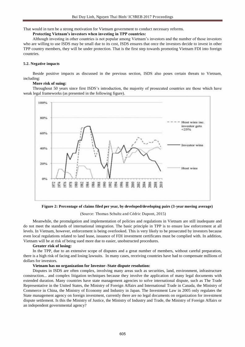
Bui Duy Linh, Nguyen Thai Binh/ ICYREB 2017 Proceedings
That would in turn be a strong motivation for Vietnam government to conduct necessary reforms. Protecting Vietnam’s investors when investing in TPP countries: Although investing in other countries is not popular among Vietnam’s investors and the number of those investors
who are willing to use ISDS may be small due to its cost, ISDS ensures that once the investors decide to invest in other TPP country members, they will be under protection. That is the first step towards promoting Vietnam FDI into foreign countries.
5.2. Negative impacts
Beside positive impacts as discussed in the previous section, ISDS also poses certain threats to Vietnam, including:
More risk of suing: Throughout 50 years since first ISDS’s introduction, the majority of prosecuted countries are those which have
weak legal frameworks (as presented in the following figure).
Figure 2: Percentage of claims filed per year, by developed/developing pairs (3-year moving average)
(Source: Thomas Schultz and Cédric Dupont, 2015)
Meanwhile, the promulgation and implementation of policies and regulations in Vietnam are still inadequate and do not meet the standards of international integration. The basic principle in TPP is to ensure law enforcement at all levels. In Vietnam, however, enforcement is being overlooked. This is very likely to be prosecuted by investors because even local regulations related to land lease, issuance of FDI investment certificates must be complied with. In addition, Vietnam will be at risk of being sued more due to easier, unobstructed procedures.
Greater risk of losing: In the TPP, due to an extensive scope of disputes and a great number of members, without careful preparation,
there is a high risk of facing and losing lawsuits. In many cases, receiving countries have had to compensate millions of dollars for investors.
Vietnam has no organization for Investor–State dispute resolution: Disputes in ISDS are often complex, involving many areas such as securities, land, environment, infrastructure
construction... and complex litigation techniques because they involve the application of many legal documents with extended duration. Many countries have state management agencies to solve international dispute, such as The Trade Representative in the United States, the Ministry of Foreign Affairs and International Trade in Canada, the Ministry of Commerce in China, the Ministry of Economy and Industry in Japan. The Investment Law in 2005 only regulates the State management agency on foreign investment, currently there are no legal documents on organization for investment dispute settlement. Is this the Ministry of Justice, the Ministry of Industry and Trade, the Ministry of Foreign Affairs or an independent governmental agency?
605

Bui Duy Linh, Nguyen Thai Binh/ ICYREB 2017 Proceedings
6. Some suggestions
Firstly, Viet Nam should make every effort to prevent disputes arising, raise awareness of the risk of lawsuits. The prevention of disputes is very important such as compliance with the procedures for licensing, evaluation, clarification of local incentives and laws of Vietnam.
Secondly, it is necessary to create a friendly cooperative environment that will help investors and the state understand each other and move towards common interests. Therefore, when a dispute arises, the government can negotiate on the basis of a willingness to cooperate and maintain a good relationship with foreign investors.
Thirdly, Vietnam should also train experts and lawyers understanding the rules of international arbitration institutions. In the practice of resolving international disputes by arbitration, it is clear that the lack of understanding leads to undue errors that may expose the government to the risk of losing a lawsuit.
Last but not least, ISDS not only serves as a mechanism to protect foreign investors but also forms a measure to protect host countries from the abuse of ISDS. Therefore, Vietnam should ensure in-depth understanding of safeguard measures to prevent and deal with ISDS proceedings. These safeguard measures include: transparent arbitral proceedings, amicus curiae submissions, non-disputing party submissions; Expedited review of attorneys' fees; Review procedure for an interim award; Binding joint interpretations by TPP Parties; Time limits on bringing a claim; And rules to prevent a claimant pursuing the same claim in parallel proceedings.
7. Conclusion
At present, there are still a lot of controversy surrounding ISDS in TPP as well as the controversy over the rules and content of the mechanism. For investors from Vietnam as well as member countries, ISDS protects the interests of investors through requiring governments to respect foreign investment activities in its territory. However, for the governments especially developing countries like Vietnam, ISDS seems to be a challenge. Vietnam may not take advantage of the benefits of ISDS as the scale of offshore investment is small and not focus on TPP countries. On the contrary, Vietnam faces a lot of visible risk and its huge consequences. To deal with this type of dispute effectively Vietnam needs carefully study the ISDS regulations to provide legal direction for protecting the interests as well as minimizing the risks that the government may face.
Reference
[1] BBC News. (2015), Trans-Pacific free trade deal agreed creating vast partnership, http://www.bbc.com/news/business-34444799
[2] Carvalho, P. (2016). Investor-State Arbitration and the Rule of Law: Debunking the Myths. [online] Available at: https://www.cis.org.au/app/uploads/2016/04/rr13.pdf.
[3] HUFBAUER, G. (2016). ITRANS-PACIFIC PARTNERSHIP: AN ASSESSMENT. Peterson Institute for International Economics.
[4] International law (2014), Vietnam National University Press, Hanoi. [5] Journal of Democracy and Law, Investor – State Dispute Settlement in the Trans-Pacific Partnership Agreement, [6] http://tcdcpl.moj.gov.vn/qt/tintuc/Pages/phap-luat-kinh-te.aspx?ItemID=146 [7] Journal of Law, TPP and the possibility of Vietnam being sued in investment disputes,
http://luatkhoa.org/2016/02/tpp-va-kha-nang-viet-nam-bi-khoi-kien-trong-cac-tranh-chap-dau-tu-ky-2-het/ [8] Kyla Tienhaara (2010), ISDS in the TPP agreement. [9] Le Net (2006), ICSID is even more serious than the dumping case, Vietnamese Law Consultants [10] Ministry of Foreign Affairs of Vietnam, Introduction The Trans-Pacific Partnership (TPP)
http://www.mofahcm.gov.vn/vi/mofa/nr091019080134/nr091019083649/ns110923115344 [11] Pham Duy Nghia (08/2013), “TPP – What are opportunities for Vietnam”. [12] Public Citizen, TPP’s Investment Rules Harm the Environment, http://www.citizen.org/documents/fact-sheet-tpp-
and-environment.pdf [13] Schubert, M. and Saz-Carranza, A. (2016). Esadegeo. Investor-State Dispute Settlement & the Transatlantic Trade
and Investment Partnership (TTIP), 39. [14] Schultz, T. and Dupont, C. (2014). Investment Arbitration: Promoting the Rule of Law or Over-Empowering
Investors? A Quantitative Empirical Study. SSRN Electronic Journal. [15] The Trans-Pacific Partnership (TPP) [16] UNCTAD (2017). Investor-State Dispute Settlement: Review of Developments in 2016. [online] Available at:
http://investmentpolicyhub.unctad.org/Publications/Details/172. [17] Wellhausen, R. (2016). Recent Trends in Investor–State Dispute Settlement. Journal of International Dispute
Settlement, p.idv038.
606

Le Thi Tu Oanh, Bui Thi Ngoc/ ICYREB 2017 Proceedings
International Conference For Young Researchers In Economics And Business, ICYREB 2017, October 30th 2017 Da Nang, Vietnam
Factors Affecting Outsourcing of Accounting of Enterprise
Executives In Vietnam
Le Thi Tu Oanha, Bui Thi Ngoc,b*
a Le Thi Tu Oanh, My Dinh, Ha Noi, +84, VietNam bBui Thi Ngoc, Hoang Quoc Viet, Ha Noi, +84, VietNam
A B S T R A C T
Along with the rapid development of technology, specialization through outsourcing is one of the current trends. Outsourcing is a useful solution allowing executives to focus on core business activities, reducing costs, and enhancing business efficiency. Whereby, choosing professional providers of accounting service ensuring high quality as well as bringing many benefits is one of the major concerns of the CEO. The purpose of the study is to explore factors influencing the intention to outsource accounting instead of recruiting accountants of the enterprise executives who are outsourcing accounting in Vietnam. We received 181 valid responses from survey, in which, 94 outsourced accounting services. The initial model was proposed with five factors including specificity of accounting tasks, environmental uncertainty, behavioural uncertainty, frequency of accounting transactions and trust in service providers. The analysis proved that only specificity of accounting task and the accounting behavioural uncertainty are statistically significant and have impact on the intention to outsource accounting services of the executives. The complexity in business activities of enterprises, higher demand for information of managers will lead to stronger intention of accounting outsourcing. The behavioural uncertainty of internal accounting will increase the intention of accounting outsourcing due to suspicion of honest, sufficient, and timely provision of information from internal accountants.
Keywords: Accounting; outsourcing; outsourcing accounting.
1. Introduction
1.1. Accounting Outsourcing
Since 1930s, the rapid development of accounting outsourcing in term of width and depth is increasing worldwide. Accounting outsourcing was studied by many researchers such as Coase (1937), Bendor-Samuel (1998), Klein (2005). Their findings are summarized as follows.
According to Coase (1937), accounting outsourcing is the act of subcontracting out all or parts of tasks of an accounting system in a firm to an external firm. The study of Coase only identified the subjects conducting accounting tasks but did not show which tasks could be conducted. Bendor & Samuel (1998) stated that accounting outsourcing is the transferring entire or parts of tasks of financing and accounting system to a provider. Klein (2005) provided that accounting outsourcing can be understood as the transferring of one or many functions or accounting processes to a third party, outsourcing of accounting services include full accounting package service; managing of inflow and outflow of cash; accounts receivable, accounts payable; recording invoices, taxes, financial analysis. Barthelemy (2003) provided that outsourcing of accounting means allowing others conducting functions related to finance of a company and outsourcing is appropriate for routine tasks such as entry of invoices, book-keeping, interim reporting. Watjatrakul (2005) supposed that outsourcing of accounting includes functions such as controlling daily accounting tasks, preparing monthly financial statements or even managerial information like analysis of fluctuations, estimation.
* Le Thi Tu Oanh. Tel.: +84964176633. E-mail address: [email protected] Bui Thi Ngoc. Tel.: +84989077435. E-mail address: [email protected]
607

Le Thi Tu Oanh, Bui Thi Ngoc/ ICYREB 2017 Proceedings
1.2. Advantages of accounting outsourcing
Reducing costs of enterprises: Outsourcing of accounting is considered as the most effective solution for enterprises with the fundamental benefit of reducing costs (Lacity & Willcocks 1998). Lacity has proved that the cost of salaries for the accounting system exceeds the cost of an outsourcing contract in one year. A survey showed that the IT sector decreased by 6.7% in costs of value chain from 1997-2001 (Leiblein et al. 2003). Klein (2005) provided that outsourcing of accounting helps firms reduce costs when selecting professional accounting service providers and increase flexibility when applying technology or expanding production. In particular, accounting outsourcing enables firms to avoid costs related to running the business. Klein, however, emphasized that outsourcing needs to be controlled, organized in a scientific way in order to bring benefits to firms. Kee and Robbins (2003) agreed that outsourcing helps enterprises reduce cost of accounting department, however, outsourcing decisions require accurate estimation of cost, time and considering of other opportunity costs (Kee and Robbins, 2003).
Focusing on core business activities of enterprises: Outsourcing of accounting allows firms to focus on key business areas and activities. This was the view of researchers such as Benko (1993); Quinn and Hilmer (1994); Gilley & Rasheed (2000). Reddy & Ramachandran (2008) demonstrated that 30% - 45% of the time spent on accounting tasks is used in simple transaction processing activities such as recording invoices, billing, receipts, and receiving/delivering. Whereby, outsourcing of accounting will allow firms to focus on strategic activities such as financial planning, production, sales and controlling. Gilley & Rasheed (2000) emphasized the benefits of outsourcing of accounting as specialization process and the shortest way to reach modern accounting and to focus resources on strategic activities of enterprises.
Creating flexibility and enhancing efficiency of enterprises: Previous studies have been conducted to demonstrate the effectiveness of outsourcing. Bendor-Samuel (1998) asserted that accounting outsourcing simplifies the administration, creates flexibility in management and increases business efficiency. According to Chin (2003), accounting outsourcing plays an important role in improving firms’ performance by increasing profitability, return on investment and greater capital efficiency. Krell (2007) argued that the greatest benefit of accounting outsourcing is the creating of flexibility in management and operation. In order to do that, the unit outsourcing its functions should design useful measures of outsourcing service efficiency and have cross-check measures to control outsourcing services.
Kakabadse (2001) summarized benefits of outsourcing: staff and cost reduction, quality improvement, managing quality of activities by focusing on core competencies, and finally enhancing business efficiency.
1.3. Types of outsourcing services of accounting
According to the product classification of the United Nations "Provisional Central Product Classification", accounting outsourcing services includes reviewing the financial statements; preparing financial reports; performing bookkeeping service and other accounting services.
- Reviewing financial statements is a service which reviews the annual and periodic financial statements as well as other accounting information, the scope of the review is smaller than the audit, so the level of reliability and validity is lower.
- Preparing financial statements is a service which prepares financial statements from the information provided by customers. Service providers do not certify the accuracy of the financial statements. If the contract requires preparation of tax returns, the tax declaration service is also considered as part of the preparing financial statements service.
- Bookkeeping service includes functions such as classifying, recording business transactions on book in term of currency or other measuring units, collecting documents, processing vouchers, performing accounting and bookkeeping, checking and completing vouchers, recording and preparing financial statements.
- Other accounting services are certifying, evaluating, preparing internal reports or periodic reports.
2. Research overview
Transaction cost economics (TCE) model is the main theoretical framework to examine the factors affecting outsourcing decisions of enterprises (Masten 1984, Klein 2005, Walker and Weber 1984). The outsourcing decision or using internal accounting system depends on the comparison between transaction costs including the cost of negotiating the contract, the cost of implementing the services and the salary expenses paid to the accounting department (Williamson 1985). Accounting outsourcing is preferred when there are many accounting service providers in the market (Hennart 1988). Abbott et al. (2007) distinguished between routine and non-routine accounting tasks. Routine accounting tasks include updating documents and vouchers, interim reporting, departmental reporting; Non-routine accounting tasks include preparation of financial statements at the year end. With routine accounting tasks which are often simple, repetitive, standardized, and need limited estimation, analysis of accountants, outsourcing should be used. Conversely, with non-routine accounting tasks which requires the accountants to have profound knowledgeable about the company’s activities, expertise and experience to make a decision, firms should use internal accounting system (Caplan and Emby 2004). Leah (2005) agreed with this view and supposed that accounting outsourcing is more
608

Le Thi Tu Oanh, Bui Thi Ngoc/ ICYREB 2017 Proceedings
appropriate for bookkeeping, summarizing and analysing. Dyer et al. (2000) suggested that routine accounting tasks should be outsourced. When the asset specificity is high and the tasks are complicated, outsourcing is not a suitable choice. Moreover, researchers showed the relationship between outsourcing and the educational background of the CEO, the CEO’s level of trust in the external accounting services, and asserted that the higher educational level of the CEO was linked with lower levels of outsourcing (Dyer et al, 2000).
3. Research model and hypothesis
Transaction cost economics (TCE) model was mentioned by Masten in 1984, in which factors influencing outsourcing decision of an enterprise include: specificity of accounting, environmental uncertainty, behavioural uncertainty, frequency of accounting transactions. Inheriting Masten's TCE model, Klein (2005) proved that the factor of trust also affects the accounting outsourcing decision of enterprises. Vandaele et al. (2007) focused on studying and explaining that the characteristics of accounting tasks was the primary factor affecting outsourcing decisions, followed by behavioural uncertainty and enterprises’ trust in external accountants. Therefore, the proposed research model is shown in Figure 1:
Fig. 1. Proposal research model
Specificity of accounting tasks: The specificity of accounting tasks is the driving force of outsourcing (Masten 1984; Klein 2005). The complexity of accounting tasks depends on the fields of business activities (production or service) and the CEO’s requirements of providing information (Watjatrakul 2005; Barthelemy 2003). The more complex the accounting tasks, the less intense the accounting outsourcing (Dyer et al. 2000). Thus, the first hypothesis is proposed as follows.
H1: The higher the specificity of accounting tasks, the less intensely they are outsourced. Environmental uncertainty: environmental uncertainty in this study refers to the stability and predictability of
accounting workloads as a consequence of volatility such as business results, business size and changes due to merger, consolidation, acquisition or closure of the factories. The changes of these factors change will result in changes of accounting. In such cases, accounting outsourcing is inappropriate (Masten 1984; Klein 2005; Widener and Selto 1999; Williamson 1991; Hennart 1994). Therefore, the second hypothesis is proposed as follows:
H2-
H1-
Environmental uncertainty
Behavioural uncertainty
Frequency of accounting transactions
Trust in service providers
Intention of accounting outsourcing
Specificity of accounting tasks
Age of enterprise
Business location
Business area
Enterprise size
Age, educational
level of CEO
H3+
H4-
H5+
609

Le Thi Tu Oanh, Bui Thi Ngoc/ ICYREB 2017 Proceedings
H2: The higher the environmental uncertainty in accounting tasks, the less intensely they are outsourced. Behavioural uncertainty: Behavioural uncertainty reflects difficulties in monitoring activities and supervising
people against opportunism, fraud, distortion of information, shirking responsibilities (Masten 1984; Klein 2005; Williamson 1985; Hill 1990). Behavioural uncertainty makes it difficult to assess the effectiveness of the accountants employed by the firm. So, in this case, the business wants to outsource. Therefore, the third hypothesis is proposed as follows:
H3: The higher the behavioural uncertainty in accounting tasks, the less intensely they are outsourced Frequency of accounting tasks: The frequency of accounting tasks is the amount of transactions to be recorded
and reported. Frequency can be interpreted as accounting cycle in term of week, month, quarter, year or frequency is the scale of the activities. The larger the scale, the higher the frequency of accounting tasks (Masten 1984; Klein 2005; Williamson 1985). Thus, the fourth hypothesis is proposed as follows:
H4: The higher the frequency of accounting tasks, the less intensively they are outsourced Level of trust in service providers: Klein (2005) pointed out in his research results that trust in the service
providers is an important factor in the outsourcing contract. According to Klein, trust is reflected in the following aspects: transparency in outsourcing, higher reliability and objective information provided by external accountants. When firms have confidence in external accounting services, they will choose accounting outsourcing even if the accounting specificity is high and the amount of accounting tasks is large or small (Vandaele et al. 2007). Thus, the fifth hypothesis is proposed as follows:
H5: The higher the level of trust in accounting service providers, the more intensely accounting tasks are outsourced.
4. Methodology
With the purpose of identifying factors affecting the intention of accounting outsourcing of the CEO, the authors conducted a survey by distributing questionnaires to CEOs. The questionnaire is divided into 7 parts: 1) Information of enterprise; 2) Specificity of accounting tasks; 3) Environmental uncertainty; 4) behavioural uncertainty; 5) Frequency of accounting transactions; 6) Trust in the service providers; 7) CEO’s intention of accounting outsourcing. Scales in questionnaire are inherited from previous research, specifically: In order to get information of enterprises, we used measurement scale of Noradiva et al. (2011), including control variables: age of enterprise, location, business area, educational level and training area of the CEO. The researchers added criteria to identify the size of enterprise including sales and the number of employees to comply with the classification of enterprises in Vietnam (Watjatrakul, 2005). The measurement scale of accounting specificity was inherited from researchers: Masten 1984; Klein 2005; Watjatrakul 2005; Barthelemy & Geyer 2005; Dyer at al. 2000 which included 5 questions. The measurement scale of environmental uncertainty was based on scale of researchers Masten 1984; Klein 2005; Widener and Selto 1999; Williamson 1991; Hennart 1994 which included 2 questions and 1 questions proposed by the authors. The measurement scale of behavioral uncertainty included 5 questions inherited from researchers Masten 1984; Williamson 1985; Hill 1990. The measurement scale of frequency of accounting transactions included 4 questions from scale of Masten 1984; Williamson 1985. The measurement scale of trust in service providers included 5 questions from the scale of Masten 1984; Klein (2005); Vandaele et al. 2007. The measurement scale of dependent variable which is the intention of accounting outsourcing was proposed by authors based on 4 criteria including benefits to the work, good service quality, higher flexibility compared to recruitment and application of new technology.
The measurement scales of dependent and independent variables are shown in the following table:
Table 1: The measurement scales.
Observed variables Measurement scales Source Encode 1. Specificity of accounting tasks
Accounting tasks do not require daily information
Masten 1984; Klein 2005; Watjatrakul 2005; Barthelemy & Geyer 2005; Dyer at al. 2000
Dacd_cv1
Accounting tasks are performed by accounting software
Dacd_cv2
Accounting tasks have high specificity Dacd_cv3 Firm is spending much time and money on accounting outsourcing
Dacd_cv4
Tasks require experts to perform Dacd_cv5 2.Environmental In previous year, jobs related accounting Masten 1984; Klein 2005; Bomt_1
610

Le Thi Tu Oanh, Bui Thi Ngoc/ ICYREB 2017 Proceedings
uncertainty was unstable Widener and Selto 1999; Williamson 1991; Hennart 1994
In previous year, changes of enterprise affected the business organization (restructuring the enterprise)
Bomt_2
In previous year, enterprise got taxation checking decision of tax office
New measure Bomt_3
3.Behavioural uncertainty (internal accounting)
Internal accountants are uncooperative at work
Masten 1984; Williamson 1985; Hill 1990
Bohv_1
Internal accountants are dishonest when providing information
Bohv_2
Internal accountants lack responsibility at work
Bohv_3
Internal accountants distort reporting information
Bohv_4
Changing workplace Bohv_5 4.Frequency of transactions (daily,…yearly, 6 levels)
Invoice, vouchers of transactions need to be recorded
Masten 1984; Williamson 1985
Tsgd_1
Interim reports need to be provided Tsgd_2 Periodic reports need to be provided Tsgd_3 Financial statements need to be provided Tsgd_4
5.Trust in service providers
Accounting outsourcing are transparent Masten 1984; Klein (2005); Vandaele et al. 2007
Ntin_1 Accounting outsourcing provides more accurate information
Ntin_2
Accounting outsourcing performs accounting tasks well
Ntin_3
The relationship between the CEO and external accountants is based on trust
Ntin_4
6.Intention of accounting outsourcing
I will outsource accounting as it brings many benefits for the job
New measure
Inten_1
I will outsource accounting because of good service quality
Inten_2
I will outsource accounting because it is more flexible than recruit accountants
Inten_3
I will outsource accounting as it applies new technology
Inten_4
Table 2. Sample features.
Features Number (N=94) Percentage (%) Capital Foreign invested enterprises 14 14.89%
enterprises 80 85.11% Age < 5 yrs. 43 45.74%
5 - 10 yrs. 38 40.43% >10 yrs. 13 13.83%
Location Northern 86 91.49% Central 5 5.32% Southern 3 3.19%
Fields Trade and Services 58 61.70% Constructions 15 15.96% Others 21 22.34%
Number of employees < 300 people 89 94.68% >=300 people 5 5.32%
Revenue < 10 billions dong 65 69.15% 10-50 billions dong 21 22.34% > 50 billions dong 8 8.51%
Questionnaires was distributed to enterprises via e-mail, and the number of valid respondents received was 181, however, the number of enterprises which are outsourcing accounting services was 94, accounting for 51.9%. We evaluated the intentions of outsourcing of enterprises which have outsourced accounting services to assess their intention to outsource accounting. Details of the 94 surveyed enterprises are shown in Table 2.
611

Le Thi Tu Oanh, Bui Thi Ngoc/ ICYREB 2017 Proceedings
5. Research results
5.1. Factors analysis and reliability
Initially, 5 independent variables and 1 dependent variable were measured by 25 observed variables in order to identify factors affecting the outsourcing of accounting of enterprises. According to Williams et al. (2010), sample size of 94 and the ratio of sample size and the number of observed variables of 94:25, which is greater than the ratio 3: 1, are appropriate for factor analysis. The KMO and Bartlett's test showed that the KMO = 0.808 (greater than 0.5 and less than 1) which indicates that the sampling is adequate for factor analysis. In addition, the Bartlett test revealed that the research data was statistically significant (Sig. = 0.00 ≤ 0.05) which means that variables were correlated. After the first exploratory factor analysis (Table 3), the results showed that the observed variables combined into five groups of factors, which explained about 73.69% of the variation of the observed variables but it were different from the initial anticipation, specifically:
- The variable measuring specificity of accounting tasks (Dacd_cv1) measures the accounting tasks which do not require frequent provision of information and the variable measuring the behavioral uncertainty (Bohv_5) represents accountants’ changes of workplace with loading factor less than 0.5, so it will not be used in the model
- The second, the third, the fifth variable measuring specificity of accounting tasks (Dacd_cv2, Dacd_cv3, Dacd_cv5) combining with the first, the second, the third observed variable of environmental uncertainty (Bomt_1, Bomt_2, Bomt_3) and 1 variable measuring intention of outsourcing (Inten_2) was one group.
- The fourth variable measuring specificity of accounting tasks (Dacd_cv4) combining with variables of behavioral uncertainty was one group.
After eliminating 2 observed variables, the results of the second factor analysis (Table 4) based on 23 observed variables divided into 5 groups, explained 77.15% of the variation of observed variables. Thus, the model had only 4 variables to measure intention of accounting outsourcing. Groups are labeled as follows:
- Dependent variable: intention of accounting outsourcing (IT_outs) including 3 observed variables (Inten_1, Inten_3, Inten_4).
- Independent variables: Trust in service providers (Ntin) including 4 observed variables; Behavioural uncertainty (Bohv) including 5 observed variables; specificity of accounting tasks (Dacd_cv) including 7 observed variables; frequency of accounting transactions (Tsgd) including 4 observed variables.
To confirm the correlation of the observed variables to measure independent variables, we conducted a further analysis of the reliability for each group of observed variables of each factor. Results showed that all groups had Cronbach's Alpha greater than 0.7 and Corrected Item-Total Correlation coefficients greater than 0.4. According to Kline (1998), we can assert that the observed variables are reliable and internally consistent to integrate into independent variables as the altered model.
Table 3. The first EFA analysis results.
Rotated Component Matrixa Component 1 2 3 4 5
Dacd_cv5 0.722 Dacd_cv2 0.716 Bomt_1 0.699
Dacd_cv3 0.692 Bomt_3 0.669 Inten_2 0.627 Bomt_2 0.53
Dacd_cv1 Bohv_2 0.901 Bohv_4 0.889 Bohv_3 0.886 Bohv_1 0.86
Dacd_cv4 0.616 Ntin_2 0.862 Ntin_3 0.847 Ntin_1 0.819 Ntin_4 0.747 Inten_3 0.806 Inten_4 0.801
612

Le Thi Tu Oanh, Bui Thi Ngoc/ ICYREB 2017 Proceedings
Inten_1 0.756 Bohv_5 TSgd_2 0.857 TSgd_1 0.758 TSgd_3 0.672 TSgd_4 0.558
Extraction Method: Principal Component Analysis. Rotation Method: Varimax with Kaiser Normalization.
a. Rotation converged in 7 iterations.
Table 4. The second EFA analysis results.
Rotated Component Matrixa
Component
1 2 3 4 5
Ntin_2 .877
Ntin_3 .847
Ntin_1 .833
Ntin_4 .759
Bohv_2 .897
Bohv_3 .897
Bohv_4 .895
Bohv_1 .860
Dacd_cv4 .616
Dacd_cv5 .719
Dacd_cv2 .718
Bomt_1 .718
Dacd_cv3 .682
Bomt_3 .671
Inten_2 .591
Bomt_2 .550
Inten_4 .817
Inten_3 .813
Inten_1 .746
TSgd_2 .864
TSgd_1 .775
TSgd_3 .671
TSgd_4 .579
Extraction Method: Principal Component Analysis. Rotation Method: Varimax with Kaiser Normalization.
a. Rotation converged in 7 iterations.
5.2. Analyzing and comparing groups of variables
We compared intention of accounting outsourcing of enterprises regarding controlled variables, specifically: - In term of enterprise: age of enterprise, business location, business area, enterprise size. - In term of the CEO: Age, educational level, training area. Using Compare means to find out if there is difference in the intention of accounting outsourcing between
enterprise and the CEO. The results were as follows: - Age of an enterprise: Levene’s test revealed that Sig. = 0.201 > 0.05 which means that there is not enough
evidence to conclude the age of an enterprise affects the intention of accounting outsourcing. Similarly, with business
613

Le Thi Tu Oanh, Bui Thi Ngoc/ ICYREB 2017 Proceedings
location, business area, enterprise size, the results showed that there is no difference between those controlled variables and the intention of accounting outsourcing of enterprise.
- Age of the CEO: Levene’s test provided Sig. = 0.984 > 0.05 which indicates that there is no difference between this controlled variable and the intention of accounting outsourcing. Anova test provided Sig. = 0.503 > 0.05, thus, there is not enough evidence to conclude that age of the CEO affects the intention of accounting outsourcing. Similarly, there is no difference between educational level, training area of the CEO and the intention of accounting outsourcing of the enterprise.
5.3. Regression analysis
We carry out regression analysis to measure the impact of 4 factors and controlled variable to the intention of accounting outsourcing.
Table 5. Regression analysis results – Model Summary
Model Summary
Model R R Square Adjusted R Square Std. Error of the Estimate
1 .697a .486 .410 2.74699
a. Predictors: (Constant), Training area, Age of enterprise, Bohv, Business location, Educational level, Ntin, Age of CEO, Business area, Labours, Turnover, TSgd, Dacd_cv
The results of regression analysis – Model Summary showed in table 5 provided that value of R2 is 0.410. This means that factors and controlled variables can explain 41% of the influence on accounting outsourcing of enterprise. The table 6 illustrates the hypothesis that dependent variables and controlled variables have positive impact on accounting outsourcing (Sig. <0.01)
Table 6. Regression analysis results – ANOVA. ANOVA b
Model Sum of Squares df Mean Square F Sig.
1 Regression 577.416 12 48.118 6.377 .000a
Residual 611.222 81 7.546
Total 1188.638 93
a. Predictors: (Constant), Training area, Age of enterprise, Bohv, Business location, Educational level, Ntin, Age of CEO, Business area, Labours, Turnover, TSgd, Dacd_cv
b. Dependent Variable: IT_outs
Table 7. Regression analysis results – Coefficients.
Coefficientsa
Model
Unstandardized Coefficients Standardized Coefficients
t Sig. B Std. Error Beta
1 (Constant) 1.874 2.512 .746 .458
Ntin .132 .121 .140 1.093 .277
Bohv .278 .075 .379 3.715 .000
Dacd_cv .224 .075 .370 2.991 .004
TSgd -.023 .094 -.028 -.250 .803
Age of enterprise .384 .519 .082 .740 .461
Business location -.089 .737 -.010 -.120 .904
Business area -.289 .171 -.162 -1.693 .094
Turnover -.356 .507 -.079 -.702 .485
Labours -.873 .614 -.141 -1.422 .159
Age of CEO -.647 .423 -.138 -1.530 .130
Educational level .342 .576 .053 .594 .554
Training area .032 .297 .010 .109 .914
a. Dependent Variable: IT_outs
614
Le Thi Tu Oanh, Bui Thi Ngoc/ ICYREB 2017 Proceedings
Table 7 represents the simultaneous impact of independent variables and controlled variables on the intention of accounting outsourcing. The Sig value showed that only behavioural uncertainty (Bohv), the specificity of accounting tasks (Dacd_cv) have sig. value less than 0.05 which are statistically significant. Behavioural uncertainty and specificity of accounting tasks have positive relationship with the intention of accounting outsourcing. The results also showed that there is no difference in intention of accounting outsourcing among enterprises with different ages, locations, business areas and enterprise sizes. Companies with CEOs of different ages, qualifications and training areas also have no difference in the intention of accounting outsourcing. The relationship between independent and dependent variables is illustrated by the following equation
IT_outs = 1.874 + 0.278 * Bohv + 0.224 * Dacd_cv Thus, the results of the regression analysis showed that the intention of accounting outsourcing is affected by the
behavioural uncertainty of internal accountants and specificity of accounting tasks. For any change of behavioural uncertainty of accountants such as fraud, distortion of information in updating documents, transactions, providing data, reports causing difficulties to control the performance of the management will increase the outsourcing intentions by 0.278 times. Furthermore, the results showed that there is evidence to support hypothesis H3 which is consistent with previous studies (Masten 1984; Klein 2005). In term of specificity of accounting tasks, the more complicated the accounting tasks, the more intense the intention of CEO to outsource. With more complex changes of specificity of accounting tasks, the requirement of administrative information is higher and the intention of accounting outsourcing increases by 0.224 times. This results in the rejection of the hypothesis H1 because specificity of accounting tasks has a positive impact on management's intention to outsource accounting. However, this result contrasts with study of Dyer et al. (2000) who suggested that the more complicated the accounting tasks, the less intense the intention of outsourcing.
6. Conclusion
With the purpose of explaining the intention to outsource the accounting services of CEO in Vietnam, the study relied on the TCE model with supplement of 3 observed variables measuring the intention of accounting outsourcing which are the benefits of outsourcing, the flexibility of outsourcing compared to recruitment and application of new technologies when outsourcing. The results of the analysis are consistent with the data and there is internally consistence reliability to create the scale measuring the intention of accounting outsourcing. With the data of 94 enterprises in Vietnam that outsourced accounting services, the initial model was proposed with five factors including specificity of accounting tasks, environmental uncertainty, behavioural uncertainty, frequency of accounting transactions and trust in service providers. The regression analysis proved that only specificity of accounting task and the accounting behavioural uncertainty are statistically significant and have impact on the intention to outsource accounting services of the executives. Both of these variables increase the intention of accounting outsourcing. The complexity in business activities of enterprises, higher demand for information of managers will lead to stronger intention of accounting outsourcing. Whereby, professionalism, quality and support from experts will meet the requirement of information for the CEO. Furthermore, the behavioural uncertainty of internal accounting will increase the intention of accounting outsourcing due to suspicion of honest, sufficient, and timely provision of information from accountants recruited by the enterprise.
The research results can be considered as a reference model for future research on outsourcing of accounting services in Vietnam. On the practical side, research provides useful information for accounting service providers in improving service quality, professionalism, and application of new technologies to develop services in the integration trend. For Vietnamese CEOs, the study provides the basis for choosing the best option for outsourcing rather than recruit accountants because of the benefits, flexibility and application of new technologies of outsourcing especially with the diversified demand for information, the expanding of the enterprise size and the increasing complexity of management
The limitations of research and suggestions for further research: This study only studied the intention of accounting outsourcing of enterprises which outsourced accounting but
did not study enterprises which have not outsourced accounting. This is a suggestion for researchers to find out the factors affecting the intention of enterprises which have not outsourced accounting, targeting potential customers, expanding the market services for organizations providing accounting services.
615

Le Thi Tu Oanh, Bui Thi Ngoc/ ICYREB 2017 Proceedings
References
[1] Coase, R. N. (1937). The nature of the firm. In O. Williamson & S. Winter (Eds.), The nature of the firm. Oxford: Oxford University Press.
[2] Klein, P. G. (2005). The make-or-buy decision: Lessons from empirical studies. In C. Me´nard & M. Shirley (Eds.), Handbook of institutional economics (pp. 435–464). New York: Springer.
[3] Williamson, O. (1985). Economic organization: Firms, mar- kets and policy control. New York: New York University Press.
[4] Caplan, D., & Emby, C. (2004). An investigation of whether outsourcing the internal audit function affects internal controls. Working paper, Iowa State University.
[5] Dyer, J., & Chu, W. (2000). The determinants of trust in supplier-automaker relationships in the U.S., Japan, and Korea. Journal of International Business Studies, 31(2), 259–285.
[6] Gilley, K., Greer, C., & Rasheed, A. (2004a). Human resource outsourcing and organizational performance in manufac- turing firms. Journal of Business Research, 57(3), 232–240.
[7] Gilley, K., McGee, J., & Rasheed, A. (2004b). Perceived environmental dynamism and managerial risk aversion as antecedents of manufacturing outsourcing: The moderat- ing effects of firm maturity. Journal of Small Business Management, 42(2), 117–133.
[8] Gilley, K., & Rasheed, A. (2000). Making more by doing less: An analysis of outsourcing and its effects on firm per- formance. Journal of Management, 26(4), 763–790.
[9] Hennart, J. (1988). A transaction costs theory of equity joint ventures. Strategic Management Journal, 9(4), 361–374. Hennart, J. (1989). Can the ‘‘new forms of investment’’ sub- stitute for the ‘‘old forms’’? A transaction costs perspective. Journal of International Business Studies, 20(2), 211–234.
[10] Hennart, J. (1994). The comparative institutional theory of the firm: Some implications for corporate strategy. Journal of Management Studies, 31(2), 193–207.
[11] Hill, C. (1990). Cooperation, opportunism, and the invisible hand: Implications for transaction cost theory. Academy of Management Review, 15(3), 500–513.
[12] Kakabadse, A., & Kakabadse, N. (2002). Trends in outsourc- ing: Contrasting USA and Europe. European Management Journal, 20(2), 189–198.
[13] Klein, S., Frazier, G., & Roth, V. (1990). A transaction cost analysis model of channel integration in international markets. Journal of Marketing Research, 27(2), 196–208.
[14] Kee, R.C. and Robbins, W.A. (2003), ‘‘Public sector outsourcing: a modified decision model’’, The Journal of Government Financial Management, Vol. 52 No. 2, pp. 46-52.
[15] Krell, E. (2007), ‘‘Finance and accounting outsourcing: making an informed decision’’, CMA Management, Vol. 81 7, November, pp. 38-40.
[16] Lacity, M., Willcocks, L. and Feeny, D. (2004), ‘‘Commercializing the back office at Lloyds of London. Outsourcing and strategic partnerships’’, European Management Journal, Vol. 22 No. 2, pp. 127-40.
[17] Lacity, M., & Willcocks, L. (1998). An empirical investigation of information technology sourcing practices: Lessons from experience. MIS Quarterly, 22(3), 363–408.
[18] Leiblein, M., & Miller, D. (2003). An empirical examination of transaction- and firm-level influences on the vertical boundaries of the firm. Strategic Management Journal, 24(9), 839–859.
[19] Masten, S. (1984). The organization of production: Evidence from the aerospace industry. Journal of Law and Eco- nomics, 27(2), 403–417.
[20] Masten, S. (1993). Transaction costs, mistakes, and perfor- mance: Assessing the importance of governance. Managerial and Decision Economics, 14(2), 119–129.
[21] Masten, S., Meehan, J., & Snyder, E. (1989). Vertical inte- gration in the U.S. auto industry: A note on the influence of transaction specific assets. Journal of Economic Behavior & Organization, 12(2), 265–273.
[22] Reddy & Ramachandran (2008), ‘‘Outsourcing of finance and accounting operations: the feasibility of the vertical in the Indian context’’, The ICFAI Journal of Services Marketing, Vol. 6 No. 1, pp. 23-39.
[23] Walker, G., & Weber, D. (1984). A transaction cost approach to make-or-buy decisions. Administrative Science Quar- terly, 29(3), 373–391.
[24] Watjatrakul, B. (2005). Determinants of IS sourcing decisions: A comparative study of transaction cost theory versus the resource-based view. Journal of Strategic Information Systems, 14(4), 389–415.
[25] Williamson, O. (1991). Comparative economic organization: The analysis of discrete structural alternatives. Adminis- trative Science Quarterly, 36(2), 269–296.0
616

Nguyen Thi Thu Trang / ICYREB 2017 Proceedings
International Conference For Young Researchers In Economics And Business, ICYREB 2017, October 30th 2017 Da Nang, Vietnam
Digital Banking Adoption: The Case of Vietnam
Nguyen Thi Thu Trang*
MSc, 12 Chua Boc St, Hanoi, Vietnam
A B S T R A C T
This study aims to empirical examine the factors that affect the adoption of digital banking in Vietnam. Modified Technology Acceptance Model (TAM) was applied with three dependence variables perceived usefulness, perceived ease to use and trust. A survey of 5-point scale was conducted on 272 respondents. Data were analyzed by employing factor analysis, scale reliability, correlation and multiple regression analysis. The results showed that perceived usefulness, perceived ease of use and trust are significant and all positively associated with the intention to use digital banking in Vietnam. Implications for practicing managers in banks in Vietnam and for future research about digital banking adoption in Vietnam are discussed.
Keywords: adoption; customer; digital banking; TAM; Vietnam
1. Introduction
There is no doubt that the fourth industrial revolution will fundamentally alter the way we live, work, and do business, included financial and banking sector. Digital banking has been around for years, with many experts calling it the cure for the shattered banking industry after the recent financial crisis [16]. Digital banking essentially entails the leveraging of technology to deliver banking products. It is the new paradigm that offers considerable benefit to banks and customers not only in developed countries but also developing countries like Vietnam.
In Vietnam, digital banking is very much at the beginning stage. Only 44% of customers perform bank transactions via mobile phone, smartphone, computer or tablet, however banks’ customers are moving quickly into digital banking [44]. Under the scheme on non-cash payment in Vietnam for 2016-2020, the strong push of Government and State bank of Vietnam for Vietnamese to move towards electronic payments will aid of digital banking. In order for digital banking to be successful in Vietnam, customers should primary be willing to adopt this new technology [49]. Banks, as the supplier of these services, should understand about consumer’s perception toward the acceptation of digital banking in Vietnam. The fundamental objective of this study is to identify the factors affecting the adoption of digital banking in Vietnam. By explaining intention to use digital banking, the findings of this study will not only support banks to formulate appropriate strategies to ensure rapid migration of customer to digital banking, but also provide insight into how to attract the potential customers.
The paper is organized as follows. It first reviews relevant literature in digital banking and technology adoption model. It then describes how this study was conducted. Third section is about setting research model and research hypothesizes. Section fourth attempts to justify the methodology of study. Fifth are to analyze the data findings. Finally, the author attempts to highlight a number of findings, implications of the study, limitations and potential future study relevant to the present study topic.
2. Literature Review
2.1. Digital banking
There is no standard definition about digital banking. [37] defined digital banking is a new concept in the area of electronic banking, which aims to enrich standard online and mobile banking services by integrating digital technologies. In addition, [45] described digital banking is the application of technology to ensure seamless end-to-end
* Tel: +84 969110287 E-mail address: [email protected] Author would like to thank Anh Ta Ngoc, Phuong Dang Mai and Nhi La Bich for their support in collecting data.
617

Nguyen Thi Thu Trang / ICYREB 2017 Proceedings
processing of banking transactions/operations. Digital bank can benefit both banks and customer [45]. Automation of functions and removing redundancies
would cause operating cost saving to the bank. [44] estimated that banks can increase their earning margin by as much 40% by going digital. Besides, [20] in the study revealed the ways that banks can gain efficiency and increased competitiveness benefits by reaching boarder customer, especially with the technology savvy generations. For customers, the benefits of digital banking services are more obvious [19]. Instead of visiting branch physically, customer now can digitalize from simple banking transactions such as paying bills, writing cheques, transferring funds, printing statement to more complex like submitting documents or applications forms to ask a loan or mortgage, purchasing financial products. Customer would gain the advantage of switching easily between digital banking services and perform their banking transactions at the place and time in their choice. [16] confirmed that banks can meet customer’s need with immediate, high-quality interactions and transactions are performed quickly and securely.
Although digital banking is common in many developed countries, for many developing countries, digital banking is still very much at its infancy. Of the total banking customer, the number of users of mobile phone, smartphone, computer, tablet for bank transactions in Vietnam was 44%, compared with other developed countries in Asia like Australia (96%), Japan (83%), and China (57%) [14]. Although digital banking is still unfamiliar with many bank’s customers in Vietnam, there is huge market potential for banks to explore with number of mobile phone Internet users is 55.54 million and the number of smartphone users is 28.5 million [13]. Studies about digital banking adoption in developed countries as well as developing countries like Vietnam remain very few. Therefore, this study attempts to investigate the factors that influence the intention to use digital banking in Vietnam.
2.2. Technology adoption models
Through the last two decades, the technology acceptance model (TAM) has been one of the most widely used models to investigate the individual’s adoption of a new technology [1, 3, 7, 12, 31, 35]. According to ATM model, perceived usefulness and perceived ease of use are two factors affecting attitude towards using new technology, and then affects the actual systems use [12, 48]. In this model, perceived usefulness is defined as “the degree to which a person believes that using a particular system would enhance his or her job performance” and perceived ease to use is defined as “the degree to which the prospective adopter expects the new technology adopted to be a free effort regarding its transfer and utilization” [12]. The popularity of TAM is explained by its parsimony and the wealth of empirical support for it [8, 11, 23].
Based on the original TAM model which is originally studying information system acceptance, many researches extended the model by adding additional variables to explain more about the user’s decision to adopt technologies. For examples, [14] added perceived risk and perceived benefits of Internet when explaining the online shopping behavior. [5] identified factors that influence Internet banking adoption and usage in New Zealand by applying TAM model with two additional external variables, self-efficacy and risk. [4] enhanced understanding of behavioral intention to use mobile credit card by including perceived credibility and the amount of information on mobile credit card.
3. Research model and hypothesis
Although there are studies investigating the online banking or internet banking adoption [1, 4, 5], studies for factors affecting the intension to use digital banking remain very few. To investigate the digital banking adoption in Vietnam, TAM is used as a base model including two original factors: perceived usefulness and perceived ease of use. Besides, trust and security is added to model to provide a more comprehensive theoretical perspective of user technology acceptance in the context of digital banking
3.1. Perceived usefulness
Empirical studies on TAM have suggested that perceived usefulness has a positive effect on the adoption of information technology in general and banking in particular [51]. Perceived usefulness in digital banking means that digital banking will boost user’s performance. It is the primary prerequisite because the customer will not use digital banking services unless they improve and simplify their lives and works. [2] stated that its combination of convenience, access to information and in some case cheaper and lower cost has attracted Malaysian to digital banking. [30] conducted a study to identify the factors that encourage consumers to adopt internet banking services in Thailand. With a sample size of 600, it is showed that perceived usefulness affected directly to the adoption of online banking in Thailand. Some other studies consistently showed that the perceived usefulness has the strong influence on online banking and internet banking such as [4, 6, 22, 41, 43]. There for, the following hypothesis is proposed:
H1: Perceived usefulness has a positive effect on Vietnamese intention to adopt digital banking
618

Nguyen Thi Thu Trang / ICYREB 2017 Proceedings
3.2. Perceived ease of use
A considerable amount of prior studies supported the significant effect of perceived ease of use on behavioral intention, either directly or indirectly through perceived usefulness [12, 15]. Thus customers are more likely to use digital banking services if they find easy to conduct the digital banking transaction and interact with banking system. The feature of digital banking services are applied via technology devices such as lap or mobile phone, it is not face-to-face transaction so user friendliness and the ease of use of the web sites will lessen the threat to use digital banking by the customers. However, not all the study support for the positive relationship between perceived ease of use and intention to use. [41] conducted a study in Finland and found that perceived ease of use do not influence the adoption of online banking but perceived usefulness and information on online banking. In Vietnam, as [27] pointed out, Vietnamese users have little experience in using the internet and high technology devices and therefore the ease of use of the digital banking might influence their adoption decision. There for, the following hypothesis is proposed:
H2: Perceived ease of use has a positive effect on Vietnamese intention to adopt digital banking
3.3. Trust
Trust is at the heart of all kinds of relationships and is an important element affecting consumer behavior and it determines the success of technologies adoption [7, 21, 28, 46, 50]. Previous researches has found the risk associated with online banking transaction is greater than in traditional banking [38, 52]. Because the banking transaction is related to money and its virtual environment of digital banking services, there is more concern about monetary loss due to transaction error bank account misuse, personal data loss, non-transparent information or even unexpected breakdown of system servers or disconnection from the Internet while conducting online transactions will adversely affect the adoption of digital banking services.
[29] found that consumers’ trust on security and privacy is important factor in influencing the adoption of online banking in Bangladesh, which is a developing country like Vietnam, especially at an early stage of online banking implementation. Other researches support this relationship, such as [4, 25, 30]. So the customer tends to use digital banking services if they believe that it is secured and has no privacy threats. Since the important of trust on intention to adopt digital banking, the following hypothesis is proposed:
H3. Trust will have a positive effect on Vietnamese’s intention to adopt digital banking
Fig. 1 The research model
4. Methodology
4.1. Sampling and data collection
The target population of the study is the Vietnamese commercial banks. These customers included both adopters and non-adopters digital banking. A total 300 surveys are distributed via face-to-face and online to customers. Of the total, 272 respondents were subsequently used in the analysis. The remaining surveys have been excluded for missing essential data and customer’s rejections.
Perceived usefulness
Perceived ease of use
Trust and security
Adoption of
digital banking
H1 (+)
H3 (+)
H2 (+)
619

Nguyen Thi Thu Trang / ICYREB 2017 Proceedings
Table 1. Profile of respondents
Demographics Items Percent of respondents (%) Gender Male
Female 51.7 48.3
Age group 18-30 46.6 31-40
41-50 31.2 16.3
>50 5.9 Class high school
undergraduate post graduate
20.5 37.1 42.4
The demographic profile of the respondents is shown in table 1. In the surveys, the gender distribution of the respondents is 51.7% males and 49.3% females. A large percentage of the sample were aged between 18 and 30 (46.7%) and 31-40 (31.3%), meaning that the respondents are relatively young. Majority of the respondents have college or higher education level, 42.4% of the respondents have post graduate degree and 37.1% have undergraduate degree. This demographic profile of respondents supports the literature. [18] indicated that women were less likely to conduct their banking activities online; [39, 47] found that the majority of Internet users are youths and young adults. Besides, [39, 42] indicated that adopters of Internet banking tend to be more highly educated.
4.2. Measurement Development
A survey instrument was developed for testing the hypothesis. It is advised to largely adapt the items for each construct from prior researches to ensure the content validity of the scale used [36]. Table 2 shows the sources of questions were adopted from empirical studies and are modified with digital banking content. Survey form is initially delivered to eleven executives from Vietnamese commercial banks for adjustment.
Table 2. Constructs and their sources
Constructs Number of items Sources Intention to use (IU) 3 [12, 30, 41, 46] Perceived usefulness (PU) 3 [6, 12, 41, 43] Perceived ease of use (PE) 3 [12, 15, 41, 43] Trust (TR) 3 [4, 25, 29, 30, 41, 46, 52]
A total of 9 items were developed to capture the three independent factors Perceived usefulness (PU), Perceived ease of use (PE) and Trust (TS) and a dependent factor intention to use (IU). Each item was measures by five-point Likert (strongly disagree = 1, disagree = 2, neutral = 3, agree = 4, strongly agree = 5)
5. Analysis
5.1. Factor analysis and scale reliability
The research instrument was tested for reliability using Cronbach’s Alpha. [40] suggests the minimum alpha of 0.6 is sufficed for the early stage of research. As showed in table 3, the Cronbach’s alpha values of all the constructs were found to exceed the threshold 0.6, meaning all measures demonstrated good level of reliability (Appendix A)
Table 3: Reliability Statistics
Determinants Number of items Reliability for this sample Perceived usefulness (PU) 3 0.964 Perceived ease of use (PE) 3 0.975 Trust (TR) 3 0.717
A factor analysis was conducted to develop constructs that will help analyze the questionnaire responses and to evaluate factors that will influence customer’s intention to use digital banking. The aim of factors analysis is to confirm the construct validity of the scales could be performed adequately by using principle component analysis. A number of analyses were conducted for factors analysis (Appendix B). The Kaiser-Meyer-Oklin (KMO) value was .605, which is higher than the recommended minimum of 0.6 (Kaiser, 1974) indicating that the sample size was adequate for applying factor analysis. Bartlett’s test of Sphericity was significant, supporting the factorability of the correlation matrix and the associated significance level was extremely small (0.000).
For factor extraction, principal component method was used, under the restriction that the Eigen value of each generated factor was more than one. These rotated factors with their variable constituents and factor loadings are given in appendix B.4. Three factors, PU, PE and TR were generated, which explained 85.56% of the variability of the
620

Nguyen Thi Thu Trang / ICYREB 2017 Proceedings
data. The extracted factors were then rotated using variance maximizing method (Varimax) .
5.2. Correlation analysis
Pearson correlation analysis was conducted to examine the relationship between the variables [29, 53]. As cited in [53], the correlation coefficient value (r) range from 0.10 to 0.29 is considered weak, from 0.30 to 0.49 is considered medium and from 0.50 to 1.0 is considered strong. However, according to [17] correlation coefficient should not go beyond 0.8 to avoid multicollinearity. Since the correlation coefficient are all less than 0.8 (Appendix C), the assumption that there is no multicollinearity problem is supported in this research.
5.3. Multiple regression analysis
Multiple regression analysis was conducted to examine the relationship between adoption factors for digital banking and consumer intention to use digital banking. It is a constructive statistical technique that can be used to analyze the associations between a set of independent variables and a single dependent variable [25].
Table 4: Results of testing hypothesizes
Dimension (beta) value t-value p-value Hypothesis result (Constant) .338 1.465 .144* Perceived usefulness (PU) .571 14.510 .000*** supported Perceived ease of use (PE) .184 3.955 .000*** supported Trust (TR) .126 3.344 .001*** supported R2= 0.174; Adjusted R2= 0.165; * p<0.05; ** p<0.01 , *** p<0.001 Dependent variable: Intention to use digital banking (IU)
Based on this method, the three main independent variables (adoption factors for digital banking) namely, perceived usefulness (PU), perceived ease of use (PE), trust (TR) and dependent variables (Consumer intention to use digital banking- IU) were entered together.
To determine the magnitude of effects in this study, Cohen’s rules for effects sizes were applied. According to [10, 32] R2 ranges from 1.0 percent to 5.9 percent is considered as small, between 5.9 percent to 13.8 percent is medium and above 13.8 percent is large. From Table 4, it can be observed that the coefficient of determination (R2) was 0.174, representing that 17.4 percent of intention to use digital banking can be explained by the three independent variables (Appendix D.1). The effect size, therefore, in this study is large.
The proposed model was adequate as the F-statistic was significant at the 0.1 percent level (p<0.001) (Appendix D.2). This indicates that the overall model was reasonable fit and there was a statistically significant relationship between adoption factors for digital banking and consumer’s intention to use digital banking. .
The detail of the regression output was shown in appendix D.3. From these analyses, it can be concluded that multiple regression model of this study meets the assumptions required to ensure validity of its significance test [24]. As summarized in Table 4, all the coefficient values met the discriminant validity criterion for every construct [26, 34]. The individual model variables reveals that perceived usefulness (β= 0.571, p-value<0.001), perceived ease to use (β=0.184, p-value<0.001) and trust (β= 0.126,p-value<0.001) were found to have significant and positive relationships with consumer intention to use digital banking. Therefore, all the hypotheses H1, H2, and H3 were supported. The VIF values for all the variables are less than two supporting that there is no multicollinearity issues in our study [9, 24].
6. Findings and Discussion
This study aims to identify empirically the factors influencing the intention to use digital banking. As expected, the results have supported all hypotheses that perceived usefulness, perceived ease of use and trust had positive effect on the use of digital banking.
Perceived usefulness has found to be a significant determinant to predict the intention to use the digital banking. This is consistent with previous studies on TAM model. It implies that if customers perceive digital banking services useful, they will be more likely to continue use or adopt them in. As digital banking services are still new in Vietnam, banks should try to introduce the advantage features and benefits of digital banking services. Effective media advertising such as TV advertisement, brochures, web pages or even words of mouth should be applied to spread digital banking services to customer.
Consistent with TAM model, [4, 29, 43] perceived ease to use is supported to predict the intention to use digital banking in Vietnam. This finding reflects that customer use digital banking due to ease of use process of the system. Banks in Vietnam can launch campaigns to raise the awareness of people about usage of digital banking services. User-friendly websites and applications should be applied so they will not be a barrier for customer to adopt digital banking services.
The results show that trust in security and privacy of digital banking will influence the adoption of digital banking
621
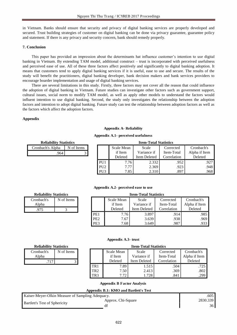
Nguyen Thi Thu Trang / ICYREB 2017 Proceedings
in Vietnam. Banks should ensure that security and privacy of digital banking services are properly developed and secured. Trust building strategies of customer on digital banking can be done via privacy guarantee, guarantee policy and statement. If there is any privacy and security concern, bank should remedy properly.
7. Conclusion
This paper has provided an impression about the determinants hat influence customer’s intention to use digital banking in Vietnam. By extending TAM model, additional construct – trust is incorporated with perceived usefulness and perceived ease of use. All of these three factors affect positively and significantly to digital banking adoption. It means that customers tend to apply digital banking services if it is useful, ease to use and secure. The results of the study will benefit the practitioners, digital banking developer, bank decision makers and bank services providers to encourage boarder implementation and usage of digital banking services.
There are several limitations in this study. Firstly, three factors may not cover all the reason that could influence the adoption of digital banking in Vietnam. Future studies can investigate other factors such as government support, cultural issues, social norm to modify TAM model, as well as apply other models to understand the factors would influent intention to use digital banking. Second, the study only investigates the relationship between the adoption factors and intention to adopt digital banking. Future study can test the relationship between adoption factors as well as the factors which affect the adoption factors.
Appendix
Appendix A- Reliability
Appendix A.1- perceived usefulness
Reliability Statistics Cronbach's Alpha N of Items
.964 3
Item-Total Statistics Scale Mean
if Item Deleted
Scale Variance if
Item Deleted
Corrected Item-Total Correlation
Cronbach's Alpha if Item
Deleted PU1 7.76 2.332 .952 .927 PU2 7.77 2.369 .923 .948 PU3 7.85 2.310 .897 .968
Appendix A.2- perceived ease to use
Reliability Statistics Cronbach's
Alpha N of Items
.975 3
Item-Total Statistics Scale Mean
if Item Deleted
Scale Variance if
Item Deleted
Corrected Item-Total Correlation
Cronbach's Alpha if Item
Deleted PE1 7.76 3.897 .914 .985 PE2 7.67 3.639 .938 .969 PE3 7.68 3.649 .987 .933
Appendix A.3- trust
Reliability Statistics Cronbach's
Alpha N of Items
.717 3
Item-Total Statistics Scale Mean
if Item Deleted
Scale Variance if
Item Deleted
Corrected Item-Total Correlation
Cronbach's Alpha if Item
Deleted TR1 7.89 1.515 .504 .725 TR2 7.50 2.413 .369 .802 TR3 7.72 1.728 .841 .299
Appendix B Factor Analysis
Appendix B.1: KMO and Bartlett's Test Kaiser-Meyer-Olkin Measure of Sampling Adequacy. .605
Bartlett's Test of Sphericity Approx. Chi-Square 2830.339 df 36
622

Nguyen Thi Thu Trang / ICYREB 2017 Proceedings
Sig. .000
Appendix B.3: Total Variance Explained Component
Initial Eigenvalues Extraction Sums of Squared Loadings
Rotation Sums of Squared Loadings
Total % of Variance
Cumulative %
Total % of Varianc
e
Cumulative %
Total % of Variance
Cumulative %
1 3.253 36.143 36.143 3.253 36.143 36.143 2.866 31.844 31.844 2 2.528 28.089 64.232 2.528 28.089 64.232 2.816 31.293 63.137 3 1.920 21.331 85.563 1.920 21.331 85.563 2.018 22.426 85.563 4 .803 8.923 94.486 5 .176 1.957 96.443 6 .136 1.509 97.953 7 .122 1.354 99.307 8 .048 .537 99.844 9 .014 .156 100.000 Extraction Method: Principal Component Analysis. Appendix B.4: Rotated Component Matrixa Component
1 2 3 PE3 .990 PE2 .967 PE1 .961 PU1 .976 PU2 .958 PU3 .951 TR3 .949 TR1 .810 TR2 .670
Appendix C: Correlations
Appendix C: Correlations PU PE TR IU
PU Pearson Correlation 1 .145* .077 .285**
Sig. (2-tailed) .016 .208 .000 N 272 272 272 272
PE Pearson Correlation .145* 1 -.043 .334**
Sig. (2-tailed) .016 .475 .000 N 272 272 272 272
TR Pearson Correlation .077 -.043 1 .331**
Sig. (2-tailed) .208 .475 .000 N 272 272 272 272
IU Pearson Correlation .285** .334** .075 1
Appendix B.2: Communalities Initial Extraction PU1 1.000 .961 PU2 1.000 .932 PU3 1.000 .908 PE1 1.000 .928 PE2 1.000 .945 PE3 1.000 .987 TR1 1.000 .661 TR2 1.000 .473 TR3 1.000 .905 Extraction Method: Principal Component Analysis.
623
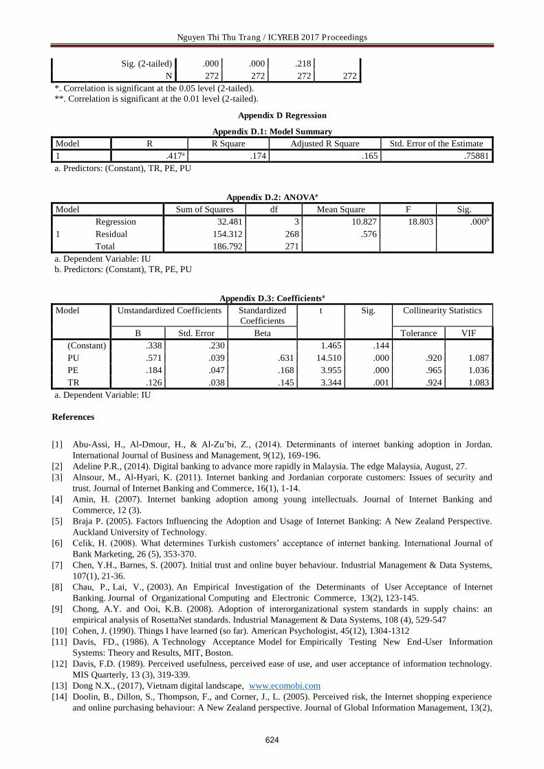
Nguyen Thi Thu Trang / ICYREB 2017 Proceedings
Sig. (2-tailed) .000 .000 .218 N 272 272 272 272
*. Correlation is significant at the 0.05 level (2-tailed). **. Correlation is significant at the 0.01 level (2-tailed).
Appendix D Regression
Appendix D.1: Model Summary Model R R Square Adjusted R Square Std. Error of the Estimate 1 .417a .174 .165 .75881 a. Predictors: (Constant), TR, PE, PU
Appendix D.2: ANOVAa
Model Sum of Squares df Mean Square F Sig.
1 Regression 32.481 3 10.827 18.803 .000b Residual 154.312 268 .576 Total 186.792 271
a. Dependent Variable: IU b. Predictors: (Constant), TR, PE, PU
Appendix D.3: Coefficientsa
Model Unstandardized Coefficients Standardized Coefficients
t Sig. Collinearity Statistics
B Std. Error Beta Tolerance VIF
(Constant) .338 .230 1.465 .144 PU .571 .039 .631 14.510 .000 .920 1.087 PE .184 .047 .168 3.955 .000 .965 1.036 TR .126 .038 .145 3.344 .001 .924 1.083
a. Dependent Variable: IU
References
[1] Abu-Assi, H., Al-Dmour, H., & Al-Zu’bi, Z., (2014). Determinants of internet banking adoption in Jordan. International Journal of Business and Management, 9(12), 169-196.
[2] Adeline P.R., (2014). Digital banking to advance more rapidly in Malaysia. The edge Malaysia, August, 27. [3] Alnsour, M., Al-Hyari, K. (2011). Internet banking and Jordanian corporate customers: Issues of security and
trust. Journal of Internet Banking and Commerce, 16(1), 1-14. [4] Amin, H. (2007). Internet banking adoption among young intellectuals. Journal of Internet Banking and
Commerce, 12 (3). [5] Braja P. (2005). Factors Influencing the Adoption and Usage of Internet Banking: A New Zealand Perspective.
Auckland University of Technology. [6] Celik, H. (2008). What determines Turkish customers’ acceptance of internet banking. International Journal of
Bank Marketing, 26 (5), 353-370. [7] Chen, Y.H., Barnes, S. (2007). Initial trust and online buyer behaviour. Industrial Management & Data Systems,
107(1), 21-36. [8] Chau, P., Lai, V., (2003). An Empirical Investigation of the Determinants of User Acceptance of Internet
Banking. Journal of Organizational Computing and Electronic Commerce, 13(2), 123-145. [9] Chong, A.Y. and Ooi, K.B. (2008). Adoption of interorganizational system standards in supply chains: an
empirical analysis of RosettaNet standards. Industrial Management & Data Systems, 108 (4), 529-547 [10] Cohen, J. (1990). Things I have learned (so far). American Psychologist, 45(12), 1304-1312 [11] Davis, FD., (1986). A Technology Acceptance Model for Empirically Testing New End-User Information
Systems: Theory and Results, MIT, Boston. [12] Davis, F.D. (1989). Perceived usefulness, perceived ease of use, and user acceptance of information technology.
MIS Quarterly, 13 (3), 319-339. [13] Dong N.X., (2017), Vietnam digital landscape, www.ecomobi.com [14] Doolin, B., Dillon, S., Thompson, F., and Corner, J., L. (2005). Perceived risk, the Internet shopping experience
and online purchasing behaviour: A New Zealand perspective. Journal of Global Information Management, 13(2),
624

Nguyen Thi Thu Trang / ICYREB 2017 Proceedings
66-88. [15] Eriksson, K., Kerem, K., and Nilsson, D. (2005). Customer acceptance of internet banking inEstonia. International
Journal of Bank Marketing, 23(2), 200-216. [16] Fergus G., Mathias U., James D., and Stefan M., (2015). Banking in a Digital World. A.T. Kearney and Efma [17] Field, A. (2005). Discovering Statistics Using SPSS, (2nd ed.). Sage Publications, London [18] Flavian, C., Guinaliu, M. and Gurrea, R. (2006). The role played by perceived usability, satisfaction and consumer
trust on website loyalty. Information and Management, 43, 1-14 [19] Gaurav S., (2017). What is Digital Banking? available at http://www.ventureskies.com/blog/digital-banking,
accessed 17 August 2017. [20] Ginovsky, J., (2015). What really is "digital banking"?. Banking Exchange. [21] Goles, T., Lee, S.J., Rao, S.V. and Warren, J. (2009). Trust violations in electronic commerce: customer concerns
and reactions. Journal of Computer Information Systems, 49 (1), 1-9. [22] Gounaris, S., Koritos, C. (2008). Investigating the drivers of internet banking adoption decision: a comparison of
three alternative frameworks. International Journal of Bank Marketing, 26(5), 282-304. [23] Guriting, P., Ndubisi, N., (2006). Borneo online banking: evaluating customer perceptions and behavioural
intention. Management Research News, 29(1/2), 6-15. [24] Hair, J., Black, W., Babin, B., Anderson, R. and Tatham, R. (2005). Multivariate Data Analysis (6th ed). Prentice-
Hall, Englewood Cliffs, NJ. [25] Hernandez, J.M.C. and Mazzon, J.A. (2007). Adoption of internet banking: proposition and implementation of an
integrated methodology approach. International Journal of Bank Marketing, 25(2), 72-88. [26] Hoang, D.T., Igel, B. and Laosirihongthong, T. (2006). The impact of total quality management on innovation,
findings from a developing country. International Journal of Quality & Reliability Management, 23(9), 1092-117. [27] Hoang, M.C. (2003). Current status of Vietnamese e-commerce. available at:
http://unpan1.un.org/intradoc/groups/public/../UNPAN008970.pdf (accessed 17 August 2017). [28] Holsapple, C.W. and Sasidharan, S. (2005). The dynamics of trust in B2C e-commerce: a research model and
agenda. Information System E-business Management, 3(4), 377-403. [29] Jahangir, N. and Begum, N. (2008). The role of perceived usefulness, perceived ease of use, security and privacy,
and customer attitude to engender customer adaption in the context of electronic banking. Africa Journal of Business Management, 2(1), 32-40.
[30] Jaruwachirathanakul, B., Fink, D., (2005). Internet Banking Adoption Strategies for a Developing country: The Case of Thailand. Internet Research, 15(3), 295-311.
[31] Jeyaraj, A., Rottman, J.W. and Lacity, M.C. (2006). A review of the predictors, linkages and biases in IT innovation adoption research. Journal of Information Technology, 21(1), 1-23.
[32] Jitpaiboon, T., Rao, S.S. (2007). A meta-analysis of quality measures in manufacturing system. International Journal of Quality and Reliability Management, 24(1), 78-102.
[33] Kaiser, H., (1974). An index of factorial simplicity. Psychometrika, 39(1), 31-36. [34] Kline, R.B. (1998). Principles and Practices of Structural Equation Modeling. Guilford, New York, NY [35] Lu, J., Yu, C.S., Liu, C. and Yao, J.E. (2003). Technology acceptance model for wireless internet. Internet
Research, 13(3), 206-22. [36] Luarn, P. and Lin, H.H., (2005). Toward an understanding of the behavioral intention to use mobile banking.
Computer in Human Behaviour, 21(6), 873-91. [37] Moeckel, C., (2013). Definition of Digital Banking. available at http://www.carolinemoeckel.com/defining-
digital-banking/. accessed 17 August 2017 [38] Mukherjee, A & Nath, P., (2003). A Model of Trust in Online Relationship Banking. International Journal
of Bank Marketing, 21(1), 5-15. [39] Nasri, W. and Charfeddine, L. (2012). Factors Affecting the Adoption of Internet Banking in Tunisia: An
Integration Theory of Acceptance Model and Theory of Planned Behaviour. The Journal of High Technology Management Research, 23, 1-14.
[40] Nunnally, J.C., (1978). Psychometric Theory, McGraw-Hill, New York, [41] Pikkarainen, T., Pikkarainen, K., Karjaluoto, K., & Pahnila, S., (2004). Consumer Acceptance of Online
Banking: An Extension of the Technology Acceptance Model. Internet Research, 14(3), 224-235. [42] Sathye, M., (1999). Adoption of Internet banking by Australian consumers: an empirical investigation.
International Journal of Bank Marketing, 17(7), 324-334. [43] Shih, Y., and Fang, K,. (2004). The use of a decomposed theory of planned behavior to study internet banking in
Taiwan. Internet Research,14(3), 213-223. [44] Sonia B., and Vinayak H.V., (2015). Digital Banking in Asia: What do consumers really want?, McKinsey &
Company [45] Standey E., (2015). Understanding digital banking. available at:
http://www.finextra.com/blogs/fullblog.aspx?blogid=10390. accessed 17 August 2017 [46] Tan, M. and Teo, T.S.H., (2000). Factors influencing the adoption of internet banking. Journal of the Association
625

Nguyen Thi Thu Trang / ICYREB 2017 Proceedings
for Information Systems, 1(1),1-42. [47] Teo, T.S.H., Lim, V.K.G., and Lai, R.Y.C., (1999). Intrinsic and extrinsic motivation in internet usage.
International Journal of Management Science, 27(1), 25–37. [48] Venkatesh, V., Morris, M. G., Davis, G. B., & Davis, F. D. (2003). User acceptance of information technology:
Toward a unified view. MIS Quarterly, 27(3), 425-478. [49] Thanh V.T.H., (2016). Digital banking- the new paradigm for commercial banks in Vietnam”, Banking journal,
21, 32- 40. [50] Yang, M.H., Chandlrees, N., Lin, B. and Chao, H.Y., (2009). The effect of perceived ethical performance of
shopping web sites on consumer trust. Journal of Computer Information Systems, 50(1), 15-24. [51] Yiu, C., Grant, K., Edgar, D., (2007). Factors Affecting the Adoption of Internet Banking in Hong Kong-
Implications for the Banking Sector. International Journal of Information Management, 27, 336–351. [52] Wang, Y., Wang, Y., Lin, H., & Tang, T., (2003). Determinants of User Acceptance of Internet Banking:
An Empirical Study. International Journal of Service Industry Management, 14(5), 501-519. [53] Wong, C.C. and Hiew, P.L., (2005). Diffusion of mobile entertainment in Malaysia: drivers and barriers.
Enformatika, 5, 263-266.
626

Le Nguyen, Nguyen Hanh/ ICYREB 2017 Proceedings
International Conference For Young Researchers In Economics And Business, ICYREB 2017, October 30th 2017 Da Nang, Vietnam
The Impact of Foreign Direct Investment, Economic Growth and
Energy Consumption on Carbon Dioxide Emission in 10 Asian
Countries
Le Nguyena, Nguyen Hanhb*
aFinance – Banking University Hanoi, Vietnam bFinance – University of Economics Ho Chi Minh City, Vietnam.
A B S T R A C T
The main purpose of this article was to explore the impact of foreign direct investment, abbreviated as FDI, the economic growth and energy consumption on carbon dioxide emissions in 10 Asian countries, including China, India, Indonesia, Malaysia, Philippines, Singapore, Thailand, Myanmar, Cambodia and Vietnam. The paper used the quintile regression of data table, the results showed that: (i) the impact of independent variables on carbon dioxin emissions are not heterogeneous across the quintile points. (ii) The impact of FDI on carbon dioxin emissions is negative; (iii) the consumption of energy contributed to the increasing of carbon dioxin emissions, with the greatest impact, which was occurred in the countries with high consumption of energy such as China or India. In addition, trade openness, size of population; industry’s structure and the financial development also had significant impacts on carbon dioxin emissions.
Keywords: FDI, carbon dioxin emissions, quintile regression, consumption of energy
1. Introduction
Climate change, global warming and other environmental issues were becoming important issues that need to be addressed and solved together by each nation and the whole of humanity. More than ever, our living environment was experiencing serious changes; referring to the causes and consequences of such changes, which could not be without the human elements. Economic development has always impacted on the environment even more or less; and human impact on the climate system was inevitably. The relationship between the activities of economic development and environmental pollution was complex. Economic development brought and aggravated the problem in environmental pollution. In contrast, the polluted environment also caused much harm and impediment to economic activities.
One of the direct causes of climate change was the rapidly increasing in greenhouse gas emissions, most of which were carbon dioxide; carbon dioxide was largely derived from human activities. Currently, the amount of carbon dioxide in the atmosphere was at the highest level in history. Therefore, the researches on the factors that impacted carbon dioxide emissions were very practical and deserved special attention. There were many endogenous and exogenous factors that affected carbon dioxide emissions. Among them, the highlights were studies on the impact of foreign direct investment (FDI), economic growth and energy consumption.
In the context of the world was developing and complex as today, Asia continued to assert its roles with international friends. According to the statistics in recent years, Asia had consistently been a leader in attracting FDI from outside, especially in Southeast Asia, China and India. Many countries in the region had maintained a high level of economic growth and the energy consumption had also shown an increasing trend. However, the current state of the environment in the area had a lot of negative developments.
With the above realities, this paper was designed to examine and measure the effects of economic growth, FDI and energy consumption on carbon dioxin emissions in 10 Asian countries from the year 2000 to 2015. The study was conducted from the beginning with samples of all 10 countries, and then divided into two smaller samples of 5 countries per sample to provide more valuable evidence. In addition, in order to help reflect more relevant aspects of carbon
* Le Nguyen. Tel.: +84908898586. E-mail address: [email protected]. Nguyen Hanh. Tel: +84975202423. Email address: [email protected].
627

Le Nguyen, Nguyen Hanh/ ICYREB 2017 Proceedings
dioxin emissions, the author also added some controllable variables to the model.
The research paper used the data from 10 selected countries in Asia, including China, India, Singapore, Thailand, Philippines, Myanmar, Malaysia, Indonesia, Cambodia and Vietnam in the period of 2000-2015, using the quintile regression of data table model. Relevant data was obtained from the World Bank database and the United Nations Conference on Trade and Development (UNCTAD).
2. Literature Review and Previous Studies on Relationship between Economic Growth, FDI and Energy Consumption on Carbon Dioxide Emission
2.1. Literature review
In examining the relationship between economic growth and environmental pollution, the Environment Kuznets Curve (EKC) hypothesis was highlighted. This was a very popular and widely used hypothesis in the study of environment and economy.
Firstly, the theory was used to describe the relationship between economic development and unequal income, but from the beginning of 1991 it became the method, which was used to describe the relationship between environmental quality (often was used to represent by carbon dioxide emission) and income per capita (real GDP per capita or income) over time. Accordingly, in the early stages of economic growth, as GDP per capita raised, the environment was recessed. Next, the recession would increase to a certain degree, and when it reached to a turning point; then it would show to have a negative impact. At this time, an increase in GDP per capita would lead to a decline in environmental pollution.
Several different arguments have been given to explain the shape of the Environmental Kuznets Curve. From a consumer's point of view, at a lower level of income, people paid more attention to employment and income than to the issues of clean-environment so the pollution would increase significantly. The points of view of the stages of economic growth was: in the early stages of industrialization, priorities were aimed to the increase of industrial outputs, rapid economic development and the use of natural resources; these actions created a series of serious pollutants. At the later stages of industrialization, as incomes rise, the trend of society became more focusing on service sectors, which were less polluted. In addition, other points of view suggested that: over time, the process of economic growth had made laws and environmental policies more stringent and more effective; in addition, modern and advanced technologies, which were widely used, also reduced the pollution.
Although the Environmental Kuznets Curve Theory was also used to explain the relationship between FDI and carbon dioxide emission; however, many studies seemed to show the prominence of a linear relationship, which was expressed through two opposite hypotheses. These were the pollution haven hypothesis and the heliospheric propagation effect hypothesis (halo effect).
The pollution haven hypothesis suggested that besides the purpose of exploiting natural resources and advantages in developing regions, FDI inflows also aimed towards to find new places in order to dispose of untreated waste; whether in developed countries, businesses were not allowed to do or could not do it due to strict regulations or high costs. In addition, for the purpose of attracting foreign investment, developing countries tended to ignore environmental
Pollution Level
Non – industrial Economy
“Turning point”
Industrial Economy
Service Economy
Income per capita (economic development)
Figure 1 Environmental Kuznets Curve
628
Le Nguyen, Nguyen Hanh/ ICYREB 2017 Proceedings
concerns through easy or non-binding rules for foreign investors. The result of this process was the dramatic shift of heavy industries, where most of the emission were likely to cause environmental pollution such as mining, paper, leather, textiles, iron and steel, commonly used as “dirty" industries, from developed to developing countries. Therefore, FDI could generally promote carbon dioxide emission (Pao and Tsai, 2011).
However, in a different approach, studies had shown that the effect of FDI on the environment, which could be reversed, when the technology of low carbon dioxide was introduced to reduce carbon dioxide emission or the FDI investment focused mainly on service industries. It was assumed that foreign companies, which invested in a country, would also use the best practical applications of management and high technologies to help a clean environment in host countries (Zarsky, 1999). This phenomenon was known as the hypothesis of heliospheric propagation effect. Similarly, Zeng and Eastin (2012) found that the FDI inflows in less developed countries generally promoted better environmental awareness.
2.2. Overview of Previous Studies
2.2.1. The relationship between economic growth and carbon dioxide emission
Many studies had found an inverse U-shaped relationship between economic growth and carbon dioxide emission as evidence to support the EKC theory. Research with 58 countries in 1980, (Grossman and Krueger, 1995) found that the relationship between per capita income and environmental recession was in accordance with the rule of inversed U curve. Lean and Smyth (2010) conducted a study, which used a vector error correcting model (VECM), to find the relationship between economic growth and carbon dioxide emission in five ASEAN countries. With the use of annual data for the period 1980-2006, empirical results suggested that, in general, there seemed to be evidences to consolidate the EKC theory in the five ASEAN countries. The study of the relationship between income and carbon dioxide emission in Spain of Esteve and Tamarit (2012) also recognized the existence of the Environmental Kuznets Curve. Furthermore, Heidari and et al. (2015) also used the PSTR model to examine the relationship between economic growth, energy consumption and carbon dioxide emission. The empirical results also consolidated the importance of EKC in ASEAN countries.
Although the theory of the relationship between economic development and environmental quality (EKC) defined an inverse U-shaped relationship between economic growth and carbon dioxide emission; however, there were some evidences to show that there were other shapes in the EKC hypothesis. By reviewing annual data for the period 1980-2011 in Saudi Arabian, Khalid and Muhammad (2013) demonstrated a linear relationship when carbon dioxide emission increased along with an increase in average income per capita; and a related N-shaped relationship was found by He and Richard (2010) when they researched in Canada during 1948-2004.
In addition, several other studies had found that EKC was null. By comparing long-run and short-term elasticity of income, Narayan and Narayan (2010) showed that no country in the sample (Indonesia, Malaysia, the Philippines and Thailand) was supported by the EKC theory. Similarly, Chandra and Tang (2013) used method of cointegration and cause and effect analysis to test the EKC theory of five ASEAN countries based on annual data from 1971 to 2008, which showed that the inversed U-shaped of EKC theory did not apply to the economies of the five ASEAN countries. Several reasons might be given to explain the significant differences in above conclusions: the samples, which were used for analysis in the studies, were different; the model and method, which were used to estimate the relationship, were different; and the variables in the model were diversified.
Therefore, many empirical studies had arisen to present the proofs of the validity of the Environmental Kuznets Curve theory; however, the results of the study were clearly lacked in uniformity.
2.2.2. The relationship between foreign direct investment and CO2 emission
Cole (2014) examined the inversed U-shaped relationship of EKC by commerce, especially the migration and replacement of "dirty" industries from the developed to the developing regions (the pollution haven hypothesis). By using specific data of commercial capital of North and South areas for highly polluted products, evidences of the pollution haven hypothesis were inspected. Merican and et al. (2007) affirmed that there was the relationship between FDI and pollution in five ASEAN countries. Using autoregressive distributed lag model (ARDL), the authors found that FDI increased emission in Malaysia, Thailand, and the Philippines; however, there seemed to be a reversed relationship between FDI and pollution in Indonesia.
Atici (2012) examined the interactions between commerce and the environment on carbon dioxide emission in ASEAN countries. Using both random and fixed effects model analysis, the results of the table showed that FDI had some impacts on carbon dioxide emission; in general, the results showed that FDI brought some benefits to ASEAN countries in reducing emission. However, the results for the group of countries including Indonesia, Malaysia, Thailand and the Philippines indicated that FDI had no significant impacts on carbon dioxide emission.
Asghari (2013) examined the pollution haven hypothesis and the heliospheric propagation effect hypothesis (halo effect hypothesis) by identifying the link between carbon dioxide emission and FDI inflows during the period 1980-
629

Le Nguyen, Nguyen Hanh/ ICYREB 2017 Proceedings
2011 in the sample group of MENA countries. Statistical results showed that FDI had a weak and negative impacts; FDI also had statistically significant relationship with carbon dioxide emission, which showed a weakness of the hypothesis of the heliospheric propagation effect.
On the other hand, (He, 2006) conducted a research in China from 1994 to 2001, the results showed that FDI played a very small role in the increasing of carbon dioxide emission.
2.2.3. Relationship between energy consumption and carbon dioxide emission
The impact of energy consumption on carbon dioxide emission was also argued by many researchers. Some studies had shown that energy consumption had a positive effect on carbon dioxide emission (Acaravci and Ozturk, 2010; Pao and et al, 2011) while others had shown that carbon dioxide emission were not related to the energy consumption (Salim et al, 2008; Apergis et al, 2010; Menyah and Wolde, 2010).
Lean and Smyth (2010) found important long-term relationships between energy consumption and carbon dioxide emission in all 5 ASEAN countries. The data of cause and effect analysis showed that there was a one-way cause and effect relationship between carbon dioxide emission and short-term consumption. Bloch and et al (2012) explored the relationship between coal consumption and carbon dioxide emission in China using both supply and demand frameworks, and their results revealed a cause and effect relationship between coal consumption and emission in both short and long term. Saboori and Sulaiman (2013) also found a two-way cause and effect relationship between energy consumption and carbon dioxide emission in all five ASEAN countries. The implication was that carbon emission and energy consumption were related closely to each other. In addition, Tang and Tan (2015) also used method of cointegration and cause and effect analysis to test the impact of energy consumption, income, and FDI on carbon dioxide emission in Vietnam. They found that energy consumption was a cause of carbon dioxide emission in both short-term and long-term. Furthermore, that paper also argued that energy consumption, FDI and income were the key of carbon dioxide emission in Vietnam. Similarly, Wang and et al (2016) also explored the relationship between urbanization, energy consumption and carbon emission on a table data from ASEAN countries using the FMOLS method. Experimental results indicated a significant positive relationship between long-term use of energy and carbon dioxide emission.
3. Research Methods
3.1. Research data
The data in this study was taken from the World Development Indicators of World Bank for most variables. Particularly data on economic growth was represented by real GDP per capita in constant USD price in 2005; the statistical data was collected from the Development Cooperation Forum of United Nations. Data were collected for 10 Asian countries: China, India, Thailand, Singapore, Philippines, Indonesia, Malaysia, Myanmar, Cambodia and Vietnam from 2000 to 2015. All variables, excepted for foreign direct investment, were converted to natural logarithms before doing the empirical analysis.
In this study, the author used table data to study the modalities of carbon dioxide emission in ASEAN countries. The use of table data had the advantages over the focusing on only one country or a period of time because the table data could provide more information, more diversity, more flexibility and limiting the multicollinearity; therefore, according to the prediction, the efficiency would increase higher (Lean and Smyth, 2010). The table data model could also adapt to the heterogeneity of the variables in the sample. Moreover, according to Baltagi (2005), table data could detect and measure better than the effects, which could not be observed in time series or cross-sectional data, which helped the author to study more complex behavioural modelling.
3.2. Research methods and regression models
In this article, the author used a fixed – effects quintile regression model to explore the impact of FDI, economic growth, and energy consumption on carbon dioxide emission. The motivation for choosing this model came from the following reasons: First, fixed-effects quintile regression could describe the full distribution with conditions of dependent variables; therefore, it helped the author to observe a more comprehensive picture of the factors, which were involved in the discharge of pollutants. In particularly, the estimation of quintile regression could provide a solution for each quintile. Using this model, the author could evaluate the mode of emission throughout the conditional distribution, especially in the countries with the highest or the lowest emission. On the other hand, OLS techniques were not suitable for creating environmental protection policies for countries with high levels of emission. Secondly, the results from the quintile regression model were strongly impacted with the abnormal observations of explained variables and were more effective than the OLS method, which made policy makers to construct better environmental protection policies.
The quintile regression model was firstly introduced by Koenker and Bassett in 1978. This method was the general of the median analysis regression with different quintile points. The quintile with condition of yi was given by
630

Le Nguyen, Nguyen Hanh/ ICYREB 2017 Proceedings
xi as formula: From the above quintile regression model, H. Zhu and et al (2016) developed a regression formula of the factors
that affected the carbon dioxide emission for the τ quintile as follows:
Where, i represented the countries, t represented the time and Yit was the level of emission.
3.3. Description of the variables
The variables, which were used in the model, were shown in the following table:
Table 1 Summary of variables used in the regression model
No Name of variables Acronym Expected sign
Sources of information
Dependent variables 1 carbon dioxide emission CO2 World Development Indicators Independent variables 2 Foreign Direct Investment FDI +/- World Development Indicators 3 Energy Consumption ENC + World Development Indicators 4 Gross Domestic Product GDP +/- UNCTADSTAT Controllable variables 5 Open trade TRADE - World Development Indicators 6 Industry structure INDUS + World Development Indicators 7 Financial development FINAN - World Development Indicators 8 Total population POP + World Development Indicators
4. Results and Discussion
4.1. Descriptive statistics
Table 2 Variables and Statistics
VARIABLE N MEAN S.D. MIN 0.25 MDN 0.75 MAX CO2 140 2.97 2.94 0.16 0.87 1.54 4.72 12.17 ENC 140 1366.39 1480.64 250.38 424.59 706.72 1763.10 7370.40 GDP 157 4900.95 9223.62 136.66 684.45 1333.99 3428.01 37923.39 POP 160 3076.21 4797.32 40.28 269.64 727.95 2338.29 13712.20 TRADE 160 119.17 101.87 0.17 48.84 103.47 139.65 439.66 INDUS 160 34.56 8.40 9.69 28.49 34.47 40.48 48.53 FDI 160 4.68 5.33 -2.76 2.00 3.23 4.71 26.52 FINAN 160 66.64 44.46 3.12 28.19 52.03 106.82 153.34
4.2. Regression results
4.2.1. Testing units
The results of the data test of the variables showed that beside the two POP and FDI variables stopped at the 0 difference, the data sequences of the remaining independent variables and the dependent CO2 variables both stopped at 1 difference.
4.2.2. Cointegration testing
For the testing of cointegration, we used the Kao Residual Cointegration Test With the Ho hypothesis: There was no cointegration between variables H1: There was at least 1 cointegration between the variables The p-value testing was zero, with a significance level of 1%, assuming Ho was rejected: the pattern existed for at
least one cointegration, indicated the relationship of the variables in the long run. The test results were consistent with the hypothesis of table data regression model.
631

Le Nguyen, Nguyen Hanh/ ICYREB 2017 Proceedings
4.2.3. Analysis of correlation between variables
All variables had a positive correlation with the CO2 dependent variable. In particular, the ENC and GDP variables showed a high positive correlation with coefficients of 0.8838 and 0.7244 respectively. FDI variables also showed a positive correlation with emission variable with coefficient of 0.5148. This result was true of initial expectations because the study was observed briefly and most of the countries in the sample were developing countries. In addition, the coefficients of the TRADE and FINAN variables were also highly correlated while the coefficients of the POP variables were not significant.
4.2.4. OLS regression results
In order to facilitate comparison, the model was first estimated by using estimation of pooled OLS regression, followed by the estimation of OLS one – way fixed effects, OLS two-way fixed effects and FMOLS regression. In general, the regression results showed that the coefficient of economic growth, FDI, trade openness and financial development were negative while the coefficients of the remaining variables are positive.
Table 3 Estimation of Pooled OLS regression for 10 Asian countries
The pooled OLS regression results indicated that energy consumption and population size and industry structure could increase carbon dioxide emission; while the other variables, which included economic growth, open trade, FDI, and financial development, had a negative impact on the dependent variables. However, only the effects of energy consumption, open trade and FDI were significant on carbon dioxide emission. While increasing energy consumption led to the increasing of carbon dioxide emission, the greater open trade and higher FDI inflows had the effect of reducing the emission of carbon dioxide. This result was similar when applied to the FMOLS model.
The results somehow changed when evaluating by the two remaining OLS regression methods (data table results were presented in the appendix). For the one-way fixed effect regression model, the results showed that the structure of the industry together with energy consumption and new FDI flows were factors that affected carbon dioxide emission. Accordingly, the industry structure showed that a similar effect in the same way, while the result of FDI and energy consumption were similar to the pooled OLS model. Finally, when considering the two-way fixed effect OLS model, only energy consumption and FDI were statistically significant, implying that these factors had real impact on carbon dioxide emission.
4.2.5. Quintile regression results
_cons -.020046 .0904321 -0.22 0.825 -.1988463 .1587543
dfinan -.0043277 .0117015 -0.37 0.712 -.0274637 .0188082
dfdi -.1095074 .0244008 -4.49 0.000 -.1577521 -.0612627
dindus .0604237 .0486641 1.24 0.216 -.0357939 .1566412
dtrade -.0113206 .0062535 -1.81 0.072 -.023685 .0010438
dpop .0001986 .0013188 0.15 0.881 -.002409 .0028061
dgdp -.0000134 .0001672 -0.08 0.936 -.0003439 .0003172
denc .0019189 .0001159 16.56 0.000 .0016898 .002148
dco2 Coef. Std. Err. t P>|t| [95% Conf. Interval]
Total 284.926981 146 1.95155466 Root MSE = .8218
Adj R-squared = 0.6539
Residual 93.8754992 139 .675363303 R-squared = 0.6705
Model 191.051482 7 27.2930688 Prob > F = 0.0000
F( 7, 139) = 40.41
Source SS df MS Number of obs = 147
632

Le Nguyen, Nguyen Hanh/ ICYREB 2017 Proceedings
Table 4 results of estimation of data table quintile regression for 10 Asian countries.
5th 10th 20th 30th 40th 50th 60th 70th 80th 90th 95th
denc 0.003***
0.003***
0.003***
0.002***
0.002***
0.002***
0.002***
0.002***
0.002***
-6.926E+09 3.635E+11
(0.000) (0.000) (0.000) (0.000) (0.000) (0.000) (0.000) (0.000) (0.000) (7.270E+09)
(4.451E+11)
dgdp -0.000
-0.000***
-0.001***
-0.001***
-0.001***
-0.001***
-0.000***
-0.000*** -0.000**
-5.585E+10 5.260E+11
(0.000) (0.000) 0.000 0.000 0.000 0.000 0.000 0.000 0.000 (6.105E+10)
(6.861E+11)
dgdp2
-0.000***
-0.000***
0.000***
0.000***
0.000***
0.000***
0.000***
0.000***
0.000*** 1.723E+07
-2.897E+08
(0.000) (0.000) 0.000 0.000 0.000 0.000 0.000 0.000 0.000 (1.888E+07)
(3.666E+08)
dpop -0.001** 0.000***
0.000*** 0.000 -0.000
0.000*** 0.000 0.000 0.000
-1.853E+10
-2.746E+12
(0.000) 0.000 0.000 0.000 0.000 0.000 0.000 0.000 0.000 (2.145E+10)
(3.397E+12)
dtrade
-0.010***
-0.002***
-0.002***
-0.002***
-0.001***
-0.000*** (0.001) -0.002** -0.004**
-1.320E+12 1.590E+12
(0.002) (0.001) 0.000 0.000 0.000 0.000 0.000 (0.001) (0.002) (1.368E+12)
(2.146E+12)
dindus
0.079***
0.015***
0.013***
0.008*** 0.012**
0.002*** 0.002* (0.001) (0.001) 4.288E+12
-3.899E+13
(0.014) (0.001) (0.001) (0.002) (0.005) 0.000 (0.001) (0.004) (0.007) (4.523E+12)
(5.101E+13)
dfdi -0.022** -0.019** 0.002*** 0.001 -0.000
-0.005***
-0.006***
-0.013***
-0.039***
-4.503E+11 8.132E+13
(0.011) (0.008) (0.001) (0.001) (0.003) 0.000 (0.002) (0.002) (0.008) (8.501E+11)
(1.017E+14)
dfinan
-0.006*** -0.000
0.002***
0.002*** 0.001
-0.001*** 0.001 (0.002)
-0.011*** 8.927E+11 6.818E+12
(0.002) 0.000 (0.001) (0.001) (0.001) 0.000 (0.001) (0.002) (0.001) (9.529E+11)
(8.272E+12)
N 147 147 147 147 147 147 147 147 147 147 147
Note: ***: significant at 1%, **: significant at 5%, *: significant at 10% Results were reported for the percentage number of 5, 10, 20, 30, 40, 50, 60, 70, 80, 90 and 95. Overall,
experimental results showed that the effects of multiple carbon emission factors were clearly not uniformed. For the FDI, at the 5 and 10 percentile quintile, the coefficient of FDI was negative at a significant level of 5%.
Next, the coefficients of the quintile at 50, 60, 70 percentile were also negative and became important at the significant level of 1%. Only the quintile at 20 percentile level showed a positive effect and the coefficients of the other quintiles were not statistically significant. This implied that the impact of FDI on carbon dioxide emission was more negative and important in low-emission countries; the evidences supported the hypothesis of halo effect in these countries. On the other hand, the impact of FDI was not significant at the highest quintile at 90, 95 percentile points; while in OLS models, it was very important, it seemed that OLS regression had overestimated the impact of FDI variables.
The coefficients of GDP variable were very important and had the negatively affect to most quintile points. The coefficients of GDP2 were also significant, which indicated negative signs at the first quintile points (5 and 10), and were positive at the next quintile points, which implied that the inversed U-shaped hypothesis was not applicable to Asian countries in this sample. The results showed that the economic growth had an impact on carbon dioxide emission: an increasing in economic growth could reduce carbon dioxide emission in the countries. On the other hand, while the coefficients of GDP showed that the negative signs in the two-way fixed-effects OLS regression model and the FMOLS model; the pooled OLS regression model and the one-way fixed-effect OLS regression model were positive. However, the coefficients of GDP in these regression models were not statistically significant. It seemed that these results suggested that the quintile regression was correcting the heterogeneous for distribution, and also might reduce the ability to underestimate or overestimate the relative coefficients of OLS regression models. These results again demonstrated the suitability of the quintile regression in the study of factors, which affected carbon dioxide emission in different countries.
In addition, the author could see that the same sign effect of energy consumption on emission was significant, which meant very high at 1% for most quintile points. However, the coefficients were not significant at the highest level
633

Le Nguyen, Nguyen Hanh/ ICYREB 2017 Proceedings
of quintile points at 90 and 95. For OLS regression model, the coefficients of energy consumption were very important; because the OLS regression model did not show the difference as same as the quintile regression model, it was not appropriate to use OLS regression in this study. In general, the results showed that increasing energy consumption in low- and medium-emission countries actually increased carbon dioxide emission, which was suitable with initial expectations because energy consumption would increase the carbon emission, unless these countries mainly used the renewable energy sources.
The results for the controllable variables in the model also provided much information. The POP ratio was clearly significant and negative at the first quintile point, suggested that a larger population size could lead to lower carbon dioxide emission in the lowest emission countries. The TRADE coefficients were negative and significant at most quintile points and negligible at the highest quintile point. This indicated that higher levels of open trade could reduce carbon dioxide emission in low-emission countries, where the carbon dioxide emission was not too high. The results of the INDUS variables showed significant impacts, suggested that the increasing in value of industry combined with the GDP had a positive effect on carbon dioxide emission in low-emission countries. The coefficients of FINAN variables had negative significance in the first quintile points. It seemed that higher level of financial development also contributed to reduce the carbon dioxide emission in low-emission countries. However, most of the results of controllable variables were not reflected in the OLS regression.
In conclude, by comparing the results of two models, the author could determine that the quintile regression model provided a completed picture of the factors, which affect on carbon dioxide emission. In addition, based on the results, the author could see that the effects of many factors in carbon dioxide emission were clearly not uniform. The impact of FDI seemed to favour the hypothesis of halo effect in low-emission countries. The results also showed that a higher level of economic development could reduce the increasing in carbon dioxide emission. Energy consumption, which increased carbon dioxide emission, was easy to see in most countries. Although statistical results showed a lot of significance in countries with low carbon dioxide emission, but the research, which was conducted for the highest quintile points, was negligible. In addition, these results did not provide evidences of the impact of factors on carbon dioxide emission in the highest emission countries.
4.2.6. Robustness testing of the model
In order to test the validity of the results, the author started a robustness testing of the model using two techniques: Technique 1: only excluded FDI variables; and Technique 2: only excluded FINAN variables from the model.
Firstly, in the first analytical technique, by excluding FDI variables from the model, the author could see that the results were almost no different from the original model. In particular, the negative impact of economic growth was becoming clear, especially at the lower quintile points. Next, energy consumption showed significant positive effects. Controllable variables such as financial development and industrial structure also had similar statistical significance. Open trade and population size had changed but were generally not very different from the initial results.
In a similar way, when applying second analytical technique: excluded financial development variables, it could be seen that the results also corresponded to the original model.
Therefore, after conducting a robustness test, the authors came to the conclusion that these test results mainly supported the previous results.
5. Regression results by group of countries
This sample was made up of countries with many differences in nature and level of development, therefore, the discrepancies was not avoidable in statistics. In order to provide more convinced evidences of the impact of economic growth, FDI and energy consumption on carbon dioxide emission, the research was continued on smaller samples; each sample included 5 countries from the original sample. Based on similarities in developmental level and environmental characteristics, the first sample consisted of five countries: Singapore, Thailand, Indonesia, Malaysia and the Philippines. These countries were more developed than other ASEAN countries and were also the most influential countries in ASEAN in the 21st century. The second sample included the remained Asian countries. These were countries that either had lower economic development such as Cambodia, Myanmar, Vietnam or large nations, which had prominent roles in energy consumption and environment (China and India).
The results of analyzing small samples showed surprising information compared to the original 10 countries. Sample 1: Singapore, Thailand, Philippines, Malaysia and Indonesia The cointegration testing at a significant level 10% also confirmed that there was at least one cointegration in the.
In other words, there was a long-term relationship between variables. Analysis of the correlation between variables indicated that population size and industry structure were negatively
correlated with carbon dioxide emission, which was different from initial results. The estimated results of FMOLS showed that economic growth and industry structure could increase carbon
dioxide emission in these countries while the impact of FDI was negative. On the other hand, when considering the estimated results of other OLS, only the FDI variable was statistically significant and its signs were negative, which
634

Le Nguyen, Nguyen Hanh/ ICYREB 2017 Proceedings
showed that the increasing in foreign direct investment could reduce carbon dioxide emission in these countries. Thus, according to estimation of OLS, the variable, which had important impact on carbon dioxide emission, was FDI; and the impact of economic growth and energy consumption were negligible in these countries.
When analyzing by using quintile regression of data table, the results were really surprising; these results indicated that energy consumption had the opposite effect at lower quintile points, which implied that the carbon dioxide emission could be reduced in low emission countries in the sample. In order to achieve this reduction, it might be due to countries with more energy efficient and environmentally friendly programs. The coefficients of FDI were very significant and negative in most of the quintile points, showed the support for the halo effect hypothesis in these countries. These foreign direct investment inflows tended to focus on less polluting sectors. The dynamics of economic growth were clearly not uniform at the quintile points. The coefficients of GDP showed negative signs in the first quintile point and positive in other next quintile points. At the same time, the coefficients of GDP2 were the opposite, which implied that although there was no support for EKC in the lowest emission countries, it still had a correlation in the form of inversed U – shape. In addition, in the low emission countries, population growth also increased emission. The industry structure also had positive coefficients, which showed that in these countries polluting industries still had a high proportion.
Robustness testing by two methods by eliminating FDI and FINAN variables also showed similar results.
6. Conclusion
With the selected sample, the empirical results for the 10 nations showed that the impact of many factors on carbon dioxide emission were clearly heterogeneous. Most of the impacts of FDI were negative, which showed the support of halo effect hypothesis for the low and medium emission countries. These results were somehow similar to Atici (2012) research. Energy consumption showed significant positive effect at most quintile points. In addition, energy consumption could increase carbon dioxide emission particularly in countries with lower carbon dioxide emission. The impact of economic growth was negative and significant in lower quintile points, which implied that countries with slower economic growth could have lower emission. Subsequently, population size showed a positive relationship with carbon dioxide emission in low emission countries and had negative impact on countries in with higher emission. Open trade and financial development also had negative impacts, while the impact of industrial structure was positive on carbon dioxide emission, especially in low emission countries.
In addition, when conducting the analysis on two small samples, each sample of 5 countries from the initial sample, the obtained results also showed many important points. The impact of FDI on both samples was similar to the initial sample. In other words, FDI had the potential to reduce emission in low and medium emission countries. The study also provided supported evidences for the EKC theory, especially in the 2nd sample, which could be seen as the shape of the relationship between economic growth and carbon dioxide emission in the form of inversed U-shaped. However, it was noteworthy that the impact of energy consumption was very different in the two samples. Countries in 1st sample showed that more efficient energy consumption when increasing energy consumption could reduce carbon dioxide emission, whereas results in 2nd sample indicated that energy consumption was important factor, which increased the carbon dioxide emission. In addition, the impact of population size was very different in the two samples. Although the countries in 2nd sample had very high population, the results showed that population growth in these countries might reduce pollution. This was not the same for 1st sample.
References
[1] Acaravci, A., Ozturk, I., 2010. On the relationship between energy consumption, CO2 emissions and economic growth in Europe. Energy 35 (12), 5412–5420
[2] Apergis, N., Payne, J.E., Menyah, K., Wolde, R.Y., 2010. On the causal dynamic between emissions, nuclear energy, renewable energy, and economic growth. Ecol. Econ. 69 (11), 2255–2260.
[3] Atici, C., 2012. Cacbon emissions, trade liberalization, and the Japan-ASEAN interaction: A group-wise examination. Journal of the Japanese and International Economies, 26(1), pp.167-178.
[4] Bloch, H., Rafiq, S., Salim, R.A., 2012. Coal consumption, CO2 emission and economic growth in China: empirical evidence and policy responses. Energy Econ. 34 (2), 518–528.
[5] Boutabba, M.A., 2014. The impact of financial development, income, energy and trade on cacbon emissions: evidence from the Indian economy. Econ. Model. 40, 33–41.
[6] Chandran, V.G.R., Tang, C.F., 2013. The impacts of transport energy consumption, foreign direct investment and income on CO2 emissions in ASEAN-5 economies. Renew. Sust.Energ. Rev. 24, 445–453.
[7] Elliott, R.J.R., Shimamoto, K., 2008. Are ASEAN countries havens for Japanese pollutionintensive industry? World Econ. 31 (2), 236–254.
[8] Esteve, V., Tamarit, C., 2012. Is there an environmental Kuznets curve for Spain? Fresh evidence from old data. Econ. Model. 29 (6), 2696–2703.
[9] He, J., 2006. Pollution haven hypothesis and environmental impacts of foreign direct investment: the case of
635

Le Nguyen, Nguyen Hanh/ ICYREB 2017 Proceedings
industrial emission of sulfur dioxide (SO2) in Chinese provinces. Ecol. Econ. 60 (1), 228–245.
[10] Heidari, H., Katircioglu, S.T., Saeidpour, L., 2015. Economic growth, CO2 emissions, and energy consumption in the five ASEAN countries. Int. J. Electr. Power Energy Syst. 64, 785–791.
[11] Khalid, A., Muhammad, J., 2013. Energy consumption, cacbon emissions and economic growth in Saudi Arabia: an aggregate and disaggregate analysis. Energ Policy 62, 1525–1532.
[12] Lean, H.H., Smyth, R., 2010. CO2 emissions, electricity consumption and output in ASEAN. Appl. Energy 87 (6), 1858–1864.
[13] Merican, Y., Yusop, Z., & Law, S. H., 2007. Foreign Direct Investment and the Pollution in Five ASEAN Nations. International Journal of Economics and Management, 1(2), pp. 245-261.
[14] Narayan, P.K., Narayan, S., 2010. Cacbon dioxide emissions and economic growth: panel data evidence from developing countries. Energ Policy 38 (1), 661–666.
[15] Saboori, B., Sulaiman, J., 2013. CO2 emissions, energy consumption and economic growth in Association of Southeast Asian Nations (ASEAN) countries: a cointegration approach. Energy 55, 813–822.
[16] Salim, R., Rafiq, S., Hassan, A.F.M.K., 2008. Causality and dynamics of energy consumption and output: evidence from non-OECD Asian countries. J. Econ. Dev. 33, 1–26.
[17] Tang, C.F., Tan, B.W., 2015. The impact of energy consumption, income and foreign direct investment on cacbon dioxide emissions in Vietnam. Energy 79, 447–454.
[18] Wang, Y., Chen, L., Kubota, J., 2016. The relationship between urbanization, energy use and cacbon emissions: evidence from a panel of Association of Southeast Asian Nations (ASEAN) countries. J. Clean. Prod. 112, 1368–1374.
636

Ngoc-Tri Ngo, Thi Thu Ha Truong/ ICYREB 2017 Proceedings
International Conference For Young Researchers In Economics And Business, ICYREB 2017, October 30th 2017 Da Nang, Vietnam
Time Series Analysis for Improving Accuracy of Stock Price
Forecasts Using Least Squares Support Vector Regression
Ngoc-Tri Ngo a, Thi Thu Ha Truong b,*
a Lecturer, Faculty of Project Management, The University of Danang – University of Science and Technology, 54 Nguyen Luong Bang, Danang,
Vietnam b Lecturer, Department of Civil Engineering, The University of Danang - College of Technology, 48 Cao Thang, Danang, Vietnam
A B S T R A C T
In recent years, financial time series forecasts have become a challenging issue and attracted many researchers. A least squares support vector regression (LSSVR) is ones of powerful forecast models. Identifying an optimal embedding dimension or lag in time series data is imperative to improve predictive accuracy of forecast models. This work analyzes the effect of lag values on performance of a LSSVR model in forecasting daily closing stock prices, i.e., Vigroup Joint Stock Company (VIC) and Joint Stock Commercial Bank for Foreign Trade of Vietnam (VCB). One-year period of data with 252 instances were collected to build and test the forecast model, in which a 90% and a 10% of the dataset were used to train and test the LSSVR model, respectively. The optimal lag of each stock price data was identified using a sensitivity analysis of the LSSVR model in prediction in terms of mean absolute error (MAE) and mean absolute percentage error (MAPE). Analytical results indicate that the LSSVR achieved the best accuracy at a lag of 4 and 3 days with 0.84% and 1.17% in MAPE in forecasting VIC and VCB data, respectively. The findings provide a useful reference for financial investors.
Keywords: time series forecasts; lag; least squares support vector regression; financial data; sensitivity analysis
1. Introduction
A stock market is an essential part of a nation’s economy, and undoubtedly the greatest amount of capital is exchanged through the stock market all over the world. In the stock market, investors can take a distinct advantage as they have impressive business acumen and can predict a future status of stock indices [1]. Therefore, predicting stock prices of listed companies and their estimated real values are important issues in the stock market [2]. Until now, a stock market prediction has been regarded as a challenging task.
In time series forecasting, a forecast model is often modeled as ( )t tR f x , where tx takes from the previous m days’ instances as indicators, i.e., 2 1( ,..., , )t t m t tx R R R and a parameter m is called embedding dimension or lag. The lag means how many historical data need to be embedded to make a prediction. Some studies have showed that lag has a significant effect on forecast accuracy [3-5]. Finding out an effective way to determine the optimal lag has still been a research question.
Recently, support vector machines (SVMs) [6] have proven an effectiveness in time series forecasts. By applying the structured risk minimization principle, SVMs seek to minimize an upper bound of the generalization error instead of the empirical error as in artificial neural networks [7]. Accordingly, the predicted results obtained by SVMs are better than those obtained by neural networks [8, 9].
Cao et al. (2001) applied SVMs to forecast five real future contracts in Chicago Mercantile Market. Analytical results showed that SVMs outperformed a back-propagation neural network (BPN) [8]. In a study by Kim (2003), SVMs were adopted to predict a future direction of the daily Korea composite stock price index. The experimental results presented that SVMs had a better predictive ability than BPN and case-based reasoning [9].
Developed by Suykens et al. [10], a least squares support vector regression (LSSVR) aims to fit a linear regressor through a given set of data points in a pattern space or in a higher dimensional feature space [11]. The LSSVR solves linear equations instead of a quadratic programming problem solved by the standard support vector regression.
* Corresponding author. Tel.: +84 905 476388.
E-mail address: [email protected]
637

Ngoc-Tri Ngo, Thi Thu Ha Truong/ ICYREB 2017 Proceedings
Therefore, the LSSVR reduces computational complexity while enhancing the efficiency of the standard SVR. This study investigates the effect of lag on the applicability of the LSSVR model in predicting two real-world
financial datasets in Vietnam stock market, namely Vigroup Joint Stock Company (VIC) and Joint Stock Commercial Bank for Foreign Trade of Vietnam (VCB). These two datasets are selected since their significant contribution to the performance of the Vietnam Stock Index (VN Index). Two measures including mean absolute error (MAE) and mean absolute percentage error (MAPE) are used to evaluate the LSSVR’s prediction ability and determine the optimal lag for each dataset.
The remainder of this study is organized as follows. Section 2 elucidates methodologies consists of a time series embedding dimension, theory of a LSSVR model, and forecast accuracy measures. Section 3 presents data preparation and analytical results. Section 4 draws conclusions and future works.
2. Methodologies
This section describes methodologies that are used to examine the effect of lag on the prediction capacity of the LSSVR model. These methodologies include time series embedding dimension, least squares support vector regression, and forecast accuracy measures.
2.1. Time series embedding dimension
In time series forecasting, the time series data are generally expanded into three-dimensional or higher dimensions space to explicit the implicit information of the series. This process of transformation is called state reconstruction, depends on the embedding dimension or lag (m) [12]. Equation (1) demonstrates the state reconstruction process of a given series 1 2, ,..., Nx x x x
. The series x
is transformed into an input matrix X of size (N-m)-by-m and an output matrix Y of size (N-m)-by-1 as follows.
1 1 2 1 1
2 2 3 1 2
1 1 3 2 1
1 2 1
,
m m m
m m m
N N m N m N N N
N N m N m N N N
m
x x x x x x
x x x x x x
Y
x x x x x x
x x x x x x
X
(1)
The output is fed back to the input and predicted values are made from previous values in the time series. The parameter m or lag significantly affects the prediction performance. In this study, an optimal value of lag is determined via a sensitivity analysis.
2.2. Least squares support vector regression
The LSSVR, an advanced machine learning technique, was proposed by Suykens et al. [10]. For solving regression problem, the LSSVR maps nonlinearly the input space into a high-dimensional feature space, and then run linear regression in the feature space. The LSSVR finds the solution by solving a set of linear equations rather than a quadratic programming problem, as in the standard SVR. In the LSSVR training process, a least square cost function is used to obtain linear set of equations in the dual space. By this way, the LSSVR has a lower computational burden while enabling good generalization capacity [13]. Figure 1 shows a general structure of the support vector regression.
638

Ngoc-Tri Ngo, Thi Thu Ha Truong/ ICYREB 2017 Proceedings
Fig. 1. Architecture of support vector regression model. In a function estimation of the LSSVR, given a training dataset 1
,N
k k kx y , the optimization problem is
formulated as
2 2
( , , ) 1
1 1min ( , )
2 2
N
kb e i
J e C e
(2)
subject to , ( ) , 1,...,k k ky x b e k N
where J(,e) is the optimization function; is the parameter of the linear approximator; ek ∊ R is error variables; C ≥ 0 is a regularization constant that represents the trade-off between the empirical error and the flatness of the function; kx is input patterns; ky is prediction labels; and N is the sample size.
Since Eq. (2) is a typical optimization problem of a differentiable function with constraints, it can be solved by using Lagrange multipliers (k ). The resulting LSSVR model for function estimation can be expressed as Eq. (3).
1
( ) ( , )N
k kk
y x K x x b
(3)
where k ,b are Lagrange multipliers and the bias term, respectively; and ( , )kK x x is the kernel function. In the feature space, the kernel function can be described as Eq. (4).
1
( , ) ( ) ( )m
k k k kk
K x x g x g x
(4)
Typical examples of kernel function are polynomial kernel and radius basis function (RBF) kernels. In highly nonlinear spaces, the RBF kernel often yields better results comparing to other proposed kernels [13]. Equation (5) expresses mathematically the RBF function.
2 2( , ) exp( / 2k kK x x x x (5)
where is the kernel parameter which controls the kernel width used to fit the training data.
2.3. Accuracy measures for stock price forecasts
To assess forecast accuracy of the LSSVR model, MAE and MAPE were used. The lower values of MAE and MAPE indicate the better forecast accuracy. Their corresponding equations are as Eq. (6) and Eq. (7).
1
1MAE '
n
i
y yn
(6)
1
1 'MAPE
n
i
y y
n y (7)
where y is the actual value; y’ is the predicted value; and n is the number of sample data.
639

Ngoc-Tri Ngo, Thi Thu Ha Truong/ ICYREB 2017 Proceedings
3. Data preparation and analytical results
3.1. Data preparation
In this section, two daily closing stock prices (VIC and VCB) were utilized to investigate the effect of lag on the LSSVR’s prediction accuracy. Both datasets were collected from a popular website that provides stock market quotes and financial news [14]. Each dataset included 252 instances, ranging from June 7th, 2016 to June 7th, 2017. The data were divided into a training dataset and a test dataset containing 90 percent and 10 percent of the data, respectively (Figure 2). Table 1 describes statistical characteristics of these datasets.
(a) Dataset 1 - VIC (a) Dataset 2 - VCB
Fig. 2. Daily closing prices of VIC and VCB.
Table 1. Summary of statistics of two stock price datasets.
VIC VCB
Data preparation
Training data From June 7th, 2016 to May 3rd, 2017
Test data From May 4th, 2017 to June 7th, 2017
Data statistics Unit 1000 VN dong 1000 VN dong
Minimum 36.490 34.150
Maximum 46.450 42.593
Average 41.813 37.198
3.2. Analytical results
Figure 3 describes a flowchart of the LSSVR model training and testing. When the value of lag is defined, the original dataset is processed into the input matrix and output matrix via the state reconstruction process [see Eq. (1)]. Transformed data are then separated into a training dataset and a test dataset. The training data of 227 instances are used to train the LSSVR model. The test data of 25 instances are then used to evaluate the performance of the trained LSSVR model.
Two hyperparameters of the LSSVR model - the regularization parameter (C) and the kernel function parameter (ơ) – are set to their default values of 10 and 0.1, respectively. The minimum lag is set as 3 days according to the theory of time series embedding dimension [12]. Since a week has 5 daily closing trading sessions, the maximum lag is taken to 10 days (2 weeks of data points). This means 10 historical data are embedded to expand the input matrix and the output matrix as displayed in Eq. (1). The optimal lag of each dataset is defined via the sensitivity analysis of MAE and MAPE values based on test dataset.
640

Ngoc-Tri Ngo, Thi Thu Ha Truong/ ICYREB 2017 Proceedings
Time series dataTime series data
State reconstructionprocess
Define lagTraining
data
Test data
A LSSVRmodel
Define hyperparameters of
a LSSVR model
The trained LSSVR model
Forecast results and predictive accuaracy
Data preparation and preprocessingTraining a prediction model
Testing a prediction model
Fig. 3. A flow chart for training and testing a LSSVR model.
Table 2 presents performance measures of the LSSVR model in forecasting daily closing stock prices of VIC and VCB during training and test phases when the lag ranged from 3 to 10 days. For the VIC dataset, in the training phase, the LSSVR model obtained the lowest values of MAE and MAPE (114 VN dong and 0.27%, respectively) at the lag of 10 days. In the test phase, the trained LSSVR model achieved the lowest values of MAE and MAPE at the lag of 4 days. Notably, the MAE and MAPE yielded 344 VN dong and 0.84%, respectively. Since the performance of the LSSVR model was confirmed in respecting with the testing phase, the optimal lag of 4 days was considered in forecasting daily stock prices of VIC. The comparison of actual and predicted values of VIC at the optimal lag is presented at Fig. 4a.
Table 2. Performance measures obtained by the LSSVR model.
Lag
Training phase Test phase
MAE
(1000 VN dong)
MAPE
(%)
MAE
(1000 VN dong)
MAPE
(%)
Dataset 1 – daily closing stock prices of VIC
Lag = 3 0.253 0.60 0.345 0.85
Lag = 4 0.193 0.46 0.344 0.84 Lag = 5 0.160 0.38 0.540 1.33
Lag = 6 0.142 0.34 0.810 2.00
Lag = 7 0.128 0.31 0.944 2.33
Lag = 8 0.116 0.28 1.221 3.01
Lag = 9 0.115 0.28 1.319 3.25
Lag = 10 0.114 0.27 1.351 3.33
Dataset 2 – daily closing stock prices of VCB
Lag = 3 0.271 0.72 0.431 1.17 Lag = 4 0.184 0.49 0.628 1.71
Lag = 5 0.137 0.37 0.693 1.88
Lag = 6 0.108 0.29 0.724 1.97
Lag = 7 0.098 0.26 0.747 2.04
Lag = 8 0.095 0.25 0.802 2.19
Lag = 9 0.099 0.26 0.860 2.35
Lag = 10 0.104 0.28 0.888 2.43 Note: Bold values denote the best performance measures among various lags.
Analytical results in Table 2 presents that the LSSVR model obtained the best performance at the lag values of 8 days and 3 days in the training phase and test phase, respectively. Particularly, the LSSVR model yielded 95 VN dong in MAE and 0.25% in MAPE in training phase at the lag of 8 days. In the test phase, the higher lag was, the lower the LSSVR’s forecast accuracy was. The trained LSSVR model obtained the best performance measures (MAE of 431 VN dong and MAPE of 1.17%) at the lag of 3 days. The results confirmed that the optimal lag of 3 units of time was used in forecasting daily closing stock prices of VCB. Obviously, Fig. 4b compares actual and predicted values of VCB at the optimal lag in the test phase.
641

Ngoc-Tri Ngo, Thi Thu Ha Truong/ ICYREB 2017 Proceedings
(a) VIC dataset (b) VCB dataset
Fig. 4. The comparison of actual and predicted values of VIC and VCB at the optimal lag in the test phase.
Fig. 5 shows the sensitivity results of MAPE values obtained when predicting daily closing stock prices of VIC and VCB. Obviously, the lag highly affected the prediction ability of the LSSVR model. With the same ratio of test set and the same prediction model, the optimal lag was totally different from each dataset. Thus, determining exactly the optimal lag could improve the accuracy of stock price forecast.
(a) VIC dataset (b) VCB dataset
Fig. 5. Prediction performance of the LSSVR model.
4. Conclusions
Financial markets play a key role in an open economy. Forecasting accurately financial time series data like stock prices significantly help investors and decision makers. In this study, two leading stock prices in Vietnam stock market (i.e., VIC and VCB) were used to validate the prediction ability of the LSSVR model.
The main contribution of this study is to indicate the influence of lag on predictive performance of the LSSVR model. The MAE and MAPE were used as measures to evaluate the prediction ability of the LSSVR with respect to different lags. The optimal lag was determined via a sensitivity analysis of MAE and MAPE. The sensitivity analysis showed that the LSSVR model yielded the best prediction ability as lag 5 days and 3 days in forecasting daily closing stock prices of VIC and VCB, respectively.
In this study, only a short 1-year period of data was adopted. Further studies should utilize a larger volume of data with different intervals such as hourly, weekly. Along with the value of lag, the forecast accuracy of a prediction model is also affected by its hyperparameters that were set default in this study. Moreover, the stock market is also influenced by other factors like interest rates, political events, and speculation that have not considered in this study.
Acknowledgements
This research has been done as a part of a 2-year research project entitled “Research and development of a time series forecasting model by integrating a sliding-window approach and a swarm intelligence algorithm-optimized support vector machines” (Code: B2017-ĐN-06-02). The authors are grateful to the Science and Technology Development Fund, The University of Danang for the financial supports.
642

Ngoc-Tri Ngo, Thi Thu Ha Truong/ ICYREB 2017 Proceedings
References
[1] Zahedi, J. and M.M. Rounaghi, Application of artificial neural network models and principal component analysis method in predicting stock prices on Tehran Stock Exchange. Physica A: Statistical Mechanics and its Applications, 2015. 438: p. 178-187.
[2] Rounaghi, M.M. and F. Nassir Zadeh, Investigation of market efficiency and Financial Stability between S&P 500 and London Stock Exchange: Monthly and yearly Forecasting of Time Series Stock Returns using ARMA model. Physica A: Statistical Mechanics and its Applications, 2016. 456: p. 10-21.
[3] Hoang, N.-D., A.-D. Pham, and M.-T. Cao, A Novel Time Series Prediction Approach Based on a Hybridization of Least Squares Support Vector Regression and Swarm Intelligence. Applied Computational Intelligence and Soft Computing, 2014.
[4] Zhang, N., T. Alemayehu, and P. Behera, Nonlinear Autoregressive (NAR) Forecasting Model for Potomac River Stage using Least Squares Support Vector Machines (LS-SVM) International Journal of Innovative Technology and Exploring Engineering, 2015. 4(9): p. 47-51.
[5] Cao, D.-Z., S.-L. Pang, and Y.-H. Bai. Forecasting exchange rate using support vector machines. in Proceedings of the Fourth International Conference on Machine Learning and Cybernetics, . 2005. Guangzhou, China.
[6] Vapnik, V.N., The nature of statistical learning theory. 1995, New York: Springer-Verlag. [7] Pai, P.-F. and C.-S. Lin, A hybrid ARIMA and support vector machines model in stock price forecasting. Omega,
2005. 33(6): p. 497-505. [8] Tay, F.E.H. and L. Cao, Application of support vector machines in financial time series forecasting. Omega, 2001.
29(4): p. 309-317. [9] Kim, K.-j., Financial time series forecasting using support vector machines. Neurocomputing, 2003. 55(1–2): p.
307-319. [10] Suykens, J.A.K., T.V. Gestel, and J.D. Brabanter, Least squares support vector machines. 2002: Singapore: World
Scientific. [11] Khemchandani, R., Jayadeva, and S. Chandra, Regularized least squares fuzzy support vector regression for
financial time series forecasting. Expert Systems with Applications, 2009. 36(1): p. 132-138. [12] Min, Z. and T. Huanq, Short Term Load Forecasting with Least Square Support Vector Regression and PSO, in
Communications in Computer and Information Science, J. Zhang, Editor. 2011, Springer Heidelberg Dordrecht London NewYork. p. 124-132.
[13] Wang, H. and D. Hu, Comparison of SVM and LS-SVM for regression, in International Conference on Neural Networks and Brain. 2005, IEEE. p. 279-283.
[14] Media, C.t.T.F. https://vn.investing.com/. 2007 [cited 2017].
643

Ph.D Ngo Duc Tien/ ICYREB 2017 Proceedings
International Conference For Young Researchers In Economics And Business, ICYREB 2017, October 30th 2017 Da Nang, Vietnam
Preparing for The Development of Digital Banking in Vietnam
Ph.D Ngo Duc Tien*
Banking and Insurance Faculty – Academy of Finance, Hanoi, Viet Nam
A B S T R A C T
The Fourth Industrial Revolution is booming in the developing world. The 4th Industrial Revolution is expected to link the technologies together, blurring the boundaries between physics, digital and biology. Industrial Revolution 4.0 provides opportunities for Vietnamese banks to form a new paradigm of activity - digital banking. In fact, digital banking is now forming in Vietnam but not fully completing. To catch up with opportunities to develop digital banking, Vietnamese government as well as Vietnamese commercial banks need to prepare good strategies. In this paper, the author will present some ways to define “digital banking” and provide some key suggestions for developing effectively digital banking in Vietnam.
Keywords: digital banking, fourth industrial revolution, e-commerce.
1. Introduction
Digital banking has become an irresistible business trend. According to experts, the potential for digital banking is impacted by the 4th Industrial Revolution along with the government's non-cash policy and schemes. Most bankers in Vietnam agree that this is a big opportunity. The big question is, how do Vietnamese banks and Vietnamese government prepare for it? Digital-banking concepts are in their early stages in Vietnam and there are few very profitable models at scale yet. But some helpful lessons are emerging. There are a variety of ways to approach digital banking. For leading banks, there are mainly four interconnected, mutually reinforcing elements: connectivity, automation, innovation, and decisioning. Connectivity refers to how can banks use rapidly growing social networks to build loyalty and competition-disrupting offerings. Automation refers to how to harness digitalization in process re-design for a better customer experience and more effective use of resources. Innovation refers to how banks should continue to renew themselves, given the rapid pace of change in the industry. Decisioning refers to how big data can be used to make better, faster, and more accurate decisions regarding customer purchase choices as well as banks’ decisions on issues such as risk. [4]
True digital banking includes much more than the provision of financial services through mobile and Internet channels. The technology so widely adopted by consumers has powerful capabilities - including greater bandwidth, advanced data security, and stronger privacy protection - that offer new opportunities for banks. Digital banking signifies completely new propositions: not only new products and services but also the possibility of a more sophisticated, digitally enabled sales force and cost savings through end-to-end process digitization.
Digital banking definition “Digital banking” often gets confused with mobile banking and online banking. Truly, all these involve digital
applications in one form or another. But what constitutes “digital banking,” or even a “digital bank” has yet to gain overwhelming agreement. We cannot have a standard definition for digital banking. Different people have given different definitions. Some of them are as follows:
Digital Banking - a new concept in the area of electronic banking, which aims to enrich standard online and mobile banking services by integrating digital technologies, for example strategic analytics tools, social media interactions, innovative payment solutions, mobile technology and a focus on user experience. [5]
Embracing a fully digital strategy requires end-to-end modernization of a bank's often outdated infrastructure. Equally important, it requires a transition from an account-based view of banking customers to one that knows them as individuals and enhances the customer experience with relevant, convenient and personalized products and services. [1]
* Corresponding author. Tel.: +84 987 822 722
E-mail address: [email protected]
644

Ph.D Ngo Duc Tien/ ICYREB 2017 Proceedings
Digital Banking is the application of technology to ensure seamless end-to-end processing of banking transactions/operations; initiated by the client, ensuring maximum utility to the client in terms of availability, usefulness and cost; to the bank in terms of reduced operating costs, zero errors and enhanced services.[11]
However, any definition of digital banking is only centered around enhancing customer service and user experience based on their engagement, expectations and experience, which can be captured in a variety of datasets resulting in a huge repository which is akin to a digital super highway. From my point of view, digital banking can be defined as a form of banking activities which based on a digital core, ensuring maximum utility to both the bank and the client in terms of cost saving and benefit enhancement.
2. Digital banking maturity model
Digital banking is a long journey which has various stages. To help banks gauge where they are and what lies ahead for them, a maturity diagram is provided here in Figure 1. In what follows, the constituents of all the four stages of the maturity diagram are described in detail.
Figure 1. Digital banking maturity model [8]
Digital banking is a long journey which has various stages. To help banks gauge where they are and what lies ahead for them, a maturity diagram is provided here in Figure 1. In what follows, the constituents of all the four stages of the maturity diagram are described in detail.
Level 1: Initiated To start with, all technology-related people with requisite skillsets and experience are recruited at various levels.
Technology paraphernalia including necessary hardware, software are procured and installed. Security department is formed informally. Importance of quality of customer data in bringing about growth in profitability and improvement in customer quality tools are procured and installed. Business processes are re-engineered in order to bring out perceptible change in the way customers are serviced. Analytical thinking and reporting is initiated and inculcated in the bank at the top level using visual analytics or descriptive analytics. Operational customer relationship management (CRM) is fully implemented. A data scientist is recruited to take care of analytics initiatives. Apart from the above qualifying criteria, in this level, banks start analyzing all business activities such as business per branch and zone, business per employee, ROE, ROA, fraudulent incidents, security related incidents, etc., using visual analytics tools.
Level 2: Managed Data about customers should be collected and stored in a centralized repository such as data warehouse (either
federated or logical or traditional enterprise wide) in order to achieve the elusive view of the customer. Data warehouse specialists should be recruited. Modern security-related software is procured and specialist is recruited to head this department. IT governance structure is fully in place. Customer data quality is improved throughout the bank. State-of-the-art analytical tools with text analytics features are procured in order to solve some of the business problems having structured data alone. In other words, analytical CRM is implemented in some form. Campaign management is conducted with the help of tools. A couple of data scientists are recruited. Business process reengineering (BPR) is carried out to bring in customer-centricity and enhancing customer experience. Security department is formally formed
645

Ph.D Ngo Duc Tien/ ICYREB 2017 Proceedings
and analytical tools are procured to monitor and analyze past events and predict future events. Apart from the above qualifying criteria and having tasted success in the previous level, banks in this level start building customer churn models for churn prediction†, which in turn help in effective customer retention and perform target marketing based on scientific customer segmentation. Lift charts are built to aid in decision making in churn and customer acquisition.
Level 3: Optimized Data quality becomes a separate function within a bank and Chief Data Quality Officer is recruited to take care of
data quality improvement at every level of customer touch point. Data stewards and information architects are recruited. Master data management tool is procured to take care of data quality issues. Data warehouse of central repository becomes fully functional and it covers almost all branches. Chief Analytics Officer (CAO) is recruited to the analytics team having half a dozen data scientists and business analysts. The organization structure is tweaked so as to accommodate the CAO to whom a bunch of specialists such as data miners/scientists, channel managers, segmentation managers, etc., report. Bank starts analyzing the unstructured data in the bank such as call center data and social media data to understand more about customers' needs, interactions, transactions and observations. Full-fledged and matured analytical CRM is implemented. State-of-the-art fraud detection analytics tools are procured, react and proactively identify transaction-related frauds in almost real-time. Digital and mobile wallets are introduced. BPR encompasses more areas so that new business and technology initiatives are in total alignment and aim towards getting maximum customer satisfaction. Apart from the above qualifying criteria and having tasted success in the previous levels, banks in this level start building market basket analysis models for performing cross-sell/upsell, default prediction models, fraud detection models, customer sentiment analysis models etc. As a consequence, cross-sell ratio increases and default rates will come down, fraudulent incidents will come down and based on customer sentiments, products will be improved and services will be bettered.
Level 4: Governed Data governance structure is fully in place with appropriate organization structure to completely take care of all
data quality-related issues. Data warehouse is fully established to take care of both structured and unstructured data of customers and achieve full view of the customers. All forms of analytics become all-pervasive in every department of the bank. Analytics becomes a commodity. Collaborative CRM, where analytical CRM is performed while servicing client, and geo-location analytics for better service to customers is fully implemented with big data analytics in the bank. Security Operations Center is in place to take care of all security-related issues in the bank. Marketing automation and optimization is completed. New technology initiatives with many possible ramifications in business such as blockchain‡, etc., are attempted and put in place after thorough testing. BPR continues to be carried out at frequent intervals in order to have customer-centricity. Apart from the above qualifying criteria and having tasted success in the previous levels, banks in this level start building customer life time values models, credit recovery models based on unstructured data analysis, etc. Customer life time value is estimated and based on that personalized marketing is performed. Geo location analytics models are built to personalize marketing efforts. Full-fledged operational, risk, fraud and human resource analytics will be implemented and their benefits are felt throughout the bank.
At every stage, data quality is improved, new positions are created and people are recruited to take care of all analytics initiatives.
3. Rationale for digital banking starts to shift in Vietnam
As has been evident for the past decade, Vietnamese consumers have been familiar to digital technology, with adoption rates for some devices, especially mobile phones. ATM usage has been more and more popular in Vietnam, and across age segments the “consumer decision journey” has increasingly moved online. The pattern for most purchases now is that they are researched online and concluded in the branch, but we are beginning to see online purchasing as well. A significant constraint on the progress of this trend is the state of regulation in many countries, which require purchases to be finalized by customers signing documents in branches, in the presence of branch employees. Meanwhile, larger numbers of Vietnamese consumers, especially younger ones, are expressing a preference for interacting through non-branch channels. This is significant for Vietnam, where even older customers can be first-time bank users, cautious of physically surrendering their money, and traditionally reassured by a brick-and-mortar bank. The story will only accelerate as a young digitally savvy generation matures. This will be the disruptive generation when it comes to banking trends. They have already taken to mobile technology and are comfortable with
† Churn prediction modeling techniques attempt to understand the precise customer behaviors and attributes which
signal the risk and timing of customer churn. The accuracy of the technique used is obviously critical to the success of any proactive retention efforts. After all, if the marketer is unaware of a customer about to churn, no action will be taken for that customer. Additionally, special retention-focused offers or incentives may be inadvertently provided to happy, active customers, resulting in reduced revenues for no good reason [10]
‡ A blockchain is a digitized, decentralized, public ledger of all cryptoccurrency transactions. Constantly growing as ‘completed’ blocks (the most recent transactions) are recorded and added to it in chronological order, it allows market participants to keep track of digital currency transactions without central recordkeeping. [10]
646

Ph.D Ngo Duc Tien/ ICYREB 2017 Proceedings
making payments digitally. Three shifts in consumer behavior signal that the time of digital banking is approaching: Internet usage is increasing in Vietnam. This includes higher penetration of mobile, Internet, and smartphones across markets. The increase in technology
usage is changing consumer behavior, including buying behavior, with social networking, peer reviewing of products, and online research becoming the norm. According to statistics of “We are Social” Company, January 1/2016: Vietnam had 47.3 million internet users (50% of the population), 35 million social network users (29 million mobile users) with 143 million phones (152% of the population). 55% of adults used smartphones, 46% of them had computers and 12% of them had tablets. Internet access time was calculated as 4 hours 39 minutes for computer, 2 hours 25 minutes for mobile phone, 2 hours18 minutes social networking access through various devices. 78% of internet users used internet every day. According to statistics of the World Bank, in 2015 in Vietnam the rate of Internet registration per 100 people is 48.3%, the rate of telephone per 100 people is 147%. Digital payments are becoming significant in Vietnam, and the evidence of the digital disruption is mounting in industry after industry. [7]
Digital banking capabilities are more and more preferable than branch proximity The majority of shopping and buying is moving from physical to digital channels in Vietnam. The impact on the
banking industry can be found in the new definition of banking convenience. The traditional definition of convenience in banking has revolved around the proximity of the branch. With the growth in digital technology and the increased acceptance of online and mobile banking, access to banking products and transactions is no longer tethered to a physical location, resulting in a redefinition of convenience. As a result, while convenience is still the primary driver of initial consideration, the importance of branches in that definition has gone down. Instead of making transaction in a bank branch, Vietnamese people now prefer having it done by a digital channel such as ATM or online, mobile banking, etc.
Figure 2. Total value of transaction through ATM and POS period 2014-2016 [6]
Unity: Billion
Consumer decision has become a multichannel journey. The impact of online shopping experience has impacted the way consumers want to purchase financial products as
well. The digital consumer has less patience for being “forced” into a physical branch to open a new account and is comfortable with managing more of their life on a digital device.
The path toward purchase (from awareness to research, subscription, and maintenance) has already become a multichannel journey for Vietnamese consumers. In the awareness stage and especially the research stage, most buyers are consulting multiple channels and returning to multichannel usage in maintaining their products after purchase. Evidence from Europe indicates that banks will be able to boost flagging customer loyalty and increase share of wallet by offering an integrated and seamless customer experience across channels.
4. Maturity stage of digital banking in Vietnam
There are three popular models of digital technology in banking sector. Firstly, the dominant banking model in which banks are actively applying information technology to change the traditional delivery model. Many banks in
647

Ph.D Ngo Duc Tien/ ICYREB 2017 Proceedings
Vietnam are now pursuing digital banking form. Secondly, the nonbank model is dominant. In the wave of start-ups, non-bank organizations thrive in many fields of finance, especially in the payment method. Up to the beginning of 2017, 20 non-bank organizations were licensed by the State Bank of Vietnam (SBV) to provide intermediary services for payment. The third model is the association between the bank and the non-bank organization. Typically, the cooperative banking model permitted by SBV is being piloted by the Military Commercial Joint Stock Bank (MB) and Viettel Group .
Some commercial banks such as Vietinbank§, Vietcombank** , Eximbank†† chose the new core-banking solutions provided by FIS or Fivser or Finacle-Infosys‡‡. This means that they have also paid attention to prepare good core-banking in order to develop digital bank in the future.
In March 2016, Vietcombank launched its digital transaction space in Hanoi and Ho Chi Minh City, where customers can experience a self-service trading area within the bank. The space for digital technology is in the project of building a modern branch model of Smart branch under Vietcombank's digital banking development strategy, with the biggest goal of satisfying the customers when experiencing consistent services across all banking channels, from traditional styles to modern ones.
On 07/05/2016, Timo Bank the product of VPBank§§ officially launched in Ho Chi Minh city with its own sales channel basing on Internet connection and Mobile banking applications. Timo Bank is a bank with no branches, transaction offices ... as a traditional banking model. [2]
On 23/02/2017, TPBank*** officially launched automated banking mode - LiveBank. This is the model that allows customers to carry out a variety of transactions and interact with the device as they are actually dealing with a banker. LiveBank is the next-generation automated banking model, which has been tested by a handful of major banks in some developed. [3]
According to experts, digital technology-powered business will contribute 44 per cent of banks’ revenues in 2018, compared with 32 per cent in 2013. Big data and business analytics help create a difference and improve efficiency. However, changes in technology investment and digital bank development will positively help reduce operating costs and profits while pose increased risks.
By deploying the best core banking software and issuing powerful automate banking facilities, some top tier commercial banks in Vietnam have approached the third stage of digital banking maturity given by the model in previous section. However, there are still number of small joint stock commercial banks that do not approach this group. Therefore, those banks need to be aware of their position in the deployment of digital banking to ensure competitiveness and avoid future lag.
5. Suggestion for commercial banks in Vietnam
Channels and offerings To position itself strategically in its market, each bank will need to find a value proposition targeted to the
segment the digital bank is trying to address. A digital bank could enter the market with a simplified core offering of four or five relatively simple products and have one or two “hook” products such as a competitively priced deposit or strong trading platform. Banks may want to present customers with an “Apple-like” experience, offering an intuitive interface and a no-defect and no-customer-leakage culture, with real-time processing capability and a test-and-learn environment. In addition, banks can offer a personalized Web experience, so that customers can receive recommended products based on their digital data (such as browsing behavior). A social and mobile-centric dimension could make sense for some banks, in which the latest digital technologies and platforms would be used to enhance their reach and offering. Banks could also offer customers “immediate satisfaction” on their Websites, with rich content management, paperless real time transacting ability, and self-directed analytics. For some banks, integrated multichannel access will become a core feature of their value proposition, including a light physical presence and agents to enhance the customer experience, as well as to promote trust and branding. Compelling cross-category offerings can be developed, for example, which might blur the line between retail banking and retailing. The digital bank can and should be a highly creative space, fostering affinity and loyalty with fun ways to engage younger customers. A cross-partner ecosystem allowing for creative collaboration and the formation of heterogeneous communities and integrated applications will be important for the maturing social-media generation. The point is that digital creativity will become an attractive customer proposition as digital adoption increases across customer segments.
Three strategic archetypes In our experience, banks have positioned themselves to take advantage of the digital opportunity with three main § Vietnam Joint Stock Commercial Bank for Industry and Trade bank ** Joint Stock Commercial Bank for Foreign Trade of Vietnam †† Vietnam Export Import Commercial Joint Stock Bank ‡‡ Three of the top five best core banking softwares in 2016 §§ Vietnam Prosperity Joint-Stock Commercial Bank *** Tien Phong Commercial Joint Stock Bank
648

Ph.D Ngo Duc Tien/ ICYREB 2017 Proceedings
archetypes. Banks have chosen these models according to the conditions governing their market, including where their market is along the digital-development curve and the vulnerability of their base to competitive pressures:
• Branch-centric, product-focused model. A follower strategy in digital. Most incumbent banks have retained branch- and product-centricity because the traditional universal-banking value proposition is strongest for them. Their sales and servicing model remains branch-based, with direct channels used as a complement and mostly for servicing. This model represents the follower strategy in digital and relies on a broader customer base across all segments and higher price premiums for value.
• Multichannel client-centric model. A leader strategy in digital. This intermediate model is still branch-centric, but it deploys sophisticated online and mobile offerings. Direct channels are used as the major servicing channels; for most banks that have developed this model, direct acquires a growing relevance for sales. This strategy is the aspirational model for digital banking: it derives value from a higher market share of tech-savvy customer segments but without price loss; it offers higher cross-selling success and higher share of wallet with lower cost to serve.
• Self-directed digital-centric model. A shaper strategy in digital. Some highly innovative European banks have adopted this very low-cost but comprehensive service offering focusing on more self-directed customers. The model relies on innovative direct channels for sales and uses a complementary light “showcase” physical presence for customer acquisition. Of the three archetypes, it has the lowest cost base for acquiring and serving customers. It is the model used by leading digital banks today, and its prevalence will expand as more countries move along the digital development arc. The model represents the attacker acquisition strategy and has taken a disproportionate share of Generation Y and tech-savvy customers to date.
Some ideas for Vietnamese commercial banks developing digital banking services Managing multichannel journey A great deal of confusion surrounds the term digital banking. Often, digital banking is equated with Internet
banking. Although digital in nature, Internet banking is a channel for conducting transactions. In contrast, digital banking touches all of a bank’s channels—from the branch to the ATM, direct sales force, call center, Internet, and mobile. This distinction is important, particularly as consumer behavior continues to evolve and become increasingly multifaceted.
Improving digital sales enablement Consumer needs, rapid technology evolution, and increasing customer and sales-force familiarity with technology
are converging in a way that is making digital sales enablement a tangible opportunity. By digital sales enablement, we mean harnessing the full range of capabilities brought by digital devices and communications and by Internet-based content to support the sales process. Early movers in Vietnam are already seeing marked improvements in sales-force capabilities and performance, an increase in customer-satisfaction levels, and higher financial performance.
Unlocking customer value with advanced data and analytics Banks that have used ADA††† have identified opportunities across the value chain, from smarter targeting of
customers and sharper risk assessment to better predictions of customer traffic in branches and call centers. ADA has become core to value creation in the retail-banking value chain. Banks worldwide are applying ADA to everything from optimizing marketing spending to making better decisions on risk, ensuring more efficient customer targeting and improving service levels in branches or call centers. For many banks, one of the main applications of ADA has helped unlock the value of customer relationships through better acquisition, development, and retention.
Digitizing the operating processes Digitization of processes, end to end, is both an essential enabler of banks’ digital customer propositions and a
significant driver of value in and of itself. Process digitization is different from pure automation in that it not only creates cost efficiencies but also value, by responding to customer demand for new and better products and services. A new approach that focuses on value is taking shape, based on the following actions: Creating a customer-centric experience from the start, by focusing on customer satisfaction with the right products as well as on engaging, best-inclass customer interfaces; Developing tailored, multichannel capabilities to serve the bank’s existing and aspirational customer base, with a state-of-the-art self-service experience that is seamlessly integrated with higher-touch channels such as video, chat, and face-to-face contact; Offering a simpler product set rather than trying to provide everything; provide the solutions that people want as transparently and simply as possible; Simplifying end-to-end processes, by identifying and optimizing the processes with the most potential while ensuring that customer needs are put above all else.
Gearing the IT engine for digital banking Banks need powerful IT capabilities to truly enable digital banking. Inefficient and piecemeal approaches will
create IT bottlenecks rather than business value. An efficient IT engine for the digital bank rests on five fundamental capabilities: A business-technology organization; a continuous solutions process; next-generation infrastructure; a simplified technology ecosystem; an advanced analytics and data management. For banks to deliver on the promises of
††† Advanced data and analytics
649

Ph.D Ngo Duc Tien/ ICYREB 2017 Proceedings
digital banking without adding needless complexity and cost, their IT operating models must be transformed in line with global best practices. IT infrastructure and applications must be strategically aligned to enhance business performance.
Scaling up your cyber-security response To counter the cyber-threat, banks should apply a risk-based approach to information security. They should
identify critical information assets, apply differentiated process- and technology-based protection to them, use threat intelligence and advanced analytics to leapfrog the cyber-security talent gap, and practice how to respond to cyber-incidents. By taking a coordinated, cross-functional approach, banks can more effectively shore up their security environment while developing a more robust ability to respond to emerging threats and recover from breaches.
6. Suggestions for the SBV
The deployment of digital products and services is a challenge for banks and for the government as well. Policies for general banking risk management and digital risk management are essential. Banking systems need to expand cooperation with retailers to expand their service capacity for digital service demands from customers while ensuring network quality, convenience and security. For its part, SBV needs to accelerate the deployment of noncash payment scheme, build a legal framework for acceptance of digital and electronic transactions and electronic signature, and coordinate with banks to manage virtual property and virtual money.
The digital banking also brings to us the dangers. If the rise of digital finance has taught us anything, it’s that eliminating cash does not eliminate black markets. Hidden in the shadowy corners of the internet, online illegal activity is thriving thanks to the birth of digital banking and other seemingly untraceable payment systems. In other less shady corners of the web, however, an increasing number of law-abiding citizens are falling victim to a range of complex and costly cybercrimes. Today online criminals have become sophisticated hackers, able to drain entire bank accounts in mere minutes. So, Vietnamese government and the SBV needs to practice some solution as below:
i. Promulgating laws, degrees and circulars guiding the development of digital banking in Vietnam and developing necessary requirements for banks or other financial institutes establishing digital banking services;
ii. Setting up personnel in charge of developing, monitoring and inspecting the operation of digital banking; iii. Coordinating between SBV and other ministries which have information warning about vulnerabilities and
security risks of IT systems such as the Ministry of Public Security, Ministry of Defense, Ministry of Information and Communications, corporations, IT companies;
Implementing policies to support and promote Vietnam's digital banks to develop their global business.
7. Conclusion
The development of digital banking is inevitable in accordance with the fourth industrial revolution. Commercial banks need to seek solutions to attract customers with new products and services to better serve them. It is important that banks must self-position and choose appropriate digitalization development strategies based on current structures, technologies, data and business models. New approaches for the banking sector in the digital age include electronic signatures, online shopping and social media center. Therefore, to be successful in developing digital banks, it is vital to define the unique character of its customers as well as what they expect and care. To survive and develop, each bank must become a technology company and a digital technology company.
References
[1] Cognizant, (2014), Digital Banking: Enhancing Customer Experience; Generating Long-Term Loyalty; [2] https://timo.vn/; [3] http://anninhthudo.vn/kinh-doanh/ngan-hang-tu-dong-live-bank-lan-dau-tien-co-mat-tai-viet-nam/719168.antd; [4] https://thefinancialbrand.com/65628/digital-banking-consumer-trends/; [5] https://thefinanser.com/2014/12/what-is-a-digital-bank.html/; [6] Report of transaction through ATM and POS/EFTPOS/EDC of the State Bank of Vietnam (2014-2016); [7] Vietnamese Ministry of Industry and Trade, (2012-2016), “Report of Vietnamese e-commerce”; [8] Institute for Development and Research in Banking Technology, India (2016), “Digital Banking Framework”; [9] http://thefinancialbrand.com/56464/digitalbankingresolutionsstrategiesgoals2016/ [10] http://www.softwareag.com/blog/reality_check/index.php/authors-forhome/what-are-businesses-aiming-forto-be-
digital-digitized-or-digitalization/ [11] http://www.carolinemoeckel.com/defining-digital-banking/
650

Nguyen Nhu Trang, Dang Phi Truong / ICYREB 2017 Proceedings
International Conference For Young Researchers In Economics And Business, ICYREB 2017, October 30th 2017 Da Nang, Vietnam
Solutions to Develop Tea Production Follow Good Agricultural
Practice (GAP) Standard: Study at Thai Nguyen
Nguyen Nhu Trang, Dang Phi Truong *
TNU – University of Economics & Business Administration, Tan Thinh ward, Thai Nguyen city
A B S T R A C T
In this article, author used the descriptive statistic methodology and interview methodology to analyze the reality of tea production follow GAP standard in Thai Nguyen. Base on result of the analysis, some difficulties which farmers met when producing Tea in GAP were identified: The production process of tea GAP is complex, farmer lack of capital and have not actively invested, they mainly rely on the support from the state budget while the state budget is quite small. Agriculture is a sector faced with a lot risk (drougt, pest…), land scale are small, insurance market have not yet developed… so that are the reason why difficulty to attracting investment from enterprise… Some solutions were suggested to attracting and using effectively captial to develop Tea GAP production.
Keywords: Adoption, Tea, GAP, Thai Nguyen
1. Introduction
In the context of globbalization, besides opportunities as tariff reductions and market expansion, the pressure on technical barriers are more stringent than ever, especially regulations of food safety. Arcording to report of IAS (2016), although Tea of Vietnam were exported over 100 countries on the world, 90% of quantity Tea exported were raw material, the price was low, and only could export to the market which has low requirements, very few products met quality standards for exporting to markets with high quality requirements. Therefore, it is necessary to produce the safe Tea products that meet the standards of the domestic market and the international market. At the present, Good Agricultural Practices (GAP) standard is one of the standards for agriculutural products which achieving food quality, hygiene and safety certification. GAP products help protect the health of producers and consumers, improve the quality of the environment as well as expand the market for Tea product.
To maintain and improve the quality of tea products to meet the high requirement of domestic consumers as well as overcome the technical Barrie for exporting, in 2009 Thai Nguyen province has developed production of GAP Tea. Many investment activities have been carried out such as: constructing infrastructure (irrigation, workshops…), supporting seed price, supporting certification fees … and mobilize the diversification of capital for invesment. However, up to now, investment in tea production follow the GAP standard has not achieved the desired results, not matching the potential advantages of the province. After 9 years of implementation, the area of Tea GAP has reached 3,76% of the total area Tea in Thai Nguyen.
This article evaluated the reality of tea production follow GAP standard in Thai Nguyen Province. Section 2 is previous reseach, section 3 is research method, section 4 analyzed the result of investment in Tea GAP production, section 5 pointed out the difficulties that farmers facing when produce Tea Gap. Section 6 proposed the solutions to promote Tea GAP production in Thai Nguyen province.
2. Previous research
Tea is a long-term industrial plant, not only a raw material for the beverage industry but also valuable in medicine with more than 20 healthful trace elements, contributing to the prevention cancer, reducing cholestorol, losing weight,
* Nguyen Nhu Trang. Tel: +84915208226
Email: [email protected]
Dang Phi Truong. Tel: +84947170685
Email: [email protected]
651

Nguyen Nhu Trang, Dang Phi Truong / ICYREB 2017 Proceedings
reducing stress. Many studies on tea plants were conducted. Previous studies on tea production focused on three main aspects: Researching on linkages in the tea production chain, production and consumption of tea, tea production under GAP standards. Researching on linkages in the tea production chain, Vu et al (2011), Ngo (2015) pointed out: The linkage in the tea production chain is very loose, the level of participation of the members is limited, the role of the members is unclear, the specialization is low, the structure of the supply chain is complex, there is no common procedure for the operation of the whole chain.
Researching on Tea production and consumption, there have research of Tran (2010), Ta (2010), Do (2011). These studies mainly used the descriptive statistical method to study the status and consumption of tea in Thai Nguyen, then suggested some solutions to develop production and promote consumption of tea. Thai Nguyen has advantages for tea production such as climate, soil. But the production and consumption of tea products in Thai Nguyen has many limitations on equipment and processing technology, uneven quality, not meet the requirements of the market, the ability to edge of label, packaging and product categories are low.
Research on tea production according to GAP standards was conducted by Pham (2014), Nguyen (2015). These two studies used descriptive statistical method to analyze the current production situation, then proposed the solutions to developing tea production in the direction of good agricultural practices. Pham (2014) directed major research into the development policies for the development of good agricultural practices, while Nguyen's research offered more diverse solutions, not only policy but also related to Production techniques (planning, planting techniques, care, harvesting, monitoring), marketing issues. Thus, there have no study on the using and the needing of investment capital for tea production under the GAP standard, this study will focus on the use and capital requirements for tea production under the GAP standard in Thai Nguyen where is famous location with Tea product, identifying the difficulties encountered with attraction and using capital in Tea GAP production, from which, suggest some sollutions to attract and use capital more effectively.
3. Research methodology
3.1. Data collection method
Secondary data collection method Secondary data used in this study were data collected from published documents such as the Statistical Yearbook,
documents from the Department of Agriculture and Rural Development on agricultural production ingeneral and Tea production in particular of Thai Nguyen province. Secondary datas were also collected through works published in specialized journals, journals, mass media..
Primary data collection method In order to have a diverse view on the current state of investment in agricultural production in the direction of
good agricultural practice in Thai Nguyen province, besides the secondary data collected from the published documents, author also use primary data. These data were collected from survey 15 household which follow good agricultural practice on Tea production by used a standardized questionnaire.
The questionnaire was divided into two parts: the demographic information of the interviewee and the main content. In the main content the author exploited the information on tea production investment which followed good agricultural practices standard and the assessment of these households about actual investment in tea production. These exploited data helped author have the viewer from the household - the main subject of tea production under good agricultural practice standard.
Daitu district was selected as a location to survey. This is one of the leading localities in the province on tea production in accordance with GAP standards.
3.2. Methods of analysising and processing data
Statistical description analysis method Statistical description analysis method was used to describe and analyze the collected data, from that provide a
comprehensive picture of the actual investment in GAP tea production in Thai Nguyen province. According to the result, author propose d some solutions to attracting and using capital Effectively for tea production in accordance with GAP standards.
4. The reality of Tea production follow GAP in Thai Nguyen
4.1. Investment into Tea production follow GAP standard
Producing Tea follow GAP standar need to compliance with strict regulations on seclection of seeds, fertilizers, chemicals, soil quality, water sources, haversting, record..etc. Those are impacted to the size of investment capital. The table below describes the required capital scale for one hectare Tea GAP.
652

Nguyen Nhu Trang, Dang Phi Truong / ICYREB 2017 Proceedings
Table 1: Capital Scale for one hectare Tea GAP
Contents Value Ratio Investment sources
Investment Infrastructure (million dong /ha) 282 43 Supporting of government and
Certification GAP fee (million dong) 6 1 Supporting of government
Technical training (million dong/model) 300 46 Supporting of government
Cost to takecare Tea anualy (million dong/ha) 65,4 10 Private
Total 653,4 100
(Sources: Result from survey of author)
The capitals for Tea production were sponsored from resources as capital from state fund, capital of private, and others. In this resources, the state capital plays the leading role, may equal 90% total capital resoureces. Capitals for Tea GAP production from private are very low and difficult to raise capital.
Investment of goverment for Tea GAP production In producing Tea GAP, the fixed cost of which higher than the fixed cost of traditional Tea. The capital from
saving of farmer is limited, it is difficult to access loans for porduction, while businessmans afraid of investment due to fragmented land, risky producton… Thus, government capital is like a pioneering role to stimualate farmers and businesses to invest in production. Government investment oftent involves support for infrastructure construction, equipment and machinery…..
According to the performance report of Thai Nguyen department of agriculture and rural development in 2015, the implementation cost for five years 2011 – 2015 in development of safe tea is 135854,4 million dong. Of which, the Asian Development Bank (ADB) loan amounted to 118131 million dong. Reciprocal funding from provincial budget is 17714,4 million dong. The investment items were followed table below:
Table 2. Capital distributed for Tea GAP production in 2011 – 2015
Content Value Ratio (%) Area Tea GAP production planning 1993 1.5 Investment in infrastructure 52023 38.3 Investment in new seed 61645 45.4 Certification of GAP standard fee 3129 2.3 Training to develop Biogas programe 7681 5.7 Training technical 5529 4.1 Another investments 3845,4 2.8 Total 135.845,4 100
Sources: Thai Nguyen department of agriculture and rural development, 2015
The largest proportion of capital allocated for investment in GAP tea was investment in replacement of new seed. The investment concentrated to change new seed because the old teas were not meet quality standard, productivity and nutrition were low. In 2011-2015, Thai Nguyen province planted 3 kinds of new Tea (LDP1 51,2%, Kim Tuyen and Ngoc Thuy 22,8%) instead of old ones.
Secondly, investment in infrastructure, this sector accounted for 38,3% of total investment in GAP tea production in Thai Nguyen. By the end of 2015, Thai Nguyen has implemented six models to support infrastructure into Tea GAP with items including: Irrigation works, traffic road, intra-field roads, packing centers…
Thirdly, Technical training in Tea GAP production accoucted for 9,8% total investment in GAP tea production. Since 2011, Thai Nguyen have been organized 411 classes to traning about processing, safe standars, technicians for Tea GAP production.
Investment of household for takecare tea GAP Beside used the limited capital supported from goverment, household often use their saving or borrow the
agricultural Bank. The average anual cost for producing and takecare of Tea are about 65,415 million dong per 1 hectare. The specific amount of capital needed to care for one hectare of tea is detailed in the following table:
Table 3. Average investment annual cost per 1 hectare
TT Items Unite Quantity Value
(million dong) I Supplies
32,075
1 muck Ton’s 27 13,5 2 Fertilizer NPK (12:5:10) Kg 1.800 8,1
653

Nguyen Nhu Trang, Dang Phi Truong / ICYREB 2017 Proceedings
3 Material to to annealing root Kg 4.000 6,8 4 Pesticides Kg 20 2 5 Watering device Piece 1 0,35 6 Pesticides sprayers Piece 3 0,6 7 Tools Piece 5 0,1 8 Electricity Kw/h 250 0,625
II Wage for labors Day/peson 33.340 1 Common labor Day/peson 455 15,925 2 Plow, harrow Day/peson 15 0,525 3 Muck for Tea Day/peson 39 1,365 4 Cut grass Day/peson 115 4,025 5 Spraying pesticides for Tea 8 times/year Day/peson 60 2,1 6 Inorganic fertilizers 4 times /year Day/peson 20 0,7 7 Annealing root Day/peson 20 0,7 8 Cut leaves 2times/year Day/peson 50 1,75 9 Create foliage Day/peson 40 1,4 10 Cut, transportation, preservation branches Day/peson 80 2,8 11 Wartering Day/peson 30 1,05 12 Technic Day/peson 20 1
Total
65,415
(Sources: Result from survey of author)
49% investment of household are used for input supplies, the remaining capital is paid for labor. According to farmers, the average production cost per one hectare of Tea GAP differs from that of conventional tea production. Cost of fertilizer and pesticide of GAP tea decreased compared to conventional tea, due to application of exact dosage and in time. That also allows farmers can record the cost of Tea GAP production, instead of conventional tea production using fertilizer and pesticides arbitrarily, both more costly and less on the health of farmers as well as consumers were affected. However, the cost for the caring, haversting and preservation of Tea GAP are higher than that one of conventional tea production.
Forcasting of the needing of investment in period 2016 - 2020 Expected funding sources for investment in tea production GAP in period 2016-2020 as shown in the table below:
Table 4. Investment capital for production of GAP tea is expected in 2016 – 2020
Investment capital resources value (million dong) Ratio (%) State buget fund 146.516 38
Credit 77.114 20
Capital of business 96.392 25
Capital of farmer 46.268 12
Another sources (ODA, …) 19.278 5
Total 385.568 100
(Sources: Thai Nguyen department of agriculture and rural development, 2016)
In the period 2016 – 2020, for the development of Tea Gap production, state capital still maitain their potition as the key role and continuosly have the supporting plan (DARD, 2016) and that count for 38% of total capital for Tea GAP.
4.2. The result of producing Tea follow GAP standard in Thai Nguyen
In recent years, increasing investment in production and processing of Tea according to GAP standards has brought positive results for industry of Tea in Vietnam in general, paticularly in Thai Nguyen. The quality of Tea Thai Nguyen has been improved, confirmed the brand name of Tea product.
Investment of goverment and private in producing Tea GAP helped improve the value of Tea in Thai Nguyen. Tea Production follow GAP standard has brought profit per one hectare higher than conventional tea production about 62,7 million dong, profit of Tea GAP about 405,5 million dong per one hectrare while profit from ordinary Tea has gotten only 342,8 millions dong/ha. The investment and development has contributed to be restructuring of rural agricultural economy, improve the income and maintaining the livehood for over 60.000 tea household in general and 1.694 Tea GAP households in paticular.
Because of the state policies supported to Tea GAP production, up till 2016, there were 735,64 ha Tea have gotten
654

Nguyen Nhu Trang, Dang Phi Truong / ICYREB 2017 Proceedings
GAP certification. But this figure is very low, only 3,76% on total Tea area. The area of Tea GAP producing is quite different among localities, Dai Tu district has the lagerst area of GAP Tea (253,8 hectares, counts of 4% total area), while Phu Binh district copletely produced conventional tea.
Table 5. The area of Tea GAP certified up to 2016
District/City Area of Tea (ha)
Area of Tea GAP certified GAP (ha)
Ratio of tea GAP (%)
1 Thai Nguyen city 1438 82.7 5,75
2 Song cong city 632 10 1,58
3 Pho Yen district 1,574 46.2 2,93
4 Dinh Hoa district 2483 89.34 3,6
5 Vo Nhai district 1114 24.7 2,22
6 Phu Luong district 4009 114.2 2,85
7 Đong Hy district 3245 114.7 3,53
8 Đai Tu district 6333 253.8 4,00
9 Phu Binh district 299 0 0,00
Total 19554,574 735.64 3,76
(Sources: Thai Nguyen department of agriculture and rural development, 2016)
5. Challenge of producing Tea GAP
Although the GAP standards for Tea production have been applied since 2009, the area of Tea that has been certified to GAP standards is still too low. By interviewed with 15 farmers, a number of reasons were indentified:
The production process of tea GAP is complex, while the disciplines of agricultural workers is usually low, farmers working with their habit and feel lazy to follow the process.
Pressure from consumers on tea products on quality of food in hygiene and safety is not much, tea producers traditionally still can sell their goods so they do not have the motivation to change.
Investment has not met the requirements of the development of tea GAP production in the province. According to the forecast of Thai Nguyen Department, 2016 – 2020 this province needs to 386,6 billion to invest in developing tea Gap. However, investment capital in agriculture is now rather thin. The investment capital of enterprises in agriculture usually accounts for a very small propotion. Most of the enterprises investing in agriculture face many difficulties in capital and investment incentives.
The investment potential of the private sector in GAP tea production has not been exploited. Agriculture is a sector that needs a lot of capital and takes long time to make a profit, and seasonality in agricultural production makes circulation and movement of capital slowly, causing capital to stagnate. On the other hand, the impact of capital on production is not directly, it through on the land, plants, animas… and can happen many risks such as: drought, floods, pests. And the small scale of land creates the fear of enterprises when investing in agriculture. In addition, the productivity of agricultural labor is low, so very difficult to attract investment capital.
6. Solutions to attracting and using effectively capital on Tea GAP production
The potential of tea GAP production is enormous. To develop tea GAP production to ensure quality, meet the requirement of domestic customers as well as international markets, investment is an important issue, decisive to the success of tea GAP production. Within the framework of this study, some recommendations were made to encourage investment in Tea Gap production in Thai Nguyen, especially private sector investment.
Firstly, continue to increase the propaganda and recommendations on the benefits of producing and consuming safe tea under the GAP standard. In order to develop clean and safe agriculture both production and consumtion need to be opened up. When consumers are aware of the quality, hygiene, safety and traceability…it will make pressure on the producers to force the producers to follow the process if they want to keep their customers. Recognizing the benefits of tea GAP production will motivate people to invest in GAP tea production.
Secondly, it is necessary to change people’s expectation of the government’s supportive capital. Propagating for Farmers to understand tea GAP production is beneficial for them and they have to invest in order to gain that benefit. Farmers should actively save and bravely use their own capital to invest profitably.
Thirdly, develop a mechanism to coordinate the implementation of different projects to capitalize and use more effective capital for tea GAP production. Examples: combine the intergration of capital from projects such as agricultural restructuring projects, new rural development programs, hightech agricultural development projects. If the investment capital can combine and were used effectively, it is an important solution to promote investment in tea GAP
655
Nguyen Nhu Trang, Dang Phi Truong / ICYREB 2017 Proceedings
production in Thai Nguyen. Fourthly, provide credit to households that convert tea production under GAP. The rural credit network should be
strengthened, the credit granted to agricultural investment be encouraged, the banks encouraged by credit instituitions to provide preferential loans to agriculture, countryside. Find the ways to give credit directly to farmers as through group lending, prioritizing with marketable commodities that farmers are in need of capital.
The fifth, it is necessary to plan capital support for agricultural production and strengthen management, avoid spreading investment, loss and waste capital. Must increase the responsibility and strictly handle the manager, for all inefficient investment behavior or loss of capital. Develop a roadmap to support capital for agricultural production by the government and release the roadmap to producers, so that production households plan to invest as well as save for future capital. Supporting of government is needed, but due to limited resources and keep the supporting so long can make the adverse effect on production.
Sixth, need a taking the link among parties to promote investment in tea GAP production in Thai Nguyen. In order to invest tea GAP production more effective, the link of 6 parties need to be sut up. Six parties include: Governemnt, enterprises, household, scientists, banks and insurance companies. Linking all six houses will improve access to capital, adavance scientific and technological advances in agricultural production, increase productivity and ruduce risk for producers. This alignment will be the premise for developing a more sustainable agriculture.
References
[1] DARD (2015), Report in evaluate the resutl in 2015 and plan for agriculture and rural development, Thai Nguyen [2] DARD (2016), Report of result in agriculture, forestry, aquatic product on 6 last month in 2016, Thai Nguyen [3] DARD (2016), Development in agriculture and rural of Thai Nguyen untill 2020 orientate 2030 planning, Thai
Nguyen [4] (IAS), 2016, Report on Tea product on April 2017, entered on May 04 in 2017, from
http://iasvn.org/homepage/Bao-cao-mat-hang-che-thang-42016-8298.htm [5] Ngô Hương Giang (2015), Xây dựng chuỗi cung ứng mặt hàng chè Thái Nguyên, Luận án tiến sĩ, Viện nghiên
cứu thương mại [6] Nguyễn Văn Nam (2015), “Phát triển vùng chè đặc sản Tân Cương”, luận văn thạc sĩ, trường Đại học Kinh tế và
Quản Trị kinh doanh Thái Nguyên. [7] Phạm Đình Hải (2014), “Hoàn thiện tổ chức và chính sách nhằm thúc đẩy thực hành nông nghiệp tốt (GAP) trong
sản xuất chè búp tươi trên địa bàn thành phố Bảo Lộc, tỉnh Lâm Đồng”, luận văn thạc sĩ kinh tế, Trường Đại học Lâm Nghiệp, Đồng Nai
[8] Tạ Thị Thanh Huyển (2011), “Nghiên cứu các hình thức tổ chức lãnh thổ sản xuất Chè ở vùng Đông Bắc Bộ theo hướng phát triển bền vững’, Luận án tiến sĩ, Đại học Kinh tế Quốc dân
[9] Trần Quang Huy (2010), Những giải pháp tăng cường mối quan hệ hợp tác trong sản xuất và tiêu thụ chè ở vùng chè trọng điểm tỉnh Thái Nguyên, Luận án tiến sĩ, Trường đại học Nông Nghiệp Hà Nội.
[10] Vũ Hồng Phương Thảo, Nguyễn Khoa Khôi, Cao Thanh Trúc (2011), “Giải pháp hoàn thiện chuỗi cung ứng trà Bảo Lộc”, đề tài nghiên cứu khoa học, Trường Đại học Kinh tế Thành phố Hồ Chí Minh
656

International Conference For Young Researchers In Economics And Business, ICYREB 2017, October 30th 2017 Da Nang, Vietnam
Exploring Factors Influencing the Success of Crowdfunding
Campaigns for Startups in Vietnam
Assoc. Prof. Tran Thi Thanh Tu*
Dinh Phuong Anh
Tang Thi Ha Thu
University of Economics and Business - Vietnam National University
A B S T R A C T
Over the past years, crowdfunding has been known as an effective funding channel for startups, especially in developed countries such as the United States, the United Kingdom and Germany. Nowadays, along with the rise of startups in Vietnam, will crowdfunding be a fruitful funding channel? What are the success determinants for a crowdfunding campaign of startups in Vietnam? With the data from five most well known crowdfunding platforms (CFP) in Vietnam, we explore the factors that are significant for the success of crowdfunding campaigns of startups. Besides, this article also sheds lights on the prospects and challenges of crowdfunding in Vietnam and proposes some recommendations for parties participating in the crowdfunding system.
Keywords: Crowdfunding, startup
1. Introduction
In recent years, crowdfunding (CF) has emerged as an effective funding channel for startups and new ventures besides traditional methods such as venture capital or angel investors. Questions about CF have been examined and investigated by a large number of researchers. Among those questions, the volume of effects of various factors contribute to the success of a CF campaign is one of the most concerning topics which various researchers had conducted studies all over the world. Some of the most cited papers on this topic are Mollick (2014), which examined factors such as target capital, duration, number of videos and images with the data from 48.526 crowdfunding projects on kickstarter.com; Ahler et al. (2015), examined the effects on information of project owners, numbers of funders and investors taking part in CF campaign and number of comments; Koch and Siering (2015) evaluated the influences of capital distribution in the business plan of each project and risk information.
However, until now we have not found any studies that sufficiently assembles factors affecting successes of CF campaigns. In recent years, even though CF is used to seek finance for new ventures in Vietnam, it is still in its infancy. Along with the growing of startups, many law drafts have been proposed, in which CF is considered as an official funding channel for small and medium enterprises, especially startups in Vietnam. This can be seen as a positive signal of the parallel development of startups and CF in Vietnam in the coming years. However, CF is still a new concept, so far we have not found any research on CF in Vietnam.
Therefore, we conduct this study: “Exploring factors influencing the success of crowdfunding campaigns for startups in Vietnam” which aims to explore and examine factors which influence the success of CF campaigns of Vietnamese startups using the data from five most well known crowdfunding platforms in the country. From the results of this study, we suggest a number of practical recommendations to increase the effectiveness of crowdfunding practices in Vietnam.
* E-mail address: [email protected], [email protected]
657

2. Overview
2.1. Crowdfunding definition
The concept of CF has its roots in crowdsourcing, which refers to using the crowd to obtain knowledge, ideas, feedback and effective solutions to develop a company or organization (Mollick, 2014). According to Belleflamme et al. (2010): “Crowdfunding involves an open call, essentially through the Internet, for the provision of financial resources either in form of donation or in exchange for some form of reward and/or voting rights.” Schwienbacher and Larralde (2010) stated that crowdfunding is a direct call for funding, in which project owners seek financial help directly from the general public instead of indirect method through financial intermediaries. However, nowadays there are more and more Crowdfunding Platforms (CFP) which act as intermediaries between entrepreneurs seeking capital and public investors, such as Fundable, Kickstarter, Kiva, SellaBrand (Schwienbacher and Larralde, 2010; Belleflamme et al., 2010). Hemer (2011) explained that it is reasonable and crucial for a CFP to function as an intermediary because of its experience and professionalism in crowdfunding comparing to both investors and project owners.
Until now, there is no most comprehensive definition to the question “What is crowdfunding?” After examining a variety of definitions, we summarize and outline the key features of CF as below:
1. Crowdfunders and backers are individuals, they may or may not be sophisticated investors. Crowdfunders do not only fund the ventures but also give ideas, provide feedback, market information and solutions to develop products.
2. The financial value of each contribution from crowdfunders is relatively small. The more funders participate in a project, the greater amount of capital the project owner will raise and the more likely that the CF campaign is successful.
3. The benefits that crowdfunders will receive can be rewards, specific rights and/or an amount of money. In the case of donation-based crowdfunding, funders do not require any benefit and right when they support the project.
4. Every CF campaign is conducted on crowdfunding platforms through the Internet. The Internet makes it easier for the funders to obtain information on the project and the project owner before they make decision. In addition, this is also a salient feature of CF compared to other funding methods because it eliminates geographic constraints between the project and funders all over the world.
2.2. The financing process of crowdfunding
There are three major parties in a crowdfunding process: Project initiator, funder and an online crowdfunding platform (CFP).
The financing process starts when the project initiator makes an application with a business plan and required information on a CFP. After passing the screening phase set out by platform providers, selected projects will be announced on CFP and begin to receive pledges from crowdfunders. At the end of crowdfunding period, if the project achieves the target amount of capital, the project owner will receive the full amount of money raised; conversely, if the target amount is not reached, all of the raised funds will be reimbursed to the contributors and the CF campaign will be considered unsuccessful.
Figure 1.Crowdfunding process
Source: Assembled from Hemer (2011); Valanciene and Jegeleviciute (2014);
Hagedorn and Pinkwart (2015).
658

3. Data and method
3.1. Variables
Table 1.Summary of variables and hypotheses
No. Factor Variables Hypothetical impact
1 Project information Project info Positive
2 Risk information Risk info Positive
3 Picture Picture Positive
4 Video Video Positive
5 Update Update Positive
6 Comment Comment Positive
7 Email Email Positive
8 Facebook Facebook Positive
9 Phone number Phone Positive
10 Founder info Team info Positive
11 Duration Duration Negative
12 Goal Goal Negative
13 Funding level No. of reward level Positive
14 Backer No. of backer Positive Dependent variables Dependent variables predict the status of project - success or failure . Five most well -known crowdfunding
platforms in Vietnam follow the “all or nothing” or threshold model, which means funders’ pledge money is only collected if the target capital amount is reached. In other words, a CF campaign will only be successful if the amount of money raised is higher or equal to the goal set by the project initiator before launching the CF campaign; projects that have the total amount of money raised lower than the goal is considered as a failed campaign. In our research, the status of the CF campaign can get one of two values: either 0 or 1. The value is 1 represents the project is successful and 0 when it is a failed campaign.
Independent variables Project information (information about how project founder distributes and uses raised capital in their
project): Information describes the project on the crowdfunding platform has significant impact on crowdfunder’s awareness (Mudamb and Schuff, 2010); the more detailed the description, the more useful it is for the funders (Cheung et al, 2008). When project initiator uploads specific information on accounting or how raised money is used in the project, the project becomes more transparent and attractive to crowdfunders. Therefore, it helps to build trust and encourages people to give comment and feedback about the product and share their idea on how to use the capital effectively.
Risk information (include commitment): One of the most crucial information people often consider before making investment decision is the risk of a project. Thus, risk information of a project is a significant factor that influences the success of a CF campaign (Koch and Siering, 2015). Information about the project's risk can be made public in the profile of the project. This helps people to learn more about the project before making their decisions. Koch and Siering (2015) stated that the information about risk could be seen as an advantage because the crowdfunders could “join hand” with the project founder to solve problems and lower the risk. In addition, making the risk information public also helps project founders to build trust with crowdfunders by showing that the project is not some type of online fraud. This will also encourage people to invest in the project and engage in the CF campaign.
Picture: Pictures often attract more attention from people than words do (Glenberg and Langston, 1992), information delivers through pictures get into our mind more quickly and has a much higher percentage of recall than normal document (Unnava and Burnkrant, 1991). Danaher et al (2006) also proved that charts, pictures, photographs have a significant impact on the number of viewers on a website and the duration of their visit. Pictures can motivate people to “click” and see the project. In other words, using pictures to promote a project can attract more attention from people and also make it easier for funders to share to their family and friends, potentially attracts more investors.
Video: Besides documents and pictures, the project initiator can use videos to present the idea about the project. They help to deliver the message to people through their eyes, their ears, their brains and they allow people to receive and remember information more effectively. Some crowdfunding project (for profit or non-profit) with a specific category such as arts, film, music… videos can be the key factor of success as they help project founders to attract funders' attention and encourage people to “put money into their project”. In the case that project has information represented in type of documents, videos and pictures, more people will choose to watch the video first (whether they
659

read the word description or not) then if they have interest and eager to learn more about the project, they will continue to read the document and look at the pictures. If the project does not have any video, people may not be eager to search and learn more about it (no matter how great the potential of the project is) (Koch and Siering, 2015).
Update: After having carried out the project for a while, crowdfunders do not only care about the quality and potential of the project but also the total number of funders as well as the total amount of money raised at that time. If the project founder often updates the status of the project, new funders will have more evidence to convince themselves that the project is worth investing (Koch and Siering, 2015). Xu et al (2014) proved that the project that usually updates their information in Kickstarter.com and indiegogo.com had a higher percentage of success than others. However, Kuppuswamy and Bayus (2013) have a different standpoint. These authors stated that by updating project information, the project founder and crowdfunders will feel that the duration of the CF campaign is reaching its end. It can have impact in two different ways: in a positive way, it will push potential funders to make their investment decisions more quickly and this will lead to a situation in which the project can be overfunded before the CF campaign ends; on the other hand, this will give the project founder more pressure to raise enough money before the CF campaign ends and in the worst situation, this also makes funders hesitant to invest in a project that is approaching the deadline. Both Giudici et al (2013) and Mollick (2014) proved that updating information can have a direct impact on the success of crowdfunding project.
Comment: the number of comments shows the engagement of crowdfunders in the project and also improves the interaction between the funders and the founder, it helps funders learn more about the project and cooperate with the founder to develop the product. (Antonento et al, 2014).
Facebook (Project’s Facebook): Crowdfunders can get project information through project’s Facebook page besides project’s profile in crowdfunding platform website. Lin et al (2013) stated that information about contributions, choices and interactions between founder and people is one of the factors leading to success. This information is made accessible on the project’s Facebook page through the comments, the number of likes and shares from the people who may or may not have invested in the project.
Email: Funders can also ask project founder about specific information and sometimes, they have to do it privately to prevent conflicts. For that reason, the email of the founder or the project is needed. Email can be another useful way for the founder and funders to communicate with each other. It helps backers learn more about the project and allows project founder to provide more information about the project or even ask for help.
Phone (founder’s phone number): In order to make communication easier for funders and project initiator, especially in emergency cases or fraud, it is necessary for the founders to provide their phone number. Uploading cell phone number in project's profile can be an effective way for the founder to build trust with the funders.
Founder information: To persuade people to invest in the project, it is necessary for the founder to introduce himself/herself in a way that is enough to convince potential funders that he and/or his team will use the amount of raised capital in the most efficient way. Wheat et al (2013) suggested that project founder information uploaded on CF campaign profile can establish the connection between the founder and the funders, helps people to understand the story of each project, the original idea as well as the mission they want to accomplish. Ahler et al (2015), Leboeuy and Schwienbacher (2015), Colombo et al (2015), Moysido and Spaeth (2016) proved that by uploading founder information, it could directly influence the success of a project.
Duration: The amount of time in which the project carries out its CF campaign to raise fund. Burtch et al (2013) pointed out that the longer a project is launched, the more opportunities it has to receive capital and the higher probability of success. On the home page of Kickstarter.com, it says that projects those are carried out in a longer duration are more likely to reach the goal than others; some of them have incredible results. However, Mollick (2014) and Muller et al. (2013) showed a different standpoint, argues that the length of duration does not guarantee that a project could be successful. They stated that duration has a negative impact on a project success. The statistic that Muller et al. (2013) calculated shows that many failed CF campaigns were carried out until the expiry day but still did not reach their goals if they did not make enough impression during the first period of the campaigns.
Goal (Project’s goal): The amount of capital the project founder seeks to raise through crowdfunding, this fund helps the founder to initiate the project, upgrade and/or develop the product. However, the goal might be set much higher than what is needed, therefore, it becomes hard to achieve. Mollick (2014), Leboey and Schwienbacher (2015), Ahler et al. (2015), came to a conclusion that the lower the goal, the higher the probability of success the project can achieve but it has to be high enough to cover all the cost of the project.
Funding level: In this paper, the funding levels can be understood as the levels of reward, which correspond to different amounts of money. Funding level, as well as reward level, is one of the most concerning factors influencing investment decision of funders (Ahler et al., 2015) and it can also work as a marketing leverage if the reward is chosen wisely (Drablos, 2015). Loboey and Schwienbacher (2015) pointed out that if the project has a lot of investment options, funders would have more chance to find the most suitable option to invest in the project.
Backer: The number of funders supporting the project. The more backers a project has, the more likely that it will succeed (Ahler et al, 2015). Molick (2014), Loeoey and Schwienbacher (2015) and Ahler et al. (2015) concluded that the number of backers had a significant impact on a project’s success.
660

3.2. Data and method
As an exploratory empirical study, the goal of this research is to explore and evaluate factors influencing the probability of success of crowdfunding campaigns in Vietnam with comparision to existing theories. Therefore, we use not only formal hypothesis testing to evaluate factors but also apply PEST analysis to examine the prospects and challenges of crowdfunding as a new form of fundraising channel for startups in Vietnam.
In order to fulfill the purposes of this study, we use the data collected from five most well-known crowdfunding platform websites in Vietnam: Betado.com, Comicola.com, Firststep.vn, Fundstart.vn, Funding.vn. We collected data from its inception in 2015 to March 2017 where every project has finished before the end of the data collection period. Among 124 projects we collected, 62 of them were successful and the other 62 projects failed. The summary of all the collected data can be found in Table 2.
The study has 14 independent variables; therefore, the minimum sample size is 14*5 = 70 samples, equivalent to 70 observations or 70 projects. The selected observations are the projects that use CF to raise capital during the period of 2015 to 2016 and must be finished before the date of collection.
It is clear that the sample size of this study is not as large as other studies from countries such as the United States, the United Kingdom or China. This is understandable due to the fact that until now CF has been a novel fundraising method in Vietnam and the number of CF campaigns is still low. The first CF projects were carried out in 2013 but have not attracted much attention. Until 2014, CF campaigns for comic books became famous, it received more attention in Vietnam. So far, there have been a small number of Vietnamese startups seeking capital through CF, therefore, the sample size collected at the five most well-known CFPs listed above is not large. In addition, CFPs in Vietnam are using the reward-based model for CF projects.
Table 2.Summary statistics
Dependent Variable Status Mean Std. Error 95% Confidence Interval
Lower Bound Upper Bound
% Achieve 0 20.714 43.998 -66.385 107.814
1 345.541 44.714 257.025 434.057
Picture 0 5.159 1.190 2.804 7.514
1 20.180 1.209 17.787 22.574
Duration 0 24.841 4.039 16.845 32.837
1 37.000 4.105 28.874 45.126
Comment 0 1.381 1.365 -1.322 4.084
1 5.885 1.388 3.138 8.632
Video 0 .540 .106 .330 .749
1 1.164 .108 .951 1.377
Update 0 .143 .142 -.138 .424
1 1.098 .144 .813 1.384
Phone 0 .143 .050 .043 .243
1 .262 .051 .161 .364
Mail 0 .794 .050 .694 .893
1 .820 .051 .719 .921
FB link 0 .825 .048 .731 .920
1 .836 .048 .740 .932
Team info 0 .190 .036 .120 .261
1 1.000 .036 .928 1.072
Project info 0 .651 .050 .553 .749
1 .918 .050 .818 1.018
Risk warning 0 .476 .061 .356 .597
1 .705 .062 .583 .827
No. of reward level 0 3.683 .252 3.183 4.182
1 4.557 .256 4.050 5.065
No. of backer 0 18.254 20.404 -22.139 58.646
661

1 189.000 20.736 147.951 230.049
Goal 0 760169206.349 139649947.372 483718187.502 1036620225.197
1 300147196.721 141920827.123 19200744.593 581093648.850
Money raised 0 199164143.063 109879492.816 -18353287.563 416681573.690
1 614410387.967 111666268.394 393355856.624 835464919.310 In the linear regression model, the Ordinary Least Squares Estimation method is a popular method used by many
researchers around the world, whereby the model considers the term Linear dependence relationship between dependent variables and independent variables in the quantitative form. Variables included in the model are required to be "quantity" variables.
However, in the literature evaluating the success or failure of CF campaigns, with dependent variables being binary variables, it is encouraged to use logistics regression models in testing hypotheses. The dependent variable in this study has only two manifestations of "success" or "failure," so the dependent variable will receive only one in two values: 1 (when CF project is successful) and 0 (when CF project failed). When linear regression model has a dependent variable is a binary variable, the regression model rejects the hypothesis of the standard deviation of the error, thus invalidating estimates or statistical tests. Therefore, only variables with coefficient Sig < 0.05 are statistically significant and are retained in the model.
In addition, Logistic Regression Models are also often used in forecasting the probability of a dependent variable (CF campaigns succeeding or failing). We measure not only the success or failure of CF campaigns with the Logistic model but also use a Multiple Regression model to examine the impact of variables on the percentage of achieving the target capital amount and the number of pledges received through CF campaigns in order to produce more accurate forecasts. This can also improve the applicability of this research paper as well as recommendations in following sections.
4. Results
4.1. Regression results
Table 3.Binary Logistics Regression results
Variables in the Equationc
B S.E. Wald Df Sig. Exp (B)
95% C.I.for EXP(B)
Lower Upper
Step 12a
Picture .160 .045 12.361 1 .000 1.173 1.073 1.282
No. of backer
.021 .006 11.045 1 .001 1.022 1.009 1.035
LnGoal -.896 .268 11.189 1 .001 .408 .242 .690
Constant 14.146 4.929 8.236 1 .004 1391372.34 In Binary Logistics Regression model, we used Odd (to predict percentage probability of success of crowdfunding
project) as a dependent variable. In this model, after testing hypotheses and eliminating all the factors having sig < 0.05 (factor that does not directly impact the probability of CF project success), we finally determined three factors: goal, picture (number of pictures) and backer (number of backers) have significant impacts on the success of Vietnamese CF campaigns.
Ln(Odds) = 14.146 + 0.16*Picture + 0.021* No of backer - 0.896* LnGoal + ue
Assuming that original probability of project is 10% and other factors are constant: Whenever the project owner uploads 1 more picture, the probability of success increases 1.53% over the original
probability and reach 11.53%.
P1 = = =0.1153=11.53%
( = 0.16, P0 =10% và = 1.173) When one more backer invests in the project, the probability of success increases 0.2%, reaching 10.2%.
P2 = = =0.102=10.2%
( = 0.021, P0 =10% và = 1.022) When the goal (the target amount of money) of the project increases 1%, the probability of success decreases
5.66% compared to the original probability and reach 4.34%.
662

P3 = = =0.0434= 4.34%
( = -0.896, P0 =10% và = 0.048)
Table 4: Multiple Linear Regression results
Coefficientsa
Model
Unstandardized Coefficients
Standardized Coefficients
T Sig. 95.0% Confidence Interval for B
B Std. Error Beta Lower Bound
Upper Bound
1
(Constant) 1214.224 360.471 3.368 .001 500.393 1928.054
Picture 13.789 2.223 .433 6.203 .000 9.387 18.192
Video 162.052 29.126 .377 5.564 .000 104.373 219.730
Mail 142.981 63.718 .148 2.244 .027 16.803 269.159
No of reward level -39.490 12.799 -.210 -3.085 .003 -64.836 -14.143
LnGoal -67.978 17.728 -.243 -3.834 .000 -103.085 -32.871
a. Dependent Variable: % achieve In Multiple Linear Regression model, the dependent variable is the percentage of achieving the goal and is
calculated by the amount of investment the project receives divided by the target initial capital amount. In this model, after testing hypotheses and eliminating all the factors having sig < 0.05, (factor that does not directly impact the probability of CF project success), we determined that there were five factors including picture (number of pictures), video (number of videos), email, funding level (number of reward levels) and goal having significant impacts on the percentage of achieving funding level.
= 0.433*Picture + 0.377* Video + 0.148* Mail- 0.210* No of reward level - 0.243* lnGoal (In this function, we used standardized coefficients to all independent variables, eliminate constant) In the Multiple Regression model, factors affecting the percentage of achieving the project's target capital amount
include: number of images, number of videos, target amount of capital, number of investment levels, email of the project founder (arranged in descending order of magnitude). In particular, the number of images, videos and email information of the project founder have a positive impact, while the other two variables have a negative impact on the percentage of achieving the target capital amount of the project. It can be seen that some of the variables appearing in the Multiple Regression model do not appear in the Logistic Regression model. In other words, some variables affect the percentage of achieving the target capital amount but do not affect the success of the project and vice versa.
4.2. Discussions
On five CFPs in Vietnam that we collected data from, the requirement that every project has to fulfil if they want their CF campaigns to be announced on the CFP is publishing project's detailed information such as the fund distribution plan, risk information (including commitments), information about project's founder and team (eg. educational background, work experience, etc.), email or phone number of the project owner and a project's official website (created by the project owner, not including the website on the CFP) if available.
According to our observation, about 90% of the projects announced on CFP have their own websites and Facebook pages, not just the project profile on the CFP. However, on foreign CFPs such as Kickstarter.com, Indiegogo.com, that requirement is optional to project owners and not mandatory as in Vietnam CFP. This explained the differences between the results of this study in Vietnam and previous studies by Mollick (2014), Koch and Siering (2015), Muller et al. (2013), Colombo et al. (2015). These researchers showed that information influences the success of the CF campaigns; meanwhile, we discover that these factors do not have much explanatory meaning for projects in Vietnam.
Moreover, we find that 90% of projects have their own Facebook and more than 80% of them had zero comment, including both successful and failed projects. Antonento et al. (2014) stated that the number of comment has a positive impact on the success of the campaign; Lin et al. (2013) showed that the project that has Facebook page would have a higher probability of success. However, in this research, we discover that those factors does not have a direct impact on the probability of success or the percentage of achieving target amount in CF campaigns in Vietnam.
Based on a study by Mollick (2014), we hypothesize that the number of videos positively influences the success of the CF project. Those projects that Mollick (2014) collected on Kickstarter.com and Indiegogo.com have a large difference between the number of videos of a successful and a failed project in the same category. As a result, video in Mollick's (2014) study has a positive impact on the success of the project (most successful projects have large amounts of video) and vice versa. According to the data collected on five CFPs in Vietnam, over 85% of CF projects uploaded
663

videos and most of them had 1 video (both successful and failed projects). Thus, it is difficult to conclude that video really has an impact on the success of a CF project. The results from the regression model also support this opinion. This explains why our results differ from Mollick (2014), with the data collected in Vietnam, we found that the number of videos did not affect the probability of success of a CF campaign.
In addition, when we study and investigate CF's in Vietnam, we find that the project’s status is usually not updated. Whether the project succeeds or fails, the project owner does not update any other information on the CFP. This leads to the fact that the level of update on the project status is not statistically significant in the Logistic model, nor does it affect the probability of success of a CF project. This result differs from previous studies by Xu et al. (2014) and Giudici et al. (2013), which showed that the level of updating has a positive impact on the success of community mobilization projects.
In terms of duration, we find that both successful and failed projects tend to set the same duration for the CF campaign (usually for a period of 15 to 90 days, but most projects run within 30 days). Successful projects will stop when the duration comes to an end. However, the failed projects also have the same duration as the successful ones.
There may be various reasons to explain this phenomenon. Firstly, in Vietnam, most project owners tend to set a funding duration for their projects as long as previous successful projects. Therefore, it is impossible to avoid large numbers of projects with the same number of days of implementation (though the final results are different). Secondly, projects on Kickstarter.com and Indiegogo.com (two CFPs used by the majority of the world's researchers) tend to end the project by the expiry date when they notice that the amount of raised capital exceeds 100% of the target capital amount. However, successful projects in Vietnam usually run to the last day with the desire to raise the largest amount of capital as well as to increase opportunity to attract new investors, meanwhile, failed projects also run until the last day, hoping that miracle would happen. Therefore, it is difficult to see the difference in the duration of the successful project compared to the failed project as well as the impact that duration has on the probability of success of CF campaigns in Vietnam. While the results of Mollick (2014), Ahlers et al. (2015), Leboey and Schwienbacher (2015), Muller et al. (2013) showed that the project implement duration negatively impacts the probability of success of projects, it is difficult to assess the impact of duration on the success of CF projects in Vietnam. This is also the reason why this variable is not statistically significant in the model.
One of the key benefits that CFP executives use to attract project owners to conduct CF campaigns on their platforms is to allow project owners to select different levels of funding and rewards for their own projects. There are websites allowing project owners to set different levels of capital contribution, while others also set funding and reward levels for each project. This led to differences in the number of reward levels at various CFPs and projects, and also shows the reason why the amount of capital contribution was not significant in the logistic regression model.
In this study, we assume that the target capital volume has a negative impact on the success of a community mobilization project, with a beta coefficient of -0.896 and a Sig value of <0.05. The results show that target amount (the goal of CF campaign) is indeed statistically significant and has a negative impact on the hypothesis. This result is in line with previous studies by Leboey and Schwienbacher (2015), Mollick (2014). According to this result, the smaller the projected target capital amount, the easier it is to attract people to invest (with a small amount of money, investors may be willing to make investments without considering for too long) and the sooner founder reaches his goal.
According to our hypothesis, the number of uploaded images will have a positive impact on the probability of success of the project. This is due to the fact that people tend to memorize images better than text. With the beta coefficient of 0.16 andSig value of <0.05, we find that the number of images is statistically significant and positively influences the probability of success of CF projects. This result confirms the hypothesis is true and is also in line with the previous research by Koch and Siering (2015).
In the previous studies, Loboey and Schwienbacher (2015), Ahlers et al. (2015) demonstrated that the greater the number of backers, the greater the amount of capital would be raised and the more likely that the project would succeed. Inheriting the results of these above researchers, we also set out the same hypothesis. The result of the logistic regression model on the number of funders shows that the beta coefficient = 0.021, the Sig value <0.05, which means the number of backers indeed has a positive effect on the probability of success of CF projects in Vietnam. However, the number of backer does not impact the percentage of achieving the target amount. The reason for this issue might be because the total amount of money a project can raise through a CF campaign depends not only on the number of backers but also the amount of fund each backer contributes to the project. For instance, a CF campaign in which the number of backers is small but each backer contributes a large amount of money for the project will be more likely to succeed than another project in which there is a greater number of backers but each backer contribute a smaller amount of fund.
It is essential to emphasize that successful and failed projects have different percentages of achieving the target amount. The factors influencing the percentage of achieving the target capital amount are unlikely to have a direct impact on the success of CF projects (successful projects with a target capital of greater than or equal to 100%). In addition, the dependent variables of the two logistic models and the Multiple Regression model were identified and measured in different ways (as they serve two different purposes), therefore, the effects of the independent variables on them will not be the same.
664

4.3. Crowdfunding in Vietnam - prospects and challenges
Though it has been used for years in funding creative projects, CF is still in its infancy in the Vietnamese market. In order to gain a comprehensive view of applying CF in funding for Vietnamese startups, it is vital to understand the context of crowdfunding. In this study, we use PEST analysis to examine the context of using CF in Vietnam. Based on PEST analysis, we also define prospects and challenges of which all partiesshould be aware before they take part in a crowdfunding campaign.
Table 5.Crowdfunding in Vietnam - prospects and challenges
Prospects Challenges Political Factors
Vietnam has a stable political climate, which would limit systematic risk and attract foreign investment. The government is implementing a variety of policies to support start-up businesses in raising capital. Authorities are establishing and finalizing the legal framework for CF in Vietnam.
- The law drafts on CF are simple and have not yet been promulgated. There has been no specific regulation and guideline for implementation of CF in Vietnam yet. This would lead to difficulties in raising capital through CF campaigns.
Economic Factors
The economy is growing with great potential and prospects. Growth is concentrated in the private sector and this is also a region has great demand for capital as well as good capital absorption. Business environment in Vietnam is considered to be more attractive in 2017, this would encourage enterprises and investor to enter Vietnamese market. The policy of reducing Corporate Income Tax facilitates the operations of enterprises. Per capita income in Vietnam is gradually increasing over years. In the long term, it is predicted that there will be an upward trend in the number of middle-class population in Vietnam - this prediction also shows the capability of investing of general population.
- The process of paying tax is complicated and time-consuming.
- Inflation in 2017 also has the potential to increase, this might lead to a reduction in the amount of investment in society.
Social Factors
- The general notion of failure in Vietnam and the fear of criticism creates a barrier for project owners to participate in CF.
- Funders are reluctant to invest in ventures and people they do not have a personal relationship.
- There is a lack of awareness of CF among people in Vietnam, includes project initiatives and potential investors.
- Consumers in Vietnam have a habit of direct shopping and lack trust with information and online transactions.
Technological Factors
The high-tech infrastructure and Internet platform in Vietnam are increasingly improving and enhancing the adaptability to online activities. The number of Internet users in Vietnam accounts for more than half of the total population and is continuously increasing. Online payment services and online transactions in Vietnam are being developed and becoming more and more popular.
- The issue of network security is of concerned.
Source: Assembled from Vu Hong Thanh and Vu Duy Linh (2016); HSBC (2017); VEPR (2017); General Statistics Office of Vietnam (2017);Pwc (2017).
665
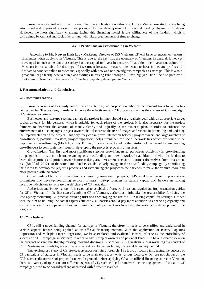
From the above analysis, it can be seen that the application conditions of CF for Vietnamese startups are being established and improved, creating great potential for the development of this novel funding channel in Vietnam. However, the most significant challenge facing this financing model is the willingness of the funders, which is constrained by cultural and social factors and will take a great amount of time to change.
5. Recommendations and Conclusions
5.1. Recommendations
From the results of this study and expert consultations, we propose a number of recommendations for all parties taking part in CF ecosystem, in order to improve the effectiveness of CF process as well as the success of CF campaigns of Vietnamese startups.
Businesses and startups seeking capital: the project initiator should set a realistic goal with an appropriate target capital amount for his venture, which is suitable for each phase of the project. It is also necessary for the project founders to distribute the amount of money clearly and logically in the business plan. In order to enhance the effectiveness of CF campaigns, project owners should increase the use of images and videos in promoting and updating the implementation of the project. This way, they can improve interaction between project owners and large numbers of crowdfunders, potential investors, project supporters; helps strengthen the social network ties which are found to be important in crowdfunding (Mollick, 2014). Further, it is also vital to utilize the wisdom of the crowd by encouraging crowdfunders to contribute their ideas in developing the projects’ products or services.
Crowdfunders: The first and most significant step for crowdfunders to participate efficiently in crowdfunding campaigns is to broaden their understanding of crowdfunding and how it works. In addition, it is vital for funders to learn about project and project owner before making any investment decision to protect themselves from investment risk (Bradford, 2012). At the same time, funders should actively engage in the crowdfunding campaign by contributing their ideas to develop the project’s products and introducing the project to their friends to make the venture more and more popular with the crowd.
Crowdfunding Platforms: In addition to connecting investors to projects, CFPs would need to set up professional committees and develop consulting services to assist startup founders in raising capital and funders in making investment decisions to increase the efficiency of CF campaigns.
Authorities and Policymakers: It is essential to establish a framework, set out regulations implementation guides for CF in Vietnam. In the first step of applying CF in Vietnam, authorities might take the responsibility for being the lead agency facilitating CF process, building trust and encouraging the use of CF in raising capital for startups. Further, with the aim of utilizing the social capital efficiently, authorities should pay more attention to enhancing capacity and competitiveness of startups as well as improving the quality of ventures to achieve the sustainable development in the long term.
5.2. Conclusions
CF is still a novel funding channel for startups in Vietnam, therefore, it needs to be clarified and understood in various aspects before being applied as an official financing method. With the application of Binary Logistics Regression and Multiple Linear Regression, we have explored and evaluated factors influencing the probability of success of a CF campaign in Vietnam in order to assist project owners and potential funders to have a clearer view on the prospect of ventures, thereby making informed decisions. In addition, PEST analysis allows revealing the context of CF in Vietnam and sheds lights on prospects as well as challenges facing this novel financing method.
This exploratory study of CF provides avenues for future research. The topic of factors influencing the success of CF campaigns of startups in Vietnam needs to be analyzed deeper with various factors, which are not shown on the CFP, such as the network of project founders. In general, before applying CF as an official financing source in Vietnam, there is a variety of questions on different aspects of CF, such as legal framework or the engagement of social in CF campaigns, need to be considered and addressed with further researches.
Box 1: Predictions on Crowdfunding in Vietnam
According to Mr. Nguyen Dinh Loc - Marketing Director of ISS Vietnam, CF will have to encounter various challenges when applying in Vietnam. This is due to the fact that the economy of Vietnam, in general, is not yet developed to such an extent that society has the capital to invest in ventures. In addition, the investment culture in Vietnam is not suitable for this type of investment because investors often want to have immediate profits and hesitate to conduct online transactions, especially with new and non-prestigious companies as startups. This is also a great challenge facing new ventures and startups in raising fund through CF. Mr. Nguyen Dinh Loc also predicted that it would take five to ten years for CF to be completely developed in Vietnam.
666

References
[1] Antonenko, P.D., Lee, B.R. & Kleinheksel, A.J, 2014, “Trends in the crowdfunding of educational technology startups”. TECHTRENDS TECH TRENDS (2014), 58-36.
[2] Arolas, E. E., & ´n-de-Guevara, F. G.-L. (2013). Towards an integrated crowdsourcing definition. Journal of Information Science , 189-200.
[3] Agrawal, A. K., Catalini, C., & Goldfarb, A. (2011). The Geography of Crowdfunding. Cambridge, MA: NATIONAL BUREAU OF ECONOMIC RESEARCH.
[4] Ahlers, G. K., Cumming, D., Günther, C., & Schweizer, D. (2015). Signaling in Equity Crowdfunding. Entrepreneurship Theory and Practice, 955-980.
[5] Belleflamme, P., Lambert, T., & Schwienbacher, A. (2010). Crowdfunding: An Industrial Organization Perspective. Prepared for the workshop Digital Business Models: Understanding Strategies’, held in Paris on June. 2010.
[6] Belleflamme, P., Lambert, T., & Schwienbacher, A. (2013). Crowdfunding: Tapping the right crowd. Journal of Business Venturing.
[7] Bradford, C. S. (2012). Crowdfunding and the Federal Securities Laws. [8] Buysere, K. D., Gajda, O., Kleverlaan, R., & Marom, D. (2012). A Framework for European Crowdfunding.
European Crowdfunding Network. [9] Chen, X.-P., Yao, X., and Kotha, S. 2009. “Entrepreneur passion and preparedness in business plan presentations:
a persuasion analysis of venture capitalists’ funding decisions,” Academy of Management Journal (52:1), pp. 199–214.
[10] Cheung, C. M., Lee, M. K. and N. Rabjohn (2008). "The impact of electronic word‐of‐mouth." Inter- net Research 18 (3), 229–247.
[11] Colombo, M. G., Franzoni, C. and Rossi-Lamastra, C. (2015), Internal Social Capital and the Attraction of Early Contributions in Crowdfunding. Entrepreneurship Theory and Practice, 39: 75–100. doi: 10.1111/etap.12118.
[12] Cordovaa, A., Dolcib, J., & Gianfrate, G. (2015). The determinants of crowdfunding success: evidence from technology projects. 3rd International Conference on Leadership, Technology and Innovation Management (pp. 115-124). Procedia-Social and Behavioral Sciences.
[13] Drabløs, C. (2015). What influences crowdfunding campaign success (Master's thesis, Universitetet i Agder; University of Agder).
[14] Gerber, E. M., Hui, J. S., & Kuo, P.-Y. (2012). Crowdfunding: Why People Are Motivated to Post and Fund Projects on Crowdfunding Platforms. Proceedings of the International Workshop on Design, Influence, and Social Technologies: Techniques, Impacts and Ethics, (p. 11).
[15] Hagedorn, A., & Pinkwart, A. (2015). The financing process of equity-based crowdfunding: An empirical analysis. Crowdfunding in Europe. Springer International Publishing, 71-85.
[16] Hemer, J. (2011). A Snapshot on Crowdfunding. Karlsruhe, Germany: Fraunhofer Institute for Systems and Innovation Research ISI.
[17] HSBC Bank. 2017. Asian Connected. Sydney: Export Council of Australia. [18] Koch, Jascha-Alexander, Siering, Michael,2015, “Crowdfunding success factors: The characteristics of
successfully funded projects on crowdfunding platform”. Working paper. [19] InfoDev. (2013). Crowdfunding’s Potential for the Developing World. Washington, DC: Finance and Private
Sector Development Department, World Bank. [20] Jegelevičiūtė, S., & Valančienė, L. (2015). Comparative analysis of the ways crowdfunding is promoted. 20th
International Scientific Conference Economics and Management - 2015 (ICEM-2015) (pp. 268-274). Procedia - Social and Behavioral Sciences .
[21] Kraus, S., Richter, C., Brem, A., Cheng, C.-F., & Chang, M.-L. (2016). Strategies for reward-based crowdfunding campaigns. Journal of Innovation & Knowledge, 13-23.
[22] Leboeuf, G., Schwienbacher, A., Cumming, D., 2015, “Crowdfunding Models: Keep-It-All vs. All-Or-Nothing”, 2015, Working paper.
[23] Lin, L. (2017). Managing the Risks of Equity Crowdfunding: Lessons from China. Journal of Corporate Law Studies.
[24] Lin, M., Prabhala, N. R., and Viswanathan, S. 2014. “Judging borrowers by the company they keep: friendship networks and information asymmetry in online peer-to-peer lending,” Management Science (59:1), pp. 17–35.
[25] Mollick, E. (2014). The dynamics of crowdfunding: An exploratory study. Journal of Business Venturing, 1-16. [26] Pazowski, P., & Czudec, W. (2014). Economic prospects and conditions of crowdfunding. Human capital without
borders. International conference management knowledge and learning, (pp. 1079-1088). Portoroz, Slovenia. [27] PwC. 2016. The long view: how will the global economic order change by 2050? [28] Rossi, M. (2014). The New Ways to Raise Capital: An Exploratory Study of Crowdfunding. International Journal
of Financial Research. [29] Röthler, D., & Wenzlaff, K. (2011). Crowdfunding Schemes in Europe. European Expert Network On Culture
667

(EENC). [30] Sigar, K. (2012). Fret no more: inapplicability of crowdfunding concerns in the internet age and the JOBS Act's
safeguards. Administrative Law Review (pp. 473-506). American Bar Association. [31] Valanciene, L., & Jegeleviciute, S. (2013). Valuation of crowdfunding: benefits and drawbacks. Economics and
Management, 39-48. [32] Valančienė, L., & Jegelevičiūtė, S. (2014). Crowdfunding for creating value: stakeholder approach. 19th
International Scientific Conference; Economics and Management 2014. Riga, Latvia: Procedia - Social and Behavioral Sciences.
[33] Tổng cục Thống kê. 2017. Tình hình kinh tế xã hội quý I năm 2017. [34] VEPR. 2017. "Báo cáo kinh tế vĩ mô Viêt Nam Quý 1/2017." [35] Vũ Hồng Thanh và Vũ Duy Linh. 2016. "Hướng phát triển dịch vụ "Mobile Banking" cho các ngân hàng Việt
Nam." Tạp chí Ngân hàng số 11-2016. [36] Wroldsen, J. S. (2012). The Social Network and the Crowdfund Act: Zuckerberg, Saverin, and Venture
Capitalists’ Dilution of the Crowd. VANDERBILT J. OF ENT. AND TECH. LAW.
668


