Online rules for container stacking - CORE

OR Spectrum (2010) 32:687–716DOI 10.1007/s00291-010-0205-4

REGULAR ARTICLE

Online rules for container stacking

Bram Borgman · Eelco van Asperen ·Rommert Dekker

Published online: 19 March 2010© The Author(s) 2010. This article is published with open access at Springerlink.com

Abstract Container stacking rules are an important factor in container terminal effi-ciency. In this paper, we investigate two concepts to increase efficiency and comparethem to several benchmark algorithms, using a discrete-event simulation tool. Thefirst concept is to use knowledge about container departure times, in order to limit thenumber of reshuffles. We stack containers leaving shortly before each other on topof each other. The second concept is the trade-off between stacking further away inthe terminal versus stacking close to the exit points and accepting more reshuffles. Itis concluded that even the use of imperfect or imprecise departure time informationleads to significant improvements in efficiency. Minimizing the difference in departuretimes proved to be important. It was also found that the trade-off between stackingfurther away in the terminal versus stacking close by the exit points and acceptingmore reshuffles leads to improvements over the benchmark.

Keywords Container stacking · Marine terminals · Simulation ·Container rehandling

B. Borgman · R. Dekker (B)Erasmus School of Economics, Erasmus University Rotterdam, Rotterdam, The Netherlandse-mail: [email protected]

B. Borgmane-mail: [email protected]

E. van AsperenCenter for Maritime Economics and Logistics, Erasmus University Rotterdam,Rotterdam, The Netherlandse-mail: [email protected]

123

brought to you by COREView metadata, citation and similar papers at core.ac.uk

provided by Erasmus University Digital Repository

https://core.ac.uk/display/43320666?utm_source=pdf&utm_medium=banner&utm_campaign=pdf-decoration-v1

688 B. Borgman et al.

1 Introduction

One of the main problems in container terminals concerns the stacking of containers.Although it is also one of the main advantages of containers, namely, that they canbe stacked on top of each other, additional work is required if the bottom container isneeded. In that case the top containers have to be moved to another place, which iscalled a reshuffle or unproductive move.

Accordingly, every terminal needs a stacking strategy. The main objectives of sucha strategy are: (1) the efficient use of storage space, (2) limiting transportation timefrom quay to stack and beyond, (and vice versa), and (3) the avoidance of reshuffles.Of course, the importance of each criterion depends from terminal to terminal. Portslike Singapore and Hong Kong have limited land space, so they need efficiently usedstorage spaces. Note also that these objectives are conflicting: you cannot maximizethem all. For example, the third objective would be optimized by having stacks of onlyone container high; however, this would lead to very inefficient use of storage space.

In stacking containers, various decision horizons can be identified. An often usedclassification has four temporal categories: long term (years, decades), medium term(months), short term (days), and real time (minutes, seconds).

Long-term decisions are strategic decisions, e.g., decisions concerning the type ofequipment (automated, manual), the stacking height, and the location and size of thestacking area.

Medium-term (or tactical) decisions concern capacity decisions, such as stack lay-out, number of vehicles used to move containers about and whether or not (and how)to do remarshalling (i.e., performing reshuffles) in the yard when no ships are beingserved.

Short-term (or operational) decisions concern finding the storage location for aparticular container and the allocation of the equipment to the various jobs scheduledin the coming hours.

Real-time decisions are decisions made when actually executing whatever part ofthe stacking process. It includes the speed and direction control of all vehicles, as wellas the cranes, and is hence mostly of importance to automated equipment.

This paper focuses primarily on the short-term decision to allocate an incomingcontainer to a stacking position. We consider an import container terminal with a highuncertainty regarding the departure time of the containers, such as terminals in Europe(Hamburg–Le Havre range) and the USA. We try to mimic the most common situationwhere imperfect or imprecise information about the departure time of a container isavailable. Moreover, we consider online stacking rules, which do not require exten-sive computations and can be used in many types of stacks and for large numbers ofcontainers. We concentrate on the trade-off between traveling and finding a positionwhich limits the likelihood of reshuffles. We use a quite realistic simulation program totest our ideas. As benchmark we take both random stacking policies as well as policieswhich use precise information on the container departure times. We do not considerdifferent sizes of container in this study as that only complicates the research.

The paper is structured as follows. We start with giving an overview of existingliterature on stacking in Sect. 2. Next we explain the set-up of our simulation model inSect. 3. The basic stacking concepts are explained in Sect. 4. The experimental set-up

123

Online rules for container stacking 689

is presented in Sect. 5, while Sect. 6 presents our benchmark algorithms. The resultsfrom the experiments are given in Sect. 7 and we finish the paper with conclusions inSect. 8.

2 Literature review

Academic literature on stacking problems is not very common yet, perhaps because theproblem does not easily lend itself to analytical solutions (Dekker et al. 2006). How-ever, in recent years, the subject seems to get more attention, because its importance isrecognized (Steenken et al. 2004). In a recent overview paper on operations researchat container terminals, Stahlbock and Voss (2008) looked at a number of aspects ofcontainer terminal operations. Among the topics surveyed were stowage planning,berth allocation, crane optimization, terminal transport optimization, and storage andstacking logistics. Their work is an extension of an earlier overview (Steenken et al.2004), which also contains a paragraph on how stacking is done in practice.

Various methods are used to tackle the stacking problem, but two main approachescan be distinguished like in job scheduling (Dekker et al. 2006). Analytical calculationswith full information on the moment a container will be retrieved from the stack. Theyare often based on integer programming and take relatively much computation time.Next there are detailed simulation studies which evaluate various stacking strategies.These strategies can be online, in which they determine for each container separatelywhere to place it independent of other incoming containers and offline, where loca-tions are found simultaneously for all containers to be offloaded from a ship. So faronly online rule-based strategies have been studied in simulation studies. These rulescan handle imperfect or imprecise information on departure times of containers. Theirstudy takes a lot of time and the results may be dependent on the simulation set-up.Dekker et al. (2006) distinguish two types of stacking strategies: category stackingand residence time stacking. The former strategy assumes that containers of the samecategory (e.g., having the same size, destination, weight, etc.) are interchangeable, andcan thus be stacked on top of each other without the risk a lower container in a stackis needed before the ones on top of it have been removed. The latter strategy does notuse categories, but instead looks at the departure times of the containers: a containercan only be stacked on top of containers that all have a (planned) departure time thatis later than the departure time of the new container.

Recent examples of the analytical approach include Kim and Hong (2006), whouse a branch-and-bound method to find an optimal solution to a stacking problemand then propose several heuristics to try to come close to the optimum, and Kanget al. (2006), who use simulated annealing to find good solutions reasonably fast.Caserta et al. (2010) combine metaheuristics and dynamic programming to improveupon the known results of Kim and Hong (2006). The problem most of these opti-mization approaches have, is that they assume perfect prior knowledge on the orderin which the containers will be picked up. However, this information is usually notknown in advance. Nevertheless, finding a theoretical optimum can be very useful as abenchmark (although the metaheuristic approaches used to make this approach com-putationally feasible are not guaranteed to find the global optimum). Other methods

123


that have been used for this include Q-Learning (Hirashima et al. 2006) and criti-cal-shaking neighborhood search (Lim and Xu 2006). Han et al. (2008) use integerprogramming with Tabu search to generate an entire yard template, which shouldminimize reshuffling moves. Froyland et al. (2008) also use integer programming,optimizing the entire terminal in an effort to maximize quay crane performance.

Detailed simulations were performed by several authors. Dekker et al. (2006) sim-ulated different stacking policies for containers in automated terminals. In particular,several variants of category stacking (with up to 90 different categories) were exam-ined and compared with a base case in which containers are stacked randomly. Thesimulations demonstrated very high peak workloads during the handling of very largecontainer ships. Category stacking was found to significantly outperform randomstacking. Considering the workload of each automated stacking crane (when selectingthe lane for an incoming container) and stacking close to the export transfer point werefound to provide additional performance benefits. There was no significant benefit tousing category stacking for containers with onward transport by short-sea/feeder, rail,truck, or barge. As the category definitions are based on information used in stowageplanning, they advocate an integration of terminal operations and stowage planning.

Duinkerken et al. (2001) also used simulation and category stacking, albeit withonly a limited number of categories. Several (reactive) reshuffling rules were tested.Reactive reshuffling means the reshuffling is done when a container on which othercontainers are stacked is demanded for retrieval, leading to a number of reshufflingoperations. This in contrast to “proactive” reshuffling, which is done when stackingcranes are idle. They evaluated several reshuffling rules (random, leveling, closestposition, and minimizing remaining stack capacity reduction). The use of catego-ries was compared with a model that required specific containers and found that thecategories lead to much better performance. Also, it was shown that the remainingstack capacity strategy lead to big improvements when compared to the other three.Duinkerken et al. (2001) also tested two “normal” stacking strategies (i.e. for when acontainer has just arrived), namely random and with dedicated lanes for a quay crane.However, using dedicated lanes is hard to do in practice, as load plans are not knownin advance. Also, this strategy did not yield much improvement over random stacking.

Saanen and Dekker (2006a,b) went into great detail in simulating a (transship-ment) container terminal with rubber-tired gantry cranes (rtg), carefully simulatingall movements of the trucks and cranes. They made a “comparison between a refined,but still traditional, strategy for operating a transshipment rtg terminal with a simplerandom stacking strategy for this type of terminal”, and measured the differences inquay crane productivity (in lifts per hour), as this is considered the most importantindicator for terminal efficiency. They found that the differences between the strate-gies was very small (about 0.7 lifts per hour). However, it was found that the numberof gantry movements is a major factor in limiting the quay crane productivity.

Finally, Park et al. (2006) used simulation to determine the best combination of anagv dispatching rule with a reactive reshuffling rule, for various amounts of con-tainers and agv’s in an automated container terminal. Their goal is to minimizethe number of reshuffling operations. Park et al. used the random, closest position(but with residence time taken into account) and minimal rsc reduction reshufflingrules from Duinkerken et al. (2001). In most cases, the minimal rsc reduction rule,

123


combined with the Container Crane Balancing (ccb) dispatching rule (the agv is sentto the crane which has the most containers waiting for it), lead to the least reshufflingoperations.

This paper elaborates on residence time stacking. In particular we consider severalresidence time classes and use that information to limit the number of reshuffles. Wecompare a number of stacking rules where we consider trade-offs between furthertraveling and the possibility of reshuffles. We also consider the case of full informa-tion, on one hand as a benchmark, but also to get some insight into the structure ofgood policies. The research approach and experimental setup of this paper build onprior work (Dekker et al. 2006) but here we have limited ourselves to relatively simplestacking rules that use less information in order to get more insight into the basicperformance of these rules. The ideas in this paper can easily be combined with thecategory stacking from Dekker et al. (2006).

3 Simulation model

The simulation model that was developed for the experiments in this paper consistsof two major components: a generator and a simulator. Although based on the samespecifications as the simulator model described in Dekker et al. (2006), the code forboth programs was rewritten from scratch. The existing code could not easily facilitatesome of the new experiments. As the tools for developing discrete-event simulationmodels, especially the language and library that were used in the original implementa-tion (Pascal and must) are less prevalent today, and programming languages in generalhave improved since the original implementation, we have chosen to rebuild the sys-tem in a modern programming language (Java) using a solid discrete-event simulationlibrary (ssj, L’Ecuyer and Buist 2005).

The generator program creates arrival and departure times of some 76,300 20ft.containers covering a period of 15 weeks of operation, including a 3-week warm-upperiod to initialize the stack. The generator is based on the same data as the generatorin Dekker et al. (2006), including sailing schedules and a modal-split matrix. Theoutput of the generator is a file that contains the ship arrivals, details of the containersto be unloaded and loaded, and the specification of the destination of each container.The departure time is specified as the planned (a.k.a. expected) departure time andthe actual (a.k.a. real) departure time. In the implementation of the generator programthe actual departure time is generated first on the basis of the sailing schedules; theexpected departure time is created from this actual departure by applying a pertur-bation function (the parameters of this function depend on the departure mode: ship,short-sea vessel, train, or truck). The destination can be another deep-sea vessel or(for import containers) a short-sea vessel, barge, train or truck. For each container thelocation of the individual container within a ship is specified. The generator takes thedetailed quay crane sequences for loading and unloading into account.

The average residence time of a container is 3.8 days; the 90%-percentile of thedwell time is 5.3 days, and the maximum dwell time is 8 days. The specifications of theinput for the generator are detailed in Voogd et al. (1999); the current implementationis documented in Borgman (2009). Most experiments in this paper are done with a

123


stack that has a total capacity of 6×34×6×3 = 3, 672 TEU. The average utilizationof the yard is therefore (76, 300 × 3.8)/(3, 672 × 12 × 7) ≈ 75%. In some experi-ments we use a stack of 8 × 34 × 6 × 4 = 6, 528 TEU with an average utilization of42%.

The simulator program reads the output of the generator and performs the stackingalgorithms. The core of the simulator itself is deterministic: the stochastic componentsare in the generator and, optionally, in the stacking algorithm. This setup facilitatesa comparison of stacking algorithms as any changes in the statistical output of thesimulator must be caused by the stacking algorithm.

Within the simulation program, the containers are loaded and unloaded from shipsand other transport modes (trucks and trains). The transport of containers from thequay to the stack is performed by Automated Guided Vehicles (agv’s); the simulationdoes not contain a detailed model of the agv’s (issues such as routing and traffic havenot been modeled). Once an agv with a container arrives at the stack, the AutomatedStacking Crane (asc’s) for the lane is tasked with lifting the container from the agvand storing it in the stacking lane. As previous research into this container terminalhas shown the ascs to be performance bottlenecks, they have been modeled in detail:the simulator calculates the time it takes for all the motion components (hoisting,lengthwise and widthwise movement) where hoisting and movement are sequentialand the length- and widthwise movement are done simultaneously. There is a singleasc per lane (based on the ect terminal, v.i.) and the simulation program maintains ajob queue for each asc. Containers that have to be reshuffled are always stored withinthe same lane. On the land side, the containers are moved to and from the stack usingstraddle carriers.

To verify that the generator works correctly, we have performed a number of tests onthe output (such as testing the distribution of the container dwell times). The simulatorwas verified using a number of test scenarios for which the values of the statisticalindicators could be determined analytically. Once the simulator had passed these tests,the simulator was benchmarked against the model described in Dekker et al. (2006);the performance of random stacking and category stacking (experiments A0 and Afrom Dekker et al. (2006)) was similar but not identical. The main difference in thetwo models is that the current simulation model has a very detailed simulation of theasc’s whereas the original model had a very simplistic model for the asc’s. As otherauthors (such as Axelrod 1997) have noted, achieving numerical identity for simula-tion models is hard. The detailed descriptions required to achieve this can rarely bepublished in papers and are too much work (with little reward) to describe in internalreports.

4 Basic concepts

In this section we present some generic concepts that form the basis of the stackingrules we will evaluate in this paper. The precise formulations will depend on the layoutof the stacking area. While we only present these formulations for one particular lay-out (in order to clarify the presentation and analysis), the formulations can be adaptedfor other layouts.

123


Ship

Quay Cranes

AGV AreaLoaded AGV

Empty AGV

Transferpoints Landside

Transferpoints Seaside

StackLanes,

one ASC per lane Platform

TransferpointSeaside

TransferpointLandside

ASC

Fig. 1 Terminal layout with details of a single lane

We want to investigate the basic concepts of stacking containers in a yard. The coredilemma is that we would like to stack a container that arrives and departs at the quayside as close to the transfer point quay-side as possible because this will minimize thetotal travel time of the stacking crane when the container enters and exits the stack.As there are many of these sea-sea containers, this would require us to stack high.Unfortunately, when we start to stack containers on top of each other, we face the riskof stacking a container on top of a container that will depart before the incoming con-tainer. This will lead to a reshuffle, which takes time. We will thus have to balance thetravel and hoisting time of the stacking crane and the time taken by reshuffle moves.

If we consider a single lane of the type of container terminal under investigation,we see that there is a single rail-mounted stacking crane that has to perform all thestacking moves for that lane. We can distinguish between containers that are movinginto the lane (i.e., that are being stacked) and containers that are moving out of the lane(they are being “unstacked”). Containers can enter and leave the lane at two sides: atthe quay side (for containers that are coming from or going to deep-sea ships) and atthe land side (for all other modes of transport). Figure 1 provides a schematic overviewof the terminal layout. The layout of this terminal has the stacking lanes perpendicularto the quay. Each lane has a length, a width, and a height. We will refer to a singleline along the length of the lane as a lane segment. A layout within this terminal con-figuration will be denoted as ‘number of lanes × length × width × height’; the basicconfiguration for our experiments will be ‘6 × 34 × 6 × 3’.

The first trade-off that is worthy of investigation is the trade-off between the timeit takes the asc to travel to a certain location and the amount of time required to(un)stack a container. For a container that has arrived on a deep-sea vessel and thatwill also depart on another deep-sea vessel, it is attractive to stack it as close to thetransfer point at the quay side as possible. If we can stack the container close to thetransfer point we save travel time of the asc both when the container is stacked and

123


when it is unstacked. Clearly the same applies for containers that arrive and departat the land-side of the stack. There is no obvious best location for containers thatarrive at the quay-side and will depart at the land side and for containers that arriveat the land side and will leave the stack at the quay side. In both cases the asc willhave to (in two stages) move the container along the entire length of the lane. At firstglance stacking the container close to the planned exit transfer point seems beneficial;however, this would imply a longer travel time of the crane. Since sea-to-land moveswill occur most when large ships are being unloaded, it would seem more beneficial tostack these container as fast as possible in order to release the crane more quickly forother moves. This would however conflict with the desire to stack sea-sea containersas close to the quay-side transfer point as possible.

The second trade-off we want to research is between the time required to stack acontainer and the number of reshuffles. Although reshuffles as such should be avoided,it is interesting to test a strategy that favors a fast stacking time during peak times witha resulting reshuffle that may occur at an off-peak time.

The overall approach of the experiments in this paper is focused on the operationaldecisions that have to be made by terminal operators. Specifically, we take the arrivalsand departures that are specified as part of the generator output and perform theseoperations. There is no global optimization or explicit planning; the operations areperformed one at a time, i.e., in a greedy fashion, whenever a container arrives. We donot consider future events such as other incoming containers.

5 Experimental setup

The experiments in this paper all use the following configuration. Experiments are runfor a 15-week period, of which 3 weeks are used for warm-up (to initialize the stack).As some stacking rules have a stochastic component (such as selecting a position atrandom), we use ten replications to get statistically robust results. These replicationsare used to compute the 95% confidence intervals of the mean.

We assume that there are sufficient agvs and straddle carriers to ensure that theseresources do not act as bottlenecks. The basic configuration for the stacking area ismodeled on part of the automated ect Delta Terminal at the Port of Rotterdam, TheNetherlands. We have chosen to use only a part of the actual stack area in these exper-iments to clarify the discussion and to facilitate the analysis. Thus, our stacking areahas far fewer lanes than the actual terminal; the length of the lanes, the maximumstacking height, and the number of asc’s per lane are based on the configuration atthe ect Delta terminal.

There are thus just six lanes, each equipped with a single asc (Some containerterminals have multiple asc’s per lane. This would make the problem more difficultto study as we would have to model the interaction between multiple cranes in detail.We therefore limit ourselves to a single asc which is the configuration at the Deltaterminal.) per lane to mirror the configuration at the Delta terminal and Each line is34 teu long, for a total of 6 × 34 = 204 ground positions (measured in teu). (TheDelta terminal has some additional room for reefer containers in each lane but we havenot taken these containers into account for our experiments so we present the layout

123


without this reefer area.) The maximum stacking height is three containers. Each lanehas six lane segments. We denote the configuration as 6 × 34 × 6 × 3 (six lanes, eachlane being 34 teu long, 6 segments per lane, and a maximum stacking height of 3containers). The number of lanes and the maximum stacking height will be changedfor some experiments to evaluate the performance of the stacking rules under inves-tigation. For these experiments we use a single size of container, the standard 20 ft.container, as a mix of different sizes of container would make the comparison of thestacking rules more complicated. We thus skipped all other sizes of containers in thegenerator’s output file. The number of 20 ft. containers is a good fit with the base layout.

We will use Random Stacking (rs) and an implementation of the Leveling algorithm(lev) described in Duinkerken et al. (2001) as benchmarks for the experiments.

6 Benchmark algorithms

In this section we introduce the basic algorithms used for comparison in the experi-ments.

6.1 Random stacking

Random stacking is a straightforward way of determining a stacking position for anew container. Basically, the new container is placed at a randomly chosen allowedlocation, with every allowed location having an equal probability of being chosen. Wehave implemented this as follows:

1. Select a random lane.2. Select a random position in the lane.3. Check whether we could stack at this position.4. If so: stack here.5. If not: start again in the next lane.

Given enough tries this algorithm is guaranteed to find an available location (in ourimplementation, we have set the limit at 5,000 tries, which has proven sufficient). Thisalgorithm is also applied for reshuffling, with the difference that we then only want tosearch the lane the container is in.

6.2 Leveling

The idea is to fill lanes in layers, so that all empty ground positions are filled withcontainers first, before containers are stacked upon others. The stacking lane is filledfrom the transfer point quayside on. This strategy is taken from the earlier work ofDuinkerken et al. (2001). It is an intuitive strategy, but it does not use most of theavailable information. We thus get the following steps:

1. Choose a random lane with at least one available position.2. Search for the first empty location, from the transfer point quayside towards the

transfer point landside, row for row (i.e., widthwise).

123


3. If found: stack there.4. If not found: search all existing piles (of the same size and type), from the transfer

point landside towards the transfer point quayside, row for row, for the lowest (i.e.,search lowest piles first) stack location and stack on the location found first.

This algorithm is also applied for reshuffling, with the difference that we only searchthe lane the container is in.

7 Experiments

In this section we will present our experiments with a number of stacking rules. Wefollow the same structure for each experiment. We first present the design of thestacking rule. Next, we formulate a number of hypotheses regarding the performanceof the stacking rule. The results are presented in tabular form and we discuss theresults in terms of our hypotheses. The hypotheses are tested using the 95% confi-dence intervals of the mean; we accept that there is a significant difference if theseintervals do not overlap. In the interest of clarity and brevity we only present a subsetof the total experimental results; a comprehensive list of results is listed in Borgman(2009).

The performance of a stacking algorithm is measured with the following statistics:

Exit time (etq and etl). The exit time is the time (in hours) it takes to remove acontainer from the stack and have it ready for onwardtransport (to the quay or to a truck/train/barge). Thistime is measured for each side (quay-side and land-side) of the stack and will be listed as etq and etl,respectively. The exit time is the main performanceindicator for a stacking algorithm. It is negatively influ-enced by stacking further away from the exit point andby any reshuffles that are needed to retrieve the con-tainer. When a container enters the stack, the time ittakes to perform this operation is determined by theworkload of the asc (how many jobs are in the currentjob queue) and the time it takes the asc to move thecontainer to its position. There are no reshuffles whencontainers are stored in the stack; reshuffles only occurwhen a container has to leave the stack.

asc workload (asc). The automated stacking cranes are critical componentsfor the overall performance so we measure the percent-age of time that the asc’s are busy. (The asc workloadwill be denoted as asc in the results.)

Reshuffles (rdc and roc). For the unproductive reshuffle moves, we measure thenumber of reshuffles (denoted as rdc) as a percent-age of the total number of container movements. Toget an indication of the number of reshuffles that hap-pen per move, we also measure the reshuffle occasions

123


(as a percentage of the total number of container move-ments, denoted as roc); a single reshuffle occasionimplies one or more reshuffles. These numbers are notabsolute indicators of performance as the time of thereshuffle is not taken into consideration. A reshufflethat occurs when the workload is low has less impacton the overall performance than a reshuffle during apeak workload, for example when (un)loading a verylarge vessel.

Ground position usage (gpu). We report only the average percentage of ground posi-tions that are in use (denoted by gpu) as the vari-ous stacking strategies have differing preferences forstacking on the ground.

7.1 Experiment 1: leveling with departure times (LDT)

The first experiment is on the influence of knowing the exact departure times of allcontainers. This can be exploited by only stacking containers on top of other contain-ers, if the new container departs at an earlier time than the one below it, i.e., residencetime stacking.

In practice the actual departure time is not known. However, it is valuable as areference case to determine the best possible performance of such a stacking rule. Fora more realistic scenario, we use the expected departure time that is also part of thegenerator output file.

We differentiate between containers both arriving and leaving at the quay and othercontainers (i.e., containers arriving or departing at the truck loading point). The con-tainers both arriving and leaving at the quay (the sea–sea containers) should be stackedclose to the transfer point quayside, because every meter they move towards the transferpoint landside is a waste.

The dwell time, or better the departure time of a container, can be used when deter-mining where to stack it. Containers departing before the containers below them willnever lead to a reshuffle. We would like to exploit this to the maximum and stack ashigh as possible, because this means other positions remain free for other containerswhich depart later. The first priority when searching for a place to stack is thus to findthe piles which have such a container on top.

Second, and again in the interests of keeping options open, we want to find theposition where the difference between departure times is as small as possible, sincethis means that there are more possibilities for stacking other containers on top ofthem, using as little space as possible. We thus select from the piles the one where thedifference in departure times would be smallest.

If we can find no pile with a container on top that will depart after the new container,we have to stack it elsewhere. Preferably, we do this on the ground, so no reshuffleswill occur. From the available positions on the ground, we want to stack it as close tothe transfer point as possible, so that travel times are minimized.

123


Should we still not be able to find a position, we have to stack the container on anexisting pile, rendering a reshuffle inevitable. To minimize the number of reshuffles,we place the container on the highest pile available, so that no or few containers can bestacked on top of them, each of which would lead to another reshuffle. In case severalof these piles are available, we select the pile closest to the transfer point, in order tominimize travel time for the asc.

In summary, we use the following algorithm, which we shall call “ldt” (Levelingwith Departure Times) (in each step we look at all lane segments):

1. Stack the new container (departing at T = Tn) at that pile, where the top containerdeparts at time T = To, To > Tn , and To − Tn is minimal and on which thecontainer may technically be stacked (i.e., pile is not full).

2. If no position was found yet: stack the container on an empty ground location.Sea–sea containers are to be stacked as close to the transfer point quayside aspossible.

3. Stack at a pile of the highest height available, as close to the transfer point aspossible.

For sea–land and land–sea containers we do not have a preference for a particu-lar part of the lane, since they have to traverse it in full anyway. However, becausesea–sea containers prefer the sea (quay) side of the lane, sea–land containers shouldbe stacked away from them, as close to the transfer point landside as possible, whenthe two types are both included in an experiment. Since we select the stacking locationbased on departure times, the two types may become mixed. If only sea–sea containersare included, the algorithm automatically stacks the containers near the transfer pointquayside, but with land containers included, it may not do this. Since this removes theadvantage of stacking near the quayside, we can choose to separate the piles, so thatsea–sea containers may not be stacked on land–sea containers and vice versa. How-ever, as this means there are less options for optimizing residence times, it remains tobe seen which is best.

We compare the ldt algorithm with random stacking, leveling, and a modified ver-sion of random stacking (rs-dt), in which the algorithm searches for a random pilewith the top container’s departure time being after the new container’s departure time.If no such pile is found, the container is stacked randomly, according to the randomstacking algorithm. We use this to see which part of the differences between ordinaryrandom stacking and the ldt algorithm is caused by the “random” part and which partis caused by the lack of perfect information.

7.1.1 Hypotheses

Because of the great advantage of perfect information regarding the departure times,we expect to see a very big improvement for relevant statistics, compared to randomstacking and leveling. In particular, we look at the reshuffle percentages (which weexpect will be lower for this algorithm), time to exit (will also be lower), asc workload(will also be lower, as it is related to the previous ones), stack usage (will be slightlylower due to containers exiting quicker), and ground position usage (will be much

123


lower than with leveling, which maximizes ground usage. We cannot say in advancehow it compares with random stacking).

The effects of the rs-dt algorithm should be similar to those of ldt with regardto random stacking and leveling, because of the extra information. However, becausethe pile selection process is still very basic, it probably will not perform as good asldt.

The experiments with expected, rather than actual, departure times should still bebetter than random stacking and leveling, i.e., the same effects should occur as withperfect information. We do expect these effects to be somewhat weaker, since theinformation is less reliable and hence some poor decisions are likely to be made.

On the basis of these considerations we formulate the following hypotheses:

Hypothesis 1.1 The ldt stacking algorithm will have a lower number of reshuffles,a lower exit time and a lower asc workload than the benchmarks rsand lev.

Hypothesis 1.2 The rs-dt stacking algorithm will have a better performance than rs,but worse than ldt.

Hypothesis 1.3 Mixing piles in the ldt stacking algorithm will lead to less reshuffleswhen compared to not mixing piles.

Hypothesis 1.4 Mixing piles in the ldt stacking algorithm will lead to higher exittimes compared to not mixing piles.

7.1.2 Experimental setup

We have varied two parameters for this experiment; the first is the departure time(actual or real departure time vs. expected departure time) and the second parametercontrols whether mixed piles are allowed (mixed vs. unmixed).

In this experiment we are particularly interested in the value of the perfect informa-tion regarding departure times. We therefore compare the results to random stacking.We would also like to know whether it is better to allow mixed piles or not. The dif-ference is measured by looking at the times it takes for a container to enter and leavethe stack.

7.1.3 Results

We have listed the results of all experiments in a single table to facilitate comparison(see Table 4). The first column of Table 4 lists the number of the experiment. Theresults for the benchmark algorithms are included as experiment “0”. As expected,the ldt algorithm in its various forms outperforms the random stacking and level-ing benchmarks. Less reshuffles occur and exit times and asc workloads are lower.Ground position usage is also lower.

The relative performance of rs-dt is as predicted: better than the benchmark butworse than ldt. It is also of note that the modified random stacking algorithm (usingreal departure times), outperforms the ldt when the latter is using expected departuretimes. Using expected data, rather than actual, leads to a big performance drop forldt.

123


The effects of mixed piles are inconclusive. When using actual data, mixed pileslead to less reshuffles but an increased exit time. However, using expected data, theylead to more reshuffles (and also an increased exit time). These effects are also foundin the other stack layouts, albeit somewhat weaker.

We have tested this strategy for some larger stacks as well. In larger stacks thereis little improvement in the results for expected times, unlike those for actual times.Moreover, the results for expected times actually deteriorate when going from 6 lanes,3 high to 6 lanes, 4 high.

7.1.4 Discussion

From the results, it becomes clear that ldt’s departure times have a big impact, evenwhen they are not exactly known. Even partially random stacking, using departuretimes only to a limited extent, leads to big improvements across the board. Still, thereremains a big gap between the results of expected and actual departure times, espe-cially in bigger stacks, where little improvement, if any, is seen in comparison tosmaller stacks. This is most dramatically the case when going from height 3 to 4 with6 lanes, where performance actually drops, despite an increase of stacking options.This is probably due to any mistakes made being punished more heavily with extrareshuffles at higher stack levels.

Using mixed piles seems to be not such a good idea. In some cases, there is animprovement in the number of reshuffles (as was expected), but in others there isnone. In all cases, mixed piles lead to longer exit times.

Our conclusion with respect to the hypotheses is:

Hypothesis 1.1: Confirmed.Hypothesis 1.2: Confirmed.Hypothesis 1.3: Rejected.Hypothesis 1.4: Confirmed.

7.2 Experiment 2: LDT with departure time classification (DTC)

In the first experiment we have used the information from the generator program onthe actual and expected departure times. We now take a different approach to modeluncertain departure time information.

We use the data from the arrivals file to define a limited number of classes. Theboundaries of these classes are calculated from the arrivals file by taking the quintilesor the 20th, 40th, 60th, 80th and 100th percentiles of the residence time. This givesus five classes of almost equal size, for the initial residence times at least. We use fiveclasses because the maximum stacking height in these experiments is either three orfour. It is likely that using more classes would yield better results but a larger numberof classes would be a less accurate reflection of the uncertainty of the residence time.The classes are listed in Table 1.

We use the algorithm from experiment 1 for this experiment too, only when the timedifference is calculated we do not use the actual time or the expected time from thefile, but instead use the class value from Table 1 (based on either the actual or expected

123


Table 1 The five classes of container departure times used in experiment 2

Class Actual times Expected times

From (h) To (h) From (h) To (h)

1 0 68.2 0 68.0

2 68.2 79.4 68.0 79.4

3 79.4 92.4 79.4 92.3

4 92.4 111.6 92.3 112.5

5 111.6 ∞ 112.5 ∞The maximum time any container in the used arrivals file will stay is 192.2 h

departure time). This means that lower classes will be stacked on top of higher classes,thereby ensuring no reshuffles occur, unless no suitable pile or ground position couldbe found.

Note that a container’s class will change over time as its departure time comesnearer. This means that the lower classes will be more prevalent in the stack, becauseevery high class will at one time become a low class.


To test this algorithm, we used the settings of Experiment 1 (see Sect. 5), because wewant to compare the different method of estimating departure times with the originaland with perfect knowledge. We also experiment with classes based upon expecteddeparture times, to see whether the double uncertainty gives any different results. Wecompare this algorithm to the entire Experiment 1 (ldt), including random stacking(rs), leveling (lev), and rs-dt. We also modified the rs-dt algorithm to work withdeparture time classes (this version being referred to as rs-dtc).

7.2.2 Hypotheses

We expect this algorithm to have a better performance than ldt-exp because it uses realdeparture times to define the classes. The algorithm may have a problem with smallstacks, where space is in short supply and some suboptimal decisions may have to bemade. In larger stacks, we expect that ldt-dtc will perform almost as good as nor-mal ldt with real departure times. We expect similar effects with the use of expecteddeparture times. Because the classes are then based on imperfect information, we doexpect a drop in performance, when compared to ldt-dtc.

Hypothesis 2.1 The ldt-dtc algorithm with real departure times will have a lowernumber of reshuffles, a lower exit time, and a lower asc workloadthan ldt-exp, but higher than ldt.

Hypothesis 2.2 The ldt-dtc algorithm with expected departure times will have ahigher number of reshuffles, a higher exit time, and a higher ascworkload than ldt-exp and ldt.

123


Hypothesis 2.3 The ldt-dtc-exp will have a higher number of reshuffles, a higherexit time, and a higher asc workload than ldt-dtc-real.

7.2.3 Results

The results for a 6 × 34 × 6 × 3-stack are in Table 4. For brevity, we have not includedthe results for mixed piles, since their performance is similar to the previous experi-ment and they only complicate the presentation.

For the 6 × 34 × 6 × 3-stack, the ldt-dtc performs much worse than normalldt with expected departure times. The random stacking version of the departuretime classes algorithm (rs-dtc) also performs significantly weaker, compared tors-dt, and even compared to lev; in fact, the performance of rs-dtc is similar to rs.Interestingly, the results for ldt-dtc-exp are slightly (yet significantly) better thanldt-dtc-real. For the rs-dtc algorithm, the same applies. This is probably due to thefollowing effect: when no “nice” stacking position can be found (this happens in asmuch as 40% of the cases, we found), a container is put on another pile, certainly caus-ing a reshuffle when real departure times are used. However, when expected departuretimes are used, there is a small probability that, because of the error in departure timeestimation, no reshuffle is caused. This leads to a slight advantage for expected times,and hence to this counterintuitive insight.

However, the results differ significantly for larger stacks, as can be seen in Table 5(a 8 × 34 × 6 × 4-stack). In this larger stack, there are no problems finding a suit-able spot for the ldt-dtc-real algorithm, and thus its advantage of certainly knowingwhether a reshuffle will occur is enough to yield better results. This leads to resultsalmost as good as when using normal ldt. There is also a big improvement for theldt-dtc-exp algorithm, which now actually performs better than ldt-exp. This isprobably due to the used classes providing a bigger “margin of error”, leading to lessmistakes in determining which container departs first.

Interestingly, rs-dtc-real algorithm does not seem to benefit much from a largerstack. Apparently, its method of trying to find any suitable pile, without regard for thesmallest class difference, leads to very inefficient stacking.

7.2.4 Discussion

Using the suggested five classes gives a very good result and a very good approxi-mation of the results of actual departure times, provided there is enough space in thestack. For that case, we can confirm the hypotheses but as the results for the smallerstack differ, we cannot confirm them.

Hypothesis 2.1: Rejected.Hypothesis 2.2: Rejected.Hypothesis 2.3: Rejected.

123


Closest match level 2



Transfer point quay side

Full piles

1234567

Fig. 2 Example case for experiment 3. Maximum stacking height is 3 containers. The two piles to the rightare closest to the transfer point, but are full. Three other options are available though

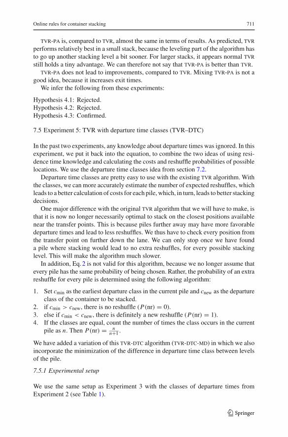
7.3 Experiment 3: traveling distance versus reshuffling (TVR)

In this experiment, we do not use residence time knowledge, but rather try to optimizethe selection of a location in some other way.

Suppose we only have sea-sea containers. As stated previously, these containersshould be stacked as close to the transfer point quayside as possible, because they botharrive and leave the lane there. Leveling all the way down the lane would thus not be agood idea; we want to stack as high as possible at the beginning of the lane, and leavethe end of the lane empty, if possible. Of course, we could just stack new containersas close to the transfer point as possible, by stacking them on top of each other, butthis has the unwanted side effect of leading to reshuffles, because the order in whichcontainers arrive and leave is mostly random.

However, since we also do not want to level too much, a compromise solutionshould be better. Whenever a container arrives at a lane (maximum stacking height n),we can say there are n possibilities to stack it: at every possible height layer, as closeto the transfer point quayside as possible. For example, if n = 3, we may get thescenario from Fig. 2. The ground positions closest to the transfer point are full, but thenext one is only stacked 2 out of 3 high. This is the best position from the distanceviewpoint, but it has a high risk of leading to reshuffles, with two containers under it.The next position has the same risk, but it is further away, so therefore not as good,and we henceforth discard it for this decision.

We then encounter a pile with only one container. This means that the risk of reshuf-fling is lower, but unfortunately the pile is also further away from the transfer point.Still, it may be a good candidate to investigate. The sixth ground position is empty,and while it is still further away from the transfer point, there is no risk of causingreshuffles. This is the final candidate for stacking, because although there are moreground positions ahead, none of them is better in terms of reshuffling risk than theones we already selected, and they are all worse in terms of distance to travel.

Now that we found the “best” (note that we do not use residence times or categorieshere, these factors seriously complicate matters) three piles, we need to choose whichone is best, i.e., which one has the lowest associated cost in time. Time costs consist

123


of two parts: extra asc driving time and time due to reshuffling. The latter will oftenbe greater, but it is not certain it will occur.

The asc driving time can easily be calculated using the distance from the transferpoint to the selected ground position and the asc’s lengthwise and widthwise speeds.Lifting times can also be calculated, since we know exactly at which level the containeris and will be stacked. The cost of reshuffling is more difficult to determine, because itis not known in advance where to a container would be reshuffled. We assume this tobe a (configurable) time period of driving away. The lifting times are also not known,so we estimate the lifting time to be that of a container in the middle of a pile (i.e., atthe level of half the maximum height). The cost of a reshuffle is then multiplied bythe expected number of reshuffles that putting the container at a particular place willgenerate. This gives the following cost function to minimize:

min[2 · TTqp + Lqp + (TTr + L r) · ER(n)] (1)

where TTqp is the travel time from the transfer point quayside to the target pile, TTr

is the (fixed) travel time for reshuffles, Lqp and Lr are the lifting times per container(including pickup, lift up, lift down and set down) for the container itself and reshuf-fles, respectively, and ER(n) is the expected number of reshuffles. The travel time tothe pile has to be doubled because containers need to go back to the transfer pointat one time; reshuffling can lead to a position closer to the transfer point, so we donot double that time. We will use TTr as a penalty factor to vary the relative cost ofreshuffles in our experiments.

A new container can, by itself, only generate one extra reshuffle, at most. Anyother reshuffles were already in the pile when the container was stacked, or are addedlater. This means that we have to calculate the probability P(nr) of the new containerleading to an extra reshuffle. Since we assume every container in a pile has an equalchance of being chosen, this gives the following formula:

P(nr) = n − 1

n, (2)

where n is the height of the pile. We use this probability as ER(n) in Eq. 1.Summarizing, we use the following algorithm:

1. Select for every possible stacking level the (available) position closest to the trans-fer point quayside, if any position is available.

2. Calculate the costs of every position, according to Eq. 1 (using Eq. 2).3. Select the position with the lowest cost and stack there.

While this algorithm can stack sea–sea containers of a single type, it is easy to extendthe algorithm for other containers. As discussed in the previous experiment, sea–landand land–sea containers should be stacked as close to the transfer point landside aspossible. We can determine costs in the same way.

123



In this experiment we are particularly interested in the value of putting sea–sea con-tainers close to the transfer point quayside. We therefore compare the results to randomstacking. We would also like to know what the effects of different penalties (i.e., TTr inEq. 1) are. (Here, we report a subset of the experiments described in Borgman (2009)with values of the reshuffling movement penalty ranging from −0.03 to 0.04.) Thedifference is measured by looking at the times it takes for a container to enter andleave the stack.

We compare this algorithm with random stacking, leveling and a modified versionof random stacking, which we shall refer to as tprl (Transfer Point Random Level),in which the algorithm chooses one of the possibilities offered (i.e. it randomly selectsthe level where the container is to be stacked). This means containers will be nearthe quay, and since we know one of the positions is the “best” one, we can see theinfluence of the complicated calculations, when we compare it with chance.

7.3.2 Hypotheses

Again, we predict this algorithm will always outperform the basic random stackingand leveling algorithms. We again look at the reshuffle percentage (which we expectwill be lower for this algorithm), time to exit (will also be lower), asc workload (willalso be lower, as it is related to the previous ones), stack usage (will be slightly lowerdue to containers exiting quicker) and ground position usage (will be somewhat lowerthan with leveling, which maximizes ground usage).

The ground usage depends on the reshuffling movement penalty applied. A higherpenalty will lead to more containers being stacked on the ground and this leads to ahigher ground position usage. A high penalty would lead to the algorithm behaving asnormal leveling. This would also mean that the effect of allowing to stack 4 containerson top of each other, rather than 3, would be almost completely gone (there is still aminor effect on crane lifting times). Low penalties, on the other hand, would lead toa very low ground position usage, with high piles near the transfer points.

In any case, when only sea–sea containers are included, the algorithm will stackcontainers mostly next to the transfer point quayside and will stack less and less con-tainers further away. This would mean that the average pile height would be decreasingin a monotone way, when going away from the transfer point.

We expect the modified random stacking algorithm tprl to perform worse thanthe original random stacking (and, for that matter, all other algorithms tested in thissection), especially when there is a lot of space in the stack. This is because modifiedrandom stacking will too often build high piles, while the other algorithms place morecontainers on the ground, which leads to less reshuffles.

On the basis of these considerations we define these hypotheses:

Hypothesis 3.1 The best tvr stacking algorithm will have a lower number of reshuf-fles, a lower exit time and a lower asc workload than the benchmarksrs and lev.

Hypothesis 3.2 The tprl stacking algorithm will have a worse performance than tvr.

123


0

1

2

3

4

5 10 15 20 25 30

Ave

rage

Pile

Hei

ght

Position (TEU from TPQ)

Average Pile Height for entire stack, p=0.0

all containerssea-sea containers only

0

1

2

3

4

5 10 15 20 25 30

Ave

rage

Pile

Hei

ght

Position (TEU from TPQ)

Average Pile Height for entire stack, p=0.03

all containerssea-sea containers only

Fig. 3 Time-average pile height for the entire stack for penalty value 0 (left) and 0.03 (right). Stack layout:8 × 34 × 6 × 4

Hypothesis 3.3 The tprl stacking algorithm will have a worse performance than rsand lev.

Hypothesis 3.4 The tvr stacking algorithm is equal to lev with a high penalty andonly sea–sea containers.

Hypothesis 3.5 The best tvr stacking algorithm will lead to a monotone decreasingaverage pile height away from the transfer point quayside, when usingonly sea–sea containers. and tprl.

Hypothesis 3.6 The tvr stacking algorithm, with very low penalties, will have a worseperformance than rs, lev, and tprl

7.3.3 Results

See Table 4 for the results of Experiment 3. We can see that the tvr algorithm per-formed better than random stacking on all statistics, but compared to basic levelingthe differences are minute. Even the best tvr version, in this experiment with a mov-ing penalty for reshuffles of 0.0 h, scores only marginally less reshuffles and slightlylower exit times. It should be noted, however, that these results are still statisticallysignificant and outside the 95% confidence interval.

The very low penalty value of −0.03 h results in very low ground position usage,meaning high piles. This in turn leads to more reshuffles and higher exit times.

What further becomes clear is that penalties from −0.01 and higher yield almostthe same results. Lower penalties give different (worse) scores (with the low groundposition usage as predicted). With higher penalties, the results approach the benchmarkresult of leveling, but a penalty of 0.03 does not mean that the algorithm is the sameyet. For larger stacks, the same behavior is observed, although the value of −0.01,from whereon the results are very similar, appears to be somewhat higher for largerstacks. (The full set of results are in Borgman (2009)).

The tprl performs slightly worse than leveling, especially on larger stacks, in termsof exit times and reshuffle occasions, but not by the amount we expected. Moreover,it performs better than normal random stacking (rs). The number of actual reshufflesis higher though, because the ground position usage is lower and piles are higher.

To illustrate the effect of the penalty value on the pile heights along the length ofthe lane, we have graphed the time-averaged pile height in Fig. 3. We have selected a

123


slightly larger and higher stack configuration (8 × 34 × 6 × 4 layout) as this configu-ration provided the clearest graphical illustration. If the penalty is zero (left), then theaverage pile height is the same for both types of containers up to position 20. Beyondthat, there are no sea–sea containers which means that the penalty value causes thetwo types of containers (sea–sea versus land–sea/sea–land) to be spatially separated.If we increase the penalty value to, e.g., 0.03, we see more sea–sea containers beingmoved along the entire length of the lane. The line for all containers shows that thesea–sea containers can no longer be stacked at the landside: more are now stackedtowards the quayside and the average pile height increases.

7.3.4 Discussion

The tprl algorithm performs not as bad as expected. This is likely partially due to theforced stacking near the transfer points, which leads to lower exit times, even com-pared to leveling. However, reshuffles are also consistently lower than with randomstacking. A possible explanation lies in the fact that, on average, there is about a 33%probability (25% for stacking of height 4) of tprl stacking in any of the possiblestack layers. With random stacking, however, the probability for stacking on top of ahigh pile increases with an increased stack usage. In the biggest stack tested (8 lanes,4 high, which naturally had the lowest stack usage), random stacking had a groundposition usage of 76.1% (1,632 piles on average) and a stack usage of 42.1% (average2,748.3 teu in the stack at any time). This means piles were, on average, 1.68 (outof 4) containers high. Random stacking thus had a 1 − 0.761 = 23.9% probability ofselecting an empty ground position and 76.1% probability of selecting one of anotherheight (which was, on average, 1.68). This gives the expected pile height of randomstacking as 0.239×0+0.761×1.68 ≈ 1.28). tprl, on the other hand, had 25% prob-ability of choosing an empty ground position, and 75% of choosing an existing pile,of which the average height was 1 × 0.25 + 2 × 0.25 + 3 × 0.25 = 1.5. This givesthe expected pile height stacked upon as 0.25 × 0 + 0.75 × 1.5 = 1.125. Since this isa lower number, the expected number of reshuffles caused is also lower for tprl thanfor random stacking. For smaller stacks, the probability for random stacking to stackon an existing pile only becomes greater, so this explanation applies there as well.

A reshuffle movement penalty of −0.01 hours appears to not lead to very badresults. There are only slight drops in performance compared to the higher penalties.We expect this is due to the feature of the algorithm which estimates the lifting time forreshuffles (Lr in Eq. 1). This variable is 0.019 h for a 4-high stack. When the penaltyof −0.01 is added, this still leaves a sizable reshuffling penalty of 0.009 h, which isusually more than the cost of driving a little further, which the algorithm chooses todo. Hence, the value of −0.01 h, which is not possible to have as a travel time inreality, still gives acceptable results.

The results show that different reshuffle movement penalties lead to different out-comes. Also, the best value in terms of the primary performance measures (etq andetl) is not the same for every stack configuration. See Table 2 for an overview of thebest penalties per setup we found in the experiments. More specifically, a maximumheight of 3 requires a lower penalty than one of height 4.

123


Table 2 Best penalties found inExperiment 3

Penalties are reshufflemovement penalties in hours

Max height Lanes Best penalty all Best penalty sea–sea

3 6 0.01 0.01

3 8 0.01 0.01

4 6 0.03 0.03

4 8 0.03 0.03

5 5 0.04 0.04

tvr performs better than the benchmark tests if we focus on our primary perfor-mance indicator, the exit time; when no residence time information is available, thisis a good strategy to use. tprl is also better than normal random stacking, but tvryields much greater benefits and, since it requires no extra information, is the preferredoption.

Thus, we accept the hypotheses H3.1, H3.2, H3.4, H3.5, and H3.6; we reject hypoth-esis H3.3.

Hypothesis 3.1: Confirmed.Hypothesis 3.2: Confirmed.Hypothesis 3.3: Rejected.Hypothesis 3.4: Confirmed.Hypothesis 3.5: Confirmed.Hypothesis 3.6: Confirmed.

7.4 Experiment 4: peak-adjusted TVR

In Experiment 3, we argued that sea–sea containers should be stacked as close to thetransfer point quayside as possible, because every move further on is a waste of time.Likewise, we stated that sea–land and land–sea containers should be stacked near thetransfer point landside, because for them distance does not matter (as they need totraverse the entire lane anyway), and they are out of the way for sea–sea containersthere.

There is a slight problem with this reasoning, though. The above is true only if thetime spent driving across the lane by ascs for sea–land containers is valued the sameat every point in time. However, since sea containers often arrive and depart many ata time (i.e., in a jumbo or deep sea ship), there are big peaks in crane workload. Atthese times, it would be not such a great idea to move sea–land containers all the wayacross the lane.

In this experiment, we try to counter this problem and extend the algorithm ofExperiment 3, by not putting the sea–land containers next to the transfer point land-side, but somewhat further away. This is achieved by dividing every lane segment intotwo parts; one for sea–sea containers (near the transfer point quayside) and one forother containers (near the transfer point landside). We then stack all containers as closeto the transfer point quayside, but in their own part of the segment. The size of thetwo parts is a configurable parameter. In the experiments it was set to 74% for sea–sea

123


containers (which is roughly the fraction of that type in 20 ft. containers). There isalso an option to allow stacking of sea–sea containers in the land part.


In this experiment we are particularly interested in the value of putting sea–sea con-tainers close to the transfer point quayside. We therefore compare the results to randomstacking. We would also like to know what the effects of different penalties are. Thedifference is measured by looking at the times it takes for a container to enter andleave the stack.

It would not make much sense to test this algorithm with sea–sea containers only,because it is aimed only at improving the combination of both types.

7.4.2 Hypotheses

In this experiment, we expect roughly the same results as in Experiment 3. The questionis which algorithm will perform better.

We also expect a slightly lower exit time in Experiment 4 than in Experiment 3,when using a low penalty in both. This is because there should be slightly less pressureon the crane at peak times, while there is no other change (sea–sea containers shouldnot be interfering with other containers). With a high penalty and a small stack, theleveling process is less efficient because of the two parts, which probably increasesthe exit time and the number of reshuffles, when compared to Experiment 3.

Regarding the mixed or unmixed version of the algorithm, we expect there to bevery little difference (if any at all) between both results when using a big stack. Thisis because there will likely not be a need for any sea–sea containers to be put in the“land” part, especially with low penalties, and even if there was a need, there is plentyof space. In small stacks, on the other hand, there will probably be larger differences,since a lack of space is far more an issue. We cannot predict in advance which versionis best, because they both have their advantages and drawbacks. Mixed segments leavemore room for the sea–sea containers, but this goes at the expense of land containers.

Thus, allowing sea–sea containers in the land part offers some extra possibilities,which may be needed in a small stack. However, it could also limit the options to stacksea–land containers, which could undo this. Generally speaking, a high reshufflingpenalty will level out the stack, and thus also increase the number of sea–sea contain-ers in the land part. Conversely, there should be very little difference in the results ofallowing and not allowing the mix, when a low penalty (which encourages high piles)is used.

Our hypotheses for tvr-pa are:

Hypothesis 4.1 The best tvr-pa stacking algorithm will have a lower exit time thanthe best tvr.

Hypothesis 4.2 Allowing sea–sea containers in the land part in the tvr-pa stackingalgorithm will lead to more reshuffles for smaller stacks (comparedto not mixing).

123


Table 3 Results of experiment 3 versus 4

Exp. Description ROC RDC GPU ASC ETQ ETL 90% 90%% % % % (h) (h) ETQ ETL

0 LEV 62.20 80.60 99.35 63.17 0.84 0.53 2.52 1.44

0 RS 69.32 134.11 84.68 69.41 1.83 1.15 5.48 3.64

3 TPRL 58.91 116.67 90.21 61.89 0.77 0.49 2.26 1.33

3 TVR (penalty 0.0) 45.64 92.03 89.30 45.66 0.21 0.16 0.38 0.28

4 TVR-PA (mixed, 0.0) 46.07 85.99 86.98 46.89 0.21 0.18 0.40 0.29

4 TVR-PA (unmixed, 0.0) 46.07 85.99 86.98 46.89 0.21 0.18 0.40 0.29

3 TVR (penalty 0.03) 45.12 64.38 99.52 47.20 0.19 0.17 0.34 0.26

4 TVR-PA (mixed, 0.03) 44.42 64.36 98.72 47.43 0.20 0.17 0.37 0.28

4 TVR-PA (unmixed, 0.03) 43.89 64.91 98.74 47.14 0.20 0.17 0.35 0.27

Stack layout: 6 × 34 × 6 × 4. The “90%” values are the average 90% percentile values

Hypothesis 4.3 Allowing sea–sea containers in the land part in the tvr-pa stackingalgorithm will lead to longer exit times (compared to not mixing).

7.4.3 Results

The results for Experiment 4 with the stack configuration that is used throughout thispaper are in Table 4. Furthermore, we have also done some experiments with a stackthat has a higher capacity and thus a lower utilization; see Table 3 for the results ofthis experiment for a relatively big 6 lane, 4 high stack.

In the case of a small stack, the tvr-pa algorithm seems to perform slightly worsecompared to normal tvr. Both exit times and reshuffles are up, as well as asc work-load. In the table two penalty values are shown, but these results also appear with otherpenalties.

With a larger stack, however, the results are less clear. With a low penalty, reshufflesare up, but with a high penalty they are down, all compared to the tvr equivalent.Normal tvr’s exit times appear to be slightly lower than those of tvr-pa, but thedifferences are minute and well inside the 95% confidence intervals. asc workloadsalso differ slightly, with a slightly lower value for normal tvr.

In both setups, there are differences between the results for mixed (i.e. allowingsea–sea containers to be stacked in the “land” part) and unmixed tvr-pa. Unmixedexit times are generally lower than mixed. These differences are small, but (for thesmall stack) outside the 95% confidence interval limits, so they are significant.

7.4.4 Discussion

When using tvr-pa, it appears that not mixing the two parts of the stack is best. Thesea–sea containers in the land section take up much valuable space and also have tomove further to get there. Whether to mix or not to mix only matters when space istight. With the larger stack the algorithm almost never puts sea–sea containers in theland section.

123


tvr-pa is, compared to tvr, almost the same in terms of results. As predicted, tvrperforms relatively best in a small stack, because the leveling part of the algorithm hasto go up another stacking level a bit sooner. For larger stacks, it appears normal tvrstill holds a tiny advantage. We can therefore not say that tvr-pa is better than tvr.

tvr-pa does not lead to improvements, compared to tvr. Mixing tvr-pa is not agood idea, because it increases exit times.

We infer the following from these experiments:

Hypothesis 4.1: Rejected.Hypothesis 4.2: Rejected.Hypothesis 4.3: Confirmed.

7.5 Experiment 5: TVR with departure time classes (TVR–DTC)

In the past two experiments, any knowledge about departure times was ignored. In thisexperiment, we put it back into the equation, to combine the two ideas of using resi-dence time knowledge and calculating the costs and reshuffle probabilities of possiblelocations. We use the departure time classes idea from section 7.2.

Departure time classes are pretty easy to use with the existing tvr algorithm. Withthe classes, we can more accurately estimate the number of expected reshuffles, whichleads to a better calculation of costs for each pile, which, in turn, leads to better stackingdecisions.

One major difference with the original tvr algorithm that we will have to make, isthat it is now no longer necessarily optimal to stack on the closest positions availablenear the transfer points. This is because piles further away may have more favorabledeparture times and lead to less reshuffles. We thus have to check every position fromthe transfer point on further down the lane. We can only stop once we have founda pile where stacking would lead to no extra reshuffles, for every possible stackinglevel. This will make the algorithm much slower.

In addition, Eq. 2 is not valid for this algorithm, because we no longer assume thatevery pile has the same probability of being chosen. Rather, the probability of an extrareshuffle for every pile is determined using the following algorithm:

1. Set cmin as the earliest departure class in the current pile and cnew as the departureclass of the container to be stacked.

2. if cmin > cnew, there is no reshuffle (P(nr) = 0).3. else if cmin < cnew, there is definitely a new reshuffle (P(nr) = 1).4. If the classes are equal, count the number of times the class occurs in the current

pile as n. Then P(nr) = nn+1 .

We have added a variation of this tvr-dtc algorithm (tvr-dtc-md) in which we alsoincorporate the minimization of the difference in departure time class between levelsof the pile.


We use the same setup as Experiment 3 with the classes of departure times fromExperiment 2 (see Table 1).

123


7.5.2 Hypotheses

Hypothesis 5.1 The best tvr-dtc stacking algorithm will have lower exit times,reshuffles and asc workloads than the best tvr algorithm.

Hypothesis 5.2 The best tvr-dtc stacking algorithm will have lower exit times,reshuffles and asc workloads than the best ldt-dtc algorithm.

Hypothesis 5.3 The tvr-dtc-md stacking algorithm will have lower exit times,reshuffles and asc workloads than the tvr-dtc algorithm.

Since this algorithm combines “the best of both worlds”, in this case of the two ideaswe use to improve stacking efficiency (ldt and tvr), we expect it to perform betterthan the two ideas individually, when comparing the “best” penalties for both algo-rithms. For other penalties, this may not be the case, especially for negative penalties.This is because the residence time knowledge allows us to make better estimates ofreshuffle probabilities, which will lead to a very high number of reshuffles, since thesepenalties favor reshuffles, rather than penalize them.

7.5.3 Results

The results in Table 4 show that tvr-dtc outperforms normal tvr and ldt-dtc. Thetvr-dtc-md variation further improves the exit times; this combination of featuresprovides the best performance for this stack configuration. However, we have alsoperformed this experiment for the larger 8 × 34 × 6 × 4 stack (Table 5) and in thatcase neither tvr-dtc nor tvr-dtc-md improve upon ldt-dtc.

7.5.4 Discussion

Apparently, the combination of tvr and ldt-dtc is a good idea for a relatively fullstack. The tvr-dtc-md algorithm displays better performance still, which indicatesthat minimizing the difference in classes between levels of the piles is worthwhile.For a larger stack, the performance of ldt-dtc and tvr-dtc is very similar. Herethe tvr-dtc-md algorithm does not show an advantage over the tvr-dtc algorithm.From this, we conjecture that there is little room for further improvement of thesealgorithms and that the larger stack that was evaluated in these experiments does nothighlight the differences. From Experiment 5 we conclude:

Hypothesis 5.1: Confirmed.Hypothesis 5.2: Rejected.Hypothesis 5.3: Rejected.

8 Conclusion

In this paper we have evaluated the performance of a number of online stacking strat-egies. We have used data from practice to generate scenarios of container movementsfor an automated container terminal. These scenarios were then processed by a sim-ulation model in which the various stacking strategies were implemented. The mainresults are listed in Tables 4 and 5.

123


Table 4 Results of experiments 0–5

Exp. Description ROC RDC GPU ASC ETQ ETL 90% 90%% % % % (h) (h) ETQ ETL

0 LEV 62.92 81.10 99.60 59.44 0.48 0.33 1.30 0.76

0 RS 69.44 107.69 89.56 62.70 0.73 0.47 2.09 1.23

1 RS-DT (real) 35.27 52.10 82.94 54.44 0.37 0.26 0.94 0.56

1 RS-DT (exp) 38.11 55.53 82.81 54.80 0.40 0.28 1.04 0.61

1 LDT (unmixed, real) 10.20 15.21 87.39 49.93 0.21 0.17 0.42 0.30

1 LDT (unmixed, exp) 17.49 23.19 87.12 50.61 0.24 0.19 0.51 0.35

1 LDT (mixed, real) 9.09 13.62 86.64 49.62 0.22 0.18 0.44 0.32

1 LDT (mixed, exp) 17.12 22.52 86.37 50.52 0.25 0.20 0.54 0.38

2 RS-DTC (real) 68.28 101.06 87.54 61.26 0.73 0.47 2.20 1.21

2 RS-DTC (exp) 67.59 99.87 87.44 61.17 0.72 0.46 2.18 1.18

2 LDT-DTC (unmixed, real) 39.83 62.13 96.72 56.53 0.53 0.34 1.59 0.73

2 LDT-DTC (unmixed, exp) 38.15 58.97 96.45 56.24 0.50 0.32 1.46 0.69

3 TPRL 62.82 95.35 96.41 57.78 0.43 0.29 1.13 0.66

3 TVR (p = −0.03) 80.01 131.68 75.85 57.90 0.66 0.42 1.87 1.09

3 TVR (p = −0.01) 64.85 102.93 96.68 55.87 0.43 0.29 1.11 0.66

3 TVR (p = 0) 62.24 94.95 99.35 57.01 0.40 0.28 1.02 0.62

3 TVR (p = 0.03) 63.71 86.50 99.65 57.57 0.40 0.28 1.00 0.61

3 TVR (p = 0.04) 63.52 84.76 99.65 57.61 0.40 0.27 1.00 0.60

4 TVR-PA (unmixed, p = −0.03) 77.73 126.89 76.00 56.86 0.56 0.38 1.54 0.92

4 TVR-PA (unmixed, p = 0) 63.41 95.58 98.70 57.11 0.41 0.28 1.07 0.62

4 TVR-PA (unmixed, p = 0.03) 64.80 90.13 99.48 57.43 0.40 0.28 1.03 0.62

4 TVR-PA (mixed, p = −0.03) 77.34 126.12 75.94 56.97 0.57 0.38 1.57 0.94

4 TVR-PA (mixed, p = 0.0) 63.23 95.49 98.66 57.13 0.41 0.28 1.07 0.63

4 TVR-PA (mixed, p = 0.03) 63.52 90.60 99.50 57.69 0.42 0.28 1.08 0.63

5 TVR-DTC (p = 0) 32.62 47.44 95.20 52.28 0.28 0.21 0.65 0.39

5 TVR-DTC (p = 0.01) 30.19 43.26 97.43 52.37 0.28 0.21 0.67 0.39

5 TVR-DTC (p = 0.03) 30.82 43.68 97.91 52.63 0.30 0.22 0.74 0.41

5 TVR-DTC-MD (p = 0.01) 22.78 29.88 91.60 50.65 0.19 0.17 0.38 0.30

Stack layout: 6×34 ×6×3. The “90%” values are the average 90% percentile values. p is used to indicatethe values for the reshuffle penalty TTr

The relatively simple, greedy strategies that were evaluated in this paper providemore insight into the basic trade-offs for stacking at an automated container terminal.The strategies operate in an online mode: the stacking location is selected on the basisof the current state of the stack and the parameters of the incoming container. We donot consider the stream of containers that will follow it.

Using detailed simulation experiments we have evaluated stacking rules from twoperspectives. On the one hand we have investigated stacking rules that are based ondeparture time information. As a reference case, precise information on the actualtime of departure was used. For more realistic rules, we have considered expected

123


Table 5 Results of experiments 0–5 for stack layout: 8 × 34 × 6 × 4

Exp Description ROC RDC GPU ASC ETQ ETL 90% 90%% % % % (h) (h) ETQ ETL

0 RS 65.77 118.35 76.14 54.38 0.41 0.30 0.99 0.61

0 LEV 52.63 52.64 99.54 48.53 0.21 0.19 0.38 0.31

1 RS-DT (real) 14.16 27.44 53.92 43.15 0.17 0.16 0.31 0.26

1 RS-DT (exp) 19.43 33.69 53.79 43.67 0.19 0.17 0.34 0.28

1 LDT (unmixed, real) 0.04 0.07 54.88 39.68 0.13 0.12 0.20 0.19

1 LDT (unmixed, exp) 10.55 11.97 54.62 40.42 0.14 0.13 0.22 0.20

2 RS-DTC (real) 51.82 97.88 68.32 51.29 0.35 0.26 0.82 0.50

2 RS-DTC (exp) 51.02 96.70 68.03 51.19 0.34 0.25 0.77 0.48

2 LDT-DTC (real) 1.94 3.97 75.64 42.06 0.13 0.13 0.21 0.20

2 LDT-DTC (exp) 3.64 5.49 75.54 42.16 0.13 0.13 0.21 0.20

3 TVR (p = 0) 47.68 96.34 85.22 45.85 0.21 0.18 0.40 0.30

5 TVR-DTC (p = 0) 11.74 20.35 74.96 41.51 0.14 0.13 0.22 0.20

5 TVR-DTC (p = 0.01) 1.16 1.25 81.61 41.22 0.13 0.13 0.20 0.19

5 TVR-DTC (p = 0.03) 0.02 0.02 82.22 41.24 0.13 0.13 0.20 0.19

5 TVR-DTC-MD (p = 0.01) 8.21 10.49 67.59 41.09 0.13 0.13 0.20 0.20

The “90%” values are the average 90% percentile values

departure times and departure time classes. For the latter, we have used the departuretimes to formulate a number of classes and then used this class information to evaluatepotential stacking locations. The aim is to create the piles in such a way that the highercontainers have a lower class (i.e., will depart sooner) than the containers below them.The best performance is achieved if every container has a class that directly precedesthe class of the container below it.

On the other hand we have looked into the trade-off between the travel time ofthe stacking crane versus the probability of reshuffles. We aim to stack an incomingcontainer as fast as possible but we are willing to accept a longer use of the stackingcrane if we can reduce the probability of future reshuffles.

We have found that rules with a limited number of classes for the remaining res-idence time work very well. The experiments in this paper show that, for the largerstack, the algorithms that use these classes perform similar to algorithms that use theexact departure times. From this we conclude that even imprecise information on thisdeparture time is very valuable.

The performance of the travel time versus reshuffling stacking rules shows a clearadvantage with respect to the reference stacking rules. We have formulated an exten-sion of this stacking rule to attempt to reduce the exit time during future peak workloadperiods but we found no significant improvement. A combination of the travel timesversus reshuffling stacking rule with the departure time classes was also evaluated.Experiments with this rule confirm that it is beneficial to create piles of high qual-ity, i.e., piles where the difference in departure time class between levels is exactlyone.

123


We have tested the strategies using a small number of variations of the basic layout(in terms of the number of lanes, the lane width and length, and the maximum stackingheight). The overall layout of the yard has been the same for all experiments and itwould be interesting to evaluate these simple rules for other basic layouts such aslanes that are parallel rather than perpendicular to the quay or with multiple asc’sper lane. The experiments in this paper have been limited to the standard twenty footcontainer; further research is needed to investigate the performance of the online rulesfor heterogeneous container types (40-foot reefers). Another interesting direction forfuture research would be to differentiate the uncertainty regarding residence times forthe various modes of onwards transport as the uncertainty regarding sea–land trans-ports is typically higher than the uncertainty regarding sea–sea transports. Finally, acomparison of these greedy, online stacking rules with optimization approaches thatdo look ahead, such as strategies that process the containers of an entire ship at a time,would be interesting.

Open Access This article is distributed under the terms of the Creative Commons Attribution Noncom-mercial License which permits any noncommercial use, distribution, and reproduction in any medium,provided the original author(s) and source are credited.

References

Axelrod R (1997) Simulating social phenomena. In: Advancing the art of simulation in the social sciences,Springer, Berlin, pp 21–40

Borgman B (2009) Improving container stacking efficiency using simulation. Master’s thesis, ErasmusSchool of Economics, Erasmus University Rotterdam. http://hdl.handle.net/2105/5040. Economicsand Informatics programme

Caserta M, Voß S, Sniedovich M (2010) Applying the corridor method to a blocks relocation problem. ORSpectr. doi:10.1007/s00291-009-0176-5

Dekker R, Voogd P, van Asperen E (2006) Advanced methods for container stacking. OR Spectr 28:563–586

Duinkerken MB, Evers JJ, Ottjes JA (2001) A simulation model for integrating quay transport and stackingpolicies in automated terminals. In: Proceedings of the 15th European simulation multiconference(ESM2001). SCS, Prague

Froyland G, Koch T, Megow N, Duane E, Wren H (2008) Optimizing the landside operation of a containerterminal. OR Spectr 30:53–75

Han Y, Lee LH, Chew EP, Tan KC (2008) A yard storage strategy for minimizing traffic congestion in amarine container transshipment hub. OR Spectr 30:697–720

Hirashima Y, Takeda K, Harada S, Deng M, Inoue A (2006) A Q-learning for group-based plan of containertransfer scheduling. JSME Int J Ser C 49(2):473–479

Kang J, Oh MS, Ahn EY, Ryu KR, Kim KH (2006) Planning for intra-block remarshalling in a containerterminal. In: Ali M, Dapoigny R (eds) Advances in applied artificial intelligence, Springer, Berlin, pp1211–1220

Kim KH, Hong GP (2006) A heuristic rule for relocating blocks. Comput Oper Res 33:940–954L’Ecuyer P, Buist E (2005) Simulation in Java with SSJ. In: Kuhl ME, Steiger NM, Armstrong FB, Joines

JA (eds) Proceedings of the 2005 winter simulation conference, pp 611–620Lim A, Xu Z (2006) A critical-shaking neighborhood search for the yard allocation problem. Eur J Oper

Res 174:1247–1259Park BJ, Choi HR, Kwon HK, Kang MH (2006) Simulation analysis on effective operation of handling

equipments in automated container terminal. In: AI 2006: Advances in artificial intelligence, LectureNotes in Computer Science, vol 4304, Springer, Berlin, pp 1231–1238

Saanen YA, Dekker R (2006a) Intelligent stacking as way out of congested yards? Part 1. Port Technol Int31:87–92

123

http://hdl.handle.net/2105/5040

http://dx.doi.org/10.1007/s00291-009-0176-5


Saanen YA, Dekker R (2006) Intelligent stacking as way out of congested yards? Part 2. Port Technol Int32:80–86

Stahlbock R, Voss S (2008) Operations research at container terminals: a literature update. OR Spectr30:1–52

Steenken D, Voss S, Stahlbock R (2004) Container terminal operation and operations research ù a classifi-cation and literature review. OR Spectr 26:3–49

Voogd P, Dekker R, Meersmans PJ (1999) FAMAS-Newcon: a generator program for stacking in the ref-erence case. Tech. Rep. EI-9943/A, Econometric Institute, Erasmus University Rotterdam

123

Documents

Online rules for container stacking - CORE