Open-pit-geomechanics-and-mine-planning-integration

UNIVERSIDAD DE CHILE

FACULTAD DE CIENCIAS FÍSICAS Y MATEMÁTICAS

DEPARTAMENTO DE INGENIERÍA CIVIL DE MINAS

OPEN PIT GEOMECHANICS AND MINE PLANNING INTEGRATION: DESIGN & ECONOMINC ASSESSMENT OF A SUBSURFACE SLOPE

DEFORMATION MONITORING CAMPAIGN

TESIS PARA OPTAR AL GRADO DE MAGÍSTER EN MINERÍA

MEMORIA PARA OPTAR AL TÍTULO DE INGENIRO CIVIL DE MINAS

CARLOS JAVIER HÖLCK TEUBER

PROFESOR GUÍA:

RAÚL CASTRO RUIZ, PhD

PROFESOR CO-GUÍA:

JUAN LUIS YARMUCH GUZMÁN, MSc

MIEMBROS DE LA COMISIÓN:

ELEONORA WIDZYK-CAPEHART, PhD

JOHN READ, PhD

SANTIAGO DE CHILE

2016

[i]

RESUMEN DE LA MEMORIA PARA

OPTAR AL TÍTULO DE: Ingeniero Civil de

Minas y Magíster en Minería. POR: Carlos Javier Hölck Teuber.

FECHA: 14/03/2016. PROFESOR GUÍA: Raúl Castro Ruiz.

OPEN PIT GEOMECHANICS AND MINE PLANNING INTEGRATION: DESIGN & ECONOMIC ASSESSMENT OF A SUBSURFACE SLOPE

DEFORMATION MONITORING CAMPAIGN La geomecánica y planificación minera son áreas de la minería a cielo abierto

íntimamente relacionadas, ya que las restricciones geomecánicas limitan al diseño minero y, así, los planes mineros factibles. El diseño y los planes

mineros han de empujar los límites de lo que la geomecánica permite, para asegurar operaciones mineras competitivas y mantener un nivel de riesgo al

personal y operaciones aceptable. Luego, se requiere del monitoreo geotécnico para adquirir datos de calidad que permitan un diseño minero de alto nivel.

Sin embargo, la relación entre geomecánica y planificación minera no se

extiende al diseño e implementación de programas de monitoreo. En general, los programas de monitoreo de deformaciones superficiales son diseñados con

posterioridad al inicio de la operación del rajo y cuando se han identificado signos de inestabilidad en la superficie de los taludes.

El monitoreo de deformaciones del subsuelo permite alertar sobre fallas en

desarrollo semanas antes de que estas se hagan notar en superficie. Luego, se debería diseñar campañas de monitoreo de deformaciones del subsuelo

durante el proceso de planificación minera, considerando el diseño minero en la instalación de instrumentos geotécnicos previo a la construcción de la mina.

Lo que permitiría registrar el proceso de relajación del macizo a medida que la

construcción progresa y adquirir datos más exhaustivos del comportamiento del macizo rocoso (antes que con monitoreo superficial), con el fin de optimizar

el diseño de taludes futuros y adoptar medidas correctivas para evitar fallas.

En esta tesis, fueron diseñadas una serie de campañas de monitoreo de

deformaciones del subsuelo usando In-Place Inclinometers, ShapeAccelArrays

y Networked Smart Markers (NSMs) como equipos de monitoreo. Las opciones fueron aplicadas a una mina teórica desarrollada como parte de la tesis y

comparadas en términos de costos, cantidad y calidad de los datos recopilados.

Los resultados indican a la opción de NSMs cada 2[m] como la más eficiente

en cuanto a costos ya que: (1) presenta el menor costo por unidad de datos

adquiridos (US$57.21) y (2) 5 veces mayor vida útil, lo que permitiría obtener el doble de datos que la siguiente mejor opción, (3) se financia con un aumento

de 2° en el ángulo de talud y (4) aumenta el VAN del proyecto en 3.2%.

[ii]

ABSTRACT OF THE THESIS TO OPT TO

THE DEGREE OF: Mining Engineer and

Master in Mining. BY: Carlos Javier Hölck Teuber.

DATE: 14/03/2016. SUPERVISOR: Raúl Castro Ruiz.

OPEN PIT GEOMECHANICS AND MINE PLANNING INTEGRATION: DESIGN & ECONOMIC ASSESSMENT OF A SUBSURFACE SLOPE

DEFORMATION MONITORING CAMPAIGN Open pit geomechanics and mine planning are two closely related areas in the

development of an open pit mine since geotechnical constrains limit the possible mine designs and, thus, the feasible mine plans. Mine designs and

plans have to push the limits of what rock mass geomechanics allow to assure competitive mine operations, while maintaining acceptable levels of risk to

operations and personnel. Therefore, geotechnical monitoring programs are required to acquire good quality data to be used as input for mine design.

However, the relation between geomechanics and mine planning does not

extend to monitoring programs’ design and implementation. Generally, surface deformation monitoring programs are designed after the project is in operation

and signs of slope instability have been identified on the surface.

Subsurface deformation monitoring can alert about developing failures weeks before any sign of instability is noted on the surface. Therefore, subsurface

deformation monitoring campaigns should be designed along the mine planning process and considering the mine’s design to install geotechnical

instrumentation prior to the construction of the slopes. This methodology would allow to register the rock mass relaxation process as construction

progresses and to acquire more comprehensive data about rock mass

behaviour, in advanced of surface monitoring, towards future slope design optimization and adoption of remedial measurements to avoid failure.

In this thesis, a series of subsurface deformation monitoring campaign were designed using In-Place Inclinometers, ShapeAccelArrays and Networked

Smart Markers as monitoring devices. All options were applied to a theoretical

open pit developed as part of this work. The campaigns were compared in terms of cost, quantity and quality of gathered data.

The results showed that the campaign using NSMs installed every 2 meters was the most cost-efficient option as it represented: (1) the lowest cost per

unit of gathered data (US$57.21), (2) five times longer lifespan, which allowed

to gather twofold the amount of data compared with the next best option, (3) be financing of the campaign through steepening of the slopes by 2° and (4)

increase in project’s original NPV by 3.2%.

DEDICATION

[iii]

To my parents, sister and grandmother, without

whom I would not have had the patience and fortitude

to finish this work.

ACKNOWLEDGMENT

[iv]

First and foremost I would like to thank my parents Carlos and Carmen Gloria, my sister Beatriz and my grandmother Norma for their affection and

unconditional support throughout this important and longer than expected part

of my life.

Thanks to Macarena Haase, my school friends (La Cofradía), my

university mates, Diablos and all my colleagues from office 301 (former 101) for always being there when some distraction was required to release stress.

I am also grateful to the thesis committee: to Dr. Eleonora Widzyk-

Capehart for her constant support and guidance during the development of the thesis, to Juan Luis Yarmuch for bringing new ideas to this work, to Dr.

John Read for his constant assistance through the entire development of this master’s thesis and to Dr. Raúl Castro for choosing me to develop this work.

Finally, the Author would like to acknowledge the support of: Fundación

CSIRO Chile through the Smart Open Pit Slope Management Project under the auspices of CORFO; the University of Chile, Advanced Mining Technology

Center and CODELCO, who have provided strong support to the Project from its commencement.

TABLE OF CONTENT

[v]

INTRODUCTION ................................................................................... 1

1.1. Objectives ............................................................................ 2

1.1.1. General Objective ............................................................... 2

1.1.2. Specific Objectives .............................................................. 2

1.1.3. Hypothesis ......................................................................... 3

1.1.3.1. Hypothesis 1 .................................................................. 3

1.1.3.2. Hypothesis 2 .................................................................. 3

1.2. Justification of the R&D .......................................................... 3

1.3. Scope of Work ...................................................................... 4

1.3.1. Introduction .......................................................................... 4

1.3.2. Chapters Overview ................................................................ 4

1.4. Chapter Summary ................................................................. 6

LITERATURE REVIEW: OPEN PIT ROCK SLOPES STABILITY AND DEFORMATION

MONITORING ....................................................................................... 7

2.1. Open Pit Slope Design and Stability ......................................... 7

2.2. Importance of Geotechnical Instrumentation .......................... 11

2.3. Geotechnical Instrumentation for Civil Engineering Applications 12

2.3.1. Groundwater Pressure Monitoring Devices ........................... 12

2.3.2. Soil or Rock Mass Deformation Monitoring Devices ................ 13

2.3.3. Load and Strain in Structural Members Monitoring Devices .... 15

2.3.4. Total Stress Monitoring Devices .......................................... 16

2.3.5. Guidelines for Geotechnical Instrumentation ........................ 16

2.3.6. Monitoring Applications ..................................................... 17

2.4. Open Pit Mines Geotechnical Instrumentation & Monitoring ....... 18

2.4.1. Groundwater Monitoring .................................................... 19

2.4.2. Movement Monitoring ........................................................ 19

2.4.2.1. Surface Deformations.................................................... 20

2.4.2.2. Subsurface deformation ................................................ 23

2.4.3. Currently Available Subsurface Deformation Sensing Instruments’ Limitations for Open Pit Mining Applications...................................... 25

[vi]

2.4.4. Guidelines for Open Pit Instrumentation and Monitoring ........ 26

2.4.5. Open Pit Deformation Monitoring Applications ...................... 27

2.5. Open Pit Geomechanics and Mine Planning Integration ............. 28

2.6. Conclusions of the Literature Review ..................................... 29

IMPLEMENTATION OF A NOVEL SUBSURFACE DEFORMATION SENSING

TECHNOLOGY – NETWORKED SMART MARKERS CASE STUDY .................. 31

3.1. The Networked Smart Markers System .................................. 31

3.2. Trial Site Description ........................................................... 32

3.3. First NSM Open Pit Trial ....................................................... 34

3.3.1. Laboratory Testing and System Preparation ......................... 34

3.3.2. Installation of the System .................................................. 35

3.4. Operation of the System ...................................................... 36

3.4.1. Improvements to the NSM System ...................................... 39

3.5. Second NSM Open Pit Trial ................................................... 41

3.5.1. System Installation Procedure ............................................ 42

3.6. Recommendations to Improve the System ............................. 43

3.6.1. System’s Current Development .......................................... 43

3.6.2. System’s Future Developments .......................................... 44

3.7. Chapter Summary ............................................................... 44

MINE PLAN ........................................................................................ 45

4.1. DeepMine ........................................................................... 45

4.2. Definition of the Mine Plan and Phases using DeepMine .................. 46

4.2.1. Block Model Characteristics ................................................... 47

4.2.2. GeoModel Definition .......................................................... 47

4.2.3. Mining Environment Definition ............................................ 48

4.2.4. Pit Collection Definition ...................................................... 51

4.2.5. Economic Environment Definition ........................................ 52

4.2.6. Mine Plan Settings ............................................................ 52

4.2.7. Resulting Mine Plan ........................................................... 55

4.2.8. Resulting Phases .............................................................. 58

4.3. Pushbacks Design ............................................................... 58

4.4. Chapter Summary ............................................................... 59

[vii]

DESIGN OF A SLOPE DEFORMATION MONITORING CAMPAIGN PRIOR TO MINE

CONSTRUCTION ................................................................................. 61

5.1. Monitoring Campaign Design ................................................ 61

5.1.1. Aspects to Be Assessed ..................................................... 62

5.1.2. Parameter to Be Measured ................................................. 63

5.1.3. Remedial Measurements .................................................... 63

5.1.4. Critical Sectors Selection ................................................... 63

5.1.5. Shallow Angle Boreholes Instrumentation Campaigns ............ 65

5.1.5.1. Phase V1 Monitoring – Shallow Angle Boreholes’ Layout .... 66




5.1.5.5. Shallow Angle Boreholes’ Drilling Campaign Summary ...... 72

5.1.5.6. In-Place Inclinometers (IPIs) Shallow Angle Boreholes

Installation ................................................................................ 72

5.1.5.7. In-Place Inclinometers’ (IPIs) Shallow Angle Boreholes

Campaign Costs ......................................................................... 73

5.1.5.8. Networked Smart Markers Shallow Angle Boreholes

Installation ................................................................................ 74

5.1.5.9. NSM’s Shallow Angle Boreholes Campaign Costs............... 75

5.1.6. Steep Angle Boreholes Instrumentation Campaign ................ 76

5.1.6.1. Phase V1 Monitoring – Steep Angle Boreholes’ Layout ....... 76




5.1.6.5. Steep Angle Boreholes Drilling Campaign Summary .......... 81

5.1.6.6. In-Place Inclinometers Steep Angle Boreholes Campaign

Installation ................................................................................ 82

5.1.6.7. In-Place Inclinometer’s Steep Angle Boreholes Campaign

Instrumentation Costs ................................................................ 82

5.1.6.8. ShapeAccelArrays Steep Angle Boreholes Campaign

Installation ................................................................................ 83

5.1.6.9. ShapeAccelArray’s Steep Angle Boreholes Campaign Costs 85

[viii]

5.1.6.10. Networked Smart Markers Steep Angle Boreholes Campaign

Installation ................................................................................ 85

5.1.6.11. NSM’s Steep Angle Boreholes Campaign Costs................ 86

5.2. Alternatives Comparison ...................................................... 87

5.3. Potential Economic Gain ....................................................... 88

5.3.1. General ........................................................................... 88

5.3.2. Analysis without Instrumentation Expenses .......................... 89

5.3.3. Analysis Considering Instrumentation Expenses .................... 91

5.3.3.1. Shallow Angle Boreholes Instrumentation Campaign ......... 91

5.3.3.2. Steep Angle Boreholes Instrumentation Campaign ............ 92

5.3.4. Conclusions of the Economical Assessment .......................... 94

5.4. Recommendations ............................................................... 94

5.5. Chapter Summary ............................................................... 94

GENERAL DISCUSSION ....................................................................... 96

6.1. Relevance of the Mine Plan ................................................... 96

6.2. Networked Smart Marker System Validation ........................... 96

6.3. Monitoring Campaigns ......................................................... 97

6.3.1. Campaigns Configuration ................................................... 97

6.3.2. Subsurface Deformation Detection at Great Depths ............... 97

6.3.3. Campaigns Comparison ..................................................... 98

6.3.4. Economic Analysis ............................................................ 99

CONCLUSIONS AND RECOMMENDATIONS ............................................ 101

7.1. General Conclusions ........................................................... 101

7.2. Recommendations .............................................................. 103

BIBLIOGRAPHY ................................................................................. 104

APPENDICES ..................................................................................... 112

APPENDIX A : Diaphragm Piezometers and Rock Mass Deformation Sensing

Technologies Characteristics .............................................................. 112

APPENDIX B : DeepMine Elements Description ..................................... 116

APPENDIX C : Yearly Copper Cut-Off Grades for the Leaching and Concentrator Plants .......................................................................... 120

APPENDIX D : Processing Plants Yearly Operation ................................ 120

[ix]

APPENDIX E : Phases Geometry for the Theoretical Mine Obtained Using the

Software DeepMine (Volumes) ........................................................... 122

APPENDIX F : Phases Geometry for the Theoretical Mine Relaxed Using Vulcan

(Volumes) ....................................................................................... 124

APPENDIX G : Phases Geometry for the Theoretical Mine Relaxed Using

Vulcan (Topography) ........................................................................ 126

APPENDIX H : In-Place Inclinometers (IPIs) Shallow Angle Boreholes

Campaign Costs Calculation .............................................................. 128

APPENDIX I : Quantity of Networked Smart Markers (NSMs) in Each Phase

for a Shallow Angle Boreholes Campaign ............................................ 131

APPENDIX J : Networked Smart Markers (NSMs) Shallow Angle Boreholes


APPENDIX K : In-Place Inclinometers (IPIs) Steep Angle Boreholes Campaign Costs Calculation ............................................................................. 137

APPENDIX L : Quantity of MEMS Sensors per Borehole Instrumented Using ShapeAccelArrays (SAAs) .................................................................. 141

APPENDIX M : ShapeAccelArrays (SAAs) Steep Angle Boreholes Monitoring


APPENDIX N : Quantity of Networked Smart Markers (NSMs) in Each Phase

for a Steep Angle Boreholes Campaign ............................................... 144

APPENDIX O : Networked Smart Markers (NSMs) Steep Angle Boreholes


APPENDIX P : Implementation of Novel Subsurface Deformation Sensing

Device for Open Pit Slope Stability Monitoring - The Networked Smart Markers (NSMs) System ............................................................................... 152

APPENDIX Q : Understanding of Rock Mass Behaviour through the

Development of an Integrated Sensing Platform .................................. 167

LIST OF FIGURES

[x]

Figure 1: Open Pit Mine Slope’s Configuration (Kliche, 2011) ..................... 8

Figure 2: Hoek’s (1970) Slope Angel v/s Slope Height (Lorig et al., 2009) ... 9

Figure 3: Haines and Terbrugge’s (1991) Slope Angel v/s Slope Height Chart

(Lorig et al., 2009) ............................................................................... 9

Figure 4: Networked Smart Marker ....................................................... 31

Figure 5: NSM System’s Antenna .......................................................... 31

Figure 6: Reader Station ..................................................................... 32

Figure 7: Monitoring Campaign Sketch .................................................. 33

Figure 8: First NSM Installation Diagram ............................................... 36

Figure 9: Second NSM Installation Diagram ........................................... 41

Figure 10: Leaching Plant Unsatisfactory Operation................................. 50

Figure 11: Pit Shells Views – Plant (Left), East-West (Right Top), North-South (Right Bottom) ................................................................................... 51

Figure 12: Ramps Setup (modified after Hustrulid et al., 2013) ................ 53

Figure 13: Loading Area Setup ............................................................. 55

Figure 14: Mine Operation ................................................................... 57

Figure 15: Final Cash Flow ................................................................... 57

Figure 16: Boreholes’ Layout ................................................................ 65

Figure 17: Boreholes’ Layout in Plan View (a) – Boreholes’ Layout Looking North (b) – Shallow Angle Boreholes Campaign Phase V1 ........................ 67

Figure 18: Boreholes’ Layout in Plan View – Shallow Angle Boreholes Campaign Phase V4 ........................................................................................... 68

Figure 19: Boreholes’ Layout Looking North – Shallow Angle Boreholes Campaign Phase V4 ............................................................................ 68

Figure 20: Boreholes’ Layout in Plan View – Shallow Angle Boreholes Campaign Phase V8 ........................................................................................... 69

Figure 21: Boreholes’ Layout Looking South – Shallow Angle Boreholes Campaign Phase V8 ............................................................................ 69

Figure 22: Boreholes’ Layout Looking South – Shallow Angle Boreholes Campaign Phase V9 ............................................................................ 70

Figure 23: Boreholes’ Layout – Shallow Angle Boreholes Campaign Phase V9 ........................................................................................................ 71

[xi]

Figure 24: Boreholes’ Layout Plan View (Left) – Boreholes’ Layout Looking

North (Right) – Steep Angle Boreholes Campaign Phase V1 .................. 77

Figure 25: Boreholes’ Layout Plan View (Left) – Boreholes’ Layout Looking North (Right) – Steep Angle Boreholes Campaign Phase V4 .................. 78

Figure 26: Boreholes’ Layout Looking South – Steep Angle Boreholes Campaign Phase V8 ............................................................................ 79

Figure 27: Boreholes’ Layout Plan View – Steep Angle Boreholes Campaign Phase V8 ........................................................................................... 79

Figure 28: Boreholes’ Layout Plant View – Steep Angle Boreholes Campaign Phase V9 ........................................................................................... 80

Figure 29: Boreholes’ Layout Looking South – Steep Angle Boreholes Campaign Phase V9 ............................................................................ 81

Figure 30: Project’s NPV Evolution as Slope Angle Increases .................... 89

Figure 31: Total Waste Extraction ......................................................... 90

Figure 32: Total Metal (Cu) Production .................................................. 90

Figure 33: Project’s NPV Evolution as Slope Angle Increases – Shallow Angle

Boreholes .......................................................................................... 92

Figure 34: Project’s NPV Evolution as Slope Angle Increases – Steep Angle Boreholes .......................................................................................... 93

Figure. D.1: Leaching Plant Yearly Operation ........................................ 121

Figure. D.2: Concentrator Plant Yearly Operation ................................... 121

Figure. E.1: DeepMine Phases 01 to 04 ................................................ 122







Figure. E.8: DeepMine Phase 29 .......................................................... 124

Figure. F.1: Vulcan Phases .................................................................. 124

Figure. F.2: Vulcan Phases V1 to V4 ..................................................... 124

Figure. F.3: Vulcan Phases V5 to V8 ..................................................... 125

Figure. F.4: Vulcan Phases V9 to V12 ................................................... 125

Figure. G.1: Open Pit Phases V1 to V7 Geometry ................................... 126

[xii]

Figure. G.2: Open Pit Phases V8 to V12 Geometry ................................. 127

Figure. P.1: Networked Smart Marker .................................................. 155

Figure. P.2: First NSM installation diagram ........................................... 158

Figure. P.3: NSM’s connectivity ........................................................... 158

Figure. P.4: Both ways signal strength ................................................. 159

Figure. Q.1: Crown pillar defined at Palabora mine (after Glazer and Hepworth,

2004) .............................................................................................. 170

Figure. Q.2: Seismic monitoring at the site (after Glazer and Hepworth, 2004)

....................................................................................................... 171

Figure. Q.3: Plan view of Los Bronces-Andina interaction area (after Google

Maps, 2015) ..................................................................................... 171

Figure. Q.4: Summary of surface and underground geotechnical monitoring

methods ........................................................................................... 172

Figure. Q.5: Smart Marker sensor ........................................................ 180

Figure. Q.6: Networked Smart Markers 3D data representation of six weeks ....................................................................................................... 180

Figure. Q.7: Networked Smart Markers 2D data representation of six weeks

....................................................................................................... 181

Figure. Q.8: Enhanced Networked Smart Markers performing as subsurface

monitoring and later as cave trackers combined with conventional cave trackers in an open pit-underground interaction scenario ........................ 184

LIST OF TABLES

[xiii]

Table 1: NSM’s Connectivity ................................................................. 37

Table 2: Both Ways Signal Strength ...................................................... 38

Table 3: Troubleshooting Summary ...................................................... 39

Table 4: System Improvements ........................................................... 40

Table 5: Orebody’s Rock Type Distribution ............................................. 47

Table 6: GeoModel Definition Summary ................................................. 47

Table 7: Operational Costs and Capacities Summary ............................... 49

Table 8: Adjustment Factors Summary .................................................. 50

Table 9: Economic Environment Definition Summary .............................. 52

Table 10: Mine Plan Settings ................................................................ 52

Table 11: Truck’s Fleet Estimation ........................................................ 53

Table 12: Ramps Dimensions ............................................................... 54

Table 13: Loading Area Dimensions ...................................................... 54

Table 14: DeepMine Phases Scheduling ................................................. 56

Table 15: Redefined Phases Scheduling ................................................. 59

Table 16: Boreholes’ Characteristics – Shallow Angle Boreholes Campaign Phase V1 ........................................................................................... 67

Table 17: Boreholes’ Characteristics – Shallow Angle Boreholes Campaign

Phase V4 ........................................................................................... 69


Phase V8 ........................................................................................... 70


Phase V9 ........................................................................................... 71

Table 20: Shallow Angle Boreholes Campaign Drilling Summary ............... 72

Table 21: Monitoring Time Span – IPI’s Shallow Angle Boreholes Campaign 73

Table 22: IPI Strings and Sensors Required in a Shallow Angle Boreholes

Campaign .......................................................................................... 73

Table 23: In-Place Inclinometer’s Shallow Angle Boreholes Campaign

Instrumentation Costs ......................................................................... 74

Table 24: Monitoring Time Span – NSM’s Shallow Angle Boreholes Campaign

........................................................................................................ 75

[xiv]

Table 25: Quantity of NSM Required in a Shallow Angle Boreholes Campaign

........................................................................................................ 75

Table 26: Smart Marker’s Shallow Angle Boreholes Campaign Instrumentation Costs ................................................................................................ 76

Table 27: Boreholes’ Characteristics – Steep Angle Boreholes Campaign Phase V1 .................................................................................................... 77




Table 31: Steep Angle Boreholes Drilling Campaign Summary .................. 82

Table 32: Monitoring Time Span – IPI’s and SAA’s Steep Angle Boreholes

Campaign .......................................................................................... 82

Table 33: In-Place Inclinometer’s Steep Angle Boreholes Campaign


Table 34: SAA length and Quantity per Phase to be monitored ................. 84

Table 35: ShapeAccelArray’s Steep Angle Boreholes Campaign


Table 36: Quantity of NSM Required in a Steep Angle Boreholes Campaign 86

Table 37: Networked Smart Marker’s Steep Angle Boreholes Campaign Instrumentation Costs ......................................................................... 86

Table 38: Monitoring Campaigns Comparison ......................................... 87

Table 39: Shallow Angle Boreholes Instrumentation Campaign Costs over Time

........................................................................................................ 91

Table 40: Steep Angle Boreholes Instrumentation Campaign Costs over Time

........................................................................................................ 93

Table. A.1: Diaphragm Piezometers Characteristics ................................ 112

Table. A.2: Soil or Rock Mass Deformation Monitoring Devices ................ 112

Table. A.3: Open Pit Subsurface Deformation Monitoring Devices ............ 115

Table. C.1: Yearly Cut-off Grade .......................................................... 120

Table. H.1: In-Place Inclinometers Shallow Angle Boreholes Campaign Layout

Data ................................................................................................ 128

Table. H.2: In-Place Inclinometer’s Costs ............................................. 129

[xv]

Table. H.3: In-Place Inclinometer Shallow Angle Boreholes Campaign Costs

....................................................................................................... 129

Table. H.4: In-Place Inclinometer Shallow Angle Boreholes Campaign and Drilling Costs .................................................................................... 130

Table. I.1: Quantity of NSMs per Borehole – Phase V1 Shallow Angle Boreholes Campaign ......................................................................................... 131




Table. J.1: Networked Smart Markers Shallow Angle Boreholes Campaign Layout Data ...................................................................................... 132

Table. J.2: Networked Smart Markers Costs .......................................... 133

Table. J.3: Networked Smart Markers 2-meter Spacing Shallow Angle

Boreholes Campaign Costs .................................................................. 134

Table. J.4: Networked Smart Markers 4-meter Spacing Shallow Angle Boreholes Campaign Costs .................................................................. 136

Table. J.5: Networked Smart Markers 2 and 4-meter Spacing Shallow Angle Boreholes Campaign and Drilling Costs ................................................. 137

Table. K.1: In-Place Inclinometers Steep Angle Boreholes Campaign Layout Data ................................................................................................ 138

Table. K.2: In-Place Inclinometer’s Costs .............................................. 139

Table. K.3: In-Place Inclinometer Steep Angle Boreholes Campaign Costs 139

Table. K.4: In-Place Inclinometer Steep Angle Boreholes Campaign and Drilling Costs ............................................................................................... 140

Table. L.1: Quantity of ShapeAccelArray Measuring Points per Borehole ... 141

Table. M.1: ShapeAccelArray Steep Angle Boreholes Campaign Layout Data

....................................................................................................... 142

Table. M.2: ShapeAccelArray’s Costs .................................................... 143

Table. M.3: ShapeAccelArray Steep Angle Boreholes Campaign Costs ...... 143

Table. M.4: ShapeAccelArray Steep Angle Boreholes Campaign and Drilling Costs ............................................................................................... 144

Table. N.1: Quantity of NSMs per Borehole – Phase V1 Steep Angle Boreholes Campaign ......................................................................................... 144

[xvi]

Table. N.2: Quantity of NSMs per Borehole – Phase V4 Steep Angle Boreholes

Campaign ......................................................................................... 144



Table. O.1: Networked Smart Markers Steep Angle Boreholes Campaign Layout Data ...................................................................................... 146

Table. O.2: Networked Smart Markers Costs ......................................... 147

Table. O.3: Networked Smart Markers 2-meter Spacing Steep Angle Boreholes

Campaign Costs ................................................................................ 148

Table. O.4: Networked Smart Markers 4-meter Spacing Steep Angle Boreholes

Campaign Costs ................................................................................ 149

Table. O.5: Networked Smart Markers 2 and 4-meter Spacing Steep Angle

Boreholes Campaign and Drilling Costs ................................................. 151

Table. P.1: Troubleshooting summary .................................................. 160

Table. P.2: System improvements ....................................................... 161

Table. Q.1: Description of technologies for space-based monitoring ......... 174

Table. Q.2: Description of technologies for airborne monitoring ............... 175

Table. Q.3: Description of technologies for ground-based monitoring ....... 176

Table. Q.4: Technologies applied in the mining industry for underground

monitoring ........................................................................................ 178

CHAPTER 1

[1]

INTRODUCTION

Natural aging process experienced by large open pit mines around the

world presents several challenges to mining companies to maintain a profitable operation. This is particularly evident in Chile, which presents a mature mining

industry with several aged open pit currently in operation (four over 100 years old, one over 50 and several more with 20 years and expected lifespans over

50 years). These current conditions lead to increased operational costs during mine’s lifespan due to higher stripping rates, longer hauling distances and

higher stress levels, among others variables. In addition, with the continuous decrease in mineral grades the open pit mining system is slowly loosing

competitive advantage over time.

To remain competitive with open pit operation, the mining companies are considering steepening of open pits walls and assessing the feasibility of

excavation with vertical slopes to lower the stripping ratio and increase the quantity of profitable ore. The slope steepening requires good understanding

of the geotechnical/geological variables and other conditions affecting the slope design and governing its stability.

Stability assessments for open pit designs are currently based on Factors

of Safety (FoS) and Probability of Failure (PoF). Both factors are highly dependent on the designers’ experience and assumptions, introducing

uncertainty into the stability assessments. Therefore, the determination of whether a certain design is stable requires the management of uncertainty

levels while maintaining low risk levels of slope failures.

The levels of uncertainty in slope stability assessments can be decreased by incorporating different data sources as input to a standardized slope design

process. Therefore, proper instrumentation and monitoring campaigns should be design and implemented as the data provides an insight into the actual rock

mass behaviour subjected to mining operations. These campaigns or programmes would gather data related to deformations and other relevant

phenomena occurring in the rock mass, as mining operations progress, to increase the knowledge of rock mass behaviour and enable informed decisions

making in slope design and subsequent rock excavation.

[2]

1.1. Objectives

1.1.1. General Objective

The general objective of the R&D in this thesis was to design a

geotechnical instrumentation and monitoring campaign for slope stability purposes with specific focus on obtaining data related to subsurface rock mass

deformations and for implementation prior to construction of the open pit mines. For this purpose, the design of the geotechnical monitoring programme

would use the mine plan and pushbacks design as input.

1.1.2. Specific Objectives

The following activities were undertaken to accomplish the main

objective of this thesis:

Completion of a thorough literature review on open pit slope stability and on rock mass/slope deformation monitoring in metalliferous open pit

mines – State-of-the-Art. Assessment of the technical feasibility to use new wireless geotechnical

instruments, the Networked Smart Markers, for the design of a subsurface deformation monitoring programme in rock slopes.

Development of a theoretical open pit design and the associated mine plan to be used as an input for the design of monitoring programme.

Design of two different types of subsurface deformation monitoring programmes: (1) shallow angle boreholes campaign based on the usage

of In-Place Inclinometers (IPI) and Networked Smart Markers (NSM) in boreholes inclined around 40° and (2) steep angle boreholes campaign

based on the usage of In-Place Inclinometers (IPI), Networked Smart

Markers (NSM) and ShapeAccelArrays (SAA) in boreholes inclined around 60°.

Determination of implementation costs and benefits of all 5 subsurface deformation monitoring alternatives:

IPI shallow angle boreholes campaign. NSM shallow angle boreholes campaign.

IPI steep angle boreholes campaign. NSM steep angle boreholes campaign.

SAA steep angle boreholes campaign. Comparison of all campaigns in terms of operational lifespan, quantity

of mine sectors to be monitored, quantity of monitored points, amount of gathered data, each campaign’s total cost and the cost per unit of

acquired data. Evaluation of the potential economic benefit of subsurface deformation

monitoring based on the cost savings produced by steepening slopes’

angles.

[3]

1.1.3. Hypothesis

Currently, there is no common practice available for the implementation

of open pit subsurface deformation monitoring campaign for slope stability assessment. Furthermore, a subsurface deformation monitoring campaign has

never been designed to be implemented prior to mine construction.

1.1.3.1. Hypothesis 1

It is hypothesized that designing and implementing a monitoring

campaign with instruments installed before mine’s construction is technically feasible, economically affordable and will maximise the benefits obtained from

such investment to:

1. Deliver higher quality and more abundant ground behaviour data for

slope stability assessments.

2. Be technically feasible and economically affordable if undertaken in early stages of a mining project.

3. Focus on relevant zones of the mines, for instance, higher walls, pit slopes that expose more mineral and worst geotechnical quality zones.

4. Allow monitoring of the entire destressing process experienced by the rock mass as mine slopes are developed.

5. Provide more comprehensive data for slope stability assessments.

1.1.3.2. Hypothesis 2

It is hypothesized that the monitoring campaign based on the use of

novel Networked Smart Markers (NSM) technology for deformation monitoring would overcome several disadvantages of currently available geotechnical

instruments, including:

1. Short lifespan.

2. Limited application depth.

3. Limited number of sensors per borehole.

4. Limited coexistence of sensors in a single location inside a borehole.

5. Low tolerance to localized shear deformations.

6. Installation and maintenance issues due to the presence of cables inside

boreholes.

1.2. Justification of the R&D

Several events of slope failures in the past four decades (for example: at Bingham Canyon in Utah, U.S.A in 1967; Radomiro Tomic in Calama, Chile

on March 23rd, 2013 and again at Bingham Canyon on April 10th, 2013) demonstrated the lack of understanding of geotechnical and geological

variables involved in slope design process and slope’s response to active

[4]

mining operations. This understanding becomes increasingly important as

steeper, more aggressive slopes designs are implemented to reduce stripping

ratios and to increase profitable ore quantity, while maintaining acceptable safety levels.

Slope failures, often life threatening with significant economic losses and damage to companies’ corporate image, follow stability assessments based on

highly variable rock mass classification systems and not on actual rock

mass/slope behaviour as mine development progress. The rock mass behaviour can be assessed using geotechnical instrumentation. However, the

selection and application of these instruments should be well-designed to yield the benefit of preventing or reducing the impact of slope failures.

Therefore, the thesis entitled: “Open Pit Geomechanics and Mine

Planning Integration: Design and Economical Assessment of a Subsurface Slope Deformation Monitoring Campaign” addressed the design of a

monitoring campaign to be implemented from the commencement of mining operations.

1.3. Scope of Work

1.3.1. Introduction

Historically geotechnical instrumentation and monitoring research and

developments have been directed at resolving mechanics issues in civil engineering. Often the guidelines and applications arising from this R&D

cannot be transferred directly to monitoring the performance of rock slopes in open pit mines. Consequently, there is a need to develop geotechnical

instrumentation procedures for monitoring the actual behavior of the rock mass in the pit walls as mining proceeds; this need was the starting point for

the R&D outlined in this thesis.

The procedures followed and work performed during the study are described in the seven (7) chapters overviewed in the following section.

1.3.2. Chapters Overview

The framework of the seven (7) chapters in the thesis is outlined as follows:

Chapter 1 provides an overview of the scope of the thesis and the motivation to perform this study.

Chapter 2 presents a literature review of issues related to slope stability,

geotechnical monitoring in open pit mines and integration of geomechanics and mine planning. It conducts critical analyses of surface and subsurface rock

[5]

mass deformation monitoring and analysis of the instruments characteristic

including their advantages and disadvantages for open pit applications.

Chapter 3 describes the first implementation, in an open pit mine, of novel Networked Smart Markers (NSM) system for subsurface rock mass

deformation sensing, with the assessment of the system’s ability to communicate through rock and its suitability for becoming an integrated

sensing platform coupling various sensors. The instrumentation case study is

presented and analysed as follows:

1. Description of the Networked Smart Markers (NSM) technology.

2. Explanation of the NSMs first open pit trial. 3. Evaluation and recommendations based on the first trial of NSMs.

4. Improvements to the implementation procedure.

5. Development and implementation of the second NSM open pit trial. 6. Presentation of final results, evaluation and recommendations.

Chapter 4 develops a theoretical open pit mine design and its associated mine plan to be used as inputs in the design of the subsurface deformation

monitoring programmes. The mine plan is obtained according to the following

steps:

1. Select a block model to design an open pit mine.

2. Define mine’s pushbacks. 3. Establish the production plan.

4. Define most critical sectors in terms of slope stability based on the

pushbacks’ geometry and geotechnical properties.

Chapter 5 presents the development of five different monitoring

campaigns. First, a shallow angle boreholes campaign considering the development of boreholes following the slope’s inclination to be instrumented

using either In-Place Inclinometers or Networked Smart Markers. Then, a

steep angle boreholes campaign using drill holes inclined at 60° to be instrumented using In-Place Inclinometers or Networked Smart Markers or

ShapeAccelArrays. These campaigns are to be designed prior to mine construction and subject to variations in geotechnical domain, rock type and

development stages of the open pit (pushbacks). The characteristics of the campaigns under consideration include: campaigns operational lifespan,

quantity of mine sectors to be monitored, quantity of monitored points, amount of gathered data, each campaign’s total cost and the cost per unit of

acquired data. Finally, the potential economic benefit of subsurface deformation monitoring is evaluated. To design and evaluate the campaigns

the following steps are followed:

[6]

1. Define five instrumentation campaigns for all critical zones:

a. Shallow angle boreholes campaign:

i. Using In-Place Inclinometers (IPI). ii. Using Networked Smart Markers (NSM).

b. Steep angle boreholes campaign: i. Using In-Place Inclinometers (IPI)

ii. Using Networked Smart Markers (NSM). iii. Using ShapeAccelArray (SAA).

2. Compare quantity and quality of gathered data for each monitoring campaigns.

3. Perform an economic evaluation and comparison of the monitoring campaigns.

Chapter 6 develops a general discussion over the main outcomes of this

thesis. The discussion covers the literature review, the relevance of mine planning in the design of monitoring campaigns, the validation of the novel

Networked Smart Marker technology, the monitoring campaigns designs and the comparison of those designs.

Chapter 7 presents general conclusions and recommendation for further

research and development.

1.4. Chapter Summary

This chapter provided an introductory information of the studies

undertaken towards the completion of the thesis work entitled “Open Pit Geomechanics and Mine Planning Integration: Design and Economical

Assessment of a Subsurface Slope Deformation Monitoring Campaign”. The

objectives, significance and rationale, hypotheses, the scope and the methodology of the research are briefly described.

This chapter also includes a brief overview of the thesis’ chapters:

1. Literature review of open pit slope stability and rock mass deformation sensing;

2. Case study to analyse the first field installation of novel Networked Smart Markers (NSM);

3. Design of a theoretical open pit mine to be used as input to define subsurface deformation monitoring campaigns;

4. Design of subsurface deformation monitoring campaigns, and

5. Economic evaluation of all campaigns considering mine’s expected extraction sequence.

CHAPTER 2

[7]

LITERATURE REVIEW: OPEN PIT ROCK SLOPES

STABILITY AND DEFORMATION MONITORING

The literature review aims to merge open pit slope design and stability

knowledge with the state of the art in rock mass deformation monitoring techniques as slope stability and deformation monitoring are two very closely

related aspects of open pit mining.

2.1. Open Pit Slope Design and Stability

Open pit slopes design has not changed significantly over the last few

decades (since the 1960s) (Stacey et al., 2003) and still depends mainly on the designer’s experience, quality of data and shovel-truck operations while

dealing with many sources of uncertainty. However, open pit mines have undergone important changes during that time that have led to, for example,

deeper pits (surpassing 1,000-meter in depth) and higher stress levels and

tensile deformations (Stacey & Xianbin, 2004). These new conditions add complexity to achieving long lasting, stable mine slopes and to reaching slope

design main objectives, i.e. fulfil mine’s economic needs and maximize financial returns while minimizing risks to operations safety, reaching optimal

ore recovery and minimizing waste extraction (Stacey, 2009).

Mine slope design process is a standardized activity. It is heavily influenced by the experience of the designer, who uses as main inputs a

geological model, a structural model, material properties contained in a rock mass model and a hydrogeological model (Stacey, 2009). These models form

part of the geotechnical model, which varies from one mine site to another and contains important sources of uncertainty as all its components attempt

to explain the outcomes of random geological processes that originated the orebody for which the mine will be developed. For instance, for rock mass

controlled failures, it is commonly assumed that rock mass is an isotropic mass (Lorig et al., 2009), which, in most cases, represents a simplistic approach.

The uncertainty levels cannot be eliminated through the entire mine slope design and stability assessments process although, if adequate measures are

taken, uncertainty can be reduced.

Rock slope design, including stability assessments, is an iterative process undertaken at three main scales: bench, inter-ramp and overall (Figure 1).

Each one of them has to be defined for every geotechnical domain contained in the geotechnical model and is characterized by a certain slope failure mode

that is most likely to occur in each particular geotechnical domain and at a certain scale (Lorig et al., 2009; Kliche, 2011; Wesseloo & Read, 2009).

[8]

The iterative process

commences at a bench level;

the bench parameters are defined and its stability

evaluated. If the assessment results in unstable benches, the

parameters are redefined and its stability re-evaluated. If

benches are considered stable, their parameters and ramps’

locations (result of mine planning) are used to define a

preliminary inter-ramp slope angles, for which the stability is

assessed. Subsequently, if this evaluation results in an unstable

inter-ramp slope, the parameters are redefined and the stability is re-

evaluated. If inter-ramp slope is considered stable, the overall slope angle will be defined by the inter-ramp slopes included within the overall slope. Finally,

overall slope’s stability is assessed to determine whether the entire pit slope is stable (Lorig et al., 2009).

The type of stability assessment performed depends on the scale at

which the evaluation is made. At bench scale, as failure is mainly controlled by structures near surface and the action of gravity, kinematic (stereonets)

and limit equilibrium analyses are performed. For inter-ramp and overall scales, more complex failure modes, such as, rock mass failures and non-

daylighting wedges can occur. Therefore, limit equilibrium, numerical modelling and rock mass analyses are performed (Lorig et al., 2009), since

such failures behave in complex manners with influence of great scale structures and rock bridges breakage (rock mass properties).

In stability analysis at a rock mass scale, attempts are made to

determine the potential of slope failure based on rock mass strength relying on rock mass classification systems, after inter-ramp stability evaluations have

been performed and resulted in stable inter-ramp slopes.

Preliminary overall slope designs are developed at early stages of the project using slope angle versus slope height empirical charts, which are based

on real cases of failed and stable pit slopes and their Factors of Safety (FoS)

Figure 1: Open Pit Mine Slope’s Configuration (Kliche, 2011)

[9]

(see Figure 2 and Figure 3) (Lorig

et al., 2009; Hoek, 1970; Hoek &

Bray, 1981; Sjöberg, 1999; Wyllie & Mah, 2004). The main drawback

of these charts is that FoS are not comparable for different mines

and that they do not consider rock mass properties. The latter has

been addressed to a certain extent by Haines & Terbrugge’s (1991)

chart (Figure 3), which considers the MRMR rock mass classification

system, and Sjöberg (2000), which considers rock hardness.

After an initial assessment

using empirical charts, more sophisticated analyses are made

using limit equilibrium methods, which assume homogeneous

materials, and Hoek design charts based on circular failures (Hoek &

Bray, 1981), which are not representative of rock slopes which, generally,

present more complex failure modes.

Figure 3: Haines and Terbrugge’s (1991) Slope Angel v/s Slope Height Chart (Lorig et al.,

2009)

For complex scenarios, numerical models are employed as they provide

more representative solutions within acceptable margins of error and are able

Figure 2: Hoek’s (1970) Slope Angel v/s Slope

Height (Lorig et al., 2009)

[10]

to incorporate more particular characteristics of every problem, such as,

precise problem’s geometries, different rock types, ground water presence,

explicit structures and rock mass defects. Numerical model are also able to determine potential deformation magnitudes and failing rock displacement

(Lorig et al., 2009). However, high number of inputs requires extended time to undertake numerical modelling and often the solution must be developed

specifically for a particular problem (case orientated solution) and even then the models might not capture all the variability and uncertainties of rock mass’

anisotropic properties.

Regardless of the stability assessment techniques employed, the evaluation to determine if a certain design meets the stability requirements

needed for the construction of stable slopes relies on factors that are calculated using parameters with some degree of uncertainty and that have an inherent

risk component: (1) the Factor of Safety (FoS), defined as the ratio between nominal capacity of analysed structure and demands over it, (Wesseloo &

Read, 2009) and (2) the Probability of Failure (PoF), defined as the joint probability of unsatisfactory slope performance (failure) occurring along any

of the potential slip surfaces for a certain slope (El-Ramly, et al., 2002).

FoS equal to 1 represents limit equilibrium and a stable design, assuming that the data used to calculate this FoS is correct. However, for kinematic,

limit equilibrium and numerical analyses, a tolerable value of FoS greater than 1 is defined to accept a certain structure as stable (bench, inter-ramp slope,

overall slope scale). This value is defined by the designers based on their experience and/or based on a trial-and error process over time (Wesseloo &

Read, 2009) in an attempt to account for the uncertainties in the data used to calculate the FoS of the design. Thus, there is no certainty whether the risk

induced in the stability assessment, by the variability of material properties,

is properly addressed by the FoS greater than 1. The experience-based acceptable value definition also causes the Factors of Safety not to be

comparable from one mine site to another or even between different areas of the same mine. Consequently, any FoS may or may not be conservative

depending on the input data variability and usage (Fillion & Hadjigeorgiou, 2015), a fact that introduces risk to all assessments based on FoS.

To account for the risk associated with every design, due to the

variability in the parameters defining its FoS (mainly anisotropic characteristics of rock masses), the Probability of Failure (PoF) is introduced (Priest & Brown,

1983; McQuillan et al., 2015). However, even the PoF is highly dependent on the input parameters used, as shown by Venter (2015). In any case, it is the

decision maker who defines the acceptable level of risk and determines which design to implement (Frith & Colwell, 2011). Thus, the selection of a certain

design depends on personal experience, which generally results in over-

[11]

conservative designs being implemented, since it is known that the acceptance

criteria (FoS and PoF) have important sources of variability.

This entire design process leads to the belief that implemented slope designs are, in most cases, over-conservative to meet safety objectives of

slope design while moving away from the economic goals. On this basis, it is often endeavoured to steepen slope angles, when willing or requiring to lower

operational costs to remain competitive, as explained by Stacey (2009). There

are several documented examples of such redesigns (Brackley et al., 1985; Thompson, 1989; Schellman et al., 2006; Ekkerd et al., 2011; Hewson et al.,

2011) or cases, such as the one presented by Rougier et al. (2015), where near vertical double benches (20-meter high) were implemented, including the

construction and assessment of a 52-meter high pilot vertical slope at CODELCO’s Mina Sur mine in northern Chile (CODELCO, 2014).

These new, more aggressive designs require more than just conservative

assumptions to be used to maintain safe operations. They require more scientific approach based on actual data to better understand how a certain

rock mass behaves when subjected to open pit mining operations. The understanding of that behaviour can be achieved by geotechnical data

acquisition and its proper interpretation. Hence, an implementation of geotechnical monitoring programmes is required, as shown by Brackley et al.

(1985), Thompson (1989), Schellman et al. (2006), Ekkerd et al. (2011), Hewson et al. (2011), CODELCO (2014), Hormazabal et al. (2011a) and

Hormazabal et al. (2011b). In all those examples, geotechnical instrumentation was taken into consideration and applied after the open pit

had been in operation for several years. However, much valuable information that could had been used for stability assessments purposes (relative to rock

mass behaviour) produced in previous years had been lost and could not be

applied to improve the state of knowledge about the rock mass and slope designs performance as mining operations progress.

2.2. Importance of Geotechnical Instrumentation

Geotechnical instrumentation and performance monitoring have been widely studied for its application in civil engineering projects. Their importance

and guidelines for application have been discussed in several publications such as Dunnicliff (1993a), Dunnicliff et al. (2012), Dunnicliff (2012) and Stern &

Dunnicliff (1975). Their importance lies in the fact that soils and rock masses cannot be fully described and understood by using mean values of cohesion,

friction angle and uniaxial compression strength as a result of the soil/rock inherent heterogeneous properties. Instead, empirical values of cohesion and

friction angle are derived from rock mass rating schemes calibrated based on

experience (Karzulovic & Read, 2009); an alternative that still represents a rough approximation to real conditions and does not consider important

[12]

sources of uncertainty such as the presence of defects within the rock (foliation

planes, structures, faults), ground water behaviour, and blasting induced rock

mass damage. Therefore, geotechnical instrumentation is particularly important for engineering projects where rock mass behaviour influences the

outcomes since it allows registering real performance data of materials properties, which are difficult to assess by other means (Dunnicliff et al.,

2012).

The data acquired from instrumentation and their proper interpretation during all stages of an engineering project serves investigative and monitoring

purposes (Eberhardt & Stead, 2011): to minimize damage to adjacent structures, support use of the observational method, reveal unknown

conditions, assess construction methods, design remedial measures to address future and/or developing problems, improve performance, document

performance for evaluation of damages, show that monitored zone’s performance is safe, warn about imminent failure or unsafe conditions,

advance in the state-of-knowledge, control operations, fulfil regulations and inform stakeholder (Marr, 2013; Dunnicliff & Powderham, 2001). In addition,

it is known (Dunnicliff et al., 2012), that during the construction of the geotechnical projects, monitoring campaigns save money by improving

project’s competitiveness. However, this approach has not been fully incorporated in the mining industry yet.

Geotechnical instrumentation can serve investigative purposes only if

monitoring campaigns are properly design and propitiously implemented to gather reliable data intended to answer particular questions about ground

performance; if there are no questions to be answered, there is no need for geotechnical monitoring (Dunnicliff et al., 2012).

2.3. Geotechnical Instrumentation for Civil Engineering Applications

Geotechnical instrumentation for civil engineering projects can be organised by the type of variable that the instruments can measure. Those

variables are: groundwater pressure, soil or rock mass deformation, load and

strain in structural members and total stress.

2.3.1. Groundwater Pressure Monitoring Devices

Groundwater pressure can be monitored using various types of piezometers (Dunnicliff, 1993b). These devices are differentiated based on the

transducer used to transform water pressure into an electrical signal. The most

common technologies are observation wells, open standpipe piezometers (Casagrande piezometer) (Fannin & Jaakkola, 1999), vibrating wire

[13]

piezometers, pneumatic piezometers, twin-tube hydraulic piezometers,

flushable piezometers and fibre-optic piezometers (Dunnicliff, 2012).

Fibre-optic based devices are the latest developed technology and can be divided into Distributed Brillouin and Raman Scattering, Fibre Bragg

Gratings (FBG) and Fabry-Pérot Interferometric, based on the fibre optic surveying technique used to register the pressure changes (Inaudi & Glisic,

2007).

Besides observation wells and open standpipe piezometers, piezometers are sealed devices that can be installed inside boreholes and at various depths

to register multipoint pore water pressure (Eberhardt & Stead, 2011; Huang et al., 2012). The instruments are then sealed into position using sand,

bentonite and/or grout (mixture of cement, sand, water and in some cases

bentonite) to isolate all stratus crossed by the borehole, thus avoiding preferential water flow along the drill hole, which would cause erroneous

readings (Casagrande, 1949; Contreras et al., 2008a; Contreras et al., 2008b).

APPENDIX A contains Table. A.1 that briefly describe the diaphragm

piezometers, their strengths, drawbacks and precisions.

2.3.2. Soil or Rock Mass Deformation Monitoring Devices

Soil or rock mass deformation can be divided into horizontal and vertical deformations, and tilt variations. This Section discusses the most common

devices utilised in civil engineering projects to monitor the various types of

deformations; it is not intended to give a thorough description of them.

The rates of horizontal and vertical deformations can be determined by

using surveying methods: total stations and robotic total stations to determine the position of objectives (prisms) fixed to the zone to be monitored, as shown

and explained by Cook (2006), Kontogianni et al. (2007) and Psimoulis & Stiros

(2013). Several types of radar and GPS based monitoring stations, which are described further in this section, can also be employed for this task.

Probe extensometers and fixed borehole extensometers are instruments used to register distance variations between two or more points along a single

axis and, thus, determine, for example, soil deformations along a borehole’s

axis. Their most common use is in determining vertical deformations, as explained and applied by Bayoumi (2011). Borehole extensometers are

composed of tensioned rods anchored at several points along the borehole.

An alternative to borehole extensometers are the liquid level gauges.

These devices are employed to determine relative vertical deformations

[14]

between two or more points in embankments (mainly settlement) either by

interpretation of fluid pressure or liquid level in a monometer. Additionally,

settlement platforms are devices meant to monitor settlement in embankments and soft ground as described by Dunnicliff (2012).

Tiltmeters are devices employed to register rotations (tilt changes) of structures or points located in or on the ground. In the latest years,

Microelectromechanical Systems (MEMS) have been introduced as transducer

for these sensors (Seller & Taylor, 2008; Sheahan et al., 2008) allowing determination of the inclination of a structure based on deviations from the

direction of the gravitational force.

Time Domain Reflectometry (TDR) are instruments composed of a

coaxial cable that can be scanned by an electric pulse to determine

deformation or breakage of the cable. This is achieved by interpreting the velocity of the signal in the cable, the time of travel of an electric pulse and

the impedance change along the cable. This information is then used to determine the location where ground deformations are occurring; it cannot,

however, determine the magnitude of those deformations. TDRs are commonly installed in vertical boreholes, as explained in O'Connor & Dowding (1999).

Probe and in-place inclinometers are more sophisticated devices used to

monitor subsurface horizontal displacements, when installed inside boreholes equipped with metallic casings to properly position the inclinometers

(Dunnicliff, 2012). Probe inclinometers work in boreholes of up to 400-meter deep. The probe is lowered through a cased borehole and lifted at regular

intervals. At each interval, one inclination measurement is taken. All those measurements are then used to determine a profile of deformation along the

borehole. In-place inclinometer, on the other hand, consists of a series of probes connected together and placed permanently inside the borehole. This

alternative can be used in boreholes of up to 100 meters deep. According to Mikkelsen (2003), to allow correct measurements, the deepest end of the

string has to be installed 3 to 6 meters in stable ground, where no displacements are developed.

A novel type of device, to register deformations, is a fibre-optic based

instrument, which uses the sensing technique mentioned for fibre-optic piezometers to register subsurface deformations as an in-place inclinometer

(Pei et al., 2012).

An alternative for inclinometers are the more recently developed ShapeAccelArrays (SAAs) (Dunnicliff, 2012; Abdoun et al., 2010) which do not

require casing to be installed in the boreholes as the space between SAA and the borehole’s wall is filled using sand (Locat et al., 2010). The maximum

[15]

length for an SAA string is 100 meters, however, several strings can be

installed in a single borehole to cover grater depths.

Crack gauges or jointmeters are devices used to measure the opening of tension cracks located on the surface of the rock mass while convergence

gauges (tape extensometers) are designed to monitor convergence of reinforced excavations or tunnels (Dunnicliff, 2012).

Global positioning system (GPS) is used to monitor variations on points’

position by sending timing signals to a ground receiver using satellites, which allows this system to track three dimensional variations in position of a certain

point on the surface (Dunnicliff, 2012; Sakurai & Shimizu, 2006). The receivers located on Earth require connection to three (3) different satellites to

determine their horizontal position and four (4) satellites for 3D positioning

(including height determination).

Acoustic emission represents an early warning system mainly applied for

early slope failure detection. It works by capturing and interpreting the sound waves generated by the stress acting over the soil or rock mass as they deform

and/or break (Dunnicliff, 2012; Dixon et al., 2003).

For further reference about instruments description, strengths, drawbacks and precisions see Table. A.2 in APPENDIX A.

2.3.3. Load and Strain in Structural Members Monitoring Devices

Load and strain in structural members of monitoring instruments are divided into two groups: load cells and strain gauges. Both devices measure

extensions and compression that are then interpreted as load or strain. Strain gauges are used in applications where load cells cannot be installed (Dunnicliff,

2012).

Load cells’ transducers are either electrical resistance or vibration wires (three or more) placed on the perimeter of a steel or aluminium alloy cylinder

(Dunnicliff, 2012).

Surface-mounted strain gauges are divided according to the measuring method that the device employs according to four categories: mechanical,

electrical resistance, vibrating wire and fibre optics (Bennett, 2008). The devices are typically welded to the structure to be monitored and come in two

configurations of 50 mm and 100 to 200 mm long gauges (Dunnicliff, 2012).

Embedment strain gauges are devices meant to measure strain in concrete using mainly vibrating wire principles. They are available in two

[16]

configurations: the first is a 100-200 mm long device composed of two flanges

holding a pre-tensioned bare vibrating wire (thus, it requires some protection

to allow proper functioning) and the second is a mild steel cylinder containing a vibrating wire transducer in the middle of the steel bar (Dunnicliff, 2012).

2.3.4. Total Stress Monitoring Devices

Total stress can be monitored by using two main devices: embedment

earth pressure cells and contact earth cells. They are used to gather data

intended to improve feature designs (Dunnicliff, 2012).

Embedment earth pressure cells are devices design to measure stress

inside the ground. The instrument is composed of two rectangular or circular (200 mm diameter) steel plates welded together at its perimeter. The cavity

between plates is filled with liquid and is connected by tubing to a pressure

transducer (Dunnicliff, 2012).

Contact earth pressure cells are devices meant to measure stress on the

face of a structural element. These devices are similar in design to the embedment earth pressure cells but with one of the plates acting as an inactive

face, which is thicker than the active plate (face) located on the surface of the

structure to be monitored (Dunnicliff, 2012).

2.3.5. Guidelines for Geotechnical Instrumentation

There are several books and other publications on topics related to geotechnical monitoring from instruments descriptions (Dunnicliff, 2012) and

application (Dunnicliff et al., 2012) to recommendations on how to contract

monitoring services to receive the most value of such investment (Dunnicliff & Powderham, 2001).

Dunnicliff et al. (2012) in describing the benefits of geotechnical monitoring, defines a systematic approach to plan a geotechnical monitoring

campaign and presents guidelines and application examples. Every monitoring

programme has to be design and implemented as a support to the observational method, summarized by Dunnicliff et al. (2012) after Peck

(1969), in the following eight (8) steps (explained in more detail in Patel (2012)):

1. Exploration sufficient to establish at least the general nature, pattern

and properties of the deposits, but not necessarily in detail. 2. Assessment of the most probable conditions and the most unfavourable

conceivable deviations from these conditions. 3. Establishment of the design based on a working hypothesis of behaviour

anticipated under the most probable conditions.

[17]

4. Selection of quantities as construction proceeds and calculations of their

anticipated values on the basis of the working hypothesis.

5. Calculations of values of the same quantities under the most unfavourable conditions compatible with the available data concerning

the subsurface conditions. 6. Selection in advanced of a course of action or modification of design for

every foreseeable significant deviation of the observational findings from those predicted on the bases of the working hypothesis.

7. Measurement of quantities to be observed and evaluation of actual conditions.

8. Modification of design to suit actual conditions.

Subsequently, the monitoring campaigns’ design has to follow a well-defined systematic approach composed by the following steps (Dunnicliff et al.

2012):

1. Define the projects conditions. 2. Predict mechanisms that control the behaviour.

3. Define the geotechnical questions that need to be answered. 4. Identify, analyse, allocate and plan for control of risks.

5. Select the parameters to be monitored. 6. Predict magnitudes of change.

7. Devise remedial actions. 8. Assign tasks for the construction phase.

9. Select instruments. 10. Select instruments locations.

11. Plan documentation of factors that may influence measured data. 12. Establish procedures for ensuring data correctness.

13. List the specific purpose of each instrument.

14. Prepare budget. 15. Prepare instrumentation system design report.

16. Plan installation. 17. Plan regular calibration and maintenance.

18. Plan data collection and data management. 19. Prepare contract documents.

20. Update budget.

2.3.6. Monitoring Applications

There are several examples of geotechnical monitoring application in

literature applicable to a scenario that could, to a certain extent, resemble open pit mining characteristics, such as, natural rock slopes (Locat et al.,

2010; Angeli et al., 2000; Gili et al., 2000; Kane et al., 1996), dams (Alba et al., 2006; Hofmann et al., 2015; Caci et al., 2015) and levees (similar to small

scale tailing dumps) (Abdoun et al., 2010).

[18]

In all these cases, the most commonly monitored variables are

groundwater pressure and surface and subsurface deformations for which the

most frequently used monitoring devices are piezometers, extensometers, TDR, GPS, total stations and, lately, scanning laser.

2.4. Open Pit Mines Geotechnical Instrumentation & Monitoring

Before any attempt to design and/or implement a geotechnical monitoring program is made, the purpose of the geotechnical instrumentation

has to be defined to assist in answering specific questions about ground/structure interaction: if there are no questions, there should be no

instrumentation (Dunnicliff et al., 2012; Eberhardt & Stead, 2011).

Since, in open pit mining projects, there is no control over the construction material (rock mass) properties, such as, its strength, there are

many uncertainties in the open pit slopes design process, slope construction and, subsequently, slope performance, as explained in Section 2.1. Therefore,

several questions relative to ground/structure interaction can be asked, particularly related to slope stability, which implies the need for geotechnical

monitoring programmes implementation.

Geotechnical instrumentation for open pit mining serves investigative purposes, such as, acquiring better understanding of the ground conditions for

pre-feasibility and design stages, providing input values for the design process and registering changing ground behaviour as mining progress. It also serves

monitoring purposes by checking the performance of the design, validating models, delimiting design calculations and providing warning of unstable

conditions, which allows remediation actions to improve safety and/or to reduce damages by, for instance, modifying the design (Eberhardt & Stead,

2011; Marr, 2013).

Geotechnical instrumentation also helps in the implementation of the observational method, which is appropriate to be applied when geotechnical

behaviour is difficult to predict (Dunnicliff et al., 2012), as is the case for the majority of the open pit rock slopes.

There are many benefits of slope monitoring; more specific for open pit

mining operations, as outlined by Hawley et al. (2009), are:

1. Maintain safe operating conditions to protect personnel and equipment. 2. Provide advance notice of zones of potentially unstable ground so that

mine plans can be modified to minimise the impact of slope displacements.

[19]

3. Provide geotechnical information for analyses of any slope instability

mechanism that develops, the design of appropriate remedial action

plans and conducting future slope design. 4. Assess the performance of the implemented slope design.

Even though many variables can be monitor using geotechnical instrumentation, not all of them are relevant to open pit rock slopes stability.

The four main variables that can be registered using geotechnical

instrumentation are: groundwater pore pressure, soil or rock mass deformation, load and strain in structural members, and total stress

(Dunnicliff, 2012).

In open pit mining projects, the behaviour of groundwater pressure and

ground movement (displacement monitoring) are the main variables to be

concerned with as they influence or give insight into rock slopes’ performance and, thus, slope’s stability at a given time or for the future (Hawley et al.,

2009).

2.4.1. Groundwater Monitoring

The presence of groundwater within the rock mass induces positive pore

pressure, which reduces the effective stress over the rock mass. This effect leads to a reduction in rock mass shear strength and affects the stability of

slopes as pore pressure varies (Read et al., 2009 and Read et al., 2013).

Since groundwater is the only aspect of a slope design that can be

artificially modified (Read et al., 2009), slope dewatering and depressurization

is becoming a common practice to improve slope’s stability by increasing the effective stress as result of lowering the water table. However, to determine

whether a dewatering campaign is being effective, pore pressure monitoring is required (Lomberg et al., 2013) since something that is not measured

cannot be improved.

In case of open pit mine operations, diaphragm piezometers, particularly vibrating wire piezometers, are the most commonly used devices to monitor

pore pressure. A brief description of these devises can be found in the diaphragm piezometers Table. A.1 in APPENDIX A along with a list of

piezometers’ strengths, drawbacks and precisions.

2.4.2. Movement Monitoring

It has been stated (Hawley et al., 2009) that displacement monitoring

should be stablished as soon as possible during early stages of open pit mining operations to address the various safety and investigative purposes already

discussed (Eberhardt & Stead, 2011).

[20]

Furthermore, movement monitoring is of particular interest for open pit

stability, since open pit projects are placed near surface in low-stress

environments, which produces gravity driven failures. Therefore, detectable displacements are produced prior to failure (Hawley et al., 2009). The

detection of these movements allows for early warning of developing or imminent failure.

In addition, not only quantitative but also qualitative deformation

monitoring is important. The latter is mainly applied to surface deformations through visual inspection performed by mine personnel (Hawley et al., 2009).

The soil or rock mass movement in open pit mines can be divided into two separate categories: surface and subsurface deformations.

2.4.2.1. Surface Deformations

Surface deformation detection allows, in some cases, to identify developing failures from hours to weeks before occurrence (Hawley et al.,

2009). This enables to take measurements, which could be used to take action to minimize damages and avoid loss of life, but which does not help in avoiding

the failure.

The most common surface deformation monitoring techniques are visual inspection (quantitative), cross-crack measurements using crackmeters

(wireline extensometers), survey monitoring, Global Positioning System (GPS), photogrammetry, ground-based and satellite-based Interferometric

Synthetic Aperture Radar (InSAR) and laser scanning (LiDAR).

Visual inspections are observations of the terrain by mine site personnel looking for qualitative evidence of ground movements on a daily basis. It is

performed by trained and experienced mine personnel who report rockfalls, new cracks’ development and elongations of the old ones. This technique must

be supported by geotechnical instrumentation to acquire quantitative data to

characterize any detected movement (Hawley et al., 2009).

Crackmeters are used to monitor the development of tension crack

mainly in the crest of the slope. The technique works by fixing steel pins at each side of a crack. The distance between pins is measured periodically using

measuring tape, Vernier calliper or micrometer; thus, determining the

progression of the crack. Alternatively, a wireline extensometer can be used to automate the process, which consist of a wire anchored to a side of the

crack, passed over a pulley and tensioned using a weight. Changes in the weight’s position or pulley’s movements can be used to determine the

displacement across the crack (Hawley et al., 2009).

[21]

Survey monitoring techniques allow to determine the absolute position

of several points located on the surface of the pit. The most common

technologies are electronic distance measurements (EDM), total stations and robotic total stations which determine the variations on prisms’ 3D position

between consecutive measurements with high precision (Hawley et al., 2009). This technique has the advantage of very precise measurements over short

distances (few kilometres) from the point to be measured and, in the case of robotic total stations, not much personnel involvement is required. Some

disadvantages are the need of prisms installed in the area of interest, changes in prisms’ position not related to ground deformation, collection of point

measurements, the dependence of the system’s accuracy on atmospheric conditions (dust, temperature, pressure, humidity) among others. A better

understanding of surveying methods in open pit mining with a case study can be found in Jooste & Cawood (2006). In this case study, several technologies

from visual inspection to the GeoMos system are described.

Global positioning system (GPS) utilizes the same principle of differential mode described for civil engineering problems. For open pit mines monitoring,

a network of GPS receivers is deployed in the area to be studied. This system allows to take measurements with a 5 to 10[mm] accuracy (Sakurai & Shimizu,

2006). Despite its precision, the system presents several drawbacks. For instance, the loss of satellite connection when GPS is installed in deep sectors

of the pit and the system requires GPS receivers permanently installed in the

position to be monitored or mine personnel touring the sector to be monitored with a handheld receiver to survey each point.

Photogrammetry is a technique that employs georeferenced digital photographs to map the pit walls and structures and perform 3D geotechnical

measurements, such as, changes on pit faces over time with a precision of 5

to 10[mm] at 100 metres to the photographed rock face (Hawley et al., 2009). A description of the applications of a commercially available photogrammetry

solution (Sirovision) can be found in Little (2006).

Ground-based SAR, airborne SAR and satellite-based SAR (InSAR) work

using the same device, Interferometric Synthetic Aperture Radars. The three

options differ only in the platform on which the synthetic aperture radar is mounted. This technology uses the principle of phase differentiation from the

signal sent and returned to the radar to create topographic maps and monitor terrain deformations based on SAR images acquired at different times

(Espinoza & Mora, 2012).

Ground-based SAR systems, such as, LiSALab and IBIS radars are versions of the SAR technology that uses a radar moving along a rail. These

devices have to be installed within a couple of kilometres to the zone to be

[22]

monitored and have direct sight line. Ground-based SAR present the main

advantage of near real time (5 to 10 minutes between scans) monitoring with

a resolution ranging from 0.5 to 4 metres. They can detect movements in the scale of millimetres (as small as 0.1[mm]) without the need of reflector

installed in the area of interest. However, these versions of SAR systems can cover an area of only around 5 square kilometres in the line of sight of the

radar and measurements are affected by atmospheric conditions. Finally, if the displacements in the slope between measurements are greater than 5[mm]

the signal phase can be ambiguous. The application of both radars are described in Kristensen & Blikra (2013) and Severin et al. (2011).

InSAR is a particular type of SAR technology that presents the main

advantage of precise monitoring of broad areas. It can register millimetre ground movements; however, it does not produces good results in very steep

areas, cannot work in areas covered with vegetation, does not work well with significant ground movements and depends on satellite availability, which at

the best presents a 4-days satellite visit time. Therefore, real time monitoring is not possible (Hawley et al., 2009). Colombo & MacDonald (2015) list

available satellites, which provide different visiting times and details on data processing while Jarosz & Wanke (2003) and Baran & Stewart (2003) present

mine scale applications of InSAR technology.

Airborne SAR represents an alternative to the usage of InSAR that has not been applied to open pit mines monitoring yet. It has the advantage of

providing more flexible observations schedule due to the independency from international satellite usage. However, to achieve optimal results, the exact

location and altitude of the plane has to be determined during the entire process.

An alternative to the usage of ground-based SAR are the real aperture

radars (RAR), such as, Reutech and GroundProbe radars. They register the travel time of a signal of known amplitude, wavelength and velocity when it is

sent, reflected and received again in the radar. The displacement is calculated from the wave shift between the sent and received signal. The measurements

obtained are similar to the ones obtained using ground-based SAR, but the

former are less sensitive to atmospheric conditions. Both technologies present similar drawbacks. Bellett et al. (2015) compares both technologies (ground-

based SAR and RAR) in terms of its functional principles and targeted and broad monitoring while Harries et al. (2006) present a mine scale application

of a GroundProbe radar.

Terrestrial laser scanning (TLS) using light detection and ranging (LiDAR) is a technique to scan ground surface similar to radars, but using a different

type of signal that produces less accurate results. Since this technology is less

[23]

accurate than radars and can only scan small areas (up to 10 square

kilometres), it is not widely used for open pit slope stability monitoring

purposes. However, it can be used to determine the topography of inaccessible slopes, such as, failed zones. When calibrated against reference targets LiDAR

scanning can produce 3D representations of the scanned zone with a density over 10,000 points. The accuracy for such case can be in the centimetre scale

at a range up to 2,000 metres (Hawley et al., 2009).

There are two main laser scanning technologies: time-of-flight and phase-shift scanners. The former works by measuring the elapse time between

the generation and return of each laser pulse. That time is then used to determine the distance from the sensor to the reflective surface (Flood, 2001).

The latter compares the light reflected by the surveyed zone with the emitted light to determine a phase shift that allows to determine range.

Hutchison & Howarth (2015) describe the application of ground-based

LiDAR to monitor rockfall and slope failure in open pit mines.

For further information about all the technologies described in this

section (brief description, strengths, drawbacks and precisions), see Table. A.2

in APPENDIX A.

2.4.2.2. Subsurface deformation

Subsurface deformation monitoring is commonly less sophisticated than surface deformation monitoring and, in some cases, more expensive due to

the cost of the boreholes required for instruments’ installation. However,

subsurface deformations monitoring produces more detailed and reliable information when is needed to locate a sliding surface or study the propagation

of subsurface deformations (Hawley et al., 2009). Furthermore, this type of monitoring can detect evidence of a developing failure months before the

deformations propagate to the surface of the slope, as shown by Lynch & Malovinchko (2006) and Little (2006), where seismic monitoring in the

Navachab open pit provided a 6-week warning of a large slope failure before any movement detection using prisms in the surface was made. This fact may

lead to the prediction of slope failures giving enough time to react and avoid the failure, for example, by implementing a change in design or removing

overburden.

Subsurface deformation monitoring also helps to fulfil one of the steps embodied in the observational method, “selection of quantities to be observed

as construction proceeds and calculation of their anticipated values under the most unfavourable conditions compatible with the available data concerning

the subsurface conditions” (Dunnicliff et al., 2012). Data gathered can help decrease levels of uncertainty in open pit slope design and give a better

[24]

understanding of mine’s performance almost in real time. Thus, it may become

a valuable source of early notice of unexpected and potentially catastrophic

failures and, therefore, diminishing risk levels involved in slope design, construction and mines’ operation.

Generally, subsurface monitoring method in open pit mines relies on the usage of inclinometers, time domain reflectometers (TDRs), extensometers

and micro-seismic arrays (Hawley et al., 2009). Besides those proven devices,

in the late 10 years, a new technology developed for civil engineering projects is starting to be applied in open pit mines, e.g. the ShapeAccelArrays (SAAs),

and a promising wireless technology is being currently developed specifically for its application in open pit mining, e.g. the Networked Smart Markers

(NSMs). All these devices, with the exception of micro-seismic arrays and NSMs, were described in Section 2.3.2.

Micro-seismic arrays consist of the installation of several seismic sensors

(geophones) surrounding a specific rock volume to be monitored (Lynch & Malovinchko, 2006), usually near the surface and at the bottom of the

monitored zone inside short vertical and long inclined boreholes. These sensors register the small seismic events produced by rock’s brittle fracture

development and locate them by triangulating the arrival time of the seismic wave to different geophones. The seismic events can be located and

quantified. Hence, by routine monitoring, 3D data of where rock mass breakage or movement is occurring can be acquired before any sign of rock

deformation can be detected on the surface (Hawley et al., 2009). However, gathered data need to be processed and analysed for further interpretation

and the location of seismic events have many sources of uncertainty, such as, noise not related to seismic events, which may lead to location errors for a

single event in the scale of metres.

Networked Smart Markers (NSMs) are wireless electronic devices developed by Elexon Electronics, specifically for open pit applications,

(Whiteman, 2010) to register various variables of rock mass behaviour. They are battery-operated, radio transceivers built-in a 34.5[cm] long and 6.35[cm]

diameter plastic casing filled with epoxy for improved blasting resistance. Each

Marker has an identifying ID and needs to be activated before the device is installed and grouted in the ground. NSMs work as a system when several

NSMs are installed sequentially inside a borehole: they are tied together in a string, which allows installation to any depth within the borehole as long as

the spacing between two consecutive NSMs in the string does not exceed the maximum communication range (5 metres). The NSMs are grouted into

position inside the drill hole, permitting the Markers to move with the surrounding rock as the rock mass deforms. When operating, each Marker

sends a signal to the next Marker in the string to contact it. This process is

[25]

repeated until the signal reaches an antenna positioned at the top of the

borehole, which must be located no farther than 5 metres away from the

uppermost NSM in the string. The antenna is a modified NSM connected to a cable that links the grouted string of NSMs with the Reader Station

(datalogger) (Widzyk-Capehart et al., 2015).

This type of communication through rock mass unlocks the possibility to

merge different sensors inside the NSMs device. This development is currently

in progress by integrating piezometers and accelerometers (to work as inclinometer) in the NSMs to create the Enhanced Network Smart Markers

(ENSM). Finally, the absence of cables within the holes allows this system to monitor progressive deformations as well as shearing zones without Markers

being broken.

For further information about all the technologies described in this section (brief description, strengths, drawbacks and precisions) see Table. A.3

in APPENDIX A.

2.4.3. Currently Available Subsurface Deformation Sensing

Instruments’ Limitations for Open Pit Mining Applications

Most geotechnical instruments have been developed to address civil engineering geotechnical problems, where slopes are designed to be stable in

long term. Thus, when applied to open pit problems, they present limitations, which make it difficult to achieve optimal results for subsurface deformation

monitoring. Since slopes in open pit mines are often temporary and must be excavated closer to the stability limit to meet the economic needs of an open

pit project, subsurface deformation monitoring devices will have limited operational life and perhaps will fail even before being mined out (Cawood &

Stacey, 2006).

Both probe or in-place inclinometers are employed in mining to measure horizontal displacements along vertical drill holes relative to the borehole’s

bottom. However, deformations usually occur due to sliding plans or are localized in thin shear zones, these devices present short operational life

mainly due to excessive casing deformation (probe inclinometer) or components breakage (in-place inclinometers). Another limitation of this

technology is the maximum array length of 100 meters (for in-place inclinometers). For probe inclinometer an important drawback is the inability

to perform real time monitoring.

Time domain reflectometers (TDRs) are able to detect the location where ground deformation are occurring (localized shearing deformation) but cannot

determine the magnitude of those deformations (Hawley et al., 2009). When

[26]

the cable is damaged or breaks at a certain point, no more data can be

gathered from the cable breakage point downwards.

Borehole extensometers are best suited to monitor known structures (Girard, 2001) and are not intended to detect unexpected failures or spread

subsurface deformations.

Micro-seismic arrays present problems when trying to identify different seismic events and when trying to precisely locate them. Micro-seismic arrays

cannot define the magnitude of the deformation producing the seismic events. It is also difficult to identify real events from noise due to low signal to noise

ratio; data sets have to be manually filtered to remove non-events in those cases (Wesseloo & Sweby, 2008). Meyer (2015) presents a case were seismic

events originally located 150 metres apart needed the application of different

events location methods and data processing to reduce them to a more accurate cluster with an extension of 5 metres. Although the geophones were

installed in a compact seismic array. Vinoth et al. (2015) present a case study that employs a dense array of geophones (less than 200-metre spacing) in an

attempt to achieve an accuracy in events location within 5 metres.

ShapeAccelArrays (SAAs) are presented as an alternative to traditional inclinometers with the main benefit of higher interrogation frequency,

commonly, every one minute. SAAs have a maximum length of 100 metres, but several arrays can be installed in a single borehole to cover greater depths.

Some drawbacks of this device are that each particular array has a different accuracy due to the nature of the calibration process, gathered data can exhibit

significant drift (due to incorrect voltage supply) and, when installed in inclined boreholes, SAA cannot distinguish torsion from tilting of the array, which can

lead to measure displacements that do not exist (Swarbrick & Clarke, 2015).

Despite the fact that Networked Smart Markers (NSMs) tests present promising results leading to overcoming the limitations of traditional

subsurface deformation sensing technologies (Widzyk-Capehart et al., 2015; Whiteman, 2010) (when applied to open pit mining problems), NSMs and

ENSMs still require more development and extensive testing to be considered as an alternative to the existing techniques.

2.4.4. Guidelines for Open Pit Instrumentation and Monitoring

There are no guidelines specifically designed for open pit slopes deformation monitoring. Eberhardt & Stead (2011) and Hawley et al. (2009)

present guidelines, which are mainly the same ones presented and explained by Dunnicliff et al. (2012) and Dunnicliff (1993c) for civil engineering projects.

These authors mainly highlight the importance, potential and utility of

[27]

geotechnical monitoring and give some qualitative recommendations for its

application.

With regards to cut slopes in rock (like in open pit mines) Dunnicliff (2012) states that geotechnical instrumentation may not be appropriate to

forewarn the instability since brittle fractures are expected and, thus, movements and failure will be sudden. However, several other authors

(Eberhardt & Stead, 2011; Hawley et al., 2009; Zvarivadza, 2015 and Cawood

& Stacey, 2006) disagree with this assessment for open pit mining projects. The latter opinion is reinforced by cases, such as, the one in Navachab mine

(Naismith & Wessels, 2005) and Bingham Canyon mine (Pankow et al., 2014) where, due to geotechnical instrumentation, developing failures were detected

weeks before their occurrence, which allow mine evacuation.

Cawood & Stacey (2006) went one step further from the standard guidelines for geotechnical instrumentation by recognizing the association

between the slope design process and slope deformation monitoring campaign planning. They establish that an adequate geotechnical model and thorough

understanding of the studied rock mass behaviour are required to answer questions, such as, where will movement take place? What magnitude of

movement will occur? How rapidly will movement occur? The correct answers to these questions will lead to a properly designed and robust monitoring

campaign and to its proper implementation in an open pit mine environment.

2.4.5. Open Pit Deformation Monitoring Applications

There are several case studies in the literature, describing the usage of

deformation monitoring devices for mine slopes stability management, for instance, Little (2006), Naismith & Wessels (2005) and Chiwaye et al. (2015).

These cases consider the usage of surface and subsurface deformation sensing technologies applied separately or simultaneously, mainly as a warning

system. Hence, most of the studied cases do not consider the possibility of using all gathered geotechnical data in improving future slope designs and

optimizing slope angles nor the detection of unknown instabilities located far from the areas already under survey. This situation leads to a suboptimal

resources utilization.

Furthermore, all the cases lack planning of the monitoring campaign during the slope design process and a separate treatment given to surface and

subsurface deformation data, despite the fact that both types of data are correlated, since they are part of the same process and used together can give

a better estimation of the potential volume of material that may fail. Even in

cases where extensive surface and subsurface deformation monitoring is performed (Chiwaye et al., 2015), the correlation is not studied; rather data

correlation is limited to the integration of data from different instruments in a

[28]

single software platform to be able to trigger alarms due to a combination of

factors (data coming from different type of devices) or ease the creation of

reports (data management) (Ramsden et al., 2015).

2.5. Open Pit Geomechanics and Mine Planning Integration

As stated by Eberhardt & Stead (2011), geotechnical instrumentation of

mining operations extends from prefeasibility studies to mine closure or even beyond closure (Hawley et al., 2009). It helps to ensure economic feasibility

and safety of mine operations. Other authors, such as, Hawley et al. (2009) and Cawood & Stacey (2006) state that displacement monitoring should be

established as soon as possible during the early stages of open pit mining operations. The earliest stage possible is before mine operations begin prior

to any excavation. This would allow registering of the entire deformation process suffered by the rock mass, as deformations begin with the rock mass

perturbation i.e. with mining.

Monitoring programmes should be considered from the design stages of a mining project. This fact is considered by Cawood & Stacey (2006) and

Stacey (2009) who recognised that geotechnical monitoring is an important aspect of the design process and established a close correlation between the

slope design process and geotechnical monitoring since geotechnical

instruments installed prior to any mine excavation can provide important benchmark information to validate designs assumptions, modify future designs

and plan future monitoring campaigns (Hawley et al., 2009).

However, this task also requires coordination of the geotechnical and

mine planning departments as only when slope’s geotechnical model has been

developed can there be any understanding of how the slope will behave and, therefore, what monitoring devices are appropriate (Cawood & Stacey, 2006).

Geotechnical monitoring should be consider a part of the mine planning process, since monitoring represents a fundamental aspect of the design and,

mine planning is the process prior to design operational implementation (Williams et al., 2009). The mine plan should be used as input to define how,

when and where geotechnical monitoring systems should be installed.

There are no examples nor case studies where slope monitoring programs were designed prior to mines construction and/or as part of the mine

plan. Williams et al. (2009) established that the relation between the geotechnical and mine planning group, regarding geotechnical monitoring, is

mainly concentrated in the mine production planning stage. Therefore, it is not surprising that all cases reviewed present slope monitoring being implemented

during mine’s operation or after indication of slope deformation have been detected.

[29]

2.6. Conclusions of the Literature Review

This chapter has stablished that, despite the major changes experienced

by open pit mines over the last decades, the slope design process has remained practically the same; it has to deal with important sources of

geotechnical uncertainty and relays on fudge factors, such as, the Factor of Safety (FoS) and the Probability of Failure (PoF) to deal with the uncertainty.

This situation leads, in many cases, to over-conservative slope designs being implemented which increases the mine’s operational cost. These designs

ignore the behaviour of the rock mass (in qualitative terms) subjected to open

pit mining in early stages of the mining process.

The inherent uncertainty associated to rock slope design implies that it

is necessary to regularly monitor the implemented designs (open pit walls) performance to confirm their stability or take measurements when

performance results to be substandard. Therefore, rock mass deformation

monitoring programmes are required to identify instabilities before any sector of the mine becomes hazardous.

However, geotechnical monitoring technologies specifically designed for open pit applications are mainly focussed on rock mass’ surface deformation

sensing. These technologies perform adequately but only allow to warn about

imminent failures when no measurements to avoid them can be taken anymore. To be able to predict failures with sufficient anticipation to take

remedial measurements and avoid its occurrence, attention has to be paid to subsurface rock mass deformations. Although subsurface deformation sensing

technologies have been developed to tackle civil engineering problems, thus these technologies present important flaws when applied in open pit mining

projects, ending with short instruments operational life. To overcome those flaws, a new subsurface rock mass deformation sensing technology,

specifically design for open pit mining usage is under development, the Enhanced Networked Smart Markers (ENSM). This new technology also

considers the inclusion of piezometers in the same device. Hence, it will allow to monitor the most important variables for slope stability (groundwater pore

pressure and rock mass subsurface deformation) using a single device.

However, once the problems relative to the instruments are solved a new problem arises: How to instrument mine slopes? There are no clear and

specific guidelines to determine which sector of the open pit to monitor, using which devices and how many of them.

Open pit mines are, essentially, geotechnical projects in constant

construction. Thus, it is important to advance in the state-of-knowledge about the material in which the project is placed. This means acquiring knowledge in

a certain extraction phase and applying it in the upcoming phases. To fulfil this

[30]

objective, geotechnical instrumentation is crucial (Dunnicliff et al., 2012). ,

The author believes that subsurface deformation programmes have to be

included as part of the mine plan, since subsurface deformations start with the construction of the mine. This will allow the installation of instrumentation in

critical areas of the open pit as soon as possible, ideally before the extraction commences. Thus, allowing to capture data about the relaxation process

experienced by the rock mas as the slope is constructed and about deformations occurred after the slope is totally constructed. This data can then

be used to improve the slope designs for future pushbacks and to create slope stability alarms based on total displacements. Since the gathered data will

allow to differentiate between expected deformations due to relaxation of the rock mass and deformations produced by developing failures.

CHAPTER 3

[31]

IMPLEMENTATION OF A NOVEL SUBSURFACE

DEFORMATION SENSING TECHNOLOGY –

NETWORKED SMART MARKERS CASE STUDY

3.1. The Networked Smart Markers System

Networked Smart Markers (NSMs) are electronic

devices developed by Elexon Electronics, company based in Brisbane Australia specialising in developing electronic

solutions for various industrial applications.

The NSMs are based on an ore flow and recovery tracking device called Smart Markers (SM), but enhanced with

the ability to communicate wirelessly between each other using radio frequency. The wireless communication enables

signal transfer through rock up to a distance of five meters.

The devices are battery-operated with built-in radio transceivers in a 34.5[cm] long and 6.35[cm] diameter plastic

casing filled with epoxy for improved blasting resistance (Figure 4). Each Marker has an identifying ID, which is

activated when the Marker is installed in the ground and is transferred to the Reader Station (data acquisition system), where all data is gathered regularly.

NSM devices work as a system installed

sequentially inside boreholes. For the borehole installation, a series of NSMs are tied together in a string,

which allows installation within the borehole as long as the spacing between two consecutive NSMs does not

exceed the maximum communication range. The NSMs are sealed inside the drill hole using grout, permitting

them to move with the surrounding rock as the rock mass deforms. Each Marker sends a signal to the next Marker

in the string, a process that continues until the signal

reaches an antenna (Figure 5) positioned at the top of the grouted borehole. The antenna must be located no

farther than 5 meters away from the uppermost NSM in the string and around 1 meter below ground surface. It

consists of a modified NSM connected to a cable that links the grouted string of NSMs with the Reader Station

Figure 4: Networked Smart

Marker

Figure 5: NSM System’s Antenna

[32]

(Figure 6), located in an accessible, safe, and stable zone of the mine, where

all data is gathered.

The radio signal strength registered between neighbouring NSMs is gathered regularly. Variations of

signal strength indicate possible Markers’ movement, which can then be used to establish a qualitative indicator of in-

ground rock mass movement as a function of relative

displacements between sensors. This type of communication unlocks new possibilities for the subsurface application of

NSM technology in open pit mines.

The main objectives for the implementation of the

NSM system and associated infrastructure in an operating

open pit mine was to demonstrate that the system can be applied in open pit environments and can transmit a signal

wirelessly through the rock mass without major interference to mining operations.

3.2. Trial Site Description

The first trial test of the NSM system for an open pit mine application was held at CODELCO’s Mina Sur mine. Mina Sur mine is a mature copper mine

located in the north of Chile, now approaching its closure date and which was being used to test new technologies for open pit operations.

The mine is characterized for the presence of a cemented gravel strata

placed in the upper-most portion of the pit. This is a brittle, fairly homogeneous material without presence of geological structures which gives similar

properties to the material in its whole extension. Based on these homogeneous geomechanical properties, CODELCO planned an innovation project to prove

the feasibility of constructing vertical slopes in the highest sector of the mine (CODELCO, 2014). This more aggressive slope design allows the reduction in

stripping rate, diminishing the mine’s operational costs.

The proposed design consisted of a 150 meters long and 52 meters high vertical wall. It was constructed in four stages defined by four 13-meter high

benches. The wall was developed using a regular shovel-truck fleet for the first two stages and a remotely operated fleet to finish the lowest portion of the

slope in a zone without groundwater presence.

In parallel to the slope design process, the implementation of a geotechnical monitoring campaign was planned to register gravel’s response

during the construction of the vertical slope. This monitoring campaign considered surveying surface and subsurface rock mass deformation to

Figure 6: Reader Station

[33]

determine whether the vertical slope remains stable in the long term. Figure

7 shows geotechnical instrumentation installed at the trial site.

Figure 7: Monitoring Campaign Sketch

For surface monitoring, an IBIS radar was installed at the opposite side of the pit, in front of the vertical slope. This device periodically registered

superficial deformations of the vertical slope and its vicinity. This data was used to define thresholds based on values of deformation rate to trigger safety

alarms. Prisms were also installed at the crest of the slope and at the slope

face as construction progressed. They were monitored using a total station located close to the radar.

For subsurface monitoring purposes, a probe inclinometer was considered and used in two cased boreholes located 48.5 meters away from

each end of the vertical slope and 5 meters behind the crest of the slope.

Pro

be I

nclinom

ete

r

Probe Inclinometer

NSM

[34]

In addition, it was decided to install two boreholes instrumented using

NSMs. Each NSM borehole was located 2 meter away from an inclinometer drill

hole as shown in Figure 7. This was conceived to allow comparisons between data gathered using both types of instruments.

3.3. First NSM Open Pit Trial

3.3.1. Laboratory Testing and System Preparation

First generation prototype NSMs were tested during the manufacturing process and, subsequently, at the Advanced Mining Technology Centre (AMTC)

facilities at the University of Chile, Santiago. For the tests at the AMTC, the NSMs were arranged in a sequence and tied together using two ropes placed

on diametrically opposed sides of each Marker. Both ropes were able to withstand 1.5 times the weight of all NSMs in the finished string, preventing

torsion of the NSM’s chain assembly and keeping the devices in a vertical position during installation of the string down the borehole and subsequent

grouting process. This arrangement also ensured that the ropes could be cut within the borehole, due to roughness of the rock material, allowing the

Markers to move freely with the deforming rock mass one the grout sets and fix the Marker in the desired position.

The strings were completed using a 2 meters top to bottom spacing

between two consecutive NSM in the chain. This allows redundancy in NSM’s communication, since every device can reach 5 meters effective

communication which allowing them to be connected to the two nearest NSMs in both directions. The strings assembling process was the following:

1. Every string was constructed from bottom up.

2. The lower-most NSM was placed on a table larger than the separation between consecutive NSMs.

3. The first cord was tied to the bottom of this NSM. It was fixed using electrical tape and then one of the moulding marks, located at opposite

sides of each device, was used to guide the cord to the top of the NSM,

where the cord was fixed again using electrical tape. 4. The lower knot was secured using a plastic strap.

5. The second cord was tied to the top of the lowest NSM in the string and align with the moulding mark located opposite to the one used to guide

the first cord. 6. The second cord was fixed using electrical tape.

7. Both cords were secured in the top end of the NSM using three plastic straps.

8. All plastic straps were covered using duct tape. 9. The cords going alongside the NSM were covered using duct tape.

[35]

10. Both cords were marked at the spacing distance between two

consecutive NSMs (2 meters in this case). Measurements were made

from the top of the NSM already tied to the array. 11. The marks were placed in the lower end of the next NSM in the string.

12. Both cords were aligned to moulding marks and fixed using electrical tape to the bottom end of the Marker.

13. Cords were secured using a plastic strap around the NSM lowest end. 14. The moulding marks were used to guide both cords alongside the

Marker. 15. Both cords were fixed, aligned to the moulding marks, to the top end of

the Marker using electrical tape. 16. Cords were secured using three plastic straps around Marker’s top end.

17. Plastic straps were covered using duct tape. 18. Both cords going beside the NSM were covered using duct tape.

19. Steps 10 to 18 were repeated until the array was completed. 20. Both cords were marked at the distance required between the NSM in

the top of the array and the borehole’s collar.

21. The numbers (ID) of all NSMs in the finished array were registered, to enable configuration of the Reader Station.

After two strings of Markers were fully assembled, the ropes were marked above the topmost NSM indicating the depth at which the array should

be placed inside the borehole. These marks were placed at the collar of the

drill hole during site installation.

3.3.2. Installation of the System

For the site trial, two 53-meter deep boreholes were drilled five meters behind the crest of the trial slope, approximately 43 meter away from each

other and parallel to inclinometer’s boreholes (Figure 7). Both drill holes were

instrumented using 22 NSMs’ strings and two meters spacing between consecutive devices. After each string was lowered into position, the end of

the string was tied to a trestle located directly above borehole’s collar, to hold the Markers in place.

Both boreholes were completed with an antenna placed two meters

above the uppermost NSM in the string, around one meter below the ground surface. The antennas were connected by a cable to a Splitter-Box located

approximately 50 meters away from the closest borehole along the bench. The main feedline was buried in a shallow ditch between the Splitter-Box and a

Reader Station placed on a trolley approximately 100 meters away from the Splitter-Box (Figure 8).

Subsequently, the boreholes were sealed using cement-sand-water

grout mixture, which was poured down the hole from the collar. Before both

[36]

boreholes were completely sealed, the antenna was fixed in the upper end of

each hole at the required depth of approximately one meter below the collar.

The antenna cables were reconnected to the Splitter-Box and then to the Reader Station.

Figure 8: First NSM Installation Diagram

The Reader Station was powered using solar energy, allowing it to work

autonomously. Data from NSMs was gathered at a pre-set frequency and was stored on the Reader until manually retrieved by mine’s personnel using a

hand-held scanner.

3.4. Operation of the System

Shortly after the installation of the system the string installed in the farthest borehole stopped functioning. Several attempts were made to regain

communication without positive results, so it was decided to leave this drill hole.

[37]

The remaining borehole performed well for approximately 6 weeks. Table

1 shows the signal strength and NSM connectivity in this borehole, where 2.2

to 2.23 represent the NSMs in the string from top to the bottom (2.1 is not listed as it is the Reader). The boxes represent signal strength for neighbouring

Markers at 2, 4, 6, 8 meters of distance in both directions, negative for overlaying and positive for underlying Markers. NSM # 2.2 does not show

signal strength above it, because it is the upper-most Marker and NSM # 2.23 does not show signal strength below it because it is the lowest Marker. Colours

represent signal strength links. Green for high signal strength links, yellow for average signal strength and orange for low signal strength.

Table 1: NSM’s Connectivity

Table 2 shows signal strength in both directions for every 2 and 4 meters

distance links in the string, where the numbers written as “XX/YY” represent “Receiver-A-signal/Receiver-B-signal”, yellow boxes represent NSM’s position

in the string and grey boxes, the grouted space that the signal has to cover between the markers. Regarding the directions of signal strength, green

represents good quality signal strength and red poor quality. Table 2 also shows that only 55% of the NSM present 4 meters links, leaving no redundancy

in communication at other points in the string. From those links, only 18% present good quality signal links i.e. 10% of the whole string. In addition, there

is a single 2 meters link between Markers 2.11 and 2.12, which is of poor quality. It was observed, while on-site, that multiple attempts were sometimes

needed to route packets deeper to this Marker.

The data in Table 1 and Table 2 also indicate that the NSMs located deeper in the borehole had higher signal strength between Markers than those

at the uppermost part of the borehole. This difference was thought to be the result of an elongation of the ropes caused by NSMs’ weight and the load

caused by the grout poured from the top of the borehole. It was deduced that the NSMs at the bottom of the holes were closer than 2 meters from each

other, while the NSMs further up the hole were farther than 2 meters apart.

-8 47

-6 51 59

-4 23 25 38 40 36 30 27 30 48 57 58

-2 54 42 56 47 56 53 60 59 52 29 57 52 54 48 51 54 51 55 57 56 59

2.2 2.3 2.4 2.5 2.6 2.7 2.8 2.9 2.10 2.11 2.12 2.13 2.14 2.15 2.16 2.17 2.18 2.19 2.20 2.21 2.22 2.23

2 52 52 49 50 50 58 54 61 54 33 54 59 53 52 51 50 51 54 57 56 56

4 29 26 35 34 38 28 27 33 48 57 57

6 52 57

8 41

Above

Below

Communication

Distance [m]

NSM #

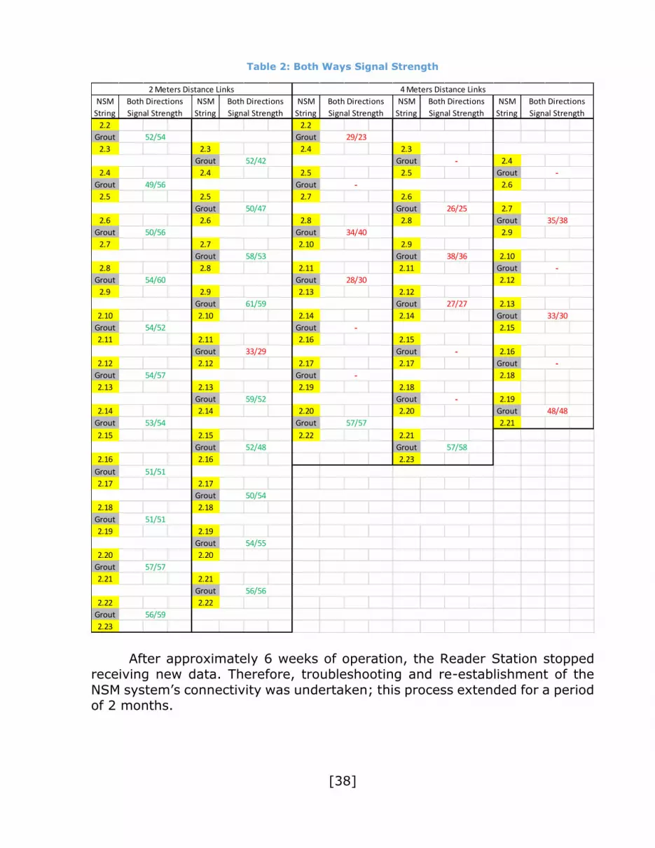
[38]

Table 2: Both Ways Signal Strength

After approximately 6 weeks of operation, the Reader Station stopped receiving new data. Therefore, troubleshooting and re-establishment of the

NSM system’s connectivity was undertaken; this process extended for a period of 2 months.

2.2 2.2

Grout Grout

2.3 2.3 2.4 2.3

Grout Grout 2.4

2.4 2.4 2.5 2.5 Grout

Grout Grout 2.6

2.5 2.5 2.7 2.6

Grout Grout 2.7

2.6 2.6 2.8 2.8 Grout

Grout Grout 2.9

2.7 2.7 2.10 2.9

Grout Grout 2.10

2.8 2.8 2.11 2.11 Grout

Grout Grout 2.12

2.9 2.9 2.13 2.12

Grout Grout 2.13

2.10 2.10 2.14 2.14 Grout

Grout Grout 2.15

2.11 2.11 2.16 2.15

Grout Grout 2.16

2.12 2.12 2.17 2.17 Grout

Grout Grout 2.18

2.13 2.13 2.19 2.18

Grout Grout 2.19

2.14 2.14 2.20 2.20 Grout

Grout Grout 2.21

2.15 2.15 2.22 2.21

Grout Grout

2.16 2.16 2.23

Grout

2.17 2.17

Grout

2.18 2.18

Grout

2.19 2.19

Grout

2.20 2.20

Grout

2.21 2.21

Grout

2.22 2.22

Grout

2.23

2 Meters Distance Links

57/57

56/59

NSM

String

Both Directions

Signal Strength

49/56

50/56

54/60

54/52

54/57

53/54

Both Directions

Signal Strength

NSM

String

52/54

33/29

59/52

52/48

50/54

54/55

51/51

51/51

52/42

50/47

58/53

61/59

26/25

34/40

NSM

String

Both Directions

Signal Strength

NSM

String

Both Directions

Signal Strength

29/23

56/56

NSM

String

Both Directions

Signal Strength

-

57/57

57/58

-

48/48

4 Meters Distance Links

-

35/38

-

33/30

-

-

-

38/36

28/30

27/27

-

-

[39]

3.4.1. Improvements to the NSM System

There were several improvements made to the system to improve its

performance after the installation. For instance, cables were unearthed and installed inside galvanized conduit ducts, the Splitter Box was protected using

a metal box and the motherboard inside the Reader Station was replaced by an up-to-dated version.

However, subsequently, communication to both boreholes was lost

again. Laboratory testing was performed using spare NSMs, identifying several possible causes for this issue. Table 3 provides a list of identified faults and/or

causes for this system’s malfunctioning and the level of contribution to the problem of each cause.

Table 3: Troubleshooting Summary

Detected

Fault Possibility Comment

Likelihood

Contribution

Poor 2-hop

Distance

Connection

Poor marker

communication

range

Different performance between

individual NSMs.

Antenna performance randomly

distributed, causing short NSMs range.

Likely.

Strong

contribution.

Atmospheric

noise

penetrating

bench

Bottom-Markers may have more

success in 2-hop links due to them

receiving less background RF

atmospheric noise.

Markers receiving higher background

noise will have low range.

Unlikely.

Medium

contribution.

Poor RF

properties of

Earth/Ground

The ground and/or grout composition

might be significantly different over

borehole’s length.

Unlikely.

Medium

contribution.

Markers

Becoming

Non-

Contactable

Marker

software

problem

A possible firmware fault was

discovered that could cause a Marker

to get stuck in an un-contactable state.

Likely.

Strong

contribution.

Marker battery

problem

Batteries may have drained during

shipment of NSMs for this trial because

they were shipped “pre-activated” to

simplify the installation procedure.

Unlikely.

May have

strong

contribution in

the case of a

flat battery,

but no NSMs

showed this.

Broke

installation rope

Possibly, the ropes broke during Marker

installation leaving some NSMs out of

rage.

Possible but

unlikely. Rope

breaking

would have

been noticed.

Rope elongation

Rope stretch expanded the planned

distance between Markers. The

distance for 2-hop links exceeded the

Markers’ communication rage.

Likely.

Strong

contribution.

[40]

A second installation with second generation prototype NSM was

scheduled for the same trial site. Table 4 provides a summary of improvements

made to the system prior to the second installation, which were deemed of high importance after the evaluation.

Table 4: System Improvements

Possible Issue Improvements Made

Out-of-spec antenna tuning, which may

result in poor Marker communication

range.

Automatic testing of Marker’s antenna

tuning during manufacturing.

Antenna ranges tested in the ground

before grouting the hole.

Software locking up on individual Markers.

Second generation software resolved

known bugs and significantly improved

reliability.

New generation release was and continues

to be extensively tested at Elexon.

Limited access to Reader required site

visits, which placed additional work load on

mine personnel and Project Team.

Remote access to Reader with a GSM

modem to enable administrative tasks to

be performed by AMTC and Elexon

remotely.

Antenna cabling getting damaged.

Antenna cable protected with specifically

designed cover to prevent physical impact

damage.

Uneven filling of the boreholes due to

excessively viscous grout and to the

pouring process.

A new, thinner grout mixture was

employed.

The grout was pumped through PVC pipes

from the bottom of the boreholes instead

of just pouring it from the boreholes’

collar.

NSM testing after grouting.

NSM tested above ground.

NSM tested in the hole for an extended

period (several days) before grouting.

[41]

3.5. Second NSM Open Pit Trial

A second mine site trial was planned to test the performance of the

system with the improvements made to the installation procedures, the devices and the overall NSM system. For this purpose, two new boreholes, 10

and 40 meters deep, were drilled in the vicinity of the long-lasting working NSM borehole from the first trial. This time placed approximately 10 meters

behind the crest of the slope. The 10-meter drill hole was located behind the first trial borehole, while the 40-meter borehole was perforated 10 meters

away from those drill holes in the direction of the Splitter Box.

The drill holes used for the first trial were disconnected from the Splitter Box to allow connection of the antennas used for both newer boreholes. This

allows the reutilization of NSM system associated infrastructure already installed in the mine (Splitter Box, main feedline and Reader Station) for the

10 and 40-meter boreholes (Figure 9).

Figure 9: Second NSM Installation Diagram

[42]

Both boreholes were instrumented in sequence. The 10-meter borehole,

with five NSMs at a 2-meter separation, allowed for initial testing of the

installation before the deeper borehole was instrumented. The 40-meter drill hole was left with 35 NSM Markers (1-meter separation) hanging inside it.

After the grout poured in the shallower drill hole set overnight and getting confirmation that the NSMs in that borehole were performing as planned, the

second borehole was filled with grout. A final communication test was run after the dipper borehole had the antenna in position and was completely filled, thus

verifying that the system was working under specifications.

3.5.1. System Installation Procedure

During this installation, NSMs strings were put together using a climbing

kernmantle rope capable of withstanding 3.5 time the weight of 35 devices in the string. This minimized elongation of the rope caused by NSM’s weight.

Cables from both antennas to the Splitter Box and the main feedline connecting the Reader Station with the Splitter Box were installed inside

galvanized conduit ducts. The strings were left hanging and working inside the boreholes for one week before grouting them. This allowed to test signal

strength and the detection of any possible communication problem.

The boreholes were sealed using an improved grouting procedure and 1:1:2.5 cement:sand:water grout. The grout mixture was pumped from the

bottom of the drill hole to the top using 1½” inches diameter PVC tubes to: (1) avoid placing additional weight on the NSMs and the rope as the borehole

was filled; (2) ensure that the borehole was completely filled, avoiding the formation of air gaps within the grout column; and (3) minimize NSMs’ tilting

and displacement. The NSM antennas were installed at last, located right above and in contact with the top-most NSM in the boreholes (0m spacing),

placed approximately one meter below ground surface and sealed with sand

instead of grout to make it possible to recover the antennas, if needed.

After the boreholes were fully grouted and the antennas buried with

sand, a communication test was performed using the Reader Station. It showed that wireless linkage between NSMs grouted in the drill holes was

successful.

The system’s Reader Station was improved with the integration of a GSM modem. This modem enabled remote access to the Reader Station using

wireless networks, simplifying the operation of the system as the operator was able to interact with the Reader from their office. The improvement also

allowed software updates, firmware modifications and command execution

related to data downloads without having to send an operator to the studied site.

[43]

Four months after the second trial installation, all NSMs in both boreholes

were still reachable showing good quality links. Data was being gathered at

short time intervals without problems. This test proved that the installation procedure for the second trial overcame the faults and problems registered

during the first trial, ending up with a robust site installation. The system also demonstrated that, using NSMs, it was possible to have wireless data

transmission through rock in open pit slopes.

3.6. Recommendations to Improve the System

After both mine site trial installations, the ability of the NSM system to

wirelessly transmit data through the rock mass under an operative open pit mine constrains was demonstrated.

Every faults and problems identified during the first trial were examined

and taken into account for an improved installation in the second trial. This produced a reliable and robust installation procedure, applicable for similar

installations. If an installation is planned for boreholes over 100 meters deep, installation procedures will need to be improved or changed.

With regards to the particular devices, NSMs demonstrated to be a

robust solution for rock mass geotechnical instrumentation, being able to withstand particular conditions encountered in this type of material and

overcoming common problems encountered when applying other geotechnical instruments in open pit mining environment. For instance, blocked boreholes,

broken in-hole cables and boreholes’ casing excessively deformed. All of these assures NSMs’ long lifespan under open pit mining conditions, allowing 2-

meter deformations while still having good quality communication and proper

system functioning.

3.6.1. System’s Current Development

It is planned to use the NSMs and their wireless data transmission capabilities as an in-ground platform for geotechnical monitoring. This

platform will integrate different sensors to monitor subsurface variables in a

single device, able to operate autonomously for over 10 years. Sensors’ shortcomings for mining applications, such as, limitations related to in-ground

cable connections will be overcome with this integration.

In that regard, a new version of NSMs called Enhanced Network Smart

Markers (ENSM) is being developed to integrate further sensors. ENSM are

being designed to overcome some limitations of the currently available and commonly used sensing technologies, such as:

Limited depth application.

[44]

Instruments’ short lifespan.

Low tolerance to abrupt shearing.

Limited number of devices per borehole. Low coexistence of sensors in a single location.

Installation and performance issues due to the presence of cables inside the boreholes.

3.6.2. System’s Future Developments

Future installations of the system will consider using ENSM. These devices will be deployed in more complex and fully operative open pit

environments including groundwater presence, higher rates of subsurface deformations and complex interactions between mining operations.

Since future trials will be conducted with full-scale open pit slopes, it will

be necessary to instrument 300-meter deep boreholes; in this case, using strings will be too heavy to be manually handled. These new conditions will

require more specific installation procedures and specially design hardware to lower ENSM devices inside the boreholes.

Proper data gathering frequency has to be defined for the ENSM to

capture changes experienced by studied variables in material with different properties. In brittle rock masses, it will require higher data collection

frequencies to capture deformations than in ductile rock masses, which are characterised by more progressive deformations.

To obtain useful information from gathered data, tools to manipulate and

process this data and a visualization software are being developed. These will allow near-real time data processing and variables monitoring (for all sensors

integrated in ENSM).

Finally, ENSMs’ enclosure will be redesign to allow easier construction of

strings, facilitating the attachment of a large quantity of devices to a single

string or easy handling with new installation method.


This chapter provided a thorough description of the Networked Smart

Marker (NSM) system and its associate infrastructure. It also included case studies for the two first open pit NSM installation, featuring installation

procedures, problems and faults analyses and improvements of the NSM system from the first installation to the second one. Finally, it presented

current and future developments of the system, which are intended to produce a more robust and widely applicable system for all different open pit mining

conditions.

CHAPTER 4

[45]

MINE PLAN

The first step to plan any geotechnical monitoring campaign is the

definition of the conditions of the project to be monitored. Thus, during this research and prior to the design of any monitoring campaign, open pit’s mine

plan and pushbacks were obtained from a theoretical bock model. For this tasks, the software DeepMine was used. The pushbacks defined in DeepMine

were then relaxed using the software Vulcan to obtain smooth operative phases, avoiding major changes to assure that the obtained mine plan

remained valid.

Since the purpose to develop a mine plan and associated phases (project conditions) is to guide the deployment of the instruments to obtain the best

results from the monitoring campaign for slope stability assessments, the development of a detailed mine plan and fully operational phases design

(including berms and ramps) was considered to be out of the scope of this chapter and thesis.

4.1. DeepMine

DeepMine (BOAMine SpA, 2015) is a software solution for strategic open pit mine planning from an economic perspective that avoids the usage of

predefined phases (pushbacks). As output, it delivers the size of the mine

considering amount of material to be mined and processed. It also delivers mine’s lifespan and the value of the operation in terms of net present value

(NPV). To do so, the software creates decision trees based on the studied mining configuration. Approximate dynamic programming is used to explore

multiple branching in those decision trees to obtain the best outcome based on operation’s economic value.

Pushbacks are automatically produced as the result of software’s

calculations, considering operational constrains using Lerchs and Grossman pit shells as input to define operative phases. The resulting pushbacks are

associated with the mine plan and can be used as a guide for mine design e.g. a plan that establishes when every pushback has to be mined to obtain the

best possible economical outcome.

To produce such results, DeepMine works with a block model given as an input used by the software to perform the calculations and with the

definition of four elements in the mine planner: The GeoModel, the Mining Environments, the Pit Collections and the Economic Environments. These

elements use the information contained in the block model and can be defined

[46]

to apply uncertainty on the resulting mine plans by, for example, modifying

commodities prices, operational costs and taxes over time.

A brief description of all the modules that the user has to define to solve the mine plan is presented in the following list:

1. The GeoModel contains the block model representing the ore deposit and

the topography. Here the maximum admissible overall slope angles have to be defined.

2. The Mining Environments define operational parameters related with mine, stocks plants and dumps’ location, operations, capacities,

investments and costs. All this data (extraction and processing information) is used to determine cash flows of the project per year.

3. The Pit Collections define a set of pit shells resulting from the application

of Lerchs and Grossman algorithm to solve the ultimate pit problem using as input a GeoModel, a Mining Environment and a series of yearly

prices for every commodity to be mined. 4. The Economic Environments define the first year of mine’s operation, a

discount rate for the cash flow, prices and selling costs per year for every commodity contained in the block model. Finally, a tax rate is defined

for the entire operation. 5. The Mine Plans are the final output of the software. To produce them,

the user defines the first year of operations, maximum life of mine (LOM), maximum sinking rate for a single phase in term of benches

(number of block in a vertical section) per year, maximum number of active phases every year, maximum phase length, minimum phase width

and, optionally, minimum and maximum phase weight. Finally, the GeoModel, Mining Environment, Pit Collections and Economic

Environment are used as input.

Refer to APPENDIX B for further information regarding the components defined in DeepMine to obtain the mine plans.

4.2. Definition of the Mine Plan and Phases using DeepMine

The definition of a coherent Mine Plan using DeepMine was an iterative

process. This process involved working with a theoretical block model for a copper ore deposit. The four main areas of the software (GeoModel, Mining

Environment, Pit Collection and Economic Environment) were defined at the very beginning and the iterations were focused on continuous modification of

the Mining Environment. These modifications induced changes in the Pit Collection that were automatically processed by the software. The GeoModel

and Economic Environment were not modified in this process.

[47]

All the iteration induced changes to the preliminary Mine Plan looking for

smooth mine productions over time, plants operating at full capacity and

stockpile/re-handling minimum usage.

4.2.1. Block Model Characteristics

A theoretical block model was used to produce a mine plan with associated extraction phases. This model was constructed by 30[m] long,

30[m] wide and 15[m] high blocks, arranged in a volume of 1,620 by 1,620

meters (54x54 blocks) footprint and 720 meters (24 blocks) depth.

The model contained four different types of rock: waste, oxides,

oxide/sulphide transition zone and sulphide ore. Every type of rock contains information about total copper and soluble copper content. The orebody

presented an average copper grade of 0.16[%Cu]. Table 5 presents the

orebody’s main characteristics.

Table 5: Orebody’s Rock Type Distribution

Rock Type Weight [kton] Average Copper

Grade [%Cu]

Maximum Copper

Grade [%Cu]

Oxide Ore 158,513.74 0.07 0.83

Sulphide/Oxide

Transition Ore 255,104.36 0.20 1.24

Sulphide Ore 505,283.44 0.16 1.72

Waste Rock 1,177,483.74 0.03 0.30

4.2.2. GeoModel Definition

The GeoModel was defined enabling the resulting phases to have different slope angles, representing with these sectors two different rock

qualities. Good quality rock will have steeper slope angles compared to poor quality rock. Table 6 summarizes the definition of these zones, where bearing

represents the dip direction of the slope with respect to the geographic North Pole and angle represents the overall slope’s angle.

Table 6: GeoModel Definition Summary

Pit Zones Bearing Angle

Good Quality Rock Mass 0° 50°

Good Quality Rock Mass 90° 50°

Poor Quality Rock Mass 180° 40°

Poor Quality Rock Mass 270° 40°

[48]

4.2.3. Mining Environment Definition

The definition of a Mining Environment was an iterative process. It

started by establishing 2015 as the first year of mine operation and the determination of the need to have two plants to process all different ores

coming from the mine. A leaching plant for oxide and transition ores and a concentrator plant to process sulphide ores.

The iterative part of the process was made to define the combination of

mine and processing plants’ capacities that produced the best economic outcomes. The first step was to evaluate several mine’s annual capacities in a

range from 10,000[kton] up to 80,000[kton] matched with over dimensioned and fixed plants capacities. The resultant Mine Plan’s NPVs (net present values)

were assessed concluding that the higher values of this indicator were obtained with a mine capacity of 40,000[kton]. This evaluation also showed that the

first plant entering into production was the leaching plant; this information was used to define the next step in the production of a feasible mine plan.

The next iterations involved the evaluation of different leaching plant

capacities. All alternatives explored in this process considered that the leaching plant was going to be fed with oxide and oxide/sulphide transition ores and it

was assumed copper recoveries of 75% for oxide ores and 65% for oxide/sulphide transition ores. The evaluation of a suitable plant capacity was

based on the resulting LOM and then on the Mine Plan’s NPV value, as it was observed that small plant capacities resulted in LOMs around 6 years, which

was not coherent with an ore body as big as the one used for this project. This part of the process ended with an annual capacity for the leaching plant of

9,000[kton] and a lifespan of 13 years from 2015 to 2027.

Subsequently, the concentrator plant characteristics were established. The alternatives studied in these iterations considered that the concentrator

plant was going to process all sulphide ores coming from the mine. The recovery in this plant was set at 90% for all copper contained in sulphide ores.

The evaluation of suitable capacities was strongly influences by resulting LOMs as small concentrators drastically reduced the lifespan of the mine. Mine Plan’s

NPV’s showed that the most profitable concentrator capacity was 7,000[kton]

per year. The operation of this plant had to start in year 2017, working for 15 years to end its operation in 2031. This result was obtained considering the

previously described leaching pant.

Although the defined combination of mine, leaching plant and

concentrator plant capacities gave the best result in terms of NPV,

operationally it presented several concerns, including:

1. Mine production was uneven.

[49]

2. Plants presented some years of extremely low utilization.

Two different methods were used to overcome these issues based on the

control of the amount of re-handled material feed into each plant and on limiting the surplus for both the leaching and concentrator plants.

To be able to control the re-handling, two stockpiles were defined. The

first one was intended to stock oxide and oxide/sulphide transition ores to feed the leaching plant. It was configured to hold 18,000[kton] per year the,

twofold of the leaching plant capacity. The second stockpile was meant to feed the concentrator plant and store exclusively sulphide ores. Its capacity was of

14,000[kton] per year, which was twofold the capacity of the concentrator plant. Thus, each stockpile could hold approximately one day of mine capacity.

Table 7 summarizes all relevant costs and capacities.

As the stockpiles had to be defined by its yearly capacity, an important problem arose as the software tended to uncover high grade ores by producing

large quantities of material that went directly to stockpiles. This produced the highest cash flows in early stages of the project and, thus, a better economic

results, but it also produced high amounts of stocked material that lasted

several years in such condition. The stockpile material was sent to the processing plants in the last years of the project. Another problem that

emerged was that during the last years of plants’ operation, no re-handling and surplus limits were defined while the plants were processing, mostly,

stocked material, as shown in Figure 10.

Table 7: Operational Costs and Capacities Summary

Annual Capacities Operational Costs

Mine 40,000[kton] 2.25[US$/ton]

Concentrator 7,000[kton] 9.40[US$/ton]

Leaching 9,000[kton] 4.30[US$/ton]

Sulphide Ore Stockpile 14,000[kton]

Assumed as part of

concentrator’s operational

costs

Oxide and Ox./Sulphide

Transition Ore Stockpile 18,000[kton]

Assumed as part of

leaching’s operational costs

Dumps Unlimited Assumed as part of mine’s

operational costs

[50]

To overcome these problems the surplus was limited. The definition of

surplus limits was performed yearly for each plant. The results of this process

is shown in Table 8. This constraint controlled the amount of material, in excess of the mined ore, to be sent to the processing plants that can be mined.

The process resulted in lower extraction of stock material in early stages of mine’s life and higher amounts of mined material sent directly to the plants.

Figure 10: Leaching Plant Unsatisfactory Operation

Table 8: Adjustment Factors Summary

Year

2015 2016 2017 2018 2019 2020 2021 2022 2023 2024 2025 2026 2027 2028 2029 2030

Concentrator Surplus Limit [kton]

0 0 0 4,000 5,000 1,000 5,000 1,000 0 5,000 3,000 0 5,000 0 0 0

Leaching Surplus Limit [kton]

2,000 2,450 2,900 3,350 3,800 4,250 4,700 0 500 1,000 0 0 0 0 0 0

Sulphide Ore Stockpile Re-handling Capacity [kton]

0 0 0 1,400 1,400 1,400 1,400 1,400 1,400 1,400 1,400 1,400 1,400 1,400 1,400 1,400

Oxide and Oxide/Sulphide Transition Ore Stockpile Re-handling Capacity [kton]

1,800 1,800 1,800 1,800 1,800 1,800 1,800 1,800 1,800 1,800 900 1,800 900 900 900 900

89788245 8030

9000

1135

5698

7228

5025

1539 1243635 844 35 0 0 0

737 948

7862

3299

1755

3966

7441 7757

4668

0

1000

2000

3000

4000

5000

6000

7000

8000

9000

10000

2015 2016 2017 2018 2019 2020 2021 2022 2023 2024 2025 2026 2027 2028 2029 2030

Leac

hin

g P

lan

t O

re S

up

ply

[kt

on

]

Year

From Mine From Stockpile

[51]

The amount of the re-handled material per year was defined for each

plant in an iterative process year by year to further improve the distribution

of plant’s stock supply. This process started by setting the maximum amount of re-handled material at 20% of the matching plant capacity. Then, the values

were reduced, when possible, to maximize the amount of mine material fed to the plant while saturating plants capacity. Table 8 summarizes the re-handled

material per year for both plants.

4.2.4. Pit Collection Definition

The Pit Collection for the Mine Plan was defined using a vector of 40

different prices for the copper. The prices defining that vector were homogeneously distributed between 0 and 3[US$/lb].

The GeoModel was associated with the generation of Pit Collection to use

slope angles contained in the GeoModel to define the precedence list for block’s extraction.

This process should have resulted in 40 different pit shells. However, the first 8 pit shells did not contain any blocks because of the low commodity prices

defined in the first eight intervals of the price vector. Figure 11 shows the 32

different pit shells resulting from this process.

Figure 11 also shows the different slope angles as defined in the

GeoModel and captured by the pit shells. It is worth mentioning the importance of producing many pit shells as those will be used as guide to generate the

extraction phases. More pit shells means more flexibility for DeepMine to

generate the geometry of the phases and, thus, better results in producing operative phases.

Figure 11: Pit Shells Views – Plant (Left), East-West (Right Top), North-South (Right

Bottom)

N

O

N

[52]

4.2.5. Economic Environment Definition

With regard to the Economic Environment, copper price was set at

3[US$/lb] for the entire mine’s lifespan. This value was stablished considering the price predictions made in August 2015 by the Chilean Central Bank

(2.9[US$/lb]). For simplicity, no taxes were considered. Table 9 contains all the parameters used to define the Economic Environment.

Table 9: Economic Environment Definition Summary

Economic Environment Definition

Discount Rate 8[%]

Copper Price 3[US$/lb]

Copper Sales Cost 0.4[US$/lb]

Tax and Royalty 0[%]

4.2.6. Mine Plan Settings

Before obtaining the final mine plan, some parameter had to be provided for the software to produce logical operative phases. These parameters are

listed in Table 10.

Maximum Life of Mine (LOM) defines the maximum number of years that

DeepMine will consider to do the extraction of the mine. In this case, the LOM’s

input value was defined as 30 years, which assured that every resulting mine plan had a shorter life than the input LOM. Therefore, any possible mine plan

was not restricted by the LOM.

Table 10: Mine Plan Settings

Parameter Magnitude

Maximum Life of Mine (LOM) 30[years]

Maximum Active Phases Simultaneously 5

Maximum Phase Length 1,000[m]

Minimum Phase Width 100[m]

Maximum Sinking Rate per Year 10[benches]

The number of active phases that can be operating simultaneously adds flexibility to mine planning, hence, it allows for more possible extraction

alternatives.

Minimum phase width is a critical parameter for the operation of the mine and, thus, for the definition of the phases; it has to be properly

estimated. Therefore, an estimation of the shovel-truck fleet that this mine will need for its operation was required.

[53]

Since the mine has a production rate of 40,000[kton] per year, around

111,000[ton] of material have to be moved per day. It was assumed that a

hauling cycle time would be 30[min] and an operational factor would be 65%, which gave 15.6 hours of operation per day. Table 11 shows the number of

trucks that the mine would require fulfilling its production and their capacity.

Table 11: Truck’s Fleet Estimation

Parameter Magnitude

Truck Capacity

[ton/cycle] 18 20 32 46 68 78 120 160 180

Production

[ton/hr] 36 40 64 92 136 156 240 320 360

Daily Production

[ton/day] 561.6 624.0 998.4 1,435.2 2,121.6 2,433.6 3,744.0 4,992.0 5,616.0

Truck Fleet 198 178 111 77 52 46 30 22 20

A fleet of twenty 180[ton] capacity trucks were selected as reference for the determination of the ramp width. It was decided to consider two ways

24[m] wide ramps. This width was defined based on the dimensions listed in Table 12 and shown in Figure 12, which considered the dimensions of a

Komatsu 730E truck.

Figure 12: Ramps Setup (modified after Hustrulid et al., 2013)

Ditch

Safety Berm

Safety Distance

Safety Distance

Safety Dist.

Truck Width

Truck Width

Total Ramp Width

[54]

Table 12: Ramps Dimensions

Parameter Magnitude

Ditch 1[m]

Safety Berm (Pit Side) 1.72[m]

Truck Width (x2) 7.54[m]

Safety Berm (Bench Side) 0[m]

Safety Distances (Total) 6[m]

Total Ramp Width 24[m]

In the next step, a shovel was selected to match the Komatsu 730E

trucks. A simple operational rule was used for preliminary shovels selection: a shovel had to be able to load a truck in less than 3 cycles. As the selected

trucks had a capacity of 111[m3], shovel’s bucket had to have a capacity of at

least 37[m3]. Hence, a Komatsu PC8000-6 shovel with a bucket capacity of 42[m3] was selected.

The minimum loading width was calculated based on the dimensions of selected trucks and shovel plus safety distances as listed in Table 13 and

shown in Figure 13 where one truck - shove configuration is considered.

Table 13: Loading Area Dimensions

Parameter Magnitude

Safety Berm (Pit Side) 1.72[m]

Truck Width 7.54[m]

Safety Distances 6[m]

Shovel Width 18.6[m]

Spalling 5[m]

Total Loading Width 39[m]

The worst case scenario is the occurrence of a loading area alongside a hauling ramp. This combination required an operational width of 63[m] but,

as this was not a detailed design, important contingencies might be expected. It was decided to work with a minimum phase width of 100[m].

The maximum sinking rate is referred to the number of benches that can

be vertically mined as part of a single phase. This, again, allows for more possible extraction alternatives.

Finally, the Mine Plan was solved using Deep Mode and a Guidance

Amount of 80%. Deep Mode allows the software to explore all possible alternatives to generate a mine plan under the defined parameters and

constrains given in DeepMine.

[55]

Figure 13: Loading Area Setup

4.2.7. Resulting Mine Plan

DeepMine calculations resulted in 16 years of operation divided into 29

different phases. It considered the extraction of 355,029.04[kton] of material, 88,163.04[kton] of sulphide ores were processed in the concentrator plant and

95,306.37[kton] of oxide and oxide/sulphide transition ores were processed in the leaching plant. Mine’s stripping rate was 1.28. The scheduling of the 29

phases is shown in Table 14.

The mine started its production in year 2015, operating to supply the leaching plant since that year, while the concentrator plan started its operation

in year 2017. The minimum cut-off grades were 0.10%Cu for the leaching plant and 0.18%Cu for the concentrator plant. APPENDIX C presents the cut-

off grades per year for each plant.

Figure 14 shows mine operational levels, which started its regimen in 2018, with around 33,000[kton] per year, until 2026 when mine production

began to decrease. It also shows an anomaly in year 2022, when mine production had an abrupt drop, which was not of concern as it occurred in the

8th year of mine production, when hauling fleet reached its operational life. Thus, it was planned to renew the hauling fleet close to the date, where the

drop in mine production was produced, process that considered the decrease in production. Furthermore, this abrupt drop in mine production was accepted

as the mine plan was not the main focus of this thesis.

Safety

Dist.

Safety

Dist.

Safety

Dist.

Safety

Berm

Truck Width Shovel Width Spalling

Total Loading Width

[56]

Table 14: DeepMine Phases Scheduling

Year

Phase 2015 2016 2017 2018 2019 2020 2021 2022 2023 2024 2025 2026 2027 2028 2029 2030

1

2

3

4

5

6

7

8

9

10

11

12

13

14

15

16

17

18

19

20

21

22

23

24

25

26

27

28

29

Figure. D.1 and Figure. D.2, which show operations for both plants over

time can be found in APPENDIX D.

In terms of the economic value, DeepMine results established a project’s NPV of 644.27[MMUS$]. However, this value did not consider capital

expenses; investments in the mine, leaching plant and concentrator plant construction. This simplification facilitated the iteration process that led to the

described results.

However, the investments were incorporated in the manual calculations of the new NPV values as follows:

[57]

1. 142.11[MMUS$] for mine’s capital expenses in year 2014.

2. 148.07[MMUS$] for leaching plant’s capital expenses in year 2014.

3. 167.47[MMUS$] for concentrator plant’s capital expenses in year 2016.

Figure 14: Mine Operation

Figure 15: Final Cash Flow

8987 8894

14488 14149 14155 1487012803 13380 12802 12751

80745775 6529 5626

2441158

1382489

1060

7700 83314280

64321286 2352

5420

2123

2082 0 403

0 176

7770 4625

1391

12846 10252 1745020750

5604

1592714006

17055

5819

13909

7196

275 0

0

5000

10000

15000

20000

25000

30000

35000

40000

2015 2016 2017 2018 2019 2020 2021 2022 2023 2024 2025 2026 2027 2028 2029 2030

Min

e P

rod

uct

ion

[kt

on

]

Year

Sent to Plant Sent to Stockpile Waste

-290,18

54,54

-78,78

211,27

105,5395,15122,15

73,0556,16

-1,94

44,46 21,06 18,47 26,26 9,46 20,32 5,01

-300

-200

-100

0

100

200

2014 2015 2016 2017 2018 2019 2020 2021 2022 2023 2024 2025 2026 2027 2028 2029 2030

Cas

h F

low

[M

MU

S$]

Year

[58]

Therefore, the NPV was calculated to be 210.51[MMUS$]. Figure 15

shows the final cash flow of the project, which considers capital expenses for

the mine and plants.

4.2.8. Resulting Phases

Generated phases were analysed considering two main aspects: geometry and extraction period.

With respect to the geometry, several disperse phases composed of

isolated blocks and phases formed by too few blocks to be operationally feasible were found. Both cases represented a major problem for mine’s

operations, which needed to be solved to generate an operative open pit.

Adjacent phases that were planned to be extracted in the same period or in sequence were also found. There was no reason to have those phases as

separate pushbacks as they would have complicated the extraction of the mine adding unnecessary phases and creating scheduling problems.

Hence, a modification and/or a merger of phases presenting problems in

terms of geometry an extraction period was made. APPENDIX E presents isometric views of all 29 phases generated by DeepMine arranged by their

extraction sequence.

4.3. Pushbacks Design

The phases’ geometries that had to be modified and/or merged into bigger and continuous pushbacks were constructed using Vulcan.

Each phase’ size, its position within the block model and the year when they were planned to be extracted was analysed. It is assumed that the mine

plan and economic revenue would not suffer major changes as a result of this

process as the period in which every phase was planned to be extracted remained the same and no blocks were added or erased from the phases. The

process also maintained bench height (15 meters) and overall slope angles defined in DeepMine. Berms design was not considered and bench face angle

remained vertical as it was defined by blocks’ faces.

The modifications produced 12 phases as follow (see APPENDIX E for further information regarding this process):

1. Phase V1: It was formed by DeepMine’s phase 01 plus the narrow portions of phase 02 and one isolated block form phase 03.

2. Phase V2: It was formed by DeepMine’s phase 02 without its narrow

portions.

[59]

3. Phase V3: It was formed by merging phase 05 with phase 03 without

the isolated block that was added to phase V1.

4. Phase V4: It was formed by DeepMine’s phase 04 without their isolated blocks.

5. Phase V5: It was formed by merging the phases 06, 07 and 09 plus the isolated blocks from phase 04.

6. Phase V6: It was formed by merging the phases 08, 11 and 14, and adding an isolated block from phase 16.

7. Phase V7: It was formed by DeepMine’s phase 10. 8. Phase V8: It was formed by merging the phases 12, 13 and 17.

9. Phase V9: It was formed by merging the phases 15, 16, 23 and 25. 10. Phase V10: It was formed by merging the phases 18, 19, 20, 21, 24, 26,

27 and 28. 11. Phase V11: It was formed by phase 22.

12. Phase V12: It was formed by phase 29.

This process ended with the extraction of the mine scheduled as shown in Table 15.

APPENDIX F presents isometric views of the 12 phases.

Table 15: Redefined Phases Scheduling

Year

Phase 2015 2016 2017 2018 2019 2020 2021 2022 2023 2024 2025 2026 2027 2028 2029 2030

V1

V2

V3

V4

V5

V6

V7

V8

V9

V10

V11

V12


This chapter presented the development of a mine plan for the extraction

of a theoretical orebody. The process was developed using the software DeepMine with a model composed of 69,984 blocks containing information

about copper grades with an average grade of 0.16[%Cu] for the entire

[60]

orebody. The mine plan called for the duration of 16 years divided into 12

phases.

CHAPTER 5

[61]

DESIGN OF A SLOPE DEFORMATION MONITORING

CAMPAIGN PRIOR TO MINE CONSTRUCTION

Drilling campaigns are commonly performed to understand the

mechanisms involved in mine slopes failure. This campaigns are carried out after failure has occurred aiming to gather data, such as UCS values, and for

structural analyses to be used as input for back analyses and redefinition of geotechnical domains. It does not have preventive value and does not study

the actual rock mass’ behaviour under mining conditions. Therefore, open pit mines’ geotechnical monitoring always responds to processes or failures

observed as mining develops. It is a reactive response and, thus, it does not capture the development of the whole failure, as the process triggering the

observed failure has been occurring for a long time and all data from this development period has already been lost. Furthermore, the data, if obtained,

is not transformed into information that can be used to reassess or redesign mine slopes for future pushbacks. For example, when steepening slope angles

in geotechnical domains, where rock mass behaves outstandingly and where,

if slope angle is increased by few degrees, tens of millions tonnes of waste material may not be extracted from the mine producing important savings in

mine costs. This could extend mine’s lifespan or allow economical extraction of new marginal, superficial orebodies.

To overcome the gap in the knowledge about rock mass behaviour before

failure, mines’ geotechnical monitoring should be considered and designed from feasibility stages of the project. In this Chapter, monitoring campaigns

to register subsurface rock mass deformation will be designed considering mine’s pushbacks geometry and mine plan throughout mine’s lifespan.

The objective of this Chapter is to design instrumentation campaigns for

subsurface rock mass deformation monitoring using three different instruments: Networked Smart Markers (NSM), In-Place Inclinometers (IPI)

and ShapeAccelArrays (SAAs). The mine plan and the geometry of mine’s phases (project conditions) will be used as guidance to determine where and

how to deploy the instruments to achieve the best results from the monitoring campaigns designed towards better assessment of mine slope stability.

5.1. Monitoring Campaign Design

The nature of the project to be instrumented has been described from the mine planning perspective in Chapter 4. Due to the scale of the phases to

be monitored (rock mass scale), the failure mode of interest corresponds to rock mass failures. Toppling, wedge and plane failure (structurally controlled

[62]

failures) are less likely to be detected by the proposed campaigns, since there

are better techniques to do this, such as, visual inspection and various surface

deformation monitoring techniques.

5.1.1. Aspects to Be Assessed

Every geotechnical instrumentation campaign has to be designed to answer specific questions relative to ground performance, i.e. it has to have a

purpose. To define the questions that justify the implementation of

instrumentation campaigns in open pit mining, the effort was focused on the biggest concerns of mining industry and particularly of open pit mines

operations: safety and competitiveness.

From the safety perspective, the main concern is pit slope performance

and stability. Thus, the following questions arose:

1. What is the initial geotechnical condition of the rock mass prior to slope construction?

2. Do the mine slopes constructed in complex areas perform satisfactorily during all of mine’s operational lifespan?

3. Do final pit slopes perform satisfactorily until the end of mine operations?

These questions focus the efforts on monitoring slopes constructed in the worsts geotechnical domains and, since long term Factors of Safety are

difficult to assess, also on the slope with the longest service life to account for the loss of competence experimented by the rock mass degradation process.

With respect to competitiveness, to lower the operational costs is a

common alternative, which can be achieved by steepening slope angles to diminish waste extraction. However, this solution requires a good

understanding of ground performance which leads to the question:

1. Is it possible to steepen the slope angle while maintaining low risks conditions for personnel and operational safety?

This question led to the instrumentation of the walls with greater

potential for steeper slopes’ angles, i.e. slopes with shallower angles initially.

Therefore, the selection of critical sectors of the mine was led to monitor slopes constructed in the worsts geotechnical domains, the slope with the

longest service life and slopes with shallower angles. The monitoring might also allow fulfilling other purposes not considered as main goals of this

monitoring campaign, such as, assessing whether slopes’ constructions

[63]

sequences are adequate, identifying excessive deformation and/or heave and

identifying unforeseen hazards.

5.1.2. Parameter to Be Measured

In open pit mining projects, it is difficult to determine whether a slope is

performing safely, since failure processes not only depend on rock mass strength but also on the type of failure under development. Thus, it was

decided to measure subsurface deformations as, depending on its progression,

subsurface deformations can indicate the development of non-daylighting failures and allows detection of developing failures prior to the observation of

any sign of failure on the surface. This might also allow to undertake corrective measures before the failure becomes imminent.

The rock mass’s behaviour greatly varies from one project to another

and also within the same open pit project. Thus, it is important to answer the first question to have reference values and to define warning levels and safety

thresholds: What is the initial geotechnical condition of the rock mass prior to slope construction for each project?

Three different instruments were considered to fulfil the purpose of this

campaign: an established technology, the In-Place Inclinometers (IPI); a technology that is starting to be utilized in mining projects, the

ShapeAccelArrays (SAAs); and a novel technology, the Networked Smart Markers (NSM).

5.1.3. Remedial Measurements

If it is identified that a certain pit slope is not performing safely, remedial measurements have to be undertaken. These measurements have to be

defined beforehand and could consider:

1. Evacuation of the sector.

2. Reduction of slope’s angle.

3. Removal of overburden. 4. Redesign of mine slopes.

5. Construction of catch berms. 6. Closure and abandonment of the sector.

5.1.4. Critical Sectors Selection

The sectors of the open pit to be instrumented were selected following the criteria explained in Section 5.1 and by answering the questions raised in

that Section under Point 5.1.1.

[64]

For safety concerns, it was decided to instrument the south-western part

of phase V1 to account for the understanding of the initial conditions of the

poorest quality rock mass.

In an attempt to account for the assessment to steepen slope angles in

future phases, it was decided to monitor the southern part of phase V4, as this was one of the shallowest slopes in the pit. The data acquired from these

sectors could influence steepening neighbouring phases V5, V6, V9 and/or

V10. Data gathered from monitoring phase V1, at early stages of the project, could also be used to fulfil this purpose, as this phase was also located in poor

quality rock mass and presented the shallowest slope angle. Then, the instrumentation installed to monitor phase V1 could help in assessing safety

concerns and steepening of the slopes.

To assess long term stability, attention was placed on phases V8, V9, V10 and V11, as those phases unveil the final pit’s wall. Particularly, the

northern side of phase V8 was selected as a critical area, since it is the first phase to unveil the final pit’s wall. Furthermore, this portion of the pit’s final

wall is the longest standing one: nine (9) years from the moment it starts to be unveil and four (4) years from the moment it is totally uncovered, lasting

in operation until mine’s closure (year 2030). Another aspect taken into consideration when selecting phase V8 over the others was that phase V8

unveiled the steepest side of the pit’s final wall, which made it the less conservatively designed pit slope.

Some areas of particular concern for stability are convex pit walls

(bullnoses), as those sectors experiment a stress relaxation due to a lack of confinement. This situation reduces rock mass strength and cause instability

problems.

Pit’s walls uncovered by the extraction of phase V4 and phase V9 presented such condition; hence, both sectors were selected as critical areas

to be instrumented. In phase V4, only surface monitoring was advised for bullnoses as they remain in service for less than one year and do not cover

the whole depth of the pit at this stage. On the other hand, the bullnoses in the eastern wall of phase V9 remained in service for more than 3 years until

the end of mine’s operations along the entire depth of the final pit. Thus, subsurface deformation monitoring was advised and will be described further

on.

The monitoring plan of all the selected sectors fulfilled the objectives established in Section 5.1, point 5.1.1 and provided a possibility to also study

the sectors adjacent to the monitored areas.

[65]

Therefore, two campaigns were design: a shallow angle boreholes

campaign (IPIs and NSMs) and a steep angle boreholes campaign (IPIs, SAAs

and NSMs).

The shallow angle boreholes campaign considered boreholes that

followed the inclination of pit’s walls, instrumented using NSMs and IPIs. This campaign assured a relatively constant distance from every borehole to the

pit’s wall regardless of the depth.

The steep angle boreholes campaign was intended to allow a comparison among NSMs, IPIs and ShapeAccelArrays (SAAs), which would have required

boreholes dipping at around 60° and that moved farther from the pit’s wall as depth increased.

5.1.5. Shallow Angle Boreholes Instrumentation Campaigns

The shallow angle boreholes campaign had intended to entirely fulfil the purpose described before trying to understand the rock mass behaviour by

monitoring mine slopes at full scale. Therefore, the campaign was designed to capture information of the entire relaxation (decompression) process

experienced by the rock mass as each phase was extracted, exposing the limits

of a subsequent phase. It also intended to register the eventual initiation of rock mass failures at the deeper portion of a slope.

Hence, for this purpose, the instruments were deployed inside incline boreholes located 10 meters behind the external limit of the phase before

phase’s extraction began, as

shown in Figure 16.

The 10-meter distance

had to be measured after considering the berm width,

otherwise the drill holes might

have outcrop. Boreholes had to be inclined to follow slope’s

inclination to allow the instruments to capture useful

data. If vertical boreholes were used, the deepest instruments

will be installed more than two hundred meters behind pit’s

wall were no displacements were expected to develop.

10[m]

Berm Width

Figure 16: Boreholes’ Layout

[66]

The boreholes had to be drilled up to 15 meters (measured vertically)

bellow the deepest bench in the phase to be monitored. This allowed to install

several instruments in a portion of the rock mass not directly affected by the relaxation process experienced by the rock as the phase was extracted. These

instruments would then gather data that would be used to contrast the data obtained in the zone influenced by the extraction of the phase as a mean to

assure data correctness.

To define the separation between instrumented boreholes, an influence area was established, over the pit’s wall, of 2,000 square meters as a failure

area of concern for mine’s operation and safety. The relaxation process is a transitionary state of the rock mass and is highly dependent on the transition

zone between the exposed pit wall and the intact material i.e. around the blasted material zone (approximately 15 meters high). Then the influence zone

of every instrumented boreholes moves down the wall as it is being exposed. This prompted the definition of a mobile influence zone 50 meters high, 40

meters wide and moving vertically down the pit’s wall centred in the transition between intact material and exposed wall. Hence, the separation between

boreholes was defined at 40 meters (Figure 16).

In addition, if rock mass failures are assumed to be a great scale circular failures, the proposed layout was still able to register the occurrence of the

most dangerous failures. Furthermore, if a circular failure of 2,000 square meters footprint on the slope (approximately 25 meters radius) had developed

between two instrumented boreholes, both drill holes would have been able to register the displacements produced by the developing failure.

This shallow angle boreholes campaign would require to drill boreholes

dipping at around 40°. Thus, ShapeAccelArrays (SAAs), was not a feasible alternative as they had to slide in the borehole under the force of gravity,

which limits boreholes’ dipping angle to a minimum of approximately 60°. Subsequently, the proposed campaign was only feasible using In-place

Inclinometers (IPI) that could be placed into position using placement tubes and using Networked Smart Markers (NSMs), discrete devices (not a string per

se), which could be pushed inside the boreholes to their final position.

5.1.5.1. Phase V1 Monitoring – Shallow Angle Boreholes’ Layout

To monitor phase V1, boreholes were drilled 10 meters behind the limits

of this phase in its south-western part, considering the berm width in the crest of the slope, as shown in Figure 16. This was in the area, where phase V3 was

located, as shown and enumerated in Figure 17(a) showing the pit after the

extraction of phase V1. Figure 17(b) also shows the drill holes in a vertical section looking north. The separation between boreholes diminished with

depth due to the geometry of the sector. Borehole’s deepest ends were

[67]

separated by 30.3 meters (boreholes 1 to 5) and 40 meters for boreholes 6, 7

and 8.

This sector of the pit covered a length of 320[m] measured at the crest of the slope and thus would have needed 8 boreholes to be monitored. The

characteristics of each borehole are listed in Table 16. Where length represents the distance between both ends of each borehole.

Table 16: Boreholes’ Characteristics – Shallow Angle Boreholes Campaign Phase V1

Borehole Height [m] Length [m] Angle of Dip

1 277.50 439.64 39.14°

2 277.50 423.39 40.95°

3 277.50 411.95 42.35°

4 277.50 409.64 42.64°

5 277.50 424.98 40.77°

6 192.96 290.35 41.65°

7 187.50 285.90 40.98°

8 187.50 307.20 37.61°

Figure 17: Boreholes’ Layout in Plan View (a) – Boreholes’ Layout Looking North (b) – Shallow Angle Boreholes Campaign Phase V1

1 2

3 4 5

6 7 8

a b

[68]


To monitor phase V4,

boreholes were drilled 10 meters behind the limits of the phase in its

southern part, as shown in Figure 16, i.e. considering the berm width

in the crest of the slope, which occurred in phase V5 (southern part

of the pit), as shown in Figure 18. Figure 19 shows a vertical section

looking north to better understand the boreholes’ layout.

This sector of phase V5

covered a length of 320[m] and thus will require 8 boreholes to be

monitored. The characteristics of each borehole are listed in Table 17.

Boreholes in this sector also

decreased their separation as depth increased. Thus, all the boreholes

were separated by 21.7 meters at their deepest end.

Figure 19: Boreholes’ Layout Looking North – Shallow Angle Boreholes Campaign Phase V4

Figure 18: Boreholes’ Layout in Plan View – Shallow Angle Boreholes Campaign Phase V4

9 10

11 1

2

13 1

4

15 1

6

[69]



9 227.57 376.85 37.15°

10 217.50 352.28 38.13°

11 217.50 349.70 38.46°

12 215.18 347.84 38.22°

13 202.50 316.86 39.72°

14 202.50 313.00 40.31°

15 202.50 322.83 38.85°

16 202.50 342.64 36.23°


To monitor phase V8,

boreholes were drilled 10 meters

behind the limits of this phase in its northern part, as shown in Figure

16, considering the berm width in the crest of the slope. The sector

was located outside of the final pit’s northern limit, as shown in Figure

20. Figure 21 shows the drill holes in a vertical section looking south.

This particular sector of the pit

wall covered a length of 561[m] along the crest of the slope and thus

needed 14 boreholes to be monitored. The characteristics of

each borehole are listed in Table 18.

Figure 21: Boreholes’ Layout Looking South – Shallow Angle Boreholes Campaign Phase V8

Figure 20: Boreholes’ Layout in Plan View – Shallow Angle Boreholes Campaign Phase V8

[70]

Again, the separation of the boreholes decreased with depth up to 17.4

meters at their deepest end.



17 330.00 495.18 41.79°

18 330.00 475.22 43.98°

19 330.00 458.11 46.08°

20 330.00 442.71 48.19°

21 330.00 433.30 49.61°

22 330.00 428.58 50.35°

23 326.28 422.21 50.60°

24 313.14 404.09 50.80°

25 312.43 402.43 50.93°

26 310.49 397.09 51.44°

27 308.49 393.10 51.70°

28 307.50 392.35 51.60°

29 292.50 374.65 51.33°

30 292.50 374.90 51.28°


To monitor phase V9 boreholes were drilled 10 meters behind the limits

of this phase, as shown in Figure 16, considering the berm width in the crest of the slope. This was in the bullnose located in the eastern wall of the open

pit and outside the final pit’s wall, as shown in Figure 23 (plan view). Figure 22 shows the drill holes in a vertical section looking south.

This sector of the mine covered a length of 440[m] divided in two

different areas (two bullnoses) and thus needed 11 boreholes to be monitored.

Figure 22: Boreholes’ Layout Looking South – Shallow Angle Boreholes Campaign Phase V9

[71]

The characteristics of each borehole are listed in Table 19 (borehole’s deepest end separation is 37.8 meters for boreholes 31 to 34 and 31.7 meters

for boreholes 35 to 41).



31 318.06 441.08 46.14°

32 322.50 450.59 45.70°

33 322.50 462.93 44.16°

34 322.50 447.35 46.13°

35 120.00 241.45 29.80°

36 120.00 262.24 27.23°

37 120.00 255.24 28.04°

38 120.00 244.19 29.43°

39 120.00 214.81 33.96°

40 120.00 236.29 30.52°

41 120.00 255.61 28.00°

Figure 23: Boreholes’ Layout – Shallow Angle Boreholes Campaign Phase V9

[72]

For further references on critical sectors selection and plan views of all

mine’s pit geometries, after the extraction of every phase, can be found in

APPENDIX G.

5.1.5.5. Shallow Angle Boreholes’ Drilling Campaign Summary

In summary, a total of 41 boreholes had to be drilled in four stages. These stages were defined by the year when the phase to be monitored started

to be extracted. Boreholes had to be drilled the year before the extraction of

the phase to be monitored starts.

The entire shallow angle boreholes campaign totalized 15,120.75 meters

to be drilled and an investment around 4,536,000[US$], as shown in Table 20, considering the cost of 300[US$] per drilled meter.

Table 20: Shallow Angle Boreholes Campaign Drilling Summary

Phase Total Number

of Boreholes

Meters to be

Drilled [m]

Total Cost

[US$]

V1 8 2,993.05 897,915

V4 8 2,722.00 816,600

V8 14 5,893.92 1,768,176

V9 11 3,511.78 1,053,534

Total 41 15,120.75 4,536,225

5.1.5.6. In-Place Inclinometers (IPIs) Shallow Angle Boreholes Installation

In-Place Inclinometers (IPI) are a proven technology used to register

subsurface displacement along a borehole with a high level of precision and resolution at a millimetre scale. However, they can only monitor displacement

in boreholes up to 100-meter long. In addition, it is not feasible to install more than three IPI arrays in the same borehole due to constrains related to

borehole’s casing and the space to accommodate the instruments and cables placed beside them within the hole. Furthermore, IPI cannot resist the effects

of nearby blasting and is not possible to retrieve them from the boreholes once the casing starts to bend due to rock mass deformations.

These IPI characteristics forced modifications within the ideal plan for

the monitoring campaign, which considered the instrumentation of the slope prior to its construction. Firstly, as IPI have a maximum monitoring length of

100 meters, only the deepest 100 meters of every borehole will be instrumented, which aims to detect the initiation of a potential great scale

failure. Secondly, the devices had to be installed after the wall was completely exposed to avoid IPI’s damage due to blasting. These constrains makes it

impossible to monitor Phases V1 and V4 as the phases where the instruments

have to be deployed (V3 and V5 respectively) start to be extracted before the

[73]

walls unveiled by phase V1 and V4 are fully exposed. Table 21 presents the

starting date for the monitoring period and the end of this period and

summarizes the period of time that every phase could be monitored using IPIs.

Table 21: Monitoring Time Span – IPI’s Shallow Angle Boreholes Campaign

Phase

Start of

Monitoring

Period

End of

Monitoring

Period

Monitoring

Feasibility

Monitoring

Time Span

[Years]

V1 End of 2018 Beginning of

2017 Not Feasible 0


2019 Not Feasible 0

V8 End of 2027 End of 2030 Feasible 3


Table 22 presents the number of 100-meter long IPI strings that will be required to monitor every critical sector and the number of 2-meter long

sensors composing these IPI strings. However, to simplify the installation, IPI’s

had to be installed as 3 separate strings in each borehole. The deepest string was composed of 10 sensors and the remaining 2 strings composed of 20

sensors.

Table 22: IPI Strings and Sensors Required in a Shallow Angle Boreholes Campaign

Phase Quantity of IPI Strings Quantity of Sensors

V8 42 700

V9 33 550

Total 41 1,250

5.1.5.7. In-Place Inclinometers’ (IPIs) Shallow Angle Boreholes Campaign

Costs

To estimate the cost of this particular campaign configuration, the

following factors were considered:

1. The IPIs to be installed in each borehole were divided in 3 strings to ease the installation due to the low borehole’s inclination.

2. The deepest string was composed of 10 sensors, the middle string of 20 sensors and the upper-most string of 20 sensors, totalling 50 sensors in

a 100-meter length IPI. 3. The inclinometer casing was installed along the entire length of the

borehole. 4. Placement tubing was used to place the 3 strings in every boreholes.

[74]

5. Each string was connected to a datalogger (located 100 meters away

from slope’s crest) using its own signal cable.

6. Signal cables running from each borehole’s collar to the datalogger were protected inside galvanized conduit pipes.

7. Each datalogger can gather data from a maximum of 5 IPI strings.

These consideration were used in calculating the monitoring cost as

shown in Table 23. This cost does not include drilling cost.

Table 23: In-Place Inclinometer’s Shallow Angle Boreholes Campaign Instrumentation Costs

Phase Investment Year Instrumentation Cost

[US$]

V8 End of 2027 1,288,976

V9 End of 2029 921,412

Total - 2,210,387

For more detail information about In-Place Inclinometers’ shallow angle boreholes campaign costs calculation see APPENDIX H.

5.1.5.8. Networked Smart Markers Shallow Angle Boreholes Installation

Network Smart Marker is a sensing platform that allows registering different variables of the rock mass while installed in vertical, incline or

horizontal boreholes. The variables that this instrument can register depends on the sensors embedded in each device. For example, subsurface

displacements can be measured using MEMS accelerometers and magnetometer or groundwater pressure by using piezometers.

Since NSMs can communicate with each other wirelessly using radio

frequency signals, they can be installed to any depth as long as the spacing between NSMs does not exceed their communication range. Designed to be

blasting resistant, they can be installed prior to the construction of the pit’s wall to be monitored, thus registering deformations that account for the

relaxation process experienced by the rock mass due to: the extraction of material, weathering of the rock mass (induced deformations), blasting

damage and/or unknown causes. This characteristics allow to cover all the

requirements of the shallow angle boreholes monitoring campaign proposed in this work.

Table 24 presents the starting date for the monitoring period and the end of this period.

[75]

Table 24: Monitoring Time Span – NSM’s Shallow Angle Boreholes Campaign

Phase

Start of

Monitoring

Period

End of

Monitoring

Period

Monitoring

Feasibility

Monitoring

Time Span

[Years]


2017 Feasible 2


2019 Feasible 1


V9 Ends of 2022 End of 2030 Feasible 8

Two different campaign settings were proposed. The first one

considered an installation of one NSM every 2 meters inside every borehole. The other one considered the installation of one NSM every 4 meters in every

borehole. A summary of both alternatives is presented in Table 25.

Table 25: Quantity of NSM Required in a Shallow Angle Boreholes Campaign

Phase Quantity of NSMs (2-meter

spacing)

Quantity of NSMs (4-meter

spacing)

V1 1,491 743

V4 1,357 677

V8 2,942 1,467

V9 1,751 872

Total 7,541 3,759

APPENDIX I contains detailed information about quantities of NSMs per borehole in each phase.

5.1.5.9. NSM’s Shallow Angle Boreholes Campaign Costs

The costs for this particular campaign were estimated taking the

following assumptions:

1. The boreholes had a diameter of 11.43[cm] (4.5”). 2. The entire length of every drill hole was instrumented and monitored.

3. No casing was installed. 4. The devices were fully grouted in position within the borehole.

5. Each instrumented borehole has an antenna placed close to the collar,

one meter below surface. 6. Every antenna is connected via cable to a splitter box with a maximum

of 6 antennas per splitter box. 7. Each splitter box is connected via cable to a single reader station

(datalogger) located 100 meter away from slope’s crest. 8. The signal cables running from each borehole’s collar to the splitter box

and from there to the reader station are protected inside galvanized conduit pipes.

[76]

The costs presented in Table 26 were obtained based on these

considerations; drilling costs were not considered.

Table 26: Smart Marker’s Shallow Angle Boreholes Campaign Instrumentation Costs

Phase Investment Year

Instrumentation Cost

(2-meter spacing)

[US$]


(4-meter spacing)

[US$]

V1 End of 2014 809,789 689,796

V4 End of 2017 738,513 629,429

V8 End of 2021 1,587,734 1,351,117

V9 Ends of 2022 956,225 815,218

Total - 4,092,261 3,485,559

Refer to APPENDIX J for further information about the costs calculation

for the Smart Marker’s shallow angle boreholes campaign.

5.1.6. Steep Angle Boreholes Instrumentation Campaign

Three different alternatives were considered as possible choices to

monitor the slopes using a steep angle boreholes instrumentation campaign: a proven technology, In-Place Inclinometers (IPIs), an instrument that is

starting to be utilized to monitor subsurface displacements in mining operations, the ShapeAccelArray (SAA) and a novel technology, the wireless

Networked Smart Markers (NSMs).

Since the critical sectors selected were the same for the shallow angle boreholes and steep angle boreholes monitoring campaign, the location of all

boreholes on the surface remained the same as well as their quantity. However, the angle of dip had to be restricted to a minimum of about 60° to

avoid problems during the installation of the ShapeAccelArrays (SAAs). Thus, the position of all boreholes’ deepest end was changed, they were positioned

further from the pit’s wall in the steep angle boreholes campaign as compared to the shallow angle boreholes scenario. Boreholes’ separation at their lowest

end also changed and became more variable than in the shallow angle

boreholes campaign setup.

5.1.6.1. Phase V1 Monitoring – Steep Angle Boreholes’ Layout

The steep angle boreholes monitoring campaign for Phase V1 required the development of eight (8) boreholes located in the south-wester part of the

pit produced after the extraction of Phase V1 (Figure 24). Table 27 presents

boreholes’ vertical height, total length from collar to bottom, dipping angle and the separation of the deepest end of every drill hole to the pit’s wall.

[77]

Table 27: Boreholes’ Characteristics – Steep Angle Boreholes Campaign Phase V1


Deepest End’s

Distance to

Wall

1 277.50 321.54 59.7° 175.78 [m]

2 277.50 318.12 60.7° 170.31 [m]

3 277.50 316.19 61.4° 169.15 [m]

4 277.50 315.80 61.5° 172.65 [m]

5 277.50 317.25 61.0° 178.40 [m]

6 192.96 225.56 58.8° 121.55 [m]

7 187.50 219.15 58.8° 121.43 [m]

8 187.50 223.25 57.1° 122.72 [m]


With regards to Phase V4, the steep angle boreholes campaign involved

the instrumentation of eight (8) boreholes dipping between 62° and 56°, as shown in Figure 25. Boreholes’ average separation from pit’s wall, at its

deepest end, was 152 meters. Table 28 summarizes the most relevant characteristics of these holes, such as, total length and dipping angle.

Figure 24: Boreholes’ Layout Plan View (Left) – Boreholes’ Layout Looking North (Right) – Steep Angle Boreholes Campaign Phase V1

1 2 3

4 5

6 7

8

[78]



Deepest End’s

Distance to

Wall

9 227.57 261.02 60.7° 152.44

10 217.50 245.96 62.2° 151.71

11 217.50 249.24 60.8° 151.25

12 215.18 251.68 58.8° 151.21

13 202.50 230.06 61.7° 150.84

14 202.50 229.45 62.0° 150.95

15 202.50 234.91 59.5° 153.13

16 202.50 243.13 56.4° 153.25

Figure 25: Boreholes’ Layout Plan View (Left) – Boreholes’ Layout Looking North (Right) – Steep Angle Boreholes Campaign Phase V4

9

10

12

11

13

14

15

16

[79]


Phase V8 steep angle boreholes campaign required the drilling of 14

boreholes located as shown in Figure 26 and

Figure 27.

The characteristics

of these boreholes and the separation of their

deepest end from the pit’s wall are presented

in Table 29.

Figure 27: Boreholes’ Layout Plan View – Steep Angle Boreholes Campaign Phase V8

23 2

4

Figure 26: Boreholes’ Layout Looking South – Steep Angle Boreholes Campaign Phase V8

[80]



Deepest End’s

Distance to

Wall

17 330.00 393.57 57.0° 164.71 [m]

18 330.00 384.14 59.2° 157.50 [m]

19 330.00 374.65 61.7° 151.91 [m]

20 330.00 367.57 63.9° 150.77 [m]

21 330.00 388.05 58.3° 99.78 [m]

22 330.00 385.08 59.0° 96.11 [m]

23 326.28 379.02 59.4° 96.02 [m]

24 313.14 361.36 60.1° 95.77 [m]

25 312.43 359.57 60.3° 95.78 [m]

26 310.49 354.31 61.2° 96.13 [m]

27 308.49 351.26 61.4° 96.40 [m]

28 307.50 350.70 61.3° 96.01 [m]

29 292.50 332.58 61.6° 97.29 [m]

30 292.50 333.09 61.4° 95.61 [m]


With regards to Phase V9, the steep angle

boreholes campaign involved the usage of 11 boreholes

dipping between 64° and 57°. These drill holes were

divided into two groups to

monitor different bullnoses presented in the pit as

shown in Figure 28 and Figure 29. Boreholes’

average separation from pit’s wall, at its deepest

end, was 103 meters. Table 30 presents the most

relevant characteristics of these eleven drill holes.

31

32

33

34

35

36

37

38

39

40

41

Figure 28: Boreholes’ Layout Plant View – Steep Angle Boreholes Campaign Phase V9

[81]

Figure 29: Boreholes’ Layout Looking South – Steep Angle Boreholes Campaign Phase V9



Deepest End’s

Distance to

Wall

31 318.06 376.05 57.8° 107.54 [m]

32 322.50 384.78 56.9° 97.28 [m]

33 322.50 393.14 55.1° 104.39 [m]

34 322.50 382.94 57.4° 125.59 [m]

35 120.00 138.68 59.9° 83.38 [m]

36 120.00 143.22 56.9° 87.76 [m]

37 120.00 139.07 59.6° 81.49 [m]

38 120.00 137.76 60.6° 89.30 [m]

39 120.00 133.35 64.1° 100.52 [m]

40 120.00 133.52 64.0° 126.95 [m]

41 120.00 141.88 57.8° 131.09 [m]

5.1.6.5. Steep Angle Boreholes Drilling Campaign Summary

In summary, similarly to the shallow angle boreholes campaign, the

steep angle boreholes campaign required a total of 41 boreholes to be drilled in four stages. These boreholes had to be drilled the year before the extraction

of the phase to be monitored starts.

As shown in Table 31, the entire steep angle boreholes campaign totalled 15,120.75 meters to be drilled and an investment of around 4,536,000[US$].

This value assumes a cost of 300[US$] per drilled meter.

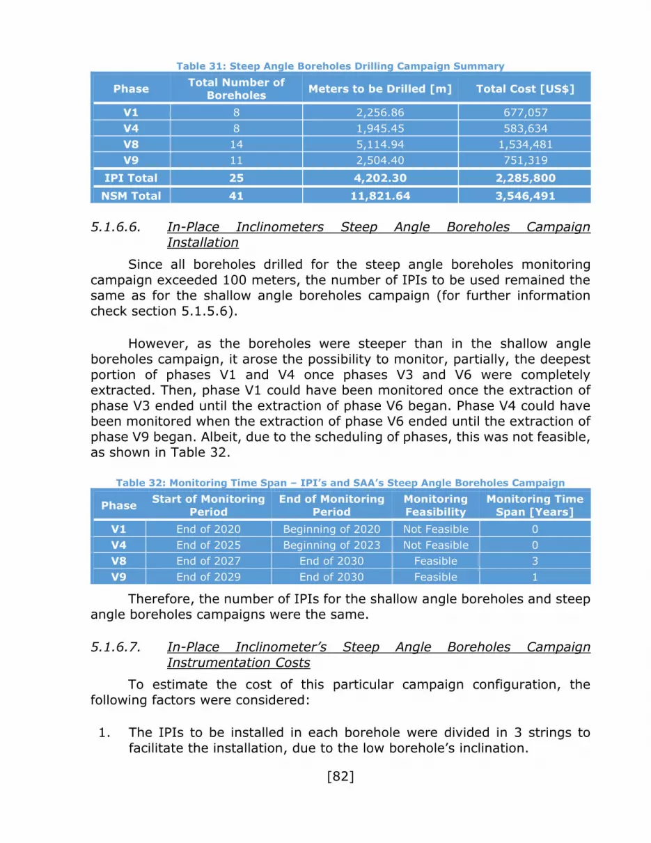
[82]

Table 31: Steep Angle Boreholes Drilling Campaign Summary

Phase Total Number of

Boreholes Meters to be Drilled [m] Total Cost [US$]

V1 8 2,256.86 677,057

V4 8 1,945.45 583,634

V8 14 5,114.94 1,534,481

V9 11 2,504.40 751,319

IPI Total 25 4,202.30 2,285,800

NSM Total 41 11,821.64 3,546,491

5.1.6.6. In-Place Inclinometers Steep Angle Boreholes Campaign Installation

Since all boreholes drilled for the steep angle boreholes monitoring

campaign exceeded 100 meters, the number of IPIs to be used remained the same as for the shallow angle boreholes campaign (for further information

check section 5.1.5.6).

However, as the boreholes were steeper than in the shallow angle

boreholes campaign, it arose the possibility to monitor, partially, the deepest

portion of phases V1 and V4 once phases V3 and V6 were completely extracted. Then, phase V1 could have been monitored once the extraction of

phase V3 ended until the extraction of phase V6 began. Phase V4 could have been monitored when the extraction of phase V6 ended until the extraction of

phase V9 began. Albeit, due to the scheduling of phases, this was not feasible, as shown in Table 32.

Table 32: Monitoring Time Span – IPI’s and SAA’s Steep Angle Boreholes Campaign

Phase Start of Monitoring

Period

End of Monitoring

Period

Monitoring

Feasibility

Monitoring Time

Span [Years]

V1 End of 2020 Beginning of 2020 Not Feasible 0

V4 End of 2025 Beginning of 2023 Not Feasible 0



Therefore, the number of IPIs for the shallow angle boreholes and steep angle boreholes campaigns were the same.

5.1.6.7. In-Place Inclinometer’s Steep Angle Boreholes Campaign

Instrumentation Costs

To estimate the cost of this particular campaign configuration, the

following factors were considered:

1. The IPIs to be installed in each borehole were divided in 3 strings to

facilitate the installation, due to the low borehole’s inclination.

[83]

2. The deepest string was composed of 10 sensors, the middle string of 20

sensors and the upper-most string of 20 sensors, totalling 50 sensors in

a 100-meter length IPI. 3. The casing was installed along the entire length of the borehole.

4. Placement tubing was used to place the 3 strings in every borehole. 5. Each string was connected to a datalogger (located 100 meters behind

slope’s crest) using its own signal cable. 6. Signal cables running from each borehole’s collar to the datalogger were

protected inside galvanized conduit pipes. 7. Each datalogger can gather data from a maximum of 5 strings.

These considerations were used in calculating the monitoring cost as

shown in Table 33. This cost does not include drilling cost.

Table 33: In-Place Inclinometer’s Steep Angle Boreholes Campaign Instrumentation Costs

Phase Investment Year Instrumentation Cost [US$]

V8 End of 2027 1,225,164

V9 End of 2029 838,890

Total - 2,064,054

For more detail information about In-Place Inclinometer’s steep angle

boreholes campaign costs calculation see APPENDIX K.

5.1.6.8. ShapeAccelArrays Steep Angle Boreholes Campaign Installation

ShapeAccelArrays are relatively new instruments developed to register

displacements in all directions perpendicular to a borehole’s axis regardless of its angle of dip (inclination). However, due to technical constraints SAA cannot

be installed in boreholes shallower than 60°.

These devices started to be applied in soils and now are being increasingly applied to monitor mine slopes. However, SAA cannot resist

nearby blasting and has a maximum length of 100 meters.

These limitations of the SAA forced the modification of some of the aspects of the shallow angle boreholes monitoring campaign, which considers

the instrumentation of the slope prior to its construction. Thus, drill holes will have to be drilled after the pit wall to be monitored is fully exposed, which

makes it impossible to register the deformations produced by the relaxation process experimented by the rock mass as the wall is excavated.

Table 32 presents the starting date for the monitoring period and the

end of this period defined by the date when the instrumented zone starts to be mined. These dates also define the feasibility to monitor a certain sector

[84]

using SAAs, as in some cases the phase where SAAs have to be located begins

to be mined before the wall to be monitored is fully exposed.

To monitor a wall at full scale, several SAA have to be installed in sequence inside a single borehole. The lowest portion of the boreholes would

be instrumented with 100-meter long SAA while the remaining portion (less than 100 meters) would be instrumented with a custom length SAA

(uppermost SAA). Table 34 shows the quantity and length of the SAA to be

installed, per phase and borehole.

Table 34: SAA length and Quantity per Phase to be monitored

Phase Borehole Quantity of 100-

meter SAA

Uppermost SAA

Length [m]

Total Quantity

of SAA Strings

V8

17 3 93.5 4

18 3 84.0 4

19 3 74.5 4

20 3 67.5 4

21 3 88.0 4

22 3 85.0 4

23 3 79.0 4

24 3 61.0 4

25 3 59.5 4

26 3 54.0 4

27 3 51.0 4

28 3 50.5 4

29 3 32.5 4

30 3 33.0 4

Total 42 - 56

V9

31 3 76.0 4

32 3 84.5 4

33 3 93.0 4

34 3 82.5 4

35 1 38.5 2

36 1 43.0 2

37 1 39.0 2

38 1 37.5 2

39 1 33.0 2

40 1 33.5 2

41 1 41.5 2

Total 19 - 30

APPENDIX L presents the number of MEMS sensors in every borehole

using the described configuration of SAA.

[85]

5.1.6.9. ShapeAccelArray’s Steep Angle Boreholes Campaign Costs

SAA’s cost estimation was performed considering the following

assumptions:

1. HQ boreholes (96[mm] outer diameter) were considered for SAA

installation. 2. No casing was required to install the devices in the boreholes.

3. A maximum of three (3) SAA strings were installed in each drill hole.

4. The entire length of each borehole was instrumented and monitored. 5. No especial hardware was required for the installation.

6. Each string was connected to a datalogger (located 100 meters away from slope’s crest) using its own signal cable.

7. The signal cables running from each borehole’s collar to the datalogger were protected inside galvanized conduit pipes.

8. Each datalogger can gather data from a maximum of 20 strings. 9. The space between the SAAs and the borehole’s wall was filled with sand

once the SAAs were in its installation position.

Table 35 presents the estimated costs without considering drilling expenses.

Table 35: ShapeAccelArray’s Steep Angle Boreholes Campaign Instrumentation Costs

Phase Investment Year Instrumentation Cost

[US$]

V8 End of 2027 2,386,785

V9 End of 2029 1,169,829

Total - 3,556,614

Refer to APPENDIX M for further information about ShapeAccelArray’s

steep angle boreholes campaign costs calculation.

5.1.6.10. Networked Smart Markers Steep Angle Boreholes Campaign

Installation

The monitoring periods for every phase was the same for both the steep

angle and shallow angle boreholes campaign (Table 24).

The NSM’s characteristics already described in Section 5.1, point 5.1.5.6 fulfilled all the requirements of the steep angle boreholes monitoring

campaign. The only difference between the shallow angle and steep angle boreholes campaign was the number of NSMs per borehole, as the boreholes

in the steep angle boreholes campaign were shorter.

[86]

Two different campaign settings were proposed. The first one considered

the installation of one NSM every 2 meters inside each borehole. The second

considered the installation of one NSM every 4 meters. A summary of both alternatives is presented in Table 36.

Table 36: Quantity of NSM Required in a Steep Angle Boreholes Campaign

Phase Quantity of NSMs (2-meter

spacing)


spacing)

V1 1,124 560

V4 968 482

V8 2,551 1,272

V9 1,246 621

Total 5,889 2,935

APPENDIX N presents detail information about quantities of NSMs per

borehole in each phase (Table. N.1 through Table. N.4).

5.1.6.11. NSM’s Steep Angle Boreholes Campaign Costs

The costs for NSM’s steep angle boreholes campaign were estimated taking into account the same considerations as for the NSM’s shallow angle

boreholes campaign. However, the inclination and, thus, length of the

boreholes were different for this case, since a steep angle boreholes campaign considered steeper and shorter drill holes.

Table 37 summarizes the costs of instrumentation per phase but the cost of drilling is not included.

Table 37: Networked Smart Marker’s Steep Angle Boreholes Campaign Instrumentation

Costs

Phase Investment Year


[US$] (2-meter

spacing)


[US$] (4-meter

spacing)

V1 End of 2014 615,529 525,054

V4 End of 2017 533,302 455,339

V8 End of 2021 1,381,756 1,176,581

V9 Ends of 2022 689,956 589,695

Total - 3,220,544 2,746,669

For more detailed information about Networked Smart Marker’s steep angle boreholes campaign costs calculation see APPENDIX O.

[87]

5.2. Alternatives Comparison

All campaigns defined in this work were compared according to six

criteria, as shown in Table 38. These criteria were: the number of years that every campaign was able to monitor the pit’s walls, the number of critical

sector that each campaign could have monitored monitor i.e. number of phases to be monitored, the amount of monitoring points, the amount of

gathered data, total cost of the campaign (including drilling costs) and cost per quantity of acquired data in each campaign.

The amount of gathered data was calculated as the product of the

monitoring period and monitored points. Thus, it allowed for a more accurate comparison towards which campaign allowed to gather more information of a

certain critical sectors that required to be studied.

Table 38: Monitoring Campaigns Comparison

Shallow Angle Boreholes Campaign

Steep Angle Boreholes Campaign

NSM

2[m]

NSM

4[m]

IPI

2[m]

NSM

2[m]

NSM

4[m]

IPI

2[m]

SAA

0.5[m]

Monitoring

Period [Years] 20 20 4 20 20 4 4

Monitored Phases

4 4 2 4 4 2 2

Monitored Points

7,541 3,759 1,250 5,889 2,935 1,250 15,230

Amount of

Gathered Data 150,820 75,180 5,000 117,780 58,700 5,000 60,920

Total Cost [US$]

8,628,486 8,021,784 5,032,097 6,767,035 6,293,160 4,349,854 5,842,414

Acquired Data Cost [US$]

57.21 106.70 1,006.42 57.45 107.21 869.97 95.90

Based on the predefined criteria, NSM technology showed to be the only one, in both 2-meter and 4-meter spacing configurations, able to fulfil all the

requirements of the shallow angle boreholes campaign. It had the longest lifespan of all alternatives, surpassing the others by 16 years and thus could

have gathered the greatest amount of data among all the alternatives. Finally, both the shallow angle and steep angle boreholes 2-meter spacing NSM’s

configurations also presented the lowest cost per unit of acquired data.

IPIs could be deployed in either shallow angle or steep angle boreholes campaigns being in both cases the cheapest alternative in terms of total costs.

However, this alternative could have monitored only 100-meter boreholes or the deepest 100 meters in drill holes of greater depth and could have only

been installed to monitor final pit’s walls. These constrains resulted in the highest cost per unit of acquired data among all alternatives.

[88]

It is worth mentioning that by using IPIs, the data processing would need

to correct the data and account for borehole’s inclination. This might have led

to additional costs and work for mine site personnel.

With regards to SAA, this alternative could have only been used in steep

angle boreholes campaigns to monitor final pit’s walls. SAAs allowed for the greatest number of monitored points per borehole and thus per monitoring

campaign but, due to the short lifespan of this alternative, the amount of

gathered data was practically the same as in the least extensive (4-meter spacing) NSM campaign. In addition, the data gathered by SAAs covered a

much smaller area and time frame than the NSM alternative, which ended with similar costs per unit of acquired data compared with the 4-meter separation

NSM campaign and significantly higher costs per unit of acquired data compared with the 2-meter separation NSM campaign (≈67% higher for

SAAs).

5.3. Potential Economic Gain

This section presents an assessment of the potential economic gain

obtained due to steepening of the wall, based on the modification of the open pit developed in Chapter 4. The evaluation considers the economic benefits

obtained due to the reduction of the stripping rate (reduction in mine costs)

and to the increase of mine recovery (increase in benefits) when the slopes are steepened by 1° at a time.

Since open pit slopes performance data acquisition may allow to safely steepen the pit’s walls in future pushbacks, the economic assessment will rely

on projects Net Present Values (NPVs) to incorporate the effect of temporality

and scheduling for every slope angle scenario.

5.3.1. General

To estimate the potential economic benefit that steeper slopes may render and that could justifies the investment in subsurface slope deformation

monitoring campaigns, the mine plan developed in Chapter 4 is used as a

starting point (base case). This mine presents two types of slopes, the first one, is located in good quality rock mass, covers the north and west portions

of the pit and has an overall slope angle of 50°. The second slope type is located in poor quality rock mass, covers the south and east portions of the

pit and has an overall slope angle of 40°.

The economic assessment is performed through a sensibility analysis using DeepMine that studies the evolution of the project’s NPV as the slope

angles for the entire perimeter (50° and 40° slopes) of the open pit are steepened simultaneously by 1° at a time up to a 60°/50° slope angles

[89]

scenario. At first, this process is carried out without considering the installation

of instrumentation to understand the evolution of ore and waste extraction

and their relation with NPV evolution. Then, the same process is repeated incorporating the instrumentation expenses for all monitoring campaigns

proposed in this thesis (IPI, SAA and NSM) to determine the scenario where instrumentation produces economic benefits to the project.

5.3.2. Analysis without Instrumentation Expenses

For this case, no instrumentation expenses were considered when steepening the slope angle simultaneously in the good and poor quality rock

mass from 50° to 60° and from 40° to 50°, respectively. This evaluation produced the expected increase in NPV showed in Figure 30, as slope angles

increased.

Figure 30: Project’s NPV Evolution as Slope Angle Increases

Figure 30 shows an unexpected behavior with the first increased degree.

In this case, a steeper slope angle produces a lower NPV, which can be a consequence of the trade-off between the case in which the only change is a

steeper slope and the case in which the savings produced by a steeper slope

allow to deepen the pit and access more ore. The consequences of this trade-off can be seen in Figure 31 and Figure 32.

210,51 210,25

223,25

229,19231,57 232,43

234,74

241,13

245,87

257,24260,42

180

190

200

210

220

230

240

250

260

270

50°/40° 51°/41° 52°/42° 53°/43° 54°/44° 55°/45° 56°/46° 57°/47° 58°/48° 59°/49° 60°/50°

NP

V [

MM

US

$]

Slope Angle Good Quality Rock/Poor Quality Rock

[90]

Figure 31: Total Waste Extraction

Figure 32: Total Metal (Cu) Production

154875,22

150211,33

140921,50

146021,30

141388,03

137018,93

130404,62

135719,64

126445,30

122329,33

128602,19

100000

110000

120000

130000

140000

150000

160000

50°/40° 51°/41° 52°/42° 53°/43° 54°/44° 55°/45° 56°/46° 57°/47° 58°/48° 59°/49° 60°/50°

Waste

[kto

n]


521,77

517,68519,95

532,76

541,77

532,43

538,09

532,22

538,07

552,35

530,80

500

510

520

530

540

550

560

50°/40° 51°/41° 52°/42° 53°/43° 54°/44° 55°/45° 56°/46° 57°/47° 58°/48° 59°/49° 60°/50°

Meta

l (C

u) [

kto

n]


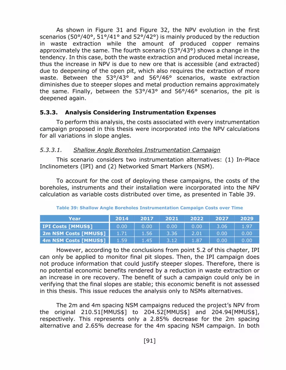
[91]

As shown in Figure 31 and Figure 32, the NPV evolution in the first

scenarios (50°/40°, 51°/41° and 52°/42°) is mainly produced by the reduction

in waste extraction while the amount of produced copper remains approximately the same. The fourth scenario (53°/43°) shows a change in the

tendency. In this case, both the waste extraction and produced metal increase, thus the increase in NPV is due to new ore that is accessible (and extracted)

due to deepening of the open pit, which also requires the extraction of more waste. Between the 53°/43° and 56°/46° scenarios, waste extraction

diminishes due to steeper slopes and metal production remains approximately the same. Finally, between the 53°/43° and 56°/46° scenarios, the pit is

deepened again.

5.3.3. Analysis Considering Instrumentation Expenses

To perform this analysis, the costs associated with every instrumentation

campaign proposed in this thesis were incorporated into the NPV calculations for all variations in slope angles.

5.3.3.1. Shallow Angle Boreholes Instrumentation Campaign

This scenario considers two instrumentation alternatives: (1) In-Place Inclinometers (IPI) and (2) Networked Smart Markers (NSM).

To account for the cost of deploying these campaigns, the costs of the

boreholes, instruments and their installation were incorporated into the NPV calculation as variable costs distributed over time, as presented in Table 39.

Table 39: Shallow Angle Boreholes Instrumentation Campaign Costs over Time

Year 2014 2017 2021 2022 2027 2029

IPI Costs [MMUS$] 0.00 0.00 0.00 0.00 3.06 1.97

2m NSM Costs [MMUS$] 1.71 1.56 3.36 2.01 0.00 0.00

4m NSM Costs [MMUS$] 1.59 1.45 3.12 1.87 0.00 0.00

However, according to the conclusions from point 5.2 of this chapter, IPI

can only be applied to monitor final pit slopes. Then, the IPI campaign does not produce information that could justify steeper slopes. Therefore, there is

no potential economic benefits rendered by a reduction in waste extraction or

an increase in ore recovery. The benefit of such a campaign could only be in verifying that the final slopes are stable; this economic benefit is not assessed

in this thesis. This issue reduces the analysis only to NSMs alternatives.

The 2m and 4m spacing NSM campaigns reduced the project’s NPV from

the original 210.51[MMUS$] to 204.52[MMUS$] and 204.94[MMUS$],

respectively. This represents only a 2.85% decrease for the 2m spacing alternative and 2.65% decrease for the 4m spacing NSM campaign. In both

[92]

cases, the costs due to instrumentation are recovered by steepening the slopes

by 2°, which produces a 3.21% NPV increase considering the 2m spacing

campaign or a 3.41% NPV increase considering the 4m spacing campaign, as shown in Figure 33.

Figure 33: Project’s NPV Evolution as Slope Angle Increases – Shallow Angle Boreholes

5.3.3.2. Steep Angle Boreholes Instrumentation Campaign

This scenario considers three instrumentation alternatives: (1) In-Place

Inclinometers (IPI), (2) ShapeAccelArrays (SAA) and (3) Networked Smart Markers (NSM).

To account for the cost of deploying these campaigns, the costs of the

boreholes, instruments and their installation were incorporated into the NPV calculation as variable costs distributed over time, as presented in Table 40.

However, as stablished in point 5.2 of this chapter, IPI and SAA can only

be applied to monitor final pit slopes. Thus, the IPI and SAA campaigns do not produce information that could justify steeper slopes. Therefore, there is no

potential economic benefits rendered by a reduction in waste extraction or an increase ore recovery when applying those campaigns. The benefit of such a

204,52 204,26

217,26

223,21225,58 226,45

228,76

235,14

239,88

251,25254,43

204,94 204,68

217,68

223,63226,00 226,87

229,18

235,56

240,30

251,68254,85

180

190

200

210

220

230

240

250

260

270

50°/40° 51°/41° 52°/42° 53°/43° 54°/44° 55°/45° 56°/46° 57°/47° 58°/48° 59°/49° 60°/50°

NP

V [

MM

US

$]


NPV NSM 2m Shallow Angle NPV NSM 4m Shallow Angle

[93]

campaign could only be in verifying that the final slopes are stable; this

economic benefit is not assessed in this thesis.

Therefore, the analysis focused only on the two most expensive (in terms of total cost) instrumentation alternatives: 2m and 4m spacing NSMs steep

angle boreholes campaigns.

Table 40: Steep Angle Boreholes Instrumentation Campaign Costs over Time

Year 2014 2017 2021 2022 2027 2029

IPI Costs [MMUS$] 0.00 0.00 0.00 0.00 2.76 1.59

SAA Costs [MMUS$] 0.00 0.00 0.00 0.00 3.92 1.92

2m NSM Costs [MMUS$] 1.29 1.12 2.92 1.44 0.00 0.00

4m NSM Costs [MMUS$] 1.20 1.04 2.71 1.34 0.00 0.00

The 2m and 4m spacing NSM campaigns reduced the project’s NPV from the original 210.51[MMUS$] to 205.85[MMUS$] and 206.18[MMUS$],

respectively (Figure 34). This represents only a 2.21% decrease for the 2m spacing alternative and 2.06% decrease for the 4m spacing NSM campaign.

Figure 34: Project’s NPV Evolution as Slope Angle Increases – Steep Angle Boreholes

205,85 205,59

218,59

224,53226,91 227,77

230,08

236,47

241,21

252,58255,76

206,18 205,91

218,92

224,86227,24 228,10

230,41

236,80

241,54

252,91256,08

180

190

200

210

220

230

240

250

260

270

50°/40° 51°/41° 52°/42° 53°/43° 54°/44° 55°/45° 56°/46° 57°/47° 58°/48° 59°/49° 60°/50°

NP

V [

MM

US

$]


NPV NSM 2m Steep Angle NPV NSM 4m Steep Angle

[94]

In both cases, the costs due to instrumentation are recovered by

steepening the slopes by 2°, which produces a 3.84% NPV increase

considering the 2m spacing campaign or a 4.00% increase considering the 4m spacing campaign.

5.3.4. Conclusions of the Economical Assessment

The previous economic assessments showed that in both the shallow and

steep boreholes instrumentation campaigns, an increase of 2° in the pit’s

slopes allow to cover the expenses for the two most expensive monitoring campaigns: the 2m spacing NSM campaigns with a cost of US$8,628,486 for

the shallow angle boreholes configuration and US$6,293,160 for the steep angle boreholes configuration.

However, as shown in Figure 33 and Figure 34, the NPV’s change from

the 50°/40° scenario to the 51°/41° scenario represents an atypical case, as the NPV decreases. If the expected behaviour would occur and the NPV

increased by an amount equal to half the difference between the NPV’s for the 50°/40° and 52°/42° scenarios, the NPV for the 51°/41° scenario would be

210.89[MMUS$] for the shallow and 212.22[MMUS$] for the steep angle boreholes campaigns instrumented with NSM installed every 2 meters.

Subsequently, in both cases, a 1° slope angle increase would pay for the most expensive monitoring campaigns proposed in this thesis.

5.4. Recommendations

Albeit surface deformation monitoring was not part of the scope of this thesis, it is recommended to compliment the subsurface deformation

monitoring campaigns proposed in this work with surface deformation

monitoring programmes. For instance, slope deformation radars could be used to monitor the behaviour of large areas of the open pit and correlate surface

deformation data with subsurface deformation data. Another recommendation is to use prisms and/or GPS to monitor the position of the instrumented

boreholes’ collar assuring that the boreholes used to monitor subsurface deformations do not move as rigid blocks.


In this chapter two different subsurface deformation monitoring campaigns were designed. The first was a shallow angle boreholes campaign,

which considered the deployment of either 100-meter long In-Place Inclinometers (IPI) or Networked Smart Markers (NSMs). The second, a steep

angle boreholes campaign, was meant to use either 100-meter long IPI,

ShapeAccelArrays (SAAs) or NSMs.

[95]

All campaigns were compared in terms of quantity of gathered data and

costs. This process showed NSMs as the devices that provided data at the

lowest cost.

Finally, an assessment of the potential economic benefit due to

steepening of the entire perimeter of the open pit by 1° at a time, from a 50°/40° (slope angle in good quality rock /slope angle in poor quality rock)

configuration up to a 60°/50° was made.

This evaluation showed how a 1° slope angle increase could finance the most expensive subsurface deformation monitoring campaign proposed in this

thesis, the 2m spacing NSM shallow angle boreholes monitoring campaign. It also showed that a 2° produces a 3.21% NPV increase considering the 2m

spacing campaign or a 3.41% increase considering the 4m spacing shallow

angle boreholes campaign and a 3.84% NPV increase considering the 2m spacing campaign or a 4.00% increase considering the 4m spacing in a steep

angle boreholes monitoring campaign.

CHAPTER 6

[96]

GENERAL DISCUSSION

This chapter presents a thorough discussion of all the results obtained in

this thesis and explain how all the aspects of this work are interrelated.

6.1. Relevance of the Mine Plan

The elaboration of a mine plan and pushbacks design allowed to define

the project conditions. These project conditions were used as the main inputs to define the monitoring campaigns, particularly, for the selection of the open

pit sectors to be monitored.

Based on the overall mine design, critical sectors were defined; these were sectors with high probability to present stability issues. Subsequently,

mine’s pushbacks coupled with their extraction scheduling (coming from the mine plan) were considered to assess the feasibility to instrument the selected

critical sector of the mine. This allows to discard some sectors that could not be instrumented because by the time they would had been instrumented,

extraction would have already started, prematurely disabling the instruments.

Another relevant aspect of early monitoring campaign design was that drilling campaigns intended for other purposes, such as, geotechnical or

geological survey could be adapted to house geotechnical instrumentation in the future. This would have made the subsurface deformation monitoring

campaigns more economic, since drilling cost represented more than half of the cost for the entire monitoring campaign.

6.2. Networked Smart Marker System Validation

After two mine scale trials, the Networked Smart Marker System

demonstrated its ability to transmit data wirelessly through rock and grout, fulfilling the objective of both trials. This presented the NSMs as a possible

platform to extend the sensing capabilities to other variables within the rock mass, such as, ground water pore pressure and subsurface deformations.

These results allowed to consider such a novel technology (NSMs) as a valid alternative for the monitoring campaigns proposed in this thesis.

Furthermore, NSMs are a promising alternative to overcome major

drawbacks of other devices considered for the monitoring campaigns (SAA and IPI). For instance, NSMs eliminate problems related to in-hole cables, minimise

the possibility of device breakage due to localized shear deformations, eliminate the need for boreholes’ casing, do no present limits for application

[97]

depth and quantity of NSMs per drill hole and allow the coexistence of various

sensors and thus measurements at the same point.

In addition, the NSM system is flexible allowing for operation even when some NSMs in the string do not function properly (as long as those NSMs are

not consecutive ones that would extend the communication range between working sensors beyond the upper limit) or, if some NSMs in the upper portion

of the borehole are mined out, the rest of the string can be rehabilitated by

installing a new antenna at the top of the remaining portion of the NSM string.

However, NSMs do present some drawbacks, for example, the system

needs boreholes with diameter greater than 11.4 centimetres (4.5 inches) and NSMs’ sealing requires greater amounts of grout than the alternative

technologies.

6.3. Monitoring Campaigns

6.3.1. Campaigns Configuration

From the three alternative devices, NSM, IPI and SAA, selected and evaluated, NSM is the only technology that can fulfil all the requirements for a

shallow angle boreholes monitoring campaign and be installed prior to the extraction of the pushback that exposes the slope to be monitored. This is

possible because NSMs are the only blasting resistance technology. IPI can be installed in boreholes with a shallow angle configuration, i.e. inclined following

the inclination of the slope to be monitored, but they have to be deployed after the slope is fully exposed. Hence, IPI cannot register the slope relaxation

process. The same conditions are applicable to SAA installed in a steep angle boreholes configuration. In addition, both IPI and SAA technologies can only

be utilized to monitor final walls.

Regardless of the type of instrument installed in the boreholes, the collar of each drill hole should be monitored using surface deformation monitoring

technologies, such as, GPS or prisms. This will allow to assure that the boreholes are not moving as a rigid block i.e. that, despite the fact that no

movement is registered along the borehole, the instrumented portion of the slope is moving as one piece. It is also advisable to complement subsurface

deformation monitoring with spread surface deformation monitoring using, for example, slope radars. These will gather near real time data which when

coupled with subsurface deformation data, would generate a more precise

estimation of the amount of material that is moving and might fail.

6.3.2. Subsurface Deformation Detection at Great Depths

It is known (Stacey et al., 2003) that the stain behind a pit’s wall increases in horizontal extension with depth. This increment is highly

[98]

dependent on in situ stress ratio k. For 400-metre high slopes (similar to the

open pit designed for this thesis) strain can extend horizontally between 10

(k=0.5) and 110 (k=2.0) metres behind slope’s face. Then, it is crucial to have a good estimation of the k value for the mine site to be monitored to determine

whether a campaign using boreholes dipping 60° will produce useful data or not.

Therefore, a steep angle boreholes campaign instrumented using IPI is

feasible only if k values for the studied mine are 2.0 or higher because the lowest ends of all boreholes are located, on average, 109 metres behind the

slope’s face and the instruments are installed only in the deepest 100 metres of every borehole. At such depth, movements are unlikely to occur and, if

some movement is produced, it will be of very small magnitude and thus it will be difficult to register it.

In the case of NSMs or SAAs, the steep angle boreholes campaign can

be modified to install the devices up to a depth were important levels of deformation are expected to occur. This situation will reduce or produce the

loss of important data from deformations occurring at the slope’s toe. This problem will not occur for the shallow angle boreholes campaign as boreholes’

distance to the slope’s face is 10 metres (constant at any depth). Thus, even with k values close to 0.5 deformations should be registered.

6.3.3. Campaigns Comparison

After comparing the three types of instruments considered in this thesis, it has been established that the best performing alternative is the NSM system.

This conclusion is based on its application flexibility, which allows the installation in sectors where the other technologies cannot be used. This

advantage over IPI and SAA is heavily influenced by the NSM’s resistance to nearby blasting and by lack of restriction on installation depth or inclination.

NSMs present a practical life longer than IPI and SAA even though NSMs

have a maximum operational life due to the usage of batteries as oppose to IPI and SAA. This condition is due to NSMs resistance to harsh mining

conditions and wireless communication through rock (no in-hole cables are required).

In terms of costs, the NSMs installed every 2 metres showed to be the

most cost-effective alternative. This configuration presents the lowest cost per unit of gathered data and will be reinforced with the addition of further sensors

within the same NSM enclosure i.e. with the Enhanced Networked Smart Markers (ENSM). Since ENSM configuration will increase the quantity of

acquired data by measuring various rock mass variables at a single point (deformation, groundwater pore pressure, micro-seismic and others).

[99]

6.3.4. Economic Analysis

This thesis addressed the economic benefits of the geotechnical

monitoring by evaluating its influence on safe increase of the slope’s angle to improve the project’s economic performance by reducing costs associated with

the extraction of waste and increasing the economic benefits associated with the higher ore extraction.

The evaluation showed that:

1. The In-Place Inclinometer and ShapeAccelArray alternatives being able only to monitor final slopes (in the shallow and the steep angle boreholes

configuration) do not generate the potential to steepen future slopes. Thus, these technologies do not generate economic benefits from the

point of view analysed in this thesis and only generate the benefit of

determining whether the final slopes are stable or not.

2. All the Networked Smart Marker (NSM) alternatives reported significant economic benefits to the project when allowing to increase the slope

angle by 2°. However, if the expected behaviour occurs, a 1° slope angle increase allows to finance any NSM monitoring campaign and to report

some minor economic benefit.

3. Both NSM configurations in shallow and steep angle boreholes campaigns present marginal differences in terms of NPV. The difference

between the most economic and most expensive alternatives, in terms of NPV, is 1.66[MMUS$], which represents a 0.79% of the project’s

original NPV.

Since all the NSM monitoring campaigns are economically feasible and the cost differences between the various alternatives are minimal, the

selection of the NSM campaign configuration should be based on the quality and quantity of acquired data.

These economic benefits (NPV behaviour) should be increased in open

pits greater in depth than the one studied in this thesis, since a deeper open pit implies greater amounts of stripped material and thus greater cost savings

when steepening the slopes. Thus, it is not only technically feasible to implement the instrumentation campaigns described in this thesis but also it

is economically efficient.

Other benefits, which were not studied from an economic perspective in this thesis but which could contribute to justify the investment in subsurface

deformation monitoring using NSMs might be the avoidance of harm to personnel and/or damage to the equipment (cost saving) due to early warning

[100]

of imminent failure. If failure was avoided, the operation would benefit from

cost savings due to remedial measurements (remediation costs) that were not

necessary, as there was no failure to amend.

CHAPTER 7

[101]

CONCLUSIONS AND RECOMMENDATIONS 7.1. General Conclusions

This thesis commenced with a thorough literature review of open pit

slope stability and the importance of rock mass deformation monitoring for

open pit mining projects. It was stated that slope monitoring plays a fundamental role in slope stability assessments and open pit slopes’ design.

This literature review also stablished the State-of-the-Art of rock mass/slope deformation monitoring techniques in metalliferous open pit mines. It

acknowledged that there are no geotechnical instrumentation guidelines specially developed to address the various characteristics of open pit mines’

rock slopes. It was thus concluded that:

The slope design process deals with a large amount of uncertainty sources and attempts to account for these uncertainty using fudge

factors, such as FoS and PoF. However, this approach tend to produce over-conservative slope designs.

The actual slope behaviour has to be studied to account for the uncertainties involved in the slope design process. This behaviour can

be studied through data obtained using geotechnical instrumentation to monitor surface and subsurface rock mass deformations.

Subsurface rock mass deformation monitoring allows to predict developing failures before the failure becomes imminent and thus allows

to take corrective measurements towards avoiding the failure. Most geotechnical instruments used to register subsurface rock mass

deformations have been developed to monitor civil engineering projects.

Therefore, they present several limitation when applied to open pit mining projects:

Short lifespan.

Limited application depth.

Limited number of sensors per borehole.

Limited coexistence of sensors in a single location inside a

borehole.

Low tolerance to localized shear deformations.

Installation and maintenance issues due to the presence of

cables inside boreholes.

A new geotechnical monitoring technology, the Networked Smart

Markers (NSM), promises to overcome those drawbacks by enabling through

rock wireless data transmission. The technical feasibility of this wireless data

[102]

transmission was proven after testing of these devices in two mine scale trials

for sixteen months, as describe in this thesis.

Five subsurface deformation monitoring campaigns were designed aiming to achieve the highest possible revenue due to subsurface deformation

monitoring and the surface monitoring campaigns commonly deployed in the most important open pits in the world. These campaigns were designed as an

integral part of the slope design process and closely related to the mine plan.

This allowed to focus the monitoring effort on the most relevant zones for a particular open pit project.

The campaigns consisted of a shallow angle and a steep angle boreholes installation both with boreholes drilled in the same location but with different

inclinations. The shallow angle boreholes campaign used IPI or NSM devices

installed in boreholes with the same inclination of the slope’s face at a distance of 10 metres plus the berm width behind the slope face. The steep angle

boreholes installation used NSM, IPI or SAA devices installed in boreholes with a minimum inclination around 60° at a distance of 10 metres plus the berm

width behind the slope face.

All alternatives were compared in terms of campaigns’ operational lifespan, quantity of mine sectors to be monitored, quantity of monitored

points, amount of gathered data, total cost and the cost per unit of acquired data.

The results obtained clearly show that the proposed campaigns are

technically feasible, with NSMs installation being the most technically advantageous.

Moreover, an economical evaluation was undertaken considering the evolution of the instrumented mine project’s NPV when steepening the slope

angle by 1° at a time. This assessment incorporated the potential benefit of

lower waste stripping ratio and additional ore extraction, which showed the economic viability of all studied alternatives. The campaigns using NSMs were

the most advantageous, in particular, the campaign that considered the installation of one NSM every four metres, which presented the lowest cost per

unit of gathered data.

Therefore, it has been proven that with these campaigns more abundant ground behaviour and better quality data, including slope decompression

process monitoring, can be obtained due to longer monitoring periods. This results in more comprehensive database that allows to differentiate normal

deformations, due to slope decompression, from deformations produced by developing failures.

[103]

However, it was also established that, among all the NSM alternative

campaigns, the cost was a variable of marginal relevance and that the choice

among NSM campaigns had to be founded on the quantity and quality of gathered data that each campaign configuration would produce.

In terms of quantity of gathered data, both 2m spacing NSM campaigns produce the greatest quantity of subsurface deformation data. With regards to

quality of data, the shallow angle boreholes configuration provided better

results for the reasons explained and discussed in Chapter 6, such as, the boreholes’ constant distance to the slope’s face at any depth. Thus, the 2m

spacing NSMs shallow angle boreholes monitoring campaign proved to be the best alternative to implement from a techno-economic perspective.

The information obtained from this campaign can also be complemented

with surface deformation monitoring data allowing better estimation of the amount of moving rock mass.

7.2. Recommendations

Since the first two trials described in this thesis were conducted prior to the development of this work and were intended to prove wireless data

transitions, it is recommended to develop further trials incorporating the methodology and parameters used in this thesis.

The objective of these trials would be to compare the new generation of

NSMs, the Enhanced Networked Smart Markers (ENSMs), with proven technologies, such as, IPI and piezometers installed in close vicinity to the

ENSMs. The mine scale trials can be less extensive in terms of the amount of instrumented boreholes. It could involve two to five boreholes over 100 metres

deep, ideally covering the entire depth of the slope to be monitored, instrumented using NSMs and IPIs.

These trial should also be used to prove the numerical results obtained

by Stacey et al., (2003) relative to the horizontal and vertical extension of the strain induced behind the slope due to mining.

CHAPTER 8

[104]

BIBLIOGRAPHY

1. Abdoun, T., Bennett, V., Dobry R., Koelewijn A. & Thevanayagam S.

(2010), Real-Time Monitoring of Full-Scale Levee Testing. In Proceedings of the 7th International Conference on Physical Modelling in

Geotechnics. Zurich (pp. 1711-1176). 2. Alba, M., Fregonese, L., Prandi, F., Scaioni, M. & Valgoi, P. (2006),

Structural Monitoring of a Large Dam by Terrestrial Laser Scanning. International Archives of Photogrammetry, Remote Sensing and Spatial

Information Science, 36 (5), 6-11. 3. Angeli, M., Pasuto, A. & Silvano, S. (2000), A critical review of landslide

monitoring experiences. Engineering and Geology, 55 (3), 133-147. 4. Baran, I. & Stewart, M. P. (2003), Small Scale Surface Deformation

Monitoring in Mining Regions using Differential Radar Interferometry. In Proceedings of the 11th FIG Symposium on Deformation Measurements,

Santorini, Greece, 2003. (pp. 25-28). 5. Bayoumi, A. (2011), On the Evaluation of Settlement Measurements

Using Borehole Extensometers. Geotechnical and Geological

Engineering, 29 (1), 75-90. 6. Bellett, P., Noon, D., Leva, D. & Rivolta, C. (2015), 3D and 2D Radars

for Open-Pit Slope Monitoring. In Proceedings of International Symposium on Slope Stability in Open Pit Mining and Civil Engineering.

SAIMM (pp. 591-606). 7. Bennett, P. (2008), Distributed Optical Fibre Strain Measurements in

Civil Engineering. Geotechnical News, 26 (4), 23-26. 8. BOAMine SpA. (2015). DeepMine 2.2 User Manual. BOAMine SpA:

Santiago. 9. Brackley, I. J. A., Welensky, P. & O’Connell-Jones, G. (1985), Slope

Stability at an Opencast Quartz Mine. Journal of the South African Institute of Mining and Metallurgy, 85 (2), 33.

10. Caci, V., Stahl, H., Bekiri, E., Milevski, S. & Glavinceski, M. (2015), Improving Existing Monitoring System in Six Dams by Automation and

Central Data Management. In Proceedings of the Ninth International

Symposium on Field Measurements on Geomechanics. ACG (pp. 137-148).

11. Casagrande, A. (1949), Soil Mechanics in the Design and Construction of the Logan Airport. Harvard University, Graduate School of

Engineering, 1949. 12. Cawood, F. T. & Stacey, T. R. (2006), Survey and Geotechnical Slope

Monitoring Considerations. Journal South African Institute of Mining and Metallurgy, 106 (7), 495-502.

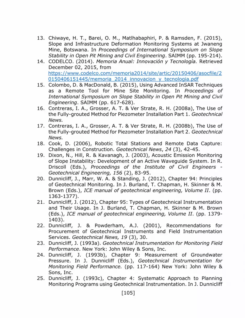
[105]

13. Chiwaye, H. T., Barei, O. M., Matlhabaphiri, P. & Ramsden, F. (2015),

Slope and Infrastructure Deformation Monitoring Systems at Jwaneng Mine, Botswana. In Proceedings of International Symposium on Slope

Stability in Open Pit Mining and Civil Engineering. SAIMM (pp. 195-214). 14. CODELCO. (2014). Memoria Anual: Innovación y Tecnología. Retrieved

December 02, 2015, from

https://www.codelco.com/memoria2014/site/artic/20150406/asocfile/20150406151445/memoria_2014_innovacion_y_tecnologia.pdf

15. Colombo, D. & MacDonald, B. (2015), Using Advanced InSAR Techniques as a Remote Tool for Mine Site Monitoring. In Proceedings of

International Symposium on Slope Stability in Open Pit Mining and Civil Engineering. SAIMM (pp. 617-628).

16. Contreras, I. A., Grosser, A. T. & Ver Strate, R. H. (2008a), The Use of the Fully-grouted Method for Piezometer Installation Part 1. Geotechnical

News. 17. Contreras, I. A., Grosser, A. T. & Ver Strate, R. H. (2008b), The Use of

the Fully-grouted Method for Piezometer Installation Part 2. Geotechnical News.

18. Cook, D. (2006), Robotic Total Stations and Remote Data Capture: Challenges in Construction. Geotechnical News, 24 (3), 42-45.

19. Dixon, N., Hill, R. & Kavanagh, J. (2003), Acoustic Emission Monitoring

of Slope Instability: Development of an Active Waveguide System. In R. Driscoll (Eds.), Proceedings of the Institute of Civil Engineers -

Geotechnical Engineering, 156 (2), 83-95. 20. Dunnicliff, J., Marr, W. A. & Standing, J. (2012), Chapter 94: Principles

of Geotechnical Monitoring. In J. Burland, T. Chapman, H. Skinner & M. Brown (Eds.), ICE manual of geotechnical engineering, Volume II. (pp.

1363-1377). 21. Dunnicliff, J. (2012), Chapter 95: Types of Geotechnical Instrumentation

and Their Usage. In J. Burland, T. Chapman, H. Skinner & M. Brown (Eds.), ICE manual of geotechnical engineering, Volume II. (pp. 1379-

1403). 22. Dunnicliff, J. & Powderham, A.J. (2001), Recommendations for

Procurement of Geotechnical Instruments and Field Instrumentation Services. Geotechnical News, 19 (3), 30.

23. Dunnicliff, J. (1993a). Geotechnical Instrumentation for Monitoring Field

Performance. New York: John Wiley & Sons, Inc. 24. Dunnicliff, J. (1993b), Chapter 9: Measurement of Groundwater

Pressure. In J. Dunnicliff (Eds.), Geotechnical Instrumentation for Monitoring Field Performance. (pp. 117-164) New York: John Wiley &

Sons, Inc. 25. Dunnicliff, J. (1993c), Chapter 4: Systematic Approach to Planning

Monitoring Programs using Geotechnical Instrumentation. In J. Dunnicliff



[106]

(Eds.), Geotechnical Instrumentation for Monitoring Field Performance.

(pp. 37-44) New York: John Wiley & Sons, Inc.

26. Eberhardt, E. & Stead, D. (2011), Chapter 8.5: Geotechnical Instrumentation. In P. Darling (Ed.), SME Mining Engineering Handbook.

(pp. 551-571). USA: Society for Mining, Metallurgy, and Exploration, Inc.

27. Ekkerd, J. N., Ruest, M. R. & Rankhododo, N. E. (2011), De Beers Venetia Mine Cut 4 Slope Optimization. In Proceedings of International

Symposium on Rock Slope Stability in Open Pit Mining and Civil Engineering. Canadian Rock Mechanics Association.

28. El-Ramly, H., Morgenstern, N. R., & Cruden, D. M. (2002), Probabilistic Slope Stability Analysis for Practice. Canadian Geotechnical Journal, 39

(3), 665-683. 29. Espinoza, A & Mora, O. (2012). InSAR Technology at El Teniente South

Open Pit. Retrieved January 11, 2016, from http://www.altamira-information.com/files_upload_site/pdf_publications/2012_Mora_et_al_

MineraChilena.PDF (in Spanish).

30. Fannin, R. J. & Jaakkola, J. (1999), Hydrological response of hillslope soils above a debris-slide headscarp. Canadian Geotechnical Journal, 36,

1111-1122. 31. Fillion, M-H. & Hadjigeorgiou J. (2015), Implications of Collecting

Additional Data on the Slope Design in an Open Pit Operation. In Proceedings of International Symposium on Slope Stability in Open Pit

Mining and Civil Engineering. SAIMM (pp. 1-14). 32. Flood, M. (2001), LiDAR Activities and Research Priorities in the

Commercial Sector. International Archives of Photogrammetry Remote Sensing and Spatial Information Sciences, 34 (3/W4), 3-8.

33. Frith, R. & Colwell, M. (2011), Chapter 8.1: Introduction to Ground Mechanics. In P. Darling (Ed.), SME Mining Engineering Handbook. (pp.

463-470). USA: Society for Mining, Metallurgy, and Exploration, Inc. 34. Gili, J., Corominas, J. & Riua, J (2000), Using Global Positioning System

Techniques in Landslide Monitoring. Engineering and Geology, 55 (3),

167-192. 35. Girard, J. M. (2001), Assessing and Monitoring Open Pit Mine Highwalls.

In Proceedings of the 32nd Annual Institute on Mining Health, Safety and Research. Salt Lake City, Utah. (pp. 159-171).

36. Haines, A. & Terbrugge, P. J. (1991), Preliminary Estimate of Rock Slope Stability Using Rock Mass Classification Systems. In 7th Congress of

International Society of Rock Mechanics. (pp. 887–892). Aachen, Germany.

37. Harries, N., Noon, D. & Rowley, K. (2006), Case Study of Slope Stability Radar Used in Open Cut Mines. In Proceedings of International

Symposium on Stability of Rock Slopes in Open Pit Mining and Civil Engineering. SAIMM (pp. 335-342).

http://www.altamira-information.com/files_upload_site/pdf_publications/2012_Mora_et_al_MineraChilena.PDF



[107]

38. Hawley, M., Marisett, S., Beale, G. & Stacey, P. (2009), Chapter 12:

Performance Assessment and Monitoring. In J. Read & P. Stacey (Eds.),

Guidelines for Open Pit Slope Design. (pp. 327-380). Collingwood: CSIRO PUBLISHING.

39. Hewson, S., Butcher, R. & Dunn M. (2011), Optimization of the Eastern Pit Wall of the Superpit: An Example of a Stage Capital-Delivered

Geotechnical Design to Increase Project Value. In Proceedings of International Symposium on Rock Slope Stability in Open Pit Mining and

Civil Engineering. Canadian Rock Mechanics Association. 40. Hoek, E. & Bray, J. (1981). Rock Slope Engineering 3rd eds. London:

Institute of Mining and Metallurgy. 41. Hoek, E. (1970), Estimating the stability of excavated slopes in opencast

mines. In Transactions of Institute of Mining and Metallurgy, Section A: Mining Industry 79. (pp. A109–A132).

42. Hofmann, J., Löwen, W. & Herrmann, R. A. (2015), LiDAR – Systems for Stability Proof of a Reservoir Dam. In Proceedings of the Ninth

International Symposium on Field Measurements on Geomechanics. ACG

(pp. 107-116). 43. Hormazabal, E., Tapia, M., Fuenzalida, R. & Zúñiga, G. (2011a), Slope

Optimization for the Hypogene Project at Carmen de Andacollo Pit, Chile. In Proceedings of International Symposium on Rock Slope Stability in

Open Pit Mining and Civil Engineering. Canadian Rock Mechanics Association.

44. Hormazabal, E., Almarza, C. & Pizarro, E. (2011b), Slope Design for Maricunga Mine in Chile. In Proceedings of International Symposium on

Rock Slope Stability in Open Pit Mining and Civil Engineering. Canadian Rock Mechanics Association.

45. Huang, A., Lee, J., Ho, Y., Chiu, Y. & Cheng, S. (2012), Stability monitoring of rainfall-induced deep landslides through pore pressure

profile measurements. The Japanese Geotechnical Society. 46. Hustrulid, W. A., Kuchta, M. & Martin, R. K. (2013). Open Pit Mine

Planning & Design 3rd Edition, Volume 1 - Fundamentals. Leiden: CRC

Press. 47. Hutchison, B. J. & Howarth, J. (2015), Kanmantoo Mine Rockfall and

Rock Wall Failures: I-Site 8820 Laser Scanning Application. In Proceedings of International Symposium on Slope Stability in Open Pit

Mining and Civil Engineering. SAIMM (pp. 543-562). 48. Inaudi, D. & Glisic, B. (2007), Overview of fiber optic sensing

technologies for geotechnical instrumentation and monitoring. Geotechnical News, 25(3), 27-31.

49. Jarosz, A. & Wanke, D. (2003), Use of InSAR for Monitoring of Mining Deformations. In Proceedings of Fringe 2003 Workshop. Frascati, Italy

(pp. 1-5). 50. Jooste, M. A. & Cawood, F. T. (2006), Survey Slope Stability Monitoring:

Lessons from Venetia Diamond Mine. In Proceedings of the International

[108]

Symposium on Stability of Rock Slopes in Open Pit Mining and Civil

Engineering. SAIMM (pp. 361-363).

51. Kane, W. F., Beck, T. J., Anderson, N. O. & Perez, H. (1996), Remote Monitoring of Unstable Slopes Using Time Domain Reflectometry. In

Proceedings of the Thematic Conference on Geologic Remote Sensing. Environmental Research Institute of Michigan, 2, 421-431.

52. Karzulovic, A. & Read, J. (2009), Chapter 5: Rock Mass Model. In J. Read & P. Stacey (Eds.), Guidelines for Open Pit Slope Design. (pp. 83-140).

Collingwood: CSIRO PUBLISHING. 53. Kliche, C. A. (2011), Chapter 8.3: Slope Stability. In P. Darling (Ed.),

SME Mining Engineering Handbook. (pp. 495-525). USA: Society for Mining, Metallurgy, and Exploration, Inc.

54. Kontogianni, V., Kornarou, S. & Stathis, S. (2007), Monitoring with Electronic Total Stations: Performance and Accuracy of Prismatic and

Non-prismatic Reflectors. Geotechnical News, 25 (1), 30-33. 55. Kristensen, L. & Blikra, L. H. (2013), Monitoring Displacement on the

Mannen Rockslide in Western Norway. In Landslide Science and Practice.

Springer Berlin Heidelberg (pp. 251-256). 56. Little, M. (2006), Slope Monitoring Strategy at Pprust Open Pit

Operation. In Proceedings of the International Symposium on Stability of Rock Slopes in Open Pit Mining and Civil Engineering. SAIMM (pp.

211-230). 57. Locat, J., Cloutier, C., Lord, P. E., Therrien, P., Jacob, C., Nadeau, A.,

Hébert, D., Couture, R., Charbonneau, F., Singhroy, V., Murnaghan, K., Danisch, L., Jaboyedoff, M., Pedrazzini, A. & Gravel, S. (2010), An

Integrated Mass Movement Monitoring System for Rockslide Hazard Assessment at Gascons, Gaspé Peninsula, Québec: An Overview. GEO

2010, Calgary, Alberta. 58. Lomberg, C., Ream, I., O’Rourke, R. & Read, J. (2013), Chapter 6:

Monitoring and Design Reconciliation. In G. Beale & J. Read (Eds.), Guidelines for Evaluating Water in Pit Slope Stability. (pp. 363-390).

Collingwood: CSIRO PUBLISHING.

59. Lorig, L., Stacey, P. & Read, J. (2009), Chapter 10: Slope Design Methods. In J. Read & P. Stacey (Eds.), Guidelines for Open Pit Slope

Design. (pp. 237-264). Collingwood: CSIRO PUBLISHING. 60. [80] Lynch, R. A. & Malovinchko, D. A. (2006), Seismology and Slope

Stability in Open Pit Mines. In Proceedings of International Symposium on Slope Stability in Open Pit Mining and Civil Engineering. SAIMM (pp.

375-390). 61. Marr, W. A. (2013), Instrumentation and Monitoring of Slope Stability.

In M. A. Pando, D. Pradel, C. Meehan & J. F. Labuz (Eds.), Proceedings Geo-Congress 2013: Stability and Performance of Slopes and

Embankments III. (pp. 2231-2252). 62. McQuillan, A., Canbulat, I., Makusha, G. & Priest, G. (2015),

Implementing Probabilistic Designs at Anglo American Coal Open Cut

[109]

Mines. In Proceedings of International Symposium on Slope Stability in

Open Pit Mining and Civil Engineering. SAIMM (pp. 401-412).

63. Meyer, S. (2015), Slope Deformation Mechanics from Microseismic Monitoring. In Proceedings of International Symposium on Slope

Stability in Open Pit Mining and Civil Engineering. SAIMM (pp. 181-194). 64. Mikkelsen, P. E. (2003), Advances in Inclinometer Data Analysis. In F.

Myrvoll (Eds.), Proceedings of the Symposium on Field Measurements in Geomechanics. (pp. 555-567). Oslo: A. A. Balkema.

65. Naismith, W. A., & Wessels, S. D. N. (2005), Management of a Major Slope Failure at Nchanga Open Pit, Chingola, Zambia. Journal-South

African Intitute of Mining and Metallurgy, 105 (9), 619-626. 66. O'Connor, K. M. & Dowding, C. H. (1999), Chapter 5: Monitoring

Localized Deformation in Rock. In K. M. O'Connor & C. H. Dowding (Eds.), Geomeasurements by Pulsing TDR Cables and Probes. Boca

Raton: CRC Press. 67. Pankow, K. L., Moore, J. R., Hale, J. M., Koper, K. D., Kubacki, T.,

Whidden, K. M., & McCarter, M. K. (2014), Massive Landslide at Utah

Copper Mine Generates Wealth of Geophysical Data. GSA Today, 24 (1), 4-9.

68. Patel, D. (2012), Chapter 100: Observational Method. In J. Burland, T. Chapman, H. Skinner & M. Brown (Eds.), ICE manual of geotechnical

engineering, Volume II. (pp. 1379-1403). 69. Peck, R. B. (1969), Advantages and Limitations of the Observational

Method in Applied Soil Mechanics. Géotechnique, 19 (2), 171-187. 70. [50] Pei, H. F., Yin, J. H., Zhu, H. H., Hong, C. Y., Jin, W., & Xu, D. S.

(2012), Monitoring of Lateral Displacements of a Slope Using a Series of Special Fibre Bragg Grating-Based In-Place Inclinometers. Measurement

Science and Technology, 23 (2), 1-8. 71. Priest, S. D. & Brown, E. T. (1983), Probabilistic Stability Analysis of

Variable Rock Slopes. Institution of Mining and Metallurgy Transactions, 92.

72. Psimoulis, P. A. & Stiros, S. C. (2013), Measuring Deflections of a Short-

Span Railway Bridge Using a Robotic Total Station. Journal of Bridge Engineering, 18 (2), 182.

73. Ramsden, F., Audigé, E. & Fagan, C. (2015), A Comprehensive and Integrated Slope Monitoring Approach for Enhanced Effectiveness:

Application at Debswana’s Jwaneng Mine in Botswana. In Proceedings of International Symposium on Slope Stability in Open Pit Mining and Civil

Engineering. SAIMM (pp. 629-640). 74. Read, J., Beale, G., Ruest, M. & Robotham, M. (2013), Introduction

Chapter. In G. Beale & J. Read (Eds.), Guidelines for Evaluating Water in Pit Slope Stability. (pp. 1-18). Collingwood: CSIRO PUBLISHING.

75. Read, J., Jakubec, J. & Beale, G. (2009), Chapter 2: Field Data Collection. In J. Read & P. Stacey (Eds.), Guidelines for Open Pit Slope

Design. (pp. 15-52). Collingwood: CSIRO PUBLISHING.

[110]

76. Rougier, M., Ruest, M., Gauthier, P. & Horwitz, A. (2015), The Use of

Head Drilling and of Structural Data from Digital Photography obtained

by Drone Survey to Justify Slope Steepening at Victor Diamond Mine. In Proceedings of International Symposium on Stability of Rock Slopes in

Open Pit Mining and Civil Engineering. SAIMM (pp. 485-504). 77. Sakurai, S. & Shimizu, N. (2006), Monitoring the Stability if Slopes by

GPS. In Proceedings of the International Symposium on Stability of Rock Slopes in Open Pit Mining and Civil Engineering. SAIMM (pp. 353-359).

78. Schellman, M., Sepulveda, R. & Karzulovic, A. (2006), Slope Design for the East Wall of Mantoverde Mine, Chañaral, Chile. In Proceedings of

International Symposium on Stability of Rock Slopes in Open Pit Mining and Civil Engineering. SAIMM (pp. 451-470).

79. Seller, J. B. & Taylor, R. (2008), MEMS Basics. Geotechnical News, 26 (1), 32-33.

80. Severin, J., Eberhardt, E., Leoni, L. & Fortin, S. (2011), Use of Ground-Based Synthetic Aperture Radar to Investigate Complex 3-D Pit Slope

Kinematics. In Proceedings of International Symposium on Rock Slope

Stability in Open Pit Mining and Civil Engineering. Vancouver (pp. 18-21).

81. Sheahan, T. C., Mazzei, D. & McRae, J. (2008), Performance Testing of MEMES-Based Tilt Sensors. Geotechnical News, 26 (1), 33-36.

82. Sjöberg, J. (2000), Failure Mechanism for High Slopes in Hard Rock. In W. A. Hustrulid, K. M. McCarter & D. J. A. Van Zyl (Eds.), Slope Stability

in Surface Mining. (pp. 71–80). Colorado: SME. 83. Sjöberg, J. (1999), Chapter 4: Case Study Database. In Analysis of Large

Scale Rock Slopes, PhD Thesis. (pp. 201-280). Lulea: Lulea University of Technology.

84. Stacey, P. (2009), Chapter 1: Fundamentals of Slope Design. In J. Read & P. Stacey (Eds.), Guidelines for Open Pit Slope Design. (pp. 1-14).

Collingwood: CSIRO PUBLISHING. 85. Stacey, T. R. (2009), Design – A strategic issue. Journal of the South

African Institute of Mining & Metallurgy, 109 (3), 157-162.

86. Stacey, T.R. & Xianbin, Y. (2004), "Extension" in large open pit slopes and possible consequences. 4th International Conference and Exhibition

on Mass Mining, Santiago Chile 22-25 August 2004. 87. Stacey, T. R., Xianbin, Y., Armstrong, R., & Keyter, G. J. (2003), New

Slope Stability Considerations for Deep Open Pit Mines. Journal of the South African Institute of Mining and Metallurgy, 103 (6), 373.

88. Stern, L. I. & Dunnicliff. C. J. (1975). Performance Monitoring for Geotechnical Construction. Baltimore: ASTM International.

89. Swarbrick, G. E. & Clarke, S. J. (2015), Shape Accel Arrays – Comparative Performance in a Mining Application. In Proceedings of the

Ninth International Symposium on Field Measurements in Geomechanics. ACG (pp. 195-206).

[111]

90. Thompson, P. W. (1989), Slope Stability at Finsch Mine. In Proceedings

of Rock Slope Stability Symposium. South African National Group on

Rock Mechanics (pp. 1-10). 91. Venter, J. (2015), Probability of Failure in Open Pit Slope Design. In

Proceedings of International Symposium on Slope Stability in Open Pit Mining and Civil Engineering. SAIMM (pp. 413-422).

92. Vinoth, S., Kumar, L. A., & Kumar, E. (2015), Slope Stability Monitoring by Quantification and Behavior of Microseismic Events in an Opencast

Coal Mine. Geological Society of India, 85 (4), 450-456. 93. Wesseloo, J., & Read, J. (2009), Chapter 9: Acceptance Criteria. In J.

Read & P. Stacey (Eds.), Guidelines for Open Pit Slope Design. (pp. 221-236). Collingwood: CSIRO PUBLISHING.

94. Wesseloo, J., & Sweby, G. J. (2008), Microseismic Monitoring of Hard Rock Mine Slopes. In Proceedings of SHIRMS. Australian Centre for

Geomechanics, Perth. (pp. 433-450). 95. Whiteman, D.S. (2010), The Smart Marker system - A new tool for

measuring underground ore body flow in block and sub-level mines. 2nd

International Symposium on Block and Sublevel Caving, Perth, Australia. (pp. 603-622).

96. Widzyk-Capehart, E., Hölck, C., Fredes, O., Pedemonte, I. & Steffen, S. 2015. Implementation of Novel Subsurface Deformation Sensing Device

for Open Pit Slope Stability Monitoring – The Networked Smart Markers System. In Proceedings of the 23rd International Symposium on Mine

Planning and Equipment Selection (MPES 2015). SAIMM (pp. 203-214). 97. Williams, P., Floyd, J., Chitombo, G. & Maton, T. (2009), Chapter 11:

Design Implementation. In J. Read & P. Stacey (Eds.), Guidelines for Open Pit Slope Design. (pp. 265-326). Collingwood: CSIRO

PUBLISHING. 98. Wyllie, D. C. & Mah, C. W. (2004). Rock Slope Engineering, Civil and

Mining, 4th eds. London: Spon Press. 99. Zvarivadza, T. (2015), Rock Slope Design at Great Depth as Open Pit

Mining Progress beyond the Available Experience Base: Expected

Behaviour and Potentially Robust Design Approaches. In Proceedings of Mine Planning and Equipment Selection Conference. SAIMM (pp. 565-

582).

CHAPTER 9

[112]

APPENDICES APPENDIX A: Diaphragm Piezometers and Rock Mass

Deformation Sensing Technologies Characteristics

Table. A.1: Diaphragm Piezometers Characteristics

Technology Description Strengths & Drawbacks Precision

Piezometers

Piezometers are designed to measure fluid or groundwater pore

pressures in a variety of applications. They are typically installed in boreholes in in-situ soils, rocks, foundations or earth/rock fills, grouted with a specific mixture. Closed piezometers type are the most commonly used on the mining industry.

Acceptable time response to pressure variations.

Easy to adapt it to an automatic

recording device.

Grouting properties are critical to prevent surface water from altering piezometer data.

Long cables are susceptible to

damage due to borehole movements.

Not possible to check the calibration of the instrument once installed.

±0.1% F.S. for the vibrating wire type.

Table. A.2: Soil or Rock Mass Deformation Monitoring Devices

Technique Description Strengths & Drawbacks Precision

Robotic Total Stations

(Prisms

Monitoring)

Robotic Total Stations are devices that combine a theodolite with Electromagnetic Distance Measurement (EDM) system to measure horizontal and vertical angles along with distance. This allows the surveyor to measure 3D coordinates of points remotely, typically targeted by the placement of reflective prisms.

Ability to provide 3D position of the point of interest.

Unable to monitoring during misty

weather.

Installation of monitoring prisms at the suspected likely unstable slope zone or area of interest.

Accuracy from 0.6 to 3 mm.

Range from 1,000 up to

3,000 m

Borehole Extensometers

Designed to monitor directional or axial deformations in the rock mass. Individual wires are attached to an anchor at the bottom of the hole, and the axial movement relative to the anchor is recorded.

Automated and remote readings.

Possible to measure multiple points.

Complicated to install in long boreholes.

Up to 0.005 mm.

Tilt Meters

Tilt meters use the bubble principle to measure the gradient of inclination of a ground point. The bubble movements are measured

and then converted into an estimate of the instrument’s tilt.

High precision measurements obtained.

Used to monitor movements that are expected to contain a rotational component.

Expensive in comparison with radar

monitoring. For a 500 x 500 meters area is approximately 36,000$/month.

Require additional calibration after some time to maintain the same accuracy as initially.

1 nanoradian (0.0002

arcseconds)

[113]

Table. A.2 (CONTINUATION)


Time Domain Reflectometry

(TDR)

TDR is an electronic instrument that locates faults in metallic cables. If the coaxial cable installed in a vertical hole suffers an impedance change due to kinking of the cable, the TDR detects the exact distance to the point.

High precision on fault location.

Inability to measure large ground

displacements due to the breakage of the wires and thus loss of a signal.

Useful to sense localized shear and concentrated shear strain.

±1% of the cable distance.

Inclinometers

Generally used to measure lateral subsurface displacement in vertical

holes. Inclination measured by the device is used to determine the movement perpendicular to the drill hole axis.

Very detailed displacement path.

In large boreholes and big ground movements, they have short lifespan due to breakage of the casing and/or in-hole cable.

Very useful to study gradual

inclination changes.

They can detect differential

movements of 0.5–1.0 mm per 10 m length of

borehole.

ShapeAccelArray

(SAA)

Electronic instruments with triaxial MEMS accelerometers inside a 30cm rigid segment. Several segments can be put together to measure 3-D ground deformation in depths. The arrays goes from 30 cm to 100 m long.

Installed in vertical holes to obtain

horizontal deformation data in real time.

Also possible to install horizontally to measure vertical deformation.

± 1.5 mm for 32 m SAA.

Cross-Crack Measurements

Crackmeters are devices composed of a steel rod installed at either side of the crack. The distance between steel rods is measured periodically using measuring tape, Vernier caliper or micrometer to determine the crack aperture.

Provides an insight to in-ground

movements.

Simple monitoring devices.

Potentially unstable working area.

0.1 mm.

Global Positioning

System

(GPS)

Space-based satellite navigation

system provides points location using the timing of signals sent by different satellites to ground receivers located in the position to be surveyed. The time is used to determine the distance from the receiver to all those satellites. These distances allow to precisely determine the position of the receiver.

Line-of-sight is not required between receivers.

Not dependent on weather

conditions.

Requires mine personnel to go to all the different points to be surveyed.

Requires unobstructed line of sight to

four or more GPS satellites.

Satellite visibility is obstructed in deep point of the pit.

Under 20 mm.

Visual Inspection

Visual observation of the studied zone to detect the occurrence of cracks, or the evidence displacements.

Requires experienced geotechnical staff.

It must be complemented by

instrumentation to provide a quantitative basis for defining the exact amount of movement.

Qualitative.

Photogrammetry

Integrates 3D spatial data with 2D visual data to create spatially accurate representations of the surface topology of the rock. Structural properties (orientation, length, spacing, and others) can be determined using this technique.

Integration of the photogrammetry with mine planning software systems makes possible to use the data in real time for mine design, mine planning and mine operating purposes.

Provides a permanent 3D record of

the mapped areas.

Provides low cost geological mapping.

Only one person needed to use this

technique.

Digital imaging systems require ground proofing and cannot be used to determine the physical features of the structures.

Accuracy ranges

from 2 cm at a distance of 50 m

to 10 cm at distances of up

to 3 km.

[114]

Table. A.2 (CONTINUATION)


Ground-Based SAR

Uses the same principle as the satellite-based method but the images are acquired by a radar moving along a rail a couple of kilometers away from the area of interest. The monitored zone can be up to four kilometers away from the radar.

Measurements can be taken during day and night and in any weather conditions.

Provides high spatial density of observations.

Fast (5-10 min monitoring period).

Short range (<5 km)

Limited field of view, which may cause shadowing problems.

Not intended to monitor broad areas.

Resolution of about 0.5 – 4 m,

depending on the monitoring

distance and the atmospheric conditions.

Precision in the scale of

millimeters.

Airborne Synthetic

Aperture Radar

(Airborne-SAR)

It uses the same principles as the InSAR but, in this case, the instrument is mounted on an airplane.

Independency from international satellites for data gathering.

It uses a relatively unstable platform.

Very important to know the exact location of the plane for best results.

-

Interferometric Synthetic

Aperture Radar (InSAR)

It uses the difference in phases between successive SAR images to determine ground movement. SARs send microwave signals to the zone to be monitored and register the reflection of the sent signal. Then, interferometric techniques are used to obtain information about 3D deformation from the phase difference between the waves sent and received by the satellite.

It works in all weather conditions.

It allows to monitor inaccessible sector of the pit.

Good technique to monitor broad areas.

Dependency on international satellites availability for data gathering.

It may not produce good results when monitoring steep zones.

Real time monitoring is not feasible.

If displacements between successive SAR images is higher than 23 cm InSAR may not be able to quantify it.

On the scale of centimeters to millimeters.

Light Detection and Ranging

(LiDAR)

This technique uses laser pulses reflected by the surface to be measured to create a three-dimensional (3D) representation of the scanned target with a density of >10,000 points per square meter. It is an optical remote sensing technique that uses the properties of scattered reflected light to determine the range between the monitored object and the sensor.

Able to create a high accurate 3D

digital elevation model.

High resolution images.

Relatively inexpensive.

Flexible data collection and processing system.

Can be used to monitor relatively small areas to survey (from 1 to 10 square kilometers).

Need for experienced personnel to

understand the limitations of the TLS.

Necessity for a proper data collection campaign to avoid shadowed regions.

Systematic errors are +/-

25mm at 1,000 meters.

Random errors are generally between 0

and 10 mm.

[115]

Table. A.3: Open Pit Subsurface Deformation Monitoring Devices

Technology Description Strengths & Drawbacks Precision

Seismic or Micro-seismic

Monitoring

Micro-seismic monitoring is the passive observation of very small-scale earthquakes as a result of human activities or industrial processes such as mining. Brittle fractures in rock radiate seismic waves, and if they are recorded sufficiently clearly by different seismographs, the seismic event’s origin time, location and source parameters, deformation and location can be estimated. Geophones are usually the sensor of choice in most mining applications.

Very unique system to locate fractures developing within the rock mass.

Geophones don’t need power to

operate.

Signal degradation if the sensors are far from the target.

Limitation to response to high-frequency waves.

Geophones are used to triangulate

the position of the movement that originated the measured wave.

For a IMS 4.5Hz Geophone the

distortion measurement

frequency is 12 Hz.

Smart Markers

Autonomous electronic devices capable of monitoring mineral flow and ore recovery in block/panel and sublevel caving mines.

Each device has its own identifying

ID, allowing to pinpoint its location when installed in the rock mass.

When recovered in a drawpoint the Marker is identified by a Reader. Having both the initial and final positions of the devices, ore flow can be inferred.

The actual path of the marker from

its installation position to its extraction position (drawpoint) cannot be registered.

Qualitative.

Networked Smart Markers

(NSM)

Autonomous electronic devices capable of monitoring relative displacement between Markers.

Each device has its own identifying

ID, allowing to pinpoint its location when installed in the rock mass.

The devices do not require in borehole wires.

The devices are blasting resistant.

Allow to detect slipping surface location.

The Markers are capable of hosting

different types of sensors (Enhanced Networked Smart Markers configuration).

Qualitative.

Enhanced Networked

Smart Markers

(ENSM)

Autonomous electronic devices capable of monitoring various geotechnical variables, such as, groundwater pore pressure and rock mass subsurface deformation.

Each device maintains all the

advantages of NSMs.

Able to register the behavior of various variables at the same point.

Able to work, simultaneously, as piezometer, inclinometer and extensometer.

Depends on the characteristics of

the installed sensors.

[116]

APPENDIX B: DeepMine Elements Description

DeepMine is a software solution for strategic open pit mine planning from

an economic perspective that avoids the usage of predefined phases. As output, it delivers the size of the mine considering amount of material to be

mined and processed. It also delivers mine’s lifespan and the value of the operation in terms of net present value (NPV). To do so, the software creates

decision trees based on the studied mining configuration. Approximate dynamic programming is used to explore multiple branching in those decision

trees to obtain the best outcome based operation’s economic value.

Pushbacks are automatically produced as the result of software’s calculations, considering operational constrains using and Lerchs and

Grossman pit shells as input to define operative phases. The resulting pushbacks are associated with the mine plan and can be used as a guide for

mine design e.g. a plan that establishes when every pushback has to be mined

to obtain the best possible economical outcome.

To produce such results, DeepMine works with a block model given as

an input and with the definition of four elements in the mine planner: The GeoModel, the Mining Environments, the Pit Collections and the Economic

Environments. These elements use the information contained in the block

model and can be defined to apply uncertainty on the resulting mine plans by, for example, modifying commodities prices, operational costs and taxes over

time.

Block Model Description

The block model is the main input used by the software to perform their

calculations, as the information contained in it is technical data.

This model contains data, such as, block’s size and position, ore grade

of different commodities contained in the block, weight, density, rock type, topography and can also have user defined variables.

GeoModels

The GeoModel contains the block model representing the ore deposit and topography. Here the blocks are arranged in a three-dimensional, regular grid

containing only one block in each position.

To define a GeoModel, the block model to be used has to be selected, block model’s orientation has to be defined and the variables contained in it

identified for the DeepMine to recognize them as inputs to generate the mine plan.

[117]

When the block model is properly loaded to the GeoModel, maximum

admissible overall slope angles have to be defined. This can be done by

defining several bearing-slope pairs that define the maximum slope inclination for a particular bearing.

Mining Environments

Mining Environments define operational parameters related with mine

and plants’ operations. They are divided into general, operation, mine, plants,

stockpiles and dumps.

In the section on general information, the user provides a name for the

Mining Environment, a description of it and defines the first year of operation.

For the operation section, the user can define fixed operational costs per year of operation, investments to be made each year, depreciation over

investment also per year of mine’s operation and closure costs to be applied on the last year of mine’s operation. All this data is used to determine cash

flows of the project per year.

Mine defines the open pit’s properties. The user provides mining costs and mine’s production capacity per year and, optionally, a cost adjustment

factor.

Plants section is where the user defines the different processing plants needed to process all types of ore coming from the mine. This section is divided

into four parts: basic properties, costs & capacities, recoveries and filters. In basic properties, the user gives a name to the plant and its description;

optionally, he/she can define the plant’s location and whether it is set as the primary plant or not. For costs & capacities, the user has to define a base plan

cost and processing capacity per year. In addition, processing costs per block, average transport cost to the plant, surplus limits and other user defined

restrictions can be set in this section. Surplus limits restricts the amount of

ore exceeding plants capacity that can be mined in a certain period, i.e. it limits the amount of ore that goes directly to stockpiles and thus reducing the

re-handling in future periods. In the recoveries section, the user defines which rock type will be processed in each plant, the commodity that will be recovered

and the percentage of its recovery. Plants section ends with the definition of filters to stablish limitations to the plant based on block’s properties.

Stockpiles are defined by basic properties, costs & capacities,

associations, initial state and filters. In the section of basic properties, a name and description is given to the stockpile and, optionally, its location. Costs &

capacities is where the user has to define the total capacity of the stock, its

[118]

maximum re-handling capacity per year. It also gives the option to add an

average transport cost form the mine to that particular stockpile. In the

association tab, every stockpile is designated to feed a certain plant; this designation includes an associated re-handling cost. The definition of initial

state for the stockpile establishes the quantity of material contained in the stock at the beginning of operations. This is optional and assumes

homogeneous mixing among rock type fractions and average grades per commodity. The user can also define filters to establish limitations to stocks

operations based on block’s properties.

Finally, dumps require the definition of its basic properties and costs & capacities. In basic properties, the user individualises every dump with a

name, its description and location. Costs & capacities tag is where the user defines an average transport cost to every dump and their maximum capacity.

Pit Collections

Pit Collections define a set of pit shells resulting from the application of Lerchs and Grossman algorithm to solve the ultimate pit problem. To do this,

Pit Collections has to be associated with a predefined GeoModel and Mining Environment. It also requires the definition of four tabs: general, extraction,

plants and prices.

Pit Collections are defined with a name associated with a specific GeoModel and Mining Environment in the general tab. The GeoModel provides

slopes angles used to define a block precedence list for the Lerchs and Grossman algorithm. While the Mining Environment provides all the

operational parameters for mine and planta operation, which can be verified in two tabs: extraction and plants. In the extraction tab, the user can verify

that the dumps are located in a suitable place and that the extraction and transport to dumps costs are correct. The plants section is the same plants tab

in the Mining Environment section. The user can also modify the value of the parameters obtained from the Mining Environment. These new values will not

modify the selected Mining Environments; they will only be defined in the Pit Collections.

The only tab that the user has to define for the Pit Collections is prices.

A series of increasing prices is defined for every commodity to be mined. The quantity of pit shell generated will be the same as the quantity of different

prices defined in this part.

Economic Environments

The Economic Environments are defined by four tabs: general,

commodity prices, sales costs and taxes & royalties.

[119]

In the general tab, the Economic Environments is defined by a name,

establishing the first year of mine’s operation and setting a discount rate for

the cash flow. Then, in the next two tabs, prices and selling costs are given per year for every commodity contained in the block model. Finally, a tax rate

is set for the entire operation.

Mine Plan

Mine Plans are the final output of the software. The user has to configure

the Mine Plan choosing among deterministic, stochastic and flexible mine plans.

Subsequently, the user defines the general properties of the Mine Plan, establishes the first year of operations and selects a GeoModel, Mining

Environment, Pit Collections and Economic Environment to serve as inputs to

Mine Plan’s calculations. In the next step, he/she assigns the basic parameter for the resolution of the problem. These parameter are the maximum life of

mine (LOM), maximum sinking rate for a single phase in term of benches (number of block in a vertical section) per year, maximum number of active

phases every year, maximum phase length, minimum phase width and, optionally, minimum and maximum phase weight.

Pit Collection Guidance percentage can be used to relax how the Pit

Collection used for the Mine Plan determines the geometry of the resulting phases.

The user has to select the solver mode used by DeepMine. The user has

three possible options from the fastest to the slowest: quick mode, balance mode and deep mode. Since DeepMine uses approximate dynamic

programming to solve the Mine Plan, the more time spent in calculations the better the results.

Finally, the maximum Sinking Rate for the Mine Plan has to be defined.

This means the maximum number of benches that can be extracted in every phase in a year.

The resulting Mine Plan delivers a yearly extraction sequence for the mine presenting the destination and processing of each block and operations

data, such as, cut-of grades, plants utilization and stripping rates. In addition,

extraction phases that do not consider optimum design but can be used as a robust guide to design operative phases are also provided.

[120]

APPENDIX C: Yearly Copper Cut-Off Grades for the

Leaching and Concentrator Plants

Table. C.1 present the cut-off grades per year of operation for each

plant.

Table. C.1: Yearly Cut-off Grade

Cut-off Grades [%Cu]

Year Leaching

Plant

Concentrator

Plant

2015 0.11 -

2016 0.11 -

2017 0.14 0.20

2018 0.15 0.32

2019 0.14 0.27

2020 0.19 0.23

2021 0.11 0.22

2022 0.14 0.18

2023 0.13 0.19

2024 0.10 0.27

2025 - 0.25

2026 - 0.23

2027 - 0.18

2028 - 0.18

2029 - 0.20

2030 - 0.24

Mean 0.13 0.23

APPENDIX D: Processing Plants Yearly Operation

Figure. D.1 shows leaching plant’s operation during the mine’s life. It presents an even supply of ore (9,000[kton] per year) from the first year of

production and dropping in year 2023, close to plants closure. Year 2024 represents a particular case where the leaching plant is mainly supplied with

long term stocked material (low grade material).

Figure. D.2 presents concentrator’s plant operation. This plan starts operating in year 2017 and starts its regimen in year 2018 maintaining a

processing rate of around 7,000[kton] per year until year 2029 when production starts to decrease. The last year of plant’s operation (2030) was

mainly supplied with long-term stocked material (low-grade material). Figure. D.2 also presents the possibility of processing only stocked material in year

2031, however, this possibility was not considered in the mine plan as it was decided to finish al mine’s operations in year 2030.

[121]

Figure. D.1: Leaching Plant Yearly Operation

Figure. D.2: Concentrator Plant Yearly Operation

8987 8894 8880

71857850

8988

72008393

71846282

1444148

1235

0 105 105

17901123

0

1790597

1790

1790

878

1790

878

0 0 00

1000

2000

3000

4000

5000

6000

7000

8000

9000

10000

2015 2016 2017 2018 2019 2020 2021 2022 2023 2024 2025 2026 2027 2028 2029 2030

Pro

cese

d M

ate

rial

[kt

on

]

Year

Leaching Plant Operation


5608

69646305

5881 56034987

56186469 6630

5627 5294 5626

2441

1580 0

0

0667

1088 1369

1369

1369527 351

13691369

1369

1369

1369

0

1000

2000

3000

4000

5000

6000

7000

8000

2015 2016 2017 2018 2019 2020 2021 2022 2023 2024 2025 2026 2027 2028 2029 2030

Pro

cese

d M

ate

rial

[kt

on

]

Year

Concentrator Plant Operation


[122]

APPENDIX E: Phases Geometry for the Theoretical Mine

Obtained Using the Software DeepMine (Volumes)

This appendix contains isometric views of the 29 phases produced by

DeepMine (Figure. E.1 to Figure. E.8). Portions of some phases are enclosed in red circles because they are isolated or too small to be extracted. It is

evident that phases 5, 7, 9, 14, 19, 20, 21, 25, 26, 27, 28 and 29 are too small to be consider as single phases.

Figure. E.1: DeepMine Phases 01 to 04



Phase 01 Phase 02 Phase 03 Phase 04



[123]









[124]

Figure. E.8: DeepMine Phase 29

APPENDIX F: Phases Geometry for the Theoretical Mine Relaxed Using Vulcan (Volumes)

Figure. F.1: Vulcan Phases

Figure. F.2: Vulcan Phases V1 to V4

Phase 29

Phase V1 Phase V2 Phase V3 Phase V4

[125]





[126]

APPENDIX G: Phases Geometry for the Theoretical Mine

Relaxed Using Vulcan (Topography)

Figure. G.1: Open Pit Phases V1 to V7 Geometry

Phase V1

Phase V3

Phase V5

Phase V2

Phase V4

Phase V6 & V7

[127]

Figure. G.2: Open Pit Phases V8 to V12 Geometry

Phase V8 Phase V9

Phase V11 Phase V10

Phase V12

[128]

APPENDIX H: In-Place Inclinometers (IPIs) Shallow Angle

Boreholes Campaign Costs Calculation

Table. H.1 presents data about the system’s layout. It contains the

quantity of dataloggers per phases and shows which borehole is connected to a particular datalogger. It also contains the distances form every borehole’s

collar to its corresponding datalogger. Since every borehole contains 3 IPI strings and each datalogger can receive information from only 5 strings, there

are some boreholes connected to different dataloggers.

Table. H.1: In-Place Inclinometers Shallow Angle Boreholes Campaign Layout Data

Phase Borehole’s ID Datalogger ID Distance from Borehole’s Collar to

Datalogger [m]

Phase V8

17 1 - 98.14 -

18 1 2 105.68 97.07

19 2 - 100.00 -

20 2 3 118.00 97.49

21 3 - 106.40 -

22 4 - 103.61 -

23 4 5 103.83 101.93

24 5 - 100.09 -

25 5 6 105.45 104.00

26 6 - 100.00 -

27 7 - 100.91 -

28 7 8 101.31 101.25

29 8 - 99.36 -

30 8 9 106.69 100.00

Total - 9 2,051.19

Phase V9

31 1 - 91.70 -

32 1 2 111.95 118.78

33 2 - 100.00 -

34 2 3 98.26 100.00

35 4 - 99.89 -

36 4 5 109.06 68.63

37 5 - 100.00 -

38 5 6 135.98 77.19

39 6 - 108.38 -

40 7 - 109.25 -

41 7 8 78.36 100.00

Total - 8 1,607.43

TOTAL - 17 3,658.62

[129]

Table. H.2 presents all data required to estimate the costs for the In-

Place Inclinometers’ shallow angle boreholes campaign.

Table. H.2: In-Place Inclinometer’s Costs

In-Place Inclinometers - Unitary Costs

Casing [US$/m] 29.67

Casing Coupling [US$/m] 8.17

Locking Cap [per borehole] 46.00

MEMS IPI Gage Tube [US$/m] 25.25

Serial IPI Biaxial Sensor [US$/m] 437.50

Sensor wheels [US$/m] 73.50

Top Wheel [per borehole] 157.00

IPI Placement Tubing [US$/m] 16.67

IPI Placement Tubing Coupling [US$/m] 11.67

In-Line Wheels [US$/m] 24.50

Jumper Cable [per borehole] 256.50

Bus Cable [per borehole] 189.00

Signal Cable [US$/m] 5.25

Conduit [US$/m] 2.00

Datalogger [US$] 700.00

Table. H.3: In-Place Inclinometer Shallow Angle Boreholes Campaign Costs

In-Place Inclinometers Shallow Angle Boreholes Campaign

Phase Borehole’s

ID IPIs [US$]

Cable IPI-Collar [US$]

Cable Collar-

Datalogger [US$]

Conduit [US$]

Datalogger [US$]

Phase V8

17 79,763.50 16,034.50 - - -

18 79,763.50 14,399.44 - - -

19 79,763.50 12,997.84 - - -

20 79,763.50 11,736.33 - - -

21 79,763.50 10,965.49 - - -

22 79,763.50 10,578.85 - - -

23 79,763.50 10,057.04 - - -

24 79,763.50 8,572.71 - - -

25 79,763.50 8,436.73 - - -

26 79,763.50 7,999.29 - - -

27 79,763.50 7,672.44 - - -

28 79,763.50 7,611.00 - - -

29 79,763.50 6,161.08 - - -

30 79,763.50 6,181.56 - - -

Total - 1,116,689 139,404 22,473 4,110 6,300

[130]

Table. H.3 (CONTINUATION)

Phase Borehole’s

ID IPIs [US$]


Cable Collar-

Datalogger [US$]

Conduit [US$]

Datalogger [US$]

Phase V9

31 79,763.50 11,602.80 - - -

32 79,763.50 12,381.83 - - -

33 79,763.50 13,392.68 - - -

34 79,763.50 12,116.42 - - -

35 79,763.50 -4,750.22 - - -

36 79,763.50 -3,047.17 - - -

37 79,763.50 -3,620.59 - - -

38 79,763.50 -4,525.77 - - -

39 79,763.50 -6,932.48 - - -

40 79,763.50 -5,172.91 - - -

41 79,763.50 -3,590.28 - - -

Total - 877,398 17,854.31 17,338 3,221 5,600

The information contained in Table. H.1 and Table. H.2 presents all data

required to estimate the costs for the In-Place Inclinometers’ shallow angle boreholes campaign.

Table. H.2 was used to calculate the costs presented in Table. H.3 and Table. H.4. Table. H.3 presents the different items involved in the cost

estimation for an IPI monitoring campaign per borehole. Table. H.4 shows the total cost of the campaign with and without the drilling cost.

Table. H.4: In-Place Inclinometer Shallow Angle Boreholes Campaign and Drilling Costs

In-Place Inclinometers Shallow Angle Boreholes Campaign

Instrumentation Cost [US$] Instrumentation plus Drilling Cost [US$]

Phase V8 1,288,976 3,057,152

Phase V9 921,412 1,974,946

Total 2,210,387 5,032,097

[131]

APPENDIX I: Quantity of Networked Smart Markers (NSMs)

in Each Phase for a Shallow Angle Boreholes Campaign

Table. I.1: Quantity of NSMs per Borehole – Phase V1 Shallow Angle Boreholes Campaign

Phase Borehole Quantity of NSMs (2-meter) Quantity of NSMs (4-meter)

V1

1 219 109

2 211 105

3 205 102

4 204 102

5 212 106

6 145 72

7 142 71

8 153 76

Total 1,491 743



V4

9 188 94

10 176 88

11 174 87

12 173 86

13 158 79

14 156 78

15 161 80

16 171 85

Total 1,357 677



V8

17 247 123

18 237 118

19 229 114

20 221 110

21 216 108

22 214 107

23 211 105

24 202 101

25 201 100

26 198 99

27 196 98

28 196 98

29 187 93

30 187 93

Total 2,942 1,467

[132]



V9

31 220 110

32 225 112

33 231 115

34 223 111

35 120 60

36 131 65

37 127 63

38 122 61

39 107 53

40 118 59

41 127 63

Total 1,751 872

APPENDIX J: Networked Smart Markers (NSMs) Shallow Angle Boreholes Campaign Costs Calculation

Table. J.1 and Table. J.2 present all data required to estimate NSM’s

costs. Table. J.1: Networked Smart Markers Shallow Angle Boreholes Campaign Layout Data

Phase Reader Station

Borehole’s ID

Antenna-Splitter Box Distance [m]

Splitter Box-Reader Distance [m]

Total Distance [m]

Phase V1

Reader 1

1 114.81

50

164.81

2 79.38 129.38

3 53.72 103.72

4 53.51 103.51

5 77.79 127.79

6 113.76 163.76

Reader 2 7 53.77

50 103.77

8 53.34 103.34

Total 2 - 600.07 100 1,000.07

Phase V4

Reader 3

9 121.11

50

171.11

10 93.57 143.57

11 58.70 108.70

12 46.01 96.01

13 82.50 132.50

14 113.54 163.54

Reader 4 15 57.08

50 107.08

16 49.76 99.76

Total 2 - 622.26 100 1,022.26

[133]

Table. J.1 (CONTINUATION)


Borehole’s ID

Antenna-Splitter Box Distance [m]

Splitter Box-Reader Distance [m]

Total Distance [m]

Phase V8

Reader 5

17 110.29

50

160.29

18 75.78 125.78

19 52.53 102.53

20 55.24 105.24

21 81.04 131.04

22 115.52 165.52

Reader 6

23 113.95

50

163.95

24 82.75 132.75

25 56.08 106.08

26 57.16 107.16

27 81.06 131.06

28 114.98 164.98

Reader 7 29 53.57

50 103.57

30 53.41 103.41

Total 3 - 1,103.36 150 1,803.36

Phase V9

Reader 8

31 71.73

50

121.73

32 75.84 125.84

33 60.68 110.68

34 72.02 122.02

Reader 9

35 86.39

50

136.39

36 49.96 99.96

37 56.81 106.81

38 84.60 134.60

39 119.54 169.54

40 87.70 137.70

Reader 10 41 50.00 50 100.00

Total 3 - 815.27 150 1,365.27

TOTAL 10 - 3,140.97 500.00 5,190.97

Table. J.2: Networked Smart Markers Costs

Networked Smart Markers - Unitary Costs

Antenna [US$] 505

ENSM with Embedded Accelerometer [US$] 180

ENSM with Embedded Piezometer [US$] 540

Reader Station [US$] 7,026

Signal Cable [US$/m] 1

Galvanized Conduit Pipe [US$/m] 2

[134]

Table. J.1 presents data about the system’s layout. It contains the

quantity of readers per phases and shows which borehole is connected to a

certain Reader Station. It also contains the distances form every borehole’s collar to the Splitter Box and from there to its corresponding Reader Station.

The information contained in Table. J.1 and Table. J.2 was used to calculate the costs presented in the following three tables. Table. J.3 presents

the costs of a campaign using NSM spaced by 2 meters. Table. J.4 shows the

costs of a campaign using NSM with a 4-meter spacing. Finally, Table. J.5 summarizes the previous two tables adding the corresponding drilling costs to

each campaign.

Table. J.3: Networked Smart Markers 2-meter Spacing Shallow Angle Boreholes Campaign

Costs

Networked Smart Markers Shallow Angle Boreholes Campaign 2-meter Spacing

Phase Borehole’s ID NSMs [US$]

Cable Antenna-Splitter Box

[US$]

Conduit [US$]

Grout [US$]

Datalogger [US$]

Total [US$]

Phase V1

1 39,925 112.99 230.05 76,561.31 - -

2 38,485 78.12 159.06 73,729.59 - -

3 37,405 52.86 107.64 71,743.27 - -

4 37,225 52.66 107.22 71,338.04 - -

5 38,665 76.55 155.87 74,002.41 - -

6 26,605 111.95 227.94 50,555.95 - -

7 26,065 52.91 107.73 49,796.35 - -

8 28,045 52.49 106.88 53,498.01 - -

Reader-Splitter Box

0 98.41 200.37 0 - -

Total - 272,420 688.93 1,402.77 521,224.9 14,052 809,789

Phase V4

9 34,345 119.18 242.68 65,621.27 - -

10 32,185 92.08 187.48 61,337.83 - -

11 31,825 57.76 117.62 60,902.54 - -

12 31,645 45.28 92.19 60,580.07 - -

13 28,945 81.18 165.30 55,176.58 - -

14 28,585 111.73 227.50 54,505.89 - -

15 29,485 56.17 114.38 56,215.71 - -

16 31,285 48.97 99.71 59,662.95 - -

Reader-Splitter Box

0 98.41 200.37 0 - -

Total - 248,300 710.77 1,447.23 474,002.8 14,052 738,513

[135]




[US$]

Conduit [US$]

Grout [US$]

Datalogger [US$]

Total [US$]

Phase V8

17 44,965 108.54 220.99 86,226.81 - -

18 43,165 74.57 151.84 82,751.99 - -

19 41,725 51.70 105.26 79,762.12 - -

20 40,285 54.36 110.69 77,086.72 - -

21 39,385 79.75 162.38 75,454.13 - -

22 39,025 113.68 231.48 74,625.28 - -

23 38,485 112.13 228.32 73,512.59 - -

24 36,865 81.43 165.81 70,356.56 - -

25 36,685 55.19 112.37 70,070.87 - -

26 36,145 56.25 114.52 69,147.59 - -

27 35,785 79.77 162.43 68,452.99 - -

28 35,785 113.15 230.39 68,315.06 - -

29 34,165 52.72 107.35 65,236.27 - -

30 34,165 52.56 107.02 65,282.25 - -

Reader-Splitter Box

0 147.61 300.56 0 - -

Total - 536,630 1,233.41 2,511.42 1,026,281 21,078 1,587,734

Phase V9

31 40,105 70.59 143.74 76,806.54 - -

32 41,005 74.63 151.96 78,457.52 - -

33 42,085 59.71 121.58 80,609.35 - -

34 40,645 70.87 144.31 77,900.85 - -

35 22,105 85.01 173.10 42,052.80 - -

36 24,085 49.17 100.12 45,660.68 - -

37 23,365 55.91 113.83 44,451.70 - -

38 22,465 83.26 169.53 42,517.52 - -

39 19,765 117.63 239.52 37,408.27 - -

40 21,745 86.30 175.72 41,143.04 - -

41 23,365 49.20 100.19 44,519.75 - -

Reader-Splitter Box

0 147.61 300.56 0 - -

Total - 320,735 949.91 1,934.16 611,528 21,078 956,225

Table. J.5 table summarizes the previous two tables adding the corresponding drilling costs to each campaign.

[136]

Table. J.4: Networked Smart Markers 4-meter Spacing Shallow Angle Boreholes Campaign

Costs

Networked Smart Markers Shallow Angle Boreholes Campaign 4-meter Spacing



[US$]

Conduit [US$]

Grout [US$]

Datalogger [US$]

Total [US$]

Phase V1

1 20,125 112.99 230.05 78,715.32 - -

2 19,405 78.12 159.06 75,805.27 - -

3 18,865 52.86 107.64 73,760.20 - -

4 18,865 52.66 107.22 73,335.40 - -

5 19,585 76.55 155.87 76,078.09 - -

6 13,465 111.95 227.94 51,985.44 - -

7 13,285 52.91 107.73 51,186.66 - -

8 14,185 52.49 106.88 55,005.82 - -

Reader-Splitter Box

0 98.41 200.37 0 - -

Total - 137,780 688.93 1,402.77 535,872.2 14,052 689,796

Phase V4

9 17,425 119.18 242.68 67,461.97 - -

10 16,345 92.08 187.48 63,061.04 - -

11 16,165 57.76 117.62 62,606.17 - -

12 15,985 45.28 92.19 62,283.69 - -

13 14,725 81.18 165.30 56,723.55 - -

14 14,545 111.73 227.50 56,033.28 - -

15 14,905 56.17 114.38 57,801.85 - -

16 15,805 48.97 99.71 61,347.00 - -

Reader-Splitter Box

0 98.41 200.37 0 - -

Total - 125,900 710.77 1,447.23 487,318.6 14,052 629,429

Phase V8

17 22,645 108.54 220.99 88,654.97 - -

18 21,745 74.57 151.84 85,082.24 - -

19 21,025 51.70 105.26 82,014.04 - -

20 20,305 54.36 110.69 79,260.31 - -

21 19,945 79.75 162.38 77,568.98 - -

22 19,765 113.68 231.48 76,720.55 - -

23 19,405 112.13 228.32 75,588.27 - -

24 18,685 81.43 165.81 72,334.33 - -

25 18,505 55.19 112.37 72,048.64 - -

26 18,325 56.25 114.52 71,086.20 - -

27 18,145 79.77 162.43 70,372.02 - -

28 18,145 113.15 230.39 70,234.09 - -

29 17,245 52.72 107.35 67,076.98 - -

30 17,245 52.56 107.02 67,122.95 - -

Reader-Splitter Box

0 147.61 300.56 0 - -

Total - 271,130 1,233.41 2,511.42 1,055,165 21,078 1,351,117

[137]




[US$]

Conduit [US$]

Grout [US$]

Datalogger [US$]

Total [US$]

Phase V9

31 20,305 70.59 143.74 78,960.55 - -

32 20,665 74.63 151.96 80,670.28 - -

33 21,205 59.71 121.58 82,880.86 - -

34 20,485 70.87 144.31 80,094.02 - -

35 11,305 85.01 173.10 43,227.71 - -

36 12,205 49.17 100.12 46,953.08 - -

37 11,845 55.91 113.83 45,704.95 - -

38 11,485 83.26 169.53 43,712.02 - -

39 10,045 117.63 239.52 38,465.69 - -

40 11,125 86.30 175.72 42,298.37 - -

41 11,845 49.20 100.19 45,772.99 - -

Reader-Splitter Box

0 147.61 300.56 0 - -

Total - 162,515 949.91 1,934.16 628,740.5 21,078 815,218

Table. J.5: Networked Smart Markers 2 and 4-meter Spacing Shallow Angle Boreholes Campaign and Drilling Costs

NSMs Shallow Angle Boreholes Campaign 2-meter Spacing

NSMs Shallow Angle Boreholes Campaign 4-meter Spacing

Instrumentation Cost [US$]

Instrumentation plus Drilling Cost [US$]


Instrumentation plus Drilling Cost [US$]

Phase V1 809,789 1,707,704 689,796 1,587,711

Phase V4 738,513 1,555,113 629,429 1,446,029

Phase V8 1,587,734 3,355,910 1,351,117 3,119,293

Phase V9 956,225 2,009,759 815,218 1,868,752

Total 4,092,261 8,628,486 3,485,559 8,021,785

APPENDIX K: In-Place Inclinometers (IPIs) Steep Angle Boreholes Campaign Costs Calculation

Table. K.1 and Table. K.2 present all data required to estimate the costs for an In-Place Inclinometers’ steep angle boreholes campaign.

Table. K.1 presents data about the system’s layout. It contains the

quantity of dataloggers per phases and shows which borehole is connected to a particular datalogger. It also contains the distances form every borehole’s

collar to its corresponding datalogger. Since every borehole contains 3 IPI

[138]

strings and each datalogger can receive information from only 5 strings, there

are some boreholes connected to different dataloggers.

Table. K.1: In-Place Inclinometers Steep Angle Boreholes Campaign Layout Data

In-Place Inclinometers Steep Angle Boreholes Campaign

Phase Borehole’s ID Datalogger ID Distance from Borehole’s Collar to

Datalogger [m]

Phase V8

17 1 - 98.14 -

18 1 2 105.68 97.07

19 2 - 100.00 -

20 2 3 118.00 97.49

21 3 - 106.40 -

22 4 - 103.61 -

23 4 5 103.83 101.93

24 5 - 100.09 -

25 5 6 105.45 104.00

26 6 - 100.00 -

27 7 - 100.91 -

28 7 8 101.31 101.25

29 8 - 99.36 -

30 8 9 106.69 100.00

Total - 9 2,051.19

Phase V9

31 1 - 91.70 -

32 1 2 111.95 118.78

33 2 - 100.00 -

34 2 3 98.26 100.00

35 4 - 99.89 -

36 4 5 109.06 68.63

37 5 - 100.00 -

38 5 6 135.98 77.20

39 6 - 108.38 -

40 7 - 109.25 -

41 7 8 78.36 100.00

Total - 8 1,607.43

TOTAL - 17 3,658.62

The information contained in Table. K.1 and Table. K.2 was used to calculate the costs presented in the following two tables. Table. K.3 presents

all different items involved in the cost estimation for an IPI monitoring

[139]

campaign per borehole. Table. K.4 shows the total cost of the campaign with

and without considering the drilling cost.

Table. K.2: In-Place Inclinometer’s Costs

In-Place Inclinometers - Unitary Costs

Casing [US$/m] 29.67

Casing Coupling [US$/m] 8.17

Locking Cap [per borehole] 46.00

MEMS IPI Gage Tube [US$/m] 25.25

Serial IPI Biaxial Sensor [US$/m] 437.50

Sensor wheels [US$/m] 73.50

Top Wheel [per borehole] 157.00

IPI Placement Tubing [US$/m] 16.67

IPI Placement Tubing Coupling [US$/m] 11.67

In-Line Wheels [US$/m] 24.50

Jumper Cable [per borehole] 256.50

Bus Cable [per borehole] 189.00



Datalogger [US$] 700.00

Table. K.3: In-Place Inclinometer Steep Angle Boreholes Campaign Costs


Phase Borehole’s

ID IPIs [US$]


Cable Collar-

Datalogger [US$]

Conduit [US$]

Datalogger [US$]

Phase V8

17 79,763.50 7,710.78 - - -

18 79,763.50 6,938.39 - - -

19 79,763.50 6,161.41 - - -

20 79,763.50 5,581.03 - - -

21 79,763.50 7,258.43 - - -

22 79,763.50 7,015.39 - - -

23 79,763.50 6,519.22 - - -

24 79,763.50 5,072.41 - - -

25 79,763.50 4,925.53 - - -

26 79,763.50 4,495.14 - - -

27 79,763.50 4,244.64 - - -

28 79,763.50 4,199.26 - - -

29 79,763.50 2,714.44 - - -

30 79,763.50 2,756.62 - - -

Total - 1,116,689.00 75,592.67 22,472.59 4,110.07 6,300.00

[140]

Table. K.3 (CONTINUATION)

Phase Borehole’s

ID IPIs [US$]


Cable

Collar-Datalogger

[US$]

Conduit [US$]

Datalogger [US$]

Phase V9

31 79,763.50 6,275.60 - - -

32 79,763.50 6,991.06 - - -

33 79,763.50 7,676.05 - - -

34 79,763.50 6,840.33 - - -

35 79,763.50 -13,168.55 - - -

36 79,763.50 -12,797.22 - - -

37 79,763.50 -13,137.26 - - -

38 79,763.50 -13,243.91 - - -

39 79,763.50 -13,605.25 - - -

40 79,763.50 -13,591.32 - - -

41 79,763.50 -12,906.66 - - -

Total - 877,398.50 -64,667.15 17,337.81 3,220.88 5,600.00

Table. K.4: In-Place Inclinometer Steep Angle Boreholes Campaign and Drilling Costs



Phase V8 1,225,164 2,759,645

Phase V9 838,890 1,590,209

Total 2,064,054 4,349,854

[141]

APPENDIX L: Quantity of MEMS Sensors per Borehole

Instrumented Using ShapeAccelArrays (SAAs)

Table. L.1: Quantity of ShapeAccelArray Measuring Points per Borehole

Phase Borehole

Quantity of

Measuring Points

in 100-meter SAA

Quantity of

Measuring Points

in Uppermost SAA

Total Quantity of

Measuring Points

V8

17 600 187 787

18 600 168 768

19 600 149 749

20 600 135 735

21 600 176 776

22 600 170 770

23 600 158 758

24 600 122 722

25 600 119 719

26 600 108 708

27 600 102 702

28 600 101 701

29 600 65 665

30 600 66 666

Total 8,400 1,826 10,226

V9

31 600 152 752

32 600 169 769

33 600 186 786

34 600 165 765

35 200 77 277

36 200 86 286

37 200 78 278

38 200 75 275

39 200 66 266

40 200 67 267

41 200 83 283

Total 3,800 1,204 5,004

APPENDIX M: ShapeAccelArrays (SAAs) Steep Angle Boreholes Monitoring Campaign Costs Calculation

Table. M.1 and Table. M.2 present all data required to estimate the costs

for a ShapeAccelArray’s steep angle boreholes campaign. Table. M.1 presents

data about the system’s layout. It contains the quantity of dataloggers per

[142]

phases and shows which borehole is connected to a particular datalogger. It

also contains the distances form every borehole’s collar to its corresponding

datalogger. In this case every datalogger can be connected to a maximum of 20 SAA strings.

Table. M.1: ShapeAccelArray Steep Angle Boreholes Campaign Layout Data

ShapeAccelArray Steep Angle Boreholes Campaign

Phase Borehole’s ID Datalogger ID Distance from Borehole’s Collar to Datalogger [m]

Phase V8

17 1 2,768.20

18 1 2,285.30

19 1 2,100.00

20 1 2,252.88

21 1 2,678.26

22 2 2,417.65

23 2 2,008.00

24 2 2,100.00

25 2 2,333.10

26 2 2,899.97

27 3 2,535.18

28 3 1,883.91

29 3 2,219.97

30 3 2,518.28

Total - 3 33,000.70

Phase V9

31 1 2,337.01

32 1 2,605.62

33 1 2,315.75

34 1 2,388.06

35 2 1,216.86

36 2 983.20

37 2 1,245.51

38 2 1,577.55

39 2 1,943.93

40 2 1,599.53

41 2 1,267.16

Total - 2 19,480.17

TOTAL - 5 52,480.87

The information contained in Table. M.1 and Table. M.2 was used to

calculate all costs presented in Table. M.3 and Table. M.4. Table. M.3 presents the different items involved in the cost estimation for a SAA steep angle

[143]

boreholes monitoring campaign (per borehole). Table. M.4 shows the total cost

of the campaign with and without considering the drilling cost.

Table. M.2: ShapeAccelArray’s Costs

SAA Steep Angle Boreholes Campaign - Unitary Costs

ShapeAccelArray [US$/m] 450.00



Datalogger [US$] 4,000.00

Table. M.3: ShapeAccelArray Steep Angle Boreholes Campaign Costs


Phase Borehole’s

ID SAAs [US$]

Cable SAA-Collar

[US$]

Cable Collar-

Datalogger [US$]

Conduit [US$]

Sand [US$]

Datalogger [US$]

Phase V8

17 177,075.00 3,047.63 2,768.20 264.13 104.31 -

18 172,800.00 2,898.00 2,285.30 218.06 101.79 -

19 168,525.00 2,748.38 2,100.00 200.37 99.27 -

20 165,375.00 2,638.13 2,252.88 214.96 97.42 -

21 174,600.00 2,961.00 2,678.26 255.55 102.85 -

22 173,250.00 2,913.75 2,417.65 230.68 102.05 -

23 170,550.00 2,819.25 2,008.00 191.60 100.46 -

24 162,450.00 2,535.75 2,100.00 200.37 95.69 -

25 161,775.00 2,512.13 2,333.10 222.62 95.30 -

26 159,300.00 2,425.50 2,899.97 276.71 93.84 -

27 157,950.00 2,378.25 2,535.18 241.90 93.04 -

28 157,725.00 2,370.38 1,883.91 179.76 92.91 -

29 149,625.00 2,086.88 2,219.97 211.82 88.14 -

30 149,850.00 2,094.75 2,518.28 240.29 88.27 -

Total - 2,300,850.0 36,429.8 33,000.7 3,148.8 1,355.34 12,000.0

Phase V9

31 169,200.00 2,772.00 2,337.01 222.99 99.67 -

32 173,025.00 2,905.88 2,605.62 248.62 101.92 -

33 176,850.00 3,039.75 2,315.75 220.96 104.18 -

34 172,125.00 2,874.38 2,388.06 227.86 101.39 -

35 62,325.00 202.13 1,216.86 232.22 36.71 -

36 64,350.00 225.75 983.20 187.63 37.91 -

37 62,550.00 204.75 1,245.51 237.68 36.85 -

38 61,875.00 196.88 1,577.55 301.05 36.45 -

39 59,850.00 173.25 1,943.93 370.97 35.26 -

40 60,075.00 175.88 1,599.53 305.24 35.39 -

41 63,675.00 217.88 1,267.16 241.82 37.51 -

Total - 1,125,900.0 12,988.5 19,480.2 2,797.0 663.22 8,000.0

[144]

Table. M.4: ShapeAccelArray Steep Angle Boreholes Campaign and Drilling Costs



Phase V8 2,386,785 3,921,266

Phase V9 1,169,829 1,921,148

Total 3,556,614 5,842,414

APPENDIX N: Quantity of Networked Smart Markers (NSMs) in Each Phase for a Steep Angle Boreholes

Campaign

Table. N.1: Quantity of NSMs per Borehole – Phase V1 Steep Angle Boreholes Campaign

Phase Borehole Quantity of NSMs (2-meter

spacing)


spacing)

V1

1 160 80

2 159 79

3 158 79

4 157 78

5 158 79

6 112 56

7 109 54

8 111 55

Total 1,124 560



spacing)


spacing)

V4

9 130 65

10 122 61

11 124 62

12 125 62

13 115 57

14 114 57

15 117 58

16 121 60

Total 968 482

[145]



spacing)


spacing)

V8

17 196 98

18 192 96

19 187 93

20 183 91

21 194 97

22 192 96

23 189 94

24 180 90

25 179 89

26 177 88

27 175 87

28 175 87

29 166 83

30 166 83

Total 2,551 1,272



spacing)


spacing)

V9

31 188 94

32 192 96

33 196 98

34 191 95

35 69 34

36 71 35

37 69 34

38 68 34

39 66 33

40 66 33

41 70 35

Total 1,246 621

[146]

APPENDIX O: Networked Smart Markers (NSMs) Steep

Angle Boreholes Campaign Costs Calculation

Table. O.1 and Table. O.2 present all data required to estimate the costs

of a NSM steep angle boreholes monitoring campaign. Table. O.1 presents data about the system’s layout. It contains the quantity of readers per phases and

shows which borehole is connected to a certain Reader. It also contains the distances form every borehole’s collar to the Splitter Box and from there to

the Reader.

Table. O.1: Networked Smart Markers Steep Angle Boreholes Campaign Layout Data


Borehole’s ID

Antenna to Splitter Box Distance [m]

Splitter Box to Reader Distance [m]

Total Distance [m]

Phase V1

Reader 1

1 114.81

50

164.81

2 79.38 129.38

3 53.72 103.72

4 53.51 103.51

5 77.79 127.79

6 113.76 163.76

Reader 2 7 53.77

50 103.77

8 53.34 103.34

Total 2 - 600.07 100 1,000.07

Phase V4

Reader 3

9 121.11

50

171.11

10 93.57 143.57

11 58.70 108.70

12 46.01 96.01

13 82.50 132.50

14 113.54 163.54

Reader 4 15 57.08

50 107.08

16 49.76 99.76

Total 2 - 622.26 100 1,022.26

Phase V8

Reader 5

17 110.29

50

160.29

18 75.78 125.78

19 52.53 102.53

20 55.24 105.24

21 81.04 131.04

22 115.52 165.52

Reader 6

23 113.95

50

163.95

24 82.75 132.75

25 56.08 106.08

26 57.16 107.16

27 81.06 131.06

28 114.98 164.98

Reader 7 29 53.57

50 103.57

30 53.41 103.41

Total 3 - 1,103.36 150 1,803.36

[147]

Table. O.1 (CONTINUATION)


Borehole’s ID

Antenna to Splitter Box Distance [m]

Splitter Box to Reader Distance [m]

Total Distance [m]

Phase V9

Reader 8

31 71.73

50

121.73

32 75.84 125.84

33 60.68 110.68

34 72.02 122.02

Reader 9

35 86.39

50

136.39

36 49.96 99.96

37 56.81 106.81

38 84.60 134.60

39 119.54 169.54

40 87.70 137.70

Reader 10 41 50.00 50 100.00

Total 3 - 815.27 150 1,365.27

TOTAL 10 - 3,140.97 500 5,190.97

The information contained in Table. O.1 and Table. O.2 was used to

calculate the costs presented in the following three tables. Table. O.3 presents the costs of a campaign using NSM spaced by 2 meters. Table. O.4 shows the

costs of a campaign using NSM with a 4-meter spacing. Table. O.5 summarizes the previous two tables adding the drilling costs to each campaign.

Table. O.2: Networked Smart Markers Costs

Unitary Costs

Antenna [US$] 505

ENSM with Embedded Accelerometer [US$] 180

ENSM with Embedded Piezometer [US$] 540

Reader Station [US$] 7,026

Signal Cable [US$/m] 1

Galvanized Conduit Pipe [US$/m] 2

[148]

Table. O.3: Networked Smart Markers 2-meter Spacing Steep Angle Boreholes Campaign

Costs

NSMs 2-meter Spacing



[US$]

Conduit [US$]

Grout [US$]

Datalogger [US$]

Total [US$]

Phase V1

1 29,305.00 112.99 230.054 55,997.70 - -

2 29,125.00 78.12 159.057 55,389.08 - -

3 28,945.00 52.86 107.639 55,052.81 - -

4 28,765.00 52.66 107.222 55,000.67 - -

5 28,945.00 76.55 155.865 55,248.85 - -

6 20,665.00 111.95 227.938 39,287.65 - -

7 20,125.00 52.91 107.733 38,166.31 - -

8 20,485.00 52.49 106.884 38,882.61 - -

Reader-Splitter Box

- 98.41 200.37 0 - -

Total - 206,360 688.94 1,402.7 393,025.7 14,052 615,529

Phase V4

9 23,905.00 119.18 242.68 45,455.16 - -

10 22,465.00 92.08 187.48 42,842.29 - -

11 22,825.00 57.76 117.62 43,407.05 - -

12 23,005.00 45.28 92.19 43,836.55 - -

13 21,205.00 81.18 165.30 40,056.09 - -

14 21,025.00 111.73 227.50 39,963.67 - -

15 21,565.00 56.17 114.38 40,909.21 - -

16 22,285.00 48.97 99.71 42,341.98 - -

Reader-Splitter Box

- 98.41 200.37 0 - -

Total - 178,280 710.76 1,447.2 338,812 14,052 533,302

Phase V8

17 35,785.00 108.54 220.99 68,539.05 - -

18 35,065.00 74.57 151.84 66,883.39 - -

19 34,165.00 51.70 105.26 65,237.01 - -

20 33,445.00 54.36 110.69 64,012.41 - -

21 35,425.00 79.75 162.38 67,562.72 - -

22 35,065.00 113.68 231.48 67,056.26 - -

23 34,525.00 112.13 228.32 66,001.12 - -

24 32,905.00 81.43 165.81 62,929.32 - -

25 32,725.00 55.19 112.37 62,619.17 - -

26 32,365.00 56.25 114.52 61,692.12 - -

27 32,005.00 79.77 162.43 61,168.92 - -

28 32,005.00 113.15 230.39 61,067.04 - -

29 30,385.00 52.72 107.35 57,909,91 - -

30 30,385.00 52.56 107.02 58,004,62 - -

Reader-Splitter Box

- 147.61 300.56 0 - -

Total - 466,250 1,233.41 2,511.4 890,683 21,078 1,381,756

[149]




[US$]

Conduit [US$]

Grout [US$]

Datalogger [US$]

Total [US$]

Phase V9

31 34,345.00 70.59 143.74 65,473.78 - -

32 35,065.00 74.63 151.96 67,001.64 - -

33 35,785.00 59.71 121.58 68,461.08 - -

34 34,885.00 70.87 144.31 66,682.84 - -

35 12,925.00 85.01 173.10 24,152.64 - -

36 13,285.00 49.17 100.12 24,947.09 - -

37 12,925.00 55.91 113.83 24,222.89 - -

38 12,745.00 83.26 169.53 24,003.03 - -

39 12,385.00 117.63 239.52 23,231.01 - -

40 12,385.00 86.30 175.72 23,262.27 - -

41 13,105.00 49.20 100.19 24,720.98 - -

Reader-Splitter Box

- 147.61 300.56 0 - -

Total - 229,835 949.89 1,934.2 436,159.3 21,078 689,956

Table. O.4: Networked Smart Markers 4-meter Spacing Steep Angle Boreholes Campaign Costs

NSMs 4-meter Spacing



[US$]

Conduit [US$]

Grout [US$]

Datalogger [US$]

Total [US$]

Phase V1

1 14,905 112.99 230.05 57,564.25 - -

2 14,725 78.12 159.06 56,955.63 - -

3 14,725 52.86 107.64 56,599.78 - -

4 14,545 52.66 107.22 56,547.64 - -

5 14,725 76.55 155.87 56,795.82 - -

6 10,585 111.95 227.94 40,384.24 - -

7 10,225 52.91 107.73 39,243.32 - -

8 10,405 52.49 106.88 39,979.20 - -

Reader-Splitter Box

0 98.41 200.37 0 - -

Total - 104,840 688.94 1,402.7 404,070 14,052 525,054

Phase V4

9 12,205 119.18 242.68 46,727.99 - -

10 11,485 92.08 187.48 44,036.78 - -

11 11,665 57.76 117.62 44,621.13 - -

12 11,665 45.28 92.19 45,070.21 - -

13 10,765 81.18 165.30 41,191.84 - -

14 10,765 111.73 227.50 41,079.84 - -

15 10,945 56.17 114.38 42,064.54 - -

16 11,305 48.97 99.71 43,536.48 - -

Reader-Splitter Box

0 98.41 200.37 0 - -

Total - 90,800 710.76 1,447.2 348,328 14,052 455,338

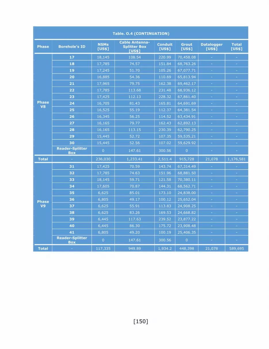
[150]




[US$]

Conduit [US$]

Grout [US$]

Datalogger [US$]

Total [US$]

Phase V8

17 18,145 108.54 220.99 70,458.08 - -

18 17,785 74.57 151.84 68,763.26 - -

19 17,245 51.70 105.26 67,077.71 - -

20 16,885 54.36 110.69 65,813.94 - -

21 17,965 79.75 162.38 69,462.17 - -

22 17,785 113.68 231.48 68,936.12 - -

23 17,425 112.13 228.32 67,861.40 - -

24 16,705 81.43 165.81 64,691.69 - -

25 16,525 55.19 112.37 64,381.54 - -

26 16,345 56.25 114.52 63,434.91 - -

27 16,165 79.77 162.43 62,892.13 - -

28 16,165 113.15 230.39 62,790.25 - -

29 15,445 52.72 107.35 59,535.21 - -

30 15,445 52.56 107.02 59,629.92 - -

Reader-Splitter Box

0 147.61 300.56 0 - -

Total - 236,030 1,233.41 2,511.4 915,728 21,078 1,176,581

Phase V9

31 17,425 70.59 143.74 67,314.49 - -

32 17,785 74.63 151.96 68,881.50 - -

33 18,145 59.71 121.58 70,380.11 - -

34 17,605 70.87 144.31 68,562.71 - -

35 6,625 85.01 173.10 24,838.00 - -

36 6,805 49.17 100.12 25,652.04 - -

37 6,625 55.91 113.83 24,908.25 - -

38 6,625 83.26 169.53 24,668.82 - -

39 6,445 117.63 239.52 23,877.22 - -

40 6,445 86.30 175.72 23,908.48 - -

41 6,805 49.20 100.19 25,406.35 - -

Reader-Splitter

Box 0 147.61 300.56 0 - -

Total - 117,335 949.89 1,934.2 448,398 21,078 589,695

[151]

Table. O.5: Networked Smart Markers 2 and 4-meter Spacing Steep Angle Boreholes

Campaign and Drilling Costs

2-meter Spacing 4-meter Spacing


Instrumentation plus Drilling Cost

[US$]


Instrumentation plus Drilling Cost

[US$]

Phase V1 615,529 1,292,586 525,054 1,202,111

Phase V4 533,302 1,116,936 455,338 1,038,973

Phase V8 1,381,756 2,916,237 1,176,581 2,711,062

Phase V9 689,956 1,441,275 589,695 1,341,014

Total 3,220,544 6,767,035 2,746,669 6,293,160

[152]

APPENDIX P: Implementation of Novel Subsurface

Deformation Sensing Device for Open Pit Slope Stability Monitoring - The Networked Smart Markers (NSMs) System

Authors

Eleonora Widzyk-Capehart, Carlos Hölck, Osvaldo Fredes, Ivan Pedemonte,

Simon Steffen.

Abstract

Comprehensive and rigorous surface and subsurface monitoring to determine slope displacement in open pit mining is one of the most important

means for assessing overall slope performance. The monitoring campaigns are aimed towards achieving and maintaining safe operating conditions, providing

advance notice of zones of potentially unstable ground, providing geotechnical information for analysing any slope instability mechanism that develops,

designing appropriate remedial action plans, and assessing the performance of the implemented slope design.

Today’s surface displacement monitoring instruments are sophisticated;

they include automated wireline extensometers, universal EDM total stations, 3D digital photogrammetry and laser scanning, and ground-based and

satellite-based radar. Together, they can provide a real-time 3D record of any surface movements that may be taking place around the walls of the pit.

However, in-ground displacement monitoring instruments are less sophisticated. Typically, they include shear strips and/or time domain

reflectometers (TDRs), extensometers, and inclinometers placed in boreholes to locate or examine the propagation of subsurface movement after evidence

of subsurface deformation has been detected at the surface. Less regularly, they are placed where it is anticipated that movement may not be detected by

surface instruments. Rarely, if ever, they are able to detect in real-time

subsurface deformation as it develops and propagates to the surface.

This paper describes the first steps in the implementation of the novel

Networked Smart Markers (NSM) technology for subsurface deformation monitoring in large open pits. A case study of the trial installation at an open

pit mine in Chile shows the importance of a well-designed installation, resulting

in a robust and successful installation. This procedure would lead towards a more comprehensive monitoring campaign with further development of the

NSM platform for multi-sensor, multi-variable monitoring.

Slope Design and Stability

Geological processes responsible for rock mass generation create ore

bodies with variable geotechnical, structural and hydrogeological

[153]

characteristics across the mine sites Read and Stacey (2009), yet the process

of rock slope design and construction is standardized across the sites.

Generally, rock slope designers rely on information acquired through experience and summarized as guidelines for designing slope angles as a

function of slope’s height and rock mass quality Wyllie and Mah (2004).

Rock mass quality, assessed according to rock mass classification

systems, enables definition of rock mass competence based on qualitative

criteria (Karzulovic and Read, 2009). However, these systems only provide a common base to assess rock mass quality or resistance; they do not overcome

the problem of uncertainties when determining the actual strength of rock masses and when designing the slopes, which increases the risk of slope

failure.

Slope Monitoring Instrumentation

Slope monitoring and proper data interpretation is essential in any

surface mining operation as monitoring devices add value at any stage of the project (from pre-feasibility to closure). On one hand, they serve monitoring

purposes to satisfy safety regulations through monitoring and reporting on changing conditions as mining progresses, verifying if the slope performance

is acceptable and warning of future failures or unsafe slope conditions. On the

other hand, the data allows better understanding of ground characteristics, a knowledge which can be used as input toward an optimized design, as it

reveals information related to instabilities, means and methods used by personnel involved in geotechnical projects, management of mine

developments or operations, delivery of objective report to stakeholders, evaluation of damage to mine site infrastructure, enhancement to operational

performance and improvements to the state-of-art (Eberhardt and Stead, 2011; Marr, 2013).

These functions of slope monitoring can assist in overcoming

uncertainties in slope design, reducing risks and improving understanding of rock mass’ response to mining activities. It is, thus, highly desirable and

recommended to implement geotechnical instrumentation for monitoring subsurface and surface deformations at each stage of a mining project

(Dunnicliff, 1993; Hawley et al., 2009). This is particularly crucial when aggressive slope designs are planned or implemented in deep pits to overcome

difficulties inherent to older open pits, such as, lower ore grades, higher operational costs, as a result of greater stripping rates, optimum balance

between ore recovery, safety conditions and financial returns (Stacey, 2009).

[154]

Current practices on Open Pit Slope Deformation Monitoring

Nowadays, slope monitoring practices show a clear dichotomy between

monitoring of surface and subsurface deformations, as the data is analysed separately, except perhaps for some cases in natural slopes, such as outlined

by Locat et al., 2010. Several authors (Mphathiwa and Cawood, 2014; Wessels and Naismith, 2005; Mc Gavigan, 2006; Kayesa , 2006; Little, 2006; Severin

et al., 2011) have shown that more effort is applied to surface deformation monitoring based mainly on the application of slope stability radar systems,

LiDAR, geodetic prisms and GPS for near real-time monitoring covering large areas. In addition, space-borne InSAR technology can be used to remotely

detect deformations at a scale of millimetres to centimetres over large areas that might be inaccessible for the installation of other types of instruments or

when real-time monitoring is not mandatory. The satellite-based microwave radar generates an image based on the difference between two successive

phase measurements in the flight path of the satellite (Eberhardt and Stead, 2011). Some instruments are better suited to specific failure modes; for

instance, surface wireline extensometers can obtain a direct measurement of

the displacement in a toppling failure by monitoring the crack width changes at the crest of a slope (Wyllie and Mah, 2004).

Subsurface monitoring tends to be less extensive relying on less sophisticated instruments, such as, TDRs, shear strips, extensometers, Shape

Acceleration Array (SAA) (Abdoun et al., 2009), geophones (Lynch and

Malovichko, 2006), and probe and in-place inclinometers. Generally, these devices have initially been developed to address civil engineering problems

and, subsequently, have been applied in mining environments (Abdoun et al., 2009). For instance, inclinometers and SAA, which register progressive

deformations, do not perform well under localized shear deformation as experienced in mining rock masses (Dowding and O’Connor, 2000). Therefore,

these instruments are not fully applicable to open pit monitoring in their current forms, yet are applied successfully in civil engineering areas. Their

apparent lack of compatibility or adaptability to mining conditions could be the main reason why they are not widely applied in mining yet, despite the fact

that, in principle, these instruments provide functional data of the moving rock volume and early notice of deformations.

Among other instruments, probe inclinometers, which measure

subsurface deformations in open pit mine operations, show a short operational lifespan as the large stiffness of rock generates high localized shear causing

kinking of inclinometer casings that would stop the probe’s movement through the casing. However, Dowding and O’Connor (2000) have stated that installing

a metallic coaxial cable through or outside the casing and grouting it to be used as a TDR system, at the same time as the inclinometer, can extend the

life of the inclinometer borehole by several months. Their experience serves

[155]

to show the importance of using appropriate instruments to conduct accurate

measurements and to add value of having several instruments in the same

measurement area.

Lynch and Malovichko (2006) have shown that surface instruments can

measure ground movement a couple of months after its surface initiation is detected by in-ground instruments.

Networked Smart Markers (NSM) System

Smart Markers

Smart Markers are electronic devices developed by Elexon Electronics

(Whiteman, 2010). They are battery-operated, radio transceivers built-in a 34.5[cm] long and 6.35[cm] diameter plastic casing filled with epoxy for

improved blasting resistance (Figure. P.1). Each Marker has an identifying ID, which is activated when the marker is installed in the ground, and is read by

the Reader (data acquisition system), when the Marker is placed in close vicinity to the acquisition system.

Smart Markers have been used in underground caving mines to track

ore flow and ore recovery. A large number of Smart Markers have been installed within drill holes near sublevel caving production blast-rings or in the

orebody of block caves. Smart Markers’ deployment into the subsidence cave has also been accomplished (Steffen and Kuiper, 2014).

In underground caving mines,

the Markers are retrieved by an LHD at the draw point and

identified by the Readers installed in the ceiling of the

drawpoints, cross cuts, perimeter drives or ore-passes,

as the LHD passes the Reader (Whiteman, 2010). The data

gathered can then be retrieved from the Reader using a hand-

held Scanner or be downloaded

directly to the mine office if the Reader is connected to a mine’s

LAN or WiFi network. This data allows to infer rock movement

and flow patterns for the fragmented material inside the caving operation (Whiteman, 2010).

Figure. P.1: Networked Smart Marker

[156]

Networked Smart Markers (NSM)

Smart Markers enhanced with the ability to communicate wirelessly

between each other using radio frequency are called Networked Smart Markers (NSMs). Currently, the wireless communication enables signal transfer through

rock up to a distance of five meters. This type of communication unlocks new possibilities for the subsurface application of NSM technology in open pits. First

prototypes of the NSMs were tested in an underground block cave and have been in operation now for more than two years.

NSMs work as a system installed sequentially inside a borehole. A series

of NSMs are tied together in a string, which allows installation to any depth within the borehole as long as the spacing between two consecutive NSMs in

the string does not exceed the maximum communication range. The NSMs are then sealed inside the drill hole with grout, permitting the NSMs to move with

the surrounding rock as the rock mass deforms and each Marker sends a signal to the next marker in the string. This process continues until the signal reaches

an antenna positioned at the top of the borehole, which must be located no farther than 5 meters away from the uppermost NSM in the string. The

antenna is a modified NSM connected to a cable that links the grouted string of NSMs with the Reader Station.

The radio signal strength registered between neighbouring NSMs is

gathered regularly. Variations of signal strengths indicate possible movement of the Markers, which can then be used to establish a qualitative indicator of

in-ground rock mass movement as a function of relative displacements of the sensors.

Case Study

First NSM Open Pit Installation

The main objectives for the implementation of the NSM system and

associated infrastructure in an operating open pit mine were to demonstrate that the system can be applied in open pit environment and can transmit a

signal wirelessly through the rock mass.

Trial Preparation

First generation prototype NSMs were tested during the manufacturing

process and subsequently at the Advanced Mining Technology Centre (AMTC) facilities at the University of Chile, Santiago. For the tests at the AMTC, the

NSMs were arranged in a sequence and tied together using two ropes placed on diametrically opposed sides of each marker. The ropes were able to

withstand 1.5 times the weight of all NSMs attached in-line (each NSM weights 1.26 [kg]), preventing torsion of the roped-NSM assembly and keeping the

NSMs in a vertical position during installation of the string down the borehole.

[157]

This arrangement also ensured that the ropes could be cut within the borehole,

due to roughness of the rock material, allowing the markers to move freely

with the deforming rock mass.

After the Markers’ arrays were completed, the ropes were marked above

the topmost NSM indicating the depth at which the array should be placed inside the borehole. These marks were placed at the collar of the drill hole.

Installation

For the first site trial, two 53-meter deep boreholes were drilled five meters behind the crest of the trial slope and approximately 47 meter away

from each other. The boreholes were instrumented with NSMs; a string of twenty two NSMs was installed in each borehole, with a two meter spacing

between each consecutive NSM. Each string was complete with an antenna

placed two meters above the uppermost NSM in the borehole and approximately one meter below the ground surface (Figure. P.2).

After each string of NSMs was lowered into the borehole, the end of the string was tied to a trestle to hold the Markers in place. Subsequently, the

boreholes were sealed using cement-sand-water mixture, which was poured

down the hole from the collar. Before both boreholes were completely sealed, the antenna was placed in the upper end of each hole at the required depth of

approximately one meter below the collar. The antennas were connected via a cable with a Splitter-Box located approximately 50 meters away from the

closest borehole along the bench.

The main feedline was installed between the Splitter-Box and the Reader Station and was buried in a shallow ditch for protection. The Reader Station

was installed on a trolley, approximately 100 meters away from the Splitter-Box (Figure. P.2), and placed in an accessible, safe, and stable zone of the

mine.

The Reader Station was powered using solar energy, allowing it to work autonomously. Data from NSMs was gathered at a set frequency and was

stored on the Reader until manually retrieved using a hand-held scanner.

System Operation

The system performed well for approximately 6 weeks. Figure. P.3 shows

an example of the signal strength and NSM connectivity in one of the instrumented boreholes where the consecutive numbers starting from 2.2 and

ending in 2.23 represent the NSMs in the drill hole from top to the bottom (2.1 is not listed as it is the Reader). Coloured boxes indicate signal strength for

neighbouring markers at 1, 2, 3, 4 hops of distance in each direction (up and

[158]

down). NSM # 2.2 does not show signal strength above it and NSM # 2.23

does not show signal strength below it because they are at the end of the chain

of Markers. Green boxes represent high signal strength links, yellow boxes indicate an average signal strength, and orange boxes specify low signal

strength.

Figure. P.2: First NSM installation diagram

Figure. P.3: NSM’s connectivity

-4 47

-3 51 59

-2 23 25 38 40 36 30 27 30 48 57 58

-1 54 42 56 47 56 53 60 59 52 29 57 52 54 48 51 54 51 55 57 56 59

2.2 2.3 2.4 2.5 2.6 2.7 2.8 2.9 2.10 2.11 2.12 2.13 2.14 2.15 2.16 2.17 2.18 2.19 2.20 2.21 2.22 2.23

+1 52 52 49 50 50 58 54 61 54 33 54 59 53 52 51 50 51 54 57 56 56

+2 29 26 35 34 38 28 27 33 48 57 57

+3 52 57

+4 41

Se

pa

ra

tio

n b

etw

ee

n N

SM

s

NSMs ID

[159]

Figure. P.4 presents signal strength in both directions for every 1 and 2 hop link in the string, where “XX/YY” is “Receiver-A-signal/Receiver-B-signal”.

Figure. P.4 shows that only 55% of the NSM present 2-hop links, leaving no redundancy in communication at other points in the string. In addition, there

is a single 1-hop link between Markers 2.11 and 2.12, which is of poor quality. For these Markers, it was observed that multiple attempts were sometimes

needed to route packets deeper to this marker.

Figure. P.4: Both ways signal strength

The data in Figure. P.3 and Figure. P.4 also indicate that the NSMs

located at the bottom of the borehole had higher signal strength readings between Markers than those at the uppermost part of the borehole. This

difference was thought to be the result of an elongation of the ropes caused by the weight of the NSMs and the impact of the grout poured from the top of

the borehole. It was deduced that the NSMs at the bottom of the holes were closer to each other than 2 meters, while the NSMs further up the hole were

farther than 2 meters apart.

After approximately 6 weeks of operation, the Reader stopped receiving new data. Therefore, over a period of 2 months, troubleshooting and re-

establishment of the NSM system’s connectivity was attempted.

System Improvements

The improvements addressed several areas of the installed system to

provide a better overall performance. For example, cables were disconnected and re-installed inside galvanized conduit ducts, the Splitter Box was protected

inside a metal box and the motherboard inside the Reader was replaced by an updated version.

However, after the improvements were in place, communication was

again lost to both boreholes. Through laboratory testing of spare NSMs and

[160]

thorough examination of the installation, a number of possible causes for lost

communications were identified.

Table. P.1 provides a summary of detected faults and/or deduced reasons for the interruptions of the system functionality.

Table. P.1: Troubleshooting summary

Detected

Fault Possibility Comment

Likelihood

Contribution

Poor 2-hop

distance

communication

Poor Marker

Communication

Range

Performance difference between

individual markers. Marker antenna

performance randomly distributed

causing short range in some NSMs.

Likely

Strong contribution

Atmospheric

noise

penetrating

bench

Bottom-Markers may have more

success in 2-hop links due to them

receiving less background RF

atmospheric noise. Markers

receiving higher background noise

will have reduced range.

Unlikely

Medium contribution

Poor RF

Properties of

Earth/Ground

The ground and/or grout

composition might be significantly

different over the length of the

borehole.

Unlikely

Medium contribution

Markers

becoming non-

contactable

Marker

Software

Problem

A possible firmware fault was

discovered that could cause a

Marker to get stuck in an un-

contactable state.

Likely

Strong contribution

Marker Battery

Problem

Batteries may have drained during

shipment of NSMs for this trial

because they were shipped “pre-

activated” to simplify the installation

procedure.

Unlikely

May have strong

contribution in the

case of a flat

battery, but no

NSMs showed

drained batteries

Broken

Installation

Rope

Possibly, the ropes broke during

Marker installation leaving some

NSMs out of rage.

Highly likely

(for at least one hole

due to total weight

of sensors/grouting)

Strong contribution

Rope

Elongation

Rope stretch expanded the planned

distance between Markers. The

distance for 2-hop links exceeded

the Markers’ communication rage.

Likely

Strong contribution

Table. P.2 provides a summary of improvements made to the system

prior to the second installation, which were deemed of high importance after the evaluation.

[161]

Table. P.2: System improvements

Possible Issue Improvements

Out-of-spec antenna tuning, which

may result in poor marker

communication range.

Automatic testing of Marker’s antenna tuning

during manufacturing.

Antenna ranges tested in the ground before

grouting the hole.

Software locking up on individual

Markers.

Second generation software resolved known

bugs and significantly improved reliability.

New generation release was and continues to

be extensively tested at Elexon.

Limited access to Reader required site

visits, which placed additional work

load on mine personnel and Project

Team.

Remote access to Reader with a GSM modem

to enable administrative tasks to be

performed by AMTC and Elexon remotely.

Antenna cabling getting damaged. Antenna cable protected with specifically

designed cover to prevent physical impact

damage.

NSM testing after grouting. NSM tested above ground.

NSM tested in the hole for an extended

period (several days) before grouting.

Second NSM Open Pit Installation

A second installation with second generation prototype NSM was

scheduled for the same trial site.

The second mine site trial was intended to test the improvements made

to the installation procedures, the devices and the overall NSM system. For this installation, two new boreholes, 10 and 40 meters deep, were drilled in

the same sector of the mine, approximately 10 meters behind the crest of the slope. The 10-meter drill hole was located behind the 52-meter borehole

closest to the Splitter Box from the first installation, while the 40-meter

borehole was placed 10 meters away from the 10-meter drill hole in the direction of the Splitter Box.

The boreholes were instrumented in sequence. The 10-meter borehole, equipped with five NSMs, allowed for initial testing of the installation before

the deeper hole was instrumented. The 40-meter drill hole was instrumented

with 35 NSM markers and grouted after confirmation that the installation in the shallower hole was performing as planned.

[162]

Installation Procedure

The NSMs were tied together using a single climbing kernmantle rope

(capable of holding 3.5 time the weight of 35 connected NSMs) to prevent an extensive elongation of the rope due to weight of the NSMs. Cables from both

boreholes to the Splitter Box and the main feedline to the Reader Station were installed inside galvanized conduit ducts. The NSMs were left hanging within

the boreholes for one week before sealing them with grout. This allowed for testing of the signal strength and the detection of any possible communication

losses.

An improved grouting procedure was used to seal the boreholes. The grouting was poured from the bottom of the hole to the top to: (1) avoid

placing additional weight on the NSMs and the rope; (2) minimise disturbance to the NSMs positions; and (3) ensure an even filling of the boreholes without

air gaps inside the grout column. The NSM antennas were installed at zero spacing (0 m) from the top-most NSM in the boreholes (approximately one

meter below ground surface) and sealed with sand to make it possible to retrieve the antennas, if needed.

After both boreholes were sealed, communications were tested from the

Reader Station showing successful wireless communications between the NSMs inside the hole. Three months after the second installation, new data

was still being gathered at short time intervals showing good quality linkage between all NSM in both boreholes. This proves that the second installation

procedure was robust and addressed the shortcomings of the first installation. The system also demonstrated that wireless data transmission through rock in

open pit installation is possible.

Other Considerations

All issues encountered during the first installation of the instruments were identified and properly addressed prior and during the second installation

to establish reliable and robust installation procedures that can be applied for similar open pit implementations in the future. Common problems of other

devices, such as in-hole cable breakage, boreholes’ blockage and excessive casing deformation, have been eliminated or reduced to minimum likelihood

of occurrence. Deformations of up to two meters will still allow proper system functioning. To-date, the NSMs proved to be robust to guarantee long term

reliability and operation lifespan under open pit mining conditions.

However, the Networked Smart Marker System is still in a prototype stage and requires more research, development and field testing. A number of

desirable characteristics have been identified, which are still being investigated, such as:

[163]

Increasing the through-ground radio communication range. A longer

range would make installation more resilient to variance in installation

distances and signal loss.

Creating smaller and more easily deployable Readers.

Implementing a more user-friendly user interface, which would enable

any mine site operator to interact with the system. The current Reader’s

user-interface still requires special training.

Conclusions

Both field tests have proven that the Networked Smart Marker system

can be applied in open pit mine environment to transmit data wirelessly through the rock mass with the second installation working without problems

for several months. The implementation of the NSMs in the field showed an importance of thorough preparation and understanding of the issues among

all the parties involved in the field trials.

Currently, a new version of NSMs called Enhanced Network Smart Markers (ENSM) is under development to integrate other sensors within the

NSM platform. It is expected that the ENSM will overcome some of the limitations of the currently available and used sensing technologies, such as:

Limited coexistence of sensors in a single location,

Limited number of sensors per borehole,

Instruments’ short lifespan,

Limited depth application,

Low tolerance to abrupt shear deformations, and

Installation and maintenance issues due to the presence of cables inside

boreholes.

Future Developments

It is envisaged that NSMs will be used as a monitoring technology platform to integrate various sensors to monitor subsurface variables. As the

NSM platform is designed to provide the wireless data transmission through the rock and an autonomous operation for up to 10 years, it is reasonable to

assume that it will overcome the shortcomings of other sensing devices and/or their cable-based connections, which can be damaged by ground movement.

Future installations of the ENSMs are planned to be carried out in higher

slope walls, which would involve boreholes up to 300 meters deep. This will require modifications to the installation procedure for lowering the NSMs into

boreholes, including specially designed hardware to lower the strings of NSMs as the sensors’ weight will be difficult to handle manually.

[164]

In addition, the future implementations would need to consider more

complex and fully operative mining environments with ground water presence

and high rates of deformation.

Determination of proper data collection frequency for the ENSM to

register variations of studied variables depending on rock mass’ characteristics at various depths would be investigated towards inclusion in the future system.

For example, brittle materials will require a higher frequency of deformation

measurements than ductile rock masses.

The integration of a GSM modem within the Reader Station is under

development and testing to enable remote access to the Reader Station via wireless networks, allowing the operators to interact with the Reader directly

without having to be physically present at the monitored site. This

implementation will allow remote software updates, firmware modifications and command execution related to data downloads.

Visualization software and tools to manipulate data are being developed for real or near-real time data processing. For following stages of development,

this software will include capabilities to process data from sensors integrated

within the ENSMs.

Finally, a redesign of the ENSM enclosure to make it easier to connect

large numbers of sensors in one string will be investigated.

Acknowledgement

The Authors would like to acknowledge the support of: Fundación CSIRO Chile through the Smart Open Pit Slope Management Project under the

auspices of CORFO; the University of Chile, Advanced Mining Technology Center and the mining company, who have provided strong support to the

Project from its commencement.

References

Abdoun, T., Bennett, V., Dobry, R., Koelewijn, A. and Thevanayagam, S.

(2009) Real-time monitoring of full-scale levee testing. Conference on Soil Mechanics and Geotechnical Engineering, Alexandria, Egypt. p. 2048-2051.

Dowding, C.H. and O’Connor, K. M. (2000) Comparison of TDR and

Inclinometers for Slope Monitoring. ASCE Geotechnical Special Technical Publication, No. 106. p. 80-90.

[165]

Dunnicliff, J. (1993) Geotechnical Instrumentation: An Overview. In:

Dunnicliff, J. (ed.). Geotechnical Instrumentation for Monitoring Field

Performance. New York: John Wiley and Sons, Inc.

Eberhardt, E. and Stead, D. (2011) Geotechnical Instrumentation. In: Darling

P. (ed.). SME Mining Engineering Handbook. USA: Society for Mining, Metallurgy, and Exploration, Inc.

Hawley, M., Marisett, S., Beale, G. and Stacey, P. (2009) Performance

Assessment and Monitoring. In: Read, J. and Stacey, P. (eds.). Guidelines for Open Pit Slope Design. Collingwood: CSIRO Publishing.

Karzulovic, A. and Read, J. (2009) Rock Mass Model. In: Read, J. and Stacey,

P. (eds.). Guidelines for Open Pit Slope Design. Collingwood: CSIRO Publishing.

Kayesa, G. (2006) Prediction of Slope Failure at Letlhakane Mine with the

Geomos Slope Monitoring System. International Symposium on Stability of Rock Slopes in Open Pit Mining and Civil Engineering, pp. 605-622.

Little, M.J. (2006) Slope Monitoring Strategy at Prust Open Pit Operation.

International Symposium on Stability of Rock Slopes in Open Pit Mining and Civil Engineering. p. 211-230.

Locat, J., Cloutier, C., Lord, P.E., Therrien, P., Jacob, C., Nadeau, A., Hébert,

D., Couture, R., Charbonneau, F., Singhroy, V., Myrnaghan, K., Danisch, L., Jaboyedoff, M., Pedrazzini, A. and Gravel, S. (2010) An Integrated Mass

Movement Monitoring System for Rockslide Hazard Assessment at Gascons, Gaspé Peninsula, Québec: An Overview. GEO 2010, Calgary, Alberta. p. 35-

43.

Lynch, R.A. and Malovichko, D.A. (2006) Seismology and slope stability in open pit mines. International Symposium on Stability of Rock Slopes in Open

Pit Mining and Civil Engineering. p. 375-390.

Marr, W.A. (2013) Instrumentation and Monitoring of Slope Stability. Geo-Congress 2013. p. 2231-2252.

Mc Gavigan, G. (2006) Management of Subsidence Associated with the Mining of the Roof of the Sishen Cave. An Application of the Slope Stability Radar.

International Symposium on Stability of Rock Slopes in Open Pit Mining and

Civil Engineering. p. 595-604.

[166]

Mphathiwa, N. and Cawood, F.T. (2014) Design Principles for Optimizing an

Established Survey Slope Monitoring System. The Journal of the Southern

African Institute of Mining and Metallurgy. 114 (6). p. 463-470.

Read, J. and Stacey, P. (2009) Guidelines for Open Pit Slope Design.

Collingwood: CSIRO Publishing.

Severin, J., Eberhardt, E., Leoni, L. and Fortin, S. (2011) Use of Ground-Based Synthetic Aperture Radar to Investigate Complex 3-D Slope Kinematics.

Proceedings, Slope Stability 2011: International Symposium on Rock Slope Stability in Open Pit Mining and Civil Engineering.

Stacey, P. (2009) Fundamentals of Slope Design. In: Read, J. and Stacey, P.

(eds.). Guidelines for Open Pit Slope Design. Collingwood: CSIRO Publishing.

Steffen, S. and Kuiper, P. (2014) Case Study: Improving SLC Recovery by Measuring Ore Flow with Electronic Markers. 3rd International Symposium on

Block and Sublevel Caving 2014, Santiago, Chile. p. 328-336.

Wessels, S.D.N. and Naismith, W.A. (2005) Management of a Major Slope Failure at Nchanga Open Pit, Chingola, Zambia. The Third Southern African

Conference on Base Metals. p. 391-405.

Whiteman, D.S. (2010) The Smart Marker system - A new tool for measuring underground ore body flow in block and sub-level mines. 2nd International

Symposium on Block and Sublevel Caving, Perth, Australia. p. 603-622.

Wyllie, D.C. and Mah, C.W. (2004) Movement monitoring. In: Wyllie, D.C. and

Mah, C.W. (eds.). Rock Slope Engineering. 4th Edition. New York: Spon Press.

[167]

APPENDIX Q: Understanding of Rock Mass Behaviour

through the Development of an Integrated Sensing Platform

E Widzyk-Capehart1, C Hölck Teuber2, O Fredes3, V Rivero4, E Sanchez5, I Pedemonte6, N Gonzalez7 and S Steffen8

1. Associate Researcher, University of Chile, Advanced Mining Technology Center (AMTC),

2007 Tupper Av., Santiago, Chile, Email: [email protected]

2. MSc Student, Universidad de Chile, 2007 Tupper Av., Santiago, Chile, Email:

[email protected]

3. MSc Student, University of Chile, 2007 Tupper Av., Santiago, Chile, Email:

[email protected]

4. Geomechanics Engineer, Itasca S.A., Santiago, Chile, Email: [email protected]:

5. MSc Student, University of Chile, 2007 Tupper Av., Santiago, Chile, Email:

[email protected]

6. MSc Student, University of Chile, 2007 Tupper Av., Santiago, Chile,

Email:[email protected]

7. Software Engineer, CSIRO Chile, 2007 Tupper Av., Santiago, Chile, Email:

[email protected]

8. Manager for Mining, Elexon Electronics Ltd., 253 Leitchs Rd, Brendale QLD 4500,

Australia, Email: [email protected]

ABSTRACT

This paper summarises the research, development and initial application

of a sensing platform that has the potential to monitor subsurface deformations, pore pressure and other variables simultaneously to gain a

better understanding of rock mass behaviour. The platform is based on Networked Smart Markers (NSMs) devices, which, with their ability for wireless

communication between individual sensors and the possibility of real-time data

acquisition and processing, will assist in the development of predictive tools to better assess rock mass behaviour.

A good opportunity to implement this technology is in the specific application of transitioning from an open pit mine to an underground caving

operation. One of the key elements to maintaining the mining business during

such a transition is having a good understanding of the unique geotechnical conditions of mutual influence created during the open pit to underground

interaction. The knowledge acquisition will require the implementation of a robust platform for geotechnical monitoring, which could be enhanced by

incorporating the NSMs. The integration of sensors within the NSMs would

mailto:[email protected]

[168]

enable the collection of additional data about rock mass behaviour (i.e. caving

propagation and crown pillar fracturing), which could be used to improve the

management of mining operations and, specifically, allow the development of reliable predictive tools based on the data collected.

INTRODUCTION

A good understanding of rock mass behaviour can only be obtained through geotechnical monitoring using adequate instrumentation. A

monitoring campaign implemented throughout the mine life gathers evidence of the rock mass’s response to mining activities, which could be used in future

mine design processes to achieve safer and more efficient operations. At the same time, the proactive use of monitoring information can reduce the

possibility or seriousness of incidents occurring, such as slope failures (Blachowski, Ellefmo and Ludvigsen, 2011), which can have serious

consequences for operations. There are numerous benefits associated with

implementing a robust monitoring program, including improved risk management related to mining operation (Marr, 2013) and an empirical

comprehension of operational performance when a specific mining plan is introduced or changes in production rates are implemented or made. Thus,

efforts towards collecting more and better-quality data are fundamental for improving the mining business.

While not new, the concept of geotechnical monitoring is critical for the

future continuation of the mining business, specifically the transition from large open pit (OP) operations to mass underground (UG) cave mines. In this

context, understanding the geomechanical aspects related to OP and UG interaction is one of the key elements towards enabling successful transitions.

A monitoring platform should assess at least the following aspects:

caving propagation, in terms of the cave back position crown pillar response, which is significant for the period of simultaneous

OP–UG operation the progression of subsidence, which allows risk-prone areas to be

identified slope stability.

In this paper, the OP–UG transition problem is described, including the

currently available technology that could be applied or has already been applied in similar mining environments for geotechnical monitoring. Networked

Smart Marker (NSM) technology is introduced, and its benefits are highlighted when it is incorporated into a monitoring campaign as a sensing platform.

[169]

Open Pit – Underground Interaction

During the mine life, economic considerations (mainly) can lead to a

decision to change the exploitation method (transitioning from OP to UG or from UG to OP) or to carry out OP and UG operations simultaneously. Whatever

the case, it is very probable that there will be periods with high levels of interaction between the two operations, which can generate highly complex

scenarios from the perspective of geotechnical management. Several cases have occurred where it has been possible to anticipate significant levels of

interaction between mines operated using OP and UG block caving methods within the same mining area.

Open pit to underground

Nowadays, the transition from surface to UG mining and OP mines operating over old UG workings are the most prominent case of OP–UG

interaction. Currently, there are several large OP mines (eg Chuquicamata, Chile; Grasberg, Indonesia; Bingham Canyon, USA and Resolution, USA)

conducting engineering studies to make the transition from OP to UG mining via caving methods (Flores and Karzulovic, 2002; Flores, 2006; Brown, 2007).

The reason to move to UG mining is essentially to extend the mine life and/or optimise the benefit of the mining exploitation. As the mineralised zone goes

deeper, the cost of the next pushback to access the ore may become less economically viable than the development of an UG mine. However, the

transition point is not unique, with a range of options possible (Snowden,

2015; Finch, 2012) depending on the criteria assumed for the estimation. The ultimate solution relies on economic and risk factors and production rates,

among other factors.

The decision to choose caving methods to continue surface mining is

often based on production targets (cost and volume), the variables of which

are of similar orders of magnitude for the two mining methods (Flores, 2004).

As part of the transition process, it is expected that a period of

simultaneous exploitation will take place to mitigate the lower production volumes of the UG mine during ramp-up (Flores, 2006). During this process,

one of the main geotechnical challenges is to maintain the stability of the

crown pillar (see Figure. Q.1 and Figure. Q.2), which is the portion of rock between the bottom of the pit and the position of the cave back. Managing the

stability of the crown pillar is important to reduce the likelihood and severity of undesirable events such as instability of the pit slopes, mud rush, air blast

and the entry of dilution in the UG mine (Stacey and Terbrugge, 2000; Flores, 2006).

[170]

The Palabora mine was the first mine to successfully perform the

transition from a large OP to a block caving mine (Brown, 2007). The

operational management of the crown pillar at the site, with all of the associated problems encountered during the process, has been discussed in

detail by various authors (Glazer and Hepworth, 2004; Moss, Diachenko and Townsed, 2006; Brummer, Moss and Casten, 2006).

Figure. Q.1: Crown pillar defined at Palabora mine (after Glazer and Hepworth, 2004)

Simultaneous operations

The El Teniente mine in Chile is one of the largest UG mines in the world.

Since 2013, it has been operating as an OP mine located at the edge of the subsidence crater generated by the caving process (Codelco, 2014). Different

conditions have been identified in the interaction between Anglo American’s

OP mine Los Bronces in Chile and Codelco Andina Division’s neighbouring block caving mine, Rio Blanco (Díaz, 2014). Both mines are active operations, which

implies a strong interaction between the east wall of the pit and the active subsidence crater of Andina (Figure. Q.3). In this instance, the main challenges

for the OP mine are to meet the objectives of the mining plan and, simultaneously, to maintain safe operating conditions while the crater expands

towards the Los Bronces area.

[171]

Figure. Q.2: Seismic monitoring at the site (after Glazer and Hepworth, 2004)

Geotechnical monitoring of open pit – underground interaction

Currently, there

are not enough real cases of OP to UG

transition to establish general empirical rules

for generating safe operational conditions

during the transition

phase. For the same reason, the few

attempts undertaken to define interaction

design guidelines, in particular the work

done by Flores (2006), have not yet been

sufficiently validated. To date, when

subsidence craters have developed, the general recommendation has been to

Figure. Q.3: Plan view of Los Bronces-Andina interaction area (after Google Maps, 2015)

[172]

avoid surface mining in the subsidence zone where large-scale fracturing can

be observed (Díaz, 2014). Even if design guidelines did exist, continuous

geotechnical monitoring is crucial for managing a successful transition process. Two phenomena are of particular interest:

1. the process of initiation and propagation of caving 2. the surface displacements generally associated with subsidence caused

by the progression of caving towards the surface.

A general overview of the most widely applied instrumentation techniques for geotechnical monitoring of the aforementioned critical aspects

is shown in Figure. Q.4.

Figure. Q.4: Summary of surface and underground geotechnical monitoring methods

[173]

Surface monitoring

As shown in Figure. Q.4, there is a wide variety of available technology

to monitor ground movement, which can be classified into three categories: space, airborne and ground-based observations. Examples of the application

of these techniques are given by Díaz (2014), who mainly described the technologies currently used at the Los Bronces mine to monitor surface

movements but also covered the entire spectrum of instrumentation, including total station, radar, crack meters, time domain reflectometry (TDR) cables,

photogrammetry and interferometric synthetic aperture radar (InSAR). InSAR and radar are used to monitor the pit slopes and infrastructure in the areas of

interaction with the active subsidence crater of Coldelco’s Rio Blanco mine. InSAR helps to identify the general areas of movement at different scales (in

the range of metres, centimetres and millimetres), while radar generates a real-time inspection of the ground displacements. In his work, Díaz (2014)

also presented a benchmarking of the geomechanical instrumentation applied for controlling subsidence in four other mines (Kiruna, Perseverance, El

Teniente and the Deep Ore Zone (DOZ)). His work confirmed that the strategy

of combining real-time data acquisition with various instrumentation/ techniques to detect movement at a larger scale is currently the standard in

the mining industry. Díaz (2014) highlights the experience of the El Teniente mine, which operates as an OP mine on the edge of a subsidence crater

(Espinoza and Mora, 2012; Espinoza, Mora and Sánchez, 2014), where mainly InSAR was applied. Photogrammetry and InSAR have also been applied in

other mining environments, as described by Mora, Álvarez and Amor (2013).

Brief descriptions of the space-based, airborne and ground-based monitoring techniques are compared in Table. Q.1, Table. Q.2 and Table. Q.3

respectively. This is presented for subsequent comparison with the proposed in-ground monitoring platform based on NSMs. The main references used for

developing this review were Raghu, Singh and Ghose (2006), Mawell (2014), Hawley et al (2009), Patikova (2004) and McClusky and Tregoning (2013).

Underground monitoring

According to Brown (2007), the following four techniques are the most commonly used for assessing cave propagation:

1. methods based on open holes

2. cavity measurement or surveying 3. TDR

4. seismic or microseismic monitoring.

[174]

Table. Q.1: Description of technologies for space-based monitoring

Technique Description Strengths and drawbacks Precision

Global Positioning system (GPS)

Space-based satellite navigation system provides points location using the timing of signals sent by different satellites to ground

receivers located in the position to be surveyed. The time is used to determine the distance from the receiver to all of the satellites.

These distances allow for

precise determination of the position of the receiver.

• Line of sight is not required

between receivers. • Not dependent on weather

conditions. • Requires mine personnel to

go to all the different points to be surveyed.

• Requires unobstructed line of sight to four or more GPS satellites.

Satellite visibility is

obstructed in deep point of the pit.

Under 20 mm

Interferometric synthetic

aperture radar

(InSAR)

Uses the difference in phases between successive SAR images to determine ground movement. SARs send

microwave signals to the zone to be monitored and register the reflection of the sent signal. Then, interferometric

techniques are used to obtain information about 3D

deformation from the phase difference between the waves sent and received by the satellite.

• Works in all weather conditions.

• Allows monitoring of inaccessible sectors of the pit.

• Good technique for monitoring broad areas.

• Dependent on international satellites’ availability for data gathering.

• May not produce good results

when monitoring steep zones.

• Real-time monitoring is not feasible.

• If displacement between successive SAR images is higher than 23 cm,

• InSAR may not be able to quantify it.

On the scale of

centimetres to

millimetres

These methods, which are described in detail in Table. Q.4, are generally

used in combination, but only the last two have proven to be versatile enough to apply systematically.

A good example of TDR application can be seen in Szwedzicki, Widijanto

and Sinaga (2004), which describes the application of this technique at the DOZ mine in Indonesia to monitor changes in the size and shape of the cavity

and simultaneously estimate the rate of cave propagation.

The application of the seismic method at the Palabora mine for

monitoring the response of the crown pillar is described in detail by Glazer and

[175]

Hepworth (2004). The method consisted of installing recording stations around

the cave on different levels. Nine of these stations were installed on the

production and development levels, four in the OP and eight in an abandoned exploration shaft and a deep borehole. Some of the important factors to take

into account are the sensitivity of the recording stations to locate events with an acceptable level of accuracy and the extent of the sensor network to provide

reliable and precise data. Glazer and Hepworth (2004) remarks that mine seismology studies cannot solve problems on their own and that they must be

supplemented with other data, such as seismic passive tomography.

Table. Q.2: Description of technologies for airborne monitoring


Synthetic aperture

radar (SAR)

Uses the same principles as InSAR but the instrument is mounted on an airplane.

Independency from international satellites for data gathering.

Uses a relatively unstable platform. Very important to know the exact

location of the plane for best results.

-

NETWORKED SMART MARKERS

Currently available subsurface deformation sensing technologies have some important constraints in their application in OPs, including a limited

number of sensors per borehole, limited application depth, short lifespan and a low tolerance to abrupt shear deformation due to the presence of cables for

data transfer. The technology presented in this paper, the NSM system, aims to address these drawbacks and thus create a new method for sub-superficial

monitoring of rock mass to assess slope stability and/or subsidence effects at a UG mine.

Sensors developments and applications

Smart Markers

Smart Markers were developed as an autonomous electronic device that

is capable of monitoring mineral flow and ore recovery. The device consists of a battery and built-in radio transceiver placed within a high-impact resistant

plastic case that is filled with epoxy to improve blasting resistance (see Figure. Q.5). The markers have been developed by Elexon Electronics, and each

device weighs 1.26 kg, is 34.5 cm long and 6.35 cm in diameter (Widzyk-Capehart et al, 2015). The markers are placed in an orebody that is to be

extracted using the caving method and are then automatically identified via radio transmission when the load-haul-dump (LHD) machine extracts the

fragmented material containing the marker through the drawpoint. The markers are detected by readers located in the vicinity of the LHD’s path. To

date, Smart Markers have been successfully tested as gravity flow trackers in

[176]

block caving operations (Steffen and Kuiper, 2014; Viera et al, 2014) and

sublevel caving mines (Steffen and Kuiper, 2014; Whiteman, 2010).

Table. Q.3: Description of technologies for ground-based monitoring


Visual inspection

Visual observation of

the studied zone to detect the occurrence of cracks or evidence displacements.

Requires experienced geotechnical staff.

Must be complemented by instrumentation to provide a quantitative basis for defining the

exact amount of movement.

Qualitative

Cross-crack measurements

Crackmeters are devices composed of a steel rod installed at either side of the crack.

The distance between

steel rods is measured periodically using a measuring tape, Vernier calliper or micrometer to determine the crack

aperture.

Provides an insight into in-ground

movements. Simple monitoring devices. Potentially unstable working area.

0.1 mm

Photogrammetry

Integrates 3D spatial data with 2D visual data to create spatially

accurate representations of the surface topology of the

rock. Structural properties (i.e. orientation, length and

spacing) can be determined using this technique.

Integration of photogrammetry with mine planning software systems makes it possible to use the data in real time for mine design, mine planning and mine operating

purposes. Provides a permanent 3D record of

the mapped areas.

Provides low-cost geological mapping.

Only one person needed to use the

technique. Digital imaging systems require

ground proofing and cannot be used to determine the physical features of the structures.

Accuracy

ranges from 2 cm at a distance

of 50 m to 10 cm at

distances of

up to 3 km

LiDAR

This technique uses

laser pulses reflected by the surface to be measured to create a 3D representation of the scanned target with a density of >10 000

points/m2. It is an

optical remote sensing technique that uses the properties of scattered reflected light to determine the range between the monitored

object and the sensor.

Able to create a highly accurate 3D digital elevation model.

High-resolution images. Relatively inexpensive.

Flexible data collection and processing system.

Can be used to monitor relatively small areas (from 1 to 10 km2).

Need for experienced personnel to understand the limitations of the

terrestrial laser scanning. Requires a proper data collection

campaign to avoid shadowed regions.

Systematic errors are

±25 mm at 1000 m,

random

errors are generally between 0 and 10 mm

[177]

Table. Q.3 (CONTINUATION)


Ground-based interferometric

synthetic aperture

radar

Uses the same principle as the satellite-based method but the images are acquired by a radar

moving along a rail a couple of kilometres away from the area of interest. The monitored zone can be up to 4 km from the radar.

Measurements can be taken during

day and night and in any weather conditions.

Provides high spatial density of observations.

Fast (5–10 min monitoring period). Short range (<5 km) Limited field of view, which may

cause shadowing problems. Not intended to monitor broad

areas.

Resolution of about

0.5–4 m, depending on

the monitoring distance and the

atmospheric

conditions, precision in the scale of millimetres

Robot total stations (prisms

monitoring)

Robot total stations are

devices that combine a theodolite with

electromagnetic distance measurement system to measure horizontal and vertical angles along with

distance. This allows the surveyor to measure 3D coordinates of points remotely, typically targeted by the

placement of reflective prisms.

Ability to provide 3D position of the point of interest.

Unable to monitor during misty weather.

Installation of monitoring prisms at a likely unstable slope zone or area of interest.

Accuracy from 0.6 to

3 mm, range from 1000–

3000 m

Tilt meters

Tilt meters use the bubble principle to

measure the gradient of inclination of a ground point. The bubble movements are measured and then

converted into an estimate of the instrument’s tilt.

High-precision measurements obtained.

Used to monitor movements that are expected to contain a rotational

component. Expensive in comparison with radar

monitoring. A 500 × 500 m area costs approximately $36 000/month.

Requires additional calibration after some time to maintain accuracy.

1 nanoradian (0.0002

arcseconds)

The application of Smart Markers in underground mines allows a better understanding of mineral flow behaviour and ore recovery. However, they

cannot identify the location or track the evolution of the cave back as can be done with microseismic monitoring.

Networked Smart Markers

NSMs are Smart Markers equipped with an antenna for data transmission via radio frequency, enabling wireless communication between sensors

through rock (Steffen et al, 2016). The signal strength variation between the markers indicates the relative distance between communicating markers as

the rock moves.

[178]

Table. Q.4: Technologies applied in the mining industry for underground monitoring


Inclinometers

Generally used to measure lateral subsurface displacement in vertical holes. Inclination measured by the

device is used to determine the movement perpendicular to the drill hole axis.

Very detailed displacement

path. Short lifespan in large

boreholes and big ground movements due to breakage of the casing.

Very useful to study gradual

inclination changes.

Can detect differential

movements of 0.5–1.0 mm

per 10 m length of hole

Borehole extensometers

Designed to monitor directional or axial deformations in the rock mass. Individual wires are attached to an anchor at the

bottom of the hole, and the axial movement relative to

the anchor is recorded.

Automated and remote readings.

Possible to measure multiple points.

Complicated to install in long boreholes.

Up to 0.005 mm

Piezometers

Designed to measure fluid or

pore-water pressure in a variety of applications. They are typically installed in boreholes in in situ soils, rocks, foundations or earth/rock fills and are

grouted with a specific mixture. Closed piezometers are the most commonly used in the mining environment.

Acceptable time response to pressure variations.

Easy to adapt to an

automatic recording device. Grouting properties are

critical to preventing surface water from contaminating piezometer data.

Long lines are susceptible to damage due to borehole movements.

Not possible to check the calibration of the instrument

once installed.

±0.1 per cent Full Scale for the vibrating

wire type

Cavity measurements/

surveying

Traditional methods of general survey measurement and positioning such as

levels, total stations, photogrammetric cameras or a combination of them.

Conventional survey techniques are very reliable methods if well done.

In most cases, they require an experienced operator to gather the information

correctly.

Depends on the method

used

Seismic or Microseismic

monitoring

Microseismic monitoring is the passive observation of very small-scale earthquakes as a result of human activities or industrial processes such as

mining. Brittle fractures in rock radiate seismic waves, and if they are recorded

sufficiently by different seismograms, the seismic event’s origin time, source parameters, deformation and

location can be estimated. Geophones are usually used in mining applications.

Very unique system to locate fractures developing within the rock mass.

Geophones don’t need power to operate.

Signal degradation if the sensors are far from the target.

Only to respond to high-frequency waves.

Geophones are used to triangulate the position of

the movement that originated the measured wave.

For an Institute of

Mine Seismology

4.5 Hz geophone, the

distortion measurement frequency is

12 Hz

[179]

Table. Q.4 (CONTINUATION)


Time domain Reflectometry

(TDR)

TDR is an electronic instrument that locates faults in metallic cables. If the coaxial cable installed in a vertical hole suffers an impedance change due to

kinking, the TDR detects the exact distance to that point.

High precision on fault location.

Inability to measure large

ground displacements due to the breakage of the wires and thus loss of signal.

Useful to sense localised and concentrated shear strain.

±1 per cent of the cable distance

ShapeAccelArray (SAA)

Electronic instruments with triaxial micro-electromechanical system accelerometers inside a 30

cm rigid segment. Several segments can be put together

to measure 3D ground deformation in depths from 30 cm to 100 m.

Installed in vertical holes to obtain horizontal deformation data in real

time. Also possible to install

horizontally to measure vertical deformation.

±1.5 mm for 32 m SAA

Smart Markers

Autonomous electronic devices capable of monitoring mineral flow and ore recovery in block/panel and sublevel caving mines.

Each device has its own identifying ID, allowing its location to be pinpointed

when installed in the rock mass.

When recovered in a drawpoint, the marker is identified by a reader.

Ore flow can be inferred

from the initial and final positions of the devices.

The actual path of the marker from its installation position to its extraction position (drawpoint) cannot be registered.

Qualitative

These new communication capabilities opened up a number of new applications for NSMs. NSMs were recently installed at an OP mine to

determine their applicability to monitor deformations behind the pit slope (Widzyk-Capehart et al, 2015). The NSMs were installed sequentially inside a

borehole using several NSMs tied to a single cord. After installation of the markers, the boreholes were grouted so as to fix the NSMs in their initial

placement position until the occurrence of deformations, which would force the sensors to move with the surrounding rock.

The installation distance between consecutive markers must not exceed

the current maximum communication range of 5 m to enable uninterrupted signal transfer between markers. The radio signal transfer between markers is

repeated until the signal reaches a modified NSM near the surface that functions as an antenna and is connected via cable to the reader station, where

all data is regularly gathered at predefined intervals (Widzyk-Capehart et al,

[180]

2015). The data acquired from the sensors is

downloaded into the reader and then sent via

3G modem to a predefined online server, which makes it possible to obtain the data

remotely. The raw data is processed and can be represented in a graphical form (Figure.

Q.6 and Figure. Q.7). The semi-horizontal axis indicates the marker’s number, organised

according to a predefined order of installation, with the closest to the XYZ origin being the

closest to the surface. The vertical axis refers to the signal strength between two consecutive markers and is called the

received signal strength indicator’ (RSSI). The RSSI values range from 0 to 64. Signal strength depends on the distance between markers and the

propagation media. When installed, the initial values of RSSI are not important. This only becomes important to measure the difference in values

after the installation. Laboratory tests indicate that short-term fluctuations of

five to ten in the RSSI values may be the result of temporary changes in the surrounding conditions. If the distance between markers is static and the

conditions stable, the maximum change in RSSI values is around three points. The Z axis corresponds to the average weekly values obtained during

consecutive weeks. Figure. Q.6 and Figure. Q.7 show the average value of one week compared with the average values obtained during the subsequent five

weeks (six weeks are represented in total).


Figure. Q.5: Smart Marker sensor

[181]

It is important to observe the variation of RSSI values of the same

marker over time as it represents the change in distance between markers,

which enables the assessment of rock movement. The change in distance between markers is due to the movement of the rock in the vicinity of the

marker’s initial installation.


ENHANCED NETWORKED SMART MARKERS

The qualitative assessment of rock mass movement is based on the

variations of the registered signals’ strengths, which does not provide the sensitivity to measure small-scale ground movement in the range of

millimetres. However, the NSM sensing platform and data transmission method allows for enhancement of the markers with sensors. This concept

foresees the integration of other sensors within the current NSM, which can be accomplished within the same robust and field-validated platform. Thus, a new

version of NSM, Enhanced Networked Smart Markers (ENSMs), is currently under development to enable a quantitative assessment of rock mass

behaviour associated with ground deformation and pore pressure monitoring.

Accelerometer

Tilt measurement can be performed by placing an accelerometer and

magnetometer within the ENSM. To detect movement before the material reaches its yield strength, the accelerometers need to have sufficient accuracy.

The required accuracy depends on the material where the system will be installed – brittle material will fail at smaller strain levels than ductile material.

[182]

To cover a wide range of materials, a sensor with a high tilt resolution has

been chosen. The accuracy of the selected accelerometer will be confirmed by

performing validation testing in the laboratory and at mine environments in 2016.

Pore pressure sensor

Considering the overall benefits of geotechnical instrumentation,

groundwater monitoring is a highly important task. Pore pressure is closely

related to rock mass strength as a reduction in groundwater pressure increases the effective stress of the in situ rock mass and, consequently, increases the

shear strength. In some cases, dewatering the rock mass is the only alternative that mine personnel have to increase resistance and reduce the

probability of slope failure (Beale, Price and Waterhouse, 2013).

Currently, the most common instruments used to measure pore pressure are piezometers, which are classified according to the type of transducer

employed to register variations in water pressure (Lomberg et al, 2013). An open standpipe piezometer is the least sophisticated variant, consisting of a

plastic pipe with a perforated lower section within a filter element composed of coarse sand sealed by a layer of compacted bentonite pellets on top.

However, the major limitation of this type of instrument is its slow response to piezometric change (Dunnicliff, 1993). In addition, these piezometers

register the average pressure in a column of water but do not allow for measurements at a single point. Thus, they are not widely used in mining

environments.

Diaphragm piezometers measure pressure by allowing water to enter the sensor through a porous filter. After the water enters the sensor, it fills the

space between the filter and a diaphragm, deforming the latter. The instrument uses a transducer to measure the deformation and relate it to a

pressure value. These sensors typically rely on pneumatic, vibrating wire, twin-tube hydraulic, flushable, semiconductor and piezoresistive transducers

to make a reading.

Diaphragm piezometers stabilise after a pressure change over a period that ranges from seconds to several minutes. While pneumatic piezometers

are unable to measure negative pore pressure, vibrating wire piezometers can measure pressure of 50 kPa below atmospheric pressure. Electrical

piezometers have a significantly smaller time lag than pneumatic, hydraulic and flushable sensors as the volume of water displaced at the diaphragm is

extremely small. These characteristics give electrical sensors an advantage

over pneumatic sensors (Mikkelsen and Green, 2003).

[183]

Electronic pore pressure sensors and accelerometers are currently being

implemented inside the NSMs. The exterior of the pore pressure sensor is

covered with a mesh screen, which protects the sensor from getting clogged up by grout or other fines, but will allow water to pass through it. The pore

pressure sensor marker uses a piezoelectric transducer with an accuracy of 0.1 per cent of full scale. The piezo transducer is used in ranges of up to 30

bar and can withstand an overpressure of at least 300 per cent (i.e. three times the nominal pressure). Above 30 bar, the transducer is a thinfilm

Wheatstone measuring bridge and has an accuracy of between 0.15 and 0.2 per cent of full scale. It can withstand an overpressure of at least 200 per cent.

Temperature compensation is applied to maintain accuracy across the marker’s operating range of 0–50°C.

A string of vibrating wire piezometers can be installed in a single

borehole to provide multipoint measurements. Generally, only two to five sensors are installed in the same hole as technical issues prevent the

installation of more. However, six or more instruments can be installed in HQ or RC holes (Read et al, 2013). The use of ENSMs will make it possible to install

a greater number of pore pressure sensors. This will enable the definition of hydrostatic profiles with more measurement points in a single borehole

because the wireless data transmission capabilities of the devices allow for any number of NSMs to be installed as long as the distance between neighbouring

markers is kept below their transmission range.

ENSMs would therefore allow mine personnel to correlate the pore pressure change rate with the propagation of deformation in the rock mass.

Monitoring open pit – underground interaction

As discussed previously, ENSMs could be used for subsurface monitoring of deformations or as gravity flow trackers for a caving mine. The information

gathered from these sensors could then be integrated with all the other mine site data to improve the understanding of the rock mass behaviour during the

interaction, adding valuable new information such as:

Understanding crown pillar response. Information captured from ENSMs could be used to identify locations experiencing deformation within the

crown pillar. The data from the ENSMs could be combined with microseismic monitoring data and the geological, geotechnical, and

structural models of the mine, which would improve understanding of the mechanisms of mobilisation and thus increase confidence in the

predictions of rock mass response. This new system provides

information that could improve risk management associated with subsidence, which could influence the decision to extend OP life during

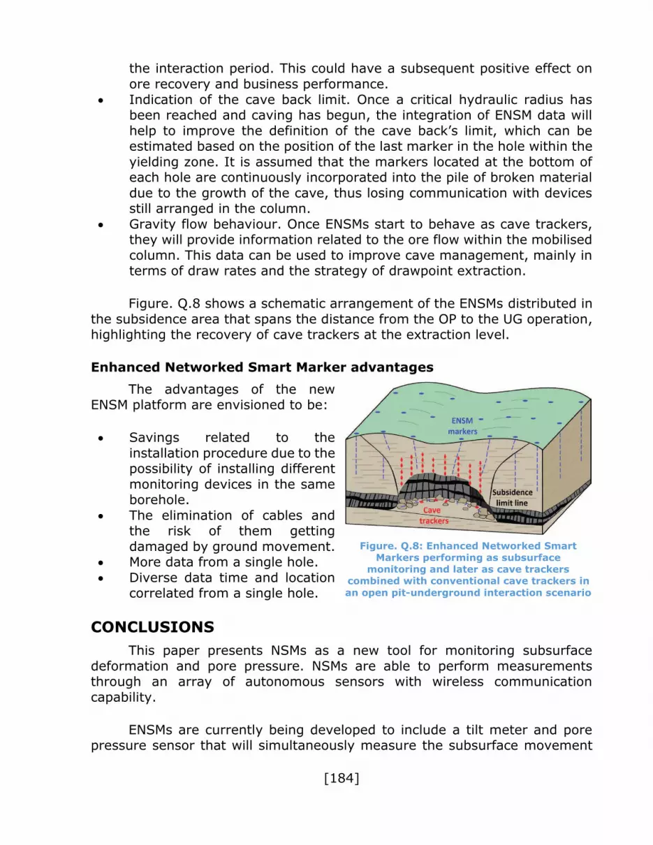
[184]

the interaction period. This could have a subsequent positive effect on

ore recovery and business performance.

Indication of the cave back limit. Once a critical hydraulic radius has been reached and caving has begun, the integration of ENSM data will

help to improve the definition of the cave back’s limit, which can be estimated based on the position of the last marker in the hole within the

yielding zone. It is assumed that the markers located at the bottom of each hole are continuously incorporated into the pile of broken material

due to the growth of the cave, thus losing communication with devices still arranged in the column.

Gravity flow behaviour. Once ENSMs start to behave as cave trackers, they will provide information related to the ore flow within the mobilised

column. This data can be used to improve cave management, mainly in terms of draw rates and the strategy of drawpoint extraction.

Figure. Q.8 shows a schematic arrangement of the ENSMs distributed in

the subsidence area that spans the distance from the OP to the UG operation, highlighting the recovery of cave trackers at the extraction level.

Enhanced Networked Smart Marker advantages

The advantages of the new ENSM platform are envisioned to be:

Savings related to the

installation procedure due to the possibility of installing different

monitoring devices in the same borehole.

The elimination of cables and the risk of them getting

damaged by ground movement. More data from a single hole.

Diverse data time and location correlated from a single hole.

CONCLUSIONS

This paper presents NSMs as a new tool for monitoring subsurface

deformation and pore pressure. NSMs are able to perform measurements through an array of autonomous sensors with wireless communication

capability.

ENSMs are currently being developed to include a tilt meter and pore pressure sensor that will simultaneously measure the subsurface movement

Figure. Q.8: Enhanced Networked Smart Markers performing as subsurface

monitoring and later as cave trackers combined with conventional cave trackers in

an open pit-underground interaction scenario

[185]

and pore pressure along the entire length of the borehole. When processed in

real time, this data will provide an improved understanding of the effects of

various operational activities, including UG mining in the vicinity of the OP, on rock mass behaviour.

The main advantages of ENSMs are their wireless communication capabilities and the ability to collect disparate data (displacement and pore

pressure) at the same time and location.

ACKNOWLEDGEMENTS

The authors would like to acknowledge the support of Fundación CSIRO Chile through the Smart Open Pit Slope Management Project under the

auspices of the Production Development Corporation (CORFO), the University of Chile, Advanced Mining Technology Center and the mining companies that

provided strong support to the project from its commencement.

REFERENCES

Beale, G, Price, M and Waterhouse, J, 2013. Framework: assessing water in

slope stability, in Guidelines for Evaluating Water in Pit Slope Stability

(eds: G Beale and J Read), pp 19–64 (CSIRO Publishing: Melbourne).

Blachowski, J, Ellefmo, S and Ludvigsen, E, 2011. Monitoring system for

observations of rock mass deformations caused by sublevel caving mining system, Acta Geodynamica et Geomaterialia, 8(3)163: 335–344.

Brown, E, 2007. Block Caving Geomechanics: The International Caving Study

1997–2004, second edition (Julius Kruttschnitt Mineral Research Centre: Brisbane).

Brummer, R, Moss, A and Casten, T, 2006. The transition from open pit to

underground mining: an unusual slope failure mechanism at Palabora, in Proceedings International Symposium on Stability of Rock Slopes in

Open Pit Mining and Civil Engineering, pp 411–420 (The South African Institute of Mining and Metallurgy: Johannesburg).

Codelco, 2014. Operación de Rajo Sur en El Teniente aportó más de 56 mil

toneladas de cobre en su primer año (in Spanish) [online]. Available from: <https://www.codelco.com/operacion-de-rajosur-en-el-teniente-

aporto-mas-de-56-mil-toneladas-de/prontus_codelco/2014-01-10/153920.html> [Accessed: 22 January 2015].

[186]

Díaz, D, 2014. Geomechanical status and action plans for interaction between

Andina subsidence crater and Los Bronces pit, MSc thesis, Universidad

de Los Andes, Santiago.

Dunnicliff, J, 1993. Geotechnical Instrumentation for Monitoring Field

Performance, 608 p (John Wiley and Sons: New York).

Espinoza, A and Mora, O, 2012. InSAR technology at El Teniente South Open Pit, in Revista Minería Chilena (in Spanish) [online]. Available from:

<http://www.altamira-information.com/files_upload_site/pdf_ publications/2012_Mora_et_al_MineraChilena.PDF> [Accessed: 16

September 2015].

Espinoza, A, Mora, O and Sánchez, F, 2014. Application of InSAR technologies to measure the subsidence at El Teniente’s Mine, in Proceedings Third

International Symposium on Block and Sublevel Caving: Caving 2014 (ed: R Castro) (Universidad de Chile: Santiago).

Finch, A, 2012. Open pit to underground [online], International Mining,

January 2012:88–90. Available from: http://www.infomine. com/publications/docs/InternationalMining/Finch2012.pdf [Accessed:

16 September 2015].

Flores, G, 2004. Geotechnical challenges of the transition from open pit to underground mining at Chiquicamata Mine, in Proceedings Fourth

International Conference and Exhibition on Mass Mining (MassMin 2004) (eds: M A Alfaro and A Karzulovic), pp 591–605 (Instituto de Ingenieros

de Chile: Santiago).

Flores, G, 2006. Rock mass response to the transition from open pit to underground cave mining, PhD thesis, University of Queensland,

Brisbane.

Flores, G and Karzulovic, A, 2002. Geotechnical guidelines from a transition from open pit to underground mining, benchmarking report, Project ICS-

II, Task 4.

Glazer, S and Hepworth, N, 2004. Seismic monitoring of block cave crown pillar – Palabora Mining Company, RSA, in Proceedings Fourth

International Conference and Exhibition on Mass Mining (MassMin 2004) (eds: M A Alfaro and A Karzulovic), pp 565 – 569 (Instituto de Ingenieros

de Chile: Santiago).

[187]

Google Maps, 2015. Available from: https://www.google.es/maps/@-

33.1501683,-70.2793249,4695m/data=!3m1!1e3 [Accessed: 18

August 2015].

Hawley, M, Marisett, S, Beale, G and Stacey, P, 2009. Performance

assessment and monitoring, in Guidelines for Open Pit Slope Design (eds: J Read and P Stacey), pp 343–362 (CSIRO Publishing: Melbourne).

Lomberg, C, Ream, I, O’Rourke, R and Read, J, 2013. Monitoring and design

reconciliation, in Guidelines for Evaluating Water in Pit Slope Stability (eds: G Beale and J Read), pp 363–389 (CSIRO Publishing: Melbourne).

Marr, W A, 2013. Instrumentation and monitoring of slope stability, in

Proceedings Geo-Congress 2013, pp 2224–2245 (American Society of Civil Engineers: Reston).

Mawell, S, 2014. Microseismic Imaging of Hydraulic Fracturing: Improved

Engineering of Unconventional Shale Reservoirs, 214 p (Society of Exploration Geophysicists: Tulsa).

McClusky, S and Tregoning, P, 2013. Background paper on subsidence

monitoring and measurement with a focus on coal seam gas (CSG) activities, paper prepared for the NSW Chief Scientist and Engineer,

Research School of Earth Sciences, The Australian National University, Canberra.

Mikkelsen, P E and Green, G E, 2003. Piezometers in fully grouted boreholes,

in Proceedings Sixth International Symposium on Field Measurements in Geomechanics (ed: F Myrvoll), pp 545–553 (A A Balkema: Rotterdam).

Mora, O, Álvarez, I and Amor, E, 2013. Slope stability study in open pit and

underground mines by means of forensic analysis and radar interferometry, in Proceedings Slope Stability Conference 2013 (ed: P

Dight), pp 1021–1032 (Australian Centre for Geomechanics: Perth).

Moss, A, Diachenko, S and Townsed, P, 2006. Interaction between the block cave and the pit slopes at Palabora mine, in Proceedings International

Symposium on Stability of Rock Slopes in Open Pit Mining and Civil Engineering, pp 399–410 (The South African Institute of Mining and

Metallurgy: Johannesburg).

Patikova, A, 2004. Digital photogrammetry in the practice of open pit mining, The International Archives of the Photogrammetry, Remote Sensing and

Spatial Information Sciences, 35:707–710.

https://www.google.es/maps/@-33.1501683,-70.2793249,4695m/data=!3m1!1e3

https://www.google.es/maps/@-33.1501683,-70.2793249,4695m/data=!3m1!1e3

[188]

Raghu, N, Singh, A and Ghose, K, 2006. Engineered Rock Structures in Mining

and Civil Construction, 514 p (Taylor and Francis: London).

Read, J, Beale, G, Ruest, M and Robotham, M, 2013. Site characterisation, in Guidelines for Evaluating Water in Pit Slope Stability (eds: G Beale and

J Read), pp 65–152 (CSIRO Publishing: Melbourne).

Snowden, 2015. Open pit, underground or both? – Part 1: open pit followed by underground mining [online]. Available from:

<http://www.snowdengroup.com/news/2015/06/30/openpit-underground-or-both> [Accessed: 16 September 2015].

Stacey, T R and Terbrugge, P J, 2000. Open pit to underground – transition

and interaction, in Proceedings Third International Conference and Exhibition on Mass Mining (MassMin 2000) (ed: G Chitombo), pp 97–104

(The Australasian Institute of Mining and Metallurgy: Melbourne).

Steffen, S and Kuiper, P, 2014. Case study: improving SLC recovery by measuring ore flow with electronic markers, in Proceedings Third

International Symposium on Block and Sublevel Caving: Caving 2014 (ed: R Castro), pp 328–336 (Universidad de Chile: Santiago).

Steffen, S, Poulsen, J, van As, A, Talud, S, Watt, G and Sheng Ooi, J, 2016.

Wireless system for monitoring cave back propagation, in Proceedings Seventh International Conference and Exhibition on Mass Mining

(MassMin 2016), (The Australasian Institute of Mining and Metallurgy: Melbourne).

Szwedzicki, T, Widijanto, E and Sinaga, F, 2004. Propagation of a caving

zone, a case study from PT Freeport, Indonesia, in Proceedings Fourth International Conference and Exhibition on Mass Mining (MassMin 2004)

(eds: M A Alfaro and A Karzulovic), pp 508–512 (Instituto de Ingenieros de Chile: Santiago).

Viera, E, Montecino, M and Melendez, M, 2014. First step in monitoring gravity

flow at El Teniente mine: Installation stage in Block-2, Esmeralda mine, in Proceedings Third International Symposium on Block and Sublevel

Caving: Caving 2014 (ed: R Castro), pp 348-355 (University of Chile: Santiago).

Whiteman, D S, 2010, The Smart Marker system – a new tool for measuring

underground ore body flow in block and sub-level mines, Mining Technology, 119(3):182–192.

[189]

Widzyk-Capehart, E, Hölck, C, Fredes, O and Pedemonte, I, 2015.

Implementation of novel subsurface deformation sensing device for open

pit slope stability monitoring – the Networked Smart Markers System, in Proceedings 23rd International Symposium on Mine Planning and

Equipment Selection (MPES 2015), pp 203–212 (The South African Institute of Mining and Metallurgy: Johannesburg).

Documents

Open-pit-geomechanics-and-mine-planning-integration