Optimal Retail Price Promotions - Dialnet

Anales de Estudios Economicos y Empresariales, Vol. XVI, 2006, 9-36 9

Optimal Retail Price Promotions

Tor Beltov1, Steffen Jørgensen1, Georges Zaccour2

1 Department of Business and Economics, University of Southern Denmark, Odense,

Denmark

2 Chair in Game Theory and Management, GERAD, HEC Montreal, Canada

Abstract The paper proposes a dynamic optimization model for a retailer’s

price promotions of two brands in a product category. There is no general con-

census in empirical marketing literature on what are the impacts of a promotion

on intertemporal consumer behavior. This paper will focus on three effects: (1)

The immediate, and positive, impact of a price deal on the sales of a promoted

brand; (2) Brand substitution, where some consumers switch from a nonpromoted

brand to a lower priced promoted brand; and (3) Consumers stockpile a promoted

brand during a deal period, which affects postpromotional demand. The paper

characterizes the magnitude of discounts as well as the timing and durations

of promotions. Optimal policies for a myopic and a forward looking retailer are

identified. We also provide comparative statics that identify the dependence of

discounts and durations upon key model parameters.

Keywords Retailing, Price Promotions, Consumer Stockpiling, Mathematical

Programming.

JEL Classification C61, M31, M37.

Correspondence to: Georges Zaccour (e-mail: [email protected])

10 Tor Beltov, Steffen Jørgensen, Georges Zaccour

1 Introduction

A very popular practice in the marketing of consumer packaged goods are tem-

porary reductions of the retail price. A retail price promotion, or price deal, is a

reduction of a brand’s regular consumer price, lasting for a short period of time.

Retail price promotions are accompanied by in-store signs and off-shelf displays,

and will be featured in newspapers, television, and radio. Price reductions can

take various forms: A “shelf-price” reduction applies to any buyer of the brand,

whereas price reductions based on coupons apply only to those who redeem a

coupon. This paper will be concerned with shelf-price reductions only.

The success of a promotion depends on many things, for instance, the profits

made on the promoted item, the cannibalization caused by customers who switch

from regular-priced brands to a promoted item, increased sales of products that

are complementary to the promoted product, and its ability to increase store

traffic and get more sales of items at regular prices (Mulhern and Leone (1991),

Blattberg and Neslin (1993)).

When making strategic decisions about promotions, retailers must rely on

their expectations of consumers’ reactions (Kalwani and Yim (1992)). Here it

is helpful to consider the categorization of reactions introduced by Pauwels et

al. (2002) who distinguish the immediate effects of price promotions (short-term

changes in sales) and the adjustment (or transient) effects that prevail in the

transition period between the immediate response and a long-run equilibrium

state. The latter reflects the permanent effects of a promotion’s impact, being

carried forward to affect the long-run state. Anderson and Simester (2004) notes

that some confusion here seems to rest in the definition of what ”long run” should

mean.

In the empirical marketing literature there is mixed evidence about signs

and magnitudes of the longer-term effects. Blattberg et al. (1995) write that

this is ”probably the most debated issue in the promotional literature and one for

which the jury is ‘still‘ out” (p. G127). Pauwels et al. (2002) noted that “...the

Optimal Retail Price Promotions 11

net impact of promotions on dynamic consumer response remains an empirical

puzzle in marketing literature” (p. 424)).

However, as to the immediate effect of a price promotion, it is widely agreed

that a deal leads to an increase in sales of the promoted brand during the pro-

motional period (Guadagni and Little (1983), Moriarty (1985), Gupta (1988),

Blattberg and Neslin (1990), Walters (1991), Mulhern and Leone (1991), Blat-

tberg et al. (1995)). This effect is being caused by consumers who buy the brand

earlier and in larger quantities than usually, consumers who switch from compet-

ing brands and/or stores, and consumers who only buy the category occasionally.

Increased sales of a promoted item can also come from previous nonbuyers who

choose to enter the market now (Moriarty (1985)). On the other hand, the brand

choice effect imply that a promotion causes a decrease in current sales of compet-

ing brands within the category (Guadagni and Little (1983), Kumar and Leone

(1988), Walters (1991)).

Pauwels et al. (2002) note that adjustment effects can be positive or negative,

and their sign and size affect significantly the profitability of the promotion. Ad-

justment effects include many influences, but this paper will focus upon a single

one, consumers’ stockpiling. This means that a promoted brand suffers from a

reduction of its postpromotion sales due to forward buying. Consumers stockpile

the promoted brand, having the rational expectation that the promotion only

lasts for a short period of time after which the price returns to its regular level.

The empirical evidence of postdeal troughs seems mixed. Neslin et al. (1985), An-

derson and Simester (2004) report postdeal troughs; studies by Moriarty (1985),

Grover and Srinivasan (1992) find only small or no such effects. On the other

hand, economic studies of household inventory behavior suggest that purchase

acceleration should exist (Neslin et al. (1985), Gupta (1988)).

The empirical research on the permanent effects of promotions is not conclu-

sive and discusses a number of issues, for example, that price deals may result in

less loyalty toward the brand. We conclude that the impacts of a promotion are


not universally agreed upon, and cannot possibly be, since variations over prod-

uct categories and store types can be considerable. There may also be regional

and cultural differences in the ways consumers react to deals. The empirical lit-

erature has mainly assessed the impacts of promotions on a case-by-case basis,

using a variety of statistical methods on data from specific product categories.

The price promotion literature has predominantly been concerned with em-

pirical analyses of the impacts of promotions. There are a few prescriptive studies

which are related to the topic of this paper. Rao and Thomas (1973) suggested

a dynamic programming model to determine the optimal price-off and the num-

ber of times to promote a single brand during a fixed planning horizon. Optimal

solutions were derived by numerical methods for a number of parameter sets.

Rao (1991) studied retail price promotions in a duopoly and argued that promo-

tional decisions are part of a more general decision problem. Thus, a retailer first

chooses a regular price for a brand, and then makes the promotional decisions.

The latter have two elements: the depth and the frequency of promotions. Thus,

the retailer’s pricing problem is solved consecutively. This idea will be exploited

in what is to follow. Tellis and Zufryden (1995) proposed an elaborate model for

a retailer’s optimal timing and depth of discounts, combined with the optimal

timing and quantity of the retailer’s orders from manufacturers. Trade deals are

offered by manufacturers and the model accounts for inventories at both con-

sumer and retail levels. The model incorporates multiple brands and deals and

incorporates a consumer response model based on brand choice, category inci-

dence, and quantity events. Due to the complexity of the resulting mathematical

programming model, the authors used numerical simulations to characterize op-

timal solutions and their sensitivity to parameter values.

1.1 Overview of Model and Results

We set up an intertemporal model of a retailer’s promotional activities and the

aim is to study the problem of optimal duration, timing, and depth of discounts.


The solution of the resulting mathematical programming problem should pri-

marily be seen as a retailer decision support tool, but the issues of promotion

frequency and depth of discounts can be interesting in other contexts, too. For

example, frequency and depth of discounts may have an impact on consumers’

price expectations (Kalwani and Yim (1992)).

Methodologically, the approach is normative and analytical.. Being normative,

the paper complements the (sparse) literature on optimal retail price promotions

over time. Being analytical, the paper complements the results obtained by nu-

merical methods. As is well known, analytical solutions yield results of greater

generality than those obtained by numerical methods. More general results, how-

ever, come at the cost that the model. needs to be analytically tractable, that is,

sufficiently simple. However, we believe that our simplistic model illustrate some

(although not all) of the significant issues in the optimal design of retail price

promotions.

The model supposes that a retailer has two brands in a specific category, and

that one brand only is promoted at a time. (In most of the simulations in Tellis

and Zufryden (1995), brands should not be promoted simultaneously. They noted,

however, that if one brand carries a very high margin and the other has a very

high sensitivity to discounts, it may be profitable to discount both brands).). An

important reason for promoting brands one at a time is that the retailer incurs

an opportunity cost: customers who are loyal to the discounted brand buy the

product at the discounted price, but would have bought it at the regular price.

When two brands are discounted simultaneously, this effect is reinforced.

We take three effects of a price promotion into account:

1. The direct influence on the sales of a promoted brand during the promotional

period

2. Brand substitution: Some consumers switch from the nonpromoted brand to

the lower priced, promoted brand


3. Consumers stockpile a promoted brand during a deal period which affects the

postdeal demand of the promoted brand.

Our main findings are the following:

– The discount on a brand should be smaller, the more damaging a promotion

of the brand will be for the current demand for the other brand

– When the impact of a discount on the demand for brand increases, the depth

of a discount should be increased

– The discount on each brand decreases as its regular demand rates increases.

For a sufficiently high regular demand, the brand should not be promoted

– The discount of of a brand should be smaller, the larger the regular price of

the other brand

– If a discount has a low impact on demand, the deal period is short, and

the stockpiling effect is large, the discount should be smaller, the higher the

brand’s regular price (margin)

– The larger the stockpiling effect, the smaller the discount

– The longer the duration of a deal, the higher the discount.

– If the effects of the promotion of brand 1 last one period, the optimal discount

of brand 2 will be less than the discount that applies when the effects of

promoting brand 1 last for two or three periods

– Under a symmetry assumption, brand 1 should have a smaller discount than

brand 2 if the stockpiling effect of promoting brand 1 is larger than that of

brand 2

– A forward-looking retailer takes into account the impacts of deals on future

demand and applies a smaller discount than a myopic retailer

– Promoting the two brands is not equally attractive.

The paper progresses as follows. Section 2 suggests a dynamic model of a

retailer’s price promotion decisions. The aim is to determine optimally the depth

of discounts and the duration and timing of price deals. Section 3 determines an


optimal solution for a myopic and a forward-looking retailer, respectively, and

discusses the managerial implications of the model’s recommendations. Section

4 concludes and points to some limitations of the model. We also offer some

suggestions for future research in the challenging, but complicated area of retail

promotions.

2 Dynamic Model of Retail Price Promotions

A retailer has two brands, 1 and 2, in a specific product category. Time t is

measured continuously and the retailer’s planning period starts at t = 0 and

ends at t = T. The length T of the planning period is fixed. Typically, price

promotions are short-run activities, and we can safely omit discounting of future

profits.

To characterize the retailer’s promotion plan, let time instants θ1 [θ2] denote

the start [the end] of a promotion of brand 1, and let η1 [η2] denote the start

[the end] of a promotion of brand 2. Thus, θ2 − θ1 [η2 − η1] is the duration of a

promotion of brand 1 [2]. If θ2 = θ1 [η2 = η1], brand 1 [2] is not promoted. Since

we have assumed that deals do not overlap, it must hold that θ2 ≤ η1. There are

five subintervals to consider:

[0, θ1) : No brand is promoted

[θ1, θ2] : Brand 1 is promoted

(θ2, η1) : No brand is promoted

[η1, η2] : Brand 2 is promoted

(η2, T ] : No brand is promoted.

If θ2 = η1 the promotion of brand 2 starts at the very moment where the pro-

motion of brand 1 ends. If, for instance, θ1 = θ2, we take it to mean that brand

1 is not promoted.

Our next task is to specify the demand conditions in the five subintervals. As

already said, we focus upon three effects of retail price promotions:


– The immediate effect on the demand for a promoted brand

– The effects of brand switching within the category

– Consumers’ stockpiling affect negatively postdeal demand.

These modeling choices are crucial since they will be the main drivers of the

results that are to follow.

2.1 Demand and Revenue Functions

This section describes demands and revenues during the five subintervals stated

above. We adopt the standard assumption that the retailer is concerned with

category revenue. Let p1 and p2 denote the regular prices of brand 1 and 2,

respectively, and suppose that these prices have been fixed at time t = 0. A

regular price is constant over time and is valid during any period in which a

brand is not promoted.

A regular price being constant means that the basic demand and cost con-

ditions do not change over time. In particular this means that manufacturers’

transfer prices and the retailer’s processing costs are constant throughout the re-

tailer’s planning period. Defining retail prices p1 and p2 as being net of purchase

and processing costs, one can view p1 and p2 as margins.

It should be noted that most retail promotions are triggered by manufacturers’

trade deals (i.e., temporary cuts in transfer prices). A manufacturer’s intention is

that the retailer should increase her orders and reduce consumer prices. There is,

however, a substantial amount of evidence showing that although retailers take

advantage of a trade deal, the volume of retailer forward buying and impacts on

consumer prices are not clear. For instance, a retailer may stockpile items bought

at a discount and sell these goods at regular retail prices later on. A retailer may

pocket part (or all) of the price savings offered by manufacturers. In view of the

lack of a clear connection between the availability and size of a trade deal and

subsequent retail price promotions, our model does not include trade deals.


First time interval, [0, θ1), where no brand is promoted

Denote by q1 > 0, q2 > 0 the (regular) demand rates of the two brands during

the time interval [0, θ1). The category revenue rate is

K = p1q1 + p2q2,

which we view as the retailer’s baseline revenue. The category revenue over the

time interval [0, θ1) equals θ1K.

Second time interval, [θ1, θ2], where brand 1 is promoted

The demand rates of both brands are affected by the depth of the discount

of brand 1. Let p∗1 and dθ denote the promotion price and the discount (cents-off

the regular price), respectively, of brand 1 during its promotion. Thus

p∗1 = p1 − dθ ⇐⇒ dθ = p1 − p∗1.

In what follows, the discount will be the retailer’s decision variable.

Blattberg et al. (1995) state that “little is known about the shape of the deal

effect curve, though it determines the “optimal” dealing amounts” (p. 127). Here

we assume that demand rates are given by the linear functions:

q1(dθ) = q1 + β1dθ, q2(dθ) = q2 − ε2dθ, (1)

in which β1 > 0 and ε2 ≥ 0 are constants. In (1), β1 measures the marginal impact

of the promotion of brand 1 on its own demand rate. The higher the discount on

brand 1, the larger its demand rate during the promotion period. The parameter

ε2 reflects the effect of brand switching within the category, that is, the impact

on the demand for brand 2 of a promotion of brand 1. Thus, an incresing number

of brand 2 buyers switch to brand 1 as the discount on the latter increases. For

ε2 = 0, brand 2 customers are completely loyal to their brand.


We assume β1 > ε2, that is, a promotion has a stronger marginal impact on

the demand for the promoted brand 1 than on the demand for brand 2 (e.g.,

Blattberg and Neslin (1990)). The reason is that brand 1 increases its sales to

its regular customers, to occasional buyers, and to consumers who switch from

brand 2.

The category revenue rate is

K∗(dθ) = (p1 − dθ)[q1 + β1dθ] + p2 [q2 − ε2dθ] = (2)

K + (p1β1 − p2ε2 − q1)dθ − β1(dθ)2,

and the category revenue over the time interval [θ1, θ2] equals (θ2 − θ1)K∗.

Third time interval, (θ2, η1), where no brand is promoted

In general, postpromotion demand could be affected by the duration of the

promotion, the depth of the discount, or both. The duration of the promotion

affects postpromotion demands from the simple reason that the longer the du-

ration, the more consumers will have the opportunity to buy and stockpile the

promoted brand.

We suppose that postpromotion demand for brand 1 is affected by the depth

of discount, such that the steeper the discount, the more stockpiling, and the

smaller the postpromotion demand for brand 1. For brand 2, however, no such

effect is assumed. Our hypothesis thus is that brand 2 buyers may exploit the

price differential, by switching to brand 1 during its promotion (cf. (1)), but

brand 2 buyers do not stockpile on brand 1.

Demand rates during the time interval (θ2, η1) are represented by tildes and

are given by

q1(dθ) = q1 − σ1dθ, q2 = q2, (3)

in which σ1 ≥ 0 is a constant. The value of σ1 reflects the effect of stockpiling of

brand 1 buyers.



K(dθ) = p1[q1 − σ1dθ] + p2q2 = K − p1σ1dθ,

and the category revenue over the time interval (θ2, η1) equals (η1 − θ2)K. Due

to our assumptions, we have K ≤ K, which says that postpromotion category

revenue will not exceed baseline category revenue.

Fourth time interval, [η1, η2], where brand 2 is promoted

Let p∗2 = p2−dη and dη = p2−p∗2 denote the promotion price and the discount,

respectively, of brand 2. Demand functions during the promotion of brand 2 are

given by

q1(dθ, dη) = q1(dθ)− ε1dη = q1 − σ1dθ − ε1dη

q2(dθ, dη) = q2 + β2dη = q2 + β2dη, (4)

in which ε1 ≥ 0 and β2 > 0 are constants. In (4), the parameter ε1 measures

substitution from brand 1 to brand 2. The parameter β2 measures the direct

impact of promoting brand 2 on its own demand. We assume β2 > ε1. (Grover and

Srinivasan (1992) note that cross-promotional effects most likely are asymmetric,

which means that the ε−parameters in (1) and (4) have different values. The

reason is a difference in brand equity).

Notice that the inclusion of the term σ1dθ in (4) means that the stockpiling

effect of the promotion of brand 1 is present not only in the immediate postdeal

period (θ2, η1), but also in the time interval (η1, η2) during which brand 2 is

promoted. If the stockpiling effect has vanished before time η1, one omits the

term σ1dθ in (4).


Ko(dθ, dη) = p1[q1(dθ)− ε1dη] + (p2 − dη)[q2 + β2dη] = (5)

K + (p2β2 − p1ε1 − q2)dη − β2(dη)2,


and the category revenue over the time interval [η1, η2] equals (η2 − η1)Ko.

Fifth time interval, (η2,T], where no brand is promoted

The postdeal demand rate of brand 2, but not of brand 1, is affected by the

promotion of brand 2 and we specify the postpromotion demand rates as follows:

q1(dθ, dη) = q1 − σ1dθ, q2(dθ, dη) = q2 − σ2dη, (6)

in which σ2 ≥ 0 is a parameter that reflects the influence of the promotion of

brand 2 on the postdeal demand rate of this brand. If the effect of the promotion

of brand 1 has expired before time η2, one omits the term σ1dθ in (6).


K(dθ, dη) = K − p2σ2dη, (7)

and the category revenue over the time interval (η2, T ] equals (T −η2)K. It holds

that K ≤ K, that is, postpromotion category revenue after two promotions will

not exceed the baseline revenue.

2.2 Profit Function

Although displays and feature advertising could influence demand, the possible

synergies between these activities and price discounts have only been sporadically

researched in the empirical literature (Blattberg et al. (1995)). We suppose that

advertising and displaying a brand does not affect the demand rates during a

promotion. The implication is that advertising and display enter the model as a

cost only, penalizing promotions with long durations and making it less attractive

to promote all the time.

For both brands, the costs of feature advertising and display are C(t) = at,

where a is a positive constant. Thus, costs are independent of which brand is

promoted and they will depend only on the length of the time interval during


which a brand is promoted. (For simplicity, advertising and display activities

start at the same time where a price deal starts. One may argue that advertising

should start before a promotion starts. This situation can easily be handled, but

does not add much to the understanding of optimal promotions).

When the brands are promoted over time periods [θ1, θ2] and [η1, η2], respec-

tively, advertising costs amount to

∫ θ2

θ1

atdt =a

2(θ2

2 − θ21) , Aθ,

∫ η2

η1

atdt =a

2(η2

2 − η21) , Aη. (8)

The profit of the retailer is category revenues minus advertising costs over the

planning period [0, T ]:

J(θ1, dθ, θ2, η1, dη, η2) = θ1K + (θ2 − θ1)K∗ −Aθ+

(η1 − θ2)K + (η2 − η1)Ko −Aη + (T − η2)K.

3 Optimal Retail Price Promotions

The retailer’s problem is a multi-stage decision problem and an optimal promo-

tion plan is a set of decisions {θ1, dθ, θ2, η1, dη, η2},determining the depths of the

discounts as well as the durations and timing of the two promotions. We deter-

mine an optimal plan under two alternative assumptions concerning the retailer’s

optimizing behavior:

– The retailer is a dynamic optimizer who takes into account that the current

decision affects the state of the system, now and in the future (Rao and

Thomas (1978), Tellis and Zufryden (1995))

– The retailer is myopic and believes that a current decision influences the

current state of the system only, or does not care about the influence of the

current decision upon future states (Vilcassim and Chintagunta (1995)).


3.1 Forward-Looking Retailer

Rao (1991) suggested to view promotional decision making as a three-stage prob-

lem. In stage one, the retailer fixes the regular prices of the brands. In stage two,

the depths of promotions are determined, and in stage three the frequencies of

promotions are decided. Such sequential reasoning may resemble actual promo-

tional decision making behavior where a retailer defines a promotion menu, which

is a rule that sets the regular prices as well as the depths of possible discounts.

When it comes to the decision whether or not to discount, and the answer is

affirmative, the menu is invoked. Then it remains to be determined for how long

a period the deal should go on. This paper adopts a similar approach. Thus,

Section 2.1.1 determines the optimal discounts and this provides the menu since

regular prices have been fixed already. (The determination of these prices is a

straightforward exercise in optimization). Given the menu, the decision whether

or not to discount, and for how long a period, amounts in our setup to the de-

termination of the duration and timing of the two promotions. This problem is

dealt with in Section 2.1.3.

3.1.1 Optimal Discounts When Durations are Fixed For the determination of

the optimal discounts in the menu, the advertising costs in (8) are irrelevant and

can be disregarded. Our first result is the following:

Proposition 1 Whenever positive, optimal discounts of brands 1 and 2 are given

by

d∗θ =1

2β1

[p1β1 − p2ε2 − q1 − p1σ1

T − θ2

θ2 − θ1

](9)

d∗η =1

2β2

[p2β2 − p1ε1 − q2 − p2σ2

T − η2

η2 − η1

](10)


and the optimal profit over the planning period [0, T ] is

J(d∗θ, d∗η) = −[Aθ + Aη] + TK − (T − η2)p2σ2d

∗η − (T − θ2)p1σ1 +

(η2 − η1)[(p2β2 − p1ε1 − q2)d∗η − β2(d∗η)2] +

(θ2 − θ1)[(p1β1 − p2ε2 − q1)d∗θ − β1(d∗θ)

2]. (11)

Eq. (11) shows that the optimal profit consists of

– Aθ + Aη : Total advertising cost

– TK : Aggregate category revenue if there were no promotions at all

– −[(T − η2)p2σ2d∗η + (T − θ2)p1σ1d

∗θ] : Aggregate loss of postpromotional rev-

enues, caused by the two promotions

– The last two terms represent incremental revenues, generated by the two

promotions. In the first term we have

(p2β2 − p1ε1 − q2)d∗η − β2(d∗η)2 = Ko − K, (12)

which is the difference between the category revenue rate during the promo-

tion of brand 2 and the prepromotion category revenue rate. In the second

term we have

(p1β1 − p2ε2 − q1)d∗θ − β1(d∗θ)

2 = K∗ − K, (13)

which has a similar interpretation. By the optimality of the discounts, the

differences on the right-hand sides of (12) and (13) are positive; otherwise

there should be no promotion.

3.1.2 Postoptimality Analyses Partial differentiations in (9) and (10) provide

the following results.

– Effect of promoting brand 2 [1] on the current demand for brand 1 [2] : It holds

that ∂d∗θ∂ε2

< 0,∂d∗η∂ε1

< 0, which is intuitive. The discount on a brand should be


smaller, the more damage a promotion of this brand will do to the current

demand for the other brand. Thus, if brand substitution is significant, the

retailer should discount moderately or even refrain from promoting. Another

interpretation lies in brand loyalty related to consumer responses to price

cuts (Guadagni and Little (1983)). If, for example, brand 2 customers are

very loyal to their brand (ε2 ' 0), brand 1 can have a deep discount without

affecting demand for brand 2 very much. To put this into perspective, Raju

et al. (1990) found that brands with a strong brand loyalty are less often

promoted than brands with weaker loyalty.

– Effect of promoting brand i on its current demand : It holds that ∂d∗θ∂β1

< 0,∂d∗η∂β2

> 0, which is intuitive. As the marginal impact of a discount on the

demand for brand increases, the depth of a discount should be increased.

– Effect of a brand’s regular demand on its discount: It holds that ∂d∗θ∂q1

< 0,∂d∗η∂q2

< 0, which means that the discount on each brand decreases as its regular

demand rates increases. For a sufficiently high regular demand, the brand

should not be promoted. The intuition is simple: when demand already is

high, there is less need for a promotion.

– Effect of the regular price (margin) of brand 1 [2] on the discount of brand 2

[1]: It holds that ∂d∗θ∂p2

< 0,∂d∗η∂p1

< 0, saying that the discount of brand 1 [2]

should be smaller, the larger the regular price of brand 2 [1]. The reason is

brand substitution: When, for example, brand 1 is sold at a discount, brand

2 buyers switch to brand 1. They pay the discounted price, but if they had

stayed with brand 2, they would have paid the regular price p2. The higher

that price, the larger the opportunity loss for the retailer.

– Effect of the regular price (margin) of a brand on its discount: It holds that∂d∗θ∂p1

= 12β1

[β1 − σ1

T−θ2θ2−θ1

],

∂d∗η∂p2

= 12β2

[β2 − σ2

T−η2η2−η1

]. It suffices to illustrate

the first result and we see that ∂d∗θ∂p1

< 0 if β1(θ2 − θ1) < σ1(T − θ2). The

latter inequality can be fulfilled if a discount has a low impact β1 on demand,

the deal period θ2 − θ1 is short, and the stockpiling effect σ1 is large. Under


such circumstances, the discount of brand 1 should be smaller, the higher

the brand’s regular price (margin). The intuition is that a high-margin brand

should have only a light (or no) discount if discounting is inefficient in raising

demand, the deal is limited to a very short period, and the postpromotional

decrease in demand is considerable.

– Effect of stockpiling on a discount: It holds that ∂d∗θ∂σ1

< 0,∂d∗η∂σ2

< 0, which

is intuitive: The larger the stockpiling effect (decrease in postpromotional

demand), the smaller the discount.

– Effect of the duration of a deal on the discount: We have ∂d∗θ∂(θ2−θ1)

> 0,∂d∗η

∂(η2−η1)> 0, which states that the longer the duration of a deal, the higher

the discount. The intuition lies in the fact that running a deal over a longer

period of time means higher costs of advertising and display. To pay for these

costs, more extra demand needs to be generated which requires a steeper

discount.

Next we examine the impact on optimal discounts of changing the stockpiling

effect in the demand specifications. These effects are reflected in the σ′s appearing

in the demand functions. Note that the results so far developed have assumed

that the postpromotional effects of the first promotion last three periods. Note,

due to the finite horizon date T , the stockpiling effect of the second promotion

can last one period only.

– Postpromotional effects last for one or two periods: If the effects of the pro-

motion of brand 1 last two periods, the only change is in the postprom . on

revenue K, cf. (7), which obviously increases. The interesting case is when

the effects of promoting brand 1 last one period. Then three things change:

the revenue Ko during the promotion of brand 2, the optimal discount d∗η,

and the postpromotion revenue K. Using (10) with σ2 = 0 shows that the

optimal discount d∗η of brand 2 will be less than the discount that applies

when the effects of promoting brand 1 last for two or three periods. To see

the intuition of this result, note that when the effects of the first promotion


last one period only, the depth of the first discount does not influence that of

the second discount (cf. (10)). Hence, even after a deep discount of brand 1,

demand has recovered when it comes to the promotion of brand 2. Hence the

discount of this brand can be lighter.

Finally, we wish to compare the two optimal discounts. Clearly, given the

number of parameters involved, this task requires a symmetry assumption:

p1 = p2 = p, q1 = q2 = q, β1 = β2 = β (14)

ε1 = ε2 = ε, θ2 − θ1 = η2 − η1,

which means that the two brands have the same regular price and demand rate.

Moreover, the impact of a promotion of a brand on the brand’s own demand is

the same for both brands, as is the impact of a promotion on the demand for the

other brand. Finally, the durations of the promotions are equal. Using (9) and

(10) yields

d∗θ

>

=

<

d∗η ⇐⇒ σ1(T − θ2)

<

=

>

σ2(T − η2). (15)

in which it holds that T − θ2 > T − η2. Thus, postpromotion effects will last

longer for brand 1 than for brand 2 (which is an artifact of the finite horizon).

Using (15) one can conclude that brand 1 should have a smaller discount than

brand 2 (d∗θ < d∗η) if σ1 > σ2. The latter means that a promotion of brand 1

causes more damage to postpromotion demand than a promotion of brand 2.

Consider the extreme cases

(i): σ1 = 0, σ2 > 0, (ii): σ1 > 0, σ2 = 0, (iii): σ1 = σ2 = 0,

and recall that a σ−parameter being zero means that there are no stockpiling

effect of a promotion on future demand. It holds in Case (i) that d∗θ > d∗η and

d∗θ < d∗η in Case (ii). The intuition here is simple: a discount can be steeper if


there is no postpromotional decrease in demand. In Case (iii) the brands are

completely symmetric and will have the same discount, d∗θ = d∗η.

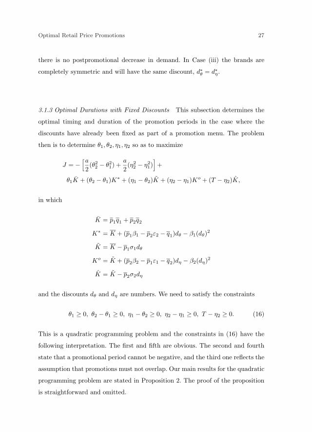
3.1.3 Optimal Durations with Fixed Discounts This subsection determines the

optimal timing and duration of the promotion periods in the case where the

discounts have already been fixed as part of a promotion menu. The problem

then is to determine θ1, θ2, η1, η2 so as to maximize

J = −[a

2(θ2

2 − θ21) +

a

2(η2

2 − η21)

]+

θ1K + (θ2 − θ1)K∗ + (η1 − θ2)K + (η2 − η1)Ko + (T − η2)K,

in which

K = p1q1 + p2q2

K∗ = K + (p1β1 − p2ε2 − q1)dθ − β1(dθ)2

K = K − p1σ1dθ

Ko = K + (p2β2 − p1ε1 − q2)dη − β2(dη)2

K = K − p2σ2dη

and the discounts dθ and dη are numbers. We need to satisfy the constraints

θ1 ≥ 0, θ2 − θ1 ≥ 0, η1 − θ2 ≥ 0, η2 − η1 ≥ 0, T − η2 ≥ 0. (16)

This is a quadratic programming problem and the constraints in (16) have the

following interpretation. The first and fifth are obvious. The second and fourth

state that a promotional period cannot be negative, and the third one reflects the

assumption that promotions must not overlap. Our main results for the quadratic

programming problem are stated in Proposition 2. The proof of the proposition

is straightforward and omitted.


Proposition 2 If 0 < θ1 < θ2 < η1 < η2 < T , the optimal time instants and

durations are given by

θ1 =1a[K∗ − K], θ2 =

1a[K∗ − K]

η1 =1a[Ko − K], η2 =

1a[Ko − K] (17)

and

θ2 − θ1 =1a[K − K] =

p1σ1dθ

a≥ 0

η2 − η1 =1a[K − K] =

p2σ2dη

a≥ 0, (18)

respectively. The durations of the promotions are related by

η2 − η1 =p1σ1dθ + p2σ2dη

a− (θ2 − θ1). (19)

3.1.4 Postoptimality Analyses

– Relationship between durations. By (19), the duration of the second promotion

is a linearly decreasing function of the duration of the first promotion (and vice

versa). This is a consequence of the fact that the problem of determining the

duration of promotions essentially is one of allocating a fixed amount of time,

κ , (p1σ1dθ+p2σ2dη)�a > 0, among two promotions. The quantity κ has the

following interpretation. Its numerator equals K − K and represents the loss

in revenue per unit of time, caused by the promotions. The denominator is the

advertising cost per unit of time. Hence κ is the decrease in postpromotion

revenue per advertising dollar. If the advertising cost parameter a increases,

the duration of at least one of the promotions must be reduced. At least

one promotion can be extended in time if the loss of revenue diminishes. To


compare the durations of the promotions consider the inequalities

θ2 − θ1

>

=

<

η2 − η1 ⇐⇒ p1σ1dθ

>

=

<

p2σ2dη, (20)

derived from (19). Suppose that σ1 = σ2, that is, the impacts of the promo-

tions on postpromotion demands are the same. The upper inequalities in (20)

show that brand 1 is promoted for a longer period of time than brand 2 if

p1 = p2 and dθ > dη. Thus, having two brands with the same regular price,

the retailer should promote for the longer period of time the brand that gets

the largest discount.

– Relationship between depth of discount and duration. The results in (18) show

that the duration of a promotion increases with the depth of the (fixed)

discount. Thus, a promotion with a deep discount should last longer than

one involving a more modest discount. This confirms a result in Rao and

Thomas (1973) and has already been noted in Section 2.2.2 - although it

certainly disagrees with the practice of having short campaigns with deep

discounts.

– Time interval between promotions. Recalling that K∗ and Ko are the category

revenues during the promotion of brands 1 and 2, respectively, we get from

(17)

η1 − θ2 =1a(Ko −K∗),

and hence

Ko

>

=

<

K∗ =⇒ η1

>

=

=

θ2. (21)

The expression in (21) states the following. If Ko > K∗, the category revenue

earned by promoting brand 2 exceeds that of brand 1 and then there will be


no promotion in the time interval [θ2, η1]. Otherwise, the category revenue

when promoting brand 2, Ko, falls short of that of brand 1, K∗; Then the

promotion of brand 2 starts when the promotion of brand 1 ends. The reason

is that it pays to extend as far as possible the more profitable promotion of

brand 1 and this is done by setting its terminal date θ2 equal to the starting

date η1 of the second promotion.

3.2 Myopic Retailer

When the retailer is myopic, the problem of determining optimal discounts is

straightforward. We report the results without proofs. Optimal discounts (de-

noted by δ∗θ and δ∗η) are symmetric, and are given by

δ∗θ =1

2β1[p1β1 − p2ε2 − q1]

δ∗η =1

2β2[p2β2 − p1ε1 − q2]. (22)

The optimal duration and timing of promotions are the same as for the forward-

looking retailer.

¿From Proposition 1 we have the optimal discounts of a forward-looking re-

tailer:

d∗θ =1

2β1[p1β1 − p2ε2 − q1]−

p1σ1(T − θ2)2β1(θ2 − θ1)

d∗η =1

2β2[p2β2 − p1ε1 − q2]−

p2σ2(T − η2)2β2(η2 − η1)

. (23)

Using (22) and (23) yields

d∗θ = δ∗θ −p1σ1(T − θ2)2β1(θ2 − θ1)

d∗η = δ∗η −p2σ2(T − η2)2β2(η2 − η1)

(24)


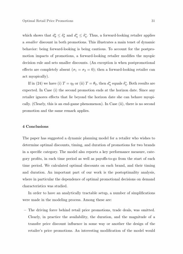
which shows that d∗θ ≤ δ∗θ and d∗η ≤ δ∗η . Thus, a forward-looking retailer applies

a smaller discount in both promotions. This illustrates a main tenet of dynamic

behavior: being forward-looking is being cautious. To account for the postpro-

motion impacts of promotions, a forward-looking retailer modifies the myopic

decision rule and sets smaller discounts. (An exception is when postpromotional

effects are completely absent (σ1 = σ2 = 0); then a forward-looking retailer can

act myopically).

If in (24) we have (i) T = η2 or (ii) T = θ2, then d∗η equals δ∗η . Both results are

expected. In Case (i) the second promotion ends at the horizon date. Since any

retailer ignores effects that lie beyond the horizon date she can behave myopi-

cally. (Clearly, this is an end-game phenomenon). In Case (ii), there is no second

promotion and the same remark applies.

4 Conclusions

The paper has suggested a dynamic planning model for a retailer who wishes to

determine optimal discounts, timing, and duration of promotions for two brands

in a specific category. The model also reports a key performance measure, cate-

gory profits, in each time period as well as payoffs-to-go from the start of each

time period. We calculated optimal discounts on each brand, and their timing

and duration. An important part of our work is the postoptimality analysis,

where in particular the dependence of optimal promotional decisions on demand

characteristics was studied.

In order to have an analytically tractable setup, a number of simplifications

were made in the modeling process. Among these are:

– The driving force behind retail price promotions, trade deals, was omitted.

Clearly, in practice the availability, the duration, and the magnitude of a

transfer price discount influence in some way or another the design of the

retailer’s price promotions. An interesting modification of the model would


be to superimpose a (parsimonious) trade deal pattern on the five-period

planning horizon, to see how the design of such a scheme would impact the

retailer’s promotional decisions. Such an extension is complicated, also from

the reason that the extent of the retailer pass-through of trade deals needs to

be modeled. A further modification would involve the manufacturers of the

two brands as active decision makers in the game

– Demand functions are linear. Since the shape of the deal effect curve has only

little or no empirical support (Blattberg et al. (1995)), it seems worthwhile to

(i) extend the model to include more general demand specifications, and (ii)

to intensify the empirical work on assessing the shape of demand functions

during promotional periods

– Feature advertising and display activities did not influence demand during a

promotion. To remedy this simplification, one would need to incorporate the

levels of these activities as decision variables that affect demand levels during

promotions. An obstacle here is the lack of knowledge of the simultaneous

effects of advertising, displays, and discounts on demand. Also in this area

there is a clear need for empirical research

– Our setup allows for at most one promotion of each of the brands. A more

elaborate framework would involve more periods such that multiple promo-

tions of each brand would be possible.

Acknowledgements The paper has benefited from the comments of seminar partic-

ipants at GERAD, HEC Montreal and CentER, Tilburg University. This work was

partially supported by NSERC-Canada.

5 Appendix

The appendix presents the solution of the dynamic programming problem in

Section 2.2.1. Denote by Ji the value function at stage i ∈ {1, 2, ..., 5}. The value


function measures the optimal profit-to-go as of stage i and will be calculated in

backward time.

Stage five starts at time t = η2 and we have

J5 = (T − η2)K = (T − η2)(K − p1σ1dθ − p2σ2dη).

At stage 4, which starts at t = η1, we find J4 from

J4 = −Aη + maxdη

{(η2 − η1)Ko + J5} = −Aη +

maxdη

{(η2 − η1)[p1(q1 − σ1dθ − ε1dη) +

(p2 − dη)(q2 + β2dη)] + J5}.

Note that Ko is a strictly concave function of dη. Performing the maximization

yields the optimal discount of brand 2. Whenever positive, it is given by

d∗η =1

2β2

[p2β2 − p1ε1 − q2 − p2σ2

T − η2

η2 − η1

],

and using d∗η one can calculate J4 :

J4 = −Aη − (T − η2)p2σ2d∗η + (T − η1)K +

(η2 − η1)[(p2β2 − p1ε1 − q2)d∗η − p1σ1dθ − β2(d∗η)2].

At stage 3, which starts at t = θ2, e determine J3 :

J3 = (η1 − θ2)K + J4 =

−Aη − (T − η2)p2σ2d∗η + (T − θ2)[K − p1σ1dθ] +

(η2 − η1)[(p2β2 − p1ε1 − q2)d∗η − β2(d∗η)2].


At stage 2, starting at t = θ1, we determine J2:

J2 = −Aθ + maxd

θ

{(θ2 − θ1)K∗ + J3} = −Aθ +

maxd

θ

{(θ2 − θ1)[(p1 − dθ)(q1 + β1dθ) + p2(q2 − ε2dθ)] + J3} .

Note that K∗ is strictly concave in dθ. Performing the maximization provides the

optimal discount for brand 1:

d∗θ =1

2β1

[p1β1 − p2ε2 − q1 − p1σ1

T − θ2

θ2 − θ1

].

Then J2 can be calculated:

J2 = −Aθ −Aη − (T − η2)p2σ2d∗η − (T − θ2)p1σ1d

∗θ + (T − θ1)K +

(η2 − η1)[(p2β2 − p1ε1 − q2)d∗η − β2(d∗η)2] +

(θ2 − θ1)[(p1β1 − p2ε2 − q1)d∗θ − β1(d∗θ)

2].

At stage 1, which starts at time zero, we have the profit for the entire plan-

ning period:

J = θ1K + J2 =

TK − [Aθ + Aη]− [(T − η2)p2σ2d∗η + (T − θ2)p1σ1d

∗θ] +

(η2 − η1)[(p2β2 − p1ε1 − q2)d∗η − β2(d∗η)2] +

(θ2 − θ1)[(p1β1 − p2ε2 − q1)d∗θ − β1(d∗θ)

2].

Finally, inserting the optimal discounts into J yields the optimal value of the

retailer’s objective function, in terms of the parameters only.


References

1. Anderson, E. and Simester, D. I.(2004): Long-Run Effects of Promotion Depth on

New Versus Established Customers: Three Field Studies. Marketing Science 23, pp.

4-20.

2. Blattberg, R. C. and Neslin, S. A. (1990): Sales Promotion: Concepts, Methods,

and Strategies. Englewood Cliffs. N.J.: Prentice-Hall.

3. Blattberg, R. C. and Neslin, S. A. (1993): Sales Promotion Models. In J. Eliash-

berg and G. L. Lilien (eds.), Handbooks in Operations Research and Management

Science, Vol. 5, Marketing. Amsterdam: North-Holland.

4. Blattberg, R. C., Briesch, R. and Fox, E. J.(1995): How Promotions Work. Mar-

keting Science 14, pp. 122-32.

5. Grover, R. and Srinivasan, V. (1992): Evaluating the Multiple Effects of Retail Pro-

motions on Brand Loyal and Brand Switching Segments. Journal of Marketing Re-

search 29, pp. 72-81.

6. Guadagni, P. M., Little, J.D.C. (1983): A Logit Model of Brand Choice Calibrated

on Scanner Data. Marketing Science 2, pp. 203-38.

7. Gupta, S. (1988): Impact of Sales Promotions on When, What, and How Much to

Buy. Journal of Marketing Research 25, pp. 342-55.

8. Kalwani, M. U. and Yim, C. K. (1992): Consumer Price and Promotion Expecta-

tions: An Experimental Study. Journal of Marketing Research 29, pp. 90-100.

9. Kumar, V. and Leone, R. (1988): Measuring the Effect of Retail Store Promotions

on Brand and Store Substitution. Journal of Marketing Research 25, pp. 178-85.

10. Moriarty, M. M. (1985): Retail Promotional Effects on Intra- and Inter-Brand Sales

Performance. Journal of Retailing 61, pp. 27-48.

11. Mulhern, F. J. and Leone, R. P. (1991): Implicit Price Bundling of Retail Products:

A Multiproduct Approach to Maximizing Store Profitability. Journal of Marketing

55, pp. 63-76.

12. Neslin, S. A., Henderson, C.M. and Quelch, J.A.(1985): Consumer Promotions and

the Acceleration of Product Purchases. Marketing Science 4, pp. 147-65.

13. Pauwels, K., Hanssens, M. and Siddarth, S. (2002): The Long-Term Effects of Price

Promotions on Category Incidence, Brand Choice, and Purchase Quantity. Journal

of Marketing Research 39, pp. 421-39.


14. Raju, J. S., Srinivasan, V. and Lal, R. (1990): The Effects of Brand Loyalty on

Competitive Price Promotion Strategies. Management Science 36, pp. 276-304.

15. Rao, R. C. (1991): Pricing and Promotions in Asymmetric Duopolies. Marketing

Science 10, pp. 131-44.

16. Rao, V. R. and Thomas, L. J. (1973): Dynamic Models for Sales Promotion Policies.

Operational Research Quarterly 24, pp. 403-17.

17. Tellis, G. J. and Zufryden, F. S. (1995): Tackling the Retailer Decision Maze: Which

Brands to Discount, How Much, When and Why?. Marketing Science 14, pp. 271-99.

18. Vilcassim, N. J. and Chintagunta, P. K.(1995): Investigating Retailer Product Cat-

egory Pricing from Household Scanner Panel Data. Journal of Retailing 71, pp.

103-28.

19. Walters, R. G. (1991): Assessing the Impact of Retail Price Promotions on Product

Substitution, Complementary Purchase, and Interstore Sales Displacements. Jour-

nal of Marketing 55(2), pp.17-28.

Documents

Optimal Retail Price Promotions - Dialnet