Optimal Robot Localization in Trees�Kathleen Romanik y Sven SchuiererzAbstractThe problem of localization, i.e. of a robot �nding its po-sition on a map, is an important task for autonomousmobile robots. It has applications in numerous ar-eas of robotics ranging from aerial photography to au-tonomous vehicle exploration. In this paper we presenta new strategy for a robot to �nd its position on a mapwhere the map is represented as a geometric tree. Ourstrategy exploits to a high degree the self-similaritiesthat may occur in the environment.We use the framework of competitive analysis to an-alyze the performance of our strategy. In particular, weshow that the distance traveled by the robot is at mostO(pn) times longer than the shortest possible route tolocalize the robot, where n is the number of verticesof the tree. This is a signi�cant improvement over thebest known previous bound of O(n2=3). Moreover, sincethere is a lower bound of (pn), our strategy is optimalup to a constant factor.Using the same approach we can also show that theproblem of searching for a target in a geometric tree,where the robot is given a map of the tree and the loca-tion of the target but does not know its own position,can be solved by a strategy with a competitive ratio ofO(pn), which is again optimal up to a constant factor.�The �rst author is supported by DIMACS. DIMACS is anNSF Science and Technology Center funded under contract STC-88-09648 and also receives support from the New Jersey Commis-sion on Science and Technology. The second author is supportedby the Deutsche Forschungsgemeinschaft under grant No. Ot64/8-1, \Diskrete Probleme", under grants of the Natural Sci-ences and Engineering Research Council of Canada, from theInformation Technology Research Centre of Ontario, and by anNSERC international fellowship.yDIMACS, Rutgers University, Piscataway, NJ 08855-1179,email: romanik@dimacs.rutgers.eduzInstitut f�ur Informatik, Universit�at Freiburg, Am Flughafen17, Geb. 051, D-79110 Freiburg, Fed. Rep. of Germany, e-mail:schuiere@informatik.uni-freiburg.de

1 IntroductionIn many tasks of autonomous mobile robots it is as-sumed that the robot has a map of its environment andknows its location on the map. However, in some sit-uations the robot may not know in advance where itscorrect position on the map is and has to determine iton-line. This is called the robot localization problem.Usually it is assumed that this problem can be solvedby using sensor data and allowing the robot to moveonly a small amount. But if the environment consistsof many self-similar parts, this approach may not besu�cient.Although in robotics this issue has been addressed innumerous contexts, ranging from aerial photography toautonomous vehicles for the exploration of landscapes[10, 12, 14, 15], a more rigorous analysis of the problemin a well-de�ned theoretical framework has only beenconsidered very recently. Here, the environment of therobot is assumed to be a simple or multiply connectedpolygon P and the robot is assumed to have access toits local visibility polygon V , i.e. all the points thatare visible from its position, via a range sensing device.The robot is also assumed to have a compass so thatit knows its orientation. The �rst task of the robot isto determine its possible placements within P ; that is,all p 2 P such that the visibility polygon of p equalsV . Guibas, Motwani, and Raghavan provide a data-structure that allows e�cient enumeration of all suchpositions [7].If more than one placement exists, then the robot hasto travel to certain points of the polygon that allow it todistinguish between the di�erent placements. Ideally itshould not travel much farther than necessary. In orderto measure the performance of a localization strategywe employ the framework of competitive analysis [13].If L(p; P ) is the length of a shortest path to localize arobot \waking" in polygon P at position p, a strategy Sis called c-competitive if the length of the path traveledby a robot using strategy S is at most c times L(p; P ),for all possible polygons P and points p 2 P . The valuec is called the competitive ratio of S.There have been two approaches to the localizationproblem. The �rst by Dudek, Romanik, and Whitesides[6] considers the full complexity of the problem and uti-lizes a decomposition of the polygon P into visibilitycells such that the same set of vertices of P is visible

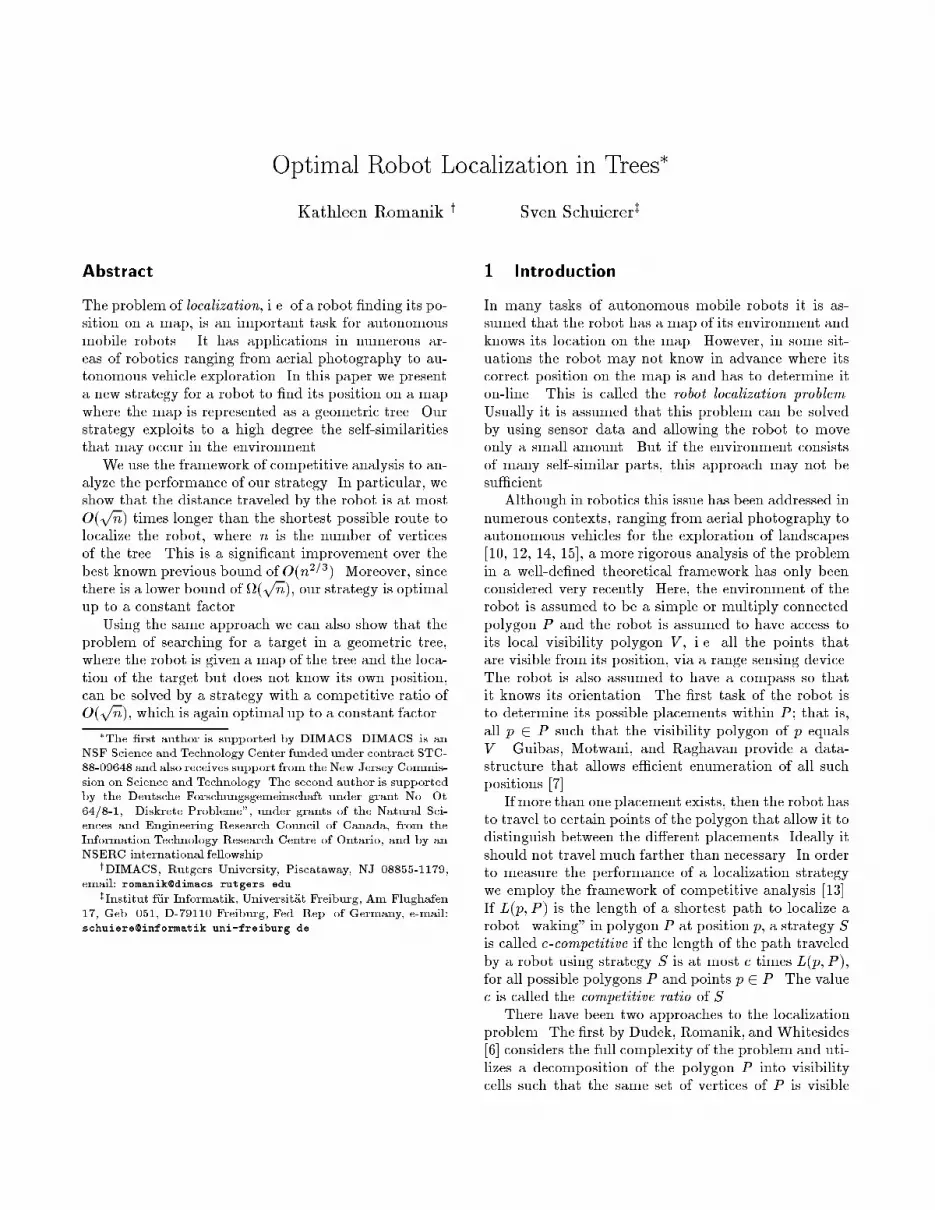
bq1 q2d st pnn=2 n=2Figure 1: A geometric tree for which every on-line local-ization strategy is no better than (pn)-competitive.from each point in a cell. This decomposition is used asthe underlying structure for a simple strategy where therobot repeatedly travels to the closest point that elimi-nates at least one of the possible placements. It is easyto show that if there are k possible placements, thenthe strategy is k-competitive. Furthermore, if k � pn,where n is the number of vertices of the polygon, thenit can be shown that k is the best competitive ratiopossible [6].The second approach, proposed by Kleinberg, leavesaside all concerns raised by the visibility structure of Pand abstracts the combinatorial nature of the problem[9]. In this context two types of environments are con-sidered: bounded-degree trees embedded in IEd (calledgeometric trees) and rectangle packings in the plane.In these environments the robot has no use of visionother than to know the orientation of all edges incidentto its current location. For geometric trees Kleinbergprovides a strategy with a competitive ratio of O(n2=3),where n is the number of vertices of degree greater thantwo, and for rectangle packings a strategy with a com-petitive ratio of O(nq log lognlogn ), where n is the numberof rectangles.Kleinberg also provides a lower bound of (pn) forthe localization problem in geometric trees, which is il-lustrated by the example in Figure 1. If the true place-ment s of the robot is at the bottom of the dth spiketo the right of spike t, where pn < d � 2pn, then alocalization strategy either has to explore all spikes be-tween t and s or travel to one of the end points q1 or q2of the base b of the tree. In each case the total distancetraveled by the robot is (n) while the shortest path tolocalize the robot is the path from s to t, which is oflength at most 3pn+ 1.In this paper we consider only geometric trees asenvironments, and we present a localization strategythat has a competitive ratio of O(pn). The �rst and

last steps of our strategy are essentially the same as inKleinberg's O(n2=3) strategy. However, in the middlesteps we explore periodic patterns in the tree to elim-inate all but O(pn) possible placements of the robotby traveling no more than O(pn) times the length of ashortest path to localize the robot. In view of the exam-ple in Figure 1 our strategy is optimal up to a constantfactor and, hence, settles the asymptotic complexity ofon-line robot localization in trees, thus solving an openproblem posed by Kleinberg [9].A di�erent important problem in robotics is search-ing for a target in an unknown environment [2, 3, 5, 4,8, 11]. If a map of the environment and the position ofthe target on the map are given, but the robot's positionon the map is not given, then Figure 1 again provides anexample of an (pn) lower bound for the competitiveratio of an on-line strategy. We show that our approachcan be used to obtain a strategy that solves the search-ing problem with a competitive ratio of O(pn), whichis optimal up to a constant factor.The paper is organized as follows. In the next sec-tion we give formal de�nitions of the main geometricconcepts and list the notation we use. Section 3 con-tains the main part of the paper where we present ourlocalization strategy. In Section 4 we show how to adaptour strategy to searching for a target.2 De�nitionsIn this section we de�ne some of the notation that weuse in the paper. The environments that we considerfor robot localization are geometric trees.De�nition 2.1 A geometric tree T = (V;E) is a treeembedded into IEd such that each v 2 V is a point andeach e 2 E is a polygonal path whose end points lie inV . The paths of E intersect only at points in V , andthey do not induce any cycles.We assume that T has a bounded degree �. We saya vertex of T is non-degenerate if it has a degree greaterthan two. The size of T , denoted by jT j, is then de�nedas the number of non-degenerate vertices of T . In theremainder of the paper the term vertex is used to referto a non-degenerate vertex except if explicitly statedotherwise.We assume that the robot's initial position is locatedat a vertex of T since the closest vertex v can be reachedby performing a two-way spiral search that travels atmost nine times the distance from the robot's originallocation to v [1]. It is the robot's task to determineat which vertex of T it is located by traveling from itsstarting point in T and collecting enough information torule out all but one possible start location. We denotethe set of all possible start locations of the robot (calledplacements) by P . As in Kleinberg's work, we assume

that the robot knows its current orientation, and it hasno use of vision other than to know the orientation ofall edges incident to its current location.In order to describe the motion of the robot we as-sume that the robot has a local coordinate system thatis relative to the robot's starting position, i.e. the origin0 of the local coordinate system is at the location wherethe robot \wakes up". In order to distinguish betweenpoints in the global coordinate system and points inthe local coordinate system we use the convention thatpoints and paths in the local coordinate system are de-noted by over-lined letters, such as p, q, P, etc. Weuse standard vector addition and scalar multiplicationto denote translations and scalings, i.e. if � and � arereals, v is vector and S is a d-dimensional set, then�v + �S = f�v + �s j s 2 Sg.When dealing with paths in T we use the standardde�nition of length of a polygonal path (using the L2norm) for the length of a path P, which we denote by�(P). We use sp(T; p; q) to denote the unique simplepath between two points p and q in T . The distancebetween p and q denoted by dT (p; q) is de�ned as thelength of sp(T; p; q). Since the robot is often directedto travel along a non-simple path in T (for example,when it explores part of T using depth-�rst search), fora non-simple path P with start point s and end point t,we use �(P) to denote the length traveled by the robotand �sp(P) to denote sp(T; s; t). If p and q are twopoints on P, then we denote the subpath of P from pto q by Ppq. The concatenation of two paths P1 and P2is denoted by P1 � P2, where we assume that the pathP2 is translated so that its start point is the end pointof P1. For p 2 T , the ball of radius d around p, denotedby Bd(p), is de�ned as the set of all points of T that canbe reached by traveling no more than distance d fromp. We say that path P1 is isomorphic to path P2 if sometranslation of P1 is equal to P2 and all edges adjacentto any vertex on P1 have the same orientation as theedges adjacent to the corresponding vertex on P2 (see,for example, Figure 2). We write P1 � P2 in this case.The following is a summary of some of the notationwe use in the paper. Note that the last two items areintroduced in the next section.� T - Geometric tree where robot is located� n - Number of vertices of T� Bd(p) - Ball of radius d around p in T� sp(T; u; v) - Unique shortest path between uand v in T� �(P); �sp(P) - Length of path P; length of theshortest path from the start to the end point of P� p0 - Robot's \wake up" position in T

y zu v w xFigure 2: Path sp(T; u; v) is isomorphic to sp(T;w; x)but not to sp(T; y; z).� P - Set of possible placements of the robot in T� T - Geometric tree T in the robot's localcoordinate system� 0 - Origin of T (corresponds to p0 in T )� T ex - Part of T explored by the robot� % - Radius of a ball around p0 withB%(p0) � p0 + T ex � B2%(p0)3 A New Localization StrategyOur localization strategy consists of four main steps.The following pseudo-code gives a rough impression ofhow the strategy works.Strategy Localize-by-Placement-Separation (LPS)Input: A geometric tree T = (V;E) with nvertices;Output: The position of the robot in T ;Variables: The set of placements P ;The tree T ex that has been explored;P := V ; T ex := f0g;Step 1: Perform a spiral search until eitherjT exj > 2pn or jP j = 1;Step 2: Identify a critical path of T ex;Step 3: Eliminate close placements until p0 62 p+ T ex,for all p; p0 2 P ;Step 4: Eliminate the remaining placements using agreedy strategy;end Localize-by-Placement-Separation;It should be noted that in the above strategy Steps1 and 4 are essentially the same steps as in the strategyproposed by Kleinberg [9]. The only exception is thatin Kleinberg's strategy up to n2=3 vertices are visited bythe Spiral Search in Step 1. After analyzing each step

of the strategy we will be able to prove the followingtheorem.Theorem 1 Let T be a geometric tree. Strategy LPSachieves a competitive ratio of O(pn) for localizing arobot in T .3.1 Step 1: Spiral SearchIn Step 1 of Strategy LPS the robot performs a spi-ral search [1] as follows: starting at the origin it per-forms successive depth-�rst searches, each time visitingall points within distance d of the origin (where initiallyd is set to 1) and then doubling d if it has not localizeditself. During the search the robot keeps track of thesize jT exj of the explored subtree T ex and the set P ofall possible placements of the robot, i.e., the set of allp 2 T with p + T ex � T . If jP j = 1, then the robotstops its search and outputs p 2 P as its position in T .At the end of the spiral search the robot has seen allpoints within distance d=2 of its wake up position, sofor % = d=2; B%(p0) � p0 + T ex � B2%(p0). If it has notyet eliminated all but one placement, then the lengthof a shortest path to localize the robot is at least %. Itis shown in [9] that the distance traveled by the robotin Step 1 is bounded by 8�jT exj% = O(pn%).3.2 Step 2: Identifying a Critical PathIf after Step 1 there are at least two placements p1 andp2 with p2 2 p1+T ex, then in Step 2 the robot identi�esa \critical path" of T ex and in Step 3 it travels alongan extension of this path eliminating placements untilthere are no pairs left with p2 2 p1 + T ex. In doing so,the robot travels a distance of at most O(pn%), and atthe end at most pn placements remain.Before describing Step 2 we de�ne somemore notionsabout paths. If P is a directed simple path and � �1, then the �-repetition of P, denoted by P�, is thepath formed by concatenating together � copies of P insuccession. If 0 � � < 1, then P� is the subpath of Pbeginning at its start point with length equal to ��(P).If � < 0, then P� is the path P�� translated so thatits end point coincides with the start point of P. Notethat although P is a simple path, P� may not be (seeFigure 3).If P is a path such that P � Q�, for � 2 [2;1),then P is called a periodic path and Q is called a periodof P. The number � is called the periodicity of P w.r.t.Q. The path Q is called an integral period if � is aninteger.A tree T is called a comb-tree if there is a simple pathQ with start point s and end point t and a simple path Salso with start point s such that T is given by the unionofQk (the base of T ) and the sets ki(t�s)+S (the spikesof T ), for 1 � i � m where 0 = k1 < � � � < km = k arenatural numbers (see Figure 3).

P P3s QS tFigure 3: A period that yields a periodic path that isnot a simple path. The path P3 is a comb-tree withbase Q3 and spikes S, (t � s) + S, 2(t � s) + S, and3(t� s) + S.If U = fv1; : : : ; vkg is a set of vertices of T , then Uinduces a periodic path if there is a path Q such thatsp(T; vi; vi+1) � Qki, for some natural numbers ki. Theset U induces a comb-tree if the vertices of U are theleaves of a comb-tree.Kleinberg [9] proves a crucial lemma stating that allplacements within p + T ex, for a placement p, are ona periodic path or a comb-tree of T . We extend thislemma by proving that after the robot has traveled atmost O(pn%) all pairs of placements p1 and p2 withp2 2 p1 + T ex are on the same periodic path or comb-tree of T ex. First we state Kleinberg's lemma.Lemma 3.1 [9] If p is a placement in P , then the setof all placements that are contained in (p+T ex) induceseither a simple periodic path or a comb-tree.If the periodic path that contains all the placementsin (p + T ex) is simple, then we denote this path by Cpand call it the critical path of p. If the placements in-duce a comb-tree, then the critical path of p is the baseof the comb-tree. The critical path Cp of p correspondsto a path Cp = �p+Cp in T ex. One problem that arisesis if pi and pj are two di�erent placements, then Cpiand Cpj are not necessarily the same, as shown in Fig-ure 4. However, in such cases the robot can e�cientlyeliminate at least one placement by traveling a distanceof O(%), as the next lemma shows.Lemma 3.2 If p1, p01, p2, and p02 are placements inP such that p01 2 p1 + T ex and p02 2 p2 + T ex,then either the robot can eliminate p1 or p2 by trav-eling to the point (p01 � p1) + (p02 � p2) in T ex, or theset f0; p01 � p1; p02 � p2; (p01 � p1) + (p02 � p2)g induces asimple periodic path or a comb-tree in T ex.Proof: Let Pi be the path from pi to p0i, for i = 1; 2.Since p2 + T ex is isomorphic to p01 + T ex, there is apath Q02 isomorphic to P2 starting at p01 in p01 + T exand P1 �Q02 � (p1 + T ex) [ (p01 + T ex). If p0 equals p1,then the robot can follow the path P1 � Q02 to its end.

p2 p3 p4 T exp1Figure 4: An example where the critical path of p1 andp2 is not isomorphic to the critical path of p3 and p4.p2p02P2Q01 p01P1 Q02p1Figure 5: �p1 + P1 � Q02 and �p2 + P2 � Q01 start andend in the same point.Similarly, there is a path Q01 isomorphic to P1 start-ing at p02 in p02+T ex and P2�Q01 � (p2+T ex)[(p02+T ex).If p0 equals p2, then the robot can follow the pathP2 � Q01 to its end (see Figure 5).If the robot is able to follow both paths �p1+P1�Q02and �p2+P2 �Q01 from 0 to q = (p01�p1)+(p02�p2) inT , then since P1 � Q01 and P2 � Q02, by [9, Lemma 3,Claim 1] f0; p01� p1; p02 � p2; (p01 � p1) + (p02 � p2)g in-duces a simple periodic path or a comb-tree in T ex. 2If the robot cannot follow path P1 � Q02 to its end,then p1 is not a placement, and similarly for path P2�Q01and p2. Thus, by traveling a distance of at most 16%(2%+ 2% to the end of each of the two compound pathsand back) the robot can either eliminate one or both ofp1 and p2, or it can determine that p01� p1, p02� p2 and(p01�p1)+(p02�p2) are part of the same simple periodicpath or comb-tree in T ex.In fact, if the robot eliminates one of the placementspi, i = 1; 2, then it eliminates all placements p suchthat there is another placement at p+ (p0i � pi); hence,the vertex v = (p0i � pi) in T ex does not correspond toa placement in any translation of T ex anymore.This suggests a method for Step 2 of StrategyLPS. The robot begins with two vertices v1; v2 2 T exthat correspond to two placements contained in some

translation of T ex, and it tries to follow the pathssp(T;0; v1)�sp(T;0; v2) and sp(T;0; v2)�sp(T;0; v1) totheir end points. If it succeeds, then it �nds the periodicpath or comb-tree in T ex induced by f0; v1; v2; v1 + v2g;otherwise, at least one of v1 and v2 is eliminated fromconsideration. One by one it considers all the othervertices in T ex, each time eliminating more placementsfrom P or adding them to the periodic path or comb-tree of T ex induced by the previously considered ver-tices. Since the robot travels a distance of at most 16%for each v 2 T ex, and jT exj = 2pn, it travels no morethan 32%pn in Step 2.After the execution of Step 2, let U be the set ofall vertices v 2 T ex such that there are placements p1and p2 in P with v = p1 � p2. Note that for all v1 andv2 in U , the set f0; v1; v2g induces a simple periodicpath or a comb-tree by Lemma 3.2. If jU j � 3, then[9, Lemma 3, Claim 2] implies that U induces a simpleperiodic path P or a comb-tree T in T ex. If U inducesa comb-tree T , then the robot moves to the base of thiscomb-tree and each p 2 P is translated likewise. In thiscase we denote the base of T by P . If we denote theset of translated placements again by U , then U alsoinduces the periodic path P in this case.Two placements p and p0 are called a critical pairif p0 2 p + T ex. We denote the set of all critical pairsby Rcr. For each critical pair (p; p0) 2 Rcr the path�p+sp(T; p; p0) is an integral period of P by Lemma3.1.We can show that there is a period of P that dividesall paths �p+ sp(T; p; p0) where (p; p0) is a critical pair.The length of this path is the greatest common divisorof the lengths �(sp(T; p; p0)).Lemma 3.3 If P is a periodic path and fQ1; : : : ;Qmgis a set of integral periods of P, then there exists aunique period Q of P, called the maximal period of Pw.r.t. fQ1; : : : ;Qmg such that(i) Q is an integral period of Qi, for all 1 � i � m,and(ii) if Q0 is an integral period of Qi, for all 1 � i � m,then Q0 is also an integral period of Q.Corollary 3.4 There is a maximal period Dex of Pw.r.t. Rcr. It is called the critical period of P.Note that the above corollary in particular impliesthat the distance between any critical pair of placementsis at least �(Dex). With the help of the critical periodwe now extend the path P that contains all the place-ments in T ex. Let � be the largest integer such that D�exis contained in T ex. For simplicity of presentation weassume that T ex is symmetric w.r.t. Dex and � is alsothe largest number such that D��ex is contained in T ex.(This can easily be achieved by exploring the shorterside.) The path obtained by concatenating D��ex and

D�ex is called the critical path of T ex w.r.t. P and is de-noted by Cex. Note that �(Cex) � 4% and that if (p; p0)is a critical pair, then the distance between p and p0 isat most �(Cex)=2. Since Dex is also a period of Cex, wealso call Dex the critical period of Cex w.r.t. Rcr .We summarize the situation after Step 2 in the fol-lowing lemma.Lemma 3.5 After Step 2 of Strategy LPS there is asimple periodic path Cex in T ex called the critical pathof T ex, such that p = p0 � p 2 Cex, for all (p; p0) 2 Rcr .The critical period has a number of important prop-erties.Lemma 3.6 Let Q be a subset of Rcr . If Dex is thecritical period of Cex w.r.t. Rcrand Eex is the criticalperiod of Cex w.r.t. Q, then Dex is an integral period ofEex, i.e. there is an integer k � 1 such that Eex = Dkex.3.3 Step 3: Eliminating Close PlacementsIf after Step 2 there are critical pairs of placements, thenin Step 3 the robot explores branches emanating fromthe critical path Cex until either it has found a periodictree Pex with pn vertices or there are no more criticalpairs. If it succeeds in �nding a periodic tree Pex withpn vertices, then there is some point where the treeP2pnex of 2n vertices formed by concatenating together2pn copies of Pex di�ers from T . The robot can �ndone such mismatch by exploring only a small portion ofP2pnex . It then propagates this initial mismatch towards0 until all critical pairs are eliminated.3.3.1 Exploring a Periodic TreeAfter the robot has identi�ed the critical path Cex, itextends the critical path to a tree that shares the pe-riodicity of Cex w.r.t. Rcr . This is done by consideringthe vertices v1; : : : ; vl of T ex in the sequence that therobot encountered them during the last execution of thespiral search. For each vertex vi the robot tries to fol-low a path that is isomorphic to the path sp(T ;0; vi)from each k-repetition Dkex of the critical period. It ei-ther succeeds in following this path to its end point, orit �nds the �rst point where this path di�ers from T .To describe this strategy more precisely, we �rst de-�ne a few terms.De�nition 3.1 Let q be a point in T and P be a pathin T that starts at point s and ends at point t. If q0 isthe last intersection point of P with sp(T ; s; q), then q0is called the P-ancestor of q, denoted by P-anc(q). Thepath Psq0 � sp(T ; q0; q) � sp(T ; q; q0) � Pq0t is the path Paugmented by q (see Figure 6).

q0q s tT PFigure 6: Augmenting the path P by the point q: Therobot follows the path P from s to q0 = P-anc(q), trav-els to q and back, and then follows the rest of P .Cexvi 0 Dexvi �Dex vi �D2exvi �D3exFigure 7: The Dkex-neighbours of vi, for 1 � k � 3.Note that vi � D2ex is not a vertex and vi � D3ex =D3ex � sp(T ;0; vi).The robot explores a non-simple path Pex in T thatshares the periodicity of Cex w.r.t.Rcr. Initially, Pex =Cex. The robot then augments Pex by the vertices vi.For each vertex vi in T ex, if Cex-anc(vi) is containedin Dmex and t is the end point of Dm�1ex , then the robotattempts to follow the paths Dkex � sp(T ; t; vi), for 0 �k < �(Cex)=�(Dex). The last point where the pathDkex�sp(T ; t; vi) is isomorphic to a path in T starting fromp0 is called the Dkex-neighbour of vi and is denoted byvi�Dkex. See Figure 7 for an illustration. The strategyaugments Pex by each vi � Dkex and then updates P ,Rcr, and Dex before examining vi+1. It halts wheneither Rcr is empty or Pex contains pn vertices.Since jT exj = 2pn, there is one side of Cex withrespect to the origin such that the size of the part ofT ex that is connected to this side is greater than orequal to pn. In order to simplify the presentation weconsider in the following only this side of Cex and thepart of T ex that is connected to it. We denote thishalf of the explored tree again by T ex and also this halfof the critical path by Cex. Thus we assume that theorigin is located at one end point of Cex. Note that thisimplies that if (p; p0) is a critical pair, then the distance

between p and p0 is at most �(Cex).Strategy Periodic-TreeInput: T , P and the explored tree T ex with verticesv1; : : : ; vpn;Output: A path Pex in T that is periodic w.r.t.Rcrand contains � pn vertices or Rcr = ;;P1 := P ; Rcr1 := Rcr ; P1 := Cex;let D1 be the maximal period of Cex w.r.t. Rcr1 ;i := 1;while jPij < pn and Rcri 6= ; dolet vi be next unvisited vertex among v1; : : : ; vpn;let ki be the periodicity of Cex w.r.t. Di;let Pi+1 := Pi;for j := 0 to ki � 1 dovisit uj := vi � Dji ;augment Pi+1 by uj ;end for;update the set of placements Pi+1 using Pi+1;update the critical pairs Rcri+1 using Pi+1;let Di+1 be the maximal period of Cex w.r.t. Rcri+1;i := i + 1;end while;P := Pi; Pex := Pi; Rcr := Rcri ;end Periodic-Tree;It is easy to see that Strategy Periodic-Tree haltssince after at most pn iterations of the while loop, Pexwill have pn vertices. Also, it is straightforward toshow that after each iteration of the loop, the start andend point of the maximal period Qi of P i w.r.t. Rcriare the same as the start and end point of the maximalperiod Di of Cex w.r.t. Rcri (that is, �sp(Qi) = �(Di)).To bound the distance that the robot travels duringStrategy Periodic-Tree we �rst observe that it travelsno more than O(%) to visit each Dkex-neighbour of avertex vi, and it halts when it has visitedpn neighboursthat are vertices of T . In order to show that the robottravels no more than O(pn%), it su�ces to show thatthe robot visits no more than O(pn) neighbours thatare not vertices of T . Since the periodicity of Cex w.r.t.Dex is never greater than the number of vertices of T ex,which is 2pn, it visits no more than 2pn Dj1-neighboursof v1 in the �rst iteration of the while loop. In eachiteration where the robot visits a neighbour that is nota vertex of T , the length of the critical period Di at leastdoubles in length by Lemma 3.6, and thus the numberof neighbours visited in the next iteration is at least cutin half. The total number of neighbours visited in alliterations where the robot visits a neighbour that is nota vertex of T is thus bounded by 2pn + pn + 12pn +14pn � � �+ 1 < 4pn.Lemma 3.7 The robot travels a distance of O(pn%)during the execution of Strategy Periodic-Tree, and after

executing it either there are no critical pairs left or ithas found a path Pex in T that is periodic w.r.t.Rcrandcontains � pn vertices.3.3.2 Extending the Critical PathAfter having explored Pex in the local neighbourhoodof the wake-up position, there still may exist criticalpairs. Since jPexj � pn, jP2pnex j � 2n and, thus,there are points, called mismatches, where P2pnex andT di�er locally. We show that by traveling to at mostdlogne vertices of P2pnex the robot can �nd an initialmismatch. This mismatch is then propagated closerto 0 until the closest mismatch q� to Pex is identi�ed.Since q� is beyond the end of Pex, the maximal periodof the part of P2pnex from 0 to q� is longer than Pex.Since dT (p; p0) � �(Cex) = �sp(Pex) for any criticalpair (p; p0), this implies that Rcr = ;.Lemma 3.8 If P is some set of placements in T , thenthere is a vertex v 2 P2pnex such that p+sp(P2pnex ;0; v) 6�T , for at least half of the placements p in P .Proof: Let U be the set of pairs (p; v) with p 2 Pand v 2 P2pnex such that p + sp(P2pnex ;0; v) 6� T . Foreach p 2 P , we denote the set of pairs in U with �rstcomponent p by Up. Since jUpj � jP2pnex j � jT j � n, thesize of U is jU j � jP jn. If Uv is the set of pairs withsecond component v, then Pv2P2pnex jUvj = jU j � jP jn.Hence, the average size of the 2n sets Uv is jP j=2 and,thus, there is at least one vertex v 2 P2pnex with jUvj �jP j=2. 2If we apply Lemma 3.8 repeatedly we obtain the fol-lowing corollary.Corollary 3.9 There are � = dlog jP je verticesv1; : : : ; v� in P2pnex such that, for each p 2 P , thereis a vertex vip such that p+ sp(P2pnex ;0; vip ) 6� T .Let v1; : : : ; v� be the vertices of Corollary 3.9, wherewe assume that the vertices are numbered accordingto the sequence of their C2pnex -ancestors, i.e. we as-sume that C2pnex -anc(vi) is before C2pnex -anc(vi+1) onC2pnex . Note that these vertices can be computed givenT and P2pnex without any additional exploration by therobot. The robot travels along C2pnex visiting the verticesv1; : : : ; v� in sequence until the �rst vertex vi0 is iden-ti�ed for which p0 + sp(P2pnex ;0; vi0) 6� T (see Figure 8for an illustration). The distance of each vertex vi toC2pnex is at most 2%; hence, the robot travels a distance

v4Cex v1 v2 v3C2pnexFigure 8: At most dlogne vertices need to be exploredto identify the mismatch in v4.of at most �(C2pnex )+4 dlogne % = (4pn+4 dlogne)% inorder to identify vi0 . We denote by q0 the last commonpoint of sp(P2pnex ;0; vi0) and T .In order to �nd the closest mismatch to Cex, therobot executes a strategy calledMismatch-Propagation.It returns to 0 on C2pnex and on its way visits points thatare isomorphic to q0. It �rst travels by multiples of Cexexamining neighbours of q0 until it �nds one that isnot a mismatch. It then examines all the neighbours ofq0 on the last repetition of Cex by visiting neighboursthat are multiples of Dex along the path. It �nds theclosest mismatch to 0 among the Dkex-neighbours of q0 ithas examined and repeats the process starting from thispoint. If the robot reaches Pex before Rcr = ;, then itexplores the entire part of the tree P2pnex between thismismatch and the end of Pex.More precisely, if m is the smallest integer such thatPmex contains q0, and t is the end point of Cm�1ex , thenthe Ckex-neighbour of q0 (q0 � Ckex) is the last pointwhere Ckex � sp(P2pnex ; t; q0) is isomorphic to a path inT . Similarly, if l is the smallest integer such that Qlexcontains q0, and s is the end point of Dl�1ex , then theDkex-neighbour of q0 (q0 � Dkex) is the last point whereDkex � sp(P2pnex ; s; q0) is isomorphic to a path in T . Therobot �rst visits the neighbours q0 � Ckex of q0 for de-creasing k starting fromm�2 until it �nds a neighbourthat is not a mismatch.The robot then explores the neighbours q0 � Djexof q0 between q0 � Ckex and q0 � Ck+1ex and �nds thesmallest j such that q1 = q0 � Djex is a mismatch (seeFigure 9 for an illustration). It then updates P , Rcr ,and Dex according to what it has explored, and thepropagation is repeated starting from q1. It continuesuntil eitherRcr = ; or Pex is reached. In the latter case,the remainder of the tree P2pnex from the mismatch toPex is explored.

Cexq0q0 � Ckex q0 � Ck+1exC2pnexq0 �Dj0ex

Figure 9: Starting from mismatch q0 the closest mis-match found by propagation is q0 � Dj0ex. All Dex-neighbours of q0 between q0 � Ckex and q0 � Ck+1ex areexplored.Pseudo-code for Strategy Mismatch-Propagation isbelow. We assume for simplicity of presentation thatDi is an integral period of Cex in all iterations of theouter while loop.Strategy Mismatch-PropagationInput: The tree T , the set of placements P , theperiodic paths Pex, Cex, and the point q0;Output: A set of placements P where Rcr = ;;P0 := P ; D0 = Dex;P0 = Pex [ sp(T ;0; q0);i := 0;while Rcr 6= ; dolet Pi+1 be P i;let m be the integer such that Pmex contains qi;k := m � 2; visit qi � Ckex;augment Pi+1 by qi � Ckex;while qi � Ckex is a mismatch dok := k � 1; visit qi � Ckex;augment Pi+1 by qi � Ckex;end while;/� qi �Ckex is a match, qi � Ck+1ex is a mismatch �/let l be the integer such that Dli contains theC2pnex -ancestor of qi � Ckex;let � be the periodicity of Cex w.r.t. Di;for j := l to l + � � 1 dovisit qi � Dji ; augment P i+1 by qi � Dji ;end for;let j0 be minfj j qi � Dji is a mismatchg;/� qi � Dl+��1i = qi � Ck+1ex is a mismatch �/qi+1 := qi �Dj0i ;

update the set of placements Pi+1 using Pi+1;update the critical pairs Rcr using Pi+1;let Di+1 be the maximal period of Cex w.r.t. Rcr;i := i + 1;end while;P := Pi;end Mismatch-Propagation;To show that StrategyMismatch-Propagation is cor-rect we must show that it halts and at the end Rcr = ;.Observe that the period of the part of P i+1 betweenqi � Ckex and qi � Ck+1ex inclusive, which the robot ex-plores in one iteration of the outer while loop, deter-mines the new critical period Di+1. Since this part ofPi+1 contains at least one mismatch (qi�Ck+1ex ) and atleast one match (qi�Ckex), the new period of Cex w.r.t.Rcr is di�erent from Di. By Lemma 3.6 the critical pe-riod at least doubles in length. In the extreme casethat qi � Ck+1ex is the closest mismatch of qi � Ckex (i.e.,if j0 = l + � � 1) the new period Di+1 equals Cex andthe distance between any two placements is longer than�(Cex). Hence, Rcr becomes empty and the strategyhalts.Otherwise, after the iteration of the outer while loopthe mismatch qi is propagated forward towards Pex,and eventually Pex is reached in some iteration i0. Initeration i0 all Di0-neighbours between the end of Pexand the last mismatch found are explored. Since theDi0-neighbours of qi0 that are contained in Pex havealready been visited during the construction of Pex,Pex contains only matches and the closest mismatchq� to the origin that is found is located after the end ofPex. This again implies that the distance between twoplacements is longer than �(Cex), so Rcr = ; and thestrategy halts.In order to determine the distance traveled by therobot during Strategy Mismatch-Propagation we lookat the di�erent parts of the strategy. Since d0 =dT (0; C2pnex -anc(q0)) � 2pn�(Cex), the robot visits nomore than O(pn) Ckex-neighbours during the executionof the strategy, and it travels no more than 2pn�(Cex)along C2pnex visiting these neighbours. Since each neigh-bour is no farther than 2% from C2pnex and �(Cex) � 2%,the robot travels no more than O(pn%) during this partof the strategy.Since in each iteration of the outer while loop thecritical period Di at least doubles in length by the aboveargument, the number of Dji -neighbours between qi+1�Ckex and qi+1 � Ck+1ex visited in the next iteration is atleast cut in half. Therefore, using a similar argumentto the one used for Strategy Periodic-Tree, it can beshown that the robot visits a total of no more than 2pnDjex-neighbours and thus travels no more than O(pn%)

during this part of the strategy. Therefore, we have thefollowing lemma.Lemma 3.10 The robot travels a distance of O(pn%)during the execution of Strategy Mismatch-Propagationand after executing it, there are no critical pairs left.3.4 Step 4: Greedy EliminationSince 2pn vertices of T have been visited by the robotat the end of Step 1 and Rcr = ; at the end of Step 3,we can show that at the beginning of Step 4 the numberof remaining placements is less than pn.Lemma 3.11 If jT exj � 2pn and Rcr = ;, then jP j <pn.Proof: The proof is by contradiction. Assume thatjP j � pn. Since there are no critical pairs, P\p+T ex =fpg for all p 2 P . However, by [9, Lemma 8] (a com-binatorial argument) there is at least one placement psuch that jP \ p+ T exj � 1n jT exjjP j � 2 { a contradic-tion. 2In order to eliminate the remaining placements therobot visits the closest point q such that at least oneplacement is eliminated. Since dT (0; q) is no more thanthe shortest distance to localize the robot, a repeatedapplication of this step guarantees that Step 4 has acompetitive ratio of at most pn.4 Searching for a Target in a TreeAs was pointed out in the introduction we are also in-terested in the searching variant of the problem wherea robot has to �nd a target t marked on the map ofthe environment, but the robot is not given its startingposition. We also apply Strategy LPS except with aslightly altered Step 4. Note that after Step 1 if t is notreached, then the distance between the starting positions of the robot and t is at least %. Hence, after Step 3the robot has traveled a distance of O(pndT (s; t)) andthere are k � pn possible placements for the robot andthus k possible locations t1; : : : ; tk of t in T . In Step 4the robot now repeatedly attempts to visit the closestpossible target among t1; : : : ; tk until the true locationof the target is identi�ed. Obviously, the robot travelsat most a distance of pndT (s; t) in Step 4. This provesthe following theorem.Theorem 2 Let T be a geometric tree and t be a pointin T . There is a strategy that achieves a competitiveratio of O(pn) for a robot to �nd t given the coordinatesof t in T .

5 ConclusionsWe have presented a new localization strategy for an au-tonomous mobile robot. The environment of the robotis represented by a geometric tree of constant degree inarbitrary dimensions. We assume that the robot knowsits current orientation, and it has no use of vision otherthan to be able to detect the orientation of all edgesincident to its current location. Our strategy achieves acompetitive ratio of O(pn) if the tree contains n nodesof degree greater than or equal to three. Since there isa geometric tree which provides a lower bound exampleof (pn) for the competitive ratio of any localizationstrategy, our strategy is optimal up to a constant factor.Challenges that remain for future work are to trans-fer the strategies developed for geometric trees to themore realistic setting of polygons in the plane and toinvestigate the complexity of the localization problemin graph structures that allow cycles.References[1] R. Baeza-Yates, J. C. Culberson, and G. J. E.Rawlins. Searching in the plane. Information andComputation, 106:234{252, 1993.[2] E. Bar-Eli, P. Berman, A. Fiat, and P. Yan. Onlinenavigation in a room. J. Algorithms, 17:319{341,1994.[3] M. Betke, R. Rivest, and M. Singh. Piecemeallearning of an unknown environment. In SixthACM Conf. on Comput. Learning Theory, pp. 277{286, July 1993.[4] A. Blum, P. Raghavan, and B. Schieber. Navigat-ing in unfamiliar geometric terrain. In Proc. 23rdACM Symp. Theory Comput., pp. 494{503, 1991.[5] A. Blum and P. Chalasani. An on-line algorithmfor improving performance in navigation. In Proc.34th IEEE Symp. Found. Comput. Sci., pp. 2{11,1993.[6] G. Dudek, K. Romanik, and S. Whitesides. Local-izing a robot with minimum travel. In Proc. 6thACM-SIAM Symp. on Discrete Algos., pp. 437{446, 1995.[7] L. Guibas, R. Motwani, and P. Raghavan. Therobot localization problem in two dimensions. InProc. 3rd ACM-SIAM Symp. on Discrete Algos.,pp. 259{268, 1992.[8] B. Kalyanasundaram and K. Pruhs. A competi-tive analysis of nearest neighbor based algorithmsfor searching unknown scenes. In Proc. 9th Symp.Theoret. Aspects Comput. Sci., pp. 147{157, 1992.

[9] J. M. Kleinberg. The localization problem for mo-bile robots. In Proc. 35th IEEE Symp. Found.Comput. Sci., pp. 521{531, 1994.[10] D. Miller, D. Atkinson, B. Wilcox, and A. Mishkin.Autonomous navigation and control of a Marsrover. In T. Nishimura, editor, Automatic Controlin Aerospace, pp. 111{114, Pergamon Press, 1989.[11] C. H. Papadimitriou and M. Yannakakis. Shortestpaths without a map. In Proc. 16th Internat. Col-loq. Automata Lang. Program., pp. 610{620, 1989.[12] C. Shen and G. Nagy. Autonomous navigationto provide long-distance surface traverses for Marsrover sample return missions. In Proc. IEEE Intl.Symp. Intelligent Control, pp. 362{367, 1989.[13] D. D. Sleator and R. E. Tarjan. Amortized e�-ciency of list update and paging rules. Communi-cations of the ACM, 28:202{208, 1985.[14] W. Thompson, H. Pick, B. Bennett, M. Heinrichs,S. Savitt, and K. Smith. Map-based localization:the `drop-o�' problem. In Proc. DARPA ImageUnderstanding Workshop, pp. 706{719, 1990.[15] Y. Yacoob and L. Davis. Computational groundand airborne localization over rough terrain. Tech-nical Report CS-TR-2788, Univ. of Maryland,1988.