Embed Size (px)
Citation preview
Optimising the seismicperformance of steel and steel-concrete
structures by standardising material quality control
(OPUS)
doi:10.2777/79330
Optim
ising the seismic perform
ance of steel and steel-concrete structures by standardising material quality control (O
PUS)
EUEU
R 25893
KI-NA-25893-EN
-N
Despite modern seismic standards, like Eurocode 8, admit ductile design of steel and composite structures, current European production standards don’t provide adequate limitations on steel mechanical properties limiting free application of such approach. Additional safety factors and design checks, aiming to guarantee optimal plastic hinges’ location, must be foreseen, reducing practical applicability and possible advantages of seismic ductile design. The proposal investigated the influence of material scattering on structural performance of a set of case studies designed according to Eurocodes. These structures were probabilistically analysed and used as applicative case studies in order to quantify:
the benefit of introducing upper limits on yielding stress —Re,H (fy) — at the production plant;
the effective contribution of γOVfactor in the capacity design formula;
the effectiveness of EN1998-1-1 seismic design procedure;
the assessment of the harmonisation level between production and structural standard.
These analyses were performed adopting a Monte Carlo simulation technique based on the following parts:
materials’ properties probabilistic model able to represent actual scattering of European steel production;
executive protocol for a profitable application of Incremental Dynamic Analysis technique on case studies;
probabilistic procedure for analysing all results obtained from IDA simulations.
More than 106 of non-linear dynamic analyses were carried out during the project.
Moreover, the proposal defined preliminary guidelines for the planning of a future harmonisation between structural standards and production standards able to maintain actual high safety levels of steel and steel-concrete structures against seismic actions.
Studies and reports
Research and Innovation EUR 25893 EN

EUROPEAN COMMISSION Directorate-General for Research and Innovation Directorate G — Industrial Technologies Unit G.5 — Research Fund for Coal and Steel
E-mail: [email protected] [email protected]
Contact: RFCS Publications
European Commission B-1049 Brussels
HOW TO OBTAIN EU PUBLICATIONS Free publications: • via EU Bookshop (http://bookshop.europa.eu);
• at the European Union’s representations or delegations. You can obtain their contact details on the Internet (http://ec.europa.eu) or by sending a fax to +352 2929-42758.
Priced publications: • via EU Bookshop (http://bookshop.europa.eu).
Priced subscriptions (e.g. annual series of the Official Journal of the European Union and reports of cases before the Court of Justice of the European Union): • via one of the sales agents of the Publications Office of the European Union
(http://publications.europa.eu/others/agents/index_en.htm).
European Commission
Research Fund for Coal and SteelOptimising the seismic performance of steel and steel-concrete structures by standardising material quality control
(OPUS)
A. Braconi and M. FinettoRiva Acciaio S.p.A.
Viale Certosa 249, 20151 Milano, ITALY
H. Degee and N. HausoulUniversité de Liège
Place du XX Aout 7, 4000, Liège, BELGIUM
B. Hoffmeister and M. GündelRheinisch-Westfälische Technische Hochschule Aachen
Templergraben 55, 52056 Aachen, GERMANY
S. A. Karmanos, P. Pappa and G. VarelisUniversity of Thessaly Research CommitteeArgonauton & Filellinon, 38221 Volos, GREECE
V. Rinaldi and R. ObialaArcelorMittal
Rue de Luxembourg 66, 4009 Esch-sur-Alzette, LUXEMBOURG
M. Hjaij and H. SomjaINSA de Rennes
CS 14315, Avenue des Buttes de Coesmes 20, 35043 Rennes, FRANCE
M. Badalassi, S. Caprili and W. SalvatoreUniversità di Pisa
Lungarno Pacinotti 43, 56100 Pisa, ITALY
Grant Agreement RFSR-CT-2007-00039 1 July 2007 to 30 June 2010
Final report
Directorate-General for Research and Innovation
2013 EUR 25893 EN

LEGAL NOTICE
Neither the European Commission nor any person acting on behalf of the Commission is responsible for the use which might be made of the following information.
The views expressed in this publication are the sole responsibility of the authors and do not necessarily reflect the views of the European Commission.
More information on the European Union is available on the Internet (http://europa.eu). Cataloguing data can be found at the end of this publication. Luxembourg: Publications Office of the European Union, 2013 ISBN 978-92-79-29037-4 doi:10.2777/79330 © European Union, 2013 Reproduction is authorised provided the source is acknowledged. Printed in Luxembourg Printed on white chlorine-free paper
Europe Direct is a service to help you find answers to your questions about the European Union
Freephone number (*):00 800 6 7 8 9 10 11
(*) Certain mobile telephone operators do not allow access to 00 800 numbers or these calls may be billed.
Table of contents
Final Summary 7 1. Variability of mechanical properties of steel products and its modeling 15 1.1. Investigated steel products 15 1.2. The statistical description of steel mechanical properties variability 16 1.3. Structural steels for profiles and plates 16 1.4. Steel reinforcing bars 19 1.5. Concrete properties 21 1.6. Steel products scattering vs. existing models 22 1.7. Probabilistic model of steel products properties 27 1.7.1. Correlation between normally and log-normally distributed variable set 27 1.8. Uni-axial constitutive law for steel 29 1.8.1. The database of experimental stress-strain curves 29 1.8.2. Numerical benchmark for stress-strain law 30 2. Definition and design of case studies 33 2.1. Definition and design of case study 1, 2, 14 and 15 35 2.1.1. Design procedure for low and moderate seismicity 35 2.1.2. Design of case studies 36 2.1.2.1. Building 1 36 2.1.2.2. Building 2 36 2.1.2.3. Building 14 38 2.1.2.4. Building 15 38 2.2. Definition and design of case study 3, 4 and 16 39 2.3. Definition and design of case study 9 and 10 43 2.4. Definition and design of case study 5, 12 and 13 43 2.5. Definition and design of case study 6, 7, 8 and 9 45 3. Numerical modeling of case studies and seismic behavior assessment 49 3.1. Numerical modeling: benchmarks 49 3.1.1. Definition of model parameters 49 3.1.1.1. ABAQUS 49 3.1.1.2. DYNACS 50 3.1.1.3. FINELG 51 3.1.1.4. OPENSEES 51 3.1.2. Bracing member 52 3.1.2.1. Simple bar under cyclic displacement - cross-section HEA200, bending/buckling about the weak axis z-z 52 3.1.2.2. Simple bar under cyclic displacement - cross-section UPN160 53 3.1.2.3. Simple bar under cyclic displacement - cross-section Tubular (D=139.7 mm, t=6.3 mm) 54 3.1.2.4. Simple bar under cyclic displacement - cross-section 2L 120x120x10 55 3.1.3. Portal Frame 56 3.1.4. Braced Frame 57 3.2. Non-linear simulations on designed case studies 58 3.2.1. Building 1, 2, 14 and 15 58 3.2.2. Building 9 and 10 61 3.2.3. Building 6, 7, 8 and 9 64 3.2.4. Building 5, 12 and 13 67 3.2.5. Building 3, 4 and 16 70 3.2.6. Identified collapse criteria to be used in IDA 73 4. Probabilistic procedure for seismic safety evaluation 75 4.1. Review of existing probabilistic methods 75 4.1.1. Reliability methods 76 4.1.1.1. Computation of Pf in closed form: Numerical integration 76 4.1.1.2. First order reliability methods (FORM) 76 4.1.1.2.1. The Cornell reliability index 76 4.1.1.2.2. The Hasofer Lind reliability index 76
3
4.1.1.3. Second order reliability methods (SORM) 77 4.1.1.4. Simulation methods 77 4.1.1.4.1. Plain Monte Carlo method 78 4.1.1.4.2. Importance sampling methods 78 4.1.1.5. Direct methods 78 4.1.1.5.1. Updating methods 78 4.1.1.5.2. Adaptive sampling 79 4.1.1.5.3. Directional simulation 79 4.1.1.5.3.1. Directional simulation with importance sampling 79 4.1.1.6. Response surface methods 79 4.1.2. Combination of RS and sampling 80 4.1.2.1. Reliability of structural systems 80 4.1.2.2. Time-variant reliability problems 80 4.1.2.2.1. Basics and the classical random vibration theory 80 4.1.2.2.2. A discrete approach to random vibrations 81 4.1.2.2.3. Extension to non-linear limit states 81 4.1.2.2.4. Importance sampling using elementary events (ISEE) 82 4.1.2.2.5. Extension to non-linear problems 82 4.1.2.2.6. The domain decomposition method (DDM) 82 4.1.2.2.7. Subset simulation 82 4.1.3. Final consideration and final choice for the probabilistic approach 82 4.2. Incremental Dynamic Analysis: general issues and operative framework 84 4.3. European Seismic Hazard and Seismic input 87 4.3.1. Generation of artificial accelerograms 88 4.4. Probabilistic procedure for analyzing IDA outputs 91 4.4.1. Application of probabilistic procedure 92 5. Investigation on IDA results: influence of material properties scattering 95 5.1. Investigation on building 1, 2, 14 and 15 95 5.1.1. First indications 97 5.2. Investigation on building 6, 7, 8 and 9 97 5.2.1. Validation of acceptance limit for steel-concrete plastic hinge 101 5.2.2. Conclusions 102 5.3. Investigation on building 10 and 11 102 5.4. Investigation on building 5, 12 and 13 106 5.5. Investigation on building 3, 4 and 16 108 5.5.1. Building 3: Frames 3x - 3y, EBF with short links 109 5.5.2. Building 16: frames 16x – 16y, EBF with short shear links 112 5.5.3. Building 4: Frames 4x – 4y, EBF with long bending links 114 6. Probabilistic assessment of structural performance 119 6.1. Pf in seismic reliability 121 6.1.1. Definition of an acceptance threshold for Pf,N 122 6.2. Investigation on building 3, 4 and 16 123 6.3. Investigation on building 10 and 11 127 6.4. Investigation of building 6, 7, 8 and 9 129 6.5. Investigation on building 5, 12 and 13 130 6.6. Investigation on building 1, 2, 14 and 15 132 6.7. Remarks on obtained results 134 7. Analyses of actual production and structural standards 135 7.1. Hardening ratio and over-strength coefficient for analyzed steel grades 135 7.2. Graphical comparison between EN production standards and Eurocodes requirements 137 7.3. Graphical comparison between EN production standards and ISO-DIS limits 140 7.3.1. Structural steel for profiles 141
7.4. Evaluation of γOV efficiency in the capacity design rules 143 7.4.1. Application of proposed method to capacity design formula 144 8. Conclusions and future perspectives 149
4

References 151 Annex 1: structural case study forms 155 Annex 2: Experimental testing on steel reinforcement – WP1 technical report 165
5

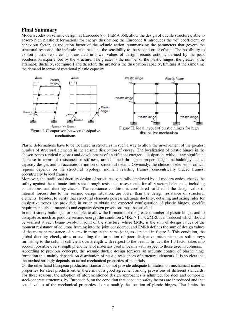
Final Summary Modern codes on seismic design, as Eurocode 8 or FEMA 350, allow the design of ductile structures, able to absorb high plastic deformations for energy dissipation; the Eurocode 8 introduces the “q” coefficient, or behaviour factor, as reduction factor of the seismic action, summarizing the parameters that govern the structural response, the inelastic resources and the sensibility to the second-order effects. The possibility to exploit plastic resources is translated in lower values of design seismic actions, defined by the peak acceleration experienced by the structure. The greater is the number of the plastic hinges, the greater is the attainable ductility, see figure 1 and therefore the greater is the dissipation capacity, limiting at the same time the demand in terms of rotational plastic capacity.
Figure I. Comparison between dissipative
mechanisms
Figure II. Ideal layout of plastic hinges for high
dissipative mechanism
Plastic deformations have to be localized in structures in such a way to allow the involvement of the greatest number of structural elements in the seismic dissipation of energy. The localization of plastic hinges in the chosen zones (critical regions) and development of an efficient energetic dissipation, without any significant decrease in terms of resistance or stiffness, are obtained through a proper design methodology, called capacity design, and an accurate definition of structural details. Obviously, the choice of elements’ critical regions depends on the structural typology: moment resisting frames; concentrically braced frames; eccentrically braced frames. Moreover, the traditional ductility design of structures, generally employed by all modern codes, checks the safety against the ultimate limit state through resistance assessments for all structural elements, including connections, and ductility checks. The resistance condition is considered satisfied if the design value of internal forces, due to the seismic design situation, are lower than the design resistance of structural elements. Besides, to verify that structural elements possess adequate ductility, detailing and sizing rules for dissipative zones are provided; in order to obtain the expected configuration of plastic hinges, specific requirements about materials and capacity design provisions must be satisfied. In multi-storey buildings, for example, to allow the formation of the greatest number of plastic hinges and to dissipate as much as possible seismic energy, the condition ΣMRc ≥ 1.3 × ΣMRb is introduced which should be verified at each beam-to-column joint of the structure, where ΣMRc is the sum of design values of the moment resistance of columns framing into the joint considered, and ΣMRb defines the sum of design values of the moment resistance of beams framing in the same joint, as depicted in figure 3. This condition, the global ductility check, aims at avoiding the formation of poor dissipative mechanisms as soft-storeys furnishing to the column sufficient overstrength with respect to the beams. In fact, the 1.3 factor takes into account possible overstrength phenomena of materials used in beams with respect to those used in columns. According to previous concepts, the seismic ductile design foresees an accurate control of plastic hinge formation that mainly depends on distribution of plastic resistances of structural elements. It is so clear that the method strongly depends on actual mechanical properties of materials. On the other hand European production standards do not provide adequate limitation on mechanical material properties for steel products either there is not a good agreement among provisions of different standards. For these reasons, the adoption of aforementioned design approaches is admitted, for steel and composite steel-concrete structures, by Eurocode 8, on the condition that adequate safety factors are introduced and that actual values of the mechanical properties do not modify the location of plastic hinges. That limits the
7
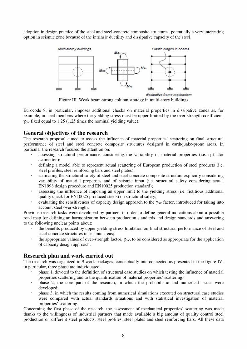
adoption in design practice of the steel and steel-concrete composite structures, potentially a very interesting option in seismic zone because of the intrinsic ductility and dissipative capacity of the steel.
Figure III. Weak beam-strong column strategy in multi-story buildings
Eurocode 8, in particular, imposes additional checks on material properties in dissipative zones as, for example, in steel members where the yielding stress must be upper limited by the over-strength coefficient,
γOV fixed equal to 1.25 (1.25 times the nominal yielding value).
General objectives of the research The research proposal aimed to assess the influence of material properties’ scattering on final structural performance of steel and steel concrete composite structures designed in earthquake-prone areas. In particular the research focused the attention on:
assessing structural performance considering the variability of material properties (i.e. q factor estimation);
defining a model able to represent actual scattering of European production of steel products (i.e. steel profiles, steel reinforcing bars and steel plates);
estimating the structural safety of steel and steel-concrete composite structure explicitly considering variability of material properties and of seismic input (i.e. structural safety considering actual EN1998 design procedure and EN10025 production standard);
assessing the influence of imposing an upper limit to the yielding stress (i.e. fictitious additional quality check for EN10025 produced steels) on structural safety;
evaluating the sensitiveness of capacity design approach to the γOV factor, introduced for taking into account steel over-strength.
Previous research tasks were developed by partners in order to define general indications about a possible road map for defining an harmonization between production standards and design standards and answering to the following unclear points about:
the benefits produced by upper yielding stress limitation on final structural performance of steel and steel-concrete structures in seismic areas;
the appropriate values of over-strength factor, γOV, to be considered as appropriate for the application of capacity design approach.
Research plan and work carried out The research was organized in 9 work-packages, conceptually interconnected as presented in the figure IV; in particular, three phase are individuated:
phase 1, devoted to the definition of structural case studies on which testing the influence of material properties scattering and to the quantification of material properties’ scattering;
phase 2, the core part of the research, in which the probabilistic and numerical issues were developed;
phase 3, in which the results coming from numerical simulations executed on structural case studies were compared with actual standards situations and with statistical investigation of material properties’ scattering.
Concerning the first phase of the research, the assessment of mechanical properties’ scattering was made thanks to the willingness of industrial partners that made available a big amount of quality control steel production on different steel products: steel profiles, steel plates and steel reinforcing bars. All these data
8
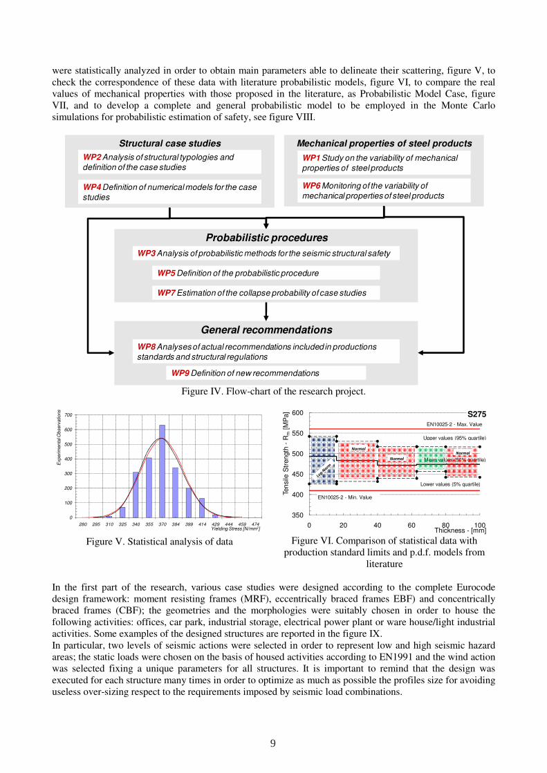
were statistically analyzed in order to obtain main parameters able to delineate their scattering, figure V, to check the correspondence of these data with literature probabilistic models, figure VI, to compare the real values of mechanical properties with those proposed in the literature, as Probabilistic Model Case, figure VII, and to develop a complete and general probabilistic model to be employed in the Monte Carlo simulations for probabilistic estimation of safety, see figure VIII.
Figure IV. Flow-chart of the research project.
Figure V. Statistical analysis of data
Figure VI. Comparison of statistical data with
production standard limits and p.d.f. models from literature
In the first part of the research, various case studies were designed according to the complete Eurocode design framework: moment resisting frames (MRF), eccentrically braced frames EBF) and concentrically braced frames (CBF); the geometries and the morphologies were suitably chosen in order to house the following activities: offices, car park, industrial storage, electrical power plant or ware house/light industrial activities. Some examples of the designed structures are reported in the figure IX. In particular, two levels of seismic actions were selected in order to represent low and high seismic hazard areas; the static loads were chosen on the basis of housed activities according to EN1991 and the wind action was selected fixing a unique parameters for all structures. It is important to remind that the design was executed for each structure many times in order to optimize as much as possible the profiles size for avoiding useless over-sizing respect to the requirements imposed by seismic load combinations.
Mechanical properties of steel products
WP6 Monitoring of the variability of
mechanical properties of steel products
WP1 Study on the variability of mechanical
properties of steel products
Structural case studies
WP4 Definition of numerical models for the case
studies
WP2 Analysis of structural typologies and
definition of the case studies
Probabilistic procedures
WP3 Analysis of probabilistic methods for the seismic structural safety
WP5 Definition of the probabilistic procedure
WP7 Estimation of the collapse probability of case studies
General recommendations
WP8 Analyses of actual recommendations included in productions
standards and structural regulations
WP9 Definition of new recommendations
0
100
200
300
400
500
600
700
280 295 310 325 340 355 370 384 399 414 429 444 459 474
Expe
rim
en
tal O
bserv
atio
ns
Yielding Stress [N/mm2]
350
400
450
500
550
600
0 20 40 60 80 100
Ten
sile
Str
en
gth
-R
m[M
Pa]
Thickness - [mm]
S275
Mean values (50% quartile)
Upper values (95% quartile)
Lower values (5% quartile)
EN10025-2 - Min. Value
EN10025-2 - Max. Value
Normal
Normal
Normal
9
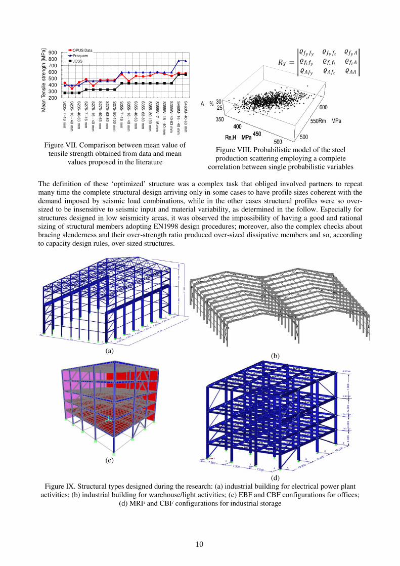
Figure VII. Comparison between mean value of
tensile strength obtained from data and mean values proposed in the literature
Figure VIII. Probabilistic model of the steel production scattering employing a complete
correlation between single probabilistic variables The definition of these ‘optimized’ structure was a complex task that obliged involved partners to repeat many time the complete structural design arriving only in some cases to have profile sizes coherent with the demand imposed by seismic load combinations, while in the other cases structural profiles were so over-sized to be insensitive to seismic input and material variability, as determined in the follow. Especially for structures designed in low seismicity areas, it was observed the impossibility of having a good and rational sizing of structural members adopting EN1998 design procedures; moreover, also the complex checks about bracing slenderness and their over-strength ratio produced over-sized dissipative members and so, according to capacity design rules, over-sized structures.
(a) (b)
(c)
(d)
Figure IX. Structural types designed during the research: (a) industrial building for electrical power plant activities; (b) industrial building for warehouse/light activities; (c) EBF and CBF configurations for offices;
(d) MRF and CBF configurations for industrial storage
200
300
400
500
600
700
800
900
S235-
7 -1
6 m
m
S235-
16 -
40 m
m
S235-
40-6
3 m
m
S275-
7 -1
6 m
m
S275-
16 -
40 m
m
S275-
40-6
3 m
m
S275-
63-8
0 m
m
S275-
80-1
00 m
m
S355-
7 -1
6 m
m
S355-
16 -
40 m
m
S355-
40-6
3 m
m
S355-
63-8
0 m
m
S355-
80-1
00 m
m
S355W
-7 -1
6 m
m
S355W
-16 -
40 m
m
S355W
-40-6
3 m
m
S460M
-16 -
40 m
m
S460M
-40-6
3 m
m
Mean
Ten
sile
str
en
gth
[M
Pa]
OPUS Data
Proquam
JCSS
350
400
450
500Re,HMPa 500
550
600
RmMPa2530A%350
400
450
500Re,HMPa
=
H
11
.88
0
7.300
7.4
25
21
.91
0
G
2.6
05
7.300F
7 .300E
7.300D
51.100Y
ZX
7 .3001C
7.300B
29.000
7.300A2
D
1st floor
4.0
00
2nd f loor
4.0
00
3rd floor
5.0
00
10.000
4t h floor
7.0
00
C
Y
10.000
Z
X1
B
7.5002
10.0007.5003
A7.500
4
10
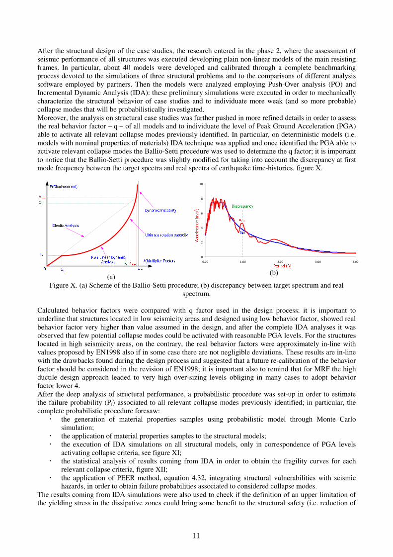
After the structural design of the case studies, the research entered in the phase 2, where the assessment of seismic performance of all structures was executed developing plain non-linear models of the main resisting frames. In particular, about 40 models were developed and calibrated through a complete benchmarking process devoted to the simulations of three structural problems and to the comparisons of different analysis software employed by partners. Then the models were analyzed employing Push-Over analysis (PO) and Incremental Dynamic Analysis (IDA): these preliminary simulations were executed in order to mechanically characterize the structural behavior of case studies and to individuate more weak (and so more probable) collapse modes that will be probabilistically investigated. Moreover, the analysis on structural case studies was further pushed in more refined details in order to assess the real behavior factor – q – of all models and to individuate the level of Peak Ground Acceleration (PGA) able to activate all relevant collapse modes previously identified. In particular, on deterministic models (i.e. models with nominal properties of materials) IDA technique was applied and once identified the PGA able to activate relevant collapse modes the Ballio-Setti procedure was used to determine the q factor; it is important to notice that the Ballio-Setti procedure was slightly modified for taking into account the discrepancy at first mode frequency between the target spectra and real spectra of earthquake time-histories, figure X.
(a)
(b)
Figure X. (a) Scheme of the Ballio-Setti procedure; (b) discrepancy between target spectrum and real spectrum.
Calculated behavior factors were compared with q factor used in the design process: it is important to underline that structures located in low seismicity areas and designed using low behavior factor, showed real behavior factor very higher than value assumed in the design, and after the complete IDA analyses it was observed that few potential collapse modes could be activated with reasonable PGA levels. For the structures located in high seismicity areas, on the contrary, the real behavior factors were approximately in-line with values proposed by EN1998 also if in some case there are not negligible deviations. These results are in-line with the drawbacks found during the design process and suggested that a future re-calibration of the behavior factor should be considered in the revision of EN1998; it is important also to remind that for MRF the high ductile design approach leaded to very high over-sizing levels obliging in many cases to adopt behavior factor lower 4. After the deep analysis of structural performance, a probabilistic procedure was set-up in order to estimate the failure probability (Pf) associated to all relevant collapse modes previously identified; in particular, the complete probabilistic procedure foresaw:
the generation of material properties samples using probabilistic model through Monte Carlo simulation;
the application of material properties samples to the structural models; the execution of IDA simulations on all structural models, only in correspondence of PGA levels
activating collapse criteria, see figure XI; the statistical analysis of results coming from IDA in order to obtain the fragility curves for each
relevant collapse criteria, figure XII; the application of PEER method, equation 4.32, integrating structural vulnerabilities with seismic
hazards, in order to obtain failure probabilities associated to considered collapse modes. The results coming from IDA simulations were also used to check if the definition of an upper limitation of the yielding stress in the dissipative zones could bring some benefit to the structural safety (i.e. reduction of
0
2
4
6
8
10
0.00 1.00 2.00 3.00 4.00
11
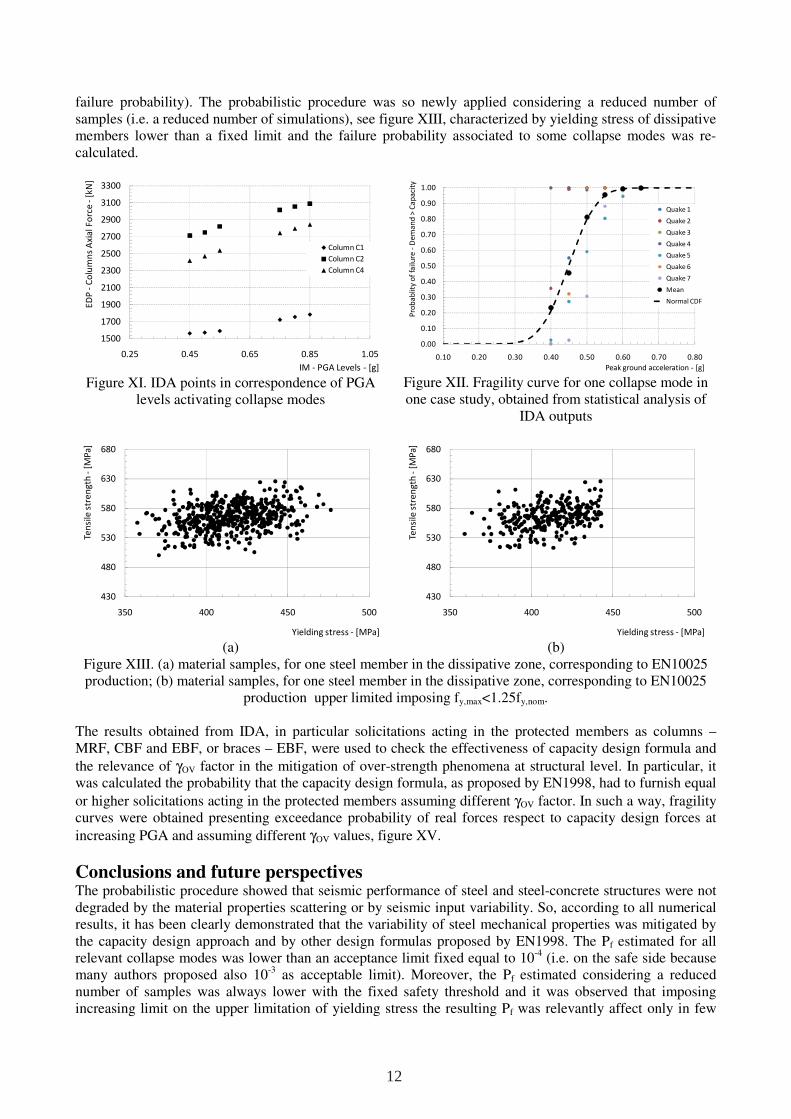
failure probability). The probabilistic procedure was so newly applied considering a reduced number of samples (i.e. a reduced number of simulations), see figure XIII, characterized by yielding stress of dissipative members lower than a fixed limit and the failure probability associated to some collapse modes was re-calculated.
Figure XI. IDA points in correspondence of PGA
levels activating collapse modes
Figure XII. Fragility curve for one collapse mode in one case study, obtained from statistical analysis of
IDA outputs
(a)
(b)
Figure XIII. (a) material samples, for one steel member in the dissipative zone, corresponding to EN10025 production; (b) material samples, for one steel member in the dissipative zone, corresponding to EN10025
production upper limited imposing fy,max<1.25fy,nom. The results obtained from IDA, in particular solicitations acting in the protected members as columns – MRF, CBF and EBF, or braces – EBF, were used to check the effectiveness of capacity design formula and
the relevance of γOV factor in the mitigation of over-strength phenomena at structural level. In particular, it was calculated the probability that the capacity design formula, as proposed by EN1998, had to furnish equal
or higher solicitations acting in the protected members assuming different γOV factor. In such a way, fragility curves were obtained presenting exceedance probability of real forces respect to capacity design forces at
increasing PGA and assuming different γOV values, figure XV.
Conclusions and future perspectives The probabilistic procedure showed that seismic performance of steel and steel-concrete structures were not degraded by the material properties scattering or by seismic input variability. So, according to all numerical results, it has been clearly demonstrated that the variability of steel mechanical properties was mitigated by the capacity design approach and by other design formulas proposed by EN1998. The Pf estimated for all relevant collapse modes was lower than an acceptance limit fixed equal to 10-4 (i.e. on the safe side because many authors proposed also 10-3 as acceptable limit). Moreover, the Pf estimated considering a reduced number of samples was always lower with the fixed safety threshold and it was observed that imposing increasing limit on the upper limitation of yielding stress the resulting Pf was relevantly affect only in few
1500
1700
1900
2100
2300
2500
2700
2900
3100
3300
0.25 0.45 0.65 0.85 1.05
ED
P -
Co
lum
ns
Axi
al
Fo
rce
-[k
N]
IM - PGA Levels - [g]
Column C1
Column C2
Column C4
0.00
0.10
0.20
0.30
0.40
0.50
0.60
0.70
0.80
0.90
1.00
0.10 0.20 0.30 0.40 0.50 0.60 0.70 0.80
Pro
ba
blit
y o
f fa
ilure
-D
em
an
d >
Ca
pa
city
Peak ground acceleration - [g]
Quake 1
Quake 2
Quake 3
Quake 4
Quake 5
Quake 6
Quake 7
Mean
Normal CDF
430
480
530
580
630
680
350 400 450 500
Ten
sile
str
en
gth
-[M
Pa
]
Yielding stress - [MPa]
430
480
530
580
630
680
350 400 450 500
Ten
sile
str
en
gth
-[M
Pa
]
Yielding stress - [MPa]
12
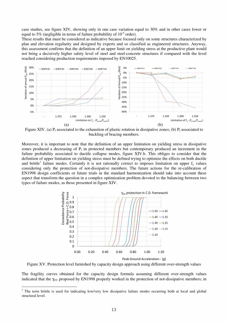
case studies, see figure XIV, showing only in one case variation equal to 30% and in other cases lower or equal to 5% (negligible in terms of failure probability of 10-4 order). These results that must be considered as indicative because focused only on some structures characterized by plan and elevation regularity and designed by experts and so classified as engineered structures. Anyway, this assessment confirms that the definition of an upper limit on yielding stress at the productive plant would not bring a decisively higher safety level of steel and steel-concrete structures if compared with the level reached considering production requirements imposed by EN10025.
(a)
(b)
Figure XIV. (a) Pf associated to the exhaustion of plastic rotation in dissipative zones; (b) Pf associated to buckling of bracing members.
Moreover, it is important to note that the definition of an upper limitation on yielding stress in dissipative zones produced a decreasing of Pf in protected members but contemporary produced an increment in the failure probability associated to ductile collapse modes, figure XIV.b. This obliges to consider that the definition of upper limitation on yielding stress must be defined trying to optimize the effects on both ductile and brittle1 failure modes. Certainly it is not rationally correct to imposes limitation on upper fy values considering only the protection of not-dissipative members. The future actions for the re-calibration of EN1998 design coefficients or future trials in the standard harmonization should take into account these aspect that transform the question in a complex optimization problem devoted to the balancing between two types of failure modes, as those presented in figure XIV.
Figure XV. Protection level furnished by capacity design approach using different over-strength values
The fragility curves obtained for the capacity design formula assuming different over-strength values
indicated that the γOV proposed by EN1998 properly worked in the protection of not-dissipative members; in
1 The term brittle is used for indicating low/very low dissipative failure modes occurring both at local and global structural level.
-5%
0%
5%
10%
15%
20%
25%
30%
- 1.375 1.350 1.300 1.250
Va
ria
tio
n o
f a
nn
ua
l P
fail
(Ris
k)
Limitation on fy - (fy,max/fy,nom)
4EBFX B1 4EBFX B3 4EBFX B4 4EBFX B6 4EBFY B1
-40%
-35%
-30%
-25%
-20%
-15%
-10%
-5%
0%
5%
- 1.375 1.350 1.300 1.250V
ari
ati
on
of
An
nu
al P
fail
(Ris
k)
Limitation of fy - (fy,max/fy,nom)
4EBFX Br1 4EBFX Br2 4EBFY Br1 4EBFY Br2
0
0.1
0.2
0.3
0.4
0.5
0.6
0.7
0.8
0.9
1
0.00 0.20 0.40 0.60 0.80 1.00 1.20
Exc
ee
da
nce
Pro
ba
bili
ty
Re
al
Fo
rce
> C
.D.
Fo
rce
Peak Ground Acceleration - [g]
γOV protection in C.D. framework
1.50 1.45
1.40 1.35
1.30 1.25
1.20 1.15
1.10
13
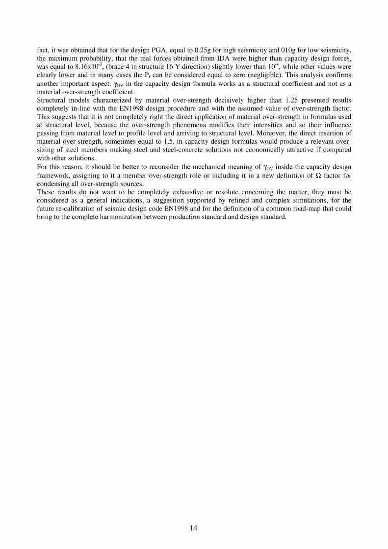
fact, it was obtained that for the design PGA, equal to 0.25g for high seismicity and 010g for low seismicity, the maximum probability, that the real forces obtained from IDA were higher than capacity design forces, was equal to 8.16x10⁻³, (brace 4 in structure 16 Y direction) slightly lower than 10-4, while other values were clearly lower and in many cases the Pf can be considered equal to zero (negligible). This analysis confirms
another important aspect: γOV in the capacity design formula works as a structural coefficient and not as a material over-strength coefficient. Structural models characterized by material over-strength decisively higher than 1.25 presented results completely in-line with the EN1998 design procedure and with the assumed value of over-strength factor. This suggests that it is not completely right the direct application of material over-strength in formulas used at structural level, because the over-strength phenomena modifies their intensities and so their influence passing from material level to profile level and arriving to structural level. Moreover, the direct insertion of material over-strength, sometimes equal to 1.5, in capacity design formulas would produce a relevant over-sizing of steel members making steel and steel-concrete solutions not economically attractive if compared with other solutions.
For this reason, it should be better to reconsider the mechanical meaning of γOV inside the capacity design
framework, assigning to it a member over-strength role or including it in a new definition of Ω factor for condensing all over-strength sources. These results do not want to be completely exhaustive or resolute concerning the matter; they must be considered as a general indications, a suggestion supported by refined and complex simulations, for the future re-calibration of seismic design code EN1998 and for the definition of a common road-map that could bring to the complete harmonization between production standard and design standard.
14
1. Variability of mechanical properties of steel products and its modeling The preliminary phase of the research was focused on the following objectives:
assessment of the material properties scattering; selection of appropriate stress strain model for numerical simulations; definition of a probabilistic model for the material properties.
Firstly, the investigation about the material properties scattering was carried out on the basis of production data kindly furnished by industrial partners and external industries; the scattering of mechanical properties, as yielding stress, tensile strength and ultimate elongation, was assessed for different steel products. Statistical investigations were carried out organizing collected data in homogeneous groups, in terms of product and according to classification proposed by relative production standard [1.1, 1.2, 1.3 and 1.4] and by structural design standards [1.5, 1.6 and 1.7]. Secondly, the collection of material data also concerned the stress-strain curves obtained by industrial partners during quality checks; a database was created and elaborated in order to define a stress strain law, whose shape/aspect ratio depends from mechanical properties monitored at industrial level during quality checks. The assumed stress-strain model was compared with experimental testing carried out during another research project [1.8]: aspect ratio of the cycle and dissipate energy were considered in order to evaluate the suitability of selected model. Finally, on the basis of the statistical information collected for the material scattering evaluation, the probabilistic model of the steel products mechanical properties, employed during the research project, was fixed. The model was defined as multi-variables in which the statistical interdependencies between yielding stress, tensile strength and elongation at fracture were considered. For sake of completeness, the statistical parameters assumed for the probabilistic models were compared also with information and modelling parameters used in a previous research or suggested as suitable for probabilistic evaluation of structural safety [1.9 and 1.10].
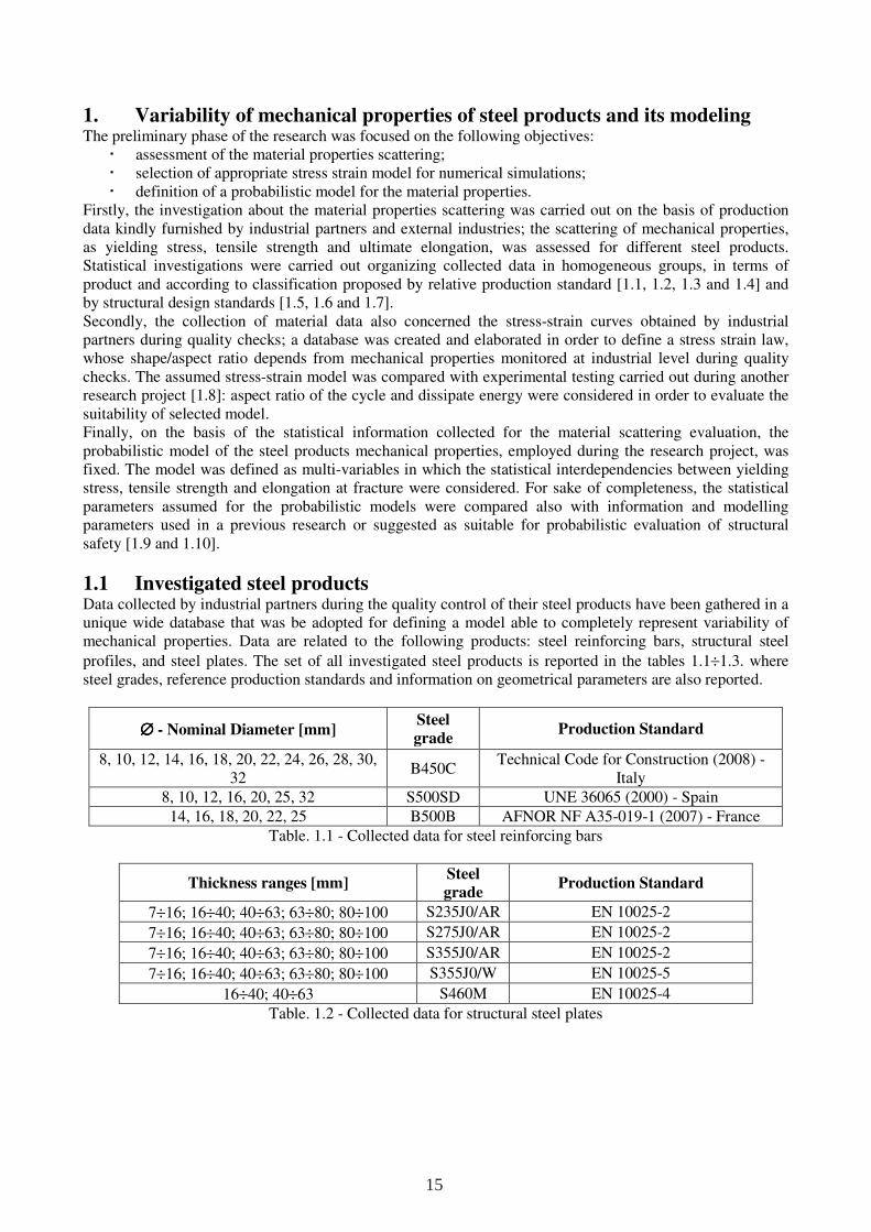
1.1 Investigated steel products Data collected by industrial partners during the quality control of their steel products have been gathered in a unique wide database that was be adopted for defining a model able to completely represent variability of mechanical properties. Data are related to the following products: steel reinforcing bars, structural steel
profiles, and steel plates. The set of all investigated steel products is reported in the tables 1.1÷1.3. where steel grades, reference production standards and information on geometrical parameters are also reported.
∅∅∅∅ - Nominal Diameter [mm] Steel
grade Production Standard
8, 10, 12, 14, 16, 18, 20, 22, 24, 26, 28, 30, 32
B450C Technical Code for Construction (2008) -
Italy 8, 10, 12, 16, 20, 25, 32 S500SD UNE 36065 (2000) - Spain
14, 16, 18, 20, 22, 25 B500B AFNOR NF A35-019-1 (2007) - France
Table. 1.1 - Collected data for steel reinforcing bars
Thickness ranges [mm] Steel
grade Production Standard
7÷16; 16÷40; 40÷63; 63÷80; 80÷100 S235J0/AR EN 10025-2
7÷16; 16÷40; 40÷63; 63÷80; 80÷100 S275J0/AR EN 10025-2
7÷16; 16÷40; 40÷63; 63÷80; 80÷100 S355J0/AR EN 10025-2
7÷16; 16÷40; 40÷63; 63÷80; 80÷100 S355J0/W EN 10025-5
16÷40; 40÷63 S460M EN 10025-4
Table. 1.2 - Collected data for structural steel plates
15
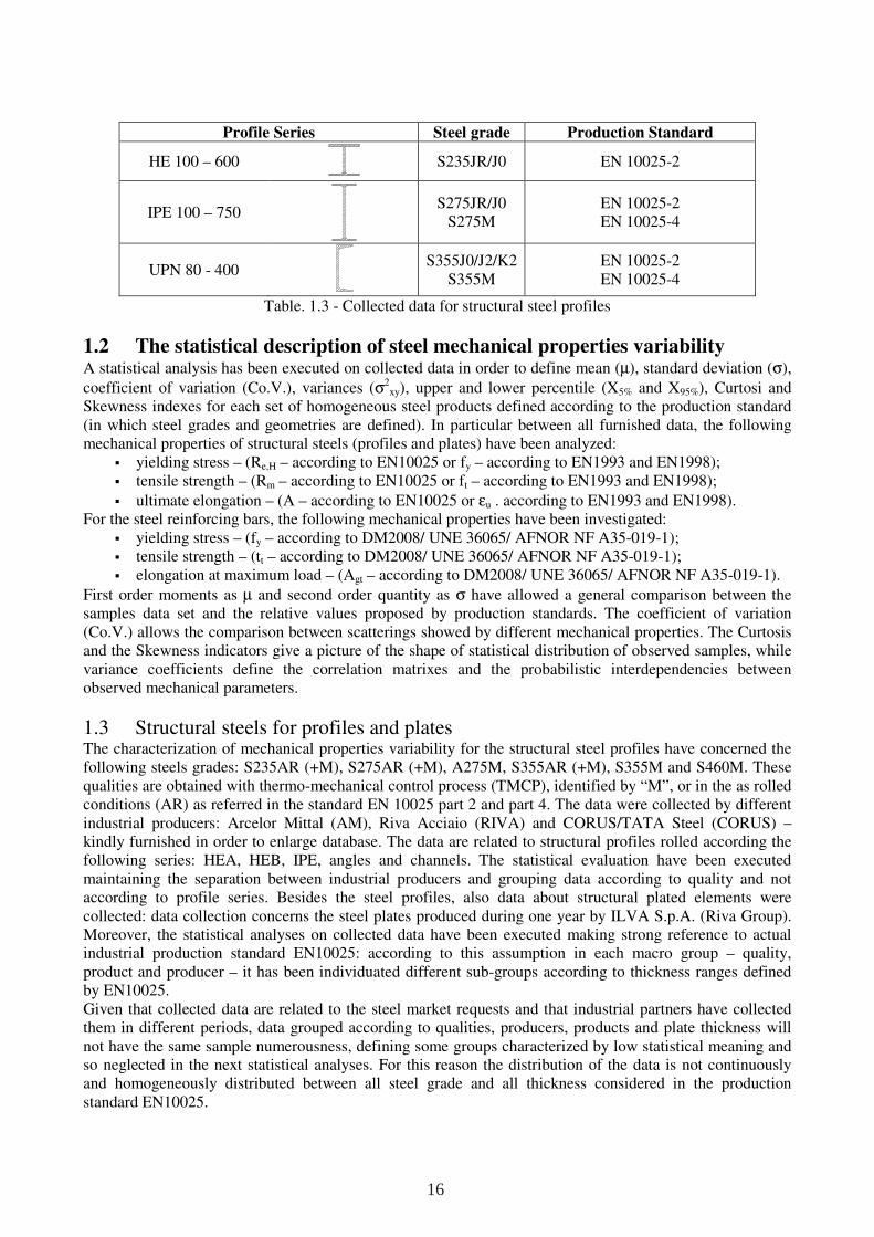
Profile Series Steel grade Production Standard
HE 100 – 600
S235JR/J0 EN 10025-2
IPE 100 – 750
S275JR/J0 S275M
EN 10025-2 EN 10025-4
UPN 80 - 400
S355J0/J2/K2 S355M
EN 10025-2 EN 10025-4
Table. 1.3 - Collected data for structural steel profiles
1.2 The statistical description of steel mechanical properties variability A statistical analysis has been executed on collected data in order to define mean (µ), standard deviation (σ),
coefficient of variation (Co.V.), variances (σ2xy), upper and lower percentile (X5% and X95%), Curtosi and
Skewness indexes for each set of homogeneous steel products defined according to the production standard (in which steel grades and geometries are defined). In particular between all furnished data, the following mechanical properties of structural steels (profiles and plates) have been analyzed:
yielding stress – (Re,H – according to EN10025 or fy – according to EN1993 and EN1998); tensile strength – (Rm – according to EN10025 or ft – according to EN1993 and EN1998);
ultimate elongation – (A – according to EN10025 or εu . according to EN1993 and EN1998). For the steel reinforcing bars, the following mechanical properties have been investigated:
yielding stress – (fy – according to DM2008/ UNE 36065/ AFNOR NF A35-019-1); tensile strength – (tt – according to DM2008/ UNE 36065/ AFNOR NF A35-019-1); elongation at maximum load – (Agt – according to DM2008/ UNE 36065/ AFNOR NF A35-019-1).
First order moments as µ and second order quantity as σ have allowed a general comparison between the samples data set and the relative values proposed by production standards. The coefficient of variation (Co.V.) allows the comparison between scatterings showed by different mechanical properties. The Curtosis and the Skewness indicators give a picture of the shape of statistical distribution of observed samples, while variance coefficients define the correlation matrixes and the probabilistic interdependencies between observed mechanical parameters.
1.3 Structural steels for profiles and plates The characterization of mechanical properties variability for the structural steel profiles have concerned the following steels grades: S235AR (+M), S275AR (+M), A275M, S355AR (+M), S355M and S460M. These qualities are obtained with thermo-mechanical control process (TMCP), identified by “M”, or in the as rolled conditions (AR) as referred in the standard EN 10025 part 2 and part 4. The data were collected by different industrial producers: Arcelor Mittal (AM), Riva Acciaio (RIVA) and CORUS/TATA Steel (CORUS) – kindly furnished in order to enlarge database. The data are related to structural profiles rolled according the following series: HEA, HEB, IPE, angles and channels. The statistical evaluation have been executed maintaining the separation between industrial producers and grouping data according to quality and not according to profile series. Besides the steel profiles, also data about structural plated elements were collected: data collection concerns the steel plates produced during one year by ILVA S.p.A. (Riva Group). Moreover, the statistical analyses on collected data have been executed making strong reference to actual industrial production standard EN10025: according to this assumption in each macro group – quality, product and producer – it has been individuated different sub-groups according to thickness ranges defined by EN10025. Given that collected data are related to the steel market requests and that industrial partners have collected them in different periods, data grouped according to qualities, producers, products and plate thickness will not have the same sample numerousness, defining some groups characterized by low statistical meaning and so neglected in the next statistical analyses. For this reason the distribution of the data is not continuously and homogeneously distributed between all steel grade and all thickness considered in the production standard EN10025.
16
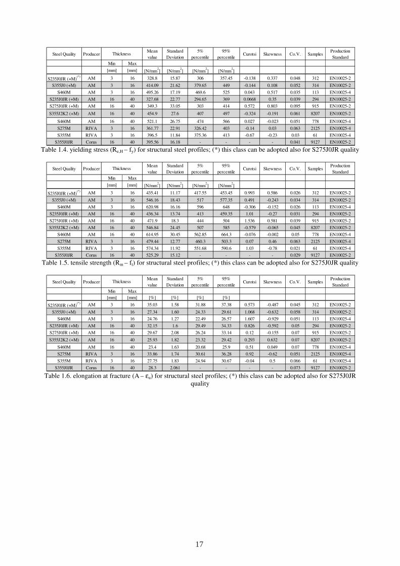
Table 1.4. yielding stress (Re,H – fy) for structural steel profiles; (*) this class can be adopted also for S275J0JR quality
Table 1.5. tensile strength (Rm – ft) for structural steel profiles; (*) this class can be adopted also for S275J0JR quality
Table 1.6. elongation at fracture (A – εu) for structural steel profiles; (*) this class can be adopted also for S275J0JR
quality
Steel Quality ProducerMean
value
Standard
Deviation
5%
percentile
95%
percentileCurotsi Skewness Co.V. Samples
Production
Standard
Min Max
[mm] [mm] [N/mm2] [N/mm
2] [N/mm
2] [N/mm
2]
S235J0JR (+M)(*) AM 3 16 328.8 15.87 306 357.45 -0.138 0.337 0.048 312 EN10025-2
S355J0 (+M) AM 3 16 414.09 21.62 379.65 449 -0.144 0.108 0.052 314 EN10025-2
S460M AM 3 16 495.26 17.19 469.6 525 0.043 0.517 0.035 113 EN10025-4
S235J0JR (+M) AM 16 40 327.68 22.77 294.65 369 0.0668 0.35 0.039 294 EN10025-2
S275J0JR (+M) AM 16 40 349.3 33.05 303 414 0.572 0.803 0.095 915 EN10025-2
S355J2K2 (+M) AM 16 40 454.9 27.6 407 497 -0.324 -0.191 0.061 8207 EN10025-2
S460M AM 16 40 521.1 26.75 474 566 0.027 -0.023 0.051 778 EN10025-4
S275M RIVA 3 16 361.77 22.91 326.42 403 -0.14 0.03 0.063 2125 EN10025-4
S355M RIVA 3 16 396.5 11.84 375.36 413 -0.67 -0.23 0.03 61 EN10025-4
S355J0JR Corus 16 40 395.56 16.18 - - - - 0.041 9127 EN10025-2
Thickness
Steel Quality ProducerMean
value
Standard
Deviation
5%
percentile
95%
percentileCurotsi Skewness Co.V. Samples
Production
Standard
Min Max
[mm] [mm] [N/mm2] [N/mm
2] [N/mm
2] [N/mm
2]
S235J0JR (+M)(*) AM 3 16 435.41 11.17 417.55 453.45 0.993 0.586 0.026 312 EN10025-2
S355J0 (+M) AM 3 16 546.16 18.43 517 577.35 0.491 -0.243 0.034 314 EN10025-2
S460M AM 3 16 620.98 16.16 596 648 -0.306 -0.152 0.026 113 EN10025-4
S235J0JR (+M) AM 16 40 436.34 13.74 413 459.35 1.01 -0.27 0.031 294 EN10025-2
S275J0JR (+M) AM 16 40 471.9 18.3 444 504 1.536 0.581 0.039 915 EN10025-2
S355J2K2 (+M) AM 16 40 546.84 24.45 507 585 -0.579 -0.065 0.045 8207 EN10025-2
S460M AM 16 40 614.95 30.45 562.85 664.3 -0.076 -0.002 0.05 778 EN10025-4
S275M RIVA 3 16 479.44 12.77 460.3 503.3 0.07 0.46 0.063 2125 EN10025-4
S355M RIVA 3 16 574.34 11.92 551.68 590.6 1.03 -0.78 0.021 61 EN10025-4
S355J0JR Corus 16 40 525.29 15.12 - - - - 0.029 9127 EN10025-2
Thickness
Steel Quality ProducerMean
value
Standard
Deviation
5%
percentile
95%
percentileCurotsi Skewness Co.V. Samples
Production
Standard
Min Max
[mm] [mm] [%] [%] [%] [%]
S235J0JR (+M)(*) AM 3 16 35.03 1.58 31.88 37.38 0.573 -0.487 0.045 312 EN10025-2
S355J0 (+M) AM 3 16 27.34 1.60 24.33 29.61 1.068 -0.632 0.058 314 EN10025-2
S460M AM 3 16 24.76 1.27 22.49 26.57 1.607 -0.929 0.051 113 EN10025-4
S235J0JR (+M) AM 16 40 32.15 1.6 29.49 34.33 0.826 -0.592 0.05 294 EN10025-2
S275J0JR (+M) AM 16 40 29.67 2.08 26.24 33.14 0.12 -0.155 0.07 915 EN10025-2
S355J2K2 (+M) AM 16 40 25.93 1.82 23.32 29.42 0.293 0.632 0.07 8207 EN10025-2
S460M AM 16 40 23.4 1.63 20.68 25.9 0.51 0.049 0.07 778 EN10025-4
S275M RIVA 3 16 33.86 1.74 30.61 36.28 0.92 -0.62 0.051 2125 EN10025-4
S355M RIVA 3 16 27.75 1.83 24.94 30.67 -0.04 0.5 0.066 61 EN10025-4
S355J0JR Corus 16 40 28.3 2.061 - - - - 0.073 9127 EN10025-2
Thickness
17
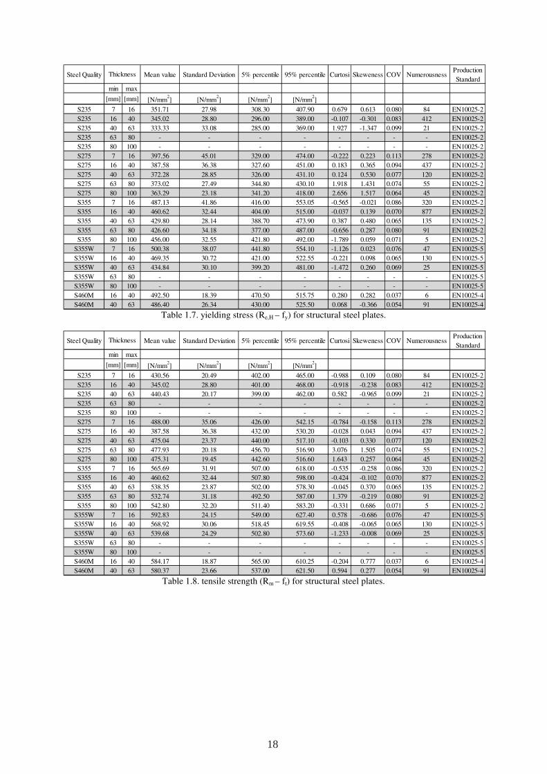
Table 1.7. yielding stress (Re,H – fy) for structural steel plates.
Table 1.8. tensile strength (Rm – ft) for structural steel plates.
Steel Quality Mean value Standard Deviation 5% percentile 95% percentile Curtosi Skeweness COV NumerousnessProduction
Standard
min max
[mm] [mm] [N/mm2] [N/mm
2] [N/mm
2] [N/mm
2]
S235 7 16 351.71 27.98 308.30 407.90 0.679 0.613 0.080 84 EN10025-2
S235 16 40 345.02 28.80 296.00 389.00 -0.107 -0.301 0.083 412 EN10025-2
S235 40 63 333.33 33.08 285.00 369.00 1.927 -1.347 0.099 21 EN10025-2
S235 63 80 - - - - - - - - EN10025-2
S235 80 100 - - - - - - - - EN10025-2
S275 7 16 397.56 45.01 329.00 474.00 -0.222 0.223 0.113 278 EN10025-2
S275 16 40 387.58 36.38 327.60 451.00 0.183 0.365 0.094 437 EN10025-2
S275 40 63 372.28 28.85 326.00 431.10 0.124 0.530 0.077 120 EN10025-2
S275 63 80 373.02 27.49 344.80 430.10 1.918 1.431 0.074 55 EN10025-2
S275 80 100 363.29 23.18 341.20 418.00 2.656 1.517 0.064 45 EN10025-2
S355 7 16 487.13 41.86 416.00 553.05 -0.565 -0.021 0.086 320 EN10025-2
S355 16 40 460.62 32.44 404.00 515.00 -0.037 0.139 0.070 877 EN10025-2
S355 40 63 429.80 28.14 388.70 473.90 0.387 0.480 0.065 135 EN10025-2
S355 63 80 426.60 34.18 377.00 487.00 -0.656 0.287 0.080 91 EN10025-2
S355 80 100 456.00 32.55 421.80 492.00 -1.789 0.059 0.071 5 EN10025-2
S355W 7 16 500.38 38.07 441.80 554.10 -1.126 0.023 0.076 47 EN10025-5
S355W 16 40 469.35 30.72 421.00 522.55 -0.221 0.098 0.065 130 EN10025-5
S355W 40 63 434.84 30.10 399.20 481.00 -1.472 0.260 0.069 25 EN10025-5
S355W 63 80 - - - - - - - - EN10025-5
S355W 80 100 - - - - - - - - EN10025-5
S460M 16 40 492.50 18.39 470.50 515.75 0.280 0.282 0.037 6 EN10025-4
S460M 40 63 486.40 26.34 430.00 525.50 0.068 -0.366 0.054 91 EN10025-4
Thickness
Steel Quality Mean value Standard Deviation 5% percentile 95% percentile Curtosi Skeweness COV NumerousnessProduction
Standard
min max
[mm] [mm] [N/mm2] [N/mm
2] [N/mm
2] [N/mm
2]
S235 7 16 430.56 20.49 402.00 465.00 -0.988 0.109 0.080 84 EN10025-2
S235 16 40 345.02 28.80 401.00 468.00 -0.918 -0.238 0.083 412 EN10025-2
S235 40 63 440.43 20.17 399.00 462.00 0.582 -0.965 0.099 21 EN10025-2
S235 63 80 - - - - - - - - EN10025-2
S235 80 100 - - - - - - - - EN10025-2
S275 7 16 488.00 35.06 426.00 542.15 -0.784 -0.158 0.113 278 EN10025-2
S275 16 40 387.58 36.38 432.00 530.20 -0.028 0.043 0.094 437 EN10025-2
S275 40 63 475.04 23.37 440.00 517.10 -0.103 0.330 0.077 120 EN10025-2
S275 63 80 477.93 20.18 456.70 516.90 3.076 1.505 0.074 55 EN10025-2
S275 80 100 475.31 19.45 442.60 516.60 1.643 0.257 0.064 45 EN10025-2
S355 7 16 565.69 31.91 507.00 618.00 -0.535 -0.258 0.086 320 EN10025-2
S355 16 40 460.62 32.44 507.80 598.00 -0.424 -0.102 0.070 877 EN10025-2
S355 40 63 538.35 23.87 502.00 578.30 -0.045 0.370 0.065 135 EN10025-2
S355 63 80 532.74 31.18 492.50 587.00 1.379 -0.219 0.080 91 EN10025-2
S355 80 100 542.80 32.20 511.40 583.20 -0.331 0.686 0.071 5 EN10025-2
S355W 7 16 592.83 24.15 549.00 627.40 0.578 -0.686 0.076 47 EN10025-5
S355W 16 40 568.92 30.06 518.45 619.55 -0.408 -0.065 0.065 130 EN10025-5
S355W 40 63 539.68 24.29 502.80 573.60 -1.233 -0.008 0.069 25 EN10025-5
S355W 63 80 - - - - - - - - EN10025-5
S355W 80 100 - - - - - - - - EN10025-5
S460M 16 40 584.17 18.87 565.00 610.25 -0.204 0.777 0.037 6 EN10025-4
S460M 40 63 580.37 23.66 537.00 621.50 0.594 0.277 0.054 91 EN10025-4
Thickness
18
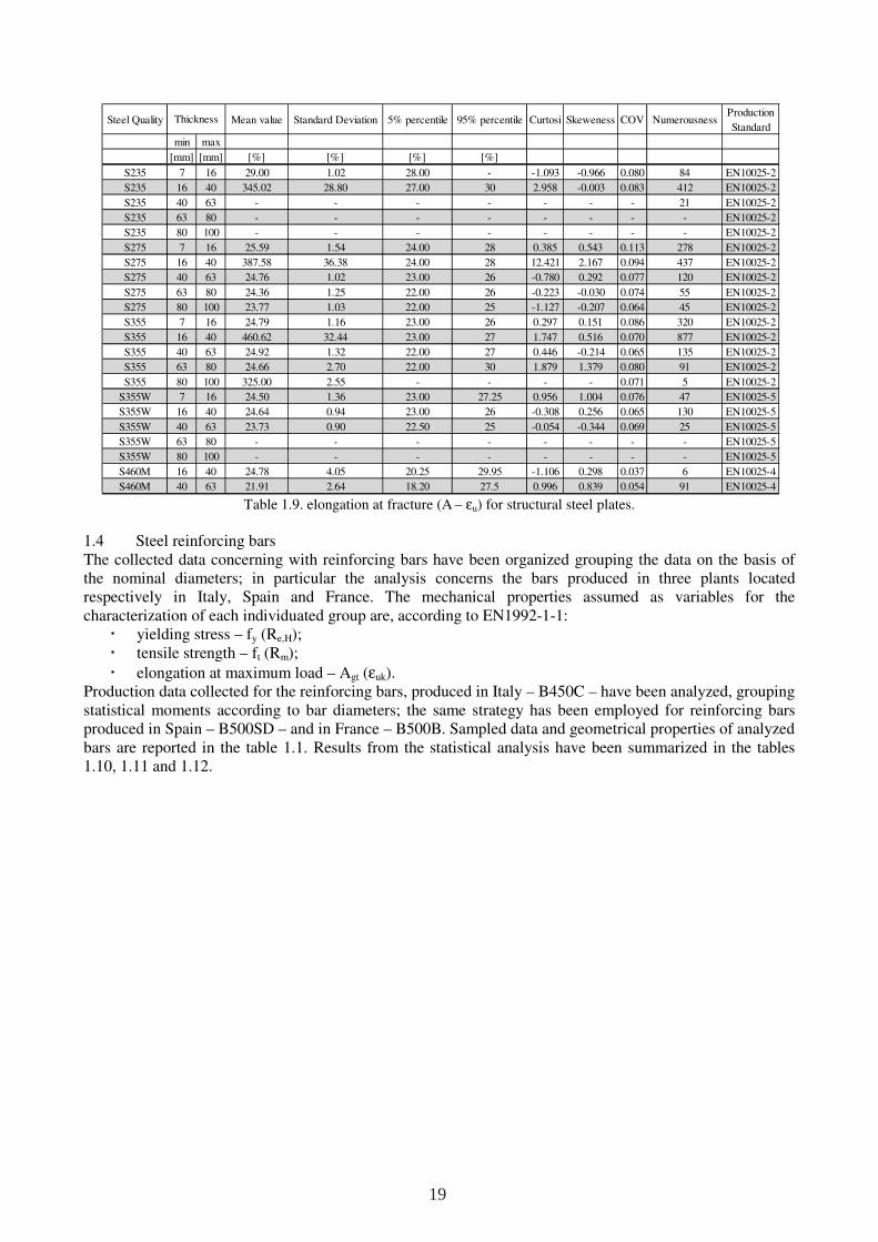
Table 1.9. elongation at fracture (A – εu) for structural steel plates.
1.4 Steel reinforcing bars The collected data concerning with reinforcing bars have been organized grouping the data on the basis of the nominal diameters; in particular the analysis concerns the bars produced in three plants located respectively in Italy, Spain and France. The mechanical properties assumed as variables for the characterization of each individuated group are, according to EN1992-1-1:
yielding stress – fy (Re,H); tensile strength – ft (Rm);
elongation at maximum load – Agt (εuk). Production data collected for the reinforcing bars, produced in Italy – B450C – have been analyzed, grouping statistical moments according to bar diameters; the same strategy has been employed for reinforcing bars produced in Spain – B500SD – and in France – B500B. Sampled data and geometrical properties of analyzed bars are reported in the table 1.1. Results from the statistical analysis have been summarized in the tables 1.10, 1.11 and 1.12.
Steel Quality Mean value Standard Deviation 5% percentile 95% percentile Curtosi Skeweness COV NumerousnessProduction
Standard
min max
[mm] [mm] [%] [%] [%] [%]
S235 7 16 29.00 1.02 28.00 - -1.093 -0.966 0.080 84 EN10025-2
S235 16 40 345.02 28.80 27.00 30 2.958 -0.003 0.083 412 EN10025-2
S235 40 63 - - - - - - - 21 EN10025-2
S235 63 80 - - - - - - - - EN10025-2
S235 80 100 - - - - - - - - EN10025-2
S275 7 16 25.59 1.54 24.00 28 0.385 0.543 0.113 278 EN10025-2
S275 16 40 387.58 36.38 24.00 28 12.421 2.167 0.094 437 EN10025-2
S275 40 63 24.76 1.02 23.00 26 -0.780 0.292 0.077 120 EN10025-2
S275 63 80 24.36 1.25 22.00 26 -0.223 -0.030 0.074 55 EN10025-2
S275 80 100 23.77 1.03 22.00 25 -1.127 -0.207 0.064 45 EN10025-2
S355 7 16 24.79 1.16 23.00 26 0.297 0.151 0.086 320 EN10025-2
S355 16 40 460.62 32.44 23.00 27 1.747 0.516 0.070 877 EN10025-2
S355 40 63 24.92 1.32 22.00 27 0.446 -0.214 0.065 135 EN10025-2
S355 63 80 24.66 2.70 22.00 30 1.879 1.379 0.080 91 EN10025-2
S355 80 100 325.00 2.55 - - - - 0.071 5 EN10025-2
S355W 7 16 24.50 1.36 23.00 27.25 0.956 1.004 0.076 47 EN10025-5
S355W 16 40 24.64 0.94 23.00 26 -0.308 0.256 0.065 130 EN10025-5
S355W 40 63 23.73 0.90 22.50 25 -0.054 -0.344 0.069 25 EN10025-5
S355W 63 80 - - - - - - - - EN10025-5
S355W 80 100 - - - - - - - - EN10025-5
S460M 16 40 24.78 4.05 20.25 29.95 -1.106 0.298 0.037 6 EN10025-4
S460M 40 63 21.91 2.64 18.20 27.5 0.996 0.839 0.054 91 EN10025-4
Thickness
19
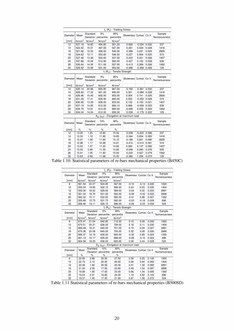
Table 1.10. Statistical parameters of re-bars mechanical properties (B450C)
Table 1.11 Statistical parameters of re-bars mechanical properties (B500SD)
Diameter MeanStandard
Deviation
5%
percentile
95%
percentileSkewness Curtosi Co.V.
Sample
Numerousness
[mm] N/mm2 N/mm2 N/mm2 N/mm2
12 527.18 16.85 494.80 551.20 -0.626 -0.034 0.032 237
14 523.52 15.01 497.00 547.00 -0.261 0.029 0.029 1416
16 521.66 12.33 499.00 540.00 -0.389 0.031 0.024 2829
18 524.62 13.11 500.80 546.00 -0.227 0.504 0.025 519
20 527.48 13.48 503.00 547.00 -0.243 0.021 0.026 1407
24 537.88 15.04 512.90 560.00 -0.427 0.102 0.028 639
26 535.64 14.05 511.00 557.00 -0.413 0.399 0.026 1062
30 529.52 15.56 501.00 553.60 -0.386 -0.258 0.029 129
Diameter MeanStandard
Deviation
5%
percentile
95%
percentileSkewness Curtosi Co.V.
Sample
Numerousness
[mm] N/mm2 N/mm2 N/mm2 N/mm2
12 635.14 20.96 600.80 667.20 -0.192 -0.361 0.033 237
14 626.90 17.32 601.00 656.00 0.301 -0.086 0.028 1416
16 626.96 15.46 602.00 653.00 0.304 0.741 0.025 2829
18 631.09 17.41 605.90 665.00 0.505 -0.350 0.028 519
20 630.95 13.39 609.00 653.00 0.132 0.150 0.021 1407
24 637.19 14.85 612.00 660.10 0.066 -0.059 0.023 639
26 635.79 14.81 613.00 660.00 -0.099 0.335 0.023 1062
30 634.04 14.04 612.00 656.00 -0.039 -0.179 0.022 129
Diameter MeanStandard
Deviation
10%
percentile
90%
percentileSkewness Curtosi Co.V.
Sample
Numerousness
[mm] % % % %
12 13.05 1.25 10.80 15.00 -0.208 -0.222 0.096 237
14 13.33 1.10 11.90 14.60 -0.344 0.654 0.083 1416
16 13.47 1.08 11.60 15.10 -0.189 0.931 0.080 2829
18 12.98 1.17 10.99 14.61 -0.410 -0.314 0.091 519
20 13.03 1.07 11.20 14.60 0.060 0.137 0.082 1407
24 13.05 0.99 11.30 14.60 -0.048 0.280 0.076 639
26 13.41 1.05 11.60 15.00 -0.233 0.027 0.079 1062
30 13.63 0.99 11.98 15.20 -0.380 1.056 0.073 129
fy (Re) - Yielding Stress
ft (Rm) - Tensile Strength
Agt (εuk) - Elongation at maximum load
Diameter MeanStandard
Deviation
5%
percentile
95%
percentileSkewness Curtosi Co.V.
Sample
Numerousness
[mm] N/mm2 N/mm2 N/mm2 N/mm2
8 561.54 22.27 524.95 597.00 -0.10 -0.13 0.040 1000
10 555.04 19.65 522.15 589.00 0.24 0.03 0.035 1404
12 559.30 18.22 529.00 589.00 -0.04 0.02 0.033 2891
16 561.34 18.70 531.00 592.00 -0.08 -0.02 0.033 2896
20 562.32 15.11 532.00 585.00 -0.41 0.88 0.027 1392
25 555.69 15.75 531.75 582.00 -0.03 -0.18 0.028 696
32 556.46 19.11 526.15 586.00 -0.06 -0.03 0.034 524
Diameter MeanStandard
Deviation
5%
percentile
95%
percentileSkewness Curtosi Co.V.
Sample
Numerousness
[mm] N/mm2 N/mm2 N/mm2 N/mm2
8 675.47 21.54 640.95 712.00 0.15 0.09 0.032 1000
10 670.51 20.31 636.00 706.00 0.18 0.11 0.030 1404
12 669.48 18.31 640.00 701.00 0.15 0.04 0.027 2891
16 670.36 20.08 640.00 705.00 0.32 0.09 0.030 2896
20 666.37 16.19 639.00 693.00 -0.35 0.89 0.024 1392
25 661.13 16.17 635.00 688.00 -0.08 -0.10 0.024 696
32 664.06 18.29 636.00 693.85 0.06 0.44 0.028 524
Diameter MeanStandard
Deviation
10%
percentile
90%
percentileSkewness Curtosi Co.V.
Sample
Numerousness
[mm] % % % %
8 22.85 2.88 20.00 27.50 0.56 0.25 0.126 1000
10 22.73 2.12 20.00 26.00 0.56 2.64 0.093 1404
12 22.26 1.82 20.00 25.00 0.51 1.32 0.082 2891
16 21.00 2.05 17.50 23.80 0.45 1.04 0.097 2896
20 19.89 1.90 17.00 23.00 0.66 1.04 0.095 1392
25 19.24 2.01 16.80 24.00 1.19 2.82 0.104 696
32 19.37 1.40 17.50 21.90 0.87 1.06 0.072 524
fy (Re) - Yielding Stress
ft (Rm) - Tensile Strength
Agt (εuk) - Elongation at maximum load
20
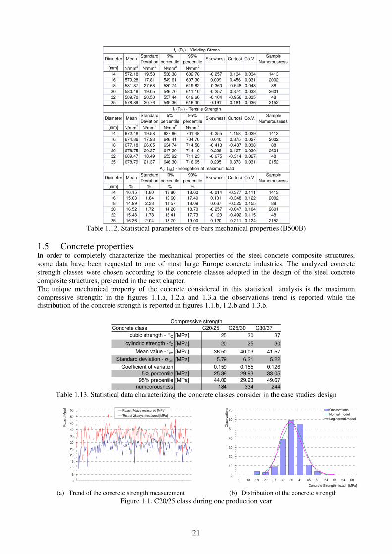
Table 1.12. Statistical parameters of re-bars mechanical properties (B500B)
1.5 Concrete properties In order to completely characterize the mechanical properties of the steel-concrete composite structures, some data have been requested to one of most large Europe concrete industries. The analyzed concrete strength classes were chosen according to the concrete classes adopted in the design of the steel concrete composite structures, presented in the next chapter. The unique mechanical property of the concrete considered in this statistical analysis is the maximum compressive strength: in the figures 1.1.a, 1.2.a and 1.3.a the observations trend is reported while the distribution of the concrete strength is reported in figures 1.1.b, 1.2.b and 1.3.b.
Table 1.13. Statistical data characterizing the concrete classes consider in the case studies design
(a) Trend of the concrete strength measurement
(b) Distribution of the concrete strength
Figure 1.1. C20/25 class during one production year
Diameter MeanStandard
Deviation
5%
percentile
95%
percentileSkewness Curtosi Co.V.
Sample
Numerousness
[mm] N/mm2 N/mm2 N/mm2 N/mm2
14 572.18 19.58 538.38 602.70 -0.257 0.134 0.034 1413
16 579.28 17.81 549.61 607.30 0.009 0.456 0.031 2002
18 581.87 27.68 530.74 619.82 -0.360 -0.548 0.048 88
20 580.48 19.05 546.70 611.10 -0.257 0.374 0.033 2601
22 589.70 20.50 557.44 619.66 -0.104 -0.956 0.035 48
25 578.89 20.76 545.36 616.30 0.191 0.181 0.036 2152
Diameter MeanStandard
Deviation
5%
percentile
95%
percentileSkewness Curtosi Co.V.
Sample
Numerousness
[mm] N/mm2 N/mm2 N/mm2 N/mm2
14 672.48 19.58 637.66 701.48 -0.255 1.158 0.029 1413
16 674.86 17.93 646.41 704.70 0.040 0.375 0.027 2002
18 677.18 26.05 634.74 714.58 -0.413 -0.437 0.038 88
20 678.75 20.37 647.20 714.10 0.228 0.127 0.030 2601
22 689.47 18.49 653.92 711.23 -0.675 -0.314 0.027 48
25 678.79 21.37 646.30 716.65 0.295 0.373 0.031 2152
Diameter MeanStandard
Deviation
10%
percentile
90%
percentileSkewness Curtosi Co.V.
Sample
Numerousness
[mm] % % % %
14 16.15 1.80 13.80 18.60 -0.014 -0.377 0.111 1413
16 15.03 1.84 12.60 17.40 0.101 -0.348 0.122 2002
18 14.99 2.33 11.57 18.09 0.067 -0.525 0.155 88
20 16.52 1.72 14.20 18.70 -0.257 -0.047 0.104 2601
22 15.48 1.78 13.41 17.73 -0.123 -0.492 0.115 48
25 16.36 2.04 13.70 19.00 0.120 -0.211 0.124 2152
fy (Re) - Yielding Stress
ft (Rm) - Tensile Strength
Agt (εuk) - Elongation at maximum load
Concrete class C20/25 C25/30 C30/37
cubic strength - RC [MPa] 25 30 37
cylindric strength - fC [MPa] 20 25 30
Mean value - fcm [MPa] 36.50 40.03 41.57
Standard deviation - σfcm [MPa] 5.79 6.21 5.22
Coefficient of variation 0.159 0.155 0.126
5% percentile [MPa] 25.36 29.93 33.05
95% precentile [MPa] 44.00 29.93 49.67
numeorousness 184 334 244
Compressive strength
0
5
10
15
20
25
30
35
40
45
50
55
Rc,a
ct
[Mp
a]
Rc,act 7days measured [MPa]
'Rc,act 28days measured [MPa]
0
10
20
30
40
50
60
70
9 13 18 22 27 32 36 41 45 50 54 59 64 68
Concrete Strength - fc,act [MPa]
Observ
ations Observations
Normal model
Log-normal model
21
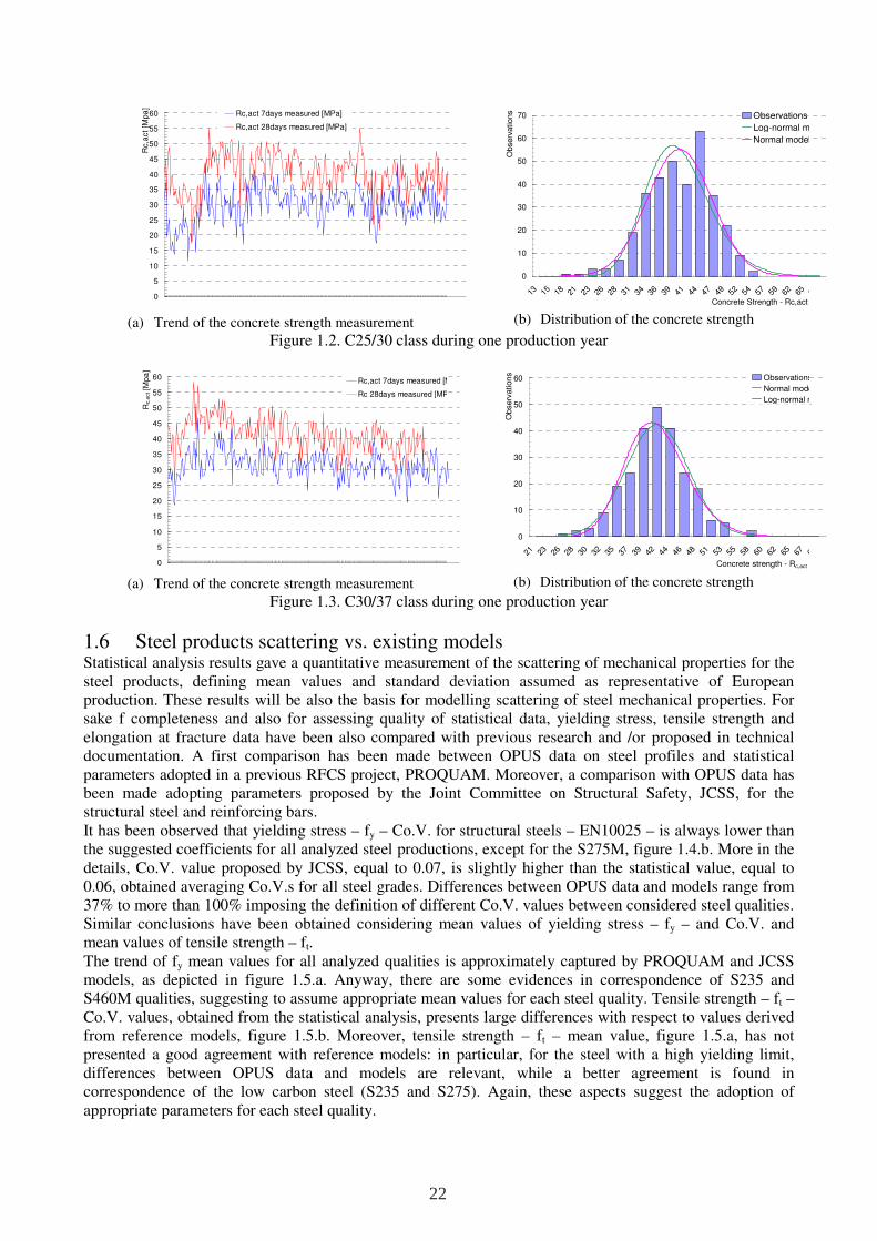
(a) Trend of the concrete strength measurement (b) Distribution of the concrete strength
Figure 1.2. C25/30 class during one production year
(a) Trend of the concrete strength measurement (b) Distribution of the concrete strength
Figure 1.3. C30/37 class during one production year
1.6 Steel products scattering vs. existing models Statistical analysis results gave a quantitative measurement of the scattering of mechanical properties for the steel products, defining mean values and standard deviation assumed as representative of European production. These results will be also the basis for modelling scattering of steel mechanical properties. For sake f completeness and also for assessing quality of statistical data, yielding stress, tensile strength and elongation at fracture data have been also compared with previous research and /or proposed in technical documentation. A first comparison has been made between OPUS data on steel profiles and statistical parameters adopted in a previous RFCS project, PROQUAM. Moreover, a comparison with OPUS data has been made adopting parameters proposed by the Joint Committee on Structural Safety, JCSS, for the structural steel and reinforcing bars. It has been observed that yielding stress – fy – Co.V. for structural steels – EN10025 – is always lower than the suggested coefficients for all analyzed steel productions, except for the S275M, figure 1.4.b. More in the details, Co.V. value proposed by JCSS, equal to 0.07, is slightly higher than the statistical value, equal to 0.06, obtained averaging Co.V.s for all steel grades. Differences between OPUS data and models range from 37% to more than 100% imposing the definition of different Co.V. values between considered steel qualities. Similar conclusions have been obtained considering mean values of yielding stress – fy – and Co.V. and mean values of tensile strength – ft. The trend of fy mean values for all analyzed qualities is approximately captured by PROQUAM and JCSS models, as depicted in figure 1.5.a. Anyway, there are some evidences in correspondence of S235 and S460M qualities, suggesting to assume appropriate mean values for each steel quality. Tensile strength – ft – Co.V. values, obtained from the statistical analysis, presents large differences with respect to values derived from reference models, figure 1.5.b. Moreover, tensile strength – ft – mean value, figure 1.5.a, has not presented a good agreement with reference models: in particular, for the steel with a high yielding limit, differences between OPUS data and models are relevant, while a better agreement is found in correspondence of the low carbon steel (S235 and S275). Again, these aspects suggest the adoption of appropriate parameters for each steel quality.
0
5
10
15
20
25
30
35
40
45
50
55
60
Rc,a
ct
[Mp
a]
Rc,act 7days measured [MPa]
Rc,act 28days measured [MPa]
0
10
20
30
40
50
60
70
13 15 18 21 23 26 28 31 34 36 39 41 44 47 49 52 54 57 59 62 65 67
Concrete Strength - Rc,act [MPa]
Observ
ations Observations
Log-normal model
Normal model
0
5
10
15
20
25
30
35
40
45
50
55
60
Rc,a
ct [
Mp
a]
Rc,act 7days measured [MPa]
Rc 28days measured [MPa]
0
10
20
30
40
50
60
21 23 26 28 30 32 35 37 39 42 44 46 48 51 53 55 58 60 62 65 67 69
Concrete strength - Rc,act [MPa]
Observ
ations Observations
Normal model
Log-normal model
22
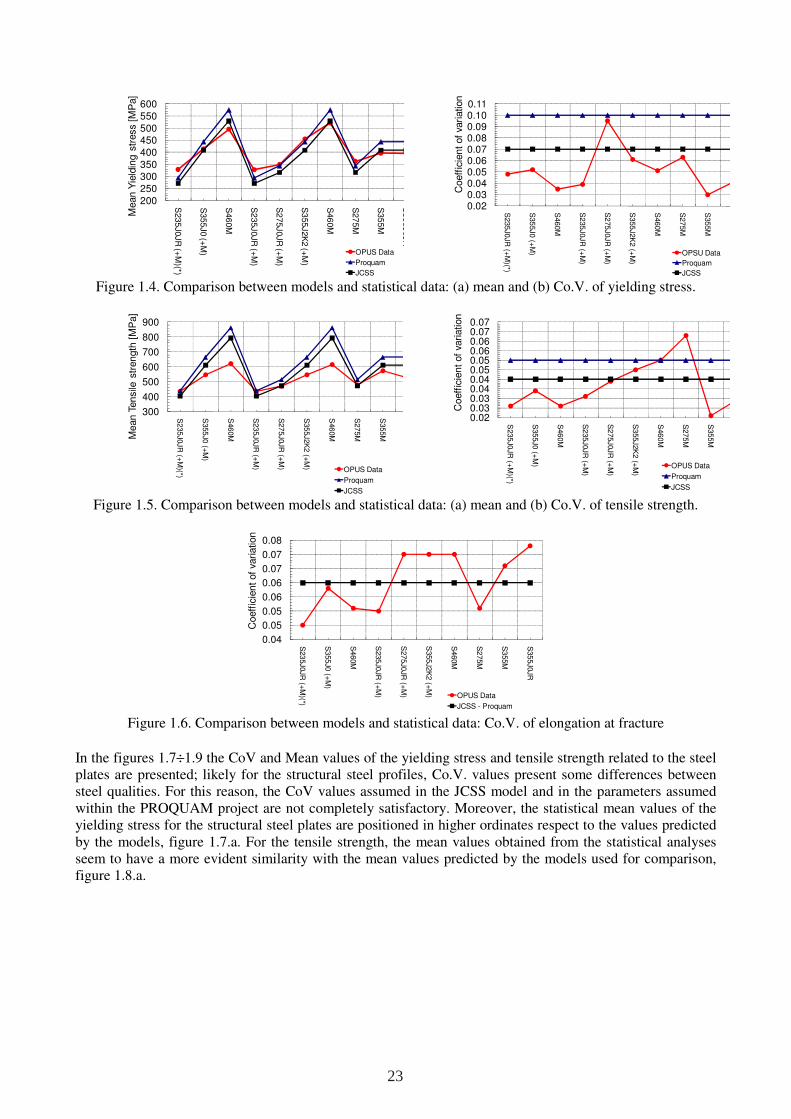
Figure 1.4. Comparison between models and statistical data: (a) mean and (b) Co.V. of yielding stress.
Figure 1.5. Comparison between models and statistical data: (a) mean and (b) Co.V. of tensile strength.
Figure 1.6. Comparison between models and statistical data: Co.V. of elongation at fracture
In the figures 1.7÷1.9 the CoV and Mean values of the yielding stress and tensile strength related to the steel plates are presented; likely for the structural steel profiles, Co.V. values present some differences between steel qualities. For this reason, the CoV values assumed in the JCSS model and in the parameters assumed within the PROQUAM project are not completely satisfactory. Moreover, the statistical mean values of the yielding stress for the structural steel plates are positioned in higher ordinates respect to the values predicted by the models, figure 1.7.a. For the tensile strength, the mean values obtained from the statistical analyses seem to have a more evident similarity with the mean values predicted by the models used for comparison, figure 1.8.a.
200250300350400450500550600
S235
J0JR
(+M
)(*)
S355
J0 (+
M)
S46
0M
S2
35J0JR
(+M
)
S2
75J0JR
(+M
)
S3
55J2K
2 (+
M)
S46
0M
S27
5M
S35
5M
S3
55J0JR
Mean
Yie
ldin
g s
tress [
MP
a]
OPUS Data
Proquam
JCSS
0.020.030.040.050.060.070.080.090.100.11
S235J0JR
(+M
)(*)
S355J0 (+
M)
S460M
S235J0JR
(+M
)
S275J0JR
(+M
)
S355J2K
2 (+
M)
S460M
S275M
S355M
S355J0JR
Coeff
icie
nt
of
vari
ation
OPSU Data
Proquam
JCSS
300
400
500
600
700
800
900
S235J0JR
(+M
)(*)
S355J0 (+
M)
S460M
S235J0JR
(+M
)
S275J0JR
(+M
)
S355J2K
2 (+
M)
S460M
S275M
S355MM
ean
Ten
sile
str
en
gth
[M
Pa]
OPUS Data
Proquam
JCSS
0.020.030.030.040.040.050.050.060.060.070.07
S235J0JR
(+M
)(*)
S355J0 (+
M)
S460M
S235J0JR
(+M
)
S275J0JR
(+M
)
S355J2K
2 (+
M)
S460M
S275M
S355M
Coeff
icie
nt
of
vari
ation
OPUS Data
Proquam
JCSS
0.04
0.05
0.05
0.06
0.06
0.07
0.07
0.08
S235J0JR
(+M
)(*)
S355J0 (+
M)
S460M
S235J0JR
(+M
)
S275J0JR
(+M
)
S355J2K
2 (+
M)
S460M
S275M
S355M
S355J0JR
Coeff
icie
nt
of
vari
ation
OPUS Data
JCSS - Proquam
23
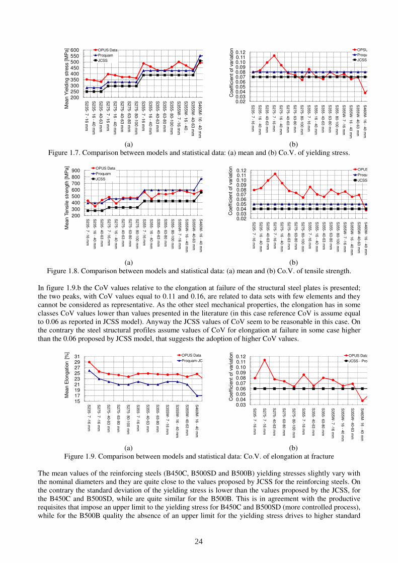
(a) (b) Figure 1.7. Comparison between models and statistical data: (a) mean and (b) Co.V. of yielding stress.
(a) (b) Figure 1.8. Comparison between models and statistical data: (a) mean and (b) Co.V. of tensile strength.
In figure 1.9.b the CoV values relative to the elongation at failure of the structural steel plates is presented; the two peaks, with CoV values equal to 0.11 and 0.16, are related to data sets with few elements and they cannot be considered as representative. As the other steel mechanical properties, the elongation has in some classes CoV values lower than values presented in the literature (in this case reference CoV is assume equal to 0.06 as reported in JCSS model). Anyway the JCSS values of CoV seem to be reasonable in this case. On the contrary the steel structural profiles assume values of CoV for elongation at failure in some case higher than the 0.06 proposed by JCSS model, that suggests the adoption of higher CoV values.
(a) (b) Figure 1.9. Comparison between models and statistical data: Co.V. of elongation at fracture
The mean values of the reinforcing steels (B450C, B500SD and B500B) yielding stresses slightly vary with the nominal diameters and they are quite close to the values proposed by JCSS for the reinforcing steels. On the contrary the standard deviation of the yielding stress is lower than the values proposed by the JCSS, for the B450C and B500SD, while are quite similar for the B500B. This is in agreement with the productive requisites that impose an upper limit to the yielding stress for B450C and B500SD (more controlled process), while for the B500B quality the absence of an upper limit for the yielding stress drives to higher standard
200250300350400450500550600
S2
35-
7 -1
6 m
m
S235
-16 -
40 m
m
S235
-40
-63 m
m
S2
75-
7 -1
6 m
m
S275
-16 -
40 m
m
S275
-40
-63 m
m
S275
-63
-80 m
m
S275
-80-1
00 m
m
S3
55-
7 -1
6 m
m
S355
-16 -
40 m
m
S355
-40
-63 m
m
S355
-63
-80 m
m
S355
-80-1
00 m
m
S35
5W
-7 -1
6 m
m
S35
5W
-1
6 -
40 …
S3
55W
-40-6
3 m
m
S460
M-16
-40 m
m
Mean
Yie
ldin
g s
tress [
MP
a] OPUS Data
Proquam
JCSS
0.020.030.040.050.060.070.080.090.100.110.12
S235-
7 -1
6 m
m
S235-
16 -
40 m
m
S235-
40-6
3 m
m
S275-
7 -1
6 m
m
S275-
16 -
40 m
m
S275-
40-6
3 m
m
S275-
63-8
0 m
m
S275-
80-1
00 m
m
S355-
7 -1
6 m
m
S355-
16 -
40 m
m
S355-
40-6
3 m
m
S355-
63-8
0 m
m
S355-
80-1
00 m
m
S355W
-7 -1
6 m
m
S355W
-16 -
40 m
m
S355W
-40-6
3 m
m
S460M
-16 -
40 m
m
Coeff
icie
nt
of
vari
ation OPSU Data
Proquam
JCSS
200
300
400
500
600
700
800
900
S235-
7 -1
6 m
m
S235-
16 -
40 m
m
S235-
40-6
3 m
m
S275-
7 -1
6 m
m
S275-
16 -
40 m
m
S275-
40-6
3 m
m
S275-
63-8
0 m
m
S275-
80-1
00 m
m
S355-
7 -1
6 m
m
S355-
16 -
40 m
m
S355-
40-6
3 m
m
S355-
63-8
0 m
m
S355-
80-1
00 m
m
S355W
-7 -1
6 m
m
S355W
-16 -
40 m
m
S355W
-40-6
3 m
m
S460M
-16 -
40 m
m
Mean
Ten
sile
str
en
gth
[M
Pa]
OPUS Data
Proquam
JCSS
0.020.030.040.050.060.070.080.090.100.110.12
S235-
7 -1
6 m
m
S235-
16 -
40 m
m
S235-
40-6
3 m
m
S275-
7 -1
6 m
m
S275-
16 -
40 m
m
S275-
40-6
3 m
m
S275-
63-8
0 m
m
S275-
80-1
00 m
m
S355-
7 -1
6 m
m
S355-
16 -
40 m
m
S355-
40-6
3 m
m
S355-
63-8
0 m
m
S355-
80-1
00 m
m
S355W
-7 -1
6 m
m
S355W
-16 -
40 m
m
S355W
-40-6
3 m
m
S460M
-16 -
40 m
m
Coeff
icie
nt
of
vari
ation OPUS Data
Proquam
JCSS
151719212325272931
S23
5-
7 -1
6 m
m
S27
5-
7 -1
6 m
m
S275
-40-6
3 m
m
S275
-63-8
0 m
m
S27
5-
80
-10
0 m
m
S35
5-
7 -1
6 m
m
S355
-40-6
3 m
m
S355
-63-8
0 m
m
S3
55W
-7 -1
6 m
m
S3
55W
-16
-4
0 m
m
S35
5W
-40-6
3 m
m
S46
0M
-16 -
40
mm
Mean
Elo
ngation
[%
]
OPUS Data
Proquam-JCSS
0.030.040.050.060.070.080.090.100.110.12
S235
-7 -1
6 m
m
S275
-7 -1
6 m
m
S275-
40-6
3 m
m
S275-
63-8
0 m
m
S275
-80-1
00
mm
S355
-7 -1
6 m
m
S355-
40-6
3 m
m
S355-
63-8
0 m
m
S35
5W
-7 -1
6 m
m
S35
5W
-16 -
40
mm
S355
W-
40-6
3 m
m
S460
M-
16 -
40
mm
Coeff
icie
nt
of
vari
ation OPUS Data
JCSS - Proquam
24
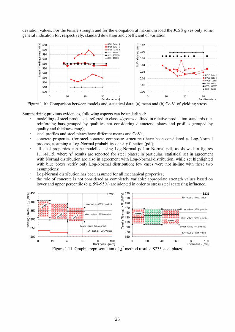
deviation values. For the tensile strength and for the elongation at maximum load the JCSS gives only some general indication for, respectively, standard deviation and coefficient of variation.
Figure 1.10. Comparison between models and statistical data: (a) mean and (b) Co.V. of yielding stress. Summarizing previous evidences, following aspects can be underlined:
modelling of steel products is referred to classes/groups defined in relative production standards (i.e. reinforcing bars grouped by qualities not considering diameters; plates and profiles grouped by quality and thickness rang);
steel profiles and steel plates have different means and CoVs; concrete properties (for steel-concrete composite structures) have been considered as Log-Normal
process, assuming a Log-Normal probability density function (pdf); all steel properties can be modelled using Log-Normal pdf or Normal pdf, as showed in figures
1.11÷1.15, where χ2 results are reported for steel plates; in particular, statistical set in agreement with Normal distribution are also in agreement with Log-Normal distribution, while set highlighted with blue boxes verify only Log-Normal distribution; few cases were not in-line with these two assumptions;
Log-Normal distribution has been assumed for all mechanical properties; the role of concrete is not considered as completely variable: appropriate strength values based on
lower and upper percentile (e.g. 5%-95%) are adopted in order to stress steel scattering influence.
Figure 1.11. Graphic representation of χ2 method results: S235 steel plates.
500
510
520
530
540
550
560
570
580
590
600
0 10 20 30 40
Me
an
-Y
ield
ing
str
ess
[MP
a]
Bar diameter - [mm]
OPUS Data - B
OPUS Data - S
OPUS - Data B
JCSS - B450C
JCSS - S500SD
JCSS - B500B
0.00
0.01
0.02
0.03
0.04
0.05
0.06
0.07
0 10 20 30
Co
V -
Yie
ldin
g s
tre
ss
Bar diameter - [mm]
OPUS Data - B
OPUS Data - S
OPUS - Data B
JCSS - B450C
JCSS - S500SD
JCSS - B500B
200
250
300
350
400
450
0 20 40 60 80 100
Yie
ldin
g S
tress -
Re
H[M
Pa]
Thickness - [mm]
S235
Mean values (50% quartile)
Upper values (95% quartile)
Lower values (5% quartile)
EN10025-2 - Min. Values
350
370
390
410
430
450
470
490
510
530
0 20 40 60 80 100
Ten
sile
Str
en
gth
-R
m[M
Pa]
Thickness - [mm]
S235
Mean values (50% quartile)
Upper values (95% quartile)
Lower values (5% quartile)
EN10025-2 - Min. Value
EN10025-2 - Max. Value
Normal
Normal
25
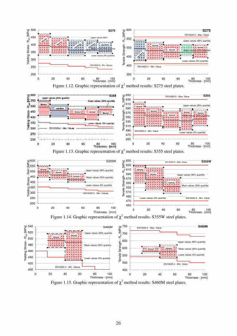
Figure 1.12. Graphic representation of χ2 method results: S275 steel plates.
Figure 1.13. Graphic representation of χ2 method results: S355 steel plates.
Figure 1.14. Graphic representation of χ2 method results: S355W steel plates.
Figure 1.15. Graphic representation of χ2 method results: S460M steel plates.
200
250
300
350
400
450
500
0 20 40 60 80 100
Yie
ldin
g S
tress
-R
eH
[MP
a]
Thickness - [mm]
S275
Mean values (50% quartile)
Upper values (95%
Lower values (5% quartile)
EN10025-2 - Min. Values
Log-Norm
350
400
450
500
550
600
0 20 40 60 80 100
Ten
sile
Str
en
gth
-R
m[M
Pa]
Thickness - [mm]
S275
Mean values (50% quartile)
Upper values (95% quartile)
Lower values (5% quartile)
EN10025-2 - Min. Value
EN10025-2 - Max. Value
Normal
Normal
Normal
450
470
490
510
530
550
570
590
610
630
650
0 20 40 60 80 100
Ten
sile
Str
en
gth
-R
m[M
Pa]
Thickness - [mm]
S355
Mean values (50% quartile)
Upper values (95% quartile)
Lower values (5% quartile)EN10025-2 - Min. Value
EN10025-2 - Max. Value
Normal
Normal
Normal
NormalNormal
200
250
300
350
400
450
500
550
600
0 20 40 60 80 100
Yie
ldin
g S
tress -
ReH
[M
Pa]
Thickness - [mm]
S355W
Mean values (50% quartile)
Upper values (95% quartile)
Lower values (5% quartile)
EN10025-5 - Min. Values
Normal
Normal
Normal
450
470
490
510
530
550
570
590
610
630
650
0 20 40 60 80 100
Ten
sile
Str
en
gth
-R
m[M
Pa]
Thickness - [mm]
S355W
Mean values (50% quartile)
Upper values (95% quartile)
Lower values (5% quartile) EN10025-5 - Min. Value
EN10025-5 - Max. Value
Normal
Normal
Normal
400
420
440
460
480
500
520
540
0 20 40 60 80 100
Yie
ldin
g S
tress
-R
eH
[MP
a]
Thickness - [mm]
S460M
Mean values (50% quartile)
Upper values (95% quartile)
Lower values (5% quartile)
EN10025-4 - Min. Values
NormalNormal
450
500
550
600
650
700
750
0 20 40 60 80 100
Ten
sile
Str
en
gth
-R
m[M
Pa]
Thickness - [mm]
S460M
Mean values (50% quartile)
Upper values (95% quartile)
Lower values (5% quartile)
EN10025-4 - Min. Value
EN10025-4 - Max. Value
Normal Normal
26
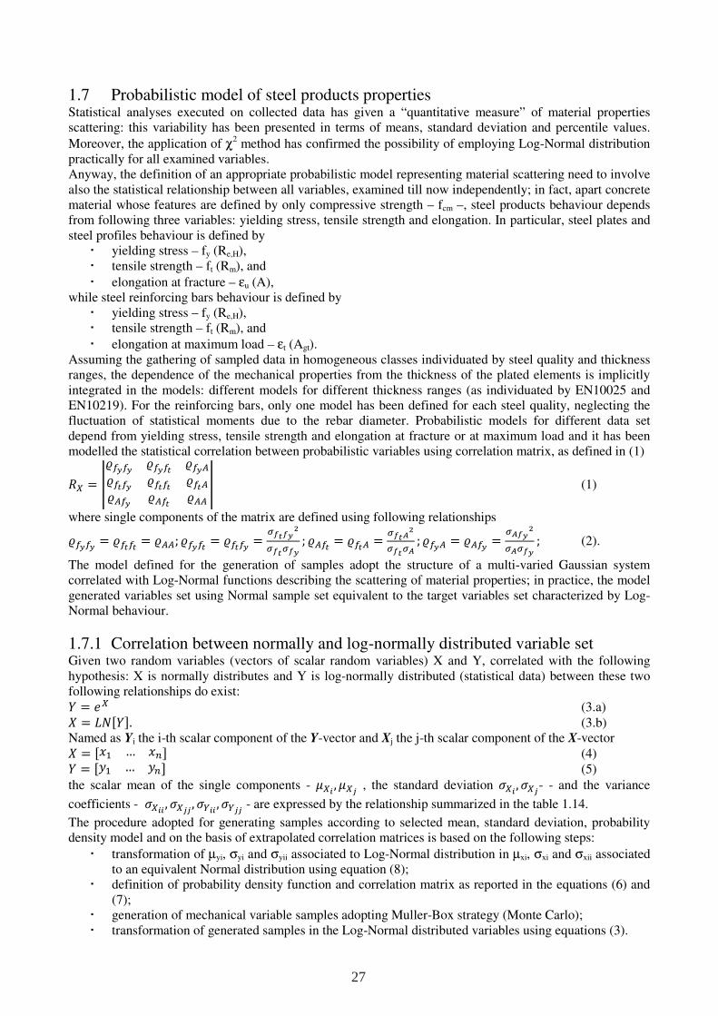
1.7 Probabilistic model of steel products properties Statistical analyses executed on collected data has given a “quantitative measure” of material properties scattering: this variability has been presented in terms of means, standard deviation and percentile values.
Moreover, the application of χ2 method has confirmed the possibility of employing Log-Normal distribution practically for all examined variables. Anyway, the definition of an appropriate probabilistic model representing material scattering need to involve also the statistical relationship between all variables, examined till now independently; in fact, apart concrete material whose features are defined by only compressive strength – fcm –, steel products behaviour depends from following three variables: yielding stress, tensile strength and elongation. In particular, steel plates and steel profiles behaviour is defined by
yielding stress – fy (Re,H), tensile strength – ft (Rm), and
elongation at fracture – εu (A), while steel reinforcing bars behaviour is defined by
yielding stress – fy (Re,H), tensile strength – ft (Rm), and
elongation at maximum load – εt (Agt). Assuming the gathering of sampled data in homogeneous classes individuated by steel quality and thickness ranges, the dependence of the mechanical properties from the thickness of the plated elements is implicitly integrated in the models: different models for different thickness ranges (as individuated by EN10025 and EN10219). For the reinforcing bars, only one model has been defined for each steel quality, neglecting the fluctuation of statistical moments due to the rebar diameter. Probabilistic models for different data set depend from yielding stress, tensile strength and elongation at fracture or at maximum load and it has been modelled the statistical correlation between probabilistic variables using correlation matrix, as defined in (1)
= (1)
where single components of the matrix are defined using following relationships = = ; = = ; = = ; = = ; (2).
The model defined for the generation of samples adopt the structure of a multi-varied Gaussian system correlated with Log-Normal functions describing the scattering of material properties; in practice, the model generated variables set using Normal sample set equivalent to the target variables set characterized by Log-Normal behaviour.
1.7.1 Correlation between normally and log-normally distributed variable set Given two random variables (vectors of scalar random variables) X and Y, correlated with the following hypothesis: X is normally distributes and Y is log-normally distributed (statistical data) between these two following relationships do exist: = (3.a) = . (3.b) Named as Yi the i-th scalar component of the Y-vector and Xj the j-th scalar component of the X-vector = … (4) = … (5)
the scalar mean of the single components - ! , # , the standard deviation $! , $#- - and the variance
coefficients - $!! , $## , $%!! , $%## - are expressed by the relationship summarized in the table 1.14.
The procedure adopted for generating samples according to selected mean, standard deviation, probability density model and on the basis of extrapolated correlation matrices is based on the following steps:
transformation of µyi, σyi and σyii associated to Log-Normal distribution in µxi, σxi and σxii associated to an equivalent Normal distribution using equation (8);
definition of probability density function and correlation matrix as reported in the equations (6) and (7);
generation of mechanical variable samples adopting Muller-Box strategy (Monte Carlo); transformation of generated samples in the Log-Normal distributed variables using equations (3).
27
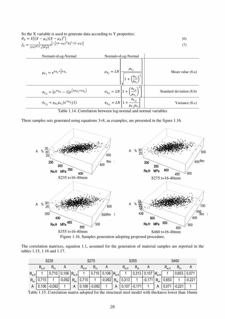
So the X variable is used to generate data according to Y properties: = &' − )' − )* (6) = '+,)- ⁄ /‖12‖ 345'462)71285'462)9 (7)
Normal↔Log-Normal Normal↔Log-Normal
%! = 62!:+2! ! = ;<<<<= %!>1 + A$%! %!B
+CDDDDE Mean value (8.a)
$%!! = 2!! − 1F+62!:2!G $!! = H1 + I$%!! %!J+K Standard deviation (8.b)
$%!# = ! %!'2!!L1) $!# = M1 + $%!# %# %!N Variance (8.c)
Table 1.14. Correlation between log-normal and normal variables Three samples sets generated using equations 3÷8, as examples, are presented in the figure 1.16.
S235 t=16-40mm S275 t=16-40mm
S355 t=16-40mm S460 t=16-40mm Figure 1.16. Samples generation adopting proposed procedure.
The correlation matrixes, equation 1.1, assumed for the generation of material samples are reported in the tables 1.15, 1.16 and 1.17.
Table 1.15. Correlation matrix adopted for the structural steel model with thickness lower than 16mm
250300
350400
Re,HMPa400
450
RmMPa
253035
A%250
300350
400Re,HMPa
300350
400450
Re,HMPa400
450
500
RmMPa
2530A%
300350
400450
Re,HMPa
350
400
450
500Re,HMPa 500
550
600
RmMPa
2530A%350
400
450
500Re,HMPa
450
500
550
600Re,HMPa 550
600
650
700
RmMPa
1618202224
A%450
500
550
600Re,HMPa
Re,H Rm A Re,H Rm A Re,H Rm A Re,H Rm A
Re,H 1 0,710 0,106 Re,H 1 0,710 0,106 Re,H 1 0,313 0,107 Re,H 1 0,653 0,071
Rm 0,710 1 -0,092 Rm 0,710 1 -0,092 Rm 0,313 1 -0,171 Rm 0,653 1 -0,221
A 0,106 -0,092 1 A 0,106 -0,092 1 A 0,107 -0,171 1 A 0,071 -0,221 1
S235 S275 S355 S460
28
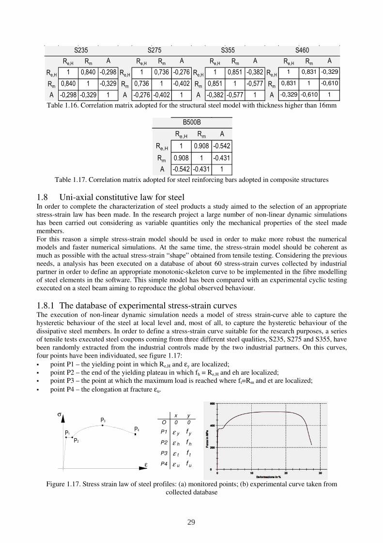
Table 1.16. Correlation matrix adopted for the structural steel model with thickness higher than 16mm
Table 1.17. Correlation matrix adopted for steel reinforcing bars adopted in composite structures
1.8 Uni-axial constitutive law for steel In order to complete the characterization of steel products a study aimed to the selection of an appropriate stress-strain law has been made. In the research project a large number of non-linear dynamic simulations has been carried out considering as variable quantities only the mechanical properties of the steel made members. For this reason a simple stress-strain model should be used in order to make more robust the numerical models and faster numerical simulations. At the same time, the stress-strain model should be coherent as much as possible with the actual stress-strain “shape” obtained from tensile testing. Considering the previous needs, a analysis has been executed on a database of about 60 stress-strain curves collected by industrial partner in order to define an appropriate monotonic-skeleton curve to be implemented in the fibre modelling of steel elements in the software. This simple model has been compared with an experimental cyclic testing executed on a steel beam aiming to reproduce the global observed behaviour.
1.8.1 The database of experimental stress-strain curves The execution of non-linear dynamic simulation needs a model of stress strain-curve able to capture the hysteretic behaviour of the steel at local level and, most of all, to capture the hysteretic behaviour of the dissipative steel members. In order to define a stress-strain curve suitable for the research purposes, a series of tensile tests executed steel coupons coming from three different steel qualities, S235, S275 and S355, have been randomly extracted from the industrial controls made by the two industrial partners. On this curves, four points have been individuated, see figure 1.17:
point P1 – the yielding point in which Re,H and εy are localized; point P2 – the end of the yielding plateau in which fh = Re,H and eh are localized; point P3 – the point at which the maximum load is reached where ft=Rm and et are localized;
point P4 – the elongation at fracture εu.
Figure 1.17. Stress strain law of steel profiles: (a) monitored points; (b) experimental curve taken from
collected database
Re,H Rm A Re,H Rm A Re,H Rm A Re,H Rm A
Re,H 1 0,840 -0,298 Re,H 1 0,736 -0,276 Re,H 1 0,851 -0,382 Re,H1 0,831 -0,329
Rm 0,840 1 -0,329 Rm 0,736 1 -0,402 Rm 0,851 1 -0,577 Rm0,831 1 -0,610
A -0,298 -0,329 1 A -0,276 -0,402 1 A -0,382 -0,577 1 A -0,329 -0,610 1
S355 S460S235 S275
Re,H Rm A
Re,H 1 0.908 -0.542
Rm 0.908 1 -0.431
A -0.542 -0.431 1
B500B
ε
σ
P1
P2
P3
P4
x y
O 0 0
P1 ε y f y
P2 ε h f h
P3 ε t f t
P4 ε u f u
29
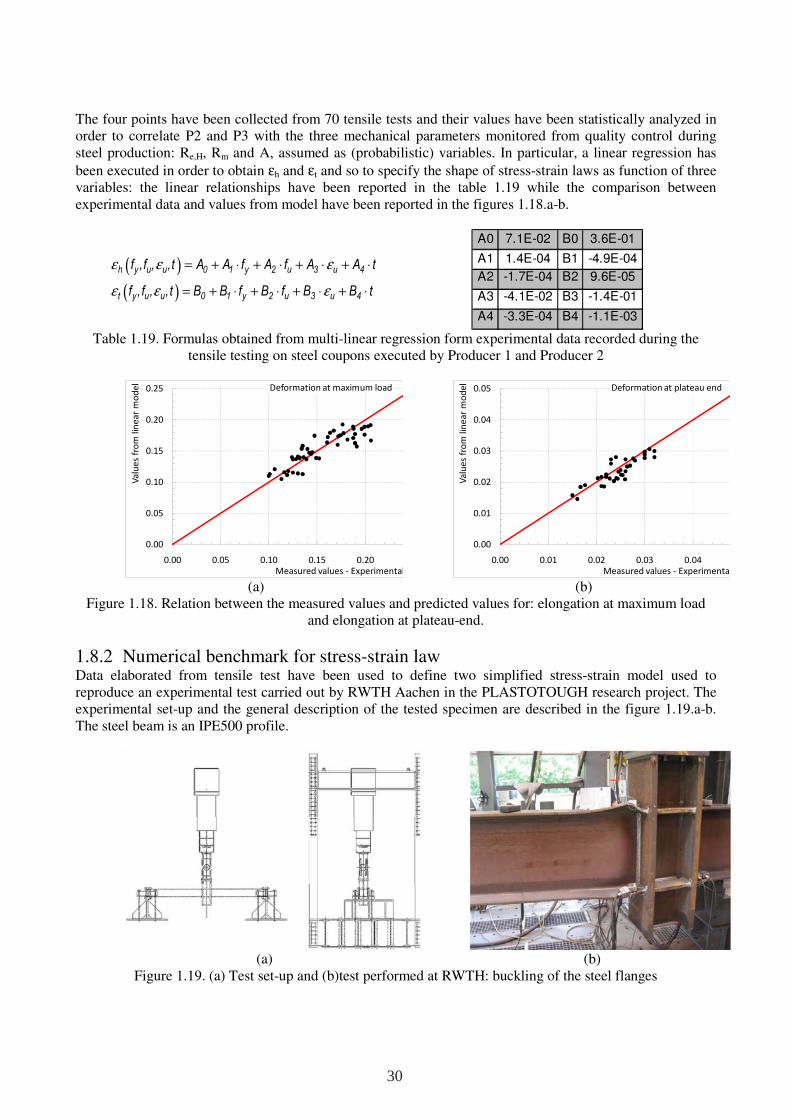
The four points have been collected from 70 tensile tests and their values have been statistically analyzed in order to correlate P2 and P3 with the three mechanical parameters monitored from quality control during steel production: Re,H, Rm and A, assumed as (probabilistic) variables. In particular, a linear regression has
been executed in order to obtain εh and εt and so to specify the shape of stress-strain laws as function of three variables: the linear relationships have been reported in the table 1.19 while the comparison between experimental data and values from model have been reported in the figures 1.18.a-b.
( )
( )
ε ε ε
ε ε ε
= + ⋅ + ⋅ + ⋅ + ⋅
= + ⋅ + ⋅ + ⋅ + ⋅
h y u u 0 1 y 2 u 3 u 4
t y u u 0 1 y 2 u 3 u 4
f ,f , ,t A A f A f A A t
f ,f , ,t B B f B f B B t
Table 1.19. Formulas obtained from multi-linear regression form experimental data recorded during the
tensile testing on steel coupons executed by Producer 1 and Producer 2
(a) (b) Figure 1.18. Relation between the measured values and predicted values for: elongation at maximum load
and elongation at plateau-end.
1.8.2 Numerical benchmark for stress-strain law Data elaborated from tensile test have been used to define two simplified stress-strain model used to reproduce an experimental test carried out by RWTH Aachen in the PLASTOTOUGH research project. The experimental set-up and the general description of the tested specimen are described in the figure 1.19.a-b. The steel beam is an IPE500 profile.
(a) (b) Figure 1.19. (a) Test set-up and (b)test performed at RWTH: buckling of the steel flanges
A0 7.1E-02 B0 3.6E-01
A1 1.4E-04 B1 -4.9E-04
A2 -1.7E-04 B2 9.6E-05
A3 -4.1E-02 B3 -1.4E-01
A4 -3.3E-04 B4 -1.1E-03
0.00
0.05
0.10
0.15
0.20
0.25
0.00 0.05 0.10 0.15 0.20
Va
lue
s fr
om
lin
ea
r m
od
el
Measured values - Experimental tests
Deformation at maximum load
0.00
0.01
0.02
0.03
0.04
0.05
0.00 0.01 0.02 0.03 0.04
Va
lue
s fr
om
lin
ea
r m
od
el
Measured values - Experimental tests
Deformation at plateau end
30
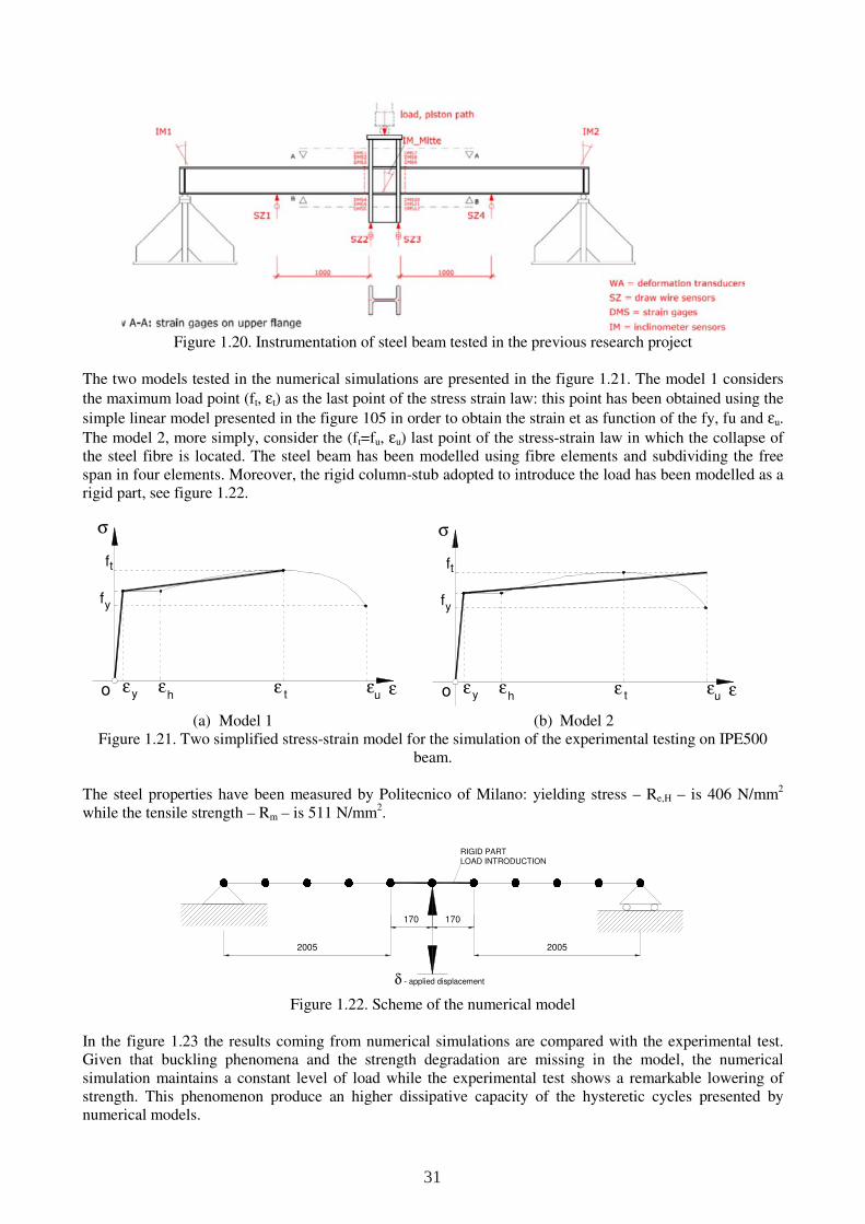
Figure 1.20. Instrumentation of steel beam tested in the previous research project
The two models tested in the numerical simulations are presented in the figure 1.21. The model 1 considers
the maximum load point (ft, εt) as the last point of the stress strain law: this point has been obtained using the
simple linear model presented in the figure 105 in order to obtain the strain et as function of the fy, fu and εu.
The model 2, more simply, consider the (ft=fu, εu) last point of the stress-strain law in which the collapse of the steel fibre is located. The steel beam has been modelled using fibre elements and subdividing the free span in four elements. Moreover, the rigid column-stub adopted to introduce the load has been modelled as a rigid part, see figure 1.22.
(a) Model 1 (b) Model 2
Figure 1.21. Two simplified stress-strain model for the simulation of the experimental testing on IPE500 beam.
The steel properties have been measured by Politecnico of Milano: yielding stress – Re,H – is 406 N/mm2 while the tensile strength – Rm – is 511 N/mm2.
Figure 1.22. Scheme of the numerical model
In the figure 1.23 the results coming from numerical simulations are compared with the experimental test. Given that buckling phenomena and the strength degradation are missing in the model, the numerical simulation maintains a constant level of load while the experimental test shows a remarkable lowering of strength. This phenomenon produce an higher dissipative capacity of the hysteretic cycles presented by numerical models.
o ε
σ
ε ε εyεh t u
fy
ft tf
yf
uthεy εεε
σ
εo
170 170
2005 2005
RIGID PARTLOAD INTRODUCTION
δ - applied displacement
31
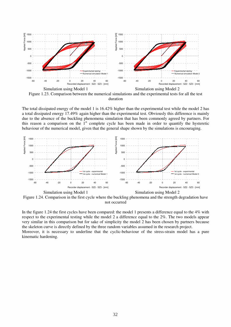
Simulation using Model 1 Simulation using Model 2
Figure 1.23. Comparison between the numerical simulations and the experimental tests for all the test duration
The total dissipated energy of the model 1 is 16.42% higher than the experimental test while the model 2 has a total dissipated energy 17.49% again higher than the experimental test. Obviously this difference is mainly due to the absence of the buckling phenomena simulation that has been commonly agreed by partners. For this reason a comparison on the 1st complete cycle has been made in order to quantify the hysteretic behaviour of the numerical model, given that the general shape shown by the simulations is encouraging.
Simulation using Model 1 Simulation using Model 2
Figure 1.24. Comparison in the first cycle where the buckling phenomena and the strength degradation have not occurred
In the figure 1.24 the first cycles have been compared: the model 1 presents a difference equal to the 4% with respect to the experimental testing while the model 2 a difference equal to the 2%. The two models appear very similar in this comparison but for sake of simplicity the model 2 has been chosen by partners because the skeleton curve is directly defined by the three random variables assumed in the research project. Moreover, it is necessary to underline that the cyclic-behaviour of the stress-strain model has a pure kinematic hardening.
-1500
-1000
-500
0
500
1000
1500
-60 -40 -20 0 20 40 60
Recorded displacement - SZ2 - SZ3 - [mm]
Ap
plie
d F
orc
e [
kN
]
Experimental testing
Numerical simulation Model 1
-1500
-1000
-500
0
500
1000
1500
-60 -40 -20 0 20 40 60
Recorded displacement - SZ2 - SZ3 - [mm]
Ap
plie
d F
orc
e [
kN
]
Experimental testing
Numerical simulation Model 2
-1500
-1000
-500
0
500
1000
1500
-60 -40 -20 0 20 40 60
Recorder displacement - SZ2 - SZ3 - [mm]
Ap
plie
d F
orc
e [
kN
]
1st cycle - experimental
1st cycle - numerical Model 1
-1500
-1000
-500
0
500
1000
1500
-60 -40 -20 0 20 40 60
Recorder displacement - SZ2 - SZ3 - [mm]
Ap
plie
d F
orc
e [
kN
]
1st cycle - experimental
1st cycle - numerical Model 2
32
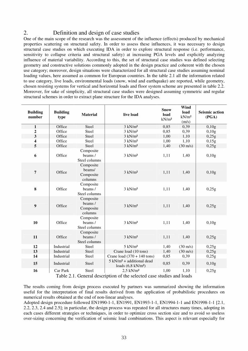
2. Definition and design of case studies One of the main scope of the research was the assessment of the influence (effects) produced by mechanical properties scattering on structural safety. In order to assess these influences, it was necessary to design structural case studies on which executing IDA in order to explore structural response (i.e. performance, sensitivity to collapse criteria and structural safety) at increasing PGA levels and explicitly analyzing influence of material variability. According to this, the set of structural case studies was defined selecting geometry and constructive solutions commonly adopted in the design practice and coherent with the chosen use category; moreover, design situations were characterized for all structural case studies assuming nominal loading values, here assumed as common for European countries. In the table 2.1 all the information related to use category, live loads, environmental loads (snow, wind and earthquake) are reported, while geometry, chosen resisting systems for vertical and horizontal loads and floor system scheme are presented in table 2.2. Moreover, for sake of simplicity, all structural case studies were designed assuming symmetric and regular structural schemes in order to extract plane structure for the IDA analyses.
Building
number
Building
type Material live load
Snow
load
kN/m²
Wind
load
kN/m² (m/s)
Seismic action
(PGA)
1 Office Steel 3 kN/m² 0,85 0,39 0,10g 2 Office Steel 3 kN/m² 0,85 0,39 0,10g 3 Office Steel 3 kN/m² 1,00 1,10 0,25g 4 Office Steel 3 kN/m² 1,00 1,10 0,15g 5 Office Steel 3 kN/m² 1,40 (30 m/s) 0,25g
6 Office Composite
beams / Steel columns
3 kN/m² 1,11 1,40 0,10g
7 Office
Composite beams/
Composite columns
3 kN/m² 1,11 1,40 0,10g
8 Office Composite
beams / Steel columns
3 kN/m² 1,11 1,40 0,25g
9 Office
Composite beams /
Composite columns
3 kN/m² 1,11 1,40 0,25g
10 Office Composite
beams / Steel columns
3 kN/m² 1,11 1,40 0,10g
11 Office Composite
beams / Steel columns
3 kN/m² 1,11 1,40 0,25g
12 Industrial Steel 5 kN/m² 1,40 (30 m/s) 0,25g 13 Industrial Steel Crane load (10 tons) 1,40 (30 m/s) 0,25g 14 Industrial Steel Crane load (370 + 140 tons) 0,85 0,39 0,25g
15 Industrial Steel 5 kN/m² + additional dead
loads (6,8 kN/m²) 0,85 0,39 0,10g
16 Car Park Steel 2,5 kN/m² 1,00 1,10 0,25g
Table 2.1. General description of the selected case studies and loads The results coming from design process executed by partners was summarized showing the information useful for the interpretation of final results derived from the application of probabilistic procedures on numerical results obtained at the end of non-linear analyses. Adopted design procedure followed EN1990-1-1, EN1991, EN1993-1-1, EN1994-1-1 and EN1998-1-1 [2.1, 2.2, 2.3, 2.4 and 2.5]; in particular, the design process was repeated for all structures many times, adopting in each cases different strategies or techniques, in order to optimize cross section size and to avoid so useless over-sizing concerning the verification of seismic load combinations. This aspect is relevant especially for
33
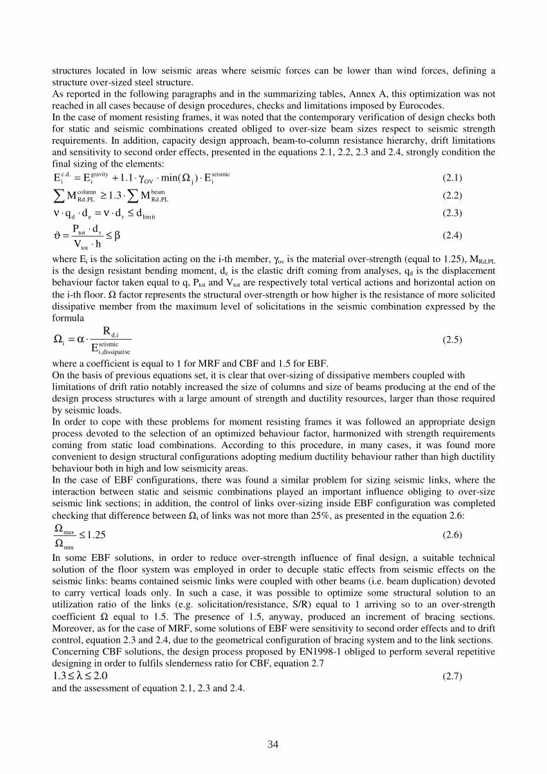
structures located in low seismic areas where seismic forces can be lower than wind forces, defining a structure over-sized steel structure. As reported in the following paragraphs and in the summarizing tables, Annex A, this optimization was not reached in all cases because of design procedures, checks and limitations imposed by Eurocodes. In the case of moment resisting frames, it was noted that the contemporary verification of design checks both for static and seismic combinations created obliged to over-size beam sizes respect to seismic strength requirements. In addition, capacity design approach, beam-to-column resistance hierarchy, drift limitations and sensitivity to second order effects, presented in the equations 2.1, 2.2, 2.3 and 2.4, strongly condition the final sizing of the elements:
seismic
ijOV
gravity
i
.d.c
i E)min(1.1EE ⋅Ω⋅γ⋅+= (2.1)
∑∑ ⋅≥ beam
PL,Rd
column
PL,Rd M3.1M (2.2)
itlimred dddq ≤⋅ν=⋅⋅ν (2.3)
β≤⋅
⋅=ϑ
hV
dP
tot
rtot (2.4)
where Ei is the solicitation acting on the i-th member, γov is the material over-strength (equal to 1.25), MRd,PL is the design resistant bending moment, de is the elastic drift coming from analyses, qd is the displacement behaviour factor taken equal to q, Ptot and Vtot are respectively total vertical actions and horizontal action on
the i-th floor. Ω factor represents the structural over-strength or how higher is the resistance of more solicited dissipative member from the maximum level of solicitations in the seismic combination expressed by the formula
seismicedissipativ,i
i,d
iE
R⋅α=Ω (2.5)
where a coefficient is equal to 1 for MRF and CBF and 1.5 for EBF. On the basis of previous equations set, it is clear that over-sizing of dissipative members coupled with limitations of drift ratio notably increased the size of columns and size of beams producing at the end of the design process structures with a large amount of strength and ductility resources, larger than those required by seismic loads. In order to cope with these problems for moment resisting frames it was followed an appropriate design process devoted to the selection of an optimized behaviour factor, harmonized with strength requirements coming from static load combinations. According to this procedure, in many cases, it was found more convenient to design structural configurations adopting medium ductility behaviour rather than high ductility behaviour both in high and low seismicity areas. In the case of EBF configurations, there was found a similar problem for sizing seismic links, where the interaction between static and seismic combinations played an important influence obliging to over-size seismic link sections; in addition, the control of links over-sizing inside EBF configuration was completed
checking that difference between Ωi of links was not more than 25%, as presented in the equation 2.6:
25.1min
max ≤Ω
Ω (2.6)
In some EBF solutions, in order to reduce over-strength influence of final design, a suitable technical solution of the floor system was employed in order to decuple static effects from seismic effects on the seismic links: beams contained seismic links were coupled with other beams (i.e. beam duplication) devoted to carry vertical loads only. In such a case, it was possible to optimize some structural solution to an utilization ratio of the links (e.g. solicitation/resistance, S/R) equal to 1 arriving so to an over-strength
coefficient Ω equal to 1.5. The presence of 1.5, anyway, produced an increment of bracing sections. Moreover, as for the case of MRF, some solutions of EBF were sensitivity to second order effects and to drift control, equation 2.3 and 2.4, due to the geometrical configuration of bracing system and to the link sections. Concerning CBF solutions, the design process proposed by EN1998-1 obliged to perform several repetitive designing in order to fulfils slenderness ratio for CBF, equation 2.7
0.23.1 ≤λ≤ (2.7) and the assessment of equation 2.1, 2.3 and 2.4.
34
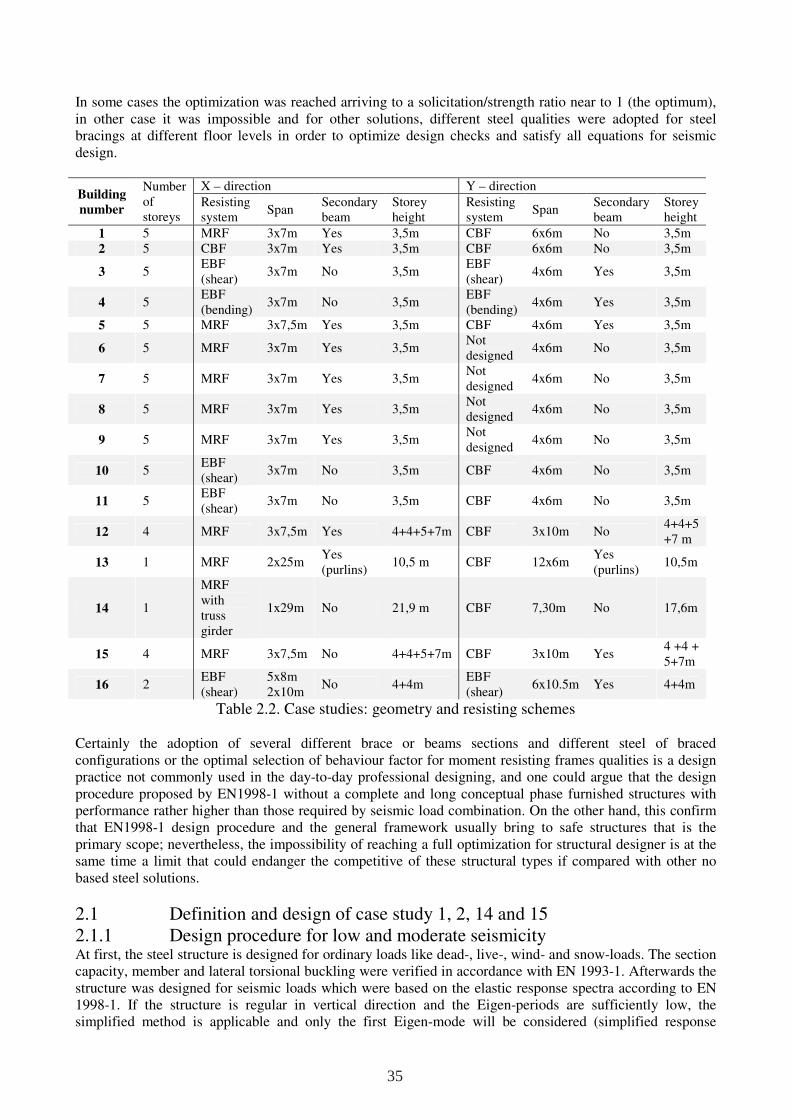
In some cases the optimization was reached arriving to a solicitation/strength ratio near to 1 (the optimum), in other case it was impossible and for other solutions, different steel qualities were adopted for steel bracings at different floor levels in order to optimize design checks and satisfy all equations for seismic design.
Building
number
Number of storeys
X – direction Y – direction
Resisting system
Span Secondary beam
Storey height
Resisting system
Span Secondary beam
Storey height
1 5 MRF 3x7m Yes 3,5m CBF 6x6m No 3,5m 2 5 CBF 3x7m Yes 3,5m CBF 6x6m No 3,5m
3 5 EBF (shear)
3x7m No 3,5m EBF (shear)
4x6m Yes 3,5m
4 5 EBF (bending)
3x7m No 3,5m EBF (bending)
4x6m Yes 3,5m
5 5 MRF 3x7,5m Yes 3,5m CBF 4x6m Yes 3,5m
6 5 MRF 3x7m Yes 3,5m Not designed
4x6m No 3,5m
7 5 MRF 3x7m Yes 3,5m Not designed
4x6m No 3,5m
8 5 MRF 3x7m Yes 3,5m Not designed
4x6m No 3,5m
9 5 MRF 3x7m Yes 3,5m Not designed
4x6m No 3,5m
10 5 EBF (shear)
3x7m No 3,5m CBF 4x6m No 3,5m
11 5 EBF (shear)
3x7m No 3,5m CBF 4x6m No 3,5m
12 4 MRF 3x7,5m Yes 4+4+5+7m CBF 3x10m No 4+4+5 +7 m
13 1 MRF 2x25m Yes (purlins)
10,5 m CBF 12x6m Yes (purlins)
10,5m
14 1
MRF with truss girder
1x29m No 21,9 m CBF 7,30m No 17,6m
15 4 MRF 3x7,5m No 4+4+5+7m CBF 3x10m Yes 4 +4 + 5+7m
16 2 EBF (shear)
5x8m 2x10m
No 4+4m EBF (shear)
6x10.5m Yes 4+4m
Table 2.2. Case studies: geometry and resisting schemes Certainly the adoption of several different brace or beams sections and different steel of braced configurations or the optimal selection of behaviour factor for moment resisting frames qualities is a design practice not commonly used in the day-to-day professional designing, and one could argue that the design procedure proposed by EN1998-1 without a complete and long conceptual phase furnished structures with performance rather higher than those required by seismic load combination. On the other hand, this confirm that EN1998-1 design procedure and the general framework usually bring to safe structures that is the primary scope; nevertheless, the impossibility of reaching a full optimization for structural designer is at the same time a limit that could endanger the competitive of these structural types if compared with other no based steel solutions.
2.1 Definition and design of case study 1, 2, 14 and 15 2.1.1 Design procedure for low and moderate seismicity
At first, the steel structure is designed for ordinary loads like dead-, live-, wind- and snow-loads. The section capacity, member and lateral torsional buckling were verified in accordance with EN 1993-1. Afterwards the structure was designed for seismic loads which were based on the elastic response spectra according to EN 1998-1. If the structure is regular in vertical direction and the Eigen-periods are sufficiently low, the simplified method is applicable and only the first Eigen-mode will be considered (simplified response
35
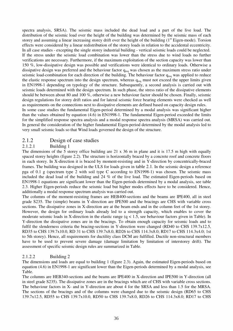
spectra analysis, SRSA). The seismic mass included the dead load and a part of the live load. The distribution of the seismic load over the height of the building was determined by the seismic mass of each storey and assuming a linear increasing storey drift over the height of the building (1st Eigen-mode). Torsion effects were considered by a linear redistribution of the storey loads in relation to the accidental eccentricity. In all case studies - excepting the single storey industrial building - vertical seismic loads could be neglected. If the stress under the seismic load combination was lower than the stress due to wind loads no further verifications are necessary. Furthermore, if the maximum exploitation of the section capacity was lower than 150 %, low-dissipative design was possible and verifications were identical to ordinary loads. Otherwise a dissipative design was preferred and the behaviour factor qreq was chosen as the maximum stress ratio under seismic load-combination for each direction of the building. The behaviour factor qreq was applied to reduce the elastic response spectrum into the design spectrum, whereas qreq must not exceed the upper limits given in EN1998-1 depending on typology of the structure. Subsequently, a second analysis is carried out with seismic loads determined with the design spectrum. In such phase, the stress ratio of the dissipative elements should be between about 80 and 100 %, otherwise a new behaviour factor should be chosen. Finally, seismic design regulations for storey drift ratios and for lateral seismic force bearing elements were checked as well as requirements on the connections next to dissipative elements are defined based on capacity design rules. In some case studies the fundamental Eigen-period determined by a modal analysis was significant higher than the values obtained by equation (4.6) in EN1998-1. The fundamental Eigen-period exceeded the limits for the simplified response spectra analysis and a modal response spectra analysis (MRSA) was carried out. In general the consideration of the higher fundamental Eigen-period determined by the modal analysis led to very small seismic loads so that Wind loads governed the design of the structure.
2.1.2 Design of case studies 2.1.2.1 Building 1 The dimensions of the 5 storey office building are 21 x 36 m in plane and it is 17.5 m high with equally spaced storey heights (figure 2.2). The structure is horizontally braced by a concrete roof and concrete floors in each storey. In X-direction it is braced by moment-resisting and in Y-direction by concentrically-braced
frames. The building was designed in the ULS for loads given in table 2.1. In the seismic design a reference pga of 0.1 g (spectrum type 2 with soil type C according to EN1998-1) was chosen. The seismic mass included the dead load of the building and 24 % of the live load. The estimated Eigen-periods based on EN1998-1 equations are significant lower than the Eigen-periods determined by a modal analysis, see table 2.3. Higher Eigen-periods reduce the seismic load but higher modes effects have to be considered. Hence, additionally a modal response spectrum analysis was carried out. The columns of the moment-resisting frames are HEB400-sections and the beams are IPE400, all in steel grade S235. The (simple) beams in Y-direction are IPE500 and the bracings are CHS with variable cross sections. The dissipative zones in X-direction are at the beam ends and in the column feet of the 1st storey. However, the design for ordinary loads already led to a strength capacity, which enables to cover the moderate seismic loads in X-direction in the elastic range (q < 1.5, see behaviour factors given in Table). In Y-direction the dissipative zones are in the bracings. To obtain enough capacity for seismic loads and to fulfil the slenderness criteria the bracing-sections in Y-direction were changed (RD40 to CHS 139.7x12.5, RD35 to CHS 139.7x10.0, RD 31 to CHS 139.7x8.0, RD26 to CHS 114.3x8.0; RD17 to CHS 114.3x4.0; 1st to 5th storey). Hence, all requirements for ductility class DCM are fulfilled. Ductile non-structural members have to be used to prevent severe damage (damage limitation by limitation of interstorey drift). The assessment of specific seismic design rules are summarized in Table.
2.1.2.2 Building 2 The dimensions and loads are equal to building 1 (figure 2.3). Again, the estimated Eigen-periods based on equation (4.6) in EN1998-1 are significant lower than the Eigen-periods determined by a modal analysis, see Table. The columns are HEB340-sections and the beams are IPE400 in X-direction and IPE500 in Y-direction (all in steel grade S235). The dissipative zones are in the bracings which are of CHS with variable cross sections. The behaviour factors in X- and in Y-direction are about 4 for the SRSA and less than 1.5 for the MRSA. The sections of the bracings and of the columns were changed due to the seismic design (RD65 to CHS 139.7x12.5, RD55 to CHS 139.7x10.0, RD50 to CHS 139.7x8.0, RD26 to CHS 114.3x8.0; RD17 to CHS
36
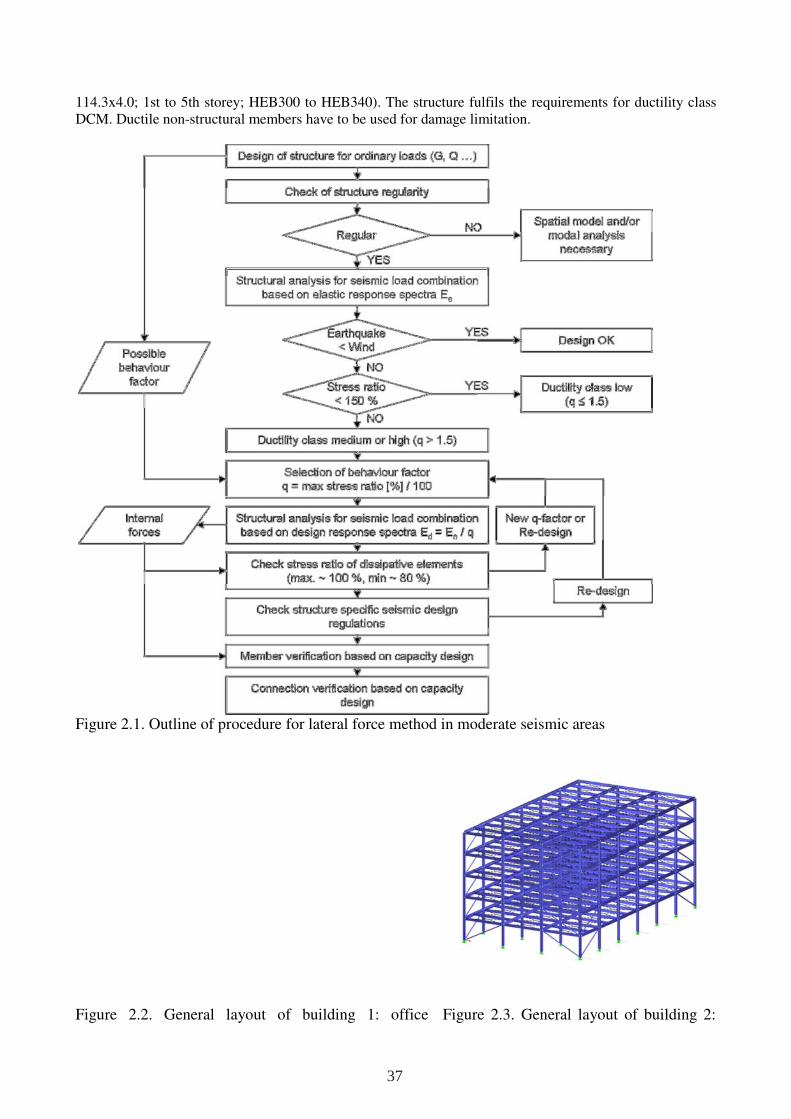
114.3x4.0; 1st to 5th storey; HEB300 to HEB340). The structure fulfils the requirements for ductility class DCM. Ductile non-structural members have to be used for damage limitation.
Figure 2.1. Outline of procedure for lateral force method in moderate seismic areas
Figure 2.2. General layout of building 1: office Figure 2.3. General layout of building 2:
37
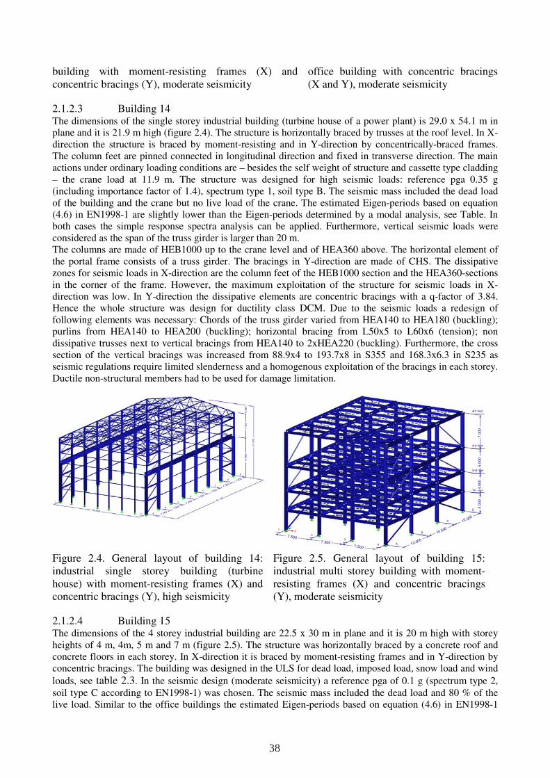
building with moment-resisting frames (X) and concentric bracings (Y), moderate seismicity
office building with concentric bracings (X and Y), moderate seismicity
2.1.2.3 Building 14 The dimensions of the single storey industrial building (turbine house of a power plant) is 29.0 x 54.1 m in plane and it is 21.9 m high (figure 2.4). The structure is horizontally braced by trusses at the roof level. In X-direction the structure is braced by moment-resisting and in Y-direction by concentrically-braced frames. The column feet are pinned connected in longitudinal direction and fixed in transverse direction. The main actions under ordinary loading conditions are – besides the self weight of structure and cassette type cladding – the crane load at 11.9 m. The structure was designed for high seismic loads: reference pga 0.35 g (including importance factor of 1.4), spectrum type 1, soil type B. The seismic mass included the dead load of the building and the crane but no live load of the crane. The estimated Eigen-periods based on equation (4.6) in EN1998-1 are slightly lower than the Eigen-periods determined by a modal analysis, see Table. In both cases the simple response spectra analysis can be applied. Furthermore, vertical seismic loads were considered as the span of the truss girder is larger than 20 m. The columns are made of HEB1000 up to the crane level and of HEA360 above. The horizontal element of the portal frame consists of a truss girder. The bracings in Y-direction are made of CHS. The dissipative zones for seismic loads in X-direction are the column feet of the HEB1000 section and the HEA360-sections in the corner of the frame. However, the maximum exploitation of the structure for seismic loads in X-direction was low. In Y-direction the dissipative elements are concentric bracings with a q-factor of 3.84. Hence the whole structure was design for ductility class DCM. Due to the seismic loads a redesign of following elements was necessary: Chords of the truss girder varied from HEA140 to HEA180 (buckling); purlins from HEA140 to HEA200 (buckling); horizontal bracing from L50x5 to L60x6 (tension); non dissipative trusses next to vertical bracings from HEA140 to 2xHEA220 (buckling). Furthermore, the cross section of the vertical bracings was increased from 88.9x4 to 193.7x8 in S355 and 168.3x6.3 in S235 as seismic regulations require limited slenderness and a homogenous exploitation of the bracings in each storey. Ductile non-structural members had to be used for damage limitation.
Figure 2.4. General layout of building 14: industrial single storey building (turbine house) with moment-resisting frames (X) and concentric bracings (Y), high seismicity
Figure 2.5. General layout of building 15: industrial multi storey building with moment-resisting frames (X) and concentric bracings (Y), moderate seismicity
2.1.2.4 Building 15 The dimensions of the 4 storey industrial building are 22.5 x 30 m in plane and it is 20 m high with storey heights of 4 m, 4m, 5 m and 7 m (figure 2.5). The structure was horizontally braced by a concrete roof and concrete floors in each storey. In X-direction it is braced by moment-resisting frames and in Y-direction by concentric bracings. The building was designed in the ULS for dead load, imposed load, snow load and wind
loads, see table 2.3. In the seismic design (moderate seismicity) a reference pga of 0.1 g (spectrum type 2, soil type C according to EN1998-1) was chosen. The seismic mass included the dead load and 80 % of the live load. Similar to the office buildings the estimated Eigen-periods based on equation (4.6) in EN1998-1
H
11
.88
0
7.300
7.4
25
21
.91
0
G
2.6
05
7.300F
7 .300E
7.300D
51.100Y
ZX
7 .3001C
7.300B
29.000
7.300A2
D
1st floor
4.0
00
2nd f loor
4.0
00
3rd floor
5.0
00
10.000
4t h floor
7.0
00
C
Y
10.000
Z
X1
B
7.5002
10.0007.5003
A7.500
4
38
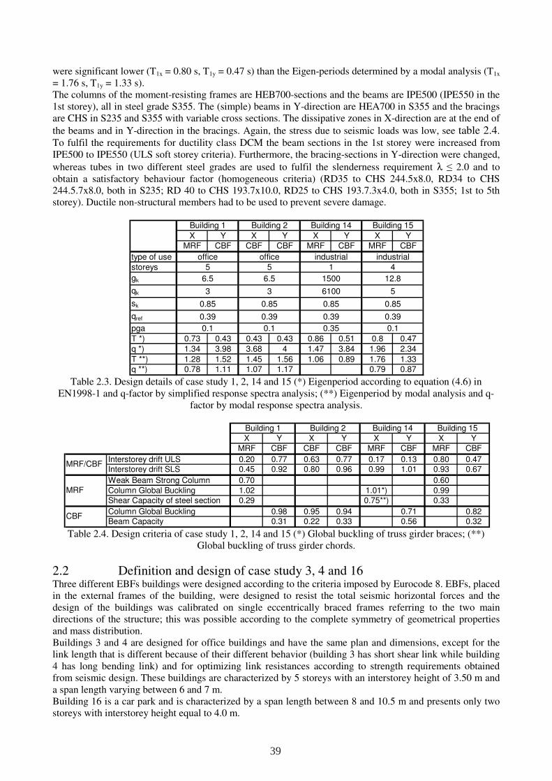
were significant lower (T1x = 0.80 s, T1y = 0.47 s) than the Eigen-periods determined by a modal analysis (T1x = 1.76 s, T1y = 1.33 s). The columns of the moment-resisting frames are HEB700-sections and the beams are IPE500 (IPE550 in the 1st storey), all in steel grade S355. The (simple) beams in Y-direction are HEA700 in S355 and the bracings are CHS in S235 and S355 with variable cross sections. The dissipative zones in X-direction are at the end of
the beams and in Y-direction in the bracings. Again, the stress due to seismic loads was low, see table 2.4. To fulfil the requirements for ductility class DCM the beam sections in the 1st storey were increased from IPE500 to IPE550 (ULS soft storey criteria). Furthermore, the bracing-sections in Y-direction were changed,
whereas tubes in two different steel grades are used to fulfil the slenderness requirement λ ≤ 2.0 and to obtain a satisfactory behaviour factor (homogeneous criteria) (RD35 to CHS 244.5x8.0, RD34 to CHS 244.5.7x8.0, both in S235; RD 40 to CHS 193.7x10.0, RD25 to CHS 193.7.3x4.0, both in S355; 1st to 5th storey). Ductile non-structural members had to be used to prevent severe damage.
Table 2.3. Design details of case study 1, 2, 14 and 15 (*) Eigenperiod according to equation (4.6) in
EN1998-1 and q-factor by simplified response spectra analysis; (**) Eigenperiod by modal analysis and q-factor by modal response spectra analysis.
Table 2.4. Design criteria of case study 1, 2, 14 and 15 (*) Global buckling of truss girder braces; (**)
Global buckling of truss girder chords.
2.2 Definition and design of case study 3, 4 and 16 Three different EBFs buildings were designed according to the criteria imposed by Eurocode 8. EBFs, placed in the external frames of the building, were designed to resist the total seismic horizontal forces and the design of the buildings was calibrated on single eccentrically braced frames referring to the two main directions of the structure; this was possible according to the complete symmetry of geometrical properties and mass distribution. Buildings 3 and 4 are designed for office buildings and have the same plan and dimensions, except for the link length that is different because of their different behavior (building 3 has short shear link while building 4 has long bending link) and for optimizing link resistances according to strength requirements obtained from seismic design. These buildings are characterized by 5 storeys with an interstorey height of 3.50 m and a span length varying between 6 and 7 m. Building 16 is a car park and is characterized by a span length between 8 and 10.5 m and presents only two storeys with interstorey height equal to 4.0 m.
X Y X Y X Y X YMRF CBF CBF CBF MRF CBF MRF CBF
type of use
storeys
gk
qk
sk
qref
pga
T *) 0.73 0.43 0.43 0.43 0.86 0.51 0.8 0.47
q *) 1.34 3.98 3.68 4 1.47 3.84 1.96 2.34
T **) 1.28 1.52 1.45 1.56 1.06 0.89 1.76 1.33q **) 0.78 1.11 1.07 1.17 0.79 0.87
6100
1500
1
industrial industrial
4
12.8
5
0.85
0.39
0.35
0.85
0.39
0.1
3
0.85
0.39
0.1
6.5
5
office office
5
6.5
0.1
0.39
0.85
3
Building 15Building 14Building 2Building 1
X Y X Y X Y X Y
MRF CBF CBF CBF MRF CBF MRF CBF
Interstorey drift ULS 0.20 0.77 0.63 0.77 0.17 0.13 0.80 0.47Interstorey drift SLS 0.45 0.92 0.80 0.96 0.99 1.01 0.93 0.67
Weak Beam Strong Column 0.70 0.60
Column Global Buckling 1.02 1.01*) 0.99
Shear Capacity of steel section 0.29 0.75**) 0.33
Column Global Buckling 0.98 0.95 0.94 0.71 0.82Beam Capacity 0.31 0.22 0.33 0.56 0.32
CBF
MRF/CBF
Building 1 Building 2 Building 14 Building 15
MRF
39
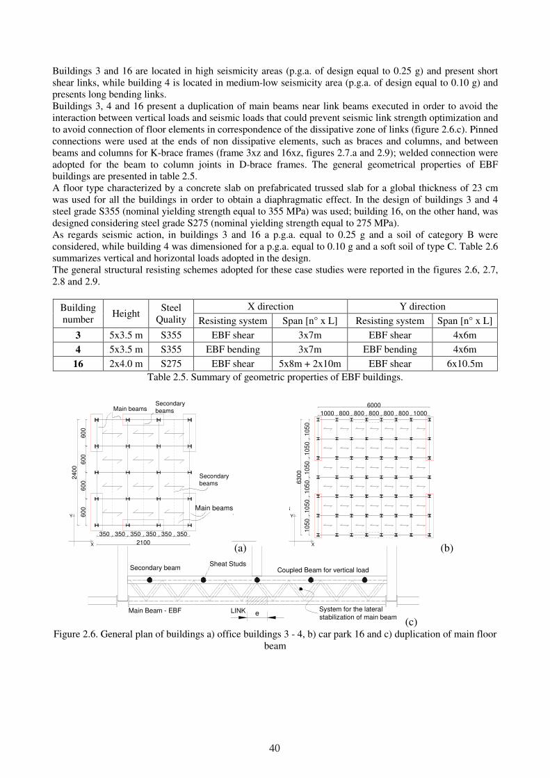
Buildings 3 and 16 are located in high seismicity areas (p.g.a. of design equal to 0.25 g) and present short shear links, while building 4 is located in medium-low seismicity area (p.g.a. of design equal to 0.10 g) and presents long bending links. Buildings 3, 4 and 16 present a duplication of main beams near link beams executed in order to avoid the interaction between vertical loads and seismic loads that could prevent seismic link strength optimization and to avoid connection of floor elements in correspondence of the dissipative zone of links (figure 2.6.c). Pinned connections were used at the ends of non dissipative elements, such as braces and columns, and between beams and columns for K-brace frames (frame 3xz and 16xz, figures 2.7.a and 2.9); welded connection were adopted for the beam to column joints in D-brace frames. The general geometrical properties of EBF buildings are presented in table 2.5. A floor type characterized by a concrete slab on prefabricated trussed slab for a global thickness of 23 cm was used for all the buildings in order to obtain a diaphragmatic effect. In the design of buildings 3 and 4 steel grade S355 (nominal yielding strength equal to 355 MPa) was used; building 16, on the other hand, was designed considering steel grade S275 (nominal yielding strength equal to 275 MPa). As regards seismic action, in buildings 3 and 16 a p.g.a. equal to 0.25 g and a soil of category B were considered, while building 4 was dimensioned for a p.g.a. equal to 0.10 g and a soft soil of type C. Table 2.6 summarizes vertical and horizontal loads adopted in the design. The general structural resisting schemes adopted for these case studies were reported in the figures 2.6, 2.7, 2.8 and 2.9.
Building number
Height Steel
Quality X direction Y direction
Resisting system Span [n° x L] Resisting system Span [n° x L]
3 5x3.5 m S355 EBF shear 3x7m EBF shear 4x6m
4 5x3.5 m S355 EBF bending 3x7m EBF bending 4x6m
16 2x4.0 m S275 EBF shear 5x8m + 2x10m EBF shear 6x10.5m
Table 2.5. Summary of geometric properties of EBF buildings.
(a) (b)
(c) Figure 2.6. General plan of buildings a) office buildings 3 - 4, b) car park 16 and c) duplication of main floor
beam
Y
X
Main beams
240
0
60
06
00
60
060
0
2100
350350350350350350
Y
Secondarybeams
SecondarybeamsMain beams
1000 800 800 800 800 800 1000
6000
105
01
05
01
050
105
010
50
10
50
63
00
Main beams
X
Y
e
Sheat Studs
LINKMain Beam - EBF
Coupled Beam for vertical load
System for the lateral stabilization of main beam
Secondary beam
40
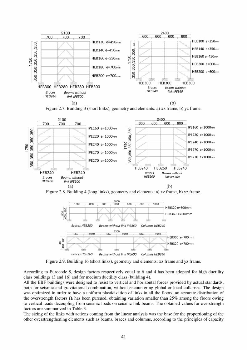
(a) (b) Figure 2.7. Building 3 (short links), geometry and elements: a) xz frame, b) yz frame.
(a) (b) Figure 2.8. Building 4 (long links), geometry and elements: a) xz frame, b) yz frame.
Figure 2.9. Building 16 (short links), geometry and elements: xz frame and yz frame.
According to Eurocode 8, design factors respectively equal to 6 and 4 has been adopted for high ductility class buildings (3 and 16) and for medium ductility class (building 4). All the EBF buildings were designed to resist to vertical and horizontal forces provided by actual standards, both for seismic and gravitational combination, without encountering global or local collapses. The design was optimized in order to have a uniform plasticization of links in all the floors: an accurate distribution of the overstrength factors Ωi has been pursued, obtaining variation smaller than 25% among the floors owing to vertical loads decoupling from seismic loads on seismic link beams. The obtained values for overstrength factors are summarized in Table 3. The sizing of the links with actions coming from the linear analysis was the base for the proportioning of the other overstrengthening elements such as beams, braces and columns, according to the principles of capacity
350
350
35
035
035
0
17
50
700 700 700
HEB300 HEB300HEB280 HEB280
BracesHEB240
Beams withoutlink IPE500
HEB120 e=450mm
HEB140 e=450mm
HEB160 e=550mm
HEB180 e=700mm
HEB200 e=700mm
2100
35
03
50
35
03
50
350
17
50
600 600 600 6002400
HEB300 HEB300 HEB300
HEB100 e=250mm
HEB140 e=350mm
HEB160 e=450mm
HEB200 e=600mm
HEB200 e=600mm
BracesHEB240
Beams withoutlink IPE360
700 7002100
35
03
50
35
03
50
35
0
17
50
700
HEB240 HEB240
IPE160 e=1000mm
IPE220 e=1000mm
IPE240 e=1000mm
IPE270 e=1000mm
IPE270 e=1000mm
BracesHEB200
Beams withoutlink IPE500
35
035
035
035
035
01
750
600 600 600 6002400
IPE160 e=1000mm
IPE220 e=1000mm
IPE240 e=1000mm
IPE270 e=1000mm
IPE270 e=1000mm
HEB240HEB260HEB240
BracesHEB200
Beams withoutlink IPE360
40
040
080
0
1000 800 800 1000800 800 800
40
08
00
1050 1050 1050105010506300
1050
400
HEB320 e=600mm
HEB360 e=600mm
Braces HEB280 Beams without link IPE360
HEB300 e=700mm
HEB320 e=700mm
Columns HEB240
6000
Braces HEB260 Beams without link IPE600 Columns HEB240
41
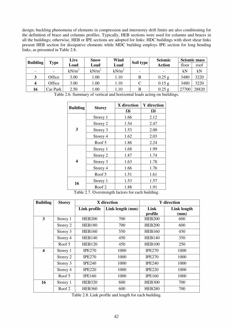
design; buckling phenomena of elements in compression and interstorey drift limits are also conditioning for the definition of brace and columns profiles. Typically, HEB sections were used for columns and braces in all the buildings; otherwise, HEB or IPE sections are adopted for links: HDC buildings with short shear links present HEB section for dissipative elements while MDC building employs IPE section for long bending links, as presented in Table 2.8.
Building Type Live
Load Snow
Load Wind
Load Soil type
Seismic
Action Seismic mass floor roof
- - kN/m2 kN/m2 kN/m2 - - kN kN
3 Office 3.00 1.00 1.10 B 0.25 g 3480 3220
4 Office 3.00 1.00 1.10 C 0.15 g 3480 3220
16 Car Park 2.50 1.00 1.10 B 0.25 g 27700 28820 Table 2.6. Summary of vertical and horizontal loads acting on buildings.
Building Storey X direction Y direction
Ωi Ωi
3
Storey 1 1.66 2.12
Storey 2 1.54 2.47
Storey 3 1.53 2.00
Storey 4 1.62 2.03
Roof 5 1.86 2.24
4
Storey 1 1.68 1.99
Storey 2 1.87 1.74
Storey 3 1.63 1.78
Storey 4 1.66 1.76
Roof 5 1.51 1.61
16 Storey 1 1.53 1.57
Roof 2 1.88 1.91 Table 2.7. Overstrength factors for each building.
Building Storey X direction Y direction
Link profile Link length (mm) Link
profile Link length
(mm) 3 Storey 1 HEB200 700 HEB200 600
Storey 2 HEB180 700 HEB200 600
Storey 3 HEB160 550 HEB160 450
Storey 4 HEB140 450 HEB140 350
Roof 5 HEB120 450 HEB100 250
4 Storey 1 IPE270 1000 IPE270 1000
Storey 2 IPE270 1000 IPE270 1000
Storey 3 IPE240 1000 IPE240 1000
Storey 4 IPE220 1000 IPE220 1000
Roof 5 IPE160 1000 IPE160 1000
16 Storey 1 HEB320 600 HEB300 700
Roof 2 HEB360 600 HEB280 700
Table 2.8. Link profile and length for each building.
42
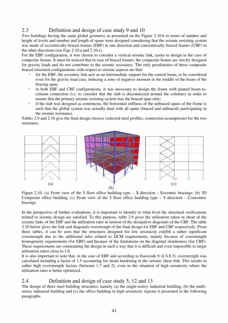
2.3 Definition and design of case study 9 and 10 Two buildings having the same global geometry as presented on the Figure 2.10.b in terms of number and height of levels and number and length of spans were designed considering that the seismic resisting system was made of eccentrically braced frames (EBF) in one direction and concentrically braced frames (CBF) in the other directions (see Figs 2.10.a and 2.10.c). For the EBF configuration, it was chosen to consider a vertical seismic link, easier to design in the case of composite beams. It must be noticed that in case of braced frames, the composite beams are strictly designed for gravity loads and do not contribute to the seismic resistance. The only peculiarities of these composite braced structural configurations with respect to seismic aspects are that:
for the EBF, the eccentric link acts as an intermediate support for the central beam, to be considered even for the gravity load case, inducing a zone of negative moment in the middle of the beam of the bracing span;
in both EBF and CBF configurations, it was necessary to design the frame with pinned beam-to-column connection (i.e. to consider that the slab is disconnected around the columns) in order to ensure that the primary seismic resisting system was the braced span only;
if the slab was designed as continuous, the horizontal stiffness of the unbraced spans of the frame is such that the global system was actually dual with all spans (braced and unbraced) participating in the seismic resistance.
Tables 2.9 and 2.10 give the final design choices (selected steel profiles, connection assumptions) for the two structures.
(a)
(b)
(c)
Figure 2.10. (a) Front view of the 5 floor office building type – X-direction – Eccentric bracings; (b) 3D Composite office building; (c) Front view of the 5 floor office building type – Y-direction – Concentric bracings
In the perspective of further evaluations, it is important to identify to what level the structural verifications related to seismic design are satisfied. To this purpose, table 2.9 gives the utilization ratios in shear of the seismic links of the EBF and the utilization ratio in tension of the dissipative diagonals of the CBF. The table 2.10 below gives the link and diagonals overstrengh of the final design for EBF and CBF respectively. From these tables, it can be seen that the structures designed for low seismicity exhibit a rather significant overstrength due to the additional rules related to DCM requirements, mainly because of overstrength homogeneity requirements (for EBF) and because of the limitations on the diagonal slenderness (for CBF). These requirements are constraining the design in such a way that it is difficult and even impossible to target utilization ratios close to 1.0. It is also important to note that, in the case of EBF and according to Eurocode 8 (§ 6.8.3), overstrength was calculated including a factor of 1.5 accounting for strain hardening in the seismic shear link. This results in rather high overstrength factors (between 1.7 and 2), even in the situation of high seismicity where the utilization ratio is better optimized.
2.4 Definition and design of case study 5, 12 and 13
The design of three steel building structures, namely (a) the single-storey industrial building, (b) the multi-storey industrial building and (c) the office building in high seismicity regions is presented in the following paragraphs.
43
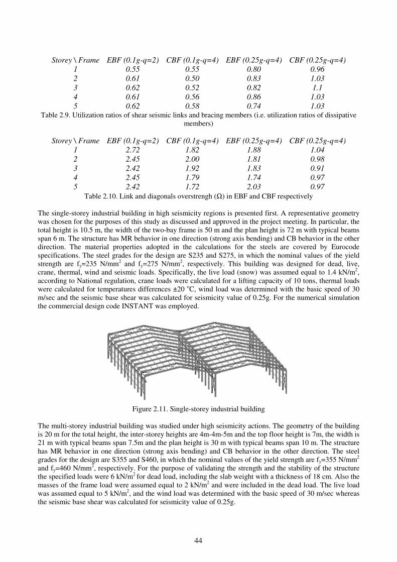
Storey \ Frame EBF (0.1g-q=2) CBF (0.1g-q=4) EBF (0.25g-q=4) CBF (0.25g-q=4)
1 0.55 0.55 0.80 0.96
2 0.61 0.50 0.83 1.03
3 0.62 0.52 0.82 1.1
4 0.61 0.56 0.86 1.03
5 0.62 0.58 0.74 1.03 Table 2.9. Utilization ratios of shear seismic links and bracing members (i.e. utilization ratios of dissipative
members)
Storey \ Frame EBF (0.1g-q=2) CBF (0.1g-q=4) EBF (0.25g-q=4) CBF (0.25g-q=4)
1 2.72 1.82 1.88 1.04
2 2.45 2.00 1.81 0.98
3 2.42 1.92 1.83 0.91
4 2.45 1.79 1.74 0.97
5 2.42 1.72 2.03 0.97
Table 2.10. Link and diagonals overstrengh (Ω) in EBF and CBF respectively The single-storey industrial building in high seismicity regions is presented first. A representative geometry was chosen for the purposes of this study as discussed and approved in the project meeting. In particular, the total height is 10.5 m, the width of the two-bay frame is 50 m and the plan height is 72 m with typical beams span 6 m. The structure has MR behavior in one direction (strong axis bending) and CB behavior in the other direction. The material properties adopted in the calculations for the steels are covered by Eurocode specifications. The steel grades for the design are S235 and S275, in which the nominal values of the yield strength are fy=235 N/mm2 and fy=275 N/mm2, respectively. This building was designed for dead, live, crane, thermal, wind and seismic loads. Specifically, the live load (snow) was assumed equal to 1.4 kN/m2, according to National regulation, crane loads were calculated for a lifting capacity of 10 tons, thermal loads were calculated for temperatures differences ±20 oC, wind load was determined with the basic speed of 30 m/sec and the seismic base shear was calculated for seismicity value of 0.25g. For the numerical simulation the commercial design code INSTANT was employed.
Figure 2.11. Single-storey industrial building
The multi-storey industrial building was studied under high seismicity actions. The geometry of the building is 20 m for the total height, the inter-storey heights are 4m-4m-5m and the top floor height is 7m, the width is 21 m with typical beams span 7.5m and the plan height is 30 m with typical beams span 10 m. The structure has MR behavior in one direction (strong axis bending) and CB behavior in the other direction. The steel grades for the design are S355 and S460, in which the nominal values of the yield strength are fy=355 N/mm2 and fy=460 N/mm2, respectively. For the purpose of validating the strength and the stability of the structure the specified loads were 6 kN/m2 for dead load, including the slab weight with a thickness of 18 cm. Also the masses of the frame load were assumed equal to 2 kN/m2 and were included in the dead load. The live load was assumed equal to 5 kN/m2, and the wind load was determined with the basic speed of 30 m/sec whereas the seismic base shear was calculated for seismicity value of 0.25g.
44
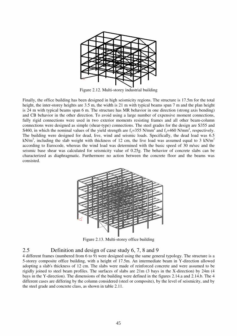
Figure 2.12. Multi-storey industrial building
Finally, the office building has been designed in high seismicity regions. The structure is 17.5m for the total height, the inter-storey heights are 3.5 m, the width is 21 m with typical beams span 7 m and the plan height is 24 m with typical beams span 6 m. The structure has MR behavior in one direction (strong axis bending) and CB behavior in the other direction. To avoid using a large number of expensive moment connections, fully rigid connections were used in two exterior moments resisting frames and all other beam-column connections were designed as simple (shear-type) connections. The steel grades for the design are S355 and S460, in which the nominal values of the yield strength are fy=355 N/mm2 and fy=460 N/mm2, respectively. The building were designed for dead, live, wind and seismic loads. Specifically, the dead load was 6.5 kN/m2, including the slab weight with thickness of 12 cm, the live load was assumed equal to 3 kN/m2
according to Eurocode, whereas the wind load was determined with the basic speed of 30 m/sec and the seismic base shear was calculated for seismicity value of 0.25g. The behavior of concrete slabs can be characterized as diaphragmatic. Furthermore no action between the concrete floor and the beams was consisted.
Figure 2.13. Multi-storey office building
2.5 Definition and design of case study 6, 7, 8 and 9
4 different frames (numbered from 6 to 9) were designed using the same general typology. The structure is a 5-storey composite office building, with a height of 17.5m. An intermediate beam in Y-direction allowed adopting a slab's thickness of 12 cm. The slabs were made of reinforced concrete and were assumed to be rigidly joined to steel beam profiles. The surfaces of slabs are 21m (3 bays in the X-direction) by 24m (4 bays in the Y-direction). The dimensions of the building were defined in the figures 2.14.a and 2.14.b. The 4 different cases are differing by the column considered (steel or composite), by the level of seismicity, and by the steel grade and concrete class, as shown in table 2.11.
45
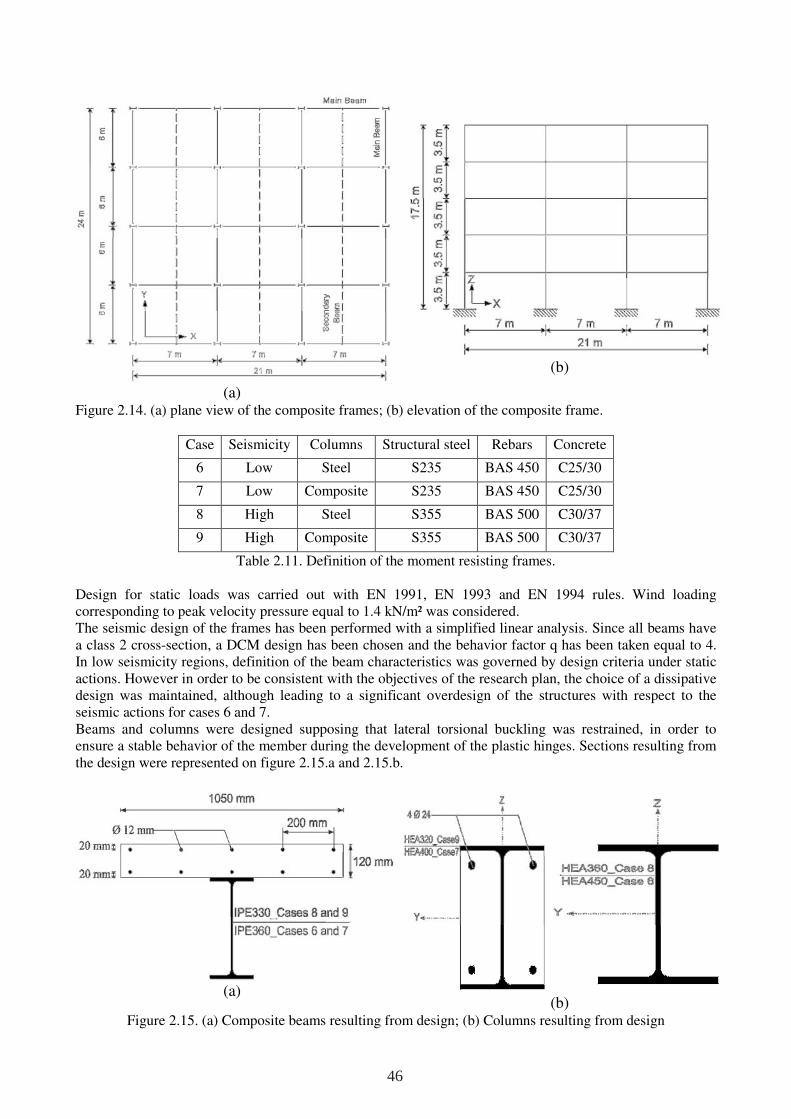
(a)
(b)
Figure 2.14. (a) plane view of the composite frames; (b) elevation of the composite frame.
Case Seismicity Columns Structural steel Rebars Concrete
6 Low Steel S235 BAS 450 C25/30
7 Low Composite S235 BAS 450 C25/30
8 High Steel S355 BAS 500 C30/37
9 High Composite S355 BAS 500 C30/37
Table 2.11. Definition of the moment resisting frames. Design for static loads was carried out with EN 1991, EN 1993 and EN 1994 rules. Wind loading corresponding to peak velocity pressure equal to 1.4 kN/m² was considered. The seismic design of the frames has been performed with a simplified linear analysis. Since all beams have a class 2 cross-section, a DCM design has been chosen and the behavior factor q has been taken equal to 4. In low seismicity regions, definition of the beam characteristics was governed by design criteria under static actions. However in order to be consistent with the objectives of the research plan, the choice of a dissipative design was maintained, although leading to a significant overdesign of the structures with respect to the seismic actions for cases 6 and 7. Beams and columns were designed supposing that lateral torsional buckling was restrained, in order to ensure a stable behavior of the member during the development of the plastic hinges. Sections resulting from the design were represented on figure 2.15.a and 2.15.b.
(a)
(b) Figure 2.15. (a) Composite beams resulting from design; (b) Columns resulting from design
46
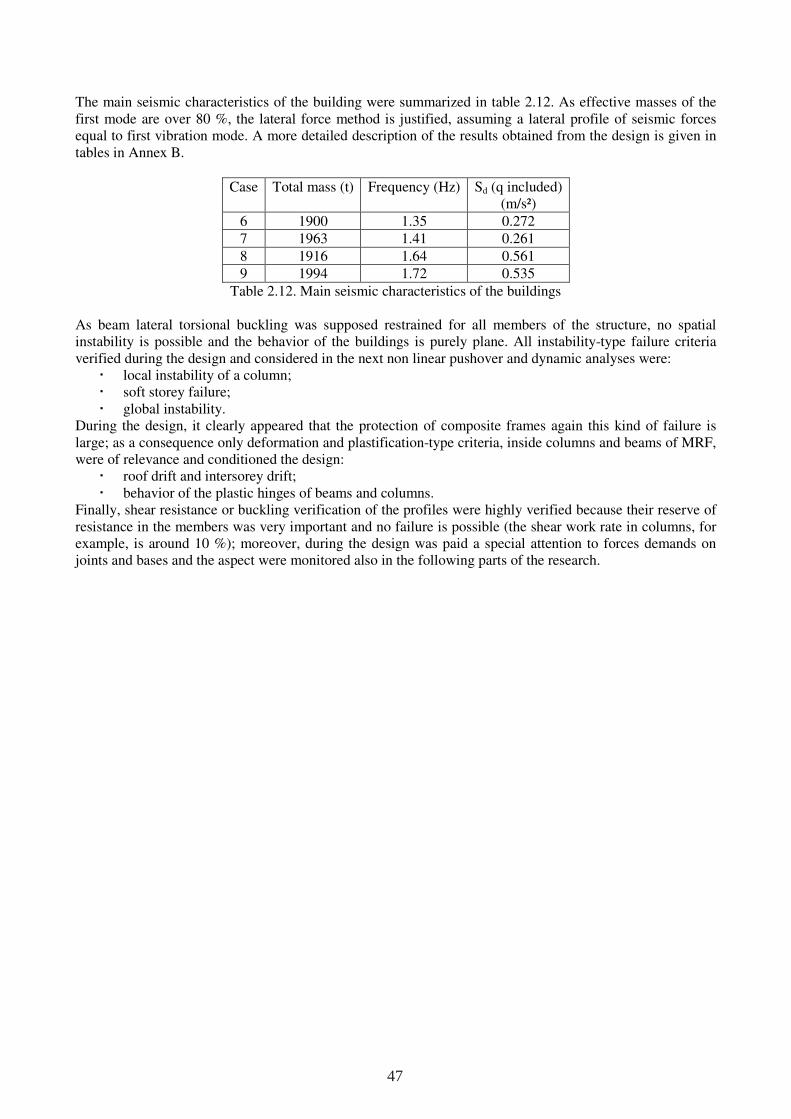
The main seismic characteristics of the building were summarized in table 2.12. As effective masses of the first mode are over 80 %, the lateral force method is justified, assuming a lateral profile of seismic forces equal to first vibration mode. A more detailed description of the results obtained from the design is given in tables in Annex B.
Case Total mass (t) Frequency (Hz) Sd (q included) (m/s²)
6 1900 1.35 0.272 7 1963 1.41 0.261
8 1916 1.64 0.561 9 1994 1.72 0.535
Table 2.12. Main seismic characteristics of the buildings As beam lateral torsional buckling was supposed restrained for all members of the structure, no spatial instability is possible and the behavior of the buildings is purely plane. All instability-type failure criteria verified during the design and considered in the next non linear pushover and dynamic analyses were:
local instability of a column; soft storey failure; global instability.
During the design, it clearly appeared that the protection of composite frames again this kind of failure is large; as a consequence only deformation and plastification-type criteria, inside columns and beams of MRF, were of relevance and conditioned the design:
roof drift and intersorey drift; behavior of the plastic hinges of beams and columns.
Finally, shear resistance or buckling verification of the profiles were highly verified because their reserve of resistance in the members was very important and no failure is possible (the shear work rate in columns, for example, is around 10 %); moreover, during the design was paid a special attention to forces demands on joints and bases and the aspect were monitored also in the following parts of the research.
47

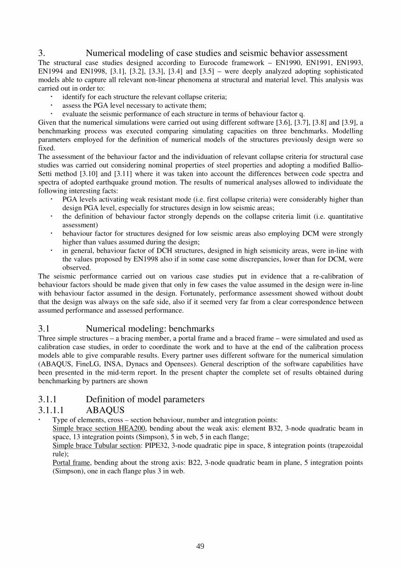
3. Numerical modeling of case studies and seismic behavior assessment The structural case studies designed according to Eurocode framework – EN1990, EN1991, EN1993, EN1994 and EN1998, [3.1], [3.2], [3.3], [3.4] and [3.5] – were deeply analyzed adopting sophisticated models able to capture all relevant non-linear phenomena at structural and material level. This analysis was carried out in order to:
identify for each structure the relevant collapse criteria; assess the PGA level necessary to activate them; evaluate the seismic performance of each structure in terms of behaviour factor q.
Given that the numerical simulations were carried out using different software [3.6], [3.7], [3.8] and [3.9], a benchmarking process was executed comparing simulating capacities on three benchmarks. Modelling parameters employed for the definition of numerical models of the structures previously design were so fixed. The assessment of the behaviour factor and the individuation of relevant collapse criteria for structural case studies was carried out considering nominal properties of steel properties and adopting a modified Ballio-Setti method [3.10] and [3.11] where it was taken into account the differences between code spectra and spectra of adopted earthquake ground motion. The results of numerical analyses allowed to individuate the following interesting facts:
PGA levels activating weak resistant mode (i.e. first collapse criteria) were considerably higher than design PGA level, especially for structures design in low seismic areas;
the definition of behaviour factor strongly depends on the collapse criteria limit (i.e. quantitative assessment)
behaviour factor for structures designed for low seismic areas also employing DCM were strongly higher than values assumed during the design;
in general, behaviour factor of DCH structures, designed in high seismicity areas, were in-line with the values proposed by EN1998 also if in some case some discrepancies, lower than for DCM, were observed.
The seismic performance carried out on various case studies put in evidence that a re-calibration of behaviour factors should be made given that only in few cases the value assumed in the design were in-line with behaviour factor assumed in the design. Fortunately, performance assessment showed without doubt that the design was always on the safe side, also if it seemed very far from a clear correspondence between assumed performance and assessed performance.
3.1 Numerical modeling: benchmarks Three simple structures – a bracing member, a portal frame and a braced frame – were simulated and used as calibration case studies, in order to coordinate the work and to have at the end of the calibration process models able to give comparable results. Every partner uses different software for the numerical simulation (ABAQUS, FineLG, INSA, Dynacs and Opensees). General description of the software capabilities have been presented in the mid-term report. In the present chapter the complete set of results obtained during benchmarking by partners are shown
3.1.1 Definition of model parameters 3.1.1.1 ABAQUS Type of elements, cross – section behaviour, number and integration points:
Simple brace section HEA200, bending about the weak axis: element B32, 3-node quadratic beam in space, 13 integration points (Simpson), 5 in web, 5 in each flange; Simple brace Tubular section: PIPE32, 3-node quadratic pipe in space, 8 integration points (trapezoidal rule); Portal frame, bending about the strong axis: B22, 3-node quadratic beam in plane, 5 integration points (Simpson), one in each flange plus 3 in web.
49
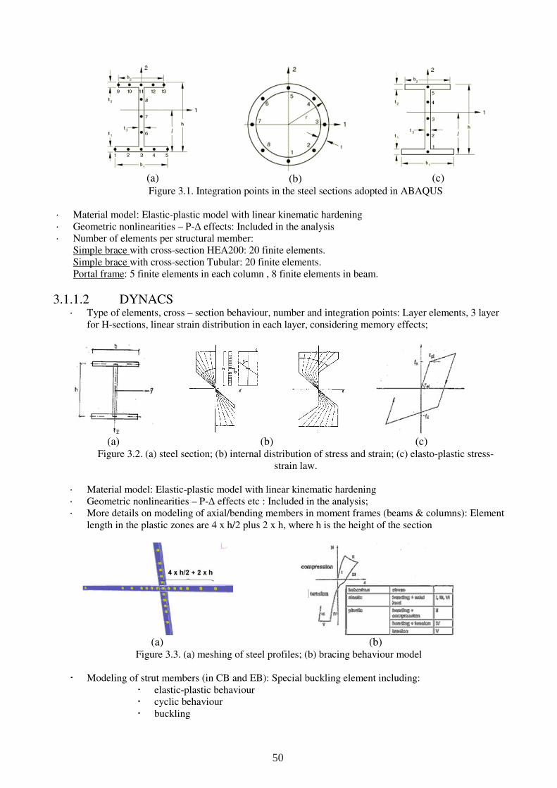
(a)
(b)
(c)
Figure 3.1. Integration points in the steel sections adopted in ABAQUS
Material model: Elastic-plastic model with linear kinematic hardening Geometric nonlinearities – P-∆ effects: Included in the analysis Number of elements per structural member:
Simple brace with cross-section HEA200: 20 finite elements. Simple brace with cross-section Tubular: 20 finite elements. Portal frame: 5 finite elements in each column , 8 finite elements in beam.
3.1.1.2 DYNACS Type of elements, cross – section behaviour, number and integration points: Layer elements, 3 layer
for H-sections, linear strain distribution in each layer, considering memory effects;
(a)
(b)
(c)
Figure 3.2. (a) steel section; (b) internal distribution of stress and strain; (c) elasto-plastic stress-strain law.
Material model: Elastic-plastic model with linear kinematic hardening Geometric nonlinearities – P-∆ effects etc : Included in the analysis; More details on modeling of axial/bending members in moment frames (beams & columns): Element
length in the plastic zones are 4 x h/2 plus 2 x h, where h is the height of the section
(a)
(b)
Figure 3.3. (a) meshing of steel profiles; (b) bracing behaviour model
Modeling of strut members (in CB and EB): Special buckling element including: elastic-plastic behaviour cyclic behaviour buckling
50
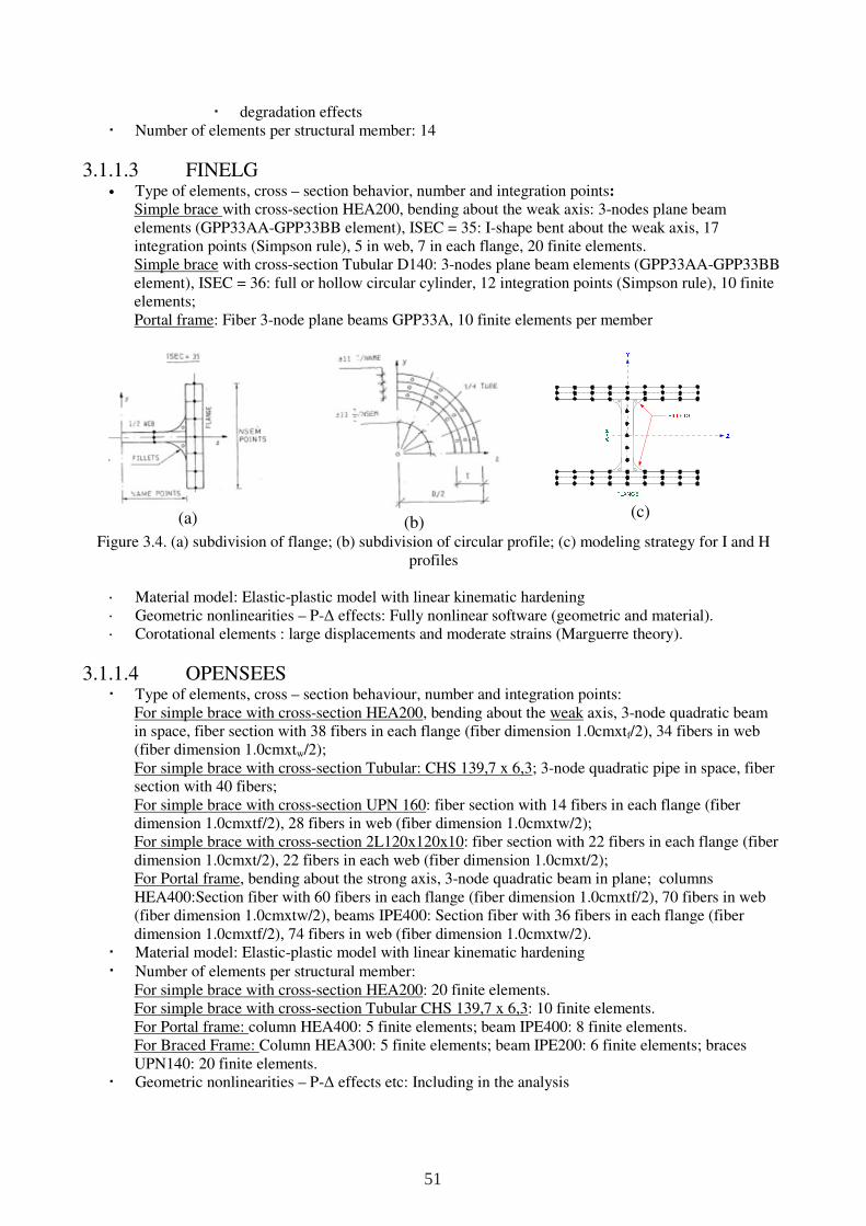
degradation effects Number of elements per structural member: 14
3.1.1.3 FINELG • Type of elements, cross – section behavior, number and integration points:
Simple brace with cross-section HEA200, bending about the weak axis: 3-nodes plane beam elements (GPP33AA-GPP33BB element), ISEC = 35: I-shape bent about the weak axis, 17 integration points (Simpson rule), 5 in web, 7 in each flange, 20 finite elements. Simple brace with cross-section Tubular D140: 3-nodes plane beam elements (GPP33AA-GPP33BB element), ISEC = 36: full or hollow circular cylinder, 12 integration points (Simpson rule), 10 finite elements; Portal frame: Fiber 3-node plane beams GPP33A, 10 finite elements per member
(a)
(b)
(c)
Figure 3.4. (a) subdivision of flange; (b) subdivision of circular profile; (c) modeling strategy for I and H profiles
Material model: Elastic-plastic model with linear kinematic hardening Geometric nonlinearities – P-∆ effects: Fully nonlinear software (geometric and material). Corotational elements : large displacements and moderate strains (Marguerre theory).
3.1.1.4 OPENSEES Type of elements, cross – section behaviour, number and integration points:
For simple brace with cross-section HEA200, bending about the weak axis, 3-node quadratic beam in space, fiber section with 38 fibers in each flange (fiber dimension 1.0cmxtf/2), 34 fibers in web (fiber dimension 1.0cmxtw/2); For simple brace with cross-section Tubular: CHS 139,7 x 6,3; 3-node quadratic pipe in space, fiber section with 40 fibers; For simple brace with cross-section UPN 160: fiber section with 14 fibers in each flange (fiber dimension 1.0cmxtf/2), 28 fibers in web (fiber dimension 1.0cmxtw/2); For simple brace with cross-section 2L120x120x10: fiber section with 22 fibers in each flange (fiber dimension 1.0cmxt/2), 22 fibers in each web (fiber dimension 1.0cmxt/2); For Portal frame, bending about the strong axis, 3-node quadratic beam in plane; columns HEA400:Section fiber with 60 fibers in each flange (fiber dimension 1.0cmxtf/2), 70 fibers in web (fiber dimension 1.0cmxtw/2), beams IPE400: Section fiber with 36 fibers in each flange (fiber dimension 1.0cmxtf/2), 74 fibers in web (fiber dimension 1.0cmxtw/2).
Material model: Elastic-plastic model with linear kinematic hardening Number of elements per structural member:
For simple brace with cross-section HEA200: 20 finite elements. For simple brace with cross-section Tubular CHS 139,7 x 6,3: 10 finite elements. For Portal frame: column HEA400: 5 finite elements; beam IPE400: 8 finite elements. For Braced Frame: Column HEA300: 5 finite elements; beam IPE200: 6 finite elements; braces UPN140: 20 finite elements.
Geometric nonlinearities – P-∆ effects etc: Including in the analysis
51
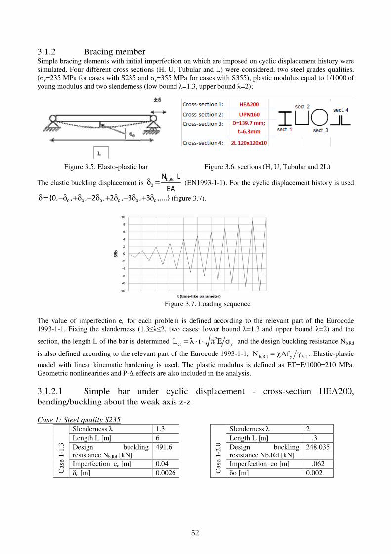
3.1.2 Bracing member Simple bracing elements with initial imperfection on which are imposed on cyclic displacement history were simulated. Four different cross sections (H, U, Tubular and L) were considered, two steel grades qualities, (σy=235 MPa for cases with S235 and σy=355 MPa for cases with S355), plastic modulus equal to 1/1000 of young modulus and two slenderness (low bound λ=1.3, upper bound λ=2);
Figure 3.5. Elasto-plastic bar Figure 3.6. sections (H, U, Tubular and 2L)
The elastic buckling displacement is δ = b,Rd
0
N L
EA (EN1993-1-1). For the cyclic displacement history is used
δ = −δ +δ − δ + δ − δ + δ0 0 0 0 0 00, , , 2 , 2 , 3 , 3 ,.... (figure 3.7).
Figure 3.7. Loading sequence
The value of imperfection eο for each problem is defined according to the relevant part of the Eurocode 1993-1-1. Fixing the slenderness (1.3≤λ≤2, two cases: lower bound λ=1.3 and upper bound λ=2) and the
section, the length L of the bar is determined 2
cr yL E= λ ⋅ ι ⋅ π σ and the design buckling resistance Nb,Rd
is also defined according to the relevant part of the Eurocode 1993-1-1, b Rd y M1N Af= χ γ
,. Elastic-plastic
model with linear kinematic hardening is used. The plastic modulus is defined as ET=E/1000=210 MPa. Geometric nonlinearities and P-∆ effects are also included in the analysis.
3.1.2.1 Simple bar under cyclic displacement - cross-section HEA200, bending/buckling about the weak axis z-z
Case 1: Steel quality S235
Cas
e 1-1
.3
Slenderness λ 1.3 Length L [m] 6 Design buckling resistance Nb,Rd [kN]
491.6
Imperfection eο [m] 0.04 δο [m] 0.0026
Cas
e 1-2
.0
Slenderness λ 2 Length L [m] .3 Design buckling resistance Nb,Rd [kN]
248.035
Imperfection eο [m] .062 δο [m] 0.002
52
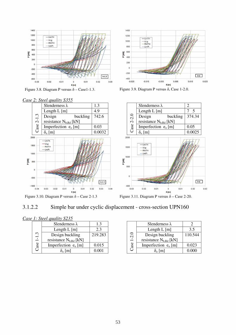
Figure 3.8. Diagram P versus δ – Case1-1.3.
Figure 3.9. Diagram P versus δ, Case 1-2.0.
Case 2: Steel quality S355
Cas
e 2-1
.3
Slenderness λ 1.3 Length L [m] 4.9
Design buckling resistance Nb,Rd [kN]
742.6
Imperfection eο [m] 0.03
δο [m] 0.0032
Cas
e 2-2
.0
Slenderness λ 2 Length L [m] 7 5
Design buckling resistance Nb,Rd [kN]
374.34
Imperfection eο [m] 0.05
δο [m] 0.0025
Figure 3.10. Diagram P versus δ – Case 2-1.3
Figure 3.11. Diagram P versus δ – Case 2-20.
3.1.2.2 Simple bar under cyclic displacement - cross-section UPN160
Case 1: Steel quality S235
Cas
e 1-1
.3
Slenderness λ 1.3 Length L [m] 2.3
Design buckling resistance Nb,Rd [kN]
219.283
Imperfection eο [m] 0.015
δο [m] 0.001
Cas
e 1-2
.0
Slenderness λ 2 Length L [m] 3.5
Design buckling resistance Nb,Rd [kN]
110.544
Imperfection eο [m] 0.023
δο [m] 0.000
53
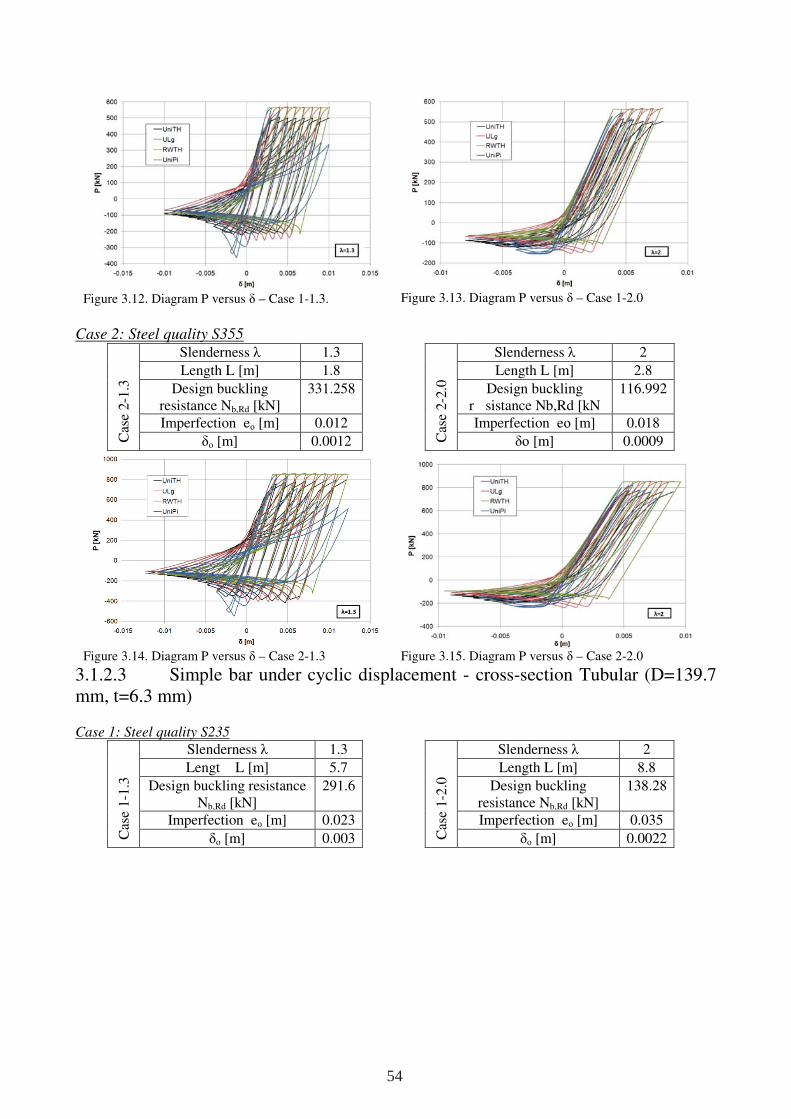
Figure 3.12. Diagram P versus δ – Case 1-1.3.
Figure 3.13. Diagram P versus δ – Case 1-2.0
Case 2: Steel quality S355
Cas
e 2-1
.3
Slenderness λ 1.3 Length L [m] 1.8
Design buckling resistance Nb,Rd [kN]
331.258
Imperfection eο [m] 0.012
δο [m] 0.0012
Cas
e 2-2
.0
Slenderness λ 2 Length L [m] 2.8
Design buckling r sistance Nb,Rd [kN
116.992
Imperfection eο [m] 0.018
δο [m] 0.0009
Figure 3.14. Diagram P versus δ – Case 2-1.3
Figure 3.15. Diagram P versus δ – Case 2-2.0
3.1.2.3 Simple bar under cyclic displacement - cross-section Tubular (D=139.7 mm, t=6.3 mm)
Case 1: Steel quality S235
Cas
e 1-1
.3
Slenderness λ 1.3 Lengt L [m] 5.7
Design buckling resistance Nb,Rd [kN]
291.6
Imperfection eο [m] 0.023
δο [m] 0.003
Cas
e 1-2
.0
Slenderness λ 2 Length L [m] 8.8
Design buckling resistance Nb,Rd [kN]
138.28
Imperfection eο [m] 0.035
δο [m] 0.0022
54
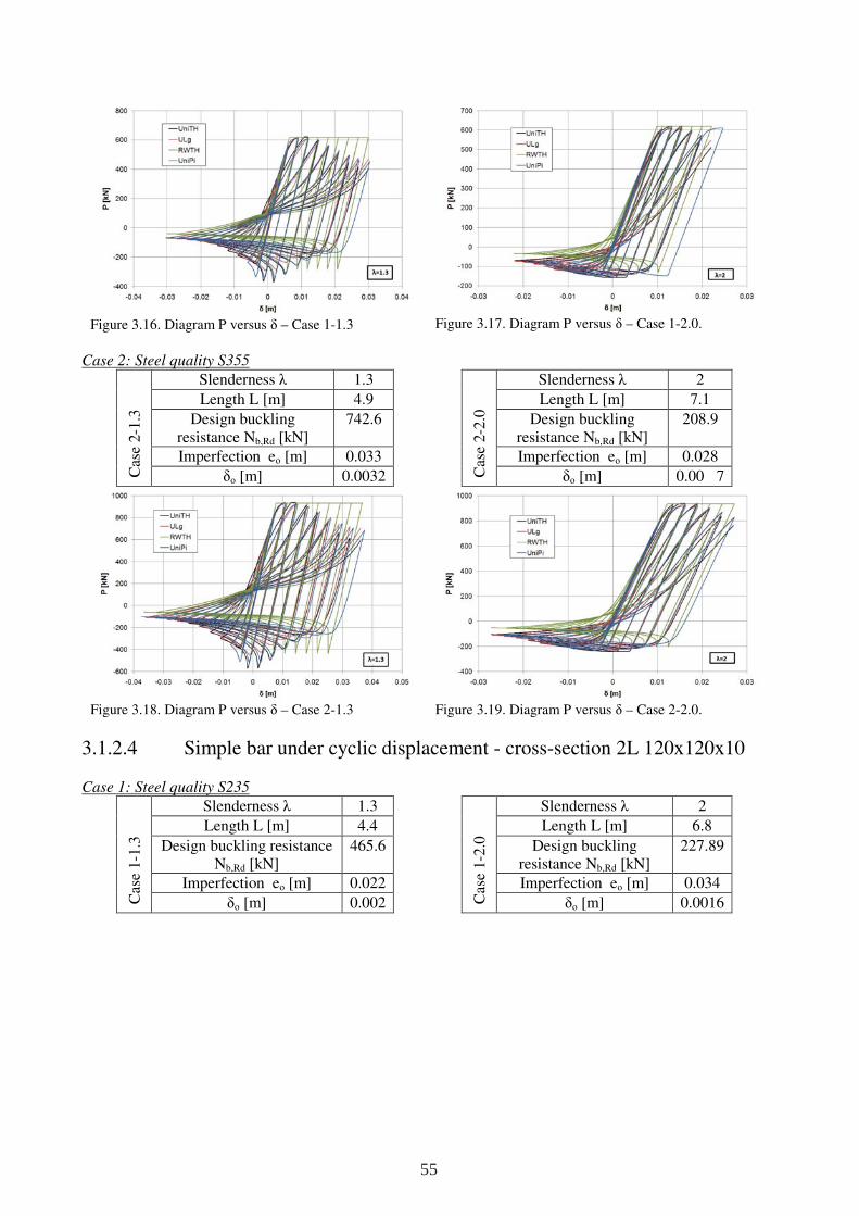
Figure 3.16. Diagram P versus δ – Case 1-1.3
Figure 3.17. Diagram P versus δ – Case 1-2.0.
Case 2: Steel quality S355
Cas
e 2-1
.3
Slenderness λ 1.3 Length L [m] 4.9
Design buckling resistance Nb,Rd [kN]
742.6
Imperfection eο [m] 0.033
δο [m] 0.0032
Cas
e 2-2
.0
Slenderness λ 2 Length L [m] 7.1
Design buckling resistance Nb,Rd [kN]
208.9
Imperfection eο [m] 0.028
δο [m] 0.00 7
Figure 3.18. Diagram P versus δ – Case 2-1.3
Figure 3.19. Diagram P versus δ – Case 2-2.0.
3.1.2.4 Simple bar under cyclic displacement - cross-section 2L 120x120x10
Case 1: Steel quality S235
Cas
e 1-1
.3
Slenderness λ 1.3 Length L [m] 4.4
Design buckling resistance Nb,Rd [kN]
465.6
Imperfection eο [m] 0.022
δο [m] 0.002
Cas
e 1-2
.0
Slenderness λ 2 Length L [m] 6.8
Design buckling resistance Nb,Rd [kN]
227.89
Imperfection eο [m] 0.034
δο [m] 0.0016
55
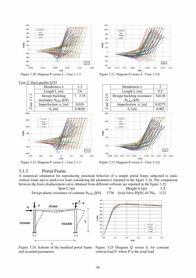
Figure 3.20. Diagram P versus δ – Case 1-1.3
Figure 3.21. Diagram P versus δ – Case 1-2.0.
Case 2: Steel quality S355
Cas
e 2-1
.3
Slenderness λ 1.3 Length L [m] 3.6
Design buckling resistance Nb,Rd [kN]
7 3.35
Imperfection eο [m] 0.018
δο [m] 0.0026
Cas
e 2-2
.0
Slenderness λ 2 Length L [m] 5.5
Design buckling resistance Nb,Rd [kN]
344.26
Imperfection eο [m] 0.0275
δο [m] 0.002
Figure 3.22. Diagram P versus δ – Case 2-1.3
Figure 3.23. Diagram P versus δ – Case 2-2.0
3.1.3 Portal Frame A numerical simulation for reproducing structural behavior of a simple portal frame subjected to static vertical loads and to push-over load considering the parameters reported in the figure 3.24. The comparison between the force-displacement curve obtained from different software are reported in the figure 3.25.
Span L [m] 6 Height h [m] 3.5 Design plastic resistance of columns NPl,Rd [kN] 3736 Axial force P[kN] =0.3NPl 1121
Figure 3.24. Scheme of the modeled portal frame and assumed parameters
Figure 3.25 Diagram Q versus δ, for constant vertical load P, where P is the axial load.
56
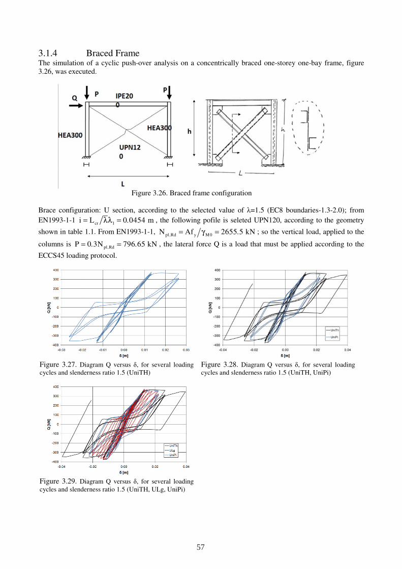
3.1.4 Braced Frame The simulation of a cyclic push-over analysis on a concentrically braced one-storey one-bay frame, figure 3.26, was executed.
Figure 3.26. Braced frame configuration
Brace configuration: U section, according to the selected value of λ=1.5 (EC8 boundaries-1.3-2.0); from
EN1993-1-1 cr 1i L 0 0454 m= λλ = . , the following pofile is seleted UPN120, according to the geometry
shown in table 1.1. From EN1993-1-1, pl Rd y M 0N Af 2655 5 kN= γ =
,. ; so the vertical load, applied to the
columns is pl RdP 0 3N 796 65 kN= =
,. . , the lateral force Q is a load that must be applied according to the
ECCS45 loading protocol.
Figure 3.27. Diagram Q versus δ, for several loading cycles and slenderness ratio 1.5 (UniTH)
Figure 3.28. Diagram Q versus δ, for several loading cycles and slenderness ratio 1.5 (UniTH, UniPi)
Figure 3.29. Diagram Q versus δ, for several loading cycles and slenderness ratio 1.5 (UniTH, ULg, UniPi)
57
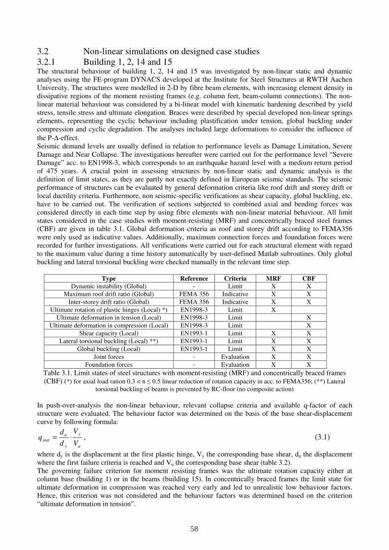
3.2 Non-linear simulations on designed case studies 3.2.1 Building 1, 2, 14 and 15 The structural behaviour of building 1, 2, 14 and 15 was investigated by non-linear static and dynamic analyses using the FE-program DYNACS developed at the Institute for Steel Structures at RWTH Aachen University. The structures were modelled in 2-D by fibre beam elements, with increasing element density in dissipative regions of the moment resisting frames (e.g. column feet, beam-column connections). The non-linear material behaviour was considered by a bi-linear model with kinematic hardening described by yield stress, tensile stress and ultimate elongation. Braces were described by special developed non-linear springs elements, representing the cyclic behaviour including plastification under tension, global buckling under compression and cyclic degradation. The analyses included large deformations to consider the influence of
the P-∆-effect. Seismic demand levels are usually defined in relation to performance levels as Damage Limitation, Severe Damage and Near Collapse. The investigations hereafter were carried out for the performance level “Severe Damage” acc. to EN1998-3, which corresponds to an earthquake hazard level with a medium return period of 475 years. A crucial point in assessing structures by non-linear static and dynamic analysis is the definition of limit states, as they are partly not exactly defined in European seismic standards. The seismic performance of structures can be evaluated by general deformation criteria like roof drift and storey drift or local ductility criteria. Furthermore, non seismic-specific verifications as shear capacity, global buckling, etc. have to be carried out. The verification of sections subjected to combined axial and bending forces was considered directly in each time step by using fibre elements with non-linear material behaviour. All limit states considered in the case studies with moment-resisting (MRF) and concentrically braced steel frames (CBF) are given in table 3.1. Global deformation criteria as roof and storey drift according to FEMA356 were only used as indicative values. Additionally, maximum connection forces and foundation forces were recorded for further investigations. All verifications were carried out for each structural element with regard to the maximum value during a time history automatically by user-defined Matlab subroutines. Only global buckling and lateral torsional buckling were checked manually in the relevant time step.
Type Reference Criteria MRF CBF
Dynamic instability (Global) - Limit X X
Maximum roof drift ratio (Global) FEMA 356 Indicative X X
Inter-storey drift ratio (Global) FEMA 356 Indicative X X
Ultimate rotation of plastic hinges (Local) *) EN1998-3 Limit X
Ultimate deformation in tension (Local) EN1998-3 Limit X
Ultimate deformation in compression (Local) EN1998-3 Limit X
Shear capacity (Local) EN1993-1 Limit X X
Lateral torsional buckling (Local) **) EN1993-1 Limit X X
Global buckling (Local) EN1993-1 Limit X X
Joint forces - Evaluation X X
Foundation forces - Evaluation X X
Table 3.1. Limit states of steel structures with moment-resisting (MRF) and concentrically braced frames (CBF) (*) for axial load ration 0.3 < n ≤ 0.5 linear reduction of rotation capacity in acc. to FEMA356; (**) Lateral
torsional buckling of beams is prevented by RC-floor (no composite action) In push-over-analysis the non-linear behaviour, relevant collapse criteria and available q-factor of each structure were evaluated. The behaviour factor was determined on the basis of the base shear-displacement curve by following formula:
u
y
y
u
statV
V
d
dq ⋅= , (3.1)
where dy is the displacement at the first plastic hinge, Vy the corresponding base shear, du the displacement where the first failure criteria is reached and Vu the corresponding base shear (table 3.2). The governing failure criterion for moment resisting frames was the ultimate rotation capacity either at column base (building 1) or in the beams (building 15). In concentrically braced frames the limit state for ultimate deformation in compression was reached very early and led to unrealistic low behaviour factors. Hence, this criterion was not considered and the behaviour factors was determined based on the criterion “ultimate deformation in tension”.
58
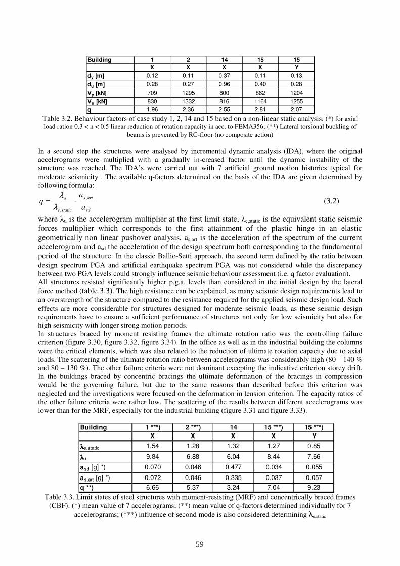
Table 3.2. Behaviour factors of case study 1, 2, 14 and 15 based on a non-linear static analysis. (*) for axial load ration 0.3 < n < 0.5 linear reduction of rotation capacity in acc. to FEMA356; (**) Lateral torsional buckling of
beams is prevented by RC-floor (no composite action) In a second step the structures were analysed by incremental dynamic analysis (IDA), where the original accelerograms were multiplied with a gradually in-creased factor until the dynamic instability of the structure was reached. The IDA’s were carried out with 7 artificial ground motion histories typical for moderate seismicity . The available q-factors determined on the basis of the IDA are given determined by following formula:
sd
arts
statice
u
a
aq
,
,
⋅=λ
λ (3.2)
where λu is the accelerogram multiplier at the first limit state, λe,static is the equivalent static seismic forces multiplier which corresponds to the first attainment of the plastic hinge in an elastic geometrically non linear pushover analysis, as,art is the acceleration of the spectrum of the current accelerogram and asd the acceleration of the design spectrum both corresponding to the fundamental period of the structure. In the classic Ballio-Setti approach, the second term defined by the ratio between design spectrum PGA and artificial earthquake spectrum PGA was not considered while the discrepancy between two PGA levels could strongly influence seismic behaviour assessment (i.e. q factor evaluation). All structures resisted significantly higher p.g.a. levels than considered in the initial design by the lateral
force method (table 3.3). The high resistance can be explained, as many seismic design requirements lead to an overstrength of the structure compared to the resistance required for the applied seismic design load. Such effects are more considerable for structures designed for moderate seismic loads, as these seismic design requirements have to ensure a sufficient performance of structures not only for low seismicity but also for high seismicity with longer strong motion periods. In structures braced by moment resisting frames the ultimate rotation ratio was the controlling failure criterion (figure 3.30, figure 3.32, figure 3.34). In the office as well as in the industrial building the columns were the critical elements, which was also related to the reduction of ultimate rotation capacity due to axial loads. The scattering of the ultimate rotation ratio between accelerograms was considerably high (80 – 140 % and 80 – 130 %). The other failure criteria were not dominant excepting the indicative criterion storey drift. In the buildings braced by concentric bracings the ultimate deformation of the bracings in compression would be the governing failure, but due to the same reasons than described before this criterion was neglected and the investigations were focused on the deformation in tension criterion. The capacity ratios of the other failure criteria were rather low. The scattering of the results between different accelerograms was lower than for the MRF, especially for the industrial building (figure 3.31 and figure 3.33).
Table 3.3. Limit states of steel structures with moment-resisting (MRF) and concentrically braced frames
(CBF). (*) mean value of 7 accelerograms; (**) mean value of q-factors determined individually for 7
accelerograms; (***) influence of second mode is also considered determining λe,static
Building 1 2 14 15 15
X X X X Y
dy [m] 0.12 0.11 0.37 0.11 0.13
du [m] 0.28 0.27 0.96 0.40 0.28
Vy [kN] 709 1295 800 862 1204
Vu [kN] 830 1332 816 1164 1255
q 1.96 2.36 2.55 2.81 2.07
Building 1 ***) 2 ***) 14 15 ***) 15 ***)
X X X X Y
λλλλe,static 1.54 1.28 1.32 1.27 0.85
λλλλu 9.84 6.88 6.04 8.44 7.66
asd [g] *) 0.070 0.046 0.477 0.034 0.055
as,art [g] *) 0.072 0.046 0.335 0.037 0.057
q **) 6.66 5.37 3.24 7.04 9.23
59
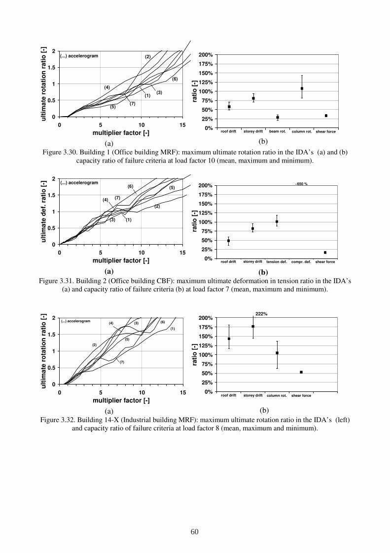
(a) (b)
Figure 3.30. Building 1 (Office building MRF): maximum ultimate rotation ratio in the IDA’s (a) and (b) capacity ratio of failure criteria at load factor 10 (mean, maximum and minimum).
(a) (b) Figure 3.31. Building 2 (Office building CBF): maximum ultimate deformation in tension ratio in the IDA’s
(a) and capacity ratio of failure criteria (b) at load factor 7 (mean, maximum and minimum).
(a) (b)
Figure 3.32. Building 14-X (Industrial building MRF): maximum ultimate rotation ratio in the IDA’s (left) and capacity ratio of failure criteria at load factor 8 (mean, maximum and minimum).
0
0.5
1
1.5
2
0 5 10 15
multiplier factor [-]
ult
ima
te r
ota
tio
n r
ati
o [
-]
(1)
(6)
(3)
(7)(5)
(2)
(4)
(...) accelerogram
roof drift storey drift beam rot. column rot. shear force0%
25%
50%
75%
100%
125%
150%
175%
200%
rati
o [
-]
0
0.5
1
1.5
2
0 5 10 15
multiplier factor [-]
ult
ima
te d
ef.
ra
tio
[-]
(1)
(6)
(3)
(7)
(5)
(2)
(4)
(...) accelerogram
roof drift storey drift tension def. shear force0%
25%
50%
75%
100%
125%
150%
175%
200%
rati
o [
-]
compr. def.
~650 %
0
0.5
1
1.5
2
0 5 10 15
multiplier factor [-]
ult
ima
te r
ota
tio
n r
ati
o [
-]
(1)
(6)(3)
(7)
(5)
(2)
(4)(...) accelerogram
roof drift storey drift column rot. shear force0%
25%
50%
75%
100%
125%
150%
175%
200%
rati
o [
-]
222%
60
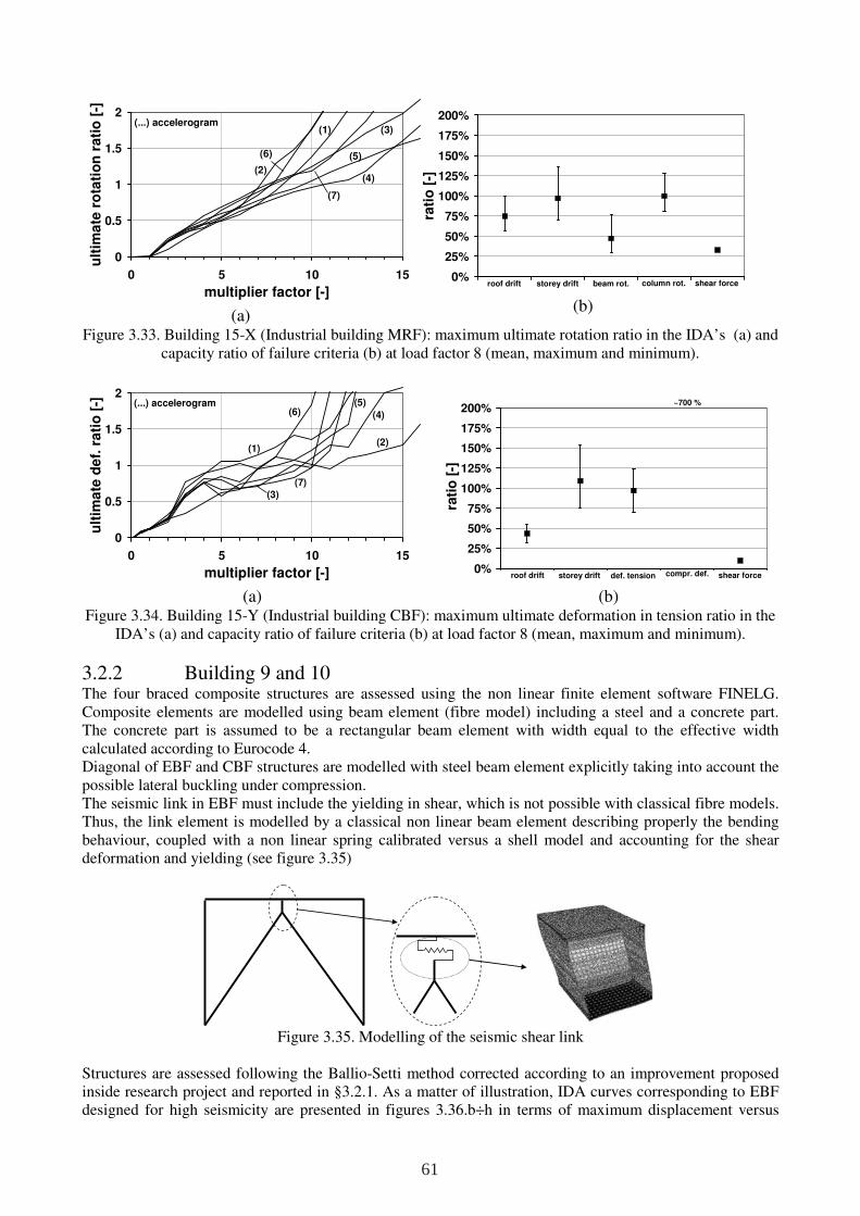
(a) (b)
Figure 3.33. Building 15-X (Industrial building MRF): maximum ultimate rotation ratio in the IDA’s (a) and capacity ratio of failure criteria (b) at load factor 8 (mean, maximum and minimum).
(a) (b) Figure 3.34. Building 15-Y (Industrial building CBF): maximum ultimate deformation in tension ratio in the
IDA’s (a) and capacity ratio of failure criteria (b) at load factor 8 (mean, maximum and minimum).
3.2.2 Building 9 and 10 The four braced composite structures are assessed using the non linear finite element software FINELG. Composite elements are modelled using beam element (fibre model) including a steel and a concrete part. The concrete part is assumed to be a rectangular beam element with width equal to the effective width calculated according to Eurocode 4. Diagonal of EBF and CBF structures are modelled with steel beam element explicitly taking into account the possible lateral buckling under compression. The seismic link in EBF must include the yielding in shear, which is not possible with classical fibre models. Thus, the link element is modelled by a classical non linear beam element describing properly the bending behaviour, coupled with a non linear spring calibrated versus a shell model and accounting for the shear deformation and yielding (see figure 3.35)
Figure 3.35. Modelling of the seismic shear link
Structures are assessed following the Ballio-Setti method corrected according to an improvement proposed inside research project and reported in §3.2.1. As a matter of illustration, IDA curves corresponding to EBF designed for high seismicity are presented in figures 3.36.b÷h in terms of maximum displacement versus
0
0.5
1
1.5
2
0 5 10 15
multiplier factor [-]
ult
ima
te r
ota
tio
n r
ati
o [
-]
(1)
(6)
(3)
(7)
(5)
(2)(4)
(...) accelerogram
roof drift storey drift beam rot. column rot. shear force0%
25%
50%
75%
100%
125%
150%
175%
200%
rati
o [
-]
0
0.5
1
1.5
2
0 5 10 15
multiplier factor [-]
ult
ima
te d
ef.
ra
tio
[-]
(1)
(6)
(3)
(7)
(5)
(2)
(4)
(...) accelerogram
roof drift storey drift def. tension shear force0%
25%
50%
75%
100%
125%
150%
175%
200%
rati
o [
-]
compr. def.
~700 %
61
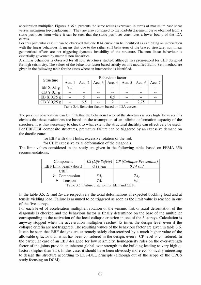
acceleration multiplier. Figures 3.36.a. presents the same results expressed in terms of maximum base shear versus maximum top displacement. They are also compared to the load-displacement curve obtained from a static pushover from where it can be seen that the static pushover constitutes a lower bound of the IDA curves. For this particular case, it can be observed that one IDA curve can be identified as exhibiting an intersection with the linear behaviour. It means that due to the rather stiff behaviour of the braced structure, non linear geometrical effects are not triggering dynamic instability of the structure. The non linear behaviour is essentially governed by material non linearities. A similar behaviour is observed for all four structures studied, although less pronounced for CBF designed for high seismicity. The values of the behaviour factor based strictly on this modified Ballio-Setti method are given in the following table for the cases where an intersection is identified.
Structure Behaviour factor
Acc. 1 Acc. 2 Acc. 3 Acc. 4 Acc. 5 Acc. 6 Acc. 7 EB X 0,1 g 7,5 -- -- -- -- -- -- CB Y 0,1 g -- -- -- -- -- -- --
EB X 0,25 g -- 5 -- 6,5 -- -- -- CB Y 0,25 g -- 6,5 -- 2 -- 2,75 3
Table 3.4. Behavior factors based on IDA curves.
The previous observations can let think that the behaviour factor of the structures is very high. However it is
obvious that these evaluations are based on the assumption of an infinite deformation capacity of the structure. It is thus necessary to check to what extent the structural ductility can effectively be used. For EBF/CBF composite structures, premature failure can be triggered by an excessive demand on the ductile zones:
for EBF with short links: excessive rotation of the link for CBF: excessive axial deformation of the diagonals.
The limit values considered in the study are given in the following table, based on FEMA 356 recommendations:
Component LS (Life Safety) CP (Collapse Prevention)
EBF Link beam (short) 0.11 rad 0.14 rad
CBF: Compression Tension
5∆c
7∆t
7∆c
9∆t
Table 3.5. Failure criterion for EBF and CBF.
In the table 3.5, ∆c and ∆T are respectively the axial deformations at expected buckling load and at tensile yielding load. Failure is assumed to be triggered as soon as the limit value is reached in one of the five storeys. For each level of acceleration multiplier, rotation of the seismic link or axial deformation of the diagonals is checked and the behaviour factor is finally determined on the base of the multiplier corresponding to the activation of the local collapse criterion in one of the 5 storeys. Calculation is anyway stopped when the acceleration multiplier reaches 15 times the design level even if the collapse criteria are not triggered. The resulting values of the behaviour factor are given in table 3.6. It can be seen that EBF designs are extremely safely characterized by a much higher value of the allowable q-factor than what has been considered in the design, even if CP level is considered. In the particular case of an EBF designed for low seismicity, homogeneity rules on the over-strength factor of the joints provide an inherent global over-strength to the building leading to very high q-factors (higher than 7.5). In this case, it should have been obviously more economically interesting to design the structure according to EC8-DCL principle (although out of the scope of the OPUS study focusing on DCM).
62
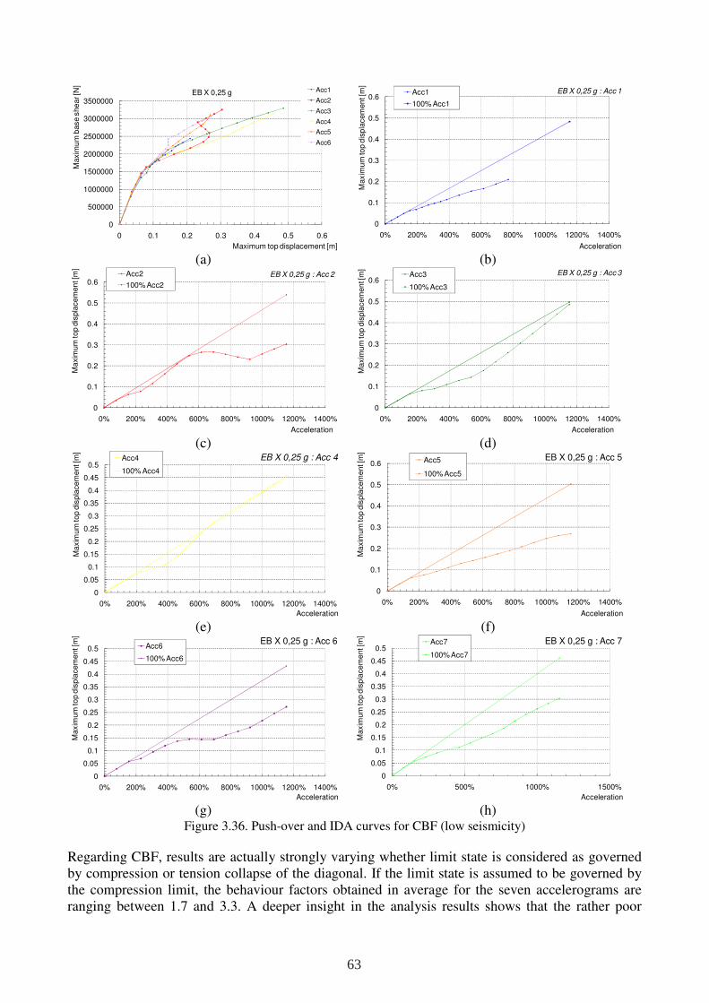
(a)
(b)
(c)
(d)
(e)
(f)
(g)
(h)
Figure 3.36. Push-over and IDA curves for CBF (low seismicity)
Regarding CBF, results are actually strongly varying whether limit state is considered as governed by compression or tension collapse of the diagonal. If the limit state is assumed to be governed by the compression limit, the behaviour factors obtained in average for the seven accelerograms are ranging between 1.7 and 3.3. A deeper insight in the analysis results shows that the rather poor
0
500000
1000000
1500000
2000000
2500000
3000000
3500000
0 0.1 0.2 0.3 0.4 0.5 0.6
Maxim
um
base s
he
ar [N
]
Maximum top displacement [m]
EB X 0,25 g Acc1
Acc2
Acc3
Acc4
Acc5
Acc6
0
0.1
0.2
0.3
0.4
0.5
0.6
0% 200% 400% 600% 800% 1000% 1200% 1400%
Maxim
um
top
dis
pla
cem
en
t [m
]
Acceleration
EB X 0,25 g : Acc 1Acc1
100% Acc1
0
0.1
0.2
0.3
0.4
0.5
0.6
0% 200% 400% 600% 800% 1000% 1200% 1400%
Ma
xim
um
to
p d
ispla
ce
men
t [m
]
Acceleration
EB X 0,25 g : Acc 2Acc2
100% Acc2
0
0.1
0.2
0.3
0.4
0.5
0.6
0% 200% 400% 600% 800% 1000% 1200% 1400%
Ma
xim
um
top
dis
pla
ce
men
t [m
]
Acceleration
EB X 0,25 g : Acc 3Acc3
100% Acc3
0
0.05
0.1
0.15
0.2
0.25
0.3
0.35
0.4
0.45
0.5
0% 200% 400% 600% 800% 1000% 1200% 1400%
Ma
xim
um
to
p d
isp
lace
me
nt [m
]
Acceleration
EB X 0,25 g : Acc 4Acc4
100% Acc4
0
0.1
0.2
0.3
0.4
0.5
0.6
0% 200% 400% 600% 800% 1000% 1200% 1400%
Ma
xim
um
to
p d
isp
lace
me
nt [m
]
Acceleration
EB X 0,25 g : Acc 5Acc5
100% Acc5
0
0.05
0.1
0.15
0.2
0.25
0.3
0.35
0.4
0.45
0.5
0% 200% 400% 600% 800% 1000% 1200% 1400%
Ma
xim
um
to
p d
isp
lace
me
nt [m
]
Acceleration
EB X 0,25 g : Acc 6Acc6
100% Acc6
0
0.05
0.1
0.15
0.2
0.25
0.3
0.35
0.4
0.45
0.5
0% 500% 1000% 1500%
Ma
xim
um
to
p d
isp
lace
me
nt [m
]
Acceleration
EB X 0,25 g : Acc 7Acc7
100% Acc7
63
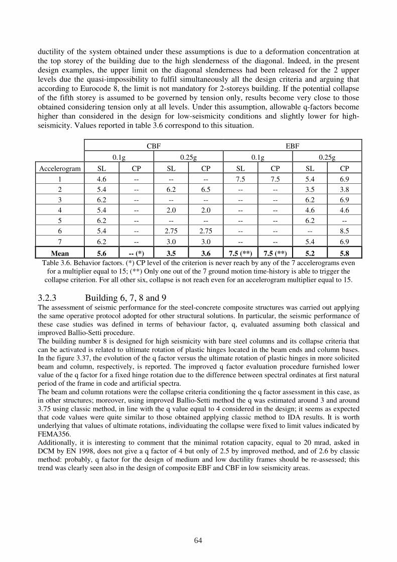
ductility of the system obtained under these assumptions is due to a deformation concentration at the top storey of the building due to the high slenderness of the diagonal. Indeed, in the present design examples, the upper limit on the diagonal slenderness had been released for the 2 upper levels due the quasi-impossibility to fulfil simultaneously all the design criteria and arguing that according to Eurocode 8, the limit is not mandatory for 2-storeys building. If the potential collapse of the fifth storey is assumed to be governed by tension only, results become very close to those obtained considering tension only at all levels. Under this assumption, allowable q-factors become higher than considered in the design for low-seismicity conditions and slightly lower for high-seismicity. Values reported in table 3.6 correspond to this situation.
CBF EBF
0.1g 0.25g 0.1g 0.25g
Accelerogram SL CP SL CP SL CP SL CP
1 4.6 -- -- -- 7.5 7.5 5.4 6.9
2 5.4 -- 6.2 6.5 -- -- 3.5 3.8
3 6.2 -- -- -- -- -- 6.2 6.9
4 5.4 -- 2.0 2.0 -- -- 4.6 4.6
5 6.2 -- -- -- -- -- 6.2 --
6 5.4 -- 2.75 2.75 -- -- -- 8.5
7 6.2 -- 3.0 3.0 -- -- 5.4 6.9
Mean 5.6 -- (*) 3.5 3.6 7.5 (**) 7.5 (**) 5.2 5.8
Table 3.6. Behavior factors. (*) CP level of the criterion is never reach by any of the 7 accelerograms even for a multiplier equal to 15; (**) Only one out of the 7 ground motion time-history is able to trigger the
collapse criterion. For all other six, collapse is not reach even for an accelerogram multiplier equal to 15.
3.2.3 Building 6, 7, 8 and 9 The assessment of seismic performance for the steel-concrete composite structures was carried out applying the same operative protocol adopted for other structural solutions. In particular, the seismic performance of these case studies was defined in terms of behaviour factor, q, evaluated assuming both classical and improved Ballio-Setti procedure. The building number 8 is designed for high seismicity with bare steel columns and its collapse criteria that can be activated is related to ultimate rotation of plastic hinges located in the beam ends and column bases. In the figure 3.37, the evolution of the q factor versus the ultimate rotation of plastic hinges in more solicited beam and column, respectively, is reported. The improved q factor evaluation procedure furnished lower value of the q factor for a fixed hinge rotation due to the difference between spectral ordinates at first natural period of the frame in code and artificial spectra. The beam and column rotations were the collapse criteria conditioning the q factor assessment in this case, as in other structures; moreover, using improved Ballio-Setti method the q was estimated around 3 and around 3.75 using classic method, in line with the q value equal to 4 considered in the design; it seems as expected that code values were quite similar to those obtained applying classic method to IDA results. It is worth underlying that values of ultimate rotations, individuating the collapse were fixed to limit values indicated by FEMA356. Additionally, it is interesting to comment that the minimal rotation capacity, equal to 20 mrad, asked in DCM by EN 1998, does not give a q factor of 4 but only of 2.5 by improved method, and of 2.6 by classic method: probably, q factor for the design of medium and low ductility frames should be re-assessed; this trend was clearly seen also in the design of composite EBF and CBF in low seismicity areas.
64
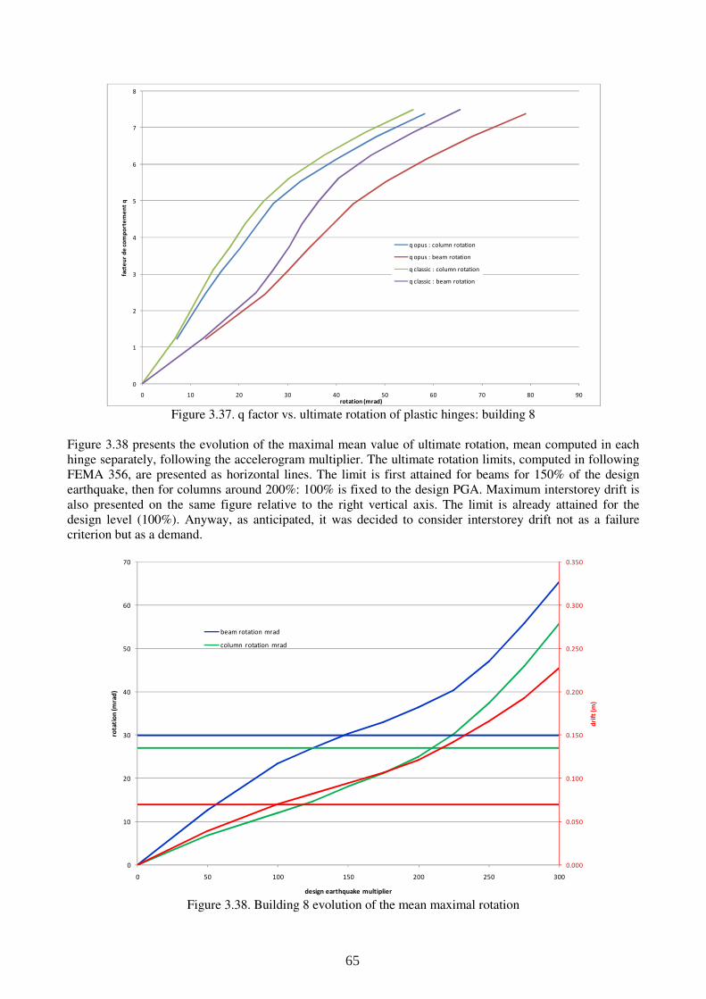
Figure 3.37. q factor vs. ultimate rotation of plastic hinges: building 8
Figure 3.38 presents the evolution of the maximal mean value of ultimate rotation, mean computed in each hinge separately, following the accelerogram multiplier. The ultimate rotation limits, computed in following FEMA 356, are presented as horizontal lines. The limit is first attained for beams for 150% of the design earthquake, then for columns around 200%: 100% is fixed to the design PGA. Maximum interstorey drift is also presented on the same figure relative to the right vertical axis. The limit is already attained for the design level (100%). Anyway, as anticipated, it was decided to consider interstorey drift not as a failure criterion but as a demand.
Figure 3.38. Building 8 evolution of the mean maximal rotation
0
1
2
3
4
5
6
7
8
0 10 20 30 40 50 60 70 80 90
fact
eu
r d
e c
om
po
rte
me
nt
q
rotation (mrad)
q opus : column rotation
q opus : beam rotation
q classic : column rotation
q classic : beam rotation
0.000
0.050
0.100
0.150
0.200
0.250
0.300
0.350
0
10
20
30
40
50
60
70
0 50 100 150 200 250 300
dri
ft (
m)
rota
tio
n (
mra
d)
design earthquake multiplier
beam rotation mrad
column rotation mrad
65
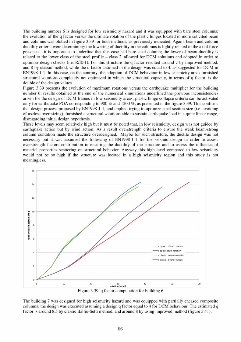
The building number 6 is designed for low seismicity hazard and it was equipped with bare steel columns; the evolution of the q factor versus the ultimate rotation of the plastic hinges located in more solicited beam and columns was plotted in figure 3.39 for both methods, as previously indicated. Again, beam and column ductility criteria were determining: the lowering of ductility in the columns is lightly related to the axial force presence – it is important to underline that this case had bare steel column; the lower of beam ductility is related to the lower class of the steel profile – class 2, allowed for DCM solutions and adopted in order to
optimize design checks (i.e. R/S>1). For this structure the q factor resulted around 7 by improved method, and 8 by classic method, while the q factor assumed in the design was equal to 4, as suggested for DCM in EN1998-1-1. In this case, on the contrary, the adoption of DCM behaviour in low seismicity areas furnished structural solutions completely not optimized in which the structural capacity, in terms of q factor, is the double of the design values. Figure 3.39 presents the evolution of maximum rotations versus the earthquake multiplier for the building number 6; results obtained at the end of the numerical simulations underlined the previous inconsistencies arisen for the design of DCM frames in low seismicity areas: plastic hinge collapse criteria can be activated only for earthquake PGA corresponding to 900 % and 1200 %, as presented in the figure 3.39. This confirms that design process proposed by EN1998-1-1, and applied trying to optimize steel section size (i.e. avoiding of useless over-sizing), furnished a structural solutions able to sustain earthquake load in a quite linear range, disregarding initial design hypothesis. These levels may seem relatively high but it must be noted that, in low seismicity, design was not guided by earthquake action but by wind action. As a result overstrength criteria to ensure the weak beam-strong column condition made the structure overdesigned. Maybe for such structure, the ductile design was not necessary but it was assumed the following of EN1998-1-1 for the seismic design in order to assess overstrength factors contribution in ensuring the ductility of the structure and to assess the influence of material properties scattering on structural behavior. Anyway this high level compared to low seismicity would not be so high if the structure was located in a high seismicity region and this study is not meaningless.
Figure 3.39. q factor computation for building 6
The building 7 was designed for high seismicity hazard and was equipped with partially encased composite columns; the design was executed assuming a design q factor equal to 4 for DCM behaviour. The estimated q factor is around 8.5 by classic Ballio-Setti method, and around 8 by using improved method (figure 3.41).
0
2
4
6
8
10
12
14
16
0 10 20 30 40 50 60
fact
eu
r d
e c
om
po
rte
me
nt
q
rotation (mrad)
q opus : column rotation
q opus : beam rotation
q classic : column rotation
q classic : beam rotation
66
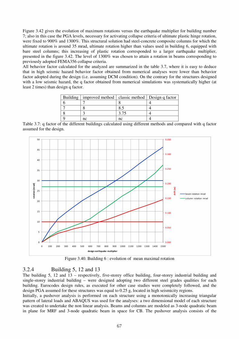
Figure 3.42 gives the evolution of maximum rotations versus the earthquake multiplier for building number 7; also in this case the PGA levels, necessary for activating collapse criteria of ultimate plastic hinge rotation, were fixed to 900% and 1300%. This structural solution had steel-concrete composite columns for which the ultimate rotation is around 35 mrad, ultimate rotation higher than values used in building 6, equipped with bare steel columns; this increasing of plastic rotation corresponded to a larger earthquake multiplier, presented in the figure 3.42. The level of 1300% was chosen to attain a rotation in beams corresponding to previously adopted FEMA356 collapse criteria. All behavior factor calculated for the analyzed are summarized in the table 3.7, where it is easy to deduce that in high seismic hazard behavior factor obtained from numerical analyses were lower than behavior factor adopted during the design (i.e. assuming DCM condition). On the contrary for the structures designed with a low seismic hazard, the q factor obtained from numerical simulations was systematically higher (at least 2 times) than design q factor.
Building improved method classic method Design q factor 6 7 8 4 7 8 8.5 4 8 3 3.75 4 9 nc nc 4
Table 3.7: q factor of the different buildings calculated using different methods and compared with q factor assumed for the design.
Figure 3.40. Building 6 : evolution of mean maximal rotation
3.2.4 Building 5, 12 and 13 The building 5, 12 and 13 – respectively, five-storey office building, four-storey industrial building and single-storey industrial building – were designed adopting two different steel grades qualities for each building. Eurocodes design rules, as executed for other case studies were completely followed, and the design PGA assumed for these structures was equal to 0.25 g, located in high seismicity regions. Initially, a pushover analysis is performed on each structure using a monotonically increasing triangular pattern of lateral loads and ABAQUS was used for the analyses: a two dimensional model of each structure was created to undertake the non linear analysis. Beams and columns are modeled as 3-node quadratic beam in plane for MRF and 3-node quadratic beam in space for CB. The pushover analysis consists of the
0.000
0.050
0.100
0.150
0.200
0.250
0.300
0.350
0
5
10
15
20
25
30
35
40
45
50
0 100 200 300 400 500 600 700 800 900 1000 1100 1200 1300 1400 1500
dri
ft (
m)
rota
tio
n (
mra
d)
design earthquake multiplier
beam rotation mrad
column rotation mrad
67
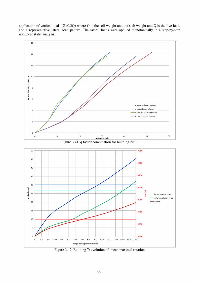
application of vertical loads (G+0.3Q) where G is the self weight and the slab weight and Q is the live load, and a representative lateral load pattern. The lateral loads were applied monotonically in a step-by-step nonlinear static analysis.
Figure 3.41. q factor computation for building Nr. 7
Figure 3.42. Building 7: evolution of mean maximal rotation
0
2
4
6
8
10
12
14
16
0 10 20 30 40 50 60
fact
eu
r d
e c
om
po
rte
me
nt
q
rotation (mrad)
q opus : column rotation
q opus : beam rotation
q classic : column rotation
q classic : beam rotation
0.000
0.050
0.100
0.150
0.200
0.250
0.300
0.350
0
5
10
15
20
25
30
35
40
45
50
0 100 200 300 400 500 600 700 800 900 1000 1100 1200 1300 1400 1500
dri
ft (
m)
rota
tio
n (
mra
d)
design earthquake multiplier
beam rotation mrad
column rotation mrad
drift m
68
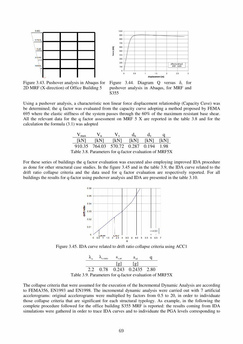
Figure 3.43. Pushover analysis in Abaqus for 2D MRF (X-direction) of Office Building 5
Figure 3.44. Diagram Q versus δ, for pushover analysis in Abaqus, for MRF and S355
Using a pushover analysis, a characteristic non linear force displacement relationship (Capacity Cuve) was be determined; the q factor was evaluated from the capacity curve adopting a method proposed by FEMA 695 where the elastic stiffness of the system passes through the 60% of the maximum resistant base shear. All the relevant data for the q factor assessment on MRF 5 X are reported in the table 3.8 and for the calculation the formula (3.1) was adopted
Vmax Vu Vy du dy q [kN] [kN] [kN] [kN] [kN] [kN]
910.35 764.03 570.72 0.287 0.194 1.98 Table 3.8. Parameters for q-factor evaluation of MRF5X
For these series of buildings the q factor evaluation was executed also employing improved IDA procedure as done for other structural case studies. In the figure 3.45 and in the table 3.9, the IDA curve related to the drift ratio collapse criteria and the data used for q factor evaluation are respectively reported. For all buildings the results for q-factor using pushover analysis and IDA are presented in the table 3.10.
Figure 3.45. IDA curve related to drift ratio collapse criteria using ACC1
uλ e static,λ s arta
,
sda q
[g] [g]
2.2 0.78 0.243 0.2435 2.80 Table 3.9. Parameters for q-factor evaluation of MRF5X
The collapse criteria that were assumed for the execution of the Incremental Dynamic Analysis are according to FEMA356, EN1993 and EN1998. The incremental dynamic analysis were carried out with 7 artificial accelerograms: original accelerograms were multiplied by factors from 0.5 to 20, in order to individuate those collapse criteria that are significant for each structural typology. As example, in the following the complete procedure followed for the office building S355 MRF is reported: the results coming from IDA simulations were gathered in order to trace IDA curves and to individuate the PGA levels corresponding to
69
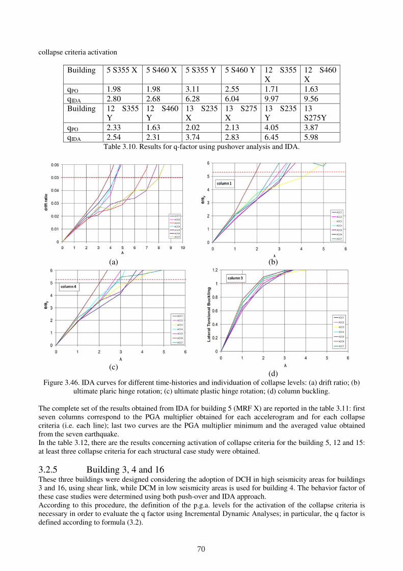
collapse criteria activation
Building 5 S355 X 5 S460 X 5 S355 Y 5 S460 Y 12 S355 X
12 S460 X
qPO 1.98 1.98 3.11 2.55 1.71 1.63
qIDA 2.80 2.68 6.28 6.04 9.97 9.56 Building 12 S355
Y 12 S460 Y
13 S235 X
13 S275 X
13 S235 Y
13 S275Y
qPO 2.33 1.63 2.02 2.13 4.05 3.87 qIDA 2.54 2.31 3.74 2.83 6.45 5.98
Table 3.10. Results for q-factor using pushover analysis and IDA.
(a)
(b)
(c)
(d) Figure 3.46. IDA curves for different time-histories and individuation of collapse levels: (a) drift ratio; (b)
ultimate plaric hinge rotation; (c) ultimate plastic hinge rotation; (d) column buckling. The complete set of the results obtained from IDA for building 5 (MRF X) are reported in the table 3.11: first seven columns correspond to the PGA multiplier obtained for each accelerogram and for each collapse criteria (i.e. each line); last two curves are the PGA multiplier minimum and the averaged value obtained from the seven earthquake. In the table 3.12, there are the results concerning activation of collapse criteria for the building 5, 12 and 15: at least three collapse criteria for each structural case study were obtained.
3.2.5 Building 3, 4 and 16 These three buildings were designed considering the adoption of DCH in high seismicity areas for buildings 3 and 16, using shear link, while DCM in low seismicity areas is used for building 4. The behavior factor of these case studies were determined using both push-over and IDA approach. According to this procedure, the definition of the p.g.a. levels for the activation of the collapse criteria is necessary in order to evaluate the q factor using Incremental Dynamic Analyses; in particular, the q factor is defined according to formula (3.2).
70
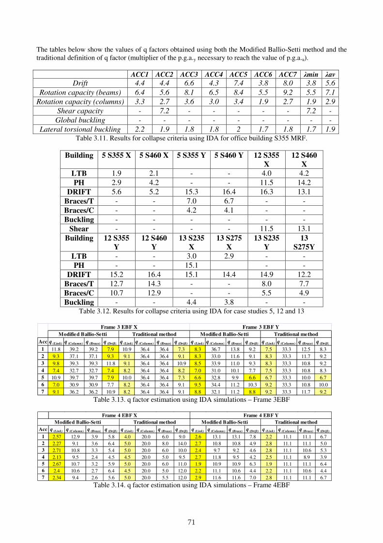
The tables below show the values of q factors obtained using both the Modified Ballio-Setti method and the traditional definition of q factor (multiplier of the p.g.a.y necessary to reach the value of p.g.a.u).
ACC1 ACC2 ACC3 ACC4 ACC5 ACC6 ACC7 λmin λav
Drift 4.4 4.4 6.6 4.3 7.4 3.8 8.0 3.8 5.6
Rotation capacity (beams) 6.4 5.6 8.1 6.5 8.4 5.5 9.2 5.5 7.1
Rotation capacity (columns) 3.3 2.7 3.6 3.0 3.4 1.9 2.7 1.9 2.9
Shear capacity - 7.2 - - - - - 7.2 -
Global buckling - - - - - - - - -
Lateral torsional buckling 2.2 1.9 1.8 1.8 2 1.7 1.8 1.7 1.9
Table 3.11. Results for collapse criteria using IDA for office building S355 MRF.
Building 5 S355 X 5 S460 X 5 S355 Y 5 S460 Y 12 S355
X
12 S460
X
LTB 1.9 2.1 - - 4.0 4.2
PH 2.9 4.2 - - 11.5 14.2
DRIFT 5.6 5.2 15.3 16.4 16.3 13.1
Braces/T - - 7.0 6.7 - -
Braces/C - - 4.2 4.1 - -
Buckling - - - - - -
Shear - - - - 11.5 13.1
Building 12 S355
Y
12 S460
Y
13 S235
X
13 S275
X
13 S235
Y
13
S275Y
LTB - - 3.0 2.9 - -
PH - - 15.1 - -
DRIFT 15.2 16.4 15.1 14.4 14.9 12.2
Braces/T 12.7 14.3 - - 8.0 7.7
Braces/C 10.7 12.9 - - 5.5 4.9
Buckling - - 4.4 3.8 - - Table 3.12. Results for collapse criteria using IDA for case studies 5, 12 and 13
Table 3.13. q factor estimation using IDA simulations – Frame 3EBF
Table 3.14. q factor estimation using IDA simulations – Frame 4EBF
Acc q (Link) q (Column) q (Brace) q (Drift) q (Link) q (Column) q (Brace) q (Drift) q (Link) q (Column) q (Brace) q (Drift) q (Link) q (Column) q (Brace) q (Drift)
1 11.8 39.2 39.2 7.9 10.9 36.4 36.4 7.3 8.3 36.7 13.8 9.2 7.5 33.3 12.5 8.3
2 9.3 37.1 37.1 9.3 9.1 36.4 36.4 9.1 8.3 33.0 11.6 9.1 8.3 33.3 11.7 9.2
3 9.8 39.3 39.3 11.8 9.1 36.4 36.4 10.9 8.5 33.9 11.0 9.3 8.3 33.3 10.8 9.2
4 7.4 32.7 32.7 7.4 8.2 36.4 36.4 8.2 7.0 31.0 10.1 7.7 7.5 33.3 10.8 8.3
5 10.9 39.7 39.7 7.9 10.0 36.4 36.4 7.3 6.6 32.8 9.9 6.6 6.7 33.3 10.0 6.7
6 7.0 30.9 30.9 7.7 8.2 36.4 36.4 9.1 9.5 34.4 11.2 10.3 9.2 33.3 10.8 10.0
7 9.1 36.2 36.2 10.9 8.2 36.4 36.4 9.1 8.8 32.1 11.2 8.8 9.2 33.3 11.7 9.2
Frame 3 EBF X Frame 3 EBF Y
Traditional method Traditional methodModified Ballio-Setti Modified Ballio-Setti
Acc q (Link) q (Column) q (Brace) q (Drift) q (Link) q (Column) q (Brace) q (Drift) q (Link) q (Column) q (Brace) q (Drift) q (Link) q (Column) q (Brace) q (Drift)
1 2.57 12.9 3.9 5.8 4.0 20.0 6.0 9.0 2.6 13.1 13.1 7.8 2.2 11.1 11.1 6.7
2 2.27 9.1 3.6 6.4 5.0 20.0 8.0 14.0 2.7 10.8 10.8 4.9 2.8 11.1 11.1 5.0
3 2.71 10.8 3.3 5.4 5.0 20.0 6.0 10.0 2.4 9.7 9.2 4.6 2.8 11.1 10.6 5.3
4 2.13 9.5 2.4 4.5 4.5 20.0 5.0 9.5 2.7 11.8 9.5 4.2 2.5 11.1 8.9 3.9
5 2.67 10.7 3.2 5.9 5.0 20.0 6.0 11.0 1.9 10.9 10.9 6.3 1.9 11.1 11.1 6.4
6 2.4 10.6 2.7 6.4 4.5 20.0 5.0 12.0 2.2 11.1 10.6 4.4 2.2 11.1 10.6 4.4
7 2.34 9.4 2.6 5.6 5.0 20.0 5.5 12.0 2.9 11.6 11.6 7.0 2.8 11.1 11.1 6.7
Frame 4 EBF X Frame 4 EBF Y
Modified Ballio-Setti Traditional method Modified Ballio-Setti Traditional method
71
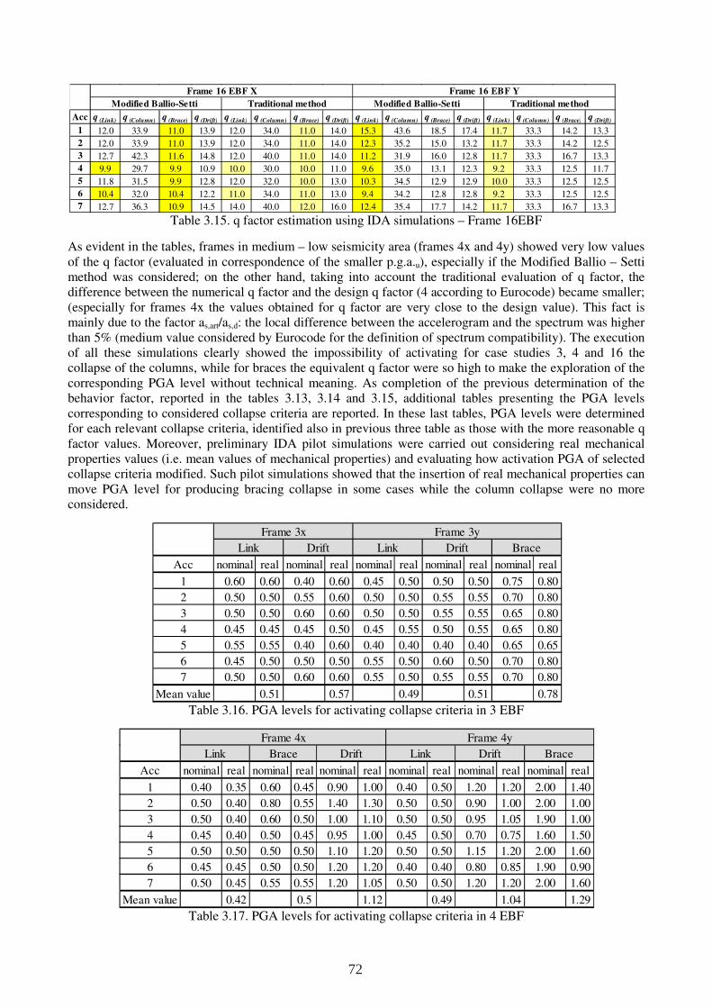
Table 3.15. q factor estimation using IDA simulations – Frame 16EBF
As evident in the tables, frames in medium – low seismicity area (frames 4x and 4y) showed very low values of the q factor (evaluated in correspondence of the smaller p.g.a.u), especially if the Modified Ballio – Setti method was considered; on the other hand, taking into account the traditional evaluation of q factor, the difference between the numerical q factor and the design q factor (4 according to Eurocode) became smaller; (especially for frames 4x the values obtained for q factor are very close to the design value). This fact is mainly due to the factor as,art/as,d: the local difference between the accelerogram and the spectrum was higher than 5% (medium value considered by Eurocode for the definition of spectrum compatibility). The execution of all these simulations clearly showed the impossibility of activating for case studies 3, 4 and 16 the collapse of the columns, while for braces the equivalent q factor were so high to make the exploration of the corresponding PGA level without technical meaning. As completion of the previous determination of the behavior factor, reported in the tables 3.13, 3.14 and 3.15, additional tables presenting the PGA levels corresponding to considered collapse criteria are reported. In these last tables, PGA levels were determined for each relevant collapse criteria, identified also in previous three table as those with the more reasonable q factor values. Moreover, preliminary IDA pilot simulations were carried out considering real mechanical properties values (i.e. mean values of mechanical properties) and evaluating how activation PGA of selected collapse criteria modified. Such pilot simulations showed that the insertion of real mechanical properties can move PGA level for producing bracing collapse in some cases while the column collapse were no more considered.
Table 3.16. PGA levels for activating collapse criteria in 3 EBF
Table 3.17. PGA levels for activating collapse criteria in 4 EBF
Acc q (Link) q (Column) q (Brace) q (Drift) q (Link) q (Column) q (Brace) q (Drift) q (Link) q (Column) q (Brace) q (Drift) q (Link) q (Column) q (Brace) q (Drift)
1 12.0 33.9 11.0 13.9 12.0 34.0 11.0 14.0 15.3 43.6 18.5 17.4 11.7 33.3 14.2 13.3
2 12.0 33.9 11.0 13.9 12.0 34.0 11.0 14.0 12.3 35.2 15.0 13.2 11.7 33.3 14.2 12.5
3 12.7 42.3 11.6 14.8 12.0 40.0 11.0 14.0 11.2 31.9 16.0 12.8 11.7 33.3 16.7 13.3
4 9.9 29.7 9.9 10.9 10.0 30.0 10.0 11.0 9.6 35.0 13.1 12.3 9.2 33.3 12.5 11.7
5 11.8 31.5 9.9 12.8 12.0 32.0 10.0 13.0 10.3 34.5 12.9 12.9 10.0 33.3 12.5 12.5
6 10.4 32.0 10.4 12.2 11.0 34.0 11.0 13.0 9.4 34.2 12.8 12.8 9.2 33.3 12.5 12.5
7 12.7 36.3 10.9 14.5 14.0 40.0 12.0 16.0 12.4 35.4 17.7 14.2 11.7 33.3 16.7 13.3
Traditional methodModified Ballio-Setti Traditional methodModified Ballio-Setti
Frame 16 EBF X Frame 16 EBF Y
Acc nominal real nominal real nominal real nominal real nominal real
1 0.60 0.60 0.40 0.60 0.45 0.50 0.50 0.50 0.75 0.80
2 0.50 0.50 0.55 0.60 0.50 0.50 0.55 0.55 0.70 0.80
3 0.50 0.50 0.60 0.60 0.50 0.50 0.55 0.55 0.65 0.80
4 0.45 0.45 0.45 0.50 0.45 0.55 0.50 0.55 0.65 0.80
5 0.55 0.55 0.40 0.60 0.40 0.40 0.40 0.40 0.65 0.65
6 0.45 0.50 0.50 0.50 0.55 0.50 0.60 0.50 0.70 0.80
7 0.50 0.50 0.60 0.60 0.55 0.50 0.55 0.55 0.70 0.80
Mean value 0.51 0.57 0.49 0.51 0.78
Frame 3x Frame 3y
Link Drift Link Drift Brace
Acc nominal real nominal real nominal real nominal real nominal real nominal real
1 0.40 0.35 0.60 0.45 0.90 1.00 0.40 0.50 1.20 1.20 2.00 1.40
2 0.50 0.40 0.80 0.55 1.40 1.30 0.50 0.50 0.90 1.00 2.00 1.00
3 0.50 0.40 0.60 0.50 1.00 1.10 0.50 0.50 0.95 1.05 1.90 1.00
4 0.45 0.40 0.50 0.45 0.95 1.00 0.45 0.50 0.70 0.75 1.60 1.50
5 0.50 0.50 0.50 0.50 1.10 1.20 0.50 0.50 1.15 1.20 2.00 1.60
6 0.45 0.45 0.50 0.50 1.20 1.20 0.40 0.40 0.80 0.85 1.90 0.90
7 0.50 0.45 0.55 0.55 1.20 1.05 0.50 0.50 1.20 1.20 2.00 1.60
Mean value 0.42 0.5 1.12 0.49 1.04 1.29
Frame 4x Frame 4y
Link Drift BraceLink Brace Drift
72
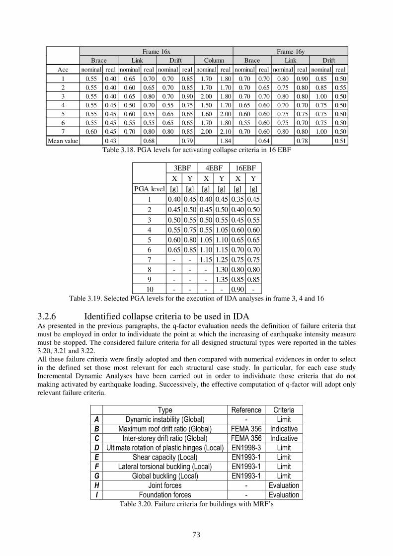
Table 3.18. PGA levels for activating collapse criteria in 16 EBF
Table 3.19. Selected PGA levels for the execution of IDA analyses in frame 3, 4 and 16
3.2.6 Identified collapse criteria to be used in IDA As presented in the previous paragraphs, the q-factor evaluation needs the definition of failure criteria that must be employed in order to individuate the point at which the increasing of earthquake intensity measure must be stopped. The considered failure criteria for all designed structural types were reported in the tables 3.20, 3.21 and 3.22. All these failure criteria were firstly adopted and then compared with numerical evidences in order to select in the defined set those most relevant for each structural case study. In particular, for each case study Incremental Dynamic Analyses have been carried out in order to individuate those criteria that do not making activated by earthquake loading. Successively, the effective computation of q-factor will adopt only relevant failure criteria.
Type Reference Criteria
A Dynamic instability (Global) - Limit
B Maximum roof drift ratio (Global) FEMA 356 Indicative
C Inter-storey drift ratio (Global) FEMA 356 Indicative
D Ultimate rotation of plastic hinges (Local) EN1998-3 Limit
E Shear capacity (Local) EN1993-1 Limit
F Lateral torsional buckling (Local) EN1993-1 Limit
G Global buckling (Local) EN1993-1 Limit
H Joint forces - Evaluation
I Foundation forces - Evaluation Table 3.20. Failure criteria for buildings with MRF’s
Acc nominal real nominal real nominal real nominal real nominal real nominal real nominal real
1 0.55 0.40 0.65 0.70 0.70 0.85 1.70 1.80 0.70 0.70 0.80 0.90 0.85 0.50
2 0.55 0.40 0.60 0.65 0.70 0.85 1.70 1.70 0.70 0.65 0.75 0.80 0.85 0.55
3 0.55 0.40 0.65 0.80 0.70 0.90 2.00 1.80 0.70 0.70 0.80 0.80 1.00 0.50
4 0.55 0.45 0.50 0.70 0.55 0.75 1.50 1.70 0.65 0.60 0.70 0.70 0.75 0.50
5 0.55 0.45 0.60 0.55 0.65 0.65 1.60 2.00 0.60 0.60 0.75 0.75 0.75 0.50
6 0.55 0.45 0.55 0.55 0.65 0.65 1.70 1.80 0.55 0.60 0.75 0.70 0.75 0.50
7 0.60 0.45 0.70 0.80 0.80 0.85 2.00 2.10 0.70 0.60 0.80 0.80 1.00 0.50
Mean value 0.43 0.68 0.79 1.84 0.64 0.78 0.51
Column Brace Link Drift
Frame 16x Frame 16y
Brace Link Drift
X Y X Y X Y
PGA level [g] [g] [g] [g] [g] [g]
1 0.40 0.45 0.40 0.45 0.35 0.45
2 0.45 0.50 0.45 0.50 0.40 0.50
3 0.50 0.55 0.50 0.55 0.45 0.55
4 0.55 0.75 0.55 1.05 0.60 0.60
5 0.60 0.80 1.05 1.10 0.65 0.65
6 0.65 0.85 1.10 1.15 0.70 0.70
7 - - 1.15 1.25 0.75 0.75
8 - - - 1.30 0.80 0.80
9 - - - 1.35 0.85 0.85
10 - - - - 0.90 -
3EBF 4EBF 16EBF
73
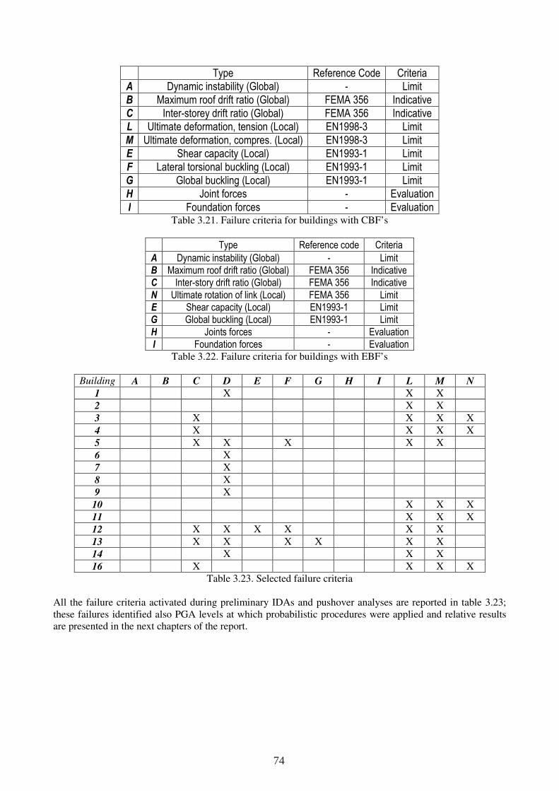
Type Reference Code Criteria
A Dynamic instability (Global) - Limit
B Maximum roof drift ratio (Global) FEMA 356 Indicative
C Inter-storey drift ratio (Global) FEMA 356 Indicative
L Ultimate deformation, tension (Local) EN1998-3 Limit
M Ultimate deformation, compres. (Local) EN1998-3 Limit
E Shear capacity (Local) EN1993-1 Limit
F Lateral torsional buckling (Local) EN1993-1 Limit
G Global buckling (Local) EN1993-1 Limit
H Joint forces - Evaluation
I Foundation forces - Evaluation Table 3.21. Failure criteria for buildings with CBF’s
Type Reference code Criteria A Dynamic instability (Global) - Limit B Maximum roof drift ratio (Global) FEMA 356 Indicative C Inter-story drift ratio (Global) FEMA 356 Indicative N Ultimate rotation of link (Local) FEMA 356 Limit E Shear capacity (Local) EN1993-1 Limit G Global buckling (Local) EN1993-1 Limit H Joints forces - Evaluation I Foundation forces - Evaluation
Table 3.22. Failure criteria for buildings with EBF’s
Building A B C D E F G H I L M N
1 X X X
2 X X
3 X X X X
4 X X X X
5 X X X X X
6 X
7 X
8 X
9 X
10 X X X
11 X X X
12 X X X X X X
13 X X X X X X
14 X X X
16 X X X X Table 3.23. Selected failure criteria
All the failure criteria activated during preliminary IDAs and pushover analyses are reported in table 3.23; these failures identified also PGA levels at which probabilistic procedures were applied and relative results are presented in the next chapters of the report.
74
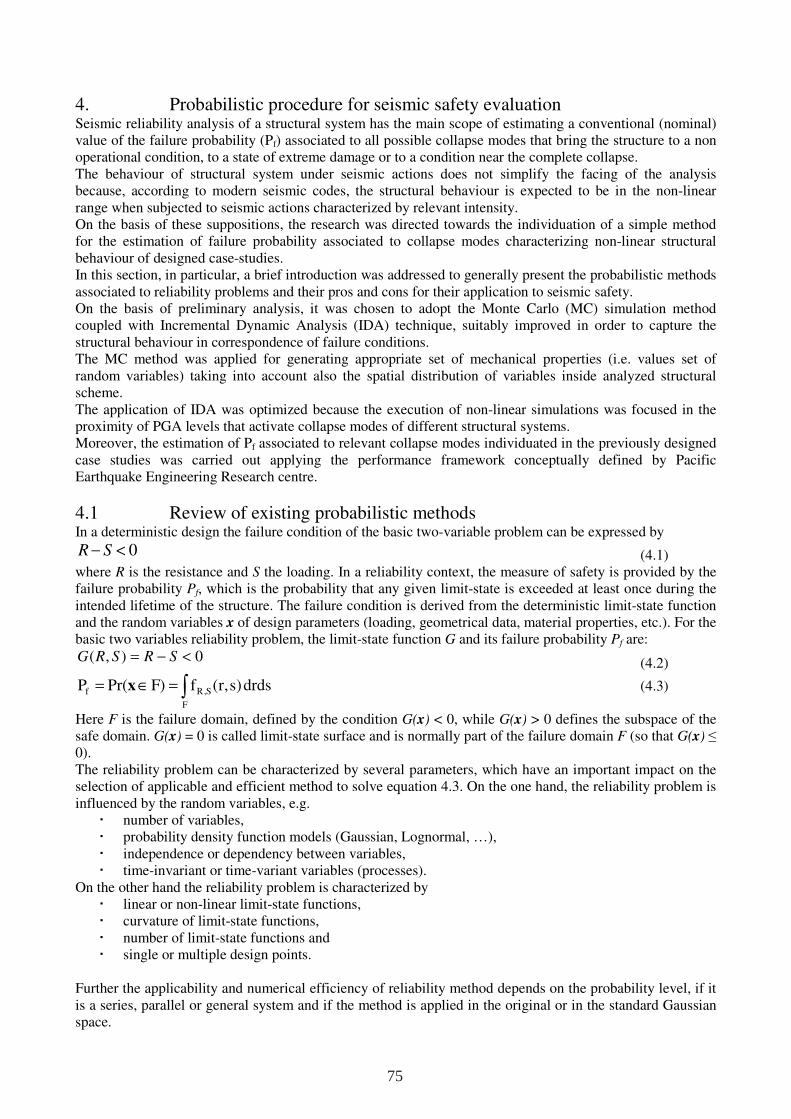
4. Probabilistic procedure for seismic safety evaluation Seismic reliability analysis of a structural system has the main scope of estimating a conventional (nominal) value of the failure probability (Pf) associated to all possible collapse modes that bring the structure to a non operational condition, to a state of extreme damage or to a condition near the complete collapse. The behaviour of structural system under seismic actions does not simplify the facing of the analysis because, according to modern seismic codes, the structural behaviour is expected to be in the non-linear range when subjected to seismic actions characterized by relevant intensity. On the basis of these suppositions, the research was directed towards the individuation of a simple method for the estimation of failure probability associated to collapse modes characterizing non-linear structural behaviour of designed case-studies. In this section, in particular, a brief introduction was addressed to generally present the probabilistic methods associated to reliability problems and their pros and cons for their application to seismic safety. On the basis of preliminary analysis, it was chosen to adopt the Monte Carlo (MC) simulation method coupled with Incremental Dynamic Analysis (IDA) technique, suitably improved in order to capture the structural behaviour in correspondence of failure conditions. The MC method was applied for generating appropriate set of mechanical properties (i.e. values set of random variables) taking into account also the spatial distribution of variables inside analyzed structural scheme. The application of IDA was optimized because the execution of non-linear simulations was focused in the proximity of PGA levels that activate collapse modes of different structural systems. Moreover, the estimation of Pf associated to relevant collapse modes individuated in the previously designed case studies was carried out applying the performance framework conceptually defined by Pacific Earthquake Engineering Research centre.
4.1 Review of existing probabilistic methods In a deterministic design the failure condition of the basic two-variable problem can be expressed by
0<− SR (4.1) where R is the resistance and S the loading. In a reliability context, the measure of safety is provided by the failure probability Pf, which is the probability that any given limit-state is exceeded at least once during the intended lifetime of the structure. The failure condition is derived from the deterministic limit-state function and the random variables x of design parameters (loading, geometrical data, material properties, etc.). For the basic two variables reliability problem, the limit-state function G and its failure probability Pf are:
0),( <−= SRSRG (4.2)
∫=∈=F
S,Rf drds)s,r(f)FPr(P x
(4.3)
Here F is the failure domain, defined by the condition G(x) < 0, while G(x) > 0 defines the subspace of the safe domain. G(x) = 0 is called limit-state surface and is normally part of the failure domain F (so that G(x) ≤ 0). The reliability problem can be characterized by several parameters, which have an important impact on the selection of applicable and efficient method to solve equation 4.3. On the one hand, the reliability problem is influenced by the random variables, e.g.
number of variables, probability density function models (Gaussian, Lognormal, …), independence or dependency between variables, time-invariant or time-variant variables (processes).
On the other hand the reliability problem is characterized by linear or non-linear limit-state functions, curvature of limit-state functions, number of limit-state functions and single or multiple design points.
Further the applicability and numerical efficiency of reliability method depends on the probability level, if it is a series, parallel or general system and if the method is applied in the original or in the standard Gaussian space.
75
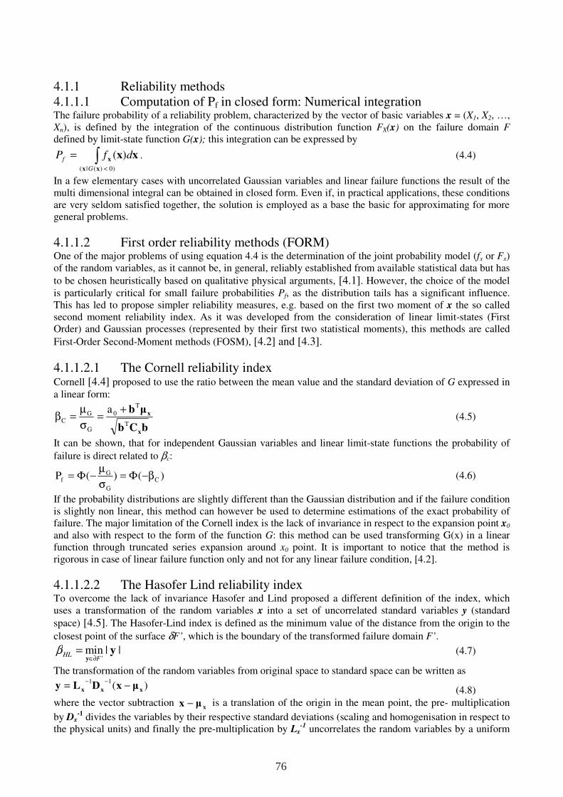
4.1.1 Reliability methods 4.1.1.1 Computation of Pf in closed form: Numerical integration The failure probability of a reliability problem, characterized by the vector of basic variables x = (X1, X2, …, Xn), is defined by the integration of the continuous distribution function FX(x) on the failure domain F defined by limit-state function G(x); this integration can be expressed by
∫<
=)0)(|(
)(xx
x xxG
f dfP . (4.4)
In a few elementary cases with uncorrelated Gaussian variables and linear failure functions the result of the multi dimensional integral can be obtained in closed form. Even if, in practical applications, these conditions are very seldom satisfied together, the solution is employed as a base the basic for approximating for more general problems.
4.1.1.2 First order reliability methods (FORM) One of the major problems of using equation 4.4 is the determination of the joint probability model (fx or Fx) of the random variables, as it cannot be, in general, reliably established from available statistical data but has
to be chosen heuristically based on qualitative physical arguments, [4.1]. However, the choice of the model is particularly critical for small failure probabilities Pf, as the distribution tails has a significant influence. This has led to propose simpler reliability measures, e.g. based on the first two moment of x the so called second moment reliability index. As it was developed from the consideration of linear limit-states (First Order) and Gaussian processes (represented by their first two statistical moments), this methods are called
First-Order Second-Moment methods (FOSM), [4.2] and [4.3].
4.1.1.2.1 The Cornell reliability index Cornell [4.4] proposed to use the ratio between the mean value and the standard deviation of G expressed in a linear form:
bCb
µb
x
x
T
T
0
G
GC
a +=
σ
µ=β
(4.5)
It can be shown, that for independent Gaussian variables and linear limit-state functions the probability of
failure is direct related to βc:
)()(P C
G
Gf β−Φ=
σ
µ−Φ=
(4.6)
If the probability distributions are slightly different than the Gaussian distribution and if the failure condition is slightly non linear, this method can however be used to determine estimations of the exact probability of failure. The major limitation of the Cornell index is the lack of invariance in respect to the expansion point x0 and also with respect to the form of the function G: this method can be used transforming G(x) in a linear function through truncated series expansion around x0 point. It is important to notice that the method is rigorous in case of linear failure function only and not for any linear failure condition, [4.2].
4.1.1.2.2 The Hasofer Lind reliability index To overcome the lack of invariance Hasofer and Lind proposed a different definition of the index, which uses a transformation of the random variables x into a set of uncorrelated standard variables y (standard
space) [4.5]. The Hasofer-Lind index is defined as the minimum value of the distance from the origin to the
closest point of the surface δF’, which is the boundary of the transformed failure domain F’.
||min'
yy F
HL∂∈
=β
(4.7)
The transformation of the random variables from original space to standard space can be written as
)(11
xxx µxDLy −=−−
(4.8)
where the vector subtraction xµx − is a translation of the origin in the mean point, the pre- multiplication
by Dx-1 divides the variables by their respective standard deviations (scaling and homogenisation in respect to
the physical units) and finally the pre-multiplication by Lx-1 uncorrelates the random variables by a uniform
76
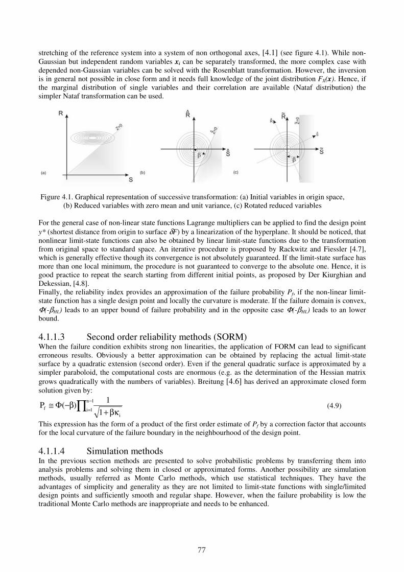
stretching of the reference system into a system of non orthogonal axes, [4.1] (see figure 4.1). While non-Gaussian but independent random variables xi can be separately transformed, the more complex case with depended non-Gaussian variables can be solved with the Rosenblatt transformation. However, the inversion is in general not possible in close form and it needs full knowledge of the joint distribution FX(x). Hence, if the marginal distribution of single variables and their correlation are available (Nataf distribution) the simpler Nataf transformation can be used.
Figure 4.1. Graphical representation of successive transformation: (a) Initial variables in origin space,
(b) Reduced variables with zero mean and unit variance, (c) Rotated reduced variables For the general case of non-linear state functions Lagrange multipliers can be applied to find the design point
y* (shortest distance from origin to surface δF) by a linearization of the hyperplane. It should be noticed, that nonlinear limit-state functions can also be obtained by linear limit-state functions due to the transformation from original space to standard space. An iterative procedure is proposed by Rackwitz and Fiessler [4.7], which is generally effective though its convergence is not absolutely guaranteed. If the limit-state surface has more than one local minimum, the procedure is not guaranteed to converge to the absolute one. Hence, it is good practice to repeat the search starting from different initial points, as proposed by Der Kiurghian and Dekessian, [4.8]. Finally, the reliability index provides an approximation of the failure probability Pf, if the non-linear limit-state function has a single design point and locally the curvature is moderate. If the failure domain is convex,
Φ(-βHL) leads to an upper bound of failure probability and in the opposite case Φ(-βHL) leads to an lower bound.
4.1.1.3 Second order reliability methods (SORM) When the failure condition exhibits strong non linearities, the application of FORM can lead to significant erroneous results. Obviously a better approximation can be obtained by replacing the actual limit-state surface by a quadratic extension (second order). Even if the general quadratic surface is approximated by a simpler paraboloid, the computational costs are enormous (e.g. as the determination of the Hessian matrix
grows quadratically with the numbers of variables). Breitung [4.6] has derived an approximate closed form solution given by:
∏−
= βκ+β−Φ≅
1n
1ii
f1
1)(P
(4.9)
This expression has the form of a product of the first order estimate of Pf by a correction factor that accounts for the local curvature of the failure boundary in the neighbourhood of the design point.
4.1.1.4 Simulation methods In the previous section methods are presented to solve probabilistic problems by transferring them into analysis problems and solving them in closed or approximated forms. Another possibility are simulation methods, usually referred as Monte Carlo methods, which use statistical techniques. They have the advantages of simplicity and generality as they are not limited to limit-state functions with single/limited design points and sufficiently smooth and regular shape. However, when the failure probability is low the traditional Monte Carlo methods are inappropriate and needs to be enhanced.
77
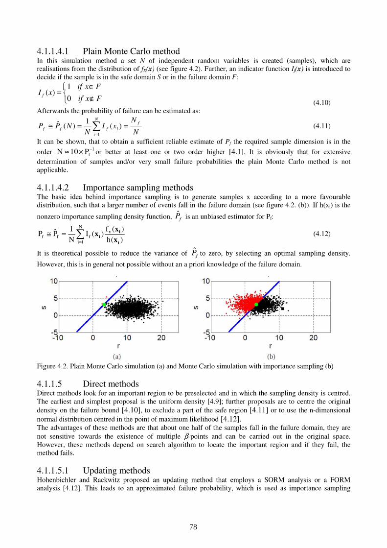
4.1.1.4.1 Plain Monte Carlo method In this simulation method a set N of independent random variables is created (samples), which are realisations from the distribution of fX(x) (see figure 4.2). Further, an indicator function If(x) is introduced to decide if the sample is in the safe domain S or in the failure domain F:
∉
∈=
Fxif
FxifxI f
0
1)(
(4.10) Afterwards the probability of failure can be estimated as:
∑=
==≅N
i
f
ifffN
NxI
NNPP
1
)(1
)(ˆ
(4.11)
It can be shown, that to obtain a sufficient reliable estimate of Pf the required sample dimension is in the
order 1
fP10N −×≈ or better at least one or two order higher [4.1]. It is obviously that for extensive
determination of samples and/or very small failure probabilities the plain Monte Carlo method is not applicable.
4.1.1.4.2 Importance sampling methods The basic idea behind importance sampling is to generate samples x according to a more favourable distribution, such that a larger number of events fall in the failure domain (see figure 4.2. (b)). If h(xi) is the
nonzero importance sampling density function, fP is an unbiased estimator for Pf:
∑=
=≅N
1i
xfff
)(h
)(f)(I
N
1PP
i
ii
x
xx
(4.12)
It is theoretical possible to reduce the variance of fP to zero, by selecting an optimal sampling density.
However, this is in general not possible without an a priori knowledge of the failure domain.
Figure 4.2. Plain Monte Carlo simulation (a) and Monte Carlo simulation with importance sampling (b)
4.1.1.5 Direct methods Direct methods look for an important region to be preselected and in which the sampling density is centred. The earliest and simplest proposal is the uniform density [4.9]; further proposals are to centre the original
density on the failure bound [4.10], to exclude a part of the safe region [4.11] or to use the n-dimensional
normal distribution centred in the point of maximum likelihood [4.12]. The advantages of these methods are that about one half of the samples fall in the failure domain, they are
not sensitive towards the existence of multiple β-points and can be carried out in the original space. However, these methods depend on search algorithm to locate the important region and if they fail, the method fails.
4.1.1.5.1 Updating methods Hohenbichler and Rackwitz proposed an updating method that employs a SORM analysis or a FORM analysis [4.12]. This leads to an approximated failure probability, which is used as importance sampling
78
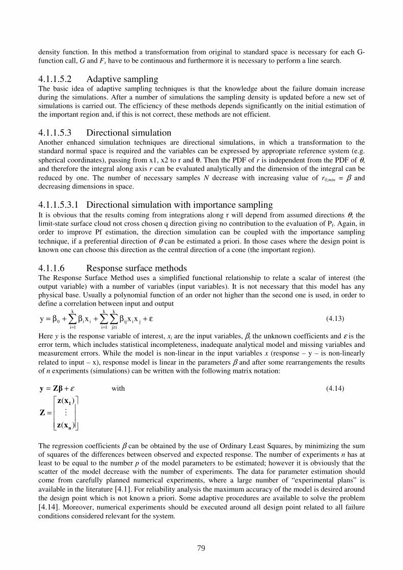
density function. In this method a transformation from original to standard space is necessary for each G-function call, G and Fx have to be continuous and furthermore it is necessary to perform a line search.
4.1.1.5.2 Adaptive sampling The basic idea of adaptive sampling techniques is that the knowledge about the failure domain increase during the simulations. After a number of simulations the sampling density is updated before a new set of simulations is carried out. The efficiency of these methods depends significantly on the initial estimation of the important region and, if this is not correct, these methods are not efficient.
4.1.1.5.3 Directional simulation Another enhanced simulation techniques are directional simulations, in which a transformation to the standard normal space is required and the variables can be expressed by appropriate reference system (e.g.
spherical coordinates), passing from x1, x2 to r and θ. Then the PDF of r is independent from the PDF of θ, and therefore the integral along axis r can be evaluated analytically and the dimension of the integral can be
reduced by one. The number of necessary samples N decrease with increasing value of r0,min = β and decreasing dimensions in space.
4.1.1.5.3.1 Directional simulation with importance sampling It is obvious that the results coming from integrations along r will depend from assumed directions θ; the limit-state surface cloud not cross chosen q direction giving no contribution to the evaluation of Pf. Again, in order to improve Pf estimation, the direction simulation can be coupled with the importance sampling
technique, if a preferential direction of θ can be estimated a priori. In those cases where the design point is known one can choose this direction as the central direction of a cone (the important region).
4.1.1.6 Response surface methods The Response Surface Method uses a simplified functional relationship to relate a scalar of interest (the output variable) with a number of variables (input variables). It is not necessary that this model has any physical base. Usually a polynomial function of an order not higher than the second one is used, in order to define a correlation between input and output
ε+β+β+β= ∑∑∑= ≥=
k
1ij
k
ijiij
k
1iii0 xxxy
(4.13)
Here y is the response variable of interest, xi are the input variables, βi the unknown coefficients and ε is the error term, which includes statistical incompleteness, inadequate analytical model and missing variables and measurement errors. While the model is non-linear in the input variables x (response – y – is non-linearly
related to input – x), response model is linear in the parameters β and after some rearrangements the results of n experiments (simulations) can be written with the following matrix notation:
ε+= Zβy with (4.14)
=
)(
)(
n
1
xz
xz
Z M
The regression coefficients β can be obtained by the use of Ordinary Least Squares, by minimizing the sum of squares of the differences between observed and expected response. The number of experiments n has at least to be equal to the number p of the model parameters to be estimated; however it is obviously that the scatter of the model decrease with the number of experiments. The data for parameter estimation should come from carefully planned numerical experiments, where a large number of “experimental plans” is
available in the literature [4.1]. For reliability analysis the maximum accuracy of the model is desired around the design point which is not known a priori. Some adaptive procedures are available to solve the problem [4.14]. Moreover, numerical experiments should be executed around all design point related to all failure conditions considered relevant for the system.
79

4.1.2 Combination of RS and sampling 4.1.2.1 Reliability of structural systems The reliability of realistic structures cannot be adequate described by a single limit-state function. A number of failure modes leads to a system whose safety depends on the state of its components, which can be defined by physical elements and failure modes. The systems can be grouped to three kinds of arrangements. If the system has no redundancy and failure of any component leads to the failure of the whole system, it is called a series system. It can be described with binary indicators as follows, where 1 stands for functioning state and 0 for failed state:
)(min
11
ini
n
i
iS SSSK∈
=
== ∏
(4.15)
Complementary arrangements are called parallel systems, where failure of all components is required for failure of the system:
)S(max)S1(1S i
n1i
n
1i
iSK∈
=
=−−= ∏
(4.16)
Normally systems fail if some but not all of their components fail (general system): it is important to individuate which elements must fail to cause structural failure. Here a set C of components are called cut set, if their failure leads to failure of the system; when the number of components in C is the minimum required for the system to fail, C is called minimal cut set. A set P of components is called path set, if their survival ensures the system survival; when P has the minimum necessary number of components it is called minimal path set. A general binary system can be described as a serial arrangement of its minimal cut set or as parallel arrangement of its minimal path sets.
=
−−=
∈∈= ∈
∏ ∏ )(maxmin)1(11
1
jIjNi
N
i Ij
jS SSSiCC
C
iC
K
(4.17)
=
−−=
∈∈= ∈
∏ ∏ )(minmax111
1
SjSSiPP
P
iP
IjNi
N
i Ij
jSK
(4.18)
The failure domain of these systems can be described for serial systems by
U Ui i
ii GFF 0)( ≤== x , (4.19)
for parallel systems by
IIi
i
i
i GFF 0)( ≤== x
(4.20)
and for general systems (minimal cut set representation) by:
U U IIi i Ij
i
Ij
i
iCiC
GFF∈∈
≤== 0)(x
(4.21)
To evaluate the system probability of failure )Pr( FPf ∈= x , a FORM approximation can be used. For
series, parallel or general system the reliability can be expressed by [4.15]:
)(1, Rβ,Φ−=seriesfP
(4.22)
)(, Rβ,−Φ=parallelfP
(4.23)
∑ ∑ ∑=
−
= +=
−−++−=n
i
n
i
n
ij
n
n
jiigeneralf CCCCCP1
1
1 11
1, Pr)1(PrPr LK
(4.24)
where C1,...,Ci,...,Cj,...,Cn are the individuated cut-set of the system
4.1.2.2 Time-variant reliability problems 4.1.2.2.1 Basics and the classical random vibration theory As discussed in the first section, seismic actions are time-variant and therefore they have to be described by stochastic processes, depending random variables for any argument t. The goal of time-variant reliability problems is to find the probability that the structure stays in the safe domain during a prescribed time interval
80
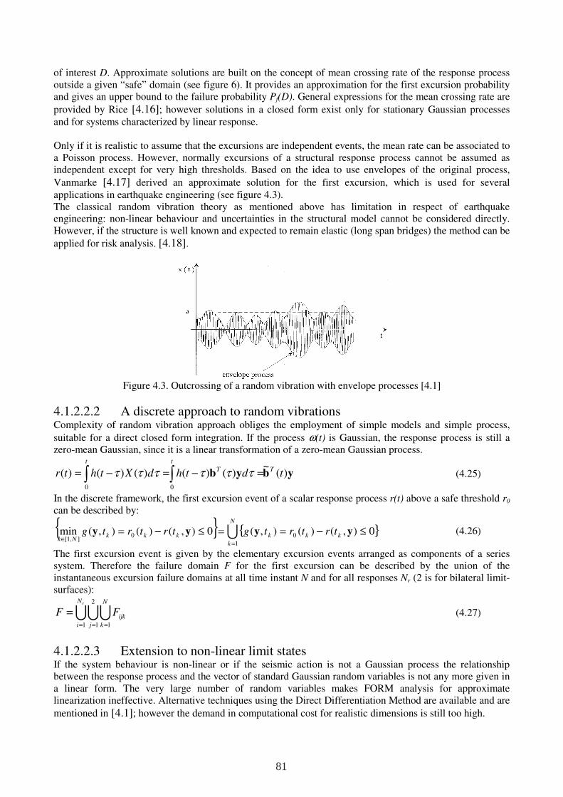
of interest D. Approximate solutions are built on the concept of mean crossing rate of the response process outside a given “safe” domain (see figure 6). It provides an approximation for the first excursion probability and gives an upper bound to the failure probability Pf(D). General expressions for the mean crossing rate are
provided by Rice [4.16]; however solutions in a closed form exist only for stationary Gaussian processes and for systems characterized by linear response. Only if it is realistic to assume that the excursions are independent events, the mean rate can be associated to a Poisson process. However, normally excursions of a structural response process cannot be assumed as independent except for very high thresholds. Based on the idea to use envelopes of the original process,
Vanmarke [4.17] derived an approximate solution for the first excursion, which is used for several applications in earthquake engineering (see figure 4.3). The classical random vibration theory as mentioned above has limitation in respect of earthquake engineering: non-linear behaviour and uncertainties in the structural model cannot be considered directly. However, if the structure is well known and expected to remain elastic (long span bridges) the method can be
applied for risk analysis. [4.18].
Figure 4.3. Outcrossing of a random vibration with envelope processes [4.1]
4.1.2.2.2 A discrete approach to random vibrations Complexity of random vibration approach obliges the employment of simple models and simple process,
suitable for a direct closed form integration. If the process ω(t) is Gaussian, the response process is still a zero-mean Gaussian, since it is a linear transformation of a zero-mean Gaussian process.
ybyb )(~
)()()()()(00
tdthdXthtrT
t
T
t
∫∫ =−=−= ττττττ
(4.25)
In the discrete framework, the first excursion event of a scalar response process r(t) above a safe threshold r0
can be described by:
UN
k
kkkkkkNk
trtrtgtrtrtg1
00],1[
0),()(),(0),()(),(min=
∈≤−==≤−= yyyy
(4.26)
The first excursion event is given by the elementary excursion events arranged as components of a series system. Therefore the failure domain F for the first excursion can be described by the union of the instantaneous excursion failure domains at all time instant N and for all responses Nr (2 is for bilateral limit-surfaces):
UUUrN
i j
N
k
ijkFF1
2
1 1= = =
= (4.27)
4.1.2.2.3 Extension to non-linear limit states If the system behaviour is non-linear or if the seismic action is not a Gaussian process the relationship between the response process and the vector of standard Gaussian random variables is not any more given in a linear form. The very large number of random variables makes FORM analysis for approximate linearization ineffective. Alternative techniques using the Direct Differentiation Method are available and are
mentioned in [4.1]; however the demand in computational cost for realistic dimensions is still too high.
81
4.1.2.2.4 Importance sampling using elementary events (ISEE) A very effective importance sampling method for time-variant reliability problems is introduced by Au and
Beck [4.18], in which the importance sampling density is suggested by the formulation of the first excursion problem as a sequence of time-invariant excursions as discussed in the previous section (series system). A proper importance sampling density (ISD) for the first excursion is built weighting the sampling densities relative to the elementary events. The optimal sampling density for the elementary excursion and further the simulation formula for a corresponding random vector are summarized in [4.1]. The special effectiveness is contributed on the one hand, that the applied weights are non-zero only if the associated elementary failure region has non-zero probability Pk (which is conditional probability Pk = Pr(Fk|F)). On the other hand the number of PDF evaluations can be significantly reduced. The procedure is applicable for any number of possible failure modes and their mutual correlation and allows multiple excitations. However, in its original form it is limited to linear deterministic structures.
4.1.2.2.5 Extension to non-linear problems Nevertheless ISEE can be extended to non-linear problems. In this case the computation of the elementary excursion probabilities Pk is no longer straightforward; however, it can be approximately evaluated by FORM or SORM analysis.
4.1.2.2.6 The domain decomposition method (DDM) A similar procedure is presented by Katafygiotis and Cheung [4.19], based on the idea, that the first excursion union can be expressed as a union of mutually exclusive event. For the same reasons, this approach can only be used for deterministic linear structures.
4.1.2.2.7 Subset simulation This method belongs to the class of adaptive sampling procedure. The idea is to express the failure probability as a product of a number of conditional probabilities of intermediate failure events. These are chosen to form a sequence in which every event failure domain contains the corresponding domain of the next event. In this manner the computation of a small Pf is split into the computation of several larger probabilities, which corresponds to more frequent events. That way a small Pf can be reduced to the product of affordable conditional probabilities (i.e. 10-6 in 6 times 10-1). The first step can be done by a plain MC simulation. Following conditional simulations can be done by advanced simulations as the Metropolis
method [4.20]. As the method effectiveness is rather insensitive to the type of proposal sampling density, uniform density centred at the latest sample with a given width can be used. Even if the number of samples is reduced in comparison to the plain MC method, the number of simulations is still in order up to a few thousands.
4.1.3 Final consideration and final choice for the probabilistic approach In general reliability problems in earthquake engineering have (i) non-linear limit-state functions, (ii) high curvatures of the limit-state functions as well as (iii) multiple design points are possible. Hence, only robust procedure can be applied. FORM and SORM methods have a limited efficiency for this type of problems, while can be considered as valuable for codes calibration and reliability problems on simple systems. As known from previous researches and technical literature survey, the time-variant approaches are practically not employable in the seismic reliability because the complexity of the problem is already high for linear systems and become higher and higher when system behave non-linearly. Simulations methods appears to be more reliable because they do not need in general to a-priori knowledge of the limit state function but at the same time in order to estimate with certain accuracy failure probability they need a large number of numerical simulations. In last decades many optimization techniques devoted to the improvement of simulation methods have been defined in order to reduce the computational work (i.e. numerical simulations); importance sampling is one of most used and appears to be promising in the failure probability estimation but at the same time it needs to know the failure domain, in order to more favourably generate samples for the probabilistic analyses. Many other methods have been proposed and based on the same general idea adopted in the importance sampling: Monte Carlo, Directional Simulations, Adaptative Sampling and so on use Importance Sampling techniques for improving their convergence to a solutions, Other methods have been based on a strong
82
statistical interpretation of the results, focusing the attention at the definition of an appropriate function linking structural response (output variables) to seismic hazard/material variability (input variables): the surface response technique. This method is characterized by same problems of previous methods: it works in the prediction of response around design point. Summarizing, direct simulation methods as Monte Carlo appear to be more reliable technique but at the same time appropriate measures in order to increase the knowledge of structural system under study and reliability of failure probability estimation must be considered. So, the knowledge of the structural system under examination is the basis for a successful or unsuccessful application of Monte Carlo method because, in general, structural system subjected to seismic actions are characterized by the following features:
number of design points that must be investigated; number of limit-state functions; number of probabilistic variables; distributions for each variable (Gaussian, Lognormal, …); independence or dependence between probabilistic variables of the system.
On the other hand, seismic actions are in general time-variant variables (processes) and therefore reliability problems in earthquake engineering are time-variant reliability problems. So for OPUS purposes, the problem is transformed in a time-invariant problem (i.e. looking only at extreme values) and a Monte Carlo simulation technique can be applied in a more efficient way; moreover, a probabilistic procedure able to furnish a good estimation of failure probability for all identified design point can be also defined. According to these final consideration, the research project adopts the following general approach devoted to the effectively evaluation of seismic reliability for all structural case studies designed during the research:
step 1. Deep knowledge of structural systems. The knowledge about the structural behaviour of the case studies was completed and determined thorough several numerical simulations, adopting non-linear static and dynamic analyses.
step 2. Nonlinear modelling and collapse modalities assessment. Each structural system was described by accurate nonlinear models individuating the relevant collapse criteria.
step 3. Characterization of seismic hazard. Seismic actions were modelled adopting parameters and hazard proposed by EN1998-1-1; in particular, hazard function (i.e. annual exceedance probability) for European seismicity is taken from EN1998-1-1 and calibrated according to design parameters associated to ultimate limit state verification. Seven seismic inputs to be adopted in the numerical simulations were artificially generated from response spectra adopted in the design.
step 4. Probabilistic model of mechanical variables. Scattering of steel products was represented by a multi-variable model where yielding stress – Re,H (fy) –, tensile strength –
Rm (ft) – and elongation at fracture – A (εu) were considered with their probabilistic interdependencies.
step 5. Execution of nonlinear analyses and optimal planning of numerical simulations. The correlation between the seismic demand and the structural response of case studies was defined employing non-linear dynamic analyses; peak ground acceleration (PGA) of selected seismic inputs was varied according to appropriate levels chosen in order to activate collapse modes. In such a way, the number of simulations characterized by failures according to different modes was increased.
step 6. Probabilistic procedure for Pf estimation. Numerical results coming from dynamic analyses were analyzed employing a statistical procedure that furnishes fragility curves and yearly threshold exceedance probability of the relevant collapse modes for each case study.
The numerical simulations are executed using Incremental Dynamic Analysis techniques, suitable for the analysis of structural response at different PGA levels. Moreover, this technique has been extensively adopted by several earthquake research centre all around the world as tools to assess seismic safety of structural systems. The step 1 and step 2 were developed during the design and the seismic assessment of structural case studies (chapter 2 and 3); the individuation of PGA levels adopted in the step 5 were defined during the seismic assessment developed in the chapter 3; the probabilistic model of the steel products mechanical properties
83
was defined during the collection of industrial data, whose results are summarized in the chapter 1 and chapter 7. Step 3, step 6 and loading IDA execution protocol of step 5 are presented in the following parts.
4.2 Incremental Dynamic Analysis: general issues and operative framework Incremental Dynamic Analysis represents most advanced and complete analysis method where the single seismic input (i.e. ground motion time-history) is repetitively analyzed scaling its intensity according to a scalar parameter. The IDA study is now a multi-purpose and widely applicable method whose objectives, are:
thorough understanding of the range of response or “demands” versus the range of potential levels of a ground motion record,
better understanding of the structural implications of rarer / more severe ground motion levels, better understanding of the changes in the nature of the structural response as the intensity of ground
motion increases (e.g., changes in peak deformation patterns with height, onset of stiffness and strength degradation and their patterns and magnitudes),
producing estimates of the dynamic capacity of the global structural system. Moreover, the adoption of multiple earthquake time-histories and so the execution of multi-record IDA on the same structural system gives also how stable or how variable are investigated parameters from one ground motion record to another. The comparison between figure 4.4 and figure 4.5 shows the different quality of results between single IDA (using one seismic input) and multi-IDA (using various seismic input). In the second case, EDP (Engineering Demand Parameter) is affected by variability of seismic input, giving so for each PGA level the variability of the structural response: investigated parameters can be displacements, forces, bending moments or other parameters that can be effectively correlated to damage state or expected structural performance both at local and global level; moreover, the application of 7 earthquakes allows the statistical treatment of the output for each PGA level quantifying response variability. In the examples showed in figure 4.4 and figure 4.5, compressive axial forces acting in bracing elements or columns, maximum plastic rotation of seismic links or inter-story drift, effective EDP to be correlated to structural collapse criteria, are presented. The power of the IDA and the quality of its results make it suitable for a direct implementation in a probabilistic framework owing to the statistical analysis of the output, for example, the estimation of the annual probability that the demand exceeds the limit-state or structural capacity of a single member or a structural system can be estimated (presented in the next paragraph). Moreover, IDA technique can be employed also, considering at the same time seismic input and mechanical properties variability, through an appropriate modelling of the structural members. Anyway, IDA technique is quite time-consuming and the contemporary variability of seismic input and mechanical properties greatly increase the required number of numerical simulations: for each dynamic analysis a set of mechanical properties and a IM (Intensity Measure of earthquake) level is considered. Each IDA curve, as those presented in figures 4.4 and 4.5, requires many points to be realized and each point corresponds to a single analysis whose results are the extreme (min/max) value of selected EDP. The total number of simulations required for a single structural system would be defined by the following expression:
iationsvarpropertyQuakeintPo,IDAtotal NNNN −××= where NIDA is the number adopted for tracing IDA curve,
NQuake represents the number of employed earthquake time-histories and Nproperty represents the variation of mechanical properties (samples set) inside the structure. In order to save computational time, the following IDA protocol is chosen:
for each structural types, the relevant collapse criteria are identified; for each identified collapse criteria, activation PGA level is determined (PGAcollapse,i); IDA curves are defined using outputs correspondence to PGAcollapse,i only.
84
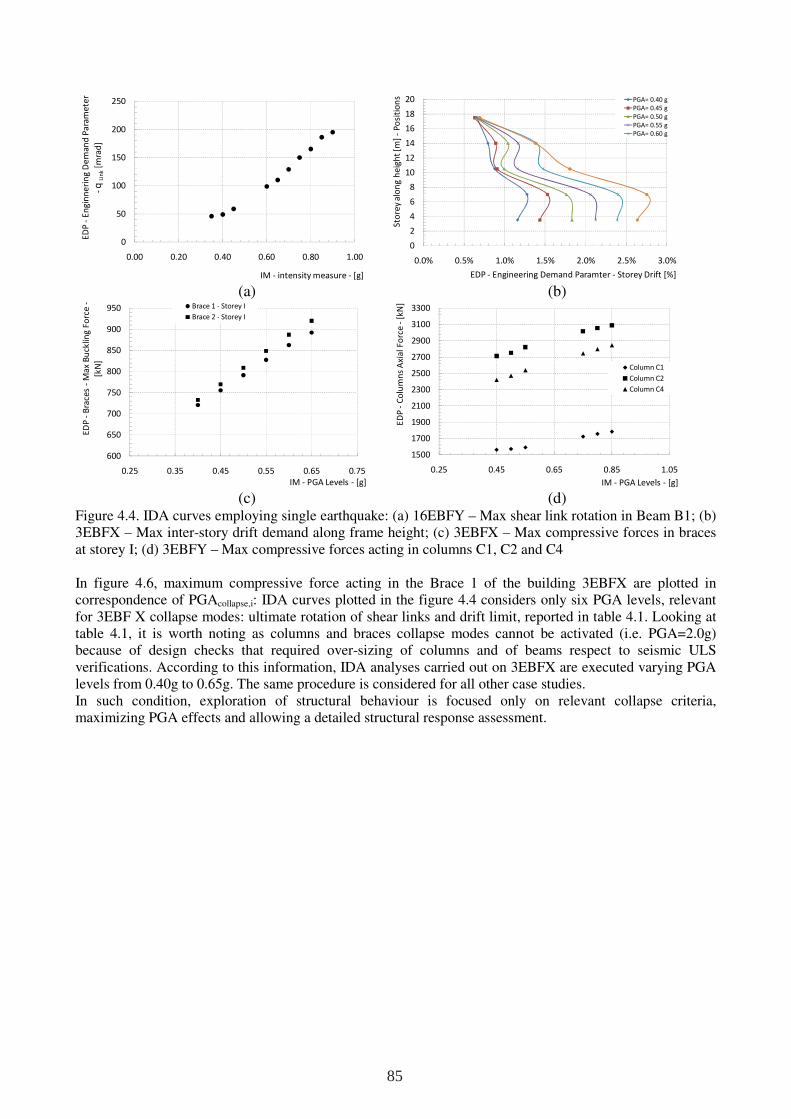
(a)
(b)
(c)
(d)
Figure 4.4. IDA curves employing single earthquake: (a) 16EBFY – Max shear link rotation in Beam B1; (b) 3EBFX – Max inter-story drift demand along frame height; (c) 3EBFX – Max compressive forces in braces at storey I; (d) 3EBFY – Max compressive forces acting in columns C1, C2 and C4 In figure 4.6, maximum compressive force acting in the Brace 1 of the building 3EBFX are plotted in correspondence of PGAcollapse,i: IDA curves plotted in the figure 4.4 considers only six PGA levels, relevant for 3EBF X collapse modes: ultimate rotation of shear links and drift limit, reported in table 4.1. Looking at table 4.1, it is worth noting as columns and braces collapse modes cannot be activated (i.e. PGA=2.0g) because of design checks that required over-sizing of columns and of beams respect to seismic ULS verifications. According to this information, IDA analyses carried out on 3EBFX are executed varying PGA levels from 0.40g to 0.65g. The same procedure is considered for all other case studies. In such condition, exploration of structural behaviour is focused only on relevant collapse criteria, maximizing PGA effects and allowing a detailed structural response assessment.
0
50
100
150
200
250
0.00 0.20 0.40 0.60 0.80 1.00
ED
P -
En
gin
ne
rin
g D
em
an
d P
ara
me
ter
-q
Lin
k[m
rad
]
IM - intensity measure - [g]
0
2
4
6
8
10
12
14
16
18
20
0.0% 0.5% 1.0% 1.5% 2.0% 2.5% 3.0%
Sto
rey
alo
ng
he
igh
t [m
] -
Po
siti
on
s
EDP - Engineering Demand Paramter - Storey Drift [%]
PGA= 0.40 g
PGA= 0.45 g
PGA= 0.50 g
PGA= 0.55 g
PGA= 0.60 g
600
650
700
750
800
850
900
950
0.25 0.35 0.45 0.55 0.65 0.75
ED
P -
Bra
ces
-M
ax
Bu
cklin
g F
orc
e -
[kN
]
IM - PGA Levels - [g]
Brace 1 - Storey I
Brace 2 - Storey I
1500
1700
1900
2100
2300
2500
2700
2900
3100
3300
0.25 0.45 0.65 0.85 1.05
ED
P -
Co
lum
ns
Axi
al
Fo
rce
-[k
N]
IM - PGA Levels - [g]
Column C1
Column C2
Column C4
85
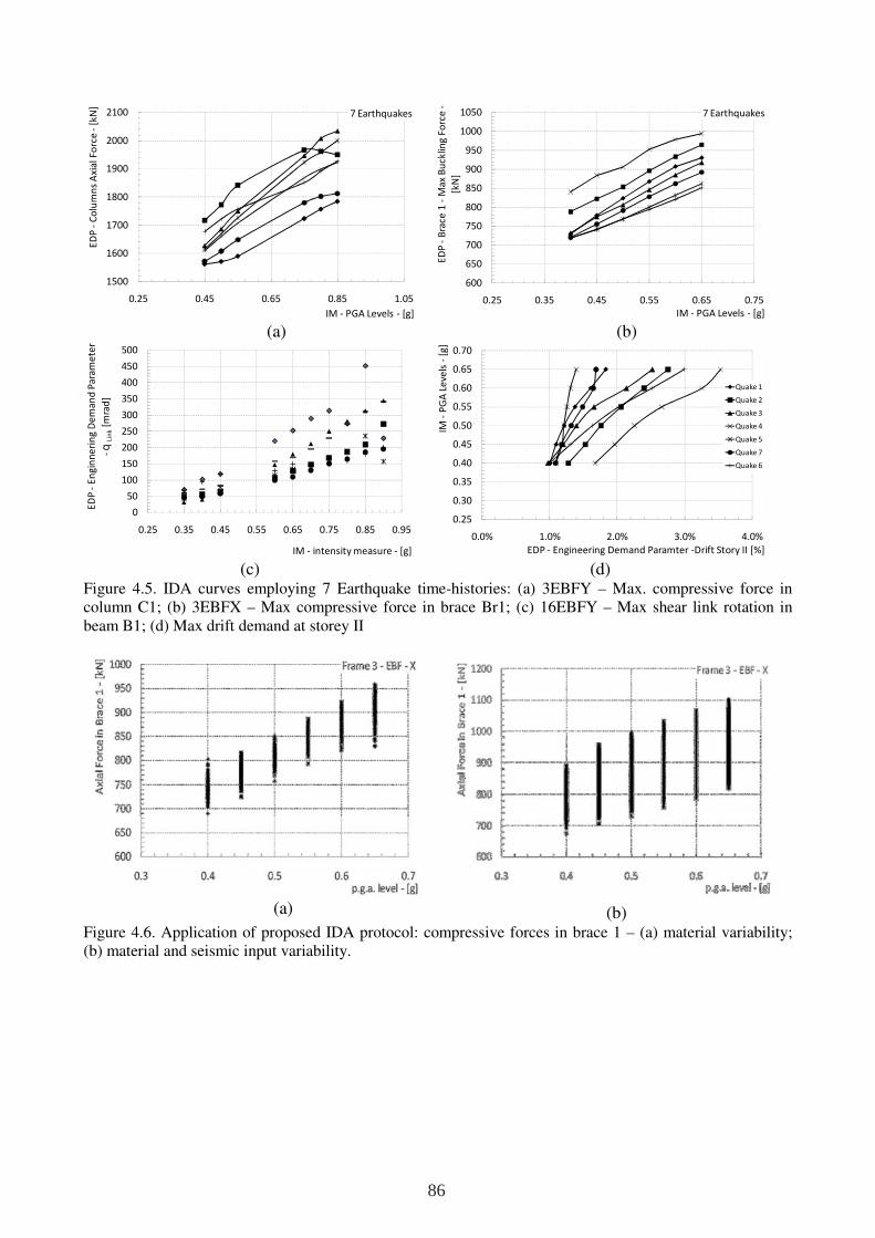
(a)
(b)
(c)
(d)
Figure 4.5. IDA curves employing 7 Earthquake time-histories: (a) 3EBFY – Max. compressive force in column C1; (b) 3EBFX – Max compressive force in brace Br1; (c) 16EBFY – Max shear link rotation in beam B1; (d) Max drift demand at storey II
(a)
(b)
Figure 4.6. Application of proposed IDA protocol: compressive forces in brace 1 – (a) material variability; (b) material and seismic input variability.
1500
1600
1700
1800
1900
2000
2100
0.25 0.45 0.65 0.85 1.05
ED
P -
Co
lum
ns
Axi
al
Fo
rce
-[k
N]
IM - PGA Levels - [g]
7 Earthquakes
600
650
700
750
800
850
900
950
1000
1050
0.25 0.35 0.45 0.55 0.65 0.75
ED
P -
Bra
ce 1
-M
ax
Bu
cklin
g F
orc
e -
[kN
]
IM - PGA Levels - [g]
7 Earthquakes
0
50
100
150
200
250
300
350
400
450
500
0.25 0.35 0.45 0.55 0.65 0.75 0.85 0.95
ED
P -
En
gin
ne
rin
g D
em
an
d P
ara
me
ter
-q
Lin
k[m
rad
]
IM - intensity measure - [g]
0.25
0.30
0.35
0.40
0.45
0.50
0.55
0.60
0.65
0.70
0.0% 1.0% 2.0% 3.0% 4.0%
IM -
PG
A L
eve
ls -
[g]
EDP - Engineering Demand Paramter -Drift Story II [%]
Quake 1
Quake 2
Quake 3
Quake 4
Quake 5
Quake 7
Quake 6
86
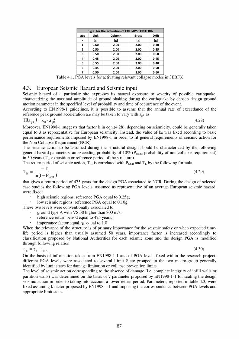
Table 4.1. PGA levels for activating relevant collapse modes in 3EBFX
4.3. European Seismic Hazard and Seismic input Seismic hazard of a particular site expresses its natural exposure to severity of possible earthquake, characterizing the maximal amplitude of ground shaking during the earthquake by chosen design ground motion parameter in the specified level of probability and time of occurrence of the event. According to EN1998-1 guidelines, it is possible to assume that the annual rate of exceedance of the reference peak ground acceleration agR may be taken to vary with agR as:
( ) k
gR0gR akaH −⋅= (4.28)
Moreover, EN1998-1 suggests that factor k in eqn.(4.28), depending on seismicity, could be generally taken equal to 3 as representative for European seismicity. Instead, the value of k0 was fixed according to basic performance requirements imposed by EN1998-1 in order to fit general requirements of seismic action for the Non Collapse Requirement (NCR). The seismic action to be assumed during the structural design should be characterized by the following general hazard parameters: an exceeding probability of 10% (PNCR, probability of non collapse requirement) in 50 years (TL, exposition or reference period of the structure). The return period of seismic action, TR, is correlated with PNCR and TL by the following formula
( )NCR
LR
P1ln
TT
−
−= (4.29)
that gives a return period of 475 years for the design PGA associated to NCR. During the design of selected case studies the following PGA levels, assumed as representative of an average European seismic hazard, were fixed:
high seismic regions: reference PGA equal to 0.25g; low seismic regions: reference PGA equal to 0.10g.
These two levels were conventionally associated to: ground type A with VS,30 higher than 800 m/s; reference return period equal to 475 years;
importance factor equal, γI, equal to 1.0 When the relevance of the structure is of primary importance for the seismic safety or when expected time-life period is higher than usually assumed 50 years, importance factor is increased accordingly to classification proposed by National Authorities for each seismic zone and the design PGA is modified through following relation
R,gIg aa ⋅γ= (4.30)
On the basis of information taken from EN1998-1-1 and of PGA levels fixed within the research project, different PGA levels were associated to several Limit State grouped in the two macro-group generally identified by limit states for damage limitation or collapse prevention limits. The level of seismic action corresponding to the absence of damage (i.e. complete integrity of infill walls or
partition walls) was determined on the basis of ν parameter proposed by EN1998-1-1 for scaling the design seismic action in order to taking into account a lower return period. Parameters, reported in table 4.3, were fixed assuming k factor proposed by EN1998-1-1 and imposing the correspondence between PGA levels and appropriate limit states.
p.g.a. for the activation of COLLAPSE CRITERIA
acc Link Column Brace Drfit
- [g] [g] [g] [g]
1 0.60 2.00 2.00 0.40
2 0.50 2.00 2.00 0.55
3 0.50 2.00 2.00 0.60
4 0.45 2.00 2.00 0.45
5 0.55 2.00 2.00 0.40
6 0.45 2.00 2.00 0.50
7 0.50 2.00 2.00 0.60
87
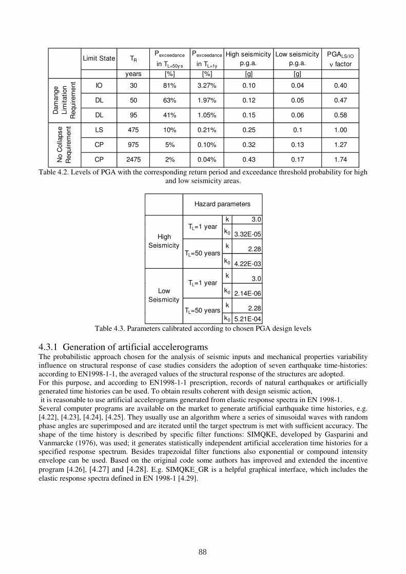
Table 4.2. Levels of PGA with the corresponding return period and exceedance threshold probability for high
and low seismicity areas.
Table 4.3. Parameters calibrated according to chosen PGA design levels
4.3.1 Generation of artificial accelerograms The probabilistic approach chosen for the analysis of seismic inputs and mechanical properties variability influence on structural response of case studies considers the adoption of seven earthquake time-histories: according to EN1998-1-1, the averaged values of the structural response of the structures are adopted. For this purpose, and according to EN1998-1-1 prescription, records of natural earthquakes or artificially generated time histories can be used. To obtain results coherent with design seismic action, it is reasonable to use artificial accelerograms generated from elastic response spectra in EN 1998-1. Several computer programs are available on the market to generate artificial earthquake time histories, e.g. [4.22], [4.23], [4.24], [4.25]. They usually use an algorithm where a series of sinusoidal waves with random phase angles are superimposed and are iterated until the target spectrum is met with sufficient accuracy. The shape of the time history is described by specific filter functions: SIMQKE, developed by Gasparini and Vanmarcke (1976), was used; it generates statistically independent artificial acceleration time histories for a specified response spectrum. Besides trapezoidal filter functions also exponential or compound intensity envelope can be used. Based on the original code some authors has improved and extended the incentive
program [4.26], [4.27] and [4.28]. E.g. SIMQKE_GR is a helpful graphical interface, which includes the elastic response spectra defined in EN 1998-1 [4.29].
Limit State TR
Pexceedance
in TL=50y s
Pexceedance
in TL=1y
High seismicity
p.g.a.
Low seismicity
p.g.a.
PGALS/IO
ν factor
years [%] [%] [g] [g]
IO 30 81% 3.27% 0.10 0.04 0.40
DL 50 63% 1.97% 0.12 0.05 0.47
DL 95 41% 1.05% 0.15 0.06 0.58
LS 475 10% 0.21% 0.25 0.1 1.00
CP 975 5% 0.10% 0.32 0.13 1.27
CP 2475 2% 0.04% 0.43 0.17 1.74
Dam
ange
Lim
itation
Requirem
ent
No C
olla
pse
Requirem
ent
k 3.0
k0 3.32E-05
k 2.28
k0 4.22E-03
k 3.0
k0 2.14E-06
k 2.28
k0 5.21E-04
High
Seismicity
Low
Seismicity
TL=1 year
TL=50 years
TL=1 year
TL=50 years
Hazard parameters
88
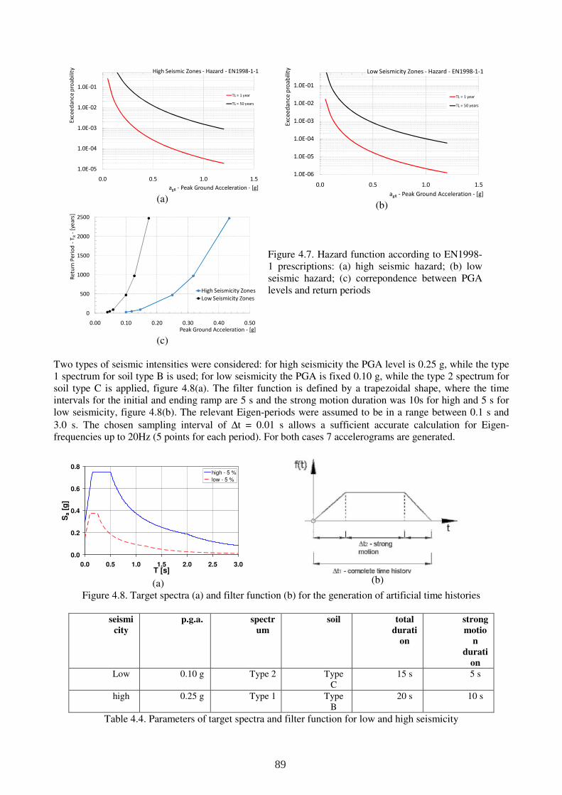
(a)
(b)
(c)
Figure 4.7. Hazard function according to EN1998-1 prescriptions: (a) high seismic hazard; (b) low seismic hazard; (c) correpondence between PGA levels and return periods
Two types of seismic intensities were considered: for high seismicity the PGA level is 0.25 g, while the type 1 spectrum for soil type B is used; for low seismicity the PGA is fixed 0.10 g, while the type 2 spectrum for soil type C is applied, figure 4.8(a). The filter function is defined by a trapezoidal shape, where the time intervals for the initial and ending ramp are 5 s and the strong motion duration was 10s for high and 5 s for low seismicity, figure 4.8(b). The relevant Eigen-periods were assumed to be in a range between 0.1 s and
3.0 s. The chosen sampling interval of ∆t = 0.01 s allows a sufficient accurate calculation for Eigen-frequencies up to 20Hz (5 points for each period). For both cases 7 accelerograms are generated.
(a)
(b)
Figure 4.8. Target spectra (a) and filter function (b) for the generation of artificial time histories
seismi
city
p.g.a. spectr
um
soil total
durati
on
strong
motio
n
durati
on
Low 0.10 g Type 2 Type C
15 s 5 s
high 0.25 g Type 1 Type B
20 s 10 s
Table 4.4. Parameters of target spectra and filter function for low and high seismicity
1.0E-05
1.0E-04
1.0E-03
1.0E-02
1.0E-01
0.0 0.5 1.0 1.5
Exc
ee
da
nce
pro
ab
ilit
y
agR - Peak Ground Acceleration - [g]
High Seismic Zones - Hazard - EN1998-1-1
TL = 1 year
TL = 50 years
1.0E-06
1.0E-05
1.0E-04
1.0E-03
1.0E-02
1.0E-01
0.0 0.5 1.0 1.5
Exc
ee
da
nce
pro
ab
ility
agR - Peak Ground Acceleration - [g]
Low Seismicity Zones - Hazard - EN1998-1-1
TL = 1 year
TL = 50 years
0
500
1000
1500
2000
2500
0.00 0.10 0.20 0.30 0.40 0.50
Re
turn
Pe
rio
d -
TR
-[y
ea
rs]
Peak Ground Acceleration - [g]
High Seismicity Zones
Low Seismicity Zones
0.0
0.2
0.4
0.6
0.8
0.0 0.5 1.0 1.5 2.0 2.5 3.0T [s]
Sa [
g]
high - 5 %
low - 5 %
89
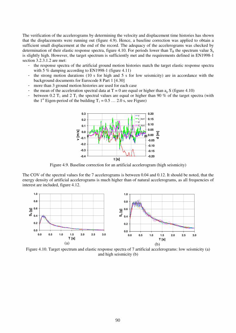
The verification of the accelerograms by determining the velocity and displacement time histories has shown that the displacements were running out (figure 4.9). Hence, a baseline correction was applied to obtain a sufficient small displacement at the end of the record. The adequacy of the accelerograms was checked by determination of their elastic response spectra, figure 4.10. For periods lower than TB the spectrum value Sa is slightly high. However, the target spectrum is sufficiently met and the requirements defined in EN1998-1 section 3.2.3.1.2 are met:
- the response spectra of the artificial ground motion histories match the target elastic response spectra with 5 % damping according to EN1998-1 (figure 4.11)
- the strong motion durations (10 s for high and 5 s for low seismicity) are in accordance with the background documents for Eurocode 8 Part 1 [4.30]
- more than 3 ground motion histories are used for each case - the mean of the acceleration spectral data at T = 0 are equal or higher than ag S (figure 4.10) - between 0.2 T1 and 2 T1 the spectral values are equal or higher than 90 % of the target spectra (with
the 1st Eigen-period of the building T1 = 0.5 … 2.0 s, see Figure)
Figure 4.9. Baseline correction for an artificial accelerogram (high seismicity)
The COV of the spectral values for the 7 accelerograms is between 0.04 and 0.12. It should be noted, that the energy density of artificial accelerograms is much higher than of natural accelerograms, as all frequencies of interest are included, figure 4.12.
(a)
(b)
Figure 4.10. Target spectrum and elastic response spectra of 7 artificial accelerograms: low seismicity (a) and high seismicity (b)
-0.4
-0.3
-0.2
-0.1
0.0
0.1
0.2
0.3
0 5 10 15 20
t [s]
v [
m/s
]
-0.20
-0.15
-0.10
-0.05
0.00
0.05
0.10
0.15
0.20
d [
m]
v
v_korr
d
d_korr
0.0
0.2
0.4
0.6
0.8
1.0
0.0 0.5 1.0 1.5 2.0 2.5 3.0
T [s]
Sa [
g]
0.0
0.2
0.4
0.6
0.8
1.0
0.0 0.5 1.0 1.5 2.0 2.5 3.0
T [s]
Sa [
g]
90
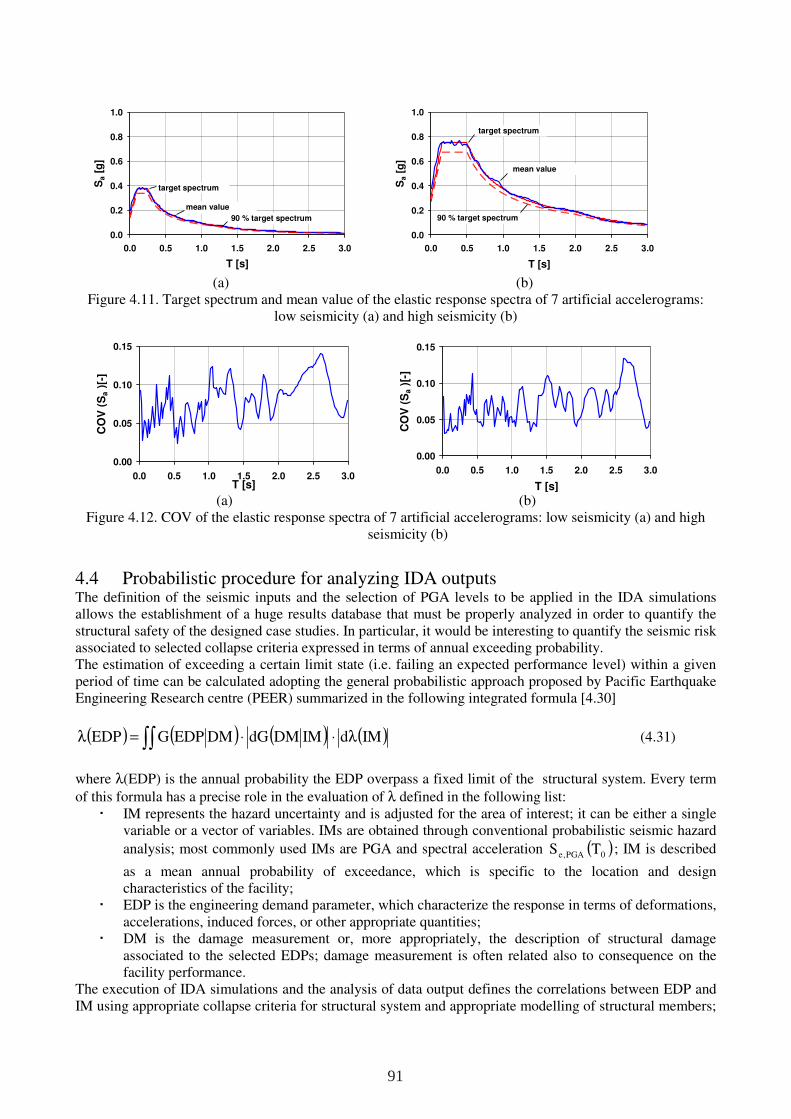
(a)
(b)
Figure 4.11. Target spectrum and mean value of the elastic response spectra of 7 artificial accelerograms: low seismicity (a) and high seismicity (b)
(a)
(b)
Figure 4.12. COV of the elastic response spectra of 7 artificial accelerograms: low seismicity (a) and high seismicity (b)
4.4 Probabilistic procedure for analyzing IDA outputs The definition of the seismic inputs and the selection of PGA levels to be applied in the IDA simulations allows the establishment of a huge results database that must be properly analyzed in order to quantify the structural safety of the designed case studies. In particular, it would be interesting to quantify the seismic risk associated to selected collapse criteria expressed in terms of annual exceeding probability. The estimation of exceeding a certain limit state (i.e. failing an expected performance level) within a given period of time can be calculated adopting the general probabilistic approach proposed by Pacific Earthquake Engineering Research centre (PEER) summarized in the following integrated formula [4.30]
( ) ( ) ( ) ( )∫∫ λ⋅⋅=λ IMdIMDMdGDMEDPGEDP (4.31)
where λ(EDP) is the annual probability the EDP overpass a fixed limit of the structural system. Every term
of this formula has a precise role in the evaluation of λ defined in the following list: IM represents the hazard uncertainty and is adjusted for the area of interest; it can be either a single
variable or a vector of variables. IMs are obtained through conventional probabilistic seismic hazard
analysis; most commonly used IMs are PGA and spectral acceleration ( )0PGA,e TS ; IM is described
as a mean annual probability of exceedance, which is specific to the location and design characteristics of the facility;
EDP is the engineering demand parameter, which characterize the response in terms of deformations, accelerations, induced forces, or other appropriate quantities;
DM is the damage measurement or, more appropriately, the description of structural damage associated to the selected EDPs; damage measurement is often related also to consequence on the facility performance.
The execution of IDA simulations and the analysis of data output defines the correlations between EDP and IM using appropriate collapse criteria for structural system and appropriate modelling of structural members;
0.0
0.2
0.4
0.6
0.8
1.0
0.0 0.5 1.0 1.5 2.0 2.5 3.0
T [s]
Sa [
g]
target spectrum
90 % target spectrum
mean value
0.0
0.2
0.4
0.6
0.8
1.0
0.0 0.5 1.0 1.5 2.0 2.5 3.0
T [s]
Sa [
g]
target spectrum
90 % target spectrum
mean value
0.00
0.05
0.10
0.15
0.0 0.5 1.0 1.5 2.0 2.5 3.0T [s]
CO
V (
Sa )
[-]
0.00
0.05
0.10
0.15
0.0 0.5 1.0 1.5 2.0 2.5 3.0
T [s]
CO
V (
Sa )
[-]
91
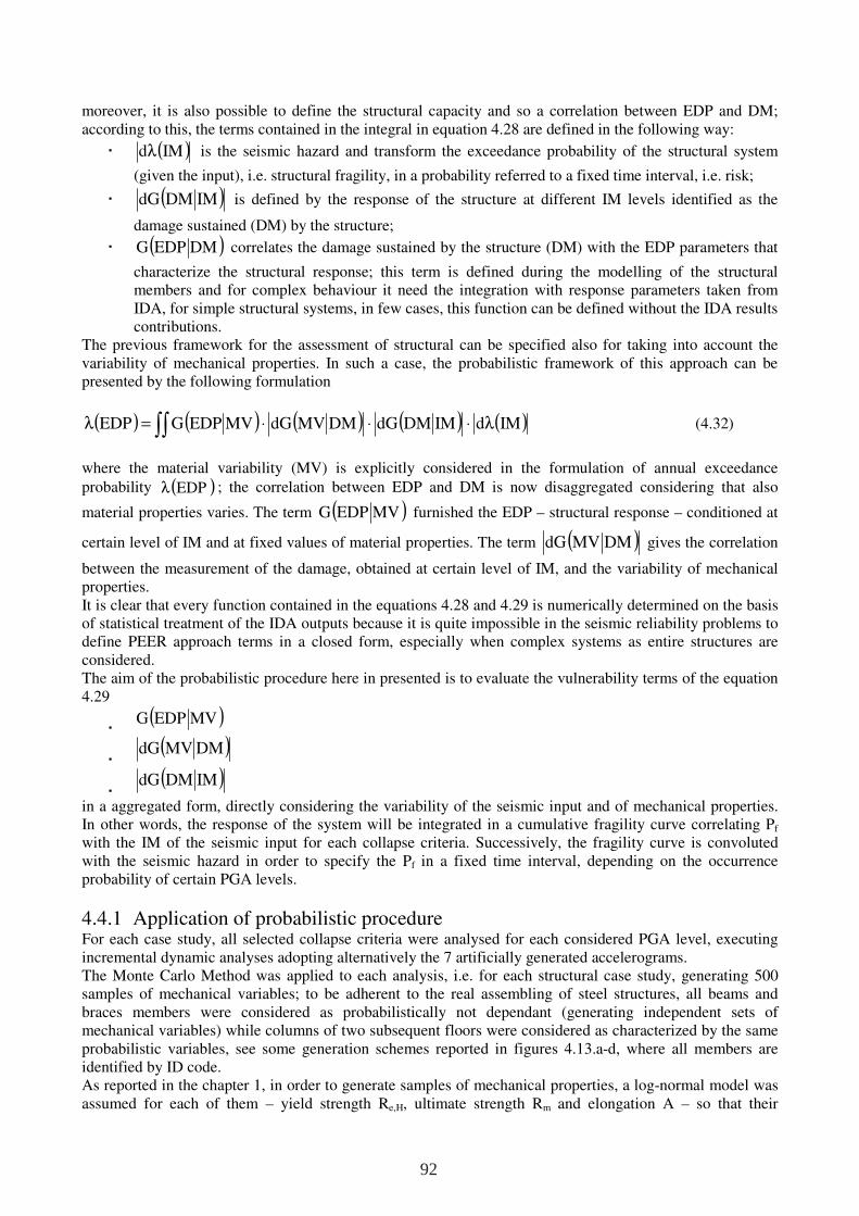
moreover, it is also possible to define the structural capacity and so a correlation between EDP and DM; according to this, the terms contained in the integral in equation 4.28 are defined in the following way:
( )IMdλ is the seismic hazard and transform the exceedance probability of the structural system
(given the input), i.e. structural fragility, in a probability referred to a fixed time interval, i.e. risk;
( )IMDMdG is defined by the response of the structure at different IM levels identified as the
damage sustained (DM) by the structure;
( )DMEDPG correlates the damage sustained by the structure (DM) with the EDP parameters that
characterize the structural response; this term is defined during the modelling of the structural members and for complex behaviour it need the integration with response parameters taken from IDA, for simple structural systems, in few cases, this function can be defined without the IDA results contributions.
The previous framework for the assessment of structural can be specified also for taking into account the variability of mechanical properties. In such a case, the probabilistic framework of this approach can be presented by the following formulation
( ) ( ) ( ) ( ) ( )∫∫ λ⋅⋅⋅=λ IMdIMDMdGDMMVdGMVEDPGEDP (4.32)
where the material variability (MV) is explicitly considered in the formulation of annual exceedance
probability ( )EDPλ ; the correlation between EDP and DM is now disaggregated considering that also
material properties varies. The term ( )MVEDPG furnished the EDP – structural response – conditioned at
certain level of IM and at fixed values of material properties. The term ( )DMMVdG gives the correlation
between the measurement of the damage, obtained at certain level of IM, and the variability of mechanical properties. It is clear that every function contained in the equations 4.28 and 4.29 is numerically determined on the basis of statistical treatment of the IDA outputs because it is quite impossible in the seismic reliability problems to define PEER approach terms in a closed form, especially when complex systems as entire structures are considered. The aim of the probabilistic procedure here in presented is to evaluate the vulnerability terms of the equation 4.29
( )MVEDPG
( )DMMVdG
( )IMDMdG
in a aggregated form, directly considering the variability of the seismic input and of mechanical properties. In other words, the response of the system will be integrated in a cumulative fragility curve correlating Pf with the IM of the seismic input for each collapse criteria. Successively, the fragility curve is convoluted with the seismic hazard in order to specify the Pf in a fixed time interval, depending on the occurrence probability of certain PGA levels.
4.4.1 Application of probabilistic procedure For each case study, all selected collapse criteria were analysed for each considered PGA level, executing incremental dynamic analyses adopting alternatively the 7 artificially generated accelerograms. The Monte Carlo Method was applied to each analysis, i.e. for each structural case study, generating 500 samples of mechanical variables; to be adherent to the real assembling of steel structures, all beams and braces members were considered as probabilistically not dependant (generating independent sets of mechanical variables) while columns of two subsequent floors were considered as characterized by the same probabilistic variables, see some generation schemes reported in figures 4.13.a-d, where all members are identified by ID code. As reported in the chapter 1, in order to generate samples of mechanical properties, a log-normal model was assumed for each of them – yield strength Re,H, ultimate strength Rm and elongation A – so that their
92
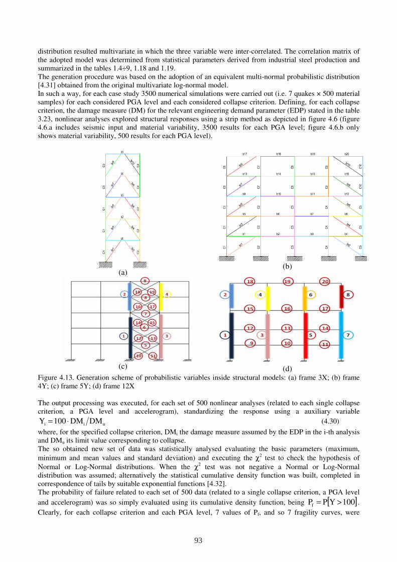
distribution resulted multivariate in which the three variable were inter-correlated. The correlation matrix of the adopted model was determined from statistical parameters derived from industrial steel production and summarized in the tables 1.4÷9, 1.18 and 1.19. The generation procedure was based on the adoption of an equivalent multi-normal probabilistic distribution [4.31] obtained from the original multivariate log-normal model. In such a way, for each case study 3500 numerical simulations were carried out (i.e. 7 quakes × 500 material samples) for each considered PGA level and each considered collapse criterion. Defining, for each collapse criterion, the damage measure (DM) for the relevant engineering demand parameter (EDP) stated in the table 3.23, nonlinear analyses explored structural responses using a strip method as depicted in figure 4.6 (figure 4.6.a includes seismic input and material variability, 3500 results for each PGA level; figure 4.6.b only shows material variability, 500 results for each PGA level).
(a)
(b)
(c)
(d) Figure 4.13. Generation scheme of probabilistic variables inside structural models: (a) frame 3X; (b) frame 4Y; (c) frame 5Y; (d) frame 12X The output processing was executed, for each set of 500 nonlinear analyses (related to each single collapse criterion, a PGA level and accelerogram), standardizing the response using a auxiliary variable
uii DMDM100Y ⋅= (4.30)
where, for the specified collapse criterion, DMi the damage measure assumed by the EDP in the i-th analysis and DMu its limit value corresponding to collapse. The so obtained new set of data was statistically analysed evaluating the basic parameters (maximum,
minimum and mean values and standard deviation) and executing the χ2 test to check the hypothesis of
Normal or Log-Normal distributions. When the χ2 test was not negative a Normal or Log-Normal distribution was assumed; alternatively the statistical cumulative density function was built, completed in correspondence of tails by suitable exponential functions [4.32]. The probability of failure related to each set of 500 data (related to a single collapse criterion, a PGA level
and accelerogram) was so simply evaluated using its cumulative density function, being [ ]100YPPf >= .
Clearly, for each collapse criterion and each PGA level, 7 values of Pf, and so 7 fragility curves, were
93
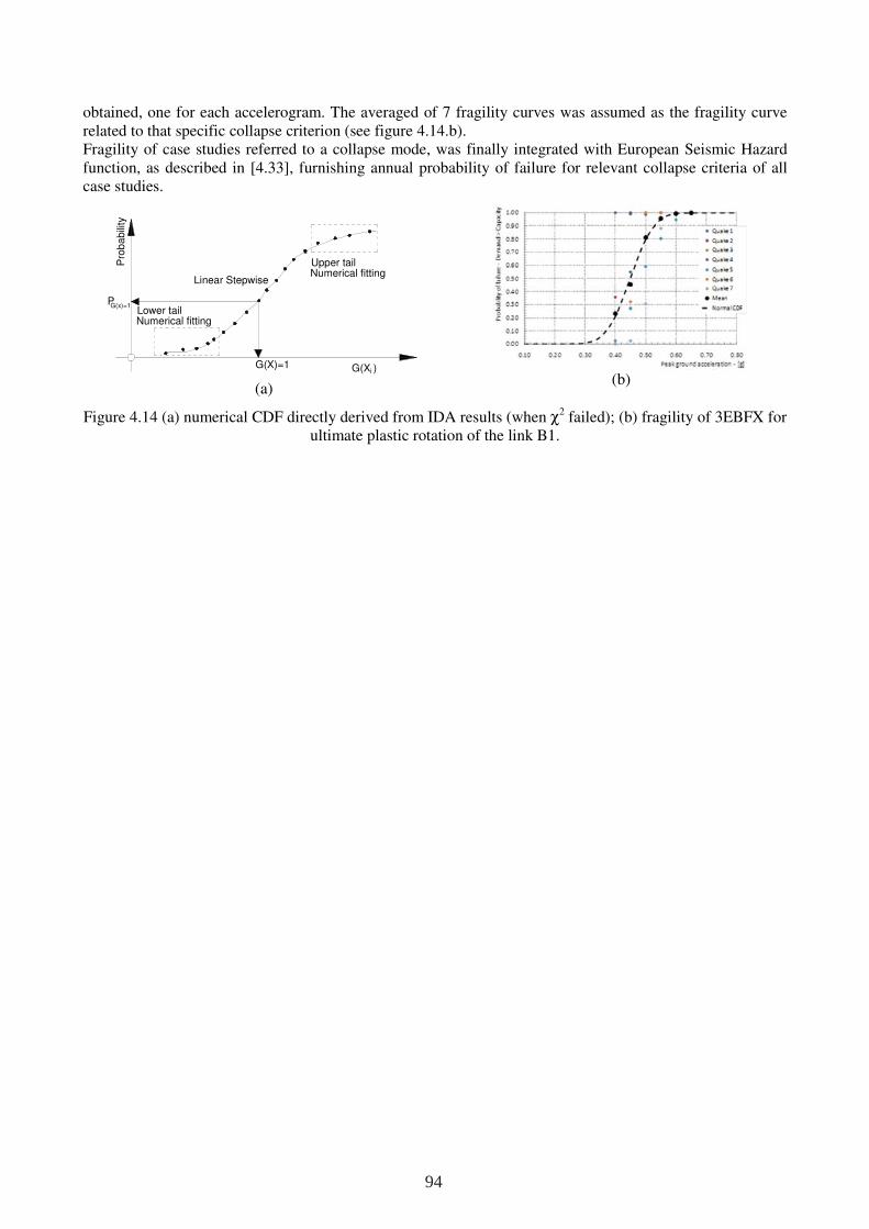
obtained, one for each accelerogram. The averaged of 7 fragility curves was assumed as the fragility curve related to that specific collapse criterion (see figure 4.14.b). Fragility of case studies referred to a collapse mode, was finally integrated with European Seismic Hazard function, as described in [4.33], furnishing annual probability of failure for relevant collapse criteria of all case studies.
(a)
(b)
Figure 4.14 (a) numerical CDF directly derived from IDA results (when χ2 failed); (b) fragility of 3EBFX for ultimate plastic rotation of the link B1.
Pro
babili
ty
Linear Stepwise
Upper tailNumerical fitting
Lower tailNumerical fitting
G(X )iG(X)=1
PG(x)=1
94
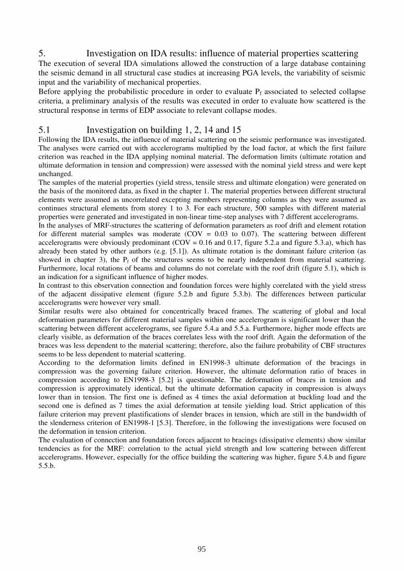
5. Investigation on IDA results: influence of material properties scattering The execution of several IDA simulations allowed the construction of a large database containing the seismic demand in all structural case studies at increasing PGA levels, the variability of seismic input and the variability of mechanical properties. Before applying the probabilistic procedure in order to evaluate Pf associated to selected collapse criteria, a preliminary analysis of the results was executed in order to evaluate how scattered is the structural response in terms of EDP associate to relevant collapse modes.
5.1 Investigation on building 1, 2, 14 and 15 Following the IDA results, the influence of material scattering on the seismic performance was investigated. The analyses were carried out with accelerograms multiplied by the load factor, at which the first failure criterion was reached in the IDA applying nominal material. The deformation limits (ultimate rotation and ultimate deformation in tension and compression) were assessed with the nominal yield stress and were kept unchanged. The samples of the material properties (yield stress, tensile stress and ultimate elongation) were generated on the basis of the monitored data, as fixed in the chapter 1. The material properties between different structural elements were assumed as uncorrelated excepting members representing columns as they were assumed as continues structural elements from storey 1 to 3. For each structure, 500 samples with different material properties were generated and investigated in non-linear time-step analyses with 7 different accelerograms. In the analyses of MRF-structures the scattering of deformation parameters as roof drift and element rotation for different material samples was moderate (COV = 0.03 to 0.07). The scattering between different accelerograms were obviously predominant (COV = 0.16 and 0.17, figure 5.2.a and figure 5.3.a), which has already been stated by other authors (e.g. [5.1]). As ultimate rotation is the dominant failure criterion (as showed in chapter 3), the Pf of the structures seems to be nearly independent from material scattering. Furthermore, local rotations of beams and columns do not correlate with the roof drift (figure 5.1), which is an indication for a significant influence of higher modes. In contrast to this observation connection and foundation forces were highly correlated with the yield stress of the adjacent dissipative element (figure 5.2.b and figure 5.3.b). The differences between particular accelerograms were however very small. Similar results were also obtained for concentrically braced frames. The scattering of global and local deformation parameters for different material samples within one accelerogram is significant lower than the scattering between different accelerograms, see figure 5.4.a and 5.5.a. Furthermore, higher mode effects are clearly visible, as deformation of the braces correlates less with the roof drift. Again the deformation of the braces was less dependent to the material scattering; therefore, also the failure probability of CBF structures seems to be less dependent to material scattering. According to the deformation limits defined in EN1998-3 ultimate deformation of the bracings in compression was the governing failure criterion. However, the ultimate deformation ratio of braces in compression according to EN1998-3 [5.2] is questionable. The deformation of braces in tension and compression is approximately identical, but the ultimate deformation capacity in compression is always lower than in tension. The first one is defined as 4 times the axial deformation at buckling load and the second one is defined as 7 times the axial deformation at tensile yielding load. Strict application of this failure criterion may prevent plastifications of slender braces in tension, which are still in the bandwidth of the slenderness criterion of EN1998-1 [5.3]. Therefore, in the following the investigations were focused on the deformation in tension criterion. The evaluation of connection and foundation forces adjacent to bracings (dissipative elements) show similar tendencies as for the MRF: correlation to the actual yield strength and low scattering between different accelerograms. However, especially for the office building the scattering was higher, figure 5.4.b and figure 5.5.b.
95
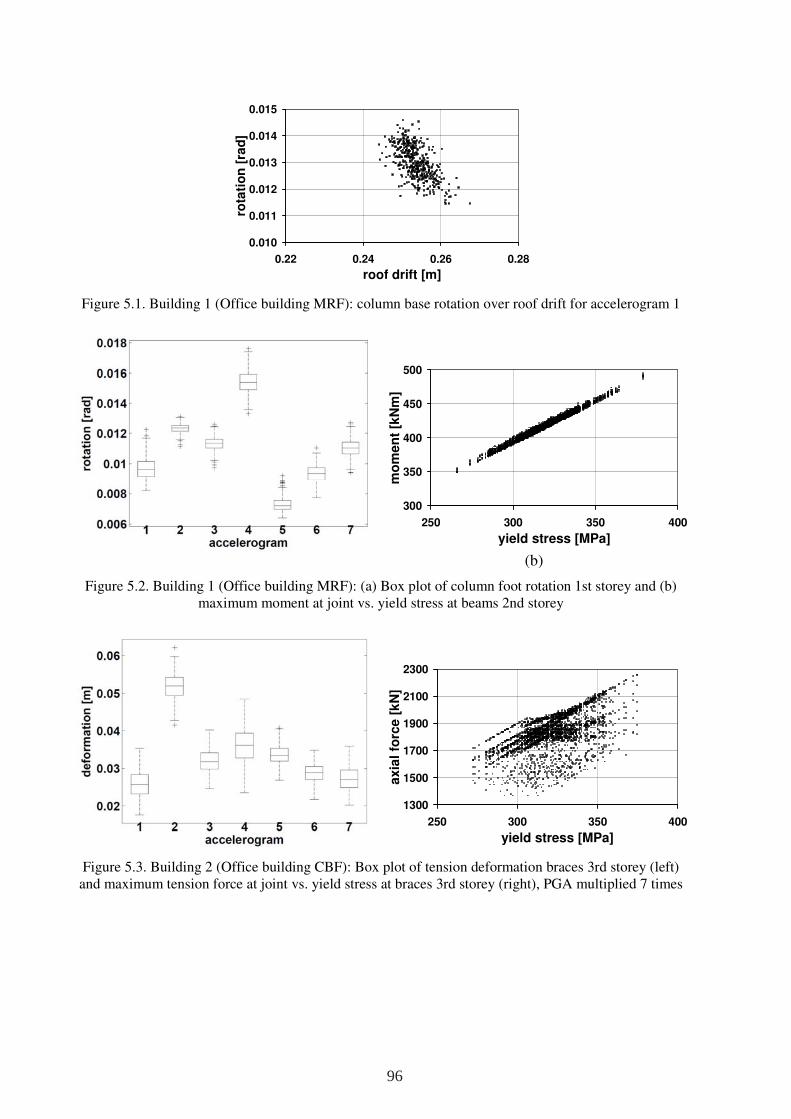
Figure 5.1. Building 1 (Office building MRF): column base rotation over roof drift for accelerogram 1
(b)
Figure 5.2. Building 1 (Office building MRF): (a) Box plot of column foot rotation 1st storey and (b) maximum moment at joint vs. yield stress at beams 2nd storey
Figure 5.3. Building 2 (Office building CBF): Box plot of tension deformation braces 3rd storey (left) and maximum tension force at joint vs. yield stress at braces 3rd storey (right), PGA multiplied 7 times
0.010
0.011
0.012
0.013
0.014
0.015
0.22 0.24 0.26 0.28
roof drift [m]
rota
tio
n [
rad
]
300
350
400
450
500
250 300 350 400
yield stress [MPa]
mo
men
t [k
Nm
]
1300
1500
1700
1900
2100
2300
250 300 350 400
yield stress [MPa]
axia
l fo
rce [
kN
]
96
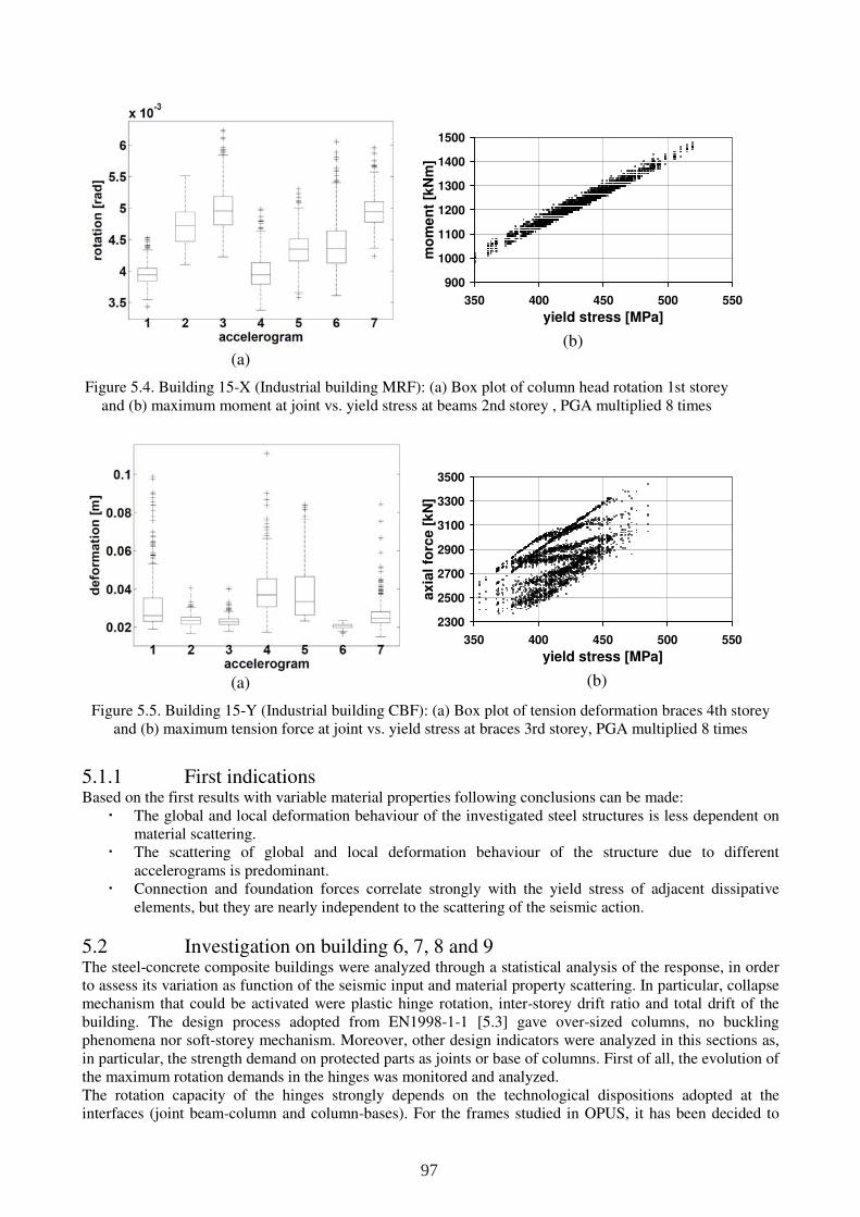
(a)
(b)
Figure 5.4. Building 15-X (Industrial building MRF): (a) Box plot of column head rotation 1st storey and (b) maximum moment at joint vs. yield stress at beams 2nd storey , PGA multiplied 8 times
(a)
(b)
Figure 5.5. Building 15-Y (Industrial building CBF): (a) Box plot of tension deformation braces 4th storey and (b) maximum tension force at joint vs. yield stress at braces 3rd storey, PGA multiplied 8 times
5.1.1 First indications Based on the first results with variable material properties following conclusions can be made:
The global and local deformation behaviour of the investigated steel structures is less dependent on material scattering.
The scattering of global and local deformation behaviour of the structure due to different accelerograms is predominant.
Connection and foundation forces correlate strongly with the yield stress of adjacent dissipative elements, but they are nearly independent to the scattering of the seismic action.
5.2 Investigation on building 6, 7, 8 and 9 The steel-concrete composite buildings were analyzed through a statistical analysis of the response, in order to assess its variation as function of the seismic input and material property scattering. In particular, collapse mechanism that could be activated were plastic hinge rotation, inter-storey drift ratio and total drift of the building. The design process adopted from EN1998-1-1 [5.3] gave over-sized columns, no buckling phenomena nor soft-storey mechanism. Moreover, other design indicators were analyzed in this sections as, in particular, the strength demand on protected parts as joints or base of columns. First of all, the evolution of the maximum rotation demands in the hinges was monitored and analyzed. The rotation capacity of the hinges strongly depends on the technological dispositions adopted at the interfaces (joint beam-column and column-bases). For the frames studied in OPUS, it has been decided to
900
1000
1100
1200
1300
1400
1500
350 400 450 500 550
yield stress [MPa]
mo
me
nt
[kN
m]
2300
2500
2700
2900
3100
3300
3500
350 400 450 500 550
yield stress [MPa]
ax
ial
forc
e [
kN
]
97
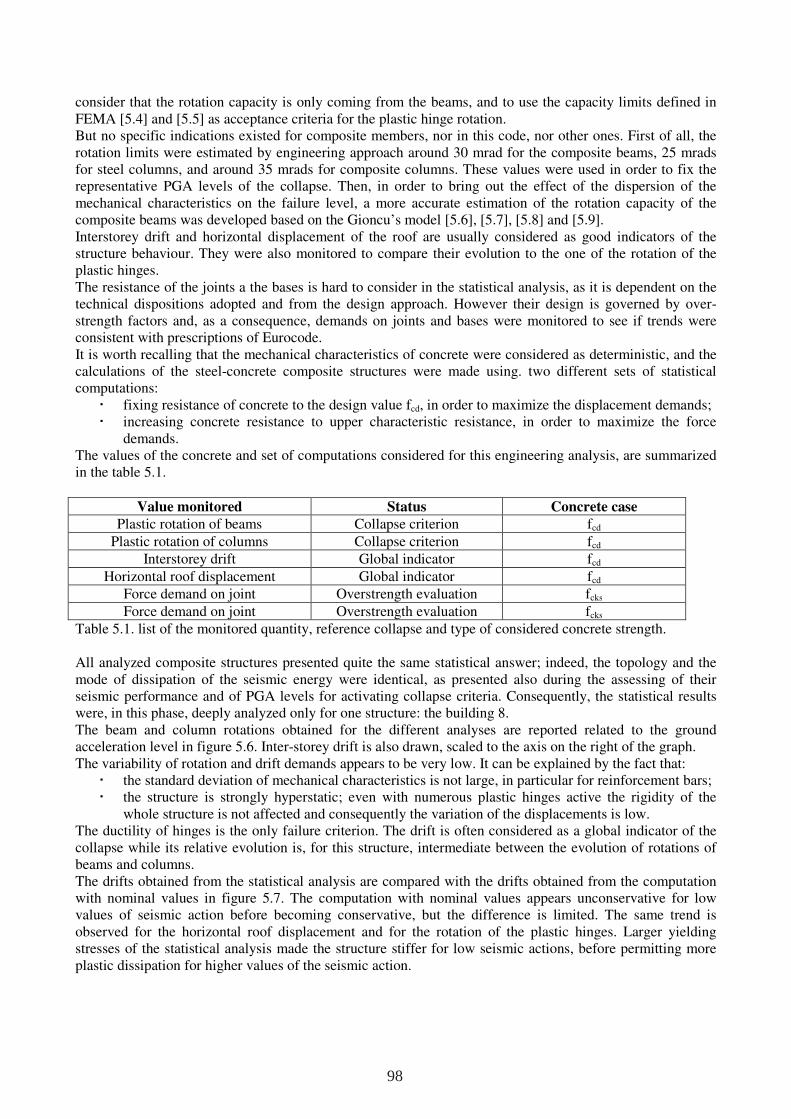
consider that the rotation capacity is only coming from the beams, and to use the capacity limits defined in FEMA [5.4] and [5.5] as acceptance criteria for the plastic hinge rotation. But no specific indications existed for composite members, nor in this code, nor other ones. First of all, the rotation limits were estimated by engineering approach around 30 mrad for the composite beams, 25 mrads for steel columns, and around 35 mrads for composite columns. These values were used in order to fix the representative PGA levels of the collapse. Then, in order to bring out the effect of the dispersion of the mechanical characteristics on the failure level, a more accurate estimation of the rotation capacity of the composite beams was developed based on the Gioncu’s model [5.6], [5.7], [5.8] and [5.9]. Interstorey drift and horizontal displacement of the roof are usually considered as good indicators of the structure behaviour. They were also monitored to compare their evolution to the one of the rotation of the plastic hinges. The resistance of the joints a the bases is hard to consider in the statistical analysis, as it is dependent on the technical dispositions adopted and from the design approach. However their design is governed by over-strength factors and, as a consequence, demands on joints and bases were monitored to see if trends were consistent with prescriptions of Eurocode. It is worth recalling that the mechanical characteristics of concrete were considered as deterministic, and the calculations of the steel-concrete composite structures were made using. two different sets of statistical computations:
fixing resistance of concrete to the design value fcd, in order to maximize the displacement demands; increasing concrete resistance to upper characteristic resistance, in order to maximize the force
demands. The values of the concrete and set of computations considered for this engineering analysis, are summarized in the table 5.1.
Value monitored Status Concrete case Plastic rotation of beams Collapse criterion fcd
Plastic rotation of columns Collapse criterion fcd Interstorey drift Global indicator fcd
Horizontal roof displacement Global indicator fcd Force demand on joint Overstrength evaluation fcks Force demand on joint Overstrength evaluation fcks
Table 5.1. list of the monitored quantity, reference collapse and type of considered concrete strength. All analyzed composite structures presented quite the same statistical answer; indeed, the topology and the mode of dissipation of the seismic energy were identical, as presented also during the assessing of their seismic performance and of PGA levels for activating collapse criteria. Consequently, the statistical results were, in this phase, deeply analyzed only for one structure: the building 8. The beam and column rotations obtained for the different analyses are reported related to the ground acceleration level in figure 5.6. Inter-storey drift is also drawn, scaled to the axis on the right of the graph. The variability of rotation and drift demands appears to be very low. It can be explained by the fact that:
the standard deviation of mechanical characteristics is not large, in particular for reinforcement bars; the structure is strongly hyperstatic; even with numerous plastic hinges active the rigidity of the
whole structure is not affected and consequently the variation of the displacements is low. The ductility of hinges is the only failure criterion. The drift is often considered as a global indicator of the collapse while its relative evolution is, for this structure, intermediate between the evolution of rotations of beams and columns. The drifts obtained from the statistical analysis are compared with the drifts obtained from the computation with nominal values in figure 5.7. The computation with nominal values appears unconservative for low values of seismic action before becoming conservative, but the difference is limited. The same trend is observed for the horizontal roof displacement and for the rotation of the plastic hinges. Larger yielding stresses of the statistical analysis made the structure stiffer for low seismic actions, before permitting more plastic dissipation for higher values of the seismic action.
98
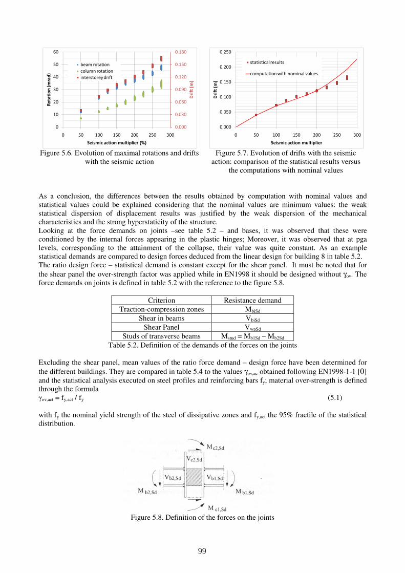
Figure 5.6. Evolution of maximal rotations and drifts
with the seismic action
Figure 5.7. Evolution of drifts with the seismic action: comparison of the statistical results versus
the computations with nominal values
As a conclusion, the differences between the results obtained by computation with nominal values and statistical values could be explained considering that the nominal values are minimum values: the weak statistical dispersion of displacement results was justified by the weak dispersion of the mechanical characteristics and the strong hyperstaticity of the structure. Looking at the force demands on joints –see table 5.2 – and bases, it was observed that these were conditioned by the internal forces appearing in the plastic hinges; Moreover, it was observed that at pga levels, corresponding to the attainment of the collapse, their value was quite constant. As an example statistical demands are compared to design forces deduced from the linear design for building 8 in table 5.2. The ratio design force – statistical demand is constant except for the shear panel. It must be noted that for
the shear panel the over-strength factor was applied while in EN1998 it should be designed without γov. The force demands on joints is defined in table 5.2 with the reference to the figure 5.8.
Criterion Resistance demand Traction-compression zones MbiSd
Shear in beams VbiSd Shear Panel VwpSd
Studs of transverse beams Mstud = Mb1Sd – Mb2Sd Table 5.2. Definition of the demands of the forces on the joints
Excluding the shear panel, mean values of the ratio force demand – design force have been determined for
the different buildings. They are compared in table 5.4 to the values γov,ac obtained following EN1998-1-1 [0] and the statistical analysis executed on steel profiles and reinforcing bars fy; material over-strength is defined through the formula γov,act = fy,act / fy (5.1)
with fy the nominal yield strength of the steel of dissipative zones and fy,act the 95% fractile of the statistical distribution.
Figure 5.8. Definition of the forces on the joints
0.000
0.030
0.060
0.090
0.120
0.150
0.180
0
10
20
30
40
50
60
0 50 100 150 200 250 300
Dri
ft (
m)
Ro
tati
on
(m
rad
)
Seismic action multiplier (%)
beam rotation
column rotation
interstorey drift
0.000
0.050
0.100
0.150
0.200
0.250
0 50 100 150 200 250 300
Dri
ft (
m)
Seismic action multiplier
statistical results
computation with nominal values
99
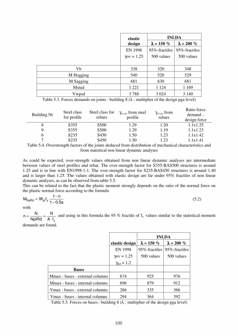
elastic
design
INLDA
λλλλ = 150 % λλλλ = 200 %
EN 1998 95%-fractiles 95%-fractiles
γov = 1.25 500 values 500 values
Vb 338 320 348
M Hogging 540 520 529
M Sagging 681 630 681
Mstud 1 221 1 124 1 169
Vwpsd 3 788 3 024 3 140 Table 5.3. Forces demands on joints : building 8 (λ : multiplier of the design pga level)
Building Nr Steel class for profile
Steel class for rebars
γov,ac from steel profile
γov,ac from rebars
Ratio force demand –
design force 8 S355 S500 1.29 1.20 1.1x1.25 9 S355 S500 1.29 1.19 1.1x1.23 6 S235 S450 1.50 1.23 1.1x1.42 7 S235 S450 1.50 1.23 1.1x1.41
Table 5.4. Overstrength factors of the joints deduced from distribution of mechanical characteristics and from statistical non linear dynamic analyses
As could be expected, over-strength values obtained from non linear dynamic analyses are intermediate between values of steel profiles and rebar. The over-strength factor for S355-BAS500 structures is around 1.25 and is in line with EN1998-1-1. The over-strength factor for S235-BAS450 structures is around 1.40 and is larger than 1.25. The values obtained with elastic design are far under 95% fractiles of non linear dynamic analyses, as can be observed from table 5.5. This can be related to the fact that the plastic moment strongly depends on the ratio of the normal force on the plastic normal force according to the formula
a5.01
n1fWM yplNyRd
−
−= (5.2)
with
yfA
N
NplRd
Nn == and using in this formula the 95 % fractile of fy, values similar to the statistical moment
demands are found.
elastic design
INLDA
λλλλ = 150 % λλλλ = 200 %
EN 1998 95%-fractiles 95%-fractiles
γov = 1.25 500 values 500 values
γRd = 1.2
Bases
Mmax - bases - external columns 674 925 976
Mmax - bases - internal columns 696 879 912
Vmax - bases - external columns 266 335 366
Vmax - bases - internal columns 294 364 392 Table 5.5. Forces on bases : building 8 (λ : multiplier of the design pga level)
100
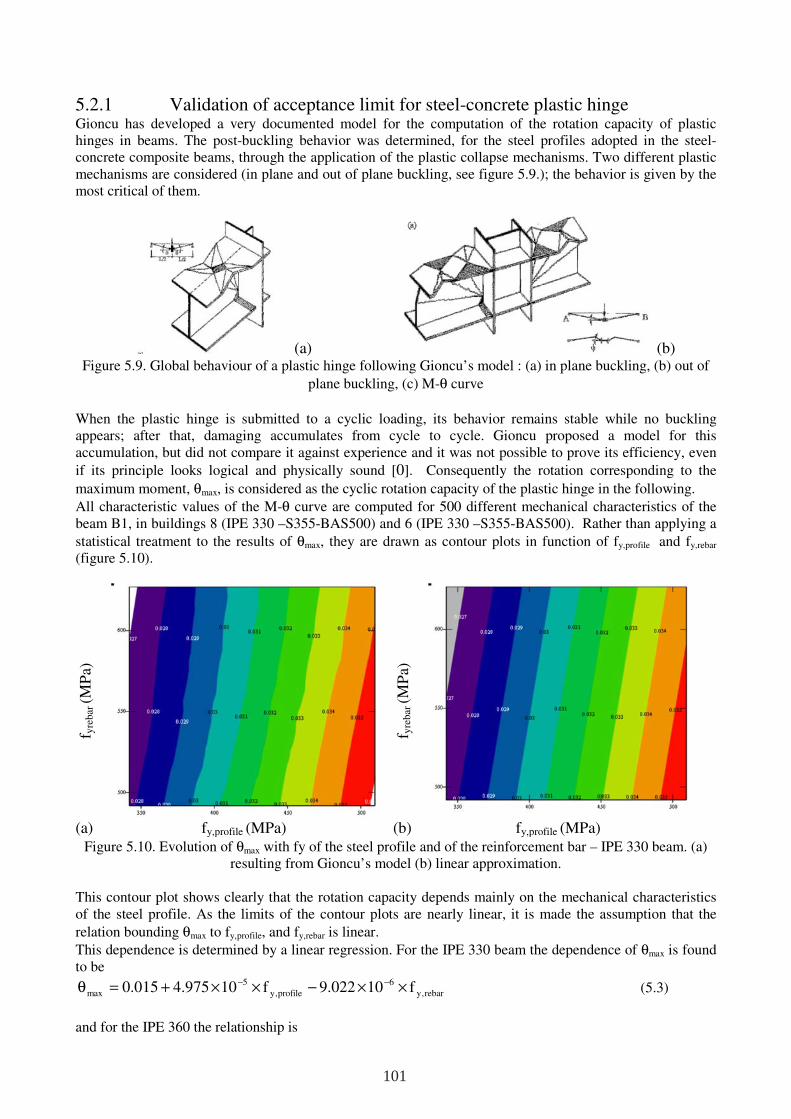
5.2.1 Validation of acceptance limit for steel-concrete plastic hinge Gioncu has developed a very documented model for the computation of the rotation capacity of plastic hinges in beams. The post-buckling behavior was determined, for the steel profiles adopted in the steel-concrete composite beams, through the application of the plastic collapse mechanisms. Two different plastic mechanisms are considered (in plane and out of plane buckling, see figure 5.9.); the behavior is given by the most critical of them.
(a) (b) Figure 5.9. Global behaviour of a plastic hinge following Gioncu’s model : (a) in plane buckling, (b) out of
plane buckling, (c) M-θ curve
When the plastic hinge is submitted to a cyclic loading, its behavior remains stable while no buckling appears; after that, damaging accumulates from cycle to cycle. Gioncu proposed a model for this accumulation, but did not compare it against experience and it was not possible to prove its efficiency, even
if its principle looks logical and physically sound [0]. Consequently the rotation corresponding to the
maximum moment, θmax, is considered as the cyclic rotation capacity of the plastic hinge in the following.
All characteristic values of the M-θ curve are computed for 500 different mechanical characteristics of the beam B1, in buildings 8 (IPE 330 –S355-BAS500) and 6 (IPE 330 –S355-BAS500). Rather than applying a
statistical treatment to the results of θmax, they are drawn as contour plots in function of fy,profile and fy,rebar
(figure 5.10).
f yre
bar
(M
Pa)
f yre
bar
(M
Pa)
(a) fy,profile (MPa) (b) fy,profile (MPa) Figure 5.10. Evolution of θmax with fy of the steel profile and of the reinforcement bar – IPE 330 beam. (a)
resulting from Gioncu’s model (b) linear approximation. This contour plot shows clearly that the rotation capacity depends mainly on the mechanical characteristics of the steel profile. As the limits of the contour plots are nearly linear, it is made the assumption that the
relation bounding θmax to fy,profile, and fy,rebar is linear.
This dependence is determined by a linear regression. For the IPE 330 beam the dependence of θmax is found to be
rebar,y
6
profile,y
5
max f10022.9f10975.4015.0 ××−××+=θ −− (5.3)
and for the IPE 360 the relationship is
101
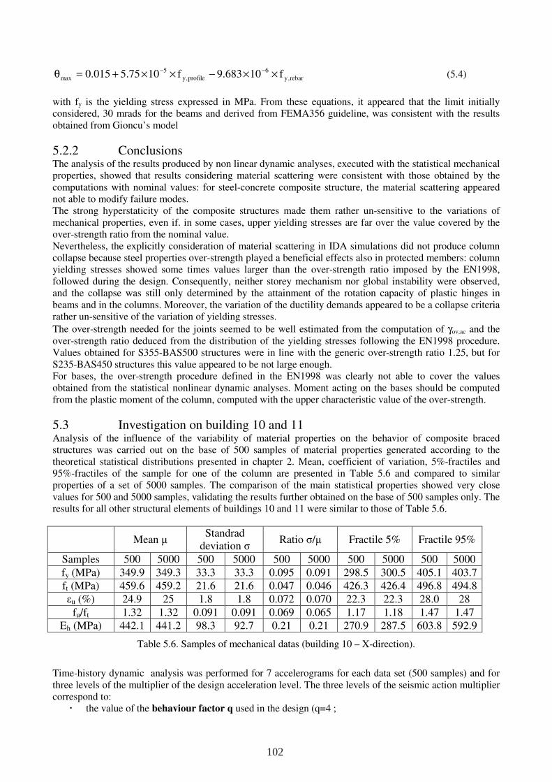
rebar,y
6
profile,y
5
max f10683.9f1075.5015.0 ××−××+=θ −− (5.4)
with fy is the yielding stress expressed in MPa. From these equations, it appeared that the limit initially considered, 30 mrads for the beams and derived from FEMA356 guideline, was consistent with the results obtained from Gioncu’s model
5.2.2 Conclusions The analysis of the results produced by non linear dynamic analyses, executed with the statistical mechanical properties, showed that results considering material scattering were consistent with those obtained by the computations with nominal values: for steel-concrete composite structure, the material scattering appeared not able to modify failure modes. The strong hyperstaticity of the composite structures made them rather un-sensitive to the variations of mechanical properties, even if. in some cases, upper yielding stresses are far over the value covered by the over-strength ratio from the nominal value. Nevertheless, the explicitly consideration of material scattering in IDA simulations did not produce column collapse because steel properties over-strength played a beneficial effects also in protected members: column yielding stresses showed some times values larger than the over-strength ratio imposed by the EN1998, followed during the design. Consequently, neither storey mechanism nor global instability were observed, and the collapse was still only determined by the attainment of the rotation capacity of plastic hinges in beams and in the columns. Moreover, the variation of the ductility demands appeared to be a collapse criteria rather un-sensitive of the variation of yielding stresses.
The over-strength needed for the joints seemed to be well estimated from the computation of γov,ac and the over-strength ratio deduced from the distribution of the yielding stresses following the EN1998 procedure. Values obtained for S355-BAS500 structures were in line with the generic over-strength ratio 1.25, but for S235-BAS450 structures this value appeared to be not large enough. For bases, the over-strength procedure defined in the EN1998 was clearly not able to cover the values obtained from the statistical nonlinear dynamic analyses. Moment acting on the bases should be computed from the plastic moment of the column, computed with the upper characteristic value of the over-strength.
5.3 Investigation on building 10 and 11 Analysis of the influence of the variability of material properties on the behavior of composite braced structures was carried out on the base of 500 samples of material properties generated according to the theoretical statistical distributions presented in chapter 2. Mean, coefficient of variation, 5%-fractiles and 95%-fractiles of the sample for one of the column are presented in Table 5.6 and compared to similar properties of a set of 5000 samples. The comparison of the main statistical properties showed very close values for 500 and 5000 samples, validating the results further obtained on the base of 500 samples only. The results for all other structural elements of buildings 10 and 11 were similar to those of Table 5.6.
Mean µ
Standrad deviation σ
Ratio σ/µ Fractile 5% Fractile 95%
Samples 500 5000 500 5000 500 5000 500 5000 500 5000
fy (MPa) 349.9 349.3 33.3 33.3 0.095 0.091 298.5 300.5 405.1 403.7 ft (MPa) 459.6 459.2 21.6 21.6 0.047 0.046 426.3 426.4 496.8 494.8 εu (%) 24.9 25 1.8 1.8 0.072 0.070 22.3 22.3 28.0 28
fu/ft 1.32 1.32 0.091 0.091 0.069 0.065 1.17 1.18 1.47 1.47 Eh (MPa) 442.1 441.2 98.3 92.7 0.21 0.21 270.9 287.5 603.8 592.9
Table 5.6. Samples of mechanical datas (building 10 – X-direction).
Time-history dynamic analysis was performed for 7 accelerograms for each data set (500 samples) and for three levels of the multiplier of the design acceleration level. The three levels of the seismic action multiplier correspond to:
the value of the behaviour factor q used in the design (q=4 ;
102
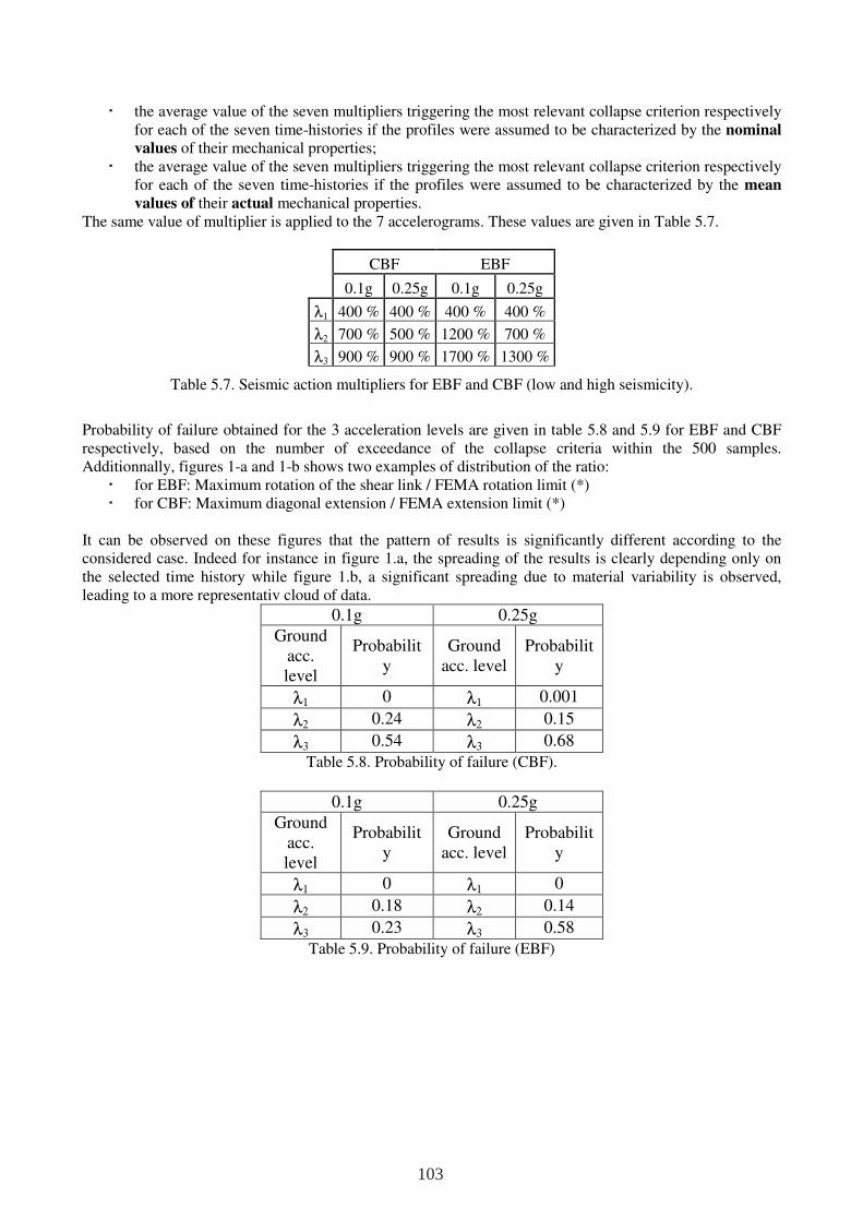
the average value of the seven multipliers triggering the most relevant collapse criterion respectively for each of the seven time-histories if the profiles were assumed to be characterized by the nominal
values of their mechanical properties; the average value of the seven multipliers triggering the most relevant collapse criterion respectively
for each of the seven time-histories if the profiles were assumed to be characterized by the mean
values of their actual mechanical properties. The same value of multiplier is applied to the 7 accelerograms. These values are given in Table 5.7.
CBF EBF
0.1g 0.25g 0.1g 0.25g
λ1 400 % 400 % 400 % 400 %
λ2 700 % 500 % 1200 % 700 %
λ3 900 % 900 % 1700 % 1300 %
Table 5.7. Seismic action multipliers for EBF and CBF (low and high seismicity).
Probability of failure obtained for the 3 acceleration levels are given in table 5.8 and 5.9 for EBF and CBF respectively, based on the number of exceedance of the collapse criteria within the 500 samples. Additionnally, figures 1-a and 1-b shows two examples of distribution of the ratio:
for EBF: Maximum rotation of the shear link / FEMA rotation limit (*) for CBF: Maximum diagonal extension / FEMA extension limit (*)
It can be observed on these figures that the pattern of results is significantly different according to the considered case. Indeed for instance in figure 1.a, the spreading of the results is clearly depending only on the selected time history while figure 1.b, a significant spreading due to material variability is observed, leading to a more representativ cloud of data.
0.1g 0.25g Ground
acc. level
Probability
Ground acc. level
Probability
λ1 0 λ1 0.001
λ2 0.24 λ2 0.15
λ3 0.54 λ3 0.68
Table 5.8. Probability of failure (CBF).
0.1g 0.25g Ground
acc. level
Probability
Ground acc. level
Probability
λ1 0 λ1 0
λ2 0.18 λ2 0.14
λ3 0.23 λ3 0.58
Table 5.9. Probability of failure (EBF)
103
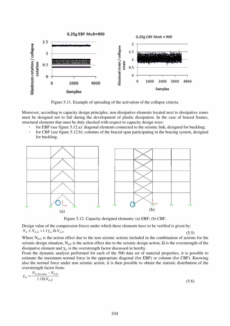
Figure 5.11. Example of spreading of the activation of the collapse criteria.
Moreover, according to capacity design principles, non dissipative elements located next to dissipative zones must be designed not to fail during the development of plastic dissipation. In the case of braced frames, structural elements that must be duly checked with respect to capacity design were:
for EBF (see figure 5.12.a): diagonal elements connected to the seismic link, designed for buckling; for CBF (see figure 5.12.b): columns of the braced span participating in the bracing system, designed
for buckling.
(a)
(b)
Figure 5.12. Capacity designed elements: (a) EBF; (b) CBF.
Design value of the compression forces under which these elements have to be verified is given by:
, ,1.1d d G ov d EN N Nγ≥ + Ω (5.5)
Where Nd,G is the action effect due to the non seismic actions included in the combination of actions for the
seismic design situation, Nd,E is the action effect due to the seismic design action, Ω is the overstrength of the
dissipative element and γov is the overstrength factor discussed in hereby. From the dynamic analysis performed for each of the 500 data set of material properties, it is possible to estimate the maximum normal force in the appropriate diagonal (for EBF) or column (for CBF). Knowing also the normal force under non seismic action, it is then possible to obtain the statistic distribution of the overstrength factor from:
, ,max ,
,1.1
d dyn d G
ov
d E
N N
Nγ
−=
Ω (5.6)
104

Figures 5.13.a to 5.13.d illustrates the spreading of the calculated overstrength for some particular cases from which the observations already made for collapse probability in terms of relative dependency on material varaibility and on ground motion time-history can again be made. Tables 5.10.a and 5.10.b gives the 95 % fractile of the overstrength factor obtain respectively for EBF and CBF designed for low and high seismicity for the two levels of acceleration multiplier defined above and for each level of the structure. Overstrength factors appear to depend strongly on the acceleration multiplier, although values to be considered for comparison with the recommended EN 1998 values are the figures in bold in the tables since they are associated with a amplitude of structural deformations corresponding to the behaviour factor used for design. In these tables, it can be identified that the actual overstrength is ranging from less than 1.0 (for storeys overdesigned by slenderness criteria) up to 1.82, which is by far higher than the value of 1.25 proposed by EN 1998-1.
Figure 5.13. Examples of over-strength coefficient distributions.
Storey\Level Low High Low High Low High
λ1 λ1 λ2 λ2 λ3 λ3 1 1.13 1.82 1.32 2.00 1.45 2.45
2 0.84 1.59 0.89 1.55 1.09 2.15 3 0.86 1.48 0.94 1.59 1.05 1.83
4 1.02 1.75 1.15 1.86 1.28 2.20
5 0.67 1.00 1.00 1.00 1.10 1.45
Table 5.10.a. Over-strength factor (CBF)
Storey\Level Low High Low High Low High
λ1 λ1 λ2 λ2 λ3 λ3 1 1.35 1.13 2.73 1.57 3.00 3.00
2 1.41 1.15 2.82 1.56 3.10 3.10 3 1.41 0.98 3.00 1.22 3.35 3.35
4 1.27 0.79 2.91 1.00 3.20 3.20
5 1.41 0.54 3.91 0.71 4.50 4.50
Table 5.10.b. Over-strength factor (EBF).
105
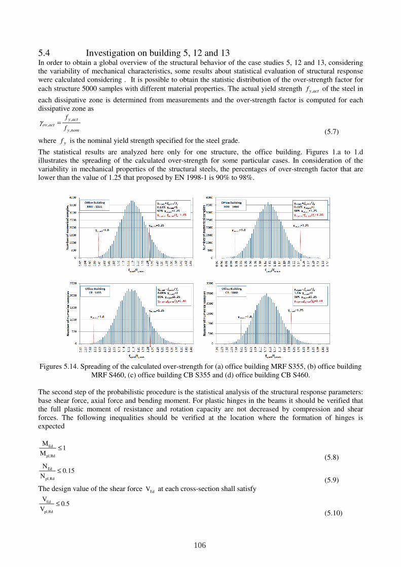
5.4 Investigation on building 5, 12 and 13 In order to obtain a global overview of the structural behavior of the case studies 5, 12 and 13, considering the variability of mechanical characteristics, some results about statistical evaluation of structural response were calculated considering . It is possible to obtain the statistic distribution of the over-strength factor for
each structure 5000 samples with different material properties. The actual yield strength ,y actf of the steel in
each dissipative zone is determined from measurements and the over-strength factor is computed for each dissipative zone as
,,
,
y act
ov act
y nom
f
f=γ
(5.7)
where yf is the nominal yield strength specified for the steel grade.
The statistical results are analyzed here only for one structure, the office building. Figures 1.a to 1.d illustrates the spreading of the calculated over-strength for some particular cases. In consideration of the variability in mechanical properties of the structural steels, the percentages of over-strength factor that are lower than the value of 1.25 that proposed by EN 1998-1 is 90% to 98%.
Figures 5.14. Spreading of the calculated over-strength for (a) office building MRF S355, (b) office building
MRF S460, (c) office building CB S355 and (d) office building CB S460. The second step of the probabilistic procedure is the statistical analysis of the structural response parameters: base shear force, axial force and bending moment. For plastic hinges in the beams it should be verified that the full plastic moment of resistance and rotation capacity are not decreased by compression and shear forces. The following inequalities should be verified at the location where the formation of hinges is expected
Ed
pl Rd
M1
M,
≤
(5.8)
Ed
pl Rd
N0 15
N,
.≤
(5.9) The design value of the shear force EdV at each cross-section shall satisfy
Ed
pl Rd
V0 5
V,
.≤
(5.10)
106
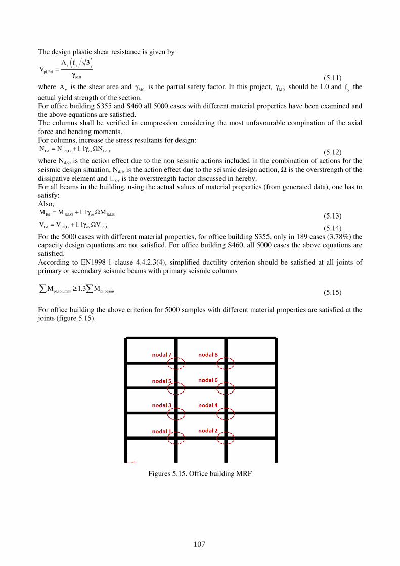
The design plastic shear resistance is given by
( )v y
pl Rd
M0
A f 3V , =
γ (5.11)
where vA is the shear area and M0γ is the partial safety factor. In this project, M0γ should be 1.0 and yf the
actual yield strength of the section. For office building S355 and S460 all 5000 cases with different material properties have been examined and the above equations are satisfied. The columns shall be verified in compression considering the most unfavourable compination of the axial force and bending moments.
For columns, increase the stress resultants for design:
Ed Ed G ov Ed EN N 1 1 N, ,
.= + γ Ω (5.12)
where Nd,G is the action effect due to the non seismic actions included in the combination of actions for the
seismic design situation, Nd,E is the action effect due to the seismic design action, Ω is the overstrength of the dissipative element and ov is the overstrength factor discussed in hereby. For all beams in the building, using the actual values of material properties (from generated data), one has to satisfy: Also,
Ed Ed G ov Ed EM M 1 1 M, ,
.= + γ Ω (5.13)
Ed Ed G ov Ed EV V 1 1 V, ,
.= + γ Ω (5.14)
For the 5000 cases with different material properties, for office building S355, only in 189 cases (3.78%) the capacity design equations are not satisfied. For office building S460, all 5000 cases the above equations are satisfied. According to EN1998-1 clause 4.4.2.3(4), simplified ductility criterion should be satisfied at all joints of primary or secondary seismic beams with primary seismic columns
pl columns pl beamsM 1 3 M, ,.≥∑ ∑ (5.15)
For office building the above criterion for 5000 samples with different material properties are satisfied at the joints (figure 5.15).
Figures 5.15. Office building MRF
107
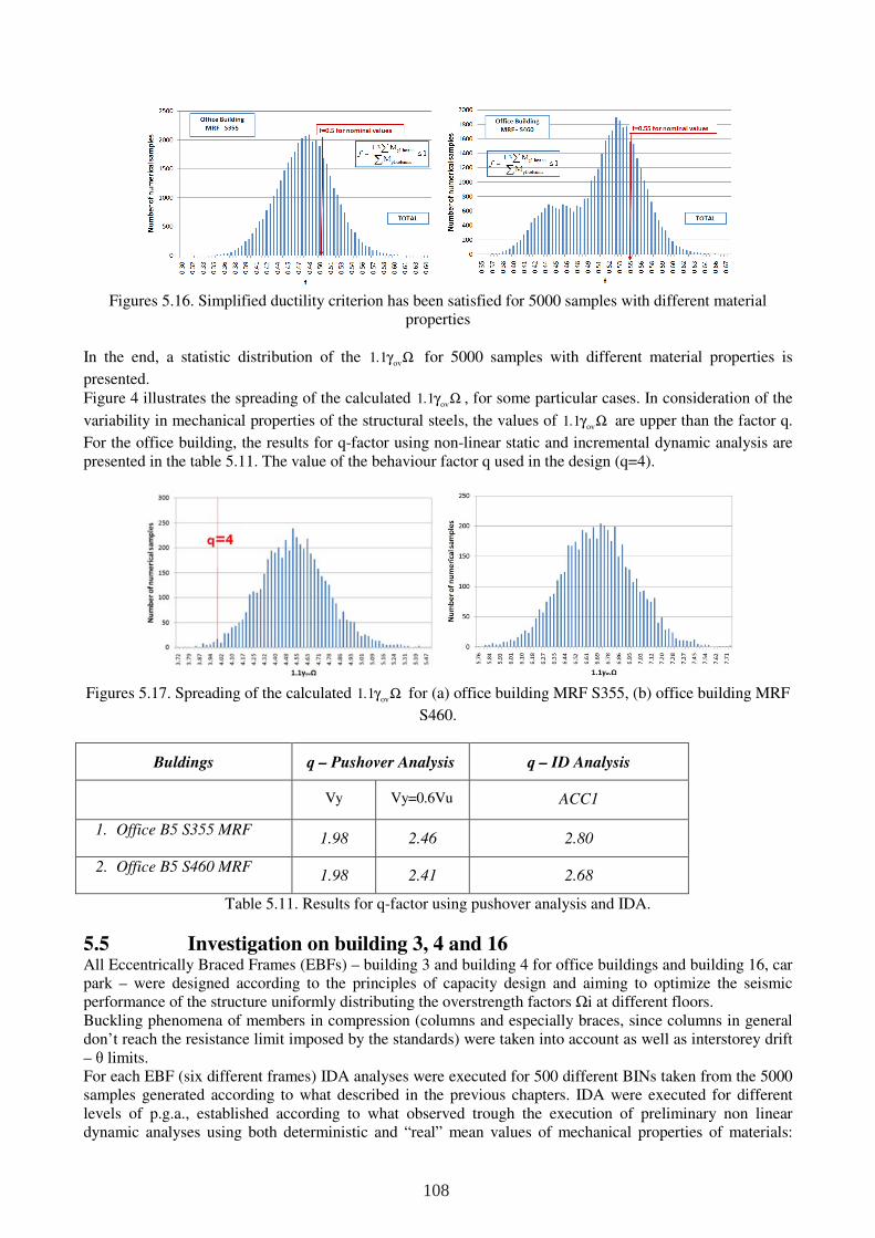
Figures 5.16. Simplified ductility criterion has been satisfied for 5000 samples with different material
properties
In the end, a statistic distribution of the ov1 1. γ Ω for 5000 samples with different material properties is
presented. Figure 4 illustrates the spreading of the calculated ov1 1. γ Ω , for some particular cases. In consideration of the
variability in mechanical properties of the structural steels, the values of ov1 1. γ Ω are upper than the factor q.
For the office building, the results for q-factor using non-linear static and incremental dynamic analysis are presented in the table 5.11. The value of the behaviour factor q used in the design (q=4).
Figures 5.17. Spreading of the calculated ov1 1. γ Ω for (a) office building MRF S355, (b) office building MRF
S460.
Buldings q – Pushover Analysis q – ID Analysis
Vy Vy=0.6Vu ACC1
1. Office B5 S355 MRF 1.98 2.46 2.80
2. Office B5 S460 MRF 1.98 2.41 2.68
Table 5.11. Results for q-factor using pushover analysis and IDA.
5.5 Investigation on building 3, 4 and 16 All Eccentrically Braced Frames (EBFs) – building 3 and building 4 for office buildings and building 16, car park – were designed according to the principles of capacity design and aiming to optimize the seismic performance of the structure uniformly distributing the overstrength factors Ωi at different floors. Buckling phenomena of members in compression (columns and especially braces, since columns in general don’t reach the resistance limit imposed by the standards) were taken into account as well as interstorey drift – θ limits. For each EBF (six different frames) IDA analyses were executed for 500 different BINs taken from the 5000 samples generated according to what described in the previous chapters. IDA were executed for different levels of p.g.a., established according to what observed trough the execution of preliminary non linear dynamic analyses using both deterministic and “real” mean values of mechanical properties of materials:
108
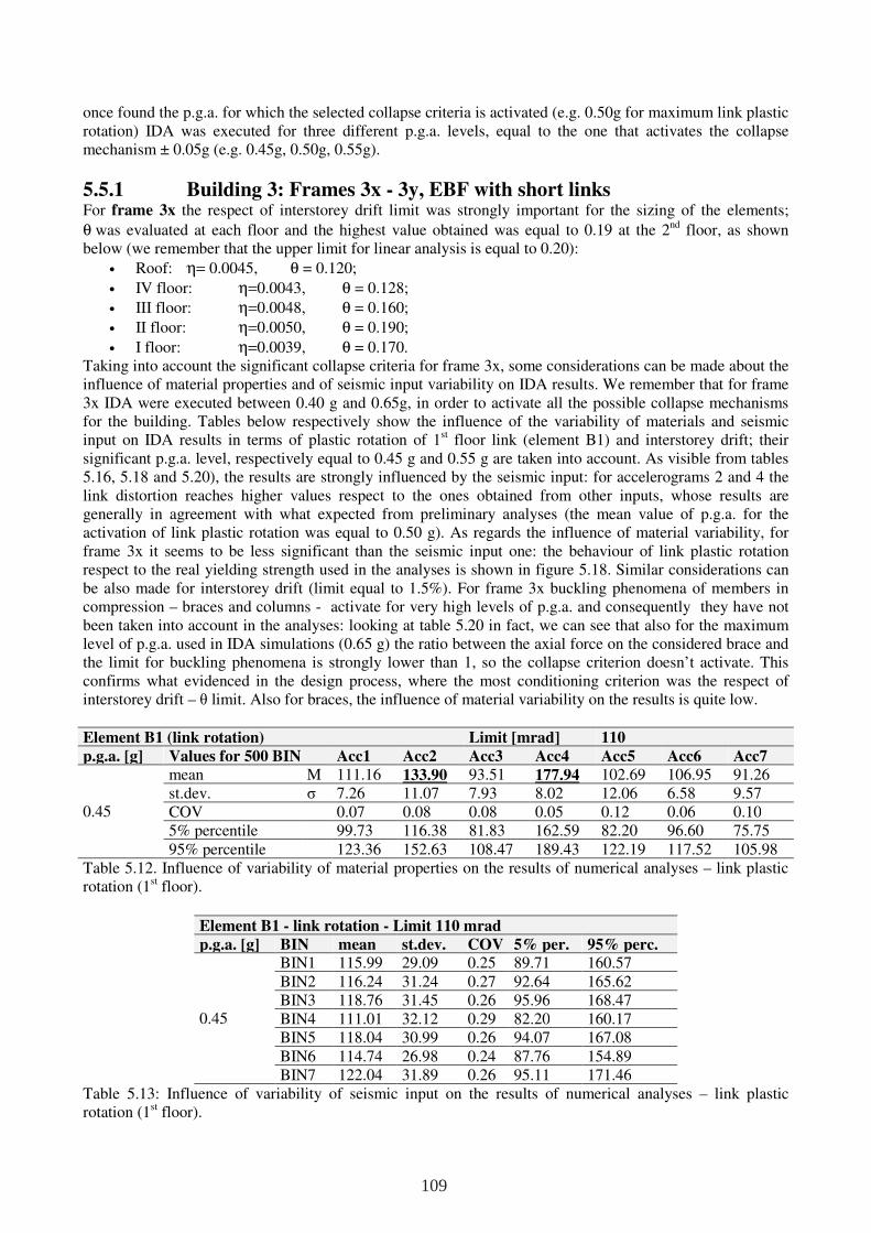
once found the p.g.a. for which the selected collapse criteria is activated (e.g. 0.50g for maximum link plastic rotation) IDA was executed for three different p.g.a. levels, equal to the one that activates the collapse mechanism ± 0.05g (e.g. 0.45g, 0.50g, 0.55g).
5.5.1 Building 3: Frames 3x - 3y, EBF with short links For frame 3x the respect of interstorey drift limit was strongly important for the sizing of the elements;
θ was evaluated at each floor and the highest value obtained was equal to 0.19 at the 2nd floor, as shown below (we remember that the upper limit for linear analysis is equal to 0.20):
• Roof: η= 0.0045, θ = 0.120;
• IV floor: η=0.0043, θ = 0.128;
• III floor: η=0.0048, θ = 0.160;
• II floor: η=0.0050, θ = 0.190;
• I floor: η=0.0039, θ = 0.170. Taking into account the significant collapse criteria for frame 3x, some considerations can be made about the influence of material properties and of seismic input variability on IDA results. We remember that for frame 3x IDA were executed between 0.40 g and 0.65g, in order to activate all the possible collapse mechanisms for the building. Tables below respectively show the influence of the variability of materials and seismic input on IDA results in terms of plastic rotation of 1st floor link (element B1) and interstorey drift; their significant p.g.a. level, respectively equal to 0.45 g and 0.55 g are taken into account. As visible from tables 5.16, 5.18 and 5.20), the results are strongly influenced by the seismic input: for accelerograms 2 and 4 the link distortion reaches higher values respect to the ones obtained from other inputs, whose results are generally in agreement with what expected from preliminary analyses (the mean value of p.g.a. for the activation of link plastic rotation was equal to 0.50 g). As regards the influence of material variability, for frame 3x it seems to be less significant than the seismic input one: the behaviour of link plastic rotation respect to the real yielding strength used in the analyses is shown in figure 5.18. Similar considerations can be also made for interstorey drift (limit equal to 1.5%). For frame 3x buckling phenomena of members in compression – braces and columns - activate for very high levels of p.g.a. and consequently they have not been taken into account in the analyses: looking at table 5.20 in fact, we can see that also for the maximum level of p.g.a. used in IDA simulations (0.65 g) the ratio between the axial force on the considered brace and the limit for buckling phenomena is strongly lower than 1, so the collapse criterion doesn’t activate. This confirms what evidenced in the design process, where the most conditioning criterion was the respect of interstorey drift – θ limit. Also for braces, the influence of material variability on the results is quite low.
Element B1 (link rotation) Limit [mrad] 110
p.g.a. [g] Values for 500 BIN Acc1 Acc2 Acc3 Acc4 Acc5 Acc6 Acc7
0.45
mean M 111.16 133.90 93.51 177.94 102.69 106.95 91.26 st.dev. σ 7.26 11.07 7.93 8.02 12.06 6.58 9.57 COV 0.07 0.08 0.08 0.05 0.12 0.06 0.10 5% percentile 99.73 116.38 81.83 162.59 82.20 96.60 75.75 95% percentile 123.36 152.63 108.47 189.43 122.19 117.52 105.98
Table 5.12. Influence of variability of material properties on the results of numerical analyses – link plastic rotation (1st floor).
Element B1 - link rotation - Limit 110 mrad
p.g.a. [g] BIN mean st.dev. COV 5% per. 95% perc.
0.45
BIN1 115.99 29.09 0.25 89.71 160.57 BIN2 116.24 31.24 0.27 92.64 165.62 BIN3 118.76 31.45 0.26 95.96 168.47 BIN4 111.01 32.12 0.29 82.20 160.17 BIN5 118.04 30.99 0.26 94.07 167.08 BIN6 114.74 26.98 0.24 87.76 154.89 BIN7 122.04 31.89 0.26 95.11 171.46
Table 5.13: Influence of variability of seismic input on the results of numerical analyses – link plastic rotation (1st floor).
109
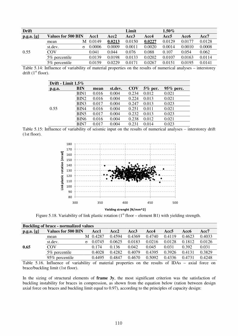
Drift Limit 1.50%
p.g.a. [g] Values for 500 BIN Acc1 Acc2 Acc3 Acc4 Acc5 Acc6 Acc7
0.55
mean M 0.0149 0.0213 0.0150 0.0227 0.0129 0.0177 0.0128
st.dev. σ 0.0006 0.0009 0.0011 0.0020 0.0014 0.0010 0.0008
COV 0.041 0.044 0.076 0.088 0.107 0.054 0.062
5% percentile 0.0139 0.0198 0.0133 0.0202 0.0107 0.0163 0.0114
5% percentile 0.0159 0.0229 0.0171 0.0267 0.0151 0.0195 0.0141
Table 5.14: Influence of variability of material properties on the results of numerical analyses – interstorey drift (1st floor).
Drift - Limit 1.5%
p.g.a. BIN mean st.dev. COV 5% per. 95% perc.
0.55
BIN1 0.016 0.004 0.234 0.012 0.021 BIN2 0.016 0.004 0.224 0.013 0.021 BIN3 0.017 0.004 0.247 0.013 0.023 BIN4 0.016 0.004 0.251 0.011 0.021 BIN5 0.017 0.004 0.232 0.013 0.023 BIN6 0.016 0.004 0.238 0.012 0.021 BIN7 0.017 0.004 0.231 0.014 0.023
Table 5.15: Influence of variability of seismic input on the results of numerical analyses – interstorey drift (1st floor).
Figure 5.18. Variability of link plastic rotation (1st floor – element B1) with yielding strength.
Buckling of brace - normalized values
p.g.a. [g] Values for 500 BIN Acc1 Acc2 Acc3 Acc4 Acc5 Acc6 Acc7
0.65
mean M 0.4287 0.4594 0.4369 0.4740 0.4119 0.4623 0.4033
st.dev. σ 0.0745 0.0625 0.0183 0.0216 0.0128 0.1812 0.0126
COV 0.174 0.136 0.042 0.045 0.031 0.392 0.031
5% percentile 0.4028 0.4282 0.4079 0.4395 0.3926 0.4131 0.3829
95% percentile 0.4495 0.4847 0.4670 0.5092 0.4336 0.4731 0.4248
Table 5.16. Influence of variability of material properties on the results of IDAs – axial force on brace/buckling limit (1st floor). In the sizing of structural elements of frame 3y, the most significant criterion was the satisfaction of buckling instability for braces in compression, as shown from the equation below (ration between design axial force on braces and buckling limit equal to 0.97), according to the principles of capacity design:
80
90
100
110
120
130
140
150
160
170
180
300 350 400 450 500
Lin
k p
last
ic r
ota
tio
n [
mra
d]
Yielding strenght [N/mm^2]
110
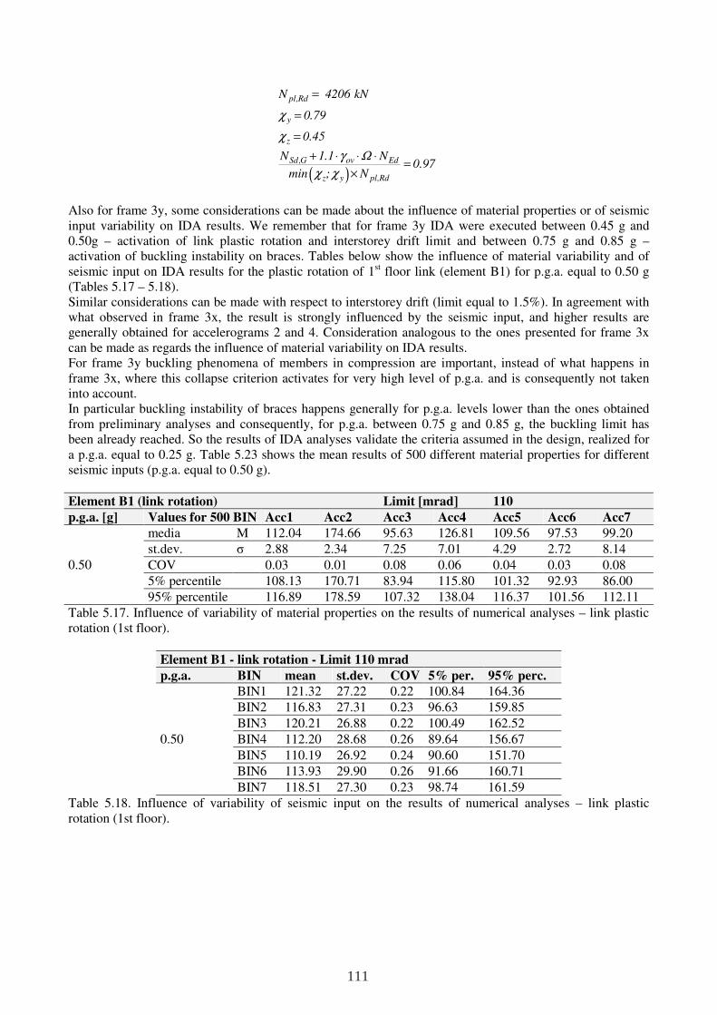
Also for frame 3y, some considerations can be made about the influence of material properties or of seismic input variability on IDA results. We remember that for frame 3y IDA were executed between 0.45 g and 0.50g – activation of link plastic rotation and interstorey drift limit and between 0.75 g and 0.85 g – activation of buckling instability on braces. Tables below show the influence of material variability and of seismic input on IDA results for the plastic rotation of 1st floor link (element B1) for p.g.a. equal to 0.50 g (Tables 5.17 – 5.18). Similar considerations can be made with respect to interstorey drift (limit equal to 1.5%). In agreement with what observed in frame 3x, the result is strongly influenced by the seismic input, and higher results are generally obtained for accelerograms 2 and 4. Consideration analogous to the ones presented for frame 3x can be made as regards the influence of material variability on IDA results. For frame 3y buckling phenomena of members in compression are important, instead of what happens in frame 3x, where this collapse criterion activates for very high level of p.g.a. and is consequently not taken into account. In particular buckling instability of braces happens generally for p.g.a. levels lower than the ones obtained from preliminary analyses and consequently, for p.g.a. between 0.75 g and 0.85 g, the buckling limit has been already reached. So the results of IDA analyses validate the criteria assumed in the design, realized for a p.g.a. equal to 0.25 g. Table 5.23 shows the mean results of 500 different material properties for different seismic inputs (p.g.a. equal to 0.50 g).
Element B1 (link rotation) Limit [mrad] 110
p.g.a. [g] Values for 500 BIN Acc1 Acc2 Acc3 Acc4 Acc5 Acc6 Acc7
0.50
media M 112.04 174.66 95.63 126.81 109.56 97.53 99.20
st.dev. σ 2.88 2.34 7.25 7.01 4.29 2.72 8.14
COV 0.03 0.01 0.08 0.06 0.04 0.03 0.08
5% percentile 108.13 170.71 83.94 115.80 101.32 92.93 86.00
95% percentile 116.89 178.59 107.32 138.04 116.37 101.56 112.11
Table 5.17. Influence of variability of material properties on the results of numerical analyses – link plastic rotation (1st floor).
Element B1 - link rotation - Limit 110 mrad
p.g.a. BIN mean st.dev. COV 5% per. 95% perc.
0.50
BIN1 121.32 27.22 0.22 100.84 164.36
BIN2 116.83 27.31 0.23 96.63 159.85
BIN3 120.21 26.88 0.22 100.49 162.52
BIN4 112.20 28.68 0.26 89.64 156.67
BIN5 110.19 26.92 0.24 90.60 151.70
BIN6 113.93 29.90 0.26 91.66 160.71
BIN7 118.51 27.30 0.23 98.74 161.59 Table 5.18. Influence of variability of seismic input on the results of numerical analyses – link plastic rotation (1st floor).
( )
pl,Rd
y
z
Sd,G ov Ed
z y pl,Rd
N 4206 kN
0.79
0.45
N 1.1 N0.97
min ; N
χ
χ
γ Ω
χ χ
=
=
=
+ ⋅ ⋅ ⋅=
×
111
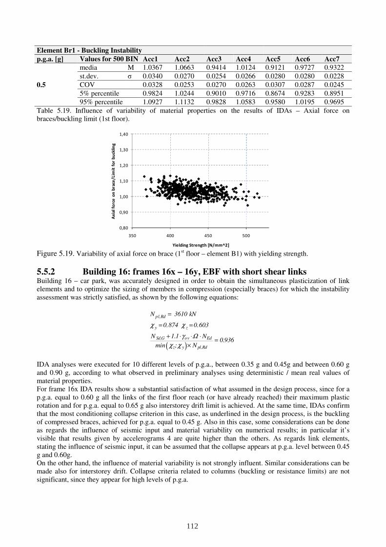
Element Br1 - Buckling Instability
p.g.a. [g] Values for 500 BIN Acc1 Acc2 Acc3 Acc4 Acc5 Acc6 Acc7
0.5
media M 1.0367 1.0663 0.9414 1.0124 0.9121 0.9727 0.9322
st.dev. σ 0.0340 0.0270 0.0254 0.0266 0.0280 0.0280 0.0228
COV 0.0328 0.0253 0.0270 0.0263 0.0307 0.0287 0.0245
5% percentile 0.9824 1.0244 0.9010 0.9716 0.8674 0.9283 0.8951
95% percentile 1.0927 1.1132 0.9828 1.0583 0.9580 1.0195 0.9695
Table 5.19. Influence of variability of material properties on the results of IDAs – Axial force on braces/buckling limit (1st floor).
Figure 5.19. Variability of axial force on brace (1st floor – element B1) with yielding strength.
5.5.2 Building 16: frames 16x – 16y, EBF with short shear links Building 16 – car park, was accurately designed in order to obtain the simultaneous plasticization of link elements and to optimize the sizing of members in compression (especially braces) for which the instability assessment was strictly satisfied, as shown by the following equations:
IDA analyses were executed for 10 different levels of p.g.a., between 0.35 g and 0.45g and between 0.60 g and 0.90 g, according to what observed in preliminary analyses using deterministic / mean real values of material properties. For frame 16x IDA results show a substantial satisfaction of what assumed in the design process, since for a p.g.a. equal to 0.60 g all the links of the first floor reach (or have already reached) their maximum plastic rotation and for p.g.a. equal to 0.65 g also interstorey drift limit is achieved. At the same time, IDAs confirm that the most conditioning collapse criterion in this case, as underlined in the design process, is the buckling of compressed braces, achieved for p.g.a. equal to 0.45 g. Also in this case, some considerations can be done as regards the influence of seismic input and material variability on numerical results; in particular it’s visible that results given by accelerograms 4 are quite higher than the others. As regards link elements, stating the influence of seismic input, it can be assumed that the collapse appears at p.g.a. level between 0.45 g and 0.60g. On the other hand, the influence of material variability is not strongly influent. Similar considerations can be made also for interstorey drift. Collapse criteria related to columns (buckling or resistance limits) are not significant, since they appear for high levels of p.g.a.
( )
pl,Rd
y z
Sd,G ov Ed
z y pl,Rd
N 3610 kN
0.874 0.603
N 1.1 N0.936
min ; N
χ χ
γ Ω
χ χ
=
= =
+ ⋅ ⋅ ⋅=
×
0,80
0,90
1,00
1,10
1,20
1,30
1,40
350 400 450 500
Ax
ial
forc
e o
n b
race
/L
imit
fo
r b
uck
lin
g
Yielding Strength [N/mm^2]
112
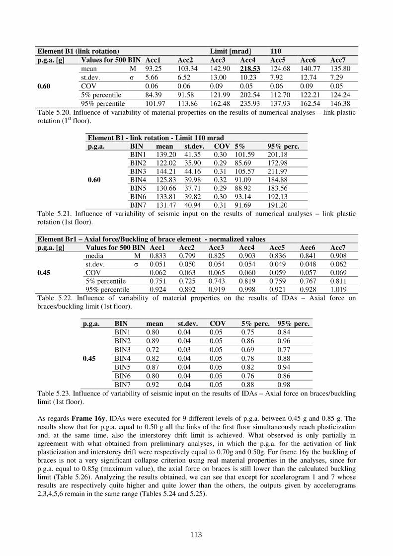
Element B1 (link rotation) Limit [mrad] 110
p.g.a. [g] Values for 500 BIN Acc1 Acc2 Acc3 Acc4 Acc5 Acc6 Acc7
0.60
mean M 93.25 103.34 142.90 218.53 124.68 140.77 135.80
st.dev. σ 5.66 6.52 13.00 10.23 7.92 12.74 7.29
COV 0.06 0.06 0.09 0.05 0.06 0.09 0.05
5% percentile 84.39 91.58 121.99 202.54 112.70 122.21 124.24
95% percentile 101.97 113.86 162.48 235.93 137.93 162.54 146.38
Table 5.20. Influence of variability of material properties on the results of numerical analyses – link plastic rotation (1st floor).
Element B1 - link rotation - Limit 110 mrad
p.g.a. BIN mean st.dev. COV 5% 95% perc.
0.60
BIN1 139.20 41.35 0.30 101.59 201.18 BIN2 122.02 35.90 0.29 85.69 172.98 BIN3 144.21 44.16 0.31 105.57 211.97 BIN4 125.83 39.98 0.32 91.09 184.88 BIN5 130.66 37.71 0.29 88.92 183.56 BIN6 133.81 39.82 0.30 93.14 192.13 BIN7 131.47 40.94 0.31 91.69 191.20
Table 5.21. Influence of variability of seismic input on the results of numerical analyses – link plastic rotation (1st floor).
Element Br1 – Axial force/Buckling of brace element - normalized values
p.g.a. [g] Values for 500 BIN Acc1 Acc2 Acc3 Acc4 Acc5 Acc6 Acc7
0.45
media M 0.833 0.799 0.825 0.903 0.836 0.841 0.908 st.dev. σ 0.051 0.050 0.054 0.054 0.049 0.048 0.062 COV 0.062 0.063 0.065 0.060 0.059 0.057 0.069 5% percentile 0.751 0.725 0.743 0.819 0.759 0.767 0.811 95% percentile 0.924 0.892 0.919 0.998 0.921 0.928 1.019
Table 5.22. Influence of variability of material properties on the results of IDAs – Axial force on braces/buckling limit (1st floor).
p.g.a. BIN mean st.dev. COV 5% perc. 95% perc.
0.45
BIN1 0.80 0.04 0.05 0.75 0.84
BIN2 0.89 0.04 0.05 0.86 0.96
BIN3 0.72 0.03 0.05 0.69 0.77
BIN4 0.82 0.04 0.05 0.78 0.88
BIN5 0.87 0.04 0.05 0.82 0.94
BIN6 0.80 0.04 0.05 0.76 0.86
BIN7 0.92 0.04 0.05 0.88 0.98
Table 5.23. Influence of variability of seismic input on the results of IDAs – Axial force on braces/buckling limit (1st floor). As regards Frame 16y, IDAs were executed for 9 different levels of p.g.a. between 0.45 g and 0.85 g. The results show that for p.g.a. equal to 0.50 g all the links of the first floor simultaneously reach plasticization and, at the same time, also the interstorey drift limit is achieved. What observed is only partially in agreement with what obtained from preliminary analyses, in which the p.g.a. for the activation of link plasticization and interstorey drift were respectively equal to 0.70g and 0.50g. For frame 16y the buckling of braces is not a very significant collapse criterion using real material properties in the analyses, since for p.g.a. equal to 0.85g (maximum value), the axial force on braces is still lower than the calculated buckling limit (Table 5.26). Analyzing the results obtained, we can see that except for accelerogram 1 and 7 whose results are respectively quite higher and quite lower than the others, the outputs given by accelerograms 2,3,4,5,6 remain in the same range (Tables 5.24 and 5.25).
113
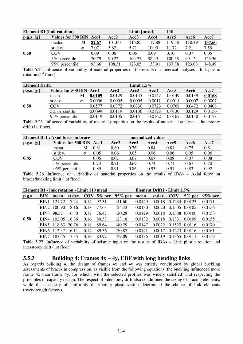
Element B1 (link rotation) Limit [mrad] 110
p.g.a. [g] Values for 500 BIN Acc1 Acc2 Acc3 Acc4 Acc5 Acc6 Acc7
0.50
media M 82.67 101.00 115.85 117.88 119.58 110.49 137.60
st.dev. σ 7.07 5.62 5.71 10.90 11.72 7.21 7.55
COV 0.09 0.06 0.05 0.09 0.10 0.07 0.05
5% percentile 70.79 90.22 104.77 98.49 100.58 99.12 123.36
95% percentile 93.66 108.31 123.05 133.91 137.88 123.08 148.49
Table 5.24. Influence of variability of material properties on the results of numerical analyses – link plastic rotation (1st floor).
Element Drift1 Limit 1.5%
p.g.a. [g] Values for 500 BIN Acc1 Acc2 Acc3 Acc4 Acc5 Acc6 Acc7
0.50
mean M 0.0109 0.0129 0.0145 0.0147 0.0149 0.0139 0.0168 st.dev. σ 0.0006 0.0005 0.0005 0.0011 0.0011 0.0007 0.0007 COV 0.0577 0.0372 0.0330 0.0723 0.0768 0.0472 0.0408 5% percentile 0.0099 0.0119 0.0136 0.0128 0.0130 0.0129 0.0156 95% percentile 0.0119 0.0135 0.0151 0.0162 0.0167 0.0150 0.0178
Table 5.25. Influence of variability of material properties on the results of numerical analyses – Interstorey drift (1st floor).
Element Br1 : Axial force on brace normalized values
p.g.a. [g] Values for 500 BIN Acc1 Acc2 Acc3 Acc4 Acc5 Acc6 Acc7
0.85
mean M 0.81 0.80 0.76 0.84 0.81 0.75 0.81 st.dev. σ 0.05 0.06 0.05 0.06 0.06 0.05 0.06 COV 0.06 0.07 0.07 0.07 0.08 0.07 0.08 5% percentile 0.73 0.71 0.69 0.74 0.71 0.67 0.70 95% percentile 0.89 0.91 0.86 0.93 0.91 0.83 0.92
Table 5.26. Influence of variability of material properties on the results of IDAs – Axial force on braces/buckling limit (1st floor).
Element B1 - link rotation - Limit 110 mrad Element Drift1 - Limit 1.5%
p.g.a. BIN mean st.dev. COV 5% per. 95% per. mean st.dev. COV 5% per. 95% per.
0.50
BIN1 121.72 17.24 0.14 97.31 141.60 0.0149 0.0018 0.1234 0.0123 0.0171
BIN2 100.90 18.16 0.18 77.63 124.43 0.0130 0.0020 0.1505 0.0105 0.0156
BIN3 98.57 16.80 0.17 76.47 120.28 0.0129 0.0018 0.1388 0.0106 0.0153
BIN4 102.05 16.36 0.16 80.57 123.18 0.0132 0.0018 0.1331 0.0109 0.0155
BIN5 118.63 20.76 0.18 89.64 140.29 0.0147 0.0022 0.1520 0.0116 0.0170
BIN6 112.37 16.11 0.14 89.36 130.87 0.0141 0.0017 0.1223 0.0116 0.0161
BIN7 107.55 17.35 0.16 83.97 129.09 0.0136 0.0019 0.1365 0.0111 0.0159 Table 5.27. Influence of variability of seismic input on the results of IDAs – Link plastic rotation and interstorey drift (1st floor).
5.5.3 Building 4: Frames 4x – 4y, EBF with long bending links As regards building 4, the design of frames 4x and 4y was strictly conditioned by global buckling assessments of braces in compression, as visible from the following equations (the buckling influenced more frame 4x than frame 4y, for which, with the selected profiles was widely satisfied) and respecting the principles of capacity design. The respect of interstorey drift also conditioned the sizing of bracing elements, while the necessity of uniformly distributing plasticization determined the choice of link elements (overstrength factors).
114
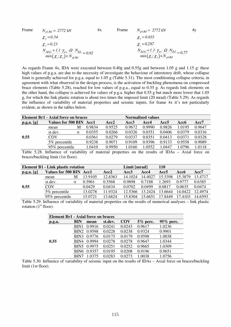
Frame 4x Frame 4y
As regards Frame 4x, IDA were executed between 0.40g and 0.55g and between 1.05 g and 1.15 g: these high values of p.g.a. are due to the necessity of investigate the behaviour of interstorey drift, whose collapse limit is generally achieved for p.g.a. equal to 1.05 g (Table 5.31). The most conditioning collapse criteria, in agreement with what observed in the design process, is the activation of buckling phenomena on compressed brace elements (Table 5.28), reached for low values of p.g.a., equal to 0.55 g. As regards link elements on the other hand, the collapse is achieved for values of p.g.a. higher that 0.55 g but much more lower that 1.05 g, for which the link plastic rotation is about two times the imposed limit (20 mrad) (Table 5.29). As regards the influence of variability of material properties and seismic inputs, for frame 4x it’s not particularly evident, as shown in the tables below.
Element Br1 - Axial force on braces Normalized values
p.g.a. [g] Values for 500 BIN Acc1 Acc2 Acc3 Acc4 Acc5 Acc6 Acc7
0.55
mean M 0.9834 0.9525 0.9672 0.9990 0.9826 1.0195 0.9647 st.dev. σ 0.0355 0.0266 0.0326 0.0351 0.0406 0.0379 0.0316 COV 0.0361 0.0279 0.0337 0.0351 0.0413 0.0371 0.0328 5% percentile 0.9238 0.9071 0.9109 0.9396 0.9133 0.9558 0.9089 95% percentile 1.0410 0.9950 1.0160 1.0552 1.0447 1.0796 1.0118
Table 5.28. Influence of variability of material properties on the results of IDAs – Axial force on braces/buckling limit (1st floor).
Element B1 - Link plastic rotation Limit [mrad] 110
p.g.a. [g] Values for 500 BIN Acc1 Acc2 Acc3 Acc4 Acc5 Acc6 Acc7
0.55
mean M 13.9105 12.8363 14.1024 14.4027 15.5398 15.3879 13.4717 st.dev. σ 0.5961 0.5568 0.9898 0.7188 1.2693 0.9777 0.6385 COV 0.0429 0.0434 0.0702 0.0499 0.0817 0.0635 0.0474 5% percentile 13.0278 11.9324 12.5366 13.2424 13.6644 14.0422 12.4974 95% percentile 15.0721 13.6824 15.8304 15.6651 17.8449 17.4103 14.6593
Table 5.29. Influence of variability of material properties on the results of numerical analyses – link plastic rotation (1st floor).
Element Br1 - Axial force on braces
p.g.a. BIN mean st.dev. COV 5% perc. 95% perc.
0.55
BIN1 0.9916 0.0241 0.0243 0.9617 1.0236 BIN2 0.9598 0.0228 0.0238 0.9324 0.9901 BIN3 0.9776 0.0175 0.0179 0.9598 1.0038 BIN4 0.9994 0.0278 0.0278 0.9647 1.0344 BIN5 0.9975 0.0251 0.0252 0.9665 1.0309 BIN6 0.9357 0.0195 0.0208 0.9196 0.9651 BIN7 1.0375 0.0283 0.0273 1.0038 1.0756
Table 5.30. Influence of variability of seismic input on the results of IDAs – Axial force on braces/buckling limit (1st floor).
( )
pl,Rd
y
z
Sd,G ov Ed
z y pl,Rd
N 2772 kN
0.633
0.287
N 1.1 N0.77
min ; N
χ
χ
γ Ω
χ χ
=
=
=
+ ⋅ ⋅ ⋅=
×
( )
pl,Rd
y
z
Sd,G ov Ed
z y pl,Rd
N 2772 kN
0.54
0.23
N 1.1 N0.92
min ; N
χ
χ
γ Ω
χ χ
=
=
=
+ ⋅ ⋅ ⋅=
×
115
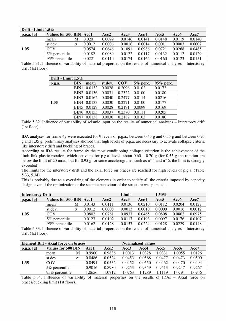
Drift - Limit 1.5%
p.g.a. [g] Values for 500 BIN Acc1 Acc2 Acc3 Acc4 Acc5 Acc6 Acc7
1.05
mean M 0.0201 0.0099 0.0146 0.0141 0.0148 0.0119 0.0140 st.dev. σ 0.0012 0.0006 0.0016 0.0014 0.0011 0.0003 0.0007 COV 0.0574 0.0646 0.1091 0.0986 0.0721 0.0268 0.0485 5% percentile 0.0182 0.0089 0.0122 0.0117 0.0132 0.0112 0.0129 95% percentile 0.0221 0.0110 0.0174 0.0162 0.0160 0.0123 0.0151
Table 5.31. Influence of variability of material properties on the results of numerical analyses – Interstorey drift (1st floor).
Drift - Limit 1.5%
p.g.a. BIN mean st.dev. COV 5% perc. 95% perc.
1.05
BIN1 0.0132 0.0028 0.2096 0.0102 0.0172 BIN2 0.0136 0.0031 0.2322 0.0100 0.0180 BIN3 0.0162 0.0040 0.2477 0.0114 0.0216 BIN4 0.0133 0.0030 0.2271 0.0100 0.0177 BIN5 0.0129 0.0028 0.2191 0.0099 0.0169 BIN6 0.0155 0.0037 0.2370 0.0111 0.0205 BIN7 0.0138 0.0030 0.2187 0.0103 0.0180
Table 5.32. Influence of variability of seismic input on the results of numerical analyses – Interstorey drift (1st floor). IDA analyses for frame 4y were executed for 9 levels of p.g.a., between 0.45 g and 0.55 g and between 0.95 g and 1.35 g: preliminary analyses showed that high levels of p.g.a. are necessary to activate collapse criteria like interstorey drift and buckling of braces. According to IDA results for frame 4y the most conditioning collapse criterion is the achievement of the limit link plastic rotation, which activates for p.g.a. levels about 0.60 – 0.70 g (for 0.55 g the rotation are below the limit of 20 mrad, but for 0.95 g for some accelerograms, such as n° 4 and n° 6, the limit is strongly exceeded). The limits for the interstorey drift and the axial force on braces are reached for high levels of p.g.a. (Table 5.33, 5.34). This is probably due to a oversizing of the elements in order to satisfy all the criteria imposed by capacity design, even if the optimization of the seismic behaviour of the structure was pursued.
Interstorey Drift Limit 1.50%
p.g.a. [g] Values for 500 BIN Acc1 Acc2 Acc3 Acc4 Acc5 Acc6 Acc7
1.05
mean M 0.0143 0.0111 0.0136 0.0210 0.0112 0.0204 0.0127 st.dev. σ 0.0012 0.0008 0.0013 0.0010 0.0009 0.0016 0.0012 COV 0.0802 0.0761 0.0937 0.0465 0.0808 0.0802 0.0975 5% percentile 0.0123 0.0102 0.0117 0.0193 0.0097 0.0176 0.0107 95% percentile 0.0162 0.0128 0.0157 0.0224 0.0128 0.0229 0.0148
Table 5.33. Influence of variability of material properties on the results of numerical analyses – Interstorey drift (1st floor).
Element Br1 - Axial force on braces Normalized values
p.g.a. [g] Values for 500 BIN Acc1 Acc2 Acc3 Acc4 Acc5 Acc6 Acc7
1.35
mean M 0.9900 0.9836 1.0013 1.0328 1.0331 1.0055 1.0126 st.dev. σ 0.0486 0.0524 0.0453 0.0568 0.0477 0.0473 0.0500 COV 0.0491 0.0532 0.0452 0.0550 0.0462 0.0470 0.0494 5% percentile 0.9016 0.8980 0.9253 0.9359 0.9513 0.9247 0.9267 95% percentile 1.0656 1.0712 1.0763 1.1289 1.1119 1.0794 1.0956
Table 5.34. Influence of variability of material properties on the results of IDAs – Axial force on braces/buckling limit (1st floor).
116
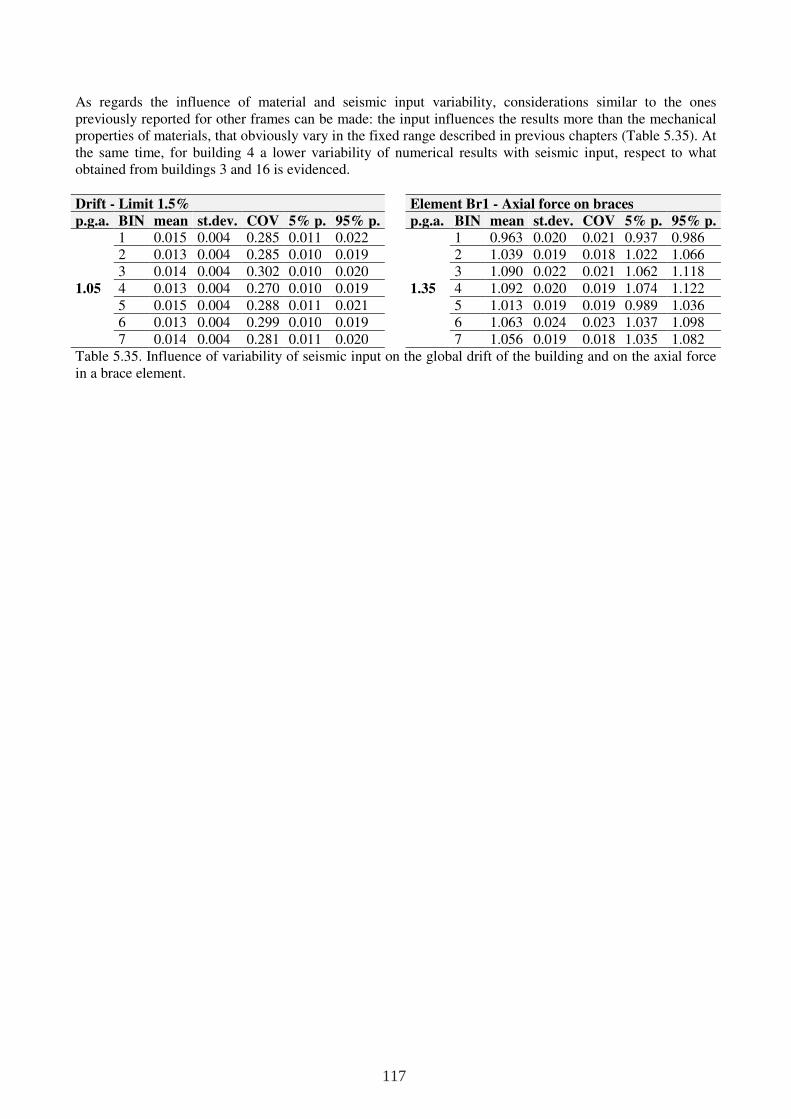
As regards the influence of material and seismic input variability, considerations similar to the ones previously reported for other frames can be made: the input influences the results more than the mechanical properties of materials, that obviously vary in the fixed range described in previous chapters (Table 5.35). At the same time, for building 4 a lower variability of numerical results with seismic input, respect to what obtained from buildings 3 and 16 is evidenced.
Drift - Limit 1.5% Element Br1 - Axial force on braces
p.g.a. BIN mean st.dev. COV 5% p. 95% p. p.g.a. BIN mean st.dev. COV 5% p. 95% p.
1.05
1 0.015 0.004 0.285 0.011 0.022
1.35
1 0.963 0.020 0.021 0.937 0.986 2 0.013 0.004 0.285 0.010 0.019 2 1.039 0.019 0.018 1.022 1.066 3 0.014 0.004 0.302 0.010 0.020 3 1.090 0.022 0.021 1.062 1.118 4 0.013 0.004 0.270 0.010 0.019 4 1.092 0.020 0.019 1.074 1.122 5 0.015 0.004 0.288 0.011 0.021 5 1.013 0.019 0.019 0.989 1.036 6 0.013 0.004 0.299 0.010 0.019 6 1.063 0.024 0.023 1.037 1.098 7 0.014 0.004 0.281 0.011 0.020 7 1.056 0.019 0.018 1.035 1.082
Table 5.35. Influence of variability of seismic input on the global drift of the building and on the axial force in a brace element.
117

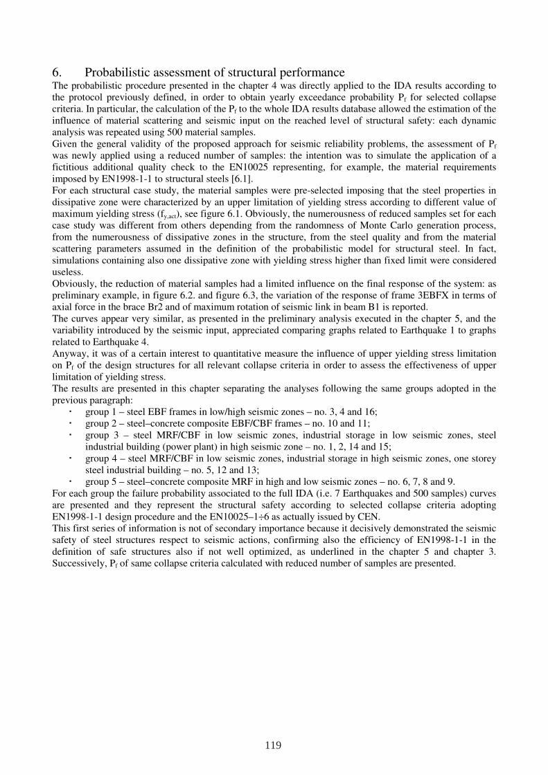
6. Probabilistic assessment of structural performance The probabilistic procedure presented in the chapter 4 was directly applied to the IDA results according to the protocol previously defined, in order to obtain yearly exceedance probability Pf for selected collapse criteria. In particular, the calculation of the Pf to the whole IDA results database allowed the estimation of the influence of material scattering and seismic input on the reached level of structural safety: each dynamic analysis was repeated using 500 material samples. Given the general validity of the proposed approach for seismic reliability problems, the assessment of Pf was newly applied using a reduced number of samples: the intention was to simulate the application of a fictitious additional quality check to the EN10025 representing, for example, the material requirements imposed by EN1998-1-1 to structural steels [6.1]. For each structural case study, the material samples were pre-selected imposing that the steel properties in dissipative zone were characterized by an upper limitation of yielding stress according to different value of maximum yielding stress (fy,act), see figure 6.1. Obviously, the numerousness of reduced samples set for each case study was different from others depending from the randomness of Monte Carlo generation process, from the numerousness of dissipative zones in the structure, from the steel quality and from the material scattering parameters assumed in the definition of the probabilistic model for structural steel. In fact, simulations containing also one dissipative zone with yielding stress higher than fixed limit were considered useless. Obviously, the reduction of material samples had a limited influence on the final response of the system: as preliminary example, in figure 6.2. and figure 6.3, the variation of the response of frame 3EBFX in terms of axial force in the brace Br2 and of maximum rotation of seismic link in beam B1 is reported. The curves appear very similar, as presented in the preliminary analysis executed in the chapter 5, and the variability introduced by the seismic input, appreciated comparing graphs related to Earthquake 1 to graphs related to Earthquake 4. Anyway, it was of a certain interest to quantitative measure the influence of upper yielding stress limitation on Pf of the design structures for all relevant collapse criteria in order to assess the effectiveness of upper limitation of yielding stress. The results are presented in this chapter separating the analyses following the same groups adopted in the previous paragraph:
group 1 – steel EBF frames in low/high seismic zones – no. 3, 4 and 16; group 2 – steel–concrete composite EBF/CBF frames – no. 10 and 11; group 3 – steel MRF/CBF in low seismic zones, industrial storage in low seismic zones, steel
industrial building (power plant) in high seismic zone – no. 1, 2, 14 and 15; group 4 – steel MRF/CBF in low seismic zones, industrial storage in high seismic zones, one storey
steel industrial building – no. 5, 12 and 13; group 5 – steel–concrete composite MRF in high and low seismic zones – no. 6, 7, 8 and 9.
For each group the failure probability associated to the full IDA (i.e. 7 Earthquakes and 500 samples) curves are presented and they represent the structural safety according to selected collapse criteria adopting EN1998-1-1 design procedure and the EN10025–1÷6 as actually issued by CEN. This first series of information is not of secondary importance because it decisively demonstrated the seismic safety of steel structures respect to seismic actions, confirming also the efficiency of EN1998-1-1 in the definition of safe structures also if not well optimized, as underlined in the chapter 5 and chapter 3. Successively, Pf of same collapse criteria calculated with reduced number of samples are presented.
119
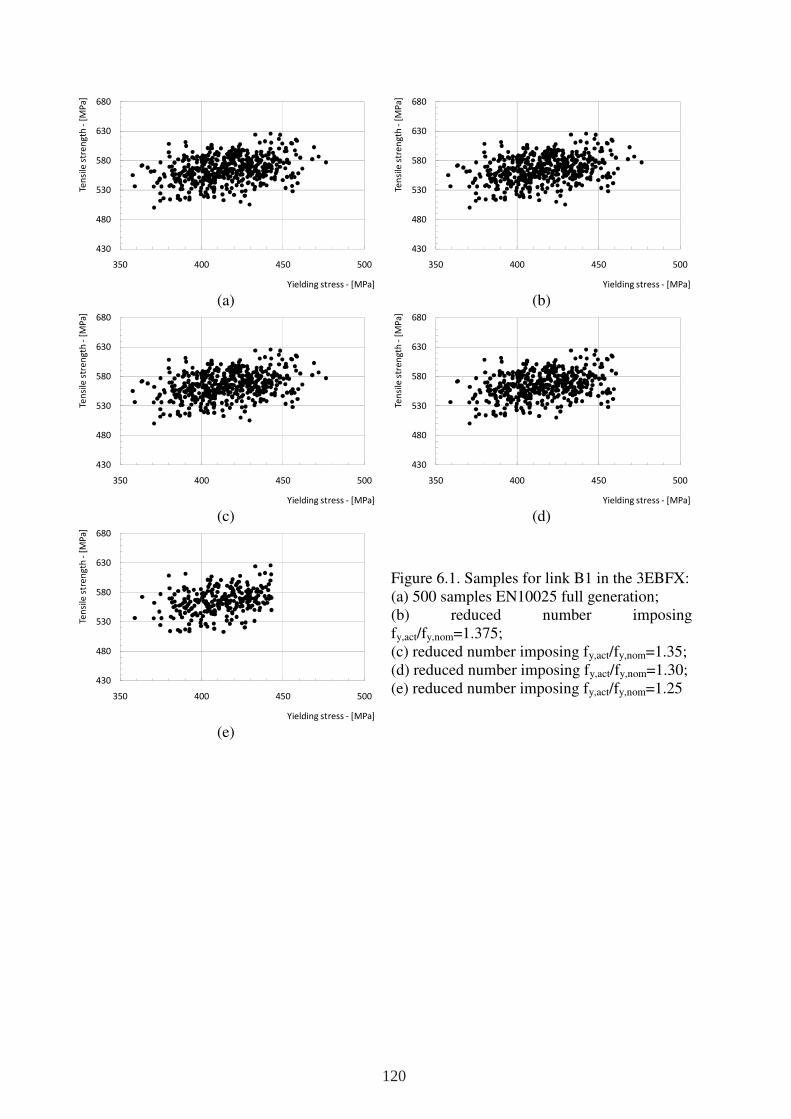
(a)
(b)
(c)
(d)
(e)
Figure 6.1. Samples for link B1 in the 3EBFX: (a) 500 samples EN10025 full generation; (b) reduced number imposing fy,act/fy,nom=1.375; (c) reduced number imposing fy,act/fy,nom=1.35; (d) reduced number imposing fy,act/fy,nom=1.30; (e) reduced number imposing fy,act/fy,nom=1.25
430
480
530
580
630
680
350 400 450 500
Ten
sile
str
en
gth
-[M
Pa
]
Yielding stress - [MPa]
430
480
530
580
630
680
350 400 450 500
Ten
sile
str
en
gth
-[M
Pa
]
Yielding stress - [MPa]
430
480
530
580
630
680
350 400 450 500
Ten
sile
str
en
gth
-[M
Pa
]
Yielding stress - [MPa]
430
480
530
580
630
680
350 400 450 500
Ten
sile
str
en
gth
-[M
Pa
]
Yielding stress - [MPa]
430
480
530
580
630
680
350 400 450 500
Ten
sile
str
en
gth
-[M
Pa
]
Yielding stress - [MPa]
120
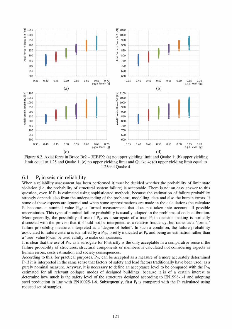
(a)
(b)
(c)
(d)
Figure 6.2. Axial force in Brace Br2 – 3EBFX: (a) no upper yielding limit and Quake 1; (b) upper yielding limit equal to 1.25 and Quake 1; (c) no upper yielding limit and Quake 4; (d) upper yielding limit equal to
1.25and Quake 4.
6.1 Pf in seismic reliability When a reliability assessment has been performed it must be decided whether the probability of limit state violation (i.e. the probability of structural system failure) is acceptable. There is not an easy answer to this question, even if Pf is estimated using sophisticated methods, because the estimation of failure probability strongly depends also from the understanding of the problems, modelling, data and also the human errors. If some of these aspects are ignored and when some approximations are made in the calculations the calculate Pf becomes a nominal value Pf,N: a formal measurement that does not taken into account all possible uncertainties. This type of nominal failure probability is usually adopted in the problems of code calibration. More generally, the possibility of use of Pf,N as a surrogate of a total Pf in decision making is normally discussed with the proviso that it should not be interpreted as a relative frequency, but rather as a ‘formal’ failure probability measure, interpreted as a ‘degree of belief’. In such a condition, the failure probability associated to failure criteria is identified by a Pf,N, briefly indicated as Pf, and being an estimation rather than a ‘true’ value Pf can be used validly to make comparisons. It is clear that the use of Pf,N as a surrogate for Pf strictly is the only acceptable in a comparative sense if the failure probability of structures, structural components or members is calculated not considering aspects as human errors, costs estimation and society consequences. According to this, for practical purposes, Pf,N can be accepted as a measure of a more accurately determined Pf if it is interpreted in the same sense that factors of safety and load factors traditionally have been used, as a purely nominal measure. Anyway, it is necessary to define an acceptance level to be compared with the Pf,N estimated for all relevant collapse modes of designed buildings, because it is of a certain interest to determine how much is the safety level of the structures designed according to EN1998-1-1 and adopting steel production in line with EN10025-1-6. Subsequently, first Pf is compared with the Pf calculated using reduced set of samples.
600
650
700
750
800
850
900
950
1000
1050
0.35 0.40 0.45 0.50 0.55 0.60 0.65 0.70
Axi
al F
orc
e in
Bra
ce B
r2 [
kN
]
p.g.a. level - [g]
600
650
700
750
800
850
900
950
1000
1050
0.35 0.40 0.45 0.50 0.55 0.60 0.65 0.70
Axi
al F
orc
e in
Bra
ce B
r2 [
kN
]
p.g.a. level - [g]
600
650
700
750
800
850
900
950
1000
1050
1100
0.35 0.40 0.45 0.50 0.55 0.60 0.65 0.70
Axi
al F
orc
e in
Bra
ce B
r2 [
kN
]
p.g.a. level - [g]
600
650
700
750
800
850
900
950
1000
1050
1100
0.35 0.40 0.45 0.50 0.55 0.60 0.65 0.70
Axi
al F
orc
e in
Bra
ce B
r2 [
kN
]
p.g.a. level - [g]
121
(a)
(b)
(c)
(d)
Figure 6.3. Maximum rotation in shear link B1, 3EBFX frame: (a) no upper yielding limit and Quake 1; (b) upper yielding limit equal to 1.25 and Quake 1; (c) no upper yielding limit and Quake 4; (d) upper yielding
limit equal to 1.25and Quake 4.
6.1.1 Definition of an acceptance threshold for Pf,N The model codes handle seismic risk by specifying earthquake design loading conditions and then requiring strength levels adequate to resist those loads. The earthquake condition under which the design requirements apply is the design–level earthquake (DBE identified as NCR from EN1998-1-1): a hypothetical, large event causing ground shaking estimated to have a 10% probability of exceedance in 50 years (0.21% annual probability, 475 – year return period); it is also implicit that no design standard can provide for 100% confidence of life safety under DBE. Several investigators [6.2], [6.3], [6.4], examined the safety margin (the difference) between strength (capacity) and load (demand). The ratio of the mean value of the margin to its standard deviation they called the reliability index, β (the inverse of the coefficient of variation of the margin). In particular, they calculated (Pf) the proability that any particular element of various structures will be overstressed during its lifetime, expressing Pf with a PDF function of β in order to measure the safety. Many authors found that the β reflected in existing buildings for ordinary (non-seismic) loading conditions varies between 3.0 and 4.0, depending on the suddenness and consequences of element failure. If the safety
margin (β) was normally distributed, these values, 3.0 and 4.0, would correspond to Pf between 1.3×10⁻³ and 3.2×10⁻⁵ per structural element during the design life of 50 years. They recommended also for seismic loading a β of 1.75, equivalent (again assuming normal distribution) to a Pf on the order of 4.0×10⁻² that the element will be overstressed in the design-level earthquake [6.4]. Again, this reliability index β refers to failure of one building component, where failure is typically defined in the context of seismic loading as fracture, rather than yielding. Overstress of a single component is considered life-threatening damage, but is not equivalent to the probability of casualties. More recently, other studies and researches have been carried out in order to defined adequate threshold as acceptance level for seismic reliability problems [6.5] fixing, for ordinary buildings, a Pf threshold equal to 10-3 for building elements and 10-4 for emergence response facilities (for strategic buildings or for critical equipments contained in ordinary buildings – i.e. sprinkler).
0.000
0.050
0.100
0.150
0.200
0.250
0.35 0.40 0.45 0.50 0.55 0.60 0.65 0.70
Lin
k R
ota
tio
n -
Lin
kB
1 -
[ra
d]
p.g.a. level - [g]
0.000
0.050
0.100
0.150
0.200
0.250
0.35 0.40 0.45 0.50 0.55 0.60 0.65 0.70
Lin
k R
ota
tio
n -
Lin
kB
1 -
[ra
d]
p.g.a. level - [g]
0.000
0.050
0.100
0.150
0.200
0.250
0.300
0.350
0.400
0.35 0.40 0.45 0.50 0.55 0.60 0.65 0.70
Lin
k R
ota
tio
n -
Lin
kB
1 -
[ra
d]
p.g.a. level - [g]
0.000
0.050
0.100
0.150
0.200
0.250
0.300
0.350
0.400
0.35 0.40 0.45 0.50 0.55 0.60 0.65 0.70
Lin
k R
ota
tio
n -
Lin
kB
1 -
[ra
d]
p.g.a. level - [g]
122
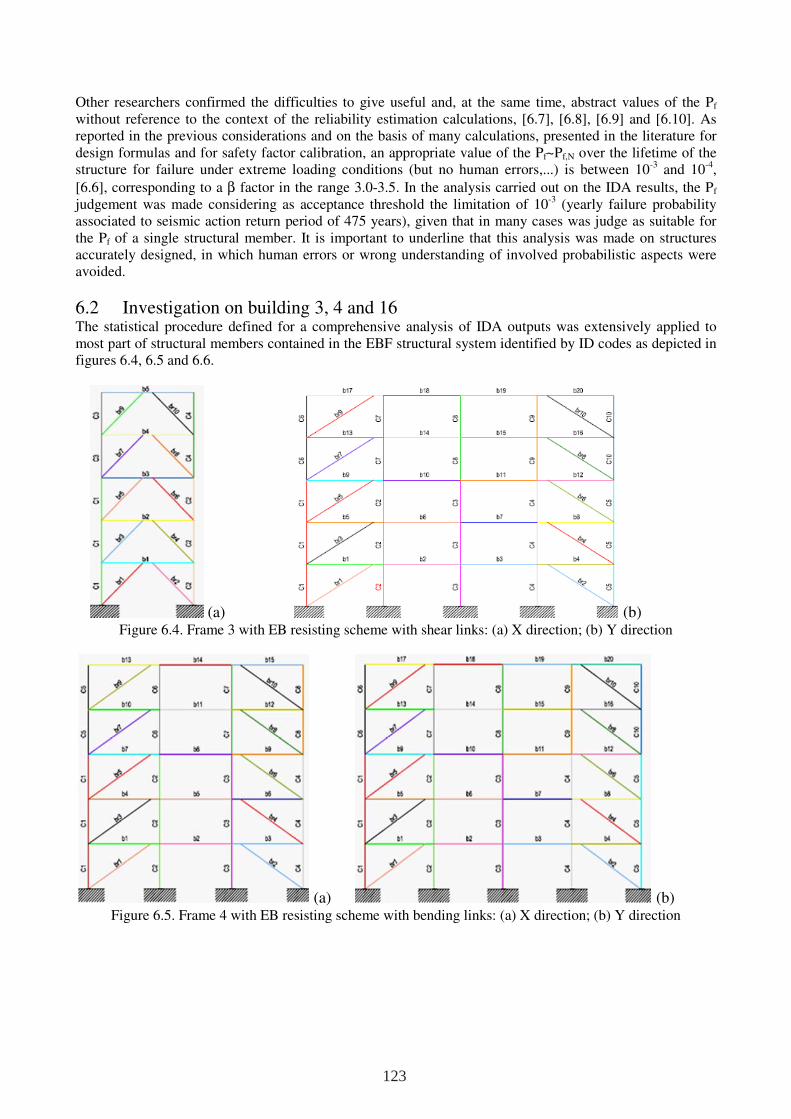
Other researchers confirmed the difficulties to give useful and, at the same time, abstract values of the Pf without reference to the context of the reliability estimation calculations, [6.7], [6.8], [6.9] and [6.10]. As reported in the previous considerations and on the basis of many calculations, presented in the literature for design formulas and for safety factor calibration, an appropriate value of the Pf~Pf,N over the lifetime of the structure for failure under extreme loading conditions (but no human errors,...) is between 10-3 and 10-4,
[6.6], corresponding to a β factor in the range 3.0-3.5. In the analysis carried out on the IDA results, the Pf judgement was made considering as acceptance threshold the limitation of 10-3 (yearly failure probability associated to seismic action return period of 475 years), given that in many cases was judge as suitable for the Pf of a single structural member. It is important to underline that this analysis was made on structures accurately designed, in which human errors or wrong understanding of involved probabilistic aspects were avoided.
6.2 Investigation on building 3, 4 and 16 The statistical procedure defined for a comprehensive analysis of IDA outputs was extensively applied to most part of structural members contained in the EBF structural system identified by ID codes as depicted in figures 6.4, 6.5 and 6.6.
(a) (b) Figure 6.4. Frame 3 with EB resisting scheme with shear links: (a) X direction; (b) Y direction
(a) (b) Figure 6.5. Frame 4 with EB resisting scheme with bending links: (a) X direction; (b) Y direction
123
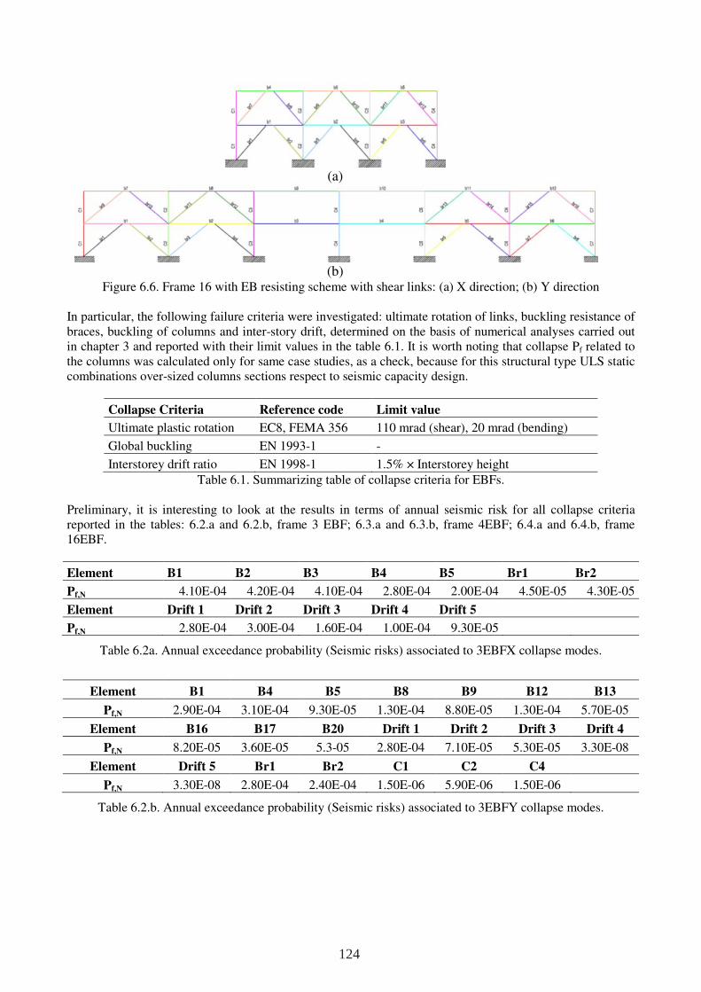
(a)
(b)
Figure 6.6. Frame 16 with EB resisting scheme with shear links: (a) X direction; (b) Y direction In particular, the following failure criteria were investigated: ultimate rotation of links, buckling resistance of braces, buckling of columns and inter-story drift, determined on the basis of numerical analyses carried out in chapter 3 and reported with their limit values in the table 6.1. It is worth noting that collapse Pf related to the columns was calculated only for same case studies, as a check, because for this structural type ULS static combinations over-sized columns sections respect to seismic capacity design.
Collapse Criteria Reference code Limit value
Ultimate plastic rotation EC8, FEMA 356 110 mrad (shear), 20 mrad (bending)
Global buckling EN 1993-1 -
Interstorey drift ratio EN 1998-1 1.5% × Interstorey height Table 6.1. Summarizing table of collapse criteria for EBFs.
Preliminary, it is interesting to look at the results in terms of annual seismic risk for all collapse criteria reported in the tables: 6.2.a and 6.2.b, frame 3 EBF; 6.3.a and 6.3.b, frame 4EBF; 6.4.a and 6.4.b, frame 16EBF.
Element B1 B2 B3 B4 B5 Br1 Br2
Pf,N 4.10E-04 4.20E-04 4.10E-04 2.80E-04 2.00E-04 4.50E-05 4.30E-05
Element Drift 1 Drift 2 Drift 3 Drift 4 Drift 5
Pf,N 2.80E-04 3.00E-04 1.60E-04 1.00E-04 9.30E-05
Table 6.2a. Annual exceedance probability (Seismic risks) associated to 3EBFX collapse modes.
Element B1 B4 B5 B8 B9 B12 B13
Pf,N 2.90E-04 3.10E-04 9.30E-05 1.30E-04 8.80E-05 1.30E-04 5.70E-05
Element B16 B17 B20 Drift 1 Drift 2 Drift 3 Drift 4
Pf,N 8.20E-05 3.60E-05 5.3-05 2.80E-04 7.10E-05 5.30E-05 3.30E-08
Element Drift 5 Br1 Br2 C1 C2 C4
Pf,N 3.30E-08 2.80E-04 2.40E-04 1.50E-06 5.90E-06 1.50E-06
Table 6.2.b. Annual exceedance probability (Seismic risks) associated to 3EBFY collapse modes.
124
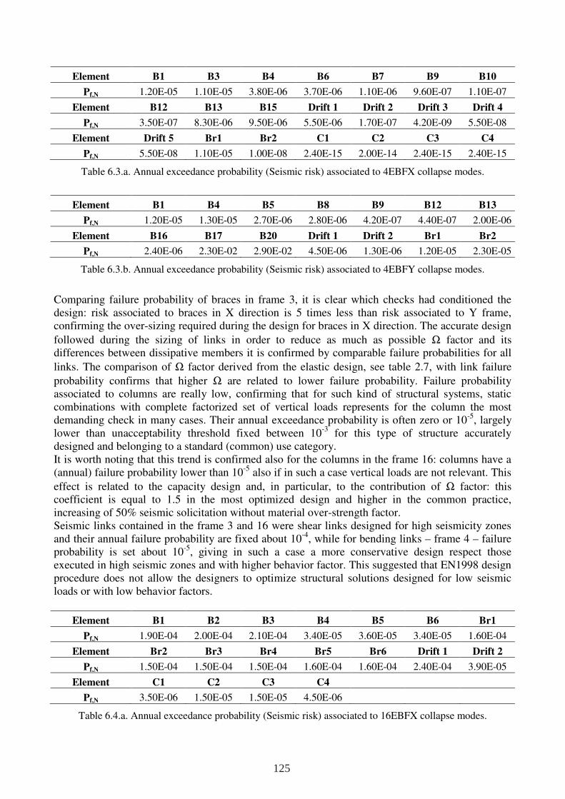
Element B1 B3 B4 B6 B7 B9 B10
Pf,N 1.20E-05 1.10E-05 3.80E-06 3.70E-06 1.10E-06 9.60E-07 1.10E-07
Element B12 B13 B15 Drift 1 Drift 2 Drift 3 Drift 4
Pf,N 3.50E-07 8.30E-06 9.50E-06 5.50E-06 1.70E-07 4.20E-09 5.50E-08
Element Drift 5 Br1 Br2 C1 C2 C3 C4
Pf,N 5.50E-08 1.10E-05 1.00E-08 2.40E-15 2.00E-14 2.40E-15 2.40E-15
Table 6.3.a. Annual exceedance probability (Seismic risk) associated to 4EBFX collapse modes.
Element B1 B4 B5 B8 B9 B12 B13
Pf,N 1.20E-05 1.30E-05 2.70E-06 2.80E-06 4.20E-07 4.40E-07 2.00E-06
Element B16 B17 B20 Drift 1 Drift 2 Br1 Br2
Pf,N 2.40E-06 2.30E-02 2.90E-02 4.50E-06 1.30E-06 1.20E-05 2.30E-05
Table 6.3.b. Annual exceedance probability (Seismic risk) associated to 4EBFY collapse modes.
Comparing failure probability of braces in frame 3, it is clear which checks had conditioned the design: risk associated to braces in X direction is 5 times less than risk associated to Y frame, confirming the over-sizing required during the design for braces in X direction. The accurate design
followed during the sizing of links in order to reduce as much as possible Ω factor and its differences between dissipative members it is confirmed by comparable failure probabilities for all
links. The comparison of Ω factor derived from the elastic design, see table 2.7, with link failure
probability confirms that higher Ω are related to lower failure probability. Failure probability associated to columns are really low, confirming that for such kind of structural systems, static combinations with complete factorized set of vertical loads represents for the column the most demanding check in many cases. Their annual exceedance probability is often zero or 10-5, largely lower than unacceptability threshold fixed between 10-3 for this type of structure accurately designed and belonging to a standard (common) use category. It is worth noting that this trend is confirmed also for the columns in the frame 16: columns have a (annual) failure probability lower than 10-5 also if in such a case vertical loads are not relevant. This
effect is related to the capacity design and, in particular, to the contribution of Ω factor: this coefficient is equal to 1.5 in the most optimized design and higher in the common practice, increasing of 50% seismic solicitation without material over-strength factor. Seismic links contained in the frame 3 and 16 were shear links designed for high seismicity zones and their annual failure probability are fixed about 10-4, while for bending links – frame 4 – failure probability is set about 10-5, giving in such a case a more conservative design respect those executed in high seismic zones and with higher behavior factor. This suggested that EN1998 design procedure does not allow the designers to optimize structural solutions designed for low seismic loads or with low behavior factors.
Element B1 B2 B3 B4 B5 B6 Br1
Pf,N 1.90E-04 2.00E-04 2.10E-04 3.40E-05 3.60E-05 3.40E-05 1.60E-04
Element Br2 Br3 Br4 Br5 Br6 Drift 1 Drift 2
Pf,N 1.50E-04 1.50E-04 1.50E-04 1.60E-04 1.60E-04 2.40E-04 3.90E-05
Element C1 C2 C3 C4
Pf,N 3.50E-06 1.50E-05 1.50E-05 4.50E-06
Table 6.4.a. Annual exceedance probability (Seismic risk) associated to 16EBFX collapse modes.
125
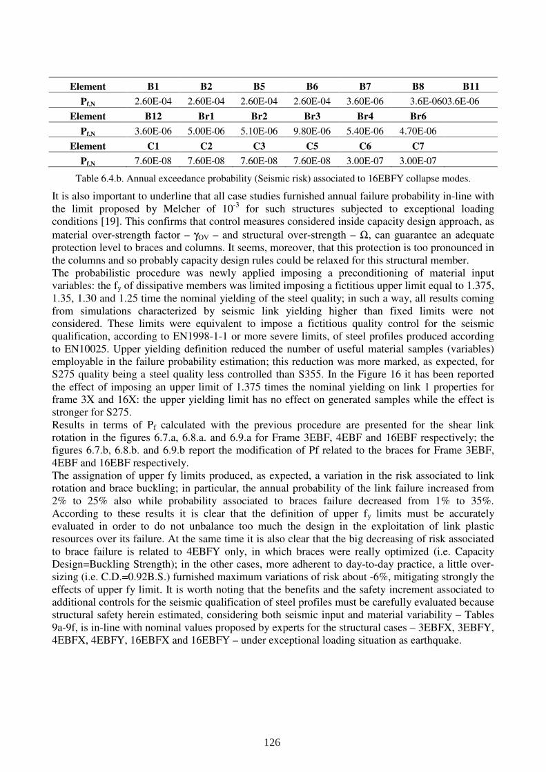
Element B1 B2 B5 B6 B7 B8 B11
Pf,N 2.60E-04 2.60E-04 2.60E-04 2.60E-04 3.60E-06 3.6E-0603.6E-06
Element B12 Br1 Br2 Br3 Br4 Br6
Pf,N 3.60E-06 5.00E-06 5.10E-06 9.80E-06 5.40E-06 4.70E-06
Element C1 C2 C3 C5 C6 C7
Pf,N 7.60E-08 7.60E-08 7.60E-08 7.60E-08 3.00E-07 3.00E-07
Table 6.4.b. Annual exceedance probability (Seismic risk) associated to 16EBFY collapse modes.
It is also important to underline that all case studies furnished annual failure probability in-line with the limit proposed by Melcher of 10-3 for such structures subjected to exceptional loading conditions [19]. This confirms that control measures considered inside capacity design approach, as
material over-strength factor – γOV – and structural over-strength – Ω, can guarantee an adequate protection level to braces and columns. It seems, moreover, that this protection is too pronounced in the columns and so probably capacity design rules could be relaxed for this structural member. The probabilistic procedure was newly applied imposing a preconditioning of material input variables: the fy of dissipative members was limited imposing a fictitious upper limit equal to 1.375, 1.35, 1.30 and 1.25 time the nominal yielding of the steel quality; in such a way, all results coming from simulations characterized by seismic link yielding higher than fixed limits were not considered. These limits were equivalent to impose a fictitious quality control for the seismic qualification, according to EN1998-1-1 or more severe limits, of steel profiles produced according to EN10025. Upper yielding definition reduced the number of useful material samples (variables) employable in the failure probability estimation; this reduction was more marked, as expected, for S275 quality being a steel quality less controlled than S355. In the Figure 16 it has been reported the effect of imposing an upper limit of 1.375 times the nominal yielding on link 1 properties for frame 3X and 16X: the upper yielding limit has no effect on generated samples while the effect is stronger for S275. Results in terms of Pf calculated with the previous procedure are presented for the shear link rotation in the figures 6.7.a, 6.8.a. and 6.9.a for Frame 3EBF, 4EBF and 16EBF respectively; the figures 6.7.b, 6.8.b. and 6.9.b report the modification of Pf related to the braces for Frame 3EBF, 4EBF and 16EBF respectively. The assignation of upper fy limits produced, as expected, a variation in the risk associated to link rotation and brace buckling; in particular, the annual probability of the link failure increased from 2% to 25% also while probability associated to braces failure decreased from 1% to 35%. According to these results it is clear that the definition of upper fy limits must be accurately evaluated in order to do not unbalance too much the design in the exploitation of link plastic resources over its failure. At the same time it is also clear that the big decreasing of risk associated to brace failure is related to 4EBFY only, in which braces were really optimized (i.e. Capacity Design=Buckling Strength); in the other cases, more adherent to day-to-day practice, a little over-sizing (i.e. C.D.=0.92B.S.) furnished maximum variations of risk about -6%, mitigating strongly the effects of upper fy limit. It is worth noting that the benefits and the safety increment associated to additional controls for the seismic qualification of steel profiles must be carefully evaluated because structural safety herein estimated, considering both seismic input and material variability – Tables 9a-9f, is in-line with nominal values proposed by experts for the structural cases – 3EBFX, 3EBFY, 4EBFX, 4EBFY, 16EBFX and 16EBFY – under exceptional loading situation as earthquake.
126
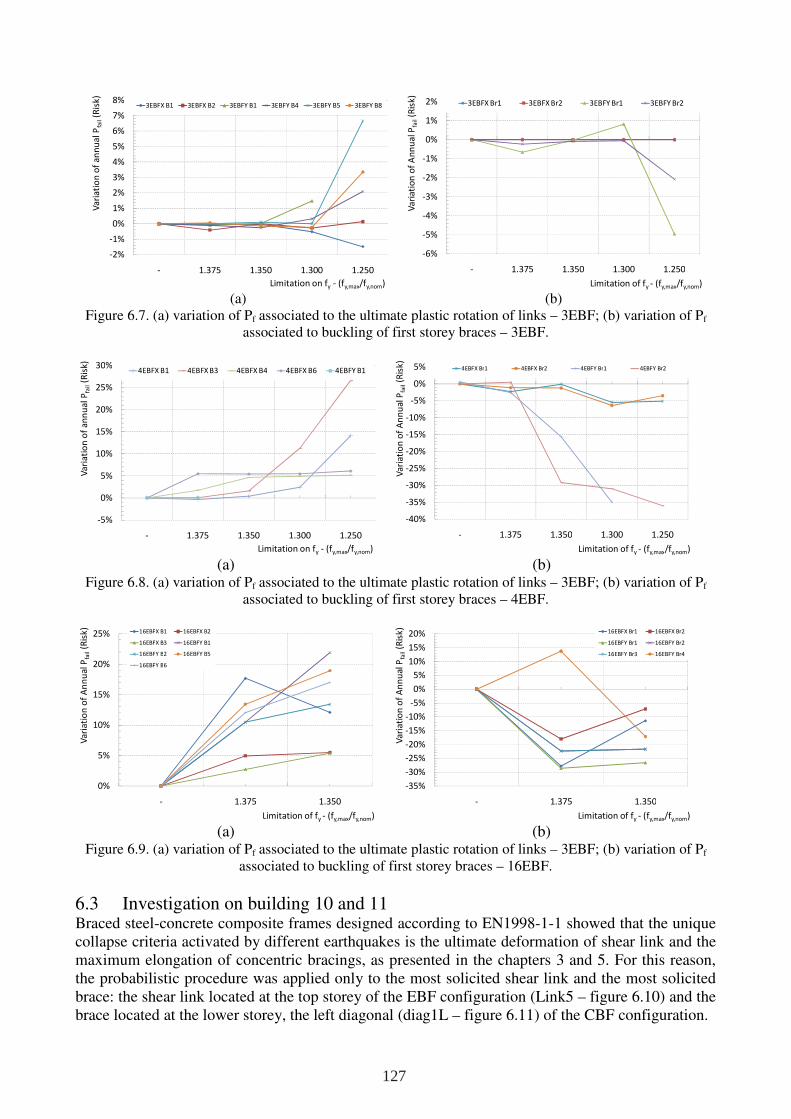
(a)
(b)
Figure 6.7. (a) variation of Pf associated to the ultimate plastic rotation of links – 3EBF; (b) variation of Pf associated to buckling of first storey braces – 3EBF.
(a) (b) Figure 6.8. (a) variation of Pf associated to the ultimate plastic rotation of links – 3EBF; (b) variation of Pf
associated to buckling of first storey braces – 4EBF.
(a)
(b)
Figure 6.9. (a) variation of Pf associated to the ultimate plastic rotation of links – 3EBF; (b) variation of Pf associated to buckling of first storey braces – 16EBF.
6.3 Investigation on building 10 and 11 Braced steel-concrete composite frames designed according to EN1998-1-1 showed that the unique collapse criteria activated by different earthquakes is the ultimate deformation of shear link and the maximum elongation of concentric bracings, as presented in the chapters 3 and 5. For this reason, the probabilistic procedure was applied only to the most solicited shear link and the most solicited brace: the shear link located at the top storey of the EBF configuration (Link5 – figure 6.10) and the brace located at the lower storey, the left diagonal (diag1L – figure 6.11) of the CBF configuration.
-2%
-1%
0%
1%
2%
3%
4%
5%
6%
7%
8%
- 1.375 1.350 1.300 1.250
Va
ria
tio
n o
f a
nn
ua
l P
fail
(Ris
k)
Limitation on fy - (fy,max/fy,nom)
3EBFX B1 3EBFX B2 3EBFY B1 3EBFY B4 3EBFY B5 3EBFY B8
-6%
-5%
-4%
-3%
-2%
-1%
0%
1%
2%
- 1.375 1.350 1.300 1.250
Va
ria
tio
n o
f A
nn
ua
l Pfa
il(R
isk
)
Limitation of fy - (fy,max/fy,nom)
3EBFX Br1 3EBFX Br2 3EBFY Br1 3EBFY Br2
-5%
0%
5%
10%
15%
20%
25%
30%
- 1.375 1.350 1.300 1.250
Va
ria
tio
n o
f a
nn
ua
l P
fail
(Ris
k)
Limitation on fy - (fy,max/fy,nom)
4EBFX B1 4EBFX B3 4EBFX B4 4EBFX B6 4EBFY B1
-40%
-35%
-30%
-25%
-20%
-15%
-10%
-5%
0%
5%
- 1.375 1.350 1.300 1.250
Va
ria
tio
n o
f A
nn
ua
l Pfa
il(R
isk
)
Limitation of fy - (fy,max/fy,nom)
4EBFX Br1 4EBFX Br2 4EBFY Br1 4EBFY Br2
0%
5%
10%
15%
20%
25%
- 1.375 1.350
Va
ria
tio
n o
f A
nn
ua
l Pfa
il(R
isk
)
Limitation of fy - (fy,max/fy,nom)
16EBFX B1 16EBFX B2
16EBFX B3 16EBFY B1
16EBFY B2 16EBFY B5
16EBFY B6
-35%
-30%
-25%
-20%
-15%
-10%
-5%
0%
5%
10%
15%
20%
- 1.375 1.350
Va
ria
tio
n o
f A
nn
ua
l Pfa
il(R
isk
)
Limitation of fy - (fy,max/fy,nom)
16EBFX Br1 16EBFX Br2
16EBFY Br1 16EBFY Br2
16EBFY Br3 16EBFY Br4
127
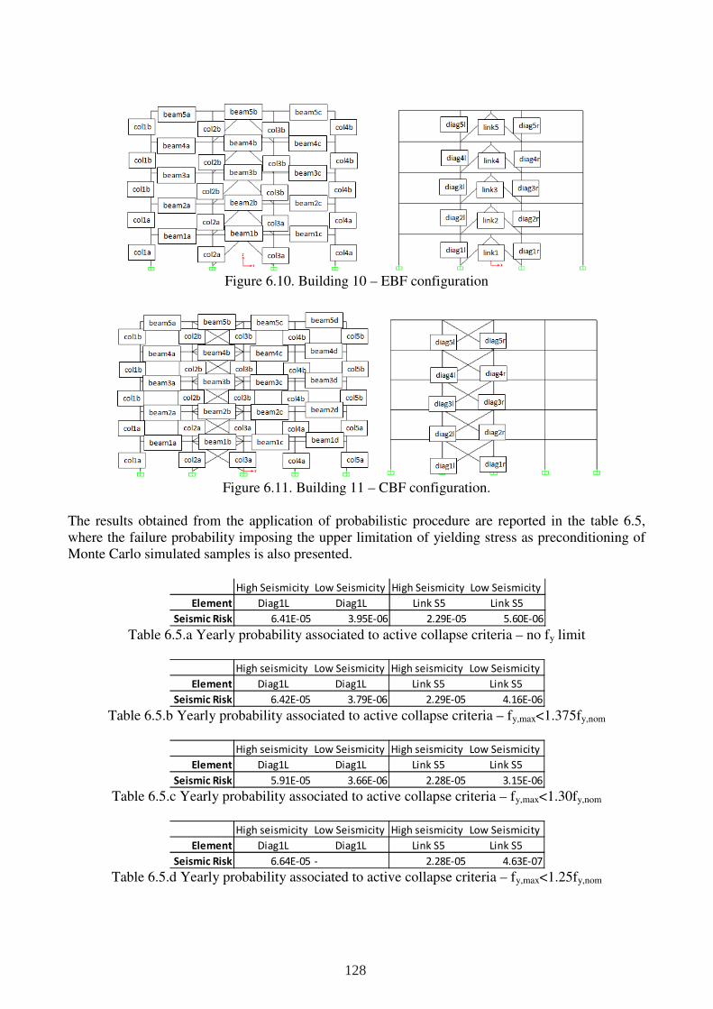
Figure 6.10. Building 10 – EBF configuration
Figure 6.11. Building 11 – CBF configuration.
The results obtained from the application of probabilistic procedure are reported in the table 6.5, where the failure probability imposing the upper limitation of yielding stress as preconditioning of Monte Carlo simulated samples is also presented.
Table 6.5.a Yearly probability associated to active collapse criteria – no fy limit
Table 6.5.b Yearly probability associated to active collapse criteria – fy,max<1.375fy,nom
Table 6.5.c Yearly probability associated to active collapse criteria – fy,max<1.30fy,nom
Table 6.5.d Yearly probability associated to active collapse criteria – fy,max<1.25fy,nom
High Seismicity Low Seismicity High Seismicity Low Seismicity
Element Diag1L Diag1L Link S5 Link S5
Seismic Risk 6.41E-05 3.95E-06 2.29E-05 5.60E-06
High seismicity Low Seismicity High seismicity Low Seismicity
Element Diag1L Diag1L Link S5 Link S5
Seismic Risk 6.42E-05 3.79E-06 2.29E-05 4.16E-06
High seismicity Low Seismicity High seismicity Low Seismicity
Element Diag1L Diag1L Link S5 Link S5
Seismic Risk 5.91E-05 3.66E-06 2.28E-05 3.15E-06
High seismicity Low Seismicity High seismicity Low Seismicity
Element Diag1L Diag1L Link S5 Link S5
Seismic Risk 6.64E-05 - 2.28E-05 4.63E-07
128
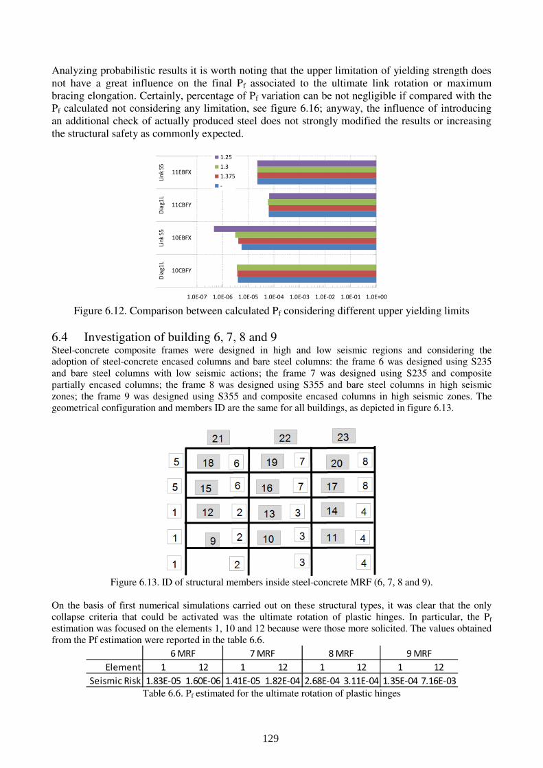
Analyzing probabilistic results it is worth noting that the upper limitation of yielding strength does not have a great influence on the final Pf associated to the ultimate link rotation or maximum bracing elongation. Certainly, percentage of Pf variation can be not negligible if compared with the Pf calculated not considering any limitation, see figure 6.16; anyway, the influence of introducing an additional check of actually produced steel does not strongly modified the results or increasing the structural safety as commonly expected.
Figure 6.12. Comparison between calculated Pf considering different upper yielding limits
6.4 Investigation of building 6, 7, 8 and 9 Steel-concrete composite frames were designed in high and low seismic regions and considering the adoption of steel-concrete encased columns and bare steel columns: the frame 6 was designed using S235 and bare steel columns with low seismic actions; the frame 7 was designed using S235 and composite partially encased columns; the frame 8 was designed using S355 and bare steel columns in high seismic zones; the frame 9 was designed using S355 and composite encased columns in high seismic zones. The geometrical configuration and members ID are the same for all buildings, as depicted in figure 6.13.
Figure 6.13. ID of structural members inside steel-concrete MRF (6, 7, 8 and 9).
On the basis of first numerical simulations carried out on these structural types, it was clear that the only collapse criteria that could be activated was the ultimate rotation of plastic hinges. In particular, the Pf estimation was focused on the elements 1, 10 and 12 because were those more solicited. The values obtained from the Pf estimation were reported in the table 6.6.
Table 6.6. Pf estimated for the ultimate rotation of plastic hinges
1.0E-07 1.0E-06 1.0E-05 1.0E-04 1.0E-03 1.0E-02 1.0E-01 1.0E+00
10CBFY
10EBFX
11CBFY
11EBFX
Dia
g1
LLi
nk
S5D
iag
1L
Lin
k S5
1.25
1.3
1.375
-
Element 1 12 1 12 1 12 1 12
Seismic Risk 1.83E-05 1.60E-06 1.41E-05 1.82E-04 2.68E-04 3.11E-04 1.35E-04 7.16E-03
9 MRF6 MRF 7 MRF 8 MRF
129
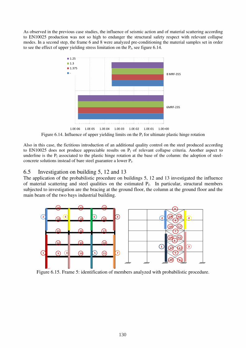
As observed in the previous case studies, the influence of seismic action and of material scattering according to EN10025 production was not so high to endanger the structural safety respect with relevant collapse modes. In a second step, the frame 6 and 8 were analyzed pre-conditioning the material samples set in order to see the effect of upper yielding stress limitation on the Pf, see figure 6.14.
Figure 6.14. Influence of upper yielding limits on the Pf for ultimate plastic hinge rotation
Also in this case, the fictitious introduction of an additional quality control on the steel produced according to EN10025 does not produce appreciable results on Pf of relevant collapse criteria. Another aspect to underline is the Pf associated to the plastic hinge rotation at the base of the column: the adoption of steel-concrete solutions instead of bare steel guarantee a lower Pf.
6.5 Investigation on building 5, 12 and 13 The application of the probabilistic procedure on buildings 5, 12 and 13 investigated the influence of material scattering and steel qualities on the estimated Pf. In particular, structural members subjected to investigation are the bracing at the ground floor, the column at the ground floor and the main beam of the two bays industrial building.
Figure 6.15. Frame 5: identification of members analyzed with probabilistic procedure.
1.0E-06 1.0E-05 1.0E-04 1.0E-03 1.0E-02 1.0E-01 1.0E+00
6MRF-235
8 MRF-355
1.25
1.3
1.375
-
130
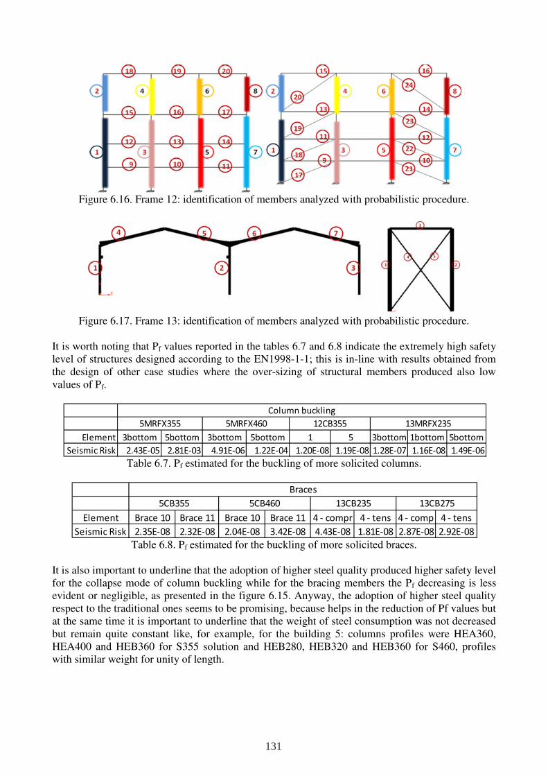
Figure 6.16. Frame 12: identification of members analyzed with probabilistic procedure.
Figure 6.17. Frame 13: identification of members analyzed with probabilistic procedure.
It is worth noting that Pf values reported in the tables 6.7 and 6.8 indicate the extremely high safety level of structures designed according to the EN1998-1-1; this is in-line with results obtained from the design of other case studies where the over-sizing of structural members produced also low values of Pf.
Table 6.7. Pf estimated for the buckling of more solicited columns.
Table 6.8. Pf estimated for the buckling of more solicited braces.
It is also important to underline that the adoption of higher steel quality produced higher safety level for the collapse mode of column buckling while for the bracing members the Pf decreasing is less evident or negligible, as presented in the figure 6.15. Anyway, the adoption of higher steel quality respect to the traditional ones seems to be promising, because helps in the reduction of Pf values but at the same time it is important to underline that the weight of steel consumption was not decreased but remain quite constant like, for example, for the building 5: columns profiles were HEA360, HEA400 and HEB360 for S355 solution and HEB280, HEB320 and HEB360 for S460, profiles with similar weight for unity of length.
Element 3bottom 5bottom 3bottom 5bottom 1 5 3bottom 1bottom 5bottom
Seismic Risk 2.43E-05 2.81E-03 4.91E-06 1.22E-04 1.20E-08 1.19E-08 1.28E-07 1.16E-08 1.49E-06
12CB355 13MRFX2355MRFX4605MRFX355
Column buckling
Element Brace 10 Brace 11 Brace 10 Brace 11 4 - compr 4 - tens 4 - comp 4 - tens
Seismic Risk 2.35E-08 2.32E-08 2.04E-08 3.42E-08 4.43E-08 1.81E-08 2.87E-08 2.92E-08
5CB355 5CB460 13CB235 13CB275
Braces
131
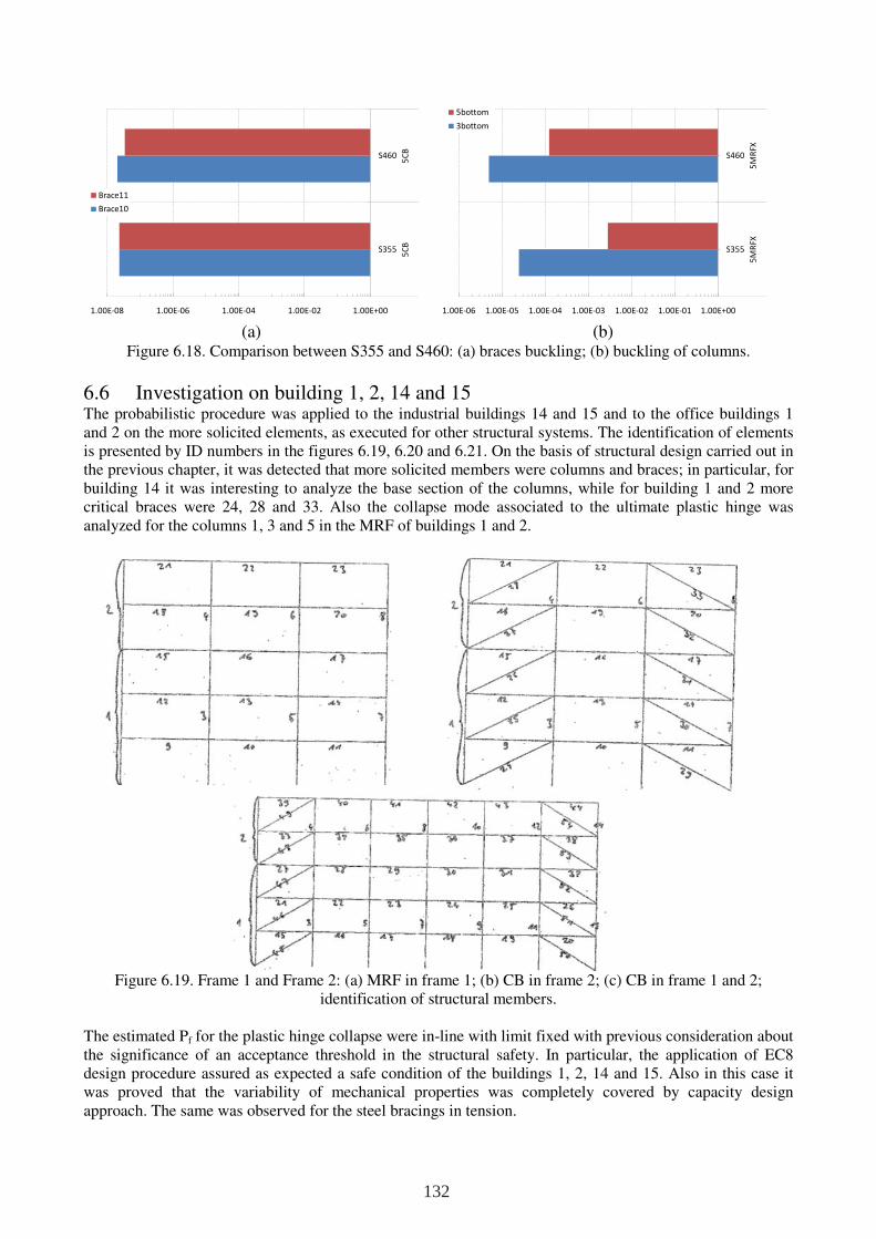
(a)
(b)
Figure 6.18. Comparison between S355 and S460: (a) braces buckling; (b) buckling of columns.
6.6 Investigation on building 1, 2, 14 and 15 The probabilistic procedure was applied to the industrial buildings 14 and 15 and to the office buildings 1 and 2 on the more solicited elements, as executed for other structural systems. The identification of elements is presented by ID numbers in the figures 6.19, 6.20 and 6.21. On the basis of structural design carried out in the previous chapter, it was detected that more solicited members were columns and braces; in particular, for building 14 it was interesting to analyze the base section of the columns, while for building 1 and 2 more critical braces were 24, 28 and 33. Also the collapse mode associated to the ultimate plastic hinge was analyzed for the columns 1, 3 and 5 in the MRF of buildings 1 and 2.
Figure 6.19. Frame 1 and Frame 2: (a) MRF in frame 1; (b) CB in frame 2; (c) CB in frame 1 and 2;
identification of structural members. The estimated Pf for the plastic hinge collapse were in-line with limit fixed with previous consideration about the significance of an acceptance threshold in the structural safety. In particular, the application of EC8 design procedure assured as expected a safe condition of the buildings 1, 2, 14 and 15. Also in this case it was proved that the variability of mechanical properties was completely covered by capacity design approach. The same was observed for the steel bracings in tension.
1.00E-08 1.00E-06 1.00E-04 1.00E-02 1.00E+00
S355
S460
5C
B5
CB
Brace11
Brace10
1.00E-06 1.00E-05 1.00E-04 1.00E-03 1.00E-02 1.00E-01 1.00E+00
S355
S460
5M
RFX
5M
RFX
5bottom
3bottom
132
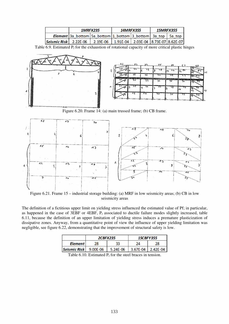
Table 6.9. Estimated Pf for the exhaustion of rotational capacity of more critical plastic hinges
Figure 6.20. Frame 14: (a) main trussed frame; (b) CB frame.
Figure 6.21. Frame 15 – industrial storage building: (a) MRF in low seismicity areas; (b) CB in low seismicity areas
The definition of a fictitious upper limit on yielding stress influenced the estimated value of Pf; in particular, as happened in the case of 3EBF or 4EBF, Pf associated to ductile failure modes slightly increased, table 6.11, because the definition of an upper limitation of yielding stress induces a premature plasticization of dissipative zones. Anyway, from a quantitative point of view the influence of upper yielding limitation was negligible, see figure 6.22, demonstrating that the improvement of structural safety is low.
Table 6.10. Estimated Pf for the steel braces in tension.
133
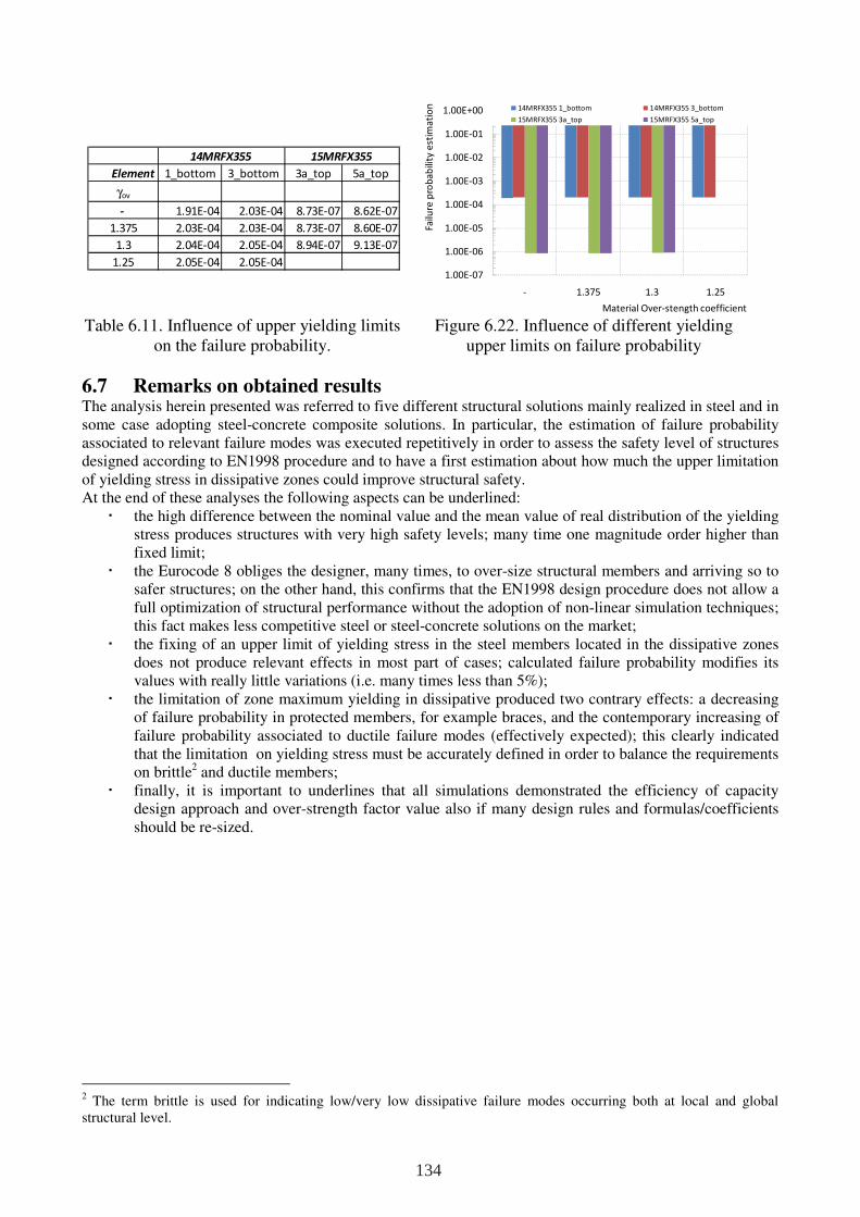
Table 6.11. Influence of upper yielding limits
on the failure probability. Figure 6.22. Influence of different yielding
upper limits on failure probability
6.7 Remarks on obtained results The analysis herein presented was referred to five different structural solutions mainly realized in steel and in some case adopting steel-concrete composite solutions. In particular, the estimation of failure probability associated to relevant failure modes was executed repetitively in order to assess the safety level of structures designed according to EN1998 procedure and to have a first estimation about how much the upper limitation of yielding stress in dissipative zones could improve structural safety. At the end of these analyses the following aspects can be underlined:
the high difference between the nominal value and the mean value of real distribution of the yielding stress produces structures with very high safety levels; many time one magnitude order higher than fixed limit;
the Eurocode 8 obliges the designer, many times, to over-size structural members and arriving so to safer structures; on the other hand, this confirms that the EN1998 design procedure does not allow a full optimization of structural performance without the adoption of non-linear simulation techniques; this fact makes less competitive steel or steel-concrete solutions on the market;
the fixing of an upper limit of yielding stress in the steel members located in the dissipative zones does not produce relevant effects in most part of cases; calculated failure probability modifies its values with really little variations (i.e. many times less than 5%);
the limitation of zone maximum yielding in dissipative produced two contrary effects: a decreasing of failure probability in protected members, for example braces, and the contemporary increasing of failure probability associated to ductile failure modes (effectively expected); this clearly indicated that the limitation on yielding stress must be accurately defined in order to balance the requirements on brittle2 and ductile members;
finally, it is important to underlines that all simulations demonstrated the efficiency of capacity design approach and over-strength factor value also if many design rules and formulas/coefficients should be re-sized.
2 The term brittle is used for indicating low/very low dissipative failure modes occurring both at local and global structural level.
Element 1_bottom 3_bottom 3a_top 5a_top
γov
- 1.91E-04 2.03E-04 8.73E-07 8.62E-07
1.375 2.03E-04 2.03E-04 8.73E-07 8.60E-07
1.3 2.04E-04 2.05E-04 8.94E-07 9.13E-07
1.25 2.05E-04 2.05E-04
15MRFX35514MRFX355
1.00E-07
1.00E-06
1.00E-05
1.00E-04
1.00E-03
1.00E-02
1.00E-01
1.00E+00
- 1.375 1.3 1.25
Failu
re p
rob
ab
ility
est
ima
tio
n
Material Over-stength coefficient
14MRFX355 1_bottom 14MRFX355 3_bottom
15MRFX355 3a_top 15MRFX355 5a_top
134
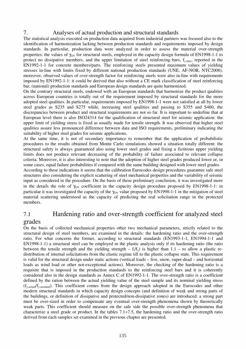
7. Analyses of actual production and structural standards The statistical analysis executed on production data acquired from industrial partners was focused also to the identification of harmonization lacking between production standards and requirements imposed by design standards. In particular, production data were analyzed in order to assess the material over-strength
properties: the values of γOV for structural steels, employed in the capacity design formula of EN1998-1-1 to protect no dissipative members, and the upper limitation of steel reinforcing bars, fy,max, reported in the EN1992-1-1 for concrete members/parts. The reinforcing steels presented maximum values of yielding stresses in-line with limits fixed by different national production standards (UNE, AF-NOR, NTC2008); moreover, observed values of over-strength factor for reinforcing steels were also in-line with requirements imposed by EN1992-1-1: it could be derived that also without a CE mark classification of steel reinforcing bar, (national) production standards and European design standards are quite harmonized. On the contrary structural steels, endowed with an European standards that harmonize the product qualities across European countries is totally out of the requirement imposed by structural standards for the more adopted steel qualities. In particular, requirements imposed by EN1998-1-1 were not satisfied at all by lower steel grades as S235 and S275 while, increasing steel qualities and passing to S355 and S460, the discrepancies between product and structural requirements are not so far. It is important to underline that at European level there is also ISO24314 for the qualification of structural steel for seismic application: the upper limit of yielding stress is fixed as usually made for tensile strength. It was observed that higher steel qualities assure less pronounced difference between data and ISO requirements, preliminary indicating the suitability of higher steel grades for seismic applications. At the same time, it is not of secondary importance to remember that the application of probabilistic procedures to the results obtained from Monte Carlo simulations showed a situation totally different: the structural safety is always guaranteed also using lower steel grades and fixing a fictitious upper yielding limits does not produce relevant decreasing of the probability of failure associated to relevant collapse criteria. Moreover, it is also interesting to note that the adoption of higher steel grades produced lower or, in some cases, equal failure probabilities if compared with the same building designed with lower steel grades. According to these indications it seems that the calibration Eurocodes design procedures guarantee safe steel structures also considering the explicit scattering of steel mechanical properties and the variability of seismic input as considered in the procedure. On the basis of these preliminary conclusion, it was investigated more
in the details the role of γOV coefficient in the capacity design procedure proposed by EN1998-1-1: in
particular it was investigated the capacity of the γOV value proposed by EN1998-1-1 in the mitigation of steel material scattering understood as the capacity of predicting the real solicitation range in the protected members.
7.1 Hardening ratio and over-strength coefficient for analyzed steel grades On the basis of collected mechanical properties other two mechanical parameters, strictly related to the structural design of steel members, are examined in the details: the hardening ratio and the over-strength ratio. For what concerns the former, according to structural standards (EN1993-1-1, EN1994-1-1 and EN1998-1-1) a structural steel can be employed in the plastic analysis only if its hardening ratio (the ratio between the tensile strength and the yielding strength – ft/fy) is higher than 1.1 – to allow a plastic re-distribution of internal solicitations from the elastic regime till to the plastic collapse state. This requirement is valid for the structural design under static actions (vertical loads – live, snow, super-dead – and horizontal loads as wind load or other not-exceptional actions). Moreover, the checking of the hardening ratio is a requisite that is imposed in the production standards to the reinforcing steel bars and it is coherently considered also in the design standards as Annex C of EN1992-1-1. The over-strength ratio is a coefficient defined by the ration between the actual yielding value of the steel sample and its nominal yielding stress (fy,actual/fy,nominal). This coefficient comes from the design approach adopted in the Eurocodes and other modern structural standards in which capacity design concepts (and definition of weak and strong parts of the buildings, or definition of dissipative and protected/non-dissipative zones) are introduced: a strong part must be over-sized in order to compensate any eventual over-strength phenomena shown by theoretically weak parts. This coefficient should measure on the safe side the possible over-strength phenomena that characterize a steel grade or product. In the tables 7.1÷7.5, the hardening ratio and the over-strength ratio derived from each samples set examined in the previous chapter are presented.
135
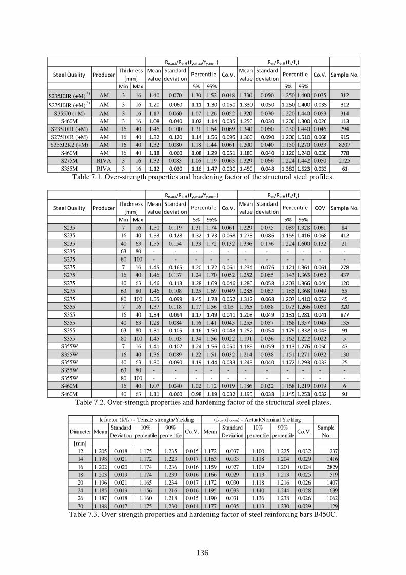
Table 7.1. Over-strength properties and hardening factor of the structural steel profiles.
Table 7.2. Over-strength properties and hardening factor of the structural steel plates.
Table 7.3. Over-strength properties and hardening factor of steel reinforcing bars B450C.
Steel Quality ProducerMean
value
Standard
deviationCo.V.
Mean
value
Standard
deviationCo.V. Sample No.
Min Max 5% 95% 5% 95%
S235J0JR (+M)(*) AM 3 16 1.40 0.070 1.30 1.52 0.048 1.330 0.050 1.250 1.400 0.035 312
S275J0JR (+M)(*) AM 3 16 1.20 0.060 1.11 1.30 0.050 1.330 0.050 1.250 1.400 0.035 312
S355J0 (+M) AM 3 16 1.17 0.060 1.07 1.26 0.052 1.320 0.070 1.220 1.440 0.053 314
S460M AM 3 16 1.08 0.040 1.02 1.14 0.035 1.250 0.030 1.200 1.300 0.026 113
S235J0JR (+M) AM 16 40 1.46 0.100 1.31 1.64 0.069 1.340 0.060 1.230 1.440 0.046 294
S275J0JR (+M) AM 16 40 1.32 0.120 1.14 1.56 0.095 1.360 0.090 1.200 1.510 0.068 915
S355J2K2 (+M) AM 16 40 1.32 0.080 1.18 1.44 0.061 1.200 0.040 1.150 1.270 0.033 8207
S460M AM 16 40 1.18 0.060 1.08 1.29 0.051 1.180 0.040 1.120 1.240 0.030 778
S275M RIVA 3 16 1.32 0.083 1.06 1.19 0.063 1.329 0.066 1.224 1.442 0.050 2125
S355M RIVA 3 16 1.12 0.030 1.16 1.47 0.030 1.450 0.048 1.382 1.523 0.033 61
Thickness
[mm]Percentile
Re,act/Re,H (fy,max/fy,nom) Rm/Re,H (ft/fy)
Percentile
Steel Quality ProducerMean
value
Standard
deviationCo.V.
Mean
value
Standard
deviationCOV Sample No.
Min Max 5% 95% 5% 95%
S235 7 16 1.50 0.119 1.31 1.74 0.061 1.229 0.075 1.089 1.328 0.061 84
S235 16 40 1.53 0.128 1.32 1.73 0.068 1.273 0.086 1.159 1.416 0.068 412
S235 40 63 1.55 0.154 1.33 1.72 0.132 1.336 0.176 1.224 1.600 0.132 21
S235 63 80 - - - - - - - - - - -
S235 80 100 - - - - - - - - - - -
S275 7 16 1.45 0.165 1.20 1.72 0.061 1.234 0.076 1.121 1.361 0.061 278
S275 16 40 1.46 0.137 1.24 1.70 0.052 1.252 0.065 1.143 1.363 0.052 437
S275 40 63 1.46 0.113 1.28 1.69 0.046 1.280 0.058 1.203 1.366 0.046 120
S275 63 80 1.46 0.108 1.35 1.69 0.049 1.285 0.063 1.185 1.368 0.049 55
S275 80 100 1.55 0.099 1.45 1.78 0.052 1.312 0.068 1.207 1.410 0.052 45
S355 7 16 1.37 0.118 1.17 1.56 0.05 1.165 0.058 1.073 1.266 0.050 320
S355 16 40 1.34 0.094 1.17 1.49 0.041 1.208 0.049 1.131 1.281 0.041 877
S355 40 63 1.28 0.084 1.16 1.41 0.045 1.255 0.057 1.168 1.357 0.045 135
S355 63 80 1.31 0.105 1.16 1.50 0.043 1.252 0.054 1.179 1.332 0.043 91
S355 80 100 1.45 0.103 1.34 1.56 0.022 1.191 0.026 1.162 1.222 0.022 5
S355W 7 16 1.41 0.107 1.24 1.56 0.050 1.189 0.059 1.113 1.276 0.050 47
S355W 16 40 1.36 0.089 1.22 1.51 0.032 1.214 0.038 1.151 1.271 0.032 130
S355W 40 63 1.30 0.090 1.19 1.44 0.033 1.243 0.040 1.172 1.293 0.033 25
S355W 63 80 - - - - - - - - - - -
S355W 80 100 - - - - - - - - - - -
S460M 16 40 1.07 0.040 1.02 1.12 0.019 1.186 0.022 1.168 1.219 0.019 6
S460M 40 63 1.11 0.060 0.98 1.19 0.032 1.195 0.038 1.145 1.253 0.032 91
Re,act/Re,H (fy,max/fy,nom) Rm/Re,H (ft/fy)
Thickness
[mm]Percentile Percentile
Diameter MeanStandard
Deviation
10%
percentile
90%
percentileCo.V. Mean
Standard
Deviation
10%
percentile
90%
percentileCo.V.
Sample
No.
[mm]
12 1.205 0.018 1.175 1.235 0.015 1.172 0.037 1.100 1.225 0.032 237
14 1.198 0.021 1.172 1.223 0.017 1.163 0.033 1.118 1.204 0.029 1416
16 1.202 0.020 1.174 1.236 0.016 1.159 0.027 1.109 1.200 0.024 2829
18 1.203 0.019 1.174 1.239 0.016 1.166 0.029 1.113 1.213 0.025 519
20 1.196 0.021 1.165 1.234 0.017 1.172 0.030 1.118 1.216 0.026 1407
24 1.185 0.019 1.156 1.216 0.016 1.195 0.033 1.140 1.244 0.028 639
26 1.187 0.018 1.160 1.218 0.015 1.190 0.031 1.136 1.238 0.026 1062
30 1.198 0.017 1.175 1.230 0.014 1.177 0.035 1.113 1.230 0.029 129
k factor (ft/fy) - Tensile strength/Yielding (fy,act/fy,nom) - Actual/Nominal Yielding
136
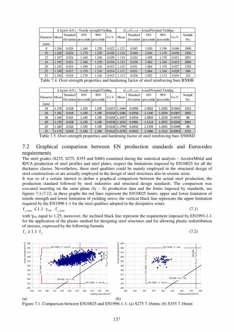
Table 7.4. Over-strength properties and hardening factor of steel reinforcing bars B500B
Table 7.5. Over-strength properties and hardening factor of steel reinforcing bars S500SD
7.2 Graphical comparison between EN production standards and Eurocodes requirements The steel grades (S235, S275, S355 and S460) examined during the statistical analysis – ArcelorMittal and RIVA production of steel profiles and steel plates, respect the limitations imposed by EN10025 for all the thickness classes. Nevertheless, these steel qualities could be mainly employed in the structural design of steel constructions or are actually employed in the design of steel structures also in seismic areas. It was so of a certain interest to define a graphical comparison between the actual steel production, the production standard followed by steel industries and structural design standards. The comparison was executed inserting on the same plane (fy – ft) production data and the limits imposed by standards, see figures 7.1÷7.12; in these graphs the red lines represent the EN10025 limits: upper and lower limitation of tensile strength and lower limitation of yielding stress; the vertical black line represents the upper limitation required by the EN1998-1-1 for the steel qualities adopted in the dissipative zones
nom,yOVmax,y f1.1f ⋅γ⋅≤ (7.1)
with γOV equal to 1.25; moreover, the inclined black line represent the requirement imposed by EN1993-1-1 for the application of the plastic method for designing steel structures and for allowing plastic redistribution of stresses, expressed by the following formula
yt f1.1f ⋅≥ (7.2)
(a)
(b)
Figure 7.1. Comparison between EN10025 and EN1998-1-1: (a) S275 7-16mm; (b) S355 7-16mm
Diameter MeanStandard
Deviation
10%
percentile
90%
percentileCo.V. Mean
Standard
Deviation
10%
percentile
90%
percentileCo.V.
Sample
No.
[mm]
8 1.204 0.026 1.160 1.250 0.022 1.123 0.045 1.050 1.194 0.040 1000
10 1.208 0.024 1.170 1.250 0.020 1.110 0.040 1.044 1.178 0.036 1404
12 1.197 0.024 1.160 1.240 0.020 1.119 0.024 1.058 1.178 0.021 2891
16 1.195 0.021 1.160 1.230 0.018 1.123 0.038 1.062 1.184 0.033 2896
20 1.185 0.016 1.160 1.210 0.013 1.125 0.031 1.064 1.170 0.027 1392
25 1.190 0.017 1.170 1.210 0.014 1.111 0.031 1.064 1.164 0.028 696
32 1.194 0.018 1.170 1.220 0.015 1.113 0.038 1.052 1.172 0.034 524
k factor (ft/fy) - Tensile strength/Yielding (fy,act/fy,nom) - Actual/Nominal Yielding
Diameter MeanStandard
Deviation
10%
percentile
90%
percentileCo.V. Mean
Standard
Deviation
10%
percentile
90%
percentileCo.V.
Sample
No.
[mm]
14 1.176 0.018 1.150 1.200 0.0157 1.1444 0.0392 1.0932 1.1932 0.0342 1413
16 1.165 0.018 1.140 1.190 0.0154 1.1586 0.0356 1.1140 1.2024 0.0307 2002
18 1.164 0.019 1.140 1.190 0.0160 1.1637 0.0554 1.0834 1.2259 0.0476 88
20 1.170 0.018 1.150 1.190 0.0158 1.1610 0.0381 1.1114 1.2072 0.0328 2601
22 1.169 0.016 1.150 1.190 0.0136 1.1794 0.0410 1.1193 1.2341 0.0348 48
25 1.173 0.014 1.160 1.190 0.0122 1.1578 0.0415 1.1046 1.2122 0.0359 2152
k factor (ft/fy) - Tensile strength/Yielding (fy,act/fy,nom) - Actual/Nominal Yielding
350
370
390
410
430
450
470
490
510
530
550
250 270 290 310 330 350 370 390 410 430 450
Yielding stress [N/mm2]
Tensile
str
ength
[N
/mm
2]
EN 10025 - 4 - max Rm
EN 10025 - 4 - min Rm
EN
1002
5 -
4 -
min
Re
EN1993 - Rm>1.1Re
EN
1998 -
Re,a
ct<
1.1
γ ovR
e,n
om
450
470
490
510
530
550
570
590
610
630
650
300 325 350 375 400 425 450 475 500
Yielding stress [N/mm2]
Tensile
str
ength
[N
/mm
2]
EN 10025 - 4 - max R
EN 10025 - 4 - min Rm
EN
1002
5 -
4 -
min
Re
EN1993 - Rm>1.1Re
EN
1998 -
Re,a
ct<
1.1
γ ovR
e,n
om
137
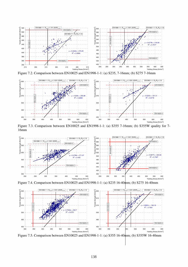
Figure 7.2. Comparison between EN10025 and EN1998-1-1: (a) S235, 7-16mm; (b) S275 7-16mm
Figure 7.3. Comparison between EN10025 and EN1998-1-1: (a) S355 7-16mm; (b) S355W quality for 7-16mm
Figure 7.4. Comparison between EN10025 and EN1998-1-1: (a) S235 16-40mm; (b) S275 16-40mm
Figure 7.5. Comparison between EN10025 and EN1998-1-1: (a) S355 16-40mm; (b) S355W 16-40mm
y = 0.4444x + 274.25
R2 = 0.3684
340
360
380
400
420
440
460
480
500
520
215 265 315 365 415 465 515
Yielding Stress [N/mm2]
Tensile
Str
eng
th [N
/mm
2]
EN10025-2
EN10025-2
EN1993-1-1: Rm/Re>1,10
EN
10025-2
EN1998-1-1: Re,act>1,1X1.25XRe,nom
y = 0.6778x + 218.56
R2 = 0.7577
400
420
440
460
480
500
520
540
560
580
600
200 250 300 350 400 450 500 550 600 650
Yielding Stress [N/mm2]
Tensile
Str
eng
th [N
/mm
2]
EN10025-2
EN10025-2
EN1993-1-1: Rm/Re>1,10
EN
10025-2
EN1998-1-1: Re,act<1,10X1.25XRe,nom
y = 0.636x + 255.88
R2 = 0.6959
450
490
530
570
610
650
300 350 400 450 500 550 600 650
Yielding Stress [N/mm2]
Tensile
Str
eng
th [N
/mm
2]
EN1993-1-1: Rm/Re>1,10
EN10025-2
EN10025-2
EN
1002
5-2
EN1998-1-1: Re,act<1,10X1.25XRe,nom
y = 0.5222x + 331.51
R2 = 0.6778
450
490
530
570
610
650
300 350 400 450 500 550 600 650
Yielding Stress [N/mm2]
Tensile
Str
eng
th [N
/mm
2]
EN1993-1-1: Rm/Re>1,10
EN10025-5
EN10025-5
EN
1002
5-5
EN1998-1-1: Re,act<1,10X1.25XRe,nom
y = 0.4789x + 271.97
R2 = 0.435
300
350
400
450
500
550
200 250 300 350 400 450 500
Yielding Stress [N/mm2]
Tensile
Str
eng
th [N
/mm
2]
EN1993-1-1: Rm/Re>1,10
EN10025-2
EN10025-2
EN
10025
-2
EN1998-1-1: Re,act<1,10X1.25XRe,nom
y = 0.6677x + 224.64
R2 = 0.7327
400
420
440
460
480
500
520
540
560
580
600
200 250 300 350 400 450 500 550 600
Yielding Stress [N/mm2]
Tensile
Str
eng
th [N
/mm
2]
EN10025-2
EN10025-2
EN1993-1-1: Rm/Re>1,10
EN
10025-2
EN1998-1-1: Re,act<1,10X1.25XRe,nom
y = 0.7006x + 232.7
R2 = 0.6751
450
490
530
570
610
650
300 350 400 450 500 550 600 650
Yielding Stress [N/mm2]
Tensile
Str
eng
th [N
/mm
2]
EN1993-1-1: Rm/Re>1,10
EN10025-2
EN10025-2
EN
10025-2
EN1998-1-1: Re,act<1,10X1.25XRe,nom
y = 0.8581x + 166.18
R2 = 0.7691
450
490
530
570
610
650
300 350 400 450 500 550 600 650
Yielding Stress [N/mm2]
Tensile
Str
eng
th [N
/mm
2]
EN1993-1-1: Rm/Re>1,10
EN10025-5
EN10025-5
EN
10025-5
EN1998-1-1: Re,act<1,10X1.25XRe,nom
138
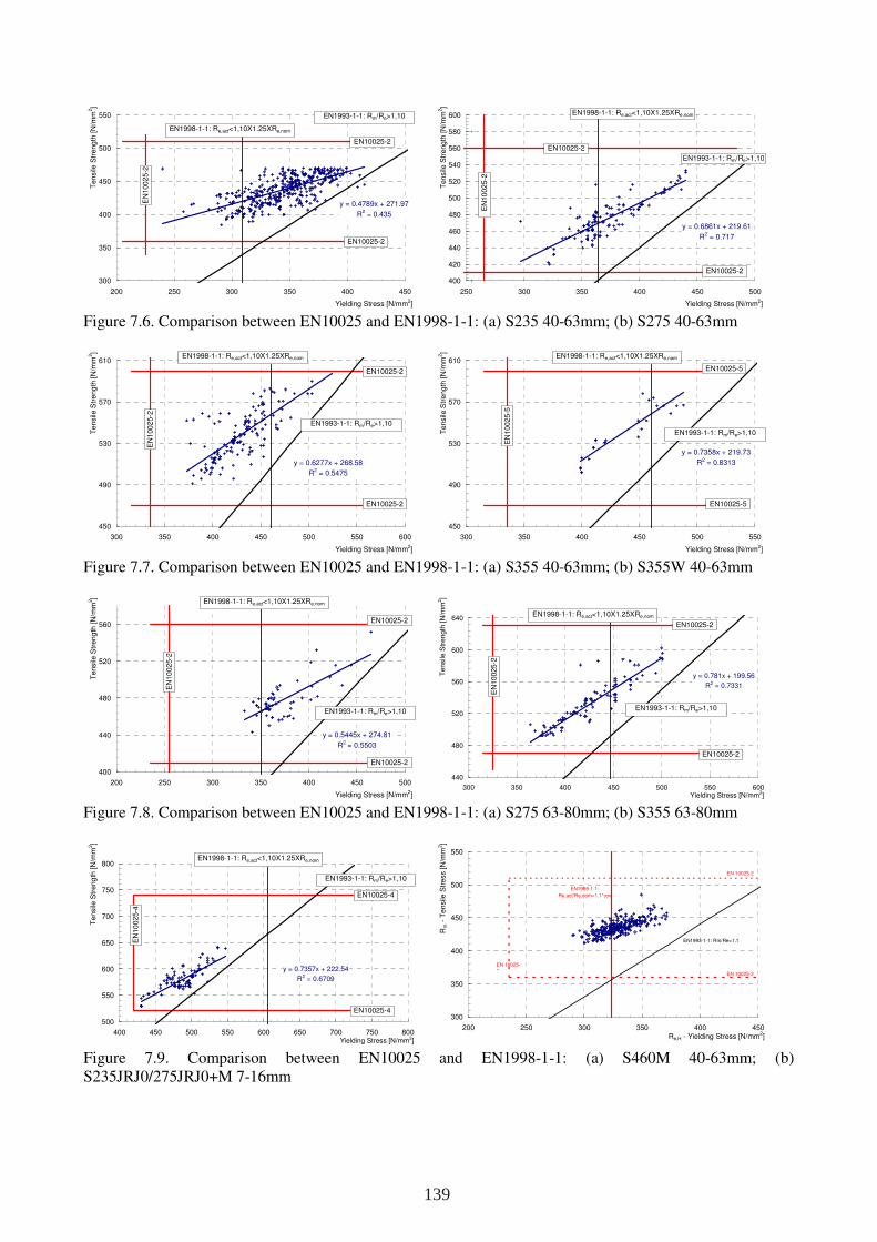
Figure 7.6. Comparison between EN10025 and EN1998-1-1: (a) S235 40-63mm; (b) S275 40-63mm
Figure 7.7. Comparison between EN10025 and EN1998-1-1: (a) S355 40-63mm; (b) S355W 40-63mm
Figure 7.8. Comparison between EN10025 and EN1998-1-1: (a) S275 63-80mm; (b) S355 63-80mm
Figure 7.9. Comparison between EN10025 and EN1998-1-1: (a) S460M 40-63mm; (b) S235JRJ0/275JRJ0+M 7-16mm
y = 0.4789x + 271.97
R2 = 0.435
300
350
400
450
500
550
200 250 300 350 400 450
Yielding Stress [N/mm2]
Tensile
Str
eng
th [N
/mm
2]
EN1993-1-1: Rm/Re>1,10
EN10025-2
EN10025-2
EN
10025
-2
EN1998-1-1: Re,act<1,10X1.25XRe,nom
y = 0.6861x + 219.61
R2 = 0.717
400
420
440
460
480
500
520
540
560
580
600
250 300 350 400 450 500
Yielding Stress [N/mm2]
Tensile
Str
eng
th [N
/mm
2]
EN10025-2
EN10025-2
EN1993-1-1: Rm/Re>1,10
EN
10025-2
EN1998-1-1: Re,act<1,10X1.25XRe,nom
y = 0.6277x + 268.58
R2 = 0.5475
450
490
530
570
610
300 350 400 450 500 550 600
Yielding Stress [N/mm2]
Tensile
Str
eng
th [N
/mm
2]
EN1993-1-1: Rm/Re>1,10
EN10025-2
EN10025-2
EN
10025-2
EN1998-1-1: Re,act<1,10X1.25XRe,nom
y = 0.7358x + 219.73
R2 = 0.8313
450
490
530
570
610
300 350 400 450 500 550
Yielding Stress [N/mm2]
Tensile
Str
eng
th [N
/mm
2]
EN1993-1-1: Rm/Re>1,10
EN10025-5
EN10025-5E
N10
025-5
EN1998-1-1: Re,act<1,10X1.25XRe,nom
y = 0.5445x + 274.81
R2 = 0.5503
400
440
480
520
560
200 250 300 350 400 450 500
Yielding Stress [N/mm2]
Tensile
Str
eng
th [N
/mm
2]
EN1993-1-1: Rm/Re>1,10
EN10025-2
EN10025-2
EN
10
025-2
EN1998-1-1: Re,act<1,10X1.25XRe,nom
y = 0.781x + 199.56
R2 = 0.7331
440
480
520
560
600
640
300 350 400 450 500 550 600Yielding Stress [N/mm2]
Tensile
Str
ength
[N
/mm
2]
EN1993-1-1: Rm/Re>1,10
EN10025-2
EN10025-2
EN
10025-2
EN1998-1-1: Re,act<1,10X1.25XRe,nom
y = 0.7357x + 222.54
R2 = 0.6709
500
550
600
650
700
750
800
400 450 500 550 600 650 700 750 800Yielding Stress [N/mm2]
Tensile
Str
eng
th [N
/mm
2]
EN1993-1-1: Rm/Re>1,10
EN10025-4
EN10025-4
EN
10
025-4
EN1998-1-1: Re,act<1,10X1.25XRe,nom
300
350
400
450
500
550
200 250 300 350 400 450Re,H - Yielding Stress [N/mm2]
Rm
- T
en
sile
Str
ess [
N/m
m2]
EN 10025-2
EN 10025-2
EN 10025-
2
EN1993-1-1: Rm/Re>1,1
EN1998-1-1:
Re,act/Re,nom<1,1*γov
139
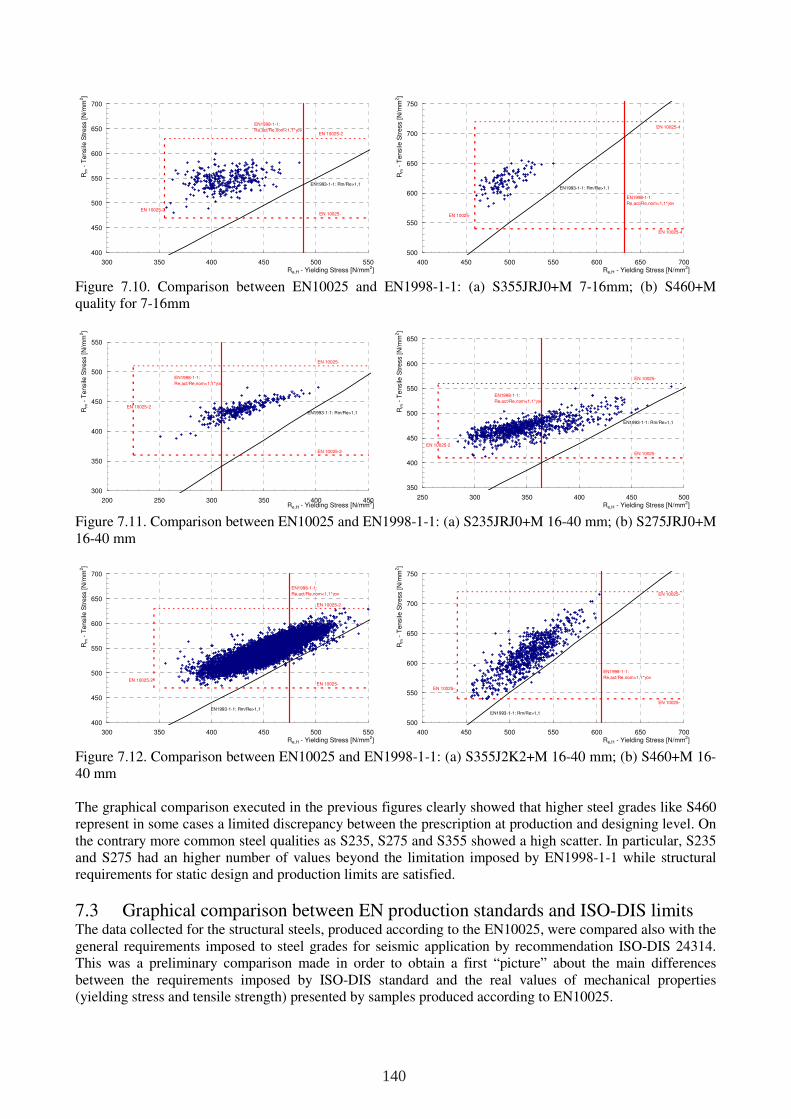
Figure 7.10. Comparison between EN10025 and EN1998-1-1: (a) S355JRJ0+M 7-16mm; (b) S460+M quality for 7-16mm
Figure 7.11. Comparison between EN10025 and EN1998-1-1: (a) S235JRJ0+M 16-40 mm; (b) S275JRJ0+M 16-40 mm
Figure 7.12. Comparison between EN10025 and EN1998-1-1: (a) S355J2K2+M 16-40 mm; (b) S460+M 16-40 mm The graphical comparison executed in the previous figures clearly showed that higher steel grades like S460 represent in some cases a limited discrepancy between the prescription at production and designing level. On the contrary more common steel qualities as S235, S275 and S355 showed a high scatter. In particular, S235 and S275 had an higher number of values beyond the limitation imposed by EN1998-1-1 while structural requirements for static design and production limits are satisfied.
7.3 Graphical comparison between EN production standards and ISO-DIS limits The data collected for the structural steels, produced according to the EN10025, were compared also with the general requirements imposed to steel grades for seismic application by recommendation ISO-DIS 24314. This was a preliminary comparison made in order to obtain a first “picture” about the main differences between the requirements imposed by ISO-DIS standard and the real values of mechanical properties (yielding stress and tensile strength) presented by samples produced according to EN10025.
400
450
500
550
600
650
700
300 350 400 450 500 550Re,H - Yielding Stress [N/mm2]
Rm
- T
en
sile
Str
ess [
N/m
m2]
EN 10025-
2
EN 10025-2
EN 10025-2
EN1993-1-1: Rm/Re>1,1
EN1998-1-1:
Re,act/Re,nom<1,1*γov
500
550
600
650
700
750
400 450 500 550 600 650 700Re,H - Yielding Stress [N/mm2]
Rm
- T
en
sile
Str
ess [
N/m
m2]
EN 10025-4
EN 10025-4
EN 10025-
4
EN1993-1-1: Rm/Re>1,1
EN1998-1-1:
Re,act/Re,nom<1,1*γov
300
350
400
450
500
550
200 250 300 350 400 450Re,H - Yielding Stress [N/mm2]
Rm
- T
en
sile
Str
ess [
N/m
m2]
EN 10025-2
EN 10025-
2
EN 10025-2
EN1993-1-1: Rm/Re>1,1
EN1998-1-1:
Re,act/Re,nom<1,1*γov
350
400
450
500
550
600
650
250 300 350 400 450 500Re,H - Yielding Stress [N/mm2]
Rm
- T
en
sile
Str
ess [
N/m
m2]
EN 10025-
2
EN 10025-
2
EN 10025-2
EN1993-1-1: Rm/Re>1,1
EN1998-1-1:
Re,act/Re,nom<1,1*γov
400
450
500
550
600
650
700
300 350 400 450 500 550Re,H - Yielding Stress [N/mm2]
Rm
- T
en
sile
Str
ess [
N/m
m2]
EN 10025-
2
EN 10025-2
EN 10025-2
EN1993-1-1: Rm/Re>1,1
EN1998-1-1:
Re,act/Re,nom<1,1*γov
500
550
600
650
700
750
400 450 500 550 600 650 700Re,H - Yielding Stress [N/mm2]
Rm
- T
en
sile
Str
ess [
N/m
m2]
EN1993-1-1: Rm/Re>1,1
EN1998-1-1:
Re,act/Re,nom<1,1*γov
EN 10025-
4
EN 10025-
4
EN 10025-
4
140
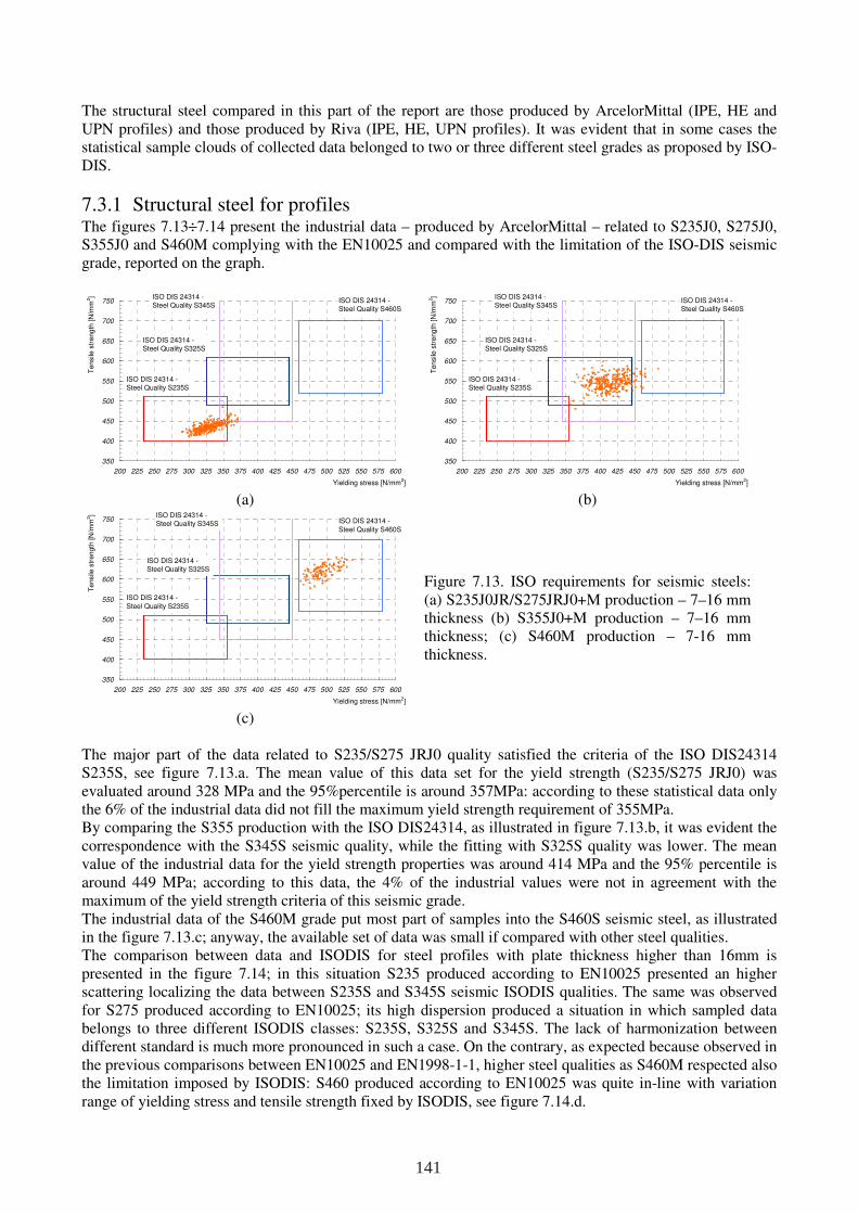
The structural steel compared in this part of the report are those produced by ArcelorMittal (IPE, HE and UPN profiles) and those produced by Riva (IPE, HE, UPN profiles). It was evident that in some cases the statistical sample clouds of collected data belonged to two or three different steel grades as proposed by ISO-DIS.
7.3.1 Structural steel for profiles The figures 7.13÷7.14 present the industrial data – produced by ArcelorMittal – related to S235J0, S275J0, S355J0 and S460M complying with the EN10025 and compared with the limitation of the ISO-DIS seismic grade, reported on the graph.
(a)
(b)
(c)
Figure 7.13. ISO requirements for seismic steels: (a) S235J0JR/S275JRJ0+M production – 7–16 mm thickness (b) S355J0+M production – 7–16 mm thickness; (c) S460M production – 7-16 mm thickness.
The major part of the data related to S235/S275 JRJ0 quality satisfied the criteria of the ISO DIS24314 S235S, see figure 7.13.a. The mean value of this data set for the yield strength (S235/S275 JRJ0) was evaluated around 328 MPa and the 95%percentile is around 357MPa: according to these statistical data only the 6% of the industrial data did not fill the maximum yield strength requirement of 355MPa. By comparing the S355 production with the ISO DIS24314, as illustrated in figure 7.13.b, it was evident the correspondence with the S345S seismic quality, while the fitting with S325S quality was lower. The mean value of the industrial data for the yield strength properties was around 414 MPa and the 95% percentile is around 449 MPa; according to this data, the 4% of the industrial values were not in agreement with the maximum of the yield strength criteria of this seismic grade. The industrial data of the S460M grade put most part of samples into the S460S seismic steel, as illustrated in the figure 7.13.c; anyway, the available set of data was small if compared with other steel qualities. The comparison between data and ISODIS for steel profiles with plate thickness higher than 16mm is presented in the figure 7.14; in this situation S235 produced according to EN10025 presented an higher scattering localizing the data between S235S and S345S seismic ISODIS qualities. The same was observed for S275 produced according to EN10025; its high dispersion produced a situation in which sampled data belongs to three different ISODIS classes: S235S, S325S and S345S. The lack of harmonization between different standard is much more pronounced in such a case. On the contrary, as expected because observed in the previous comparisons between EN10025 and EN1998-1-1, higher steel qualities as S460M respected also the limitation imposed by ISODIS: S460 produced according to EN10025 was quite in-line with variation range of yielding stress and tensile strength fixed by ISODIS, see figure 7.14.d.
350
400
450
500
550
600
650
700
750
200 225 250 275 300 325 350 375 400 425 450 475 500 525 550 575 600
Yielding stress [N/mm2]
Ten
sile
str
eng
th [
N/m
m2]
ISO DIS 24314 - Steel Quality S325S
ISO DIS 24314 - Steel Quality S235S
ISO DIS 24314 - Steel Quality S345S
ISO DIS 24314 - Steel Quality S460S
350
400
450
500
550
600
650
700
750
200 225 250 275 300 325 350 375 400 425 450 475 500 525 550 575 600
Yielding stress [N/mm2]
Te
nsile
str
en
gth
[N
/mm
2]
ISO DIS 24314 - Steel Quality S325S
ISO DIS 24314 -
Steel Quality S235S
ISO DIS 24314 - Steel Quality S345S ISO DIS 24314 -
Steel Quality S460S
141
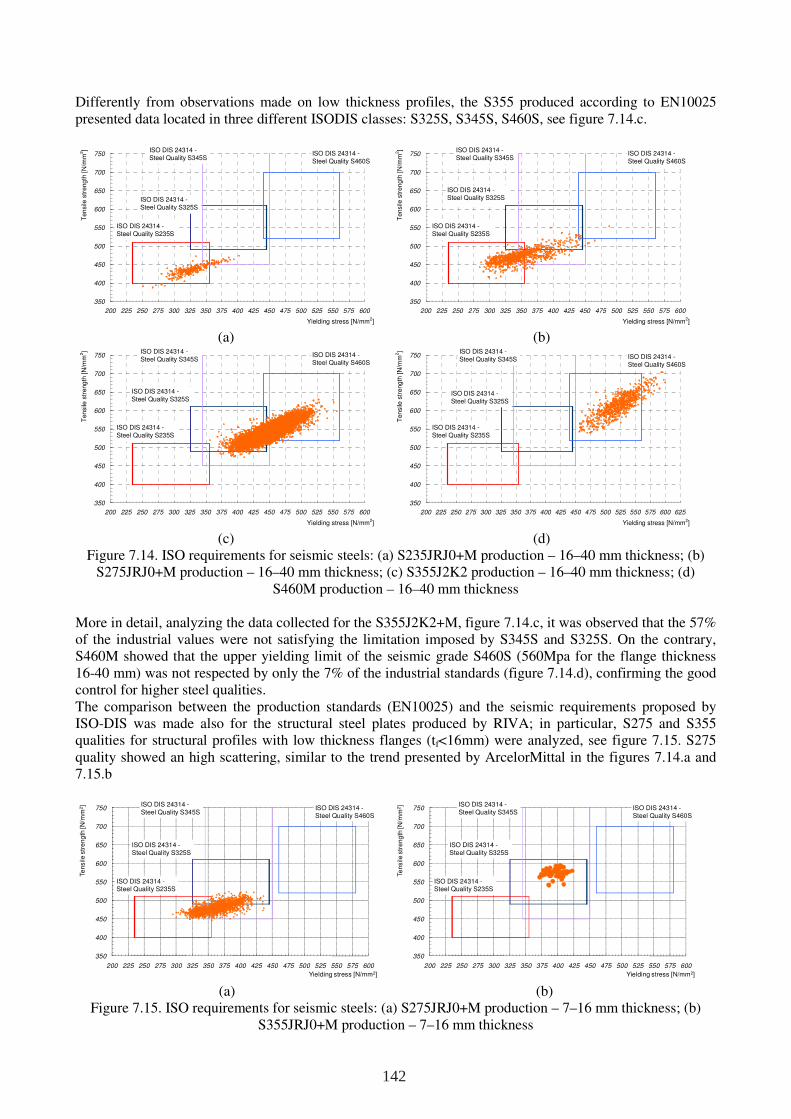
Differently from observations made on low thickness profiles, the S355 produced according to EN10025 presented data located in three different ISODIS classes: S325S, S345S, S460S, see figure 7.14.c.
(a)
(b)
(c)
(d)
Figure 7.14. ISO requirements for seismic steels: (a) S235JRJ0+M production – 16–40 mm thickness; (b) S275JRJ0+M production – 16–40 mm thickness; (c) S355J2K2 production – 16–40 mm thickness; (d)
S460M production – 16–40 mm thickness More in detail, analyzing the data collected for the S355J2K2+M, figure 7.14.c, it was observed that the 57% of the industrial values were not satisfying the limitation imposed by S345S and S325S. On the contrary, S460M showed that the upper yielding limit of the seismic grade S460S (560Mpa for the flange thickness 16-40 mm) was not respected by only the 7% of the industrial standards (figure 7.14.d), confirming the good control for higher steel qualities. The comparison between the production standards (EN10025) and the seismic requirements proposed by ISO-DIS was made also for the structural steel plates produced by RIVA; in particular, S275 and S355 qualities for structural profiles with low thickness flanges (tf<16mm) were analyzed, see figure 7.15. S275 quality showed an high scattering, similar to the trend presented by ArcelorMittal in the figures 7.14.a and 7.15.b
(a)
(b)
Figure 7.15. ISO requirements for seismic steels: (a) S275JRJ0+M production – 7–16 mm thickness; (b) S355JRJ0+M production – 7–16 mm thickness
350
400
450
500
550
600
650
700
750
200 225 250 275 300 325 350 375 400 425 450 475 500 525 550 575 600
Yielding stress [N/mm2]
Ten
sile
str
eng
th [
N/m
m2]
ISO DIS 24314 - Steel Quality S325S
ISO DIS 24314 - Steel Quality S235S
ISO DIS 24314 - Steel Quality S345S
ISO DIS 24314 - Steel Quality S460S
350
400
450
500
550
600
650
700
750
200 225 250 275 300 325 350 375 400 425 450 475 500 525 550 575 600
Yielding stress [N/mm2]
Ten
sile
str
eng
th [
N/m
m2]
ISO DIS 24314 - Steel Quality S325S
ISO DIS 24314 - Steel Quality S235S
ISO DIS 24314 - Steel Quality S345S
ISO DIS 24314 - Steel Quality S460S
350
400
450
500
550
600
650
700
750
200 225 250 275 300 325 350 375 400 425 450 475 500 525 550 575 600 625
Yielding stress [N/mm2]
Ten
sile
str
eng
th [
N/m
m2]
ISO DIS 24314 - Steel Quality S325S
ISO DIS 24314 - Steel Quality S235S
ISO DIS 24314 - Steel Quality S345S ISO DIS 24314 -
Steel Quality S460S
350
400
450
500
550
600
650
700
750
200 225 250 275 300 325 350 375 400 425 450 475 500 525 550 575 600
Te
nsile
str
en
gth
[N/m
m2]
Yielding stress [N/mm2]
ISO DIS 24314 -Steel Quality S325S
ISO DIS 24314 -Steel Quality S235S
ISO DIS 24314 -Steel Quality S345S
ISO DIS 24314 -Steel Quality S460S
350
400
450
500
550
600
650
700
750
200 225 250 275 300 325 350 375 400 425 450 475 500 525 550 575 600
Te
nsile
str
en
gth
[N/m
m2]
Yielding stress [N/mm2]
ISO DIS 24314 -Steel Quality S325S
ISO DIS 24314 -Steel Quality S235S
ISO DIS 24314 -Steel Quality S345S
ISO DIS 24314 -Steel Quality S460S
142
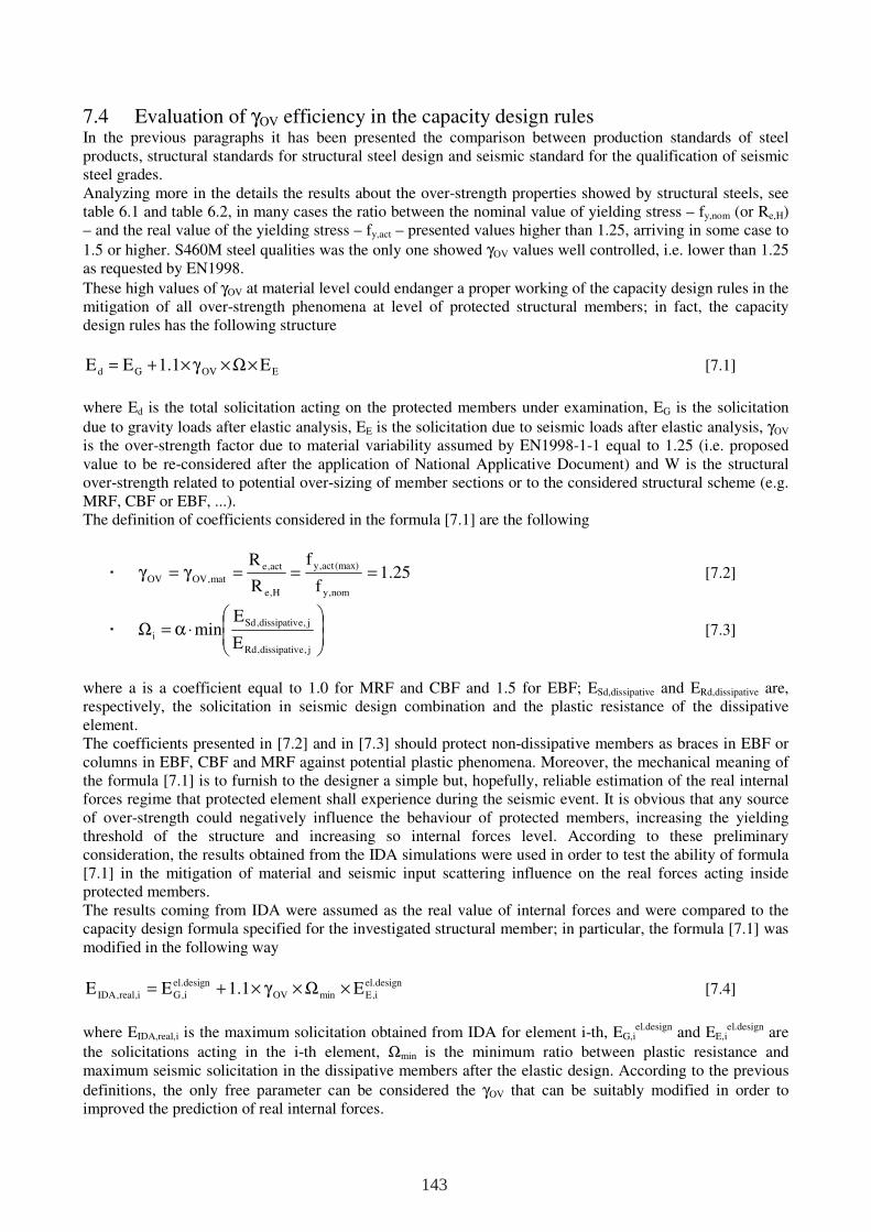
7.4 Evaluation of γOV efficiency in the capacity design rules In the previous paragraphs it has been presented the comparison between production standards of steel products, structural standards for structural steel design and seismic standard for the qualification of seismic steel grades. Analyzing more in the details the results about the over-strength properties showed by structural steels, see table 6.1 and table 6.2, in many cases the ratio between the nominal value of yielding stress – fy,nom (or Re,H) – and the real value of the yielding stress – fy,act – presented values higher than 1.25, arriving in some case to
1.5 or higher. S460M steel qualities was the only one showed γOV values well controlled, i.e. lower than 1.25 as requested by EN1998.
These high values of γOV at material level could endanger a proper working of the capacity design rules in the mitigation of all over-strength phenomena at level of protected structural members; in fact, the capacity design rules has the following structure
EOVGd E1.1EE ×Ω×γ×+= [7.1]
where Ed is the total solicitation acting on the protected members under examination, EG is the solicitation
due to gravity loads after elastic analysis, EE is the solicitation due to seismic loads after elastic analysis, γOV is the over-strength factor due to material variability assumed by EN1998-1-1 equal to 1.25 (i.e. proposed value to be re-considered after the application of National Applicative Document) and W is the structural over-strength related to potential over-sizing of member sections or to the considered structural scheme (e.g. MRF, CBF or EBF, ...). The definition of coefficients considered in the formula [7.1] are the following
25.1f
f
R
R
nom,y
(max)act,y
H,e
act,e
mat,OVOV ===γ=γ [7.2]
⋅α=Ω
j,edissipativ,Rd
j,edissipativ,Sd
iE
Emin [7.3]
where a is a coefficient equal to 1.0 for MRF and CBF and 1.5 for EBF; ESd,dissipative and ERd,dissipative are, respectively, the solicitation in seismic design combination and the plastic resistance of the dissipative element. The coefficients presented in [7.2] and in [7.3] should protect non-dissipative members as braces in EBF or columns in EBF, CBF and MRF against potential plastic phenomena. Moreover, the mechanical meaning of the formula [7.1] is to furnish to the designer a simple but, hopefully, reliable estimation of the real internal forces regime that protected element shall experience during the seismic event. It is obvious that any source of over-strength could negatively influence the behaviour of protected members, increasing the yielding threshold of the structure and increasing so internal forces level. According to these preliminary consideration, the results obtained from the IDA simulations were used in order to test the ability of formula [7.1] in the mitigation of material and seismic input scattering influence on the real forces acting inside protected members. The results coming from IDA were assumed as the real value of internal forces and were compared to the capacity design formula specified for the investigated structural member; in particular, the formula [7.1] was modified in the following way
design.el
i,EminOV
design.el
i,Gi,real,IDA E1.1EE ×Ω×γ×+= [7.4]
where EIDA,real,i is the maximum solicitation obtained from IDA for element i-th, EG,i
el.design and EE,iel.design are
the solicitations acting in the i-th element, Ωmin is the minimum ratio between plastic resistance and maximum seismic solicitation in the dissipative members after the elastic design. According to the previous
definitions, the only free parameter can be considered the γOV that can be suitably modified in order to improved the prediction of real internal forces.
143
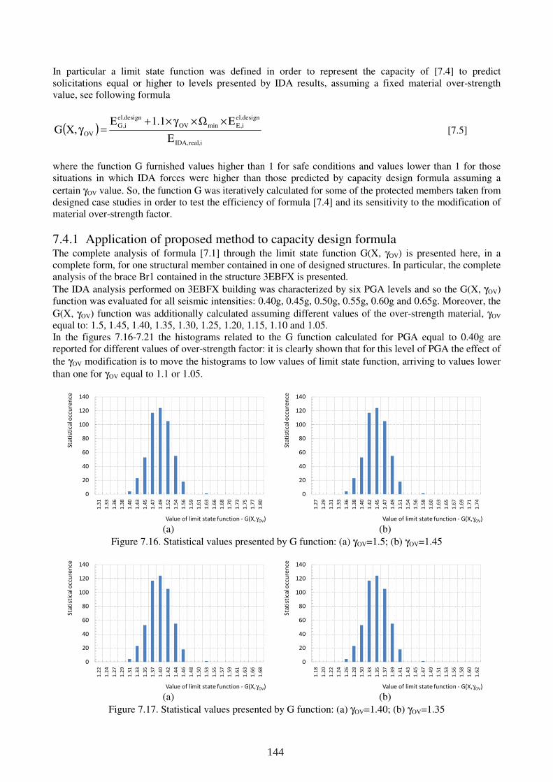
In particular a limit state function was defined in order to represent the capacity of [7.4] to predict solicitations equal or higher to levels presented by IDA results, assuming a fixed material over-strength value, see following formula
( )i,real,IDA
design.el
i,EminOV
design.el
i,G
OVE
E1.1E,XG
×Ω×γ×+=γ [7.5]
where the function G furnished values higher than 1 for safe conditions and values lower than 1 for those situations in which IDA forces were higher than those predicted by capacity design formula assuming a
certain γOV value. So, the function G was iteratively calculated for some of the protected members taken from designed case studies in order to test the efficiency of formula [7.4] and its sensitivity to the modification of material over-strength factor.
7.4.1 Application of proposed method to capacity design formula The complete analysis of formula [7.1] through the limit state function G(X, γOV) is presented here, in a complete form, for one structural member contained in one of designed structures. In particular, the complete analysis of the brace Br1 contained in the structure 3EBFX is presented.
The IDA analysis performed on 3EBFX building was characterized by six PGA levels and so the G(X, γOV) function was evaluated for all seismic intensities: 0.40g, 0.45g, 0.50g, 0.55g, 0.60g and 0.65g. Moreover, the
G(X, γOV) function was additionally calculated assuming different values of the over-strength material, γOV equal to: 1.5, 1.45, 1.40, 1.35, 1.30, 1.25, 1.20, 1.15, 1.10 and 1.05. In the figures 7.16-7.21 the histograms related to the G function calculated for PGA equal to 0.40g are reported for different values of over-strength factor: it is clearly shown that for this level of PGA the effect of
the γOV modification is to move the histograms to low values of limit state function, arriving to values lower
than one for γOV equal to 1.1 or 1.05.
(a)
(b)
Figure 7.16. Statistical values presented by G function: (a) γOV=1.5; (b) γOV=1.45
(a)
(b)
Figure 7.17. Statistical values presented by G function: (a) γOV=1.40; (b) γOV=1.35
0
20
40
60
80
100
120
140
1.3
1
1.3
3
1.3
6
1.3
8
1.4
0
1.4
3
1.4
5
1.4
7
1.4
9
1.5
2
1.5
4
1.5
6
1.5
9
1.6
1
1.6
3
1.6
6
1.6
8
1.7
0
1.7
3
1.7
5
1.7
7
1.8
0
Sta
tist
ica
l occ
ure
nce
Value of limit state function - G(X,γOV)
0
20
40
60
80
100
120
140
1.2
7
1.2
9
1.3
1
1.3
3
1.3
6
1.3
8
1.4
0
1.4
2
1.4
5
1.4
7
1.4
9
1.5
1
1.5
4
1.5
6
1.5
8
1.6
0
1.6
3
1.6
5
1.6
7
1.6
9
1.7
1
1.7
4
Sta
tist
ica
l occ
ure
nce
Value of limit state function - G(X,γOV)
0
20
40
60
80
100
120
140
1.2
2
1.2
4
1.2
7
1.2
9
1.3
1
1.3
3
1.3
5
1.3
7
1.4
0
1.4
2
1.4
4
1.4
6
1.4
8
1.5
0
1.5
3
1.5
5
1.5
7
1.5
9
1.6
1
1.6
3
1.6
6
1.6
8
Sta
tist
ica
l occ
ure
nce
Value of limit state function - G(X,γOV)
0
20
40
60
80
100
120
140
1.1
8
1.2
0
1.2
2
1.2
4
1.2
6
1.2
8
1.3
0
1.3
3
1.3
5
1.3
7
1.3
9
1.4
1
1.4
3
1.4
5
1.4
7
1.4
9
1.5
1
1.5
3
1.5
6
1.5
8
1.6
0
1.6
2
Sta
tist
ica
l occ
ure
nce
Value of limit state function - G(X,γOV)
144
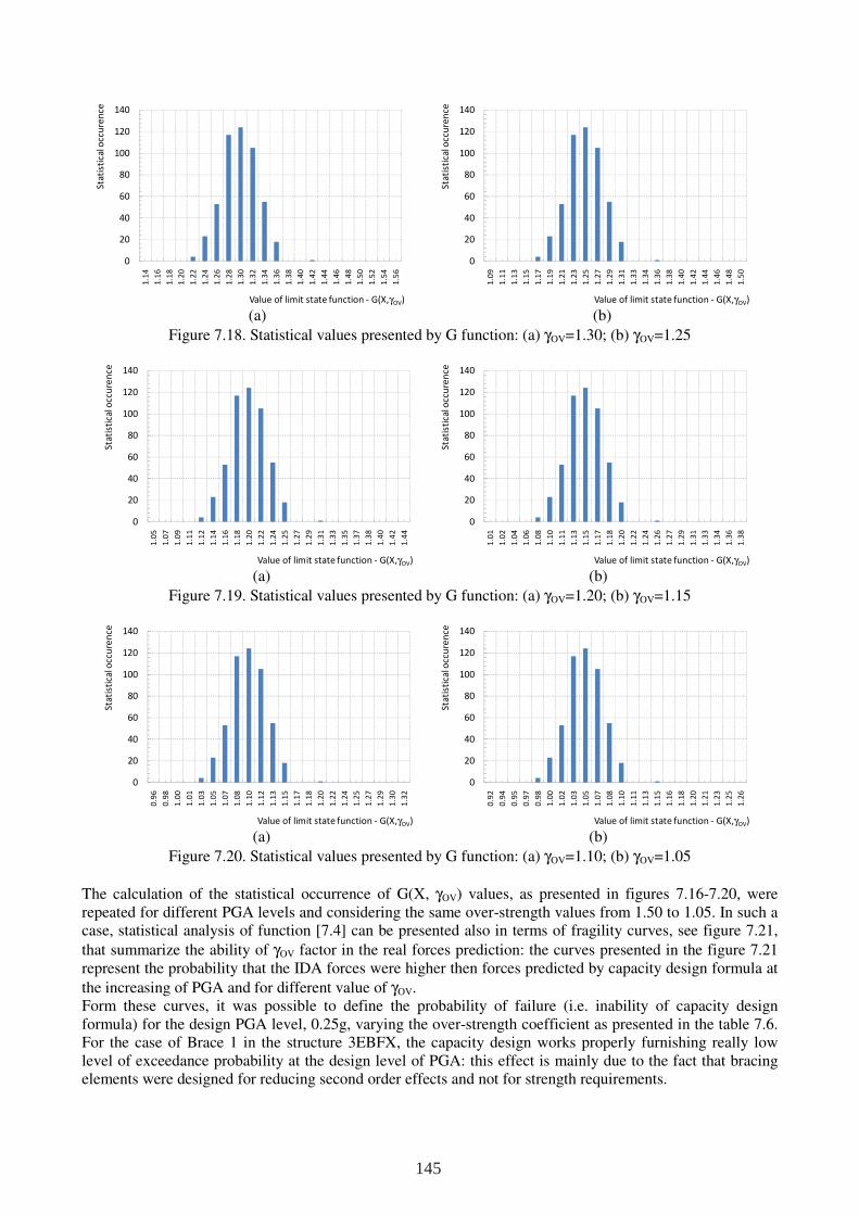
(a)
(b)
Figure 7.18. Statistical values presented by G function: (a) γOV=1.30; (b) γOV=1.25
(a)
(b)
Figure 7.19. Statistical values presented by G function: (a) γOV=1.20; (b) γOV=1.15
(a)
(b)
Figure 7.20. Statistical values presented by G function: (a) γOV=1.10; (b) γOV=1.05
The calculation of the statistical occurrence of G(X, γOV) values, as presented in figures 7.16-7.20, were repeated for different PGA levels and considering the same over-strength values from 1.50 to 1.05. In such a case, statistical analysis of function [7.4] can be presented also in terms of fragility curves, see figure 7.21,
that summarize the ability of γOV factor in the real forces prediction: the curves presented in the figure 7.21 represent the probability that the IDA forces were higher then forces predicted by capacity design formula at
the increasing of PGA and for different value of γOV. Form these curves, it was possible to define the probability of failure (i.e. inability of capacity design formula) for the design PGA level, 0.25g, varying the over-strength coefficient as presented in the table 7.6. For the case of Brace 1 in the structure 3EBFX, the capacity design works properly furnishing really low level of exceedance probability at the design level of PGA: this effect is mainly due to the fact that bracing elements were designed for reducing second order effects and not for strength requirements.
0
20
40
60
80
100
120
140
1.1
4
1.1
6
1.1
8
1.2
0
1.2
2
1.2
4
1.2
6
1.2
8
1.3
0
1.3
2
1.3
4
1.3
6
1.3
8
1.4
0
1.4
2
1.4
4
1.4
6
1.4
8
1.5
0
1.5
2
1.5
4
1.5
6
Sta
tist
ica
l occ
ure
nce
Value of limit state function - G(X,γOV)
0
20
40
60
80
100
120
140
1.0
9
1.1
1
1.1
3
1.1
5
1.1
7
1.1
9
1.2
1
1.2
3
1.2
5
1.2
7
1.2
9
1.3
1
1.3
3
1.3
4
1.3
6
1.3
8
1.4
0
1.4
2
1.4
4
1.4
6
1.4
8
1.5
0
Sta
tist
ica
l occ
ure
nce
Value of limit state function - G(X,γOV)
0
20
40
60
80
100
120
140
1.0
5
1.0
7
1.0
9
1.1
1
1.1
2
1.1
4
1.1
6
1.1
8
1.2
0
1.2
2
1.2
4
1.2
5
1.2
7
1.2
9
1.3
1
1.3
3
1.3
5
1.3
7
1.3
8
1.4
0
1.4
2
1.4
4
Sta
tist
ica
l occ
ure
nce
Value of limit state function - G(X,γOV)
0
20
40
60
80
100
120
140
1.0
1
1.0
2
1.0
4
1.0
6
1.0
8
1.1
0
1.1
1
1.1
3
1.1
5
1.1
7
1.1
8
1.2
0
1.2
2
1.2
4
1.2
6
1.2
7
1.2
9
1.3
1
1.3
3
1.3
4
1.3
6
1.3
8
Sta
tist
ica
l occ
ure
nce
Value of limit state function - G(X,γOV)
0
20
40
60
80
100
120
140
0.9
6
0.9
8
1.0
0
1.0
1
1.0
3
1.0
5
1.0
7
1.0
8
1.1
0
1.1
2
1.1
3
1.1
5
1.1
7
1.1
8
1.2
0
1.2
2
1.2
4
1.2
5
1.2
7
1.2
9
1.3
0
1.3
2
Sta
tist
ica
l occ
ure
nce
Value of limit state function - G(X,γOV)
0
20
40
60
80
100
120
140
0.9
2
0.9
4
0.9
5
0.9
7
0.9
8
1.0
0
1.0
2
1.0
3
1.0
5
1.0
7
1.0
8
1.1
0
1.1
1
1.1
3
1.1
5
1.1
6
1.1
8
1.2
0
1.2
1
1.2
3
1.2
5
1.2
6
Sta
tist
ica
l occ
ure
nce
Value of limit state function - G(X,γOV)
145
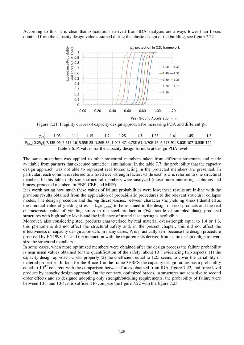
According to this, it is clear that solicitations derived from IDA analyses are always lower than forces obtained from the capacity design value assumed during the elastic design of the building, see figure 7.22.
Figure 7.21. Fragility curves of capacity design approach for increasing PGA and different γOV
Table 7.6. Pf values for the capacity design formula at design PGA level
The same procedure was applied to other structural members taken from different structures and made available from partners that executed numerical simulations. In the table 7.7, the probability that the capacity design approach was not able to represent real forces acting in the protected members are presented. In particular, each column is referred to a fixed over-strength factor, while each row is referred to one structural member. In this table only some structural members were analyzed (those more interesting, columns and braces, protected members in EBF, CBF and MRF). It is worth noting how much these values of failure probabilities were low; these results are in-line with the previous results obtained from the application of probabilistic procedures to the relevant structural collapse modes. The design procedure and the big discrepancies, between characteristic yielding stress (identified as the nominal value of yielding stress – fy,k=fy,nom) to be assumed in the design of steel products and the real characteristic value of yielding stress in the steel production (5% fractile of sampled data), produced structures with high safety levels and the influence of material scattering is negligible. Moreover, also considering steel products characterized by real material over-strength equal to 1.4 or 1.3, this phenomena did not affect the structural safety and, in the present chapter, this did not affect the effectiveness of capacity design approach. In many cases, Pf is practically zero because the design procedure proposed by EN1998-1-1 and the interaction with the requirements derived from static design oblige to over-size the structural members. In some cases, when more optimized members were obtained after the design process the failure probability is near usual values obtained for the quantification of the safety, about 10-4, evidencing two aspects: (1) the capacity design approach works properly (2) the coefficient equal to 1.25 seems to cover the variability of material properties. In fact, for the Brace 1 in the frame 3EBFX the capacity design failure has a probability equal to 10-12 coherent with the comparison between forces obtained from IDA, figure 7.22, and force level produce by capacity design approach. On the contrary, optimized braces, in structures not sensitive to second order effects and so designed adopting only strength/buckling requirements, the probability of failure were between 10-3 and 10-4; it is sufficient to compare the figure 7.22 with the figure 7.23
0
0.1
0.2
0.3
0.4
0.5
0.6
0.7
0.8
0.9
1
0.00 0.20 0.40 0.60 0.80 1.00 1.20
Exc
ee
da
nce
Pro
ba
bili
ty
Re
al
Fo
rce
> C
.D.
Fo
rce
Peak Ground Acceleration - [g]
γOV protection in C.D. framework
1.50 1.45
1.40 1.35
1.30 1.25
1.20 1.15
1.10
γOV 1.05 1.1 1.15 1.2 1.25 1.3 1.35 1.4 1.45 1.5
Pfail_(0.25g) 7.13E-09 5.51E-16 5.55E-25 1.26E-35 1.04E-47 4.73E-61 1.70E-75 6.57E-91 3.60E-107 3.53E-124
146
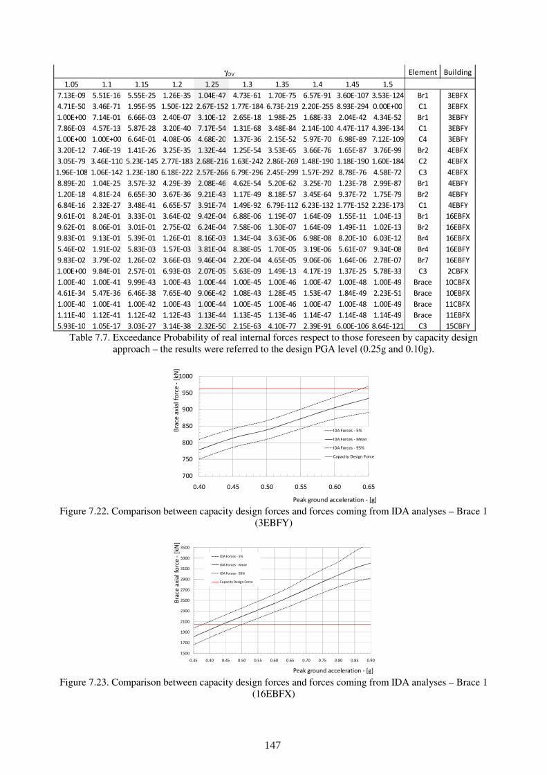
Table 7.7. Exceedance Probability of real internal forces respect to those foreseen by capacity design
approach – the results were referred to the design PGA level (0.25g and 0.10g).
Figure 7.22. Comparison between capacity design forces and forces coming from IDA analyses – Brace 1
(3EBFY)
Figure 7.23. Comparison between capacity design forces and forces coming from IDA analyses – Brace 1
(16EBFX)
Element Building
1.05 1.1 1.15 1.2 1.25 1.3 1.35 1.4 1.45 1.5
7.13E-09 5.51E-16 5.55E-25 1.26E-35 1.04E-47 4.73E-61 1.70E-75 6.57E-91 3.60E-107 3.53E-124 Br1 3EBFX
4.71E-50 3.46E-71 1.95E-95 1.50E-122 2.67E-152 1.77E-184 6.73E-219 2.20E-255 8.93E-294 0.00E+00 C1 3EBFX
1.00E+00 7.14E-01 6.66E-03 2.40E-07 3.10E-12 2.65E-18 1.98E-25 1.68E-33 2.04E-42 4.34E-52 Br1 3EBFY
7.86E-03 4.57E-13 5.87E-28 3.20E-40 7.17E-54 1.31E-68 3.48E-84 2.14E-100 4.47E-117 4.39E-134 C1 3EBFY
1.00E+00 1.00E+00 6.64E-01 4.08E-06 4.68E-20 1.37E-36 2.15E-52 5.97E-70 6.98E-89 7.12E-109 C4 3EBFY
3.20E-12 7.46E-19 1.41E-26 3.25E-35 1.32E-44 1.25E-54 3.53E-65 3.66E-76 1.65E-87 3.76E-99 Br2 4EBFX
3.05E-79 3.46E-110 5.23E-145 2.77E-183 2.68E-216 1.63E-242 2.86E-269 1.48E-190 1.18E-190 1.60E-184 C2 4EBFX
1.96E-108 1.06E-142 1.23E-180 6.18E-222 2.57E-266 6.79E-296 2.45E-299 1.57E-292 8.78E-76 4.58E-72 C3 4EBFX
8.89E-20 1.04E-25 3.57E-32 4.29E-39 2.08E-46 4.62E-54 5.20E-62 3.25E-70 1.23E-78 2.99E-87 Br1 4EBFY
1.20E-18 4.81E-24 6.65E-30 3.67E-36 9.21E-43 1.17E-49 8.18E-57 3.45E-64 9.37E-72 1.75E-79 Br2 4EBFY
6.84E-16 2.32E-27 3.48E-41 6.65E-57 3.91E-74 1.49E-92 6.79E-112 6.23E-132 1.77E-152 2.23E-173 C1 4EBFY
9.61E-01 8.24E-01 3.33E-01 3.64E-02 9.42E-04 6.88E-06 1.19E-07 1.64E-09 1.55E-11 1.04E-13 Br1 16EBFX
9.62E-01 8.06E-01 3.01E-01 2.75E-02 6.24E-04 7.58E-06 1.30E-07 1.64E-09 1.49E-11 1.02E-13 Br2 16EBFX
9.83E-01 9.13E-01 5.39E-01 1.26E-01 8.16E-03 1.34E-04 3.63E-06 6.98E-08 8.20E-10 6.03E-12 Br4 16EBFX
5.46E-02 1.91E-02 5.83E-03 1.57E-03 3.81E-04 8.38E-05 1.70E-05 3.19E-06 5.61E-07 9.34E-08 Br4 16EBFY
9.83E-02 3.79E-02 1.26E-02 3.66E-03 9.46E-04 2.20E-04 4.65E-05 9.06E-06 1.64E-06 2.78E-07 Br7 16EBFY
1.00E+00 9.84E-01 2.57E-01 6.93E-03 2.07E-05 5.63E-09 1.49E-13 4.17E-19 1.37E-25 5.78E-33 C3 2CBFX
1.00E-40 1.00E-41 9.99E-43 1.00E-43 1.00E-44 1.00E-45 1.00E-46 1.00E-47 1.00E-48 1.00E-49 Brace 10CBFX
4.61E-34 5.47E-36 6.46E-38 7.65E-40 9.06E-42 1.08E-43 1.28E-45 1.53E-47 1.84E-49 2.23E-51 Brace 10EBFX
1.00E-40 1.00E-41 1.00E-42 1.00E-43 1.00E-44 1.00E-45 1.00E-46 1.00E-47 1.00E-48 1.00E-49 Brace 11CBFX
1.11E-40 1.12E-41 1.12E-42 1.12E-43 1.13E-44 1.13E-45 1.13E-46 1.14E-47 1.14E-48 1.14E-49 Brace 11EBFX
5.93E-10 1.05E-17 3.03E-27 3.14E-38 2.32E-50 2.15E-63 4.10E-77 2.39E-91 6.00E-106 8.64E-121 C3 15CBFY
γOV
700
750
800
850
900
950
1000
0.40 0.45 0.50 0.55 0.60 0.65
Bra
ce a
xia
l fo
rce
-[k
N]
Peak ground acceleration - [g]
IDA Forces - 5%
IDA Forces - Mean
IDA Forces - 95%
Capacity Design Force
1500
1700
1900
2100
2300
2500
2700
2900
3100
3300
3500
0.35 0.40 0.45 0.50 0.55 0.60 0.65 0.70 0.75 0.80 0.85 0.90
Bra
ce a
xia
l fo
rce
-[k
N]
Peak ground acceleration - [g]
IDA Forces - 5%
IDA Forces - Mean
IDA Forces - 95%
Capacity Design Force
147
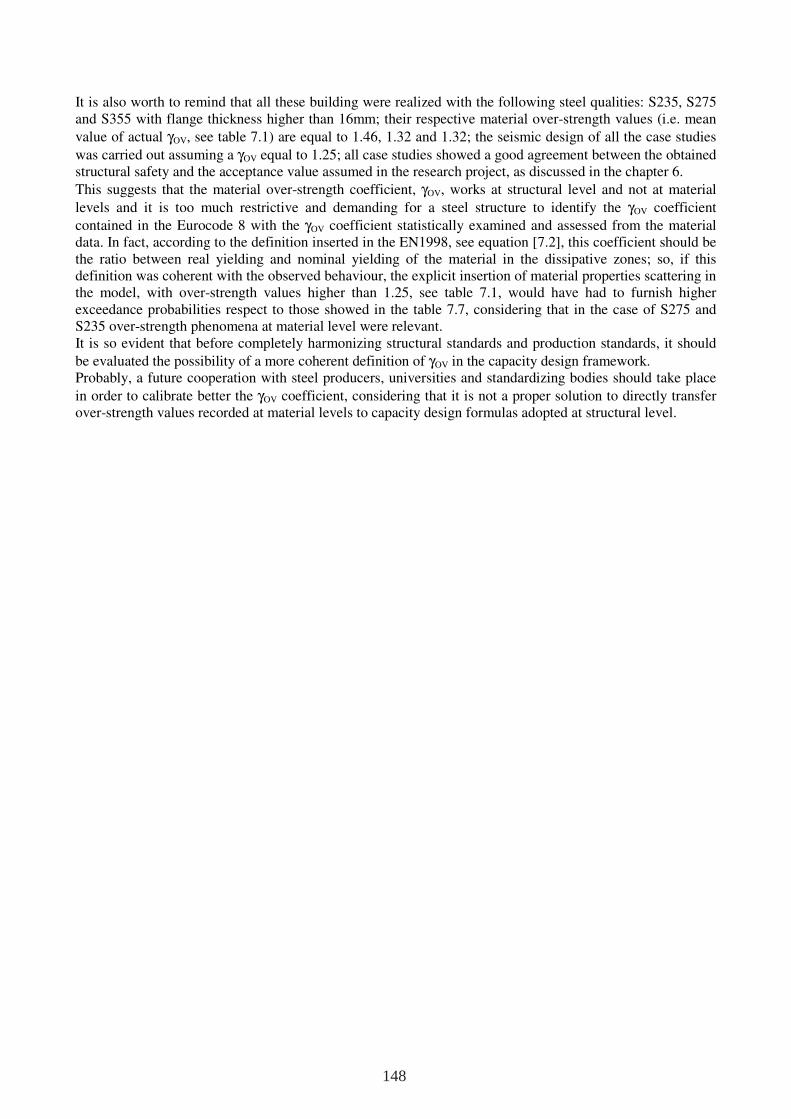
It is also worth to remind that all these building were realized with the following steel qualities: S235, S275 and S355 with flange thickness higher than 16mm; their respective material over-strength values (i.e. mean
value of actual γOV, see table 7.1) are equal to 1.46, 1.32 and 1.32; the seismic design of all the case studies
was carried out assuming a γOV equal to 1.25; all case studies showed a good agreement between the obtained structural safety and the acceptance value assumed in the research project, as discussed in the chapter 6.
This suggests that the material over-strength coefficient, γOV, works at structural level and not at material
levels and it is too much restrictive and demanding for a steel structure to identify the γOV coefficient
contained in the Eurocode 8 with the γOV coefficient statistically examined and assessed from the material data. In fact, according to the definition inserted in the EN1998, see equation [7.2], this coefficient should be the ratio between real yielding and nominal yielding of the material in the dissipative zones; so, if this definition was coherent with the observed behaviour, the explicit insertion of material properties scattering in the model, with over-strength values higher than 1.25, see table 7.1, would have had to furnish higher exceedance probabilities respect to those showed in the table 7.7, considering that in the case of S275 and S235 over-strength phenomena at material level were relevant. It is so evident that before completely harmonizing structural standards and production standards, it should
be evaluated the possibility of a more coherent definition of γOV in the capacity design framework. Probably, a future cooperation with steel producers, universities and standardizing bodies should take place
in order to calibrate better the γOV coefficient, considering that it is not a proper solution to directly transfer over-strength values recorded at material levels to capacity design formulas adopted at structural level.
148
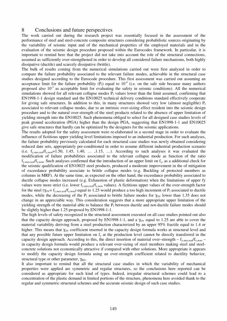
8 Conclusions and future perspectives The work carried out during the research project was essentially focused in the assessment of the performance of steel and steel-concrete composite structures considering probabilistic sources originating by the variability of seismic input and of the mechanical properties of the employed materials and in the evaluation of the seismic design procedure proposed within the Eurocodes framework. In particular, it is important to remind here that the project did not take into account the role of the structural connections, assumed as sufficiently over-strengthened in order to develop all considered failure mechanisms, both highly dissipative (ductile) and scarcely dissipative (brittle). The bulk of results coming from the numerical simulations carried out were first analyzed in order to compare the failure probability associated to the relevant failure modes, achievable in the structural case studies designed according to the Eurocode procedure. This first assessment was carried out assuming an acceptance limit for the failure probability (Pf) equal to 10-4 (i.e. on the safe side because many authors proposed also 10-3 as acceptable limit for evaluating the safety in seismic conditions). All the numerical simulations showed for all relevant collapse modes Pf values lower than the limit assumed, confirming that EN1998-1-1 design standard and the EN10025 technical delivery conditions standard effectively cooperate for giving safe structures. In addition to this, in many structures showed very low (almost negligible) Pf associated to relevant collapse modes, due to an intrinsic over-sizing effect resident into the seismic design procedure and to the natural over-strength of the steel products related to the absence of upper limitation of yielding strength into the EN10025. Such phenomena obliged to select for all designed case studies levels of peak ground acceleration (PGA) higher than the design PGA, suggesting that EN1998-1-1 and EN10025 give safe structures that hardly can be optimized by the designers for the seismic applications. The results adopted for the safety assessment were re-elaborated in a second stage in order to evaluate the influence of fictitious upper yielding level limitations imposed to an industrial production. For such analyses, the failure probability previously calculated for each structural case studies was newly obtained considering reduced date sets, appropriately pre-conditioned in order to assume different industrial production scenario (i.e. fy,max,real/fy,nom=1.50, 1.45, 1.40, … ,1.15, …). According to such analyses it was evaluated the modification of failure probabilities associated to the relevant collapse mode as function of the ratio fy,max,real/fy,nom. Such analyses confirmed that the introduction of an upper limit on fy, as a additional check for the seismic qualification of EN10025 steel products, produced a moderate improvement in the of mitigation of exceedance probability associate to brittle collapse modes (e.g. Buckling of protected members as columns in MRF). At the same time, as expected on the other hand, the exceedance probability associated to ductile collapse modes increased (e.g. Exhaustion of plastic deformation) when the limitations of upper fy values were more strict (i.e. lower fy,max,real/fy,nom values). A fictitious upper values of the over-strength factor
for the steel (γOV= fy,max,real/fy,nom) equal to 1.25 would produce a too high increment of Pf associated to ductile
modes, while the decreasing of the Pf associated to brittle failure modes for γOV lower than 1.35 does not change in an appreciable way. This consideration suggests that a more appropriate upper limitation of the yielding strength of the material able to balance the Pf between ductile and not-ductile failure modes should be slightly higher than 1.25 proposed by EN1998-1-1. The high levels of safety recognized in the structural assessment executed on all case studies pointed out also
that the capacity design approach, proposed by EN1998-1-1, and a γOV equal to 1.25 are able to cover the material variability deriving from a steel production characterized by an upper 95% fractile equal to 1.4 or
higher. This means that γOV coefficient inserted in the capacity design formula works at structural level and that any possible future upper limitation on fy at the production level cannot be directly transferred in the capacity design approach. According to this, the direct insertion of material over–strength – fy,max,real/fy,nom – in capacity design formula would produce a relevant over-sizing of steel members making steel and steel-concrete solutions not economically attractive if compared with other solutions. More appropriate it appears to modify the capacity design formula using an over-strength coefficient related to ductility behavior,
structural type or other parameter, γRD. It also important to remind that all the structural case studies in which the variability of mechanical properties were applied are symmetric and regular structures, so the conclusions here reported can be considered as appropriate for such kind of types. Indeed, irregular structural schemes could lead to a concentration of the plastic demand in limited portions of the structure, phenomena here avoided thank to the regular and symmetric structural schemes and the accurate seismic design of such case studies.
149

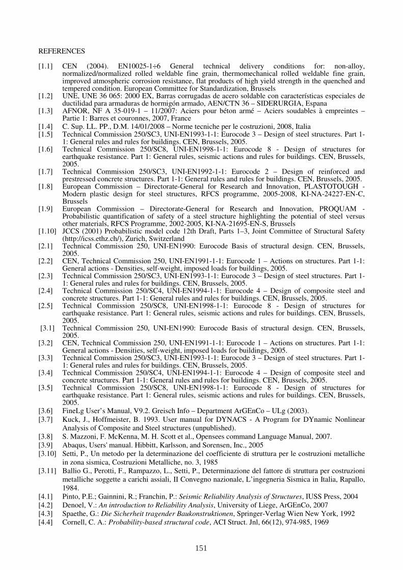
REFERENCES [1.1] CEN (2004). EN10025-1÷6 General technical delivery conditions for: non-alloy,
normalized/normalized rolled weldable fine grain, thermomechanical rolled weldable fine grain, improved atmospheric corrosion resistance, flat products of high yield strength in the quenched and tempered condition. European Committee for Standardization, Brussels
[1.2] UNE, UNE 36 065: 2000 EX, Barras corrugadas de acero soldable con características especiales de ductilidad para armaduras de hormigón armado, AEN/CTN 36 – SIDERURGIA, Espana
[1.3] AFNOR, NF A 35-019-1 – 11/2007: Aciers pour béton armé – Aciers soudables à empreintes – Partie 1: Barres et couronnes, 2007, France
[1.4] C. Sup. LL. PP., D.M. 14/01/2008 – Norme tecniche per le costruzioni, 2008, Italia [1.5] Technical Commission 250/SC3, UNI-EN1993-1-1: Eurocode 3 – Design of steel structures. Part 1-
1: General rules and rules for buildings. CEN, Brussels, 2005. [1.6] Technical Commission 250/SC8, UNI-EN1998-1-1: Eurocode 8 - Design of structures for
earthquake resistance. Part 1: General rules, seismic actions and rules for buildings. CEN, Brussels, 2005.
[1.7] Technical Commission 250/SC3, UNI-EN1992-1-1: Eurocode 2 – Design of reinforced and prestressed concrete structures. Part 1-1: General rules and rules for buildings. CEN, Brussels, 2005.
[1.8] European Commission – Directorate-General for Research and Innovation, PLASTOTOUGH - Modern plastic design for steel structures, RFCS programme, 2005-2008, KI-NA-24227-EN-C, Brussels
[1.9] European Commission – Directorate-General for Research and Innovation, PROQUAM - Probabilistic quantification of safety of a steel structure highlighting the potential of steel versus other materials, RFCS Programme, 2002-2005, KI-NA-21695-EN-S, Brussels
[1.10] JCCS (2001) Probabilistic model code 12th Draft, Parts 1–3, Joint Committee of Structural Safety (http://icss.ethz.ch/), Zurich, Switzerland
[2.1] Technical Commission 250, UNI-EN1990: Eurocode Basis of structural design. CEN, Brussels, 2005.
[2.2] CEN, Technical Commission 250, UNI-EN1991-1-1: Eurocode 1 – Actions on structures. Part 1-1: General actions - Densities, self-weight, imposed loads for buildings, 2005.
[2.3] Technical Commission 250/SC3, UNI-EN1993-1-1: Eurocode 3 – Design of steel structures. Part 1-1: General rules and rules for buildings. CEN, Brussels, 2005.
[2.4] Technical Commission 250/SC4, UNI-EN1994-1-1: Eurocode 4 – Design of composite steel and concrete structures. Part 1-1: General rules and rules for buildings. CEN, Brussels, 2005.
[2.5] Technical Commission 250/SC8, UNI-EN1998-1-1: Eurocode 8 - Design of structures for earthquake resistance. Part 1: General rules, seismic actions and rules for buildings. CEN, Brussels, 2005.
[3.1] Technical Commission 250, UNI-EN1990: Eurocode Basis of structural design. CEN, Brussels, 2005.
[3.2] CEN, Technical Commission 250, UNI-EN1991-1-1: Eurocode 1 – Actions on structures. Part 1-1: General actions - Densities, self-weight, imposed loads for buildings, 2005.
[3.3] Technical Commission 250/SC3, UNI-EN1993-1-1: Eurocode 3 – Design of steel structures. Part 1-1: General rules and rules for buildings. CEN, Brussels, 2005.
[3.4] Technical Commission 250/SC4, UNI-EN1994-1-1: Eurocode 4 – Design of composite steel and concrete structures. Part 1-1: General rules and rules for buildings. CEN, Brussels, 2005.
[3.5] Technical Commission 250/SC8, UNI-EN1998-1-1: Eurocode 8 - Design of structures for earthquake resistance. Part 1: General rules, seismic actions and rules for buildings. CEN, Brussels, 2005.
[3.6] FineLg User’s Manual, V9.2. Greisch Info – Department ArGEnCo – ULg (2003). [3.7] Kuck, J., Hoffmeister, B. 1993. User manual for DYNACS - A Program for DYnamic Nonlinear
Analysis of Composite and Steel structures (unpublished). [3.8] S. Mazzoni, F. McKenna, M. H. Scott et al., Opensees command Language Manual, 2007. [3.9] Abaqus, Users' manual. Hibbitt, Karlsson, and Sorensen, Inc., 2005 [3.10] Setti, P., Un metodo per la determinazione del coefficiente di struttura per le costruzioni metalliche
in zona sismica, Costruzioni Metalliche, no. 3, 1985 [3.11] Ballio G., Perotti, F., Rampazzo, L., Setti, P., Determinazione del fattore di struttura per costruzioni
metalliche soggette a carichi assiali, II Convegno nazionale, L’ingegneria Sismica in Italia, Rapallo, 1984.
[4.1] Pinto, P.E.; Gainnini, R.; Franchin, P.: Seismic Reliability Analysis of Structures, IUSS Press, 2004 [4.2] Denoel, V.: An introduction to Reliability Analysis, University of Liege, ArGEnCo, 2007 [4.3] Spaethe, G.: Die Sicherheit tragender Baukonstruktionen, Springer-Verlag Wien New York, 1992 [4.4] Cornell, C. A.: Probability-based structural code, ACI Struct. Jnl, 66(12), 974-985, 1969
151
[4.5] Hasofer, A. M.; Lind, N.C.: Exact and invariant second-moment code format; Jnl Eng. Mech. Div. –ASCE, 100 (EM1), p. 111-121, 1974
[4.6] Breitung, K.: Asymtotic approcimations for multinormal integrals, Jnl Eng. Mech. – ASCE, 115(7), p.1577-1582, 1984
[4.7] Rackwitz, R.; Fiessler, B.: Structural reliability under combined random load sequences, Computers and Structures, 9, p. 489-494, 1978
[4.8] Der Kiureghuian, A.; Dakessian, T.: Multiple design points in the first and second order reliability
analysis, Structural Safety, 20, p. 37-49, 1998 [4.9] Shinozuka, M.: Basic analysis of structural safety, J. of Struct. Eng., ASCE, 109, p. 721-740, 1983 [4.10] Ibrahim, Y.: Observations of applications of importance sampling in structural reliability analysis,
Structural safety, 9, p. 269-271, 1991 [4.11] Harbitz, A.: An efficient sampling method for probability of failure calculation, Structural Safety, 3,
p. 109-116, 1986 [4.12] Hohenbichler, M.; Rackwitz, R.: Improvements of second-order reliability estimates by importance
sampling, Jnl Eng. Mech. – ASCE, 114, p. 2195-2199, 1988 [4.13] Melchers, R.E.: Importance sampling in structural systems, Structural Safety, 6, 3-10, 1989 [4.14] Bucher, C.G.; Bourgund, V.A.: Fast and efficient response surface approach for structural
reliability problems, Prob. Eng. Mech., 7, p. 183-190, 1992 [4.15] Hohenbichler, M.; Rackwitz, R.: First-order concepts in system reliability, Structural Safety, 1, p.
177-188, 1983 [4.16] Rice, S.O.: Mathematical analysis of random noise, Bell System Tech. J., 23-24, 1944 Vanmarke,
E.H.: On the distribution of the first-passage time for normal stationary random processes, Jnl Appl. Mech. ASME, 42, p. 215-220, 1975
[4.17] Der Kiureghuian, A.: The geometry of random vibrations and solutions by form and sorm, Prob. Eng. Mech., 15(1), p. 81-90, 2000
[4.18] Au, S.K.; Beck, J.L.: On the first-excursion probability for linear systems by very efficient
importance sampling, Prob. Eng. Mech., 16(3), 193-207, 2000 [4.19] Katafygiotis, L.S.; Cheung, S.H.: On the calculation of the failure probability corresponding to a
union failure domains, In Proc. of 4th Int. Conf. on Comput. Stoch. Mech., Corfu Greece, 2002 [4.20] Metropolis, N. et al: Equations of state calculations by fast computing machines, Journ. of Chem.
Phys., 21 (6) p. 1087-1092, 1953 [4.21] Engelund, S. and Rackwitz, R.: A benchmark study on importance sampling techniques in structural
reliability, Structural Safety, 12, p. 255-276, 1993 [4.22] Meskouris, K.: Baudynamik – Modelle, Methoden, Praxisbeispiele. Ernst & Sohn, Berlin 1999 [4.23] Naumoski, N. D.: User Manual – Program SYNTH, generation of artificial accelerograms
compatible with a target spectrum, May 1998 [4.24] User Manual – SIMQKE: A program for artificial motion generation
[4.25] Gasparini, D.; Vanmarcke, E.H.: Simulated Earthquake Motions Compatible with Prescribed
Response Spectra, M.I.T. Department of Civil Engineering Research Report R76-4, Order No. 527, January 1976
[4.26] Booth, E.: Corrections and modifications to SIMQKE1 (VAX version), http://www.booth-seismic.co.uk/simqke_errors.htm
[4.27] Vanmarcke, E.H.; Fenton, G.A.; Heredia-Zavoni, E.: SIMQKE-II Conditioned Earthquake Ground
Motion Simulator, User’s Manual, Version 2, February 1997 [4.28] Gelfi, P.: User Manual - SIMQKE_GR Version 1.2, March 2006 [4.29] Commission of the European Communities: Background Documents for Eurocode 8 Part 1, Volume
1 – Seismic input data, May 1988 [4.30] Cornell CA, Krawinkler H. “Progress and challenges in seismic performance assessment.” PEER
Center News 2000; 3: 2. [4.31] Tamast G., Bounds for probability in multivariate normal distribution, I.S.I. Proceedings, 203-204,
1977. [4.32] Braconi, A., Badalassi, M., Salvatore, W., Modeling of European steel qualities mechanical
properties scattering and its influence on Eurocode 8 design requirements, 14th ECEE Proceedings - European Conference on Earthquake Engineering, Ohrid, Macedonia, August 30 – September 03, 2010
152
[4.33] Technical Commission 250/SC8, UNI-EN1998-1-1: Eurocode 8 - Design of structures for earthquake resistance. Part 1: General rules, seismic actions and rules for buildings. CEN, Brussels, 2005
[5.1] Kook, S. K. 1994. Beitrag zur Definition der Bauwerksregulari-tät und zur Bestimmung der Verhaltensbeiwerte für die Erdbebenbemessung von Stahlbauten. PhD-thesis. Series at Institute for Steel Structures at RWTH Aachen University Volume 27.
[5.2] EN 1998-3: Eurocode 8: Design of structures for earthquake resistance – Part 3: Assessment and retrofitting of buildings; French version EN 1998-3:2005
[5.3] EN 1998-1: Eurocode 8: Design of structures for earthquake resistance – Part 1: General rules, seismic actions and rules for buildings; French version EN 1998-1:2004
[5.4] FEMA-350: Recommended Seismic Design Criteria for new steel moment frames buildings, Federal Emergency Management Agency, June 2000
[5.5] FEMA-356: Guideline for Seismic Rehabilitation of Buildings, Federal Emergency Management Agency, 2002
[5.6] Gioncu, V., Mateescu, G., Petcu, D., Anastasiadis, A. (2000): Prediction of available ductility by means of local plastic mechanism method: DUCTROT computer program. In Moment Resistant Connections of Steel Frames in Seismic Areas. Design and Reliability (ed. F.M. Mazzolani), E&FN Spon London, 95-146
[5.7] Victor Gioncu, Federico M. Mazzolani, Ductility of seismic resistant steel structures. 2002. [5.8] Gioncu, V. and Petcu, D.: Available rotation capacity of wide-flange beams and columns, Part 1.
Theoretical approaches. Journal of Constructional Steel Research, 1997, 44, JCSR 1487. [5.9] V. Gioncu and D. Petcu, Available rotation capacity of wide-flange beams and beam–columns part 2.
Experimental and numerical tests, Journal of Constructional Steel Research 43 (1997) (1–3), pp. 219–244.
[5.10] Nofal S : Determination of ductility limits of steel and composite beams for use in reliability analyses, doctoral thesis, in preparation for 2011.
[5.11] Van Dang Tran, Nguyen Quang Huy, Somja H. Etude de la capacité de rotation d’un poteau mixte acier- béton, rapport de stage Master INSA, 2010
[6.1] Cornell, C.A., 1969, “Structural Safety Specification Based on Second-Moment Reliability,”Proc.,
Symposium of the International Association of Bridge and Structural Engineers, London [6.2] Hasofer, A.M., and N. Lind, 1974, “An Exact and Invariant First-Order Reliability Format,” in
Journal of Engineering Mechanics, ASCE, vol. 100, No. EM1, February 1974, pp. 111-121 [6.3] Ellingwood, B., Galambos, T.V., MacGregor, J.G., and Cornell, C.A., 1980, Development of a
Probability Based Criterion for American National Standard A58, Washington, DC: Special Publication 577, National Bureau of Standards, 222 pp.
[6.4] K. Porter, C. Scawthorn, C. Taylor and N. Blais, Appropriate Seismic Reliability for Critical Equipment Systems – Recommendations Based on Regional Analysis of Financial and Life Loss, NCEER Project Numbers 94-6201 and 95-6201, MCEER, State University of New York at Buffalo, 1998
[6.5] Melchers, R. E., Structural Reliability Analysis and Prediction – 2nd Edition, John Wiley & Sons, Chichester, England, 2002.
[6.6] Legerer, F., Code theory – a new branch of engineering science, Structural Reliability and Codified Design, Lind, N.C. (Ed.), SM Study No.3, University of Waterloo, Ontario, 113-127
[6.7] Veniziano, D., Basic Principles and Methods of Structural Safety, Bulletin D’Information No. 112, Comité Européen du Béton, Paris, 1976, 212-288
[6.8] Veneziano, D., Casciati, F., Faravelli, L., Methods of Seismic Fragility for Complicated Systems, Proc. Second Conf. on the Safety of Nuclear Installations (CSNI), Specialist Meeting on Probabilistic Methods in Seismic Risk Assessment for NPP, Livermore, 1983, California
[6.9] Ditlevsen, O. Madsen, H.O., Structural Reliability Methods, John Wiley & Sons, Chichester, 1996, Englnad
153

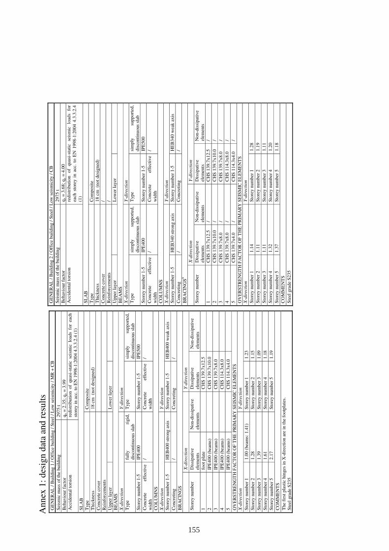
An
nex
1:
des
ign
dat
a an
d r
esult
s
GE
NE
RA
L /
Buil
din
g 1
/ O
ffic
e bu
ildin
g /
Ste
el /
Low
sei
smic
ity /
MR
+ C
B
Sei
smic
mas
s o
f th
e bu
ild
ing
297
5 t
B
ehav
iou
r fa
cto
r q
x =
2.3
5;
qy =
3.9
9
Acc
iden
tal
tors
ion
re
dis
trib
uti
on
of
qu
asi-
stat
ic s
eism
ic l
oad
s fo
r ea
ch
sto
rey
in
acc
. to
EN
19
98
-1:2
00
4 4
.3.3
.2.4
(1)
SL
AB
T
yp
e C
om
po
site
T
hic
kn
ess
18
cm
(n
ot
des
ign
ed)
Co
ncr
ete
cover
Rei
nfo
rcem
ents
Up
per
lay
er
L
ow
er l
ayer
BE
AM
S
X-d
irec
tio
n
Y-d
irec
tio
n
Typ
e fu
lly
rigid
, d
isco
nti
nuo
us
slab
T
yp
e si
mply
su
pp
ort
ed,
dis
con
tin
uous
slab
Sto
rey n
um
ber
1-5
IP
E4
00
S
tore
y n
um
ber
1-5
IP
E5
00
Co
ncr
ete
effe
ctiv
e w
idth
/
Co
ncr
ete
effe
ctiv
e w
idth
/
CO
LU
MN
S
X-d
irec
tio
n
Y-d
irec
tio
n
Sto
rey n
um
ber
1-5
H
EB
40
0 s
tron
g a
xis
S
tore
y n
um
ber
1-5
H
EB
400
wea
k a
xis
Co
ncr
etin
g /
Co
ncr
etin
g /
BR
AC
ING
S
X
-dir
ect
ion
Y-d
irec
tion
Sto
rey n
um
ber
D
issi
pat
ive
elem
ents
N
on-d
issi
pat
ive
elem
ents
D
issi
pat
ive
elem
ents
N
on-d
issi
pat
ive
elem
ents
1
fo
ot
pla
te
C
HS
13
9.7
x1
2.5
2
IPE
40
0 (
bea
ms)
CH
S 1
39
.7x
10.0
3
IPE
40
0 (
bea
ms)
CH
S 1
39
.7x
8.0
4
IPE
40
0 (
bea
ms)
CH
S 1
14
.3x
8.0
5
IPE
40
0 (
bea
ms)
CH
S 1
14
.3x
4.0
OV
ER
ST
RE
NG
TH
FA
CT
OR
OF
TH
E P
RIM
AR
Y S
EIS
MIC
EL
EM
EN
TS
X
-dir
ecti
on
Y-d
irec
tio
n
Sto
rey n
um
ber
1
1.0
0 (
bea
ms:
1.4
1)
Sto
rey
num
ber
1
1.2
3
Sto
rey n
um
ber
2
1.2
8
Sto
rey
num
ber
2
1.1
5
Sto
rey n
um
ber
3
1.3
9
Sto
rey
num
ber
3
1.0
9
Sto
rey n
um
ber
4
1.6
1
Sto
rey
num
ber
4
1.1
8
Sto
rey n
um
ber
5
2.1
7
Sto
rey
num
ber
5
1.1
9
CO
MM
EN
TS
Th
e fi
rst
pla
stic
hin
ges
in
X-d
irec
tion
are
in
the
foo
tpla
tes.
S
teel
gra
de
S2
35
GE
NE
RA
L /
Bu
ildin
g 2
/ O
ffic
e b
uil
din
g /
Ste
el /
Low
sei
smic
ity
/ C
B
Sei
smic
mas
s of
the
bu
ild
ing
2
97
5 t
Beh
avio
ur
fact
or
qx =
3.6
8;
qy =
4.0
0
Acc
iden
tal
tors
ion
re
dis
trib
uti
on
o
f qu
asi-
stat
ic
seis
mic
lo
ads
for
each
sto
rey i
n a
cc.
to E
N 1
99
8-1
:20
04
4.3
.3.2
.4
(1)
SL
AB
Typ
e C
om
po
site
T
hic
kn
ess
18
cm
(n
ot
des
ign
ed)
Co
ncr
ete
cov
er
/
Rei
nfo
rcem
ents
/
Up
per
lay
er
L
ow
er l
ayer
BE
AM
S
X-d
irec
tio
n
Y-d
irec
tion
Typ
e si
mp
ly
sup
po
rted
, d
isco
nti
nu
ous
slab
T
yp
e si
mp
ly
sup
port
ed,
dis
con
tin
uo
us
slab
Sto
rey n
um
ber
1-5
IP
E4
00
S
tore
y n
um
ber
1-5
IP
E5
00
Co
ncr
ete
effe
ctiv
e w
idth
/
Co
ncr
ete
effe
ctiv
e w
idth
/
CO
LU
MN
S
X-d
irec
tio
n
Y-d
irec
tion
Sto
rey n
um
ber
1-5
H
EB
34
0 s
tro
ng a
xis
S
tore
y n
um
ber
1-5
H
EB
34
0 w
eak
ax
is
Co
ncr
etin
g
/ C
on
cret
ing
/
BR
AC
ING
S9
X
-dir
ect
ion
Y-d
irect
ion
Sto
rey n
um
ber
D
issi
pat
ive
elem
ents
N
on-d
issi
pat
ive
elem
ents
D
issi
pat
ive
elem
ents
N
on
-dis
sip
ativ
e el
emen
ts
1
CH
S 1
39
.7x
12
.5
/ C
HS
13
9.7
x1
2.5
/
2
CH
S 1
39
.7x
10
.0
/ C
HS
13
9.7
x1
0.0
/
3
CH
S 1
39
.7x
8.0
/
CH
S 1
39
.7x
8.0
/
4
CH
S 1
39
.7x
8.0
/
CH
S 1
14
.3x
8.0
/
5
CH
S 1
39
.7x
4.0
/
CH
S 1
14
.3x
4.0
/
OV
ER
ST
RE
NG
TH
FA
CT
OR
OF
TH
E P
RIM
AR
Y S
EIS
MIC
EL
EM
EN
TS
X
-dir
ecti
on
Y-d
irec
tion
Sto
rey n
um
ber
1
1.1
4
Sto
rey n
um
ber
1
1.2
8
Sto
rey n
um
ber
2
1.1
1
Sto
rey n
um
ber
2
1.1
9
Sto
rey n
um
ber
3
1.1
1
Sto
rey n
um
ber
3
1.1
1
Sto
rey n
um
ber
4
1.3
2
Sto
rey n
um
ber
4
1.2
0
Sto
rey n
um
ber
5
1.3
7
Sto
rey n
um
ber
5
1.1
8
CO
MM
EN
TS
Ste
el g
rad
e S
23
5
155
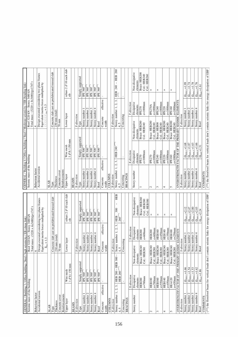
GE
NE
RA
L /
Buil
din
g 3
/ O
ffic
e buil
din
g /
Ste
el /
hig
h s
eism
icit
y /
EB
(sh
ear
link)
Sei
smic
mas
s of
the
buil
din
g
Roo
f 3220 k
N –
Sto
rey 3
480
kN
T
ota
l m
ass
: (3
220 +
4x3480)/
g=
1747 t
Beh
avio
ur
fact
or
6
Acc
iden
tal
tors
ion
Des
ign
ex
ecute
d c
onsi
der
ing t
wo p
lane
fram
es
Equiv
alen
t in
erti
a fo
rces
mult
ipli
ed b
y
δec
c =
1.3
SL
AB
T
ype
Con
cret
e sl
ab c
ast
on p
refa
bri
cate
d t
russ
ed s
lab
Thic
kn
ess
23
0 m
m (
tota
l)
Con
cret
e co
ver
70
mm
Rei
nfo
rcem
ents
Upper
lay
er
Wir
e m
esh
1
8 /
150 m
m
Low
er l
ayer
re
bar
s 2
10 e
ach s
lab
rib
BE
AM
S
X-d
irect
ion
Y-d
irect
ion
Type
Sim
ply
sup
port
ed
Type
Sim
ply
support
ed
Sto
rey n
um
ber
1
IPE
500
(**)
S
tore
y n
um
ber
1
IPE
360
(**
)
Sto
rey n
um
ber
2
IPE
500
(**)
S
tore
y n
um
ber
2
IPE
360
(**
)
Sto
rey n
um
ber
3
IPE
500
(**)
S
tore
y n
um
ber
3
IPE
360
(**
)
Sto
rey n
um
ber
4
IPE
500
(**)
S
tore
y n
um
ber
4
IPE
360
(**
)
Roo
f IP
E 5
00
(**)
R
oo
f IP
E 3
60
(**
)
Con
cret
e ef
fect
ive
wid
th
- C
on
cret
e ef
fect
ive
wid
th
-
CO
LU
MN
S
X-d
irect
ion
Y-d
irect
ion
Sto
rey n
um
ber
1,
2,
3,
4, 5
HE
B 2
80 –
HE
B 3
00 –
H
EB
260 (*
**)
S
tore
y n
um
ber
1,
2,
3,
4,
5
HE
B
300
–
HE
B
260
(**
*)
Con
cret
ing
- C
on
cret
ing
-
BR
AC
ING
S
X
-dir
ect
ion
Y-d
irect
ion
Sto
rey n
um
ber
D
issi
pat
ive
elem
ents
N
on-d
issi
pat
ive
elem
ents
D
issi
pat
ive
elem
ents
N
on-d
issi
pat
ive
elem
ents
1
HE
B200
e=700m
m
Bra
ce:
HE
B240
Col.
: H
EB
28
0
HE
B200
e=600m
m
Bra
ce:
HE
B260
Col.
: H
EB
280
Col.
: H
EB
300
2
HE
B180
e=700m
m
Bra
ce:
HE
B240
Col.
: H
EB
28
0
HE
B200
e=600m
m
=
3
HE
B160
e=550m
m
Bra
ce:
HE
B240
Col.
: H
EB
28
0
HE
B160
e=450m
m
=
4
HE
B140
e=450m
m
Bra
ce:
HE
B240
Col.
: H
EB
28
0
HE
B140
e=350m
m
=
5
HE
A120
e=
450m
m
Bra
ce:
HE
B240
Col.
: H
EB
28
0
HE
B100
e=250m
m
=
OV
ER
ST
RE
NG
TH
FA
CT
OR
OF
TH
E P
RIM
AR
Y S
EIS
MIC
EL
EM
EN
TS
X-d
irect
ion
Y-d
irect
ion
Sto
rey n
um
ber
1
Ωst
ory
1 =
1.6
6
Sto
rey n
um
ber
1
Ωst
ory
1 =
2.1
2
Sto
rey n
um
ber
2
Ωst
ory
2 =
1.5
4
Sto
rey n
um
ber
2
Ωst
ory
2 =
2.4
7
Sto
rey n
um
ber
3
Ωst
ory
3 =
1.5
3
Sto
rey n
um
ber
3
Ωst
ory
3 =
2.0
0
Sto
rey n
um
ber
4
Ωst
ory
4 =
1.6
2
Sto
rey n
um
ber
4
Ωst
ory
4 =
2.0
3
Roo
f Ω
roo
f =1.8
6
Roo
f Ω
roo
f =2.2
4
CO
MM
EN
TS
(**)
the
floor/
roof
bea
m f
or
ver
tica
l lo
ads
don’t
conta
in s
eism
ic l
inks
for
ener
gy d
issi
pat
ion o
f E
BF
GE
NE
RA
L /
Bu
ildin
g 4
/ O
ffic
e buil
din
g /
Ste
el /
Moder
ate
seis
mic
ity /
EB
(ben
din
g l
ink)
Sei
smic
mas
s of
the
buil
din
g
Roo
f 32
20 k
N –
Sto
rey 3
480 k
N
Tota
l m
ass
: (3
22
0 +
4x3480)/
g=
1747 t
Beh
avio
ur
fact
or
4
Acc
iden
tal
tors
ion
Des
ign e
xec
ute
d c
onsi
der
ing t
wo p
lan
e fr
ames
E
quiv
alen
t in
erti
a fo
rces
mult
ipli
ed b
y
ecc
= 1
.3
SL
AB
Type
Con
cret
e sl
ab c
ast
on p
refa
bri
cate
d t
russ
ed s
lab
Thic
knes
s 23
0 m
m (
tota
l)
Concr
ete
cover
70
mm
Rei
nfo
rcem
ents
Upper
lay
er
Wir
e m
esh
1
8 /
150 m
m
Low
er l
ayer
re
bar
s 2
1
0 e
ach s
lab
rib
BE
AM
S
X-d
irect
ion
Y-d
irect
ion
Type
Sim
ply
support
ed
Type
Sim
ply
su
pport
ed
Sto
rey n
um
ber
1
IPE
500
(**)
Sto
rey n
um
ber
1
IPE
360
(**)
Sto
rey n
um
ber
2
IPE
500
(**)
Sto
rey n
um
ber
2
IPE
360
(**)
Sto
rey n
um
ber
3
IPE
500
(**)
Sto
rey n
um
ber
3
IPE
360
(**)
Sto
rey n
um
ber
4
IPE
500
(**)
Sto
rey n
um
ber
4
IPE
360
(**)
Roof
IPE
500
(**)
Roo
f IP
E 3
60
(**)
Concr
ete
effe
ctiv
e w
idth
-
Con
cret
e ef
fect
ive
wid
th
-
CO
LU
MN
S
X-d
irect
ion
Y-d
irect
ion
Sto
rey n
um
ber
1,
2,
3,
4, 5
HE
B 2
40 (*
**)
S
tore
y n
um
ber
1,
2,
3,
4,
5
HE
B
240
– H
EB
260
(***)
Concr
etin
g
- C
on
cret
ing
-
BR
AC
ING
S
X
-dir
ect
ion
Y-d
irect
ion
Sto
rey n
um
ber
D
issi
pat
ive
elem
ents
N
on-d
issi
pat
ive
elem
ents
D
issi
pat
ive
elem
ents
N
on-d
issi
pat
ive
elem
ents
1
IPE
27
0
e=10
00m
m
Bra
ce:
HE
B20
0
Col.
: H
EB
24
0
IPE
270
e=100
0m
m
Bra
ce:
HE
B2
00
Co
l.:
HE
B2
40
Co
l.:
HE
B2
60
2
IPE
27
0
e=10
00m
m
Bra
ce:
HE
B20
0
Col.
: H
EB
24
0
IPE
270A
e=
100
0m
m
=
3
IPE
24
0
e=10
00m
m
Bra
ce:
HE
B00
Col.
: H
EB
24
0
IPE
240
e=100
0m
m
=
4
IPE
22
0
e=10
00m
m
Bra
ce:
HE
B20
0
Col.
: H
EB
24
0
IPE
220
e=100
0m
m
=
5
IPE
16
0
e=10
00m
m
Bra
ce:
HE
B20
0
Col.
: H
EB
24
0
IPE
160
e=100
0m
m
=
OV
ER
ST
RE
NG
TH
FA
CT
OR
OF
TH
E P
RIM
AR
Y S
EIS
MIC
EL
EM
EN
TS
X-d
irect
ion
Y-d
irect
ion
Sto
rey n
um
ber
1
Ωst
ory
1 =
1.6
8
Sto
rey n
um
ber
1
Ωst
ory
1 =
1.9
9
Sto
rey n
um
ber
2
Ωst
ory
2 =
1.8
7
Sto
rey n
um
ber
2
Ωst
ory
2 =
1.7
4
Sto
rey n
um
ber
3
Ωst
ory
3 =
1.6
3
Sto
rey n
um
ber
3
Ωst
ory
3 =
1.7
8
Sto
rey n
um
ber
4
Ωst
ory
4 =
1.6
6
Sto
rey n
um
ber
4
Ωst
ory
4 =
1.7
6
Roof
Ωro
of =
1.5
1
Roo
f Ω
roof =
1.6
1
CO
MM
EN
TS
(**)
the
floor/
roo
f bea
m f
or
ver
tica
l lo
ads
don
’t c
onta
in s
eism
ic l
inks
for
ener
gy d
issi
pat
ion o
f E
BF
156
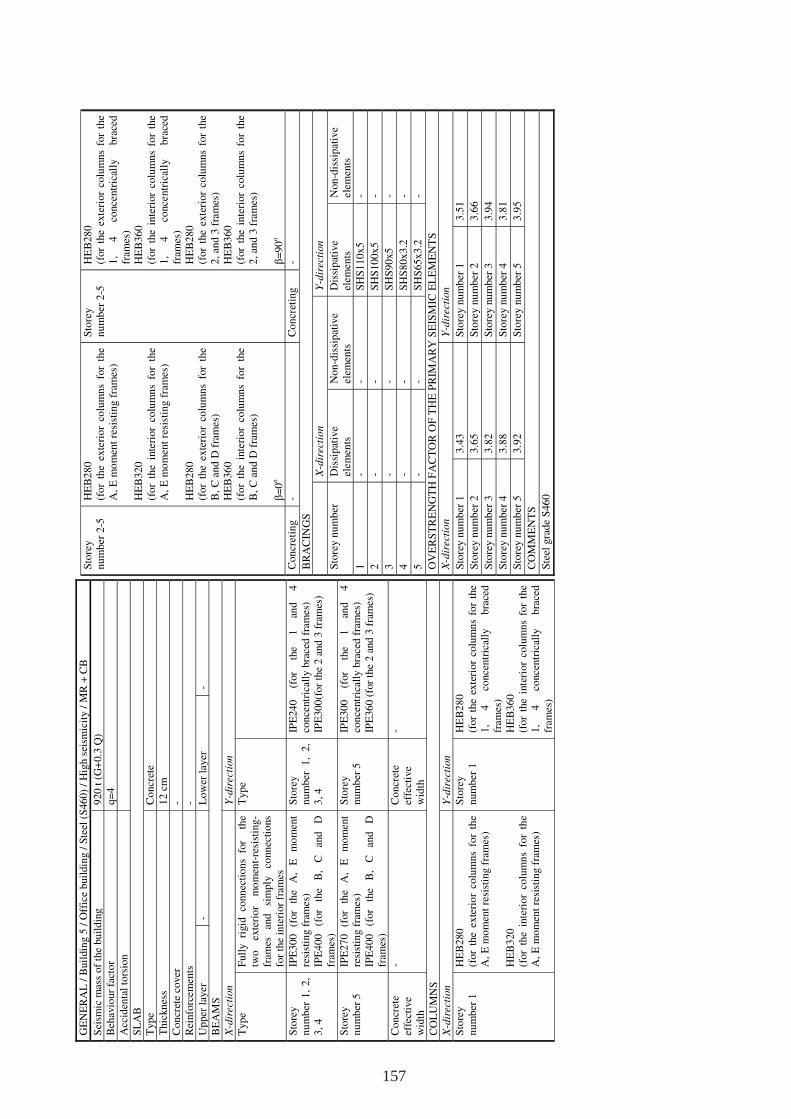
GE
NE
RA
L /
Buil
din
g 5
/ O
ffic
e b
uil
din
g /
Ste
el (
S460
) /
Hig
h s
eism
icit
y /
MR
+ C
B
Sei
smic
mas
s of
the
bu
ild
ing
920
t (
G+
0.3
Q)
Beh
avio
ur
fact
or
q=
4
Acc
iden
tal
tors
ion
SL
AB
T
yp
e C
oncr
ete
Thic
kn
ess
12 c
m
Co
ncr
ete
cover
-
Rei
nfo
rcem
ents
-
Up
per
lay
er
- L
ow
er l
ayer
-
BE
AM
S
X-d
irect
ion
Y-d
irect
ion
Typ
e F
ull
y
rigid
co
nn
ecti
on
s fo
r
the
two
exte
rio
r m
om
ent-
resi
stin
g-
fram
es
and
si
mply
co
nn
ecti
ons
for
the
inte
rior
fram
es
Typ
e
Sto
rey
nu
mb
er 1
, 2,
3,
4
IPE
30
0
(for
the
A,
E
mo
men
t re
sist
ing f
ram
es)
IPE
40
0
(for
the
B,
C
and
D
fr
ames
)
Sto
rey
num
ber
1
, 2,
3, 4
IPE
24
0
(for
the
1
and
4
con
centr
ical
ly b
race
d f
ram
es)
IPE
30
0(f
or
the
2 a
nd
3 f
ram
es)
Sto
rey
nu
mb
er 5
IP
E2
70
(for
the
A,
E
mo
men
t re
sist
ing f
ram
es)
IPE
40
0
(for
the
B,
C
and
D
fr
ames
)
Sto
rey
num
ber
5
IPE
30
0
(for
the
1
and
4
con
centr
ical
ly b
race
d f
ram
es)
IPE
36
0 (
for
the
2 a
nd
3 f
ram
es)
Co
ncr
ete
effe
ctiv
e w
idth
- C
oncr
ete
effe
ctiv
e w
idth
-
CO
LU
MN
S
X-d
irect
ion
Y-d
irect
ion
Sto
rey
nu
mb
er 1
H
EB
280
(f
or
the
exte
rio
r co
lum
ns
for
the
A,
E m
om
ent
resi
stin
g f
ram
es)
HE
B3
20
(f
or
the
inte
rior
colu
mn
s fo
r th
e A
, E
mo
men
t re
sist
ing f
ram
es)
Sto
rey
num
ber
1
HE
B2
80
(for
the
exte
rior
colu
mn
s fo
r th
e 1,
4
conce
ntr
ical
ly
bra
ced
fram
es)
HE
B3
60
(for
the
inte
rior
colu
mns
for
the
1,
4
conce
ntr
ical
ly
bra
ced
fram
es)
Sto
rey
nu
mb
er 2
-5
HE
B2
80
(f
or
the
exte
rio
r co
lum
ns
for
the
A,
E m
om
ent
resi
stin
g f
ram
es)
HE
B3
20
(f
or
the
inte
rior
colu
mn
s fo
r th
e A
, E
mo
men
t re
sist
ing f
ram
es)
HE
B2
80
(f
or
the
exte
rio
r co
lum
ns
for
the
B,
C a
nd
D f
ram
es)
HE
B3
60
(f
or
the
inte
rior
colu
mn
s fo
r th
e B
, C
an
d D
fra
mes
) β
=0ο
Sto
rey
nu
mb
er 2
-5
HE
B2
80
(f
or
the
exte
rior
colu
mn
s fo
r th
e 1
, 4
co
nce
ntr
ical
ly
bra
ced
fram
es)
HE
B3
60
(f
or
the
inte
rior
colu
mn
s fo
r th
e 1
, 4
co
nce
ntr
ical
ly
bra
ced
fram
es)
HE
B2
80
(f
or
the
exte
rior
colu
mn
s fo
r th
e 2
, an
d 3
fra
mes
) H
EB
36
0
(for
the
inte
rior
colu
mn
s fo
r th
e 2
, an
d 3
fra
mes
) β
=9
0ο
Co
ncr
etin
g
- C
on
cret
ing
-
BR
AC
ING
S
X
-dir
ecti
on
Y-d
irec
tion
Sto
rey n
um
ber
D
issi
pat
ive
elem
ents
N
on
-dis
sip
ativ
e el
emen
ts
Dis
sip
ativ
e el
emen
ts
Non
-dis
sip
ativ
e el
emen
ts
1
- -
SH
S1
10
x5
-
2
- -
SH
S1
00
x5
-
3
- -
SH
S9
0x
5
-
4
- -
SH
S8
0x
3.2
-
5
- -
SH
S6
5x
3.2
-
OV
ER
ST
RE
NG
TH
FA
CT
OR
OF
TH
E P
RIM
AR
Y S
EIS
MIC
EL
EM
EN
TS
X-d
irec
tio
n
Y-d
irec
tion
Sto
rey n
um
ber
1
3.4
3
Sto
rey n
um
ber
1
3.5
1
Sto
rey n
um
ber
2
3.6
5
Sto
rey n
um
ber
2
3.6
6
Sto
rey n
um
ber
3
3.8
2
Sto
rey n
um
ber
3
3.9
4
Sto
rey n
um
ber
4
3.8
8
Sto
rey n
um
ber
4
3.8
1
Sto
rey n
um
ber
5
3.9
2
Sto
rey n
um
ber
5
3.9
5
CO
MM
EN
TS
Ste
el g
rad
e S
46
0
157
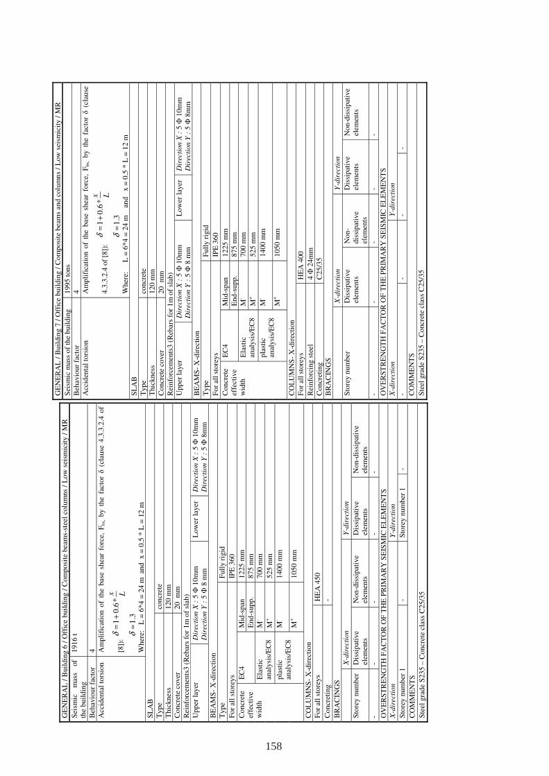
GE
NE
RA
L /
Buil
din
g 6
/ O
ffic
e buil
din
g /
Com
posi
te b
eam
s-st
eel
colu
mns
/ L
ow
sei
smic
ity /
MR
Sei
smic
m
ass
of
the
buil
din
g
1916
t
Beh
avio
ur
fact
or
4
Acc
iden
tal
tors
ion
Am
pli
fica
tion o
f th
e bas
e sh
ear
forc
e, F
bx, b
y t
he
fact
or δ (
clau
se 4
.3.3
.2.4
of
[8])
: 1
0.6
*
1.3
x Lδ δ
=+
=
Wh
ere:
L
= 6
*4 =
24 m
an
d x =
0.5
* L
= 1
2 m
SL
AB
T
ype
con
cret
e
Thic
knes
s 120 m
m
Co
ncr
ete
cover
20 m
m
Rei
nfo
rcem
ents
3 (
Reb
ars
for
1m
of
slab
)
Upp
er l
ayer
D
irec
tion X
: 5
Φ 1
0m
m
Dir
ecti
on Y
: 5
Φ 8
mm
Low
er l
ayer
D
irect
ion X
: 5
Φ 1
0m
m
Dir
ect
ion Y
: 5
Φ 8
mm
BE
AM
S-
X-d
irec
tion
Type
Full
y r
igid
For
all
store
ys
IPE
360
Co
ncr
ete
effe
ctiv
e w
idth
EC
4
Mid
-span
1225
mm
E
nd-s
upp.
875 m
m
Ela
stic
an
alysi
s/E
C8
M-
700 m
m
M+
525 m
m
pla
stic
an
alysi
s/E
C8
M-
1400
mm
M+
1050
mm
CO
LU
MN
S-
X-d
irec
tion
For
all
store
ys
HE
A 4
50
Co
ncr
etin
g
-
BR
AC
ING
S
X
-dir
ect
ion
Y-d
irect
ion
Sto
rey n
um
ber
D
issi
pat
ive
elem
ents
N
on-d
issi
pat
ive
elem
ents
D
issi
pat
ive
elem
ents
N
on-d
issi
pat
ive
elem
ents
-
- -
- -
OV
ER
ST
RE
NG
TH
FA
CT
OR
OF
TH
E P
RIM
AR
Y S
EIS
MIC
EL
EM
EN
TS
X
-dir
ect
ion
Y-d
irec
tion
Sto
rey n
um
ber
1
- S
tore
y n
um
ber
1
-
CO
MM
EN
TS
Ste
el g
rade
S23
5 –
Concr
ete
clas
s C
25/3
5
GE
NE
RA
L /
Bu
ildin
g 7
/ O
ffic
e b
uil
din
g /
Co
mp
osi
te b
eam
s an
d c
olu
mn
s /
Low
sei
smic
ity /
MR
Sei
smic
mas
s o
f th
e b
uil
din
g
19
95
ton
s
Beh
avio
ur
fact
or
4
Acc
iden
tal
tors
ion
Am
pli
fica
tio
n o
f th
e b
ase
shea
r fo
rce,
Fbx,
by t
he
fact
or δ (
clau
se
4.3
.3.2
.4 o
f [8
]):
1
0.6
*
1.3
x Lδ δ
=+
=
Wh
ere:
L =
6*
4 =
24
m
an
d
x =
0.5
* L
= 1
2 m
S
LA
B
Typ
e co
ncr
ete
Thic
kn
ess
12
0 m
m
Co
ncr
ete
cover
2
0
mm
Rei
nfo
rcem
ents
3 (
Reb
ars
for
1m
of
slab
)
Up
per
lay
er
Dir
ect
ion
X :
5 Φ
10
mm
Dir
ect
ion
Y :
5 Φ
8 m
m
Lo
wer
lay
er
Dir
ecti
on
X :
5 Φ
10
mm
Dir
ecti
on
Y :
5 Φ
8m
m
BE
AM
S-
X-d
irec
tio
n
Typ
e F
ull
y r
igid
Fo
r al
l st
ore
ys
IPE
36
0
Co
ncr
ete
effe
ctiv
e w
idth
EC
4
Mid
-sp
an
12
25
mm
En
d-s
up
p.
87
5 m
m
Ela
stic
an
alysi
s/E
C8
M-
70
0 m
m
M+
52
5 m
m
pla
stic
an
alysi
s/E
C8
M-
14
00
mm
M+
10
50
mm
CO
LU
MN
S-
X-d
irec
tio
n
Fo
r al
l st
ore
ys
HE
A 4
00
Rei
nfo
rcin
g s
teel
4
Φ 2
4m
m
Co
ncr
etin
g
C2
5/3
5
BR
AC
ING
S
X
-dir
ecti
on
Y
-dir
ecti
on
Sto
rey n
um
ber
D
issi
pat
ive
elem
ents
N
on
-d
issi
pat
ive
elem
ents
Dis
sip
ativ
e el
emen
ts
No
n-d
issi
pat
ive
elem
ents
- -
- -
-
OV
ER
ST
RE
NG
TH
FA
CT
OR
OF
TH
E P
RIM
AR
Y S
EIS
MIC
EL
EM
EN
TS
X-d
irect
ion
Y-d
irec
tion
- -
- -
CO
MM
EN
TS
Ste
el g
rad
e S
23
5 –
Co
ncr
ete
clas
s C
25/3
5
158
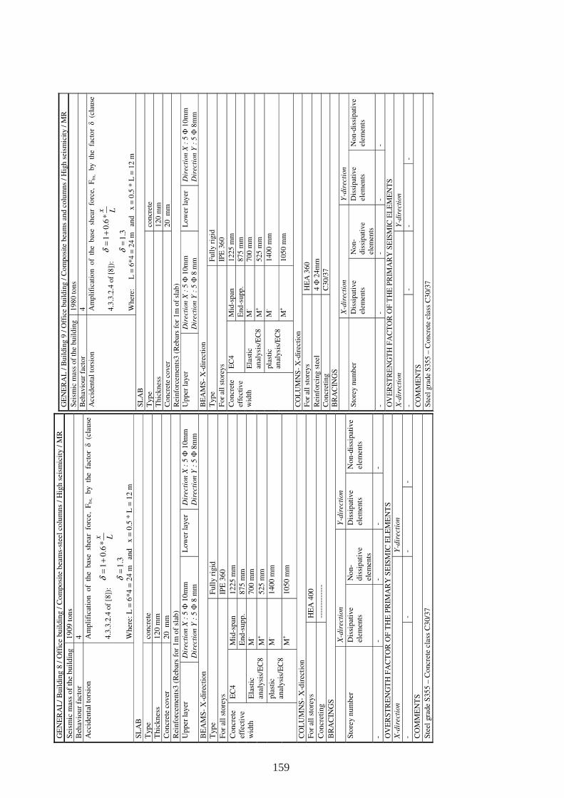
GE
NE
RA
L/
Buil
din
g 8
/ O
ffic
e bu
ildin
g /
Co
mpo
site
bea
ms-
stee
l co
lum
ns
/ H
igh s
eism
icit
y /
MR
Sei
smic
mas
s of
the
buil
din
g
19
09 t
on
s B
ehav
iou
r fa
cto
r 4
Acc
iden
tal
tors
ion
Am
pli
fica
tion of
the
bas
e sh
ear
forc
e, F
bx,
by th
e fa
ctor δ (c
lause
4.3
.3.2
.4 o
f [8
]):
1
0.6
*
1.3
x Lδ δ
=+
=
Wher
e: L
= 6
*4 =
24 m
a
nd
x
= 0
.5 *
L =
12 m
SL
AB
Typ
e co
ncr
ete
Thic
knes
s 12
0 m
m
Concr
ete
cover
20
m
m
Rei
nfo
rcem
ents
3 (
Reb
ars
for
1m
of
slab
) U
pper
lay
er
Dir
ecti
on
X :
5 Φ
10
mm
Dir
ecti
on
Y :
5 Φ
8 m
m
Low
er l
ayer
D
irect
ion
X :
5 Φ
10m
m
Dir
ect
ion
Y :
5 Φ
8m
m
BE
AM
S-
X-d
irec
tion
Typ
e F
ull
y r
igid
For
all
store
ys
IPE
36
0
Concr
ete
effe
ctiv
e w
idth
EC
4
Mid
-sp
an
122
5 m
m
End-s
up
p.
875
mm
E
last
ic
anal
ysi
s/E
C8
M-
700
mm
M+
525
mm
pla
stic
an
alysi
s/E
C8
M-
140
0 m
m
M+
105
0 m
m
CO
LU
MN
S-
X-d
irec
tion
For
all
store
ys
HE
A 4
00
Concr
etin
g
----
----
----
-
BR
AC
ING
S
X
-dir
ecti
on
Y-d
irect
ion
Sto
rey n
um
ber
D
issi
pat
ive
elem
ents
N
on-
dis
sip
ativ
e el
emen
ts
Dis
sip
ativ
e el
emen
ts
Non-d
issi
pat
ive
elem
ents
- -
- -
-
OV
ER
ST
RE
NG
TH
FA
CT
OR
OF
TH
E P
RIM
AR
Y S
EIS
MIC
EL
EM
EN
TS
X-d
irec
tion
Y-d
irect
ion
- -
- -
CO
MM
EN
TS
Ste
el g
rade
S35
5 –
Co
ncr
ete
clas
s C
30/3
7
GE
NE
RA
L /
Buil
din
g 9
/ O
ffic
e buil
din
g /
Com
po
site
bea
ms
and c
olu
mns
/ H
igh
sei
smic
ity /
MR
Sei
smic
mas
s of
the
buil
din
g
198
0 t
ons
Beh
avio
ur
fact
or
4
Acc
iden
tal
tors
ion
Am
pli
fica
tion
of
the
bas
e sh
ear
forc
e, F
bx,
by th
e fa
cto
r δ (c
lause
4.3
.3.2
.4 o
f [8
]):
10
.6*
1.3
x Lδ δ
=+
=
Wher
e: L
= 6
*4 =
24 m
a
nd
x
= 0
.5 *
L =
12
m
SL
AB
Typ
e co
ncr
ete
Thic
knes
s 120 m
m
Concr
ete
cover
20 m
m
Rei
nfo
rcem
ents
3 (
Reb
ars
for
1m
of
slab
) U
pper
lay
er
Dir
ect
ion
X :
5 Φ
10m
m
Dir
ect
ion
Y :
5 Φ
8 m
m
Low
er l
ayer
D
irec
tion X
: 5
Φ 1
0m
m
Dir
ecti
on Y
: 5
Φ 8
mm
BE
AM
S-
X-d
irec
tion
Typ
e F
ull
y r
igid
For
all
store
ys
IPE
36
0
Concr
ete
effe
ctiv
e w
idth
EC
4
Mid
-span
1225
mm
End
-supp.
875 m
m
Ela
stic
an
alysi
s/E
C8
M-
700 m
m
M+
525 m
m
pla
stic
an
alysi
s/E
C8
M-
1400
mm
M+
1050
mm
CO
LU
MN
S-
X-d
irec
tion
For
all
store
ys
HE
A 3
60
Rei
nfo
rcin
g s
teel
4 Φ
24m
m
Concr
etin
g C
30
/37
BR
AC
ING
S
X
-dir
ecti
on
Y-d
irec
tion
Sto
rey n
um
ber
D
issi
pat
ive
elem
ents
N
on-
dis
sipat
ive
elem
ents
Dis
sipat
ive
elem
ents
N
on-d
issi
pat
ive
elem
ents
- -
- -
-
OV
ER
ST
RE
NG
TH
FA
CT
OR
OF
TH
E P
RIM
AR
Y S
EIS
MIC
EL
EM
EN
TS
X-d
irec
tion
Y-d
irect
ion
- -
- -
CO
MM
EN
TS
Ste
el g
rade
S355
– C
oncr
ete
clas
s C
30/3
7
159
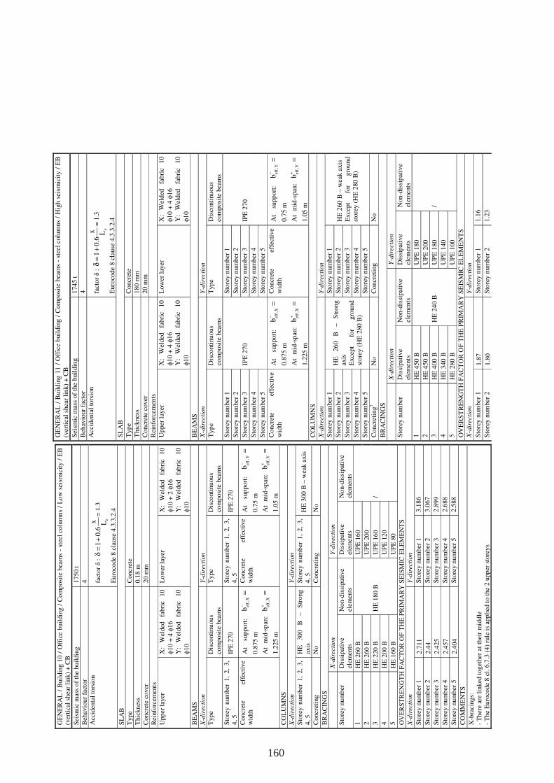
GE
NE
RA
L /
Buil
din
g 1
0 /
Off
ice
buil
din
g /
Co
mp
osi
te b
eam
s -
stee
l co
lum
ns
/ L
ow
sei
smic
ity /
EB
(v
erti
cal
shea
r li
nk)
+ C
B
Sei
smic
mas
s o
f th
e buil
din
g
175
0 t
Beh
avio
ur
fact
or
4
Acc
iden
tal
tors
ion
fact
or δ :
ex
10
.6L
δ=
+=
1.3
Eu
roco
de
8 c
lause
4.3
.3.2
.4
SL
AB
T
ype
Concr
ete
Thi
ckn
ess
0.1
8 m
Co
ncr
ete
cover
2
0 m
m
Rei
nfo
rcem
ents
Up
per
lay
er
X:
Wel
ded
fa
bric
1
0
φ10
+ 4
φ1
6
Y:
Wel
ded
fa
bric
1
0
φ10
Lo
wer
lay
er
X:
Wel
ded
fa
bri
c 1
0
φ1
0 +
2 φ
16
Y
: W
elded
fa
bri
c 1
0
φ1
0
BE
AM
S
X-d
irec
tio
n
Y-d
irec
tion
Typ
e D
isco
nti
nuo
us
com
posi
te b
eam
s T
ype
Dis
cont
inuo
us
com
posi
te b
eam
s
Sto
rey n
um
ber
1,
2,
3,
4,
5
IPE
270
S
tore
y n
um
ber
1,
2,
3,
4, 5
IP
E 2
70
Co
ncr
ete
effe
ctiv
e w
idth
A
t su
pp
ort
: ef
f,X
b−
=
0.8
75
m
At
mid
-sp
an:
eff
,Xb
+=
1.2
25
m
Concr
ete
effe
ctiv
e w
idth
A
t su
ppo
rt:
eff
,Yb
−=
0.7
5 m
At
mid
-span
: ef
f,Y
b+
=
1.0
5 m
CO
LU
MN
S
X-d
irec
tio
n
Y-d
irec
tion
Sto
rey n
um
ber
1,
2,
3,
4,
5
HE
3
00
B
–
Str
on
g
axis
S
tore
y n
um
ber
1,
2,
3,
4, 5
H
E 3
00
B –
wea
k a
xis
Co
ncr
etin
g N
o
Concr
etin
g N
o
BR
AC
ING
S
X
-dir
ecti
on
Y-d
irec
tion
Sto
rey n
um
ber
D
issi
pat
ive
elem
ents
N
on
-dis
sipat
ive
elem
ents
D
issi
pat
ive
elem
ents
N
on-d
issi
pat
ive
elem
ents
1
HE
260
B
HE
180
B
UP
E 1
60
/
2
HE
260
B
UP
E 2
00
3
HE
220
B
UP
E 1
60
4
HE
200
B
UP
E 1
20
5
HE
160
B
UP
E 8
0
OV
ER
ST
RE
NG
TH
FA
CT
OR
OF
TH
E P
RIM
AR
Y S
EIS
MIC
EL
EM
EN
TS
X-d
irec
tio
n
Y-d
irec
tion
Sto
rey n
um
ber
1
2.7
11
Sto
rey n
um
ber
1
3.1
86
Sto
rey n
um
ber
2
2.4
4 S
tore
y n
um
ber
2
3.0
67
Sto
rey n
um
ber
3
2.4
25
Sto
rey n
um
ber
3
2.8
99
Sto
rey n
um
ber
4
2.4
57
Sto
rey n
um
ber
4
2.6
88
Sto
rey n
um
ber
5
2.4
04
Sto
rey n
um
ber
5
2.5
88
CO
MM
EN
TS
X-b
raci
ngs:
-
Ther
e ar
e li
nked
to
get
her
at
thei
r m
idd
le
- T
he
Euro
cod
e 8
cl.
6.7
.3 (
4)
rule
is
appli
ed t
o t
he
2 upper
sto
reys
GE
NE
RA
L /
Buil
din
g 1
1 /
Off
ice
buil
din
g /
Com
po
site
bea
ms
- st
eel
colu
mn
s /
Hig
h s
eism
icit
y /
EB
(v
erti
cal
shea
r li
nk)
+ C
B
Sei
smic
mas
s o
f th
e bu
ild
ing
1
74
5 t
Beh
avio
ur
fact
or
4
Acc
iden
tal
tors
ion
fact
or δ :
ex
10
.6L
δ=
+=
1.3
Eu
roco
de
8 c
lause
4.3
.3.2
.4
SL
AB
Ty
pe
Co
ncr
ete
Th
ickn
ess
18
0 m
m
Co
ncr
ete
cover
2
0 m
m
Rei
nfo
rcem
ents
Up
per
lay
er
X:
Wel
ded
fa
bri
c 1
0
φ1
0 +
4 φ
16
Y
: W
elded
fa
bri
c 1
0
φ1
0
Lo
wer
lay
er
X:
Wel
ded
fa
bri
c 1
0
φ1
0 +
4 φ
16
Y:
Wel
ded
fa
bri
c 1
0
φ1
0
BE
AM
S
X-d
irect
ion
Y
-dir
ect
ion
Ty
pe
Dis
conti
nu
ous
com
posi
te b
eam
s T
yp
e D
isco
nti
nu
ou
s co
mp
osi
te b
eam
s
Sto
rey n
um
ber
1
IPE
270
Sto
rey n
um
ber
1
IPE
27
0
Sto
rey n
um
ber
2
Sto
rey n
um
ber
2
Sto
rey n
um
ber
3
Sto
rey n
um
ber
3
Sto
rey n
um
ber
4
Sto
rey n
um
ber
4
Sto
rey n
um
ber
5
Sto
rey n
um
ber
5
Co
ncr
ete
effe
ctiv
e w
idth
A
t su
pp
ort
: ef
f,X
b−
=
0.8
75
m
At
mid
-sp
an:
eff
,Xb
+=
1.2
25
m
Co
ncr
ete
effe
ctiv
e w
idth
A
t su
pp
ort
: ef
f,Y
b−
=
0.7
5 m
At
mid
-sp
an:
eff
,Yb
+=
1.0
5 m
C
OL
UM
NS
X-d
irect
ion
Y
-dir
ect
ion
Sto
rey n
um
ber
1
HE
2
60
B
–
Str
on
g
axis
E
xce
pt
for
gro
un
d
sto
rey
(H
E 2
80
B)
Sto
rey n
um
ber
1
HE
26
0 B
– w
eak a
xis
E
xce
pt
for
gro
un
d
sto
rey (
HE
280
B)
Sto
rey n
um
ber
2
Sto
rey n
um
ber
2
Sto
rey n
um
ber
3
Sto
rey n
um
ber
3
Sto
rey n
um
ber
4
Sto
rey n
um
ber
4
Sto
rey n
um
ber
5
Sto
rey n
um
ber
5
Co
ncr
etin
g7
No
Co
ncr
etin
g N
o
BR
AC
ING
S
X
-dir
ecti
on
Y-d
irect
ion
Sto
rey n
um
ber
D
issi
pat
ive
elem
ents
N
on
-dis
sip
ativ
e el
emen
ts
Dis
sip
ativ
e el
emen
ts
No
n-d
issi
pat
ive
elem
ents
1
H
E 4
50 B
HE
24
0 B
UP
E 1
80
/
2
HE
45
0 B
U
PE
20
0
3
HE
40
0 B
U
PE
18
0
4
HE
34
0 B
U
PE
14
0
5
HE
28
0 B
U
PE
10
0
OV
ER
ST
RE
NG
TH
FA
CT
OR
OF
TH
E P
RIM
AR
Y S
EIS
MIC
EL
EM
EN
TS
X-d
irect
ion
Y
-dir
ect
ion
Sto
rey n
um
ber
1
1.8
7
Sto
rey n
um
ber
1
1.1
6
Sto
rey n
um
ber
2
1.8
0
Sto
rey n
um
ber
2
1.2
3
160
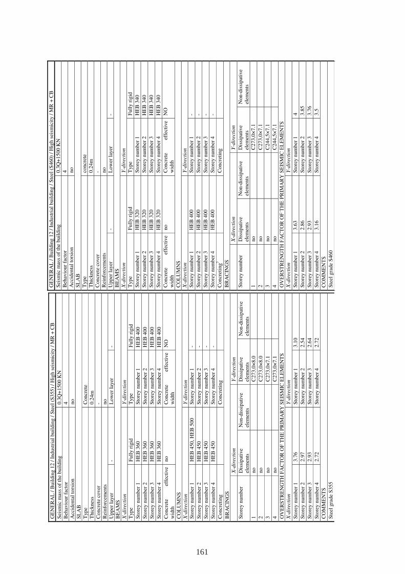
GE
NE
RA
L /
Bu
ildin
g 1
2 /
Ind
ust
rial
buil
din
g /
Ste
el (
S3
55
) /
Hig
h s
eism
icit
y /
MR
+ C
B
Sei
smic
mas
s o
f th
e buil
din
g
0.3
Q+
1500
KN
B
ehav
iour
fact
or
4
Acc
iden
tal
tors
ion
no
SL
AB
T
yp
e C
on
cret
e
Thic
knes
s 0.2
4m
C
oncr
ete
cover
-
Rei
nfo
rcem
ents
no
Up
per
lay
er
- L
ow
er l
ayer
-
BE
AM
S
X-d
irect
ion
Y-d
irect
ion
Typ
e F
ull
y r
igid
T
ype
Fu
lly r
igid
Sto
rey n
um
ber
1
HE
B 3
60
S
tore
y n
um
ber
1
HE
B 4
00
Sto
rey n
um
ber
2
HE
B 3
60
S
tore
y n
um
ber
2
HE
B 4
00
Sto
rey n
um
ber
3
HE
B 3
60
S
tore
y n
um
ber
3
HE
B 4
00
Sto
rey n
um
ber
4
HE
B 3
60
S
tore
y n
um
ber
4
HE
B 4
00
Co
ncr
ete
effe
ctiv
e w
idth
n
o
Con
cret
e ef
fect
ive
wid
th
NO
CO
LU
MN
S
X-d
irect
ion
Y-d
irect
ion
Sto
rey n
um
ber
1
HE
B 4
50
, H
EB
50
0
Sto
rey n
um
ber
1
-
Sto
rey n
um
ber
2
HE
B 4
50
S
tore
y n
um
ber
2
-
Sto
rey n
um
ber
3
HE
B 4
50
S
tore
y n
um
ber
3
-
Sto
rey n
um
ber
4
HE
B 4
50
S
tore
y n
um
ber
4
-
Co
ncr
etin
g
C
on
cret
ing
BR
AC
ING
S
X
-dir
ect
ion
Y-d
irec
tion
Sto
rey n
um
ber
D
issi
pat
ive
elem
ents
N
on-d
issi
pat
ive
elem
ents
D
issi
pat
ive
elem
ents
N
on
-dis
sip
ativ
e el
emen
ts
1
no
C273
,0×
8.0
2
no
C273
,0×
8.0
3
no
C273
,0×
7.1
4
no
C273
,0×
7.1
OV
ER
ST
RE
NG
TH
FA
CT
OR
OF
TH
E P
RIM
AR
Y S
EIS
MIC
EL
EM
EN
TS
X-d
irect
ion
Y-d
irect
ion
Sto
rey n
um
ber
1
3.7
6
Sto
rey n
um
ber
1
3.1
0
Sto
rey n
um
ber
2
2.9
7
Sto
rey n
um
ber
2
2.5
4
Sto
rey n
um
ber
3
2.9
3
Sto
rey n
um
ber
3
2.6
4
Sto
rey n
um
ber
4
2.7
2
Sto
rey n
um
ber
4
2.7
2
CO
MM
EN
TS
Ste
el g
rade
S355
GE
NE
RA
L /
Buil
din
g 1
2 /
Ind
ust
rial
buil
din
g /
Ste
el (
S46
0)
/ H
igh s
eism
icit
y /
MR
+ C
B
Sei
smic
mas
s of
the
bu
ildin
g
0.3
Q+
15
00
KN
Beh
avio
ur
fact
or
4
Acc
iden
tal
tors
ion
no
SL
AB
Type
concr
ete
Thic
kn
ess
0.2
4m
C
on
cret
e co
ver
-
Rei
nfo
rcem
ents
n
o
Up
per
lay
er
- L
ow
er l
ayer
-
BE
AM
S
X-d
irect
ion
Y-d
irect
ion
Type
Fu
lly r
igid
T
ype
Fu
lly r
igid
Sto
rey n
um
ber
1
HE
B 3
20
S
tore
y n
um
ber
1
HE
B 3
40
Sto
rey n
um
ber
2
HE
B 3
20
S
tore
y n
um
ber
2
HE
B 3
40
Sto
rey n
um
ber
3
HE
B 3
20
S
tore
y n
um
ber
3
HE
B 3
40
Sto
rey n
um
ber
4
HE
B 3
20
S
tore
y n
um
ber
4
HE
B 3
40
Con
cret
e ef
fect
ive
wid
th
no
C
on
cret
e ef
fect
ive
wid
th
NO
CO
LU
MN
S
X-d
irect
ion
Y-d
irect
ion
Sto
rey n
um
ber
1
HE
B 4
00
S
tore
y n
um
ber
1
-
Sto
rey n
um
ber
2
HE
B 4
00
S
tore
y n
um
ber
2
-
Sto
rey n
um
ber
3
HE
B 4
00
S
tore
y n
um
ber
3
-
Sto
rey n
um
ber
4
HE
B 4
00
S
tore
y n
um
ber
4
-
Con
cret
ing
7
C
on
cret
ing
BR
AC
ING
S
X
-dir
ect
ion
Y-d
irect
ion
Sto
rey n
um
ber
D
issi
pat
ive
elem
ents
N
on
-dis
sip
ativ
e el
emen
ts
Dis
sipat
ive
elem
ents
N
on
-dis
sipat
ive
elem
ents
1
no
C2
73
,0×
7.1
2
no
C2
73
,0×
7.1
3
no
C2
44
,5×
7.1
4
no
C2
44
,5×
7.1
OV
ER
ST
RE
NG
TH
FA
CT
OR
OF
TH
E P
RIM
AR
Y S
EIS
MIC
EL
EM
EN
TS
X-d
irect
ion
Y-d
irect
ion
Sto
rey n
um
ber
1
3.6
3
Sto
rey n
um
ber
1
4
Sto
rey n
um
ber
2
2.8
6
Sto
rey n
um
ber
2
3.8
5
Sto
rey n
um
ber
3
2.9
3
Sto
rey n
um
ber
3
3.7
6
Sto
rey n
um
ber
4
3.1
6
Sto
rey n
um
ber
4
3.5
CO
MM
EN
TS
Ste
el g
rade
S46
0
161
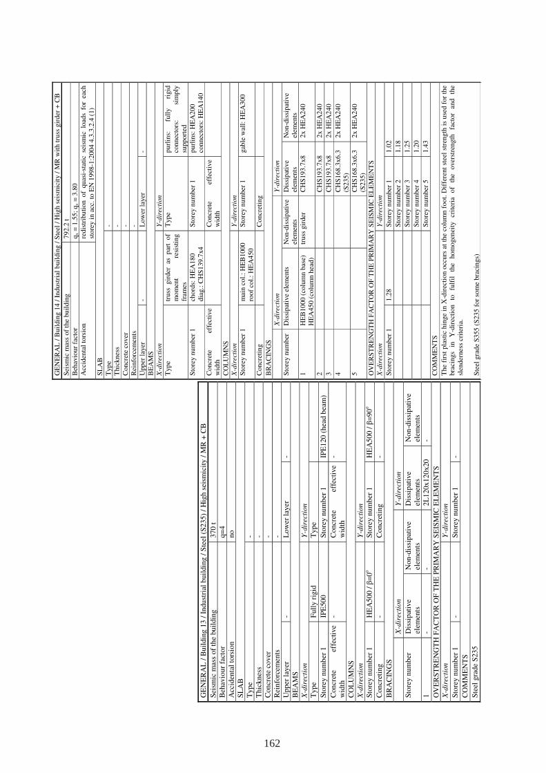
GE
NE
RA
L /
Bu
ildin
g 1
3 /
In
du
stri
al b
uil
din
g /
Ste
el (
S2
35)
/ H
igh
sei
smic
ity /
MR
+ C
B
Sei
smic
mas
s of
the
bu
ildin
g
37
0 t
B
ehav
iou
r fa
cto
r q=
4
Acc
iden
tal
tors
ion
no
SL
AB
Type
-
Thic
kn
ess
- C
on
cret
e co
ver
-
Rei
nfo
rcem
ents
-
Up
per
lay
er
- L
ow
er l
ayer
-
BE
AM
S
X-d
irec
tion
Y-d
irec
tion
Type
Full
y r
igid
T
yp
e
Sto
rey n
um
ber
1
IPE
50
0
Sto
rey n
um
ber
1
IPE
120
(h
ead b
eam
)
Con
cret
e ef
fect
ive
wid
th
- C
oncr
ete
effe
ctiv
e w
idth
-
CO
LU
MN
S
X-d
irec
tion
Y-d
irec
tion
Sto
rey n
um
ber
1
HE
A5
00 /
β=
0ο
S
tore
y n
um
ber
1
HE
A5
00
/ β
=9
0ο
Con
cret
ing
- C
oncr
etin
g -
BR
AC
ING
S
X
-dir
ecti
on
Y-d
irec
tion
Sto
rey n
um
ber
D
issi
pat
ive
elem
ents
N
on
-dis
sipat
ive
elem
ents
D
issi
pat
ive
elem
ents
N
on
-dis
sip
ativ
e el
emen
ts
1
- -
2L
12
0x
12
0x20
-
OV
ER
ST
RE
NG
TH
FA
CT
OR
OF
TH
E P
RIM
AR
Y S
EIS
MIC
EL
EM
EN
TS
X
-dir
ecti
on
Y-d
irec
tion
Sto
rey n
um
ber
1
- S
tore
y n
um
ber
1
-
CO
MM
EN
TS
Ste
el g
rad
e S
23
5
GE
NE
RA
L /
Buil
din
g 1
4 /
In
dust
rial
buil
din
g /
Ste
el /
Hig
h s
eism
icit
y /
MR
wit
h t
russ
gir
der
+ C
B
Sei
smic
mas
s of
the
bu
ildin
g
792.2
t
Beh
avio
ur
fact
or
qx
= 1
.55;
qy =
3.8
0
Acc
iden
tal
tors
ion
redis
trib
uti
on o
f quas
i-st
atic
sei
smic
load
s fo
r ea
ch
store
y i
n a
cc.
to E
N 1
998-1
:2004
4.3
.3.2
.4 (
1)
SL
AB
Typ
e -
Thic
knes
s -
Concr
ete
cover
-
Rei
nfo
rcem
ents
-
Upp
er l
ayer
-
Low
er l
ayer
-
BE
AM
S
X-d
irect
ion
Y-d
irect
ion
Typ
e tr
uss
gir
der
as
p
art
of
m
om
ent
resi
stin
g
fram
es
Typ
e pu
rlin
s:
full
y
rigid
co
nn
ecto
rs:
sim
ply
su
pport
ed
Sto
rey n
um
ber
1
chord
s: H
EA
18
0
dia
g.:
CH
S1
39.7
x4
Sto
rey n
um
ber
1
pu
rlin
s: H
EA
200
conn
ecto
rs:
HE
A14
0
Concr
ete
effe
ctiv
e w
idth
Concr
ete
effe
ctiv
e w
idth
CO
LU
MN
S
X-d
irect
ion
Y-d
irect
ion
Sto
rey n
um
ber
1
mai
n c
ol.
: H
EB
1000
roof
col.
: H
EA
450
Sto
rey n
um
ber
1
gab
le w
all:
HE
A30
0
Concr
etin
g
C
oncr
etin
g
BR
AC
ING
S
X
-dir
ect
ion
Y-d
irect
ion
Sto
rey n
um
ber
D
issi
pat
ive
elem
ents
N
on
-dis
sip
ativ
e el
emen
ts
Dis
sip
ativ
e el
emen
ts
Non
-dis
sip
ativ
e el
emen
ts
1
HE
B10
00 (
colu
mn
bas
e)
HE
A450
(co
lum
n h
ead)
truss
gir
der
C
HS
193
.7x8
2x H
EA
240
2
CH
S193
.7x8
2x H
EA
240
3
CH
S193
.7x8
2x H
EA
240
4
CH
S168
.3x6
.3
(S2
35)
2x H
EA
240
5
CH
S168
.3x6
.3
(S2
35)
2x H
EA
240
OV
ER
ST
RE
NG
TH
FA
CT
OR
OF
TH
E P
RIM
AR
Y S
EIS
MIC
EL
EM
EN
TS
X-d
irect
ion
Y-d
irect
ion
Sto
rey n
um
ber
1
1.2
8
Sto
rey n
um
ber
1
1.0
2
Sto
rey n
um
ber
2
1.1
8
Sto
rey n
um
ber
3
1.2
5
Sto
rey n
um
ber
4
1.2
0
Sto
rey n
um
ber
5
1.4
3
CO
MM
EN
TS
The
firs
t pla
stic
hin
ge
in X
-dir
ecti
on o
ccurs
at
the
colu
mn f
oo
t. D
iffe
rent
stee
l st
rength
is
use
d f
or
the
bra
cings
in
Y-d
irec
tion
to
fulf
il
the
hom
ogen
eity
cr
iter
ia
of
the
over
stre
ngth
fa
ctor
and
the
slen
der
nes
s cr
iter
ia.
Ste
el g
rad
e S
355
(S
235 f
or
som
e bra
cings)
162
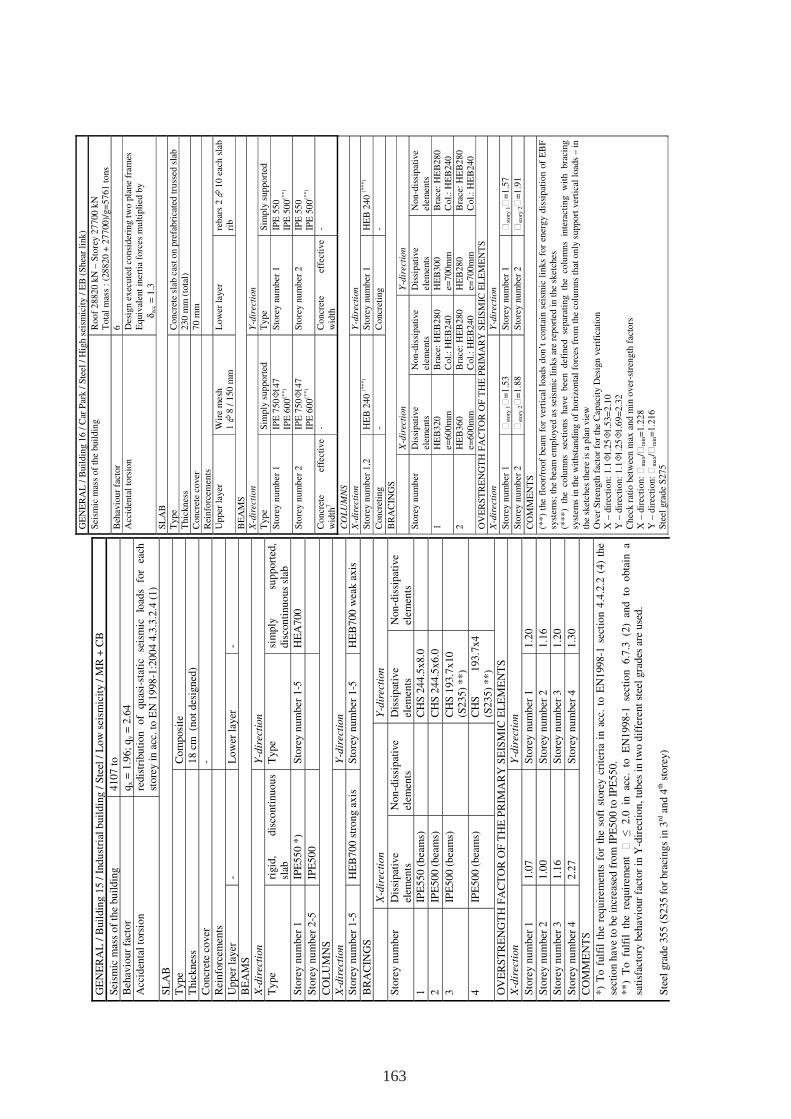
GE
NE
RA
L /
Buil
din
g 1
5 /
Ind
ust
rial
buil
din
g /
Ste
el /
Lo
w s
eism
icit
y /
MR
+ C
B
Sei
smic
mas
s o
f th
e bu
ild
ing
4
107
to
Beh
avio
ur
fact
or
qx =
1.9
6;
qy =
2.6
4
Acc
iden
tal
tors
ion
redis
trib
uti
on
of
qu
asi-
stat
ic
seis
mic
lo
ads
for
each
st
ore
y i
n a
cc. to
EN
19
98
-1:2
00
4 4
.3.3
.2.4
(1)
SL
AB
Type
Co
mp
osi
te
Thic
kn
ess
18
cm
(n
ot
des
ign
ed)
Con
cret
e co
ver
-
Rei
nfo
rcem
ents
Up
per
lay
er
- L
ow
er l
ayer
-
BE
AM
S
X-d
irec
tion
Y-d
irec
tion
Type
rigid
, dis
conti
nu
ou
s sl
ab
Typ
e si
mp
ly
sup
port
ed,
dis
con
tinu
ous
slab
Sto
rey n
um
ber
1
IPE
55
0 *
) S
tore
y n
um
ber
1-5
H
EA
700
Sto
rey n
um
ber
2-5
IP
E5
00
CO
LU
MN
S
X-d
irec
tion
Y-d
irec
tion
Sto
rey n
um
ber
1-5
H
EB
70
0 s
tro
ng a
xis
S
tore
y n
um
ber
1-5
H
EB
700
wea
k a
xis
BR
AC
ING
S
X
-dir
ecti
on
Y-d
irec
tion
Sto
rey n
um
ber
D
issi
pat
ive
elem
ents
N
on
-dis
sip
ativ
e el
emen
ts
Dis
sip
ativ
e el
emen
ts
Non
-dis
sip
ativ
e el
emen
ts
1
IPE
55
0 (
bea
ms)
CH
S 2
44
.5x
8.0
2
IPE
50
0 (
bea
ms)
CH
S 2
44
.5x
6.0
3
IPE
50
0 (
bea
ms)
CH
S 1
93
.7x
10
(S2
35
) *
*)
4
IPE
50
0 (
bea
ms)
CH
S
193
.7x
4
(S2
35
) *
*)
OV
ER
ST
RE
NG
TH
FA
CT
OR
OF
TH
E P
RIM
AR
Y S
EIS
MIC
EL
EM
EN
TS
X-d
irec
tion
Y-d
irec
tion
Sto
rey n
um
ber
1
1.0
7
Sto
rey n
um
ber
1
1.2
0
Sto
rey n
um
ber
2
1.0
0
Sto
rey n
um
ber
2
1.1
6
Sto
rey n
um
ber
3
1.1
6
Sto
rey n
um
ber
3
1.2
0
Sto
rey n
um
ber
4
2.2
7
Sto
rey n
um
ber
4
1.3
0
CO
MM
EN
TS
*)
To
fulf
il t
he
req
uir
emen
ts f
or
the
soft
sto
rey c
rite
ria
in a
cc.
to E
N1
998
-1 s
ecti
on 4
.4.2
.2 (
4)
the
sect
ion
hav
e to
be
incr
ease
d f
rom
IP
E5
00
to I
PE
55
0.
**
) T
o
fulf
il
the
req
uir
emen
t
≤
2
.0
in
acc.
to
E
N1
99
8-1
se
ctio
n
6.7
.3
(2)
and
to
obta
in
a sa
tisf
acto
ry b
ehav
iour
fact
or
in Y
-dir
ecti
on
, tu
bes
in t
wo
dif
fere
nt
stee
l gra
des
are
use
d.
Ste
el g
rad
e 35
5 (
S23
5 f
or
bra
cings
in 3
rd a
nd
4th s
tore
y)
GE
NE
RA
L /
Bu
ildin
g 1
6 /
Car
Par
k /
Ste
el /
Hig
h s
eism
icit
y /
EB
(S
hea
r li
nk
)
Sei
smic
mas
s o
f th
e bu
ild
ing
R
oo
f 2
882
0 k
N –
Sto
rey
27
700
kN
T
ota
l m
ass
: (2
88
20
+ 2
77
00
)/g=
57
61
to
ns
Beh
avio
ur
fact
or
6
Acc
iden
tal
tors
ion
Des
ign
ex
ecu
ted
co
nsi
der
ing t
wo
pla
ne
fram
es
Eq
uiv
alen
t in
erti
a fo
rces
mu
ltip
lied
by
δec
c =
1.3
S
LA
B
Typ
e C
on
cret
e sl
ab c
ast
on
pre
fab
rica
ted
tru
ssed
sla
b
Thic
kn
ess
23
0 m
m (
tota
l)
Co
ncr
ete
cover
7
0 m
m
Rei
nfo
rcem
ents
Up
per
lay
er
Wir
e m
esh
1
8
/ 1
50
mm
L
ow
er l
ayer
re
bar
s 2
1
0 e
ach
sla
b
rib
BE
AM
S
X-d
irect
ion
Y-d
irect
ion
Typ
e S
imp
ly s
up
po
rted
T
ype
Sim
ply
sup
po
rted
Sto
rey n
um
ber
1
IPE
75
0
14
7
IPE
60
0(*
*)
Sto
rey n
um
ber
1
IPE
55
0
IPE
50
0(*
*)
Sto
rey n
um
ber
2
IPE
75
0
14
7
IPE
60
0(*
*)
Sto
rey n
um
ber
2
IPE
55
0
IPE
50
0(*
*)
Co
ncr
ete
effe
ctiv
e w
idth
7
- C
on
cret
e ef
fect
ive
wid
th
-
CO
LU
MN
S
X-d
irect
ion
Y-d
irect
ion
Sto
rey n
um
ber
1,2
H
EB
24
0 (*
**)
Sto
rey n
um
ber
1
HE
B 2
40
(**
*)
Co
ncr
etin
g
- C
on
cret
ing
-
BR
AC
ING
S
X
-dir
ecti
on
Y-d
irect
ion
Sto
rey n
um
ber
D
issi
pat
ive
elem
ents
N
on
-dis
sip
ativ
e el
emen
ts
Dis
sip
ativ
e el
emen
ts
No
n-d
issi
pat
ive
elem
ents
1
H
EB
32
0
e=6
00
mm
B
race
: H
EB
28
0
Co
l.:
HE
B2
40
HE
B3
00
e=
700
mm
B
race
: H
EB
28
0
Co
l.:
HE
B2
40
2
H
EB
36
0
e=6
00
mm
B
race
: H
EB
28
0
Co
l.:
HE
B2
40
HE
B2
80
e=
700
mm
B
race
: H
EB
28
0
Co
l.:
HE
B2
40
O
VE
RS
TR
EN
GT
H F
AC
TO
R O
F T
HE
PR
IMA
RY
SE
ISM
IC E
LE
ME
NT
S
X-d
irect
ion
Y-d
irect
ion
Sto
rey n
um
ber
1
st
ory
1
=1
.53
Sto
rey n
um
ber
1
st
ory
1
=1
.57
Sto
rey n
um
ber
2
st
ory
2
=1
.88
Sto
rey n
um
ber
2
st
ory
2
=1
.91
CO
MM
EN
TS
(**
) th
e fl
oor/
roo
f bea
m f
or
ver
tica
l lo
ads
do
n’t
co
nta
in s
eism
ic l
inks
for
ener
gy
dis
sip
atio
n o
f E
BF
sy
stem
s; t
he
bea
m e
mp
loyed
as
seis
mic
lin
ks
are
rep
ort
ed i
n t
he
sket
ches
(*
**
) th
e co
lum
ns
sect
ion
s h
ave
bee
n
def
ined
se
par
atin
g
the
colu
mn
s in
tera
ctin
g
wit
h
bra
cing
syst
ems
in t
he
wit
hst
and
ing
of
ho
rizo
nta
l fo
rces
fro
m t
he
colu
mn
s th
at o
nly
su
pp
ort
ver
tica
l lo
ads
– i
n
the
sket
ches
ther
e is
a p
lan
vie
w
Over
Str
ength
fac
tor
for
the
Cap
acit
y D
esig
n v
erif
icat
ion
X
– d
irec
tio
n:
1.1
1.2
5
1.5
3=
2.1
0
Y –
dir
ecti
on:
1.1
1.2
5
1.6
9=
2.3
2
Ch
eck r
atio
bet
wee
n m
ax a
nd
min
over
-str
eng
th f
acto
rs
X –
dir
ecti
on:
max/
min=
1.2
28
Y
– d
irec
tio
n:
max/
min=
1.2
16
S
teel
gra
de
S2
75
163

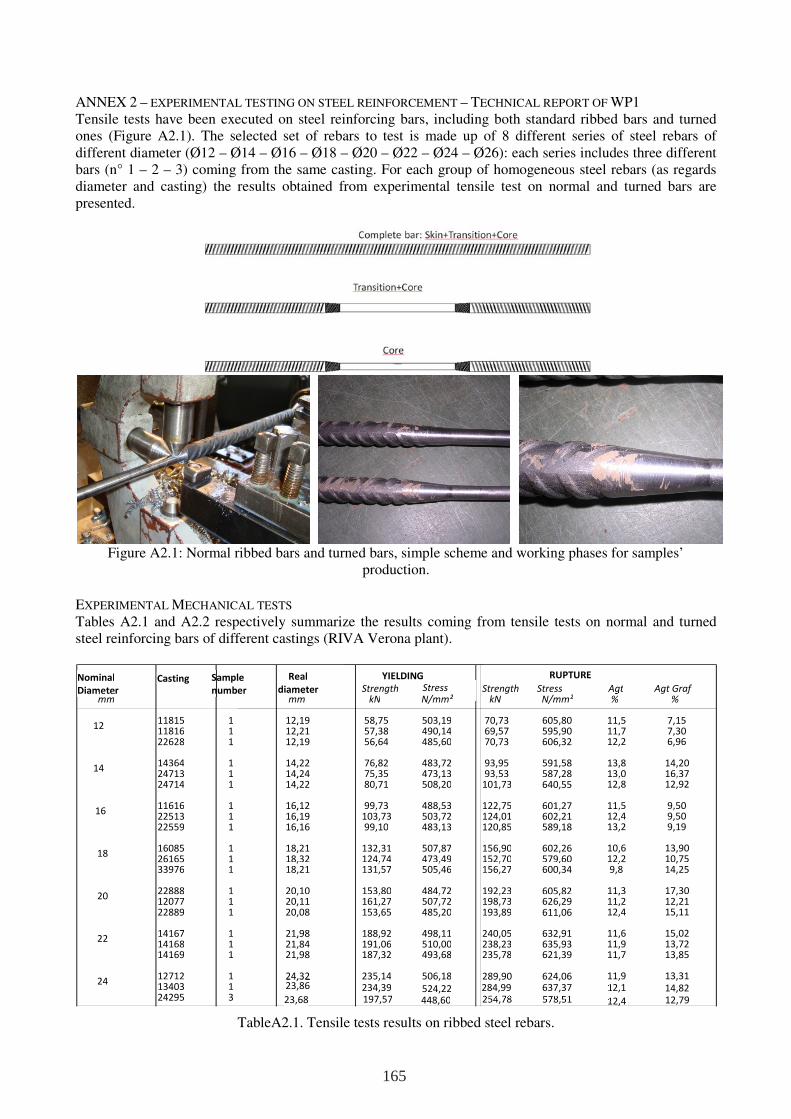
ANNEX 2 – EXPERIMENTAL TESTING ON STEEL REINFORCEMENT – TECHNICAL REPORT OF WP1 Tensile tests have been executed on steel reinforcing bars, including both standard ribbed bars and turned ones (Figure A2.1). The selected set of rebars to test is made up of 8 different series of steel rebars of different diameter (Ø12 – Ø14 – Ø16 – Ø18 – Ø20 – Ø22 – Ø24 – Ø26): each series includes three different bars (n° 1 – 2 – 3) coming from the same casting. For each group of homogeneous steel rebars (as regards diameter and casting) the results obtained from experimental tensile test on normal and turned bars are presented.
Figure A2.1: Normal ribbed bars and turned bars, simple scheme and working phases for samples’ production.
EXPERIMENTAL MECHANICAL TESTS Tables A2.1 and A2.2 respectively summarize the results coming from tensile tests on normal and turned steel reinforcing bars of different castings (RIVA Verona plant).
TableA2.1. Tensile tests results on ribbed steel rebars.
197,57 448,60 254,78 578,51 12,4 12,79
RUPTUREYIELDING
12
16
14
18
20
24
22
23,68
Nominal
Diameter Casting Sample
number
Real
diameter Strength Stress Strength Stress Agt Agt Graf mm mm kN N/mm² kN N/mm² % %
11815 1 12,19 58,75 503,19 70,73 605,80 11,5 7,1511816 1 12,21 57,38 490,14 69,57 595,90 11,7 7,3022628 1 12,19 56,64 485,60 70,73 606,32 12,2 6,96
14364 1 14,22 76,82 483,72 93,95 591,58 13,8 14,20 24713 1 14,24 75,35 473,13 93,53 587,28 13,0 16,37 24714 1 14,22 80,71 508,20 101,73 640,55 12,8 12,92
11616 1 16,12 99,73 488,53 122,75 601,27 11,5 9,5022513 1 16,19 103,73 503,72 124,01 602,21 12,4 9,5022559 1 16,16 99,10 483,13 120,85 589,18 13,2 9,19
16085 1 18,21 132,31 507,87 156,90 602,26 10,6 13,90 26165 1 18,32 124,74 473,49 152,70 579,60 12,2 10,75 33976 1 18,21 131,57 505,46 156,27 600,34 9,8 14,25
22888 1 20,10 153,80 484,72 192,23 605,82 11,3 17,30 12077 1 20,11 161,27 507,72 198,73 626,29 11,2 12,21 22889 1 20,08 153,65 485,20 193,89 611,06 12,4 15,11
14167 1 21,98 188,92 498,11 240,05 632,91 11,6 15,02 14168 1 21,84 191,06 510,00 238,23 635,93 11,9 13,72 14169 1 21,98 187,32 493,68 235,78 621,39 11,7 13,85
12712 1 24,32 235,14 506,18 289,90 624,06 11,9 13,31 13403 1 23,8624295 3
234,39 14,82 12,1 637,37 284,99 524,22
165
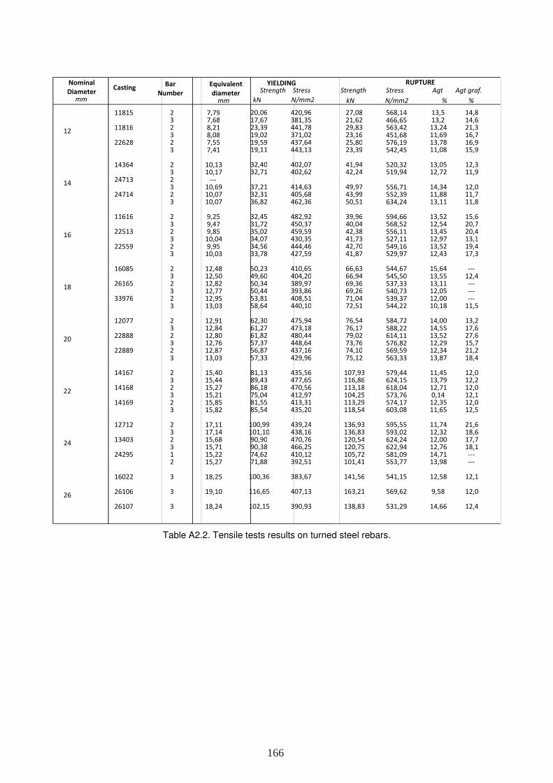
Table A2.2. Tensile tests results on turned steel rebars.
Nominal
Diameter Casting
Bar
Number
Equivalent
diameter Strength Stress Strength Stress Agt Agt graf.
mm mm kN N/mm2 kN N/mm2 % %
11815 2 7,79 20,06 420,96 27,08 568,14 13,5 14,83 7,68 17,67 381,35 21,62 466,65 13,2 14,6
11816 2 8,21 23,39 441,78 29,83 563,42 13,24 21,33 8,08 19,02 371,02 23,16 451,68 11,69 16,7
22628 2 7,55 19,59 437,64 25,80 576,19 13,78 16,93 7,41 19,11 443,13 23,39 542,45 11,08 15,9
14364 2 10,13 32,40 402,07 41,94 520,32 13,05 12,33 10,17 32,71 402,62 42,24 519,94 12,72 11,9
24713 2 ---3 10,69 37,21 414,63 49,97 556,71 14,34 12,0
24714 2 10,07 32,31 405,68 43,99 552,39 11,88 11,73 10,07 36,82 462,36 50,51 634,24 13,11 11,8
11616 2 9,25 32,45 482,92 39,96 594,66 13,52 15,63 9,47 31,72 450,37 40,04 568,52 12,54 20,7
22513 2 9,85 35,02 459,59 42,38 556,11 13,45 20,43 10,04 34,07 430,35 41,73 527,11 12,97 13,1
22559 2 9,95 34,56 444,46 42,70 549,16 13,52 19,43 10,03 33,78 427,59 41,87 529,97 12,43 17,3
16085 2 12,48 50,23 410,65 66,63 544,67 15,64 ---3 12,50 49,60 404,20 66,94 545,50 13,55 12,4
26165 2 12,82 50,34 389,97 69,36 537,33 13,11 ---3 12,77 50,44 393,86 69,26 540,73 12,05 ---
33976 2 12,95 53,81 408,51 71,04 539,37 12,00 ---3 13,03 58,64 440,10 72,51 544,22 10,18 11,5
12077 2 12,91 62,30 475,94 76,54 584,72 14,00 13,23 12,84 61,27 473,18 76,17 588,22 14,55 17,6
22888 2 12,80 61,82 480,44 79,02 614,11 13,52 27,63 12,76 57,37 448,64 73,76 576,82 12,29 15,7
22889 2 12,87 56,87 437,16 74,10 569,59 12,34 21,23 13,03 57,33 429,96 75,12 563,33 13,87 18,4
14167 2 15,40 81,13 435,56 107,93 579,44 11,45 12,03 15,44 89,43 477,65 116,86 624,15 13,79 12,2
14168 2 15,27 86,18 470,56 113,18 618,04 12,71 12,03 15,21 75,04 412,97 104,25 573,76 0,14 12,1
14169 2 15,85 81,55 413,31 113,29 574,17 12,35 12,03 15,82 85,54 435,20 118,54 603,08 11,65 12,5
12712 2 17,11 100,99 439,24 136,93 595,55 11,74 21,63 17,14 101,10 438,16 136,83 593,02 12,32 18,6
13403 2 15,68 90,90 470,76 120,54 624,24 12,00 17,73 15,71 90,38 466,25 120,75 622,94 12,76 18,1
24295 1 15,22 74,62 410,12 105,72 581,09 14,71 ---2 15,27 71,88 392,51 101,41 553,77 13,98 ---
16022 3 18,25 100,36 383,67 141,56 541,15 12,58 12,1
26106 3 19,10 116,65 407,13 163,21 569,62 9,58 12,0
26107 3 18,24 102,15 390,93 138,83 531,29 14,66 12,4
20
16
12
14
18
22
24
26
RUPTUREYIELDING
166
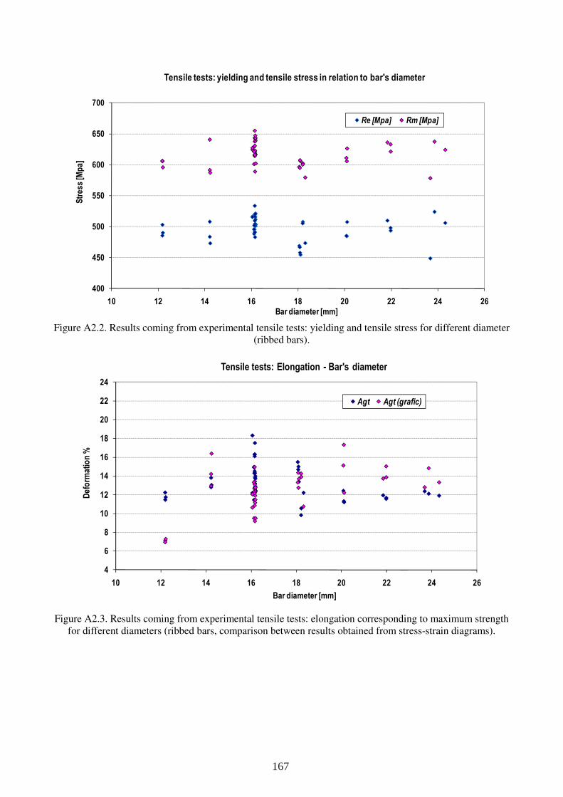
Figure A2.2. Results coming from experimental tensile tests: yielding and tensile stress for different diameter
(ribbed bars).
Figure A2.3. Results coming from experimental tensile tests: elongation corresponding to maximum strength
for different diameters (ribbed bars, comparison between results obtained from stress-strain diagrams).
400
450
500
550
600
650
700
10 12 14 16 18 20 22 24 26
Str
ess
[Mp
a]
Bar diameter [mm]
Tensile tests: yielding and tensile stress in relation to bar's diameter
Re [Mpa] Rm [Mpa]
4
6
8
10
12
14
16
18
20
22
24
10 12 14 16 18 20 22 24 26
De
form
ati
on
%
Bar diameter [mm]
Tensile tests: Elongation - Bar's diameter
Agt Agt (grafic)
167
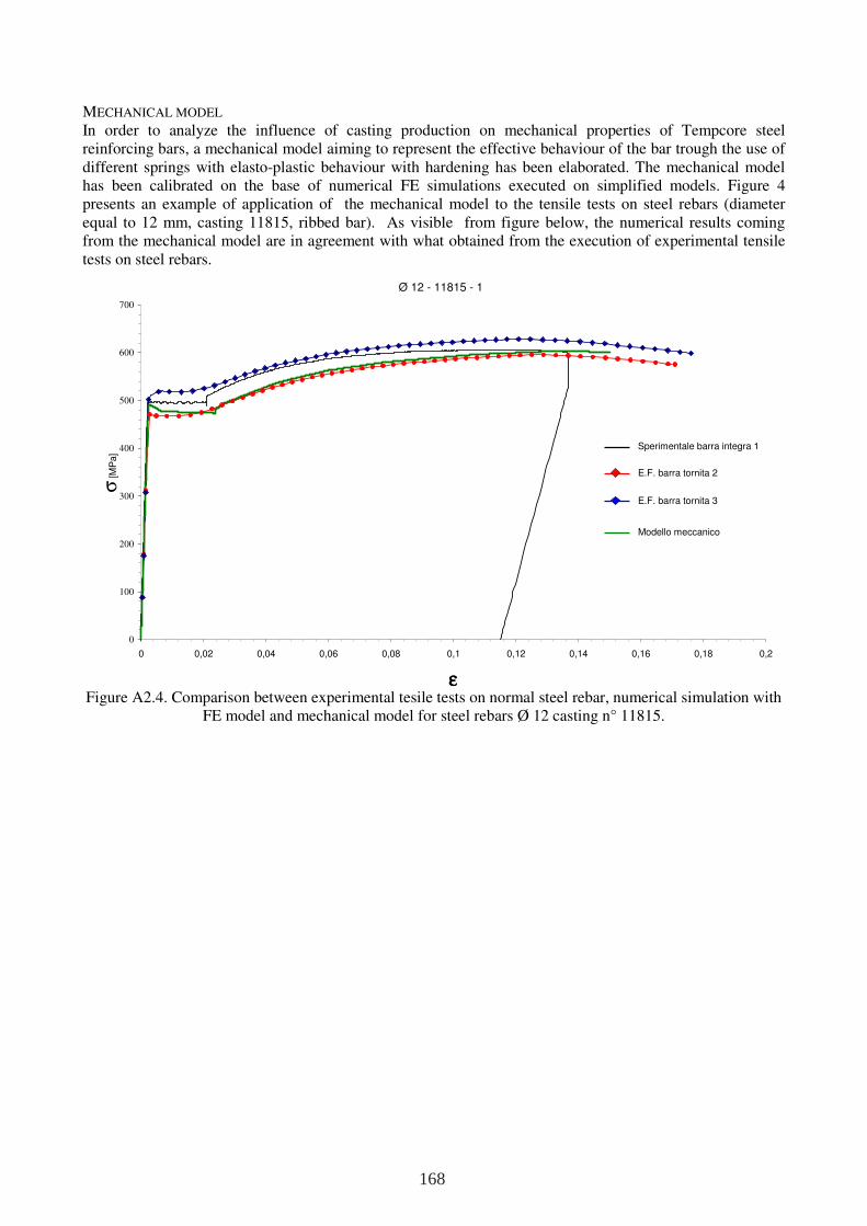
MECHANICAL MODEL In order to analyze the influence of casting production on mechanical properties of Tempcore steel reinforcing bars, a mechanical model aiming to represent the effective behaviour of the bar trough the use of different springs with elasto-plastic behaviour with hardening has been elaborated. The mechanical model has been calibrated on the base of numerical FE simulations executed on simplified models. Figure 4 presents an example of application of the mechanical model to the tensile tests on steel rebars (diameter equal to 12 mm, casting 11815, ribbed bar). As visible from figure below, the numerical results coming from the mechanical model are in agreement with what obtained from the execution of experimental tensile tests on steel rebars.
Figure A2.4. Comparison between experimental tesile tests on normal steel rebar, numerical simulation with
FE model and mechanical model for steel rebars Ø 12 casting n° 11815.
Ø 12 - 11815 - 1
0
100
200
300
400
500
600
700
0 0,02 0,04 0,06 0,08 0,1 0,12 0,14 0,16 0,18 0,2
εεεε
σ [M
Pa]
Sperimentale barra integra 1
E.F. barra tornita 2
E.F. barra tornita 3
Modello meccanico
168
List of Acronyms ACC Accelerogram CB Concentric brace CBF Concentrically braced frame CDF Cumulative density function CHS Circular hollow section CoV Coefficient of variation CP Collapse prevention DBE Design basis earthquake DCH Ductility class high DCL Ductility class low DCM Ductility class medium DDM Domain decomposition method DM Damage measure EBF Eccentically braced frame EDP Engineering demand parameter FORM First order reliability methods IDA Incremental dynamic analysis IM Intensity measure IO Immediate occupancy ISD Importance sampling density ISEE Importance sampling using elementary events JCSS Joint Committee on Structural Safety LS Life safety MC Monte Carlo MRF Moment resisting frame MRSA Modal response spectra analysis MV Material variability NCR Non collapse requirement PDF Probability density function PEER PEER Pacific Earthquake Engineering Research Pf failure probability Pf,N nominal failure probability PGA Peak ground acceleration PO Push-Over analysis RFCS Research fund for coal and steel SLS Serviceability Limit State SORM Second order reliability methods TMCP Thermo mechanical rolling process ULS Ultimate Limit State
169
List of figures Figure I. Comparison between dissipative mechanisms……………………………………………………….7 Figure II. Ideal layout of plastic hinges for high dissipative mechanism……………………………………...7 Figure III. Weak beam-strong column strategy in multi-story buildings………………………………………8 Figure IV. Flow-chart of the research project………………………………………………………………….9 Figure V. Statistical analysis of data…………………………………………………………………………...9 Figure VI. Comparison of statistical data with production standard limits and p.d.f. models from literature Figure VII. Comparison between mean value of tensile strength obtained from data and mean values
proposed in the literature………………………………………………………………………10 Figure VIII. Probabilistic model of the steel production scattering employing a complete correlation between
single probabilistic variables……………………………………………………………………10 Figure IX. Structural types designed during the research: (a) industrial building for electrical power plant
activities; (b) industrial building for warehouse/light activities; (c) EBF and CBF configurations for offices; (d) MRF and CBF configurations for industrial storage……………………………10
Figure X. (a) Scheme of the Ballio-Setti procedure; (b) discrepancy between target spectrum and real spectrum……………………………………………………………………………………….11
Figure XI. IDA points in correspondence of PGA levels activating collapse modes………………………12 Figure XII. Fragility curve for one collapse mode in one case study, obtained from statistical analysis of IDA
outputs…………………………………………………………………………………………12 Figure XIII. (a) material samples, for one steel member in the dissipative zone, corresponding to EN10025
production; (b) material samples, for one steel member in the dissipative zone, corresponding to EN10025 production upper limited imposing fy,max<1.25fy,nom…………………………….......12
Figure XIV. (a) Pf associated to the exhaustion of plastic rotation in dissipative zones; (b) Pf associated to buckling of bracing members…………………………………………………………………14
Figure XV. Protection level furnished by capacity design approach using different over-strength values……………………………………………………………………………………………14
Figure 1.1. C20/25 class during one production year………………………………………………………21 Figure 1.2. C25/30 class during one production year………………………………………………………22 Figure 1.3. C30/37 class during one production year………………………………………………………...22 Figure 1.4. Comparison between models and statistical data: (a) mean and (b) Co.V. of yielding
stress…………………………………………………………………………………………….23 Figure 1.5. Comparison between models and statistical data: (a) mean and (b) Co.V. of tensile
strength………………………………………………………………………………………….23 Figure 1.6. Comparison between models and statistical data: Co.V. of elongation at fracture………………23 Figure 1.7. Comparison between models and statistical data: (a) mean and (b) Co.V. of yielding
stress…………………………………………………………………………………………….24 Figure 1.8. Comparison between models and statistical data: (a) mean and (b) Co.V. of tensile
strength…………………………………………………………………………………………24 Figure 1.9. Comparison between models and statistical data: Co.V. of elongation at fracture………………24 Figure 1.10. Comparison between models and statistical data: (a) mean and (b) Co.V. of yielding
stress…………………………………………………………………………………………….25
Figure 1.11. Graphic representation of χ2 method results: S235 steel plates…………………………………25
Figure 1.12. Graphic representation of χ2 method results: S275 steel plates…………………………………26
Figure 1.13. Graphic representation of χ2 method results: S355 steel plates…………………………………26
Figure 1.14. Graphic representation of χ2 method results: S355W steel plates………………………………26
Figure 1.15. Graphic representation of χ2 method results: S460M steel plates………………………………26 Figure 1.16. Samples generation adopting proposed procedure……………………………………………28 Figure 1.17. Stress strain law of steel profiles: (a) monitored points; (b) experimental curve taken from
collected database………………………………………………………………………………29 Figure 1.18. Relation between the measured values and predicted values for: elongation at maximum load
and elongation at plateau-end…………………………………………………………………30 Figure 1.19. (a) Test set-up and (b)test performed at RWTH: buckling of the steel flanges…………………30 Figure 1.20. Instrumentation of steel beam tested in the previous research project………………………….31
170
Figure 1.21. Two simplified stress-strain model for the simulation of the experimental testing on IPE500 beam……………………………………………………………………………………………31
Figure 1.22. Scheme of the numerical model………………………………………………………………31 Figure 1.23. Comparison between the numerical simulations and the experimental tests for all the test
duration…………………………………………………………………………………………32 Figure 1.24. Comparison in the first cycle where the buckling phenomena and the strength degradation have
not occurred……………………………………………………………………………………32 Figure 2.1. Outline of procedure for lateral force method in moderate seismic areas………………………37 Figure 2.2. General layout of building 1: office building with moment-resisting frames (X) and concentric
bracings (Y), moderate seismicity………………………………………………………………37 Figure 2.3. General layout of building 2: office building with concentric bracings (X and Y), moderate
seismicity……………………………………………………………………………………….38 Figure 2.4. General layout of building 14: industrial single storey building (turbine house) with moment-
resisting frames (X) and concentric bracings (Y), high seismicity……………………………..38 Figure 2.5. General layout of building 15: industrial multi storey building with moment-resisting frames (X)
and concentric bracings (Y), moderate seismicity……………………………………………38 Figure 2.6. General plan of buildings a) office buildings 3 - 4, b) car park 16 and c) duplication of main floor
beam.............................................................................................................................................40 Figure 2.7. Building 3 (short links), geometry and elements: a) xz frame, b) yz frame...................................41 Figure 2.8. Building 4 (long links), geometry and elements: a) xz frame, b) yz frame....................................41 Figure 2.9. Building 16 (short links), geometry and elements: xz frame and yz frame....................................41 Figure 2.10. (a) Front view of the 5 floor office building type – X-direction – Eccentric bracings; (b) 3D
Composite office building; (c) Front view of the 5 floor office building type – Y-direction – Concentric bracings……………………………………………………………………………43
Figure 2.11. Single-storey industrial building………………………………………………………………44 Figure 2.12. Multi-storey industrial building…………………………………………………………………45 Figure 2.13. Multi-storey office building..........................................................................................................45 Figure 2.14. (a) plane view of the composite frames; (b) elevation of the composite frame………………46 Figure 2.15. (a) Composite beams resulting from design; (b) Columns resulting from design………………46 Figure 3.1. Integration points in the steel sections adopted in ABAQUS…………………………………….50 Figure 3.2. (a) steel section; (b) internal distribution of stress and strain; (c) elasto-plastic stress-strain
law………………………………………………………………………………………………50 Figure 3.3. (a) meshing of steel profiles; (b) bracing behaviour model………………………………………50 Figure 3.4. (a) subdivision of flange; (b) subdivision of circular profile; (c) modeling strategy for I and H
profiles………………………………………………………………………………………….51 Figure 3.5. Elasto-plastic bar…………………………………………………………………………………52 Figure 3.6. sections (H, U, Tubular and 2L)………………………………………………………………….52 Figure 3.7. Loading sequence………………………………………………………………………………52 Figure 3.8. Diagram P versus δ – Case1-1.3…………………………………………………………………53 Figure 3.9. Diagram P versus δ, Case 1-2.0…………………………………………………………………..53 Figure 3.10. Diagram P versus δ – Case 2-1.3………………………………………………………………53 Figure 3.11. Diagram P versus δ – Case 2-20………………………………………………………………53 Figure 3.12. Diagram P versus δ – Case 1-1.3………………………………………………………………..54 Figure 3.13. Diagram P versus δ – Case 1-2.0………………………………………………………………54 Figure 3.14. Diagram P versus δ – Case 2-1.3………………………………………………………………54 Figure 3.15. Diagram P versus δ – Case 2-2.0………………………………………………………………54 Figure 3.16. Diagram P versus δ – Case 1-1.3………………………………………………………………55 Figure 3.17. Diagram P versus δ – Case 1-2.0………………………………………………………………55 Figure 3.18. Diagram P versus δ – Case 2-1.3………………………………………………………………55 Figure 3.19. Diagram P versus δ – Case 2-2.0………………………………………………………………55 Figure 3.20. Diagram P versus δ – Case 1-1.3………………………………………………………………56 Figure 3.21. Diagram P versus δ – Case 1-2.0………………………………………………………………56 Figure 3.22. Diagram P versus δ – Case 2-1.3………………………………………………………………56 Figure 3.23. Diagram P versus δ – Case 2-2.0………………………………………………………………56 Figure 3.24. Scheme of the modeled portal frame and assumed parameters…………………………………56
171
Figure 3.25 Diagram Q versus δ, for constant vertical load P, where P is the axial load…………………….56 Figure 3.26. Braced frame configuration……………………………………………………………………..57 Figure 3.27. Diagram Q versus δ, for several loading cycles and slenderness ratio 1.5 (UniTH)……………57 Figure 3.28. Diagram Q versus δ, for several loading cycles and slenderness ratio 1.5 (UniTH, UniPi)……57 Figure 3.29. Diagram Q versus δ, for several loading cycles and slenderness ratio 1.5 (UniTH, ULg,
UniPi)…………………………………………………………………………………………57 Figure 3.30. Building 1 (Office building MRF): maximum ultimate rotation ratio in the IDA’s (a) and (b)
capacity ratio of failure criteria at load factor 10 (mean, maximum and minimum)…………60 Figure 3.31. Building 2 (Office building CBF): maximum ultimate deformation in tension ratio in the IDA’s
(a) and capacity ratio of failure criteria (b) at load factor 7 (mean, maximum and minimum)………………………………………………………………………………………60
Figure 3.32. Building 14-X (Industrial building MRF): maximum ultimate rotation ratio in the IDA’s (left) and capacity ratio of failure criteria at load factor 8 (mean, maximum and minimum)………...60
Figure 3.33. Building 15-X (Industrial building MRF): maximum ultimate rotation ratio in the IDA’s (a) and capacity ratio of failure criteria (b) at load factor 8 (mean, maximum and minimum)…………61
Figure 3.34. Building 15-Y (Industrial building CBF): maximum ultimate deformation in tension ratio in the IDA’s (a) and capacity ratio of failure criteria (b) at load factor 8 (mean, maximum and minimum)……………………………………………………………………………………….61
Figure 3.35. Modelling of the seismic shear link……………………………………………………………61 Figure 3.36. Push-over and IDA curves for CBF (low seismicity)…………………………………………63 Figure 3.37. q factor vs. ultimate rotation of plastic hinges: building 8……………………………………65 Figure 3.38. Building 8 evolution of the mean maximal rotation…………………………………………….65 Figure 3.39. q factor computation for building 6……………………………………………………………66 Figure 3.40. Building 6 : evolution of mean maximal rotation………………………………………………67 Figure 3.41. q factor computation for building Nr. 7………………………………………………………....68 Figure 3.42. Building 7: evolution of mean maximal rotation……………………………………………….68 Figure 3.43. Pushover analysis in Abaqus for 2D MRF (X-direction) of Office Building 5…………………69 Figure 3.44. Diagram Q versus δ, for pushover analysis in Abaqus, for MRF and S355…………………….69 Figure 3.45. IDA curve related to drift ratio collapse criteria using ACC1…………………………………69 Figure 3.46. IDA curves for different time-histories and individuation of collapse levels: (a) drift ratio; (b)
ultimate plaric hinge rotation; (c) ultimate plastic hinge rotation; (d) column buckling……….70 Figure 4.1. Graphical representation of successive transformation: (a) Initial variables in origin space, (b)
Reduced variables with zero mean and unit variance, (c) Rotated reduced variables…………..77 Figure 4.2. Plain Monte Carlo simulation (a) and Monte Carlo simulation with importance sampling
(b)……………………………………………………………………………………………….78 Figure 4.3. Outcrossing of a random vibration with envelope processes [4.1]……………………………….81 Figure 4.4. IDA curves employing single earthquake: (a) 16EBFY – Max shear link rotation in Beam B1; (b)
3EBFX – Max inter-story drift demand along frame height; (c) 3EBFX – Max compressive forces in braces at storey I; (d) 3EBFY – Max compressive forces acting in columns C1, C2 and C4………………………………………………………………………………………………85
Figure 4.5. IDA curves employing 7 Earthquake time-histories: (a) 3EBFY – Max. compressive force in column C1; (b) 3EBFX – Max compressive force in brace Br1; (c) 16EBFY – Max shear link rotation in beam B1; (d) Max drift demand at storey II………………………………………86
Figure 4.6. Application of proposed IDA protocol: compressive forces in brace 1 – (a) material variability; (b) material and seismic input variability………………………………………………………86
Figure 4.7. Hazard function according to EN1998-1 prescriptions: (a) high seismic hazard; (b) low seismic hazard; (c) correpondence between PGA levels and return periods.............................................89
Figure 4.8. Target spectra (a) and filter function (b) for the generation of artificial time histories…………89 Figure 4.9. Baseline correction for an artificial accelerogram (high seismicity)……………………………90 Figure 4.10. Target spectrum and elastic response spectra of 7 artificial accelerograms: low seismicity (a)
and high seismicity (b)…………………………………………………………………………90 Figure 4.11. Target spectrum and mean value of the elastic response spectra of 7 artificial accelerograms:
low seismicity (a) and high seismicity (b)………………………………………………………91 Figure 4.12. COV of the elastic response spectra of 7 artificial accelerograms: low seismicity (a) and high
seismicity (b)……………………………………………………………………………………91
172
Figure 4.13. Generation scheme of probabilistic variables inside structural models: (a) frame 3X; (b) frame 4Y; (c) frame 5Y; (d) frame 12X………………………………………………………………93
Figure 4.14 (a) numerical CDF directly derived from IDA results (when χ2 failed); (b) fragility of 3EBFX for ultimate plastic rotation of the link B1.........................................................................................94
Figure 5.1. Building 1 (Office building MRF): column base rotation over roof drift for accelerogram 1…...96 Figure 5.2. Building 1 (Office building MRF): (a) Box plot of column foot rotation 1st storey and (b)
maximum moment at joint vs. yield stress at beams 2nd storey………………………………96 Figure 5.3. Building 2 (Office building CBF): Box plot of tension deformation braces 3rd storey (left) and
maximum tension force at joint vs. yield stress at braces 3rd storey (right), PGA multiplied 7 times……………………………………………………………………………………………96
Figure 5.4. Building 15-X (Industrial building MRF): (a) Box plot of column head rotation 1st storey and (b) maximum moment at joint vs. yield stress at beams 2nd storey , PGA multiplied 8 times…….97
Figure 5.5. Building 15-Y (Industrial building CBF): (a) Box plot of tension deformation braces 4th storey and (b) maximum tension force at joint vs. yield stress at braces 3rd storey, PGA multiplied 8 times……………………………………………………………………………………………97
Figure 5.6. Evolution of maximal rotations and drifts with the seismic action………………………………99 Figure 5.7. Evolution of drifts with the seismic action: comparison of the statistical results versus the
computations with nominal values……………………………………………………………99 Figure 5.8. Definition of the forces on the joints……………………………………………………………..99 Figure 5.9. Global behaviour of a plastic hinge following Gioncu’s model : (a) in plane buckling, (b) out of
plane buckling, (c) M-θ curve…………………………………………………………………101
Figure 5.10. Evolution of θmax with fy of the steel profile and of the reinforcement bar – IPE 330 beam. (a) resulting from Gioncu’s model (b) linear approximation……………………………………...101
Figure 5.11. Example of spreading of the activation of the collapse criteria………………………………..104
Figure 5.12. Capacity designed elements: (a) EBF; (b) CBF………………………………………………104
Figure 5.13. Examples of over-strength coefficient distributions…………………………………………105
Figures 5.14. Spreading of the calculated over-strength for (a) office building MRF S355, (b) office building MRF S460, (c) office building CB S355 and (d) office building CB S460…………………106
Figures 5.15. Office building MRF…………………………………………………………………………107 Figures 5.16. Simplified ductility criterion has been satisfied for 5000 samples with different material
properties………………………………………………………………………………………108 Figures 5.17. Spreading of the calculated ov1 1. γ Ω for (a) office building MRF S355, (b) office building MRF
S460……………………………………………………………………………………………108
Figure 5.18. Variability of link plastic rotation (1st floor – element B1) with yielding strength……………110 Figure 5.19. Variability of axial force on brace (1st floor – element B1) with yielding strength…………112 Figure 6.1. Samples for link B1 in the 3EBFX: (a) 500 samples EN10025 full generation; (b) reduced
number imposing fy,act/fy,nom=1.375; (c) reduced number imposing fy,act/fy,nom=1.35; (d) reduced number imposing fy,act/fy,nom=1.30; (e) reduced number imposing fy,act/fy,nom=1.25……………120
Figure 6.2. Axial force in Brace Br2 – 3EBFX: (a) no upper yielding limit and Quake 1; (b) upper yielding limit equal to 1.25 and Quake 1; (c) no upper yielding limit and Quake 4; (d) upper yielding limit equal to 1.25and Quake 4………………………………………………………………...121
Figure 6.3. Maximum rotation in shear link B1, 3EBFX frame: (a) no upper yielding limit and Quake 1; (b) upper yielding limit equal to 1.25 and Quake 1; (c) no upper yielding limit and Quake 4; (d) upper yielding limit equal to 1.25and Quake 4………………………………………………122
Figure 6.4. Frame 3 with EB resisting scheme with shear links: (a) X direction; (b) Y direction………….123 Figure 6.5. Frame 4 with EB resisting scheme with bending links: (a) X direction; (b) Y direction……….123 Figure 6.6. Frame 16 with EB resisting scheme with shear links: (a) X direction; (b) Y direction………124 Figure 6.7. (a) variation of Pf associated to the ultimate plastic rotation of links – 3EBF; (b) variation of Pf
associated to buckling of first storey braces – 3EBF.................................................................127 Figure 6.8. (a) variation of Pf associated to the ultimate plastic rotation of links – 3EBF; (b) variation of Pf
associated to buckling of first storey braces – 4EBF.................................................................127 Figure 6.9. (a) variation of Pf associated to the ultimate plastic rotation of links – 3EBF; (b) variation of Pf
associated to buckling of first storey braces – 16EBF...............................................................127
173
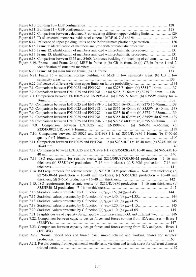
Figure 6.10. Building 10 – EBF configuration……………………………………………………………128 Figure 6.11. Building 11 – CBF configuration……………………………………………………………128 Figure 6.12. Comparison between calculated Pf considering different upper yielding limits………………129 Figure 6.13. ID of structural members inside steel-concrete MRF (6, 7, 8 and 9)………………………….129 Figure 6.14. Influence of upper yielding limits on the Pf for ultimate plastic hinge rotation……………….130 Figure 6.15. Frame 5: identification of members analyzed with probabilistic procedure…………………..130 Figure 6.16. Frame 12: identification of members analyzed with probabilistic procedure…………………131 Figure 6.17. Frame 13: identification of members analyzed with probabilistic procedure…………………131 Figure 6.18. Comparison between S355 and S460: (a) braces buckling; (b) buckling of columns…………132 Figure 6.19. Frame 1 and Frame 2: (a) MRF in frame 1; (b) CB in frame 2; (c) CB in frame 1 and 2;
identification of structural members…………………………………………………………132 Figure 6.20. Frame 14: (a) main trussed frame; (b) CB frame……………………………………………133 Figure 6.21. Frame 15 – industrial storage building: (a) MRF in low seismicity areas; (b) CB in low
seismicity areas………………………………………………………………………………133 Figure 6.22. Influence of different yielding upper limits on failure probability…………………………….134 Figure 7.1. Comparison between EN10025 and EN1998-1-1: (a) S275 7-16mm; (b) S355 7-16mm….......137 Figure 7.2. Comparison between EN10025 and EN1998-1-1: (a) S235, 7-16mm; (b) S275 7-16mm……138 Figure 7.3. Comparison between EN10025 and EN1998-1-1: (a) S355 7-16mm; (b) S355W quality for 7-
16mm…………………………………………………………………………………………138 Figure 7.4. Comparison between EN10025 and EN1998-1-1: (a) S235 16-40mm; (b) S275 16-40mm…...138 Figure 7.5. Comparison between EN10025 and EN1998-1-1: (a) S355 16-40mm; (b) S355W 16-40mm…138 Figure 7.6. Comparison between EN10025 and EN1998-1-1: (a) S235 40-63mm; (b) S275 40-63mm…...139 Figure 7.7. Comparison between EN10025 and EN1998-1-1: (a) S355 40-63mm; (b) S355W 40-63mm....139 Figure 7.8. Comparison between EN10025 and EN1998-1-1: (a) S275 63-80mm; (b) S355 63-80mm…...139 Figure 7.9. Comparison between EN10025 and EN1998-1-1: (a) S460M 40-63mm; (b)
S235JRJ0/275JRJ0+M 7-16mm……………………………………………………………….139 Figure 7.10. Comparison between EN10025 and EN1998-1-1: (a) S355JRJ0+M 7-16mm; (b) S460+M
quality for 7-16mm…………………………………………………………………………….140 Figure 7.11. Comparison between EN10025 and EN1998-1-1: (a) S235JRJ0+M 16-40 mm; (b) S275JRJ0+M
16-40 mm………………………………………………………………………………………140 Figure 7.12. Comparison between EN10025 and EN1998-1-1: (a) S355J2K2+M 16-40 mm; (b) S460+M 16-
40 mm…………………………………………………………………………………………140 Figure 7.13. ISO requirements for seismic steels: (a) S235J0JR/S275JRJ0+M production – 7–16 mm
thickness (b) S355J0+M production – 7–16 mm thickness; (c) S460M production – 7-16 mm thickness………………………………………………………………………………………141
Figure 7.14. ISO requirements for seismic steels: (a) S235JRJ0+M production – 16–40 mm thickness; (b) S275JRJ0+M production – 16–40 mm thickness; (c) S355J2K2 production – 16–40 mm thickness; (d) S460M production – 16–40 mm thickness……………………………………142
Figure 7.15. ISO requirements for seismic steels: (a) S275JRJ0+M production – 7–16 mm thickness; (b) S355JRJ0+M production – 7–16 mm thickness………………………………………………142
Figure 7.16. Statistical values presented by G function: (a) γOV=1.5; (b) γOV=1.45………………………144
Figure 7.17. Statistical values presented by G function: (a) γOV=1.40; (b) γOV=1.35……………………….144
Figure 7.18. Statistical values presented by G function: (a) γOV=1.30; (b) γOV=1.25……………………….145
Figure 7.19. Statistical values presented by G function: (a) γOV=1.20; (b) γOV=1.15……………………….145
Figure 7.20. Statistical values presented by G function: (a) γOV=1.10; (b) γOV=1.05………………………145
Figure 7.21. Fragility curves of capacity design approach for increasing PGA and different γOV………….146 Figure 7.22. Comparison between capacity design forces and forces coming from IDA analyses – Brace 1
(3EBFY)………………………………………………………………………………………147 Figure 7.23. Comparison between capacity design forces and forces coming from IDA analyses – Brace 1
(16EBFX)……………………………………………………………………………………147 Figure A2.2: Normal ribbed bars and turned bars, simple scheme and working phases for samples’
production……………………………………………………………………………………165 Figure A2.2. Results coming from experimental tensile tests: yielding and tensile stress for different diameter
(ribbed bars)……………………………………………………………………………………167
174

Figure A2.3. Results coming from experimental tensile tests: elongation corresponding to maximum strength for different diameters (ribbed bars, comparison between results obtained from stress-strain diagrams)………………………………………………………………………………………167
Figure A2.4. Comparison between experimental tesile tests on normal steel rebar, numerical simulation with FE model and mechanical model for steel rebars Ø 12 casting n° 11815……………………..168
175
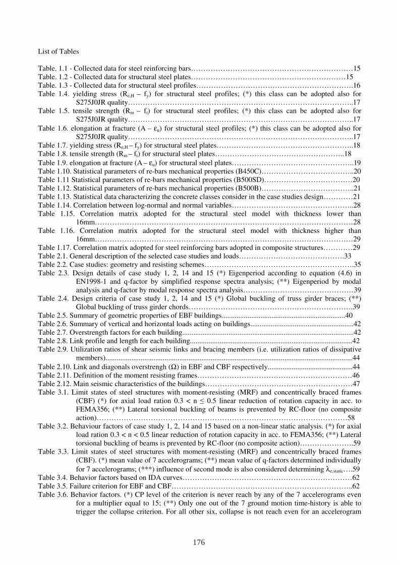
List of Tables Table. 1.1 - Collected data for steel reinforcing bars…………………………………………………………15 Table. 1.2 - Collected data for structural steel plates………………………………………………………15 Table. 1.3 - Collected data for structural steel profiles……………………………………………………….16 Table 1.4. yielding stress (Re,H – fy) for structural steel profiles; (*) this class can be adopted also for
S275J0JR quality………………………………………………………………………………..17 Table 1.5. tensile strength (Rm – ft) for structural steel profiles; (*) this class can be adopted also for
S275J0JR quality………………………………………………………………………………..17
Table 1.6. elongation at fracture (A – εu) for structural steel profiles; (*) this class can be adopted also for S275J0JR quality………………………………………………………………………………..17
Table 1.7. yielding stress (Re,H – fy) for structural steel plates………………………………………………..18 Table 1.8. tensile strength (Rm – ft) for structural steel plates……………………………………………..18
Table 1.9. elongation at fracture (A – εu) for structural steel plates…………………………………………..19 Table 1.10. Statistical parameters of re-bars mechanical properties (B450C)………………………………..20 Table 1.11 Statistical parameters of re-bars mechanical properties (B500SD)………………………………20 Table 1.12. Statistical parameters of re-bars mechanical properties (B500B)………………………………..21 Table 1.13. Statistical data characterizing the concrete classes consider in the case studies design…………21 Table 1.14. Correlation between log-normal and normal variables…………………………………………..28 Table 1.15. Correlation matrix adopted for the structural steel model with thickness lower than
16mm……………………………………………………………………………………………28 Table 1.16. Correlation matrix adopted for the structural steel model with thickness higher than
16mm……………………………………………………………………………………………29 Table 1.17. Correlation matrix adopted for steel reinforcing bars adopted in composite structures…………29 Table 2.1. General description of the selected case studies and loads…………………………………….33 Table 2.2. Case studies: geometry and resisting schemes…………………………………………………….35 Table 2.3. Design details of case study 1, 2, 14 and 15 (*) Eigenperiod according to equation (4.6) in
EN1998-1 and q-factor by simplified response spectra analysis; (**) Eigenperiod by modal analysis and q-factor by modal response spectra analysis………………………………………39
Table 2.4. Design criteria of case study 1, 2, 14 and 15 (*) Global buckling of truss girder braces; (**) Global buckling of truss girder chords………………………………………………………….39
Table 2.5. Summary of geometric properties of EBF buildings...................................................................40 Table 2.6. Summary of vertical and horizontal loads acting on buildings........................................................42 Table 2.7. Overstrength factors for each building.............................................................................................42 Table 2.8. Link profile and length for each building........................................................................................42 Table 2.9. Utilization ratios of shear seismic links and bracing members (i.e. utilization ratios of dissipative
members)......................................................................................................................................44
Table 2.10. Link and diagonals overstrengh (Ω) in EBF and CBF respectively..............................................44 Table 2.11. Definition of the moment resisting frames………………………………………………………46 Table 2.12. Main seismic characteristics of the buildings……………………………………………………47 Table 3.1. Limit states of steel structures with moment-resisting (MRF) and concentrically braced frames
(CBF) (*) for axial load ration 0.3 < n ≤ 0.5 linear reduction of rotation capacity in acc. to FEMA356; (**) Lateral torsional buckling of beams is prevented by RC-floor (no composite action)…………………………………………………………………………………………58
Table 3.2. Behaviour factors of case study 1, 2, 14 and 15 based on a non-linear static analysis. (*) for axial load ration 0.3 < n < 0.5 linear reduction of rotation capacity in acc. to FEMA356; (**) Lateral torsional buckling of beams is prevented by RC-floor (no composite action)………………….59
Table 3.3. Limit states of steel structures with moment-resisting (MRF) and concentrically braced frames (CBF). (*) mean value of 7 accelerograms; (**) mean value of q-factors determined individually
for 7 accelerograms; (***) influence of second mode is also considered determining λe,static….59 Table 3.4. Behavior factors based on IDA curves……………………………………………………………62 Table 3.5. Failure criterion for EBF and CBF………………………………………………………………..62 Table 3.6. Behavior factors. (*) CP level of the criterion is never reach by any of the 7 accelerograms even
for a multiplier equal to 15; (**) Only one out of the 7 ground motion time-history is able to trigger the collapse criterion. For all other six, collapse is not reach even for an accelerogram
176
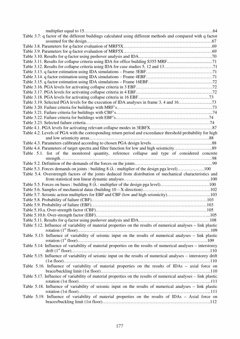
multiplier equal to 15……………………………………………………………………………64 Table 3.7: q factor of the different buildings calculated using different methods and compared with q factor
assumed for the design………………………………………………………………………….67 Table 3.8. Parameters for q-factor evaluation of MRF5X……………………………………………………69 Table 3.9. Parameters for q-factor evaluation of MRF5X……………………………………………………69 Table 3.10. Results for q-factor using pushover analysis and IDA…………………………………………..70 Table 3.11. Results for collapse criteria using IDA for office building S355 MRF.........................................71 Table 3.12. Results for collapse criteria using IDA for case studies 5, 12 and 13……………………………71 Table 3.13. q factor estimation using IDA simulations – Frame 3EBF………………………………………71 Table 3.14. q factor estimation using IDA simulations – Frame 4EBF………………………………………71 Table 3.15. q factor estimation using IDA simulations – Frame 16EBF……………………………………..72 Table 3.16. PGA levels for activating collapse criteria in 3 EBF…………………………………………….72 Table 3.17. PGA levels for activating collapse criteria in 4 EBF…………………………………………….72 Table 3.18. PGA levels for activating collapse criteria in 16 EBF…………………………………………73 Table 3.19. Selected PGA levels for the execution of IDA analyses in frame 3, 4 and 16…………………..73 Table 3.20. Failure criteria for buildings with MRF’s………………………………………………………..73 Table 3.21. Failure criteria for buildings with CBF’s………………………………………………………...74 Table 3.22. Failure criteria for buildings with EBF’s………………………………………………………74 Table 3.23. Selected failure criteria…………………………………………………………………………74 Table 4.1. PGA levels for activating relevant collapse modes in 3EBFX……………………………………87 Table 4.2. Levels of PGA with the corresponding return period and exceedance threshold probability for high
and low seismicity areas………………………………………………………………………88 Table 4.3. Parameters calibrated according to chosen PGA design levels…………………………………...88 Table 4.4. Parameters of target spectra and filter function for low and high seismicity……………………..89 Table 5.1. list of the monitored quantity, reference collapse and type of considered concrete
strength………………………………………………………………………………………….98 Table 5.2. Definition of the demands of the forces on the joints……………………………………………..99
Table 5.3. Forces demands on joints : building 8 (λ : multiplier of the design pga level)………………100 Table 5.4. Overstrength factors of the joints deduced from distribution of mechanical characteristics and
from statistical non linear dynamic analyses…………………………………………………..100
Table 5.5. Forces on bases : building 8 (λ : multiplier of the design pga level)……………………………100 Table 5.6. Samples of mechanical datas (building 10 – X-direction)……………………………………….102 Table 5.7. Seismic action multipliers for EBF and CBF (low and high seismicity)………………………...103 Table 5.8. Probability of failure (CBF)……………………………………………………………………103 Table 5.9. Probability of failure (EBF)……………………………………………………………………103 Table 5.10.a. Over-strength factor (CBF)…………………………………………………………………105 Table 5.10.b. Over-strength factor (EBF)…………………………………………………………………...105 Table 5.11. Results for q-factor using pushover analysis and IDA…………………………………………108 Table 5.12. Influence of variability of material properties on the results of numerical analyses – link plastic
rotation (1st floor)………………………………………………………………………………109 Table 5.13: Influence of variability of seismic input on the results of numerical analyses – link plastic
rotation (1st floor)…………………………………………………………………………….109 Table 5.14: Influence of variability of material properties on the results of numerical analyses – interstorey
drift (1st floor)………………………………………………………………………………….110 Table 5.15: Influence of variability of seismic input on the results of numerical analyses – interstorey drift
(1st floor)………………………………………………………………………………………110 Table 5.16. Influence of variability of material properties on the results of IDAs – axial force on
brace/buckling limit (1st floor)………………………………………………………………...110 Table 5.17. Influence of variability of material properties on the results of numerical analyses – link plastic
rotation (1st floor)……………………………………………………………………………...111 Table 5.18. Influence of variability of seismic input on the results of numerical analyses – link plastic
rotation (1st floor)……………………………………………………………………………...111 Table 5.19. Influence of variability of material properties on the results of IDAs – Axial force on
braces/buckling limit (1st floor)……………………………………………………………….112
177
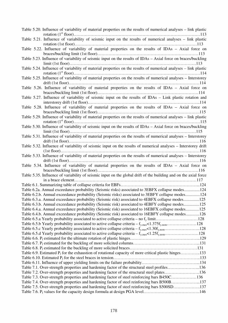
Table 5.20. Influence of variability of material properties on the results of numerical analyses – link plastic rotation (1st floor)………………………………………………………………………………113
Table 5.21. Influence of variability of seismic input on the results of numerical analyses – link plastic rotation (1st floor)……………………………………………………………………………113
Table 5.22. Influence of variability of material properties on the results of IDAs – Axial force on braces/buckling limit (1st floor)………………………………………………………………113
Table 5.23. Influence of variability of seismic input on the results of IDAs – Axial force on braces/buckling limit (1st floor)………………………………………………………………………………113
Table 5.24. Influence of variability of material properties on the results of numerical analyses – link plastic rotation (1st floor)………………………………………………………………………………114
Table 5.25. Influence of variability of material properties on the results of numerical analyses – Interstorey drift (1st floor)…………………………………………………………………………………114
Table 5.26. Influence of variability of material properties on the results of IDAs – Axial force on braces/buckling limit (1st floor)………………………………………………………………114
Table 5.27. Influence of variability of seismic input on the results of IDAs – Link plastic rotation and interstorey drift (1st floor)……………………………………………………………………..114
Table 5.28. Influence of variability of material properties on the results of IDAs – Axial force on braces/buckling limit (1st floor)……………………………………………………………….115
Table 5.29. Influence of variability of material properties on the results of numerical analyses – link plastic rotation (1st floor)………………………………………………………………………………115
Table 5.30. Influence of variability of seismic input on the results of IDAs – Axial force on braces/buckling limit (1st floor)………………………………………………………………………………115
Table 5.31. Influence of variability of material properties on the results of numerical analyses – Interstorey drift (1st floor)…………………………………………………………………………………116
Table 5.32. Influence of variability of seismic input on the results of numerical analyses – Interstorey drift (1st floor)………………………………………………………………………………………116
Table 5.33. Influence of variability of material properties on the results of numerical analyses – Interstorey drift (1st floor)…………………………………………………………………………………116
Table 5.34. Influence of variability of material properties on the results of IDAs – Axial force on braces/buckling limit (1st floor)………………………………………………………………116
Table 5.35. Influence of variability of seismic input on the global drift of the building and on the axial force in a brace element……………………………………………………………………………117
Table 6.1. Summarizing table of collapse criteria for EBFs………………………………………………...124 Table 6.2a. Annual exceedance probability (Seismic risks) associated to 3EBFX collapse modes...............124 Table 6.2.b. Annual exceedance probability (Seismic risks) associated to 3EBFY collapse modes..............124 Table 6.3.a. Annual exceedance probability (Seismic risk) associated to 4EBFX collapse modes...............125 Table 6.3.b. Annual exceedance probability (Seismic risk) associated to 4EBFY collapse modes...............125 Table 6.4.a. Annual exceedance probability (Seismic risk) associated to 16EBFX collapse modes.............125 Table 6.4.b. Annual exceedance probability (Seismic risk) associated to 16EBFY collapse modes.............126 Table 6.5.a Yearly probability associated to active collapse criteria – no fy limit…………………………128 Table 6.5.b Yearly probability associated to active collapse criteria – fy,max<1.375fy,nom…………………128 Table 6.5.c Yearly probability associated to active collapse criteria – fy,max<1.30fy,nom…………………….128 Table 6.5.d Yearly probability associated to active collapse criteria – fy,max<1.25fy,nom……………………128 Table 6.6. Pf estimated for the ultimate rotation of plastic hinges…………………………………………..129 Table 6.7. Pf estimated for the buckling of more solicited columns………………………………………...131 Table 6.8. Pf estimated for the buckling of more solicited braces…………………………………………131 Table 6.9. Estimated Pf for the exhaustion of rotational capacity of more critical plastic hinges…………..133 Table 6.10. Estimated Pf for the steel braces in tension……………………………………………………..133 Table 6.11. Influence of upper yielding limits on the failure probability…………………………………...134 Table 7.1. Over-strength properties and hardening factor of the structural steel profiles…………………..136 Table 7.2. Over-strength properties and hardening factor of the structural steel plates…………………….136 Table 7.3. Over-strength properties and hardening factor of steel reinforcing bars B450C………………136 Table 7.4. Over-strength properties and hardening factor of steel reinforcing bars B500B………………...137 Table 7.5. Over-strength properties and hardening factor of steel reinforcing bars S500SD……………….137 Table 7.6. Pf values for the capacity design formula at design PGA level………………………………….146
178

Table 7.7. Exceedance Probability of real internal forces respect to those foreseen by capacity design approach – the results were referred to the design PGA level (0.25g and 0.10g)……………..147
Table A2.1. Tensile tests results on ribbed steel rebars..................................................................................165 Table A2.2. Tensile tests results on turned steel rebars..................................................................................166
179


European Commission EUR 25893 — Optimising the seismic performance of steel and steel-concrete structures by
standardising material quality control (OPUS) Luxembourg: Publications Office of the European Union 2013 — 179 pp. — 21 × 29.7 cm ISBN 978-92-79-29037-4doi:10.2777/79330


EUROPEAN COMMISSION Directorate-General for Research and Innovation Directorate G — Industrial Technologies Unit G.5 — Research Fund for Coal and Steel
E-mail: [email protected] [email protected]
Contact: RFCS Publications
European Commission B-1049 Brussels
HOW TO OBTAIN EU PUBLICATIONS Free publications: • via EU Bookshop (http://bookshop.europa.eu);
• at the European Union’s representations or delegations. You can obtain their contact details on the Internet (http://ec.europa.eu) or by sending a fax to +352 2929-42758.
Priced publications: • via EU Bookshop (http://bookshop.europa.eu).
Priced subscriptions (e.g. annual series of the Official Journal of the European Union and reports of cases before the Court of Justice of the European Union): • via one of the sales agents of the Publications Office of the European Union
(http://publications.europa.eu/others/agents/index_en.htm).
Optimising the seismicperformance of steel and steel-concrete
structures by standardising material quality control
(OPUS)
doi:10.2777/79330
Optim
ising the seismic perform
ance of steel and steel-concrete structures by standardising material quality control (O
PUS)
EUEU
R 25893
KI-NA-25893-EN
-N
Despite modern seismic standards, like Eurocode 8, admit ductile design of steel and composite structures, current European production standards don’t provide adequate limitations on steel mechanical properties limiting free application of such approach. Additional safety factors and design checks, aiming to guarantee optimal plastic hinges’ location, must be foreseen, reducing practical applicability and possible advantages of seismic ductile design. The proposal investigated the influence of material scattering on structural performance of a set of case studies designed according to Eurocodes. These structures were probabilistically analysed and used as applicative case studies in order to quantify:
the benefit of introducing upper limits on yielding stress —Re,H (fy) — at the production plant;
the effective contribution of γOVfactor in the capacity design formula;
the effectiveness of EN1998-1-1 seismic design procedure;
the assessment of the harmonisation level between production and structural standard.
These analyses were performed adopting a Monte Carlo simulation technique based on the following parts:
materials’ properties probabilistic model able to represent actual scattering of European steel production;
executive protocol for a profitable application of Incremental Dynamic Analysis technique on case studies;
probabilistic procedure for analysing all results obtained from IDA simulations.
More than 106 of non-linear dynamic analyses were carried out during the project.
Moreover, the proposal defined preliminary guidelines for the planning of a future harmonisation between structural standards and production standards able to maintain actual high safety levels of steel and steel-concrete structures against seismic actions.
Studies and reports
Research and Innovation EUR 25893 EN


