Embed Size (px)
Citation preview
OUTDOOR & LABORATORY CORROSION STUDIES OF ALUMINUMMETAL - MATRIX COMPOSITES
A THESIS SUBMITTED TO THE GRADUATE DIVISION OF THEUNIVERSITY OF HAWAI'I IN PARTIAL FULFILLMENT
OF THE REQUIREMENTS FOR THE DEGREE OF
MASTER OF SCIENCE
IN
MECHANICAL ENGINEERING
AUGUST 2004
By
George A. Hawthorn
Thesis Committee:
Lloyd H. Hihara, Chairperson
Bruce E. Liebert
Marcelo Kobayashi

111
ACKNOWLEDGMENTS
The author wishes to express his gratitude for the significant contributions to this work
made by Dr. Lloyd H. Hihara. Without Dr. Hihara's continued guidance, trust and
enthusiasm, this huge undertaking would never have been possible. The author would
also like to express his gratitude to Dr. Hihara, Alex Niemi, Ryan Sugamoto, Ben
Respicio and Justin Wade for their help in fabricating and setting up the corrosion test
sites on Oahu. Thanks also go to Chester Tonokawa and Arielle Shirland of HECO for
their help with test site maintenance. The author would like to thank Thanigai Arasu
Govindaraju for preparing the A16061-T6 standard specimens used in the outdoor and
immersion experiments in addition to Dr. Kent Ross, Dr. Hongbo Ding, Raghu
Srinivasan and Dr. Ralph Adler for their contributions to this project. Initial funding for
this project was provided from the Concurrent Technologies Corporation (CTC) through
the sponsorship of the U.S. Army Industrial Ecology Center under Contract DAAE30-98
C-I050 as part of the National Defense Center for Environmental Excellence program.
The author is grateful to the former technical liaison contacts Mr. Brian Deforce and Mr.
Robert Mason at CTC. Current funding is provided form the Pacific Rim Corrosion
Research Program (PRCRP) through the sponsorship ofthe U.S. Army TACOM-ARDEC
under contract DAAE30-03-C-I071. The author is grateful to the program manager Mr.
Bob Zanowicz, and for the support of Dr. Joseph Argento, Mr. John Theis and Mr.
Donald Skelton. Finally, the author would like to thank the thesis committee consisting

IV
of Dr. Lloyd H. Hihara, Dr. Bruce E. Liebert and Dr. Marcelo Kobayashi for their time,
patience and valuable contributions.

v
ABSTRACT
Eight aluminum metal-matrix composites (MMCs) containing SiC, B4C or Ah03
reinforcing particulate with volume fractions ranging from 5% to 50% were studied in
both outdoor and laboratory experiments. Corrosion rates were determined and
compared to those of monolithic A16061-T6 under the same conditions. All of the metal
matrix composites corroded at much higher rates than A16061-T6 both in the field
experiments and in controlled laboratory experiments. Corrosion rates of MMCs
increased as the volume fraction of the reinforcing particulate increased. The observed
increase in corrosion rates of MMCs with higher volume fractions of SiC, B4C or Ah03
may be due to galvanic corrosion resulting from an increase in the number of cathodic
sites as well as the formation of micro-crevices at the particulate-matrix interface. In
SiC/AI MMCs, the purity and hence the resistivity of the SiC used seems to have an
effect on the corrosion rate. In most of the field and laboratory experiments, A16092
T6/SiC/50p showed higher corrosion rates than AI6092-T6/SiC/50p (Gr.). Anodic
polarization of the MMCs in deaerated 3.15 wt.% sodium chloride (NaCl) and O.5M
sodium sulfate (Na2S04) solutions show that the pitting potentials and passive current
densities of all eight MMCs are similar having values close to those of A16061-T6.

VI
TABLE OF CONTENTS
Acknowledgments . .. . . . . . . . . . . .. . . . . . . . . . . . . . . . . . . . . . . . . . . . . . . . . . . . . . . . . . . . . . . . . . . . . . ... ... iii
Abstract V
List of Tables vii
List of Figures viii
Chapter 1: Introduction............................................................................ 1
Chapter 2: Literature Review 8
Chapter 3: Outdoor Experiment.. . . . . . . . . . . . . . . . . . . . . . . . . . . . . . . . . . . . . . . . . . . . . . . . . . . . . . . . . . . . . . . 10
Chapter 4: Weather and Atmospheric Monitoring 20
Chapter 5: Humidity Chamber Experiment 27
Chapter 6: Immersion Experiment 32
Chapter 7: Polarization Experiments 40
Chapter 8: Conclusion 47
Appendix A ... . . . . . . . . . . . . . . . . . . . . . . . . . . . . . . . . . . . . . . . . . . . . . . . . . . . . . . . . . . . . . . . . . . . . . . . . . . . . . . . .. 52
Appendix B 56
Appendix C 65
Appendix D .. .. . . . . . . . . . . . . . . . . . . . . . . . . . . . . . . . . . . . . . . . . . . . . . . . . . . . . . . . . . . . . . . . . . . . . . . . . . 68
References .. . . . . . . . . . . . . . . . . . . . . . . . . . . . . . . . . . . . . . . . . . . . . . . . . . . . . . . . . . . . . . . . . . . . . . . . . ... 73

Vll
LIST OF TABLES
Table 1.1 Comparison of A16061-T6 and A16092-T6 1
Table 1.2 Resistivities of materials used in metal-matrix composites 2
Table 3.1 Metal-matrix composite exposure intervals at each test site 14
Table 4.2 Weather and atmospheric data for 90 day exposure at corrosion test sites 23
Table 4.3 Weather and atmospheric data for 180 day exposure at corrosion
test sites 23
Table 4.4 Weather and atmospheric data for 360 day exposure at corrosion
test sites 23
Table C.1 Comparison of the major ionic constituents of different types
of seawater. . . .. . . .. . . . .. . .. . . .. . . . .. . . . . .. . .. . .. . .. . . .. . .. . .. . . . . . . . .. . .. . .. . .. .. ...... 65
Table C.2 Initial pH values of electrolytes used in immersion experiment............... 66
Table C.3 Final pH values of electrolytes used in immersion experiment............... 66
Table D.1 Pitting potentials and passive current densities for MMCs and A16061-T6
in 3.15 wt.% NaCl and 0.5M NaZS04 68

V111
LIST OF FIGURES
Figure 1.1 Microstructure of A16092-T6/SiC/5p 4
Figure 1.2 Microstructure of A16092-T6/SiC/l Op 4
Figure 1.3 Microstructure of A16092-T6/SiC/20p 5
Figure 1.4 Microstructure ofA16092-T6/SiC/40p 5
Figure 1.5 Microstructure of A16092-T6/SiC/50p 6
Figure 1.6 Microstructure of A16092-T6/SiC(Gr.)/50p 6
Figure 1.7 Microstructure of A16092-T6/B4C/20p 7
Figure 1.8 Microstructure of A16092-T6/Ab03/20p 7
Figure 3.1 Location of atmospheric corrosion test sites on Oahu.. .. .. . .. .. .. .. .. 11
Figure 3.2 Nylon 6/6 (Polyamide) insulators securing MMC specimen 12
Figure 3.3 Typical arrangement ofMMCs at test sites 13
Figure 3.4 A16092-T6/SiC/40p MMC exposed for 90 days - before and after
cleaning 15
Figure 3.5 Average corrosion rates ofMMCs and A16061-T6 after 90 day
exposure 16
Figure 3.6 Average corrosion rates ofMMCs and A16061-T6 after 180 day
exposure 17
Figure 3.7 Average corrosion rates ofMMCs and A16061-T6 after 360 day
exposure 17
Figure 4.1 Time of wetness (TOW) ofleafwetness sensor at Manoa test site 24

IX
Figure 4.2 Time of wetness (TOW) of leaf wetness sensor at Coconut Island
test site 25
Figure 5.1 MMC specimens after 90 day exposure in humidity chamber 28
Figure 5.2 Corrosion rates ofMMCs exposed for 90 days in humidity chamber 30
Figure 6.1 MMC in electrolyte after 90 day immersion......... 33
Figure 6.2 Corrosion rates ofMMCs and Al6061-T6 after 90 day immersion 35
Figure 6.3 EDXA of Al6092-T6/SiC/20p immersed in 3.15 wt.% NaCl 36
Figure 6.4 EDXA of Al6092-T6/SiC/20p immersed in ASTM sea water... 36
Figure 6.5 EDXA of Al6092-T6/SiC/20p immersed in real sea water 37
Figure 7.1 MMC polarization electrodes ready for final polishing 41
Figure 7.2 Typical polarization cell arrangement 43
Figure 7.3 Anodic polarization in deaerated 3.15 wt.% sodium chloride solution.. 44
Figure 7.4 Anodic polarization in deaerated 0.5M sodium sulfate solution 45
Figure 8.1 Generic polarization plot for Al6061-T6 and a noble
particulate with increasing volume fraction 48
Figure 8.2 Generic polarization plot for Al6061-T6 and Ah03, SiC and
B4C particulate........................... 49
Figure 8.3 Large voids in Al6092-T6/SiC/50p (Gr.) MMC 50
Figure Al Metallographic image of Al6092-T6/SiC/5p 52
Figure A2 Metallographic image of Al6092-T6/SiC/1 Op 52
Figure A3 Metallographic image of Al6092-T6/SiC/20p 53
Figure A4 Metallographic image of Al6092-T6/SiC/40p 53

x
Figure A.5 Metallographic image of A16092-T6/SiC/50p 54
Figure A.6 Metallographic image of AI6092-T6/SiC/50p (Gr.) 54
Figure A.7 Metallographic image of AI6092-T6/B4C/20p 55
Figure A.8 Metallographic image of AI6092-T6/Alz03/20p 55
Figure B.l Typical dimensions of 316 stainless steel test rack used at Manoa
(Lyon Arboretum) and Coconut Island test sites 56
Figure B.2 Typical dimensions of TREX® test rack used at Hawaiian Electric
Company (HECO) test sites 57
Figure B.3 Typical dimensions and front view of TREX® test rack used at
Hawaiian Electric Company (HECO) test sites 58
Figure BA Arrangement of metal-matrix composite disks (at left) on test racks
at all six atmospheric corrosion test sites 59
Figure B.5 Manoa (Lyon Arboretum) test site - wet......... 60
Figure B.6 Coconut Island test site - marine 60
Figure B.7 Campbell Industrial Park test site - industrial 61
Figure B.8 Kahuku test site - marine 61
Figure B.9 Waipahu test site - dry, light industrial 62
Figure B.l 0 Ewa Nui test site - agricultural........................................... 62
Figure B.ll Chloride candle and leaf wetness sensor. .. .. .. . . .. . .. .. . .. . . . . .. . . . .. .. . 63
Figure B.12 Davis Vantage Pro weather station 63
Figure B.13 Calibration curve for chloride candle measurements using an Orion
290A ISE/pH meter and an ion (CI-) selective electrode (9617BN) 64

xi
Figure C.1 EDXA of A16092-T61B4C/20p immersed in 3.15 wt.% NaCl 67
Figure Co2 EDXA of A16092-T6/Ah03/20p immersed in 3.15 wt.% NaCl 67
Figure D.l Anodic polarization of A16092-T6/SiC/5p at 30°C with scan rate
oflmV/sec 68
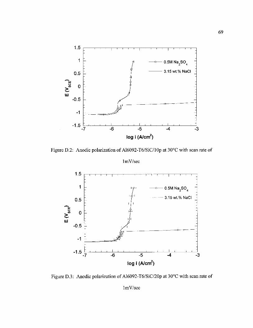
Figure Do2 Anodic polarization of A16092-T6/SiC/lOp at 30°C with scan rate
of lmV/sec 69
Figure D.3 Anodic polarization of A16092-T6/SiC/20p at 30°C with scan rate
of lmV/sec 69
Figure D.4 Anodic polarization of A16092-T6/SiC/40p at 30°C with scan rate
of lmV/sec 70
Figure D.5 Anodic polarization of A16092-T6/SiC/50p at 30°C with scan rate
of lmV/sec 70
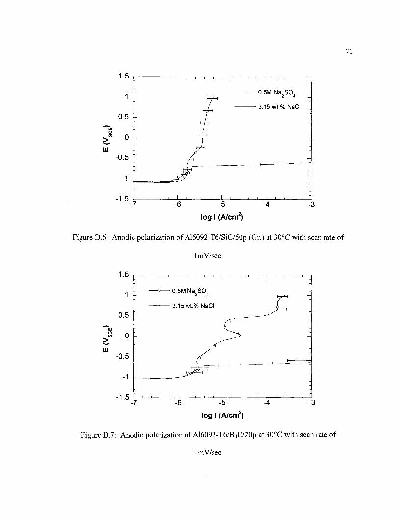
Figure D.6 Anodic polarization of A16092-T6/SiC/50p (Or.) at 30°C with scan
rate of lmV/sec 71
Figure D.7 Anodic polarization of A16092-T6/B4C/20p at 30°C with scan rate
oflmV/sec 71
Figure D.8 Anodic polarization of A16092-T6/Ah03/20p at 30°C with scan rate
of lmV/sec 72
Figure D.9 Anodic polarization of A1606l-T6 at 30°C with scan rate of lmV/sec 72

1
CHAPTER 1
INTRODUCTION
For almost 25 years, the engineering and design community have been using aluminum
metal-matrix composites (MMC) in an attempt to reduce structural weight and
dramatically improve performance. MMC is a general term that encompasses
discontinuously reinforced aluminum (DRA) composites. Of particular interest are
MMCs consisting of an aluminum matrix reinforced with ceramic particles such as
silicon carbide (SiC), boron carbide (B4C) or aluminum oxide (Ah03) in varying volume
loadings. Al6092 is a matrix formulation manufactured by DWA Aluminum Composites
in California. Table 1.1 indicates that Al6061 and Al6092 contain similar quantities of
magnesium (Mg) and silicon (Si) alloying elements. Magnesium silicide (Mg2Si)
second-phase intermetallic particles serve to strengthen the aluminum matrix through
precipitation hardening during the heat treatment process.
Table 1.1: Comparison of A16061-T6 and A16092-T6
Maximum Amounts Specified (Wt.%)
Si Fe Cu Mn Mg Cr Zn Ti
A160610.40 - 0.8 0.7
0.15 -0.15 0.8 -1.2 0.04 -0.35 0.25 0.15
[1] 0.40
A160920.75 0.09 0.83 1.05 0.05- - -[2]

2
Volume loadings of 15 to 25% are suitable for structural applications, and loadings of 30
to 55% for CTE and thermal-management applications. Current applications include the
use of 6092/SiC117.5p DRA for extruded Fan Exit Guide Vanes (FEGV's) for Pratt &
Whitney's high by-pass gas turbine engines on the Boeing 777 and thin gage sheet for
both F-16 ventral fins and fuel access covers [2]. Other applications include
2009/SiC/15p aircraft hydraulic components for the F-18 ElF, 6092/SiC/17.5p brake fins
for Walt Disney World thrill rides, and Global Positioning System (GPS) satellite
electronic packaging chip carriers produced from 6063/SiCI50p forgings [2]. Other
potential applications for DRA include sporting goods such as golf equipment, bicycle
frames and components, and spent nuclear fuel containers utilizing Boron Carbide (B4C)
particle reinforcement in lieu of SiC [2]. Despite the many benefits ofMMC technology,
metal-matrix composites suffer from preferential corrosion because of their
nonhomogeneous composition and structure. In particular, aluminum alloy matrix
materials are very susceptible to corrosion when the dispersoid is a noble phase, such as
SiC [3]. Table 1.2 shows the resistivities ofthe aluminum and ceramics used.
Table 1.2: Resistivities ofmaterials used in metal-matrix composites
Resistivities of Selected Materials
Ceramic Purity (%) Resistivity (n-cm) Reference
SiC (black) 97.0 10° [4]
SiC (green) 99.3 106 [4]
B4C 99.5 101 [4]
Ah0 3 99.7 >1014 [5]
Al6061-T6 98.0 4 x 10,6 [6]

3
The MMCs selected for this corrosion project were manufactured by DWA Aluminum
Composites using 6092 aluminum powder in combination with different volume fractions
of SiC, B4C and Ah03 particulate. The aluminum powder and ceramic particulate were
homogeneously blended and vacuum-hot-pressed into cylindrical billets. In this case,
each billet was manufactured with the same processing and thermomechanical history. In
addition, after pressing, each billet underwent the same T6 heat treatment. The billets,
ranging from 3.56 inches to 3.75 inches in diameter, were cut into 0.1 inch thick wafers
using an electric discharge machining (EDM) technique. Each wafer was then abrasive
grit blasted to remove the recast layer. The eight aluminum metal matrix composites
selected included A16092-T6/SiC (black) with 5, 10, 20, 40 and 50% volume fractions in
addition to A16092-T6/SiC/50p (green), A16092-T6/B4C/20p and A16092-T6/Ah03/20p.
Metallographic specimens of each MMC were prepared by setting 0.25 inch diameter
disks in Buehler Epo-Thin low viscosity epoxy. The specimens were polished in a multi
step process using a Buehler Ecomet 6 variable speed polisher. The face of each
specimen was ground flat with 320 grit silicon carbide paper and then reground with a 30
micron Ultra-Prep diamond grinding disk. Subsequent refinement of the MMC surface
included polishing with 9, 3, 1, 0.25 and 0.05 micron Metadi Supreme polycrystalline
diamond suspensions. The images shown in Figures 1.1 through 1.8 were captured using
a Nikon Epiphot optical microscope in conjunction with Buehler Omnimet software. It is
clear from the metallographic images that the SiC, B4C and Ah03 particles are irregular
in shape and randomly distributed. Also, it is apparent that the average particulate size

4
increases as the volume fraction of the MMC increases. This is intentional and necessary
in order to achieve the higher volume fractions.
Figure 1.1: Microstructure of A16092-T6/SiC/5p
Figure 1.2: Microstructure of A16092-T6/SiC/1 Op

Figure 1.3: Microstructure of AI6092-T6/SiC/20p
Figure 1.4: Microstructure of A16092-T6/SiC/40p
5
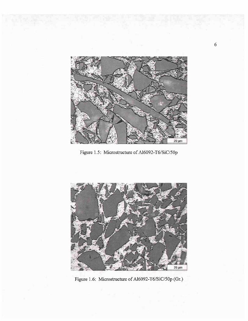
Figure 1.5: Microstructure of A16092-T6/SiC/50p
Figure 1.6: Microstructure of A16092-T6/SiC/50p (Gr.)
6

Figure 1.7: Microstructure of A16092-T61B4C/20p
.',
'., .", .
J .. -
Figure 1.8: Microstructure of A16092-T6/AhOi20p
Figures A.I through A.8 in Appendix A show the eight MMCs at a lower magnification
thereby revealing the macroscopic uniformity of the microstructure.
7

8
CHAPTER 2
LITERATURE REVIEW
Due to the wide availability of aluminum MMCs compared to other more exotic metal
composites, corrosion research has focused on aluminum MMCs containing boron,
graphite, SiC, Ab03 and mica [7]. In the late 1960s literature on the corrosion ofMMCs
began to appear. Initially the focus was on boron monofilament/aluminum (BMP/AI)
MMCs [8] but by the early 1970s the research had expanded to include graphite
fiber/aluminum (Gr/AI) MMCs [7]. It wasn't until the end of the 1970s that research on
the corrosion of alumina fiber/aluminum (Ab03/AI) and magnesium MMCs was
published [9-12]. Corrosion literature pertaining to silicon carbide/aluminum (SiC/AI)
MMCs [7] became available in the early 1980s along with literature on lead, depleted
uranium and stainless steel MMCs. The reinforcement particles used can be classified as
insulators in the case of boron and Ab03, semiconductors in the case of SiC and
conductors in the case of graphite [13]. The emphasis of much of the corrosion literature
has been the study of galvanic corrosion between the MMC's matrix and reinforcement.
Evidence has shown that galvanic corrosion occurs in B/AI and SiC/AI MMCs. For
SiC/AI MMCs in aqueous solutions, hydrogen evolution (proton reduction) and oxygen
reduction can occur on the SiC particles which act as an inert electrode [14]. The pitting
potential (EpIT) of SiC/AI MMCs is very similar to that of the monolithic matrix material
suggesting that the pitting resistance of the passive layer on the aluminum is unaffected
by the addition of silicon carbide particles [14]. Alumina (Ah03) has a resistivity of
9
about 1014 O-cm [15] indicating little or no galvanic corrosion between the aluminum
matrix and the Ah03 particulate. However, in accelerated corrosion tests of Ah03/Al
(2% Li) MMCs in environments containing chlorides, the corrosion rate of the
alumina/AI MMC was in most cases slightly higher than that of 6061-T6 aluminum [16].
Literature discussing the corrosion of aluminum reinforced with boron filaments (BFs)
indicates that corrosion rates increase with an increase in the content of BFs due to an
escalation in the number of aluminum-boride cathodic sites [17]. Boron/aluminum
MMCs experience severe corrosion in chloride environments and are significantly less
corrosion resistant than unreinforced aluminum alloys [18]. Few studies have been
conducted in which various MMCs with a wide range of particulate type and volume
fraction have been exposed to diverse real-world environmental conditions. Oxidizing or
halide containing environments can induce pitting of the matrix metal of MMCs exposed
to those environments [14]. The presence of noble reinforcing particles can accelerate
pitting of the MMC matrix due to galvanic effects [14] and discontinuous SiC/AI MMCs
are susceptible to localized corrosion in the form of mild to moderate pitting exposed in
splash/spray and marine atmospheric environments [18]. Corrosion rates of SiC/AI
MMCs immersed in real seawater are much higher than those observed in atmospheric
testing [18]. Corrosion rates of SiC/AI MMCs immersed in seawater are generally higher
than those for unreinforced aluminum alloys in the same solutions [18]. Discontinuous
SiC/AI MMCs corrode at the particle matrix interface due to crevices that form in those
regions [19-21]. The crevices are preferential sites for pitting [18].

10
CHAPTER 3
OUTDOOR EXPERIMENT
3.1 Introduction
Atmospheric corrosion IS an electrochemical process involving a metal, corrosion
products, a surface electrolyte, and the atmosphere [22]. On the basis of all the testing,
outdoor atmospheres have been broadly classified into three qualitative categories: rural,
industrial, and marine [23]. For the purpose of this corrosion study, rural and agricultural
classifications are used interchangeably. In addition, two more outdoor classifications,
namely wet and dry were identified. All of these atmospheric climates can be found on
the island of Oahu therefore six test sites were selected with the intent of exposing the
MMC specimens to these diverse atmospheric conditions. Test site selection was
primarily dependent on three criteria; each of the five outdoor atmospheric classifications
needed to be represented, each site had to be reasonably accessible, and each site had to
be sufficiently secure to reduce the risk of vandalism or theft. Figure 3.1 shows the
location of six atmospheric test sites on the island of Oahu. Test sites are located at the
Lyon Arboretum in Manoa Valley (A), on Coconut Island in Kanehoe Bay (B), Campbell
Industrial Park (C), Kahuku (D), Ewa Nui (E), and Waipahu (H). The Lyon Arboretum
and Coconut Island sites are on University of Hawai'i property and the remaining sites
are on Hawaiian Electric Company (HECO) property. Once the test sites were selected,
racks were designed to hold the MMC specimens in addition to holding weather and
atmospheric monitoring equipment. Test site maintenance which includes changing

11
chloride candles, downloading weather data, photographing and/or retrieving specimens
is performed on a monthly basis.
Figure 3.1: Location ofatmospheric corrosion test sites on Oahu
3. 2 Materials
Test racks were designed and constructed using 316 stainless steel and TREX®. TREX®
is a "wood-like" composite made from recycled wood chips and recycled polyethylene.
Racks on HECO property had to be non-conductive and therefore were constructed
entirely from TRE~. Test racks on UH property comprised of TREX® slats on a
stainless steel frame. Two test racks on Coconut Island were secured to a concrete slab
with stainless steel bolts, but the remaining test racks were anchored with four 83 lb
concrete blocks such that they can withstand winds up to 100 miles per hour. In addition,
12
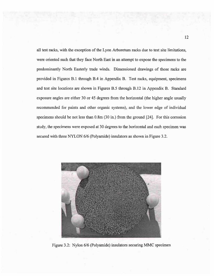
all test racks, with the exception of the Lyon Arboretum racks due to test site limitations,
were oriented such that they face North East in an attempt to expose the specimens to the
predominantly North Easterly trade winds. Dimensioned drawings of those racks are
provided in Figures B.l through B.4 in Appendix B. Test racks, equipment, specimens
and test site locations are shown in Figures B.5 through B.12 in Appendix B. Standard
exposure angles are either 30 or 45 degrees from the horizontal (the higher angle usually
recommended for paints and other organic systems), and the lower edge of individual
specimens should be not less than 0.8m (30 in.) from the ground [24]. For this corrosion
study, the specimens were exposed at 30 degrees to the horizontal and each specimen was
secured with three NYLON 6/6 (Polyamide) insulators as shown in Figure 3.2.
Figure 3.2: Nylon 6/6 (Polyamide) insulators securing MMC specimen

13
3.3 Procedure
Each MMC disk was stamped with an alphanumeric code using a Telisis Benchmark 320
pin stamping system. The disks were washed in acetone followed by ultrasonic cleaning
in deionized water. After drying, each specimen was weighed on a Mettler AE163
electronic balance. The weight of each specimen was measured in grams to four decimal
places. Ten sets of each of the eight MMCs were exposed at the six test sites resulting in
a total of 480 specimens included in the field study. Figure 3.3 shows a typical
arrangement of the MMC specimens on a test rack at Coconut Island.
Figure 3.3: Typical arrangement ofMMCs at test sites
14
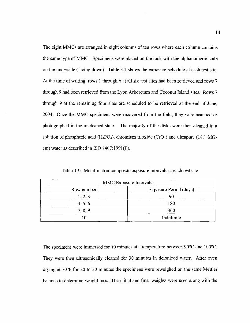
The eight MMCs are arranged in eight columns of ten rows where each column contains
the same type of MMC. Specimens were placed on the rack with the alphanumeric code
on the underside (facing down). Table 3.1 shows the exposure schedule at each test site.
At the time of writing, rows 1 through 6 at all six test sites had been retrieved and rows 7
through 9 had been retrieved from the Lyon Arboretum and Coconut Island sites. Rows 7
through 9 at the remaining four sites are scheduled to be retrieved at the end of June,
2004. Once the MMC specimens were recovered from the field, they were scanned or
photographed in the uncleaned state. The majority of the disks were then cleaned in a
solution of phosphoric acid (H3P04), chromium trioxide (Cr03) and ultrapure (18.1 Mn-
cm) water as described in ISO 8407:1991(E).
Table 3.1: Metal-matrix composite exposure intervals at each test site
MMC Exposure Intervals
Row number Exposure Period (days)
1,2,3 90
4,5,6 180
7,8,9 360
10 Indefinite
The specimens were immersed for 10 minutes at a temperature between 90°C and 100°C.
They were then ultrasonically cleaned for 30 minutes in deionized water. After oven
drying at 70°F for 20 to 30 minutes the specimens were reweighed on the same Mettler
balance to determine weight loss. The initial and final weights were used along with the

15
surface area of each specimen to calculate the average weight loss and thus the average
corrosion rate for each MMC. The average corrosion rate defined in (l) is given in grams
per meter squared per day (gmd).
A C. R (d) Initial Wt.(g) - Final Wt.(g)verage orrOSlOn ate gm =----------'--::,-------------"---'------
Surface Area (m2 )x Exposure (days)(1)
Figure 3.4 shows an A16092-T6/SiC/40p specImen that was exposed at the Lyon
Arboretum test site for 90 days. The specimen is shown before and after cleaning.
Figure 3.4: A16092-T6/SiC/40p MMC exposed for 90 days - before and after cleaning
In addition to the MMCs at each test site, ten A16061-T6 specimens were also exposed at
each site for the same durations in order to obtain a baseline corrosion rate of aluminum

16
in its monolithic form. The A16061-T6 coupons measuring 2 inches by 2 inches by 0.125
inches were stamped, cleaned and weighed in the same manner as the eight metal matrix
composites.
3.4 Results
Average corrosion rates for the 90 day, 180 day and 360 day exposures are provided in
Figures 3.5, 3.6, and 3.7. Data for 360 day exposure corrosion rates has been collected
for two of the test sites, namely Manoa and Coconut Island. Figure 3.7 compares average
corrosion rates over 90, 180 and 360 day exposures for those sites.
Average Corrosion Rates of MMCs and A16061·T6 after 90 Day Exposure
0.•
0,35
0.3'0E~B 0.25"lrt:C
~ 0.2
go
C,) 0.15
0,1
0,05
o
QA·Manoa
• B· Coconut Is
IIlC·CIP
_0· Kahuku
El E • Waipahu
_H ·Ewa Nui
A: AJ6092·T6ISiClSpB: AJ6092·T6ISiCllOpC: AI6092·T6ISiCI20p0: A16092·T6ISiC/40pE: AI6092·T6ISiC/50pH: A16092·T6ISiC/50p (Gr )J: A16092·T6JB,C120pK: AI6092·T6IAI,0,J20pL: AI6061·T6
A (5p) B(10p) C (2Op) 0(4Op) E (SOp) H (SOp Gr) J (B4C) K (Al203) L (6061)
Figure 3.5: Average corrosion rates ofMMCs and A16061-T6 after 90 day exposure

Average Corrosion Rates of MMCs and A16061·T6 after 180 Day Exposure
02
17
0.18
0.18
0.14
:aE..!!! 0.12
~0:: 0.1co
~ 0.08oo
CA- Manoa
• B - Coconut Is
L9C· CIPliD . Kahuku
l'JE -Waipahu
IIH· Ewa Nui
A: A16092·T6ISiC/SpB: AI6092.T6ISiC/10pC: AJ6092·T6ISiCI2Op0: AJ6092·T6ISiCl40pE: AI6092·T6ISiC/SOpH: AJ6092·T61SiG/SOp (Gr )J: AI6092·T6IB,CI20pK: AI6092·T6/AI,0,J20pL: AI6061·T6
0.08
0.04
0,02
oA(Sp) B(10p) C(20p) D(4Op) E(SOp) H (SOp Gr.) J (B4C) K(AI203) L(6061)
Figure 3.6: Average corrosion rates ofMMCs and A16061-T6 after 180 day exposure
Average Corrosion Rates of MMCs and AI6061-T6 after 90,180 and 360 Day Exposures
0.45
04
035
:a 03
E..!!!.!l 025..0::co 0.2.~
oo 0.15
0.1
005
o
D AI6092·T6ISiCJ5p
IIAI6092·T6/SiC/10p
E:I AI6092·T6/SiC/20p
II A16092·T6ISiCJ40p
CI A16092·T6ISiCJSOp
II AI6092·T6ISiCJSOp(Gr)
l'J AJ6092·T61B4CI2Op
l'J AJ6092·T6IA1203l2Op
IIAI6061·T6
Figure 3.7: Average corrosion rates ofMMCs and A16061-T6 after 360 day exposure

18
3.5 Discussion
Some trends are clearly visible from the corrosion data obtained. Corrosion rate of an
MMC generally increases with an increase in volume fraction of the reinforcement. At
the end of the 90 day exposure, A16092-T6/SiC/50p at Coconut Island was the worst
performing MMC having a corrosion rate more than 80 times that of A16061-T6 at the
same site exposed for the same duration. Even the best performing MMC, A16092
T6/SiC/10p at the Ewa Nui test site had a corrosion rate almost 10 times greater than
A16061-T6 at the same site. Three of the eight MMCs have the same twenty percent
volume fraction of reinforcement but A16092/B4C/20p generally appears to corrode at a
higher rate than either SiC or Ah03 reinforced aluminum. This is likely due to the
resistivity of the reinforcements since boron carbide is generally considered to be a
conductor, silicon carbide a semi-conductor and aluminum oxide an insulator. Corrosion
rates for all of the MMCs at the Manoa (Lyon Arboretum) and Coconut Island test sites
were comparable for the 90, 180 and 360 day exposures despite significant differences in
atmospheric and weather conditions at the two sites. The data collected for the 360 day
exposure only included two test sites, namely Manoa and Coconut Island, but Figure 3.7
shows some convergence of the corrosion rates of the MMCs at those sites. Not only are
the corrosion rates of each MMC diminishing throughout the year, but the differences
between the MMCs are becoming less obvious to the extent that one MMC has no clear
corrosion advantage over another. After one year, the difference between the worst
performing MMC at the Manoa site compared to A16061-T6 at the same site had
decreased by almost seventy five percent i.e. from 138 times to less than 39 times the
19
corrosion rate. The same was true at the Coconut Island site where the corrosion rate of
the worst performing MMC was initially more than 80 times greater than that of A1606l
T6. After one year the difference had been reduced by more than two thirds to a
corrosion rate that was 28 times greater than monolithic aluminum. This decreasing trend
could be due to the undercutting and subsequent elimination of cathodic reinforcement
particles (SiC, B4C or Ah03) and/or iron-rich intermetallics in the aluminum matrix.
Undercutting of the reinforcing particulate or intermetallics is caused by the dissolution
of the surrounding aluminum matrix. As the MMC corrodes the cathodic site may be left
in relief. Eventually the particle can be sufficiently undercut that it falls or is washed off
the surface of the composite.

20
CHAPTER 4
WEATHER AND ATMOSHPERIC MONITORING
4.1 Introduction
In order to correlate the corrosion rates of different MMCs at different test sites, it is
necessary to understand the environment in which the specimens are exposed. Standard
ASTM or ISO methods for measuring atmospheric chloride or sulfur dioxide
concentrations can be found in the literature. However, standards for weather monitoring
in terms of corrosion testing are hard to find, but at the very least, a quality weather
station should be installed at each site as near to the specimens as possible [24]. The
accurate monitoring of temperature, humidity, rainfall and chloride deposition rates is
essential for any outdoor corrosion study since these variables have the greatest effect on
corrosion rates.
4.2 Materials
Weather and atmospheric conditions at each test site were monitored and logged
continuously with N.I.S.T. (National Institute of Standards and Technology) certified
Davis Vantage Pro weather stations and data loggers. Time of wetness (TOW) of the
specimens was determined using Davis leaf wetness sensors also at 30 degrees to the
horizontal. The leaf wetness sensor uses a scale from 0 to 15 to represent wetness. A
value of 0 indicates that the sensor is completely dry whereas a value of 15 indicates that
the sensor is completely wet. Chloride (Cn deposition rates were measured using the

21
wet candle method as described in ASTM G 140-96 and ISO 9225:1992(E). Initially,
sulfur dioxide (S02) concentrations were measured with sulfation plates as described in
ASTM G9l-97 and ISO 9225: 1992(E). The sulfation plates (two per site per month)
were manufactured and analyzed by an Industrial Hygiene Accredited Laboratory
(AIHA), but after collecting data for three months it became clear that there was a
problem with some or all aspects of the process. It was decided that accurate S02
monitoring would require a different approach or technique and therefore S02 monitoring
by the sulfation plate method was stopped. Figures B.ll and B.12 in Appendix B show
the weather and atmospheric monitoring equipment used at each test site.
4.3 Procedure
A Davis Vantage Pro weather station at each test site measures and records independent
weather variables such as temperature, humidity, atmospheric pressure, rainfall, wind
speed, wind direction, leaf wetness and UV. Other dependent variables such as dew
point, evapotranspiration and heat index are calculated in real time. Some of the
parameters such as temperature are averaged for each 30 minute period, whereas others,
such as rainfall, are totaled. In all, more than thirty data points are written to an internal
data logger every half an hour. The data stored at each site is downloaded once a month.
Chloride candles are exposed in the field for approximately thirty days and then brought
back to the lab for analysis. The gauze wick is soaked in the remaining ultrapure water
and 100mL of that solution is poured into a beaker. 2mL of 5M sodium nitrate (NaN03)
is added to the beaker which serves as an ionic strength adjustor (ISA). Chloride candle

22
analysis is performed in the lab with an Orion 290A ISE/pH meter and an ion (Cn
selective electrode (9617BN). Figure B.13 in Appendix B shows a calibration curve
generated with solutions of known cr concentration. Actual and measured
concentrations are shown. The cr deposition rates for the Manoa test site are maximum
theoretical rates since cr ions were only detected for the months of November in 2003
and March in 2004. The values shown were calculated using cr concentrations just
below the lower limit of detection possible with an Orion 290A ISE/pH meter and an ion
(Cn selective electrode (9617BN). The lowest concentration of cr detectable with an
Orion 290A ISE/pH meter and an ion (Cn selective electrode (9617BN) is 1.0 x 10⁻⁴M
therefore a concentration of 9.0 x 1O-5M was assumed for those months when no cr ions
were detected.
4.4 Results
Tables 4.2, 4.3 and 4.4 show the weather and atmospheric data collected at each of the
sites during 90, 180 and 360 day exposures. Values in the TOW columns represent the
percentage of the total exposure time when the leaf wetness sensor showed a value of 15
indicating that the specimens were completely wet. The data shows that Manoa and
Coconut Island are very different sites in terms of temperature, humidity, rainfall, time of
wetness and chloride deposition rates. However, Figure 3.7 shows that corrosion rates of
MMCs exposed at those two sites for one year are very similar.

Table 4.2: Weather and atmospheric data for 90 day exposure at corrosion test sites
23
Weather and atmospheric data obtained during 90 day exposure at corrosion test sitesTest Site Avg. Temp Avg. Rain TOW (% of Avg. cr
(OF) Humidity (inches) exposure Deposition(%RH) time) Rate
(mg/m2/day)Manoa 72.0 82.9 62.0 28.6 6.5
Coconut Is. 77.5 73.7 8.6 12.4 64.6Campbell 82.7 60.6 4.1 4.0 17.3Kahuku 80.3 71.8 20.1 8.8 47.0Waipahu 81.3 63.8 11.6 1.5 8.0EvaNui 80.6 64.0 2.2 1.4 6.4
Table 4.3: Weather and atmospheric data for 180 day exposure at corrosion test sites
Weather and atmospheric data obtained during 180 day exposure at corrosion test sitesTest Site Avg. Temp Avg. Rain TOW (% of Avg. cr
(OF) Humidity (inches) exposure Deposition(%RH) time) Rate
(mg/m2/day)Manoa 73.3 83.1 140.9 26.1 7.0
Coconut Is. 78.4 74.9 25.6 8.2 58.3Campbell 81.0 63.2 17.9 5.3 24.4Kahuku 78.1 73.4 52.0 13.6 89.9Waipahu 79.4 66.9 31.1 6.6 10.7EvaNui 78.6 67.4 32.5 6.1 9.4
Table 4.4: Weather and atmospheric data for 360 day exposure at corrosion test sites
Weather and atmospheric data obtained during 360 day exposure at corrosion test sitesTest Site Avg. Temp Avg. Rain TOW (% of Avg. cr
(OF) Humidity (inches) exposure Deposition(%RH) time) Rate
(mg/m2/day)Manoa 72.3 85.0 333.9 31.4 5.9
Coconut Is. 76.8 76.2 101.8 14.9 93.4

24
Leaf wetness sensors, in addition to providing data indicating the percentage of the total
exposure time at each test site when specimens are completely wet, may also provide an
insight into how the specimens transition for the wet to the dry state. Figure 4.1 shows
the time of wetness (TOW) of the leaf wetness sensor at the Lyon Arboretum during the
90 day exposure period. In contrast, Figure 4.2 shows the time of wetness (TOW) of the
leaf wetness sensor at the Coconut Island test site during the same 90 day exposure.
Tim. of W.tne••1Lyon ArboJetum T•• Site Dunng 10 OIly Ex_re
7000
8000
5000
E~ 4000 -::l
IIIt~ 30.00 -
11-
2000
1000 ~
000
n .." _ ....0 , 2 3 4 ! • 7 • • to " 12 13 " 15
W.fl1••
Figure 4.1: Time of wetness (TOW) ofleafwetness sensor at Manoa test site

25
Tlmo 0' Wotno. 01 Cooonut I"ond To. Silo During 80 Coy Expo....
4500
4000
3500
3000
~FI! 2500 -
"..tUl 20 00'Iiit.
1500 -
1000
f
500 -1'""1.
000R R .... "'" "'" ... "'" n ...... F'I n II
0 1 2 , • 5 e 1 • • 10
"U ., " "
W.tn..
Figure 4.2: Time of wetness (TOW) ofleafwetness sensor at Coconut Island test site
4.5 Discussion
It should be noted that the Manoa test site had seven times the rainfall of the Coconut
Island test site in the same 90 day period. The average temperature and humidity in
Manoa for that period were lower and higher respectively. However, the percentage of
the exposure time when the leaf wetness sensor was completely wet was only greater by a
factor of about 2.3. Figure 4.1 indicates that the leaf wetness sensor and therefore the
specimens in Manoa were for the most part either wet or dry and the figure implies a
rapid transition between those states. In contrast, Figure 4.2 implies a more gradual
transition between the wet and dry states of the specimens at the Coconut Island site. The
marked difference in cr deposition rates at the Manoa and Coconut Island test sites,

26
i.e. 6.5 compared to 64.6 mg/m2/day respectively, may explain the difference seen in the
two figures. It is possible that salt on the leaf wetness sensor, and thus on the specimens,
may delay or retard the transition from the wet to the dry state. The weather data shown
in the tables above have to a great extent validated the test site selection process. The
atmospheric conditions at each site vary considerably in terms of humidity, rainfall, time
of wetness, cr deposition rates and wind. However, temperature variations are limited
by the negligible differences in test site elevation. The Manoa site has the highest
elevation at 520 feet above sea level whereas the Coconut Island site has the lowest
elevation at only ten feet above sea level. Accurately and tediously correlating the
atmospheric and weather data with the corrosion rates observed will provide a less
simplistic analysis of metal-matrix composite performance in different environmental
conditions.

27
CHAPTER 5
HUMIDITY CHAMBER EXPERIMENT
5.1 Introduction
Correlating the corrosion rates of MMCs to real-world environmental conditions is a
complex undertaking due to the multitude of weather and atmospheric variables that the
MMCs may be exposed to. Humidity chamber experiments are more easily controlled
having only three adjustable parameters. At the start of the experiment the electrolyte
determines which ions if any are on the surface of the MMC. Once the experiment has
started the only other variables are temperature and humidity which are easily controlled.
5.2 Materials
A tile cutting saw with diamond blade was used to cut 1 inch by 1 inch squares from the
MMC disks manufactured by DWA Aluminum Composites. Acrylic holders capable of
holding three specimens of the same type in the vertical position with minimal specimen
holder contact were designed and manufactured.
5.3 Procedure
Each specimen was stamped with an identification number, washed in acetone and
ultrasonically cleaned in deionized water. After drying, each specimen was weighed on a
Mettler AE163 electronic balance. The weight of each specimen was measured in grams
to four decimal places. The specimens were placed in the holders then immersed for one

28
minute in beakers containing one of four electrolytes. All of the eight MMC types were
immersed in ASTM sea water, 3.15 wt% sodium chloride (NaCl) and 0.5M sodium
sulfate (NazS04) solutions. In addition, the following MMCs, AI6092/SiC/20p,
Al6092/B4C/20p and A16092/Alz03/20p were immersed in real sea water obtained from
the Waikiki Aquarium resulting in twenty seven holders and eighty one specimens.
Table C.1 in Appendix C lists the major ionic constituents found in different types of
seawater and more specifically, in the seawater used for this experiment. It should be
noted that the chloride (Cn ion content of 3.15 wt.% NaCI solution, Waikiki Aquarium
seawater and ASTM seawater is 19,108, 19,582 and 20,488 ppm respectively. After
immersion, each set of three specimens was immediately placed inside a humidity
chamber. The temperature and humidity inside the chamber was maintained at 300 e and
85% (RH) respectively for 90 days.
Figure 5.1: MMC specimens after 90 day exposure in humidity chamber

29
Atmospheric conditions inside the chamber were controlled via an Electro-tech model
514 automatic humidity controller, a Cole Parmer mode12186-20 Digi-sense temperature
controller and an Evenflo humidifier containing ultrapure water. After 90 days the
speCImens were removed from the chamber and scanned or photographed in the
uncleaned state. Figure 5.1 shows the specimens after they were removed from the
humidity chamber. The majority of the exposed coupons were then cleaned in a solution
of phosphoric acid (H3P04), chromium trioxide (Cr03) and ultrapure (18.1 MO-cm)
water as described in ISO 8407:1991(E). The specimens were immersed for 10 minutes
at a temperature between 90°C and 100°C. They were then ultrasonically cleaned for 30
minutes in deionized water. After oven drying at 70°F for 20 to 30 minutes the
specimens were reweighed on the same Mettler balance to determine weight loss.
5.4 Results
As shown in equation (1), the initial and final weights were used along with the surface
area and exposure time of each specimen to calculate the average weight loss and thus the
average corrosion rate for each MMC. Figure 5.2 shows the corrosion rates for each of
the MMCs exposed to the different electrolytes. The average corrosion rate is given in
grams per meter squared per day (gmd).

30
Average Corrosion Rates of MMCs after 90 Days in Humidity Chamber
K (AI203)J (B4C)
A: AI6092-T6/SiC/5pB: AI6092-T6/SiC/10pC: AI6092-T6/SiCI20p0: AI6092-T6/SiC/40pE: AI6092-T6/SiC/50pH: AI6092-T6/SiC/50p (Gr.)
J: AI6092-T61B4C/20p
K: AI6092-T6/Alz0 3120p
H (SOp Gr.)E (SOp)o (40p)C (20p)B (10p)A (5p)
o
0.3
o AS1M Sea Water
II 3.15 wt% NaCI
0.25 ~ O.5M Sodium Sulfate
II Real Sea Water
:c 0.2
ES.sIIIa:: 0.15c:0'iiig0U 0.1
;.;.:
0.05
Figure 5.2: Corrosion rates ofMMCs exposed in humidity chamber for 90 days
5,5 Discussion
As in the field study, the corrosion rates were generally found to increase with an
increase in the volume fraction of the particulate reinforcement. The corrosion rates of
the specimens dipped in ASTM sea water, 3.15 wt.% NaCl and real sea water were
similar. Of the three MMCs having a volume fraction of 20 percent, Al6092-
T6/Ah03/20p had a consistently lower corrosion rate than the B4C reinforced aluminum.
This may be due to the much greater resistivity of Ah03 compared to B4C. This
explanation is further reinforced by the corrosion rates of the three MMCs dipped in
ASTM sea water. Of the three, the highest corrosion rate was the SiC MMC followed by

31
B4C and Ah03 MMCs. This trend follows the respective resistivities of 10°, 101 and 1014
as shown in Table 1.2. The corrosion rate for A16092-T6/SiC/50p was consistently
greater than that of A16092-T6/SiC/50p (Gr.) which contains a higher purity SiC
reinforcement.
32
CHAPTER 6
IMMERSION EXPERIMENT
6.1 Introduction
Immersion experiments in aerated solutions containing aggressive ions provide some of
the most hostile environments for aluminum alloys and aluminum MMCs. Corrosion
rates may be many times higher when compared to MMCs exposed at corrosion test sites.
6.2 Materials
As in the humidity chamber experiment, a tile cutting saw with diamond blade was used
to cut 1 inch by 1 inch squares from the MMC disks manufactured by DWA Aluminum
Composites. A16061-T6 coupons measuring 2.0 inches by 2.0 inches were cut with a
low-speed saw. Acrylic holders capable of holding three specimens of the same type in
the vertical position with minimal specimen-holder contact were designed and
manufactured.
6.3 Procedure
Each specimen was stamped with an identification number, washed in acetone and
ultrasonically cleaned in deionized water. After drying, each specimen was weighed on a
Mettler AE163 electronic balance. The weight of each specimen was measured in grams
to four decimal places. The specimens were placed in the holders then placed in 250ml
beakers. The pH of the five electrolytes to be used in the immersion experiment was

33
measured with an Orion 290A ISE/pH meter and an Orion pH triode 9107BN electrode.
200mL of solution was added to each beaker and the beakers were covered to reduce
evaporation while still allowing oxygen to diffuse into the electrolyte. All of the eight
MMC types and the A16061-T6 coupons were immersed in ASTM sea water, 3.15 wt%
sodium chloride (NaCl) and O.5M sodium sulfate (Na2S04) solutions. In addition, the
following MMCs, AI6092/SiC/20p, A16092/B4C/20p and AI6092/Ah03/20p were
immersed in ultrapure (18.1 Mil-em) water and real sea water obtained from the Waikiki
Aquarium. Three A16061-T6 coupons were immersed in real sea water. Table C.l in
Appendix C lists the major ionic constituents found in different types of seawater and
more specifically, in the seawater used for this experiment.
Figure 6.1: MMC in electrolyte after 90 day immersion
34
The aquariums used contained thirty four beakers and one hundred and two specimens.
After arranging the beakers in two aquariums, deionized water was added to within 0.5
inches of the tops of the beakers. The aquariums were covered and the water was
maintained at 30°C with an electric submersible aquarium heater in an effort to maintain
the temperature of the solutions in the beakers. After 90 days the beakers were removed
and the pH of the solution in each beaker was re-measured with the same Orion 290A
ISE/pH meter and an Orion pH triode 9107BN electrode. Figure 6.1 shows three MMC
coupons in a beaker at the end of the 90 day immersion. Initial and final pH data is
provided in Table C.2 and Table C.3 in Appendix C. The specimens were removed from
the beakers, dried and scanned or photographed in the uncleaned state. The majority of
the exposed coupons were then cleaned in a solution of phosphoric acid (H3P04),
chromium trioxide (Cr03) and ultrapure (18.1 MO-cm) water as described in ISO
8407: 1991(E). The specimens were immersed for 10 minutes at a temperature between
90°C and 100°C. They were then ultrasonically cleaned for 30 minutes in deionized
water. After oven drying at 70°F for 20 to 30 minutes the specimens were reweighed on
the same Mettler balance to determine weight loss.
6.4 Results
As shown in equation (1), the initial and final weights were used along with the surface
area and exposure time of each specimen to calculate the average weight loss and thus the
average corrosion rate for each MMC and the A16061-T6 coupons. Figure 6.2 shows the
average corrosion rates for each of the MMCs and A16061-T6 immersed in the different

35
electrolytes. The average corrosion rate is given in grams per meter squared per day
(gmd).
Average Corrosion Rates of MMCs and A16061-T6 after 90 Day Immersion
1.6
1.4
1.2
'CE 1,9
~0:: 0.6
"o'iiieo 0.6U
0.4
0.2
o
IJASTM Sea Water
113.15 wt% NaCI
ts:I O.5M Sodium Sulfate
1118.1 MO-cm Water
~ Real Sea Water
A: A16092-T6/SiC/5pB: A16092-T6/SiC/1 OpC: A16092-T6/SiC/20pD: A16092-T6/SiC/40pE: A/6092-T6/SiC/50pH: A16092-T6/SiC/50p(Gr.)J: A16092-T6/B4C/20p
K: AI6092-T6/AI20 3/20p
L: A16061-T6
A (Sp) B (10p) C (20p) D(40p) E (SOp) H (SOp Gr.) J (B4C) K (AI203) L (6061)
Figure 6.2: Corrosion rates ofMMCs and A16061-T6 after 90 day immersion
Five MMC specimens were selected for Energy Dispersive X-ray Analysis (EDXA) after
the 90 day immersion experiment to determine the composition of the corrosion products
on the surface of each coupon. The five MMCs selected included Al6092/SiC/20p
immersed in 3.15 wt% NaCI, ASTM sea water and real sea water. Also, A16092-
T6/B4C120p and A16092-T61Al203120p immersed in ASTM sea water. Figures 6.3 , 6.4
and 6.5 show the data collected from a 600 micron by 400 micron area from the three
A16092/SiC/20p MMC specimens.

o Kal
Figure 6.3: EDXA of A16092-T6/SiC/20p immersed in 3.15 wt.% NaCl
soon
300~
36
C.Kb1
t
Figure 6.4: EDXA of A16092-T6/SiCI20p immersed in ASTM sea water

37
CaKblK I
IKal
81
Figure 6.5: EDXA of AI6092-T6/SiC/20p immersed in real sea water
EDXA results for the B4C and Ah03 MMCs are shown in Figures C.I and C.2 in
Appendix C.
6.5 Discussion
The data in Figure 6.2 shows an increase in corrosion rate with a corresponding increase
in the volume fraction of the particulate reinforcement. As in the humidity chamber
experiment, the corrosion rates of the three MMCs having reinforcement volume
fractions of 20 percent exhibit corrosion behavior that may be partly explained by the
relative resistivities of the reinforcement material. Of the three 20p MMCs in most of the
solutions, the highest corrosion rates were observed in the B4C MMC followed by SiC
and Ah03 MMCs. This trend maintains Ah03 as the best performer and follows the

38
respective resistivities of 101,10° and 1014 as shown in Table 1.2. The corrosion rates of
all of the MMCs in 3.15 wt.% NaCI are markedly higher than corresponding rates in
ASTM sea water or real sea water. In each case where the specimen was immersed in
either ASTM sea water or real sea water, EDXA analysis indicated the presence of
magnesium hydroxide (Mg(OH)2) and not calcium carbonate (CaC03) as expected. It is
suggested that the Mg(OH)2 covered the cathodic sites on the composite thereby reducing
the rate of corrosion in both ASTM and real sea water. Figures C.l and C.2 in Appendix
C show EDXA results of A16092-T6/B4C/20p and A16092-T6/Ah03/20p after immersion
in 3.15 wt.% NaC!. In both cases there are no peaks to suggest the presence of either
magnesium or calcium. This is expected since 3.15 wt.% NaCI solution shouldn't
contain either element. However, the result may help to confirm that sea water is the
source of the magnesium rather than the 6092 matrix material which does contain small
amounts of magnesium as shown in Table 1.1. Real sea water and ASTM sea water have
natural corrosion inhibitors in addition to providing some form of solution buffering.
Both ASTM sea water and real sea water became more neutral over the 90 day
immersion experiment. ASTM sea water had an initial pH of 8.2 and the real sea water
had an initial pH close to 7.8 but after the experiment was completed the pH of both
solutions was close to 7.5. The other three solutions became more alkaline ending with
pH ranges of 7.4 to 8.7. Since all of the solutions were aerated in the sense that oxygen
was allowed, both proton reduction (hydrogen evolution) and oxygen reduction could
take place on cathodic sites. For MMCs in 0.5M Na2S04, 3.15 wt.% NaCI or ultrapure
water, the higher corrosion rates and hence increase in hydrogen evolution and/or oxygen

39
reduction could result in the consumption of H+ ions and the production of OH- ions.
Both reactions could shift the pH ofthe solutions in the alkaline direction.

40
CHAPTER 7
POLARIZAnON EXPERIMENTS
7.1 Introduction
A complete set of anodic polarization experiments for the eight MMCs and A16061-T6 in
this study required fifty four individual polarizations employing thirty eight electrodes.
7. 2 Materials
Four lcm by lcm squares were cut from the eight types of MMC disks manufactured by
DWA Aluminum Composites using a low-speed saw and high concentration diamond
blade. Six 1cm by 1cm squares were also cut from A16061-T6 coupons. Once the
MMCs and aluminum were cut, the comers were radiused to reduce stress concentrations
and the backs of the electrodes were sanded using 320 grit silicon carbide paper. The
specimens were cleaned in acetone and dried. A 0.0325 inch copper wire approximately
12 inches in length was attached to the back of each MMC and aluminum electrode with
silver conductive epoxy (MG Chemicals 8331-14g) and cured in an oven at 70°C for 20
minutes. Once cured, the copper wire was threaded through the center of a 9 inch long
glass tube having on O.D. of 9/32 inch. The back face and sides of each electrode was
coated with Loctite 0151 Hysol® epoxi-patch adhesive (manufactured by Loctite Corp.)
in addition to being bonded and sealed to the glass rod such that the front face was the
only part of the MMC or aluminum exposed to the atmosphere. The electrode was cured
in an oven at 70°C for two hours. The face of each electrode was ground flat with 320

41
grit silicon carbide paper followed by 600 grit silicon carbide paper. After grinding with
600 grit silicon carbide paper, each electrode was viewed under an optical microscope to
check for crevices between the edges of the electrode face and the surrounding epoxy. In
addition, the resistance between the face of the electrode and the end of the copper wire
was measured to ensure good conductivity. Resistances ranging from 0.5n to 1.0n were
found to be ideal.
Figure 7.1: MMC polarization electrodes ready for final polishing
Subsequent refinement of the MMC or aluminum electrode surface included polishing
with 1, 0.3 and 0.05 micron deagglomerated alpha alumina polish until a "mirror-like"
finish was achieved. The electrodes were polished on Buehler Ecomet 6 variable speed

42
polishers using Buehler microc1oth polishing wheels. Figure 7.1 shows two electrodes
after grinding with 320 grit silicon carbide paper.
7. 3 Procedure
Polarization experiments for the MMCs were conducted usmg a Princeton Applied
Research Potentiostat/Galvanostat Model 273A controlled with DOS based software.
Polarization experiments for the A16061-T6 were conducted using a Princeton Applied
Research Potentiostat/Galvanostat Model 283 controlled with Windows® based software.
All of the anodic polarization experiments were run in either deaerated 3.15 wt.% sodium
chloride (NaCl) solution or deaerated 0.5M sodium sulfate (NaS04) solution. In both
cases the cell was deaerated with nitrogen (N2) gas that was 99.999% pure. A typical
polarization cell set up is shown in Figure 7.2. The cell contained a working electrode, a
platinum counter electrode, a glass luggin probe that provided connectivity to a calomel
reference electrode, a gas dispersion tube and a thermometer. The jacketed cell was
connected to a Fisher Scientific model 9100 Isotemp refrigerated circulator that
maintained the electrolyte inside the cell at 30°C. For each of the polarization
experiments, the cell was filled with electrolyte and allowed to reach operating
temperature while the working electrode was repolished with 0.05 micron alumina polish.
The electrode was rinsed in ultrapure water and placed in a beaker of ultrapure water to
prevent the oxide layer from drying out. The electrode was then placed in the cell and
electrolyte was drawn through the luggin probe to the reference electrode.

43
Figure 7.2: Typical polarization cell arrangement
Nitrogen gas was bubbled into the cell to deaerate the electrolyte, and the potential
between the working electrode and the reference electrode was monitored for one hour.
After an hour the cell was completely deaerated and the open circuit potential (OCP) had
been reached. The electrode was then polarized at a scan rate of 1mV/sec from the open
circuit potential to -O.5VSCE in 3.15 wt.% NaCI to obtain pitting potentials, and from the
open circuit potential to 1.0VSCE in O.5M Na2S04 to obtain passive current densities.
7.4 Results
Figure 7.3 represents twenty seven experiments and provides data obtained from anodic
polarizations in deaerated 3.15 wt.% sodium chloride (NaCl) solution. Figure 7.4 also

44
represents twenty seven experiments and provides data obtained from anodic
polarizations in deaerated 0.5M sodium sulfate (Na2S04) solution.
-0.5
-0.6
-0.7
- -0.8wu
~Ul
w-0.9
-1
-1.1
---- AJ6OU·TllISiCI5p
- AlB092·TllISiCI1Op
- - - - AJ6On-T6JSlCIlOp
• •••• AJ6lJ92·TllIS~Op
• -. - Al6On·TllIS~Op
• •• - AlSon·TelSlClSOp (Gr l
~ - A16ll92·T1lJII.IC/2Op
......... 11160n·T6tAl203l2Op
• 11160fil.T5
..,
-3-1.2 '-------'---'---'---'--'----'-------'------'----l.---J'--"---'----'---'---'---'---'-----'----l.---J
-7
Figure 7.3: Anodic polarization in deaerated 3.15 wt.% sodium chloride solution
It should be noted that each curve in the above figures is an average curve obtained from
three experiments conducted with two electrodes per MMC or A16061-T6 per solution.
The first electrode was polarized once whereas the second electrode was polarized twice.
The electrode to be polarized a second time was removed from the cell and reground on
600 grit silicon carbide paper before being reused for the third experiment. It was
repolished using 1, 0.3 and 0.05 micron deagglomerated alpha alumina polish until a
"mirror-like" finish was achieved.

45
.. ,
____ AI6092·T6/SICJ5p
-.0 - "'16092·T6/SlCI10p
- - ... - - AI6092·TelSlCJ2Op
• • .. • • NtlO92-TllISICUOp
• -. - Al609:2·T8lSlCI5Op
• ••- Al6092.TllISoCI5Op (Gr.)
- .. _.T6IB&CI2Op
......... Al6092-TelN2031'2Op
• _1·18
.'
..r~"-', ..-.,....... -_ .......i ,'-.-
, :. ~
~ '"!,a
-1 .__~_n__ '--
0.5
-0.5
-3-5
log I (Alent)
-6
-1.5 l-"-----'--..L...-..L...-....L...-..l.-...........-'---'--'---'-.....L............--I..--1.---'---'----Jl-............
-7
Figure 7.4: Anodic polarization in deaerated O.5M sodium sulfate solution
Table D.I in Appendix D provides the pitting potentials and passive current densities for
the eight MMCs and A1606l-T6 in both solutions. In addition, plots with data error bars
for each of the MMCs and A1606l-T6 in both solutions are shown in Figures D.l through
D.9 in Appendix D.
7. 5 Discussion
The polarization experiments reveal the negligible differences in open circuit potential,
pitting potential or passive current densities between most of the metal-matrix
composites. The one exception is the anodic polarization of A16092-T6/B4C/20p in
deaerated O.5M sodium sulfate solution which exhibits odd behavior requiring further
46
study. However, generally, the differences during polarization between the metal-matrix
composites and A16061-T6 in either solution aren't sufficient to explain the differences in
corrosion rates.

47
CHAPTER 8
CONCLUSION
Corrosion of aluminum-based MMCs may initiate due to galvanic coupling between the
reinforcing phase and the matrix, selective corrosion at the reinforcement/matrix interface
or matrix defects formed during the manufacturing process [25]. Fabrication of MMCs
can lead to the formation of intermetallic particles due to reactions between the
particulate and matrix or the precipitation of compounds [26]. The outdoor, humidity
chamber and immersion experiments all indicate that corrosion rates of aluminum MMCs
increases as the volume fraction of the reinforcing particulate increases. This is most
likely due to an increase in the galvanic-corrosion rate between the noble SiC, B4C or
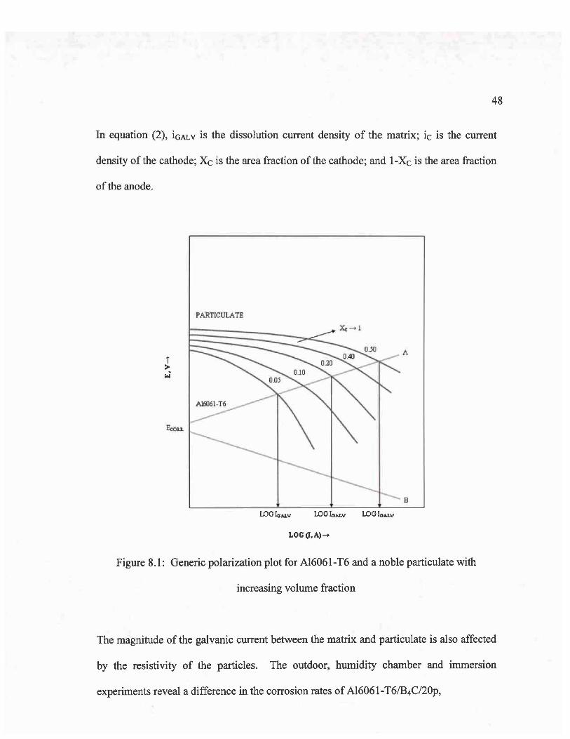
Ah03 particles and the aluminum matrix. Figure 8.1 shows a theoretical increase in the
galvanic current (Log IGALv) as the area fraction of the reinforcement increases [26].
Generic cathodic curves for the noble particulate intersect the anodic curve for A16061
T6 at higher currents as the area fraction increases resulting in an increase in IGALv. That
increase translates directly into higher dissolution rates of the aluminum matrix yielding
higher corrosion rates. The cathode limited galvanic current between the matrix and
particulate can be expressed as a function of the area fraction and hence volume fraction
of the reinforcement [26].
(2)
48
In equation (2), iGALV is the dissolution current density of the matrix; ic is the current
density ofthe cathode; Xc is the area fraction of the cathode; and I-Xc is the area fraction
of the anode.
PARTICUlATE
Xi; -+ 1
t>~
A16061-T6-,,----F.eou..
LOG Iol'.Lv LOG Iol'.Lv LOG Iol'.Lv
A
B
LOG (I,A)-+
Figure 8.1: Generic polarization plot for A16061-T6 and a noble particulate with
increasing volume fraction
The magnitude of the galvanic current between the matrix and particulate is also affected
by the resistivity of the particles. The outdoor, humidity chamber and immersion
experiments reveal a difference in the corrosion rates of AI6061-T6IB4C/20p,

49
A16061-T6/SiC/20p and AI6061-T6/AhOJ!20p. Table 1.2 shows the resistivities of the
reinforcing particles used in the MMCs that were tested. Since the area fractions of those
particular MMCs are approximately the same, the difference in corrosion rates may be
explained by the difference in the resistivities of the particulate. The higher the
resistivity of the particulate, the larger the ohmic losses through the reinforcement
resulting in a reduction in galvanic corrosion [26].
t>lol
Eeou..
PARTICULATE
A16061.T6
WGlton
LOG (I.A) .....
A
B
Figure 8.2: Generic polarization plot for A16061-T6 and Ah03, SiC and B4C particulate

50
Figure 8.2 shows theoretical cathodic curves for Ah03, SiC and B4C intersecting the
anodic curve for A16061-T6. As the resistivity (p) of the noble particulate decreases, the
galvanic current increases.Line C-D in Figure 8.2 represents the ohmic loss between B4C
and SiC at a fixed current value. In addition to the influence that volume fraction and
particle resistivity have on corrosion, the microstructure of each MMC may also have a
significant effect. One of the MMCs manufactured for this study showed inconsistencies
in processing. Large voids can clearly be seen in the matrix of the A16092-T6/SiC/50p
(Gr.) MMC shown in Figure 8.3. It is unclear at this time if the presence of such voids
had a major effect on corrosion rates. Specimens with manufacturing voids retrieved
from test sites showed an increase in weight after cleaning. The increase in weight could
be due to corrosion products remaining in the voids.
Figure 8.3: Large voids in AI6092-T6/SiC/50p (Gr.) MMC

51
It is thought that the interface between the particulate and the matrix is one of the primary
initiation sites for corrosion due to the formation of micro-crevices between the two
phases. If this is the case, the corrosion rates of higher volume fraction MMCs may be
exacerbated by an increase in the number of interfaces and therefore the number of
micro-crevices. Iron-rich intermetallic particles may also provide initiation sites for
corrosion. Corrosion may also be affected by differences in particle size, shape and
distribution. Figures 1.7, 1.8 and 1.3 show that A16092/B4C/20p and A16092/Ah03/20p
MMCs have a similar appearance, whereas the particles in the AI6092/SiC/20p MMC
exhibit more variety in terms of size, shape and distribution.

APPENDIX A
Figure A.I: Metallographic image of A16092-T6/SiC/5p
Figure A.2: Metallographic image of A16092-T6/SiC/IOp
52

Figure A.3: Metallographic image of AI6092-T6/SiC/20p
Figure A.4: Metallographic image of A16092-T6/SiC/40p
53

Figure A.S: Metallographic image of A16092-T6/SiC/SOp
Figure A.6: Metallographic image of A16092-T6/SiC/SOp (Gr.)
S4

Figure A.7: Metallographic image of A16092-T6/B4C120p
Figure A.8: Metallographic image of A16092-T61Alz03120p
55
ApPENDIX B
56
1---------3ft-O i n --------.;
c
VII
+,+-"T
c
~
VII
+YN
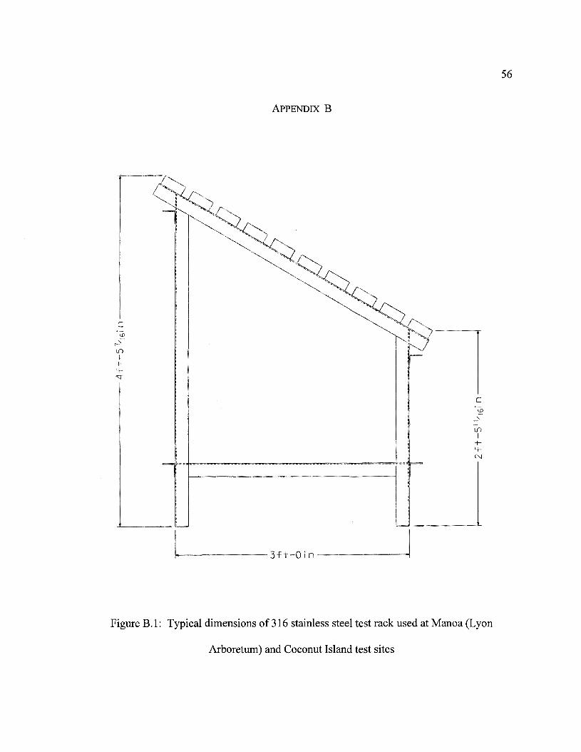
Figure B.1: Typical dimensions of 316 stainless steel test rack used at Manoa (Lyon
Arboretum) and Coconut Island test sites

c
57
c
LllI
4+N
Figure B.2: Typical dimensions ofTREX® test rack used at Hawaiian Electric Company
(HECD) test sites

Ht--O i n
~-l.-~-":1 ?
l-
f
! J! .. -
[ ]LI
e-J l.--
Figure B.3: Typical dimensions and front view of TREX® test rack used at Hawaiian
Electric Company (HECO) test sites. Arrangement and dimensions are similar for
stainless steel racks
58

59
I----~----.-.-~---- ,,- ---- - , - - 7ft-(J in-~~~~ -·· ~~~~_..~---i
Figure B.4: Arrangement of metal-matrix composite disks (at left) on test racks at all six
atmospheric corrosion test sites

Figure B.5: Manoa (Lyon Arboretum) test site - wet
Figure B.6: Coconut Island test site - marine
60

Figure 8.7: Campbell Industrial Park test site - industrial
Figure 8.8: Kahuku test site - marine
61

Figure B.9: Waipahu test site - dry, light industrial
Figure B.1O: Ewa Nui test site - agricultural
62
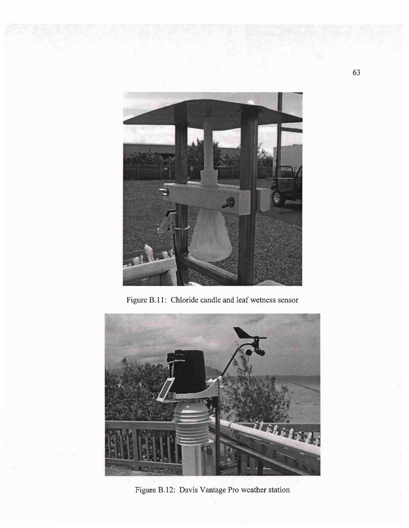
Figure B.ll: Chloride candle and leaf wetness sensor
Figure B.12: Davis Vantage Pro weather station
63

64
Concentration measurements made with cr ion-selective electrode
0.0045
0.004
o0.0035
0.003
~ 0.0025
Ucoo 0.002
-.... Actual Concentration
<> Measured Conentration0.0015
0.001
0.0005
900BOO700600500400300200100
o+---~--_--~_--~__~ --~~--~--~
o
cr mg/m2lday
Figure B.13: Calibration curve for chloride candle measurements using an Orion 290A
ISE/pH meter and an ion (CI-) selective electrode (9617BN)

65
ApPENDIX C
Table C.1: Comparison of the major ionic constituents of different types of seawater
CoconutThe Oceans,
IonWaikiki*
island*ASTM* IAPSO Prentice-Hall, Inc.,
(ppm)(ppm)
(ppm) (ppm) Newyork,1942(ppm)
Calcium,429.50 365.77 516.66 432 400.1Ca++
Magnesium,1513.58 1319.84 1731.6 1348 1272Mg++
Sodium,10461.5 9113.82 lOll 8 11266 10556.1Na+
Potassium,356.13 323.24 396.74 411 380K+
Chloride,19581.5 17074.23 20488 19900 18980
Cl-
Sulfate2663.46 2294.38 2596.6 N/A 2649
S04--
Bromine61.10 54.34 141.57 N/A 64.6
Br
* Analysis performed by Dr.Huebert, Dept. of Oceanography, University of Hawai'i atManoa.
It should be noted that a 3.15 wt.% NaCl solution theoretically contains 19,107.9 ppm ofthe chloride (Cn ion.

Table C.2: Initial pH values of electrolytes used in immersion experiment
66
pH of electrolytes at start of 90 day immersion experiment
ASTM Sea3.15 wt.% NaCl 0.5MNazS04
18.1 MO-cmReal Sea WaterWater Water
8.204 5.843 6.695 7.000 7.773
T = 20.6 °C T = 20.5 °C T = 21.2 °C - T = 19.8 °C
Table C.3: Final pH values of electrolytes used in immersion experiment
pH of electrolytes after 90 day immersion experiment (T = 29.1 °C)
ASTM Sea 3.15 wt.% 0.5M 18.1 MO- Real SeaWater NaCl NaZS04 cm Water Water
Al6092-7.539 8.045 8.714
T6/SiC/5pAl6092-
7.487 8.090 8.621T6/SiC/lOp
Al6092-7.469 8.140 8.651 7.860 7.428
T6/SiC/20pAl6092-
7.526 8.602 8.613T6/SiC/40p
Al6092-7.429 8.653 8.329
T6/SiC/50pAl6092-
T6/SiC/50p 7.511 8.760 8.729(Gr.)
Al6092-7.483 8.414 8.581 7.710 7.559
T6/B4C/20pAl6092-
7.646 7.434 8.152 7.372 7.504T6/Ab03/2Op
Al6061-T6 7.540 7.650 8.150 7.690

K 1 O~OO
!lilIOO
NlOO
Figure C.1: EDXA of A16092-T6/B4C/20p immersed in 3.15 wt.% NaCl
67
Figure Co2: EDXA of A16092-T6/Ah03/20p immersed in 3.15 wt.% NaCl

68
ApPENDIX D
Table D.l: Pitting potentials and passive current densities for MMCs and A1606l-T6 in
3.15 wt.% NaCl and 0.5M Na2S04
3.15 wt.% NaCl 0.5MNa2S04
Epit(VSCE) ipass(A/cm2)
A16092-T6/SiC/5p -0.727 -5.267
A16092-T6/SiC/l Op -0.712 -5.319
A16092-T6/SiC/20p -0.712 -5.347
A16092-T6/SiC/40p -0.712 -5.331
A16092-T6/SiC/50p -0.712 -4.684
A16092-T6/SiC/50p (Gr.) -0.712 -5.198
A16092-T6/B4C/20p -0.727 -3.606
A16092-T6/Ah03/2Op -0.681 -5.222
A16061-T6 -0.732 -5.378
----0-- O.5M NazSO4
-- 3.15wt.% NaCI
1.5
1
0.5-wU
>I/l a-w-0.5
-1
-1.5-7 -6 -4 -3
Figure D.1: Anodic polarization of A16092-T6/SiC/5p at 30°C with scan rate of 1mV/sec
----0---- O.5M Na2SO4
-- 3.15 wt.% NaCI
1.5
1
0.5
-wu a>lI)-w
-0.5
-1
-1.5-7 -6 -4 -3
69
Figure D.2: Anodic polarization of AI6092-T6/SiC/lOp at 30D C with scan rate of
lmV/sec
----0---- O.5M Na2SO4
-- 3.15wt.% NaCI
1.5
1
0.5
-wu a>lI)-w
-0.5
-1
-1.5-7 -6 -4 -3
Figure D.3: Anodic polarization of A16092-T6/SiC/20p at 30DC with scan rate of
lmV/sec

1.5
1
0.5-wu a>1/)-w-0.5
-1
-1.5-7 -6
----0---- O.5M NazSO4
-- 3.15 wt.% NaCI
-4 -3
70
Figure D.4: Anodic polarization of A16092-T6/SiC/40p at 30°C with scan rate of
lmV/sec
----0---- O.5M NazSO4
-- 3.15wt.% NaCI
1.5
1
0.5
-wu a>1/)-w
-0.5
-1
-1.5-7 -6 -4 -3
Figure D.5: Anodic polarization of A16092-T6/SiC/SOp at 30°C with scan rate of
lmV/sec
1.5
1
0.5
-wuI/) 0>-w
-0.5
-1
-1.5-7 -6
------0----- O.5M Na2SO4
-- 3.15wt.% NaCI
-4 -3
71
Figure D.6: Anodic polarization of Al6092-T6/SiC/50p (Gr.) at 30°C with scan rate of
1mV/sec
-----0---- O.5M Na2SO4
-- 3.15wt.% NaCI
1.5
1
0.5
-wu
0I/)
>-w-0.5
-1
-1.5-7 -6 -4 -3
Figure D.7: Anodic polarization of Al6092-T6/B4C120p at 30°C with scan rate of
1mV/sec

----0- O.5M NazS04
-- 3.15wt.% NaCI
1.5
1
0.5
-wu a>lJ)-w
-0.5
-1
-1.5-7 -6 -4 -3
72
Figure D.8: Anodic polarization of AI6092-T6/Ah03/20p at 30°C with scan rate of
lmV/sec
1.5
1
0.5
-wulJ) a>-w
-0.5
-1
-1.5-7 -6
-- 3.15wt.% NaCI
-4 -3
Figure D.9: Anodic polarization of A1606l-T6 at 30°C with scan rate of lmV/sec

73
REFERENCES
1. Castle Metals, Aluminum Plate Quik Guide, A.M. Castle & Co, 2003.
2. DWA Aluminum Composites, www.dwa-dra.com. 2004.
3. R. C. Paciej, V.S. Agarwala, "Influence of Processing Variables on the Corrosion
Susceptibility of Metal-Matrix Composites", Corrosion, Vol. 44, No. 10, pp. 680-684,
1988.
4. Ceradyne, Inc., Ceramics for Severe Environments, 2001
5. R.E. Bolz and G.L. Tuve, CRC Handbook of Tables for Applied Engineering Science
(2nd Edn), p262-264, CRC Press, Boca Raton, FL, 1973.
6. ASM International, ASMSpecialty Handbook: Aluminum and Aluminum Alloys, 1993
7. Harrigan, W.C.J., Metal Matrix Composites, in Metal Matrix Composites: Processing
and Interfaces. 1991, Academic Press. p.1-16.
8. Hill, R.J. and W.F. Stuhrke, The Preparation and Properties ofCast Boron-Aluminum
Composites. Fibre Science and Technology, 1968. 1(1): p.25 - 42.
9. Brenner, S.S., J. Appl. Phys., 1962.33: p.33.
10. Brenner, S.S., J. Metals, 1962. 14(11): p.808.
11. Sutton, W.H., Whisker Composite Materials - A Prospectus for the Aerospace
Designer. Astronautics and Aeronautics, 1966(August): p.46.
12. Sutton, W.H. and J. Chorn, Metals Engin. Quart., 1963.3(1): p.44.
13. Greenwood, N.N. and Earnshaw, A., Chemistry of the Elements; 1984, Oxford,
Pergamon Press.

74
14. Hihara, L.R., Metal Matrix Composites, in Corrosion Tests and Standards:
Application and Interpretation. 1995, ASTM. p.531-542
15. Bolz, R.E. and Tuve, G.L., CRC Handbook of Tables for Applied Engineering
Science, Second ed., CRC Press, 1973, p.262.
16. Champion, AR., Krueger,W.H., Hartmann, H.S., and Dhingra, A.K., in Proceedings
of the 1978 International Conference on Composite Materials, ICCM/2, Toronto,
Canada, April 1978, The Metallurgical Society of AIME, p.883-904.
17. Pohlman, S.L. , Corrosion, Vo1.34, 1978, p.l56-159.
18. Aylor, D.M., Taylor, D., Corrosion ofMetal Matrix Composites in Metals Handbook
Ninth Edition, Volume 13 Corrosion, ASM International, 1987, p.859-863.
19. Aylor, D.M., Moran, P.J., Preprint 202, Proceedings ofthe Corrosion/86 Symposium,
National Association of Corrosion Engineers, 1986.
20. Dejarnette, H.M., Crowe, c.R., Naval Surface Weapons Center, unpublished
research, 1982.
21. Lore, K.D., Wolf, J.S., Abstract 154, The Electochemical Society, Oct 1981.
22. V. Kucera, E. Mattsson, "Atmospheric Corrosion" in Corrosion Mechanisms (New
York, NY: Marcel Dekker, 1987).
23. S. W. Dean, "Corrosion Testing of Metals Under Natural Atmospheric Conditions",
in Corrosion Testing and Evaluation: Silver Anniversary Volume, R. Baboian, S. W.
Dean, eds., ASTM STP 1000 (Philadelphia, PA: ASTM, 1990).
24. H. H. Lawson, B. C. Syrett, Atmospheric Corrosion Test Methods, NACE
International, 1995.

75
25. K. A. Lucas, H. Clarke, Corrosion of Aluminum-Based Metal Matrix Composites,
Research Studies Press Ltd., 1993, p.49.
26. Hihara, L. H., Corrosion of Metal-Matrix Composites in Metals Handbook Ninth
Edition, Volume 13B Corrosion, ASM International, 2004, publication pending.