Embed Size (px)
Citation preview

UNCORRECTED PROOF
Overall distributed model intercomparison project results
Seann Reed, Victor Koren, Michael Smith*, Ziya Zhang, Fekadu Moreda,Dong-Jun Se, DMIP Participants1
National Institute of Water and Atmospheric Research, New Zealand
Received 7 May 2003; revised 25 September 2003; accepted 29 March 2004
Abstract
This paper summarizes results from the Distributed Model Intercomparison Project (DMIP) study. DMIP simulations from
twelve different models are compared with both observed streamflow and lumped model simulations. The lumped model
simulations were produced using the same techniques used at National Weather Service River Forecast Centers (NWS-RFCs) for
historical calibrations and serve as a useful benchmark for comparison. The differences between uncalibrated and calibrated
model performance are also assessed. Overall statistics are used to compare simulated and observed flows during all time steps,
flood event statistics are calculated for selected storm events, and improvement statistics are used to measure the gains from
distributed models relative to the lumped models and calibrated models relative to uncalibrated models. Although calibration
strategies for distributed models are not as well defined as strategies for lumped models, the DMIP results show that some
calibration efforts applied to distributed models significantly improve simulation results. Although for the majority of basin-
distributed model combinations, the lumped model showed better overall performance than distributed models, some distributed
models showed comparable results to lumped models in many basins and clear improvements in one or more basins. Noteworthy
improvements in predicting flood peaks were demonstrated in a basin distinguishable from other basins studied in its shape,
orientation, and soil characteristics. Greater uncertainties inherent to modeling small basins in general and distinguishable inter-
model performance on the smallest basin (65 km2) in the study point to the need for more studies with nested basins of various
sizes. This will improve our understanding of the applicability and reliability of distributed models at various scales.
q 2004 Published by Elsevier B.V.
Keywords: Distributed hydrologic modeling; Model intercomparison; Radar precipitation; Rainfall–runoff; Hydrologic simulation
1. Introduction
By ingesting radar-based precipitation products
and other new sources of spatial data describing
the land surface, there is potential to improve the
quality and resolution of National Weather Service
(NWS) river and stream forecasts through the use of
distributed models. The Distributed Model Intercom-
parison Project (DMIP) was initiated to evaluate the
capabilities of existing distributed hydrologic models
forced with operational quality radar-based precipi-
tation forcing. This paper summarizes DMIP results.
The results provide insights into the simulation
capabilities of 12 distributed models and suggest
0022-1694/$ - see front matter q 2004 Published by Elsevier B.V.
doi:10.1016/j.jhydrol.2004.03.031
Journal of Hydrology xx (0000) xxx–xxx
www.elsevier.com/locate/jhydrol
1 See Appendix A.
* Corresponding author. Address: Hydrology Lab., Office of
Hydrologic Development, Research Hydrologists, WOHD-12
NOAA/National Weather Service, 1325 East-West Highway,
20910, SIlver Spring, MD, USA.
E-mail address: [email protected] (M. Smith).
HYDROL 14503—11/6/2004—21:20—SIVABAL—106592 – MODEL 3 – pp. 1–34
ARTICLE IN PRESS
1
2
3
4
5
6
7
8
9
10
11
12
13
14
15
16
17
18
19
20
21
22
23
24
25
26
27
28
29
30
31
32
33
34
35
36
37
38
39
40
41
42
43
44
45
46
47
48
49
50
51
52
53
54
55
56
57
58
59
60
61
62
63
64
65
66
67
68
69
70
71
72
73
74
75
76
77
78
79
80
81
82
83
84
85
86
87
88
89
90
91
92
93
94
95
96

UNCORRECTED PROOF
areas for further research. Smith et al. (2004b) provide
a more detailed explanation of the motivations for the
DMIP project and a description of the basins modeled.
As discussed by Smith et al. (2004b), although the
potential benefits of using distributed models are
many, the actual benefits of distributed modeling in an
operational forecasting environment, using opera-
tional quality data are largely unknown. This study
analyzes model simulation results driven by observed,
operational quality, precipitation data.
The NWS hydrologic forecasting requirements
span a large range of spatial and temporal scales.
NWS River Forecast Centers (RFCs) routinely
forecast flows and stages for over 4000 points on
river systems in the United States using the NWS
River Forecast System (NWSRFS). The sizes of
basins typically modeled at RFCs range anywhere
from 300 to 5000 km2. For flash-floods on smaller
streams and urban areas, basin-specific flow or stage
forecasts are only produced at a limited number of
locations; however, Weather Forecast Offices (WFOs)
evaluate the observed and forecast precipitation data
and Flash Flood Guidance (FFG) (Sweeney, 1992)
provided by RFCs to produce flash-flood watches and
warnings. Lumped models are currently used at RFCs
for both river forecasting and to generate FFG.
Given the prominence of lumped models in current
operational systems, a key question addressed by
DMIP is whether or not a distributed model can
provide comparable or improved simulations relative
to lumped models at RFC basin scales. In addition, the
potential benefits of using a distributed model to
produce hydrologic simulations at interior points are
examined, although with limited interior point data in
this initial study. Statistics comparing distributed
model simulations to observed flows and statistics
comparing the performance of distributed model and
lumped model simulations are presented in this paper.
Previous studies on some of the DMIP basins have
shown that depending on basin characteristics, the
application of a distributed or semi-distributed model
may or may not improve outlet simulations over
lumped simulations (Zhang et al., 2003; Koren et al.,
2003a; Boyle et al., 2001; Carpenter et al., 2001;
Vieux and Moreda, 2003; Smith et al., 1999).
There is no generally accepted definition for
distributed hydrologic modeling in the literature. For
purposes of this study, we define a distributed model
as any model that explicitly accounts for spatial
variability inside a basin and has the ability to produce
simulations at interior points without explicit cali-
bration at these points. The scales of parent basins of
interest in this study are those modeled by RFCs. This
relatively broad definition allows us compare models
of widely varying complexities in DMIP. Those with a
stricter definition of distributed modeling might argue
that some rainfall–runoff models evaluated in this
study are not true distributed models because they
simply apply conceptual lumped modeling techniques
to smaller modeling units. It is true that several DMIP
models use algorithms similar to those of traditional
lumped models for runoff generation, but in many
cases, methods have been devised to estimate the
spatial variability of model parameters within a basin.
Several DMIP modelers have also worked on methods
to estimate spatially variable routing parameters.
Therefore, all models do consider the spatial vari-
ations of properties within the DMIP parent basins in
some way.
The parameter estimation problem is a bigger
challenge for distributed hydrologic modeling than for
lumped hydrologic modeling. Although some par-
ameters in conceptual lumped models can be related
to physical properties of a basin, these parameters are
most commonly estimated through calibration
(Anderson, 2003; Smith et al., 2003; Gupta et al.,
2003). Initial parameters for distributed models are
commonly estimated using spatial datasets describing
soils, vegetation, and landuse; however, these so-
called physically based parameter values are often
adjusted through subsequent calibration to improve
streamflow simulations. These adjustments may
account for many factors, including the inability of
model equations and parameterizations to represent
the true basin physics and heterogeneity, scaling
effects, and the existence of input forcing errors.
Given that parameter adjustments are used to get
better model performance, the distinction between
physically based parameters and conceptual model
parameters becomes somewhat blurred. Although
calibration strategies for distributed models are not
as well defined as those for lumped models, a number
of attempts have been made to use physically based
parameter estimates to aid or constrain calibration
and/or simulate the effects of parameter uncertainty
(Koren et al., 2003a; Leavesley et al., 2003;
HYDROL 14503—11/6/2004—21:20—SIVABAL—106592 – MODEL 3 – pp. 1–34
S. Reed et al. / Journal of Hydrology xx (0000) xxx–xxx2
ARTICLE IN PRESS
97
98
99
100
101
102
103
104
105
106
107
108
109
110
111
112
113
114
115
116
117
118
119
120
121
122
123
124
125
126
127
128
129
130
131
132
133
134
135
136
137
138
139
140
141
142
143
144
145
146
147
148
149
150
151
152
153
154
155
156
157
158
159
160
161
162
163
164
165
166
167
168
169
170
171
172
173
174
175
176
177
178
179
180
181
182
183
184
185
186
187
188
189
190
191
192

UNCORRECTED PROOF
Vieux and Moreda, 2003; Carpenter et al., 2001;
Christiaens and Feyen, 2002; Madsen, 2003;
Andersen et al., 2001; Senarath et al., 2000; Refsgaard
and Knudsen, 1996; Khodatalab et al., 2004). In
addition, Andersen et al. (2001) incorporate multiple
sites into their calibration strategy and Madsen (2003)
use multiple criteria (streamflow and groundwater
levels) for calibrating a distributed model, techniques
that are not possible with lumped models. A key to
effectively applying these approaches is that valid
physical reasoning goes into deriving the initial
parameter estimates.
To get a better handle on the parameter estimation
problem for distributed models, participants were
asked to submit both calibrated and uncalibrated
distributed model results. The improvements gained
from calibration are quantified in this paper. Uncali-
brated results were derived using parameters that were
estimated without the benefit of using the available
time-series discharge data. Some of the uncalibrated
parameter estimates used by DMIP participants are
based on direct objective relationships with soils,
vegetation, and topography data while others rely
more on subjective estimates from known calibrated
parameter values for nearby or similar basins. Both
these objective and subjective estimation procedures
are physically based to some degree. Calibrated
simulations submitted by DMIP participants incor-
porate any adjustments that were made to the
uncalibrated parameters in order to produce better
matches with observed hydrographs.
In the DMIP study area, data sets from a few nested
stream gauges in the Illinois River basin (Watts,
Savoy, Kansas, and Christie) are available to evaluate
model performance at interior points. In an attempt to
understand the models’ abilities to blindly simulate
flows at ungauged points, the DMIP modeling
instructions did not allow use of data from interior
points for model calibration. However, it is recog-
nized that an alternative approach that uses interior
point data in calibration may help to improve
simulations at basin outlets (e.g. Andersen et al.,
2001). Only one of these interior basins (Christie) is
significantly smaller (65 km2) than the basins typi-
cally modeled by RFCs using lumped models
(300–5000 km2). As discussed below, the results
for Christie are distinguishable from the results for the
larger basins because of lower simulation accuracy
and the relative performance of different models is not
the same in Christie as it is for larger basins.
In this paper, all model comparisons are made
based on streamflow, an integrated measure of
hydrologic response, at basin and subbasin outlets.
The focus is on streamflow analysis because no
reliable measurements of other hydrologic variables
(e.g. soil moisture, evaporation) were obtained for this
study, and because streamflow (and the corresponding
stage) forecast accuracy is the bottom line for many
NWS hydrologic forecast products. Use of only
observed streamflow for evaluation does limit our
ability to make conclusions about the distributed
models’ representations of internal watershed
dynamics. Therefore, it is hoped that future phases
of DMIP can include comparisons of other hydrologic
variables.
Following this Section 1, a Section 2 briefly
describes the participant models, the NWS lumped
model runs used for comparison, and events chosen
for analysis. Next, Section 3 focus on the overall
performance of distributed models, comparisons
among lumped and distributed models, and compari-
sons among calibrated and uncalibrated models at all
gauged locations. The variability of model simu-
lations at ungauged interior points and trends in
variability with scale are also discussed. Overall
statistics and event statistics defined by Smith et al.
(2004b) are presented for different models and
different basins.
2. Methods
2.1. Participant models and submissions
Twelve different participants from academic,
government, and private institutions submitted results
for the August 2002 DMIP workshop. Table 1
provides some information about participants and
general characteristics of the participating models.
The first column of Table 1 lists the main affiliations
for each participant, and the two or three letter
abbreviation for each affiliation shown in this column
will be used throughout this paper to denote results
submitted by that group. Since detailed descriptions of
the DMIP models are available elsewhere in the
literature or this issue (See Table 1, Column 3),
HYDROL 14503—11/6/2004—21:20—SIVABAL—106592 – MODEL 3 – pp. 1–34
S. Reed et al. / Journal of Hydrology xx (0000) xxx–xxx 3
ARTICLE IN PRESS
193
194
195
196
197
198
199
200
201
202
203
204
205
206
207
208
209
210
211
212
213
214
215
216
217
218
219
220
221
222
223
224
225
226
227
228
229
230
231
232
233
234
235
236
237
238
239
240
241
242
243
244
245
246
247
248
249
250
251
252
253
254
255
256
257
258
259
260
261
262
263
264
265
266
267
268
269
270
271
272
273
274
275
276
277
278
279
280
281
282
283
284
285
286
287
288

UNCORRECTED PROOF
Table 1
Participant information and general model characteristics
Participant Modeling
system name
Primary reference (s) Primary application Spatial unit for
rainfall–runoff
calculations
Rainfall–
runoff/vertical flux
model
Channel routing
method
Agricultural Research
Service (ARS)
SWAT Neitsch et al. (2002)
and Di Luzio and
Arnold (2004)
Land management/
agricultural
Hydrologic response
unit (HRU) (6–7 km2)
Multi-layer soil water
balance
Muskingum
University of Arizona
(ARZ)
SAC-SMA Khodatalab et al.
(2004)
Streamflow forecasting Subbasin (avg. size
,180 km2)
SAC-SMA Kinematic wave
Danish Hydraulics
Institute (DHI)
Mike 11 Havno et al. (1995)
and Butts et al. (2004)
Forecasting, design, water
management
Subbasins
(,150 km2)
NAM Full dynamic wave
solution
Environmental
Modeling Center
(EMC)
NOAH Land
Surface Model
http://www.emc.ncep.
noaa.gov/mmb/gcp/
noahlsm/
README_2.2.htm
Land-atmosphere interactions
for climate and weather
prediction models, off-line
runs for data assimilation and
runoff prediction
,160 km2 (1/8th
degree grids)
Multi-layer soil water
and energy balance
Linearized St Venant
equation
Hydrologic Research
Center (HRC)
HRCDHM Carpenter and
Georgakakos (2003)
Streamflow forecasting Subbasins
(59–85 km2)
SAC-SMA Kinematic wave
Massachusetts
Institute of
Technology (MIT)
tRIBS Ivanov et al. (2004) Streamflow forecasting, soil
moisture prediction, slope
stability
TIN (,0.02 km2) Continuous profile
soil-moisture
simulation with
topographicaly
driven, lateral,
element to element
interaction
Kinematic wave
Office of Hydrologic
Development (OHD)
HL-RMS Koren et al. (2003a,b) Streamflow forecasting 16 km2 grid cells SAC-SMA Kinematic wave
University of
Oklahoma (OU)
r.water.fea Vieux (2001) Streamflow forecasting 1 km2 or smaller Event based Green-
Ampt infiltration
Kinematic wave
University of
California at Berkeley
(UCB)
VIC-3L Liang, et al. (1994)
and Liang and Xi
(2001)
Land-atmosphere interactions ,160 and ,80 km2
(1/8th, 1/16th degree
grids)
Multi-layer soil water
and energy balance
One parameter simple
routing
Utah State University
(UTS)
TOPNET Bandaragoda et al.
(2004)
Streamflow forecasting Subbasins (,90 km2) TOPMODEL Kinematic wave
University of
Waterloo, Ontario
(UWO)
WATFLOOD Kouwen et al. (1993) Streamflow forecasting 1-km grid WATFLOOD Linear storage routing
Wuhan University
(WHU)
LL-II – Streamflow forecasting 4-km grid Multi-layer finite
difference model
Full dynamic wave
solution
HY
DR
OL
14
50
3—
11
/6/2
00
4—
21
:20
—S
IVA
BA
L—
10
65
92
–M
OD
EL
3–
pp
.1
–3
4
S.
Reed
eta
l./
Jou
rna
lo
fH
ydro
log
yxx
(00
00
)xxx–
xxx4
AR
TIC
LE
INP
RE
SS
28
9
29
0
29
1
29
2
29
3
29
4
29
5
29
6
29
7
29
8
29
9
30
0
30
1
30
2
30
3
30
4
30
5
30
6
30
7
30
8
30
9
31
0
31
1
31
2
31
3
31
4
31
5
31
6
31
7
31
8
31
9
32
0
32
1
32
2
32
3
32
4
32
5
32
6
32
7
32
8
32
9
33
0
33
1
33
2
33
3
33
4
33
5
33
6
33
7
33
8
33
9
34
0
34
1
34
2
34
3
34
4
34
5
34
6
34
7
34
8
34
9
35
0
35
1
35
2
35
3
35
4
35
5
35
6
35
7
35
8
35
9
36
0
36
1
36
2
36
3
36
4
36
5
36
6
36
7
36
8
36
9
37
0
37
1
37
2
37
3
37
4
37
5
37
6
37
7
37
8
37
9
38
0
38
1
38
2
38
3
38
4

UNCORRECTED PROOF
only general characteristics of these models are
provided in Table 1.
Table 1 highlights both differences and similarities
among modeling approaches. Some models only
consider the water balance, while others (e.g. UCB,
EMC, and MIT) calculate both the energy and water
balance at the land surface. The sizes of the water
balance modeling elements chosen for DMIP appli-
cations range from small triangulated irregular net-
work (TIN) modeling units (,0.02 km2) to
moderately sized subbasin units (,100 km2). Some
models account directly or indirectly for the effects of
topography on the soil-column water balance while
others only explicitly use topographic information for
channel and/or overland flow routing calculations.
There tend to be fewer differences in the choice of a
basic channel routing technique than the choice of a
rainfall–runoff calculation method. Many participants
use a kinematic wave approximation to the Saint-
Venant equations while only a few use a more
complex diffusive wave or fully dynamic solution.
The methods used to estimate parameters and
subdivide channel networks in applying these routing
techniques do vary and are described in the individual
participant papers and the references provided. It
should be kept in mind that the accuracy of
simulations presented in this paper reflect not only
the appropriateness of the model structure, parameter
estimation procedures, and computational schemes of
the individual models, but also the skill, experience,
and time commitment of the individual modelers to
these particular basins.
The level of DMIP participation varied among
participants and is indicated in Table 2. Some
participants were able to submit all 30 simulations
requested in the modeling instructions (i.e. both
calibrated and uncalibrated results for all model
points), while others submitted more limited results.
An ‘x’ in Table 2 indicates that a flow time series was
received for the specified basin and case. Table 2
shows that 198 out of a possible 360 time series files
(30 cases £ 12 models) were submitted and analyzed
(55%). Given that research funding was not provided
for participation in DMIP (aside from a small amount
of travel money), this high level of participation is
encouraging. Results analyzed in this paper are based
on simulation time-series submitted to the NWS
Office of Hydrologic Development (OHD). It is
expected that individual participants may include
more updated or comprehensive results for their
models in other papers in this special issue.
In order to encourage as much participation as
possible, there was some flexibility allowed in the
types of submissions accepted for DMIP. Footnotes in
Table 2 indicate some of the non-standard sub-
missions that were accepted. Due to non-standard
and/or partial submissions, some graphics and tables
presented in this paper cannot include all participant
models; however, they do reflect all submissions
usable for the type of analysis presented. For example,
all models were run in continuous simulation mode
with the exception of the University of Oklahoma
(OU) event simulation model. It is difficult to
objectively compare event and continuous simulation
models because event simulation models must include
some type of scheme to define initial soil moisture
conditions, an inherent feature in continuous simu-
lation models. Overall statistics could not be com-
puted for the OU results, but event statistics were
computed when possible.
The University of California at Berkeley (UCB)
submitted daily rather than hourly simulation results
so only limited analyses (overall bias) of UCB results
are included in this paper.
To be fair to all participants, it was agreed at the
August 2002 workshop that analysis of any results
submitted after the workshop should be clearly
marked if they were to be included in this paper.
Although the Massachusetts Institute of Technology
(MIT) group was only able to submit simulations
covering a part of the DMIP simulation time period
prior to the August 2002 workshop, MIT was able to
submit simulations covering the entire DMIP period
in January 2003. Since the final simulations from MIT
are not much different than the initial simulations
during the overlapping time period, and use of the
entire time period for analyses makes statistical
comparisons more meaningful, statistics from the
January 2003 MIT submissions are presented in this
paper.
For those modelers who did submit calibrated
results, calibration strategies varied widely in their
level of sophistication, the amount of effort required,
and the amount of effort invested specifically for
the DMIP project. No target objective functions
were prescribed for calibration so, for example,
HYDROL 14503—11/6/2004—21:20—SIVABAL—106592 – MODEL 3 – pp. 1–34
S. Reed et al. / Journal of Hydrology xx (0000) xxx–xxx 5
ARTICLE IN PRESS
385
386
387
388
389
390
391
392
393
394
395
396
397
398
399
400
401
402
403
404
405
406
407
408
409
410
411
412
413
414
415
416
417
418
419
420
421
422
423
424
425
426
427
428
429
430
431
432
433
434
435
436
437
438
439
440
441
442
443
444
445
446
447
448
449
450
451
452
453
454
455
456
457
458
459
460
461
462
463
464
465
466
467
468
469
470
471
472
473
474
475
476
477
478
479
480

UNCORRECTED PROOF
some participants may have placed more emphasis
on fitting flood peaks than obtaining a zero
simulation bias for the calibration period. This is
not a big concern in evaluating DMIP results
because a variety of statistics are considered and
results indicate that models with good results based
on one statistical criterion typically have good
results for other statistical criteria as well. Discus-
sion of participant parameter estimation and cali-
bration strategies is beyond the scope of this paper
but information about participant-specific procedures
can be found in the references listed in Table 1.
2.2. Lumped model
To provide a ‘standard’ for comparison, both
calibrated and uncalibrated lumped simulations were
generated at OHD for all of the gauged DMIP
locations. Techniques used to generate lumped
simulations are the same as those used for operational
forecasting at most NWS River Forecast Centers
(RFCs). The Sacramento Soil Moisture Accounting
(SAC-SMA) model (Burnash et al., 1973; Burnash,
1995) is used for rainfall–runoff calculations and the
unit hydrograph model is used for channel
Table 2
Level of participation
Model Christie Kansas Savoy4 Savoy5 Eldon Blue Watts4 Watts5 Tiff City Tahlequah
Cal Unc Cal Unc Cal Unc Cal Unc Cal Unc Cal Unc Cal Unc Cal Unc Cal Unc Cal Unc
Gaged Locations
ARS £ £ £ £ £ £ £ £ £ £ £ £ £ £ £ £ £ £ £ £
ARZ £ £ £ £
DHI £
EMC £ £ £ £ £ £ £ £ £ £
HRC £ £ £ £ £ £ £ £ £ £ £ £ £ £ £ £ £ £
MITa £ £ £ £ £ £
OHD £ £ £ £ £ £ £ £ £ £ £ £ £ £ £ £ £ £ £ £
OUb £ £ £ £ £ £ £ £ £ £
UCBc £
UTS £ £ £ £ £ £ £ £ £ £ £ £ £ £ £ £ £ £ £ £
UWO £ £ £ £ £ £ £ £ £ £ £ £ £ £ £ £ £ £ £ £
WHUd £
Eldp1 Blup1 Blup2 Wttp1 Tifp1
Cal Unc Cal Unc Cal Unc Cal Unc Cal Unc
Ungaged locations
ARS £ £ £ £ £ £ £ £ £ £
ARZ £ £
DHI £ £
EMC £ £ £ £ £
HRC £ £ £ £ £ £ £ £ £ £
MITa £ £ £ £ £ £
OHD £ £ £ £ £ £ £ £
OUb £ £ £ £
UCBc
UTS £ £ £ £ £ £ £ £ £ £
UWO £ £ £ £ £ £ £ £ £ £
WHUd
a Time series submitted in January 2003 that cover the entire DMIP study period are analyzed for this paper to make statistical comparisons
more meaningful.b Simulations submitted only for selected events.c Results have a daily time step.d Calibration is based on only 1 year of observed flow (1998). Results submitted January 2003.
HYDROL 14503—11/6/2004—21:20—SIVABAL—106592 – MODEL 3 – pp. 1–34
S. Reed et al. / Journal of Hydrology xx (0000) xxx–xxx6
ARTICLE IN PRESS
481
482
483
484
485
486
487
488
489
490
491
492
493
494
495
496
497
498
499
500
501
502
503
504
505
506
507
508
509
510
511
512
513
514
515
516
517
518
519
520
521
522
523
524
525
526
527
528
529
530
531
532
533
534
535
536
537
538
539
540
541
542
543
544
545
546
547
548
549
550
551
552
553
554
555
556
557
558
559
560
561
562
563
564
565
566
567
568
569
570
571
572
573
574
575
576

UNCORRECTED PROOF
flow routing. For the DMIP basin calibration runs,
SAC-SMA parameters were estimated using manual
calibration at OHD following the strategy typically
used at RFCs and described by Smith et al. (2003) and
Anderson (2003). As defined by Smith et al. (2004b),
the calibration period was June 1, 1993 to May 31,
1999. Model parameters routinely used for oper-
ational forecasting in the DMIP basins by the
Arkansas-Red Basin RFC (ABRFC) could not be
used directly to produce lumped simulations because
these parameters are based on 6-h calibrations (hourly
simulations are the standard in DMIP) with gauged-
based rainfall, and it is well known that SAC-SMA
model results are sensitive to the time step used
for model calibration (Koren et al., 1999; Finnerty
et al., 1997).
Lumped SAC-SMA parameters derived for the
DMIP basins are given in Table 3. No snow model
was included in the lumped runs for these basins
because snow has a very limited effect on the
hydrology of the DMIP basins. For the lumped
DMIP runs, constant climatological mean monthly
values for potential evaporation (PE) (mm/day) were
used. In the SAC-SMA model, evapotranspiration
(ET) demand is defined as the product of PE and a PE
adjustment factor, which is related to the vegetation
state. During manual calibration, PE adjustment
factors are initially assigned based on regional
knowledge but may be adjusted during the calibration
process to remove seasonal biases. The ET demand
values used for calibrated lumped DMIP runs are also
given in Table 3.
Because climatological mean ET demand values
were used for lumped runs, the only observed input
forcing required to produce the lumped model
simulations was hourly rainfall. Hourly time series
of lumped rainfall to force lumped model runs were
obtained by computing the areal averages from
hourly multi-sensor rainfall grids (the same rainfall
grids used to drive the distributed models being
tested). Areal averages for a basin were computed
using all rainfall grid cells with their center point
inside the basin. Algorithms used to develop the
multi-sensor rainfall products used in this study are
described by Seo and Breidenbach (2002), Seo et al.
(2000), Seo et al. (1999) and Fulton et al. (1998).
There are some known biases in the cumulative
precipitation estimates during the study period that
are discussed further in the results section (see also
Johnson et al., 1999; Young et al., 2000; ‘About the
StageIII Data’, http://www.nws.noaa.gov/oh/hrl/
dmip/stageiii_info.htm; Wang et al., 2000; Guo
et al., 2004). Smith et al. (2004a) discuss the spatial
variability of the precipitation data over the DMIP
basins independently of the hydrologic model
application.
For gauged interior points (Kansas, Savoy,
Christie, and Watts (when calibration is done at
Tahlequah)), there are no fully calibrated lumped
results. That is, no manual calibrations against
observed streamflow were attempted at these points;
however, we refer to lumped, interior point
Table 3
SAC-SMA and ET demand parameters for 1-h Lumped calibrations
Parameter Blue Eldon,
Christie
Tahlequah,
Watts,
Kansas, Savoy
Tiff City
Uztwm (mm) 45 50 40 70
Uzfwm (mm) 50 25 35 34
Uzk (day21) 0.5 0.35 0.25 0.25
Pctim 0.005 0 0.005 0.002
Adimp 0 0 0.1 0
Riva 0.03 0.035 0.02 0.025
Zperc 500 500 250 250
Rexp 1.8 2 1.7 1.6
Lztwm (mm) 175 120 80 135
Lzfsm (mm) 25 25 27 21
Lzfpm (mm) 100 75 200 125
Lzsk (day21) 0.05 0.08 0.08 0.12
Lzpk (day21) 0.003 0.004 0.002 0.003
Pfree 0.05 0.25 0.1 0.15
Rserv 0.3 0.3 0.3 0.3
Month ET
Demand
(mm/day)
Jan 1.1 0.75 0.77 0.77
Feb 1.2 0.8 0.93 0.83
Mar 1.6 1.4 1.70 1.42
Apr 2.4 2.1 2.68 2.48
May 3.5 3.2 3.81 3.96
Jun 4.8 4.3 5.25 5.44
Jul 5.1 5.8 5.97 5.93
Aug 4.2 5.7 5.87 5.86
Sep 3.4 3.9 4.02 3.97
Oct 2.4 2.3 2.37 2.36
Nov 1.6 1.2 1.24 1.24
Dec 1.1 0.8 0.82 0.81
HYDROL 14503—11/6/2004—21:20—SIVABAL—106592 – MODEL 3 – pp. 1–34
S. Reed et al. / Journal of Hydrology xx (0000) xxx–xxx 7
ARTICLE IN PRESS
577
578
579
580
581
582
583
584
585
586
587
588
589
590
591
592
593
594
595
596
597
598
599
600
601
602
603
604
605
606
607
608
609
610
611
612
613
614
615
616
617
618
619
620
621
622
623
624
625
626
627
628
629
630
631
632
633
634
635
636
637
638
639
640
641
642
643
644
645
646
647
648
649
650
651
652
653
654
655
656
657
658
659
660
661
662
663
664
665
666
667
668
669
670
671
672

UNCORRECTED PROOF
simulations using the calibrated SAC-SMA parameter
estimates from parent basins as calibrated runs. As
shown in Table 3, the calibrated SAC-SMA par-
ameters for Eldon and Christie are the same, as are the
parameters for Tahlequah, Watts, Kansas, and Savoy.
There was an attempt to calibrate Tahlequah separ-
ately from Watts; however, since this analysis led to
similar parameters for both Tahlequah and Watts,
lumped simulation results used for analysis in DMIP
were generated using the same SAC-SMA parameters
for both Tahlequah and Watts.
To generate uncalibrated lumped SAC-SMA
parameters for parent basins and interior points,
areal averages of gridded a priori SAC-SMA par-
ameters defined by Koren et al. (2003b) were used.
Uncalibrated ET demand estimates were derived by
averaging gridded ET demand estimates computed by
Koren et al. (1998). Koren et al. (1998) produced 10-
km mean monthly grids of PE and PE adjustment
factors for the conterminous United States.
Hourly unit hydrographs for each of the parent
basins (Blue, Tahlequah, Watts, Eldon, and Tiff City)
were derived initially using the Clark time-area
approach (Clark, 1945) and then adjusted (if necess-
ary) during the manual calibration procedure. No
manual adjustments were made to the Clark unit
hydrographs for uncalibrated runs. Unit hydrographs
for interior point simulations were derived using the
same method but with no manual adjustment for both
‘calibrated’ and uncalibrated runs.
Fig. 1a and b show unit hydrographs used for the
lumped simulations. Looking at the unit hydrographs
for parent basins (Fig. 1a), the general trend that larger
basins tend to peak later makes sense. Tahlequah is
the largest basin, followed by Tiff City, Watts, Blue,
and Eldon (See Smith et al. (2004b) for exact basin
sizes). The shape of the Blue unit hydrograph is
somewhat unusual because it has a flattened peak and
no tail. The different hydrologic response character-
istics for the Blue River are also seen in the observed
data and distributed modeling results. The same
sensible trend is evident in Fig. 1b for the smaller
basins.
2.3. Events selected
For statistical analysis, between 16 and 24 storm
events were selected for each basin. Tables 4–8 list
events selected for Tahlequah and Watts, Kansas,
Savoy, Eldon and Christie, and Blue, respectively.
In some cases, the same time windows were selected
for both interior points and parent basins (e.g. Eldon
and Christie), while in other cases the time windows
are slightly different to better capture the event
hydrograph (e.g. Kansas and Savoy event windows
are different than the parent basins Tahlequah and
Watts). Fewer events were used for the Savoy analysis
because the available Savoy observed flow data
record does not start until October, 1995. For the
Blue River, some seemingly significant events were
excluded from the analysis because of significant
periods of missing streamflow observations.
The selection of storms was partially subjective
and partially objective. The method for selection was
primarily visual inspection of observed streamflow
and the corresponding mean areal rainfall values.
Although the goal of forecasting floods tends to
encourage analysis primarily of large events, we are
also interested in studying model performance over a
range of event sizes and the relationships between
Fig. 1. Unit hydrographs for (a) parent basins, and (b) interior
points.
HYDROL 14503—11/6/2004—21:20—SIVABAL—106592 – MODEL 3 – pp. 1–34
S. Reed et al. / Journal of Hydrology xx (0000) xxx–xxx8
ARTICLE IN PRESS
673
674
675
676
677
678
679
680
681
682
683
684
685
686
687
688
689
690
691
692
693
694
695
696
697
698
699
700
701
702
703
704
705
706
707
708
709
710
711
712
713
714
715
716
717
718
719
720
721
722
723
724
725
726
727
728
729
730
731
732
733
734
735
736
737
738
739
740
741
742
743
744
745
746
747
748
749
750
751
752
753
754
755
756
757
758
759
760
761
762
763
764
765
766
767
768

UNCORRECTED PROOF
model structure and simulation performance over
various flow ranges. Therefore, all of the largest
storms were selected, several moderately sized
storms, and a few small storms. To the degree
possible, storms were selected uniformly throughout
the study period (approximately the same number
each year) and from different seasons.
Due to the subjective nature of defining the event
windows and the fact that different OHD personnel
selected event windows for different basins, there are
some subtle differences in how much of the storm tails
are included in the event windows. For example,
Eldon event windows tend to include less of the
hydrograph tail than windows defined for other
basins. This means that storm volumes for selected
events shown in Table 7 may not reflect all of the
runoff associated with that particular event. Also, in a
few cases, multiple flood peaks occurring close in
time were treated as one event (e.g. Event 21 for
Tahlequah and Watts) in one basin but as separate
events for another basin (e.g. Events 22–24 for
Eldon). These small differences in how event
windows were defined for different basins have little
impact on the conclusions of this paper.
3. Results and discussion
Overall statistics, event statistics, and event
improvement statistics will be presented and discussed.
Mathematical definitions of the statistics used here are
provided by Smith et al. (2004b). The event improve-
ment statistics (flood runoff improvement, peak flow
improvement, and peak time improvement) are used to
measure the improvement from distributed models
relative to lumped models and the improvement from
calibrated models relative to uncalibrated models.
3.1. Overall Statistics
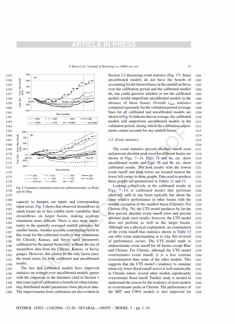
Fig. 2a and b show the cumulative simulation
errors for models applied to the Watts and Blue River
basins. The vertical gray line in these figures indicates
the end of the calibration period. The trends in these
graphs reflect known historical bias characteristics in
the radar rainfall archives. At several times during the
1990’s, there were improvements to the algorithms
used to produce multi-sensor precipitation grids
at RFCs, and therefore the statistical characteristics
of multi-sensor precipitation grids archived at
Table 4
Selected events for tahlequah and watts
Event Start time End time Tahlequah
Peak (m3 s21)
Watts
Peak (m3 s21)
Tahlequah
volume (mm)
Watts
volume (mm)
1 1/13/1995 0:00 1/26/1995 24:00 430 345 50.6 54.1
2 3/4/1995 16:00 3/11/1995 15:00 202 191 15.3 17.5
3 4/20/1995 0:00 4/30/1995 23:00 362 402 31.4 38.4
4 5/7/1995 0:00 5/14/1995 23:00 580 535 52.8 51.6
5 6/3/1995 0:00 6/19/1995 23:00 436 410 56.9 58.8
6 5/10/1996 16:00 5/17/1996 13:00 262 252 18.1 20.9
7 9/26/1996 0:00 10/4/1996 23:00 542 590 35 37
8 11/4/1996 12:00 11/14/1996 23:00 498 525 32.9 38.8
9 11/24/1996 1:00 12/5/1996 9:00 483 449 63.1 71.8
10 2/19/1997 2:00 2/25/1997 23:00 597 536 38.8 41.2
11 8/17/1997 0:00 8/23/1997 23:00 42 62 4.94 5.8
12 1/4/1998 0:00 1/16/1998 23:00 729 727 81.5 84.6
13 3/16/1998 0:00 3/26/1998 23:00 349 315 48.4 49.6
14 10/5/1998 0:00 10/11/1998 23:00 206 179 17 14.9
15 2/7/1999 0:00 2/15/1999 23:00 276 233 28.4 23.2
16 4/4/1999 0:00 4/10/1999 23:00 132 151 17.3 22.4
17 5/4/1999 0:00 5/11/1999 23:00 370 343 35.7 31.7
18 6/24/1999 0:00 7/6/1999 23:00 556 627 48.4 55.9
19 1/2/2000 0:00 1/9/2000 23:00 40 45 5.71 5.31
20 5/26/2000 0:00 6/1/2000 23:00 191 170 14.3 12.6
21 6/15/2000 13:00 7/10/2000 23:00 992 870 191 172
HYDROL 14503—11/6/2004—21:20—SIVABAL—106592 – MODEL 3 – pp. 1–34
S. Reed et al. / Journal of Hydrology xx (0000) xxx–xxx 9
ARTICLE IN PRESS
769
770
771
772
773
774
775
776
777
778
779
780
781
782
783
784
785
786
787
788
789
790
791
792
793
794
795
796
797
798
799
800
801
802
803
804
805
806
807
808
809
810
811
812
813
814
815
816
817
818
819
820
821
822
823
824
825
826
827
828
829
830
831
832
833
834
835
836
837
838
839
840
841
842
843
844
845
846
847
848
849
850
851
852
853
854
855
856
857
858
859
860
861
862
863
864

UNCORRECTED PROOF
the ABRFC have changed over time (Young et al.,
2000; ‘About the StageIII Data’, http://www.nws.
noaa.gov/oh/hrl/dmip/stageiii_info.htm). In the ear-
lier years of multi-sensor precipitation processing,
gridded products tended to underestimate the amount
of rainfall relative to gauge-only rainfall estimates.
The underestimation of simulated flows in the early
years seen in Fig. 2 is consistent with this known
trend. In the latter part of the total simulation period
(June 1999–July 2000), the fact that the slopes of
the cumulative error curves tend to level off for
several of the models is a positive indicator that issues
of rainfall bias are being dealt with in the multi-sensor
rainfall processing procedures; however, a longer
Table 6
Selected events for Savoy
Event Start time End time Peak (m3 s21) Volume (mm)
1 5/10/1996 16:00 5/13/1996 13:00 190 24.7
2 9/26/1996 0:00 10/4/1996 23:00 26 10.5
3 11/5/1996 13:00 11/14/1996 23:00 313 55.4
4 11/24/1996 2:00 12/4/1996 9:00 202 86.6
5 2/20/1997 2:00 2/25/1997 23:00 274 47.4
6 8/17/1997 0:00 8/20/1997 23:00 10 1.5
7 1/4/1998 0:00 1/16/1998 23:00 823 135
8 3/16/1998 0:00 3/24/1998 23:00 137 47.1
9 10/5/1998 0:00 10/10/1998 23:00 166 24.9
10 2/7/1999 0:00 2/13/1999 23:00 150 24.1
11 4/3/1999 0:00 4/8/1999 23:00 93 22.9
12 5/4/1999 0:00 5/8/1999 23:00 184 24.5
13 6/29/1999 0:00 7/5/1999 23:00 350 45.3
14 1/2/2000 0:00 1/5/2000 23:00 25 4.1
15 5/26/2000 0:00 5/31/2000 23:00 145 19.9
16 6/16/2000 13:00 7/8/2000 23:00 651 204
Table 5
Selected events for Kansas
Event Start time End time Peak (m3 s21) Volume (mm)
1 1/13/1995 0:00 1/18/1995 23:00 60 30.7
2 3/6/1995 0:00 3/10/1995 23:00 22 12.8
3 5/6/1995 0:00 5/12/1995 23:00 94 47.7
4 6/8/1995 0:00 6/15/1995 23:00 27 40.2
5 5/10/1996 17:00 5/14/1996 23:00 14 6.99
6 9/26/1996 0:00 9/29/1996 23:00 79 17.2
7 11/6/1996 0:00 11/12/1996 23:00 27 16.4
8 11/24/1996 2:00 12/4/1996 23:00 45 46.4
9 2/20/1997 0:00 2/25/1997 23:00 272 53.9
10 8/17/1997 0:00 8/21/1997 23:00 5 3.92
11 1/4/1998 0:00 1/14/1998 23:00 72 61.3
12 3/16/1998 0:00 3/24/1998 23:00 37 38
13 10/5/1998 0:00 10/11/1998 23:00 27 13.8
14 2/7/1999 0:00 2/11/1999 23:00 85 26.4
15 4/4/1999 0:00 4/9/1999 23:00 8 9.35
16 5/4/1999 0:00 5/9/1999 23:00 89 39.5
17 6/24/1999 0:00 7/6/1999 23:00 162 57.3
18 1/3/2000 0:00 1/7/2000 23:00 6 4.37
19 5/27/2000 0:00 5/30/2000 23:00 9 4.61
20 6/16/2000 0:00 7/4/2000 23:00 538 207
HYDROL 14503—11/6/2004—21:20—SIVABAL—106592 – MODEL 3 – pp. 1–34
S. Reed et al. / Journal of Hydrology xx (0000) xxx–xxx10
ARTICLE IN PRESS
865
866
867
868
869
870
871
872
873
874
875
876
877
878
879
880
881
882
883
884
885
886
887
888
889
890
891
892
893
894
895
896
897
898
899
900
901
902
903
904
905
906
907
908
909
910
911
912
913
914
915
916
917
918
919
920
921
922
923
924
925
926
927
928
929
930
931
932
933
934
935
936
937
938
939
940
941
942
943
944
945
946
947
948
949
950
951
952
953
954
955
956
957
958
959
960

UNCORRECTED PROOF
period of record will be required to confirm this
observation. For future hydrologic studies with multi-
sensor precipitation grids, OHD plans to do reanalysis
of archived multi-sensor precipitation grids to remove
biases and other errors; however it was not possible to
do this analysis prior to DMIP.
Fig. 2 shows that not all modelers placed priority
on minimizing simulation bias during the calibration
period as a criterion for calibration. NWS calibration
strategies (Smith et al., 2003; Anderson, 2003), do
emphasize producing a low cumulative simulation
bias over the entire calibration period and this strategy
is reflected in the lumped (LMP) model results. The
cumulative error for the Watts LMP model at the end
of the calibration period is about 297 mm or 4.1%
and the cumulative error for the Blue LMP model is
about 221 mm or 1.5%. As one might expect, several
of the calibrated distributed models (ARS, LMP,
ARZ, OHD, and HRC) also produce relatively small
cumulative errors over the calibration period. Models
that do achieve a small bias over the calibration period
tend to underestimate flows more in earlier years
(to about mid-1997), reflecting low rainfall estimates,
and overestimate flows in the later years up to the end
of the calibration period, in an attempt maintain a
small simulation bias over the whole period.
In the DMIP modeling instructions, a distinct
calibration period from June 1, 1993, to May 31,
1999, and validation period from June 1, 1999, to
July 31, 2000 were defined. However, many of the
statistics presented in this paper are computed over a
single time period that overlaps both the original
calibration and validation periods: April 1, 1994, to
July 31, 2000. There are several reasons for this. One
reason that the validation statistics are not presented
separately in most graphs and tables is that the
original validation period is relatively short and
contains only a few or no significant storm events
(no significant events on the Blue River). Early on in
DMIP the intention was to have a longer validation
period (i.e. through July, 2001) but the energy
forcing data required for some of the models was
Table 7
Selected events for Eldon and Christie
Event Start time End time Eldon peak
(m3 s21)
Eldon
volume (mm)
Christie peak
(m3 s21)
Christie
volume (mm)
1 11/4/1994 14:00 11/8/1994 24:00 152 27 9 20.4
2 1/13/1995 6:00 1/17/1995 23:00 289 43.6 9 24.9
3 4/20/1995 1:00 4/22/1995 23:00 205 19.8 4 11.8
4 5/6/1995 18:00 5/11/1995 23:00 532 62.8 26 42.9
5 6/9/1995 1:00 6/12/1995 23:00 133 28.7 3 0.6
6 1/18/1996 13:00 1/20/1996 23:00 217 14.3 1 2.1
7 4/22/1996 1:00 4/23/1996 4:00 221 9.42 6 3.2
8 5/10/1996 23:00 5/13/1996 12:00 189 15.6 2 5.4
9 9/26/1996 5:00 9/29/1996 23:00 874 62.8 53 48.4
10 11/7/1996 1:00 11/10/1996 23:00 429 38.3 7 20.1
11 11/16/1996 22:00 11/18/1996 23:00 129 11.9 4 8.0
12 11/24/1996 1:00 11/25/1996 15:00 347 28.2 10 14.7
13 2/20/1997 14:00 2/24/1997 23:00 893 62.3 51 43.3
14 1/4/1998 1:00 1/7/1998 23:00 894 75.7 62 41.7
15 1/8/1998 1:00 1/11/1998 18:00 197 39.3 7 21.6
16 3/15/1998 20:00 3/22/1998 23:00 217 54.4 9 33.6
17 10/5/1998 15:00 10/8/1998 23:00 274 20.8 4 6.6
18 3/12/1999 19:00 3/16/1999 23:00 187 32.8 8 23
19 5/4/1999 3:00 5/7/1999 23:00 351 30.1 12 18.6
20 6/30/1999 1:00 7/2/1999 23:00 100 10.2 1 2.5
21 5/26/2000 1:00 5/29/2000 23:00 260 20.8 2 5.5
22 6/17/2000 1:00 6/20/2000 18:00 303 31.7 9 18.6
23 6/20/2000 19:00 6/24/2000 23:00 1549 106 136 86.2
24 6/28/2000 1:00 7/1/2000 23:00 407 38.9 40 58.8
HYDROL 14503—11/6/2004—21:20—SIVABAL—106592 – MODEL 3 – pp. 1–34
S. Reed et al. / Journal of Hydrology xx (0000) xxx–xxx 11
ARTICLE IN PRESS
961
962
963
964
965
966
967
968
969
970
971
972
973
974
975
976
977
978
979
980
981
982
983
984
985
986
987
988
989
990
991
992
993
994
995
996
997
998
999
1000
1001
1002
1003
1004
1005
1006
1007
1008
1009
1010
1011
1012
1013
1014
1015
1016
1017
1018
1019
1020
1021
1022
1023
1024
1025
1026
1027
1028
1029
1030
1031
1032
1033
1034
1035
1036
1037
1038
1039
1040
1041
1042
1043
1044
1045
1046
1047
1048
1049
1050
1051
1052
1053
1054
1055
1056

UNCORRECTED PROOF
only available through July 31, 2000, and therefore
the validation period duration was shortened. We feel
that for most graphs and tables, separately presenting
numerous statistical results for a distinct, but short,
validation period will not strengthen the conclusions
of this paper, but rather, would add unnecessary
length and detail. The starting date for the April,
1994 – July, 2000 statistical analysis period
(10 months after the June 1993 calibration start
date) allows for a model warm-up period to minimize
the effects of initial conditions on results. Unless
otherwise noted, this analysis period is used for all
statistics presented.
Fig. 3a and b show the overall Nash-Sutcliffe
efficiency (Nash and Sutcliffe, 1970) for uncalibrated
and calibrated models respectively for all basins while
Fig. 4a and b show the overall modified correlation
coefficients, rmod (McCuen and Snyder, 1975;
Smith et al., 2004b). Tables 9 and 10 list the overall
statistics used to produce Figs. 3 and 4. It is desirable
to have both Nash-Sutcliffe and rmod values close to
one. In Figs. 3a and 4a, dashed lines indicate
the arithmetic average of uncalibrated results. In
Figs. 3b and 4b, dashed lines for both the average of
uncalibrated and calibrated results are shown (each
point used to draw these lines is the average of all
model results for a given basin). These lines show an
across the board improvement in average model
performance after calibration.
Note that the results labeled ‘Watts4’ and ‘Savoy4’
shown in Figs. 3 and 4 correspond to modeling
instruction number 4 described by Smith et al.
(2004b), which specifies calibration at Watts rather
than at Tahlequah. Results for ‘Watts5’ and ‘Savoy5’
from calibration at Tahlequah are similar to ‘Watts4’
and ‘Savoy4’ (see discussion below), and therefore
are not included on these graphs.
The basins in Figs. 3 and 4 are listed from left to
right in order of increasing drainage area. A
noteworthy trend is that both the Nash–Sutcliffe
efficiency and correlation coefficient are poorer (on
average) for the smaller interior points (particularly
for Christie and Kansas). A primary contributing
factor to this may be that smaller basins have less
Table 8
Selected events for Blue
Event Start time End time Peak (m3 s21) Volume (mm)
1 4/25/1994 0:00 5/8/1994 23:00 224 59.1
2 11/12/1994 0:00 11/27/1994 23:00 215 43.8
3 12/7/1994 0:00 12/13/1994 23:00 142 22
4 3/12/1995 0:00 3/20/1995 23:00 148 30.2
5 5/6/1995 0:00 5/21/1995 23:00 289 71.8
6 9/17/1995 0:00 9/24/1995 23:00 47 5.1
7 9/26/1996 0:00 10/11/1996 23:00 156 10.6
8 10/19/1996 0:00 11/3/1996 23:00 253 37.4
9 11/6/1996 0:00 11/21/1996 23:00 483 48.4
10 11/23/1996 0:00 12/6/1996 23:00 230 62.3
11 2/18/1997 0:00 3/5/1997 23:00 194 44.9
12 3/25/1997 0:00 3/30/1997 23:00 60 6.1
13 6/9/1997 0:00 6/16/1997 23:00 130 8.2
14 12/20/1997 0:00 12/28/1997 23:00 120 22
15 1/3/1998 0:00 1/14/1998 23:00 176 59.3
16 3/6/1998 0:00 3/13/1998 23:00 118 15.8
17 3/14/1998 0:00 3/29/1998 23:00 204 51.6
18 1/28/1999 0:00 2/2/1999 23:00 25 3.6
19 3/27/1999 0:00 4/7/1999 23:00 172 17
20 6/22/1999 0:00 7/6/1999 23:00 29 5.7
21 9/8/1999 0:00 9/24/1999 23:00 17 3.4
22 12/9/1999 0:00 12/19/1999 23:00 26 3.0
23 2/22/2000 0:00 3/2/2000 23:00 11 2.6
24 4/29/2000 0:00 5/11/2000 23:00 23 4.8
HYDROL 14503—11/6/2004—21:20—SIVABAL—106592 – MODEL 3 – pp. 1–34
S. Reed et al. / Journal of Hydrology xx (0000) xxx–xxx12
ARTICLE IN PRESS
1057
1058
1059
1060
1061
1062
1063
1064
1065
1066
1067
1068
1069
1070
1071
1072
1073
1074
1075
1076
1077
1078
1079
1080
1081
1082
1083
1084
1085
1086
1087
1088
1089
1090
1091
1092
1093
1094
1095
1096
1097
1098
1099
1100
1101
1102
1103
1104
1105
1106
1107
1108
1109
1110
1111
1112
1113
1114
1115
1116
1117
1118
1119
1120
1121
1122
1123
1124
1125
1126
1127
1128
1129
1130
1131
1132
1133
1134
1135
1136
1137
1138
1139
1140
1141
1142
1143
1144
1145
1146
1147
1148
1149
1150
1151
1152
UNCORRECTED PROOF
capacity to dampen out inputs and corresponding
input errors. Fig. 5 shows that observed streamflows in
small basins do in fact exhibit more variability than
streamflows on larger basins, making accurate
simulation more difficult. There is also more uncer-
tainty in the spatially averaged rainfall estimates for
smaller basins. Another possible contributing factor to
this trend for the calibrated results is that simulations
for Christie, Kansas, and Savoy used parameters
calibrated for the parent basin only, without the use of
streamflow data from the Christie, Kansas, or Savoy
gauges. However, this cannot be the only factor since
the trend exists for both calibrated and uncalibrated
results.
The fact that calibrated models have improved
statistics on average over uncalibrated models agrees
with the consensus in the literature cited in Section 1
that some type of calibration is beneficial when estima-
ting distributed model parameters from physical data.
The improvements from calibration are also evident in
Section 3.2 discussing event statistics (Fig. 17). Since
uncalibrated models do not have the benefit of
accounting for the known biases in the rainfall archives
over the calibration period and the calibrated models
do, one could question whether or not the calibrated
models would outperform uncalibrated models in the
absence of these biases. Overall rmod statistics
computed separately for the validation period (average
lines for all calibrated and uncalibrated models are
shown in Fig. 6) indicate that on average, the calibrated
models still outperform uncalibrated models in the
validation period, during which the calibration adjust-
ments cannot account for any rainfall biases.
3.2. Event statistics
The event statistics percent absolute runoff error
and percent absolute peak error for different basins are
shown in Figs. 7–14. Figs. 7a and 8a, etc. show
uncalibrated results and Figs. 7b and 8b, etc. show
calibrated results. The best results with the lowest
event runoff and peak errors are located nearest the
lower left corner in these graphs. Data used to produce
these graphs are summarized in Tables 11 and 12.
Looking collectively at the calibrated results in
Figs. 7 – 14, a calibrated model that performs
relatively well in one basin typically has about the
same relative performance in other basins with the
notable exception of the smallest basin (Christie). For
Christie (Fig. 7b), the UTS model produces by far the
best percent absolute event runoff error and percent
absolute peak error results; however, the UTS model
does not perform as well in the larger basins.
Although not a physical explanation, an examination
of the event runoff bias statistics shown in Table 13
can offer some understanding as to why this reversal
of performance occurs. The UTS model tends to
underestimate event runoff for all basins except Blue
and Christie. For Christie, although the UTS model
overestimates event runoff, it is a less extreme
overestimation than some of the other models. This
suggests that the UTS model’s tendency to simulate
relatively lower flood runoff serves it well statistically
in Christie where several other models significantly
overestimate flood runoff. Further study is needed to
understand the reason for the tendency of most models
to overestimate peaks in Christie. The performance of
the MIT and UWO models is also improved for
Fig. 2. Cumulative simulation errors for calibrated models: (a) Watts
and (b) Blue.
HYDROL 14503—11/6/2004—21:20—SIVABAL—106592 – MODEL 3 – pp. 1–34
S. Reed et al. / Journal of Hydrology xx (0000) xxx–xxx 13
ARTICLE IN PRESS
1153
1154
1155
1156
1157
1158
1159
1160
1161
1162
1163
1164
1165
1166
1167
1168
1169
1170
1171
1172
1173
1174
1175
1176
1177
1178
1179
1180
1181
1182
1183
1184
1185
1186
1187
1188
1189
1190
1191
1192
1193
1194
1195
1196
1197
1198
1199
1200
1201
1202
1203
1204
1205
1206
1207
1208
1209
1210
1211
1212
1213
1214
1215
1216
1217
1218
1219
1220
1221
1222
1223
1224
1225
1226
1227
1228
1229
1230
1231
1232
1233
1234
1235
1236
1237
1238
1239
1240
1241
1242
1243
1244
1245
1246
1247
1248

UNCORRECTED PROOF
Christie relative to the performance of these models in
the parent basin for Christie (Eldon, Fig. 10b).
For the calibrated results, the three models that
consistently exhibit the best performance on basins
other than Christie (LMP, OHD, and HRC) all use the
SAC-SMA model for soil moisture accounting. The
OHD and HRC distributed modeling approaches both
combine features of conceptual lumped models for
rainfall–runoff calculations and physically based
routing models. Although only available for the
Blue River, the DHI submission showed comparable
performance to these three models. Similar to
the OHD and HRC models, the DHI modeling
approach for the results presented here was to
subdivide the Blue River into smaller units (eight
subbasins supplied by OHD), apply conceptual rain-
fall–runoff modeling methods to those smaller units
(again, methods like those used in lumped models),
Fig. 3. Overall Nash-Sutcliffe efficiency for April 1994–July 2000: (a) uncalibrated models and (b) calibrated models.
HYDROL 14503—11/6/2004—21:20—SIVABAL—106592 – MODEL 3 – pp. 1–34
S. Reed et al. / Journal of Hydrology xx (0000) xxx–xxx14
ARTICLE IN PRESS
1249
1250
1251
1252
1253
1254
1255
1256
1257
1258
1259
1260
1261
1262
1263
1264
1265
1266
1267
1268
1269
1270
1271
1272
1273
1274
1275
1276
1277
1278
1279
1280
1281
1282
1283
1284
1285
1286
1287
1288
1289
1290
1291
1292
1293
1294
1295
1296
1297
1298
1299
1300
1301
1302
1303
1304
1305
1306
1307
1308
1309
1310
1311
1312
1313
1314
1315
1316
1317
1318
1319
1320
1321
1322
1323
1324
1325
1326
1327
1328
1329
1330
1331
1332
1333
1334
1335
1336
1337
1338
1339
1340
1341
1342
1343
1344

UNCORRECTED PROOF
and then use a physically based method to route the
water to the outlet (DHI used a fully dynamic solution
of the St. Venant equation). The same eight subbasins
used by DHI were also used in the earlier modeling
studies by Boyle et al. (2001) and Zhang et al. (2003).
For the better performing models, the percent
absolute peak errors shown in Figs. 7–14 are
noticeably higher for the three smallest basins, while
the percent absolute runoff errors appear to be less
sensitive to basin size.
Improvement indices quantifying the benefits of
calibration on event statistics are described in Section
3.3, but comparing uncalibrated and calibrated graphs
in Figs. 7–14 also provides a sense of the gains that
were made from calibration for various models. The
scales for uncalibrated and calibrated graph pairs are
Fig. 4. Overall rmod for April 1994–July 2000: (a) uncalibrated models and (b) calibrated models.
HYDROL 14503—11/6/2004—21:20—SIVABAL—106592 – MODEL 3 – pp. 1–34
S. Reed et al. / Journal of Hydrology xx (0000) xxx–xxx 15
ARTICLE IN PRESS
1345
1346
1347
1348
1349
1350
1351
1352
1353
1354
1355
1356
1357
1358
1359
1360
1361
1362
1363
1364
1365
1366
1367
1368
1369
1370
1371
1372
1373
1374
1375
1376
1377
1378
1379
1380
1381
1382
1383
1384
1385
1386
1387
1388
1389
1390
1391
1392
1393
1394
1395
1396
1397
1398
1399
1400
1401
1402
1403
1404
1405
1406
1407
1408
1409
1410
1411
1412
1413
1414
1415
1416
1417
1418
1419
1420
1421
1422
1423
1424
1425
1426
1427
1428
1429
1430
1431
1432
1433
1434
1435
1436
1437
1438
1439
1440

UNCORRECTED PROOF
Table 9
Overall Nash–Sutcliffe efficiencies for Fig. 3
Christie Kansas Savoy4 Eldon Blue Watts4 Tiff City Tahlequah
Uncalibrated
LMP 0.29 0.36 0.61 0.61 0.63 0.71 0.54 0.72
ARS 25.03 22.29 0.44 0.17 0.14 20.28 21.35 20.33
ARZ 20.70 20.29
EMC 0.06 0.22 0.34 0.25 0.40 0.37 0.35 0.38
HRC 0.28 0.27 0.66 0.30 0.34 20.24 0.55
MIT 0.59 0.36 0.61
OHD 20.15 0.52 0.66 0.70 0.52 0.69 0.15 0.75
UTS 20.69 0.23 0.06 0.60 0.31 0.42 0.04 0.62
UWO 20.46 0.11 0.10 0.29 20.06 0.03 0.05 0.10
Calibrated
LMP 20.26 0.53 0.71 0.85 0.72 0.83 0.69 0.87
ARS 22.58 20.69 0.60 0.37 0.33 0.38 20.06 0.27
ARZ 0.46 0.72
DHI 0.73
HRC 0.67 0.68 0.79 0.68 0.81 0.71 0.82
MIT 0.12 0.57 0.53
OHD 20.43 0.66 0.72 0.80 0.73 0.82 0.66 0.85
UTS 0.59 0.47 0.52 0.76 0.58 0.72 0.57 0.76
UWO 0.10 0.01 0.35 0.51 0.21 0.48 0.32 0.58
WHU 0.14
Table 10
Overall modified correlation coefficients ðrmod) for Fig. 4
Christie Kansas Savoy4 Eldon Blue Watts4 Tiff City Tahlequah
Uncalibrated
LMP 0.58 0.46 0.70 0.60 0.77 0.80 0.65 0.86
ARS 0.18 0.24 0.74 0.59 0.64 0.47 0.34 0.46
ARZ 0.41 0.45
EMC 0.53 0.46 0.37 0.29 0.57 0.68 0.67 0.64
HRC 0.60 0.60 0.82 0.22 0.60 0.46 0.70
MIT 0.50 0.64 0.62
OHD 0.47 0.56 0.74 0.73 0.71 0.86 0.54 0.88
UTS 0.33 0.52 0.42 0.79 0.60 0.63 0.51 0.68
UWO 0.40 0.54 0.40 0.52 0.52 0.52 0.53 0.54
Calibrated
LMP 0.46 0.61 0.75 0.88 0.86 0.85 0.73 0.93
ARS 0.24 0.35 0.57 0.53 0.64 0.67 0.50 0.56
ARZ 0.74 0.81
DHI 0.78
HRC 0.69 0.73 0.81 0.79 0.86 0.79 0.87
MIT 0.55 0.49 0.50
OHD 0.43 0.63 0.74 0.89 0.86 0.87 0.72 0.89
UTS 0.78 0.44 0.49 0.70 0.74 0.72 0.63 0.75
UWO 0.54 0.61 0.60 0.59 0.57 0.67 0.62 0.72
WHU 0.56
HYDROL 14503—11/6/2004—21:20—SIVABAL—106592 – MODEL 3 – pp. 1–34
S. Reed et al. / Journal of Hydrology xx (0000) xxx–xxx16
ARTICLE IN PRESS
1441
1442
1443
1444
1445
1446
1447
1448
1449
1450
1451
1452
1453
1454
1455
1456
1457
1458
1459
1460
1461
1462
1463
1464
1465
1466
1467
1468
1469
1470
1471
1472
1473
1474
1475
1476
1477
1478
1479
1480
1481
1482
1483
1484
1485
1486
1487
1488
1489
1490
1491
1492
1493
1494
1495
1496
1497
1498
1499
1500
1501
1502
1503
1504
1505
1506
1507
1508
1509
1510
1511
1512
1513
1514
1515
1516
1517
1518
1519
1520
1521
1522
1523
1524
1525
1526
1527
1528
1529
1530
1531
1532
1533
1534
1535
1536

UNCORRECTED PROOF
the same, and in general, the uncalibrated results are
more scattered, dictating the domain and range
required for the graph pairs presented. A big
improvement from an uncalibrated to a calibrated
result for an individual model does not necessarily
indicate better calibration techniques were used for
that model. It could mean that the scheme used with
that model to estimate initial (uncalibrated) model
parameters is less effective and therefore the potential
gain from calibration is greater.
Not all participants in DMIP defined calibration in
the same way, and varying levels of emphasis were
placed on calibration. For example, EMC submitted
only uncalibrated results. Among uncalibrated
models, the relative performance of the EMC model
is interesting because it varies quite a bit among
different basins. It is surprising that the relatively
coarse resolution EMC model (1/8 degree grid boxes)
does relatively well in terms of the percent peak error
statistics for Christie (similar performance to the
calibrated UTS model). Visual examination of event
hydrographs reveals that the EMC model predicts
relatively good flood volume and peak flow estimates
for Christie. However, as might be expected with such
a coarse resolution, the shapes of hydrographs are
rather poor (wide at the top with steep recessions).
Some caution is warranted in interpreting the
results for Christie given that some of the distributed
Christie submissions were generated by models with a
relatively coarse computational resolution compared
to the size of the basin (e.g. EMC and OHD). These
models would not satisfy the criterion suggested by
Kouwen and Garland (1989) that at least five
subdivisions are required to provide a meaningful
representation of a basin’s area and drainage pattern
with a distributed model. Numerical experiments run
in OHD using multi-sensor precipitation data in and
around the DMIP basins suggest a similar criterion.
These experiments showed that representing a basin
using ten or more elements significantly reduces the
error dependency on the scale of rainfall averaging.
3.3. Event improvement statistics
Fig. 15a–c show flood runoff, peak flow, and peak
time improvement for calibrated distributed models
relative to the ‘standard’ calibrated lumped model.
There are 51 points (model-basin combinations) shown
in each of Fig. 15a–c. To prevent outliers in small
basins from dominating the graphing ranges for all
basins, different plotting scales are used for the three
smallest basins (Christie, Kansas, and Savoy). There
are more cases when the lumped model outperforms a
distributed model (negative improvement) than when a
distributed model outperforms the lumped model.
Only 14% of cases show flood runoff improvement
greater than zero, 33% show peak flow improvement
greater than zero, and 22% show peak time improve-
ment greater than zero. The percentages of cases with
flood runoff and peak flow improvement statistics
greater than 25% are 43 and 51%, respectively, and in
33% of cases, peak time improvements are greater than
21 h. Therefore, although there are many cases where
certain calibrated distributed models cannot outper-
form the calibrated lumped model, there are also
Fig. 5. Coefficients of Variation (CV) for hourly streamflow, April
1994–July 2000 (*Savoy period is October 1995–July 2000).
Fig. 6. Overall rmod: Averaged values for calibrated and
uncalibrated models during the validation period (June 1999–July
2000).
HYDROL 14503—11/6/2004—21:20—SIVABAL—106592 – MODEL 3 – pp. 1–34
S. Reed et al. / Journal of Hydrology xx (0000) xxx–xxx 17
ARTICLE IN PRESS
1537
1538
1539
1540
1541
1542
1543
1544
1545
1546
1547
1548
1549
1550
1551
1552
1553
1554
1555
1556
1557
1558
1559
1560
1561
1562
1563
1564
1565
1566
1567
1568
1569
1570
1571
1572
1573
1574
1575
1576
1577
1578
1579
1580
1581
1582
1583
1584
1585
1586
1587
1588
1589
1590
1591
1592
1593
1594
1595
1596
1597
1598
1599
1600
1601
1602
1603
1604
1605
1606
1607
1608
1609
1610
1611
1612
1613
1614
1615
1616
1617
1618
1619
1620
1621
1622
1623
1624
1625
1626
1627
1628
1629
1630
1631
1632

UNCORRECTED PROOF
Fig. 7–14. Event percent absolute runoff error versus event percent absolute peak error for (a) uncalibrated and (b) calibrated cases.
HYDROL 14503—11/6/2004—21:21—SIVABAL—106592 – MODEL 3 – pp. 1–34
S. Reed et al. / Journal of Hydrology xx (0000) xxx–xxx18
ARTICLE IN PRESS
1633
1634
1635
1636
1637
1638
1639
1640
1641
1642
1643
1644
1645
1646
1647
1648
1649
1650
1651
1652
1653
1654
1655
1656
1657
1658
1659
1660
1661
1662
1663
1664
1665
1666
1667
1668
1669
1670
1671
1672
1673
1674
1675
1676
1677
1678
1679
1680
1681
1682
1683
1684
1685
1686
1687
1688
1689
1690
1691
1692
1693
1694
1695
1696
1697
1698
1699
1700
1701
1702
1703
1704
1705
1706
1707
1708
1709
1710
1711
1712
1713
1714
1715
1716
1717
1718
1719
1720
1721
1722
1723
1724
1725
1726
1727
1728

UNCORRECTED PROOF
Fig. 7–14. (continued)
HYDROL 14503—11/6/2004—21:21—SIVABAL—106592 – MODEL 3 – pp. 1–34
S. Reed et al. / Journal of Hydrology xx (0000) xxx–xxx 19
ARTICLE IN PRESS
1729
1730
1731
1732
1733
1734
1735
1736
1737
1738
1739
1740
1741
1742
1743
1744
1745
1746
1747
1748
1749
1750
1751
1752
1753
1754
1755
1756
1757
1758
1759
1760
1761
1762
1763
1764
1765
1766
1767
1768
1769
1770
1771
1772
1773
1774
1775
1776
1777
1778
1779
1780
1781
1782
1783
1784
1785
1786
1787
1788
1789
1790
1791
1792
1793
1794
1795
1796
1797
1798
1799
1800
1801
1802
1803
1804
1805
1806
1807
1808
1809
1810
1811
1812
1813
1814
1815
1816
1817
1818
1819
1820
1821
1822
1823
1824

UNCORRECTED PROOF
a significant number of cases when distributed models
perform at a level close to or better than the lumped
model.
Among calibrated models applied to multiple
basins, no one model was able to produce positive
improvements for all types of statistics (flood runoff,
peak flow, and peak time) in all basins; however, the
OHD model exhibited positive improvements in peak
flow for all basins. The largest percentage gains and the
most numerous cases with gains from distributed
models are in predicting the peak flows for the Blue
River and Christie (Fig. 15b). Three models (OHD,
DHI, and HRC) showed peak flow improvement for the
Blue River and four models (UTS, UWO, OHD, and
MIT) showed peak flow improvement for Christie.
Among the parent basins in DMIP, the Blue River has
distinguishable shape, orientation, and soil character-
istics (See Smith et al. 2004b; Zhang et al., 2003). One
possible explanation for the improved calibrated, peak
flow results in Christie is that the lumped ‘calibrated’
model parameters (from the parent basin calibration)
are scale dependent and will not outperform par-
ameters that account for spatial variability in the basin
if transferred directly from a parent basin to interior
points without adjustment.
Fig. 16a–c show flood runoff, peak flow, and peak
time improvement for uncalibrated distributed models
relative to the uncalibrated lumped model. As with the
calibrated models, there are more model-basin
combinations when a lumped model outperforms a
distributed model (negative improvement) than when
a distributed model outperforms a lumped model.
There are 56 model-basin cases plotted in each of Fig.
16a–c. Flood runoff improvement is positive in 22%
of cases, peak flow improvement positive in 25% of
cases, and peak time improvement positive in 24% of
cases. The percent of cases with improvement
statistics greater than or equal to 25% is 40% for
flood runoff and 45% for peak flow, and in 25% of
cases, peak time improvements are greater than 21 h.
The percentage of cases in which improvement is seen
from uncalibrated lumped to uncalibrated distributed
models is similar to the percentage of cases where
improvement was seen from calibrated lumped to
Table 11
Event percent absolute runoff error used for Figs. 6–13
Christie Kansas Savoy4 Eldon Blue Watts4 Tiff City Tahlequah
Uncalibrated
LMP 32.4 26.9 29.1 30.2 30.9 23.1 30.8 23.7
ARS 93.8 66.1 30.4 46.3 57.0 47.0 75.8 48.7
ARZ 65.0 27.2
EMC 37.3 31.5 17.1 45.0 32.3 21.5 33.1 18.8
HRC 26.5 17.9 25.5 68.3 16.1 37.5 15.6
MIT 43.7 33.7 39.8
OHD 34.8 26.8 28.3 27.4 38.1 22.5 39.4 21.7
OU 70.0 35.5 43.0
UTS 74.5 39.5 39.3 31.7 67.5 38.4 75.8 32.7
UWO 72.5 49.7 42.0 38.1 86.5 42.9 59.3 42.0
Calibrated
LMP 52.8 23.7 21.1 18.5 22.5 12.9 22.9 12.6
ARS 63.7 49.7 26.9 42.3 47.2 32.2 52.6 35.4
ARZ 48.2 22.7
DHI 24.2
HRC 27.1 16.0 20.9 26.1 18.0 24.0 17.0
MIT 46.8 45.1 34.0
OHD 55.4 23.8 19.9 16.4 24.7 11.9 23.3 11.3
OU 55.2 35.0 29.9
UTS 31.4 26.1 24.7 25.8 41.6 20.3 35.7 17.5
UWO 56.6 36.8 45.1 34.2 55.3 39.9 53.8 34.1
WHU 49.5
HYDROL 14503—11/6/2004—21:21—SIVABAL—106592 – MODEL 3 – pp. 1–34
S. Reed et al. / Journal of Hydrology xx (0000) xxx–xxx20
ARTICLE IN PRESS
1825
1826
1827
1828
1829
1830
1831
1832
1833
1834
1835
1836
1837
1838
1839
1840
1841
1842
1843
1844
1845
1846
1847
1848
1849
1850
1851
1852
1853
1854
1855
1856
1857
1858
1859
1860
1861
1862
1863
1864
1865
1866
1867
1868
1869
1870
1871
1872
1873
1874
1875
1876
1877
1878
1879
1880
1881
1882
1883
1884
1885
1886
1887
1888
1889
1890
1891
1892
1893
1894
1895
1896
1897
1898
1899
1900
1901
1902
1903
1904
1905
1906
1907
1908
1909
1910
1911
1912
1913
1914
1915
1916
1917
1918
1919
1920

UNCORRECTED PROOF
calibrated distributed. Note that the performance of
the uncalibrated lumped model (and the OHD
uncalibrated model) is governed in a large part by
the a-priori SAC-SMA parameter estimation pro-
cedures defined by Koren et al. (2003b).
An interesting trend in the peak time improvement
for both calibrated and uncalibrated results compared
to lumped results (Figs. 15c and 16c) is that less
improvement is achieved in larger basins (basins are
listed from left to right in order of increasing drainage
area on the x-axis). In fact, none of the distributed
models outperform the lumped models in predicting
peak time for the three largest basins. Although a
definitive reason for this cannot be identified from the
analyses done for this paper, one causative factor to
consider from our experience in running the OHD
distributed model is that the predicted peak time from
a physically based routing scheme (with velocities
dependent on flow rate) is more sensitive to errors in
runoff depth estimation from soil moisture accounting
than a linear (e.g. unit hydrograph) routing scheme
with constant velocities at all flow levels. Therefore, if
runoff is overestimated, the distributed model would
tend to predict an earlier peak and if the volume is
underestimated the distributed model would tend to
predict a later peak, while the unit hydrograph would
predict the same peak time regardless of runoff depth.
This factor would likely have a greater impact in
larger basins.
Fig. 17a–c summarize the improvements gained
from calibration. Fig. 17a shows flood runoff
improvement gained by calibration for each model
in each basin, Fig. 17b shows the peak flow
improvement, and Fig. 17c shows the peak time
improvement. There are 53 points (model-basin
combinations) shown in each of Fig. 17a–c. The
majority of points show gains from calibration.
Positive flood runoff improvement is seen for 91%
of the cases shown, positive peak flow improvement is
attained in 66% of the cases, and positive peak time
improvement is seen in 70% of the cases.
An interesting note about the OHD results shown
in Fig. 17a–c is that this distributed model showed, in
some cases, comparable or greater improvements due
Table 12
Event percent absolute peak error used for Figs. 6–13
Christie Kansas Savoy4 Eldon Blue Watts4 Tiff City Tahlequah
Uncalibrated
LMP 67.1 57.1 54.5 53.4 42.8 30.5 37.6 25.6
ARS 246.3 106.1 52.2 49.6 39.2 35.2 51.8 38.1
ARZ 104.3 88.2
EMC 55.9 63.9 76.4 68.6 41.7 33.9 43.0 34.5
HRC 72.9 67.2 32.2 61.2 89.9 115.8 69.3
MIT 62.4 66.5 43.2
OHD 88.3 52.8 49.4 45.3 40.3 30.3 42.6 24.7
OU 62.1 48.5 47.5
UTS 59.4 62.3 69.7 43.9 61.4 33.1 58.3 27.9
UWO 75.9 61.8 69.1 58.0 51.2 35.0 49.8 29.1
Calibrated
LMP 126.0 55.8 52.0 26.0 34.8 30.2 31.9 25.8
ARS 191.5 78.7 56.2 55.9 35.7 39.5 50.9 44.6
ARZ 41.1 33.2
DHI 31.2
HRC 53.2 47.4 35.3 33.1 32.9 32.8 25.9
MIT 96.4 54.1 38.7
OHD 115.0 53.0 49.0 25.8 25.0 26.4 30.8 20.5
OU 64.9 47.4 64.1
UTS 59.0 65.9 67.0 41.0 45.9 36.1 43.3 37.6
UWO 74.9 63.9 64.5 54.6 70.0 30.2 50.8 29.0
WHU 51.9
HYDROL 14503—11/6/2004—21:21—SIVABAL—106592 – MODEL 3 – pp. 1–34
S. Reed et al. / Journal of Hydrology xx (0000) xxx–xxx 21
ARTICLE IN PRESS
1921
1922
1923
1924
1925
1926
1927
1928
1929
1930
1931
1932
1933
1934
1935
1936
1937
1938
1939
1940
1941
1942
1943
1944
1945
1946
1947
1948
1949
1950
1951
1952
1953
1954
1955
1956
1957
1958
1959
1960
1961
1962
1963
1964
1965
1966
1967
1968
1969
1970
1971
1972
1973
1974
1975
1976
1977
1978
1979
1980
1981
1982
1983
1984
1985
1986
1987
1988
1989
1990
1991
1992
1993
1994
1995
1996
1997
1998
1999
2000
2001
2002
2003
2004
2005
2006
2007
2008
2009
2010
2011
2012
2013
2014
2015
2016
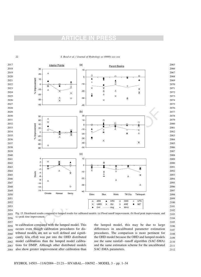
UNCORRECTED PROOF
to calibration compared with the lumped model. This
occurs even though calibration procedures for dis-
tributed models are not as well defined and signifi-
cantly less effort was put into the OHD distributed
model calibrations than the lumped model calibra-
tions for DMIP. Although other distributed models
also show greater improvement after calibration than
the lumped model, this may be due to large
differences in uncalibrated parameter estimation
procedures. The comparison is more pertinent for
the OHD model because the OHD and lumped models
use the same rainfall–runoff algorithm (SAC-SMA)
and the same estimation scheme for the uncalibrated
SAC-SMA parameters.
Fig. 15. Distributed results compared to lumped results for calibrated models. (a) Flood runoff improvement, (b) flood peak improvement, and
(c) peak time improvement.
HYDROL 14503—11/6/2004—21:21—SIVABAL—106592 – MODEL 3 – pp. 1–34
S. Reed et al. / Journal of Hydrology xx (0000) xxx–xxx22
ARTICLE IN PRESS
2017
2018
2019
2020
2021
2022
2023
2024
2025
2026
2027
2028
2029
2030
2031
2032
2033
2034
2035
2036
2037
2038
2039
2040
2041
2042
2043
2044
2045
2046
2047
2048
2049
2050
2051
2052
2053
2054
2055
2056
2057
2058
2059
2060
2061
2062
2063
2064
2065
2066
2067
2068
2069
2070
2071
2072
2073
2074
2075
2076
2077
2078
2079
2080
2081
2082
2083
2084
2085
2086
2087
2088
2089
2090
2091
2092
2093
2094
2095
2096
2097
2098
2099
2100
2101
2102
2103
2104
2105
2106
2107
2108
2109
2110
2111
2112

UNCORRECTED PROOF
Each data point shown in Figs. 15–17 is an
aggregate measure of the performance of a specific
model in a specific basin for many events. Data used
to produce Figs. 15 – 17 are summarized in
Tables 14–16. Plotting all of the statistical results
for all the events, all basins, and all models would be
too lengthy for this paper. However, a few plots
showing results for individual events are included
here to illustrate the significant scatter in model
performance on different events.
Fig. 18a (uncalibrated) and b (calibrated), plots of
the peak flow errors from the distributed model versus
the peak flow errors from the lumped model for the
Eldon basin, show significant scatter. Each point
Fig. 16. Distributed results compared to lumped results for uncalibrated models. (a) Flood runoff improvement, (b) flood peak improvement, and
(c) peak time improvement.
HYDROL 14503—11/6/2004—21:21—SIVABAL—106592 – MODEL 3 – pp. 1–34
S. Reed et al. / Journal of Hydrology xx (0000) xxx–xxx 23
ARTICLE IN PRESS
2113
2114
2115
2116
2117
2118
2119
2120
2121
2122
2123
2124
2125
2126
2127
2128
2129
2130
2131
2132
2133
2134
2135
2136
2137
2138
2139
2140
2141
2142
2143
2144
2145
2146
2147
2148
2149
2150
2151
2152
2153
2154
2155
2156
2157
2158
2159
2160
2161
2162
2163
2164
2165
2166
2167
2168
2169
2170
2171
2172
2173
2174
2175
2176
2177
2178
2179
2180
2181
2182
2183
2184
2185
2186
2187
2188
2189
2190
2191
2192
2193
2194
2195
2196
2197
2198
2199
2200
2201
2202
2203
2204
2205
2206
2207
2208

UNCORRECTED PROOF
represents a result for a single model and a single
event. For points below the 45 degree line, the
distributed model outperforms the lumped model. For
Eldon, it is interesting to see more cases with gains
going from uncalibrated lumped to uncalibrated
distributed than going from calibrated lumped to
calibrated distributed. Eldon is somewhat unusual in
this regard, as indicated by the results in Figs. 15b and
16b. Perhaps in the case of Eldon spatial variability is
an important factor in runoff generation but less
Fig. 17. Calibrated results compared to uncalibrated results. (a) Flood runoff improvement, (b) flood peak improvement, and (c) peak time
improvement.
HYDROL 14503—11/6/2004—21:21—SIVABAL—106592 – MODEL 3 – pp. 1–34
S. Reed et al. / Journal of Hydrology xx (0000) xxx–xxx24
ARTICLE IN PRESS
2209
2210
2211
2212
2213
2214
2215
2216
2217
2218
2219
2220
2221
2222
2223
2224
2225
2226
2227
2228
2229
2230
2231
2232
2233
2234
2235
2236
2237
2238
2239
2240
2241
2242
2243
2244
2245
2246
2247
2248
2249
2250
2251
2252
2253
2254
2255
2256
2257
2258
2259
2260
2261
2262
2263
2264
2265
2266
2267
2268
2269
2270
2271
2272
2273
2274
2275
2276
2277
2278
2279
2280
2281
2282
2283
2284
2285
2286
2287
2288
2289
2290
2291
2292
2293
2294
2295
2296
2297
2298
2299
2300
2301
2302
2303
2304

UNCORRECTED PROOF
Table 13
Event percent runoff bias
Christie Kansas Savoy4 Eldon Blue Watts4 Tiff City Tahlequah
Calibrated
LMP 49.1 20.5 210.5 22.1 7.3 20.8 11.4 22.1
ARS 35.3 0.1 24.1 218.0 35.1 28.1 10.7 211.5
ARZ 2 2 33.7 2 2 1.2 2 2
DHI 2 2 2 2 210.8 2 2 2
HRC 13.3 21.4 27.1 6.0 4.8 11.2 9.5
MIT 24.6 237.9 223.0
OHD 52.7 1.2 28.7 0.3 14.6 1.5 14.3 20.6
OU 236.8 220.6 28.5
UTS 21.6 211.0 22.3 214.1 28.0 26.9 29.7 25.8
UWO 53.7 27.5 12.3 26.7 49.2 21.3 33.1 18.8
WHU 11.4
Table 14
Event improvement statistics: distributed results compared to lumped results for calibrated models
ARS HRC OHD UTS UWO OU ARZ MIT DHI WHU
Flood runoff
Christie 210.9 22.6 21.4 23.9 6.0
Kansas 226.1 23.4 20.1 22.4 213.2 231.7
Savoy 26.2 4.8 1.0 23.9 217.4 227.4
Eldon 223.8 22.5 2.1 27.4 215.7 226.7
Blue 224.7 23.6 22.3 219.2 232.8 215.8 211.5 21.7 220.9
Watts 219.5 25.1 0.9 27.5 227.1 29.9
Tiff City 229.6 21.0 20.3 212.7 230.9
Tahlequah 222.7 24.2 1.4 24.8 221.4 217.1
Flood Peak
Christie 265.4 11.0 67.0 51.1 29.7
Kansas 222.9 2.6 2.8 210.1 28.1 29.2
Savoy 24.2 4.6 3.0 215.0 212.5 10.9
Eldon 229.9 29.3 0.3 215.0 228.6 228.1
Blue 20.8 1.7 9.9 211.1 235.1 216.2 23.9 3.6 213.6
Watts 29.4 22.7 3.8 25.9 20.1 23.1
Tiff City 219.0 20.9 1.1 211.4 218.9
Tahlequah 218.7 0.0 5.4 211.8 23.2 239.0
Peak time
Christie 28.5 21.6 21.4 2.3 20.2
Kansas 22.8 1.0 2.0 1.1 0.6 2.2
Savoy 23.8 1.9 0.3 20.4 24.3 211.8
Eldon 27.8 22.5 21.1 0.5 24.8 22.8
Blue 213.5 22.3 3.3 4.5 22.8 210.1 23.4 20.8 216.7
Watts 222.3 20.7 22.2 21.4 25.3 29.4
Tiff City 216.7 20.5 21.5 21.3 22.3
Tahlequah 229.6 24.2 25.9 26.0 23.7 215.0
HYDROL 14503—11/6/2004—21:21—SIVABAL—106592 – MODEL 3 – pp. 1–34
S. Reed et al. / Journal of Hydrology xx (0000) xxx–xxx 25
ARTICLE IN PRESS
2305
2306
2307
2308
2309
2310
2311
2312
2313
2314
2315
2316
2317
2318
2319
2320
2321
2322
2323
2324
2325
2326
2327
2328
2329
2330
2331
2332
2333
2334
2335
2336
2337
2338
2339
2340
2341
2342
2343
2344
2345
2346
2347
2348
2349
2350
2351
2352
2353
2354
2355
2356
2357
2358
2359
2360
2361
2362
2363
2364
2365
2366
2367
2368
2369
2370
2371
2372
2373
2374
2375
2376
2377
2378
2379
2380
2381
2382
2383
2384
2385
2386
2387
2388
2389
2390
2391
2392
2393
2394
2395
2396
2397
2398
2399
2400

UNCORRECTED PROOF
important in affecting hydrograph shape so the
lumped calibration is able to account for the spatially
variable runoff generation, leaving less potential for
gains from distributed runoff and routing in the
calibrated case.
We infer based on DMIP results and other
results reported in the literature (Zhang et al., 2003;
Koren et al., 2003a; Smith et al., 2004a) that spatially
variability of rainfall does have a big impact on
hydrograph shape in the Blue River and this is why
noticeable gains are achieved by running a distributed
model. Similar to Fig. 18a and b; Fig. 19a (uncali-
brated) and 19b (calibrated) show the peak flow errors
from distributed models versus the peak flow errors
from the lumped model, but for the Blue basin.
However, to remove some of the scatter and
emphasize the significant improvements possible for
the Blue river basin, only results from the three best
performing models (in terms of event peak flows for
Blue) are plotted.
To force the same domain and range for plotting in
Figs. 18 and 19, the plotting range is defined by the
range of errors that existed in the lumped model
simulations. Since the maximum errors for distributed
models are greater than the maximum errors for
lumped models, some data points are not seen in
Figs. 18 and 19.
3.4. Additional analysis for interior points
One of the big benefits of using distributed models
is that they are able to produce simulations at interior
points; however, studies are needed to quantify the
accuracy and uncertainty of interior point simulations.
Streamflow data from a limited number of interior
points were provided in DMIP. These interior points
include Watts (given calibration at Tahlequah),
Savoy, Kansas, and Christie. Based on the presen-
tation and discussion of overall and event-based
statistics above, it is seen that some models are able to
Table 15
Event improvement statistics: distributed results compared to lumped results for uncalibrated models
ARS HRC OHD UTS UWO OU ARZ MIT EMC
Christie 261.6 22.5 242.2 240.1 25.0
Kansas 239.3 0.3 20.1 212.7 223.0 243.3 24.7
Savoy 21.2 11.3 0.9 210.2 212.7 235.7 214.5 12.1
Eldon 216.1 4.7 2.8 21.6 27.9 214.9
Blue 226.1 237.4 27.1 236.6 255.6 29.8 22.8 21.3
Watts 224.0 6.9 0.6 215.6 219.9 24.3 216.8 1.5
Tiff City 245.0 26.1 27.9 241.5 226.3 22.0
Tahlequah 224.8 8.2 2.0 28.8 218.2 218.8 4.9
Christie 2179.2 221.2 7.7 28.8 11.2
Kansas 249.0 215.8 4.3 25.2 24.7 25.0 26.8
Savoy 2.3 212.7 5.1 215.2 214.6 249.8 27.8 221.9
Eldon 3.9 21.2 8.1 9.5 24.6 215.2
Blue 3.7 218.4 2.5 218.6 28.4 210.4 223.7 1.1
Watts 24.7 259.4 0.3 22.5 24.4 257.6 212.6 23.3
Tiff City 214.2 267.2 24.3 217.7 210.4 24.6
Tahlequah 212.5 243.7 0.9 22.3 23.5 222.0 28.9
Christie 27.0 21.6 5.9 7.1 7.5
Kansas 21.5 1.2 4.4 27.3 22.7 5.0 25.5
Savoy 20.1 26.8 0.2 221.1 211.4 28.6 0.5 210.1
Eldon 22.3 3.4 3.0 0.7 29.1 210.9
Blue 218.1 22.0 22.8 0.7 24.5 28.2 23.1 214.4
Watts 212.1 26.4 21.3 22.8 218.6 28.7 21.2 211.6
Tiff City 217.8 25.6 24.1 21.4 211.9 217.2
Tahlequah 228.3 25.2 23.5 28.0 221.3 220.6 220.3
HYDROL 14503—11/6/2004—21:21—SIVABAL—106592 – MODEL 3 – pp. 1–34
S. Reed et al. / Journal of Hydrology xx (0000) xxx–xxx26
ARTICLE IN PRESS
2401
2402
2403
2404
2405
2406
2407
2408
2409
2410
2411
2412
2413
2414
2415
2416
2417
2418
2419
2420
2421
2422
2423
2424
2425
2426
2427
2428
2429
2430
2431
2432
2433
2434
2435
2436
2437
2438
2439
2440
2441
2442
2443
2444
2445
2446
2447
2448
2449
2450
2451
2452
2453
2454
2455
2456
2457
2458
2459
2460
2461
2462
2463
2464
2465
2466
2467
2468
2469
2470
2471
2472
2473
2474
2475
2476
2477
2478
2479
2480
2481
2482
2483
2484
2485
2486
2487
2488
2489
2490
2491
2492
2493
2494
2495
2496

UNCORRECTED PROOF
produce reasonable simulations for these interior
points, although errors are typically greater than for
parent basins.
Another question that can be investigated with
DMIP data is whether a model calibrated at a smaller
basin (Watts) shows advantages in simulating flows at
a common interior point with a model calibrated at a
larger parent basin (Tahlequah). One of the tests
requested in the DMIP modeling instructions (instruc-
tion 4) was for modelers to calibrate models at Watts
and submit the resulting simulations for both Watts
and two interior points (Savoy and an ungauged point)
without using interior flow information. Modeling
instruction 5 requested that the same be done for
Tahlequah, with interior simulations generated at
Watts, Savoy, and Kansas. For the common points
(Watts and Savoy) from instructions 4 and 5, Figs. 20
and 21 compare the event percent absolute runoff
error and percent absolute peak error statistics. Points
above the 1:1 line indicate improvement after
calibration at Watts. For the percent absolute runoff
error results (Figs. 20a and 21a), none of the models
showed significant improvement after calibration at
Watts. This is perhaps not surprising considering the
conclusion from the lumped calibration of Tahlequah
and Watts that the same SAC-SMA parameter set
produces reasonable results in both basins. For the
peak flow error results, only the UTS model showed
improvement.
Simulations were also requested at several
ungauged interior points. One way to examine these
results in the absence of observed streamflow data is to
compare coefficients of variation (CVs) from different
models. Simulated (calibrated) and observed CVs for
flow are plotted against drainage area in Fig. 22a and b.
The area range plotted in Fig. 22a encompasses all of
Table 16
Event improvement statistics: calibrated results compared to uncalibrated results
ARS HRC OHD UTS UWO OU ARZ LMP MIT
Flood runoff
Christie 30.2 220.6 43.1 15.8 220.5
Kansas 16.3 20.6 0.5 13.4 12.9 14.8 3.1
Savoy 3.4 2.0 2.4 14.7 3.8 16.7 8.4
Eldon 4.0 4.5 11.0 6.0 3.9 11.7
Blue 9.8 42.2 13.3 25.8 31.2 0.5 8.4 5.5
Watts 14.7 21.7 10.5 18.3 3.1 4.5 10.2
Tiff City 23.3 13.6 16.2 40.3 5.6 7.9
Tahlequah 13.3 21.3 2.1 15.1 7.8 13.1 11.1
Flood peak
Christie 54.8 226.7 0.4 1.0 258.9
Kansas 27.5 19.7 20.7 23.6 22.1 22.9 1.3
Savoy 24.0 19.8 0.1 2.7 4.6 63.2 2.5
Eldon 26.3 23.1 19.5 2.9 3.4 27.4
Blue 3.5 28.1 15.4 15.5 218.7 1.1 8.0 27.8
Watts 24.3 57.1 3.9 23.0 4.8 54.9 0.4
Tiff City 1.0 83.1 11.8 15.0 21.0 5.7
Tahlequah 54.8 226.7 0.4 1.0 258.9
Peak time
Christie 0.0 1.5 25.8 23.3 1.5
Kansas 1.7 2.7 4.8 11.3 6.2 0.1 2.9
Savoy 21.0 11.3 2.7 23.3 9.8 20.6 2.625
Eldon 20.5 21.0 0.8 4.7 27.1 5.2
Blue 4.5 20.3 6.1 3.8 1.6 21.5 0.0 20.3
Watts 26.8 9.0 2.0 4.7 16.6 2.6 3.3
Tiff City 0.53 4.65 2.06 20.41 9.12 20.53
Tahlequah 0.2 2.5 21.2 3.5 19.2 7.1 1.5
HYDROL 14503—11/6/2004—21:21—SIVABAL—106592 – MODEL 3 – pp. 1–34
S. Reed et al. / Journal of Hydrology xx (0000) xxx–xxx 27
ARTICLE IN PRESS
2497
2498
2499
2500
2501
2502
2503
2504
2505
2506
2507
2508
2509
2510
2511
2512
2513
2514
2515
2516
2517
2518
2519
2520
2521
2522
2523
2524
2525
2526
2527
2528
2529
2530
2531
2532
2533
2534
2535
2536
2537
2538
2539
2540
2541
2542
2543
2544
2545
2546
2547
2548
2549
2550
2551
2552
2553
2554
2555
2556
2557
2558
2559
2560
2561
2562
2563
2564
2565
2566
2567
2568
2569
2570
2571
2572
2573
2574
2575
2576
2577
2578
2579
2580
2581
2582
2583
2584
2585
2586
2587
2588
2589
2590
2591
2592

UNCORRECTED PROOF
the DMIP basins while Fig. 22b provides a more
detailed look at results for smaller basins. In Fig. 22a,
the LMP, OHD, and HRC models reasonably approxi-
mate the trend of increasing CV with decreasing
drainage area over the scales of most DMIP basins. It is
not possible to infer much about the accuracy of
simulated CV values for the range of scales shown in
Fig. 22b because only one point with observed data
(Christie at 65 km2) is available. However, it is
interesting that the UTS model, which had the best
percent absolute runoff error and peak flow statistics
for Christie among calibrated models, tends to under-
estimate the CV for Christie, as it does for the larger
basins with observed data. It turns out that the standard
deviation of flows predicted by the UTS model for
Christie is close to that of the observed data but the
mean flow predicted by the UTS model is too high, due
primarily to high modeled base flows.
Fig. 18. Distributed percent absolute peak flow errors vs. lumped percent absolute peak flow errors for Eldon events: (a) uncalibrated and (b)
calibrated models.
HYDROL 14503—11/6/2004—21:21—SIVABAL—106592 – MODEL 3 – pp. 1–34
S. Reed et al. / Journal of Hydrology xx (0000) xxx–xxx28
ARTICLE IN PRESS
2593
2594
2595
2596
2597
2598
2599
2600
2601
2602
2603
2604
2605
2606
2607
2608
2609
2610
2611
2612
2613
2614
2615
2616
2617
2618
2619
2620
2621
2622
2623
2624
2625
2626
2627
2628
2629
2630
2631
2632
2633
2634
2635
2636
2637
2638
2639
2640
2641
2642
2643
2644
2645
2646
2647
2648
2649
2650
2651
2652
2653
2654
2655
2656
2657
2658
2659
2660
2661
2662
2663
2664
2665
2666
2667
2668
2669
2670
2671
2672
2673
2674
2675
2676
2677
2678
2679
2680
2681
2682
2683
2684
2685
2686
2687
2688
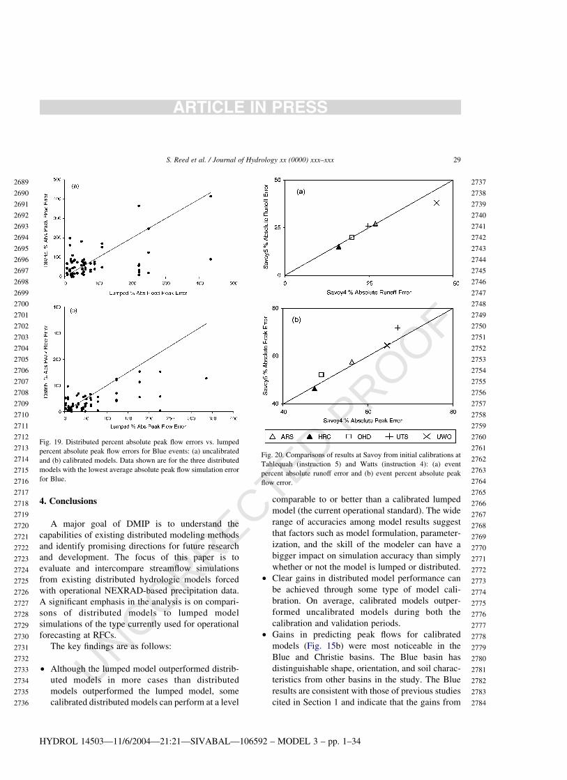
UNCORRECTED PROOF
4. Conclusions
A major goal of DMIP is to understand the
capabilities of existing distributed modeling methods
and identify promising directions for future research
and development. The focus of this paper is to
evaluate and intercompare streamflow simulations
from existing distributed hydrologic models forced
with operational NEXRAD-based precipitation data.
A significant emphasis in the analysis is on compari-
sons of distributed models to lumped model
simulations of the type currently used for operational
forecasting at RFCs.
The key findings are as follows:
† Although the lumped model outperformed distrib-
uted models in more cases than distributed
models outperformed the lumped model, some
calibrated distributed models can perform at a level
comparable to or better than a calibrated lumped
model (the current operational standard). The wide
range of accuracies among model results suggest
that factors such as model formulation, parameter-
ization, and the skill of the modeler can have a
bigger impact on simulation accuracy than simply
whether or not the model is lumped or distributed.
† Clear gains in distributed model performance can
be achieved through some type of model cali-
bration. On average, calibrated models outper-
formed uncalibrated models during both the
calibration and validation periods.
† Gains in predicting peak flows for calibrated
models (Fig. 15b) were most noticeable in the
Blue and Christie basins. The Blue basin has
distinguishable shape, orientation, and soil charac-
teristics from other basins in the study. The Blue
results are consistent with those of previous studies
cited in Section 1 and indicate that the gains from
Fig. 19. Distributed percent absolute peak flow errors vs. lumped
percent absolute peak flow errors for Blue events: (a) uncalibrated
and (b) calibrated models. Data shown are for the three distributed
models with the lowest average absolute peak flow simulation error
for Blue.
Fig. 20. Comparisons of results at Savoy from initial calibrations at
Tahlequah (instruction 5) and Watts (instruction 4): (a) event
percent absolute runoff error and (b) event percent absolute peak
flow error.
HYDROL 14503—11/6/2004—21:21—SIVABAL—106592 – MODEL 3 – pp. 1–34
S. Reed et al. / Journal of Hydrology xx (0000) xxx–xxx 29
ARTICLE IN PRESS
2689
2690
2691
2692
2693
2694
2695
2696
2697
2698
2699
2700
2701
2702
2703
2704
2705
2706
2707
2708
2709
2710
2711
2712
2713
2714
2715
2716
2717
2718
2719
2720
2721
2722
2723
2724
2725
2726
2727
2728
2729
2730
2731
2732
2733
2734
2735
2736
2737
2738
2739
2740
2741
2742
2743
2744
2745
2746
2747
2748
2749
2750
2751
2752
2753
2754
2755
2756
2757
2758
2759
2760
2761
2762
2763
2764
2765
2766
2767
2768
2769
2770
2771
2772
2773
2774
2775
2776
2777
2778
2779
2780
2781
2782
2783
2784

UNCORRECTED PROOF
applying a distributed simulation model at NWS
forecast basin scales (on the order of 1000 km2)
will depend on the basin characteristics. Christie is
distinguishable in this study because of its small
size.
† Christie had distinguishable results from the larger
basins studied, not just in overall statistics, but in
relative inter-model performance compared with
larger basins. One explanation offered for the
improved calibrated, peak flow results (Fig. 15b) is
that the lumped ‘calibrated’ model parameters
(from the parent basin calibration, Eldon) are scale
dependent and distributed model parameters that
account for spatial variability within Eldon are less
scale dependent. Some caution is advised in
interpreting the results for Christie for model
submissions with a relatively coarse cell resolution
compared to the size of the basin (e.g. EMC
and OHD). Since no other basins in DMIP are
comparable in size to Christie, more studies on
small, nested basins are needed to confirm and
better understand these results.
† Among calibrated results, models that combine
techniques of conceptual rainfall – runoff and
physically based distributed routing consistently
showed the best performance in all but the smallest
basin. Gains from calibration indicate that deter-
mining reasonable a priori parameters directly
from physical characteristics of a watershed is
generally a more difficult problem than defining
reasonable parameters for a conceptual lumped
model through calibration.
† Simulations for smaller interior basins where no
explicit calibration was done exhibited reasonable
performance in many cases, although not as good
statistically as results for larger, parent basins. The
relatively degraded performance in smaller basins
occurred both in cases when parent basins were
calibrated and when they were uncalibrated, so the
degraded performance was not simply a function of
the fact that no explicit calibration at interior points
was allowed.
Fig. 21. Comparisons of results at Watts from initial calibrations at
Tahlequah (instruction 5) and Watts (instruction 4): (a) event
percent absolute runoff error and (b) event percent absolute peak
flow error.
Fig. 22. Flow coefficients of variation for observed flows (solid line)
and modeled flows (for both gaged and ungaged locations): (a) all
basin sizes and (b) a closer look at the small basins.
HYDROL 14503—11/6/2004—21:21—SIVABAL—106592 – MODEL 3 – pp. 1–34
S. Reed et al. / Journal of Hydrology xx (0000) xxx–xxx30
ARTICLE IN PRESS
2785
2786
2787
2788
2789
2790
2791
2792
2793
2794
2795
2796
2797
2798
2799
2800
2801
2802
2803
2804
2805
2806
2807
2808
2809
2810
2811
2812
2813
2814
2815
2816
2817
2818
2819
2820
2821
2822
2823
2824
2825
2826
2827
2828
2829
2830
2831
2832
2833
2834
2835
2836
2837
2838
2839
2840
2841
2842
2843
2844
2845
2846
2847
2848
2849
2850
2851
2852
2853
2854
2855
2856
2857
2858
2859
2860
2861
2862
2863
2864
2865
2866
2867
2868
2869
2870
2871
2872
2873
2874
2875
2876
2877
2878
2879
2880

UNCORRECTED PROOF
† Distributed models designed for research can be
applied successfully using operational quality data.
Several models responded similarly to long term
biases in archived multi-sensor precipitation grids.
Ease of implementation could not be measured
directly. However, an indirect indicator operational
practicability is that several participants were able
to submit a full set or nearly a full set of
simulations (Table 2) with no financial support
and in a relatively short time.
This study did not address the question of whether
or not simulation model improvements will translate
into operational forecast improvements. One import-
ant issue in operational forecasting is the use offorecast
precipitation data. Because forecast precipitation data
have a lower resolution and are much more uncertain
than the observed precipitation used in this study, the
benefits of distributed models may diminish for longer
lead times that rely more heavily on forecast
precipitation data. This assumption needs further
study, but if true, greater benefits from distributed
models would be expected for shorter lead times that
are close to the response time of a basin. For example,
analysis of several isolated storms in the Blue River
indicates an average time between the end of rainfall
and peak streamflow of about 9 h and an average time
between the rainfall peak and the streamflow peak of
about 18 h. Forecasts in this range of lead times could
benefit without using any forecast precipitation.
5. Recommendations
The analyses in this paper addressed the following
questions: Can distributed models exhibit simulation
performance comparable to or better than existing
lumped models used in the NWS? Are there
differences in relative model performance when
different distributed models are applied to different
basins? Does calibration improve the performance of
distributed models? The results also help to formulate
useful questions that merit further investigation. For
example: Why does one particular model perform
relatively well in one basin but not as well in another
basin? Because the widely varying structural com-
ponents in participating models (e.g. different rain-
fall–runoff algorithms, routing algorithms, and model
element sizes) have interacting and compensating
effects, it is difficult to infer reasons for differences in
model performance. More controlled studies in which
only one model component is changed at a time will
be required to answer questions related to causation.
Much work lies ahead to gain a clearer and deeper
understanding of the results presented in this paper.
Several other papers in this issue already begin to
examine the underlying reasons for our results. Scale
and uncertainty issues figure to be critical research
topics that will require further study. An important
potential benefit of using distributed models is the
ability to produce simulations at small, ungauged
locations. However, given uncertainty in available
inputs, the spatial and temporal scales where explicit
distributed modeling can provide the most useful
products (and benefits relative to lumped modeling) is
not clear. Forecasters will need guidance to define the
confidence they should have in forecasts at various
modeling scales. This is true for both lumped and
distributed models. A recent NWS initiative to
produce probabilistic quantitative precipitation esti-
mates (PQPE) should help support this type of effort.
Information about precipitation uncertainty can be
incorporated into hydrologic forecasts through the use
of ensemble simulations (e.g. Carpenter and Georga-
kakos, 2004).
Concurrent with future studies to improve our
understanding, efforts are also needed to develop
software that can test these techniques in an
operational forecasting environment. All results pre-
sented in this paper were produced in an off-line
simulation mode. Design for the forecasting environ-
ment raises a number of scientific and software issues
that were not addressed directly in this paper. Issues
such as model run-times, ease of use, and ease of
parameterization are very important for successful
operational implementation. Related issues to con-
sider are capabilities to ingest both observed and
forecast precipitation, update model states, and
produce ensemble forecasts as necessary. A project
to create and test an operational version of the OHD
distributed model is currently in progress.
Finally, several ideas for future intercomparison
work (e.g. DMIP Phase II) were suggested at the
August 2002 DMIP workshop. These suggestions
included defining a community-wide distributed
modeling system, separating the comparisons of
HYDROL 14503—11/6/2004—21:22—SIVABAL—106592 – MODEL 3 – pp. 1–34
S. Reed et al. / Journal of Hydrology xx (0000) xxx–xxx 31
ARTICLE IN PRESS
2881
2882
2883
2884
2885
2886
2887
2888
2889
2890
2891
2892
2893
2894
2895
2896
2897
2898
2899
2900
2901
2902
2903
2904
2905
2906
2907
2908
2909
2910
2911
2912
2913
2914
2915
2916
2917
2918
2919
2920
2921
2922
2923
2924
2925
2926
2927
2928
2929
2930
2931
2932
2933
2934
2935
2936
2937
2938
2939
2940
2941
2942
2943
2944
2945
2946
2947
2948
2949
2950
2951
2952
2953
2954
2955
2956
2957
2958
2959
2960
2961
2962
2963
2964
2965
2966
2967
2968
2969
2970
2971
2972
2973
2974
2975
2976

UNCORRECTED PROOF
routing and rainfall runoff techniques, using synthetic
simulations to complement work with real world data,
doing more uncertainty analysis (e.g. ensemble
simulations), looking in more detail at differences in
model structures to improve our understanding of
cause and effect, assessing the impact of model
element size in a more systematic manner, identifying
additional basins where scale issues can be studied
effectively and where other processes such as snow
modeling can be investigated, using additional
sources of observed data for model verification (e.g.
soil moisture), and using a longer verification period.
Appendix A
DMIP Participants: Jeff Arnoldb, Christina Ban-
daragodac, Allyson Bingemand, Rafael Brase, Michael
Buttsf, Theresa Carpenterg, Zhengtao Cuih, Mauro
Diluzioi, Konstantine Georgakakosg, Anubhav Gaurh,
Jianzhong Guol, Hoshin Guptaj, Terri Hoguej, Valeri
Ivanove, Newsha Khodatalabj, Li Lank, Xu Liangl,
Dag Lohmannm, Ken Mitchellm, Christa Peters-
Lidardm, Erasmo Rodriguezd, Frank Seglenieksd,
Eylon Shamirj, David Tarbotonc, Baxter Vieuxh,
Enrique Vivonie, and Ross Woodsn
1. Office of Hydrologic Development,
NOAA/NWS, Silver Spring, Maryland
2. USDA-Agricultural Research Service, Temple,
Texas
3. Utah State University, Logan, Utah
4. University of Waterloo, Ontario, Canada
5. Massachusetts Institute of Technology, Cam-
bridge, Massachusetts
6. DHI Water and Environment, Horsholm, Den-
mark
7. Hydrologic Research Center, San Diego, Cali-
fornia
8. University of Oklahoma, Norman, Oklahoma
9. TAES-Blacklands Research Center, Temple,
Texas
10. University of Arizona, Tucson, Arizona
11. Wuhan University, Wuhan, China
12. University of California at Berkeley, Berkeley,
California
13. NOAA/NCEP, Camp Springs, Maryland
References
Anderson, E., (2003). Calibration of Conceptual Hydrologic Models
for Use XSC DC DC XAAAQQver Forecasting (copy available
on request from: Hydrology Laboratory, Office of Hydrologic
Development, NOAA/National Weather Service, (1325) East-
West Highway, Silver Spring, MD 20910).
Andersen, J., Refsgaard, J.C., Jensen, H.J., 2001. Distributed
hydrological modeling of the senegal river basin-model
construction and validation. Journal of Hydrology 247,
200–214.
Bandaragoda, C., Tarboton, D., Woods, R., 2004. Application of
topmodel in the distributed model intercomparison Project.
Journal of Hydrology, xxthis issue.
Boyle, D.P., Gupta, H.V., Sorooshian, S., Koren, V., Zhang, Z.,
Smith, M., 2001. Toward Improved Streamflow Forecasts:
Value of Semi-distributed Modeling. Water Resources Research
37(11), 2749–2759.
Burnash, R.J., 1995. The NWS river forecast system - catchment
modeling. In: Singh, V.P., (Ed.), Computer Models of
Watershed Hydrology, Water Resources Publications, Littleton,
CO, pp. 311–366.
Burnash, R.J., Ferral, R.L., McGuire, R.A., 1973. A Generalized
Streamflow Simulation System Conceptual Modeling for
Digital Computers, US Department of Commerce National
Weather Service and State of California Department of Water.
Butts, M.B., Payne, J.T., Kristensen, M., Madsen, H., 2004. An
Evaluation of the impact of model structure and complexity on
hydrologic modelling uncertainty for streamflow prediction.
Journal of Hydrology this issue.
Carpenter, T.M., Georgakakos, K.P., 2004. Impacts of parametric
and radar rainfall uncertainty on the ensemble streamflow
simulations of a distributed hydrologic model. Journal of
Hydrology this issue.
Carpenter, T.M., Georgakakos, K.P., Spersflagea, J.A., 2001. On the
parametric and NEXRAD-radar sensitivities of a distributed
hydrologic model suitable for operational use. Journal of
Hydrology 253, 169–193.
Christiaens, K., Feyen, J., 2002. Use of sensitivity and uncertainty
measures in distributed hydrological modeling with an appli-
cation to the MIKE SHE model. Water Resources Research
38(9), 1169.
Clark, C.O., 1945. Storage and the unit hydrograph. Transactions of
the American Society of Civil Engineers 110, 1419–1446.
Di Luzio, M., Arnold, J., 2004. Gridded precipitation input toward
the improvement of streamflow and water quality assessments.
Journal of Hydrology this issue.
Finnerty, B.D., Smith, M.B., Seo, D.J., Koren, V., Moglen, G.E.,
1997. Space-time scale sensitivity of the Sacramento model to
radar-gage precipitation inputs. Journal of Hydrology 203,
21–38.
Fulton, R.A., Breidenbach, J.P., Seo, D.J., Miller, D.A., O’Bannon,
T., 1998. The WSR-88D rainfall algorithm. Weather and
Forecasting 13, 377–395.
Guo, J., Liang, X., Leung, L.R., 2004. Impacts of different
precipitation data sources on water budget simulated by
HYDROL 14503—11/6/2004—21:22—SIVABAL—106592 – MODEL 3 – pp. 1–34
S. Reed et al. / Journal of Hydrology xx (0000) xxx–xxx32
ARTICLE IN PRESS
2977
2978
2979
2980
2981
2982
2983
2984
2985
2986
2987
2988
2989
2990
2991
2992
2993
2994
2995
2996
2997
2998
2999
3000
3001
3002
3003
3004
3005
3006
3007
3008
3009
3010
3011
3012
3013
3014
3015
3016
3017
3018
3019
3020
3021
3022
3023
3024
3025
3026
3027
3028
3029
3030
3031
3032
3033
3034
3035
3036
3037
3038
3039
3040
3041
3042
3043
3044
3045
3046
3047
3048
3049
3050
3051
3052
3053
3054
3055
3056
3057
3058
3059
3060
3061
3062
3063
3064
3065
3066
3067
3068
3069
3070
3071
3072

UNCORRECTED PROOF
the VIC-3L hydrological model. Journal of Hydrology this
issue.
Gupta, H.V., Sorooshian, S., Hogue, T.S., Boyle, D.P., 2003. In:
Duan, Q., Gupta, H.V., Sorooshian, S., Rousseau, A., Turcotte,
R. (Eds.), Advances in Automatic Calibration of Watershed
Models, Calibration of Watershed Models, Water Science and
Application 6, American Geophysical Union, pp. 9–28.
Havno, K., Madsen, M.N., Dorge, J., 1995. Mike 11—A
Generalized River Modelling Package. In: Singh, V.P., (Ed.),
Computer Models of Watershed Hydrology, Water Resources
Publications, Colorado, USA, pp. 733–782.
Ivanov, V.Y., Vivoni, E.R., Bras, R.L., Entekhabi, D., 2004.
Preserving high-resolution surface and rainfall data in oper-
ational-scale basin hydrology: a fully-distributed physically-
based approach. Journal of Hydrology this issue.
Johnson, D., Smith, M., Koren, V., Finnerty, B., 1999. Comparing
mean areal precipitation estimates from NEXRAD and rain
gauge networks. Journal of Hydrologic Engneering 4(2),
117–124.
Khodatalab, N., Gupta, H., Wagener, T., Sorooshian, S., 2004.
Calibration of a semi-distributed hydrologic model for stream-
flow estimation along a river system. Journal of Hydrology this
issue.
Koren, V, Schaake, J., Duan, Q., Smith, M., Cong, S., September
(1998). PET Upgrades to NWSRFS—Project Plan, HRL
Internal Report, (copy available on request from: Hydrology
Laboratory, Office of Hydrologic Development, NOAA/
National Weather Service, 1325 East-West Highway, Silver
Spring, MD 20910).
Koren, V.I., Finnerty, B.D., Schaake, J.C., Smith, M.B., Seo, D.J.,
Duan, Q.Y., 1999. Scale dependencies of hydrologic models to
spatial variability of precipitation. Journal of Hydrology 217,
285–302.
Koren, V., Reed, S., Smith, M., Zhang, Z., Seo, D.J., 2003a. In
review, Hydrology Laboratory Research Modeling System (HL-
RMS) of the National Weather Service. Journal. of Hydrology.
Koren, V., Smith, M., Duan, Q., 2003b. Use of a priori parameter
estimates in the derivation of spatially consistent parameter sets
of rainfall–runoff models. In: Duan, Q., Sorooshian, S., Gupta,
H., Rosseau, A., Turcotte, R. (Eds.), Advances in the Calibration
of Watershed Models, AGU Water Science and Applications
Series.
Kouwen, N., Garland, G., 1989. Resolution considerations in using
radar rainfall data for flood forecasting. Canadian Journal of
Civil Engineering 16, 279–289.
Kouwen, N., Soulis, E.D., Pietroniro, A., Donald, J., Harrington,
R.A., 1993. Grouped Response units for distributed hydrologic
modelling. Journal of Water Resources Planning and Manage-
ment 119(3), 289–305.
Leavesley, G.H., Hay, L.E., Viger, R.J., Markstrom, S.L., 2003. Use
of a priori parameter-estimation methods to constrain cali-
bration of distributed-parameter models. In: Duan, Q., Sor-
ooshian, S., Gupta, H., Rosseau, A., Turcotte, R. (Eds.),
Advances in the Calibration of Watershed Models, AGU
Water Science and Applications Series.
Liang, X., Xie, Z., 2001. A new surface runoff parameterization
with subgrid-scale soil heterogeneity for land surface models.
Advances in Water Resources 24, 1173–1193.
Liang, X., Lettenmaier, D.P., Wood, E.F., Burges, S.J., 1994. A
simple hydrologically based model of land surface water and
energy fluxes for general circulation models. Journal of
Geophysical Research 99(D7), 14,415–14,428.
Madsen, H., 2003. Parameter estimation in distributed hydrological
catchment modelling using automatic calibration with multiple
objectives. Advances in Water Resources 26, 205–216.
McCuen, R.H., Snyder, W.M., 1975. A proposed index for
comparing hydrographs. Water Resources Research 11(6),
1021–1024.
Nash, J.E., Sutcliffe, J.V., 1970. River flow forecasting through
conceptual models part I— a discussion of principles. Journal of
Hydrology 10, 282–290.
Neitsch, S.L., Arnold, J.G, Kiniry, J.R., Williams, J.R., King, K.W.,
2000. Soil and Water Assessment Tool Theoretical Documen-
tation, Version 2000, Texas Water Resources Institute (TWRI),
Report TR-191, College Station, TX, 506pp.
Refsgaard, J.C., Knudsen, J., 1996. Operational validation and
intercomparison of different types of hydrological models.
Water Resources Research 32(7), 2189–2202.
Senarath, S.U.S., Ogden, F.L., Downer, C.W., Sharif, H.O., 2000.
On the calibration and verification of two-dimensional,
distributed, Hortonian, continuous watershed models. Water
Resources Research 36(6), 1510–1595.
Seo, D.-J., Breidenbach, J.P., 2002. Real-time correction of
spatially nonuniform bias in radar rainfall using rain gage
measurements. J. Hydrometeorology 3, 93–111.
Seo, D.-J., Breidenbach, J.P., Johnson, E.R., 1999. Real-time
estimation of mean field bias in radar rainfall data. Journal of
Hydrology, 233.
Seo, D.-J., Breidenbach, J.P., Fulton, R.A., Miller, D.A., O’Bannon,
T., 2000. Real-time adjustment of range-dependent biases in
WSR-88D rainfall data due to nonuniform vertical profile of
reflectivity. Journal of Hydrometeorology 1(3), 222–240.
Smith, M.B., Koren, V., Johnson, D., Finnerty, B.D., Seo, D.-J.,
1999. Distributed Modeling: Phase 1 Results, NOAA Technical
Report NWS 44, National Weather Service Hydrology Labora-
tory, 210 pp. Copies available upon request.
Smith, M.B., Laurine, D., Koren, V., Reed, S., Zhang, Z., 2003.
Hydrologic model calibration in the National Weather Service.
In: Duan, Q., Sorooshian, S., Gupta, H., Rosseau, A., Turcotte,
R. (Eds.), Advances in the Calibration of Watershed Models,
AGU Water Science and Applications Series.
Smith, M.B., Koren, V.I., Zhang, Z., Reed, S.M., Pan, J.-J., Moreda,
F., Kuzmin, V., 2004aa. Runoff response to spatial variability in
precipitation: an analysis of observed data. Journal of
Hydrology this issue.
Smith, M.B., Seo, D.-J., Koren, V.I., Reed, S., Zhang, Z., Duan, Q.-
Y., Cong, S., Moreda, F., Anderson, R., 2004bb. The Distributed
Model Intercomparison Project (DMIP): an overview. Journal
of Hydrology this issue.
Sweeney, T.L., 1992. Modernized Areal Flash Flood Guidance,
NOAA Technical Memorandum NWS Hydro 44, Silver Spring,
MD.
HYDROL 14503—11/6/2004—21:22—SIVABAL—106592 – MODEL 3 – pp. 1–34
S. Reed et al. / Journal of Hydrology xx (0000) xxx–xxx 33
ARTICLE IN PRESS
3073
3074
3075
3076
3077
3078
3079
3080
3081
3082
3083
3084
3085
3086
3087
3088
3089
3090
3091
3092
3093
3094
3095
3096
3097
3098
3099
3100
3101
3102
3103
3104
3105
3106
3107
3108
3109
3110
3111
3112
3113
3114
3115
3116
3117
3118
3119
3120
3121
3122
3123
3124
3125
3126
3127
3128
3129
3130
3131
3132
3133
3134
3135
3136
3137
3138
3139
3140
3141
3142
3143
3144
3145
3146
3147
3148
3149
3150
3151
3152
3153
3154
3155
3156
3157
3158
3159
3160
3161
3162
3163
3164
3165
3166
3167
3168

UNCORRECTED PROOF
Vieux, B.E., 2001. Distributed Hydrologic Modeling Using GIS,
Water Science and Technology Series, vol. 38. Kluwer,
Norwell, MA, 293 pp. ISBN 0-7923-7002-3.
Vieux, B.E., Moreda, F., 2003. Ordered Physics-Based Parameter
Adjustment of a Distributed Model. In: Duan, Q., Sorooshian,
S., Gupta, H., Rosseau, A., Turcotte, R. (Eds.), Advances in the
Calibration of Watershed Models, AGU Water Science and
Applications Series.
Wang, D., Smith, M.B., Zhang, Z., Reed, S., Koren, V., 2000.
Statistical comparison of mean areal precipitation estimates
from WSR-88D, operational and historical gage networks, 15th
Conference on Hydrology, AMS, January 9–14, Long Beach,
CA.
Young, C.B., Bradley, A.A., Krajewski, W.F., Kruger, A., 2000.
Evaluating NEXRAD Multisensor precipitation estimates for
operational hydrologic forecasting. Journal of Hydrometeorol-
ogy 1, 241–254.
Zhang, Z., Koren, V., Smith, M., 2004. Comparison of continuous
lumped and semi-distributed hydrologic modeling using
NEXRAD data. Journal of Hydrologic Engneering in press.
HYDROL 14503—11/6/2004—21:22—SIVABAL—106592 – MODEL 3 – pp. 1–34
S. Reed et al. / Journal of Hydrology xx (0000) xxx–xxx34
ARTICLE IN PRESS
3169
3170
3171
3172
3173
3174
3175
3176
3177
3178
3179
3180
3181
3182
3183
3184
3185
3186
3187
3188
3189
3190
3191
3192
3193
3194
3195
3196
3197
3198
3199
3200
3201
3202
3203
3204
3205
3206
3207
3208
3209
3210
3211
3212
3213
3214
3215
3216
3217
3218
3219
3220
3221
3222
3223
3224
3225
3226
3227
3228
3229
3230
3231
3232
3233
3234
3235
3236
3237
3238
3239
3240
3241
3242
3243
3244
3245
3246
3247
3248
3249
3250
3251
3252
3253
3254
3255
3256
3257
3258
3259
3260
3261
3262
3263
3264