Parallelization of BVH and BSP onthe GPU

MASTERARBEIT

zur Erlangung des akademischen Grades

Master of Science

im Rahmen des Studiums

Software Engineering & Internet Computing

eingereicht von

Martin Imre, BSc.Matrikelnummer 0853761

an der Fakultät für Informatik

der Technischen Universität Wien

Betreuung: Univ.Prof. Dipl.-Ing. Dr.techn. Werner Purgathofer

Wien, 14. Juni 2016Martin Imre Werner Purgathofer

Technische Universität WienA-1040 Wien Karlsplatz 13 Tel. +43-1-58801-0 www.tuwien.ac.at

Parallelization of BVH and BSP onthe GPU

MASTER’S THESIS

submitted in partial fulfillment of the requirements for the degree of

Master of Science

in

Software Engineering & Internet Computing

by

Martin Imre, BSc.Registration Number 0853761

to the Faculty of Informatics

at the TU Wien

Advisor: Univ.Prof. Dipl.-Ing. Dr.techn. Werner Purgathofer

Vienna, 14th June, 2016Martin Imre Werner Purgathofer

Technische Universität WienA-1040 Wien Karlsplatz 13 Tel. +43-1-58801-0 www.tuwien.ac.at

Erklärung zur Verfassung derArbeit

Martin Imre, BSc.Gaullachergasse 13/9-11, 1160 Wien

Hiermit erkläre ich, dass ich diese Arbeit selbständig verfasst habe, dass ich die verwen-deten Quellen und Hilfsmittel vollständig angegeben habe und dass ich die Stellen derArbeit – einschließlich Tabellen, Karten und Abbildungen –, die anderen Werken oderdem Internet im Wortlaut oder dem Sinn nach entnommen sind, auf jeden Fall unterAngabe der Quelle als Entlehnung kenntlich gemacht habe.

Wien, 14. Juni 2016Martin Imre

v

Acknowledgements

First and foremost I want to thank Robert F. Tobler for offering this topic to me andbeing my advisor during the early stages. Unfortunately he can not see the result of mywork. Next I want to thank Werner Purgathofer for taking over the role of my thesis’advisor. I want to thank the VRVis Zentrum für Virtual Reality und VisualisierungForschungs-GmbH for providing me with the opportunity to implement my approachwithin one of their frameworks.

I also want to thank Stefan Maierhofer for supervising me and providing feedbackthroughout all phases of my work. A special thank goes to Georg Haaser and HaraldSteinlechner for supporting me during the later phases. Amongst all the help received bythem, I am more than thankful for countless hours of debugging and re-evaluating ofideas as well as helping with the evaluation.

Furthermore I want to thank Katharina Keuenhof for proofreading my thesis and keepingme from going insane by providing moral support, not only in form of weekly cakedeliveries. Finally I want to thank all my flatmates for taking over chores and leavingfood for me during the time intensive phases.

vii

Kurzfassung

Rendering ist ein wichtiger Teil der Computergraphik und Visualisierung. Damit Bilderrealistisch dargestellt werden können, sind Reflektionen, Schatten und weitere Lichtstreu-ungen nötig. Um diese zu berechnen, werden Techniken wie Ray-tracing, View-frustum-culling und Transparenzsortierung eingesetzt. Mit Hilfe von Beschleunigungsdatenstruk-turen ist es möglich, diese Algorithmen auf die Traversierung von Baumstrukturen zureduzieren welche auf der Graphikhardware realisiert werden können. Der Fokus dieserDiplomarbeit liegt auf zwei Datenstrukturen, nämlich Bounding Volume Hierarchies(BVH) und Binary Space Partitioning (BSP).

Üblicherweise ist es schwierig den Aufbau dieser Strukturen zu parallelisieren und dieKonstruktionszeiten sind sehr hoch. Steigende Leistung und die stark parallele Architekturmoderner Grafikarten (Graphic Processing Units, oder GPUs) motivieren jedoch dazuauch die Konstruktion dieser Strukturen zu parallelisieren.

In der Implementierungsphase dieser Arbeit wurden mögliche Ausgangspunkte zumSimplifizieren einer parallelisierten Konstruktion eines BSP-Baums identifiziert. Einhybrider Algorithmus wird vorgestellt um die langen Konstruktionszeiten von BSP-Bäumen zu umgehen.

Dafür wird die Szene mit Hilfe eines uniformen Netzes in Zellen zerteilt, welche lediglichüber eine kleine Anzahl an Dreiecken verfügen. Danach wird parallel in jeder nicht-leerenZelle ein BSP-Baum gebaut. Auf diese Art kann man eine effiziente Transparenzsortierungumsetzen, in dem man zuerst die Zellen und dann die darin enthaltenen BSP-Bäumesortiert.

Die Evaluierung hat gezeigt, dass eine Erhöhung der Anzahl an Zellen im Netz nurbegrenzt die Aufbauzeit reduziert. Ebenso für das Sortieren, kristallisierte sich eineNetzgröße von 25 für die beste Performanz heraus.

Der gezeigte hybride Algorithmus und die Datenstruktur versprechen die typischenProbleme einer einzelnen BSP-Baumstruktur zu überwinden. Gleichzeitig verhindernHardwarelimitierungen aktueller GPUs derzeit noch die allgemeine Anwendung fürbeliebige Szenen.

ix

Abstract

Rendering is a central point in computer graphics and visualization. In order to displayrealistic images reflections, shadows and further realistic light diffusions is needed. Toobtain these, ray tracing, view frustum culling as well as transparency sorting amongothers are commonly used techniques. Given the right acceleration structure, saidprocedures can be reduced to tree traversals, which it is often parallelized on the graphicshardware. In this thesis we focus on Bounding Volume Hierarchy (BVH) and BinarySpace Partition (BSP) which are used as such acceleration structures.

The problem with these structures is that their build time is often very high and thegeneration hardly parallelizable. The rising computational power and the highly parallelcomputation model of Graphics Processing Units (GPU) motivates to improve upon theparallelization of BVH and BSP algorithms.

Among other algorithmic exploration during the implementation phase of this thesis,possible foundation for simplifying the general problem of BSP-Tree generation in parallelhas been made. A hybrid algorithm is introduced to bypass the long construction timeof BSP-Trees by reducing the problem size to a small amount.

The scene is split via the usage of an uniform grid so that every cell contains only a smallamount of triangles. Then a BSP-Tree is built in each of the grid’s nonempty cells inparallel. Thus transparency sorting can be done by first sorting the cells and then thesmall BSP-Trees.

Evaluation showed that increasing the number of grid cells only leads to a decrease inbuild times up to a certain point. Also for sorting, the performance peaks around a gridsize of 25 and decreases thereafter.

The explained hybrid algorithm and its data-structure seem to theoretically overcometypical problems of the single BSP-Tree generation. However, limitations of the GPUstill have a high influence on this procedure.

xi

Contents

Kurzfassung ix

Abstract xi

Contents xiii

1 Introduction 11.1 Rendering . . . . . . . . . . . . . . . . . . . . . . . . . . . . . . . . . . . 11.2 Acceleration Structures . . . . . . . . . . . . . . . . . . . . . . . . . . . . 31.3 Graphics Processing Unit . . . . . . . . . . . . . . . . . . . . . . . . . . . 31.4 Goal Of Thesis . . . . . . . . . . . . . . . . . . . . . . . . . . . . . . . . . 4

2 Related work 52.1 Bounding Volume Hierarchy . . . . . . . . . . . . . . . . . . . . . . . . . 52.2 Binary Space Partitioning . . . . . . . . . . . . . . . . . . . . . . . . . . . 72.3 Tree Traversal . . . . . . . . . . . . . . . . . . . . . . . . . . . . . . . . . 7

3 Background 93.1 Rendering . . . . . . . . . . . . . . . . . . . . . . . . . . . . . . . . . . . 93.2 Bounding Volume Hierarchy . . . . . . . . . . . . . . . . . . . . . . . . . 113.3 Binary Space Partitioning . . . . . . . . . . . . . . . . . . . . . . . . . . . 173.4 Parallel Random-Access Machine. . . . . . . . . . . . . . . . . . . . . . . 20

4 OpenCL 254.1 Introduction . . . . . . . . . . . . . . . . . . . . . . . . . . . . . . . . . . 254.2 History . . . . . . . . . . . . . . . . . . . . . . . . . . . . . . . . . . . . . 254.3 Architecture . . . . . . . . . . . . . . . . . . . . . . . . . . . . . . . . . . 264.4 Code Example . . . . . . . . . . . . . . . . . . . . . . . . . . . . . . . . . 284.5 Usage . . . . . . . . . . . . . . . . . . . . . . . . . . . . . . . . . . . . . . 29

5 Implementation 335.1 Bounding Volume Hierarchy . . . . . . . . . . . . . . . . . . . . . . . . . 335.2 Binary Space Partitioning . . . . . . . . . . . . . . . . . . . . . . . . . . . 385.3 Limitation Of The GPU . . . . . . . . . . . . . . . . . . . . . . . . . . . 52

xiii

6 Evaluation 576.1 Setup . . . . . . . . . . . . . . . . . . . . . . . . . . . . . . . . . . . . . . 576.2 Root Node Selection . . . . . . . . . . . . . . . . . . . . . . . . . . . . . . 596.3 Grid Size . . . . . . . . . . . . . . . . . . . . . . . . . . . . . . . . . . . . 606.4 Comparing Implementations . . . . . . . . . . . . . . . . . . . . . . . . . 62

7 Conclusion and Future Work 677.1 Future Work . . . . . . . . . . . . . . . . . . . . . . . . . . . . . . . . . . 68

List of Figures 69

List of Tables 70

List of Algorithms 71

Bibliography 73

CHAPTER 1Introduction

1.1 Rendering

Computer generated images are becoming more realistic every day. Yet they are notperfect and take some time in advance to be computed. Although hardware is stillimproving from one generation to the next, it still takes quick algorithms to computethese images within a short time.

Realistic images typically consist of several fine details such as reflections, shadows andother light diffusions. Since these are generally not easy to calculate for a whole image,it is split in smaller parts. These splits are then organized in so-called acceleration datastructures which offer fast traversal. A typical use for traversing such a structure wouldbe ray tracing, frustum culling as well as transparency sorting.

1.1.1 Ray Tracing

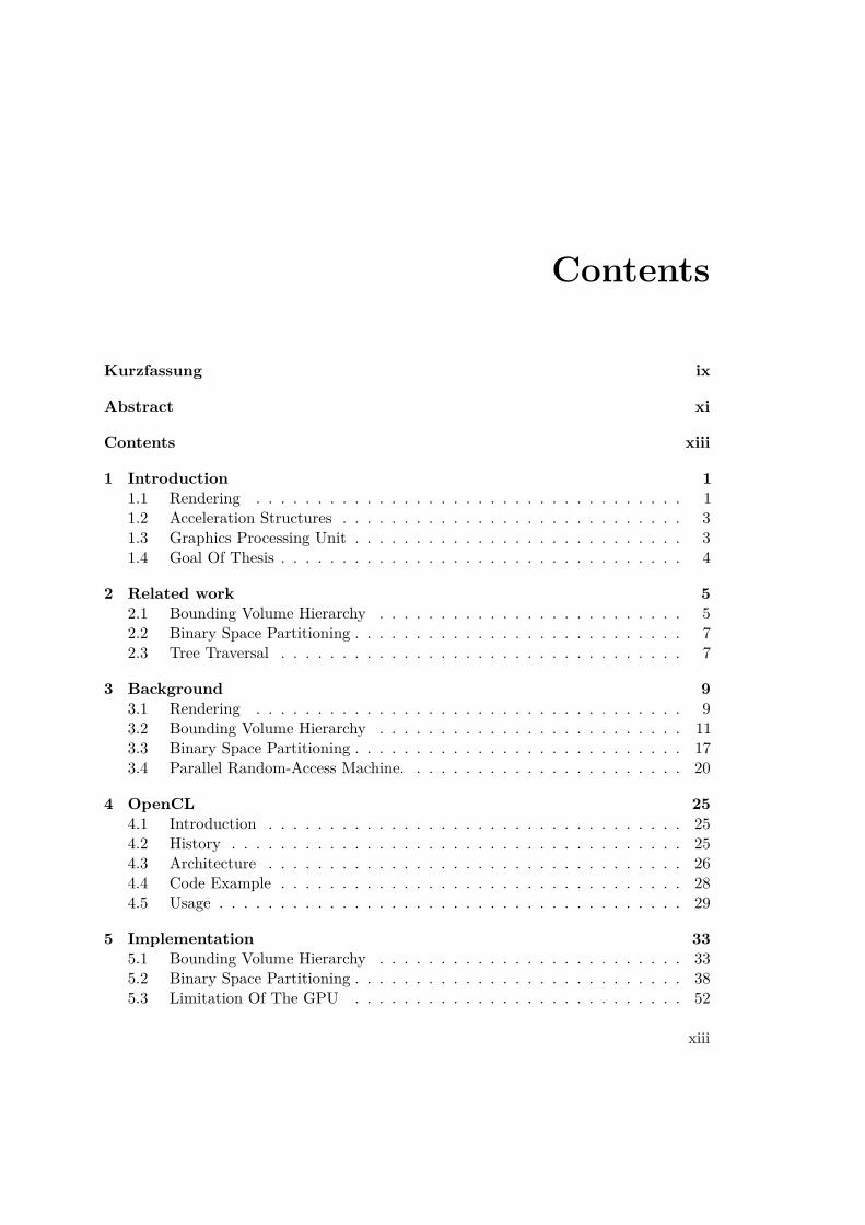
Ray tracing is a central algorithm in the domain of rendering. Arisen in the 1970s,it is still used when it comes to calculating reflections, shadows and transparencies ingenerated scenes. When applying ray tracing — roughly speaking — an eye ray issent into the scene where it is reflected, absorbed, or goes through objects. In order tocalculate those intersections the ray has to be checked against every object in the scene.Since the amount of objects in a scene has risen enormously since the introduction of raytracing, it is necessary to simplify this procedure. In Figure 1.1 a figurative example forray tracing is shown.

1.1.2 Culling

View frustum culling is used to determine which objects of a given scene have to bedisplayed. When it comes to rendering, a scene is often bigger than what is displayed. It

1

1. Introduction

Figure 1.1: Ray tracing example [Hen08]

is therefore needed to evaluate what will be seen from a given point of view. Throughculling it can easily be obtained which objects needs to be rendered and which can becompletely ignored for the current view point.

1.1.3 Transparency Sorting

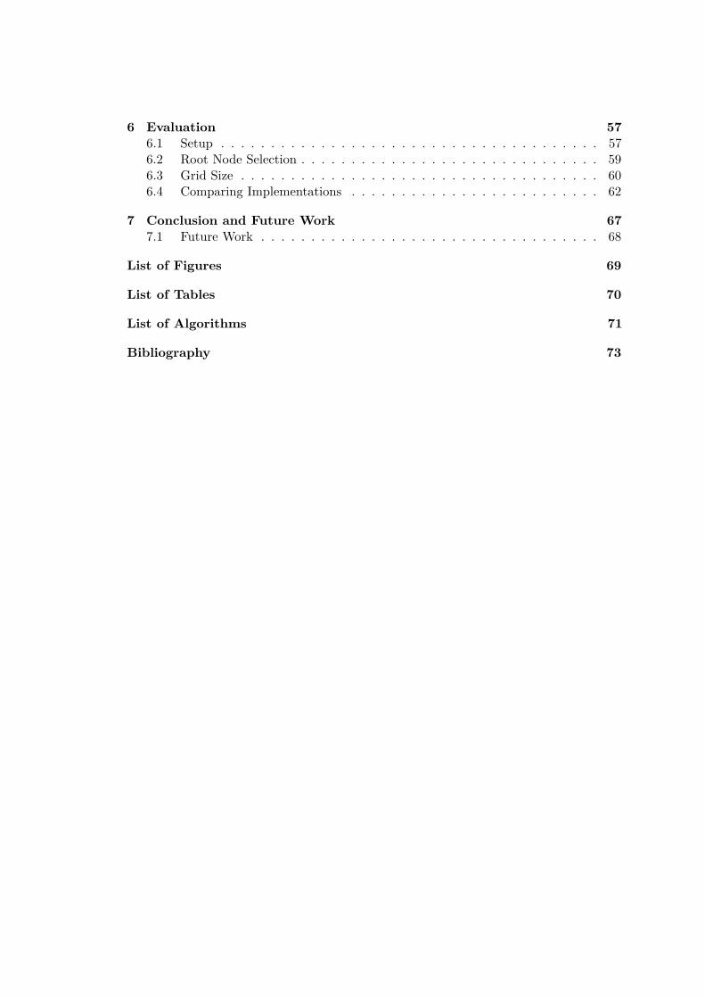
For realistic images it is typically needed that some objects have to be (half-)transparent.In order to render these transparencies efficiently, a back to front rendering is applied.This implies that the transparent objects need to be sorted in the order of their appearance.For this process several transparency sorting algorithms are applied, depending on thescene details. Figure 1.2 shows an example of one of these algorithms.

(a) Image with alpha blending (b) Image with transparency sorting

Figure 1.2: An example for transparency sorting from AMD’s Mecha demo [AMD], inthe left image (a) alpha blending leads to the wrong result, while in in the right image(b) transparency sorting yields the correct one

2

1.2. Acceleration Structures

1.2 Acceleration Structures

As already mentioned in the introduction (Section 1.1), acceleration structures are usedto achieve the formerly described parts of rendering in a fast way. These structures arecharacterized by fast and cheap traversals and good approximation of real objects in ascene. In this thesis we focus on bounding volume hierarchy (BVH) and binary spacepartitioning (BSP) which will be introduced in section 1.2.1 and section 1.2.2 respectively.Further acceleration structures that are generally used are the k-d tree as well as thequadtree and the octree which are special cases of the BSP.

1.2.1 Bounding Volume Hierarchy

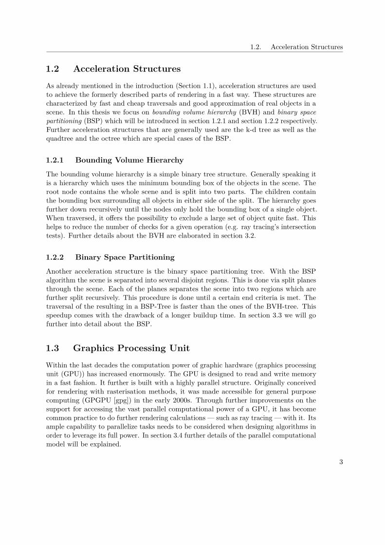
The bounding volume hierarchy is a simple binary tree structure. Generally speaking itis a hierarchy which uses the minimum bounding box of the objects in the scene. Theroot node contains the whole scene and is split into two parts. The children containthe bounding box surrounding all objects in either side of the split. The hierarchy goesfurther down recursively until the nodes only hold the bounding box of a single object.When traversed, it offers the possibility to exclude a large set of object quite fast. Thishelps to reduce the number of checks for a given operation (e.g. ray tracing’s intersectiontests). Further details about the BVH are elaborated in section 3.2.

1.2.2 Binary Space Partitioning

Another acceleration structure is the binary space partitioning tree. With the BSPalgorithm the scene is separated into several disjoint regions. This is done via split planesthrough the scene. Each of the planes separates the scene into two regions which arefurther split recursively. This procedure is done until a certain end criteria is met. Thetraversal of the resulting in a BSP-Tree is faster than the ones of the BVH-tree. Thisspeedup comes with the drawback of a longer buildup time. In section 3.3 we will gofurther into detail about the BSP.

1.3 Graphics Processing Unit

Within the last decades the computation power of graphic hardware (graphics processingunit (GPU)) has increased enormously. The GPU is designed to read and write memoryin a fast fashion. It further is built with a highly parallel structure. Originally conceivedfor rendering with rasterisation methods, it was made accessible for general purposecomputing (GPGPU [gpg]) in the early 2000s. Through further improvements on thesupport for accessing the vast parallel computational power of a GPU, it has becomecommon practice to do further rendering calculations — such as ray tracing — with it. Itsample capability to parallelize tasks needs to be considered when designing algorithms inorder to leverage its full power. In section 3.4 further details of the parallel computationalmodel will be explained.

3

1. Introduction

1.4 Goal Of ThesisWith this thesis we aim to improve the aforementioned algorithms and implement them forthe GPU. The practical part of this thesis will be laid out within the OpenCL framework.It further will contain a higher level of accessibility to use the implementation within anF# or C# environment. As framework for the higher level handles the Aardvark renderingframework of VRVis will be used. The general goal is to construct and implement efficientand fast algorithms for BVH-and BSP-tree construction as well as traversal within theOpenCL. The reason for this is that we want to bypass the data transfer between theCPU and the GPU during rendering.

The desired use case for the BVH-tree was frustum culling and transparency sorting withthe BSP-Tree. Throughout the implementation stage we came across certain road blocksand had insights showing that the starting idea would lead to unnecessary overhead.After reevaluation on the already implemented details and the plan for this thesis wecame to a solution for each of the desired use cases. For frustum culling we will justevaluate every triangle in parallel. For transparency sorting we are using BSP-Trees afterseparating the input scene into small cells with the use of an grid. Further details aboutBVH-tree and BSP-grid generation will be explained Chapter 5.

4

CHAPTER 2Related work

2.1 Bounding Volume Hierarchy

Since automatic generation of bounding volume hierarchies was introduced by Goldsmithet al. [GS87] in 1987 an ample amount of advances have been made in this field. In thebeginning there where several heuristic approaches used for the creation of BVH-trees.Goldsmith et al. not only introduced the idea of automatically generated BVH but alsosuggested different heuristics. Among their proposal one could find the general idea ofadding the node which leads to the least increased surface area. This — so-called —surface area heuristic (SAH) is now commonly used in the generation of BVH-trees. Ize etal. [AKL13] developed different measures to further analyze the quality of a BVH-tree.Unfortunately the use of these metrics is not common and sometimes not possible duringconstruction.

2.1.1 Construction Methods

Throughout the last decades several approaches for generating a BVH-tree on the centralprocessing unit (CPU) as well as on the GPU have been introduced. The typical algorithmin this case a top-down construction. These top-down methods [GS87, Wal07, KIS+12,BHH15a] commonly start with the whole scene as root node and continue splitting ituntil only the nodes of the BVH-tree consist of as single object. Further bottom upmethods have also been considered and used [WBKP08, GHFB13, BHH15b]. In the caseof agglomerative clustering approaches the leaves are first created containing a singlegeometry. The next step combines two leaves together to and connects them with aparent node. Further those nodes are then connected in a recursive fashion until theyresult in a full BVH-tree.

5

2. Related work

2.1.2 Parallel Construction

Alongside the already mentioned methods, huge ameliorations and innovations havebeen made in the area of parallel construction of BVH-trees. Ize et al. [IWP07] showedan approach where the BVH-tree is created asynchronously. This way they tackle theproblem of the degrading quality of a BVH throughout the lifetime of a scene.

Lauterbach et al. [LGS+09] introduced two construction algorithms. Their first methodused a linear ordering from a Morton code1, while the other one uses a top-down approachwhich employs the surface area heuristic. Further they combined both algorithms andremoved bottlenecks for them to work on the GPU.

Pantaleoni et al. [PL10] introduced a combined approach which leverages the a greedySAH approach as well as the LBVH approach of Lauterbach et al. [LGS+09].

Soping et al. [SBU11] altered the BVH generation algorithm and split it into single tasks.These separate tasks are then completed in parallel when the method is run on a GPU.They reported speedup up to five times in comparison to Lauterbach’s algorithm.

Karras [Kar12] introduced a new method for generating a BVH-trees as well as octreesand k-d trees. Their main contribution was the creation of a radix tree which they usedfor their final construction algorithm. The full procedure leans on Lauterbach et al.’smethod by also using the Morton codes and then sorting them with said radix tree.Further contributions are the building of a BVH-tree and further assigning boundingboxes to every internal node in parallel.

Later Karras et al. [KA13] introduced a new algorithm that leverages the capabilities ofparallel computation for tree optimization. They first generate at BVH-tree and performa set of optimizations on it. After these adaptations of the original tree are done, apost-processing step to further enhance the quality of the final BVH-tree is executed.

2.1.3 Update Based Techniques

Since the quality of a BVH has a huge influence of the traversal performance, severalupdate methods have been proposed. These updates (e.g. refitting, tree rotations) wereoriginally used in off-line2 construction. Kopta et al. [KIS+12] adapted those techniquesto also work on animated scenes. They improve the quality of a BVH by rearrangingnodes in the tree instead of rebuilding the whole tree during the refitting phase. Furtherthey added different variations of their algorithm and showed that they can accomplishmajor improvements to former algorithms.

Another interesting approach was introduced by Ernst et al. [EG07]. Clipping thetriangles in the scene before creating the BVH itself allows the creation of higher qualityBVH-trees. This approach is commonly used amongst the newer construction methods.

1The Morton code is a way to encode multidimensional data in one dimension2on-line construction happens at run time, while off-line methods work in advance

6

2.2. Binary Space Partitioning

2.2 Binary Space PartitioningSince binary space partitioning was introduced in 1969 by Schumacker et al. [SD69],several advances have been made. A decade later Fuchs et al. [FKN80] used the approachin the area of computer graphics. From there on different developments where made.Chin et al. [CF89] showed how to use multiple BSP-Trees for shadow generation. Ize etal. [IWP08] leveraged the possibilities BSP-Trees offer for ray tracing. Uysal et al. [USC13]applied BSP for hidden surface removal. They have also showed how to implement it onin a parallel way with CUDA. Another interesting approach is the RBSP by Budge etal. [BCNJ08]. Their algorithm restricts the allowed split plane at each level and thereforespeeds up the construction significantly.Further restriction of the BSP leads to k-d trees. Since their construction time is moreadequate for real time usage they have been studied more thoroughly within the domainof rendering. In 2007 Shevtsov et al. [SSK07] introduced algorithms to construct andtraverse k-d trees in parallel. A year later Zhou et al. [ZHWG08] presented the firstparallel implementation of a k-d tree on the GPU. Doggett et al. [CKL+10] showed howto incorporate the SAH into the k-d tree construction in a parallel fashion. With Wu etal. [WZL11a] a year later the first implementation of a SAH generated k-d tree on theGPU was published. This year Yang et al. [YYWX16] introduced a new method — themulti-split k-d tree — that exploits ideas of the octree and allows faster high qualitygeneration of a k-d tree in parallel.Arya [Ary02] analyzed BSP’s worst case height and size in the case of axis-parallel linesegments. Further Hershberger et al. [HS03] showed additional complexity bounds.Since BSP being a general data structure used in many fields, several advances have beenmade. Listing them all would be beyond the scope of this thesis; at this point we referan interested reader to Tóth [Tót05] report.

2.3 Tree TraversalThe main focus of this thesis lies on the two acceleration structures (BVH and BSP).However it is also important to mention what has been changed throughout the lastdecades in the area of traversal methods and applications. Due to the parallelismin nowadays’ GPU architectures a common method — using a stack — has becomesuboptimal when it comes to memory footprint. Foley et al. [FS05] introduced twomethods to traverse a tree without a stack: KD-Restart and KD-Backtrack. To overcomethe increase of visited nodes and the back pointer problem of these methods respectively,KD-Jump [HL09] was introduced. This technique tricks by using a small stack-likestructures with only a few integers. Also a hybrid algorithm of the stack based methodand the KD-Restart has been proposed. The so-called short stack uses a small stack toovercome memory usage and reverts to KD-Restart in certain cases.Another interesting technique proposed already in the 90s is using ropes while traversing.MacDonald et al. [MB90] introduced the rope trees and their usages in ray tracing

7

2. Related work

traversal. Later Havran et al. [HBZ98] implemented said technique and showed thatit leads to a speedup during the traversal phase. These so-called ropes link leaves ofa BSP-Tree to their neighbors. Here the fact that at a given node a splitting planeprunes one dimension is abused. Therefore the rope tree created at that leaf is justtwo-dimensional. They showed that the construction of ropes is bounded by O(n logn)with n denoting the number of leaves in the original BSP-Tree. They further showedthat the construction of rope trees lies in O(n). Therefore the complexity during BSPconstruction is not increased, while the traversal cost is reduced drastically. Unfortunatelythere is no further research in parallelization of these rope trees.

A special mention here goes to Andrysco et al.’s matrix tree [AT11]. Based on Andrysco etal. [AT10] they built a data structure which achieves O(1) insert and leaf finding. Theyfurther showed how to extend their structure in order to use it as general representationfor BSP-Trees

8

CHAPTER 3Background

3.1 Rendering

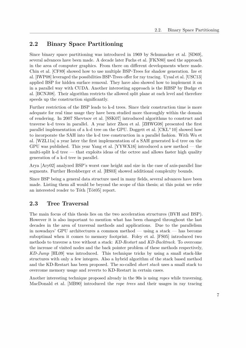
As already mentioned in Section 1.1 it takes an ample amount of calculations to obtain arealistic scene. In this section we will describe how rendering takes place. The first — andmost naive — rendering algorithm was the painter’s algorithm. When used, the painter’salgorithm first sorts the polygons in the scene by their distance to the viewpoint. Inthe next step those objects are rendered back to front. Although it displays the correctimage, it often re-renders certain parts of the image and is not suitable for transparencies.In case of overlapping structures it further runs into a hurdle while sorting back to frontas shown in Figure 3.1.

Figure 3.1: Overlapping objects or polygons can cause the painter’s algorithm to fail [Muł]

The next step in terms of rendering algorithm was ray casting. Introduced by Ap-pel [App68] in 1968 it was the first ray tracing algorithm. The main flow of the algorithm

9

3. Background

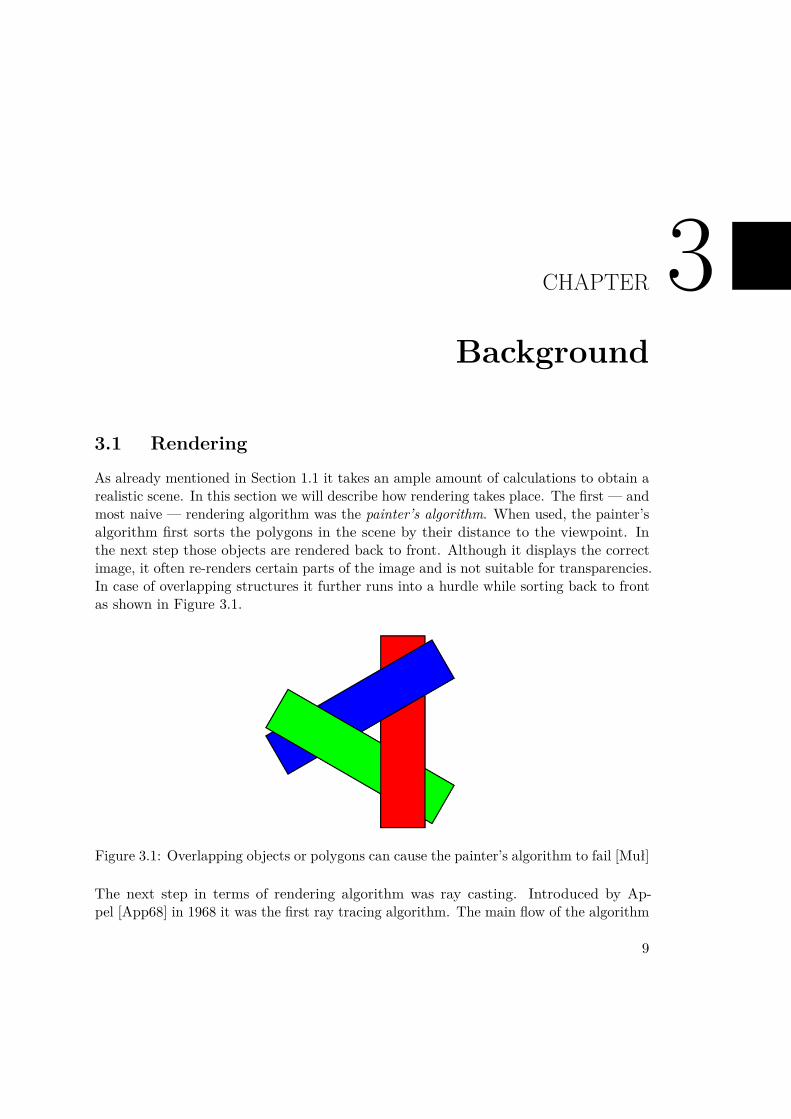
is shooting a — so-called — eye ray from the position of the viewer in order to find theclosest intersecting object. This object’s properties — such as material or transparency —are then inspected and the object is drawn. This process is repeated for every coordinatealong one axis. The ray casting algorithm therefore draws from left to right (using thex-axis) and therefore does not need to overdraw certain areas. Although this saves time,a major drawback is that finding intersections is needed. This may take a long time sinceevery object in the scene has to be tested. A schematic example of how the algorithmworks can be seen in Figure 3.2 whereas Figure 3.2a shows a 2-dimensional example andFigure 3.2b displays the 3-dimensional case.

(a) Ray casting example 2D [Ado] (b) Ray casting example 3D [imga]

Figure 3.2: These images show ray casting in 2D (a) and 3D (b)

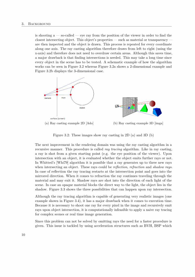
The next improvement in the rendering domain was using the ray casting algorithm in arecursive manner. This procedure is called ray tracing algorithm. Like in ray casting,a ray is shot from a given starting point (e.g. the eye position of the viewer). Uponintersection with an object, it is evaluated whether the object emits further rays or not.In Whitted’s [Whi79] algorithm it is possible that a ray generates up to three new rayswhen intersecting an object. These rays could be reflection, refraction and shadow rays.In case of reflection the ray tracing restarts at the intersection point and goes into themirrored direction. When it comes to refraction the ray continues traveling through thematerial and may exit it. Shadow rays are shot into the direction of each light of thescene. In case an opaque material blocks the direct way to the light, the object lies in theshadow. Figure 3.3 shows the three possibilities that can happen upon ray intersection.

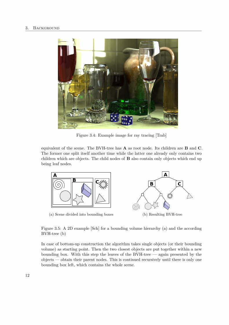
Although the ray tracing algorithm is capable of generating very realistic images (oneexample shown in Figure 3.4), it has a major drawback when it comes to execution time.Because it is necessary to shoot one ray for every pixel in the image and recursively emitrays upon object intersection, it is computationally infeasible to apply a naive ray tracingfor complex scenes or real time image generation.

Since this problem can not be solved by omitting rays the need for a faster procedure isgiven. This issue is tackled by using acceleration structures such as BVH, BSP which

10

3.2. Bounding Volume Hierarchy

Figure 3.3: A schematic example of how the ray tracing algorithm works [Vog13]

will be explained in Section 3.2 and Section 3.3.

There exist further algorithms for rendering such as the scanline algorithm and raster-ization. The former one goes through a scene line by line and renders the frontmostobjects or polygons. The latter one subdivides the scene into a grid and subsequentlygoes through the grid and checks each cell for primitives to render. Since these algorithmslie outside the focus of this thesis we will not further discuss them here.

3.2 Bounding Volume HierarchyThe bounding volume hierarchy is a simple acceleration structure. There are severalapproaches on how to build a BVH-tree where the original one was top-down. In case ofthe top-down generation a bounding box containing the whole scene is created to beginwith. In the next step this bounding box — which is also the root node of the resultingBVH-tree — is split into half. Each of these halves represent a tighter bounding boxto their containing objects. These new nodes in the tree are then further subdividedrecursively. This happens in the same manner as with the root node until a certain endcriteria is met (e.g. a node contains only one object).

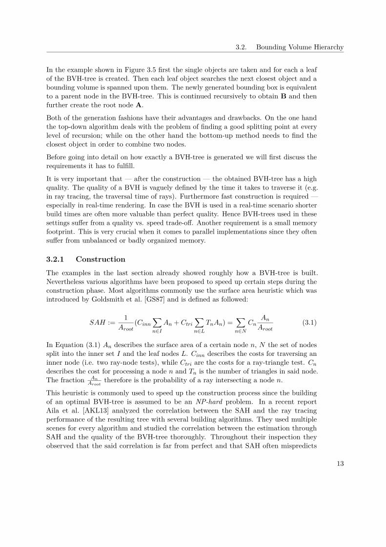
Figure 3.5 offers a 2-dimensional example of a bounding volume hierarchy. The scene inFigure 3.5a contains five bounding boxes, whereas the bigger ones are named A, B andC. B is further split into 2 unnamed bounding volumes. Figure 3.5b displays the tree

11

3. Background

Figure 3.4: Example image for ray tracing [Trab]

equivalent of the scene. The BVH-tree has A as root node. Its children are B and C.The former one split itself another time while the latter one already only contains twochildren which are objects. The child nodes of B also contain only objects which end upbeing leaf nodes.

(a) Scene divided into bounding boxes (b) Resulting BVH-tree

Figure 3.5: A 2D example [Sch] for a bounding volume hierarchy (a) and the accordingBVH-tree (b)

In case of bottom-up construction the algorithm takes single objects (or their boundingvolume) as starting point. Then the two closest objects are put together within a newbounding box. With this step the leaves of the BVH-tree — again presented by theobjects — obtain their parent nodes. This is continued recursively until there is only onebounding box left, which contains the whole scene.

12

3.2. Bounding Volume Hierarchy

In the example shown in Figure 3.5 first the single objects are taken and for each a leafof the BVH-tree is created. Then each leaf object searches the next closest object and abounding volume is spanned upon them. The newly generated bounding box is equivalentto a parent node in the BVH-tree. This is continued recursively to obtain B and thenfurther create the root node A.

Both of the generation fashions have their advantages and drawbacks. On the one handthe top-down algorithm deals with the problem of finding a good splitting point at everylevel of recursion; while on the other hand the bottom-up method needs to find theclosest object in order to combine two nodes.

Before going into detail on how exactly a BVH-tree is generated we will first discuss therequirements it has to fulfill.

It is very important that — after the construction — the obtained BVH-tree has a highquality. The quality of a BVH is vaguely defined by the time it takes to traverse it (e.g.in ray tracing, the traversal time of rays). Furthermore fast construction is required —especially in real-time rendering. In case the BVH is used in a real-time scenario shorterbuild times are often more valuable than perfect quality. Hence BVH-trees used in thesesettings suffer from a quality vs. speed trade-off. Another requirement is a small memoryfootprint. This is very crucial when it comes to parallel implementations since they oftensuffer from unbalanced or badly organized memory.

3.2.1 Construction

The examples in the last section already showed roughly how a BVH-tree is built.Nevertheless various algorithms have been proposed to speed up certain steps during theconstruction phase. Most algorithms commonly use the surface area heuristic which wasintroduced by Goldsmith et al. [GS87] and is defined as followed:

SAH := 1Aroot

(Cinn∑n∈I

An + Ctri∑n∈L

TnAn) =∑n∈N

CnAnAroot

(3.1)

In Equation (3.1) An describes the surface area of a certain node n, N the set of nodessplit into the inner set I and the leaf nodes L. Cinn describes the costs for traversing aninner node (i.e. two ray-node tests), while Ctri are the costs for a ray-triangle test. Cndescribes the cost for processing a node n and Tn is the number of triangles in said node.The fraction An

Aroottherefore is the probability of a ray intersecting a node n.

This heuristic is commonly used to speed up the construction process since the buildingof an optimal BVH-tree is assumed to be an NP-hard problem. In a recent reportAila et al. [AKL13] analyzed the correlation between the SAH and the ray tracingperformance of the resulting tree with several building algorithms. They used multiplescenes for every algorithm and studied the correlation between the estimation throughSAH and the quality of the BVH-tree thoroughly. Throughout their inspection theyobserved that the said correlation is far from perfect and that SAH often mispredicts

13

3. Background

the outcome. Nevertheless they also noticed that top-down sweep-based algorithmsoften underestimate the actual performance when using the SAH. Although Aila et al.proposed two new measurements1 for the quality of a BVH-tree, neither of them is usableduring construction.

Parallel construction

The most recent publication in the area of parallel construction for BVH-trees dates backto 2013. Karras et al. [KA13] achieved significant speedup compared to early algorithmsand made it possible to obtain a 90% ray tracing performance compared to off-linealgorithms. Their work seems to be a giant leap towards using BVH for ray tracing ininteractive applications.

Their algorithm is split into three phases: processing, optimization and post-processing.Additionally they add an optional phase zero which is triangle splitting.

Optional Phase 0: Triangle splitting

Since triangle splitting does not always add a performance gain it is only optional. To doso they make use of Ernst et al.’s [EG07] algorithm which constructs the AABB of eachtriangle and recursively splits them. Karras et al. introduced a heuristic that tries toovercome the problem of triangle splitting by only performing splits that improve theresulting performance. They first limit the amount of splits via

smax = bβ ∗mc (3.2)

where m is the number of triangles in the scene and β is an adjustable parameter. Theadvantage of limiting the amount of splits lies in the predictability of memory usage.This limited amount of splits is then distributed throughout the triangles by calculatinga priority pt for every triangle t. Further they use a scale factor D and determine thenumber of splits for a triangle via st = bD ∗ ptc. The scale factor is chosen as large aspossible so that it still satisfies ∑

st ≤ smax.

When selecting split planes it is important that internal nodes near the root of theBVH-tree do not overlap. Therefore triangles that cross the split plane of the root nodeneed to be split to increase the performance. This leads to the authors’ conclusionof splitting every AABB which intersects the spatial median plane. They define theimportance of split planes by how early it is considered during the construction of theinitial BVH. This is examined by using two Morton codes for the minimum and maximumcoordinates of the AABB and finding the highest differing bit.

Phase 1: Processing

The major part of this phase it to generate a BVH which is then further optimized inPhase 2. This is done by applying Karras’ [Kar12] algorithm. The main part of this

1The two quality measures are End-point overlap (EPO) and Leaf count variability (LCV). Thesemetrics describe the additional work used by nodes with overlapping bounding boxes and the standarddeviation of the number of leaves intersected respectively.

14

3.2. Bounding Volume Hierarchy

algorithm is generating a binary radix tree which is then used for sorting the primitivesaccording to the Morton codes of their center. In order to achieve this in a parallelfashion, they used a special layout which is described as follows: I and L are the setsof Internal and Leaf nodes. I0 is the root node. The left child node is located at Iγ orLγ (in case of a leaf node) while the right child is at position Iγ+1 or Lγ+1 respectively.This layout offers the property that every internal node either has the same index as itsfirst or last covered key. This holds for every inner node, since for its interval [i, j] thechildren always cover [i, γ] and [γ + 1, j].

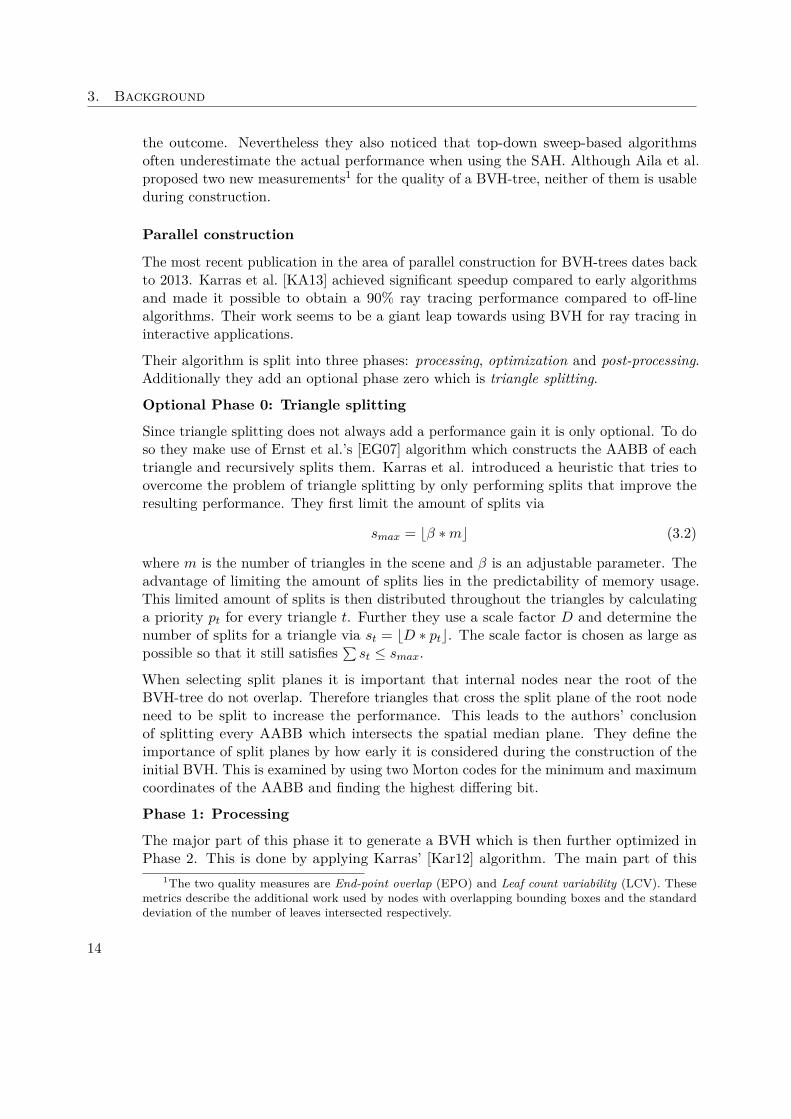
This means that the root node covers the range [0, n− 1] with the children containing[0, γ] and [γ + 1, n− 1] respectively. The radix tree in Figure 3.6 illustrates this layoutby horizontally aligning each internal node with the leaf it corresponds to. The split inthe tree is always at the first differing bit. The horizontal bars show the range that iscovered by the internal node.

Figure 3.6: This radix tree (by Karass [Kar12]) has an index for every internal node,which corresponds to either the first leaf it covers or the last one. To visualize this, theinternal nodes are aligned with they leaf the correspond to.

For the construction of a binary radix tree with this layout, it is necessary to find thekeys covered by the internal nodes. Due to this layout it is trivial to obtain one end of aninternal node’s range. For obtaining the other end the following simple algorithm is used.

Every internal node Ii is processed in parallel. The first step is to find the direction dof the given node. This is done by evaluation the neighbors’ keys ki−1 and ki+1. Thedirection is either +1 for i being the beginning of the covered interval or −1 for its end.Moreover — through construction ki and ki+d belong to Ii and ki−d belongs to Ii’s siblingnode Ii−d. Thus all keys belonging to Ii have the same prefix, but a different one to Ii’ssibling’s. Therefore the prefix can be bound by δmin = δ(i, i− d) with δ(i, j) > δmin forall keys kj covered by Ii. This allows to choose d so that δ(i, i+ d) corresponds to thelarger one of δ(i, i− 1) and δ(i, i+ 1).

The other end of the interval is then found by maximizing l so that δ(i, i+ ld) > δmin.This it done by iteratively trying powers of 2 until the condition lmax > l is violated.

15

3. Background

Via binary search in the range [0, lmax − 1] the other end is found. Finally it is given byj = i+ ld.

Therefore the length of Ii’s prefix is obtained by δ(i, j) which is denoted as δnode. Withthis information the split position γ can be obtained by applying binary search tomaximize s ∈ [0, l − 1] that satisfies δ(i, i+ sd) > δnode. Depending on the direction dof the node γ is either i+ sd in case of d = +1 or i+ sd− 1 for d = −1. Now that i, jand γ are known, the children of Ii cover the ranges [min(i, j), γ] and [γ + 1,max(i, j)].Comparing the ends of the ranges respectively gives the information if the child is a leafor not which is then referenced at node γ or γ + 1.

Our implementation of this procedure is shown in Section 5.1.1.

With the constructed radix tree the last step of generating a BVH-tree is done by assigninga bounding box for every internal node. Therefore a bottom-up traversal is used bystarting one thread per leaf. At every internal node only the second arriving thread isallowed to process the node and pass through to its parent. The drawback of this is theO(n) time complexity.

Phase 2: Optimization

In the topological optimization phase Karras et al. [KA13] minimize the SAH cost byso-called treelet rotations. A treelet is defined as a subtree of the BVH-tree with internalnodes of the BVH-tree being potential leaves of the treelet. First, a bottom-up traversalis done to determine a processing order of the nodes so that overlapping subtrees can notbe processed simultaneously. For every node encountered during the traversal a treelet isformed with the node itself as root and a fixed number of descendants as treelet nodesand leaves. The treelet is then optimized by finding a corresponding binary tree thatminimizes the SAH costs of the given treelet.

When forming a treelet it is better to maximize its SAH cost so that the reduction stephas a higher potential. Therefore the treelet root and its children are taken in the firststep. Further the treelet formation continues iteratively by turning the treelet leaf withthe largest surface area into an internal node. Thus the leaf is removed from the setof leaves and its children are added to said set. This process goes on until the chosenamount of treelet leaves are in the set.

At this point a naive approach would consider every possible binary tree for a given treeletand select the one leading to the minimum SAH costs. This — obviously — inefficientsolution is infeasible for a fast algorithm. Therefore several measures are taken to improvethe efficiency of this procedure. First of all a predefined order to compute the binary trees’SAH costs is generated. Therefore a dynamic programming technique called memoizationcan be applied. Memoization is used whenever small sub results need to be calculated inorder to obtain a bigger result. These sub results are stored — so-called memoized — inorder to avoid recomputing them. In the case of treelet optimization memoization isapplied to store the binary trees and their SAH costs. This way every possible binarytree is processed more efficiently.

16

3.3. Binary Space Partitioning

Phase 3: Post-processing

In the post-processing phase the resulting BVH undergoes a simple transformation inorder to be usable by a given traversal algorithm. In their case, Karras et al. [KA13],collapse certain subtrees to leaves with their triangles as linear list and transform thedata so that Woop’s [Woo04] intersection test can be used. Since this phase is dependenton the used traversal algorithm, we omit further details here.

3.3 Binary Space Partitioning

Another great acceleration data structure is the binary space partitioning tree. In contraryto the BVH described in Section 3.2 a BSP-Tree splits the scene arbitrarily in every level.Therefore a node in the resulting BSP-Tree does not contain a certain bounding box butthe split plane which is used at it. The BSP-Tree therefore represents a fundamentalconcept in computer graphics: binary space subdivision. Although BSP is generally goodfor rendering purposes they are believed to be numerically unstable, infeasible to buildand expensive to traverse. One of its advantages during buildup — the sheer possibilitiesfor split planes at every level — is also the drawback that makes them costly to optimize.

The most common form of BSP used in practice is the k-d tree. k-d trees are a specialform of BSP-Trees that only allow axis-aligned splitting planes. This obviously reducesthe buildup time significantly as the number of possible splits diminishes drastically.Although k-d trees seem to be a promising alternative, we strongly believe that BSP-Treescan achieve better performance for real-time rendering. This belief stems from the factthat theoretically BSP has to outperform k-d trees when it comes to traversal.

Current-state BSP are not used in real-time rendering due to having a bad trade-offbetween build time and quality. Ize et al. [IWP08] showed that it is possible to useBSP-traversal for ray tracing in a competitive manner to k-d tree-traversal. Whilethey have focused on the traversal algorithm itself and therefore constructed a BSPof higher quality, they still managed to limit the buildup complexity of the BSP-Treeto O(n log2 n)2. Although their ray tracing algorithm led to a reduction of triangleintersections by a factor 4, the higher traversal cost at each node reduces the speedup to1.1 compared to the k-d tree. Through this they stated that it is either necessary to evenfurther reduce triangle intersections or traversal costs to achieve a higher —and thereforesignificant — performance increase. Ize et al. have also not spent time on optimizing thebuildup algorithm which therefore leads to an overall worse performance than a k-d treebased approach.

3.3.1 Construction Method

The construction of a high-quality binary space partitioning is believed to be an intractableproblem. This comes from the fact that there is an ample amount of possible split planes

2k-d tree buildup is asymptotically bound by O(n log n)

17

3. Background

for every partition. Theoretically the quantity of these splits is infinite. This beingsaid, Havran [Hav00] showed that for a k-d tree only splitting planes tangent to theclipped triangles are actually required. Therefore a k-d tree construction algorithmonly has to consider 6 axis-aligned planes for every triangle which bounds the partitionpossibilities to O(6n). Ize et al. [IWP08] explained that extending this reasoning wouldlead to O(n3) or even more split candidates for a general BSP, even this is an infeasibleamount of investigation steps for every split. Therefore most construction procedureshave used only a restricted pool of allowed split planes. Budge et al. [BCNJ08] introducedthe — so-called — restricted binary space partitioning. Their approach only allows asmall subset of possible plane normals on every split. This way they limit the complexityfor the construction of a RBSP-Tree to O(M3 +MN logN) where M is the number ofallowed directions for split plane normals and N denotes the triangles in the scene. Asalready mentioned, a k-d tree — again — is a special case of the RBSP-Tree with thesplit planes restricted to the previously mentioned 6 planes.

The general construction algorithm for a BSP-Tree is roughly the same as common k-dtree building methods, with the only difference in the splitting phase. First the wholescene is taken and a split plane P0 is chosen. This separates the scene into two partitions:behind P0 and in front of P0. In the next step the same procedure is applied in the twohalf-spaces. This is recursively done until no further splits are introduced. The stoppingcriteria can vary depending on the implementation but may be a fixed number of totalsplits, a certain heuristic that implies no improvement in further splits or just the simplefact that there is nothing to partition any further.

In case of the k-d tree, splitting does not take any planes but axis-aligned ones. Furtherduring the construction of a k-d tree the process cycles through the axes so that —w.o.l.g. — first the x-axis is taken, then the y-axis and the z-axis afterwards. The cyclethen restarts with the x-axis. We will display the BSP-Tree (and in fact the k-d tree)construction on a simple example.

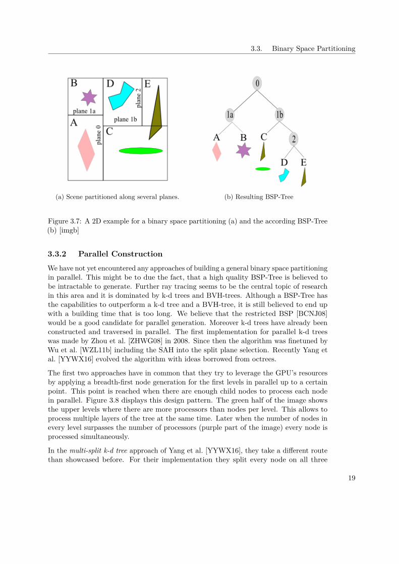
Figure 3.7 shows a schematic example of a two-dimensional scene and the binary spacepartitioning applied to it. In Figure 3.7a we see a scene with several primitives andsome split planes while Figure 3.7b displays the according BSP-Tree3. In this case thescene is first split along plane 0 and the root node is generated. The next recursive stepis to take the partition in front of plane 0 in consideration. There the split plane 1ais used. This leaves us with the two regions A and B which both cannot further bepartitioned. The algorithm continues behind plane 0 where plane 1b is used to split thescene. This also includes the problem of splitting a triangle. In this simple example thetriangle is referenced in both subtrees instead of being split into two smaller ones. Thesubdivision in front of plane 1b now contains only region C. Since this part of the scenesolely contains the green circle and the reference to the early encountered triangle, afurther split is not necessary. On the side behind plane 1b there are still two primitivesthat can be split alongside another plane (plane 2) leading to region D and E. Here thealgorithm cannot further split the partitions and therefore comes to an end.

3Since this is a 2d-example and all splits are aligned with x- and y-axis it is also a k-d tree

18

3.3. Binary Space Partitioning

(a) Scene partitioned along several planes. (b) Resulting BSP-Tree

Figure 3.7: A 2D example for a binary space partitioning (a) and the according BSP-Tree(b) [imgb]

3.3.2 Parallel Construction

We have not yet encountered any approaches of building a general binary space partitioningin parallel. This might be to due the fact, that a high quality BSP-Tree is believed tobe intractable to generate. Further ray tracing seems to be the central topic of researchin this area and it is dominated by k-d trees and BVH-trees. Although a BSP-Tree hasthe capabilities to outperform a k-d tree and a BVH-tree, it is still believed to end upwith a building time that is too long. We believe that the restricted BSP [BCNJ08]would be a good candidate for parallel generation. Moreover k-d trees have already beenconstructed and traversed in parallel. The first implementation for parallel k-d treeswas made by Zhou et al. [ZHWG08] in 2008. Since then the algorithm was finetuned byWu et al. [WZL11b] including the SAH into the split plane selection. Recently Yang etal. [YYWX16] evolved the algorithm with ideas borrowed from octrees.

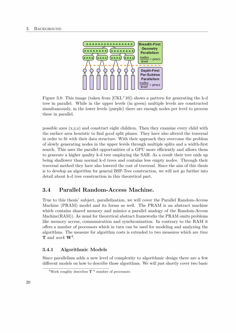
The first two approaches have in common that they try to leverage the GPU’s resourcesby applying a breadth-first node generation for the first levels in parallel up to a certainpoint. This point is reached when there are enough child nodes to process each nodein parallel. Figure 3.8 displays this design pattern. The green half of the image showsthe upper levels where there are more processors than nodes per level. This allows toprocess multiple layers of the tree at the same time. Later when the number of nodes inevery level surpasses the number of processors (purple part of the image) every node isprocessed simultaneously.

In the multi-split k-d tree approach of Yang et al. [YYWX16], they take a different routethan showcased before. For their implementation they split every node on all three

19

3. Background

Figure 3.8: This image (taken from [CKL+10]) shows a pattern for generating the k-dtree in parallel. While in the upper levels (in green) multiple levels are constructedsimultaneously, in the lower levels (purple) there are enough nodes per level to processthese in parallel.

possible axes (x,y,z) and construct eight children. Then they examine every child withthe surface area heuristic to find good split planes. They have also altered the traversalin order to fit with their data structure. With their approach they overcome the problemof slowly generating nodes in the upper levels through multiple splits and a width-firstsearch. This uses the parallel opportunities of a GPU more efficiently and allows themto generate a higher quality k-d tree employing the SAH. As a result their tree ends upbeing shallower than normal k-d trees and contains less empty nodes. Through theirtraversal method they have also lowered the cost of traversal. Since the aim of this thesisis to develop an algorithm for general BSP-Tree construction, we will not go further intodetail about k-d tree construction in this theoretical part.

3.4 Parallel Random-Access Machine.

True to this thesis’ subject, parallelization, we will cover the Parallel Random-AccessMachine (PRAM) model and its forms as well. The PRAM is an abstract machinewhich contains shared memory and mimics a parallel analogy of the Random-AccessMachine(RAM)). As usual for theoretical abstract frameworks the PRAM omits problemslike memory access, communication and synchronization. In contrary to the RAM itoffers a number of processors which in turn can be used for modeling and analyzing thealgorithms. The measure for algorithm costs is extended to two measures which are timeT and work W4.

3.4.1 Algorithmic Models

Since parallelism adds a new level of complexity to algorithmic design there are a fewdifferent models on how to describe those algorithms. We will just shortly cover two basic

4Work roughly describes T * number of processors

20

3.4. Parallel Random-Access Machine.

distinctions which are the Single Instruction Multiple Data (SIMD) and the MultipleInstruction Multiple Data (MIMD) model.

SIMD Model

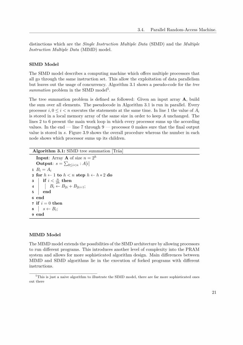
The SIMD model describes a computing machine which offers multiple processors thatall go through the same instruction set. This allow the exploitation of data parallelismbut leaves out the usage of concurrency. Algorithm 3.1 shows a pseudo-code for the treesummation problem in the SIMD model5.

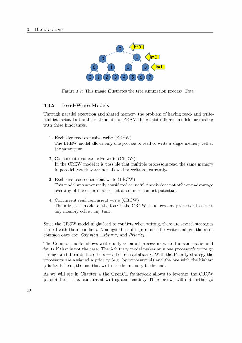
The tree summation problem is defined as followed: Given an input array A, buildthe sum over all elements. The pseudocode in Algorithm 3.1 is run in parallel. Everyprocessor i, 0 ≤ i < n executes the statements at the same time. In line 1 the value of Aiis stored in a local memory array of the same size in order to keep A unchanged. Thelines 2 to 6 present the main work loop in which every processor sums up the accordingvalues. In the end — line 7 through 9 — processor 0 makes sure that the final outputvalue is stored in s. Figure 3.9 shows the overall procedure whereas the number in eachnode shows which processor sums up its children.

Algorithm 3.1: SIMD tree summation [Träa]Input: Array A of size n = 2hOutput: s = ∑

0≤i<n : A[i]1 Bi = Ai2 for h← 1 to h < n step h← h ∗ 2 do3 if i < n

2h then4 Bi ← B2i +B2i+1;5 end6 end7 if i = 0 then8 s← Bi;9 end

MIMD Model

The MIMD model extends the possibilities of the SIMD architecture by allowing processorsto run different programs. This introduces another level of complexity into the PRAMsystem and allows for more sophisticated algorithm design. Main differences betweenMIMD and SIMD algorithms lie in the execution of forked programs with differentinstructions.

5This is just a naive algorithm to illustrate the SIMD model, there are far more sophisticated onesout there

21

3. Background

Figure 3.9: This image illustrates the tree summation process [Träa]

3.4.2 Read-Write Models

Through parallel execution and shared memory the problem of having read- and write-conflicts arise. In the theoretic model of PRAM there exist different models for dealingwith these hindrances.

1. Exclusive read exclusive write (EREW)The EREW model allows only one process to read or write a single memory cell atthe same time.

2. Concurrent read exclusive write (CREW)In the CREW model it is possible that multiple processors read the same memoryin parallel, yet they are not allowed to write concurrently.

3. Exclusive read concurrent write (ERCW)This model was never really considered as useful since it does not offer any advantageover any of the other models, but adds more conflict potential.

4. Concurrent read concurrent write (CRCW)The mightiest model of the four is the CRCW. It allows any processor to accessany memory cell at any time.

Since the CRCW model might lead to conflicts when writing, there are several strategiesto deal with those conflicts. Amongst those design models for write-conflicts the mostcommon ones are: Common, Arbitrary and Priority.

The Common model allows writes only when all processors write the same value andfaults if that is not the case. The Arbitrary model makes only one processor’s write gothrough and discards the others — all chosen arbitrarily. With the Priority strategy theprocessors are assigned a priority (e.g. by processor id) and the one with the highestpriority is being the one that writes to the memory in the end.

As we will see in Chapter 4 the OpenCL framework allows to leverage the CRCWpossibilities — i.e. concurrent writing and reading. Therefore we will not further go

22

3.4. Parallel Random-Access Machine.

into detail about the relationship about the read-write models since we will only need toconsider the CRCW.

23

CHAPTER 4OpenCL

4.1 Introduction

The OpenCL framework is an open, royalty-free standard which serves multiple platformsand offers the possibilities of parallel programming. It not only targets personal computersand systems, but also mobile devices, servers and embedded platforms. In this chapterwe will explain how the OpenCL is structured and how we will make use of it, as well asgive a short insight into its history.

4.2 History

Initiated by Apple Inc. OpenCL had its first release in August 2009 accompanying MacOS X Snow Leopard as version 1.0. Originally the idea was a proposal in collaborationwith technical teams of AMD, IBM, Qualcomm, Intel and Nvidia. It was then submittedto the Khronos Group which has been taking care of developing the OpenCL frameworksince then. The Khronos Compute Working Group was formed in June 2008, it containsrepresentatives of CPU, GPU and embedded-processor manufacturers as well as softwarecompanies. The first technical specification for the OpenCL was publicly released onDecember 8th, 2008. Shortly after that, different vendors announced that they will addfull support for the OpenCL to their toolkits.

Two years later, in June 2010 OpenCL 1.1 was approved by the Khronos Group. Itincluded more functionality for parallel programming and performance. The followingyear the specification for OpenCL 1.1 was released with another set of features offeringmore possibilities to developers. Just two years later, in November 2013, OpenCL 2.0was announced and technical specifications were released. Amongst its features, the mostnotable one was the Android driver extension, allowing Android devices to run OpenCLcode. In November last year the specification for OpenCL 2.1 was released.

25

4. OpenCL

The latest version of the specification was released this year in March bearing the version2.2.

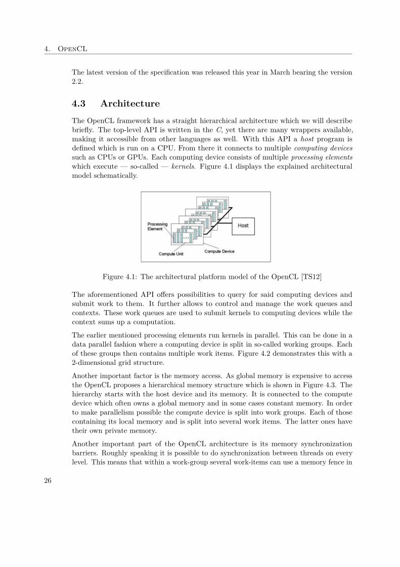
4.3 ArchitectureThe OpenCL framework has a straight hierarchical architecture which we will describebriefly. The top-level API is written in the C, yet there are many wrappers available,making it accessible from other languages as well. With this API a host program isdefined which is run on a CPU. From there it connects to multiple computing devicessuch as CPUs or GPUs. Each computing device consists of multiple processing elementswhich execute — so-called — kernels. Figure 4.1 displays the explained architecturalmodel schematically.

Figure 4.1: The architectural platform model of the OpenCL [TS12]

The aforementioned API offers possibilities to query for said computing devices andsubmit work to them. It further allows to control and manage the work queues andcontexts. These work queues are used to submit kernels to computing devices while thecontext sums up a computation.

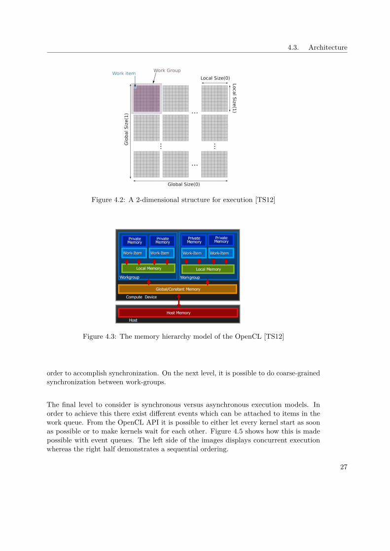
The earlier mentioned processing elements run kernels in parallel. This can be done in adata parallel fashion where a computing device is split in so-called working groups. Eachof these groups then contains multiple work items. Figure 4.2 demonstrates this with a2-dimensional grid structure.

Another important factor is the memory access. As global memory is expensive to accessthe OpenCL proposes a hierarchical memory structure which is shown in Figure 4.3. Thehierarchy starts with the host device and its memory. It is connected to the computedevice which often owns a global memory and in some cases constant memory. In orderto make parallelism possible the compute device is split into work groups. Each of thosecontaining its local memory and is split into several work items. The latter ones havetheir own private memory.

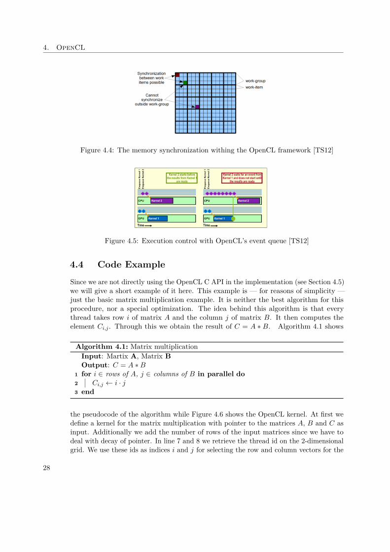
Another important part of the OpenCL architecture is its memory synchronizationbarriers. Roughly speaking it is possible to do synchronization between threads on everylevel. This means that within a work-group several work-items can use a memory fence in

26

4.3. Architecture

Figure 4.2: A 2-dimensional structure for execution [TS12]

Figure 4.3: The memory hierarchy model of the OpenCL [TS12]

order to accomplish synchronization. On the next level, it is possible to do coarse-grainedsynchronization between work-groups.

The final level to consider is synchronous versus asynchronous execution models. Inorder to achieve this there exist different events which can be attached to items in thework queue. From the OpenCL API it is possible to either let every kernel start as soonas possible or to make kernels wait for each other. Figure 4.5 shows how this is madepossible with event queues. The left side of the images displays concurrent executionwhereas the right half demonstrates a sequential ordering.

27

4. OpenCL

Figure 4.4: The memory synchronization withing the OpenCL framework [TS12]

Figure 4.5: Execution control with OpenCL’s event queue [TS12]

4.4 Code Example

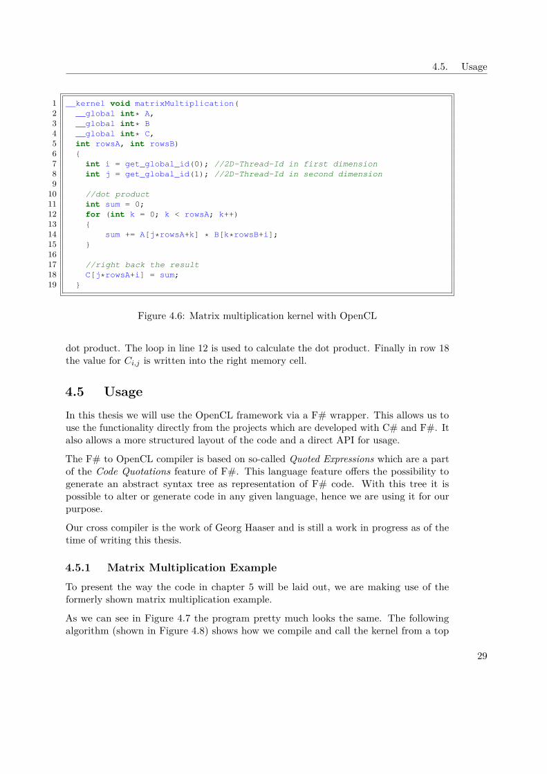
Since we are not directly using the OpenCL C API in the implementation (see Section 4.5)we will give a short example of it here. This example is — for reasons of simplicity —just the basic matrix multiplication example. It is neither the best algorithm for thisprocedure, nor a special optimization. The idea behind this algorithm is that everythread takes row i of matrix A and the column j of matrix B. It then computes theelement Ci,j . Through this we obtain the result of C = A ∗ B. Algorithm 4.1 shows

Algorithm 4.1: Matrix multiplicationInput: Martix A, Matrix BOutput: C = A ∗B

1 for i ∈ rows of A, j ∈ columns of B in parallel do2 Ci,j ← i · j3 end

the pseudocode of the algorithm while Figure 4.6 shows the OpenCL kernel. At first wedefine a kernel for the matrix multiplication with pointer to the matrices A, B and C asinput. Additionally we add the number of rows of the input matrices since we have todeal with decay of pointer. In line 7 and 8 we retrieve the thread id on the 2-dimensionalgrid. We use these ids as indices i and j for selecting the row and column vectors for the

28

4.5. Usage

1 __kernel void matrixMultiplication(2 __global int* A,3 __global int* B4 __global int* C,5 int rowsA, int rowsB)6 {7 int i = get_global_id(0); //2D-Thread-Id in first dimension8 int j = get_global_id(1); //2D-Thread-Id in second dimension910 //dot product11 int sum = 0;12 for (int k = 0; k < rowsA; k++)13 {14 sum += A[j*rowsA+k] * B[k*rowsB+i];15 }1617 //right back the result18 C[j*rowsA+i] = sum;19 }

Figure 4.6: Matrix multiplication kernel with OpenCL

dot product. The loop in line 12 is used to calculate the dot product. Finally in row 18the value for Ci,j is written into the right memory cell.

4.5 UsageIn this thesis we will use the OpenCL framework via a F# wrapper. This allows us touse the functionality directly from the projects which are developed with C# and F#. Italso allows a more structured layout of the code and a direct API for usage.

The F# to OpenCL compiler is based on so-called Quoted Expressions which are a partof the Code Quotations feature of F#. This language feature offers the possibility togenerate an abstract syntax tree as representation of F# code. With this tree it ispossible to alter or generate code in any given language, hence we are using it for ourpurpose.

Our cross compiler is the work of Georg Haaser and is still a work in progress as of thetime of writing this thesis.

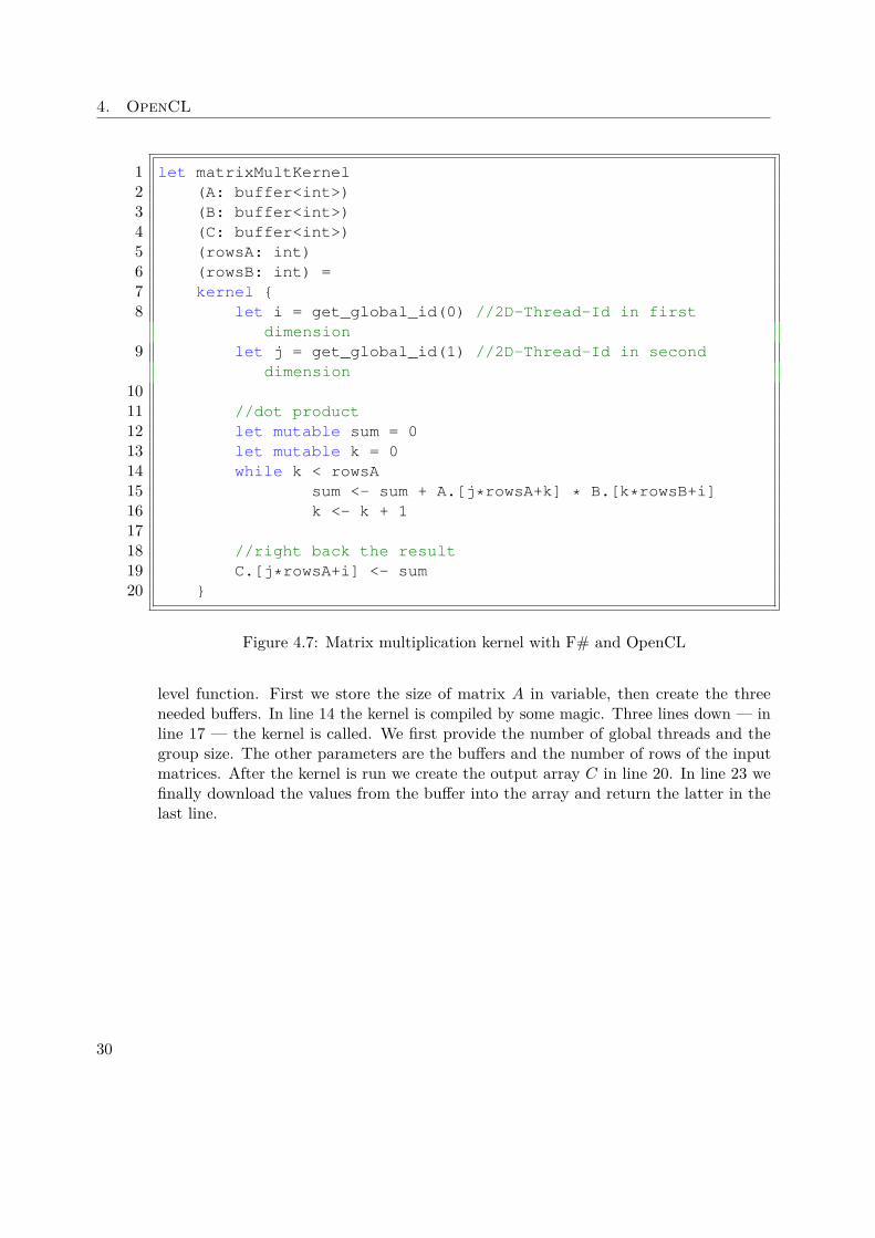
4.5.1 Matrix Multiplication Example

To present the way the code in chapter 5 will be laid out, we are making use of theformerly shown matrix multiplication example.

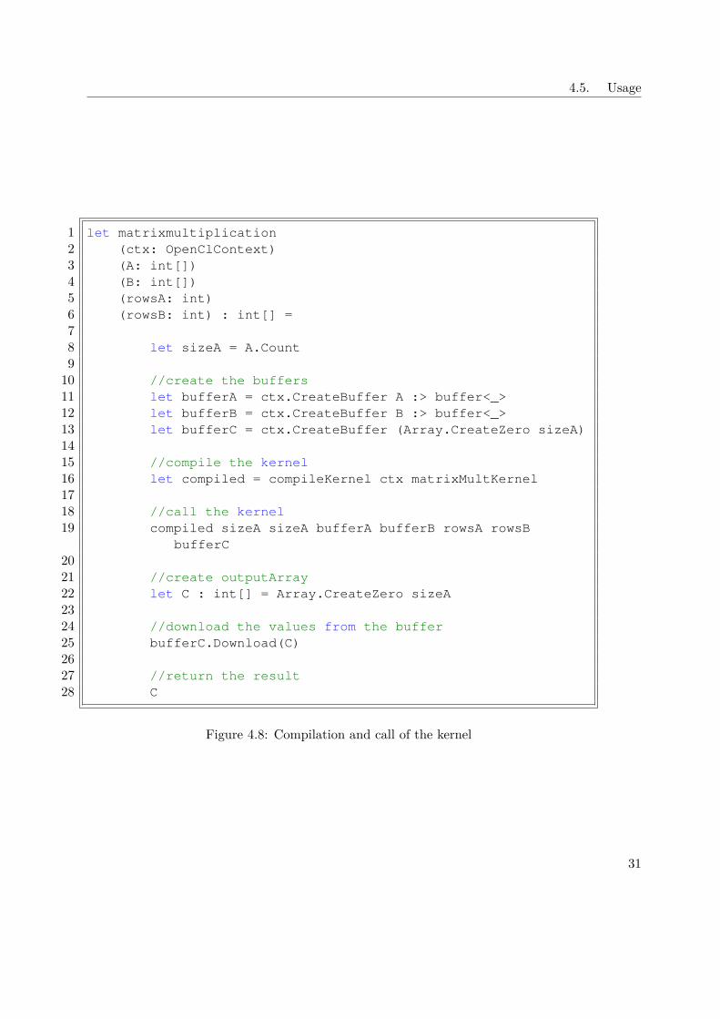
As we can see in Figure 4.7 the program pretty much looks the same. The followingalgorithm (shown in Figure 4.8) shows how we compile and call the kernel from a top

29

4. OpenCL

1 let matrixMultKernel2 (A: buffer<int>)3 (B: buffer<int>)4 (C: buffer<int>)5 (rowsA: int)6 (rowsB: int) =7 kernel {8 let i = get_global_id(0) //2D-Thread-Id in first

dimension9 let j = get_global_id(1) //2D-Thread-Id in second

dimension1011 //dot product12 let mutable sum = 013 let mutable k = 014 while k < rowsA15 sum <- sum + A.[j*rowsA+k] * B.[k*rowsB+i]16 k <- k + 11718 //right back the result19 C.[j*rowsA+i] <- sum20 }

Figure 4.7: Matrix multiplication kernel with F# and OpenCL

level function. First we store the size of matrix A in variable, then create the threeneeded buffers. In line 14 the kernel is compiled by some magic. Three lines down — inline 17 — the kernel is called. We first provide the number of global threads and thegroup size. The other parameters are the buffers and the number of rows of the inputmatrices. After the kernel is run we create the output array C in line 20. In line 23 wefinally download the values from the buffer into the array and return the latter in thelast line.

30

4.5. Usage

1 let matrixmultiplication2 (ctx: OpenClContext)3 (A: int[])4 (B: int[])5 (rowsA: int)6 (rowsB: int) : int[] =78 let sizeA = A.Count9

10 //create the buffers11 let bufferA = ctx.CreateBuffer A :> buffer<_>12 let bufferB = ctx.CreateBuffer B :> buffer<_>13 let bufferC = ctx.CreateBuffer (Array.CreateZero sizeA)1415 //compile the kernel16 let compiled = compileKernel ctx matrixMultKernel1718 //call the kernel19 compiled sizeA sizeA bufferA bufferB rowsA rowsB

bufferC2021 //create outputArray22 let C : int[] = Array.CreateZero sizeA2324 //download the values from the buffer25 bufferC.Download(C)2627 //return the result28 C

Figure 4.8: Compilation and call of the kernel

31

CHAPTER 5Implementation

This chapter will deal with the implementation detail of the thesis. Throughout theimplementation of the discussed data structures we came across certain road blocks andcame to a realization that changed the planned implementation. In this place we aregoing to describe the thought process and development of the final data structure andalgorithms.

We will mostly focus on the algorithms themselves. First we will describe the implemen-tation of the bounding volume hierarchy. Then we will show the problem that arose forour usage scenario.

The second part of this chapter displays our take on parallelizing the binary spacepartitioning and incorporating it into the BVH. This will be followed by demonstratinganother complication that occurred.

The third part gives insight into our solution for the aforementioned problems by com-bining a grid with the BSP.

The use cases we had in mind for said data structures were culling queries1 for the BVHand sorting queries2 for the BSP.

5.1 Bounding Volume Hierarchy

The first part of the implementation focuses on the bounding volume hierarchy. Asalready mentioned in Section 3.2.1 we planned on implementing Karras et al. [LGS+09]construction method. While they used the CUDA framework we used the OpenCLframework within our F# ecosystem.

1Frustum culling, see Section 1.1.22Transparency sorting, see Section 1.1.3

33

5. Implementation

The first step in the implementation was to reproduce Karras’ [Kar12] algorithm forparallel construction, his will be shown in Section 5.1.1. We further planned on im-plementing the second step treelet optimization, followed by early triangle splitting asexplained in Section 3.3.2.

5.1.1 BVH Construction

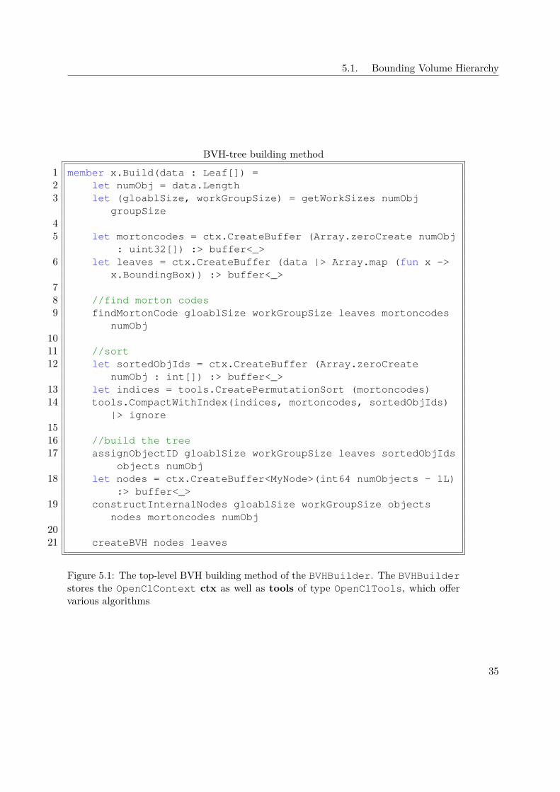
The top-level function to build the BVH-tree is shown in Figure 5.1. First we create thenecessary arrays to store the leaves and the nodes during the parallel run on the GPU.We then generate the morton code for each Leaf and sort them. Then we prepare thedata for the BVH-tree construction. With the call to constructInternalNodes, whichis the compiled version of constructInternalNodesKernel we build the BVH-tree. Inthe last line we put together the resulting data in a simple struct.

Since it is not possible to link to different data structures within the structs for theinternal nodes we save the id of the child and parent nodes. To do so, our implementationstores the ids within the nodes with a shift for leaves. While internal nodes have theid range from 0 (root) to n− 1 (rightmost internal node), leaves take up the negativesnumbers. Leaf 0 therefore has the id −1, while the leaf n− 1 has the id −n. This waywe can distinguish between internal nodes and leaves during operations.

The tree layout is designed according to Karras [Kar12] as shown in Section 3.2.1.

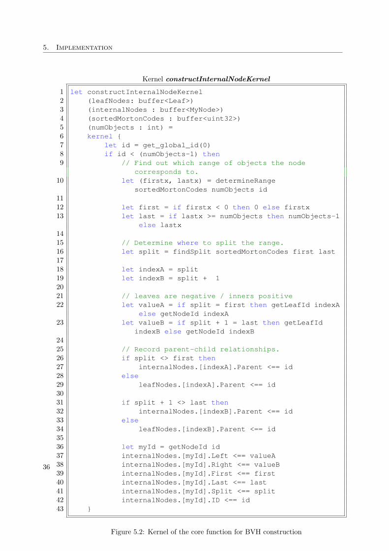
Figure 5.2 shows the kernel of the core function for the creation of the BVH-tree.First we obtain the id of the thread, leading to two interesting parts of the algorithm.determineRange finds the range that is covered by the internal node given by the id.After obtaining this range we determine the split position with the findSplit function.Having found the range and the split position, we can link the nodes to each other(line18 to 40)3.

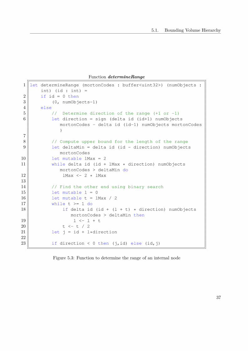
To determine the range we are using binary search on the sorted Morton codes. InFigure 5.3 we see the function used to find the covered range for every internal node.First we check if we have the root node in which case we return the full range.

We first make use of the delta function to determine the direction of this node. Saidfunction returns the length of the common prefix for the Morton codes on positions givenby the first two arguments. In line 9 to 12 we calculate an upper bound for the size of therange. With this upper bound we start a binary search to find the other end of the range.The final range is given by the node’s (also thread’s) id and the result of the calculationin line 21. The last line ensures that the range is always in the for (i, j) with i < j.

The findSplit function works roughly the same way as the determineRange function.A binary search is used to find highest differing bit in the Morton codes within the twoends of a node’s range.

3For this we defined the operator (<==) in order to be able to directly write to a memory location.

34

5.1. Bounding Volume Hierarchy

BVH-tree building method1 member x.Build(data : Leaf[]) =2 let numObj = data.Length3 let (gloablSize, workGroupSize) = getWorkSizes numObj

groupSize45 let mortoncodes = ctx.CreateBuffer (Array.zeroCreate numObj

: uint32[]) :> buffer<_>6 let leaves = ctx.CreateBuffer (data |> Array.map (fun x ->

x.BoundingBox)) :> buffer<_>78 //find morton codes9 findMortonCode gloablSize workGroupSize leaves mortoncodes

numObj1011 //sort12 let sortedObjIds = ctx.CreateBuffer (Array.zeroCreate

numObj : int[]) :> buffer<_>13 let indices = tools.CreatePermutationSort (mortoncodes)14 tools.CompactWithIndex(indices, mortoncodes, sortedObjIds)

|> ignore1516 //build the tree17 assignObjectID gloablSize workGroupSize leaves sortedObjIds

objects numObj18 let nodes = ctx.CreateBuffer<MyNode>(int64 numObjects - 1L)

:> buffer<_>19 constructInternalNodes gloablSize workGroupSize objects

nodes mortoncodes numObj2021 createBVH nodes leaves

Figure 5.1: The top-level BVH building method of the BVHBuilder. The BVHBuilderstores the OpenClContext ctx as well as tools of type OpenClTools, which offervarious algorithms

35

5. Implementation

Kernel constructInternalNodeKernel

1 let constructInternalNodeKernel2 (leafNodes: buffer<Leaf>)3 (internalNodes : buffer<MyNode>)4 (sortedMortonCodes : buffer<uint32>)5 (numObjects : int) =6 kernel {7 let id = get_global_id(0)8 if id < (numObjects-1) then9 // Find out which range of objects the node

corresponds to.10 let (firstx, lastx) = determineRange

sortedMortonCodes numObjects id1112 let first = if firstx < 0 then 0 else firstx13 let last = if lastx >= numObjects then numObjects-1

else lastx1415 // Determine where to split the range.16 let split = findSplit sortedMortonCodes first last1718 let indexA = split19 let indexB = split + 12021 // leaves are negative / inners positive22 let valueA = if split = first then getLeafId indexA

else getNodeId indexA23 let valueB = if split + 1 = last then getLeafId

indexB else getNodeId indexB2425 // Record parent-child relationships.26 if split <> first then27 internalNodes.[indexA].Parent <== id28 else29 leafNodes.[indexA].Parent <== id3031 if split + 1 <> last then32 internalNodes.[indexB].Parent <== id33 else34 leafNodes.[indexB].Parent <== id3536 let myId = getNodeId id37 internalNodes.[myId].Left <== valueA38 internalNodes.[myId].Right <== valueB39 internalNodes.[myId].First <== first40 internalNodes.[myId].Last <== last41 internalNodes.[myId].Split <== split42 internalNodes.[myId].ID <== id43 }

Figure 5.2: Kernel of the core function for BVH construction

36

5.1. Bounding Volume Hierarchy

Function determineRange

1 let determineRange (mortonCodes : buffer<uint32>) (numObjects :int) (id : int) =

2 if id = 0 then3 (0, numObjects-1)4 else5 // Determine direction of the range (+1 or -1)6 let direction = sign (delta id (id+1) numObjects

mortonCodes - delta id (id-1) numObjects mortonCodes)

78 // Compute upper bound for the length of the range9 let deltaMin = delta id (id - direction) numObjects

mortonCodes10 let mutable lMax = 211 while delta id (id + lMax * direction) numObjects

mortonCodes > deltaMin do12 lMax <- 2 * lMax1314 // Find the other end using binary search15 let mutable l = 016 let mutable t = lMax / 217 while t >= 1 do18 if delta id (id + (l + t) * direction) numObjects

mortonCodes > deltaMin then19 l <- l + t20 t <- t / 221 let j = id + l*direction2223 if direction < 0 then (j,id) else (id,j)

Figure 5.3: Function to determine the range of an internal node

37

5. Implementation

5.1.2 Treelet Optimization & Triangle Splitting

After the BVH-tree has been generated by the shown algorithm the optimization phasewould begin. In order to optimize the structure of the BVH-tree every node needs itsassociated SAH. As Karras et al. [Kar12, LGS+09] have shown, the best way to do thisis a parallel bottom-up traversal. They started a thread for every leaf in the tree andfollowed the parent pointer. Whenever a thread encounters an internal node it incrementsan internal counter and — if the counter is 0 — terminates. The second thread arrivingat each internal node is the one that processes it. Karras [Kar12] used this method tocalculate the bounding boxes for every node while later Karras et al. [KA13] did thesame for SAH calculation as well as treelet generation and optimization.

During the implementation of said optimization and bottom-up traversal we realizedthat we are, in fact, starting a thread for every leaf in order to calculated the neededdata — bounding boxes — for our culling queries. Therefore instead of using thesethreads for traversing the BVH-tree we could already use them for evaluating everyleaf with the actual query. This results in work of O(n) and time of O(1). Although atraversal of the final tree would lead to — theoretical — work of O(logn) we still wouldhave to write and compact an array with visibility flags for every leaf node. Therefore wewould again end up doing O(n) work and thus lose the advantage of using the BVH-tree.

After some consideration we also came to the result that even a parallel traversal can notimprove this situation. This stems from the fact that classical parallel traversal — mostlyused for ray tracing — is used for doing multiple traversals at the same time. Frustumculling — on the other hand — is only one query per scene leading to one traversal. Inorder to parallelize this, a synchronized data structure (e.g. a stack or queue) would beneeded.

After reconsideration of bounding volume hierarchy in our scenario we omitted theoptimization since it is unnecessary in our use case.

5.2 Binary Space Partitioning

As already explained in the theory part of this thesis (see Section 3.3) constructingan optimal BSP is believed to be an NP-Hard problem. Our first idea to parallelizethe BSP-Tree construction was to gradually decrease split planes evaluated per treedepth according to a-thread-to-nodes ratio. This approach would be similar to Budge etal.’s[BCNJ08].

At this point of the implementation we already had implemented the BVH and thoughtabout combining it with the BSP. Through some discussion the idea arose that we coulduse the BVH to split the scene into small sets and build a BSP-Tree for each of thesesets.

Due to the construction algorithm of the BVH-tree, fortunately it has the nice propertythat every internal node contains information about the range of leaves it covers. We

38

5.2. Binary Space Partitioning

therefore though of an early exit during the construction to obtain small sets of leaves.This would leave us with a fast way to separate the scene and tiny instance for the harderproblem of generating a BSP-Tree.

The necessary full BSP-Tree construction within a single kernel leads to limitations suchas no recursive functions and no dynamic memory allocation. This implies the needfor a stackless construction. In order to use all those small BSP-Trees for transparencysorting, a kernel handling this scenario was necessary as well. In the following sections(Section 5.2.1 construction and Section 5.2.2 traversal) we show how we implementedthose two kernels.

5.2.1 BSP-Tree Construction

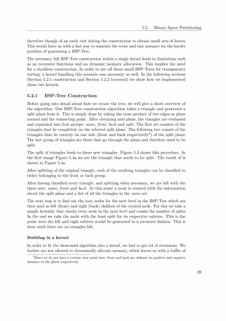
Before going into detail about how we create the tree, we will give a short overview ofthe algorithm. Our BSP-Tree construction algorithm takes a triangle and generates asplit plane from it. This is simply done by taking the cross product of two edges as planenormal and the connecting point. After obtaining said plane, the triangles are evaluatedand separated into four groups: same, front, back and split. The first set consists of thetriangles that lie completely on the selected split plane. The following two consist of thetriangles that lie entirely on one side (front and back respectively4) of the split plane.The last group of triangles are those that go through the plane and therefore need to besplit.

The split of triangles leads to three new triangles. Figure 5.4 shows this procedure. Inthe first image Figure 5.4a we see the triangle that needs to be split. The result of isshown in Figure 5.4a.

After splitting of the original triangle, each of the resulting triangles can be classified toeither belonging to the front or back group.

After having classified every triangle, and splitting when necessary, we are left with thethree sets: same, front and back. At this point a node is created with the informationabout the split plane and a list of all the triangles in the same set.

The next step is to find out the root nodes for the next level in the BSP-Tree which arethen used as left (front) and right (back) children of the created node. For this we take asimple heuristic that checks every node in the next level and counts the number of splits.In the end we take the node with the least split for its respective subtree. This is thepoint were the left and right subtree would be generated in a recursive fashion. This isdone until there are no triangles left.

Building in a kernel

In order to fit the showcased algorithm into a kernel, we had to get rid of recursions. Wefurther are not allowed to dynamically allocate memory, which leaves us with a buffer of

4Since we do not have a certain view point here, front and back are defined via positive and negativedistance to the plane respectively

39

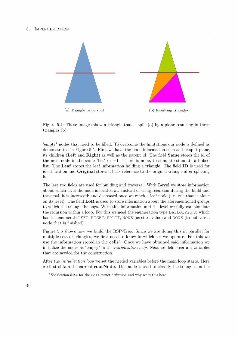
5. Implementation

(a) Triangle to be split (b) Resulting triangles

Figure 5.4: These images show a triangle that is split (a) by a plane resulting in threetriangles (b)

"empty" nodes that need to be filled. To overcome the limitations our node is defined asdemonstrated in Figure 5.5. First we have the node information such as the split plane,its children (Left and Right) as well as the parent id. The field Same stores the id ofthe next node in the same "list" or −1 if there is none, to simulate simulate a linkedlist. The Leaf stores the leaf information holding a triangle. The field ID is used foridentification and Original stores a back reference to the original triangle after splittingit.

The last two fields are used for building and traversal. With Level we store informationabout which level the node is located at. Instead of using recursion during the build andtraversal, it is increased; and decreased once we reach a leaf node (i.e. one that is aloneon its level). The field LoR is used to store information about the aforementioned groupsto which the triangle belongs. With this information and the level we fully can simulatethe recursion within a loop. For this we need the enumeration type LeftOrRight whichhas the enumerals LEFT, RIGHT, SPLIT, NONE (as start value) and DONE (to indicate anode that is finished).

Figure 5.6 shows how we build the BSP-Tree. Since we are doing this in parallel formultiple sets of triangles, we first need to know in which set we operate. For this weuse the information stored in the cells5. Once we have obtained said information weinitialize the nodes as "empty" in the initialization loop. Next we define certain variablesthat are needed for the construction.

After the initialization loop we set the needed variables before the main loop starts. Herewe first obtain the current rootNode. This node is used to classify the triangles on the

5See Section 5.2.4 for the Cell struct definition and why we it this here

40

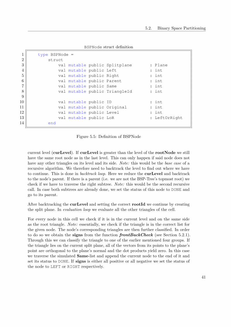
5.2. Binary Space Partitioning

BSPNode struct definition1 type BSPNode =2 struct3 val mutable public Splitplane : Plane4 val mutable public Left : int5 val mutable public Right : int6 val mutable public Parent : int7 val mutable public Same : int8 val mutable public TriangleId : int9

10 val mutable public ID : int11 val mutable public Original : int12 val mutable public Level : int13 val mutable public LoR : LeftOrRight14 end

Figure 5.5: Definition of BSPNode

current level (curLevel). If curLevel is greater than the level of the rootNode we stillhave the same root node as in the last level. This can only happen if said node does nothave any other triangles on its level and its side. Note: this would be the base case of arecursive algorithm. We therefore need to backtrack the level to find out where we haveto continue. This is done in backtrack loop. Here we reduce the curLevel and backtrackto the node’s parent. If there is a parent (i.e. we are not the BSP-Tree’s topmost root) wecheck if we have to traverse the right subtree. Note: this would be the second recursivecall. In case both subtrees are already done, we set the status of this node to DONE andgo to its parent.

After backtracking the curLevel and setting the correct rootId we continue by creatingthe split plane. In evaluation loop we evaluate all the other triangles of the cell.

For every node in this cell we check if it is in the current level and on the same sideas the root triangle. Note: essentially, we check if the triangle is in the correct list forthe given node. The node’s corresponding triangles are then further classified. In orderto do so we obtain the signs from the function frontBackCheck (see Section 5.2.1).Through this we can classify the triangle to one of the earlier mentioned four groups. Ifthe triangle lies on the current split plane, all of the vectors from its points to the plane’spoint are orthogonal to the plane’s normal and the dot products yield zero. In this casewe traverse the simulated Same-list and append the current node to the end of it andset its status to DONE. If signs is either all positive or all negative we set the status ofthe node to LEFT or RIGHT respectively.

41

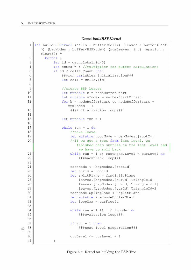
5. Implementation

Kernel buildBSPKernel1 let buildBSPkernel (cells : buffer<Cell>) (leaves : buffer<Leaf

>) (bspNodes : buffer<BSPNode>) (numLeaves: int) (epsilon :float32) =

2 kernel {3 let id = get_global_id(0)4 let extra = 5 //multiplier for buffer calculations5 if id < cells.Count then6 ###run variables initialization###7 let cell = cells.[id]89 //create BSP Leaves

10 let mutable k = nodeBufferStart11 let mutable vIndex = vertexStartOffset12 for k = nodeBufferStart to nodeBufferStart +

numNodes - 113 ###initialization loop###1415 let mutable run = 11617 while run = 1 do18 //take leave19 let mutable rootNode = bspNodes.[rootId]20 //if we got a root from last level, we

finished this subtree in the last level andwe have to roll back

21 while run = 1 && rootNode.Level < curLevel do22 ###backtrack loop###2324 rootNode <- bspNodes.[rootId]25 let curId = rootId26 let splitPlane = findSplitPlane27 leaves.[bspNodes.[curId].TriangleId]28 leaves.[bspNodes.[curId].TriangleId+1]29 leaves.[bspNodes.[curId].TriangleId+230 rootNode.Splitplane <- splitPlane31 let mutable i = nodeBufferStart32 let loopMax = curFreeId3334 while run = 1 && i < loopMax do35 ###evaluation loop###3637 if run = 1 then38 ###next level preparation###3940 curLevel <- curLevel + 141 }

Figure 5.6: Kernel for building the BSP-Tree

42

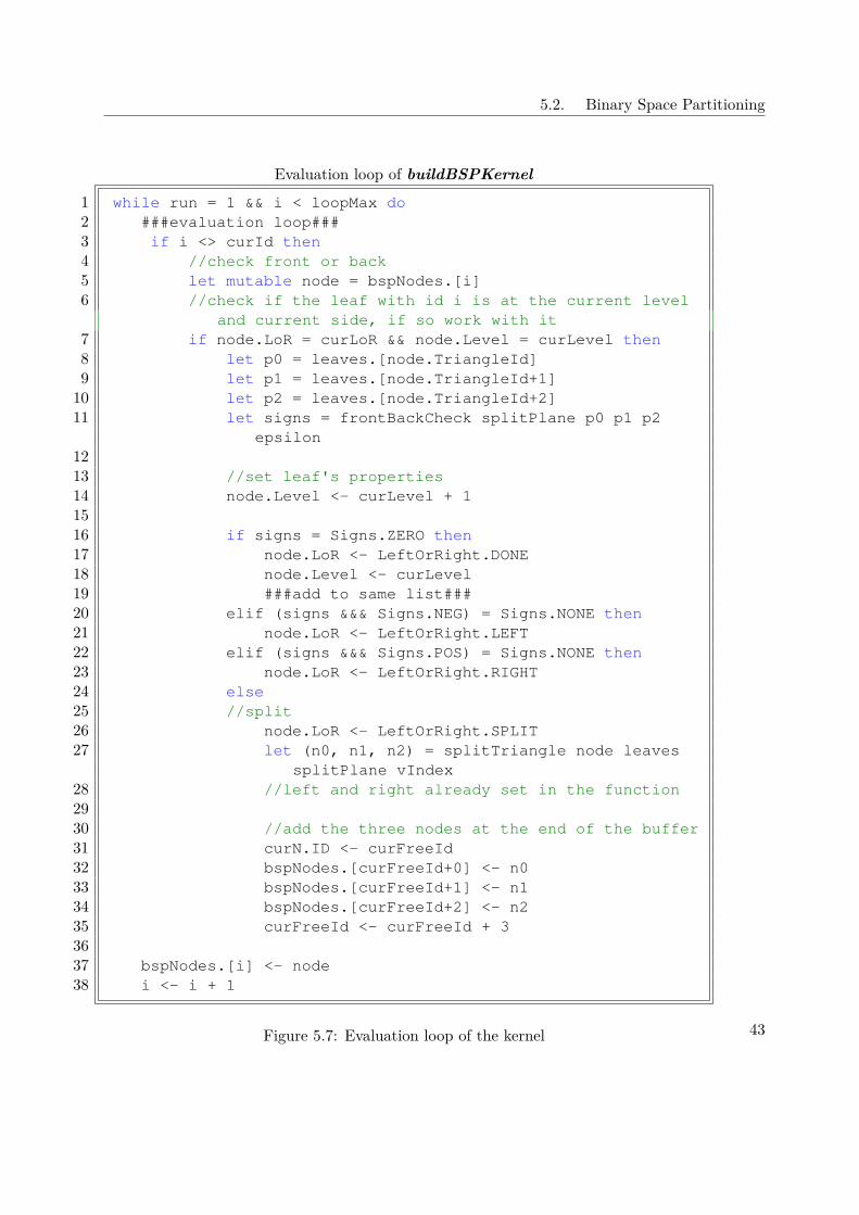
5.2. Binary Space Partitioning

Evaluation loop of buildBSPKernel1 while run = 1 && i < loopMax do2 ###evaluation loop###3 if i <> curId then4 //check front or back5 let mutable node = bspNodes.[i]6 //check if the leaf with id i is at the current level

and current side, if so work with it7 if node.LoR = curLoR && node.Level = curLevel then8 let p0 = leaves.[node.TriangleId]9 let p1 = leaves.[node.TriangleId+1]

10 let p2 = leaves.[node.TriangleId+2]11 let signs = frontBackCheck splitPlane p0 p1 p2

epsilon1213 //set leaf's properties14 node.Level <- curLevel + 11516 if signs = Signs.ZERO then17 node.LoR <- LeftOrRight.DONE18 node.Level <- curLevel19 ###add to same list###20 elif (signs &&& Signs.NEG) = Signs.NONE then21 node.LoR <- LeftOrRight.LEFT22 elif (signs &&& Signs.POS) = Signs.NONE then23 node.LoR <- LeftOrRight.RIGHT24 else25 //split26 node.LoR <- LeftOrRight.SPLIT27 let (n0, n1, n2) = splitTriangle node leaves

splitPlane vIndex28 //left and right already set in the function2930 //add the three nodes at the end of the buffer31 curN.ID <- curFreeId32 bspNodes.[curFreeId+0] <- n033 bspNodes.[curFreeId+1] <- n134 bspNodes.[curFreeId+2] <- n235 curFreeId <- curFreeId + 33637 bspNodes.[i] <- node38 i <- i + 1

Figure 5.7: Evaluation loop of the kernel 43

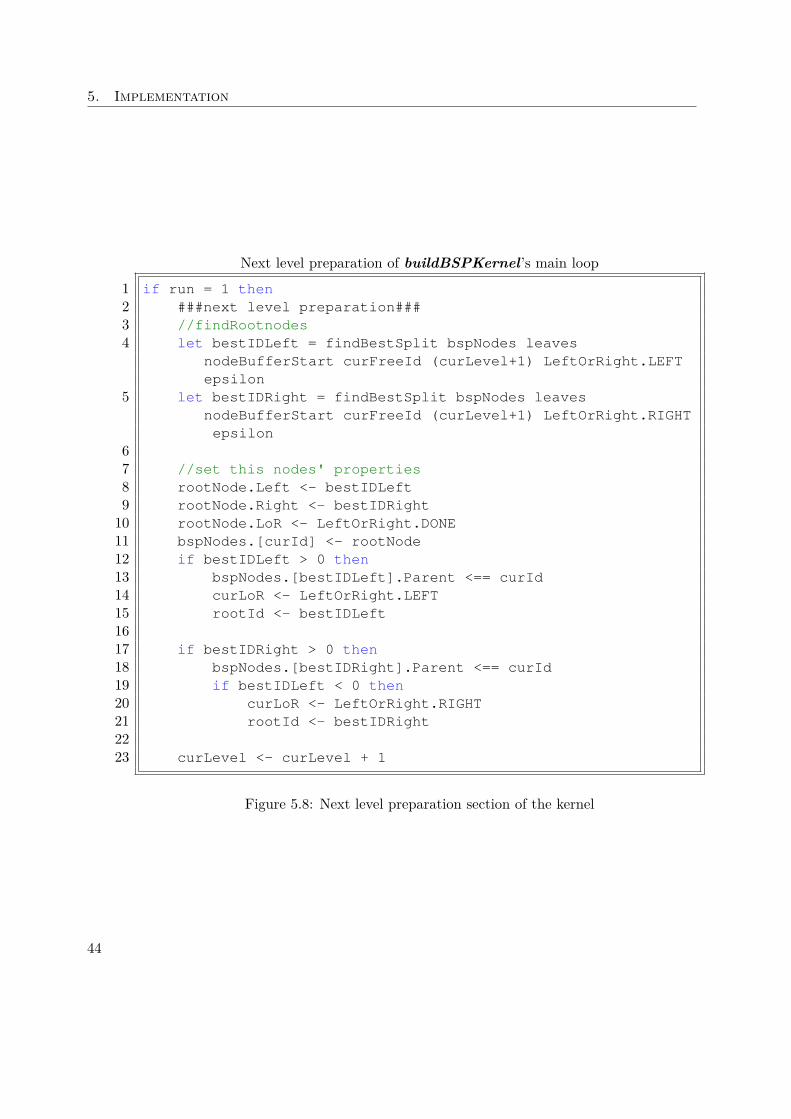
5. Implementation

Next level preparation of buildBSPKernel’s main loop1 if run = 1 then2 ###next level preparation###3 //findRootnodes4 let bestIDLeft = findBestSplit bspNodes leaves

nodeBufferStart curFreeId (curLevel+1) LeftOrRight.LEFTepsilon

5 let bestIDRight = findBestSplit bspNodes leavesnodeBufferStart curFreeId (curLevel+1) LeftOrRight.RIGHTepsilon

67 //set this nodes' properties8 rootNode.Left <- bestIDLeft9 rootNode.Right <- bestIDRight

10 rootNode.LoR <- LeftOrRight.DONE11 bspNodes.[curId] <- rootNode12 if bestIDLeft > 0 then13 bspNodes.[bestIDLeft].Parent <== curId14 curLoR <- LeftOrRight.LEFT15 rootId <- bestIDLeft1617 if bestIDRight > 0 then18 bspNodes.[bestIDRight].Parent <== curId19 if bestIDLeft < 0 then20 curLoR <- LeftOrRight.RIGHT21 rootId <- bestIDRight2223 curLevel <- curLevel + 1

Figure 5.8: Next level preparation section of the kernel

44

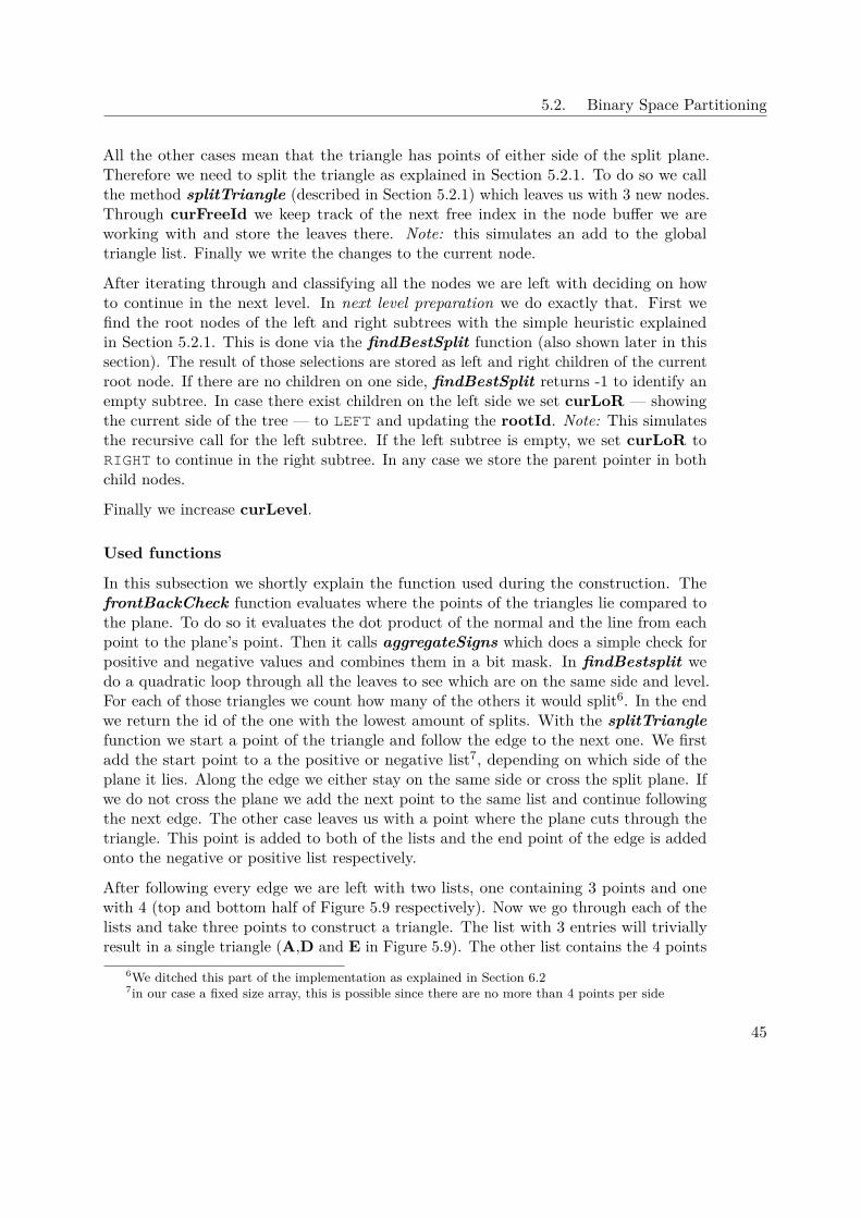
5.2. Binary Space Partitioning

All the other cases mean that the triangle has points of either side of the split plane.Therefore we need to split the triangle as explained in Section 5.2.1. To do so we callthe method splitTriangle (described in Section 5.2.1) which leaves us with 3 new nodes.Through curFreeId we keep track of the next free index in the node buffer we areworking with and store the leaves there. Note: this simulates an add to the globaltriangle list. Finally we write the changes to the current node.

After iterating through and classifying all the nodes we are left with deciding on howto continue in the next level. In next level preparation we do exactly that. First wefind the root nodes of the left and right subtrees with the simple heuristic explainedin Section 5.2.1. This is done via the findBestSplit function (also shown later in thissection). The result of those selections are stored as left and right children of the currentroot node. If there are no children on one side, findBestSplit returns -1 to identify anempty subtree. In case there exist children on the left side we set curLoR — showingthe current side of the tree — to LEFT and updating the rootId. Note: This simulatesthe recursive call for the left subtree. If the left subtree is empty, we set curLoR toRIGHT to continue in the right subtree. In any case we store the parent pointer in bothchild nodes.

Finally we increase curLevel.

Used functions

In this subsection we shortly explain the function used during the construction. ThefrontBackCheck function evaluates where the points of the triangles lie compared tothe plane. To do so it evaluates the dot product of the normal and the line from eachpoint to the plane’s point. Then it calls aggregateSigns which does a simple check forpositive and negative values and combines them in a bit mask. In findBestsplit wedo a quadratic loop through all the leaves to see which are on the same side and level.For each of those triangles we count how many of the others it would split6. In the endwe return the id of the one with the lowest amount of splits. With the splitTrianglefunction we start a point of the triangle and follow the edge to the next one. We firstadd the start point to a the positive or negative list7, depending on which side of theplane it lies. Along the edge we either stay on the same side or cross the split plane. Ifwe do not cross the plane we add the next point to the same list and continue followingthe next edge. The other case leaves us with a point where the plane cuts through thetriangle. This point is added to both of the lists and the end point of the edge is addedonto the negative or positive list respectively.

After following every edge we are left with two lists, one containing 3 points and onewith 4 (top and bottom half of Figure 5.9 respectively). Now we go through each of thelists and take three points to construct a triangle. The list with 3 entries will triviallyresult in a single triangle (A,D and E in Figure 5.9). The other list contains the 4 points

6We ditched this part of the implementation as explained in Section 6.27in our case a fixed size array, this is possible since there are no more than 4 points per side

45

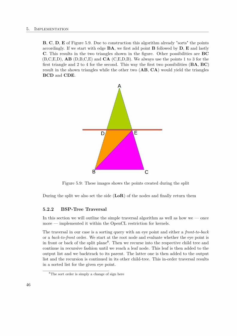
5. Implementation

B, C, D, E of Figure 5.9. Due to construction this algorithm already "sorts" the pointsaccordingly. If we start with edge BA, we first add point B followed by D, E and lastlyC. This results in the two triangles shown in the figure. Other possibilities are BC(B,C,E,D), AB (D,B,C,E) and CA (C,E,D,B). We always use the points 1 to 3 for thefirst triangle and 2 to 4 for the second. This way the first two possibilities (BA, BC)result in the shown triangles while the other two (AB, CA) would yield the trianglesBCD and CDE.

Figure 5.9: These images shows the points created during the split

During the split we also set the side (LoR) of the nodes and finally return them

5.2.2 BSP-Tree Traversal

In this section we will outline the simple traversal algorithm as well as how we — oncemore — implemented it within the OpenCL restriction for kernels.

The traversal in our case is a sorting query with an eye point and either a front-to-backor a back-to-front order. We start at the root node and evaluate whether the eye point isin front or back of the split plane8. Then we recurse into the respective child tree andcontinue in recursive fashion until we reach a leaf node. This leaf is then added to theoutput list and we backtrack to its parent. The latter one is then added to the outputlist and the recursion is continued in its other child-tree. This in-order traversal resultsin a sorted list for the given eye point.

8The sort order is simply a change of sign here

46

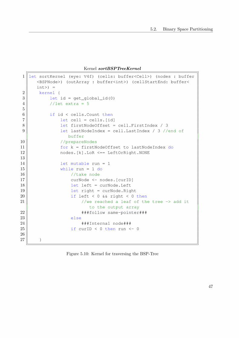
5.2. Binary Space Partitioning

Kernel sortBSPTreeKernel1 let sortKernel (eye: V4f) (cells: buffer<Cell>) (nodes : buffer

<BSPNode>) (outArray : buffer<int>) (cellStartEnd: buffer<int>) =

2 kernel {3 let id = get_global_id(0)4 //let extra = 556 if id < cells.Count then7 let cell = cells.[id]8 let firstNodeOffset = cell.FirstIndex / 39 let lastNodeIndex = cell.LastIndex / 3 //end of

buffer10 //prepareNodes11 for k = firstNodeOffset to lastNodeIndex do12 nodes.[k].LoR <== LeftOrRight.NONE1314 let mutable run = 115 while run = 1 do16 //take node17 curNode <- nodes.[curID]18 let left = curNode.Left19 let right = curNode.Right20 if left < 0 && right < 0 then21 //we reached a leaf of the tree -> add it

to the output array22 ###follow same-pointer###23 else24 ###Internal node###25 if curID < 0 then run <- 02627 }

Figure 5.10: Kernel for traversing the BSP-Tree

47

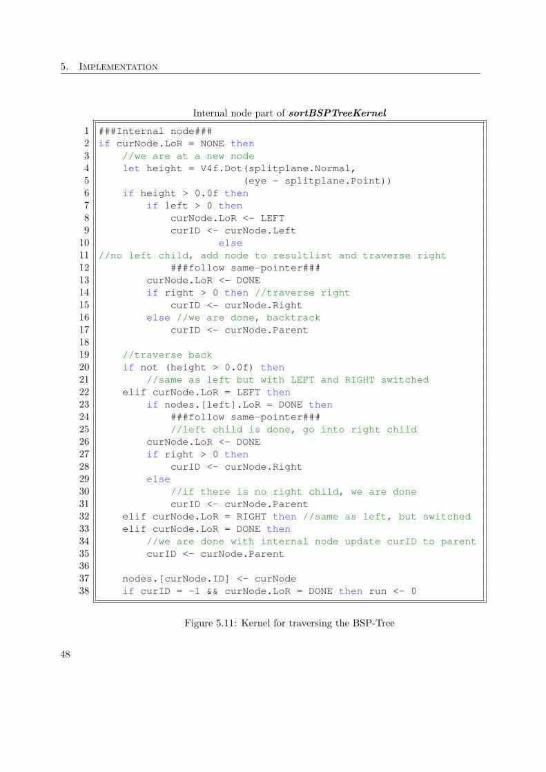
5. Implementation

Internal node part of sortBSPTreeKernel1 ###Internal node###2 if curNode.LoR = NONE then3 //we are at a new node4 let height = V4f.Dot(splitplane.Normal,5 (eye - splitplane.Point))6 if height > 0.0f then7 if left > 0 then8 curNode.LoR <- LEFT9 curID <- curNode.Left

10 else11 //no left child, add node to resultlist and traverse right12 ###follow same-pointer###13 curNode.LoR <- DONE14 if right > 0 then //traverse right15 curID <- curNode.Right16 else //we are done, backtrack17 curID <- curNode.Parent1819 //traverse back20 if not (height > 0.0f) then21 //same as left but with LEFT and RIGHT switched22 elif curNode.LoR = LEFT then23 if nodes.[left].LoR = DONE then24 ###follow same-pointer###25 //left child is done, go into right child26 curNode.LoR <- DONE27 if right > 0 then28 curID <- curNode.Right29 else30 //if there is no right child, we are done31 curID <- curNode.Parent32 elif curNode.LoR = RIGHT then //same as left, but switched33 elif curNode.LoR = DONE then34 //we are done with internal node update curID to parent35 curID <- curNode.Parent3637 nodes.[curNode.ID] <- curNode38 if curID = -1 && curNode.LoR = DONE then run <- 0

Figure 5.11: Kernel for traversing the BSP-Tree

48

5.2. Binary Space Partitioning

To fit this algorithm into a kernel, we — again — have to deal with the limitationsexplained in the beginning of Section 5.2.1. In order to achieve this we use the sameworkaround as already shown in Section 5.2.1. Figure 5.10 shows the traversal. Afteridentifying the correct range in the global buffer we first set every node’s LoR to NONE.In the main loop we first check if we are currently dealing with a leaf. In this case we addit to the output list and traverse the simulated Same-list. Via a counter we keep trackof where in the output buffer we are storing the current entries. We further backtrack tothe leaf’s parent. Note: this would be the base case of a recursive algorithm

If we are working on a node we identify the current stage via the node’s LoR. The firstcase is a — so far — unseen node. Here we first check on which side of the split planethe eye point is, and then set the LoR to the side we are going to traverse. In case thereis no child on this side, we again add the Same-List to the output and set the traversalto DONE.

In case the working node has its LoR set, we know we have to traverse the respectivesubtree. If this subtree is done, we add the current node and it’s Same-List to the outputand set the traversal to the other side. Here we set LoR to DONE to indicate that oneside is already done and we just update curID to match the other child. In the othercase we update curID to indicate we continue with the subtree. Note: this represents arecursive call.

The last case is DONE. The first one corresponds to a node that has finished both subtreesand therefore the status is set to DONE. The latter one indicates a finished subtree andtherefore we backtrack to its parent node. Note: this would be the return of a recursivecall.

The end of the loop writes back the changes to the node and checks if we have arrived atthe cell’s root node.

5.2.3 Conceptual Error

After having everything set up we re-evaluated the concept of this idea. The property ofthe BVH-tree — as we constructed it — is also the doom to our idea of usage. Sincethe triangles are sorted by the Morton codes of their centers’ a triangle could potentiallyspread through multiple cells. Even in that case it would still only end up in one BVH-node. This will essentially lead to errors when sorting since it is not possible to decide ifa cell is in front or at the back of another.

Figure 5.12 showcases this problem. On the left we see a scene, which simply containstwo overlapping triangles. The yellow and green line mark the bounding boxes of theirrespective triangles. On the left hand-side of in the scene with have the larger trianglewhose result is symbolized as node A in the BVH-tree. On the right side we have thetriangle in the back and schematically shown as the node B. In this case we alreadystruggle to tell if node A is in front of node B without checking the triangles.

49

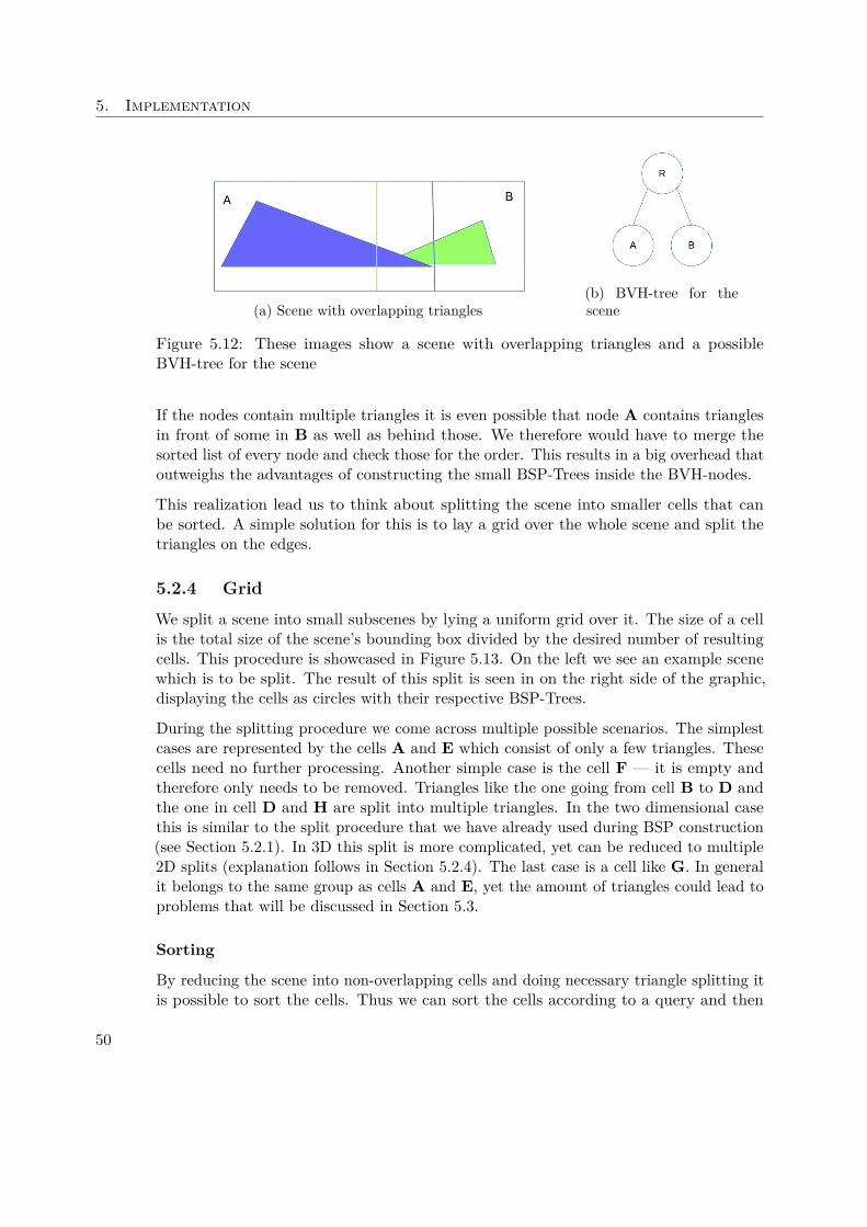
5. Implementation

(a) Scene with overlapping triangles(b) BVH-tree for thescene

Figure 5.12: These images show a scene with overlapping triangles and a possibleBVH-tree for the scene

If the nodes contain multiple triangles it is even possible that node A contains trianglesin front of some in B as well as behind those. We therefore would have to merge thesorted list of every node and check those for the order. This results in a big overhead thatoutweighs the advantages of constructing the small BSP-Trees inside the BVH-nodes.

This realization lead us to think about splitting the scene into smaller cells that canbe sorted. A simple solution for this is to lay a grid over the whole scene and split thetriangles on the edges.

5.2.4 Grid

We split a scene into small subscenes by lying a uniform grid over it. The size of a cellis the total size of the scene’s bounding box divided by the desired number of resultingcells. This procedure is showcased in Figure 5.13. On the left we see an example scenewhich is to be split. The result of this split is seen in on the right side of the graphic,displaying the cells as circles with their respective BSP-Trees.

During the splitting procedure we come across multiple possible scenarios. The simplestcases are represented by the cells A and E which consist of only a few triangles. Thesecells need no further processing. Another simple case is the cell F — it is empty andtherefore only needs to be removed. Triangles like the one going from cell B to D andthe one in cell D and H are split into multiple triangles. In the two dimensional casethis is similar to the split procedure that we have already used during BSP construction(see Section 5.2.1). In 3D this split is more complicated, yet can be reduced to multiple2D splits (explanation follows in Section 5.2.4). The last case is a cell like G. In generalit belongs to the same group as cells A and E, yet the amount of triangles could lead toproblems that will be discussed in Section 5.3.

Sorting

By reducing the scene into non-overlapping cells and doing necessary triangle splitting itis possible to sort the cells. Thus we can sort the cells according to a query and then

50

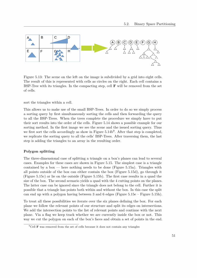
5.2. Binary Space Partitioning

Figure 5.13: The scene on the left on the image is subdivided by a grid into eight cells.The result of this is represented with cells as circles on the right. Each cell contains aBSP-Tree with its triangles. In the compacting step, cell F will be removed from the setof cells.

sort the triangles within a cell.

This allows us to make use of the small BSP-Trees. In order to do so we simply processa sorting query by first simultaneously sorting the cells and then forwarding the queryto all the BSP-Trees. When the trees complete the procedure we simply have to puttheir sort results into the order of the cells. Figure 5.14 shows a possible example for oursorting method. In the first image we see the scene and the issued sorting query. Thuswe first sort the cells accordingly as show in Figure 5.14b9. After that step is completed,we replicate the sorting query to all the cells’ BSP-Trees. After traversing them, the laststep is adding the triangles to an array in the resulting order.

Polygon splitting

The three-dimensional case of splitting a triangle on a box’s planes can lead to severalcases. Examples for these cases are shown in Figure 5.15. The simplest case is a trianglecontained by a box — here nothing needs to be done (Figure 5.15a). Triangles withall points outside of the box can either contain the box (Figure 5.15d), go through it(Figure 5.15c) or lie on the outside (Figure 5.15b). The first case results in a quad thesize of the box. The second scenario yields a quad with the 4 cutting points on the planes.The latter case can be ignored since the triangle does not belong to the cell. Further it ispossible that a triangle has points both within and without the box. In this case the splitcan end up with a polygon having between 3 and 6 edges (Figure 5.15e – Figure 5.15h).

To treat all these possibilities we iterate over the six planes defining the box. For eachplane we follow the relevant points of our structure and split its edges on intersections.We add the intersection points to the list of relevant points and continue with the nextplane. Via a flag we keep track whether we are currently inside the box or not. Thisway we cut the polygon on each of the box’s faces and obtain a set of points in the end.

9Cell F was removed from the set of cells because it does not contain any triangles

51

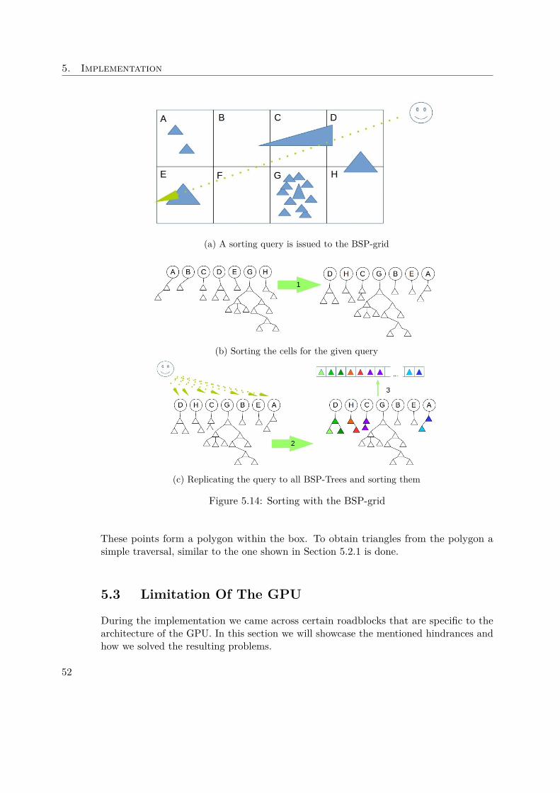
5. Implementation

(a) A sorting query is issued to the BSP-grid

(b) Sorting the cells for the given query

(c) Replicating the query to all BSP-Trees and sorting them

Figure 5.14: Sorting with the BSP-grid

These points form a polygon within the box. To obtain triangles from the polygon asimple traversal, similar to the one shown in Section 5.2.1 is done.

5.3 Limitation Of The GPU

During the implementation we came across certain roadblocks that are specific to thearchitecture of the GPU. In this section we will showcase the mentioned hindrances andhow we solved the resulting problems.

52

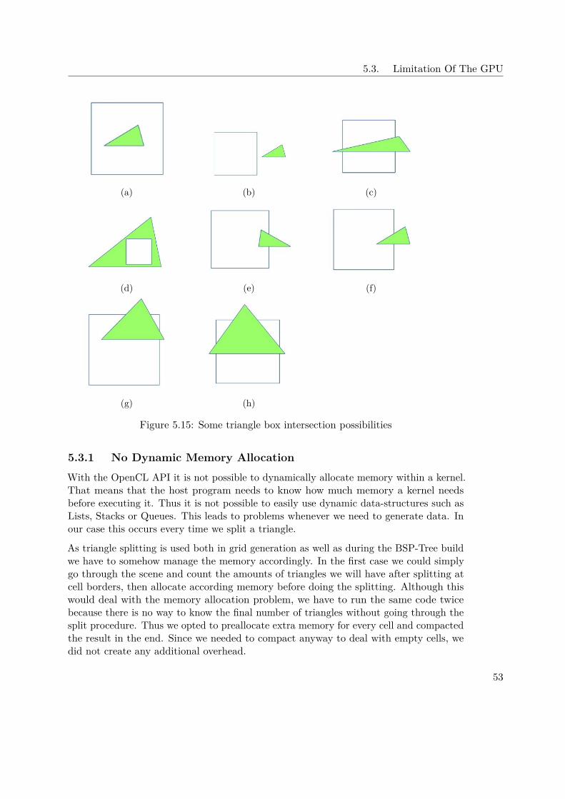
5.3. Limitation Of The GPU

(a) (b) (c)

(d) (e) (f)

(g) (h)

Figure 5.15: Some triangle box intersection possibilities

5.3.1 No Dynamic Memory Allocation

With the OpenCL API it is not possible to dynamically allocate memory within a kernel.That means that the host program needs to know how much memory a kernel needsbefore executing it. Thus it is not possible to easily use dynamic data-structures such asLists, Stacks or Queues. This leads to problems whenever we need to generate data. Inour case this occurs every time we split a triangle.

As triangle splitting is used both in grid generation as well as during the BSP-Tree buildwe have to somehow manage the memory accordingly. In the first case we could simplygo through the scene and count the amounts of triangles we will have after splitting atcell borders, then allocate according memory before doing the splitting. Although thiswould deal with the memory allocation problem, we have to run the same code twicebecause there is no way to know the final number of triangles without going through thesplit procedure. Thus we opted to preallocate extra memory for every cell and compactedthe result in the end. Since we needed to compact anyway to deal with empty cells, wedid not create any additional overhead.

53

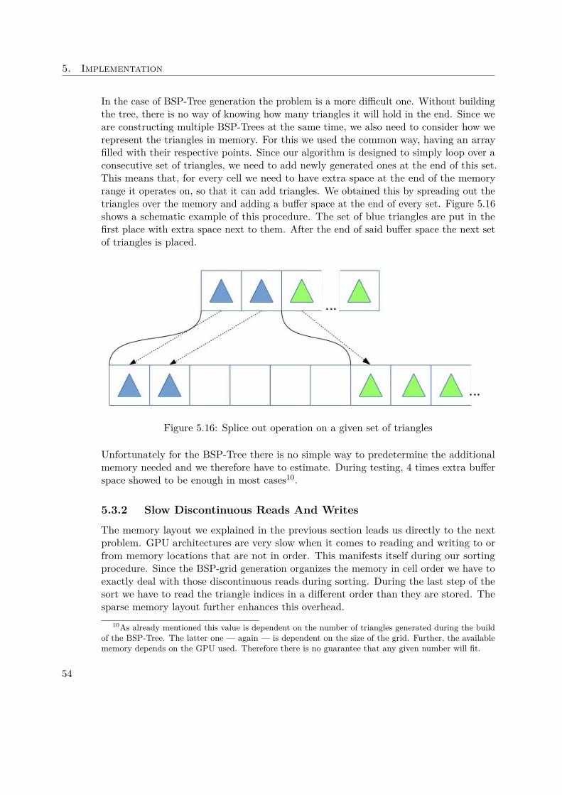
5. Implementation

In the case of BSP-Tree generation the problem is a more difficult one. Without buildingthe tree, there is no way of knowing how many triangles it will hold in the end. Since weare constructing multiple BSP-Trees at the same time, we also need to consider how werepresent the triangles in memory. For this we used the common way, having an arrayfilled with their respective points. Since our algorithm is designed to simply loop over aconsecutive set of triangles, we need to add newly generated ones at the end of this set.This means that, for every cell we need to have extra space at the end of the memoryrange it operates on, so that it can add triangles. We obtained this by spreading out thetriangles over the memory and adding a buffer space at the end of every set. Figure 5.16shows a schematic example of this procedure. The set of blue triangles are put in thefirst place with extra space next to them. After the end of said buffer space the next setof triangles is placed.

Figure 5.16: Splice out operation on a given set of triangles

Unfortunately for the BSP-Tree there is no simple way to predetermine the additionalmemory needed and we therefore have to estimate. During testing, 4 times extra bufferspace showed to be enough in most cases10.

5.3.2 Slow Discontinuous Reads And Writes

The memory layout we explained in the previous section leads us directly to the nextproblem. GPU architectures are very slow when it comes to reading and writing to orfrom memory locations that are not in order. This manifests itself during our sortingprocedure. Since the BSP-grid generation organizes the memory in cell order we have toexactly deal with those discontinuous reads during sorting. During the last step of thesort we have to read the triangle indices in a different order than they are stored. Thesparse memory layout further enhances this overhead.

10As already mentioned this value is dependent on the number of triangles generated during the buildof the BSP-Tree. The latter one — again — is dependent on the size of the grid. Further, the availablememory depends on the GPU used. Therefore there is no guarantee that any given number will fit.

54

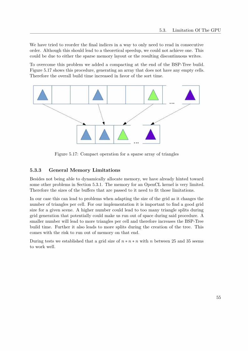
5.3. Limitation Of The GPU

We have tried to reorder the final indices in a way to only need to read in consecutiveorder. Although this should lead to a theoretical speedup, we could not achieve one. Thiscould be due to either the sparse memory layout or the resulting discontinuous writes.

To overcome this problem we added a compacting at the end of the BSP-Tree build.Figure 5.17 shows this procedure, generating an array that does not have any empty cells.Therefore the overall build time increased in favor of the sort time.

Figure 5.17: Compact operation for a sparse array of triangles

5.3.3 General Memory Limitations

Besides not being able to dynamically allocate memory, we have already hinted towardsome other problems in Section 5.3.1. The memory for an OpenCL kernel is very limited.Therefore the sizes of the buffers that are passed to it need to fit those limitations.

In our case this can lead to problems when adapting the size of the grid as it changes thenumber of triangles per cell. For our implementation it is important to find a good gridsize for a given scene. A higher number could lead to too many triangle splits duringgrid generation that potentially could make us run out of space during said procedure. Asmaller number will lead to more triangles per cell and therefore increases the BSP-Treebuild time. Further it also leads to more splits during the creation of the tree. Thiscomes with the risk to run out of memory on that end.

During tests we established that a grid size of n ∗ n ∗ n with n between 25 and 35 seemsto work well.

55

CHAPTER 6Evaluation

We have to evaluate certain properties of the BSP-grid, to see if we can replace thecurrently used, highly optimized CPU implementation of the BSP-Tree in the Aardvarkrendering framework. Most interesting is the sorting performance since transparencysorting the tree’s primary use case. Secondly we have to make sure that build times ofthe BSP-grid are reasonable fast to avoid off-line generation.

Another interesting property is the total amount of triangles we obtain throughout thebuildup phase, because we want to keep them as small as possible.

Further we are interested in finding the optimal settings for the BSP-grid. Thus we haveexamined grid sizes from 11 up to 50.

Finally we also searched for weaknesses in our design as well as hardware dependentbottlenecks of our implementation for future improvements.

6.1 SetupFirst we give a brief overview of our test setup.

All of our performance tests2 were run with 10 builds of the chosen implementation witha total of 100 sort operations. Stable results made further iterations unnecessary.

Furthermore we have only used one hardware setup as the prototype was build to testwhether this approach can outperform the currently used BSP-Tree or not.

6.1.1 Hardware

For evaluation we used the following hardware1Full single-threaded tree generation on the GPU2Note that the analysis of node selection methods is not a performance test

57

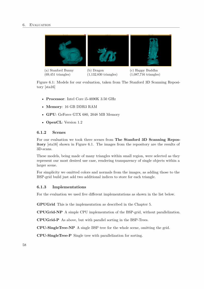
6. Evaluation

(a) Stanford Bunny(69,451 triangles)

(b) Dragon(1,132,830 triangles)

(c) Happy Buddha(1,087,716 triangles)

Figure 6.1: Models for our evaluation, taken from The Stanford 3D Scanning Reposi-tory [sta16]

• Processor: Intel Core i5-4690K 3.50 GHz

• Memory: 16 GB DDR3 RAM

• GPU: GeForce GTX 680, 2048 MB Memory

• OpenCL: Version 1.2

6.1.2 Scenes

For our evaluation we took three scenes from The Stanford 3D Scanning Repos-itory [sta16] shown in Figure 6.1. The images from the repository are the results of3D-scans.

These models, being made of many triangles within small region, were selected as theyrepresent our most desired use case, rendering transparency of single objects within alarger scene.

For simplicity we omitted colors and normals from the images, as adding those to theBSP-grid build just add two additional indices to store for each triangle.

6.1.3 Implementations

For the evaluation we used five different implementations as shown in the list below.

GPUGrid This is the implementation as described in the Chapter 5.

CPUGrid-NP A simple CPU implementation of the BSP-grid, without parallelization.

CPUGrid-P As above, but with parallel sorting in the BSP-Trees.

CPU-SingleTree-NP A single BSP tree for the whole scene, omitting the grid.

CPU-SingleTree-P Single tree with parallelization for sorting.

58

6.2. Root Node Selection

The BSP-grid implementations have a single parameter specifying the grid size. A gridsize of n leads to splitting the scene into n3 cells, before removing the empty ones.

Both CPU implementations of the BSP-grid use the CPU-SingleTree in their grid cells.This tree does not implement a heuristic for building, but simply adds the triangles ininput order. The tree construction is quadratically and sorting is linearly proportional tothe number of triangles.

The grid generation time in both the GPU and the CPU implementations is proportionalto the number of triangles, since we just take each and find cell for it. Building theBSP-Tree in the cells differs between the CPU and the GPU implementation. The CPUimplementation uses the CPU-SingleTree and therefore obtains its runtime properties.The GPU implementation, however, originally3 looped over all triangles quadraticallyduring the build in order to find an appropriate root node for every level4. The sort is asimple tree traversal with a theoretical complexity of O(n).

Since we are using parallel algorithms we have to further look how the parallelizationplays a role for runtime properties. When parallelized over triangles, the grid generationis dominated by sorting the triangles in cell order, leading to a theoretical complexity ofO(logn)5 for n triangles.

The BSP-Tree generation is parallelized over the grid cells with each of them working onall of their triangles in cubic fashion. The reason for this is that we try to reduce splitsby finding the triangle with least splits for every node added in a quadratic loop. Forsorting the BSP-Trees we also parallelize over the cells, whereas every cell has to traverseits tree. Hence the runtime is linearly proportional to the number of triangles in everycell. Note that for the BSP-grid the number of triangles per tree is tremendously smallerthan for a single BSP-Tree.

6.2 Root Node SelectionDuring the evaluation we tracked down a bottleneck in the quadratic loop that selectsa proper root node at every level of the BSP-Trees. This method was chosen in orderto keep the amount of resulting number of triangles as small as possible to be ableto stay within the memory limitations of the GPU. As the high build times seemedunreasonable we have inspected the differences in triangle generation between the leastsplitting method 6 and a simple random select7. We evaluated the difference in trianglesadded for our three test scenes with grid sizes of 25, 30 and 35.

To our surprise, the random select only shows an average increase of 0.15% overall addedtriangles with respect to the least splitting variant. This value is highly skewed towards

3See Section 6.2 why we changed it4See Section 5.2.1 for the implementation5The interested reader is forwarded to Cole’s parallel merge sort [Col93]6Explained in Section 5.2.1 as findBestSplit7In fact we are always selecting the triangle which is added last

59

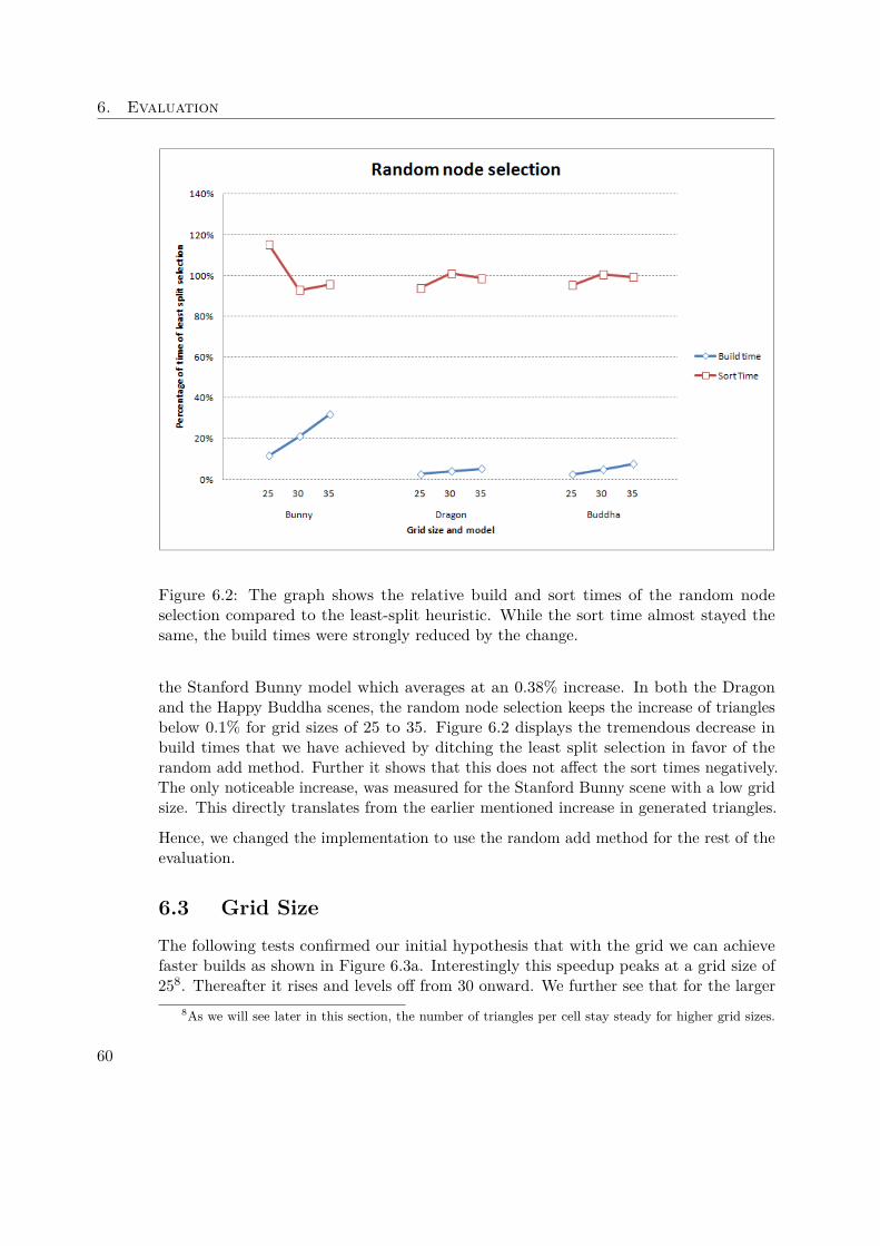
6. Evaluation

Figure 6.2: The graph shows the relative build and sort times of the random nodeselection compared to the least-split heuristic. While the sort time almost stayed thesame, the build times were strongly reduced by the change.

the Stanford Bunny model which averages at an 0.38% increase. In both the Dragonand the Happy Buddha scenes, the random node selection keeps the increase of trianglesbelow 0.1% for grid sizes of 25 to 35. Figure 6.2 displays the tremendous decrease inbuild times that we have achieved by ditching the least split selection in favor of therandom add method. Further it shows that this does not affect the sort times negatively.The only noticeable increase, was measured for the Stanford Bunny scene with a low gridsize. This directly translates from the earlier mentioned increase in generated triangles.

Hence, we changed the implementation to use the random add method for the rest of theevaluation.

6.3 Grid SizeThe following tests confirmed our initial hypothesis that with the grid we can achievefaster builds as shown in Figure 6.3a. Interestingly this speedup peaks at a grid size of258. Thereafter it rises and levels off from 30 onward. We further see that for the larger

8As we will see later in this section, the number of triangles per cell stay steady for higher grid sizes.

60

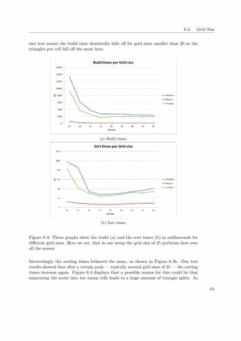
6.3. Grid Size

two test scenes the build time drastically falls off for grid sizes smaller than 20 as thetriangles per cell fall off the most here.

(a) Build times

(b) Sort times

Figure 6.3: These graphs show the build (a) and the sort times (b) in milliseconds fordifferent grid sizes. Here we see, that in our setup the grid size of 25 performs best overall the scenes

Interestingly the sorting times behaved the same, as shown in Figure 6.3b. Our testresults showed that after a certain peak — typically around grid sizes of 25 — the sortingtimes increase again. Figure 6.4 displays that a possible reason for this could be thatseparating the scene into too many cells leads to a huge amount of triangle splits. As

61

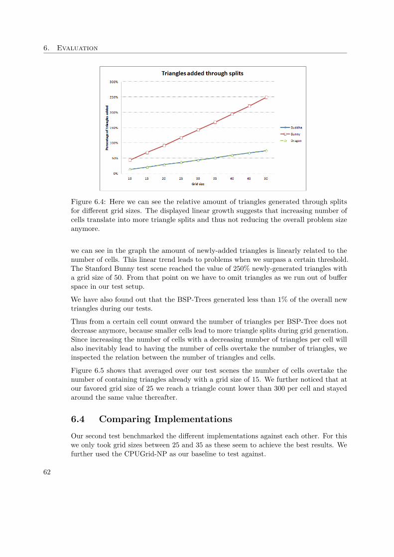
6. Evaluation

Figure 6.4: Here we can see the relative amount of triangles generated through splitsfor different grid sizes. The displayed linear growth suggests that increasing number ofcells translate into more triangle splits and thus not reducing the overall problem sizeanymore.

we can see in the graph the amount of newly-added triangles is linearly related to thenumber of cells. This linear trend leads to problems when we surpass a certain threshold.The Stanford Bunny test scene reached the value of 250% newly-generated triangles witha grid size of 50. From that point on we have to omit triangles as we run out of bufferspace in our test setup.

We have also found out that the BSP-Trees generated less than 1% of the overall newtriangles during our tests.

Thus from a certain cell count onward the number of triangles per BSP-Tree does notdecrease anymore, because smaller cells lead to more triangle splits during grid generation.Since increasing the number of cells with a decreasing number of triangles per cell willalso inevitably lead to having the number of cells overtake the number of triangles, weinspected the relation between the number of triangles and cells.

Figure 6.5 shows that averaged over our test scenes the number of cells overtake thenumber of containing triangles already with a grid size of 15. We further noticed that atour favored grid size of 25 we reach a triangle count lower than 300 per cell and stayedaround the same value thereafter.

6.4 Comparing ImplementationsOur second test benchmarked the different implementations against each other. For thiswe only took grid sizes between 25 and 35 as these seem to achieve the best results. Wefurther used the CPUGrid-NP as our baseline to test against.

62

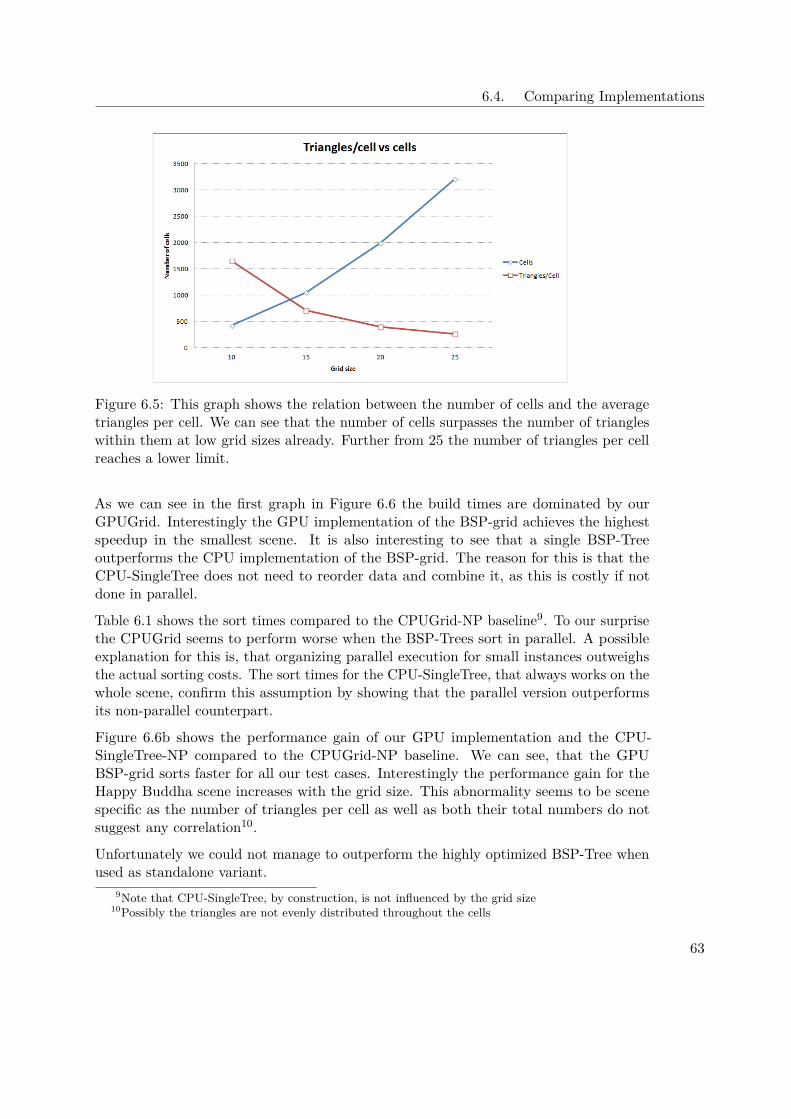
6.4. Comparing Implementations

Figure 6.5: This graph shows the relation between the number of cells and the averagetriangles per cell. We can see that the number of cells surpasses the number of triangleswithin them at low grid sizes already. Further from 25 the number of triangles per cellreaches a lower limit.

As we can see in the first graph in Figure 6.6 the build times are dominated by ourGPUGrid. Interestingly the GPU implementation of the BSP-grid achieves the highestspeedup in the smallest scene. It is also interesting to see that a single BSP-Treeoutperforms the CPU implementation of the BSP-grid. The reason for this is that theCPU-SingleTree does not need to reorder data and combine it, as this is costly if notdone in parallel.

Table 6.1 shows the sort times compared to the CPUGrid-NP baseline9. To our surprisethe CPUGrid seems to perform worse when the BSP-Trees sort in parallel. A possibleexplanation for this is, that organizing parallel execution for small instances outweighsthe actual sorting costs. The sort times for the CPU-SingleTree, that always works on thewhole scene, confirm this assumption by showing that the parallel version outperformsits non-parallel counterpart.

Figure 6.6b shows the performance gain of our GPU implementation and the CPU-SingleTree-NP compared to the CPUGrid-NP baseline. We can see, that the GPUBSP-grid sorts faster for all our test cases. Interestingly the performance gain for theHappy Buddha scene increases with the grid size. This abnormality seems to be scenespecific as the number of triangles per cell as well as both their total numbers do notsuggest any correlation10.

Unfortunately we could not manage to outperform the highly optimized BSP-Tree whenused as standalone variant.

9Note that CPU-SingleTree, by construction, is not influenced by the grid size10Possibly the triangles are not evenly distributed throughout the cells

63

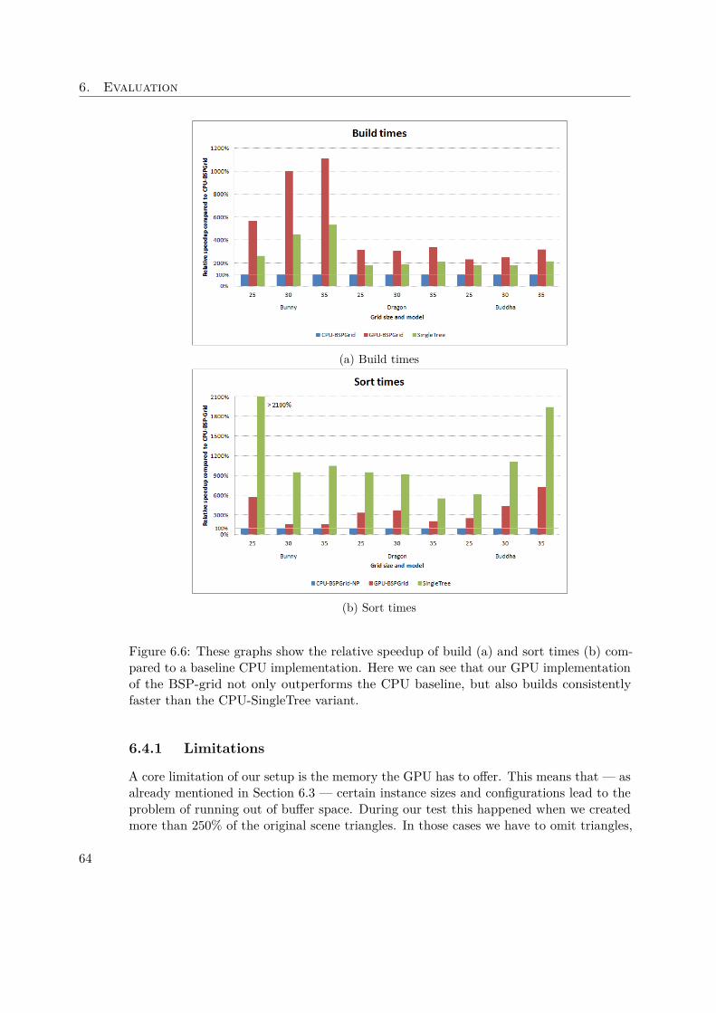
6. Evaluation

(a) Build times

(b) Sort times

Figure 6.6: These graphs show the relative speedup of build (a) and sort times (b) com-pared to a baseline CPU implementation. Here we can see that our GPU implementationof the BSP-grid not only outperforms the CPU baseline, but also builds consistentlyfaster than the CPU-SingleTree variant.

6.4.1 Limitations

A core limitation of our setup is the memory the GPU has to offer. This means that — asalready mentioned in Section 6.3 — certain instance sizes and configurations lead to theproblem of running out of buffer space. During our test this happened when we createdmore than 250% of the original scene triangles. In those cases we have to omit triangles,

64

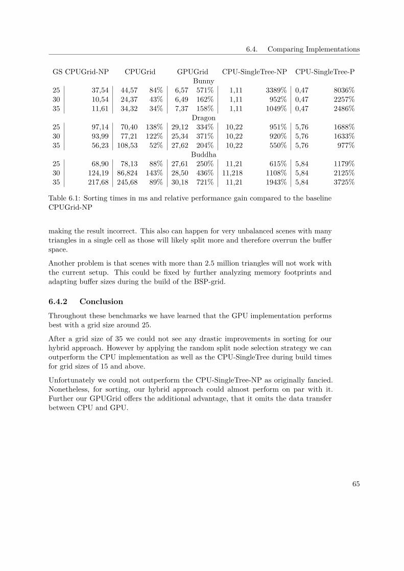
6.4. Comparing Implementations

GS CPUGrid-NP CPUGrid GPUGrid CPU-SingleTree-NP CPU-SingleTree-PBunny

25 37,54 44,57 84% 6,57 571% 1,11 3389% 0,47 8036%30 10,54 24,37 43% 6,49 162% 1,11 952% 0,47 2257%35 11,61 34,32 34% 7,37 158% 1,11 1049% 0,47 2486%

Dragon25 97,14 70,40 138% 29,12 334% 10,22 951% 5,76 1688%30 93,99 77,21 122% 25,34 371% 10,22 920% 5,76 1633%35 56,23 108,53 52% 27,62 204% 10,22 550% 5,76 977%

Buddha25 68,90 78,13 88% 27,61 250% 11,21 615% 5,84 1179%30 124,19 86,824 143% 28,50 436% 11,218 1108% 5,84 2125%35 217,68 245,68 89% 30,18 721% 11,21 1943% 5,84 3725%

Table 6.1: Sorting times in ms and relative performance gain compared to the baselineCPUGrid-NP

making the result incorrect. This also can happen for very unbalanced scenes with manytriangles in a single cell as those will likely split more and therefore overrun the bufferspace.

Another problem is that scenes with more than 2.5 million triangles will not work withthe current setup. This could be fixed by further analyzing memory footprints andadapting buffer sizes during the build of the BSP-grid.

6.4.2 Conclusion

Throughout these benchmarks we have learned that the GPU implementation performsbest with a grid size around 25.

After a grid size of 35 we could not see any drastic improvements in sorting for ourhybrid approach. However by applying the random split node selection strategy we canoutperform the CPU implementation as well as the CPU-SingleTree during build timesfor grid sizes of 15 and above.

Unfortunately we could not outperform the CPU-SingleTree-NP as originally fancied.Nonetheless, for sorting, our hybrid approach could almost perform on par with it.Further our GPUGrid offers the additional advantage, that it omits the data transferbetween CPU and GPU.

65

CHAPTER 7Conclusion and Future Work

We presented a hybrid approach for BSP-Tree generation on the GPU. Our algorithmcombines a simple uniform grid and a common BSP-Tree. The so-called BSP-grid is thenfully sortable and achieves reasonable sort times.

By splitting the scene into multiple subscenes we decreased the instance sizes for BSP-Treeconstruction tremendously. With this reduction it is possible to build a BSP-grid infeasible time for a given scene.

Throughout the implementation process of our algorithm we came across differentroadblocks. Originally we planned on making use of the well-researched BVH-trees forfrustum culling. As established during implementation we could not use them to lowerthe complexity for said problem.

We then tried to obtain a scene splitting by making use of a BVH-tree in Karras’ [Kar12]fashion. Since this tree is designed to roughly sort the primitives of a scene, it is notpossible to use it for transparency sorting. Further the limitations of GPU programmingtake their toll during the BSP-grid building phase.

For our implementation we used an F# to OpenCL cross-compiler1 for simpler embeddinginto the current framework. This way the code is not only cleaner, but also more easilymaintainable.

Evaluation showed that we could outperform a CPU implementation by a large margin.We further found out that an increasing grid sizes benefit the BSP-grid only up to acertain point. Thus we pinpointed this value at 25 for the current settings.

Our approach further offers the advantage that it is fully implemented on the GPU,meaning there is no need for data transfer between GPU and CPU.

1See Section 4.5

67

7. Conclusion and Future Work

7.1 Future WorkOur implementation offers huge optimization potential. First of all it might be possibleto reduce memory usage by precalculating and estimating triangle splits for grid andBSP-Tree generation respectively. Further the memory layout could be changed to reducesplicing and compacting operations.

Another weak point of the algorithm is the BSP-Tree generation itself. Its complexitywas already reduced by omitting the root node selection. However, this might lead tosituations where we run out of buffer memory. With a different memory layout it mightalso be possible to add the triangles in different ways than simply looping through them.

Further we believe that with certain adaptions the BVH-tree can be used instead of thegrid. This could possibly be done by altering its construction process to employ trianglesplitting.

Lastly it might be possible to create smaller subscenes by using an octree instead ofa grid. This way the scene could be recursively split until cells reach a certain limitof triangles to process, thus creating the possibility to further optimize the BSP-Treesthemselves.

68

List of Figures

1.1 Ray tracing example . . . . . . . . . . . . . . . . . . . . . . . . . . . . . . . . 21.2 Transparency sorting example . . . . . . . . . . . . . . . . . . . . . . . . . . . 2

3.1 Painter’s algorithm Problem . . . . . . . . . . . . . . . . . . . . . . . . . . . . 93.2 Transparency sorting example . . . . . . . . . . . . . . . . . . . . . . . . . . . 103.3 Ray tracing schematic example . . . . . . . . . . . . . . . . . . . . . . . . . . 113.4 Ray traced image example . . . . . . . . . . . . . . . . . . . . . . . . . . . . . 123.5 Transparency sorting example . . . . . . . . . . . . . . . . . . . . . . . . . . . 123.6 Karass’ radix tree design . . . . . . . . . . . . . . . . . . . . . . . . . . . . . . 153.7 BSP example . . . . . . . . . . . . . . . . . . . . . . . . . . . . . . . . . . . . 193.8 k-d tree construction pattern . . . . . . . . . . . . . . . . . . . . . . . . . . . 203.9 Tree summation illustration . . . . . . . . . . . . . . . . . . . . . . . . . . . . 22

4.1 OpenCL architectural model . . . . . . . . . . . . . . . . . . . . . . . . . . . 264.2 OpenCL 2-dimensional work structure grid . . . . . . . . . . . . . . . . . . . 274.3 OpenCL Memory hierarchy . . . . . . . . . . . . . . . . . . . . . . . . . . . . 274.4 OpenCL Memory synchronization . . . . . . . . . . . . . . . . . . . . . . . . 284.5 OpenCL event queue . . . . . . . . . . . . . . . . . . . . . . . . . . . . . . . . 284.6 OpenCL Matrix multiplication . . . . . . . . . . . . . . . . . . . . . . . . . . 294.7 F# Matrix multiplication . . . . . . . . . . . . . . . . . . . . . . . . . . . . . 304.8 F# host program . . . . . . . . . . . . . . . . . . . . . . . . . . . . . . . . . . 31

5.1 Top level BVH builder . . . . . . . . . . . . . . . . . . . . . . . . . . . . . . . 355.2 Kernel of the core function for BVH construction . . . . . . . . . . . . . . . . 365.3 Function to determine the range of an internal node . . . . . . . . . . . . . . 375.4 Triangle split result . . . . . . . . . . . . . . . . . . . . . . . . . . . . . . . . 405.5 Definition of BSPNode . . . . . . . . . . . . . . . . . . . . . . . . . . . . . . . 415.6 Kernel for building the BSP-Tree . . . . . . . . . . . . . . . . . . . . . . . . . 425.7 Evaluation loop of the kernel . . . . . . . . . . . . . . . . . . . . . . . . . . . 435.8 Next level preparation section of the kernel . . . . . . . . . . . . . . . . . . . 445.9 Triangle splitting example . . . . . . . . . . . . . . . . . . . . . . . . . . . . . 465.10 Kernel sortBSPTreeKernel . . . . . . . . . . . . . . . . . . . . . . . . . . . 475.11 Internal node part of sortBSPTreeKernel . . . . . . . . . . . . . . . . . . . 485.12 Conceptual Errors . . . . . . . . . . . . . . . . . . . . . . . . . . . . . . . . . 50

69

5.13 Grid Generation example . . . . . . . . . . . . . . . . . . . . . . . . . . . . . 515.14 BSP-grid sorting example . . . . . . . . . . . . . . . . . . . . . . . . . . . . . 525.15 Triangle Box intersections . . . . . . . . . . . . . . . . . . . . . . . . . . . . . 535.16 Array splice out . . . . . . . . . . . . . . . . . . . . . . . . . . . . . . . . . . 545.17 Array compact . . . . . . . . . . . . . . . . . . . . . . . . . . . . . . . . . . . 55

6.1 Test scenes . . . . . . . . . . . . . . . . . . . . . . . . . . . . . . . . . . . . . 586.2 Node selection build and sort times . . . . . . . . . . . . . . . . . . . . . . . . 606.3 Build and sort times for different grid sizes . . . . . . . . . . . . . . . . . . . 616.4 Triangles generated for different grid sizes . . . . . . . . . . . . . . . . . . . . 626.5 Triangles per cell chart . . . . . . . . . . . . . . . . . . . . . . . . . . . . . . . 636.6 Build and sort times for different implementations . . . . . . . . . . . . . . . 64

List of Tables

6.1 Sort time comparison . . . . . . . . . . . . . . . . . . . . . . . . . . . . . . . 65

70

List of Algorithms

3.1 SIMD tree summation . . . . . . . . . . . . . . . . . . . . . . . . . . . . . . 21

4.1 Matrix multiplication . . . . . . . . . . . . . . . . . . . . . . . . . . . . . . 28

71

Bibliography

[Ado] Adok. 2d ray tracing example.

[AKL13] Timo Aila, Tero Karras, and Samuli Laine. On quality metrics of boundingvolume hierarchies. In High-Performance Graphics 2013, Anaheim, Califor-nia, USA, July 19-21, 2013. Proceedings, pages 101–108, 2013.

[AMD] AMD. Ati mecha demo screenshot.

[App68] Arthur Appel. Some techniques for shading machine renderings of solids. InAmerican Federation of Information Processing Societies: AFIPS ConferenceProceedings: 1968 Spring Joint Computer Conference, Atlantic City, NJ,USA, 30 April - 2 May 1968, pages 37–45, 1968.

[Ary02] Sunil Arya. Binary space partitions for axis-parallel line segments: Size-heighttradeoffs. Inf. Process. Lett., 84(4):201–206, 2002.

[AT10] Nathan Andrysco and Xavier Tricoche. Matrix trees. Comput. Graph. Forum,29(3):963–972, 2010.

[AT11] Nathan Andrysco and Xavier Tricoche. Implicit and dynamic trees forhigh performance rendering. In Proceedings of the Graphics Interface 2011Conference, May 25-27, 2011, St. John’s, Newfoundland, Canada, pages143–150, 2011.

[BCNJ08] B. C. Budge, D. Coming, D. Norpchen, and K. I. Joy. Accelerated buildingand ray tracing of restricted bsp trees. In Interactive Ray Tracing, 2008. RT2008. IEEE Symposium on, pages 167–174, Aug 2008.

[BHH15a] Jirí Bittner, Michal Hapala, and Vlastimil Havran. Incremental BVH con-struction for ray tracing. Computers & Graphics, 47:135–144, 2015.

[BHH15b] Jirí Bittner, Michal Hapala, and Vlastimil Havran. Incremental BVH con-struction for ray tracing. Computers & Graphics, 47:135–144, 2015.

[CF89] Norman Chin and Steven Feiner. Near real-time shadow generation usingBSP trees. In Proceedings of the 16th Annual Conference on ComputerGraphics and Interactive Techniques, SIGGRAPH 1989, Boston, MA, USA,July 31 - August 4, 1989, pages 99–106, 1989.

73

[CKL+10] Byn Choi, Rakesh Komuravelli, Victor Lu, Hyojin Sung, Robert L. BocchinoJr., Sarita V. Adve, and John C. Hart. Parallel SAH k-d tree construction.In Proceedings of the ACM SIGGRAPH/EUROGRAPHICS Conference onHigh Performance Graphics 2010, Saarbrücken, Germany, June 25-27, 2010,pages 77–86, 2010.

[Col93] Richard Cole. Correction: Parallel merge sort. SIAM J. Comput., 22(6):1349,1993.

[EG07] M. Ernst and G. Greiner. Early split clipping for bounding volume hierarchies.In 2007 IEEE Symposium on Interactive Ray Tracing, pages 73–78, Sept2007.

[FKN80] Henry Fuchs, Zvi M. Kedem, and Bruce F. Naylor. On visible surfacegeneration by a priori tree structures. In Proceedings of the 7th AnnualConference on Computer Graphics and Interactive Techniques, SIGGRAPH1980, Seattle, Washington, USA, July 14-18, 1980, pages 124–133, 1980.

[FS05] Tim Foley and Jeremy Sugerman. Kd-tree acceleration structures for aGPU raytracer. In Proceedings of the ACM SIGGRAPH/EUROGRAPHICSSymposium on Graphics Hardware 2005, Los Angeles, California, USA, July30-31, 2005, pages 15–22, 2005.

[GHFB13] Yan Gu, Yong He, Kayvon Fatahalian, and Guy E. Blelloch. Efficient BVHconstruction via approximate agglomerative clustering. In High-PerformanceGraphics 2013, Anaheim, California, USA, July 19-21, 2013. Proceedings,pages 81–88, 2013.

[gpg] General-purpose computing on graphics processing units.

[GS87] Jeffrey Goldsmith and John Salmon. Automatic creation of object hierarchiesfor ray tracing. IEEE Computer Graphics and Applications, 7(5):14–20, 1987.

[Hav00] Vlastimil Havran. Heuristic ray shooting algorithms. PhD thesis, Citeseer,2000.

[HBZ98] Vlastimil Havran, Jirí Bittner, and Jirí Zára. Ray tracing with rope trees. Inin Proceedings of 13th Spring Conference On Computer Graphics, Budmericein Slovakia, pages 130–139, 1998.

[Hen08] Henrik. Ray traceing diagram, 2008.

[HL09] David M. Hughes and Ik Soo Lim. Kd-jump: a path-preserving stacklesstraversal for faster isosurface raytracing on gpus. IEEE Trans. Vis. Comput.Graph., 15(6):1555–1562, 2009.

74

[HS03] John Hershberger and Subhash Suri. Binary space partitions for 3d subdi-visions. In Proceedings of the Fourteenth Annual ACM-SIAM Symposiumon Discrete Algorithms, January 12-14, 2003, Baltimore, Maryland, USA.,pages 100–108, 2003.

[imga] 3d ray tracing example.

[imgb] Binay space partitioning example.

[IWP07] Thiago Ize, Ingo Wald, and Steven G. Parker. Asynchronous BVH construc-tion for ray tracing dynamic scenes on parallel multi-core architectures. InEurographics Symposium on Parallel Graphics and Visualization, EGPGV2007, Lugano, Switzerland, May 20-21, 2007, pages 101–108, 2007.

[IWP08] T. Ize, I. Wald, and S. G. Parker. Ray tracing with the bsp tree. In InteractiveRay Tracing, 2008. RT 2008. IEEE Symposium on, pages 159–166, Aug 2008.

[KA13] Tero Karras and Timo Aila. Fast parallel construction of high-qualitybounding volume hierarchies. In High-Performance Graphics 2013, Anaheim,California, USA, July 19-21, 2013. Proceedings, pages 89–100, 2013.

[Kar12] Tero Karras. Maximizing parallelism in the construction of bvhs, octrees,and k-d trees. In Proceedings of the EUROGRAPHICS Conference on HighPerformance Graphics 2012, Paris, France, June 25-27, 2012, pages 33–37,2012.

[KIS+12] Daniel Kopta, Thiago Ize, Josef B. Spjut, Erik Brunvand, Al Davis, andAndrew E. Kensler. Fast, effective BVH updates for animated scenes. InSymposium on Interactive 3D Graphics and Games, I3D ’12, Costa Mesa,CA, USA, March 09 - 11, 2012, pages 197–204, 2012.

[LGS+09] Christian Lauterbach, Michael Garland, Shubhabrata Sengupta, David P.Luebke, and Dinesh Manocha. Fast BVH construction on gpus. Comput.Graph. Forum, 28(2):375–384, 2009.

[MB90] J. David MacDonald and Kellogg S. Booth. Heuristics for ray tracing usingspace subdivision. The Visual Computer, 6(3):153–166, 1990.

[Muł] Wojciech Muła. Painters problem.

[PL10] Jacopo Pantaleoni and David Luebke. HLBVH: hierarchical LBVH con-struction for real-time ray tracing of dynamic geometry. In Proceedings ofthe ACM SIGGRAPH/EUROGRAPHICS Conference on High PerformanceGraphics 2010, Saarbrücken, Germany, June 25-27, 2010, pages 87–95, 2010.

[SBU11] D. Sopin, D. Bogolepov, and D. Ulyanov. Real-time sah bvh constructionfor ray tracing dynamic scenes. 2011.

75

[Sch] Schreiberx. Bounding volume hierarchy example.

[SD69] R. Schumacher and Air Force Human Resources Laboratory. Training Re-search Division. Study for Applying Computer-generated Images to VisualSimulation. AFHRL-TR. Air Force Human Resources Laboratory, Air ForceSystems Command, 1969.

[SSK07] Maxim Shevtsov, Alexei Soupikov, and Alexander Kapustin. Highly paral-lel fast kd-tree construction for interactive ray tracing of dynamic scenes.Comput. Graph. Forum, 26(3):395–404, 2007.

[sta16] The stanford 3d scanning repository, 2016.

[Tót05] Csaba D Tóth. Binary space partitions: Recent developments. Combinatorialand Computational Geometry. MSRI Publications, 52:529–556, 2005.

[Träa] Jesper Larsson Träff. Summation on the pram example.

[Trab] Gilles Tran. Glasses, persistence of vision raytracer (pov ray) - hall of fame.

[TS12] Jonathan Tompson and Kristofer Schlachter. An introduction to the openclprogramming model. Person Education, 2012.

[USC13] Murat Uysal, Baha Sen, and Canan Celik. Hidden surface removal using bsptree with cuda. Global Journal on Technology, 3(0), 2013.

[Vog13] Günther Voglsam. Real-time ray tracing on the gpu -ray tracing using cudaand kd-trees, 2013.

[Wal07] Ingo Wald. On fast construction of sah-based bounding volume hierarchies.In Proceedings of the 2007 IEEE Symposium on Interactive Ray Tracing, RT’07, pages 33–40, Washington, DC, USA, 2007. IEEE Computer Society.

[WBKP08] B. Walter, K. Bala, M. Kulkarni, and K. Pingali. Fast agglomerativeclustering for rendering. In Interactive Ray Tracing, 2008. RT 2008. IEEESymposium on, pages 81–86, Aug 2008.

[Whi79] Turner Whitted. An improved illumination model for shaded display. InProceedings of the 6th Annual Conference on Computer Graphics and Inter-active Techniques, SIGGRAPH 1979, Chicago, Illinois, USA, August 8-10,1979, page 14, 1979.

[Woo04] Sven Woop. A ray tracing hardware architecture for dynamic scenes. PhDthesis, Universität des Saarlandes, 2004.

[WZL11a] Zhefeng Wu, Fukai Zhao, and Xinguo Liu. SAH kd-tree construction on GPU.In Proceedings of the ACM SIGGRAPH/EUROGRAPHICS Conference onHigh Performance Graphics 2011, Vancouver, Canada, August 5-7, 2011,pages 71–78, 2011.

76

[WZL11b] Zhefeng Wu, Fukai Zhao, and Xinguo Liu. SAH kd-tree construction on GPU.In Proceedings of the ACM SIGGRAPH/EUROGRAPHICS Conference onHigh Performance Graphics 2011, Vancouver, Canada, August 5-7, 2011,pages 71–78, 2011.

[YYWX16] Xin Yang, Bing Yang, Pengjie Wang, and Duanqing Xu. MSKD: multi-splitkd-tree design on GPU. Multimedia Tools Appl., 75(2):1349–1364, 2016.

[ZHWG08] Kun Zhou, Qiming Hou, Rui Wang, and Baining Guo. Real-time kd-treeconstruction on graphics hardware. ACM Trans. Graph., 27(5):126, 2008.

77