arX

iv:1

406.

0541

v1 [

mat

h.S

T]

2 Ju

n 20

14 Parameter identifiability of discrete Bayesiannetworks with hidden variables

Elizabeth S. AllmanDepartment of Mathematics and Statistics

University of Alaska Fairbanks

John A. RhodesDepartment of Mathematics and Statistics

University of Alaska Fairbanks

Elena StanghelliniDipartimento di Economia Finanza e Statistica

Universita di Perugia

Marco ValtortaDeptartment of Computer Science and Engineering

University of South Carolina

June 2, 2014

Abstract

Identifiability of parameters is an essential property for astatistical modelto be useful in most settings. However, establishing parameter identifiabil-ity for Bayesian networks with hidden variables remains challenging. In thecontext of finite state spaces, we give algebraic arguments establishing iden-tifiability of some special models on small DAGs. We also establish that,for fixed state spaces, generic identifiability of parameters depends only onthe Markov equivalence class of the DAG. To illustrate the use of these re-sults, we investigate identifiability for all binary Bayesian networks with upto five variables, one of which is hidden and parental to all observable ones.

1

Surprisingly, some of these models have parameterizationsthat are generi-cally 4-to-one, and not 2-to-one as label swapping of the hidden states wouldsuggest. This leads to interesting difficulties in interpreting causal effects.

1 Introduction

A Directed Acyclic Graph (DAG) can represent the factorization of a joint distri-bution of a set of random variables. To be more precise, a Bayesian network is apair (G,P), where G is a DAG and P is a joint probability distribution of variablesin one-to-one correspondence with the nodes of G, with the property that eachvariable is conditionally independent of its non-descendants given its parents. Itfollows from this definition that the joint probability P factors according to G, asthe product of the conditional probabilities of each node given its parents. Thusa discrete Bayesian network is fully specified by a DAG and a set of conditionalprobability tables, one for each node given its parents (Neapolitan, 1990, 2004).

A causal Bayesian network is a Bayesian network enhanced with a causal in-terpretation. Work initiated by Pearl (1995, 2009) investigated the identification ofcausal effects in causal Bayesian networks when some variables are assumed ob-servable and others are hidden. In a non-parametric setting, with no assumptionsabout the state space of variables, there is a complete algorithm for determiningwhich causal effects between variables are identifiable (Huang and Valtorta, 2006,Shpitser and Pearl, 2008, Tian and Pearl, 2002, Pearl, 2012).

0

1 2 3 4

Figure 1: The DAG of a Bayesian network studied by Kuroki and Pearl (2014),denoted 4-2b in the Appendix.

As powerful as this theory is, however, it does not address identifiability whenassumptions are made on the nature of the variables. Indeed,by specializing tofinite state spaces, causal effects that were non-identifiable according to the theoryabove may become identifiable. One particular example, withDAG shown inFigure 1, has been studied by Kuroki and Pearl (2014). If the state space of hiddenvariable 0 is finite, and observable variables 1 and 4 have state spaces of larger

2

sizes, then the causal effect of variable 2 on variable 3 can be determined, forgeneric parameter choices.

In this paper we study in detail identification properties ofcertain small Bayesiannetworks, as a first step toward developing a systematic understanding of identi-fication in the presence of finite hidden variables. While this includes an anal-ysis of the model with the DAG above, our motivation is different from that ofKuroki and Pearl (2014), and results were obtained independently. We make athorough study of networks with up to five binary variables, one of which is un-observable and parental to all observable ones, as shown in Table 3 of the Ap-pendix. This leads us to develop some basic tools and arguments that can be ap-plied more generally to questions of parameter identifiability. Then, for each suchbinary model, we determine a valuek ∈ N∪ {∞} such that the marginalizationfrom the full joint distribution to that over the observablevariables is genericallyk-to-one. Although we restrict this exhaustive study to binary models for simplic-ity, straightforward modifications to our arguments would extend them to largerstate spaces. A typical requirement for such an extended identifiability result isthat the state spaces of observable variables be sufficient large, relative to that ofthe hidden variable, as in the result of Kuroki and Pearl (2014) described above.(In particular, that result restricted to finite state spaces follows easily from ourframework, and can be obtained for continuous state spaces of observable vari-ables using arguments of Allman, Matias, and Rhodes (2009).)

We use the term “DAG model” for the collection of all Bayesiannetworkswith the same DAG and specification of state spaces for the variables. With theconditional probability tables of nodes given their parents forming the parametersof the model, we thus allow these tables to range over all valid tables of a fixedsize to give the parameter space of such a model.

In dealing with discrete unobserved variables, one well-understood identifia-bility issue is sometimes calledlabel swapping. If the latent variable hasr states,there arer! parameter choices, obtained by permuting the state labelsof the latentvariable, that generate the same observable distribution.Thus the parametriza-tion map is generically at leastr!-to-one. For models with a single binary latentvariable, it is thus commonly expected that parameterizations are either infinite-to-one due to a parameter space of too high a dimension, or 2-to-one due to labelswapping. Our work, however, finds surprisingly simple examples such that themapping is 4-to-one, so that more subtle non-identifiability issues arise. The im-plications of this for determining causal effects are also explored.

Our analysis arises from an algebraic viewpoint of the identifiability problem.

3

With finite state spaces the parameterization maps for DAG models with hiddenvariables are polynomial. Given a distribution arising from the model, the param-eters are identifiable precisely when a certain system of multivariate polynomialequations has exactly one solution (up to label-swapping ofstates for hidden vari-ables). Though in principle computational algebra software can be used to inves-tigate parameter identifiability, the necessary calculations are usually intractablefor even moderate size DAGs and/or state spaces. In addition, one runs into issuesof complex versus real roots, and the difficulty of determining when real roots liewithin stochastic bounds. While our arguments are fundamentally algebraic, theydo not depend on any machine computations.

If a single polynomialp(x) in one variable is given, of degreen, then it is wellknown that the map fromC toC that it defines will be genericallyn-to-one. Indeedthe equationp(x) = a will be of degreen for each choice ofa, and generically willhaven distinct roots. This fact generalizes to polynomial maps from Cn to Cm;there always exists ak∈ N∪{∞} such that the map is genericallyk-to-one.

However if p(x) has real coefficients, and is instead viewed as a map from(a subset of)R to R, it may not have a generick-to-one behavior. For instance,from a typical graph of a cubic one sees there can be a sets of positive measure onwhich it is 3-to-one, and others on which it is one-to-one, aswell as an exceptionalset of measure zero on which the cubic is 2-to-one. While thisexceptional setarises since a polynomial may have repeated roots, the lack of a generick-to-onebehavior is due to passing from considering a complex domainfor the function,to a real one.

The fact that the polynomial parameterizations for the models investigatedhere have a generick-to-one behavior on their parameter space thus depends on theparticular form of the parameterizations. For those binarymodels in Table 3, weprove this essentially one model at a time, while obtaining the value fork. In thecase of finitek, our arguments actually go further and characterize thek elementsof φ−1(φ(θ)) in terms of a genericθ . Of course whenk= 2 this is nothing morethan label swapping, but for the cases ofk= 4 more is required. Precise statementsappear in later sections. In some cases, we also give descriptions of an exceptionalsubset ofΘ where the generic behavior may not hold. In all cases, the reader candeduce such a set from our arguments.

After setting terminology in Section 2, in Section 3 we establish that, when allvariables have fixed finite state spaces, Markov equivalent DAGs specify parame-ter equivalent models. More specifically, there is a invertible rational map betweengeneric parameters on the DAGs which lead to the same distributions. Thus in

4

answering generic identifiability questions one need only consider Markov equiv-alence classes of DAGs. In Section 4 we revisit the fundamental result due toKruskal (1977), as developed in Allman et al. (2009) for identifiability questions.We give an explicit identifiability procedure for the DAG it most directly appliesto. We also use our proof technique for this explicit Kruskalresult to obtain anidentification procedure for a different specific DAG. Thesetwo DAGs are basiccases whose known identifibility can be leveraged to study other models.

In Section 5 these general theorems, combined with auxiliary arguments, areenough to determine generic identifiability of all the binary DAG models we cata-log. Although we do not push these arguments toward exhaustive consideration ofnon-binary models here, in many cases it would be straightforward to do so. Forinstance if all variables associated to a DAG have the same size state space, littlein our arguments needs to be modified. For models in which different variableshave different size finite state spaces, one must be more careful, but many gener-alizations are fairly direct. Finally in Section 6 we investigate the implications ofthe generically 4-to-one parameterization uncovered for one of these models.

We view the main contribution of this paper not as the determination of pa-rameter identifiability for the specific binary models we consider, but rather asthe development of the techniques by which we establish our results. We believethese examples will lead to a more general understanding of identifiability for fi-nite state DAG models. Ultimately, one would like fairly simple graphical rules todetermine which parameters are identifiable, and perhaps even to yield formulasfor them in terms of the joint distribution. While it is unclear to what extent this ispossible, even partial results covering only certain classes of DAGs, or some statespaces, would be useful.

Ultimately, establishing similar results for more generalgraphical models, notspecified by a DAG, would be desirable. Some work in this context already exists;see, for example, Stanghellini and Vantaggi (2013). However, in both the DAGand more general setting, investigations are still at a rudimentary level.

2 Discrete DAG models and parameter identifiabil-ity

The models we consider are specified in part by DAGsG = (V,E) in which nodesv∈V represent random variablesXv, and directed edges inE imply certain inde-pendence statements for the joint distribution of all variables (Lauritzen, 1996). A

5

bipartition ofV = O⊔H is given, in which variables associated to nodes inO orH are observable or hidden, respectively. Finally, we fix finite state spaces, of sizenv for each variableXv.

A DAG G entails a collection of conditional independence statements on thevariables associated to its nodes, via d-separation, or an equivalent separation cri-terion in terms of the moral graph on ancestral sets. A joint distribution of vari-ables satisfies these statements precisely when it has a factorization according toG as

P= ∏v∈V

P(Xv|Xpa(v)),

with pa(v) denoting the set of parents ofv in G . We refer to the conditional prob-abilitiesθ = (P(Xv|Xpa(v)))v∈V as theparametersof the DAG model, and denotethe space of all possible choices of parameters byΘ = ΘG ,{nv}. The parameteri-zation map for the joint distribution of all variables, bothobservable and hidden,is denoted

φ : Θ→ ∆(∏v∈V nv)−1,

where∆k is thek-dimensional probability simplex of stochastic vectors inRk+1.Thus φ(Θ) is precisely the collection of all probability distributions satisfyingthe conditional independence statements associated toG (and possibly additionalones).

Since the probability distribution for the model with hidden variables is ob-tained from that of the fully observable model, its parameterization map is

φ+ = σ ◦φ : Θ→ ∆(∏v∈Onv)−1,

whereσ denotes the appropriate map marginalizing over hidden variables. Thesetφ+(Θ) is thus the collection of all observable distributions thatarise from thehidden variable model. This collection depends not only on the DAG and desig-nated state spaces of observable variables, but also on the state spaces of hiddenvariables, even though the sizes of hidden state spaces are not readily apparentfrom an observable joint distribution.

With all variables having finite state spaces, the parameterspaceΘ can beidentified with the closure of an open subset of[0,1]L, for someL. We refer toLas the dimension of the parameter space. The dimension ofΘ is easily seen to be

dim(Θ) = ∑v∈V

(

(nv−1) ∏w∈pa(v)

nw

)

. (1)

6

In the case of all binary variables, this simplifies to

dim(Θ) = ∑v∈V

2|pa(v)| =∞

∑k=0

mk2k, (2)

wheremk is the number of nodes inG with in-degreek.

If a statement is said to hold forgeneric parametersor genericallythen wemean it holds for all parameters in a set of the formΘrE, where the exceptionalsetE is a proper algebraic subset ofΘ. (Recall analgebraic subsetis the zero setof a finite collection of multivariate polynomials.) As proper algebraic subsets ofRn are always of Lebesgue measure zero, a statement that holds generically canfail only on a set of measure zero.

As an example of this language, for any DAG model with all variables finiteand observable, generic parameters lead to a distribution faithful to the DAG, inthe sense that those conditional independence statements implied by d-separationrules will hold, and no others (Meek, 1995). Equivalently, ageneric distributionfrom such a model is faithful to the DAG.

There are several notions of identifiability of parameters of a model; we referthe reader to Allman et al. (2009). The strictest notion, that the parameterizationmap is one-to-one, is easily seen to hold when all DAG variables are observablewith mild additional assumptions (e.g., positivity of all parameters). If a modelhas hidden variables, then this is too strict a notion of identifiability, as the well-known issue of label swapping arises: One can permute the names of the states ofhidden variables, making appropriate changes to associated parameters, withoutchanging the joint distribution of the observable variables. For a model with oner-state hidden variable, label swapping implies that for anygenericθ1 ∈ Θ thereare at leastr!− 1 other pointsθ j ∈ Θ with φ+(θ1) = φ+(θ j). But since theseare isolated parameter points that differ only by state labeling, this issue does notgenerally limit the usefulness of a model, provided that we remain aware of itwhen interpreting parameters.

The strongest useful notion of identifiability for models with hidden variablesis that for genericθ1 ∈ Θ, if φ+(θ1) = φ(θ2)

+, thenθ1 and θ2 differ only upto label swapping for hidden variables. This notion is our primary focus in thispaper, which we refer to it asgeneric identifiability up to label swapping. Inparticular, for models with a single binary hidden variableit is equivalent to theparameterization map being generically 2-to-one.

7

3 Markov equivalence and parameter identifiability

Two DAGs on the same sets of observable and hidden nodes are said to beMarkovequivalentif they entail the same conditional independence statements through d-separation. (Note this notion does not distinguish betweenobservable and hid-den variables; all are treated as observable.) Thus for fixedchoices of statespaces of the variables, two different but Markov equivalent DAGs, G1

∼= G2,have different parameter spacesΘ1,Θ2, and different parameterization maps, yetφ1(Θ1) = φ2(Θ2).

For studying identifiability questions, it is helpful to first explore the relation-ship between parameterizations for Markov equivalent graphs. A simple example,with no hidden variables, is instructive. Consider the DAGson two observablenodes

1→ 2, 1← 2,

which are equivalent, since neither entails any independence statements. Now theparticular probability distributionP(X1 = i,X2 = j) = Pi j with

P=

(

1/2 01/2 0

)

requires parameters on the first DAG to be

P(X1) = (1/2,1/2), P(X2|X1) =

(

1 01 0

)

,

while parameters on the second DAG can be

P(X2) = (1,0), P(X1|X2) =

(

1/2 1/2t 1− t

)

for any t ∈ [0,1]. Thus this particular distribution has identifiable parameters foronly one of these DAGs. (Here and in the rest of the paper conditional probabilitytables specifying parameters have rows corresponding to states of conditioning,i.e. parent, variables.)

Of course, this probability distribution was a special one,and is atypical forthese models, which are easily seen to have generically identifiable parameters (asdo all DAG models without hidden variables). Nonetheless, it illustrates the needfor ‘generic’ language and careful arguments for results such as the following.

8

Theorem 1.With all variables having fixed finite state spaces, considertwo Markovequivalent DAGs,G1 andG2, possibly with hidden nodes. If the parameterizationmapφ+

1 is generically k-to-one for some k∈ N, thenφ+2 is also generically k-to-

one.In particular if such a model has parameters that are generically identifiable

up to label swapping, so does every Markov equivalent model.

This theorem is a consequence of the following:

Lemma 2. With all variables having finite state spaces, consider two Markovequivalent DAGs,G1 and G2, with parameter spacesΘi and parameterizationmapsφi, i ∈ {1,2}, for the joint distribution of all variables. Then there aregeneric subsets Si ⊆Θi and a rational homeomorphismψ : S1→ S2, with rationalinverse, such that for allθ ∈ S1

φ1(θ) = φ2(ψ(θ)).

Proof. Recall that an edgei → j of a DAG is said to be covered if pa( j) =pa(i)∪{i}. By Chickering (1995), Markov equivalent DAGs differ by applying asequence of reversals of covered edges.

We thus first assume theGi differ by the reversal of a single covered edgei→ j of G1. LetW = paG1

(i) = paG2( j), so paG1

( j) =W∪{i}, paG2(i) =W∪{ j}.

Now anyθ ∈Θ1 is a collection of conditional probabilitiesP(Xv|Xpa(v)), includingP(Xi|W),P(Xj |Xi,W). From these, successively define

P(Xi,Xj |W) = P(Xj |Xi,W)P(Xi|W),

P(Xj |W) = ∑k

P(Xi = k,Xj |W),

P(Xi|Xj ,W) = P(Xi,Xj |W)/P(Xj |W).

Using these last two conditional probabilities, along withthose specified byθ forall v 6= i, j, define parametersψ(θ) ∈ Θ2. Now ψ is defined and continuous onthe setS1 whereP(Xi|W) andP(Xj |Xi,W) are strictly positive.

One easily checks that the same construction applied to the edge j → i in G2

gives the inverse map.If G1,G2 differ by a sequence of edge reversals, one defines theSi as subsets

where all parameters related to the reversed edges are strictly positive, and letψbe the composition of the maps for the individual reversals.

9

Proof of Theorem 1.SupposeΘ1 has a generic subsetSon which bothφ+1 is k-to-

one and the mapψ of Lemma 2 is invertible. Thenψ(S) will be a generic subsetof Θ2, and the identity

φ+2 (θ) = φ+

1 (ψ−1(θ))

from Lemma 2 shows thatφ+2 is k-to-one onφ(S). Thus we need only establish

the existence of such anS.Let S1 = Θ1rE1, S2 = Θ2rE2 be the generic sets of Lemma 2. LetS′1 =

Θ1rE′1 be a generic set on whichφ+1 is k-to-one. We may thus assumeE1,E′1,E2

are all proper algebraic subsets. Sinceφ+1 is genericallyk-to-one with finitek, the

set(φ+1 )−1(φ+

1 (E1)) must be contained in a proper algebraic subset ofΘ1, sayE′′1 .We may therefore takeS= Θ1r (E′1∪E′′1).

4 Two special models

In this section, we explain how one may explicitly solve for parameter values froma joint distribution of the observable variables for modelsspecified by two specificDAGs with hidden nodes.

Parameter identifiability of the model with DAG shown in Figure 2, is an in-stance of a more general theorem of Kruskal (1977). See also (Stegeman and Sidiropoulos,2007, Rhodes, 2010). However, known proofs of the full Kruskal theorem do notyield an explicit procedure for recovering parameters. Nonetheless, a proof of arestricted theorem (the essential idea of which is not original to this work, andhas been rediscovered several times) does. We include this argument for Theorem3 below, since it is still not widely known and provides motivation for the ap-proach to the proof of Theorem 4 for models associated to a second DAG, shownin Figure 3. Our analysis of the second model appears to be entirely novel. Forboth models, we characterize the exceptional parameters for which these proce-dures fail, giving a precise characterization of a set containing all non-identifiableparameters.

4.1 Explicit cases of Kruskal’s Theorem

The model we consider has the DAG of model 3-0 in Table 3, also shown in Figure2 for convenience.

Parameters for the model are:

10

0

1 2 3

Figure 2: The DAG of model 3-0, the Kruskal model

1. p0 = P(X0) ∈ ∆n0−1, a stochastic vector giving the distribution for then0-state hidden variableX0.

2. For each ofi = 1,2,3, an0×ni stochastic matrixMi = P(Xi|X0).

We use the following terminology.

Definition. The Kruskal row rankof a matrixM is the maximal numberr suchthat every set ofr rows ofM is linearly independent.

Note that the Kruskal row rank of a matrix may be less than its rank, which isthe maximalr such thatsomeset ofr rows is independent.

Our special case of Kruskal’s Theorem is the following:

Theorem 3. Consider the model represented by the DAG of model 3-0, wherevariables Xi have ni ≥ 2 states, with n1,n2 ≥ n0. Then generic parameters of themodel are identifiable up to label swapping, and an algebraicprocedure for de-termination of the parameters from the joint probability distribution P(X1,X2,X3)can be given.

More specifically, ifp0 has no zero entries, M1,M2 have rank n0, and M3 hasKruskal row rank at least 2, then the parameters can be found through determina-tion of the roots of certain n0-th degree univariate polynomials and solving linearequations. The coefficients of these polynomials and linearsystems are rationalexpressions in the joint distribution.

Proof. For simplicity, consider first the casen0=n1=n2=n. LetP=P(X1,X2,X3)be a probability distribution of observable variables arising from the model, viewedas an×n×n3 array.

MarginalizingP overX3 (i.e., summing over the 3rd index), we obtain a matrixwhich, in terms of the unknown parameters, is the matrix product

P··+ = P(X1,X2) = MT1 diag(p0)M2.

11

Similarly, if M3 = (mi j ), then the slices ofP with third index fixed ati (i.e., theconditional distributions givenXi = i, up to normalization) are

P··i = P(X1,X2,X3 = i) = MT1 diag(p0)diag(M3(·, i))M2,

whereM3(·, i) is theith column ofM3.AssumingM1,M2 are non-singular, andp0 has no zero entries,P··+ is invert-

ible and we seeP−1··+P··i = M−1

2 diag(M3(·, i))M2. (3)

Thus the entries of the columns ofM3 can be determined (without order) by find-ing the eigenvalues of theP−1

··+P··i, and the rows ofM2 can be found by computingthe corresponding left eigenvectors, normalizing so the entries add to 1. (IfM3

has repeated entries in theith column, the eigenvectors may not be uniquely de-termined. However, since the matricesP−1

··+P··i for various i commute, andM3

has Kruskal row rank 2 or more, the set of these matrices do uniquely determinea collection of simultaneous 1-dimensional eigenspaces. We leave the details tothe reader.) This determinesM2 andM3, up to the simultaneous ordering of theirrows.

A similar calculation withP··iP−1··+ determinesM1, andM3, up to the row order.

Since the rows ofM3 are distinct (because it has Kruskal rank 2), fixing someordering of them fixes a consistent order of the rows of all of theMi .

Finally, one determinesp0 from M−T1 P··+M−1

2 = diag(p0).

The hypotheses on the rank and Kruskal rank of the parameter matrices can beexpressed through the non-vanishing of minors, so all assumption on parametersused in this procedure can be phrased as the non-vanishing ofcertain polynomials.As a result, the exceptional set where it cannot be performedis contained in aproper algebraic subset of the parameter set.

Since the computations to perform the procedure involve computing eigenval-ues and eigenvectors of matrices whose entries are rationalin the joint distribution,the second paragraph of the theorem is justified.

In the more general case ofn1,n2 ≥ n0, one can apply the argument above ton0×n0×n3 subarrys ofP corresponding to submatrices ofM1 andM2 that areinvertible. All such subarrays will lead to the same eigenvalues of the matricesanalogous to those of equation (3), so eigenvectors can be matched up to recon-struct entire rows ofM1 andM2. The vectorp0 is determined by a formula similarto that above, using a subarray of the marginalizationP··+.

12

4.2 Another special model

The model we consider next has the DAG of model 4-3b in Table 3,reproducedin Figure 3 for convenience.

0

2 1 3 4

Figure 3: The DAG of model 4-3b.

Parameters for the model are:

1. p0 = P(X0) ∈ ∆n0−1, a stochastic vector giving the distribution for then0-state hidden variableX0.

2. Stochastic matricesM1 = P(X1|X0) of sizen0× n1; Mi = P(Xi|X0,X1) ofsizen0n1×ni for i = 2,3; andM4 = P(X4|X0,X3) of sizen0n3×n4.

Theorem 4. Consider the model represented by the DAG of model 4-3b, wherevariables Xi have ni ≥ 2 states, with n2,n4 ≥ n0. Then generic parameters of themodel are identifiable up to label swapping, and an algebraicprocedure for deter-mination of the parameters from the joint probability distribution P(X1,X2,X3,X4)can be given.

More specifically, supposep0,M1,M3 have no zero entries, the n0× n2 andn0×n4 matrices

Mi2 = P(X2|X0,X1 = i), 1≤ i ≤ n1, and

M j4 = P(X4|X0,X3 = j), 1≤ j ≤ n3

have rank n0, and there exists some i, i′ with 1 ≤ i < i′ ≤ n1 such that for all1≤ j < j ′ < n3, 1≤ k < k′ ≤ n4 the entries of M3 satisfy inequality(7) below.Then from the resulting joint distribution the parameters can be found throughdetermination of the roots of certain n-th degree univariate polynomials and solv-ing linear equations. The coefficients of these polynomialsand linear systems arerational expressions in the entries of the joint distribution.

13

Proof. Consider first the casen0= n2=n4=n. With P=P(X1,X2,X3,X4) viewedas ann1×n×n3×n array, we work withn×n ‘slices’ of P,

Pi, j = P(X1 = i,X2,X3 = j,X4),

i.e., we essentially condition onX1,X3, though omit the normalization.Note that these slices can be expressed as

Pi, j = (Mi2)

TDi, jMj4, (4)

whereDi, j = diag(P(X0,X1 = i,X3 = j)) is the diagonal matrix given in terms ofparameters by

Di, j(k,k) = p0(k)M1(k, i)M3((k, i), j),

andMi2 andM j

4 are as in the statement of the Theorem.Equation (4) implies for 1≤ i, i′ ≤ n1 and 1≤ j, j ′ ≤ n3 that

P−1i, j Pi, j ′P

−1i′, j ′Pi′, j = (M j

4)−1D−1

i, j Di, j ′D−1i′, j ′Di′, jM

j4, (5)

and the hypotheses on the parameters imply the needed invertibility. But thisshows the rows ofM j

4 are left eigenvectors of this product.In fact, if i 6= i′, j 6= j ′, then the eigenvalues of this product are distinct, for

generic parameters. To see this, note the eigenvalues are

M3((k, i), j ′)M3((k, i′), j)/(M3((k, i), j)M3((k, i

′), j ′)), (6)

for 1≤ k≤ n, so distinctness of eigenvalues is equivalent to

M3((k, i), j ′)M3((k, i′), j)M3((k

′, i), j)M3((k′, i′), j ′)

6= M3((k, i), j)M3((k, i′), j ′)M3((k

′, i), j ′)M3((k′, i′), j), (7)

for all 1≤ k< k′ ≤ n. Thus a generic choice ofM3 leads to distinct eigenvalues.With distinct eigenvalues, the eigenvectors are determined up to scaling. But

since each row ofM j4 must sum to 1, the rows ofM j

4 are therefore determined byP.

The ordering of the rows of theM j4 has not yet been determined. To do this,

first fix an arbitrary ordering of the rows ofM14, say, which imposes an arbitrary

labeling of the states forX0. Then using equation (4), fromPi,1(M14)−1 we can

determineDi,1 andMi2 with their rows ordered consistently withM1

4. For j ≥ 1,using equation (4) again, from(Mi

2)−TPi, j we can determineDi, j andM j

4 with aconsistent row order. ThusM2 andM4 are determined.

14

To determine the remaining parameters, again appealing to equation (4), wecan recover the distributionP(X0,X1,X2) using

(Mi2)−TPi, j(M

j4)−1 = diag(P(X0,X1 = i,X3 = j)).

With X0 no longer hidden, it is straightforward to determine the remaining param-eters.

The general case ofn0≤ n2,n4, is handled by considering subarrays, just as inthe proof of the preceding theorem.

Remark. In the case of all binary variables, the expression in (6) is just the con-ditional odds ratio for the observed variablesX1,X3, conditioned onX0. The in-equality (7) can thus be interpreted as saying there is a non-zero 3-way interactionbetween the variablesX0,X1,X2, which is the generic situation.

5 Small binary DAG models

All variables are assumed binary throughout this section. In Table 3 of the Ap-pendix, we list each of the binary DAG models with one latent node which isparental to up to 4 observable nodes. We number the graphs asA-Bx whereA= |O| = |V|−1 is the number of observed variables,B= |E|− |O| is the num-ber of directed edges between the observed variables, andx is a letter appended todistinguish between several graphs with these same features. As the table presentsonly the case that all variables are binary, the observable distribution lies in a spaceof dimension 2A−1.

The primary information in this table is in the column fork, indicating theparameterization map is genericallyk-to-one. As discussed in the introduction,the existence of such ak is not obvious, and does not follow from the behavior ofgeneral polynomial maps in real variables.

The models 4-3e and 4-3f, for which the parameterization maps are generically4-to-one, are particularly interesting cases, as for thesemodels there are non-identifiability issues that arise neither from overparameterization (in the sense ofa parameter space of larger dimension than the distributionspace) nor from labelswapping. While these models are ones that can plausibly be imagined as beingused for data analysis, they have a rather surprising failure of identifiability, whichis explored more precisely in Section 6.

We now turn to establishing the results in Table 3.

15

For many of the modelsA-Bx the dimension of the parameter space com-puted by equation (2) exceeds the dimension 2A−1 of the probability simplex inwhich the joint distribution of observed variables lies. Inthese cases, the follow-ing Proposition applies to show the parameterization is generically infinite-to-one.We omit its proof for brevity.

Proposition 5. Let f : S→ Rm be any map defined by real polynomials, where S

is an open subset ofRn and n> m. Then f is generically infinite-to-one.

This proposition applies to all models in Table 3 with an infinite-to-one pa-rameterization, with the single exception of 4-2a. For thatmodel, amalgamatingX1 andX2 together, and likewiseX3 andX4, we obtain a model with two 4-stateobserved variables that are conditionally independent given a binary hidden vari-ableX0. One can show that the probability distributions for this model forms an11-dimensional object, and then a variant of Proposition 5 applies.

For models 3-0 and 4-3b (and the Markov equivalent 4-3a), specializing The-orems 3 and 4 of the previous section to binary variables yields the claims in thetable.

For the remaining models, the strategy is to first marginalize or condition onan observable variable to reduce the model to one already understood. One thenattempts to ‘lift’ results on the reduced model back to the original one.

We consider in detail only some of the models, indicating howthe argumentswe give can be adapted to others with minor modifications.

5.1 Model 4-1

0

1 2 3 4

Figure 4: The DAG of model 4-1.

Referring to Figure 4, since node 2 is a sink, marginalizing over X2 gives aninstance of model 3-0 with the same parameters, after discarding P(X2|X0,X1).Thus generically all parameters exceptP(X2|X0,X1) are determined, up to labelswapping.

16

But note that if the (unknown) joint distribution ofX0,X1,X2,X3 is written asan 8×2 matrixU , with

U((i, j,k), ℓ) = P(X0 = ℓ,X1 = i,X2 = j,X3 = k),

andM4 = P(X4|X0), then the matrix productUM4 has entries

(UM4)((i, j,k), ℓ) = P(X1 = i,X2 = j,X3 = k,X4 = ℓ),

which form the observable joint distribution. Since generically M4 is invertible,from the observable distribution and each of the already identified label swappingvariants ofM4 we can findU . FromU we marginalize to obtainP(X0,X1,X2) andP(X0,X1). Under the generic condition thatP(X0),P(X1|X0) are strictly positive,P(X0,X1) is as well, and so we can computeP(X2|X0,X1)=P(X0,X1,X2)/P(X0,X1).

Models 4-0 and 4-2d are handled similarly, by marginalizingover the sinknodes 4 and 3, respectively.

An alternative argument for model 4-1 and 4-0 proceeds by amalgamating theobserved variables,X1,X2, into a single 4-state variable, and applying Theorem 3directly to that model. We leave the details to the reader.

5.2 Models 4-2b,c

Up to renaming of nodes, the DAGs for models 4-2b and 4-2c are Markov equiva-lent. Thus by Theorem 1, it is enough to consider model 4-2c, as shown in Figure5.

0

2 1 3 4

Figure 5: The DAG of model 4-2c.

We condition onX1 = j, j = 1,2 to obtain two related models. LettingX( j)i

denote the conditioned variable at nodei, the resulting observable distributionsare

P(X( j)2 ,X( j)

3 ,X( j)4 ) = P(X2,X3,X4 | X1 = j)

= P(X1 = j)−1P(X1 = j,X2,X3,X4).

17

With a hidden variableX( j)0 and observed variablesX( j)

2 ,X( j)3 ,X( j)

4 , these distribu-tions arise from a DAG like that of model 3-0. With parametersfor the originalmodelp0 = P(X0), 2×2 matricesMi = P(Xi|X0) for i = 1,4, and 2×4 matricesMi = P(Xi | X0,X1), i = 2,3 andej the standard basis vector, parameters for theconditioned models are:

1. the vector

p( j)0 = P(X( j)

0 ) = P(X0|X1 = j)

= P(X1 = j)−1P(X0,X1 = j)

=1

pT0 M1ej

(diag(p0)M1ej),

2. the 2×2 stochastic matrixM(i)4 = P(X(i)

4 |X(i)0 ) = M4, and

3. for i = 2,3, the 2×2 stochastic matrixM( j)i = P(X( j)

i |X( j)0 ), whose rows are

the(0, j) and(1, j) rows ofMi.

Now if p0 and columnj of M1 have non-zero entries, it follows thatp( j)0 has

no zero entries. If additionallyM( j)2 ,M( j)

3 ,M4 all have rank 2, by Theorem 3 theparameters of these conditioned models are identifiable, upto the labeling of thestates of the hidden variable. As these assumptions are generic conditions on theparameters of the original model, we can generically identify the parameters ofthe conditioned models.

In particular,M4 can be identified up to reordering its rows, and is invertible.But letU denote the (unknown) 8×2 matrix withU((i, j,k), ℓ) = P(X0 = ℓ,X1 =i,X2 = j,X3 = k). ThenP = UM4, has as its entries the observable distributionP(X1,X2,X3,X4). ThusU = PM−1

4 can be determined fromP. SinceU is thedistribution of the induced model onX0,X1,X2,X3 with no hidden variables, it isthen straightforward to identify all remaining parametersof the original model.

Thus all parameters are identifiable generically, up to label swapping. Morespecifically, they are identifiable provided that for eitherj = 0 or 1 the three ma-

tricesM4,M( j)2 ,M( j)

3 have rank 2, andp0 and thejth column ofM1 have non-zeroentries.

5.3 Models 4-3e,f

Due to Markov equivalence, we need consider only 4-3e, as shown in Figure 6.

18

0

2 1 3 4

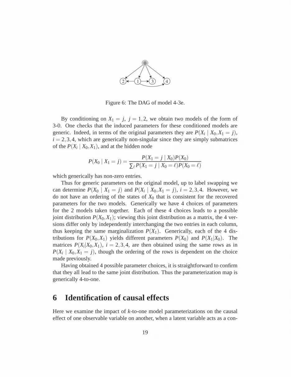
Figure 6: The DAG of model 4-3e.

By conditioning onX1 = j, j = 1,2, we obtain two models of the form of3-0. One checks that the induced parameters for these conditioned models aregeneric. Indeed, in terms of the original parameters they are P(Xi | X0,X1 = j),i = 2,3,4, which are generically non-singular since they are simplysubmatricesof theP(Xi | X0,X1), and at the hidden node

P(X0 | X1 = j) =P(X1 = j | X0)P(X0)

∑ℓP(X1 = j | X0 = ℓ)P(X0 = ℓ)

which generically has non-zero entries.Thus for generic parameters on the original model, up to label swapping we

can determineP(X0 | X1 = j) andP(Xi | X0,X1 = j), i = 2,3,4. However, wedo not have an ordering of the states ofX0 that is consistent for the recoveredparameters for the two models. Generically we have 4 choicesof parametersfor the 2 models taken together. Each of these 4 choices leadsto a possiblejoint distributionP(X0,X1); viewing this joint distribution as a matrix, the 4 ver-sions differ only by independently interchanging the two entries in each column,thus keeping the same marginalizationP(X1). Generically, each of the 4 dis-tributions for P(X0,X1) yields different parametersP(X0) and P(X1|X0). ThematricesP(Xi|X0,X1), i = 2,3,4, are then obtained using the same rows as inP(Xi | X0,X1 = j), though the ordering of the rows is dependent on the choicemade previously.

Having obtained 4 possible parameter choices, it is straightforward to confirmthat they all lead to the same joint distribution. Thus the parameterization map isgenerically 4-to-one.

6 Identification of causal effects

Here we examine the impact ofk-to-one model parameterizations on the causaleffect of one observable variable on another, when a latent variable acts as a con-

19

founder. For simplicity we assume that the latent variable is binary, though ourdiscussion can be extended to a more general setting.

According to Theorem 3.2.2 (Adjusting for Direct Causes), p. 73 of Pearl(2009), the causal effect ofXi on Xj can be obtained from model parameters byan appropriate sum over the states of the other direct causesof Xj . This sum isinvariant under a relabeling of the states of those direct causes, and therefore thecausal effect is not affected by label swapping if one of these is latent. As aninstance, the causal effect ofX1 on X2 in model 4-2b is:

P(X2 | do(X1 = x1)) = P(X2 | X1 = x1,X0 = 1)P(X0 = 1)

+P(X2 | X1 = x1,X0 = 2)P(X0 = 2). (8)

Thus when label swapping is the only source of parameter non-identifiability,causal effects are uniquely determined by the observable distribution.

Things are more complex when parameter non-identifiabilityarises in otherways. For example, model 4-3e has one binary latent variablebut a 4-to-1 pa-rameterization. In Table 1 two choices of parameters, (1), (2), are given for thismodel, as well as the common observable distribution they produce. These param-eters and their two variants from label swapping at node 0 give the four elementsof the fiber of the observable distribution.

For any parameters of model 4-3e, the causal effect ofX1 on X2 is again asgiven in equation (8). However, due to the 4-to-1 parameterization, there can betwo different causal effects that are consistent with an observable distribution. Assuch, there may be distributions such that one causal effectleads to the conclu-sion that there is a positive effect ofX1 on X2 (i.e., settingX1 = 2 gives a higherprobability of X2 = 2 than settingX1 = 1), while the other causal effect leads tothe conclusion that there is a negative effect ofX1 on X2. Indeed, the observabledistribution in Table 1 is such an instance. In Table 2 the twocausal effects cor-responding to that given distribution are shown. Here parameters (2) lead to apositive effect ofX1 on X2, while parameters (1) lead to a negative effect.

More generally, for generic observable distributions of this model, choicesof parameters that differ other than by label swapping will give different causaleffects. However, it varies whether the effects have the same or different signs.

7 Conclusion

Paraphrasing Pearl (2012), the problem of identifying causal effects in non-parametricmodels has been “placed to rest” by the proof of completenessof thedo-calculus

20

Table 1: A rational example for model 4-3e. The parameter choices (1) and (2)lead to the same observable distribution, shown at the bottom. For the 4×2 matrixparameters, row indices refer to states of a pair of parentsi < j ordered lexico-graphically as (1,1), (1,2), (2,1), (2,2), with the first entry referring to parenti, andthe second to parentj.(1)

p0 =(

2/5 3/5)

M1 =

(

2/5 3/514/15 1/15

)

M2 =

2/5 3/53/5 2/54/5 1/59/10 1/10

M3 =

1/5 4/59/20 11/201/2 1/22/5 3/5

M4 =

1/2 1/27/10 3/104/5 1/53/5 2/5

(2)

p′0 =(

1/5 4/5)

M′1 =

(

4/5 1/57/10 3/10

)

M′2 =

2/5 3/59/10 1/104/5 1/53/5 2/5

M′3 =

1/5 4/52/5 3/51/2 1/29/20 11/20

M′4 =

1/2 1/23/5 2/54/5 1/57/10 3/10

P(X1,X2,X3 = 1,X4 = 1) = P(X1,X2,X3 = 1,X4 = 2) =[

116/625 34/62527/500 39/1250

] [

32/625 13/62563/2500 17/1250

]

P(X1,X2,X3 = 2,X4 = 1) = P(X1,X2,X3 = 2,X4 = 2) =[

128/625 52/625171/2500 24/625

] [

44/625 31/62581/2500 21/1250

]

21

Table 2: The causal effects ofX1 on X2 for the example in Table 1.Parameters (a) (b) (a)−(b)

P(X2 = 2 | do(X1 = 2)) P(X2 = 2 | do(X1 = 1))

(1) 11/50 9/25 −7/50

(2) 17/50 7/25 3/50

and related graphical criteria. In this paper we show that the introduction of mod-est (parametric) assumptions on the size of the state spacesof variables allowsfor identifiability of parameters that otherwise would be non-identifiable. Causaleffects can be computed from identified parameters, if desired, but our techniquesallow for the recovery of all parameters. In the process of proving parameter iden-tifiability for several small networks, we use techniques inspired by a theoremof Kruskal, and other novel approaches. This framework can be applied to othermodels as well.

We have at least three reasons to extend the work described inthis paper. Thefirst is to develop new techniques and to prove new theoretical results for param-eter identifiability; this provides the foundation of our work. A second is to reachthe stage at which one can easily determine parameter identifiability for DAGmodels with hidden variables that are used in statistical modeling; this motivatesour work. A third and related focus of future work is to address the scalabilityof our approach and to automate it. As noted above many of our arguments donot depend on variables being binary. Also, a strategy that we used successfullyto handle larger models is to first marginalize or condition on an observable vari-able to reduce the model to one already understood, and then to ‘lift’ results onthe reduced model back to the original one. We are working towards turning thisstrategy into an algorithm.

Acknowledgments

The authors thank the American Institute of Mathematics, where this work wasbegun during a workshop on Parameter Identification in Graphical Models, andcontinued through AIM’s SQuaRE program.

22

Appendix

Table 3 shows all DAGs with 4 or fewer observable nodes and onehidden nodethat is a parent of all observable ones. See Section 5 for model naming conven-tion. Markov equivalent graphs appear on the same line. The dimension of theparameter space is dim(Θ), and 2A− 1 is the dimension of the probability sim-plex in which the joint distribution lies. The parameterization map is genericallyk-to-one.

Table 3: Small binary DAG models.

Model Graph dim(Θ) 2A−1 k2-B, B≥ 0 ≥ 5 3 ∞

3-0

0

1 2 3 7 7 23-Bx, B≥ 1 ≥ 9 7 ∞

4-0

0

1 2 3 4 9 15 2

4-1

0

1 2 3 4 11 15 2

4-2a

0

1 2 3 4 13 15 ∞

4-2b,c

0

1 2 3 4 ,

0

2 1 3 4 13 15 2

4-2d

0

1 3 2 4 15 15 2

4-3a,b

0

1 2 3 4 ,

0

2 1 3 4 15 15 2Continued on next page

23

Table 3 – continued from previous pageModel Graph dim(Θ) 2A−1 k

4-3c,d

0

1 3 2 4 ,

0

1 2 4 3 17 15 ∞

4-3e,f

0

2 1 3 4 ,

0

1 2 3 4 15 15 4

4-3g

0

1 2 3 4 17 15 ∞

4-3h

0

1 2 4 3 25 15 ∞

4-3i

0

1 2 3 4 25 15 ∞4-Bx, B≥ 4 ≥ 19 15 ∞

References

Allman, E., C. Matias, and J. Rhodes (2009): “Identifiability of parameters inlatent structure models with many observed variables,”Ann. Statist., 37, 3099–3132.

Chickering, D. M. (1995): “A transformational characterization of equivalentBayesian network structures,” inProceedings of the Eleventh Annual Confer-ence on Uncertainty in Artificial Intelligence (UAI-95), San Francisco, CA:Morgan Kaufmann, 87–98.

Huang, Y. and M. Valtorta (2006): “Pearl’s calculus of intervention is complete,”in Proceedings of the Twenty-second Conference on Uncertainty in ArtificialIntelligence (UAI-06), 217–224.

Kruskal, J. (1977): “Three-way arrays: rank and uniquenessof trilinear decompo-

24

sitions, with application to arithmetic complexity and statistics,”Linear Algebraand Appl., 18, 95–138.

Kuroki, M. and J. Pearl (2014): “Measurement bias and effectrestoration in causalinference,”Biometrika, 101, 423–437.

Lauritzen, S. L. (1996):Graphical models, Oxford Statistical Science Series, vol-ume 17, New York: The Clarendon Press Oxford University Press, Oxford Sci-ence Publications.

Meek, C. (1995): “Strong completeness and faithfulness in Bayesian networks,”in Proceedings of the Eleventh Annual Conference on Uncertainty in ArtificialIntelligence (UAI-95), San Francisco, CA: Morgan Kaufmann, 411–418.

Neapolitan, R. E. (1990):Probabilistic Reasoning in Expert Systems: Theory andAlgorithms, New York, NY: John Wiley and Sons.

Neapolitan, R. E. (2004):Learning Bayesian Networks, Upper Saddle River, NJ:Pearson Prentice Hall.

Pearl, J. (1995): “Causal diagrams for empirical research,” Biometrika, 82, 669–710.

Pearl, J. (2009):Causality: Models, reasoning, and inference, Cambridge Uni-versity Press, Cambridge, second edition.

Pearl, J. (2012): “The do-calculus revisited,” inProceedings of the Twenty-eighthConference on Uncertainty in Artificial Intelligence (UAI-12), 4–11.

Rhodes, J. (2010): “A concise proof of Kruskal’s theorem on tensor decomposi-tion,” Linear Algebra and its Applications, 432, 1818–1824.

Shpitser, I. and J. Pearl (2008): “Complete identification methods for the causalhierarchy,”J. Mach. Learn. Res., 9, 1941–1979.

Stanghellini, E. and B. Vantaggi (2013): “Identification ofdiscrete concentrationgraph models with one hidden binary variable,”Bernoulli, 19, 1920–1937, URLhttp://dx.doi.org/10.3150/12-BEJ435.

Stegeman, A. and N. D. Sidiropoulos (2007): “On Kruskal’s uniqueness conditionfor the Candecomp/Parafac decomposition,”Linear Algebra Appl., 420, 540–552.

25

Tian, J. and J. Pearl (2002): “A general identification condition for causal effects,”in Proceedings of the Eighteenth National Conference on Artificial Intelligence(AAAI-02), 567–573.

E.S. Allman, DEPARTMENT OFMATHEMATICS AND STATISTICS, UNIVERSITY OF ALASKA

FAIRBANKS , FAIRBANKS , AK 99775, USA,esallman@alaska.edu

J.A. Rhodes, DEPARTMENT OFMATHEMATICS AND STATISTICS, UNIVERSITY OF ALASKA

FAIRBANKS , FAIRBANKS , AK 99775, USA,j.rhodes@alaska.edu

E. Stanghellini, DIPARTIMENTO DI ECONOMIA FINANZA E STATISTICA , UNIVERSITA DI

PERUGIA, 06100 PERUGIA, ITALY , elena.stanghellini@stat.unipg.it

M. Valtorta, DEPARTMENT OFCOMPUTERSCIENCE AND ENGINEERING, UNIVERSITY OF

SOUTH CAROLINA , COLUMBIA , SC 29208, USA,MGV@cse.sc.edu

26