Pareto approximations for the bicriteria scheduling problem

J. Parallel Distrib. Comput. 66 (2006) 393–402www.elsevier.com/locate/jpdc

Pareto approximations for the bicriteria scheduling problem�

Vittorio Bilò∗, Michele Flammini, Luca MoscardelliDipartimento di Informatica, Università di L’Aquila, Via Vetoio loc. Coppito, I-67100 L’Aquila, Italy

Received 17 December 2004; accepted 12 July 2005Available online 19 September 2005

Abstract

In this paper, we consider the online bicriteria version of the classical Graham’s scheduling problem in which two cost measures mustbe simultaneously minimized.

We present a parametric family of online algorithms Fm ={Ak |1�k�m}, such that, for each fixed integer k, Ak is(

2m−km−k+1 , m+k−1

k

)-

competitive. Then we prove that, for m = 2 and 3, the tradeoffs on the competitive ratios realized by the algorithms in Fm correspondto the Pareto curve, that is they are all and only the optimal ones, while for m > 3 they give an r-approximation of the Pareto curve withr = 5

4 for m = 4, r = 65 for m = 5, r = 1.186 for m = 6 and so forth, with r always less than 1.295. Unfortunately, for m > 3, obtaining

Pareto curves is not trivial, as they would yield optimal algorithms for the single criterion case in correspondence of the extremal tradeoffs.

However, the situation seems more promising for the intermediate cases. In fact, we prove that for 5 processors the tradeoff(

73 , 7

3

)of

A3 ∈ F5 is optimal.Finally, we extend our results to the general d-dimensional case with corresponding applications to the Vector Scheduling problem.

© 2005 Elsevier Inc. All rights reserved.

Keywords: Multiprocessor scheduling; Online algorithms; Multicriteria optimization

1. Introduction

In this paper, we consider the multicriteria version of theclassical Graham’s scheduling problem in which each job ischaracterized by a d-tuple of costs, typically representing itsrequirement of d different resources. Jobs must be scheduledon m identical machines so as to minimize the makespan ormaximum resource utilization per processor with respect tothe d cost measures simultaneously. In such a setting, partic-ularly relevant is the bicriteria case in which the resourcesare the two fundamental ones, that is time and memory, bothin a scheduling and in a load balancing scenario. In a similar

� Work supported by the IST Programme of the EU under Contract No.IST-1999-14186 (ALCOM-FT), by the EU RTN project ARACNE, bythe Italian Research Project REAL-WINE, partially funded by the ItalianMinistry of Education, University and Research and by the Italian CNRproject CNRG003EF8.

∗ Corresponding author.E-mail addresses: [email protected] (V. Bilò), [email protected]

(M. Flammini), [email protected] (L. Moscardelli).

0743-7315/$ - see front matter © 2005 Elsevier Inc. All rights reserved.doi:10.1016/j.jpdc.2005.07.006

way, besides the time, the other measure could represent anallocation cost associated to the jobs that must be balancedas much as possible on the various machines while keepinga low completion time.

The single criterion version of this problem has beenextensively investigated in the literature since 1966, whenGraham proposed his

(2 − 1

m

)-competitive algorithm [12],

which has been proven to be optimal for m = 2 and 3 in [8].Nowadays much progress has been achieved in this field ofresearch, but despite the efforts of many researchers the de-termination of optimal online algorithms for m > 3 is stillan open problem.

In particular, in [8] it has been proved that for any m�4no algorithm can be less than 1 + 1√

2≈ 1.707-competitive.

This lower bound was improved in [3] to 1+ 1√2+�m, which

becomes 1.837 for large values of m. In [2], the authors pre-sented the first (2 − �)-competitive deterministic algorithmfor every m, where � = 1

70 , while the competitive ratiosof all previous algorithms approached 2 as m → ∞. This

http://www.elsevier.com/locate/jpdc

mailto:[email protected]



394 V. Bilò et al. / J. Parallel Distrib. Comput. 66 (2006) 393–402

upper bound has been improved to 1.945 in [17] and thento 1.923 in [1], where a new lower bound of 1.852 hasalso been shown for m�80. Finally, in [10] the authorsachieved a competitive ratio improving upon [1] for m�64

and approaching 1 +√

1+ln 22 < 1.9201 as m → ∞. For

the special case m = 4 a 1.733-competitive algorithm waspresented in [7] together with a lower bound of 1.731019and similar results for low values of m. A more detailed listof related results can be found in [4,9].

Considerable attention has been devoted to the topic ofscheduling so as to simultaneously optimize more than onecriterion, like the makespan, the average completion time,the minimum lateness and so forth. In such a setting, a set ofschedules is said to be “Pareto optimal’’ if no schedule existsthat is simultaneously better, in terms of the considered cri-teria, than any of the schedules in that set. Various bicriteriascheduling problems have been approached using the ideaof Pareto-optimal schedules [5,13–15,18–20,23,24]. Otherpapers have approached bicriteria scheduling by boundingthe value of one criterion and then optimizing the other one[16,21,22].

In this paper, we consider the bicriteria extension of Gra-ham’s scheduling problem in which jobs are characterizedby a pair of non-negative rational costs, representing forinstance a processing time and a memory size. Every jobmust be scheduled on one of the m processors so as to min-imize the time makespan and the maximum memory occu-pation per processor simultaneously. In such a setting, analgorithm is said (ct , cs)-competitive if it is independentlyct -competitive on the time and cs-competitive on the mem-ory. Since in general the two competitive ratios are conflict-ing, we are interested in finding algorithms that realize goodtradeoffs.

We present a parametric family of online algorithms Fm ={Ak|1�k�m}, such that each Ak is

(2m−k

m−k+1 , m+k−1k

)-

competitive, thus realizing m different time versus memorytradeoffs ranging from (2 − 1/m, m) to (m, 2 − 1/m).Even if it may seem that some of the above algorithmshave very high values on one of the two cost measures,we prove that, for m = 2 and 3, the tradeoffs on the com-petitive ratios of the family Fm correspond to the Paretocurve, that is they are all and only the optimal ones. More-over, we show that for m > 3 the families Fm give anr-approximation of the Pareto curve with r = 5

4 for m = 4,r = 6

5 for m = 5, r = 1.186 for m = 6 and so forth,with r always less than 1.295. Unfortunately, the task ofobtaining Pareto curves for m > 3 is not trivial, as theextremal tradeoffs would yield optimal algorithms for thesingle criterion case. However, we show that the situation issubstantially different and more promising for the interme-diate tradeoffs, as the algorithm A3 ∈ F5 is optimal for 5processors.

Finally, we extend our family of algorithms to the gen-eral d-dimensional case in which we have to simultane-ously optimize d different cost measures, and prove that

each algorithm is(

2m−k1m−k1+1 , . . . ,

m+kl−1−kl

kl−1−kl+1 , . . . ,m+kd−1−1

kd−1

)-

competitive, where l = 2, . . . , d − 1, 1�kl �m for l =1, . . . , d−1 and kl �kl+1 for l = 1, . . . , d−2. We then showthat there exists a suitable algorithm in this family obtainedby setting kl = m−l�m−1

d� for each l = 1, . . . , d−1, which

achieves a maximum competitive ratio equal to d + 1 − dm

,

in spite of an �(

log dlog log d

)lower bound.

A problem related to the one investigated in this paperand to the best of our knowledge never considered underan online point of view is known as Vector Scheduling[6,11]. It consists in minimizing the maximum makespanwith respect to d different cost measures. Since the min-imization of the maximum competitive ratio is a strongerform of Vector Scheduling, as a consequence of our resultsa (d +1− d

m)-competitive algorithm is obtained also for this

problem.The paper is organized as follows: In Section 2, we intro-

duce the notation and necessary definitions. In Section 3, wepresent our family of algorithms for the bicriteria case andprove the corresponding competitive ratios. In Section 4, weprove bicriteria lower bounds allowing the evaluation of theperformances of our families in terms of distance from thePareto curve. In Section 5, we extend our results to the gen-eral d-dimensional case and finally, in the last section, wegive some conclusive remarks and open questions.

2. Definitions and notation

Let us first give the necessary notation and definitionsfor the bicriteria case with just two dimensions, leaving theextension to the following sections. We denote by m thenumber of machines and by � = 〈p1, . . . , pn〉 the sequenceof the input jobs. Each job pj with 1�j �n is characterizedby a pair of costs (tj , sj ), where tj represents the processingtime of pj and sj its memory size or occupation. Everyjob must be scheduled on one of the m processors so asto minimize the time makespan and the maximum memoryoccupation per processor simultaneously.

A scheduling algorithm A is online if it assigns each jobpj of � to one of the m machines without any knowledgeof the successive jobs. We denote by T i

j (A) the completiontime of machine i once scheduled the jth job according to Aand by Tj the total processing time of the first j jobs, that is∑j

h=1 th or analogously∑m

i=1 T ij (A). Similarly, let Si

j (A)

be the memory occupation on machine i once scheduled thejth job according to A and Sj be the total memory occupationof the first j jobs. The time and memory costs of A aret (A, �) = maxm

i=1Tin(A) and s(A, �) = maxm

i=1Sin(A). For

the sake of simplicity, when the algorithm A is clear fromthe context, we will drop A from the notation.

Let t∗(�) be the minimum time makespan required toprocess � independently from the memory cost measure.Similarly, let s∗(�) be the minimum memory occupation permachine required by � ignoring the time.

V. Bilò et al. / J. Parallel Distrib. Comput. 66 (2006) 393–402 395

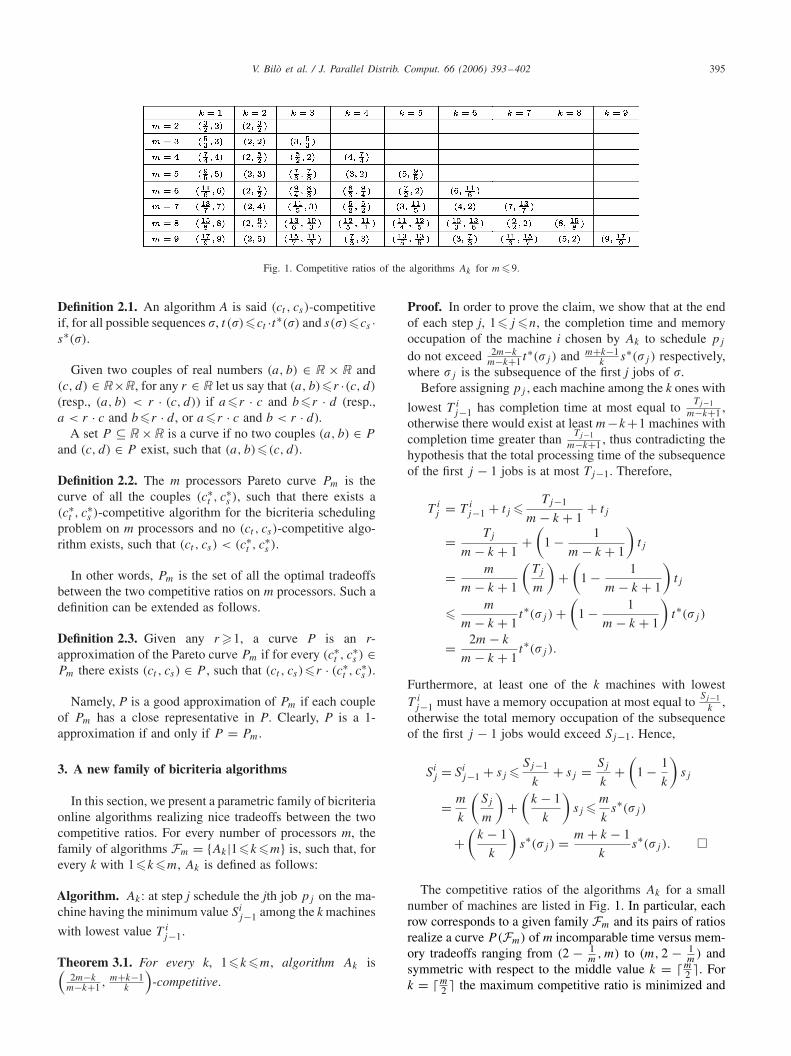
Fig. 1. Competitive ratios of the algorithms Ak for m�9.

Definition 2.1. An algorithm A is said (ct , cs)-competitiveif, for all possible sequences �, t (�)�ct ·t∗(�) and s(�)�cs ·s∗(�).

Given two couples of real numbers (a, b) ∈ R × R and(c, d) ∈ R×R, for any r ∈ R let us say that (a, b)�r ·(c, d)

(resp., (a, b) < r · (c, d)) if a�r · c and b�r · d (resp.,a < r · c and b�r · d , or a�r · c and b < r · d).

A set P ⊆ R×R is a curve if no two couples (a, b) ∈ P

and (c, d) ∈ P exist, such that (a, b)�(c, d).

Definition 2.2. The m processors Pareto curve Pm is thecurve of all the couples (c∗

t , c∗s ), such that there exists a

(c∗t , c

∗s )-competitive algorithm for the bicriteria scheduling

problem on m processors and no (ct , cs)-competitive algo-rithm exists, such that (ct , cs) < (c∗

t , c∗s ).

In other words, Pm is the set of all the optimal tradeoffsbetween the two competitive ratios on m processors. Such adefinition can be extended as follows.

Definition 2.3. Given any r �1, a curve P is an r-approximation of the Pareto curve Pm if for every (c∗

t , c∗s ) ∈

Pm there exists (ct , cs) ∈ P , such that (ct , cs)�r · (c∗t , c

∗s ).

Namely, P is a good approximation of Pm if each coupleof Pm has a close representative in P. Clearly, P is a 1-approximation if and only if P = Pm.

3. A new family of bicriteria algorithms

In this section, we present a parametric family of bicriteriaonline algorithms realizing nice tradeoffs between the twocompetitive ratios. For every number of processors m, thefamily of algorithms Fm = {Ak|1�k�m} is, such that, forevery k with 1�k�m, Ak is defined as follows:

Algorithm. Ak: at step j schedule the jth job pj on the ma-chine having the minimum value Si

j−1 among the k machines

with lowest value T ij−1.

Theorem 3.1. For every k, 1�k�m, algorithm Ak is(2m−k

m−k+1 , m+k−1k

)-competitive.

Proof. In order to prove the claim, we show that at the endof each step j, 1�j �n, the completion time and memoryoccupation of the machine i chosen by Ak to schedule pj

do not exceed 2m−km−k+1 t∗(�j ) and m+k−1

ks∗(�j ) respectively,

where �j is the subsequence of the first j jobs of �.Before assigning pj , each machine among the k ones with

lowest T ij−1 has completion time at most equal to

Tj−1m−k+1 ,

otherwise there would exist at least m−k+1 machines withcompletion time greater than

Tj−1m−k+1 , thus contradicting the

hypothesis that the total processing time of the subsequenceof the first j − 1 jobs is at most Tj−1. Therefore,

T ij = T i

j−1 + tj � Tj−1

m − k + 1+ tj

= Tj

m − k + 1+

(1 − 1

m − k + 1

)tj

= m

m − k + 1

(Tj

m

)+

(1 − 1

m − k + 1

)tj

� m

m − k + 1t∗(�j ) +

(1 − 1

m − k + 1

)t∗(�j )

= 2m − k

m − k + 1t∗(�j ).

Furthermore, at least one of the k machines with lowestT i

j−1 must have a memory occupation at most equal toSj−1

k,

otherwise the total memory occupation of the subsequenceof the first j − 1 jobs would exceed Sj−1. Hence,

Sij = Si

j−1 + sj � Sj−1

k+ sj = Sj

k+

(1 − 1

k

)sj

= m

k

(Sj

m

)+

(k − 1

k

)sj � m

ks∗(�j )

+(

k − 1

k

)s∗(�j ) = m + k − 1

ks∗(�j ). �

The competitive ratios of the algorithms Ak for a smallnumber of machines are listed in Fig. 1. In particular, eachrow corresponds to a given family Fm and its pairs of ratiosrealize a curve P(Fm) of m incomparable time versus mem-ory tradeoffs ranging from (2 − 1

m, m) to (m, 2 − 1

m) and

symmetric with respect to the middle value k = �m2 . For

k = �m2 the maximum competitive ratio is minimized and


is always at most equal to 3 − 4m+1 if m is odd and 3 − 2

mif m is even, thus approaching 3 as m goes to infinity. Set-ting k = 1 (resp., k = m) is equivalent to schedule the jobson the m machines according to the Graham’s algorithm ap-plied only on the time (resp., memory) cost measure. In fact,the same competitive ratio (2 − 1

m) is achieved for such a

measure.Some of the above algorithms seem to have an unreason-

able high value for one of the two competitive ratios, as inthe cases k = 1 or m. However, in the next section we showthat P(Fm) coincides with the Pareto curve Pm for m�3and is a good approximation of Pm for m > 3.

4. Lower bounds

In this section, we provide suitable lower bounds on thecompetitive ratios of the online bicriteria scheduling problemallowing to prove the optimality or r-approximation of thecurves P(Fm).

All the lower bounds are based on the following tech-nique. Given a bicriteria algorithm A, we select a subset Fof k < m processors and an input sequence � = �1 · · · · · �q

obtained by the concatenation of a finite number q of similarsubsequences �i . Each �i corresponds to a subsequence ofvariable length terminating with the first job that A sched-ules on one of the processors of F. The jth job pi,j of �i

has costs (�i�j , 1/�l−j+1) with �i , �j , � and l determinedas follows. �i is a sufficiently large scaling parameter mak-ing sure that at each subsequence i the processing times ofthe jobs belonging to the previous subsequences are neg-ligible. When considering the time measure, this allows tohandle each subsequence in the same way, that is ignoringthe allocation of the jobs of the previous subsequences. Inorder to obtain the claimed lower bounds, the terms �j arechosen in such a way that, if the algorithm A is less than ct -competitive on the time, then each subsequence i has lengthli � l, that is in at most l steps one job is scheduled on oneof the processors of F. Thus, if � is sufficiently large, sinceduring a subsequence the memory occupation of the jobs ateach step is multiplied times � and the last job is scheduledon one processor of F, at the end of each subsequence anhigh overall memory occupation on F is obtained with re-spect to the other processors. As a consequence, running asufficient number of subsequences q in such a way that thereexist optimal solutions with a balanced memory occupationof the processors, a high competitive ratio cs is forced onthe memory.

Even if for the sake of brevity we do not claim it explic-itly, all the symmetric lower bounds obtained from the onesbelow by exchanging the two cost measures hold.

The following lemma states that if we want to be less than2-competitive on one cost measure, then we are forced to paythe worst possible competitive ratio on the other one, that ism. As a consequence, the optimal extremal tradeoffs, that isthe ones in which one of the two competitive ratios is less

than 2, are yielded by optimal single-criterion algorithmsthat ignore one of the two cost measures.

Lemma 4.1. No (ct , cs)-competitive algorithm for the bi-criteria scheduling problem exists with ct < 2 and cs < m.

Proof. Assume by contradiction that there exists a (ct , cs)-competitive algorithm with ct < 2 and cs < m and let Fcontain a single processor M chosen arbitrarily among the mavailable ones. Recalling the above general description of the

lower bound technique, let �i = �i with � =(

(m+1)ct

2−ct+ 1

),

� = 2mcs

m−cs+ 1 and �j = 1.

Then each subsequence �i of � = �1 · · · · · �q has lengthli �m, as A cannot schedule two jobs of �i on the samemachine. In fact, this would cause a time load on such amachine at least equal to 2�i , that compared with the value�i + (m + 1)�i−1, which is a trivial upper bound on theoptimal offline solution (it is obtained spreading only the�i jobs among all the machines), gives a competitive ratiostrictly greater than ct since � >

(m+1)ct

2−ct. Moreover, since

the last job of �i is scheduled on M and each pi,j has amemory occupation exactly � times the one of pi,j−1, atthe end of every subsequence the memory load of machineM is always at least � times the one of any other machine.Let q be the smallest integer such that the memory loadSM of M can be spread on all the m machines so as tofill each of them of a value at least equal to 1. Then s∗(�)

can be upper bounded by 1 plus the maximum memoryload of a job (at most 1

� ) and the maximum memory load

among the machines not belonging to F (at most SM

� ). Thus

s∗(�)�1 + 1� + SM

� � SM

m+ SM

� + SM

� = SM�+2m

�m, since

SM �m�1. This implies that the algorithm has a memorycompetitive ratio equal to SM

s∗(�)�SM

�m

SM(�+2m)> cs , since

� > 2mcs

m−cs: a contradiction. �

As a direct consequence of the above lemma, the familiesF2 and F3 are optimal.

Theorem 4.1. P(F2) = P2 and P(F3) = P3.

Proof. For m = 2 the claim derives by observing that noalgorithm can be less than 3

2 competitive on one cost measure[8] and that by Lemma 4.1 one of the two competitive ratiosmust always be at least equal to 2. Therefore, P(F2) containsall and only the optimal tradeoffs.

Similarly, for m = 3, no algorithm can be less than 53

competitive on one cost measure [8] and by Lemma 4.1 theonly optimal tradeoffs are the one contained in P(F3). �

We now prove a general lower bound useful for deter-mining the approximation ratios of the curves P(Fm) form > 3.

Again, according to our lower bound technique, we se-lect a subset F of k processors such that 2�k��m

2 . Given


any (ct , cs)-competitive algorithm A with ct <(

2 + 1� m

k−1 )

,

assuming by contradiction that cs < mk

, the costs of thejobs are determined as follows. We set �i = �i with � =(

m2m(2+ 1⌈

mk−1

⌉)−ct

)and � = m4

mk−cs

, while each subsequence

�i is divided into phases of m − k + 1 jobs and the value �j

is incremented during every phase in such a way that �j = 1if j �m − k + 1 and �j = c(c + 1)n−2 with c = �m−k+1

k−1 if (w − 1)(m − k + 1) + 1�j �n(m − k + 1) and w > 1,i.e., for the wth phase.

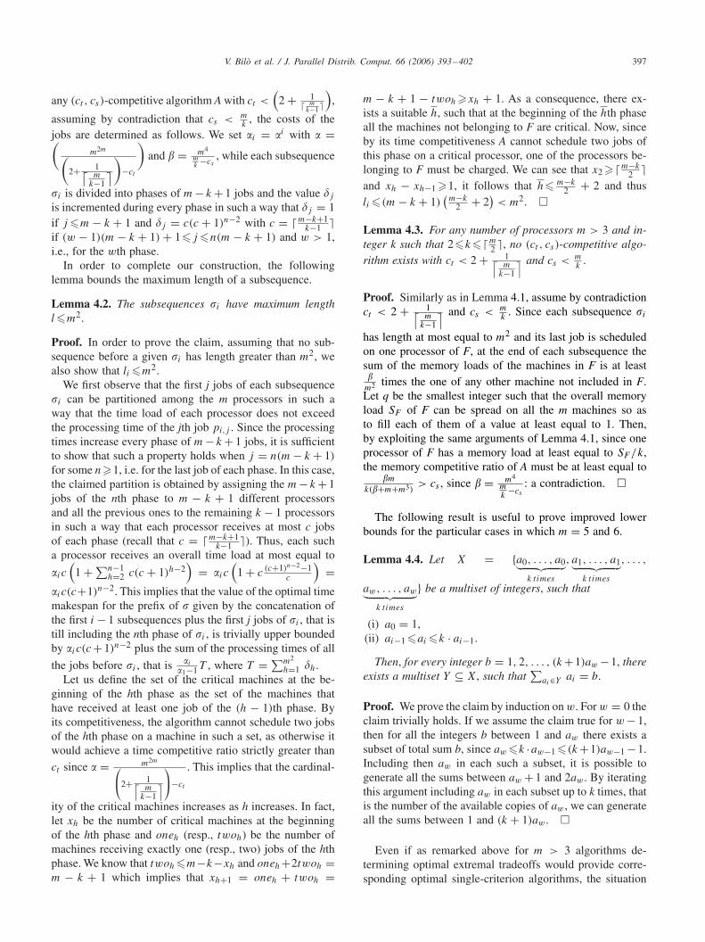
In order to complete our construction, the followinglemma bounds the maximum length of a subsequence.

Lemma 4.2. The subsequences �i have maximum lengthl�m2.

Proof. In order to prove the claim, assuming that no sub-sequence before a given �i has length greater than m2, wealso show that li �m2.

We first observe that the first j jobs of each subsequence�i can be partitioned among the m processors in such away that the time load of each processor does not exceedthe processing time of the jth job pi,j . Since the processingtimes increase every phase of m− k + 1 jobs, it is sufficientto show that such a property holds when j = n(m − k + 1)

for some n�1, i.e. for the last job of each phase. In this case,the claimed partition is obtained by assigning the m− k + 1jobs of the nth phase to m − k + 1 different processorsand all the previous ones to the remaining k − 1 processorsin such a way that each processor receives at most c jobsof each phase (recall that c = �m−k+1

k−1 ). Thus, each sucha processor receives an overall time load at most equal to

�ic(

1 + ∑n−1h=2 c(c + 1)h−2

)= �ic

(1 + c

(c+1)n−2−1c

)=

�ic(c+1)n−2. This implies that the value of the optimal timemakespan for the prefix of � given by the concatenation ofthe first i − 1 subsequences plus the first j jobs of �i , that istill including the nth phase of �i , is trivially upper boundedby �ic(c + 1)n−2 plus the sum of the processing times of all

the jobs before �i , that is �i

�1−1T , where T = ∑m2

h=1 �h.Let us define the set of the critical machines at the be-

ginning of the hth phase as the set of the machines thathave received at least one job of the (h − 1)th phase. Byits competitiveness, the algorithm cannot schedule two jobsof the hth phase on a machine in such a set, as otherwise itwould achieve a time competitive ratio strictly greater thanct since � = m2m⎛

⎝2+ 1⌈m

k−1

⌉⎞⎠−ct

. This implies that the cardinal-

ity of the critical machines increases as h increases. In fact,let xh be the number of critical machines at the beginningof the hth phase and oneh (resp., twoh) be the number ofmachines receiving exactly one (resp., two) jobs of the hthphase. We know that twoh �m−k−xh and oneh+2twoh =m − k + 1 which implies that xh+1 = oneh + twoh =

m − k + 1 − twoh �xh + 1. As a consequence, there ex-ists a suitable h, such that at the beginning of the hth phaseall the machines not belonging to F are critical. Now, sinceby its time competitiveness A cannot schedule two jobs ofthis phase on a critical processor, one of the processors be-longing to F must be charged. We can see that x2 ��m−k

2 and xh − xh−1 �1, it follows that h� m−k

2 + 2 and thusli �(m − k + 1)

(m−k

2 + 2)

< m2. �

Lemma 4.3. For any number of processors m > 3 and in-teger k such that 2�k��m

2 , no (ct , cs)-competitive algo-rithm exists with ct < 2 + 1⌈

mk−1

⌉ and cs < mk

.

Proof. Similarly as in Lemma 4.1, assume by contradictionct < 2 + 1⌈

mk−1

⌉ and cs < mk

. Since each subsequence �i

has length at most equal to m2 and its last job is scheduledon one processor of F, at the end of each subsequence thesum of the memory loads of the machines in F is at least�m2 times the one of any other machine not included in F.Let q be the smallest integer such that the overall memoryload SF of F can be spread on all the m machines so asto fill each of them of a value at least equal to 1. Then,by exploiting the same arguments of Lemma 4.1, since oneprocessor of F has a memory load at least equal to SF /k,the memory competitive ratio of A must be at least equal to

�m

k(�+m+m3)> cs , since � = m4

mk

−cs

: a contradiction. �

The following result is useful to prove improved lowerbounds for the particular cases in which m = 5 and 6.

Lemma 4.4. Let X = {a0, . . . , a0︸︷︷︸k times

, a1, . . . , a1︸︷︷︸k times

, . . . ,

aw, . . . , aw︸︷︷︸k times

} be a multiset of integers, such that

(i) a0 = 1,(ii) ai−1 �ai �k · ai−1.

Then, for every integer b = 1, 2, . . . , (k +1)aw −1, thereexists a multiset Y ⊆ X, such that

∑ai∈Y ai = b.

Proof. We prove the claim by induction on w. For w = 0 theclaim trivially holds. If we assume the claim true for w − 1,then for all the integers b between 1 and aw there exists asubset of total sum b, since aw �k ·aw−1 �(k +1)aw−1 −1.Including then aw in each such a subset, it is possible togenerate all the sums between aw + 1 and 2aw. By iteratingthis argument including aw in each subset up to k times, thatis the number of the available copies of aw, we can generateall the sums between 1 and (k + 1)aw. �

Even if as remarked above for m > 3 algorithms de-termining optimal extremal tradeoffs would provide corre-sponding optimal single-criterion algorithms, the situation


seems to be more promising for the intermediate cases. Infact, as a direct consequence of the following lemma, algo-rithm A3 ∈ F5 realizes an optimal tradeoff

( 73 , 7

3

) ∈ P5 for5 processors.

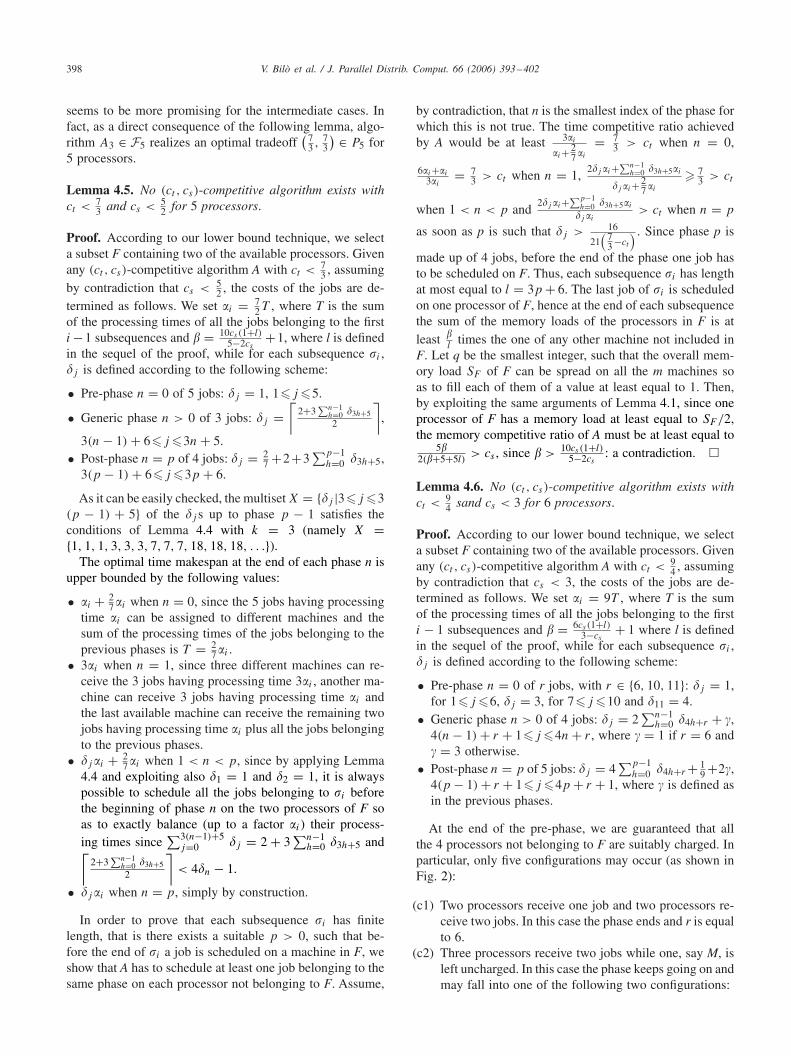
Lemma 4.5. No (ct , cs)-competitive algorithm exists withct < 7

3 and cs < 52 for 5 processors.

Proof. According to our lower bound technique, we selecta subset F containing two of the available processors. Givenany (ct , cs)-competitive algorithm A with ct < 7

3 , assumingby contradiction that cs < 5

2 , the costs of the jobs are de-termined as follows. We set �i = 7

2T , where T is the sumof the processing times of all the jobs belonging to the firsti −1 subsequences and � = 10cs (1+l)

5−2cs+1, where l is defined

in the sequel of the proof, while for each subsequence �i ,�j is defined according to the following scheme:

• Pre-phase n = 0 of 5 jobs: �j = 1, 1�j �5.

• Generic phase n > 0 of 3 jobs: �j =⌈

2+3∑n−1

h=0 �3h+52

⌉,

3(n − 1) + 6�j �3n + 5.• Post-phase n = p of 4 jobs: �j = 2

7 +2+3∑p−1

h=0 �3h+5,3(p − 1) + 6�j �3p + 6.

As it can be easily checked, the multiset X = {�j |3�j �3(p − 1) + 5} of the �j s up to phase p − 1 satisfies theconditions of Lemma 4.4 with k = 3 (namely X ={1, 1, 1, 3, 3, 3, 7, 7, 7, 18, 18, 18, . . .}).

The optimal time makespan at the end of each phase n isupper bounded by the following values:

• �i + 27�i when n = 0, since the 5 jobs having processing

time �i can be assigned to different machines and thesum of the processing times of the jobs belonging to theprevious phases is T = 2

7�i .• 3�i when n = 1, since three different machines can re-

ceive the 3 jobs having processing time 3�i , another ma-chine can receive 3 jobs having processing time �i andthe last available machine can receive the remaining twojobs having processing time �i plus all the jobs belongingto the previous phases.

• �j�i + 27�i when 1 < n < p, since by applying Lemma

4.4 and exploiting also �1 = 1 and �2 = 1, it is alwayspossible to schedule all the jobs belonging to �i beforethe beginning of phase n on the two processors of F soas to exactly balance (up to a factor �i) their process-ing times since

∑3(n−1)+5j=0 �j = 2 + 3

∑n−1h=0 �3h+5 and⌈

2+3∑n−1

h=0 �3h+52

⌉< 4�n − 1.

• �j�i when n = p, simply by construction.

In order to prove that each subsequence �i has finitelength, that is there exists a suitable p > 0, such that be-fore the end of �i a job is scheduled on a machine in F, weshow that A has to schedule at least one job belonging to thesame phase on each processor not belonging to F. Assume,

by contradiction, that n is the smallest index of the phase forwhich this is not true. The time competitive ratio achievedby A would be at least 3�i

�i+ 27 �i

= 73 > ct when n = 0,

6�i+�i

3�i= 7

3 > ct when n = 1,2�j�i+∑n−1

h=0 �3h+5�i

�j�i+ 27 �i

� 73 > ct

when 1 < n < p and2�j�i+∑p−1

h=0 �3h+5�i

�j�i> ct when n = p

as soon as p is such that �j > 16

21(

73 −ct

) . Since phase p is

made up of 4 jobs, before the end of the phase one job hasto be scheduled on F. Thus, each subsequence �i has lengthat most equal to l = 3p + 6. The last job of �i is scheduledon one processor of F, hence at the end of each subsequencethe sum of the memory loads of the processors in F is atleast �

ltimes the one of any other machine not included in

F. Let q be the smallest integer, such that the overall mem-ory load SF of F can be spread on all the m machines soas to fill each of them of a value at least equal to 1. Then,by exploiting the same arguments of Lemma 4.1, since oneprocessor of F has a memory load at least equal to SF /2,the memory competitive ratio of A must be at least equal to

5�2(�+5+5l)

> cs , since � >10cs (1+l)

5−2cs: a contradiction. �

Lemma 4.6. No (ct , cs)-competitive algorithm exists withct < 9

4 sand cs < 3 for 6 processors.

Proof. According to our lower bound technique, we selecta subset F containing two of the available processors. Givenany (ct , cs)-competitive algorithm A with ct < 9

4 , assumingby contradiction that cs < 3, the costs of the jobs are de-termined as follows. We set �i = 9T , where T is the sumof the processing times of all the jobs belonging to the firsti − 1 subsequences and � = 6cs (1+l)

3−cs+ 1 where l is defined

in the sequel of the proof, while for each subsequence �i ,�j is defined according to the following scheme:

• Pre-phase n = 0 of r jobs, with r ∈ {6, 10, 11}: �j = 1,for 1�j �6, �j = 3, for 7�j �10 and �11 = 4.

• Generic phase n > 0 of 4 jobs: �j = 2∑n−1

h=0 �4h+r + �,4(n − 1) + r + 1�j �4n + r , where � = 1 if r = 6 and� = 3 otherwise.

• Post-phase n = p of 5 jobs: �j = 4∑p−1

h=0 �4h+r + 19 +2�,

4(p − 1) + r + 1�j �4p + r + 1, where � is defined asin the previous phases.

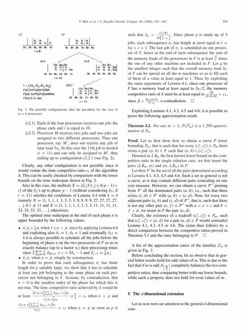
At the end of the pre-phase, we are guaranteed that allthe 4 processors not belonging to F are suitably charged. Inparticular, only five configurations may occur (as shown inFig. 2):

(c1) Two processors receive one job and two processors re-ceive two jobs. In this case the phase ends and r is equalto 6.

(c2) Three processors receive two jobs while one, say M, isleft uncharged. In this case the phase keeps going on andmay fall into one of the following two configurations:


Fig. 2. The possible configurations after the pre-phase for the case ofm = 6 processors.

(c2.1) Each of the four processors receives one job: thephase ends and r is equal to 10.

(c2.2) Processor M receives two jobs and two jobs areassigned to two different processors. Thus oneprocessor, say M ′, does not receive any job oftime load 3�i . In this case the 11th job is needed(r = 11) and can only be assigned to M ′, thusending up to configuration c2.2.1 (see Fig. 2).

Clearly, any other configuration is not possible since itwould violate the time competitive ratio ct of the algorithmA. This can be easily checked by comparison with the lowerbounds on the time makespan shown in Fig. 2.

Also in this case, the multiset X = {�j |3�j �4(p−1)+r} of the �j ’s up to phase p − 1 (without considering �11 ifr = 11) satisfies the conditions of Lemma 4.4 with k = 4(namely X = {1, 1, 1, 1, 3, 3, 3, 3, 9, 9, 9, 9, 27, 27, 27, 27,

. . .} if r �= 11 and X = {1, 1, 1, 1, 3, 3, 3, 3, 11, 11, 11, 11,

33, 33, 33, 33, . . .} otherwise).The optimal time makespan at the end of each phase n is

upper bounded by the following values:

• �j�i + 19�i when 1�n < p, since by applying Lemma 4.4

and exploiting also �1 = 1, �2 = 1 and eventually �11 =4 it is always possible to schedule all the jobs before thebeginning of phase n on the two processors of F so as toexactly balance (up to a factor �i) their processing timessince 2

∑n−1h=0 �4h+r + � < 5�n − 1 and Ti−1 = 1

9�i ;• �j�i when n = p, simply by construction.

In order to prove that each subsequence �i has finitelength for p suitably large, we show that A has to scheduleat least one job belonging to the same phase on each pro-cessor not belonging to F. Assume, by contradiction, thatn > 0 is the smallest index of the phase for which this isnot true. The time competitive ratio achieved by A would be

at least2�j�i+

(∑n−1h=0 �4h+r+�

)�i

�j�i+ 19 �i

� 94 > ct when n < p and

2�j�i+(∑p−1

h=0 �4h+r+�)�i

�j�i> ct when n = p as soon as p is

such that �p >1+18�

36(

94 −ct

) . Since phase p is made up of 5

jobs, each subsequence �i has length at most equal to l =4p + r + 1. The last job of �i is scheduled on one proces-sor of F, hence at the end of each subsequence the sum ofthe memory loads of the processors in F is at least �

ltimes

the one of any other machine not included in F. Let q bethe smallest integer such that the overall memory load SF

of F can be spread on all the m machines so as to fill eachof them of a value at least equal to 1. Then, by exploitingthe same arguments of Lemma 4.1, since one processor ofF has a memory load at least equal to SF /2, the memorycompetitive ratio of A must be at least equal to 3�

�+6+6l> cs ,

since � >6cs (1+l)

3−cs: a contradiction. �

Exploiting Lemmas 4.1, 4.3, 4.5 and 4.6, it is possible toprove the following approximation result.

Theorem 4.2. For any m > 3, P(Fm) is a 1.295-approxi-mation of Pm.

Proof. Let us first show how to obtain a curve P lowerbounding Pm, that is such that for every (c∗

t , c∗s ) ∈ Pm there

exists a pair (a, b) ∈ P such that (a, b)�(c∗t , c

∗s ).

Denoted as LBm the best known lower bound on the com-petitive ratio in the single criterion case, we first insert thepairs (LBm, m) and (m, LBm) in P.

Let then P ′ be the set of all the pairs determined accordingto Lemma 4.1, 4.3, 4.5 and 4.6. Such a set in general is nota curve, as it may contain different pairs coinciding on onecost measure. However, we can obtain a curve P ′′ pruningfrom P ′ all the dominated pairs (a, b), i.e., such that thereexists (c, d) ∈ P ′ with (a, b) < (c, d). Now, for every twoadjacent pairs (a, b) and (c, d) of P ′′, that is, such that thereis not any other pair (e, f ) ∈ P ′′ with a < e < c and b >

f > d, we insert in P the pair (a, d).Clearly, the existence of a tradeoff (c∗

t , c∗s ) ∈ Pm, such

that (c∗t , c

∗s ) < (a, d) for a pair (a, d) ∈ P would contradict

Lemma 4.1, 4.3, 4.5 or 4.6. The claim then follows by adirect comparison between the competitive ratios proved inTheorem 3.1 and the ones belonging to P. �

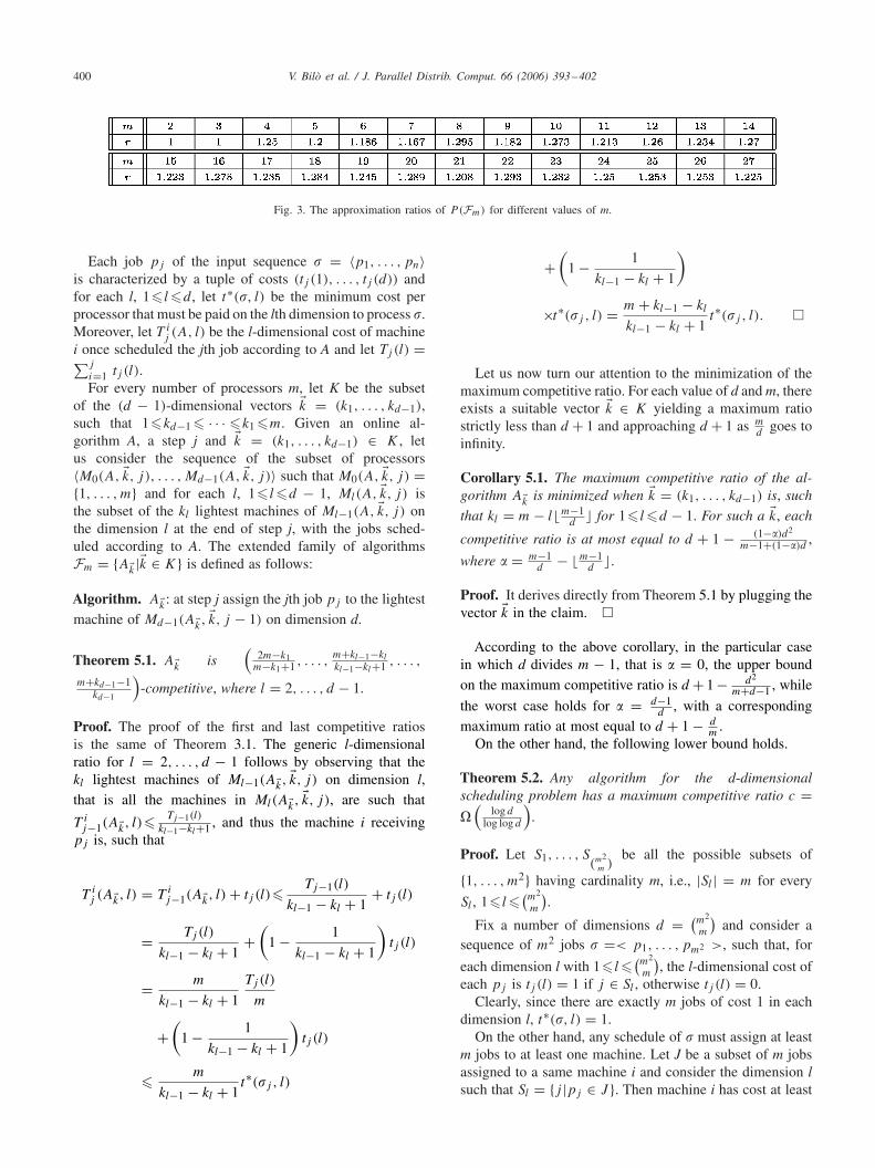
A list of the approximation ratios of the families Fm isgiven in Fig. 3.

Before concluding the section, let us observe that in gen-eral better results hold for odd values of m. This is due to thefact that if m is odd A⌈

m2

⌉ completely balances the two com-

petitive ratios, thus comparing better with our lower bounds,while such a property does not hold for even values of m.

5. The d-dimensional extension

Let us now turn our attention to the general d-dimensionalcase.


Fig. 3. The approximation ratios of P(Fm) for different values of m.

Each job pj of the input sequence � = 〈p1, . . . , pn〉is characterized by a tuple of costs (tj (1), . . . , tj (d)) andfor each l, 1� l�d , let t∗(�, l) be the minimum cost perprocessor that must be paid on the lth dimension to process �.Moreover, let T i

j (A, l) be the l-dimensional cost of machinei once scheduled the jth job according to A and let Tj (l) =∑j

i=1 tj (l).For every number of processors m, let K be the subset

of the (d − 1)-dimensional vectors �k = (k1, . . . , kd−1),such that 1�kd−1 � · · · �k1 �m. Given an online al-gorithm A, a step j and �k = (k1, . . . , kd−1) ∈ K , letus consider the sequence of the subset of processors〈M0(A, �k, j), . . . , Md−1(A, �k, j)〉 such that M0(A, �k, j) ={1, . . . , m} and for each l, 1� l�d − 1, Ml(A, �k, j) isthe subset of the kl lightest machines of Ml−1(A, �k, j) onthe dimension l at the end of step j, with the jobs sched-uled according to A. The extended family of algorithmsFm = {A�k|�k ∈ K} is defined as follows:

Algorithm. A�k: at step j assign the jth job pj to the lightestmachine of Md−1(A�k, �k, j − 1) on dimension d.

Theorem 5.1. A�k is(

2m−k1m−k1+1 , . . . ,

m+kl−1−kl

kl−1−kl+1 , . . . ,

m+kd−1−1kd−1

)-competitive, where l = 2, . . . , d − 1.

Proof. The proof of the first and last competitive ratiosis the same of Theorem 3.1. The generic l-dimensionalratio for l = 2, . . . , d − 1 follows by observing that thekl lightest machines of Ml−1(A�k, �k, j) on dimension l,that is all the machines in Ml(A�k, �k, j), are such that

T ij−1(A�k, l)�

Tj−1(l)

kl−1−kl+1 , and thus the machine i receivingpj is, such that

T ij (A�k, l) = T i

j−1(A�k, l) + tj (l)�Tj−1(l)

kl−1 − kl + 1+ tj (l)

= Tj (l)

kl−1 − kl + 1+

(1 − 1

kl−1 − kl + 1

)tj (l)

= m

kl−1 − kl + 1

Tj (l)

m

+(

1 − 1

kl−1 − kl + 1

)tj (l)

� m

kl−1 − kl + 1t∗(�j , l)

+(

1 − 1

kl−1 − kl + 1

)

×t∗(�j , l) = m + kl−1 − kl

kl−1 − kl + 1t∗(�j , l). �

Let us now turn our attention to the minimization of themaximum competitive ratio. For each value of d and m, thereexists a suitable vector �k ∈ K yielding a maximum ratiostrictly less than d + 1 and approaching d + 1 as m

dgoes to

infinity.

Corollary 5.1. The maximum competitive ratio of the al-gorithm A�k is minimized when �k = (k1, . . . , kd−1) is, such

that kl = m − l�m−1d

� for 1� l�d − 1. For such a �k, each

competitive ratio is at most equal to d + 1 − (1−�)d2

m−1+(1−�)d,

where � = m−1d

− �m−1d

�.

Proof. It derives directly from Theorem 5.1 by plugging thevector �k in the claim. �

According to the above corollary, in the particular casein which d divides m − 1, that is � = 0, the upper boundon the maximum competitive ratio is d + 1 − d2

m+d−1 , while

the worst case holds for � = d−1d

, with a correspondingmaximum ratio at most equal to d + 1 − d

m.

On the other hand, the following lower bound holds.

Theorem 5.2. Any algorithm for the d-dimensionalscheduling problem has a maximum competitive ratio c =�

(log d

log log d

).

Proof. Let S1, . . . , S(m2

m )be all the possible subsets of

{1, . . . , m2} having cardinality m, i.e., |Sl | = m for every

Sl , 1� l�(m2

m

).

Fix a number of dimensions d = (m2

m

)and consider a

sequence of m2 jobs � =< p1, . . . , pm2 >, such that, for

each dimension l with 1� l�(m2

m

), the l-dimensional cost of

each pj is tj (l) = 1 if j ∈ Sl , otherwise tj (l) = 0.Clearly, since there are exactly m jobs of cost 1 in each

dimension l, t∗(�, l) = 1.On the other hand, any schedule of � must assign at least

m jobs to at least one machine. Let J be a subset of m jobsassigned to a same machine i and consider the dimension lsuch that Sl = {j |pj ∈ J }. Then machine i has cost at least


m on dimension l and the claim follows by observing that

d = (m2

m

), that is m = �(

log dlog log d

). �

Before concluding the section, let us remark that ouralgorithms with maximum competitive ratio c are also c-competitive for the Vector Scheduling problem. In fact, d-dimensional scheduling is a stronger form of Vector Schedul-ing, as for each dimension it compares the cost paid bythe algorithm with the optimum for that single dimension,while in Vector Scheduling such a cost is compared withthe minimum maximum cost on all dimensions that can beachieved by any solution. Such a value is clearly at leastequal to each single optimum. The reverse implication doesnot hold and optimal Vector Scheduling solutions exist inwhich some competitive ratios in d-dimensional schedulingare even equal to the number of processors.

6. Conclusions

In this paper, we have given online algorithms for thebicriteria extension of the classical Graham’s schedulingproblem that realize good tradeoffs among the two com-petitive ratios. Such results have been extended to the gen-eral d-dimensional case, where a good performance of ouralgorithms has been shown for the maximum competitiveratio minimization with consequent applications to VectorScheduling, a problem that to the best of our knowledge hasnot been investigated under an online point of view.

Concerning the bicriteria case, a natural open standingquestion is the reduction of the approximation ratio form > 3 processors. In particular, we conjecture the existence

of a general(

2 + k−1m−k

, mk

)lower bound improving on the(

2 + 1� mk−1 ,

mk

)of Lemma 4.3, but so far we have been

able to prove it only for particular cases, like the ones ofLemmas 4.5 and 4.6.

Similarly, in the general d-dimensional case, it would benice to reduce the �(log d/ log log d) ÷ d + 1 − d

mgap be-

tween the lower and upper bound on the maximum compet-itive ratio.

Finally, a worth investigating research direction is theextension to other objectives, like for instance the totalweighted completion time, and to other scheduling models.

References

[1] S. Albers, Better bounds for online scheduling, SIAM J. Comput.29 (2) (1999) 459–473.

[2] Y. Bartal, A. Fiat, H. Karloff, R. Vohra, New algorithms for an ancientscheduling problem, J. Comput. System Sci. 51 (3) (1995) 359–366.

[3] Y. Bartal, H. Karloff, Y. Rabani, A better lower bound for onlinescheduling, Inform. Process. Lett. 50 (3) (1994) 113–116.

[4] A. Borodin, R. El-Yaniv, Online Computation and CompetitiveAnalysis, Cambridge University Press, Cambridge, 1998.

[5] S. Chakrabarti, C. Phillips, A.S. Schulz, D.B. Shmoys, C. Stein,J. Wein, Improved approximation algorithms for minsum criteria,

Proceedings of the 23rd International Colloqium on Automata,Languages and Programming (ICALP), Lecture Notes in ComputerScience, vol. 1099, Springer, Berlin, 1996, pp. 646–657.

[6] C. Chekuri, S. Khanna, On multi-dimensional packing problems, in:Proceedings of the 10th Annual ACM–SIAM Symposium on DiscreteAlgorithms (SODA), ACM Press, New York, 1999, pp. 185–194.

[7] B. Chen, A. van Vliet, G. Woeginger, New lower and upper boundsfor online scheduling, Oper. Res. Lett. 16 (1994) 221–230.

[8] U. Faigle, W. Kern, G. Turan, On the performance of onlinealgorithms for partition problems, Acta Cybernet. 9 (1989) 107–119.

[9] A. Fiat, G. Woeginger (Eds.), Online Algorithms: The State of Art,Lecture Notes in Computer Science, vol. 1442, Springer, Berlin,1998.

[10] R. Fleischer, M. Wahl, Online scheduling revisited, J. Scheduling 3(2000) 343–355.

[11] M.N. Garofalakis, Y.E. Ioannidis, Scheduling issues in multimediaquery optimization, ACM Comput. Surveys 27 (4) (1995) 590–592.

[12] R.L. Graham, Bounds on multiprocessing timing anomalies, SIAMJ. Appl. Math. 17 (2) (1969) 416–429.

[13] J.A. Hoogeveen, Minimizing maximum promptness and maximumlateness on a single machine, Math. Oper. Res. 21 (1996) 100–114.

[14] J.A. Hoogeveen, Single machine scheduling to minimize a functionof two or three maximum cost criteria, J. Algorithms 21 (2) (1996)415–433.

[15] J.A. Hoogeveen, S.L. van de Velde, Minimizing total completiontime and maximum cost simultaneously is solvable in polynomialtime, Oper. Res. Lett. 17 (1995) 205–208.

[16] C.A.J. Hurkens, M.J. Coster, On the makespan of a scheduleminimizing total completion time for unrelated parallel machines,1996, Unpublished Manuscript.

[17] D.R. Karger, S.J. Phillips, E. Torng, A better algorithm for an ancientscheduling problem, J. Algorithms 20 (1996) 400–430.

[18] S.T. McCormick, M.L. Pinedo, Scheduling n independent jobs on muniform machines with both flow time and makespan objectives: aparametric approach, ORSA J. Comput. 7 (1992) 63–77.

[19] R.T. Nelson, R.K. Sarin, R.L. Daniels, Scheduling with multipleperformance measures: the one-machine case, Management Sci. 32(1986) 464–479.

[20] A. Rasala, C. Stein, E. Torng, P. Uthaisombut, Existence theoremslower bounds and algorithms for scheduling to meet two objectives,in: Proceedings of the 13th Annual ACM–SIAM Symposium onDiscrete Algorithms (SODA), ACM Press, New York, 2002, pp. 723–731.

[21] B.D. Shmoys, E. Tardos, An approximation algorithm for thegeneralized assignment problem, Math. Programming A 62 (1993)461–474.

[22] W.E. Smith, Various optimizers for single-stage production, NavalRes. Logistics Quart. 3 (1956) 59–66.

[23] C. Stein, J. Wein, On the existence of scheduling that are near-optimalfor both makespan and total weighted completion time, Oper. Res.Lett. 21 (1997) 115–122.

[24] L.N. Van Wassenhove, F. Gelders, Solving a bicriterion schedulingproblem, European J. Oper. Res. 4 (1980) 42–48.

Vittorio Bilò received his degree in Com-puter Science and his Ph.D. degree in Com-puter Science at the University of L’Aquilain 2001 and 2005, respectively. He is an as-sistant professor at the Department of Math-ematics “Ennio De Giorgi” of the Universityof Lecce since January 2005. His researchinterests include algorithms and computa-tional complexity, communication problemsin interconnection networks and game theo-retical issues in non-cooperative networks.


Michele Flammini received his degreein Computer Science at the University ofL’Aquila in 1990 and his Ph.D. degreein Computer Science at the University ofRome “La Sapienza” in 1995. He is fullprofessor at the Computer Science Depart-ment of the University of L’Aquila sinceMarch 2005. His research interests includealgorithms and computational complexity,communication problems in interconnectionnetworks and routing. He has authored andco-authored more than 60 papers in his fieldof interest published in the most reputedinternational conferences and journals.

Luca Moscardelli received his degreein Computer Science at the Universityof L’Aquila in 2004. He is currently aPh.D. Student in Computer Science at theUniversity of L’Aquila. His research inter-ests include algorithms and computationalcomplexity and game theoretical issues innon-cooperative networks.

Documents

Pareto approximations for the bicriteria scheduling problem