Partial Differential Equations for Engineering Math 312, Spring

Partial Differential Equations for Engineering

Math 312, Spring 2021

Jens Lorenz

May 7, 2021

Department of Mathematics and Statistics,UNM, Albuquerque, NM 87131

Contents

1 The Heat Equation; Initial and Boundary Conditions 41.1 Derivation of the 3D Heat Equation . . . . . . . . . . . . . . . . 41.2 Boundary Conditions . . . . . . . . . . . . . . . . . . . . . . . . . 61.3 A 1D Initial–Boundary Value Problem for the Heat Equation . . 61.4 More on Eigenvalues and Eigenfunctions . . . . . . . . . . . . . . 91.5 Examples of the 1D Heat Equation . . . . . . . . . . . . . . . . . 111.6 Energy Estimate and Uniqueness of Solutions . . . . . . . . . . . 141.7 The Inhomogeneous Heat Equation . . . . . . . . . . . . . . . . . 151.8 The Heat Equation: Relation to Eigenvalue Problems . . . . . . 181.9 Series Expansion . . . . . . . . . . . . . . . . . . . . . . . . . . . 251.10 Well-Posed and Ill–Posed Problems . . . . . . . . . . . . . . . . . 26

2 Review: Second–Order ODEs with Constant Coefficients 282.1 General Solution . . . . . . . . . . . . . . . . . . . . . . . . . . . 282.2 Initial Value Problems . . . . . . . . . . . . . . . . . . . . . . . . 292.3 Boundary Value Problems . . . . . . . . . . . . . . . . . . . . . . 302.4 An Eigenvalue Problem . . . . . . . . . . . . . . . . . . . . . . . 32

3 Second–Order Cauchy–Euler Equations 353.1 General Solution . . . . . . . . . . . . . . . . . . . . . . . . . . . 35

4 A Boundary Value Problem for the Laplace Equation in a Rect-angle 37

5 The Laplace Operator in Polar Coordinates 41

6 The Laplace Equation on the Unit Disk 446.1 A Dirichlet Problem . . . . . . . . . . . . . . . . . . . . . . . . . 446.2 Properties of the Poisson Kernel . . . . . . . . . . . . . . . . . . 466.3 Solution of the Dirichlet Problem . . . . . . . . . . . . . . . . . . 486.4 Dirac’s Delta Function . . . . . . . . . . . . . . . . . . . . . . . . 50

1

7 The Heat Equation on the Line 527.1 The 1D Heat Kernel . . . . . . . . . . . . . . . . . . . . . . . . . 527.2 Solution of the Heat Equation . . . . . . . . . . . . . . . . . . . . 537.3 Derivation of the Heat Kernel . . . . . . . . . . . . . . . . . . . . 557.4 The Heat Equation with Extra Terms . . . . . . . . . . . . . . . 57

8 First Order PDEs 60

9 The 1D Wave Equation 669.1 Derivation of the Equation . . . . . . . . . . . . . . . . . . . . . . 669.2 d’Alembert’s Formula . . . . . . . . . . . . . . . . . . . . . . . . 669.3 The 1D Wave Equation in a Strip . . . . . . . . . . . . . . . . . . 689.4 Terminology for Sinusoidal Waves . . . . . . . . . . . . . . . . . . 72

10 The Wave Equation in a Disk 7310.1 Separation of Variables in Polar Coordinates . . . . . . . . . . . 7310.2 Introduction of Bessel Functions of the First Kind . . . . . . . . 7410.3 Application to the Wave Equation . . . . . . . . . . . . . . . . . 7710.4 Expansion in Terms of Bessel Functions . . . . . . . . . . . . . . 7910.5 The Γ–Function . . . . . . . . . . . . . . . . . . . . . . . . . . . . 8110.6 Sturm’s Comparison Theorem . . . . . . . . . . . . . . . . . . . . 8310.7 The Zeros of Jm(x) . . . . . . . . . . . . . . . . . . . . . . . . . . 84

11 Poisson’s Equation in R3 8811.1 Physical Interpretation of Poisson’s Equation in R3 . . . . . . . . 8811.2 Use of the Potential . . . . . . . . . . . . . . . . . . . . . . . . . 9111.3 Poisson’s Equation in R3 . . . . . . . . . . . . . . . . . . . . . . . 91

11.3.1 The Newtonian Potential . . . . . . . . . . . . . . . . . . 9211.3.2 Uniqueness of a Decaying Solution . . . . . . . . . . . . . 9411.3.3 Remarks on the Relation −∆Φ = δ0 . . . . . . . . . . . . 9611.3.4 Remarks on Coulomb’s Law for Point Charges . . . . . . 97

11.4 Application of the Potential u(x) . . . . . . . . . . . . . . . . . . 98

12 Auxiliary Results 10012.1 Term–by–Term Differentiation of a Series . . . . . . . . . . . . . 10012.2 Some Integrals . . . . . . . . . . . . . . . . . . . . . . . . . . . . 10312.3 The Green–Gauss Theorem and Integration by Parts . . . . . . . 10512.4 Binomial Coefficients and Leibniz Rule . . . . . . . . . . . . . . . 106

13 The Heat Equation and the Wave Equation in a Rectangle 10813.1 The Heat Equation in a Rectangle . . . . . . . . . . . . . . . . . 10813.2 The Wave Equation in a Rectangle . . . . . . . . . . . . . . . . . 110

14 Poisson’s Equation in R2 113

2

15 Green’s Functions for BVPs 11615.1 An Ordinary BVP . . . . . . . . . . . . . . . . . . . . . . . . . . 11615.2 The Dirichlet Problem for Poisson’s Equation in the Half–Space

R3+ . . . . . . . . . . . . . . . . . . . . . . . . . . . . . . . . . . . 118

16 The Wave Equation in Spherical Coordinates 12416.1 The Lapacian in Spherical Coordinates . . . . . . . . . . . . . . . 12416.2 The Wave Equation in a Ball . . . . . . . . . . . . . . . . . . . . 124

16.2.1 The Spherical Bessel Equation . . . . . . . . . . . . . . . 12516.2.2 Legendre’s Equation . . . . . . . . . . . . . . . . . . . . . 127

16.3 Legendre Polynomials . . . . . . . . . . . . . . . . . . . . . . . . 12816.4 Expansion in Terms of Legendre Polynomials . . . . . . . . . . . 13316.5 All Eigenvalues of Legendre’s Equation . . . . . . . . . . . . . . . 13416.6 Harmonic Functions in Spherical Coordinates . . . . . . . . . . . 13516.7 Solutions of the Associated Legendre Equation . . . . . . . . . . 13716.8 Spherical Harmonics as Eigenfunctions of the Laplace–Beltrami

Operator . . . . . . . . . . . . . . . . . . . . . . . . . . . . . . . 14316.9 Spherical Harmonics are Restrictions of Harmonic Polynomials

to the Unit Sphere . . . . . . . . . . . . . . . . . . . . . . . . . . 147

17 Review I 15017.1 Scalar ODEs . . . . . . . . . . . . . . . . . . . . . . . . . . . . . 15017.2 A Matrix Equation . . . . . . . . . . . . . . . . . . . . . . . . . . 15017.3 An Inhomogeneous Heat Equation . . . . . . . . . . . . . . . . . 15017.4 An Inhomogeneous Wave Equation . . . . . . . . . . . . . . . . . 15117.5 An Inhomogeneous Heat Equation with Time–Dependent Source 15217.6 The Wave Equation in a Rectangle . . . . . . . . . . . . . . . . . 15217.7 First Order PDEs . . . . . . . . . . . . . . . . . . . . . . . . . . . 15317.8 Laplace’s Equation in a Rectangle . . . . . . . . . . . . . . . . . 15517.9 Laplace’s Equation in a Disk . . . . . . . . . . . . . . . . . . . . 15717.10Laplace’s Equation in an Annulus . . . . . . . . . . . . . . . . . . 15717.11The Heat Equation in a Rectangle . . . . . . . . . . . . . . . . . 15917.12The Heat Equation with Inhomogeneous Term and Initial Con-

dition . . . . . . . . . . . . . . . . . . . . . . . . . . . . . . . . . 159

18 Review II 16018.1 2D Laplace Equation in Polar Coordinates . . . . . . . . . . . . . 16018.2 2D Wave Equation in Polar Coordinates . . . . . . . . . . . . . . 16018.3 3D Laplace Equation in Spherical Coordinates . . . . . . . . . . 16118.4 3D Wave Equation in Spherical Coordinates . . . . . . . . . . . . 162

3

1 The Heat Equation; Initial and Boundary Condi-tions

1.1 Derivation of the 3D Heat Equation

Read Haberman Sect. 1.2, 1.5We assume that the specific heat c, the material density ρ, and the thermal

conductivity K0 are constants.Let x = (x, y, z) denote the space variable and let t denote the time variable.

The temperature function is

u(x, t) = u(x, y, z, t)

and

e(x, t) = cρ u(x, t)

is the thermal energy. By Fourier’s law of heat conduction, the vector function

q(x, t) = −K0∇u(x, t) (1.1)

is the heat flux. Here

∇u(x, t) = (ux, uy, uz)(x, t)

denotes the gradient of the temperature function u(x, t). Note that ∇u(x, t)points in the direction of increasing temperature and q(x, t) points in the op-posite direction.

Let B denote a rectangular box with sides of length ∆x,∆y,∆z. Withn = n(x) we denote the unit outward normal at the point x on the surface S ofB. We will use the temperature function u(x, t) to compute the heat energy Hwhich flows into B through the surface S in the time interval from t to t+ ∆t.

The box B has six rectangular surfaces. Let us consider the sides S1 andS2 which are perpendicular to i. On S1 we have n = −i, on S2 we have n = i.

Let

x = (x, y, z) and x + ∆x i = (x+ ∆x, y, z)

denote two corners of the box B. To leading order, the heat energy enteringthe box through the surface S1 in the time interval [t, t+ ∆t] is

H1 = i · q(x, y, z, t) ∆y∆z∆t .

(Note that the vector i points inside the box B at the surface S1.)The corresponding energy through the surface S2 is

H2 = −i · q(x+ ∆x, y, z, t) ∆y∆z∆t .

Using Fourier’s law (1.1) one obtains that

H1 +H2 = K0

(ux(x+ ∆x, y, z)− ux(x, y, z)

)∆y∆z∆t .

4

Here, to leading order,

ux(x+ ∆x, y, z)− ux(x, y, z) = uxx(x, y, z, t) ∆x .

This yields that

H1 +H2 = K0uxx(x, y, z, t) ∆V∆t

where

∆V = ∆x∆y∆z

is the volume of the box B. Adding the heat flux through the other four sidesof B one obtains that

H = K0∇2u(x, y, x, t)∆V∆t

is the heat energy entering the box B through its surface in the time intervalfrom t to t+ ∆t. Here

∇2u(x, y, x, t) = (uxx + uyy + uzz)(x, y, z, t)

denotes the Laplacian of the function u(x, y, z, t).The heat flux through the surface of B changes the temperature in B. Since

ρ∆V is the mass in B one obtains that

cρ∆V(u(x, y, z, t+ ∆t)− u(x, y, z, t)

)∼ H = K0∇2u(x, y, x, t) ∆V∆t .

In the limit ∆V → 0,∆t→ 0 one obtains the heat equation,

cρ ut(x, y, z, t) = K0∇2u(x, y, z, t) .

The equation is also written as

ut = k(uxx + uyy + uzz) with k = K0/(cρ)

or

ut = k∆u

where

∆ = ∇2

is another notation for the Laplace operator.

5

1.2 Boundary Conditions

Read Haberman Sect. 1.3Let D ⊂ R3 denote a domain with surface S. Let n(x) denote the unit

outward normal at x ∈ S.The heat equation

ut(x, y, z, t) = k∇2u(x, y, z, t) for x ∈ D, t ≥ 0 , (1.2)

with initial condition

u(x, 0) = F (x) for x ∈ D ,

has to be supplemented by boundary conditions. The following three boundaryconditions are often used in applications.

1. Dirichlet Boundary Conditions

u(x, t) = G(x, t) for x ∈ S, t ≥ 0 . (1.3)

Here G(x, t) is a given function, the temperature at the boundary surface S ofthe domain D.

2. Neumann Boundary Conditions

−K0n(x) · ∇u(x, t) = H(x, t) for x ∈ S, t ≥ 0 . (1.4)

The outward component of the heat flux vector −K0∇u(x, t) is a given functionH(x, t) at the boundary surface S. If one chooses H(x, t) ≡ 0 then one obtainsthe homogeneous Neumann boundary condition: No heat flux occurs throughthe boundary surface S.

3. Newton’s Law of Cooling

−K0n(x) · ∇u(x, t) = C(u(x, t)−G(x, t)

)for x ∈ S, t ≥ 0 . (1.5)

Here the constant C > 0 is the heat transfer coefficient, which is assumed tobe known. The temperature difference u(x, t) − G(x, t) is proportional to theheat flux through the boundary surface. If G(x, t) < u(x, t) then heat energyleaves the domain D at the point x ∈ S; cooling occurs inside D.

1.3 A 1D Initial–Boundary Value Problem for the Heat Equa-tion

Read Haberman Sect. 2.3Consider the 1D heat equation

ut(x, t) = kuxx(x, t) for 0 ≤ x ≤ L and t ≥ 0 (1.6)


u(x, 0) = f(x) for 0 ≤ x ≤ L (1.7)

6

and homogeneous Dirichlet boundary conditions

u(0, t) = u(L, t) = 0 for t ≥ 0 . (1.8)

In the PDE (1.6), k is a positive constant assumed to be known.We first ignore the initial condition and determine solutions of the PDE in

separated variables. The boundary conditions will be enforced soon.Let

u(x, t) = φ(x)G(t) for 0 ≤ x ≤ L and t ≥ 0 .

The PDE requires that

φ(x)G′(t) = kφ′′(x)G(t) ,

thus

G′(t)

G(t)= k

φ′′(x)

φ(x).

One obtains that G′(t)/G(t) and φ′′(x)/φ(x) must be constant:

G′(t)

G(t)= −kλ

φ′′(x)

φ(x)= −λ

The ODE G′(t) = −kλG(t) has the solution

G(t) = G(0)e−kλt .

One expects the solution u(x, t) to decay to zero as t→∞. Clearly, the functionG(t) = G(0)e−kλt decays to zero as t→∞ if λ > 0.

The ODE for φ(x) reads

φ′′(x) + λφ(x) = 0 .

If λ > 0 then the general solution is

φ(x) = c1 cos(√λx) + c2 sin(

√λx)

where c1 and c2 are free constants.If we impose the boundary conditions

φ(0) = φ(L) = 0

we obtain that c1 = 0. Also, c2 = 0 unless

sin(√λL) = 0 . (1.9)

The above condition requires that

7

√λL = nπ

for some n ∈ N, i.e,

λ = λn = (nπ/L)2 for n = 1, 2, 3, . . .

We have obtained the following solutions of the heat equation ut = kuxx satis-fying the boundary conditions (1.8):

un(x, t) = Bn sin(nπx/L)e−k(nπ/L)2 t

for n = 1, 2, 3, . . . Here Bn ∈ R is an arbitrary constant. Clearly, any finite sumof the form

u(x, t) =

M∑n=1

Bn sin(nπx/L)e−k(nπ/L)2 t

also satisfies the heat equation and the homogeneous Dirichlet boundary con-ditions (1.8). Here M ∈ N is arbitrary.

We can choose M =∞ if the series

u(x, t) =

∞∑n=1


converges to a smooth function u(x, t) which can be differentiated term by term.The initial condition (1.7) requires that

f(x) = u(x, 0) =∞∑n=1

Bn sin(nπx/L) for 0 ≤ x ≤ L .

One can show the following: If f(x) is a continuously differentiable functionssatisfying the boundary conditions

f(0) = f(L) = 0

then the series representation

f(x) =

∞∑n=1

Bn sin(nπx/L) for 0 ≤ x ≤ L

holds with

Bn =2

L

∫ L

0f(x) sin(nπx/L) dx .

Also, the function u(x, t) defined by

u(x, t) =

∞∑n=1


8

is a C∞ function for 0 ≤ x ≤ L and t > 0. This function u(x, t) is the uniquesolution of the PDE (1.6) with initial condition (1.7) and boundary condition(1.8).

1.4 More on Eigenvalues and Eigenfunctions

Consider the BVP

−φ′′(x) = λφ(x) for 0 ≤ x ≤ L, φ(0) = φ(L) = 0 . (1.10)

Claim: If λ ≤ 0 then φ ≡ 0 is the only solution.Proof: a) If λ = 0 then the general solution of the ODE is φ(x) = c1 + c2x.

The boundary conditions imply that c1 = c2 = 0.b) Let λ = −ω2 < 0 whereω > 0. The general solution of the ODE φ′′ = ω2φ

is

φ(x) = c1eωx + c2e

−ωx .

The boundary conditions require

c1 + c2 = 0, c1eωL + c2e

−ωL = 0 .

In matrix form: (1 1eωL e−ωL

)(c1

c2

)=

(00

).

The determinant of the matrix is

e−ωL − eωL 6= 0

and c1 = c2 = 0 follows.

Exercise: Consider the BVP (1.10) for λ ∈ C \ R. Prove the φ ≡ 0 is theonly solution.

Orthogonality of Eigenfunctions: Let C[a, b] denote the vector spaceof all continuous functions φ : [a, b] → C. For φ, ψ ∈ C[a, b] one defines theL2–inner product by

(φ, ψ) = (φ, ψ)L2 =

∫ b

aφ(x)ψ(x) dx .

(Here φ(x) is the complex conjugate of φ(x).) The corresponding L2–norm is

‖φ‖ =

√∫ b

a|φ(x)|2 dx .

In the following, let [a, b] = [0, L]. We have obtained that the eigenvalueproblem (1.10) has the eigenvalues

λn = (nπ/L)2, n = 1, 2, 3, . . .

9

with eigenfunctions

φn(x) = sin(nπx/L) .

Lemma 1.1 The following orthogonality relation holds

(φm, φn) =L

2δmn for m,n ∈ N .

Here δmn is the Kronecker symbol

δmn =

0 if m 6= n1 if m = n

.

Proof: a) First let m = n. We have

(φn, φn) = ‖φn‖2

=

∫ L

0sin2(nπx/L) dx (substitute ξ = πx/L)

=L

π

∫ π

0sin2(nξ) dξ

Since sin2(nξ) + cos2(nξ) = 1 and since∫ π

0sin2(nξ) dξ =

∫ π

0cos2(nξ) dξ

one obtains that ‖φn‖2 = L2 .

b) Let m 6= n. We have

(φm, φn) =

∫ L

0sin(mπx/L) sin(nπx/L) dx

=L

π

∫ π

0sin(mξ) sin(nξ) dξ

Using Euler’s identity

eiα = cosα+ i sinα, e−iα = cosα− i sinα

one can express the sine functions by the exponential function and obtain that(φm, φn) = 0 for m 6= n.

c) Another proof for m 6= n uses that φm and φn are eigenfunctions todifferent eigenvalues,

−φ′′m = λmφm, −φ′′n = λnφn .

Using integration by parts and the boundary conditions on obtains

10

λm(φm, φn) = (λmφm, φn)

= −∫ L

0φ′′mφn dx

= −∫ L

0φmφ

′′n dx

= λn(φm, φn)

Since λm 6= λn one obtains that (φm, φn) = 0.

1.5 Examples of the 1D Heat Equation

Example 1: Consider the IBVP

ut(x, t) = uxx(x, t) for 0 ≤ x ≤ π, t ≥ 0 ,

u(x, 0) = sinx for 0 ≤ x ≤ π ,u(0, t) = u(π, 0) = 0 for t ≥ 0 .

Separation of variables

u(x, t) = φ(x)G(t)

leads to the eigenvalue problem

−φ′′(x) = λφ(x) for 0 ≤ x ≤ L, φ(0) = φ(L) = 0

and the time–function

G(t) = G(0)e−λt .

The eigenvalue problem has the eigenvalues λn = n2 and eigenfunctions

φn(x) = sin(nx) for n = 1, 2, . . .

Any function of the form

u(x, t) =

M∑n=1

Bn sin(nx)e−n2t

satisfies the heat equation and the boundary conditions. Given the initial con-dition u(x, 0) = sinx, one obtains the solution

u(x, t) = e−t sinx .


11


u(x, 0) = sin3 x for 0 ≤ x ≤ π ,u(0, t) = u(π, 0) = 0 for t ≥ 0 .

We will write the initial function f(x) = sin3 x as a linear combination of theeigenfunctions φn(x) = sin(nx).

Claim:

sin3 x =3

4sinx− 1

4sin(3x)

Derivation using Euler’s identity: From

sinx =1

2i(eix − e−ix)

obtain that

sin3 x = − 1

8i

(e3ix − 3eix + 3e−ix − e−3ix

)= −1

4· 1

2i

(e3ix − e−3ix

)+

3

4· 1

2i

(eix − e−ix

)= −1

4sin(3x) +

3

4sinx

Obtain the following solution of the IBVP:

u(x, t) =3

4(sinx)e−t − 1

4sin(3x)e−9t .



u(x, 0) = x(π − x) for 0 ≤ x ≤ π ,u(0, t) = u(π, 0) = 0 for t ≥ 0 .

We will write the initial function f(x) = x(π − x) as a series

x(π − x) =∞∑n=1

Bn sin(nx) .

Multiply the above equation by sin(jx), integrate over 0 ≤ x ≤ π, and useLemma 1.1 to obtain that∫ π

0x(1− x) sin(jx) dx =

π

2Bj .

We now use that the eigenfunction

12

φj(x) = sin(jx)

satisfies −φ′′j = j2φj . Using integration by parts and using that f ′′(x) = −2holds for the function f(x) = x(1− x) one obtains that

Bj =2

π

∫ π

0f(x) sin(jx) dx

= − 2

πj2

∫ π

0f(x)φ′′j (x) dx

= − 2

πj2

∫ π

0f ′′(x)φj(x) dx

=4

πj2

∫ π

0sin(jx) dx

= − 4

πj3cos(jx)

∣∣∣π0

Here

cos(jπ) =

−1 if j is odd

1 if j is even.

Therefore,

cos(jx)∣∣∣π0

=

−2 if j is odd

0 if j is even.

Obtain

Bj =

8πj3

if j is odd

0 if j is even.

One obtains the sine–series representation

x(1− x) =8

π

∞∑j=0

sin((2j + 1)x)

(2j + 1)3.

The solution of the IBVP is

u(x, t) =8

π

∞∑j=0

sin((2j + 1)x)

(2j + 1)3e−(2j+1)2t .



u(x, 0) = 1 for 0 ≤ x ≤ π ,u(0, t) = u(π, 0) = 0 for t ≥ 0 .

We will write the initial function f(x) = 1 as a series

13

1 =

∞∑n=1

Bn sin(nx) .

We have

Bn =2

π

∫ π

0sin(nx) dx

=2

π· 1

n

(− cos(nx)

)∣∣∣π0

Thus Bn = 4πn if n is odd and Bn = 0 if n is even. Obtain

u(x, t) =4

π

∞∑n=1,n odd

1

ne−n

2t sin(nx)

=4

π

(e−t sinx+

1

3e−9t sin(3x) + . . .

)1.6 Energy Estimate and Uniqueness of Solutions

Consider the IBVP

ut(x, t) = kuxx(x, t) for 0 ≤ x ≤ L, t ≥ 0 ,

u(x, 0) = f(x) for 0 ≤ x ≤ L ,

u(0, t) = u(L, 0) = 0 for t ≥ 0 .

Here k is a given positive constant.If u(x, t) is a solution then

E(t) =1

2

∫ L

0u2(x, t) dx =

1

2‖u(·, t)‖2

is often called the energy at time t, but this is typically not the heat energy.One obtains through integration by parts

d

dtE(t) =

∫ L

0u(x, t)ut(x, t) dx

= k

∫ L

0u(x, t)uxx(x, t) dx

= −k∫ L

0(ux)2(x, t) dx

≤ 0

Therefore, E(t) ≤ E(0) for t ≥ 0.Assume that u(x, t) and v(x, t) are two solutions of the IBVP. Then the

function

14

w(x, t) = u(x, t)− v(x, t)

solves the IBVP with initial data

w(x, 0) = 0 for 0 ≤ x ≤ L .

The energy estimate implies that∫ L

0w2(x, t) dx ≤ 0 for t ≥ 0 ,

thus w ≡ 0, u ≡ v.The argument proves that the IBVP cannot have more than one solution.

1.7 The Inhomogeneous Heat Equation

First recall that the homogeneous IVP

u′(t) = Lu(t), u(0) = u0 ,

has the solution

uhom(t) = eLtu0

and the inhomogeneous IVP

u′(t) = Lu(t) + q(t), u(0) = u0 ,

has the solution

u(t) = eLtu0 +

∫ t

0eL(t−s)q(s) ds .

The term

uinh(t) =

∫ t

0eL(t−s)q(s) ds

satisfies

u′inh(t) = q(t) + L

∫ t

0eL(t−s)q(s) ds

= q(t) + Luinh(t)

and uinh(0) = 0.The ODE example shows: If one can solve a homogeneous IVP, then one

can also solve a corresponding inhomogeneous IVP. The idea works for manyPDEs.

Consider the homogeneous heat equation with homogeneous boundary con-ditions

15


u(x, 0) = f(x) for 0 ≤ x ≤ π ,u(0, t) = u(π, 0) = 0 for t ≥ 0 .

The solution is

u(x, t) =∞∑n=1

Bn sin(nx)e−n2t

with

Bn =2

π

∫ π

0f(y) sin(ny) dy .

Therefore,

u(x, t) =2

π

∞∑n=1

e−n2t sin(nx)

∫ π

0sin(ny)f(y) dy

=

∫ π

0G(x, y, t)f(y) dy

with

G(x, y, t) =2

π

∞∑n=1

e−n2t sin(nx) sin(ny) .

One can show that inhomogeneous heat equation (with homogeneous boundaryconditions)

ut(x, t) = uxx(x, t) + q(x, t) for 0 ≤ x ≤ π, t ≥ 0 ,


has the solution

u(x, t) =

∫ π

0G(x, y, t)f(y) dy +

∫ t

0

∫ π

0G(x, y, t− s)q(y, s) dyds .

This generalizes the ODE formula

u(t) = eLtu0 +

∫ t

0eL(t−s)q(s) ds

to the inhomogeneous PDE.


16

ut(x, t) = uxx(x, t) + sin(2x) for 0 ≤ x ≤ π, t ≥ 0 ,

u(x, 0) = 0 for 0 ≤ x ≤ π ,u(0, t) = u(π, 0) = 0 for t ≥ 0 .

In the following, we will exchange summations and integrations. This canbe justified, but we will leave the justification for later.

Set

Int(x, t− s) =

∫ π

0G(x, y, t− s) sin(2y) dy .

Then the solution of the IBVP is

u(x, t) =

∫ t

0Int(x, t− s) ds .

We have

Int =2

π

∞∑n=1

∫ π

0φn(x)φn(y)φ2(y) dye−n

2(t−s) .

Here

∞∑n=1

∫ π

0φn(y)φ2(y) dy =

π

2.

Therefore,

Int = φ2(x)e−4(t−s) = sin(2x)e−4(t−s)

and

u(x, t) = sin(2x)

∫ t

0e−4(t−s) ds

= sin(2x)e−4t

∫ t

0e4s ds

= sin(2x)e−4t 1

4(e4t − 1)

=1

4sin(2x)(1− e−4t)

It is easy to check that the function u(x, t) satisfies the homogeneous initialand boundary conditions. Also,

ut(x, t) = sin(2x)e−4t

uxx(x, t) = − sin(2x)(1− e−4t)

= sin(2x)(e−4t − 1)

17

Thus

uxx(x, t) + sin(2x) = sin(2x)e−4t = ut(x, t) .

We have checked that the function u(x, t) given above solves the IBVP.

Next consider a problem with inhomogeneous boundary data:

ut(x, t) = uxx(x, t) + q(x, t) for 0 ≤ x ≤ π, t ≥ 0 ,

u(x, 0) = f(x) for 0 ≤ x ≤ π ,u(0, t) = α(t) for t ≥ 0

u(π, t) = β(t) for t ≥ 0 .

The function

p(x, t) = α(t) +1

π(β(t)− α(t))x

satisfies the boundary conditions

p(0, t) = α(t) and p(π, t) = β(t) .

If one defines a new unknown function v(x, t) by

v(x, t) = u(x, t)− p(x, t)

then one obtains an inhomogeneous heat equation for v(x, t) with homogeneousboundary conditions.

1.8 The Heat Equation: Relation to Eigenvalue Problems

Example 6:Consider the heat equation with initial and boundary conditions:

ut(x, t) = uxx(x, t) for 0 ≤ x ≤ 1, t ≥ 0 , (1.11)

u(x, 0) = f(x) for 0 ≤ x ≤ 1 , (1.12)

u(0, t) = 0 for t ≥ 0 (1.13)

u(1, t) + ux(1, t) = 0 for t ≥ 0 . (1.14)

Recall Newton’s law of cooling:

−K0n(x) · ∇u(x, t) = C(u(x, t)− g(x, t)

)for x ∈ S, t ≥ 0 . (1.15)

If we have n = i, g(x, t) ≡ 0 then Newton’s law becomes

−Kux = Cu, (C/K)u+ ux = 0 .

If C/K = 1 we obtain the boundary condition (1.14).

18

Using separation of variables, we first obtain solutions of the heat equationsatisfying the homogeneous boundary conditions. Let

u(x, t) = φ(x)G(t)

and obtain

φ′′(x)

φ(x)=G′(t)

G(t)= −λ ,

thus

G(t) = G(0)e−λt .

Here λ is the separation constant. If λ = p2, p > 0, then the φ–equation becomes

φ′′(x) + p2φ(x) = 0

with general solution

φ(x) = a cos(px) + b sin(px) .

The boundary condition u(0, t) = 0 yields that a = 0. For b = 1 one obtainsthat

φ(x) = sin(px), φ′(x) = p cos(px) .

The boundary condition (1.14) requires that

sin p+ p cos p = 0 ,

thus

−p = tan p .

Sketching the graphs of the functions tan p and −p for p > 0 it is easy to seethat the equation tan p = −p has a sequence of solution pj with

(j − 1

2)π < pj < jπ for j = 1, 2, . . .

and

pj ∼ (j − 1

2)π

for j large.We will show below that the eigenvalue problem

−φ′′(x) = λφ(x), φ(0) = 0 = φ(1) + φ′(1)

has only the eigenvalues λj = p2j where

tan pj = −pj , j = 1, 2, . . .

19

The corresponding eigenfunctions are

φj(x) = sin(pjx) .

This suggests to write the solution of the problem (1.11)-(1.14) in the form

u(x, t) =∞∑j=1

bj sin(pjx)e−p2j t

where the coefficients bj must be determined by the initial condition

u(x, 0) =∞∑j=1

bj sin(pjx) = f(x) for 0 ≤ x ≤ 1 .

Notation: Let C[0, 1] denote the vector space of all functions φ : [0, 1]→ Cwhich are continuous. If φ, ψ ∈ C[0, 1] one defines their inner product by

(φ, ψ) =

∫ 1

0φ(x)ψ(x) dx .

Lemma 1.2 Let

φj(x) = sin(pjx), j = 1, 2, . . .

where

−φ′′j (x) = p2jφj(x), φj(0) = 0 = φj(1) + φ′j(1) .

For j 6= k we have orthogonality:

(φj , φk) = δjk if j 6= k .

Proof: We use integration by parts.

−p2j

∫ 1

0φjφk dx =

∫ 1

0φ′′jφk dx

= φ′jφk|10 −∫ 1

0φ′jφ

′k dx

= φ′jφk|10 − φjφ′k|10 +

∫ 1

0φjφ

′′k dx

= φ′jφk|10 − φjφ′k|10 − p2k

∫ 1

0φjφk dx

Here the boundary term BT is zero at x = 0, thus

BT = φ′j(1)φk(1)− φj(1)φ′k(1) .

Using the boundary conditions

20

φj(1) + φ′j(1) = 0 = φk(1) + φ′k(1)

it is easy to check that the boundary term is zero, BT = 0. One obtains theequation

−p2j (φj , φk) = −p2

k(φj , φk) .

Since p2j 6= p2

k for j 6= k the orthogonality follows. If one assumes the expansion

∞∑j=1

bj sin(pjx) = f(x) for 0 ≤ x ≤ 1

then one obtains that∫ 1

0f(x) sin(pkx) dx = bk

∫ 1

0sin2(pkx) dx .

From this equation one can compute bk.Assume that the coefficients bj are computed in this way. One can prove:

If f(x) is a continuous function then the formula

u(x, t) =

∞∑j=1

bj sin(pjx)e−p2j t

defines a solution of the heat equation for 0 ≤ x ≤ 1, t > 0. The boundaryconditions are satisfied for t > 0. Also,∫ 1

0(u(x, t)− f(x))2 dx→ 0 as t→ 0 + .

Consider the eigenvalue problem

−φ′′(x) = λφ(x), φ(0) = 0 = φ(1) + φ′(1) . (1.16)

We have determined all positive eigenvalues,

λj = p2j where pj > 0 and tan pj = −pj , j = 1, 2, . . .

We will show that there are no other eigenvalues.Consider λ = 0. If λ = 0 then φ(x) = a + bx. One easily checks that the

boundary conditions imply that a = b = 0.Let λ = −p2 < 0, p > 0. The general solution of the ODE φ′′ = p2φ is

φ(x) = aepx + be−px .

The boundary condition φ(0) = 0 yields that

a+ b = 0 .

Since

21

φ(1) = aep + be−p

φ′(1) = apep − bpe−p

one obtains that the boundary condition at x = 1 requires that

aep(1 + p) + be−p(1− p) = 0 .

In matrix form, one obtains the condition(1 1

ep(1 + p) e−p(1− p)

)(ab

)=

(00

)This implies a = b = 0 unless the determinant of the matrix is zero. Thedeterminant is zero if and only if

e−p(1− p) = ep(1 + p) ,

i.e.,

e2p =1− p1 + p

.

It is easy to check that this equation has no positive solution p. Therefore, theeigenvalue problem (1.16) has no negative eigenvalue λ = −p2.

Suppose that the eigenvalue problem (1.16) has an eigenvalue λ ∈ C\R. Weuse integration by parts, as in the proof of Lemma 1.2. The boundary termsdrop out.

Suppose that −φ′′ = λφ and φ satisfies the boundary conditions. We have

λ‖φ‖2 = (φ, λφ)

= (φ,−φ′′)= (−φ′′, φ)

= (λφ, φ)

= λ‖φ‖2

Therefore, if φ is not identical zero, then λ = λ, i.e., λ is real.

Example 7: Consider the heat equation with initial and boundary condi-tions:

ut(x, t) = uxx(x, t) for 0 ≤ x ≤ 1, t ≥ 0 , (1.17)

u(x, 0) = f(x) for 0 ≤ x ≤ 1 , (1.18)

u(0, t) = 0 for t ≥ 0 (1.19)

βu(1, t) + ux(1, t) = 0 for t ≥ 0 . (1.20)

22

Here β is a real parameter. We want to show that the sign of β is important. Ifthe boundary condition (1.20) models Newton’s law of cooling (with g(t) ≡ 0)then β ≥ 0.

The eigenvalue problem obtained by separation of variables is

−φ′′(x) = λφ(x), φ(0) = 0 = βφ(1) + φ′(1) . (1.21)

If λ = p2, p > 0, then

φ(x) = a cos(px) + b sin(px)

and the boundary condition φ(0) = 0 implies that a = 0. For b = 1 we have

φ(1) = sin p, φ′(1) = p cos p ,

and the boundary condition 0 = βφ(1) + φ′(1) requires that

β sin p+ p cos p = 0 .

For β = 0 one obtains the equation cos p = 0. This leads to the eigenvalues

λj = p2j with pj = (j − 1

2)π, j = 1, 2, . . .

Let β 6= 0. Obtain the equation

tan p = − 1

βp .

Sketching the functions tan p and −p/β for p > 0 one obtains that there existsa sequence of positive solutions pj with

0 < p1 < p2 < p3 < . . . and pj →∞ .

To summarize, for every coefficient β ∈ R the eigenvalue problem (1.21) hasa sequence of positive eigenvalues λj = p2

j with λj →∞.

Can there be other real eigenvalues? Consider λ = 0, thus φ(x) = a+bx.The boundary condition φ(0) = 0 implies a = 0. Then the boundary conditionβφ(1) + φ′(1) = 0 requires that

0 = βb+ b = b(β + 1) .

One obtains that λ = 0 is an eigenvalues of (1.21) if and only if β = −1. Wewill show that there exists a negative eigenvalue if β < −1.

Assume that λ = −p2 < 0 is an eigenvalue, p > 0. The general solution ofthe equation φ′′(x) = p2φ(x) is

φ(x) = aepx + be−px .

The boundary conditions require that(1 1

ep(β + p) e−p(β − p)

)(ab

)=

(00

)23

The number λ = −p2 is an eigenvalue if and only if the determinant of thematrix is zero. This holds if and only if

ep(β + p) = e−p(β − p) .

It’s easy to check that p = −β, p > 0, is no solution.Assuming β + p 6= 0 one obtains

e2p =β − pβ + p

. (1.22)

If β ≥ 0 there is no solution p > 0. Let β < 0. The function

g(p) =β − pβ + p

satisfies

g′(p) =−2β

(β + p)2

thus

g(0) = 1, g′(0) = − 2

β=

2

|β|.

Since the function h(p) = e2p satisfies

h(0) = 1, h′(0) = 2 ,

one obtains that the equation (1.22) has a solution p0 with

0 < p0 < |β|

if β < −1. Thus, for β < −1 the eigenvalue problem (1.21) has the negativeeigenvalue

λ0 = −p20 .

In the solution formula

u(x, t) =∞∑j=0

bjφj(x)e−λjt

for the heat equation problem the term

b0φ0(x)ep20t

grows exponentially. This shows that β < −1 is not physically reasonable.

24

1.9 Series Expansion

Let L2(0, π) denote the space of all functions f : (0, π)→ R with∫ π

0f2(x) dx <∞ .

For f, g ∈ L2(0, π) let

(f, g) =

∫ π

0f(x)g(x) dx and ‖f‖ =

√(f, f) .

Recall that the functions

φn(x) = sin(nx), n = 1, 2, . . .

satisfy

(φm, φn) =π

2δmn .

Let f ∈ L2(0, π). Let’s assume that

f(x) =

∞∑n=1

Bnφn(x) (1.23)

and proceed formally to obtain

Bn =2

π(φn, f) .

In the following, let Bn be defined by this equation.One can prove:

‖f(x)−N∑n=1

Bnφn(x)‖ → 0 as n→∞ .

In this sense, the equation (1.23) holds for all f ∈ L2(0, π).Consider the IBVP



where f ∈ L2(0, π). Set

u(x, t) =∞∑n=1

Bn sin(nx)e−n2t . (1.24)

One can prove that the series defines a function

u ∈ C∞(

[0, π]× (0,∞)).

25

The series can be differentiated arbitrarily often term by term for t > 0. There-fore, u(x, t) satisfies

ut(x, t) = uxx(x, t)

for 0 ≤ x ≤ π and t > 0. Also,

u(0, t) = u(π, 0) = 0 for t > 0 .

Furthermore, one can prove that

‖f(x)− u(x, t)‖ → 0 as t→ 0 + .

In this sense, the C∞–function u(x, t) defined by (1.24) for t > 0 satisfies theinitial condition u(x, 0) = f(x).

1.10 Well-Posed and Ill–Posed Problems

We want to show by example that the forward heat equation is well–posedwhereas the backward heat equation is ill–posed.

Consider the IBVP for the forward heat equation


u(x, 0) = f(x) for 0 ≤ x ≤ π ,u(0, t) = u(π, 0) = 0 for t ≥ 0 ,

where f ∈ L2(0, π). The problem has the unique solution

u(x, t) =

∫−0πG(x, y, t)f(y) dy

where

G(x, y, t) =2

π

∞∑n=1

e−n2t sin(nx) sin(ny) .

Also, the energy estimate yields that

‖u(·, t)‖ ≤ ‖f‖ for t ≥ 0 .

If u(x, t) denotes the solution with perturbed initial data

u(x, 0) = f(x) + εg(x)

then

‖u(·, t)− u(·, t)‖ ≤ ε‖g‖ .

Thus, if the data get perturbed a little, then the solutions get perturbed a little.The solution depends continuously on the data.

Consider the IBVP for the backward heat equation

26


u(x, 0) = sin(nx) for 0 ≤ x ≤ π ,u(0, t) = u(π, 0) = 0 for t ≥ 0 .

The function

u(x, t) = sin(nx)en2t

is a solution. We have

‖u(x, 0)‖ = ‖ sin(nx)‖ =√π/2

and

‖u(x, t)‖ = ‖ sin(nx)‖en2t =√π/2en

2t .

For t > 0 one cannot estimate ‖u(x, t‖ by ‖u(x, 0)‖If

fn(x) =1

nsin(nx)

then

un(x, t) =1

nsin(nx)en

2t .

We have

‖un(x, 0)‖ → 0 as n→∞ ,

but

‖un(x, t)‖ → ∞ as n→∞ for t > 0 .

The solution does not depend continuously on the data. The IBVP for thebackward heat equation is ill–posed.

27

2 Review: Second–Order ODEs with Constant Co-efficients

2.1 General Solution

Consider the differential operator L defined by

Ly(x) = ay′′(x) + by′(x) + cy(x)

where a, b, c are real or complex constants and a 6= 0. We want to determinethe general solution of the homogeneous equation

Ly = 0 .

Using the ansatz

y(x) = epx ,

where p is a parameter, one obtains the characteristic equation

ap2 + bp+ c = 0 .

The solutions are

p1,2 = − b

2a± 1

2a

√b2 − 4ac .

Case 1: b2 − 4ac 6= 0In this case, p1 6= p2 and the general solution of the equation Ly = 0 is

y(x) = c1ep1x + c2e

p2x .

Here c1 and c2 are arbitrary constants.Case 2: b2 − 4ac = 0In this case, p1 = p2 = p = − b

2a . The general solution of Ly = 0 is

y(x) = c1epx + c2xe

px .

Here c1 and c2 are arbitrary constants.

Remarks: If p = α+ iβ with real α, β, then

epx = eαxeiβx = eαx(cosβx+ i sinβx) .

Thus, the real part of p determines the exponential behavior of the functionepx and the imaginary part of p determines the wavelength of the oscillatorybehavior of epx. Note that the wavelength of the function cosβx is L = 2π/|β|.One calls β the wave number of the oscillation cosβx. Roughly speaking, |β| isthe number of waves of the oscillation if x varies from 0 to 2π.

If the independent variable is time, we write

ept = eαteiβt = eαt(cosβt+ i sinβt) .

28

In this case, the oscillation cosβt has period T = 2π/|β| and one calls β thefrequency of the oscillation.

2.2 Initial Value Problems

Consider the equation

y′′(t) = λy(t) ,

where λ is a real constant. We want to determine the solution satisfying theinitial conditions

y(0) = b0, y′(0) = b1 .

Case 1: λ = ω2 > 0, ω > 0. The general solution is

y(t) = c1eωt + c2e

−ωt .

The initial conditions require

y(0) = c1 + c2 = b0, y′(0) = c1ω − c2ω = b1 .

These are two conditions for the constants c1 and c2. We write these in matrixform as (

1 1ω −ω

)(c1

c2

)=

(b0b1

).

Note that the determinant of the matrix is

detA = −2ω 6= 0 .

One obtains that

c1 =1

2b0 +

1

2ωb1, c2 =

1

2b0 −

1

2ωb1 .

Thus, the solution of the initial–value problem is

y(t) = b0eωt + e−ωt

2+b1ω

eωt − e−ωt

2.

Recall the definitions

cosh τ =1

2(eτ + e−τ ), sinh τ =

1

2(eτ − e−τ ) .

Using these notations,

y(t) = b0 cosh(ωt) +b1ω

sinh(ωt) .

Case 2: λ = −ω2 < 0, ω > 0. The general solution is

y(t) = c1eiωt + c2e

−iωt .

29

The initial conditions require

y(0) = c1 + c2 = b0, y′(0) = c1iω − c2iω = b1 .


1 1iω −iω

)(c1

c2

)=

(b0b1

).

Note that the determinant of the matrix is

detA = −2iω 6= 0 .

One obtains that

c1 =1

2b0 +

1

2iωb1, c2 =

1

2b0 −

1

2iωb1 .

Thus, the solution of the initial–value problem is

y(t) = b0eiωt + e−iωt

2+b1ω

eiωt − e−iωt

2i.

Here

eiωt + e−iωt

2= cosωt,

eiωt − e−iωt

2i= sinωt .

One obtains:

y(t) = b0 cos(ωt) +b1ω

sin(ωt) .

Case 3: λ = 0. In this case, the general solution is

y(t) = c1 + c2t .

The solution of the initial value problem is

y(t) = b0 + b1t .

2.3 Boundary Value Problems


y′′(x) = λy(x), 0 ≤ x ≤ π ,

where λ is a real constant. We want to determine the solution satisfying theboundary conditions

y(0) = b0, y(π) = b1 .

Case 1: λ = ω2 > 0, ω > 0. The general solution is

30

y(x) = c1eωx + c2e

−ωx .


y(0) = c1 + c2 = b0, y(π) = c1eωπ + c2e

−ωπ = b1 .


1 1eωπ e−ωπ

)(c1

c2

)=

(b0b1

).

We see that the determinant of the matrix is

detA = e−ωπ − eωπ 6= 0 .

Therefore, the boundary value problem has a unique solution if λ > 0.

Case 2: λ = −ω2 < 0, ω > 0. The general solution is

y(t) = c1eiωt + c2e

−iωt .


y(0) = c1 + c2 = b0, y(π) = c1eiωπ + c2e

−iωπ = b1 .


1 1eiωπ e−iωπ

)(c1

c2

)=

(b0b1

).

We see that the determinant of the matrix is

detA = e−iωπ − eiωπ = −2i sin(ωπ) .

We see that the boundary value problem has a unique solution if and only ifthe positive number ω is not an integer.

In case that ω = n ∈ 1, 2, . . . we have detA = 0. Then, for most boundarydata b0, b1, the above matrix equation has no solution and the boundary valueproblem has no solution. If it happens that the matrix equation is solvable, thenthe solution of the equation is not unique and the solution of the boundary valueproblem is not unique.

Case 3: λ = 0. In this case, the general solution is

y(t) = c1 + c2t .

One obtains that the boundary value problem is uniquely solvable.

31

2.4 An Eigenvalue Problem

Consider the boundary value problem

−φ′′(x) = λφ(x) for 0 ≤ x ≤ 1 (2.1)

αφ(0) + βφ′(0) = 0 (2.2)

γφ(1) + δφ′(1) = 0 (2.3)

where α, β, γ, δ ∈ R and

(α, β) 6= (0, 0) 6= (γ, δ) .

The number λ ∈ is called an eigenvalue if the boundary value problem has asolution φ(x) which is not identically zero.

We will show that all eigenvalues λ are real and that eigenfunctions todifferent eigenvalues are orthogonal.

Lemma 2.1 Assume that the functions φ, ψ ∈ C2[0, 1] satisfy the boundaryconditions. Then ∫ 1

0φψ′′ dx =

∫ 1

0φ′′ψ dx .

Proof: Using integration by parts we have

∫ 1

0φψ′′ dx = φψ′|10 −

∫ 1

0φ′ψ′ dx

= φψ′|10 − φ′ψ|10 +

∫ 1

0φ′′ψ dx

Consider the boundary term at x = 1:

BT1 = φ(1)ψ′(1)− φ′(1)ψ(1) .

If δ = 0 in (2.3) then φ(1) = ψ(1) = 0 and BT1 = 0 follows. If δ 6= 0 then

φ′(1) = −γφ(1)/δ, ψ′(1) = −γψ(1)/δ .

Again, it follows that BT1 = 0. With the same arguments, BT0 = 0. Thisproves the lemma.

Lemma 2.2 All eigenvalues of the eigenvalue problem (2.1)–(2.3) are real.

Proof: Let λ ∈ C be an eigenvalue and let φ : [0, 1] → C, φ ∈ C2, denote theeigenfunction. We have

32

−λ∫ 1

0φφ dx =

∫ 1

0φφ′′ dx

=

∫ 1

0φ′′φdx

= −λ∫ 1

0φφ dx

Since ∫ 1

0φ(x)φ(x) dx =

∫ 1

0|φ(x)|2 dx > 0

it follows that λ = λ, thus λ is real.

Lemma 2.3 All eigenfunctions of the eigenvalue problem (2.1)–(2.3) to differ-ent eigenvalues are orthogonal.

Proof: Let φ1 and φ2 denote eigenfunctions to the eigenvalues λ1 and λ2 whereλ1 6= λ2.

We have

λ1

∫ 1

0φ1φ2 dx =

∫ 1

0λ1φ1φ2 dx

= −∫ 1

0φ′′1φ2 dx

= −∫ 1

0φ1φ

′′2 dx

= λ2

∫ 1

0φ1φ2 dx

Since λ1 6= λ2 it follows that∫ 1

0 φ1φ2 dx = 0.

Lemma 2.4 Consider the eigenvalue problem

−φ′′(x) = λφ(x) for 0 ≤ x ≤ 1 (2.4)

αφ(0) + φ′(0) = 0 (2.5)

γφ(1) + φ′(1) = 0 (2.6)

1) If α ≤ 0 ≤ γ then all eigenvalues λ are non–negative.2) If α ≤ 0 ≤ γ and (α, γ) 6= (0, 0) then all eigenvalues λ are strictly

positive.

Proof: Let φ(x) denote an eigenfunction to the eigenvalue λ. Since λ ∈ R wemay assume that φ(x) is real valued.

33

We have

−λ∫ 1

0φ2 dx =

∫ 1

0φφ′′ dx

= φφ′|10 −∫ 1

0(φ′)2 dx

The boundary term is

φφ′|10 = φ(1)φ′(1)− φ(0)φ′(0)

= −γφ2(1) + αφ2(0)

≤ 0

since α ≤ 0 ≤ γ. Therefore,

−λ∫ 1

0φ2 dx ≤ −

∫ 1

0(φ′)2 dx ≤ 0 .

This implies that λ ≥ 0. Also, λ > 0 unless φ′ ≡ 0. The case φ′ ≡ 0 only occursif

φ(x) = const = c 6= 0 .

The function φ(x) ≡ c satisfies the boundary conditions only of α = γ = 0.

34

3 Second–Order Cauchy–Euler Equations

3.1 General Solution

An equation of the form

Ly(x) ≡ ax2y′′(x) + bxy′(x) + cy(x) = 0, x > 0 ,

where a, b, c are real or complex constants and a 6= 0, is called a Cauchy–Eulerequation. To determine the general solution one uses the ansatz

y(x) = xr

where r is a parameter. One obtains the characteristic equation

ar(r − 1) + br + c = 0 .

If this quadratic equation has two distinct solutions r1 and r2, then the generalsolution of Ly = 0 is

y(x) = c1xr1 + c2x

r2 .

If r1 = r2 = r, then the general solution of the equation Ly = 0 is

y(x) = c1xr + c2x

r lnx .

Example 1: Ly(x)= x2y′′(x)− 2y(x) = 0The characteristics equation is

r(r − 1)− 2 = 0

with solutions

r1 = 2, r2 = −1 .

The general solution of Ly = 0 is

y(x) = c1x2 +

c2

x.

Example 2: x2y′′ + xy′ + y = 0The characteristics equation is

r(r − 1) + r + 1 = 0

with solutions

r1 = i, r2 = −i .

The general solution is

y(x) = c1xi + c2x

−i .

35

Since the equation Ly = 0 has only real coefficients, one wants to obtain ageneral solution in real form.

We have x = elnx for x > 0, thus

xi = ei lnx

= cos(lnx) + i sin(lnx)

and

x−i = e−i lnx

= cos(lnx)− i sin(lnx)

Since the functions xi and x−i are solutions of Ly = 0 one obtains that

cos(lnx) =1

2(xi + x−i) and sin(lnx) =

1

2i(xi − x−i)

are also solutions of the equation Ly = 0.Thus, we can write the general solution of Ly = 0 as

y(x) = d1 cos(lnx) + d2 sin(lnx)

where d1 and d2 are arbitrary constants. Note that the solution oscillates rapidlyas x→ 0.

36

4 A Boundary Value Problem for the Laplace Equa-tion in a Rectangle

In Section 1.5 we considered the heat equation with homogeneous Dirichletboundary conditions and an initial condition u(x, 0) = f(x).

In Example 2 we had

f(x) = sin3 x =3

4sinx− 1

4sin(3x) (4.1)

and in Example 3 we had

f(x) = x(1− x) =8

π

∞∑j=0

sin((2j + 1)x)

(2j + 1)3(4.2)

We used separation of variables to solve the heat equation.In this section we consider the Laplace equation

∆u(x, y) = (uxx + uyy)(x, y) = 0

in the square

D = (0, π)× (0, π)

with boundary conditions

u(0, y) = u(π, y) = 0 for 0 ≤ y ≤ π (4.3)

u(x, 0) = 0 for 0 ≤ x ≤ π (4.4)

u(x, π) = f(x) for 0 ≤ x ≤ π (4.5)

First ignore the boundary conditions and determine solutions of ∆u = 0 inseparated variables,

u(x, y) = X(x)Y (y) .

One obtains the equations

X ′′(x) = λX(x) and Y ′′(y) = −λY (y)

where λ is the separation constant. If we impose the homogeneous Dirichletconditions

X(0) = X(π) = 0

then the function u(x, y) = X(x)Y (y) satisfies the boundary conditions (4.3).The BVP

X ′′(x) = λX(x), X(0) = X(π) = 0 ,

has the eigenvalues λ = λn = −n2 for n = 1, 2, . . . and the eigenfunctions

37

Xn(x) = sin(nx) .

For λ = −n2 the Y –equation

Y ′′(y) = −λY (y)

has the general solution

Yn(y) = aeny + be−ny .

The functions

un(x, y) = c sin(nx)Yn(y)

satisfy ∆un = 0 and satisfy the two homogeneous boundary conditions (4.3).The boundary condition u(x, 0) = 0 applied to un(x, y) leads to the requirementYn(0) = 0, thus a = −b. One obtains that the functions

un(x, y) = cn sin(nx)(eny − e−ny), n = 1, 2, . . .

satisfy the PDE and the three homogeneous boundary conditions (4.3), (4.4).It remains to satisfy the inhomogeneous boundary condition

u(x, π) = f(x) for 0 ≤ x ≤ π .

Example 1: Let f(x) = sinx. We consider

u1(x, y) = c1 sinx(ey − e−y)

with

u1(x, π) = c1 sinx(eπ − e−π) .

Requiring that u1(x, π) = f(x) = sinx leads to

c1 =1

eπ − e−π.

The solution of ∆u = 0 with the boundary conditions (4.3), (4.4), (4.5) andf(x) = sinx is

u(x, y) = sinxey − e−y

eπ − e−π.

Example 2: Let

f(x) = sin3 x =3

4sinx− 1

4sin(3x) .

We consider

u(x, y) = c1 sinx(ey − e−y) + c3 sin(3x) (e3y − e−3y)

38

with

u(x, π) = c1 sinx(eπ − e−π) + c3 sin(3x) (e3π − e−3π) .

The boundary condition

u(x, π) = f(x) = sin3 x =3

4sinx− 1

4sin(3x)

leads to

c1 =3

4

1

eπ − e−πand c3 = −1

4

1

e3π − e−3π.

The solution is

u(x, y) =3

4sinx

ey − e−y

eπ − e−π− 1

4sin(3x)

e3y − e−3y

e3π − e−3π.

Example 3: Let

f(x) = x(1− x) =8

π

∞∑j=0

sin((2j + 1)x)

(2j + 1)3

and consider

u(x, y) =8

π

∞∑j=0

cj(2j + 1)−3 sin((2j + 1)x)(e(2j+1)y − e−(2j+1)y

).

To obtain that

u(x, π) = f(x)

we choose

cj =1

e(2j+1)π − e−(2j+1)π.

The solution is

u(x, y) =8

π

∞∑j=0

sin((2j + 1)x)

(2j + 1)3· e

(2j+1)y − e−(2j+1)y

e(2j+1)π − e−(2j+1)π. (4.6)

Remarks: Consider the solution u(x, y) of Example 3 at the corner point

P = (x, y) = (0, π) .

We have

u(x, π) = f(x) = x(1− x) and uxx(x, π) = f ′′(x) = −2 .

Also, u(0, y) = 0 for 0 ≤ y ≤ π, thus

39

uyy(0, π) = 0 .

This shows that u(x, y) does not satisfy Laplace’s equation at the corner pointP = (0, π). One can prove that the solution (4.6) is a C∞–function in the opensquare D = (0, π)× (0, π). But u(x, y) is not a C2–function in the closed squareD = [0, π]× [0, π] since ∆u(0, π) = −2 6= 0.

In general, if one considers Laplace’s equation in an open region D withDirichlet boundary conditions, the solution u(x, y) will satisfy

uxx(x, y) + uyy(x, y) = 0

at every point (x, y) in the open region D, but not necessarily for points (x, y)on the boundary of D.

40

5 The Laplace Operator in Polar Coordinates

Let

r =√x2 + y2, φ = arctan(y/x) (5.1)

denote polar coordinates in the (x, y)–plane. If u(x, y) and u(r, φ) are functionssatisfying

u(x, y) = u(√

x2 + y2, arctan(y/x))

(5.2)

then u(x, y) and u(r, φ) represent the same function in the plane.Strictly speaking, one has to be careful how to choose the arctan–branch.

One should choose

φ = arctan(y/x)

so that

x = r cosφ and y = r sinφ if r =√x2 + y2 .

Assume that u(x, y) and u(r, φ) are smooth functions satisfying (5.2). Wewant to express the Laplacian

∆u = uxx + uyy

in terms of u. In the following, we will assume r > 0.Let r(x, y) and φ(x, y) denote the functions given by (5.1).We have

rx =x

r

rxx =1

r− x

r2rx =

1

r− x2

r3

ry =y

r

ryy = =1

r− y2

r3

φx =1

1 + y2/x2(−y/x2) = − y

r2

φxx = 2y

r3rx =

2xy

r4

φy =1

1 + y2/x2· 1

x=

x

r2

φyy = −2x

r3ry = −2xy

r4

The following equations are easy consequences:

41

(rx)2 + (ry)2 = 1

(φx)2 + (φy)2 =

1

r2

rxφx + ryφy = 0

rxx + ryy =1

rφxx + φyy = 0

From (5.2) it follows that

ux = urrx + uφφx

uxx = urr(rx)2 + 2urφrxφx + urrxx + uφφxx + uφφ(φx)2

and a similar equations holds for uyy. Just replace x by y. Therefore,

uxx + uyy = urr

((rx)2 + ry)

2)

+ uφφ

((φx)2 + (φy)

2)

+2urφ(rxφx + ryφy) + ur(rxx + ryy) + uφ(φxx + φyy)

= urr +1

rur +

1

r2uφφ

The equation

∆u = uxx + uyy = urr +1

rur +

1

r2uφφ

expresses the Lapacian in polar coordinates. It is common to drop the tildenotation and write

∆u = uxx + uyy = urr +1

rur +

1

r2uφφ . (5.3)

Example: Let

u(x, y) =1

x2 + y2= (x2 + y2)−1 .

We have

u(r, φ) = r−2

ur(r, φ) = −2r−3

urr(r, φ) = 6r−4

Using the formula

∆u = urr +1

rur +

1

r2uφφ

42

one obtains

∆u =6

r4− 2

r4=

4

r4.

Let us check this by computing

∆u = uxx + uyy .

We have

ux = −2x(x2 + y2)−2

uxx = −2(x2 + y2)−2 + 8x2(x2 + y2)−3

uy = −2y(x2 + y2)−2

uyy = −2(x2 + y2)−2 + 8y2(x2 + y2)−3

Therefore,

∆u = −4(x2 + y2)−2 + 8x2 + y2

(x2 + y2)3

= 4(x2 + y2)−2

The two results agree. For this example, the computation of the Laplacianis simpler if one uses u = 1/r2.

43

6 The Laplace Equation on the Unit Disk

6.1 A Dirichlet Problem

Let

D = (x, y) ∈ R2 : x2 + y2 < 1

denote the open unit disk with boundary curve

S = (x, y) ∈ R2 : x2 + y2 = 1 .

The set D = D ∪ S is the closed unit disk.Let f : S → R denote a continuous function. We want to determine a

function u : D → R satisfying u ∈ C(D), u ∈ C2(D) and

∆u = 0 in D, u = f on S . (6.1)

This is the Dirichlet problem for the Laplace equation in the unit disk.In polar coordinates, the equations (6.1) become

urr +1

rur +

1

r2uφφ = 0 for 0 ≤ r < 1 and φ ∈ R ,

u(1, φ) = f(φ) for φ ∈ R .

Here the functions f(φ) and u(r, φ) must be 2π–periodic in φ.We first ignore the boundary condition and determine solutions of the PDE

in separated variables,

u(r, φ) = R(r)Φ(φ) .

The PDE becomes

R′′(r)Φ(φ) +1

rR′(r)Φ(φ) +

1

r2R(r)Φ′′(φ) = 0 ,

thus

r2R′′(r) + rR′(r)

R(r)= −Φ′′(φ)

Φ(φ)= λ .

Here λ is the separation constant. Since Φ(φ) has to be 2π–periodic one obtainsthat

λ = λn = n2 for n ∈ Z .

The equation

Φ′′ + n2Φ = 0

has the 2π–periodic solutions

Φn(φ) = einφ for n ∈ Z .

44

The corresponding equation for R(r) is the Cauchy–Euler equation

r2R′′(r) + rR′(r)− n2R(r) = 0 . (6.2)

The ansatz R(r) = rp leads to the quadratic equation

p(p− 1) + p− n2 = 0 ,

thus p2 = n2, p = ±n. For n ∈ Z, n 6= 0, the general solution of the equation(6.2) is

R(r) = arn + br−n .

For n = 0 the general solution is

R(r) = a+ b ln r .

For n = 1, 2, . . . the functions r−n are singular at r = 0; also, the function ln ris singular at r = 0. Since we want to determine solutions un(r, φ) which aresmooth in D, these singular solutions are not of interest.

One obtains the following smooth solutions of the equation ∆u = 0 in D inseparated variables:

u0(r, φ) = c0 and un(r, φ) = rn(ane

inφ + bne−inφ

)for n = 1, 2, . . .

This suggests to try to solve the Dirichlet problem (6.1) by a function ofthe form

u(r, φ) =∞∑

n=−∞cnr|n| einφ . (6.3)

The coefficients cn must be determined by the boundary condition u(1, φ) =f(φ).

We first proceed formally, ignoring questions of convergence. The boundarycondition u(1, φ) = f(φ) requires that

f(φ) =

∞∑n=−∞

cneinφ .

Since ∫ π

−πeinαe−ijα dα = 2πδnj

one obtains that

cn =1

2π

∫ π

−πf(α)e−inα dα .

Using these coefficients cn in (6.3) and exchanging integration and summationone obtains

45

u(r, φ) =1

2π

∫ π

−π

( ∞∑n=−∞

r|n| ein(φ−α))f(α)dα . (6.4)

The function

P (r, θ) =1

2π

∞∑n=−∞

r|n| einθ (6.5)

is called the Poisson kernel for Laplace’s equation in the unit disk.

6.2 Properties of the Poisson Kernel

We will now become more careful and consider issues of convergence. Does theseries (6.5) converge? We will prove that it converges for 0 ≤ r < 1, but theconvergence for r = 1 is doubtful. For r = 1 the series (6.5) certainly does notconverge absolutely.

We now derive another formula for the Poisson kernel for 0 ≤ r < 1. Set

w = reiθ, w = re−iθ for 0 ≤ r < 1 .

Using the geometric sum formula we have

2πP (r, θ) =

∞∑n=0

wn +

∞∑n=1

wn

=1

1− w+

w

1− w

=1− w + (1− w)w

(1− w)(1− w)

=1− |w|2

|1− w|2

=1− r2

1− 2r cos θ + r2

In the last equation we have used that

1− w = 1− r(cos θ + i sin θ) ,

thus

|1− w|2 = (1− r cos θ)2 + r2 sin2 θ .

This proves that

P (r, θ) =1

2π

1− r2

1− 2r cos θ + r2for 0 ≤ r < 1, φ ∈ R . (6.6)

We now derive some properties of the Poisson kernel, which will be usedlater to get a better understanding of the Dirichlet problem (6.1).

46

First note that

1− 2r cos θ + r2 = (1− r)2 + 2r(1− cos θ)

≥ (1− r)2 > 0

for 0 ≤ r < 1. Thus, the denominator in (6.6) is positive for 0 ≤ r < 1.For later use we note the following: Let

1

2≤ r < 1 and 0 < δ ≤ |θ| ≤ π .

Then

1− 2r cos θ + r2 ≥ 2r(1− cos θ) ≥ cδ > 0

where

cδ = 1− cos δ > 0 .

One obtains that

0 < P (r, θ) ≤ 1

2π

1− r2

cδ(6.7)

for 12 ≤ r < 1, 0 < δ ≤ |θ| ≤ π. The estimate (6.7) implies that

P (r, θ)→ 0 as r → 1− if 0 < |θ| ≤ π . (6.8)

On the other hand, for θ = 0 we have

2πP (r, 0) =1− r2

(1− r)2=

1 + r

1− r,

thus

P (r, θ)→∞ as r → 1− if θ = 0 . (6.9)

Recall formula (6.5) for the Poisson kernel P (r, θ), which is valid for 0 ≤r < 1, θ ∈ R. Since ∫ π

−πeinθ dθ = 2π δn0

one obtains that ∫ π

−πP (r, θ) dθ = 1 for 0 ≤ r < 1 . (6.10)

Summary: For 0 ≤ r < 1, θ ∈ R the Poisson kernel is given by the formulas

47

P (r, θ) =1

2π

∞∑n=−∞

r|n| einθ (6.11)

=1

2π

1− r2

1− 2r cos θ + r2(6.12)

The following holds:

∫ π

−πP (r, θ) dθ = 1 for 0 ≤ r < 1 (6.13)

0 < P (r, θ) <∞ for 0 ≤ r < 1, θ ∈ R (6.14)

P (r, θ)→ 0 as r → 1− if 0 < |θ| ≤ π (6.15)

P (r, θ)→∞ as r → 1− if θ = 0 . (6.16)

A more refined form of (6.15) is

0 < P (r, θ) ≤ 1

2π

1− r2

cδfor

1

2≤ r < 1, 0 < δ ≤ |θ| ≤ π (6.17)

where cδ = 1− cos δ > 0.

Remarks about Dirac’s Delta Function: Paul Dirac (1902-1984), anEnglish theoretical physicist, introduced the Delta function, δ(x). He formallyused a function satisfying

δ(x) =

0 for x 6= 0∞ for x = 0

and ∫ ∞−∞

δ(x) dx = 1 .

He used the Delta function to make a calculation like∫ ∞−∞

f(x)δ(x) dx = f(0) .

However, an ordinary function δ(x) with these properties does not exist. Lau-rent Schwartz (1915-2002), a French mathematician, made the mathematicsprecise by introducing distribution theory. In distribution theory, the δ–distributionis the assignment f → f(0) where f is a function in the Schwartz space.

6.3 Solution of the Dirichlet Problem

Recall the definitions of the open unit diskD and its boundary S. Let f : S → Rbe a continuous function. We claim that function

u(r, φ) =

∫ π−π P (r, φ− α)f(α) dα for 0 ≤ r < 1

f(φ) for r = 1(6.18)

48

solves the Dirichlet problem for Laplace’s equation in D with boundary data f .Recall that the functions r|n| einθ satisfy Laplace’s equation for n = 0, 1, 2 . . .

Since the series in (6.11) converges absolutely for 0 ≤ r < 1 one can show thatu(r, φ) is a C∞– function in D satisfying Laplace’s equation in D. Trivially, thefunction u(r, φ) given in (6.18) satisfies the boundary condition.

The main difficulty is to prove that u(r, φ) is continuous at every boundarypoint (r0, φ0) = (1, φ0). Let ε > 0 be given. There exists δ > 0 so that

|f(φ)− f(φ0)| ≤ ε for |φ− φ0| ≤ 2δ .

In the following, we assume that |φ− φ0| ≤ δ and 12 ≤ r < 1. We have

u(r, φ) =

∫ π

−πP (r, φ− α)f(α), dα (substitute φ− α = θ)

= −∫ −π+φ

π+φP (r, θ)f(φ− θ) dθ

=

∫ π+φ

−π+φP (r, θ)f(φ− θ) dθ

=

∫ π

−πP (r, θ)f(φ− θ) dθ

In the last equation we have used periodicity.Using (6.13) we obtain

|u(r, φ)− f(φ0)| ≤∫ π

−πP (r, θ)|f(φ− θ)− f(φ0)| dθ

≤∫ δ

−δP (r, θ)|f(φ− θ)− f(φ0)| dθ + 2|f |∞

∫δ≤|θ|≤π

P (r, θ) dθ

If |φ− φ0| ≤ δ and |θ| ≤ δ then

|φ− θ − φ0| ≤ 2δ, thus |f(φ− θ)− f(φ0)| ≤ ε .

This yields that

|u(r, φ)− f(φ0)| ≤ ε+ 2|f |∞∫δ≤|θ|≤π

P (r, θ) dθ .

Using the estimate (6.17) obtain that∫δ≤|θ|≤π

P (r, θ) dθ ≤ 1− r2

cδwhere cδ = 1− cos δ > 0 .

Therefore, there exists δ > 0 so that

|u(r, φ)− f(φ0)| ≤ 2ε if |φ− φ0| ≤ δ and 1− δ ≤ r < 1 .

This proves continuity of the function u(r, φ) at the point (r, φ0).

49

6.4 Dirac’s Delta Function

Recall the formula for Poisson’s kernel:

P (r, θ) =1

2π

1− r2

1− 2r cos θ + r2for 0 ≤ r < 1, |θ| ≤ π .

We have

∫ π

−πP (r, θ) dθ = 1 for 0 ≤ r < 1

P (r, θ)→ 0 as r → 1− if 0 < |θ| ≤ πP (r, θ)→∞ as r → 1− if θ = 0 .

This may suggest to write

P (1, θ) = δ0(θ) for |θ| ≤ π

where

δ0(θ) =

0 for 0 < |θ| ≤ π∞ for θ = 0

and ∫ π

−πδ0(θ) dθ = 1 .

Recall: If f ∈ C2π then the solution of ∆u = 0 in D is

u(r, φ) =

∫ π

−πP (r, θ)f(θ + φ) dθ for 0 ≤ r < 1 .

Also,

u(1, φ) = f(φ) .

If we formally take the limit r → 1− in the equation for u(r, φ) then we obtain

f(φ) = u(1, φ)

=

∫ π

−πP (1, θ)f(θ + φ) dθ

=

∫ π

−πδ0(θ)f(θ + φ) dθ .

Thus, formally, the Dirac Delta function δ0 has the property∫ π

−πδ0(θ)f(θ + φ) dθ = f(φ) .

Just taking φ = 0 one obtains

50

∫ π

−πδ0(θ)f(θ) dθ = f(0) .

The trouble is: A function δ0(θ) with the above properties does not exist.Dirac’s formal introduction of the delta–function lead to the mathematical the-ory of distributions. The French mathematician Laurent Schwartz (1915–2002)played a major role.

51

7 The Heat Equation on the Line

7.1 The 1D Heat Kernel

The function

G(x, t) =1√4πt

e−x2/4t, x ∈ R, t > 0 ,

is called the heat kernel in one space dimension.We have

Gx(x, t) = G(x, t)(−x/2t)Gxx(x, t) = G(x, t)(−1/2t) +G(x, t)(x2/4t2)

Gt(x, t) = −1

2t−3/2 1√

4πe−x

2/4t +G(x, t)(x2/4t2)

= (−1/2t)G(x, t) +G(x, t)(x2/4t2)

This shows that

Gt(x, t) = Gxx(x, t) for x ∈ R, t > 0 .

Thus, G(x, t) satisfies the heat equation in the open upper half–plane.It is easy to check that

G(x, t)→ 0 as t→ 0+ for x 6= 0

G(x, t)→∞ as t→ 0+ for x = 0

Integration of a Gaussian

Lemma 7.1 ∫ ∞−∞

e−x2dx =

√π

Proof: Set

J =

∫ ∞−∞

e−x2dx .

Then we have

J2 =

∫ ∞−∞

∫ ∞−∞

e−x2−y2 dxdy

=

∫ 2π

0

∫ ∞0

e−r2r drdφ

= π

∫ ∞0

2re−r2dr

= π

∫ ∞0

e−qdq

= π

52

This proves the lemma.

Lemma 7.2 ∫ ∞−∞

G(x, t) dx = 1 for t > 0 .

Proof: We use the substitution q = x/√

4t and the previous lemma:

∫ ∞−∞

G(x, t) dx =1√4πt

∫ ∞−∞

e−x2/4t dx

=1√4πt

√4t

∫ ∞−∞

e−q2dq

= 1

7.2 Solution of the Heat Equation

Consider the heat equation

ut(x, t) = uxx(x, t) for x ∈ R, t > 0 .


u(x, t) = f(x) for x ∈ R .

We will assume that f : R→ R is a given continuous, bounded function.We claim that the function

u(x, t) =

∫∞−∞G(x− y, t)f(y) dy for t > 0

f(x) for t = 0(7.1)

solves the heat equation. Since G(x, t) is a C∞–functions for t > 0 whichsatisfies the heat equation for t > 0 one can show that the function u(x, t)defined above is a C∞–function for t > 0 which satisfies the heat equation fort > 0.

It remains to prove that u(x, t) is continuous at every point (x, t) = (x0, 0).We will use the following lemma.

Lemma 7.3 Let δ > 0. Then∫|x|≥δ

G(x, t) dx→ 0 as t→ 0 + .

Proof: Using the substitution q = x/√

4t we obtain for t > 0:

53

∫|x|≥δ

G(x, t) dx = 2

∫ ∞δ

G(x, t) dx

=2√4πt

∫ ∞δ

e−x2/4t dx

=2√4πt

√4t

∫ ∞δ/√

4te−q

2dq

The claim follows.

Fix any x0 ∈ R and let ε > 0 be given. There exists δ > 0 so that

|f(x)− f(x0)| ≤ ε for |x− x0| ≤ 2δ .

In the following we will assume that |x− x0| ≤ δ. We have for t > 0:

u(x, t) =

∫ ∞−∞

G(x− y, t)f(y) dy

=

∫ ∞−∞

G(y − x), t)f(y) dy (substitute q = y − x)

=

∫ ∞−∞

G(q, t)f(q + x) dq

Using Lemma 7.2 we obtain that

|u(x, t)− f(x0)| ≤∫ ∞−∞

G(q, t)|f(q + x)− f(x0)| dq

≤∫|q|≤δ

G(q, t)|f(q + x)− f(x0)| dq + 2M

∫|q|≤δ

G(q, t) dq

where M > 0 is a constant with

|f(x)| ≤M for all x ∈ R .

Since |q| ≤ δ and |x− x0| ≤ δ yields that |q + x− x0| ≤ 2δ we obtain that

|f(q + x)− f(x0)| ≤ ε .

Therefore,

|u(x, t)− f(x0)| ≤ ε+ 2M

∫|q|≥δ

G(q, t) dq .

Using Lemma 7.3 it follows that there exists δ > 0 so that

|u(x, t)− f(x0)| ≤ 2ε

for |x − x0| ≤ δ and 0 < t ≤ δ. This proves that u(x, t) is continuous at thepoint (x, t) = (x0, 0).

54

7.3 Derivation of the Heat Kernel

Consider the heat equation

ut(x, t) = uxx(x, t), x ∈ R, t ≥ 0 .

Try to obtain solutions in separated variables,

u(x, t) = X(x)T (t) .

One obtains

X(x)T ′(t) = X ′′(x)T (t) ,

thus

X ′′(x)

X(x)=T ′(t)

T (t)= −λ = −k2 .

Since one expects T (t) to decay as t → ∞ it is reasonable to choose a non–positive separation constant, −λ = −k2 ≤ 0. One obtains

T (t) = T (0)e−k2t .

The equation

X ′′(x) + k2X(x) = 0

has the solution

eikx, k ∈ R .

The corresponding solution of the heat equation is

uk(x, t) = eikxe−k2t .

If the initial condition

u(x, 0) = f(x) , x ∈ R ,

is given, one should try to write f(x) as a combination of the functions eikx.This leads to the Fourier representation of f(x).

Fourier Transformation: Let f : R → C be a continuous functions ofmoderate decrease, i.e,

|f(x)| ≤ A

1 + x2for x ∈ R

for some constant A. The function

f(k) =1√2π

∫ ∞−∞

e−ikxf(x) dx for k ∈ R (7.2)

55

is called the Fourier transform of f . One can prove that f(k) is continuous. Iff(k) is also of moderate decrease, the Fourier inversion formula holds:

f(x) =1√2π

∫ ∞−∞

eikxf(k) dk for x ∈ R . (7.3)

See [Stein, Sharkarchi: Fourier Analysis].Since the solution of the heat equation with initial condition

u(x, 0) = eikx, x ∈ R ,

has the solution

uk(x, t) = eikxe−k2t

it is plausible that the solution u(x, t) with initial condition

u(x, 0) = f(x) =1√2π

∫ ∞−∞

eikxf(k) dk for x ∈ R ,

is

u(x, t) =1√2π

∫ ∞−∞

eikxf(k)e−k2t dk .

We now proceed formally and use the formula (7.2) for f(k). (We use thevariable y instead of x.) One obtains

u(x, t) =1

2π

∫ ∞−∞

∫ ∞−∞

eik(x−y)e−k2tf(y) dydk

=1

2π

∫ ∞−∞

∫ ∞−∞

eik(x−y)e−k2t dkf(y)dy

where we have exchanged the order of integration.We will now prove that

1

2π

∫ ∞−∞

eikxe−k2t dk =

√1

4πte−x

2/4t = G(x, t) for x ∈ R, t > 0 .

This will be the derivation of the heat kernel via Fourier transformation.Set

g(x) =

∫ ∞−∞

eikxe−k2t dk for t > 0 .

Then we have

g(0) =

∫ ∞−∞

e−k2t dk (substitute q = k

√t)

=1√t

∫ ∞−∞

e−q2dq

=

√π

t

56

and

g′(x) = i

∫ ∞−∞

eikx k e−k2t dk

=−i2t

∫ ∞−∞

eikx (−2kt) e−k2t dk

=−i2t

∫ ∞−∞

eikxd

dke−k

2t dk

=i

2tix

∫ ∞−∞

eikxe−k2t dk

= − x2tg(x)

The ODE initial value problem

g′(x) = − x2tg(x), g(0) =

√π

t,

has the unique solution

g(x) =

√π

te−x

2/4t .

Therefore,

1

2π

∫ ∞−∞

eikxe−k2t dk =

1

2π

√π

te−x

2/4t

=1√4πt

e−x2/4t

= G(x, t)

7.4 The Heat Equation with Extra Terms

Recall the heat kernel

G(x, t) =1√4πt

e−x2/4t, x ∈ R, t > 0 ,

and recall that the solution of the initial value problem

ut(x, t) = uxx(x, t), u(x, 0) = f(x) ,

is

u(x, t) =

∫ ∞−∞

G(x− y, t)f(y) dy .

Here we assume that f : R→ R is a continuous, bounded function.

Example 1: Consider the IVP

57

ut(x, t) = uxx(x, t)− bu(x, t), u(x, 0) = f(x) , (7.4)

where b ∈ R is a constant. Let

u(x, t) = v(x, t)e−bt

where v(x, t) is a new unknown. Assuming that ut = uxx−bu it is easy to checkthat vt = vxx.

Details: We have

ut = vte−bt − bve−bt = vte

−bt − bu

and

uxx = vxxe−bt .

Therefore, ut = uxx − bu yields that

vte−bt − bu = vxxe

−bt − bu ,

and vt = vxx follows.Since f(x) = u(x, 0) = v(x, 0) one obtains that

v(x, t) =

∫ ∞−∞

G(x− y, t)f(y) dy,

thus

u(x, t) = e−bt∫ ∞−∞


It is easy to check that this formula gives a solution of the IVP (7.4).


ut(x, t) + aux(x, t) = uxx(x, t), u(x, 0) = f(x) , (7.5)

where a ∈ R is a constant. Assume that u(x, t) is a solution and set

v(x, t) := u(x+ at, t) .

We have

vt(x, t) = ut(x+ at, t) + aux(x+ at, t)

= uxx(x+ at, t)

= vxx(x, t)

thus

u(x+ at, t) = v(x, t) =

∫ ∞−∞


58

Setting x+ at = ξ, x = ξ − at, one obtains that

u(ξ, t) =

∫ ∞−∞

G(ξ − at− y, t)f(y) dy .

It is easy to check that this formula gives a solution of the IVP (7.5).

Example 3: The IVP

ut(x, t) + aux(x, t) + bu(x, t) = uxx(x, t), u(x, 0) = f(x) , (7.6)

has the solution

u(x, t) = e−bt∫ ∞−∞

G(x− at− y, t)f(y) dy .

59

8 First Order PDEs

Problem 1: Consider the IVP

ut(x, t) + aux(x, t) = 0, u(x, 0) = f(x) , (8.1)

where f(x) is a smooth function and a ∈ R is a constant. The function

u(x, t) = f(x− at)

solves the IVP since u(x, 0) = f(x) and

ut(x, t) = −af ′(x− at) and ux(x, t) = f ′(x− at) .

Let us show that there is no other solution:Let x0 ∈ R be fixed and consider the line given by

(x(t), t) = (x0 + at, t), t ≥ 0 .

Assume that u(x, t) solves (8.1) and set

h(t) = u(x0 + at, t), t ≥ 0 .

We have h(0) = u(x0, 0) = f(x0) and

h′(t) = aux(x0 + at, t) + ut(x0 + at, t) = 0 ,

thus h(t) ≡ f(x0). This proves that u(x0 + at, t) = f(x0). Setting

x = x0 + at, x0 = x− at ,

one obtains that

u(x, t) = f(x− at) .

The line

(x(t), t) = (x0 + at, t), t ≥ 0 ,

is called the characteristic in the (x, t)–plane starting at the point (x0, 0). Thesolution u(x, t) of the IVP carries the value f(x0) on this line. The functionf(x) is carried with velocity a into the future. If a > 0 the characteristics moveto the right with speed a; if a < 0 they move to the left.

Problem 2: Adding of a Forcing.Consider the IVP

ut(x, t) + aux(x, t) = F (x, t), u(x, 0) = f(x) , (8.2)

where f(x) is a smooth function, a ∈ R is a constant, and F (x, t) is a continuousfunction.

Assume that u(x, t) solves the IVP. As in Problem 1, we fix x0 ∈ R andconsider the characteristic line

60

(x(t), t) = (x0 + at, t), t ≥ 0 .

Set

h(t) = u(x0 + at, t), t ≥ 0 .

We have h(0) = f(x0) and

h′(t) = ut(x0 + at, t) + aux(x0 + at) = F (x0 + at, t) ,

thus

u(x0 + at) = h(t) = f(x0) +

∫ t

0F (x0 + as, s) ds .

Setting

x = x0 + at, x0 = a− at ,

one obtains that

u(x, t) = f(x− at) +

∫ t

0F (x− at+ as, s) ds .

It is easy to check that the formula gives a solution of the IVP (8.2).

Example 1: The IVP

ut + aux = 1, u(x, 0) = sinx ,

has the solution

u(x, t) = sin(x− at) + t .

Problem 3: Addition of a Zero–Order TermConsider the IVP

ut(x, t) + aux(x, t) = bu(x, t) + F (x, t), u(x, 0) = f(x) , (8.3)

where f(x) is a smooth function, a and b are real constants, and F (x, t) is acontinuous function.

Assume that u(x, t) is a solution. As in the previous examples, we fix x0 ∈ Rand consider u(x, t) along the characteristic (x0 + at, t). Set

h(t) = u(x0 + at), t ≥ 0 .

We have h(0) = f(x0) and

h′(t) = ut(x0 + at, t) + aux(x0 + at, t)

= bu(x0 + at, t) + F (x0 + at, t)

= bh(t) + g(t)

61

with

g(t) = F (x0 + at, t) .

The IVP

h′(t) = bh(t) + g(t), h(0) = f(x0) ,

has the solution

h(t) = f(x0)ebt +

∫ t

0eb(t−s)g(s) ds .

This leads to the solution formula

u(x, t) = ebtf(x− at) +

∫ t

0eb(t−s)F (x− at+ as, s) ds .

Problem 4: Variable Signal SpeedConsider the IVP

ut(x, t) + a(x, t)ux(x, t) = 0, u(x, 0) = f(x) , (8.4)

where f(x) and a(x, t) are smooth functions. Fix x0 ∈ R and consider a line inthe (x, t)–plane parameterized by t:

(ξ(t), t), t ≥ 0 ,

with ξ(0) = x0. Let u(x, t) solve the IVP (8.4) and set

h(t) = u(ξ(t), t) .

One obtains that h(0) = u(x0, 0) = f(x0) and

h′(t) = ut(ξ(t), t) + ξ′(t)ux(ξ(t), t) .

This suggests how to choose ξ(t): Assume that

ξ′(t) = a(ξ(t), t), ξ(0) = x0 .

Then obtain that h′(t) ≡ 0, thus

u(ξ(t), t) = h(t) ≡ f(x0) .

The line

(ξ(t), t), t ≥ 0 ,

where

ξ′(t) = a(ξ(t), t), ξ(0) = x0 ,

is the characteristic in the (x, t)–plane starting at the point (x0, 0). The solutionu(x, t) of the IVP (8.4) is constant along any characteristic.

62


ut + xux = 0, u(x, 0) = sinx .

The characteristic IVP is

ξ′(t) = ξ(t), ξ(0) = x0 .

One obtains that

ξ(t) = x0et .

Given x ∈ R and t ≥ 0 determine x0 ∈ R so that

x0et = x .

Clearly, x0 = xe−t. This yields that

u(x, t) = sin(e−tx) .

Check: We have u(x, 0) = sinx and

ut(x, t) = −e−tx cos(e−tx), ux(x, t) = e−t cos(e−tx) .

It follows that

ut(x, t) + xux(x, t) = 0 .

Problem 5: Shock FormationConsider an IVP for the Inviscid Burgers’ Equation:

ut(x, t) + u(x, t)ux(x, t) = 0, u(x, 0) = sinx . (8.5)

Assume that u(x, t) is a solution for t ≥ 0. As above, fix x0 ∈ R and let

ξ′(t) = u(ξ(t), t), ξ(0) = x0 .

If one sets

h(t) = u(ξ(t), t)

then h(0) = sinx0 and

h′(t) = ut(ξ(t), t) + ξ′(t)ux(ξ(t), t)

= ut(ξ(t), t) + u(ξ(t), t)ux(ξ(t), t)

= 0

It follows that

h(t) ≡ sinx0 ≡ u(ξ(t), t) .

63

Therefore,

ξ(t) = x0 + t sinx0 .

Along any straight line

(x0 + t sinx0, t)

the solution (if it exists) carries the value sinx0.First, take x0 = π/2, thus sinx0 = 1. Along the line(π

2+ t, t

)the solution carries the value

u(π/2 + t, t) = sin(π/2) = 1 .

Second, take x0 = π, thus sinx0 = 0. Along the line

(π, t)

the solution carries the value

u(π, t) = sin(π) = 0 .

However, the lines (π2

+ t, t)

and (π, t)

intersect at t = π/2. This leads to a contradiction since u(x, t) carries the value1 on the first line and the value 0 on the second line.

For the IVP (8.5) one can show that a smooth solution exists for 0 ≤ t < 1,but at time t = 1 a shock starts to form.

The inviscid Burgers’ equation is a simple model for shock formation. Forthe viscous Burgers’ equation ut + uux = νuxx with ν > 0 the viscosity termνuxx smoothes the shocks. One can show that a smooth solution exists for0 ≤ t <∞.

Derivation of a Solution for 0 ≤ t < 1: Consider the IVP (8.5). Fix0 ≤ t < 1 and consider the function

φ(x0) = x0 + t sinx0, x0 ∈ R .

The function increases strictly and

φ(x0)→∞ for x0 →∞, φ(x0)→ −∞ for x0 → −∞ .

Therefore, for every x ∈ R there exists a unique x0 ∈ R with

x = x0 + t sinx0 . (8.6)

Set

64

u(x, t) = u(x0 + t sinx0, t) = sinx0 .

The function u(x, t) is defined for x ∈ R and 0 ≤ t < 1. It satisfies u(x0, 0) =sinx0 for all x0 ∈ R. Set

h(t) = u(x0 + t sinx0, t) for 0 ≤ t < 1 .

Then h(t) ≡ sinx0 and

0 = h′(t)

= ut(x0 + t sinx0, t) + sinx0 ux(x0 + t sinx0, t)

= ut(x0 + t sinx0, t) + u(x0 + t sinx0, t)ux(x0 + t sinx0, t)

This proves that ut + uux = 0 for x ∈ R, 0 ≤ t < 1.Remark: One can use the implicit function theorem so show that the

solution x0 = x0(x, t) of (8.6) depends smoothly on (x, t). Therefore, u(x, t) isa smooth function defined for x ∈ R, 0 ≤ t < 1.

It is not difficult to generalize the above example. Consider Burgers’ equa-tion with initial condition

u(x, 0) = f(x) for x ∈ R

where f ∈ C1(R). Assume that for some T > 0 the following holds: For0 ≤ t < T and for all x ∈ R the equation

x0 + tf(x0) = x

has a unique solution x0 = x0(x, t). Then the function

u(x, t) = f(x0(x, t))

defined for x ∈ R and 0 ≤ t < T satisfies Burgers’ equation for 0 ≤ t < T andsatisfies u(x, 0) = f(x).

65

9 The 1D Wave Equation

9.1 Derivation of the Equation

Imagine a homogeneous string placed along the x–axis in the interval 0 ≤ x ≤ L.Assume it is set to vibrate vertically and the function u(x, t) describes thevertical displacement as a function of position x and time t.

Let N ∈ N denote a large integer; let h = L/N denote a step–size, and letxn = nh, n = 0, 1, . . . , N .

If ρ > 0 is the density of the string (assumed to be constant), then the massin the interval [xn − h/2, xn + h/2] is ρh. By Newton’s law,

ρhutt(xn, t) = force .

The force is linked to the position of the neighbors,

yn+1 = u(xn+1, t) and yn−1 = u(xn−1, t) ,

and the tension of the string. In a simple model one assumes that the forcecoming from the right is τ(yn+1 − yn)/h and the force coming from the left is−τ(yn − yn−1)/h. Here τ > 0 is the coefficient of tension of the string. (Theforces are assumed to be accurate to order O(h2).)

One obtains

utt(xn, t) ∼τ

ρ· 1

h

(yn+1 − ynh

− yn − yn−1

h

).

As h→ 0 one obtains the equation

utt(x, t) = c2uxx(x, t) , (9.1)

where c2 = τ/ρ.The equation utt = c2uxx is the 1D wave equation. With similar arguments

one can derive the 2D and 3D wave equations,

utt = c2(uxx + uyy) and utt = c2(uxx + uyy + uzz) .

9.2 d’Alembert’s Formula

The 1D wave equation can be written as( ∂2

∂t2− c2 ∂

2

∂x2

)u(x, t) = 0

where

∂2

∂t2− c2 ∂

2

∂x2=( ∂∂t

+ c∂

∂x

)( ∂∂t− c ∂

∂x

).

Therefore, if the function u(x, t) has the form

u(x, t) = f(x− ct) + g(x+ ct) (9.2)

66

with smooth functions f and g, then u(x, t) solves the wave equation.The term f(x − ct) describes the motion of the function f(x) to the right

at speed c (assuming c > 0) since the value f(x0) is carried along the line

(x(t), t) = (x0 + ct, t) .

The term g(x+ ct) describes motion to the left.Consider the Cauchy Problem for the 1D wave equation,

utt(x, t) = c2uxx(x, t) for x ∈ R, t ≥ 0 , (9.3)

u(x, 0) = F (x) for x ∈ R , (9.4)

ut(x, 0) = G(x) for x ∈ R , (9.5)

where F (x) and G(x) are given smooth functions.Assuming the form (9.2) for u(x, t) one obtains the following equations for

f(x) and g(x):

f(x) + g(x) = F (x)

−cf ′(x) + cg′(x) = G(x)

The second equation holds if

−cf(x) + cg(x) =

∫ x

0G(s) ds =: H(x) .

In matrix form, (1 1−c c

)(f(x)g(x)

)=

(F (x)G(x)

),

thus

1

2c

(c −1c 1

)(F (x)G(x)

)=

(f(x)g(x)

).

One obtains that

f(x) =1

2F (x)− 1

2cH(x)

g(x) =1

2F (x) +

1

2cH(x)

Obtain the solution formula

u(x, t) = f(x− ct) + g(x+ ct)

=1

2

(F (x− ct) + F (x+ ct)

)+

1

2c

(H(x+ ct)−H(x− ct)

)=

1

2

(F (x− ct) + F (x+ ct)

)+

1

2c

∫ x+ct

x−ctG(s) ds

67

The equation

u(x, t) =1

2

(F (x− ct) + F (x+ ct)

)+

1

2c

∫ x+ct

x−ctG(s) ds (9.6)

is called d’Alembert’s formula for the solution of the wave equation.It is one of the rare cases of an explicit and rather simple general solution

of a PDE.One can use the formula to discuss the domain of dependence and the do-

main of influence for the 1D wave equation. The discussion shows that distur-bances travel at speed c in positive and negative direction.

For F–data (prescribing u at time zero), c is the sharp speed of propagation.For G–data (prescribing ut at time zero), c is the maximal speed of propagation.

9.3 The 1D Wave Equation in a Strip

See Haberman, Set. 4.4.Consider the wave equation utt = c2uxx with initial and boundary condi-

tions:

utt(x, t) = c2uxx(x, t) for 0 ≤ x ≤ π, t ≥ 0 ,

u(x, 0) = F (x) for 0 ≤ x ≤ π ,ut(x, 0) = G(x) for 0 ≤ x ≤ π ,u(0, t) = u(π, 0) = 0 for t ≥ 0 .

We proceed as for the heat equation in a strip. The ansatz

u(x, t) = φ(x)h(t)

leads to

h′′(t)

h(t)= c2 φ

′′(x)

φ(x)= −c2λ

where we expect λ > 0. The eigenvalue problem

−φ′′(x) = λφ(x), φ(0) = φ(π) = 0 ,

has the eigenvalues and eigenfunctions

λn = n2, φn(x) = sin(nx) for n = 1, 2, . . .

The corresponding equation for h(t) is

h′′(t) + c2n2h(t) = 0

with solutions

hn(t) = an cos(nct) + bn sin(nct) .

68

The functions

un(x, t) = sin(nx)hn(t)

solve the wave equation and satisfy the boundary conditions

un(0, t) = un(π, 0) = 0 for t ≥ 0 .

Let

u(x, t) =∞∑n=1

an cos(nct) sin(nx) +∞∑n=1

bn sin(nct) sin(nx) . (9.7)

The coefficients an and bn must be determined by the initial conditions.The equation

u(x, 0) = F (x) =∞∑n=1

an sin(nx)

requires that

an =2

π

∫ π

0sin(ny)F (y) dy .

The equation

ut(x, 0) = G(x) =∞∑n=1

bn nc sin(nx)

requires that

bn =2

π

1

nc

∫ π

0sin(ny)G(y) dy .

Next, we will use trigonometric identities to show that the solution u(x, t)can be written in the form

u(x, t) = R(x− ct) + S(x+ ct) .

The term R(x − ct) describes the motion of the profile R(x) to the right atspeed c. The term S(x+ ct) describes the motion of the profile S(x) to the leftat speed c.

Recall that

cos(α+ β) = cosα cosβ − sinα sinβ

cos(α− β) = cosα cosβ + sinα sinβ

thus

sinα sinβ =1

2

(cos(α− β)− cos(α+ β)

).

For

69

α = nx, β = nct

obtain

sin(nx) sin(nct) =1

2

(cos(n(x− ct))− cos(n(x+ ct))

).

Similarly,

sin(α+ β) = sinα cosβ + sinβ cosα

sin(α− β) = sinα cosβ − sinβ cosα

thus

sinα cosβ =1

2

(sin(α− β) + sin(α+ β)

).

For

α = nx, β = nct

obtain

sin(nx) cos(nct) =1

2

(sin(n(x− ct)) + sin(n(x+ ct))

).

The function u(x, y) given by (9.7) is a sum of functions

un(x, t) = sin(nx)(an cos(nct) + bn sin(nct)

)=

an2

(sin(n(x− ct)) + sin(n(x+ ct))

)+bn2

(cos(n(x− ct))− cos(n(x+ ct)

)=

1

2

(an sin(n(x− ct)) + bn cos(n(x− ct))

)+

1

2

(an sin(n(x+ ct))− bn cos(n(x+ ct))

)Therefore,

u(x, t) = R(x− ct) + S(x+ ct)

with

R(x) =1

2

∞∑n=1

(an sin(nx) + bn cos(nx)

)S(x) =

1

2

∞∑n=1

(an sin(nx)− bn cos(nx)

)

Example: Consider the IBVP for the 1D wave equation in a strip:

70

utt(x, t) = c2uxx(x, t) for 0 ≤ x ≤ π, t ≥ 0 ,

u(x, 0) = sin(x) for 0 ≤ x ≤ π ,ut(x, 0) = sin(3x) for 0 ≤ x ≤ π ,u(0, t) = u(π, 0) = 0 for t ≥ 0 .

We have

sinx = F (x) =∞∑n=1

an sin(nx)

for a1 = 1 and an = 0 for n ≥ 2. Also,

sin(3x) = G(x) =

∞∑n=1

bn nc sin(nx)

for b3 = 1/(3c) and bn = 0 for n 6= 3.The general process described above gives the solution

u(x, t) = sinx cos(ct) +1

3csin(3x) sin(3ct) .

If one wants to write the solution in the form

u(x, t) = R(x− ct) + S(x+ ct)

then one uses that

sinx cos(ct) =1

2

(sin(x− ct) + sin(x+ ct)

)and

sin(3x) sin(3ct) =1

2

(cos(3(x− ct))− cos(3(x+ ct))

).

Obtain

R(x− ct) =1

2sin(x− ct) +

1

6ccos(3(x− ct))

S(x+ ct) =1

2sin(x+ ct)− 1

6ccos(3(x+ ct))

thus

R(x) =1

2sin(x) +

1

6ccos(3x)

S(x) =1

2sin(x)− 1

6ccos(3x)

71

9.4 Terminology for Sinusoidal Waves

Let

u(x, t) = A sin(

2π(x

λ− ft)

)= A sin

(2π

λ(x− ct)

)with c = λf

= A sin(kx− ωt

)with k = 2π/λ and ω = 2πf

A : amplitude

λ : wave length

f : frequency

c = λf : wave speed

k = 2π/λ : angular wave number

ω = 2πf : angular frequency

72

10 The Wave Equation in a Disk

10.1 Separation of Variables in Polar Coordinates

Consider the 2D wave equation in polar coordinates,

utt = c2 ∆u = c2(urr +

1

rur +

1

r2uφφ

). (10.1)

We consider the equation in the unit disk, i.e., for 0 ≤ r ≤ 1 and φ ∈ R whereφ→ u(r, φ, t) is 2π–periodic. The boundary and initial conditions are

u(1, φ, t) = 0 for φ ∈ R, t ≥ 0 , (10.2)

u(r, φ, 0) = α(r, φ) for φ ∈ R, 0 ≤ r ≤ 1 , (10.3)

ut(r, φ, 0) = β(r, φ) for φ ∈ R, 0 ≤ r ≤ 1 . (10.4)

Here α(r, φ) and β(r, φ) are given smooth functions which are 2π–periodic in φ.The ansatz

u(r, φ, t) = v(r, φ)T (t)

leads to

T ′′(t)

T (t)=c2∆v(r, φ)

v(r, φ)= −ω2, ω ≥ 0 , (10.5)

thus

Tω(t) = αω cos(ωt) + βω sin(ωt) for ω > 0 (10.6)

and

T0(t) = α0 + β0t for ω = 0 . (10.7)

For the function v(r, φ) one obtains the equation

∆v(r, φ) + k2v(r, φ) = 0 (10.8)

with k = ω/c ≥ 0. Equation (10.8) is called a Helmholtz equation.Equation (10.8) leads us to an eigenvalue problem since the solutions of

interest must be non–trivial. They must satisfy the boundary condition

v(1, φ) = 0 for φ ∈ R

and, of course, v(r, φ) must be 2π–periodic in φ. In polar coordinates, theHelmholtz equation reads

vrr +1

rvr +

1

r2vφφ + k2v = 0 . (10.9)

Using the ansatz

v(r, φ) = V (r)Φ(φ)

73

one obtains

r2V ′′(r) + rV ′(r)

V (r)+

Φ′′(φ)

Φ(φ)+ r2k2 = 0 .

Since Φ′′(φ)/Φ(φ) must be constant and Φ(φ) must be 2π–periodic, obtain that

Φ′′(φ) +m2Φ(π) = 0 where m ∈ N0 = 0, 1, 2, . . . .

Therefore,

Φm(φ) = am cos(mφ) + bm sin(mφ) for m = 1, 2, . . .

and

Φ0(φ) = a0 .

For the function V (r) obtain the equation

r2V ′′(r) + rV ′(r) + (r2k2 −m2)V (r) = 0 (10.10)

and the boundary condition V (1) = 0.For k = 0 obtain the Cauchy–Euler equation

r2V ′′(r) + rV ′(r)−m2V (r) = 0 . (10.11)

For m ≥ 1 the general solution is

V (r) = arm + br−m .

Since r−m is singular at r = 0 and we want to have a solution u(r, φ, t) which issmooth at r = 0, the term br−m can be ignored. Then the boundary conditionV (1) = 0 yields that V ≡ 0. For m = 0 the general solution of (10.11) is

V (r) = a+ b ln r .

Again, the singular term b ln r can be ignored and the boundary conditionV (1) = 0 yields that V ≡ 0.

Therefore, we will consider the equation (10.10) only for k > 0 and m ∈ N0.

10.2 Introduction of Bessel Functions of the First Kind

To study the equation (10.10) with the boundary condition V (1) = 0 we intro-duce the variable z = rk and let

V (r) = f(z) = f(rk)

where f(z) is a new unknown function. Obtain

V ′(r) = kf ′(rk) = kf ′(z)

V ′′(r) = k2f ′′(rk) = k2f ′′(z)

74

The equation (10.10) becomes

z2f ′′(z) + zf ′(z) + (z2 −m2)f(z) = 0 (10.12)

and the boundary condition V (1) = 0 becomes f(k) = 0.Equation (10.12) is called Bessel’s differential equation of index m.

Regular Solutions of Bessel’s Equation: To study the solutions of(10.12) for z ∼ 0 let us first neglect the term z2f(z) and consider the Cauchy–Euler equation

z2y′′(z) + zy′(z)−m2y(z) = 0 .

For m ≥ 1 the general solution is

y(z) = azm + bz−m

and for m = 0 the general solution is

y(z) = a+ b log z .

The functions z−m and log z are singular at z = 0 whereas zm and z0 = 1 arewell–behaved. To obtain a solution of (10.12) which is regular at z = 0 use theansatz

f(z) = zm∞∑n=0

anzn

and derive the power series coefficients an. We have

f(z) = zm∞∑n=0

anzn

f ′(z) = mzm−1∞∑n=0

anzn + zm

∞∑n=0

nanzn−1

f ′′(z) = m(m− 1)zm−2∞∑n=0

anzn + 2mzm−1

∞∑n=0

nanzn−1 + zm

∞∑n=0

n(n− 1)anzn−2

zf ′(z) = zm∞∑n=0

anzn(m+ n)

z2f ′′(z) = zm∞∑n=0

anzn(m(m− 1) + 2mn+ n(n− 1)

)Therefore,

Lf(z) = z2f ′′(z) + zf ′(z) + (z2 −m2)f(z) = zm∞∑n=0

anznAn + zm

∞∑n=0

anzn+2

75

with

An = m(m− 1) + 2mn+ n(n− 1) +m+ n−m2 = n(n+ 2m) .

This yields that

Lf(z) = zm( ∞∑n=0

anAnzn +

∞∑n=2

an−2zn)

= zm(a0A0 + a1A1z +

∞∑n=2

(anAn + an−2)zn)

One obtains that Lf(z) ≡ 0 if and only if

a0A0 = 0

a1A1 = 0

anAn = −an−2 for n ≥ 2

Since A0 = 0 the coefficient a0 is free. By convention,

a0 =1

2mm!.

Since A1 6= 0 obtain that a1 = 0 and then an = 0 for all odd n. This yields that

f(z) = zm∞∑j=0

a2jz2j where a0 =

1

2mm!

and

a2j = −a2j−2

A2jwith A2j = 2j(2j + 2m) = 4j(j +m) .

By induction, it follows that

a2j =(−1)j

j!(j +m)!· 1

2m+2j. (10.13)

Induction Argument: Formula (10.13) holds for j = 0. Suppose it holdsfor j − 1:

a2j−2 =(−1)j−1

(j − 1)!(j − 1 +m)!· 1

2m+2j−2.

Then

a2j = −a2j−2/A2j =(−1)j

j!(j +m)!· 1

2m+2j.

We have derived the formula

76

Jm(z) =(z

2

)m ∞∑j=0

(−1)j

j!(j +m)!

(z2

)2j

for the Bessel function of the first kind on index m.Since j! grows much faster then |z|2j for j → ∞ it is not difficult to prove

that the power series converges absolutely for all z ∈ C. The function Jm(z) isentire.

For our application, it is important to understand the behavior of Jm(x) for0 ≤ x <∞. For x ∼ 0 we have

Jm(x) ∼ 1

m!

(x2

)m.

Consider Bessel’s differential equation for 0 < x <∞:

f ′′(x) +1

xf ′(x) +

(1− m2

x2

)f(x) = 0 .

If x is large it makes sense to neglect the term −m2/x2 and to replace the term1/x by a small ε > 0. This leads to the approximate equation

y′′(x) + εy′(x) + y(x) = 0 .

The even simpler equation

y′′(x) + y(x) = 0

has the oscillatory solutions

y(x) = a cosx+ b sinx .

For small ε > 0, the term εy′(x) adds a damping. These somewhat vagueconsiderations suggest that the Bessel function Jm(x) decays to zero as x→∞and oscillates, where 2π is the approximate period. One can prove that Jm(x)has a sequence of positive zeros xmn,

0 < xm1 < xm2 < xm3 < . . .

with xmn →∞ as n→∞. For large x the following approximation holds

Jm(x) ∼√

2

πxcos(x− π

4−mπ

2

).

(Haberman, formula (7.8.3))

10.3 Application to the Wave Equation

Recall the equation (10.10):

r2V ′′(r) + rV ′(r) + (r2k2 −m2)V (r) = 0 (10.14)

77

and the boundary condition V (1) = 0. The function V (r) = Jm(kr) satisfiesthe differential equation and the boundary condition 0 = v(1) = Jm(k) requiresthat the parameter k is a zero of Jm(x), thus

k = xmn for some n ∈ N .

One obtains that the functions

Vmn(r) = Jm(rxmn) , r ≥ 0 ,

satisfy the differential equation (10.14) and the boundary condition Vmn(1) = 0for m ∈ N0 and n ∈ N.

The functions

vmn,c(r, φ) = Vmn(r) cos(mφ) and vmn,s(r, φ) = Vmn(r) sin(mφ)

satisfy the differential equation (10.9),

vrr +1

rvr +

1

r2vφφ + k2v = 0 (10.15)

for k = xmn. Recall that k = ω/c, thus ω = ωmn = xmnc.For simplicity, assume the the initial function β(r, φ) in the initial condition

(10.4) is zero, thus

ut(r, φ, 0) = 0 .

Then the terms sin(xmnct) will not be present in the solution u(r, φ, t) and oneobtains the following series representation of the solution of the wave equation(10.1) with boundary condition (10.2):

u(r, φ, t) =∞∑m=0

∞∑n=1

AmnVmn(r) cos(mφ) cos(xmnct)

+

∞∑m=1

∞∑n=1

BmnVmn(r) sin(mφ) cos(xmnct)

Here

Vmn(r) = Jm(rxmn) .

The coefficients Amn and Bmn must be determined by the expansion of theinitial function u(r, φ, 0) = α(r, φ):

α(r, φ) =

∞∑m=0

∞∑n=1

AmnVmn(r) cos(mφ) +

∞∑m=1

∞∑n=1

BmnVmn(r) sin(mφ) (10.16)

78

10.4 Expansion in Terms of Bessel Functions

Lemma 10.1 Fix m ∈ N0 and let j, n ∈ N. Set

fj(r) = Vmj(r) = Jm(rxmj)

fn(r) = Vmn(r) = Jm(rxmn)

Then ∫ 1

0rfj(r)fn(r) dr = δjn

1

2

(J ′m(xmj)

)2. (10.17)

Proof: The functions fj(r) and fn(r) solve the differential equation (10.14)with k = xmj and k = xmn, respectively. Therefore, for r > 0:

(rf ′j)′ + (x2

mjr −m2/r)fj = 0 (10.18)

(rf ′n)′ + (x2mnr −m2/r)fn = 0 (10.19)

Multiply (10.18) by fn and multiply (10.19) by fj . Then integrate to obtain:

∫ 1

0(rf ′j)

′fn dr +

∫ 1

0(x2mjr −m2/r)fjfn dr = 0∫ 1

0(rf ′n)′fj dr +

∫ 1

0(x2mnr −m2/r)fjfn dr = 0

By subtraction obtain:

∫ 1

0(rf ′j)

′fn dr −∫ 1

0(rf ′n)′fj dr +

(x2mj − x2

mn

)∫ 1

0rfjfn dr = 0 .

Here

x2mj − x2

mn 6= 0

if j 6= n. Using that fj(1) = fn(1) = 0 one obtains through integration by partsthat ∫ 1

0(rf ′j)

′fn dr =

∫ 1

0(rf ′n)′fj dr .

It follows that ∫ 1

0rfjfn dr = 0 for j 6= n .

If n = j multiply (10.18) by rf ′j and integrate to obtain that

79

∫ 1

0rf ′j(rf

′j)′ dr + x2

mj

∫ 1

0r2fjf

′j dr −m2

∫ 1

0fjf′j dr = 0 . (10.20)

Here

m2

∫ 1

0fjf′j dr = 0 .

(Use integration by parts if m 6= 0.) With y = rf ′j the first integral in (10.20)is

∫ 1

0yy′ dr =

1

2

∫ 1

0(y2)′ dr

=1

2y2(1)

=1

2(f ′j(1))2

=1

2x2mj

(J ′m(xmj)

)2

Also, ∫ 1

0r2fjf

′j dr =

∫ 1

0(−2rfjfj − r2f ′jfj) dr ,

thus ∫ 1

0r2fjf

′j dr = −

∫ 1

0rf2j dr .

The equation ∫ 1

0rf2j dr =

1

2

(J ′m(xmj)

)2

follows and the lemma is proved.

Consider two functions

Vm1j(r) cos(m1φ) and Vm2n(r) cos(m2φ)

which occur in the expansion of the initial value u(r, φ, 0) = α(r, φ) given above.Consider the integral of the product of the two functions over the disk

0 ≤ r ≤ 1, 0 ≤ φ ≤ 2π .

We claim that the integral is zero unless m1 = m2 and j = n.Recall that the element of area in polar coordinates is

r drdφ .

80

The integral of the product is a product of integrals,

∫ 2π

0

∫ 1

0Vm1j(r) cos(m1φ)Vm2n(r) cos(m2φ) rdrdφ

=

∫ 2π

0cos(m1φ) cos(m2φ) dφ ·

∫ 1

0rVm1j(r)Vm2n(r) dr .

If m1 6= m2 then the integral of the product of the cosines is zero. If m1 = m2

but j 6= n then integral of the product of the Bessel functions is zero by theprevious lemma.

The same orthogonality holds if cos(mφ) is replaced by sin(mφ). Therefore,the expansion functions occurring in (10.16) are all orthogonal to each other.One can show that any smooth function α(r, φ) can be written in the seriesform (10.16).

10.5 The Γ–Function

For s > 0 one defines

Γ(s) =

∫ ∞0

ts−1e−t dt .

Clearly,

Γ(1) =

∫ ∞0

e−t dt = 1 .

The functional equation:

Γ(s+ 1) =

∫ ∞0

tse−t dt

= −∫ ∞

0tse−t|∞0 + s

∫ ∞0

ts−1e−t dt

= sΓ(s)

It follows that

Γ(n+ 1) = n! for n = 0, 1, 2, . . .

For s = 12 one obtains, using the substitution

t1/2 = τ, 2dτ = t−1/2dt ,

Γ(1

2) =

∫ ∞0

t−1/2e−t dt

= 2

∫ ∞0

e−τ2dτ

=√π

81

Let j ∈ 0, 1, 2, . . .. We have

Γ(1

2) =

√π

Γ(1 +1

2) =

1

2

√π

Γ(2 +1

2) =

3

2· 1

2

√π

Γ(3 +1

2) =

5

2· 3

2· 1

2

√π

Γ(j + 1 +1

2) =

1 · 3 . . . (2j + 1)

2j+1

√π

Here

1 · 3 · 5 . . . (2j + 1) =(2j + 1)!

2jj!.

This yields

Γ(j + 1 +

1

2

)=

(2j + 1)!

22j+1 j!

√π .

For m ≥ 0,m ∈ R we have

Jm(x) =(x

2

)m ∞∑j=0

(−1)j

j!Γ(j + 1 +m)

(x2

)2j

This series representation shows the following:

Lemma 10.2 For m = 12 we have

J1/2(x) =

√2

πxsinx, x > 0 .

Proof: We have

J1/2(x) =(x

2

)1/2∞∑j=0

(−1)j

j! Γ(j + 1 + 12)

(x2

)2j

=( 2

πx

)1/2· x

2·∞∑j=0

(−1)j 22j+1

(2j + 1)!

(x2

)2j

=( 2

πx

)1/2·∞∑j=0

(−1)j x2j+1

(2j + 1)!

=( 2

πx

)1/2sinx

It follows that the zeros of J1/2(x) are

x1/2,n = nπ, n = 0, 1, 2 . . .

82

10.6 Sturm’s Comparison Theorem

Theorem 10.1 Let g1, g2 : (a, b)→ denote two continuous functions with

g1(x) < g2(x) for a < x < b .

Let y1, y2 : (a, b)→ R denote two C2–functions with

y′′1(x) + g1(x)y1(x) = 0 for a < x < b

y′′2(x) + g2(x)y2(x) = 0 for a < x < b

Assume that a < p < q < b and

y1(p) = y1(q) = 0, y1(x) > 0 for p < x < q ,

i.e., p and q are two consecutive zeros of y1. Then there exists

p < x∗ < q with y2(x∗) = 0 .

Proof: Suppose that y2(x) > 0 for p < x < q. We have

y′′1y2 + g1y1y2 = 0

y′′2y1 + g2y2y1 = 0

Therefore,

y′′1y2 − y′′2 = (g1 − g2)y1y2 > 0 for p < x < q .

It follows that ∫ q

p(y′′1y2 − y′′2y1) dx > 0 .

Also,

∫ q

py′′1y2 dx = y′1y2|qp −

∫ q

py′1y′2 dx∫ q

py′′2y2 dx = y′2y1|qp −

∫ q

py′1y′2 dx

Therefore,

∫ q

p(y′′1y2 − y′′2y1) dx = y′1y2|qp

= y′1(q)y2(q)− y′1(p)y2(p)

Here y′1(q) ≤ 0 ≤ y′1(p) and y2(p) ≥ 0, y2(q) ≥ 0. One obtains a contradictions.

83

10.7 The Zeros of Jm(x)

Let m ≥ 0. We show here how to use Sturm’s theorem to obtain informationabout the zeros of Jm(x).

Recall that Jm(x) satisfies Bessel’s equation:

x2J ′′m(x) + xJ ′m(x) + (x2 −m2)Jm(x) = 0 .

Fix m and define the function wm(x) by

Jm(x) = x−1/2wm(x), x > 0 .

(This is the Liouville transform to obtain an equation for wm(x) without firstderivative term. In fact, p(x) = 1/x and P (x) = lnx and e−P (x)/2 = x−1/2.)

Lemma 10.3 The function wm(x) satisfies the differential equation

w′′m(x) +(

1−m2 − 1

4

x2

)wm(x) = 0, x > 0 .

Proof: Assume

x2f ′′ + xf ′ + (x2 −m2)f = 0

and f = x−1/2w Then we have

f ′ = x−1/2w′ − 1

2x−3/2w

f ′′ = x−1/2w′′ − x−3/2w′ +3

4x−5/2w

This yields that

0 = x3/2w′′ − x1/2w′ +3

4x−1/2w + x1/2w′ − 1

2x−1/2w + (x2 −m2)x−1/2w

= x3/2w′′ +1

4x−1/2w + x−1/2(x2 −m2)w

It follows that

w′′ +(

1− m2 − 1/4

x2w)

= 0 .

Remark: For m = 1/2 the differential equation for wm has constant coeffi-

cients, w′′1/2 + w1/2 = 0. This is consistent with the above result for J1/2(x) =

cx−1/2 sinx.Case 1: Let 0 ≤ m < 1

2 . We apply Sturm’s theorem with

g1(x) ≡ 1, g2(x) = 1−m2 − 1

4

x2.

84

It is clear that g2(x) > 1 for all x > 0. Let

y1(x) = sin(x− α)

and

y2(x) = wm(x) .

Here α ≥ 0 is arbitrary. The function y1(x) has zeros

p = α < q = α+ π .

By Sturm’s theorem, the function y2 = wm has a zero between α and α + π.Since α is arbitrary, we obtain that the function Jm(x) has a sequence of positivezeros, denoted by xmn, n = 1, 2, . . .:

0 < xm1 < xm2 < xm3 < . . .

(If m > 0 then xm0 = 0 is also a zero of Jm(x).)For fixed m, the zeros of Jm(x) cannot accumulate at some finite value x.

Otherwise, one would obtain that

Jm(x) = J ′m(x) = 0 ,

and Jm(x) ≡ 0 would be implied.Furthermore, we claim that, for 0 ≤ m < 1

2 :

xm,n+1 − xm,n < π .

In other words, any two consecutive zeros of Jm(x) have a distance less than πfor 0 ≤ m < 1

2 . This follows from Sturm’s theorem applied with

y1(x) = sin(x− xm,n) .

We summarize:

Theorem 10.2 Let 0 ≤ m < 12 . The function Jm(x) has infinitely many

positive zeros. These can be ordered as a sequence:

0 < xm1 < xm2 < xm3 < . . .

We have

xmn →∞ as n→∞

and

xm,n+1 − xm,n < π, n = 1, 2, . . .

85

Case 2: m > 12 . The function wm(x) satisfies

w′′m(x) + g2(x)wm(x) = 0

with

g2(x) = 1− x−2(m2 − 1

4

)< 1 .

For x > m we have

g2(x) > g2(m) =1

4m2=: g1(x) .

We know that

y1(x) = sin( x

2m− α

)solves

y′′1 +1

4m2y1 = 0

and y1 has infinitely many positive zeros. It follows that, again, Jm(x) has asequence of positive zeros,

0 < xm1 < xm2 < xm3 < . . .

We claim that

xm,n+1 − xm,n > π .

This follows from

g2(x) < 1

since the solutions y3(x) of

y′′3 + y3 = 0

have zeros with distance π. We consider

y3(x) = sin(x− xm,n) .

Then, by Sturm’s theorem, y3 has a zero strictly between xm,n and xm,n+1,which yields xm,n+1 − xm,n > π.

Theorem 10.3 Let m > 12 . The function Jm(x) has infinitely many positive

zeros. These can be ordered as a sequence:

0 < xm1 < xm2 < xm3 < . . .

We have

xmn →∞ as n→∞

86

and

xm,n+1 − xm,n > π, n = 1, 2, . . .

87

11 Poisson’s Equation in R3

Notations: Let

e1 =

100

, e2

010

, e3

001

denote the standard basis of R3. For

x =

x1

x2

x3

=

3∑j=1

xjej ∈ R3

let

|x| =√x2

1 + x22 + x2

3

denote the Euclidean norm. For r > 0 let

Br = x ∈ R3 : |x| ≤ r

denote the ball of radius r centered at zero. Let

∂Br = x ∈ R3 : |x| = r

denote the surface of the ball Br.

11.1 Physical Interpretation of Poisson’s Equation in R3

Let Q be a point charge at the point y ∈ R3 and let q be a point charge atx ∈ R3. By Coulomb’s law, the electro static force F of Q on q is

F = kQq1

|x− y|2x− y|x− y|

.

Here k is a constant that depends on the units used for charge, force, andlength.1 Therefore, the electric field generated by the charge Q at the point yis

E(x) = kQx− y|x− y|3

.

The force field E(x) has the potential

u(x) =kQ

|x− y|.

This means that

−∇u(x) = −gradu(x) = E(x), x 6= y .

The following results about the function |x|−1 are useful.

1It is common to write k = 14πε0

, where ε0 = 8.859 · 10−12Coul2 ·N−1 ·m−2. The formulafor the force F then holds in vacuum.

88

Lemma 11.1 Let r = r(x) = |x| = (x21 + x2

2 + x23)1/2. Then we have, for all

x 6= 0,

Djr =xjr

Dj

(1

r

)= − xj

r3

∇(1

r

)= − x

r3

D2j

(1

r

)= −|x|−5(|x|2 − 3x2

j )

DiDj

(1

r

)= 3|x|−5xixj for i 6= j

∆(1

r

)= 0

It is easy to show that |x| may be replaced by |x−y| with y fixed. For example,

∇x1

|x− y|= − x− y

|x− y|3.

This yields −∇u(x) = E(x), as claimed above.By the above lemma, the potential u(x) satisfies Laplace’s equation, ∆u(x) =

0, at every point x 6= y. At x = y, the potential u(x) has a singularity, markingthe point y where the charge Q, which generates the field, is located.

It is not difficult to generalize to N point charges: Assume that there are Npoint charges Q1, . . . , QN located at y(1), . . . , y(N). They generate the electricfield

E(x) = k∑i

Qix− y(i)

|x− y(i)|3

with potential

u(x) = k∑i

Qi

|x− y(i)|.

At each point x = y(i) the potential has a singularity, but in the set

R3 \ y(1), . . . , y(N)

the function u(x) satisfies Laplace’s equation, ∆u = 0.It is plausible that Coulomb’s law can be extended from point charges to

continuously distributed charges. Let V ⊂ R3 denote a bounded region and letf : R3 → R denote a smooth function with f(y) = 0 for y ∈ R3 \ V . Assumethat f describes a smooth charge distribution in V . What is the electric fieldE(x) generated by the charge distribution f?

Suppose that Vi ⊂ V denotes a small volume about the point y(i). Let

Qi =

∫Vi

f(y)dy ∼ f(y(i)) vol(Vi)

89

denote the charge in Vi. Assume that

V = V1 ∪ V2 ∪ . . . ∪ VNwhere the Vi are disjoint.

For the electric field E(x) generated by the charge distribution f obtain:

E(x) ∼ k∑i

Qix− y(i)

|x− y(i)|3

∼ k∑i

f(y(i))x− y(i)

|x− y(i)|3vol(Vi)

∼ k

∫R3

f(y)x− y|x− y|3

dy

An extension of Coulomb’s law for point charges says that the charge distribu-tion f generates the elctric field

E(x) = k

∫R3

f(y)x− y|x− y|3

dy .

The function

u(x) = k

∫R3

f(y)

|x− y|dy (11.1)

satisfies

−∇u(x) = E(x), x ∈ R3 ,

i.e., u(x) is a potential of the electric field E(x).(The formula for E(x) cannot be deduced rigorously from Coulomb’s law

for point charges, but may be considered as a reasonable extension of the law.)If u is defined by (11.1), we expect that ∆u = 0 in regions where f = 0. We

also expect a simple relation between ∆u and f in regions where f is not zero.We will show that, under suitable assumptions on the function f(y), we have

−∆u = 4πkf =1

ε0f

if u is defined by (11.1). To summarize, an interpretation of Poisson’s equation

−∆u = f

is the following: The function f is a charge distribution, generating an electricfield, and (modulo a constant factor 4πk) the solution u of Poisson’s equation−∆u = f is a potential of this field.

90

11.2 Use of the Potential

Let E(x) denote an electric field with potential u(x), i.e.,

−∇u(x) = E(x) .

Let q denote a point charge. The electric force on q is

F (x) = qE(x) .

Let

Γ : x(s) ∈ R3, 0 ≤ s ≤ L ,

denote a smooth path in R3, parametrized by arclength s. The path goes fromP0 = x(0) to PL = x(L). The unit tangent vector to Γ at the point x(s) isx′(s).

If q moves from P0 to PL along Γ then the work done by the field F is

W = q

∫ L

0E(x(s)) · x′(s) ds .

We have

d

dsu(x(s)) = ∇u(x(s)) · x′(s) = −E(x(s)) · x′(s) ,

thus

W = −q∫ L

0

d

dsu(x(s)) ds = qu(P0)− qu(PL) .

This is the work done by the field F (x) = qE(x).The work done against the field is

−W = q(u(PL)− u(P0)

).

Thus

qu(P )

represents the potential energy of the point charge q at the point P ∈ R3.

11.3 Poisson’s Equation in R3

In this section we consider Poisson’s equation in R3,

−∆u = f(x), x ∈ R3 ,

where f : R3 → R is a given function. We will prove that the fundamentalsolution

Φ(x) =1

4π|x|can be used to obtain the only decaying solution u of Poisson’s equation.

91

11.3.1 The Newtonian Potential

Let f ∈ Cc(R3). This means that f : R3 → R is a continuous function andthere exists R > 0 with f(z) = 0 if |z| ≥ R.

Define2

u(x) = (Φ ∗ f)(x) =

∫R3

Φ(y)f(x− y) dy, x ∈ R3 . (11.2)

Note: The function Φ(y) is not integrable over R3 since it decays too slowly.However, the above integral is finite since f has compact support. All integralsin this section effectively extend over a finite region only. We call this regionU = BM ; here M depends on x.

The function u = Φ ∗ f is called the Newtonian potential (or Coulomb’spotential) of f .

We will show:

Theorem 11.1 If f ∈ C2c (R3) then u = Φ ∗ f ∈ C2(R3) and

−∆u(x) = f(x) for all x ∈ R3 .

Auxiliary results:

Theorem 11.2 (Gauss–Green theorem) Let U ⊂ R3 be a bounded open setwith C1 boundary ∂U and unit outward normal

n = (n1, n2, n3), nj = nj(y), y ∈ ∂U .

If u ∈ C1(U) then ∫UDju dx =

∫∂Uunj dS . (11.3)

Replacing u with uv one obtains:

Theorem 11.3 (integration by parts) If u, v ∈ C1(U) then∫U

(Dju)v dx = −∫UuDjv dx+

∫∂Uuvnj dS . (11.4)

Proof of Theorem 11.1:1. By Taylor,

f(z + hej) = f(z) + hDjf(z) +Rj(z, h)

with|Rj(z, h)| ≤ Ch2 .

Therefore,

u(x+ hej)− u(x) = h

∫R3

Φ(y)Djf(x− y) dy +O(h2) .

2The function (Φ ∗ f)(x) given by equation (11.2) is called the convolution of Φ and f .

92

Divide by h and let h→ 0. Obtain that Dju(x) exists and

Dju(x) =

∫R3

Φ(y)Djf(x− y) dy .

To summarize, we have justified to differentiate equation (11.2) under the inte-gral sign.

2. Let us write Dyj = ∂/∂yj . Since Djf(x− y) = −Dyjf(x− y) we have

Dju(x) = −∫

Φ(y)Dyjf(x− y) dy .

We want to integrate by parts and move Dyj to Φ(y). However Φ(y) is notsmooth at y = 0. Therefore, we first remove a small ball Bε about the origin.

Let U = BM where M is large, and let Uε = BM \Bε. We have

Dju(x) = −∫BM

Φ(y)Dyjf(x− y) dy

= −∫Bε

. . .−∫Uε

. . .

As ε→ 0, the first integral goes to zero. (Note that |Φ(y)| ≤ C|y|−1. Therefore,the integral over Bε is ≤ Cε2.) In the second integral we can integrate by parts.Note that the unit outward3 normal on ∂Bε is

n(y) = −yε, |y| = ε .

Obtain that

−∫Uε

Φ(y)Dyjf(x−y) dy =

∫Uε

DjΦ(y)f(x−y) dy−∫∂Bε

Φ(y)f(x−y)(−yj/ε) dS(y) .

As ε → 0, the boundary term goes to zero since Φ(y) = 14πε for y ∈ ∂Bε and

area(∂Bε) = 4πε2. As ε→ 0, we obtain

Dju(x) =

∫R3

DjΦ(y)f(x− y) dy .

3. As above, we can differentiate again under the integral sign and put thederivative on f ,

D2ju(x) =

∫R3

DjΦ(y)Djf(x− y) dy

= −∫R3

DjΦ(y)Dyjf(x− y) dy

= −∫Bε

. . .−∫Uε

. . .

=: −I1,ε,j − I2,ε,j

3Here outward refers to the domain Uε.

93

We obtain that |I1,ε,j | ≤ ε. In the second integral, we integrate by parts,

−I2,ε,j =

∫Uε

D2jΦ(y)f(x− y) dy −

∫∂Bε

DjΦ(y)f(x− y)(−yj/ε) dS(y) .

Since ∆Φ(y) = 0 in Uε, the first terms sum to zero if we sum over j = 1, 2, 3.It remains to discuss the boundary terms: We have

DjΦ(y) = − 1

4π

yjε3

for y ∈ ∂Bε .

Therefore, the above boundary term is

BT (ε, j) = − 1

4π

∫∂Bε

y2j

ε4f(x− y) dS(y) .

Summation yields

3∑j=1

BT (ε, j) = − 1

4πε2

∫∂Bε

f(x− y) dS(y)

= −f(x− yε)

whereyε ∈ ∂Bε .

As ε→ 0 we obtain that ∆u(x) = −f(x).

11.3.2 Uniqueness of a Decaying Solution

There are many harmonic functions on Rn. For example,

v(x1, x2) = a+ bx1 + cx2, v(x1, x2) = x21 − x2

2, v(x1, x2) = ex1 cos(x2)

are solutions of ∆v = 0. Therefore, the solution

u(x) =

∫R3

Φ(y)f(x− y) dy =

∫R3

Φ(x− y)f(y) dy (11.5)

of the equation −∆u = f is not unique. We will show, however, that (11.5) isthe only decaying solution.

We first prove a decay estimate for the function u defined in (11.5).

Lemma 11.2 Let f ∈ Cc be supported in BR. Then, if |x| ≥ 2R, u = Φ ∗ fsatisfies the bound

|u(x)| ≤ ‖f‖L1

2π

1

|x|where

‖f‖L1 =

∫R3

|f(y)| dy

is the L1–norm of f .

94

Proof: If |x| ≥ 2R and |y| ≤ R, then

|x− y| ≥ |x| − |y| ≥ 1

2|x| .

Therefore,

Φ(x− y) ≤ 1

2π

1

|x|.

It follows that

|u(x)| ≤∫|y|≤R

Φ(x− y)|f(y)| dy

≤ 1

2π

1

|x|‖f‖L1 for |x| ≥ 2R .

This proves the lemma. We next show an important property of harmonic functions, the mean–

value property.Let ωn denote the surface area of the unit ball in Rn. For example, ω3 = 4π.

Theorem 11.4 Let Ω ⊂ Rn be an open set. Let u ∈ C2(Ω) and let ∆u = 0 inΩ. Let BR(x) ⊂ Ω. Then we have

u(x) =1

ωnRn−1

∫∂BR(x)

u(y) dS(y) . (11.6)

Proof: We may assume x = 0. For 0 < r ≤ R define the function

φ(r) =1

ωnrn−1

∫∂Br

u(y) dS(y) .

It is clear that limr→0 φ(r) = u(0) and φ(R) is the right–hand side in (11.6).We now show that φ′(r) = 0 for 0 < r ≤ R. This implies that φ is constant andshows (11.6).

Changing variables, y = rz, in the right–hand side of (11.6), we have

φ(r) =1

ωn

∫∂B1

u(rz) dS(z) .

Therefore,

φ′(r) =1

ωn

∫∂B1

∑j

Dju(rz)zj dS(z) .

Since n(z) = z for z ∈ ∂B1 one obtains by Theorem 11.2 (the Gauss–Greentheorem): ∫

∂B1

v(z)zj dS(z) =

∫B1

∂

∂zjv(z) dz .

Since∂

∂zjDju(rz) = r(D2

ju)(rz)

and∑

j D2ju(rz) = 0, it follows that φ′(r) = 0.

We can now extend Theorem 11.1 by a uniqueness statement.

95

Theorem 11.5 Let f ∈ C2c (R3). Then the Newtonian potential of f, u = Φ∗f ,

satisfies −∆u = f and |u(x)| → 0 as |x| → ∞. Furthermore, if v ∈ C2 is anyfunction with −∆v = f and

v(x)→ 0 as |x| → ∞ , (11.7)

then v = u.

Proof: It remains to show the uniqueness statement, v = u. By definition,(11.7) means that for any ε > 0 there is R > 0 with |v(x)| < ε if |x| ≥ R. Setw = v− u. Then ∆w = 0 and w(x)→ 0 as |x| → ∞. Suppose that there existsx ∈ R3 with |w(x)| > 0. Choose 0 < ε < |w(x)|. By Theorem 11.4 (with n = 3)we know that

w(x) =1

ω3R2

∫∂BR(x)

w(y) dS(y) . (11.8)

However, if R is large enough, then |w(y)| < ε for y ∈ ∂BR(x). For such R theright–hand side of (11.8) is < ε in absolute value, a contradiction.

11.3.3 Remarks on the Relation −∆Φ = δ0

We want to explain what it means that the function Φ(x) = 14π

1|x| , x ∈ R3, x 6=

0, satisfies the equation−∆Φ = δ0

in the sense of distributions. Here δ0 denotes Dirac’s δ–distribution with unitmass at x = 0.

The distributional equation −∆Φ = δ0 means that for every test functionv ∈ C∞c we have

〈−∆Φ, v〉 = 〈δ0, v〉 , (11.9)

and, by definition of the distributions −∆Φ and δ0, this means that

−∫R3

Φ(y)(∆v)(y) dy = v(0) for all v ∈ C∞c . (11.10)

To show (11.10), let v ∈ C∞c and set f = −∆v. Then f ∈ C∞c ; let u = Φ ∗ f ,as above. We know that −∆u = f , and v = u by Theorem 11.5. Therefore,

v(0) = u(0)

=

∫R3

Φ(0− y)f(y) dy

=

∫R3

Φ(y)f(y) dy

= −∫R3

Φ(y)(∆v)(y) dy

Thus we have proved (11.10), i.e., we have proved that −∆Φ = δ0 in the senseof distributions.

If one has shown that

96

−∆Φ(y) = δ0(y)

then one can give the following intuitive argument showing that the function

u(x) =

∫R3

Φ(x− y)f(y) dy (11.11)

satisfies

−∆u(x) = f(x) .

Apply the operator −∆ to (11.11) and assume that one can apply −∆ underthe integral sign. Obtain:

−∆u(x) =

∫R3

−∆Φ(x− y)f(y) dy

=

∫R3

δ0(x− y)f(y) dy

= f(x)

11.3.4 Remarks on Coulomb’s Law for Point Charges

Let Q1, . . . , QN denote point charges at the points y(1), . . . , y(N) ∈ R3. Theygenerate an electric field E(x) which has the potential

u(x) =1

4πε0

N∑j=1

Qj

|x− y(j)|.

In the sense of distributions, we have

−∆( 1

4π

1

|x− y(j)|

)= δ0(x− y(j)) ,

thus

−∆u(x) =N∑j=1

Qjε0

δ0(x− y(j)) .

On the other hand, if ρ(y) is a smooth charge distribution, we have argued thatit generates an electric field with potential

u(x) =1

4πε0

∫R3

ρ(y)

|x− y|dy

which satisfies

−∆u(x) =ρ(x)

ε0.

This suggests that we should assign to the point Qj at the point y(j) the chargedistribution function

97

Qj δ0(x− y(j)) .

11.4 Application of the Potential u(x)

Let E(x) denote the electric field determined by a charge distribution f(x). LetΓ denote a curve in R3 from point x(1) to point x(2). Assume that the pointcharge q moves from x(1) to x(2) along Γ. What is the work done by the fieldE(x) during this motion? The force at q at the point x ∈ Γ is E(x).

If q is displaced by a vector D and a constant force F acts on q during thisdisplacement the work done by F is

W = F ·D =3∑j=1

FjDj .

Assume that the curve Γ is parameterized by

γ(s) =(γ1(s), γ2(s), γ3(s)

), 0 ≤ s ≤ L .

The tangent vector to the curve Γ at the point γ(s) is γ′(s). The work done bythe force qE(x) during the motion of q along Γ is

W = q

∫ L

0E(γ(s)) · γ′(s) ds .

Assume that the function u(x) is a potential of E(x), i.e.,

−∇u(x) = E(x), x ∈ R3 .

Set

φ(s) = u(γ(s)), 0 ≤ s ≤ L .

Then

φ′(s) = ∇u(γ(s)) · γ′(s)= −E(γ(s)) · γ′(s)

Therefore,

W = −q∫ L

0φ′(s) ds

= −q(φ(L)− φ(0)

)= −q

(u(γ(L))− u(γ(0))

)= q

(u(x(1))− u(x(2))

)

98

This is an application of the potential u(x).

Example: Assume the point charge Q = 1Coulomb is located at the originand the point charge q = 1Coulomb moves from the distance 1meter to thedistance 2meter away from the origin. The work done by the electric fieldgenerated by Q is

W = q( kQ

1meter− kQ

2meter

)=

1

2

kqQ

meter

=1

2· 1

4πε0

Coul2

meter

=1

8π· 1012

8.859Newtonmeter

=1

8π· 1012

8.859Joule

99

12 Auxiliary Results

12.1 Term–by–Term Differentiation of a Series

In Chapter 6 we considered the Poisson kernel

P (r, θ) =1

2π

∞∑n=−∞

r|n|einθ , 0 ≤ r < 1, φ ∈ R .

As shown in Chapter 6, every term

un(r, θ) = r|n| einθ

satisfies the Laplace equation

∆un(r, θ) = 0 for r ≥ 0, φ ∈ R .

We want to show that P (r, θ) satisfies the Laplace equation for

0 ≤ r < 1, φ ∈ R .

To show this, we must justify that we can exchange differentiation and summa-tion.

In general, one cannot exchange two limit process as the following exampleshows:

Example: Consider the functions

fj(x) = xj for 0 ≤ x < 1, j = 1, 2, 3, . . .

We have

limj→∞

xj = 0 for 0 ≤ x < 1 ,

thus

limx→1−

limj→∞

xj = 0 .

On the other hand,

limx→1−

xj = 1 for all j = 1, 2, . . .

thus

limj→∞

limx→1−

xj = 1 .

If the two limit process, x → 1− and j → ∞, are exchanged in order, oneobtains two different results.

Notation: If f : [a, b]→ C is a continuous function then

|f |∞ = maxa≤x≤b

|f(x)|

denotes the maximum norm of f .

100

Theorem 12.1 For j = 1, 2, . . . let fj ∈ C2[a, b] and assume

∞∑j=1

|fj |∞ < ∞ (12.1)

∞∑j=1

|f ′j |∞ < ∞ (12.2)

C :=

∞∑j=1

|f ′′j |∞ < ∞ (12.3)

Then the function

f(x) =

∞∑j=1

fj(x)

is differentiable for a ≤ x ≤ b and

f ′(x) =

∞∑j=1

f ′j(x) for a ≤ x ≤ b .

The theorem says that, under the given assumptions, the limit process of sum-mation and differentiation can be exchanged in order,

d

dx

∞∑j=1

fj(x) =∞∑j=1

d

dxfj(x) .

Proof: The estimates (12.1) and (12.2) imply convergence of the series

f(x) :=

∞∑j=1

fj(x) and g(x) :=

∞∑j=1

f ′j(x) for 0 ≤ x ≤ 1 .

In the following, let x and x + h denote two distinct points in the interval[a, b]. We have

fj(x+ h) = f(xj) +

∫ h

0f ′j(x+ s) ds

f ′j(x+ s) = f ′j(x) +

∫ s

0f ′′j (x+ τ) dτ

Therefore,

fj(x+ h)− fj(x) = hf ′j(x) +

∫ h

0

∫ s

0f ′′j (x+ τ) dτds .

The double integral can be estimated:

101

∣∣∣ ∫ h

0

∫ s

0f ′′j (x+ τ) dτds

∣∣∣ ≤ 1

2h2 |f ′′j |∞ .

Using (12.3) this yields that∣∣∣ ∞∑j=1

fj(x+ h)−∞∑j=1

fj(x)− h∞∑j=1

f ′j(x)∣∣∣ ≤ 1

2h2C .

Dividing by h we obtain that∣∣∣1h

(f(x+ h)− f(x))− g(x)∣∣∣ ≤ |h|

2C .

As h→ 0 obtain that f ′(x) exists and

f ′(x) = g(x) =∞∑j=1

fj(x) .

It is not difficult to generalize the result of Theorem 12.1 to sequences offunctions fj of two or more variables.

The following lemma will be used for application to the Poisson kernel.

Lemma 12.1 Let 0 < r0 < 1 and let m ∈ N. Then the following seriesconverges:

∞∑j=1

jmrj0 <∞ .

Proof: Set yj = jmrj0 and fix ε > 0 with

r0 < r0 + ε < 1 .

We have

yj+1

yj=(j + 1

j

)mr0 ≤ r0 + ε < 1

for all large j since (j + 1

j

)m→ 1 as j →∞ .

The estimate

yj+1 ≤ (r0 + ε)yj for j ≥ J

follows for some J ∈ N. Therefore,

yJ+j ≤ yJ(r0 + ε)j for j = 0, 1, 2, . . .

Convergence of the given series follows since the geometric series

102

∞∑j=0

(r0 + ε)j

converges. The lemma can be use to show that the sequence

∞∑n=1

rneinθ

converges absolutely for

0 ≤ r ≤ r0 < 1 .

Also, if one differentiates term–by–term w.r.t. θ and considers

∞∑n=1

inrneinθ

the maximum norm over

0 ≤ r ≤ r0

converges if 0 < r0 < 1 is fixed. This hold for all derivatives taken term–by–term.

It follows that the Poisson kernel

P (r, θ) =1

2π

∞∑n=−∞

r|n|einθ , 0 ≤ r < 1, φ ∈ R ,

is a C∞–function and all derivatives can be obtained using term–by–term dif-ferentiation. Since the functions

rneinθ and rne−inθ

are harmonic, it follows that

∆P (r, θ) = 0 for 0 ≤ r < 1, θ ∈ R .

12.2 Some Integrals

Let

|x| =√x2

1 + . . .+ x2n

denote the Euclidean norm of the vector x ∈ Rn. Let λ ∈ R denote a parameterand let r0 > 0.

103

Lemma 12.2 In the following integrals, the function x→ 1/|x|λ is a functionon R3 \ 0.

a) The integral

I(λ) =

∫|x|≤r0

dx

|x|λ

is finite if and only if λ < 3.b) The integral

J(λ) =

∫|x|≥r0

dx

|x|λ

is finite if and only if λ > 3.

Proof: The surface area of a ball of radius r is 4πr2. Therefore,

I(λ) = 4π

∫ r0

0r2−λ dr .

For λ 6= 3 obtain that

I(λ) =4π

3− λr3−λ

∣∣∣r00.

If λ < 3 obtain the finite value

I(λ) =4π

3− λr3−λ

0 .

For λ > 3 obtain that I(λ) =∞ since

r3−λ →∞ as r → 0 + .

For λ = 3 obtain

I(3) = 4π

∫ r0

0

dr

r

= 4π (ln r)∣∣∣r00

= ∞

since

ln r → −∞ as r → 0 + .

b) The proof for J(λ) is similar.

Remarks: a) If λ ≥ 3 then I(λ) =∞ since the singularity of the function

1

|x|λ, x ∈ R3 \ 0 ,

at x = 0 is too strong. If 0 < λ < 3 then one says that the singularity of thefunction 1/|x|λ at x = 0 is integable.

104

b) If λ ≤ 3 then J(λ) = ∞ since the function 1/|x|λ decays too slowly as|x| → ∞.

It is easy to generalize the results of the lemma to integrals of 1/|x|λ in Rn.The value λ = 3 becomes λ = n.

12.3 The Green–Gauss Theorem and Integration by Parts

First recall the fundamental theorem of calculus and integration by parts.For f ∈ C1[a, b] we have∫ b

af ′(y) dy = f |ba = f(b)− f(a) .

If f, g ∈ C1[a, b] then∫ b

a(fg)′(y) dy = (fg)|ba = f(b)g(b)− f(a)g(a) ,

thus ∫ b

afg′ dy = (fg)|ba −

∫ b

af ′g dy .

(Integration by parts)

The Green–Gauss Theorem: Let D ⊂ Rk be an open, bounded set withsmooth boundary ∂D. Let n(y) ∈ Rk denote the unit outward normal at theboundary point y ∈ ∂D. For f ∈ C1(D) we have∫

DDjf(y) dy =

∫∂D

f(y)nj(y) dS(y), j = 1, 2, . . . , k .

Here

Dj =∂

∂yj

and nj(y) is the j–th component of n(y).The Green–Gauss Theorem is a generalization of the fundamental theorem

of calculus.

In the following simple example, the result of the Green–Gauss theorem isdeduced from the fundamental theorem of calculus.

Let D ⊂ R2 denote the rectangle

D = (0, L)× (0, H) .

For the first component of the unit outward normal we have

n1(y) =

0 for y = (y1, 0)0 for y = (y1, H)1 for y = (L, y2)−1 for y = (0, y2)

105

If f ∈ C1(D) then

∫DD1f(y) dy =

∫ H

0

∫ L

0D1f(y1, y2) dy1dy2

=

∫ H

0

(f(L, y2)− f(0, y2)

)dy2

=

∫∂D

f(y)n1(y) dS(y)

12.4 Binomial Coefficients and Leibniz Rule

Let j, n ∈ N0 with 0 ≤ j ≤ n. The binomial coefficients are defined by(nj

)=

n!

j!(n− j)!=n(n− 1) · · · (n+ 1− j)

j!.

A set of n elements has (nj

), n choose j ,

subsets of j elements.It is easy to check that(

nj − 1

)+

(nj

)=

(n+ 1j

).

Therefore, the binomial coefficients appear in Pascal’s triangle.

Proof: (n

j − 1

)+

(nj

)=

n!

(j − 1)!(n+ 1− j)!+

n!

j!(n− j)!

=n!j + n!(n+ 1− j)j!(n+ 1− j)!

=

(n+ 1j

)

Leibniz Rule: Let f, g ∈ Cn[a, b]. Let D = d/dx. Then

Dn(fg) =

n∑j=0

(nj

)(Djf)(Dn−jg) .

Proof by induction in n. Using the induction assumption, we have

106

Dn+1(fg) =

n∑j=0

(nj

)(Dj+1f)(Dn−jg) +

n∑j=0

(nj

)(Djf)(Dn+1−jg)

=n+1∑j=1

(n

j − 1

)(Djf)(Dn+1−jg) +

n∑j=0

(nj

)(Djf)(Dn+1−jg)

= (Dn+1f)g +n∑j=1

(n

j − 1

)(Djf)(Dn+1−jg)

+f(Dn+1g) +

n∑j=1

(nj

)(Djf)(Dn+1−jg)

=n+1∑j=0

(n+ 1j

)(Djf)(Dn+1−jg)

This completes the induction argument.

107

13 The Heat Equation and the Wave Equation in aRectangle

Let D ⊂ R2 denote the rectangle

D = (0, L)× (0, H)

and let ∂D denote its boundary.

13.1 The Heat Equation in a Rectangle

Consider the IBVP

ut = uxx + uyy for (x, y) ∈ D, t ≥ 0 ,

u(x, y, t) = 0 for (x, y) ∈ ∂D, t ≥ 0 ,

u(x, y, 0) = α(x, y) for (x, y) ∈ D .

The ansatz in separated variables

u(x, y, t) = φ(x, y)h(t)

leads to

h′(t)

h(t)=

∆φ(x, y)

φ(x, y)= −λ .

One obtains the eigenvalue problem

−∆φ(x, y) = λφ(x, y) in D, φ(x, y) = 0 for (x, y) ∈ ∂D (13.1)

and the equation

h′(t) = −λh(t) .

To solve the eigenvalue problem, let

φ(x, y) = f(x)g(y)

and obtain

−f ′′(x)g(y)− f(x)g′′(y) = λf(x)g(y) ,

thus

−f ′′(x)

f(x)− g′′(y)

g(y)= λ .

Also,

f(0) = f(L) = 0 and g(0) = g(H) = 0 .

108

The eigenvalue problem

−f ′′(x) = µf(x), f(0) = f(L) = 0


µn =(nπL

)2, fn(x) = sin(nπx/L) for n = 1, 2, . . .

Similarly, the eigenvalue problem

−g′′(y) = κg(y), g(0) = g(H) = 0


κm =(mπH

)2, gm(y) = sin(mπy/H) for m = 1, 2, . . .

The eigenvalue problem (13.1) has the eigenvalues

λnm = µn + κm =(nπL

)2+(mπH

)2

and eigenfunctions

φnm(x, y) = sin(nπx/L) sin(mπy/H

for (n,m) ∈ N× N.If one can write the initial function

u(x, y, 0) = α(x, y)

as a series

α(x, y) =

∞∑n=1

∞∑m=1

αnmφnm(x, y)

then one obtains the solution

u(x, y, t) =∞∑n=1

∞∑m=1

αnmφnm(x, y) e−λnmt .

Note that ∫Dφn1m1(x, y)φn2m2(x, y) dxdy = 0

unless n1 = n2 and m1 = m2. Also,∫Dφ2nm(x, y) dxdy =

LH

4.

Therefore,

αnm =4

LH

∫Dφnm(x, y)α(x, y) dxdy .

109

Example 1: Let D = (0π)× (0, π) and consider the IBVP

ut = uxx + uyy for (x, y) ∈ D, t ≥ 0 ,

u(x, y) = 0 for (x, y) ∈ ∂D ,

u(x, y, 0) = sinx sin(2y) for (x, y) ∈ D .

We have L = H = π and

α(x, y) = u(x, y, 0) = sinx sin(2y) .

Since L = H = π obtain that

φnm(x, y) = sin(nx) sin(my) and λnm = n2 +m2 .

Therefore,

α(x, y) = φ12(x, y), λ12 = 5 .


u(x, y, t) = sinx sin(2y) e−5t .

13.2 The Wave Equation in a Rectangle

See Haberman, Sect. 7.3.Consider the IBVP

utt = c2(uxx + uyy) for (x, y) ∈ D, t ≥ 0 ,

u(x, y) = 0 for (x, y) ∈ ∂D ,

u(x, y, 0) = α(x, y) for (x, y) ∈ D ,

ut(x, y, 0) = β(x, y) for (x, y) ∈ D .

The ansatz in separated variables

u(x, y, t) = φ(x, y)h(t)

leads to the eigenvalue problem

−∆φ(x, y) = λφ(x, y) in D, φ(x, y) = 0 for (x, y) ∈ ∂D (13.2)

and the equation

h′′(t) + c2λh(t) = 0 . (13.3)

The eigenvalue problem is the same as for the heat equation. One obtains theeigenfunctions

110

φnm(x, y) = sin(nπx/L) sin(mπy/H)

and the corresponding eigenvalues

λnm =(nπL

)2+(mπH

)2.

With λ = λnm = k2nm the equation (13.3) has the general solution

hnm(t) = anm cos(knmct) + bnm sin(knmct) .

The functions

unm(x, y, t) = φnm(x, y)hnm(t)

solve the wave equation and satisfy the boundary condition

unm(x, y, t) = 0 for (x, y) = ∂D .

Let

u(x, y, t) =

∞∑n=1

∞∑m=1

φnm(x, y)hnm(t) .

Then the initial condition for u requires that

α(x, y) = u(x, y, 0) =∞∑n=1

∞∑m=1

φnm(x, y) anm

and the initial condition for ut requires that

β(x, y) = ut(x, y, 0) =

∞∑n=1

∞∑m=1

φnm(x, y) bnmknmc .

These series expansions of the initial functions α(x, y) and β(x, y) determinethe coefficients anm and bnm.

Example 2: Consider the wave equation

utt = c2∆u

in the square D = (0, π)× (0, π) with boundary condition

u(x, y, t) = 0 for (x, y) ∈ ∂D

and initial conditions

u(x, y, 0 = 0 for (x, y) ∈ D

and

ut(x, y, 0 = sin(2x) sin(3y) for (x, y) ∈ D .

111

We have

φ23(x, y) = sin(2x) sin(3y) = ut(x, y, 0)

and

λ23 = 22 + 32 = 13, k23 =√

13 .

One obtains

b23 k23 c = 1, b23 =1√13 c

and

bnm = 0 for (n,m) 6= (2, 3) .


u(x, y, t) =1√13 c

sin(2x) sin(3y) sin(√

13 ct) .

It is easy to check that the boundary and initial conditions are satisfied. Also,

utt = −13c2u ,

∆u = −(4 + 9)u = −13u

thus utt = c2∆u.

112

14 Poisson’s Equation in R2

Let f : R2 → R denote a C2–function with compact support, i.e., there existsR > 0 so that f(y) = 0 for |y| ≥ R. Here

y = (y1, y2) ∈ R2, |y|2 = y21 + y2

2 .

Let

Φ(y) = ln |y| for y ∈ R2, y 6= 0 .

Theorem 14.1 The function

u(x) =

∫R2

Φ(y)f(x− y) dy, x ∈ R2 ,

satisfies

∆u(x) = 2πf(x) for x ∈ R2 .

Proof: We have for j = 1, 2:

∂

∂yjΦ(y) =

yjy2

1 + y22

and

∂2

∂y2j

Φ(y) =1

y21 + y2

2

−2y2j

(y21 + y2

2)2

thus

∆Φ(y) = 0 for y ∈ R2, y 6= 0 .

Fix x ∈ R and choose R > 0 so large that

f(x− y) = 0 for |y| ≥ R .

Set

BR = y ∈ R2 : |y| < R and Bε = y ∈ R2 : |y| < ε .

With

Γε = ∂Bε = y ∈ R2 : |y| = ε

we denote the boundary curve of Bε. Clearly, Γε is the circle of radius ε centeredat y = 0.

The singularities of the functions

Φ(y) = ln |y| and∂

∂yjΦ(y) =

yjy2

1 + y22

113

at y = 0 are integrable. Therefore,

∂

∂xju(x) =

∫R2

Φ(y)∂

∂xjf(x− y) dy

= −∫R2

Φ(y)∂

∂yjf(x− y) dy

=

∫R2

( ∂

∂yjΦ(y)

)f(x− y) dy

Differentiating again,

∂2

∂x2j

u(x) = −∫R2

( ∂

∂yjΦ(y)

) ∂

∂yjf(x− y) dy

= −∫Bε

. . .−∫BR\Bε

. . .

=: Int1 + Int2

We have ∣∣∣ ∂∂yj

Φ(y)∣∣∣ ≤ 1

|y|and ∫

Bε

dy

|y|=

∫ ε

0

∫ 2π

0

1

rrdrdφ = 2πε .

Therefore,

|Int1| = O(ε) .

Also,

Int2 =

∫BR\Bε

( ∂2

∂y2j

Φ(y))f(x− y) dy −

∫Γε

( ∂

∂yjΦ(y)

)f(x− y)nj(y) dS(y)

=: Int3,j + Int4,j

Here

n(y) =(n1(y), n2(y)

)= − y

|y|for y ∈ Γε

is the unit outward normal on Γε. (Outward refers to the domain BR \Bε.)Since ∆Φ(y) = 0 for y 6= 0 one obtains that

2∑j=1

Int3,j = 0 .

Also, since

114

nj(y) = − yj|y|

we have

−( ∂

∂yjΦ(y)

)nj(y) =

y2j

|y|3

and

−2∑j=1

( ∂

∂yjΦ(y)

)nj(y) =

1

|y|=

1

εfor y ∈ Γε .

It follows that

2∑j=1

Int4,j =1

ε

∫Γε

f(x− y) dy =1

ε2πεf(x− yε)

for some yε ∈ Γε. Therefore,

∆u(x) = O(ε) + 2πf(x− yε) .

For ε→ 0 one obtains that

∆u(x) = 2πf(x) .

Theorem 14.1 yields: If f ∈ C20 (R2) then the function

u(x) =1

2π

∫R2

ln(|y|)f(x− y) dy

satisfies

∆u(x) = f(x) for x ∈ R2 .

115

15 Green’s Functions for BVPs

15.1 An Ordinary BVP

Consider the BVP

−u′′(x) = f(x), u(0) = u(1) = 0

where f ∈ C[0, 1] is a given function. It is easy to prove that there exists aunique solution.

We construct a solution as follows: Let

u(x) = −∫ x

0(x− y)f(y) dy .

We have

u′(x) = −∫ x

0f(y) dy ,

thus

−u′′(x) = f(x) .

To obtain a solution of the BVP let

u(x) = u(x) + cx .

We determine the constant c so that u(1) = 0. This yields

c = −u(1) =

∫ 1

0(1− y)f(y) dy .

Obtain

u(x) =

∫ x

0(y − x)f(y) dy +

∫ 1

0x(1− y)f(y) dy

=

∫ x

0(y − x+ x− xy)f(y) dy +

∫ 1

xx(1− y)f(y) dy

=

∫ x

0y(1− x)f(y) dy +

∫ 1

xx(1− y)f(y) dy

The Green’s function for the BVP is

G(x, y) =

y(1− x) for 0 ≤ y ≤ x ≤ 1x(1− y) for 0 ≤ x ≤ y ≤ 1

The solution of the BVP is

u(x) =

∫ 1

0G(x, y)f(y) dy for 0 ≤ x ≤ 1 .

By our construction, it is clear that u(x) solves the BVP.

116

But we want to check this formally in a different way. Since

G(0, y) = G(1, y) = 0 for 0 ≤ y ≤ 1

it follows that u(0) = u(1) = 0. Also,

−Gx(x, y) =

y for 0 ≤ y < x ≤ 1

y − 1 for 0 ≤ x < y ≤ 1

Therefore,

−u′(x) =

∫ 1

0−Gx(x, y)f(y) dy

=

∫ x

0yf(y) dy +

∫ 1

x(y − 1)f(y) dy

Differentiation yields that

−u′′(x) = xf(x)− (x− 1)f(x) = f(x) .

A more formal argument: We have

−Gxx(x, y) =

0 for x 6= y∞ for x = y

and ∫ 1

0−Gxx(x, y) dx = −Gx(1, y) +Gx(0, y) + (1− y) = 1 .

Therefore,

−Gxx(x, y) = δ(x− y)

and

u(x) =

∫ 1

0G(x, y)f(y) dy

yields that

−u′′(x) =

∫ 1

0−Gxx(x, y)f(y) dy

=

∫ 1

0δ(x− y)f(y) dy

= f(x)

117

15.2 The Dirichlet Problem for Poisson’s Equation in the Half–Space R3

+

Let

U = R3+ = x ∈ R3 : x3 > 0 .

The boundary of the half–space U is the plane

∂U = x ∈ R3 : x3 = 0

and the unit outward normal on ∂U is the vector

n(y) = (0, 0,−1), y ∈ ∂U .

Consider the Dirichlet Problem

−∆u(x) = f(x) for x ∈ U, u(x) = g(x) for x ∈ ∂U . (15.1)

We assume that f(x) and g(x) are given smooth functions with compact sup-port.

Recall that

Φ(x) =1

4π|x|, x ∈ R3, x 6= 0 ,

is the fundamental solution of Poisson’s equation −∆u(x) = f(x) in R3.For x = (x1, x2, x3) ∈ U let x = (x1, x2,−x3). Consider the Green’s function

G(x, y) = Φ(x− y)− Φ(x− y)

defined for x ∈ U , y ∈ U , y 6= x.We claim that the solution of the Dirichlet problem (15.1) is given by

u(x) =

∫UG(x, y)f(y) dy +

∫∂UK(x, y)g(y) dS(y)

where

K(x, y) = − ∂

∂n(y)G(x, y) =

∂

∂y3G(x, y) .

We have u(x) = u1(x) + u2(x) with

u1(x) =

∫UG(x, y)f(y) dy for x ∈ U

and

u2(x) =

∫∂U K(x, y)g(y) dS(y) for x ∈ U

g(x) for x ∈ ∂U

118

Lemma 15.1 Define

u1(x) =

∫UG(x, y)f(y) dy for x ∈ U .

Then

−∆u1(x) = f(x) for x ∈ U, u1(x) = 0 for x ∈ ∂U .

Proof: We have

∆Φ(x− y) = 0 for x 6= y .

Therefore, if x ∈ U then

∆Φ(x− y) = 0 for all y ∈ U .

It follows that

∆x

∫U

Φ(x− y)f(y) dy = 0 for x ∈ U .

Therefore,

−∆u1(x) = −∆

∫U

Φ(x− y)f(y) dy for x ∈ U .

The proof that

−∆u1(x) = f(x) for x ∈ U

follows in the same way as in the case of the equation −∆u(x) = f(x) in R3.In a formal sense,

−∆Φ(x) = δ(x), −∆Φ(x− y) = δ(x− y) .

This argument yields that

−∆u1(x) =

∫U−∆Φ(x− y)f(y) dy

=

∫Uδ(x− y)f(y) dy

= f(x)

Next, let us show that u1(x) = 0 for x ∈ ∂U . If x ∈ ∂U then x = x and thetwo functions

Φ(x− y) and Φ(x− y)

are identical as functions of y ∈ ∂U, y 6= x. Therefore,

G(x, y) = 0 for x, y ∈ ∂U, x 6= y .

119

At y = x the two functions Φ(x, y) and Φ(x, y) are not defined. But thesingularities are integrable. It follows that

u1(x) = 0 for x ∈ ∂u .

Lemma 15.2 We have

K(x, y) =∂

∂y3G(x, y) =

x3

2π|x− y|3for x ∈ U, y ∈ ∂U .

Proof: For x ∈ U, y ∈ ∂U it holds that

1

|x− y|=

( 3∑j=1

(xj − yj)2)−1/2

∂

∂y3

1

|x− y|=

x3 − y3

|x− y|3∂

∂y3

1

|x− y|=

x3 − y3

|x− y|3

Since |x− y| = |x− y| one obtains that

K(x, y) =1

4π|x− y|3(x3 − y3 − (x3 − y3)

)=

x3

2π|x− y|3.

Note: For x ∈ U, y ∈ ∂U we have

K(x, y) =1

2π

x3((x1 − y1)2 + (x2 − y2)2 + x2

3

)3/2.

Therefore, if (y1, y2) 6= (x1, x2), then

K(x, y)→ 0 as x3 → 0 .

If x ∈ U, y ∈ ∂U and

(y1, y2) = (x1, x2)

then

K(x, y) =1

2π

x3

x33

=1

2πx23

→∞ as x3 → 0 .

Lemma 15.3 We have∫R2

K(x, y) dy = 1 for all x ∈ U .

120

Proof: Fix x ∈ U and consider the integral

I =

∫R2

((x1 − y1)2 + (x2 − y2)2 + x2

3

)−3/2dy .

Introducing polar coordinates in the plane ∂U , centered at (x1, x2), we have

I =

∫ 2π

0

∫ ∞0

(r2 + x23)−3/2r drdφ

= 2π

∫ ∞0

(r2 + x23)−3/2r dr ( substitute r = x3ρ)

= 2πx23

∫ ∞0

(x23ρ

2 + x23)−3/2ρ dρ

=2π

x3

∫ ∞0

ρ

(ρ2 + 1)3/2dρ ( substitute ρ2 + 1 = v, 2ρdρ = dv)

=π

x3

∫ ∞1

dv

v3/2

=π

x3(−2v−1/2)|∞1

=2π

x3

It follows that ∫R2

K(x, y) dy =x3

2πI = 1 .

Lemma 15.4 Let g : ∂U → R denote a continuous, bounded function. Set

u2(x) =

∫∂UK(x, y)g(y) dS(y)

for x ∈ U . Then

∆u2(x) = 0 for all x ∈ U .

Also, the function given by

u2(x) =

∫∂U K(x, y)g(y) dS(y) for x ∈ U

g(x) for x ∈ ∂U

for x ∈ U is continuous

Proof: Let x ∈ U and let ε = x3/2. We have

(∆Φ)(x− y) = 0 if |y3| < ε

and

(∆Φ)(x− y) = 0 if |y3| < ε

121

Therefore,

∆xG(x, y) = 0 for x ∈ U, |y3| <x3

2.

It follows that

∂

∂y3∆xG(x, y) = 0 for x ∈ U and y ∈ ∂U

and

∆xK(x, y) = 0 for x ∈ U and y ∈ ∂U .

Therefore,

∆u2(x) = ∆x

∫∂UK(x, y)g(y) dS(y) = 0 .

To show continuity of the function u2(x) at the points x ∈ ∂U we fix a point

x0 = (x01, x

02, 0) ∈ ∂U .

We have for x ∈ U :

u2(x)− g(x0) =

∫∂UK(x, y)(g(y)− g(x0)) dS(y) .

Let ε > 0 be given. There exists δ > 0 with

|g(y)− g(x0)| ≤ ε if |y − x0| ≤ δ, y ∈ ∂U .

Set

Mδ = y ∈ ∂U : |y − x0| ≤ δ .

In the following, let x ∈ U and let

|x− x0| ≤ δ

2.

We have

|u2(x)− g(x0)| ≤∫∂UK(x, y)|g(y)− g(x0)| dS(y)

=

∫Mδ

. . .+

∫∂U\Mδ

. . .

=: Int1 + Int2

Clearly, Int1 ≤ ε since |g(y)− g(x0)| ≤ ε for y ∈Mδ.To estimate Int2 note that y ∈ ∂U \Mδ implies that

122

|y − x| = |y − x0 + x0 − x|≥ |y − x0| − |x0 − x|

≥ 1

2|y − x0|

In the last estimate we have used that |y − x| ≥ δ and |x− x0| ≤ δ2 .

One obtains:

K(x, y) =x3

2π

1

|x− y|3≤ x3

2π

8

|x0 − y|3.

Therefore,

Int2 ≤ 2|g|∞8x3

2πInt3

with

Int3 =

∫∂U\Mδ

1

|x0 − y|3dS(y) .

Let

Uδ = y ∈ R2 : |y| ≥ δ .

We have, using polar coordinates,

Int3 =

∫Uδ

dy

|y|3

=

∫ 2π

0

∫ ∞δ

1

r3r drdφ

= 2π

∫ ∞δ

dr

r2

=2π

δ

It follows that

Int2 ≤Cx3

δ

where C is a constant independent of x. There exists δ > 0 so that

Cx3

δ≤ ε for 0 < x3 ≤ δ .

Therefore,

|u2(x)− g(x0)| ≤ 2ε if x ∈ U and |x− x0| ≤ δ

2and 0 < x3 ≤ δ .

123

16 The Wave Equation in Spherical Coordinates

16.1 The Lapacian in Spherical Coordinates

x = r sin θ cosφ

y = r sin θ sinφ

z = r cos θ

r =√x2 + y2 + z2

φ = arctan(y/x)

θ = arccos( z√

x2 + y2 + z2

)The angle φ is the azimuthal angel; θ is the polar angle.

The Laplacian:

∆v(r, θ, φ) =1

r2(r2vr)r +

1

r2 sin θ(sin θ vθ)θ +

1

r2 sin2 θvφφ

16.2 The Wave Equation in a Ball

We consider the wave equation

utt = c2∆u

in a ball of radius a. We require the boundary condition

u(a, θ, φ, t) = 0 .

Let

u(r, θ, φ, t) = v(r, θ, φ)h(t) .

One obtains

h′′(t)

h(t)= c2 ∆v(r, θ, φ)

v(r, θ, φ)= −ω2 = −(ck)2 with k = ω/c .

The equation

h′′(t) + k2c2h(t) = 0

has the solutions

h(t) = A cos(kct) +B sin(kct) .

Consider the eigenvalue problem

∆v + k2v = 0, v(a, θ, φ) = 0 .

124

Let

v(r, θ, φ) = R(r)Θ(θ)Φ(φ) .

Substitute this ansatz into

∆v + k2v = 0

and divide by v to obtain

1

Rr2(r2Rr)r +

1

Θr2 sin θ(sin θΘθ)θ +

1

Φr2 sin2 θΦφφ + k2 = 0 . (16.1)

Multiply by r2 sin2 θ.Obtain that

Φ′′

Φ= const =: −m2 .

Here m must be an integer to make Φ(φ) periodic with period 2π.Substituting Φ′′/Φ = −m2 into (16.1) one obtains

1

R(r2Rr)r +

1

Θ sin θ(sin θΘθ)θ −

m2

sin2 θ+ r2k2 = 0 . (16.2)

There are two terms depending only on r and two terms depending only on θ.Call the separation constant Q. Obtain

1

sin θ(sin θΘ′)′ +

(Q− m2

sin2 θ

)Θ = 0 . (16.3)

and

(r2R′)′ + (r2k2 −Q)R = 0 . (16.4)

The R–equation

r2R′′ + 2rR′ + (k2r2 −Q)R = 0 (16.5)

is called a spherical Bessel equation. (A difference to the R–equation, that oneobtains in 2D polar coordinates, is the factor 2 in the equation above. Also, inthe 2D equation the constant Q becomes m2, where Φ′′+m2Φ = 0. In 3D, theconstant Q comes from the Θ-equation.)

16.2.1 The Spherical Bessel Equation

First consider (16.5) for k = 0. One obtains an Euler equation, and the ansatz

R(r) = rλ

leads to the indicial equation

λ(λ+ 1) = Q .

125

The θ–equation will require to choose

Q = Qn = n(n+ 1), n = 0, 1, . . .

For Q = n(n+ 1) the indicial equation has the roots

λ1 = n, λ2 = −n− 1 .

This yields the general solution

R(r) = αrn +β

rn+1

of (16.5) for k = 0 and Q = n(n+ 1). The boundary conditions

R(0) finite, R(a) = 0

yield R ≡ 0.Consider (16.5) for k > 0. One can transform to Bessel’s equation as follows:

Define

x = kr, y(x) = y(kr) = r1/2R(r) .

(Note that the factor r1/2 was not present in 2D.) Obtain:

R(r) = r−1/2y(kr)

R′(r) = −1

2r−3/2y(kr) + kr−1/2y′(kr)

R′′(r) =3

4r−5/2y(kr)− kr−3/2y′(kr) + k2r−1/2y′′(kr)

Therefore, if R(r) satisfies (16.5), then we have

0 = r1/2(r2R′′ + 2rR′ + (k2r2 −Q)R

)= k2r2y′′(kr)− rky′(kr) +

3

4y(kr) + 2kry′(kr)− y(kr) + (k2r2 −Q)y(kr)

= x2y′′(x) + xy′(x) + (x2 −Q− 1

4)y(x)

We have derived the equation

x2y′′(x) + xy′(x) +(x2 −Q− 1

4

)y(x) = 0 ,

which is Bessel’s equation of index√Q+ 1

4 .

If Q = n(n+ 1) then

Q+1

4= (n+

1

2)2 ,

i.e., we obtain Bessel’s equation of index n+ 12 .

126

Summary: Using polar coordinates in 2D, Helmholtz equation ∆v+k2v =0 leads to Bessel’s equation of index m for the R–equation, where m = 0, 1, 2 . . .The index m is determined by the Φ–equation.

Using spherical coordinates, the 3D Helmholtz equation ∆v+k2v = 0 leadsto Bessel’s equation of index n+ 1

2 for the R–equation, where n = 0, 1, 2 . . . Theindex n is determined by the Θ–equation.

In 3D, the index m, coming from the Φ–equation, is present in the Θ–equation, but is not present in the R–equation.

16.2.2 Legendre’s Equation

The Θ equation (16.3) reads

Θ′′ +cos θ

sin θΘ′ +

(Q− m2

sin2 θ

)Θ = 0 . (16.6)

Recall that 0 < θ < π. Thus we may write

Θ(θ) = P (cos θ)

Θ′(θ) = − sin θ P ′(cos θ)

Θ′′(θ) = − cos θ P ′(cos θ) + sin2 θ P ′′(cos θ)

If Θ(θ) solves (16.6) and if P (cos θ) = Θ(θ) then obtain

sin2 θ P ′′(cos θ)− 2 cos θ P ′(cos θ) +(Q− m2

sin2 θ

)P (cos θ) = 0 . (16.7)

Set x = cos θ. Obtain

(1− x2)P ′′(x)− 2xP ′(x) +(Q− m2

1− x2

)P (x) = 0 . (16.8)

This equation is called an associated Legendre equation. The points x = ±1are regular singular points.

We may assume m to be integer. Then one can show that (16.8) has non-trivial solutions that are bounded for −1 < x < 1 if only if Q = n(n + 1) and−n ≤ m ≤ n with integers n.

We now assume

Q = n(n+ 1)

with integer n, n ≥ 0. Then, for m = 0, one obtains Legendre’s equation

(1− x2)P ′′(x)− 2xP ′(x) + n(n+ 1)P (x) = 0 . (16.9)

Remark: If m = 0 then Φ(φ) = const, i.e., we consider solutions v(r, θ, φ) ofHelmholtz’s equation that are independent of φ.

127

16.3 Legendre Polynomials

Lemma 16.1 The n–th degree polynomial

P (x) = Dn(

(x2 − 1)n), D =

d

dx,

solves Legendre’s equation (16.9).

Proof: Let

w(x) = (x2 − 1)n, w′(x) = 2nx(x2 − 1)n−1 ,

thus

(1− x2)w′ + 2nxw = 0 . (16.10)

Recall Leibniz’ rule,

Dn+1(fg) =n+1∑j=0

(n+ 1j

)(Djf)(Dn+1−jg)

= fDn+1g + (n+ 1)(Df)(Dng) +1

2n(n+ 1)(D2f)(Dn−1g) + . . .

Apply Dn+1 to (16.10),

(1−x2)Dn+2w−2x(n+1)Dn+1w−n(n+1)Dnw+2nxDn+1w+2n(n+1)Dnw = 0

thus

(1− x2)Dn+2w − 2xDn+1w + n(n+ 1)Dnw = 0

This shows that Dnw solves Legendre’s equation and completes the proof. The polynomial

Pn(x) =1

n!2nDn(

(x2 − 1)n)

(16.11)

is called the n–th Legendre polynomial. Formula (16.11) is called Rodrigues’formula for the Legendre polynomial Pn(x) of degree n.

We claim that the normalization factor 1/(n!2n) is chosen so that Pn(1) = 1.In other words, we have

Lemma 16.2 The n–th Legendre polynomial, defined by (16.11), satisfies

Pn(1) = 1 .

Proof: We have

Dn(

(x+ 1)n(x− 1)n)

=n∑j=0

(nj

)Dj(

(x+ 1)n)Dn−j

((x− 1)n

)

128

Evaluate at x = 1. Note that, for j ≥ 1, the term Dn−j((x − 1)n) is zero atx = 1. For j = 0 obtain:

(Dj((x+ 1)n)Dn−j((x− 1)n)

)∣∣∣x=1

=(

(x+ 1)nDn((x− 1)n))∣∣∣x=1

= 2n n! .

This is the value of the above sum at x = 1. The lemma is proved. The following theorem of the French mathematician Michel Rolle (1652–

1719) is a special case of the mean value theorem:

Theorem 16.1 Let f ∈ C[a, b] ∩ C1(a, b) denote a real–valued function. Iff(a) = f(b) then there exists a < ξ < b with f ′(ξ) = 0.

Using Rolle’s theorem, it is easy to show:

Lemma 16.3 The n–th Legendre polynomial Pn(x) has n simple zeros in theopen interval −1 < x < 1.

Proof: The function

f(x) = (x2 − 1)n = (x+ 1)n(x− 1)n

satisfies

Djf(−1) = Djf(1) = 0 for j = 0, 1, . . . , n− 1 .

Since f(−1) = f(1) there exists −1 < ξ < 1 with Df(ξ) = 0. Since

Df(−1) = Df(ξ) = Df(1) = 0

there exist ξ1, ξ2 with

−1 < ξ1 < ξ < ξ2 < 1

so that

D2f(ξ2) = D2f(ξ2) = 0 .

If n ≥ 3 then

D2f(−1) = D2f(ξ1) = D2f(ξ2) = D2f(1) = 0 .

Therefore, D3f has three distinct zeros in the interval (−1, 1), etc. For series expansions in terms of the polynomials Pn(x) one has to know

orthogonality in the L2–inner product.

129

Lemma 16.4 The sequence of Legendre polynomials,

Pn(x) =1

n!2nDn((x2 − 1)n), n = 0, 1, . . .

satisfies ∫ 1

−1Pm(x)Pn(x) =

2δmn2n+ 1

, m, n = 0, 1, . . .

Proof: Orthogonality: For m < n it follows through integration by parts that∫ 1

−1Dm

((x2 − 1)m

)Dn(

(x2 − 1)n)dx = 0 .

(Move Dn to the first factor through integration by parts.)Normalization: We claim that∫ 1

−1

(Pn(x)

)2dx =

2

2n+ 1. (16.12)

For the left–hand side in (16.12) we have

lhs =1

22n(n!)2

∫ 1

−1Dn(

(x2 − 1)n)Dn(

(x2 − 1)n)dx

=(2n)!

22n(n!)2J

with

J =

∫ 1

−1(1− x2)n dx .

To obtain the last equation we have used n fold integration by parts, notingthat

D2n(

(x2 − 1)n)

= D2nx2n = (2n)! .

It remains to compute J . We will prove:∫ 1

−1(1− x2)n dx =

22n+1(n!)2

(2n+ 1)!. (16.13)

To show this, we will use Euler’s Beta function and its relation to the Γ function.By definition,

B(p, q) =

∫ 1

0tp−1(1− t)q−1 dt, Γ(z) =

∫ ∞0

e−ttz−1 dt,

for p > 0, q > 0, z > 0.

130

Lemma 16.5 For all p > 0, q > 0,

B(p, q) =Γ(p)Γ(q)

Γ(p+ q).

A proof is given below.Using the substitution

x2 = y, 2x dx = dy, dx =1

2y−1/2 dy

we have

J = 2

∫ 1

0(1− x2)n dx

=

∫ 1

0y−1/2(1− y)n dy

= B(1

2, n+ 1)

=Γ(1

2)Γ(n+ 1)

Γ(n+ 32)

Here Γ(n+ 1) = n!. Also, using the fundamental functional equation for the Γfunction, Γ(z + 1) = zΓ(z),

Γ(1

2+ 1) =

1

2Γ(

1

2)

Γ(1

2+ 2) = Γ(

3

2+ 1) =

3

2

1

2Γ(

1

2)

Γ(1

2+ n+ 1) =

1 · 3 · . . . · (2n+ 1)

2n+1Γ(

1

2)

Therefore,

Γ(12)

Γ(n+ 32)

=2n+1

1 · 3 · . . . · (2n+ 1)

=22n+1n!

(2n+ 1)!

Obtain, with lhs the left–hand side of (16.12),

lhs =(2n)!J

22n(n!)2

=(2n)!22n+1

22n(2n+ 1)!

=2

2n+ 1

131

This completes the proof of (16.12).Proof of Lemma 16.5: Using the substitution

x2 = t, 2x dx = dt ,

one obtains that

∫ ∞0

x2p−1e−x2dx =

1

2

∫ ∞0

tp−1e−t dt

=1

2Γ(p)

We will evaluate the integral

I =

∫ ∞0

∫ ∞0

x2p−1y2q−1e−x2−y2 dxdy

in two ways: (a) using Fubini’s theorem, (b) using polar coordinates. Obtain(a):

I =(∫ ∞

0x2p−1e−x

2dx)(∫ ∞

0y2q−1e−y

2dy)

=1

4Γ(p)Γ(q)

Also, (b), using x = r cosφ, y = r sinφ,

I =

∫ π/2

φ=0

∫ ∞r=0

r2p+2q−2(cos2p−1 φ) (sin2q−1 φ) e−r2r drdφ

=(∫ ∞

0r2p+2q−1e−r

2dr)(∫ π/2

0cos2p−1 φ sin2q−1 φdφ

)=:

1

2Γ(p+ q)I1

To evaluate I1 we will use the substitution

t = cos2 φ, dt = −2 sinφ cosφdφ .

We have

I1 =1

2

∫ π/2

0(cos2p−2 φ) (sin2q−2 φ )2 sinφ cosφdφ

=1

2

∫ π/2

0(cos2p−2 φ) (1− cos2 φ)q−1 2 sinφ cosφdφ

=1

2

∫ 1

0tp−1(1− t)q−1 dt

=1

2B(p, q)

132

We have shown that

I =1

4Γ(p)Γ(q) =

1

4Γ(p+ q)B(p, q) ,

which proves the lemma.

16.4 Expansion in Terms of Legendre Polynomials

In the function space H = L2(−1, 1) one defines the inner product and normby

(f, g) =

∫ 1

−1f(x)g(x) dx, ‖f‖2 = (f, f) .

Then the sequence of Legendre polynomials,

Pn(x), n = 0, 1, . . .

is an orthogonal sequence in H with

‖Pn‖2 =2

2n+ 1.

Let

Πn = span1, x, . . . , xn = spanP0, P1, . . . , Pn

denote the subspace of H consisting of all polynomials of degree ≤ n. If f ∈ His given, denote by

fn =n∑j=0

αjPj

the best approximation to f in Πn. One can show that fn is characterized bythe orthogonality condition

f − fn ⊥ Πn .

In other words, one needs to find fn ∈ Πn so that

(f − fn, Pk) = 0, k = 0, . . . , n .

This yields

αk =2k + 1

2

∫ 1

−1f(x)Pk(x) dx .

One can prove that

‖f − fn‖ → 0 as n→∞ .

This follows, essentially, from the Weierstrass Approximation Theorem.

133

16.5 All Eigenvalues of Legendre’s Equation


(1− x2)P ′′(x)− 2xP ′(x) = −QP (x), P (−1) and P (1) finite .

We claim that the eigenvalues Qn = n(n+ 1) are the only eigenvalues.Suppose that

(1− x2)S′′(x)− 2xS′(x) = −λS(x), S(−1) and S(1) finite

and λ 6= Qn for all n. We claim that S ≡ 0.We have

((1− x2)S′)′ + λS = 0

((1− x2)P ′)′ +QP = 0

for Q = Qn and P = Pn. Obtain

((1− x2)S′)′P + λSP = 0

((1− x2)P ′)′S +QPS = 0

Integration over −1 ≤ x ≤ 1 and integration by parts implies that

(S, P ) =

∫ 1

−1S(x)P (x) dx = 0

for every Legendre polynomial P = PnLet

Πn = span1, x, . . . , xn = spanP0, P1, . . . , Pn

denote the vector space of all polynomials of degree ≤ n. If f ∈ Πn is arbitrarythen

(S, f) = 0 .

Therefore,

‖S − f‖2 = (S − f, S − f)

= ‖S‖2 + ‖f‖2

thus

‖S‖ ≤ ‖S − f‖ for all f ∈ Πn .

134

Let ε > 0 be given. By Weierstrass’ approximation theorem there exists apolynomial f with

|S − f |∞ ≤ ε .

It follows that

‖S‖2 ≤ 2ε2 .

Since ε > 0 is arbitrary, one obtains that S = 0.

16.6 Harmonic Functions in Spherical Coordinates

Recall the Laplacian in spherical coordinates

∆v(r, θ, φ) =1

r2(r2vr)r +

1

r2 sin θ(sin θ vθ)θ +

1

r2 sin2 θvφφ .

The ansatz

v(r, θ, φ) = R(r)Θ(θ)Φ(φ)

leads to

1

Rr2(r2Rr)r +

1

Θr2 sin θ(sin θΘθ)θ +

1

r2 sin2 θ

Φφφ

Φ= 0 . (16.14)

Obtain

Φ′′ +m2Φ = 0 .

Multiply the equation (16.14) by r2 and call the separation constant Q. Obtain

(r2R′)′ −QR = 0

1

sin θ(sin θΘ′)′ +

(Q− m2

sin2 θ

)Θ = 0 .

The Θ–equation will lead to

Q = n(n+ 1) for n ∈ N0 .

Then the R–equation becomes

r2R′′ + 2rR′ − n(n+ 1)R = 0 .

The ansatz

R(r) = rλ

leads to the quadratic

λ2 + λ− n(n+ 1) = 0

135

with solutions

λ1 = n, λ2 = −n− 1 .

The general solution of the R–equation is

R(r) = Arn +Br−(n+1) .

The Θ–equation reads

Θ′′ +cos θ

sin θΘ′ +

(Q− m2

sin2 θ

)Θ = 0 . (16.15)

Using the transformation

Θ(θ) = P (cos θ)

one obtains the associated Legendre equation for P = P (x):

(1− x2)P ′′(x)− 2xP ′(x) +(Q− m2

1− x2

)P (x) = 0 . (16.16)

For m = 0 and Q = n(n+ 1) one obtains Legendre’s equation

(1− x2)P ′′(x)− 2xP ′(x) + n(n+ 1)P (x) = 0 . (16.17)

Lemma 16.6 The n–th degree polynomial

P (x) = Dn(

(x2 − 1)n), D =

d

dx,

solves Legendre’s equation.

The proof is given in Section 16.3.The polynomial

Pn(x) =1

n!2nDn(

(x2 − 1)n)

(16.18)

is called the n–th Legendre polynomial. The above formula is called Rodrigues’formula for the Legendre polynomial Pn(x) of degree n.

Examples:

P0(x) = 1

P1(x) = x

P2(x) = (3x2 − 1)/2

Note that the functions

(Arn +Br−(n+1))Pn(cos θ)

are harmonic functions in R3 \ 0. These functions do not depend on φ.

136

Consider the associated Legendre equation with Q = n(n+ 1):

(1− x2)y′′ − 2xy′ +(n(n+ 1)− m2

1− x2

)y = 0 (16.19)

Here n and m are integers. It is remarkable that a solution P (x) = Pn(x) ofthe equation for m = 0 leads, in a simple way, to a nontrivial solution for anyinteger m with 1 ≤ m ≤ n.

Lemma 16.7 Let 1 ≤ m ≤ n with integers m and n. The function

y(x) = (1− x2)m/2DmP (x), −1 < x < 1 ,

solves (16.19) if P (x) solves Legendre’s equation,

(1− x2)P ′′(x)− 2xP ′(x) + n(n+ 1)P (x) = 0 . (16.20)

16.7 Solutions of the Associated Legendre Equation

The associated Legendre equation reads

(1− x2)y′′ − 2xy′ +(n(n+ 1)− m2

1− x2

)y = 0 (16.21)

Here n and m are integers. It is remarkable that a solution P (x) = Pn(x) ofthe equation for m = 0 leads, in a simple way, to a nontrivial solution for anyinteger m with 1 ≤ m ≤ n.

Lemma 16.8 Let 1 ≤ m ≤ n with integers m and n. The function

y(x) = (1− x2)m/2DmP (x), −1 < x < 1 ,

solves (16.21) if P (x) solves Legendre’s equation,

(1− x2)P ′′(x)− 2xP ′(x) + n(n+ 1)P (x) = 0 . (16.22)

Proof: Let u = DmP . We derive an equation satisfied by u by differentiating(16.22) m times:

We have

Dm((1− x2)P ′′) = (1− x2)u′′ − 2mxu′ −m(m− 1)u

Dm(−2xP ′) = −2xu′ − 2mu

Therefore,

(1− x2)u′′ − 2x(m+ 1)u′ + (n2 + n−m2 −m)u = 0 .

We have

137

u = (1− x2)−m/2y

u′ = (1− x2)−m/2y′ +mx(1− x2)−m2−1y

u′′ = (1− x2)−m/2y′′ + 2mx(1− x2)−m2−1y′

+(m(1− x2)−

m2−1 +m(m+ 2)x2(1− x2)−

m2−2)y

Substitute these expressions for u, u′, u′′ into the equation for u and multiplyby (1− x2)m/2. Obtain for y = (1− x2)m/2u:

(1− x2)y′′ +Q1y′ +Q2y = 0

where

Q1 = (1− x2)2mx(1− x2)−1 − 2x(m+ 1) = −2x

and

Q2 = m+m(m+ 2)x2(1− x2)−1 (from u′′)

− 2(m+ 1)mx2(1− x2)−1 (from u′)

+ n(n+ 1)−m2 −m fromu

= n(n+ 1) + (1− x2)−1(m(m+ 2)x2 − 2m(m+ 1)x2 −m2(1− x2)

)= n(n+ 1)− m2

1− x2

This proves the lemma. If P = Pn is the n–th Legendre polynomial, then the function y(x) defined

in the previous lemma is nontrivial for 1 ≤ m ≤ n. In fact, if m is even, then yis a polynomial of degree n. If m is odd, then y is a polynomial of degree n− 1multiplied by

√1− x2.

For our discussion of spherical harmonics below, it will be convenient tointroduce the following functions:

Pmn (x) =(−1)m

2n n!(1− x2)m/2Dm+nXn, X = x2 − 1 , (16.23)

for −n ≤ m ≤ n. The functions Pmn (x) are called associated Legendre functionsof order m. Since

Pn(x) =1

2n n!DnXn, X = x2 − 1

is the Legendre polynomial of degree n, we have

Pmn (x) = (−1)m(1− x2)m/2DmPn(x) for 0 ≤ m ≤ n .

However, the formula (16.23) makes sense also for −n ≤ m ≤ −1.

Example:

138

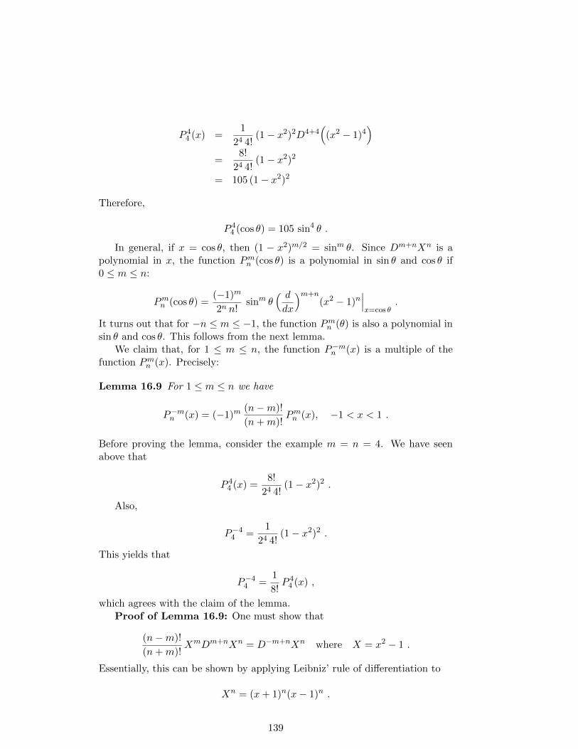
P 44 (x) =

1

24 4!(1− x2)2D4+4

((x2 − 1)4

)=

8!

24 4!(1− x2)2

= 105 (1− x2)2

Therefore,

P 44 (cos θ) = 105 sin4 θ .

In general, if x = cos θ, then (1 − x2)m/2 = sinm θ. Since Dm+nXn is apolynomial in x, the function Pmn (cos θ) is a polynomial in sin θ and cos θ if0 ≤ m ≤ n:

Pmn (cos θ) =(−1)m

2n n!sinm θ

( ddx

)m+n(x2 − 1)n

∣∣∣x=cos θ

.

It turns out that for −n ≤ m ≤ −1, the function Pmn (θ) is also a polynomial insin θ and cos θ. This follows from the next lemma.

We claim that, for 1 ≤ m ≤ n, the function P−mn (x) is a multiple of thefunction Pmn (x). Precisely:

Lemma 16.9 For 1 ≤ m ≤ n we have

P−mn (x) = (−1)m(n−m)!

(n+m)!Pmn (x), −1 < x < 1 .

Before proving the lemma, consider the example m = n = 4. We have seenabove that

P 44 (x) =

8!

24 4!(1− x2)2 .

Also,

P−44 =

1

24 4!(1− x2)2 .

This yields that

P−44 =

1

8!P 4

4 (x) ,

which agrees with the claim of the lemma.Proof of Lemma 16.9: One must show that

(n−m)!

(n+m)!XmDm+nXn = D−m+nXn where X = x2 − 1 .

Essentially, this can be shown by applying Leibniz’ rule of differentiation to

Xn = (x+ 1)n(x− 1)n .

139

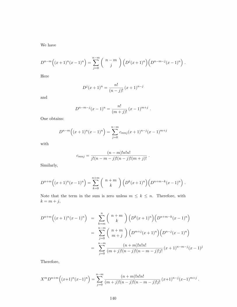
We have

Dn−m(

(x+ 1)n(x− 1)n)

=

n−m∑j=0

(n−mj

)(Dj(x+ 1)n

)(Dn−m−j(x− 1)n

).

Here

Dj(x+ 1)n =n!

(n− j)!(x+ 1)n−j

and

Dn−m−j(x− 1)n =n!

(m+ j)!(x− 1)m+j .

One obtains:

Dn−m(

(x+ 1)n(x− 1)n)

=n−m∑j=0

cmnj(x+ 1)n−j(x− 1)m+j

with

cmnj =(n−m)!n!n!

j!(n−m− j)!(n− j)!(m+ j)!.

Similarly,

Dn+m(

(x+ 1)n(x− 1)n)

=n+m∑k=0

(n+mk

)(Dk(x+ 1)n

)(Dn+m−k(x− 1)n

).

Note that the term in the sum is zero unless m ≤ k ≤ n. Therefore, withk = m+ j,

Dn+m(

(x+ 1)n(x− 1)n)

=n∑

k=m

(n+mk

)(Dk(x+ 1)n

)(Dn+m−k(x− 1)n

)=

n−m∑j=0

(n+mm+ j

)(Dm+j(x+ 1)n

)(Dn−j(x− 1)n

)

=

n−m∑j=0

(n+m)!n!n!

(m+ j)!(n− j)!(n−m− j)!j!(x+ 1)n−m−j(x− 1)j

Therefore,

XmDn+m(

(x+1)n(x−1)n)

=

n−m∑j=0

(n+m)!n!n!

(m+ j)!(n− j)!(n−m− j)!j!(x+1)n−j(x−1)m+j .

140

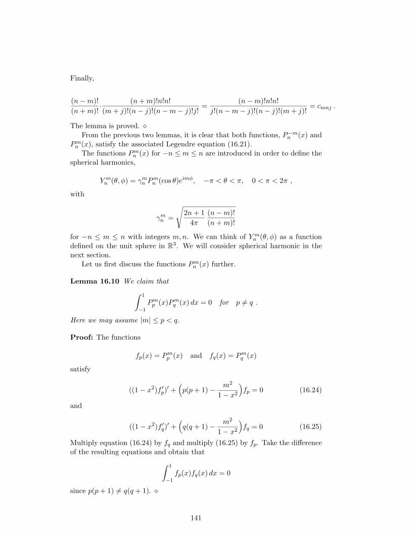
Finally,

(n−m)!

(n+m)!· (n+m)!n!n!

(m+ j)!(n− j)!(n−m− j)!j!=

(n−m)!n!n!

j!(n−m− j)!(n− j)!(m+ j)!= cmnj .

The lemma is proved. From the previous two lemmas, it is clear that both functions, P−mn (x) and

Pmn (x), satisfy the associated Legendre equation (16.21).The functions Pmn (x) for −n ≤ m ≤ n are introduced in order to define the

spherical harmonics,

Y mn (θ, φ) = γmn P

mn (cos θ)eimφ, −π < θ < π, 0 < π < 2π ,

with

γmn =

√2n+ 1

4π

(n−m)!

(n+m)!

for −n ≤ m ≤ n with integers m,n. We can think of Y mn (θ, φ) as a function

defined on the unit sphere in R3. We will consider spherical harmonic in thenext section.

Let us first discuss the functions Pmn (x) further.

Lemma 16.10 We claim that∫ 1

−1Pmp (x)Pmq (x) dx = 0 for p 6= q .

Here we may assume |m| ≤ p < q.

Proof: The functions

fp(x) = Pmp (x) and fq(x) = Pmq (x)

satisfy

((1− x2)f ′p)′ +(p(p+ 1)− m2

1− x2

)fp = 0 (16.24)

and

((1− x2)f ′q)′ +(q(q + 1)− m2

1− x2

)fq = 0 (16.25)

Multiply equation (16.24) by fq and multiply (16.25) by fp. Take the differenceof the resulting equations and obtain that∫ 1

−1fp(x)fq(x) dx = 0

since p(p+ 1) 6= q(q + 1).

141

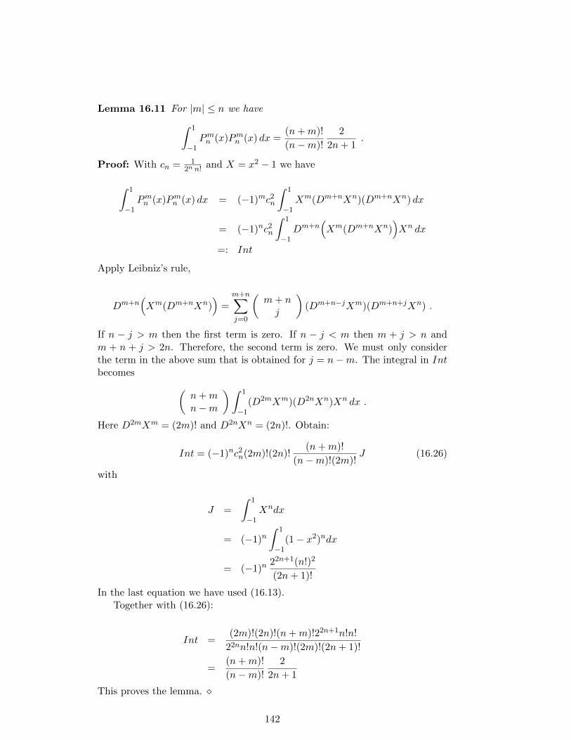
Lemma 16.11 For |m| ≤ n we have∫ 1

−1Pmn (x)Pmn (x) dx =

(n+m)!

(n−m)!

2

2n+ 1.

Proof: With cn = 12n n! and X = x2 − 1 we have

∫ 1

−1Pmn (x)Pmn (x) dx = (−1)mc2

n

∫ 1

−1Xm(Dm+nXn)(Dm+nXn) dx

= (−1)nc2n

∫ 1

−1Dm+n

(Xm(Dm+nXn)

)Xn dx

=: Int

Apply Leibniz’s rule,

Dm+n(Xm(Dm+nXn)

)=

m+n∑j=0

(m+ nj

)(Dm+n−jXm)(Dm+n+jXn) .

If n − j > m then the first term is zero. If n − j < m then m + j > n andm + n + j > 2n. Therefore, the second term is zero. We must only considerthe term in the above sum that is obtained for j = n−m. The integral in Intbecomes (

n+mn−m

)∫ 1

−1(D2mXm)(D2nXn)Xn dx .

Here D2mXm = (2m)! and D2nXn = (2n)!. Obtain:

Int = (−1)nc2n(2m)!(2n)!

(n+m)!

(n−m)!(2m)!J (16.26)

with

J =

∫ 1

−1Xndx

= (−1)n∫ 1

−1(1− x2)ndx

= (−1)n22n+1(n!)2

(2n+ 1)!

In the last equation we have used (16.13).Together with (16.26):

Int =(2m)!(2n)!(n+m)!22n+1n!n!

22nn!n!(n−m)!(2m)!(2n+ 1)!

=(n+m)!

(n−m)!

2

2n+ 1

This proves the lemma.

142

16.8 Spherical Harmonics as Eigenfunctions of the Laplace–Beltrami Operator

Let r, θ, φ denote the usual spherical coordinates. Recall the expression for theLaplacian in spherical coordinates,

∆v =1

r2(r2vr)r +

1

r2

(vθθ + cot θ vθ +

1

sin2 θvφφ

).

If Y (θ, φ) is a function on the unit sphere, then define the Laplace–Beltramioperator L by

LY = Yθθ + cot θ Yθ +1

sin2 θYφφ .

If v(r, θ, φ) = R(r)Y (θ, φ) then we can write the Helmholtz’ equation

∆v + k2v = 0

as

1

r2(r2R′)′Y +

R

r2LY + k2RY = 0 .

Equivalently,

1

R(r2R′)′ + k2r2 +

1

YLY = 0 .

Denoting the separation constant by Q we obtain

(r2R′)′ + (k2r2 −Q)R = 0

−LY = QY

As we have seen, the R–equation is an Euler–equation for k = 0 and leads toBessel’s equation for k > 0. The equation

−LY (θ, φ) = QY (θ, φ)

is an eigenvalue problem for the Laplace–Beltrami operator L. It turns out thatwe have already determined eigenvalues and eigenfunctions of L.

Theorem 16.2 Let m,n denote integers with −n ≤ m ≤ n and let

Pmn (x) =(−1)m

2nn!(1− x2)m/2Dm+n

((x2 − 1)n

)denote the solution of the associated Legendre equation constructed above. Thenthe function

Y (θ, φ) = Pmn (cos θ)eimφ

is an eigenfunction of −L to the eigenvalue Q = Qn = n(n+ 1).

143

Proof: If one substitutes Z(θ, φ) = Θ(θ)Φ(φ) into the equation

LZ +QZ = 0

then one obtains

Θ′′Φ + (cot θ)Θ′Φ +1

sin2 θΘΦ′′ +QΘΦ = 0 .

Equivalently,

1

Θ

(Θ′′ + (cot θ)Θ′

)+

1

sin2 θ

Φ′′

Φ+Q = 0 .

If

Φ′′ +m2Φ = 0

then the equation for Θ becomes

Θ′′ + (cot θ)Θ′ +(Q− m2

sin2 θ

)Θ = 0 .

The function

Θ(θ) = Pmn (cos θ)

satisfies this equation with Q = n(n+ 1) and the function Φ(φ) = eimφ satisfiesthe equation Φ′′ +m2Φ = 0. This proves the theorem.

One can show that the 2n+ 1 eigenfunctions

Zmn (θ, φ) = Pmn (cos θ)eimφ, −n ≤ m ≤ n ,

to the eigenvalue Qn = n(n + 1) of −L are linearly independent. This followssince these functions are orthogonal with respect to the L2–inner product onthe unit sphere. Therefore, the eigenvalue Qn = n(n + 1) has multiplicity atleast 2n+ 1.

One can prove that the system of functions

Zmn (θ, φ), −n ≤ m ≤ n, n = 0, 1, . . .

is complete in L2.One can prove that the operator −L has the eigenvalues Qn = n(n + 1)

where n = 0, 1, 2, . . .. Each eigenvalue n(n + 1) has multiplicity 2n + 1. Wehave constructed an orthonormal basis of eigenfunctions for L,

Y mn (θ, φ) = γmn P

mn (cos θ)eimφ, −n ≤ m ≤ n ,

where γmn is defined as above,

γmn =

√2n+ 1

4π

(n−m)!

(n+m)!.

Example: The spherical harmonic Y 12 is

144

Y 12 (θ, φ) = −3

2

√5

6πcos θ sin θ eiφ .

Let us continue the discussion of harmonic functions

v(r, θ, φ) = R(r)Y (θ, φ) .

With Q = n(n+ 1), the R–equation is an Euler equation with general solution

R(r) = c1rn +

c2

rn+1.

Assume Q = n(n+ 1). Substitute

Y (θ, φ) = Θ(θ)Φ(φ)

into

Yθθ + cot θ Yθ +1

sin2 θYφφ + n(n+ 1)Y = 0 .

Divide by Y . Obtain

1

Θ

(Θ′′ + cot θΘ′

)+

1

sin2 θ

Φ′′

Φ+ n(n+ 1) = 0 .

With Φ′′/Φ = −m2 obtain

Θ′′ + cot θΘ′ +(n(n+ 1)− m2

sin2 θ

)Θ = 0 .

Let Θ(θ) = P (cos θ),

Θ′ = − sin θ P ′, Θ′′ = − cos θ P ′ + sin2 θP ′′ .

Obtain

sin2 θ P ′′ − 2 cos θ P ′ +(n(n+ 1)− m2

sin2 θ

)P = 0 .

If x = cos θ, then sin2 θ = 1− x2, thus

(1− x2)P ′′ − 2xP ′ +(n(n+ 1)− m2

1− x2

)P = 0 .

The functions Pmn (x) satisfy this equation for −n ≤ m ≤ n. Then

Zmn (θ, φ) := Pmn (cos θ)eimφ

satisfies

−LZmn = n(n+ 1)Zmn .

We claim that the system of functions

145

Y mn (θ, φ), −n ≤ m ≤ n, n = 0, 1, . . .

is an orthonormal system in L2(S) where S is the unit sphere in R3. Recallthat the element of area for the unit sphere S is

dS = sin θ dθdφ .

Integration over the sphere S:∫SZ dS =

∫ 2π

0

∫ π

0Z(θ, φ) sin θ dθdφ

The L2–inner–product of two functions defined on S is:

(Z1, Z2) =

∫SZ1Z2 dS

The L2–norm is:

‖Z‖ = (Z,Z)1/2

Orthogonality: If m1 6= m2 then∫ 2π

0e−im1φeim2φ dφ = 0 .

If n1 6= n2 then

∫ π

0Pmn1

(cos θ)Pmn2(cos θ) sin θ dθ =

∫ 1

−1Pmn1

(x)Pmn2(x) dx

= 0

Therefore, if m1 6= m2 or n1 6= n2 then(Zm1n1, Zm2

n2

)= 0 .

Normalization:

‖Zmn ‖2 = 2π

∫ 1

−1(Pmn )2(x) dx

=4π

2n+ 1

(n+m)!

(n−m)!

= (1/γmn )2

Therefore, the functions

Y mn (θ, φ), −n ≤ m ≤ n, n = 0, 1, . . .

146

form an orthonormal system in L2(S). One can prove that this systen is com-plete, i.e., if y = y(θ, φ) is any function in L2(S) then the series

∞∑n=0

n∑m=−n

amnYmn (θ, φ) with amn = (Y m

n , y)

converges to y w.r.t. the L2–norm on S.

16.9 Spherical Harmonics are Restrictions of Harmonic Poly-nomials to the Unit Sphere

We have

Y mn (θ, φ) = γmn Pmn (cos θ)eimφ

where

Pmn (x) =1

2nn!(1− x2)m/2Dm+nXn, X = x2 − 1 .

Set

v(r, θ, φ) = rnY mn (θ, φ)

to obtain a function defined in all space.Claim:

∆v = 0

Proof: We have

∆v =1

r2(r2vr)r +

1

r2Lv

Here

L(rnY mn ) = −rnn(n+ 1)Y m

n

Also,

(rn)r = nrn−1

r2(rn)r = nrn+1

(r2vr)r = n(n+ 1)rnY mn

This shows that ∆v = 0.Definition: A function

p(x, y, z), (x, y, z) ∈ R3 ,

is called homogeneous of degree n if

p(λx, λy, λz) = λnp(x, y, z)

147

for all (x, y, z) ∈ R3 and all λ ∈ R.Clearly, any function of the form

T (x, y, z) = xn1yn2zn3

with nonnegative integers nj is a polynomial which is homogeneous of degreen = n1 +n2 +n3. Any sum of such terms, of the same degree n, is a polynomialthat is homogeneous of degree n.

Harmonic polynomials that are homogeneous of degree n can be studiedwith algebraic methods. We want to show:

Theorem 16.3 If one writes the function

v(r, θ, φ) = rnY mn (θ, φ)

in Cartesian coordinates x, y, z, then one obtains a polynomial in x, y, z whichis homogeneous of degree n.

Proof: It suffices to prove this for 0 ≤ m ≤ n. We have

v = crn sinm θ (Dm+nXn)|x=cos θ eimφ

Here

eimφ = (cosφ+ i sinφ)m

is a sum of terms

cosl φ sinm−l φ, 0 ≤ l ≤ m .

Also,

Xn = (x2 − 1)n =n∑j=0

cjnx2n−2j = x2n + c1nx

2n−2 + . . . .

Therefore, Dm+nXn is a sum of terms

xn−m−2j , n−m ≥ n−m− 2j ≥ 0 .

It follows that v is a sum of terms

H = rn sinm θ cosn−m−2j θ cosl φ sinm−l φ

where

0 ≤ l ≤ m and n−m− 2j ≥ 0 .

Recall that

x = r sin θ cosφ

y = r sin θ sinφ

z = r cos θ

148

Therefore,

H = rn sinl θ cosl φ sinm−l θ sinm−l φ cosn−m−2j θ

= xlym−lrn−m cosn−m−2j θ

= xlym−lr2jzn−m−2j

= xlym−l(x2 + y2 + z2)jzn−m−2j

This is a polynomial which is homogeneous of degree n.

2D Analogy. Consider

p(x, y) = (x+ iy)n, q(x, y) = (x− iy)n .

It is easy to see that p(x, y) and q(x, y) are harmonic polynomials which arehomogeneous of degree n. The corresponding restrictions to the unit circle are

p(cosφ, sinφ) = einφ

q(cosφ, sinφ) = e−inφ

The functions e±inφ are the ‘spherical harmonics’ on the unit circle in 2D. Theyare restrictions to the unit circle of the homogeneous polynomials p and q.

3D Generalization. The functions Y mn (θ, φ), defined on the unit sphere

in R3, are the generalizations of the functions e±inφ defined on the unit circlein R2. The expansion in terms of the spherical harmonics Y m

n (θ, φ) generalizesthe Fourier expansion in terms of the functions e±inφ.

149

17 Review I

17.1 Scalar ODEs

Solve the IVP

α′(t) = λα(t) + h(t), α(0) = α0 .

The solution is

α(t) = eλtα0 +

∫ t

0eλ(t−s) h(s) ds .

17.2 A Matrix Equation

Let A ∈ Cn×n. Let φ ∈ Cn be an eigenvector of A,

Aφ = λφ .

Consider the IVP

u′(t) = Au(t) + φ, u(0) = 0 .

Ansatz:

u(t) = α(t)φ

where α(t) is a scalar function.The equation u′(t) = Au(t) + φ becomes

α′(t)φ = α(t)λφ+ φ ,

thus

α′(t) = λα(t) + 1, α(0) = 0 .

Assuming λ 6= 0, the solution is

α(t) =

∫ t

0eλ(t−s) ds =

1

λ(eλt − 1) .

Therefore,

u(t) =1

λ(eλt − 1)φ .

17.3 An Inhomogeneous Heat Equation

Consider the IBVP

ut = uxx + sin(3x)

u(0, t) = u(π, t) = 0

u(x, 0) = 0

150

Ansatz:

u(x, t) = α(t) sin(3x)

Note that sin(3x) is an eigenfunction of the operator ∂2/∂x2.Obtain

ut(x, t) = α′(t) sin(3x)

uxx(x, t) = −9α(t) sin(3x)

The equation ut = uxx + sin(3x) leads to

α′(t) = −9α(t) + 1 .

Since α(0) = 0 obtain

α(t) =

∫ t

0e−9(t−s) ds =

1

9(1− e−9t)

and

u(x, t) =1

9(1− e−9t) sin(3x) .

17.4 An Inhomogeneous Wave Equation

Consider the IBVP

utt = c2uxx + sin(3x)

u(0, t) = u(π, t) = 0

u(x, 0) = 0

ut(x, 0) = 0

Ansatz:


Note that sin(3x) is an eigenfunction of the operator ∂2/∂x2.Obtain the IVP

α′′(t) + 9c2α(t) = 1, α(0) = α′(0) = 0 .

The constant function

αs(t) ≡1

9c2

is a special solution. The general solution is

α(t) =1

9c2+A cos(3ct) +B sin(3ct) .

151

The condition α(0) = 0 yields that A = − 19c2

and the condition α′(0) = 0 yieldsthat B = 0. Therefore,

α(t) =1

9c2(1− cos(3ct))

u(x, t) =1

9c2(1− cos(3ct)) sin(3x)

17.5 An Inhomogeneous Heat Equation with Time–DependentSource

Consider the IBVP

ut = uxx + eεt sin(3x)

u(0, t) = u(π, t) = 0

u(x, 0) = 0

Ansatz:


Note that sin(3x) is an eigenfunction of the operator ∂2/∂x2.Proceeding as in Sect. 17.3 leads to the IVP

α′(t) = −9α(t) + eεt, α(0) = 0 .

The solution is

α(t) =

∫ t

0e−9(t−s)eεs ds

= e−9t

∫ t

0e(9+ε)s ds

=1

9 + ε(eεt − e−9t)

Obtain the solution

u(x, t) =1

9 + ε(eεt − e−9t) sin(3x) .

If ε > 0, the growing forcing term eεt sin(3x) in the heat equation leads to agrowing solution u(x, t).

17.6 The Wave Equation in a Rectangle

Let D = (0, L)× (0, H).Consider the IBVP

152

utt = c2(uxx + uyy) in D × [0,∞)

u(x, y, t) = 0 on ∂D × [0,∞)

u(x, y, 0) = 0 in D

ut(x, y, 0) = sin(2x) sin(3y) in D

Note that

φ23(x, y) = sin(2x) sin(3y)

is an eigenfunction of the Laplace operator ∆:

∆φ23 = (−4− 9)φ23 = −13φ23 .

Ansatz:

u(x, y, t) = h(t)φ23(x, y)

Obtain the IVP

h′′(t) + 13c2h(t) = 0, h(0) = 0, h′(0) = 1 .

The solution of the IVP is

h(t) =1√13c

sin(√

13ct) .

The solution of the wave equation is

u(x, t) =1√13c

sin(√

13ct) sin(2x) sin(3y) .

17.7 First Order PDEs

Consider the IVP

ut(x, t) + aux(x, t) = F (x, t), u(x, 0) = f(x) .

Assume that u(x, t) is a solution.Fix x0 and set

h(t) = u(x0 + at, t) .

Obtain

h′(t) = F (x0 + at, t), h(0) = f(x0) .

Therefore,

u(x0 + at, t) = h(t) = f(x0) +

∫ t

0F (x0 + as, s) ds .

153

If x0 + at = x then x0 = x− at. Therefore, the solution is

u(x, t) = h(t) = f(x− at) +

∫ t

0F (x− at+ as, s) ds .

If F ≡ 0 then

u(x, t) = f(x− at) .

If a > 0 then the profile u(x, 0) = f(x) moves at speed a to the right.

Variable Signal Speed:Consider the IVP

ut(x, t) + a(x, t)ux(x, t) = 0, u(x, 0) = f(x) .

Fix x0 and let

ξ′(t) = a(ξ(t), t), ξ(0) = x0 .

The characteristic line starting at the point (x, t) = (x0, 0) consists of the points

(ξ(t), t), t ≥ 0 .

If u(x, t) is a solution and

h(t) := u(ξ(t), t)

then h(0) = u(x0, 0) = f(x0) and

h′(t) = ut(ξ(t), t) + ξ′(t)ux(ξ(t), t) ≡ 0 .

Therefore, the solution u(x, t) carries the value f(x0) along the characteristicline starting at (x0, 0).

Example:

ut(x, t) + tux(x, t) = 0, u(x, 0) = f(x) .

The IVP

ξ′(t) = t, ξ(0) = x0

has the solution

ξ(t) =t2

2+ x0 .

Obtain

u(t2

2+ x0, t) = f(x0) ,

thus

u(x, t) = f(x− t2

2) .

154

17.8 Laplace’s Equation in a Rectangle

Let D = (0, π) × (0, 1). Consider the equation ∆u = 0 in D with boundaryconditions

u(0, y) = u(π, y) = 0 for 0 < y < 1

u(x, 0) = sinx for 0 < x < π

u(x, 1) = sin(2x) for 0 < x < π

To solve the problem, let u = u1 + u2 where u1 and u2 are harmonic functionssatisfying

u1(0, y) = u1(π, y) = 0 for 0 < y < 1

u1(x, 0) = sinx for 0 < x < π

u1(x, 1) = 0 for 0 < x < π

and

u2(0, y) = u1(π, y) = 0 for 0 < y < 1

u2(x, 0) = 0 for 0 < x < π

u1(x, 1) = sin(2x) for 0 < x < π

To solve the problems, let

u1(x, t) = (sinx)h(y)

and

u2(x, t) = (sin 2x)g(y) .

Obtain

0 = ∆u1 = −(sinx)h(y) + (sinx)h′′(y) ,

thus

h′′(y) = h(y) .

The boundary conditions are

h(0) = 1 and h(1) = 0 .

Obtain

h(y) = aey + be−y

where

155

a+ b = 1, ae+ b/e = 1 .

The solution of the linear system for a and b is

a = − 1

e2 − 1, b =

e2

e2 − 1.

Therefore,

h(y) = − ey

e2 − 1+

e2−y

e2 − 1

and

u1(x, y) = (sinx)e2−y − ey

e2 − 1.

Similarly,

0 = ∆u2 = −4(sin 2x)g(y) + (sin 2x)g′′(y) ,

thus

g′′(y) = 4g(y) .

The boundary conditions are

g(0) = 0 and g(1) = 1 .

Obtain

g(y) = ae2y + be−2y

where

a+ b = 0, ae2 + b/e2 = 0 .

The solution of the linear system for a and b is

a =1

e2 − 1/e2, b =

−1

e2 − 1/e2.

Therefore,

g(y) =e2y

e2 − 1/e2− e−2y

e2 − 1/e2

and

u2(x, y) = (sin 2x)( e2y

e2 − 1/e2− e−2y

e2 − 1/e2

).

The solution of the given problem is

u(x, y) = u1(x, y) + u2(x, y) .

156

17.9 Laplace’s Equation in a Disk

Let

B5 = (x, y) ∈ R2 ; x2 + y2 < 25

denote the disk of radius 5, centered at the origin. We want to determine afunction u(r, φ) with ∆u = 0 in B5 and

u(5, φ) = cos(2φ) + 7 sin(3φ) for φ ∈ R .

We know that the functions

rn(A cos(nφ) +B sin(nφ)

)are harmonic. Determine

u1(r, φ) = Ar2 cos(2φ)

with

u1(5, φ) = cos(2φ) .

This requires A = 125 , thus

u1(r, φ) = (r/5)2 cos(2φ) .

Determine

u2(r, φ) = Br3 sin(3φ)

with

u2(5, φ) = 7 sin(3φ) .

This requires B = 7125 , thus

u2(r, φ) = 7(r/5)3 sin(3φ) .

Together, the solution of the given problem is

u(r, φ) = (r/5)2 cos(2φ) + 7(r/5)3 sin(3φ) .

17.10 Laplace’s Equation in an Annulus

Let

A = (x, y) ∈ R2 : 1 < x2 + y2 < 25 .

We want to determine a function u(r, φ) for which ∆u = 0 in A and

u(1, φ) = 1 + sin(2φ) for φ ∈ R ,

u(5, φ) = 0 for φ ∈ R .

157

Determine harmonic functions u1 and u2 with

u1(1, φ) = 1

u1(5, φ) = 0

and

u2(1, φ) = sin(2π)

u2(5, φ) = 0

Then u = u1 + u2.Obtain

u1(r, φ) = A+B ln r .

The boundary conditions require that

1 = u1(1, φ) = A

and

0 = u1(5, φ) = A+B ln 5 .

Therefore,

u1(r, φ) = 1− ln r

ln 5.

For u2(r, φ) obtain that

u2(r, φ) = Ar2 sin(2φ) +B1

r2sin(2φ) .

The boundary conditions require that

A+B = 1 and 25A+B

25= 0 .

Obtain that

A =−1

(25)2 − 1, B =

(25)2

(25)2 − 1,

thus

u2(r, φ) =1

(252)− 1

((25)2

r2− r2

)sin(2φ) .

The solution of the given problem is

u(r, φ) = u1(r, φ) + u2(r, φ) .

158

17.11 The Heat Equation in a Rectangle

Let

D = (0, π)× (0, π) .

Consider the IBVP

ut = ∆u+ sinx sin(2y) for D × [0,∞)

u = 0 for (x, y, t) ∈ ∂D × [0,∞)

u = 0 for t = 0

Note: The function

φ(x, y) = sinx sin(2y)

satisfies the boundary condition and is an eigenfunction of ∆.Ansatz:

u(x, y, t) = α(t) sinx sin(2y) .

Obtain

α′(t) = −5α(t) + 1, α(0) = 0 .

u(x, y, t) =1

5(1− e−5t) sinx sin(2y) .

17.12 The Heat Equation with Inhomogeneous Term and InitialCondition


ut = uxx + sinx for 0 < x < π, t ≥ 0

with boundary condition

u(0, t) = u(π, t) = 0

and initial condition

u(x, 0) = sin(2x) .

Solution:

u(x, t) = e−4t sin(2x) + (1− e−t) sin(2x) .

159

18 Review II

18.1 2D Laplace Equation in Polar Coordinates

∆v = vrr +1

rvr +

1

r2vφφ = 0

Let

v = R(r)Φ(φ) .

Obtain

Φ(φ) = eimφ, m ∈ Z .

The equation

r2R′′ + rR′ −m2R = 0

has the solution

R(r) = r|m| .

Obtain the harmonic functions:

v(r, φ) = r|m|eimφ, m ∈ Z .

18.2 2D Wave Equation in Polar Coordinates

Consider the wave equation

utt = c2∆u .

Let

u(r, φ, t) = v(r, φ)T (t) .

Obtain

T ′′(t) + ω2T (t) = 0, ω = kc ,

and

∆v + k2v = 0 .

Let

v(r, φ) = R(r)Φ(φ) .

Obtain

Φm(φ) = eimφ, m ∈ Z ,

and

160

r2R′′ + rR′ + (r2k2 −m2)R = 0 .

Introduce the function f(x) by

f(rk) = R(r) .

Obtain Bessel’s differential equation for f(x):

x2f ′′(x) + xf ′(x) + (x2 −m2)f(x) = 0 .

Bessel functions of the first kind are solutions which are regular at x = 0. Theseare the Bessel functions

Jm(x) =(x

2

)m ∞∑0

(−1)j

j!Γ(j +m+ 1)

(x2

)2j for m ∈ Z .

(Note that J−m(x) = (−1mJm(x).) Obtain

R(r) = Jm(rk) for m ∈ Z, k > 0 .

Solutions of the 2D–Helmholtz equation:

v(r, φ) = Jm(rk)eimφ, m ∈ Z, k > 0 .

Solutions of the 2D–Wave equation:

u(r, φ, t) = Jm(rk)eimφ(A cos(ωt) +B sin(ωt)

)where ω = ck .

The parameter k becomes discrete,

k = xmj/a for m ∈ Z, j ∈ N ,

if the boundary condition

u(a, φ, t) = 0

is required.

18.3 3D Laplace Equation in Spherical Coordinates

∆v =1

r2(r2vr)r +

1

r2 sin θ(sin θvθ)θ +

1

r2 sin2 θvφφ = 0

Let

v(r, θ, φ) = R(r)Θ(θ)Φ(φ) .

Obtain

Φ(φ) = eimφ, m ∈ Z .

Let

161

Θ(θ) = P (cos θ), x = cos θ .

Obtain the associate Legendre equation

(1− x2)P ′′(x)− 2xP ′(x) +(Q− m2

1− x2

)P (x) = 0

and

(r2R′)′ −QR = 0 .

The equation for P (x) yields that

Q = n(n+ 1), n = 0, 1, 2 . . .

It is remarkable that the eigenvalues Q = n(n+ 1) do not depend on m. Solu-tions for which P (±1) is finite are the Legendre functions

Pmn (x) =(−1)m

2nn!(1− x2)m/2Dn+m((x2 − 1)n) for − n ≤ m ≤ n .

(Note that P−mn (x) is a multiple of Pmn (x).)Obtain the harmonic functions:

v(r, θ, φ) = rnPmn (cos θ)eimφ for − n ≤ m ≤ n, n = 0, 1, . . .

Remark: In 2D the R–equation depends on the parameter m ∈ Z, whereΦ′′+m2Φ = 0. In 3D the R–equation depends on the parameter n ∈ N0, whichappears the Θ–equation.

18.4 3D Wave Equation in Spherical Coordinates

Let

u(r, θ, φ, t) = v(r, θ, φ)T (t) .

Obtain

T ′′(t) + ω2T (t) = 0, ω = kc ,

and

∆v + k2v = 0 .

Let

v(r, θ, φ) = R(r)Θ(θ)Φ(φ) .

The equations for Θ and for Φ are the same as for the Laplace equation: Obtain

Θ(θ) = P (cos θ), x = cos θ ,

162

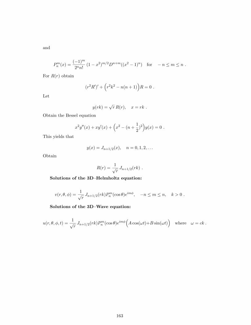
and

Pmn (x) =(−1)m

2nn!(1− x2)m/2Dn+m((x2 − 1)n) for − n ≤ m ≤ n .

For R(r) obtain

(r2R′)′ +(r2k2 − n(n+ 1)

)R = 0 .

Let

y(rk) =√r R(r), x = rk .

Obtain the Bessel equation

x2y′′(x) + xy′(x) +(x2 − (n+

1

2)2)y(x) = 0 .

This yields that

y(x) = Jn+1/2(x), n = 0, 1, 2, . . .

Obtain

R(r) =1√rJn+1/2(rk) .

Solutions of the 3D–Helmholtz equation:

v(r, θ, φ) =1√rJn+1/2(rk)Pmn (cos θ)eimφ, −n ≤ m ≤ n, k > 0 .

Solutions of the 3D–Wave equation:

u(r, θ, φ, t) =1√rJn+1/2(rk)Pmn (cos θ)eimφ

(A cos(ωt)+B sin(ωt)

)where ω = ck .

163

Documents

Partial Differential Equations for Engineering Math 312, Spring