Partially-shared zero-suppressed multi-terminal BDDs: concept, algorithms and applications

Form Methods Syst Des (2010) 36: 198–222DOI 10.1007/s10703-010-0095-8

Partially-shared zero-suppressed multi-terminal BDDs:concept, algorithms and applications

Kai Lampka · Markus Siegle · Joern Ossowski ·Christel Baier

Published online: 10 June 2010© Springer Science+Business Media, LLC 2010

Abstract Multi-Terminal Binary Decision Diagrams (MTBDDs) are a well accepted tech-nique for the state graph (SG) based quantitative analysis of large and complex systemsspecified by means of high-level model description techniques. However, this type of De-cision Diagram (DD) is not always the best choice, since finite functions with small satis-faction sets, and where the fulfilling assignments possess many 0-assigned positions, mayyield relatively large MTBDD based representations. Therefore, this article introduces zero-suppressed MTBDDs and proves that they are canonical representations of multi-valuedfunctions on finite input sets. For manipulating DDs of this new type, possibly defined overdifferent sets of function variables, the concept of partially-shared zero-suppressed MTB-DDs and respective algorithms are developed. The efficiency of this new approach is demon-strated by comparing it to the well-known standard type of MTBDDs, where both types ofDDs have been implemented by us within the C++-based DD-package JINC. The bench-marking takes place in the context of Markovian analysis and probabilistic model checkingof systems. In total, the presented work extends existing approaches, since it not only allowsone to directly employ (multi-terminal) zero-suppressed DDs in the field of quantitativeverification, but also clearly demonstrates their efficiency.

K. Lampka (�)Computer Engineering and Communication Networks Lab., ETH Zurich, Zurich, Switzerlande-mail: [email protected]

M. SiegleInst. for Comp. Eng., Univ. of the German Federal Armed Forces Munich, Munich, Germanye-mail: [email protected]

J. Ossowski · C. BaierInst. for Theoretical Comp. Sc., Technical University Dresden, Dresden, Germany

J. Ossowskie-mail: [email protected]

C. Baiere-mail: [email protected]

mailto:[email protected]




Form Methods Syst Des (2010) 36: 198–222 199

Keywords Binary Decision Diagrams and their algorithms · Quantitative verification ofsystems · Symbolic data structures for performance analysis

1 Introduction

1.1 Motivation

Finite state/transition systems (also called state graphs (SG)) are a fundamental ingredientwhen it comes to formal, automatized reasoning about the qualitative and quantitative be-havior of systems. Contemporary tools for evaluating system behavior accept a high-levelmodel description as input rather than the plain state/transition system. However, for analyz-ing a high-level system model, it has to be transformed into a state/transition-system whichincorporates all possible behavior. This step, known as state space exploration, expands allconcurrency as contained in the high-level model. It may therefore lead to an exponentialblow-up in the number of system states, which is known as the notorious state space explo-sion problem.

Decision diagrams (DDs) are directed acyclic graphs for representing finite functions.They have shown to be very helpful when it comes to the generation, representation andanalysis of extremely large state/transition-systems, easing the restriction imposed on thesize and complexity of models and thus systems to be analyzed. Multi-Terminal Binary De-cision Diagrams (MTBDDs) are among the most efficient techniques for the state basedquantitative analysis of large and complex systems, commonly described by Markovian ex-tensions of well known high-level model description techniques, e.g. Stochastic ProcessAlgebra [7] or Generalized Stochastic Petri Nets [3], among many others. The success ofmodeling and evaluation tools such as the probabilistic symbolic model checker PRISM[20], the stochastic process algebra tool CASPA [11] (both based on MTBDDs) or the mod-eling and analysis tool SMART [25] (based on multi-valued DDs) is largely due to theefficiency of the employed symbolic data structures. In the context of such high-level modeldescriptions, a model’s state usually consists of many state counters, each referring to thestate of a local process, to the current value of a specific process parameter, to the numberof tokens in a specific place of a Petri net, etc. When making use of MTBDDs in such asetting, each state counter is encoded in binary form by n bits, leading to a large numberof bit positions filled with zeroes and to a possible small number of encodings of reachablestates with respect to all possible 2n state labellings. In such a setting, MTBDDs are notthe best choice, since finite functions with small satisfaction sets, and where the fulfillingassignments possess many 0-assigned positions, may yield relatively large MTBDD basedrepresentations. The 0-suppressing (0-sup) reduction rule as introduced by Minato in [15]has the potential to improve such situations, since, contrary to MTBDDs, it avoids allocatingnodes for 0-assigned bit-positions. Thus, this reduction rule helps to reduce memory spaceand thus computation time when generating and manipulating symbolic representations ofstate/transition systems underlying high-level model specifications, thereby ultimately en-abling the analysis of larger systems. However, there is a significant problem attached to theusage of Minato’s 0-suppressing reduction rule.

When considering two (or more) zero-suppressed Binary Decision Diagrams (ZBDDs)defined on different sets of variables, the sharing and manipulation of their graphs turnsout to be more complex than in case of standard BDDs or in the case of ZBDDs with aglobal set of variables. The Shannon expansion [23] requires that for deducing the functionrepresented by a node of a ZBDD, the set of its variables F must be known since skipped

200 Form Methods Syst Des (2010) 36: 198–222

variables from F are assumed to be 0-sup, whereas skipped variables not in F , which arealso defined within the respective environment, are assumed to have a don’t-care semantics.Consequently, in the presence of multi-rooted DDs [22], as provided by standard implemen-tations such as CUDD [26] or the recently developed package JINC [9, 19], the nodes of theZBDDs lose their uniqueness as soon as the represented functions are defined on differentsets of variables. This is why in a wide range of applications standard implementations ofZBDDs cannot be employed directly.

There are many applications where several functions, depending on different sets of vari-ables, need to be manipulated at the same time. For example, symbolic model checkingrequires the execution of a (symbolic) reachability analysis, where a high-level model’sstate/transition system is given as a DD Trans. The symbolic representation of Trans iscommonly defined over two sets of variables, namely the s-variables, encoding the valuesof the potential source states and the t-variables, encoding the values of the potential targetstates. Thus each path within the DD defines at least one state-to-state-transition. Contraryto this, the symbolic structure Unexpl, encoding the set of unexplored states, solely takesthe s-variables as input. For obtaining all transitions emanating from the states of Unexpl,one must multiply DDs Trans and Unexpl, even though they are defined on differentsets of variables. In the presence of Minato’s 0-sup reduction rule and when recursing onthe DDs for applying operators such as multiplication, it is essential, that one distinguisheswhether a variable is an input variable or not for the respective DD, since this determinesthe applicable semantics, i.e. dnc- or 0-sup. Standard shared DD environments as providedby CUDD [26] solely assume global sets of variables, therefore their implementations ofZBDDs fail to apply operators to DDs with differing sets of variables.

1.2 Contributions

In [12, 13] we had introduced an extension of Minato’s ZBDDs to the multi-terminal case,thereby obtaining zero-suppressed Multi-Terminal Binary Decision Diagrams (ZMTBDDs),and used this data structure for the quantitative analysis of systems. In the present article wedescribe this extension in full detail, show that this new type of decision diagram (DD) is acanonical representation for multi-valued functions on finite input sets and introduce algo-rithms for efficiently manipulating DDs of that kind. When applying Minato’s 0-suppressing(0-sup) reduction rule, the sharing of the graphs of the DDs is not trivial any more. For de-ducing the function represented by a 0-sup DD’s graph correctly, the set of Boolean inputvariables must be known. Thus, within (fully) shared DD-environments as provided by con-temporary DD-packages, nodes of a 0-sup DD lose their uniqueness, if the DDs are meant tobe defined on differing sets of variables. To solve this problem in an efficient way, this paperdevelops the concept of partially shared zero-suppressed DDs (pZDDs), and also introducesnew algorithms for manipulating them. Most importantly, a new variant of Bryant’s wellknown Apply-algorithm [4] will be discussed. The newly obtained pZApply-algorithmnot only allows one to implement pZDDs within standard shared DD-environments, such asCUDD or JINC, but also supports the application of non-zero-preserving operators, i.e. ofoperators op where 0op0 �= 0 holds (such as nand and nor).

The concept of partially shared DDs as presented here is not the only solution to theproblem of differing sets of variables, orthogonal procedures exist: Since the semantics ofnodes in a shared 0-sup DD relies on a fixed variable set, one could either work with differentshared 0-sup DDs for each relevant variable set and transformation algorithms, or work witha single shared pseudo-reduced 0-sup DD (where don’t care nodes are allocated at the levelsof those variables which are not in the input set and reducedness is understood in a level-wise fashion). We did not implement these approaches, since it must be expected that both


alternatives would lead to rather inefficient solutions. For the first alternative, we expectthat the transformation algorithms are very time-consuming. For the second alternative, wewould lose all advantages of suppressing zeroes, since pseudo-reduced ZBDDs agree withpseudo-reduced BDDs.

For evaluating the efficiency of the presented approach, the paper compares pZDDs tothe well-known MTBDDs, where as a matter of fairness we have implemented both typesof DDs within the same DD packages, namely within the C++-based DD-package JINC. Asdemonstrated by various case studies, ZDDs turn out to be superior to MTBDDs in terms ofmemory—and thus run-time efficiency, when it comes to the stochastic performance evalu-ation and/or probabilistic model checking of large and complex systems.

1.3 Related work

Verification of stochastic systems plays an important part when it comes to ensuring the cor-rectness of timed (soft-real-time) systems. Over the last decade, many derivatives of decisiondiagrams (DDs) were developed, which have turned out to be very useful for representingstochastic transition relations. The most prominent types in this context are multi-terminalBinary Decision Diagrams (MTBDDs) [1, 6, 24] and (multi-terminal) Multi-valued DecisionDiagrams (MDDs) [5, 10]. However, all these derivatives are mainly extensions of BinaryDecision Diagrams (BDDs) [2, 14], for which Bryant [4] designed algorithms for efficientlymanipulating them and keeping them reduced. Variants of his algorithms have been imple-mented in contemporary DD-packages providing multi-rooted DDs [22] defined on a globalset of variables. In this area, Minato’s idea of employing the 0-sup-reduction rule is alsowell known, and ZBDDs have found their way into several contemporary DD-packages. Inhis work [15, 16], Minato focuses on the representation of combinatorial sets, rather thanon the representation of characteristic functions of sets encoded as bit strings, which is thereason why the concept of ZBDD local sets of input variables was not considered before (cf.Sect. 2, p. 203 for more details). To the best of our knowledge, previous work on 0-sup DDs[15, 16, 27] did not consider the multi-terminal case. Furthermore, it required, when apply-ing n-ary operators to ZBDDs, that all operands be defined on the same set of variables formaking the manipulating algorithms work properly. This work overcomes these limitationby developing the concept of partially shared 0-sup DDs, which makes it possible to imple-mented 0-sup DDs with differing sets of input variables within a single DD environment inan intuitive way. Since this idea also applies to Minato’s standard 0-sup BDDs, this articleclearly extends previous works and thus ultimately allows one to employ zero-suppressedDDs in a wide range of applications.

1.4 Organization

Section 2 presents the background material and repeats some useful concepts with respectto Boolean functions and their representation. Section 3 introduces our new type of DD anddiscusses its canonicity aspects. Section 4 introduces the concept of partially shared 0-supDD and presents generic algorithms for efficiently manipulating them. Section 5 describesour implementation of pZDDs within JINC, as well as the benchmarking experiments car-ried out, and Sect. 6 concludes the paper.

2 Background material

Let B = {0,1} be the set of Booleans, N = {0,1,2, . . .} the set of naturals, and R the setof reals and let D be a finite set of function values (here D ⊂ R). Let V be some global


(finite) set of Boolean variables on which a strict total ordering π is defined. The set ofvariables F := {v1, . . . , vn} ⊆ V employed in a Boolean function f is referred to as set offunction variables (or, synonymously, input variables) of f . Variable vi is essential for aBoolean function if and only if at least for one assignment to the variables of f it holds thatf (v1, . . . , vi−1,0, vi+1, . . . , vn) �= f (v1, . . . , vi−1,1, vi+1, . . . , vn). Otherwise the variable vi

is not essential. A non-essential variable is also commonly known as don’t-care (dnc) vari-able.

Canonical representations of Boolean functions Two Boolean functions are equivalent,if and only if their function values coincide for all inputs. A representation of a Booleanfunction is called canonical if each function f has exactly one representation of this type.A representation is strongly canonical if two equivalent functions have the same represen-tation, no matter what their sets of (input or function) variables are. If for identical sets ofessential variables and different sets of (input or function) variables the representation oftwo equivalent function is not the same, we refer to them as weakly canonical. In this sense,the canonical disjunctive normal form (CDNF) is a weakly canonical representation.

For example, consider the two functions f1 := x1x2 + x1(1 − x2) and f2 := x1. Obvi-ously these functions are equivalent. However, since the functions possess different sets ofvariables, their CDNFs differ.

Co-factors and expansion Let f : Bn → B be a Boolean function and let F be the set of

its variables. Function f can be expanded with respect to its variables. If one expands onlyone variable, e.g. vi , one ends up with the two cofactors of f with respect to vi , namely (a)the one-cofactor f |vi :=1 := f (v1, . . . , vi−1,1, vi+1, . . . , vn) or (b) the zero-cofactor f |vi :=0 :=f (v1, . . . , vi−1,0, vi+1, . . . , vn). If the variable to be expanded is clear from the context, wewill use the simplified notation f1 and f0 for referring to the respective cofactors, which arealso denominated positive and negative cofactor. For all vi ∈ F it holds:

f := vif (v1, . . . , vi−1,1, vi+1, . . . , vn) + (1 − vi )f (v1, . . . , vi−1,0, vi+1, . . . , vn)

This so-called Shannon-expansion, introduced in 1938 by Shannon in the context of switch-ing functions [23], can be recursively applied until all n variables are made constant. Theexpansion can be applied for an arbitrary subset F ′ ⊆ F , where the notation f |v ′ :=b refers tothe sub-function derived from function f by assigning the values contained in the Booleanvector b to the variables in F ′.

Don’t care semantics for variables (dnc-semantics) A variable vk is a dnc variable if andonly if its one- and zero-cofactors are identical. Let function g := f |v ′ :=b and let vk be a dncvariable of g. Applying the Shannon expansion to g with respect to vk one obtains:

g = (1 − vk)g0 + vkg1 since vk is dnc we have g′ = g0 = g1 and thus:g = ((1 − vk) + vk)g

′= g′

(1)

Variable vk is therefore a non-essential variable for function g. Thus one does not need toconsider variables of such kind when expanding function g, a sub-function of f . As a resultit is also clear that within a BDD no nodes for such variables need to be allocated withinthe graph representing g (cf. discussion below). At this point it is important to note thatnevertheless vk may still be essential for function f .


0-suppressing semantics for variables (0-sup-semantics) A variable vk is 0-sup if and onlyif its one-cofactor is the constant zero-function (f1 = 0). Applying the Shannon expansionto a function f and a 0-sup variable vk yields:

f = (1 − vk)f0 + vkf1 where f1 = 0 since vk is 0-suppressed

= (1 − vk)f0 (2)

In contrast to the dnc-case, it is obvious that variable vk cannot be ignored.

Binary Decision Diagrams and derivatives A Binary Decision Diagram (BDD) is a di-rected acyclic graph for representing Boolean functions [2, 4, 14]. It consists of a set ofinner nodes and a set of terminal nodes, where the inner nodes are labeled by Boolean vari-ables and terminal nodes carry values from {0,1}. Each inner node possesses two children,a 0- and a 1-child, connected to the respective parent node by an incoming 0- or 1-edge. Ifthe variables labeling the inner nodes appear in the same order on every path one speaks ofan ordered BDD. An ordered BDD is reduced (in the standard, dnc-sense), if no isomorphicsubgraphs exist and no dnc-nodes exist (where a non-terminal node of a BDD is a dnc-nodeif its 1- and 0-edge point to the same child). Since the associated variable of such a nodeis a dnc-variables and thus not essential for the respective function f , dnc-nodes can safelybe omitted (dnc reduction) [2, 4]. Reduced ordered BDDs (ROBDDs) are known to be astrongly canonical representation of Boolean functions. Within a single BDD-environment,each allocated BDD-node represents therefore a unique Boolean function [22].

A node referring to a 0-sup-variable is a 0-sup node, its outgoing 1-edge points to theterminal 0-node. Reducing ordered (isomorphism-free) BDDs by eliminating 0-sup-nodesrather than dnc-nodes leads to ZBDDs [15]. A ZBDD is a weakly canonical representationof a Boolean function [22].

A note on combinatorial sets As already pointed out in the introduction, Minato origi-nally developed ZBDDs for representing combinatorial sets [15, 16]. Instead of representingsuch sets by their usual characteristic function, he uses a different semantics: His symbolicrepresentation only depends on those variables which are contained in at least one validcombination of the combinatorial set. With this kind of encoding, it turns out that ZBDDsare actually strongly canonical representations and that dnc-reduced BDDs are only weaklycanonical representations of combinatorial sets. In the following, however, we will stick tothe usual interpretation, i.e. solely non-essential variables are considered as being irrelevantfor the function under consideration.

3 Data structure

We consider n-ary pseudo-Boolean functions, i.e. functions of the type f : Bn → D. When

shifting the co-domain of standard reduced ordered BDDs from B to D one obtainsMTBDDs. Analogously, by extending reduced ordinary ZBDDs we obtain ZMTBDDs.

Definition 1 An ordered ZMTBDD is a tuple A = (KNT , KT , F , var, then, else,

value, root) where

1. KNT is the set of non-terminal (inner) nodes and KT the set of terminal nodes, where|KT | ≥ 1 and KNT ∩ KT = ∅.


2. F = {x1, x2, . . . , xn} ⊆ V is a finite (possibly empty) set of Boolean variables. t �∈ V is apseudo-variable, labeling the terminal nodes and solely used for technical reasons. π is astrict total ordering on the elements of F ∪ {t} such that ∀xi ∈ F : xi <π t.

3. var : KNT ∪ KT → F ∪ {t} such that ∀k ∈ KNT ∪ KT : var(k) = t ⇔ k ∈ KT .4. then : KNT → KNT ∪ KT such that ∀n ∈ KNT : var(n) <π var(then(n)).5. else : KNT → KNT ∪ KT such that ∀n ∈ KNT : var(n) <π var(else(n)).6. value : KT → D, where D ⊂ R.7. root ∈ KNT ∪ KT .

A ZMTBDD is called reduced if the following conditions apply:

1. (Isomorphism rule) There are no isomorphic nodes; i.e. ∀n,m ∈ KNT :n �= m ⇒ (var(n) �= var(m) ∨ then(n) �= then(m) ∨ else(n) �= else(m))

and ∀n,m ∈ KT : n �= m ⇒ (value(n) �= value(m))

2. (0-suppressing rule) There is no inner node whose then-successor is the terminal0-node; i.e. �n ∈ KNT : then(n) ∈ KT ∧ value(then(n)) = 0.

Let k, l ∈ KNT ∪ KT and let F ⊆ V . We now introduce a notation for the set of Booleanvariables which are from F but have a smaller or greater order than var(k):

F beforek := {xi ∈ F |xi <π var(k)}

F afterk := {xi ∈ F |xi >π var(k)}

With the help of this notation, the semantics of a ZMTBDD node with respect to a set ofBoolean variables can be defined as follows:

Definition 2 The pseudo-Boolean function f (n, F ) represented by ZMTBDD-noden ∈ KNT ∪ KT and variable set F ⊆ V is recursively defined as follows:

• If n ∈ KT then

f (n, F ) :=( ∏

xi∈F

(1 − xi )

)∗ value(n)

• Else, if n ∈ KNT and var(n) �∈ F , then f (n, F ) is undefined.• Else (if n ∈ KNT and var(n) ∈ F )

f (n, F ) :=∏

xi∈F beforen

(1 − xi ) ∗ [var(n) ∗ f (then(n), F aftern )

+ (1 − var(n)) ∗ f (else(n), F aftern )]

The last defining equation of Definition 2 is a combination of the Shannon expansionfor Boolean functions [23] and the application of the 0-sup-reduction rule. According toDefinition 2, the Boolean function represented by the combination of a ZMTBDD nodeand a set of Boolean variables is uniquely determined and finally gives that ZMTBDDs arecanonical representations of pseudo Boolean functions, which is shown now.

Weak canonicity of ZMTBDDs is based on the following two theorems.


Fig. 1 Constructing ZDDs

Theorem 1 (Existence) Let F = {x1, x2, . . . , xn} ⊆ V be a set of Boolean variables. Foreach pseudo-Boolean function f defined on F and given strict total ordering π on V thereexists a ZMTBDD-based representation.

Proof For simplicity, the proof is for the Boolean case only. Its extension to the pseudo-Boolean case is straight-forward. The proof is by induction on the number of variables n =|F |. Without loss of generality we assume the ordering x1 <π · · · <π xn <π t.

Base case: For the case n = 0 (i.e. F = ∅), assume that f is represented by a non-terminal. This leads to a contradiction, since the function var for that non-terminal wouldbe undefined. Thus, since f is a constant, it can only be represented by the terminal carryingthe value of f .

Induction step: Assume that the conjecture holds for all (n − 1)-ary Boolean functionsdefined on {x2, . . . , xn}. We show that then the conjecture also holds for the n-ary Booleanfunction f defined on {x1, x2, . . . , xn}. We expand f as

f (x1, . . . , xn) = x1 · f1(x2, . . . , xn) + (1 − x1) · f0(x2, . . . , xn)

where f1(x2, . . . , xn) = f (1, x2, . . . , xn) and f0(x2, . . . , xn) = f (0, x2, . . . , xn). According tothe induction hypothesis, both f1 and f0 have ZBDD representations.

Case 1: If f1 = f0 �= 0 then f1 and f0 are both represented by (k, {x2, . . . , xn}), wherek ∈ KNT ∪ {e}, e ∈ KT and value(e) = 1 (i.e. k can be the terminal one-node). In thiscase f can be represented by (m, {x1, . . . , xn}) as shown in Fig. 1(a).

Case 2: If f1 = f0 = 0 then f1 and f0 are both represented by (k, {x2, . . . , xn}), where k ∈KT and value(k) = 0 (the terminal zero-node). In this case f is also represented by thezero-node, i.e. by (0, {x1, . . . , xn}) as shown in Fig. 1(b).

Case 3: If f1 �= f0 and f1 �= 0 then x1 is essential for f . If f1 is represented by(k, {x2, . . . , xn}) and f0 is represented by (l, {x2, . . . , xn}), then f can be represented by(m, {x1, . . . , xn}) as shown in Fig. 1(c).


Fig. 2 (a) Weak canonicalrepresentation. (b) Illustrating theproof

Case 4: If f1 �= f0 and f1 = 0 then x1 is essential for f , but due to the zero-suppressing rulef is represented by the same node as f0. If f0 is represented by (l, {x2, . . . , xn}), then f

can only be represented by (l, {x1, . . . , xn}) as shown in Fig. 1(d). �

Theorem 2 (Canonicity) Let F = {x1, x2, . . . , xn} ⊆ V be a set of Boolean variables withtotal strict ordering π on V . Let B and C be reduced ZMTBDDs defined on their variable setsB = C = F , representing the functions fB and fC, respectively. If fB = fC, then ZMTBDDsB and C are isomorphic.

Proof Consider the following two Boolean functions: f1(x1, x2) = x1x2 + x1(1 − x2) andf2(x1) = x1, which are equivalent. We observe that the corresponding ZBDDs are not thesame, as shown in Fig. 2(a), since their variable sets are not identical. Therefore ZBDDsare a weakly canonical representation of Boolean functions. The proof is once again byinduction on the number of variables n = |F |. Without loss of generality we assume theordering x1 <π x2 <π · · · <π xm <π t with m ≥ n.

Base case: For the case n = 0 (i.e. F = ∅) fB = fC is constant. Let c be the value offB = fC. Then, the root of B as well as C is a terminal node labeled with c.

Induction step: We will now assume that the root nodes of B and C are non-terminalnodes, each labeled with variable xk , where xk is the first not zero assigned variable infB = fC according to the fixed ordering π . Let v be the root of B and w be the root ofC. Let v0 = else(v), v1 = then(v), w0 = else(w) and w1 = then(w) (see Fig. 2(b)).For ξ ∈ {0,1}, as B and C are reduced, we get fvξ

= fwξ(with variable set {xk+1, . . . , xn}).

By induction step the sub-ZBDD with root nodes vξ , wξ and variable set {xk+1, . . . , xn} areisomorphic. Hence, B and C are isomorphic. �

In a nutshell, function variables skipped on a path within the ZDD leading to a terminalnon-zero node are interpreted as being 0-assigned. Contrary to this, non-function variablesare interpreted as don’t care variables as commonly eliminated within standard reduced or-dered BDDs [2, 4]. In the following, only reduced ordered types of DDs are considered.Since we have defined D ⊂ R, we can combine the values of terminal nodes by arithmeticoperators, but it should be emphasized that the concepts described in this paper carry overto more general domains. A ZBDD is a special case of a ZMTBDD, namely D = B, conse-quently the concept of partially-shared DDs and the algorithms introduced next also appliesto them. For making the discussion as generic as possible we will therefore from now onspeak of 0-sup DDs (ZDDs), addressing the multi-terminal as well as the Boolean type.A concrete case distinction is only made where necessary.


4 Partially shared ZDDs: concept and algorithms

Contemporary DD-packages provide strong canonical representations of Boolean andpseudo-Boolean functions. Since nodes can then even be shared among different symbol-ically represented functions, these packages provide fully shared DD-environments, alsoknown as multi-rooted DDs [22]. This concept is a major source of the efficiency when itcomes to the manipulation of DDs, since memory requirements are reduced and the like-lihood of finding a pre-computed result in the respective operator-dependent cache is alsoincreased. However, due to weak canonicity, in the presence of multi-rooted DDs, ZDD-nodes lose their uniqueness as soon as the represented functions are defined on different setsof variables. Up to now, this has truly limited the application of 0-sup DDs. As an example,one may think of state graph based symbolic quantitative verification of systems where, aspointed out at the end of Sect. 1.1, standard ZDD implementations and their manipulatingalgorithms fail to even execute a symbolic reachability analysis, if not somehow adapted. Tosolve this problem, this work introduces now the concept of partially shared ZDDs (pZDDs)and presents generic algorithms for efficiently manipulating DDs of that kind. This allowsto implement and manipulate 0-sup DDs within (standard) fully shared DD-environments,even though the functions to be represented may not have the same set of input variables.

4.1 Concept of partially shared ZDDs (pZDDs)

When working with pZDDs, i.e. with ZDDs having different sets of input variables, eachnode must be associated with a set of variables such that one can correctly deduce the repre-sented function from the graph rooted in that node. Thus, two ZDD-nodes represent the samefunction, if not only their subgraphs are isomorphic but also their sets of variables are iden-tical. Therefore, the notion of equality of pZDD nodes must be refined. From now on, twonodes are considered as representing the same function if and only if their sub-graphs areidentical, as well as their sets of function variables! This gives the following rules concern-ing node equality (where N , M ⊆ V are the variable sets associated with nodes n and m):

Definition 3 Isomorphism of pZDD-nodes

1. Non-terminal case (n,m ∈ KNT ):

n ≡ m ⇔ var(n) = var(m),else(n) = else(m),then(n) = then(m) and N = M

2. Terminal case (n,m ∈ KT ):

n ≡ m ⇔ value(n) = value(m) and N = M

Each time an algorithm tests for node equality, e.g. for deciding whether the recursioncan be terminated or when looking up pre-computed results in the operator-dependent cache,the above rules are applicable. Instead of actually storing a set of variables for each node (orat least a reference to such sets), we do this only for each pZDD object. As a consequence,within a shared BDD-environment a pZDD object is now uniquely defined by its root nodeplus its set of (function) variables. When applying now operators on pZDDs, one not onlyrecurses on the operand DDs, but also iterates over their sets of variables. At any time anode is accessed, it can be therefore associated with a unique set of variables. This strategyhas the main advantage that it leads to memory and computation time savings, since a sin-gle graph represents now different functions and the sharing of graphs can be significantlyincreased.


Fig. 3 Allocating multi-rooted pZDDs within standard DD-environments

An exemplification is provided by Fig. 3. Let the set of all variables defined in theshared DD-environment be V G := {v1, v2, v3}. If the graphs of Fig. 3(a) and (b) are bothinterpreted as standard shared ZDDs, i.e. V Z1 = V G, they represent different functions,namely the Boolean function fZ1 := (1 − v1) + v1v3 in case of Fig. 3(a) and fZ1 :=(1 − v1)(1 − v2) + v1(1 − v2)v3 in case of Fig. 3(b). However, if the variables v1 andv3 are the only function variables for the function represented by node k1, the graphs ofFig. 3(a) and (b) are interpreted as the same function. In contrast, the ZDDs of Fig. 3(b)and (c) have isomorphic graphs but are intended to represent different functions. By defin-ing sets of variables for each node, where V n1 = V G, and V k1 = {v1, v3}, and interpretingeach (sub-)graph over the respective set, the correct interpretation is achieved. This allowsone to store ZDDs with different sets of function variables as multi-rooted graphs, as it iscommon within shared BDD-environments. This situation is illustrated in Fig. 3(d) whereZ1 and Z2 are represented by different roots in the same graph. In contrast to nodes n1 andk1, the nodes n2 and k2, as well as n3 and k3 can still be merged, since they have isomorphicsub-graphs and identical sets of function variables.

As shown by this example, if one statically equips each node with a set of functionvariables, only a sharing of sub-graphs representing the same function is achieved. However,if one equips only pZDDs objects with sets of function variables, the sharing is significantlyincreased, as illustrated in Fig. 3(e), but as a result nodes lose their uniqueness. Therefore,when operating on pZDDs, one must always pass the set of function variables of the operandDDs as additional argument to the manipulating algorithms. While iterating jointly on thegraphs and sets of function variables of the operand pZDDs, each node can be dynamicallyassociated with a set of function variables.

4.2 Applying binary operators to pZDDs

A symbolic representation of a function f := goph is computed by executing the genericpZApply-algorithm or its variants. However, before we give details on the algorithms wecomment on the generation of sets of function variables when applying binary operatorsto pZDDs. Furthermore, we will also briefly introduce the concept of operator functions,which keeps the pZApply-algorithm and its variants more generic, due to the separation ofoperator-specific terminal conditions and the pZApply-specific recursion.


4.2.1 Function variables in case of binary operators

Contrary to existing implementations, the algorithms for manipulating pZDDs must not onlycompute the result pZDD-graph, i.e. return its root node, but also need to generate the correctset of function variables. Let F be the set of function variables to be associated with theresult node res for representing the result function f , and let N and M be the sets offunction variables of the operand pZDDs, the graphs of which are rooted in node n and m

respectively. When computing res := nopm the following situations must be covered:

F = N ∪ M: Once the pZDD-graph for representing f has been generated nothing needsto be done, since all variables are essential for the result function f .

F ⊂ N ∪ M: When computing the pZDD-graph for representing f some variables havebecome non-essential. The minimal set F for function f can be determined on-the-fly, i.e.while generating the result pZDD-graph or by executing a depth-first traversal on the latteronce the recursion has terminated. Either way this allows one to find out which variablesare associated only with dnc-nodes, and can therefore be considered as non-essential andthus eliminated.

When removing non-essential variables from F , it is required to execute a reduction routineon the result pZDD-graph, eliminating all respective dnc-nodes. However, this can only bedone once the result pZDD-graph for representing f has been computed. Therefore, and forkeeping the discussion on the pZApply-algorithm(s) as simple as possible, we concentratein the following on the pZDD-graph generating routines and simply take N ∪ M as the setof function variables of the result pZDD-object; further (implementation) details are givenat the end of Sect. 5.1.

4.2.2 Operator function (op-function)

Operator functions are (sub-)routines which steer the recursive behavior of the pZApply-algorithm(s), such that the latter does not have to contain all of the operator-specific termi-nation criteria itself. This is extremely useful since the conditions for terminating a recursiondepend on the binary operator. When working with reduced DDs, one may reach the termi-nal node of one operand DD earlier, while the partner DD still needs to be traversed further.In some such cases, it is possible to terminate the recursion of the traversing algorithms.As input the op-functions take two pZDD-nodes n and m, as well as the associated setsof function variables N and M. These sets are necessary since contrary to existing workhere the new rule for node equality (cf. Definition 3) has to be applied. As return value anop-function either gives back the reference to the pZDD-node representing the result ofnopm or the empty reference ε, also commonly known as NULL-pointer. In the latter casethe pZDD manipulating algorithm must proceed with the recursion, since the conditions fortermination are not satisfied. Since the concept of partially shared pZDDs also applies topartially shared ZBDDs, we first introduce operator functions for Boolean operators, whichalso turn out to be more complex than heir arithmetic counterparts.

op-functions implementing binary operators

1. op = ∧: In case of node-equality, the ∧-function may only terminate the recursion ifthe current sets of function variables are identical. In case of reaching a terminal andnon-terminal node, the situation is as follows: Due to the different semantics of skippedvariables, a dnc-semantics for the remaining variables in case of reaching the terminal


Algorithm 4.1 pZDD op-functions for Boolean operators

ZAnd(n, N ,m, M)

(0) node res := ε;(1) IF (n = m && N = M)(2) THEN res := n;(3) ELSE IF (n = 0-node ‖

m = 0-node)(4) THEN res := 0-node;(5) ELSE IF (n = 1-node &&

m = 1-node)(6) THEN res := 1-node;(7) RETURN res;

(a) op-function for op= ∧

ZOr(n, N ,m, M)

(0) node res := ε;(1) IF (n = m && N = M)(2) THEN res := n;(3) ELSE IF (n = 0-node)(4) THEN res := m;(5) ELSE IF (m = 0-node)(6) THEN res := n;(7) RETURN res;

(b) op-function for op= ∨

ZSetMinus(n, N ,m, M)

(0) node res := ε;(1) IF (n = m && N = M)(2) THEN res := 0-node;(3) ELSE IF (m = 0-node)(4) THEN res := n;(5) ELSE IF (n = 0-node)(6) THEN res := 0-node;(7) RETURN res;

(c) op-function for op= \

0-node and a 0-sup-semantics in case of the terminal 1-node, one may only terminate therecursion, if either one of the nodes is the terminal 0-node, or one of the input nodes isthe terminal 1-node with its associated set of variables being empty. In case both inputnodes are the terminal 1-node, the recursion can also be terminated, where the terminal1-node can be returned as result. Otherwise the recursion must proceed further.

2. op= ∨: In case of node-equality the ∨-function behaves like the ∧-function. But whenreaching terminal nodes the situation differs. When reaching terminal 1-nodes, the re-cursion can only be terminated if also the set of variables matches. In case of reaching aterminal 0-node the ∨-function can also terminate, but contrary to the ∧-function not theterminal 0-node but the other input node is delivered as result.

3. op = \ (difference): The \ operator-function steers the pZApply-algorithm in sucha way, that the difference of two binary encoded sets is computed. I.e. the \ opera-tor function allows us to compute f := g ∧ ¬h with a single (recursive) call to thepZApply-algorithm, rather than first negating function h and than computing the con-junction of g and ¬h as it is necessary in case of BDDs. For computing the complementof a function, one solely needs than to evaluate the expression 1-node \ h by callingpZApply(\,1-node, H, h, H, . . .). Concerning the terminal case distinctions one maynote that analogously to the above op-functions the \ operator-function only terminatesthe recursion of the pZApply-algorithm in case of node equality, if also the set of func-tion variables matches. Contrary to this terminal 0-nodes terminate the recursion any-way, where either f or the terminal 0-node are returned as result, depending on thefact whether g or f represented the constant 0-function. We have found that functionZSetMinus is of great value during the symbolic computation of the set of reachablestates of a high-level model.

The pseudo-code of the above op-functions is given in Algorithm 4.1, where n and m referto the nodes of the current recursion, and the sets N and M refer to their sets of functionvariables.

op-functions implementing arithmetic operators

The op-functions for op ∈ {∗, ÷, +, −} can be implemented analogously to the Booleanones. In case both input nodes are terminal nodes the respective op-function simply needsto return a terminal node labeled with (value(n) op value(m)), as long as the operation


is a valid arithmetic operation, otherwise op-function specific conditions apply. In case ofthe terminal 0-node and 1-node one must not necessarily descend to the terminal nodeswithin both graphs, a termination of the recursion by returning the partner node as result isoften possible. E.g. in case of the op-functions implementing + and − one simply returnsthe partner node as result, as the terminal 0-node is the neutral element for + and −. Whencomputing ÷ and ∗ for two pZDDs and encountering a terminal 1-node in one of the graphs,the recursion can also be terminated. Since 1 is the neutral element here, the partner noderepresents the result, where in case of the division the non-commutativity must be respected,as well as the error case that the divisor equals 0.

4.2.3 The generic pZApply-algorithm

The algorithm takes a binary operator op, i.e. a reference to the operator-function, the re-spective operand pZDDs, i.e. their root nodes n and m and their sets of function variables Nand M as input. Its basic idea is that for a given pair of nodes (n,m) and their sets of vari-ables (N , M), a recursion for each variable v ∈ (N ∪ M) is executed. I.e., while descendingthe operand pZDDs rooted in node n and m, the algorithm has to stop for each such vari-able v, in order to trigger the required recursion. The behavior depends hereby on the fact,whether v is 0-sup, not essential or an ordinary variable within the current path. The pseudo-code of the generic pZApply-algorithm is given as Algorithm 4.2. As input parameters, thealgorithm takes the binary operator to be executed, the root nodes (n, m) of the pZDDs tobe combined, and their sets of (function) variables (N , M). In lines 1 and 2, the terminalcondition is tested with the help of the respective operator function (cf. Algorithm 4.1). Ifthis is not successful, one checks the op-function specific cache (op-cache), if the result isalready known from a previous recursion (lines 3–4). Note that the sets N and M must alsobe considered, since the sets of variables are not stored within the pZDD-nodes themselves.In case the look-up is not successful, the recursion must be entered:

The pseudo-code of lines 5 and 6 prepares the new sets of variables as required in thenext recursion. The pseudo-code of lines 7–9 handles the ordinary branching in case no-skipping of variables appeared within the traversed graphs. The code of lines 10–21 coversthe case that the current variable vc is a skipped variable exclusively in one of the graphs.In such a case one executes at first line 11 or 17, for entering the else-branch of therecursion. Concerning the then-branch, the behavior is more complex. It depends on thecircumstances, whether variable vc is a function variable of the respective pZDD or it is not.I.e. one either interprets vc as 0-sup. or as not essential variable within the respective graph.In case vc is considered as being 0-sup, line 13 or alternatively line 19 is executed. In casevc is considered as being not essential, one assumes a dnc-semantics and executes line 15 oralternatively line 21.

Lines 22–29 cover the case that the variable vc is skipped within both graphs. For theelse-branch, the current pair of nodes (n and m) is the pair of children nodes, since the0-children of the fictitious nodes being skipped are the current node n and m themselves(line 23). Concerning the then-branch the following cases must be covered: (a) the variableis a variable for both graphs: here the standard 0-sup-branching rules apply, which meansthat in both cases the 0-node is the then-child to be recursed on (line 25); (b) the variableis a non-function variable for one of the graphs and 0-sup for the other. Here the branchingrules follows a dnc-rule in one case and a 0-sup-rule in the other case, which means that inthe dnc-case one does not traverse any further, i.e. one passes the current node into the thenrecursion. Contrary to this, the case of a 0-sup-semantics yields a passing of the 0-node intothe then recursion (lines 27 and 29). Finally when returning from the recursion, one either


Algorithm 4.2 The generic pZApply-algorithm

pZApply(op,n, N ,m, M)

(0) node res, e, t;var vn := min(N ), vm := min(M), vc := min(N ∪ M);

/∗ Check terminal condition ∗/

(1) res := op(n, N ,m, M);(2) IF res �= ε THEN RETURN res;

/∗ Check op-cache if result is already known ∗/

(3) res = cacheLookup(op, n, N ,m, M);(4) IF res �= ε THEN RETURN res;

/∗ Remove variables from sets ∗/

(5) N := N \ {vc};(6) M := M \ {vc};/∗ (A) No level is skipped ∗/

(7) IF var(n) = vc && var(m) = vc THEN

(8) e := pZApply(op,else(n), N ,else(m), M);(9) t := pZApply(op,then(n), N ,then(m), M);

/∗ (B) Skipped a level only in one of the pZDD ∗/

(10) ELSE IF var(n) = vc THEN

(11) e := pZApply(op,else(n), N ,m, M);(12) IF vc = vm THEN

(13) t := pZApply(op,then(n), N ,0-node, M);(14) ELSE

(15) t := pZApply(op,then(n), N ,m, M);(16) ELSE IF var(m) = vc THEN

(17) e := pZApply(op,n, N ,else(m), M);(18) IF vc = vn THEN

(19) t := pZApply(op,0-node, N ,then(m), M)

(20) ELSE

(21) t := pZApply(op,n, N ,then(m), M);

/∗ (C) Skipped a level in both pZDDs ∗/

(22) ELSE

(23) e := pZApply(op,n, N ,m, M);(24) IF vn = vc && vm = vc

(25) t := pZApply(op,0-node, N ,0-node, M);(26) ELSE IF vc = vn

(27) t := pZApply(op,0-node, N ,m, M);(28) ELSE IF vc = vm

(29) t := pZApply(op,n, N ,0-node, M);

/∗ Allocate new node, respecting (ZDD) isomorphism and 0-sup. rule ∗/

(30) res := getUniqueZMTBDDNode(vc, t, e});/∗ Insert result into op-cache and terminate recursion ∗/

(31) cacheInsert(op, n, N ,m, M, res);(32) RETURN res;


newly allocates a new pZDD-node representing f n opf m (line 30), or, in case it alreadyexists, simply re-use the respective node as to be found within the list of allocated nodeswith label vc. This result is then inserted into the op-cache, where also the respective sets ofvariables must be provided. Now the algorithm can terminate by passing the obtained nodeas its result to the calling function.

It is not difficult to see that such an extensive treatment of all variables as done withinthe pZApply-algorithm is sometimes unnecessary. In the following, we therefore identifyspecial cases for which we describe improved variants of the pZApply-algorithm.

4.2.4 Variants of the pZApply-algorithm

Fully shared ZDDs and zero-preserving op-functions In case of pZDDs having identicalsets of variables and zero-preserving op-functions (0op0 = 0), the pZApply-algorithmcan be simplified. This simplification yields an algorithm whose recursive behavior corre-sponds to the one of Minato’s recursive ZBDD-algorithms [15, 16]. The obtained variantwill be referred to as fsZApply-algorithm in the following.

Like Bryant’s original Apply-algorithm and Minato’s original ZBDD-algorithms, thisvariant only recurses on variables for which a node is actually allocated. In case a variable isskipped in one operand, the fsZApply algorithm follows a 0-sup-rule, which means whenrecursing into the else-branch the current node is the next node to be traversed, whereasthe then-branch recursion takes the 0-node as argument. The fsZApply-algorithm canbe derived from the pZApply-algorithm by omitting lines 5–6, 12, 14–15, 18, 20–21 and22–29, by adapting the Boolean tests of lines 7, 10 and 16 accordingly, and modifying thefunction calls of lines 1, 3 and 30, 31, such that the sets of variables are not needed any more.Since the fsZApply algorithm solely recurses on variables where nodes are actually allo-cated within the current path, it can only be applied for operators which are zero-preserving.This stems from the fact that in case of paths leading to the terminal 0-node skipped vari-ables refer to dnc-nodes, which must be considered when replacing the function value 0 witha value �= 0. This is also the reason why the computation of the complement of pZDDs ismuch more complex than in case of non-0-sup DDs.

In the context of our work this fully shared variant allows us to efficiently manipulateall pZDDs which are defined on the same set of function variables. As we recently noticed,this variant is also described in [27], which is not surprising, since this algorithm covers thestandard implementation of an Apply-algorithm for 0-sup DDs employed within a fullyshared DD environment.

Non-shared ZDDs In case two pZDDs have no variable in common, they can be manip-ulated by a specialized pZApply-algorithm which we refer to as nsZApply-algorithm.The simplification is mainly based on the fact that certain case distinctions of thegeneric pZApply-algorithm can be omitted. In contrast to the fsZApply-algorithm, thensZApply-algorithm still requires to stop for each variable from N ∪ M, no matter if itencounters a node for this variable on the current path or not. This variant is obtained bysimply omitting lines 7–9, 12–14, and 18–20 of the pZApply-algorithm.

The pZAnd-algorithm Again, we consider the computation of f := nopm, where n andm are the root nodes of the operand DDs and N , M are the respective sets of variables.The pZApply and nsZApply-algorithms execute two recursive calls for each variable v ∈F := N ∪ M. This is less efficient than the original Apply-style algorithms [4, 15, 16,27], since the latter algorithms only need to recurse on those variables for which nodes are


actually allocated. In order to achieve the same efficiency, we now present another variant ofthe pZApply-algorithm for the special case op ∈ {∧,∗}, which we denominate as pZAnd-algorithm.

When skipping a variable, one assumes a 0-sup- or a dnc semantics, depending onwhether the associated variable is a variable or not for the respective pZDD. In case ofnon- and partially shared ZDDs this led to many case distinctions. If one assumes now thata variable v is skipped in both pZDDs, the following scenarios appear:

1. The omission results from different semantics, i.e. in case of the pZDD rooted in noden the current variable v is assumed to be dnc and in case of the pZDD rooted in node m

it is assumed to be 0-sup or the other way round. According to the Shannon-expansionit follows that n = n1 = n0 and m1 = 0. This can now be employed for computing f :=n ∗ m as follows:

f = ((1 − v)n0 + vn1) ∗ (vm1 + (1 − v)m0) with m1 = 0= (1 − v)n0 m0 + 0 with n0 = n it follows: f = (1 − v)nm0

Thus the representation of function f solely depends on the expansion of (1 − v) nm0,where the pZDD rooted in node m0 is the current node m itself, according to the 0-sup-reduction rule.

2. The omission results from the same semantics:(a) Under the dnc-semantics v /∈ N ∪ M and therefore nothing needs to be done.(b) When the 0-sup-semantics is applicable, also nothing needs to be done, since one

has:

f = v(0 ∗ 0) + (1 − v)(m0 ∗ n0) = 0 + (1 − v)(m0 ∗ n0),

which is the semantics of a node to be 0-sup. Consequently, one solely needs totraverse the 0-children of the two “fictitious 0-sup-nodes” being skipped, which arethe current nodes m and n themselves.

The above conclusions allow one to significantly simplify the pZApply-algorithm for op ∈{∧,∗}, where the resulting pZAnd-algorithm only stops for variables where actually nodesare allocated, rather than executing two recursive calls for each variable v ∈ N ∪ M. Thisallows one furthermore to omit the sets of variables, as it was required in case of the genericpZApply and nsZApply-algorithm. Since the pZAnd-algorithm implements the samebehavior as the fsZApply algorithm, i.e. the algorithm must solely recurse on variablesfor which actually nodes are allocated, it can be derived from the fsZApply algorithm asdiscussed above.

4.3 The pZOpAbstract-operator

The abstraction from a variable v is implemented by the pZOpAbstract-algorithm, calledwith a respective op-function. The pZOpAbstract-algorithm constructs a representationof the function h := f |v=0 opf |v=1, so that variable v is not essential for function h anymore. Since h’s set of function variables is trivially given by H := F \ {v} we will onceagain focus on the pZDD-graph generating procedure. This procedure must not only elimi-nate all nodes label with the respective variable v, but must also consider the case that v is0-sup on the current path.

The pseudo-code of the generic pZOpAbstract-algorithm is given as Algorithm 4.3.It takes the following arguments as input parameters:


Algorithm 4.3 The pZOpAbstract-algorithm

pZOpAbstract(op, N abs, n, N )

(0) node t, e, res;/∗ Reached terminal nodes, end of recursion ∗/

(1) IF (N = ∅ ‖ N abs = ∅)

(2) THEN res := n;

/∗ Check op-cache if result is already known ∗/

(3) res := cacheLookup(pZOpAbstract,op, N abs , n, N );(4) IF res �= ε THEN RETURN res;

(5) var vi := min(N abs ), vn := var(n);(6) N abs := N abs \ vi ;/∗ Variable to be abstracted is located below vi ∗/

(7) WHILE vi > min(N ) DO N := N \ min(N ); END

/∗ Reached variable to be abstracted ∗/

(8) IF vn ≥ vi THEN

/∗ Variable to be abstracted is 0-sup ∗/

(9) IF vi �= vn THEN

(10) t := 0-node;(11) e := pZOpAbstract(op, N abs , n, N );

/∗ Reached node carrying variable to be abstracted ∗/

(12) ELSE

(13) t := pZOpAbstract(op, N abs ,then(n), N );(14) e := pZOpAbstract(op, N abs ,else(n), N );

/∗ Merge collapsing paths ∗/

(15) res := pZApply(op, t, N , e, N );

/∗ Reached node carrying variable not to be abstracted ∗/

(16) ELSE

(17) t := pZOpAbstract(op, N abs ,then(n), N );(18) e := pZOpAbstract(op, N abs ,else(n), N );(19) res := getUniqueZMTBDDNode(vn, t, e);

/∗ Insert result into pZOpAbstract-cache and terminate recursion ∗/

(20) cacheInsert(pZOpAbstract,op, N abs , n, N , res);(21) RETURN res;

1. the binary operator op for steering the merging of collapsing paths,2. the set of variables to be abstracted from (N abs ),3. the root node of the pZDD to be manipulated (n), and4. the set N representing the set of variables of the pZDD to be manipulated.

In lines 1–2 one tests if the terminal condition for terminating the recursion is satisfied. Ifthis is the case, a respective node is returned, otherwise one tests at first if a result from aprevious recursion is known (lines 3–4). In case the cache-look-up does not deliver such aresult, the recursion is entered, where three different cases must be covered (lines 6–19):


1. The pseudo-code of line 7 simply causes a skipping of levels referring to 0-sup variablesnot to be abstracted from, since the resulting pZDD does not need to contain here anynode as well.

2. The pseudo-code of lines 8–15 covers the case, that the variable to be removed is 0-supor appears in the current path.

3. The pseudo-code of lines 16–19 covers the case, that the algorithm reached a node refer-ring to a variable not to be abstracted.

As one may note, in line 15 the pZApply and not the ZApply-algorithm is called formerging the collapsing paths, even though the pZDD-graphs to be merged are defined onthe same set of variables. This is correct, since in case of non-zero-preserving operators itmight be necessary to allocate nodes for variables which were previously omitted. However,in case of zero-preserving operators, one may call here the ZApply-algorithm for mergingcollapsing paths, rather than calling the more generic pZApply-algorithm (lines 2 and 15).

Depending on the operator op passed as an argument, the pZOpAbstract implementsthe following operations:

1. In case op ∈ {∨,+} it implements the existential quantification, where the algorithmcan also be simplified; One only needs to take care of nodes labeled with variables to beabstracted from. I.e. contrary to a generic variant, the handling of 0-sup variables to beabstracted is then not necessary.

2. In case op ∈ {∧,∗} the pZOpAbstract-algorithm implements the universal quantifi-cation. Contrary to the above setting, a 0-sup variable to be abstracted from must beconsidered on the current path, since f |v=0 ∗ 0 = 0. I.e. one can immediately terminatethe current recursion and return the terminal 0-node as result.

It is straight forward to extend the pZOpAbstract-algorithm to the case of abstractingfrom sets of variables instead of a singe variable.

5 Applications

In this section we present and discuss some empirical results in order to evaluate the useful-ness of the new data structure. The measured data is obtained when employing pZDDs inthe context of model-based performance evaluation and quantitative verification of systems,which is also an important part of our work. As already pointed out in the introduction,this area of application enforces the manipulation of DDs which are defined on differentsets of variables, which in case of 0-sup DDs requires the use of our new algorithms. Theexperiments were carried out within our own DD library JINC, since this provided us witha comfortable implementation environment. However, it would also be possible to build asimilar implementation based on different DD environments, such as CUDD, for example.

5.1 Implementation

In a first step we implemented pZDDs within CUDD and successfully employed the ob-tained package within our new symbolic performance evaluation engine which we devel-oped for the Möbius modeling framework (cf. Sect. 5.2). However, integrating the obtainedpZDD package into the stochastic, symbolic model checkers PRISM [20] and CASPA [11],which also make use of CUDD, turned out to be cumbersome. The reason for this is asfollows: ZDDs, contrary to MTBDDs, need to be equipped with sets of function variables.When translating high-level model descriptions into state/transition systems one commonly


generates symbolic representations of transition functions. Their function variables encodethe values of the state counters before and after the resp. (high-level) activity has been exe-cuted. Thus, one needs to know which Boolean function variables are associated with whichstate counter of the high-level model, enabling one to extend the (module-local) transitionfunctions, their symbolic representation respectively, with the respective set of functionvariables. The a posteriori extraction of such internal information would have been verywork-intensive, so that we decided to employ our own (fully) symbolic probabilistic modelchecker PROMOC [21], which also supports the PRISM input language and its symbolic se-mantics. However, contrary to PRISM and CASPA, PROMOC is based on the DD-packageJINC, rather than on CUDD. Thus we integrated the concept of pZDDs within JINC. Over-all, this strategy allowed us not only to benchmark pZDDs with the tool PROMOC, but alsowith our symbolic performance analysis engine of Möbius, where in case of the latter wesimply had to replace CUDD by JINC, which was straight-forward.

JINC [9, 19] is an object-oriented BDD library written in C++. Its key features can besummarized as follows:

1. Clean object-oriented API to reduce errors while implementing symbolic algorithms andto make source code more readable.

2. All data-structures needed for an efficient BDD library (such as unique tables, hash ta-bles, variables, memory pool, etc.) are implemented as templates with regard to mod-ern programming techniques (that enables current compilers to generate well optimizedcode) and can be used for regular and weighted variants. This allows an easy handling,when implementing new types of DDs.

3. Advanced techniques for memory management, where JINC uses a memory pool in orderto prevent memory fragmentation and for faster memory allocation.

4. For increasing the hits in the table of pre-computed results, the package uses a delayedgarbage collection. Like in other BDD packages the reference count is used to identifynodes to be deleted, but contrary to other packages we solely mark the root nodes anddelay the recursive marking of their subgraphs. This comes at the cost that the number ofdead nodes cannot be used to start the garbage collection. Instead, the number of deletedfunctions (or root nodes) is used to decide if the garbage collection should be executed.The advantage of doing so is that deleting and reusing the DD can be performed inconstant time. As a result, the computed tables are deleted less frequently which leads toan increased number of hits in the computed table.

5. Insertion of variables at any position of the variable ordering.6. All reordering methods are based on the swap of two neighboring variables. This enables

all reordering methods for a new DD type to be implemented as soon as the swap functionis available.

When implementing pZDDs and their algorithms we decided to store the set of variablesfor each pZDD object as a cube set, represented by its own BDD. As a consequence, thealgorithms operating on pZDDs not only traverse the respective graphs, but at the sametime traverse the BDDs representing the sets of function variables. This approach is efficientbecause it supports the existence test in linear time, i.e. it can be checked in linear time if avariable is inside a cube set. However, in our implementation the variable set for functionscomputed when applying binary operators to pZDDs may not be minimal. The reason forthis is the fact that we assign the union of the sets of function variables of the operandpZDD-objects as set of function variables to the newly generated pZDD object. It mightoccur, that some of the function variables are not essential for the resulting function andcould therefore be eliminated from the set of function variables (and the dnc-nodes referring


to these variable could be eliminated). On the other hand, our strategy implements pZDDsand their algorithms in a straight-forward manner, since the union of two cube sets can becomputed very efficiently by standard BDD operation, where the resulting BDD serves asrepresentation of the set of function variables of the resulting pZDD. In case of cofactorand exists calculation, the set of variables of the ZDD to be generated can be obtained byapplying a set-minus on the respective sets of variables.

5.2 pZDDs in the context of Markov reward models

In the past decade, DDs have been successfully employed for efficiently representing sto-chastic state graphs (SG). Many different approaches have been proposed for efficientlygenerating such symbolic representations from high-level model descriptions, such as Gen-eralized Stochastic Petri Net [3], Stochastic Process Algebra [7], among others. Roughlyspeaking, the proposed schemes can be divided into the classes of monolithic—and com-positional approaches. Applying a compositional scheme means that the SG of the overallmodel is constructed from smaller components, commonly from symbolic representationsof the SGs of submodels or partitions (submodel- or partition-local SGs). Compositionalityturned out to be crucial [8], since (a) it reduces the runtime, as not all sequences of indepen-dent activities have to be extracted explicitly and (b) it induces regularity on the symbolicstructures and thus reduces the peak memory consumption.

[12] introduced the activity-local SG generation for efficiently generating state graphs(SGs) or activity-labeled continuous time Markov chains (CTMCs) as underlying high-level model descriptions. For representing such low-level models, [12] employed pZDDs,where as high-level descriptions Markovian extensions of well-known model descriptiontechniques as mentioned above were considered. For numerically computing the measuresof interest specified on high-level models, the latter must be transformed into a continuoustime Markov chain (CTMC), annotated with reward values. If a high-level model descrip-tion technique does not possess a symbolic semantics, symbolic representations of annotatedCTMCs can only be deduced from a high-level model description by explicitly executingthe high-level model and encoding of the detected state-to-state transitions. For doing this ina memory and run-time efficient manner, the activity-local SG generation scheme exploitslocal information of high-level model constructs only. I.e. for keeping explicit SG gener-ation and encoding of transitions as partial as possible, the scheme exploits a dependencyrelation on the activities and partitions the set of transitions into subsets, each containingthe transition associated with a specific activity. The symbolic representations of the ob-tained activity-local transition systems depend hereby solely on the binary variables encod-ing those state counters which are connected to the respective activity (= dependent statevariables (SVs)). A symbolic representation of the overall CTMC is constructed by applyinga symbolic composition scheme on the previously generated activity-local structures, yield-ing the potential CTMC. For extracting the reachable states, one must execute symbolicreachability analysis. Since symbolic composition and symbolic reachability analysis arethe most time consuming part (70–99% of the CPU time) of the activity-local scheme, thisgives an adequate framework for benchmarking pZDDs. We implemented the activity-localscheme within the Möbius modeling framework [18], where our implementation allows usto use either MTBDDs or pZDDs. This makes it possible not only to use the same numberof variables with both data structures, but also to maintain the same variable ordering whenconstructing the symbolic representations. For the experiments, several benchmark modelsfrom the literature were analyzed. Here we present results for the Kanban model and theFlexible Manufacturing System (FMS) model, both included in the standard case studies of


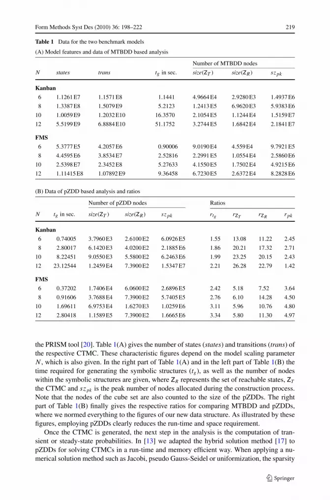
Table 1 Data for the two benchmark models

(A) Model features and data of MTBDD based analysis

Number of MTBDD nodes

N states trans tg in sec. size(ZT ) size(ZR) szpk

Kanban

6 1.1261 E7 1.1571 E8 1.1441 4.9664 E4 2.9280 E3 1.4937 E6

8 1.3387 E8 1.5079 E9 5.2123 1.2413 E5 6.9620 E3 5.9383 E6

10 1.0059 E9 1.2032 E10 16.3570 2.1054 E5 1.1244 E4 1.5159 E7

12 5.5199 E9 6.8884 E10 51.1752 3.2744 E5 1.6842 E4 2.1841 E7

FMS

6 5.3777 E5 4.2057 E6 0.90006 9.0190 E4 4.559 E4 9.7921 E5

8 4.4595 E6 3.8534 E7 2.52816 2.2991 E5 1.0554 E4 2.5860 E6

10 2.5398 E7 2.3452 E8 5.27633 4.1550 E5 1.7502 E4 4.9215 E6

12 1.11415 E8 1.07892 E9 9.36458 6.7230 E5 2.6372 E4 8.2828 E6

(B) Data of pZDD based analysis and ratios

Number of pZDD nodes Ratios

N tg in sec. size(ZT ) size(ZR) szpk rtg rZTrZR

rpk

Kanban

6 0.74005 3.7960 E3 2.6100 E2 6.0926 E5 1.55 13.08 11.22 2.45

8 2.80017 6.1420 E3 4.0200 E2 2.1885 E6 1.86 20.21 17.32 2.71

10 8.22451 9.0550 E3 5.5800 E2 6.2463 E6 1.99 23.25 20.15 2.43

12 23.12544 1.2459 E4 7.3900 E2 1.5347 E7 2.21 26.28 22.79 1.42

FMS

6 0.37202 1.7406 E4 6.0600 E2 2.6896 E5 2.42 5.18 7.52 3.64

8 0.91606 3.7688 E4 7.3900 E2 5.7405 E5 2.76 6.10 14.28 4.50

10 1.69611 6.9753 E4 1.6270 E3 1.0259 E6 3.11 5.96 10.76 4.80

12 2.80418 1.1589 E5 7.3900 E2 1.6665 E6 3.34 5.80 11.30 4.97

the PRISM tool [20]. Table 1(A) gives the number of states (states) and transitions (trans) ofthe respective CTMC. These characteristic figures depend on the model scaling parameterN , which is also given. In the right part of Table 1(A) and in the left part of Table 1(B) thetime required for generating the symbolic structures (tg), as well as the number of nodeswithin the symbolic structures are given, where ZR represents the set of reachable states, ZT

the CTMC and szpk is the peak number of nodes allocated during the construction process.Note that the nodes of the cube set are also counted to the size of the pZDDs. The rightpart of Table 1(B) finally gives the respective ratios for comparing MTBDD and pZDDs,where we normed everything to the figures of our new data structure. As illustrated by thesefigures, employing pZDDs clearly reduces the run-time and space requirement.

Once the CTMC is generated, the next step in the analysis is the computation of tran-sient or steady-state probabilities. In [13] we adapted the hybrid solution method [17] topZDDs for solving CTMCs in a run-time and memory efficient way. When applying a nu-merical solution method such as Jacobi, pseudo Gauss-Seidel or uniformization, the sparsity


Table 2 Comparison of MTBDDs and pZDDs with the UMTS model

Nodes Savings Run-time in sec. Savings

n k States MTBDD pZDD in % MTBDD pZDD in % E[π ]

8 6 2529 18274 12437 31.94 54 35 35.19 44

8 7 12673 35303 24183 31.50 91 49 46.15 30

8 8 395 8703 5615 35.48 12 10 16.67 20

10 6 3941 31888 23823 25.29 198 109 44.95 111

10 7 19761 66085 45873 30.58 472 243 48.52 72

10 8 6931 43466 31134 28.37 185 100 45.95 50

12 6 833 20415 13638 33.20 486 277 43.00 289

12 7 28417 101605 64910 36.12 1892 984 47.99 178

12 8 2815 42024 28462 32.27 358 208 41.90 116

of pZDDs pays off another time, leading to a clear reduction of CPU-time consumptions bya factor between 2 and 3. As a consequence, when employing pZDDs instead of MTBDDs,performance measures for the FMS model and a scaling parameter of N = 12 (resulting inmore than 111 million states) can be computed in ≈ 4 h instead of ≈ 12 h (for further detailsplease refer to [13]).

5.3 pZDDs in the context of probabilistic model checking

The model that is used for this benchmark study is a simplification of the UMTS system.It represents the mechanism to request validation keys for different domains (like phone orInternet access). The model also identifies whether a synchronization failure occurs, i.e. ifa used key is older than the stored key in the UMTS card. The system size depends on thenumber of slots n on the UMTS card, as well as on the number of keys k that are requestedat a time. (Note, that the model size collapses if k is a divider of n.) We specified this modelby employing the symbolic probabilistic model checker PROMOC, which is based on thePRISM input language and the JINC package.

For probabilistic model checking, a symbolic representation of the transition matrix isderived directly from the PRISM model specification. Each matrix entry mi,j hereby definesthe transition probability that the system moves from state i to state j . For investigating thestationary probability of states with a given property one needs to solve a system of linearequations and to calculate the expected number of requests (E[π]) to reach a synchroniza-tion failure. Since PROMOC uses a fully symbolic linear solver (which is far less efficientthan the hybrid solution methods mentioned at the end of Sect. 5.2), our experiments werelimited to relatively small values of n and k. Nevertheless, the benchmark results in Table 2show that pZDDs clearly outperform regular MTBDDs in both size and run-time, where therun-time advantage stems from the fact that fewer DD-nodes induce fewer recursive calls ofthe DD-manipulating algorithms as well as of the symbolic numerical solution algorithm.

6 Conclusion

In this paper we extended ZBDDs [15] to the multi-terminal case, in order to employ the0-sup-reduction rule in the context of symbolic, quantitative analysis of systems. For effi-ciently working with ZDDs defined on differing sets of function variables we introduced


the concept of partially shared ZDDs and described the respective algorithms for manip-ulating them. This not only allowed us to implement pZDDs within standard shared DD-environments, such as CUDD [26] or JINC [9], but also supports the application of non-zero-preserving operators to them. The efficiency of the introduced approach was then demon-strated by analyzing case studies from different contexts, where pZDDs turned out to requireless memory space and less CPU time if compared to the standard type of MTBDDs. Thesuperior performance of pZDDs can be explained by the following reasons: (a) It is typicalthat matrices derived from high-level model descriptions are sparsely populated. (b) Manypositions of the bit strings encoding system states (and thus referring to the indices of reach-able states) carry the value 0, and ZDDs are very efficient at representing sets of such bitstrings. (c) The concept of partially shared ZDDs avoids the insertion of dnc-nodes. It there-fore keeps the symbolic structures compact and even allows to represent different functionsby the same graph. Furthermore, the size reduction of the symbolic structures also leads torun-time advantages.

References

1. Formal Methods in System Design (1997) 10(2–3). Special Issue on Multi-Terminal Binary DecisionDiagrams

2. Akers SB (1978) Binary decision diagrams. IEEE Trans Comput C-27(6):509–5163. Balbo G, Conte G, Donatelli S, Franceschinis G, Ajmone Marsan M, Ajmone Marsan M (1995) Mod-

elling with generalized stochastic Petri nets. Wiley, New York4. Bryant RE (1986) Graph-based algorithms for Boolean function manipulation. IEEE Trans Comput

C-35(8):677–6915. Ciardo G, Lüttgen G, Miner AS (2007) Exploiting interleaving semantics in symbolic state-space gener-

ation. Form Methods Syst Des 31(1):63–1006. de Alfaro L, Kwiatkowska M, Norman G, Parker D, Segala R (2000) Symbolic model checking for

probabilistic processes using MTBDDs and the Kronecker representation. In: Graf S, Schwartzbach M(eds) Proc. of the 6th int. conference on tools and algorithms for the construction and analysis of systems(TACAS’00). LNCS, vol 1785. Springer, Berlin, pp 395–410

7. Hermanns H, Herzog U, Mertsiotakis V (1998) Stochastic process algebras—between LOTOS andMarkov chains. Comput Netw ISDN Syst 30(9–10):901–924

8. Hermanns H, Kwiatkowska M, Norman G, Parker D, Siegle M (2003) On the use of MTBDDs forperformability analysis and verification of stochastic systems. J Log Algebr Program 56(1–2):23–67

9. JINC BDD package. www.jossowski.de10. Kam T, Villa T, Brayton R, Sangiovanni-Vincentelli A (1998) Multi-valued decision diagrams: theory

and applications. Mult Valued Log 4(1–2):9–6211. Kuntz M, Siegle M, Werner E (2004) Symbolic performance and dependability evaluation with the tool

CASPA. In: Proc. of EPEW. LNCS, vol 3236. Springer, Berlin, pp 293–30712. Lampka K, Siegle M (2006) Activity-local state graph generation for high-level stochastic models. In:

Meassuring, modeling, and evaluation of systems 2006, April 2006, pp 245–26413. Lampka K, Siegle M (2006) Analysis of Markov reward models using zero-supressed multi-terminal

decision diagrams. In: Proceedings of VALUETOOLS 2006 (CD-edition), October 200614. Lee CY (1959) Representation of switching circuits by binary-decision programs. Bell Syst Tech J

38:985–99915. Minato S (1993) Zero-suppressed BDDs for set manipulation in combinatorial problems. In: Proc. of the

30th ACM/IEEE design automation conference (DAC), Dallas (Texas), USA, June 1993, pp 272–27716. Minato S (2001) Zero-suppressed BDDs and their applications. Int J Softw Tools Technol Transf

3(2):156–17017. Miner A, Parker D (2004) Symbolic representations and analysis of large state spaces. In: Baier Ch,

Haverkort B, Hermanns H, Katoen J-P, Siegle M (eds) Validation of stochastic systems, Dagstuhl (Ger-many), 2004. LNCS, vol 2925. Springer, Berlin, pp 296–338

18. Möbius web page. www.moebius.crhc.uiuc.edu19. Ossowski J, Baier C (2008) A uniform framework for weighted decision diagrams and its implementa-

tion. Int J Softw Tools Technol Transf 10(5):425–44120. PRISM. www.prismmodelchecker.org

http://www.jossowski.de

http://www.moebius.crhc.uiuc.edu

http://www.prismmodelchecker.org


21. PROMOC modeling tool. www.jossowski.de22. Sasao T, Fujita M (eds) (1996) Representations of discrete functions, vol 1. Kluwer Academic, Dor-

drecht23. Shannon CS (2000) Eine symbolische Analyse von Relaisschaltkreisen. In: Ein/Aus. Brinkmann und

Bose, Berlin. The article originally appeared with the title: A symbolic analysis of switching circuits inTrans. AIEE 57 (1938), 713

24. Siegle M (2001) Advances in model representation. In: de Alfaro L, Gilmore S (eds) Proc. of the jointint. workshop, PAPM-PROBMIV 2001, Aachen (Germany). LNCS, vol 2165. Springer, Berlin, pp 1–22

25. SMART. www.cs.ucr.edu/~ciardo/SMART26. Somenzi F (1998) CUDD: Colorado University decision diagram package release27. Wegener I (2000) Branching programs and binary decision diagrams. SIAM, Philadelphia

http://www.jossowski.de

http://www.cs.ucr.edu/~ciardo/SMART

Documents

Partially-shared zero-suppressed multi-terminal BDDs: concept, algorithms and applications