Embed Size (px)
Citation preview

Patterns in Space and TimeInvestigating the Structure and Variability of Sagittarius A*
with Radio Interferometry
Christiaan Dirk Brinkerink


Patterns in Space and TimeInvestigating the Structure and Variability of Sagittarius A*
with Radio Interferometry
Proefschrift
ter verkrijging van de graad van doctoraan de Radboud Universiteit Nijmegen
op gezag van de rector magnificus prof. dr. J.H.J.M. van Krieken,volgens besluit van het college van decanen
in het openbaar te verdedigen opwoensdag 22 september 2021
om 12.30 uur precies
door
Christiaan Dirk Brinkerink
geboren op 30 april 1980te Neede

Promotor: Prof. dr. H.D.E. Falcke
Manuscriptcommissie: Prof. dr. H.T. KoelinkProf. dr. A.J. LevanDr. E.G. KördingDr. I.M. van Bemmel Joint Institute for VLBI ERICProf. dr. H.J. van Langevelde Universiteit Leiden
© 2021, Christiaan Dirk BrinkerinkPatterns in Space and Time: Investigating the Structure and Variability of Sagittarius A* withRadio InterferometryThesis, Radboud University NijmegenFront cover: A stylised view of VLA antennas and the Galactic Center ’minispiral’, generated bythe author.Back cover: Stylised view of a footpath in ’Heerlijkheid Beek’, generated by the author.Cover & pagemarker design: Christiaan BrinkerinkIllustrated; with bibliographic information and Dutch summary
ISBN: 978-94-6421-423-9


Contents
1 Introduction 11.1 Gravity and black holes . . . . . . . . . . . . . . . . . . . . . . . . . . . . . . . 11.2 The phenomenon of accretion . . . . . . . . . . . . . . . . . . . . . . . . . . . 5
1.2.1 Astrophysical context . . . . . . . . . . . . . . . . . . . . . . . . . . . . 51.2.2 The Eddington luminosity . . . . . . . . . . . . . . . . . . . . . . . . . 61.2.3 The Eddington accretion rate . . . . . . . . . . . . . . . . . . . . . . . . 71.2.4 Models for accretion at different Eddington ratios . . . . . . . . . . . . . 91.2.5 The Mdot-Sigma plane . . . . . . . . . . . . . . . . . . . . . . . . . . . 101.2.6 Disk outflows and jets . . . . . . . . . . . . . . . . . . . . . . . . . . . 13
1.3 Observational signatures of black hole accretion . . . . . . . . . . . . . . . . . . 151.4 History of Sagittarius A* . . . . . . . . . . . . . . . . . . . . . . . . . . . . . . 19
1.4.1 Early detections and interpretation . . . . . . . . . . . . . . . . . . . . . 191.4.2 The spectrum of SgrA* . . . . . . . . . . . . . . . . . . . . . . . . . . 201.4.3 Spectral models for SgrA* . . . . . . . . . . . . . . . . . . . . . . . . . 201.4.4 Morphology . . . . . . . . . . . . . . . . . . . . . . . . . . . . . . . . 231.4.5 Polarisation . . . . . . . . . . . . . . . . . . . . . . . . . . . . . . . . . 24
1.5 Measurement of radio waves, radio interferometry and VLBI . . . . . . . . . . . 261.5.1 Flux density in radio . . . . . . . . . . . . . . . . . . . . . . . . . . . . 261.5.2 Signal amplification and filtering . . . . . . . . . . . . . . . . . . . . . . 271.5.3 Radio interferometry . . . . . . . . . . . . . . . . . . . . . . . . . . . . 271.5.4 Measuring the interference pattern: correlation . . . . . . . . . . . . . . 291.5.5 Aperture synthesis . . . . . . . . . . . . . . . . . . . . . . . . . . . . . 331.5.6 Data calibration . . . . . . . . . . . . . . . . . . . . . . . . . . . . . . . 351.5.7 Useful interferometric observables: closure phases and closure amplitudes 36
1.6 In this thesis . . . . . . . . . . . . . . . . . . . . . . . . . . . . . . . . . . . . . 36
2 Asymmetric structure in SgrA* at 3mm from closure phase measurements withVLBA, GBT, and LMT 392.1 Introduction . . . . . . . . . . . . . . . . . . . . . . . . . . . . . . . . . . . . . 39

ii Contents
2.2 Observations and initial data reduction . . . . . . . . . . . . . . . . . . . . . . . 422.3 Verifying the nature of non-zero closure phases . . . . . . . . . . . . . . . . . . 452.4 Results . . . . . . . . . . . . . . . . . . . . . . . . . . . . . . . . . . . . . . . . 46
2.4.1 Detection of non-zero closure phases . . . . . . . . . . . . . . . . . . . 462.4.2 Modeling source asymmetry using closure phases . . . . . . . . . . . . . 462.4.3 Testing the significance of the observed asymmetry . . . . . . . . . . . . 48
2.5 Discussion . . . . . . . . . . . . . . . . . . . . . . . . . . . . . . . . . . . . . . 492.6 Summary and conclusions . . . . . . . . . . . . . . . . . . . . . . . . . . . . . 57
3 Micro-arcsecond structure of Sagittarius A* revealed by high-sensitivity 86 GHzVLBI observations 593.1 Introduction . . . . . . . . . . . . . . . . . . . . . . . . . . . . . . . . . . . . . 603.2 Observations and data reduction . . . . . . . . . . . . . . . . . . . . . . . . . . 633.3 Results . . . . . . . . . . . . . . . . . . . . . . . . . . . . . . . . . . . . . . . . 65
3.3.1 Mapping and self-calibration of SgrA∗ . . . . . . . . . . . . . . . . . . 653.3.2 Constraining the size of SgrA∗ using closure amplitudes . . . . . . . . . 69
3.4 Constraints on the size-frequency relation and the scattering law . . . . . . . . . 743.5 Summary and conclusions . . . . . . . . . . . . . . . . . . . . . . . . . . . . . 793.A Closure amplitude model fitting technique . . . . . . . . . . . . . . . . . . . . . 82
4 Frequency-dependent time lags in Sgr A* 834.1 Introduction . . . . . . . . . . . . . . . . . . . . . . . . . . . . . . . . . . . . . 844.2 Observations and data reduction . . . . . . . . . . . . . . . . . . . . . . . . . . 854.3 Analysis and results . . . . . . . . . . . . . . . . . . . . . . . . . . . . . . . . . 874.4 Discussion and conclusion . . . . . . . . . . . . . . . . . . . . . . . . . . . . . 924.5 Acknowledgements . . . . . . . . . . . . . . . . . . . . . . . . . . . . . . . . . 96
5 Persistent time lags in light curves of Sagittarius A*: evidence of outflow 995.1 Introduction . . . . . . . . . . . . . . . . . . . . . . . . . . . . . . . . . . . . . 100
5.1.1 Observed spectrum . . . . . . . . . . . . . . . . . . . . . . . . . . . . . 1005.1.2 Observed morphology . . . . . . . . . . . . . . . . . . . . . . . . . . . 1005.1.3 Time-domain studies . . . . . . . . . . . . . . . . . . . . . . . . . . . . 1015.1.4 Questions addressed in this work . . . . . . . . . . . . . . . . . . . . . . 103
5.2 Observations . . . . . . . . . . . . . . . . . . . . . . . . . . . . . . . . . . . . 1035.2.1 Observation epochs, array configuration and spectral setup . . . . . . . . 1035.2.2 Data calibration and reduction . . . . . . . . . . . . . . . . . . . . . . . 104
5.3 Data analysis . . . . . . . . . . . . . . . . . . . . . . . . . . . . . . . . . . . . 1055.3.1 Extracting light curves . . . . . . . . . . . . . . . . . . . . . . . . . . . 1055.3.2 Detection of time lags . . . . . . . . . . . . . . . . . . . . . . . . . . . 1105.3.3 Checks with synthetic data . . . . . . . . . . . . . . . . . . . . . . . . . 113
5.4 Results . . . . . . . . . . . . . . . . . . . . . . . . . . . . . . . . . . . . . . . . 118

Contents iii
5.5 Discussion and Conclusions . . . . . . . . . . . . . . . . . . . . . . . . . . . . 119
6 Summary 137
7 Samenvatting 141
A Research Data Management 145
Bibliography 149
List of Publications 155
About the author 161
Acknowledgments 163


To Mum


The truth may be puzzling. It may take some work to grapple with. It may be counterintuitive. Itmay contradict deeply held prejudices. It may not be consonant with what we desperately want
to be true. But our preferences do not determine what’s true. We have a method, and thatmethod helps us to reach not absolute truth, only asymptotic approaches to the truth — never
there, just closer and closer, always finding vast new oceans of undiscovered possibilities.Cleverly designed experiments are the key.
Carl Sagan


Chapter1Introduction
This thesis treats the study of the supermassive black hole at the center of our Galaxy, which wecommonly refer to as ’Sagittarius A*’, through the use of several measurement techniques thatinvolve radio telescopes. In this introduction I will first of all highlight what black holes are, andwhy we study them. I will then go into more detail on Sagittarius A* in particular. Moving on tothe subject of instrumentation and measurements, I will illustrate how our use of radio telescopeshelps us find out about black hole properties and the behaviour of the gas that surrounds them.This introduction concludes by briefly describing the subjects of the following chapters.
1.1 Gravity and black holes
Gravity as a phenomenon is intuitively understood by humans. We understand that things fallfaster when they fall farther, and our sense (or fear) of heights is intimately linked to this un-derstanding. For instance, in our childhood we quickly learn how to catch a ball that is throwntoward us. This is quite an impressive feat – catching a ball involves modeling its acceleratedmotion and predicting its trajectory at a subconscious level. In his work "Dialogues ConcerningTwo New Sciences", Galileo Galilei systematically quantified the behaviour of falling bodiesand investigated what factors influence the rate at which different objects fall. He found1 thatgravitational acceleration, when measured at the Earth’s surface, means that the vertical speedof a falling object changes by a specific amount per time interval - and not, say, per verticaldistance interval. Isaac Newton applied a quantitative model of gravity to celestial objects withgreat success, showing that the motions of the heavenly bodies follow the same rules as everydayobjects falling here on Earth. Our picture of gravity underwent yet another revolution with AlbertEinstein’s work, who modeled gravity as a geometrical phenomenon: a warping of both spaceand time that is linked to the distribution of matter and energy (Einstein, 1915). In the theory ofgeneral relativity, spacetime is not simply the backdrop against which the events of the universeplay out. Rather, its structure is itself affected by the presence and behaviour of mass and energyin it. This radically different view of gravity would provide exciting new ways to study the
1Although he was not the first one to find this - that honour belongs to Nicole Oresme, see Clagett (1968).

2 Chapter 1 : Introduction
gravitational field of extremely compact objects.
In order to study the structure that spacetime itself has, we need to have a way to express therelation between different events in it. An event is a combination of a time and a place, and has aset of unique coordinates in any map of spacetime. When we wish to express the distance betweentwo events, we already know how to do this for the spatial distance ("the distance between placeA and place B is 5 kilometres") and we know how to do this for the temporal distance ("MomentX happens 2 seconds before moment Y"). However, we can use the speed of light to express sep-aration in time and separation in space in the same way and combine them, so that the spacetimedistance between two events can be expressed as a single number. Distances in the three spatialdimensions can be combined in the usual way using Pythagoras’ rule, 3A =
√3G2 + 3H2 + 3I2, but
time needs to be treated somewhat differently. We will also need to have some way to deal withvariations in the structure of spacetime from place to place as we consider different scenarios.This is where the language of relativity comes in.
In both special and general relativity, we can express the geometry of spacetime in terms of aquantity called the invariant spacetime interval, which gives us the spacetime distance betweentwo events in spacetime. If one starts with the postulate that the local speed of light as measured byany observer always has the same value (a notion that is strongly supported by our measurements),one arrives at a particular form in which time and space can be combined into a geometry ofspacetime. For ’flat’ (Minkowski) spacetime, which is devoid of matter and energy, the invariantspacetime interval can be written out as:
3B2 = −223g2 = −3 (2C)2 + 3G2 + 3H2 + 3I2, (1.1)
where 3B2 is the length squared of the interval, 2 is the speed of light, 3g is the proper time interval(which refers to the time interval between the events as measured by an observer moving from oneevent to the other on a straight, non-accelerated trajectory or a geodesic), and the 3C, 3G, 3H, 3Iterms refer to the coordinate differences between two events in time and the three spatial directionsrespectively, in units that are determined by how 2 is expressed. This expression immediatelytells us something very interesting: the measurement of time can work out differently for differentobservers. Depending on their state of motion, different observers will measure different values of3G, 3H and 3I for the separation between a given pair of events in their respective reference frames.But the spacetime interval that they should both measure is invariant, so they must therefore getdifferent values for 3C as well: as measured in their own reference frames, they get different valuesfor the time interval that passes between the two events. This gives rise to the phenomenon of’time dilation’, where observers measure that the rate at which time passes for other observersmoving with respect to them is slowed down. To make the difference clear, C is also referred to as’coordinate time’ because it depends on the choice of coordinate system.

1.1 Gravity and black holes 3
Flat spacetime is a special case – if we consider non-empty spacetime, the invariant interval canlook quite different. Making the move to general relativity, the general expression for the invariantspacetime interval (hereafter simply called ’interval’) is:
3B2 = 6`a3G`3Ga = 6003G
03G0 + 6013G03G1 + 6023G
03G2 + . . . + 6333G33G3, (1.2)
where we have illustrated the Einstein summation convention (where a repeated index that appearsin an upper and a lower form indicates a summation over all values of that index) and ` and aboth run over 4 dimensions which are labeled 0, 1, 2, and 3 (one is temporal and three are spatial).This notation needs some explaining! In the above expression 3B2 is the length squared of thespacetime interval that is associated with an infinitesimal displacement in spacetime along thefour dimensions, subtly different from the case for flat spacetime where this displacement didn’tneed to be infinitesimal. The components of this infinitesimal displacement are indicated by 3G0
thru 3G3, where the dimension with index 0 indicates the time dimension by convention. Theterm 6`a represents the spacetime metric. The metric written down in this form is a covarianttensor with two indices, both of which run over all four spacetime coordinates - the metric thushas 16 components, 10 of which are independent in General Relativity (the metric is symmetric:6`a = 6a`). It encodes the local structure of spacetime, and when ’fed’ with two copies ofan infinitesimal displacement four-vector it yields a scalar: the spacetime distance between twoinfinitesimally separated spacetime events. This infinitesimal distance can be integrated along apath through spacetime to get the spacetime separation for any pair of events. Choosing the pathso that it maximises the proper time elapsed gives us a geodesic, or the equivalent of a straightline in curved spacetime.
Revisiting the metric for flat spacetime, we see that it only has four nonzero components:600 = −1, 611 = 622 = 633 = 1. We see that the interval is real for spacelike separations,where the positive spatial term 3G2 + 3H2 + 3I2 wins out over the negative temporal term −3 (2C)2.The interval is zero for lightlike separations, where a pulse of light sent from one event preciselyreaches the other. Finally, the interval is imaginary for timelike separations, which is the classof separations where one event can communicate to the other using a message travelling slowerthan light. It should be noted that the sign convention for the space and time components of theinvariant interval can be chosen oppositely as well, but this makes no difference to the physicsthat follows from it. Choosing one representation over the other is a matter of convention and taste.
When we now consider a point mass at the origin, it should affect the geometry of spacetime ina spherically symmetric way as no spatial direction is preferred over another. It therefore makessense to express the interval using spherical coordinates. When we do this first for flat spacetime,we get the following expression:
3B2 = −3 (2C)2 + 3A2 + A23\2 + A2 sin2 \3q2, (1.3)
where A is the radial coordinate, \ is the polar angle and q is the azimuthal angle. The solution tothe geometry of spacetime that follows from the Einstein equations for a stationary point mass in

4 Chapter 1 : Introduction
a vacuum was derived by Karl Schwarzschild in 1916, just months after Einstein had publishedhis paper introducing general relativity. This metric is known as the Schwarzschild metric, andits invariant interval can be written in spherical coordinates as:
3B2 = −223g2 = −(1 − 2�"22A)3 (2C)2 + (1 − 2�"
22A)−13A2 + A23\2 + A2 sin2 \3q2, (1.4)
where " is the mass of the central object and � is the universal gravitational constant. Wesee that the factors in the radial and temporal terms have changed with respect to those for flatspacetime. We also notice that something strange happens at a radius of 2�"
22 : the factors in theC (temporal) and A (radial) terms tend to zero and infinity, respectively. We are dealing with acoordinate singularity at this radius: a place where this coordinate system stops working and adifferent one is needed to give us insight into what physically happens there.
After Schwarzschild’s solution got published, it took decades of debate before the nature of thisspecial radius became fully apparent (Finkelstein, 1958). It turned out that this critical radiusA = 2�"
22 defines a so-called ’event horizon’, a one-way virtual boundary that prevents any causalcontact from its interior to the rest of the universe but still allows for matter or energy to enterthe enclosed region. This behaviour cannot readily be seen when considering the spacetimein Schwarzschild coordinates, which is why it took some time before it was worked out usingdifferent choices of coordinates (Misner et al., 1973; Finch, 2015).
Besides the one-way character of the event horizon, there are other strange effects that manifestthemselves when matter approaches the horizon as seen by a faraway observer. One of theseeffects is that of extreme gravitational redshift, where the apparent frequency of any radiationemitted from objects close to the event horizon is strongly reduced as the radiation escapes toinfinity. This is a form of time dilation that does not depend on differences in the state of motionbetween two observers, like we saw earlier, but on the different positions that observers can havein a gravitational field. The strength of this phenomenon can be expressed when we considerthe ratio of coordinate time to proper time for a stationary particle (i.e., 3\ = 3q = 3A = 0)sitting outside the event horizon as measured by a faraway observer. This quantity expresses the’slowdown factor’ of time close to the black hole. We use expression 1.4, setting 3\, 3q and 3Ato zero, and re-arranging terms to get the relation between proper time and coordinate time for astationary observer:
3C
3g=
1√1 − 2�"
22A
. (1.5)
This expression tells us that the ratio of elapsed coordinate time (or: time as measured by anobserver at infinity, whose own 3g and 3C are practically the same) to proper time for a stationaryobserver or particle close to the horizon diverges as we let the particle quasistatically approach thehorizon. The gravitational time dilation does not simply become very large, it becomes infinite!Observers at large distances thus never observe anything crossing the event horizon as it falls in.Instead, matter will seem to approach the horizon ever more slowly and any radiation emitted

1.2 The phenomenon of accretion 5
from it will be redshifted into obscurity. Locally, an observer falling in together with the accretingmatter will observe no such slowing of time but will cross the event horizon (an unremarkableevent for that observer) in finite proper time. This can be understood when radial freefallingmotion is considered using different coordinates to describe the same Schwarzschild spacetime,such as Lemaître coordinates (Lemaître, 1933).
For several decades, these debates about black holes were mostly academic – they centered aroundproperly understanding the theory and not so much around explaining the observed phenomenaof the universe. The notion that black holes might exist as real, physical objects, and not merelyas theoretical constructs, dawned in the 1960s with the discovery that quasars are the active nucleiof galaxies (Schmidt, 1963). In these sources, practically all emission comes from a concentratedregion in the center of a galaxy, meaning that some kind of energetic process must be taking placethere in order to liberate all that energy. Understanding the workings of such powerful ’centralengines’ necessitated finding a physical mechanism by which they could be powered – and themost promising physical mechanism for this was accretion onto a compact and massive object. Inthis same time period, Penrose (1965) brought black holes closer to reality from the theoreticalside by showing that under suitable physical circumstances, collapsing matter should indeed forma black hole – even without the assumption of perfect spherical or even rotational symmetry.
1.2 The phenomenon of accretion
1.2.1 Astrophysical context
In the context of astrophysics, accretion is the process where diffuse matter (gas or plasma),moving under the influence of gravity, falls onto or into a central object (e.g., a planet, a star, ora black hole). Because the diffuse matter generally has nonzero net angular momentum, it tendsto form a disk structure around the central object. Within this accretion disk, various physicalprocesses can facilitate the transport of energy and angular momentum between different zones ofthe disk. By exchanging angular momentum with other regions of the accretion flow, matter canfall onto (or into) the central object. In this introduction, I will specifically focus on the processof accretion onto black holes as that is the relevant context for this thesis.
As the accreting material descends progressively deeper into the gravitational potential well ofthe black hole, its gravitational potential energy is converted into other forms of energy. Oneof the prominent forms is heat: by viscous dissipation of energy through some form of – likelymagnetically mediated – friction, accreting gas in binary stellar systems can be heated up totemperatures of millions of Kelvins in the inner region of the accretion disk (Shakura & Sunyaev,1973). Such high gas temperatures give the accretion flow a particular spectral signature, withthe emitted frequency distribution depending on the specifics of the geometry and density of theaccretion flow.

6 Chapter 1 : Introduction
Black hole accretion works over a wide range of scales. On smaller scales, it can occur in closebinary stellar systems where one of the components is a black hole. If the orbital separationbetween the two components is small enough, the black hole can draw matter from the outer layerof the secondary component (dubbed the ’donor’) which then forms an accretion disk around itas it still possesses angular momentum (Figure 1.1). On large scales, accretion typically occursfrom a more diffuse reservoir of gas such as the collective products of strong stellar winds in agalactic core. These diffuse gas clouds can accrete onto a supermassive black hole at the centerof that galaxy if their relative velocity is sufficiently low to become gravitationally bound to theblack hole.
Figure 1.1: Artist impression of a black hole binary. The companion or donor star, visible on theright, loses gas to the accreting black hole which is surrounded by an accretion disk. The black holeitself is too small to be seen at this scale. A small fraction of the accreting material may escape in theform of disk winds or, as pictured here, a high-velocity jet. Image credit: NASA/CXC/M. Weiss.
1.2.2 The Eddington luminosity
Black hole accretion has been studied extensively, both analytically from first principles andthrough numerical simulation. For an extensive review of black hole accretion (both in stellar

1.2 The phenomenon of accretion 7
systems and in active galactic nuclei), see Abramowicz & Fragile (2013). In order to classifyaccreting systems, one important parameter to consider is the rate at which matter is suppliedto the system (the accretion rate). When we want to define different behavioural regimes ofaccretion, it is useful to start by considering a simple situation in which diffuse and fully ionizedhydrogen is accreting onto some compact object in a spherically symmetric way.
As this hydrogen accretes, we can imagine that the gravitational potential energy of the plasma isconverted into radiative energy through some conversion process. As we increase the accretionrate, the opacity of the accreting plasma will increase as its density grows, and the relativeinfluences of gravitational attraction and outward-pointing radiation pressure will shift. Forsimplicity, we can assume that most of the radiated power comes from directly around our centralobject. In such a scenario, we can ask ourselves the question: "How much power should ourcentral object need to radiate for its radiation pressure to balance the attractive gravitational forceit exerts on the surrounding plasma?". This power is called the Eddington luminosity (Eddington,1920). Writing it down in the physically relevant terms, we get the following expression (Rybicki& Lightman, 1979):
!Edd =3c�"<?2
f), (1.6)
which is valid for neutral but fully ionized hydrogen. In setting up this expression, we make use ofthe fact that the gravitational influence is dominated by the mass of the protons (represented with<? in the equation) as they represent most of the mass of the plasma, while the influence fromradiative pressure is dominated by the Thomson cross-section of the electrons (represented by f) )as they dominate the interaction with electromagnetic radiation. � is the universal gravitationalconstant, " is the mass of the accreting object and 2 is the speed of light. When we assume amass for the accreting object, the corresponding Eddington luminosity can be calculated. Notethat the expression for the Eddington luminosity does not contain any term for the distance tothe central object, as the outward-pointing acceleration from radiation pressure has the sameinverse-square radial dependence as the inward-pointing gravitational acceleration. If the forcesbalance at one particular radius, they will also balance at any other radius when we assume thatboth the gravitationally dominant mass and the primary source of radiation are colocated in thecenter of the system.
1.2.3 The Eddington accretion rateWe can now picture a situation where the accretion rate is such that the rate of gravitational energyconversion reaches the Eddington luminosity. For isotropic, spherical accretion, we would expectthe accretion flow to experience significant effects from radiation pressure at this point – likelychanging the overall character of the accretion flow. If we want to calculate a critical accretionrate using the Eddington luminosity, we will need to make assumptions as to the radius where thegravitational potential energy of the accreting gas actually gets converted into radiative energy.
8 Chapter 1 : Introduction
We will also need to assume some efficiency factor for this process. If we consider an object witha well-defined surface, such as a white dwarf or a neutron star, we can assume that the lower limitfor the radius at which the potential energy of the infalling material gets liberated is the stellarradius. Let us consider gas that is moving in from some large radius 'outer to an inner radius'inner, and look at the power available from the rate of change in gravitational potential energy ofthe accreting matter. Assuming a radially infalling motion for the accreting gas, we can set up thefollowing expression for accretion power:
!acc = [ ¤<(−�"'outer
+ �"
'inner
). (1.7)
For objects that have a well-defined surface, the efficiency parameter [ can reach a significantfraction of unity as eventually all the gravitational potential energy of the material falling onto thesurface will be converted into thermal energy and radiated away (Sibgatullin & Sunyaev, 2000),the only lost energy being carried away by the fraction of material that escapes from the accretionflow. However, for black holes the situation is somewhat more subtle. As black holes do nothave an observable surface, there is no guarantee that the infalling material gets to convert itsgravitational potential energy into radiation before it disappears at the event horizon. The hot gasmay simply disappear behind the horizon before it has a chance to radiate its heat away. In thiscase, the efficiency factor in our expression will have a value much smaller than 1. The exactvalue of this efficiency factor depends on other physical parameters and specifics of the accretionflow under consideration. Equating the Eddington luminosity to the above expression for theaccretion power, and assuming 'out to be much larger than 'in so that the corresponding term canbe neglected, we get an expression for the Eddington accretion rate:
¤<Edd =3c<?2'in
[f). (1.8)
For a black hole, we can substitute the Schwarzschild radius 'Sch = 2�"22 for 'in, which then gives
us:¤<Edd =
6c<?�"
[f)2= !Edd ·
2[22 . (1.9)
The factor of 2 typically gets absorbed into the accretion efficiency parameter [, so that the Edding-ton luminosity and the Eddington accretion rate are related by the expression !Edd = [ ¤<Edd2
2.Theoretically, in the context of black hole accretion the value of the efficiency parameter [can range from ∼0.06 for a non-rotating black hole to ∼0.4 for a maximally rotating black hole(Novikov&Thorne, 1973). A fiducial value that is often picked for the efficiency parameter, basedon observations of accreting sources (Soltan, 1982), is ∼0.1, which means that the mass-to-energyconversion of an accreting black hole can be appreciably more efficient than it is for stellar fusion(proton-proton) where it is ∼ 0.007. While the radiative efficiency of an accretion flow arounda black hole depends on many specifics of the accretion regime and the environment, the Ed-dington accretion rate provides a useful general scale to use in the classification of accretion flows.

1.2 The phenomenon of accretion 9
1.2.4 Models for accretion at different Eddington ratios
Apart from setting the energy budget for the accretion luminosity, the accretion rate directly in-fluences the density of the accretion disk and thereby the optical depth of the system. The specificcombination of radiative power and optical depth has consequences for the relative importancethat radiation plays in the dynamics of the accreting system: if an accretion disk cannot coolefficiently because it has a large optical depth in combination with high accretion power, it will getgeometrically thick because the trapped radiation heats the gas to a high temperature which bringsthe gas close to virial temperatures. This yields an accretion flow that behaves very differentlyfrom a system where the gas can cool efficiently through radiation, which keeps the accretion diskgeometrically thin. At the other end of the scale is the regime of very low accretion rates, wherethe gas has such a low density that again it cannot cool efficiently through radiation – this timebecause of a lack of Coulomb interactions between its particles. The accreting gas thus reachesextremely high temperatures and we again get a geometrically thick accretion disk. To explorethe range of possible configurations for an accreting system properly, we can set up a full systemof 1D accretion equations, which describe the necessary relations for continuity of mass, energyconservation and angular momentum transport (Accretion power in astrophysics, section 11.4).The set of solutions to these 1D equations gives us a basic insight into the different possiblephysical configurations that an accreting system can have. When considering accretion rates, it isconvenient to express the accretion rate as a fraction of the Eddington accretion rate. This fractionis often also called the ’Eddington ratio’ of an accreting system. Several types of accretion flowshave been identified over the years, valid for different ranges of Eddington ratios. These types aredescribed in the following paragraphs.
Models for accretion disks based on physical principles were first proposed byWeizsäcker (1948),but left the mechanisms for angular momentum redistribution open. The earliest self-consistentmodel of an accretion flow was formulated by Shakura & Sunyaev (1973). This model describesa geometrically thin, optically thick accretion disk where the energy liberated through viscousdissipation is radiated locally everywhere. The spectrum radiated by this flat accretion disk thuslooks like a sum of blackbodies, as each ring in the disk radiates at thermal equilibrium. Thissolution holds for intermediate Eddington ratios of ∼0.1 to ∼1. The accretion flow depicted inthe middle panel of Figure 1.2 falls in this regime.
Begelman (1978) presented a solution for radiation-pressure dominated, super-Eddington accre-tion flows, initially applied to black hole accretion inside massive stars. Later, this mode ofaccretion was suggested to be applicable to other accreting systems as well, specifically in AGNthat undergo super-Eddington accretion (Kawaguchi, 2004; Ohsuga & Mineshige, 2007). Thisclass of solutions is characterised by a hot accretion flow where radiation is trapped due to thelarge optical depth of the system, and where the local disk thickness is equal to the radius or evenlarger. The left panel of Figure 1.2 shows an example of this behaviour.

10 Chapter 1 : Introduction
Figure 1.2: Gas density distributions in different accretion regimes, demonstrated by 2D axisymmetricradiation-magnetohydrodynamic simulationswith different disk densities onto a stellar-mass black holeof 10 "�. Left: an initial disk density of 1 g/cm3 gives a high Eddington ratio accretion flow, withradiation trapped in the optically thick ’slim’ disk. Middle: an initial disk density of 10−4 g/cm3 yieldsa geometrically thin, optically thick disk with an intermediate Eddington ratio. Right: an initial diskdensity of 10−8 g/cm3 results in a geometrically thick, optically thin disk with an advection-dominatedaccretion flow at a low Eddington ratio. Streamlines for the accretion flow are indicated by theblue/green lines. Figure reproduced from Ohsuga & Mineshige (2011).
For very low-Eddington accretion flows ( ¤" < 0.005 ¤"Edd), which are expected to have low den-sities, an accretion model was proposed by Shapiro et al. (1976) (see also Rees et al. (1982) andIchimaru (1977)) where the plasma develops a two-temperature state. In this regime the ionshave high temperatures as they are unable to lose their energy efficiently (by either radiation orinteraction with the electrons), whereas the electrons cool muchmore quickly through interactionswith the magnetic field, and thus have significantly lower temperatures. Such a two-temperatureaccretion flow may form in the inner region of an accretion flow, and be connected to a largerShakura-Sunyaev thin disk at its outer boundary. An example of this regime is visible in the rightpanel of Figure 1.2.
1.2.5 The Mdot-Sigma plane
The current understanding in accretion theory is that theEddington ratio is not the only variable thatdetermines the accretion flow type. These days, the unification picture makes use of classificationof accretion flows in the so-called ¤" − Σ (’Mdot-Sigma’) plane. Expressing the accretion rateas a fraction of the Eddington accretion rate along one axis and of the vertically integrated disksurfce density denoted by Σ along the other axis, we can identify the types of solutions that can

1.2 The phenomenon of accretion 11
hold for a given radius in an accreting system as a function of the effective viscosity parameter U,which is defined as in the alpha-prescription introduced by Shakura & Sunyaev (1973). The valueof U is an important parameter when considering the regions in the ¤" − Σ map: it parametrisesthe effective plasma viscosity in a dimensionless form in the following expression:
a = U2B�, (1.10)
where a is the plasma viscosity as used in the 1D accretion equations, 2B is the local sound speedin the plasma and � is the local scale height of the accretion disk. This functional relation wasmotivated by a consideration of turbulence as the primary source for viscosity: the mixing ratescales with the sound speed, and eddies in the flow are limited in size by the local scale height ofthe accretion disk. Depending on the value that is chosen for U, different families of solutions forthe accretion equations can be found that each show a specific relation between the accretion rateand the disk surface density.
The map of solutions is shown in a simplified form in Figure 1.3. An important point is that sucha map is only valid for one particular radial position in an accreting system, and that changing theradial position under consideration will change the appearance of the map. Furthermore, the equa-tions used to identify these solution types assume that we are dealing with a single-temperatureaccretion flow, where the electrons and protons share the same temperature. This assumption maybe violated in cases of very low plasma densities.
TheMdot-Sigmamap shows multiple regions that may share the same values for U but still exhibitdifferent behaviour. Ucrit is the value for the viscosity parameter that separates the different fami-lies of solutions. The zones indicated in this diagram, separated by dashed, dotted and dash-dottedlines, indicate where the influences of different physical mechanisms dominate. Regions wherethe disk is optically thin/thick can be identified, as well as regions where gas pressure or radiationpressure dominates. Furthermore, the dominant term of heat loss for the local plasma can beidentified as being either radiation or advection (i.e., transportation to smaller radii). Note that thevalue for Ucrit can change as a different radius is considered - and so, the character of an accretiondisk can in principle be quite different in different radial zones. The solution families indicatedin the diagram with symbols I-IV correspond to types of accretion flows, and a short overview ofthem is given here.
Solutions of type I are optically thick and can be either gas-pressure dominated or radiation-pressure dominated. The high-Eddington ratio segment of this class yields radiatively inefficientaccretion flows with puffed-up disks that are supported by radiation pressure, also known as’slim disks’ which have a local thickness that is similar to the local radius. In this regime, thegenerated radiation gets trapped in the disk because of the high optical depth of the accretion flow.The energy in the radiation field and the accreting matter predominantly gets transported inwardrather than radiated away, classifying this type as a so-called ’advection dominated accretion

12 Chapter 1 : Introduction
Figure 1.3: The general structure of the Mdot-Sigma plane, taken from Frank et al. (2002). BranchI covers Shakura-Sunyaev flows (bottom) and slim disks (top). Branch II covers Shakura-Sunyaevflows (right) and Shapiro-Lightman-Eardley (SLE) flows (left). Branch III covers SLE flows (right)and advection-dominated accretion flows (ADAFs, left). Finally, branch IV covers the ’Polish donut’class (Abramowicz et al., 1978). The vertical dashed line indicates the boundary between opticallythin flows (to the left) and optically thick flows (to the right).
flow’ (ADAF). See Mineshige & Ohsuga (2007) for a review of this regime as it occurs for AGN.For lower Eddington ratios, the type I solutions enter an unstable regime (downwards-slopinglines in the diagram). The lower segment of type I, which is once again stable, yields ’classic’Shakura-Sunyaev accretion disks that are radiatively efficient, geometrically thin, optically thickand predominantly supported by gas pressure. See Blaes (2007) for a review of this indermediateEddington ratio accretion flow type in AGN. The solutions that lie along this branch in zone I areclassified as ’cold’ accretion flows, in contrast to the configurations found in the left segment ofzone II and in zone III which are classified as ’hot’.
Type II and III solutions take the accretion flow into a different regime. At low Eddington ratiosand low surface densities, cooling the ions in the accretion flow becomes problematic. The wedge
1.2 The phenomenon of accretion 13
defined by the intersection of the optically thin region with the region where radiation-coolingis the dominant heat loss mechanism defines a parameter space where the single-temperatureassumption may break down for regions within the accretion flow. The reason for this is becauseof the low disk surface density in this part of the parameter space, Coulomb interactions betweenthe plasma particles will be rare and the accreting gas will not be able to radiate away its internalenergy efficiently: most of the kinetic energy is locked into the ions because of their highermass, but this energy is not shared efficiently with the electrons that would be able to radiate thisenergy efficiently. Thermal energy thus gets advected inwards along with the accreting matter.The electrons in such an accretion flow may cool through processes that do not require closeparticle interactions, such as synchrotron radiation, but the electrons are themselves not heatedefficiently by the ions in the accretion flow. This recipe for a two-temperature accretion flowwas first formulated by Shapiro et al. (1976), which describes an accreting system where thetwo-temperature model features in the inner region (the boundary of zone II and zone III in theMdot-sigma diagram corresponds to mixed accretion flows of this type). Yuan (2007) presents areview of this type of low-Eddington accretion flows in AGN.
Zone IV describes accretion flows that are commonly called ’Polish donuts’ (Abramowicz et al.,1978). These are radiation-supported, thick accretion disks that are almost spherical in naturebut do have a clearly defined rotation axis. Their accretion efficiency (the fraction of potentialenergy converted into radiation) is very low, and as such they can exhibit accretion far above theEddington limit. Cases with U > 1 (in zone IV) are generally considered to be unphysical, butthere may be circumstances where that condition can (temporarily) be reached (Frank et al., 2002,paragraph 7.6).
1.2.6 Disk outflows and jets
As the accreting material within a disk is lowered into closer orbits, it must lose angular mo-mentum – and this extracted angular momentum must go somewhere. An obvious channel forextraction of angular momentum from an accretion disk comes in the form of matter outflows.From observations of protostars, microquasars and AGN we know that such accreting systems,across a wide range of scales, often show fast outflows in the form of collimated winds or ofplasma jets. These jets are thought to be intimately linked to magnetic processes occurring in theaccretion flow (see Pudritz et al. (2012) for an overview of source types and general discussion).In the context of black hole accretion, the two fundamental jet launching models that have had thelargest impact are the Blandford-Znajek model (Blandford & Znajek, 1977) and the Blandford-Payne model (Blandford & Payne, 1982).
The Blandford-Znajek model describes a process whereby a magnetised accretion flow pushesmagnetic flux inward, closer to a black hole with nonzero spin, amplifying the magnetic fieldat small radii. Angular momentum and energy are then extracted from the rotating black hole

14 Chapter 1 : Introduction
through the forced corotation (frame dragging) of the magnetic field threading the ergosphere,which winds up the field into a helical configuration and generates a Poynting flux away from thesystem, along the spin axis of the black hole. This process has been associated with the launchingof highly relativistic jets. A schematic illustration of this process is shown in Figure 1.5.
The Blandford-Payne model (Blandford & Payne, 1982) is a separate jet-launching mechanismthat was proposed a few years later. In this model, plasma is launched from the accretion diskboundary layer by being ’flung out’ along magnetic field lines anchored in the disk, where thefield orientation in the poloidal plane exceeds a critical angle outwards from the spin axis of theaccretion disk. The jet launching region for this model is much larger than in the Blandford-Znajekcase, and initial plasma launching speeds are lower. In reality, jet launching in AGN is expectedto feature some combination of these two jet launching mechanisms.
Irrespective of the jet launching mechanisms that are assumed to be operational, Blandford &Königl (1979) investigated the expected general properties of a conically expanding jet launchedfrom an accretion flow. They operated on the assumption that such a jet is close to isothermalalong its axis – i.e., the temperature of the particles in the jet does not drop with increasing dis-tance from the black hole, whereas the magnetic energy density and the particle number densitydo. This property then yields a flat radio spectrum for such a jet. Observationally, AGN haveindeed been associated with flat core radio spectra. The cores of AGN are therefore thought toharbour unresolved expanding and accelerating jets. A fundamental feature of an expanding jet isthe varying position along the jet axis of the apparent core of emission, when we look at differentradio frequencies. Due to the fact that the jet has a non-constant density along its axis, the locationof the photosphere (the point where the optical depth is unity) depends on the frequency of theemission under consideration. This situation provides several powerful ways to test the theory:we can look for core shifts in jets, where the centroid of emission shifts along the jet axis withobserving frequency (a prime example being the jet in M87, see Hada et al. (2011)), and wecan look for variability time lags in jets as variations in the emissivity of the outflowing plasmatypically become visible sooner at higher observing frequencies (used to generate predictions forSgrA* in Falcke et al. (2009)).
The notion that plasma jets are produced from some accretion flows invites the question: underwhat circumstances do jets form, and how do their properties depend on the state of the accretionflow? Falcke & Biermann (1995) coupled the Blandford-Königl jet model to the overall massand energy budget of an accreting system and showed that the theoretically expected emissionmatches observed flux densities over a wide range of frequencies (radio to X-ray) and accretionrates. The relation between accretion flows and the jets they sometimes produce remains quite anactive field of investigation, see e.g. Sbarrato et al. (2014).
Relativistic plasma jets themselves are also studied intensively, as they can have a significant

1.3 Observational signatures of black hole accretion 15
impact on the environment of the accreting system over a wide range of scales. Their largevelocities compared to the surrounding material, combined with the presence of strong magneticfields, provide conditions that are highly conducive to the acceleration of electrons and cosmic raysto high energies. Particle acceleration is thought to be possible close to the jet launching region,where the accelerated electrons are thought to be responsible for e.g. high-energy gamma-rayemission that has been observed from accreting systems. At much larger scales, the radio lobesof AGNs are formed around the points where the plasma jet from the central engine impacts theintergalactic medium and causes turbulent plasma structures to form that show a slowly coolingpopulation of fast electrons emitting in radio. These radio lobes are also considered to be strongcandidate sites for the generation of high-energy cosmic rays. Furthermore, the deposition ofenergy into the circumgalactic medium by relativistic plasma jets is thought to lower the rateat which the galaxy accretes gas from the intergalactic medium. In this way, the activity of anaccreting supermassive black hole in the center of a galaxy can indirectly impact the star formationrate in that same galaxy, and in this way its long-term evolution. Open questions in the research onplasma jets include the nature of their acceleration profiles, their collimation mechanisms, theirtransverse structure, their specific sites of particle acceleration and their specific dependence onblack hole spin parameters.
1.3 Observational signatures of black hole accretionIn 1971, the Uhuru X-ray satellite observed a region of the sky in the Cygnus constellation. Inthis region, an X-ray source associated with a blue supergiant had previously been discovered.Uhuru measured strong and rapidly varying X-ray emission that seemingly came from the locationof a blue supergiant star on the sky (Oda et al., 1971). Such a high X-ray flux density cannotbe generated by a supergiant star, so an alternative explanation for the X-ray source needed tobe found. The rapid time variability of the X-ray source, with temporal features as fast as onemillisecond (Rothschild et al., 1974), suggested it was an accreting object. Its mass (∼15 "�,Orosz et al. (2011)) could be derived from the radial motion variations of the blue supergiant andthe periodicity of emission from the system, and it was concluded that Cygnus X-1 had to be ablack hole as it was found to be too massive to be a neutron star. This made Cygnus X-1 the moststrongly observationally supported black hole candidate at that point.
The observational signatures of accreting systems vary considerably according to their scale,inclination, obscuration and accretion rate. Accretion flows in X-ray binary star systems can cyclethrough different accretion states over relatively short timescales (Tananbaum et al., 1972), andin that way they provide excellent laboratories for studying accretion dynamics. Their spectralsignature in X-rays can be plotted in a so-called hardness-intensity diagram (HID), where thespectral slope of the X-ray emission is plotted against the X-ray luminosity (see Figure 1.6). Theevolution of these systems shows up as a typical q-shaped curve, with a quiescent (’low/hard’)state in the bottom right and a flaring (’high/soft’) state at the top left. According to our current

16 Chapter 1 : Introduction
Figure 1.4: Illustration of the Blandford-Znajek mechanism, where energy and angular momentumare extracted from the ergosphere of a rotating black hole via magnetic interaction. Initially straightmagnetic field lines, anchored in the orbiting plasma, get twisted up and cause part of the plasma inthe ergosphere to attain a negative total energy – where its binding energy is larger than its rest-massenergy (red-coloured segment). The extracted energy gets transported out of the equatorial plane alonga jet structure, where plasma is accelerated by magnetic pressure from coiled field lines. Throughthis mechanism, energy is extracted from the black hole itself rather than from the accreting plasma.Figure from Semenov et al. (2004).
understanding, these emission states are the consequence of very different accretion disk config-urations. The low/hard state has a low-density disk or corona and a plasma jet associated with it,while the high/soft state has a flatter, denser disk but not necessarily a jet. The changes betweenaccretion states are thought to be a function of the varying supply rate of gas to the accretion disk.
Compelling evidence for stellar-mass black holes in binary systems comes from gravitationalwave observations (Abbott et al., 2016). The merger events observed by this highly sensitivenetwork of gravitational wave detectors can only be successfully modeled by invoking binaryblack holes, as no other proposed type of object is compact enough to yield gravitational wave-forms of the observed strength and frequency. To date, LIGO/VIRGO has reported detections

1.3 Observational signatures of black hole accretion 17
Figure 1.5: Geometry of the Blandford-Payne mechanism. Packets of plasma are strongly coupledto the magnetic field, and are constrained in their motion to move along field lines. Close to the diskmidplane, if the outwards inclination of the (corotating) magnetic field lines away from the verticaldirection is 30◦ or more it is energetically favourable for the packet to ’slide’ to larger radii and gainkinetic energy. In this way, an outflow can be launched from close to the disk boundary layer. Figurefrom Jafari (2019).
of black hole mergers in the mass range from a few Solar masses up to several tens of Solar masses.
Figure 1.6: Left: state changes in an observed X-ray binary system, visible in a hardness-intensitydiagram (HID). Right: schematic depiction of the states and their transitions. Figures from Belloniet al. (2005) and Fender et al. (2004).
Observational evidence for another type of black hole came from observations of active galacticnuclei (AGN). The systematic study of what later proved to be AGN effectively started in 1943,

18 Chapter 1 : Introduction
when Carl Seyfert published a catalog of galaxies of which the nuclei exhibited broad spectral lineemission (Seyfert, 1943). Research into these sources entered a phase of rapid development withradio observations done in the 1950s and 1960s. With the resolving power for radio observationssteadily improving and more spectral studies being performed, it became clear that these objectsshowed highly redshifted spectral lines and were very compact. One of the explanations offeredwas that these were Galactic objects of very high density with a large gravitational redshift. How-ever, other aspects of the spectral observations (specifically the presence of forbidden lines in theiroptical spectra, necessitating the presence of low-density gas in the source) pointed towards themhaving an extragalactic character, with the redshift having a cosmological nature. The relativelyfast optical variability of these sources (on timescales of ∼days) suggested that they are compactin nature (Smith & Hoffleit, 1963). It thus became clear that these sources were situated at cosmo-logical distances from the Milky Way (Schmidt, 1963), and exhibited tremendous luminosities.Apparently, the nuclei of many faraway galaxies were harbouring powerful engines that show upbrightly in radio and sometimes in optical as well. Given their rate of energy conversion, thesecentral engines were also found to be likely responsible for powering large ’radio lobes’ beyondthe limits of the host galaxies themselves, through the expulsion of fast plasma jets. Salpeter(1964) and Zel’dovich (1964) proposed that this engine is powered by accretion of gas onto asupermassive black hole.
Further observational evidence for the existence of supermassive black holes comes from themeasurement of spatially resolved lensed synchrotron emission from the orbiting plasma directlyaround the supermassive black hole (Event Horizon Telescope Collaboration et al., 2019a) atthe center of the M87 elliptical galaxy. The observed emission distribution is consistent with agravitationally lensed plasma flow around a dark object. This is the first observation of a blackhole candidate that provides direct support for the existence of an event horizon, as opposed to amassive object with an observable surface.
Nowadays, the body of evidence supporting the existence of black holes, both stellar-mass andsupermassive ones, is extensive. Besides the X-ray and AGN studies mentioned, observationsof stellar velocity distributions in several nearby galaxies have shown the presence of dark andconcentrated masses (Kormendy & Richstone, 1995), while more recently analysis of individualstellar dynamics around the Galactic center points to the existence of a highly compact but prac-tically invisible mass of ∼4 ×106 "� at the center of the Milky Way (Ghez et al., 2008; Genzelet al., 2010). Observations done in infrared over the cource of multiple decades show a centralstar cluster where the individual stars move on Keplerian orbits around the same locus. The massconcentrated in this point apparently completely dominates the orbital dynamics of these stellarorbits, but the associated object is generally faint in infrared outside of the short time intervalswhen it flares up and gets up to tens of times brighter Dodds-Eden et al. (2011).
In AGN, the scale of the accreting system is several orders of magnitude larger than in X-ray

1.4 History of Sagittarius A* 19
binaries. All associated timescales are correspondingly longer. We may never observe an AGNchanging accretion states as its supply rate of gas is only expected to vary significantly overtimescales of hundreds of thousands or even millions of years. We can however see the pastactivity of some AGNs by studying the current appearance of their jets and hot spots. It appearsthat the jets of AGN have limited duty cycles when considered over longer timescales (Schawinskiet al., 2015), and thus AGN seem to experience different states much like X-ray binaries do. AGNare indeed classified into radio-quiet and radio-loud categories, where the latter category has aprominent jet that is responsible for the radio emission. However, the reason for this dichotomyis not clearly understood yet and multiple causes (among which are accretion rate, BH spin,BH mass, environment) have been put forward as potential explanations (Retana-Montenegro &Röttgering, 2017, and references therein).
1.4 History of Sagittarius A*
It seems that our Milky Way, like many other galaxies, harbours a supermassive black hole at itscenter. In this subsection I will describe where this notion comes from and what support for itwe currently have. The center of our Milky Way is heavily obscured to us at optical wavelengths,with gas and dust in the plane of the Galaxy, along our line of sight towards the Galactic center,providing practically complete extinction of all optical radiation coming from there to us. Thisobscuration is less severe at longer wavelengths, and from infrared (IR) down to radio we cansuccessfully probe the nuclear environment of our Galaxy. As such, the history of observationsthat led to our current understanding of what our Galactic center harbours is quite extensive.
1.4.1 Early detections and interpretation
In 1931, as part of his investigation into the noise on transatlantic transmissions, Karl Jansky madethe first detection of radio emission coming from the Galactic Center (Jansky, 1933). Generalinterest in active galactic nuclei prompted further study into the center of our Milky Way withinfrared detections reported by Becklin & Neugebauer (1968). Measurements from the early70s showed that multiple radio structures could be identified around the Galactic center, one ofwhich appeared to be compact (Downes & Martin, 1971). Balick & Brown (1974) reported thedetection of a bright compact radio component at the Galactic center with an angular size smallerthan 1 arcsecond, which was later dubbed Sagittarius A* (For a more extensive history of theearly observations of SgrA*, see Goss et al. (2003)). Coupled with velocity measurements ofcircumnuclear gas clouds done in infrared (Wollman et al., 1977), it became evident that theGalactic center harbours a compact and massive object that dominates the local motion of gasand stars, having a mass of approximately 4 million Solar masses. Stellar motion studies, wherethe motions of the central nuclear starcluster were tracked over multiple years using infrared

20 Chapter 1 : Introduction
imaging with adaptive optics, further strengthened this picture (Ghez et al., 2008; Genzel et al.,2010). Reid & Brunthaler (2004), using VLBI, found that the proper motion of Sagittarius A*with respect to the Galactic center is zero within the measurement uncertainties. This resultshowed that the object associated with the compact radio emission accounts for a significantfraction of the 4 million solar masses present in the Galactic center from earlier studies. Themost stringent constraints currently on mass and distance to SgrA* that are currently availablehave been derived from IR interferometric measurements using VLTI with the GRAVITY in-strument. Analysis of the close passage around SgrA* of the S2 star, observed with GRAVITY,shows that the trajectory of the star can best be described by relativistic geodetic motion in aSchwarzschild metric (Gravity Collaboration et al., 2018a, 2020a). The best-fitting mass forSgrA* from the fit of the stellar orbit in the latter publication is 4.262 ± 0.012stat ± 0.06sys × 106
"�, together with a distance of 8249 ± 9stat ± 45sys pc. This means that the expected angular sizeof the ’shadow’ (the lensed projection of the photon sphere on the sky) of SgrA* is the largestfor any SMBH, close to 50 `as, and this brings it within reach for high-frequency VLBI to resolve.
The results cited above provide evidence for the presence of a compact massive object, likely ablack hole, surrounded by an accretion flow at the Galactic center. The specific nature of theprocesses occurring there have been addressed by a host of other observations and studies. Thesehave provided insight into the local plasma conditions, magnetic field structure and flow dynamicsin SgrA*, and are discussed in the following paragraphs.
1.4.2 The spectrum of SgrA*
The radio and submm spectrum of SgrA* (see Figure 1.7) shows a bump in the submm range,which is indicative of synchrotron emission where high-temperature electrons are moving throughmagnetic fields within a limited volume, comparable to the scale of the event horizon (Falckeet al., 1998, 2009; Melia & Falcke, 2001) – suggesting that this emission comes from very closeto the black hole. The low-frequency end of the radio spectrum is relatively flat (the spectralindex is ∼0.28 between 1.4 and 22 GHz), which suggests that we see a photosphere that is locatedat larger radii for lower frequencies. The infrared side of the synchrotron bump, above ∼1 THz,shows a steep drop of flux density with frequency (the spectral index is ∼-1.7, Gillessen et al.(2006)) which can be shallower when Sgr A* is in a flaring state (Witzel et al., 2018).
The radio emission from SgrA* has been relatively stable over multiple decades, with short-termvariability (up to 10% in flux density in radio, climbing to 50% in the submm) that keeps re-turning to an apparent long-term equilibrium (Falcke, 1999; Macquart & Bower, 2006; Dexteret al., 2014). In the near-IR, the quiescent flux density has not been measured with confidenceso far because the source is not always detectable. However, the variability in NIR is much morepronounced than in radio and submm, with the flux density at 2.2 `m varying around 0.017 mJyin quiescence and up to ∼8 mJy during preiods of increased activity. Despite the relatively rare

1.4 History of Sagittarius A* 21
Figure 1.7: Collected measurements and a fitted multiwavelength spectrum of SagittariusA*, fromMarkoff et al. (2007). The flat spectrum at radio frequencies is evident, as is the submm bump and thesteeper drop in flux density at infrared frequencies and above. This figure incorporates measurementsfrom multiple observations, which are specified in the referenced publication.
nature of these bright episodes, the source cannot be said to flare as the flux density appears toshow continuous variability according to a power law (Fazio et al., 2018). In X-rays, the spectrumof SgrA* shows a second bump that is commonly interpreted as a Compton-upscattered copyof the synchrotron bump. Regarding flux density variability, SgrA* shows a weak quiescentemission interspersed by much brighter and relatively short flares (∼1.1 per day, typically lastingfor less than an hour).
SgrA* appears to be an extremely low Eddington ratio source. From parallels with stellar-massaccreting black holes, it may therefore be expected to harbour a (weak) jet (Falcke et al., 1993).However, given the expected weakness of such a jet it is very challenging to verify its presenceby measuring the source morphology (Markoff et al., 2007).
1.4.3 Spectral models for SgrA*
A general fit to the observed spectrum of SgrA* from higher radio frequencies to IR is providedby an analytical self-similar model for low-Eddington accretion, dubbed an advection-dominatedaccretion flow (ADAF), in which relativistically hot and magnetised low-density gas accretesonto a black hole with low radiative efficiency (Narayan et al., 1995). However, this model does

22 Chapter 1 : Introduction
not naturally generate sufficient emission at lower radio frequencies to reproduce SgrA*’s flatspectrum there. This extra radio emission can for instance be generated through the inclusion of anonthermal distribution of electrons (Mahadevan, 1998; Özel et al., 2000; Yuan et al., 2003), butinitial models required relatively high accretion rates that were incompatible with the observedrotation measure from the inner accretion flow (Agol, 2000; Quataert & Gruzinov, 2000; Boweret al., 2003; Marrone et al., 2007). It should be mentioned here that while this original model wastermed the ’ADAF model’, the general character of a low-Eddington accretion flow is expected tobe advection-dominated in any case - so, strictly speaking all models discussed here are ADAFmodels. The variables with the strongest influence on the observed spectrum in this context arethe topology and strength of the magnetic field and the electron energy distribution as a functionof location in the accretion flow.
A different class of model that was put forward is the compact jet model, which provides ascenario where accelerated electrons in the jet region generate the required low-frequency radioemission (Falcke et al., 2000). The rationale for this model follows from the ubiquitous presenceof jets in low-Eddington AGN, with SgrA* being a low-Eddington system as well (Falcke et al.,1993). In the jet model, the submm-bump emission is primarily generated in the ’jet nozzle’(or: ’launching’) region, which is the region from where the jet starts its acceleration out tolarger radii. This jet nozzle is situated at only a few Schwarzschild radii from the black hole,comparable to the radii within which the submm bump emission is primarily generated in othermodels. Expansion of the plasma in the accelerating jet, chiefly along its direction of motion,means that the density, temperature and magnetic energy density inside it evolve with distanceaccording to simple relations which also dictate the resulting jet radiation emission profile. Inthis model, the emission at lower frequencies is naturally generated from the jet region and fitsthe observed radio spectrum quite well along with the submm bump. Technically, the jet modelcan also be called an ADAF but differs from it in terms of where the emission responsible forthe submm bump is chiefly generated (jet / jet nozzle versus inner accretion flow), not in termsof the density or temperature of the inner accretion flow. Both classes of models are consideredcandidates for SgrA* as the details of electron acceleration in the inner accretion flow and jetregion are not yet fully understood.
More recently, motivated by results from general-relativistic magnetohydrodynamic (GRMHD)simulations, another dimension of the parameter space has become a prominent subject of study:the topology of the magnetic field in the inner accretion flow. Depending on the magneticproperties of the accreting plasma flow, there are different scenarios possible for the buildupof magnetic field close to the black hole. In one such scenario, dubbed ’standard and normalevolution’ (SANE), magnetic flux does not keep building up over time directly outside the eventhorizon, and the magnetic field plays no important dynamical role except to facilitate the radialtransport of angular momentum. The magnetic field strength close to the event horizon remainsmodest and does not present a barrier to accreting material (Narayan et al., 2012). The alternative

1.4 History of Sagittarius A* 23
scenario is one where a strong buildup of net magnetic flux close to the horizon does occur whichleads to a ’magnetically arrested disk’ (MAD, Igumenshchev et al. (2003); Narayan et al. (2012)),where the strong magnetic field close the horizon provides radial support for the sub-Keplerianorbiting material there. Between these models there are no significant differences in terms ofpredicted outflow and accretion rates, but their different configurations of plasma and magneticfield close to the black hole have consequences for the expected emission coming from there. TheMAD/SANE paradigm has for instance featured prominently in the theoretical analysis of M87*data from the Event Horizon Telescope, which showed that the observed source morphology wasstill compatible with several models from both classes, with MAD models fitting over a widerrange of parameters than SANEmodels did (Event Horizon Telescope Collaboration et al., 2019b).
The magnetic aspect of the parameter space links us to yet another dimension of the uncertaintysurrounding low-density accretion flows in simulations: the role of particle (mainly electron)acceleration. As GRMHD simulations cover the behaviour of the bulk flow (i.e., the ions) ratherthan the dynamics of the electrons, the relation describing the energy distribution of the electronsin different parts of the accretion flow is a free parameter.
Jets appear naturally in these simulations, but depending on the particle acceleration recipe theemission can appear either disk- or jet-dominated. Moving beyond a purely thermal distributionfor the electron energies, a prescription where the electron energies follow a thermal distributioncombined with an accelerated power-law (the ^-distribution) shows an improved match with theradio-to-infrared spectrum for SgrA* (Davelaar et al., 2018). However, it should be stressed thatchoosing the prescription for the electron energy distribution is at present still a separate stepwhich, although they can be physically motivated, allows for multiple different options. Hence,any observational data on the morphology and the behaviour of the emitting plasma (inflow oroutflow) helps to provide strong constraints on this theoretical component.
1.4.4 Morphology
The environment of SgrA*, considered on scales of arcseconds on the sky, shows complex struc-tures when viewed in radio and X-ray (Figure 1.8). Multiple structures can be recognized withinthe extended radio structure closest to SgrA*, called SgrA West (the so-called ’minispiral’),which have been interpreted from spectroscopic observations as streams of gas following theinfluence of the gravitational potential of SgrA*. The region in and around the minispiral hasbeen extensively searched for features that might have resulted from past SgA* activity.
One such feature was identified in X-ray data, showing up as a linear enhancement in X-ray mapsof Sgr AWest (Li et al., 2013). The linear feature is oriented along a line pointing towards SgrA*,and appears to be aligned with a shock structure in the radio map of the East-West arm in theminispiral. If it is indeed linked to SgrA*, this feature suggests a period of enhanced activity

24 Chapter 1 : Introduction
Figure 1.8: The complex structure of the environment of SagittariusA*. Left image: the gas complexnamed SgrAWest, imaged in false colours in different spectral ranges: X-rays in purple, IR ingold, and radio in orange/red. In the right part of the image, the ’minispiral’ surrounding SgrA* isvisible in radio. Right image: A closer-up view of the center of the minispiral, imaged using theVLA at 5GHz. SgrA* is visible as the bright dot in the center. Left image credit: VLA; HST;Spitzer; CXC. A. Angelich (NRAO/AUI/NSF); NASA/JPL-Caltech/ESA/CXC/STScI. Right imagecredit: NRAO/AUI/NSF,J-H Zhao, W.M. Goss.
for SgrA* in the relatively recent past. X-ray emissions from other gas complexes in the generalvicinity of SgrA* have been interpreted as being light echoes from SgrA* that correspond to astate of higher activity in the past 500 years (Ryu et al., 2013).
Whenwe look at the compact structure of SgrA* in radio at low frequencies (below approximately43 GHz), we see that SgrA* appears as a Gaussian with a size that scales with the inverse squareof the observing frequency (see Figures 1.9 and 1.10). This effect is attributed to the presenceof a scattering screen located ∼3 kpc away along our line of sight towards the Galactic center(Bower et al., 2014). At 22 GHz, the scattering screen shows substructure that makes the sourceappear mostly Gaussian but with small-amplitude fine structure superimposed (Gwinn et al.,2014). Moving to higher frequencies, the observed source size shrinks but begins to deviatefrom the lambda-squared scattering law: the source appears larger than expected if using only thescattering relation to predict the source size (Bower et al., 2004; Doeleman et al., 2008). Thissuggests that the intrinsic size of the source, that is the size it would have on the sky without thescattering screen being present, starts to factor into our size measurements at those frequencies.Disentangling the intrinsic size-frequency relation from the influence of the scattering screen hasbeen a focus of recent investigations, and analysis done so far indicates that the intrinsic size ofSgrA* scales with _1.3 (Bower, 2006; Falcke et al., 2009). The morphology of SgrA* at 86GHz

1.4 History of Sagittarius A* 25
has been shown to be non-Gaussian and asymmetric (Ortiz-León et al., 2016; Issaoun et al., 2019,Chapter 3 in this thesis), although whether this is due to intrinsic structure or the influence ofscattering is not yet established. At the finest angular scales, the Event Horizon Telescope (EHT)has observed SgrA* with a resolution of ∼25 `as, the results of which will be presented in aforthcoming paper.
Figure 1.9: The appearance of SgrA* at wavelengths from 7mm to 6 cm, as observed using theVLBA. Note the different angular scales below each plot. Figure adapted from Lo et al. (1999).
Figure 1.10: The observed size of Sagittarius A* across a range of observing wavelengths. Plottedis the major axis size divided by wavelength squared, as a function of observing wavelength. For thelonger wavelengths, the lambda-squared relation holds. Moving to shorter wavelengths, the measuredsource size begins to deviate from this relation. Figure taken from Bower et al. (2006).

26 Chapter 1 : Introduction
1.4.5 PolarisationBesides source morphology (studied in radio using VLBI) and variability (studied in radio, IRand X-ray using various telescopes), the polarisation of the radiation coming from SgrA* carriesits own information with it and presents opportunities for us to learn about the nature of the source.
In the radio spectrum, SgrA* shows a source-integrated fractional linear polarisation that rangesfrom less than 0.1 percent at 4.8GHz and less than 1 percent at 86GHz to ∼12 percent at 150GHzand ∼22 percent at 400 GHz (Bower et al., 1999a,b; Aitken et al., 2000). This trend can beunderstood in terms of the influence of optical depth and scattering on the polarisation propertiesof synchrotron radiation, where we see a smaller synchrotron emission region with a lower opticaldepth at higher frequencies. SgrA* also shows circular polarisation at lower radio frequencies(see Figure 1.11), with a trend that does not increase as steeply with frequency as the trend forlinear polarisation does (Bower et al., 2002; Muñoz et al., 2012, and references therein).
Figure 1.11: The measured linear and circular polarisation fractions for SgrA* as a function offrequency. Figure and sources from Muñoz et al. (2012).
EHT observations performed in 2013 show a trend of larger fractional linear polarisations onsmaller angular scales (Johnson et al., 2015). These measurements suggest that the magneticfield at those angular scales is highly ordered, which lends support to a model where the inneraccretion flow is threaded by a strong and aligned magnetic field (Gold et al., 2017).
Time-variable polarisation has been detected in GRAVITY observations, where the polarisationangle on the sky appears to follow the circular motion of the emission centroid (Gravity Collab-

1.5 Measurement of radio waves, radio interferometry and VLBI 27
oration et al., 2018b). This result is interpreted as arising from orbital motion of the emissionregion in a strong poloidal magnetic field, an interpretation that also suggests that we see thefootpoint of a jet from SgrA*, close to face-on (8 = 160 ± 10◦).
1.5 Measurement of radio waves, radio interferometry andVLBI
The material presented in this thesis discusses results that have been obtained through interfer-ometric measurements in the radio spectrum, using the two techniques of connected-elementinterferometry and Very Long Baseline Interferometry (VLBI). In this subsection, the fundamen-tal concepts pertaining to this technique are discussed at a basic level.
1.5.1 Flux density in radio
The spectral flux density of radio waves is normally expressed in units called Janskys, afterKarl Jansky who first identified Galactic radio emission in 1933 (Jansky, 1933). One Janskyis equivalent to 10−23 erg/s/Hz/cm2. Thus, when multiplied by an antenna effective area anda frequency bandwidth in the appropriate units, it gives us received power. Expressed in SIunits, one Jansky is equivalent to 10−26 W/Hz/m2. The brightest radio sources at frequenciesabove 1 GHz have flux densities of around 10 Janskys, but weaker sources down to micro-Janskyscan be detected if appropriate collecting areas, spectral bandwidths and integration times are used.
1.5.2 Signal amplification and filtering
As the flux density from astrophysical sources in radio is typically very low once their radiationreaches Earth, the first step in the processing chain is to amplify the incoming radio waves. Formost radio telescopes operating at frequencies above 1 GHz, initial amplification is done byfocusing the radio waves into a small area with a parabolic reflector. In that focal point, theradio waves are electrically sampled using one or more feeds (technically, these are the actualantennas), which transforms the signal into an oscillating voltage on an electrical line. This signalis then amplified and filtered in several stages before being digitally sampled and sent on to thecorrelator (for connected-element interferometry) or locally stored on digital media (as is the casefor VLBI). For higher frequencies, parts of this receiver chain can be cooled in order to minimisethe addition of noise to the signal.

28 Chapter 1 : Introduction
Figure 1.12: Schematic view of the components of a typical heterodyne receiver system. The skysignal comes in at the top of the figure, and is focused by an antenna. The signal is then pre-amplified,and mixed with a stable frequency provided by the local oscillator. This mixed signal is then low-passfiltered and amplified further before being sampled in the digitizer stage. Depending on the specificsystem, if the IF bandwidth is very large it may also be channelized into multiple separate limited-bandwidth signals before being digitized. Once digitized, in a connected-element interferometer thesignal has its delay corrected and is correlated in real time with the signals from the other antennas. Ina VLBI system, the digitized signal is recorded onto storage media and is later processed in a correlatorfacility (which is typically at a different location). Figure taken from Thompson et al. (2017).
1.5.3 Radio interferometry
Let’s think about how we can might high angular resolutions when observing in radio. Radiowavelengths are very long compared to those of visible light, and so you might get the impressionthat there is an inherent limit to the angular resolution we can attain with them. Fortunately, this isnot the case – we can reach extremely fine angular scales with our radio telescopes, and it follows

1.5 Measurement of radio waves, radio interferometry and VLBI 29
from the way we can combine the signals that they receive. To explain how this is possible, let usconsider a simple model for a radio source we might observe.
When we imagine observing a spatially incoherent astrophysical radio source (i.e., an object orsystem of which the different sub-regions emit radiation in an independent and unsynchronisedway) at a certain observing frequency, the wavefronts arriving at us from the different regionswithin that source will exhibit an interference pattern, giving us a summed waveform that willvary with our position. The further away the source is located, the smaller the solid angle itsubtends and the more closely the wavefronts from its different sub-regions will match each otherin their propagation direction. This means that for a faraway source, subtending a small angleon the sky, the interference pattern associated with this source will only start to become apparentover larger spatial scales (see Figure 1.13 for a simplified depiction of this relation). If we arepositioned closer to the source, the spatial variations in the collective waveform will be morepronounced over a given distance as the arrival directions of the components of the wavefrontdiffer more from each other.
The central thought behind interferometry is that we can gain information about the source struc-ture by measuring the spatial structure of this inferference pattern. This is done through themeasurement of correlated flux density: we measure the waveform at different locations andcorrelate these time series with each other to quantify how similar they are. The relatively lowfrequencies of radio waves allow us to capture phase information and convert the received radiowaves to electrical signals that can be sampled, processed and correlated by computer systems.This correlation product is averaged over a short time interval (the integration time) to gainsensitivity and reduce the data rate. We thus get a measurement of correlated spectral powerper baseline (see Figure 1.14). This correlated flux density is also expressed in Janskys, butonly pertains to a specific component of the spatial variation of the interference pattern. Whenwe sample many such pairs of sites or baselines, we can start to reconstruct the general spa-tial variation of the interference pattern and attempt to image the source. For sources of smallangular size, there is a one-to-one correspondence between the 2D Fourier components of thesource image on the sky and the visibilities sampled by the different baselines in an interferometer.
Mathematically, this relation between the interference pattern structure and the on-sky sourcegeometry is captured in the Van Cittert-Zernike theorem (van Cittert, 1934; Zernike, 1938):
Γ12(D, E, 0) =x
� (;, <)4−2c8(D;+E<) d; d<, (1.11)
which expresses the mutual coherence function Γ between points labeled 1 and 2 as the integralof the source brightness distribution over the sky � (;, <) convolved with a complex phase termthat incorporates the baseline geometry expressed in the (D, E)-plane. This plane is definedorthogonally to the pointing direction (phase center), with the D direction oriented Eastwards andthe E-direction oriented Northwards. Both D and E are expressed in observing wavelengths. The

30 Chapter 1 : Introduction
Figure 1.13: A simplified depiction of the influence of source size on wavefront structure. In theseplots, a source with 100 components, each radiating with a different wavelength and amplitude,radiates waves that are sampled by a dense detector array (curved white line at bottom of frame), witha snapshot of the sampled instantaneous amplitude for the three cases shown in corresponding framesof the bottom row. Top left: all 100 components are located within a fraction of the shortest consideredwavelength. The aggregate source approximates the behaviour of a point source, with the wavefrontbeing coherent across the full detector array. Top middle: the components are scattered over a largerregion, such that their separation is larger than the shortest wavelength but smaller than the longestwavelength. The wavefront is no longer coherent across the full detector array, but is still coherent onshorter length scales. Top right: the components are scattered over distances larger than the longestwavelength. The wavefront now shows a lot of substructure across the detector array, with an evenshorter corresponding coherence length. Shorter-scale variations in amplitude across the detectorarray translate to a more rapid decrease in correlated flux density between two locations in the detectorarray as their mutual separation increases. In this depiction, the relative scales of source-detectorseparation, source size, detector array size and wavelength have all been strongly altered from their’natural’ values for the sake of clarity. Figure by the author.
third component (F) in the arguments for Γ12 indicates the separation between points 1 and 2along the line of sight towards the phase center. To account for the delay correction between the

1.5 Measurement of radio waves, radio interferometry and VLBI 31
Figure 1.14: Fundamental workings of a radio interferometer (quasi-monochromatic case). The twoantennas are tracking a source in the B̂ direction as it transits. As the geometrical delay g6 changeswith the shifting geometry, the correlator output (formed by the averaged multiplication of the twosignal voltages) shows the real part of the depicted dependence on g6 (the actual correlation product isa complex quantity, which also has phase information included). In an actual system, the geometricaldelay is corrected for the boresight direction B̂ before correlation, and the correlation products aregenerated for many simultaneous observing frequencies for each baseline. Image credit: NRAO.
received signals it is set to zero. ; and < are defined as the direction cosines measured fromthe phase center, and can be approximated as angles expressed in radians for small source sizes.From this expression is it directly apparent that for a compact source (with ; and < small) weneed long baselines (with D and E large) in order to discern its structure. The similarity to theFourier transform is also immediately apparent, and this similarity greatly simplifies the way inwhich visibilities can be used in imaging.
1.5.4 Measuring the interference pattern: correlation
In modern radio astronomy, interferometric measurements are performed by digitally recordingthe waveform of incoming radio waves at different locations (typically referred to as ’antennas’,

32 Chapter 1 : Introduction
’sites’ or ’stations’) preserving their phase information, and correlating the received waveformseither in real-time or later using the recorded data. Let us first consider a basic correlator that doesnot correct for the geometrical time delay and only uses real-valued input signals. This correlatormultiplies the voltages of two different voltage time series coming from different antennas andintegrates this product over a short time. If we imagine two identical antennas receiving a narrow-band (monochromatic) signal and assume a short integration time so that we have a stationarygeometry, the correlator response can be expressed as:
'12 = 〈+1(C)+2(C)〉 = 12+
2 cos (lg6), (1.12)
where '12 is the response expressing correlated flux density (a value that can be expressed inJanskys with appropriate calibration), +1(C) and +2(C) are the voltages in the two input signals, lis the angular frequency of the incoming radiation and g6 is the signal propagation time differencefrom the chosen direction on the sky (the ’phase center’) to the two antennas. The productlg6 is thus the phase difference that is measured between the input signals. When we allowthe observation geometry to change over time as the Earth rotates, we see that the correlatorresponse evolves over time because g6 changes. The value of '12 will thus change over time ina corresponding way: it will vary between a minimum value (signals in antiphase, response isnegative) and a maximum value (signals in phase, response is positive). When the signals have arelative phase of c/2 radians, the correlator reponse will be zero. There are thus two cases wherethe correlator response is zero: the phase difference between the input signals can be either c/2or −c/2 radians. To resolve this ambiguity and get a clear phase relationship out from our voltagemeasurements, we can use a complex correlator. This type of correlator accepts complex-valuedinputs and yields a complex-valued output:
'̃12 = 〈+̃1(C)+̃2(C)〉 = 12+
2(cos (lg6) + 8 sin (lg6)). (1.13)
In this expression, values denoted with a tilde symbol are complex-valued. The complex-valuedinput signals are generated from the sampled voltages by applying a c/2-radian phase shift to thereal-valued input and adding the resulting signal to the original in quadrature (i.e., as imaginaryvalues). The complex-valued measurements of correlated flux density ('̃12) are termed ’interfero-metric visibilities’, or simply ’visibilities’. These are expressed in units of Janskys, and pertain to aspecific baseline orientation (i.e., angular scale and direction on the sky) and a specific spectral bin.
Modern correlators are somewhat more complex than depicted in the example above. Whencorrelating the waveform data, the correlator needs to apply a so-called ’correlator model’. Thismodel provides the time delays with which the various signals from different antennas need tobe shifted with respect to one another in order to correct for the geometry of antenna placement:generally, the sky signal does not reach all antennas at the same time and so there is a time offsetin the recorded waveforms. The correlator model also incorporates corrections for the differentrelative velocities that the antennas have along the line of sight to the source, because of theEarth’s rotation. This movement makes the delay change over time, and gives rise to the ’delay

1.5 Measurement of radio waves, radio interferometry and VLBI 33
rate’, or the derivative of delay with respect to time. The correlator applies delay and delay ratecorrections to the input data streams and sums the correlated data over limited integration timesbefore outputting it. The correlated data can still show the effects of residual errors in delayand delay rate (for instance, as a consequence of atmospheric variability affecting the signal pathlength for different antennas), which will need to be calibrated out in data processing.
In the case of VLBI, extra factors need to be taken into account when correlating. Because allsites operate using separate hardware, steps need to be taken to synchronise the clocks at eachof the locations. Without clock synchronisation, no successful correlation can be performed asthere is no way to know the correct time offset between the signals. In addition, differentialclock rates mean that the apparent frequencies present in the recorded waveforms will shift andso further limit (or even destroy) the quality of the correlation products. Therefore, in modernVLBI networks, each site has a local stable clock which often comes in the form of a hydrogenmaser. The signals derived from these local clocks are then disciplined using an external referenceof the shared GPS clock in the form of a pulse-per-second (PPS) signal. Next to accurate andshared timekeeping, the positions of the sites also need to be carefully established and tracked- particulariy for VLBI at high frequencies where the observing wavelength is comparable tothe yearly motion of the sites due to continental drift, solid-Earth tidal displacement, or ice sheetmovement. These effects can all be incorporated into the correlator model up to a certain accuracy.
As with a single reflector, the angular resolution that can be attained by an interferometer dependson the projected lateral separation between the elements of the array into a plane perpendicularto the viewing direction (�), combined with the wavelength of the observed radiation (_):
\ = 20_
�, (1.14)
where 20 is a constant of a order unity that depends on the precise geometry of the array. When_ and � are expressed in the same units, \ is expressed in radians. In the above expression, theangular resolution has been defined as the angle from the boresight to the first null in the Airydisk pattern (this definition is called the Rayleigh criterion).
Through the years, the resolution attained by VLBI experiments has gradually improved as longerbaselines were probed and shorter wavelengths were used. Today, the highest resolutions so farhave been reached by RadioAstron (11 `as on a single baseline at 22GHz, Sobolev et al. (2017))using space VLBI and by the Event Horizon Telescope (20 `as at 230GHz, Event HorizonTelescope Collaboration et al. (2019c)) using a global network of facilities.
1.5.5 Aperture synthesis
At any given time, each pair of antennas in an interferometer yields information on the sourcebrightness distribution along only one direction on the sky and at one angular scale. As time

34 Chapter 1 : Introduction
progresses and the observation of an astrophysical source continues, the rotation of the Earthgenerally causes the projected baseline geometry to change in both length and direction. This factcan be exploited to gain a better coverage of the (D, E)-plane and improve eventual source imagequality. For highly variable sources of which the geometry can change on timescales shorter thanthe observation window, this can be a problem in image reconstruction as one of their implicitassumptions (a stationary source brightness distribution) is thereby violated.
Although an interferometer reaches the same angular resolution as a single telescope with anaperture of the same width, there are two major differences between these systems. One is thatan interferometer has a much smaller collecting area than a single-aperture telescope of the sameoverall diameter, and as such it is correspondingly less sensitive. The other difference is that thepoint spread function on the sky, or ’dirty beam’, of an interferometer is affected by the fact thatonly a limited number of points in the virtual aperture are sampled (see Figure 1.15). As thesynthesised dirty beam is equivalent to the Fourier transform of the aperture, this changes thepoint spread function from an Airy disk (valid for a fully sampled circular aperture) to somethingmuch more irregular, typically with sidelobe structures in different directions on the sky. This hasconsequences for the way in which images are constructed using interferometric data. Becausethe aperture filling is incomplete, many different source geometries may be compatible withthe measured cross-correlations: the points in the (D, E)-plane for which no measurements weremade provide these extra degrees of freedom. As such, different assumptions on source structurecan be adopted to provide additional constraints such as point-like source components, smoothbrightness variations, or a mostly dark image (Högbom, 1974; Cornwell & Evans, 1985; Akiyamaet al., 2017; Chael et al., 2018).
1.5.6 Data calibration
After correlation, for both connected-element interferometers and VLBI networks, further dataprocessing needs to take place before the data is ready to be scientifically analysed. The first stepthat needs to be taken is to couple the signal strengths of the correlated data to physical units. Forthis reason, interferometric measurements generally include a brief scan on a source of knownflux density (the flux density calibrator). This can be a well-studied extragalactic source, or aSolar system object for which a reliable emission model is available. The ratio of the modeledflux density to the amplitudes of the measured correlation products provides the correction factorthat can be pre-applied to all the measurements in that observation.
Flux scaling is however not the only correction that needs to be applied. For one, the Earth’satmosphere affects the propagation of radio signals in multiple ways. Differences in air densityor water vapour content along the lines of sight of the antennas generally lead to time-varyingresidual delays that need to be calibrated out. The optical depth of the atmosphere is generally

1.5 Measurement of radio waves, radio interferometry and VLBI 35
Figure 1.15: The role of aperture synthesis in inproving (D, E)-coverage. Top row, left: the layout ofthe antennas of the the Karl G. Jansky Very Large Array (VLA) in A-configuration on the local mapplane. Middle: the instantaneous, sparse (D, E)-coverage provided by the full array, with every pairof antennas representing one baseline vector. Right: as the Earth rotates, the projected geometry ofthe array with respect to the source direction changes over time, providing a more extended (but stillincomplete) filling of the (D, E)-plane. Here, it is shown for a source at zero declination. The secondand third rows show the aperture-synthesised (D, E)-coverage for sources at various declinations, eachof which will have a correspondingly different point spread function (dirty beam). Plots: G. Roekeand P. Hinz, University of Arizona.

36 Chapter 1 : Introduction
greater than zero, meaning that the sky signal will get attenuated and extra noise (uncorrelated,local sky emission not coming from the source of interest) is introduced into the recorded signals.The receiver systems used at each antenna also typically have time-varying gains, delays andnoise levels which affect the phase and amplitude of the recorded signal as well, and the antennastructures themselves are also likely to have time-varying characteristics that affect their effectiveaperture size and spillover characteristics. The standard way to deal with these residual delaysand gain variations is to regularly observe calibrator sources as part of the scientific observation.A suitable calibrator source is a source close to the target of interest on the sky which has a stablemorphology and flux density, and (if relevant for the observation) stable polarisation properties.Measurements of the calibrator source can then be used to calibrate the measurements on thescience target as the correction factors in phase and amplitude can be derived from them, inter-polated in time and applied to the science measurements.
The calibration measures mentioned above are often sufficient to correct connected-element in-terferometry data. For VLBI at high frequencies (∼43GHz and above), the phase stability acrosseven one scan is often insufficient to apply meaningful phase corrections based on neighbouringcalibrator scans. When phase or amplitude calibration of interferometric visibilities is prob-lematic, other observables can be constructed from combinations of visibilities that cancel outstation-based amplitude or phase errors. These observables are closure phases and closure am-plitudes.
1.5.7 Useful interferometric observables: closure phases and closure am-plitudes
Closure phases (Jennison, 1958) can be constructed by using the visibilities from a closed loopof stations in the array, where we assume that the visibilities were measured over the same timeinterval, the same frequency range and the same polarisation product:
q1,2,...,= =∑
q1,2 + q2,3 + . . . + q=,1. (1.15)
Because all station-based phase errors figure in this expression twice with opposite signs, theycancel out for this observable. Generally, closure phases are used over groups of three stationsforming a triangle although they can be constructed using loops over more than three stations.Limiting the number of visibilities involved keeps the baseline-based errors from growing toolarge and lowering the quality of the result. In general, closure phases yield information onthe aggregate degree of asymmetry of the observed source along the directions sampled by thebaselines in the loop. They are difficult to interpret directly, but are useful in model fitting andimage reconstruction algorithms.
Closure amplitudes (Twiss et al., 1960) are combinations of visibility measurements designed insuch a way as to cancel out station-based gain errors. Closure amplitudes can be formed using

1.6 In this thesis 37
baselines between at least four stations, by combining the visibilities so that each station gainfigures into both the numerator and the denominator of a ratio of visibility products:
�12,34 =|+12 | |+34 ||+13 | |+24 |
. (1.16)
As each station appears once in the numerator and once in the denominator, station-based gainswill divide out. Note that a fully-connected group of four stations (with 6 baselines between them)can yield 6 different closure amplitudes - but only two of those provide independent information, asthey each use different selections of baselines within the quadrangle. As is the case with closurephases, closure amplitudes are hard to interpret directly but encode source structure ignoringstation amplitude gain errors. Care must be taken when considering the behaviour of errorsor uncertainties on closure quantities, as they typically exhibit non-Gaussian error distributionseven if the underlying error distributions for the visibility measurements involved are themselvesGaussian (Blackburn et al., 2019).
1.6 In this thesisAt this point, we have collected numerous pieces of evidence that firmly support the existenceof black holes and that broadly characterise the nature of the plasma flows around them. Evenso, many aspects of these systems are still poorly understood. How do plasma jets pick up theirmatter? What structure do magnetic fields close to black hole event horizons have? Both thesupermassive black hole at the center of the M87 elliptical galaxy (M87*) and SgrA* have low-Eddington accretion flows, yet M87* exhibits a clear large-scale jet while SgrA* does not. Is thisa matter of inclination, or is there more to it?
The fact that SgrA* presents an excellent opportunity for imaging at high frequencies furthermakes it necessary for us to understand the nature of its emission very clearly. If we want toproperly interpret what EHT will see, we need to connect the behaviour of SgrA* at other wave-lengths and scales to the behaviour of the plasma flow close to its event horizon, so that we maypaint a single consistent picture. When we look at SgrA*, we wish to know what we actually see– from where around the BH does the emission originate? Given that the effects of interstellarscattering make it challenging to discern the size, shape and fundamental placement of SgrA*’sphotosphere at longer wavelengths, we need to make use of all the channels we have availablefor obtaining information about the intrinsic structure of SgrA*. One of these channels is theuse of high-resolution interferometry at high observing frequencies to discern the morphology ofSgrA* while avoiding the strong scattering at longer wavelengths. A second channel is studyingthe character of source variability across different frequencies and looking for a relation there.These two channels form the focus of the research presented in this thesis.
I present my papers as four chapters. Chapter 2 presents a closure phase analysis of VLBI mea-surements taken by the VLBA, GBT and LMT together at 86 GHz. This network of antennas has

38 Chapter 1 : Introduction
given us a resolution that is sufficient to identify an East-West asymmetry in the emission fromSgrA* that may be intrinsic in nature.
In chapter 3 I present the results from an imaging and closure amplitude analysis of the VLBA +GBT + LMT dataset, yielding the most accurate angular size measurement of SgrA* at 86GHzobtained to date. I also discuss the size-frequency relation obtained from historical measurementsand investigate how robust this relation is when different functional forms for the size vs wave-length are considered.
Chapter 4 discusses the analysis of simultaneous light curves measured by ALMA and the VLA,in which we found evidence for a time lag relation across frequencies ranging from 48 to 19GHz. This time lag is interpreted in the context of expanding plasma volumes, and coupled to thesize-frequency relation for SgrA* an estimate is made on the outflow velocity of these plasmaclouds.
A more extensive search for time lags in light curves of SgrA* is presented in Chapter 5. I makeuse of multi-epoch wideband VLA data to study the persistence of time lags in the frequencyrange from 48 to 18GHz. I detect time lags in a few epochs, but not in all. The chapterincludes a discussion on the probable causes for this result, and on strategies for future light curvemeasurements.

1.6 In this thesis 39


Chapter2Asymmetric structure in Sgr A* at 3 mm from
closure phase measurements with VLBA, GBT,and LMT
Christiaan Brinkerink, Cornelia Müller, Heino Falcke, Geoffrey Bower, Thomas Krichbaum,Edgar Castillo, Adam Deller, Sheperd Doeleman, Raquel Fraga-Encinas, Ciriaco Goddi,
Antonio Hernández-Gómez, David Hughes, Michael Kramer, Jonathan Léon-Tavares, LaurentLoinard, Alfredo Montaña, Monika Mościbrodzka, Gisela Ortiz-León, David
Sanchez-Arguelles, Remo Tilanus, Grant Wilson, Anton Zensus
MNRAS, 462, 2, 1382-1392 (2016)
Abstract
We present the results of a closure phase analysis of 3mm very long baseline in-terferometry (VLBI) measurements performed on SagittariusA* (SgrA*). We haveanalyzed observations made in May 2015 using the Very Long Baseline Array, theRobert C. Byrd Green Bank Telescope and the Large Millimeter Telescope AlfonsoSerrano and obtained non-zero closure phase measurements on several station tri-angles - indicative of a non-point-symmetric source structure. The data are fittedwith an asymmetric source structure model in SgrA*, represented by a simple two-component model, which favours a fainter component due East of the main source.This result is discussed in light of a scattering screen with substructure or an intrin-sically asymmetric source.
2.1 IntroductionThe supermassive black hole candidate at the center of our Galaxy (associated with the radiosource SagittariusA*, or SgrA*) offers a prime possibility to study the physical phenomena

42 Chapter 2 : Asymmetric structure in Sgr A*
associated with accretion onto a supermassive black hole (Genzel et al., 2010; Falcke & Markoff,2013; Goddi et al., 2017). SgrA* is thought to accrete at an extremely low Eddington ratio (Falckeet al., 1993; Quataert & Gruzinov, 2000), an accretion regime analogous to the low-hard state inX-ray binaries and for which a jet component is expected to manifest. These expected physicalbehaviours and their interplay make it challenging to formulate fully self-consistent models forSgrA* that simultaneously explain its spectrum, its variability and its size and shape on the sky.The expected angular size of the event horizon of SgrA* on the sky (50 `as, Falcke et al., 2000) isthe largest of any known black hole candidate. This makes it a prime target for studies using verylong baseline interferometry at mm wavelengths (mm-VLBI), which can attain spatial resolutionsthat are comparable to the expected shadow size on the sky (Doeleman et al., 2008; Falcke &Markoff, 2013).
A second reason to use VLBI measurements at short wavelengths is due to the interstellar scat-tering that is encountered when looking at the Galactic Center in radio (Backer, 1978). SgrA*exhibits an apparent size on the sky that is frequency-dependent, scaling with _2 (the exact ex-ponent depends on the specific type of turbulence in the interstellar plasma, see Lu et al., 2011a)for observing wavelengths longer than about 7mm (43GHz, Bower et al., 2006). This is due tointerstellar scattering by free electrons: at these wavelengths, the scattering size is significantlygreater than the intrinsic source size and as such the apparent source size is dominated by thescattering effect. At wavelengths shorter than 7mm, the apparent source size breaks away fromfrom the _2-relation and the intrinsic source size can be more easily recovered after quadraturesubtraction of the known scattering size for that wavelength (Falcke et al., 2009). The shorterthe observing wavelength, the more prominent the intrinsic source size and shape shine through.The relation between the intrinsic source size (i.e., the size after correcting for the scatteringeffect) and the observing wavelength has also been investigated, showing that the emission regionitself shrinks with decreasing observing wavelength too. At an observing wavelength of 1.3mm(230GHz), the size of SgrA* on the sky has been shown to be even smaller than the expectedprojected horizon diameter of the black hole (Doeleman et al., 2008).
The present view is that the cm- to mm-wavelength spectrum of SgrA* is generated by partiallyself-absorbed synchrotron emission from hot plasma moving in strong magnetic fields close to theputative event horizon of the black hole, a model supported by recent observations and analysesthereof (Doeleman et al., 2008; Fish et al., 2011; Lu et al., 2011a; Bower et al., 2014; Gwinnet al., 2014; Fish et al., 2016; Broderick et al., 2016, and references therein). See Falcke &Markoff (2013) for a recent review on our current understanding of the nature of SgrA*. How-ever, the specific part of the black hole environment where this emission is thought to come fromis subject to debate. Many properties of the bulk accretion flow such as density, temperatureand magnetic field strength can be investigated using general-relativistic magnetohydrodynamic(GRMHD) simulations, and results from different modern simulations paint a consistent picture.However, much depends on the specific prescription for the electron temperature that is used

2.1 Introduction 43
throughout the accretion flow. For SgrA*, the inner region of the accretion disk has been putforward as the main emission region candidate if certain electron temperature prescriptions areused (e.g., Narayan et al., 1995), but other physically motivated prescriptions indicate that the jetlaunching region may dominate mm-wavelength emission instead (e.g., Mościbrodzka & Falcke,2013). These different models yield comparable predictions for the expected overall size of thesource at 86GHz, but predict different source shapes.
To resolve this debate, gathering more accurate knowledge of the detailed brightness distributionof the source on the sky (particularly its asymmetry) plays an important role. Observations at3.5mm (86GHz) provide an excellent way of studying this geometry: the emission comes fromthe inner accretion region, but it is not so strongly lensed as the 1.3mm emission is thought to be.This means that the apparent source shape at 3.5mm provides the best insight into which regionsof the inner accretion flow form the source of the radiation that we receive.
The only telescope arrays that can reach the angular resolution on the sky required to poten-tially discern this asymmetry are the High-Sensitivity Array (HSA), the Global mm-VLBI Array(GMVA), and the Event Horizon Telescope (EHT, Doeleman et al., 2008). Before 2015 theseVLBI arrays offered limited North-South (D, E) coverage for SgrA*, which is in the Southern sky(RA: 17h45m40s, DEC: -29d00m28s), and have thusfar left the question of asymmetric sourcestructure open. With the inclusion of the Large Millimeter Telescope Alfonso Serrano (LMT)in the HSA as of the first semester of 2015 (see Ortiz-León et al., 2016, for the description ofVLBI implementation at LMT), the (D, E) coverage at 3.5mm has been improved dramatically(see Fig. 2.1).
Using observations at longer wavelengths (ranging from 7mm to 6 cm), for which interstellarscattering dominates the observed source size, it has been shown that the scattered source has anelongated, approximately Gaussian structure (Shen et al., 2005; Bower et al., 2006) with majorand minor axes that scale with observing wavelength as 1maj,scatt = 1.32 ± 0.02 mas cm−2 and1min,scatt = 0.67 ± 0.02 mas cm−2 respectively (Bower et al., 2015a). This observed Gaussianhas a well-defined position angle of 81.8◦ ± 0.2◦ East of North. Extrapolated to _=3.48mm, thisrelation yields a scattering size of (160 ± 2) × (81 ± 2) `as. Recent measurements at 3.5mm,done with the VLBA and the LMT, indicate that the observed size is (216 ± 5) × (143 ± 8) `as,at a position angle of 80.5◦ ± 4◦ East of North - indicating that the intrinsic structure of SgrA* ispartially resolved and yielding an estimate for the intrinsic size after quadrature subtraction of thescattering size of (147± 7) × (120± 12) `as at a position angle 80◦ ± 7◦ (Ortiz-León et al., 2016,note that we quote the more conservative closure amplitude derived results here). Moreover, theclosure phases measured by that work are mentioned to be consistent with the expected valuesproduced from the effects of interstellar scattering alone, although the cause for the non-zeroclosure phases may yet be intrinsic to the source.

44 Chapter 2 : Asymmetric structure in Sgr A*
Some recent results do suggest the presence of (possibly time-variable) asymmetry in SgrA*,however. Persistent source asymmetry for SgrA* has been measured at 230GHz in observationsby the EHT, where an East-West asymmetry is suggested by simple model fitting results (Fishet al., 2016). Tentative evidence for (transient) source asymmetry has also been seen in obser-vations from 2012 at 43GHz, as reported by Rauch et al. (2016), where one 2-hour subintervalin an 8-hour observation showed a secondary South-Eastern source component at a separationof approximately 1.5mas. This timescale is too short for the perceived structural variationto be due to changes in the scattering screen, and would point to intrinsic structural change inthe source. However, the significance of this secondary component is quoted to be at the 2-f level.
In this work, we present our first findings obtained from observations of SgrA* at 3mm, involvingthe Very Long Baseline Array (VLBA), the Green Bank Telescope (GBT) and the newly addedLarge Millimeter Telescope (LMT) in Mexico. Section 2 details the observations, as well as thedata reduction steps performed. In Section 3, we discuss possible instrumental causes for non-zeroclosure phases and verify that our observations are not significantly affected by them. Section 4presents the measured closure phases and the model fit results. Section 5 contains discussion onthe results and offers our interpretation of them. Finally, our conclusion is stated in Section 6.
2.2 Observations and initial data reductionWe present our analysis based on data from a single epoch of 3mm HSA observations, whichwas recorded on May 23rd, 2015 (5:00 to 14:00 UT, project code BF114B). The track has theVLBA together with LMT and GBT as participating facilities. Of the VLBA, the followingstations were involved in the observation: Brewster (BR), Fort Davis (FD), Kitt Peak (KP), LosAlamos (LA), Mauna Kea (MK), North Liberty (NL), OVRO (OV) and Pie Town (PT). Onlyleft-circular polarisation data was recorded, at a center frequency of 86.068GHz and a samplerate of 1024Ms/s (2-bit) - this translates to an effective on-sky bandwidth of 480MHz, which isdivided up into 16 IFs of 32MHz each. The 16th IF falls partly out of the recording band andwas flagged throughout our dataset. We used 3C 279 and 3C 454.3 as fringe finder sources. Ourcheck-source and secondary fringe finder was NRAO530, and observations were done in scansof 5 minutes, alternating between NRAO530 and SgrA* for most of the tracks. Pointing for theVLBA was done at 43 GHz on suitable SiO masers every half hour, while the LMT and GBT didtheir pointing independently during the same time intervals (taking ∼10 minutes). For the VLBApointing solutions, we assumed that the offset between the optical axis at 3mm and at 7mm foreach station antenna had remained stable since the last calibration run done before our observation.
The data were correlated with the VLBA DiFX software correlator (v. 2.3) in Socorro, and initialdata calibration was done in AIPS (Greisen, 2003). System temperature (Tsys) measurements andgaincurves for LMT and GBT were imported separately, as they were not included in the a-prioricalibration information provided by the correlator. Edge channels in each IF were flagged (five

2.2 Observations and initial data reduction 45
channels on each side out of 64 channels, corresponding to ∼16% of the subband), and the AIPStask APCAL was used to solve for the receiver temperatures and atmospheric opacity and to set theamplitude scale. In the initial FRING step, we used the primary fringe finder scans to correct forcorrelator model delay offsets and for the delay differences between IFs (’manual phasecal’), thesolutions of which were then applied to all scans in the data set. The second FRING run solvedfor the delays and rates for all sources, using a solution interval of two minutes, while combiningall IFs (APARM(5) = 1). Failed solutions that were flagged by the FRING task (about 10% ofthe total) were left out for the remainder of data reduction. No fringes on baselines to MK werefound, but all other baselines did yield clear detections. At this point, the fringe-fitted data werefully frequency-averaged (channel-averaged and IF-averaged) to a single channel, and exportedto UVFITS and loaded into Difmap (Shepherd, 1997).
Low source elevations during the observation can in principle cause the atmospheric coherencetime to be very limited, leading to a loss of signal quality when time-averaging data that has beencalibrated too coarsely in time. To verify that coherence issues would not be affecting our dataquality, separate FRING runs were done with solution intervals shorter than two minutes. Thelength of the solution intervals in this range was found to have no significant impact on the laterderived closure phase values, only increasing their uncertainties. Shorter solution intervals forFRING resulted in a larger fraction of failed solutions.
Without an accurate a-priori model of a source, phase and amplitude calibration in VLBI isnotoriously tricky: the amplitude uncertainties after calibration can be as large as 10%-30% forVLBI data at 3mmwavelengths (Martí-Vidal et al., 2012). The main reason for this is incompleteknowledge of the gain-elevation dependences, the presence of residual antenna pointing and focuserrors and the highly-variable atmosphere, for which the applied opacity correction only partiallycorrects the time-variable absorption. For this reason, our primary goal was to look at quantitieswhich are not station-based and which are free from local gain variations. The closure phase issuch a quantity.
Closure phase is the phase of the product of visibilities (equivalently, the sum of phases) takenfrom three connected baselines forming a triangle where station order is respected (Jennison,1958). Closure phases are unaffected by station-based phase fluctuations, which are typicallycaused by tropospheric delays due to variable weather, clock drifts from the local maser, ortime-dependent characteristics of the receiver system. Such station-based phase offsets cancelout when forming the closure phase. See Rogers et al. (1995) for an extended discussion on thecharacteristics of closure phase uncertainties.
We used Difmap to time-average the fringe-fitted, frequency-averaged data as exported fromAIPSfrom 0.5-second integrations into 10-second blocks (command: uvaver 10, true). This stepwas also tested with different averaging intervals, and the 10-second interval was found to yield

46 Chapter 2 : Asymmetric structure in Sgr A*
the highest signal-to-noise ratio (SNR) for the eventual closure phase measurements. The timeaveraging was done to obtain a higher SNR per datapoint, while respecting the coherence timeof the atmosphere (∼10 s to 20 s at 86GHz). Longer time averaging intervals (15s, 30s) werefound to yield compatible results, but with slightly worse noise characteristics. We chose not tophase-selfcalibrate the data in AIPS (beyond fringe-fitting at the two-minute timescale) before thisstep, for the main reason that it would result in a significant fraction (over 50%) of the remainingvisibilities being flagged because of failed solutions from low SNR. Instead, we chose to use theclosure phases derived from the 10-second averaged data directly in the subsequent stage of datareduction. The use of closure phases sidesteps the (station-based) noise issues associated withindividual visibilities, avoiding a large source of error in the resulting data. The second rationalefor this approach is that we wanted to perform this analysis in as much amodel-independent way aspossible. To assess the possible influence of frequency-dependent data artefacts on the calculatedclosure phases, the closure phase calculations were also done using exported data from AIPSwhere all 15 IFs were kept separate and in which each IF was channel-averaged. This alternativemethod was found to yield fully compatible closure phase values, but with slightly larger closurephase errors.
The SNR for each time- and IF-averaged closure phase measurement was high enough to avoidthe potential issue of phase wrapping when averaging. We therefore averaged the closure phasemeasurements using error-weighted summation on the phase values. We estimated the associatederror on the averaged value according to fcp = fscan/
√=, where fscan is the standard deviation of
the observed closure phase distribution over one scan and√= is the square root of the number of
measurements averaged within one scan (typically, = ≈ 30). If the SNR per measurement weretoo low, the occurrence of phase wrapping when averaging the closure phase values would biasthe result towards zero.
NRAO530 exhibits known asymmetry in source structure (Bower et al., 1997; Lu et al., 2011b).Using NRAO530 as a check-source for our closure phase measurements, we recover clear closurephase trends over time on most station triangles (see Fig. 2.2 for the clearest of these). When weapply the same averaging scheme to the closure phase measurements for SgrA*, we see that theclearest closure phase measurements - with the highest SNR - are typically obtained on trianglesthat have both LMT and GBT as participating stations (see Fig. 2.3). All of these triangles showclosure phase deviations away from zero with consistent sign, suggesting an asymmetry in thesource image for SgrA*. The relatively large closure phases measured for the GBT-LMT-KPtriangle in comparison with the other triangles shown is a natural consequence of the greaterEast-West extent of this triangle: the model-fitting results (discussed in Section 4) show the samerelatively large closure phases on this triangle, as indicated by the continuous lines in the plots.We have verified that this larger closure phase variation is not due to the station performance atKP by studying the stability of the amplitudes and phases of the visibilities on baselines to KPobtained close to the 7:00 - 8:00 UT time interval, the fringe fitting solutions (delay and rate),

2.3 Verifying the nature of non-zero closure phases 47
the bandpass response, as well as the atmospherical stability and system temperature behaviour.None of these parameters showed aberrant behaviour.
Measurements with high SNR are also obtained on small and ‘degenerate’ triangles. Degeneratetriangles are triangles that have one short baseline on which the fringe spacing on the sky is muchlarger than the scattered source size, and for which the visibility has an expected phase of zero.This high SNR is expected due to the large visibility amplitudes that these triangles have on theirshort baselines. We find that the triangles involving VLBA stations NL or OV show the lowestSNR. In the case of NL triangles, this is likely caused by the low maximum elevation of SgrA*in the local sky. For OV it is likely due to the bad weather causing high (and rapidly fluctuating)atmospheric opacity at the site on the day of the observation.
2.3 Verifying the nature of non-zero closure phases
There is a danger that non-zero closure phases can be caused by various instrumental causes.Phase variations in the bandpass can potentially cause non-zero closure phases for a point source.This closure phase bias is given by:
ΔqBP = arg(∫
61(a)6∗2(a)3a)+ arg
(∫62(a)6∗3(a)3a
)+
arg(∫
63(a)6∗1(a)3a),
(2.1)
where the 68 (a)-terms are the complex frequency-dependent gains for antenna 8, and the integralis performed over the full observed frequency band. We checked for phase slopes across allIFs by running the AIPS task BPASS on our check-source NRAO530 (to obtain a high SNR)with a solution interval of 5 hours, and the resulting bandpass correction does not exhibit phaseslopes of more than 20 degrees across the full 0.5GHz bandwidth for any station. By simulatingpoint source data observed by one triangle and introducing a range of thermal noise and differentphase slopes across the band for one antenna, we have separately verified that phase slopes be-low 2 radians (∼116 degrees) over the full bandwidth have no significant effect on the measuredclosure phases. Closure phase measurements taken in separate subbands also show results highlyconsistent with what we see from combined subbands. We are therefore confident that the closurephases we see are not caused by bandpass calibration irregularities.
Another possible instrumental cause for non-zero closure phases is the presence of polarisationleakage for significantly linearly polarised sources. Although our observation is LCP only, theRCP component of incoming radiation bleeds into the LCP signal chain in a limited way, andthis may cause anomalous closure phases. The expression describing the closure phase bias from

48 Chapter 2 : Asymmetric structure in Sgr A*
polarisation leakage is given by:
Δqpol = arg (1 + % · �1 exp 8k1 + (% · �2 exp 8k2)∗) +arg (1 + % · �2 exp 8k2 + (% · �3 exp 8k3)∗) +arg (1 + % · �3 exp 8k3 + (% · �1 exp 8k1)∗)
(2.2)
In the above expression, % represents the linear polarisation fraction of the source while �8 is thecomplex polarisation leakage term from RCP to LCP for a given antenna i. k8 is the differencebetween the position angle on the sky of the source polarisation vector and the parallactic angleof antenna 8. When we use an upper bound for the correlated linear polarisation of SgrA* at3mm as being 2% (Bower et al., 1999b; Macquart et al., 2006) and the magnitude of the complexD-terms as being at most 10% (as indicated by recent GMVA results: see Table 1 in Martí-Vidalet al., 2012), we get negligible leakage-induced closure phase errors (Δqpol < 6 · 10−4 deg) if welet the k8-values vary so as to get the maximum possible polarisation leakage.
2.4 Results
2.4.1 Detection of non-zero closure phases
The four triangles formed by the LMT, GBT and one of the four southwest VLBA stations (FD,KP, LA or PT) are the triangles that show the clearest evolution of closure phase with time. Theysuggest closure phase trends for SgrA* with time that seem mutually compatible (see Fig. 2.3),due to the roughly similar orientations and lengths in the (D, E) plane probed by their baselines.We note that the magnitude of the closure phase deviation from zero depends on the extent ofthe triangles in a nonlinear fashion, as was tested for a range of triangle geometries using simplesource models with asymmetry, potentially explaining why the closure phases on the GBT-LMT-KP triangle are larger than those seen on the other triangles in the plot. However, all of thesetriangles show closure phase deviations away from zero in the same direction.
2.4.2 Modeling source asymmetry using closure phases
We wish to investigate the possible presence of point asymmetry of SgrA* using closure phasemeasurements. The simplest model that can exhibit any asymmetry and non-zero closure phasesis a model using two point source components, with the two components having unequal fluxdensities. Although the average scattering ellipse would suggest that any point-like source com-ponents should show up as 2D Gaussians, the fact that the scattering screen itself can imposesubstructure on even smaller angular scales provides additional motivation for this simple model.We thus use model components that would actually appear to us on the sky as unscattered pointsources. More complicated source models are of course possible (for instance a source model withtwo components with different shapes, or having more than two components), but we will restrict

2.4 Results 49
ourselves to this simple two-component model to avoid overinterpretation of our measurements.Thus, the model fitting we do in this work is meant to investigate whether the non-zero closurephases we see are compatible with an observed source asymmetry in some specific direction onthe sky. The possible causes of any observed asymmetry (intrinsic or scattering) will be discussedin section 5.
In the model fitting, we determine the placement on the sky and the relative flux density of asecondary source component that gives the closure phase evolution that is most consistent withour observations. To determine the best fit parameters, we use the j2 statistic to compare theclosure phases generated by the source model to the measured closure phases. In the model fittingprocedure, the position of the secondary component on the sky and its flux density expressed as afraction of the flux density of the main component are varied independently. The fitting procedurewas tested using our observations of NRAO530, using a range of flux density ratios (0.01 to 0.99,step size 0.01) and possible secondary source component positions on the sky (up to 600 `asseparation in both RA and DEC, with step size 30 `as - forming a square grid on the sky) thatwas motivated by existing maps for NRAO530 at 3mm (Lu et al., 2011b). The favoured positionfor the secondary source component is in excellent agreement with the source structure from ourpreliminary mapping results (full mapping results will be published separately), capturing thelocation of the dominant secondary source component. These outcomes are also in line with thepreviously observed structure for NRAO530 at 86 GHz (Lu et al., 2011b), validating this simplemodel fitting approach. See Figure 2.4 for an illustration of this fit result.
For SgrA*, the position of the secondary component relative to the primary component on the skywas independently varied from −400 `as to 400 `as with step size 20 `as in both right ascensionand declination, and the dimensionless flux density ratio of the secondary to the primary compo-nent was varied from 0.01 to 0.99 in steps of 0.01. The source model used thus has three freeparameters. The resulting closure phases as a function of time were simulated for all triangles andthe j2 statistic was calculated using the model curves with all of our observed data for SgrA*.For practically all flux density ratios, the best-fit position on the sky for the secondary componentis ∼ 100 `as East of the primary component (Fig. 2.5). The flux density ratio exhibits multiplelocal minima in j2, at 0.03, 0.11 and 0.70 respectively. The flux density ratio is evidently notwell-constrained by closure phases only. To constrain this flux density ratio, careful amplitudecalibration of the data is needed. Results based on the fully calibrated dataset will be the subject ofa separate publication. As full amplitude calibration is a tricky and involved process particularlyfor LMT and GBT, we have avoided relying on amplitude calibration here. While the directionof the source asymmetry on the sky is well-constrained, the uncertainty in the flux density ratioimplies that there is significant uncertainty in the angular separation of the secondary componentwith respect to the primary.
We have done this minimum j2 search for different choices regarding the triangles included. We

50 Chapter 2 : Asymmetric structure in Sgr A*
have considered the following options: 1) all triangles, 2) only triangles including either GBT orLMT, 3) only triangles involving both LMT and GBT, 4) all triangles without the LMT, 5) alltriangles without the GBT, 6) VLBA-only triangles. We find the previously quoted secondarycomponent position to give the lowest j2 scores for all of these cases, with the strongest signif-icance for case 3. It appears that inclusion of VLBA-only triangles diminishes the significanceof the result, as these triangles tend to add only noise to the data to be fitted to. We show themodeled closure phase evolution for several triangles in Fig. 2.3, along with the reduced j2 resultsfor both the two-component model and the zero model. The overall j2 scores for the best-fittingmodel and the zero-model can be seen in Table 2.1. The two-component model shows a betterfit than the symmetric ‘zero’ model, with the significance of this difference varying according towhich set of triangles is considered. We do not expect to find reduced j2 scores very close to1, since the two-component model is likely an oversimplified representation of the actual sourcegeometry. However, this simple model fit does indicate the direction on the sky for which Sgr A*shows asymmetry.
The GBT-LMT-KP triangle exhibits the strongest deviations from zero in its closure phases. Thisgives rise to the question whether the model-fitting results are dominated by the influence ofthis individual triangle. To investigate this possibility, we consider the j2 scores we get whenomitting any of those 3 stations from the array, limiting ourselves to the triangles that can beformed with the other stations. The results are shown in the left column of Figure 2.6. We see thatthe preference for an offset secondary source component to the East persists in all cases, but thatthe significance of the result is affected by the omission of the station in question. For instance,leaving out the LMT gives a fit result that is much less constrained in the North-South direction -as can be expected from the (D, E) coverage offered by the LMT. The favoured offset position ofthe secondary source component also persists when any other station from the array is dropped.These results indicate that the fit results are not dominated by possible data artefacts associatedwith a specific station or baseline.
The relatively rapid changes in the measured closure phase on the GBT-LMT-KP triangle (seeFigure 2.3) are not fully captured by the 2-component source model, and suggest a possible time-variable source structure for SgrA*. Time-segmentation of the measurement data into 1-hourblocks and running the model-fit algorithm on these individual timeframes however shows nosignificant deviation of the secondary component in the time segment for 7 to 8 UT versus thebest-fit position seen in other blocks: the found positional offsets for different time blocks aremutually compatible. This however only indicates a constant structure when the 2-point sourcemodel is assumed. More sophisticated model fits may still exhibit time-variable structure.

2.5 Discussion 51
2.4.3 Testing the significance of the observed asymmetry
We need to verify that the asymmetry in SgrA* as suggested by the closure phase measurementsis significant. To this end, we have synthesized a control dataset in which every data point hasthe same measurement error as the corresponding measurement point in the original dataset. Themeasurement values in this control dataset have values drawn from a zero-mean normal distribu-tion using the original measurement errors for the standard deviation. We thus get a simulatedset of closure phases that corresponds to a point-symmetric source on the sky, with zero closurephases for all independent triangles to within measurement errors. Searching for the best-fittingtwo-component model using this simulated dataset in the way described above, we see that thebest-fit j2 is comparable to the zero-offset j2 (see Table 2.1 and Fig. 2.7). This in contrast to theresults we get with the real dataset, where we see that the two-component model fit consistentlyshows a preference for an offset source component. For the zero-closure phase control dataset, wealso see that the best j2 value does not show a clear dependence on the flux density ratio - whichis to be expected, as the best-fit position of the secondary component tends to be at the origin andhence produces zero closure phases regardless of flux density ratio.
We have further assessed the uncertainty in the fitted position for the secondary source componentusing a bootstrapping algorithm. Bootstrapping was done by synthesizing a new closure phasedataset from the existing closure phase data by repeatedly picking measurement points at randomand independently from the measured dataset and adding these to a new, synthesized dataset.The final synthesized dataset contains as many data points as the original, but typically containsmultiple copies of several original measurement points and misses other original measurementpoints. Such a synthesized dataset was generated 1000 times and the model fitting procedure wasperformed on each of them. This yielded a distribution of best-fit secondary source componentpositions which we used to define confidence intervals on this position, see Figure 2.8. Themajor advantage of bootstrapping is that it is robust against the presence of a subset of data pointsthat would otherwise dominate the results of a model fitting procedure. As the result from thebootstrapping procedure agrees with the result from the original model fitting, we conclude thatthe asymmetry of the source we see from the original model fitting is something that is present inthe dataset as a whole rather than something arising from a small selection of measurement points.
2.5 Discussion
We argue that VLBI observations at 3mm probe a sweet spot in frequency, making them ideallysuited to investigate the source structure and size. This is on one hand because the influenceof interstellar scattering diminishes strongly with increasing frequency - observations at lowerfrequencies are more strongly influenced by scattering effects (leaving little to no opportunity tostudy intrinsic source structure). On the other hand, observations at higher frequencies are ex-

52 Chapter 2 : Asymmetric structure in Sgr A*
Table 2.1: Sgr A* j2 scores for the best-fit 2-component model (‘2pt’) and zero-closure phase model(‘0’), shown for the actual closure phase measurements and for the synthetic, zero-compatible dataset.Each line in the table is valid for a different combination of selected stations in the array. Columnsheaded j2/d.o.f. indicate the j2 value and the degrees of freedom, while columns headed j2
red givethe reduced j2 figures for convenience.
Stations in triangles j2/d.o.f. (2pt) j2red (2pt) j2/d.o.f. (0) j2
red (0)
MeasurementsAll 2252/1564 1.440 2432/1567 1.552GBT and/or LMT 1116/889 1.255 1283/892 1.438both LMT and GBT 135/118 1.140 241/121 1.994no LMT 1608/1025 1.569 1657/1028 1.612no GBT 1624/1088 1.493 1683/1091 1.543no KP 1499/1025 1.463 1590/1028 1.547VLBA only 1120/671.0 1.669 1149/674.0 1.705
Synthetic dataAll 1576/1564 1.008 1580/1567 1.009GBT and/or LMT 886/889 0.996 889/892 0.997both LMT and GBT 104/118 0.884 109/121 0.904no LMT 1044/1025 1.019 1050/1028 1.021no GBT 1110/1088 1.020 1113/1091 1.020no KP 1027/1025 1.002 1030/1028 1.002VLBA only 688/671.0 1.026 691/674.0 1.026
Figure 2.1: The (D, E)-coverage for the observa-tion of SgrA* taken on May 23rd, 2015 (6:00- 13:00 UT). Baselines within the VLBA arecoloured black, baselines to LMT and GBT arecoloured orange. No baselines toMaunaKea (MK)are shown, as we have not found fringes for SgrA*on any baseline to MK. The inclusion of LMT im-proves North-South (D, E)-coverage, while the in-clusion of GBT improves East-West coverage.

2.5 Discussion 53
Figure 2.2: Closure phase versus time for NRAO530 for the four ‘central’ triangles in the array. Theclosure phase depends nonlinearly on the East-West extent of the triangle, which is the reason theGB-LM-KP triangle exhibits a somewhat different closure phase evolution.
pected to show a source geometry that is increasingly dominated by strong lensing effects aroundthe black hole shadow. Both of these cases throw up obstacles when studying the geometry ofthe inner accretion flow itself. Observations at 3mm thus mitigate some of the complexities ofinterpretation associated with observations at longer and shorter wavelengths: while the effectsof interstellar scattering still cannot be ignored at 3mm, intrinsic source geometry can be distin-guished from scatter-induced features given multiple observations.
We deduce that SgrA* exhibits asymmetry in the East-West direction, with a source geometrythat features a weaker source component about 100 `as to the East (PA: ∼90◦) of the main source(where we note that the separation is poorly constrained). Earlier observations at 86GHz thanthose done over the last year were limited by the available (D, E) coverage, and thus the bestintrinsic source sky models were limited to anisotropic, but symmetrical (2D) Gaussians. Thescattering kernels were modeled as Gaussians as well, allowing subtraction in quadrature ofthe scattering kernel from the best-fit observed source Gaussian. This approach has yielded anintrinsic source size that showed an elongated source shape along an approximately East-West

54 Chapter 2 : Asymmetric structure in Sgr A*
Figure 2.3: Closure phase versus time for SgrA* for the four ‘central’ triangles in the array. All fourtriangles share a qualitatively similar evolution of the closure phase with time. The two-componentmodel closure phase curve derived from a global fit has been superimposed for each triangle. Reducedj2 scores per triangle for both the two-component model (label ‘2pt’) and the baseline zero closurephase model (label ‘zero’) are indicated in the top right of every plot. The simple two-componentsource model matches the measurements better than the zero closure phase model in every case. Theclosure phase evolution for the two-component model is sensitive to the East-West extent of the trianglein a nonlinear way, hence the larger predicted closure phase deviations for the GB-KP-LM triangle.

2.5 Discussion 55
Figure 2.4: The dependence of the reduced j2 statistic on secondary source position for the best-fittingflux density ratio, as found for NRAO530 (using the closure phase measurements on all triangles).There is a strong preference for the secondary component to be situated North and slightly East of themain component (sky coordinates are expressed relative to the main component). While a 2-point-source model does not capture the structure of NRAO530 in detail (as reflected by the high reduced j2
value of 11.8 for the best fit), it does capture the orientation and separation of the dominant off-centercomponent. This is illustrated by the fact that the preferred position of the secondary componentagrees with the position of the brightest off-center component found in our preliminary imaging forNRAO530 (overlaid contours). Contour levels are 1,2,4,8,16,32 and 64 percent of image maximumto guide the eye, with the absolute flux density calibration to be addressed in a future publication.The found flux density ratio between secondary and primary component is ∼0.22 for the model fit,compatible with what is found for the preliminary imaging result.
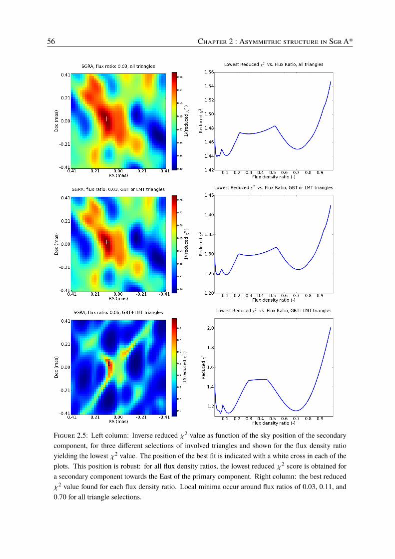
56 Chapter 2 : Asymmetric structure in Sgr A*
Figure 2.5: Left column: Inverse reduced j2 value as function of the sky position of the secondarycomponent, for three different selections of involved triangles and shown for the flux density ratioyielding the lowest j2 value. The position of the best fit is indicated with a white cross in each of theplots. This position is robust: for all flux density ratios, the lowest reduced j2 score is obtained fora secondary component towards the East of the primary component. Right column: the best reducedj2 value found for each flux density ratio. Local minima occur around flux ratios of 0.03, 0.11, and0.70 for all triangle selections.

2.5 Discussion 57
Figure 2.6: j2 landscapes for the posi-tion of the secondary source component,considered when leaving out differentkey stations. Shown in the subplots arethe j2 scores when omitting all triangleswith GB, KP, or LM respectively.
direction. We note that the best-fit position for the secondary component falls along the majoraxis of the scattering ellipse as it was measured by Bower et al. (2014, 2015a) and is also com-patible with the previously observed intrinsic elongation of the source quoted in these publications.
These observations cover a single epoch and were done in a single frequency band and in a singlepolarisation (LCP), which complicates interpretation of the observed asymmetry. On one hand,interstellar scattering of the source image can introduce small-scale scintels whose ensembleaverage influences the observed brightness distribution (Gwinn et al., 2014; Johnson & Gwinn,2015) and that may be responsible for the occurrence of non-zero closure phases (Ortiz-Leónet al., 2016). The time scale for the scattering geometry to change significantly (∼weeks) isthought to be much longer than the length of one observation (∼hours), causing the source imageto be affected by an effectively static scattering screen that may induce asymmetry in the observedimage. On the other hand, the observed asymmetry may be intrinsic to the source itself. Obser-

58 Chapter 2 : Asymmetric structure in Sgr A*
Figure 2.7: The typical j2 landscape forSgrA* as resulting from the model fit whenusing the synthetic (zero-mean) closure phasedata (using all triangles). Chi-squared scoresdo not strongly depend on flux density ratio forthe synthetic data.
Figure 2.8: Confidence regions (black lines)for the best-fit position of the secondary sourcecomponent, obtained by bootstrapping the orig-inal closure phase dataset. The innermost con-tour indicates the 68% confidence region, sur-rounded by the 95% and 99% regions respec-tively.
vations at different frequencies (e.g., at 230GHz and 43GHz) and performed at different epochs(separated in time by months) are therefore crucial in interpreting the character of this observedasymmetry.
The 86GHz observations published by Ortiz-León et al. (2016) do show non-zero closure phases,but these have been interpreted consistently as arising from interstellar scattering effects. Assuch, no dedicated closure-phase modelling comparable to the analysis presented in this workwas performed. Those data are separated in time from the observation we report in this workby approximately one month (April 27th vs May 23rd, 2015). Future studies of the non-zeroclosure phase evolution with time will help to distinguish its origin: if the observed asymmetry ispersistent across both datasets, the case for an intrinsic cause of the asymmetry will be bolsteredas scattering effects are expected to vary over shorter timescales (Johnson & Gwinn, 2015). Con-versely, if the earlier data show a different asymmetry from what we find here the likely cause forit will be confirmed as being interstellar scattering.
Interestingly, an East-West asymmetry in SgrA* is also suggested by closure phase results frommeasurements taken with the Event Horizon Telescope at 230GHz, in the Spring of 2013 (Fishet al., 2016). The observations presented in that work show closure phases at 1.3mm that arecomparable in magnitude to the values we have measured at 3.5mm, suggesting a similar degreeof source asymmetry in both observed emission patterns. While a sourcemodel with disconnected

2.6 Summary and conclusions 59
components is not necessarily favoured by the EHT data, fit results using a model consisting of2 point sources suggest a preference for an East-West asymmetry in that dataset. It is somewhatsurprising that the persistent asymmetry at 230GHz is oriented along the same direction on thesky as the asymmetry found in this work. At 230GHz a persistent asymmetry in the sourceimage is expected, and is thought to be caused by the Doppler boosting of emission from one sideof the inner accretion flow with a velocity component along our line of sight (Broderick et al.,2016). Conversely, at 86GHz this effect is not expected to be a dominant contribution to sourceasymmetry - rather, the main part of any intrinsic asymmetry is expected to be a consequenceof the relative brightness of the inner accretion flow versus emission from the footpoints of acompact jet component (Mościbrodzka et al., 2014). In the context of this model, the similarorientation of the asymmetry in the 230GHz and 86GHz observations cannot be reconciled ifboth are assumed to be intrinsic to the source.
For spectrally fitted jet models, a significant component of the emission at 86GHz is generatedaround the jet base (Mościbrodzka & Falcke, 2013), causing the corresponding source image toexhibit an asymmetry that is aligned with the jet axis to within ∼20 degrees. In this context theresults from this work, when combinedwith other existingmeasurements of SgrA* closure phasesat 3mm, offer an appropriate starting point for a more extended model fitting procedure, where theraytraced results from GRMHD simulations can be compared to the constraints on the observedsource geometry. An analogous analysis has been performed on the published 230GHz closurephase measurements in (Broderick et al., 2016), where the measurements have been interpretedwithin the context of a particular theoretical source model. This more elaborate model fittingprocedure using the full available body of 86GHz closure phase data is the focus of a separatepublication that currently is in preparation.
2.6 Summary and conclusionsWe have performed an observation of SgrA* at 86GHz, using the VLBA, the GBT, and the LMT.Elementary model fitting of a multicomponent source geometry to the closure phases from thisdataset shows a preference for an Eastern secondary source component at an on-sky separationof ∼100 `as from the primary component. This asymmetry, when considered as a standaloneobservation, may be explained by interstellar scattering effects. However, this does not excludethe possibility of the observed asymmetry being intrinsic to the source.
The results by Fish et al. (2016) at 230GHz , Ortiz-León et al. (2016) at 86GHz, and Rauchet al. (2016) at 43 GHz indicate asymmetric emission of Sgr A* at different frequencies and overdifferent time periods. In particular the closure-phase measurements performed at 230 and 43GHz point towards a similar East-West asymmetry as was found in the dataset presented in thiswork. The similar orientation of this asymmetry across these different wavelengths is a puzzling

60 Chapter 2 : Asymmetric structure in Sgr A*
result, and future analysis of 86GHz VLBI measurements done at different times will help to pindown the origin of these observed non-zero closure phases.
AcknowledgementsWe wish to express our gratitude to the MIT Haystack team (Lindy Blackburn, Laura Vertats-chitsch, Jason Soohoo), who installed the recording system at LMT and who have played aninstrumental role in making VLBI measurements possible at LMT. We thank Frank Ghigo atGBT for his help in obtaining the system temperature measurements. We thank Michael Johnsonfor illuminating discussions on the scattering screen and on closure phase statistics, and we ap-preciate the input on the draft we received from Eduardo Rós. This work is supported by the ERCSynergy Grant “BlackHoleCam: Imaging the Event Horizon of Black Holes” (Grant 610058).A.H., L.L., and G.N.O.-L. acknowledge the financial support of CONACyT, Mexico and DGAPA,UNAM.

Chapter3Micro-arcsecond structure of Sagittarius A*
revealed by high-sensitivity 86 GHz VLBIobservations
Christiaan Brinkerink, Cornelia Müller, Heino Falcke, Sara Issaoun, Kazunori Akiyama,Geoffrey Bower, Thomas Krichbaum, Adam Deller, Edgar Castillo, Sheperd Doeleman, Raquel
Fraga-Encinas, Ciriaco Goddi, Antonio Hernández-Gómez, David Hughes, Michael Kramer,Jonathan Léon-Tavares, Laurent Loinard, Alfredo Montaña, Monika Mościbrodzka, Gisela
Ortiz-León, David Sanchez-Arguelles, Remo Tilanus, Grant Wilson, Anton Zensus
A&A, 621, A119 (2019)
Abstract
The compact radio source Sagittarius A∗ (SgrA∗) in the Galactic centre is the primarysupermassive black hole candidate. General relativistic magnetohydrodynamical(GRMHD) simulations of the accretion flow around SgrA∗ predict the presence ofsub-structure at observing wavelengths of ∼ 3mm and below (frequencies of 86GHzand above). For very long baseline interferometry (VLBI) observations of SgrA∗
at this frequency the blurring effect of interstellar scattering becomes sub-dominant,and arrays such as the high sensitivity array (HSA) and the global mm-VLBI array(GMVA) are now capable of resolving potential sub-structure in the source. Suchinvestigations help to improve our understanding of the emission geometry of themm-wave emission of SgrA∗, which is crucial for constraining theoretical modelsand for providing a background to interpret 1mm VLBI data from the Event HorizonTelescope (EHT). Following the closure phase analysis in our first paper, whichindicates asymmetry in the 3mm emission of SgrA∗, here we have used the fullvisibility information to check for possible sub-structure. We extracted source sizeinformation from closure amplitude analysis, and investigate how this constrains acombined fit of the size-frequency relation and the scattering law for SgrA∗. We

62 Chapter 3 : Micro-arcsecond structure of Sagittarius A*
performed high-sensitivity VLBI observations of SgrA∗ at 3mm using the Very LongBaseline Array (VLBA) and the Large Millimeter Telescope (LMT) in Mexico ontwo consecutive days in May 2015, with the second epoch including the GreenbankTelescope (GBT). We confirm the asymmetry for the experiment including GBT.Modelling the emission with an elliptical Gaussian results in significant residual fluxof∼ 10mJy in south-eastern direction. The analysis of closure amplitudes allows us toprecisely constrain themajor andminor axis size of themain emission component. Wediscuss systematic effectswhich need to be taken into account. We consider our resultsin the context of the existing body of size measurements over a range of observingfrequencies and investigate how well-constrained the size-frequency relation is byperforming a simultaneous fit to the scattering law and the size-frequency relation.We find an overall source geometry that matches previous findings very closely,showing a deviation in fittedmodel parameters less than 3% over a time scale of weeksand suggesting a highly stable global source geometry over time. The reported sub-structure in the 3mm emission of SgrA∗ is consistent with theoretical expectationsof refractive noise on long baselines. However, comparing our findings with recentresults from 1mm and 7mm VLBI observations, which also show evidence for east-west asymmetry, we cannot exclude an intrinsic origin. Confirmation of persistentintrinsic substructure will require further VLBI observations spread out over multipleepochs.
3.1 IntroductionThe radio source Sagittarius A∗ (hereafter called SgrA∗) is associated with the supermassiveblack hole (SMBH) located at the centre of the Milky Way. It is the closest and best-constrainedsupermassive black hole candidate (Ghez et al., 2008; Gillessen et al., 2009; Reid, 2009) with amass of" ∼ 4.1×106"� at a distance of∼ 8.1 kpc as recently determined to high accuracy by theGRAVITY experiment (Gravity Collaboration et al., 2019). This translates into a Schwarzschildradius with an angular size of \RS ∼ 10 `as on the sky, while the angular size of its ‘shadow’ –meaning the gravitationally lensed image of the event horizon – is predicted to be∼ 50 `as (Falckeet al., 2000). Due to its proximity, SgrA∗ appears as the black hole with the largest angular size onthe sky and is therefore the ideal laboratory for studying accretion physics and testing general rela-tivity in the strong field regime (see, e.g. Goddi et al., 2017; Falcke &Markoff, 2013, for a review).
Radio observations of SgrA∗ have revealed a compact radio source with an optically thick spec-trum up to mm-wavelengths. In the sub-mm band the spectrum shows a turnover and becomesoptically thin. This sub-mm emission is coming from a compact region that is only a fewSchwarzschild radii in size (e.g. Falcke et al., 1998; Doeleman et al., 2008). Very Long BaselineInterferometry (VLBI) observations can now achieve angular resolution down to a few tens of `as,which is required to resolve these innermost accretion structure close to the event horizon. The

3.1 Introduction 63
advantages in going to (sub-)mm wavelengths are 1.) to witness the transition from optically thinto thick emission, 2.) to improve the angular resolution and 3.) to minimize the effect of interstel-lar scattering. At longer radio wavelengths, interstellar scattering along our line of sight towardsSgrA∗ prevents direct imaging of the intrinsic source structure and causes a ‘blurring’ of the im-age that scales withwavelength squared (e.g. Davies et al., 1976; Backer, 1978; Bower et al., 2014).
The scatter-broadened image of SgrA∗ can be modelled by an elliptical Gaussian over a rangeof wavelengths. The measured scattered source geometry scales with _2 above observing wave-lengths of ∼7mm (Bower et al., 2006) following the relation: (\maj[mas]) × (\min[mas]) =(1.31 × 0.64) (_[cm])2, with the major axis at a position angle 78◦ east of north. At shorterwavelengths this effect becomes sub-dominant, although refractive scattering could introducestochastic fluctuations in the observed geometry that vary over time. This refractive noise cancause compact sub-structure in the emission, detectable with current VLBI arrays at higher fre-quencies (Johnson & Gwinn, 2015; Gwinn et al., 2014).
Due to major developments in receiver hardware and computing that have taken place in recentyears, mm-VLBI experiments have gotten closer to revealing the intrinsic structure of SgrA∗. At1.3mm (230GHz), the Event Horizon Telescope has resolved source structure close to the eventhorizon on scales of a few Schwarzschild radii (Doeleman et al., 2008; Johnson et al., 2015).Closure phase measurements over four years of observations have revealed a persistent east-westasymmetry in the 1.3mm emission of SgrA∗ (Fish et al., 2016). This observed structure andgeometry seems intrinsic to the source and is already imposing strong constraints on general-relativistic magnetohydrodynamic (GRMHD) simulation model parameters of SgrA∗ (Brodericket al., 2016; Fraga-Encinas et al., 2016). A more recently published analysis by (Lu et al., 2018)of observations done at 230GHz including the APEX antenna reports the discovery of sourcesub-structure on even smaller scales of 20 to 30 `as that is unlikely to be caused by interstellarscattering effects.
At 3.5mm (86GHz), the combined operation of the Large Millimeter Telescope (LMT, Mex-ico) and the Green Bank Telescope (GBT, USA) together with the Very Long Baseline Array(VLBA) significantly improves the (u,v)-coverage and array sensitivity beyond what is possiblewith the VLBA by itself. Closure phase analysis indicates an observational asymmetry in the3mm emission (Ortiz-León et al., 2016; Brinkerink et al., 2016), which is consistent with ap-parent sub-structure introduced by interstellar scattering, although an interpretation in terms ofintrinsic source structure cannot be excluded given the data obtained so far. Ortiz-León et al.(2016) reported on VLBA+LMT observations at 3.5mm detecting scattering sub-structure in theemission, similar to what was found at 1.3 cm by Gwinn et al. (2014). In Brinkerink et al. (2016),using VLBA+LMT+GBT observations, we report on a significant asymmetry in the 3.5mm emis-sion of SgrA∗. Analysing the VLBI closure phases, we find that a simple model with two pointsources of unequal flux provides a good fit to the data. The secondary component is found to be

64 Chapter 3 : Micro-arcsecond structure of Sagittarius A*
located towards the east of the primary, however, the flux ratio of the two components is poorlyconstrained by the closure phase information.
It remains unclear, however, whether this observed emission sub-structure at 3.5mm is intrinsicor arises from scattering. With the body of VLBI observations reported so far we cannot con-clusively disentangle the two components. Time-resolved and multi-frequency analysis of VLBIdata can help. Besides the findings by Fish et al. (2016) at 1.3mm, Rauch et al. (2016) found asecondary off-core feature in the 7mm emission appearing shortly before a radio flare, which canbe interpreted as an adiabatically expanding jet feature (see also Bower et al., 2004).
From elliptical fits to the observed geometry of the emission, the two-dimensional size of SgrA∗
at mm-wavelength can be derived as reported by Shen et al. (2005); Lu et al. (2011a); Ortiz-Leónet al. (2016) at 3.5mm and Bower et al. (2004); Shen (2006) at 7mm. Using the known scat-tering kernel (Bower et al., 2006, 2014), this intrinsic size can be calculated from the measuredsize. The most stringent constraint on the overall intrinsic source diameter has been determinedusing a circular Gaussian model for the observed 1.3mm emission (Doeleman et al., 2008; Fishet al., 2011), as at this observing frequency the scattering effect is less dominant. More recentVLBI observations of SgrA∗ at 86GHz constrain the intrinsic, two-dimensional size of SgrA∗
to (147 ± 4)`as × (120 ± 12)`as (Ortiz-León et al., 2016) assuming a scattering model derivedfrom Bower et al. (2006) and Psaltis et al. (2015).
High-resolution measurements of time-variable source structure in the infrared regime observedduring SgrA∗ infrared flares have recently been published (Gravity Collaboration et al., 2018b),where spatial changes of the source geometry of SgrA∗ on timescales of less than 30 minutes areseen. These results suggest periodical motion of a bright source component located within ∼100`as of the expected position of the supermassive black hole, with a corrrespondingly varyingpolarisation direction. The variability timescale of SgrA∗ is expected to be significantly shorterat infrared wavelengths than at 3.5 and 1.3mm, as it is thought to be dominated by fast localvariations in electron temperature rather than changes in the bulk accretion rate.
All of these observations indicate that we start to unveil the presence of both stationary andtime-variable sub-structure in the accretion flow around SgrA∗, as expected by theoretical simu-lations (e.g. Mościbrodzka et al., 2014). In order to further put constraints on model parameters,higher-resolution and more sensitive mm-VLBI observations are required. The analysis of closurequantities helps to determine source properties without being affected by station-based errors.Closure phases indicate asymmetry in the emission when significantly deviating from zero (see,e.g. Fish et al., 2016; Brinkerink et al., 2016, for the case of SgrA∗). Closure amplitudes putconstraints on the source size (see, e.g. Ortiz-León et al., 2016; Bower et al., 2006, 2004). Imagingtechniques are based on the closure quantities. Although mm-VLBI has a number of limitations,at &3mm the current VLBI array configurations allow reconstructing the emission of SgrA∗

3.2 Observations and data reduction 65
using standard hybrid imaging techniques (Lu et al., 2011a; Rauch et al., 2016).
In this paper we have followed-up on our first analysis published in Brinkerink et al. (2016)(hereafter referred to as Paper I). Here, we focus on the closure amplitude and imaging analysis ofSgrA∗ at _ = 3.5mm obtained with the VLBA and LMT on May 22nd, 2015 and VLBA, LMT,and GBT on May 23rd, 2015. In Section 3.2 we describe the observations and data reduction.Section 3.3 discusses the results from imaging and closure amplitude analysis. In section 4, wepresent the results from a simultaneous fitting of the intrinsic size-frequency relation and thescattering relation for SgrA∗, using the combined data from this work with earlier publishedresults across a range of wavelengths. We conclude with a summary in Section 3.5.
3.2 Observations and data reductionWe performed 86GHzVLBI observations of SgrA∗. Here we present the analysis of two datasets:one epoch using the VLBA (all 86GHz capable stations1) together with the LMT (project code:BF114A) on May 22nd, 2015, and one epoch using VLBA, LMT, and GBT on May 23rd, 2015(project code: BF114B). Both observations were made in left-circular polarisation mode only, ata centre frequency of 86.068GHz and a sampling rate of 2 Gbps (512 MHz on-sky bandwidth).For fringe finding we used the primary calibrators 3C 279 and 3C 454.3 at the start and end ofthe track respectively. In between, the scans alternated every 5min between SgrA∗ and the sec-ondary fringe finder NRAO530 ([HB89] 1730-130) with short regular gaps (every ∼30 minutes)for pointing and longer GBT-only gaps every ∼4 hours for focusing.
For fringe finding and initial calibration of both datasets, we used standard methods in AIPS(Greisen, 2003) as described in Paper I. We first performed a manual phase-cal to determine theinstrumental delay differences between IFs on a 5min scan of 3C 454.3. After applying this solu-tion to all data, the second FRING run gave us solutions for delay and rate (4min solution interval,with 2min subintervals) with a combined solution for all IFs. Using shorter solution intervalsthan the length we used here resulted in more failed, and therefore flagged, FRING solutions. Alltelescopes yielded good delay and rate solutions for NRAO530. For SgrA∗, however, we foundno FRING solutions on baselines to MK (using a limiting value for the signal-to-noise ratio (S/N)of 4.3), but all other baselines yielded clear detections.
Amplitude calibration in AIPS was performed using a-priori information on weather conditionsand gain-elevation curves for each station. In the cases of the LMT and the GBT, system tem-perature measurements and gain curves were imported separately as they were not included inthe a-priori calibration information provided by the correlator pipeline. We solved for (and ap-
1Brewster (BR), Fort Davis (FD), Kitt Peak (KP), Los Alamos (LA), Mauna Kea (MK), North Liberty (NL),Owens Valley (OV) and Pie Town (PT)
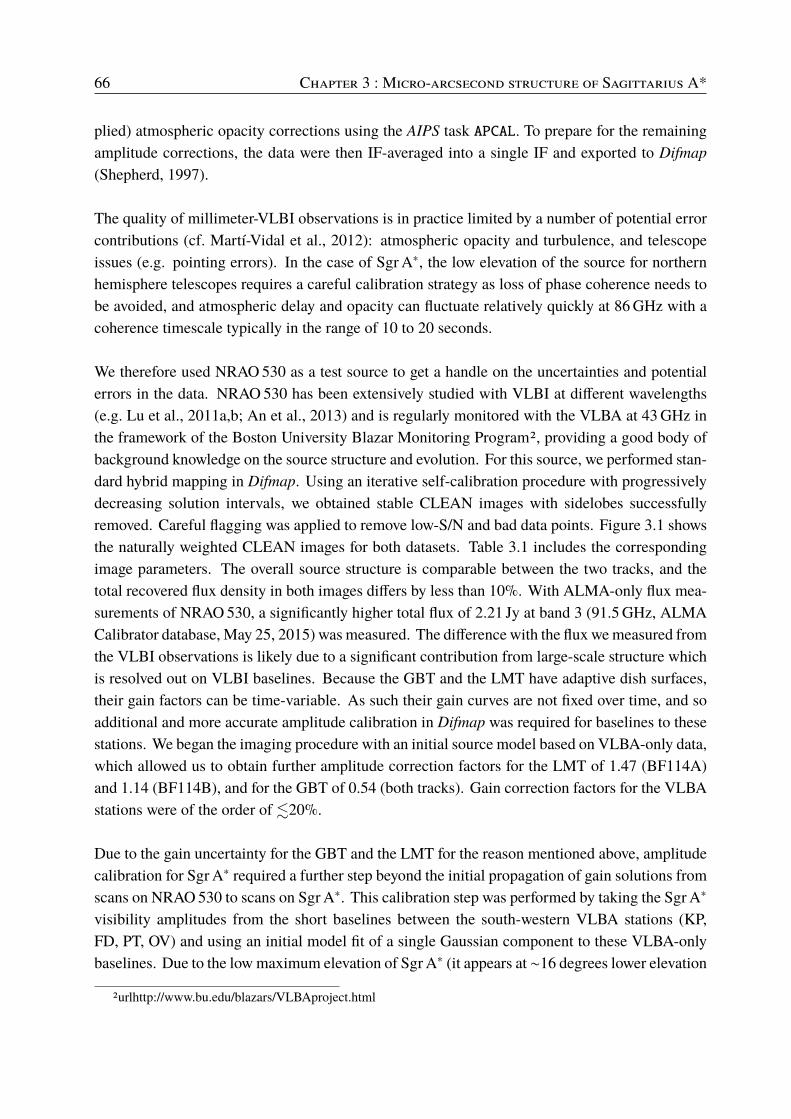
66 Chapter 3 : Micro-arcsecond structure of Sagittarius A*
plied) atmospheric opacity corrections using the AIPS task APCAL. To prepare for the remainingamplitude corrections, the data were then IF-averaged into a single IF and exported to Difmap(Shepherd, 1997).
The quality of millimeter-VLBI observations is in practice limited by a number of potential errorcontributions (cf. Martí-Vidal et al., 2012): atmospheric opacity and turbulence, and telescopeissues (e.g. pointing errors). In the case of SgrA∗, the low elevation of the source for northernhemisphere telescopes requires a careful calibration strategy as loss of phase coherence needs tobe avoided, and atmospheric delay and opacity can fluctuate relatively quickly at 86GHz with acoherence timescale typically in the range of 10 to 20 seconds.
We therefore used NRAO530 as a test source to get a handle on the uncertainties and potentialerrors in the data. NRAO530 has been extensively studied with VLBI at different wavelengths(e.g. Lu et al., 2011a,b; An et al., 2013) and is regularly monitored with the VLBA at 43GHz inthe framework of the Boston University Blazar Monitoring Program2, providing a good body ofbackground knowledge on the source structure and evolution. For this source, we performed stan-dard hybrid mapping in Difmap. Using an iterative self-calibration procedure with progressivelydecreasing solution intervals, we obtained stable CLEAN images with sidelobes successfullyremoved. Careful flagging was applied to remove low-S/N and bad data points. Figure 3.1 showsthe naturally weighted CLEAN images for both datasets. Table 3.1 includes the correspondingimage parameters. The overall source structure is comparable between the two tracks, and thetotal recovered flux density in both images differs by less than 10%. With ALMA-only flux mea-surements of NRAO530, a significantly higher total flux of 2.21 Jy at band 3 (91.5GHz, ALMACalibrator database, May 25, 2015) was measured. The difference with the flux wemeasured fromthe VLBI observations is likely due to a significant contribution from large-scale structure whichis resolved out on VLBI baselines. Because the GBT and the LMT have adaptive dish surfaces,their gain factors can be time-variable. As such their gain curves are not fixed over time, and soadditional and more accurate amplitude calibration in Difmap was required for baselines to thesestations. We began the imaging procedure with an initial source model based on VLBA-only data,which allowed us to obtain further amplitude correction factors for the LMT of 1.47 (BF114A)and 1.14 (BF114B), and for the GBT of 0.54 (both tracks). Gain correction factors for the VLBAstations were of the order of .20%.
Due to the gain uncertainty for the GBT and the LMT for the reason mentioned above, amplitudecalibration for SgrA∗ required a further step beyond the initial propagation of gain solutions fromscans on NRAO530 to scans on SgrA∗. This calibration step was performed by taking the SgrA∗
visibility amplitudes from the short baselines between the south-western VLBA stations (KP,FD, PT, OV) and using an initial model fit of a single Gaussian component to these VLBA-onlybaselines. Due to the lowmaximum elevation of SgrA∗ (it appears at ∼16 degrees lower elevation
2urlhttp://www.bu.edu/blazars/VLBAproject.html

3.3 Results 67
100
1.5 1 0.5 0 -0.5 -1 -1.5
2.4
2.2
2
1.8
1.6
1.4
1.2
1
0.8
0.6
0.4
0.2
0
-0.2
-0.4
200
50
20
10
5
2
0
FluxDensity
[mJy/beam]
Relative RA [mas]
RelativeDEC
[mas]
NRAO530 2015-05-22
50
1 0.5 0 -0.5 -1 -1.5
2.4
2.2
2
1.8
1.6
1.4
1.2
1
0.8
0.6
0.4
0.2
0
-0.2
-0.4
200
100
20
10
5
2
1
0
FluxDensity
[mJy/beam]
Relative RA [mas]
RelativeDEC
[mas]
1.5
NRAO530 2015-05-23
Figure 3.1: Naturally weighted 86GHz images of NRAO530. Left: Using data of project BF114A(2015-05-22) with VLBA and LMT. Right: Using data of project BF114B (2015-05-23) with VLBA,LMT and GBT. The contours indicate the flux density level (dashed-grey contours are negative), scaledlogarithmically and separated by a factor of two, with the lowest level set to the 3f-noise level. Thesynthesized array beam is shown as a grey ellipse in the lower left corner. Image parameters are listedin Table 3.1.
than NRAO530 at transit), the amplitude correction factors for the VLBA are typically largerfor SgrA∗ than for NRAO530 but still agree with the factors of the corresponding NRAO530observations within . 30% (except for the most northern stations BR and NL), comparable tothe findings of Lu et al. (2011a). Analogously to the data reduction steps taken for NRAO530,we used this initial source model to perform additional amplitude calibration for the GBT and theLMT. After this first round of amplitude self-calibration, iterative mapping and self-calibrationwas performed (see Sect. 3.3.1).
3.3 ResultsFollowing the closure phase analysis in Paper I, we now study the source geometry and size usinghybrid imaging (Sect. 3.3.1) and closure amplitudes (Sect. 3.3.2). In Paper I, where we studiedthe closure phase distribution to look for source asymmetry, we concentrated only on the moresensitive dataset including VLBA+LMT+GBT (project code: BF114B), while in this paper wealso include the VLBA+LMT dataset (project code: BF114A).
3.3.1 Mapping and self-calibration of SgrA∗
After amplitude correction factors were applied (as explained in Sect. 3.2), we performed aniterative mapping and self-calibration procedure including careful flagging of the SgrA∗ dataset.Amplitude and phase self-calibration were applied using increasingly shorter timesteps and nat-

68 Chapter 3 : Micro-arcsecond structure of Sagittarius A*
ural weighting. We deconvolved the image for both datasets by using elliptical Gaussian modelcomponents, since the CLEAN algorithm has difficulty fitting the visibilities when it uses pointsources. Table 3.2 gives the best-fit parameteres from this approach. Figure 3.2 shows both ofthe resulting images convolved with the clean beam.
As shown by, for example, Bower et al. (2014), when self-calibrating, the derived model candepend on the initial self-calibration model chosen for a single iteration, if the j2-landscapehas complex structure. Furthermore, as also noted by Ortiz-León et al. (2016), the resultinguncertainties on the model parameters are often underestimated, if they are based solely on theself-calibration solution. To assess the true errors, the uncertainties on the gain solutions mustalso be taken into account.
Therefore, we tested the robustness of the final model, in other words, the dependence of the self-calibration steps on input models, described as follows. We evaluated conservative uncertaintieson the model parameters of the elliptical Gaussian brightness distribution by using different start-ing parameters for the iterative self-calibration procedure, where all starting model parameterswere individually varied by up to 30%, to check the convergence on the same solution. We gen-erated 1000 random starting models to perform the initial amplitude self-calibration (Sect. 3.2).The starting model always consists of an elliptical Gaussian brightness distribution. Each of itsparameters (flux, major axis, axial ratio, position angle) was drawn from a normal distributionaround the initial model. Using these input models, iterative self-calibration steps were appliedand the resulting distribution of the model parameter was examined. For an illustration of theobserved distribution of the major axis size, please see Figure 3.3.
As expected, we find a strong correlation between input model flux density and final flux densityof the Gaussian model components. Therefore, to constrain the flux of SgrA∗, we primarily usedthe fluxes on short VLBA baselines as explained in Sect. 3.2. For both NRAO530 and SgrA∗,we find less than 10% total flux density difference between our two consecutive epochs.
We find that the model converges onto values for major axis and axial ratio (or alternatively minoraxis) that show a spread of about 10%. The position angle uncertainty is constrained to ±20◦. Wenote that this analysis shows that the distribution for the major axis in BF114B is skewed, havingan average of 222 `as, a median of 215 `as and a mode of 205 `as. The resulting major axis dis-tribution also has a hard lower bound at ∼ 200`as. This skewed distribution of parameters fromselfcal suggests that there are multiple local minima in the j2-landscape that produce differentmodel parameters from different iterations, and is therefore of limited value in determining sourcesize uncertainties. We have therefore used closure amplitude analysis to verify this estimate ofthe source size and provide more accurate uncertainties, and this process is described in the nextsection.

3.3 Results 69
0
-0.2
-0.4
-0.6
-0.8
-1
500
200
100
50
20
10
5
Relative RA [mas]
RelativeDEC
[mas]
FluxDensity
[mJy/beam]
1 0.5 0 -0.5 -1
1
0.8
0.6
0.4
0.2
0
Sgr A* 2015-05-22
0
-0.6
-0.8
-1
200
100
50
20
10
5
2
Relative RA [mas]
RelativeDEC
[mas]
FluxDensity
[mJy/beam]
1 0.5 0 -0.5 -1
1
0.8
0.6
0.4
0.2
0
-0.2
-0.4
Sgr A* 2015-05-23
Figure 3.2: Results of hybrid mapping of Sgr A* at 3mm. Top left: Beam-convolved image from thedataset of project BF114A (2015-05-22) using VLBA and LMT. Top right: Beam-convolved imagefrom the dataset of project BF114B (2015-05-23) using VLBA, LMT and GBT. The contours indicatethe flux density level (dashed-grey contours are negative), scaled logarithmically and separated by afactor of two, with the lowest level set to the 3f-noise level. Bottom left: Residual map of SgrA∗ afterprimary component subtraction from the BF114A dataset, using natural weighting. No clear patternis seen in the residual image. Bottom right: Natural-weighted residual map for Sgr A*, epoch B, aftersubtraction of the best-fitting 2D Gaussian source component. The remaining excess flux towards theeast is highly concentrated and clearly present. Both residual images use a cross to indicate the centreof the primary (subtracted) component on the sky. Image and model parameters are listed in Tables 3.1and 3.2, respectively.

70 Chapter 3 : Micro-arcsecond structure of Sagittarius A*
Figure 3.3: Distribution of major axis sizes arising from 1000 selfcal runs in which each initialmodel parameter was varied according to a Gaussian distribution with a width of 30% of the nominalparameter value. The resulting distribution of sizes shows a clear skew, with most results clusteringclose to a minimum cutoff value of 200 `as. The coloured lines indicate the mean (green), the median(cyan) and the statistical 1-f errors (red).
We find that for BF114A (VLBA+LMT), one single Gaussian component is sufficient to modelthe data (see Figure 3.2, bottom left). For the BF114B dataset with higher sensitivity due to theinclusion of the GBT, the model fitting with one Gaussian component shows a significant excessof flux towards the south-west in the residual map (see Figure 3.2, bottom right). Modellingthis feature with a circular Gaussian component yields a flux density excess of ∼ 10mJy (i.e.approximately 1% of the total flux) at ΔRA∼ 0.23 mas, ΔDEC∼ −0.05 mas from the phasecentre. Including this second component in the modelfit, results in a smooth residual map (withRMS∼0.5mJy). We checked the reliability of this feature using the same method as describedabove, where a range of initial model parameters was used as input for a selfcalibration stepthat resulted in a distribution of best-fit model parameters. We find that the position of theresidual emission is well-constrained and independent from the self-calibration starting parame-ters. The BF114A dataset, however, does not show such clear and unambiguous residual emission.
We have tested the compatibility of the BF114A dataset with the source model we find forBF114B. Subtracting the full two-component BF114B source model from the calibrated BF114Adata and looking at the residual map, we see an enhanced overall noise level and no clear evidenceof missing flux at the position of the secondary component. We further performed a separate

3.3 Results 71
amplitude and phase selfcalibration of the BF114A data using the BF114B source model, andinspected the residual map after subtraction of only the main source component of the BF114Bmodel. In this residual map, we do see an enhancement of flux density at the position of thesecondary component, but it is not as strong as the secondary component of the source model(∼ 5mJy versus 10mJy for the model). We also see apparent flux density enhancements of simi-lar strength at other positions close to the phase centre. We therefore conclude that the BF114A(D, E)-coverage and sensitivity are not sufficient to provide a clear measurement of the secondarysource component as seen for the BF114B epoch. Given that the detectability of the secondarycomponent is so marginal for BF114A, we cannot determine whether the asymmetry we see inthe BF114B epoch is a feature which persisted over the two epochs or a transient feature that wasnot present in the earlier epoch.
We emphasize that the asymmetric feature we see in the SgrA∗ emission when imaging BF114Bwas already suggested by our analysis of the closure phases of the BF114B dataset (Paper I).We find that a model consisting of two point sources results in a significantly better fit to theclosure phases, with the weaker component being located east of the primary. However, the fluxratio of the two components was left poorly constrained, resulting in j2 minima at flux ratios of0.03, 0.11, and 0.70. In the current analysis, by using the full visibility data and fitting Gaussiancomponents instead of point sources, we can constrain the flux ratio to∼0.01. The low flux densityof this secondary source component compared to the main source component makes it difficultto detect this source feature upon direct inspection of the visibility amplitudes as a function ofbaseline length. However, with model fitting it becomes clear that a single Gaussian componentsystematically underfits the amplitude trends of the data. We have thus seen evidence for this com-ponent independently in both the closure phases (Paper 1) and the visibility amplitudes (this work).
It remains unclear whether this sub-structure in the 3mm emission of SgrA∗ is intrinsic or in-duced by refractive scattering. On long baselines, refractive scattering can introduce small-scalesub-structure in the ensemble-averaged image (Johnson & Gwinn, 2015). This effect stronglydepends on the intrinsic source size and geometry. A larger source size will show smaller geo-metrical aberration from scattering compared to a point source, as different parts of the sourceimage are refracted in independent ways that tend to partially cancel out any changes in overallstructure. At _ ∼ 5mm where the intrinsic source size of SgrA∗ becomes comparable to theangular broadening, this effect is most distinct (Johnson & Gwinn, 2015). Gwinn et al. (2014)reported on the detection of scattering sub-structure in the 1.3 cm emission of SgrA∗. Assuminga Kolmogorov spectrum of the turbulence, the authors expect refractive scintillation to lead tothe flux density measured on a 3000 km east-west baseline to vary with an RMS of 10-15 mJy.Similarly, Ortiz-León et al. (2016) show that refractive effects can cause sub-structure in 3mmimages, with a RMS flux modulation of 6.6% and an evolution timescale of about two weeks.Taking these considerations into account, this sub-structure detected at long baselines in our 3mmdatasets would be consistent with scattering noise. However, given the more significant detection

72 Chapter 3 : Micro-arcsecond structure of Sagittarius A*
Table 3.1: Image & observational parameters (natural weighting)
Date (Project ID) Source Array configuration0 Beam Beam RMSyyyy-mm-dd [mas] PA [Jy/beam]
2015-05-22 (BF114A) NRAO530 VLBA+LMT 0.107×0.204 3.0◦ 0.00042015-05-23 (BF114B) NRAO530 VLBA+LMT+GBT 0.100×0.225 −6.3◦ 0.00032015-05-22 (BF114A) SgrA∗ VLBA+LMT 0.541×0.165 38.5◦ 0.00102015-05-23 (BF114B) SgrA∗ VLBA+LMT+GBT 0.147×0.286 6.4◦ 0.0005
0For VLBA: Brewster (BR), Fort Davis (FD), Kitt Peak (KP), Los Alamos (LA), Mauna Kea (MK), North Liberty(NL), OVRO (OV) and Pie Town (PT). We note that for SgrA∗ no fringes were detected to MK, which results in alarger beam size for SgrA∗ than for NRAO530.
Table 3.2: Parameters of model components from self-calibration0
Date (Project ID) ( [Jy] 1maj [`as] ratio (-) 1min [`as] PA [deg]2015-05-22 (BF114A) 1.02 ± 0.1 227.0 0.85 193.0 56.42015-05-23 (BF114B) 0.95 ± 0.1 215.3 0.77 165.8 76.5
0Note: major/minor axis uncertainties are of the order of 10%. The PA is constrained to within 15◦ (BF114A) and12◦ (BF114B). See Sect. 3.3.1 for more details.
in the dataset involving the GBT and LMT, a contribution of intrinsic sub-structure cannot beexcluded. We discuss further implications in Sect. 3.5.
3.3.2 Constraining the size of SgrA∗ using closure amplitudesClosure quantities are robust interferometric observables which are not affected by any station-based error such as noise due to weather, atmosphere or receiver performance. As one exampleof a closure quantity, the closure phase is defined as the sum of visibility phases around a closedloop, that is, at least a triangle of stations. We discuss the closure phase analysis of the SgrA∗
dataset BF144B in Paper I in detail. Here, instead of closure phases, we focus on the closureamplitude analysis of both datasets. The closure amplitude is defined as |+8 9+:; |/|+8:+ 9 ; |, fora quadrangle of stations 8, 9 , :, ; and with +8 9 denoting the complex visibility on the baselinebetween stations 8 and 9 . Using measurements of this quantity, one can determine the source sizeindependently from self-calibration, as shown in various previous publications for 3mm VLBIobservations of SgrA∗ (Doeleman et al., 2001; Bower et al., 2004; Shen et al., 2005; Bower et al.,2014; Ortiz-León et al., 2016).
In the context of this work, we are interested in a way to establish the observed size and orientationof SgrA∗ separately from self-cal. We therefore fitted a simple model of an elliptical Gaussiancomponent to the closure amplitude data, and we deconvolved the scattering ellipse using the bestavailable model (Bower et al. 2006, 2014b) afterwards. We performed a j2-analysis in fitting theGaussian parameters (major and minor axis, and position angle).

3.3 Results 73
For both datasets, BF114A and BF114B, we derived the closure amplitudes from the 10s-averagedvisibilities and fitted a simple 2D Gaussian source model to the closure amplitude data. There aresome subtleties to take into account when modelfitting with closure amplitudes. j2-minimisationalgorithms for model fitting generally assume that the errors on the measurements used are Gaus-sian. Closure amplitudes, when derived from visibilities with Gaussian errors, in general havenon-Gaussian errors that introduce a potential bias when modelfitting which depends on the S/Nand the relative amplitudes of the visibility measurements involved: because closure amplitudesare formed from a non-linear combination of visibility amplitudes (by multiplications and divi-sions), their error distribution is skewed (asymmetric). This is especially a problem in the low-S/Nregime - the skew is much less pronounced for higher S/N values, and closure amplitude errorstend toward a Gaussian distribution in the high-S/N limit. Taking the logarithm of the measuredclosure amplitude values and appropriately defining the measurement uncertainties symmetrizesthese errors, and generally results in more stable fitting results (Chael et al., 2018). For thisreason, here we have adopted the technique described in that paper.
The workflow we have adopted for the closure amplitude model fitting pipeline is outlined inFigure 3.4. We give a brief summary of the process here, and specify more details on individualsteps below. We started the process with the frequency-averaged visibility dataset output fromAIPS, in which aberrant visibilites have already been flagged. We time-averaged this dataset toten-second length segments using Difmap to improve S/N per visibility measurement. In thisstep, the uncertainties on the resulting visibilities are recalculated using the scatter within eachaveraging period. The time interval of ten seconds was experimentally confirmed to yield vector-averaged visibility amplitudes that are not significantly lower than when averaging over shortertimescales, and as such falls within the coherence timescale of the atmosphere at 86GHz. Wealso de-biased the averaged visibilities here, according to expression 9 in Chael et al. (2018). Weapplied an S/N cutoff to the averaged ten-second visibility amplitudes at this point, where we haveused different values for this cutoff to test the robustness of the model fitting results (describedbelow). Using the remaining visibilities, we calculated the closure amplitudes for each ten-secondtime interval in the dataset. We calculated the error on these closure amplitude measurementsusing standard error propagation (following expression 12 from Chael et al. (2018)), and wethen made another cut in the dataset where we discarded all measurements that have a reportedS/N below our threshold value. Lastly, we applied our station selection to the resulting dataset,dropping all closure amplitude measurements in which the omitted stations are involved. We thusobtained the dataset on which we performed model fitting.
We used bootstrapping of the closure amplitudes of each dataset to determine the error on theindividual fit parameters. Bootstrapping works by forming a new realisation of measurementdata by picking measurements from the original dataset at random (with replacement) until a newdataset is formed that has an equal number of measurements as the original dataset. As such,

74 Chapter 3 : Micro-arcsecond structure of Sagittarius A*
Figure 3.4: Overview of the pipeline used for closure amplitude model fitting. The stages involv-ing time averaging, Visibility S/N filtering, Closure amplitude S/N filtering, station selection, andbootstrapping all offer different choices as to the parameters involved.
any measurement from the original dataset may be represented either once, multiple times or notat all in the newly formed dataset – the weights of measurements in the original dataset are thusstochastically varied, emulating the drawing of a new sample of measurements. We fitted thedata with a 2D Gaussian model with three free parameters: major axis size, minor axis size andposition angle on the sky of the major axis. The j2 minimisation is done as per expression 21 inChael et al. (2018).
Besides bootstrapping, we explore the effects of different values chosen for the S/N cutoff of thevisibility amplitudes used in the model fitting. Visibilities with a low reported S/N are expectedto have a larger influence on the skewness of the closure amplitude distribution, and are thuslikely to introduce a bias in the fitting results. This effect is investigated by looking at differentcutoff values for the visibility S/Ns. All visibility measurements can be assigned a ’reportedS/N’, which is defined as the measured visibility amplitude divided by the visibility amplitudeuncertainty as determined from scatter among the measurements over a ten-second integrationperiod. Before forming closure amplitudes using a visibility dataset, this visibility dataset isfiltered by only admitting measurements that have reported S/Ns above a chosen threshold value.The constructed closure amplitudes can then be filtered again by their reported S/N. A closureamplitude S/N cutoff value of three was employed to avoid the larger bias that comes with low-S/Nmeasurements, although we found that varying this value did not significantly impact the fittingresults. The variation of visibility S/N cutoff has a more pronounced influence on fitting results,and this effect is shown in Figure 3.5. The plots in the top row of this figure show the model fittingresults for the full dataset, with all stations included. In these plots, where the blue circles indicatefitting results from the measured data, we see that the fitted model parameters show relativelyminor variation over a range of S/N cutoff values from one to four, where the minor axis size is theparameter that shows the largest spread. Above visibility S/N cutoff values of four, we see that the

3.3 Results 75
spread in the fitting results grows and that trends of fitted values with S/N cutoff start appearing.This effect is coupled to the fact that only a limited number of quadrangles are left at these highS/N cutoff values, which by themselves provide weaker constraints on source geometry becauseof the limited (D, E)-coverage they provide.
To investigate the consistency of the data regarding the convergence of best-fit model parameters,we also have performed model fits where we excluded the GBT from the array before gatheringclosure amplitude measurements and model-fitting. This was done to check if the inclusion ofthe GBT resulted in a systematic offset of fitted model parameters versus the case where the arraydoes not include the GBT. Inclusion of the GBT offers a much better east-west array resolution,which is expected to have an impact on the quality of the major axis size estimate as the observedSgrA∗ Gaussian is orientated almost east-west on the sky. Likewise, the LMT offers a significantenhancement of the north-south array resolution and should therefore yield a clear improvementin quality for the estimated minor axis size. The model fitting results for these cases are includedin Figure 3.5, in the second (no GBT) and third (no LMT) rows. It is clear that indeed, inclusionof the GBT improves the quality of the major axis size estimate (the scatter among different boot-strapping realisations is significantly smaller than for the casewhere theGBT is omitted), while theLMT is instrumental in obtaining a good estimate for the minor axis size. As a result, the accuracywith which the position angle is determined benefits from inclusion of both the GBT and the LMT.
We should note that consistency of fitted model parameters by itself does not guarantee accurateresults (only precise results). For this reason, we have generated synthetic visibility datasets withthe same (D, E)-sampling as the original measurements, where a Gaussian source model withfiducial parameter values that are close to the previously measured size of SgrA∗ (Major axis:210.4 `as, minor axis: 145.2 `as, position angle: 80 degrees east of north) was used as input.The visibility uncertainties for this synthetic dataset were scaled in such a way as to yield thesame distribution in S/N values as the original data shows. For this synthetic dataset, the fullprocessing pipeline was then used and the deviations of the fitted parameters from the fiducialinputs were inspected. These results are also plotted in Figure 3.5, using red triangles as markersfor the model fitting results and black lines to indicate the input model parameter values. For themajor axis size, we see that the fitted values typically underpredict the actual source size by 5 to10 `as, depending on which stations are involved in the array. The minor axis size is severelyunderpredicted when the LMT is left out of the array, but is close to the input value when theLMT is included. The position angle come out close to the input value in all cases, althoughthere is a small positive bias seen in the case where the full array is used. We note that they-axis ranges of these plots are different, and that the spread seen in the case of the full array aretypically much smaller than those for the other array configurations. These results from syntheticdata fitting allow us to correct for the biases that our pipeline exhibits. The bias-corrected fittedsource parameters are shown in Figure 3.6. For all model parameters we get consistent fittingresults for all visibility S/N cutoff choices up to five. Because any specific choice of S/N cutoff

76 Chapter 3 : Micro-arcsecond structure of Sagittarius A*
Figure 3.5: Rawmodel fitting results for theBF114Bdataset and for the synthetic datasetwith the same(D, E)-sampling, using different integral S/N cutoff values and different station selections. The fiducialmodel parameters used to generate the synthetic dataset with are indicated by the horizontal blacklines. For each S/N cutoff value, 31 bootstrapping realisations were performed to obtain uncertaintieson the fitted model parameter values. Each of the results from these realisations is plotted with asingle symbol. The different columns of figures show, from left to right, the major axis, minor axisand position angle results respectively. Top row: Full array, Middle row: Without the GBT, Bottomrow: Without the LMT.
value is difficult to defend for coming up with our final model parameter fitting values, we notethat the scatter of the fitted values among these different visibility S/N cutoffs is consistent withtheir uncertainties in most cases. We therefore used the average value for the model fit results upto and including the S/N cutoff of five, and for the uncertainty we use the average uncertainty forthe same data points. Our derived source geometry parameters are listed in Table 3.3, togetherwith previously reported sizes.

3.4 Constraints on the size-frequency relation and the scattering law 77
Figure 3.6: Bias-corrected model fitting results for the BF114B dataset for different station selectionsas a function of visibility S/N cutoff value. The fitted parameter values for the measured data havebeen corrected using the offset exhibited by the fits to the synthetic datasets. The results per stationselection (symbol type) have been offset along the S/N axis by a small amount for clarity.
3.4 Constraints on the size-frequency relation and the scatter-ing law
Extensive measurements of the size of SgrA* have been performed over the years at variousfrequencies, leading to an understanding of the nature of the scattering law in the direction ofthe Galactic centre (Backer, 1978; Lo et al., 1998; Bower et al., 2006; Johnson & Gwinn, 2015;Psaltis et al., 2015) as well as on the dependency of intrinsic source size on frequency both froman observational and a theoretical perspective (Bower et al., 2004, 2006; Shen, 2006; Bower et al.,2014; Mościbrodzka et al., 2014; Ortiz-León et al., 2016). Knowledge of the intrinsic source sizeat different frequencies is an important component of the research on SgrA*, because it stronglyconstrains possible models for electron temperatures, jet activity and particle acceleration.
Our size measurements of SgrA* at 86GHz, when combined with these previously publishedsize measurements over a range of frequencies, allowed us to perform a simultaneous fitting of the
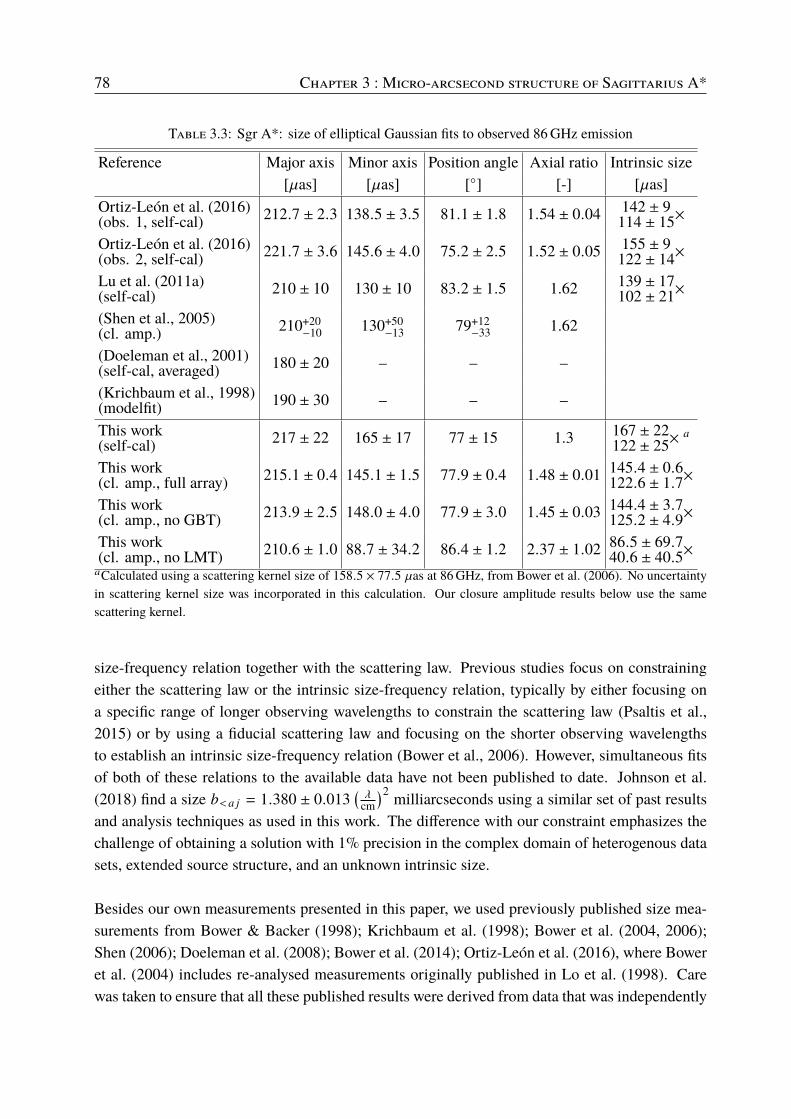
78 Chapter 3 : Micro-arcsecond structure of Sagittarius A*
Table 3.3: Sgr A*: size of elliptical Gaussian fits to observed 86GHz emission
Reference Major axis Minor axis Position angle Axial ratio Intrinsic size[`as] [`as] [◦] [-] [`as]
Ortiz-León et al. (2016)(obs. 1, self-cal) 212.7 ± 2.3 138.5 ± 3.5 81.1 ± 1.8 1.54 ± 0.04 142 ± 9
114 ± 15×
Ortiz-León et al. (2016)(obs. 2, self-cal) 221.7 ± 3.6 145.6 ± 4.0 75.2 ± 2.5 1.52 ± 0.05 155 ± 9
122 ± 14×
Lu et al. (2011a)(self-cal) 210 ± 10 130 ± 10 83.2 ± 1.5 1.62 139 ± 17
102 ± 21×
(Shen et al., 2005)(cl. amp.) 210+20
−10 130+50−13 79+12
−33 1.62
(Doeleman et al., 2001)(self-cal, averaged) 180 ± 20 – – –
(Krichbaum et al., 1998)(modelfit) 190 ± 30 – – –
This work(self-cal) 217 ± 22 165 ± 17 77 ± 15 1.3 167 ± 22
122 ± 25×0
This work(cl. amp., full array) 215.1 ± 0.4 145.1 ± 1.5 77.9 ± 0.4 1.48 ± 0.01 145.4 ± 0.6
122.6 ± 1.7×
This work(cl. amp., no GBT) 213.9 ± 2.5 148.0 ± 4.0 77.9 ± 3.0 1.45 ± 0.03 144.4 ± 3.7
125.2 ± 4.9×
This work(cl. amp., no LMT) 210.6 ± 1.0 88.7 ± 34.2 86.4 ± 1.2 2.37 ± 1.02 86.5 ± 69.7
40.6 ± 40.5×0Calculated using a scattering kernel size of 158.5 × 77.5 `as at 86GHz, from Bower et al. (2006). No uncertaintyin scattering kernel size was incorporated in this calculation. Our closure amplitude results below use the samescattering kernel.
size-frequency relation together with the scattering law. Previous studies focus on constrainingeither the scattering law or the intrinsic size-frequency relation, typically by either focusing ona specific range of longer observing wavelengths to constrain the scattering law (Psaltis et al.,2015) or by using a fiducial scattering law and focusing on the shorter observing wavelengthsto establish an intrinsic size-frequency relation (Bower et al., 2006). However, simultaneous fitsof both of these relations to the available data have not been published to date. Johnson et al.(2018) find a size 1<0 9 = 1.380 ± 0.013
(_cm
)2 milliarcseconds using a similar set of past resultsand analysis techniques as used in this work. The difference with our constraint emphasizes thechallenge of obtaining a solution with 1% precision in the complex domain of heterogenous datasets, extended source structure, and an unknown intrinsic size.
Besides our own measurements presented in this paper, we used previously published size mea-surements from Bower & Backer (1998); Krichbaum et al. (1998); Bower et al. (2004, 2006);Shen (2006); Doeleman et al. (2008); Bower et al. (2014); Ortiz-León et al. (2016), where Boweret al. (2004) includes re-analysed measurements originally published in Lo et al. (1998). Carewas taken to ensure that all these published results were derived from data that was independently

3.4 Constraints on the size-frequency relation and the scattering law 79
obtained and analysed. The measurements we include for the model fitting have been taken over atime period of multiple decades, thereby most likely representing different states of activity of thesource which may affect size measurements. This effect is expected to be small, however: at shortwavelengths because of the stable source size that has been measured over time, and at longerwavelengths because the scattering size is somuch larger than the intrinsic size. Themeasurementstaken at wavelengths close to _ = 20 cm were taken closely spaced in time, yet still show a mutualscatter that is wider than the size of their error bars suggests: this may indicate the presence ofsystematics in the data. An ongoing re-analysis of these sizes at long wavelengths (Johnson et al.,2018) suggests that these measurements are too small by up to 10%, likely impacting the resultingfits for the scattering law and intrinsic size-frequency relation. Here, we have used the values asthey have been published. Throughout this section, we use Gaussian models for both the observedsource size and for the scattering kernel. Recent work has shown that the instantaneous shape ofthe scattering kernel deviates from a Gaussian to a limited extent (Gwinn et al., 2014), but the sta-tistical average of the scattering kernel geometry is thought to be Gaussian to within a few per cent.
The set of measurements, as we have used them in the model fitting, can be seen in Figure3.7. Measurements taken at the highest of these frequencies (230GHz) are expected to featureemission coming from very close to the black hole shadow, and as such the perceived sourcesize may be significantly affected by gravitational lensing effects where the source image canbe warped into a crescent-like structure. Such strong lensing effects are not expected to play arole in source sizes as observed at lower frequencies because the inner accretion flow is opticallythick at small radii for those frequencies. We thus expect to effectively see emission coming fromsomewhat larger radii where the light paths are not significantly affected by spacetime curvaturebut are affected by interstellar scattering along our line of sight. Therefore, we performed themodel fitting both including the 230GHz size measurements (Figure 3.7) and excluding them, tosee if the expected GR lensing effects play a significant role in the appearance of the source at theshortest wavelengths. We find very little difference in the best-fit parameter values between theresults.
Simultaneous fitting of the size-frequency relation and the scattering law is done using the majoraxis size measurements only, as the uncertainties in the minor axis size measurements are toolarge to provide any meaningful constraint on the models. For the size-frequency relation, weused the following expression:
\int(_) = 0 · _1, (3.1)
where 0 and 1 are constants to be determined, \int is the intrinsic angular size in milliarcsecondsand _ is the observing wavelength in cm. For the scattering law we adopt the expression:
\scatt(_) = 2 · _2, (3.2)
where 2 is a constant to be determined and with \scatt the angular broadening through scatteringin milliarcseconds. These sizes are added in quadrature to provide the measured major axis size
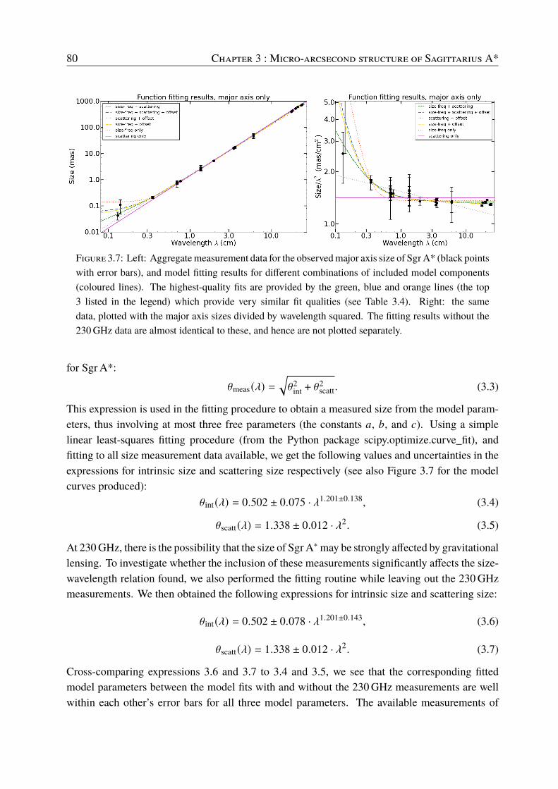
80 Chapter 3 : Micro-arcsecond structure of Sagittarius A*
Figure 3.7: Left: Aggregatemeasurement data for the observedmajor axis size of SgrA* (black pointswith error bars), and model fitting results for different combinations of included model components(coloured lines). The highest-quality fits are provided by the green, blue and orange lines (the top3 listed in the legend) which provide very similar fit qualities (see Table 3.4). Right: the samedata, plotted with the major axis sizes divided by wavelength squared. The fitting results without the230GHz data are almost identical to these, and hence are not plotted separately.
for SgrA*:
\meas(_) =√\2int + \2
scatt. (3.3)
This expression is used in the fitting procedure to obtain a measured size from the model param-eters, thus involving at most three free parameters (the constants 0, 1, and 2). Using a simplelinear least-squares fitting procedure (from the Python package scipy.optimize.curve_fit), andfitting to all size measurement data available, we get the following values and uncertainties in theexpressions for intrinsic size and scattering size respectively (see also Figure 3.7 for the modelcurves produced):
\int(_) = 0.502 ± 0.075 · _1.201±0.138, (3.4)
\scatt(_) = 1.338 ± 0.012 · _2. (3.5)
At 230GHz, there is the possibility that the size of SgrA∗may be strongly affected by gravitationallensing. To investigate whether the inclusion of these measurements significantly affects the size-wavelength relation found, we also performed the fitting routine while leaving out the 230GHzmeasurements. We then obtained the following expressions for intrinsic size and scattering size:
\int(_) = 0.502 ± 0.078 · _1.201±0.143, (3.6)
\scatt(_) = 1.338 ± 0.012 · _2. (3.7)
Cross-comparing expressions 3.6 and 3.7 to 3.4 and 3.5, we see that the corresponding fittedmodel parameters between the model fits with and without the 230GHz measurements are wellwithin each other’s error bars for all three model parameters. The available measurements of
3.5 Summary and conclusions 81
source size at 1.3mm thus seem to be compatible with the source size as predicted using the fittedsize-wavelengths relations from the other measurements.
Comparing these figures to Bower et al. (2015a), we see that the scattering size parameter for themajor axis is well within the error bars of the value calculated in that work (1maj, scatt = 1.32±0.02mas cm−2). For the intrinsic size as a function of wavelength, the powerlaw index we find is some-what larger than the powerlaw index calculated in Ortiz-León et al. (2016) (where it is quoted asbeing 1.34 ± 0.13), but still within the error bars.
The size-wavelength relation that we have used up to this point has a specific functional form: itconsists of a pure powerlaw for the size-frequency relation, combined in quadrature with a scat-tering law where scattering size scales with wavelength squared. To explore the influence that thischoice of functional form has on the results of the fitting procedure, we have performed the fit withother models for the dependence of observed size on observing wavelength as well. All modelsconsist of a combination of three components: a fixed-size component that is constant across allwavelengths, a scaled _? component (where ? is a free parameter) that is added linearly to it, anda scaled _2 component (scattering law) that is then added to the sum of the other component(s)in quadrature. Six combinations of these model components were fitted to the major axis sizemeasurement data, and each fit was done for two cases: with and without the 230 GHz observedsource sizes included in the data to be fitted to. In Table 3.4, the results of these model parameterfits are presented.
The three best-fitting models are the ’regular’ model (scattering law + general power law), the’augmented’ model (scattering law + general power law + fixed size offset), and the ’simple’model (general power law + fixed size offset). For the simple model, the best-fitting power lawindex is close to two within a few per cent. If the power law exponent from scattering can deviatefrom the theoretically ideal value of two by even a small fraction, this result suggests that theintrinsic size-frequency relation for SgrA∗ is less certain than what has been found in previouspublications. A similar conclusion was derived by Bower et al. (2006), where it was found that arelaxation of the scattering exponent to values slightly different from two undercuts the supportfor an intrinsic size-frequency relation with a non-zero power law index.
3.5 Summary and conclusionsConstraining the intrinsic size and structure of SgrA∗ at an observing wavelength of 3mm stillremains a challenge. Although the effect of interstellar scattering becomes smaller at this wave-length, it is still not negligible. GRMHD models of the accretion flow around SgrA∗ (e.g.Mościbrodzka et al., 2014) predict a certain structure in the emission which should be detectablewith current VLBI arrays. However, detection of intrinsic sub-structure could be hindered by re-
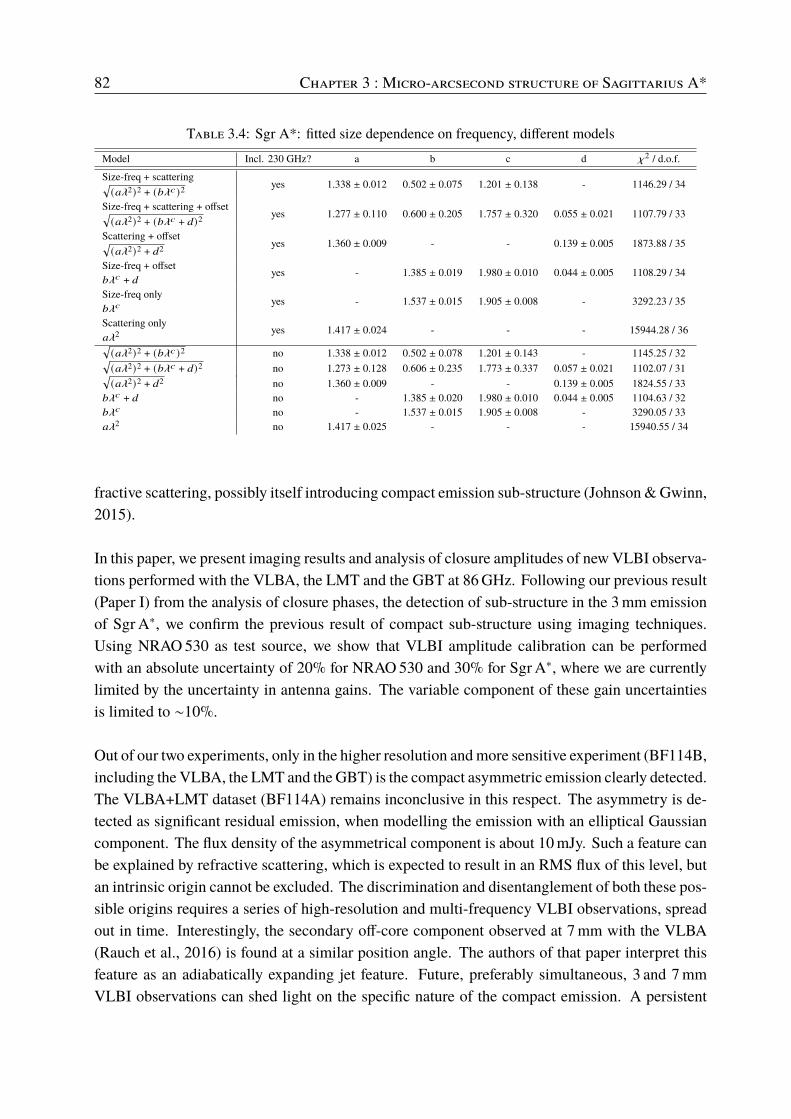
82 Chapter 3 : Micro-arcsecond structure of Sagittarius A*
Table 3.4: Sgr A*: fitted size dependence on frequency, different modelsModel Incl. 230 GHz? a b c d j2 / d.o.f.
Size-freq + scattering√(0_2)2 + (1_2)2
yes 1.338 ± 0.012 0.502 ± 0.075 1.201 ± 0.138 - 1146.29 / 34
Size-freq + scattering + offset√(0_2)2 + (1_2 + 3)2
yes 1.277 ± 0.110 0.600 ± 0.205 1.757 ± 0.320 0.055 ± 0.021 1107.79 / 33
Scattering + offset√(0_2)2 + 32 yes 1.360 ± 0.009 - - 0.139 ± 0.005 1873.88 / 35
Size-freq + offset1_2 + 3 yes - 1.385 ± 0.019 1.980 ± 0.010 0.044 ± 0.005 1108.29 / 34
Size-freq only1_2
yes - 1.537 ± 0.015 1.905 ± 0.008 - 3292.23 / 35
Scattering only0_2 yes 1.417 ± 0.024 - - - 15944.28 / 36√(0_2)2 + (1_2)2 no 1.338 ± 0.012 0.502 ± 0.078 1.201 ± 0.143 - 1145.25 / 32√(0_2)2 + (1_2 + 3)2 no 1.273 ± 0.128 0.606 ± 0.235 1.773 ± 0.337 0.057 ± 0.021 1102.07 / 31√(0_2)2 + 32 no 1.360 ± 0.009 - - 0.139 ± 0.005 1824.55 / 33
1_2 + 3 no - 1.385 ± 0.020 1.980 ± 0.010 0.044 ± 0.005 1104.63 / 321_2 no - 1.537 ± 0.015 1.905 ± 0.008 - 3290.05 / 330_2 no 1.417 ± 0.025 - - - 15940.55 / 34
fractive scattering, possibly itself introducing compact emission sub-structure (Johnson&Gwinn,2015).
In this paper, we present imaging results and analysis of closure amplitudes of newVLBI observa-tions performed with the VLBA, the LMT and the GBT at 86GHz. Following our previous result(Paper I) from the analysis of closure phases, the detection of sub-structure in the 3mm emissionof SgrA∗, we confirm the previous result of compact sub-structure using imaging techniques.Using NRAO530 as test source, we show that VLBI amplitude calibration can be performedwith an absolute uncertainty of 20% for NRAO530 and 30% for SgrA∗, where we are currentlylimited by the uncertainty in antenna gains. The variable component of these gain uncertaintiesis limited to ∼10%.
Out of our two experiments, only in the higher resolution andmore sensitive experiment (BF114B,including the VLBA, the LMT and the GBT) is the compact asymmetric emission clearly detected.The VLBA+LMT dataset (BF114A) remains inconclusive in this respect. The asymmetry is de-tected as significant residual emission, when modelling the emission with an elliptical Gaussiancomponent. The flux density of the asymmetrical component is about 10mJy. Such a feature canbe explained by refractive scattering, which is expected to result in an RMS flux of this level, butan intrinsic origin cannot be excluded. The discrimination and disentanglement of both these pos-sible origins requires a series of high-resolution and multi-frequency VLBI observations, spreadout in time. Interestingly, the secondary off-core component observed at 7mm with the VLBA(Rauch et al., 2016) is found at a similar position angle. The authors of that paper interpret thisfeature as an adiabatically expanding jet feature. Future, preferably simultaneous, 3 and 7mmVLBI observations can shed light on the specific nature of the compact emission. A persistent
3.5 Summary and conclusions 83
asymmetry, observed overmultiple epochs that are spaced apart in time bymore than the scatteringtimescale at 86GHz, would provide strong evidence for an intrinsic source asymmetry. Anotherway in which observed asymmetry may be ascribed to source behaviour rather than scatteringis when a transient asymmetry evolution is accompanied by a correlated variation in integratedsource flux density. Observations of that nature will require succesive epochs using a consistentand long-baseline array of stations involved accompanied by independent high-quality integratedflux density measurements (e.g. by ALMA).
We see that the combination of the VLBA, LMT and GBT provides the capability to pin downthe observed source geometry with unsurpassed precision because of the combination of sen-sitivity and extensive (D, E)-coverage provided, going beyond what addition of the LMT or theGBT separately can do. This combination of facilities is therefore important to involve in futureobservations that aim to measure the geometry of SgrA∗.
We also note that even with this extended array, the measurement and characterisation of complexsource structure beyond a 2D Gaussian source model is something that remains difficult. To studySgrA∗ source sub-structure at 86GHz more closely, be it either intrinsic or from scattering, evenmore extensive (D, E)-coverage and sensitivity will be needed. Recent measurements carried outwith GMVA +ALMA, the analysis of which is underway, should allow for a more advanced studyof the complex source structure of SgrA∗, as that array configuration provides unprecedentednorth-south (D, E)-coverage combined with high sensitivity on those long baselines.
Moving from source sub-structure to overall geometry, this work has reported the observed sourcegeometry of SgrA∗ with the highest accuracy to date. Addition of the GBT adds east-west re-solving power as well as extra sensitivity and redundancy in terms of measured visibilities. Wenote that the source geometry we find is very similar to that reported in (Ortiz-León et al., 2016),while the different observations were spaced almost one month apart (April 27th for BD183C,May 23rd for BF114B). Barring an unlikely coincidence, this suggests a source geometry that isstable to within just a few per cent over that time scale. At 86GHz, SgrA∗ is known to exhibitvariability in amplitude at the ∼10% level (see Paper I) on intra-day timescales. Whether theseshort-timescale variations in flux density correspond to variations in source size is an open ques-tion that can only be resolved when dense (D, E)-coverage is available at high sensitivity (beyondcurrent capabilities), as source size would need to be accurately measured multiple times withina single epoch. Alternatively, studies of the source size variability at somewhat longer timescalescan simply be done by observing SgrA∗ over multiple epochs – but the fast variations will besmeared out as a result.
From the simultaneous fitting of the scattering law and the intrinsic size-frequency relation forSgrA∗, we find values compatible with existing published results. However, if the scatteringlaw is allowed to deviate from a pure _2 law towards even a slightly different power law index,

84 Chapter 3 : Micro-arcsecond structure of Sagittarius A*
differing by for example 2% from the value two, support for the published intrinsic size/frequencyrelation often used in the literature quickly disappears. We therefore advocate a cautious stancetowards the weight given to existing models for the intrinsic size-frequency relation for SgrA∗.
AcknowledgementsWe thank the anonymous referee for providing comments that improved the quality of the paper.This work is supported by the ERC Synergy Grant “BlackHoleCam: Imaging the Event Horizonof Black Holes”, Grant 610058, Goddi et al. (2017). L.L. acknowledges the financial support ofDGAPA, UNAM (project IN112417), and CONACyT, México. S.D. acknowledges support fromNational Science Foundation grants AST-1310896, AST-1337663 and AST-1440254. G.N.O.-L.acknowledges support from the von Humboldt Stiftung. C.B. wishes to thank Michael Johnsonand Lindy Blackburn for valuable discussions which improved the robustness of the closureamplitude analysis.
3.A Closure amplitude model fitting techniqueIn the closure amplitude model fitting algorithm, we selected at random two independent closureamplitudes out of six possible ones for each quadrangle and integration time to be used in themodel fitting procedure. We performed the model fitting of the independent closure amplitudesby using a gradient descent method, where the source model parameters were iteratively altered togive successively better (lower) j2-scores until convergence is reached. The 2D Gaussian modelwe employed has three free parameters: major axis size (FWHM), minor axis size (FWHM), andthe position angle on the sky of the major axis. For every bootstrapping realisation, a random pointin the 3D model parameter space was initially chosen as a starting point, from a flat distributionusing upper limits for the major and minor axes sizes of 400 `as (and lower limits of 0 `as) toensure rapid convergence. Initial coarse step sizes are 50 `as for both major and minor axes, and0.1 radians for the position angle. For the parameter starting point, as well as for its neighboursalong all dimensions (each one step size removed from the initial point along one parameter axis),the j2 scores were calculated and the lowest-scoring point in the resulting set is taken as thestarting point for the next iteration. This sequence of steps was repeated until the best-fittingmodel parameters coincided with the starting point for that iteration (indicating a local optimumhas been reached at that parameter resolution), after which the step sizes for all parameters werereduced and the algorithm continues until the minimum step sizes are all reached. To verify thatthe general nature of the j2 landscape is conducive to this iterative method, and to ensure thatthe algorithm would not get stuck in a local optimum rather than the global optimum, we havemapped out the j2 scores over the full 3D parameter space at a low resolution for the original fullset of closure amplitudes. This investigation suggested that the j2-score varies smoothly over thefull parameter space, revealing the presence of a single global optimum.

Chapter4Frequency-dependent time lags in Sgr A*
Christiaan Brinkerink, Heino Falcke, Casey Law, Denis Barkats, Geoffrey Bower, AndreasBrunthaler, Charles Gammie, Violette Impellizzeri, Sera Markoff, Karl Menten, Monika
Moscibrodzka, Alison Peck, Anthony Rushton, Reinhold Schaaf, Melvyn Wright
A&A, 576, A14 (2015)
Abstract
Radio and mm-wavelength observations of Sagittarius A* (Sgr A*), the radio sourceassociated with the supermassive black hole at the center of our Galaxy, show thatit behaves as a partially self-absorbed synchrotron-emitting source. The measuredsize of Sgr A* shows that the mm-wavelength emission comes from a small regionand consists of the inner accretion flow and a possible collimated outflow. Existingobservations of Sgr A* have revealed a time lag between light curves at 43 GHzand 22 GHz, which is consistent with a rapidly expanding plasma flow and supportsthe presence of a collimated outflow from the environment of an accreting blackhole. Here we wish to measure simultaneous frequency-dependent time lags in thelight curves of Sgr A* across a broad frequency range to constrain direction andspeed of the radio-emitting plasma in the vicinity of the black hole. Light curvesof Sgr A* were taken in May 2012 using ALMA at 100 GHz using the VLA at48, 39, 37, 27, 25.5, and 19 GHz. As a result of elevation limits and the longitudedifference between the stations, the usable overlap in the light curves is approximatelyfour hours. Although Sgr A* was in a relatively quiet phase, the high sensitivity ofALMA and the VLA allowed us to detect and fit maxima of an observed minorflare where flux density varied by ∼10%. The fitted times of flux density maxima atfrequencies from 100 GHz to 19 GHz, as well as a cross-correlation analysis, reveala simple frequency-dependent time lag relation where maxima at higher frequencieslead those at lower frequencies. Taking the observed size-frequency relation of SgrA* into account, these time lags suggest a moderately relativistic (lower estimates:0.5c for two-sided, 0.77c for one-sided) collimated outflow.

86 Chapter 4 : Frequency-dependent time lags in Sgr A*
4.1 Introduction
The radio source Sagittarius A* (Sgr A*) at the center of our Galaxy is the best-constrainedsupermassive black hole candidate found thus far (Genzel et al. 2010; Falcke & Markoff 2013 fora review). Located at a distance of 8.3±0.4 kpc from the solar system, its mass is calculated to be4.3± 0.4 · 106 "� (Eisenhauer et al., 2003; Reid & Brunthaler, 2004; Ghez et al., 2008; Gillessenet al., 2009; Genzel et al., 2010). For a black hole of this mass, Sgr A* seems to be accretinggas at a very low rate of. 10−7 "� yr−1, as was derived from Faraday rotation measures (Boweret al., 2005; Marrone et al., 2007).
The emission from Sgr A* between frequencies of 20 GHz and 230 GHz shows flux density vari-ability of a few tens of percent on hour-long timescales, up to 100% on month-long timescales, aswell as occasional flaring behavior (Dexter et al., 2014). In radio, Sgr A* has an inverted spectrum(i.e., rising flux density with increasing frequency) that peaks at the ’submm bump’, around 350GHz, beyond which the spectrum steeply drops in the infrared regime. The radio emission isthought to originate mostly from partially self-absorbed synchrotron radiation emitted farther outfrom the black hole, while emission at frequencies corresponding to the submm bump (Falckeet al., 1998) of the Sgr A* spectrum is commonly associated with the optically thin emissionclosest to the black hole (Falcke et al., 1998; Shen et al., 2005; Bower, 2006; Doeleman et al.,2008). In the mm regime and at longer wavelengths, the flux density variation is thought to arisefrom local bulk properties (magnetic field strength, gas density, temperature) of the plasma, whilethe variability seen in infrared and X-rays is mostly attributed to changes in the population of thehigh-energy tail of the local electron energy distribution (Özel et al., 2000; Markoff et al., 2001;Yuan et al., 2003; Dodds-Eden et al., 2010; Dibi et al., 2013).
While the emission mechanisms for the radio and mm-wavelength emission of Sgr A* are under-stood fairly well, the identification of the emission with specific flow regions is still a subject ofdebate. For example, an important question is whether the radio emission is generated in a jet(Falcke et al., 1993) or in a radiatively ineffcient accretion flow (Narayan et al., 1995). Sgr A* inits flaring state fits neatly onto the fundamental plane of black hole activity (Merloni et al., 2003;Falcke et al., 2004; Plotkin et al., 2012), and as such it would be expected to feature a jet as othersources on that scaling relation do (Markoff, 2005). As yet, no direct detection of a jet has beenmade for Sgr A* despite the claimed presence of tantalizing jet-like features close to the Galacticcenter on parsec scales (Yusef-Zadeh et al., 2012; Li et al., 2013). Any putative jet structureclose to the black hole cannot be resolved below observing frequencies of ∼100 GHz becauseinterstellar scatter-broadening blurs our view of the Galactic center at such frequencies, an effectthat progressively increases with lower frequency (Lo et al., 1981; van Langevelde et al., 1992;Bower et al., 2006; Mościbrodzka et al., 2014). At higher observing frequencies, interstellarscintillation is less of a problem - in the mm-wave regime, existing VLBI networks should be ableto directly observe the proposed shadow of the event horizon with mmVLBI (Falcke et al., 2000;

4.2 Observations and data reduction 87
Doeleman et al., 2008).
There are other ways in which the nature of the emitting gas flow may be determined, however.Sgr A* exhibits an inverted radio spectrum. Flat or inverted radio spectra are commonly seenin quasars and active galactic nuclei, where the bases of radio jets resolved at high resolutionshow dominant emission at different radio frequencies as a function of distance from the core,which is due to optical depth effects (Hada et al., 2011), as has also been predicted from the-ory (Blandford & Königl, 1979; Falcke & Biermann, 1995). The multifrequency spectrum ofSgr A* (from radio to X-ray) in its flaring state looks very much like the spectrum of M81*,which has a weak jet (Bietenholz et al., 2004). The emission from an unresolved, compact jet mayexplain the inverted radio spectrum of Sgr A* (Falcke et al., 1993; Mościbrodzka & Falcke, 2013).
Presence of a jet implies that specific correlations should be detected between light curves atdifferent frequencies. As the peak frequency of radio emission changes with position along thejet axis, we expect variations in flux density at different observing frequencies to exhibit timelags relative to one another as the emitting gas moves out. Previous observations of Sgr A* madewith the VLA have indeed suggested the existence of a time lag of ∼20 to 40 minutes in fluxdensity variability between light curves measured at 43 GHz and 22 GHz, with variability in thehigher-frequency lightcurve leading that in the lower-frequency lightcurve (Yusef-Zadeh et al.,2006, 2008). Yusef-Zadeh et al. interpreted this as emission from an expanding plasma cloud (vander Laan, 1966) with velocities reaching about 0.012, but this interpretation does not take VLBAsizes into account. When coupled to the observed relation between the observing frequency andthe measured intrinsic size of Sgr A* (Bower et al., 2004; Doeleman et al., 2008), the time lagbetween 43 GHz and 22 GHz corresponds to a size difference of ∼30 light minutes. Thus, sucha time lag suggests the presence of a fast and directed outflow with a moderately relativisticspeed (Falcke et al., 2009). As the emission at observing frequencies below the submm bumpis probably all partially self-absorbed synchrotron emission, time lags may be present betweenthe light curves at any two different frequencies in that region. Measurements of time lags overa wider range of frequencies are of interest as they may aid in establishing a flow velocity pro-file, and theymay even provide an estimate of how close to the black hole the outflow can be traced.
4.2 Observations and data reductionOur VLA observations were taken on May 18, 2012 from 05:25:15 UT to 12:54:01 UT in CnBconfiguration, chosen to coincide with a Chandra observation. Light curves for Sgr A* weretaken in pairs of subbands for three basebands (X, Ka and Q), yielding 1-GHz-wide subbandsat center frequencies of 19 and 25.5 GHz (K-band), 27.48 and 37.99 GHz (Ka-band), and 39.55and 48.5 GHz (Q-band) - each using 30-second scans at an integration time of 3 seconds. Thesubbands eventually used for each center frequency were 4-7 (19 GHz), 0-7 (25.5 GHz), 0-7 (27

88 Chapter 4 : Frequency-dependent time lags in Sgr A*
GHz), 0-7 (37 GHz), 2-7 (39 GHz), and 1-2 (48 GHz). Flux and bandpass calibration were madeon the standard VLA calibrator 3C286. A monitoring loop with a period of 7.5 minutes was usedfor Sgr A*: within each iteration of this loop, J1744-3116 was used as a gain calibrator sourceand J1745-283 was used as a check-source, cycling through all three basebands in turn. Theintegration time of 3 seconds was chosen such that the RMS noise per scan was expected to be 1mJy when all subbands in a baseband were used.
The VLA data (project code: 12A-339) were initially reduced using the VLA pipeline version1.2.0 (rev. 9744) on CASA 4.1.0. After running the VLA pipeline, the sufficiently high fluxdensity of all sources allowed us to perform careful phase self-calibration on them using pro-gressively shorter solution intervals down to one integration length (3 seconds). Some subbandswere flagged in this calibration process because their calibration solutions did not converge. Thesubbands that remained unflagged were (format: baseband (subbands)) 48 GHz (1,2), 39 GHz(2-7), 37 GHz (all), 27 GHz (all), 25 GHz (all), and 19 GHz (4-7). The declination of Sgr A*combined with the latitude of the VLA means that Sgr A* never reaches an elevation over 27degrees for the VLA. Therefore the first and last parts (before approximately 6:40 UT and afterapproximately 11:50 UT) of the observation suffer from coherence loss: the source is less than18 degrees above the horizon, and the effective path length through the atmosphere for the signalvaries rapidly and strongly between antennas. As such, all data in these time windows wereflagged before recalibration.
For the ALMA track, observations were made in ALMA cycle 0 on May 18, 2012 from 03:30:47UT to 10:52:16 UT (project code: 2011.0.00887.S). The ALMA light curves for Sgr A* weretaken at ALMA bands 3, 6, and 7 using pairs of spectral windows each centered on 95, 105,247, 260, 338, and 348 GHz. Each pair of spectral windows covered 3.75 GHz bandwidth fora total of 7.5 GHz bandwidth per ALMA band. Scan lengths were chosen to yield a sensitivityof 0.5 mJy. All individual scans of Sgr A* were bracketed by either NRAO530 or J1924-292 ascalibrators, while flux density calibration was made on Titan and Neptune. At that time, ALMAhad 19 antennas available. In this paper we limit discussion to the 100 GHz ALMA data: thelight curves at 250 GHz and 340 GHz will be the subject of a future paper.
For ALMA, the source setup was somewhat more complicated because all observations in cycle 0had to be obtained in two-hour blocks. This means that the ALMAdataset consists of four separateblocks that are contiguous in time, each starting with a flux density calibrator measurement (Titanfor the first two blocks, Neptune for the latter two). Within each block, five scans on Sgr A* weremade where each of these was bracketed by scans on one of the calibrator sources NRAO530 andJ1924-292, a precaution taken because of possible calibration difficulties that might otherwiseoccur in cycle 0. Thus the scan setup for each block was (using the first letter of each source)’NSN JSJ NSN JSJ NSN’, the average switching time between bracketing calibrator scans andSgr A* scans was 2 minutes, and the time cadence on Sgr A* in each band was 15 minutes. As

4.3 Analysis and results 89
J1924-292 exhibited irregular results in its polarisation-dependent flux density levels, it was notused as a calibrator and only used as a check-source. Gain levels were stable enough to warrant theusage of NRAO530 as the only gain calibrator. The ALMA data were calibrated using a customscript based on the calibration procedure for the QA2 process of Cycle 0 data, with subsequentphase self-calibration on Sgr A* (which has a very strong unresolved component of around 2.5Jy at 100 GHz) using baselines longer than 150 k_.
From the calibrated VLA and ALMA data, the light curves for Sgr A* were obtained by averag-ing all unflagged UV visibilities per scan from all baselines longer than 150 k_, using uniformweighting for the selected baselines. We chose to only use projected baseline lengths over 150 k_because we wished to avoid any contamination from the extended emission around Sgr A*, andbaselines shorter than the chosen length show hints of structural variations over the track. Lim-iting ourselves to the longer baselines enabled us to work directly with the visibilities rather thanneeding the additional steps of imaging and model fitting. The errors on the flux density levelswere estimated using the spread in amplitude of the calibrated visibilities over each scan. Thecalibrated light-curve data can be seen in the left column of Fig. 4.1. All light curves can beseen to exhibit a gradual rise and decay, with shorter-timescale variation superimposed. Forthe calibrated VLA data, the resulting noise levels for the basebands at 19, 25, 27, 37, 39, and48 GHz are 1.4, 0.7, 1.2, 0.9, 2.6, and 12.1 mJy, respectively. Limited calibration accuracyand the flagging of several subbands degrades the sensitivity from the desired sensitivity in thehighest frequency bands. The final uncertainties in flux density are dominated by the calibrationuncertainty coming from the variability that was exhibited by the check-source: this brings thetotal relative flux density measurement uncertainty to approximately 5% for the VLA data. Forthe ALMA data, the uncertainty in flux density is approximately 5% as well - however, the errorsthere are relatively small compared to the intrinsic variability of Sgr A* at 100 GHz. We note thatthe flux calibration of the VLA data does not give a perfectly smooth spectrum for our calibratorsource J1744-3116, but this only affects the overall flux levels of the Sgr A* light curves by ∼5%and does not affect the conclusions in this paper.
4.3 Analysis and resultsThe spectral energy distribution of Sgr A* across the measured frequencies (see Fig. 4.2) has aspectral index of U = 0.41 ± 0.03 (with U defined as in (a ∝ aU) when all data (VLA + ALMA)are used for the spectral fit, and we obtain U = 0.50 ± 0.07 when only the VLA data are used.While this difference in spectral index cannot be called significant, it hints at a flattening of thespectrum as the submm bump is approached.
The VLA light curves at first sight each show a similar evolution of flux density with time: arise in flux density level between 7h and 8h/9h UT, and a more slowly diminishing flux density

90 Chapter 4 : Frequency-dependent time lags in Sgr A*
Figure 4.1: Left: Flux vs. time of Sgr A* for the VLA data (top six graphs) and the 100 GHz ALMAdata (bottom graph). The fitted FRED function is plotted as a green (gray) curve, the position of themaxima is plotted as a vertical red (dark gray) line with the uncertainty in the fit superimposed asa red-shaded (dark gray) region. Green-shaded (light gray) regions indicate the uncertainty on thefits obtained by randomly dropping half of the data points for 500 iterations - see Sect. 3 for details.Right: Flux vs. time for the calibrator sources (J1744-3116 for the VLA data, NRAO530 for theALMA data).
beyond 8h/9h UT. The observed longer-term flux evolution over the full track is overlaid withmore rapid variations in measured flux, which occur simultaneously in all frequency bands. Thesefluctuations are probably caused by atmospheric influence, which causes varying coherence lossas a function of time. The ALMA flux density measurements are highly precise, with a verysmall spread in visibility values per scan. The time cadence, however, is coarser than it is for theVLA data. Nonetheless, the evolution of flux density with time can be distinguished with highsignificance. At 100 GHz the flux density evolution is smooth, and there is a local maximum influx at around 7:45h UT, followed by a later peak around 10:00h UT.
The z-transform discrete correlation function (ZDCF) algorithm (Alexander, 1997) provides away to cross-correlate light curves that have uneven temporal sampling. This method for finding

4.3 Analysis and results 91
Figure 4.2: Averaged flux density as a func-tion of frequency for all light curves for the timeperiod between 7h and 11h UT. The error barsdenote measurement error convolved with fluxdensity variability over the track, where vari-ability is the dominant contribution. Variabilityis strongest at the highest frequencies. The spec-tral index obtained from using VLA + ALMAdata is indicated by the black line (with 1-sigmafit uncertainties filled in with gray) and yieldsU = 0.42 ± 0.03. Using the VLA data only(red/gray line, with red/light gray 1-sigma un-certainty region), U = 0.45 ± 0.07.
time lags between the VLA light curves yields a strong zero-lag component in every case (seeFig. 4.3 for an example), coming from the short-time fluctuations in the data and probablyattributable to coherence loss. These zero-time lag spikes tend to dominate the cross-correlationcurves. Although skew is apparent in most cross-correlation curves, the zero-lag peaks precludeany meaningful time lag estimates to be made this way. To derive reliable time lag estimates, wechose the simple and robust approach of fitting the longer-term flux density evolution in all lightcurves. To establish the times at which flux density maxima occur in these light curves, we fitteda smooth function to this general trend, allowing for different timescales to be associated with therise and fall. Based on the general shape of the light curves, the choice was made to employ ’fastrise, exponential decay’ (FRED) functions as fitting functions (Bhat et al., 1994) (widely used inGRB light curve fitting). These functions consist of the product of two exponentials, involvingfour free parameters:
5 (C) = � · 42√1/0 · 4−(C−Δ)/0−1/(C−Δ) , (4.1)
where � is the maximum value of 5 (C), 0 and 1 are parameters controlling the slopes of eitherside of that maximum, and Δ is the value of C for which the maximum value is reached. Becausethe FRED flux density value rises up from zero and returns to zero as its argument C is left running,it is not a suitable function to use over time intervals that are too long: we are only interested inusing it to fit a local and asymmetric feature in the light curves. To keep the general shape of thelight curves sufficiently simple to enable the fit without sacrificing too many data points, we onlyused the flux density measurements directly around the bump feature (7h - 11h UT for VLA, 6:50- 8:50 UT for ALMA). Acting on the assumption that this feature in the ALMA light curve can beattributed to the same event in the source that caused the maxima found in the VLA light curves,we used the fitting algorithm on this feature as well.
Variations on shorter timescales in the VLA light curves may affect the fit results. Therefore wealso performed the fits using a Monte Carlo approach in which, at random, half of the data points

92 Chapter 4 : Frequency-dependent time lags in Sgr A*
Table 4.1: Times of flux density maxima from curve-fitting of individual light curves. Column 1: alldata, Col. 2: subsample with MC
Frequency Time of max (1) Time of max (2)(hrs UT) (hrs UT)
100 GHz 7.65 ± 0.19 -48 GHz 7.93 ± 0.31 7.82 ± 0.9039 GHz 8.03 ± 0.14 8.01 ± 0.1237 GHz 8.17 ± 0.13 8.17 ± 0.1327 GHz 8.38 ± 0.11 8.38 ± 0.1125 GHz 7.98 ± 0.16 7.97 ± 0.1519 GHz 8.78 ± 0.29 8.72 ± 0.19
(20 out of 40) for a given VLA light curve were dropped before attempting a fit with the FREDfunction. For each light curve, this was iterated 500 times. The resulting times of maxima forall obtained fits were averaged, and the standard deviation of their distribution was calculated.These results are also plotted in Fig. 4.1, shaded in green. The large standard deviation inthe 48 GHz case indicates skew in the range of predictions made by the Monte Carlo method,causing the left limit to fall outside of the data range. High reduced j-squared values indicatethat we fitted light curves whose evolution is more complicated than can be grasped by a simplefunction; significant short-term variability remains from imperfect flux calibration. The absoluteflux density uncertainties are dominated by the calibration uncertainty of ∼5 percent for the entirelight curve (not shown in the figure). For most light curves, these results correspond well to the fitfor which all data were used. For the light curve at 48 GHz the fits are not as robust. This is mostprobably due to the relatively strong flux density variations at short timescales for the 48 GHzlight curve, combined with the short FRED rise time. The resulting best-fit values and uncer-tainties for the times of flux density maximum are shown in Fig. 4.1, and the time lags we foundare summarized in Table 4.1 where the middle column uses all data and the rightmost columnuses the average result from the Monte Carlo approach. As the ALMA data does not have manymeasurements within the relevant timewindow, theMonte Carlo approach could not be used there.
With the 25GHz data as notable exception, themaxima occur at later times for the lower observingfrequencies, which is compatible with a linear relation between observing wavelength and timeof maximum flux density. There is always the risk of misinterpreting the ALMA bump at 7:40hUT as being causally connected to the maxima in flux density found in the VLA data. To checkwhether the VLA data by themselves are consistent with the existence of these time lags, a separatefit was made using only the VLA data (Fig. 4.4), and the fit results are practically identical tothose obtained with the full data set. The time lag expected for the ALMA peak based on the VLAtime lag/frequency fit coincides with the measured value, and thus the identification of the ALMAflux density maximum as being related to the VLA flux density maxima seems justified. Thefact that the maxima occur at different times for different frequencies also precludes interpreting

4.3 Analysis and results 93
Figure 4.3: Example of a cross-correlation curve for the original light-curve data (left) and for thelight-curve data with the FRED trend subtracted (right). The skew in the CCF for the full light curvessuggests a nonzero timelag, but the zero-lag peak is too prominent to provide any useful estimate.After the fitted FRED trend is subtracted from both light curves and the cross-correlation is performedagain, the only prominent cross-correlation peak corresponds to zero time lag.
Figure 4.4: Fitted times for the flux density maxima in each baseband (relative to the 19 GHz (1.6cm) maximum), plotted as a function of observing wavelength. The figure uses the errors on the fitmaxima obtained from fitting all data points. Dark shaded regions indicate the uncertainty in fit slopeusing all light curves, lighter shaded regions indicate the uncertainty in fit slope fromVLA light curvesalone. The slopes obtained are 42 ± 14 mins/cm (all data) and 36 ± 21 mins/cm (VLA data alone).The continuous lines are time-lag predictions from the jet model by Falcke et al. (2009) assuminginclinations of 30, 60, and 90◦.

94 Chapter 4 : Frequency-dependent time lags in Sgr A*
Figure 4.5: Variability due to FRED-fitted light-curve trends (vertical axis) versus remaining vari-ability in trend-subtracted light curves (horizontal axis) for the VLA data. Both axes show standarddeviations. These quantities indicate that the long-term variability that is fitted by the FRED functionscales with the remaining short-term variability.
the observed flux density evolution as being a purely atmospheric or elevation-dependent effect.Any elevation-dependent change in measured flux density would impose a simultaneous risingand falling of all light curves, which is not what we observe.
The FRED fits follow the general, long-term trend that is present in the data. In addition to thisgeneral trend, all light curves exhibit shorter-timescale fluctuations. Cross-correlation analysis onthe original light curves therefore shows correlation contributions from both the general trends inthe data and the shorter-timescale fluctuations. If these two variability components do not exhibitthe same time lag between frequencies, interpreting the cross-correlation curves is problematic.To deal with this problem, we have subtracted the fitted FRED trends from all light curves andperformed a cross-correlation analysis on the de-trended light curves (see Fig. 4.3). This cross-correlation peaks at zero time lag, suggesting that the short-termfluctuations have a different originfrom the long-term trends. The most likely cause of the short-term fluctuations are calibrationresiduals stemming from phase-coherence loss due to the low elevation of Sgr A* at the VLAsite. While there is a correlation between the FRED variability and the residual variability asseen from Fig. 4.5, this does not imply that they share the same cause. Atmospheric influence isstronger for higher observing frequency, and this effect is unrelated to intrinsic source variability.

4.4 Discussion and conclusion 95
4.4 Discussion and conclusion
The time lags across this broad range of frequencies corroborate the picture of an expandingplasma flow with a diminishing optical depth over time. When the time lags found in this workare combined with the existing results from Yusef-Zadeh et al. (2006), they are compatible:Yusef-Zadeh et al. reported a time lag between 43 GHz and 22 GHz of 20 to 40 minutes, whilewe detect a time lag of 28 ± 9 minutes between these two frequencies when we use the linear timelag/wavelength fit based on our measurements (see Fig. 4.4 and caption).
Measurements on time lags between Sgr A* light curves at 102 and 90 GHz were performedby Miyazaki et al. (2013), and they reported the time delay between 102 GHz and 90 GHz asbeing −2.56 ± 0.9 min (i.e., the 90 GHz light curve is leading the 102 GHz light curve). Theexpected time lag between 102 and 90 GHz that would agree with the 43 GHz -22 GHz lag foundby Yusef-Zadeh et al. (2006) is quoted as being close to 3 min (with the precise value dependingon the index of the power-law distribution in electron energy), whereas an extension of the linearrelation we find in this work predicts a time lag between these frequencies of 1.7 ± 0.6 min (thisfigure increases somewhat if low inclination angles are considered, see Fig. 4.4). We stress thatthe models used to predict the time lags are very simple in all cases, and in particular measuredtime lags between closely neighboring frequencies can deviate from the predicted relation due tomore complex plasma flow properties close to the black hole. The Blandford-Königl jet modeluses a g = 1 surface, the location of which along the jet only depends on the accretion rate, andwhich is constant throughout the jet cross-section. The actual nature of any outflow may locallybe of a more chaotic character, with different regions in the jet cross-section having differentplasma densities and different optical depths, as is typically witnessed in GRMHD simulations(Mościbrodzka et al., 2014). Our measurements, obtained over a broad range of frequencies, areexpected to sample a greater spatial range of the proposed outflow. They should hence provide arobust result and a characterization of the behavior of the system as a whole, and we believe thisapproach warrants the use of a simple outflow model.
Without source size measurements, many different models of expanding plasma flows can bemade to fit our observations. Following the analysis by Yusef-Zadeh et al. (2008), where anadiabatically expanding plasma cloud was used as a model for flare occurrence in Sgr A*, thecloud expands to just ∼2.3 times the size it initially has at the 100 GHz maximum (see Figs. 4.6and 4.7) for the frequency range we record. The radii at which the lower-frequency emissionpeaks is only a few times the initial radius (which is taken to be 3 Schwarzschild radii). If weadopt the initial radius of the cloud as being ∼3 Schwarzschild radii, as was done by Yusef-Zadehet al. (2008), the associated flow velocities that occur according to this model are only around 3percent of the speed of light. This is twice the velocity that was found byYusef-Zadeh et al. (2008).
However, we can use the size-frequency relation of Sgr A* as presented in Falcke et al. (2009) as

96 Chapter 4 : Frequency-dependent time lags in Sgr A*
Figure 4.6: Normalized flux density profiles of an adiabatically expanding plasma cloud as a functionof radius for all frequencies. The continuous flux profiles use the expressions given in Yusef-Zadehet al. (2008), with a particle spectral index of 1 as was determined to be the best-fitting value inthat work. Note that the initial radius used by Yusef-Zadeh et al. (2008) (∼3 Schwarzschild radii) isdifferent from the initial radius that follows from using the size-frequency relation (∼ 11 Schwarzschildradii).
additional information with which to provide a general estimate of the gas flow velocity. Althoughwe do not have sufficient information to identify the variable emission (that we focus on) with thequiescent emission for which the size-frequency relation holds, considering the two componentsto reflect the same gas flow is the simplest hypothesis that we can consider. The size-frequencyrelation describes the measured intrinsic (i.e., corrected for interstellar scattering) size of Sgr A*as a function of observing wavelength, and has the form:
qSgr A* = (0.52 ± 0.03)mas × (_/cm)1.3±0.1. (4.2)
In this expression, qSgr A* is the angular size of Sgr A* on the sky and _ is the observing wave-length. Combining this (angular) size-frequency relation with an estimate for the distance betweenEarth and the Galactic center and taking the difference in source size for two observing frequen-cies, we obtain an expression for the projected source size difference on the sky in length units.When we assume a source inclination of 90◦ and a one-sided outflow interpretation (as was doneby Falcke et al. (2009)), we find that our data suggest an outflow velocity of ∼0.772 (WV ≈ 1.2).Using the variability seen in our measurements (Fig. 4.5) as a proxy for flare amplitude with thesize-frequency relation (Eq. 4.2), we obtain the data points that are plotted separately in Fig. 4.6.

4.4 Discussion and conclusion 97
Figure 4.7: Times of flux density maxima for different frequencies plotted against the radii at whichmaximum flux density is reached. Black data points are obtained by combining our time lags with theoutflow model used in Yusef-Zadeh et al. (2008), see also Fig. 4.6. If the initial radius is a only fewSchwarzschild radii, the estimated flow velocity reached by the expanding plasma is on the order of0.032. Orange (light gray) data points are obtained by combining our time lags with the size-frequencyrelation (Eq. 4.2), and yield a velocity of ∼0.52. Note that the initial radii are not the same for bothcases.
Because the source centroid position on the sky as a function of observing frequency is notknown, however,we can derive a lower limit on the outflow velocity by assuming identicalcentroid positions for all observing frequencies. This assumption corresponds to a two-sided jetinterpretation (the source grows symmetrically on the sky with lower observing frequency), so forthe distance traveled by the gas in one jet we can take half of the intrinsic source size difference.Taking into account the influence of light travel time with different inclination angles yields thefollowing expression for the expected time lag between observing frequencies:
Δdiff ='SgrA,diff
sin 8
(1E 5− cos 8
2
), (4.3)
with Δdiff the time lag between two observing frequencies, 'SgrA,diff the radius difference for thetwo observing frequencies as calculated using Eq. 4.2 and our distance to the Galactic center of8.3 kpc, 8 the inclination angle (angle between the flow vector and the line of sight from Sgr A*to Earth) and E 5 the flow velocity. We can express this relation in terms of E 5 and combine itwith the relation between time lag and wavelength (see Fig. 4.4). In this way, we can plot therelation between flow velocity estimate and jet inclination angle, where we place the constraintthat the flow velocity needs to be positive and lower than the speed of light. Figure 4.8 shows this

98 Chapter 4 : Frequency-dependent time lags in Sgr A*
Figure 4.8: Estimates of minimum outflow velocity (expressed in WV) as a function of the inclinationangle of the flow direction. The uncertainties have been calculated from the uncertainty in Galacticcenter distance (0.4 kpc), the uncertainties in the size-frequency relation (see Eq. 4.2) and theuncertainty in time lag vs observing wavelength (14 mins/cm, see Fig. 4.4) using standard errorpropagation.
dependence and indicates a minimum flow velocity of E 5 = 0.5c (WV = 0.58) for an inclination of60◦. Including the light travel time in the calculation breaks the symmetry around an inclinationof 90 degrees that would otherwise be present. For the two-sided outflow, we assumed here thatthe outflow component with an inclination smaller than 90 degrees is the one that is picked up inthe time lag measurements. For the two-sided jet interpretation only inclinations close to 90◦ canbe modeled reasonably in this way. Inclinations deviating significantly from 90◦ would result inambiguous time lags because of the different light travel times from the gas in the two jets. Forthe case of a one-sided jet, where the source only grows toward one side with lower observingfrequency, the lower velocity bound is approximately E 5 = 0.77c (WV = 1.2, see Figure 4.9).Figure 4.4 plots the model-predicted time lags for different inclination angles and shows that nostrong constraints are posed on the inclination angle by these data.
As these results are based upon measurements of a light-curve feature from a single track, it isprudent to perform this analysis on more light curves as they become available to verify the picturewe establish. Although the broad nature of the flux density feature that we used in the FRED fitgenerally agrees with the result of the ZDCF analysis, light curves with significant flux densitychanges over shorter timescales would offer an opportunity of using the ZDCF more effectivelyas an alternative verification of the FRED fitting results. ALMA observations at a higher timecadence taken contemporaneously with VLA observations would facilitate the cross-matching of

4.5 Acknowledgements 99
Figure 4.9: Time delays as a function of frequency, expressed in minutes before the time of maximumflux density at _ = 1.57 cm (19 GHz). Colored lines indicate the model time-lag predictions fordifferent constant outflow and inflow velocities. Orange (light gray) lines indicate outflow, blue (darkgray) lines indicate inflow. The data points, derived from the full-data FRED curve fits, suggest anoutflow with a moderately relativistic velocity, clustering around WV = 2. This figure is valid for aninclination angle of 90 degrees and is adapted from Falcke et al. (2009).
light-curve features between these frequencies.
To summarize, we have measured time lags in Sgr A* light curves from 100 GHz to 19 GHz usingALMA and the VLA. Higher-frequency light curves are seen to have their maxima at earlier timesthan the lower-frequency light curves. Coupled to the size-frequency relation for Sgr A*, thesemeasurements indicate a moderately relativistic, directed outflow from Sgr A*.
4.5 AcknowledgementsThis work was performed as part of the Chandra XVP collaboration (see http://www.sgra-star.com/collaboration-members/ for a list of collaboration members). This paper makes use ofthe following ALMA data: ADS/JAO.ALMA#2011.0.00887.S. ALMA is a partnership of ESO(representing its member states), NSF (USA) and NINS (Japan), together with NRC (Canada)and NSC and ASIAA (Taiwan), in cooperation with the Republic of Chile. The Joint ALMAObservatory is operated by ESO, AUI/NRAO and NAOJ. We thank our referee for providinguseful comments that improved the presentation of this paper.

100 Chapter 4 : Frequency-dependent time lags in Sgr A*

Chapter5Christiaan Brinkerink, Heino Falcke
to be submitted
Abstract
The compact radio source at the center of our Galaxy, SagittariusA* (SgrA*), isthe subject of intensive study as it provides a close-up view of an accreting super-massive black hole. SgrA* provides us with a prototype of a low-luminosity activegalactic nucleus (LLAGN), but interstellar scattering and the resolution limits of ourinstruments have limited our understanding of the emission sites in its inner accretionflow. The temporal variability of SgrA* can help us understand whether we see aplasma outflow or inflow in the region close to the black hole. In this work, we lookat a comprehensive set of multi-epoch data recorded with the Karl G. Jansky VeryLarge Array (VLA) to understand the persistence of the time lag relations that havebeen found in previous radio observations of SgrA*. We analyse 8 epochs of data,observed in Spring 2015, each of which has a frequency coverage from 18 to 48 GHz.We cross-correlate the calibrated light curves across twelve frequency subbands. Wealso generate synthetic data with the appropriate variability characteristics and use itto study the detectability of time lag relations in data with this sampling structure.We find that the variability amplitude increases with frequency. We see positive timelag slopes across all subbands in five out of eight epochs, with the largest slopesin the cases where a clear extremum in flux density is present. Three epochs showlag slopes close to zero. With the synthetic data analysis we show that these resultsare explained by a persistent lag relation of ∼40 min/cm that covers the bulk of thevariability, with at most 2% of the total flux density in an uncorrelated variabilitycomponent. Together with the size-frequency relation and inclination constraints thisindicates an outflow velocity with WV = 1.5, consistent with predictions of jet modelsfor SgrA*.

102 Chapter 5 : Time lags of Sgr A*
5.1 Introduction
There is significant evidence and support for the notion that the compact radio source at thecenter of our Galaxy (SagittariusA*, abbreviated as SgrA*, see Balick & Brown (1974)) isassociated with plasma flow around a supermassive black hole of approximately 4 million solarmasses. Analysis of the orbits of short-period bright stars shows that the central mass is highlyconcentrated and coincident with the region from which we see the radio emission (Reid &Brunthaler, 2004; Ghez et al., 2008; Gillessen et al., 2009; Gravity Collaboration et al., 2019).In this introduction we will focus on the different observational aspects of this radio source anddiscuss the system properties that have been derived from them.
5.1.1 Observed spectrum
SgrA* has a spectral energy distribution (SED) that shows a rising power-law across the radiospectrum, steepening into a submm-bump that starts above ∼50 GHz and peaks in the 1 - 2 THzrange (Zylka et al., 1992; Serabyn et al., 1997; Falcke et al., 1998; Zhao et al., 2003; Bower et al.,2019), before rapidly dropping into the infrared regime. The general shape of this spectrum sug-gests that we see partially self-obscured synchrotron emission, optically thick at lower frequenciesand turning over to optically thin emission at higher frequencies.
The observed spectral shape and flux density of the submm bump allow us to solve for severalproperties of the inner plasma flow: the electron number density, the magnetic field strength andthe temperature of the plasma (Falcke et al., 1993; Narayan et al., 1995; Falcke & Biermann,1996; Yuan et al., 2003; Goldston et al., 2005; Mościbrodzka et al., 2009). These results showthat the emission from the submm bump must come from the innermost part of the plasma flow:the lower-frequency part of the spectrum is self-absorbed, indicating that we are seeing into apartially transparent photosphere layer of an otherwise opaque region. This frequency-dependentphotosphere shrinks inwards as we consider higher observing frequencies, until we reach theturnover point in the spectrum: there, the photosphere disappears altogether and we see the regionclosest to the black hole. The fact that the submm spectrum of SgrA* shows this structure meansthat SgrA* is also a prime candidate for very long baseline interferometry (VLBI) observations ofits shadow by the Event Horizon Telescope (Event Horizon Telescope Collaboration et al., 2019c):the attainable angular resolution for a worldwide network of antennas observing at 230GHz allowsit to resolve the expected scale of the black hole shadow in the case of SgrA* (Falcke et al., 2000).A fundamental open question in this context is: what is the emitting plasma in this inner regiondoing? Is it part of an inflow or an outflow?
5.1.2 Observed morphology
Studies of the morphology of SgrA* with Very Long Baseline Interferometry (VLBI) at wave-lengths from 20 cm down to 1.3mm indicate an elliptical (Gaussian) shape for the source and
5.1 Introduction 103
show that the apparent source size is dominated by interstellar scattering effects at wavelengthslonger than ∼3mm (van Langevelde & Diamond, 1991; Lo et al., 1998; Bower et al., 2006), mak-ing it scale according to _2 for wavelengths in that range. At shorter wavelengths, the observedsize of SgrA* deviates from this relation: it is larger than the _2 relation predicts (Bower et al.,2004; Shen et al., 2005; Doeleman et al., 2008; Ortiz-León et al., 2016; Brinkerink et al., 2019),with the fractional difference becoming more pronounced at progressively shorter wavelengths.This is understood to be a manifestation of the intrinsic source geometry which becomes moreclearly visible as the influence from scattering loses its dominance at higher frequencies. Al-though the measured size of SgrA* at 86GHz is larger than predicted from a pure scattering sizerelation constructed using measurements at lower frequencies, the deviation of its morphologyfrom Gaussianity is modest with only ∼1% of the observed VLBI flux density not matching anelliptical Gaussian brightness distribution (Brinkerink et al., 2019). While the scattered sourcegeometry approximates an elliptical Gaussian very closely at longer wavelengths, substructure atthe sub-percent level has also been seen at 1.3 cm (23 GHz) as reported by Gwinn et al. (2014).
The observed non-Gaussian substructure manifests as an asymmetry that may either be intrinsicin origin, caused by the effects of interstellar scattering or a combination thereof (Ortiz-Leónet al., 2016; Brinkerink et al., 2016). Observations on the degree to which this observed sourceasymmetry persists over longer time scales (∼years) should resolve this origin, as the time scaleover which the influence from the scattering screen evolves is relatively short (∼weeks).
Algorithmically, disentangling the scattering effects from the contribution of the intrinsic sourcestructure is a challenging task, although in recent years significant progress has been booked inthis endeavour (Johnson & Gwinn, 2015; Johnson, 2016; Johnson et al., 2018; Issaoun et al.,2019) which allows for partial reconstruction of intrinsic source geometry from measurements ofthe scattered source image.
GivenmodernVLBI capabilities, the argumentmay be raised that jet morphology should thereforebe readily apparent when looking at SgrA* at radio-to-mm wavelengths, and in fact observationsat 7mm have indeed suggested this (Lo et al., 1998). From the theoretical side, it has been shownthat the morphology of a jet outflow of SgrA* may be such that it would appear as a highlycompact source, within the size constraints dictated by these VLBI measurements (Markoffet al., 2007). More recent VLBI measurements at 86GHz, which suffer less from the effects ofinterstellar scattering, can still be fitted with models from both jet- and disk-dominated classes(Mościbrodzka, 2017; Issaoun et al., 2019).
5.1.3 Time-domain studies
Besides the spectral and spatial dimensions, the emission from SgrA* has been studied exten-sively in the time domain as well. Of particular interest are the different states of activity that

104 Chapter 5 : Time lags of Sgr A*
SgrA* can exhibit, and the potential temporal correlations between the light curves of SgrA* indifferent parts of the electromagnetic spectrum.
Analysis by Falcke (1999) showed that a characteristic variability timescale is present at a scaleof multiple tens of days, with a suggestion of quasiperiodic behaviour at 57 days. Herrnsteinet al. (2004) presented flux density measurements of SgrA* spread out over multiple years atwavelengths of 2.0, 1.3 and 0.7 cm (15, 22 and 43 GHz), and reported tentative evidence for abi-modal activity pattern. However, the time cadence of those measurements (8 days) was suchthat the shorter potential variability timescales, at which significant variability power might beconcentrated, were not accessible. Indeed, Dexter et al. (2014) identified a characteristic timescaleof approximately 8 hours in the variability of SgrA* at high observing frequencies (230GHz andabove). Below this timescale, SgrA* exhibits a variability power spectrum that looks like rednoise, with flux density measurements separated closely in time being more strongly correlatedthan those with a larger time difference between them. Beyond this 8-hour timescale, that analysisshows that the variability has a flat power spectrum and thus indicates no systematic correlationbetween flux density variations regardless of their separation in time. More recently, a study of thevariability of SgrA* in infra-red has shown a coherence time of only 4 hours (Witzel et al., 2018)- possibly because of the shorter electron cooling timescales at the associated electron energiesand in the relevant emission regions.
The first study reporting the detection of time lags between SgrA* light curves was Yusef-Zadehet al. (2006), in which flares at 43GHz (0.7 cm)were followed by flares at 22GHz (1.3 cm) approx-imately 20 to 40 minutes later. This time lag was interpreted in the context of expanding plasmablobs as described by van der Laan (1966), where the peak of the flare emission shifts to lowerfrequencies as the plasma blob expands and its optical depth changes. A different interpretation,ascribing the variations in flux density to emission from a compact jet, was put forward by Falckeet al. (2009), where the frequency-dependent intrinsic size of SgrA* that was derived from VLBImeasurements was coupled to the measured time lag to provide support for a compact jet. In thatmodel, the plasma semi-adiabatically expands as it is accelerated along the jet axis. This scenariois also compatible with theoretical models for the outflow from a low-Eddington accreting system.
In a previous paper, we reported seeing a time lag in single-epoch VLA data of SgrA* in whicha minor flare was visible, spanning 7 different frequency bands from 100 down to 19 GHz(Brinkerink et al., 2015). The time lag relation was fitted with a linear trend in the wavelengthdomain, which yielded a slope of 42 ± 14 min/cm. Combining this time lag relation with anexpression for the intrinsic size of the source and the well-constrained distance to SgrA*, wefound that if the variability is indeed associated with an outflow it suggests mildly relativisticoutflows with a Lorentz factor of ∼2.
Measurements reported by Miyazaki et al. (2013) at higher frequencies (102 and 90 GHz) did not

5.2 Observations 105
show evidence for time lags between the two light curves. The apparent absence of a non-zerolag in this data set was theorised to either follow from the dynamics of the expanding plasma(the plasma blob might start out optically thin already, therefore not exhibiting a clear peak in itsvariability at any of the observing frequencies), or alternatively the variability seen in the lightcurves might be due to some other process besides plasma expansion – for instance in the form oforbiting hot spots in the accretion disk.
5.1.4 Questions addressed in this work
The open questions we wish to address here focus on the statistics of time lags in radio observa-tions of SagittariusA*: how consistent is the measured time lag relation, how much does it varybetween epochs? Does it ever reverse sign? Does it correlate with some other property of thesource state? Do the source variability statistics work out in such a way that a time lag should beobserved for all epochs?
In this paper, we present our findings from multiple epochs of data recorded with the VLA inthe spring of 2015. We describe the process with which the data was recorded and calibrated inSection 2, and we describe the components of our analysis in Section 3: it contains a discussionon the methods we have used to establish the light curves and their cross-correlations, as well asour synthetic data analysis with which we verify the robustness of our measurements. In Section4, we present the time lag relations we measure. We connect our results to the broader theoreticalcontext in Section 5.
5.2 Observations
5.2.1 Observation epochs, array configuration and spectral setup
The observations were carried out using the VLA (project code 15A-372, PI: C. Brinkerink).Nine observing blocks were executed between March 15th, 2015 and May 1st, 2015 (see Table5.2). For all of these observations the VLA was in A configuration, with baseline lengths of up to36.4 km. Although a total of 27 hours of observing time was allocated for this project, scheduleplanning constraints dictated a fixed scan length and structure so that they could be scheduled asshort (∼3-hour), independent observing blocks that could be executed whenever the opportunityarose. All of the observing blocks thus follow the same sequence of configuration steps and scans.For each observing block, we include flux and bandpass calibration observations on standard fluxcalibrator 3C 286, followed by rapid cycled pointings toward SgrA* (science source), J1744-3116(gain calibrator) and J1745-283 (check source). Three VLA bands are observed (K, Ka and Q)in LL and RR polarisations, each with 8.192 GHz sky bandwidth using the 3-bit sampling modefor the WIDAR correlator. Each band is covered by 64 contiguous spectral windows (SPWs),where each SPW is 128 MHz wide and contains 128 channels with a bandwidth of 1 MHz each.

106 Chapter 5 : Time lags of Sgr A*
Table 5.1: Structure of one scan block
Target Duration DescriptionJ1744-3116 30s Setup K-band receiverJ1744-3116 30s K-band gain calibration scanSgrA* 35s K-band science scanJ1745-283 35s K-band check source scanJ1745-283 30s Setup Ka-band receiverJ1745-283 30s Ka-band check source scanSgrA* 35s Ka-band science scanJ1744-3116 35s Ka-band gain calibration scanJ1744-3116 30s Setup Q-band receiverJ1744-3116 30s Q-band gain calibration scanSgrA* 35s Q-band science scanJ1745-283 35s Q-band check source scan
Table 5.2: Dates and times of the observations used for this work
No. Date Total time range Time range on SgrA*1 15 Mar 2015 11:06:04 - 14:05:30 12:06:45 - 14:04:062 30 Mar 2015 08:55:45 - 11:55:12 09:56:30 - 11:53:513 30 Mar 2015 11:55:22 - 14:54:45 12:56:00 - 14:53:214 10 Apr 2015 08:12:46 - 11:12:09 09:13:27 - 11:10:485 11 Apr 2015 08:08:36 - 11:08:03 09:09:21 - 11:06:426 11 Apr 2015 11:08:11 - 14:07:36 12:08:51 - 14:06:127 30 Apr 2015 06:53:52 - 09:53:21 07:54:36 - 09:51:578 30 Apr 2015 09:53:25 - 12:52:51 10:54:06 - 12:51:309 1 May 2015 09:28:56 - 12:28:21 10:29:36 - 12:27:00
For each of our three band tunings, we cycle through our three sources where we dwell on eachsource for 30 seconds (see Table 5.1 for the structure of one such scan block). Using this scheme,which is repeated 15 times, we get light curves for SgrA* that have a scan cadence of 6.5 minutesfor each band. Pointing scans on source NRAO530 are included in each observing block witha 1-hour cadence between these scan blocks. This scan setup gives us the necessary temporalresolution to test for the presence of time lags that follow the relation of 42 ± 14min/cm as foundin Brinkerink et al. (2015), but also for other time lag relations (see the synthetic data section fordetails).
5.2.2 Data calibration and reduction
The general strategy for data reduction was to perform the standard steps of flux and bandpasscalibration followed by gain calibration. Data set 7 could not be processed by the VLA pipeline

5.3 Data analysis 107
due to missing tables in the downloaded data set. Although the download was done multipletimes, the issue kept occurring and so the decision was made not to use the data from that epoch.
When running the VLA pipeline on the data sets (CASA version 4.7.2), a bug was found in thesetjy task where the model flux density for the gain calibrator source did not get set properlyin the model column of the measurement sets. This issue is likely due to the large data volumethat needed to be processed for each epoch. As a consequence, the model flux density for thegain calibrator remained fixed at 1 Jy for all frequencies, which is the default value in absenceof a supplied model flux density. To remedy this issue, we phase-selfcalibrated the data oneach of the three sources after running the VLA pipeline, using all baselines for J1744 andJ1745, and using only baselines of >150 k_ for SgrA*. After verifying that phases were flat andzero across each spectral window, we then frequency-averaged to yield 1 frequency channel perspectral window. Gain calibration was performed on the resulting frequency-averaged data sets,which were considerably smaller in size and as such posed no issues regarding the setting of themodel flux density for J1744, our gain calibrator source. As the last step, a further reductionin data volume was made by frequency-averaging contiguous chunks of 16 SPWs to yield onelight curve per 2-GHz frequency band. The resulting gain-calibrated data was verified to yieldsensible SEDs for SgrA* and J1745, which are shown in Figure 5.1. If we assume a constant fluxdensity over time for our calibrator source, we see that flux densities for J1745 show a variabilitybetween epochs of 6% at 19 GHz up to 20% at 47 GHz, while SgrA* shows a larger variabilityranging from 25% at 19 GHz to 40% at 47 GHz. This indicates that we do see true variability inSgrA* between epochs. The averaged SgrA* spectrum from this work is plotted in the contextof previous observations in Figure 5.2. The fact that we see somewhat higher flux densities forSgrA* than frommeasurements in earlier years is compatible with the finding that SgrA* exhibitsa rising trend in flux density over multiple decades, as was remarked in Bower et al. (2015b).
5.3 Data analysis
5.3.1 Extracting light curves
As the visibility data show constant amplitudes per scan over the range of (D, E)-distances weconsider for SgrA*, the SgrA* light curves are calculated directly from calibrated visibility datawith no intermediate imaging steps involved. To this end, the calibrated visibilities from thelonger baselines (≥ 150 k_) are averaged together per scan. These long baselines resolve outall the non-compact structure in the field of view, so that SgrA* itself is the only source witha meaningful contribution to the total flux density for these baselines. Because the VLA wasin A-configuration for these observations, the majority of baselines are longer than this chosencutoff length at all times and all observing frequencies. The resulting SgrA* light curves for eachepoch are plotted in Figure 5.3, while a sample of light curves for the calibrator source and thecheck source are shown in Figure 5.5 (the full set of light curves for these sources is included in

108 Chapter 5 : Time lags of Sgr A*
Figure 5.1: Spectral Energy Distributions plot-ted in log-log scale for the calibrator J1744-3116(left), the check source J1745-283 (middle) andSgrA* (right), for all data sets.
Appendix A).
The theoretical thermal noise for VLA ranges from ∼90 microJy per 30s scan for low K-bandto ∼300 microJy per 30s scan for high Q-band1. In these calibrated light curves, the measuredvariance per 2 GHz averaged spectral window and per 30s scan ranges from ∼1 mJy for K band to∼2.5mJy for Q band. Considering possible causes for this variability, the integrated flux densityfrom the Galactic Center within the VLA primary beams is not expected to have a significanteffect: the total emission from Sgr A West, which is comparable in angular extent to the VLAprimary beam, is expected to be several tens of Jy in this part of the radio spectrum (Law et al.,2008). The System Equivalent Flux Density for the VLA between 20 and 40GHz is ∼500 Jy2,
1From the VLA exposure calculator at https://obs.vla.nrao.edu/ect/, with the settings appropriate for our obser-vations: low elevation, 27 antennas, 3-bit sampling, natural weighting, dual polarisation, 2 GHz bandwidth, springweather
2from https://science.nrao.edu/facilities/vla/docs/manuals/oss/performance/sensitivity, consulted July 2021

5.3 Data analysis 109
Figure 5.2: The spectral data from this work, averaged over all epochs (red), and plotted togetherwith binned measurements from the past decades (blue, data from Zylka et al. (1995); Serabyn et al.(1997); Falcke et al. (1998); Zhao et al. (2003); Herrnstein et al. (2004); An et al. (2005); Marroneet al. (2006); Bower et al. (2015b); Brinkerink et al. (2015); Liu et al. (2016); Bower et al. (2019)).The theoretical jet model from Falcke et al. (2000) is shown, indicating the steepening of the spectruminto the submm bump. The model from Yuan et al. (2003) is shown as well, it reproduces this spectralsteepening but overpredicts the magnitude of the submm bump somewhat. The full set of non-binnedmeasurements used in this plot is shown in Figure 5.21 in Appendix C.
which means that the thermal noise of the system is only expected to vary by at most 10% as aconsequence of this emission. The larger difference that we find between the theoretical noisepredictions and the spread in the measured values can therefore be attributed to minor variationsin compact source flux density within a single scan. However, the scan-to-scan variations in fluxdensity are considerably larger than this (by about an order of magnitude), and hence dominatethe total variability at each frequency. For the remainder of this paper, the twelve subbands foreach data set will be indicated as K1 thru K4 (19, 21, 23 and 25 GHz), Ka1 thru Ka4 (30, 32, 34and 36 GHz) and Q1 thru Q4 (41, 43, 45 and 47 GHz), so in order of increasing frequency.An initial inspection of the SgrA* light curves shows clear variability over time within epochs,where several data sets exhibit a curvature with well-localised flux density maxima or minimaacross all bands in their general trends (most notable in this regard are epoch numbers 5, 8 and 9).We also see examples of single-scan offsets in flux density that show strong correlation across the4 subbands within one band but which do not have a counterpart in the other two bands, whichsuggests the presence of residual calibration errors of up to ∼0.03 Jy in the light curves.

110 Chapter 5 : Time lags of Sgr A*
Figure 5.3: Calibrated light curves for SgrA*, data sets 1-6, 8 and 9. All data is plotted with errorbars, which are so small as to be obscured by the data markers in most cases.
Because of the limited time interval covered by each of the light curves, they typically do notshow variation around a clear stationary flux density but rather exhibit trends over the full epochwhere the flux density changes as part of a pattern of longer-timescale variation. As a result,this longer-timescale variation (which is not completely characterised) tends to dominate the total
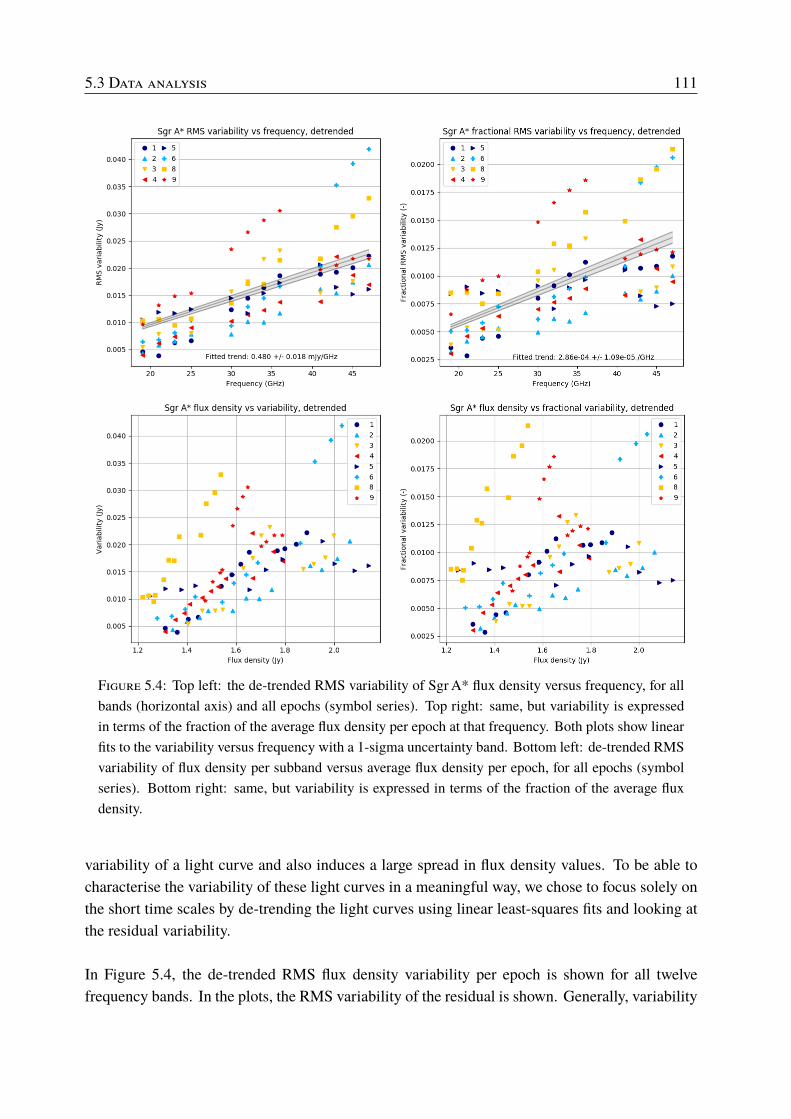
5.3 Data analysis 111
Figure 5.4: Top left: the de-trended RMS variability of SgrA* flux density versus frequency, for allbands (horizontal axis) and all epochs (symbol series). Top right: same, but variability is expressedin terms of the fraction of the average flux density per epoch at that frequency. Both plots show linearfits to the variability versus frequency with a 1-sigma uncertainty band. Bottom left: de-trended RMSvariability of flux density per subband versus average flux density per epoch, for all epochs (symbolseries). Bottom right: same, but variability is expressed in terms of the fraction of the average fluxdensity.
variability of a light curve and also induces a large spread in flux density values. To be able tocharacterise the variability of these light curves in a meaningful way, we chose to focus solely onthe short time scales by de-trending the light curves using linear least-squares fits and looking atthe residual variability.
In Figure 5.4, the de-trended RMS flux density variability per epoch is shown for all twelvefrequency bands. In the plots, the RMS variability of the residual is shown. Generally, variability

112 Chapter 5 : Time lags of Sgr A*
Figure 5.5: Examples of calibrated light curves for J1744-3116 (calibrator) and J1745-283 (checksource) for epoch 3. All data is plotted with error bars, which are obscured by the data markers inmost cases. The full set of light curves for the calibrator and the check source for all epochs can befound in Appendix A.
is larger for higher frequencies and appears to scale roughly linearly with flux density but withconsiderable variance. We find a modulation index (RMS variability as fraction of flux density)on the order of 1%, but with a growing trend towards higher flux densities. Bower et al. (2015b)reported a larger modulation index of 8% for this frequency range, but that figure includedlonger-term variability. The fact that we do not see a clear linear relation between flux densityand trend-subtracted RMS variability for any subband frequency, as would be expected from theRMS-flux relation (Uttley & McHardy, 2001; Abuter et al., 2020), may be due to the fact that weare not sensitive to this longer-term contribution to variability.
5.3.2 Detection of time lagsIn our previous time lag paper (Brinkerink et al., 2015), the time lag calculations were done byfitting Fast-Rise Exponential Decay (FRED) curves to the measured light curves in the differentfrequency bands. This was done because of the clear and consistent presence of a flux densitymaximum across multiple light curves, of which the shape lent itself well to FRED fitting. Forthe data sets presented in this paper, the flux density evolution shows different characteristics foreach epoch and so a more general way to look for lag relations between bands is needed.
To this end, multiple cross-correlation methods were considered that can deal with a non-constanttime sampling cadence for the data series. The Z-transformed Discrete Correlation Function(ZDCF) by Tal Alexander (Alexander, 1997) is such an implementation, as is the Local Cross-Correlation Function (LCCF) as described byWelsh (1999). We found that both of these methodsyield highly similar auto- and cross-correlation functions for our data sets. Out of these twomethods the LCCF was chosen for the main analysis in this paper, because of its simple andportable implementation.
For the cross-correlation parameters we chose a minimum number of 11 measurements per time

5.3 Data analysis 113
lag bin (which is the same as the recommended minimum number for the ZDCF, and advisedfrom a statistics point of view), and a minimum time lag bin width of 30 seconds (the length ofa single scan). Using these parameter values, the cross-correlation functions for all twelve lightcurves in each data set were calculated against themselves as well as each of the other eleven lightcurves in the same data set. Each cross-correlation between two different light curves from thesame data set is thus represented twice in the correlation results.
Examples of the intermediate results from this cross-correlation step are shown in Figure 5.6. Inthe cross-correlation maps shown there, the time lag relation found in Brinkerink et al. (2015)is overplotted as a black line with marker dots. Note that it is not a fit to the maxima of theplotted cross-correlation data, but it is included to provide a comparison. Each of the figuresuses a reference light curve at one of the 12 subband frequencies, and is thus one of the twelvecross-correlation plots that was generated for that particular data set. The plots in Figure 5.6were selected to show a representative range of behaviours encountered in the cross-correlationproducts: for data set 3 there is no obvious feature that correlates across all frequencies and totalvariability is limited. For data set 8 there is a strong climbing trend in flux density present in thelight curves, with a maximum being reached for the higher frequencies but not as clearly for thelower ones. For data set 9, there is a clear and consistent minimum visible in the light curves atall frequencies. We see that localised features in the light curves that correlate across all bandstend to occur over timescales corresponding to one hour or more, matching the flaring timescalereported by Yusef-Zadeh et al. (2006). In the leftmost plot, we see a case where the light curves areonly weakly correlated across the three main frequency bands (data set 3). The light curves in thesame band as the reference light curve show a relatively strong correlation peak, but this pattern isabruptly broken for the correlation functions in the other two bands. The light curves for this epochdo not show clear trends or strong variability, and calibration uncertainties can therefore causecorrelated flux density excursions that are limited to a single band as they are part of the same setof scans. In the middle plot, we see an example of a relatively broad cross-correlation function,where the location of its maximum along the lag axis is not tightly constrained (data set 8). Theobserved cross-correlation pattern may be compatible with the overplotted lag relation (which istaken from our previously found result in Brinkerink et al. (2015)), but it is also consistent withzero time lag – depending on the reference light curve used for cross-correlation, both of thesetrends can appear. The rightmost plot shows a case in which there is a robust and monotonic lagtrend visible across all bands (data set 9), which appears to lie close to the lag relation we foundin our previous paper. The associated light curves show a clearly defined minimum in their fluxdensity evolutions, which improves the clarity of the cross-correlation peaks.
In order to distill potential time lag trends from the maxima in the cross-correlation graphs gen-erated from the data, the choice was made to employ a piecewise 4th-order spline fitting to thecalculated cross-correlation functions (taking their error bars into account) and to perform a localmaximum search on this spline fit. This approach allowed us to avoid bias when identifying the
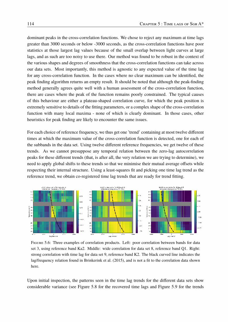
114 Chapter 5 : Time lags of Sgr A*
dominant peaks in the cross-correlation functions. We chose to reject any maximum at time lagsgreater than 3000 seconds or below -3000 seconds, as the cross-correlation functions have poorstatistics at those largest lag values because of the small overlap between light curves at largelags, and as such are too noisy to use there. Our method was found to be robust in the context ofthe various shapes and degrees of smoothness that the cross-correlation functions can take acrossour data sets. Most importantly, this method is agnostic to any expected value of the time lagfor any cross-correlation function. In the cases where no clear maximum can be identified, thepeak finding algorithm returns an empty result. It should be noted that although the peak-findingmethod generally agrees quite well with a human assessment of the cross-correlation function,there are cases where the peak of the function remains poorly constrained. The typical causesof this behaviour are either a plateau-shaped correlation curve, for which the peak position isextremely sensitive to details of the fitting parameters, or a complex shape of the cross-correlationfunction with many local maxima - none of which is clearly dominant. In those cases, otherheuristics for peak finding are likely to encounter the same issues.
For each choice of reference frequency, we thus get one ’trend’ containing at most twelve differenttimes at which the maximum value of the cross-correlation function is detected, one for each ofthe subbands in the data set. Using twelve different reference frequencies, we get twelve of thesetrends. As we cannot presuppose any temporal relation between the zero-lag autocorrelationpeaks for these different trends (that, is after all, the very relation we are trying to determine), weneed to apply global shifts to these trends so that we minimise their mutual average offsets whilerespecting their internal structure. Using a least-squares fit and picking one time lag trend as thereference trend, we obtain co-registered time lag trends that are ready for trend fitting.
Figure 5.6: Three examples of correlation products. Left: poor correlation between bands for dataset 3, using reference band Ka2. Middle: wide correlation for data set 8, reference band Q1. Right:strong correlation with time lag for data set 9, reference band K2. The black curved line indicates thelag/frequency relation found in Brinkerink et al. (2015), and is not a fit to the correlation data shownhere.
Upon initial inspection, the patterns seen in the time lag trends for the different data sets showconsiderable variance (see Figure 5.8 for the recovered time lags and Figure 5.9 for the trends

5.3 Data analysis 115
Figure 5.7: Fitted splines and detected cross-correlation peaks, for the same data sets and referencebands as shown in Figure 5.6 where cross-correlation functions for progressively higher frequencybands are vertically offset by steps of 1. Vertical black lines indicate the expected time lags based onthe previously found lag relation from Brinkerink et al. (2015), while black dots indicate the detectedmaxima of the cross-correlation spline fits. Note that when the cross-correlation function has a broadplateau, the detected peak is poorly constrained (middle plot).
fitted to these measurements). We see weakly correlated lag trends showing large outlier valuesfor three data sets (data sets 1, 2, and 3), one data set that has no clear trend pattern, becauseof poor cross-correlations (data set 6), a data set that shows consistent time lag trends in somesubbands but not in others (data set 8) and data sets with trends having a positive slope thatindicate the presence of time lags (data sets 4, 5 and 9).
We note that the data sets with cross-correlation functions that have more clearly defined peaksalso show a better consistency among their individual time lag trends for the different referencesubbands than the other data sets do. Furthermore no examples of a consistently present timelag trend with a negative slope, where low-frequency variability would lead high-frequencyvariability, is seen in any of the data sets.
5.3.3 Checks with synthetic data
While we do see clear time lags in several of our data sets, the question that immediately arises iswhy we do not always see them. The answer to this question comes down to three possibilities: 1)the time lags are always present due to the fundamental behaviour of the source, but the statisticsof variability does not always let us detect them, 2) the time lags are intrinsic but do not account forall source variability (so that they only sometimes dominate the observed variability), or 3) theyare pure chance occurrences that have no physical mechanism or pattern behind them. Despiteus now having multiple data sets available, there is still room for different interpretations of theseresults.
To address this question and investigate the likelihood of these scenarios, we must try to assessthe probability with which time lags are detected if they are indeed a fundamental property of thesource, as well as the biases we are subject to. Conversely, we also need to assess how likely it

116 Chapter 5 : Time lags of Sgr A*
Figure 5.8: The co-registered maxima of the cross-correlation functions, collectively forming theobserved time lag trends in the data sets. The trends have been shifted to minimise mutual spread.
is that we appear to see time lags in a data set where no such intrinsic relation between the lightcurves is present.

5.3 Data analysis 117
Figure 5.9: Linear time lag versus wavelength trends, fitted to the data shown in Figure 5.8.
To this end, we made use of the formalism of Gaussian processes as described in Roberts et al.(2013) to model the statistical properties of the variability of SgrA* on the time scales we haveaccess to with these light curves. Specifically, we construct a multidimensional Gaussian dis-tribution with the appropriate covariances from which realisations of synthetic light curves are

118 Chapter 5 : Time lags of Sgr A*
drawn. To illustrate the fundamental thought behind this formalism, consider for example thetask of constructing 10 samples from a light curve, not necessarily equally spaced in time. Weknow beforehand that these sampled flux density values should be correlated with one another to acertain degree. For one thing they should all have positive values, but more specifically we expectthat flux density samples spaced closely together in time should be correlated more strongly thansamples with a larger temporal separation between them. This degree of correlation is capturedin the auto-correlation function of our measured light curves: using this relation we see how thedegree of correlation between samples depends on their separation in time. We fit a functionalform to this auto-correlation function and use it as a covariance kernel function. Using this kernelfunction, we then construct a covariance matrix that is valid for a given set of sampling times.
To make matters simpler, we consider our simulated light curve as a ’standard’ function byshifting and scaling it to have zero mean, a variance of unity, and be fully characterised by itsauto-correlation function. In this case, the autocorrelation and the covariance are identical. Oursampled values thus become a draw from a 10-dimensional joint Gaussian distribution, the shapeof which is defined by the values in our covariance matrix. Every realisation of our example lightcurve is a single point in this 10-dimensional space. Many separate realisations of the light curveare calculated, and we then study the impact that our sampling cadence and limited epoch lengthhave on the light curve time lag properties we derive.
In our case, we start by modeling the flux density of SgrA* in a single subband as a function oftime. Asmentioned above, we assume the variability to be stochastic in nature, with a well-definedmean value and an auto-correlation function that does not change with time. With knowledge ofthis auto-correlation function we generate synthetic light curves that have, on average, the sameauto-correlation function as our original data does. Taking a specific realisation we then clone thislight curve for our 12 subbands, scale the copies appropriately in flux density and shift them intime according to the time lag relation we wish to investigate. These light curves are then sampledwith the same cadence as our observed data sets, with thermal noise and estimated calibrationerrors added for each virtual measurement. The resulting synthetic data is treated in exactly thesame way as our observed data: we correlate these light curves against one another and checkif we see the time lag relations that we initially put in. The process by which we search for theappropriate auto-correlation function to use in generating the synthetic light curves is describedin full in Appendix D.
With this replication of the behaviour of the measured light curves, we now investigate thedetectability of time lag trends using different intrinsic lag trends in our synthetic data. Toset up the synthetic sampled light curves for all 12 subbands, we first generate a ’master’ lightcurve using the appropriate auto-correlation function. For each of the 12 subbands we add anadditional time shift to this master light curve, according to a time lag relation we define. Wethen scale the synthetic light curve flux density values according to the average flux density for

5.3 Data analysis 119
the appropriate frequency band (see Figure 5.2). The resulting shifted, scaled light curve is thensampled following the scan setup for one epoch of the measured data sets, including the scantiming offsets that pertain to the subband in question (as is visible in Figure 5.3).
Figure 5.10: Top: the cumulative distributions of time lag slopes for synthetic light curves, fordifferent input lag relations (blue: -42 min/cm, red: 0 min/cm, green: 42 min/cm), and differentcontributions of noise (indicated by shading). We see that lag slope distributions creep closer tozero for higher noise contributions, but that the largest recovered values stay close to the input slopes.Bottom: the cumulative distributions for only the 42 min/cm synthetic lag relation, plotted for differentnoise contributions and compared to the measured cumulative distribution.
In our analysis of the synthetic light curves we test three different time lag relations. The firstone is the ’nominal’ time lag relation which we found in Brinkerink et al. (2015), 3C/3_ = 42

120 Chapter 5 : Time lags of Sgr A*
min/cm, where the variability at lower frequencies lags behind the higher frequencies. Thesecond relation is the inverse of this, 3C/3_ = −42 min/cm, as we wish to check if there is a biasintroduced by the scan timing offsets between K, Ka and Q bands. The third relation uses zerotime lag, where no shifts in time are applied to any of the light curves and the intrinsic variabilityis contemporaneous across all frequencies. For each time lag relation, we assess the influence ofmeasurement errors. We compare the distribution of lag slopes we find when no noise is presentto cases where the random uncorrelated variations in flux density (i.e. flux density variations thatare realised independently per light curve) correspond to our estimated value of ∼ 10mJy on ascan-to-scan timescale, as well as to cases where this random variability component is larger bya factor of 3, 5 or 7. For the cases where we include noise, we also include a realistic calibrationerror due to the combined influence of unmodeled minor variations in the flux density of our gaincalibrator and atmospheric effects. These errors are strongly correlated across each frequencyband, meaning that all four subbands within one frequency band show coherent flux density offsetsdue to this calibration uncertainty. We estimate the magnitude of this calibration error to be ∼30mJy, from the cross-band trend breaks in our measured data (see Figures 5.3 and 5.5, as well as thecheck source light curves in Appendix A). For each combination of parameters (time lag relation,thermal noise strength) we generate 100 realisations from which we reconstruct the observed timelag slopes in the same way as was done for our measured data, and so we get a distribution oflag slopes for each choice of parameter combination. A sample of generated sets of light curves,as well as their cross-correlations and the recovered lag trends, are shown in Appendix B. Anoverview showing the distributions of the recovered time lag slopes for all considered cases isshown in Figure 5.10.
5.4 ResultsIn our observed data sets, we reconstruct strong time lag trends in two epochs with high internalconsistency (39.6± 1.5 min/cm and 38.2± 1.4 min/cm respectively for data sets 5 and 9), anothersignificant but less consistent time lag in one epoch (43.1 ± 4.0 min/cm, for data set 8), oneweaker time lag in another epoch (18.9 ± 1.1 min/cm, for data set 4) and no clear or internallyconsistent results for the other epochs. Although the linear time lag fits for these other data setsshow relatively high confidence in the trend uncertainties (small errors in the fitted trend slopes),we consider these reconstructions less reliable as the individual lag relations show very low in-ternal consistency across all 12 subbands with a large residual scatter after their co-registration.Slope errors obtained from bootstrapping carry the implicit assumption that the data follow thepresupposed linear relation, which is not clearly present in certain cases and manifests itself as adiscrepancy between the bootstrapping errors and the spread between recovered lag trends.
We wish to understand how likely it is that a measurable time lag is detected in any given epochfor a source where a persistent time lag relation is present between the light curves at differentfrequencies. To this end, we generated synthetic data with the same general variability properties

5.5 Discussion and Conclusions 121
as those that we observed in the measured light curves. As we see from Figure 5.10, the magnitudeof the time lag trends from synthetic data tend to be underpredicted by the reconstructions, evenin the case where zero-error measurements are modeled. The true lag slopes used as input for thesynthetic light curves are plotted using vertical coloured bars in the left panel, and it is apparentthat for the non-zero time lag relations the distribution of the corresponding recovered lag slopeis such that the input lag slope value is close to an extremum of the distribution.For both the tested positive and negative time lag trends, we see an asymmetric distribution inthe recovered trends with longer tails towards zero time lag (and in a few cases even showingrecovered lags with a sign opposite from the input lag relation). For the zero-lag case, wesee a symmetrical spread in the recovered trends without any discernible bias to positive ornegative slopes. Overprediction of the lag trend slope in the reconstructions, on the other hand,is much more rare and never extends far away from the input lag slope values. The asymmetry inreconstructed lag slope distributions is more severe when calibration errors are included, causinga larger bias towards smaller measured lag trend slopes. Thus, we see that a time lag relationthat is consistently present in the data will tend to be underestimated from measurements usingthe cadence of our observations, and that among many measurements of the time lag relation thelarger reconstructed slopes are a better estimate of the true time lag relation that is present. Theset of synthetic light curves that best reproduces the distribution of time lag slopes we find in ourobservations incorporate a stronger uncorrelated noise component than our initial estimate (seethe right panel of Figure 5.10) - an uncorrelated random flux density component with a standarddeviation of ∼30 mJy per scan (plotted as ’3xthermal’) gives the best match to the observed lagdistribution. Whether this is due to an underestimation of measurement error or to an unmodeledrandom component of source variability is an open issue.
5.5 Discussion and ConclusionsIn this paper, we have presented the most comprehensive and systematic study of time lags inSagittariusA* radio observations performed to date. We find positive time lags (between 20 and40 min/cm) over a frequency range from 47 down to 19 GHz, where low-frequency variabilitylags behind high-frequency variability, for five out of eight epochs in our data. Three out of eightepochs show time lags close to zero. The larger time lags are found for epochs where the lightcurves show more pronounced local maxima or minima.
In our synthetic data analysis, we find that the reconstructed time lag slopes are typically un-derestimated with the measurement cadence and length that we have used for our observations,particularly when variability is low and no recognisable flaring occurs. The distribution of recov-ered synthetic time lag slopes closely matches the observed distribution when a lag relation of 42min/cm is assumed, together with a 30mJy uncorrelated variability component.
The lag relation found in our previous paper (Brinkerink et al., 2015) was calculated from a set

122 Chapter 5 : Time lags of Sgr A*
of light curves that showed a clear temporal maximum for all of them, and we see comparablelag slopes for the light curves that have a clear flux density extremum here – both for the mea-sured light curves and for the synthetically generated light curves. We are therefore confidentthat we have observed a persistent and consistent time lag in these results. The consistency ofthe time lag slope over multiple years of measurement (covering the time range from 2005 to2015) indicates that we are sampling some kind of characteristic velocity, scale or expansion speed.
Figure 5.11: The aggregate time lag trend fittedto themeasured time lags from data sets 5, 8 and9 after co-registration.
Combining the time lag values found in the three epochs with the largest time lag slopes, whichlie close together in value, gives us a fitted slope of 40.3± 2.0 min/cm, which is plotted in Figure5.11.When we consider the constraints on the inclination angle of a putative compact jet from SgrA*that follow from recently published results, we see that small values are favoured: Issaoun et al.(2019) report good fits for jet models with 8 ≤ 20◦, while Gravity Collaboration et al. (2020b)indicate that BH spin axis inclinations larger than 140◦ fit well for circular hotspot motion, withthe value increasing to 175◦ for helical hotspot motion. Both of these scenarios correspond to asmall angle between our line of sight and the jet direction pointing closest to us. Combining thisinformation with the size-frequency relation for SgrA* (Bower et al., 2006; Falcke et al., 2009)and our data, like we did in Brinkerink et al. (2015), results in an estimate for the associatedoutflow speed (see Figure 5.12). We find that the plasma flows out at moderately relativisticspeeds with WV ≈ 1.5, which is well within the range predicted by both analytic jet models (Falcke& Biermann, 1996) and jets in GRMHD simulations (Mościbrodzka & Falcke, 2013). Here, theassumption is made that the variability we see at the various wavelengths is associated with theangular scales given by the size-frequency relation, and not limited to any smaller sub-region ofthe source. There is some uncertainty associated with this, as the size of the flaring componenthas not been directly measured. However, given that stronger flares can reach a significant fractionof the total flux density, it seems unlikely that they are emitted at scales widely separated from

5.5 Discussion and Conclusions 123
Figure 5.12: Constant-velocity lead times w.r.t. the 19 GHz peak (calculated). Coloured curvesshow the expected time lag relations for an inclination of 20◦ when a size-frequency relation of\ [mas] = 0.52 · _[cm]1.3 is assumed. Data from this work and from Brinkerink et al. (2015) isoverplotted.
the average structure probed by VLBI. The size-frequency relation of SgrA* is well-constrainedif a particular functional form is assumed, but shows a larger uncertainty once different forms ofthe relation are considered (Brinkerink et al., 2019).
From our investigation using synthetic data with a known intrinsic time lag trend, we see thatthere is a clear bias towards smaller reconstructed time lag slopes when the employed measure-ment strategy and data calibration quality are considered. For future observations, an observingstrategy where light curves are sampled over longer time scales (i.e., over 5 or 6 hours) may aidin a more precise measurement and characterisation of these time lags, for two reasons: the largernumber of data points will reduce the impact of spurious flux density variations from calibrationuncertainties on the measured cross-correlation functions, and the likelihood of catching and fullytracing flux density excursions also increases with longer epochs.
The persistent time lag relation we observe between different radio observing frequencies providesanother benchmark by which to test theoretical emission models for SgrA*, next to the otherproperties of the source that have been taken into account in model fitting so far (spectral shape,variability strength, angular size and polarisation properties).

124 Chapter 5 : Time lags of Sgr A*
AcknowledgementsThis work was supported by the ERC Synergy Grant 610058: "BlackHoleCam: Imaging theEvent Horizon of a Black Hole". The author wishes to thank Federica Palla for her initial analysisof the data, which motivated this work.

5.5 Discussion and Conclusions 125
Appendix A: Calibrator and check source light curves
Figure 5.13: Calibrated light curves for J1744-3116 (calibrator), data sets 1-6, 8, and 9. All data isplotted with error bars, which are obscured by the data markers.
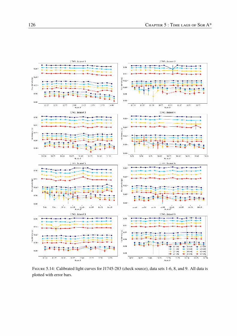
126 Chapter 5 : Time lags of Sgr A*
Figure 5.14: Calibrated light curves for J1745-283 (check source), data sets 1-6, 8, and 9. All data isplotted with error bars.

5.5 Discussion and Conclusions 127
Appendix B: synthetic light curve and correlation results
Figure 5.15: Samples of results from synthetic light curves with the inverse time lag relation andno calibration errors. The left column shows data where the inverse time lag trend was successfullyrecovered from the cross-correlations, the right column shows an example of a case where a time lagrelation with a significant error is produced.

128 Chapter 5 : Time lags of Sgr A*
Figure 5.16: Samples of results from synthetic light curves with the inverse time lag relation andwith calibration errors included. The left column shows data where the inverse time lag trend wassuccessfully recovered from the cross-correlations, the right column shows an example of a case wherea time lag relation with a significant error is produced.

5.5 Discussion and Conclusions 129
Figure 5.17: Samples of results from synthetic light curves with the zero time lag relation and nocalibration errors. The left column shows data where the zero time lag trendwas successfully recoveredfrom the cross-correlations, the right column shows an example of a case where a time lag relationwith a significant error is produced.

130 Chapter 5 : Time lags of Sgr A*
Figure 5.18: Samples of results from synthetic light curves with the zero time lag relation and withcalibration errors included. The left column shows data where the zero time lag trend was successfullyrecovered from the cross-correlations, the right column shows an example of a case where a time lagrelation with a significant error is produced.

5.5 Discussion and Conclusions 131
Figure 5.19: Samples of results from synthetic light curves with the nominal time lag relation andno calibration errors. The left column shows data where the nominal time lag trend was successfullyrecovered from the cross-correlations, the right column shows an example of a case where a time lagrelation with a significant error is produced.

132 Chapter 5 : Time lags of Sgr A*
Figure 5.20: Samples of results from synthetic light curves with the nominal time lag relation andwith calibration errors included. The left column shows data where the nominal time lag trend wassuccessfully recovered from the cross-correlations, the right column shows an example of a case wherea time lag relation with a significant error is produced.

5.5 Discussion and Conclusions 133
Appendix C: historical spectral measurements for SgrA*
Figure 5.21: The full set of historical data used for the binned plot in Figure 5.2. Measurements arefrom Zylka et al. (1995); Serabyn et al. (1997); Falcke et al. (1998); Zhao et al. (2003); Herrnsteinet al. (2004); An et al. (2005); Marrone et al. (2006); Bower et al. (2015b); Brinkerink et al. (2015);Liu et al. (2016); Bower et al. (2019). Theoretical model spectra are from Falcke et al. (2000) andYuan et al. (2003).

134 Chapter 5 : Time lags of Sgr A*
Appendix D: Finding the appropriate auto-correlation functionfor synthetic light curve data
The synthetic data pipeline starts by defining the form of the auto-correlation function that appearsto hold for our measured light curve data. As a starting point, we look at the auto-correlationfunction we measure for our original light curve data, when we consider the aggregate of lightcurves from all data sets and all frequency bands. This measured auto-correlation function isdepicted in Figure 5.22 using non-connected markers. To check for frequency dependence of theauto-correlation function, we compared the auto-correlation functions for the aggregate light curvedata split into separate frequency bands against each other, and their shapes show no detectablefrequency dependence outside the expected statistical variance.
Figure 5.22: The measured average autocorrelation function from all frequency bands in all data setscombined (separated markers), the functional form fitted to this autocorrelation function (continuousline), and the recovered autocorrelation function from a limited-length synthetic light curve generatedusing that functional form (connected markers). It is evident that the recovered auto-correlation differsfrom the prescribed form.
We approximate the shape of this auto-correlation function by using a linear combination of aGaussian (squared exponential) function and a rational quadratic function, both functions thatoften feature in the description of auto-correlation functions, ensuring that data points separatedby progressively larger time lags tend to an uncorrelated state. This function is plotted in Figure

5.5 Discussion and Conclusions 135
5.22 with a continuous line. We find that its functional form is closely approximated by:
Cov(G) = 0.4 · 4−(G/1500)2 + 0.6 ·(1 +
( G
1600
)2)−2
, (5.1)
where G is the lag time in seconds. The three free parameters that were varied to find the bestfit are the strengths of the two components (with the constraint of summing to 1, which is thezero-lag auto-correlation) and the scalings of G in both terms. Using this auto-correlation functionas the covariance function for our (normalised) Gaussian process, we generate densely sampledsynthetic time series as large as are allowed by our computational resources (see Figure 5.23for one realisation of such a light curve). These generated light curves are then shifted in timeand re-scaled in amplitude to fit with the properties of the flux density for SgrA* at variousfrequencies. We proceed to sample our synthetic data by applying the sampling cadence from thereal-world measurements to a limited segment of this ’master’ light curve.
Figure 5.23: An example of a synthetic, longer-term, densely sampled master light curve generatedusing the initial choice for covariance function (Figure 5.22). Note that the function values can benegative, as the light curve has not been shifted and scaled to the correct average and variance at thispoint.
We now check to see if we do indeed get auto-correlation functions from these sampled syntheticlight curves that look like the auto-correlation function we expect. We plot the averaged recoveredauto-correlation function from many realisations of the synthetic light curve, using the samesampling cadence as our originally measured data (Figure 5.22, connected markers) togetherwith both the originally measured and the functionally prescribed auto-correlations, and we see

136 Chapter 5 : Time lags of Sgr A*
that the recovered auto-correlation function is significantly narrower and even dips into negativevalues (indicating anti-correlation) for a range of time separations. This happens because wemeasure the auto-correlation of the sampled light curve using the average flux density of thelimited time series instead of the ’ideal’, long-term flux density average. We therefore tend tosee more pairs of points with values of opposite signs (above vs. below the average value) whencalculating our auto-correlation function, causing it to have a more rapid falloff with increasingtime difference than we would see for longer light curves where the average is closer to the ’true’average. Effectively, we miss a low-frequency component of the auto-correlation function as weonly have access to the short timescales when measuring it.The functional form of the original auto-correlation function to use when generating the syntheticlight curve data therefore needs to be chosen in such a way that the recovered shape of this functionis the same as for our real measured light curves. To this end, the behaviour of several typesof auto-correlation functions was investigated, with the function yielding the best results havingthe form of a truncated hyperbolic function. Note that this was a heuristic process where weinvestigated various functional forms in order to closely approach the measured auto-correlationcurve with our reconstructed one. The result of this iterative process is shown in Figures 5.24 and5.25. The functional form of our final auto-correlation function is given by:
Cov(G) = max
(1110−
√( G
8000
)2+ 1
100, 0
), (5.2)
where G is again the lag time in seconds, and where the function value has a lower bound of zeroimposed on it so that we avoid negative values for the auto-correlation function at large time lags.With this auto-correlation function, we generate synthetic data that has the appropriate temporalvariability characteristics to mimic the behaviour of our measured light curves.

5.5 Discussion and Conclusions 137
Figure 5.24: As Figure 5.22, but with an auto-correlation function chosen to optimise the match be-tween the measured data and the synthetic data. Although the functional form of the auto-correlationfunction differs significantly from the measured one, the recovered function closely follows the mea-sured function.
Figure 5.25: As Figure 5.23, but generated with the updated auto-correlation function from Figure5.24.

138 Chapter 5 : Time lags of Sgr A*

Chapter6Summary
Black holes and their accretion flows present us with an opportunity to study physics in extremeenvironments with strong spacetime curvature. Accreting black hole systems exist over a widerange of masses and accretion rates, which can exhibit different behaviours but which funda-mentally reflect the same type of process: the conversion of the gravitational potential energyof orbiting plasma into electromagnetic radiation and the kinetic energy of outflows. Accretingsupermassive black holes are a particularly rich source of observational data: they can be studiedover a wide range of wavelengths ranging from radio to gamma rays, and several supermassiveblack holes have a sufficiently large angular diameter on our sky to be resolved by our mostpowerful telescope systems. SagittariusA*, the source associated with the supermassive blackhole at the center of our Galaxy, is one of these rich laboratories offering us the chance to get aclose-up look into a so-called low-luminosity active galactic nucleus.
However, the detail in which we can study SgrA* also means that our models need to be suffi-ciently sophisticated to describe these details. As SgrA* appears to be a black hole accreting at alow Eddington ratio, features such as a plasma jet are expected to manifest on scales close to theevent horizon as they do for similar systems – but verifying the presence of a jet by measuring thesource morphology is made challenging by the limits that interstellar scattering imposes on theattainable resolution of our observations. We therefore need to make use of high-frequency VLBIto discern the intrinsic size and shape of SgrA*, and study its flux density variability across radiofrequencies to gather clues about the nature of the plasma flow.
To this end, I have investigated SgrA* by observing it using several different radio telescope net-works and instruments: the Karl G. Jansky Very Large Array (VLA), the High Sensitivity Array(HSA, part of which is formed by the Very Long Baseline Array or VLBA) and the AtacamaLarge Millimeter Array (ALMA).
We use HSA+LMT 86GHz observations made in spring 2015 to investigate the asymmetry inthe compact stucture of SgrA* in Chapter 2 of this thesis. The array includes two stations withextra sensitivity: the Green Bank Telescope (GBT) and the Large Millimeter Telescope (LMT).

140 Chapter 6 : Summary
The combination of this high sensitivity with the extended (D, E)-coverage gives this observationan enhanced North-South resolving power over previous observations. Through an analysis ofclosure phases, we find that there is evidence for source asymmetry. Using a simple model fit, wefind that a faint Eastern component approximately 100 `as from the main component providesthe best match with our observed closure phases. While it cannot be established from this singleepoch whether the observed asymmetry is intrinsic or caused by interstellar scattering, the detec-tion of East-West asymmetry at 230GHz and 43GHz in other observations of SgrA* providesthe tantalizing suggestion that we may be seeing intrinsic structure.
Chapter 3 presents further results from the spring 2015 HSA+LMT observations, where this timethe focus is placed on an imaging analysis and on size measurement using a closure amplitudeanalysis. The imaging shows again a slight East-West asymmetry in SgrA*, confirming the simpletwo-component model fitting result from Chapter 3. From the closure amplitude analysis we findan observed source geometry that is close to Gaussian, with a size of 215.1 ± 0.4 × 145.1 ± 1.5`as at a position angle of 77.9± 0.4 degrees East of North. Deconvolving this with the scatteringlaw from (Bower et al., 2006), we find an intrinsic size of 145.4±0.6×122.6±1.7 `as. Collatingour new measured size with earlier measurements performed over a range of wavelengths allowsus to revisit the intrinsic size-frequency relation.
In Chapter 4, we present an analysis of the variability we see in simultaneous observations ofSgrA* performed in spring 2012 using ALMA and the VLA. During a single epoch, we see a mi-nor flare which manifests itself at different time delays across different frequencies, from 100GHzdown to 19’,GHz. We recover the relation of this time delay as a function of wavelength usingfast rise exponential decay (FRED) curve fitting and see that the variability at longer observingwavelengths exhibits progressively longer time delays according to the relation 3g/3_ = 42 ± 14min/cm. This is in line with earlier observations that showed time lags between 43GHz and22GHz of a similar slope. SgrA* also shows a size that depends on observing frequency: atlonger wavelengths (above 3.5mm) its apparent size is dominated by interstellar scattering effects,and its angular size scales with wavelength squared. With source sizemeasurement done at shorterwavelengths, the intrinsic size of SgrA* can be modeled as a function of wavelength. Using thissize-frequency relation and coupling it to the observed time lags, we find that a self-consistentjetmodelwithmoderately relativistic outflow speeds bestmatches the observed time lag behaviour.
We revisit the study of time lags in Chapter 5, where we present multi-epoch observations ofSgrA*withVLAover frequencies ranging from 18 to 47GHz. We find time lags corresponding toour earlier result fromChapter 4 in three of the epochs, smaller but positive time lags in three moreepochs and negative time lags close to zero in the remaining two. The distribution of measuredtime lag slopes is compared to results from synthetic light curves, where a pre-determined time lagrelation is used as input and simulated measurements are taken according to the sampling cadenceof our real measurements. We find that the distribution of time lag slopes from our measured data

141
is consistent with a persistently present intrinsic time lag relation. Combining the time lag slopesthat lie closest to the expected intrinsic time lag yields an aggregate time lag trend of 40.3 ± 2.0min/cm. Combining this result with recent constraints on the orientation of the spin axis of SgrA*and the size-frequency relation, we again find that moderately relativistic outflow speeds withWV ≈ 1.5 best fit the measured time lags. With the persistence of time lags in radio observationsof SgrA* receiving strong support from these results, we state that theoretical models for theaccretion flow will need to reproduce these time lags in their predicted properties along with thepre-existing suite of constraints on flux density, spectral shape and source morphology.


Hoofdstuk7Samenvatting
Zwarte gaten en hun accretiestromen bieden ons een uitgelezen kans om de natuurkunde vanprocessen in gebieden met een sterke ruimte-tijdkromming te bestuderen. Accreterende zwartegaten komen voor verspreid over een breed bereik aan centrale massa’s en massastromen. Dezesystemen vertonen uiterlijk verschillend gedrag, maar vertegenwoordigen allemaal fundamenteelhetzelfde soort proces: de conversie van de gravitationele potentiële energie van baanbeschrijvendplasma naar elektromagnetische straling en de kinetische energie van de uitstromende fractie vandeze materie. Een bijzonder rijke bron van waarnemingen wordt gevormd door relatief nabijesupermassieve accreterende zwarte gaten: deze zenden doorgaans elektromagnetische stralinguit over een zeer breed gedeelte van het spectrum, van radio tot gammastraling, en enkele vanhen hebben een hoekgrootte aan onze hemel die ons in staat stelt om ze op te lossen met onzemeest geavanceerde (interferometrische) telescoopsystemen. SagittariusA* (afgekort: SgrA*),de radiobron die geassocieerd is met het centrale supermassieve zwarte gat in het centrum vanonze Melkweg, is zo’n systeem dat ons de kans biedt om van relatief dichtbij de kern van eenactief sterrenstelsel met lage helderheid (Low-Luminosity Active Galactic Nucleus, LLAGN) indetail te bestuderen.
De vele nauwkeurige metingen die we aan SgrA* kunnen doen houden echter ook in dat onzemodellen strenger getoetst worden en daarom meer gedetailleerde voorspellingen moeten kunnengeven. Aangezien SgrA* een zwart gat lijkt te zijn dat slechts op een laag tempo gas accreteertin verhouding tot de Eddington-helderheid, verwachten we kenmerken te zien die voor anderesystemen in dezelfde klasse typisch zichtbaar zijn: bijvoorbeeld een snelle straalstroom van uit-geworpen plasma die van vlak buiten de waarnemingshorizon gelanceerd wordt. Het waarnemenvan een dergelijke straalstroomwordt echter bemoeilijkt doordat het scheidend vermogen van onzewaarnemingen op de relevante frequenties beperkt wordt door de verstrooiing van de uitgezondenstraling via interstellair gas. Om de aard van de plasmaprocessen rond SgrA* goed te kunnengebrijpen moeten we ons daarom richten op interferometrische waarnemingen op kortere golf-lengtes, waar dit verstrooiiend effect kleiner is, en op de informatie die we kunnen bemachtigendoor de variabiliteit van SgrA* over verschillende radiofrequenties te bestuderen.

144 Hoofdstuk 7 : Samenvatting
Met dit doel heb ik SgrA* bestudeerd door het systeem te observeren met verschillende radio-telescopen en netwerken van telescopen: de Karl G. Jansky Very Large Array (VLA), de HighSensitivity Array (HSA, met als onderdeel hiervan de Very Long Baseline Array oftewel VLBA),en de Atacama Large Millimeter Array (ALMA).
In Hoofdstuk 2 van dit proefschrift presenteren we waarnemingen op 86GHz gedaan met deHSA+LMT in de lente van 2015, waarmee we de asymmetrie in de compacte structuur vanSgrA* onderzoeken. Het gebruikte netwerk van telescopen heeft twee extra gevoelige stations:de Green Bank Telescope (GBT) en de Large Millimeter Telescope (LMT). De combinatie vande extra (D, E)-dekking die deze stations toevoegen met hun hoge gevoeligheid betekent dat dezewaarnemingen een verbeterd oplossingsvermogen hebben in de Noord-Zuid richting ten opzichtevan eerdere waarnemingen. Middels een analyse waarbij we de fasesom over driehoekscombi-naties van stations gebruiken (zogeheten closure phases) zien we aanwijzingen voor een spatiëleasymmetrie in de helderheidsverdeling van de bron. Via het fitten van een eenvoudig modelvoor deze helderheidsverdeling concluderen we dat een zwakke extra component op ongeveer100 microboogseconden van de centrale component de best passende fasesommen geeft met onzewaarnemingen. Hoewel we hieruit nog niet kunnen concluderen wat de oorzaak is van deze waar-genomen asymmetrie (deze is ofwel intrinsiek aan de bron, ofwel het gevolg van de interstellaireverstrooiing) suggereert de asymmetrie op 230GHz en 43GHz die gevonden is middels anderewaarnemingen dat hier sprake kan zijn van de intrinsieke structuur van de bron.
Een verdere analyse van deHSA+LMTwaarnemingen van 2015wordt gepresenteerd inHoofdstuk3. Deze keer ligt de nadruk op het in kaart brengen van de structuur middels beeldvormingsalgo-ritmen en het precies meten van de hoekgrootte van de bron via de analyse van closure amplitudes.De resultaten van de beeldvormingsalgoritmen bevestigen onze conclusies op basis van de fase-sommen uit Hoofdstuk 3. De closure amplitude analyse laat zien dat de waargenomen structuurvan SgrA* verder nagenoeg Gaussisch is, met een grootte van 215.1 ± 0.4 × 145.1 ± 1.5 `asen de lange as onder een positiehoek van 77.9 ± 0.4 graden oostelijk van noordelijke richting.Door deze goottemeting te combineren met eerdere resultaten op verschillende andere frequentieskunnen we het verband tussen hoekgrootte van de bron en waarneemfrequentie aan een kritischeblik onderwerpen.
In Hoofdstuk 4 behandelen we een analyse van de variabiliteit van SgrA* over een bereik vanverschillende golflengten, gebruik makende van gelijktijdige waarnemingen die met de VLA enALMA gedaan zijn in de lente van 2012. In de gemeten variabiliteitscurves (die de variatiesin helderheid als functie van de tijd beschrijven) zien we een enkele kortdurende helderheids-verhoging binnen ons waarneemvenster, welke piekt op steeds latere tijden in de steeds lagerefrequentiebanden waarop onze metingen gedaan zijn, van 100GHz tot 19GHz. De relatie tus-sen deze tijdsvertraging en de golflengte waarop de waarnemingen gedaan zijn vatten we doorgebruik te maken van een fast rise, exponential decay(FRED) curve die aan de data gefit wordt.

145
Hiermee vinden we dat de variabiliteit op langere golflengten vertraagd is ten opzichte van die opkortere golflengten via de relatie 3g/3_ = 42 ± 14 min/cm. Deze conclusie strookt met eerdergepubliceerde resultaten, waarin andere waarnemingen een tijdsvertraging tussen 43 en 22GHzlieten zien met een vergelijkbare vertraging. De schijnbare grootte van SgrA* aan de hemelis afhankelijk van de golflengte waarop we de bron waarnemen: op langere golflengten (bovende 3.5mm) wordt de schijnbare grootte in toenemende mate gedomineerd door de effecten vaninterstellaire verstrooiïng. Met metingen van de grootte van SgrA* op kortere golflengten kan deintrinsieke grootte als functie van golflengte af worden geleid, en in combinatie met de metingenvan de tijdsvertragingen kunnen we snelheden berekenen die bereikt worden door uitstromendgas. Op deze manier vinden we dat een eenvoudig intern consistent straalstroommodel met matigrelativistische uitstroomsnelheden goed aansluit op de waargenomen tijdsvertragingen.
Een uitgebreidere analyse van de variabiliteit van SgrA* op radio-golflengten is het onderwerpvan Hoofdstuk 5, waarin data uit een set van acht waarneemsessies van SgrA* met de VLA(uitgevoerd in de loop van de lente van 2015) wordt bestudeerd. Deze waarnemingen bestrijkenfrequenties van 18 tot 47GHz, en in de variabiliteitscurves gemeten over deze verschillendefrequenties vinden we tijdsvertragingen zoals beschreven in Hoofdstuk 4 in drie van de sessies. Indrie verdere sessies vinden we tijdsvertragingen van een gelijksoortig karakter maar met kleinerewaarden, en in de resterende twee sessies vinden we tijdsvertragingen met het omgekeerde tekenmaar met zeer kleine waarden. Deze verdeling van gemeten tijdsvertragingsrelaties vergelijken wemet resultaten van gesimuleerde variabiliteitscurves, waarinwe variabiliteitscurvesmet een voorafbepaalde tijdsvertragingsrelatie genereren en nagaan inwelkemate deze tijdsvertragingen gemetenkunnen worden volgens de tijdsstructuur van onze daadwerkelijk uitgevoerde waarnemingen.Deze vergelijking wijst uit dat de verdeling van tijdsvertragingsrelaties die we in onze metingenzien consistent is met een vaste tijdsvertragingsrelatie in alle waarneemvensters die in onzereconstructies varieert vanwege de statistische eigenschappen van de variabiliteit. Een combinatievan de drie tijdsvertragingsrelaties met de grootste gereconstrueerde waarden, die allen zeer dichtbij de best passende berekende tijdsvertragingsrelatie liggen, geeft een relatie van 40.3 ± 2.0min/cm. Waneer we dit resultaat combineren met recentelijk gevonden limieten op de oriëntatievan de spin-as van SgrA* en met de relatie tussen de hoekgrootte van SgrA* en de observationelegolflengte, vinden we opnieuw dat uitstroomsnelheden met WV ≈ 1.5 het beste stroken met onzeresultaten. Met het versterken van het beeld dat SgrA* een consistente tijdsvertragingsrelatie laatzien middels dit werk stellen wij dat dit een aspect van de plasmastroming is dat correct voorspelddient te worden door theoretische modellen, naast de bestaande vereisten van fluxdichtheid,spectrale verdeling en morfologie van de bron.


AppendixAResearch Data Management
This thesis research has been carried out under the institute research data management policyof the Institute for Mathematics, Astrophysics and Prticle Physics Research at Radboud Uni-versity. The RDM policies for all departments and institutes of the University can be found athttp://www.ru.nl/rdm/vm/policy-documents/.
All observational data sets used in this thesis are available online in the long-term data archivescorresponding to the relevant organisations. The HSA data used in Chapters 2 and 3 can befound in the NRAO Science Data Archive (https://archive.nrao.edu/), under project code BF114.The two epochs indicated with A and B are identifiable from their file names. The VLA dataused in Chapter 4 is also available from the NRAO Science Data Archive, under project code12A-339. The ALMA data from chapter 4 has project code 2011.0.00887.S, and is available fromthe ALMA Science Archive at https://almascience.nrao.edu/aq/. Chapter 5 again uses VLA datathat can be found in the NRAO Science Data Archive, under project code 15A-372.


BibliographyAbbott, B. P., Abbott, R., Abbott, T. D., et al. 2016, Phys. Rev. Lett., 116, 061102Abramowicz, M., Jaroszynski, M., & Sikora, M. 1978, A&A, 63, 221Abramowicz, M. A. & Fragile, P. C. 2013, Living Reviews in Relativity, 16, 1Abuter, R., Amorim, A., Bauböck, M., et al. 2020, A&A, 638, A2Agol, E. 2000, ApJ, 538, L121Aitken, D. K., Greaves, J., Chrysostomou, A., et al. 2000, ApJ, 534, L173Akiyama, K., Kuramochi, K., Ikeda, S., et al. 2017, ApJ, 838, 1Alexander, T. 1997, in Astrophysics and Space Science Library, Vol. 218, Astronomical TimeSeries, eds. D. Maoz, A. Sternberg, & E. M. Leibowitz, 163
An, T., Baan, W. A., Wang, J.-Y., Wang, Y., & Hong, X.-Y. 2013, MNRAS, 434, 3487An, T., Goss, W. M., Zhao, J.-H., et al. 2005, ApJ, 634, L49Backer, D. C. 1978, ApJ, 222, L9Balick, B. & Brown, R. L. 1974, ApJ, 194, 265Becklin, E. E. & Neugebauer, G. 1968, ApJ, 151, 145Begelman, M. C. 1978, MNRAS, 184, 53Belloni, T., Homan, J., Casella, P., et al. 2005, A&A, 440, 207Bhat, P. N., Fishman, G. J., Meegan, C. A., et al. 1994, ApJ, 426, 604Bietenholz, M. F., Bartel, N., & Rupen, M. P. 2004, ApJ, 615, 173Blackburn, L., Pesce, D. W., Johnson, M. D., et al. 2019, arXiv e-prints, arXiv:1910.02062Blaes, O. 2007, Astronomical Society of the Pacific Conference Series, Vol. 373, Accretion Disksin AGNs (Astronomical Society of the Pacific), 75
Blandford, R. D. & Königl, A. 1979, ApJ, 232, 34Blandford, R. D. & Payne, D. G. 1982, MNRAS, 199, 883Blandford, R. D. & Znajek, R. L. 1977, MNRAS, 179, 433Bower, G.C. 2006, in Journal of PhysicsConference Series, Vol. 54, Journal of PhysicsConferenceSeries, 370–376
Bower, G. C. & Backer, D. C. 1998, ApJ, 496, L97Bower, G. C., Backer, D. C., Wright, M., et al. 1997, ApJ, 484, 118Bower, G. C., Backer, D. C., Zhao, J.-H., Goss, M., & Falcke, H. 1999a, ApJ, 521, 582

152 Bibliography
Bower, G. C., Deller, A., Demorest, P., et al. 2014, ApJ, 780, L2Bower, G. C., Deller, A., Demorest, P., et al. 2015a, ApJ, 798, 120Bower, G. C., Dexter, J., Asada, K., et al. 2019, ApJ, 881, L2Bower, G. C., Falcke, H., Herrnstein, R. M., et al. 2004, Science, 304, 704Bower, G. C., Falcke, H., Sault, R. J., & Backer, D. C. 2002, ApJ, 571, 843Bower, G. C., Falcke, H., Wright, M. C., & Backer, D. C. 2005, ApJ, 618, L29Bower, G. C., Goss, W. M., Falcke, H., Backer, D. C., & Lithwick, Y. 2006, ApJ, 648, L127Bower, G. C., Markoff, S., Dexter, J., et al. 2015b, ApJ, 802, 69Bower, G. C., Wright, M. C. H., Backer, D. C., & Falcke, H. 1999b, ApJ, 527, 851Bower, G. C., Wright, M. C. H., Falcke, H., & Backer, D. C. 2003, ApJ, 588, 331Brinkerink, C. D., Falcke, H., Law, C. J., et al. 2015, A&A, 576, A41Brinkerink, C. D., Müller, C., Falcke, H., et al. 2016, MNRAS, 462, 1382Brinkerink, C. D., Müller, C., Falcke, H. D., et al. 2019, A&A, 621, A119Broderick, A. E., Fish, V. L., Johnson, M. D., et al. 2016, ApJ, 820, 137Chael, A. A., Johnson, M. D., Bouman, K. L., et al. 2018, ApJ, 857, 23Clagett, M., eds. 1968, Nicole Oresme and the Medieval Geometry of Qualities and Motions(Madison: University of Wisconsin Press)
Cornwell, T. J. & Evans, K. F. 1985, A&A, 143, 77Davelaar, J., Mościbrodzka, M., Bronzwaer, T., & Falcke, H. 2018, A&A, 612, A34Davies, R. D., Walsh, D., & Booth, R. S. 1976, MNRAS, 177, 319Dexter, J., Kelly, B., Bower, G. C., et al. 2014, MNRAS, 442, 2797Dibi, S., Markoff, S., Belmont, R., et al. 2013, in AAS/High Energy Astrophysics Division,Vol. 13, AAS/High Energy Astrophysics Division, 108.14
Dodds-Eden, K., Gillessen, S., Fritz, T. K., et al. 2011, ApJ, 728, 37Dodds-Eden, K., Sharma, P., Quataert, E., et al. 2010, ApJ, 725, 450Doeleman, S. S., Shen, Z.-Q., Rogers, A. E. E., et al. 2001, AJ, 121, 2610Doeleman, S. S., Weintroub, J., Rogers, A. E. E., et al. 2008, Nature, 455, 78Downes, D. & Martin, A. H. M. 1971, Nature, 233, 112Eddington, A. S. 1920, The Observatory, 43, 341Einstein, A. 1915, Preussische Akademie der Wissenschaften, Sitzungsberichte, 844Eisenhauer, F., Schödel, R., Genzel, R., et al. 2003, ApJ, 597, L121Event Horizon Telescope Collaboration, Akiyama, K., Alberdi, A., et al. 2019a, ApJ, 875, L1Event Horizon Telescope Collaboration, Akiyama, K., Alberdi, A., et al. 2019b, ApJ, 875, L5Event Horizon Telescope Collaboration, Akiyama, K., Alberdi, A., et al. 2019c, ApJ, 875, L2Falcke, H. 1999, in Astronomical Society of the Pacific Conference Series, Vol. 186, The CentralParsecs of the Galaxy, eds. H. Falcke, A. Cotera, W. J. Duschl, F. Melia, & M. J. Rieke, 113
Falcke, H. & Biermann, P. L. 1995, A&A, 293, 665Falcke, H. & Biermann, P. L. 1996, A&A, 308, 321Falcke, H., Goss, W. M., Matsuo, H., et al. 1998, ApJ, 499, 731Falcke, H., Körding, E., & Markoff, S. 2004, A&A, 414, 895

Bibliography 153
Falcke, H., Mannheim, K., & Biermann, P. L. 1993, AAP, 278, L1Falcke, H., Markoff, S., & Bower, G. C. 2009, A&A, 496, 77Falcke, H. & Markoff, S. B. 2013, Classical and Quantum Gravity, 30, 244003Falcke, H., Melia, F., & Agol, E. 2000, ApJ, 528, L13Fazio, G. G., Hora, J. L., Witzel, G., et al. 2018, ApJ, 864, 58Fender, R. P., Belloni, T. M., & Gallo, E. 2004, MNRAS, 355, 1105Finch, T. K. 2015, General Relativity and Gravitation, 47, 56Finkelstein, D. 1958, Physical Review, 110, 965Fish, V. L., Doeleman, S. S., Beaudoin, C., et al. 2011, ApJ, 727, L36Fish, V. L., Johnson, M. D., Doeleman, S. S., et al. 2016, ApJ, 820, 90Fraga-Encinas, R., Mościbrodzka, M., Brinkerink, C., & Falcke, H. 2016, A&A, 588, A57Frank, J., King, A., & Raine, D. J. 2002, Accretion Power in Astrophysics: Third Edition(Cambridge University Press)
Genzel, R., Eisenhauer, F., & Gillessen, S. 2010, Reviews of Modern Physics, 82, 3121Ghez, A. M., Salim, S., Weinberg, N. N., et al. 2008, ApJ, 689, 1044Gillessen, S., Eisenhauer, F., Quataert, E., et al. 2006, in Journal of Physics Conference Series,Vol. 54, Journal of Physics Conference Series, 411–419
Gillessen, S., Eisenhauer, F., Trippe, S., et al. 2009, ApJ, 692, 1075Goddi, C., Falcke, H., Kramer, M., et al. 2017, International Journal of Modern Physics D, 26,1730001
Gold, R., McKinney, J. C., Johnson, M. D., & Doeleman, S. S. 2017, ApJ, 837, 180Goldston, J. E., Quataert, E., & Igumenshchev, I. V. 2005, ApJ, 621, 785Goss, W. M., Brown, R. L., & Lo, K. Y. 2003, Astronomische Nachrichten Supplement, 324, 497Gravity Collaboration, Abuter, R., Amorim, A., et al. 2018a, A&A, 615, L15Gravity Collaboration, Abuter, R., Amorim, A., et al. 2018b, A&A, 618, L10Gravity Collaboration, Abuter, R., Amorim, A., et al. 2019, A&A, 625, L10Gravity Collaboration, Abuter, R., Amorim, A., et al. 2020a, A&A, 636, L5Gravity Collaboration, Bauböck, M., Dexter, J., et al. 2020b, A&A, 635, A143Greisen, E. W. 2003, in Astrophysics and Space Science Library, Vol. 285, Astrophysics andSpace Science Library, eds. A. Heck, 109
Gwinn, C. R., Kovalev, Y. Y., Johnson, M. D., & Soglasnov, V. A. 2014, ApJ, 794, L14Hada, K., Doi, A., Kino, M., et al. 2011, Nature, 477, 185Herrnstein, R. M., Zhao, J.-H., Bower, G. C., & Goss, W. M. 2004, The Astronomical Journal,127, 3399
Högbom, J. A. 1974, A&AS, 15, 417Ichimaru, S. 1977, ApJ, 214, 840Igumenshchev, I. V., Narayan, R., & Abramowicz, M. A. 2003, ApJ, 592, 1042Issaoun, S., Johnson, M. D., Blackburn, L., et al. 2019, ApJ, 871, 30Jafari, A. 2019, arXiv e-prints, arXiv:1904.09677Jansky, K. G. 1933, Nature, 132, 66

154 Bibliography
Jennison, R. C. 1958, MNRAS, 118, 276Johnson, M. D. 2016, ApJ, 833, 74Johnson, M. D., Fish, V. L., Doeleman, S. S., et al. 2015, Science, 350, 1242Johnson, M. D. & Gwinn, C. R. 2015, ApJ, 805, 180Johnson, M. D., Narayan, R., Psaltis, D., et al. 2018, ApJ, 865, 104Kawaguchi, T. 2004, Progress of Theoretical Physics Supplement, 155, 120Kormendy, J. & Richstone, D. 1995, ARA&A, 33, 581Krichbaum, T. P., Graham, D. A., Witzel, A., et al. 1998, A&A, 335, L106Law, C. J., Yusef-Zadeh, F., Cotton, W. D., & Maddalena, R. J. 2008, ApJS, 177, 255Lemaître, G. 1933, Annales de la Société Scientifique de Bruxelles, 53, 51Li, Z., Morris, M. R., & Baganoff, F. K. 2013, ApJ, 779, 154Liu, H. B., Wright, M. C. H., Zhao, J.-H., et al. 2016, A&A, 593, A107Lo, K. Y., Cohen, M. H., Readhead, A. S. C., & Backer, D. C. 1981, ApJ, 249, 504Lo, K. Y., Shen, Z., Zhao, J. H., & Ho, P. T. P. 1999, in Astronomical Society of the PacificConference Series, Vol. 186, The Central Parsecs of the Galaxy, eds. H. Falcke, A. Cotera,W. J. Duschl, F. Melia, & M. J. Rieke, 72
Lo, K. Y., Shen, Z.-Q., Zhao, J.-H., & Ho, P. T. P. 1998, ApJ, 508, L61Lu, R.-S., Krichbaum, T. P., Eckart, A., et al. 2011a, A&A, 525, A76Lu, R.-S., Krichbaum, T. P., Roy, A. L., et al. 2018, ApJ, 859, 60Lu, R.-S., Krichbaum, T. P., & Zensus, J. A. 2011b, MNRAS, 418, 2260Macquart, J.-P. & Bower, G. C. 2006, ApJ, 641, 302Macquart, J.-P., Bower, G. C., Wright, M. C. H., Backer, D. C., & Falcke, H. 2006, ApJ, 646,L111
Mahadevan, R. 1998, Nature, 394, 651Markoff, S. 2005, Ap&SS, 300, 189Markoff, S., Bower, G. C., & Falcke, H. 2007, MNRAS, 379, 1519Markoff, S., Falcke, H., Yuan, F., & Biermann, P. L. 2001, A&A, 379, L13Marrone, D. P., Moran, J. M., Zhao, J.-H., & Rao, R. 2006, ApJ, 640, 308Marrone, D. P., Moran, J. M., Zhao, J.-H., & Rao, R. 2007, ApJ, 654, L57Martí-Vidal, I., Krichbaum, T. P., Marscher, A., et al. 2012, A&A, 542, A107Melia, F. & Falcke, H. 2001, ARA&A, 39, 309Merloni, A., Heinz, S., & di Matteo, T. 2003, MNRAS, 345, 1057Mineshige, S. & Ohsuga, K. 2007, Astronomical Society of the Pacific Conference Series, Vol.373, Supercritical Accretion Flow? (Astronomical Society of the Pacific), 85
Misner, C. W., Thorne, K. S., & Wheeler, J. A. 1973, Gravitation (W.H. Freeman; PrincetonUniversity Press)
Miyazaki, A., Tsuboi, M., & Tsutsumi, T. 2013, PASJ, 65, L6Mościbrodzka, M. 2017, in IAU Symposium, Vol. 322, The Multi-Messenger Astrophysics of theGalactic Centre, eds. R. M. Crocker, S. N. Longmore, & G. V. Bicknell, 43–49
Mościbrodzka, M. & Falcke, H. 2013, A&A, 559, L3

Bibliography 155
Mościbrodzka, M., Falcke, H., Shiokawa, H., & Gammie, C. F. 2014, A&A, 570, A7Mościbrodzka, M., Gammie, C. F., Dolence, J. C., Shiokawa, H., & Leung, P. K. 2009, ApJ, 706,497
Muñoz, D. J., Marrone, D. P., Moran, J. M., & Rao, R. 2012, ApJ, 745, 115Narayan, R., SÄ dowski, A., Penna, R. F., & Kulkarni, A. K. 2012, MNRAS, 426, 3241Narayan, R., Yi, I., & Mahadevan, R. 1995, Nature, 374, 623Novikov, I. D. & Thorne, K. S. 1973, in Black Holes (Les Astres Occlus), 343–450Oda, M., Gorenstein, P., Gursky, H., et al. 1971, ApJ, 166, L1Ohsuga, K. & Mineshige, S. 2007, ApJ, 670, 1283Ohsuga, K. & Mineshige, S. 2011, ApJ, 736, 2Orosz, J. A., McClintock, J. E., Aufdenberg, J. P., et al. 2011, The Astrophysical Journal, 742, 84Ortiz-León, G. N., Johnson, M. D., Doeleman, S. S., et al. 2016, ApJ, 824, 40Özel, F., Psaltis, D., & Narayan, R. 2000, ApJ, 541, 234Penrose, R. 1965, Phys. Rev. Lett., 14, 57Plotkin, R. M., Markoff, S., Kelly, B. C., Körding, E., & Anderson, S. F. 2012, MNRAS, 419,267
Psaltis, D., Özel, F., Chan, C.-K., & Marrone, D. P. 2015, ApJ, 814, 115Pudritz, R. E., Hardcastle, M. J., & Gabuzda, D. C. 2012, Space Sci. Rev., 169, 27Quataert, E. & Gruzinov, A. 2000, ApJ, 545, 842Rauch, C., Ros, E., Krichbaum, T. P., et al. 2016, A&A, 587, A37Rees, M. J., Begelman, M. C., Blandford, R. D., & Phinney, E. S. 1982, Nature, 295, 17Reid, M. J. 2009, International Journal of Modern Physics D, 18, 889Reid, M. J. & Brunthaler, A. 2004, ApJ, 616, 872Retana-Montenegro, E. & Röttgering, H. J. A. 2017, A&A, 600, A97Roberts, S., Osborne, M., Ebden, M., et al. 2013, Philosophical Transactions of the Royal Society(Part A
Rogers, A. E. E., Doeleman, S. S., & Moran, J. M. 1995, AJ, 109, 1391Rothschild, R. E., Boldt, E. A., Holt, S. S., & Serlemitsos, P. J. 1974, ApJ, 189, L13Rybicki, G. B. & Lightman, A. P. 1979, Radiative processes in astrophysics (Wiley-VCH)Ryu, S. G., Nobukawa, M., Nakashima, S., et al. 2013, PASJ, 65, 33Salpeter, E. E. 1964, ApJ, 140, 796Sbarrato, T., Padovani, P., & Ghisellini, G. 2014, Monthly Notices of the Royal AstronomicalSociety, 445, 81–92
Schawinski, K., Koss, M., Berney, S., & Sartori, L. F. 2015, MNRAS, 451, 2517Schmidt, M. 1963, Nature, 197, 1040Semenov, V., Dyadechkin, S., & Punsly, B. 2004, Science, 305, 978Serabyn, E., Carlstrom, J., Lay, O., et al. 1997, ApJ, 490, L77Seyfert, C. K. 1943, ApJ, 97, 28Shakura, N. I. & Sunyaev, R. A. 1973, A&A, 500, 33Shapiro, S. L., Lightman, A. P., & Eardley, D. M. 1976, ApJ, 204, 187

156 Bibliography
Shen, Z.-Q. 2006, Journal of Physics Conference Series, 54, 377Shen, Z.-Q., Lo, K. Y., Liang, M. C., Ho, P. T. P., & Zhao, J. H. 2005, Nature, 438, 62Shepherd, M. C. 1997, in Astronomical Data Analysis Software and Systems VI, eds. G. Hunt &H. Payne, ASP Conf. Proc. 125, 77
Sibgatullin, N. R. & Sunyaev, R. A. 2000, Astronomy Letters, 26, 699Smith, H. J. & Hoffleit, D. 1963, AJ, 68, 292Sobolev, A. M., Shakhvorostova, N. N., Alakoz, A. V., Baan, W. A., & RadioAstron Maser Team.2017, Astronomical Society of the Pacific Conference Series, Vol. 510, RadioAstron MaserObservations: a Record in Angular Resolution (Astronomical Society of the Pacific), 27
Soltan, A. 1982, MNRAS, 200, 115Tananbaum, H., Gursky, H., Kellogg, E., Giacconi, R., & Jones, C. 1972, ApJ, 177, L5Thompson, A. R., Moran, J. M., & Swenson, George W., J. 2017, Interferometry and Synthesisin Radio Astronomy, 3rd Edition (Springer, Cham)
Twiss, R. Q., Carter, A. W. L., & Little, A. G. 1960, The Observatory, 80, 153Uttley, P. & McHardy, I. M. 2001, MNRAS, 323, L26van Cittert, P. H. 1934, Physica, 1, 201van der Laan, H. 1966, Nature, 211, 1131van Langevelde, H. J. & Diamond, P. J. 1991, MNRAS, 249, 7Pvan Langevelde, H. J., Frail, D. A., Cordes, J. M., & Diamond, P. J. 1992, ApJ, 396, 686Weizsäcker, C. F. 1948, Zeitschrift Naturforschung Teil A, 3, 524Welsh, W. F. 1999, PASP, 111, 1347Witzel, G., Martinez, G., Hora, J., et al. 2018, ApJ, 863, 15Wollman, E. R., Geballe, T. R., Lacy, J. H., Townes, C. H., & Rank, D. M. 1977, ApJ, 218, L103Yuan, F. 2007, Astronomical Society of the Pacific Conference Series, Vol. 373, Advection-dominated Accretion: From Sgr A* to Other Low-luminosity AGNs (Astronomical Society ofthe Pacific), 95
Yuan, F., Quataert, E., & Narayan, R. 2003, ApJ, 598, 301Yusef-Zadeh, F., Arendt, R., Bushouse, H., et al. 2012, ApJ, 758, L11Yusef-Zadeh, F., Roberts, D., Wardle, M., Heinke, C. O., & Bower, G. C. 2006, ApJ, 650, 189Yusef-Zadeh, F., Wardle, M., Heinke, C., et al. 2008, ApJ, 682, 361Zel’dovich, Y. B. 1964, Soviet Physics Doklady, 9, 195Zernike, F. 1938, Physica, 5, 785Zhao, J.-H., Young, K. H., Herrnstein, R. M., et al. 2003, ApJ, 586, L29Zylka, R., Mezger, P. G., & Lesch, H. 1992, A&A, 261, 119Zylka, R., Mezger, P. G., Ward-Thompson, D., Duschl, W. J., & Lesch, H. 1995, A&A, 297, 83

List of Publications
Primary author papersBrinkerink, C. D., Müller, C. et al, 2019, "Micro-arcsecond structure of Sagittarius A* revealedby high-sensitivity 86 GHz VLBI observations", Astronomy and Astrophysics, 621, A119
Brinkerink, C. D., Müller, C. et al., 2016, "Asymmetric structure in Sgr A* at 3 mm from closurephase measurements with VLBA, GBT and LMT", Monthly Notices of the Royal AstronomicalSociety, 462, 1382
Brinkerink, C. D., Falcke, H. et al., 2015, "ALMA and VLA measurements of frequency-dependent time lags in Sagittarius A*: evidence for a relativistic outflow", Astronomy andAstrophysics, 576, A41
Contributing author papersKudriashov, V., Martin-Neira, M. et al., 2021, "An Event Horizon Imager (EHI) Mission ConceptUtilizingMedium Earth Orbit Sub-mm Interferometry", Chinese Journal of Space Science, 41(2),211
Issaoun, S., Johnson, M. D. et al., 2019, "The Size, Shape, and Scattering of Sagittarius A* at 86GHz: First VLBI with ALMA", The Astrophysical Journal, 871, 30
Liu, H. B., Wright, M. C. H. et al., 2016, "Linearly polarized millimeter and submillimeter con-tinuum emission of Sgr A* constrained by ALMA", Astronomy and Astrophysics, 593, A107
Fraga-Encinas, R., Mościbrodzka, M. et al., 2016, "Probing spacetime around Sagittarius A*using modeled VLBI closure phases", Astronomy and Astrophysics, 588, A57

158 List of Publications
Collaboration papers
Kocherlakota, P., Rezzolla, L. et al., EHT Collaboration, 2021, "Constraints on black-hole chargeswith the 2017 EHT observations of M87*", Physical Review D, 103, 104047
Narayan, R., Palumbo, D. et al., Event Horizon Telescope Collaboration, 2021, "The PolarizedImage of a Synchrotron-emitting Ring of Gas Orbiting a Black Hole", The Astrophysical Journal,912, 35
Liu, K., Desvignes, G. et al., 2021, "An 86-GHz search for Pulsars in the Galactic Center withthe Atacama Large Millimeter/submillimeter Array", The Astrophysical Journal, 914, 30
Issaoun, S., Johnson, M. D. et al., 2021, "Persistent Non-Gaussian Structure in the Image ofSagittarius A* at 86 GHz", The Astrophysical Journal, in press
EHT MWL Science Working Group, Event Horizon Telescope Collaboration, Fermi Large AreaTelescope Collaboration, H.E.S.S. Collaboration, MAGIC Collaboration, VERITAS Collabora-tion, 2021, "Broadband Multi-wavelength Properties of M87 during the 2017 Event HorizonTelescope Campaign", 2021, The Astrophysical Journal, 911, L11
Goddi, C.Martí-Vidal, I. et al., 2021, "Polarimetric Properties of Event Horizon Telescope Targetsfrom ALMA", The Astrophysical Journal, 910, L14
Event Horizon Telescope Collaboration, 2021, "FirstM87 Event Horizon Telescope Results. VIII.Magnetic Field Structure near The Event Horizon", The Astrophysical Journal, 910, L13
Event Horizon Telescope Collaboration, 2021, "First M87 Event Horizon Telescope Results. VII.Polarization of the Ring", The Astrophysical Journal, 910, L12
Psaltis, D., Medeiros, L. et al., EHTCollaboration, 2020, "Gravitational Test beyond the First Post-Newtonian Order with the Shadow of theM87 Black Hole", Physical Review Letters, 125, 141104
Wielgus, M., Akiyama, K. et al, 2020, "Monitoring the Morphology of M87* in 2009-2017 withthe Event Horizon Telescope", The Astrophysical Journal, 901, 67
Kim, J.-Y., Krichbaum, T. P. et al, Event Horizon Telescope Collaboration, 2020, "Event HorizonTelescope imaging of the archetypal blazar 3C 279 at an extreme 20 microarcsecond resolution",Astronomy and Astrophysics, 640, A69
Gold, R., Broderick, A. E. et al., Event Horizon Telescope Collaboration, 2020, "Verification of

List of Publications 159
Radiative Transfer Schemes for the EHT", The Astrophysical Journal, 897, 148
Broderick, A. E., Gold, R. et al., Event Horizon Telescope Collaboration, 2020, "THEMIS: AParameter Estimation Framework for the Event Horizon Telescope", The Astrophysical Journal,897, 139
AU - Roelofs, F., Janssen, M. et al., 2020, "SYMBA: An end-to-end VLBI synthetic data gen-eration pipeline. Simulating Event Horizon Telescope observations of M 87", Astronomy andAstrophysics, 636, A5
Porth, O., Chatterjee, K. et al., Event Horizon Telescope Collaboration, 2019, "The Event Hori-zon General Relativistic Magnetohydrodynamic Code Comparison Project", The AstrophysicalJournal Supplement Series, 243, 26
Bower, G. C., Dexter, J., 2019, "ALMA Observations of the Terahertz Spectrum of SagittariusA*", The Astrophysical Journal, 881, L2
Roelofs, F., Falcke, H., 2019, "Simulations of imaging the event horizon of Sagittarius A* fromspace", Astronomy and Astrophysics, 625, A124
Event Horizon Telescope Collaboration, 2019, "First M87 Event Horizon Telescope Results. VI.The Shadow and Mass of the Central Black Hole", The Astrophysical Journal, 875, L6
Event Horizon Telescope Collaboration, 2019, "First M87 Event Horizon Telescope Results. V.Physical Origin of the Asymmetric Ring", The Astrophysical Journal, 875, L5
Event Horizon Telescope Collaboration, 2019, "First M87 Event Horizon Telescope Results. IV.Imaging the Central Supermassive Black Hole", The Astrophysical Journal, 875, L4
Event Horizon Telescope Collaboration, 2019, "First M87 Event Horizon Telescope Results. III.Data Processing and Calibration", The Astrophysical Journal, 875, L3
Event Horizon Telescope Collaboration, 2019, "First M87 Event Horizon Telescope Results. II.Array and Instrumentation", The Astrophysical Journal, 875, L2
Event Horizon Telescope Collaboration, 2019, "First M87 Event Horizon Telescope Results. I.The Shadow of the Supermassive Black Hole", The Astrophysical Journal, 875, L1
Lu, R.-S., Krichbaum, T. P. et al., 2018, "Detection of Intrinsic Source Structure at∼3SchwarzschildRadii with Millimeter-VLBI Observations of SAGITTARIUS A*", The Astrophysical Journal,

160 List of Publications
859, 60
Goddi, C., Falcke, H., 2017, "BlackHoleCam: Fundamental physics of the galactic center", Inter-national Journal of Modern Physics D, 26, 1730001-239
Liu, H. B., Wright, M. C. H., 2016, "The 492 GHz emission of Sgr A* constrained by ALMA",Astronomy and Astrophysics, 593, A44
Fish, V. L., Johnson, M. D. et al., 2016, "Persistent Asymmetric Structure of Sagittarius A* onEvent Horizon Scales", The Astrophysical Journal, 820, 90
Johnson, M. D., Fish, V. L. et al., 2015, "Resolved magnetic-field structure and variability nearthe event horizon of Sagittarius A*", Science, 350, 1242
Akiyama, K., Lu, R.-S. et al., "230 GHz VLBI Observations of M87: Event-horizon-scale Struc-ture during an Enhanced Very-high-energy W-Ray State in 2012", The Astrophysical Journal, 807,150
Lu, R.-S., Fish, V. L. et al., 2013, "Fine-scale Structure of the Quasar 3C 279 Measured with 1.3mm Very Long Baseline Interferometry", The Astrophysical Journal, 772, 13
Conference proceedingsVecchio, A., Bentum, M. et al., 2021, "The Netherlands-China Low-frequency explorer (NCLE)",43rd COSPAR Scientific Assembly, 1525
Roelofs, F., Falcke, H. et al., 2020, "On the prospects of imaging Sagittarius A* from space",Perseus in Sicily: From Black Hole to Cluster Outskirts, 342, 24
Kudriashov, V., Falcke, H. et al., 2018, "System design progress in the event horizon imagingusing the concept of space-to-space VLBI from medium earth orbits", 42nd COSPAR ScientificAssembly, E1.8-17-18
Bentum, M., Boonstra, A.-J. et al., 2018, "The CubeSat Low Frequency Explorer (CLE) in LunarOrbit", 42nd COSPAR Scientific Assembly, B3.1-27-18
Goddi, C., Falcke, H. et al., 2018, "BlackHoleCam: Fundamental physics of the galactic center",Fourteenth Marcel Grossmann Meeting - MG14, 863

List of Publications 161
Brinkerink, C. D., 2015, "ALMA and VLA Measurements of Frequency-Dependent Time Lagsin Sagittarius A*: Evidence for a Relativistic Outflow", Revolution in Astronomy with ALMA:The Third Year, 499, 167
Haggard, D., Baganoff, F. K. et al., 2015, "An Update on Chandra/VLA Galactic Center Cam-paigns Targeting Sgr A* and G2", American Astronomical Society Meeting Abstracts, 225, 102.09
Haggard, D., Baganoff, F. K. et al., 2014, "Update on the Sgr A*/G2 Collison from Chandra andVLA", AAS/High Energy Astrophysics Division, 14, 100.04


About the authorWednesday April 30th, 1980 was a memorable day - it was the date of the coronation of Beatrixas Queen of the Netherlands. It was also the day I was born. Growing up in the East of theNetherlands, in the town of Neede in a house with a pleasantly large garden, two of my majorinterests were finding out how things worked and building all sorts of contraptions. I supposethose interests were fostered by my parents: my mother, with whom I had many conversationsand discussions on science and philosophy, and my father who instilled a deep appreciation formechanics and engineering in me. The ’Cosmos’ book by Carl Sagan was on our bookshelf,and as a child I was particularly enthralled by the beautiful pictures in it. I have read the bookmany times since then, captivated by the sense of wonder it conveys, and it has played an impor-tant part in buildingmy love for astronomy. As I type this at home, I see it standing inmy bookcase.
Duringmy later years in secondary school (I attended athenaeum at ’Het Assink’, in Haaksbergen),I was considering three possibilities for studies at university: biology, physics & astronomy, andaerospace engineering. I chose the latter because I was excited about the possibility of contribut-ing to space exploration that an engineering degree would offer me. Starting my studies in Delft in1998, I focused on spaceflight engineering. My interest for rocketry lead to the founding of DelftAerospace Rocket Engineering (DARE) in 2000. The following years were difficult, with mymother and several other family members passing away. Thankfully, I had solid support from myfriends and family during that time. I got my master’s degree in 2006, when I had already startedworking as a software subcontractor at Eurocontrol in Brussels. There, our team implementedtrajectory prediction algorithms as part of the automation of scheduling for incoming flights inthe TMA2010+ framework. However, I kept thinking of how much more I wanted to learn aboutastronomy and physics in general. This made me decide to go to university a second time, and soin 2007, after a year and a half in Belgium, I moved to Nijmegen to start my studies in physicsand astronomy at Radboud University.
Because of my earlier degree, the structure of my studies at Radboud was somewhat non-standardas I could dive into subjects from different study years simultaneously. I spoke with Heino onpossible thesis topics after following one of his courses, and the Event Horizon Telescope project

164 About the author
came up. We settled on a subject for my master’s thesis project, where I would analyse the resultsof a general-relativistic magnetohydrodynamic simulation of an accretion flow onto a black hole.The objective would be to assess how the outflow gets accelerated, and what properties it hasas compared to the results from analytical models. In parallel, I had the opportunity to visitUC Berkeley for two months in 2011 to get familiar with radio interferometry and the EventHorizon Telescope project. I spent time at CARMA learning about the subtleties of operating aheterogeneous interferometer array, as well as the principles and challenges of Very Long Base-line Interferometry (VLBI). My bachelor thesis on VLBI measurements with CARMA led to meobtaining my bachelor’s degree (cum laude) later in 2011. Soon after, in March 2012, I finishedmy master’s degree – for which I also was happy to receive the judicium ’cum laude’.
After concluding my studies, I rolled into my PhD program at the department of astrophysicsstraight away, working in Heino’s group on the material presented in this thesis. Although Iwas slated to finish up my program in 2016, the opportunity to be a part of the newly formedRadboud Radio Lab (RRL) presented itself to me in 2015. Excited about a chance to combinemy background in aerospace engineering with astrophysics, I became involved in the proposalwriting team for a low-frequency radio instrument that was to be included on a Chinese relaysatellite, deploying into a halo orbit beyond the Moon. This proposal got accepted and resultedin the NCLE instrument which is currently in space. Many other interesting projects within RRLcame up – among which are Astrometrix, Event Horizon Imager, PR3, EL3 and contributionsto various university courses. I intend to stay working at RRL for the foreseeable future, on thecrossroads of science and engineering.
Throughout my PhD and RRL work, I have been involved in several outreach activities inconnection to my work at the department of Astrophysics. Giving telescope tours, talks atelementary and secondary schools, public talks at amateur astronomical societies and talks forSterrenkundeclub are all things I have been doing with enthusiasm and satisfaction. I havealso invested time into generating various scientific visualisations and demonstrations of physicalprocesses. Among these are aworking audio interferometer, custom renderings of the appearancesof curved spaces, an interactive web page on the relations in interferometric imaging, and togetherwith Thomas Bronzwaer an interactive visualisation of curved spacetime around a Schwarzschildblack hole.

AcknowledgmentsAfter such a long journey, meeting many people on the way, writing the acknowledgements seemslike a daunting task. I am terrified of forgetting to mention anyone. I apologise in advance if thisis the case.
I have found the department of Astrophysics at Radboud University to be a very pleasant workingenvironment, with a culture of open communication and general friendliness, and where havingan interest in each other’s projects is encouraged. I am very happy to stay with the university inthe years ahead, working at the Radboud Radio Lab (RRL).
Heino, thank you for the trust you placed in me by hiring me and letting me try out my ownapproaches and directions. I have learned so much from you about effective writing, the academicworld, international collaboration and about always considering the bigger picture and the longerterm. I am also grateful for the opportunity you granted me to get involved in the work at RRL,even though my PhD work was not yet finished.
I also owe a great debt of gratitude to my manager at RRL. Marc, thank you for involving me inthe various interesting RRL projects and still allowing me the time to finish my PhD work. I hopeto remain involved in the exciting story of RRL for a while yet, learning a lot as I go along. Withmany other projects happening, my work on this thesis was at times in danger of getting snowedunder and postponed. I would like to thank Marijke and Gijs for making sure that I kept the endgoal in sight. Amanda, thank you for your help in the preparation for my defence - it is muchappreciated.
My thanks to the people who have kept so many aspects of the department running properly everyday throughout these years: Cisca, Esther, Marja, Helma, Perine, Monique and Merijn. Irene,thank you for the entertaining coffee break chats and for supplying many worthwhile suggestionsto put on my reading list. Thomas, I greatly enjoy the way we rapidly seem to generate ideaswhenever we sit down to work on something together. There is too little time in the day topursue all of them, but thankfully no shortage of interesting thoughts! Let’s build on that in the

166 Acknowledgments
coming years. Nela, thank you for the pleasant collaboration we had on the VLBI papers wewrote together. You always remained patient whenever I suddenly realised I had to try anotherapproach, and I am grateful for that. Sjoerd, I appreciate your readiness to tackle all sorts ofdifferent projects involving both hardware and software, and always learning new things in theprocess - you are a continuing source of inspiration. Daan, thank you for the many times I couldcount on you for guidance on how to set up computing infrastructure and how to design sensiblealgorithms. My EHT colleages Raquel, Jordy, Freek, Michael and Sara: I admire your focus andtenacity. Thank you for the many constructive discussions, and all the fun we have had at thedepartment as well as at various conferences we attended together!
During our lunch and coffee breaks I have enjoyed listening to the ’mini-lectures’ and takes onactualities provided by prof. Frank Verbunt. Frank, I much appreciate your willingness to discussand debate various science topics and the state of the world in general, with points that are clearlymade and well-defended.
I would like to thank Geoff Bower for taking the time to teach me about the fundamentals of VLBIduring my stay in Berkeley, and I thank Dick Plambeck for his unique sense of humour and forbeing a treasure trove of knowledge on instrumentation at CARMA. I still chuckle when I recallhis pithy remarks made during observing campaigns at the high site.
My family has been a consistent and enthusiastic source of support for me throughout these years.Dad andMJ, thank you for always being welcoming and for the sense of humour that we share andenjoy. Visiting Diepenheim is always a pleasure. Lientje, thank you for sharing the adventuresyou are having with Rudi, Viktor and Koert with me. I promise to come visit soon! Thijs, Barbara,Brecht, Ester, Marije en Roy, I am very happy to have you close to me as family. Thank you forbeing a part of my life. Simon, Marijn and Rens, it is a pleasure to watch you growing up! I hopewe can take you on many amazing mountain hikes in the future.
My dear Bokito’s: Alk, Kints, Luuk, Phil, Zompje, you bunch of apes, you know who you are.We have been on many memorable trips, and shared both good and tough times together. Thankyou for our gatherings, which I always look forward to.


What an astonishing thing a book is. It’s a flat object made from a tree with flexible parts onwhich are imprinted lots of funny dark squiggles. But one glance at it and you’re inside the mind
of another person, maybe somebody dead for thousands of years. Across the millennia, anauthor is speaking clearly and silently inside your head, directly to you. Writing is perhaps thegreatest of human inventions, binding together people who never knew each other, citizens ofdistant epochs. Books break the shackles of time. A book is proof that humans are capable of
working magic.
Carl Sagan, Cosmos, Part 11: The Persistence of Memory (1980)


