Embed Size (px)
Citation preview
P R A K T I K U M 3 – P E N G A N T A R P E M R O S E S A N B A H A S A A L A M I
PEMBANGKITAN SINYAL DAN FUNGSI FFT
D O W N L O A D S L I D E : H T T P : / / B I T . L Y / N L P _ 8
SIGNAL DI MATLAB
• Beberapa contoh signal:
• Sawtooth
• Square
• Tringular
• Rectangular
• Gaussian pulses
• Sinc function
• Sinus dan cosinus
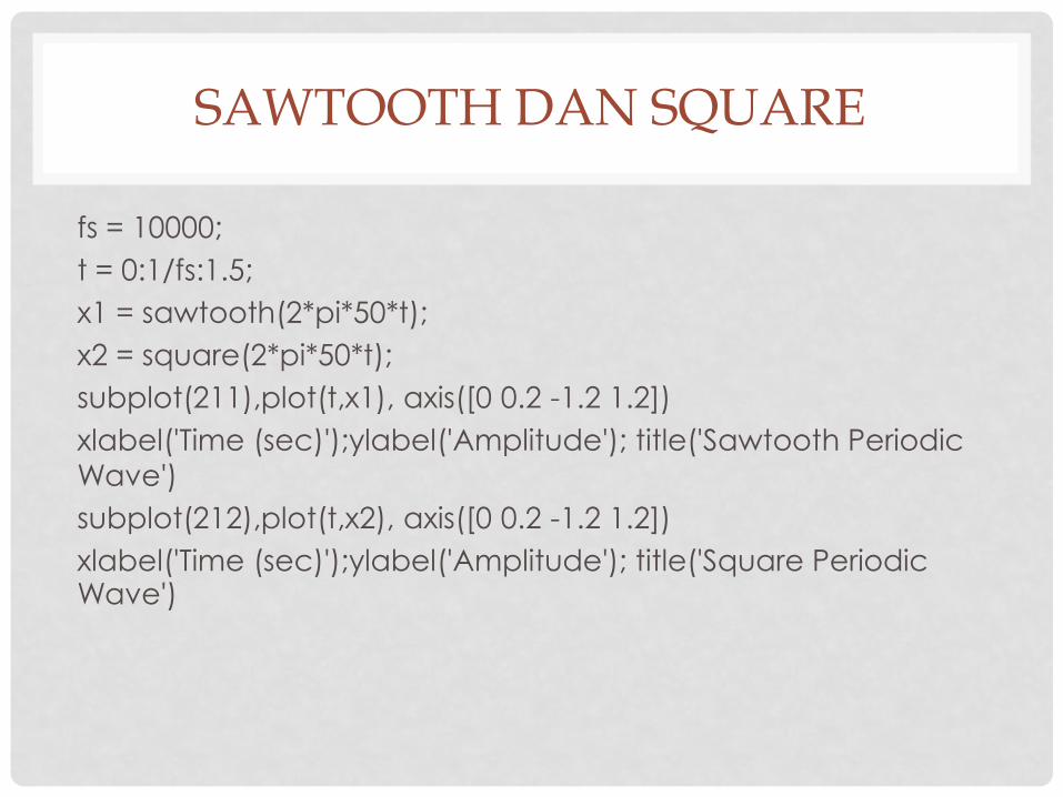
SAWTOOTH DAN SQUARE
fs = 10000;
t = 0:1/fs:1.5;
x1 = sawtooth(2*pi*50*t);
x2 = square(2*pi*50*t);
subplot(211),plot(t,x1), axis([0 0.2 -1.2 1.2])
xlabel('Time (sec)');ylabel('Amplitude'); title('Sawtooth Periodic Wave')
subplot(212),plot(t,x2), axis([0 0.2 -1.2 1.2])
xlabel('Time (sec)');ylabel('Amplitude'); title('Square Periodic Wave')
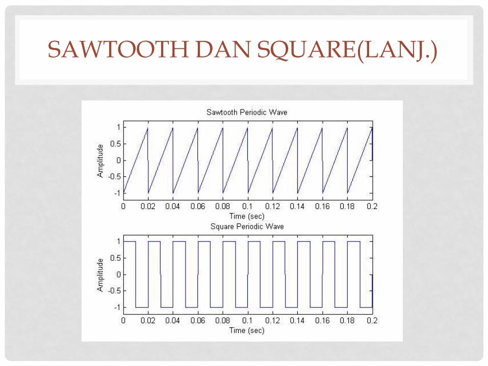
SAWTOOTH DAN SQUARE(LANJ.)
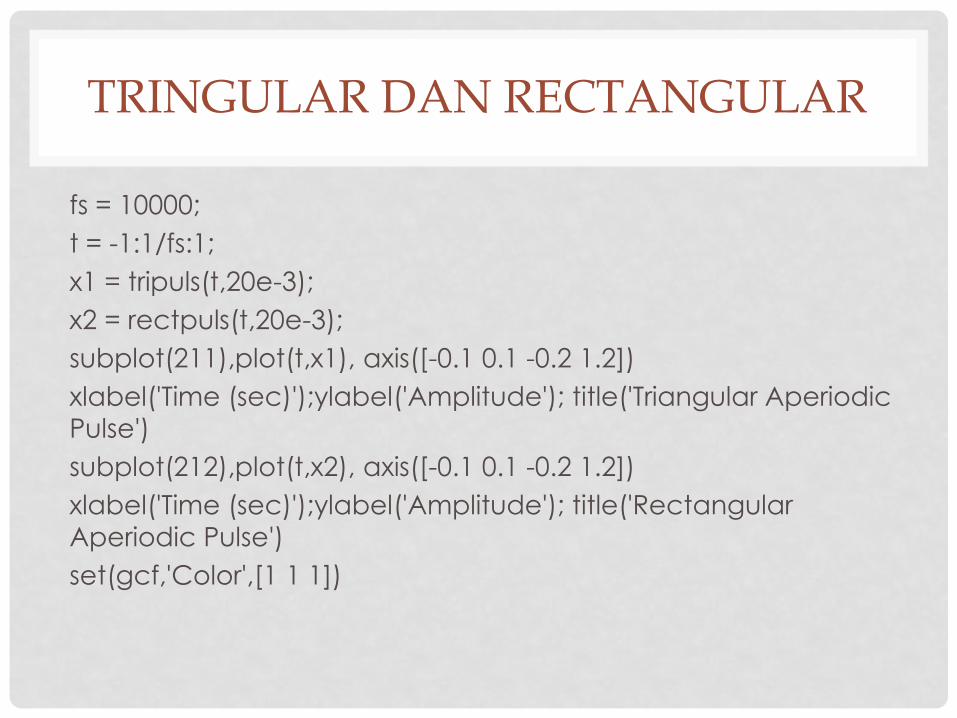
TRINGULAR DAN RECTANGULAR
fs = 10000;
t = -1:1/fs:1;
x1 = tripuls(t,20e-3);
x2 = rectpuls(t,20e-3);
subplot(211),plot(t,x1), axis([-0.1 0.1 -0.2 1.2])
xlabel('Time (sec)');ylabel('Amplitude'); title('Triangular Aperiodic Pulse')
subplot(212),plot(t,x2), axis([-0.1 0.1 -0.2 1.2])
xlabel('Time (sec)');ylabel('Amplitude'); title('Rectangular
Aperiodic Pulse')
set(gcf,'Color',[1 1 1])
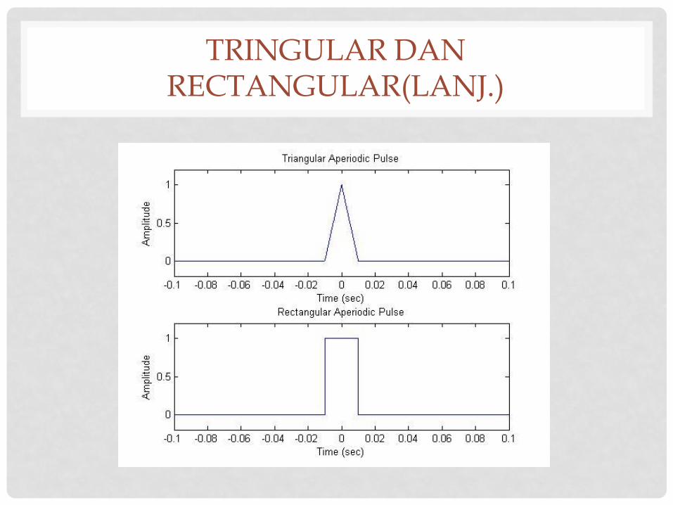
TRINGULAR DAN RECTANGULAR(LANJ.)
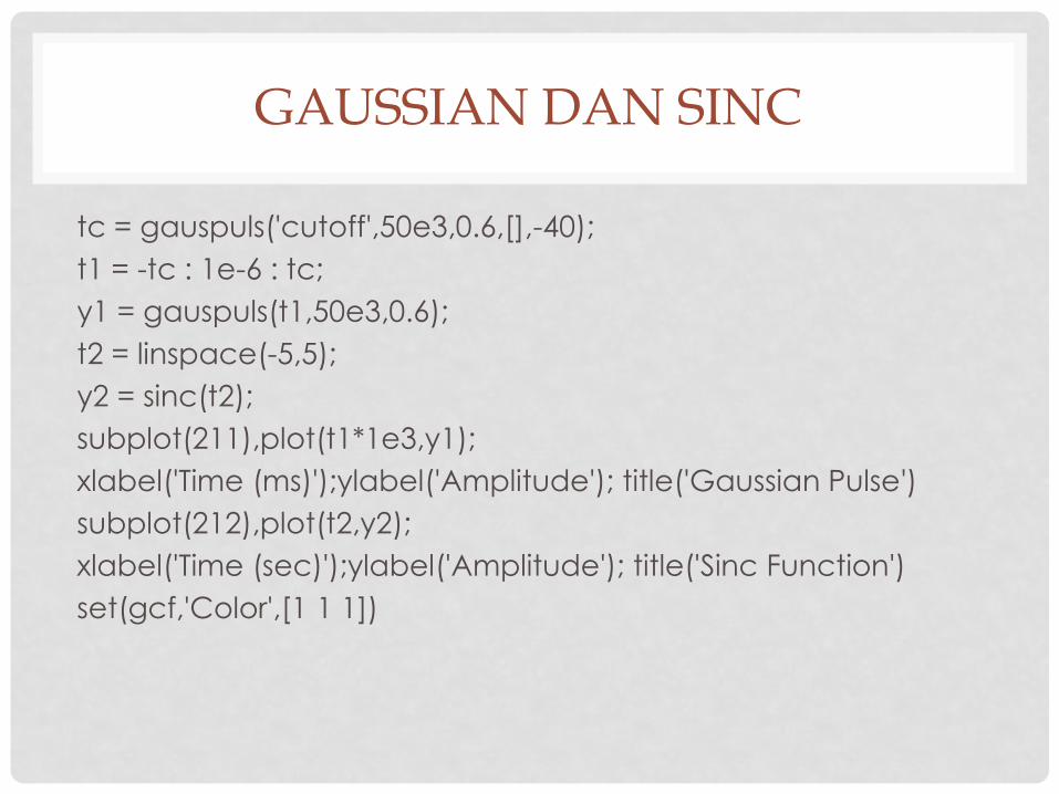
GAUSSIAN DAN SINC
tc = gauspuls('cutoff',50e3,0.6,[],-40);
t1 = -tc : 1e-6 : tc;
y1 = gauspuls(t1,50e3,0.6);
t2 = linspace(-5,5);
y2 = sinc(t2);
subplot(211),plot(t1*1e3,y1);
xlabel('Time (ms)');ylabel('Amplitude'); title('Gaussian Pulse')
subplot(212),plot(t2,y2);
xlabel('Time (sec)');ylabel('Amplitude'); title('Sinc Function')
set(gcf,'Color',[1 1 1])
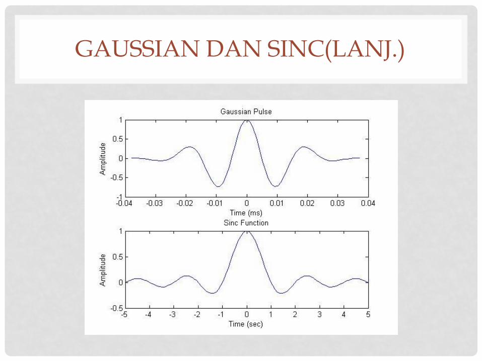
GAUSSIAN DAN SINC(LANJ.)
SINUS
f = 1;
t=0:.0001:5;
y=sin(2*pi*f*t);
plot(t,y);
ylabel ('Amplitude');
xlabel ('Time Index');
title ('Sine wave');
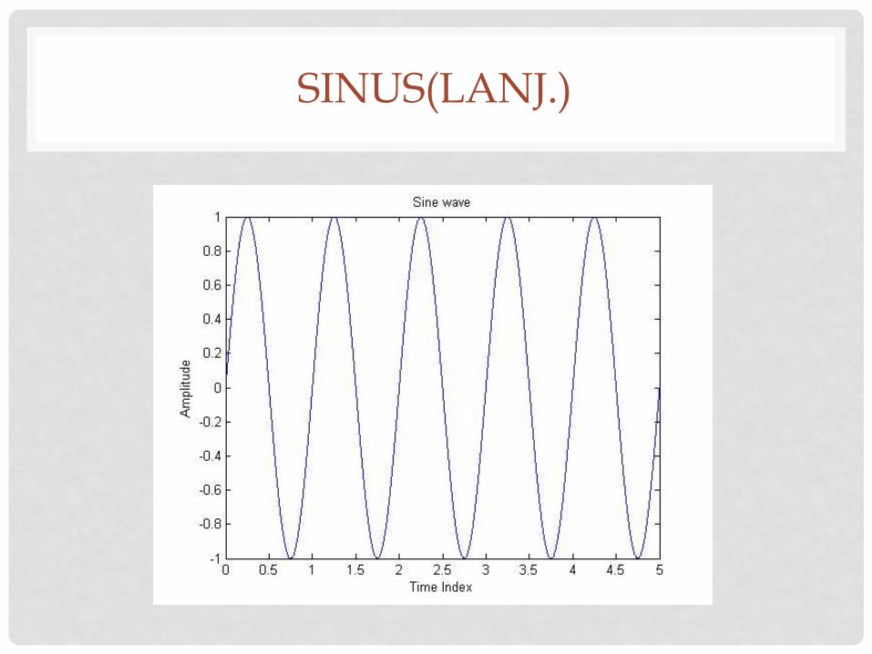
SINUS(LANJ.)
COSINUS
f = 1;
t=0:.0001:5;
y=cos(2*pi*f*t);
plot(t,y);
ylabel ('Amplitude');
xlabel ('Time Index');
title ('Cosine wave');
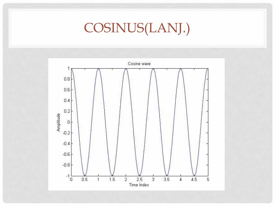
COSINUS(LANJ.)
FAST FOURIER TRANSFORM
• Fast Fourier Transform (FFT): Suatu algoritme untuk
menghitung DFT (Discrete Fourier Transform) dan
inverse-nya.
• Fourier Transform mengubah domain waktu (atau
spasial) ke domain frekuensi atau sebaliknya.
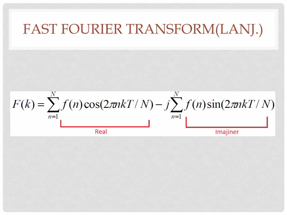
FAST FOURIER TRANSFORM(LANJ.)
FAST FOURIER TRANSFORM(LANJ.)
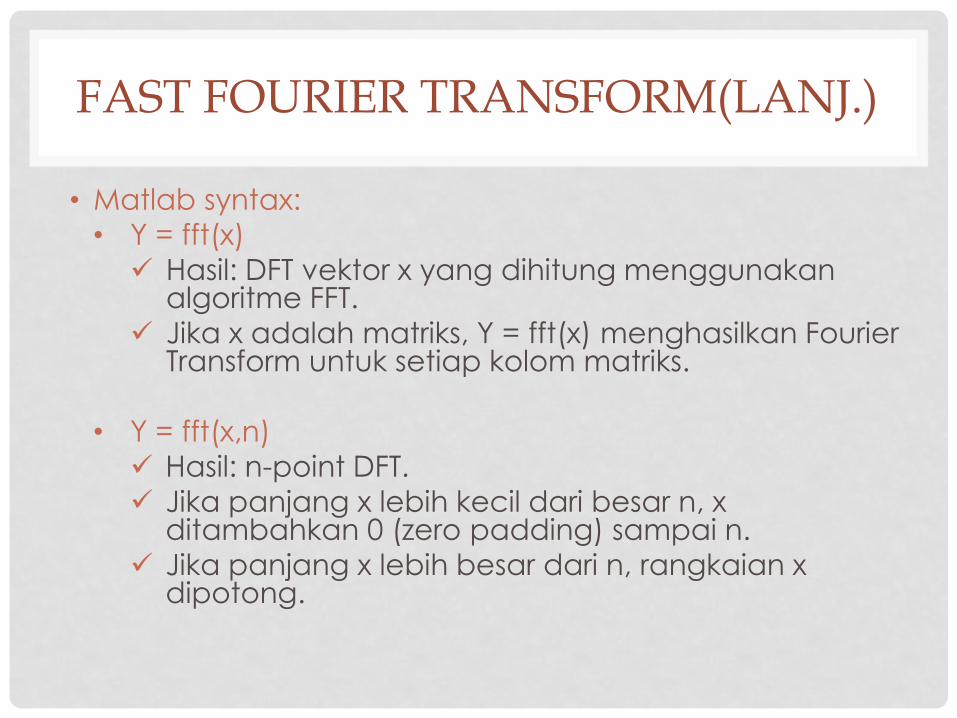
• Matlab syntax:
• Y = fft(x)
Hasil: DFT vektor x yang dihitung menggunakan algoritme FFT.
Jika x adalah matriks, Y = fft(x) menghasilkan Fourier Transform untuk setiap kolom matriks.
• Y = fft(x,n)
Hasil: n-point DFT.
Jika panjang x lebih kecil dari besar n, x ditambahkan 0 (zero padding) sampai n.
Jika panjang x lebih besar dari n, rangkaian x dipotong.
FAST FOURIER TRANSFORM(LANJ.)
• Y = fft(X,[],dim) dan Y = fft(X,n,dim)
Hasil: operasi FFT pada dimensi dim.
FAST FOURIER TRANSFORM(LANJ.)
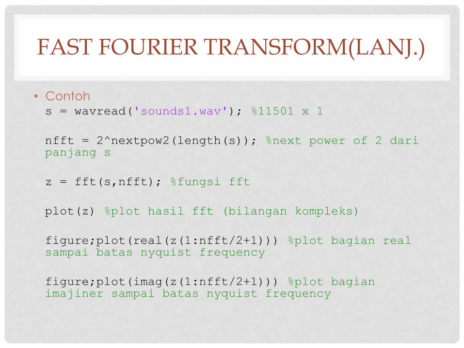
• Contoh s = wavread('sounds1.wav'); %11501 x 1
nfft = 2^nextpow2(length(s)); %next power of 2 dari panjang s
z = fft(s,nfft); %fungsi fft
plot(z) %plot hasil fft (bilangan kompleks)
figure;plot(real(z(1:nfft/2+1))) %plot bagian real sampai batas nyquist frequency
figure;plot(imag(z(1:nfft/2+1))) %plot bagian imajiner sampai batas nyquist frequency
FAST FOURIER TRANSFORM(LANJ.)
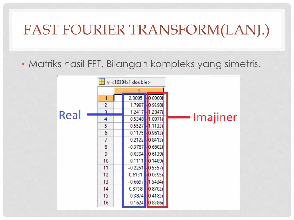
• Matriks hasil FFT. Bilangan kompleks yang simetris.
FAST FOURIER TRANSFORM(LANJ.)
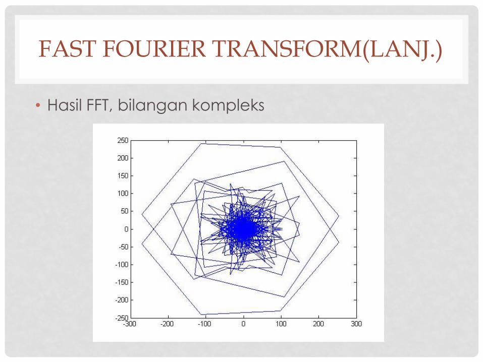
• Hasil FFT, bilangan kompleks
FAST FOURIER TRANSFORM(LANJ.)
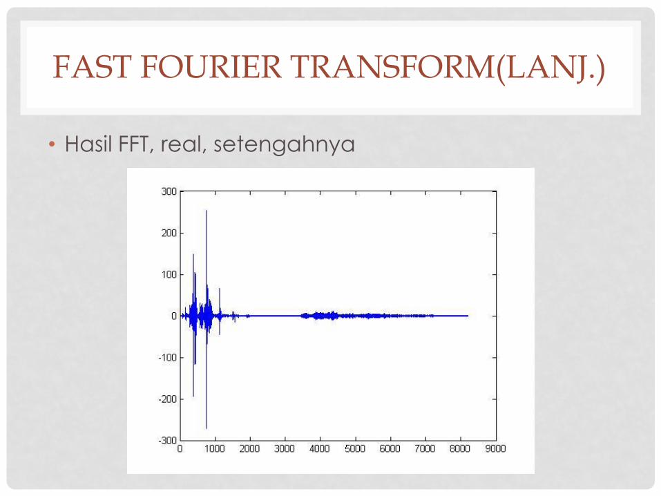
• Hasil FFT, real, setengahnya
FAST FOURIER TRANSFORM(LANJ.)
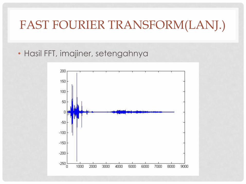
• Hasil FFT, imajiner, setengahnya
FAST FOURIER TRANSFORM(LANJ.)
• Mengembalikan sinyal dari domain frekuensi
• Y = ifft(x)
Hasil: Inverse DFT vektor x yang dihitung
menggunakan algoritme FFT.
Jika x adalah matriks, Y = ifft(x) menghasilkan
inverse DFT untuk setiap kolom matriks.
• Y = ifft(x,n)
Hasil: n-point inverse DFT.
FAST FOURIER TRANSFORM(LANJ.)
• Nyquist frequency / nyquist limit: Frekuensi tertinggi yang dapat dikodekan pada sampling rate tertentu agar dapat sepenuhnya merekonstruksi sinyal. discrete signal
fNyquist = (1/2)v, v = sampling rate
• Nyquist rate: Frekuensi sampling minimum agar tidak terjadi aliasing continuous time signal
NyquistRate = 2fMax,
fMax = frekuensi maksimum
FAST FOURIER TRANSFORM(LANJ.)
• Magnitude sinyal: Mencerminkan komponen energi
sinyal.
• Magnitude = absolut komponen real dan imajiner.
• Pada Matlab:
Misal y adalah vektor hasil FFT, m = abs(y)
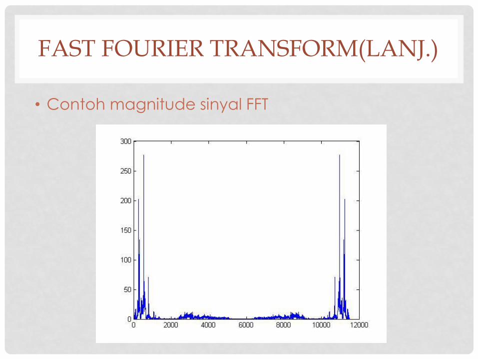
FAST FOURIER TRANSFORM(LANJ.)
• Contoh magnitude sinyal FFT
PENERAPAN FFT
• Beberapa contoh:
• Deteksi noise
• Silence removal
PENERAPAN FFT(LANJ.)
• Deteksi noise
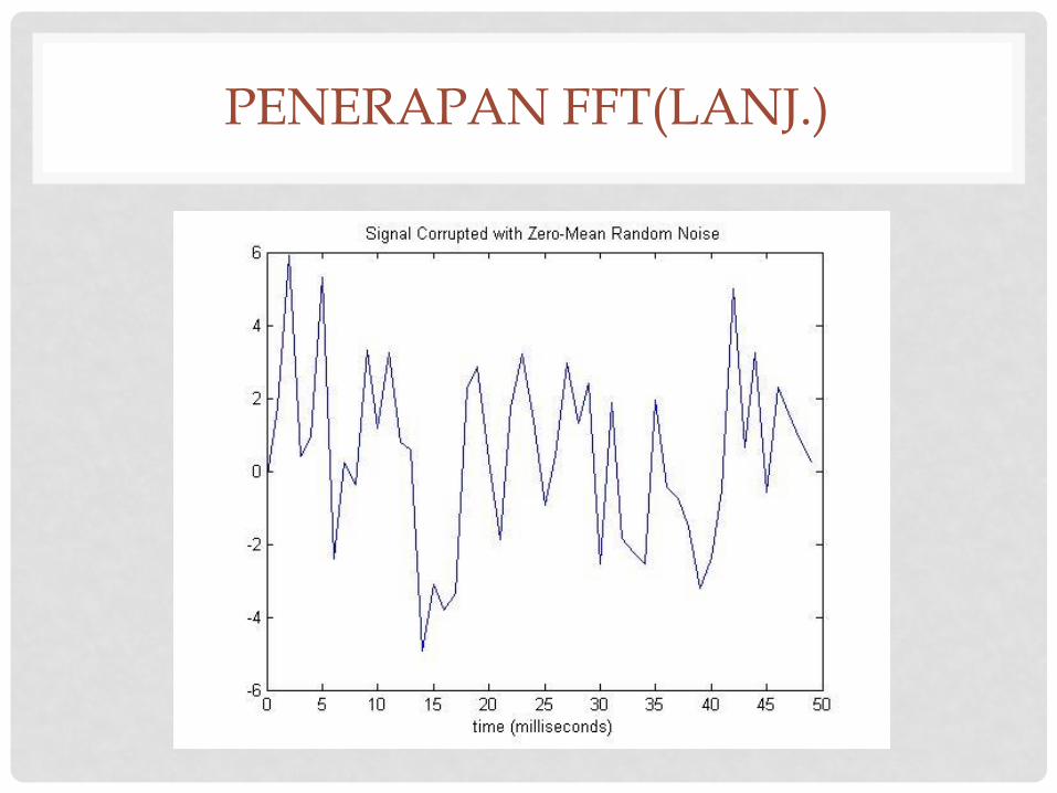
• Sulit menentukan frekuensi sinyal dengan melihat
sinyal asli.
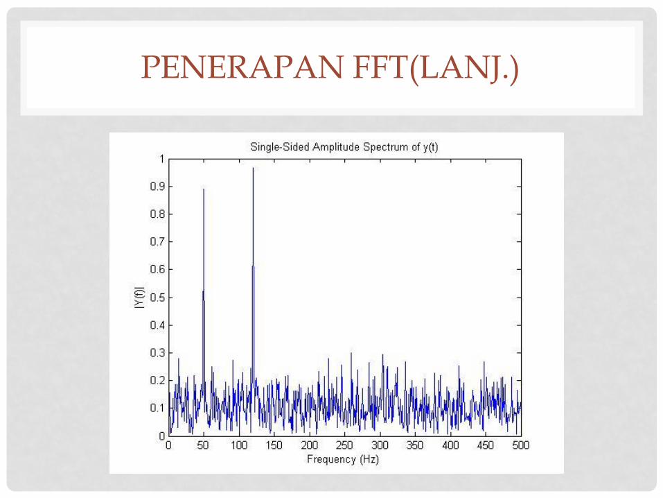
• Lebih memungkinkan pada domain frekuensi.
• DFT sinyal ber-noise menggunakan FFT.
PENERAPAN FFT(LANJ.)
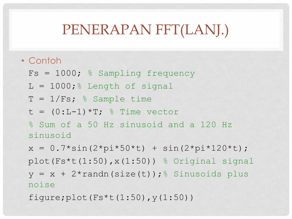
• Contoh
Fs = 1000; % Sampling frequency
L = 1000;% Length of signal
T = 1/Fs; % Sample time
t = (0:L-1)*T; % Time vector
% Sum of a 50 Hz sinusoid and a 120 Hz
sinusoid
x = 0.7*sin(2*pi*50*t) + sin(2*pi*120*t);
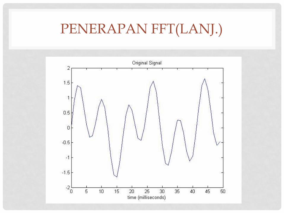
plot(Fs*t(1:50),x(1:50)) % Original signal
y = x + 2*randn(size(t));% Sinusoids plus
noise
figure;plot(Fs*t(1:50),y(1:50))
PENERAPAN FFT(LANJ.)
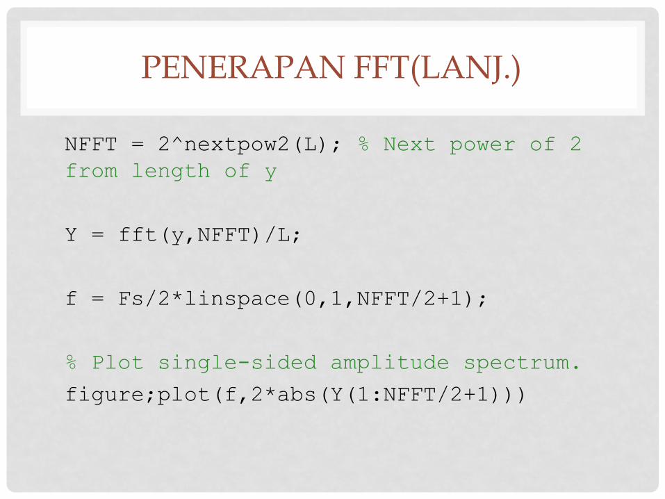
NFFT = 2^nextpow2(L); % Next power of 2
from length of y
Y = fft(y,NFFT)/L;
f = Fs/2*linspace(0,1,NFFT/2+1);
% Plot single-sided amplitude spectrum.
figure;plot(f,2*abs(Y(1:NFFT/2+1)))
PENERAPAN FFT(LANJ.)
PENERAPAN FFT(LANJ.)
PENERAPAN FFT(LANJ.)
PENERAPAN FFT(LANJ.)
• Pada domain frekuensi, alasan utama amplitudo
tidak pas di 0.7 dan 1 karena adanya noise.
PENERAPAN FFT(LANJ.)
• Silence removal
• Prinsip utama: Menghitung energi suara
kemudian dibatasi dengan threshold tertentu.
FFT abs dijumlahkan
• Jika lebih kecil dari threshold silence.
• Sinyal dibagi menjadi beberapa bagian untuk
komputasi.
PENERAPAN FFT(LANJ.)
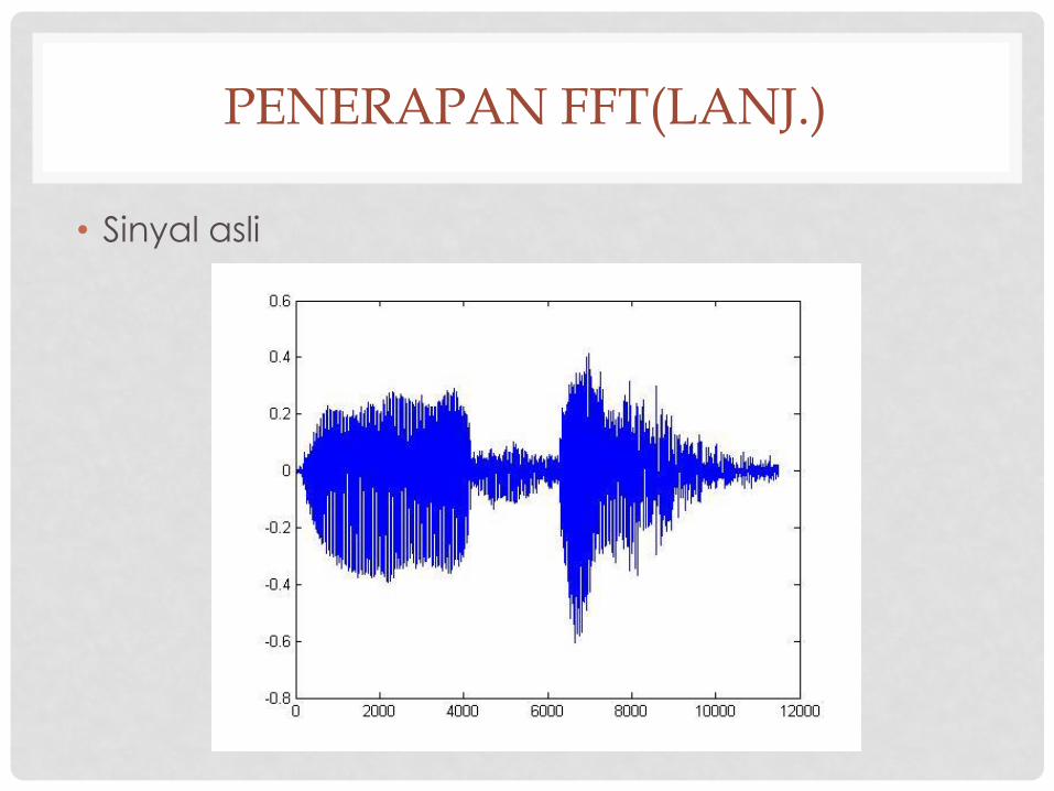
• Sinyal asli
PENERAPAN FFT(LANJ.)
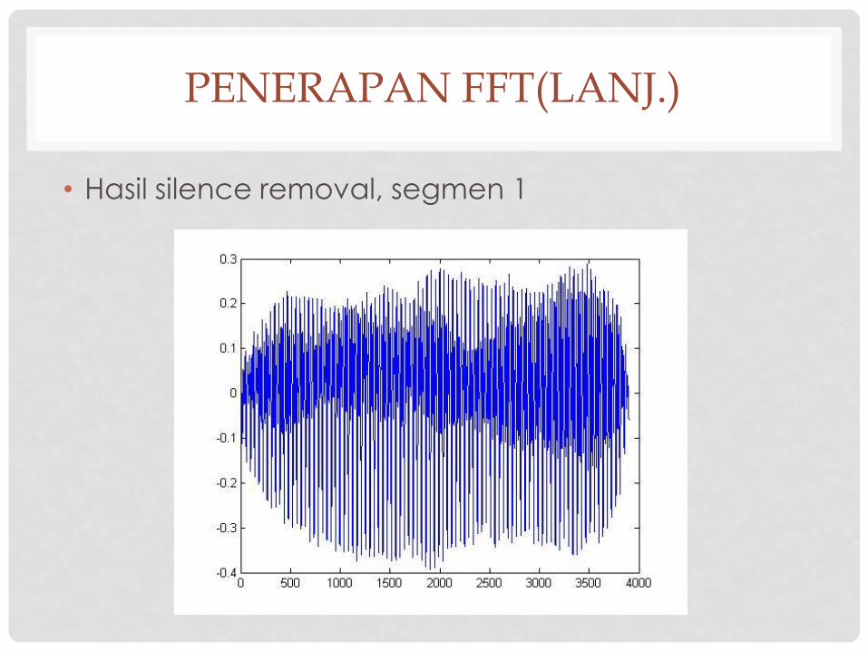
• Hasil silence removal, segmen 1
PENERAPAN FFT(LANJ.)
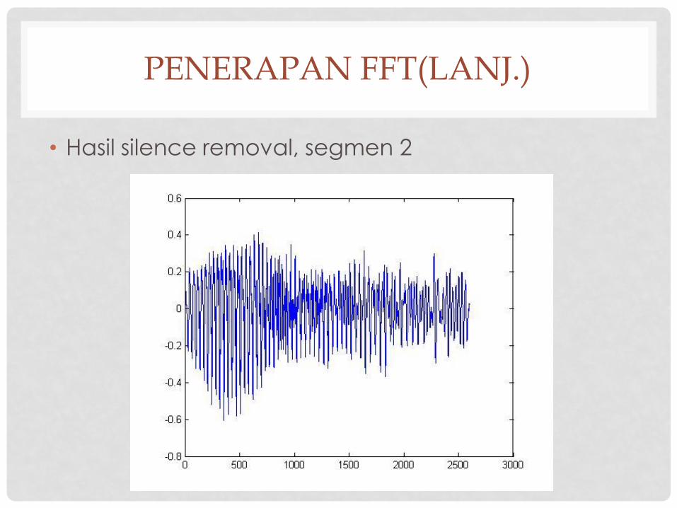
• Hasil silence removal, segmen 2
REFERENSI
• http://www.mathworks.com/help/signal/examples/
signal-generation-and-visualization.html
• http://www.mathworks.com/help/matlab/ref/fft.ht
ml
• http://www.mathworks.com/help/matlab/ref/ifft.ht
ml
LATIHAN
1. Rekamlah 1 sinyal dengan Fs = 11 KHz, 5 detik.
2. Hitunglah DFT dari sinyal tersebut dengan FFT.
Gunakan nfft = 2^nextpow2(length(vektor)); untuk
panjang FFT.
3. Plot sinyal asli, hasil FFT, kedua hasil FFT real dan
imajiner (ada 4 plot total).
4. Hitung energinya (magnitude) kemudian plot-kan.
5. Inverse-kan hasil FFT dan plot-kan.
6. Tambahkan white Gaussian noise pada sinyal dan
ulangi no 2 – 4.
LATIHAN(LANJ.)
• Dikumpulkan: Kamis, 6 Oktober 2014, 23:55 WIB ke
• Format: NLP_NIM_Prak3


