Embed Size (px)
Citation preview
University of Plymouth
PEARL https://pearl.plymouth.ac.uk
04 University of Plymouth Research Theses 01 Research Theses Main Collection
2005
PERCEIVED SIMILARITY BETWEEN
COMPLEX SOUNDS: THE
CONTRIBUTION OF ACOUSTIC,
DESCRIPTIVE AND CATEGORICAL
FEATURES
ALDRICH, KIRSTEEN M
http://hdl.handle.net/10026.1/1913
University of Plymouth
All content in PEARL is protected by copyright law. Author manuscripts are made available in accordance with
publisher policies. Please cite only the published version using the details provided on the item record or
document. In the absence of an open licence (e.g. Creative Commons), permissions for further reuse of content
should be sought from the publisher or author.
P E R C E I V E D SIMILARITY B E T W E E N C O M P L E X SOUNDS: T H E CONTRIBUTION O F ACOUSTIC, DESCRIPTIVE AND
C A T E G O R I C A L F E A T U R E S
by
K I R S T E E N M A L D R I C H
A thesis submitted to the University of Plymouth in partial fulfilment for the degree of
DOCTOR OF PfflLOSOPHY
School of Psychology Faculty of Science
In collaboration with the Engineering and Physical Sciences Research Council
January 2005

University of Plymouth Library
item No. ^ ^ ^ - w c:
KIRSTEEN ALDRICH
PERCEIVED SIMILARITY BETWEEN COMPLEX SOUNDS; THE CONTRIBUTION OF ACOUSTIC, DESCRIPTIVE AND
CATEGORICAL FEATURES
Abstract
The thesis identifies some of the most salient acoustic and descriptive features
employed in listeners' representations of sounds focussing on similarity
judgements. A range of descriptive data (including word pair and imagery/word
use) was collected alongside acoustic measures for the sound stimuli employed.
The sounds employed were initially all abstract in nature but environmental sounds
were included in later experiments. A painwise comparison task and a grouping
task were employed to collect (dis)similarity data for multidimensional scaling and
hierarchical cluster analyses. These provided visual output that represented the
sounds' perceived similarities. Following participants' similarity judgements
correlational techniques identified which of the acoustic and descriptive features
helped to explain the dimensions identified by the MDS. Results across all nine
experiments indicated that both acoustic and descriptive features contributed to
listeners' similarity judgements and that the influence of these varied for the
different sound sets employed. Familiarity with the sounds was identified as an
additional feature that played a key role in the way participants used the available
information in their grouping decisions. There was also a clear indication that the
category to which a sounds source object belonged was making an important
contribution to the similarity judgements for sounds rated as familiar. The work
highlights a complex and variable relationship in the use of descriptive and
acoustic features. Further the work has investigated the similarities and
differences in participants' judgements depending on the data collection technique
used i.e. pairwise comparison or grouping task. These findings have implications
for the development of future models of auditory cognition. The thesis suggests
that the perception of sound with particular reference to similarity is a complex
interplay of features that goes far beyond understanding acoustic features alone.
List of Contents
Chapter 1: Introduction and Review of previous literature
1.1 Introduction 1
1.2 Auditory Information in the environment 3
1.3 The use of auditory imagery 8
1.4 Verbal Encoding 13
1.5 Tasks employed to investigate prominent features of
auditory stimuli 14
1.6 Review of previous experimental findings 16
1 7 Overview of Thesis 22
1.8 Introduction to experimental series 23
Chapter 2: Experiments 1 to 3
2.1 Introduction 24
2.2 Introduction to multidimensional scaling 30
2.3 Experiment 1: the collection of cognitive and perceptual data
2.3.1 Introduction 32
2.3.2 Method 33
2.3.3 Results 37
2.3.4 Discussion 44
2.4 Experiment 2: collection of psychological descriptors
2.4.1 Introduction 46
2.4.2 Method 48
2.4.3 Results 50
2.4.4 Discussion 56
2.5 Experiment 3: Multidimensional scaling of 15 abstract sounds
2.5.1 Introduction 58
2.5.2 Method 63
2.5.3 Results 65
2.5.4 Discussion 72
2.6 General Discussion 77
Chapter 3: Experiments 4 and 5
3.1 Introduction 83
3.2 Experiment 4: the collection of cognitive and perceptual data for 112
abstract sounds
3.2.1 Introduction 86
3.2.2 Method 87
3.2.3 Results 89
3.2.4 Discussion 96
3.3 Experiment 5: grouping task
3.3.1 Introduction 98
3.3.2 Method 100
3.3.3 Results 104
3.3.4 Discussion 112
3.4 General Discussion 116
Chapter 4: Experiments 6 and 7
4.1 Review of the similarity and categorisation literature 122
4.2 Introduction to experiments 6 and 7 131
4.3 Experiment 6: the collection of acoustic and descriptive data for 60 sounds
4.3.1 Introduction 134
4.3.2 Method 135
4.3.3 Results 136
4.3.4 Discussion 142
4.4 Experiment 7: pairwise comparison task for three sound sets
4,4.11ntroduction 145
4.4.2 Method 146
4.4.3 Results 149
4.4.4 Discussion 168
4.4.5 General Discussion 170
Chapter 5: Experiments 8 and 9
5.1 Introduction 174
5.2 Experiment 8: grouping task for three sound sets
5.2.1 Introduction 177
5.2.2 Method 176
5.2.3 Results 180
5.2.4 Discussion 197
5.3 Experiment 9: grouping task for three sound sets with participants
explanations 205
5.3.1 Introduction 205
5.3.2 Method 206
5.3.3 Results 207
5.3.4 Mantel tests for association 22 7
5.3.5 Discussion 232
5.3.6 General Discussion 240
Chapter 6: conclusion
6.1 Introduction 251
6.2 Summary of experimental findings 253
6.3 Summary of experimental techniques 258
6.4 Theoretical implications 259
6.4.1 The salient acoustic features 261
6.4.2 The salient descriptive features 266
6.4.3 The salient features of sound and the similarity and
recognition literature 271
6.4.4 Implications for the categorical and similarity literature 272
6.4.5 Implications for the use ofpa/Vw/se and grouping methodologies to
collect similarity judgements 276
6.4.6 Variable Cognitive Strategies and Contextual effects 278
6.5 Practical Implications 279
6.6 Future areas of research 281
6.6.1 The role of familiarity 281
6.6.2 The salient acoustic and descriptive features of sound 281
6.6.3 The painwise versus grouping tasks 282
6.6.4 How acoustic features map onto descriptive features 283
6.7 Summary 284
Appendices
Appendix A 285
Appendix A1 - Experiment 1 - Correlations between statements
1 - 11 for each of the sound.
Appendix A2 - MANVOA results for all sounds
Appendix A3 - Experiment 2 Briefing/Instructions and 1 example
word pair page
Appendix A4 - Experiment 2 - Correlations between the word pairs
for each sound.
Appendix B 310
Appendix B1 - 112 sound stimuli and sound measures
Appendix C 315
Appendix 01 - 60 sounds and descriptions
Appendix 02 - Acoustic features for the 60 sound stimuli
Appendix D 322
Appendix D1 - participants' explanations and judges marks
References 342
List of Tables
Table 1 Number of sounds and task type employed in each experiment 23
Table 11 Descriptions of sounds used 35
Table 1ii Statements used in experiment 1 37
Table 1iii. Identification measures for sounds 39
Table 1iv Con-elations between measures of familiarity, accuracy and
speed of identification 40
Table 1 v. Mean scores for each statement/sound 41
Table 1vi Correlations between statements 1 to 11 for mobile
phone ring tone 43
Table 2i. Significantly rated adjective word pairs 52
Table 2ii. Correlations between word pairs for mobile phone ring tone 53
Table 2iil. Acoustic measures for experiment 3 sounds 54
Table 2iv Correlations between statements and acoustic measures 55
Table 2v Correlations between the word pairs and acoustic measures 55
Table 3ii Factor loadings for the three psychological descriptor factors 66
Table 3iii Spearman's Rho correlations for sound locations on D1 71
Table 4i Correlations between acoustic measures for the 112 sounds 91
Table 4ii, Mean scores and standard deviations for all 112 sounds 94
Table 4iii. Correlations between the non acoustic statements 94
Table 4iv. Correlations between the non acoustic features
from ex.'s 1,2 and 4 95
Table 4v. statements, word pairs and acoustic measures 95
Table 5i Sound locations on each identified dimension 107
Table 6i. Mean scores for each descriptive measure 138
Table 6ii Spearman's Rho correlations for descriptive measures
for similar sound set 139
Table 6iii Spearman's Rho con-elations for descriptive measures for
similar source set 139
Table 6iv Spearman's Rho correlations for descriptive measures for
unfamiliar set 140
Table 6v Correlations between acoustic and descriptive measures for
the similar sound group 141
Table 6vi Correlations between acoustic and descriptive measures for
the similar source group 141
Table 6vii Correlations between acoustic and descriptive measures for
the unfamiliar sound group 141
Table 7i, Sound locations on each dimension 150
Table 7ii. Spearman's Rho correlations for similar sound
locations on D2 154
Table 7ili. Spearman's Rho correlations for similar sound
locations on D3 154
Table 7iv. Similar source sound locations on each dimension 155
Table 7v. Spearman's Rho correlations for similar source group on D1 160
Table 7vi. Spearman's Rho correlations for similar source
locations on D3 160
Table 7vii. Sounds locations on each dimension 161
Table 7viil Spearman's Rho correlations for unfamiliar sound
locations on D1 166
Table 7ix Spearman's Rho correlations Dimension 2 167
Table 81. Sounds locations on each dimension 182
Table Sii. Spearman's Rho correlations for similar sound
locations on D3 186
Table 8iii. Sounds locations on each dimension 187
Table Siv. Spearman's Rho correlations for similar source
locations on D1 191
Table 8v. Spearman's Rho correlations for similar source
locations on 02 191
Table 8vi Spearman's Rho correlations for similar source
locations on D3 191
Table 8vii. Sounds locations on each dimension 192
Table 8vii Spearman's Rho correlations for unfamiliar sound
locations on D1 196
Table 8ix Spearman's Rho correlations for unfamiliar sound
locations on D2 197
Table 91. Sounds locations on each dimension 208
Table 9ii. Spearman's Rho correlations for similar sound
locations on D1 213
Table 9iii. Spearman's Rho correlations for similar sound
locations on 02 213
Table Siv. Spearman's Rho correlations for similar sound
locations on D3 213
Table 9v. Sounds locations on each dimension for similar
source sound set 216
Table 9vi. Spearman's Rho correlations for similar source
locations on D1 220
Table 9vii. Spearman's Rho correlations for similar source
locations on 02 220
Table 9viii. Sounds locations on each dimension for
unfamiliar sound set 222
Table 9ix. Spearman's Rho correlations for unfamiliar sound
locations on D1 225
Table 9x. Spearman's Rho correlations for unfamiliar sound
locations on 02 225
Table 9x1. Summary of results for Mantel tests across
all sound sets in experiments 7. 8 and 9 228
Table 9xii. Summary table of results from experiments 7. 8 and 9 231
List of Figures
Figure l a Schematic diagram of McAdam's (1993) stages of processing
involved in recognition and Identification 6
Figure 3a Diagrammatic example of sound presentation 64
Figure 3b Weights for individual participants on each dimension 67
Figure 3c. 3D INDSCAL solution space 68
Figure 3d MDS map for dimensions 1 and 2 69
Figure 3e MDS map for dimensions 1 and 3 69
Figure 3f MDS map for dimensions 2 and 3 70
Figure 3g. Dendrogram showing Hierarchical cluster analysis
for all sounds based on a composite similarity matrix (n=46) 72
Figure 5a Screenshot of colour sorting task 102
Figure 5b Screenshot of final sorting screen 103
Figure 5c Weights for each participant on each dimension 104
Figure 5d. MDS output for the 70 abstract sound grouping task 105
Figure 5e Dendrogram showing hierarchical cluster analysis
for all sounds based on a composite similarity matrix (n=46) 111
Figure 5f Emergency Services sound cluster 114
Figure 5g Cluster of telephone sounds from MDS output 114
Figure 7a. MDS solution for s/m//ar sound stimuli group 150
Figure 7b. Similar sound locations on dimensions 1 and 2 151
Figure 7c. Similar sound locations on dimensions 1 and 3 151
Figure 7d. Similar sound locations on dimensions 2 and 3 152
Figure 7e. Dendrogram for similar sound composite matrix 153
Figure 7f. MDS solution for similar source sound set 156
Figure 7g. MDS map for dimension 1 and 2 (similar source sound set) 157
Figure 7h. MDS map for dimension 1 and 3 (similar source sound set) 157
Figure 7i. MDS map for dimension 2 and 3 (similar source sound set) 158
Figure 7j. Hierarchical cluster analysis for similar source sound set 159
Figure 7k. MDS solution for unfamiliar sound set 162
Figure 71. Dimensions 1 and 2 for the unfamiliar sound set 163
Figure 7m. Dimensions 1 and 3 for the unfamiliar sound set 163
Figure 7n. Dimensions 2 and 3 for the unfamiliar sound set 164
Figure 7o. Dendrogram showing the clusters across all matrices
for the unfamiliar sound set 165
Figure 8a Colour sorting example screen 179
Figure 8b Sorting task screenshot 180
Figure 8c. MDS solution space for the similar sound stimuli set 181
Figure 8d. Similar sound stimuli locations on dimensions 1 and 2 183
Figure 8e. Similar sound stimuli locations on dimensions 1 and 3 183
Figure 8f. Similar sound stimuli locations on dimensions 2 and 3 184
Figure 8g, Dendrogram for similar sound composite matrix 185
Figure 8h. MDS solution space for the similar source stimuli set 187
Figure 8i. Similar source stimuli locations on dimensions 1 and 2 188
Figure 8j. Similar source stimuli locations on dimensions 1 and 3 188
Figure 8k. Similar source stimuli locations on dimensions 2 and 3 189
Figure 81. Dendrogram for similar source composite matrix 190
Figure 8m. MDS solution space for the unfamiliar stimuli set 193
Figure 8n. Unfamiliar stimuli locations on dimensions 1 and 2 194
Figure 8o. Unfamiliar stimuli locations on dimensions 1 and 3 194
Figure 8p. Unfamiliar sounds on dimensions 2 and 3 195
Figure 8q. Dendrogram of the composite matrix for unfamiliar sounds 196
Figure 9a. MDS solution space for similar sound stimuli 209
Figure 9b. Similar sound stimuli locations on dimensions 1 and 2 210
Figure 9c. Similar sound stimuli locations on dimensions 1 and 3 210
Figure 9d, Similar sound stimuli locations on dimensions 2 and 3 211
Figure 9e. Hierarchical cluster analysis for similar sound set 212
Figure 9f. Participant explanations for their grouping
decisions in percentage tenns for the similar sound group 215
Figure 9g. MDS solution for similar source sound set 216
Figure 9h. Similar source stimuli locations on dimensions 1 and 2 217
Figure 9i. Similar source stimuli locations on dimensions 1 and 3 217
Figure 9j. Similar source stimuli locations on dimensions 2 and 3 218
Figure 9k. Hierarchical cluster analysis for similar source set 219
Figure 91. Participant explanations for their grouping decisions
in percentage terms for the similar source group 221
Figure 9m. 3 dimensional solution space for the unfamiliar sound set 223
Figure 9n. Dendrogram from a hierarchical cluster analysis
for the unfamiliar sound set 224
Figure 9o. Participant explanations for their grouping decisions in
Percentage terms for the unfamiliar sound group 226
A C K N O W L E D G E M E N T S
My Supervisors
Firstly I would like to thank my supervisors Professor Judy Edworthy and Dr Elizabeth
Hellier for their continued support throughout the PhD and their unfaltering confidence in
me.
My Family
A huge thank you to my parents who have always supported me no matter which mad
course I embark on next. My partner Mark for allowing me to talk endlessly about
statistical techniques and providing a sounding board time and time again. Of course to
my son Luke who has patiently allowed his mum to say "not now I'm busy" once too often
in the last three years.
My Friends
To Mr Sid whose programming skills have gone a long way towards preventing a nervous
breakdown in bleak moments of coding madness. Lastly to all my friends who have only
heard about my PhD when it wasn 7 going quite so well but were there to support me all
the same.
Thank you All
Author's Declaration
At no time during the registration for the degree of Doctor of Philosophy has the author been registered for any other university award except the permitted Postgraduate Diploma in Psychological Research Methods.
This programme of research was supported by funding from the Engineering and Physical Sciences Research Council from October 2001 to September 2004.
This thesis is the result of the author's own investigation, carried out under the guidance of her supervisory team. Other sources are explicitly referenced.
During this period of study, the author has also completed the Postgraduate Diploma in Psychological Research Methods, and achieved the following conference contributions and publications.
Publications (or presentation of other forms of creative and performing work): Aldrich. K.. Edworthy, J.. & Hellier, E (2003) The perceptual stnjcture of abstract
sounds. Poster presentation at the Annual British Psychological Society Cognitive section conference, University of Reading, September 2003.
An extended version of the above presentation was presented to colleagues during a departmental research seminar in March 2003.
Aldrich, K., Edworthy, J & Hellier, E (2004) Ways of representing sound. Poster presented at the annual conference of the European Chapter of the Human Factors and Ergonomics Society. Delft, October 2004.
Edworthy, J.. Aldrich., K & Hellier. E (2004) Auditory Cognition: More to listening than meets the ear. Paper presented at the annual conference of the European Chapter of the Human Factors and Ergonomics Society, Delft, October 2004.
Word count of main body of thesis: 68, 340 words
Signed ^ ^ .
Date.
Chapter 1
1.1 Introduction
A fundamental feature of our everyday lives is our ability to represent and identify
auditory objects. An understanding of which features listeners are using to
identify the sounds around them is not well specified in the psychological
literature. Previous research has typically concentrated on the identification of
acoustic features used by listeners in sound identification or recognition tasks.
The present research suggests that in order to address how we represent auditory
objects it is necessary to go beyond the identification of only the most prominent
acoustic features. For example, it is suggested that many acoustic features map
on to the descriptive or associative features of sounds. The present research
suggests a complex interaction between sounds and their acoustic and
descriptive meanings. Many sounds typically represent some object or function,
some sounds serve a purpose and these additional features may also be salient
in the way sounds are represented.
The thesis aims to further our understanding of sound representation through the
investigation of perceived similarities between sounds. Of interest are both
acoustic and descriptive properties of the sounds in addition to the identification of
functional features of salience. The possibility that the category to which a
sounds source object belongs may be an important influence in similarity
judgements is also investigated.
The eariy focus in the thesis is on sounds that do not share a natural relationship
with the object that creates them. These sounds are collectively known as
abstract sounds. For the purposes of the present research the term abstract
1
sounds is used to define a subset of sounds with little previous work associated
with them. Abstract sounds are mainly modern sounds and are sounds where
associations to objects are typically learnt, such as the acquired knowledge that
allows listeners to identify a smoke alarm and its meaning. Abstract sounds can
also be less familiar sounds where such knowledge has not yet been learnt by the
listener. An example of such an unfamiliar abstract sound could be a synthesised
gun on a computer game that the listener is unfamiliar with. The category
abstract sounds does not include sounds that are typically classed as
environmental in previous work e.g. Balias (1993). Such sounds as wind chimes,
a dog barking or a fan whirring are not abstract sounds they are the sound that
the object makes naturally, it has not been artificially assigned to an object. Later
in the thesis environmental sounds are used alongside abstract sounds to
investigate specific issues about acoustic and descriptive similarity and the
influence of sounds' membership to categories. The current work brings previous
research using mainly environmental (natural) sounds up to date by including
some modern, abstract, sound stimuli. In addition, the focus will go beyond the
investigation of the acoustic sound features, extending previous research by
including the investigation of descriptive and functional features. Abstract sounds,
such as alarms and computer alerts, are becoming increasingly common in our
worid and in terms of auditory research can serve as a bridge between
environmental sounds and novel sounds or tones also used in auditory research
because of their often complex but non natural composifion.
In our everyday auditory environment when a listener tries to identify a sound
there is a multitude of information to make use of. Just like our visual
environment the auditory worid is incredibly complex. Intuitively we know listeners
can single out and identify sounds around them (e.g. a seagull) from the complex
auditory environment should they want or need to. Lass, Eastham, Parrish,
Scherbick and Ralph (1982) provided some empirical evidence to support this
intuitive notion finding that ninety percent of the environmental sounds (animal,
inanimate, musical and human) they presented to listeners were accurately
identified. However, Lass et al (1982) presented their sounds in isolation and this
is typical of experimental work using environmental sounds. Of course the real
world environment is made up from a complex mixture of sounds. However,
investigations into the complexity of the real auditory world cannot begin in any
depth until the most salient features of sounds, in isolation or otherwise, have
been identified.
1.2 Auditory information in the environment
Some authors have tackled auditory perception as a whole looking at how
listeners break down and utilise the auditory information in our environment. For
example, Bregman (1993) discusses auditory scene analysis, the process through
which we decompose the mixtures of sounds around us. Bregman (1993)
suggested that both automatic and voluntary recognition occurs using schemas
formed by prior listening. Three main processes occur in the human listener to
decompose auditory mixtures. One is the activation of learned schemas in an
automatic fashion. The second is a process that can decompose auditory
mixtures by using schemas in a voluntary way. The example given by Bregman
refers to listening out for our name if we are waiting for an appointment in a busy
room. This involves us 'trying' to hear and indicates a voluntary process. Of
course both the voluntary and automatic processes require that the knowledge
about the sound has already been formed on a previous occasion. Thirdly,
Bregman (1993) suggested it would be useful to have a partitioning method to sort
the incoming mixture into separate acoustic sources that could be used prior to
the application of any specific knowledge about the important sounds in our
environment. According to Bregman (1993) there are four main regularities that
the auditory system exploits when breaking down our auditory environment.
Firstly, unrelated sounds do not usually start and stop at the same time.
Secondly, single sounds change their properties smoothly and slowly. Thirdly,
when a body vibrates it results in an acoustic pattern in which the frequency
components are multiples of a common fundamental. Finally, many changes that
take place In an acoustic event will affect the resulting sound in the same way at
the same time. Bregman (1993) compares the principles of auditory scene
analysis with grouping principles proposed by Gestalt psychologists. That is to
say such principles exist on the whole to group sensory evidence that is derived
from the same (or closely related) environmental objects or events.
Another approach that looks at the acoustic environment as a whole is the
ecological approach taken by Gaver (1993) who proposed that everyday listening
is more about listening to events rather than the sounds themselves. Gaver
(1993) argued that the attributes of interest are those of the sound-producing
event and its environment, not those of the sound itself. Therefore, a sound
provides the listener with information about an interaction of materials at a
location in an environment. Gaver (1993) argued that more complex perceptions
must depend on the integration of these sensations but that they seem
inadequate to specify complex events. According to the ecological account the
study of perception should be aimed at Identifying ecologically relevant
dimensions of perception. Gaver (1993) suggested that there is a need to stretch
traditional psychoacoustics to include perceptual dimensions of sources as well as
the sounds themselves and a willingness to treat complex acoustic variables as
elemental. Nowadays, In many cases, the identification of sounds must go
beyond the events that cause them because many more abstract sounds are
typically created digitally where no physical event has taken place. Modern
abstract sounds such as mobile phone ring tones denote an event i.e. an
incoming phone call, but no physical event such as an item hitting the floor has
occurred. Therefore, these sounds represent the source or function in a different
way to environmental sounds. These sounds also bridge the gap between
environmental sounds such as animal noises and manmade but unfamiliar
sounds.
Research on sound quality assessment also looks at the sound event suggesting
that sound research often reduces the quality of a sound to its surface form.
Susini, McAdams and Winsberg (1999) discuss the problems associated with
studying sound quality that arise from the complexity of many environmental
sounds. These complexities have a multidimensional nature from both acoustic
and perceptual viewpoints.
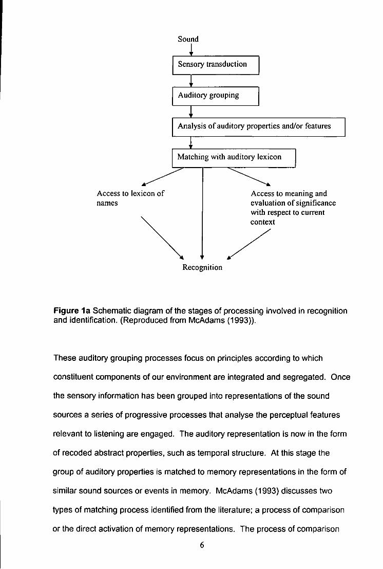
Other authors have discussed the way we process and ultimately recognise
sound but with a focus less entwined in the complexities of the auditory
environment as a whole. McAdams (1993) proposed an auditory recognition
model (figure 1a) with a series of stages but recognised from the outset that most
of the evidence that had contributed to our knowledge of sound recognition at the
time had involved experiments that presented sounds to listeners in isolation. The
stages proposed in the model, in brief, start with the peripheral auditory
representation of the acoustic signal followed by auditory grouping processes.
Access to lexicon of names
Sound
Sensory transduction
Auditory grouping
Analysis of auditory properties and/or features
Matching with auditory lexicon
Access to meaning and evaluation of significance with respect to current context
Recognition
Figure 1a Schematic diagram of the stages of processing involved in recognition and identification, (Reproduced from McAdams (1993)).
These auditory grouping processes focus on principles according to \Nh\ch
constituent components of our environment are integrated and segregated. Once
the sensory Information has been grouped into representations of the sound
sources a series of progressive processes that analyse the perceptual features
relevant to listening are engaged. The auditory representation is now In the form
of receded abstract properties, such as temporal structure. At this stage the
group of auditory properties is matched to memory representations in the form of
similar sound sources or events In memory. McAdams (1993) discusses two
types of matching process identified from the literature; a process of comparison
or the direct activation of memory representations. The process of comparison
selects the memory representation that most closely resembles the auditory
feature representation. The alternative, direct activation matching, suggests that
recognition of the sound event is determined by the memory representation that
receives the highest degree of activation above a certain threshold. For both
these processes If no match or too many matches occur then no recognition can
take place. This may be followed by the activation of items in the listener's
lexicon of names, concepts and meanings associated with the identified class of
events. It is at this point, when the identification takes place, that the listener can
take appropriate action, such as avoiding an on coming vehicle.
The model discussed by McAdams (1993) is a speculative summary description
of the recognition process. This is likely the result of the fact that this is an area
where research Is very limited but further research is essential. The process by
which we recognise a sound and the auditory representation features of
Importance in the recognition process is an essential feature of everyday life. The
present thesis aims to contribute to the identification of the salient sound features
in order to further our understanding of the recognition process. In particular the
focus is on understanding the contribution of both acoustic and descriptive
properties in relation to the source and function of the sound and how this is
identified through similarity judgements.
From a similar point of view to that discussed by McAdams (1993), Howard and
Ballas (1981) discussed the importance of the feature extraction process that
Involves Information reduction. A sound is reduced into the elemental properties
or characteristics that are transformed Into a relatively small set of distinctive
features that are the building blocks for the recognition stage. However, the
question arises again over which distinctive features are involved. Feature
reduction requires that the set of distinctive features should uniquely specify the
stimulus, preserving or enhancing perceptually important differences among
stimuli. However, the set of distinctive features discussed is as yet unspecified
with only a few highly salient features already identified in the literature such as
pitch (e.g. Deutsch, 1981; & Intons Peterson, 1981) and tempo (Solomon 1959a).
It is noted that despite feature extraction's central importance as a theoretical
construct in this area it is not well specified in the literature. Howard et al (1981)
discuss two main approaches, namely, the property list and the process
orientated approach and how these approaches play a fundamental role in many
theoretical treatments of auditory pattern recognition. The property list approach
places emphasis on the feature detectors that are filter-like devices that monitor
the incoming sensory information. Each detector is tuned to look for a particular
stimulus property (acoustic) and a set of feature detectors determines an acoustic
property list for the stimulus. The second view, the process oriented approach
assumes the feature selection process itself is internalized and context sensitive.
This approach views feature selection as a continuous ongoing process. Howard
et al (1981) avoid selecting an approach as necessarily correct but rather view
them as extremes on a continuum of possible feature selection mechanisms.
Before either of these approaches can be elaborated it is necessary to identify
which sound features are those most likely to be the salient ones required by the
feature detectors.
1.3 The use of auditory imagery
Many authors refer to the inclusion of an auditory image in the processing of
sounds. An auditory image is a relatively poorly defined concept in the literature
with ideas still not fully clarified. It is unclear whether the auditory image
discussed by the following authors is a concept that can be reconciled with the
auditory representation discussed, for example, by McAdams (1993) or whether
such Images are distinct.
The auditory system's ability to determine sound sources Is discussed by Yost
(1991) and links the research to the recognition of sound. Yost refers to the ability
of the auditory system to process complex sounds Into elements or auditory
Images, allowing the listener to determine the sources. In terms of Identification
Yost points out that an auditory image can exist without the listener being able to
identify the source. For example, a novel sound source may not have a label but
would still produce an auditory image. In this sense the auditory image Is
removed from the Idea of an auditory representation described by McAdams
(1993). McAdams (1993) suggested that If no match occurs then no activation of
items in the listener's lexicon of names, concepts or meanings associated with the
identified class of events will occur and subsequently no recognition will take
place. However, Yost (1991) does not place the emphasis of the discussion on
the recognition of the sound per se but the development of an auditory image.
Yost (1991) proposed seven acoustic variables that are likely candidates for
forming auditory images, these are; spectral separation, intensity profile,
harmonicity, spatial separation, temporal separation, common temporal onsets
and offsets and, coherent slow temporal modulation. Despite discussing the use
of auditory Images as an Integral part of determining sound sources a definition of
an auditory image is left unclear and four main questions are raised that will need
to be addressed in order to have a deeper understanding of the auditory image. It
will be necessary to identify what physical attributes of sound sources are used by
the auditory system to form auditory images, how the physical attributes are
coded In the nervous system, how these coded attributes are pooled or fused
within the auditory system and how the coded pools of information (auditory
images) are segregated so that more than one auditory image can be perceived.
Yost (1991) concluded that the formation of auditory images is an integral part of
determining sound sources. At this point Yost has returned to the contribution of
an auditory image to the focus of this discussion, the recognition of a sound, but in
terms of its source.
An alternative view of an auditory image has been presented more recently by
Patterson (2000) describing a computer model designed to explain how the
auditory system generates auditory images. The fine detail is complex and
beyond the scope of this discussion but the model assumes that a multi channel
interval histogram is the basis of auditory images. The software contains
functional and physiological modules to simulate auditory spectral analysis, neural
encoding and temporal integration (Patterson, Allehand & Giguere, 1995). The
model develops cartoons that illustrate the dynamic response of the auditory
system to more complex sounds such as everyday sounds. This provides us with
a visible example of an auditory image.
An important issue was raised by Vanderveer (as cited in Ballas & Howard, 1987)
questioning whether sound recognition involved the identification of a sound or its
source. When participants were asked to describe environmental sounds in this
work the participants typically described the event that was thought to have
caused the sound but did not describe the sound in terms of acoustic properties.
Therefore, recognition of environmental sounds was suggested to be directed to
produce semantic interpretations of the sound.
10
An unusual methodology was utilised by Intons Peterson (1980) and Intons
Peterson, Russell and Dressel (1992) to try to identify some acoustic features of
sounds that may be included In an auditory image. An auditory image is defined
by Intons Peterson (1992) as;
"the introspective persistence of an auditory experience, including one constructed
from components drawn from long term memory, in the absence of direct sensory
instigation of that experience" pg 46.
Intons Peterson and colleagues chose to investigate whether pitch and loudness
information was Included in participants' auditory Images. Of particular Interest
was whether this Information could be retrieved from Long Term Memory without
the presentation of a stimulus. In addition, the research investigated whether
loudness and pitch Information are only Included In an image when the task
demands it. In order to induce the retrieval and Inclusion of loudness information
participants were asked to equalize, or match, the loudness of two named
environmental sounds, with different loudness ratings gathered from previous
work. For example, a participant would be asked to equalize the sound of wind
chimes, classified as 'soft loudness rating' with laughter, classified as 'medium
loudness'. The results supported the hypothesis by Indicating that the time to
match the Imagined loudness of two named environmental sounds increased with
the difference between the loudness ratings of the two sounds. The same
paradigm was used to identify similar results for pitch information (Intons Peterson
et al, 1992). The research was taken to suggest that auditory images, that
represent the sound, are closely related to perceptual experience, at least with
reference to pitch and loudness Information, and this may give some Insight into
the process of encoding sound. Because participants were retrieving an auditory
image to complete the task this unusual methodology suggested two acoustic
components that could be contributing to the reduced auditory representation.
11
Work completed by Deutsch (1982) would at first appear to be at odds with Intons
Peterson's suggestion that pitch is a salient feature of an auditory image.
Deutsch (1982) identified that when listeners make pitch comparison judgements
between tones that are separated by a silent interval accuracy declines as the
interval is lengthened. Similarly, and the most relevant to the Intons Peterson et
al (1992) research was the finding that pitch retention was affected if interference
tones were played between the original tone and the to be judged tone.
However, these are both short term memory tasks whereas Intons Peterson's
(1992) work is calling for the retrieval of pitch information in auditory images from
long term memory.
The research conducted by Intons Peterson (1980) into the role of loudness in an
auditory image also identified the possible importance of a graphic or visual
image. A post experimental inquiry revealed that although the participants had
been instructed to form an auditory image during the task most participants
reported forming a visual image on 95% of trials. In addition, these participants
reported that the visual image preceded their auditory images. The participants
suggested that the visual components were not optional whilst the loudness
information was retrieved on a task dependent basis. This raises the question as
to how a participant would perform on an identification task or a recognition task
for sounds that are more abstract or unfamiliar perhaps not lending themselves to
the use of visual or graphic images. However, as suggested by Edworthy and
Hards (1999) a major problem with using visual images is that the user will
typically generate a parallel verbal label. Therefore, if the visual image is absent
because the sound is abstract or unfamiliar the question arises, will the user be
able to generate a suitable verbal label?
12
1.4 Verbal Encoding
The question of the use of a suitable verbal label was addressed by Bower &
Holyoak (1973) who investigated the influence of verbal encoding on memory
performance for non verbal material. Previous research suggested that when a
participant hears a naturalistic sound they may try to Interpret the cause of the
sound by using a comparison to a set of prototypes stored in memory. Bower et
al (1973) chose to use ambiguous stimuli selected on the basis that at least two
different Interpretations were plausible for each sound. The hypothesis was that
the sounds may be interpreted in several ways, or by using patterns that are
harder to organise because they may be more vague. Participants were required
to listen to a study tape of the ambiguous sounds and were provided with labels
for the sounds by the experimenter or asked to generate their own labels.
Participants then returned a week later for a recognition memory test consisting of
half the old and half new stimuli. The results showed that being provided with a
label for a sound was not beneficial if it was more general than one the
participants could provide themselves. Overall, while the label or Interpretation of
the sound was very influential in participants' ability to recognise a sound it was
only a contributory factor. Bower et al (1973) concluded that a participant's
memory trace was comprised of some crude physical description of the
ambiguous sound associated with a meaningful label.
This concept was extended by Edworthy et al (1999) to environmental, semi
abstract and abstract sounds to assess whether some classes of sound are easier
to retain than others. Two additional learning methods to those originally
employed by Bower et al (1973) were included (experimenter or participant label
conditions). Some participants learnt the sound using graphic images
(waveforms) provided by the experimenter or were allowed to generate their own
13
graphic images without restriction on the images used. The results of the
research suggested that the ease with which individual sounds, regardless of
class, could be remembered/recognised depended on the ease with which the
sound could be dual encoded. That is, whether both a graphic image and a
verbal label could be applied.
Another methodology that has been used to establish the involvement of verbal
information in subsequent sound identification involved the use of priming tasks.
Chiu and Schacter (1995) demonstrated that encoding a sound name by itself
does not lead to long term repetition priming whereas encoding the names and
the sounds together does. The experiments provided evidence that priming of
environmental sound identification is mediated primarily by perceptual processes,
generated within what Chiu et al (1995) called the perceptual representation
system. The authors suggested that eliminating context and other environmental
cues should remove only higher order semantic or conceptual information without
substantially altering the perceptual process of sound identification itself. This is
encouraging because of the tendency to use sounds in isolation without context in
many experimental settings.
1.5 Tasks employed to investigate prominent features of auditory stimuli
A range of different tasks that have been employed to study source and event
perception with auditory stimuli were reviewed by McAdams (1993). The first of
these is the discrimination task where sounds are modified to determine which
modifications create significant perceptual effects. McAdams (1993) suggested
that if participants are unable to hear the difference between the original sound
and a simplified version then it could be hypothesised that the acoustic
information removed from the sound was not represented in the auditory system.
14
This may suggest that considering a very high level of detail when trying to
explain auditory cognition Is unnecessary when trying to identify the main salient
sound features. Detail can be explored at a later date. However, worth
considering Is the possibility that If the sound is a familiar one to the listener they
can fill In the missing detail. Gygi, KIdd and Watson (2004) Identified that
degraded sounds were identifiable just on their temporal patterns but this does not
exclude the usefulness of other features within the sounds' auditory Image.
Matching is a task that requires the listener to identify which of the comparison
stimuli matches the test stimuli. The task Is useful because it can investigate
recognition without requiring the listener to attach a verbal label to a sound source
or event. The classification technique is used in the present work and discussed
in depth later. Briefly it involves the participants being presented with a set of
sound stimuli and being asked to sort them Into classes on the basis of which
ones go best together. Although not a very refined technique it can help to
highlight the kinds of sound properties that are worth investigating more
systematically. It can also be applied to asking participants to sort on a particular
basis for example, levels of annoyance. Finally, McAdams (1993) discusses
similarity ratings, another technique used in the present work. Similarity ratings
are used to identify salient dimensions that undertle the perceptual experience of
a small set of sounds (N<25). These dimensions can be both acoustic and non
acoustic, for example, more descriptive features such as connotations of danger
and ratings gathered from pairwlse comparisons of the sounds to be Investigated.
Overall research in this area is still very limited and as such the limited
experimental methodology reflects this fairly narrow range of work conducted to
date. However, the identification of how acoustic and descriptive sound features
interact will help to refine models of auditory cognition.
15
1.6 Review of previous experimental findings
The attempts that have been made to identify salient features of sounds used
during identification, encoding or simple cognitive judgements have considered
acoustic features as well as psychological descriptors of sounds, the effect of
context, auditory scene analysis and research addressing the possible use of an
auditory image. Research in the non acoustic area is limited and has focused
mainly on the collection of ratings for a particular sound on bipolar adjective
scales such as safe/dangerous or pleasing/annoying. It has typically been the
case, with a few exceptions, that the acoustic information about each sound has
been the primary interest. Measures typically include Root Mean Square power,
Pitch, Timbre and Frequency..
Solomon (1958) was one of the earliest researchers to systematically explore the
qualitative meaning or connotative aspects of complex sounds. The sounds
explored were not as complex as environmental sounds but were specific sounds
used by US Navy sonar men. Solomon (1958) investigated, using
multidimensional scaling, which psychological dimensions the sonar men would
respond to when placed in a complex stimulus situation. At the time of Solomon's
investigation there were four main categories of sounds differentiated by the US
Navy; warships, light craft, cargo ships and submarines. Solomon chose five
sounds from each of these categories to make up the twenty sound stimuli for the
study. The sounds were then rated on fifty scales, each defined by a pair of polar
opposite adjectives using a seven point Likert type scale e.g. Pleasant to
Unpleasant. Following analysis Solomon identified fifteen factorially pure
adjective pairs (those which were highly loaded on one and only one factor) thus
representing only one dimension of the domain tested (pleasant/unpleasant,
16
low/high, rumbling/whining, clear/hazy, calming/exciting, large/small, heavy/light,
wet/dry, even/uneven, loose/tight, relaxed/tense, colourful/colouriess,
wide/narrow, simple/complex). The factors identified were; magnitude (e.g.
heavy, large), aesthetic evaluative (e.g. beautiful, pleasant), clarity (e.g. clear,
definite), security (e.g. gentle, calming), relaxation (e.g. loose, soft), familiarity
(e.g. definite, familiar), and mood (e.g. rich, happy, deliberate). There were seven
factors extracted accounting for 42 percent of the variance in the sonarmens'
judgements. However, 42 percent is a low amount of variance leaving much of
the variance unexplained using the word pair data alone. This is not surprising
and It was not the Intention of the work to explain all of the variance using word
pairs. On the other side it could be argued that this work demonstrated a large
amount of information about sound features that was being overiooked by placing
the focus on acoustic features only.
Following this work Solomon (1959a and 1959b) analysed the sounds from the
previous (1958) research to Identify the average pressure level in each of the
eight octave bands from 37.5 to 9600cps. A series of rank order correlations were
then carried out to establish the degree of relationship between the acoustic
measure of energy level within a given octave band and the psychological
dimensions. Further analyses of the sound groupings identified three main
clusters. Solomon (1959a) proposed that experienced sonar operators utilized
rhythmic beat patterns to provide a meaningful basis for grouping similar sounds
in semantic space. Solomon presented this report to Illustrate the type of
investigation and hypotheses that may arise when a 'semantic' approach is
utilized and pointed to the area being a potentially fruitful area for future more
detailed research.
17
Little research other than the descriptive word pair data measured by Solomon
(1958) has been conducted on the descriptive features of sound. However,
recent research (Van Egmond, 2004) investigated how simple tones related to
expressed human emotions. Emotions were assessed using cartoon puppets that
portrayed an emotion such as disgust or amusement that were consistent cross
culturally. The frequency modulated noises employed focussing on roughness in
the study were shown to evoke cognitive emotions (in this case along the
pleasantness dimension) providing further evidence to support the salience of
emotional, non acoustic features in auditory research.
In 1976 Howard and Silverman used complex, non speech, signal type sounds to
investigate the distinctive features involved in their perception. The sounds were
constructed from combinations of 2 driving frequencies, 2 waveforms, high or low
frequency and 1 or 2 formant parameters. Participants were asked to rate the
degree of similarity between 120 sound pairs (combinations of 16 different
sounds) and the resulting similarity matrices were analysed using
multidimensional scaling. The analysis identified fundamental frequency,
waveform and formant parameters as the dimensions that participants used to
make their similarity judgements. However, there were only four dimensions
along which the sounds were varied and therefore this result is not surprising.
Nonetheless, it confimns intuitive notions regarding the use of the dimensions and
served to illustrate multidimensional scaling as a useful technique for identifying
dimensions in complex auditory perception.
Despite the interesting issues raised by Solomon's work it was not until 1993 that
any substantial follow up work into identifying important factors in the identification
of sounds was conducted. Ballas (1993) wanted to investigate a wider range of
18
factors than had been studied previously and include everyday environmental
sounds in the research. The features investigated were, acoustic, ecological,
perceptual and cognitive factors and the study attempted to address the lack of
details known about the salient features used in the identification of everyday
sounds. It is intuitively clear, as suggested by Ballas (1993), that listeners must
have developed skills to process and interpret complex spectral and temporal
properties in sounds. However, as is the case today there was a clear lack of
theory on the topic. This paper reported a series of experiments aimed at
addressing several different issues. The first experiment investigated how to
quantify alternative causes for a sound. For example, a click click can be
produced by a ball point pen or a stapler and Ballas. Slivinski & Harding (1986. as
cited in Ballas 1993) found that the time to identify an uncertain sound was a
function of the number of alternatives given. This first experiment determined
causal uncertainty values and identification time for 41 environmental sounds.
Identification times were recorded for every sound when a participant had a
reasonable idea about the cause of a sound. In addition, all sounds were rated
from unfamiliar to familiar (6 point scale). The results confirmed that a strong
monotonic relationship existed between identification time and Hcu. the
uncertainty statistic used.
The second experiment was quite novel in its methodology and attempted to
determine the frequency of occurrence for certain sounds in the environment.
Participants were asked to report the first sound (non speech/music) they heard
when a timer they were carrying activated. This happened about 50 times over a
period of a week for each participant. The most frequently reported sound was a
heater/air conditioning blowing air (56 reports). Half of all reports were from a
work environment. Other frequently reported sounds (20-35 reports) included;
19
clock ticking, telephone ring, and car engine running. At the other end of the
scale computer game sounds, clearing throat and rain on the roof were only
reported twice. This experiment was conducted over a decade ago and some of
the most and least frequently cited sounds may have altered during that time.
Experiment three sought judgements about the sounds to provide insight into the
perceptual and cognitive processes involved In sound Identification. Ballas (1993)
expected that these judgements might provide an insight into the cognitive
knowledge representations used to categorize everyday sounds. Ballas (1993)
proposed that perhaps identification times might vary categorically. Twenty two
rating scales were used in this experiment comprised of four main categories;
aural properties, conditions antecedent to the identification process such as
familiarity of the sound, while others focus on aspects of the identification process
itself such as ease in thinking of words to describe a sound. Following a principle
components analysis to obtain a simplified representation of the judgements,
three factors were identified that accounted for 87 percent of the variance. Factor
one was composed of ratings that were highly correlated with the ratings of
identifiability. Factor two was composed of ratings of sound timbre and factor
three from sounds in the same category as well as appearing to tap the oddity of
the sound. A cluster analysis identified four interpretable clusters of sounds.
Cluster one reflected sounds that were produced with water, cluster two was
made up of signalling sounds and sounds with connotations of danger, cluster
three contained door sounds and sounds of modulated noise, and cluster four
contained sounds with 3 or 4 transient acoustic components.
Ballas (1993) concluded that approximately three quarters of the variance in the
identification times for the 41 sounds could be related to acoustic variables and
20
ecological frequency. High ecological frequency appeared to enhance sound
identification but was not necessary for fast and accurate sound identification.
The huge variety between environmental sounds makes it difficult to arrive at
generalisations that apply to an entire class of sounds. Gygi, Kidd and Watson
(2004), motivated by speech studies, aimed to identify the sound features that
were the most useful for identifying a wide range of environmental sounds. Gygi
et al (2004) tested listeners' ability to identify diverse environmental sounds using
limited spectral information. The first experiment investigated low and high pass
filtered sounds with filter cut off points ranging from 300 to 8OOOH2. A second
experiment used octave-wide band pass filtered sounds and a third examined the
contribution of temporal factors. The results demonstrated some frequency
regions that were more informative than others for identification. The most
important frequency region was identified between 1200-2400Hz. The results
indicated that identification was high, better than 50%, when listeners' decisions
were based on temporal information but limited spectral information. Gygi et al
(2004) suggested that a more productive approach to understanding the
perception of environmental sounds would be to consider the following features of
the sounds; acoustic features, the sources and events which produced the sound
and higher order semantic features. Gygi et al proposed that acoustic features
could include the harmonic or inharmonic continuum or the salience of temporal
structure. The sources and events could be grouped as features such as impact,
water-based, or simple versus hybrid. Finally the higher order semantic features
should include features such as ecological frequency, or importance to the
listener.
21
1.7 Overview of the thesis
This chapter has introduced the main literature in the area of sound identification
and recognition and highlighted the need for further investigation to deepen our
understanding of sound perception. For example, the elemental sound properties
discussed by Howard et al (1981) are poorly defined because of a lack of
research in the area. There is also a need for investigations into more modern
sounds such as those that are digitally created. These sounds are worthy of
investigation because they may not fit some of the regularities of sounds that were
discussed by Bregman (1993) as being used by the auditory system in
recognition. Further, these sounds can be more uniform and allow better control of
the stimuli employed. Introductions to some other important research areas such
as multidimensional scaling and categorisation are left until later in the thesis to
provide the relevant context for the discussions. The next four chapters discuss a
series of experiments designed to identify some salient acoustic and descriptive
features of both abstract and environmental sounds. The experiments have
looked at both abstract and environmental sounds in relation to; the importance of
familiarity in auditory processing; the identification of salient acoustic and
descriptive sound features; and the importance of a sound's function, source or
category membership. The aim of this research was to make a start on providing
a deeper understanding of both the acoustic and descriptive features that are
salient in auditory processing as well as investigating different sound groups i.e.
environmental and abstract. The salient sound features identified in the thesis
can be applied to refining the models of auditory cognition discussed in this
chapter, such as McAdams (1993), as well as being applicable to categorisation
literature typically related to object categorisation. This concluding chapter brings
the experimental findings together and discusses the findings in the context of the
22
previous research. The final chapter also discusses areas highlighted by the
experiments within the thesis that would benefit from further investigation.
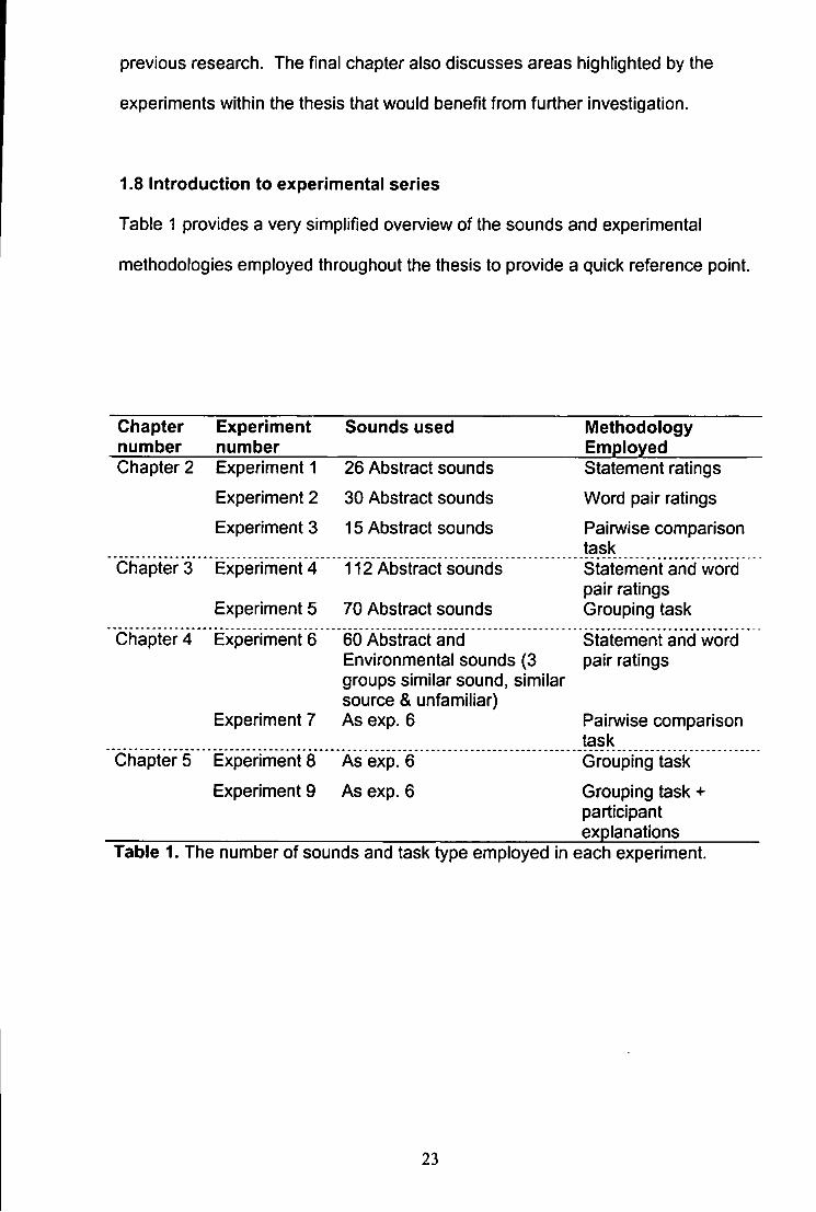
1.8 Introduction to experimental series
Table 1 provides a very simplified overview of the sounds and experimental
methodologies employed throughout the thesis to provide a quick reference point.
Chapter number
Experiment number
Sounds used Methodology Employed
Chapter 2 Experiment 1 26 Abstract sounds Statement ratings
Experiment 2 30 Abstract sounds Word pair ratings
Experiment 3 15 Abstract sounds Pain/vise comparison task
Chapter 3 Experiment 4
Experiment 5
112 Abstract sounds
70 Abstract sounds
Statement and word pair ratings Grouping task
Chapter 4 Experiment 6
Experiment 7
60 Abstract and Environmental sounds (3 groups similar sound, similar source & unfamiliar) As exp. 6
Statement and word pair ratings
Pairwise comparison task
Chapter 5 Experiment 8 As exp. 6 Grouping task
Experiment 9 As exp. 6 Grouping task + participant explanations
Table 1, The number of sounds and task type employed in each experiment.
23
Chapter 2: Experiments 1 to 3
2.1 Introduction
This chapter reports three experiments. The first two were designed to gather
acoustic and perceptual information about a small number of abstract/manmade
sounds. The third experiment employed a similarity judgement task with the aim
of identifying some of the salient acoustic and descriptive features used by
participants when making similarity judgements about the sounds.
Previous experiments have collected acoustic and perceptual information about
everyday, environmental sounds (Ballas 1993; Bonebright 2001) with the intention
of identifying salient features used in cognitive judgements such as the
recognition of a sound (Lass et al, 1982). For example, the acoustic feature of
timbre was identified by Ballas (1993) as an important factor that reflected the
clusters of sounds identified by a principle components analysis. It is necessary
to further the existing knowledge of important features of sounds used in simple
cognitive judgements. There are a huge variety of sounds in our environment and
it has yet to be established whether it Is possible to generalise about specific
sound features of importance in sound perception even within a class of sounds
(Gygi. et al, 2004). Gygi et al (2004) conducted a series of experiments using
sounds with various filters applied (e.g. band pass filters between 300 - 8000Hz)
to test listeners' ability to identify a diverse set of environmental sounds using
limited spectral information. The results indicated that identification was high,
better than 50 percent, when listeners' decisions were based on temporal
information and limited spectral information. Gygi et al (2004) suggested that a
productive approach to understanding the perception of environmental sounds
would be to consider three elements; a sound's acoustic features, the sources
24
and events which produced the sound and higher order semantic features.
However, very modern manmade sounds such as computer bleeps or mobile
phone ring tones have yet to be investigated in any detail. This group of sounds
referred to as abstract sounds throughout the thesis are interesting because they
fit between the environmental sounds investigated by Ballas (1993) for example
and the less complex but unfamiliar sounds such as tones (e.g. Keller et al, 1995).
The information collected in experiments 1 and 2 along with a range of acoustic
measures, was used to identify, in the third experiment, possible salient features
used by the participants when making similarity judgements about the abstract
sounds. As discussed many authors have suggested the importance of a variety
of factors In the identification of sounds. Susini et al (1999) highlighted the
complexity, especially of environmental sounds, and their multidimensional
nature. The aim of experiment 3 was to further the findings from the previous
research on both environmental sounds and work on simple tones. Experiment 3
applied the findings from this previous work to modern abstract sounds such as
telephone rings and alarm clocks allowing for comparison between the work in
different sound areas.
The sounds used in the first three experiments were chosen from a large selection
of sounds that were collected using a minidisk recorder and from free sound
libraries on the internet (www.findsounds.com, sounddogs.com, soundfx.com,
a1freesoundeffects.com). The criteria for inclusion were that the sounds should
be abstract in nature, that is, they must be sounds that do not naturally stem from
the source object. Abstract sounds are sounds that are typically assigned
arbitrarily to an object as opposed to the sound that the object would naturally
make. To clarify, a good example of an environmental sound is an engine
25
running. The sound the engine makes is a result of its physical properties and the
action of the engine. An abstract sound is a sound such as a mobile phone ring
tone where the sound that the phone makes is the sound arbitrarily assigned
through human intervention. As discussed they are sounds that bridge the gap
between environmental sounds and patterns and tones used in other auditory
research and can be familiar or unfamiliar to the listener.
Previous researchers have used two main types of sounds. The first type of
sounds employed have been natural sounds often referred to as environmental
sounds (Ballas, 1993; Bonebright, 2001) that have included animal noises,
engines, running water or objects moving. The main focus for the selection of
these sounds has been to include sounds that are made naturally by the source
object with just a few exceptions, such as, car horn or doorbell (Ballas, 1993).
Other researchers have concentrated on the second main sound group focussing
on sounds that are not naturally present in isolation in our environment such as
pure tones used in memory research (Deutsch, 1982; Pechmann & Mohr, 1992;
Semal & Demany, 1993). The aim of the present experiments was to extend the
research looking at cognitive judgements regarding both environmental sounds
and pure tones to Include sounds that were more modern and could be said to fit
between the two previous categories of sounds. The sounds are still in the
strictest sense sounds that are present in our environment but to set them apart
from the sounds investigated by previous research they will be classed as
'abstract' sounds. The abstract sounds used are all sounds that are assigned to
an object such as a car horn or text message alert rather than the natural sound
of a running engine for example. Therefore, inclusion of the abstract sounds may
help to clarify models of auditory cognition further.
26
As discussed by Edworthy and Hellier (2004) sounds such as modern warning
sounds are no longer constrained in terms of the sounds themselves. The signal
can nowadays be stored as digital code and the sound can therefore take a
multitude of forms. This concept can be applied to many of the abstract sounds
employed in the experiments in this chapter. Previous researchers (Ballas 1993;
Bonebright, 2001) have employed everyday environmental sounds such as
sandpaper or vacuum cleaners as well as a few more sounds that fall in the grey
area between environmental and the current definition of abstract sounds such as
bells. These environmental sounds are constrained by the physiology of the
object that makes them. For more abstract sounds such as mobile phone rings
this does not apply. Although we recognise a modern telephone ring that has
evolved from a traditional bell sound this bell was still arbitrarily assigned to a
phone. Mobile phones have moved another step away from this more familiar
sound and are no longer constrained by the physical properties of the source (i.e.
the bell). These modern phones are an excellent example of abstract sounds.
They are not constrained by the phone and the most up to date phones are
capable of playing MPS format sounds that could actually be any sound a user
desires. Selection of the sounds for experiment one and two (listed and described
in table 1i) was based on variety and features such as length and quality, and the
resulting set of sounds was representative of a range of different sources, e.g.
phones, alarms, horns.
The use of similarity judgements would help to provide data that would go some
way towards answering some fundamental questions about the identification of
sound. Of interest was how acoustic similarities may affect perceptual similarities.
Also of interest were how functional similarities affect perceived familiarities and
how the acoustic features may map onto the descriptive or associative meaning of
27
the sounds. The decision to use similarity judgements from a methodological
point of view was twofold. Firstly, such judgements provide proximity data
required to use multidimensional scaling analysis, a technique to identify hidden
structure in the data. This is a technique that has been successfully applied to
investigations of both tones and environmental sounds (Howard & Silverman,
1976; Bonebright, 2001; Lakatos, Scavone & Cook, 2002) that provides a visual
representation of the sound's location in a multi dimensional space according to
the criteria set, typically judgements of (dis)similarity. In the present study the
aim was to identify hidden sound features (acoustic or descriptive) that may be
used by listeners in similarity judgements made between sounds. Secondly, a
more theoretical reason for the selection of similarity data was that similarity is
one of the most central theoretical constructs in psychology (Medin, Goldstone &
Centner, 1993). In addition, Medin et al (1993) state that similarity is a
comparison process that itself is a fundamental cognitive function and as such
needs to be understood in more depth. Tversky (1977) raised the issue as to
which features of two objects being considered for similarity are the diagnostic
features, that is, which are the important features in the judgement. This is not a
question that has been addressed with reference to sound stimuli. There is also
an ongoing debate in the similarity literature over the extent to which similarity
judgements reflect category judgements (Medin et al. 1993). One of the purposes
of the present work was not to understand similarity judgements in isolation but
rather to add to existing knowledge in the similarity and categorisation literature
because work with sound and similarity is very limited to date.
The three experiments presented in this chapter employ different methodologies.
The first experiment, guided by work conducted by Ballas (1993) identified a
series of cognitive and perceptual features about the sounds such as how familiar
28
a sound is. The second experiment, split from the first for practical reasons,
utilised adjective word pairs identified by Solomon (1958) to collect additional
information about the sounds. In addition to the psychological measures taken in
experiments 1 and 2 a range of acoustic measures were collected to try to
evaluate the contribution of acoustic features to judgements of similarity. Again
the measures chosen were guided by previous work (Bonebright, 2001; Allen &
Bond, 1997; Solomon 1959; Gygi et al, 2004). The acoustic data and
experiments 1 and 2 were preliminary data collection experiments to build a
database of information for each of the sounds selected for testing in the third
experiment.
The third experiment in the chapter employs a pairwise comparison task that
required judgements of similarity between all the sound pairs to provide proximity
data appropriate for multidimensional scaling (MDS). Judgements of similarity are
the most commonly used method for obtaining data for multidimensional scaling
analysis (Schiffman, Reynolds & Young, 1981). MDS analysis is used, in this
instance, as an exploratory technique to obtain comparative evaluations of the
sound stimuli and identify the bases of the similarity judgements. The output
provided by MDS analysis gives a spatial representation, consisting of a
geometric configuration of points similar to a map, with each point representing
one of the stimuli. This configuration reflects the 'hidden structure' in the data and
aids understanding of the data (Kruskall & Wish, 1984). It not only identifies how
the sounds cluster together but provides an insight into the number of dimensions
that participants employed to make their similarity judgements. By identifying the
possible meaning of these dimensions using the acoustic and psychological
measures it is possible to hypothesise which of the sound features are the most
salient with respect to the similarity judgements made.
29
2.2 Introduction to Multidimensional Scaling
Environmental sounds in particular are very complex and as pointed out by Susini
et al (1999) are multidimensional in nature in terms of both acoustic and
perceptual features. Multidimensional scaling is an analysis technique that has
been employed by many researchers in the area of auditory cognition (Berglund.
Hassmen, & Preis. 2002; Bonebright 1996; Howard & Silverman 1976; Schneider
& Bissett 1981; Susini et al, 1999) in order to identify the most salient perceptual
or acoustic dimensions of sounds. The main output is a spatial representation,
consisting of a geometric configuration of points similar to a map (Kruskal et al.
1984). Each of the points corresponds to one of the objects, in the present
research each point would represent a single sound. Therefore, the more
dissimilar two items are judged to be the further apart they will appear on the map.
The output will also suggest the number of dimensions used to make the
(dis)similarity judgements and these can be labelled via visual inspection or by
using correlation techniques with measured features such as pitch. It is the
interpretation of the dimensions that gives an indication to underlying or possibly
hidden features that a participant may have used to make their similarity
judgements and hence the understanding of the resulting spatial configuration.
The graphical display produced by the MDS output enables researchers to look at
the data and explore the structure more visually than is often the case with
statistical techniques. One of the examples most frequently cited to illustrate what
MDS produces from proximities or distance measures is the recreation of a
geographical map (Schiffman eta l , 1981; Borg & Groenen, 1997). If an MDS
program is provided with a proximity matrix containing the distances between ten
cities in the UK the analysis will recreate a configuration that would fit very
accurately if placed over a map of the UK. The orientation of the axis is not
30
necessarily correct as that information is not provided but nonetheless following
rotation the output will be accurate.
MDS has four main purposes: a) as a method that represents (dis)similarity data
as distances in a low dimensional space so that the data are accessible visually;
b) a technique that tests if and how certain criteria by which one can distinguish
among different objects of interest are mirrored in corresponding empirical
differences of these objects; c) as a data analytic approach that allows the
identification of dimensions that underiie judgments of (dis)similarity; and d) as a
psychological model that explains judgements of dissimilarity in terms of a rule
that mimics a particular type of distance function (Borg et al, 1997).
31
2.3 Experiment 1: The collection of cognitive and perceptual data.
2.3.1 Introduction
The purpose of this first experiment was to gather perceptual judgements about
the sounds that will be used in later experiments. In order to identify salient
features of the sounds it was necessary to build up a database containing a
variety of information about each sound. The results will help to guide the
selection of sounds to be included in experiment 3. in addition, they will
contribute, with experiment 2 and the acoustic analysis of the sounds, to providing
the opportunity to investigate the mapping of acoustic features onto the
descriptive features of the sounds. To avoid confusion any measure included in
the current work that was not acoustic is called a descriptive measure. These will
include measures such as whether a sound is calming or exciting as well as
measures such as familiarity. The statements and measures used in this first
experiment were guided by work conducted by Ballas (1993) who identified a
range of cognitive and perceptual features of importance in the identification of
environmental sounds. These included; acoustic variables, ecological frequency
information, causal uncertainty, and sound typicality features. The sounds
included in experiment 1 are, for the most part, different in nature to those
employed by Ballas (1993) because they are all abstract in nature. Therefore,
one of the questions of interest was, whether a similar pattern of salient features
to that found by Ballas (1993) for mostly environmental sounds would apply to the
abstract sounds selected.
Following the selection of the sounds. Experiment One was designed to collect
perceptual information about all the sounds. The ratings collected included mean
identification times (MIT) measured when a participant felt they knew what the
32
sound was. the resulting description (to assess accuracy and any relationship with
MIT), responses to a series of statements asking questions about familiarity, use
of words or images and frequency of occurrence (statements listed in table l i i ) .
This experiment would gather information to address the following issues;
familiarity with the sounds; use of imagery or words when a sound is heard;
whether there is a relationship between a sound's familiarity and mean time to
identify; frequency information about the sounds; and whether a sound is judged
acoustically or by the source. Most of these questions are issues raised by Ballas
(1993) but are issues that have arisen out of other research too.
Familiarity with a sound or a sound's source, one of the issues being investigated
Is an issue that has been raised by many different authors using a variety of
experimental paradigms. Solomon (1958) identified familiarity as one of many
important factors indicated by a series of bipolar adjectives. Similariy Ballas
(1993) identified the importance of familiarity in relation to the identification of an
environmental sound.
2.3.2 Method
2.3.2.1 Participants
32 participants (7 males, 25 females) took part in the study. Participation was
restricted to people with normal or corrected-to-normal hearing. Participants were
awarded points for participation as part of the psychology undergraduate course
requirement or were paid for their time according to their preference.
2.3.2.2 Apparatus
Hewlett Packard Vectra PIN computers (with a 600 MHz Processor, 128 MB RAM
and CrystalSoundFusion""^ Soundcard operating on Windows XP) with
33
headphones were used with a purpose written program "The Encoding and Recall
of Abstract Sound" (Ian St. John, May 2002) to present sound stimuli, statements
and record data.
2.3.2.3 Stimuli
Stimuli consisted of 26 sounds, each approximately 4 seconds in length and
described in table 11. Some sounds were recorded from the real world using a
minidisc recorder (SONY minidisc, MZ - R91). All other sounds were collected
from free sound libraries available on the World Wide Web. Using Sound Forge
V.5 software the sounds were cropped to a mean length of 4 seconds with a
maximum deviation of half a second either side to ensure that an arbitrary cut off
point had minimum distorting effect upon the sound. The attenuation of the
sounds was normalized to an average of -16dB using Cooledit v l .1 software.
Sounds were normalized because Susini et al (1999) suggested that certain
acoustic characteristics perceptually dominate and overpower other less salient
ones, especially the power or loudness of a sound. An effort was made to
minimize the potential for loudness to overpower other acoustic features while
keeping the variation in the sounds' loudness as natural as possible. For
example, a fog horn that is as quiet as a doorbell would not reflect reality.
34
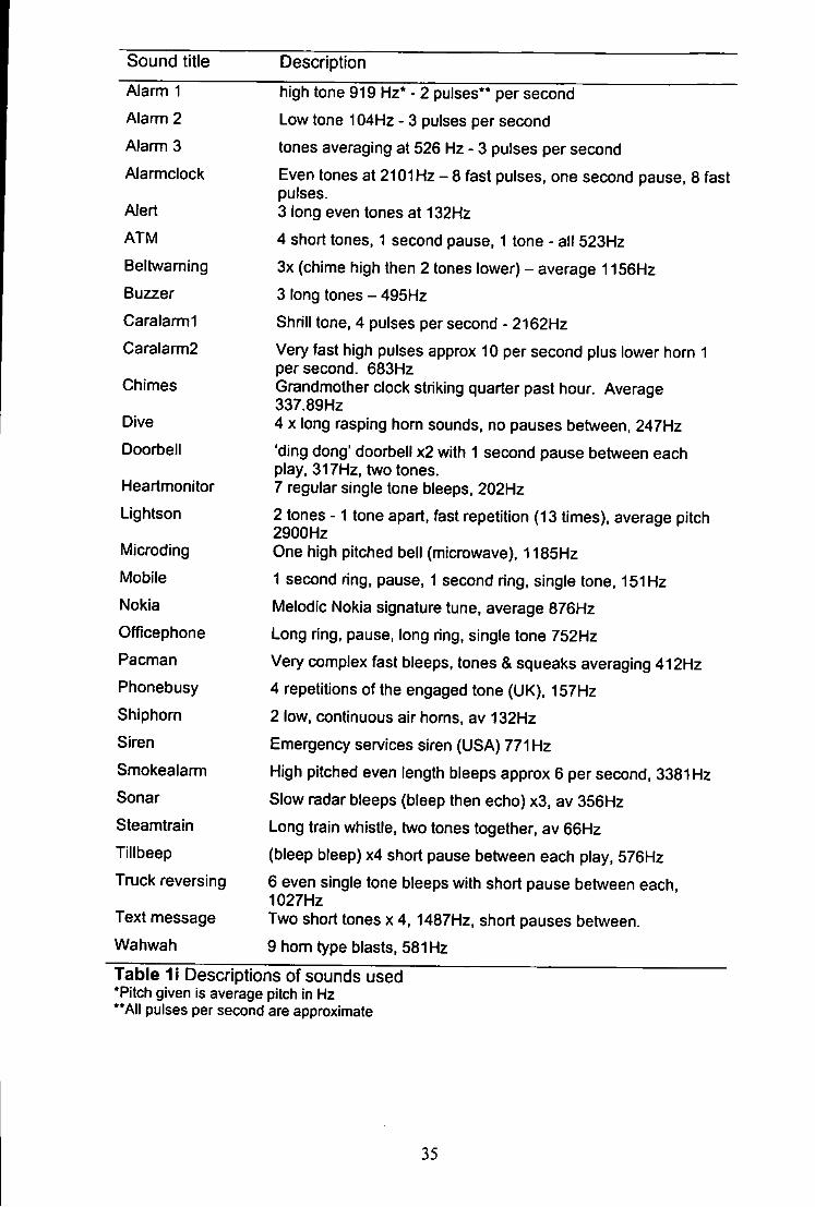
Sound title Description
Alarm 1 Alarm 2 Alarm 3 Alarmclock
Alert ATM Beltwaming Buzzer Caralarmi Caralarm2
Chimes
Dive Doorbell
Heartmonitor Lightson
Microding Mobile Nokia Officephone Pacman Phonebusy Shiphorn Siren Smokealarm Sonar Steamtrain Tillbeep Truck reversing
Text message Wahwah
high tone 919 Hz* - 2 pulses** per second Low tone 104Hz - 3 pulses per second tones averaging at 526 Hz - 3 pulses per second Even tones at 2101Hz - 8 fast pulses, one second pause, 8 fast pulses. 3 long even tones at 132Hz 4 short tones, 1 second pause, 1 tone - all 523Hz 3x (chime high then 2 tones lower) - average 1156Hz 3 long tones - 495Hz Shrill tone, 4 pulses per second - 2162Hz Very fast high pulses approx 10 per second plus lower horn 1 per second, 683Hz Grandmother clock striking quarter past hour. Average 337.89Hz 4 X long rasping horn sounds, no pauses between, 247Hz 'ding dong' doorbell x2 with 1 second pause between each play, 317Hz. two tones. 7 regular single tone bleeps, 202Hz 2 tones -1 tone apart, fast repetition (13 times), average pitch 2900Hz One high pitched bell (microwave), 1185Hz 1 second ring, pause. 1 second ring, single tone, 151 Hz Melodic Nokia signature tune, average 876Hz Long ring, pause, long ring, single tone 752Hz Very complex fast bleeps, tones & squeaks averaging 412Hz 4 repetitions of the engaged tone (UK), 157Hz 2 low. continuous air horns, av 132Hz Emergency services siren (USA) 771 Hz High pitched even length bleeps approx 6 per second. 3381Hz Slow radar bleeps (bleep then echo) x3, av 356Hz Long train whistle, two tones together, av 66Hz (bleep bleep) x4 short pause between each play, 576Hz 6 even single tone bleeps with short pause between each, 1027Hz Two short tones x 4, 1487Hz. short pauses between. 9 horn type blasts, 581 Hz
Table 1i Descriptions of sounds used *Pitch given is average pitch in Hz **AII pulses per second are approximate
35
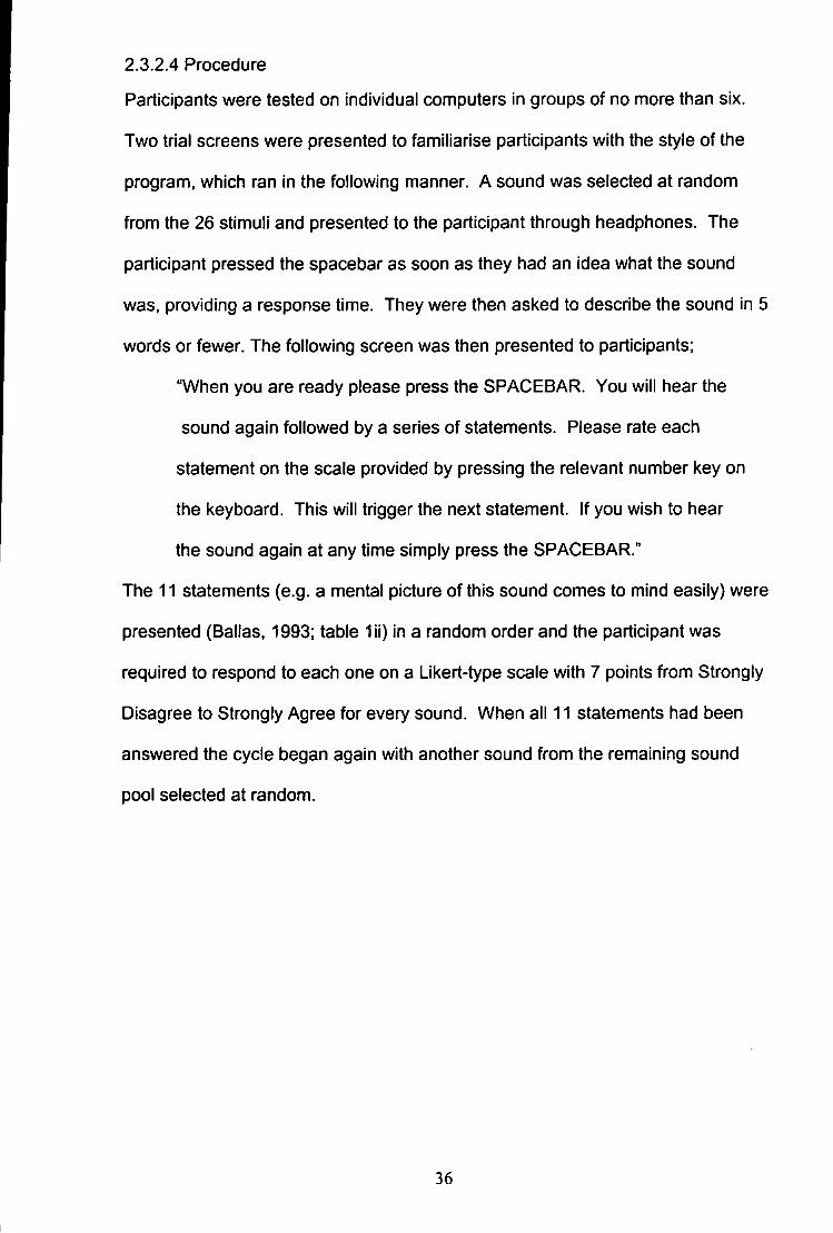
2.3.2.4 Procedure
Participants were tested on Individual computers In groups of no more than six.
Two trial screens were presented to familiarise participants with the style of the
program, which ran in the following manner. A sound was selected at random
from the 26 stimuli and presented to the participant through headphones. The
participant pressed the spacebar as soon as they had an idea what the sound
was, providing a response time. They were then asked to describe the sound In 5
words or fewer. The following screen was then presented to participants;
"When you are ready please press the SPACEBAR. You will hear the
sound again followed by a series of statements. Please rate each
statement on the scale provided by pressing the relevant number key on
the keyboard. This will trigger the next statement. If you wish to hear
the sound again at any time simply press the SPACEBAR."
The 11 statements (e.g. a mental picture of this sound comes to mind easily) were
presented (Ballas, 1993; table 1ii) In a random order and the participant was
required to respond to each one on a Likert-type scale with 7 points from Strongly
Disagree to Strongly Agree for every sound. When all 11 statements had been
answered the cycle began again with another sound from the remaining sound
pool selected at random.
36
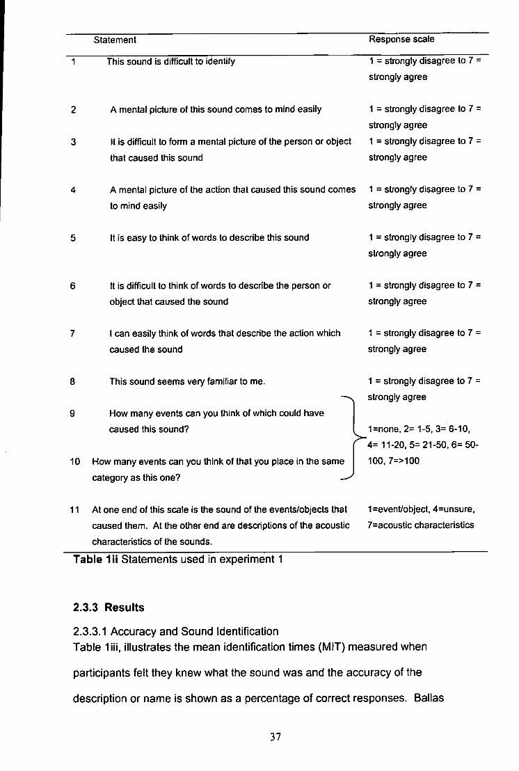
statement Response scale
This sound is difficult to identify 1 = strongly disagree to 7
strongly agree
A mental picture of this sound comes to mind easily
It is difficult to form a mental picture of the person or object
that caused this sound
1 = strongly disagree to 7
strongly agree
1 = strongly disagree to 7
strongly agree
A mental picture of the action that caused this sound comes 1 = strongly disagree to 7
to mind easily strongly agree
It is easy to think of words to describe this sound 1 = strongly disagree to 7
strongly agree
It is difficult to think of words to describe the person or
object that caused the sound
1 = strongly disagree to 7
strongly agree
I can easily think of words that describe the action which
caused the sound
1 = strongly disagree to 7
strongly agree
8 This sound seems very familiar to me.
9 How many events can you think of which could have
caused this sound?
10 How many events can you think of that you place in the same
category as this one? -
1 = strongly disagree to 7 =
strongly agree
1=none. 2= 1-5, 3= 6-10,
4= 11-20, 5= 21-50.6= 50-
100. 7=>100
11 At one end of this scale is the sound of the events/objects that
caused them. At the other end are descriptions of the acoustic
characteristics of the sounds.
Table lii Statements used in experiment 1
1 =event/object, 4=unsure.
7=acoustic characteristics
2.3.3 Results
2.3.3.1 Accuracy and Sound Identification
Table lii i, illustrates the mean identification times (IVIIT) measured when
participants felt they knew what the sound was and the accuracy of the
description or name is shown as a percentage of correct responses. Ballas
37
(1993) identified that MIT varied according to the identified categories to which the
sounds belonged, such as water or door sounds but no such pattern is evident in
the present results, mainly due to the difference in sounds selected for inclusion.
Correct response was measured following guidelines used by Marcell (2000) for
environmental sounds (inter rater reliability in final column table 1iii). As found by
Marcell (2000) although some sounds such as nokia ring were named accurately
by most participants a large number of sounds were accurately described with
several different but appropriate words. Therefore, responses were marked
correct if the following were used; a synonym for the sound label, an accurate
description of the sound source, a correct identification with extraneous
Information, or an acoustically precise alternative. In the table participants'
familiarity with the sound is measured using statement 8 - this sound is familiar to
me and the ease with which they could identify the sound was measured using
statement 1 - this sound is difficult to identify. Rescoring the data for statement 1
makes the results clearer to see in table 1iii without interference from the polarity
of the questions. Therefore, for both statements 1 and 8 the higher the score the
more familiar and the more easily identifiable the sound. The sounds are listed in
descending order according to responses on statement 8, therefore those sounds
at the top of the table have a mean rating indicating that they are familiar and
easy to identify compared to those at the bottom of the table.
38
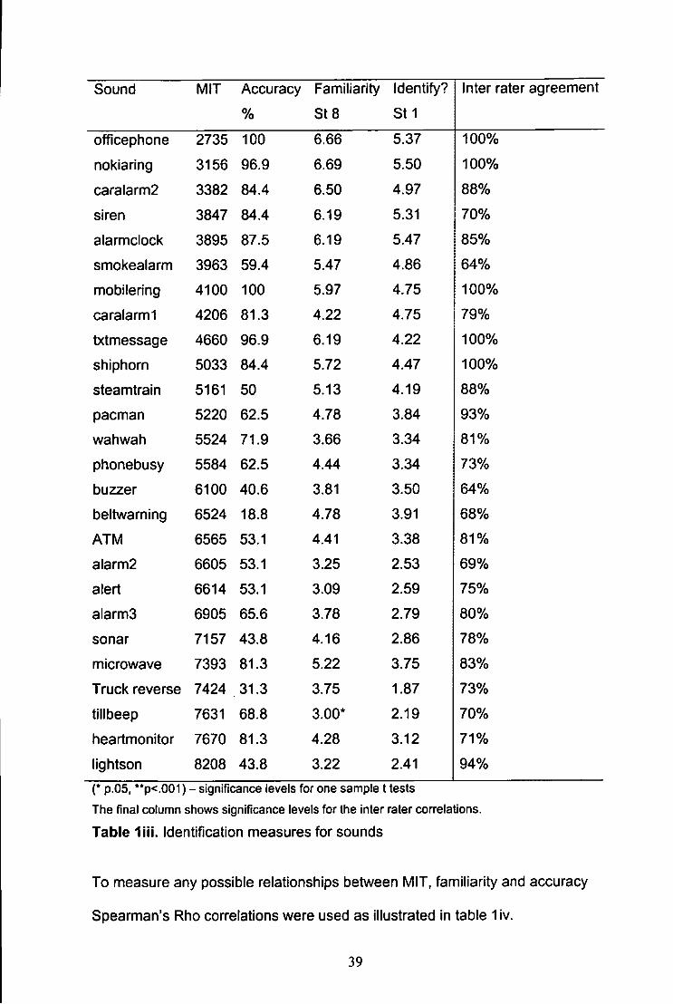
Sound MIT Accuracy Familiarity Identify? Inter rater agreement
% St 8 St 1
officephone 2735 100 6.66 5.37 100%
nokiaring 3156 96.9 6.69 5.50 100%
caralarm2 3382 84.4 6.50 4.97 88%
siren 3847 84.4 6.19 5.31 70%
alarmclock 3895 87.5 6.19 5.47 85%
smokealarm 3963 59.4 5.47 4.86 64%
mobilering 4100 100 5.97 4.75 100%
caralarmi 4206 81.3 4.22 4.75 79%
txtmessage 4660 96.9 6.19 4.22 100%
shiphorn 5033 84.4 5.72 4.47 100%
steamtrain 5161 50 5.13 4.19 88%
pacman 5220 62.5 4.78 3.84 93%
wahwah 5524 71.9 3.66 3.34 81%
phonebusy 5584 62.5 4.44 3.34 73%
buzzer 6100 40.6 3.81 3.50 64%
beltwarning 6524 18.8 4.78 3.91 68%
ATM 6565 53.1 4.41 3.38 81%
alarm2 6605 53.1 3.25 2.53 69%
alert 6614 53.1 3.09 2.59 75%
alarm3 6905 65.6 3.78 2.79 80%
sonar 7157 43.8 4.16 2.86 78%
microwave 7393 81.3 5.22 3.75 83%
Truck reverse 7424 31.3 3.75 1.87 73%
tillbeep 7631 68.8 3.00* 2.19 70%
heartmonitor 7670 81.3 4.28 3.12 71%
lightson 8208 43.8 3.22 2.41 94%
(* p.05, "p<.001) - significance levels for one sample t tests
The final column shows significance levels for the inter rater correlations.
Table Identification measures for sounds
To measure any possible relationships between MIT, familiarity and accuracy
Spearman's Rho correlations were used as Illustrated in table 1iv.
39
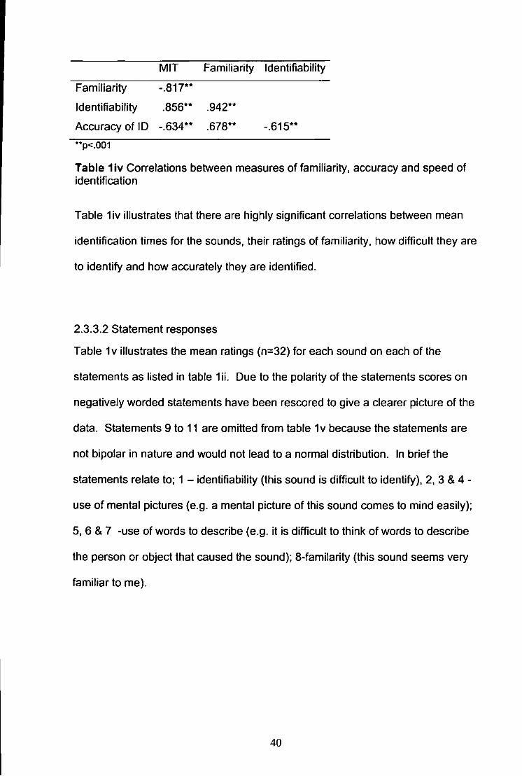
MIT Familiarity Identifiability
Familiarity -.817"
Identifiability .856" .942"
Accuracy of ID -.634" .678" -.615" "p<.001
Table 1iv Correlations between measures of familiarity, accuracy and speed of identification
Table 1iv illustrates that there are highly significant correlations between mean
identification times for the sounds, their ratings of familiarity, how difficult they are
to identify and how accurately they are identified.
2.3.3.2 Statement responses
Table 1 v illustrates the mean ratings (n=32) for each sound on each of the
statements as listed in table 1ii. Due to the polarity of the statements scores on
negatively worded statements have been rescored to give a clearer picture of the
data. Statements 9 to 11 are omitted from table 1v because the statements are
not bipolar in nature and would not lead to a normal distribution. In brief the
statements relate to; 1 - identifiability (this sound is difficult to identify). 2. 3 & 4 -
use of mental pictures (e.g. a mental picture of this sound comes to mind easily);
5, 6 & 7 -use of words to describe (e.g. it is difficult to think of words to describe
the person or object that caused the sound); 8-famiIarity (this sound seems very
familiar to me).
40
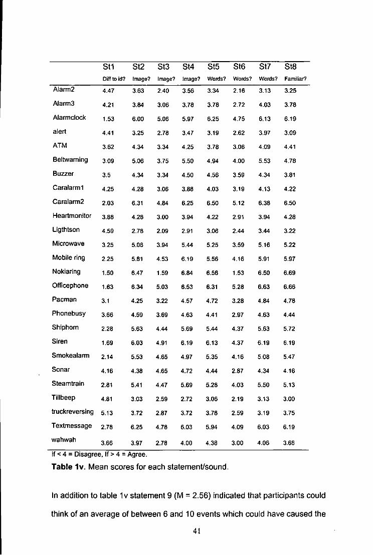
St1 St2 St3 St4 St5 St6 St7 St8 Diff to id? Image? Image? Image? Words? Words? Words? Familiar?
Alarm2 4.47 3.63 2.40 3.56 3.34 2.16 3.13 3.25
Alarms 4.21 3.84 3.06 3.78 3.78 2.72 4.03 3.78
Alarm clock 1.53 6.00 5.06 5.97 6.25 4.75 6.13 6.19
alert 4.41 3.25 2.78 3.47 3.19 2.62 3.97 3.09
ATM 3.62 4.34 3.34 4.25 3.78 3.06 4.09 4.41
Beltwaming 3.09 5.06 3.75 5.50 4.94 4.00 5.53 4.78
Buzzer 3.5 4.34 3.34 4.50 4.56 3.59 4.34 3.81
Caralarmi 4.25 4.28 3,06 3.88 4.03 3.19 4.13 4.22
Caralarm2 2.03 6.31 4.84 6.25 6.50 5.12 6.38 6.50
Heartmonitor 3.88 4.28 3.00 3.94 4.22 2.91 3.94 4.28
Ligthtson 4.59 2.78 2.09 2.91 3.06 2.44 3.44 3.22
Microwave 3.25 5.06 3.94 5.44 5.25 3.59 5.16 5.22
Mobile ring 2.25 5.81 4.53 6.19 5.56 4.16 5.91 5.97
Nokiaring 1.50 6.47 1.59 6.84 6.56 1.53 6.50 6.69
Officephone 1.63 6.34 5.03 6.53 6.31 5.28 6.63 6.66
Pacman 3.1 4.25 3.22 4.57 4.72 3.28 4.84 4.78
Phonebusy 3.66 4.59 3.69 4.63 4.41 2.97 4.63 4.44
Shiphom 2.28 5.63 4.44 5.69 5.44 4.37 5.63 5.72
Siren 1.69 6.03 4.91 6.19 6.13 4.37 6.19 6.19
Smokealarm 2.14 5.53 4.65 4.97 5.35 4.16 5.08 5.47
Sonar 4.16 4.38 4.65 4.72 4.44 2.87 4.34 4.16
Steamtrain 2.81 5.41 4.47 5.69 5.28 4.03 5.50 5.13
Tillbeep 4.81 3.03 2.59 2.72 3.06 2.19 3.13 3.00
truckreversing 5.13 3.72 2.87 3.72 3.78 2.59 3.19 3.75
Textmessage 2.78 6.25 4.78 6.03 5.94 4.09 6.03 6.19
wahwah 3.66 3.97 2.78 4.00 4.38 3.00 4.06 3.66
If < 4 = Disagree, If > 4 = Agree.
Table 1v. Mean scores for each statement/sound.
In addition to table 1v statement 9 (M = 2.56) Indicated that participants could
think of an average of between 6 and 10 events which could have caused the
41
sound. Similarly the mean score for statement 10 (M = 2.50) indicated that
participants could typically think of between 6 and 10 events that could be placed
in the same category as the sound being rated. Finally the mean score for
statement 11 (M = 3.23) indicated that overall when asked to place a sound on a
scale, ranging from the event or object that caused the sound (rating 1) to the
acoustic characteristics (rating 7), participants typically placed the sound in the
middle of the scale in the 'unsure' section around the midway point of 4.
Exceptions to this were caralarm2, mobilering, nokiaring, officephone and siren
which were all placed towards the event/object end of the scale.
2,3.3.3 Correlations between statement subgroups
An example of the correlations observed between the statements is illustrated in
table Ivi, in this instance for the mobile phone ring tone. To collapse across the
sound stimuli would make the mean scores for the statements meaningless as the
nature of the stimuli are so variable. Similar correlation tables can be seen in
appendix A1 for all the sounds. The table illustrates that there are highly
significant correlations between the three statements measuring the use of mental
imagery (2,3 & 4) and the three statements measuring the use of words (5. 6 & 7)
and this serves to demonstrate that each of the measures for words or imagery
can be considered to be reliable because similar responses are repeated across
each statement. This pattern was repeated across the majority of sounds, as
illustrated by the correlation tables for every sound in appendix A1. No sound
showed a complete lack of correlations between these two statement sub-groups
(words and imagery).
42
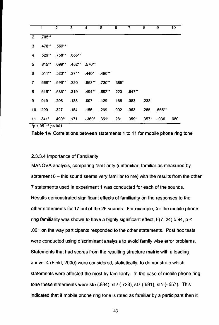
1 2 3 4 5 6 7 8 9 10
2 .705"
3 .478" .569"
4 .529" .758" .656"
5 .815" .699" .482" .570**
6 .511" .533" .371* .440* .480**
7 .666" .696" .320 .663** .730** .385*
8 .619" .686" .319 .494" .692** .223 .647**
9 .049 .208 .188 .007 .129 .166 .083 .238
10 .290 .327 .154 .156 .299 .092 .063 .286 .666**
11 .341* .490" .171 -.360* .361* .281 .359* .357* -.036 .080
*p <.05. ** p<.001
Table 1vi Correlations between statements 1 to 11 for mobile phone ring tone
2.3.3.4 Importance of Familiarity
MANOVA analysis, comparing familiarity (unfamiliar, familiar as measured by
statement 8 - this sound seems very familiar to me) with the results from the other
7 statements used in experiment 1 was conducted for each of the sounds.
Results demonstrated significant effects of familiarity on the responses to the
other statements for 17 out of the 26 sounds. For example, for the mobile phone
ring familiarity was shown to have a highly significant effect, F(7, 24) 5.94, p <
.001 on the way participants responded to the other statements. Post hoc tests
were conducted using discriminant analysis to avoid family wise error problems.
Statements that had scores from the resulting structure matrix with a loading
above .4 (Field, 2000) were considered, statistically, to demonstrate which
statements were affected the most by familiarity. In the case of mobile phone ring
tone these statements were st5 (.834), st2 (.723), st7 (.691), sti (-.557). This
indicated that if mobile phone ring tone is rated as familiar by a participant then it
43
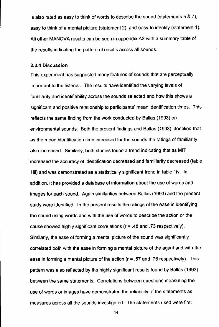
Is also rated as easy to think of words to describe the sound (statements 5 & 7),
easy to think of a mental picture (statement 2). and easy to identify (statement 1).
All other MANOVA results can be seen in appendix A2 with a summary table of
the results indicating the pattern of results across all sounds.
2.3.4 Discussion
This experiment has suggested many features of sounds that are perceptually
Important to the listener. The results have Identified the varying levels of
familiarity and identifiabllity across the sounds selected and how this shows a
significant and positive relationship to participants' mean Identification times. This
reflects the same finding from the work conducted by Ballas (1993) on
environmental sounds. Both the present findings and Ballas (1993) identified that
as the mean identification time Increased for the sounds the ratings of familiarity
also Increased. SImilariy, both studies found a trend Indicating that as MIT
increased the accuracy of identification decreased and familiarity decreased (table
liii) and was demonstrated as a statistically significant trend in table liv. In
addition, it has provided a database of information about the use of words and
images for each sound. Again similarities between Ballas (1993) and the present
study were identified. In the present results the ratings of the ease In identifying
the sound using words and with the use of words to describe the action or the
cause showed highly significant correlations (r = .48 and .73 respectively).
Similariy. the ease of forming a mental picture of the sound was significantly
correlated both with the ease in forming a mental picture of the agent and with the
ease in forming a mental picture of the action (r = .57 and .76 respectively). This
pattern was also reflected by the highly significant results found by Ballas (1993)
between the same statements. Correlations between questions measuring the
use of words or images have demonstrated the reliability of the statements as
measures across all the sounds investigated. The statements used were first
44
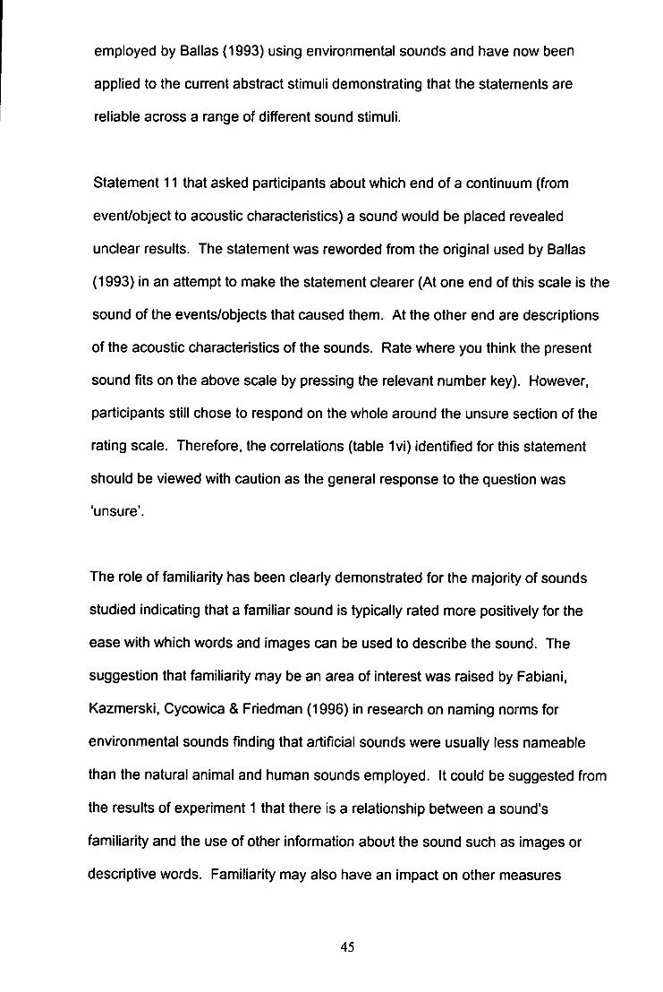
employed by Bellas (1993) using environmental sounds and have now been
applied to the current abstract stimuli demonstrating that the statements are
reliable across a range of different sound stimuli.
Statement 11 that asked participants about which end of a continuum (from
event/object to acoustic characteristics) a sound would be placed revealed
unclear results. The statement was reworded from the original used by Ballas
(1993) in an attempt to make the statement clearer (At one end of this scale is the
sound of the events/objects that caused them. At the other end are descriptions
of the acoustic characteristics of the sounds. Rate where you think the present
sound fits on the above scale by pressing the relevant number key). However,
participants still chose to respond on the whole around the unsure section of the
rating scale. Therefore, the correlations (table 1vi) identified for this statement
should be viewed with caution as the general response to the question was
'unsure'.
The role of familiarity has been cleariy demonstrated for the majority of sounds
studied indicating that a familiar sound is typically rated more positively for the
ease with which words and images can be used to describe the sound. The
suggestion that familiarity may be an area of interest was raised by Fabiani,
Kazmerski. Cycowica & Friedman (1996) in research on naming norms for
environmental sounds finding that artificial sounds were usually less nameable
than the natural animal and human sounds employed. It could be suggested from
the results of experiment 1 that there is a relationship between a sound's
familiarity and the use of other information about the sound such as images or
descriptive words. Familiarity may also have an impact on other measures
45
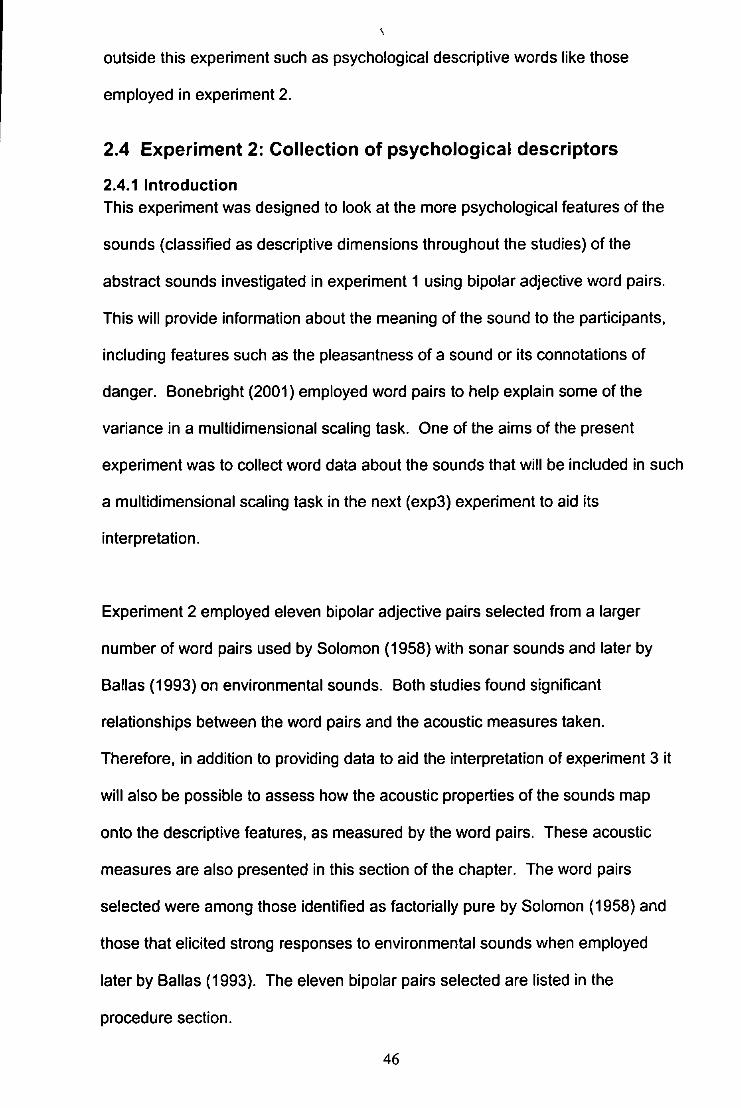
outside this experiment such as psychological descriptive words like those
employed in experiment 2.
2.4 Experiment 2: Collection of psychological descriptors
2.4.1 Introduction
This experiment was designed to look at the more psychological features of the
sounds (classified as descriptive dimensions throughout the studies) of the
abstract sounds investigated In experiment 1 using bipolar adjective word pairs.
This will provide information about the meaning of the sound to the participants,
including features such as the pleasantness of a sound or Its connotations of
danger. Bonebright (2001) employed word pairs to help explain some of the
variance In a multidimensional scaling task. One of the aims of the present
experiment was to collect word data about the sounds that will be included in such
a multidimensional scaling task In the next (exp3) experiment to aid its
Interpretation.
Experiment 2 employed eleven bipolar adjective pairs selected from a larger
number of word pairs used by Solomon (1958) with sonar sounds and later by
Ballas (1993) on environmental sounds. Both studies found significant
relationships between the word pairs and the acoustic measures taken.
Therefore, in addition to providing data to aid the interpretation of experiment 3 it
will also be possible to assess how the acoustic properties of the sounds map
onto the descriptive features, as measured by the word pairs. These acoustic
measures are also presented In this section of the chapter. The word pairs
selected were among those identified as factorially pure by Solomon (1958) and
those that elicited strong responses to environmental sounds when employed
later by Ballas (1993). The eleven bipolar pairs selected are listed in the
procedure section.
46
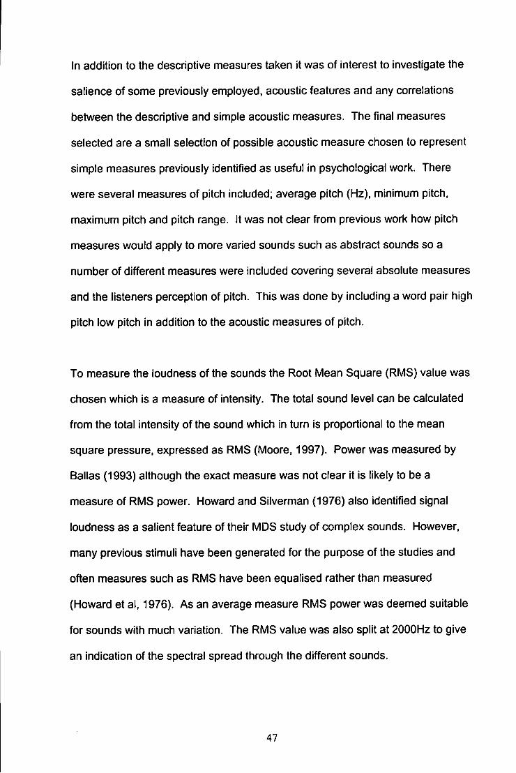
In addition to the descriptive measures taken it was of interest to investigate the
salience of some previously employed, acoustic features and any correlations
between the descriptive and simple acoustic measures. The final measures
selected are a small selection of possible acoustic measure chosen to represent
simple measures previously identified as useful in psychological work. There
were several measures of pitch included; average pitch (Hz), minimum pitch,
maximum pitch and pitch range. It was not clear from previous work how pitch
measures would apply to more varied sounds such as abstract sounds so a
number of different measures were included covering several absolute measures
and the listeners perception of pitch. This was done by including a word pair high
pitch low pitch in addition to the acoustic measures of pitch.
To measure the loudness of the sounds the Root Mean Square (RMS) value was
chosen which is a measure of intensity. The total sound level can be calculated
from the total intensity of the sound which in turn is proportional to the mean
square pressure, expressed as RMS (Moore, 1997). Power was measured by
Ballas (1993) although the exact measure was not clear it is likely to be a
measure of RMS power. Howard and Silverman (1976) also identified signal
loudness as a salient feature of their MDS study of complex sounds. However,
many previous stimuli have been generated for the purpose of the studies and
often measures such as RMS have been equalised rather than measured
(Howard et al, 1976). As an average measure RMS power was deemed suitable
for sounds with much variation. The RMS value was also split at 2000Hz to give
an indication of the spectral spread through the different sounds.
47
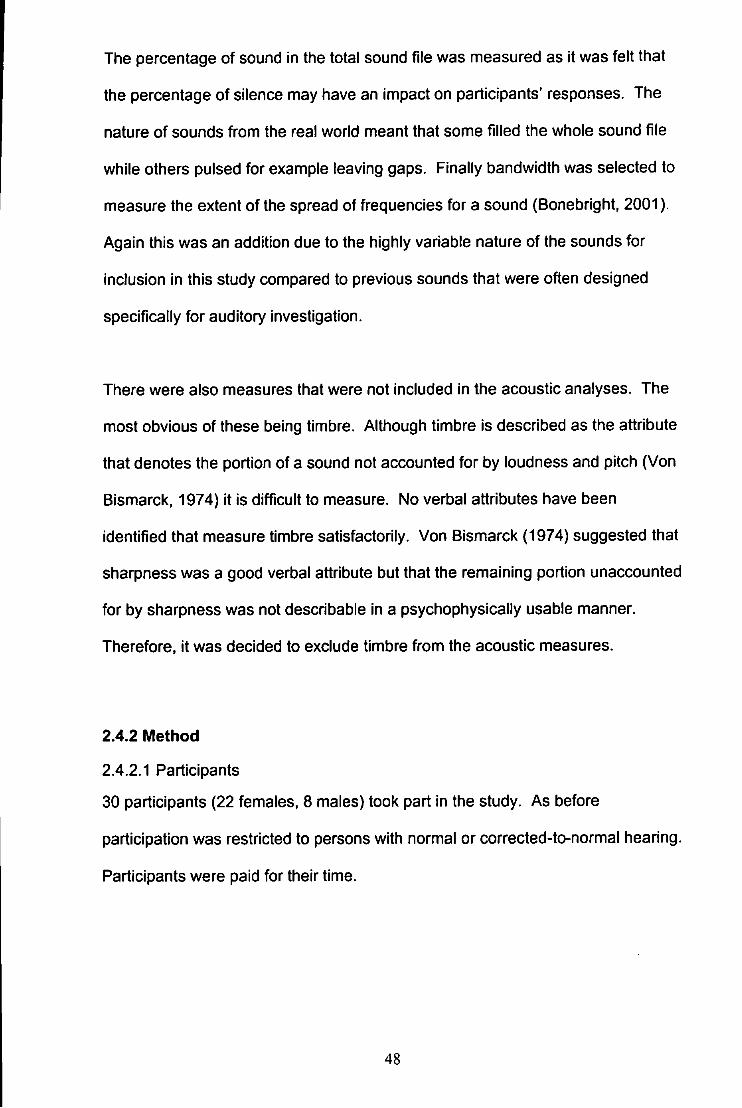
The percentage of sound in the total sound file was measured as it was felt that
the percentage of silence may have an impact on participants' responses. The
nature of sounds from the real worid meant that some filled the whole sound file
while others pulsed for example leaving gaps. Finally bandwidth was selected to
measure the extent of the spread of frequencies for a sound (Bonebright, 2001).
Again this was an addition due to the highly variable nature of the sounds for
inclusion in this study compared to previous sounds that were often designed
specifically for auditory investigation.
There were also measures that were not included in the acoustic analyses. The
most obvious of these being timbre. Although timbre is described as the attribute
that denotes the portion of a sound not accounted for by loudness and pitch (Von
Bismarck, 1974) It is difficult to measure. No verbal attributes have been
identified that measure timbre satisfactorily. Von Bismarck (1974) suggested that
sharpness was a good verbal attribute but that the remaining portion unaccounted
for by sharpness was not describable in a psychophysically usable manner.
Therefore, it was decided to exclude timbre from the acoustic measures.
2.4.2 Method
2.4.2.1 Participants
30 participants (22 females, 8 males) took part in the study. As before
participation was restricted to persons with normal or corrected-to-normal hearing.
Participants were paid for their time.
48
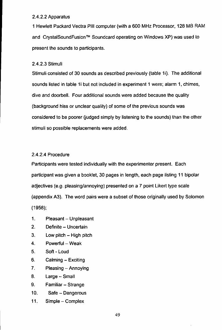
2.4.2.2 Apparatus
1 Hewlett Packard Vectra PIN computer (with a 600 MHz Processor, 128 MB RAM
and CrystalSoundFusion™ Soundcard operating on Windows XP) was used to
present the sounds to participants.
2.4.2.3 Stimuli
Stimuli consisted of 30 sounds as described previously (table 1i). The additional
sounds listed in table 11 but not included in experiment 1 were; alarm 1, chimes,
dive and doorbell. Four additional sounds were added because the quality
(background hiss or unclear quality) of some of the previous sounds was
considered to be poorer Oudged simply by listening to the sounds) than the other
stimuli so possible replacements were added.
2.4.2.4 Procedure
Participants were tested individually with the experimenter present. Each
participant was given a booklet, 30 pages in length, each page listing 11 bipolar
adjectives (e.g. pleasing/annoying) presented on a 7 point Likert type scale
(appendix A3). The word pairs were a subset of those originally used by Solomon
(1958);
1. Pleasant - Unpleasant
2. Definite - Uncertain
3. Low pitch - High pitch
4. Powerful - Weak
5. Soft - Loud
6. Calming - Exciting
7. Pleasing - Annoying
8. Large - Small
9. Familiar - Strange
10. Safe - Dangerous
11. Simple - Complex
49
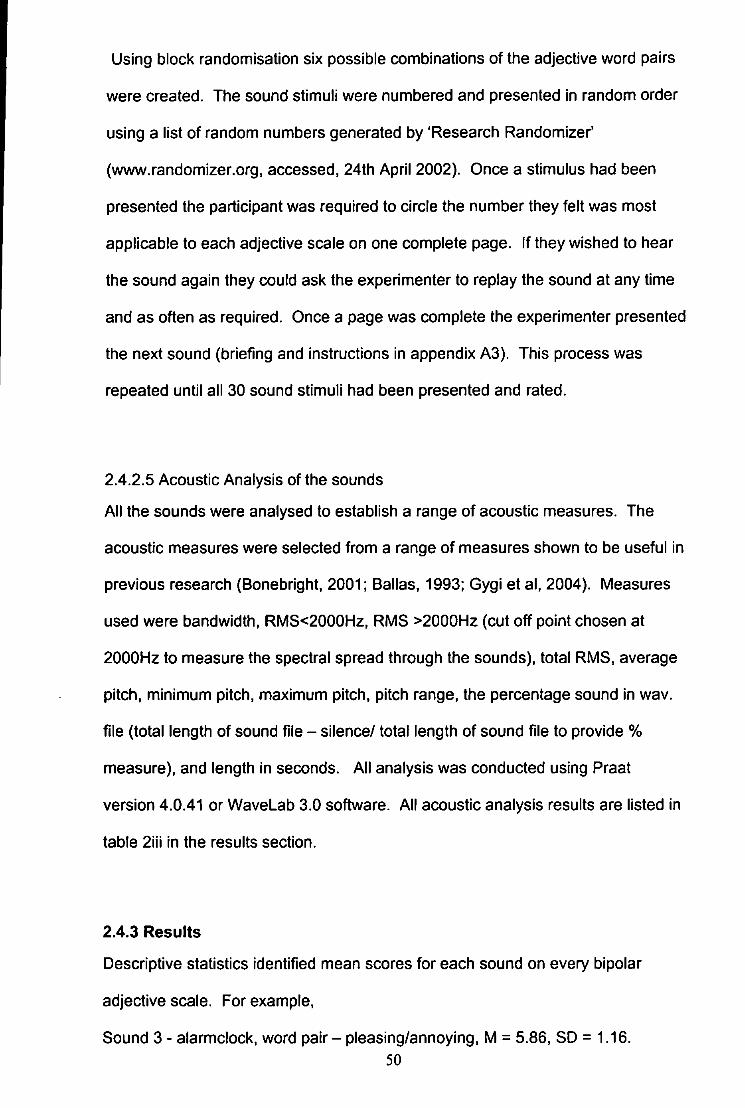
Using block randomisation six possible combinations of the adjective word pairs
were created. The sound stimuli were numbered and presented In random order
using a list of random numbers generated by 'Research Randomizer'
(www.randomizer.org, accessed, 24th April 2002). Once a stimulus had been
presented the participant was required to circle the number they felt was most
applicable to each adjective scale on one complete page. If they wished to hear
the sound again they could ask the experimenter to replay the sound at any time
and as often as required. Once a page was complete the experimenter presented
the next sound (briefing and instructions In appendix A3). This process was
repeated until all 30 sound stimuli had been presented and rated.
2.4.2.5 Acoustic Analysis of the sounds
All the sounds were analysed to establish a range of acoustic measures. The
acoustic measures were selected from a range of measures shown to be useful In
previous research (Bonebright. 2001; Ballas, 1993; Gygi et al, 2004). Measures
used were bandwidth, RMS<2000Hz, RMS >2000Hz (cut off point chosen at
2000Hz to measure the spectral spread through the sounds), total RMS, average
pitch, minimum pitch, maximum pitch, pitch range, the percentage sound in wav.
file (total length of sound file - silence/ total length of sound file to provide %
measure), and length in seconds. All analysis was conducted using Praat
version 4.0.41 or WaveLab 3.0 software. All acoustic analysis results are listed in
table 2lli In the results section.
2.4.3 Results
Descriptive statistics Identified mean scores for each sound on every bipolar
adjective scale. For example,
Sound 3 - alarmclock, word pair - pleasing/annoying, M = 5.86, SD = 1.16. 50
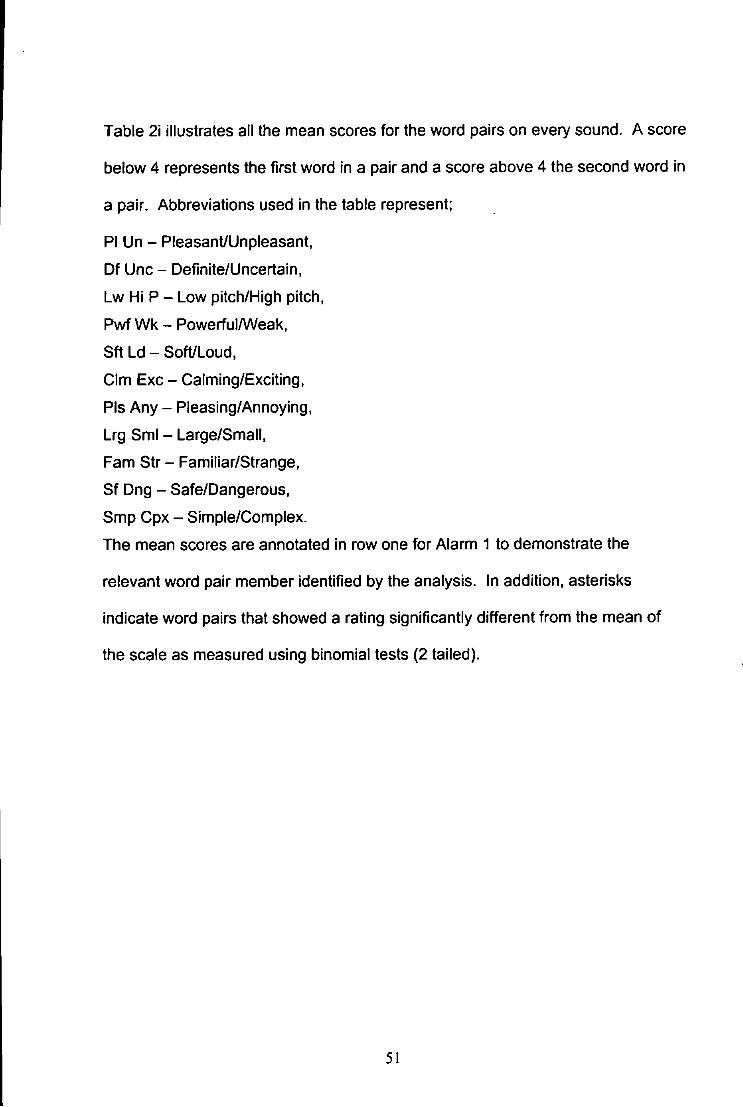
Table 2i illustrates all the mean scores for the word pairs on every sound. A score
below 4 represents the first word in a pair and a score above 4 the second word in
a pair. Abbreviations used in the table represent;
PI Un - Pleasant/Unpleasant,
Df Unc - Definite/Uncertain,
Lw Hi P - Low pitch/High pitch,
Pwf Wk - Powerful/Weak,
Sft Ld - Soft/Loud,
CIm Exc - Calming/Exciting,
Pis Any - Pleasing/Annoying,
Lrg SmI - Large/Small,
Fam Str - Familiar/Strange,
Sf Dng - Safe/Dangerous.
Smp Cpx - Simple/Complex.
The mean scores are annotated in row one for Alarm 1 to demonstrate the
relevant word pair member identified by the analysis. In addition, asterisks
indicate word pairs that showed a rating significantly different from the mean of
the scale as measured using binomial tests (2 tailed).
51
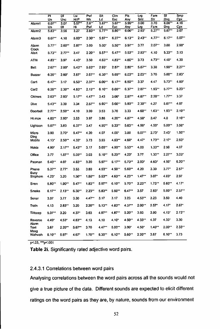
PI Df Lw Pwf Sft CIm Pis Lrg Fam Sf Smp Un Unc HiP Wk Ld Exc Any SmI Str Onq Cpx
Alarm 1 6.07" 3.07 5.57" 2.6" 5.67" 5.67" 5.90" 3.00 3.70 6.00" 4.16 Un Df Hi Pwf Ld Exc Any 1^ Fam Dng Cpx
Alami2 5.83" 3.56 3.27 2.83" 5.77" 5.60" 6.00" 2.93* 5.27" 5.67" 3.67
Alann3 6.07" 4.10 5.03" 2.30** 5.97" 6.27" 6.13" 2.43" 4.77" 6.17" 5.07'*
Alami 5.77" 2.60** 5.87" 3.00 5.00- 5.50" 5.97" 3.77 2.07" 3.00 2.90' aock Alert 5.73" 2.77" 3.47 2.20" 5.57" 5.47" 5.53" 2.53" 4.10 5.33" 3.13
ATM 4.83" 3.97 4.43* 3.50 4.63'" 4.83** 4.60" 3.73 4.73" 4.40' 4.30
Belt 2.67" 2.80' 5.43" 5.03" 2.93' 2.87* 2.80*' 5.67" 3.30 1.90** 2.27"
Buzzer 6.20" 2.60' 2.87' 2.07" 6.30" 5.60" 6.03" 2.03** 3.70 5.80" 2.83'
Carl 6.47" 3.17 6.53" 2.37" 6.00" 6.17" 6.50" 3.37 4.47 5.73" 4.80'
Car2 6.20" 2.30** 4.83" 2.13" 6.10" 6.00" 6.37" 2.07" 1.93" 5.77" 5.23"
Chimes 2.63" 2.93' 5.17" 4.47" 3.43 3.00* 2.67" 4.87" 2.20'* 1.77" 3.37
Dive 5.43" 3.30 3.34 2.57" 5.90** 5.60** 5.80" 2.30** 4.27 5.67" 4.07
Doortsell 2.77" 2.50'* 4.10 3.90 3.53 3.70 3.33 4.60** 1.63" 1.93" 2.10**
Ht mon 4.80" 2.90' 3.53 3.97 3.86 4.20" 4.87" 4.50* 3.47 4.0 2.10'*
LIghtson 5.67" 3.83 6.37" 3.47 4.90** 5.33" 5.63" 4.50* 4.50* 5.00" 3.50'
Micro 3.90 2.70* 5.47" 4.20 4.07 4.00* 3.80 5.07" 2.73' 2.43* 1.50" Ding Mobile 4.13' 2.50" 4.33' 3.73 3.93 4.63" 4.60* 4.47' 1.73" 2.17' 2.93'
Nokia 4.90* 2.17" 5.43" 3.17 5.00** 4.90" 5.53*' 4.00 1.33" 2.50 4.07
Office 3.77 1.87" 5.00" 3.03 5.10" 5.20" 4.23' 3.77 1.30" 2.27" 3.03'
Pacman 5.43" 4.07 4.63" 3.20 5.97" 6.17" 5.73" 2.93' 4.63' 4.50' 6.20"
Phone 5.37" 2.77' 3.53 3.80 4.53" 4.50" 5.60" 4.20 3.30 3.77- 2.57' Busy Shiphom 4.23* 3.20 1.50" 1.80" 5.53" 4.63" 4.23" 1.47" 3.07* 4.03' 2.97
Siren 5.80" 1.90" 5.47" 1.83" 5.97" 6.10" 5.70** 2.23" 1.73" 5.60" 4.17'
Smoke 6.17" 2.13" 6.30" 2.23" 5.83*' 5.90" 6.47" 3.57 2.83* 5.90*' 2.57"
Sonar 3.07 3.77 3.30 4.47" 3.17 3.17 3.23 4.53" 3.23 3.50 4.40
Train 4.13 2.83" 3.20 2.20" 5.13" 4.83" 4.37" 2.00" 2.57* 4.17* 2.87'
Tillbeep 5.07" 3.20 4.37' 3.63 4.97" 4.87" 5.20" 3.93 3.90 4.13* 2.73"
Reverse 4.40* 4.53' 4.83" 4.13 4.10 4.10* 4.50" 4.33" 4.37 4.33* 3.30 Alami Text 3.67 2.20" 5.67" 3.70 4.47" 5.00" 3.90* 4.50' 1.40*' 2.00" 2.33" Mssg Wahwah 6.10" 5.97' 4.67* 1.70*' 6.30" 6.10" 5.60" 2.20" 3.67 6.10" 3.73
p<.05, **p<.001
Table 21 Significantly rated adjective word pairs.
2.4.3.1 Correlations between word pairs
Analysing correlations between the word pairs across all the sounds would not
give a true picture of the data. Different sounds are expected to elicit different
ratings on the word pairs as they are, by nature, sounds from our environment
52
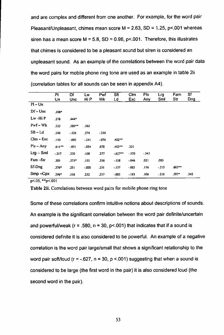
and are complex and different from one another. For example, for the word pair
Pleasant/Unpleasant, chimes mean score M = 2.63, SD = 1.25. p<.001 whereas
siren has a mean score M = 5.8. SD = 0.96, p<.001. Therefore, this illustrates
that chimes is considered to be a pleasant sound but siren is considered an
unpleasant sound. As an example of the con-elations between the word pair data
the word pairs for mobile phone ring tone are used as an example in table 2ii
(correlation tables for all sounds can be seen in appendix A4).
PI Df Lw Pwf Sfl Clm Pis Lrg Fam Sf
Un Unc HiP Wk Ld Exc Any SmI Str Dng
P l - U n
D f - U n c .390*
Lw -Hi P .278 .444*
Pwf-Wk .233 .580** .262
S f t - L d .248 -.126 .274 -.256
Clm - Exc .110 -.092 -.241 -.076 .482**
Pis - Any .611** -.051 -.054 .078 .463** .331
Lrg - SmI -.217 .330 .108 .277 -.627** -.220 -.347
Fam-Str .303 .375* .155 .356 -.158 -.046 .021 .005
Sf-Dng .376* .251 -.020 .251 -.137 -.085 .176 -.215 .605**
Smp -Cpx .396* .316 .232 .237 -.005 -.183 .106 -.216 .397* .342
p<.05,**p<.00I
Table 2ii. Correlations between word pairs for mobile phone ring tone
Some of these correlations confirm intuitive notions about descriptions of sounds.
An example is the significant correlation between the word pair definite/uncertain
and powerful/weak (r = .580, n = 30, p<.001) that indicates that if a sound is
considered definite it is also considered to be powerful. An example of a negative
correlation is the word pair large/small that shows a significant relationship to the
word pair soft/loud (r = -.627, n = 30, p <.001) suggesting that when a sound is
considered to be large (the first word in the pair) it is also considered loud (the
second word in the pair).
53
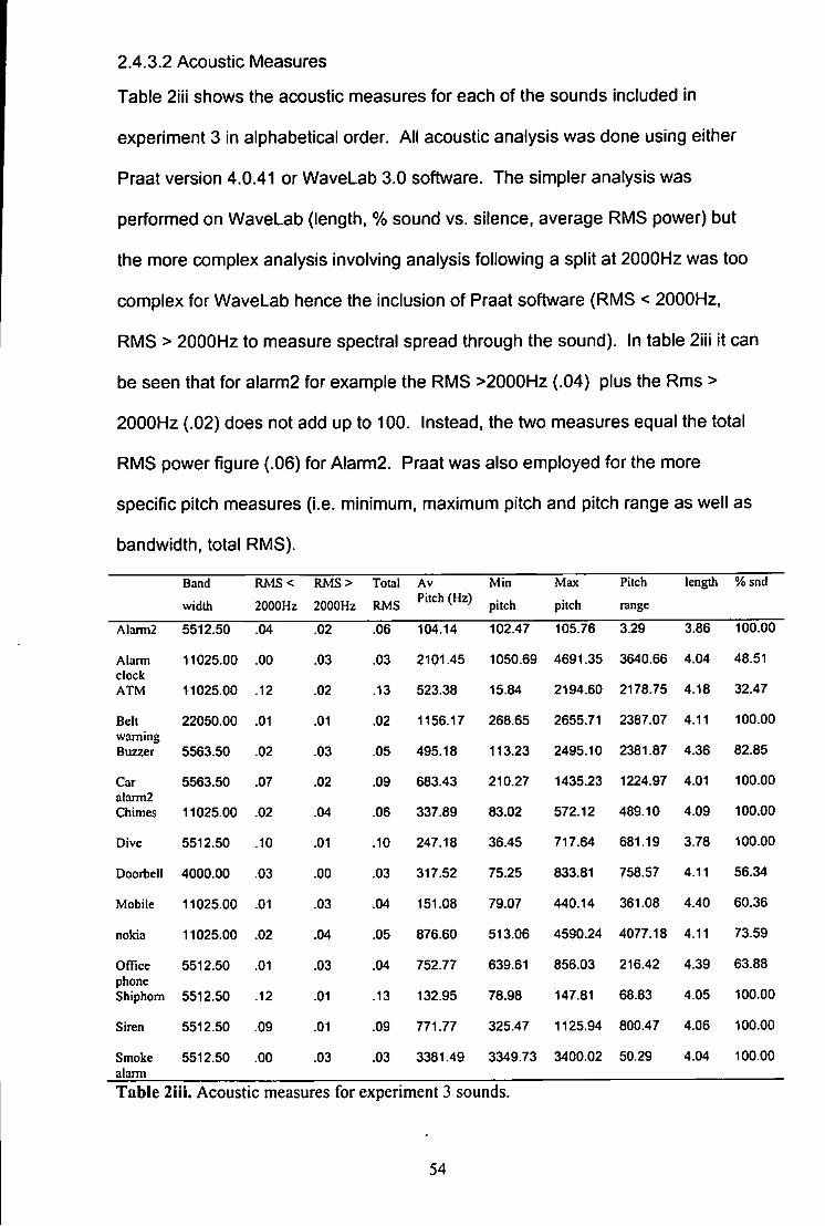
2.4.3.2 Acoustic Measures
Table 2iii shows the acoustic measures for each of the sounds included in
experiment 3 in alphabetical order. All acoustic analysis was done using either
Praat version 4.0.41 or WaveLab 3.0 software. The simpler analysis was
performed on WaveLab (length. % sound vs. silence, average RMS power) but
the more complex analysis involving analysis following a split at 2000Hz was too
complex for WaveLab hence the inclusion of Praat software (RMS < 2000Hz,
RMS > 2000Hz to measure spectral spread through the sound). In table 2iii it can
be seen that for alarm2 for example the RMS >2000Hz (.04) plus the Rms >
2000Hz (.02) does not add up to 100. Instead, the two measures equal the total
RMS power figure (.06) for Alarm2. Praat was also employed for the more
specific pitch measures (i.e. minimum, maximum pitch and pitch range as well as
bandwidth, total RMS).
Band RNiS< RMS> Total Av Min Max Pilch length % snd
width 2000Hz 2000Hz RMS Pitch (Hz) pitch pitch range
A)ann2 5512.50 .04 .02 .06 104.14 102.47 105.76 3.29 3.86 100.00
Alarm 11025.00 .00 .03 .03 2101.45 1050.69 4691.35 3640.66 4.04 48.51 clock ATM 11025.00 .12 .02 .13 523.38 15.84 2194.60 2178.75 4.18 32.47
Belt 22050.00 .01 .01 .02 1156.17 268.65 2655.71 2387.07 4.11 100.00 warning Buzzer 5563.50 .02 .03 .05 495.18 113.23 2495.10 2381.87 4.36 82.85
Car 5563.50 .07 .02 .09 683.43 210.27 1435.23 1224.97 4.01 100.00 alann2 Chimes 11025.00 .02 .04 .06 337.89 83.02 572.12 489.10 4.09 100.00
Dive 5512.50 .10 .01 .10 247.18 36.45 717.64 681.19 3.78 100.00
Doorbell 4000.00 .03 .00 .03 317.52 75.25 833.81 758.57 4.11 56.34
Mobile 11025.00 .01 .03 .04 151.08 79.07 440.14 361.08 4.40 60.36
nokia 11025.00 .02 .04 .05 876.60 513.06 4590.24 4077.18 4.11 73.59
OfTice 5512.50 .01 .03 .04 752.77 639.61 856.03 216.42 4.39 63.88 phone Shiphom 5512.50 .12 .01 .13 132.95 78.98 147.81 68.83 4.05 100.00
Siren 5512.50 .09 .01 .09 771.77 325.47 1125.94 800.47 4.06 100.00
Smoke 5512.50 .00 .03 .03 3381.49 3349.73 3400.02 50.29 4.04 100.00 alarm
Table 2iii. Acoustic measures for experiment 3 sounds.
54
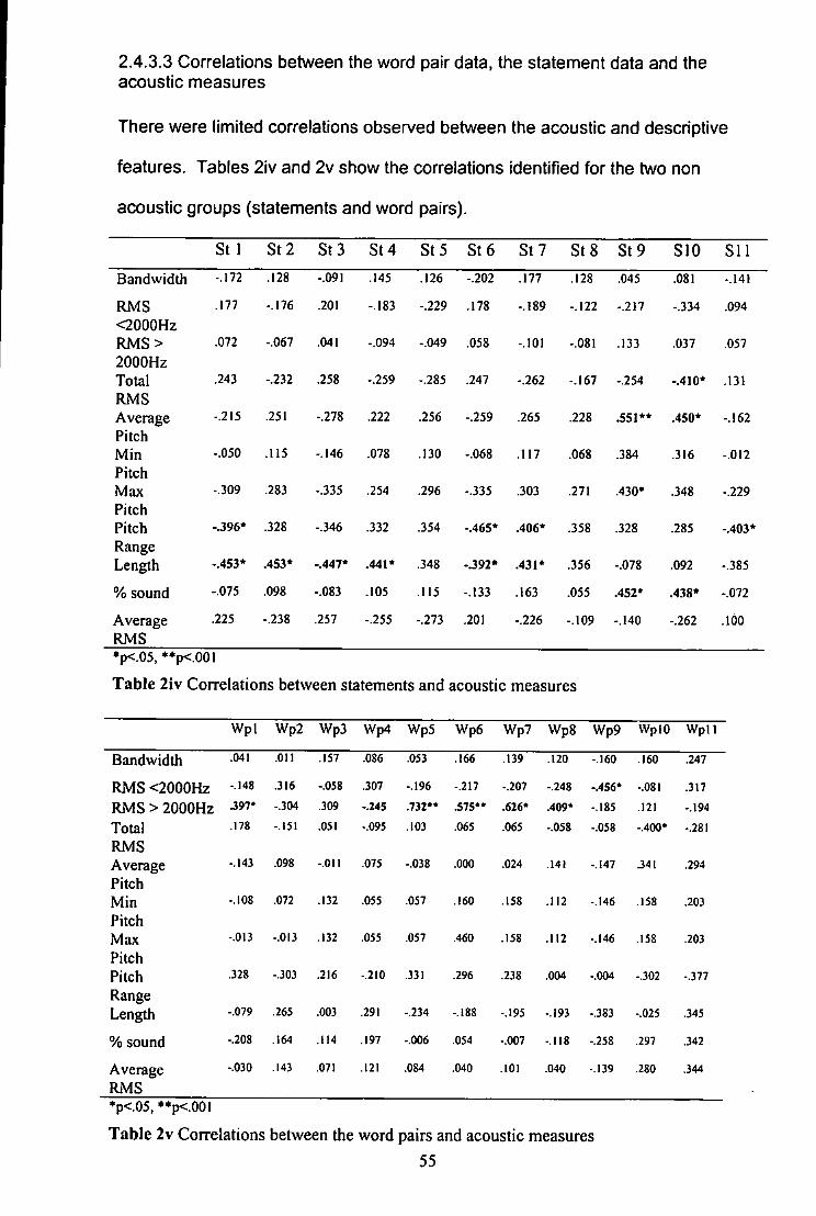
2.4.3.3 Correlations between the word pair data, the statement data and the acoustic measures
There were limited correlations observed between the acoustic and descriptive
features. Tables 2iv and 2v show the correlations identified for the two non
acoustic groups (statements and word pairs).
SU St2 SF3 S U St 5 St 6 Sil St 8 St 9 sTo sTT Bandwidth -.172 .128 -.091 .145 .126 -.202 .177 .128 .045 .081 -.141
RMS .177 -.176 .201 -.183 -.229 .178 -.189 -.122 -.217 -.334 .094 <2000Hz RMS> .072 -.067 .041 -.094 -.049 .058 -.101 -.081 .133 .037 .057 2000Hz Total .243 -.232 .258 -.259 -.285 .247 -.262 -.167 -.254 -.410* .131 RMS Average -.215 .251 -.278 .222 .256 -.259 .265 .228 .551** .450* -.162 Pitch Min -.050 .115 -.146 .078 .130 -.068 .117 .068 .384 .316 -.012 Pitch Max -.309 .283 -.335 .254 .296 -.335 .303 .271 .430* .348 -.229 Pitch Pitch -396* .328 -.346 .332 .354 -.465* .406* .358 .328 .285 -.403* Range Length -.453* .453* -.447* .441* .348 - J 9 2 * .431* .356 -.078 .092 -.385
% sound -.075 .098 -.083 .105 .115 -.133 .163 .055 .452* .438* -.072
Average .225 -.238 .257 -.255 -.273 .201 -.226 -.109 -.140 -.262 .100 RMS •p<.05,**p<.001
Table 2iv Correlations between statements and acoustic measures
Wpl Wp2 Wp3 Wp4 Wp5 Wp6 Wp7 WpS Wp9 WplO Wpll
Bandwidth .041 .011 .157 .086 .053 .166 .139 .120 -.160 .160 .247
RMS <2000Hz -.148 .316 -.058 .307 -.196 -.217 -.207 -.248 -.456* -.081 .317
RMS > 2000Hz -.304 .309 -.245 ,732** .575** .626* .409* -.185 .121 -.194
Total .178 -.151 .051 -.095 .103 .065 .065 -.058 -.058 -.400* -.281
RMS Average -.143 .098 -.011 .075 -.038 .000 .024 .141 -.147 J 4 I .294
Pitch Min -.108 .072 .132 .055 .057 .160 .158 .112 -.146 .158 .203
Pitch Max -.013 -.013 .132 .055 .057 .460 .158 .112 -.146 .158 .203
Pitch Pitch .328 -.303 .216 -.210 .331 .296 .238 .004 -.004 -.302 -.377
Range Length -.079 .265 .003 .291 -.234 -.188 -.195 -.193 -.383 -.025 .345
% sound -.208 .164 .114 .197 -.006 .054 -.007 -.118 -.258 .297 .342
Average -.030 .143 .071 .121 .084 .040 .101 .040 -.139 .280 .344
RMS *p<.05.**p<.00l Table 2v Correlations between the word pairs and acoustic measures
55
2.4.4 Discussion
This experiment has provided further information about each of the sounds in the
form of psychological descriptors and one further measure of familiarity (word pair
familiar/unfamiliar). In addition, the acoustic measures have added to the
database of information about each of the sounds.
Experiment 2 has provided data to support intuitive notions about which
perceptual measures correlate with one another. For example, as can be seen in
appendix A4, for 28 out of the 30 sounds those rated as pleasant show a
significant relationship to pleasing or the converse i.e. unpleasant and annoying.
In 18 out of 30 cases soft sounds are also judged as weak and powerful sounds
considered large. This is not a surprising finding but nonetheless valuable to
demonstrate a robust effect of these psychological descriptors across a number of
participants and sounds.
A detailed discussion of correlations between the word pair measures is not
included in either the Bellas (1993) or Solomon (1959) reports. However,
Bonebright (2001) goes in to some detail for the correlations obtained. Although
in most cases Bonebright (2001) has used different word pairs to those used in
the present research they still support intuitive notions about the environmental
sounds that were studied, such as, a weak sound showed a statistically significant
relationship to being rated as a soft sound. Bonebright's word pairs were more
descriptive word pairs for the sounds such as dull/sharp, slow/fast or
rough/smooth in comparison to the current studies focus on collecting data about
the descriptive features of the sounds.
56
Correlations between the acoustic measures and the word pairs (exp 2) and the
statements (exp 1) are limited. For the statements data the length of the sound
showed correlations with a large number of statements (1,2,3,4,6 and 7) that
measured the use of imagery and words to describe a sound. Pitch range also
showed correlations with four of the eleven statements ( 1 . 6, 7 and 11) these
statements included how difficult the sound was to identify, use of words, and the
event/object or acoustic statement. Average pitch showed a correlation with both
of the statements about the ecological frequency of the sound.
For the word pair data only three measures showed a correlation to the acoustic
measures. Definite/uncertain was correlated with the length of the sound, and
powerful/weak was correlated to the percentage of sound versus silence in the
sound. The word pair High pitch/Low pitch had the largest number of correlations
with bandwidth and the four measures of pitch, suggesting perceived pitch does
reflect actual pitch measures.
Overall the correlations between the acoustic, word pair and statement data does
not suggest that the statements or word pairs are clearly underpinned by acoustic
measures. The exception to this is the word pair high pitch/low pitch that
demonstrates strong correlations with all the measures of pitch. Whilst this finding
is not surprising there is a lack of correlations between the word pairs
representing the power of the sound. For example powerful/weak, soft/loud and
large/small do not show significant correlations to the acoustic measure for RMS
power. This suggests that the actual measure of the sound's power (RMS
measures) is not necessarily the same as the way the listener actually perceives
the power within a sound.
57
2,5 Experiment 3: Multidimensional scaling of 15 abstract sounds
2.5.1 Introduction
Experiment 3 was designed with the intention of identifying some of the salient
acoustic and non acoustic sound features used by participants when making
similarity judgements about a set of abstract sounds. It was hoped that this would
help to identify several key points. Firstly, how participants may use acoustic
similarities in their judgements and also provide information about how descriptive
similarities between the sounds may influence participants' similarity judgements.
The source of the sound or the function of the sound may also play a role In the
similarity judgements. The purpose of experiment 3 was to collect data In the
form of similarity judgements for the 15 sounds included in the experiment.
The proximity data collected using judgements of similarity was suitable for
analyses using MDS. This technique places all the sounds in a geometric
configuration and suggests a number of dimensions used to make the similarity
judgements. The location of the sounds on each identified dimension, correlated
with the data collected from experiments 1, 2 and the acoustic data, will help to
suggest meaning to the unknown features used by the participants to make their
similarity judgements.
A palnwise task was employed (similar to that used by Howard & Silverman, 1976)
that asked participants to judge the similarity of two sounds e.g. telephone ringing
and a smoke alarm. This judgement then provides a measure of similarity. The
basis on which the similarity judgement Is made is entirely up to the participant
with no guidance from the researcher. Judgements of similarity between acoustic
stimuli, as discussed previously, will provide further data to the existing knowledge
about similarity comparisons. There Is currently little data from auditory research
58
in this field. Proximity data is also the most appropriate for use with MDS analysis
that allows the identification of hidden meaning in the data and as such is
appropriate to an experiment that is exploratory in nature.
To use the pairwise comparison task it was necessary to reduce the number of
sounds because the experiment would otherwise be far too long. The 15 sounds
chosen were selected for quality and those not too similar to other sounds
selected e.g. where two sounds were similar sounds, one was excluded,
therefore, from car hom and ship horn only ship horn was retained. The aim of
this experiment was to identify which of the measured features (statements and
word pairs) were important in the participants' judgements of similarity for the 15
abstract sounds. In addition, the experiment would identify any similarities in the
way sounds are represented between the abstract sounds employed here and the
environmental sounds used in previous work (Bellas, 1993; Bonebright, 2001).
Features previously identified as salient have included; pitch, timbre, loudness,
pleasantness of the sound, familiarity with the sound, and occurrence of the
sound. For example, the pleasantness of a sound has repeatedly been identified
as a salient dimension both in experiments looking at similarity judgements
(Bonebright, 2001) and tasks investigating participants' identification of the
sounds (Solomon, 1958; Ballas, 1993). Similarly loudness has also been
consistently identified when measured through acoustic analysis, the use of word
pairs such as loud/soft or investigations of imagery (Intons-Peterson, 1980).
2.5.1.1 Further introduction to Multidimensional scaling
As briefly discussed above one of the most common data collection techniques for
MDS is the collection of similarity ratings or proximity ratings using pairwise
comparisons. Sound pair stimuli ratings are collected by pairing each sound with
59
every other in a random order. So for example, five sounds A B C D and E would
form the pairs; AB AC AD AE BC BD etc, and the participant would be required to
rate the similarity of the sounds in each pair on a seven point scale. So for fifteen
stimuli participants would rate 105 pairs (=N(N-1 )/2) where N is number of stimuli
(e.g. Bonebright, 1989). The exponential increase can be a problem for research
using sound because unlike visual items the sounds cannot be presented
simultaneously. This is an area discussed in detail in chapter 3.
There are two main types of MDS analysis used, one of which obtains an MDS
solution for the group (e.g. 5 participants) as a whole by analysing averaged data
from all participants (ALSCAL). The ALSCAL solution does not necessarily
represent any one participant (Coxon. 1982). The other, the INDSCAL method,
basically uses exactly the same proximity matrices but takes into account the
difference between the participants' data rather than collapsing across it. The
INDSCAL dimensions represent the (orthogonal) dimensions where the variation
among participants is the greatest. Each subject has a weight for each identified
dimension demonstrating the salience of each dimension for that participant.
There are three assumptions cited by Hair, Anderson, Tathan & Black (1995) that
the researcher must accept about perception. Firstly, each participant in a study
is unlikely to perceive a stimulus to have exactly the same dimensionality as other
participants (although it is thought that most people judge in terms of a limited
number of characteristics or dimensions). Secondly, different respondents may
not attach the same level of importance to a dimension, even if all respondents
perceive this dimension. Finally, a participants' judgements may not stay stable
over time.
60
Once the specific technique to be used has been selected and an MDS solution
obtained it is necessary to choose the smallest number of dimensions that provide
the best fit of the data. Interpretation of solutions derived in more than three
dimensions is very difficult and usually not considered v^orth the improvement in fit
(Hair et al, 1995). One approach to selecting the number of dimensions is to use
a stress measure. Stress or s stress, depending on the particular model used for
analysis, indicates the proportion of the variance of the disparities not accounted
for by the MDS model. The stress measure improves with an increase in the
number of dimensions used and therefore, a trade off is necessary between the fit
of the solution, the number of dimensions, and the interpretability of the solution.
This trade off is discussed by Kruskal et al (1984) who point out that it is not
useful to examine a configuration with so many dimensions you cannot
comprehend it. One simple way to check the stability of the dimensions chosen is
to split the original data and conduct separate MDS analyses for each part. To
help guide researchers in selecting an acceptable solution Kruskal et al (1984)
suggest .20 = poor, .10 = fair, .05 = good and .025 = excellent. However, there is
a concern that such benchmarks can lead to misuse because of the suggestion
that only a solution with a stress score less than .20 is acceptable. The
alternative is to plot the values against the number of dimensions and there will
frequently be an elbow in the curve which is considered to represent the
maximum appropriate number of dimensions (Schiffman et al, 1981). However, it
is important to bear in mind when making a decision on dimensionality using the
stress score that an MDS solution may have high stress as a consequence of high
error in the data and finding a precise representation for the data does not imply
anything about its scientific value (Borg et al, 1997). Kruskal et al (1984) further
the point by stating that if the m dimensional solution provides a satisfying
61
interpretation, but the (m +1) dimensional solution reveals no further structure it
may be well to use only the m dimensional solution.
In order to then interpret the chosen solution there are internal and external
methods used. External methods may relate to physical characteristics, such as
pitch judgements made by the respondents. Each of these properties is assumed
to consist of a set of numerical values of the variable concerned, one for each
point (representing a sound In this instance) in the configuration (Coxon, 1982). It
is common practice to then use multiple regression or correlation techniques to
identify any relationship between the additional external information and the
stimuli's location in the configuration. So for example if pitch shows a high
correlation with locations of the sounds on a dimension, this indicates one
possible interpretation of that dimension. For example, Bonebrlght (2001)
collected information regarding amplitude celling, the average Intensity and the
change in frequency for each of the sound stimuli used as well as the attribute
ratings such as dull/sharp. In order to attribute possible meanings to each
dimension these measures were regressed onto or correlated with the stimuli
locations on each of the dimensions. Some dimensions can be worked out simply
through close visual inspection.
An example of an area related to sound attributes that has frequently employed
MDS is the study of timbre. According to Lakatos et al (2000) most of these
studies have yielded two or three interpretable psychophysical dimensions.
Typically the dimensions identified correlate with central tendency of the sound
spectrum, a sound's transient properties (e.g. rise time, decay) and the temporal
variation in the spectral envelope or fine structure. These features are reflected in
other research that does not necessarily focus just on timbre. For example, the
62
work discussed previously by Howard & Silverman (1976) proposed fundamental
frequency, waveform and formants as possible dimension attributes or the
solution suggested by Allen & Bond (1997) identifying average frequency,
periodicity and number of peaks in amplitude spectrum. All these studies
demonstrate the practical application of multidimensional scaling as a useful
analysis technique that can be applied to sound data.
2.5.2 Method
2.5.2.1 Participants
47 psychology undergraduate students (3 male, 44 female) at the University of
Plymouth participated in the experiment. Participants were awarded points for
their participation as part of the BSc psychology course requirement. All
participants had normal or corrected to normal hearing as measured by self
report.
2.5.2.2 Apparatus
6 Hewlett Packard Vectra PIN computers (with a 600 MHz Processor, 128 MB
RAM and CrystalSoundFusion™ Soundcard operating on Windows XP) with
headphones were used with a purpose written program (Aldrich, Oct 2002) to
present the sound stimuli and record data.
2.5.2.3 Stimuli
Sound stimuli were 15 abstract sounds taken from the pool of 30 sounds used in
experiments 1 and 2. The 15 sounds chosen were selected on the basis that they
were the best quality sounds with only one exemplar for each type of sound. An
attempt was made to avoid selecting two very similar or confusable stimuli in
terms of their perceived acoustic similarity. An attempt was made to select
63
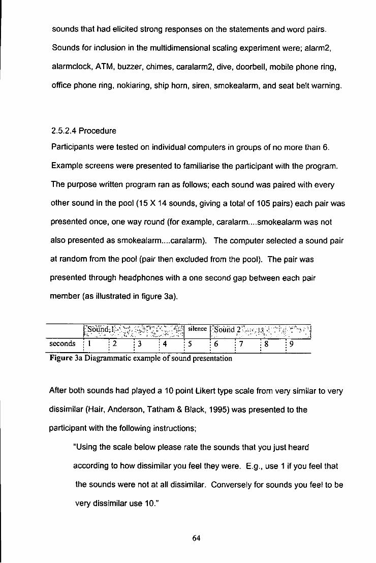
sounds that had elicited strong responses on the statements and word pairs.
Sounds for inclusion in the multidimensional scaling experiment were; alarm2.
alarmclock, ATM, buzzer, chimes, caralarm2, dive, doorbell, mobile phone ring,
office phone ring, nokiaring, ship horn, siren, smokealarm, and seat belt warning,
2.5.2.4 Procedure
Participants were tested on individual computers in groups of no more than 6.
Example screens were presented to familiarise the participant with the program.
The purpose written program ran as follows; each sound was paired with every
other sound in the pool (15 X 14 sounds, giving a total of 105 pairs) each pair was
presented once, one way round (for example, caralarm....smokealarm was not
also presented as smokealarm....caralarm). The computer selected a sound pair
at random from the pool (pair then excluded from the pool). The pair was
presented through headphones with a one second gap between each pair
member (as illustrated in figure 3a).
tSoiii silence
seconds ; I : 2 1 r~ : 3 ;
4 5 6 : 7 : 8 : 9
Figure 3a Diagrammatic example of soimd presentation
After both sounds had played a 10 point Likert type scale from very similar to very
dissimilar (Hair. Anderson, Tatham & Black, 1995) was presented to the
participant with the following instructions;
"Using the scale below please rate the sounds that you just heard
according to how dissimilar you feel they were. E.g., use 1 if you feel that
the sounds were not at all dissimilar. Conversely for sounds you feel to be
very dissimilar use 10."
64
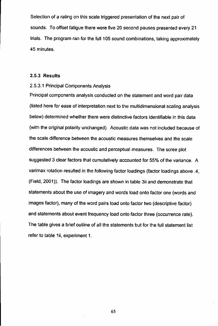
Selection of a rating on this scale triggered presentation of the next pair of
sounds. To offset fatigue there were five 20 second pauses presented every 21
trials. The program ran for the full 105 sound combinations, taking approximately
45 minutes.
2.5.3 Results
2.5.3.1 Principal Components Analysis
Principal components analysis conducted on the statement and word pair data
(listed here for ease of interpretation next to the multidimensional scaling analysis
below) determined whether there were distinctive factors identifiable in this data
(with the original polarity unchanged). Acoustic data was not included because of
the scale difference between the acoustic measures themselves and the scale
differences between the acoustic and perceptual measures. The scree plot
suggested 3 clear factors that cumulatively accounted for 55% of the variance. A
varimax rotation resulted in the following factor loadings (factor loadings above .4,
(Field, 2001)). The factor loadings are shown in table 3ii and demonstrate that
statements about the use of imagery and words load onto factor one (words and
images factor), many of the word pairs load onto factor two (descriptive factor)
and statements about event frequency load onto factor three (occurrence rate).
The table gives a brief outline of all the statements but for the full statement list
refer to table l i i , experiment 1.
65
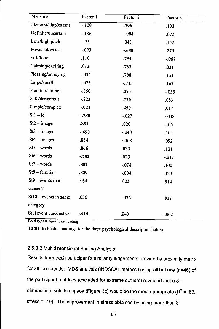
Measure Factor 1 Factor 2 Factor 3
Pleasant/Unpleasant -.109 .796 .193 Definite/uncertain -.186 -.084 .072 Low/high pitch .135 .043 .152 Powerful/weak -.090 -.680 .279 Soft/loud .110 .794 -.067 Calming/exciting .012 .763 .031 Pleasing/annoying -.034 .788 .151 Large/small -.075 -.715 .167 Familiar/strange -.350 .093 -.055 Safe/dangerous -.223 .770 .083 Simple/complex -.023 .450 .017 Stl - id -.780 -.027 -.048 St2 - images .851 .020 .106 St3 - images -.690 -.040 .109 St4 - images .834 -.068 .092 St5 - words .866 .030 .101 St6 - words -.782 .025 -.017 St7 - words .882 -.078 .100 St8-familiar .829 -.004 .124 St9 - events that .054 .003 .914 caused?
St 10 - events in same .056 -.036 .917 category
Stl 1 event...acoustics -.410 .040 -.002
Table 3ii Factor loadings for the three psychological descriptor factors.
2.5.3.2 Multidimensional Scaling Analysis
Results from each participant's similarity judgements provided a proximity matrix
for all the sounds. MDS analysis (INDSCAL method) using all but one (n=46) of
the participant matrices (excluded for extreme outliers) revealed that a 3-
dimensional solution space (Figure 3c) would be the most appropriate (R^ = .63,
stress = .19). The improvement in stress obtained by using more than 3
66
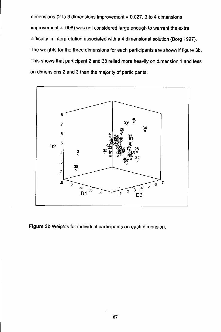
dimensions (2 to 3 dimensions improvement = 0.027, 3 to 4 dimensions
improvement = .008) v/as not considered large enough to warrant the extra
difficulty in interpretation associated with a 4 dimensional solution (Borg 1997).
The weights for the three dimensions for each participants are shown if figure 3b.
This shows that participant 2 and 38 relied more heavily on dimension 1 and less
on dimensions 2 and 3 than the majority of participants.
29 o
Figure 3b Weights for individual participants on each dimension,
67
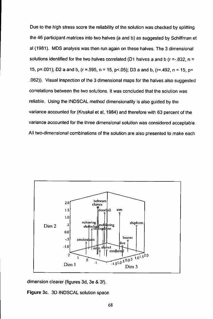
Due to the high stress score the reliability of the solution was checked by splitting
the 46 participant matrices into two halves (a and b) as suggested by Schiffman et
al (1981). MDS analysis was then run again on these halves. The 3 dimensional
solutions identified for the two halves correlated (D1 halves a and b (r =-.832, n =
15. p=.001); D2 a and b. (r =.595, n = 15. p<.05); D3 a and b, (r=.492. n = 15, p=
.062)). Visual inspection of the 3 dimensional maps for the halves also suggested
correlations between the two solutions. It was concluded that the solution was
reliable. Using the INDSCAL method dimensionality is also guided by the
variance accounted for (Kruskal et al, 1984) and therefore with 63 percent of the
variance accounted for the three dimensional solution was considered acceptable.
All two-dimensional combinations of the solution are also presented to make each
Dim 2
2.0
1.5
1.0
.5
0.0
-.5
-1.0
2
Dim 1
bcltwami chimes
IdoorHell atm
smokealaqm
nokiaring , , . alaiinclQ(UPi;*""g
shiphorn
buzzer
n al^ml cardJiarmE
Dim 3
dimension clearer (figures 3d, 3e & 3f).
Figure 3c. 30 INDSCAL solution space
68
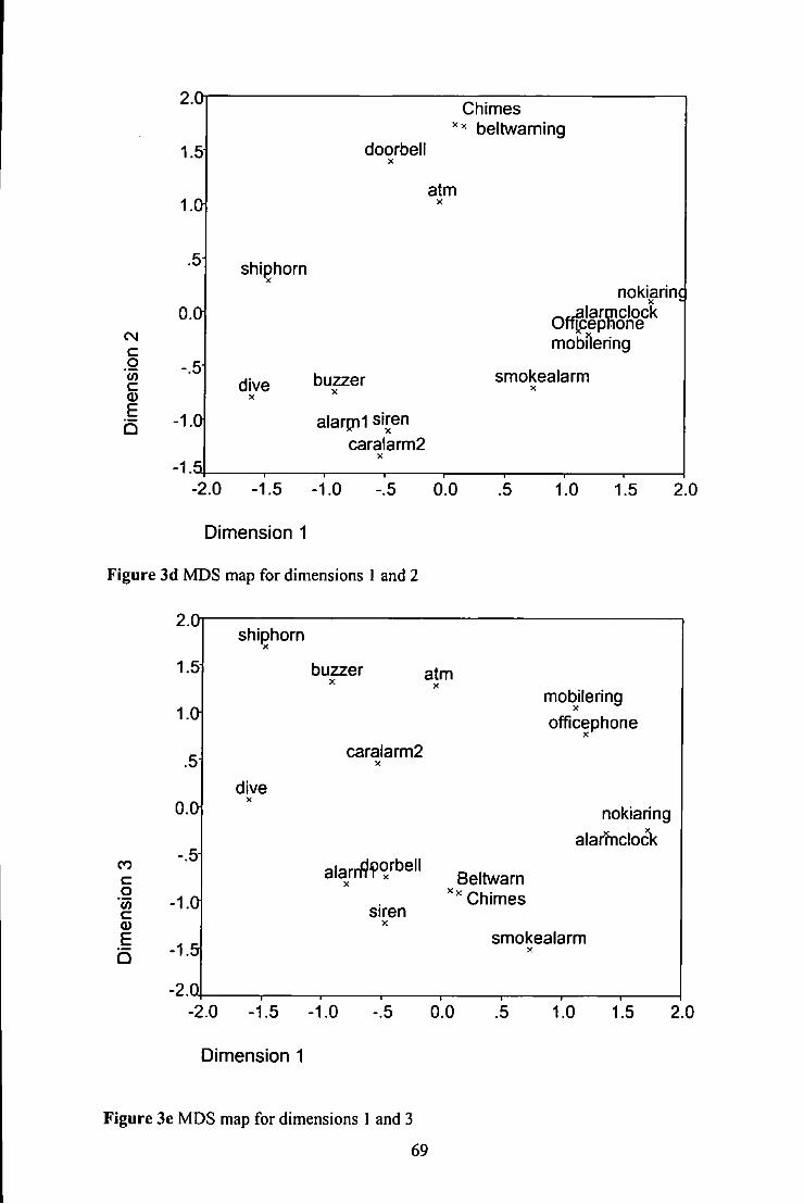
2.0
CM c o (/) c E b
.5
1.5
X
doorbell X
Chimes beltwarning
atm X
shi^horn nokiarinc
- .^ larmclock Offjpepnone mobilering
dive buzzer X
alarpil siren caralarm2
X
smokealarm X
-2.0 -1.5 -1.0 -.5
Dimension 1
Figure 3d MDS map for dimensions 1 and 2
0.0 .5 1.0 1.5 2.0
1.5
CO c g *w c a> E b
•2.0
shi^horn
buzzer atm ^ X
caralarm2 X
mobilering
officephone
dive y
alarrf??o/bell X
X
siren
Beltwarn Chimes
nokiaring alarfnclock
smokealarm X
•2.0 -1.5 -1.0 -.5 0.0
Dimension 1
1.0 1.5 2.0
Figure 3e MDS map for dimensions 1 and 3
69
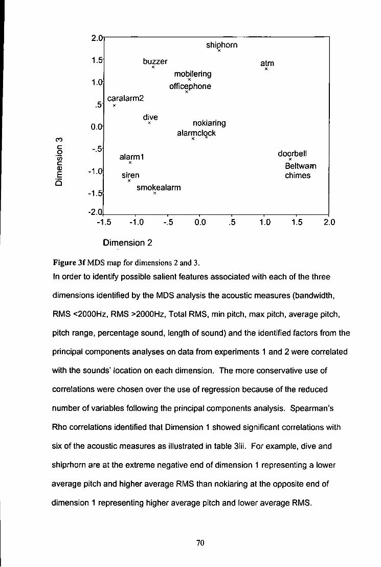
2.0
1.5
.5
CO c g w c 0} E
-.5
•1.0
•1.5
•2.Q
shipliorn X
buzzer X
caralarm2 X
mobilering
officephone X
atm X
dive X nokiaring
alarmclqck
alarml X
siren X
smokealarm X
doorbell X
Beltwam chimes
1.5 -1.0 -.5
Dimension 2
0.0 .5 1.0 1.5 2.0
Figure 3f MDS map for dimensions 2 and 3.
In order to identify possible salient features associated with each of the three
dimensions identified by the MDS analysis the acoustic measures (bandwidth,
RMS <2000Hz, RMS >2000Hz, Total RMS. min pitch, max pitch, average pitch,
pitch range, percentage sound, length of sound) and the identified factors from the
principal components analyses on data from experiments 1 and 2 were correlated
with the sounds' location on each dimension. The more conservative use of
correlations were chosen over the use of regression because of the reduced
number of variables following the principal components analysis. Spearman's
Rho correlations identified that Dimension 1 showed significant correlations with
six of the acoustic measures as Illustrated in table 3iii. For example, dive and
shiprhorn are at the extreme negative end of dimension 1 representing a lower
average pitch and higher average RMS than nokiaring at the opposite end of
dimension 1 representing higher average pitch and lower average RMS.
70
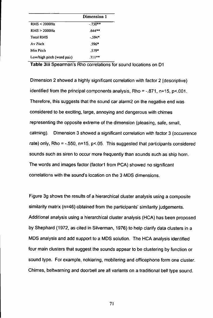
Dimension 1
RMS<2000H2 -.730**
RMS > 2000Hz .644**
Total RMS -.594*
Av Pitch .596*
Min Pilch .579*
Low/high pitch (word pair) .711**
Table 3iii Spearman's Rho correlations for sound locations on D1
Dimension 2 showed a highly significant correlation with factor 2 (descriptive)
identified from the principal components analysis, Rho = - .871, n=15, p<.001.
Therefore, this suggests that the sound car alarm2 on the negative end was
considered to be exciting, large, annoying and dangerous with chimes
representing the opposite extreme of the dimension (pleasing, safe, small,
calming). Dimension 3 showed a significant correlation with factor 3 (occurrence
rate) only, Rho = -.550, n=15, p<.05. This suggested that participants considered
sounds such as siren to occur more frequently than sounds such as ship horn.
The words and images factor (factorl from PCA) showed no significant
correlations with the sound's location on the 3 MDS dimensions.
Figure 3g shows the results of a hierarchical cluster analysis using a composite
similarity matrix (n=46) obtained from the participants' similarity judgements.
Additional analysis using a hierarchical cluster analysis (HCA) has been proposed
by Shephard (1972, as cited in Silverman, 1976) to help clarify data clusters in a
MDS analysis and add support to a MDS solution. The HCA analysis identified
four main clusters that suggest the sounds appear to be clustering by function or
sound type. For example, nokiaring, mobilering and officephone form one cluster.
Chimes, beltwarning and doorbell are all variants on a traditional bell type sound.
71
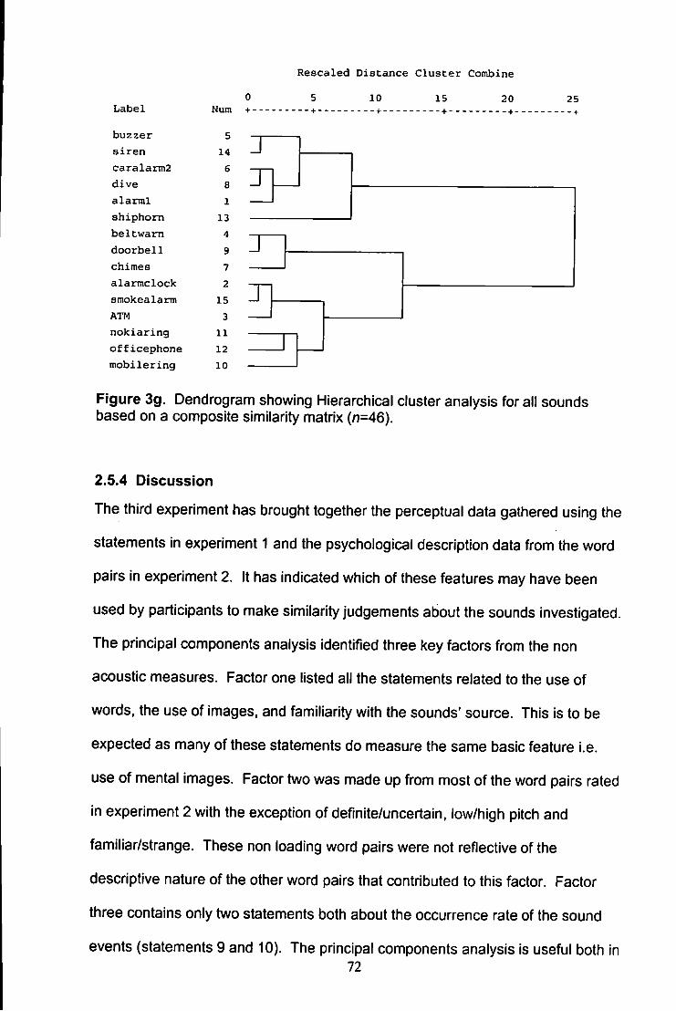
L a b e l
buzzer s i r e n caralarTn2 d i v e a l a r r a l s h i p h o m b e l t w a r n d o o r b e l l chimes a l a r m c l o c k smokealarm ATM
n o k i a r i n g o f f i c e p h o n e m o b i l e r i n g
Num
5 14 6 8 1
13 4 9 7 2
15 3
11 12 10
R e s c a l e d D i s t a n c e C l u s t e r Combine
5 10 15 20 25 - +
J J
Figure 3g. Dendrogram showing Hierarchical cluster analysis for all sounds based on a composite similarity matrix (n=46).
2.5.4 Discussion
The third experiment has brought together the perceptual data gathered using the
statements in experiment 1 and the psychological description data from the word
pairs in experiment 2. It has indicated which of these features may have been
used by participants to make similarity judgements about the sounds investigated.
The principal components analysis identified three key factors from the non
acoustic measures. Factor one listed all the statements related to the use of
words, the use of images, and familiarity with the sounds' source. This is to be
expected as many of these statements do measure the same basic feature i.e.
use of mental images. Factor two was made up from most of the word pairs rated
in experiment 2 with the exception of definite/uncertain, low/high pitch and
familiar/strange. These non loading word pairs were not reflective of the
descriptive nature of the other word pairs that contributed to this factor. Factor
three contains only two statements both about the occurrence rate of the sound
events (statements 9 and 10). The principal components analysis is useful both in 72
its own right, to help to reduce the data from the first two experiments into
meaningful groups, and secondly the obtained factors help in the identification of
the hidden meaning of the MDS dimensions.
The multidimensional scaling analysis identified a three dimensional solution and
the INDSCAL method used identified that the majority of the participants were
using the same dimensions with a similar pattern of importance given to each (D1
= .261, D2=.203, D3= .167). There were only two individuals who were unusual in
their use of the dimensions as identified by a visual inspection of the flattened
subject weights (participant 2 = 2.92 and participant, 38 = 4.28 compared to <2 for
all other participants). The weirdness ratings for participant 2 (D1 .76, D2 .34, D3
.16) and for participant 38 (D1 .75, D2 .20, D3 .11) suggests that both these
participants heavily favour dimension 1 in their similarity judgements. The
weirdness index helps to identify whether a subject is typical or not. A value close
to 1 would suggest that the subject weights are unusual. All the other participants
gave approximately equal importance to each dimension.
The MDS model is, whilst considered a relatively poor fit using Kruskal's (1984)
guidelines: stress .20 = poor, as cited in Borg et al (1997) is nonetheless
indicative of the pattern of similarity between all the sounds. The stress measure
is good enough at .19 with support provided by the R squared measure, indicating
63% of the variance is accounted for by this MDS map, to be confident that three
dimensions is the appropriate number. As discussed by Kruskal et al (1984) the
variance accounted for is an acceptable guide for the dimensionality of INDSCAL
scaling models with R squared measures of greater than 60% as the accepted
level which a model should exceed.
73
The correlation analyses between the sounds measured features and their
locations on the three dimensions have suggested that participants have rated the
sounds for similarity based on two main factors. These are acoustic and non
acoustic, descriptive features. Visual analysis of the MDS configuration and the
HCA analysis suggested a third criteria, namely, the source, function or category
membership of the sounds as contributing to similarity judgements. There may be
a distinction between source and function. Source appears to differ from function
because these sounds appear to have been grouped according to their sources'
category membership. For example, belt warning, chimes and doorbell have all
been grouped together and could arguably be classed as a category containing
bells but these bells, unlike the telephone category, do not serve the same
function. Doorbell for example has a function whereas the chimes sound serves
no such function. A few examples will help to illustrate the different features
participants have employed. Figure 3e shows that all the telephone sounds (all
rings, traditional or modern mobile) grouped closely despite considerable
differences between the actual acoustic features that make up the sounds.
Therefore, this cluster could represent either a function or a category cluster
because telephone rings all serve the same function but the source objects
'telephones' would also be members of the same category. Figure 3f highlights a
cluster of sounds that appear to group by source but not by function. It can be
seen that doorbell, belt warning and chimes (all chiming bell sounds) are grouped
closely on dimensions 2 and 3. In contrast some sounds, such as, ATM and ship
horn stand alone, and were considered to be dissimilar to the other sounds by the
participants. These less clustered sounds still tend to share at least one
dimension with other sounds. For example, ship horn shares acoustic features
represented on dimension 1 with the dive alarm as they are both located around -
1.5 on dimension 1 (low pitch, powerful). Similarly ATM and buzzer lie at around
74
1.4 on dimension 3 (occurrence rate). This illustrates that some of the sounds,
although not clustered closely, may share some but not all of the features used by
participants to make the similarity judgements.
The correlations between the three identified factors and the sounds' locations on
each dimension helps to indicate what these dimensions may be representing.
Dimension 1 showed significant correlations with only the acoustic features
(RMS<2000Hz, RMS>2000Hz, Total RMS and average pitch) with the exception
of the word pair high/low pitch. However, this word pair is reflective of the
perception of pitch rather than an absolute measure of pitch. High/low pitch word
pair correlates with average pitch (table 3iii) and therefore, considered acoustic in
nature. Therefore, table 3iii suggests that sounds that share a similar location on
dimension 1 such as dive and ship horn share similar levels of loudness and pitch
and that these are important features in similarity judgements made by the
participants. For example ship horn and the dive alarm are lower in pitch (247H2
& 132Hz respectively) and louder (average RMS -19.21 and -17.06 dB) than
sounds on the opposite end of dimension 1 such as the nokia ring (pitch 876Hz,
average RMS -27.32dB).
Dimension 2 showed a highly significant correlation with factor 2 from the PCA
analysis which reflected the descriptive measures (word pairs, experiment 2).
This suggests, as before, that sounds that share a similar location on dimension 2
are judged to be similar in terms of qualities such as their pleasantness,
connotations of danger and how exciting they are. For example, doorbell, belt
warning and chimes share similar descriptive judgements at around 1.5 on
dimension 2. The correlation is negative and indicates that this end of the
dimension is representing sounds that are more calming, pleasant and pleasing
75
than the opposite end of the dimension that represents sounds that are exciting,
unpleasant and annoying, such as, caralarm2.
Finally, dimension 3 showed a significant relationship with the rate of occurrence
for the sounds. However, the range of responses on these statements was very
limited and so this finding is treated with caution.
It is worth noting that factor one from the PCA analysis reflecting the use of words
and imagery does not correlate with any of the dimensions identified by the MDS
analysis. Although different analysis was used Ballas (1993) also found no
relationships between the sounds and measures of words or imagery use.
However, the results of the PCA from the present study identified the use of words
and imagery as an important factor when rating sounds. This finding reflects
previous research (Ballas, 1993) but this finding may not extend to more specific
judgements such as similarity judgements. The task in experiment one required
the participants to make a judgement about whether they could easily think of
words or images for the sounds. This of course does not suggest that when
participants are asked to make a similarity judgement (experiment three) between
two sounds that they choose to employ this information in their decision-making
processes. Alternatively the measures employed may not be sensitive enough to
reflect the use of words and imagery. However, at this stage this is very
speculative and the finding may be a result of the limited number of sounds
employed so the use of words and imagery measures will be retained for the next
experiment.
The Dendrogram in figure 3f has provided evidence that the clusters appear to be
formed on the basis of the source or function of the sound or in other cases on the
76
acoustic features of the sounds. For example, the three different phone sounds
have clustered together, despite their marked acoustic differences, suggesting
function or source was important in participants' similarity judgements. This is a
direct reflection of the 3 dimensional configuration from the MDS analysis in figure
3e. However, the alarm clock, smoke alarm, and ATM that form the next cluster
do not share a function or source but all sound quite similar because they are
electric style bleeps thus suggesting the importance of acoustics for this cluster.
This cluster identified in the HCA is not immediately apparent from the MDS
configuration. Therefore, the hierarchical cluster analysis provided additional
information about the way the groups were judged to be similar but provided no
information about the MDS dimensions identified.
2.6 General Discussion
These first three experiments have provided data that is indicative of features that
may be important in participants' similarity judgements about abstract sounds. It
has provided evidence, as expected, that acoustic similarities affect perceptual
similarities. Further it has suggested that similarities between the function of the
sounds does affect participants' overall similarity judgements. Experiment one
measured a set of 14 features for the sound stimuli assessing identification
accuracy and identification time, the ease of using words and images to describe
a sound and the perceived occurrence rates for the sounds. In addition,
experiment one suggested that familiarity with a sound was playing an important
role in participants' other judgements about the sounds. Experiment two furthered
the information about each sound by adding psychological descriptors and lent
support to some intuitive notions about perceptions such as sounds that are loud
are typically considered to be large. The principal components analysis reduced
the data from experiment one and two into 3 meaningful factors; words and
77
images, descriptive, and occurrence rates. These three factors, alongside the
acoustic sound measures, contributed to understanding the 3 dimensions
identified by the MDS analysis of experiment three's similarity judgements task.
The dimensions appeared to represent acoustic measures, descriptive features
such as pleasantness of a sound and the occurrence rate of the sounds.
Hierarchical cluster analysis added further suggestion that similarity judgements
may be partly made on the sounds' function or source. Therefore, these first
three experiments have suggested an interaction between acoustic similarities,
functional similarities and the use of descriptive meaning of the sounds when
participants make judgements of similarity. Therefore, it has highlighted that
similarity judgements for the sounds studied were based on much more than
acoustic features alone. As discussed previous work has often identified many
acoustic features of salience but failed to identify other contributing sound
features such as source or descriptive information because these features were
not measured for inclusion in analysis and therefore typically overiooked. These
first experiments have highlighted the importance of the inclusion of such features
in analysis.
As discussed there are many previous studies that have employed
multidimensional scaling to investigate types of sounds ranging from
environmental to pure tones. There are some clear reflections between this
previous work and the present experiments concerning the features identified as
salient. An example is an investigation (Howard et al.. 1976) using complex non
speech sounds that were systematically varied along four dimensions; frequency,
waveform, formant frequency and number of formants. The task required
participants to rate sound pairs as similar or dissimilar on a five point scale in a
similar methodology to the present experiment. A three dimensional solution was
78
identified using MDS that accounted for 59% of the variance in the data. The
salient features identified were frequency, signal loudness and tonal quality.
Whilst only acoustic measures were analysed in this work Howard et al (1976)
identified RMS power as a salient acoustic feature of the judgements. This is a
feature identified as showing highly significant correlations with dimension 1 in the
present research (total RMS. RMS<2000Hz and RMS >2000Hz). Similarly, Allen
et al (1997) identified spectral features that included frequency information but
again the study employed specific pure tones and harmonic complexes. It is the
case that the abstract sounds used in the present studies are complex in
comparison to the use of tones although perhaps in most cases not as complex
as environmental sounds. However, the point of interest is that some of the
features of sounds are being identified across all these different sound types.
More recently work carried out by Bonebright (2001) employed environmental
sounds (not abstract by the current definition) that were all sounds naturally made
by the source objects, for example, sandpaper, whirring fan, jingled keys and
electric drill. Nonetheless, the sounds employed were comparable in terms of
complexity and variety to the sounds used in the present work. Although the
methodology used varied from that used in experiment 3 to gather the proximity
data the results were still suitable for analysis using MDS. The attributes
measured were also comparable to the current work. Acoustic measures taken
were intensity, change in frequency, change in time, change in intensity, dynamic
range, peak intensity, and peak frequency, length of sound, amplitude ceiling and
frequency. Word pairs used were dull/sharp, relaxed/tense, round/angular,
unpleasant/pleasant, slow/fast, cold/hot, weak/strong, low/high, soft/loud,
uninteresting/interesting, rough/smooth, and compact/scattered. Bonebirght
(2001) found that the acoustic features did not show clear cut relationships to the
79
identified MDS dimensions. This is in contrast to the present results that
demonstrated a clear acoustic dimension (dimension 1). For Bonebright (2001)
the word pair data was more clear cut and although no detailed interpretation of
results were provided the three dimensions were roughly; D1 rough to smooth, D2
low/high and dimension 3 reflected pleasant and unpleasant word pairs. These
features may have been underpinned to some extent by acx)ustic features, an
issue that is explored in more depth in later experiments in the thesis. Some of
these features do reflect those found in the current work, for example the
importance of the pleasant/unpleasant word pair and low/high may reflect
perceptions of pitch also found to be important in the present wori<. However, the
present results identified one dimension to represent the descriptive features
rather than a spread of word pair correlations across the dimensions. However,
this may be a result of the PCA forming one strong descriptive factor.
In another reflection of the present results Ballas (1993) identified a highly
significant correlation between the speed with which participants identified a
sound, the accuracy of this identification and familiarity. Familiarity is likely to play
an important role in the way that participants have grouped sounds, in part, by
source or function. In the present results both the hierarchical cluster analysis
and the MDS analysis suggested that groups may be formed partly by function
and partly by source. This indicated the role of familiarity in the grouping
judgements because groups cannot be formed on the basis of function if the
participant is unfamiliar with the sound. It could be suggested that listeners apply
more learned knowledge about sounds that are more familiar to them and
therefore as found by Ballas (1993), Fabiani et ai (1996) and the present work
identification time is faster as familiarity increases.
80
Similar research using alternatives to proximity data has also suggested that there
are salient features of sounds used in cognitive judgements that are reflected by
experiment 3. Using Principal components analysis Ballas (1993) identified three
important factors used in the identification of environmental sound. These
features were included in experiments 1 and 2 and identified again in the present
principal components analysis. For example one factor identified from both
experiment 3 and Ballas (1993) was that identifiability, the ease with which a
mental picture is formed and the ease in using words to describe contribute to one
of the factors. The second factor in experiment 3 differs from Ballas (1993)
because experiment 3 did not measure timbre. However, the third factor
identified by Ballas (1993) also reflects features identified in experiment 3, the
occurrence rate factor. This demonstrates that the measures used, taken from
Ballas (1993) are reliable and produce reliable results across a range of different
sound stimuli.
The sounds investigated by Ballas (1993) include a few more modern, abstract
sounds than Bonebright (2001) but are still fundamentally more environmental in
nature than the sounds used in the present experiment. Differences between the
present and previous research could, as discussed, be due to the way in which
environmental sounds are physically constrained in a way that more modern
abstract sounds are not. For example, environmental sounds are largely well
known sounds and therefore the focus may be to make use of the function or
source information. In contrast to this previous experiments using very abstract
sounds such as those conducted by Solomon (1958) and Howard et al (1976)
have demonstrated that participants favour the acoustic features. Abstract
sounds in the present experiments almost bridge the gap between the two
because the abstract sounds used in the present work have a mixture of familiar
81
and less familiar sounds making them better to investigate the possible
acoustic/functional contrast. The findings have suggested that the features that
are focussed on may shift according to familiarity. It could be hypothesised that
less familiar sounds show a focus on acoustic features whilst more familiar
sounds will favour a focus on the function of the sound or its source. Therefore,
this mixture of familiar and unfamiliar sounds within the broader category of
abstract sounds demonstrates the usefulness of employing abstract sounds in
research of this kind because it fits well between traditional environmental sounds
and pure tones.
In conclusion the experiments have suggested that there were three main
dimensions used by participants when asked to make similarity judgements about
the 15 sounds studied. These were acoustic features, descriptive features, levels
of familiarity and an additional indication suggesting the use of source/function
information. Therefore, this series of experiments has furthered our
understanding of the way participants make use of acoustic similarities, functional
similarities and the descriptive or associative meaning of sounds and how these
relationships may vary according to a sound's familiarity.
82
Chapter 3: Experiments 4 and 5
3.1 Introduction
This chapter discusses experiments 4 and 5 that were designed to collect
acoustic and descriptive data about a larger number abstract sounds. Experiment
3 was conducted on a very small number of sounds (N=15) and therefore, the
experiments discussed in this chapter investigated whether the salient features
identified in experiment 3, when making similarity judgements between sounds,
would be replicated for a much larger sound set. Including a larger sound set has
several advantages. Firstly, a much larger sound set provided the opportunity to
study both familiar abstract sounds that are common in our environment and less
familiar abstract sounds. Further, the inclusion of greater numbers of sounds
should mean that the variation in both acoustic and descriptive features will be
greater and results may be more generaiisable.
Experiment 3 suggested that there were four main types of features used by
participants when making judgements of similarity about abstract sounds. These
features were acoustic features (RMS power and pitch), descriptive features
(pleasant/unpleasant, powerful/weak, soft/loud, calming/exciting, large/small,
safe/dangerous and simple/complex) and the occurrence rate of the sound.
There was also an indication that the source or function of the sound was
important in similarity judgements. Under investigation in experiments 4 and 5 is
whether these identified sound features will generalise to a much larger, 112 item,
abstract sound set.
Experiment 4 involved the investigation of 112 abstract sounds to build up a
database similar to that collected in experiments 1 and 2 for the eariier sounds
83
that included the collection of non acoustic information. Non acoustic features of
interest included questions about familiarity, use of words, use of images and
some word pair data guided by the results from the principal components analysis
of experiments 1 and 2. Analysis from experiment 2 suggested that specific word
pairs; pleasant/unpleasant, powerful/weak, soft/loud, calming/exciting,
pleasing/annoying, large/small, safe/dangerous, simple/complex were contributing
to a descriptive factor. Therefore, a selection of these descriptive word pairs were
chosen for inclusion in the present study. In addition, all the acoustic analyses
were conducted as before (bandwidth, RMS<2000H2. RMS >2000Hz, total RMS,
average pitch, minimum pitch, maximum pitch, pitch range, the percentage sound
in wav. file and length in seconds). A full table of acoustic measures for each of
the 112 sounds can be found in appendix B.
Experiment 5 aimed to identify salient features of the sounds in another similarity
based experiment designed to produce similarity matrices suitable for MDS
analysis. Seventy of the 112 abstract sounds rated in experiment 4 were used in
a grouping task that employed the same methodology used by Bonebright, Miner,
Goldsmith and Caudell (1998). Bonebright (2001) and Scavone, Lakatos, Cook,
and Harbke (2002) that was designed to overcome the unmanageable number of
word pairs that 70 sounds would produce. Seventy abstract sounds would
produce 2415 ((70 x 69)/2=2415) pairs of sounds requiring similarity judgements.
The alternative grouping task methodology is purported to provide a viable
alternative for collecting similarity judgements (Bonebright, 1996). The task
presents participants with icons that give the sounds which listeners are required
to move around a computer screen to indicate similarities between sounds. For
experiment 5 participants were required to form groups from the 70 sounds.
Bonebright (1996) conducted a study specifically designed to investigate the
84
pairwise and the grouping task methodologies employing auditory graphs and
actor's portrayals of various emotions. Bonebright identified slightly different
arrangements in the data for the two task types but both tasks reproduced the
parameters used to construct the stimuli. The data for the auditory graphs
showed that the location of the stimuli in the 3 dimensional spaces for both
methodologies was consistent for all three dimensions. There were differences in
the closeness of the stimuli on the two configurations. The grouping task stimuli
tended to lie quite close together while the pairwise task produced an output that
was more evenly spread.
All the sounds employed In experiments 4 and 5 were gathered from the internet
(www.findsounds.com, sounddogs.com, soundfx.com, a1freesoundeffects.com)
and the criteria for the sounds remained the same. That Is, all sounds were
abstract in nature, they were not the sounds that the object would naturally make.
The selection was broader for this experiment and included, for example, a range
of sirens, horns, bell sounds and computer gaming sounds rather than one
exemplar from each category group. The reasons for including different
exemplars was to address the Issue of function or source. This stemmed from the
Indication in experiment 3 that sounds may. In part, be considered similar on their
membership to a category, suggested by the cluster of bells and the cluster of
telephones. Therefore, some of the sounds chosen for inclusion In experiment 4
could be considered to belong to the same category group. These Included a
number of bells or clocks (school bell, big Ben, doorbell) a selection of phone
noises (mobile ring, office phone, ring tone) and a number of emergency sirens
(ambulance, air raid, police siren). These sounds were not selected solely for
their membership to a category but also because they were good exemplars. The
85
other sounds included were not deliberately chosen for their membership, or not,
of any particular category.
3.2 Experiment 4: The collection of cognitive and perceptual data
for 112 abstract sounds.
3.2.1 Introduction
Experiment 4 was designed to gather cognitive and perceptual data about a large
collection of abstract sounds. The statements employed in this experiment were a
selection of those originally used by Ballas (1993) and used in the current
research in experiments 1 and 2 to gather ratings data about the use of words to
describe a sound, images, and familiarity with a sound. In addition, two of the
word pairs originally used by Solomon (1958), that contributed to the descriptive
factor identified from the PCA analysis of experiments 1 and 2 were used. These
were pleasing/annoying and safe/dangerous selected because they were two of
the word pairs from experiment 2 (table 2i) that elicited strong responses for
nearly all the sounds studied. Due to the large number of sounds in experiment 4
(N =112) it was necessary to use the results from the first three experiments to
consolidate what was asked about each sound. The three statements from
experiment one regarding the use of words to describe a sound showed highly
significant correlations with each other and therefore only one statement with the
clearest wording and no negation was included. Similarly, only one statement
related to the use of imagery (statements also highly correlated in experiment 1)
was included. The word pair familiar/unfamiliar reflected the statements regarding
familiarity too closely to warrant inclusion and therefore, only 'this sound seems
very familiar to me' was included. Further, the statements regarding sound event
frequency did not identify clear results and similarly the sound...object scale
(statement 11) produced poor results so both of these scales were excluded.
86
Even with these restrictions the experiment took more than an hour for a
participant to complete and the intention was to keep the experiment as short as
possible to avoid participant fatigue. As before, the acoustic analysis was
conducted separately and all the measures used previously were included
(bandwidth, RMS<2000H2, RMS >2000Hz. total RMS, average pitch, minimum
pitch, maximum pitch, pitch range, the percentage sound in wav. file and length in
seconds).
The sounds used in experiments one to three were retained in this experiment
and that provided an opportunity to asses whether the measures were reliable
across a second set of participants and whether findings would generalise when
the sounds were placed amongst a larger number of stimuli.
3.2.2 Method
3.2.2.1 Participants
40 Psychology students from the University of Plymouth (33 females, 7 males)
took part in the study. All participants had normal or corrected- to-normal hearing.
Students were awarded points for participation as part of the psychology course
requirement.
3.2.2.2 Apparatus
The stimuli were presented using a purpose written program (Aldrich, February
2003). Six computers (Hewlett Packard Vectra's Pill with a 600 MHz Processor,
128 MB RAM and CrystalSoundFusion™ Soundcard operating on Windows
XP)with headphones were used.
87
3.2.2.3 Stimuli
The sound stimuli were 112 abstract sounds (appendix B1) that included all the
sounds used In experiments 1 to 3. These sounds were either recorded from the
real worid using a minidisk recorder (SONY minidisk, MZ -R91) or collected from
the Internet (www.flndsounds.com, sounddogs.com, soundfx.com,
a1freesoundeffects.com). Using Soundforge v.5 all the sounds were cropped to a
mean length of four seconds with a maximum deviation of half a second either
side to ensure that the cut off point had minimum distorting effect upon the sound,
in addition, the attenuation of the sounds was normalized to -16dB using Cooledit
vl.1 software.
The sounds were then further analysed, as before, using Praat version 4.0.41 or
WaveLab 3.0 software to obtain a series of acoustic measures. These were
bandwidth, the RMS power, the proportion of RMS power below 2000Hz and the
proportion above 2000Hz, the average pitch, minimum pitch, maximum pitch and
the pitch range. In addition the exact length was measured and the amount of
sound play versus silence to give a percentage of sound in the overall wav. file
was measured.
3.2.2.4 Procedure
The experiment was run in groups no larger than six participants. Each
participant was tested on an individual computer with headphones. The following
instructions were presented to participants to introduce the task
"You are going to be presented with a sound. Following the sound a series
of statements will be presented. Your task Is to rate the sound on a 7
point scale like the one shown below for each statement (using the
mouse).
When all the statements for the sound have been completed press the
l isten to Sound* button to move on to the next sound. If at any time you
88
would like a short break simply wait before pressing the l isten to Sound'
button."
Following the introduction screen a sound was selected at random from the pool
of 112 sounds and presented through headphones. The participant was required
to rate the sound on each of the following 5 scales. As discussed the scales
chosen were a subset of those used in experiments 1 and 2 to reflect the factors
identified but reduce the number of data points collected for each sound because
the number of sound stimuli was increased dramatically. The principal
components analysis of the statements from experiment 1 indicated that the
statements referring to the use of words and images all loaded highly on factor 1.
In addition, all the statements about the use of words correlated with each other
and similariy all the statements referring to the use of images showed significant
correlations. Therefore, the two statements referring to the use of words and
images with the simplest wording were selected for inclusion. As discussed the
word pairs - safe/dangerous, pleasing/annoying were included because they were
two of the word pairs from experiment 2 (table 2i) that elicited strong responses
for the nearly all the sounds studied and had high loading (.80 and .77
respectively) on the principle components analysis. The statements used for
experiment 4 were:
1. This sound seems very familiar to me (1 - strongly disagree, 7 - strongly
agree), (originally exp 1)
2. A mental picture of this sound comes to mind easily (1-7). (exp 1)
3. It is easy to think of words to describe this sound (1-7). (exp 1)
4. Pleasing (1) - Annoying (7) (originally exp 2)
5. Safe (1) - Dangerous (7). (exp 2)
3.2.3 Results The main purpose of experiment 4 was to build a database of descriptive and
acoustic measures for the 112 sounds for further analyses in experiment 5.
89
3.2.3.1 Acoustic measures
A full table of the acoustic measures for the all 112 sound stimuli can be found in
appendix B1 . Table 4i shows the correlations between the acoustic measures
across all stimuli.
90
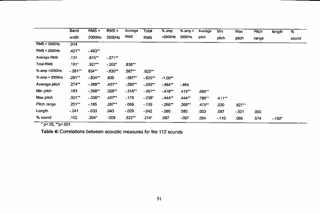
Band R M S < R M S > Average Total % amp % amp > Average Min Max Pitch length % width 2000Hz 2OOOH2 RMS R M S <2000Hz 2000Hz pitch pitch pitch range sound
RMS < 2OOOH2 .014
RMS > 2000Hz .421** - .493**
Average RMS .131 .815** - .271**
Total RMS .191* .927** - .202* .838**
% amp <2000Hz - .281** 834** - .830** .587** .625**
% amp > 2000Hz .281** - .834** .830 - .587** - .625** -1.00**
Average pitch .274** - .389** .401** - .292** - .295** - .464** -.464
Min pitch .183 -.368** .329** - .318** - .267** - .416** .416** .690**
Max pitch .321** - .338** .407** - .175 -.238* -.444** .444** .780** .41 r *
Pitch range .251** - .185 .267** -.068 -.139 -.268** .268** .475** .020 .827**
Length -.041 - .033 .043 -.029 -.042 -.080 .080 .003 .087 -.021 .000
% sound .102 .204* -.009 .322** .214* .097 -.097 .054 -.110 .066 .574 - .192*
Table 4i Correlations between acoustic measures for the 112 sounds
91
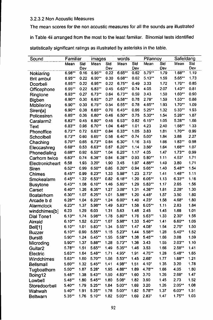
3.2.3.2 Non Acoustic Measures
The mean scores for the non acoustic measures for all the sounds are illustrated
in Table 4ii arranged from the most to the least familiar. Binomial tests identified
statistically significant ratings as illustrated by asterisks in the table.
Sound Familiar images words Pl/annoy Safe/dang Mean Std Mean Std Mean Std Mean std Mean Std
Dev Dev Dev Dev Dev
Nokiaring 6 . 9 8 " 0.16 6 . 9 5 " 0.22 6.65** 0.62 5.75** 1.79 1 .68" 1.19
Brit ambul 6 . 9 5 " 0.22 6 . 9 0 " 0.30 6.68** 0.62 5.13** 1.59 5.65** 1.73
Doorbell 6 . 9 5 " 0.22 6 . 9 5 " 0.22 6.75** 0.49 3.33 1.72 1.70** 0.85
Officephone 6 . 9 5 " 0.22 6 . 8 3 " 0.45 6.63** 0.74 4.05 2.07 1.43** 0.81
Ringtone 6 . 9 3 " 0.27 6 . 7 3 " 0.64 6.73** 0.59 3.43 1.50 1.60** 0.90
Bigben 6 . 9 0 " 0.30 6 . 9 3 " 0.27 6.58** 0.78 2.78* 1.59 1.53** 0.88
Mobitering 6 . 9 0 " 0.30 6 . 7 5 " 0.54 6 . 5 5 " 0.78 4.65** 1.93 1 .70" 1.09
Siren[a] 6 . 9 0 " 0.38 6 . 6 5 " 0.70 6 . 4 5 " 0.96 5.25** 1.32 5.33** 1.93
Policesiren 6 . 8 5 " 0.36 6 . 8 0 " 0.46 6.50** 0.75 5.30** 1.54 5.28** 1.87
Caralarm2 6 . 8 3 " 0.45 6 . 8 0 " 0.46 6.53** 0.82 6.15** 1.05 5.28** 1.66
Text 6 . 8 3 " 0.96 6 . 7 0 " 1.04 6.48** 1.01 4.23 2.40 1 . 6 8 " 1.33
Phonoffice 6 . 7 3 " 0.72 6 . 6 3 " 0.84 6.33** 1.05 3.83 1.81 1 .70" 0.99
Schoolbell 6 . 7 3 " 0.60 6 . 6 5 " 0.58 6.40** 0.74 5.00* 1.84 3.88 2.27
Chaching 6 . 7 0 " 0.65 6 . 7 3 " 0.64 6.30** 1.16 3.45 1.66 1.83** 0.98
Eleccashreg 6 . 6 8 " 0.53 6 . 6 3 " 0.67 6.20** 1.14 3.88* 1.64 1.68** 1.07
Phonedialing 6 . 6 8 " 0.92 6 . 5 0 " 1.04 6.25** 1.17 4.05 1.47 1 . 7 3 " 0.99
Carhorn twice 6 . 6 3 " 0.74 6 . 3 8 " 0.84 6.28** 0.93 5.80** 1.11 4.53* 1.71
Electronicheart 6.58 1.93 3.20* 1.90 3.45 1.97 4.88** 1.49 3.80 1.71
Siren 6 . 5 2 " 0.99 6 . 5 0 " 0.85 6.20** 0.94 5.65** 1.40 5.48** 1.54
Chimes 6 . 4 5 " 0.99 6 . 2 3 " 1.33 5.98** 1.23 2.73* 1.41 1 . 4 8 " 1.11
Smokealarm 6 . 4 5 " 1.22 6 . 5 3 " 0.82 6.18** 1.20 6.05** 1.13 6.33** 1.16
Busytone 6 . 4 3 " 1.08 6 . 1 0 " 1.46 5.85** 1.29 5.83** 1.17 2.65 1.56
Carset 6 . 4 0 " 1.26 6 . 3 5 " 1.27 3.08** 1.31 4.38** 1.81 2.28* 1.30
Boatairhorn 6 . 3 0 " 1.07 6 . 2 5 " 1.01 5.88** 1.20 4.48* 1.57 3.50 1.80
Arcade b d 6 . 2 8 " 1.04 6 . 2 0 " 1.24 6.00** 1.40 4.23* 1.58 4.68* 1.80
Alarmclock 6 . 2 3 " 1.37 5 . 9 8 " 1.49 5.83** 1.58 6.05** 1.11 2.83 1.84
windchimes[b] 6.23 1.29 6.03 1.31 5.63 1.48 2.45 1.45 1.68 1.01
Dial Tonel 6 . 1 3 " 1.74 5 . 9 8 " 1.78 5.80** 1.76 5.63** 1.33 2.30* 1.56
Airraid 6 . 1 0 " 1.52 6 . 2 3 " 1.07 5.98** 1.33 5.40** 1.41 6.60** 1.06
Bell[1] 6 . 1 0 " 1.01 5 . 8 3 " 1.34 5.55** 1.47 4.08* 1.54 2.75* 1.50
Buzzer 6 . 1 0 " 0.90 5 . 5 5 " 1.15 5.23** 1.44 5.58** 1.28 5.40** 1.52
Bursts 5 . 9 0 " 1.24 5 . 4 5 " 1.55 5.58** 1.38 5.45** 1.66 3.08 1.59
Microding 5 . 9 0 " 1.37 5 . 8 8 " 1.28 5.73** 1.36 3.43 1.55 2.03** 1.10
Guitar2 5 . 7 8 " 1.51 5 . 6 5 " 1.49 5.35** 1.46 3.53 1.66 2.58** 1.41
Electric 5 . 6 3 " 1.64 5 . 4 8 " 1.71 4.95* 1.91 4.75** 1.28 5 . 4 8 " 1.65
Windchimes 5 . 6 3 " 1.60 5 . 7 0 " 1.56 5.53** 1.45 2.68* 1.77 1.68** 1.21
Bellsmall 5 . 6 0 " 1.32 5 . 4 5 " 1.41 4.98** 1.51 4.10* 1.35 3.20 1.78
Tugboathorn 5 . 5 0 " 1.87 5.28* 1.95 4.88** 1.89 4.78** 1.66 4.05 1.80
Boing12 5 . 4 8 " 1.38 5 . 4 3 " 1.50 4.83** 1.60 3.70 1.26 2.68* 1.47
Lowbeil 5 . 4 8 " 1.80 5.45** 1.80 5.08* 1.82 3.90 1.45 2.73 1.52
Storedoorbell 5 . 4 0 " 1.79 5.25** 1.84 5.03** 1.69 3.20 1.26 2 . 0 5 " 1.08
Wahwah 5 . 4 0 " 1.91 5 . 2 5 " 1.78 5.03** 1.82 5.78** 1.37 6 . 0 3 " 1.51
Beltwarn 5 . 3 5 " 1.76 5 . 1 0 " 1.82 5.03** 1.69 2.83* 1.47 1 . 7 5 " 1.03
92
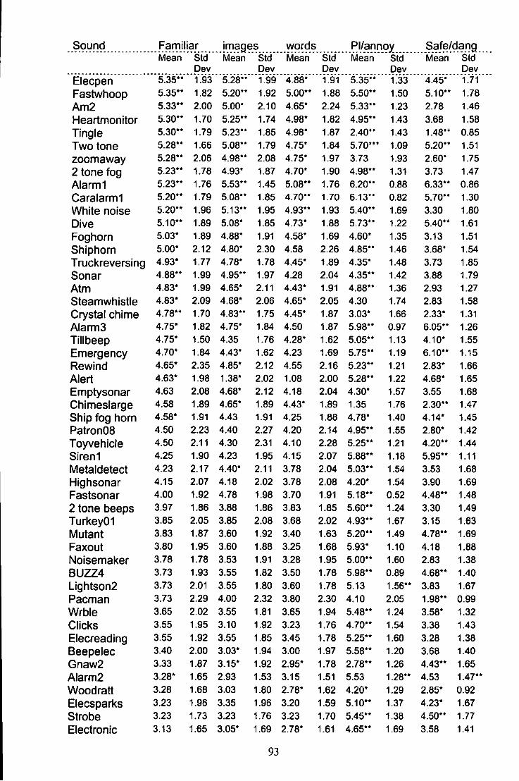
Sound Familiar images words Pl/annoy Safe/dang Mean Std Mean Std Mean Std Mean std Mean Std
Dev Dev Dev Dev Dev Elecpen 5.35** 1-93 5.28** 1.99 4.88* 1.91 5.35** 1.33 4.45* 1.71
Fastwhoop 5-35** 1.82 5 . 2 0 " 1.92 5.00** 1.88 5.50** 1.50 5.10** 1.78
Am2 5.33** 2.00 5.00* 2.10 4.65* 2.24 5.33* ' 1.23 2.78 1.46
Heartmonitor 5.30** 1.70 5.25** 1.74 4.98* 1.82 4.95** 1.43 3.68 1.58
Tingle 5.30** 1.79 5.23** 1.85 4.98* 1.87 2.40** 1.43 1.48** 0.85
Two tone 5.28** 1.66 5 . 0 8 - 1.79 4.75* 1.84 5.70*** 1.09 5.20** 1.51
zoomaway 5.28** 2.06 4.98** 2.08 4.75* 1.97 3.73 1.93 2.60* 1.75
2 tone fog 5.23** 1.78 4.93* 1.87 4.70* 1.90 4.98** 1.31 3.73 1.47
Alarm 1 5.23** 1.76 5.53** 1.45 5.08** 1.76 6.20** 0.88 6.33** 0.86
Caralarmi 5.20** 1.79 5.08** 1.85 4.70** 1.70 6.13** 0.82 5.70** 1.30
White noise 5.20** 1.96 5.13** 1.95 4.93** 1.93 5.40** 1.69 3.30 1.80
Dive 5.10** 1.89 5.08* 1.85 4.73* 1.88 5.73** 1.22 5.40** 1.61
Foghorn 5.03* 1.89 4.88* 1.91 4.58* 1.69 4.60* 1.35 3.13 1.51
Shiphorn 5.00* 2.12 4.80* 2.30 4.58 2.26 4.85** 1.46 3.68* 1.54
Truckreversing 4.93* 1.77 4.78* 1.78 4.45* 1.89 4.35* 1.48 3.73 1.85
Sonar 4.88** 1.99 4.95** 1.97 4.28 2.04 4.35** 1.42 3.88 1.79
Atm 4.83* 1.99 4.65* 2.11 4.43* 1.91 4.88** 1.36 2.93 1.27
Steamwhistle 4.83* 2.09 4.68* 2.06 4.65* 2.05 4.30 1.74 2.83 1.58
Crystal chime 4.78** 1.70 4.83** 1.75 4.45* 1.87 3.03* 1.66 2.33* 1.31
Alarms 4.75* 1.82 4.75* 1.84 4.50 1.87 5.98** 0.97 6.05** 1.26
Tillbeep 4.75* 1.50 4.35 1.76 4.28* 1.62 5.05** 1.13 4.10* 1.55
Emergency 4.70* 1.84 4.43* 1.62 4.23 1.69 5.75** 1.19 6.10** 1.15
Rewind 4.65* 2.35 4.85* 2.12 4.55 2.16 5.23** 1.21 2.83* 1.66
Alert 4.63* 1.98 1.38* 2.02 1.08 2.00 5.28** 1.22 4.68* 1.65
Emptysonar 4.63 2.08 4.68* 2.12 4.18 2.04 4.30* 1.57 3.55 1.68
Chimeslarge 4.58 1.89 4.65* 1.89 4.43* 1.89 1.35 1.76 2.30** 1.47
Ship fog horn 4.58* 1.91 4.43 1.91 4.25 1.88 4.78* 1.40 4.14* 1.45
PatronOS 4.50 2.23 4.40 2.27 4.20 2.14 4.95** 1.55 2.80* 1.42
Toyvehicle 4.50 2.11 4.30 2.31 4.10 2.28 5.25** 1.21 4.20** 1.44
Siren 1 4.25 1.90 4.23 1.95 4.15 2.07 5.88** 1.18 5.95** 1.11
Metaldetect 4.23 2.17 4.40* 2.11 3.78 2.04 5.03** 1.54 3.53 1.68
Highsonar 4.15 2.07 4.18 2.02 3.78 2.08 4.20* 1.54 3.90 1.69
Fastsonar 4.00 1.92 4.78 1.98 3.70 1.91 5.18** 0.52 4.48** 1.48
2 tone beeps 3.97 1.86 3.88 1.86 3.83 1.85 5.60** 1.24 3.30 1.49
TurkeyOI 3.85 2.05 3.85 2.08 3.68 2.02 4.93** 1.67 3.15 1.63
Mutant 3.83 1.87 3.60 1.92 3.40 1.63 5.20** 1.49 4.78** 1.69
Faxout 3.80 1.95 3.60 1.88 3.25 1.68 5.93* 1.10 4.18 1.88
Noisemaker 3.78 1.78 3.53 1.91 3.28 1.95 5.00** 1.60 2.83 1.38
BUZZ4 3.73 1.93 3.55 1.82 3.50 1.78 5.98** 0.89 4.68** 1.40
Lightson2 3.73 2.01 3.55 1.80 3.60 1.78 5.13 1.56** 3.83 1.67
Pacman 3.73 2.29 4.00 2.32 3.80 2.30 4,10 2.05 1.98** 0.99
Wrble 3.65 2.02 3.55 1.81 3.65 1.94 5.48** 1.24 3.58* 1.32
Clicks 3.55 1.95 3.10 1.92 3.23 1.76 4.70** 1.54 3.38 1.43
Elecreading 3.55 1.92 3.55 1.85 3.45 1.78 5.25** 1.60 3.28 1.38
Beepelec 3.40 2.00 3.03* 1.94 3.00 1.97 5.58** 1.20 3.68 1.40
Gnaw2 3.33 1.87 3.15* 1.92 2.95* 1.78 2.78** 1.26 4.43** 1.65
Alarm2 3.28* 1.65 2.93 1.53 3.15 1.51 5.53 1.28** 4.53 1.47**
Woodratt 3.28 1.68 3.03 1.80 2.78* 1.62 4.20* 1.29 2.85* 0.92
Elecsparks 3.23 1.96 3.35 1.96 3.20 1.59 5.10** 1.37 4.23* 1.67
Strobe 3.23 1.73 3.23 1.76 3.23 1.70 5.45** 1.38 4.50** 1.77
Electronic 3.13 1.65 3.05* 1.69 2.78* 1.61 4.65** 1.69 3.58 1.41
93
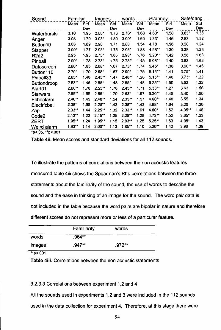
Sound Familiar Images words Pl/annoy Safe/dang Mean Std
Dev Mean Std
Dev Mean Std
Dev Mean s td
Dev Mean S i d
Dev
Waterbursts 3.10 1.95 2.88* 1.76 2.70* 1.68 4.63* 1.58 3.63* 1.33
Anger 3.08 1,79 3.03* 1.80 3.00* 1.69 1.33* 1.46 2.83 1.32
Button 10 3.03 1.89 2.90 1.71 2.88 1.54 4.78 1.56 3.20 1.24
Slapper 3.00* 1.77 2.98* 1.75 2.95* 1.88 4.58** 1.30 3.38 1.23
R2d2 2.95 1.95 2.75* 1.85 2.98* 1.76 5.20** 1.42 3.58 1.63
Pinball 2.90* 1.78 2.73* 1.75 2.73** 1.45 5.08** 1.40 3.83 1.63
Datascreen 2.80* 1.65 2.68* 1.67 2.73* 1.74 5.45* 1.38 3.90*' 1.45
Button 110 2.70* 1.70 2.68* 1.67 2.90* 1.75 5.15** 1.41 3.75* 1.41
Plnball33 2.65* 1.48 2.45** 1.47 2.48** 1.28 5.15** 1.46 3.73* 1.22
Buttondroop 2.63** 1.46 2.55* 1.48 2.55* 1.48 5.25** 1.50 3.53 1.32
AlartOI 2.60** 1.78 2.55** 1.78 2.45** 1.71 5.33** 1.27 3.63 1.56
Starwars 2.55** 1.55 2.65* 1.70 2.63* 1.67 5.20** 1.45 3.40 1.50
Echoalarm 2.40** 1.45 2.48** 1.54 2.35** 1.57 4.60** 1.48 3.55 1.34
Electricbell 2.38* 1.55 2.25** 1.43 2.38** 1.43 4.68* 1.64 3.20 1.30
Zap 2.33** 1.44 2.25** 1.32 2.33** 1.61 4.80* 1.52 4.35** 1.48
Code2 2.13** 1.22 2.15** 1.25 2.28** 1.28 4.73** 1.52 3.65* 1.23
ZERT 1.95** 1.24 1.95** 1.15 2.03** 1.25 5.25** 1.63 4.05* 1.43
Weird alarm 1.93** 1.14 2.00** 1.13 1.85** 1.10 5.20** 1.40 3.90 1.39
*p<.05, **p<.001
Table 4ii. Mean scores and standard deviations for all 112 sounds.
To illustrate the patterns of cx)rrelatlons between the non acoustic features
measured table 4ill shows the Spearman's Rho correlations between the three
statements about the familiarity of the sound, the use of words to describe the
sound and the ease In thinking of an image for the sound. The word pair data is
not included in the table because the word pairs are bipolar In nature and therefore
different scores do not represent more or less of a particular feature.
Familiarity words
words .964**
images .947** .972** **p<.001
Table 4iii, Correlations between the non acoustic statements
3.2.3.3 Correlations between experiment 1,2 and 4
All the sounds used in experiments 1,2 and 3 were Included In the 112 sounds
used in the data collection for experiment 4. Therefore, at this stage there were
94
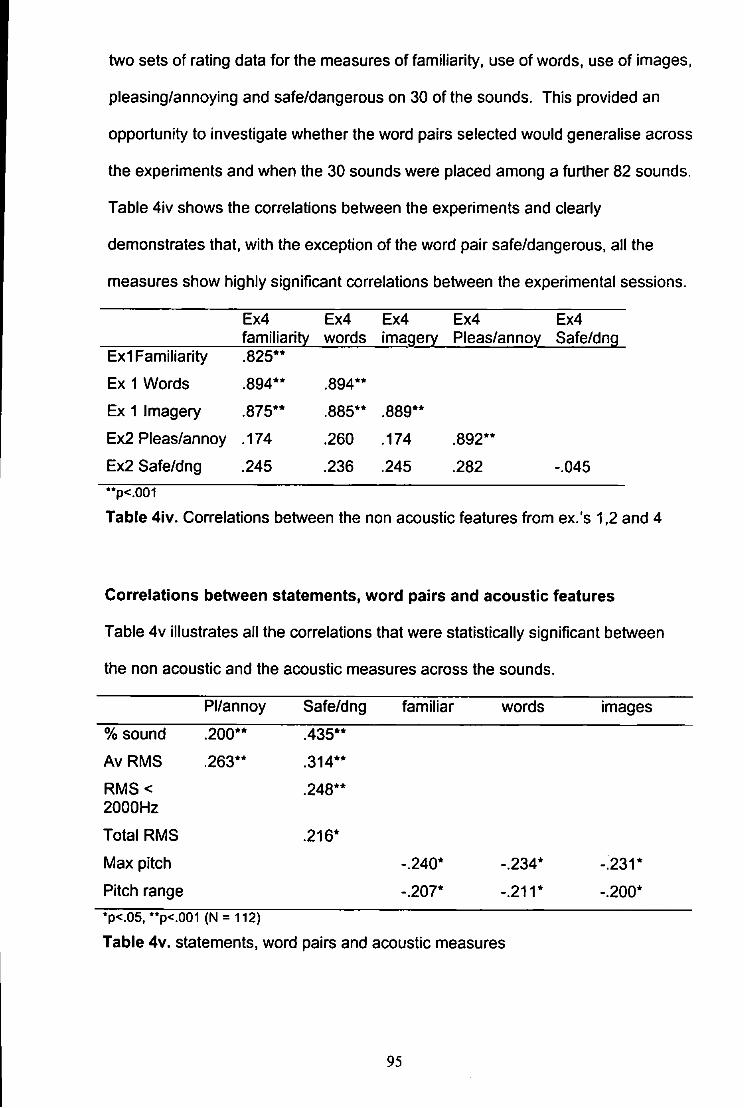
two sets of rating data for the measures of familiarity, use of words, use of images,
pleasing/annoying and safe/dangerous on 30 of the sounds. This provided an
opportunity to investigate whether the word pairs selected would generalise across
the experiments and when the 30 sounds were placed among a further 82 sounds.
Table 4iv shows the correlations between the experiments and cleariy
demonstrates that, with the exception of the word pair safe/dangerous, all the
measures show highly significant correlations between the experimental sessions.
Ex4 familiarity
Ex4 words
Ex4 imagery
Ex4 Pleas/annoy
Ex4 Safe/dng
Exi Familiarity .825"
Ex 1 Words .894" .894"
Ex 1 Imagery .875" .885" .889"
Ex2 Pleas/annoy .174 .260 .174 .892"
Ex2 Safe/dng .245 .236 .245 .282 -.045 "p<.001
Table 4iv. Correlations between the non acoustic features from ex.'s 1.2 and 4
Correlations between statements, word pairs and acoustic features
Table 4v illustrates all the correlations that were statistically significant between
the non acoustic and the acoustic measures across the sounds.
Pl/annoy Safe/dng familiar words images
% sound .200" .435"
AvRMS .263" .314"
RMS< 2000Hz
.248"
Total RMS .216*
Max pitch -.240* -.234* -:231*
Pitch range -.207* -.211* -.200* *p<.05, "p<.001 (N = 112)
Table 4v. statements, word pairs and acoustic measures
95
3.2.4 Discussion
In the same way as experiments 1 and 2 this study identified the responses to
statements about familiarity, the use of words and images, and word pair data but
for a larger 112 sound stimuli set. As such it has provided an indication as to
which features are perceptually important for the listener and how this varies
across the different sounds. For example, nokia ring and British ambulance both
elicit very strong responses to all the scales which can be cleariy seen in table 4i.
Conversely, zap and code2 were rated on the opposite ends of the statement
scales. As before the acoustic measures have formed a large database of
information for the 112 sounds.
As identified in experiment 1 familiarity appears to play a role in participants'
ratings on other scales and has been demonstrated for all the sounds studied with
respect to the highly significant correlations identified between levels of perceived
familiarity and the ease with which words or images are used by the participants
illustrated in table 4iii.
In order to see how the acoustic features map onto the statement and word pairs
across all 112 sounds table 4v shows the significant correlations. For both the
word pairs pleasing/annoying, and safe/dangerous, only measures of the sounds
power (average RMS. RMS < 2000Hz and total RMS) show significant correlations
with the exception of the overall percentage sound versus silence measure for
each sound. This is the same pattern identified between word pairs and measure
of RMS shown from experiment 2 in table 2v. Therefore, these preliminary results
suggest that the acoustic measures of RMS power map onto the descriptive
measures pleasing/annoying and safe/dangerous. The statement data shows a
different trend to the word pair data with only the acoustic measure of pitch
96
showing significant correlations with the statements about familiarity, use of words
and use of Images. Again this reflects previous correlations between acoustic
features and the statements.
Including the 30 sounds from experiments 1 and 2 in the 112 sounds employed In
the present experiment has provided the opportunity to asses the degree to which
the statements and word pair measures are reliable across different experimental
sessions and contexts (among larger sound set). Between experiments 1, 2 and 4
there are clear, highly significant correlations between the ratings on all the scales
(table 4iv) with the exception of safe/dangerous. This has demonstrated that the
scales used are reliable for the 30 abstract sounds that were included across the
different experiments. In addition, the results from experiment 4 again reflect the
results obtained by Ballas(1993) with respect to significant relationships between
the statements for the use of imagery, words to describe a sound and familiarity.
This suggests that these scales would be likely to generalise across a range of
sound stimuli.
97
3.3 Experiment 5: Grouping task
3.3.1 Introduction
Experiment 5 was conducted to identify whether the features that were identified
as salient for the similarity judgements between the 15 sounds in experiment 3
(namely; RMS power, pitch, descriptive word pairs, frequency, function & source
information) would generalise to a much larger abstract sound set that also
employs a different methodology to collect the similarity matrices.
Seventy of the 112 sound stimuli from experiment 4 were chosen for inclusion in
experiment 5. The criteria on which to exclude some of the sounds, to reduce the
stimuli set, was based on the importance of familiarity as indicated by both
experiment 1 and previous research (Solomon, 1958; Ballas, 1993; Fabiani et al,
1996). Familiarity was a measure that elicited a clear familiar/unfamiliar rating
from participants on the majority of the sound stimuli measured in experiment 4.
Therefore, if familiarity is a contributing feature in participants' similarity
judgements selecting sounds on this basis will allow investigation of whether
familiar sounds are grouped by source or function and the more unfamiliar sounds
grouped by their acoustic features. Therefore, the sounds that were rated as the
35 most familiar and the 35 least familiar using the statement 'this sound seems
very familiar to me' in experiment 4 were included in experiment 5. This will help
to demonstrate whether the similarity judgements being made by participants, as
indicated in experiment 3, are being made on more than the measured acoustic
and descriptive features.
The pairwise task used for experiment 3 to collect similarity judgements about the
sounds is not suitable for larger sounds sets. The exponential increase in the
number of sound pairs means that a stimuli set the size of the one considered for
98
this experiment (N=70) would be completely impractical. Therefore, a grouping
methodology was proposed by Bonebright (1996) as a suitable alternative to the
pairwise task for the sound stimuli. The task used for this experiment employed a
grouping task similar to that employed by Bonebright (2001) and Scavone et al
(2002). The grouping task overcomes the unmanageable number of sound pairs
that 70 sounds would produce (70 x 69/2=2415). The grouping task traditionally
used for visual or tactile stimuli (Schiffman et al, 1981) but suitable for auditory use
requires the participant to sort the stimuli (represented using icons attached to
sounds) into groups according to how they believe they relate to one another.
There are often additional constraints, such as a group must contain a minimum of
two stimuli (Bonebright. 1998) to prevent sounds being placed in isolation. The
sorting task instructions could specify an attribute to consider during the sort. e.g.
pitch or rhythm if this feature is of particular interest. Alternatively, no specific
constraints are adopted and participants free sort on the basis of (dis)similarity.
The grouping task provides information about the perceptual relations among
stimuli and produces proximity data that is suitable for multidimensional scaling
and hierarchical cluster analysis. This serves to maintain the option to use the
same basic analysis techniques across the different methodologies to provide a
basis for comparison. Bonebright (1996) discusses its suitability for auditory
stimuli, especially with large (> 25 item) stimuli sets. Of course this makes the
technique much more efficient in terms of participant time. It is, for example,
questionable whether participants could maintain a consistent set of criteria that
would be required for even 50 sounds (1125 judgements) (Scavone et al, 2002).
Scavone et al also suggest that traditional methods such as the painwise task may
set unnecessary limits on participants' perceptual, cognitive and decisional
strategies and discourage listeners' application of richer sets of perceptual and
99
cognitive criteria in their judgements. This reduced set of perceptual and
cognitive criteria may be encouraged by the use of continuous rating scales, such
as those used in experiment 3 that may encourage participants to think uni
dimensionally about the similarities between the stimuli. In order to resolve some
of the problems Scavone et a! (2002) devised a Linux based grouping task similar
to the one used in the present experiment.
For experiment 5 a new program (Aldrlch, March 2003) was written guided by the
Scavone et al (2002) work and the discussion of the technique by Bonebright et a!
(1998) who suggested the inclusion of a practice task. A practice task that
required the grouping of coloured squares would help to familiarise participants
with the task. Using this grouping technique participants are typically required to
sort the sounds into groups either by specific features (e.g. pitch) or according to
how they perceive the stimuli relate to each other. There are typically constraints
on the groups such as a minimum of two sounds per group to prevent sounds
being placed In isolation. Participants are encouraged to make changes during
their grouping process until they are entirely happy with their groups. Bonebright
(1996) identified that the two methodologies produced slightly different output with
respect to the distribution of sounds on the MDS solution. Typically the sorting
task tended to produce tighter clusters than the pairwise task.
3.3.2 Method
3.3.2.1 Participants
46 participants (8 males, 38 females) took part in the study. All participants had
normal or corrected to normal hearing. Participants were psychology students at
the University of Plymouth and were awarded points for their participation as part
of the BSc psychology course requirement
100
3.3.2.2 Apparatus
The stimuli were presented using a purpose written program ("soundsorT Aldrich,
March 2003). Six computers with headphones were used (Hewlett Packard
Vectra's PIN with a 600 MHz Processor, 128 MB RAM and CrystalSoundFusion™
Soundcard operating on Windows XP).
3.3.2.3 Stimuli
The sound stimuli used for this experiment were 70 abstract sounds (appendix B1
sound names in italics) taken from the larger pool of 112 sounds used in
experiment 4. The sounds chosen were selected because they were the sounds
rated as the 35 most familiar and the 35 least familiar as previous work has
demonstrated the importance of familiarity in Identification of sounds (Ballas,
1993).
3.3.2.4 Materials
A purpose written program was used for the experiment that employed a different
task that was more appropriate for the collection of similarity data for a large
number of sounds.
An initial briefing sheet introduced the task to the participants and included the
following instructions
"The experiment requires you to re-arrange 70 short sounds into a
maximum of 20 groups. The experiment Is not timed and how you choose
to group the sounds Is completely up to you. There are no right or wrong
answers"
101
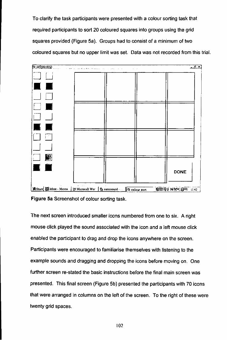
To clarify the task participants were presented with a colour sorting task that
required participants to sort 20 coloured squares into groups using the grid
squares provided (Figure 5a). Groups had to consist of a minimum of two
coloured squares but no upper limit was set. Data was not recorded from this trial.
• M m J • • • • J
• • • • J J
i _ J
• mi m DONE
! |BStart ^ I n b o x - Micros | 3yMicrotoftWor ifa samesound • |[q co lour tor t N^*^^^*^ IIA2
Figure 5a Screenshot of colour sorting task.
The next screen introduced smaller icons numbered from one to six. A right
mouse click played the sound associated with the icon and a left mouse click
enabled the participant to drag and drop the icons anywhere on the screen.
Participants were encouraged to familiarise themselves with listening to the
example sounds and dragging and dropping the icons before moving on. One
further screen re-stated the basic instructions before the final main screen was
presented. This final screen (Figure 5b) presented the participants with 70 icons
that were arranged in columns on the left of the screen. To the right of these were
twenty grid spaces.
102
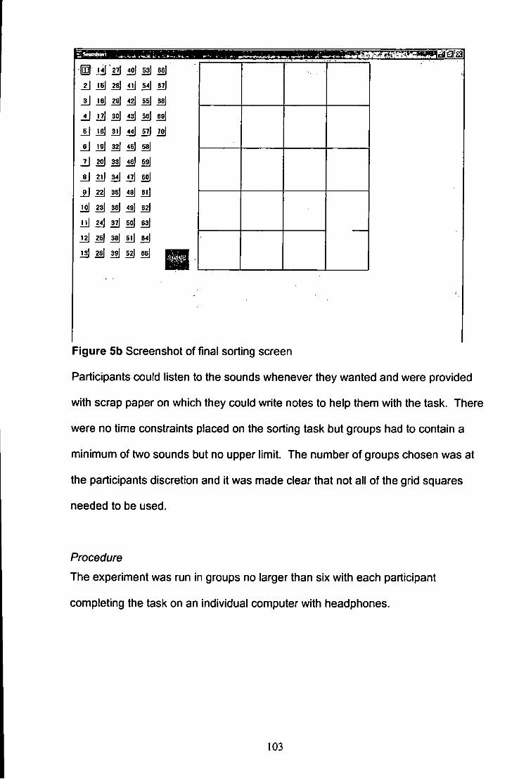
M' i l l ^161 si 16|
A] W |
li i l l
_6j 19]
JLJiol
_ej 22]
iO] 23)
III 111 Hi 25)
is j 26]
27| 40| 53)
28] l l J 54|
29| 42] 55|
30] 43| 56|
3l] 44) 57]
52| 45| 58]
m| 46| 59]
34) 50|
35) 48| BlJ
38) 49] 52|
37J 50) B3|
38) 5lJ m)
39| 52) 65]
66]
37)
B8]
39)
70)
Figure 5b Screenshot of final sorting screen
Participants could listen to the sounds whenever they wanted and were provided
with scrap paper on which they could write notes to help them with the task. There
were no time constraints placed on the sorting task but groups had to contain a
minimum of two sounds but no upper limit. The number of groups chosen was at
the participants discretion and it was made clear that not all of the grid squares
needed to be used.
Procedure
The experiment was run in groups no larger than six with each participant
completing the task on an individual computer with headphones.
103
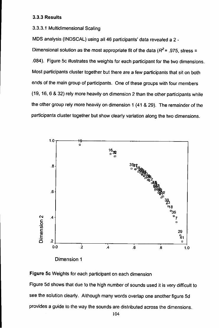
3.3.3 Results
3.3.3.1 Multidimensional Scaling
MDS analysis (INDSCAL) using all 46 participants' data revealed a 2 -
Dimensional solution as the most appropriate fit of the data (R^= .975. stress =
.084). Figure 5c illustrates the weights for each participant for the two dimensions.
Most participants cluster together but there are a few participants that sit on both
ends of the main group of participants. One of these groups with four members
(19, 16, 6 & 32) rely more heavily on dimension 2 than the other participants while
the other group rely more heavily on dimension 1 (41 & 29). The remainder of the
participants cluster together but show clearly variation along the two dimensions.
CVJ c o '« c E b
Dimension 1
Figure 5c Weights for each participant on each dimension
Figure 5d shows that due to the high number of sounds used it is very difficult to
see the solution clearly. Although many words overlap one another figure 5d
provides a guide to the way the sounds are distributed across the dimensions. 104
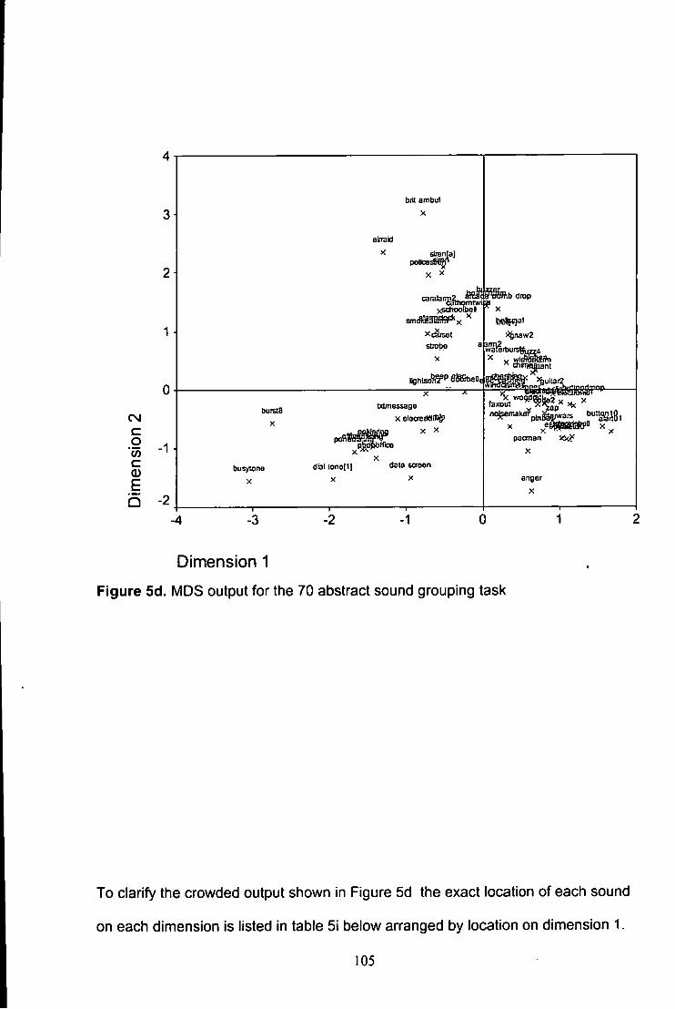
2
1
bril am bid X
aimiid
X sirenlal pOBCOE
xsdiooIbeD
Dghlso'?. Pfl&ibeD
b drop
watemu
faxout
patjnan
anger
eg c g CO c CD E
^ -1
bursts
X
busytone
X
dial tone[1] X
X 5r txtmessage
X X
ffice
data Gcraen
X
1
Dinnension 1
Figure 5d. MDS output for the 70 abstract sound grouping task
To clarify the crowded output shown in Figure 5d the exact location of each sound
on each dimension is listed in table 51 below arranged by location on dimension 1.
105
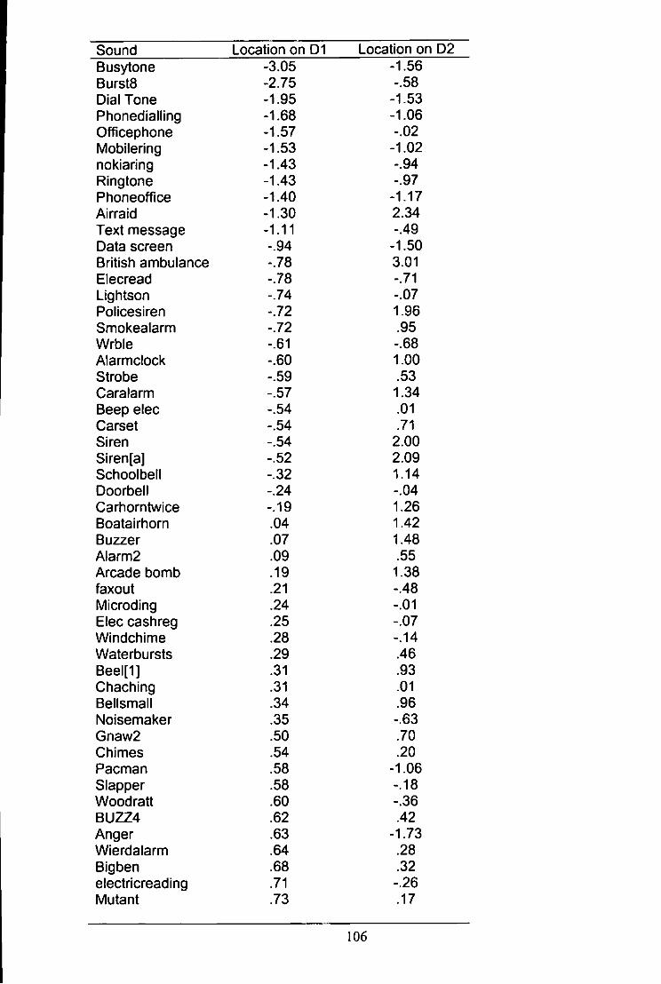
Sound Location on D1 Location on D2 Busytone -3.05 -1.56 Bursts -2.75 -.58 Dial Tone -1.95 -1.53 Phonedialling -1.68 -1.06 Officephone -1.57 -.02 Mobilering -1.53 -1.02 nokiaring -1.43 -.94 Ringtone -1.43 -.97 Phoneoffice -1.40 -1.17 Airraid -1.30 2.34 Text message -1.11 -.49 Data screen -.94 -1.50 British ambulance -.78 3.01 Elecread -.78 -.71 Lightson -.74 -.07 Policesiren -.72 1.96 Smokealarm -.72 .95 Wrble -.61 -.68 Alarmclock -.60 1.00 Strobe -.59 .53 Caralarm -.57 1.34 Beep elec -.54 .01 Carset -.54 .71 Siren -.54 2.00 Siren[a] -.52 2.09 Schoolbell -.32 1.14 Doorbell -.24 -.04 Carhorntwice -.19 1.26 Boatairhorn .04 1.42 Buzzer .07 1.48 Alarm2 .09 .55 Arcade bomb .19 1.38 faxout .21 -.48 Microding .24 -.01 Elec cashreg .25 -.07 Windchime .28 -.14 Waterbursts .29 .46 Beel[1] .31 .93 Chaching .31 .01 Bellsmall .34 .96 Noisemaker .35 -.63 Gnaw2 .50 .70 Chimes .54 .20 Pacman .58 -1.06 Slapper .58 -.18 Woodratt .60 -.36 BUZZ4 .62 .42 Anger .63 -1.73 Wierdalarm .64 .28 Bigben .68 .32 electricreading .71 -.26 Mutant .73 .17
106
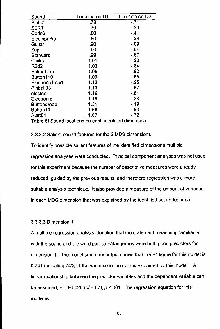
Sound Location on D1 Location on D2 Pinball .78 -.71 ZERT .79 -.23 Code2 .80 -.41 Elec sparks .80 -.24 Guitar .90 -.09 Zap .90 -.54 Starwars .99 -.67 Clicks 1.01 -.22 R2d2 1.03 -.84 Echoalarm 1.05 -.82 Button110 1.09 -.85 Electronicheart 1.12 -.25 Pinball33 1.13 -.87 electric 1.16 -.81 Electronic 1.18 -.28 Buttondroop 1.31 -.19 Button 10 1.56 -.63 AlartOI 1.67 -.72 Table 5i Sound locations on each identified dimension
3.3.3.2 Salient sound features for the 2 MDS dimensions
To identify possible salient features of the identified dimensions multiple
regression analyses were conducted. Principal component analyses was not used
for this experiment because the number of descriptive measures were already
reduced, guided by the previous results, and therefore regression was a more
suitable analysis technique. It also provided a measure of the amount of variance
in each MDS dimension that was explained by the identified sound features.
3.3.3.3 Dimension 1
A multiple regression analysis identified that the statement measuring familiarity
with the sound and the word pair safe/dangerous were both good predictors for
dimension 1. The model summary output shows that the figure for this model is
0.741 indicating 74% of the variance in the data is explained by this model. A
linear relationship between the predictor variables and the dependent variable can
be assumed, F = 96.028 (df = 67), p <.001. The regression equation for this
model is;
107
D1 = 3.705 + (familiar, -.390) + (safe/dangerous, -.537)
Therefore, as dimension 1 increases by 1 unit, familiarity decreases by .390 units
and the sounds moved from being rated as dangerous to safe as measured by the
word pair safe/dangerous. Both predictors were measured using the same 7 point
Likert-type scale. No acoustic features showed a significant relationship to the
sounds' location on this dimension.
For dimension 1 the case wise diagnostics suggest that there was one outlier,
case number 33. with a residual of 4.129 (above the 3.3 rule of thumb). The data
was re-analysed removing this case to identify its affect. The new result gives a
figure of 81%. Therefore this suggests that the inclusion of the outlier reduces
the proportion of variance accounted for and is therefore a more conservative
result. Such an outlier may suggest that there are other explanatory variables that
could be included in the model. This is not a surprising result as it is accepted that
only a selection of relevant features have been measured. For dimension 2 no
such outliers were identified.
Partial correlations were calculated to examine the unique contributions of the two
predictors on dimension 1. The partial correlation between dimension 1 and
familiarity controlling for safe-dangerous was highly significant,, r= -.789, df = 67,
p<.001. Similarly, the partial correlation between dimension 1 and safe-dangerous
controlling for familiarity was highly significant, r= -.793, df 67, p<.001. Thus each
predictor had a component of variance that was independent of the other predictor
and that correlated highly with the variance in dimension 1 that was also
independent of the other predictor.
108
3.3.3.4 Dimension 2
A multiple regression analysis identified that safe/dangerous, pleasing/annoying
and use of words were good predictors of the sounds' location on dimension 2.
The model summary output shows that the adjusted figure for this model is
0.547 indicating 55% of the variance in the data is explained by this model.
Linear relationships between the predictor variables and the dependent variable
can be assumed, F = 28.79 {df= 69), p <.001. The regression equation for this
model is;
D2 = -2.954 + (sf/dng -.650) + (pl/annoy .841) + (words .257).
Therefore, as dimension 2 increases by 1 unit the ease with which participants can
think of words to describe a sound increases by .257 units. In addition as
dimension 2 increases sounds move from being rated as safe and annoying
towards dangerous and pleasing as measured by the word pairs safe/dangerous
and pleasing/annoying. Again no acoustic features showed a relationship to the
sounds locations on dimension 2.
Partial correlations for dimension 2 also demonstrate highly significant
relationships between the predictor variables and the dimension when holding the
influence of the other variables constant. The relationship between dimension 2
and safe/dangerous, controlling for pleasing/annoying and the use of words shows
a highly significant result, r = -.680, df = 66, p<.001. The relationship between D2
and pleasing/annoying is also highly significant, controlling for the use of words
and safe/dangerous, r = .610, df=66. p<.001. Finally the relationship between D2
and the use of words, controlling for the other variables is highly significant, r =
.527, df = 66, p<.001. Again this demonstrates that the predictor variables all have
a strong relationships to dimension 2 when holding constant the affects of the
other two variables.
109
3.3.3.5 Dimension Summary
Dimension 1 - familiarity and safe/dangerous
Dimension 2 - safe/dangerous, pleasing/annoying and use of words to
describe a sound.
Figure 5e shows the Dendrogram from a hierarchical cluster analysis on the data
and helps to demonstrate the clusters that participants formed but provides no
information about possible dimensions used to make the grouping decisions.
no
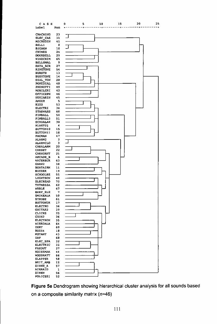
C A S E 10 15 20 L a b e l Num
CHACHING 23 ELEC_CAS 31 MICRODIN 41 BELLI 8 BIGBEN 10 CHIMES 24 DCXJRBELL 29 WINDCHIM 65 BELLSMAL 9 DATA_SCR 27 RINGTONE 54 BURSTS 13 BUSYTONE 14 DIAL_TON 28 PONEDIAL 48 PHONOFFI 49 MOBILERI 42 OFFICEPH 46 NOKIARIN 45 ANGER 5 R2D2 53 ELECTRI 34 STARWARS 60 PINBALL 50 PINBALL3 51 ECHOALAR 30 ALARTOl 4 BUTTON10 15 BUTTON11 16 PACMAN 47 ALARMS 2 ALARMCLO 3 CARALARM 20 CARSET 22 CARHORNT 21 ARCADE_B 6 WATERBUR 63 GNAW2 38 BOATAIRH 11 BUZZER 19 SCHOOLBE 55 LIGHTSON 40 ELECREAD 70 TXTMESSA 62 WRBLE 67 BEEP_ELE 7 SMOKEALA 59 STROBE 61 BUTTONDR 17 ELECTRO 36 GUITAR2 39 CLICKS 25 C0DE2 26 ELECTRON 35 WIERDALA 64 ZERT 69 BUZZ4 18 MUTANT 43 ZAP 68 ELEC_SPA 32 ELECTRIC 33 FAXOUT 37 NOISEMAK 44 WOODRATT 66 SLAPPER 58 BRIT_AMB 12 SIREN_A 57 AIRRAID 1 SIREN 56 POLICESI 52
25 • - +
3
Figure 5e Dendrogram showing hierarchical cluster analysis for all sounds based
on a composite similarity matrix (n=46)
111
3.3.4 Discussion
Analyses from the grouping task results suggested that familiarity with a sound
and the connotations of safety/ danger were important features used by
participants in their grouping decisions and accounted for 74% of the variance in
dimension 1. Familiarity was included as the major reason for the sounds' original
selection: the sounds rated as the 35 most and the 35 least familiar words were
included. Therefore, the contribution of familiarity to dimension 1 is probably a
reflection of the 'familiarity' selection criteria. Nonetheless, it still suggests the
importance of this feature in the way participants choose to group the sounds.
Familiarity was not a feature identified from the MDS analysis previously but a
feature that appeared to contribute to the way participants rated and grouped the
sounds in the preliminary rating experiments (ex.'s 1 &2). Conversely, in this
experiment familiarity was identified on dimension 1 as a feature that may be used
during the formation of groups as identified by the MDS analysis. Words to
describe a sound, how pleasant or unpleasant a sound is and the connotations of
danger explained 55% of the variance for dimension 2. This dimension may
reflect the descriptive factor that correlated with dimension 2 in experiment 3.
However, no such similarity is demonstrated between experiments 3 and 5 for
dimension 1. A further note of interest is that unlike experiment 3 none of the
acoustic features showed any relationship to the sounds' locations on the MDS
output on either dimensions in experiment 5. This is despite the finding that 45%
of the variance on dimension 2 is not accounted for by the measured non acoustic
features. This may in part be explained by the large number of sounds employed
in the experiments. This could mean that acoustic features may have been too
variable across such a large number of sounds for participants to use them
consistently enough to be clearly identifiable on one of the MDS dimensions.
112
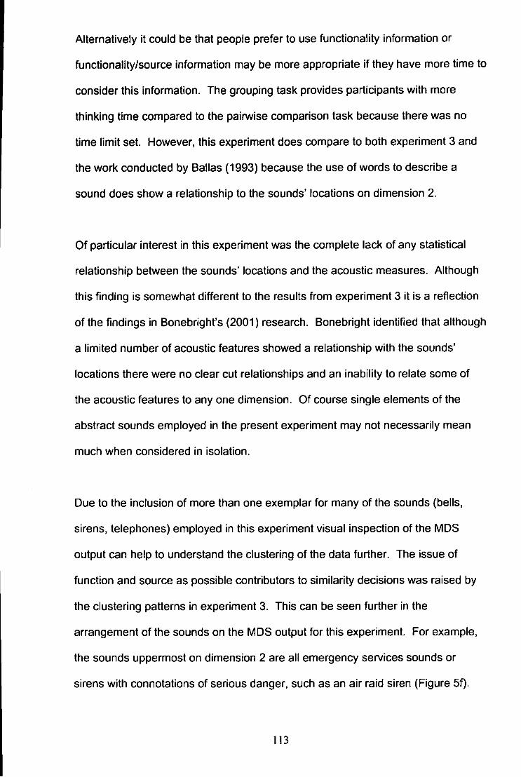
Alternatively it could be that people prefer to use functionality information or
functionality/source information may be more appropriate if they have more time to
consider this Information. The grouping task provides participants with more
thinking time compared to the pairwise comparison task because there was no
time limit set. However, this experiment does compare to both experiment 3 and
the work conducted by Ballas (1993) because the use of words to describe a
sound does show a relationship to the sounds' locations on dimension 2.
Of particular interest in this experiment was the complete lack of any statistical
relationship between the sounds' locations and the acoustic measures. Although
this finding is somewhat different to the results from experiment 3 it is a reflection
of the findings in Bonebright's (2001) research. Bonebright identified that although
a limited number of acoustic features showed a relationship with the sounds'
locations there were no clear cut relationships and an inability to relate some of
the acoustic features to any one dimension. Of course single elements of the
abstract sounds employed in the present experiment may not necessarily mean
much when considered in isolation.
Due to the inclusion of more than one exemplar for many of the sounds (bells,
sirens, telephones) employed in this experiment visual inspection of the MDS
output can help to understand the clustering of the data further. The issue of
function and source as possible contributors to similarity decisions was raised by
the clustering patterns in experiment 3. This can be seen further in the
arrangement of the sounds on the MDS output for this experiment. For example,
the sounds uppermost on dimension 2 are all emergency services sounds or
sirens with connotations of serious danger, such as an air raid siren (Figure 5f).
113
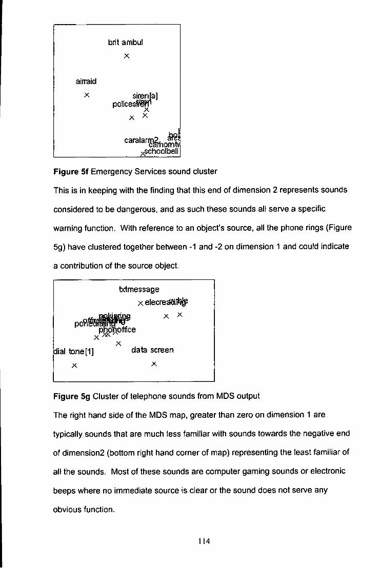
bnt ambul
airraid sinenia
;K;Schoolbell
Figure 5f Emergency Services sound cluster
This is in keeping with the finding that this end of dimension 2 represents sounds
considered to be dangerous, and as such these sounds all serve a specific
warning function. With reference to an object's source, all the phone rings (Figure
5g) have clustered together between -1 and -2 on dimension 1 and could indicate
a contribution of the source object.
Ixtmessage X elecre^lfe^
sgnag X X-
PS! pj^ffice X
dial tone[1] data screen
X X
Figure 5g Cluster of telephone sounds from MDS output
The right hand side of the MDS map. greater than zero on dimension 1 are
typically sounds that are much less familiar with sounds towards the negative end
of dimension2 (bottom right hand corner of map) representing the least familiar of
all the sounds. Most of these sounds are computer gaming sounds or electronic
beeps where no immediate source is clear or the sound does not serve any
obvious function.
114
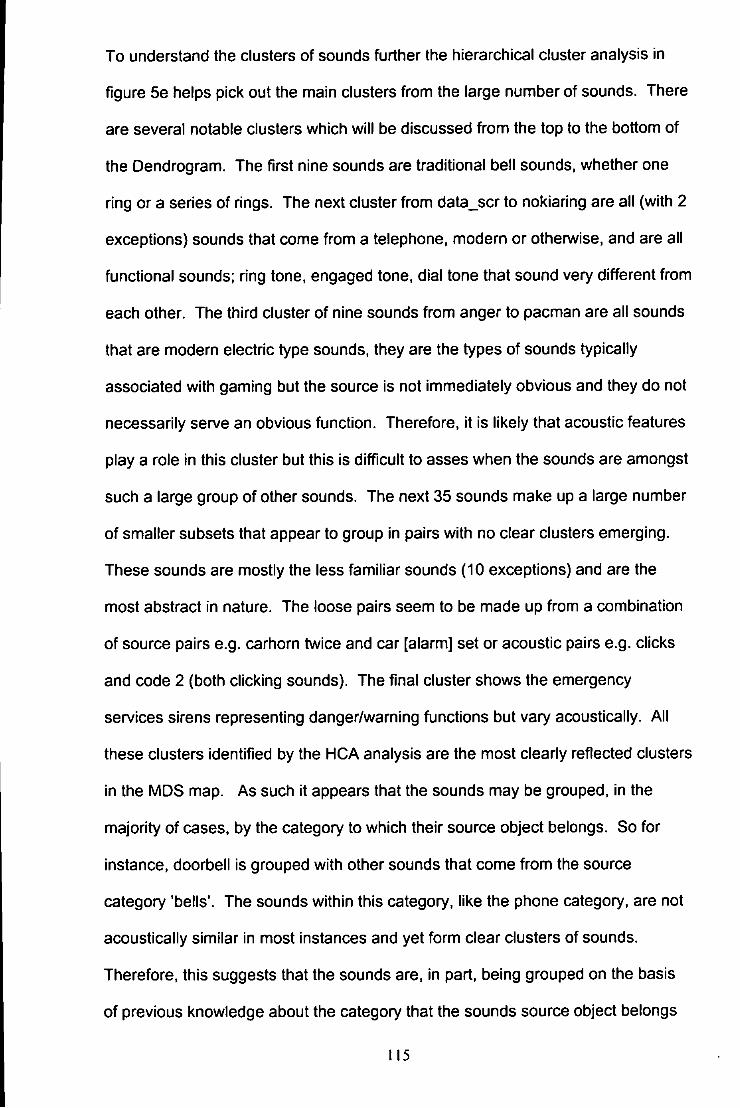
To understand the clusters of sounds further the hierarchical cluster analysis in
figure 5e helps pick out the main clusters from the large number of sounds. There
are several notable clusters which will be discussed from the top to the bottom of
the Dendrogram. The first nine sounds are traditional bell sounds, whether one
ring or a series of rings. The next cluster from data_scr to nokiaring are all (with 2
exceptions) sounds that come from a telephone, modern or otherwise, and are all
functional sounds; ring tone, engaged tone, dial tone that sound very different from
each other. The third cluster of nine sounds from anger to pacman are all sounds
that are modern electric type sounds, they are the types of sounds typically
associated with gaming but the source is not immediately obvious and they do not
necessarily serve an obvious function. Therefore, it is likely that acoustic features
play a role in this cluster but this is difficult to asses when the sounds are amongst
such a large group of other sounds. The next 35 sounds make up a large number
of smaller subsets that appear to group in pairs with no clear clusters emerging.
These sounds are mostly the less familiar sounds (10 exceptions) and are the
most abstract in nature. The loose pairs seem to be made up from a combination
of source pairs e.g. carhorn twice and car [alarm] set or acoustic pairs e.g. clicks
and code 2 (both clicking sounds). The final cluster shows the emergency
services sirens representing danger/warning functions but vary acoustically. All
these clusters identified by the HCA analysis are the most clearly reflected clusters
in the MDS map. As such it appears that the sounds may be grouped, in the
majority of cases, by the category to which their source object belongs. So for
instance, doorbell is grouped with other sounds that come from the source
category 'bells'. The sounds within this category, like the phone category, are not
acoustically similar in most instances and yet form clear clusters of sounds.
Therefore, this suggests that the sounds are, in part, being grouped on the basis
of previous knowledge about the category that the sounds source object belongs
115
to (familiar objects/sounds only) perhaps above acoustic features. However, the
descriptive measures are still being clearly indicated in the similarity judgements
as demonstrated by their relationship to the sounds location on both dimensions.
Of course it is possible that the descriptive features are being highlighted but that
they are underpinned by both the acoustic features of the sounds and the
functional aspects to each sound. The hierarchical cluster analysis suggests, from
visual inspection, that acoustic features are contributing to some of the cluster
formations but this is a tentative suggestion in light of the regression results that
did not identify any acoustic features that showed a significant relationship with the
identified MDS dimensions. Of course it must be remembered that analysis of
experiment 4 did suggest that acoustic features were mapping on to the
descriptive measures.
3.4 General Discussion
Experiments 4 and 5 have expanded the findings from experiments 1 to 3 and
identified measured sound features such as safe/dangerous that are reliably
identified as significant in participants' similarity judgements across different
experimental paradigms. This is a descriptive dimension that could be
underpinned by the acoustic features of the sounds. For example, Edworthy,
Loxley and Dennis (1991) discuss the increase in perceived urgency for example
with an increase in pitch. The measure of safe/dangerous for example could
reflect a sound's urgency. In addition, experiment 4 provided the opportunity to
assess the reliability of the scales employed across experiments 1,2 and 4. It was
identified that the scales were reliable (with the exception of safe/dangerous)
across the experiments and reflected the results obtained by Ballas (1993) using a
different set of sounds.
116
Experiment 5 introduced a different methodology from the pairwise task employed
in experiment 3 in order to gather the similarity judgements. One of the important
differences between the two methodologies to note is that experiment 3 asked
directly for a judgement of similarity between every sound pair. In experiment 5 it
is only possible to assume, as requested by the instructions, that the groups have
been formed on the basis of similarity. This may, in part, account for some of the
differences between the two experiments with respect to features that have been
identified as salient. For example, experiment 3 illustrated a strong preference for
the inclusion of acoustic features in the similarity judgements. Conversely, the
acoustic features did not show a relationship to either dimension in experiment 5.
Bonebright (1996) compared the painwise comparison task and a grouping task
and also found differences between the results. Specifically of interest to the
present findings was that the grouping task, like the present results, reflected
descriptive cues in the stimuli while the paired comparison task did not. Although
experiment 3 does reflect some more descriptive features than Bonebright's work
(1996) the acoustic features played a very prominent part on one of the
dimensions.
Another explanation for the different features identified as salient between the two
experimental paradigms is that the nature of the task in experiment 5 provides
different information to the participant and requires slightly different processing.
As discussed by Scavone et al (2002) the grouping task is less limiting in terms of
the cognitive and perceptual criteria participants could employ. For example, the
randomized presentation of pairs in the pairwise task (exp 3) makes it impossible
for participants to control the order of presentation and adjust judgements in light
of new information from a later comparison. The grouping task does not suffer
from this criticism. For example, experiment 5 provided the participants with all
117
the information at once. They were able to assess all the sounds that they must
make judgements about. As such the task required participants to form groups on
whatever basis they chose but in relation to every other sound in the experiment.
This may have allowed listeners the opportunity to assess and apply richer criteria
in their judgements (Scavone et al, 2002). Experiment 3 required a judgement
only between two sounds at any one time. It is not possible for the participant to
compare each sound with all the others in the set, even towards the end of the
experiment, as they are unaware of the total number of sounds to be rated. It is
also possible that the context in which the sounds are presented could play an
important role in the differences between the tasks. Medin et al (1993) highlight
the fact that participants' judgements of typicality may alter with the context
provided. The context in which the sounds were presented altered for the two
methodologies between experiments 3 and 5 with experiment 5 providing a rich
context in comparison to experiment 3 where pairs were judged in isolation.
Therefore, similarity judgements may shift in a systematic manner with context
(Medin et al, 1993). Further experiments that employ a core set of sounds with
variations on the additional sounds to set a context will be necessary to investigate
this possibility.
Features that have been identified as salient across experiments 3 and 5 have
been familiarity, safe/dangerous, pleasing/annoying and the use of words.
However, in experiment 5 the features are split across the dimensions very
differently from experiment 3. For example, dimension 1 in experiment 5 reflected
both familiarity and safe/dangerous. Familiarity was not reflected on a dimension
previously but identified as important in terms of rating sounds and safe/dangerous
was reflected as a descriptive feature identified on a MDS dimension previously.
Other descriptive measures in experiment five (safe/dangerous, pleasing/annoying
118
and the use of words to describe the sound) were reflected on dimension 2. From
the results it is evident that the features, whilst remaining salient, are grouping
together differently. Again it is not possible to be sure whether this is an artefact of
the methodological differences, the increased sound numbers or a combination of
both factors at this stage.
The other main feature of interest established across experiments 3 and 5 is the
way in which sounds appear to be grouped on the basis of their function or source
object. As discussed there are clear clusters identifiable both by inspection of the
MDS output and the hierarchical analysis that reflect groups formed by function or
source. For example, there is a tight cluster of emergency sounds that are varied
in actual sound but have a similar function, i.e. to warn of danger. With reference
to source the telephone cluster is the clearest example. This cluster in both the
hierarchical and the MDS analyses contains traditional telephone rings, mobile
phone ring tones and functional sounds such as the engaged tone. Nonetheless,
these sounds are clustered together and it could be argued that the source object
i.e. telephone is a contributing factor to the grouping decision. Two experiments
conducted by Dopkins and Ngo (2001) using fruits and vegetable names
confirmed previous suggestions that category relationships are taken into account
in assessments of similarity. The results suggested that when two concepts being
compared are contained in the same higher-level category e.g. telephones or
when a concept is being compared with a category to which it belongs, perceived
similarity is enhanced. The results from experiment 5 would suggest that the
participants reached a decision based on the category telephones of which mobile
phone and office phone are both a member and therefore their perceived similarity
has been incremented. Using the categories suggested by Rosch and Mervis
(1975) telephones could be considered to be the superordinate semantic category
119
as the mobile and office phone share only a few attributes. For example, a mobile
phone and an office phone do share the same purpose but they look different and
sound different. Therefore, each type of phone; mobile, office, public, would serve
as the basic level. Such theories have only addressed objects and it is therefore
difficult to assimilate sounds into these categories. Therefore, for the purposes of
explanation, it is hypothesised that prior knowledge of the object that made the
sound is what participants are categorising and that this prior knowledge is
triggered by the sound. Ballas et al (1987) discuss the finding that participants
often refer to the object/source that makes the sound rather than the sound itself
in recognition tasks. For example a participant may name a dog when identifying
a sound rather than the bark sound itself. It is likely that this can only be the case
for familiar sounds where the source of the sound is known to the listener.
Therefore, any contribution made to the clusters based on categories is only likely
to contribute to approximately half of the sounds (the more familiar) included in
experiment 5.
The lower right hand corner of the MDS configuration contains a large number of
the less familiar sound stimuli. This lower corner of the configuration does not
show clusters of sounds in the same way if compared to other areas on the map.
This finding is supported by the 35 less familiar sounds that are clustered together
on the hierarchical cluster analysis. These sounds do not show any clear clusters
in the MDS either and showed loose pairs rather than belonging to any cluster on
the HCA. This also suggests that the function or source of the sound is only
playing a key role for sounds that are more familiar to the participant. Therefore
this hints at the involvement of acoustic features for similarity judgments on these
less familiar sounds.
120
In summary, experiments 4 and 5 identified that non acoustic features played the
most prominent role in participants' similarity judgements using a large number of
sounds on a grouping task methodology. The sound features; familiarity,
safe/dangerous, pleasing/annoying and knowledge about the source or function of
the sound were identified as the most salient for this 70 item abstract sound set.
No acoustic measures were identified as the basis for either of the MDS
dimensions but experiment 4 did indicate that certain descriptive features may
map on to acoustic measures such as pitch and RMS power.
121
Chapter 4: Experiments 6 and 7
This experimental chapter introduces the similarity and categorisation literature
which is later discussed in relation to the results of these experiments and
experiments 8 and 9. The chapter also discusses two experiments designed to
investigate further the acoustic and descriptive measures indicated as salient by
experiments 1 to 5. Experiment 6, like experiments 1. 2 and 4 collected acoustic
and descriptive information for 60 sounds (3 groups of 20 sounds), both abstract
and environmental. Later in chapter 5 comparisons are made between the
pairwise task (exp. 7) and the grouping task (exp.'s 8 & 9) and this comparison
requires fewer than 25 stimuli for the painwise task. Experiment 7 was a series of
three experiments using the pairwise methodology on three different sound sets
aimed at investigating the contributions of category membership and acoustic and
descriptive features of sounds to similarity judgements.
4.1 Review of the similarity and categorisation literature
One of the main suggestions made from the current research, put simply, is that
the way participants group sounds or make similarity judgements, is guided in
some way by the way the sounds' fit in to pre-existing categories. Much of the
previous auditory research has suggested that acoustic features are the most
salient features. For example, Ballas (1993) suggested that three quarters of the
variance in identification times was related to acoustic and ecological frequency
variables. At first sight acoustic features would appear to be by far the most
important feature in sound identification. However, many results in the literature
that favour acoustic explanations reflect the fact that the experimental designs did
not consider descriptive or categorical information.
122
A brief review of some of the similarity and categorisation literature is included that
will later be argued to have relevance to the current research findings. This
research has not been conducted in the area of auditory research and will be
discussed in its original context for the purposes of the review.
Similarity is a central construct to psychology and an important Gestalt principle of
perceptual organization proposing that similar things will tend to be grouped
together (Medin et al, 1993). Hahn and Ramscar (2001) proposed, following a
review of the literature, that similarity is instrumental in the choices we make about
what categories to form initially and then how we subsequently assign items to
these categories. Therefore, because listeners in the current experiments do
appear to be forming category groups it is necessary to address whether asking
participants to make a judgement of similarity about the sound stimuli is the same
as asking them to categorise the sounds. It has been argued that similarity is too
flexible to define categories. Murphy and Medin (1985) explain that the relative
weight of a feature varies with the stimulus context and task and as such there is
no one answer to how similar one object is to another. For the purposes of the
present research Medin et al (1993) point out that multidimensional scaling can
produce stable and informative representations of similarity with fairiy good
across-subject agreement.
It is thought that context can activate context related properties so if examples
being judged share values of the activated properties then their similarity is
increased. Medin et al (1993) discuss functions of similarity. Firstly, similarity as a
heuristic, that in the absence of specific knowledge people will use similarity to
guide their actions. Medin et al (1993) cite the example of an unfamiliar snake. A
person may conclude that it is dangerous based upon its similarity to a rattlesnake.
123
Similarity judgements will often involve multiple properties. For example if stimuli x
and y are similar with respect to only one property few inferences can be made
about X even if a lot is known about y. Therefore, the multiple properties of
similarity allow for judgements to be made with more confidence. Secondly,
similarity activates properties for comparison. If comparing England and the USA
a subset of knowledge about the two will be activated and contribute to the
judgements of similarity. It is thought that the comparison of two stimuli constrains
the properties that are activated. However, for auditory stimuli it is not clear from
the literature what these features are.
Tversky's (1977. as cited in Medin et al, 1993) diagnosticity hypothesis suggests
that properties that are useful for categorisation become more salient and
consequently exert more influence on similarity judgments. Medin et al (1993)
suggest that entities entering into a comparison jointly constrain one another and
jointly determine the outcome of a similarity comparison. As such similarity is
changeable and context dependent but systematically fixed in context. This is an
important point relevant to experiment 7, 8 and 9 because the sound stimuli sets
are fixed within their own contexts. For example, one of the sets of stimuli are
unfamiliar and this might be expected to create an unfamiliar abstract sound
context, while a group of sounds emanating from similar sources might create a
well known environmental sound context.
Historically Eleanor Rosch provided an eariy general perspective on the theory of
prototypes and basic level categories beyond that of the eariy philosophers
(Lakoff. 1990). Rosch's eariy studies were based on colour and were later
extended to include primary categories of physical objects. The most
representative members of a category are called prototypical.
124
Rosch (1975) explains three different types of categories; super ordinate semantic
categories, basic level semantic categories and artificial categories. Super
ordinate semantic categories are quite abstract and as a result have a few
attributes common to all members and as such a category may consist of items
related by means of family resemblance. For example a chair and a cupboard
may belong to a category of household furniture but have few attributes in
common. Basic level semantic categories include items such as a chair or car and
are the level of abstraction where basic category cuts in the world may be made.
Finally, artificial categories enable attribute structures to be varied in a controlled
manner.
The six experiments presented in the 1975 paper confirmed Rosch's hypothesis
that the most prototypical members of the three listed categories are those that
bear the greatest family resemblance to other members of their own category with
the least overlap with other categories. Rosch proposed six major ways in which
this study was important, one of which is of particular relevance to the present
research, namely;
"it Indicates a structural rationale for the use of proximity scaling in the study of
categories, even in the absence of definable category dimensionality" p599.
In addition. Rosch (1975) proposed that the more items have In common with
other items In a class the more central those Items will be In a space derived from
proximity measures. Therefore, this research suggests that the dimension of
centrality may itself be an important aspect of and deserve to be the focus of
attention in the analysis of proximity spaces.
125
Rosch (1975) discusses knowledge as a contributory factor and how knowledge
can change a person's classification scheme. This is similar to the angle taken by
Solomon (1958) in proposing the importance of a listener's frame of reference.
Both of these studies have direct bearing on the present work as it is predicted
that participants' similarity decisions will be based, especially for a group of
sounds with a similar source, on categorical knowledge. An example comes from
one of Rosch's studies where a participants was a former aeroplane mechanic and
the list of attributes common to aeroplanes produced by most of the subjects in the
study was small compared with a lengthy list produced by this participant.
Therefore, Rosch (1975) proposed that categories such as aeroplanes can have
differing sets of correlational structures depending on a person's degree of
knowledge. Of course Rosch recognized the necessity of systematic study on
levels of expertise on classification.
Smith (1989) also views concepts as central to cognitive science due to their major
functional roles in any intelligent system and that includes human beings.
Concepts are cognitively economical and allow us to decrease the amount of
information we perceive, learn, remember, communicate and reason about. In
addition, they allow us to use past experience and the knowledge gained for future
situations.
A review of the conceptual stnjcture literature by Komatsu (1992) clarifies the
views about the different theoretical viewpoints. The similarity based view holds
that objects are classified as instances of a category by virtue of the attributes they
share with some abstract specification of the category, or with known instances of
the category. Within the similarity view itself are a further three views that are
quite different from one another: the classical view; the exemplar view and the
family resemblance view.
126
The classical view holds that concepts are defined by sets of individually
necessary and collectively sufficient attributes. It implies three things about
membership; membership of a conceptual category is clear cut, it is discrete, and
the attributes specified by a concept are individually necessary and collectively
sufficient. This view leans heavily towards economy because a single
representation is used for an entire category. Smith (1989) highlights that there
are problems that the classical view has suffered as a result of research by
linguists, philosophers and psychologists since the 1970's. For example, research
has failed to identify the definitions of most natural kind concepts. Smith (1989)
considers a tiger as an example; striped and carnivorous. If you came across a
black tiger who was surgically altered to eat only vegetables, it is likely you would
still categorize it as a tiger. Secondly there are unclear cases and Rey (1983)
cites tomatoes. People who are competent in the use of the concept fruit are often
confused as to whether a tomato is a fruit. A third problem is that it can be shown
that typical members of a concept can be categorized more efficiently than atypical
and so such typicality effects suggest that not all members of a concept are equal.
Finally, topicalities are highly correlated with family resemblance. For example,
made of wood and has four legs contributes to family resemblance for chairs but
are not necessary conditions. Rey (1983) states that the necessary and sufficient
conditions of the classical view simply do not appear to play a role in peoples'
actual acts of categorisation.
The Exemplar view states that attributes specified for a concept need not hold true
for more than one instance. As such, a concept ends up being a set of
representations, with individual representations corresponding to different
examples of that concept. However. Komatsu (1992) points out that it is unclear
127
what an exemplar representation is. This view is still fundamentally a similarity
based view in that
"an item is judged to be an instance of a concept to the extent that It is sufficiently
similar In the relevant fashion to one or more of the instance representations that constitute
the concepf p508.
Komatsu (1992) is discussing a physical object but the quote above is a particular
problem for auditory stimuli. At present it is still unclear what features are used in
order to judge stimuli as similar. Therefore, until this is understood it is not
possible to state how an auditory stimulus could be 'sufficiently similar' to any
other auditory stimuli for an item to be an instance of a concept.
In order to assess the extent to which family resemblance is employed Medin et al
(1987) conducted a series of studies requiring participants to divide stimuli, with
systematically varied features, into two groups that seemed natural or sensible to
the participants. Many versions/manipulations were used across the experimental
series, such as. adding exemplar specific information. The results found that
across 92 participants in 4 different manipulations there was a persistent absence
of sorting by family resemblance (only two participants). Medin et al (1987)
conducted further studies to evaluate the use of correlated attributes for which a
causal link is readily perceived. Medin et al (1987) concluded that family
resemblance categories may be organized not so much in terms of their surface
features or properties but in terms of a deeper underiying concepts that may give
rise to them. Rehder (1999) cites the observation that category learning and
categorisation are strongly influenced by peoples' theoretical explanatory and
causal knowledge.
A more favoured view is the similarity to prototype view where defining conditions
are seen as properties that occur in some instances but not all and they are
128
perceptually salient. A collection of such properties is called a prototype. The
similarity to prototype view discussed by Dopkins & Gleason (1997) where an
object is categorized as an instance of a concept if it is sufficiently similar to the
prototype. In prototype models, the mental representation of a category Is Its
prototype and is often defined as the exemplar with average values on all of the
dimensions along which the category's exemplars vary. Whilst this overcomes
one of the main crificisms of the classical view, namely that there need to be
sufficient and necessary properties, the view suffers from vagueness and is
unconstrained. The similarity to prototype account has been generalised to other
concepts beyond natural items like furniture or social and personality concepts.
However, work has been conducted suggesfing that boundaries between
categories are not clear cut and in addition are not discrete. Judged levels of
typicality for a category was found to vary greatly and as a result the similarity view
lost favour. In Its place the family resemblance view that according to Wittgenstein
(1953, as cited In Komatsu, 1992) proposes that categories are formed by virtue of
family resemblances among their members. Both classical and family
resemblance views explain conceptual coherence In terms of attributes shared by
the members of a category. The difference Is that in the classical view all
Instances share necessary and sufficient attributes but the family resemblance
view requires only that every attribute specified by the concept Is shared by more
than one Instance. Komatsu (1992) points out some vagueness In this viewpoint
but that it has promise for explaining things that the classical view is unable to
accommodate such as typicality effects. Unfortunately this view has lost some of
the stronger aspects of the classical view such as accounting for linguistic
meaning and that typicality effects do not in themselves clearly indicate the nature
of conceptual structure.
129
Rips (1989, as cited in Hahn et al, 2001) conducted a series of experiments
suggesting the answer is that there is a dissociation between similarity judgments
and category judgments and as such categorisation cannot be reduced to
similarity. In one of the experiments participants were asked to imagine a 3 inch
circular object. One group was asked if the object was more similar to the
category pizzas or quarters. The second group asked whether the object was
more likely to belong to the category of quarters or pizzas. The categorisation
group chose pizzas while the similarity group chose quarters therefore
demonstrating that categorisation cannot be reduced to similarity.
Smith (1989) goes on to propose that categorisation judgements go beyond
similarity by suggesting that categorisation is a fonn of induction. Inductive tasks
that people have to perform on a routine basis include determining whether an
item belongs to a particular category and estimating the probability that the item
belongs to a particular category or has a particular property. Smith (1989)
suggests there is evidence that the strategies used for these tasks are the same
as those used in categorisation. A full discussion of this concept is beyond the
scope of the current review beyond stating that Smith (1989) proposed that other
modes of induction, beyond similarity to prototype, must be considered and that
categorisation is best thought of as a case of induction.
As addressed by Hahn (2001) there seems to be little controversy over the idea
that we put things into categories when we find them similar regardless of which
particular viewpoint you prefer. An example from the present results can be seen
from experiment 5 (figure 5f) that highlights the tight cluster of various telephone
sounds placed together in the MDS configuration. However, an argument exists in
130
the literature as discussed over the degree to which similarity is defined and
whether it really serves as an explanation for the way we categorise.
4.2 Introduction to Experiments 6 and 7
The results from experiments 1 to 3 suggested that there were three main
dimensions used by participants when making judgements of similarity for abstract
sounds. Dimension 1 showed a relationship to an acoustic factor comprised of
measures of pitch and RMS power. The descriptive factor identified from the PCA
analysis correlated with dimension 2 and dimension 3 showed a relationship with
the occurrence rate of a sound in the environment. Experiments 4 and 5 used a
large 70 item sound set on a grouping task and identified familiarity,
safe/dangerous, pleasing/annoying and function or source information as salient in
participants' similarity judgements. Experiment 4 also suggested that acoustic
features of pitch and RMS power may be mapping onto some of the descriptive
measures. None of the acoustic features showed a direct relationship to the
sounds' locations on the MDS configuration for experiment 5.
The results from experiment 5 suggested that the function of the sound or the
category to which it belonged was a contributory factor to the way that participants
were making similarity judgements. The impact of category judgements could be
either in addition to the use of acoustic and perceptual information or as an
alternative strategy. However, this was difficult to quantify. Further, the unfamiliar
end of the multidimensional scaling output in experiment 5, where less familiar
sounds were concentrated, was extremely overcrowded and warranted further
investigation. Therefore, several features of the previous experiments needed to
be clarified. In order to do this it was necessary to introduce an element of control
to the sounds employed by carefully selecting sounds based on their source or
131
their acoustic characteristics. In addition, to investigate the role of familiarity
further a group of completely novel sounds was included. Three different sound
groups, each containing twenty sounds, were formed;
Similar sound - to investigate the salience of the acoustic features -10
pairs of sounds that sound similar e.g. cow moo and fog horn that come from
different sources.
Similar source- to test the salience of category information. 5 sets of 4
sounds that come from similar sources but sound different e.g. cow, sheep, pig,
horse (farmyard animals).
Unfamiliar - this group consisted of novel, unfamiliar sounds.
The configuration of the groups varies due to the nature of the matching necessary
in each group. For example in the similar sound group only pairs of similar
sounding stimuli were chosen because identifying more than two acoustically
similar stimuli was experimentally very difficult. In the similar source stimuli set 4
sounds from each source category were selected in an attempt to ensure that
there were enough exemplars to represent a category. Finally, none of the
unfamiliar sound stimuli were matched with any of the others The only criteria for
inclusion was that they were unfamiliar although an attempt was made not to
include two sounds that sounded very similar.
In order to get good matches for the similar sound pairs and good category groups
for the similar source set it was decided that it would be worthwhile including
environmental sounds. IVIost of the abstract sounds used in this experiment are
present in our environment and the inclusion of the unfamiliar sound group
represents those sounds employed in previous experiments that were unfamiliar.
A full list of the 60 sounds and their descriptions can be found in appendix C1.
The similar sound group was designed to control for the acoustic features (as
132

perceived by the listener rather than direct acoustic measurements) of the sounds.
The similar source set was designed to control for category membership with the
unfamiliar set designed to further explore the similarities and differences between
the use of familiar and unfamiliar sounds In a similarity judgement task. It is
expected in all cases that there will be a combination of salient acoustic,
descriptive and category features employed by participants In their similarity
judgements.
133
4.3 Experiment 6 : The collection of acoustic and descriptive data
for 60 sounds
4.3.1 Introduction
In line with experiments 1.2 and 4 that collected perceptual data the measures
taken were based on those used previously and the work of Ballas (1993) and
Solomon (1958). The set of statements employed was altered slightly from
experiment 4 and 5 to exclude direct statements about the use of words and
imagery because these statements had not identified any significant findings
across experiments 3 or 5 in relation to identified MDS dimensions. Because the
number of sounds in this experiment was reduced from the 112 sounds rated in
experiment 4 to 60 sounds it was possible to add a few extra measures and still
maintain an acceptable length for the experiment. Statements about familiarity
were retained and high/low pitch was added to investigate whether participants'
perceptions of pitch showed correlations to actual measures of pitch for the sound
stimuli. The additional measure would also allow further investigation of the way
the acoustic measures map onto the more descriptive measures. Calming/exciting
was also added to the word pairs in an attempt to provide more representation for
the descriptive measures as the descriptive features were identified as highly
salient features in experiment 5. Therefore, the statements selected required
ratings about familiarity, descriptive measures and perceptions of pitch. In line
with the previous experiments the acoustic measures used previously were also
measured. Therefore, experiment 6 will provide a database of information for the
60 sounds that will be used in experiments 7, 8 and 9.
134
4.3.2 Method
4.3.2.1 Participants
20 participants (3 males and 17 females) took part in the rating study. All
participants had normal or corrected to normal hearing. Participants were first
year students on the BSc Psychology degree at the University of Plymouth and
were awarded credit for their participation as part of the course requirement.
4.3.2.2 Apparatus
The stimuli were presented using a purpose written program (Aldrich, Sept, 2003).
Six computers with headphones were used (Hewlett Packard Vectra's Pill with a
600 MHz Processor. 128 MB RAM and CrystalSoundFuslon™ Soundcard
operating on Windows XP).
4.3.2.3 Stimuli
The sound stimuli for this experiment were 60 sounds, described in appendix CI
that included both abstract and more environmental or everyday sounds. Some
sounds were taken from Marcel! (2000) mariced !. Miranda (2000) marked
internet sound libraries and some sounds used in previous experiments (marked
*). The sound attenuation for all the sounds was normalized as before to -16dB
using Cooledit software. The sounds were approximately 4 seconds In length with
variation of up to half a second either way to ensure that the cut off point had the
minimum distorting effect on the sound.
4.3.2.4 Procedure
The procedure for this experiment was the same one used for experiment 4 with
the additional questions added into the program. Following some simple
introduction screens to familiarise the participant with the nature of the experiment
the program selected a sound at random from the poo! of 60 sounds. At this stage
the different sound groups were all tested together. The sound was then
135
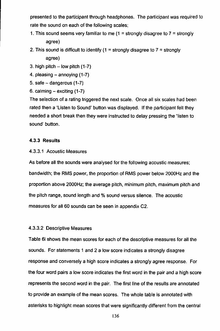
presented to the participant through headphones. The participant was required to
rate the sound on each of the following scales;
1. This sound seems very familiar to me (1 = strongly disagree to 7 = strongly
agree)
2. This sound is difficult to identify (1 = strongly disagree to 7 = strongly
agree)
3. high pitch - low pitch (1-7)
4. pleasing - annoying (1-7)
5. safe - dangerous (1-7)
6. calming - exciting (1-7)
The selection of a rating triggered the next scale. Once all six scales had been
rated then a 'Listen to Sound' button was displayed. If the participant felt they
needed a short break then they were instructed to delay pressing the 'listen to
sound' button.
4.3.3 Results
4.3.3.1 Acoustic Measures
As before all the sounds were analysed for the following acoustic measures;
bandwidth; the RMS power, the proportion of RMS power below 2000Hz and the
proportion above 2000Hz; the average pitch, minimum pitch, maximum pitch and
the pitch range, sound length and % sound versus silence. The acoustic
measures for all 60 sounds can be seen in appendix C2.
4.3.3.2 Descriptive Measures
Table 6i shows the mean scores for each of the descriptive measures for all the
sounds. For statements 1 and 2 a low score indicates a strongly disagree
response and conversely a high score indicates a strongly agree response. For
the four word pairs a low score indicates the first word in the pair and a high score
represents the second word in the pair. The first line of the results are annotated
to provide an example of the mean scores. The whole table is annotated with
asterisks to highlight mean scores that were significantly different from the central
136

cut point of 3.5 indicated by binomial tests. The results are shown in their pairs
(for the similar source group) and their category groups (for similar source group).
The Unfamiliar group is shown alphabetically.
137
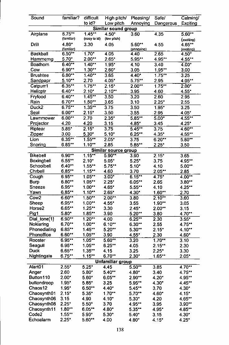
Sound familiar? difHcult High pitch/ Pleasing/ Safe/ Calming/ to id? Low pitch Annoying Dangerous Exciting
Similar sound group Airplane 6.75" 1.45** 4.50* 3.60 4.35 5.60**
(familiar) (easy to id) (low pitch) (exciting) Drill 4.80* 3.30 4.05 5.60** 4.55 4.65**
(familiar) (annoying) (exdtinq) Baskball 6.50** 1.70* 4.05 4.40 2.65 4.50* Hammemg 5.70* 2.00** 2.65* 5.95** 4.95** 4.55** Boathorn 6.40** 1.40** 1.95* 4.10 3.40 4.00* Cow 6.90** 1.30** 2.60* 3.05 1.95** 3.00 Brushtee 6.80** 1.40** 3.65 4,40* 1.75** 3.25 Sandpapr 5.10** 2.70 4,05* 5.75** 2.95 4.05** Catpurri 6.35** 1.75** 2.15* 2.00** 1.75** 2.00* Helicptr 6.40** 2.10* 2.10** 3.95 4.60 4.55* Fryfood 6.40** 1.45** 3.50 3.20 2.60 2.95 Rain 6.70** 1.50** 3.65 3.10 2.25* 2.55 Duck2 6.75** 1.35** 3.75 3.50 1.95* 3.25 Seal 6.00** 2.15* 3.50 3.55 2.95 4.05* Lawnmower 6.00** 2.70 2.35* 5.85** 5.00* 4.55** Projector 4.20 4.20 3.15 4.85* 3.45 . 4.25* Riptear 5.85* 2.15* 3.75 5.45** 3,75 4.60** Zipper 3.00 5.30* 5.10* 6.25** 4.35* 4.55** Lion 6.35** 1.55** 2.05* 3.75 6.20** 5.80** Snoring 6.85** 1.10** 2.85 5.85** 2.25* 3.50
Similar source group Bikebell 6.90** 1.15** 5.90** 3.90 2.15* 3.65 Boxingbell 6.55** 2.10* 5.05* 5.25* 3.75 4.95** Schoolbell 6.40** 1.55** 5.75** 5.10* 4.10 5.00** Chrt)ell 6.85** 1.15** 4.60 3.70 2.05** 2.85 Cough 6.95** 1.05** 3.00* 6.15** 4.75* 4.00** Burp 6.80** 1.05** 2.25* 6.05** 2.65 3,80** Sneeze 6.95** 1.00** 4,65* 5.55** 4.10 4,25** Yawn 6.85** 1.10** 2.65* 4.30* 1.60** 2.70 Cow2 6.60** 1.50** 2.00** 3.80 2.10** 3.60 Sheep 6.95** 1.00** 4.55* 3.55 1.90** 3.05 Horse2 6.65** 1.25** 3.30 2.45* 2.00** 3.15 Pig1 5.80* 1.85** 3.90 5.20** 3.80 4.70** Dial_tone[1] 6.90** 1.20** 4.00 6.25** 2.30 3.55* Nokiaring 6.70** 1.00** 6.10** 6.30** 2.55 4.75** Phonedialing 6.85** 1.45** 5,20** 5.30** 2,15* 4.10** Phonoffice 6.60** 1.05** 3.90 4,55* 2.30 4.60* Rooster 6.95** 1.05** 5.60** 3,20 1.70** 3.10 Seagull 6.95** 1.05** 6.25** 4.05 2.15** 2,30 Duck 6.65** 1.35** 4.15 3.25 2.25* 3.30 Nightingale 6.75** 1.15** 6.70** 2.30* 1.65** 2.05*
Unfamiliar group AlartOI 2.55* 5.25* 4.45 5.50** 3.85 4.70** Anger 2.60 5.80* 5,40** 4.80* 3,40 4.75** Button110 2.00* 5.60* 6.05** 2.90** 4.20* 4.95** buttondroop 1.95* 5.85* 3.25 5.95** 4.30* 4.45** Chaos12 1.95* 6.50** 4.40* 5.45** 3.70 4.30* Chaosynthd 2.15* 5.35* 1.70** 5.70** 4.60* 4.15* ChaosynthOe 3.15 4.90 4.10* 5.30* 4.20 4.65** ChaosynthOS 2.25* 5.50* 3.70 4.95** 3.95 3.90** Chaosynth11 1.80** 6.05** 4.80* 5.35** 4.95* 4.85** Code2 1.55** 5.90* 5.30* 5.40* 3.15 4.30* Echoalarm 2.25* 5.60** 4.00 4.80* 4.15* 4.25*
138
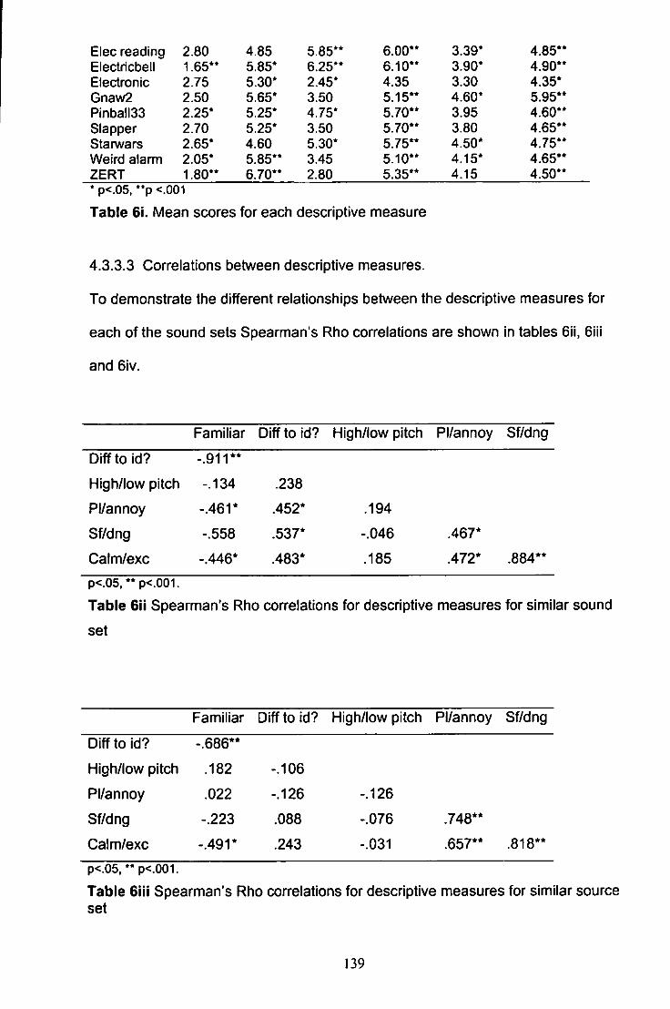
Elec reading 2,80 4.85 5.85** 6.00** 3.39* 4.85** Electricbell 1.65" 5.85* 6.25** 6.10** 3.90* 4,90** Electronic 2-75 5.30* 2.45* 4.35 3.30 4.35* Gnaw2 2.50 5.65* 3.50 5.15** 4.60* 5.95** PinbalISS 2.25* 5.25* 4.75* 5.70** 3.95 4.60** Slapper 2.70 5.25* 3.50 5.70** 3.80 4.65** Starwars 2.65* 4.60 5.30* 5.75** 4.50* 4.75** Weird alarm 2.05* 5.85** 3.45 5.10** 4.15* 4.65** ZERT 1.80** 6.70** 2.80 5.35** 4.15 4.50** * p<.05, " p <.001
Table 6i. Mean scores for each descriptive measure
4.3.3.3 Correlations between descriptive measures.
To demonstrate the different relationships between the descriptive measures for
each of the sound sets Spearman's Rho correlations are shown in tables 6ii, Bill
and 6iv.
Familiar Diff to id? High/low pitch Pl/annoy Sf/dng
Diffto id? - .911"
High/low pitch -.134 .238
Pl/annoy -.461* .452* .194
Sf/dng -.558 .537* -.046 .467*
Caim/exc -.446* .483* .185 .472* .884**
p<.05. ** p<.001.
Table 6il Spearman's Rho correlations for descriptive measures for similar sound
set
Familiar Diffto id? High/low pitch Pl/annoy Sf/dng
Diffto id? -.686**
High/low pitch .182 -.106
Pl/annoy .022 -.126 -.126
Sf/dng -.223 .088 -.076 .748**
Calm/exc -.491* .243 -.031 .657** .818**
p<.05, ** p<,001.
Table 6iil Spearman's Rho correlations for descriptive measures for similar source set
139
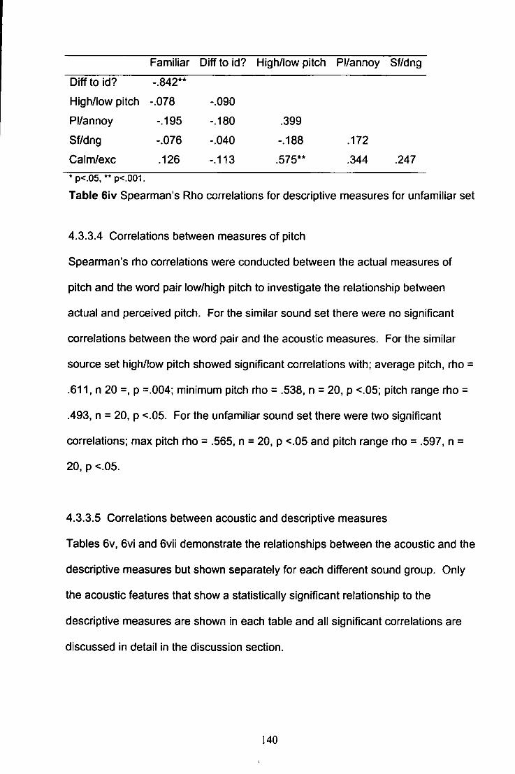
Familiar Diffto id? High/low pitcli Pl/annoy Sf/dng
Diffto id? -.842"
High/low pitch -.078 -.090
Pl/annoy -.195 -.180 .399
Sf/dng -.076 -.040 -.188 .172
Calm/exc .126 -.113 .575" .344 .247 *p<.05, p<.001.
Table 6iv Spearman's Rho correlations for descriptive measures for unfamiliar set
4.3.3.4 Correlations between measures of pitch
Spearman's rho correlations were conducted between the actual measures of
pitch and the word pair low/high pitch to investigate the relationship between
actual and perceived pitch. For the similar sound set there were no significant
correlations between the word pair and the acoustic measures. For the similar
source set high/low pitch showed significant correlations with; average pitch, rho =
.611, n 20 =. p =.004; minimum pitch rho = .538, n = 20, p <.05; pitch range rho =
.493, n = 20, p <.05. For the unfamiliar sound set there were two significant
correlations; max pitch rho = .565. n = 20, p <.05 and pitch range rho = .597, n =
20, p <.05.
4.3.3.5 Con-elations between acoustic and descriptive measures
Tables 6v, 6vi and 6vli demonstrate the relationships between the acoustic and the
descriptive measures but shown separately for each different sound group. Only
the acoustic features that show a statistically significant relationship to the
descriptive measures are shown In each table and all significant correlations are
discussed in detail in the discussion section.
140
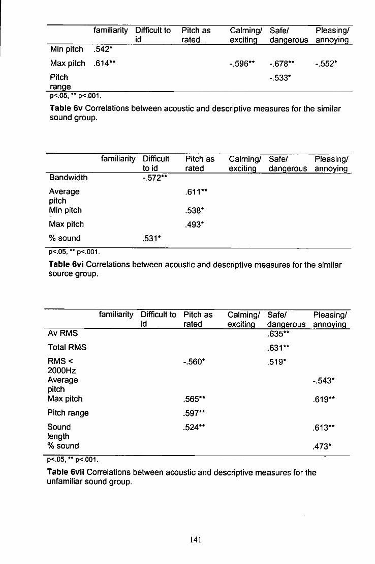
familiarity Difficult to Pitch as Calming/ Safe/ Pleasing/ id rated exciting dangerous annoying
Min pitch .542*
Max pitch .614" -.596** -.678** -.552*
Pitch -.533* range p<.05, ** p<.001. Table 6v Correlations between acoustic and descriptive measures for the similar sound group.
familiarity Difficult Pitch as Calming/ Safe/ Pleasing/ to id rated exciting dangerous annoying
Bandwidth -.572**
Average pitch Min pitch
.611**
.538* Max pitch .493*
% sound .531*
p<.05." p<.001 Table 6vi Correlations between acoustic and descriptive measures for the similar source group.
familiarity Difficult to Pitch as Calming/ Safe/ Pleasing/ id rated exciting dangerous annoying
Av RMS .635** Total RMS .631** RMS< 2000Hz Average pitch Max pitch
-.560* .519*
-.543*
.565** .619** Pitch range .597**
Sound length % sound
.524** .613**
.473* p<.05," p<.001. Table Gvii Correlations between acoustic and descriptive measures for the unfamiliar sound group.
141
4.3.4 Discussion
In keeping with experiment 1. 2 and 4 this experiment provided a database of
acoustic and descriptive information for all 60 sounds that made up the three
sound sets. It has again provided an indication of which features are perceptually
important to the listener and variations among the most strongly rated features.
For example, pleasing/annoying elicited a statistically significant response on
neariy all sounds in the unfamiliar sound set but this is not the case for the other
sound sets. Similariy calming/exciting shows the strongest responses for the
unfamiliar sound set.
For the similar source group all the sounds (with one exception) are considered to
be familiar and easy to identify but vary on all the other measures. Similariy, the
similar source group are rated as familiar and easy to identify and again vary on
the other descriptive measures. Conversely, as was the intention the unfamiliar
sound group has been rated as unfamiliar in all cases and difficult to identify.
Again the sounds vary on the other descriptive measures. The finding that
sounds were rated as familiar or unfamiliar according to their group membership is
an important finding as this was the intention when the groups were formed.
Therefore, it can be said that the selection of sounds that are familiar or unfamiliar
has been successfully achieved.
As demonstrated in previous experiments familiarity is showing statistically
significant correlations with other sound features. However, in previous
experiments the relationship identified has been between familiarity and the ease
of using words to identify a sound or the ease in using imagery. These statements
were not included in the present experiment but familiarity has shown a
relationship to the word pairs pleasing/annoying and calming/exciting.
142
In this experiment the descriptive measure high/low pitch was included to asses
whether participants' perceptions of pitch reflected the actual measures of pitch.
The comparison of actual pitch and perceived pitch identified statistically
significant correlations for both the similar source set and the unfamiliar sounds.
However, the similar sound set showed no such correlations. Across the whole
sound set and all pitch measures the similar sound set showed the widest range of
actual pitch measures. The similar sound stimuli set showed less variation in
average pitch compared to the other two sound groups. The correlations are
varied in this respect and demonstrate that perceptions of pitch do not always
correlate with actual pitch measures but for the most part correlations were as
expected.
To assess how the acoustic features map onto the descriptive information
correlations were conducted on each of the sound sets. The patterns that can be
seen in tables 6v, 6vi and 6vii vary between the different sound groups but similar
mappings between descriptive and acoustic measures are evident. Table 6v
shows the correlations for the similar sound group. This table Illustrates several
examples (max pitch + calming exciting, max pitch + pleasing/annoying) where the
acoustic and descriptive information are reflecting the urgency of the sound
(Edworthy et ai, 1991). The table also reflects a natural phenomena illustrating
that sounds that are familiar tend to be high pitched (min pitch and max pitch both
correlate with familiarity). Table 6vi is less clear but illustrates a possible temporal
link with percentage sound and difficulty in Identification. Previous research has
identified temporal patterns as an Important feature in sound recognition
(Solomon, 1959a; Gygi et al, 2004) and typically those sounds included in the
experiments with less overall sound are more rhythmic and therefore easier to
143
identify. The correlations between the actual pitch measures and the word pair
high/low pitch included as a perceptual measure of pitch has demonstrated that
participants could perceive pitch and discriminate between items of different
pitches. Finally table 6vii shows the correlations for the unfamiliar sound stimuli.
This table shows the largest number of correlations between acoustic and
descriptive measures. There is evidence that subjective and objective measures
of pitch correlate as identified for the similar source group. Again there is
evidence for the urgency of the sound playing a role with average RMS and total
RMS showing a significant relationship to safe/dangerous reflecting the
relationship between a word's loudness and its urgency as identified by Hellier,
Edworthy, Weedon, Walters and Adams (2002). Table 6vii also illustrates the
relationship between pitch and how pleasing/annoying a sound is, again relevant
to the urgency of the sound (Edworthy et al, 1991).
In summary, this experiment has confirmed that the similar sound group and the
similar source group contain sounds that are considered to be familiar and the
unfamiliar sound group is made up of sounds considered to be unfamiliar and hard
to identify. Familiarity has been shown to correlate with the word pairs
pleasing/annoying and calming/exciting continuing the previous findings of the
importance of familiarity with a sound and possibly reflecting the semantics of the
sound. Finally the correlations between acoustic and descriptive features have, in
this experiment, given a fairly consistent pattern of results with respect to the way
that the acoustic features map onto the descriptive features. The results have
identified correlations reflecting urgency and show listeners' ability to perceive and
discriminate pitch differences.
144
4.4 Experiment 7: pairwise comparison task for three sound sets
4.4.1 Introduction
There are several different points that guided the rationale for experiment 7 which
tested three different sets of sound stimuli using the pairwise methodology that
was used in experiment 3. As introduced the three sound sets contain sounds
selected on three bases; sounding the same as another sound (acoustically),
sounding different but coming from the same category as another sound or being
a completely unfamiliar sound. The decision to group sounds in this way was, in
part, due to the previous results that indicated a possible contribution of category
membership in participants' similarity judgements. Sounds appeared to be judged
as similar despite the fact that in many examples, such as the different telephone
noises, the acoustic features of the sounds were very different. These sounds
appeared to belong to either the same category, serve a similar function, or both.
It was hypothesised that participants would sort together those sounds that shared
a category membership with another sound, demonstrating the importance of
category membership. It was also expected that sounds that, from a listeners
point of view, sounded similar would also be grouped together, demonstrating the
importance of the acoustic features.
Previous research such as Dopkins et al (2001) suggested that category
relationships may be taken into account in assessments of similarity. For
example, for the similar source group the animal sounds may be grouped as
similar. However, for the similar sound group (acoustically similar sounds) the
sound's membership to a category is less accessible. Sloman, Malt and Fridman
(2001) suggested that overall similarity between objects (not acoustic objects) may
encompass both physical and functional properties. This reflects the results
145
obtained in the experiments so far because there has been a clear reflection of
both physical (acoustic) and functional properties identified as salient feature of
the sounds. Therefore, if this idea is applied to a familiar auditory object it could
be hypothesised that both acoustic and descriptive information may be used in the
similarity judgements as well as functional or categorical knowledge.
The unfamiliar group was included as a sound group for two reasons. Firstly, to
Identify whether a similar rule would apply to the unfamiliar group as Is
hypothesised to apply to the similar sound group: that acoustic and descriptive
information would influence the similarity decisions made by participants.
Secondly, it was hoped that the experiment would provide a more detailed idea of
how participants were grouping the sounds In the overcrowded bottom right hand
corner of the multidimensional scaling map from experiment 5. Although it could
be deduced from experiment 5 that the unfamiliar sounds were being grouped
together the tightness of this cluster made very difficult to get any firm Ideas about
the acoustic or descriptive sound features that were used to make the grouping
decisions. Running the unfamiliar sounds in a group of their own would expand
the scale and increase the possibility of identifying some salient dimensions used
to make the similarity judgements.
4.4.2 Method
4.4.2.1 Participants
45 participants (5 male, 40 female) took part in the study. There were 15
participants per sound group. All the participants had normal or corrected-to-
normal hearing. Participants were psychology students at the University of
Plymouth and were awarded course credit for their participation as part of the BSc
Psychology course requirement.
146
4.4.2.2 Apparatus
The stimuli were presented using a purpose written grouping program (Aldricli,
September, 2003). Six computers with headphones were used (Hewlett Packard
Vectra's PIN with a 600 MHz Processor, 128 MB RAM and CrystalSoundFusion™
Soundcard operating on Windows XP).
4.4.2.3 Stimuli
The 60 stimuli that were rated in experiment six, formed the three groups of stimuli
used in this experiment as identified in appendix C1; Similar sound, a group of
sounds (not all abstract) made up of ten pairs of sounds that sound similar but
come from different sources e.g. food frying and rain falling. Similar source, a
group of sounds comprising five sets of four sounds that come from similar
sources but do not necessarily sound the same, e.g. burp, cough, sneeze and
yawn are all human noises. The sets included were human noises, bells, birds,
farm animals and telephones.
Finally Unfamiliar, this group was comprised of unfamiliar sounds that were all
abstract in nature.
4.4.2.4 Procedure
Sample screens were presented to participants and the following instructions
given;
"During the experiment you will be presented with a series of sound
pairs (which you will hear only once). Your task will be to rate how similar
you feel the two sounds are in each pair. These judgements should be
YOUR opinion. There is no right or wrong answer."
147
From each of the described sound sets each sound was paired with every other
sound, therefore, 20 x 19 sounds giving a total of 380/2 presented one way round
provides 190 pairs for inclusion in the experiment. For example
caralarm...smokealarm was not also presented in the reverse order. The
experiment was run between participants with fifteen different participants
completing the experiment for each sound set. The participants for this
experiment were not the same as the participants who completed experiment 6.
The program selected a pair of sounds at random from the pool (this pair was then
excluded from the pool). The pair was presented through headphones with a one
second gap between each pair member. After both sounds had been played a
rating scale was presented. Participants were instructed;
"Using the scale below please rate the sounds that you just heard
according to how similar you feel they were. E.g. select 1 if you feel
that the sounds were very similar to each other. Conversely for sounds
you felt to be very dissimilar select 10"
These instructions were on every screen in case participants wanted clarification
at any time during the experiment.
The selection of a rating triggered the presentation of the next pair of sounds. To
offset fatigue there were seven 20 second pauses presented every 24 trials. A
plain screen and "20 second pause" was presented. After the pause the program
continued as before. The program ran for 190 trials and was approximately one
hour in length. Each participant judged only one complete set of sounds,
therefore, 190 pairs.
148
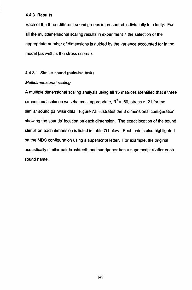
4.4.3 Results
Each of the three different sound groups is presented individually for clarity. For
all the multidimensional scaling results in experiment 7 the selection of the
appropriate number of dimensions is guided by the variance accounted for in the
model (as well as the stress scores).
4.4.3.1 Similar sound (painwise task)
Multidimensional scaling
A multiple dimensional scaling analysis using all 15 matrices identified that a three
dimensional solution was the most appropriate, R^= .60. stress = .21 for the
similar sound painwise data. Figure 7a illustrates the 3 dimensional configuration
showing the sounds' location on each dimension. The exact location of the sound
stimuli on each dimension is listed in table 7i below. Each pair is also highlighted
on the MDS configuration using a superscript letter. For example, the original
acoustically similar pair brushteeth and sandpaper has a superscript d after each
sound name.
149
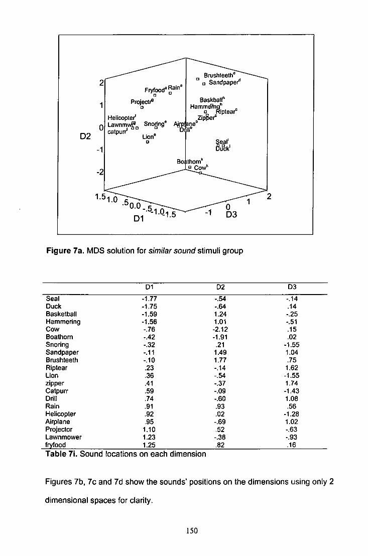
D2
Projectr* •
Helicopter* Lawnmwfi^ Snoring catpurr'
•
Baishteelh'= a Sandpaper^
Baskball^
|0
Boathom 9 Cow/'
Figure 7a, MDS solution for s/m/7ar sounc/stimuli group
D1 D2 D3
Seal -1.77 -.54 -.14 Duck -1.75 -.64 .14 Basketball -1.59 1.24 -.25 Hammering -1.56 1.01 -.51 Cow -.76 -2.12 .15 Boathom -.42 -1.91 .02 Snoring -.32 .21 -1.55 Sandpaper -.11 1.49 1.04 Brushteeth -.10 1.77 .75 Riptear .23 -.14 1.62 Lion .36 -.54 -1.55 zipper .41 -.37 1.74 Catpurr .59 -.09 -1.43 Drill .74 -.60 1.08 Rain .91 .93 .56 Helicopter .92 .02 -1.28 Airplane .95 -.69 1.02 Projector 1.10 .52 -.63 Lawnmower 1.23 -.38 -.93 fryfood 1.25 .82 .16 Table 7i. Sound locations on each dimension
Figures 7b, 7c and 7d show the sounds' positions on the dimensions using only 2
dimensional spaces for clarity.
150
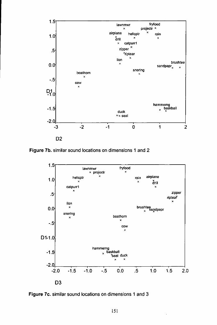
1.5
-.51
-2.Q
lawnmwr fryfood X projectr ^
airplane helicptr rain
drill > catpurrl
boathom X
zipper 'Viptear
lion ^
snoring X
brushtee sandpapr^^ ^
cow X
duck X X seal
hammemg ^ baskball ^ X
-3
D2
-2 -1
helicptr X
lawnmwr X projectr
X
fryfood
rain airplane
Figure 7b. similar sound locations on dimensions 1 and 2
1.5
1.01
.5
0.0
-.5-
D1-1.0
-1.5
-2.Q
catpun-1 X
lion X
drill X
zipper riptea?"
snoring X
' ' -^! ; ' -sapdpapr
boathom X
cow X
hammemg ^ baskball
^eal duck X X
1.0 -.5 0.0 .5 1.0 1.5 2.0 -2.0 -1.5
D3
Figure 7c. similar sound locations on dimensions 1 and 3
151
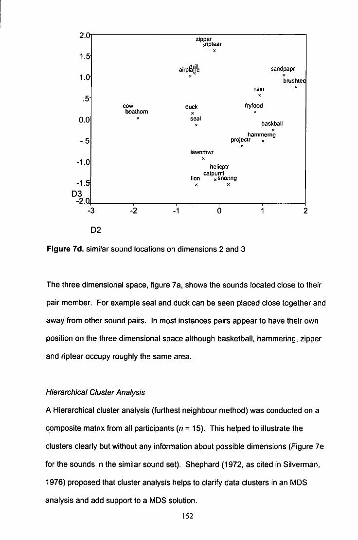
2.0
1.5
1.01
.5
0.01
-.5
-l.ffl
-1.51 D3
-2.Q
zipper >fiptear
airp;
ram
sandpapr X
bnishteel
cow boathom
duck X
seal X
lawnmwr X
fryfood
baskball X
hammerng projectr x
X
helicptr catpupn
lion X snoring X X
-2
D2
Figure 7d. similar sound locations on dimensions 2 and 3
The three dimensional space, figure 7a, shows the sounds located close to their
pair member. For example seal and duck can be seen placed close together and
away from other sound pairs. In most instances pairs appear to have their own
position on the three dimensional space although basketball, hammering, zipper
and riptear occupy roughly the same area.
Hierarchical Cluster Analysis
A Hierarchical cluster analysis (furthest neighbour method) was conducted on a
composite matrix from all participants (n = 15). This helped to illustrate the
clusters cleariy but without any information about possible dimensions (Figure 7e
for the sounds in the similar sound set). Shepherd (1972, as cited in Silverman,
1976) proposed that cluster analysis helps to clarify data clusters in an MDS
analysis and add support to a MDS solution.
152
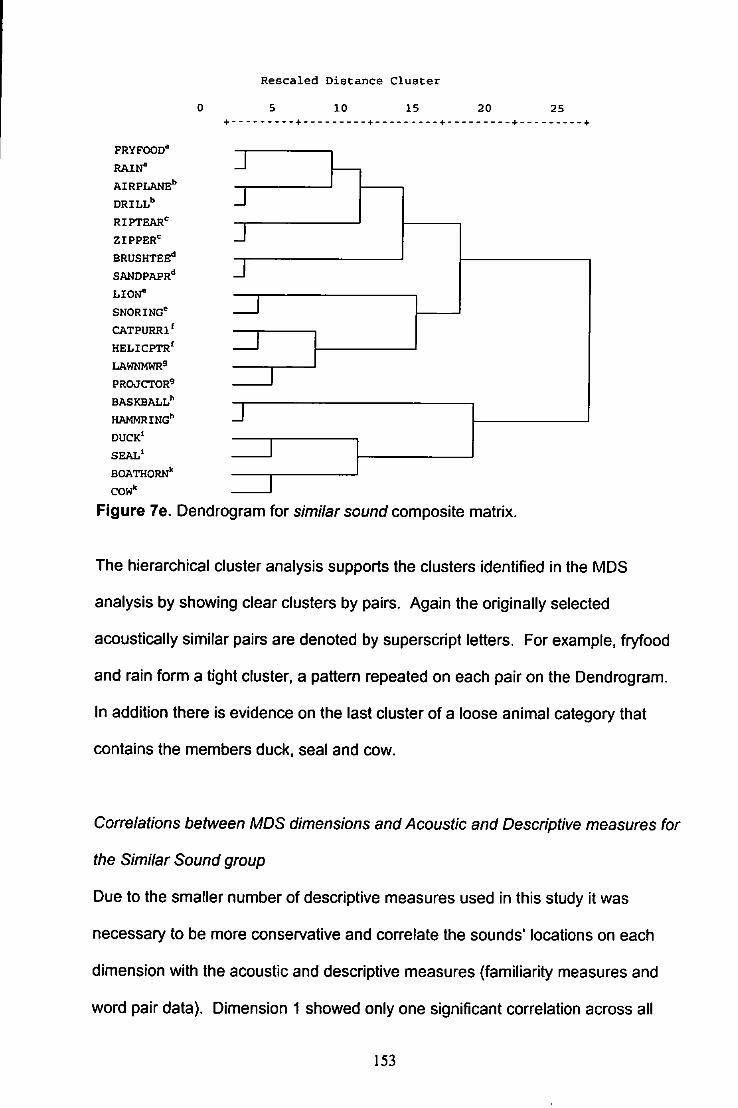
R e s c a l e d D i s t a n c e C l u s t e r
5 10 15 20 25
FRYFOOD^ RAIN* AIRPLANE** DRILL** RIPTEAR'= ZIPPER*' BRUSHTEE** SANDPAPR** LION* SNORING^ CATPURR1^ HELICPTR^ LAWNMWR9
PROJCTOR^ BASKBALL*" HAMMRING^ DUCK* SEAL*
J J J J
J BOATHORN" cow''
Figure 7e- Dendrogram for similar sound composite matrix.
The hierarchical cluster analysis supports the clusters identified in the MDS
analysis by showing clear clusters by pairs. Again the originally selected
acoustically similar pairs are denoted by superscript letters. For example, fryfood
and rain form a tight cluster, a pattern repeated on each pair on the Dendrogram.
In addition there is evidence on the last cluster of a loose animal category that
contains the members duck, seal and cow.
Correlations between MDS dimensions and Acoustic and Descriptive measures for
ttie Similar Sound group
Due to the smaller number of descriptive measures used in this study it was
necessary to be more conservative and correlate the sounds' locations on each
dimension with the acoustic and descriptive measures (familiarity measures and
word pair data). Dimension 1 showed only one significant correlation across all
153
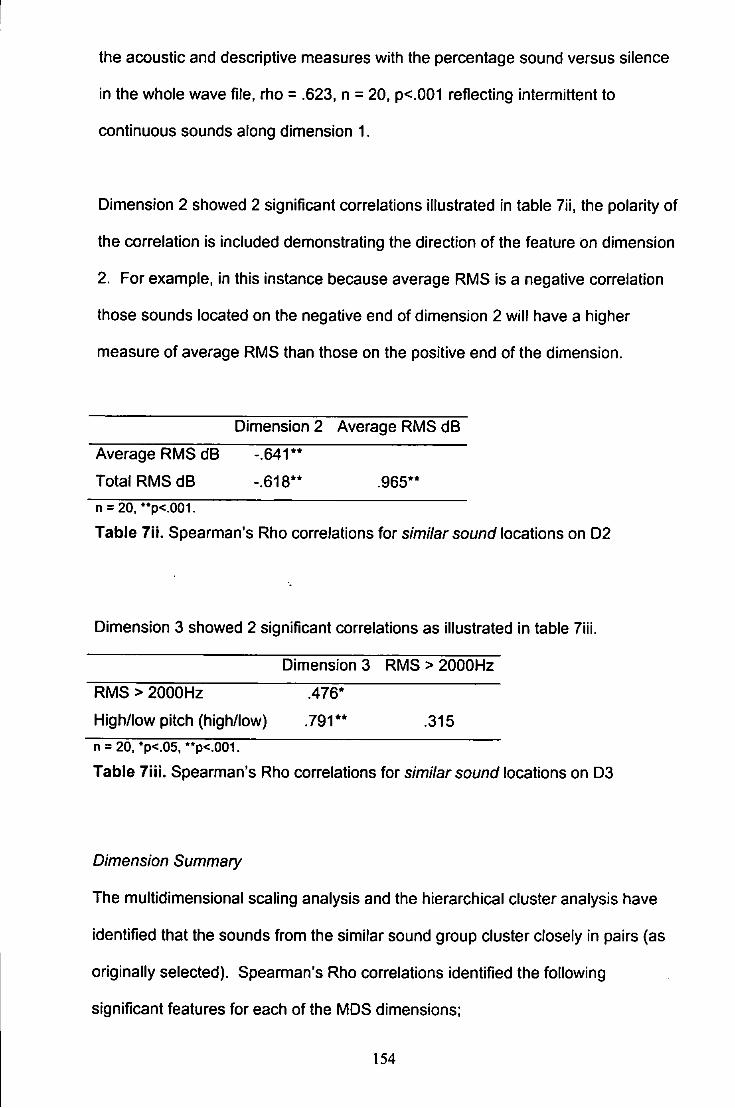
the acoustic and descriptive measures with the percentage sound versus silence
in the whole wave file, rho = .623. n = 20. p<.001 reflecting intermittent to
continuous sounds along dimension 1.
Dimension 2 showed 2 significant correlations illustrated in table 7ii, the polarity of
the correlation is included demonstrating the direction of the feature on dimension
2. For example, in this instance because average RMS is a negative correlation
those sounds located on the negative end of dimension 2 will have a higher
measure of average RMS than those on the positive end of the dimension.
Dimension 2 Average RMS dB
Average RMS dB - . 6 4 1 "
Total RMS dB - .618" .965"
n = 20. "p< 001-
Table 7ii. Spearman's Rho correlations for similar sound locations on D2
Dimension 3 showed 2 significant correlations as illustrated in table 7iii.
Dimension 3 RMS > 2000Hz
RMS > 2000Hz .476*
High/low pitch (high/low) . 7 9 1 " .315
n = 20. *p<.05. •*p<.001.
Table Tiii. Spearman's Rho correlations for similar sound locations on D3
Dimension Summary
The multidimensional scaling analysis and the hierarchical cluster analysis have
identified that the sounds from the similar sound group cluster closely in pairs (as
originally selected). Spearman's Rho correlations identified the following
significant features for each of the MDS dimensions;
154
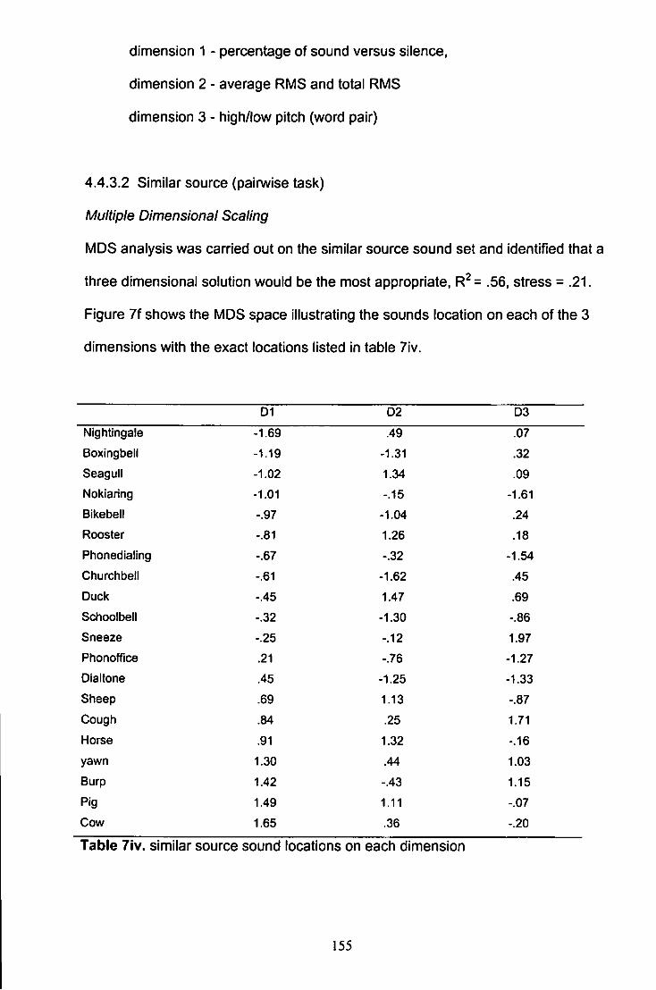
dimension 1 - percentage of sound versus silence,
dimension 2 - average RMS and total RMS
dimension 3 - high/low pitch (word pair)
4.4.3.2 Similar source (pairwise task)
Multiple Dimensional Scaling
MDS analysis was carried out on the similar source sound set and identified that a
three dimensional solution would be the most appropriate, R^= .56, stress = .21.
Figure 7f shows the MDS space illustrating the sounds location on each of the 3
dimensions with the exact locations listed in table 7iv.
D1 02 D3
Nightingale -1.69 .49 .07
Boxingbell -1.19 -1.31 .32
Seagull -1.02 1.34 .09
Nokiaring -1.01 -.15 -1.61
Bikebell -.97 -1.04 .24
Rooster -.81 1.26 .18
Phonedialing -.67 -.32 -1.54
Churchbell -.61 -1.62 .45
Duck -.45 1.47 .69
Schoolbell -.32 -1.30 -.86
Sneeze -.25 -.12 1.97
Phonoffice .21 -.76 -1.27
Dialtone .45 -1.25 -1.33
Sheep .69 1.13 -.87
Cough .84 .25 1.71
Horse .91 1.32 -.16
yawn 1.30 .44 1.03
Burp 1.42 -.43 1.15
Pig 1.49 1.11 -.07
Cow 1.65 .36 -.20
Table 7iv. similar source sound locations on each dimension
155
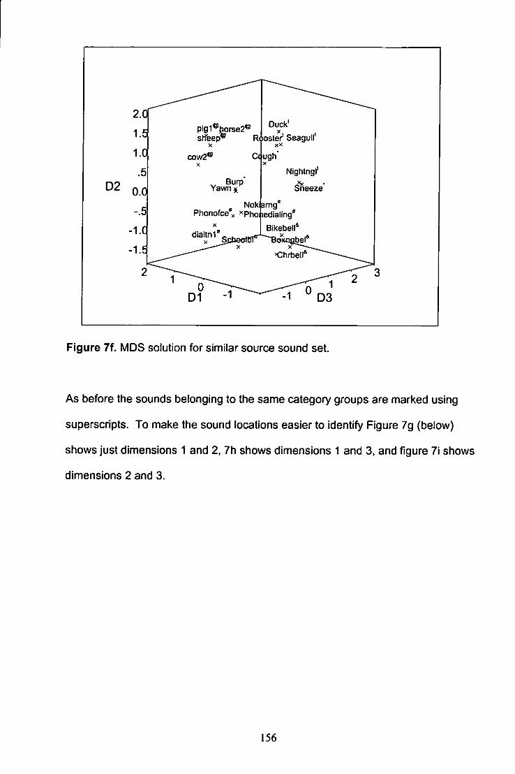
D2
2.0
1.5
1.0
.5
o.a
.,1 •1 .
2
Pig1®hpr5e2® srtfeep®
X
cow2®
Duck'
R({)oster Seagull'
V , Burp Y a w n s
Phonofce x ^Phoiiedialing
Cdugh
Nightngr
^ e e z e *
Nokpmg'
Bikebeir
^Chrbell''
dialtnl
Figure 7f. MDS solution for similar source sound set.
As before the sounds belonging to the same category groups are marked using
superscripts. To make the sound locations easier to identify Figure 7g (below)
shows just dimensions 1 and 2, 7h shows dimensions 1 and 3. and figure 7i shows
dimensions 2 and 3.
156
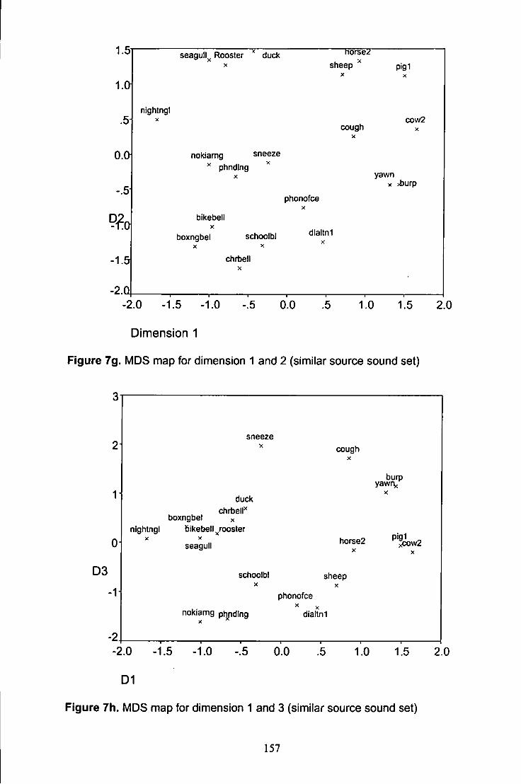
1.5
1.0
.5
0.0
-.5
0
-1.5
-2.0
seagull Rooster duck sheep
X
RorseZ
pigi X
nightngi
cough X
cow2
nokiamg sneeze ^ phnding ^
bikebell X
boxngbel schooibi X X
chrbell X
yawn X >burp
phonofce X
dialtnl
-2.0 -1.5 -1.0 -.5 0.0 .5 1.0 1.5 2.0
Dimension 1
Figure 7g, MDS map for dimension 1 and 2 (similar source sound set)
sneeze 2- X cough
X
burp yawr\,
1 duck X
chrbell'' boxngbel ^
nightngi bikebell rooster horse2 ^%w2 0
X X
seagull horse2 ^%w2
D3 schooibi sheep
-1 X X
-1 phonofce
nokiamg ptyiding ^ X
dialtnl
-2 -2.0 -1.5 -1.0 -.5 0.0 .5 1.0 1.5 2.0
D1
Figure 7h. MDS map for dimension 1 and 3 (similar source sound set)
157
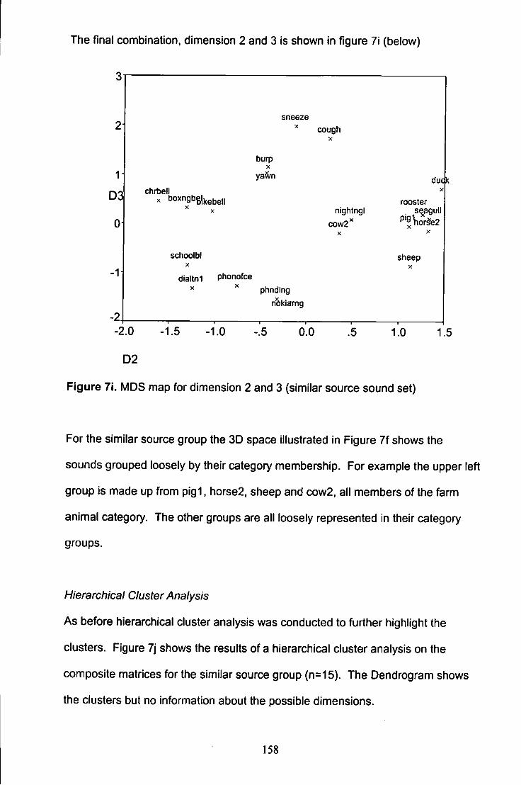
The final combination, dimension 2 and 3 is shown In figure 71 (below)
1
D3I
sneeze X cough
X
burp X
ya^n dudk chrbel
X boxngbglkebeii
schoolbl
nightngi X cow2
X
rooster seagull
sheep X
dialtnl Phonofce phnding
niSkiamg
•2.0 -1.5 -1.0
D2
0.0 .5 1.0 1.5
Figure 7i. MDS map for dimension 2 and 3 (similar source sound set)
For the similar source group the 3D space illustrated in Figure 7f shows the
sounds grouped loosely by their category membership. For example the upper left
group is made up from p ig l , horse2, sheep and cow2. all members of the farm
animal category. The other groups are all loosely represented in their category
groups.
Hierarchical Cluster Analysis
As before hierarchical cluster analysis was conducted to further highlight the
clusters. Figure 7j shows the results of a hierarchical cluster analysis on the
composite matrices for the similar source group (n=15). The Dendrogram shows
the clusters but no information about the possible dimensions.
158
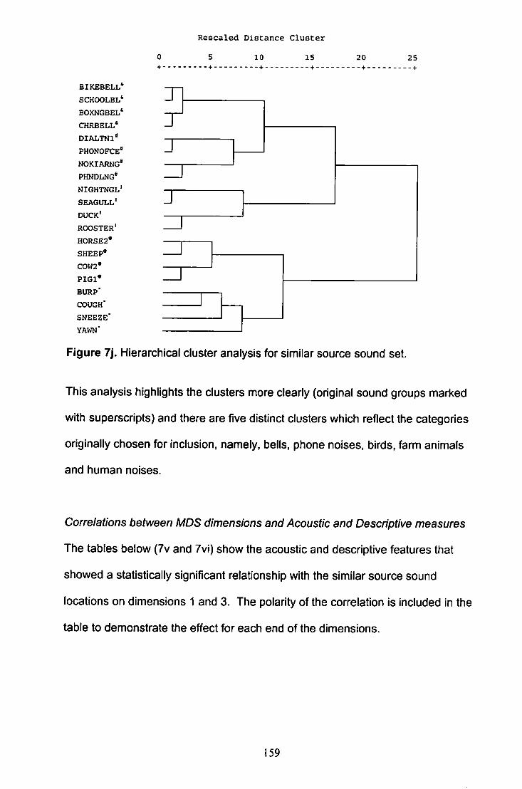
R e s c a l e d D i s t a n c e C l u s t e r
5 10 15 20 25
BIKEBELL' S C H O O L B L '
BOXNGBEL' CHRBELL* DIALTNl* PHONOFCE* NOKIARNG* PHNDLNG* NIGHTNGL' SEAGULL' DUCK' ROOSTER' H0RSE2* SHEEP* C0W2* P I G l * BURP' COUGH* SNEEZE' YAWN'
J 1 1
1
Figure 7j. Hierarchical cluster analysis for similar source sound set.
This analysis highlights the clusters more clearly (original sound groups marked
with superscripts) and there are five distinct clusters which reflect the categories
originally chosen for inclusion, namely, bells, phone noises, birds, farm animals
and human noises.
Correlations between MDS dimensions and Acoustic and Descriptive measures
The tables below (7v and 7vi) show the acoustic and descriptive features that
showed a statistically significant relationship with the similar source sound
locations on dimensions 1 and 3. The polarity of the correlation is included in the
table to demonstrate the effect for each end of the dimensions.
159
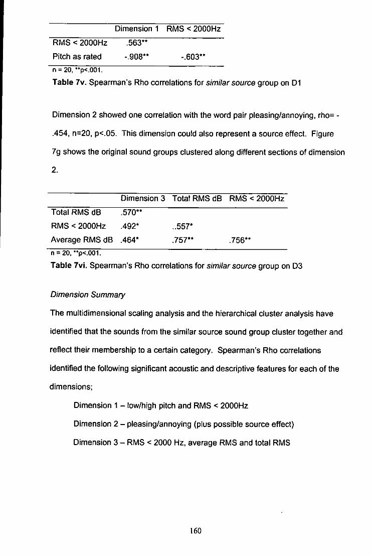
Dimension 1 RMS < 2000Hz
RMS < 2000Hz .563"
Pitch as rated -.908** -.603**
n = 20. "p<.001.
Table 7v. Spearman's Rho correlations for similar source group on D1
Dimension 2 showed one correlation with the word pair pleasing/annoying, rho= -
.454, n=20, p<.05. This dimension could also represent a source effect. Figure
7g shows the original sound groups clustered along different sections of dimension
2.
Dimension 3 Total RMS dB RMS < 2000Hz
Total RMS dB .570**
RMS < 2000Hz .492* ..557*
Average RMS dB .464* .757** .756** n = 20, **p<.001.
Table 7vi. Spearman's Rho correlations for similar source group on D3
Dimension Summary
The multidimensional scaling analysis and the hierarchical cluster analysis have
identified that the sounds from the similar source sound group cluster together and
reflect their membership to a certain category. Spearman's Rho correlations
identified the following significant acoustic and descriptive features for each of the
dimensions;
Dimension 1 - low/high pitch and RMS < 2000Hz
Dimension 2 - pleasing/annoying (plus possible source effect)
Dimension 3 - RMS < 2000 Hz. average RMS and total RMS
160
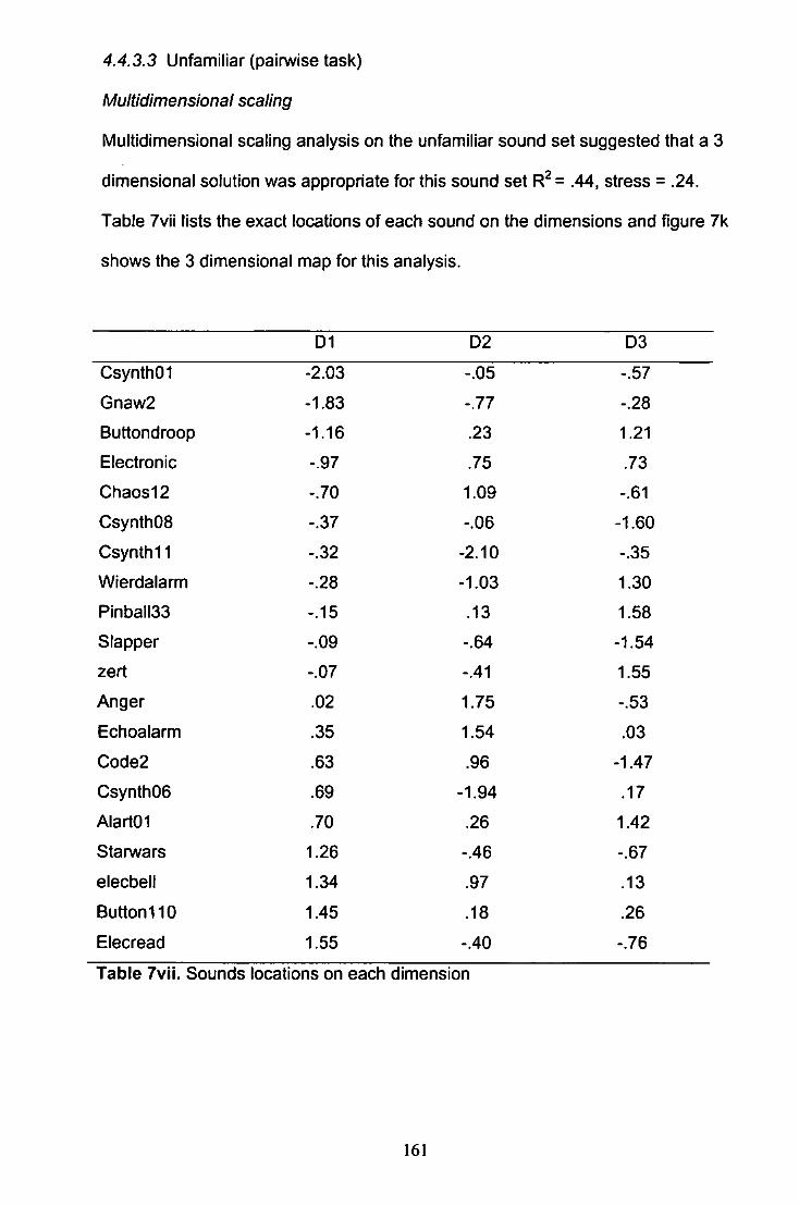
4.4.3.3 Unfamiliar (painwise task)
Multidimensional scaling
Multidimensional scaling analysis on the unfamiliar sound set suggested that a 3
dimensional solution was appropriate for this sound set = .44, stress = .24.
Table 7vii lists the exact locations of each sound on the dimensions and figure 7k
shows the 3 dimensional map for this analysis.
D1 D2 D3
CsynthOI -2.03 -.05 -.57
Gnaw2 -1.83 -.77 -.28
Buttondroop -1.16 .23 1.21
Electronic -.97 .75 .73
Chaos12 -.70 1.09 -.61
CsynthOS -.37 -.06 -1.60
Csynth l l -.32 -2.10 -.35
Wierdalarm -.28 -1.03 1.30
Pinball33 -.15 .13 1.58
Slapper -.09 -.64 -1.54
zert -.07 -.41 1.55
Anger .02 1.75 -.53
Echoalarm .35 1.54 .03
Code2 .63 .96 -1.47
CsynthOe .69 -1.94 .17
AlartOI .70 .26 1.42
Starwars 1.26 -.46 -.67
elecbell 1.34 .97 .13
Buttonl lO 1.45 .18 .26
Elecread 1.55 -.40 -.76
Table 7vii. Sounds locations on each dimension
161
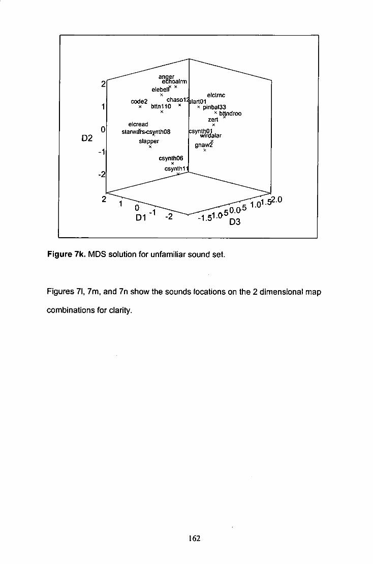
D2
elebeir
code2 chasol X bttn110 ^
elcread starw^i^iCsynthOS
slapper
elctmc '^lartOI
^ pinbaI33 ^ bttndroo
zert ^
gnaw^
csynthOb
csynthi \
: i.52.o
Figure 7k. MDS solution for unfamiliar sound set.
Figures 71, 7m, and 7n show the sounds locations on the 2 dimensional map
combinations for clarity.
162
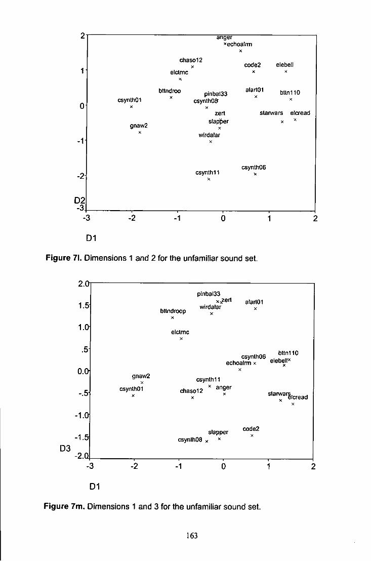
D2 -3.
anger ^echoalrm
chaso12 X code2 elebell
elctmc X
X X
csynlhOI pinbal33
csynthOff
alartOI X
bttnllO X
X
zert starwars elcread
gnaw2 slap^er
X
X ^
wirdalar X
csynthi 1 X
csynthOS X
-3 -2 -1 0
D1
Figure 71. Dimensions 1 and 2 for the unfamiliar sound set.
D3
2.0
1.5
1.01
.5
0.01
-.5
•1.0
•1.5
•2.0 •3
D1
pinbal33 x^ert
. „ . wirdalar bttndroop ^
elctmc X
alartOI X
gnaw2
csynthOI
csynthOS , ^""^^^ echoalmi x elebell^
csynthi1
chaso12 ^"r' ^•^-^^^icread
X
slapper csynthOa x
code2 X
-1 0
Figure 7m. Dimensions 1 and 3 for ttie unfamiliar sound set.
163
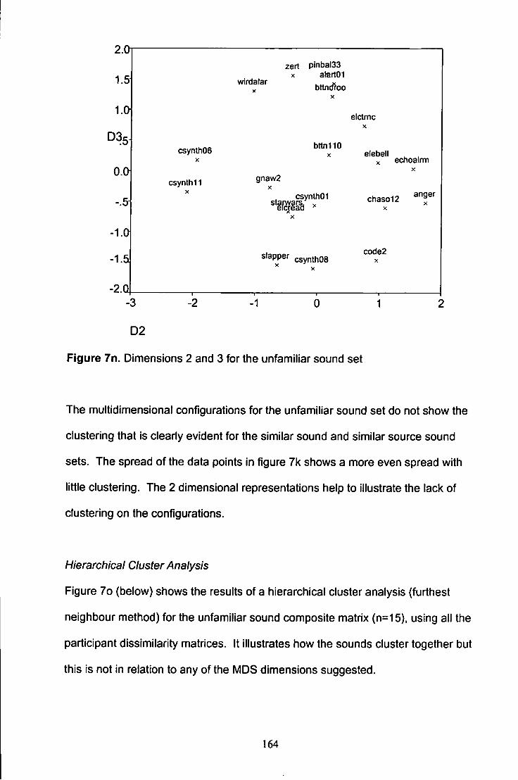
2.0
1.5
1.01
D35
0.01
-.5
-1.0
-1.5
-2.0
csynthoe X
csynthH X
wirdalar X
zert pinba!33 X atertOI
bttndfoo y.
elctmc >:
bttnllO elebell
gnaw2
csynthOI
slapper csynthOS
echoairm
chaso12
code2 X
D2
Figure 7n. Dimensions 2 and 3 for the unfamiliar sound set
The multidimensional configurations for the unfamiliar sound set do not show the
clustering that is clearly evident for the similar sound and similar source sound
sets. The spread of the data points in figure 7k shows a more even spread with
little clustering. The 2 dimensional representations help to illustrate the lack of
clustering on the configurations.
Hierarchical Cluster Analysis
Figure 7o (below) shows the results of a hierarchical cluster analysis (furthest
neighbour method) for the unfamiliar sound composite matrix (n=15). using all the
participant dissimilarity matrices. It illustrates how the sounds cluster together but
this is not in relation to any of the MDS dimensions suggested.
164
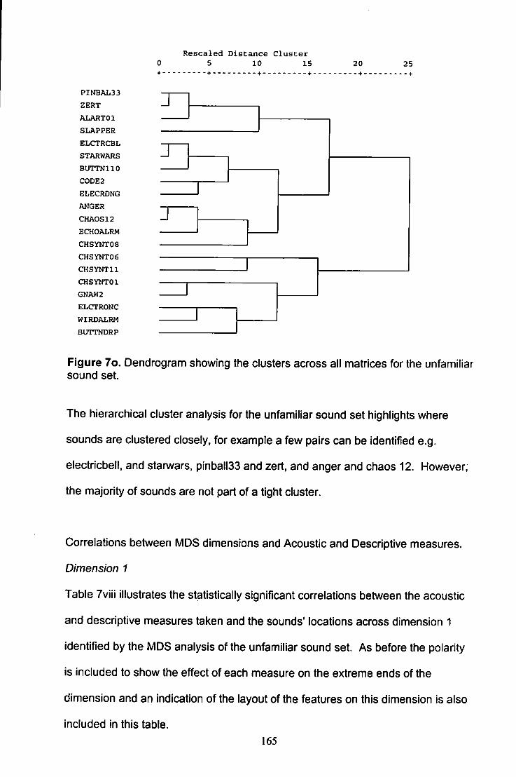
PINBAL33 ZERT ALARTOl SLAPPER ELCTRCBL STARWARS BUTTNllO CODE 2 ELECRDNG ANGER CHAOS12 ECHOALRM CHSYNTOS CHSYNT06 CHSYNTll CHSYNTOl GNAW2 ELCTRONC WIRDALRM BUTTNDRP
Re s c a l e d D i s t a n c e C l u s t e r 5 10 15 20 25
J
J
J
Figure 7o, Dendrogram showing the clusters across all matrices for the unfamiliar sound set.
The hierarchical cluster analysis for the unfamiliar sound set highlights where
sounds are clustered closely, for example a few pairs can be identified e.g.
electricbell, and starwars, pinball33 and zert, and anger and chaos 12. However,
the majority of sounds are not part of a tight cluster.
Correlations between MDS dimensions and Acoustic and Descriptive measures.
Dimension 1
Table 7viii illustrates the statistically significant correlations between the acoustic
and descriptive measures taken and the sounds' locations across dimension 1
identified by the MDS analysis of the unfamiliar sound set. As before the polarity
is included to show the effect of each measure on the extreme ends of the
dimension and an indication of the layout of the features on this dimension is also
included in this table.
165
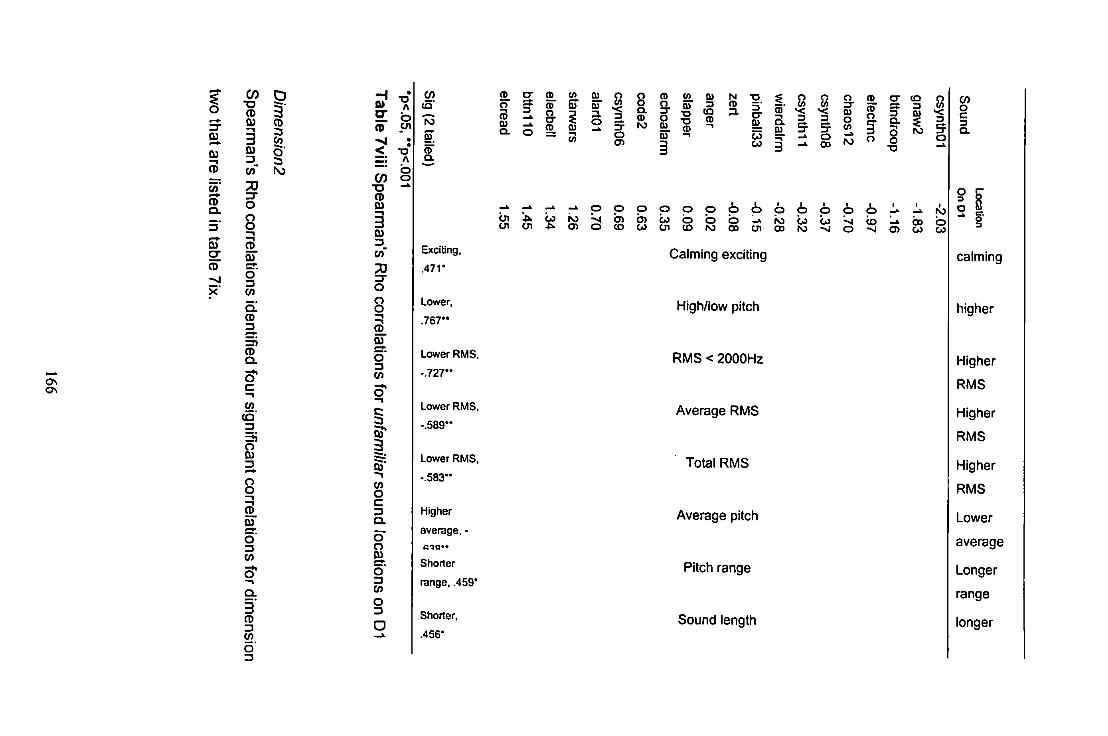
OS
21 Q) S W CD Q.
CD
x'
CO •a CD Q)
Q)
73 o
5- 8
25. 5" 3 W 5! CD 3
CD Q. 3* C —1
w CQ'
8 I 0) 5"
Q.
3' CD 3 W o' 3
CO O*
CD
* < X3 =: A
b CO o
T3 CD Q) -1
3 Q) 3 Crt 73 3 -O 8
21 5* 3 C/)
c 3 Q. O
I o' 3 CO o 3
(Q CD CT
0) -k Q. O
(D 5!. S i t o
(D O
0)
Q) •D T3 (D
Q)
CD
•g
I CO CO
(D a 01 o
00
0) 5 a .
S o
Si (O
i I
o o o 6 6 6 6 : *
Exciting,
.471*
Lower,
.767"
Lower RMS.
- .727"
Lower RMS,
- .589"
Lower RMS,
- .583"
Higher
average, -
Shorter
range, .459'
Shorter,
.456*
o c o c o O i f o r o o o o i
Calming exciting
High/low pitch
RMS < 2000Hz
Average RMS
Total RMS
Average pitch
Pilch range
Sound length
00 o O -Nj 0> O) w
CO g Q.
O
o -
calming
higher
Higher
RMS
Higher
RMS
Higher
RMS
Lower
average
Longer
range
longer
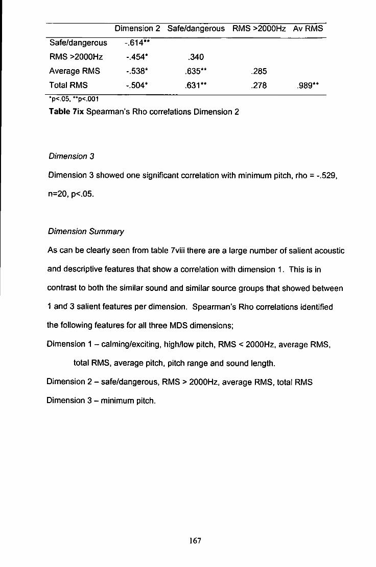
Dimension 2 Safe/dangerous RMS >2000Hz Av RMS
Safe/dangerous -.614**
RMS >2000Hz -.454* .340
Average RMS -.538* ,635** .285
Total RMS -.504* .631** .278 .989**
*p<.05. "p<.001
Table 7ix Spearman's Rho correlations Dimension 2
Dimension 3
Dimension 3 showed one significant correlation with minimum pitch, rho = -.529.
n=20. p<.05.
Dimension Summary
As can be clearly seen from table 7viii there are a large number of salient acoustic
and descriptive features that show a correlation with dimension 1. This is in
contrast to both the similar sound and similar source groups that showed between
1 and 3 salient features per dimension. Spearman's Rho correlations identified
the following features for all three MDS dimensions;
Dimension 1 - calming/exciting, high/low pitch, RMS < 2000H2, average RMS,
total RMS, average pitch, pitch range and sound length.
Dimension 2 - safe/dangerous, RMS > 2000Hz, average RMS, total RMS
Dimension 3 - minimum pitch.
167
4.4.4 Discussion
As before each sound group will be discussed individually before a more general
discussion of the results.
4.4.4.1 Similar sound group
The stimuli from this group have clustered together by their original acoustically
similar pairs. For example, duck and seal are close together on all the
dimensions. The original pair selections are also reflected in the Dendrogram.
The correlations between the MDS dimensions and the acoustic and descriptive
measures suggest that for this sound group participants are relying on just the
acoustic measures with no emphasis on the measured descriptive or perceptual
measures. By applying the acoustic features that have been identified by the
correlations to the MDS configurations it can be seen that the identified features
are likely to be accurate. For example, the sounds lawnmower and fryfood are at
the positive end of dimension 1 and have the most sound versus silence. These
two sounds are not intermittent sounds but continue throughout the 4 second
playing time. In contrast seal and duck are intermittent sounds with silent pauses
making up some of the playing time. Dimension 2 has the more powerful sounds
on the negative end (cow and boat horn) with the quieter on the positive end
(brush teeth). The other correlations show an appropriate fit in the same way.
Analysis of this sound group has suggested that participants are favouring the use
of acoustic features in their judgments of similarity or their judgements are being
based on acoustic similarity.
4.4.4.2 Similar source
The clusters were less clear in this stimuli group but the clusters are loosely
arranged by their category groups. The clearest of these is the bell group that is
168
clustered on all three dimensions. The hierarchical cluster analysis also reflects
the category groups with superscripts highlighting the original category groups.
Again the majority of features identified as salient are acoustic with the exception
of the word pair pleasing/annoying. Dimension 1 shows that the sounds are
ordered according to pitch, for example the negative end shows nightingale with
cow moo at the positive end of the dimension. Intuitively the correlation with high
pitch/low pitch makes sense. Similarly dimension 2 shows the most pleasing
sounds as the bird and animals sounds with the most annoying being the bells and
phone noises. The third dimension shows the most powerful sounds (measured
by total RMS, RMS <2000H2 and average RMS dB) to be the sneeze with the
least powerful being the dial tone and nokiaring. Again the analyses would
suggest that participants are strongly relying on the acoustic features of the
sounds alongside support for the inclusion of category information provided by
visual inspection of the MDS configurations and the hierarchical cluster analysis.
Both of these analyses techniques identified fairly clear clusters.
4.4.4.3 Unfamiliar
This set of stimuli shows very little clustering on the MDS output with quite a poor
amount of variance explained by the MDS analysis (variance explained for the
unfamiliar group = 44% (versus 60% and 56% respectively for similar sounds and
similar source groups) and should therefore be interpreted with caution. The
hierarchical cluster analysis shows some limited clustering but no groups are
clear. Despite this lack of apparent clustering a substantial number of the acoustic
and descriptive measures showed significant correlation with the sounds' locations
on the MDS configuration. Dimension 1 correlated with eight acoustic or
descriptive features (calming/exciting, high/low pitch, RMS < 2000Hz, average
RMS, total RMS, average pitch, pitch range and sound versus silence) suggesting
169
that pitch and the RMS power of the souncJ was an important part of the similarity
judgments. The spread of the acoustic measures for the unfamiliar sound set
were compared to those from the similar sound and similar source groups to check
whether there was a significantly different spread or range for the unfamiliar
sounds but no clear differences were found between the three groups.
Safe/dangerous was an important feature on dimension 2 and the power of a
sound was important here too. Dimension 3 showed only one statistically
significant correlation with the minimum pitch of the sound. As expected there was
no evidence of the use of category membership in the similarity judgements for
this sound set.
4.4.5 General Discussion
The aim of these two experiments was to test several hypotheses. Firstly, that
familiar sounds may, in part, be grouped by the category to which their source
belongs. Secondly, that participants would favour the use of acoustic features
when sounds are unfamiliar. In addition, the identification of the salient acoustic
and descriptive features used to make the similarity judgement was still a primary
interest.
The results for the similar sound set suggest that participants were able to identify
obvious acoustically similar sound pairs despite the lack of opportunity to listen to
all the sounds together. The results suggest that participants were using the
acoustic information when making their similarity judgements leading to the cleariy
identifiable pairs in the HCA analysis. The sound pairs in the similar sound group
were not selected to make up any categories although there is evidence from the
hierarchical cluster analysis of a loose and unintentional animal category (cow,
seal and duck) but this category was not reflected in the MDS output. There is
170
little visual evidence from the HCA that participants based their similarity decisions
on the sounds* membership to a certain category. Therefore, it is unlikely that for
the similar sound group participants used knowledge about a sound's membership
to a category to base their similarity judgements. It is suggested from the results
that participants used acoustic knowledge about the sounds in order to make their
similarity judgements and that this knowledge overruled any categorical
knowledge for this sound group. This suggestion is also supported by the finding
that only acoustic features showed a correlation with the sounds' locations on the
MDS configuration.
The similar source group showed clear evidence of clustering into categories.
Unlike the grouping task, where it may be expected that participants would group
all the bell sounds together, participants are unaware of the categories on which
the presented sounds were selected (similar source) because each sound pair
was presented in isolation. However, the results from experiment 7 have
suggested that category membership could be playing an important role in the
grouping, especially for the similar source sounds. Both the MDS and the
hierarchical cluster analysis showed loose but clear clusters that reflected the
categories that were originally chosen for inclusion in the experiment (bells,
phones, birds, human noises and animal noises). As discussed previously by
Hahn (2001) houses are cleariy more similar to other houses than to cars. This is
despite the fact that houses take many different forms. Therefore, it is possible
that two telephone noises (e.g. dial tone and office phone ring) presented together
will be considered much more similar to each other than a telephone and any of
the other sounds in the similar source group simply because they are both
members of the same category. This sound group showed evidence for the use of
171
both acoustic and descriptive features by participants when making similarity
judgements along side the importance of category membership information.
The clusters identified across all three of the stimuli groups are all suggesting the
importance of both acoustic and descriptive features in the judgements of
similarity. There is evidence for different interactions between the two. For
example, in experiment 3 which also used the painwise task it was also the case
that the acoustic features were the most prominent. It was only in experiment 5,
using the grouping task, that the acoustic features were less salient. This
suggests that the two tasks may be requiring a different kind of processing in order
to complete each task with the painwise task used in the present experiment
suggesting a heavier reliance on acoustic information.
Previously the sounds were all abstract in nature but this experiment has included
some environmental sounds. There does not appear to be any clustering of
sounds that represent environmental or abstract sound groups. However, this is to
be expected as many of the sounds that are defined as abstract do make up part
of our modern day environment, such as a mobile phone ring tone and could
therefore also be classed as environmental sounds. The classification is one that
a listener may not be aware of but served a function in this experimental series.
A final point of interest is that familiarity did not show a correlation with the
dimensions identified by the MDS analyses for any of the sound groups. The
sounds chosen for inclusion in this experiment were selected on the basis of being
familiar or unfamiliar. Therefore, the lack of a relationship between familiarity and
the sounds' locations on the MDS dimensions does suggest that the
familiar/unfamiliar criteria was met for all three sound groups. This is because if
172

there is little variation on a feature and it is a feature that all the stimuli share group
then participants will not be able to use it as a basis for a similarity judgement. As
discussed by Tversky (1977) features that are shared by all the objects under
consideration cannot be used to classify them and are of no diagnostic value.
173
Chapter 5: Experiments 8 and 9 (grouping)
5.1 Introduction
This experimental chapter discusses two experiments designed to evaluate the
sound groups used in experiment 7 (similar sound, similar source and unfamiliar)
but using the grouping methodology that was previously employed in experiment
5. Experiments 8 and 9 were designed to address three main questions. The first
was to asses whether the features that were identified as salient for the pairwise
task would be identified again using the grouping task methodology. Secondly, it
was hoped that the use of the unfamiliar sound set, like experiment 7, would help
to examine more closely the unfamiliar area of data identified in experiment 5.
Thirdly, as for the previous experiments the identification of salient acoustic and
non acoustic features was of interest.
Previous experiments suggested that participants favoured different sound
features when making similarity judgements depending on the methodology
employed. To recap, the pairwise task requires participants to make a judgement
about the similarity of two sounds presented one after the other over a series of
trials until all stimuli have been paired. In contrast the grouping methodology
requires participants to group the sounds on the basis of similarity by moving icons
around a screen with all sounds presented at the same time. Experiment 3, using
the piairwise task, suggested that participants favoured the use of both the
acoustic and descriptive measures in their judgements of similarity. In contrast
experiment 5 that employed the grouping task highlighted only descriptive
measures with not one of the measured acoustic features showing a significant
relationship to the sound locations on the MDS configuration. Therefore, to clarify
any methodological issues experiment 8 employed the grouping task on the same
three sets of sounds used in experiment 7 (painwise task). This would provide the
174
opportunity to compare the two methodologies for the same three stimuli sets.
When Bonebright (1996) compared the pairwise task and the grouping task it was
identified that the parameters used to construct the stimuli in the study were
represented in MDS outputs for both methodologies but that the spread of the
stimuli were slightly different. The grouping task stimuli were grouped more
closely than the pairwise. In addition, Bonebright (1996) also identified that
emotional cues were being reflected by the grouping task that were not reflected in
the pairwise results. This reflects the difference in the type of sound features
identified as salient in experiments 3 and 5. Therefore, experiment 8 will provide
an opportunity to investigate the two methodologies further with three sound sets
addressing how the stimuli cluster on the MDS configurations and the salient
acoustic and descriptive measures.
Clarification of the unfamiliar end of the MDS output in experiment 5 was
addressed in part by experiment 7 using the pain/vise methodology. Experiment 7
suggested that the unfamiliar sounds utilized almost all of the measured features
(both acoustic and descriptive) but did not employ any functional or category
information. Further investigation of this finding was also sought using the
grouping methodology in experiments 8 and 9.
Experiment 9 was a replication of experiment 8 but it was felt that some qualitative
data may provide extra information and specifically may help support the results
that suggested the use of category information in participants' judgements of
similarity. The additional experiment would also serve to provide a measure of the
grouping tasks reliability between experimental sessions.
175
The number of sounds in this experiment was not particulariy large and therefore it
was not essential that the grouping task was employed. However, Lakatos.
Scavone and Cook (2002) discuss the effects of data collection methods on MDS
solutions. Lakatos et al (2002) raised the point that more traditional methods such
as the pairwise task may set unnecessary limits on participants' perceptual,
cognitive, and decisional strategies. This is important because it may suggest that
participants are making decisions based on only the most salient dimensions,
whether that be acoustic, descriptive or categorical dependent on the stimuli
included, as a matter of economy. One of the problems levied against the
pairwise task is that it is impossible for participants to adjust a similarity rating in
light of a new criterion that they may generate on the basis of a later comparisons.
Further, the continuous use of a rating scale may encourage participants to think
uni dimensionally about the similarities between stimulus pairs. Whilst this does
not indicate which features they may favour it does suggest that acoustic,
descriptive or source features may be employed but not at the same time.
Therefore, this added support to the rationale for re using the grouping task with
the three sound sets used in experiment 7. It was hoped that any differences in
task performance could be cleariy identified.
In summary experiments 8 and 9 are designed to compare and contrast the results
obtained with previous results from experiment 7. specifically, how the stimuli
cluster and the salient acoustic and descriptive features that are identified in
participants' similarity judgements. Previous results from both the present series
of experiments and work conducted by Bonebright (1996) suggest that the spread
of the stimuli using the painwise task may be closer than for the grouping task and
the type of measured sound features utilized by participants will vary between the
176
two methodologies with the acoustic features being less favoured for the grouping
task methodology.
5.2 Experiment 8 grouping task for three sound sets
5.2.1 Introduction
This experiment used the same sound sets that were analysed and rated in
experiment 6 and used in the pairwise tasks in experiment 7. These groups were:
Similar sound - 1 0 pairs of sounds that sound similar e.g. cow moo and fog
horn, but come from a completely different source.
Similar source - 5 sets of 4 sounds that come from similar sources but sound
different e.g. cow. sheep, pig, horse (famriyard animals).
Unfamiliar - this group consisted of novel, unfamiliar sounds.
At this stage it was hypothesised that the way participants would sort the groups
would be very similar to the results from the pairwise task but results from
experiment 3 (pairwise) and experiment 5 (grouping) would suggest that it is likely
that participants would favour non acoustic features such as the descriptive and
categorical information when using this grouping methodology. It is also thought
that the simultaneous comparison of the sounds in the grouping methodology may
illuminate the use of pairs or categories to the participants (Lakatos et al, 2002)
and make the original groupings more likely to be evident than was the case in
experiment 7.
177
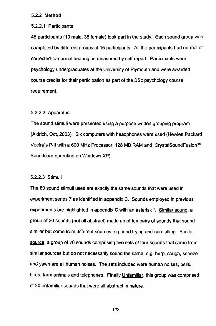
5.2.2 Method
5.2.2.1 Participants
45 participants (10 male, 35 female) took part in the study. Each sound group was
completed by different groups of 15 participants. All the participants had normal or
corrected-to-normal hearing as measured by self report. Participants were
psychology undergraduates at the University of Plymouth and were awarded
course credits for their participation as part of the BSc psychology course
requirement.
5.2.2.2 Apparatus
The sound stimuli were presented using a purpose written grouping program
(Aldrich, Oct, 2003). Six computers with headphones were used (Hewlett Packard
Vectra's Pill with a 600 MHz Processor. 128 MB RAM and CrystalSoundFusion™
Soundcard operating on Windows XP).
5.2.2.3 Stimuli
The 60 sound stimuli used are exactly the same sounds that were used in
experiment series 7 as identified in appendix C. Sounds employed in previous
experiments are highlighted in appendix C with an asterisk *. Similar sound, a
group of 20 sounds (not all abstract) made up of ten pairs of sounds that sound
similar but come from different sources e.g. food frying and rain falling. Similar
source, a group of 20 sounds comprising five sets of four sounds that come from
similar sources but do not necessarily sound the same, e.g. burp, cough, sneeze
and yawn are all human noises. The sets included were human noises, bells,
birds, farm animals and telephones. Finally Unfamiliar, this group was comprised
of 20 unfamiliar sounds that were alt abstract in nature.
178
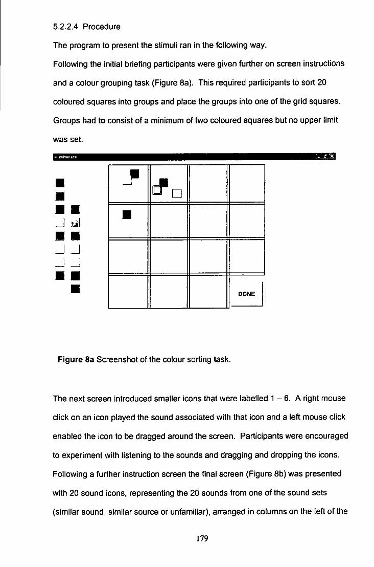
5.2.2.4 Procedure
The program to present the stimuli ran in the following way.
Following the initial briefing participants were given further on screen instructions
and a colour grouping task (Figure 8a). This required participants to sort 20
coloured squares into groups and place the groups into one of the grid squares.
Groups had to consist of a minimum of two coloured squares but no upper limit
was set.
• • •
DONE
Figure 8a Screenshot of the colour sorting task.
The next screen introduced smaller icons that were labelled 1 - 6. A right mouse
click on an icon played the sound associated with that icon and a left mouse click
enabled the icon to be dragged around the screen. Participants were encouraged
to experiment with listening to the sounds and dragging and dropping the icons.
Following a further instruction screen the final screen (Figure 8b) was presented
with 20 sound icons, representing the 20 sounds from one of the sound sets
(similar sound, similar source or unfamiliar), arranged in columns on the left of the
179
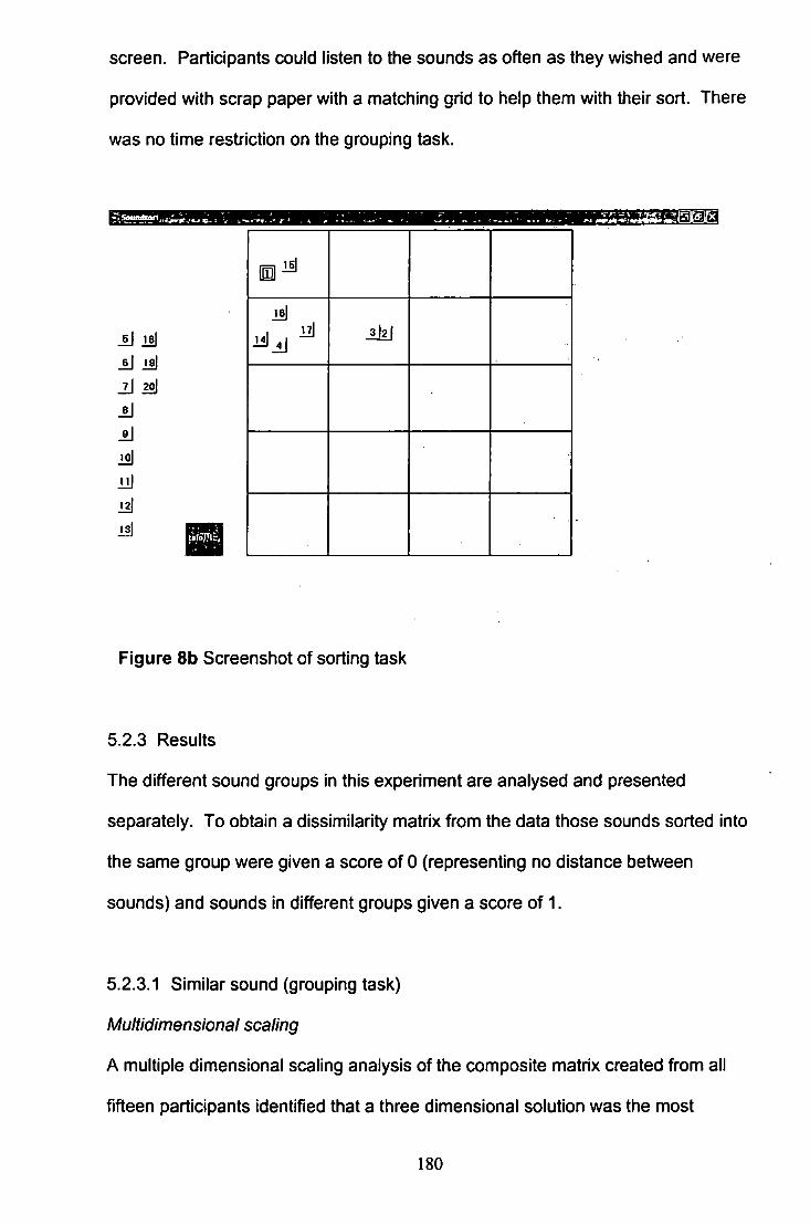
screen. Participants could listen to the sounds as often as they wished and were
provided with scrap paper with a matching grid to help them with their sort. There
was no time restriction on the grouping task.
i!j -21 I3l
_I6|
i ^
Figure 8b Screenshot of sorting task
5.2.3 Results
The different sound groups in this experiment are analysed and presented
separately. To obtain a dissimilarity matrix from the data those sounds sorted into
the same group were given a score of 0 (representing no distance between
sounds) and sounds in different groups given a score of 1.
5.2.3.1 Similar sound (grouping task)
Multidimensional scaling
A multiple dimensional scaling analysis of the composite matrix created from all
fifteen participants identified that a three dimensional solution was the most
180
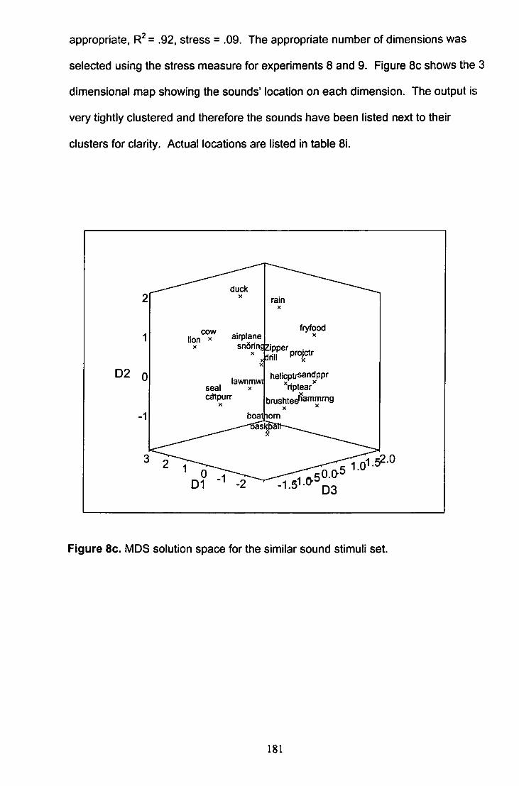
appropriate, = ,92, stress = .09. The appropriate number of dimensions was
selected using the stress measure for experiments 8 and 9. Figure 8c shows the 3
dimensional map showing the sounds' location on each dimension. The output is
very tightly clustered and therefore the sounds have been listed next to their
clusters for clarity. Actual locations are listed in table 81.
D2
cow lion ^ airplane
snSringjjpper
lawnmwil seal X cdtpun-
X
Jdrill
fryfood X
projctr
helicptrsandppr ^'riptear''
brushtee^a""f""i9
boathom
1.520
Figure 8c. MDS solution space for the similar sound stimuli set.
181
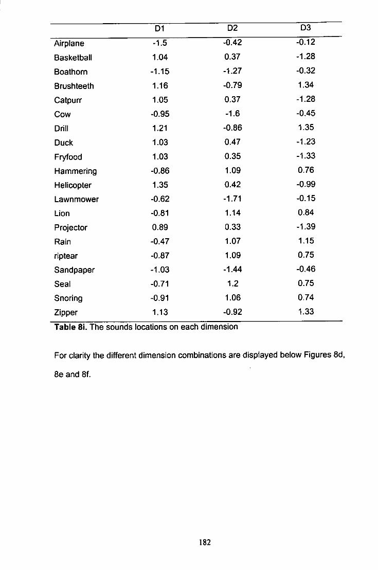
D1 D2 D3
Airplane -1.5 -0.42 -0.12
Basketball 1.04 0.37 -1.28
Boathom -1.15 -1.27 -0.32
Brushteeth 1.16 -0.79 1.34
Catpurr 1.05 0.37 -1.28
Cow -0.95 -1.6 -0.45
Drill 1.21 -0.86 1.35
Duck 1.03 0.47 -1.23
Fryfood 1.03 0.35 -1.33
Hammering -0.86 1.09 0.76
Helicopter 1.35 0.42 -0.99
Lawn mower -0.62 -1.71 -0.15
Lion -0.81 1.14 0.84
Projector 0.89 0.33 -1.39
Rain -0.47 1.07 1.15
riptear -0.87 1.09 0.75
Sandpaper -1.03 -1.44 -0.46
Seal -0.71 1.2 0.75
Snoring -0.91 1.06 0.74
Zipper 1.13 -0.92 1.33
Table 8i. The sounds locations on each dimension
For clarity the different dimension combinations are displayed below Figures 8d,
8e and 8f.
182
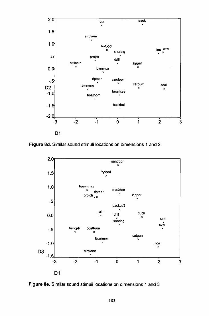
2.0
1.5
-.5 D2 -1.0
-1.5
-2.0
rain X
duck X
airplane X
fryfood X snoring
lion cow X ^
projctr X
helicptr
X
drill X zipper
^ lawnmwr X
X
riptear sandppr X
hammmg X
boathom X
X
brushtee X
baskball X
catpurr X
seal X
•3
D1
0
Figure 8d. Similar sound stimuli locations on dimensions 1 and 2.
2.0]
D3
1.5
1.0i
.5
0.0
-.5
-1.0
-1.5
sandppr X
fryfood X
hammrng
^ riptear projctr^^
ram X
brushtee X
baskball X
drill X
snoring
zipper X
heticptr boathom X X
lawnmwr X
duck X
catpun-X
seal X
cow
lion X
airplane X
-3
D1
-1
Figure Be. Similar sound stimuli locations on dimensions 1 and 3
183
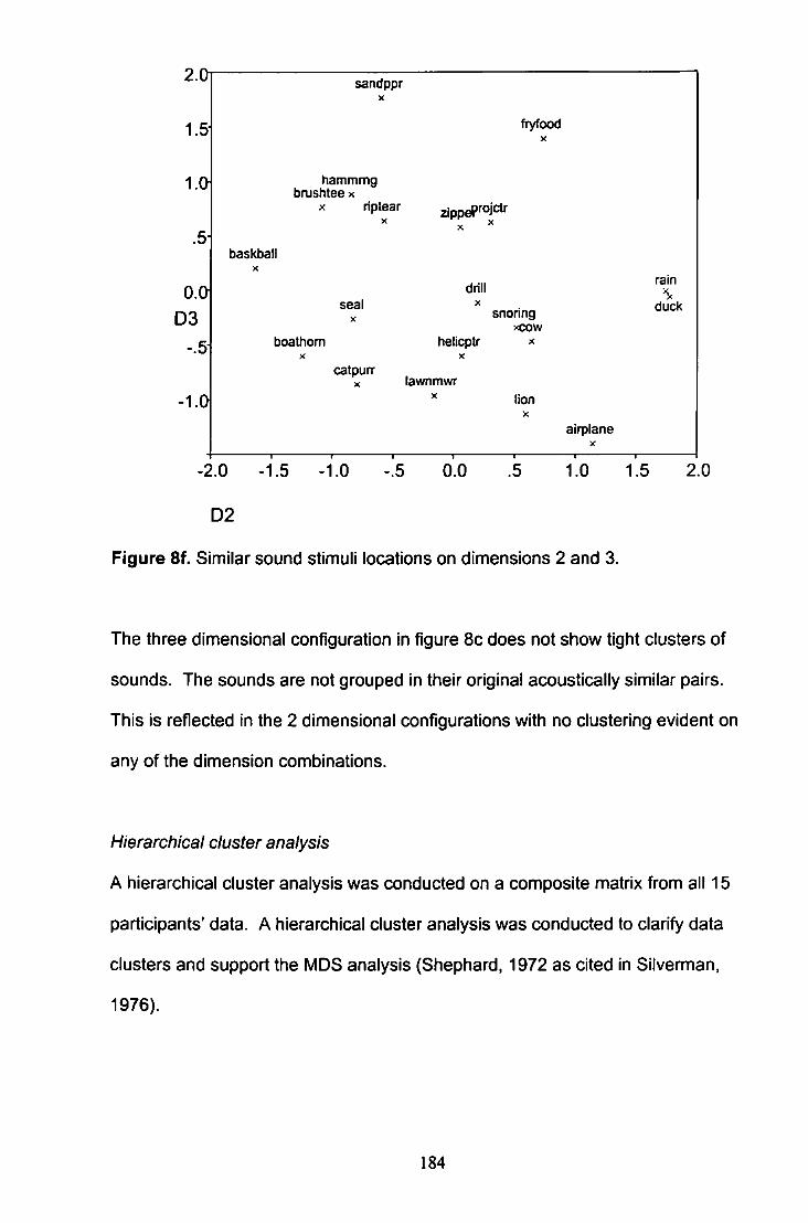
2.0
1.5-
1.01
.5
O.Ol
D3
-.5
-I.Ol
sandppr X
fryfood
hammmg bnjshtee x
baskball X
seal X
drill X
snoring xcow
boathom helicptr x X X
catpurr X lawnmwr
lion X
ram
duck
airplane X
-2.0 -1.5 -1.0
D2
0.0 .5 1.0 1.5 2.0
Figure 8f. Similar sound stimuli locations on dimensions 2 and 3.
The three dimensional configuration in figure 8c does not show tight clusters of
sounds. The sounds are not grouped in their original acoustically similar pairs.
This is reflected in the 2 dimensional configurations with no clustering evident on
any of the dimension combinations.
Hierarchical cluster analysis
A hierarchical cluster analysis was conducted on a composite matrix from all 15
participants' data. A hierarchical cluster analysis was conducted to clarify data
clusters and support the MDS analysis (Shephard. 1972 as cited in Silverman,
1976).
184
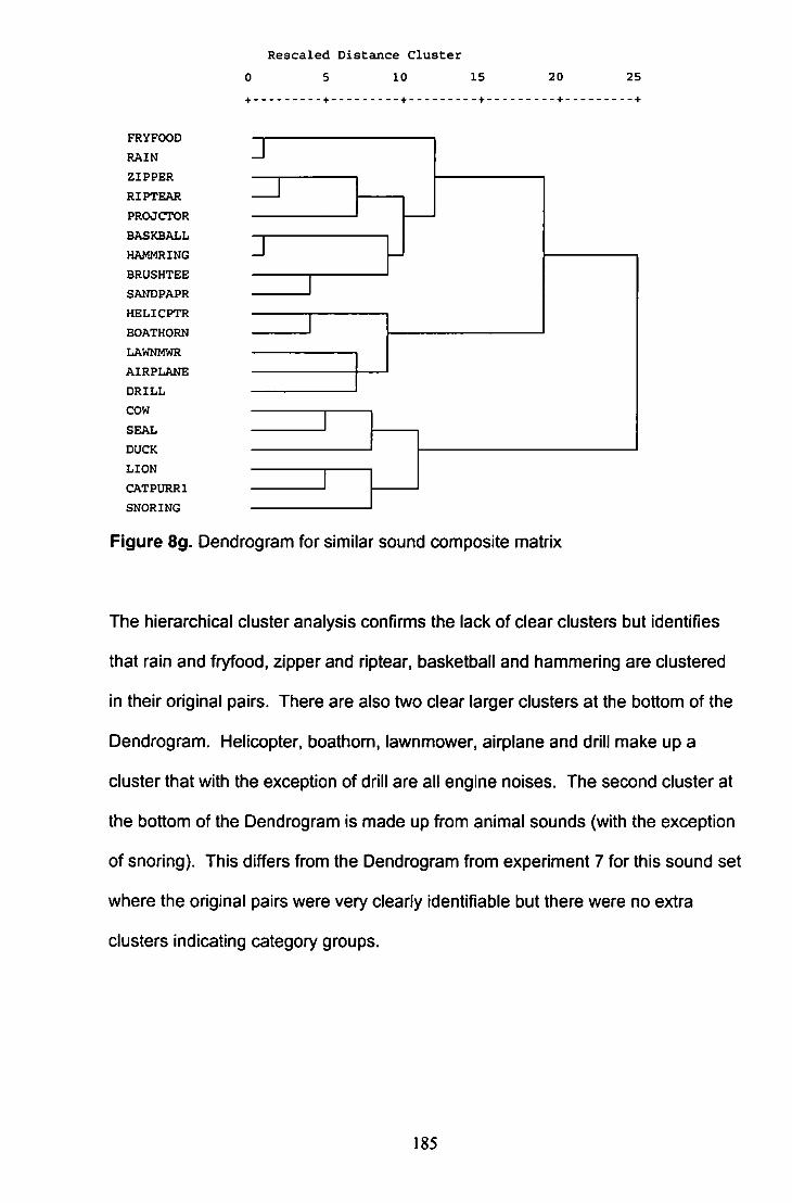
R e s c a l e d D i s t a n c e C l u s t e r 0 5 10 15 + + + + •
20 25
FRYFOOD RAIN ZIPPER RIPTEAR PROJCTOR BASKBALL HAMMRING BRUSHTEE SANDPAPR HELICPTR BOATHORN LAWNMWR AIRPLANE DRILL COW SEAL DUCK LION CATPURRl SNORING
I
I
Figure 8g. Dendrogram for similar sound composite matrix
The hierarchical cluster analysis confirms the lack of clear clusters but identifies
that rain and fryfood, zipper and riptear, basketball and hammering are clustered
in their original pairs. There are also two clear larger clusters at the bottom of the
Dendrogram. Helicopter, boathorn, lawnmower, airplane and drill make up a
cluster that with the exception of drill are all engine noises. The second cluster at
the bottom of the Dendrogram is made up from animal sounds (with the exception
of snoring). This differs from the Dendrogram from experiment 7 for this sound set
where the original pairs were very clearly identifiable but there were no extra
clusters indicating category groups.
185
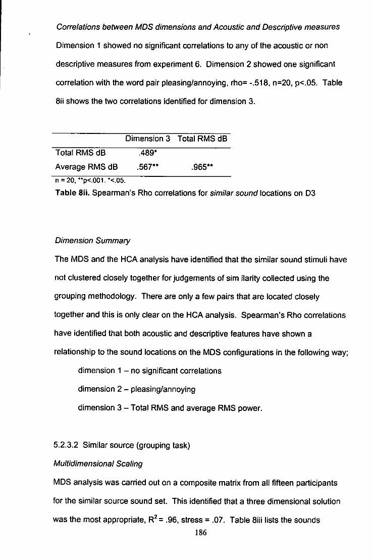
Correlations between MDS dimensions and Acoustic and Descriptive measures
Dimension 1 showed no significant correlations to any of the acoustic or non
descriptive measures from experiment 6. Dimension 2 showed one significant
correlation with the word pair pleasing/annoying, rho= -.518. n=20, p<.05. Table
8ii shows the two correlations identified for dimension 3.
Dimension 3 Total RMS dB
Total RMS dB .489*
Average RMS dB .567" .965**
n = 20. "p< .001 . *< .05 .
Table Sii. Spearman's Rho correlations for s/m/7ar sound locations on D3
Dimension Summary
The MDS and the HCA analysis have identified that the similar sound stimuli have
not clustered closely together for judgements of sim ilarity collected using the
grouping methodology. There are only a few pairs that are located closely
together and this is only clear on the HCA analysis. Spearman's Rho con-elations
have identified that both acoustic and descriptive features have shown a
relationship to the sound locations on the MDS configurations in the following way;
dimension 1 - no significant correlations
dimension 2 - pleasing/annoying
dimension 3 - Total RMS and average RMS power.
5.2.3.2 Similar source (grouping task)
(Multidimensional Scaling
MDS analysis was carried out on a composite matrix from all fifteen participants
for the similar source sound set. This identified that a three dimensional solution
was the most appropriate. R^= .96, stress = .07. Table Siii lists the sounds
186
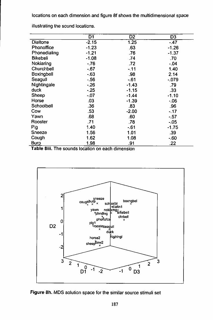
locations on each dimension and figure 8f shows the multidimensional space
illustrating the sound locations.
D1 D2 D3 Dialtone -2.15 1.25 -.47 Phonoffice -1.23 .63 -1.26 Phonedialing -1.21 .76 -1.37 Bikebeil -1.08 .74 .70 Nokiaring -.76 .72 -.04 Churchbell -.67 -.11 1.40 Boxingbell -.63 .98 2.14 Seagull -.56 -.61 -.079 Nightingale -.26 -1.43 .79 duck -.25 -1.15 .33 Sheep -.07 -1.44 -1.10 Horse .03 -1.39 -.06 Schoolbell .36 .83 .96 Cow .53 -2.00 -.17 Yawn .68 .60 -.57 Rooster .71 .78 -.05 Pig 1.40 -.61 -1.75 Sneeze 1.56 1.01 .39 Cough 1.62 1.08 -.60 Burp 1.98 .91 .22 Table Siii. The sounds location on each dimension
D2
sneeze coughburp
sch bolbl >dialtn1
nokibmg yawn '^hndlng
pho'Jjofc^ pig1
^ s t e s e a d u l l
boxngbel
biKebell chrbell
X
pightngl horse2
Figure 8h. MDS solution space for the similar source stimuli set
187
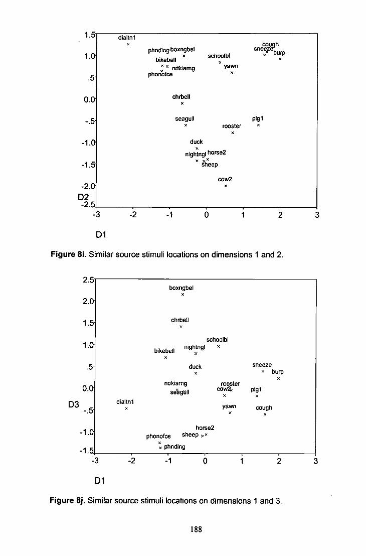
1.5
1.01
.5
0.01
-.5
•1.0
•1.5
-2.0 D2 -2.5
-3
D1
dialtnl X
phndlngboxngbel
bikebell ndkiamg
phonofce
chrtell X
seagull
schoolbl X
yawn X
duck
nightngi horse2 X
sheep
cow2 X
couph X burp
Pig1 rooster ^
X
Figure 81. Similar source stimuli locations on dimensions 1 and 2.
D3
2.5
2.0
1.5
1.0
.5
0.0
-.5
-1.01
-1.5
dialtnl X
boxngbel X
chrbell X
bikebell X
schoolbl nightngi ^
X
duck X
nokiamg sd^gtill
horse2 phonofce sheep
X phnding
sneeze X burp
X rooster
cow2< pig1 K X
yawn cough
1
D1
Figure 8j. Similar source stimuli locations on dimensions 1 and 3.
188
2.5
2.0
1.5
1.0
.5 D3
0.01
-.5
-1.01
-1.5
boxngbel
chrbell
nightngi
duck X
cow2
schoolbl
bikebell
sneeze buTT
nokiamg
dialtnl yawn cough x
horse2
sheep phonofcg
phnding
-2.5
D2
•2.0 1.5 1.0 .5 0.0 .5 1.0 1.5
Figure 8k. Similar source stimuli locations on dimensions 2 and 3.
The 3 dimensional configuration (figure 8h) shows the sounds have been clustered
loosely in their category groups. The 2 dimensional configurations show more
clearly how the sounds are placed on the different dimensions. For example on
figure 8i, the human noises cough, sneeze and burp are closely placed on
dimension 2 between .78 and 1.08. However the same figure shows that yawn is
placed further away on dimension 1
Hierarchical cluster analysis
A hierarchical cluster analysis, furthest neighbour method, was conducted on a
composite matrix from all 15 participants' data. This helped to illustrate any
clusters clearly but does not provide any information about the dimensions
identified by the MDS analysis.
189
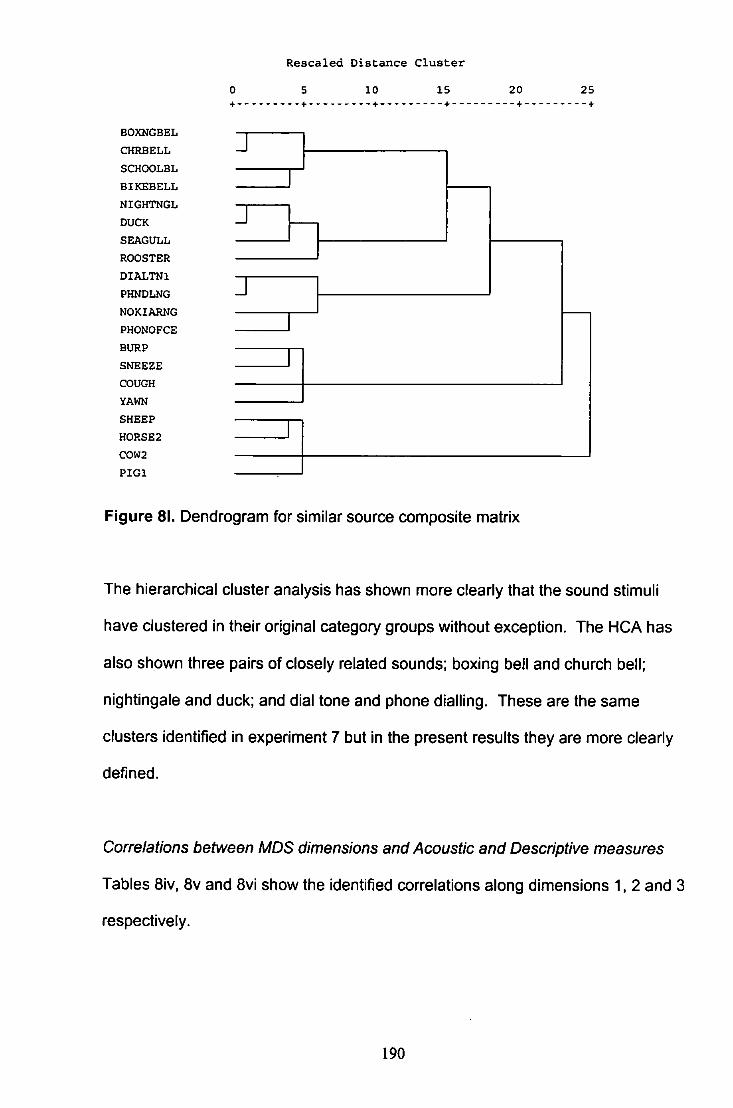
Reecaled D i s t a n c e C l u s t e r
5 10 15 20 25
BOXNGBEL CHRBELL SCHOOLBL BIKEBELL NIGHTNGL DUCK SEAGULL ROOSTER DIALTNl PHNDLNG NOKIARNG PHONOFCE BURP SNEEZE COUGH YAWN SHEEP H0RSE2 C0W2 P I G l
J
Figure 81, Dendrogram for similar source composite matrix
The hierarchical cluster analysis has shown more clearly that the sound stimuli
have clustered in their original category groups without exception. The HCA has
also shown three pairs of closely related sounds; boxing bell and church bell;
nightingale and duck; and dial tone and phone dialling. These are the same
clusters identified in experiment 7 but in the present results they are more clearly
defined.
Correlations between MDS dimensions and Acoustic and Descriptive measures
Tables 8iv, 8v and 8vi show the identified correlations along dimensions 1, 2 and 3
respectively.
190
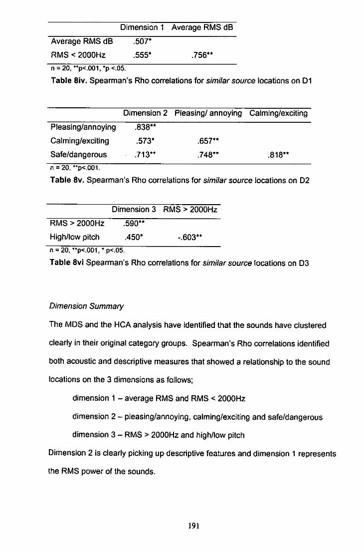
Dimension 1 Average RMS dB
Average RMS dB .507*
RMS < 2000Hz .555* .756**
n = 20. " p < . 0 0 1 , * p <.05.
Table 8iv. Spearman's Rho correlations for similar source locations on D1
Dimension 2 Pleasing/ annoying Calming/exciting
Pleasing/annoying .838**
Calming/exciting .573* .657**
Safe/dangerous .713** .748** .818**
n = 20. "p<.001.
Table 8v. Spearman's Rho correlations for s/m/7ar source locations on D2
Dimension 3 RMS > 2000Hz
RMS > 2000Hz . 590 "
High/low pitch .450* - .603"
n = 20. " p < . 0 0 1 . * p < . 0 5 .
Table 8vi Spearman's Rho correlations for similar source locations on D3
Dimension Summary
The MDS and the HCA analysis have identified that the sounds have clustered
clearly in their original category groups. Spearman's Rho correlations identified
both acoustic and descriptive measures that showed a relationship to the sound
locations on the 3 dimensions as follows;
dimension 1 - average RMS and RMS < 2000Hz
dimension 2 - pleasing/annoying, calming/exciting and safe/dangerous
dimension 3 - RMS > 2000H2 and high/low pitch
Dimension 2 is clearly picking up descriptive features and dimension 1 represents
the RMS power of the sounds.
191
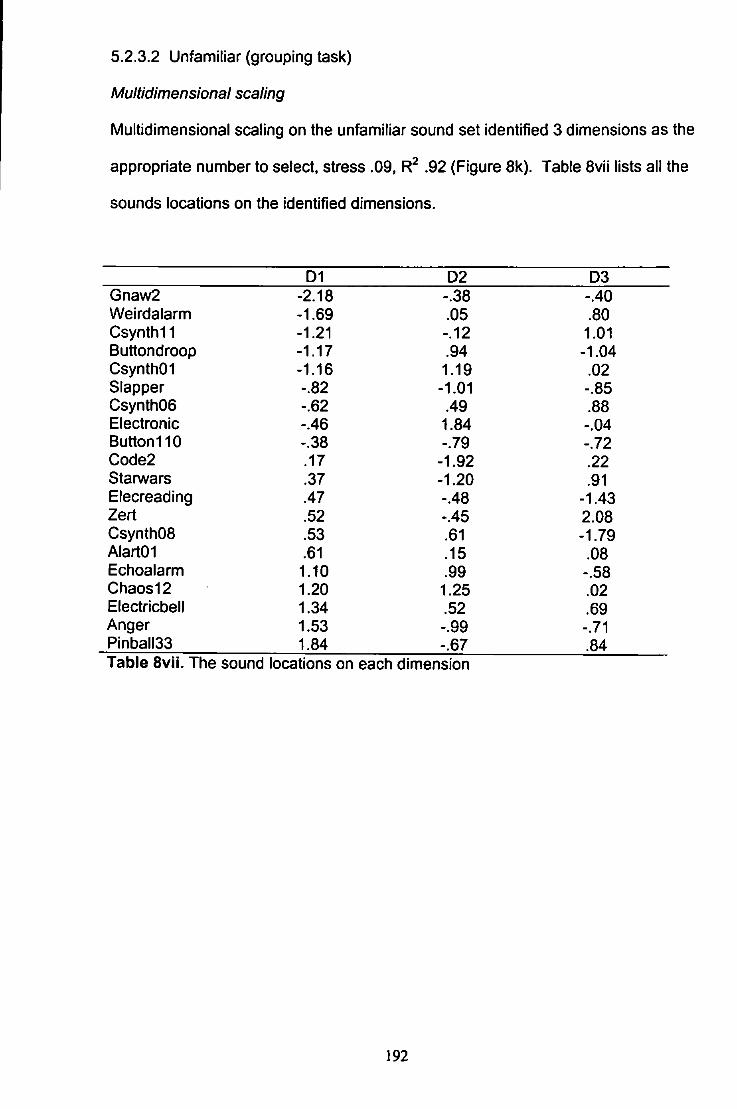
5.2.3.2 Unfamiliar (grouping task)
Multidimensional scaling
Multidimensional scaling on the unfamiliar sound set identified 3 dimensions as the
appropriate number to select, stress .09. R^ .92 (Figure 8k). Table 8vii lists all the
sounds locations on the identified dimensions.
D1 D2 D3 Gnaw2 -2.18 -.38 -.40 Weirdalarm -1.69 .05 .80 Csynthi 1 -1.21 -.12 1.01 Buttondroop -1.17 .94 -1.04 CsynthOI -1.16 1.19 .02 Slapper -.82 -1.01 -.85 CsynthOe -.62 .49 .88 Electronic -.46 1.84 -.04 Button110 -.38 -.79 -.72 Code2 .17 -1.92 .22 Starwars .37 -1.20 .91 Elecreading .47 -.48 -1.43 Zert .52 -.45 2.08 CsynthOS .53 .61 -1.79 AlartOI .61 .15 .08 Echoalarm 1.10 .99 -.58 Chaos12 1.20 1.25 .02 Electricbell 1.34 .52 .69 Anger 1.53 -.99 -.71 Pinball33 1.84 -.67 .84 Table 8vii, The sound locations on each dimension
192
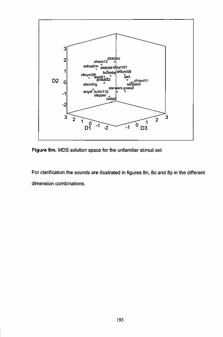
D2 0
elctrc nc chaos12 X
echoairm ejctrcbl ct syntOI
pinbali^ elecrdng
starwars angef buttnllQ
slapper code2
buhndrJchSyntoe
^ c h s y n t H wirdalnm
gnaw2
Figure 8m. MDS solution space for the unfamiliar stimuli set
For clarification the sounds are illustrated in figures 8n, 8o and 8p in the different
dimension combinations.
193
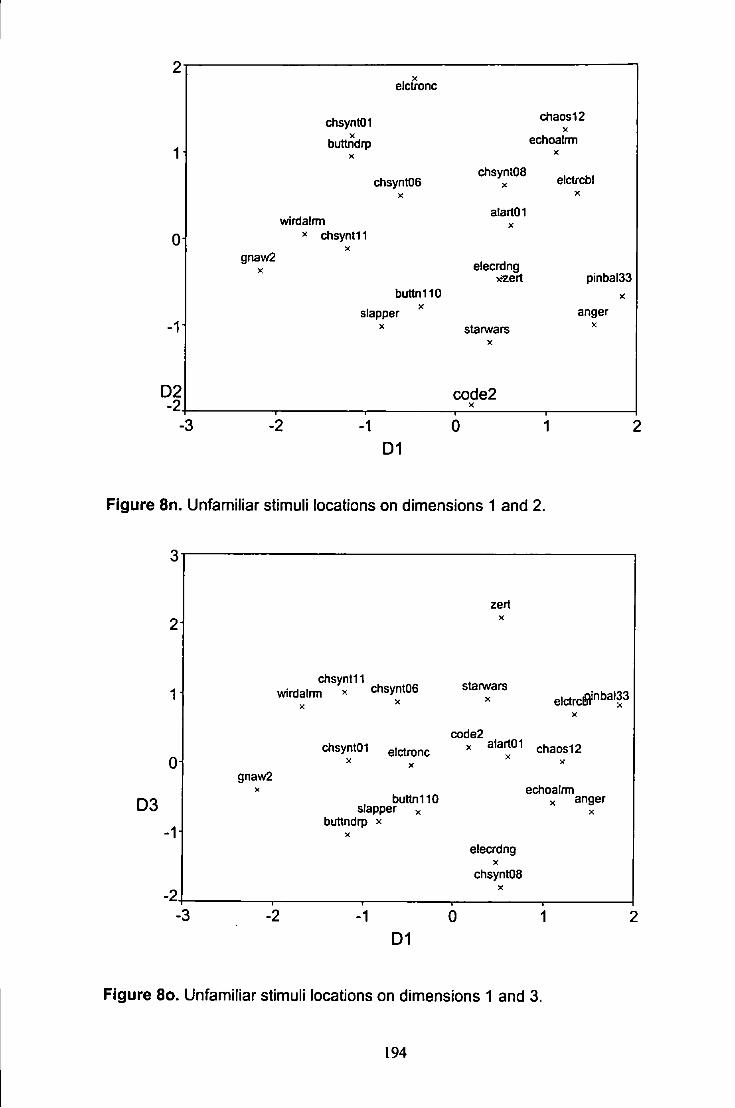
0
-1
D2 -2
X elctronc
chsyntOI chaos12 X
X buttndrp
X
echoalrm X
chsyntoe X
chsyntOS X elctrcbl
X
wirdalrm alartOI
X ^ chsynti 1
X gnaw2
X elecrdng xzert pinbal33
buttn110 X
slapper ^ anger X stanza rs
X
code2 X
X
-3 0 D1
Figure 8n. Unfamiliar stimuli locations on dimensions 1 and 2.
3
D3
-1
zert X
v . r d a J ' ' ' " * ^ ^ « e stanvars elctrcl5V"bal33
gnaw2
cUsyntOI elctronc
buttnllO slapper ^
buttndrp x X
code2 X alartOI chaos12
echoalmi ^ anger
X
elecrdng X
ChsyntOS
-3 -2 -1 0 D1
Figure 8 0 . Unfamiliar stimuli locations on dimensions 1 and 3.
194
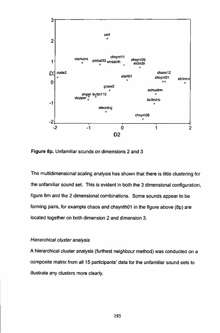
1
0
code2 X
zert
alartOI X
gnaw2 X
anger buttn110 slapper ^
chaos12 chsyntOI
X X elctronq
X
echoairm X
buttndrp X
elecrdng X
chsyntOS X
D2
Figure 8p. Unfamiliar sounds on dimensions 2 and 3
The multidimensional scaling analysis has shown that there is little clustering for
the unfamiliar sound set. This is evident in both the 3 dimensional configuration,
figure 8m and the 2 dimensional combinations. Some sounds appear to be
forming pairs, for example chaos and chsynthOI in the figure above (8p) are
located together on both dimension 2 and dimension 3.
Hierarchical cluster analysis
A hierarchical cluster analysis (furthest neighbour method) was conducted on a
composite matrix from all 15 participants' data for the unfamiliar sound sets to
illustrate any clusters more clearly.
195
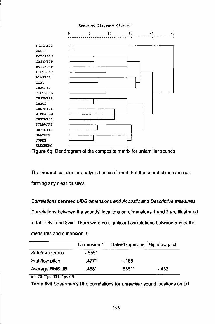
R e s c a l e d D i s t a n c e C l u s t e r
10 15 20 25 - +
PINBAL33 ANGER ECHOALRM CHSYNTOe BUTTNDRP ELCTRONC ALARTOl ZERT CHAOS12 ELCTRCBL CHSYNTll GNAW2 CHSYNTOl WIRDALRM CHSYNTOe STARWARS BUTTNllO SLAPPER C0DE2 ELECRDNG
J
Figure 8q. Dendrogram of the cx)mposite matrix for unfamiliar sounds.
The hierarchical cluster analysis has confirmed that the sound stimuli are not
forming any clear clusters.
Correlations betweer) MDS dimensions and Acoustic and Descriptive measures
Correlations between the sounds' locations on dimensions 1 and 2 are illustrated
in table 8vii and 8viii. There were no significant correlations between any of the
measures and dimension 3.
Dimension 1 Safe/dangerous High/low pitch
Safe/dangerous
High/low pitch
Average RMS dB
-.555*
.477*
.468*
-.188
.635** 432
n = 20. "p<.001,*p<.05.
Table Svii Spearman's Rho correlations for unfamiliar soun6 locations on D1
196
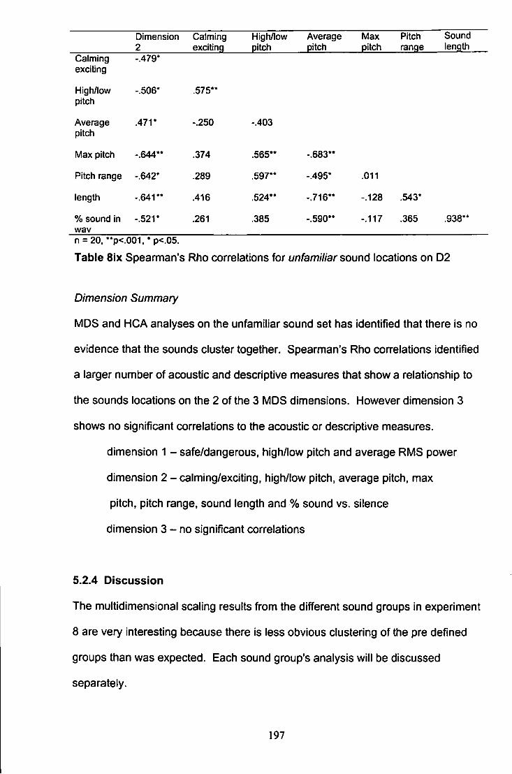
Dimension 2
Calming exciting
High/low pitch
Average pitch
Max pitch
Pitch range
Sound length
Calming exciting
-.479*
High/lov/ pitch
-.506* .575**
Average pitch
.471* -.250 -.403
Max pitch -.644** .374 .565** -.683**
Pitch range -.642* .289 .597** -.495* .011
length -.641** .416 .524** -.716** -.128 .543*
% sound in wav
-.521* .261 .385 -.590** -.117 .365 .938**
n = 20. **p<.001.*p<.05.
Table Six Spearman's Rho correlations for unfamiliar sound locations on D2
Dimension Summary
MDS and HCA analyses on the unfamiliar sound set has identified that there is no
evidence that the sounds cluster together. Spearman's Rho correlations identified
a larger number of acoustic and descriptive measures that show a relationship to
the sounds locations on the 2 of the 3 MDS dimensions. However dimension 3
shows no significant correlations to the acoustic or descriptive measures.
dimension 1 - safe/dangerous, high/low pitch and average RMS power
dimension 2 - calming/exciting, high/low pitch, average pitch, max
pitch, pitch range, sound length and % sound vs. silence
dimension 3 - no significant correlations
5.2.4 Discussion
The multidimensional scaling results from the different sound groups in experiment
8 are very interesting because there is less obvious clustering of the pre defined
groups than was expected. Each sound group's analysis will be discussed
separately.
197
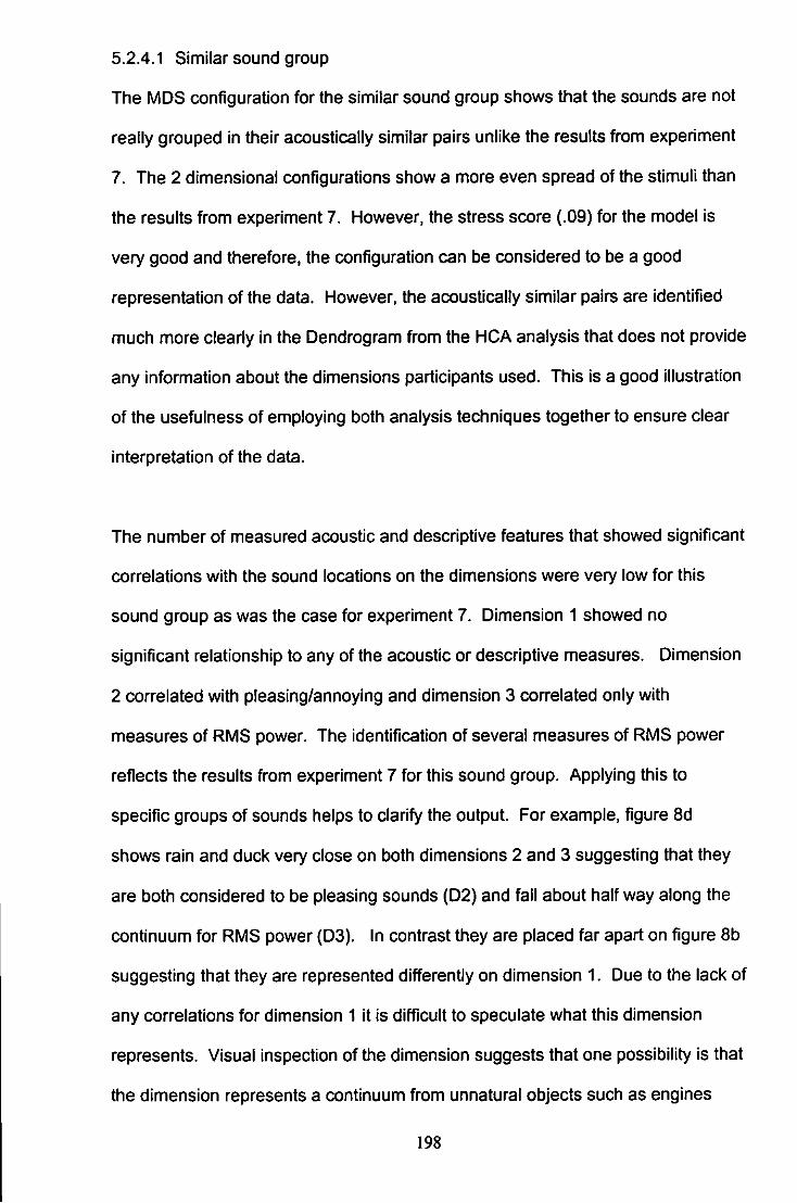
5.2.4.1 Similar sound group
The MDS configuration for the similar sound group shows that the sounds are not
really grouped in their acoustically similar pairs unlike the results from experiment
7. The 2 dimensional configurations show a more even spread of the stimuli than
the results from experiment 7. However, the stress score (.09) for the model is
very good and therefore, the configuration can be considered to be a good
representation of the data. However, the acoustically similar pairs are identified
much more clearly in the Dendrogram from the HCA analysis that does not provide
any information about the dimensions participants used. This is a good illustration
of the usefulness of employing both analysis techniques together to ensure clear
interpretation of the data.
The number of measured acoustic and descriptive features that showed significant
correlations with the sound locations on the dimensions were very low for this
sound group as was the case for experiment 7. Dimension 1 showed no
significant relationship to any of the acoustic or descriptive measures. Dimension
2 correlated with pleasing/annoying and dimension 3 correlated only with
measures of RMS power. The identification of several measures of RMS power
reflects the results from experiment 7 for this sound group. Applying this to
specific groups of sounds helps to clarify the output. For example, figure 8d
shows rain and duck very close on both dimensions 2 and 3 suggesting that they
are both considered to be pleasing sounds (D2) and fall about halfway along the
continuum for RMS power (D3). In contrast they are placed far apart on figure 8b
suggesting that they are represented differently on dimension 1. Due to the lack of
any correlations for dimension 1 it is difficult to speculate what this dimension
represents. Visual Inspection of the dimension suggests that one possibility is that
the dimension represents a continuum from unnatural objects such as engines
198
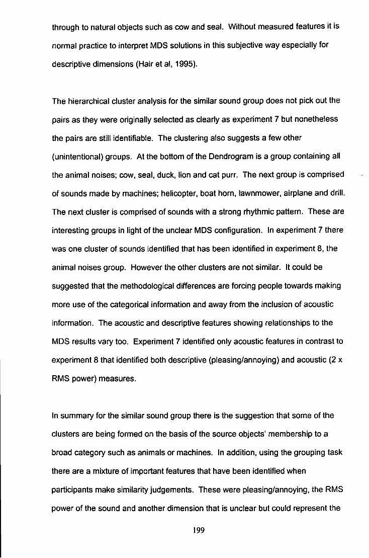
through to natural objects such as cow and seal. Without measured features it is
normal practice to interpret MDS solutions in this subjective way especially for
descnptive dimensions (Hair et al, 1995).
The hierarchical cluster analysis for the similar sound group does not pick out the
pairs as they were originally selected as clearly as experiment 7 but nonetheless
the pairs are still identifiable. The clustering also suggests a few other
(unintentional) groups. At the bottom of the Dendrogram is a group containing all
the animal noises; cow, seal, duck, lion and cat purr. The next group is comprised
of sounds made by machines; helicopter, boat horn, lawnmower. airplane and drill.
The next cluster is comprised of sounds with a strong rhythmic pattern. These are
interesting groups in light of the unclear MDS configuration. In experiment 7 there
was one cluster of sounds identified that has been identified in experiment 8, the
animal noises group. However the other clusters are not similar. It could be
suggested that the methodological differences are forcing people towards making
more use of the categorical information and away from the inclusion of acoustic
information. The acoustic and descriptive features showing relationships to the
MDS results vary too. Experiment 7 identified only acoustic features in contrast to
experiment 8 that identified both descriptive (pleasing/annoying) and acoustic (2 x
RMS power) measures.
In summary for the similar sound group there is the suggestion that some of the
clusters are being formed on the basis of the source objects' membership to a
broad category such as animals or machines. In addition, using the grouping task
there are a mixture of important features that have been identified when
participants make similarity judgements. These were pleasing/annoying, the RMS
power of the sound and another dimension that is unclear but could represent the
199
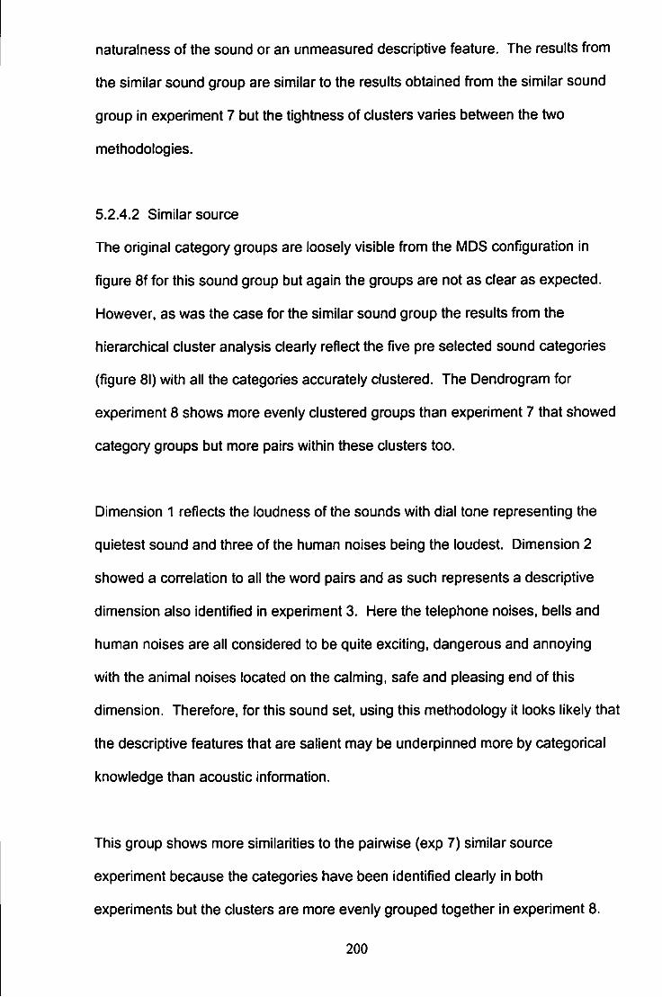
naturalness of the sound or an unmeasured descriptive feature. The results from
the similar sound group are similar to the results obtained from the similar sound
group in experiment 7 but the tightness of clusters varies between the two
methodologies.
5.2.4.2 Similar source
The original category groups are loosely visible from the MDS configuration in
figure 8f for this sound group but again the groups are not as clear as expected.
However, as was the case for the similar sound group the results ft-om the
hierarchical cluster analysis clearly reflect the five pre selected sound categories
(figure 81) with all the categories accurately clustered. The Dendrogram for
experiment 8 shows more evenly clustered groups than experiment 7 that showed
category groups but more pairs within these clusters too.
Dimension 1 reflects the loudness of the sounds with dial tone representing the
quietest sound and three of the human noises being the loudest. Dimension 2
showed a correlafion to all the word pairs and as such represents a descriptive
dimension also identified in experiment 3. Here the telephone noises, bells and
human noises are all considered to be quite exciting, dangerous and annoying
with the animal noises located on the calming, safe and pleasing end of this
dimension. Therefore, for this sound set, using this methodology it looks likely that
the descriptive features that are salient may be underpinned more by categorical
knowledge than acoustic information.
This group shows more similarities to the painwise (exp 7) similar source
experiment because the categories have been identified cleariy in both
experiments but the clusters are more evenly grouped together in experiment 8.
200
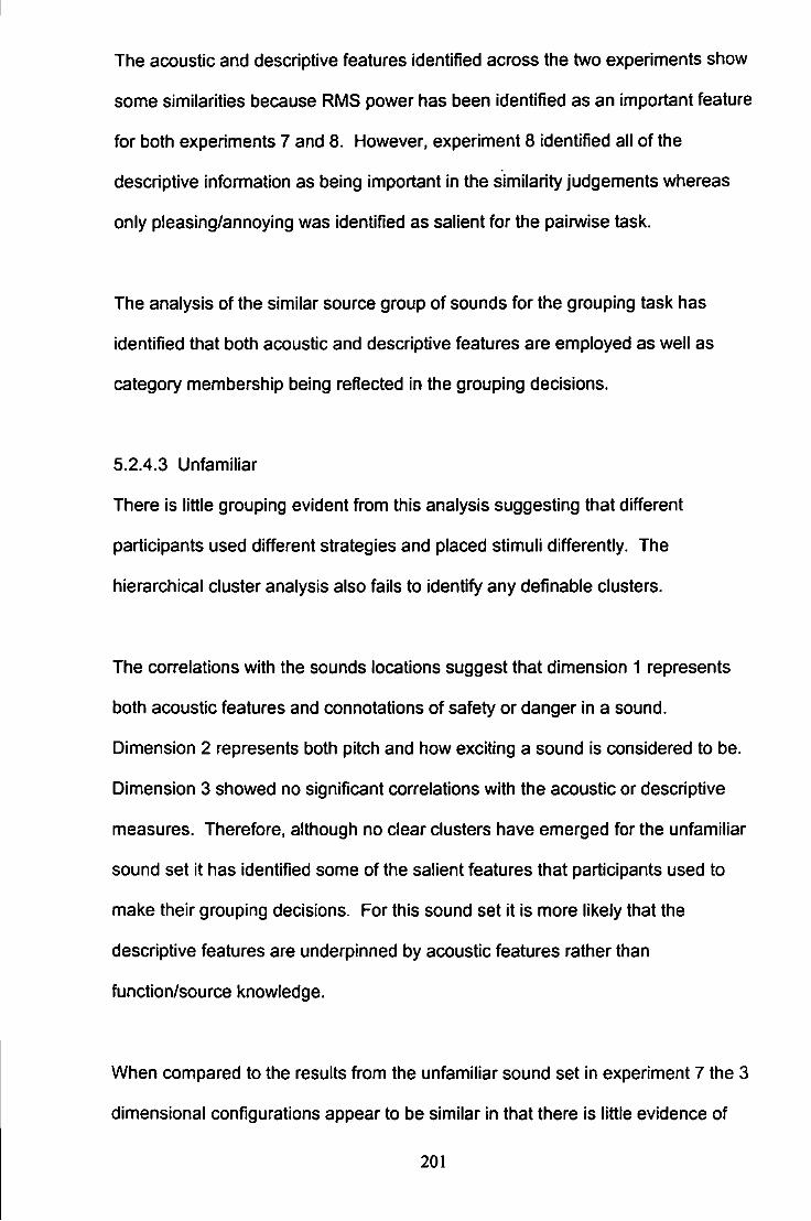
The acoustic and descriptive features identified across the two experiments show
some similarities because RMS power has been identified as an important feature
for both experiments 7 and 8. However, experiment 8 identified all of the
descriptive infomiation as being important in the similarity judgements whereas
only pleasing/annoying was identified as salient for the pairwise task.
The analysis of the similar source group of sounds for the grouping task has
Identified that both acoustic and descriptive features are employed as well as
category membership being reflected In the grouping decisions.
5.2.4.3 Unfamiliar
There is little grouping evident from this analysis suggesting that different
participants used different strategies and placed stimuli differently. The
hierarchical cluster analysis also fails to identify any definable clusters.
The correlations with the sounds locations suggest that dimension 1 represents
both acoustic features and connotations of safety or danger in a sound.
Dimension 2 represents both pitch and how exciting a sound Is considered to be.
Dimension 3 showed no significant correlations with the acoustic or descriptive
measures. Therefore, although no clear clusters have emerged for the unfamiliar
sound set It has identified some of the salient features that participants used to
make their grouping decisions. For this sound set it is more likely that the
descriptive features are underpinned by acoustic features rather than
function/source knowledge.
When compared to the results from the unfamiliar sound set in experiment 7 the 3
dimensional configurations appear to be similar in that there is little evidence of
201
any clustering. This is reflected in both of the HCA analyses for the unfamiliar
sound groups too although the pairwise task does have a slightly tighter
configuration. With respect to the salient features identified for both experiment 7
and 8 the unfamiliar sound set has elicited the largest number of measured
features with both acoustic and descriptive features showing statistically significant
relationships to the sound locations on the MDS output. The features identified as
salient are largely the same across experiment 7 and 8 with the exception of the
identification of RMS power measures in experiment 7 that are not identified in
experiment 8.
5.4.2.4 Summary
In summary, the results from experiment 8 that employed the grouping task
methodology for the 3 sound sets have identified differences in the way the stimuli
are clustered together. The painwise task (exp 7) identified close clusters that
reflected the original acoustically similar pairs (similar sound group) or the
category groups (similar source group). The grouping task identified much looser
pairs for the similar sound group than the painvise task. However, both the
grouping and the pairwise task showed an unexpected tendency to group the
similar sound group stimuli by category. This was more apparent in the grouping
task but there was evidence of an animal category in the pairwise task. The
similar source groups showed quite similar clusters across the two methodologies.
Both of the unfamiliar groups showed no evidence of clear clusters.
The different methodologies also showed differences in the acoustic and
descriptive features that were identified as salient in participants' judgements of
similarity. There is strong evidence that participants are using acoustic features
for both the pairwise task and the grouping task, especially measures of RMS
202
power. Whilst descriptive measures were found to show significant relationships
these were more variable across methodologies and sound groups. The similar
source group could be said to show the most similar pattern of clusters across the
two methodologies but this may be a result of the sounds used. It is also easiest
to see if these groups are represented in the output from MDS and HCA analyses.
This group did however demonstrate the most similarity on descriptive measures
identifying only pleasing/annoying for both experiments 7 and 8. Table 92 later in
this chapter summarises all the main findings from each of the sound groups in
experiments 7. 8 and 9 for clarity.
5.4.2.5 Comparison of the two methodologies
The results have now provided the opportunity to compare the two methodologies
on three identical sound sets. These comparisons can also be compared to the
results Bonebright (1996) obtained using two different stimuli sets; auditory graphs
and actors' portrayals of vocal affect on both the painwise and the grouping
methodologies. The present results identified a difference in the closeness of the
groups identified by the MDS analysis. Bonebright (1996) also discusses this
difference for the auditory graph results showing that the clusters were more tightly
grouped than the grouping task. This is reflected in the analysis for the three
sound groups used in experiments 7 and 8 and cleariy illustrated by the
Dendrograms from the HCA analysis. The other main finding from Bonebrights'
results that are reflected here is that despite small differences in the tightness of
the clusters or the speciflc features identifled as salient the two methodologies
provide results that are comparable.
Experiment 9 aimed to replicate experiment 8 with the collection of some
additional information. To complete the comparison between the two 203

methodologies Mantel tests that compare the similarity of the raw similarity
matrices are used to provide quantifiable comparisons.
204
5.3 Experiment 9 grouping task for three sound sets with extra
data collection
5.3.1 Introduction
Experiment 8 indicated differences in the way the sound groups were sorted by
participants and features that participants were using to make their grouping
decisions and highlighted category membership as a possible further feature but it
was felt that a more direct approach could be fruitful. Therefore, experiment 9 was
a replication of experiment 8 but requested some additional infonnation from the
participants to avoid making assumptions about why they were forming groups the
way they did.
Repeating the experiment also provided the opportunity to compare the matrices
obtained from experiments 8 and 9 for each sound set to assess the reliability of
the grouping methodology as well as a further comparison of the matrices across
the pairwise and grouping methodologies (experiments 7, 8 & 9) for all sound sets.
This would address whether the grouping task was reliable across experimental
sessions and also addresses the extent to which the matrices, reflecting the
similarity ratings, differed between the two methodologies. It would be expected
from the work conducted by Bonebright (1996) that there would be differences
between the tightness of the clusters observed between the two task types and
that the nature of the salient features may vary. Bonebright (1996) identified
tighter clusters for the pairwise methodology. In addition the results from
experiment 9 are expected to closely reflect the results obtained in experiment 8.
205
5.3.2 Method
5.3.2.1 Participants
45 participants (6 male, 39 female) took part in the study. There were 15 different
participants per sound group. All the participants had nomial or con-ected-to-
normal hearing as measured by self report. Participants were psychology
undergraduates at the University of Plymouth and were awarded course credit for
their participation as part of the BSc psychology course requirement.
5.3.2.2 Apparatus
The sound stimuli were presented using a purpose written grouping program
(Aldrich, November, 2003). Six computers with headphones were used (Hewlett
Packard Vectra's Pill with a 600 MHz Processor. 128 MB RAM and
CrystalSoundFusion™ Soundcard operating on Windows XP).
5.3.2.3 Stimuli
The 60 sound stimuli used are exactly the same sounds and groups that were
used in experiment series 7 and 8 as identified in appendix C. Similar sound, a
group of 20 sounds (not all abstract) made up of ten pairs of sounds that sound
similar but come from different sources e.g. food frying and rain falling. Similar
source, a group of 20 sounds comprised of five sets of four sounds that come from
similar sources but do not necessarily sound the same, e.g. burp, cough, sneeze
and yawn are all human noises. The sets included were human noises, bells,
birds, farm animals and telephones. Finally Unfamiliar, this group was comprised
of 20 unfamiliar sounds that were all abstract In nature. The acoustic and
psychological measures remained exactly as experiments 7 and 8.
206
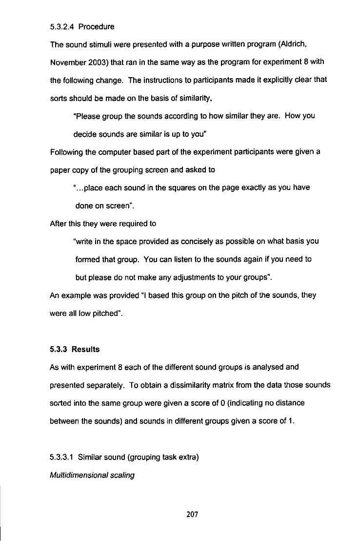
5.3.2.4 Procedure
The sound stimuli were presented with a purpose written program (Aldrich,
November 2003) that ran in the same way as the program for experiment 8 with
the following change. The instructions to participants made it explicitly clear that
sorts should be made on the basis of similarity.
"Please group the sounds according to how similar they are. How you
decide sounds are similar is up to you''
Following the computer based part of the experiment participants were given a
paper copy of the grouping screen and asked to
"...place each sound in the squares on the page exactly as you have
done on screen".
After this they were required to
"write in the space provided as concisely as possible on what basis you
formed that group. You can listen to the sounds again if you need to
but please do not make any adjustments to your groups".
An example was provided "I based this group on the pitch of the sounds, they
were all low pitched".
5.3.3 Results
As with experiment 8 each of the different sound groups is analysed and
presented separately. To obtain a dissimilarity matrix from the data those sounds
sorted into the same group were given a score of 0 (indicating no distance
between the sounds) and sounds in different groups given a score of 1.
5.3.3,1 Similar sound (grouping task extra)
Multidimensional scaling
207
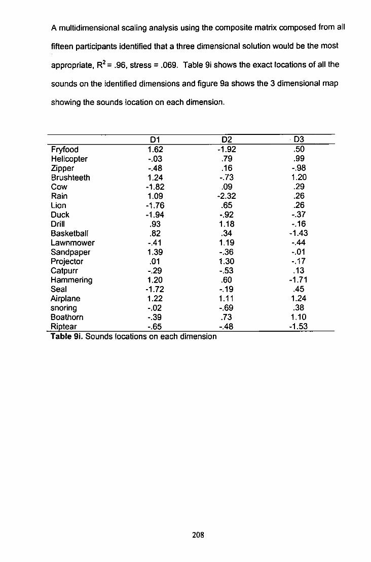
A multidimensional scaling analysis using the composite matrix composed from all
fifteen participants identified that a three dimensional solution would be the most
appropriate, = .96. stress = .069. Table 9i shows the exact locations of all the
sounds on the identified dimensions and figure 9a shows the 3 dimensional map
showing the sounds location on each dimension.
D1 D2 D3 Fryfood 1.62 -1.92 .50 Helicopter -.03 .79 .99 Zipper -.48 .16 -.98 Brushteeth 1.24 -.73 1.20 Cow -1.82 .09 .29 Rain 1.09 -2.32 .26 Lion -1.76 .65 .26 Duck -1.94 -.92 -.37 Drill .93 1.18 -.16 Basketball .82 .34 -1.43 Lawnmower -.41 1.19 -.44 Sandpaper 1.39 -.36 -.01 Projector .01 1.30 -.17 Catpurr -.29 -.53 .13 Hammering 1.20 .60 -1.71 Seal -1.72 -.19 .45 Airplane 1.22 1.11 1.24 snoring -.02 -.69 .38 Boathorn -.39 .73 1.10 Riptear -.65 -.48 -1.53 Table 9i. Sounds locations on each dimension
208
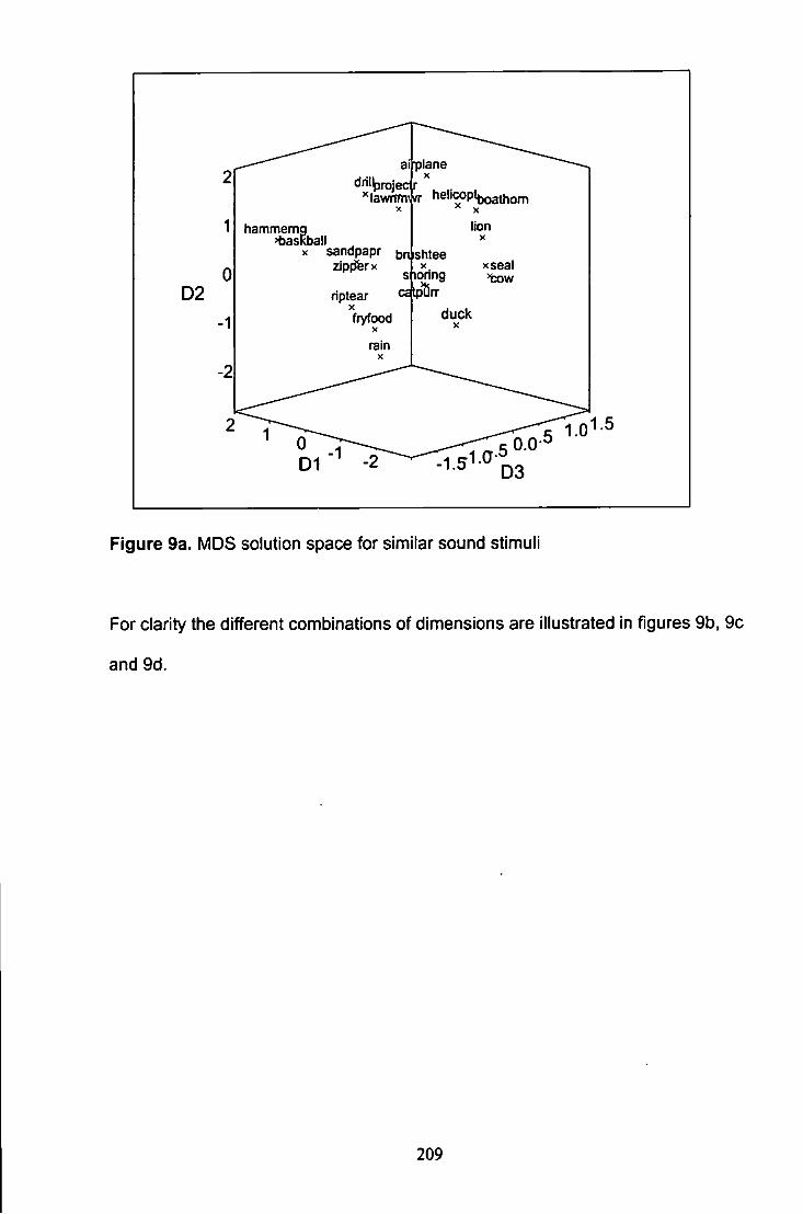
0 2
fplane driltrojedr
'lawrtmv
hammemg >basRball
X sandpapr zipfjferx
riptear
k heliwptboathom
lion
brOshtee X . xseal
sponng Irr
fryfood
Figure 9a. MDS solution space for simitar sound stimuli
For clarity the different combinations of dimensions are illustrated in figures 9b, 9c
and 9d.
209
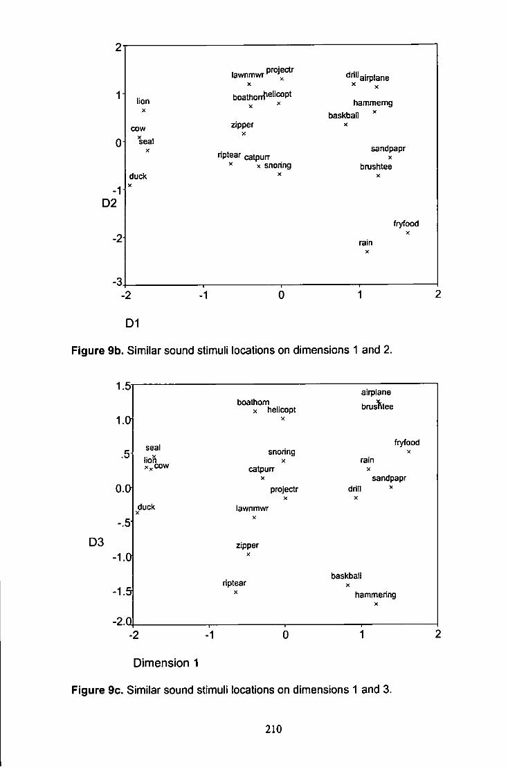
1
0
D2
lion
cow "seal
duck X
lawnmwr projectr
boathorr^elicopt
zipper X
riptear catpurr ^ X snoring
t 'lairplane
hammemg baskball
sandpapr X
brushtee
fryfood
ram X
-2 -1
D1
Figure 9b. Similar sound stimuli locations on dimensions 1 and 2.
D3
1.5
1.01
.5
O.CM
-.5
-1.0
•1.5
-2.Q
seal lioi
cow
duck
-2
boathom X helicopt
X
snonng
catpuR-
projectr X
lawnmwr X
zipper X
riptear X
-1
airplane bnjstitee
fryfood
ram X
sandpapr drill
X
baskball
hammering X
Dimension 1
Figure 9c. Similar sound stimuli locations on dimensions 1 and 3.
210
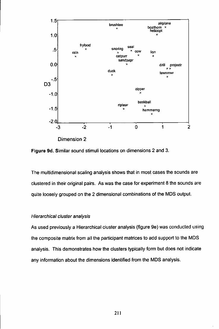
D3
1.5
1.01
.5
0.01
.5
-1.0
-1,5
-2.0
fryfood
ratn X
brushtee X
snoring ^ ^ cow
catpun-sandpapr
duck X
airplane boathom >
heHcopt
lion
drill projectr X X
lawnmwr
zipper X
baskball riptear x
^ hammemg
- 3 - 2 - 1 0 1 2
Dimension 2
Figure 9d. Similar sound stimuli locations on dimensions 2 and 3.
The multidimensional scaling analysis shows that In most cases the sounds are
clustered in their original pairs. As was the case for experiment 8 the sounds are
quite loosely grouped on the 2 dimensional combinations of the MDS output.
Hierarchical cluster analysis
As used previously a Hierarchical cluster analysis (figure 9e) was conducted using
the composite matrix from all the participant matrices to add support to the MDS
analysis. This demonstrates how the clusters typically form but does not indicate
any information about the dimensions identified from the MDS analysis.
211
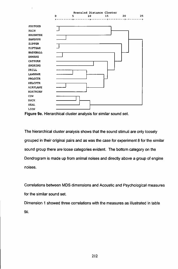
R e s c a l e d D i s t a n c e C l u s t e r 5 10 15 20 25
FRYFOOD RAIN BRUSHTEE SANDPPR ZIPPER RIPTEAR BASKBALL HMMRNG CATPURR SNORING DRILL LAWNMWR PROJCTR HELCPTR AIRPLANE BOATHORN COW DUCK SEAL LION
J
J
Figure 9e, Hierarchical cluster analysis for similar sound set.
The hierarchical cluster analysis shows that the sound stimuli are only loosely
grouped in their original pairs and as was the case for experiment 8 for the similar
sound group there are loose categories evident. The bottom category on the
Dendrogram is made up from animal noises and directly above a group of engine
noises.
Correlations between MDS dimensions and Acoustic and Psychological measures
for the similar sound set.
Dimension 1 showed three correlations with the measures as illustrated in table
gii.
212
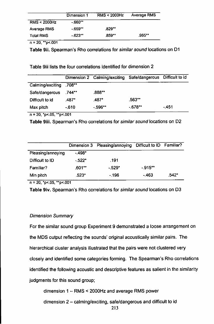
Dimension 1 RMS < 2000Hz Average RMS
RMS < 2000Hz -.660"
Average RMS -.659" .829"
Total RMS - .623" .859" .965"
n = 20. "p<.001
Table 9ii. Spearman's Rho cx)rrelations for similar sound locations on D1
Table 9iii lists the four correlations identified for dimension 2
Dimension 2 Calming/exciting Safe/dangerous Difficult to Id
Calming/exciting .708**
Safe/dangerous . 7 4 4 " .888**
Difficult to id .487* .487* .563**
Max pitch -.610 -.596** -.678** -.451
n = 20. *p<.05. **p<.001
Table 9iii. Spearman's Rho correlations for similar soured locations on 02
Dimension 3 Pleasing/annoying Difficult to ID Familiar?
Pleasing/annoying -.498*
Difficult to ID -.522* .191
Familiar? .601 ** -.529* - .915**
Min pitch .523* -. 196 -.463 .542*
n = 20, *p<-05, **p<.001
Table 9iv. Spearman's Rho correlations for s/m//ar sound locations on 03
Dimension Summary
For the similar sound group Experiment 9 demonstrated a loose arrangement on
the MDS output reflecting the sounds' original acoustically similar pairs. The
hierarchical cluster analysis illustrated that the pairs were not clustered very
closely and identified some categories forming. The Speamian's Rho correlations
identified the following acoustic and descriptive features as salient in the similarity
judgments for this sound group;
dimension 1 - RMS < 2000Hz and average RMS power
dimension 2 - calming/exciting, safe/dangerous and difficult to id 213
dimension 3 - pleasing/annoying, familiar and difficult to id.
In cx)mparison to experiments 7 and 8 experiment 9 also Identified a clear RMS
power dimension. Pleasing/annoying was also a feature identified in experiment 8
but in contrast no word pair measures were identified on experiment 7 for the
similar sound group. Both experiments 8 and 9 have also shown evidence of an
animal and machine category group.
Participant explanations for their grouping ctioices
All the additional responses given by participants were coded by two separate
mariners who were not aware of the nature of the task. All the participant
explanations and the codes provided by the markers can be seen in Appendix D1.
Three categories were used; acoustic, categorical or descriptive (of the sound).
An example from each category is used as an illustration. For the similar sound
group participant 3 "pitch, both low" is an example of an acoustic explanation. A
categorical example from participant 8 "animal noises" and a descriptive example
from participant 2 "banging sounds". Where more than one code cleariy applied
both were used. For example, for the sounds zipper and riptear the response
"both to do with clothing, zipping, ripping" was coded as both descriptive (zipping,
ripping) and categorical (to do with clothes). Inter rater reliability was checked
using Cohen's Kappa statistic and considered acceptable if the Kappa statistic
was above .70 (Howell, 1992). For the similar sound group the Kappa statistic
was .92 and therefore reliability between the markers was good.
The average number of groups used by participants in this sound set was M = 7.6,
SD = 1.45. For the similar sound group 19% of responses were rated as acoustic,
55% as categorical and 25% as descriptive (only ratings where mariners agreed
214
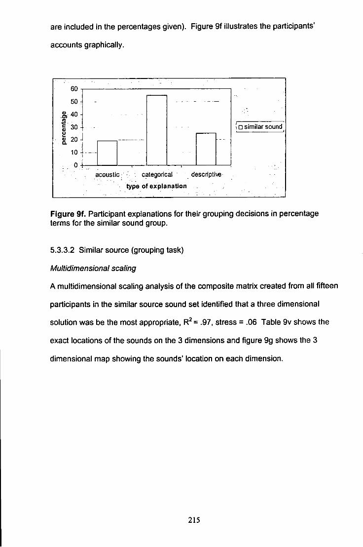
are included in the percentages given). Figure 9f illustrates the participants'
accounts graphically.
60
50
g, 40
I 20
10
0
• similar sound
acoustic; categorical descriptive
type of explanation
Figure 9f. Participant explanations for their grouping decisions in percentage terms for the similar sound group.
5.3.3.2 Similar source (grouping task)
Multidimensional scaling
A multidimensional scaling analysis of the composite matrix created from all fifteen
participants in the similar source sound set identified that a three dimensional
solution was be the most appropriate. R^= .97, stress = .06 Table 9v shows the
exact locations of the sounds on the 3 dimensions and figure 9g shows the 3
dimensional map showing the sounds' location on each dimension.
215
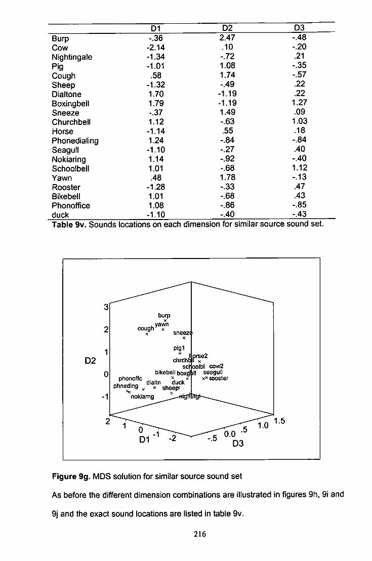
D1 D2 D3 Burp -.36 2.47 -.48 Cow -2.14 .10 -.20 Nightingale -1.34 -.72 .21 Pig -1.01 1.08 -.35 Cough .58 1.74 -.57 Sheep -1.32 -.49 .22 Dialtone 1.70 -1.19 .22 Boxingbell 1.79 -1.19 1.27 Sneeze -.37 1.49 .09 Churchbeil 1.12 -.63 1.03 Horse -1.14 .55 .18 Phonedialing 1.24 -.84 -.84 Seagull -1.10 -.27 .40 Nokiaring 1.14 -.92 -.40 Schoolbell 1.01 -.68 1.12 Yawn .48 1.78 -.13 Rooster -1.28 -.33 .47 Bikebell 1.01 -.68 .43 Phonoffice 1.08 -.86 -.85 duck -1.10 -.40 -.43 Table 9v, Sounds locations on each dimension for similar source sound set.
D2
burp .yawn
cough X X sneeze
X
blkebeil boxgtn phonoffc „ 1 ,
« h « ^ H i r , « dialtn duck phneding ^ x sheep^
nokiamg
pig1
scHoolbl cow2 seagull
x^ looster
D l " ' * -2
Figure 9g. MDS solution for similar source sound set
As before the different dimension combinations are illustrated in figures 9h, 9i and
9j and the exact sound locations are listed in table 9v.
216
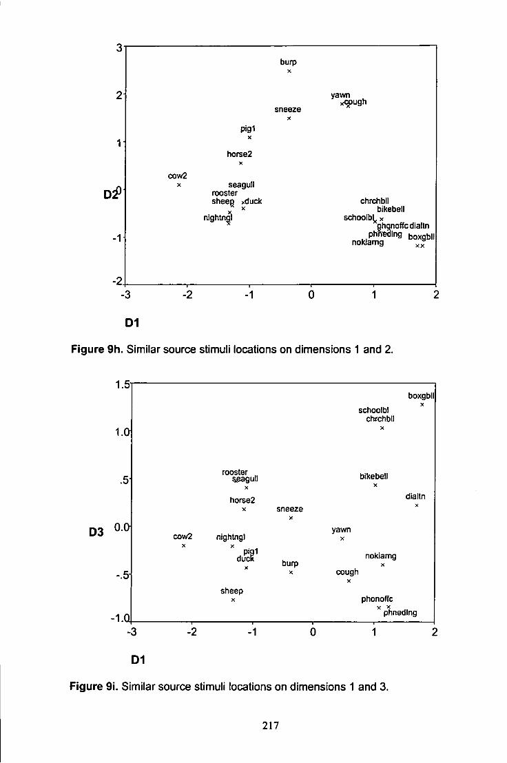
1
-2
burp X
sneeze j<
yawn x<5)ugh
pigi
horse2 X
cow2 X seagull
rooster sheeg xduck
nightn^
chrchbl) bikebell
schoolb^^ X phonoffcdialtn
phfi-eding boxgbll nokiamg
•3
D1
-1
Figure 9h. Similar source stimuli locations on dimensions 1 and 2.
1.5i
D3
.5
0.0\
-.5
1.Q
schoolbl chrchbll
X
boxgbll X
rooster gpagull
j(
bikebell X
horse2 X sneeze
X
diattn X
cow2 X
nightng)
duci X
burp X
yawn X
nokiamg X
cough
sheep X phonoffc
X X
phneding
-3 - 2 - 1 0 1
D1
Figure 9i. Similar source stimuli locations on dimensions 1 and 3.
217
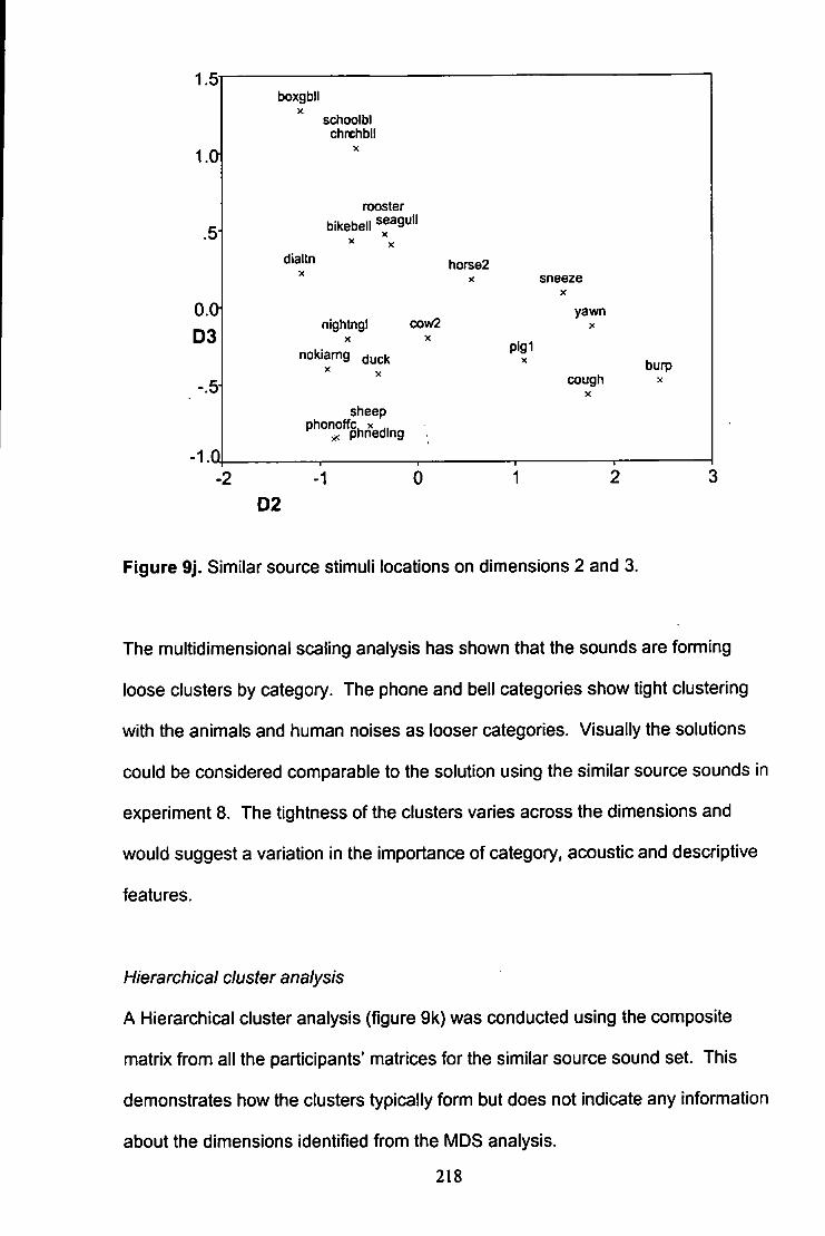
1.5
1.0
.5
O.Oj D3
-.5
-I.Q
boxgbll
schoolbl chrchbll
bikebell rooster
seagull
dialtn horse2 X sneeze
X
nightngl cow2
nokiamg jy k
sheep P^°"°%^edlng
Pig1
yawn
cough X
burp X
•2 -1 D2
0
Figure 9j. Similar source stimuli locations on dimensions 2 and 3.
The multidimensional scaling analysis has shown that the sounds are forming
loose clusters by category. The phone and bell categories show tight clustering
with the animals and human noises as looser categories. Visually the solutions
could be considered comparable to the solution using the similar source sounds in
experiment 8. The tightness of the clusters varies across the dimensions and
would suggest a variation in the importance of category, acoustic and descriptive
features.
Hierarchical cluster analysis
A Hierarchical cluster analysis (figure 9k) was conducted using the composite
matrix from all the participants' matrices for the similar source sound set. This
demonstrates how the clusters typically form but does not indicate any information
about the dimensions identified from the MDS analysis.
218
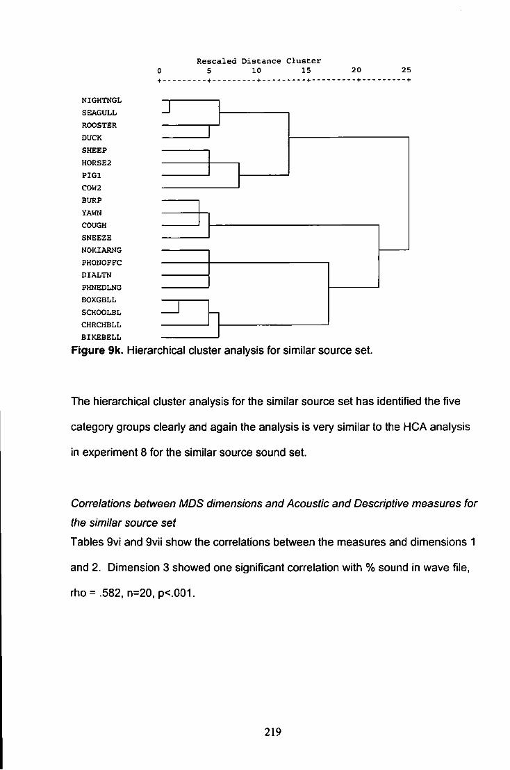
R e s c a l e d D i s t a n c e C l u s t e r 5 10 15 20 25
NIGHTNGL SEAGULL ROOSTER DUCK SHEEP H0RSE2 P I G l C0W2 BURP YAWN COUGH SNEEZE NOKIARNG PHONOFFC DIALTN PHNEDLNG BOXGBLL SCHOOLBL CHRCHBLL BIKEBELL
Figure 9k, Hierarchical cluster analysis for similar source set.
The hierarchical cluster analysis for the similar source set has identified the five
category groups clearly and again the analysis is very similar to the HCA analysis
in experiment 8 for the similar source sound set.
Correlations between MDS dimensions and Acoustic and Descriptive measures for
the similar source set
Tables Svi and 9vii show the correlations between the measures and dimensions 1
and 2. Dimension 3 showed one significant correlation with % sound in wave file,
rho= .582, n=20, p<.001.
219
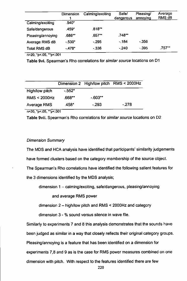
Dimension 1
Calming/exciting Safe/ dangerous
Pleasing/ annoying
Average RMS dB
Calming/exciting .540*
Safe/dangerous .459* .818**
Pleasing/annoying .686** .657** .748**
Average RMS dB -.530* -.295 -.184 -.356
Total RMS dB -.478' -.336 -.240 -.395 .757"
n=20. *p<.05. "p<.001
Table 9vi. Spearman's Rho correlations for similar source locations on D1
Dimension 2 High/low pitch RMS < 2000Hz
High/low pitch -.552*
RMS < 2000Hz .668" -.603**
Average RMS .458* -.293 -.278
n=20. *p<.05, •*p<.001
Table 9vii. Spearman's Rho con-elations for s/m//ar source locations on D2
Dimension Summary
The MDS and HCA analysis have identified that participants' similarity judgements
have formed clusters based on the category membership of the source object.
The Spearman's Rho congelations have identified the following salient features for
the 3 dimensions identified by the MDS analysis;
dimension 1 - calming/exciting, safe/dangerous, pleasing/annoying
and average RMS power
dimension 2 - high/low pitch and RMS < 2000Hz and category
dimension 3 - % sound versus silence in wave file.
Similarly to experiments 7 and 8 this analysis demonstrates that the sounds have
been judged as similar in a way that closely reflects their original category groups.
Pleasing/annoying is a feature that has been identified on a dimension for
experiments 7,8 and 9 as is the case for RMS power measures combined on one
dimension with pitch. With respect to the features identified there are few 220
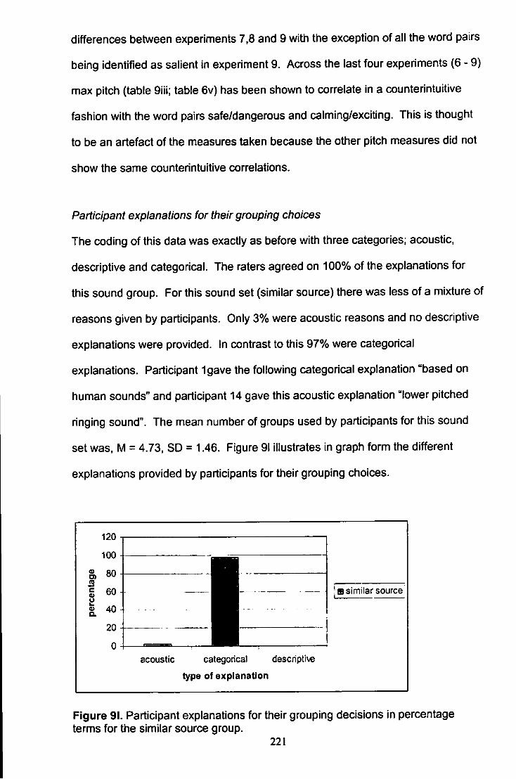
differences between experiments 7.8 and 9 with the exception of all the word pairs
being identified as salient in experiment 9. Across the last four experiments (6 - 9)
max pitch (table 9iii; table 6v) has been shown to correlate in a counterintuitive
fashion with the word pairs safe/dangerous and calming/exciting. This is thought
to be an artefact of the measures taken because the other pitch measures did not
show the same counterintuitive con-elations.
Participant explanations for their grouping choices
The coding of this data was exactly as before with three categories; acoustic,
descriptive and categorical. The raters agreed on 100% of the explanations for
this sound group. For this sound set (similar source) there was less of a mixture of
reasons given by participants. Only 3% were acoustic reasons and no descriptive
explanations were provided. In contrast to this 97% were categorical
explanations. Participant 1gave the following categorical explanation "based on
human sounds" and participant 14 gave this acoustic explanation "lower pitched
ringing sound". The mean number of groups used by participants for this sound
set was. M = 4.73, SD = 1,46, Figure 91 illustrates in graph form the different
explanations provided by participants for their grouping choices.
s similar source
acoustic categorical descriptive
type of explanation
Figure 91. Participant explanations for their grouping decisions in percentage terms for the similar source group.
221
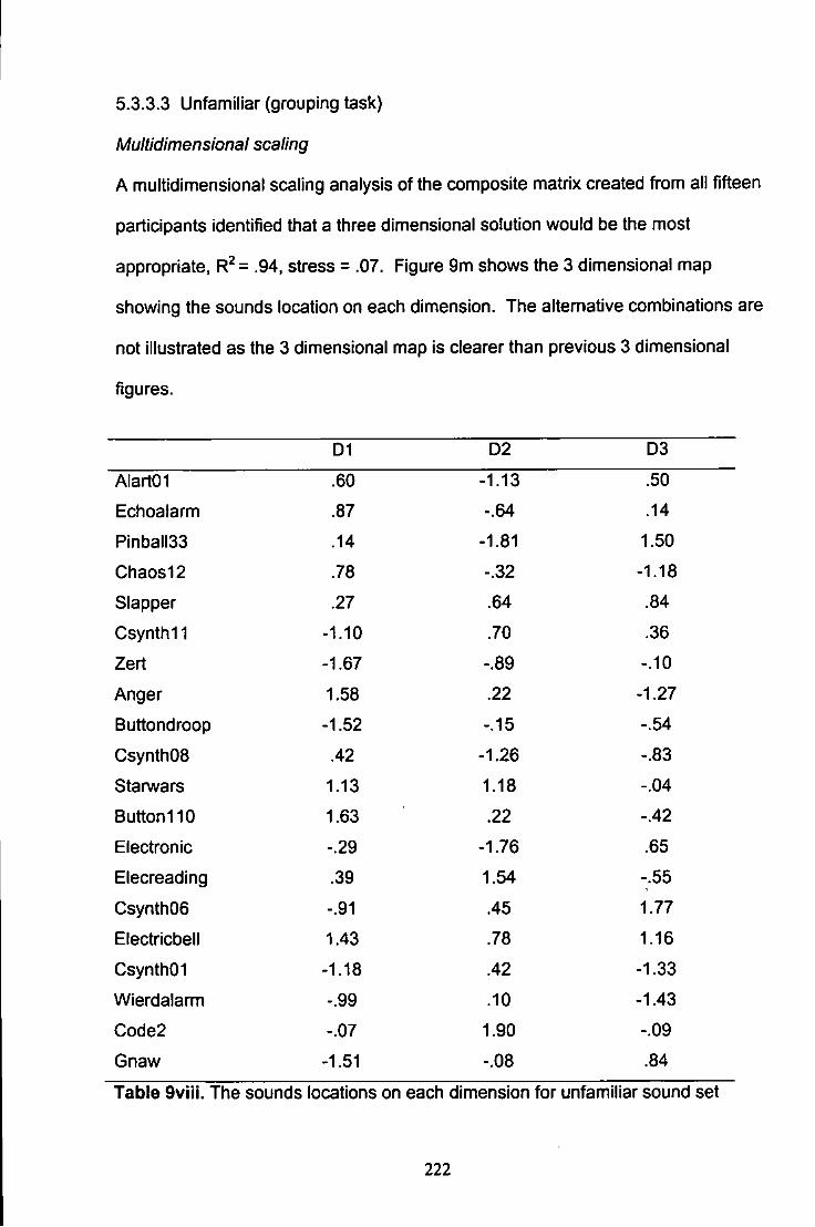
5.3.3.3 Unfamiliar (grouping task)
Multidimensional scaling
A multidimensional scaling analysis of the composite matrix created from all fifteen
participants identified that a three dimensional solution would be the most
appropriate, = .94, stress = .07. Figure 9m shows the 3 dimensional map
showing the sounds location on each dimension. The alternative combinations are
not illustrated as the 3 dimensional map is clearer than previous 3 dimensional
figures.
D1 D2 D3
AlartOI .60 -1.13 .50
Echoalarm .87 -.64 .14
Pinball33 .14 -1.81 1.50
Chaos12 .78 -.32 -1.18
Slapper .27 .64 .84
Csynth l l -1.10 .70 .36
Zert -1.67 -.89 -.10
Anger 1.58 .22 -1.27
Buttondroop -1.52 -.15 -.54
Csynth08 .42 -1.26 -.83
Starwars 1.13 1.18 -.04
Button110 1.63 .22 -.42
Electronic -.29 -1.76 .65
Elecreading .39 1.54 -.55
CsynthOe -.91 .45 1.77
Electricbell 1.43 .78 1.16
CsynthOI -1.18 .42 -1.33
Wierdalarm -.99 .10 -1.43
Code2 -.07 1.90 -.09
Gnaw -1.51 -.08 .84
Table Qviii. The sounds locations on each dimension for unfamiliar sound set
222
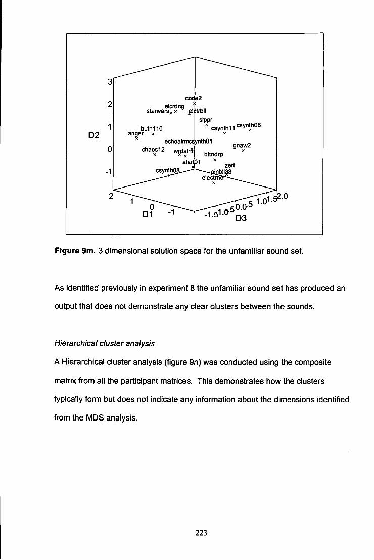
0 2
code2 elcrdng
starwarsx x ^litrbll
butn1ia anger x
chaos12 w jjalrft
sippr ''csynth1l'=sy"»^06
echoalrmcsynthOI gnaw2
bttndrp X
zert ibII33
electrnr X
aartDI csynthO
Figure 9m. 3 dimensional solution space for the unfamiliar sound set.
As identified previously in experiment 8 the unfamiliar sound set has produced an
output that does not demonstrate any clear clusters between the sounds.
Hierarchical cluster analysis
A Hierarchical cluster analysis (figure 9n) was conducted using the composite
matrix from all the participant matrices. This demonstrates how the clusters
typically form but does not Indicate any information about the dimensions identified
from the MDS analysis.
223
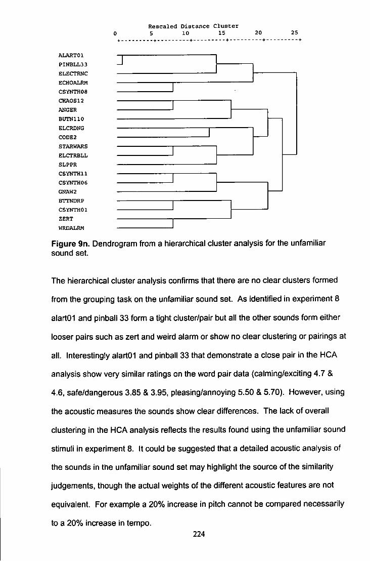
ALARTOl PINBLL33 ELECTRNC ECHOALRM CSYNTH08 CHAOS12 ANGER BUTNllO ELCRDNG C0DE2 STARWARS ELCTRBLL SLPPR CSYNTHll CSYNTH06 GNAW2 BTTNDRP CSYNTHOl ZERT WRDALRM
Res c a l e d D i s t a n c e C l u s t e r 5 10 15 20 25
J
Figure 9n. Dendrogram from a hierarchical cluster analysis for the unfamiliar sound set.
The hierarchical cluster analysis confirms that there are no clear clusters formed
from the grouping task on the unfamiliar sound set. As identified in experiment 8
alartOI and pinball 33 form a tight cluster/pair but all the other sounds form either
looser pairs such as zert and weird alarm or show no clear clustering or pairings at
all. Interestingly alartOI and pinball 33 that demonstrate a close pair in the HCA
analysis show very similar ratings on the word pair data (calming/exciting 4.7 &
4.6, safe/dangerous 3.85 & 3.95, pleasing/annoying 5.50 & 5.70). However, using
the acoustic measures the sounds show clear differences. The lack of overall
clustering in the HCA analysis reflects the results found using the unfamiliar sound
stimuli in experiment 8. It could be suggested that a detailed acoustic analysis of
the sounds in the unfamiliar sound set may highlight the source of the similarity
judgements, though the actual weights of the different acoustic features are not
equivalent. For example a 20% increase in pitch cannot be compared necessarily
to a 20% increase in tempo. 224
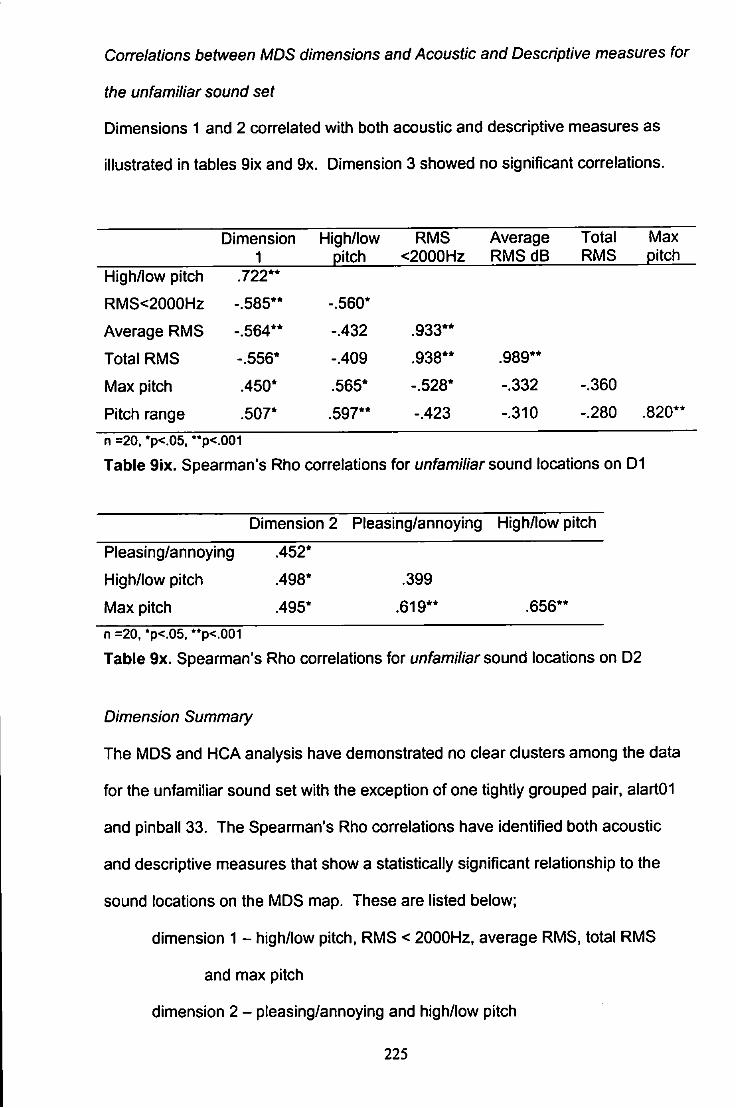
Correlations between MDS dimensions and Acoustic and Descriptive measures for
the unfamiliar sound set
Dimensions 1 and 2 correlated with both acoustic and descriptive measures as
illustrated in tables 9ix and 9x. Dimension 3 showed no significant con-elations.
Dimension High/low RMS Average Total Max 1 pitch <2000Hz RMSdB RMS pitch
High/low pitch .722**
RMS<2000Hz -.585** -.560*
Average RMS -.564** -.432 .933**
Total RMS -.556* -.409 .938** .989**
Max pitch .450* .565* -.528* -.332 -.360
Pitch range .507* .597** -.423 -.310 -.280 .820**
n =20. *p<.05. **p<.001
Table 9ix. Spearman's Rho con-elations for unfamiliar sound locations on D1
Dimension 2 Pleasing/annoying High/low pitch
Pleasing/annoying .452*
High/low pitch .498* .399
Max pitch .495* .619** .656**
n =20, *p<.05. "p<.001
Table 9x. Spearman's Rho correlations for unfamiliar sound locations on D2
Dimension Summary
The MDS and HCA analysis have demonstrated no clear clusters among the data
for the unfamiliar sound set with the exception of one tightly grouped pair. alartOI
and pinball 33. The Spearman's Rho correlations have identified both acoustic
and descriptive measures that show a statistically significant relationship to the
sound locations on the MDS map. These are listed below;
dimension 1 - high/low pitch, RMS < 2000Hz. average RMS, total RMS
and max pitch
dimension 2 - pleasing/annoying and high/low pitch 225
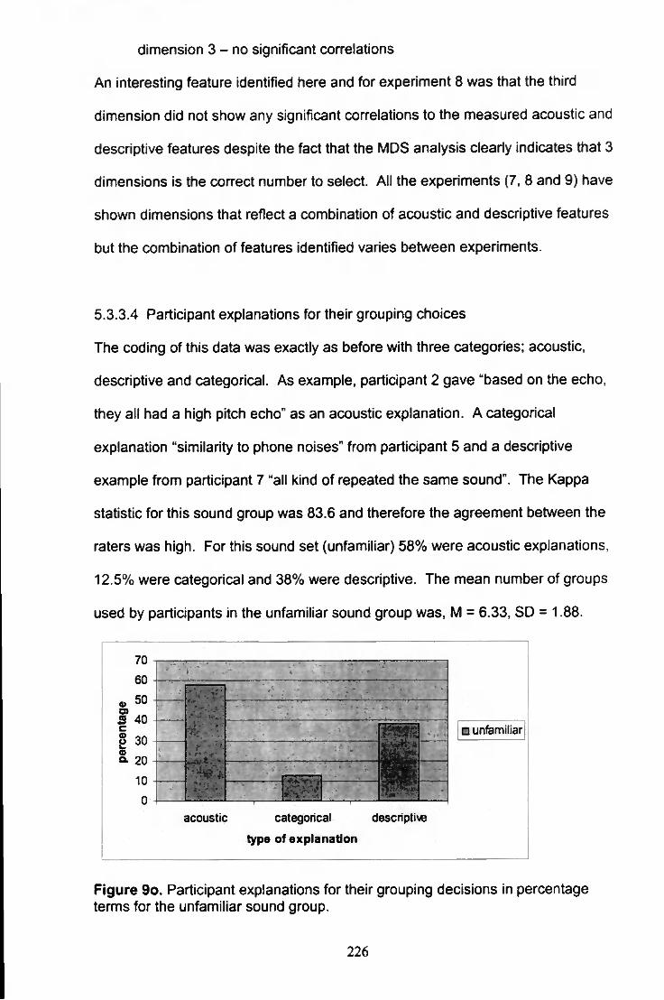
dimension 3 - no significant correlations
An interesting feature identified here and for experiment 8 was that the third
dimension did not show any significant correlations to the measured acoustic and
descriptive features despite the fact that the MDS analysis cleariy indicates that 3
dimensions is the correct number to select. All the experiments (7, 8 and 9) have
shown dimensions that reflect a combination of acoustic and descriptive features
but the combination of features identified varies between experiments.
5.3.3.4 Participant explanations for their grouping choices
The coding of this data was exactly as before with three categories; acoustic,
descriptive and categorical. As example, participant 2 gave "based on the echo,
they all had a high pitch echo" as an acoustic explanation. A categorical
explanation "similarity to phone noises" from participant 5 and a descriptive
example from participant 7 "all kind of repeated the same sound". The Kappa
statistic for this sound group was 83.6 and therefore the agreement between the
raters was high. For this sound set (unfamiliar) 58% were acoustic explanations,
12.5% were categorical and 38% were descriptive. The mean number of groups
used by participants in the unfamiliar sound group was, M = 6.33, SD = 1.88.
70 60
0) 50 O )
B 40 c o 30 V-/n w Q . 20
10 0
1 : — — 1 . _
• •i *••< • •i *••< • •i *••<
i
• •i *••<
• unfamiliar
acoustic categorical descripti\e
type of explanation
Figure 9o. Participant explanations for their grouping decisions in percentage terms for the unfamiliar sound group.
226
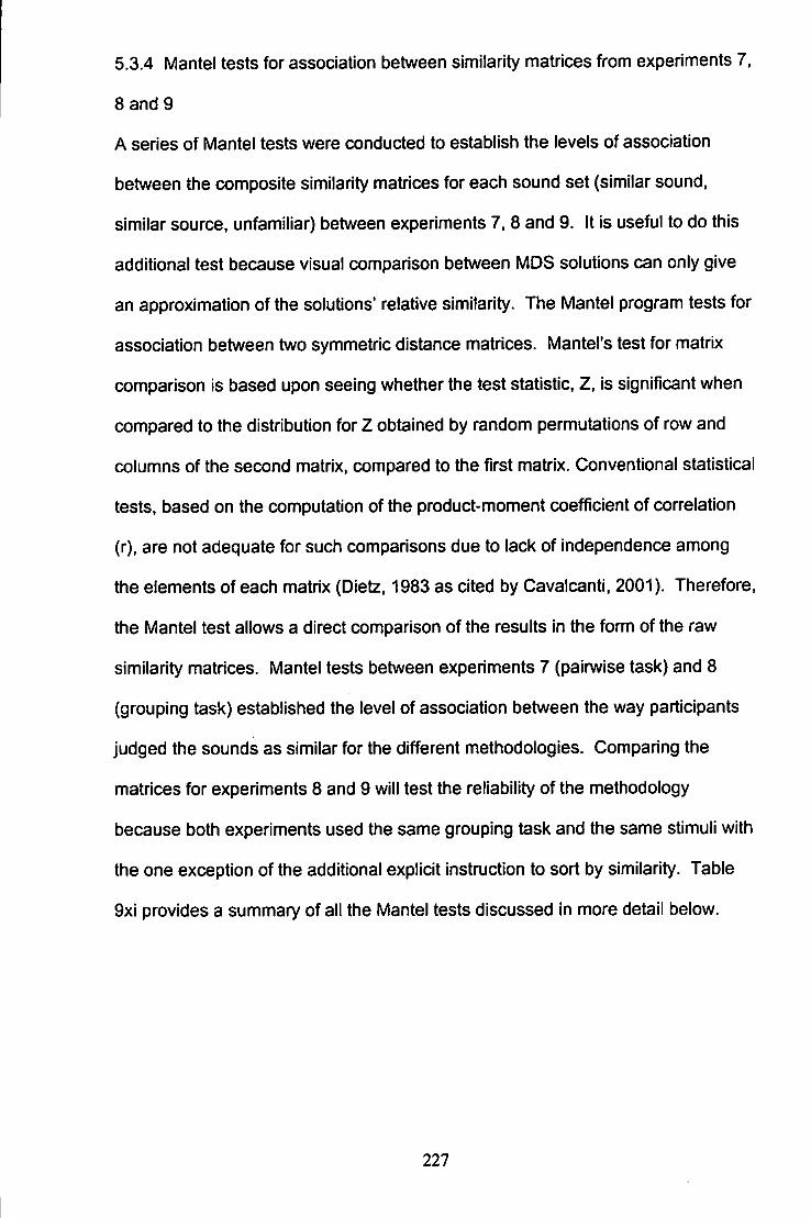
5.3.4 Mantel tests for association between similarity matrices from experiments 7.
8 and 9
A series of Mantel tests were conducted to establish the levels of association
between the composite similarity matrices for each sound set (similar sound,
similar source, unfamiliar) between experiments 7, 8 and 9. It is useful to do this
additional test because visual comparison between MDS solutions can only give
an approximation of the solutions' relative similarity. The Mantel program tests for
association between two symmetric distance matrices. Mantel's test for matrix
comparison is based upon seeing whether the test statistic, Z, is significant when
compared to the distribution for Z obtained by random permutations of row and
columns of the second matrix, compared to the first matrix. Conventional statistical
tests, based on the computation of the product-moment coefficient of correlation
(r), are not adequate for such comparisons due to lack of independence among
the elements of each matrix (Dietz, 1983 as cited by Cavalcanti, 2001). Therefore,
the Mantel test allows a direct comparison of the results in the fonn of the raw
similarity matrices. Mantel tests between experiments 7 (pairwise task) and 8
(grouping task) established the level of association between the way participants
judged the sounds as similar for the different methodologies. Comparing the
matrices for experiments 8 and 9 will test the reliability of the methodology
because both experiments used the same grouping task and the same stimuli with
the one exception of the additional explicit instruction to sort by similarity. Table
9xi provides a summary of all the Mantel tests discussed in more detail below.
227
Exp7 Exp8 Exp7 Exp8 Exp7 Exp8 ssnd ssnd ssrc ssrc unf unf
Exp 8 ssnd <.001
Exp 9 ssnd <.001 <.001
ExpB ssrc ^^g^^M <-001
Exp9 ssrc < .05 <.001
non = non significant cxDmparison.
Table 9xi . Summary of results for Mantel tests across all sound sets in experiments 7. 8 and 9.
5.3.4.1 Associations between experiment 7 (pairwise) and experiment 8(grouping
task)
The Mantel test for association between the composite matrices for the s/m/7ar
sound data collected for experiments 7 and 8 identified a statistically significant
correlation between these two matrices, r- 0.32. f(190) = 4.40, p<.001.
The Mantel test for association between the composite matrices for the s/m/7ar
source data collected for experiments 7 and 8 identified a statistically significant
correlation between the two matrices. r = 0.22, f (190) = 3.03, p <.001.
The Mantel test between the composite matrices for the unfamiliar soun6 set
collected for experiments 7 and 8 did not find a significant con*elation between the
matrices, r = 0.08. f(190) = 1.10, p = 0.14.
In summary, the similarity matrices between the painwise task and the grouping
task for similar sound group and the similar source group show highly significant
relationships. However, the matrices for the unfamiliar sound group between the
two experiments using different methodologies do not. It could be speculated that
this is because participants may be grouping the unfamiliar sounds differently from
228
each other and therefore no clear clusters are identifiable when using a composite
matrix of all 15 participants data.
5.3.4.2 Associations between experiments 7 (pairwise) and experiment 9
(grouping task)
The Mantel test for association between the composite matrices for the s/m/7ar
sound data collected for experiments 7 and 9 identified a statistically significant
correlation between the two matrices, r = 0.43, t (190) = 6.13, p <.001.
The Mantel test between the composite matrices for s/m//ar source sound group
between experiments 7 and 9 identified a significant correlation between the
matrices, r = 0.21, / (190) = 2.91, p <.05.
The Mantel test between the composite matrices for unfamiliar sound group
between experiments 7 and 9 failed to find a significant correlation between the
matrices, r = -0.05, f (190) = -0.61. p = 0.27.
In summary, the similarity matrices between experiments 7 and 9 also show a
relationship for the similar sound and similar source groups but not for the
unfamiliar sound group.
5.3.4.3 Associations between experiments 8 (grouping task) and experiment 9
(grouping task)
The Mantel test for the association between the composite matrices from
experiments 8 and 9 for the s/m/7ar sound set identified a highly significant
correlation between the two matrices, r = 0.83, f (190) = 11.35, p = <.001.
The Mantel test for the association between the composite matrices from
experiments 8 and 9 for the similar source sound set identified a highly significant
correlation between the two matrices, r = 0.95. f (190) = 13.14, p = <.001.
229
Finally, the Mantel test for association between the composite matrices for the
unfamiliar data collected for experiments 8 and 9 identified a significant correlation
between the two matrices, r = 0.33, t (190) = 4.59, p <.001.
In summary, as expected because the same methodology has been employed all
the sound group matrices showed a highly significant relationship between
experiments 8 and 9.
230
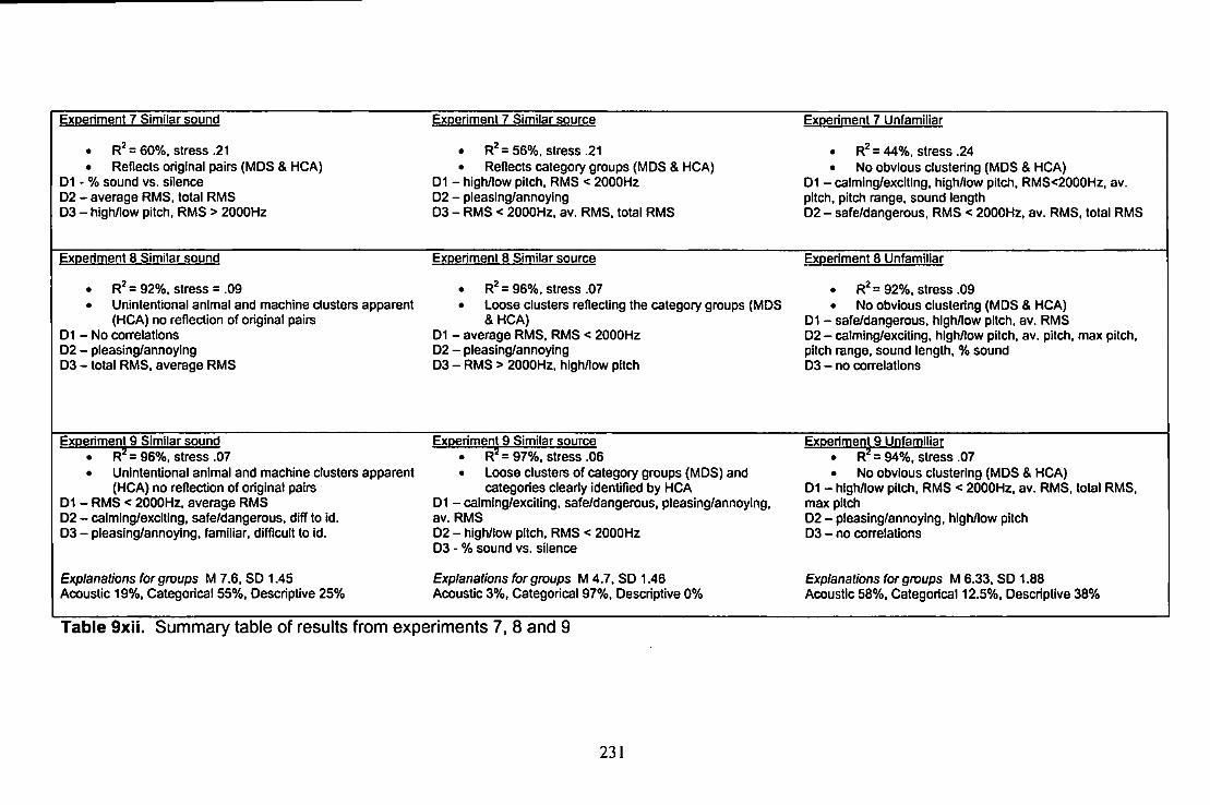
Experiment 7 Similar sound Experiment 7 Similar source Experiment 7 Unfaqiiliar
• R' = 60%. stress .21 • Reflects original pairs (MDS & HCA)
01 - % sound vs. silence 0 2 - average RMS, total RMS 0 3 - high/low pitch. RMS > 2000Hz
• R^= 56%. stress .21 • Reflects category groups (MDS & HCA)
01 - highflow pitch. RMS < 2000Hz 02 - pleasing/annoying 03 - RMS < 2000Hz. av. RMS. total RMS
. R 2 = 44%. stress .24 • No obvious clustering (MDS & HCA)
01 - calming/exciting, high/low pitch. RMS<2000Hz, av. pitch, pitch range, sound length 02 - safe/dangerous. R M S < 2000Hz. av. R M S . total R M S
Experiment 8 Similar sound Experiment 8 Similar source Experiment 8 Unfamiliar
• R^= 92%. stress = .09 • Unintentional animal and machine clusters apparent
(HCA) no reflection of original pairs 01 - No correlations D2 - pleasing/annoying 03 - total RMS. average RMS
• R^ = 96%. stress .07 • Loose clusters reflecting the category groups (MDS
&HCA) 01 - average RMS. RMS < 2000Hz 02 - pleasing/annoying 03 - RMS > 2000Hz. high/lov ^ pitch
• R^= 92%, stress .09 • No obvious clustering (MDS & HCA)
01 - safe/dangerous, high/lov f pitch, av. RMS 02 - calming/exciting, high/low pitch, av. pitch, max pitch, pitch range, sound length, % sound D3 - no correlations
Experiment 9 Similar sound • R^=96%. stress .07 • Unintentional animal and machine clusters apparent
(HCA) no reflection of original pairs 01 - RMS < 2000Hz. average RMS 02 - calming/exciting, safe/dangerous, diff to id. 0 3 - pleasing/annoying, familiar, difficult to id.
Explanations for groups M 7.6, SO 1.45 Acoustic 19%. Categorical 55%. Descriptive 25%
Experiment 9 Similar source • R^= 97%. stress .06 • Loose clusters of category groups (MDS) and
categories cleariy identified by HCA 01 - calming/exciting, safe/dangerous, pleasing/annoying, av. RMS 02 - high/low pitch, RMS < 2000Hz 03 - % sound vs. silence
Explanations for groups M 4.7. SO 1.46 Acoustic 3%, Categorical 97%. Descriptive 0%
Experiment 9 Unfamiliar • R===94%, stress .07 • No Obvious clustering (MDS & HCA)
01 - high/low pitch, RMS < 2000Hz. av. RMS, total RMS. max pitch 02 - pleasing/annoying, high/low pitch 03 - no correlations
Explanations for groups M 6.33, S D 1.88 Acoustic 58%, Categorical 12.5%. Descriptive 38%
Table 9xi i . Summary table of results from experiments 7, 8 and 9
231
5.3.5 Discussion
The results are discussed by sound groups for clarity.
5.3.5.1 Similar sound
Similarly to experiment 8 the multidimensional scaling results indicate that
participants have not grouped the sounds in their original pairs. It is quite difficult
to compare two 3 dimensional MDS configurations because the axes are likely to
be different but the MDS output of both experiments 8 and 9 for the similar sound
stimuli suggest only loose groups by pairs.
The hierarchical cluster analysis identified an unintentional cluster made up from
the four animal sounds used in this group; duck, cow, seal and lion. This was also
the case for this sound group on experiment 8. There is also an indication of a
loosely formed machine group suggesting use of a categorisation strategy. The
HCA has also identified some of the original pairs (fryfood/rain, zipper/riptear and
basketball/hammering) with the remaining pairs not clearly identified. Interestingly
it is the same 3 pairs that are the clearest from the HCA analysis of experiment 8,
suggesting reliability between the two testing sessions.
The dimensions for this MDS configuration reflect both acoustic and descriptive
features. Dimension 1 showed con-elations with measures of the sounds' RMS
power. Dimensions 2 and 3 show only the descriptive measures (calming/exciting,
safe/dangerous, difficult to identify, pleasing/annoying and familiar). An example
sound helps to illustrate how experiments 8 and 9 compare. Fryfood is located in
experiment 8 at the low end of the RMS power dimension as is the case for
experiment 9. It is also placed on the pleasing end of the pleasing/annoying
dimensions in both experiments. This helps to illustrate how similar the two
232
configurations are even though at first glance, due to differing placements of the
axis, they may appear different. Close inspection identifies similarities in the
placement of the sounds.
The addition of the extra information in this experiment helped to clarify the
reasons for participants' similarity dedsions. Responses for the similar sound
stimuli group generated a range of responses. Participants explained their
grouping decisions using acoustic (e.g. "same pitch"), descriptive (e.g. "long
zipping sounds") and categorical descriptions (e.g. "airplane sounds") but
categorical explanations accounted for 55% of the explanations provided. To
some extent this confirms the possibility, identified through visual inspection of the
MDS and HCA analyses that the participants are choosing to make use of salient
categories where possible. Fifty five percent of the explanations provided by
participants for their groups were categorical in nature even though this sound
group (similar sound) was not formed on the basis of the sounds belonging to
clear categories.
In summary, results from the similar sound group showed loose groups that
reflected the original pairs but category groups were also identified in the output.
Correlations identified that participants were using a combination of acoustic and
descriptive sound features but a stronger reliance on the descriptive features. The
additional qualitative data from participants suggests a reliance on acoustic, and
descriptive strategies with the strongest number of accounts referring to the
sounds membership to categories. The results of experiment 9 strongly reflect the
results from experiment 8 for the similar sound group indicating the reliability of the
grouping task methodology.
233
5.3.5.2 Similar source
The MDS configuration for this group has identified a model that is a good fit of the
data that has loosely identified the original groups in the similar source sound set.
In figure 9g the phones, bells and human noises groups can be seen clearly
clustered together with the animal and bird groups more loosely arranged but still
together in the configuration. The HCA analysis (figure 9k) for this sound set also
demonstrated clear clusters reflecting the sounds category membership.
Dimension 1 showed correlations with all the descriptive word pairs
(pleasing/annoying, safe/dangerous, calming/exciting) and as such seems to
represent a descriptive dimension. There is a tight cluster of sounds around the
higher end of dimension 1 made up from all the bell and phone sounds that appear
at the exciting, dangerous and annoying end of dimension 1. The loudness of the
sound is the other main feature that has shown correlations with the sounds
locations on dimension 2.
The analysis of the similar source stimuli group for experiment 9 is very similar to
the findings from experiment 8. Both experiments strongly suggest a descriptive
otive factor with the identification of all the word pairs on one dimension and the
RMS power of the sound on another dimension. Visual inspection of the MDS
configuration for this sound set cleariy reflects the sounds' category membership.
The additional information gathered in experiment 9 has suggested that
participants explain their grouping decisions almost entirely on the use of
categorical decisions with 97 percent of explanations being rated as categorical.
Therefore, this sound group has elicited a combination of acoustic and descriptive
features from the sounds that would appear to be contributing to similarity
judgements based on the sounds' membership to categories.
234
In summary, analysis of the similar source group has identified a clear RMS power
dimension and a descriptive dimension. This analysis also shows a very strong
relationship to the analysis of the similar source stimuli group in experiment 8.
suggesting the reliability of the grouping methodology between testing sessions.
Further, the participants' explanations for their grouping decisions cleariy indicated
categorical explanations for the grouping decisions made for this set of sounds
with a massive 97% of explanations being categorical in nature. This reflects the
fact that category membership was the main criteria for sounds included in this
sound set.
5.3.5.3 Unfamiliar
The arrangement of the sounds on the MDS configuration for this dimension
shows the stimuli well spread out with no obvious clusters or groups forming. The
hierarchical cluster analysis for this sound set reflects this lack of identifiable
clusters. Dimension 1 identified both pitch and the RMS power of the sounds and
dimension 2 has reflected the perceived pitch and pleasantness of the sounds. As
was the case for experiment 8 the unfamiliar sound set analyses do not give a
clear picture about the formation of any clusters and suggest no clear pattern but
nonetheless identify, as would be expected for unfamiliar sounds the largest
number of acoustic features showing correlations to MDS dimensions. This is
supported further from analysis of the additional information provided by
participants about their grouping decisions. This data demonstrated that the
unfamiliar sound group elicited heaviest reliance on acoustic features with 63% of
explanations accounting for the similarity judgements in this sound group.
235
Visual inspection of the MDS analyses and the HCA analyses for all the sound
sets across experiments 8 and 9 suggest clear similarities between the two testing
sessions for each sound group. Therefore, it can be concluded for the sound
stimuli employed here (similar sound, similar source and unfamiliar) that the
grouping task was a reliable task between experimental sessions. This is
supported by the highly significant correlations identified between the experiments
using the Mantel tests.
5.3.5.4 Participants' additional responses
One of the aims of experiment 9 was to gather extra information regarding the
basis on which participants made their grouping decisions. Experiment 8 clarified
which of the acoustic and descriptive features were being used but highlighted
again the issue suggested by experiments 5 and 7 previously that the participants
may be using category information in their similarity judgements. Experiment 5
suggested the influence of function or source and experiments 7 and 8 refined this
to suggest that the category to which the source of the sound belonged was
playing an important role. For example, if the sound is a barking noise then the
category to which a barking dog belongs could be influencing the similarity
judgements made. Therefore, to avoid making assumptions about additional
features that participants may be considering during the grouping process
participants were asked why they formed their groups. The results indicated that
for the different sound groups the strategies being employed varied.
The participant explanations provided for the similar sound group illustrated that
participants were using a combination of different sound features. Although the
majority of these (55%) were categorical both acoustic and descriptive accounts
236
were represented in participants' accounts. This group shows the most variation
in participant explanations.
Participants typically sorted the similar source stimuli into 5 groups with the
following as some of the more commonly cited reasons for group formation:
"sounds made by human beings"
"...sounds of bells"
"type of animal, they were all farm animals"
The responses given by the participants cleariy identified that the similar source
sound set was being sorted on the basis of the source objects' category
membership. This is supported by the finding that 97% of the reasons provided by
participants were rated as categorical type ratings. Although a few sounds such
as the bell sounds may share acoustic elements an effort was made to select
sounds that were quite varied acoustically.
Participants provided a very different pattern of reasons for their similarity
groupings for the unfamiliar sound group compared to the other two sound groups.
The mean number of groups formed was 6, similar to the other groups, but unlike
the other sound sets a large proportion of the reasons for grouping decisions were
acoustic. For both similar sound and similar source sets acoustic explanations
were not favoured. The unfamiliar group was characterised by a large number of
both descriptive and acoustic accounts of the groups formed. The categorical
reasons provided were typically more vague than for the other sound groups and
noticeably fewer in number. For example, rather than clear statements that the
sounds were all made by animals the reasons were more comparative such as "all
sounded like computer noises". This would suggest that participants were
searching for suitable source descriptions.
237
For both the similar sound and the similar source groups, containing familiar
sounds, the self reports indicated the importance of using category knowledge to
group the sounds. A key point is that participants were asked to sort the sounds
into groups that were similar on whatever basis they wished. They were not asked
to put the sounds into their most appropriate categories. Examples of some
frequently cited reasons given by participants for the similar sound group included;
"animal sounds"
"sounded like machines"
"all noises from transport".
Because of the variable nature of the sounds employed in these experiments
temporal measurements were difficult to take. Lots of descriptive language was
used to refer to the sharpness or rhythm in the responses. In general other
frequently given reasons (rated as acoustic) were the pitch of the sound, the
sharpness and the rhythm of the sounds. Pitch has been identified across all the
multidimensional scaling experiments (ex.'s 3, 5, 7, 8 and 9) as an important
feature in participants' similarity judgements regardless of the methodology used
to collect the similarity data.
Overall a larger number of descriptive reasons were also used where participants
used language that simply re described the sounds such as;
"brushing scnjbbing sounds"
"chirpy"
"clickety click"
This was not a characteristic used much for the other sound groups, especially
similar source where only four descriptive reasons were provided.
238
To summarise, the participants' responses have added support to some of the
suggestions made from the previous statistical results. For example, the results
from the similar sound group demonstrated that participants make use of a
combination of acoustic, categorical and descriptive strategies to make their
similarity judgements. For the similar source group there is a strong tendency
towards favouring the use of category information that was evident from visual
inspection of the MDS configurations but was not previously confirmed. Finally,
the unfamiliar sound group showed mixed strategies with acoustic features being
the most favoured but there was still a reliance on both categorical and descriptive
strategies. Of course these accounts only relate to the specific sounds employed
using the grouping methodology.
5.3.6 Mantel Tests
The mantel tests were conducted to compare each of the composite similarity
matrices generated by each of the testing sessions across experiments 7, 8 and 9.
The mantel tests identified significant associations between the composite
matrices for each of the sound groups for both methodologies. Mantel tests do not
directly compare the results gathered from the MDS or the HCA analysis but serve
to compare the raw similarity judgments. Mantel tests are used for this
comparison because product-moment correlations are not adequate for such
comparisons because of a lack of independence among the elements of each
matrix (Legendre. 2000). The Mantel test results identified that there are
correlations for each of the sound groups between the different methodologies.
For the similar sound group experiments 7, 8 and 9 all showed statistically
significant correlations. This finding Is also demonstrated by the significant
correlations between experiments 7 - 8 and 7 - 9 the same experiments for the
239
similar source stimuli group. However, the unfamiliar sound group shows a
contrast because there was no statistically significant relationship between
experiments 7 and 8 or 7 and 9. Nonetheless the similarity matrices for
experiments 8 and 9 using the same methodology did show a highly significant
correlation.
When comparing within sound groups for experiments 8 and 9 (both grouping task
experiments) there are highly significant relationships for all the sound groups.
For example, for the similar sound set experiments 8 and 9 shows, r = 0.83, t(190)
= 11.35, p <.001. This reflects the task's reliability across experimental trials and
for different sound stimuli sets. It would not be expected that the correlations
would be perfect because of individual differences in grouping decisions.
In summary, when comparing between the different methodologies mantel tests
have shown that the composite similarity matrices can be considered to be highly
correlated for the similar sound and similar source sound sets. The unfamiliar
sound sets showed different results between the methodologies and the lack of
clear clusters in the MDS and HCA analyses may suggest larger differences in
strategies. Comparison between experiments 8 and 9, both using the grouping
task, demonstrated that the different participants that completed the different
testing sessions were grouping the sounds in the same way, again demonstrating
the reliability of the methodology.
5.3.6 General Discussion
Experiments 8 and 9. employing the grouping task used a different methodology to
experiment 7 (pairwise) to investigate further which features of sounds participants
use when making similarity judgements and how the sounds are grouped together.
240
In addition, experiment 9 provided additional information in the form of self report
to further our understanding of the processes being employed by the participants.
Experiments 8 and 9 have also provided the opportunity to compare results using
the same 3 sound sets using the same methodology (with the exception of the
participants' self report after grouping process) for comparison within the present
wori< and with the research conducted by Bonebright (1996).
For clarity the general discussion is broken down into sections that discuss the
following points. Firstly, how experiments 7, 8 and 9 have clarified the
complicated unfamiliar end of the MDS analysis from experiment 5 (figure 5c).
Secondly, which acoustic and descriptive features have been identified as salient
from this final series of experiments. The differences identified between the
pairwise and the grouping tasks are discussed followed by a discussion of the
similarities between these methodologies. Finally there is a brief discussion of the
use of categories in participants' similarity judgements.
5.4.1 How the unfamiliar data from experiment 5 has been clarified
The unfamiliar sound set was included in experiments 7. 8 and 9 to try to collect
further information about the salient features of unfamiliar sounds that participants
used to make similarity judgements. Previously experiment 5, using the grouping
task, demonstrated that the least familiar sounds were grouped together.
However, the large number of sounds and the tightness of the groups made it
difficult to interpret which features of the sounds were contributing to the similarity
judgements.
Experiment 7 used the pairwise task to gather similarity judgements about the
unfamiliar sound group but failed to find any clear groups or clusters from either
241
the MDS or the HCA analysis. However, correlations between the acoustic and
descriptive features and the sounds' locations on the MDS map indicated some
salient features used by participants when the pairwise task was employed.
These were all acoustic with the exception of the word pair safe/dangerous which
is likely, following the identification of a sounds' urgency as a possible contributory
factor, to be underpinned by acoustic features. This may suggest that although
participants might be grouping the sounds in different ways (as suggested by a
lack of clusters in the MDS and HCA) they are making use of a large number of
the sounds' features.
A similar lack of clear clusters or groups was found using the grouping
methodology for the unfamiliar sounds in both experiments 8 and 9. A larger
number of statistically significant correlations than experiment 7, both acoustic and
descriptive, were identified for these two experiments (See summary table 9z).
Interestingly correlating the acoustic and descriptive features with the sounds'
locations on the MDS map failed in both experiments 8 and 9 to pick up the
meaning of the third identified dimension. The MDS stress measures indicated an
excellent fit to the data and therefore three dimensions were appropriate. Visual
inspection of the sound locations on dimension 3 does not immediately suggest
meaning for this dimension for either experiment. This could be taken to indicate
that both these analyses are picking up a salient dimension that has not been
included in the acoustic or descriptive measures taken. The extra qualitative data
collected from participants indicates possible areas that were important but were
not measured. Rhythm was mentioned in 14% of the explanations and pitch was
mentioned in 29% of the explanations. There were also many references that
could be classed as rhythmic with participants referring to speed, beat, tempo or
rhythm. Solomon (1959a) suggested that the experienced sonar operators that
242
participated in his research were utilizing rhythmic beat patterns to provide a
meaningful basis for grouping similar sounds in semantic space. Temporal
features were also investigated by Gygi et al (2004) who tested listeners' ability to
identify a range of environmental sounds using limited spectral information. The
results demonstrated the importance of temporal patterns because they were able
to remove nearly all the spectral information leaving only the temporal information
and still half of the sounds studied (35/70) showed above 50% accuracy in
identification rate.
The additional qualitative data collected in experiment 9 helped to clarify the
features used by participants when grouping the unfamiliar sound set. Compared
to the other sound sets (similar sound and similar source) participants gave a large
number of acoustic explanations (58% of explanations contained a reference to
acoustic features) and participants tried to use categorical explanations. For
example;
"...high pitched but sounded like something from a computer game"
"...its bell like ring"
"...all sound very 'space' like sounds"
However, the other main groups of explanations were descriptive and participants
typically described the sound. For example "quick clicking type sounds". One
important note is that deciding to put the explanations into three categories did
obscure the distinction between acoustic and descriptive explanations in a few
cases. It could be the case that participants did not have the necessary acoustic
language to explain their decision. The quote "quick clicking type sounds" from a
participant explanation above could represent an attempt to explain acoustic or
rhythmic features.
243
5.4.2 The salient acoustic and descriptive features
There were observable similarities and differences between the sound sets and
the different tasks with respect to the features identified as salient. The pairwise
task (experiment 7) showed participants' reliance, with the exception of
pleasing/annoying (similar source only) on the acoustic features across all three
different sound sets. This suggests that during this task participants relied almost
exclusively on acoustic information to make their similarity judgements. However,
the pairwise task was also employed in experiment 3 where a descriptive factor
was identified. Nevertheless a heavy reliance on the acoustic features was still
observed alongside the participants' categorical explanations.
The grouping task (experiments 8 and 9) showed much more variety with respect
to the identified features with both acoustic and descriptive features identified as
salient for all the sound sets. Across the sound sets there were variations in the
number of features identified by the analyses. For example, the similar sound set
showed a low number of correlations with each dimension, typically one or two
features per dimension. The similar source set also reflects this pattem of low
numbers of features for each identified dimension. The unfamiliar sound group is
slightly different with a mixture of a large number of features typically identified for
most of the dimensions. However, there is an unidentified dimension for the
unfamiliar sound group in both experiments 8 and 9. This strongly suggests that
there are salient features involved in the perception of similarity, related
specifically to unfamiliar sounds, that were not measured. It could be suggested
that sounds that are unfamiliar force the participants into using all the available
information rather than using any pre existing knowledge about the sounds source
because this may be absent for unfamiliar sounds.
244
Across experiments 7, 8 and 9 all the acoustic and non acoustic features were
identified as salient with the exceptions of bandwidth and minimum pitch that have
shown no significant relationship to the MDS dimensions. The following features
are listed according to the number of times, across experiments 7. 8 and 9, for all
sound sets, a particular feature has shown a significant relationship to a MDS
dimension.
High pitch/low pitch = 10 times (appeared on 2 dimensions for the same
sound group, same experiment x 3)
Average RMS = 9 times, appeared on all sound groups, all experiments
RMS < 2000Hz = 7 times (appeared twice x 1)
pleasing/annoying = 6
total RMS power = 5
% sound versus silence = 5
calming/exciting = 4
safe/dangerous = 4
RMS > 2000Hz = 3
Difficult to identify = 2 (appeared twice x 1)
Average pitch = 2 (unfamiliar sound set only)
Pitch range = 2 (unfamiliar sound set only)
Sound length = 2 (unfamiliar sound set only, grouping task only)
Maximum pitch = 2 (unfamiliar sound set only, grouping task only)
This list helps to demonstrate that both the acoustic and descriptive features are
prominent in participants' judgements of similarity across all sound groups. Those
features that appear the least often - difficult to identify, average pitch, pitch
range, sound length and maximum pitch were identified as salient only for the
unfamiliar sound group. This suggests that reliance on pitch information is at its
greatest for unfamiliar sounds. This finding is interesting in the light of the
perceptual measures of pitch (high/low pitch) appearing the most frequently and
for all the different sound groups.
245
5.4.3 Differences between the pairwise and the grouping tasks
One of the clearest differences between the two tasks is the way the results from
the different methodologies reflect the original sound selection for each sound
group. The painwise task reflected the original pairs (similar sound) and the
categories (similar source) quite cleariy. This is in contrast to the grouping task
where in both experiments, 8 and 9. the original pairs and categories were loosely
reflected and some new categories were identified (for the similar sound group). It
is possible to suggest that the pairwise task may have forced participants to focus
on only one dimension, typically the most obvious dimension depending on the
sound set used.
Cognitively it is likely more economical to form large categories such as animals
and machines than to wori< out which sounds are the most similar on a whole
range of different features. As discussed by Smith (1989) the partitioning of the
worid into concepts allows us to decrease the amount of information that we have
to process. It was found that about half the sounds in the similar sound group
(originally acoustically similar pairs) were fitted into new categories (animals and
machines) by the participants. This suggests that other features would be
necessary to group the remaining sounds hence the identification of many sound
features as salient in this instance. Of course this is highly speculative but there
will follow a discussion of the literature based on the debate discussing the degree
to which judgements of similarity reflect categorisation. Even if categories do
closely reflect judgements of similarity it may not always be possible to categorise
every sound.
The unfamiliar sound group is a good example of the inability to categorise all
sounds because no clear clusters were identified for either methodology and each
246
methodology suggested a large number of salient features that correlated with the
identified dimensions. It is unlikely that categorisation based on the sounds' source
can be employed if the sounds are unfamiliar to the listener. Therefore, more
common, everyday categories such as animals cannot be used. The extra self
report data from experiment 9 suggested that there were important acoustic
features that were not measured for the sounds that were being used by the
participants such as rhythm or strangeness. Measurement of the features was
problematic because of the difficulty with quantifying such features.
5.4.4 Similarities between the two grouping task experiments.
There are a few clear similarities (as expected using the same methodology)
between the analyses conducted on experiments 8 and 9 that are worthy of further
note. Firstly, in both experiments 8 and 9 for the similar sound group two
categories are highlighted by the hierarchical cluster analyses for these
experiments. For both experiments an animal category and a machine category
are quite evident despite the original sound selection being based on acoustically
similar pairs. Secondly, for both experiments using the similar source sounds one
of the dimensions was clearly descriptive representing all the word pairs used. For
example, the bell and phone sounds were rated similarly, appearing for both
experiments, on the dangerous, exciting and annoying end of the dimension.
Thirdly, for both presentations of the unfamiliar sound sets only two dimensions
showed any significant correlations to the acoustic and descriptive features
measured. The MDS analysis suggested that three dimensions was the correct
number to investigate but visual inspection of the data did not suggest possible
meaning to the unidentified dimension. However, as discussed the self report data
suggested several possible acoustic or descriptive measure of importance such as
rhythm or strangeness.
247
All of these similarities are important because they suggest that the grouping task
has produced reliable results across different experimental sessions. For
example, the finding that the similar source set elicited the same descriptive
dimension on both occasions strongly supports the suggestion that these factors
are influencing participants' grouping decisions. Similarly the finding that new
categories were formed for the similar sound data on both experiments 8 and 9
suggest the strength of the tendency to sort by category.
5.4.5 Use of categories
Throughout the results from experiments 7, 8 and 9 there is repeated evidence
that participants are making use of category information to make their similarity
judgements and this applies across both kinds of task although it presents itself
differently.
For the painwise task (exp7) both the hierarchical cluster analysis (figure 7e) and
the multidimensional scaling analysis place the similar source stimuli in their
original subgroups; fanm animals, phones, bells, human noises and birds. The
other interesting sound group with regards to categories was the similar sound
group. Despite this group being formed on the basis of acoustically similar pairs
participants demonstrated a tendency to group some sounds into categories e.g.
animals or engines. It is of particular interest for the painwise task because
participants had no knowledge about the other sounds that would be presented
and from this point of view could make no judgements about all the sounds.
Neither could they adjust previously made judgements at a later stage of the
experiment should they become aware of any obvious categories (Lakatos et al,
2002). Therefore, this suggests that information about a sound's source object
248
belonging to a certain category must be a key feature in the similarity judgement
even when two sounds are presented in isolation.
The grouping task (ex.'s 8 and 9) showed evidence for the use of category
information. This was especially evident in the similar sound group. During this
experiment, despite the fact that the sounds selected for inclusion were based on
acoustically similar pairs, the participants grouped sounds in such a way that they
exploited/reflected several unintentional categories. From the MDS and HCA
analysis new clusters based on animals, machines and beat rates were identified.
This was found to be a reliable result as it was replicated in experiment 9 for the
similar sound group. This suggested that category membership of the sounds'
source objects is of high importance because in both experiments the sounds
were grouped according to category membership. It cannot be argued that a lion
and a duck sound similar and therefore it is likely to be their membership to the
category 'animals' that has resulted in them being sorted as similar by participants.
Nonetheless the finding of a category that may reflect beat rate (as identified by
the additional information collected in experiment 9) maintains the importance of
acoustic features in similarity judgements. It has helped to suggest beat rate as a
possible salient feature that was difficult to measure in a range of sounds with
much variation. Previous research has often identified temporal patterns or beat
rates as salient (Solomon, 1959; Warren & Verbrugge. 1984) and it is therefore of
interest that it has been identified in the current research too, albeit in a different
way. McAdams (1993) discusses different stages of processing one of which is
the analysis of macro temporal properties, concerned with the rhythmic and
textural aspects of a sound or environmental event.
249
A final point Is worthy of discussion in order to improve the information gathered
from the grouping methodology. In the present research the experimental
program was written in such a way that participants had to make their grouping
decisions by placing icons within a grid structure. Allowing participants to freely
sort the sounds within one large space would allow the Inclusion of distance
between category information that Is absent from the current results. However, for
such a large number of sounds (N=70) this may be a rather demanding task for
participants to place each sound in relation to every other but would certainly
warrant further investigation.
250
Chapter 6 Conclusion
6.1 Introduction
In addition to identifying the salient acoustic and descriptive features of a
previously uninvestigated group of sounds (abstract sounds) the thesis has
presented a series of experiments that has investigated the cognitive
representation of sound. The experiments were designed to establish a deeper
understanding of which features of sounds, both acoustic and descriptive, were
salient to the listener with a specific focus on similarity. The findings have
demonstrated variable relationships between the measured features, furthered our
understanding of relationships between acoustic and more psychological features
of sounds, and addressed similarities and differences between two commonly
used methodologies in auditory perception research.
The results have cleariy demonstrated a variable relationship between acoustic,
descriptive and categorical features that appear to be mediated by both the
sounds being judged and the context in which they are presented. Whilst this is to
a point intuitively obvious the work has provided data in support of the view. An
example of this is the Important and clear difference demonstrated between
familiar and unfamiliar sounds used in the studies. Sounds that were considered
familiar by participants were shown to produce more judgements based on
descriptive features and to elicit the formation of more category-based MDS
outputs than the unfamiliar sounds. In contrast the most salient features identified
for the unfamiliar sounds were acoustic and descriptive. The qualitative data
collection was a useful addition and further supported the differences observed
between the familiar and unfamiliar sounds.
251
The relationships between acoustic, descriptive and categorical features of sounds
have not been investigated or discussed in much previous literature. The present
studies go some way towards bringing these key features together and suggesting
how the features may interact in judgements of similarity. The results do support
previous research such as that on urgency mapping (Hellier et al, 2002). At this
stage the work is only indicating where these relationships may be strong or weak.
For example, measures of pitch have been shown to have strong correlations to
word pairs that are indicative of the urgency of a particular sound.
The results also suggest that sounds were being judged differently depending on
their type. In the context of this work, type is meant to define whether the sounds
are abstract in nature or more environmental. It has been indicated by comparing
the eariy experiments that included only abstract sounds to the latter experiments
that also included environmental sounds that sounds that were abstract in nature
lead the participants to rely more on the function of the sound in their judgements.
Sounds classed as environmental, such as animal sounds were more likely to elicit
category-based judgements from participants.
The third major addition to previous work contributed by the thesis was data that
furthers our understanding of the similarities and differences between the pairwise
task and grouping tasks, both of which generate similarity data suitable for MDS
and hierarchical cluster analysis. Work that addresses this issue is in its early
stages and as such this work adds to Bonebright's (1996) preliminary comparisons
of the two tasks. The later experiments (7. 8 & 9) in the present research provided
an opportunity to directly compare the two data collection techniques on three
different sound sets. The results demonstrated that the sounds were more tightly
clustered for the pairwise comparison task than the grouping task, regardless of
252
the sound set used. The results also identified that for sounds that were familiar to
the participants there was stability and consistency in judgements between the two
tasks.
6.2 Summary of experimental findings
The first two experiments collected acoustic and descriptive information about 30
abstract sounds. These experiments were preliminary experiments designed to
create a database of information for each sound. This database provided a picture
of the features that participants considered salient when asked to rate the sounds
in isolation. The experiments suggested that participants favoured three salient
features of the sounds. The three factors identified from the PCA analysis were
the ease with which people used words or images in sound identificafion, a
descriptive factor comprised of the most descripfive word pairs and the frequency
of occurrence rate for the sounds in the environment. The third experiment
employed a painwise comparison task that required participants to make similarity
judgements for paired presentations of the 15 sounds employed. The results of
this experiment indicated, using the measured acoustic and descriptive features,
which features were considered salient to participants in their judgements of
similarity between the sounds. Three dimensions were identified using MDS
analysis as contributing to the participants' similarity judgements. These salient
dimensions were; acoustic measures of RMS power and pitch; descripfive features
such as the pleasantness of the sound; and the occurrence rate of the sounds.
Experiment 3 also gave an indication that the function of a sound was contribufing
to the way the sounds were rated for similarity in addition to the acoustic and
descripfive features. Therefore, experiments 1 to 3 showed that participants were
favouring a number of features, both acoustic and descripfive, in their judgements
about the sounds. Measures of RMS power, pitch, descripfive features,
253
occurrence rates and sound function were all highlighted as important to similarity
judgements between the abstract sounds.
Experiment 4 broadened the scope of the preliminary experiments by including
112 abstract sounds reflecting a broader range of sounds and more than one
exemplar for each sound type such as bells. Again descriptive measures for all
the sounds were collected alongside the same acoustic measurements providing a
larger database of information for the sounds.
The smaller number of sounds used (N=30) in experiments 1-3 were retained
within experiment 4. Analyses of participants' ratings for these 30 sounds
identified that the statements and word pairs used to gather the descriptive
information were reliable measures. The measures were reliable both across
different testing sessions and between the present research and the research
conducted by Bellas (1993) on environmental sounds.
Experiment 5 used 70 of the 112 sounds and was designed to build on the results
from experiment 3. This experiment employed an alternative to the painwise task
that required participants to group the sound stimuli as similar on screen. This
overcame the exponential increase in the number of sound pairs that would
require similarity judgements using the previously used pairwise task. The task
required participants to group the sounds as similar on screen simply by re
arranging icons representing each sound into groups according to similarity. One
of the main observations from the analysis of experiment 5 was that none of the
acoustic measures showed a correlation to the 2 identified MDS dimensions.
Across all the experiments in the thesis this is the only time where a lack of salient
acoustic features was identified. Using the acoustic and descriptive measures
254
from experiment 4 MDS analysis Identified that dimension 1 reflected the
importance of the sounds' familiarity and the descriptive feature safe/dangerous
and with dimension 2 reflected other descriptive data (pleasing/annoying, use of
words to describe). In addition, experiment 5. like experiment 3, suggested that
sounds were being grouped together according to their function as well as by their
descriptive features. This added evidence to suggest that a sound's membership
to a category may also be a feature in the participants' grouping decisions.
Emergency sounds (sirens - ambulance, air raid etc.) and telephone sounds
(mobile, office, dial tones etc.) were two examples of clear category clusters.
There was also a tight cluster of sounds, rated as unfamiliar, on the lower right
hand corner of the MDS map that warranted further investigation. Further,
experiments 4 and 5 suggested that certain descriptive features may be mapping
onto the acoustic measures. For example, the acoustic measure RMS power
showed a relationship to the descriptive measure safe/dangerous, suggesting the
importance of the urgency of the sound (Edworthy et al. 1991; Hellier et al. 1993).
Experiments 1 to 5 provided a rationale for creating three different sound sets
{similar sound to test for acoustic similarity. s/m//ar source to test for categorical
similarity and unfamiliar to unravel the highly clustered unfamiliar soun6s in
experiment 5) for use in the subsequent experiments. Eariy indications suggested
that the 70 sounds used in experiment 5 were being judged differently according to
a number of factors. These factors were the familiarity of the sound, the acoustic
and descriptive features of the sounds and the sound's category membership.
Therefore, these observations guided the design of the subsequent sound groups.
In addition to carefully considering which sounds to include in the sound sets both
the pairwise methodology (exp 7) and the grouping task methodology (exp.'s 8 &
9) were employed. These later experiments allowed for comparisons to be drawn
255
between the 2 different methodologies in a similar way to the work of Bonebright
(1996) using set sound groups for each task. The painwise task required
participants to make judgements about pairs of sounds. The grouping task
required participants to group the sounds on a computer screen according to the
sounds' similarity as they thought best.
Following experiment 6 that collected the same acoustic and descriptive measures
for the new sounds experiment 7 (pairwise task) collected similarity judgements for
each of the three sound sets. Using different sound sets would allow comparison
between the sound sets and with experiment 3. It identified that participants
sorted as similar, acoustically similar sounds (similar sound) using measures of
power, pitch and frequency of occurrence. Participants grouped sounds from the
same category (similar source) into category groups and acoustic characteristics
and pleasing/annoying were identified as salient. In contrast, no consistent
clusters were identified for the unfamiliar sound group and neariy all the acoustic
and descriptive measures were highlighted on one of the three identified MDS
dimensions.
Experiment 8 (grouping task) used the same three sound sets but employed the
grouping task reflected the results from experiment 7 (pairwise task). This
suggested that participants sorted sounds from the similar sound group into
acoustically similar pairs, and grouped sounds from the similar source group
together in categories using a mixture of descriptive and acoustic features. Again
the unfamiliar sounds showed little or no clustering and demonstrated the largest
selection of features overall, both acoustic and descriptive with a significant
relationship to the sounds' locations on the 3 identified dimensions.
256
Experiment 9 (grouping task) added qualitafive informafion by asking participants
for an explanafion for each group formed and suggested features that were salient
to participants' similarity grouping decisions beyond those measured. This was a
useful addition for many reasons. Firstly, the third MDS dimension for both
experiment 8 and 9 on the unfamiliar sound set was unexplained using statistical
techniques. However, the qualitative data suggested features that were not
selected for measurement (experimentally) as important to the participants with
references to tempo, beat, rhythm and speed. These particular sound features
were not measured here because of the diverse nature of the stimuli and the lack
of constancy through the course of many of the stimuli. However, the experiment
has suggested the salience of these features and detailed acoustic measurements
such as speed would be worthwhile in the future. Secondly, the qualitative data
supported the importance of both the acoustic and descriptive information,
identified statistically throughout the experiments, as well as providing further
evidence for the importance of category information in similarity judgements
across all the sound groups.
The final 3 experiments (7, 8 & 9) also highlighted the similarities and differences
between the two methodologies. The clearest difference between the two tasks
was the way that the results reflected the original selection of sounds for inclusion
in the 3 different sound groups. The pairwise task reflected the original basis for
selection (similar sound in pairs and similar source in groups) very cleariy. The
grouping task reflected these original selections more loosely and participants
showed a greater tendency to group by category whenever possible not just for
the similar source sound set. It is important to note that people are likely to group
sounds according to the most salient features which could be categorical or
acoustic, and to some extent are likely to be predetermined by the stimulus sets.
257
Throughout the results from experiments 7, 8 and 9 there was clear evidence,
from visual inspection of the MDS configurations and the HCA analyses that the
participants were making use of category information as part of their similarity
judgement strategies if the sounds were familiar. There was no evidence for the
use of category information for the unfamiliar sound set on either task.
6.3 Summary of experimental techniques
The methodologies employed throughout the PhD were based on previous work
and work that has produced interesting and informative results. The PhD has
produced further results of interest using painwise comparison and grouping tasks
and interpretable results using multidimensional scaling and hierarchical cluster
analysis to provide visual representations of the participants judgements.
Multidimensional scaling used by many previous authors in auditory work
(Berglund et al, 2002; Bonebright. 1996; Howard et al, 1976; Scheider et al, 1982;
and Susini et al 1999) was used to look at auditory stimuli from a neutral
standpoint. The technique allowed the stimuli to tell the story and then the
researcher must try to impose interpretation onto the results (MDS configurations).
The technique has been used to good effect in the present research but
interpretation of the results has been somewhat restricted by the limitations on the
number of acoustic and descriptive measurements that could be taken for each of
the stimuli, and the problems with quantifying some measure such as timbre.
There were several decisions taken to restrict the number of measures used.
These were for both practical and theoretical reasons. From a practical point of
view the decision was made to focus on a high number and variety of sounds for
investigation, but in order to do this the number of acoustic and descriptive
258
measures used were relatively small. Theoretically it was the aim of the work to
get a feel for the salient features used by participants on a broad range of sounds
rather than aiming to investigate all the possible features of interest. This meant
making some decision regarding which acoustic and descriptive analyses used in
previous work to continue through the research presented here. In addition the
work was intended to put a psychological slant on the research with a particular
interest in investigating any particular acoustic analyses that may underpin the
more psychological/descriptive judgements participants gave. This was opposed
to a more acoustic investigation and as such the auditory measures used were
taken as indicators of an auditory features salience only. Therefore, it was
decided that the more complex or difficult to quantify acoustic measures were
excluded. For example, timbre is a measure that is well known to be very difficult
to quantify and unlike pitch or loudness there is no single scale along which it is
possible compare or order the timbres of different sounds (Moore, 1997).
Roughness was also not included as an acoustic feature for investigation because
it has not been a feature included in the work on which this research was based.
Further Vassilakis (2005) describes roughness as one aspect of timbre. As such
this again makes it a difficult measure to quantify and too subjective for inclusion.
The majority of the sounds employed in the work have been taken from the
environment and as such have much variation within them. This means that they
are likely to be wide band signals which are a much more complicated matter to
analyse (Terhardt, 2000) than narrow band signals for roughness.
6.4 Theoretical Implications
The previous research can be loosely divided into two broad groups that are
relevant to the thesis; research that has used the multidimensional scaling
259
analysis with a focus on similarity judgements; and research that has looked at
recognition and identification of sounds. Both research areas have focussed on
identifying features of sounds that are salient to the listener In either a judgement
of similarity or the recognition of a sound. This means that the present work can
be discussed in the context of all of this previous research. The tasks chosen to
collect data, the pairwise task and the grouping task, were favoured because of
the obviously multidimensional nature of complex, abstract and environmental
sounds (Susini et al, 1999). It was therefore considered that an appropriate way to
investigate this complexity was to employ multidimensional scaling (MDS)
analyses techniques. Similarity judgements were the cognitive judgements
selected because many authors (Solomon 1958; Susini et al, 1999; Howard et al,
1976; McAdams, 1993) have discussed the appropriateness of this technique if
highlighting salient features of complex sounds is the investigations* focus.
An interesting point raised in the previous literature and of relevance to the current
findings is the focus of participants' judgements. For example, in sound
recognition research using environmental sounds Dallas et al (1987) suggested
that participants often refen^ed to the object/source that makes the sound rather
than the sound itself. Intons Peterson (1980) found participants to be imagining a
visual image of the object that made the sound as a by-product of forming the
requested auditory image of a given sound. Both of these researchers found
participants indicated the salience of the source object. This feature was also
identified in the current research.
There are six key theoretical points to address that have been raised by the
present experiments. These are the identification of a number of salient acoustic
features, the identification of a number of salient descriptive features and how the
260
salient features identified here and in other similarity research corresponds to the
salient features identified in recognition and identification research. Participants'
use of categories in their similarity judgements is an important issue and the
similarities, differences and usefulness of the pairwise and grouping
methodologies. Finally, the differing cognitive strategies that appear to be used by
participants depending, in part, on the context provided in an experiment.
6.4.1 The Salient Acoustic Features
Three main acoustic features v^ere identified as salient in participants' similarity
judgements. These three features were the RMS power of the sounds, the pitch of
the sounds, and their rhythm.
The power or loudness of a sound is an acoustic feature that many previous
researchers have identified as highly salient in listeners' perception of sounds. For
example, Howard et al (1976) identified signal loudness as a feature contributing
to an MDS dimension following similarity judgements for a small number of
complex unfamiliar sounds. It is also salient as discussed by Susini et al (1999)
because of the importance of not allowing features such as the loudness of a
sound to overpower less prominent features. For example, two sounds that differ
mainly in terms of loudness may be judged as different according to this dimension
with little attention given to any other features. Unfortunately, there are. as
discussed, only a limited number of auditory similarity studies. Many of these
studies, such as Bonebright's (2001) have not included RMS power as a measure
in their studies. This means it is very difficult to make clear comparisons between
previous and the current work. However, within the thesis a large amount of
experimental data from experiments 7, 8 and 9 made it possible to assess, to
some degree, the extent to which loudness measures were repeatedly identified
261
as salient. Average RMS power appeared on all 9 occasions (sound groups x
methodology), and RMS < 2000Hz appeared on 7/9 occasions. These were the
most prominent features across the 9 trials in these final experiments, with the
exception of the word pair high pitch/low pitch. The identification of RMS <
2000Hz as an acoustic feature that was frequently identified as salient supports
the suggestion made by Gygi et a! (2004). Their research tested a range of low
and high pass filtered sounds and found that the most important region for sound
identification was between 1200 and 2400H2. Although the measure used in the
present research does not fit exactly with the region identified by Gygi et al (2004)
it was designed to measure the spectral spread in percentage terms within the
sound (> 2000Hz was also included as an acoustic measure). Therefore, the
present results alongside those of Gygi et al (2004) hint at the importance of the
frequencies that are within this particular region of the sounds. Despite the fact
that Gygi et al (2004) focussed on sound recognition the research does highlight
the salience of loudness as a feature used in people's cognitive judgements about
sounds whether this is recognition, identification or similarity judgements.
Pitch was also an acoustic measure identified as a highly salient feature in many
previous studies although these have often focused on memory (Clement et al,
1999; Keller, Cowan & Saults, 1995; Semal et al, 1993) or used unusual
methodology such as the task used by Intons Peterson et al (1992) to investigate
the inclusion of pitch in an auditory image. Unfortunately pitch was not a measure
given much focus as an acoustic measure in the three key pieces of previous
research cited in the thesis. Bonebright (2001) measured change in frequency
and peak frequency but did not focus on these measurements. Similarly, in (1996)
Bonebright included low, medium or high frequency categories but again did not
focus on detailed frequency measurements. Pitch was not a measure included for
the work conducted by Ballas (1993) who investigated a wide range of specific 262
bands with centre frequencies ranging from 200Hz to 8000Hz. Solomon (1959b)
focussed on the sound spectrum, the beat rate and band pass filters but not on
pitch information. However, Howard et al (1976) speculated that one of the
dimensions identified following their similarity based task did reflect pitch although
it was not measured direcfly. In the present research pitch was identified as a
salient feature throughout the experiments and the measures included both
absolute measures of pitch, following acoustic analysis, and the perceptual
measure high pitch/low pitch to assess participants own perceptions of the overall
pitch of a sound. Research looking at urgency for example has included pitch
information and therefore allows some level of comparison. Hellier et al (1993)
identified that increases in fundamental frequency increased the perceived
urgency of the stimuli. It was suggested that pitch would possibly be a useful
discriminator of sounds because of the qualitative nature of the sensations that
result from changes in pitch. Stevens (1959) discussed pitch in terms of its
metathetic nature. That is, a variation in the quality of a sound's pitch results in a
non-additive change in perception, it is a qualitafive change. This is in contrast to
the more quantitative changes obtained by altering the loudness of a sound for
example. This highlights the different nature of these two acoustic features that
have been identified as salient features and how they create different perceptual
sensations. In summary for the acoustic measure of pitch the present research
highlighted it as a salient feature in participants' similarity judgements but
unfortunately previous research using similar methodology has not included pitch
to provide previous results for comparison.
The temporal patterns in sounds have been another highly salient feature that has
been identified in many previous investigations. For example. Yost (1991)
discussed it as a salient feature that contributes to an auditory image and Solomon
(1959b) identified it as a strong feature involved in sonar operators' sound sorting 263
decisions. Gygi et al (2004) discussed the likelihood that identification of sounds
was strongly based on temporal information by degrading other features of the
sounds but found that participants could still identify the sounds. The qualitative
data from experiment 9 identified that temporal patterns were important to
grouping decisions because participants gave a large number of references to
beat rate, rhythm and tempo in their explanations for classification. Therefore,
although this was not a measured feature in the present experiments because of
the highly variable nature of the stimuli employed the qualitative data identified the
importance of temporal patterns in line with previous research.
The results of the present studies go some way towards identifying some of the
salient features of sounds that would be useful in further development of models
such as the sound recognition model proposed by McAdams (1993) that lacked
detailed discussion of specific sound features. Subsequent research such as that
conducted by Gygi et al (2004) and evidence presented in this thesis suggest that
this model could be presented from more than an acoustic point of view.
One important point raised by McAdams is that similarity studies both previously
and demonstrated again here usually settle on 2 or 3 dimensional solutions which
is a relatively small number of dimensions. The reason being that when a large
number of sounds are judged together participants can focus on a small number of
features that are the most useful to them. The current work has demonstrated that
a MDS solution with 3 dimensions for example does not necessarily mean that
only three features are of interest as psychological and acoustic features may
show some correlations and both may represent one dimension. Nonetheless this
serves to illustrate that the techniques used for similarity judgements do highlight
264
broader acoustic and psychological features as salient and therefore can add
another level to the model but cannot address the very fine level details.
The third stage of McAdams' proposed model (figure la . chapter 1) suggested the
analysis of auditory properties and/or features. However, with respect to the
specific salient features of the sounds that have been identified in the current
research no reference was made. Therefore, this research and suggestions made
by Gygi (2004) can go some way to developing certain areas of existing sound
recognition models and propose, alongside other auditory research, that stage
three of the model could use salient features such as pitch, temporal patterns and
loudness as well as descriptive features such as connotations of danger
associated with the sound.
McAdams' (1993) model of the processing involved in sound recognition and
identification amalgamated a series of models from each stage of auditory
recognition. The model was discussed in the introduction from page 6. The
current work provides data that has relevance to the latter stages in this model but
are not of relevance to the first stage that deals with the raw representation of the
acoustic signal or the second stage looking at auditory grouping processes
because sounds in the current work were presented in isolation rather than as part
of an auditory scene.
However, the third stage where sound properties are analysed does fit with the
current work. McAdams (1993) discusses the importance of the micro temporal
properties determined by the nature of the resonant structure being set into
vibration. Although these properties are said to give us information about the
physical stnjcture of the sound source McAdams suggests this later serves to
265
allow us to identify it. Whilst this is likely to be the case the research presented
here would not place as much importance on this aspect alone. For example
abstract sounds produced electronically such as a polyphonic ring tone it is the
function of this sound that would play a large role in its recognition. For more
familiar sounds connotations of danger for example may also be important. It is
suggested that this model may be overly simplistic and fails to incorporate
psychological features of the sounds also used by the listener. Although the
model deals specifically with auditory recognition certain issues such as the likely
candidates for properties of interest can likely be generalised to other cognitive
judgements. Research has identified that there is a strong correlation between
similarity structures and the kinds of confusions made in identification tasks
(Nosofsky, 1986). Further the present work points to a more complex interaction
between a wider range of the sounds' properties than suggested by the McAdams
model.
Whilst the current work does not go against the concept of micro temporal
properties' importance it does suggest that it is insufficient for allowing sound
identification. Transformation invariants for example (the acoustic properties that
specify what is happening to the sounding object) do not necessarily have much
relevance for more modern manmade sounds. Again digitally produced sounds
remove much of this information leaving the listener to rely on other features such
as function.
Moving on to the matching of auditory properties to memory representations stage
the model's focus could be expanded beyond just auditory properties to include
psychological features of the sounds. The McAdams model, based on previous
research, appears to suggest a very bottom up structure to the recognition process
266
almost waiting for categories to be matched. With judgements of similarity the
sounds are not necessarily recognised and yet participants can group them,
forming categories and can explain their groups. It is suggested that category
information plays an important role in the sound identification and other cognitive
judgements and that the process is much more two-way. The category
information seems to help place the sound as much as the auditory properties help
trigger the category information.
Following the third stage, the analysis of auditory properties and/or features it is
proposed that rather than going straight to the auditory lexicon of names a more
complex processing stage occurs that makes use of the acoustic, descriptive and
functional information about the sound. What happens next will depend on
whether the sound is familiar to the listener or not. If the sound is familiar then the
process continues exactly as the original McAdams (1993) model. Therefore, if
the sound is familiar the current research only suggests a more detailed approach
to the features processed. However, if the sound is unfamiliar the listener may
attempt to group the sound with other 'like' sounds from their existing knowledge
using the acoustic and descriptive information available to them. If this is not
possible then no recognition will occur. If an attempt to group the sound occurs
then partial recognition may occur. For example the listener might be aware that
the sound is 'like' an alarm without knowing the function or source of that alarm.
This was drawn from the additional participant responses in experiment 9.
The identified acoustic features from the present research could also be proposed
as candidates for the distinctive features discussed by Howard et al (1981) that
are the building blocks for sound recognition. Howard et al (1981) discussed the
analysis of the incoming stimuli with respect to a set of distinctive or characteristic
267
features that form the basis for all the subsequent perceptual processing but as
pointed out at the time of the article there was relatively little research in the area.
The current research has provided several suggestions as to what some of the
building blocks could be. For example, acoustic features such as pitch, tempo and
loudness in addition to the descriptive features discussed below.
6.4.2 The Salient Descriptive Features
Gaver (1993) identified that there was a need to go beyond psychoacoustics and
include perceptual dimensions when looking at sound identification. The present
research identified many descriptive sound features that contributed to the
dimensions that participants used to make their similarity judgements. Solomon
(1958; 1959a; 1959b) conducted research that demonstrated the usefulness of
adjective word pairs as a tool for identifying descriptive sound features. Ballas
(1993) combined these word pairs with statements that asked questions about the
use of words and imagery as well as the significance of familiarity in sound
recognition. With the addition of work conducted by Bonebright (1986 & 2001)
there was a firm foundation for using word pair data to try to identify some of the
descriptive sound features which participants were making use of. The results of
the experiments presented in the thesis suggested a key role for descriptive
features that are descriptive in nature. Although the word pairs that were
employed in the present experiments often showed significant inter-correlations
this was not always the case and it could be suggested that they are all of
importance, depending on the specific sound stimuli under consideration in
participants' similarity judgements. The word pairs 'safe/dangerous',
'pleasing/annoying' and 'calming/exciting' were identified on MDS dimensions for
the majority of experiments and in experiment 5 only descriptive measures were
identified as salient in participants' similarity judgements.
268
On many occasions the results of the present experiments highlighted the
possibility that the descriptive measures were being underpinned by the acoustic
measures. Previous research (Edworthy et al, 1995) identified that many
descriptive features are likely to be underpinned by acoustic features. For
example, the adjective 'dangerous' (identified frequently as salient in the present
research) was shown to have a significant relationship to pitch, speed,
inharmonicity and rhythm. An example from the present results (experiment 6,
similar sound group) shows the descriptive measure 'calming/exciting' with a
strong correlation to the acoustic measure of maximum pitch. Similarly, in
experiment 6 (unfamiliar sounds) total RMS power showed a strong correlation to
safe/dangerous. These examples are.in line with previous research suggesting
the relationship between urgency, pitch and loudness (Hellier et at. 1993;
Edworthy et al, 1995). It is difficult to compare the results across all the different
experiments as the inclusion of different sound groups has made identifying the
underlying acoustic features difficult. Nonetheless, the results have continually
pointed to the salience of the measured descriptive features in the participants'
similarity judgements.
The statements that measured aspects of the sounds such as how easy it was to
think of words to describe a sound, taken from Bellas (1993). gave mixed results.
The results did indicate that these features of the sounds were important when
they were rated in isolation. For example in experiments 1 and 4 the statements
used (referring to the use of images and words) did elicit strong responses and
contributed to one of the factors following a principal components analysis in
experiment 3. However, when these measures were included in trying to identify
the salient features participants had used to make their similarity judgements,
269
there was only one occasion (experiment 5, dimension 2) where these statements
showed a relationship to the MDS dimensions. This would suggest that although
participants do use both words and images to describe a sound this is not
information that is carried through and used in a judgement of similarity about
sounds. Whilst it was not expected that these features would be prominent in
similarity judgements keeping them included in the analyses until experiment 5
confirmed this expectation.
The other main descriptive feature of importance was the measure of familiarity,
again a feature identified previously (Ballas, 1993) as highly salient in sound
identification. This feature was measured using direct statements about the
familiarity of the sound and by questions that asked participants how difficult a
sound was to identify. Familiarity was an important feature across the different
experiments and there were indications that the degree of familiarity a participant
has with a sound, or the source of the sound, affects the way the sounds were
rated or grouped. For example, grouping by category was not evident in any of
the experiments where sounds were rated as unfamiliar, as would be expected. In
all instances where unfamiliar sounds were employed there was no evidence of
clusters, pairs, or groups of sounds based on function or category knowledge.
This is in direct contrast to sound groups that contained familiar sounds. On all
occasions there was clear evidence that participants were using their knowledge
about the sound or its source object to group sounds either by function or source.
Whilst this is not a surprising finding it does indicate that familiarity has a strong
part to play in the way a listener subsequently rates or groups sounds. This effect
was evident for both the painwise and the grouping methodology and suggested
that familiarity is a feature that must be understood in more depth because of its
highly influential effect on the subsequent grouping or rating decisions.
270
The thesis has cleariy demonstrated the importance of extending investigations of
sound features far beyond the most obvious acoustic features. As proposed by
Gaver (1993) perceptual dimensions need to be included and this suggestion
could be extended beyond sound identification and recognition to other cognitive
judgements such as the similarity judgements employed in the current work.
6.4.3 The salient features of sound and the similarity and recognition
literature
Although the current research has focussed on methodologies that have required
judgements of similarity the results have relevance to both other similarity
research and sound recognition and identification literature. For example, the
finding that pitch is an important acoustic feature has been identified throughout
the present research but has not been a feature focussed on in most other
similarity research with the exception of Howard et al (1976) and Bonebright
(2001) who measure it in terms of low medium or high fundamental frequency
categories. Nonetheless it has been repeatedly identified as important in other
areas of auditory research. For example, due to its qualitative nature it was
identified as a highly salient feature that contributes to a sound's urgency (e.g.
Hellier et al, 1993). It was also found to contribute to an auditory image by Intons
Peterson et al (1992). Therefore, these examples demonstrate that pitch is a
salient feature for listeners beyond the task demands of the similarity judgements
used in the thesis.
Another feature identified in the similarity literature that is non-acoustic in nature is
often refen-ed to as a descriptive dimension (Bonebright, 1996). Descriptive
features, like those measured using word pairs, such as, 'safe/dangerous' or
27!
'pleasing/annoying' were identified throughout the present research as contributing
to at least one of the dimensions in all the MDS analyses. Not only have these
features been identified as salient when looking at similarity judgements but
examples of the importance of descriptive features have been demonstrated in
sound identification literature. For example. Ballas (1993) identified the word pair
'pleasant/unpleasant' as contributing to a factor that reflected sound clusters
identified in his wori<. Similariy, Solomon (1958) accounted for over forty percent
of the variance in his data by measuring descriptive features of sounds using word
pairs. Furthermore the identification of acoustic features on the same dimensions
as these descriptive measures may suggest that they are being underpinned by
acoustic measures.
6.4.4 Implications for the Categorical and Similarity Literature
The categorisation literature focuses on the categorisation of objects but the
current results have provided empirical evidence to suggest that the debate is also
applicable to the auditory domain. McAdams' (1993) model of sound recognition
discussed a stage where the collected salient properties are compared to classes
of similar sound sources or events in memory and suggests a role for category
knowledge. The model suggests a match of the closest class to the auditory
representation. Therefore, if it is assumed that this is the process that occurs, it
could account for the way that participants favour the use of categories. Several
sounds may trigger the same class as part of the matching process and hence the
sounds being considered grouped as similar. Also of interest from the current
results is that it appears to be the knowledge of the sound's source object that is
being categorised rather than the sound itself. Previous research has hinted at
this focus on the event or object rather than the sound itself. For example, Gaver
(1993) argued that the attributes of interest were those of the sound producing
272
event and its environment, not those of the sound itself. Ballas et al (1987) also
discussed results from recognition tasks that suggested participants often referred
to the object/source that made the sound rather than the sound itself. With
respect to the current research it is speculated that for familiar sounds the sound
triggers the participants' knowledge associated with the sound's source object,
which then leads to a sound being placed in a group. Therefore, this is in line with
the suggestions made by Gaver (1993) and Ballas et al (1987). This is also
supported by the finding that for unfamiliar sounds throughout the experiments, no
cleariy identifiable categorisation occun*ed. Unfamiliar sounds cannot trigger any
knowledge about the sounds' source because it will not be identifiable to the
participants. Therefore, there is no object knowledge, which means the sound
cannot be categorised on the basis of its source. As is suggested by McAdams'
(1993) model it is likely that a match of the closet class to the auditory
representation is made.
Tversky's diagnosticity hypothesis (1977) proposed that properties that are useful
for categorisation become more salient and consequently exert more influence
over similarity judgements. The acoustic and descriptive features identified in the
thesis are likely to be those features that exert the most influence over the
similarity judgements. This does not necessarily mean they are the same features
that are typically identified in sound recognition research. Of course, in many
instances the features will be salient to both types of investigation. Tversky (1977)
proposed that people sort a number of objects into clusters in order to reduce
information load and facilitate further processing. These clusters would maximise
the similarity of objects within a cluster and maximise differences between
clusters. Tversky (1977) suggested that the context in which objects are
presented has a large influence on the fonnation of clusters. Therefore, the
273
diagnosticity principle helps to explain why the sound groups were formed as they
were in the current research. For example, in the similar source set when
participants grouped all the farm animal noises together and all the phone noises
together this served to create two categories that were more similar within
themselves while maximising the differences between the sound categories.
To illustrate how category information may be employed by participants in their
similarity judgements an example cited by Tversky (1977) can be extended to
apply to auditory stimuli. Tversky (1977) suggested that the feature Year has no
diagnostic value in a set of actual animals since it is shared by all the animals and
cannot be used to classify them. This feature would gain diagnostic value if the
group were extended to include legendary animals such as a 'centaur' and
'mermaid'. Familiarity is a good example of such a diagnostic feature for the
present research. In experiments 7, 8 and 9 both the similar sound and similar
source groups contained all familiar sounds with the unfamiliar group containing
no familiar sounds. Therefore, familiarity had no diagnostic value for any of these
sound groups. However, in experiment 5 there was a mixture of familiar and less
familiar sounds and in this experiment familiarity took on clear diagnostic value
being highlighted as a salient feature on dimension 1. The concept of a sound
feature's diagnostic value could also apply to other category information such as
the sounds made by living versus non living objects or descriptive measures like
'safe/dangerous'. If ail the sounds in a group were considered dangerous then this
feature, commonly identified as salient in the present results, would no longer
have diagnostic value to participants.
An interesting point that is less applicable to non-auditory stimuli is that many of
the salient acoustic features for the present stimuli are variable through the course
274
of the sound. This variability is less common for solid objects that are typically
solid, soft, tall, short, black or red. However, pitch for example is often variable
across a four second section of a sound, an issue not discussed as a typical
problem in the object categorisation literature. Most of the sounds used in the
present research varied through their course with respect to pitch, tempo and RMS
power for example. Therefore, it could be hypothesised that features that do not
vary across the sounds' course have more diagnostic value. For example, the
category to which a sound belongs is a more prominent feature in terms of
diagnosticity than a variable acoustic feature. This is supported by the extremely
high number of categorical explanations (97%) identified by participants in their
self-report for the similar source sound set, and 55% for the similar sound set,
against a relatively low number of identified categorical features (12.5%) for the
unfamiliar sound set. In addition, experiment 5 illustrated no acoustic features with
diagnostic value although this could be simply a result of having such a large
number of sounds for participants to judge in the same experiment.
Research into the use of family resemblance (Medin et al, 1987) identified that
family resemblance categories may be organised, not in terms of surface features,
but by using deeper underlying concepts. The present work has identified a heavy
reliance on categories that are based around family resemblance, e.g. 'farm
animals' and 'human noises' in the similar source group where few acoustic or
descriptive features were identified to explain the MDS dimensions. It could be
hypothesised that the acoustic information and the descriptive information could
correspond to the surface features discussed for objects by Medin et al (1987)
when it comes to similarity judgements, and that the acoustic properties are not
the primary information that participants chose to use. The deeper underiying
concepts are those related to the already existing knowledge about the sounds'
275
source objects and how they relate to each other in the world such as membership
to the category animals.
The results of the present work have implications for the categorisation literature
because it strongly suggests that research on auditory perception has a significant
contribution to make to understanding the way that people choose to make
categorisation judgements. It has suggested that the variability within an auditory
object has provided an extra dimension to the debate. Variability is not a feature
typically discussed with the categorisation of static objects such as bottles or
animals.
6.4.5 Implications for the use of the pairwise and grouping methodologies to
collect similarity judgements
The present research has added to the currently limited understanding of how the
grouping task and the painwise task compare when assessing judgements of
similarity with auditory stimuli. Bonebright's (1996) preliminary comparison of the
palnwise and grouping tasks suggested similarities and differences between the
two methodologies that would need considerable follow-up work. The present
results have provided a body of data to further the comparison of the two
methodologies using several different sound groups.
Firstly experiment 3, using the painwise task, identified a clear difference to the
grouping task used in experiment 5 (N=70) in the salient sound features identified.
No acoustic features were identified at all for experiment 5 and this is comparable
to Bonebright's (1996) findings using the grouping task. Bonebright (1996) found
that only the descriptive features showed clear relationships to the MDS
dimensions in the grouping task for the vocal effect stimuli (portraying happiness,
276
sadness, fear or neutral emotion). For the auditory graphs, the other stimulus set
employed, both acoustic and descriptive features were highlighted. As pointed out
by Bonebright the difference in results may point to the perceptual ambiguity of the
different sound sets. Of course the experiments in the current work used different
sound sets again and so caution in comparison is necessary across the different
work. As Tversky (1977) highlighted the context in which the sounds are
presented can affect the diagnostic value of the features and hence the clusters
that are formed. The context in experiment 5 may have been too varied for
participants to use the acoustic variables successfully due to the high number of
sounds in experiment 5. The acoustic variables are often highly variable across
the duration of each of the stimuli and possibly difficult for participants to identify a
salient acoustic feature that could be consistently applied to all 70 of the sounds.
This could go some way to explaining why only descriptive features were identified
for experiment 5.
Experiments 7 and 8 provided the opportunity to compare the results from three
sound groups using both methodologies. In support of Bonebright's (1996)
research the pairwise MDS configurations showed a closer grouping of the
clusters than was evident from the grouping task configurations. This applied for
both the similar sound and similar source groups. The finding that the grouping
task tended to reflect only the descriptive features is not as clear between
experiments 7 and 8 as for experiment 5 but Bonebright (1996) also identified the
strong descriptive features on only one of the two sound sets compared.
The Mantel results, to compare the raw similarity matrices, were highly correlated
between the two different task types (pain/vise and grouping) for familiar sounds
(similar sound and similar source groups) but no such relationship was evident for
277
unfamiliar sounds. This suggests that there may be little stability in participants'
similarity judgement processes for unfamiliar sounds. It is speculated that this
may be because a more consistent strategy is applied by participants when the
sounds are familiar and may include their knowledge of the object that caused the
sound, the function of the sound, or its descriptive features. With less familiar
sounds participants may do what they can with the information available but the
strategies are likely less uniform. This is a point that could benefit from further
research to look specifically at the individual differences in grouping strategies for
familiar versus unfamiliar sounds.
6.4.6 Variable Cognitive Strategies and Contextual Effects
The results of the experiments presented suggest that the cognitive strategy is
used by participants to make similarity judgements is not fixed. There is an
indication that the strategies employed by participants are variable depending
upon the exact nature of the sounds presented, their number and the context that
is set up by a specific set of sounds. This issues was not investigated in its own
right as it was an issue that arose from the experimental series but is worthy of
future investigation. This is a difficult issue to discuss without incorporating the
categorisation literature discussed separately in section 6.4.4.
What is evident from the results in latter experiments where the sounds were
carefully selected is that the features used by participants varied between
experiments. This can be taken to suggest that the strategies used are variable
depending on the sounds employed in any one experiment. This is intuitively
clear, for example, a set of sounds, all familiar and all animal noises would have
presented a very different contextual feel than presenting half very loud familiar
sounds and half very quiet unfamiliar sounds. This would of course encourage
278
loudness to be an evident dimension and familiarity would be likely to be identified
too. Although it was not the experiment's purpose this distinction between familiar
and unfamiliar sounds was demonstrated in experiment 5 where both familiar and
unfamiliar sounds were presented together. The unfamiliar sounds were grouped
closely together but away from the more familiar sounds. The sounds chosen for
inclusion in the latter experiments (exp's 7, 8 & 9) were not chosen to investigate
this issue and as such the differences are not as clear cut as the hypothetical
example above. While it is not possible to draw firm conclusions about what
strategies the participants were using to group sounds in both experiment 5 and 7,
8 and 9 the experiments do indicate that the different sounds included were
drawing on different strategies, hence their different locations on the MDS outputs
and the different features identified as salient.
The other key feature of context is that it builds differently depending on the task
employed. For example in the grouping task once the participant has played all
the sounds the context is laid out in front of them and will be a consideration in
their grouping technique. However, for the pairwise task the context builds as the
participant proceeds through the task. In addition, the number of sounds in any
one task is also a consideration as the larger the number of sounds the less likely
it is that a dimension will be useful for making a similarity judgment about all the
sounds.
6.5 Practical Implications
One of the most important practical implications from the current research is one
that stems from the finding that participants chose to group sounds by pre-existing
categories whenever possible. For example, participants consistently grouped
familiar abstract sounds such as mobile phones and alarms with other phones or
279
alarms on every occasion where these sounds were employed within a sound set
regardless of methodology or sound set size. This suggests that in practical terms
it is necessary for sound designers to be aware that any new alarm sound or
mobile phone sound, for example, needs to fit into the pre-existing categories that
listeners already have if it is going to be recognised from a functional point of view.
The function of a sound was another feature that although not directly measured
was a cleariy observable feature in the clusters that were formed. For example,
the emergency sounds used in experiment 5 that included a range of acoustically
different sounds (e.g. air raid siren and ambulance) were clustered together
indicating the use of function as a strong feature in similarity judgements. The
basic suggestion from the research is that sound designers must design new
sounds that already fit into listeners' pre- existing categories. For example a new
alarm sound must fit the existing alarm category in order for it to be considered
functionally similar to other auditory warning sounds. Whilst there are extensive
guidelines in the literature (e.g. Hellier et al, 1993; Edworthy et al, 1995; Edworthy
et al, 2004) for the design of auditory warnings the current research would suggest
that these must be considered alongside knowledge of listeners' existing
categories for alamis, e.g. emergency sirens in order for a new auditory warning to
be functionally effective.
The results have also suggested that the functional similarity between sounds can
override acoustic similarities. This was shown cleariy in the eariy experiments
where many groups were formed apparently on the basis of function. Clusters of
telephone sounds and alarm sounds were highlighted together on several
occasions despite the clusters' acoustic differences. This finding also has
implications for the way that warnings are designed and implemented.
280
6.6 Future areas of research
This research area is still relatively under-investigated and there is still a need for
much further research. The present experiments have suggested several areas
that are worthy of considerable further investigation.
6.6.1 The role of familiarity
As discussed, familiarity has been shown to have a complex role to play in the way
participants made their judgements of similarity. The results suggested that
familiarity plays two key roles. First, if the familiarity of the sounds in the stimuli
set was variable (experiments 3 and 5) then familiarity was identified as a salient
feature from the MDS dimensions in people's similarity judgements. Secondly, if
the stimuli set was consistent, containing all familiar or all unfamiliar sounds, the
way participants grouped the sounds differed. The MDS configurations from
stimuli sets with familiar sounds showed a tendency to group using category
information whereas unfamiliar stimuli sets showed a tendency to group using
acoustic information. The fundamental role that familiarity appears to play in
participants' judgements of similarity needs to be examined more thoroughly
because the experiments presented here were not designed to explore directly this
relationship. Nonetheless the experiments found indications of familiarity's
importance as a by-product of the other research questions.
6.6.2 The salient acoustic and descriptive features of sound
The current work has gone some way to furthering our understanding of the salient
acoustic features employed by participants when asked to make judgements of
similarity about sounds. Importantly it has expanded our understanding by
highlighting the importance of descriptive features of the sounds as well as the
more commonly investigated acoustic features. The work has replicated findings
281
from previous research that identified acoustic features that contributed to the
urgency of a sound (Hellier et al, 1993; Edworthy et al; 1991; Edworthy et al,
1995). Of course, the experiments were limited to those acoustic measures that
could be easily quantified and therefore important measures such as tempo were
identified later from participant explanations but were not available for comparison
to identified MDS dimensions. Further investigation of both acoustic and
descriptive features would be useful to create a much deeper understanding of the
number of different salient features that are prominent in the listener's simple
cognitive judgements applied to more sound groups. It would also be useful to
identify which of these features would generalise to other simple cognitive
judgements, such as, which sounds listeners prefer or find the most annoying.
6.6.3 The Pairwise task versus the Grouping task
The experiments discussed here further the suggestion proposed by Bonebright
(1996) that the grouping or sorting task is a viable alternative to the pain^ ise task
with large (N >25) sound sets. Both the pairwise task and the grouping task have
been used in a range of auditory research, for example Guillaume. Pellieux,
Chastres and Drake (2003) used the pairwise comparison task to assess the
urgency of non vocal auditory warning signals identifying pitch and tone duration
as two of the salient sound features. Gygi et al (2004) used the grouping task to
investigate similarity judgements of environmental sounds identifying rhythmicity
and spectral temporal complexity as key sound features. However, comparisons
between the two task types have not been drawn in the literature. Similariy, no
research has been conducted into the most fruitful use for both the methodologies
and how they can be applied differently in auditory research as well as drawing
comparisons. Both tasks lend themselves to investigations of any preference type
judgement for both multidimensional scaling and cluster analyses and the
282
evidence from the cun-ent research suggests they are both well suited to auditory
stimuli with different constraints e.g. numbers of stimuli. Experiments 7. 8 and 9 in
the thesis have furthered the comparison work started by Bonebright (1996) and
also suggests that the two tasks are viable alternatives but further work using
many more sound sets is required.
6.6.4 How the acoustic features map onto descriptive features
This is an area worthy of clarification because the present research has identified
some relationships between the acoustic and the descriptive sound features but
the results would be clearer with further investigation. For example, experiment 5
identified that the acoustic feature total RMS was correlated with the word pair
safe/dangerous but this finding was only replicated once in experiment 7
(unfamiliar sound group). Many of the con-elations between acoustic and
descriptive sound features reflected the urgency of the sounds suggesting the
importance of urgency as a feature that was not measured by the word pair data.
For example, in experiment 6 (similar sound set) there was a clear con-elation
between measures of pitch and word pairs that reflected the urgency of the
sounds. Although there may be other word pairs not included in this research that
would have furthered our insights into the relationships between acoustic and
descriptive features the current research has gone further than previous work by
including descriptive measures alongside the acoustic sound features throughout.
There appears to be a complex relationship between acoustic, descriptive and
categorical features that suggests that descriptive features are underpinned by
both acoustic and functional features. Extensive data collection and analyses
would be useful to gauge the extent to which the descriptive features such as
283
pleasantness or connotations of danger are underpinned by a whole range of
acoustic measures beyond the scope of the present work.
6.7 Summary
The thesis has presented experiments that investigated the salient features of
complex sounds used by listeners when making similarity judgements. The
experiments employed widely used similarity based tasks; the pairwise task and
the grouping task and also provide a comparison of these tasks. The stimuli
employed included both environmental sounds and more abstract, modern
sounds. The inclusion of the abstract sounds was a useful addition to previous
work because of the ability to have some control over their familiarity as well as
bringing research up to date to include these sounds. The experiments highlight a
number of acoustic and psychological features that are salient to such judgements
in addition to previously identified features. The work has extended previous
auditory research that failed to go far beyond the identification of some salient
acoustic features to indicate the complex interplay between acoustic and
psychological features. Additional features identified as important were the
function of the sound or the category to which a sound belongs as well as the
familiarity of the sound to the participant.
The thesis has suggested the perception of sound, with particular reference to
similarity goes far beyond the use of the acoustic features of sounds. It is thought
that there is a complex interplay between familiarity, function and category
membership of a sound in addition to acoustic and psychological features.
284
Appendix A
Experiments 1-3
Appendix A1 - Experiment 1 - Correlations between statements 1 - 11 for each of
the sound.
Appendix A2 - MANVOA results for all sounds
Appendix A3 - Experiment 2 Briefing/instructions and 1 example word pair page
Appendix A4 - Experiment 2 - Correlations between the word pairs for each
sound.
285
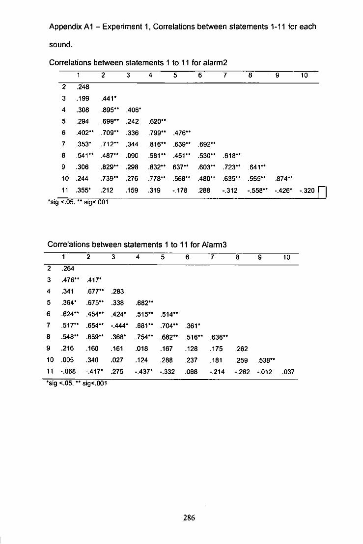
Appendix A1 - Experiment 1, Correlations between statements 1-11 for each
sound.
Conrelations between statements 1 to 11 for alarm2
1 2 3 4 5 6 7 8 9 10
2 .248
3 .199 .441* 4 .308 .895** .406* 5 .294 ,699** .242 .620** 6 .402" .709** .336 .799** .476** 7 .353* .712** .344 .816** .639** .692** 8 .541" .487** .090 .581** .451** .530** .618** 9 .306 .829** .298 .832** 637** .603** .723** .641** 10 .244 .739** .276 .778** .568** .480** .635** .555** .874** 11 .355* .212 .159 .319 -.178 .288 -.312 -.558** -.426* -.320
*sig <.05. sig<.001
Correlations between statements 1 to 11 for AIarm3
1 2 3 4 5 6 7 8 9 10 2 .264 3 .476** .417* 4 .341 .677** .283 5 .364* .675** .338 .682** 6 .624** .454** .424* .515** .514** 7 .517** .654** -.444* .681** .704** .361* 8 .548** .659** .368* .754** .682** .516** .636** 9 .216 .160 .161 .018 .167 .128 .175 .262 10 .005 .340 .027 .124 .288 .237 .181 .259 .538** 11 -.068 -.417* .275 -.437* -.332 .068 -.214 -.262 -.012 .037
'sig <.05. ** sig<.001
286
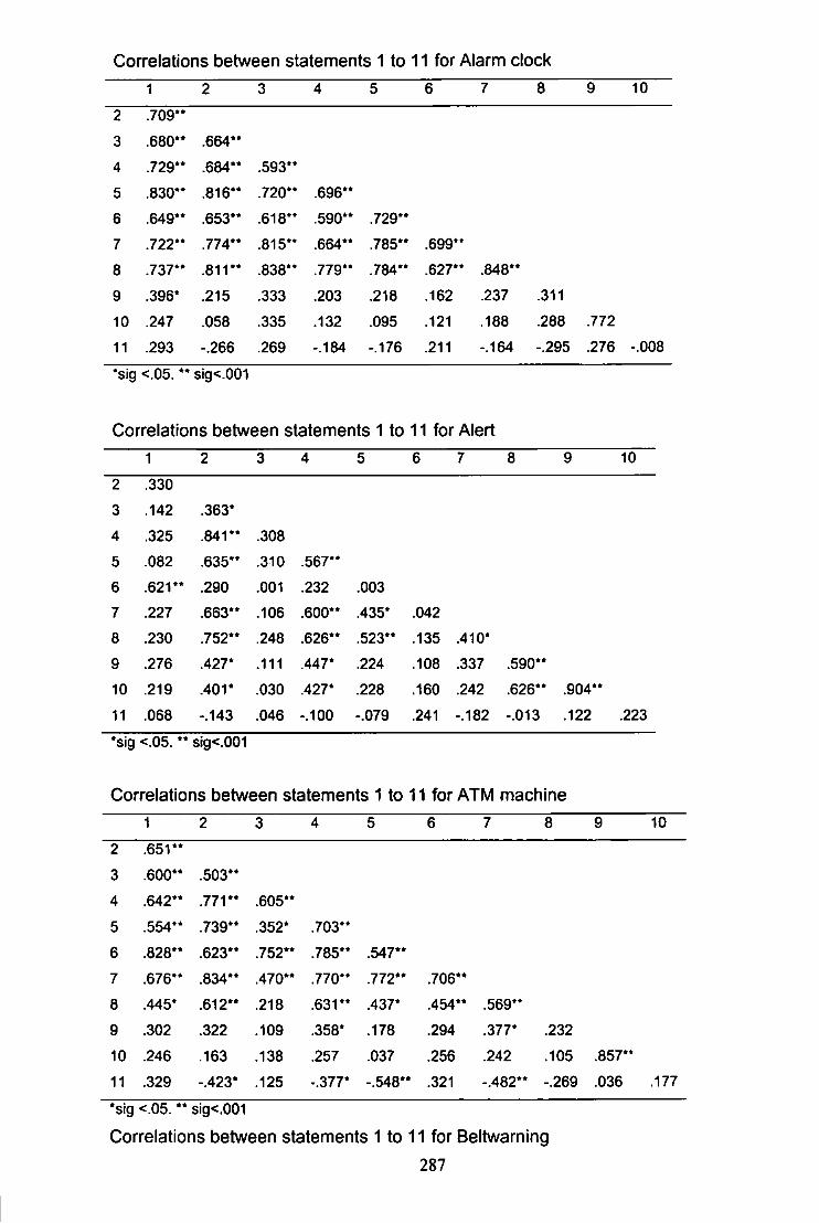
Correlations between statements 1 to 11 for Alarm clock
1 8 10
2 .709"
3 .680" .664**
4 .729" .684** .593**
5 .830" .816" .720** .696" 6 .649" .653** .618** .590** .729**
7 .722" .774** .815" .664** .785** .699*' 8 .737" .811** .838** .779** .784" .627** .848**
9 .396* .215 .333 .203 .218 .162 .237 .311
10 .247 .058 .335 .132 .095 .121 .188 .288 .772
11 .293 -.266 .269 -.184 -.176 .211 -.164 -.295 .276 -.008
*sig <.05. " sig<.001
Correlations between statements 1 to 11 for Alert
1 2 3 4 5 6 7 8 9 10
2 .330 3 .142 .363*
4 .325 .841** .308 5 .082 .635** .310 .567**
6 .621" .290 .001 .232 .003 7 .227 .663** .106 .600** .435* .042 8 .230 .752** .248 .626** .523** .135 .410* 9 .276 .427* .111 .447* .224 .108 .337 .590" 10 .219 .401* .030 .427* .228 .160 .242 .626** .904**
11 .068 -.143 .046 -.100 -.079 .241 -.182 -.013 .122 .223
*sig <.05." sig<.001
Correlations between statements 1 to 11 for ATM machine
1 2 3 4 5 6 7 8 9 10
2 .651"
3 .600" .503** 4 .642" .771" .605** 5 .554" .739** .352* .703** 6 .828" .623** .752" .785** .547**
7 .676" .834** .470" .770** .772** .706**
8 .445* .612" .218 .631** .437* .454** .569**
9 .302 .322 .109 .358* .178 .294 .377* .232
10 .246 .163 .138 .257 .037 .256 .242 .105 .857**
11 .329 -.423* .125 -.377* -.548** .321 -.482" -.269 .036 .177
•sig <.05. •* sig<.001
Correlations between statements 1 to 11 for Beltwarning
287
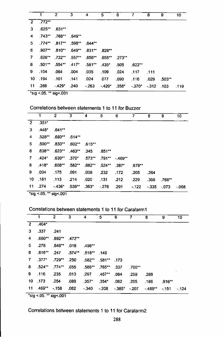
1 2 3 4 5 6 7 8 9 10 2 .772" 3 .625" .631" 4 .743" .768** .649** 5 .774" .817" .598** .644** 6 .907" .810** .649** .831" .828** 7 .626" .732** .557*' .856** .655** .273** 8 .501" .554** -417* .581** .435* .505 .622** 9 .104 .064 .004 .035 .109 .024 .117 .111 10 .194 .101 .141 .024 .077 .090 .116 .029 .503** 11 .286 -.429* .240 -.263 -.420* .358* -.370* -.312 .103 .119 *sig <.05. " sig<.001
Correlations between statements 1 to 11 for Buzzer
1 2 3 4 5 6 7 8 9 10 2 .351*
3 .448* .641** 4 .528" .693** .614" 5 .500** .830** .602** .615** 6 .638** .623** .463** .345 .651" 7 .424* .639** .370* .573** .791" -.469" 8 .418* .608** .582** .682** .524** .387* .678** 9 .004 .175 .091 .008 .232 .172 .206 .264 10 .181 .113 .214 .020 .131 .212 .229 .306 .766" 11 .274 -.436* .539** .363* -.276 .291 -.122 -.335 -.073 -.068 *sig <.05. •* sig<.001
Correlations between statements 1 to 11 for Caralarmi 1 2 3 4 5 6 7 8 9 10
2 .404* 3 .337 .241
4 .660** .692** .472** 5 .278 .649** .018 .496** 6 .616** .247 .574** .518" .146 7 .377* .729** .250 .582** .581" .173 8 .524** .774** .055 .586** .765** .337 .700** 9 .116 .235 .013 .297 .467** .064 .259 .288 10 .173 .254 .089 .357* .354* .062 .205 .186 .916" 11 .469** -.158 .062 -.340 -.208 -.385* -.207 -.489** -.151 -.124 *sig <.05. ** sig<.001
Correlations between statements 1 to 11 for Caralarm2
288
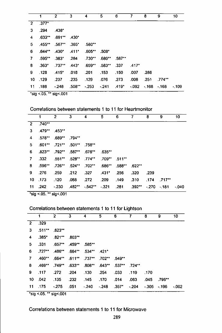
1 2 3 4 5 6 7 8 9 10
2 .377*
3 .294 .438*
4 .633** .691** .430*
5 .455** .567** .365* .580** 6 .644** .430* .411* .605** .508*
7 .595** .383* .284 .730** .680** .587*'
8 .363* .737** .443* .659** .583** .337 .417*
9 .128 .415* .018 .201 .153 .150 .007 .286
10 .129 .237 .235 .129 .076 .273 .008 .251 .774**
11 .188 -.248 .508** -.253 -.241 .419* -.092 -.168 -.168 -.109
*sig <.05. ** sig<.001
Correlations between statements 1 to 11 for Heartmonitor
1 2 3 4 5 6 7 8 9 10
2 .740** 3 .479** .453**
4 .578** .689** .794**
5 .601** .721** .501** .758** 6 .823** .792** .587** .678** .635** 7 .332 .551** .528** .774** .709** .511** 8 .596** .726** .524** .702** .686** .588** .622** 9 .276 .259 .212 .327 .431* .256 .320 .239 10 .173 .120 .068 .272 .209 .149 .310 .174 .717** 11 .242 -.230 .482** -.542** -.321 .281 .392** -.270 -.181 -.040
*slg <.05. ** sig<.001
Correlations between statements 1 to 11 for Lightson
1 2 3 4 5 6 7 8 9 10
2 .329
3 .511** .623**
4 .385* .821** .803** 5 .331 .657** .459** .585** 6 .727** .486** .664** .534** .421* 7 .460** .664** .611** .737** .702** .549** 8 .469** .749** .633** .808** .643** .537** .724** 9 .117 .272 .204 .130 .254 .033 .119 .170 10 .042 .135 .232 .145 .170 .014 .063 .045 .796** 11 .175 -.275 .051 -.240 -.248 .357* -.204 -.305 -.196 -.002
*sig <.05. ** sig<.001
Correlations between statements 1 to 11 for Microwave
289
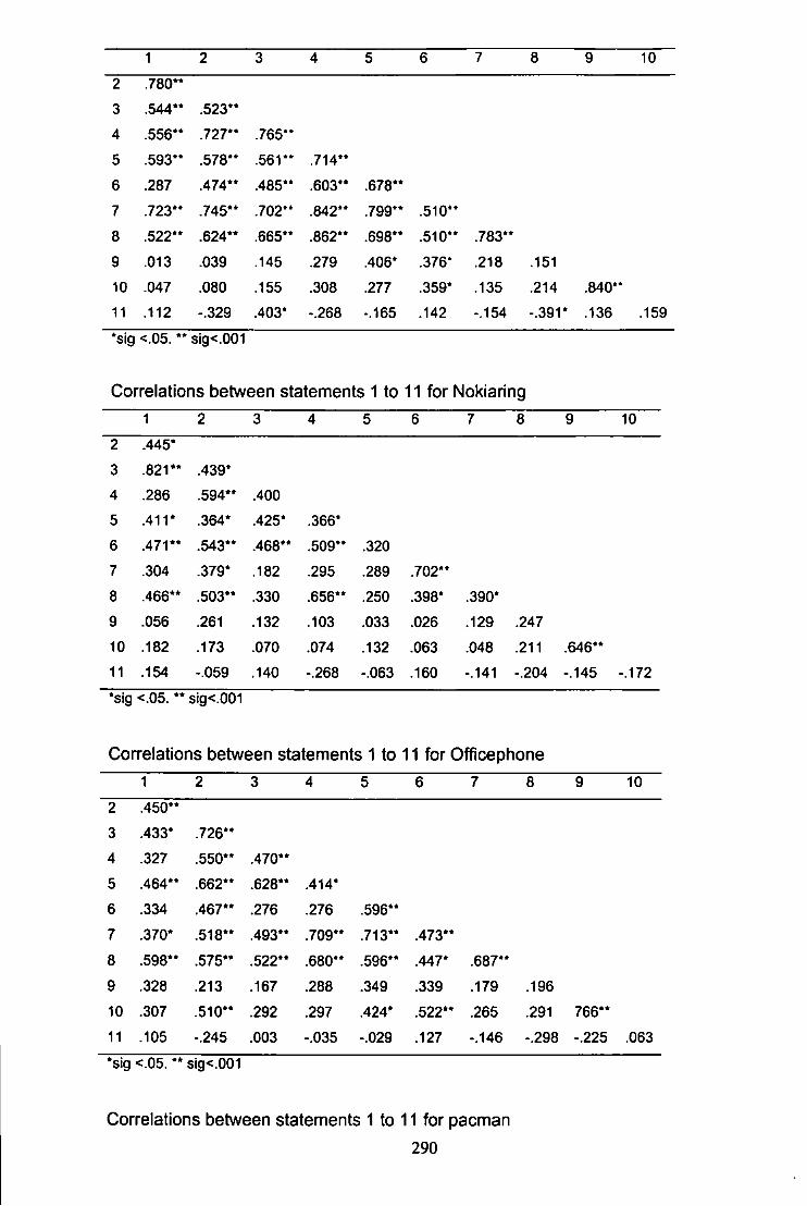
1 2 3 4 5 6 7 8 9 10
2 .780** 3 .544** .523"
4 .556** .727** .765" 5 .593" .578" .561" .714" 6 .287 .474** .485" ,603** .678** 7 .723** .745** .702" .842** .799** .510** 8 .522" .624** .665** .862** .698** .510** .783**
9 .013 .039 .145 .279 .406* .376* .218 .151 10 .047 .080 .155 .308 ,277 .359* .135 .214 .840' 11 .112 -.329 .403* -.268 -.165 ,142 -.154 -.391* .136 .159
*sig <.05. ** sig<.001
Correlations between statements 1 to 11 for Nokiaring
1 2 3 4 5 6 7 8 9 10
2 .445* 3 .821** .439* 4 .286 .594** .400 5 .411* .364* .425* .366* 6 .471" .543" .468** .509" .320 7 .304 .379* .182 -295 .289 .702** 8 .466** .503** .330 .656** .250 .398* .390* 9 .056 .261 .132 .103 .033 .026 .129 .247 10 .182 .173 .070 .074 .132 .063 .048 .211 .646** 11 .154 -.059 .140 -.268 -.063 .160 -.141 -.204 -.145 -.172 •sig <.05. " sig<.001
Correlations between statements 1 to 11 for Officephone
1 2 3 4 5 6 7 8 9 10
2 .450** 3 .433* .726" 4 .327 .550" .470** 5 .464** .662** .628** .414* 6 .334 .467** .276 .276 .596** 7 .370* .518" .493** .709** .713" .473** 8 .598** .575** .522" .680** .596** .447* .687** 9 .328 .213 .167 .288 .349 .339 .179 .196 10 .307 .510" .292 .297 .424* .522** .265 .291 766** 11 .105 -.245 .003 -.035 -.029 .127 -.146 -.298 -.225 .063
*sig <.05. ** sig<.001
Correlations between statements 1 to 11 for pacman
290
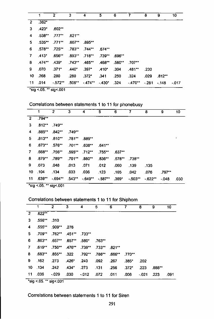
1 2 3 4 5 6 7 8 9 10 2 .362*
3 .423* .602** 4 .538** .777** .621** 5 .535** .771** .607** .895** 6 .578** .725** .783** .744** .674** 7 .413* .656** .893** .718** .739** .696** 8 .474** .439* .743** .465** .468** .580** .707** 9 .070 .371* .440* .397* .410* .304 .481** .230 10 .268 .280 .280 .372* .341 .250 .324 .029 .812** 11 .014 -.572** .506** -.474** -.430* .324 -.470** -.281 -.148 -.017
*sig <.05. ** sig<.001
Correlations between statements 1 to 11 for phonebusy 1 2 3 4 5 6 7 8 9 10
2 .794**
3 .812** .749** 4 .885** .842** .749** 5 .813** .810** .781** .889** -
6 .673'* .576** .701** .638** .641** 7 .668** .756** .595** .712** .755** .637** 8 .879** .789** .701** .880** .836** .578** .738** 9 .073 .048 .013 .071 .012 .060 .139 .135 10 .104 .134 .033 .036 .123 .105 .042 .076 .797** 11 .639** -.694** .543** -.649** -.587* ' .389* -.503** -.622** -.048 .030 •sig <.05. ** srg<.001
Correlations between statements 1 to 11 for Shiphorn 1 2 3 4 5 6 7 8 9 10
2 .622**
3 .556** .310
4 .555** .909** .276 5 .709** .762** .451** .733** 6 .863** .657** .657** .580* .763** 7 .619** .750** .476** .739** .733** .821** 8 .683** .855** .322 .792** .786** .666** .770** 9 .162 .273 .426* .240 .092 .267 .385* .202 10 .134 .242 .434* .273 .131 .256 .372* .223 .888** 11 .036 -.029 .030 -.012 .072 .011 .006 -.021 .223 .091
*sig <.05. ** sig<.001
Correlations between statements 1 to 11 for Siren
291
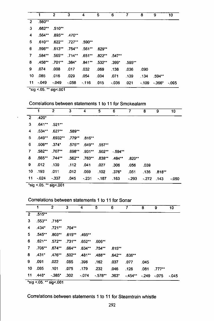
1 2 3 4 5 6 7 8 9 10 2 .560** 3 .662** .510** 4 .564** .895** .470** 5 .610** .622** .727** .590** 6 .596** .613** .754** .561** .629** 7 .584** .565** .714** .651** .822** .547** 8 .458** .701** .384* .841** .532** .399* .595** 9 .074 .008 .017 .032 .069 .138 .036 .090 10 .085 .016 .029 .054 .004 .071 .139 .134 .594** 11 -.049 -.049 -.058 -.116 .015 -.036 .021 -.109 -.366* -.095 *sig <.05. ** sig<.001
Correlations between statements 1 to 11 for Smokealarm
1 2 3 4 5 6 7 8 9 10 2 .420* 3 .641** .521** 4 .534** .627** .589** 5 ,549** .6932** .779** .816** 6 .506** .374* .575** .649** .557** 7 .582** .707** .698** .931** .902** -.594** 8 .565** .744** .562** .763** .838** .484** .820** 9 .012 .139 .112 .041 .027 .306 .056 .039 10 .193 .011 .012 .059 .102 .376* .051 .136 .818** 11 -.024 -.337 .045 -.231 -.187 .163 -.293 -.272 .143 -.050 *sig <.05. ** sig<.001
Correlations between statements 1 to 11 for Sonar
1 2 3 4 5 6 7 8 9 10 2 .515**
3 .553** .716** 4 .434* .721** .704** 5 .545** .803** .615** .495** 6 .621** .572** .731** .652** .605** 7 .706** .674** .664** .634** .754** .815** 8 .431* .476** .502** .481** .488** .642** .636** 9 .091 .022 .065 .396 .162 .037 .077 .045 10 .065 .101 .075 .179 .232 .046 .126 .081 .777** 11 .448* -.385* .302 -.074 -.578** .363* -.454** -.249 -.075 -.045 •sig <.05. ** sig<.001
Correlations between statements 1 to 11 for Steamtrain whistle
292
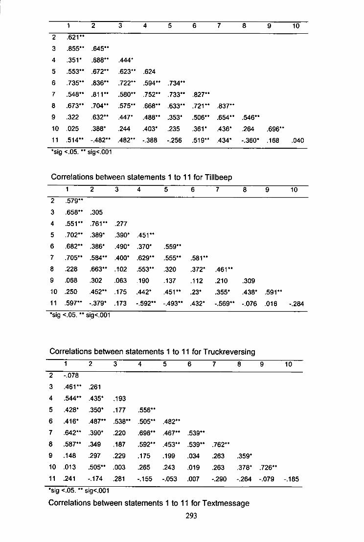
1 2 3 4 5 6 7 8 9 10 2 .621"
3 .855" .645" 4 .351* .688" .444*
5 .553" .672" .623** .624
6 .735" .836" .722** .594" .734** 7 .548" .811" .580** .752" .733** .827** 8 .673" .704" .575** .668** .633" .721" .837** 9 .322 .632" .447' .488** .353* .506** .654** .546" 10 .025 .388* .244 .403* .235 .361* .436* .264 .696** 11 .514" -.482" .482*' -.388 -.256 .519" .434* -.360* .168 .040 *sig <.05. " sig<.001
Correlations between statements 1 to 11 for Tillbeep
1 2 3 4 5 6 7 8 9 10 2 .579" 3 .658" .305 4 .551" .761" .277 5 .702" .389* .390* .451" 6 .682" .386* .490* .370* .559** 7 .705" .584** .400* .629** .555** .581" 8 .228 .663** .102 .553** .320 .372* .461** 9 .068 .302 .063 .190 .137 .112 .210 .309 10 .250 .452" .175 .442* .451" .23* .355* .438* .591** 11 .597" -.379* .173 -.592" -.493** .432* -.569** -.076 .016 -.284
*sig <.05. •* sig<.001
Correlations between statements 1 to 11 for Truckreversing
1 2 3 4 5 6 7 8 9 10 2 -.078 3 .461" .261 4 .544** .435* .193 5 .428* .350* .177 .556** 6 .416* .487** .538" .505** .482** 7 .642** .390* .220 .698** .467** .539** 8 .587** .349 .187 .592** .453** .539** .762** 9 .148 .297 .229 .175 .199 .034 .263 .359* 10 .013 .505** .003 .265 .243 .019 .263 .378* .726** 11 .241 -.174 .281 -.155 -.053 .007 -.290 -.264 -.079 -.185
'sig <.05. ** sig<.001
Correlations between statements 1 to 11 for Textmessage
293
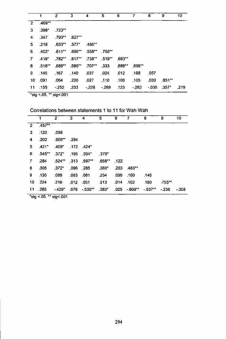
1 2 3 4 5 6 7 8 9 10
2 .469" 3 .398* .723** 4 .347 .793** .627**
5 .218 .633** .577* .486** 6 .402* .611** .696** .558** .750**
7 .419* .782** .617** .738** .519** .683**
8 .518** .689** .680** .707** .333 .689** .696**
9 .145 .167 .140 .037 .024 .012 .188 .057
10 .091 .064 .200 .027 .110 .108 .105 .030 .851** 11 .155 -.252 .233 -.226 -.299 .123 -.283 -.030 .357* .219
*sig <.05. ** sig<.001
Correlations between statements 1 to 11 for Wah Wah 1 2 3 4 5 6 7 8 9 10
2 .457**
3 .120 .059 4 .202 .606** .294 5 .421* .409* .172 .424*
6 .545** .372* .195 .394* .370* 7 .284 .524** .313 .597** .656** .122 8 .305 .372* .096 .285 .360* .203 .483** 9 .130 .088 .093 .081 .254 .096 .160 .146 10 .224 .216 .012 .051 .213 .014 .102 .180 .755** 11 .285 -.429* .079 -.530** .383* .025 -.609** -.537** -.236 -.308
sig <.05. ** sig<.001
294
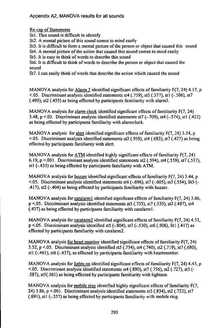
Appendix A2, MANOVA results for all sounds
Re-cap of Statements St l . This sound is difficult to identify St2. A mental picture of this sound comes to mind easily St3. It is difficult to form a mental picture of the person or object that caused this sound St4. A mental picture of the action that caused this sound comes to mind easily St5. It is easy to think of words to describe this sound St6. It is difficult to think of words to describe the person or object that caused the sound St7.1 can easily think of words that describe the action which caused the sound
MANOVA analysis for Alarm 3 identified significant effects of familiarity F(7, 24) 4.17, p <.05. Discriminant analysis identified statements st4 (.759), st5 (.577), stl (-.506), st7 (.490), st2 (.455) as being effected by participants familiarity with alarm3.
MANOVA analysis for alarm clock identified significant effects of familiarity F(7, 24) 3.48, p <.05. Discriminant analysis identified statements st7 (-.709), st4 (-.574), stl (.423) as being effected by participants familiarity with alarmclock.
MANOVA analysis for alert identified significant effects of familiarity F(7, 24) 3.54, p <.05. Discriminant analysis identified statements st2 (.950), st4 (.683), st7 (.427) as being effected by participants familiarity with alert.
MANOVA analysis for ATM identified highly significant effects of familiarity F(7, 24) 6.19, p <.001. Discriminant analysis identified statements st2 (.594), st4 (.559), st7 (.537), stl (-.435) as being effected by participants familiarity with ATM.
MANOVA analysis for buzzer identified significant effects of familiarity F(7, 24) 3.44, p <.05. Discriminant analysis identified statements st4 (-.696), st7 (-.605), st3 (.554), St5 (-.417), st2 (-.404) as being effected by participants familiarity with buzzer.
MANOVA analysis for caralarm I identified significant effects of familiarity F(7, 24) 3.86, p <.05. Discriminant analysis identified statements st5 (.755), st7 (.535), st2 (.487), st4 (.437) as being effected by participants familiarity with caralarm I.
MANOVA analysis for caralarm2 identified significant effects of familiarity F(7, 24) 4.53, p <.05. Discriminant analysis identified st5 (-.804), st7 (-.530), st6 (.506), Stl (.417) as effected by participants familiarity with caralarm2.
MANOVA analysis for heart monitor identified significant effects of familiarity F(7, 24) 3.52, p <.05. Discriminant analysis identified st5 (.754), st4 (.740), st2 (.719), st7 (.680), stl (-.461), st6 (-.437), as effected by participants familiarity with heartmonitor.
MANOVA analysis for lights on identified significant effects of familiarity F(7, 24) 4.45, p <.05. Discriminant analysis identified statements st4 (.890), st7 (.756), st2 (.727), st3 (-,587), st5(.561) as being effected by participants familiarity with lightson.
MANOVA analysis for mobile ring identified highly significant effects of familiarity F(7, 24) 3.86, p <.001. Discriminant analysis identified statements st5 (.834), st2 (.723), st7 (.691), stl (-.557) as being effected by participants familiarity with mobile ring.
295
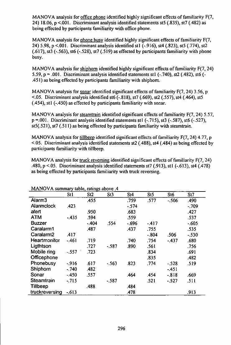
MANOVA analysis for office phone identified highly significant effects of familiarity F(7, 24) 18.06, p <.001. Discriminant analysis identified statements st5 (.835), st7 (.482) as being effected by participants familiarity with office phone.
MANOVA analysis for phone busy identified highly significant effects of familiarity F(7, 24) 5.98, p <.001. Discriminant analysis identified stl (-.916), st4 (.823), st5 (.774), st2 (.617), st3 (-.563), st6 (-.528), st7 (.519) as effected by participants familiarity with phone busy.
MANOVA analysis for shiphom identified highly significant effects of familiarity F(7, 24) 5.59, p = .001. Discriminant analysis identified statements stl (-.740), sl2 (.482), st6 (-.451) as being effected by participants familiarity with shiphom.
MANOVA analysis for sonar identified significant effects of familiarity F(7, 24) 3.56, p <.05. Discriminant analysis identified st6 (-.818), st7 (.669), st2 (.557), st4 (.464), st5 (.454), stl (-.450) as effected by participants familiarity with sonar.
MANOVA analysis for steamtrain identified significant effects of familiarity F(7, 24) 5.57, p =.001. Discriminant analysis identified statements stl (-.715), st3 (-.587), st6 (-.527), st5(.521), st7 (.511) as being effected by participants familiarity with steamtrain.
MANOVA analysis for tillbeep identified significant effects of familiarity F(7, 24) 4.77, p <.05. Discriminant analysis identified statements st2 (.488), st4 (.484) as being effected by participants familiarity with tillbeep.
MANOVA analysis for truck reversing identified significant effects of familiarity F(7, 24) .480, p <.05. Discriminant analysis identified statements st7 (.913), stl (-.613), st4 (.478) as being effected by participants familiarity with truck reversing.
MANOVA summary table, ratings above .4 Stl St2 St3 St4 St5 St6 St7
Alarms .455 .759 .577 -.506 .490 Alarmclock .423 -.574 -.709 alert .950 .683 .427 ATM -.435 .594 .559 .537 Buzzer -.404 .554 -.696 -.417 -.605 Caralarmi .487 .437 .755 .535 Caralarm2 .417 -.804 .506 -.530 Heartmonitor -.461 .719 .740 .754 -.437 .680 Ligthtson .727 -.587 .890 .561 .756 Mobile ring -.557 .723 .834 .691 Officephone .835 .482 Phonebusy -.916 .617 -.563 .823 .774 -.528 .519 Shiphorn -.740 .482 -.451 Sonar -.450 .557 .464 .454 -.818 .669 Steamtrain -.715 -.587 .521 -.527 .511 Tillbeep .488 .484 truckreversing -.613 .478 .913
296
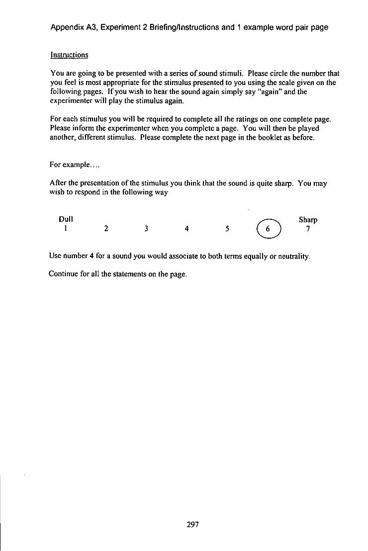
Appendix A3, Experiment 2 Briefing/Instructions and 1 example word pair page
Instructions
You are going to be presented with a series of sound stimuli. Please circle the number that you feel is most appropriate for the stimulus presented to you using the scale given on the following pages. If you wish to hear the sound again simply say "again" and the experimenter will play the stimulus again.
For each stimulus you will be required to complete all the ratings on one complete page. Please inform the experimenter when you complete a page. You will then be played another, different stimulus. Please complete the next page in the booklet as before.
For example....
After the presentation of the stimulus you think that the sound is quite sharp. You may wish to respond in the following way
Dull ^ — ^ Sharp
1 2 3 4 ^ C ) ^ Use number 4 for a sound you would associate to both terms equally or neutrality.
Continue for all the statements on the page.
297
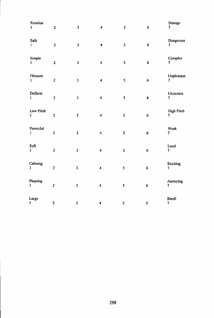
Familiar 1
Strange 7
Safe I
Dangerous 7
Simple I
Complex 7
Pleasant 1
Unpleasant 7
Definite 1
Uncertain 7
Low Pitch 1
High Pitch 7
Powerful 1
Weak 7
Soft 1
Loud 7
Calming I
Exciting 7
Pleasing I
Annoying 7
Large I
Small 7
298
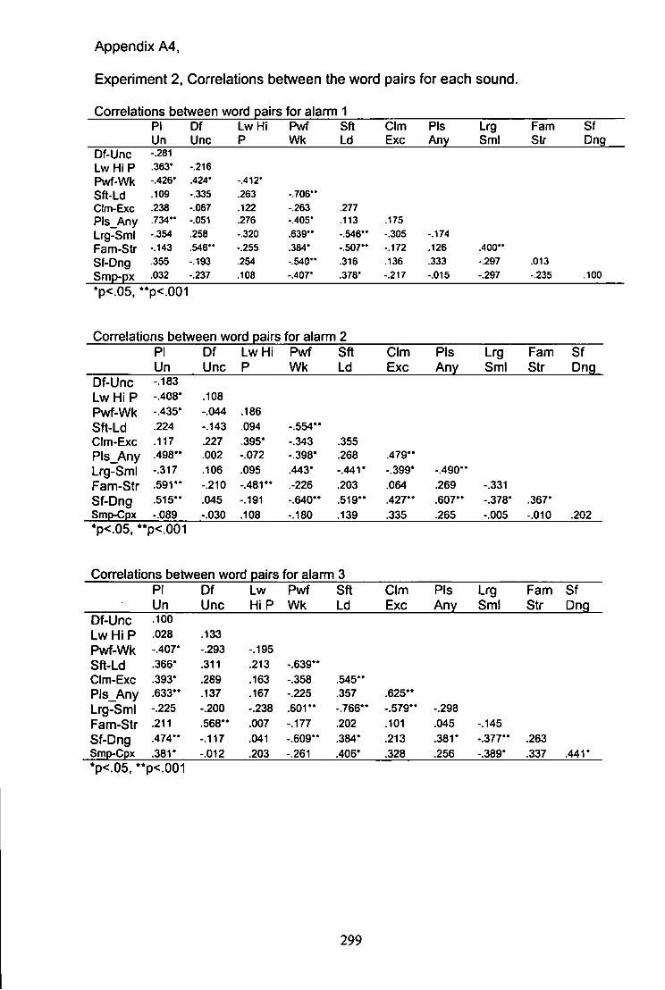
Appendix A4,
Experiment 2. Correlations between the word pairs for each sound.
Correlations between word pairs for alarm 1 PI Of Lw Hi Pwf Sft CIm PIs Lrg Fam Sf Un Unc P Wk Ld Exc Any SmI Str Dng
Df-Unc -.281
Lw HiP .363* -.216
Pwf-Wk -.426' .424' -.412'
Sft-Ld .109 -.335 .263 - .706"
CIm-Exc .238 -.067 .122 -.263 .277
Pls_Any .734*' -.051 .276 -.405* .113 .175
Lrg-SmI -.354 .258 -.320 .639" -.546*' -.305 -.174
Fam-Slr -.143 .546" -.255 .384* - .507" -.172 .126 .400*'
Sf-Dng .355 -.193 .254 - .540" .316 .136 .333 -.297 .013
Smp-px .032 -.237 .108 -.407' .378' -.217 -.015 -.297 -.235 .100
*P<.05.' *p<.001
Correlations between word pairs for alarm 2 PI Df Lw Hi Pwf Sft CIm PIs Lrg Fam Sf Un Unc P Wk Ld Exc Any SmI str Dng
Df-Unc -.183 Lw HiP -.408* .108 Pwf-Wk -.435' -.044 .186 Sft-Ld .224 -.143 .094 -.554" CIm-Exc .117 .227 .395* -.343 .355 Pls_Any .498" .002 -.072 -.398* .268 .479" Lrg-SmI -.317 .106 .095 .443' -,441* -.399' -.490" Fam-Str .59V* -.210 -.481** .-226 .203 .064 .269 -.331 Sf-Dng .515'* .045 -.191 -.640** .519" .427" .607" -.378' .367* Smp-Cpx -.089 -.030 .108 -.180 .139 .335 .265 -.005 -.010 .202 •p<.05. * *p<.001
Correlations between word pairs for alarm 3 PI Df Lw Pwf Sft CIm PIs Lrg Fam Sf Un Unc Hi P Wk Ld Exc Any SmI Str Dng
Df-Unc .100 Lw HiP .028 .133 Pwf-Wk -.407' -.293 -.195 Sft-Ld .366' .311 .213 -.639** CIm-Exc .393* .289 .163 -.358 .545" Pls_Any .633" .137 .167 -.225 .357 .625** Lrg-SmI -.225 -.200 -.238 .601" -.766" -.579*' -.298 Fam-Str .211 .568** .007 -.177 .202 .101 .045 -.145 Sf-Dng .474'* -.117 .041 -.609" .384* .213 .381* -.377" .263 Smp-Cpx .381* -.012 .203 -.261 .406* .328 .256 -.389' .337 .441' *p<.05, **p<.001
299
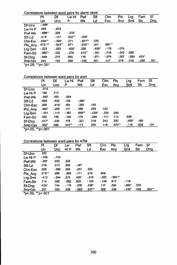
Correlations between word pairs for alarm clock PI Df Lw Hi Pwf Sft CIm Pis Lrg Fam Sf Un Unc P Wk Ld Exc Any SmI Str Dng
Df-Unc -.408* Lw HiP .255 -.072 Pwf-Wk -.688*' .326 -.378' Sft-Ld .413* -.147 .552" -.450' CIm-Exc .534" -.394' .271 -.621" .335 Pls_Any 0721** -.543" .071 -.615" .341 .681" Lrg-SmI -.223 -.032 -.400* .329 -.456* -.178 -.074 Fam-Str -.562** .332 -.270 .513" -.361 -.216 -.342 .020 Sf-Dng -.048 .274 .094 .116 -.071 -.076 -.207 -.095 .424* Smp-Cpx .245 .163 .098 -.250 .001 .147 .079 .019 -.080 .351 *P<.05, * *p<.001
Correlations between word pairs for alert PI Df Lw Hi Pwf Sft CIm Pis Lrg Fam Sf Un Unc P Wk Ld Exc Any SmI Str Dng
Df-Unc -.016 Lw HiP .180 .212 Pwf-Wk -.097 .103 -.004 Sft-Ld .089 -.025 .156 -.386' CIm-Exc .066 -.416' .165 -.265 .126 Pls_Any .390' -.206 .117 .288 .259 .143 Lrg-SmI -.101 -.113 -.167 .658" -.429* -.335 .046 Fam-Str .355 .166 -.154 .176 -.208 -.117 .115 .036 Sf-Dng .417* -.032 .178 -.327 .318 .243 .292 -.459' .195 Smp-Cpx .362* .088 .543" .173 .225 .116 .570" -.119 .028 .124 *p<.05. **p<.001
Correlations between word pairs for ATM PI Df Lw Pwf Sft CIm PIs Lrg Fam Sf Un Unc HiP Wk Ld Exc Any SmI Str Dng
Df-Unc .222 Lw HiP -.028 -.134 Pwf-Wk -.207 .030 .225 Sfl-Ld .218 .213 .265 -.187 CIm-Exc .025 -.266 .263 -.257 .325 Pls_Any .516" .290 -.093 -.171 .219 .049 Lrg-SmI -.413 -.344 .275 .435' -.218 -.322 -.581" Fam-Str .114 .300 -.082 .020 -.120 -.146 .012 -.119 Sf-Dng .436' .144 -.170 -.238 .436* .117 .294 -.386* .035 Smp-Cpx .257 .359 .038 -.389' .537" .308 .338 -.439' .048 .504** *p<.05. * *p<.001
300

Correlations between word pairs for belt waming PI Df Lw Pwf Sft CIm Pis Lrg Fam Sf Un Unc HiP Wk Ld Exc Any Sm! Str Dng
Df-Unc .556* Lw HiP .284 .153 Pwf-Wk .228 .166 -.186 Sft-Ld .360 .015 .225 -.211 CIm-Exc .319 .425* -.033 .274 .325 Pls_Any .559" .384* .092 .118 .222 .616" Lrg-SmI -.027 .096 .084 .451' -.168 -.106 -.069 Fam-Str .367* .356 -.014 .460' .154 .318 .181 .303 Sf-Dng .542'* .309 -.021 .549** .149 .453' .434* .113 .721** Smp-Cpx .273 .156 .256 -.092 .355 .078 .217 -.145 .197 .274 *P<.05, * *p<.001
Correlations between word pairs for buzzer PI Df Lw Pwf Sft CIm Pis Lrg Fam Sf Un Unc HIP Wk Ld Exc Any SmI Str Dng
Df-Unc .076 Lw HiP .232 .392* Pwf-Wk -.235 .251 .187 Sft-Ld .291 -.003 .174 -.360 CIm-Exc .367* .037 .405* -.275 .265 Pls_Any .685" .048 .140 -.005 .187 .504" Lrg-Smi -.306 .409* .081 .605*' -.503'* -.403' -.182 Fam-Str -.083 .023 -.090 -.081 -.166 .106 .000 .152 Sf-Dng .263 .138 .152 -.106 .375* .252 .104 -.314 -.183 Smp-Cpx .043 .143 .457* .160 -.152 .302 .138 .009 .160 -.112 *p<.05, **p<.001
Correlations between word pairs for caralarmi PI Df Lw Hi Pwf Sft CIm Pis Lrg Fam Sf Un Unc P Wk Ld Exc Any SmI Str Dng
Df-Unc Lw HiP Pwf-Wk Sft-Ld CIm-Exc Pls_Any Lrg-SmI Fam-Str Sf-Dng Smp-Cpx
-.318 .665*' -.518' .318 .506** .574** -.112 .040 .306 .368*
-.393* .203 -.118 -.189 -.276 -.031 .328 .071 -.085
-.520*' .356 .506** .532** -.209 -.213 .140 .399*
-.639" -.885** -.459* .546" .028 -.287 -.296
.626"
.390* -.539" .029 .327 .285
.426* -.595' .075 .379* .342
-.168 .041 -.079 .028 -.429' .209 -.474'
.305
.069 .545* •p<.05. "p<.001
301

Correlations between word pairs for caralann2 PI Df Lw Pwf Sft CIm Pis Lrg Fam Sf Un Una HIP Wk Ld Exc Any SmI Str Dng
Df-Unc -.205 Lw Hi P .126 -.102 Pwf-Wk -.387* .342 -.068 Sft-Ld .466*' -.514" .032 -.586" CIm-Exc .394* -.354 .314 -.231 .378* Pls_Any .549" -.372' .145 -.245 .296 .216 Lrg-SmI -.503" .701" -.109 .610" -.705" -.316 -.402' Fam-Str -.060 .442* .137 .260 -.376' -.074 -.141 .316 Sf-Dng .176 -.313 .315 -.198 .126 .253 .089 -.259 .028 Smp-Cpx .501" -.650" .124 -.443' .522" .375* .314 -.580" -.198 .374' *P<.05. * *p<.001
Correlations between word pairs for chimes PI Df Lw Pwf Sft CIm Pis Lrg Fam Sf Un Unc HiP Wk Ld Exc Any SmI Str Dng
Df-Unc .381* Lw HI P .051 -.240 Pwrf-Wk -.042 .538" -.183 Sft-Ld .331 -.069 .164 -.347 CIm-Exc .244 -.120 .276 -.095 .434' Pls_Any .880" .308 .237 .045 .151 .327 Lrg-SmI -.238 -.093 -.133 -.004 -.358 -.540" -.207 Fam-Str .391* .332 -.141 .082 .317 .287 .248 .128 Sf-Dng .229 .239 .062 .123 .277 .279 .197 .074 .666" Smp-Cpx .409' .234 -.006 -.130 .211 .249 .322 -.381* .018 -.073 *p<.05. **p<.001
Correlations between word pairs for dive PI Df Lw Pwf Sft CIm Pis Lrg Fam Sf Un Unc HIP Wk Ld Exc Any SmI Str Dng
Df-Unc -.033 Lw HiP -.140 .320 Pwf-Wk -.363' .639" .207 Sft-Ld .180 -.279 .050 -.269 CIm-Exc .243 -.409* .081 -.407' .477" Pls_Any .728" -.031 -.061 -.202 -.029 .077 Lrg-SmI -.170 .454' .211 .622" -.355 -.266 .119 Fam-Str -.039 .611" .334 .544" -.302 -.329 .094 .466" Sf-Dng .107 -.294 .159 -.264 .165 .335 .271 -.062 -.029 Smp-Cpx .428' .051 .341 -.271 .248 .384* .441* .003 .059 .158 •p<.05, **p<.001
302
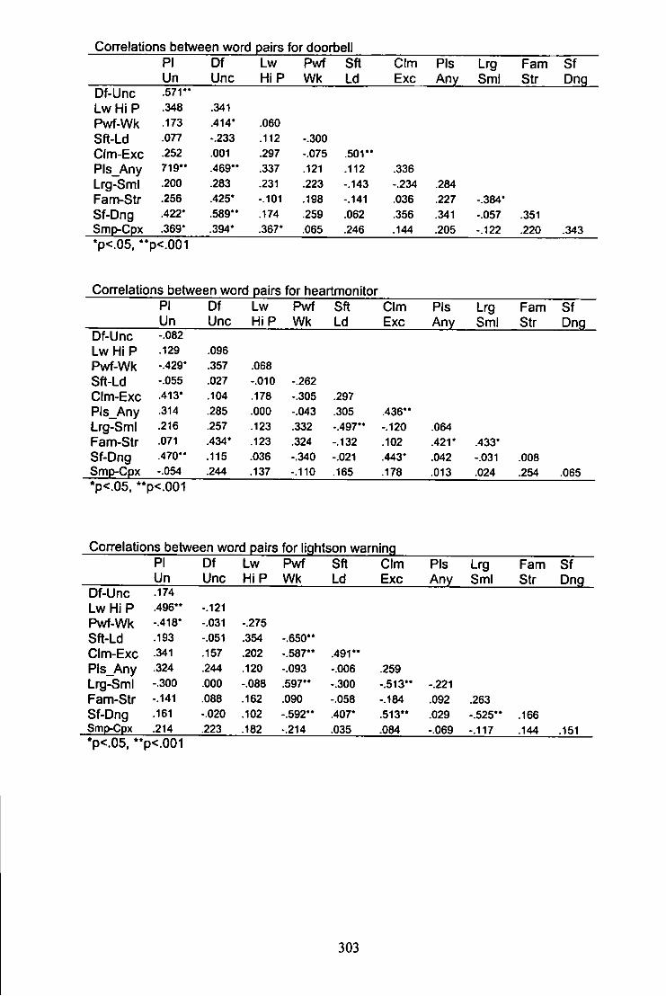
CoH'elations between word pairs for doorbell PI Df Lw Pwf Sft CIm Pis Lrg Fam Sf Un Unc HiP Wk Ld Exc Any SmI Str Dng
Df-Unc .571" Lw HiP .348 .341 Pwf-Wk .173 .414' .060 Sft-Ld .077 -.233 .112 -.300 CIm-Exc .252 .001 .297 -.075 .501" Pls_Any 719" .469" .337 .121 .112 .336 Lrg-SmI .200 .283 .231 .223 -.143 -.234 .284 Fam-Str .256 .425* -.101 .198 -.141 .036 .227 -.384' Sf-Dng .422* .589*' .174 .259 .062 .356 .341 -.057 .351 Smp-Cpx .369' .394* .367' .065 .246 .144 .205 -.122 .220 .343 *p<.05. p<.001
Correlations between word pairs for heartmonitor PI Df Lw Pwf Sft CIm Pis Lrg Fam Sf Un Unc HiP Wk Ld Exc Any SmI Str Dng
Df-Unc -.082 Lw HiP .129 .096 Pwf-Wk -.429' .357 .068 Sft-Ld -.055 .027 -.010 -.262 CIm-Exc .413' .104 .178 -.305 .297 Pls_Any .314 .285 .000 -.043 .305 .436** Lrg-SmI .216 .257 .123 .332 -.497" -.120 .064 Fam-Str .071 .434* .123 .324 -.132 .102 .421' .433* Sf-Dng .470" .115 .036 -.340 -.021 .443' .042 -.031 .008 Smp-Cpx -.054 .244 .137 -.110 .165 .178 .013 .024 .254 .065 *p<.05, "p<.001
Correlations between word pairs for lightson warning PI Df Lw Pwf Sft CIm Pis Lrg Fam Sf Un Unc HiP Wk Ld Exc Any SmI Str Dng
Df-Unc .174 Lw HiP .496** -.121 Pwf-Wk -.418* -.031 -.275 Sft-Ld .193 -.051 .354 -.650" CIm-Exc .341 .157 .202 -.587** .491" Pls_Any .324 .244 .120 -.093 -.006 .259 Lrg-SmI -.300 .000 -.088 .597** -.300 -.513" -.221 Fam-Str -.141 .088 .162 .090 -.058 -.184 .092 .263 Sf-Dng .161 -.020 .102 -.592" .407* .513" .029 -.525'* .166 Smp-Cpx .214 .223 .182 -.214 .035 .084 -.069 -.117 .144 .151 *p<,05, p<.001
303

Correlations between word pairs for microwave ding PI Df Lw Pwf Sft CIm PIs Lrg Fam Sf Un Unc HiP Wk Ld Exc Any SmI Str Dng
Df-Unc .296 Lw HiP .455* .114 Pwf-Wk -.315 .348 -.318 Sft-Ld .607" -.055 .455' -.678** CIm-Exc .485" .083 .320 -.538** .599" Pls_Any .862" .338 .383* -.253 .506*' .406' Lrg-SmI -.075 .341 -.003 .659** -.417' -.344 .052 Fam-Str .325 .433* .320 -.134 .257 .104 .473" .115 Sf-Dng -.525** .110 .252 -.247 .344 .237 .537** -.127 .562" Smp-Cpx .203 .374' -.115 .158 -.029 -.178 .176 -.026 .484* .298 *p<.05, * *p<.001
Correlations between word pairs for mobilering PI Df Lw Pwf Sft CIm PIs Lrg Fam Sf Un Unc HiP Wk Ld Exc Any SmI Str Dng
Df-Unc .390' Lw HiP .278 .444* Pwf-Wk .233 .580* .262 Sft-Ld .248 -.126 .274 -.256 CIm-Exc .110 -.092 -.241 -.076 .482" Pls_Any .611" -.051 -.054 .078 .463" .331 Lrg-SmI -.217 .330 .108 .277 -.627** -.220 -.347 Fam-Str .303 .375' .155 .356 -.158 -.046 .021 .005 Sf-Dng .376* .251 -.020 .251 -.137 -.085 .176 -.215 .605" Smp-Cpx .396' .316 .232 .237 -.005 -.183 .106 -.216 .397' .642 *p<.05, * 'p<.001
Correlations between word pairs for nokiaring PI Df Lw Pwf Sft CIm PIs Lrg Fam Sf Un Unc HiP Wk Ld Exc Any SmI str Dng
Df-Unc -.155 Lw Hi P .053 -.108 Pwf-Wk .272 .349 -.056 Sft-Ld .243 -.280 .399* -.194 CIm-Exc -.004 .077 -.094 .019 .359 Pls_Any .462' -.068 .050 .354 .299 -.013 Lrg-SmI -.018 .156 -.007 .383' -.484" -.411* -.105 Fam-Str .291 .173 -.227 .006 .025 .108 .080 -.252 Sf-Dng .502" .233 -.057 .059 .018 .208 .085 -.271 .607** Smp-Cpx .146 .133 -.171 .171 -.212 .178 -.137 .006 -.097 .211 *p<.05, "p<.001
304
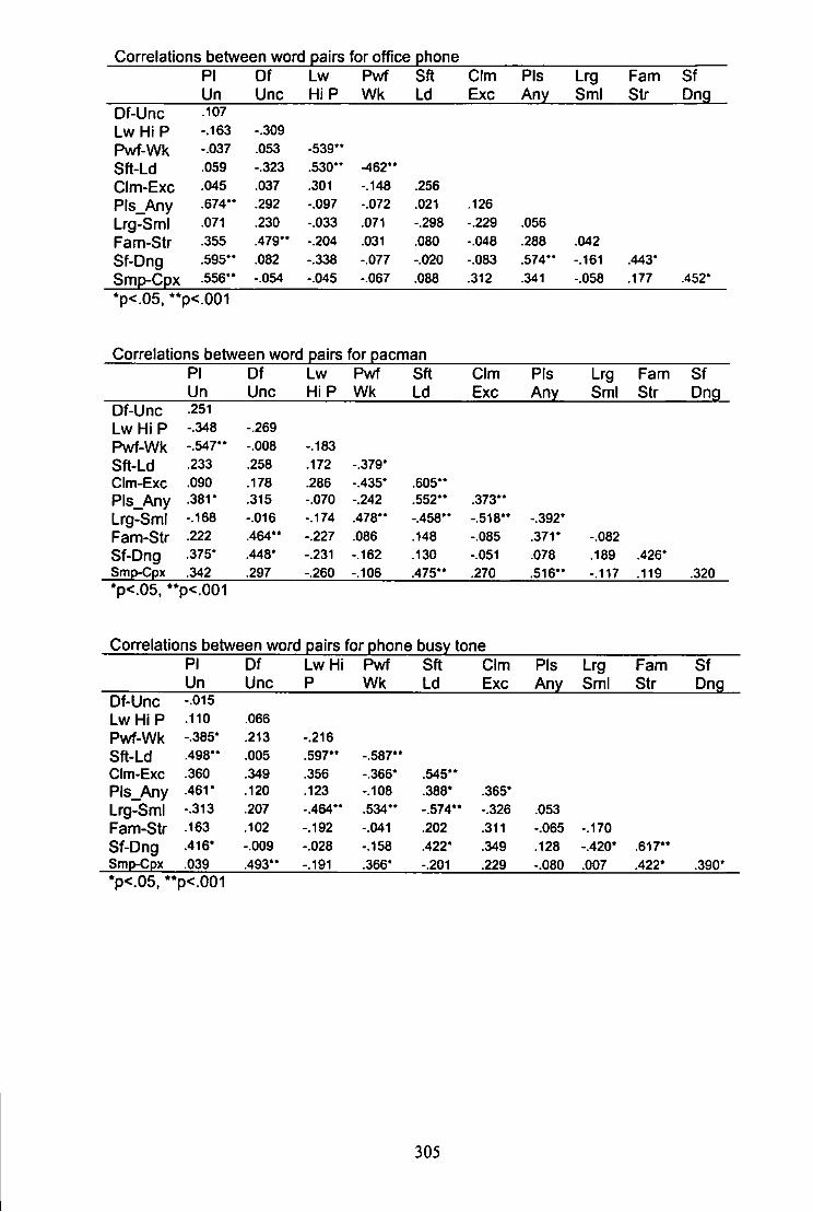
Correlations between word pairs for office phone PI Df Lw Pwf Sft CIm Pis Lrg Fam Sf Un Unc HiP Wk Ld Exc Any SmI Str Dng
Df-Unc .107 Lw HiP -.163 -.309 Pwf-Wk -.037 .053 -539*' Sft-Ld .059 -.323 .530" -462" CIm-Exc .045 .037 .301 -.148 .256 Pls_Any .674" .292 -.097 -.072 .021 .126 Lrg-SmI .071 .230 -.033 .071 -.298 -.229 .056 Fam-Str .355 .479" -.204 .031 .080 -.048 .288 .042 Sf-Dng .595" .082 -.338 -.077 -.020 -.083 .574" -.161 .443' Smp-Cpx .556" -.054 -.045 -.067 .088 .312 .341 -.058 .177 .452* *p<.05, ** p<.001
Correlations between word pairs for pacman PI Df Lw Pwf Sft CIm Pis Lrg Fam Sf Un Unc Hi P Wk Ld Exc Any SmI Str Dnp
Df-Unc .251 Lw HiP -.348 -.269 Pwf-Wk -.547" -.008 -.183 Sft-Ld .233 .258 .172 -.379* CIm-Exc .090 .178 .286 -.435* .605** Pls_Any .381' .315 -.070 -.242 .552** .373*' Lrg-SmI -.168 -.016 -.174 .478** -.458" -.518" -.392* Fam-Str .222 .464" -.227 .086 .148 -.085 .371* -.082 Sf-Dng .375' .448* -.231 -.162 .130 -.051 .078 .189 .426' Smp-Cpx .342 .297 -.260 -.106 .475" .270 .516" -.117 .119 .320 *p<.05. **p<.001
Correlations between word pairs for phone busy tone PI Df Lw Hi Pwf Sft CIm Pis Lrg Fam Sf Un Unc P Wk Ld Exc Any SmI Str Dng
Df-Unc -.015 Lw HiP .110 .066 Pwf-Wk -.385' .213 -.216 Sft-Ld .498** .005 .597" -.587*' CIm-Exc .360 .349 .356 -.366* .545" Pls_Any .461' .120 .123 -.108 .388* .365* Lrg-SmI -.313 .207 -.464" .534" -.574** -.326 .053 Fam-Str .163 .102 -.192 -.041 .202 .311 -.065 -.170 Sf-Dng .416* -.009 -.028 -.158 .422' .349 .128 -.420* .617" Smp-Cpx .039 .493** -.191 .366* -.201 .229 -.080 .007 .422* .390' *p<.05, **p<.001
305
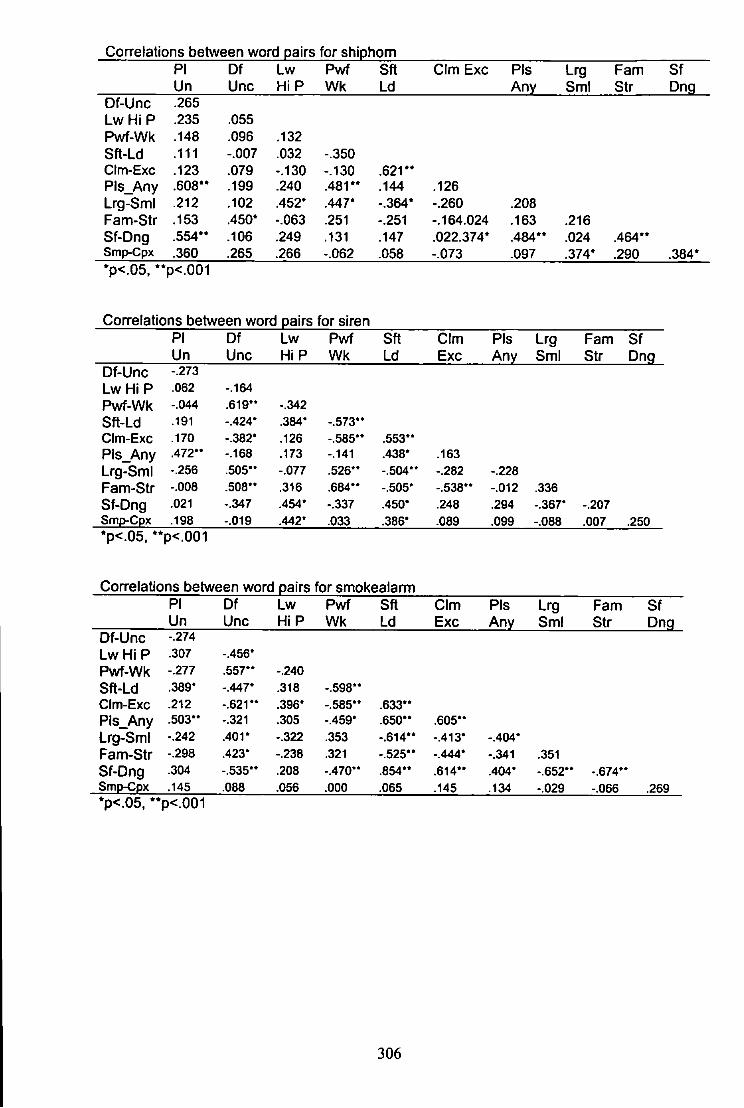
Correlations between word pairs for shiphom PI Df Lw Pwf Sft CIm Exc PIs Lrg Fam Sf Un Unc HI P Wk Ld Any SmI Str Dng
Df-Unc .265 Lw HiP .235 .055 Pwf-Wk .148 .096 .132 Sft-Ld .111 -.007 .032 -.350 CIm-Exc .123 .079 -.130 -.130 .621" Pls_Any .608** .199 .240 .481** .144 .126 Lrg-SmI .212 .102 .452* .447* -.364* -.260 .208 Fam-Str .153 .450* -.063 .251 -.251 -.164.024 .163 .216 Sf-Dng .554** .106 .249 .131 .147 .022.374* .484** .024 .464** Smp-Cpx .360 .265 .266 -.062 .058 -.073 .097 .374* .290 .384* *p<.05, ^p<.001
Correlations between word pairs for siren PI Df Lw Pwf Sft CIm PIs Lrg Fam Sf Un Unc Hi P Wk Ld Exc Any SmI Str Dng
Df-Unc -.273 Lw HiP .062 -.164 Pwf-Wk -.044 .619" -.342 Sft-Ld .191 -.424* .384' -.573" CIm-Exc .170 -.382* .126 -.585" .553*' Pls_Any .472" -.168 .173 -.141 .438* .163 Lrg-SmI -.256 .505*' -.077 .526" -.504" -.282 -.228 Fam-Str -.008 .508" .316 .684" -.505' -.538" -.012 .336 Sf-Dng .021 -.347 .454* -.337 .450* .248 .294 -.367' -.207 Smp-Cpx .198 -.019 .442' .033 .386* .089 .099 -.088 .007 .250 •p<.05, **p<.001
Correlations between word pairs for smokealarm PI Df Lw Pwf Sft CIm PIs Lrg Fam Sf Un Unc HiP Wk Ld Exc Any SmI Str Dng
Df-Unc -.274 Lw HiP .307 -.456' Pwf-Wk -.277 .557** -.240 Sft-Ld .389* -.447* .318 -.598" CIm-Exc .212 -.621" .396' -.585** .633** Pls_Any .503" -.321 .305 -.459' .650** .605** Lrg-SmI -.242 .401* -.322 .353 -.614** -.413* -.404* Fam-Str -.298 .423* -.238 .321 -.525*' -.444' -.341 .351 Sf-Dng .304 -.535'* .208 -.470" .854** .614" .404' -.652" -.674** Smp-Cpx .145 .088 .056 .000 .065 .145 .134 -.029 -.066 .269 *p<.05, "p<.001
306
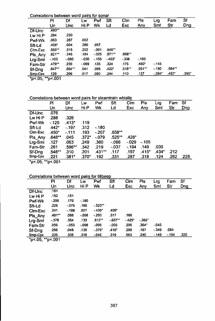
Correlations between word pairs for sonar PI Df Lw Pwf Sfl CIm Pis Lrg Fam Sf Un Unc HiP Wk Ld Exc Any Smi Str Dng
Df-Unc .493" Lw HiP .284 .230 Pwf-Wk .063 .287 .062 Sft-Ld .406' .004 .280 .057 CIm-Exc .560" .315 .252 -.001 .646" Pls_Any .821" .246 .184 -.025 .671" .698" Lrg-SmI -.103 -.080 -.030 -.155 -.453* -.338 -.180 Fam-Str .479" .239 -.099 .135 .324 .175 .460* -.145 Sf-Dng .647" .504" .041 .096 .422' .518" .551" -.150 .584" Smp-Cpx .129 .299 .017 .090 .244 .110 .137 -,394* .452' .390* *p<.05. "p<.001
Correlations between word pairs for steamtrain whistle PI Df Lw Pwf Sft CIm Pis Lrg Fam Sf Un Unc HIP Wk Ld Exc Any SmI Str Dng
Df-Unc .076 Lw HiP .288 .326 Pwf-Wk -.125 .413* .119 Sft-Ld .442* -.197 .312 -.180 CIm-Exc .450* -.111 .193 -.207 .658* * Pls_Any .648** .045 .372* -.079 .525** .428* Lrg-SmI .127 .063 .249 .360 -.066 -.029 -.105 Fam-Str .261 .596** .342 .219 -.037 -.194 .149 .030 Sf-Dng .548** .310 .201 .431** .117 .197 .415* .434* .212 Smp-Cpx .221 .381* .370* .192 .331 .287 .318 .124 .282 .228 *p<.05. ^p<.001
Correlations between word pairs for tillbeep PI Df Lw Pwf Sft CIm Pis Lrg Fam Sf Un Unc HiP Wk Ld Exc Any SmI Str Dng
Df-Unc .181 Lw HiP .152 .151 Pwf-Wk -.356 .170 -.160 Sft-Ld .226 -.075 .190 -.523" CIm-Exc .241 -.199 .027 -.435* .409* Pls_Any .481" .068 -.098 -.293 .317 .166 Lrg-SmI -.378 .354 .133 .612" -.657" -.425' -.382* Fam-Str .050 -.053 -.096 -.096 -.005 .206 .364* -.045 Sf-Dng .296 .048 .130 -.379* .410* .299 .187 -.349 .084 Smp-Cpx .235 .338 .318 -.046 .319 .063 .240 -.149 -.104 .320 *p<.05. **p<.001
307
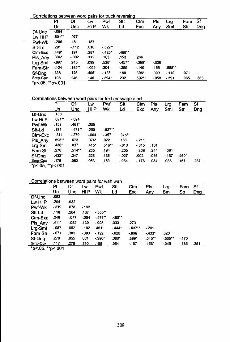
Correlations between word pairs for truck reversing PI Df Lw Pwf Sft CIm Pis Lrg Fam Sf Un Unc Hi P Wk Ld Exc Any SmI Str Dng
Df-Unc -.094 Lw HIP .601" .077 Pwf-Wk -.206 .181 .187 Sft-Ld .291 -.112 .018 -.522" CIm-Exc .449* .191 .287 -.425* .466'* Pls_Any .394* -.002 .112 .163 .153 .266 Lrg-SmI -.097 .245 .099 .528' -.457' -.399' -.028 Fam-Str -.124 .165" -.099 .304 -.359 -.140 .155 .558" Sf-Dng .338 .126 .406* -.123 .180 .395' .090 -.110 .071 Smp-Cpx .196 .246 .140 -.394* .232 .502" -.058 -.291 .065 .333 *p<.05, p<.001
Correlations between word pairs for text message alert PI Df Lw Pwf Sft CIm Pis Lrg Fam Sf Un Unc HiP Wk Ld Exc Any SmI Str Dng
Df-Unc .138 Lw Hi P .621" -.024 Pwf-Wk .152 .461* .005 Sft-Ld .185 -.471" .290 -.637" CIm-Exc -.311 -.279 -.004 -.357 .375" Pls_Any .595" .073 .374' .022 .166 -.211 Lrg-Sml .438' .037 .415* .516" -.013 -.315 .101 Fam-Str .276 .514** .235 .194 -.205 -.308 .244 -.091 Sf-Dng .432* .347 .228 .136 -.027 .002 .066 -.167 .460* Smp-Cpx .178 .082 .083 .163 -.064 -.178 .054 .085 .157 .267 *p<.05. **p<.001
Con-elations between word pairs for wah wah PI Df Lw Pwf Sft CIm Pis Lrg Fam Sf Un Unc HiP Wk Ld Exc Any SmI Str Dng
Df-Unc .053 L w H i P .294 .032 Pwf-Wk -.319 .078 -.192 Sft-Ld .118 .204 .167 -.555" CIm-Exc .246 -.077 -.054 -.573** .480" Pls_Any .411* -.062 .130 -.008 .033 .273 Lrg-Sml -.087 .052 -.102 .451' -.444* -.637** -.291 Fam-Str -.071 .301 -.303 -.122 -.028 -.096 -.433* .320 Sf-Dng .278 .055 .081 -.390' .380' .399* .545** -.535'* -.170 Smp-Cpx .117 .278 .310 .158 .064 -.107 .456* -.049 -.185 .351 *p<.05. p<.001
308
Appendix B
Experiments 4 & 5
B1 - 112 sound stimuli and sound measures
310
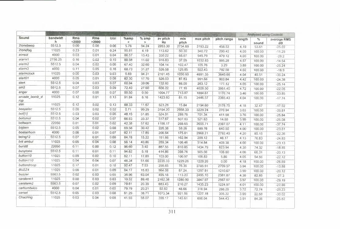
Analysed using Ccxjiedit Sound bandwidt
h Rms
<2000 Rms
>2000 total %amp
< % amp
> av pitch
Hz min max pitch
pitch pitch range length % average RMS
sound dB 2tonebeep 5512.5 0 0 0 0 0 6 0.06 5 76 94.24 2953.30 2734.69 3193 22 458.53 4 19 53.61 -25.02 2tonefog 11025 0 2 3 0.01 0.24 95.81 4.19 113.62 50.30 340.72 290.42 4.00 100.00 -11.29 airraid 4000 0 0 3 0.01 0.04 86.57 13.43 330.22 66.67 545.79 479.12 4.00 100.00 -292 alarm 1 2756.25 0 16 0.02 0.19 88.98 11.02 918.83 37.55 1032.83 995.28 4.57 100.00 -14.54 alarm2 5512.5 0.04 0.02 0.06 67.40 32.60 104.14 102.47 105.76 3.29 3.86 100.00 -25.24 alarms 4000 0.11 0.05 0.16 68.73 31.27 526.58 129.85 922.43 792.58 4.02 100.00 -189 alarmclock 11025 0 0 0 0.03 0 0 3 5.69 94.31 2101.45 1050.69 4691.35 3640.66 4.04 48.51 -35.24 alarlOl 4000 0 05 0.01 0 06 82.30 17.70 526.03 87.83 991.68 903.84 4.42 100.00 -24.38 alert 5512.5 0.04 0.03 0.07 60.94 39.06 132.60 86.00 263.12 177.12 4.05 100.00 -25.14 am2 5612.5 0.07 0 0 3 0.09 72.40 27.60 656.22 77.10 4028.50 3951.40 4.72 100.00 -22.05
4000 0.07 0 0 0 0.07 99.50 0 50 1004.77 713.87 1884.61 1170.74 3 46 100.00 •23.85 arcade_bomb_d rop
11025 0.12 0.01 0.13 91.84 8.16 1423.60 81.15 2446.57 2365.43 4.04 100.00 -17.74
atm 11025 0.12 0.02 0.13 88.33 11 67 523.28 15.84 2194.60 2178.75 4 18 32.47 -17.92 5512.5 0.00 0.02 0.02 0.71 99.29 3154.20 2958.30 3229.24 270.94 3.03 100.00 -29.81
bell[1J 5512.5 0.03 0.03 0.06 48.15 51.85 524.91 289.76 701.34 411.58 3 76 100.00 -25.84 bellsmal 5512.5 0.04 0 02 0.07 66.63 33.37 517.67 507.03 521.63 14.60 3 99 100.00 -25.08 beltwam 22050 0.01 0 01 0.02 42.38 57.62 1156.17 268.65 2655.71 2387.07 4.11 100.00 -37.74 bigben 5512.5 0.05 0 02 0.08 69.58 30.42 226.38 59.26 699.76 640.50 4 00 100.00 -23.81 bo&takhom 4000 0 06 0.01 0.07 82.11 17.89 206.64 175.81 2968.21 2792.40 4.20 85.15 -22.36 boing12 5512.5 007 0.01 0.08 84.78 15.22 191.66 162.94 209.12 46.17 4.13 76.83 -24.83 brttambul 11025 0.05 0.04 0 08 56.14 43.86 289.34 106.46 514.84 408.38 4.00 100.00 -23.13 bursts 22050 0.11 0.00 0.12 96.60 3.40 887.55 810.85 1434.79 623.94 4.30 74.32 -18.85 busylona 5512.5 0.11 0.01 0.11 94.82 5.18 414.86 398.76 505.56 106.80 4.06 66.31 -20.13 button 11) 11025 0 09 0.02 0.10 82.11 17.89 103.00 100.97 106.83 5.86 4.05 54 56 -22.12 bottom 10 11025 0 04 0.04 0.07 48.34 51.66 2235.33 1229.26 1229.26 0.00 4 1H 100.00 -26.69 buttondroop 11025 0.17 0.01 0.18 92.47 7.53 256.65 76.35 2785.91 2709.57 3.94 100.00 -13.88 BUZZ4 11025 0.08 0.01 0.09 84.17 15.83 964.08 87.24 1297.91 1210.67 3 99 100.00 -20.12 buzzer 5563.5 0.02 0 03 0 05 36.96 63.04 495.18 113.23 2495.10 2381.87 4 36 82.85 -27.3 caralarm! 11025 0.00 0.03 0 0 3 10.52 89.48 2162.38 1280.90 3847.97 2567.07 3.97 100.00 -29.19 caralarm2 5563.5 0 0 7 0.02 0 09 79.61 20.39 683.43 210.27 1435.23 1224.97 4.01 100.00 -22.66 carbomtwice 4000 0.04 001 0 0 5 79.79 20.21 92.62 48.66 316.94 268.28 3.72
3.99 72.74 -29.23
carset 5512.5 0.05 0.03 008 61.29 38.71 1073.34 921.96 1227.18 305.22 3.72 3.99 22.58 -30 02
Chaching 11025 0.03 0.04 0.08 41.93 58.07 398.17 145.61 690.04 544.43 3.91 T 84.36 -25.82
311
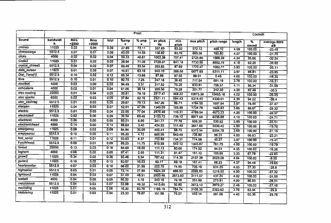
Praat Cooledit
Sound bandwidt h
Rms <2000
R m s >2000
total %amp <
% amp >
av pitch Hz
min pitch
max pitch pitch range length % sound
average RMS dB
chimos 11025 0.02 0.04 0.06 27.89 72.11 337.89 83.02 572.12 489.10 4.09 100.00 -25.49 chlmeslarge 5512.5 0.07 0.01 0.08 85.05 14.95 156.82 83.76 869.56 785.80 4.07 100.00 -21.79 clicks 4000 0.02 0.02 0.04 59.33 40.67 1003.38 757.41 2725.80 1968.39 4.24 25.66 -32.24 Code2 11025 0.01 0.02 0.02 28.94 71.06 2728.07 841.18 7733.96 6892.79 4.10 62.26 -36.92 crystal_chime3 5512.5 0.04 0.02 0.07 66.46 33.54 263.85 87.69 1770.47 1682.77 3.93 100.00 -25.11 data_screen 11025 0.01 0.06 0.07 16.81 83.19 949.19 366.58 6677.69 6311.11 3.97 88.81 -23.85 Dial_Tone[1] 5512.5 0.10 0.02 0.12 86.34 13.66 87.86 87.55 88.01 0.46 4.00 100.00 -18.35 dive 5512.5 0.10 0.01 0.10 92.75 7.25 247.18 36.45 717.64 681.19 3.78 100.00 -19.21 doorbefl 4000 0.03 0.00 0.03 94.49 5.51 317.52 75.25 833.81 758.57 4.11 56.34 -31.09 echoalarm 4000 0.02 0.01 0.04 61.66 38.14 209.58 79.28 321.77 242.50 4.29 82.48 -30.5 elec reading 22050 0.01 0.04 0.05 20.81 79.19 2217.47 408.22 10873.38 10465.16 4.02 100.00 -26.25 e/ec sparks 8000 0.02 0.03 0.05 37.84 62.16 2521.11 984.43 5314.45 4330.01 4.39 94.22 -26.4 elec_cashreg 5512.5 0.01 0.03 0.05 29.87 70.13 547.26 86.71 1784.55 1697.84 3.97 78.44 -31.47 elecpen 11025 0.04 0.03 0.07 52.91 47.09 1340.09 105.96 1734.78 1628.83 3.85 88.67 -25.32 electric 5512.5 0.01 0.03 0.04 22.96 77.04 2470.49 116.31 4789.54 4673.23 4.06 100.00 -28.57 electricbell 11025 0.02 0.06 0.08 30.54 69.46 3153.72 738.12 8977.00 6238.88 4.10 100.00 -24.71 electronic 4000 0.06 0.00 0.06 93.01 6.99 241.77 77.78 608.30 530.52 3.99 100.00 -25.51 electronicheart 4000 0.14 0.00 0.14 96.60 3.40 424.52 111.40 3641.80 3530.40 4.00 100.00 -19.76 emergency 11025 0.06 0.03 0.09 64.94 35.06 450.41 68.75 5373.54 5304.78 3.69 100.00 -21.19 emptysonar 5512.5 0.10 0.00 0.11 95.28 4.72 686.66 640.49 736.80 96.31 4.00 66.83 -22.21 fast_sonar 11025 0.11 0.01 0.12 93.63 6.37 750.89 734.31 774.58 40.27 3.97 100.00 -19.41 FastWhoop 5512.5 0.08 0.01 0.09 88.25 11.75 819.58 542.12 1303.87 761.75 4.00 100.00 -19.79 faxout 22050 0.13 0.03 0.16 84.00 16.00 111.13 60.00 174.52 94.51 4.35 100.00 •16.26 foghom 4000 0.08 0.00 0.09 97.41 2.59 111.31 81.47 191.12 109.66 3.33 67.78 -22.85 gnaw2 11025 0.34 0.02 0.36 93.46 6.54 787.42 114.30 2137.38 2023.08 4.04 100.00 -9.55 guitatZ 11025 0.10 0.02 0.12 83.07 16.93 92.77 89.18 187.41 98.23 4.37 94.48 -19.65 heartmonitor 5512.5 0.07 0.03 0.10 68.02 31.98 202.70 74.90 706.19 631.29 4.03 27.30 •28.8 highsonar 5512.5 0.03 0.01 0.05 72.14 27.86 1824.39 866.93 2086.85 1219.92 4.00 100.00 -27.32 lightson2 11025 0.04 0.03 0.07 51.49 48.51 2900.48 2673.83 3111.07 437.24 4.02 100.00 -24.99 lowbell 4000 0.04 0.00 0.05 95.22 4.78 240.18 78.18 351.99 273.81 4.00 86.93 -26.91 metaldetect 5512.5 0.04 0.03 0.07 53.68 46.32 1415.60 92.85 3972.12 3879.27 2.46 100.00 -27.46 microding 11025 0.01 0.05 0.06 16.30 83.70 1185.19 784.74 3108.36 2323.62 3.76 62.94 -29.9 Mobilering 11025 0.01 0.03 0.04 23.33 76.67 151.08 79.07 440.14 361.08 4.40 60.36 -29.76
312
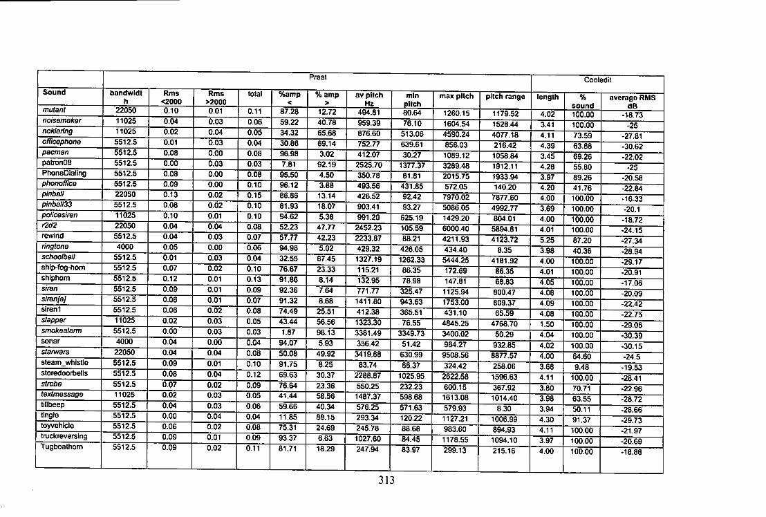
Praat Cooledit
Sound bandwidt h
R m s <2000
R m s >2000
total %amp <
% amp >
av pitch Hz
min pitch
max pitch pitch range length % sound
average RMS dB
mutant 22050 0.10 0.01 0.11 87.28 12.72 494.81 80.64 1260.15 1179.52 4.02 100.00 -18.73 noisemaker 11025 0.04 0.03 0.06 59.22 40.78 959.39 76.10 1604.54 1528.44 3.41 100.00 -25 nokiaring 11025 0.02 0.04 0.05 34.32 65.68 876.60 513.06 4590.24 4077.18 4.11 73.59 -27.81 officephone 5512.5 0.01 0.03 0.04 30.86 69.14 752.77 639.61 856.03 216.42 4.39 63.88 -30.62 pacman 5512.5 0.08 0.00 0.08 96.98 3.02 412.07 30.27 1089.12 1058.84 3.45 69.26 -22.02 patronOS 5512.5 0.00 0.03 0.03 7.81 92.19 2525.70 1377.37 3289.48 1912.11 4.28 55.80 -25 PhoneDialIng 5512.5 0.08 0.00 0.08 95.50 4.50 350.78 81.81 2015.75 1933.94 3.97 89.26 -20.58 phonoWce 5512.5 0.09 0.00 0.10 96.12 3.88 493.56 431.85 572.05 140.20 4.20 41.76 -22.84 pintyall 22050 0.13 0.02 0.15 86.86 13.14 426.52 92.42 7970.02 7877.60 4.00 100.00 -16.33 pinball33 5512.5 0.08 0.02 0.10 81.93 18.07 903.41 93.27 5086.05 4992.77 3.69 100.00 -20.1 policesiren 11025 0.10 0.01 0.10 94.62 5.38 991.20 625.19 1429.20 804.01 4.00 100.00 -18.72 r2d2 22050 0.04 0.04 0.08 52.23 47.77 2452.23 105.59 6000.40 5894.81 4.01 100.00 -24.15 rewind 5512.5 0.04 0.03 0.07 57.77 42.23 2233.87 88.21 4211.93 4123.72 5.25 87.20 -27.34 ringtone 4000 0.05 0.00 0.06 94.98 5.02 429.32 426.05 434.40 8.35 3.98 40.36 -28.94 schoofbell 5512.5 0.01 0.03 0.04 32.55 67.45 1327.19 1262.33 5444.25 4181.92 4.00 100.00 -29.17 ship-fog-horn 5512.5 0.07 0.02 0.10 76.67 23.33 115.21 86.35 172.69 86.35 4.01 100.00 -20.91 shiphom 5512.5 0.12 0.01 0.13 91.86 8.14 132.95 78.98 147.81 68.83 4.05 100.00 -17.06 siren 5512.5 0.09 0.01 0.09 92.36 7.64 771.77 325.47 1125.94 800.47 4.06 100.00 -20.09 slranfa] 5512.5 0.06 0.01 0.07 91.32 8.68 1411.80 943.63 1753.00 809.37 4.09 100.00 -22.42 siren 1 5512.5 0.06 0.02 0.08 74.49 25.51 412.38 365.51 431.10 65.59 4.08 100.00 -22.75 stapper 11025 0.02 0.03 0.05 43.44 56.56 1323.30 76.55 4845.25 4768.70 1.50 100.00 -29.06 smokealarw 5512.5 0.00 0.03 0.03 1.87 98.13 3381.49 3349.73 3400.02 50.29 4.04 100.00 -30.39 sonar 4000 0.04 0.00 0.04 94.07 5.93 356.42 51.42 984.27 932.85 4.02 100.00 -30.15 starwars 22050 0.04 0.04 0.08 50.08 49.92 3419.68 630.99 9508.56 8877.57 4.00 64.60 -24.5 steam_whistle 5512.5 0.09 0.01 0.10 91.75 8.25 83.74 66.37 324.42 258.06 3.68 9.48 -19.53 storedoorbells 5512.5 0.08 0.04 0.12 69.63 30.37 2288.87 1025.95 2622.58 1596.63 4.11 100.00 •28.41 strobe 5512.5 0.07 0.02 0.09 76.64 23.36 550.25 232.23 600.15 367.92 3.80 70.71 -22.96 textmessage 11025 0.02 0.03 0.05 41.44 58.56 1487.37 598.68 1613.08 1014.40 3.98 63.55 -28.72 tillbeep 5512.5 0.04 0.03 0.06 59.66 40.34 576.25 571.63 579.93 8.30 3.94 50.11 -28.66 tingle 5512.5 0.00 0.04 0.04 11.85 88.15 293.34 120.22 1127.21 1006.99 4.30 91.37 -29.73 toyvehicle 5512.5 0.06 0.02 0.08 75.31 24.69 245.78 88.68 983.60 894.93 4.11 100.00 -21.97 tnjckreversing 5512.5 0.09 0.01 0.09 93.37 6.63 1027.60 84.45 1178.55 1094.10 3.97 100.00 -20.69 Tugboathom 5512.5 0.09 0.02 0.11 81.71 18.29 247.94 83.97 299.13 215.16 4.00 100.00 -18.88
313
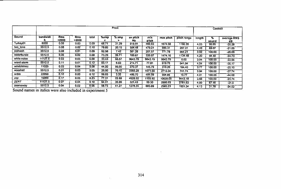
Praat Cooledit
Sound bandwldt h
R m s <20DO
R m s >2000
total %amp <
% amp >
av pitch Hz
min pitch
max pitch pitch range length % sound
average RMS dB
Turt<ey01 8000 0.06 0.03 0.09 68.71 31.29 818.91 482.63 1674.98 1192.35 4.03 90.95 -25.28 two_tone 5512.5 0.08 0.02 0.10 79.85 20.15 584.48 479.01 686.31 207.31 4.49 89.07 -21.05 wahwah 5512.5 0.08 0.01 0.09 92.58 7.42 581.26 207.57 771.78 564.21 3.92 100.00 •20.09 watertoursts 5512.5 0.06 0.02 0.08 73.29 26.71 789.67 339.67 1474.16 1134.48 4.20 94.40 -24.73 white noise 11127.5 0.03 0.05 0.08 33.43 66.57 9643.79 9643.79 9643.79 0.00 3.94 100.00 -22.95 wierd alarm 5512.5 0.11 0.01 0.12 93.17 6.83 214.71 77.81 619.75 541.94 4.04 100.00 -20.17 windchimes 11025 0.03 0.04 0.08 44.00 56.00 270.37 145.79 310.20 164.40 3.77 100.00 -25.15 woodrett 5512.5 0.01 0.03 0.05 29.90 70.10 2293.29 1971.60 2713.34 741.74 3.94 100.00 -27.74 wrtole 22050 0.12 0.00 0.12 98.65 3.35 496.70 494.09 504.66 10.77 4.01 100.00 -44.66 zap 16000 0.17 0.05 0.23 77.31 22.69 4928.92 1195.92 10639.09 9443.18 3.68 100.00 -23.74 ZERT 11127.5 0.07 0.04 0.10 64.01 35.99 321.43 99.30 2880.93 2781.63 4.00 87.46 -21.9 zoomaway 5512.5 0.04 0.02 0.08 58.73 41.27 1278.24 683.89 2585.23 1901.34 4.13 31.78 -34.52
Sound names in italics were also included in experiment 5
314
Appendix C
Experiments 6 & 7
01 - 60 sounds and descriptions
02 - Acoustic features for the 60 sound stimuli
315
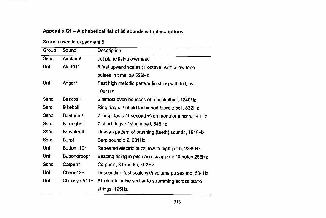
Appendix 01 - Alphabetical list of 60 sounds with descriptions
Sounds used in experiment 6
Group Sound Description
Ssnd Airplane! Jet plane flying overhead
Unf Alartor 5 fast upward scales (1 octave) with 5 low tone
pulses in time, av 526Hz
Unf Anger* Fast high melodic pattern finishing with trill, av
1004Hz
Ssnd Baskball! 5 almost even bounces of a basketball, 1240Hz
Ssrc Bikebell Ring ring x 2 of old fashioned bicycle bell, 832Hz
Ssnd Boathorn! 2 long blasts (1 second +) on monotone horn, 141 Hz
Ssrc Boxingbeil 7 short rings of single bell, 548Hz
Ssnd Brushteeth Uneven pattern of brushing (teeth) sounds, 1546Hz
Ssrc Burp! Burp sound X 2, 631 Hz
Unf Button 110* Repeated electric buzz, low to high pitch, 2235Hz
Unf Buttondroop* Buzzing rising in pitch across approx 10 notes 256Hz
Ssnd Oatpurrl Oatpurrs, 3 breaths, 402Hz
Unf Ohaos12* Descending fast scale with volume pulses too, 534Hz
Unf Chaosynthll*- Electronic noise similar to strumming across piano
strings, 195Hz
316
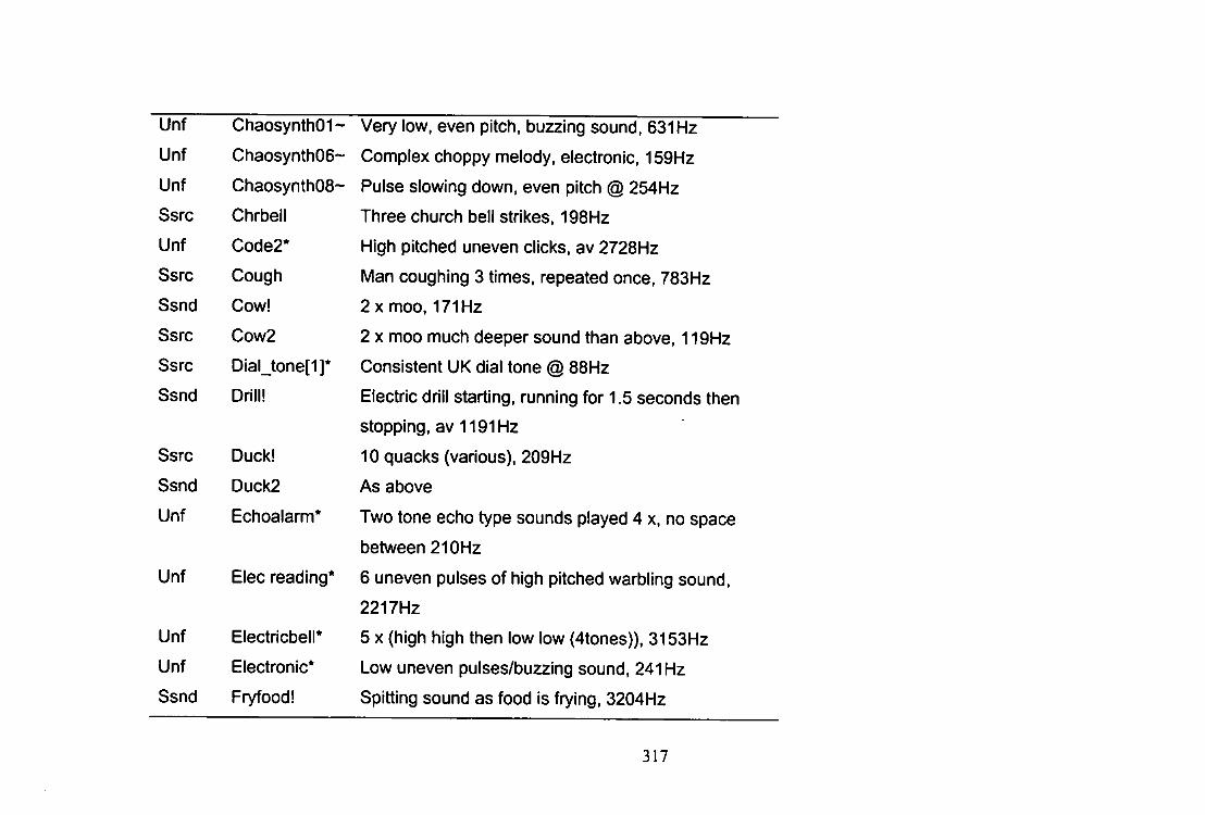
Unf ChaosynthOI- Very low, even pitch, buzzing sound, 631 Hz
Unf ChaosynthOe-" Complex choppy melody, electronic, 159Hz
Unf Chaosynth08* Pulse slowing down, even pitch @ 254Hz
Ssrc Chrbell Three church bell strikes, 198Hz
Unf Code2* High pitched uneven clicks, av 2728Hz
Ssrc Cough Man coughing 3 times, repeated once, 783H2
Ssnd Cow! 2xmoo. 171Hz
Ssrc Cow2 2 X moo much deeper sound than above, 119Hz
Ssrc DialJone[1]* Consistent UK dial tone @ 88Hz
Ssnd Drill! Electric drill starting, running for 1.5 seconds then
stopping, av 1191Hz
Ssrc Duck! 10 quacks (various). 209Hz
Ssnd Duck2 As above
Unf Echoalarm* Two tone echo type sounds played 4 x. no space
between 210Hz
Unf Elec reading* 6 uneven pulses of high pitched warbling sound,
2217Hz
Unf Electricbell* 5 x (high high then low low (4tones)), 3153Hz
Unf Electronic* Low uneven pulses/buzzing sound. 241 Hz
Ssnd Fryfood! Spitting sound as food is frying. 3204Hz
317
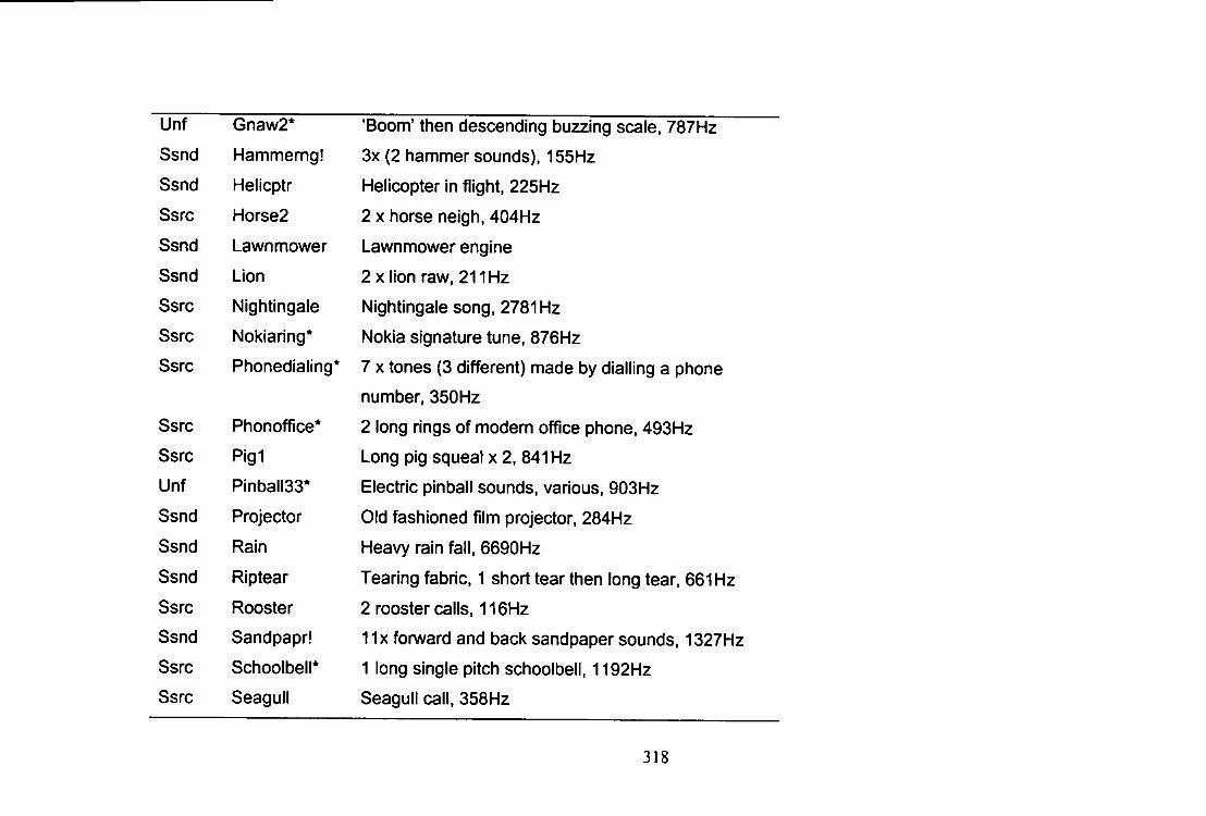
Unf Gnaw2* 'Boom' then descending buzzing scale, 787Hz
Ssnd Hammerng! 3x (2 hammer sounds). 155Hz
Ssnd Helicptr Helicopter in flight, 225Hz
Ssrc Horse2 2 X horse neigh, 404Hz
Ssnd Lawnmower Lawnmower engine
Ssnd Lion 2 X lion raw, 211 Hz
Ssrc Nightingale Nightingale song, 2781Hz
Ssrc Nokiaring* Nokia signature tune, 876Hz
Ssrc Phonedialing* 7 X tones (3 different) made by dialling a phone
number, 350Hz
Ssrc Phonoffice* 2 long rings of modem office phone. 493Hz
Ssrc Pigl Long pig squeal x 2. 841 Hz
Unf Pinball33* Electric pinball sounds, various, 903Hz
Ssnd Projector Old fashioned film projector, 284Hz
Ssnd Rain Heavy rain fall, 6690Hz
Ssnd Riptear Tearing fabric, 1 short tear then long tear. 661 Hz
Ssrc Rooster 2 rooster calls, 116Hz
Ssnd Sandpapr! 11x fonward and back sandpaper sounds, 1327Hz
Ssrc Schoolbell* 1 long single pitch schoolbell, 1192Hz
Ssrc Seagull Seagull call, 358Hz
318
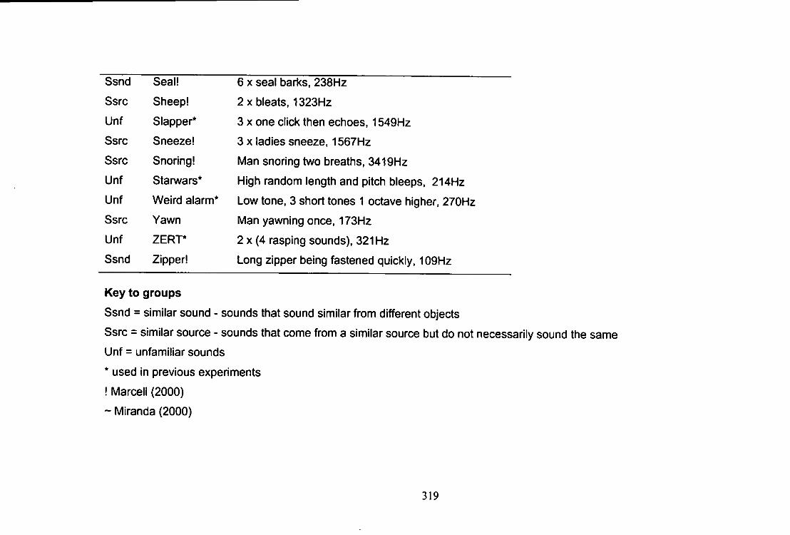
Ssnd Seal! 6 X seal barks, 238Hz
Ssrc Sheep! 2 X bleats, 1323Hz
Unf Slapper* 3 X one click then echoes, 1549Hz
Ssrc Sneeze! 3 X ladies sneeze, 1567Hz
Ssrc Snoring! Man snoring two breaths. 3419Hz
Unf Starwars* High random length and pitch bleeps. 214Hz
Unf Weird alarm* Low tone. 3 short tones 1 octave higher, 270Hz
Ssrc Yawn Man yawning once, 173Hz
Unf ZERT* 2 X (4 rasping sounds), 321 Hz
Ssnd Zipper! Long zipper being fastened quickly, 109Hz
Key to groups
Ssnd = similar sound - sounds that sound similar from different objects
Ssrc = similar source - sounds that come from a similar source but do not necessarily sound the same
Unf = unfamiliar sounds
* used in previous experiments
! Marcell (2000)
* Miranda (2000)
319
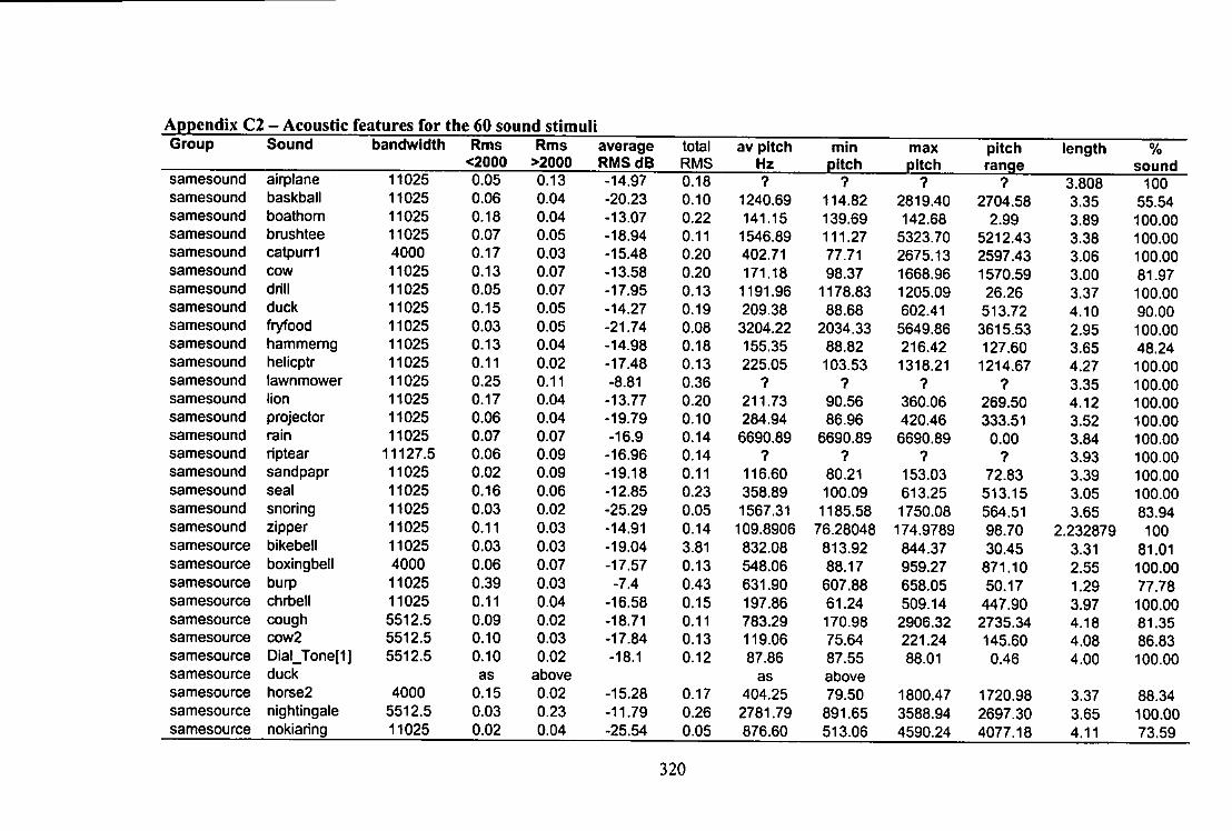
Appendix C2 ; - Acoustic features for the 60 sound stimuli Group Sound bandwidth Rms Rms average total av pitch min max pitch length %
<2000 >2000 RMS dB RMS Hz pitch pitch rancje length
sound samesound airplane 11025 0.05 0.13 -14.97 0.18 ? ? ? ? 3,808 100 samesound baskball 11025 0.06 0.04 -20.23 0.10 1240.69 114.82 2819.40 2704.58 3.35 55.54 samesound boathom 11025 0.18 0.04 -13.07 0.22 141.15 139.69 142.68 2.99 3.89 100.00 samesound bnjshtee 11025 0.07 0.05 -18.94 0.11 1546.89 111.27 5323.70 5212,43 3.38 100.00 samesound catpurri 4000 0.17 0.03 -15.48 0.20 402.71 77.71 2675.13 2597.43 3.06 100.00 samesound cow 11025 0.13 0.07 -13.58 0.20 171.18 98.37 1668.96 1570.59 3.00 81.97 samesound drill 11025 0.05 0.07 -17.95 0.13 1191.96 1178.83 1205.09 26.26 3.37 100.00 samesound duck 11025 0.15 0.05 -14.27 0.19 209.38 88.68 602.41 513.72 4.10 90.00 samesound fryfood 11025 0.03 0.05 -21.74 0.08 3204.22 2034.33 5649.86 3615.53 2.95 100.00 samesound hammemg 11025 0.13 0.04 -14.98 0.18 155.35 88.82 216.42 127.60 3.65 48.24 samesound helicptr 11025 0.11 0.02 -17.48 0.13 225.05 103.53 1318.21 1214.67 4.27 100.00 samesound lawnmower 11025 0.25 0.11 -8.81 0.36 ? ? ? ? 3.35 100.00 samesound lion 11025 0.17 0.04 -13.77 0.20 211.73 90.56 360.06 269.50 4.12 100,00 samesound projector 11025 0.06 0.04 -19.79 0.10 284.94 86.96 420.46 333.51 3.52 100.00 samesound rain 11025 0.07 0.07 -16.9 0.14 6690.89 6690.89 6690.89 0,00 3.84 100.00 samesound riptear 11127.5 0.06 0.09 -16.96 0.14 ? ? ? ? 3.93 100.00 samesound sandpapr 11025 0.02 0.09 -19.18 0.11 116.60 80.21 153.03 72.83 3.39 100.00 samesound seal 11025 0.16 0.06 -12.85 0.23 358.89 100.09 613.25 513.15 3.05 100.00 samesound snoring 11025 0.03 0.02 -25.29 0.05 1567.31 1185.58 1750,08 564.51 3.65 83,94 samesound zipper 11025 0.11 0.03 -14.91 0.14 109.8906 76.28048 174.9789 98.70 2.232879 100 samesource bikebell 11025 0.03 0.03 -19.04 3.81 832.08 813.92 844.37 30.45 3.31 81,01 samesource boxingbeil 4000 0.06 0.07 -17.57 0.13 548.06 88.17 959.27 871.10 2,55 100.00 samesource burp 11025 0.39 0.03 -7.4 0.43 631.90 607.88 658.05 50,17 1.29 77,78 samesource chrbell 11025 0.11 0.04 -16.58 0.15 197.86 61.24 509.14 447.90 3.97 100.00 samesource cough 5512.5 0.09 0.02 -18.71 0.11 783,29 170.98 2906.32 2735.34 4.18 81.35 samesource cow2 5512.5 0.10 0.03 -17.84 0.13 119.06 75.64 221.24 145.60 4.08 86.83 samesource Dial_Tone[1] 5512.5 0.10 0.02 -18.1 0.12 87.86 87.55 88.01 0.46 4.00 100.00 samesource duck as above as above samesource horse2 4000 0.15 0.02 -15.28 0.17 404.25 79.50 1800.47 1720.98 3.37 88.34 samesource nightingale 5512.5 0,03 0.23 -11.79 0,26 2781.79 891.65 3588.94 2697.30 3.65 100.00 samesource nokiaring 11025 0.02 0.04 -25.54 0.05 876.60 513.06 4590.24 4077.18 4.11 73.59
320
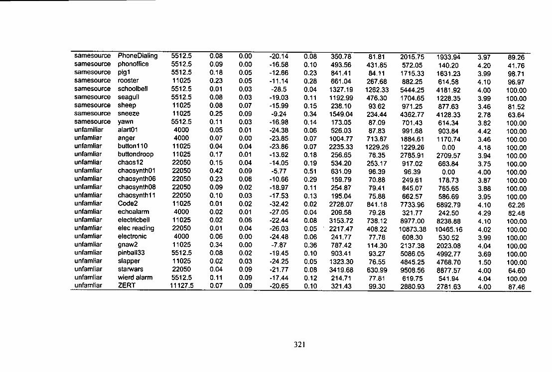
samesource PhoneDialing 5512.5 0.08 0.00 -20.14 0.08 350.78 81.81 2015.75 1933.94 3.97 89.26 samesource phonoffice 5512.5 0.09 0.00 -16.58 0.10 493.56 431.85 572.05 140.20 4.20 41.76 samesource Pig1 5512.5 0.18 0.05 -12.66 0.23 841.41 84.11 1715.33 1631.23 3.99 98.71 samesource rooster 11025 0.23 0.05 -11.14 0.28 661.04 267.68 882.25 614.58 4.10 96.97 samesource schoolbell 5512.5 0.01 0.03 -28.5 0.04 1327.19 1262.33 5444.25 4181.92 4.00 100.00 samesource seagull 5512.5 0.08 0.03 -19.03 0.11 1192.99 476.30 1704.65 1228.35 3.99 100.00 samesource sheep 11025 0.08 0.07 -15.99 0.15 238.10 93.62 971.25 877.63 3.46 81.52 samesource sneeze 11025 0.25 0.09 -9.24 0.34 1549.04 234.44 4362.77 4128.33 2.78 63.64 samesource yawn 5512.5 0.11 0.03 -16.98 0.14 173.05 87.09 701.43 614.34 3.82 100.00 unfamiliar alartOI 4000 0.05 0.01 -24.38 0.06 526.03 87.83 991.68 903.84 4.42 100.00 unfamliar anger 4000 0.07 0.00 -23.85 0.07 1004.77 713.87 1884.61 1170.74 3.46 100.00 unfamliar button 110 11025 0.04 0.04 -23.86 0.07 2235.33 1229.26 1229.26 0.00 4.18 100.00 unfamliar buttondroop 11025 0.17 0.01 -13.62 0.18 256.65 76.35 2785.91 2709.57 3.94 100.00 unfamliar chaos12 22050 0.15 0.04 -14.05 0.19 534.20 253.17 917.02 663.84 3.75 100.00 unfamliar chaosynthOI 22050 0.42 0.09 -5.77 0.51 631.09 96.39 96.39 0.00 4.00 100.00 unfamliar chaosynthOS 22050 0.23 0.06 -10.66 0.29 159.79 70.88 249.61 178.73 3.87 100.00 unfamtiar chaosynthOS 22050 0.09 0.02 -18.97 0.11 254.87 79.41 845.07 765.65 3.88 100.00 unfamliar chaosynthll 22050 0.10 0.03 -17.53 0.13 195.04 75.88 662.57 586.69 3.95 100.00 unfamliar Code2 11025 0.01 0.02 -32.42 0.02 2728.07 841.18 7733.96 6892.79 4.10 62.26 unfamliar echoalarm 4000 0.02 0.01 -27.05 0.04 209.58 79.28 321.77 242.50 4.29 82.48 unfamliar electricbell 11025 0.02 0.06 -22.44 0.08 3153.72 738.12 8977.00 8238.88 4.10 100.00 unfamliar elec reading 22050 0.01 0.04 -26.03 0.05 2217.47 408.22 10873.38 10465.16 4.02 100.00 unfamliar electronic 4000 0.06 0.00 -24.48 0.06 241.77 77.78 608,30 530.52 3.99 100.00 unfamliar gnaw2 11025 0.34 0.00 -7.87 0.36 787.42 114.30 2137.38 2023.08 4.04 100.00 unfamliar pinball33 5512.5 0.08 0.02 -19.45 0.10 903.41 93.27 5086.05 4992.77 3.69 100.00 unfamliar slapper 11025 0.02 0.03 -24.25 0.05 1323.30 76.55 4845.25 4768.70 1.50 100.00 unfamliar starwars 22050 0.04 0.09 -21.77 0.08 3419.68 630.99 9508.56 8877.57 4.00 64.60 unfamliar wierd alarm 5512.5 0.11 0.09 -17.44 0.12 214.71 77.81 619.75 541.94 4.04 100.00 unfamliar ZERT 11127.5 0.07 0.09 -20.65 0,10 321.43 99.30 2880.93 2781.63 4.00 87.46
321
Appendix D
Experiments 6 & 7
D1 - participants' explanations and judges marks
322
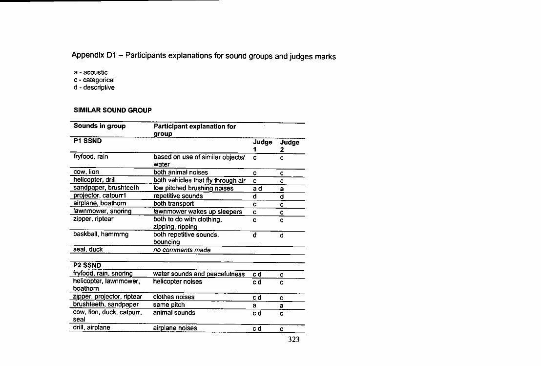
Appendix 01 - Participants explanations for sound groups and judges marks
a - acoustic c - categorical d - descriptive
SIMILAR SOUND GROUP
Sounds in group Participant explanation for group
PI SSND Judge 1
Judge 2
fryfood, rain based on use of similar objects/ water
c c
cow. lion both animal noises c c helicopter, drill both vehicles that fly through air c c sandpaper, brushteeth low pitched brushing noises ad a projector, catpurri repetitive sounds d d airplane, boathom both transport c c lawnmower, snoring lawnmower wakes up sleepers c c zipper, riptear both to do with clothing,
zipping, ripping c c
baskball. hammmg both repetitive sounds, bouncing
d d
seal, duck no comments made
P2 SSND fryfood. rain, snorinq water sounds and peacefulness cd c helicopter, lawnmower, boathom
helicopter noises cd c
zipper, projector, riptear clothes noises cd c brushteeth. sandpaper same pitch a a cow, lion, duck, catpun-. seal
animal sounds cd c
drill, airplane airplane noises cd c 323
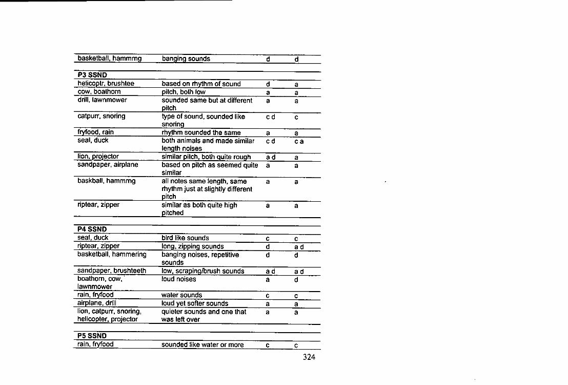
basketball, hammmq banging sounds d d
P3 SSND helicoptr. brushtee based on rhythm of sound d a cow, boalhom pitch, both low a a drill, lawnmower sounded same but at different
pitch a a
catpurr, snoring type of sound, sounded like snoring
c d c
fryfood, rain rhythm sounded the same a a seal, duck both animals and made similar
length noises c d c a
lion, projector similar pitch, both quite rough a d a sandpaper, airplane based on pitch as seemed quite
similar a a
baskball, hammrng all notes same length, same rhythm just at slightly different pitch
a a
riptear, zipper similar as both quite high pitched
a a
P4 SSND seal, duck bird like sounds c c riptear. zipper long, zipping sounds d a d basketball, hammering banging noises, repetitive
sounds d d
sandpaper, brushteeth low, scraping/brush sounds a d a d boathorn, cow, lawnmower
loud noises a d
rain, fryfood water sounds c c airplane, drill loud yet softer sounds a a lion, catpurr. snoring, helicopter, projector
quieter sounds and one that was left over
a a
P5 SSND rain, fryfood sounded like water or more
324
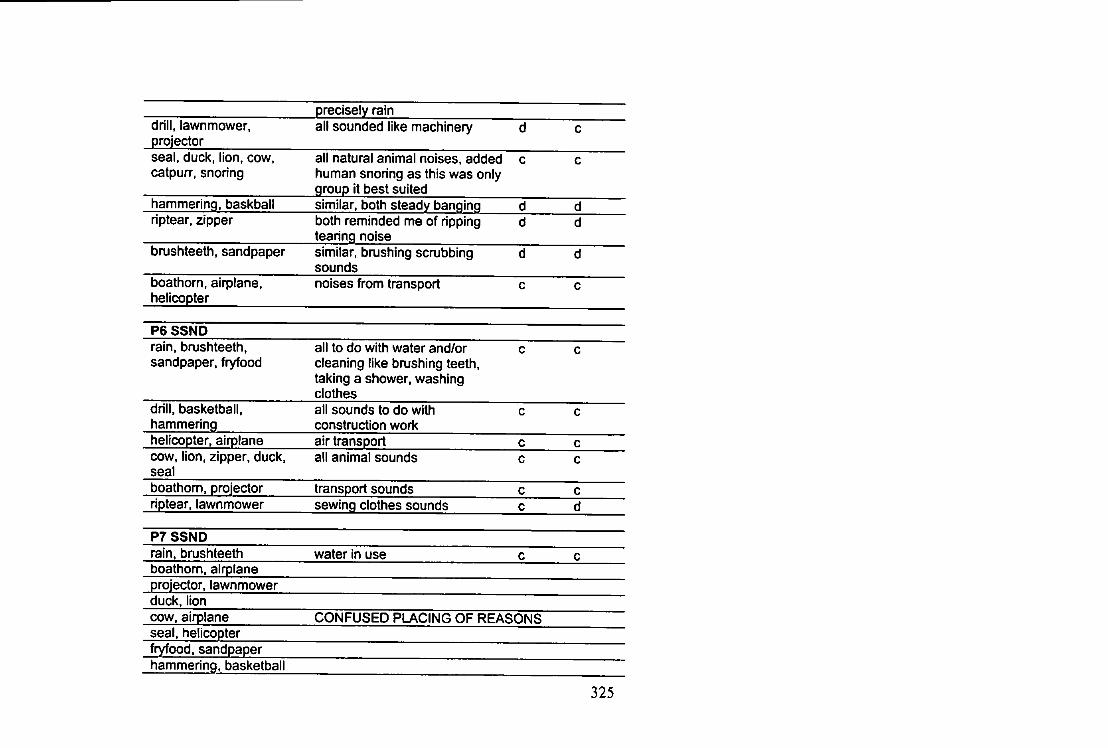
precisely rain drill, lawnmower. projector
all sounded like machinery d c
seal, duck, lion, cow. catpurr, snoring
all natural animal noises, added human snoring as this was only group it best suited
c c
hammerinq, baskball similar, both steady banging d d riptear, zipper both reminded me of ripping
tearing noise d d
brushteeth, sandpaper similar, brushing scmbbing sounds
d d
boathorn. airplane, helicopter
noises from transport c c
P6 SSND rain, brushteeth, sandpaper, fryfood
all to do with water and/or cleaning like brushing teeth, taking a shower, washing clothes
c c
drill, basketball, hammering
all sounds to do with construction work
c c
helicopter, airplane air transport c c cow, lion, zipper, duck, seal
all animal sounds c c
boathom, projector transport sounds c c riptear, lawnmower sewing clothes sounds c d
P7 SSND rain, brushteeth water in use c c boathom, airplane projector, lawnmower duck, lion cow. airplane CONFUSED PLACING OF REASONS seal, helicopter fryfood. sandpaper hammering, basketball
325
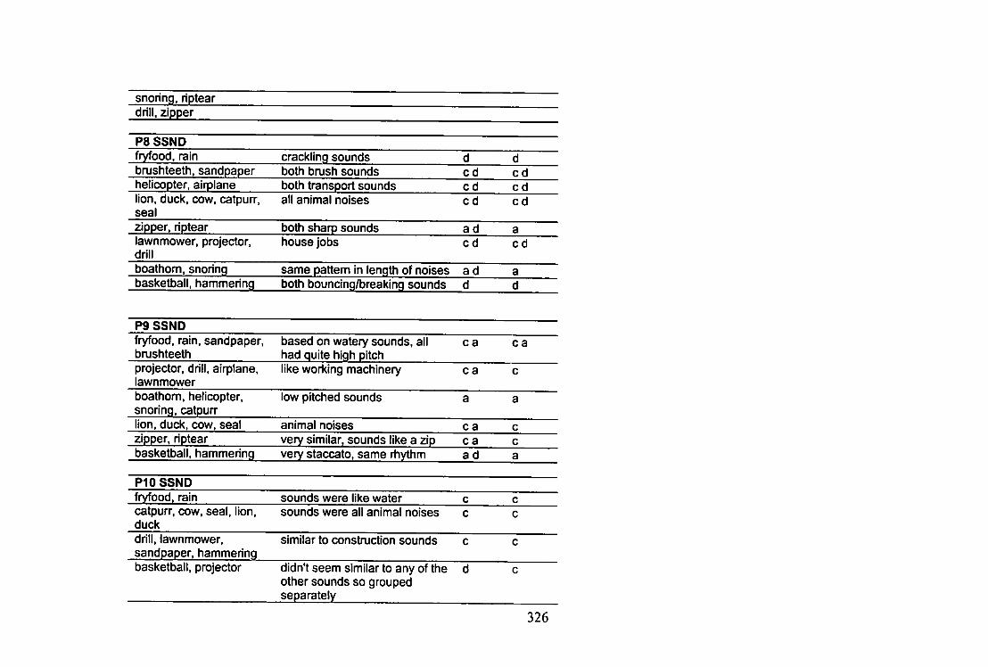
snoring, riptear drill, zipper
P8 SSND fryfood, rain crackling sounds d d brushteeth, sandpaper both bmsh sounds c d c d helicopter, airplane both transport sounds c d c d lion, duck, cow, catpurr, seal
all animal noises c d c d
zipper, riptear both sharp sounds a d a lawnmower, projector, drill
house jobs c d c d
boathom. snoring same pattern in length of noises a d a basketball, hammering both bouncing/breaking sounds d d
P9 SSND fryfood, rain, sandpaper, brushteeth
based on watery sounds, all had quite high pitch
c a c a
projector, drill, airplane, lawnmower
like wori<(ng machinery c a c
boathom, helicopter, snoring, catpurr
low pitched sounds a a
lion, duck, cow, seal animal noises c a c zipper, riptear very similar, sounds like a zip c a c basketball, hammering very staccato, same rhythm a d a
P10SSND fryfood, rain sounds were like water c c catpurr, cow, seal, lion, duck
sounds were all animal noises c c
drill, lawnmower, sandpaper, hammering
similar to construction sounds c c
basketball, projector didn't seem similar to any of the other sounds so grouped separately
d c
326
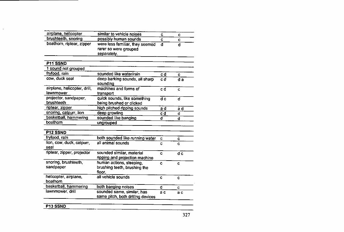
airplane, helicopter similar to vehicle noises c c brushteeth, snoring possibly human sounds c c boathom, riptear, zipper were less familiar, they seemed
rarer so were grouped separately.
d d
P11 SSND 1 sound not grouped fryfood. rain sounded like water/rain c d c cow, duck seal deep barking sounds, all sharp
sounding c d d a
airplane, helicopter, drill, lawnmower
machines and forms of transport
c d c
projector, sandpaper, brushteeth
quick sounds, like something being bnjshed or clicked
d c d
riptear. zipper high pitched ripping sounds a d a d snoring, catpun-, lion deep growling c d d basketball, hammerinq sounded like banqinq d d boathom ungrouped
PI 2 SSND fryfood, rain both sounded like running water c c lion, cow, duck, catpurr, seal
all animal sounds c c
riptear, zipper, projector sounded similar, material ripping and projection machine
c d c
snoring, bnjshteeth. sandpaper
human actions, sleeping, bnjshing teeth, bnjshing the floor.
c c
helicopter, airplane, boathom
all vehicle sounds c c
basketball, hammering both banging noises d c lawnmower, drill sounded same, similar, has
same pitch, both drilling devices a c a c
P13SSND
327
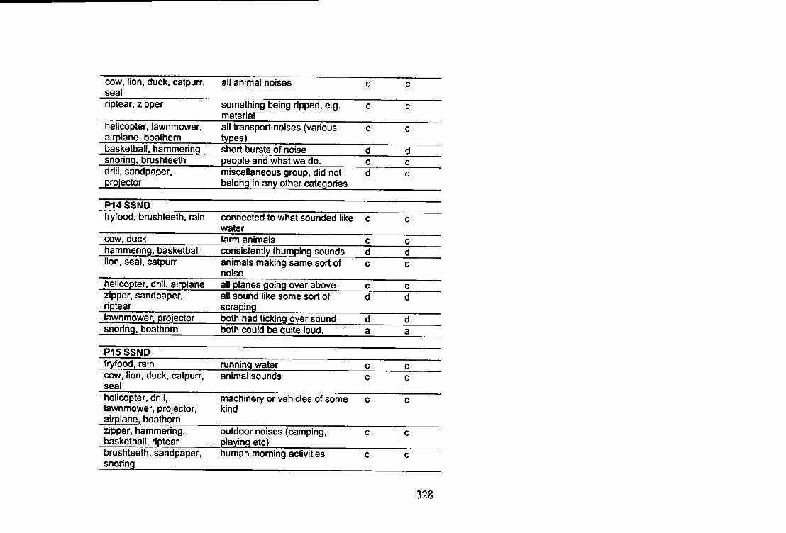
cow, lion, duck, catpurr. seal
all animal noises c c
riptear, zipper something being ripped, e.g. material
c c
helicopter, lawnmower, airplane, boathom
all transport noises (various types)
c c
basketball, hammerinq short bursts of noise d d snoring, brushteeth people and what we do. c c drill, sandpaper, projector
miscellaneous group, did not belong in any other categories
d d
P 1 4 S S N D fryfood, brushteeth, rain connected to what sounded like
water c c
cow, duck farm animals c c hammering, basketball consistently thumping sounds d d lion, seal, catpurr animals making same sort of
noise c c
helicopter, drill, airplane all planes going over above c c zipper, sandpaper, riptear
all sound like some sort of scraping
d d
lawnmower, projector both had ticking over sound d d snoring, boathom both could be quite loud. a a
P 1 5 S S N D fryfood, rain running water c c cow, lion, duck, catpurr, seal
animal sounds c c
helicopter, drill, lawnmower, projector, airplane, boathom
machinery or vehicles of some kind
c c
zipper, hammering, basketball, riptear
outdoor noises (camping, playing etc)
c c
brushteeth, sandpaper, snoring
human moming activities c c
328
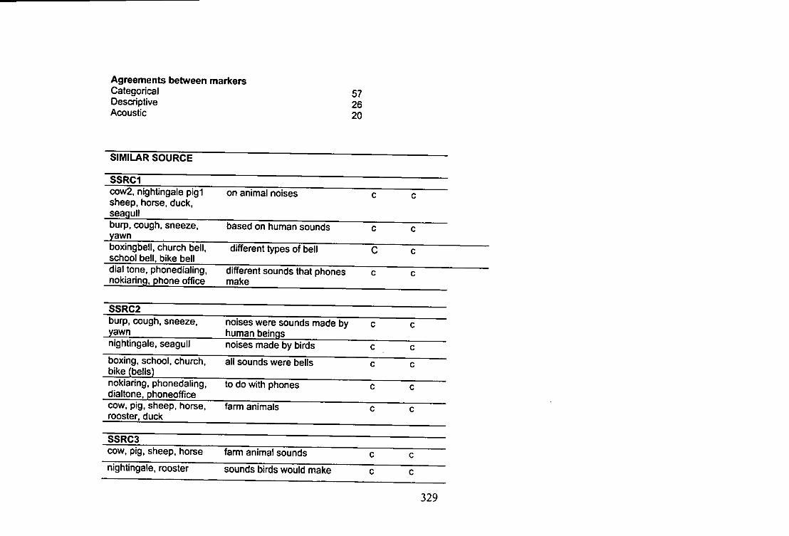
Agreements between markers Categorical Descriptive Acoustic
57 26 20
SIMILAR S O U R C E
SSRC1 cow2, nightingale pig1 sheep, horse, duck, seagull
on animal noises c c
burp, cough, sneeze, yawn
based on human sounds c c
boxingbell, church bell, school bell, bike bell
different types of bell C c
dial tone, phonedialing, nokiaring, phone office
different sounds that phones make
c c
S S R C 2 burp, cough, sneeze, yawn
noises were sounds made by human beings
c c
nightingale, seagull noises made by birds c c boxing, school, church, bike (bells)
all sounds were bells c c
nokiaring, phonedaling, dialtone, phoneoffice
to do with phones c c
cow, pig, sheep, horse, rooster, duck
farm animals c c
S S R C 3 cow, pig, sheep, horse farm animal sounds c c nightingale, rooster sounds birds would make c c
329
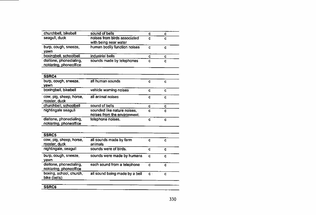
churchbell. bikebell sound of bells c c seagull, duck noises from birds associated
with being near water c c
burp, cough, sneeze, yawn
human bodily function noises c c
boxingbell, schoolbell industrial bells c c dialtone, phonedialing, nokiaring, phoneoffice
sounds made by telephones c c
S S R C 4 burp, cough, sneeze, yawn
all human sounds c c
boxingbell. bikebell vehicle waming noises c c
cow. pig. sheep, horse, rooster, duck
all animal noises c c
churchbell, schoolbell sound of bells c c nightingale seagull sounded like nature noises,
noises from the environment. c c
dialtone, phonedialing, nokiaring, phoneoffice
telephone noises. c c
S S R C 5 cow, pig, sheep, horse, rooster, duck
all sounds made by farm animals
c c
nightingale, seagull sounds were of birds. c c
burp, cough, sneeze, yawn
sounds were made by humans c c
dialtone, phonedialing. nokiaring, phoneoffice
each sound from a telephone c c
boxing, school, church, bike (bells)
all sound being made by a bell c c
S S R C 6
330
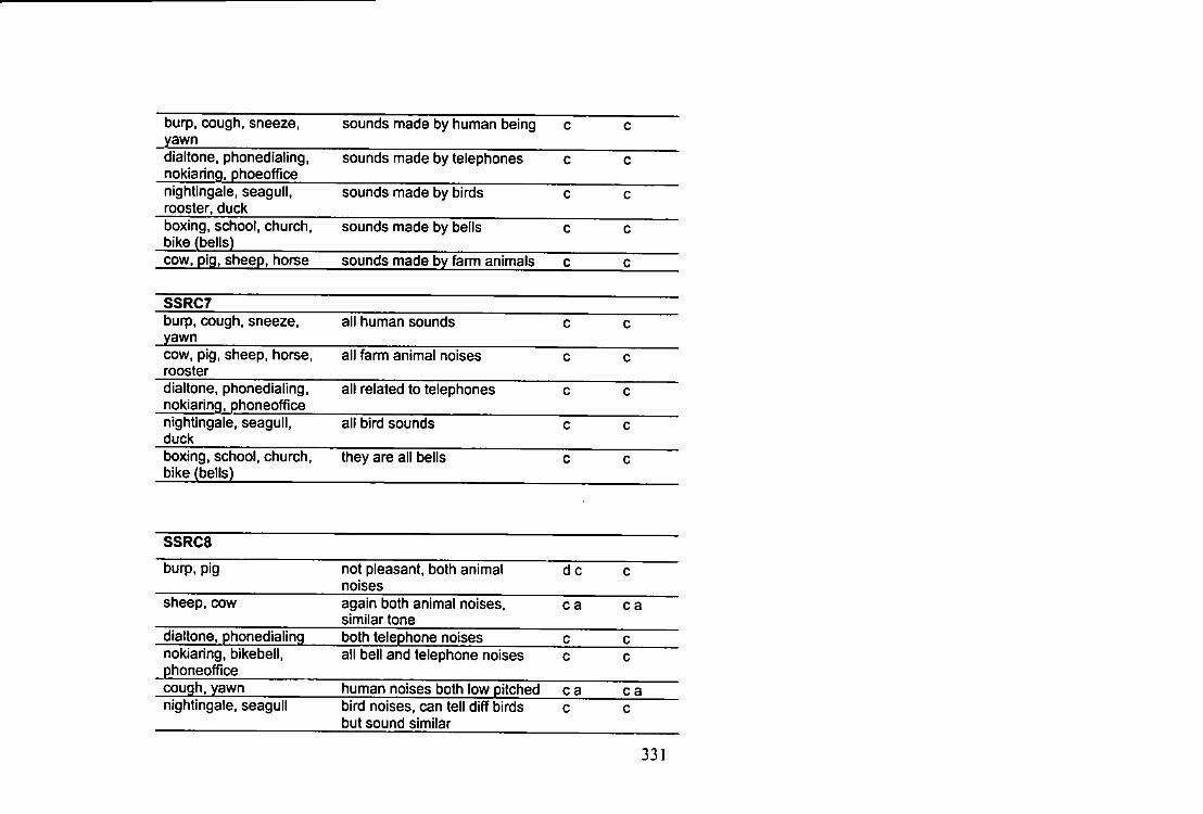
burp, cough, sneeze, yawn
sounds made by human being c c
dialtone, phonedialing, noklaring. phoeoffice
sounds made by telephones c c
nightingale, seagull, rooster, duck
sounds made by birds c c
boxing, school, church, bike (bells)
sounds made by bells c c
cow, pig, sheep, horse sounds made by fann animals c c
S S R C 7 burp, cough, sneeze, yawn
all human sounds c c
cow, pig, sheep, horse, rooster
all farm animal noises c c
dialtone, phonedialing, nokiaring, phoneoffice
all related to telephones c c
nightingale, seagull, duck
all bird sounds c c
boxing, school, church, bike (bells)
they are all bells c c
S S R C 8
burp, pig not pleasant, both animal noises
d c c
sheep, cow again both animal noises, similar tone
c a c a
diattone, phonedialing both telephone noises c c nokiaring, bikebell, phoneoffice
all bell and telephone noises c c
cough, yawn human noises both low pitched c a c a nightingale, seagull bird noises, can tell diff birds
but sound similar c c
331
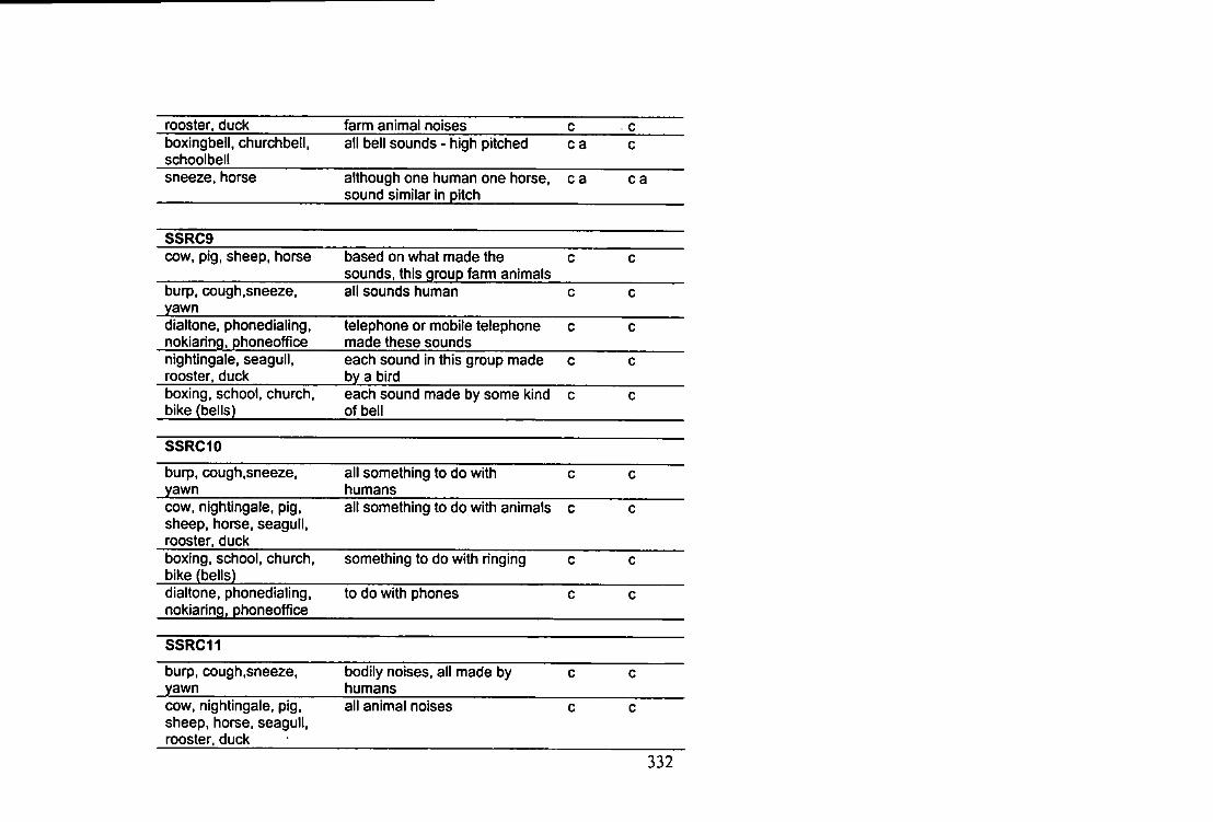
rooster, duck farm animal noises c c boxingbell, churchbell, schoolbell
all bell sounds - high pitched c a c
sneeze, horse although one human one horse, sound similar In pitch
c a c a
S S R C 9 cow, pig, sheep, horse based on what made the
sounds, this group farm animals c c
burp, cough,sneeze, yawn
all sounds human c c
dialtone. phonedialing, nokiaring. phoneoffice
telephone or mobile telephone made these sounds
c c
nightingale, seagull, rooster, duck
each sound in this group made by a bird
c c
boxing, school, church, bike (bells)
each sound made by some kind of bell
c c
S S R C 1 0
burp, cough,sneeze, yawn
all something to do with humans
c c
cow. nightingale, pig, sheep, horse, seagull, rooster, duck
all something to do with animals c c
boxing, school, church, bike (bells)
something to do with ringing c c
dialtone, phonedialing, nokiaring, phoneoffice
to do with phones c c
SSRC11
burp, cough,sneeze, yawn
bodily noises, all made by humans
c c
cow, nightingale, pig, sheep, horse, seagull, rooster, duck
all animal noises c c
332
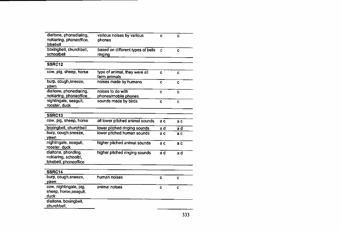
dialtone, phonedialing, nokiaring, phoneoffice, bikebell
various noises by various phones
c c
boxingbell, churchbell, schoolbell
based on different types of bells ringing
c c
S S R C 1 2
cow, pig, sheep, horse type of animal, they were all farm animals
c c
burp, cough.sneeze, yawn
noises made by humans c c
dialtone, phonedialing, nokiaring, phoneoffice
noises to do with phones/mobile phones
c c
nightingale, seagull, rooster, duck
sounds made by birds c c
S S R C 1 3 cow, pig, sheep, horse all lower pitched animal sounds a c a c boxingbell, churchbell lower pitched ringing sounds a d a d burp, cough,sneeze, yawn
lower pitched human sounds a c a c
nightingale, seagull, rooster, duck
higher pitched animal sounds a c a c
dialtone, phonding, nokiaring, schoolbl, bikebell, phoneofTice
higher pitched ringing sounds a d a d
S S R C 1 4 burp, cough,sneeze, yawn
human noises c c
cow, nightingale, pig, sheep, horse,seagull, duck
animal noises c c
churchbell.
333
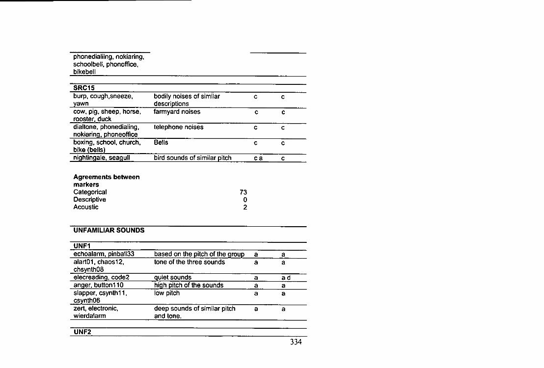
phonedialiing, nokiaring, schoolbeli. phonoffice, bikebell
SRC15 burp, cough.sneeze. yawn
bodily noises of similar descriptions
c c
cow. pig, sheep, horse, rooster, duck
farmyard noises c c
dialtone, phonedialing. nokiaring, phoneoffice
telephone noises c c
boxing, school, church, bike (bells)
Bells c c
nightingale, seagull bird sounds of similar pitch c a c
Agreements between markers Categorical Descriptive Acoustic
73 0 2
UNFAMILIAR SOUNDS
UNF1 echoalarm. pinbaII33 based on the pitch of the group a a alartOI, chaos12. chsynthOS
tone of the three sounds a a
elecreading, code2 quiet sounds a a d anger, button110 high pitch of the sounds a a slapper. csynthi 1, csynthOe
low pitch a a
zert. electronic, wierdalarm
deep sounds of similar pitch and tone.
a a
UNF2 334
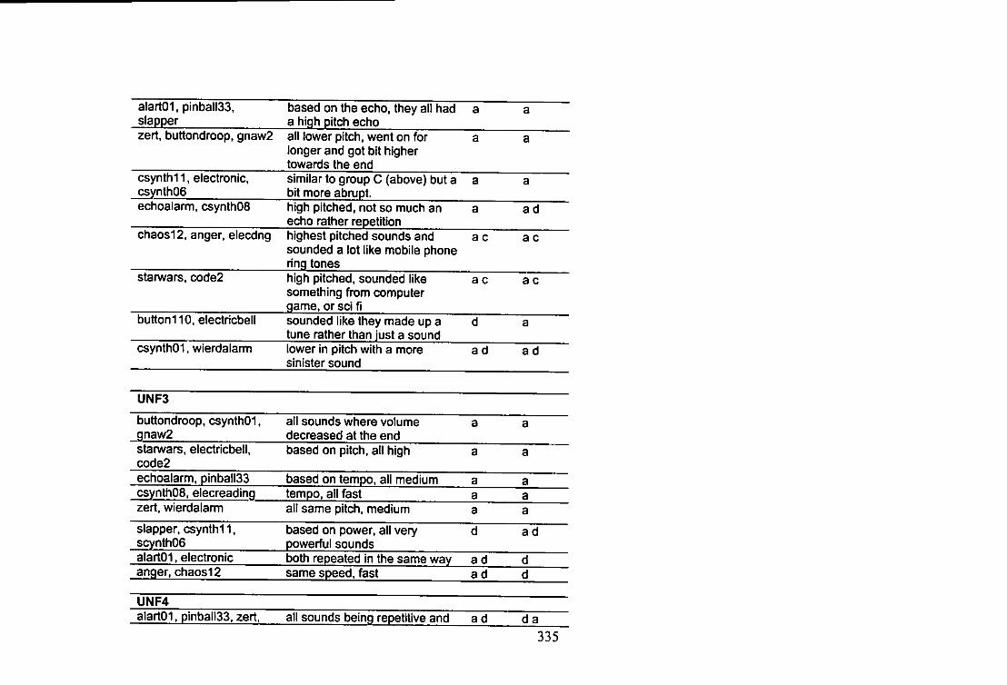
alartOI, pinball33, slapper
based on the echo, they all had a high pitch echo
a a
zert, buttondroop, gnaw2 all lower pitch, went on for longer and got bit higher towards the end
a a
csynth11, electronic. csynthOe
similar to group C (above) but a bit more abrupt.
a a
echoalarm. csynthOS high pitched, not so much an echo rather repetition
a a d
chaos12. anger, elecdng highest pitched sounds and sounded a lot like mobile phone ring tones
a c a c
starwars. code2 high pitched, sounded like something from computer game, or scl fi
a c a c
button110. electricbell sounded like they made up a tune rather than just a sound
d a
csynthOI, wierdalarm lower in pitch with a more sinister sound
a d a d
UNF3
buttondroop. csynthOI. gnaw2
all sounds where volume decreased at the end
a a
stanwars. electricbell. code2
based on pitch, all high a a
echoalarm. pinball33 based on tempo, all medium a a csynthOS. elecreading tempo, ail fast a a zert. wierdalarm all same pitch, medium a a slapper. csynth11. scynthOe
based on power, all very powerful sounds
d a d
alartOI, electronic both repeated in the same way a d d anger, chaos12 same speed, fast a d d
UNF4 alartOI, pinball33, zert. all sounds being repetitive and a d d a
335
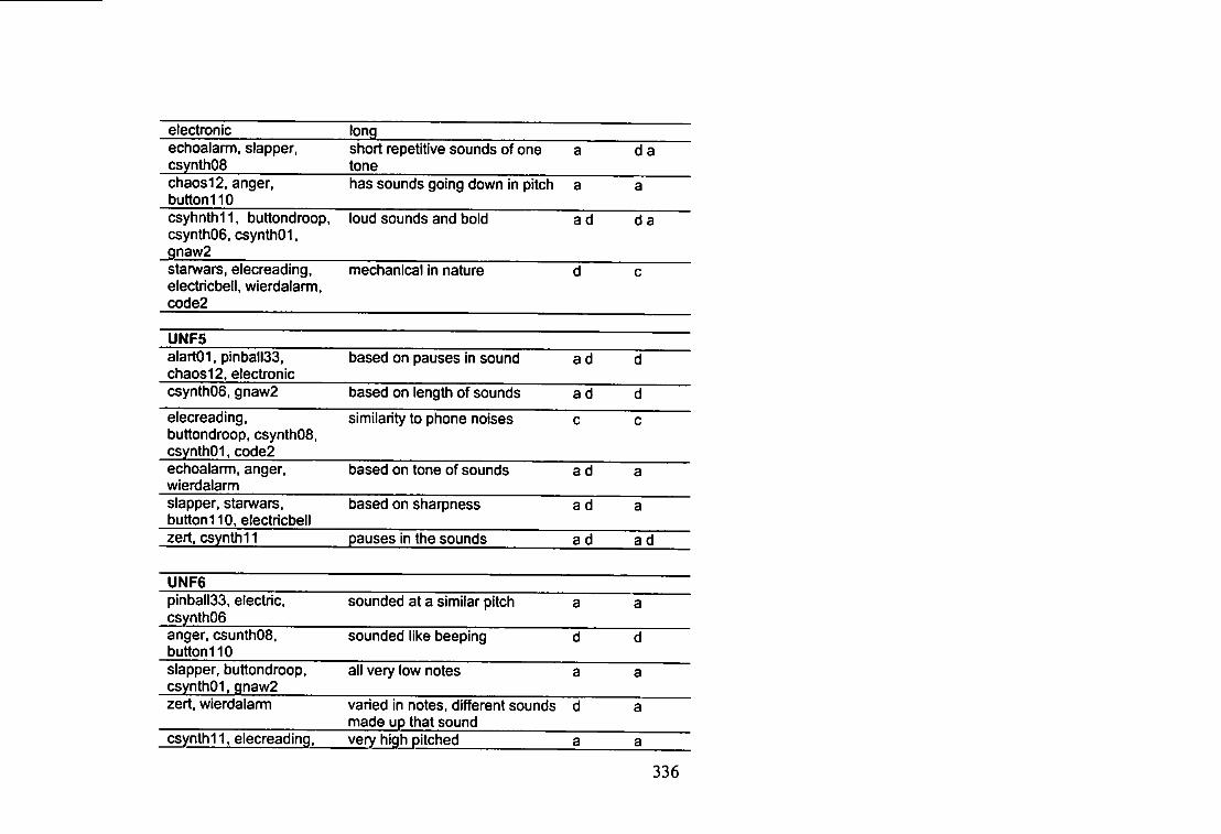
electronic long echoalarm, slapper, csynthOS
short repetitive sounds of one tone
a d a
chaos12, anger, button110
has sounds going down in pitch a a
csyhnth11, buttondroop, csynthOe. csynthOl. gnaw2
loud sounds and bold a d d a
stanwars, elecreading, electricbell, wierdalarm,
mechanical in nature d c
code2
UNF5 alartOI, ptnball33, chaos12, electronic
based on pauses in sound a d d
csynthOe, gnaw2 based on length of sounds a d d
elecreading, buttondroop, csynthOS, csynthOl, code2
similarity to phone noises c c
echoalarm. anger, wierdalarm
based on tone of sounds a d a
slapper, stanArars. button110, electricbell
based on sharpness a d a
zert, csynth11 pauses in the sounds a d a d
UNF6 pinbalISS, electric, csynthOe
sounded at a similar pitch a a
anger, csunthOS. button! 10
sounded like beeping d d
slapper, buttondroop, csynthOl, gnaw2
all very low notes a a
zert, wierdalarm varied in notes, different sounds made up that sound
d a
csynthi 1, elecreading. very high pitched a a
336
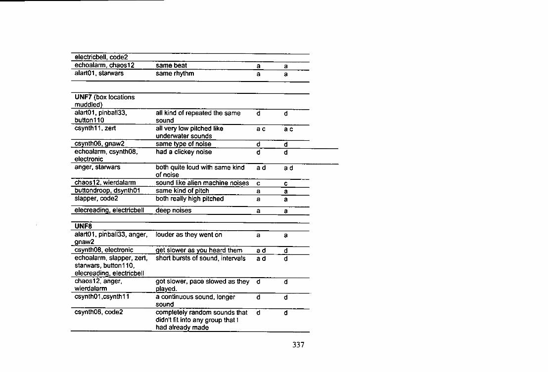
electricbell, code2 echoalarm, chaos12 same beat a a alartOI, starwars same rhythm a a
UNF7 (box locations muddled) alartOI, pinball33, button110
all kind of repeated the same sound
d d
csynth11, zert all very low pitched tike underwater sounds
a c a c
csynthOe, gnaw2 same type of noise d d echoalarm, csynthOS, electronic
had a dickey noise d d
anger, starwars both quite loud with same kind of noise
a d a d
chaos12, wierdalarm sound like alien machine noises c c buttondroop, dsynthOI same kind of pitch a a slapper, code2 both really high pitched a a
elecreading, electricbell deep noises a a
UNF8 alartOI, pinbalISS, anger, gnaw2
louder as they went on a a
csynthOS, electronic get slower as you heard them a d d echoalarm, slapper, zert, stanwars, button110,
short bursts of sound, intervals a d d
elecreading, electricbell chaos12, anger, wierdalarm
got slower, pace slowed as they played.
d d
csynth01,csynth11 a continuous sound, longer sound
d d
csynthOe, code2 completely random sounds that didn't fit into any group that 1 had already made
d d
337
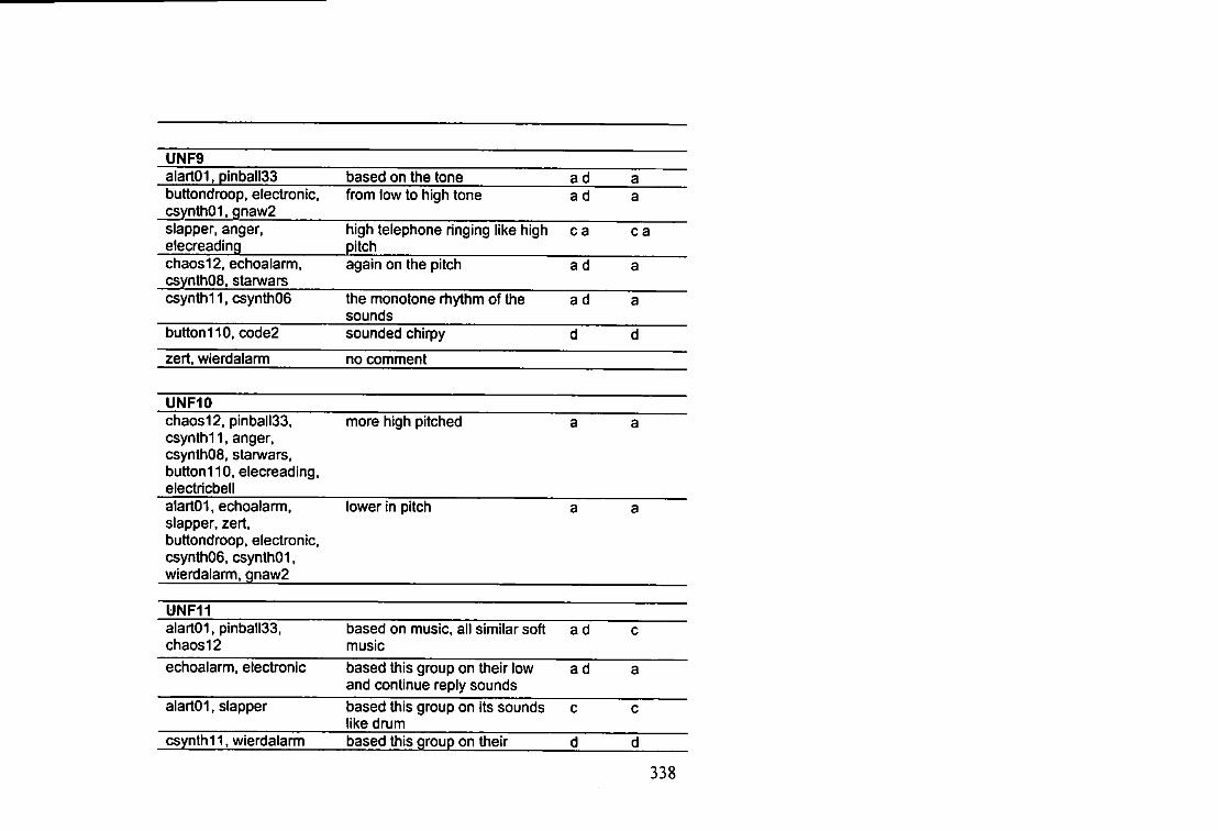
UNF9 alartOI, pinball33 based on the tone a d a buttondroop, electronic, csynthOI. gnaw2
from low to high tone a d a
slapper, anger, elecreading
high telephone ringing like high pitch
c a c a
chaos12. echoalarm. csynthOS. stanwars
again on the pitch a d a
csynthi 1, csynthOe the monotone rhythm of the sounds
a d a
button110, code2 sounded chirpy d d
zert, wierdalarm no comment
UNF10 chaos12, pinball33, csynth11, anger, csynthOS, starwars, button110. elecreading, electricbell
more high pitched a a
alartOI, echoalarm, slapper, zert, buttondroop, electronic, csynthOe, csynthOI, wierdalarm. gnaw2
lower in pilch a a
UNF11 alartOI. pinball33, chaos12
based on music, all similar soft music
a d c
echoalarm. electronic based this group on their low and continue reply sounds
a d a
alartOI, slapper based this group on its sounds like drum
c c
csynthi 1. wierdalarm based this group on their d d
338
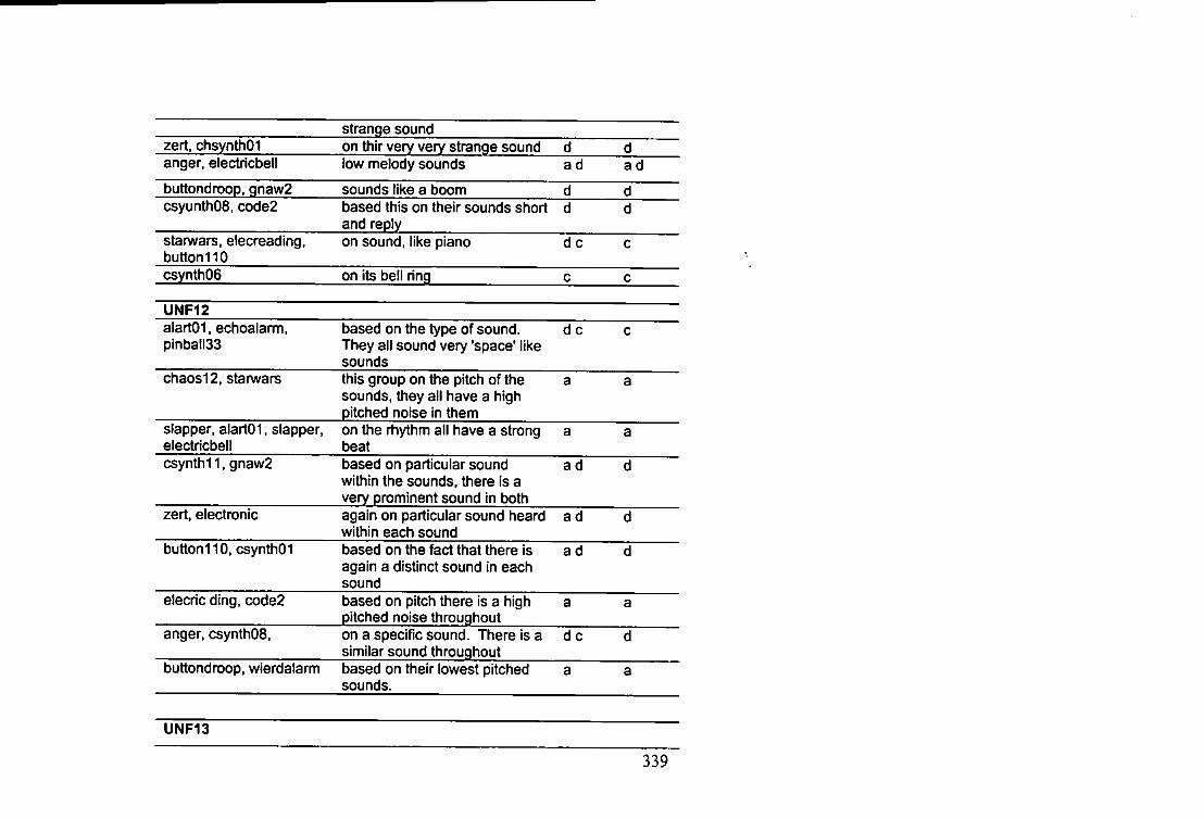
strange sound zert, chsynthOI on thir very very strange sound d d anger, electricbell low melody sounds a d a d
buttondroop, gnaw2 sounds like a boom d d csyunthOS, code2 based this on their sounds short
and reply d d
starwars, elecreading, button110
on sound, like piano d c c
csynthOe on its bell ring c c
UNF12 alartOI, echoalarm, pinbaII33
based on the type of sound. They all sound very 'space* like sounds
d c c
chaos12. starwars this group on the pitch of the sounds, they all have a high pitched noise in them
a a
slapper, alartOI, stepper, electricbell
on the rhythm all have a strong beat
a a
csynth11, gnaw2 based on particular sound within the sounds, there is a very prominent sound in both
a d d
zert, electronic again on particular sound heard within each sound
a d d
buttonllO, csynthOI based on the fact that there is again a distinct sound in each sound
a d d
elecric ding, code2 based on pitch there is a high pitched noise throughout
a a
anger. csynth08. on a specific sound. There is a similar sound throughout
d c d
buttondroop, wterdalarm based on their lowest pitched sounds.
a a
UNF13
339
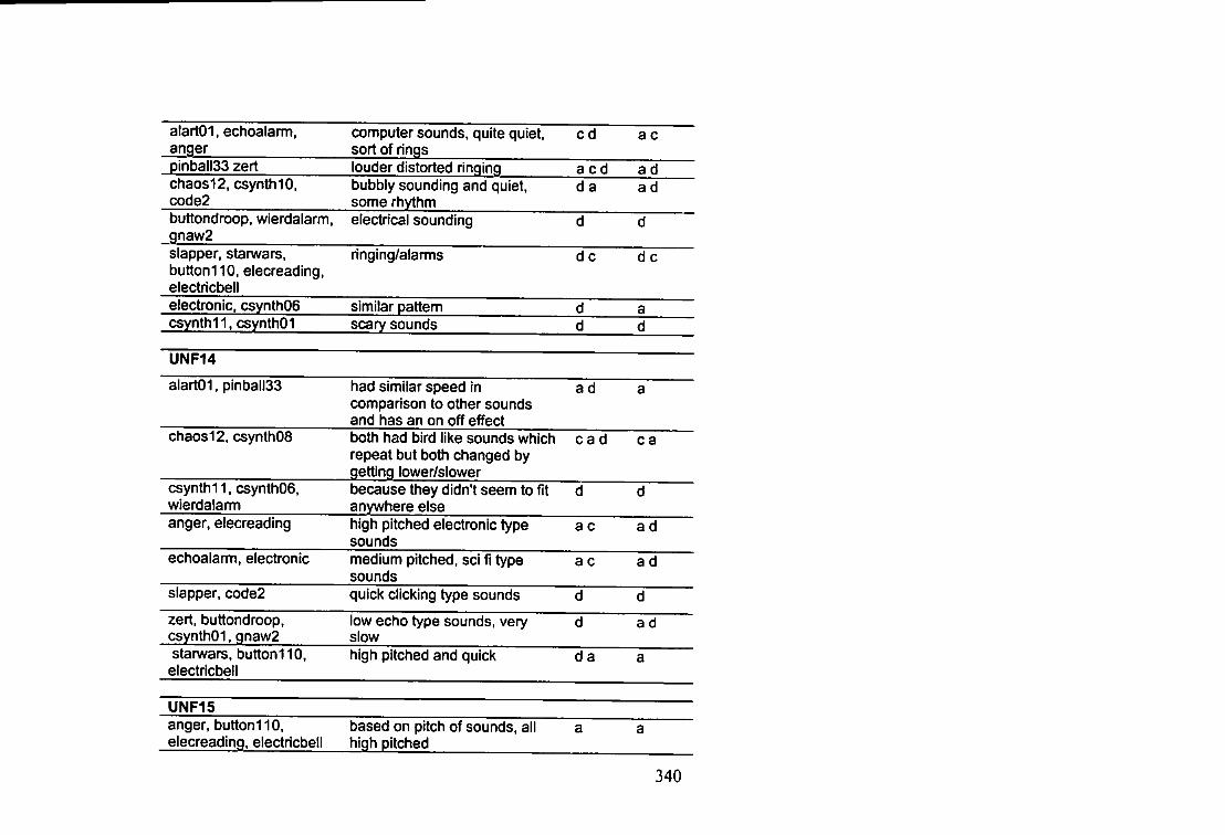
alartOI, echoalaim, anger
computer sounds, quite quiet, sort of rings
c d a c
pinball33 zert louder distorted ringing a c d a d chaos12, csynthlO. code2
bubbly sounding and quiet, some rhythm
d a a d
buttondroop, wierdalarm, gnaw2
electrical sounding d d
slapper, starwars, button110, elecreading, electricbel)
ringing/alarms d c d c
electronic, csynthOS similar pattem d a csynth11, csynthOI scary sounds d d
UNF14
alartOI. pinball33 had similar speed in comparison to other sounds and has an on off effect
a d a
chaos12, csynlhOS both had bird like sounds which repeat but both changed by getting lower/slower
c a d c a
csynth11, csynthOe, wierdalanm
because they didn't seem to fit anywhere else
d d
anger, elecreading high pitched electronic type sounds
a c a d
echoalarm, electronic medium pitched, sci fi type sounds
a c a d
slapper, code2 quick clicking type sounds d d
zert, buttondroop, csynthOI, gnaw2
low echo type sounds, very slow
d a d
starwars, button110, electricbell
high pitched and quick d a a
UNF15 anger, button110, elecreading, electricbell
based on pitch of sounds, all high pitched
a a
340
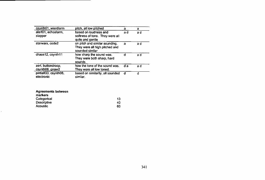
csynthOI, wierdlarm pitch, all low pitched a a alartOi, echoalarm, based on loudness and a d a d slapper softness of tone. They were all
quite and gentle starwars, code2 on pitch and similar sounding.
They were all high pitched and sounded similar
a a d
chaos12, csynth11 how sharp the sound was. They were both sharp, hard sounds
d a d
zert, buttondroop, csynth06, qnaw2
how the tone of the sound was. They were all low toned.
d a a d
pinball33, csynth08. electronic
based on similarity, all sounded similar.
d d
Agreements between markers Categorical Descriptive Acoustic
13 40 60
341
Reference List
Allen, P., & Bond, C. (1997). Multidimensional scaling of complex sounds by
school-aged children and adults. Journal of the Acoustical Society of
America, 102. 2255-2263.
Ballas, J . A., & Howard, J . H. (1987). Interpreting the Language of Environmental
Sounds. Environment ar}d Behaviour, 19, 91-114.
Ballas, J . A. (1993). Common Factors in the Identification of An Assortment of
Brief Everyday Sounds. Journal of Experimental Psychology-Human
Perception and Performance, 19, 829.
Berglund, B., Hassmen, P., & Preis, A. (2002). Annoyance and Spectral Contrast
are Cues for Similarity and Preference of Sounds. Journal of Sound and
Vibration, 250, 53-64.
Bonebright, T. L., Miner, N. E., Goldsmith, T. E., & Caudell, T. P. (1998). Data
Collection and Analysis Techniques for Evaluating the Perceptual
Qualities of Auditory Stimuli. http://wvm.icad.Org/websiteV2.0/
Conferences/ICAD98/papers/BONEBRIG.PDF, accessed June 2002.
Bonebright. T. L. (2001). Perceptual structure of everyday sounds: a
multidimensional scaling approach, http://www.acoustics.hut.fi/icad2001
proceedings/papers/bonebril .pdf accessed June 2001.
342
Bonebright. T. L. (1996). An investigation of data collection methods for auditory
stimuli: Paired comparisons versus a computer sorting task. Behavior
Research Methods lr)struments & Computers, 28, 275-278.
Borg, I. & Groenen. P. (1997). Constructing MDS Representations. In Modern
Multidimensional Scaling, Theory and Applications (pp. 15-26). New York:
Springer Verlag.
Borg, I. & Groenen, P. (1997). MDS models and Measures of Fit. In Modern
Multidimensional Scaling, Theory and Applications (pp. 29-47). New York:
Springer Verlag.
Bower, G. H, & Holyoak, K. (1973). Encoding and recognition memory for
naturalistic sounds. Journal of Experimental Psychology, 10, 360-366.
Bregman, A. S . (1993). Auditory Scene Analysis: hearing in complex
environments. In S . McAdams & E. Bigand (Eds.), Thinking in sound: the
cognitive psychology of human audition (pp. 10-36). London: Oxford
University Press.
Gavalcanti, M. J . (1988). Programa BASIC para teste de associagao entre
matrizes de distancia.CI§ncia e Cultura 40 (Suplemento): 903, [Computer
software]. Mantel for Windows Help. © 1988-2001
Chiu, C , & Schacter, D. L. (1995). Auditory priming for nonverbal information:
Implicit and explicit memory for environmental sounds. Consciousness
and Cognition, 4, 440-458.
343
Coxon, A. P. M. (1982). The user's guide to multidimensional scaling. London:
Heinemann Educational Books.
Deutsch, D. (Ed.) (1982) The Psychology of Music. New York: Academic Press.
Dopkins, S. , & Gleason, T. (1997). Comparing exemplar and prototype models of
categorization. Canadian Journal of Experimental Psychology-Revue
Canadienne de Psychologie Experimentale, 51, 212-230.
Dopkins. S. . & Ngo, C. T. (2001). The contribution of category relationships to
similarity ratings. Canadian Journal of Experimental Psychology-Revue
Canadienne de Psychologie Experimentale, 55, 244-252.
Edworthy, J . , & Hards, R. (1999). Learning auditory warnings: The effects of
sound type, verbal labelling, and imagery on the identification of alarm
sounds. International Journal of Industrial Ergonomics, 24, 603-618.
Edworthy, J . , & Hellier, E. (2004). Auditory Channel II: Complex nonverbal
auditory signals. In M. Wogalter (Ed.), Handbook of Warnings (In press)
Laurence Eribaum Associates.
Edworthy, J . , Hellier, E., & Hards, R (1995) The semantic associations of acoustic
parameters commonly used in the design of auditory information and
warning signals. Ergonomics. 38(11), 234^-236^.
Edworthy, J . , Loxley. S. , & Dennis, L (1991). Improving Auditory Warning Design
- Relationship Between Warning Sound Parameters and Perceived
Urgency. Human Factors, 33, 205-231.
344
Fabiani, M.. Kaznnerski. V. A., Cycowicz, Y. M.. & Friedman, D. (1996). Naming
norms for brief environmental sounds: Effects of age and dementia.
Psychophysiology, 33, 462-475.
Field. A. (2000). Discovering Statistics using SPSS for Windows. London: Sage
Publications.
Gaver, W. W. (1993). What in the World do We Hear. An Ecological Approach
to Auditory Event Perception. Ecological psychology, 5,1-29.
Guillaume, A., Pellieux, L., Chastres, V., & Drake, C. (2003). Judging the urgency
of nonvocal auditory warning signals: Perceptual and cognitive processes.
Journal of Experimental Psychology-Applied, 9, 196-212.
Gygi, B., Kidd, G. R.. & Watson, C. S . (2000) Identification and similarity
judgements of environmental sounds. Journal of the Acoustical Society of
America, 107 (2), 2820.
Gygi, B., Kidd, G. R., & Watson. C. S . (2004). Spectral-temporal factors in the
identification of environmental sounds. Journal of the Acoustical Society
of America, 115, 1252-1265.
Hahn, U., & Ramscar, M. (2001). Introduction: similarity and categorisation. In
U. Hahn (Ed.), Similarity and categorization (pp. 1-11). Oxford: Oxford
University Press.
345
Hair, J . , Anderson. R.. Tatham. R. L.. & Black, W. C. (1995). Multidimensional
Scaling. In J.Hair, R. Anderson, R. L. Tatham, & W. C. Black (Eds.),
Multivariate Analysis with readings (pp. 484-529). New Jersey: Prentice
Hall.
Hellier, E., Edworthy. J . , & Dennis. I. (1993) Improving Auditory Warning Design
: Quantifying and Predicting the Effects of Different Warning Parameters on
Perceived Urgency. Human Factors, 35(4), 69*3-706.
Hellier, E., Edworthy. J . , Weedon, B., Walters. K., & Adams. A. (2002). The
perceived urgency of speech warnings: Semantics versus Acoustics.
Human Factors, 44(1), 1-17.
Howard, J . H., & Silverman, E. B. (1976), A multidimensional scaling analysis of
16 complex sounds. Perception & Psychophysics, 19, 193-200.
Howard, J . H. & Ballas, J . (1981). Feature selection in auditory perception. In
D. J Getty & J . H Howard Jr. (Eds.), Auditory and Visual Pattern
recognition (pp 181-196). Hillside. N J . Eribaum.
Howell, D. C. (2002). Statistical Methods for Psychology. Boston: PWS-KENT
publishing company.
Intons-Peterson. M. J . (1980). The role of loudness in auditory imagery. Memory
& Cognition, 8, 385-393.
346
Intons-Peterson. M. J . , & Roskosewoldsen, B. B. (1989). Sensory-Perceptual
Qualities of Images. Journal of Experimental Psychology-Learning
Memory and Cognition, 15, 188-199.
Intons-Peterson, M. J . , (1992). Components of auditory imagery. In D. Reisberg
(Ed.), Auditory Imagery (pp. 45-72). New Jersey: Lawrence Eribaum
Associates.
Intons-peterson, M. J . , Russell. W., & Dressel, S. (1992). The Role of Pitch in
Auditory Imagery. Journal of Experimental Psychology-Human Perception
and Performance, 18, 233-240.
Jekosch, U. (1999). Meaning in the context of sound quality assessment.
Acustica, 85, 681-684.
Keller, T. A., Cowan, N., & Saults, J . S. (1995). Can Auditory Memory for Tone
Pitch be Rehearsed. Journal of Experimental Psychology-Learning
Memory and Cognition, 21, 635-645.
Komatsu, L, K. (1992). Recent Views of Conceptual Structure. Psychological
Bulletin, 112. 500-526.
Knjskall, J . B., & Wish, M. (1984). Multidimensional scaling. London: Sage
University Papers.
347
Lakatos, S.. Scavone, G. P., & Cook, P. R. (2004). Obtaining perceptual spaces
for large numbers of complex sounds: sensory, cognitive and decisional
constraints.www.psvcholoqv.adelaide.edu.au/psvchophvsics/librarv/FDOO/
Papers/Lakatos.pdf. accessed July 2004.
Lakoff, G. (1990). From Wittgenstein To Rosch. In Women, Fire, and Dangerous
Things. What Categories Reveal about the Mind (pp. 12-57). Chicago:
The University of Chicago Press Ltd.
Lass, N. J . , Eastham, S. K., Parrish, W. C , Scherbick, K. A., & Ralph, D. M.
(1982). Listeners Identification of Environmental Sounds. Perceptual and
Motor Skills, 55,75-76.
Legendre, P. (2000). Comparison of Permutation methods for the partial
correlation and partial mantel tests. Journal of computational stimuli, 67,
37-73.
Marcell, M. E., Borella, D., Greene, M., Kerr. E., & Rogers, S. (2000).
Confrontation naming of environmental sounds. Journal of Clinical and
Experimental Neuropsychology, 22, 830-864.
McAdams. S. (1993). Recognition of sound sources and events. In S. McAdams
& E. Bigand (Eds.), Thinking in Sound: the cognitive psychology of human
audition (pp. 146-198), London: Oxford University Press.
348
Medin, D. L.. & Wattenmaker, W. D. (1987). Family Resemblance, Conceptual
Cohesiveness, and Category Construction. Cognitive psychology, 19,
242-279.
Medin, D. L., Goldstone, R. L., & Centner, D. (1993). Respects for Similarity.
Psychological Review, 100,254-278.
Miranda, E. R., Correa, J . , & Wrights. J . (2000). Categorising complex dynamic
sounds. Organised sound, 5, 95-102.
Moore. B. (1997) An Introduction to the psychology of Hearing. 4^ edition.
Academic Press. London.
Murphy, G. L.. & Medin, D. L. (1985). The Role of Theories in Conceptual
Coherence 215. Psychological Review, 92, 289-316.
Nosofsky. R, M. (1986) Attention, Similarity, and the identification-categorization
relationship. Journal of Experimental Psychology - General 115 (1), 39-57.
Patterson, R. D. (2000) Auditory images: how complex sounds are represented in
the auditory system. Journal of the Acoustic Society of Japan (E) 21 (4),
183-190.
Patterson, R. D.. Allerhand, M. H., & Giguere, C. (1995) Time-domain modelling of
peripheral auditory processing: a modular architecture and a software
platform. Journal of Acoustic Society of America 98 (4) 1890-1894,
349
Pechmann. T., & Mohr, G. (1992). Interference in Memory for Tonal Pitch -
Implications for A Working-Memory Model. Memory & Cognition, 20,
314-320.
Rehder, B. (1999). A causal-model theory of categorization. Proceedings of the
Twenty First Annual Conference of the Cognitive Science Society, 595-
600.
Rey. G. (1983). Concepts and Stereotypes. Cognition, 15, 237-262.
Rosch. E., & Mervis. C. B. (1975). Family Resemblances: Studies on the internal
structure of categories. Cognitive psychology, 7, 573-605.
Scavone, G. P., Lakatos. S., Cook, P. R., & Harbke, C. (2002). Perceptual
spaces for sound effects obtained with an interactive similarity rating
prog ram. http://ccrma-www. Stanford. edu/'-gary/papersfisma2001.pdf
Schiffman. S.. Reynolds, M., & Young, F. (1981). Introduction to multidimensional
scaling. New York: Academic Press.
Schneider. B. A., & Bissett. R. J . (1981). The Dimensions of Tonal Experience - A
Nonmetric Multidimensional-Scaling Approach. Perception &
Psychophysics, 30, 39-48.
Semal, C , & Demany, L. (1993). Further Evidence for An Autonomous Processing
of Pitch in Auditory Short-Term-Memory. Journal of the Acoustical Society
of America, 94, 1315-1322.
350
Sloman, S. A., Malt, B. C , & Fridman. A. (2001). Categorization versus
similarity: the case of container names. In U.Hahn & M. Ramscar (Eds.).
Similarity and categorization (pp. 73-86). Oxford: Oxford University Press.
Smith. E. E. (1989). Concepts and Induction. In M. I .Posner (Ed.). Foundations of
Cognitive Psychology (pp. 501-525). London: The MIT press.
Solomon, L. N. (1958). Semantic Approach to the Perception of Complex
Sounds. Journal of the Acoustical Society of America, 30, 421-425.
Solomon, L. N. (1959a). Search for Physical correlates to psychological
dimensions of sounds. The Journal of the Acoustical Society of America,
31. 492-497.
Solomon, L. N. (1959b). Semantic reactions to systematically varied sounds. The
Journal of the Acoustical Society of America, 37, 986-990.
Stevens, S . S. (1959). On the Validity of the Loudness Scale. The Journal of the
Acoustical Society of America, 31 (7), 995-1003.
Susini, P., McAdams, S., & Winsberg, S. (1999). A multidimensional technique
for sound quality assessment. Acustica, 85, 650-656.
Terhardt, E. (2000)/\udrfo/yRoug/7nessvww.mmk.e-technik.tu-
muechen.de/persons/ter/top/roughness.html accessed 02/06/05.
Tversky. A. (1977). Features of Similarity. Psychological Review, 64, 327-352.
351
Von Bismarck. G. (1974) Timbre of steady sounds: a functional investigation of its
verbal attributes. Acustica 30, 146-159.
van Egmond, R. (2004). Emotional experience of Frequency (Modulated sounds:
Implications for the design of alarm sounds. In D. de Waard, K. A.
Brookhuis, and C. M. Weikert (Eds) Human Factors in Design (pp. 345 -
357). Maastricht, The Netherlands: Shaker Publishing.
Vassilakis (2005) Auditory Roughness
www.acousticlab.com/roughness.learnmore/More Roughness.html
accessed 02/06/05
Warren, W. H.. & Verbrugge, R. R. (1984). Auditory perception of breaking and
bouncing events: A case study in ecological acoustics. Journal of
Experimental Psychology: Human Perception and Performance, 10,
704-712.
Yost. W. A. (1991). Auditory Image Perception and Analysis - the Basis for
Hearing. Hearing Research, 56, 8-18.
352


