Journal of

Marine Science and Engineering

Article

Performance Assessment of a Planing Hull Using the SmoothedParticle Hydrodynamics Method

Bonaventura Tagliafierro 1 , Simone Mancini 2,* , Pablo Ropero-Giralda 3 , José M. Domínguez 3 ,Alejandro J. C. Crespo 3 and Giacomo Viccione 4

Citation: Tagliafierro, B.; Mancini, S.;

Ropero-Giralda, P.; Domínguez J. M.;

Crespo A.J.C.; Viccione, G.

Performance Assessment of a Planing

Hull Using the Smoothed Particle

Hydrodynamics Method. J. Mar. Sci.

Eng. 2021, 9, 244. https://doi.org/

10.3390/jmse9030244

Academic Editor: Md Jahir Rizvi

Received: 2 February 2021

Accepted: 19 February 2021

Published: 25 February 2021

Publisher’s Note: MDPI stays neutral

with regard to jurisdictional claims in

published maps and institutional affil-

iations.

Copyright: © 2021 by the authors.

Licensee MDPI, Basel, Switzerland.

This article is an open access article

distributed under the terms and

conditions of the Creative Commons

Attribution (CC BY) license (https://

creativecommons.org/licenses/by/

4.0/).

1 Department of Civil Engineering, University of Salerno, 84084 Fisciano, Italy; btagliafierro@unisa.it2 Department of Hydro and Aerodynamics, FORCE Technology, 2800 Kongens Lyngby, Denmark3 Environmental Physics Laboratory (EPhysLab), CIM-UVIGO, Universidade de Vigo, 32004 Ourense, Spain;

pablo.ropero.giralda@uvigo.es (P.R.-G.); jmdominguez@uvigo.es (J.M.D.); alexbexe@uvigo.es (A.J.C.C.)4 Environmental and Maritime Hydraulics Laboratory (LIDAM), University of Salerno, Via Giovanni Paolo II,

132, 84084 Fisciano, Italy; gviccion@unisa.it* Correspondence: simo@force.dk

Abstract: Computational Fluid Dynamics simulations of planing hulls are generally consideredless reliable than simulations of displacement hulls. This is due to the flow complexity aroundplaning hulls, especially in the bow region, where the sprays are formed. The recent and constantincreasing of computational capabilities allows simulating planing hull features, with more accurateturbulence models and advanced meshing procedures. However, mesh-based approaches basedon the finite volume methods have shown to be limited in capturing all the phenomena around aplaning hull. As such, the focus of this study is on evaluating the ability of the Smoothed ParticleHydrodynamics mesh-less method to numerically solve the 3-D flow around a planing hull andsimulate more accurately the spray structures, which is a rather challenging task to be performedwith mesh-based tools. A novel application of the DualSPHysics code for simulating a planing hullresistance test has been proposed and applied to the parent hull of the Naples warped planing hullSystematic Series. The drag and the running attitudes (heave and dynamic trim angle) are computedfor a wide range of Froude’s numbers and discussed concerning experimental values.

Keywords: DualSPHysics; Smoothed Particle Hydrodynamics; planing hull; high-speed craft; CFDsimulations; main spray; whisker spray

1. Introduction

Planing hulls are high-speed crafts where the hydrodynamic forces are more predomi-nant than the hydrostatic ones. The general behavior of the planing hull is characterizedby transition from displacement to planing regime passing through the transition mode,also called pre-planing regime.

Various methods are available at hand to calculate the hydrodynamic characteristicsof planing hulls such as experimental, analytical, and numerical. Experimental methods(ITTC HSMV Committee report, 1999 [1]) were the first developed but require expensive fa-cilities and measurement tools to be conducted. About the analytical methods, Savitsky [2]developed the analytical/empirical framework to evaluate the lift, drag, and dynamic trimangle based on a few input data (i.e., the hull dimensions, the deadrise angle, the longi-tudinal center of gravity, and the forward speed) to understand the basic hydrodynamiccharacteristics of the planing surface. Savitsky’s method and its developments still nowrepresent the most widespread method to evaluate the planing hull performance in thepreliminary assessments of the design stage (Blount, 2014 [3]).

Over the past 20 years, researchers and designers have begun to use numerical toolsbased on Computational Fluid Dynamics (CFD) methods to predict the performance ofthe planing hulls. Generally, the computational tools are less expensive than experimental

J. Mar. Sci. Eng. 2021, 9, 244. https://doi.org/10.3390/jmse9030244 https://www.mdpi.com/journal/jmse

J. Mar. Sci. Eng. 2021, 9, 244 2 of 18

tests and more reliable than analytical/empirical methods. Hence, CFD tools are nowwidely used and are considered useful especially in the early-stage design phases, whenunderstanding the behavior of the flow near and behind the hull can help designersimprove the performance of high-speed planing hulls, as pointed out, for instance, by DiCaterino et al., (2018) [4].

Recently, an increased interest toward hull performance with regards to ship resistanceand propulsion has been taking place in academia and industry. The main reason behindthe design optimization of motorboats lies on the need to maximize fuel efficiency, withpositive consequences in terms of cost-saving benefits and environmental preservation.Moreover, a pronounced interest comes from light-weight small boats in competitivesailing. A significant number of theoretical studies and experimental tests have beencarried so far, for example, in Thornhill et al., (2003) [5], Begovic and Bertorello, (2012) [6],Matveev, (2014) [7], Sukas et al., (2017) [8], Jiang et al., (2016) [9], De Marco et al., (2017) [10],Niazmand Bilandi et al., (2018) [11], Tavakoli et al., (2020) [12], to name a few. Details ofthe study conducted in the above-mentioned papers are available in the following table(Table 1).

Table 1. Details of the cited studies.

Authors Year Type of Study Type of High-Speed Craft Test Conditions V&V *

Thornhill et al. [5] 2003 Experimental Prismatic planing hull Still water no

Begovic and Bertorello [6] 2012 Experimental Prismatic and warpedplaning hull Still water no

Matveev [7] 2014 Analytical Warped planing hull Still water no

Sukas et al. [8] 2015 Experimental andNumerical

Prismatic and Warpedplaning hull Still water yes

Jiang et al. [9] 2016 Experimental andNumerical Planing trimaran hull Still water yes

De Marco et al. [10] 2017 Experimental andNumerical Stepped hull Still water yes

Niazmand Bilandi et al. [11] 2018 Analytical andExperimental Stepped hull Still water no

Tavakoli et al. [12] 2020Experimental,

Numerical, andAnalytical

Warped planing hull Still water,Regular waves yes

* Verification and Validation.

CFD has soon become an effective tool for revealing the hydrodynamic characteristicsof high-speed marine vehicles. Several pieces of research on the topic of the planing hullperformance have been carried out in the last decade using CFD tools. Among them, themost comprehensive analyses are the following:

• Fu et al., (2014) [13] showed the results from a collaborative research effort involvingtwo different CFD codes: CFDShip-Iowa and Numerical Flow Analysis – NFA. Theresults were presented and discussed examining the hydrodynamic forces, moments,hull pressures, accelerations, motions, and the multi-phase free-surface flow fieldgenerated by a prismatic planing craft at high speed in calm water and waves. Thecomparison between numerical and experimental data for still water conditionsindicated that at high Froude Number (Fr), the dynamic trim was generally under-predicted and the resistance over-predicted.

• Kandasamy et al., (2011) [14] exposed a Verification and Validation (V&V) analysisin full scale with the Unsteady Reynolds-Averaged Navier–Stokes (URANS) codeCFDShip-Iowa for two high-speed semi-planing foil-assisted catamarans. Comparingthe experimental data against the full-scale simulation results, the resistance compari-

J. Mar. Sci. Eng. 2021, 9, 244 3 of 18

son error was in the range of 9.6% to 15.5% and the dynamic trim angle comparisonerror was in the range of −44.1% to 0.8%.

• Yousefy et al., (2013) [15] conducted a comprehensive study on the existing numericaltechniques for planing craft and they used several different commercially availableCFD software programs (ANSYS-FLUENT, ANSYS-CFX, CFD Ship-Iowa, ShipFlow,Tdyn, CD-Adapco Star-CCM+) to determine the flow field around a planing hull.

• Mousaviraad et al., (2015) [16] carried out a planing hull validation using the URANScode CFDShip-Iowa applied to one of the hull models of the benchmark experimentalseries of Fridsma, 1969 [17].

• De Luca et al., (2016) [18] showed the results of a comprehensive V&V campaign ofsimulations of resistance test in still water condition using the hulls of the warpedplaning hulls of the Naples Systematic Series. The analysis depicts, for a wide range ofspeed and different hull shapes, the simulation uncertainty and the comparison errors.All the simulations in this study were carried out using the CFD software Star-CCM+.

In all the above-mentioned papers the URANS method with the Volume of Fraction(VOF) approach for the air-water interface capturing is proved to be the most effectivetool, in terms of accuracy and computational effort, for the planing hull performanceevaluation. Furthermore, the RANS-VOF has been also found as a suitable solution for thefluid-structure interaction problem (Kocaman et al., 2020 [19]), being especially relevantwhen dealing with planing hulls. Indeed, the panels of high-speed planing hulls mayexperience severe loads and slams in still water and, of course, in rough sea conditions.Several papers discuss this topic, for instance, Volpi et al., (2017) [20]. An overview of thedifferent approaches in the fluid-structure interaction application for the high-speed craftis available in a recent paper of Rosen et al., (2020) [21].

Different from the URANS-based software, only a few literature reports have dealtwith the application of the Smoothed Particle Hydrodynamic (SPH) method to numericallymodel the full 3-D ship hydrodynamics. SPH is a numerical method [22], first appliedto astrophysical simulations, and has presently gained momentum among the scientificcommunity and within the industry for solving a variety of problems (see [23,24]), thoughonly some are focused on planing hull performance. Moreover, the related carried analyseswere performed around hull portions and not for the whole hull body. For instance,Landrini et al., (2012) [25] studied the free-surface bow flow around a fast and fine ship incalm water, with an emphasis on generation and evolution of the breaking and splashingbow wave. This analysis was performed using a coupled strategy of investigation. Atemporal domain-decomposition strategy, which sequentially combines two Lagrangianmethods, was adopted: a potential-flow solution, given by a Boundary Element Method(BEM), follows the jet evolution up to the breaking and initiates a rotational solution,provided by the SPH technique. The DDG51 vessel was used as a model for the validation.Marrone et al., (2012) [26] investigated the ship wave breaking patterns using 3D SPHsimulations. Another analysis was carried out by Dashtimanesh and Gadimi, (2013) [27]that investigated, using the SPH method, the transom wave behind planing hulls. Tafuniet al., (2016) [28] investigates the bottom pressure fields and the wave elevation generatedby a planing hull in finite-depth water. Additionally, the hydroelastic problem of panelsand simple structures of high-speed crafts impacting on a calm water surface has beeninvestigated in recent years using SPH codes (e.g., Brizzolara et al., 2008 [29]) and SPHcoupled with finite element codes, SPH-FEM, (e.g., Campbell and Patel, 2010 [30] andFragassa, 2019 [31]). However, no more relevant papers have been found to investigatethe effectiveness of the SPH method for the entire hull simulation, especially for thehigh-speed craft.

The recent growth in using CFD simulations can be generally credited to the fast-growing computational capacity of entry-level solutions, which presently can balancethe high demand for resources of such methods [32]. The SPH-based DualSPHysicscode [33] is an open-source solver (LGPL license), developed mainly for coastal engineeringapplications. Specifically, the code is up to date with the newest hardware accelerator

J. Mar. Sci. Eng. 2021, 9, 244 4 of 18

facilities, such as the general-purpose graphic processor units (GPGPUs). The solveris written in CUDA language [34] to fully exploit the potential of GPUs. Numerousfunctionalities have been included over the last decade to simulate fluid-driven objectsto account for more realistic applications. The system can manage fluid-driven objectsdirectly within the SPH framework, whereas the coupled Project Chrono library [35] allowsdealing with a series of features for building up complex restraint systems. Many recentworks have shown the viability of this approach, for example, in simulating wave energyconverters [36–39], or to simulate the hydrodynamics of non-conventional vessels [40].

This work focuses on the numerical investigation, using the SPH method, of hydrody-namic performance of a typical planing hull. In particular, the parent hull of the NaplesSystematic Series (NSS), also called C1 Hull, is studied. After presenting an overview of theCFD methods on the high-speed crafts performance evaluation, reporting some cases of theSPH approach, Section 2 provides details about the implementation of the SPH formulationleveraged into the code DualSPHysics. Section 3 presents the experimental setup andSection 4 goes into the numerical setup used to carry out the current study. Section 5validates the numerical model and discusses the results of hydrodynamic characteristicssuch as resistance, heave, and dynamic trim angle. The validated SPH tool is used forgaining further insights about the physics of the investigated hull, focusing on the spraystructures. Finally, Section 6 draws conclusions and future implications of the presentedcase study.

2. DualSPHysics Code

This section deals with the implemented SPH formulation which constitutes thefoundation of the DualSPHysics code; important functionalities required to simulate thehull dynamics and high-speed flows are introduced as well.

2.1. SPH Method

When applied to describe fluid mechanics, the mesh-less SPH method is used todiscretize a volume of fluid as a set of particles, the motion of which is dictated by theNavier–Stokes (NS) equations. These particles represent the nodal points where physicalquantities (for example position, velocity, density, pressure) are approximated with aninterpolation of the values of the neighboring particles on short-ranged compact sup-port [41,42]. The technique is ideal for studying violent flows for its inherent absence ofmesh distortion and can easily deal with multi-phase simulations because each particlestores its own properties. The SPH method has been used to describe a variety of free-surface flows (wave propagation over beaches, plunging breakers, impact on structures,and dambreaks [43–49]).

The mathematical fundamentals of the SPH method are based on the approximationof any quantities by convolution integrals. Any function F can be defined by:

F(r) =∫

F(r′)W(r− r′)dr′ (1)

where W is the kernel function [50], r is the position of the point where the function isbeing computed, r′ is the position of a generic computational point. This function F can beapproximated by the interpolating particle contributions; a summation is performed allover the particles within the compact support of the kernel:

F(ra) ≈∑b

F(rb)W(ra − rb, h)mbρb

(2)

where a is the interpolated particle, b is a neighboring particle, m and ρ being the massand the density, respectively, mb/ρb the volume associated with the neighboring particleb, and h is the smoothing length. The kernel functions W fulfils several properties, suchas positivity on the compact support, normalization, and monotonically decreasing with

J. Mar. Sci. Eng. 2021, 9, 244 5 of 18

distance [51]. Several methodologies are available; one option is the piecewise polynomialQuintic Wendland kernel [52]:

W(q) = αD

(1− q

2

)4(2q + 1) 0 ≤ q ≤ 2 (3)

where αD is a real number such that the kernel ensures the normalization property(∫

Wab = 1), q = r/h is the non-dimensional distance between particles, and r is thedistance between a certain particle a and another particle b. In this way the Wendlandkernel is used here to compute interactions of particles at a distance up to the value of 2h.

In the Lagrangian framework, the differential form of the NS equations can be writtenin a discrete version using the kernel function:

dva

dt= −∑

bmb

(Pa + Pb

ρaρb+ Πab

)∇aWab + g (4)

dρa

dt= ρa ∑

b

mbρb

vab∇aWab + 2δhc ∑b(ρb − ρa)

vab∇aWab

r2ab

mbρb

(5)

where t is the time, v is the velocity, P pressure, g is the gravitational acceleration, ∇ais the gradient operator, Wab the kernel function, whose value depends on the distancebetween a and b, rab = ra − rb with rk being the position of the kth particle, and c is thespeed of sound.

The artificial viscosity term, Πab, is the artificial viscosity is added in the momen-tum equation based on the Neumann–Richtmeyer artificial viscosity, aiming to reduceoscillations and stabilize the SPH scheme, following the work of [51]:

Πab =

−α

cabρab

hvab · rabrab + η2 if vab · rab < 0;

0 if vab · rab ≥ 0;(6)

where vab = va− vb with vk being the velocity of the kth particle, cab and ρab are respectivelythe mean speed of sound and density, α is the artificial viscosity coefficient and η = 0.1 hguarantees a non-singular operator. It can be shown that Πab ∝ ν0∇2v, where ν0 is thekinematic viscosity.

In addition, a density diffusion term is implemented in DualSPHysics, which worksas a high frequency numerical noise filter improving the stability of the scheme by smooth-ing the density. The formulation is based on the density diffusion terms introduced byMolteni and Colagrossi (2009) [53] and further developed with the name of delta-SPH byAntuono et al., (2010) and Antuono et al., (2012) [44,54]. In DualSPHysics the second termin the right-hand side of the continuity Equation (5) was proposed by Fourtakas et al.,(2019) [55] as a modification of the previous cited works and δ the coefficient that controlsthe intensity of the diffusive term.

A relationship between density and pressure bonds the system of equations. Dual-SPHysics uses a weakly compressible SPH formulation (WCSPH) for modelling Newtonianfluids and, for such formulation, Tait’s equation of state is used to determine fluid pressure,P, from particle density.

P =c2ρ0

γ

((ρ

ρ0

)γ

− 1)

(7)

where ρ0 is the reference fluid density, γ is the polytropic constant. The fluid compressibilityis adjusted so that c can be artificially lowered to assure reasonable values for the timesteps.

The Symplectic time integration explicit scheme [56], which is second order accurate,takes the following form, accounting for the weakly compressible formulation, for solvingthe position of the particle a at the step n + 1:

J. Mar. Sci. Eng. 2021, 9, 244 6 of 18

rn+1/2a = rn

a +∆t2

vna

vn+1/2a = vn

a +∆t2

Fna

vn+1a = vn

a +∆t2

Fn+1/2a

rn+1a = rn

a + ∆tvn+1/2

a + vna

2

(8)

where Fa = dva/dt, and va = dra/dt.The density is updated at the subsequent temporal step by means of a similar two-step

strategy, which reads:

ρn+1/2a = ρn

a +∆t2

Rna

ρn+1a = ρn

a +2 + Rn+1/2

aρn+1/2

a∆t

2− Rn+1/2a

ρn+1/2a

∆t

(9)

where Ra = dρa/dt.As depicted in Monaghan et al., (1999) [57], a variable time stepping can be used, and

considering the Courant-Friedrich-Lewy (CFL) condition, the force terms and the viscousdiffusion term, it can be calculated as follows:

∆t = CCFLmina

√ h| fa|

,h

c + maxa|hva ·ra |r2

ab+η2

(10)

where fa is the force per unit mass.Finally, it is important to mention that the initial condition in DualSPHysics is gen-

erated using a pre-processing tool that creates particles with an initial inter-particle of dp.This value also defines the resolution used in the simulations. Fluid particles and solidparticles, either part of a floating object or of other solids, are then created following thisinitial spacing at the initial time step.

2.2. Fluid-Solid Interaction

The fluid-driven body can be easily implemented into an SPH domain. The move-ment of objects interacting with fluid particles in DualSPHysics is handled with differenttechniques. A full SPH model can deal with a rigid body by summing the total forcecontributions of the surrounding fluid. By assuming that a body is rigid, the net forceon each boundary particle is computed according to the designated kernel function andsmoothing length. Each boundary particle k experiences a force per unit mass given by:

fk = ∑b∈ f luid

fkb (11)

where fkb is the force per unit mass exerted by the fluid particle b on the boundary particlek. For the motion of a rigid body, the basic equations of rigid body dynamics can thenbe used:

MdVdt

= ∑k∈body

mk fk (12)

IdΩ

dt= ∑

k∈bodymk(rk − r0) ∧ fk (13)

J. Mar. Sci. Eng. 2021, 9, 244 7 of 18

where M is the mass of the object, I is the moment of inertia, V is the velocity, Ω theangular velocity, rk position of the particle k, and r0 the center of mass; ∧ indicates the crossproduct. Equations (12) and (13) are integrated in time to predict the values of V and Ω atthe beginning of the next time step. Each boundary particle within the body has a velocitygiven by:

vk = V + Ω ∧ (rk − r0) (14)

Finally, the boundary particles within the rigid body are moved by integratingEquation (14) in time. This approach has been checked out by Monaghan et al., (2003) [58],which shows that linear and angular momentum are conservative properties. Validationsabout buoyancy-driven motion are performed in Canelas et al., 2015 [59], where Dual-SPHysics is tested for solid objects larger than the smallest flow scales and with variousdensities.

2.3. Dynamic Boundary Conditions

DualSPHysics implements the Dynamic Boundary Condition (DBC), proposed byCrespo et al., (2007) [60], as a standard method for the definition of the boundary conditions.According to this method, the set of particles that identifies the boundary region share prop-erties that are consistent with the fluid particles, i.e., satisfying the set of Equations (4)–(6).Differently from what is done for the fluid particles, the dynamics of the boundary particlescan be controlled by other system conditions, such as they can be either fixed, when theymake up stationary elements, or they can move according to imposed/assigned functions.This approach is advantageous when considering that there is no special treatment to beapplied for the interaction with fluid particles, and has been used for several applications.

2.4. Open Boundary Conditions

DualSPHysics includes open boundary conditions through buffer zones, which aretherefore characterized as inflow/outflow areas. In principle, buffer areas are composed ofseveral layers of particles that are mainly deployed to ensure kernel completeness, thusensuring a safe process of adding/removing particles. Over those areas, the physicalquantities (velocity, density, pressure, and surface elevation) can be either imposed orextrapolated from the adjacent fluid domain. Extrapolated velocity and density are ob-tained using ghost nodes in the near fluid region, where fluid quantities are computed byinterpolation and applying the procedure proposed by Liu and Liu (2006) [61] to restorethe lack of completeness of the kernel’s support. The complete algorithm is explained indetail by Tafuni et al., (2018) in [62]. This last work presents the first implementation of theopen boundary conditions in DualSPHysics and provides a validation for the open-channelflows. Other validation for more complex channel flows can be found in Ref. [63] where avertical slot fishway is modelled.

2.5. Coupling with Project Chrono

The DualSPHysics framework handles mechanical laws among rigid bodies via thesolvers provided by Project Chrono [64]. The Project Chrono library has been implementedinto the original framework, creating an integrated interface for simulating structure-structure interaction as well. The library is primarily developed to handle very largesystems of 3D rigid bodies [65]. The coupling allows for arbitrarily shaped bodies to beconsidered, and the solver can integrate externally applied forces and torques, and theeffects of kinematic-type restrictions, dynamic-type restrictions and internal collisions. Forthe aim of this paper, the hull motion is handled by Project Chrono.

3. Benchmark Experimental Data3.1. Experimental Data

The experimental data reported in this paper refers to the hydrodynamic performanceof the C1 hull, which is part of the Naples Systematic Series (NSS). The main dimension

J. Mar. Sci. Eng. 2021, 9, 244 8 of 18

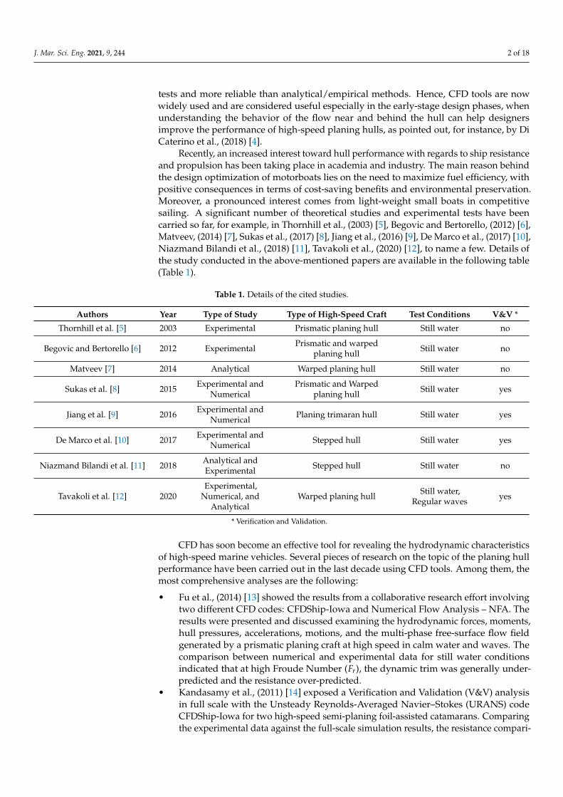
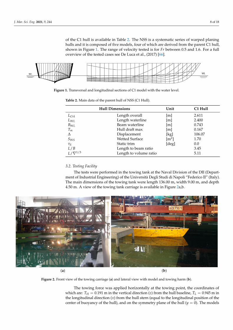
of the C1 hull is available in Table 2. The NSS is a systematic series of warped planinghulls and it is composed of five models, four of which are derived from the parent C1 hull,shown in Figure 1. The range of velocity tested is for Fr between 0.5 and 1.6. For a fulloverview of the tested cases see De Luca et al., (2017) [66].

Figure 1. Transversal and longitudinal sections of C1 model with the water level.

Table 2. Main data of the parent hull of NSS (C1 Hull).

Hull Dimensions Unit C1 Hull

LOA Length overall [m] 2.611LWL Length waterline [m] 2.400BWL Beam waterline [m] 0.743Tm Hull draft max [m] 0.167∆ Displacement [kg] 106.07SWS Wetted Surface [m2] 1.70τS Static trim [deg] 0.0L/B Length to beam ratio 3.45L/∇1/3 Length to volume ratio 5.11

3.2. Testing Facility

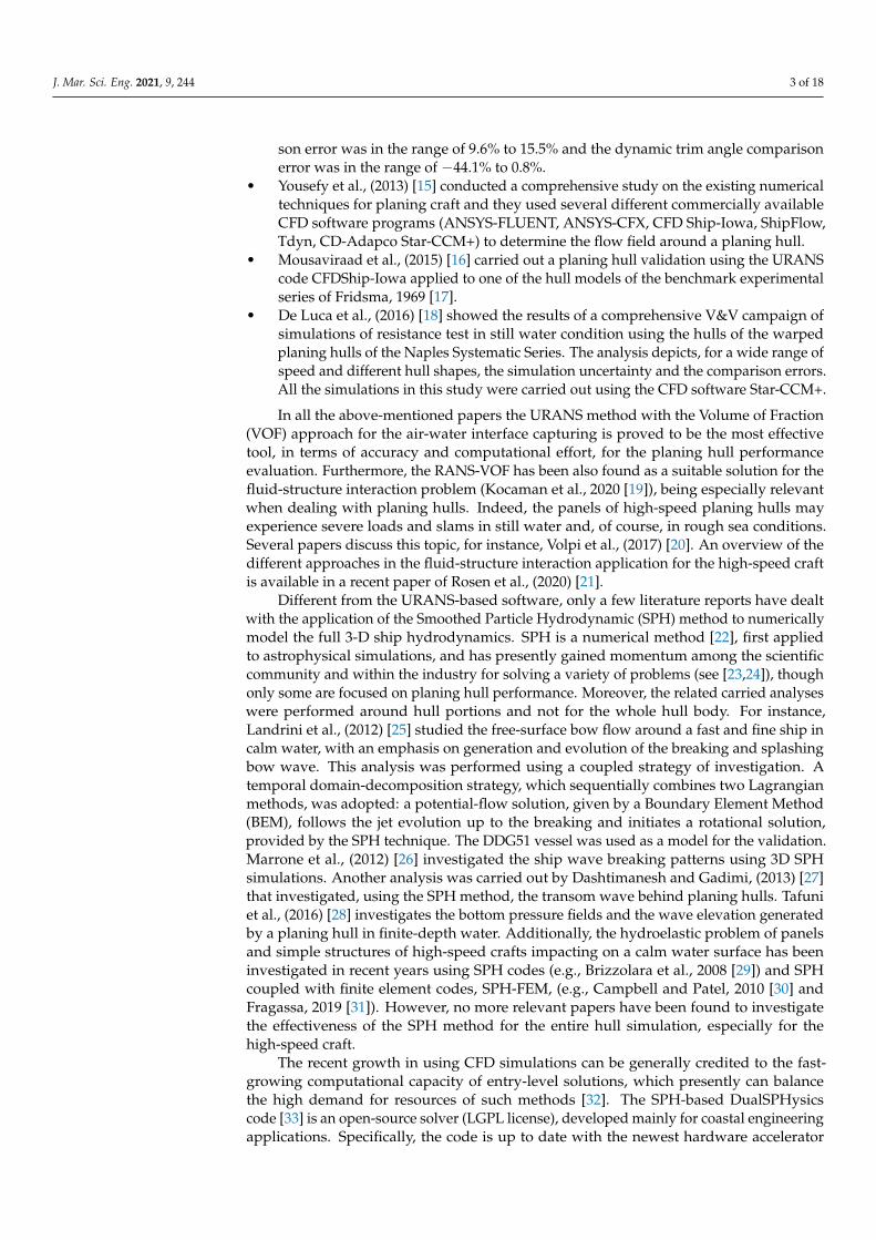
The tests were performed in the towing tank at the Naval Division of the DII (Depart-ment of Industrial Engineering) of the Università Degli Studi di Napoli “Federico II” (Italy).The main dimensions of the towing tank were length 136.00 m, width 9.00 m, and depth4.50 m. A view of the towing tank carriage is available in Figure 2a,b.

(a) (b)

Figure 2. Front view of the towing carriage (a) and lateral view with model and towing harm (b).

The towing force was applied horizontally at the towing point, the coordinates ofwhich are: TH = 0.191 m in the vertical direction (z) from the hull baseline, TL = 0.945 m inthe longitudinal direction (x) from the hull stern (equal to the longitudinal position of thecenter of buoyancy of the hull), and on the symmetry plane of the hull (y = 0). The models

J. Mar. Sci. Eng. 2021, 9, 244 9 of 18

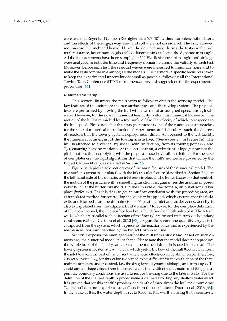
were tested at Reynolds Number (Re) higher than 3.5 · 106, without turbulence stimulators,and the effects of the surge, sway, yaw, and roll were not considered. The only allowedmotions are the pitch and heave. Hence, the data acquired during the tests are the hulltotal resistance, heave motion (also called dynamic sinkage), and the dynamic trim angle.All the measurements have been sampled at 500 Hz. Resistance, trim angle, and sinkagewere analyzed in both the time and frequency domain to assure the validity of each test.Moreover, before each test, the residual waves were measured to minimize noise and tomake the tests comparable among all the models. Furthermore, a specific focus was takento keep the experimental uncertainty as small as possible, following all the InternationalTowing Tank Conference (ITTC) recommendations and suggestions for the experimentalprocedures [66].

4. Numerical Setup

This section illustrates the main steps to follow to obtain the working model. Thekey features of this setup are the free-surface flow and the towing system. The physicaltests are performed by moving the hull with a carrier at an assigned speed through stillwater. However, for the sake of numerical feasibility, within this numerical framework, themotion of the hull is mimicked by a free-surface flow, the velocity of which corresponds tothe hull speed. Please note that this strategy represents one of the commonest approachesfor the sake of numerical reproduction of experiments of this kind. As such, the degreesof freedom that the towing system deploys must differ. As opposed to the test facility,the numerical counterpart of the towing arm is fixed (Towing system in Figure 3a). Thehull is attached to a vertical (z) slider (with no friction) from its towing point (TL andTH), ensuring heaving motions. At this last location, a cylindrical hinge guarantees thepitch motion, thus complying with the physical model overall restrictions. For the sakeof completeness, the rigid algorithms that dictate the hull’s motion are governed by theProject Chrono library, as detailed in Section 2.5.

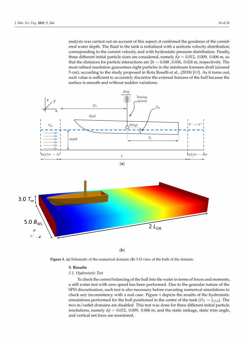
Figure 3a depicts a schematic view of the main features of the numerical model. Thefree-surface current is simulated with the inlet/outlet feature (described in Section 2.4). Atthe left-hand side of the domain, an inlet zone is placed. The buffer (buffer-in) that controlsthe motion of the particles with a smoothing function that guarantees the uniform imposedvelocity Vin at the buffer threshold. On the flip side of the domain, an outlet zone takesplace (buffer-out). For this side, to get an outflow consistent with the preceding area, anextrapolated method for controlling the velocity is applied, which ensures that the fluidexits undisturbed from the domain (V− = V+); at the inlet and outlet zones, density isalso extrapolated from the adjacent fluid domain. Moreover, for the complete definitionof the open channel, the free-surface level must be defined on both sides of it. The lateralwalls, which are parallel to the direction of the flow (y) are treated with periodic boundaryconditions (Gómez-Gesteira et al., 2012 [67]). Figure 3a reports the quantity drag as it iscomputed from the system, which represents the reaction force that is experienced by themechanical constraint handled by the Project Chrono routine.

Section 3 exposes the main geometry of the hull under study and, based on such di-mensions, the numerical model takes shape. Please note that the model does not reproducethe whole bulk of the facility; an alternate, the reduced domain is used in its stead. Thetowing system is located at DT = 1.555, which yields the bow of the hull 0.50 m away fromthe inlet to avoid the part of the current where local effects could be still in place. Therefore,L is set to twice LOA, for this value is deemed to be sufficient for the evaluation of the threemain parameters under control, i.e., the drag force, dynamic sinkage, and trim angle. Toavoid any blockage effects from the lateral walls, the width of the domain is set 5BWL, plusperiodic boundary conditions are used to reduce the drag due to the lateral walls. For thedefinition of the channel depth, a proper value is defined avoiding any shallow water effect.It is proved that for this specific problem, at a depth of three times the hull maximum draftTm, the hull does not experience any effects from the tank bottom (Duarte et al., 2016 [68]).In the wake of this, the water depth is set to 0.500 m. It is worth noticing that a sensitivity

J. Mar. Sci. Eng. 2021, 9, 244 10 of 18

analysis was carried out on account of this aspect; it confirmed the goodness of the consid-ered water depth. The fluid in the tank is initialized with a uniform velocity distribution,corresponding to the current velocity, and with hydrostatic pressure distribution. Finally,three different initial particle sizes are considered, namely dp = 0.012, 0.009, 0.006 m, sothat the distances for particle interactions are 2h = 0.048 , 0.036, 0.024 m, respectively. Themost refined resolution guarantees eight particles in the minimum foreseen draft (around5 cm), according to the study proposed in Rota Roselli et al., (2018) [69]. As it turns out,such value is sufficient to accurately discretize the external features of the hull because thesurface is smooth and without sudden variations.

Lbu f f er − in

depth

Hull

Hinge

bu f f er − out

Vin V− = V+

z

x

y

drag

TL

THDT

Towingsystem

(a)

(b)

Figure 3. (a) Schematic of the numerical domain; (b) 3-D view of the bulk of the domain.

5. Results5.1. Hydrostatic Test

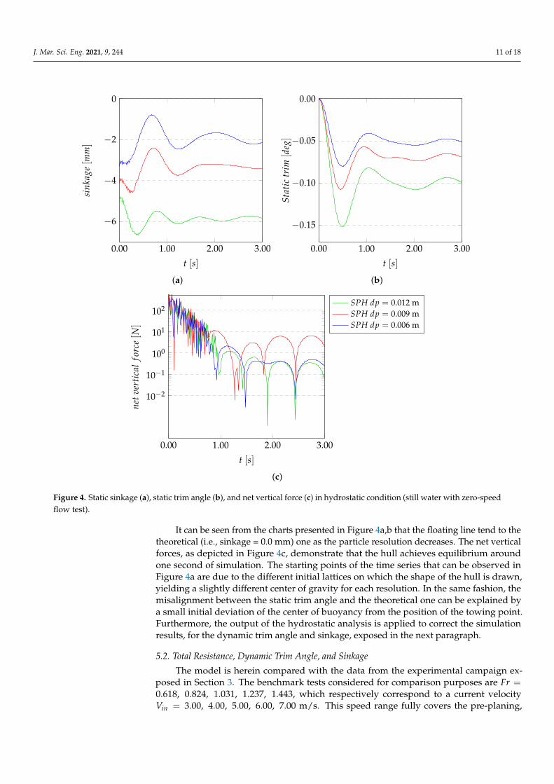
To check the correct balancing of the hull into the water in terms of forces and moments,a still water test with zero speed has been performed. Due to the granular nature of theSPH discretization, such test is also necessary before executing numerical simulations tocheck any inconsistency with a real case. Figure 4 depicts the results of the hydrostaticsimulations performed for the hull positioned in the center of the tank (DT = LOA). Thetwo in/outlet domains are disabled. This test was done for three different initial particleresolutions, namely dp = 0.012, 0.009, 0.006 m, and the static sinkage, static trim angle,and vertical net force are monitored.

J. Mar. Sci. Eng. 2021, 9, 244 11 of 18

0.00 1.00 2.00 3.00

−6

−4

−2

0

t [s]

sink

age[m

m]

(a)

0.00 1.00 2.00 3.00

−0.15

−0.10

−0.05

0.00

t [s]

Stat

ictr

im[d

eg]

(b)

0.00 1.00 2.00 3.00

10−2

10−1

100

101

102

t [s]

netv

erti

cal

forc

e[N

]

SPH dp = 0.012 mSPH dp = 0.009 mSPH dp = 0.006 m

(c)

Figure 4. Static sinkage (a), static trim angle (b), and net vertical force (c) in hydrostatic condition (still water with zero-speedflow test).

It can be seen from the charts presented in Figure 4a,b that the floating line tend to thetheoretical (i.e., sinkage = 0.0 mm) one as the particle resolution decreases. The net verticalforces, as depicted in Figure 4c, demonstrate that the hull achieves equilibrium aroundone second of simulation. The starting points of the time series that can be observed inFigure 4a are due to the different initial lattices on which the shape of the hull is drawn,yielding a slightly different center of gravity for each resolution. In the same fashion, themisalignment between the static trim angle and the theoretical one can be explained bya small initial deviation of the center of buoyancy from the position of the towing point.Furthermore, the output of the hydrostatic analysis is applied to correct the simulationresults, for the dynamic trim angle and sinkage, exposed in the next paragraph.

5.2. Total Resistance, Dynamic Trim Angle, and Sinkage

The model is herein compared with the data from the experimental campaign ex-posed in Section 3. The benchmark tests considered for comparison purposes are Fr =0.618, 0.824, 1.031, 1.237, 1.443, which respectively correspond to a current velocityVin = 3.00, 4.00, 5.00, 6.00, 7.00 m/s. This speed range fully covers the pre-planing,

J. Mar. Sci. Eng. 2021, 9, 244 12 of 18

transient, and planing regime of the C1 hull. The three resolutions used for the hydrostatictests are considered here.

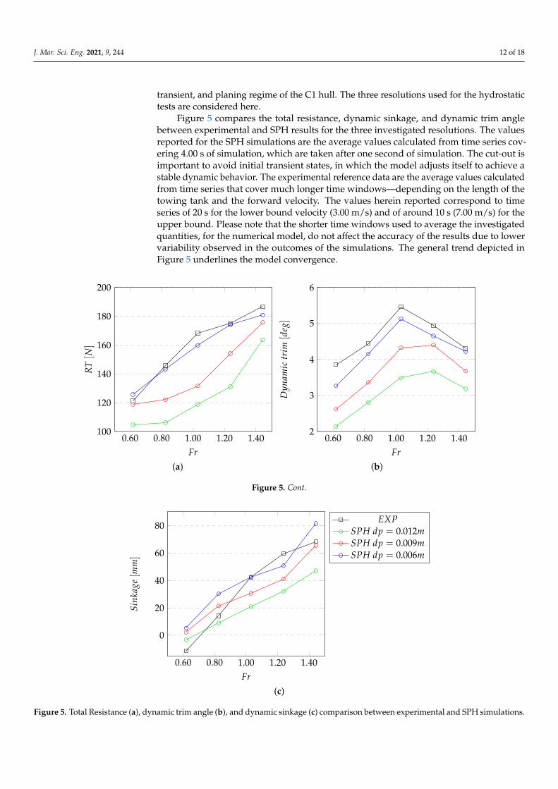
Figure 5 compares the total resistance, dynamic sinkage, and dynamic trim anglebetween experimental and SPH results for the three investigated resolutions. The valuesreported for the SPH simulations are the average values calculated from time series cov-ering 4.00 s of simulation, which are taken after one second of simulation. The cut-out isimportant to avoid initial transient states, in which the model adjusts itself to achieve astable dynamic behavior. The experimental reference data are the average values calculatedfrom time series that cover much longer time windows—depending on the length of thetowing tank and the forward velocity. The values herein reported correspond to timeseries of 20 s for the lower bound velocity (3.00 m/s) and of around 10 s (7.00 m/s) for theupper bound. Please note that the shorter time windows used to average the investigatedquantities, for the numerical model, do not affect the accuracy of the results due to lowervariability observed in the outcomes of the simulations. The general trend depicted inFigure 5 underlines the model convergence.

0.60 0.80 1.00 1.20 1.40100

120

140

160

180

200

Fr

RT[N

]

(a)

0.60 0.80 1.00 1.20 1.402

3

4

5

6

Fr

Dyn

amic

trim

[deg]

(b)

Figure 5. Cont.

0.60 0.80 1.00 1.20 1.40

0

20

40

60

80

Fr

Sink

age[m

m]

EXPSPH dp = 0.012mSPH dp = 0.009mSPH dp = 0.006m

(c)

Figure 5. Total Resistance (a), dynamic trim angle (b), and dynamic sinkage (c) comparison between experimental and SPH simulations.

J. Mar. Sci. Eng. 2021, 9, 244 13 of 18

Table 3 proposes the percentage discrepancies between the outcomes of the numericalmethod and the experimental test for the three variables under analysis, for the finestresolution dp = 0.006 m. Observing Table 3 and Figure 5, it is visible that the numericalmethod shows an acceptable agreement with the experimental results, though the dynamicsinkage error is high in the pre-planing regime. It is noteworthy to observe that the highpercentage error for the dynamic sinkage is strictly connected to the small values of thisparameter. For a more comprehensive picture about the validity of the results here exposed,it is possible to refer to the results shown in De Luca et al., 2016 [18], where the URANSCD-Adapco Star-CCM+ is used. The general trend shown in this last work is almost in linewith the results obtained through the presented SPH model for the higher resolution; it ispossible to recognize the same inaccuracy when dynamic trim predictions are considered.On the other hand, the good performance of the proposed numerical model for the runningattitude parameters directly implies the great accuracy shown by resistance prediction;details of this point are analyzed in the next sub-paragraph.

Table 3. Percentage comparison error between experimental and SPH and simulations withdp = 0.006 m for the three variables (total resistance, dynamic trim angle, and sinkage).

Fr Total Resistance Dynamic Trim angle Dynamic Sinkage

0.618 3.52% −17.92% 319.73%0.824 −1.89% −6.89% 53.41%1.031 −5.34% −6.55% 0.53%1.237 −0.55% −6.15% −16.95%1.443 −3.29% −2.04% 16.20%

All the simulations are run on an NVIDIA© GeForce RTX 2080 Ti with 12GB of RAMand their outcomes are used to evaluate the performance of the model. Using the highestresolution (dp = 0.006 m) a total number of 33.3 million particles are created at its initialstage; the presence of a current; however, contributes to a rate of in/out particles that is,on average, of around 40 million a second. This indeed affects the runtime, which finallyamounts to 104 h (≈ 4 days) per 5.00 s of physical time - on average.

5.3. Whisker Spray

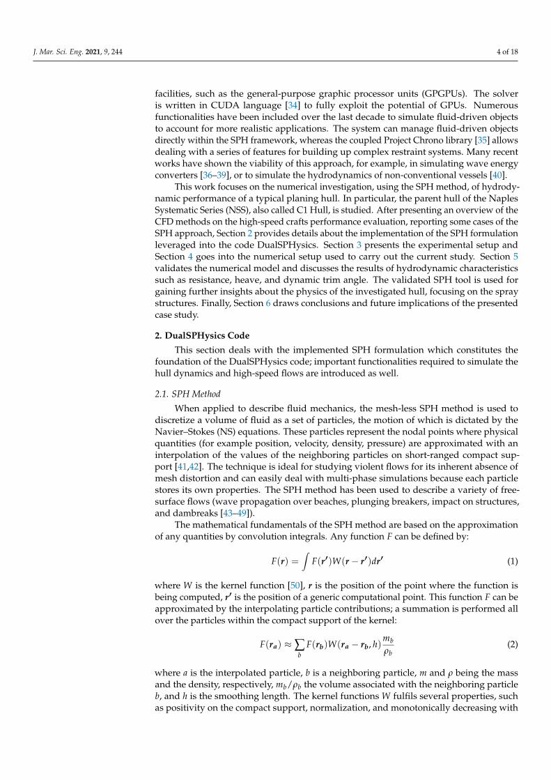
The spray region is a complex area located forward the stagnation line. Accordingto Savitsky and Morabito (2011) [70], the stagnation line is defined as “the locus of pointson the bottom along which the flow is divided into forward and aft components and onwhich the pressure is a maximum and is developed from bringing to rest the componentof free stream velocity normal to this line”. The spray region can be divided into twodifferent patterns: the whisker spray and the main spray. The whisker spray is a streamof small droplets of water projected out of the chine with a trajectory essentially equalto the local deadrise angle. The main spray, instead, is a cone-shaped discharge of water(continuous blister) with its apex located near the intersection of the stagnation line andthe chine. The outboard trajectory of the main spray is significantly elevated compared tothe whisker spray trajectory. The sprays (whisker and main) departs from the chine lineand the extension is bounded by the spray edges. The spray area on the hull bottom iscreated as the craft moves through the water at high speeds (planing regime speeds).

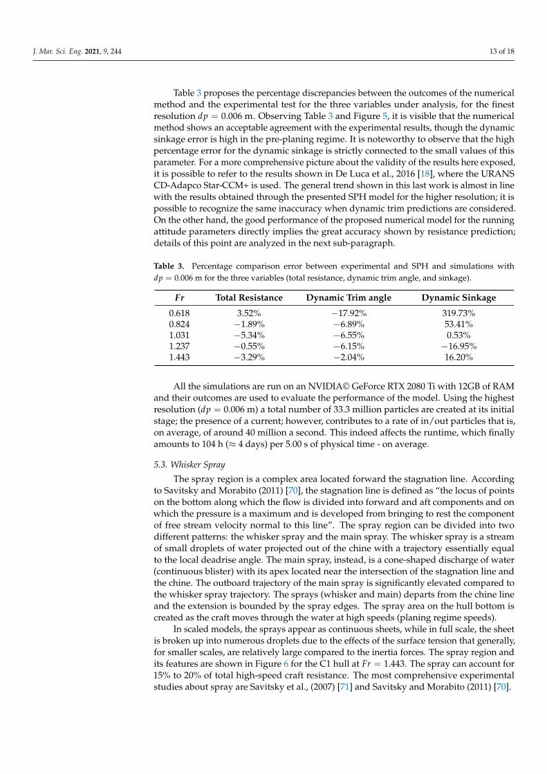
In scaled models, the sprays appear as continuous sheets, while in full scale, the sheetis broken up into numerous droplets due to the effects of the surface tension that generally,for smaller scales, are relatively large compared to the inertia forces. The spray region andits features are shown in Figure 6 for the C1 hull at Fr = 1.443. The spray can account for15% to 20% of total high-speed craft resistance. The most comprehensive experimentalstudies about spray are Savitsky et al., (2007) [71] and Savitsky and Morabito (2011) [70].

J. Mar. Sci. Eng. 2021, 9, 244 14 of 18

Figure 6. C1 hull at Fr = 1.443, (A) Whisker spray, (B) Main spray, (C) Spray edge (red line), (D) Spray root, (E) Reflectionof the spray edge.

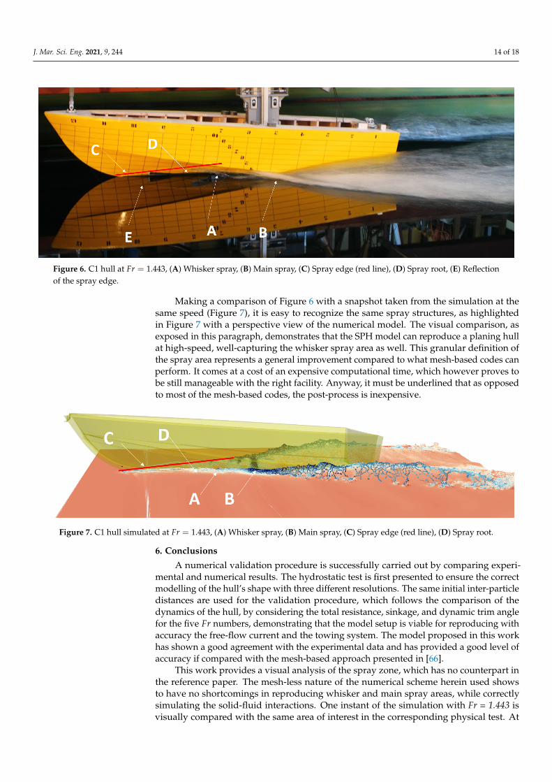
Making a comparison of Figure 6 with a snapshot taken from the simulation at thesame speed (Figure 7), it is easy to recognize the same spray structures, as highlightedin Figure 7 with a perspective view of the numerical model. The visual comparison, asexposed in this paragraph, demonstrates that the SPH model can reproduce a planing hullat high-speed, well-capturing the whisker spray area as well. This granular definition ofthe spray area represents a general improvement compared to what mesh-based codes canperform. It comes at a cost of an expensive computational time, which however proves tobe still manageable with the right facility. Anyway, it must be underlined that as opposedto most of the mesh-based codes, the post-process is inexpensive.

Figure 7. C1 hull simulated at Fr = 1.443, (A) Whisker spray, (B) Main spray, (C) Spray edge (red line), (D) Spray root.

6. Conclusions

A numerical validation procedure is successfully carried out by comparing experi-mental and numerical results. The hydrostatic test is first presented to ensure the correctmodelling of the hull’s shape with three different resolutions. The same initial inter-particledistances are used for the validation procedure, which follows the comparison of thedynamics of the hull, by considering the total resistance, sinkage, and dynamic trim anglefor the five Fr numbers, demonstrating that the model setup is viable for reproducing withaccuracy the free-flow current and the towing system. The model proposed in this workhas shown a good agreement with the experimental data and has provided a good level ofaccuracy if compared with the mesh-based approach presented in [66].

This work provides a visual analysis of the spray zone, which has no counterpart inthe reference paper. The mesh-less nature of the numerical scheme herein used showsto have no shortcomings in reproducing whisker and main spray areas, while correctlysimulating the solid-fluid interactions. One instant of the simulation with Fr = 1.443 isvisually compared with the same area of interest in the corresponding physical test. At

J. Mar. Sci. Eng. 2021, 9, 244 15 of 18

a glance, this comparison returns a clear and consistent overall picture, which allowsidentifying many features of the spray area. A whisker spray is clearly defined along withthe spray root, though slightly shifted toward the aft of the hull. The main spray structuresand the spray edges are also visible and in close agreement with the experimental ones.For the model can capture the whisker spray area with enough accuracy, this could beconsidered to be the reason for the closer estimation that the model can provide for thetotal resistance and dynamic trim angle.

This work lies down a groundwork on which subsequent experimental studies can becomplemented by numerical analyses, in the field of naval engineering. The multiphysicssolver, DualSPHysics, is employed to reproduce a test setup that is commonly used to workout the performance of planing hulls. The great versatility of the code allows building themain features of the facility with ease. For the particular case of planing hulls, where thehigh non-linearities of the fluid flow are critical, the Smoothed Particle Hydrodynamicsmethod poses a good compromise between accuracy and computational effort. As has beenshown through the information reported in this work, the model can achieve a sufficientdegree of accuracy for the evaluation of the planing hull performance. The model setup isthoroughly reported, and it is quite straightforward to reproduce if enough knowledgeabout the physical tests is at hand.

The next step of this investigation will be the application of the SPH method not onlyto the still water resistance tests but also to the planing hull simulations in regular andirregular waves [72], to extend the engineering applications of the SPH method in themarine hydrodynamic field. Furthermore, a finer resolution will be applied to investigatethe resistance of the planing hull equipped with interceptor/intruder, spray rails, andsteps.

Author Contributions: Conceptualization, S.M.; methodology, B.T. and S.M.; software, J.M.D., B.T.,P.R.-G. and A.J.C.C.; validation, B.T., S.M.; formal analysis, B.T. and P.R.-G., J.M.D.; investigation,S.M. and B.T.; resources, A.J.C.C. and G.V.; data curation, B.T. and S.M.; writing original draftpreparation, S.M., B.T., A.J.C.C., P.R.-G., G.V.; revision, S.M., B.T., A.J.C.C., J.M.D.; visualization, S.M.and B.T.; supervision, G.V. and A.J.C.C. All authors have read and agreed to the published version ofthe manuscript.

Funding: This research received no external funding.

Institutional Review Board Statement: Not applicable.

Informed Consent Statement: Not applicable.

Data Availability Statement: The experimental data presented in this study are openly available inhttps://doi.org/10.1016/j.oceaneng.2017.04.038 (accessed on 18 February 2021).

Acknowledgments: The first author of this manuscript wishes to express his gratitude to the ITsupport provided by Orlando Garcia-Feal, who made possible the use of the HPC system at monkey-island.uvigo.es.

Conflicts of Interest: The authors declare no conflict of interest.

AbbreviationsThe following abbreviations are used in this manuscript:

BEM Boundary Element MethodCCP Cone Complementary ProblemCFD Computational Fluid DynamicsCFL Courant-Friedrich-Lewy NumberDBC Dynamic Boundary ConditionDII Department of Industrial EngineeringDVI Differential Variational Inequality

J. Mar. Sci. Eng. 2021, 9, 244 16 of 18

Fr Froude NumberFVM Finite Volume MethodGPU Graphics Processing UnitHSMV High-Speed Marine VehicleITTC International Towing Tank ConferenceLCB Longitudinal position of the Center of BuoyancyNFA Numerical Flow AnalysisNS Navier–StokesNSS Naples Systematic SeriesRe Reynolds Number(U)RANS (Unsteady) Reynolds-Averaged Navier–StokesSPH Smoothed Particle HydrodynamicsV&V Verification & ValidationVOF Volume of FluidWCSPH Weakly Compressible Smoothed Particle Hydrodynamics

References1. ITTC. Model Tests of High Speed Marine Vehicles Specialist Committee; Final Report and Recommendations of the 22nd ITTC Com-

mittee; 1999. Available online: https://ittc.info/media/1510/specialist-committee-on-safety-of-high-speed-marine-vehicles.pdf(accessed on 18 February 2021).

2. Savitsky, D. Hydrodynamic Design of Planing Hulls. Mar. Technol. SNAME News 1964, 1, 71–95. [CrossRef]3. Blount, D.L. Performance by Design: Hydrodynamics for High-Speed Vessels, 1st ed.; Blount, D.L., Ed.; Donald L. Blount and

Associates, Inc.: Chesapeake, VA, USA, 2014.4. Di Caterino, F.; Bilandi, R.N.; Mancini, S.; Dashtimanesh, A.; De Carlini, M. A Numerical Way for a Stepped Planing Hull Design

and Optimization. In Proceedings of the NAV 2018, 19th International Conference on Ship and Maritime Research, Trieste, Italy,20–22 June 2018. [CrossRef]

5. Thornhill, E.; Oldford, D.; Bose, N.; Veitch, B.; Liu, P. Planing hull performance from model tests. Int. Shipbuild. Prog. 2003,50, 5–18.

6. Begovic, E.; Bertorello, C. Resistance assessment of warped hullform. Ocean. Eng. 2012, 56, 28–42. [CrossRef]7. Matveev, K.I. Hydrodynamic modeling of planing hulls with twist and negative deadrise. Ocean. Eng. 2014, 82, 14–19. [CrossRef]8. Sukas, O.F.; Kinaci, O.K.; Cakici, F.; Gokce, M.K. Hydrodynamic assessment of planing hulls using overset grids. Appl. Ocean.

Res. 2017, 65, 35–46. [CrossRef]9. Jiang, Y.; Sun, H.; Zou, J.; Hu, A.; Yang, J. Analysis of tunnel hydrodynamic characteristics for planing trimaran by model tests

and numerical simulations. Ocean. Eng. 2016, 113, 101–110. [CrossRef]10. De Marco, A.; Mancini, S.; Miranda, S.; Scognamiglio, R.; Vitiello, L. Experimental and numerical hydrodynamic analysis of a

stepped planing hull. Appl. Ocean. Res. 2017, 64, 135–154. [CrossRef]11. Bilandi, R.; Mancini, S.; Vitiello, L.; Miranda, S.; De Carlini, M. A Validation of Symmetric 2D + T Model Based on Single-Stepped

Planing Hull Towing Tank Tests. J. Mar. Sci. Eng. 2018, 6, 136. [CrossRef]12. Tavakoli, S.; Niazmand Bilandi, R.; Mancini, S.; De Luca, F.; Dashtimanesh, A. Dynamic of a planing hull in regular waves:

Comparison of experimental, numerical and mathematical methods. Ocean. Eng. 2020, 217, 107959. [CrossRef]13. Fu, T.; Brucker, K.; Mousaviraad, M.; Ikeda-Gilbert, C.; Lee, E.; O’Shea, T.; Wang, Z.; Stern, F.; Judge, C. An Assessment of

Computational Fluid Dynamics Predictions of the Hydrodynamics of High-Speed Planing Craft in Calm Water and Waves. InProceedings of the 30th Symposium on Naval Hydrodynamics Hobart, Tasmania, Hobart, Australia, 2–7 November 2014.

14. Kandasamy, M.; Ooi, S.K.; Carrica, P.; Stern, F.; Campana, E.; Peri, D.; Osborne, P.; Cote, J.; Macdonald, N.; de Waal, N. CFDvalidation studies for a high-speed foil-assisted semi-planing catamaran. J. Mar. Sci. Technol. 2011, 16, 157–167. [CrossRef]

15. Yousefi, R.; Shafaghat, R.; Shakeri, M. Hydrodynamic analysis techniques for high-speed planing hulls. Appl. Ocean. Res. 2013,42, 105–113. [CrossRef]

16. Mousaviraad, S.M.; Wang, Z.; Stern, F. URANS studies of hydrodynamic performance and slamming loads on high-speedplaning hulls in calm water and waves for deep and shallow conditions. Appl. Ocean. Res. 2015, 51, 222–240. [CrossRef]

17. Fridsma, G. A Systematic Study of the Rough-Water Performance of Planing Boats; Technical Report, Davidson Laboratory Report1275; Stevens Institute of Technology Davidson Laboratory, Castle Point Station: Hoboken, NY, USA, 1969.

18. De Luca, F.; Mancini, S.; Miranda, S.; Pensa, C. An Extended Verification and Validation Study of CFD Simulations for PlaningHulls. J. Ship Res. 2016, 60, 101–118. [CrossRef]

19. Kocaman, S.; Güzel, H.; Evangelista, S.; Ozmen-Cagatay, H.; Viccione, G. Experimental and Numerical Analysis of a Dam-BreakFlow through Different Contraction Geometries of the Channel. Water 2020, 12, 1124. [CrossRef]

20. Volpi, S.; Diez, M.; Sadat-Hosseini, H.; Kim, D.H.; Stern, F.; Thodal, R.; Grenestedt, J. Composite bottom panel slamming of a fastplaning hull via tightly coupled fluid-structure interaction simulations and sea trials. Ocean. Eng. 2017, 143, 240–258. [CrossRef]

21. Rosén, A.; Garme, K.; Razola, M.; Begovic, E. Numerical modelling of structure responses for high-speed planing craft in waves.Ocean. Eng. 2020, 217, 107897. [CrossRef]

J. Mar. Sci. Eng. 2021, 9, 244 17 of 18

22. Violeau, D.; Rogers, B. Smoothed particle hydrodynamics (SPH) for free-surface flows: Past, present and future. J. Hydraul. Res.2016, 54, 1–26. [CrossRef]

23. Gotoh, H.; Khayyer, A. On the state-of-the-art of particle methods for coastal and ocean engineering. Coast. Eng. J. 2018, 60, 1–25.[CrossRef]

24. Manenti, S.; Wang, D.; Domínguez, J.; Li, S.; Amicarelli, A.; Albano, R. SPH Modeling of Water-Related Natural Hazards. Water2019, 11, 1875. [CrossRef]

25. Landrini, M.; Colagrossi, A.; Greco, M.; Tulin, M. The fluid mechanics of splashing bow waves on ships: A hybrid BEM–SPHanalysis. Ocean. Eng. 2012, 53, 111–127. [CrossRef]

26. Marrone, S.; Bouscasse, B.; Colagrossi, A.; Antuono, M. Study of ship wave breaking patterns using 3D parallel SPH simulations.Comput. Fluids 2012, 69, 54–66. [CrossRef]

27. Dashtimanesh, A.; Ghadimi, P. A three-dimensional SPH model for detailed study of free surface deformation, just behind arectangular planing hull. J. Braz. Soc. Mech. Sci. Eng. 2013, 35, 369–380. [CrossRef]

28. Tafuni, A.; Sahin, I.; Hyman, M. Numerical investigation of wave elevation and bottom pressure generated by a planing hull infinite-depth water. Appl. Ocean. Res. 2016, 58, 281–291. [CrossRef]

29. Brizzolara, S.; Viviani, M.; Savio, L. Comparison of SPH and RANSE methods for the evaluation of impact problems in the marinefield. In Proceedings of the 8th World Congress on Computational Mechanics (WCCM8), Venice, Italy, 30 June–4 July 2008.

30. Campbell, J.; Patel, M. Modelling fluid–structure impact with the coupled FE-SPH approach. In Proceedings of the WilliamFroude Conference on Advances in Theoretical and Applied Hydrodynamic, Portsmouth, UK, 24–25 November 2010; pp. 131–137.

31. Fragassa, C. Engineering Design Driven by Models and Measures: The Case of a Rigid Inflatable Boat. J. Mar. Sci. Eng. 2019, 7, 6.[CrossRef]

32. Altomare, C.; Viccione, G.; Tagliafierro, B.; Bovolin, V.; Domínguez, J.; Crespo, A. Free-Surface Flow Simulations with SmoothedParticle Hydrodynamics Method using High-Performance Computing. In Computational Fluid Dynamics-Basic Instruments andApplications in Science; Adela Ionescu, IntechOpen: London, UK, 2018; pp. 73–100. [CrossRef]

33. Crespo, A.; Domínguez, J.; Rogers, B.; Gómez-Gesteira, M.; Longshaw, S.; Canelas, R.; Vacondio, R.; Barreiro, A.; García-Feal, O.DualSPHysics: Open-source parallel CFD solver based on Smoothed Particle Hydrodynamics (SPH). Comput. Phys. Commun.2015, 187, 204–216. [CrossRef]

34. NVIDIA; Vingelmann, P.; Fitzek, F.H. CUDA, Release: 10.2.89 [Internet]. 2020. Available online: https://developer.nvidia.com/cuda-toolkit (accessed on 18 February 2021).

35. Tasora, A.; Serban, R.; Mazhar, H.; Pazouki, A.; Melanz, D.; Fleischmann, J.; Taylor, M.; Sugiyama, H.; Negrut, D. Chrono: AnOpen Source Multi-physics Dynamics Engine. In International Conference on High Performance Computing in Science and Engineering;Springer: Cham, Switzerland, 2016; pp. 19–49. [CrossRef]

36. Brito, M.; Canelas, R.; García-Feal, O.; Domínguez, J.; Crespo, A.; Ferreira, R.; Neves, M.; Teixeira, L. A numerical tool formodelling oscillating wave surge converter with nonlinear mechanical constraints. Renew. Energy 2020, 146, 2024–2043. [CrossRef]

37. Ropero-Giralda, P.; Crespo, A.J.; Tagliafierro, B.; Altomare, C.; Domínguez, J.M.; Gómez-Gesteira, M.; Viccione, G. Efficiencyand survivability analysis of a point-absorber wave energy converter using DualSPHysics. Renew. Energy 2020, 162, 1763–1776.[CrossRef]

38. Tagliafierro, B.; Montuori, R.; Vayas, I.; Ropero-Giralda, P.; Crespo, A.; Domìnguez, J.; Altomare, C.; Viccione, G.; Gòmez-Gesteira,M. A new open source solver for modelling fluid-structure interaction: Case study of a point-absorber wave energy converterwith a power take-off unit. In Proceedings of the 11th International Conference on Structural Dynamics, Athens, Greece, 22–24June 2020. [CrossRef]

39. Ropero-Giralda, P.; Crespo, A.J.C.; Coe, R.G.; Tagliafierro, B.; Domínguez, J.M.; Bacelli, G.; Gómez-Gesteira, M. Modelling aHeaving Point-Absorber with a Closed-Loop Control System Using the DualSPHysics Code. Energies 2021, 14, 760. [CrossRef]

40. Mogan, S.C.; Chen, D.; Hartwig, J.; Sahin, I.; Tafuni, A. Hydrodynamic analysis and optimization of the Titan submarine via theSPH and Finite–Volume methods. Comput. Fluids 2018, 174, 271–282. [CrossRef]

41. Viccione, G.; Bovolin, V.; Carratelli, E.P. Defining and optimizing algorithms for neighbouring particle identification in SPH fluidsimulations. Int. J. Numer. Methods Fluids 2008, 58, 625–638. [CrossRef]

42. Domínguez, J.M.; Crespo, A.J.C.; Gómez-Gesteira, M.; Marongiu, J.C. Neighbour lists in smoothed particle hydrodynamics. Int. J.Numer. Methods Fluids 2011, 67, 2026–2042. [CrossRef]

43. Colagrossi, A.; Landrini, M. Numerical Simulation of Interfacial Flows by Smoothed Particle Hydrodynamics. J. Comput. Phys.2003, 191, 448–475. [CrossRef]

44. Antuono, M.; Colagrossi, A.; Marrone, S.; Molteni, D. Free-surface flows solved by means of SPH schemes with numericaldiffusive terms. Comput. Phys. Commun. 2010, 181, 532–549. [CrossRef]

45. Pugliese Carratelli, E.; Viccione, G.; Bovolin, V. Free surface flow impact on a vertical wall: A numerical assessment. Theor.Comput. Fluid Dyn. 2016, 30, 403–414. [CrossRef]

46. Khayyer, A.; Gotoh, H.; Falahaty, H.; Shimizu, Y. An enhanced ISPH–SPH coupled method for simulation of incompressiblefluid–elastic structure interactions. Comput. Phys. Commun. 2018, 232, 139–164. [CrossRef]

47. Domínguez, J.; Crespo, A.; Hall, M.; Altomare, C.; Wu, M.; Stratigaki, V.; Troch, P.; Cappietti, L.; Gómez-Gesteira, M. SPHsimulation of floating structures with moorings. Coast. Eng. 2019, 153, 103560. [CrossRef]

J. Mar. Sci. Eng. 2021, 9, 244 18 of 18

48. De Padova, D.; Meftah, M.; De Serio, F.; Mossa, M.; Sibilla, S. Characteristics of breaking vorticity in spilling and plunging wavesinvestigated numerically by SPH. Environ. Fluid Mech. 2019, 1–28. [CrossRef]

49. Amicarelli, A.; Manenti, S.; Albano, R.; Agate, G.; Paggi, M.; Longoni, L.; Mirauda, D.; Ziane, L.; Viccione, G.; Todeschini, S.; et al.SPHERA v.9.0.0: A Computational Fluid Dynamics research code, based on the Smoothed Particle Hydrodynamics mesh-lessmethod. Comput. Phys. Commun. 2020, 250, 107157. [CrossRef]

50. Monaghan, J.J. Smoothed particle hydrodynamics. Rep. Prog. Phys. 2005, 68, 1703–1759. [CrossRef]51. Monaghan, J.J. Smoothed Particle Hydrodynamics. Annu. Rev. Astron. Astrophys. 1992, 30, 543–574. [CrossRef]52. Wendland, H. Piecewise polynomial, positive definite and compactly supported radial basis functions of minimal degree. Adv.

Comput. Math. 1995, 4, 389–396. [CrossRef]53. Molteni, D.; Colagrossi, A. A simple procedure to improve the pressure evaluation in hydrodynamic context using the SPH.

Comput. Phys. Commun. 2009, 180, 861–872. [CrossRef]54. Antuono, M.; Colagrossi, A.; Marrone, S. Numerical diffusive terms in weakly-compressible SPH schemes. Comput. Phys.

Commun. 2012, 183, 2570–2580. [CrossRef]55. Fourtakas, G.; Dominguez, J.M.; Vacondio, R.; Rogers, B.D. Local uniform stencil (LUST) boundary condition for arbitrary 3-D

boundaries in parallel smoothed particle hydrodynamics (SPH) models. Comput. Fluids 2019, 190, 346–361. [CrossRef]56. Leimkuhler, B.; Reich, S.; Zentrum, K.; Str, H.; Skeel, R. Integration Methods for Molecular Dynamics. In Mathematical Approaches

to Biomolecular Structure and Dynamics; Springer: New York, NY, USA, 1995; Volume 82. [CrossRef]57. Monaghan, J.J.; Cas, R.A.F.; Kos, A.M.; Hallworth, M. Gravity currents descending a ramp in a stratified tank. J. Fluid Mech. 1999,

379, 39–69. [CrossRef]58. Monaghan, J.; Kos, A.; Issa, N. Fluid Motion Generated by Impact. J. Waterw. Port, Coastal, Ocean. Eng. 2003, 129, 250–259.

[CrossRef]59. Canelas, R.B.; Domínguez, J.M.; Crespo, A.J.; Gómez-Gesteira, M.; Ferreira, R.M. A Smooth Particle Hydrodynamics discretization

for the modelling of free surface flows and rigid body dynamics. Int. J. Numer. Methods Fluids 2015, 78, 581–593. [CrossRef]60. Crespo, A.; Gómez-Gesteira, M.; Dalrymple, R. Boundary conditions generated by dynamic particles in SPH methods. Comput.

Mater. Contin. 2007, 5, 173–184.61. Liu, M.; Liu, G. Restoring particle consistency in smoothed particle hydrodynamics. Appl. Numer. Math. 2006, 56, 19–36.

[CrossRef]62. Tafuni, A.; Domínguez, J.; Vacondio, R.; Crespo, A. A versatile algorithm for the treatment of open boundary conditions in

Smoothed particle hydrodynamics GPU models. Comput. Methods Appl. Mech. Eng. 2018, 342. [CrossRef]63. Novak, G.; Tafuni, A.; Domínguez, J.; Cetina, M.; Žagar, D. A Numerical Study of Fluid Flow in a Vertical Slot Fishway with the

Smoothed Particle Hydrodynamics Method. Water 2019, 11, 1928. [CrossRef]64. Team, P.D. Chrono: An Open Source Framework for the Physics-Based Simulation of Dynamic Systems. Available online:

https://github.com/projectchrono/chrono (accessed on 7 May 2020).65. Canelas, R.; Brito, M.; Feal, O.; Domínguez, J.; Crespo, A. Extending DualSPHysics with a Differential Variational Inequality:

modeling fluid-mechanism interaction. Appl. Ocean. Res. 2018, 76, 88–97. [CrossRef]66. De Luca, F.; Pensa, C. The Naples warped hard chine hulls systematic series. Ocean. Eng. 2017, 139, 205–236. [CrossRef]67. Gomez-Gesteira, M.; Rogers, B.; Crespo, A.; Dalrymple, R.; Narayanaswamy, M.; Dominguez, J. SPHysics – development of a

free-surface fluid solver – Part 1: Theory and formulations. Comput. Geosci. 2012, 48, 289–299. [CrossRef]68. Duarte, H.; Droguett, E.; Ramos Martins, M.; Lützhöft, M.; Pereira, P.; Lloyd, J. Review of practical aspects of shallow water and

bank effects. Int. J. Marit. Eng. 2016, 158, 177–186. [CrossRef]69. Rota Roselli, R.A.; Vernengo, G.; Altomare, C.; Brizzolara, S.; Bonfiglio, L.; Guercio, R. Ensuring numerical stability of wave

propagation by tuning model parameters using genetic algorithms and response surface methods. Environ. Model. Softw. 2018,103, 62–73. [CrossRef]

70. Savitsky, D.; Morabito, M. Origin and Characteristics of the Spray Patterns Generated by Planing Hulls. J. Ship Prod. Des. 2011,27, 63–83. [CrossRef]

71. Savitsky, D.; DeLorme, M.; Datla, R. Inclusion of Whisker Spray Drag in Performance Prediction Method for High-Speed PlaningHulls. Mar. Technol. 2007, 44, 35–56.

72. Verbrugghe, T.; Domínguez, J.; Altomare, C.; Tafuni, A.; Vacondio, R.; Troch, P.; Kortenhaus, A. Non-linear wave generation andabsorption using open boundaries within DualSPHysics. Comput. Phys. Commun. 2019, 240, 46–59. [CrossRef]