PHOTOCHROMIC TEXTILES

Martina Viková MSc.

In accordance with the requirements for the degree of

Doctor of Philosophy

to Heriot-Watt University

The work embodied in this text was carried out at the Scottish Borders Campus, School of Textiles and Design and off campus at the Technical University in

Liberec, Czech Republic

March 2011 The copyright in this thesis is owned by the author. Any quotation from the thesis or use of any of the information contained in it must acknowledge this thesis as the source of the quotation or information.

ABSTRACT

This thesis describes a new investigation into the relationship between the developed

colour intensity of photochromic textiles and the time of UV exposure and also the

time of relaxation. As a result of this relationship the potential of flexible textile-

based sensor constructions which might be used for the identification of radiation

intensity is demonstrated. In addition the differences between photochromic pigment

behaviour in solution and incorporated into prints on textiles are demonstrated.

Differences in the effect of the spectral power distributions of light sources on the

photochromic response are also examined. Bi-exponential functions, which are used

in optical yield (Oy) calculations, have been described to provide a good description

of the kinetics of colour change intensity of photochromic pigments, giving a good

fit. The optical yield of the photochromic reaction Oy is linearly related to the

intensity of illumination E.

The optical yield obtained from the photochromic reaction curves are

described by a kinetic model, which defines the rate of colour change initiated by

external stimulus of UV light. Verification of the kinetic model is demonstrated for

textile sensors with photochromic pigments applied by textile printing and by fibre

mass dyeing.

The thesis also describes a unique instrument developed by author, which

measures colour differences ΔE* and spectral remission curves derived from

photochromic colour change simultaneously with UV irradiation.

In this theses the photochromic behaviour of selected pigments in three

different applications (type of media – textile prints, non-woven textiles and solution

is investigated.

Acknowledgement

Many thanks are due to Professor R.M. Christie of the School of Textiles and Design, the Scottish Border Campus for his guidance, expert supervision, and encouragement throughout. Thanks are also due to Professor Jiří Militký as co-supervisor from Technical University of Liberec.

My special thanks are devoted to all the people who helped me during the time of the writing of the thesis. Great thanks are directed to my mother Mary and my husband Michael for their stand - by support. With all my love Martina

TABLE OF CONTENTS

Chapter 1 Introduction ............................................................................................................1 Chapter 2 Literature review ....................................................................................................5

2.1 Photochromism of organic compounds ........................................................................6 a) Triplet –triplet photochromism ...................................................................................8 b) Heterolytic cleavage ...................................................................................................9 c) Homolytic cleavage ..................................................................................................10 d) Trans-cis isomeration ...............................................................................................11 e) Photochromism based on tautomerism .....................................................................13 f) Photodimerisation......................................................................................................14

2.2 Basic Optical Concepts and Principles .......................................................................15 2.2.1 Maxwell’s Equations ...........................................................................................15 2.2.2 Energetic quantity inside a planar electromagnetic wave ....................................19 2.2.3 Geometric Optics .................................................................................................22 2.2.4 Radiometry ...........................................................................................................24

2.3 Spectral Functions .......................................................................................................28 2.3.1 Spectral Power Distribution .................................................................................28 2.3.2 Spectral Reflectance.............................................................................................31 2.3.3 Spectral Transmittance .........................................................................................31 2.3.4 Spectral Absorptivity ...........................................................................................32

2.4 Colours ........................................................................................................................33 2.4.1 CIE COLORIMETRY .........................................................................................34 2.4.2 CIELAB and CIELUV .........................................................................................37

2.5 Optical models of translucent media ...........................................................................40 2.5.1 Survey of fundamental light scattering theories ..................................................41 2.5.2 Kubelka-Munk’s theory .......................................................................................42 2.5.3 Colour Intensity ...................................................................................................44 2.5.4 Kinetic model of photochromic response during exposure .................................45 2.5.5 Kinetic model of the photochromic response during reversion ...........................46

2.6 Colorimetric measurement of photochromic samples ................................................47 2.6.1 Standard for the reflectance factor .......................................................................47 2.6.3 Illuminating and viewing conditions for transmitting specimens ........................50 2.7. Conclusion .............................................................................................................51

Chapter 3 Experimental ........................................................................................................53 3.1. Instrumentation ..........................................................................................................53

3.1.1 Tristimulus colorimeters and spectrocolorimeters ...............................................54 3.1.2. Spectrophotometers.............................................................................................55 (a) Transmittance measurement of transparent media ..................................................55 (b) Transmittance measurement of translucent media ..................................................56 (c) Measurement of translucent media by reflectance ..................................................60 3.1.3. Light fastness tests ..............................................................................................76

3.2 Materials .....................................................................................................................77 3.2.1 Screen printing .....................................................................................................81 3.2.2 Non - woven samples produced by Melt Blown technology ...............................83 3.2.3 Photochromic solution .........................................................................................90

Chapter 4 Resuls and discussion ...........................................................................................92 4.1 Screen-printed photochromic textiles .........................................................................92

4.1.1 Dependence of colour change on irradiance ........................................................92

4.1.2 Dependence of colour change on pigment concentration ..................................109 4.2 Non woven textiles containing the photochromic pigments ....................................119 4.3 Photochromic pigments in solution ..........................................................................126

4.3.1 Influence of spectral power distribution of light sources...................................126 4.3.2 Influence of pigment concentration in solution on shade intensity ...................130 4.3.3 Colour shift in CIE L*a*b* space for solutions and photochromic prints ........134 4.3.4 Dependence of the kinetics of photochromic change on applied media ............139

4.4 Fatigue test of photochromic prints ..........................................................................141 4.4.1 Fatigue of the photochromic reaction – exposure D65 + UV fluorescent tube ..............................................................................................................................141 4.4.2 Fatigue resistance - XENOTEST .......................................................................147

Chapter 5 Conclusion ..........................................................................................................157 List of symbols ....................................................................................................................174 Appendix A: ........................................................................................................................176 Selected measurement and their comparison with other authors ........................................176 Appendix B: ........................................................................................................................179 Author`s publications relating to the thesis ........................................................................179 Appendix C: ........................................................................................................................183 Selected author’s articles ....................................................................................................183

1

Chapter 1 INTRODUCTION Solar radiation is an important natural feature because it is a critical factor in

determining the Earth’s climate and has a significant influence on the environment.

The ultraviolet part of the solar spectrum (UV) plays an important role in many

processes in the biosphere. UV radiation has several beneficial effects but it may also

be very harmful if the UV level exceeds “safe” limits. If the level of UV radiation is

sufficiently high, the self-protection ability of some biological species is exhausted

and the subject may be severely damaged. This is of concern to the human organism,

in particular with regard to the effect on the skin and the eyes. To avoid damage from

high UV exposure, both acute and chronic, people should limit their exposure to solar

radiation by using protective measures [1, 2].

The diurnal and annual variability of solar UV radiation reaching the ground

is governed by astronomical and geographical parameters as well as by the

atmospheric conditions. Since human activities affect the atmosphere, such as

polluting the air and influencing the ozone layer, they also affect the UV radiation

reaching the ground. Consequently, the level of solar UV radiation is a highly

variable environmental parameter that differs widely in time and location.

The need to reach the public with simple-to-understand information about UV

and its possible detrimental effects has led scientists to define a parameter that can be

used as an indicator of the UV exposure (in this thesis the parameter is colour change)

[1, 2, 3].

The commercial, scientific and industrial applications of ultraviolet radiation

and the consequent need for UV measurements have increased enormously over the

last 20 years. Ultraviolet radiation has found application in semiconductor

photolithography, material curing, non-destructive testing, acceleration of chemical

processes, water purification, sterilisation, phototherapy and solarium appliances.

Concerns over the environmental and health effects of solar UV radiation penetrating

into the biosphere through the depleted ozone layer have also greatly emphasised the

urgency for accurate and reliable UV radiometry.

2

The measurement problems in terms of the UV wavelengths are much more

severe than in the visible wavelength range, since both sources and detectors tend to

be unstable in the UV region of the electromagnetic spectrum [4-8].

There is considerable interest in photochromic materials arising from the

many potential applications, which are associated with their ability to undergo

reversible, light-induced colour change. Two chemical species showing a reversible

transformation differ from one another not only in their absorption spectra but also in

their physical and chemical properties. Photochromic materials are used most widely

in ophthalmic sun-screening applications, and also find applications in security

printing, optical recording and switching, solar energy storage, nonlinear optics and

biological systems [9-19]. The existing ranges of commercial products generally

undergo positive photochromism, a light-induced transition from colourless to

coloured due to a ring-opening reaction.

Major attention has been given to research, development and perfection of

protective clothes, especially their barrier features. For these protective barriers, it is

important to understand how clothes or textiles protect the wearer against the above-

mentioned dangerous conditions associated with UV irradiation and if the protection

is only partial or the protection is time limited by ambient conditions. Most protective

fabrics are not developed for long periods of wear. In the development of these

barrier structures, it is important also to keep in mind the comfort of individuals. This

concept of protective fabrics can be considered as involving intelligent structures. A

disadvantage of such intelligent structures is a fixed response to the external stimulus

and the situation would be improved by a means for monitoring of external dangerous

conditions. Such structures are referred to as passive intelligent textiles structures.

Textile structures that produce adequate responses and are able to modulate the

degree of protection in accordance to the external stimulus (e.g., change of intensity

of UV irradiation, temperature, etc.) are known as active textile structures.

Textile structures, which react and respond, and which are able modulate the

degree of protection in accordance with the magnitude of the external stimulus are

called SMART textiles. An example of passive intelligent textiles is optical fibres,

which lead not only to a signal, but they are also sensitive to the deformation,

concentration of substances, pressure, electric power etc. A specific example of an

active intelligent textiles would a textile, which reacts by changing colour because of

its dependence on external stimulus (light, temperature). Moreover, textile based

3

sensors and active protective textiles have the advantages that the textile structure is

easy customizable by sewing, thermal bonding or glueing. In addition, there are

advantages of easy maintenance (washing, chemical cleaning) and low specific

weight with good strength and elasticity. Other good features include workability

with no need for a change of technology of production and their extremely large

specific surface. Other major advantages are the possible integration of soft type

sensors (textile-based sensors) into protective clothing system and their reasonable

price. The research described in this thesis is focused on textile-based sensors with

photochromic behaviour, involving a study of dynamic, colour and spectral behaviour

and sensitivity to modulation of the photochromic sensors.

The thesis is focused on research into the colour change kinetics of

photochromic pigments, which are applied onto a textile substrate by printing or mass

dyeing. In addition, the investigation of the pigments in organic solvent solution is

described as a comparative study. Fundamental attention is given to the relationship

between the colour change intensity and the intensity of illumination and also its

spectral distribution. The fatigue resistance, which is related to the light fastness of

the photochromic textile sensors, is also studied.

The main aim of the research described in this thesis is to investigate the

potential for utilisation of photochromic pigments from the point of view of their

capability of application in textile soft sensors. For the achievement of this main aim,

the following objectives were pursued:

• A study of the exposure and reversal of the colour change of selected

photochromic pigments

• Definition of a colour change model

• Investigation of the kinetic behaviour of photochromic textiles

• A study of photochromic response modulation with UV absorbers

• A study of the spectral sensitivity of photochromic textiles

• Evaluation of fastness properties

As a consequence of this work a new definition of optical yield of a

photochromic reaction is presented, which is described by the hysteresis of a colour

change curve. This optical yield obtained from the photochromic reaction curve is

described by a kinetic model, which defines the rate of colour change initiated by an

external stimulus – namely UV light. The kinetic model verification is demonstrated

4

on textile sensors with photochromic pigments applied by both textile printing and

fibre mass dyeing. [20]

It is envisaged that the fulfilment of these objectives will lead to the

development of simple textile sensors sensitive to UV irradiation. The colour change

would be visually perceivable and approximately linear to the irradiation intensity.

Based on the extensive experimental work a unique device concept for

photochromic measurement in reflectance mode is described, which has been

patented in the Czech Republic in the author’s name.

5

Chapter 2

LITERATURE REVIEW The main aim of thesis is oriented to the application of photochromic

pigments onto textile substrates. This chapter contains a review of literature, which

provides a theoretical basis for the research described in later chapters of this thesis.

Section 2.1 describes basic types of photochromic compounds, their main structural

features and the chemical reactions leading to the photochromic effect – the change

from the colourless to coloured forms. Photochromic change is described by a

modified Jablonski diagram, which presents a general mechanism for photochromism

in terms of electronic, radiative and nonradiative transitions. Section 2.1 thus provides

an understanding of the principles of the typical chemical processes, which have an

influence on the photochromic colour change.

A discussion about fundamental optical concepts and principles is given next

in section 2.2 illustrating how light interacts with matter in many different ways.

Most systems involve heat generation, where the light is converted into thermal

energy, inducing a magnetic or structural phase transition and changes in the physical

properties of the medium. The wide-ranging optical properties observed in solid-state

materials can be classified into a small number of general phenomena, one of which

is represented by Maxwell’s equations as described in section 2.2.1, allowing a deep

understanding of fundamental electromagnetic interaction between light, as part of

the electromagnetic spectrum, and solid matter.

Maxwell’s phenomena, together with studies of geometric optics discussed in

section 2.2.3 and of radiometry in section 2.2.4 have provided an important basis,

which have allowed the author to be successful in the construction of the unique

device for the measurement of photochromic kinetic behaviour of selected pigments

based on the pyran and naphthooxazine structures as described throughout this thesis.

Finally, colour phenomena are discussed in section 2.4 to complete the

background principles for the description of colour change during a photochromic

reaction, using CIELAB colour space, the Kubelka-Munk function and colour change

intensity.

6

A Bhν2 or ΔT

hν1

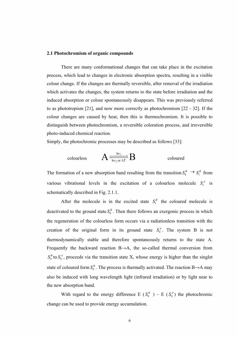
2.1 Photochromism of organic compounds

There are many conformational changes that can take place in the excitation

process, which lead to changes in electronic absorption spectra, resulting in a visible

colour change. If the changes are thermally reversible, after removal of the irradiation

which activates the changes, the system returns to the state before irradiation and the

induced absorption or colour spontaneously disappears. This was previously referred

to as phototropism [21], and now more correctly as photochromism [22 - 32]. If the

colour changes are caused by heat, then this is thermochromism. It is possible to

distinguish between photochromism, a reversible coloration process, and irreversible

photo-induced chemical reaction.

Simply, the photochromic processes may be described as follows [33]:

colourless coloured

The formation of a new absorption band resulting from the transition BS0 → BS1 from

various vibrational levels in the excitation of a colourless molecule AS1 is

schematically described in Fig. 2.1.1.

After the molecule is in the excited state BS1 the coloured molecule is

deactivated to the ground state BS0 . Then there follows an exergonic process in which

the regeneration of the colourless form occurs via a radiationless transition with the

creation of the original form in its ground state AS0 . The system B is not

thermodynamically stable and therefore spontaneously returns to the state A.

Frequently the backward reaction B→A, the so-called thermal conversion from BS0 to AS0 , proceeds via the transition state X, whose energy is higher than the singlet

state of coloured form BS0 . The process is thermally activated. The reaction B→A may

also be induced with long wavelength light (infrared irradiation) or by light near to

the new absorption band.

With regard to the energy difference E ( BS0 ) – E ( AS0 ) the photochromic

change can be used to provide energy accumulation.

7

T1A

T2A

T3A

S1A

S0A S0

A

S0B

X

S1B

S2A

(a) (b)

Fig. 2.1.1 The Jablonski-diagram: Representation of electronic, radiative and nonradiative transitions (reproduction limited to the first excited states)

As with the yield of the light energy conversion to the thermal energy, so the

accumulative capacity (difference of heats of coloured B and colourless A forms)

depends on the chemical structure of the meta-stable photoproduct, which has non-

conventional bond lengths and angles and on the dissipation of resonance energy,

which involves increased stability caused by delocalization of π electrons.

The limitation of the effect results from the second theory of thermodynamics.

Because it may be described as a thermal machine which is working between

temperatures T and T' (photochemical reaction A( AS0 ) → A( AS1 ) → B( BS0 ) at

temperature T and exothermal reaction B( BS0→ X → A( AS0 ) at temperature T'), the

final yield of accumulative capacity increases at temperature T', as does the energy of

the ground state of the “coloured“ molecule BS0 .

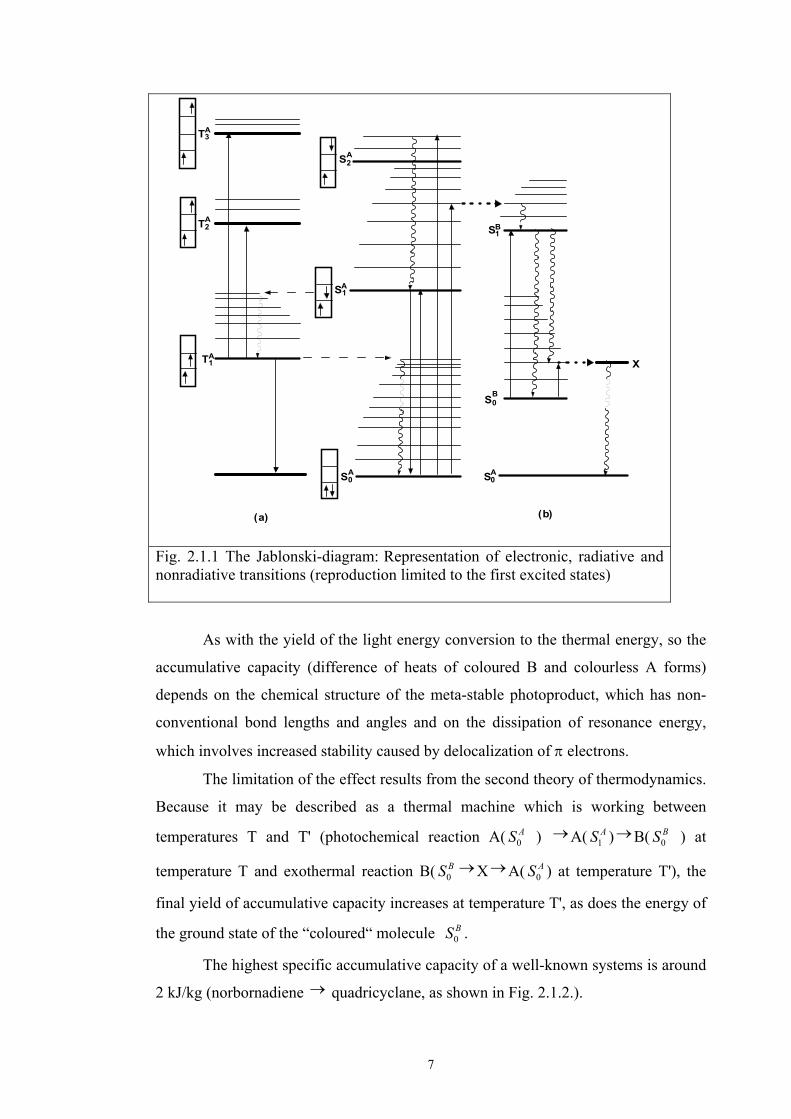
The highest specific accumulative capacity of a well-known systems is around

2 kJ/kg (norbornadiene → quadricyclane, as shown in Fig. 2.1.2.).

8

Fig. 2.1.2 Reaction: Norbornadiene → Quadricyclane

The photochromic process may be classified into several main groups as follows,

according to the mechanism of conformation changes [10,34]:

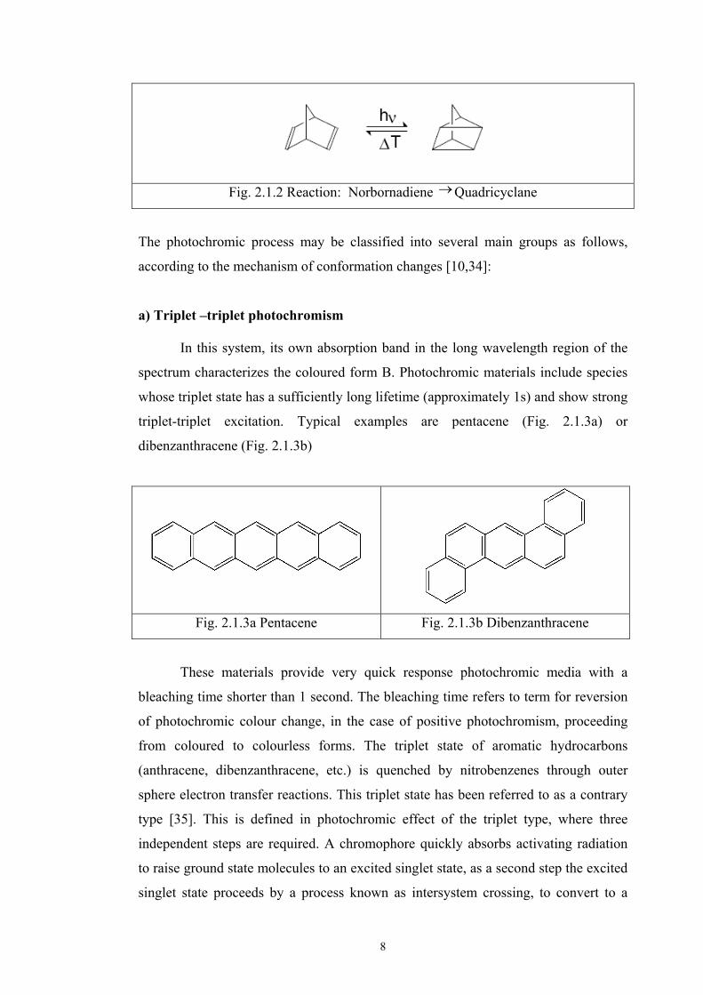
a) Triplet –triplet photochromism In this system, its own absorption band in the long wavelength region of the

spectrum characterizes the coloured form B. Photochromic materials include species

whose triplet state has a sufficiently long lifetime (approximately 1s) and show strong

triplet-triplet excitation. Typical examples are pentacene (Fig. 2.1.3a) or

dibenzanthracene (Fig. 2.1.3b)

Fig. 2.1.3a Pentacene Fig. 2.1.3b Dibenzanthracene

These materials provide very quick response photochromic media with a

bleaching time shorter than 1 second. The bleaching time refers to term for reversion

of photochromic colour change, in the case of positive photochromism, proceeding

from coloured to colourless forms. The triplet state of aromatic hydrocarbons

(anthracene, dibenzanthracene, etc.) is quenched by nitrobenzenes through outer

sphere electron transfer reactions. This triplet state has been referred to as a contrary

type [35]. This is defined in photochromic effect of the triplet type, where three

independent steps are required. A chromophore quickly absorbs activating radiation

to raise ground state molecules to an excited singlet state, as a second step the excited

singlet state proceeds by a process known as intersystem crossing, to convert to a

9

triplet state; thirdly triplet state molecules absorb incident radiation to convert from

the first triplet state level to a higher level.

The quantum yield of triplet-triplet photochromism depends on the

concentration of oxygen in the system, because oxygen causes creation of triplet

excitons. Then quantum yield depends on the relative contributions from processes,

which have an influence on the population of the triplet state such as for example

phosphorescence, radiationless transitions or intersystem conversion etc.

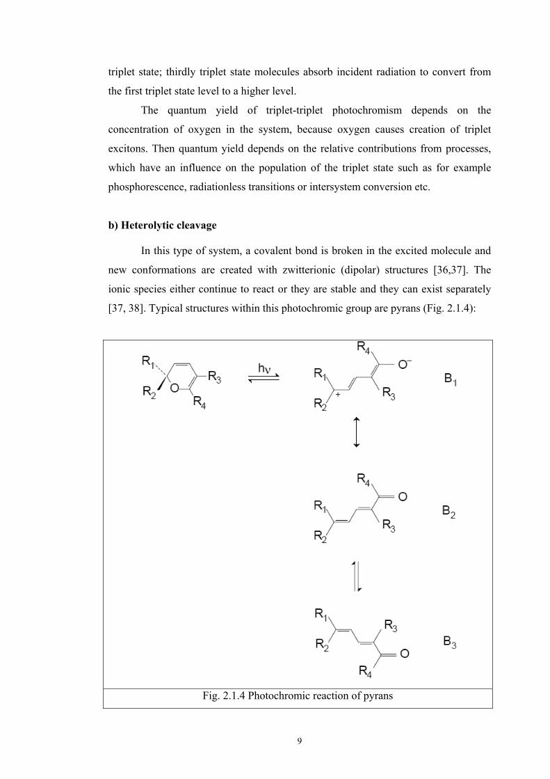
b) Heterolytic cleavage In this type of system, a covalent bond is broken in the excited molecule and

new conformations are created with zwitterionic (dipolar) structures [36,37]. The

ionic species either continue to react or they are stable and they can exist separately

[37, 38]. Typical structures within this photochromic group are pyrans (Fig. 2.1.4):

Fig. 2.1.4 Photochromic reaction of pyrans

10

Under the influence of UV irradiation, the bond is broken between carbon and oxygen

and the pyran ring is opened. Ionic structure (B1) is formed, which is similar to

merocyanine colorants and which provides intense coloration. There is also a

resonance contribution from neutral form (B2). In the photochromic process involving

pyrans, cis-trans conversion (isomer B3) and triplet–triplet absorption also play an

important role. The balance between the contributing forms (Bl, B2 and B3)

determines the resulting colour after irradiation.

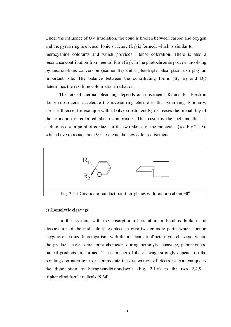
The rate of thermal bleaching depends on substituents R3 and R4. Electron

donor substituents accelerate the reverse ring closure to the pyran ring. Similarly,

steric influence, for example with a bulky substituent R2 decreases the probability of

the formation of coloured planar conformers. The reason is the fact that the sp3

carbon creates a point of contact for the two planes of the molecules (see Fig.2.1.5),

which have to rotate about 90o to create the new coloured isomers.

Fig. 2.1.5 Creation of contact point for planes with rotation about 90o

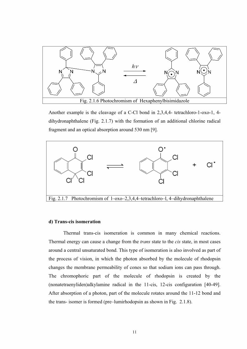
c) Homolytic cleavage In this system, with the absorption of radiation, a bond is broken and

dissociation of the molecule takes place to give two or more parts, which contain

azygous electrons. In comparison with the mechanism of heterolytic cleavage, where

the products have some ionic character, during homolytic cleavage, paramagnetic

radical products are formed. The character of the cleavage strongly depends on the

bonding configuration to accommodate the dissociation of electrons. An example is

the dissociation of hexaphenylbisimidazole (Fig. 2.1.6) to the two 2,4,5 -

triphenylimidazole radicals [9,34].

11

Fig. 2.1.6 Photochromism of Hexaphenylbisimidazole Another example is the cleavage of a C-Cl bond in 2,3,4,4- tetrachloro-1-oxo-1, 4-

dihydronaphthalene (Fig. 2.1.7) with the formation of an additional chlorine radical

fragment and an optical absorption around 530 nm [9].

Fig. 2.1.7 Photochromism of l–oxo–2,3,4,4–tetrachloro–l, 4–dihydronaphthalene

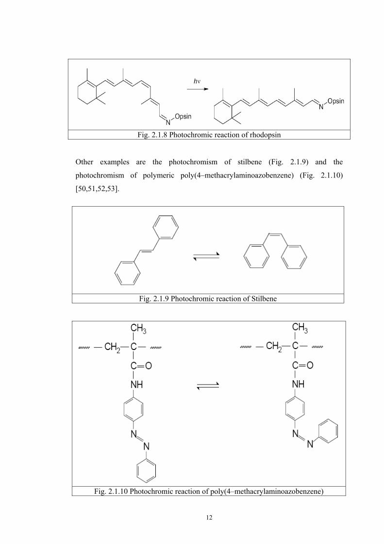
d) Trans-cis isomeration Thermal trans-cis isomeration is common in many chemical reactions.

Thermal energy can cause a change from the trans state to the cis state, in most cases

around a central unsaturated bond. This type of isomeration is also involved as part of

the process of vision, in which the photon absorbed by the molecule of rhodopsin

changes the membrane permeability of cones so that sodium ions can pass through.

The chromophoric part of the molecule of rhodopsin is created by the

(nonatetraenyliden)alkylamine radical in the 11-cis, 12-cis configuration [40-49].

After absorption of a photon, part of the molecule rotates around the 11-12 bond and

the trans- isomer is formed (pre–lumirhodopsin as shown in Fig. 2.1.8).

12

Fig. 2.1.8 Photochromic reaction of rhodopsin Other examples are the photochromism of stilbene (Fig. 2.1.9) and the

photochromism of polymeric poly(4–methacrylaminoazobenzene) (Fig. 2.1.10)

[50,51,52,53].

Fig. 2.1.9 Photochromic reaction of Stilbene

Fig. 2.1.10 Photochromic reaction of poly(4–methacrylaminoazobenzene)

13

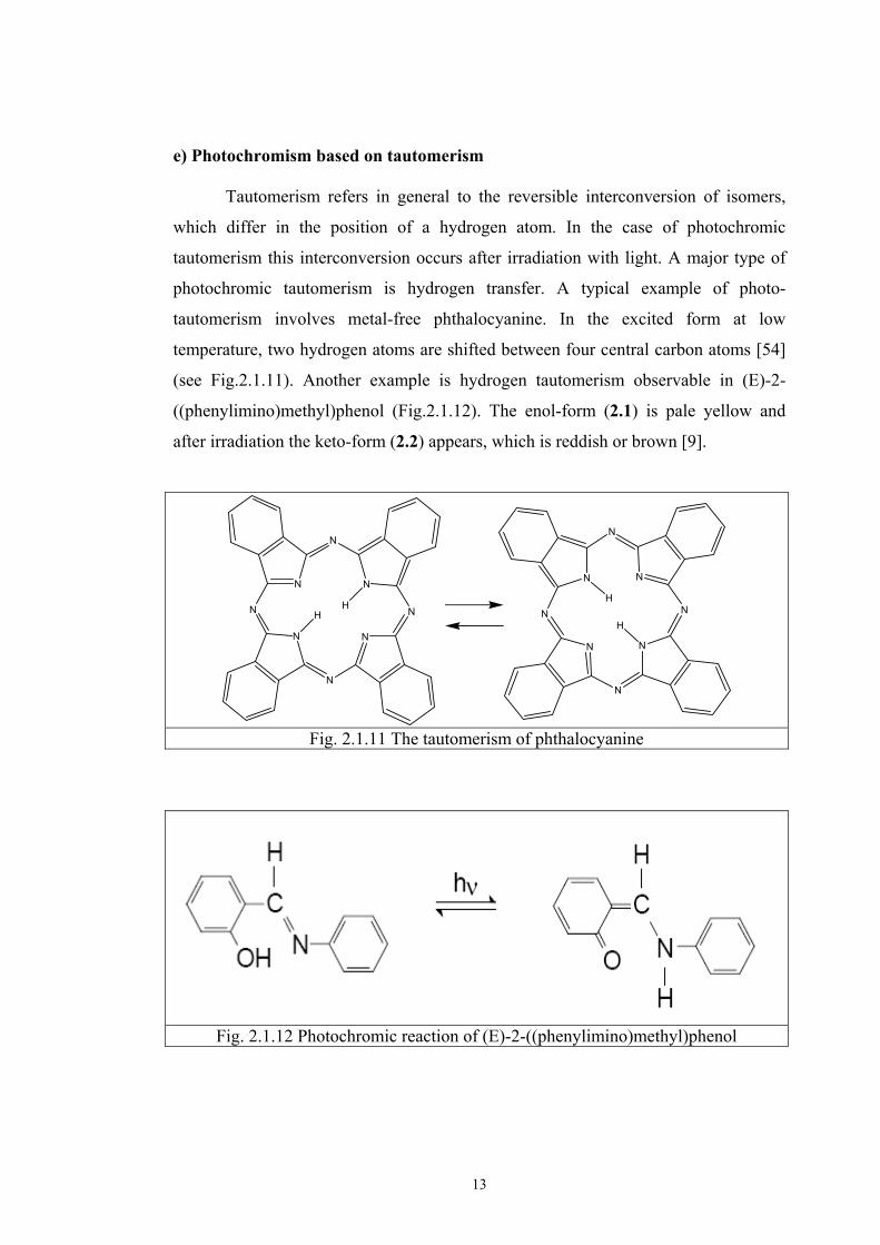
e) Photochromism based on tautomerism Tautomerism refers in general to the reversible interconversion of isomers,

which differ in the position of a hydrogen atom. In the case of photochromic

tautomerism this interconversion occurs after irradiation with light. A major type of

photochromic tautomerism is hydrogen transfer. A typical example of photo-

tautomerism involves metal-free phthalocyanine. In the excited form at low

temperature, two hydrogen atoms are shifted between four central carbon atoms [54]

(see Fig.2.1.11). Another example is hydrogen tautomerism observable in (E)-2-

((phenylimino)methyl)phenol (Fig.2.1.12). The enol-form (2.1) is pale yellow and

after irradiation the keto-form (2.2) appears, which is reddish or brown [9].

N

N

N

H

N

N

N

H NN

N

N

N

H

N

N

N

H

N

N

Fig. 2.1.11 The tautomerism of phthalocyanine

Fig. 2.1.12 Photochromic reaction of (E)-2-((phenylimino)methyl)phenol

14

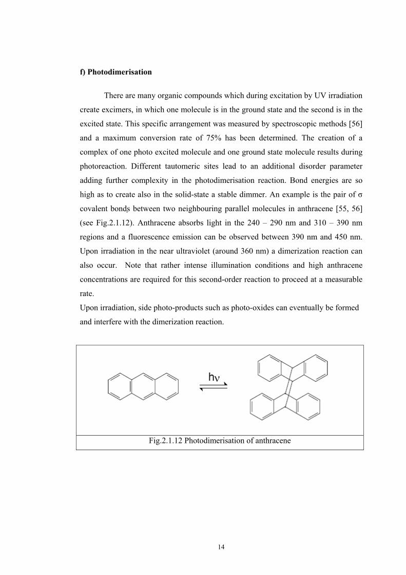
f) Photodimerisation

There are many organic compounds which during excitation by UV irradiation

create excimers, in which one molecule is in the ground state and the second is in the

excited state. This specific arrangement was measured by spectroscopic methods [56]

and a maximum conversion rate of 75% has been determined. The creation of a

complex of one photo excited molecule and one ground state molecule results during

photoreaction. Different tautomeric sites lead to an additional disorder parameter

adding further complexity in the photodimerisation reaction. Bond energies are so

high as to create also in the solid-state a stable dimmer. An example is the pair of σ

covalent bonds between two neighbouring parallel molecules in anthracene [55, 56]

(see Fig.2.1.12). Anthracene absorbs light in the 240 – 290 nm and 310 – 390 nm

regions and a fluorescence emission can be observed between 390 nm and 450 nm.

Upon irradiation in the near ultraviolet (around 360 nm) a dimerization reaction can

also occur. Note that rather intense illumination conditions and high anthracene

concentrations are required for this second-order reaction to proceed at a measurable

rate.

Upon irradiation, side photo-products such as photo-oxides can eventually be formed

and interfere with the dimerization reaction.

Fig.2.1.12 Photodimerisation of anthracene

15

2.2 Basic Optical Concepts and Principles

Today it is well known that electromagnetic phenomena are the basis for

macroscopic physics and for most microscopic processes. In particular,

electromagnetic phenomena are the essence of optics and not only in the visual part of

spectrum. An overview of the fundament concepts and principles of optics is

presented here in view of its relevance to the photochromic phenomena and the

construction of a special device, described later in this thesis, for its measurement.

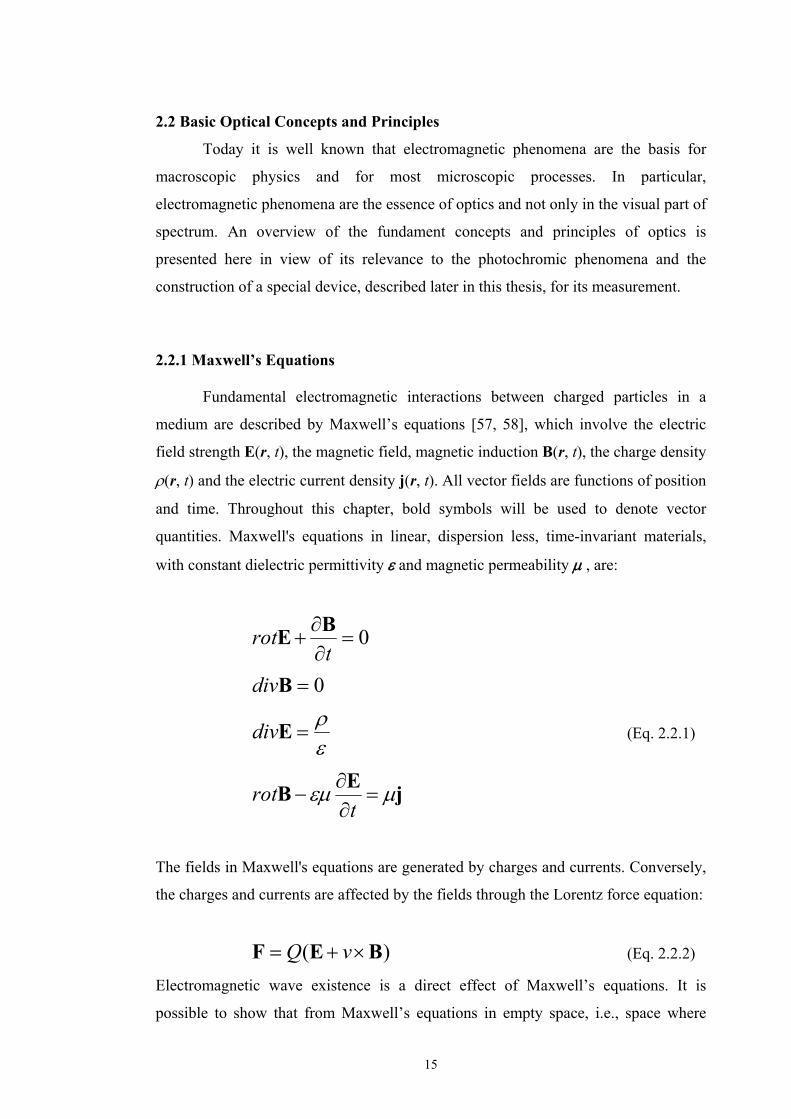
2.2.1 Maxwell’s Equations Fundamental electromagnetic interactions between charged particles in a

medium are described by Maxwell’s equations [57, 58], which involve the electric

field strength E(r, t), the magnetic field, magnetic induction B(r, t), the charge density

ρ(r, t) and the electric current density j(r, t). All vector fields are functions of position

and time. Throughout this chapter, bold symbols will be used to denote vector

quantities. Maxwell's equations in linear, dispersion less, time-invariant materials,

with constant dielectric permittivity ε and magnetic permeability μ , are:

0=∂∂

+t

rot BE

0=Bdiv

ερ

=Ediv (Eq. 2.2.1)

jEB μεμ =∂∂

−t

rot

The fields in Maxwell's equations are generated by charges and currents. Conversely,

the charges and currents are affected by the fields through the Lorentz force equation:

)( BEF ×+= vQ (Eq. 2.2.2)

Electromagnetic wave existence is a direct effect of Maxwell’s equations. It is

possible to show that from Maxwell’s equations in empty space, i.e., space where

16

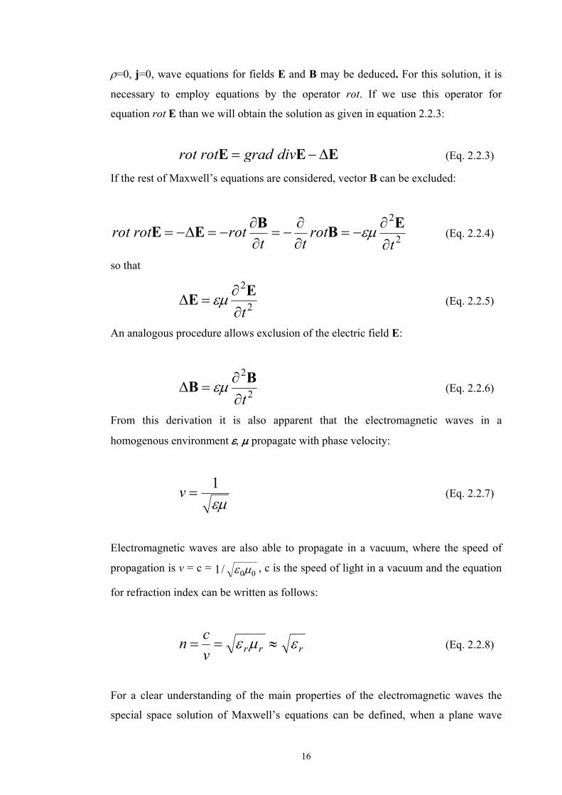
ρ=0, j=0, wave equations for fields E and B may be deduced. For this solution, it is

necessary to employ equations by the operator rot. If we use this operator for

equation rot E than we will obtain the solution as given in equation 2.2.3:

EEE Δ−= divgradrotrot (Eq. 2.2.3)

If the rest of Maxwell’s equations are considered, vector B can be excluded:

2

2

trot

ttrotrotrot

∂∂

−=∂∂

−=∂∂

−=Δ−=EBBEE εμ (Eq. 2.2.4)

so that

2

2

t∂∂

=ΔEE εμ (Eq. 2.2.5)

An analogous procedure allows exclusion of the electric field E:

2

2

t∂∂

=ΔBB εμ (Eq. 2.2.6)

From this derivation it is also apparent that the electromagnetic waves in a

homogenous environment ε, μ propagate with phase velocity:

εμ1

=v (Eq. 2.2.7)

Electromagnetic waves are also able to propagate in a vacuum, where the speed of

propagation is v = c = 00/1 με , c is the speed of light in a vacuum and the equation

for refraction index can be written as follows:

rrrvcn εμε ≈== (Eq. 2.2.8)

For a clear understanding of the main properties of the electromagnetic waves the

special space solution of Maxwell’s equations can be defined, when a plane wave

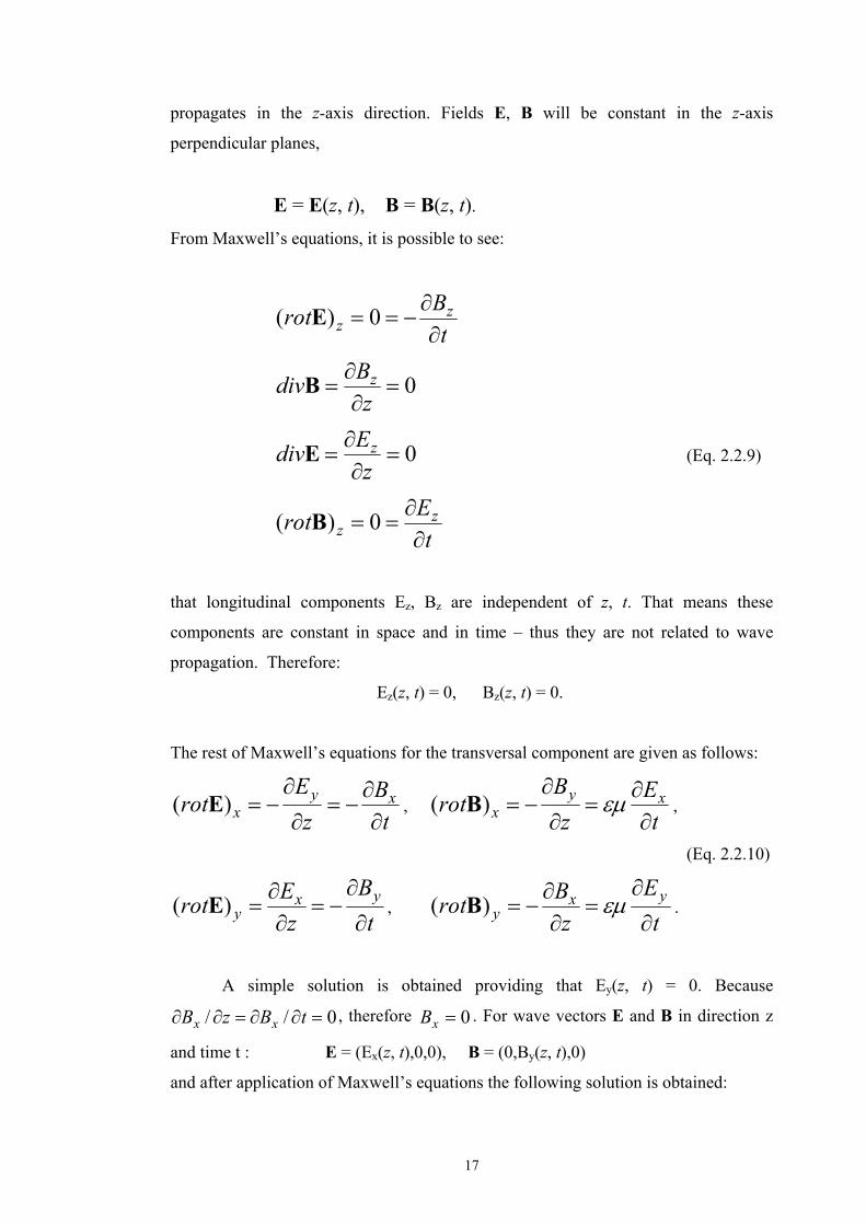
17

propagates in the z-axis direction. Fields E, B will be constant in the z-axis

perpendicular planes,

E = E(z, t), B = B(z, t). From Maxwell’s equations, it is possible to see:

t

Brot zz ∂

∂−== 0)( E

0=∂

∂=

zBdiv zB

0=∂

∂=

zEdiv zE (Eq. 2.2.9)

t

Erot zz ∂

∂== 0)( B

that longitudinal components Ez, Bz are independent of z, t. That means these

components are constant in space and in time – thus they are not related to wave

propagation. Therefore:

Ez(z, t) = 0, Bz(z, t) = 0.

The rest of Maxwell’s equations for the transversal component are given as follows:

tB

zE

rot xyx ∂

∂−=

∂∂

−=)( E , t

Ez

Brot xy

x ∂∂

=∂

∂−= εμ)( B ,

(Eq. 2.2.10)

tB

zErot yx

y ∂∂

−=∂

∂=)( E ,

tE

zBrot yx

y ∂∂

=∂

∂−= εμ)( B .

A simple solution is obtained providing that Ey(z, t) = 0. Because

0// =∂∂=∂∂ tBzB xx , therefore 0=xB . For wave vectors E and B in direction z

and time t : E = (Ex(z, t),0,0), B = (0,By(z, t),0)

and after application of Maxwell’s equations the following solution is obtained:

18

tB

zE yx

∂∂

=∂

∂− ,

tE

zB xy

∂∂

=∂

∂− εμ . (Eq. 2.2.11)

From equations 2.2.11 wave equations result:

2

2

2

2

tE

zE xx

∂∂

=∂

∂− εμ , 2

2

2

2

tB

zB yy

∂

∂=

∂

∂− εμ . (Eq. 2.2.12)

For waves Ex,By, which propagate in the positive direction of the z-axis, the

d’Alembert solution for equations 2.2.12 can be written:

)(),( vtzFtzE Ex −= , )(),( vtzFtzB By −= . (Eq. 2.2.13)

where FE, FB are forces of the electric and magnetic parts of electromagnetic

radiation. The relationship between waves Ex,By is described by equations 2.2.11,

from which follows:

)()( '' ξξ BE vFF = ⇒ .)()( constFF BE += ξξ ,

where vtz −=ξ and the constant of integration is equal to zero. In a planar wave,

which propagates in direction +z it is valid to write:

),(),( tzvBtzE yx = , εμ1

=v .

For a harmonic (monochromatic) wave, the expression:

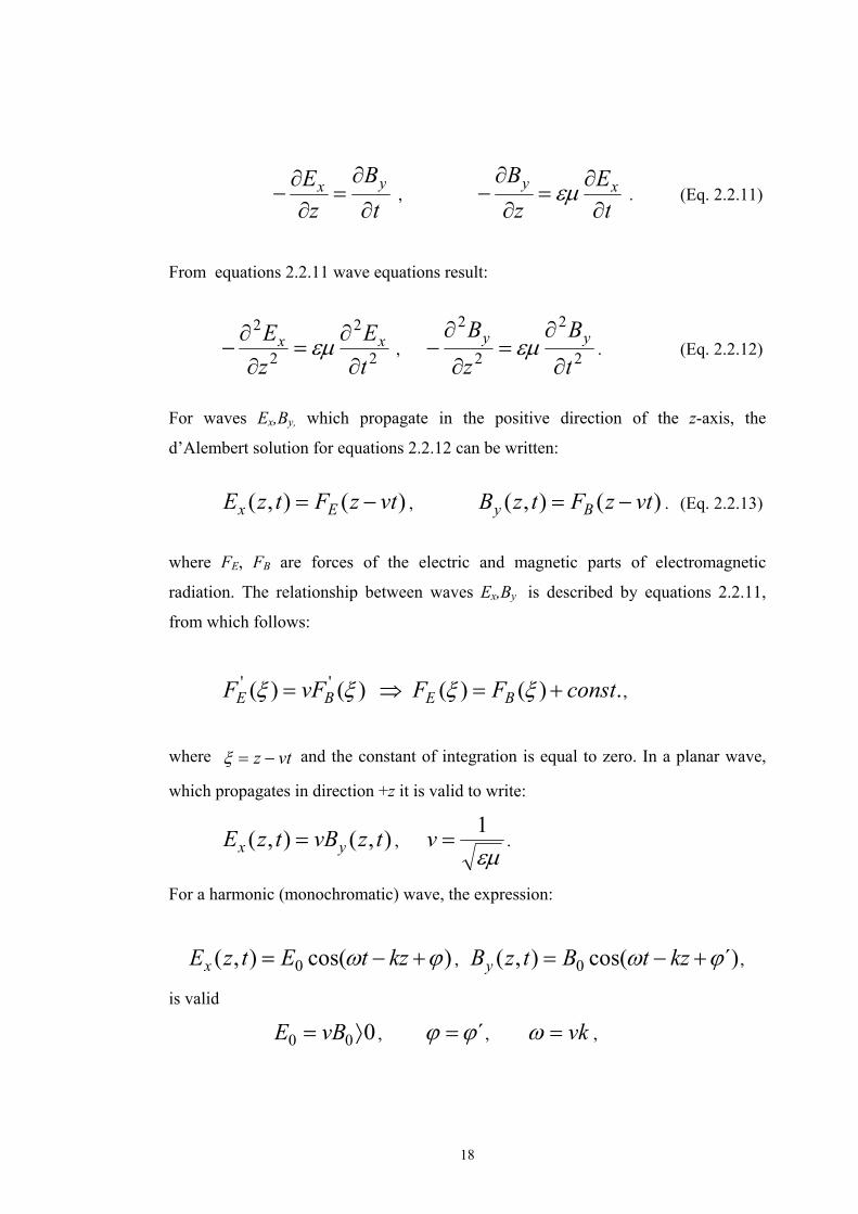
)cos(),( 0 ϕω +−= kztEtzEx , ´)cos(),( 0 ϕω +−= kztBtzBy ,

is valid

000 ⟩= vBE , ´ϕϕ = , vk=ω ,

19

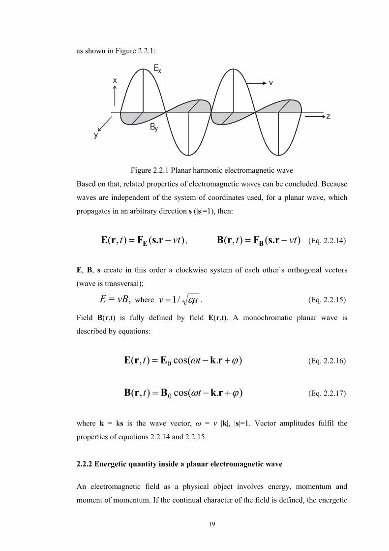
as shown in Figure 2.2.1:

Figure 2.2.1 Planar harmonic electromagnetic wave

Based on that, related properties of electromagnetic waves can be concluded. Because

waves are independent of the system of coordinates used, for a planar wave, which

propagates in an arbitrary direction s (|s|=1), then:

)(),( vtt −= s.rFrE E , )(),( vtt −= s.rFrB B (Eq. 2.2.14)

E, B, s create in this order a clockwise system of each other`s orthogonal vectors

(wave is transversal);

E = vB, where εμ/1=v . (Eq. 2.2.15)

Field B(r,t) is fully defined by field E(r,t). A monochromatic planar wave is

described by equations:

).cos(),( 0 ϕω +−= rkErE tt (Eq. 2.2.16)

).cos(),( 0 ϕω +−= rkBrB tt (Eq. 2.2.17)

where k = ks is the wave vector, ω = v |k|, |s|=1. Vector amplitudes fulfil the

properties of equations 2.2.14 and 2.2.15.

2.2.2 Energetic quantity inside a planar electromagnetic wave

An electromagnetic field as a physical object involves energy, momentum and

moment of momentum. If the continual character of the field is defined, the energetic

20

capacity of this field is described by energy density w(r,t), and it’s volume integral

wdVV∫ indicates immediate energy included with arbitrary volume V.

Based on Maxwell’s ideas [59], the density of an electromagnetic field in

nonconductive media ε, μ is given by the quadratic equation:

)(21)..(

21 22 HEw με +=+= BHDE (Eq. 2.2.18)

Where D is electrostatic induction and H is the intensity of the magnetic field.

The energetic flow density S(r,t) describes the transfer of energy in space. This

transfer of the energy is defined as energy quantity transferred through an area, which

is perpendicular to the direction of propagation per unit time (W/m2). In a time

changeable electromagnetic field in media ε, μ , the energetic flow density is

described by the Poynting vector:

HES ×= . (Eq. 2.2.19)

If the momentum density of the electromagnetic field in a vacuum is applied the

following equation results:

200 cSHEBDg =×=×= με . (Eq. 2.2.20)

Taking in to consideration that all equations for energetic quantities are quadratic in

fields and this equation is transferred to the case of a planar electromagnetic wave

equation 2.2.15 it is possible to reformulate:

E = vB ⇔ HE με = . (Eq. 2.2.21)

Therefore the electric and magnetic part of the energy density w are equal in a planar

wave and:

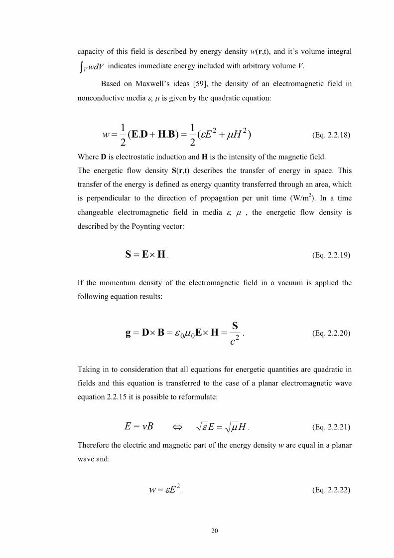
2Ew ε= . (Eq. 2.2.22)

21

With use of equations 2.2.14 and 2.2.15:

EsH ×=με , (Eq. 2.2.23)

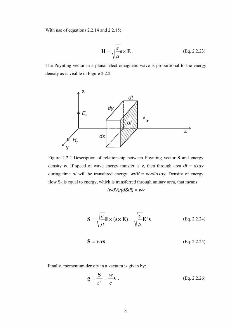
The Poynting vector in a planar electromagnetic wave is proportional to the energy

density as is visible in Figure 2.2.2:

Figure 2.2.2 Description of relationship between Poynting vector S and energy

density w. If speed of wave energy transfer is v, then through area df = dxdy

during time dt will be transfered energy: wdV = wvdtdxdy. Density of energy

flow SZ is equal to energy, which is transferred through unitary area, that means:

(wdV)/(dSdt) = wv

sEEsES 2)(με

με

=××= (Eq. 2.2.24)

sS wv= (Eq. 2.2.25)

Finally, momentum density in a vacuum is given by:

sSgcw

c== 2

. (Eq. 2.2.26)

22

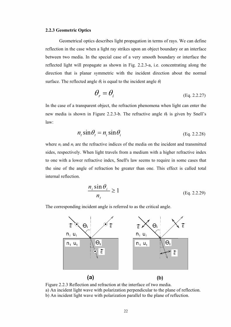
2.2.3 Geometric Optics Geometrical optics describes light propagation in terms of rays. We can define

reflection in the case when a light ray strikes upon an object boundary or an interface

between two media. In the special case of a very smooth boundary or interface the

reflected light will propagate as shown in Fig. 2.2.3-a, i.e. concentrating along the

direction that is planar symmetric with the incident direction about the normal

surface. The reflected angle θr is equal to the incident angle θi

r iθ θ= (Eq. 2.2.27)

In the case of a transparent object, the refraction phenomena when light can enter the

new media is shown in Figure 2.2.3-b. The refractive angle θt is given by Snell’s

law:

sin sint t i in nθ θ= (Eq. 2.2.28)

where nt and ni are the refractive indices of the media on the incident and transmitted

sides, respectively. When light travels from a medium with a higher refractive index

to one with a lower refractive index, Snell's law seems to require in some cases that

the sine of the angle of refraction be greater than one. This effect is called total

internal reflection.

sin 1i i

t

nn

θ≥ (Eq. 2.2.29)

The corresponding incident angle is referred to as the critical angle.

Figure 2.2.3 Reflection and refraction at the interface of two media. a) An incident light wave with polarization perpendicular to the plane of reflection. b) An incident light wave with polarization parallel to the plane of reflection.

23

The total energy in the reflected and refracted rays is equal to the energy of the

incident light, but the proportion of the intensities in these two rays will depend upon

the refractive index difference, the angle of incidence, the light polarization and

direction in which the light is passing the border. For determination of the intensity

distribution between the reflected and refracted rays the Fresnel formulae can be used

[57]. The intensity reflection coefficients R|| and R⊥ and transmission coefficients T||

and T⊥ (for the parallel and perpendicular polarization consequently) are described

by the following equations:

)(tan)(tan

coscoscoscos

2

22

ti

ti

tiit

tiit

nnnn

θθθθ

θθθθ

+−

=⎟⎟⎠

⎞⎜⎜⎝

⎛+−

=IIR

(Eq. 2.2.30)

)(sin)(sin

coscoscoscos

2

22

ti

ti

ttii

ttii

nnnn

θθθθ

θθθθ

+−

=⎟⎟⎠

⎞⎜⎜⎝

⎛+−

=⊥R

2

coscoscos2

coscos

⎟⎟⎠

⎞⎜⎜⎝

⎛+

=tiit

ii

ii

tt

nnn

nn

θθθ

θθ

IIT

(Eq. 2.2.31)

2

coscoscos2

coscos

⎟⎟⎠

⎞⎜⎜⎝

⎛+

=⊥ttii

ii

ii

tt

nnn

nn

θθθ

θθT

where the ratio of the refractive indices is due to the involvement of two different

media. It can be verified that

1=+ IIII TR

(Eq. 2.2.32)

1=+ ⊥⊥ TR

and generally R|| , R⊥ , T|| and T⊥ are called Fresnel coefficients.

24

2.2.4 Radiometry

Radiometry is the science of measuring light in any portion of the

electromagnetic spectrum. In practice, the term is usually limited to the measurement

of infrared, visible, and ultraviolet light using optical instruments [61-68]. The

measured results are usually in units of energy (joules-J) or power (watts- W). An

important sub-topic of radiometry is spectrophotometry, which specifically deals with

the effects of reflection and transmission at object boundaries as well as absorption

and scattering inside materials.

Photometry is a special case of radiometry, because photometry is the science

of the measurement of light, in terms of its perceived brightness to the human eye. It

is distinct from radiometry, which is the science of measurement of radiant energy

(including light) in terms of absolute power; rather, in photometry, the radiant power

at each wavelength is weighted by a luminosity function that models human

brightness sensitivity.

Since the basic measurement concepts are applicable to both, radiometric

quantities will be discussed first followed by corresponding relationships and

measurement units that have developed and are peculiar to photometry.

Radiant energy is the energy of electromagnetic waves and can be defined as

the energy emitted, transferred, or received in the form of electromagnetic radiation.

When a physical object absorbs light, its energy is converted into some other form. A

microwave oven, for example, heats a glass of water when the water molecules

absorb microwave radiation. The radiant energy of the microwaves is converted into

thermal energy (heat). Similarly, visible light causes an electric current to flow in a

photographic light meter when its radiant energy is transferred to the electrons as

kinetic energy. Radiant energy is denoted by Q and is recorded in units of joules (J).

In radiometry, radiant flux or radiant power is the rate of flow of

electromagnetic energy. It may be defined as the energy emitted, transferred, or

received in the form of electromagnetic radiation per unit time. It is denoted by Φ and

is in units of watts (W).

It is defined as:

dQdt

Φ = (Eq. 2.2.33)

where Q is radiant energy and t is time.

25

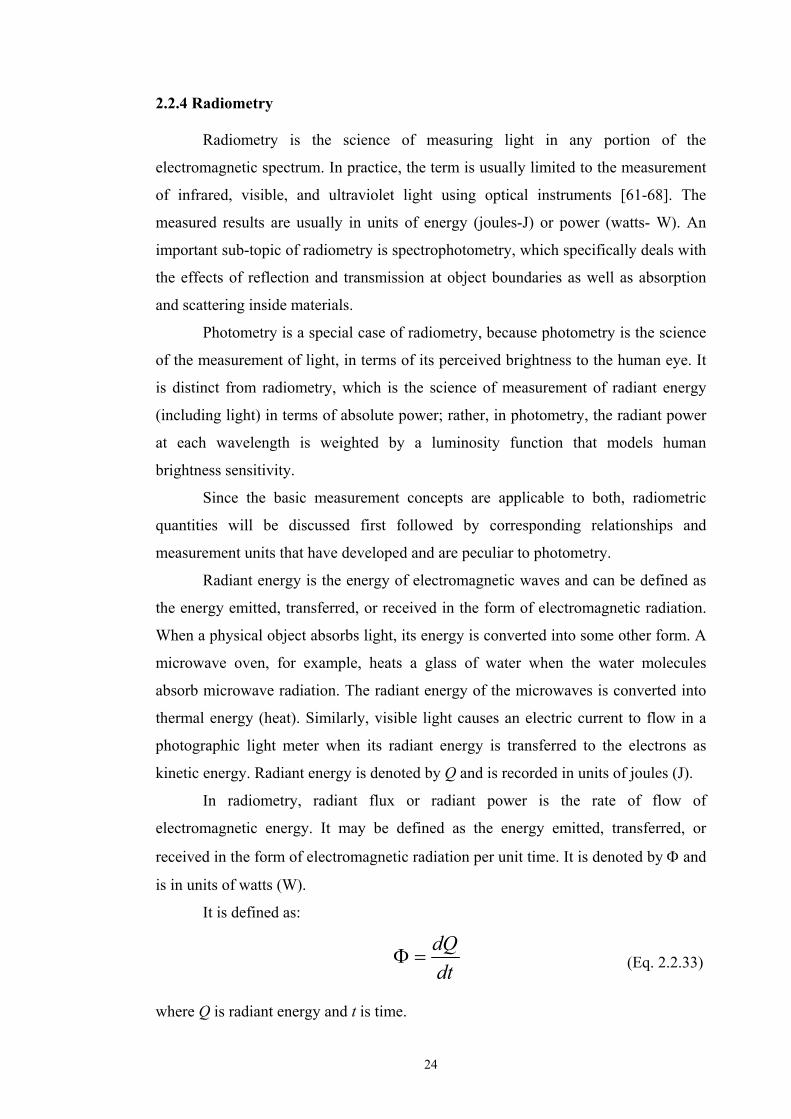
Radiant flux density is the radiant flux per unit area at a point on a surface,

where the surface can be real or imaginary (i.e., a mathematical plane). There are two

possible conditions. The flux can be arriving at the surface (Figure 2.2.4a), in which

case the radiant flux density is referred to as irradiance.

Fig. 2.2.4a Irradiance Fig. 2.2.4b Radiant exitance

Irradiance is a radiometry term for the power per unit area of electromagnetic

radiation at a surface. It is the ratio of the radiant power incident on an infinitesimally

small element of a surface to the projected area of that element, dAd, whose normal is

at an angle θd to the direction of the radiation. Irradiance is denoted by E .

cos d d

dEdAθ

Φ= (Eq. 2.2.34)

The flux can also be leaving the surface due to emission and/or reflection

(Figure 2.2.4b). The radiant flux density is then referred to as radiant excitance.

Radiant excitance (M) represents the power per unit area leaving a surface into a

hemisphere above that surface, where dAs is an infinitesimally small element of a

source of the projected area of that element of area whose normal is at an angle θs to

the direction of the radiation. The units usually used for both above mentioned terms

are watts per square meter (Wm-2).

cos s s

dMdAθ

Φ= (Eq. 2.2.35)

26

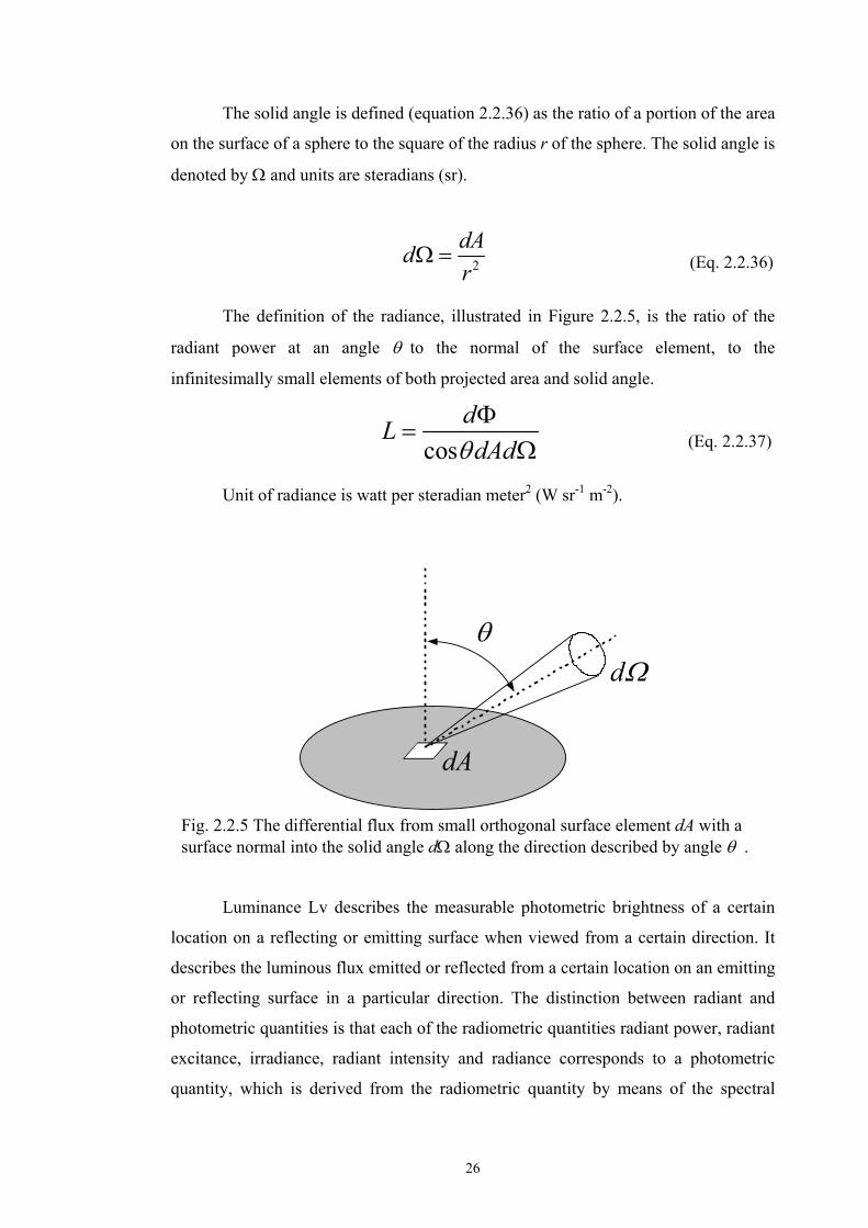
The solid angle is defined (equation 2.2.36) as the ratio of a portion of the area

on the surface of a sphere to the square of the radius r of the sphere. The solid angle is

denoted by Ω and units are steradians (sr).

2

dAdr

Ω = (Eq. 2.2.36)

The definition of the radiance, illustrated in Figure 2.2.5, is the ratio of the

radiant power at an angle θ to the normal of the surface element, to the

infinitesimally small elements of both projected area and solid angle.

cosdLdAdθΦ

=Ω (Eq. 2.2.37)

Unit of radiance is watt per steradian meter2 (W sr-1 m-2).

θdΩ

dA

Fig. 2.2.5 The differential flux from small orthogonal surface element dA with a surface normal into the solid angle dΩ along the direction described by angle θ .

Luminance Lv describes the measurable photometric brightness of a certain

location on a reflecting or emitting surface when viewed from a certain direction. It

describes the luminous flux emitted or reflected from a certain location on an emitting

or reflecting surface in a particular direction. The distinction between radiant and

photometric quantities is that each of the radiometric quantities radiant power, radiant

excitance, irradiance, radiant intensity and radiance corresponds to a photometric

quantity, which is derived from the radiometric quantity by means of the spectral

27

luminous efficacy Vλ. Equivalently, illuminance is the total luminous flux incident on

a surface, per unit area, similar to irradiance.

Radiometric term Unit Photometric term Unit

Radiance Wsr-1m-2 Luminance cd.m-2

Irradiance W.m-2 Iluminance lx

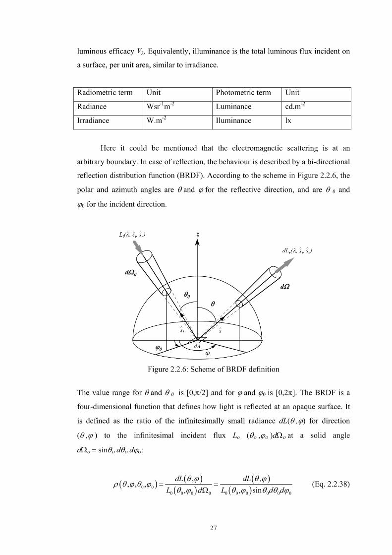
Here it could be mentioned that the electromagnetic scattering is at an

arbitrary boundary. In case of reflection, the behaviour is described by a bi-directional

reflection distribution function (BRDF). According to the scheme in Figure 2.2.6, the

polar and azimuth angles are θ and ϕ for the reflective direction, and are θ 0 and

ϕ0 for the incident direction.

θθ0

dΩ0

dΩ

ϕ0

z

θθ0

dΩ0

dΩ

ϕ0

z

Figure 2.2.6: Scheme of BRDF definition

The value range for θ and θ 0 is [0,π/2] and for ϕ and ϕ0 is [0,2π]. The BRDF is a

four-dimensional function that defines how light is reflected at an opaque surface. It

is defined as the ratio of the infinitesimally small radiance dL(θ ,ϕ) for direction

(θ ,ϕ ) to the infinitesimal incident flux Lo (θο ,ϕο )dΩο at a solid angle

dΩο = sinθο dθο dϕο:

( ) ( )( )

( )( )0 0

0 0 0 0 0 0 0 0 0 0

, ,, , ,

, , sindL dL

L d L d dθ ϕ θ ϕ

ρ θ ϕ θ ϕθ ϕ θ ϕ θ θ ϕ

= =Ω

(Eq. 2.2.38)

28

A BRDF has several important features. It is a fundamental radiometric

concept, and accordingly is used in computer graphics for photorealistic rendering of

synthetic scenes [67]. The BRDF in general depends not only on the incident and

reflected directions, but also on wavelength λ and the surface location r where the

reflection occurs. Therefore, a BRDF can generally be expressed as ρ (θ , ϕ , θο , ϕο ,

r , λ). For most surfaces, usually two or three variables dominate the behaviour.

BRDF allow also the reciprocity principle – if the incident and reflected directions are

switched, a BRDF remains the same, i.e:

( ) ( )0 0 0 0, , , , , ,ρ θ ϕ θ ϕ ρ θ ϕ θ ϕ= (Eq. 2.2.39)

The counterpart of a BRDF for transmission is called a bi-directional

transmittance distribution function (BTDF). The definition of a BTDF is similar to

Eq. (2.3.38) except that the outgoing direction points to the transmission side.

2.3 Spectral Functions

Most sources of optical radiation are spectrally dependent, and the quantities

radiance, intensity, etc. give no information about the distribution of these quantities

over wavelength. Generally, the spectral function is a physical property that varies

with wavelength and frequently is called a spectrum. The graph of a spectral function

is then called a spectral curve.

2.3.1 Spectral Power Distribution The term colour temperature is commonly used to describe the colour stimulus

specification of a light source with a single number. More specifically, the colour

temperature is expressed in degrees Kelvin. The colour temperature cannot substitute

for the exact spectral description of a colour stimulus specification, but is in practice a

rough, but tried and tested, value to describe the properties of light sources. The term

colour temperature has its origin in the theory of black body radiation. The fact that

with many artificial sources of radiation, the visible radiation is obtained as a result of

29

the heating up of a material, for example the metal filament in an electric light bulb.

For these thermal radiators, the radiated energy and its spectral distribution depend on

the temperature and absorption properties of the material. An ideal black body is

often taken as a comparison variable for colour temperatures because there are some

light sources with radiation distribution behaviour very close to that of a black body.

The temperature of the black body at which the colour is most similar to the light

source is called the colour temperature.

A spectral power distribution (SPD) is defined as the power of a light ray of

unit wavelength in a unit area perpendicular to the propagating direction. Thus, a SPD

is the light intensity according equation Eq. 2.3.4, which corresponds to the amplitude

of the Poynting vector. Therefore, in the next part of this thesis, SPDs and light

intensities will be used as equivalent terms.

The CIE has standardized a few SPDs and recommends that these should be

used whenever possible when colorimetric characterization of materials is carried out.

A further distinction is that for calculations only the relative SPD is needed. Such

theoretical sources are called illuminants. There are two standard illuminants: CIE

standard illuminant A and D65, and several secondary illuminants [68].

Practical realizations of a CIE illuminant are called CIE sources. Often an

illuminant cannot be reproduced accurately. In such cases a simulator is referred to

[68, 69]. In 1931 the CIE decided to introduce three standard illuminants, termed

illuminants A, B, and C [79]. They were chosen in such a form that illuminant A

should resemble the SPD of an average incandescent light, and it was thought that

direct sunlight might be an appropriate second choice (illuminant B) with average

daylight (illuminant C) as a further selection. During the years, it turned out that

illuminant B was very seldom used and was soon dropped. Illuminant C is still in use

in some industries, but in 1964 the CIE recommended a new set of daylight

illuminants, where the SPD was also defined in the ultraviolet (UV) part of the

spectrum [88].

One phase of daylight was selected as the most representative and is now

known as CIE standard illuminant D65. A single letter has defined one further

illuminant: Illuminant E has an SPD independent of wavelength, and it represents the

equienergy spectrum.

30

0

50

100

150

200

250

300

300 400 500 600 700 800

Wavelength [nm]

Rel

ativ

e sp

ectr

al p

ower

AD65CF11

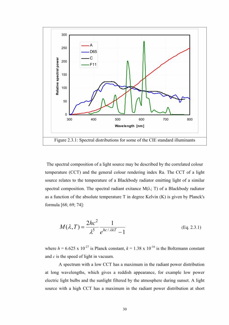
Figure 2.3.1: Spectral distributions for some of the CIE standard illuminants

The spectral composition of a light source may be described by the correlated colour

temperature (CCT) and the general colour rendering index Ra. The CCT of a light

source relates to the temperature of a Blackbody radiator emitting light of a similar

spectral composition. The spectral radiant exitance M(λ; T) of a Blackbody radiator

as a function of the absolute temperature T in degree Kelvin (K) is given by Planck's

formula [68; 69; 74]:

112),( /5

2

−= kThce

hcTM λλλ (Eq. 2.3.1)

where h = 6.625 x 10-27 is Planck constant, k = 1.38 x 10-16 is the Boltzmann constant

and c is the speed of light in vacuum.

A spectrum with a low CCT has a maximum in the radiant power distribution

at long wavelengths, which gives a reddish appearance, for example low power

electric light bulbs and the sunlight filtered by the atmosphere during sunset. A light

source with a high CCT has a maximum in the radiant power distribution at short

31

wavelengths and has a bluish appearance, e.g., diffuse skylight and special

fluorescent lamps.

2.3.2 Spectral Reflectance Spectral reflectance is defined as light reflection at an object boundary or an

interface between two media. Denoted by R(λ), it is the fraction of incident radiation

reflected by a surface.

( ) ( )( )0

IR

Iλ

λλ

= (Eq. 2.3.2)

where I (λ) and I0 (λ) are the reflected and incident intensities respectively. Spectral

reflectances apply to boundaries of all kinds of materials, including those that are

opaque, transparent and translucent.

In case of non-fluorescent materials, a spectral reflectance is independent of

the intensity of the incident light and is an intrinsic property of the material. This

property, which is referred to as the spectral linearity allows transformation of

reflectance data to other illumination conditions. Measured data for many natural

materials are available in the literature [63, 72, 68].

2.3.3 Spectral Transmittance Spectral transmittance is the ratio between the transmitted and incident

energies

( ) ( )( )0

IT

Iλ

λλ

= (Eq. 2.3.3)

where I (λ) and I0(λ) are the intensities of the transmitted and incident lights. A

spectral transmittance is also useful for prediction of the result after a light ray passes

through a thin, transparent layer such as a filter [57, 68]. The following relationship

may be used

( ) ( ) ( )0I I Tλ λ λ= (Eq. 2.3.4)

32

to compute the light intensity after the transmission. This interpretation allows the use

of a similar equation for computing the spectral power distribution of reflected light

based on spectral reflectance.

2.3.4 Spectral Absorptivity Transmittance can be plotted against the concentration of an absorbing

species, but the relationship is not linear. Spectral absorptivity is the part of light

energy absorbed by a transparent or translucent material within a unit path length (l)

of light propagation. General analytical description of spectral absorption is given by

equation Eq. 2.3.5.:

( ) ( )( ),1,

,dI

aI dl

λλ

λ= −

rr

r (Eq. 2.3.5)

The spectral absorptivity depends not only on wavelength λ, but in case of not

homogenous material also on spatial location r. With respect of the spectral linearity,

the SPD of a light after it travels from r0 to r with l = [r0 – r] can be calculated from

( ) ( )( )

0

,

0, ,

l

a dl

I I eλ

λ λ−∫

=r

0r r (Eq. 2.3.6)

where I0 (λ,r0) is the initial SPD. In the case of a homogenous material, the spectral

absorptivity is independent of location, so the simplification a(λ,r)=a(λ) can be used.

Based on that Eq. 2.3.6 becomes:

( ) ( ) ( )0

a lI I e λλ λ −= (Eq. 2.3.7)

This equation is known as Bouguer’s law. The other expression of Bouguer’s

law has a form

( ) ( )( )

( )int erna

0

a ll

IT e

Iλλ

λλ

−= = (Eq. 2.3.8)

where Tinternal(λ) is the internal spectral transmittance. Eq. 2.3.7 or 2.3.8 describes the

optical effect of absorption, which depends on the thickness l. In the case of a

homogeneous transparent solute material (ideal solution), absorption depends on the

solute concentration. Finally, the Beer’s law can by described by equation Eq. 2.3.9:

( ) ( )interna

cllT e ε λλ −= (Eq. 2.3.9)

33

where c is the concentration and ε(λ) is a spectral function, which is called absorption

coefficient. Validity of the Beer’s law is limited for low or moderate concentrations

while Bouguer’s law is rigorous for all conditions [68, 73], nevertheless both are

valid for non-turbid media.

2.4 Colours

Colours are implicated in physics, chemistry, physiology and psychology, as

well as in language and philosophy. Colours in design and clothing affect our senses

and can create predetermined responses. For example, red is associated with danger,

the red traffic light meaning “stop” to the road user, red is used as a symbol of guilt,

sin and anger, often as connected with blood or sex.

Light can be described by wavelength and spectral distributions, but colour is

the result of the interaction between light and the human eye, and the operation of the

brain on signals obtained from the eye. Light enters the eye through the cornea, a

transparent section of the sclera, which is kept moist and free from dust by the tear

ducts and by blinking of the eyelids. The light passes through a transparent flexible

lens, which acts to form an inverted image on the retina. The retina owes its

photosensitivity to a mosaic of light sensitive cells known as rods and cones, which

derive their names from their physical shape. Under ideal conditions, a normal

observer can distinguish about 10 million individual colours. Three separate types of

cone cells have been identified in the eye and the ability to distinguish colours is

associated with the fact that each of the three types is sensitive to light of a particular

range of wavelengths [63, 77]. The letters L, M, and S represent the three types of

cones with their peak sensitivities in the long, middle, and short wavelength regions,

respectively. Short cones are most sensitive to blue light, the maximum response

being at a wavelength of about 440 nm. Medium cones are most sensitive to green

light, the maximum response being at about wavelength of about 545 nm. Long cones

are most sensitive to red light, the maximum response being at about 585 nm. S cones

differ from L and M cones in morphology, neurochemistry, and spatial arrangement

in the retina, i.e. inside specific area of retina, which is called fovea centralis (there is

sharp central vision) are located L and M cones only.

34

The integration process of the three receptors reduces the entire spectrum to

three signals, one for each cone type, resulting in trichromacy. Therefore, three

signals are necessary and sufficient to describe any color.

The measurements and specifications of colours as well as transformations

among different colour systems are topics within colour science. The following

review focuses on the colour models most relevant to this thesis

[68,71,78,79,80,81,82].

2.4.1 CIE COLORIMETRY An international organization, the Commission International de L'Eclairage

(CIE), worked in the first half of the 20th century developing a method for

systematically measuring colour in relation to the wavelengths they contain [82]. This

system became known as the CIE colour system. The model was originally developed

based on the tristimulus theory of colour perception, which is known as the Young-

Helmholtz theory [69]. The CIE colour model was developed to be completely

independent of any device or other means of emission or reproduction and is based as

closely as possible on how humans perceive colour. The key elements of the CIE

model are the definitions of standard sources and the specifications for a standard

observer. The colour-matching properties of the 1931 CIE standard colorimetry

observer are defined as the colour-matching functions x (λ), y (λ) and z (λ), and

today has two standardisation 2o (1931) and 10o (1964). Using these colour-matching

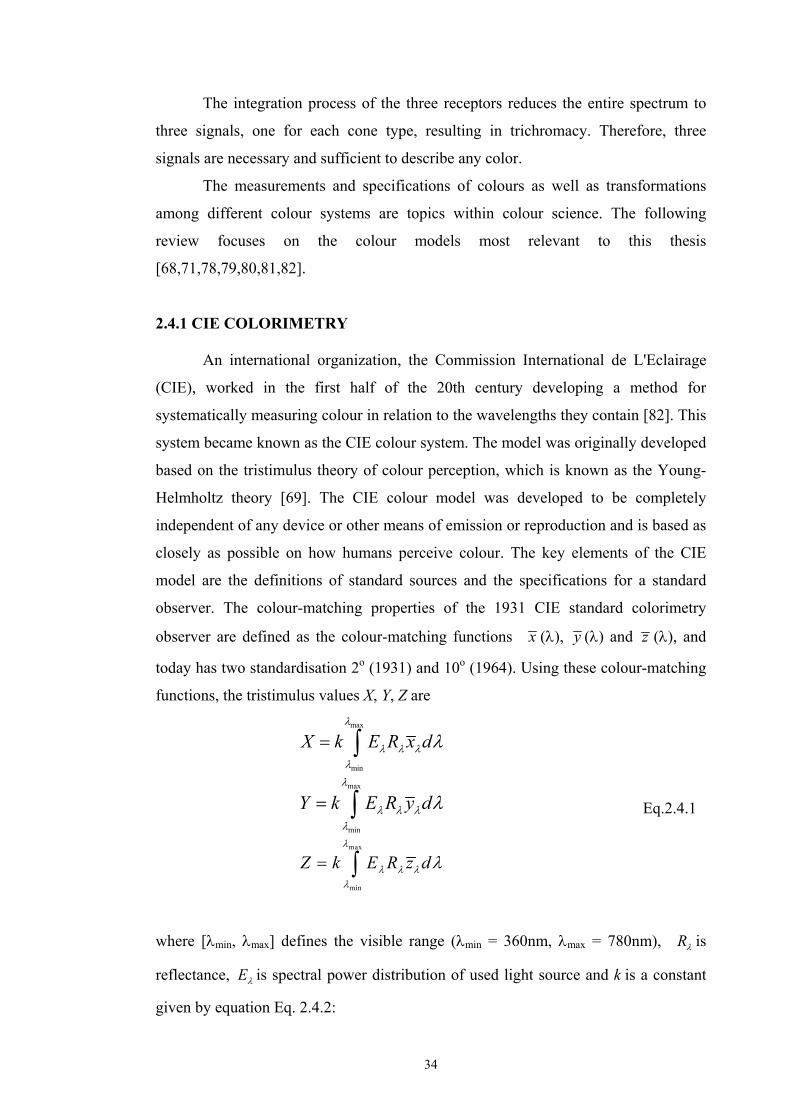
functions, the tristimulus values X, Y, Z are

max

min

X k E R x dλ

λ λ λλ

λ= ∫

max

min

Y k E R y dλ

λ λ λλ

λ= ∫ Eq.2.4.1

max

min

Z k E R z dλ

λ λ λλ

λ= ∫

where [λmin, λmax] defines the visible range (λmin = 360nm, λmax = 780nm), Rλ is

reflectance, Eλ is spectral power distribution of used light source and k is a constant

given by equation Eq. 2.4.2:

35

max

min

100k E y dλ

λ λλ

λ= ∫ Eq.2.4.2

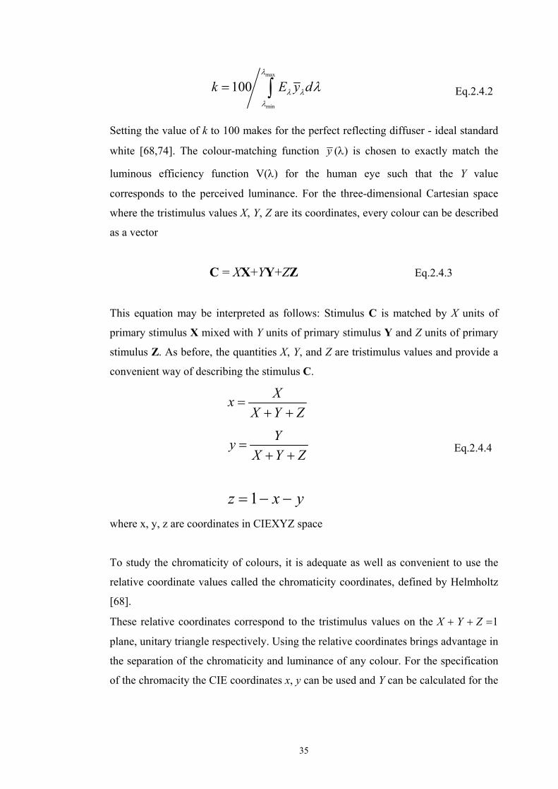
Setting the value of k to 100 makes for the perfect reflecting diffuser - ideal standard

white [68,74]. The colour-matching function y (λ) is chosen to exactly match the

luminous efficiency function V(λ) for the human eye such that the Y value

corresponds to the perceived luminance. For the three-dimensional Cartesian space

where the tristimulus values X, Y, Z are its coordinates, every colour can be described

as a vector

C = XX+YY+ZZ Eq.2.4.3

This equation may be interpreted as follows: Stimulus C is matched by X units of

primary stimulus X mixed with Y units of primary stimulus Y and Z units of primary

stimulus Z. As before, the quantities X, Y, and Z are tristimulus values and provide a

convenient way of describing the stimulus C.

Xx

X Y Z=

+ +

Yy

X Y Z=

+ + Eq.2.4.4

1z x y= − −

where x, y, z are coordinates in CIEXYZ space

To study the chromaticity of colours, it is adequate as well as convenient to use the

relative coordinate values called the chromaticity coordinates, defined by Helmholtz

[68].

These relative coordinates correspond to the tristimulus values on the X + Y + Z =1

plane, unitary triangle respectively. Using the relative coordinates brings advantage in

the separation of the chromaticity and luminance of any colour. For the specification

of the chromacity the CIE coordinates x, y can be used and Y can be calculated for the

36

specification of the luminance. The tristimulus values can be calculated from CIE x,

y, Y colour coordinates:

Eq.2.4.5

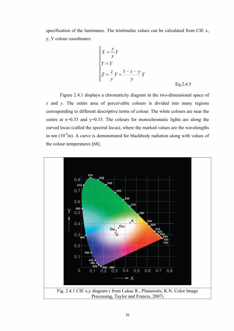
Figure 2.4.1 displays a chromaticity diagram in the two-dimensional space of

x and y. The entire area of perceivable colours is divided into many regions

corresponding to different descriptive terms of colour. The white colours are near the

centre at x=0.33 and y=0.33. The colours for monochromatic lights are along the

curved locus (called the spectral locus), where the marked values are the wavelengths

in nm (10-9m). A curve is demonstrated for blackbody radiation along with values of

the colour temperatures [68].

Fig. 2.4.1 CIE x,y diagram ( from Lukac R., Plataniotis, K.N. Color Image

Processing, Taylor and Francis, 2007)

37

The locations and chromaticity values for a number of standard CIE light sources are

also shown in the diagram.

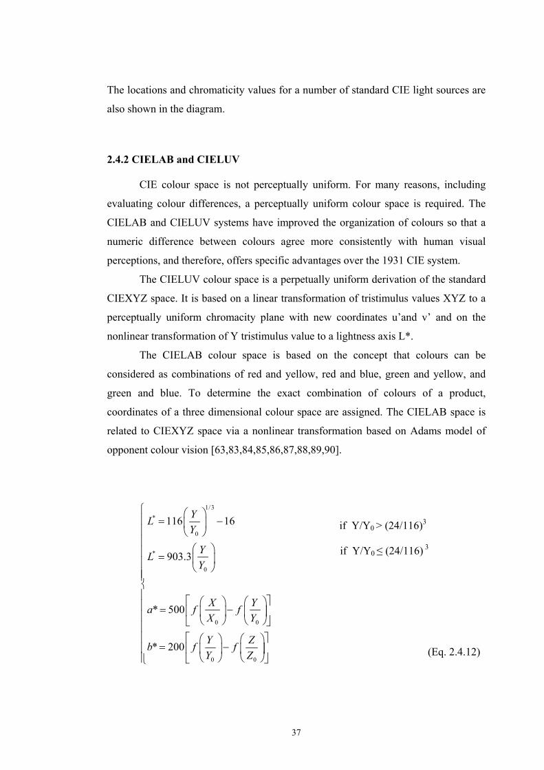
2.4.2 CIELAB and CIELUV CIE colour space is not perceptually uniform. For many reasons, including

evaluating colour differences, a perceptually uniform colour space is required. The

CIELAB and CIELUV systems have improved the organization of colours so that a

numeric difference between colours agree more consistently with human visual

perceptions, and therefore, offers specific advantages over the 1931 CIE system.

The CIELUV colour space is a perpetually uniform derivation of the standard

CIEXYZ space. It is based on a linear transformation of tristimulus values XYZ to a

perceptually uniform chromacity plane with new coordinates u’and v’ and on the

nonlinear transformation of Y tristimulus value to a lightness axis L*.

The CIELAB colour space is based on the concept that colours can be

considered as combinations of red and yellow, red and blue, green and yellow, and

green and blue. To determine the exact combination of colours of a product,

coordinates of a three dimensional colour space are assigned. The CIELAB space is

related to CIEXYZ space via a nonlinear transformation based on Adams model of

opponent colour vision [63,83,84,85,86,87,88,89,90].

if Y/Y0 > (24/116)3

if Y/Y0 ≤ (24/116) 3

(Eq. 2.4.12)

1/3*

0

*

0

0 0

0 0

116 16

903.3

* 500

* 200

YLY

YLY

X Ya f fX Y

Y Zb f fY Z

⎧ ⎛ ⎞⎪ = −⎜ ⎟⎪ ⎝ ⎠⎪

⎛ ⎞⎪ = ⎜ ⎟⎪ ⎝ ⎠⎪⎪⎨⎪ ⎡ ⎤⎛ ⎞ ⎛ ⎞⎪ = −⎢ ⎥⎜ ⎟ ⎜ ⎟⎪ ⎝ ⎠ ⎝ ⎠⎣ ⎦⎪⎪ ⎡ ⎤⎛ ⎞ ⎛ ⎞

= −⎪ ⎢ ⎥⎜ ⎟ ⎜ ⎟⎝ ⎠ ⎝ ⎠⎪ ⎣ ⎦⎩

38

(Eq. 2.4.13)

where X0, Y0 and Z0 are the CIE tristimulus values for the chosen standard illuminant

and d is ratio of X/ X0 or Y/ Y0 or Z/ Z0.

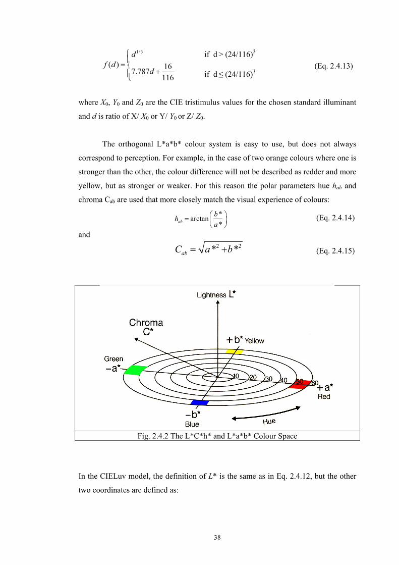
The orthogonal L*a*b* colour system is easy to use, but does not always

correspond to perception. For example, in the case of two orange colours where one is

stronger than the other, the colour difference will not be described as redder and more

yellow, but as stronger or weaker. For this reason the polar parameters hue hab and

chroma Cab are used that more closely match the visual experience of colours:

*arctan*ab

bha

⎛ ⎞= ⎜ ⎟⎝ ⎠

(Eq. 2.4.14)

and 2 2* *abC a b= + (Eq. 2.4.15)

Fig. 2.4.2 The L*C*h* and L*a*b* Colour Space

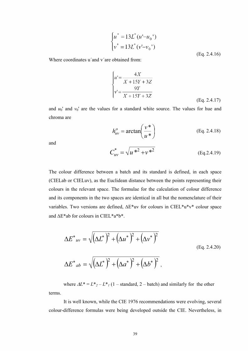
In the CIELuv model, the definition of L* is the same as in Eq. 2.4.12, but the other

two coordinates are defined as:

1/3

( ) 167.787116

df d

d

⎧⎪= ⎨

+⎪⎩

if d > (24/116)3

if d ≤ (24/116)3

39

(Eq. 2.4.16) Where coordinates u´and v´are obtained from:

(Eq. 2.4.17)

and u0' and v0' are the values for a standard white source. The values for hue and

chroma are

⎟⎠⎞

⎜⎝⎛=

**arctan

uvho

uv (Eq. 2.4.18)

and

22* ** vuCuv += (Eq.2.4.19) The colour difference between a batch and its standard is defined, in each space

(CIELab or CIELuv), as the Euclidean distance between the points representing their

colours in the relevant space. The formulae for the calculation of colour difference

and its components in the two spaces are identical in all but the nomenclature of their

variables. Two versions are defined, ΔE*uv for colours in CIEL*u*v* colour space

and ΔE*ab for colours in CIEL*a*b*.

( ) ( ) ( )222 ∗∗∗∗ Δ+Δ+Δ=Δ vuLE uv (Eq. 2.4.20)

( ) ( ) ( )222 ∗∗∗∗ Δ+Δ+Δ=Δ baLE ab , where ΔL* = L*2 – L*1 (1 – standard, 2 – batch) and similarly for the other

terms.

It is well known, while the CIE 1976 recommendations were evolving, several

colour-difference formulas were being developed outside the CIE. Nevertheless, in

40

case of measurement colorimetric properties of colour changeable materials give

simple colour difference calculation based on CIELAB colour space sufficient

reliability [118].

.

2.5 Optical models of translucent media

When a beam of light strikes a material medium, it is propagated through the

thickness of the medium, where it experiences absorption while being transmitted

according to the laws of geometrical optics. That is to say, the beam is deflected from

the rectilinear path of light expected in a vacuum because of refraction, reflection,

diffraction, and diffusion. This happens a number of times depending on the quality

of the medium (homogeneous or not, transparent or opaque, smooth or rough). The

beam is then deprived of absorbed parts at each wavelength and the resulting emitted

spectrum constitutes the spectrum of reflectance.

Reflectance measures the capacity of a surface to reflect the incident energy flux,

given that the medium beneath this surface can absorb photons and diffuse light once

or many times. Reflectance is defined as the ratio of reflected to incident radiation

energy flux for a given wavelength and is thus a dimensionless quantity, usually

expressed as a percentage.

The reflectance spectrum consists of a plot of reflectance values R versus

wavelength λ in the visible spectrum range (from 380 to 780 nm). One curve R(λ)

uniquely characterizes one colour: the reflectance spectrum objectively quantifies the

colour itself.

When light impinges on dispersed particles, such as pigmented fibres, in

addition to being partially absorbed, it is also scattered, changing its direction

arbitrarily and several times in space. Light that passes through such a turbid media

loses a considerable part of its intensity, and the relationship between the colorant

concentration and the observed spectral response becomes more and more

complicated. The analysis of light scattering in translucent, turbid media, such as

clouds, ice structures, human tissues, food, paper and textiles is a wide and yet

increasingly active research field. Hereafter, a few of the classical approaches are

reviewed. An extended survey of the reflectance theories for the reflectance of

diffusing media is given in reference [91].

41

2.5.1 Survey of fundamental light scattering theories

Rayleigh scattering is a fundamental theory that provides a tool to analyze the

phenomenon of light scattered by air molecules [92]. According to this theory, the

scattering power is strongly wavelength-dependent, which explains the blue

appearance of the sky away from the sun. The theory can be extended to light

scattered from particles with a diameter of up to a maximum of a tenth of the radiant

wavelength. This restriction makes the theory impractical for analyzing the scattering

of light in technical opaque or translucent media.

The Mie theory [92], on the other hand, describes the scattered light from a

single spherical particle with a diameter that may be even larger than the scattered

wavelength. Mie scattering is less wavelength-dependent than Rayleigh scattering and

explains the almost white glare around the sun and the neutral colours of fog and

clouds. It is a single scattering theory that ignores any rescattered light from

neighbouring particles. Therefore, without being further extended, this approach does

not strictly apply to light scattered from an assembly of particles.

To circumvent this disadvantage, the multiple scattering approaches are

proposed for particle crowding with an average separation between particles greater

than three particle diameters. However, when the particle crowding gets tighter, the

problem of dependent scattering begins to increase as Mie scattering starts to fail, due

to wavelength-dependent interference between the neighbouring scatterers.

Nevertheless, most colorimetric problems do not require such elaborate handling and,

in technology, more emphasis is placed on simpler calculation methods.

One of the most important simplified scattering approaches is based on a

theory known in astrophysics as radiative transfer [93]. In its original form it studies

the transmission of light through absorbing and scattering media such as stellar and

planetary atmospheres. The radiative transfer equations are rather complex and the

multichannel technique is a suitable approach that overcomes the imposed

complexity. This technique subdivides the analyzed medium into as many channels as

needed, each of them covering a different range of angles from the perpendicular to

the horizontal [94]. Each channel is supplied with specific absorption and scattering

coefficients, which determine how much light is being absorbed and scattered into

other channels. The interesting aspect of this concept is its ability to connect the

series of coefficients directly to Mie’s theory. This helps to incorporate fundamental

42

properties of the scatterer into the model, such as the particle size and the refractive

index.

Reducing the number of channels considered even further, one arrives at the

case of two-flux models proposed by Schuster [95] and other authors. However, the

Kubelka & Munk model, which is presented in the following section, is probably the

most recognized approach and best suits the purpose of analyzing light scattered

within textile fabrics and by colorant particles.

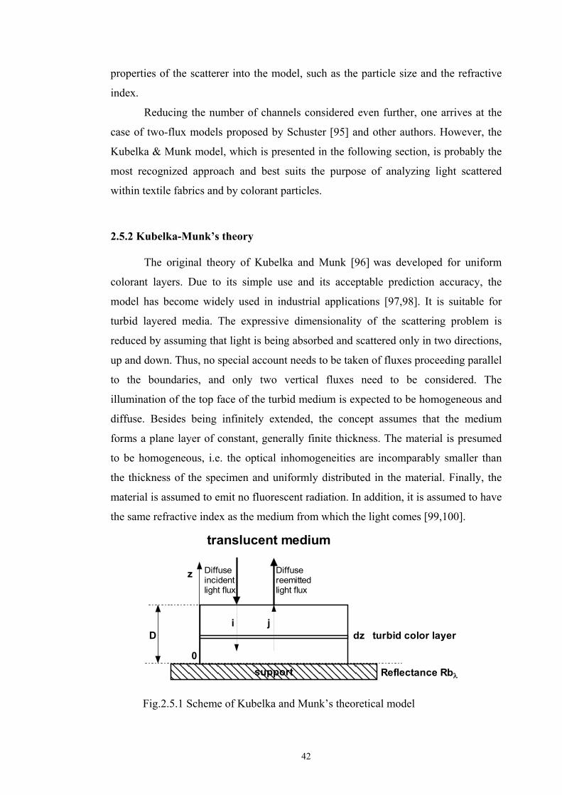
2.5.2 Kubelka-Munk’s theory

The original theory of Kubelka and Munk [96] was developed for uniform

colorant layers. Due to its simple use and its acceptable prediction accuracy, the

model has become widely used in industrial applications [97,98]. It is suitable for

turbid layered media. The expressive dimensionality of the scattering problem is

reduced by assuming that light is being absorbed and scattered only in two directions,

up and down. Thus, no special account needs to be taken of fluxes proceeding parallel

to the boundaries, and only two vertical fluxes need to be considered. The

illumination of the top face of the turbid medium is expected to be homogeneous and

diffuse. Besides being infinitely extended, the concept assumes that the medium

forms a plane layer of constant, generally finite thickness. The material is presumed

to be homogeneous, i.e. the optical inhomogeneities are incomparably smaller than

the thickness of the specimen and uniformly distributed in the material. Finally, the

material is assumed to emit no fluorescent radiation. In addition, it is assumed to have

the same refractive index as the medium from which the light comes [99,100].

support

z

0

D dz turbid color layeri j

translucent medium

Diffuseincidentlight flux

Diffusereemittedlight flux

Reflectance Rbλ

Fig.2.5.1 Scheme of Kubelka and Munk’s theoretical model

43

As depicted in Figure 2.5.1 the colorant layer has a total thickness D and is in direct

optical contact with a backing of reflectance Rbλ. The model analyzes two fluxes

through an elementary layer of thickness dz, the flux iλ(z) proceeding downward, and

jλ(z) simultaneously upward. The depth parameter z is considered to be zero at the

background of the layer and D at the illuminated interface of the layer.

During its passage through dz, the upward flux jλ(z) is attenuated by absorption αλ ·

dz and by scattering downwards σλ · dz. At the same time, jλ(z) gains by scattering

from the opposed flux amount to σλ · dz yielding the flux variation djλ(z) per

thickness element dz :

)().()(.)( zjzidz

zdjλλλλλ

λ σασ +−= ,

(Eq. 2.5.1)

The corresponding variation of the downward flux iλ(z) is derived in the same manner

with the exception that dz is negative, as the process is occurring in the reverse

direction,

)().()(.)( zizjdz

zdiλλλλλ

λ σασ +−=−

(Eq. 2.5.2)

The differential equations 2.5.1 and 2.5.2 obtained describe the net changes of both

light fluxes, iλ(z) and jλ(z). The equations are classified as the two-constant theory,

referring to the introduced colorant optical coefficients, absorption and scattering.

Kubelka and Munk solved this system of equations and obtained the

reflectance value associated with a given wavelength in the case of an infinite R∞λ or

finite Rλ painted layer, in terms of the absorption and scattering coefficients and the

reflectance of the support Rbλ, as expressed in Eq. 2.5.3:

⎥⎦

⎤⎢⎣

⎡⎟⎟⎠

⎞⎜⎜⎝

⎛−⎟⎟

⎠

⎞⎜⎜⎝

⎛−−−

⎥⎦

⎤⎢⎣

⎡⎟⎟⎠

⎞⎜⎜⎝

⎛−⎟⎟

⎠

⎞⎜⎜⎝

⎛−−−

=

∞∞∞

∞

∞∞∞

∞∞

∞

∞

λλ

λλ

λλλ

λλ

λλ

λλλ

λλ

λ

σ

σ

RR

DR

RRR

RR

DR

RRR

RR

R

bb

bb

1exp1

1exp1

. (Eq. 2.5.3)

44

In practice, R∞λ is the reflectance of a layer that is thick enough to completely hide

the support [99], that is, the limiting reflectance that is not modified by any additional

thickness of the same material [100]. Moreover, the calculation of R∞λ allows the

ratio αλ/σλ to be obtained by inversion of equation 2.5.4:

λ

λ

λ

λ

λ

λλ σ

ασα

σα 21 2

2

+−+=∞R . (Eq. 2.5.4)

( ) SKRR /

21 2

=−

=∞

∞

λ

λ

λ

λ

σα

(Eq. 2.5.5)

K/S function is the Kubelka-Munk function.

2.5.3 Colour Intensity

Considering that significant current and future research is directed towards the

development of Smart textile sensors with photochromic pigments, which can react

under UV irradiation, it is necessary for the purposes of their calibration to provide an

objective description of visual colour change. The Kubelka – Munk function forms

the basis of one possible solution for spectrophotometric description of colour

appearance. In the case of photochromic pigments, the changes of spectral

characteristic before and after illumination, expressed by the integral equation 2.5.6,

can be considered [20,115]:

( ) λλdSKI ∫=760

380 (Eq. 2.5.6)

The value I represents shade intensity. In practice it is obtained by integration

using equation 2.5.6 expressed by the sum in equation 2.5.7:

∑=

Δ=760

380)/(

iiSKI λ (Eq. 2.5.7)

Δλ depends on the band pass of spectrophotometer (usually 10 nm).

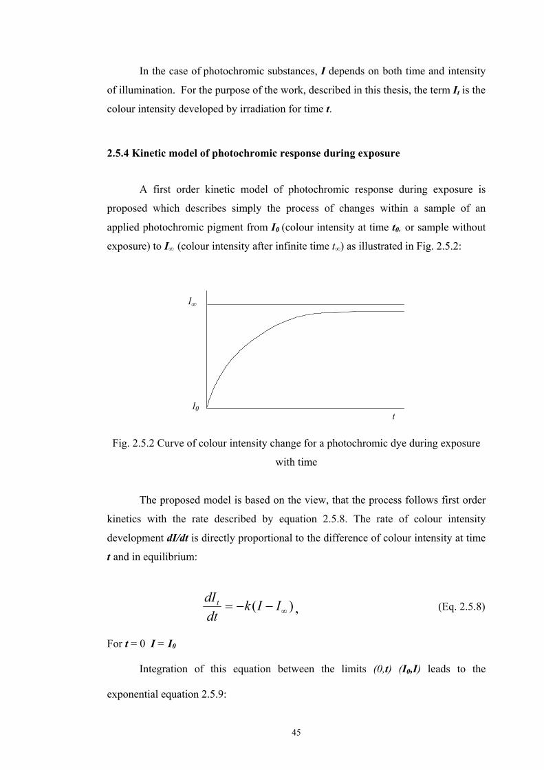
45

In the case of photochromic substances, I depends on both time and intensity

of illumination. For the purpose of the work, described in this thesis, the term It is the

colour intensity developed by irradiation for time t.

2.5.4 Kinetic model of photochromic response during exposure

A first order kinetic model of photochromic response during exposure is

proposed which describes simply the process of changes within a sample of an

applied photochromic pigment from I0 (colour intensity at time t0, or sample without

exposure) to I∞ (colour intensity after infinite time t∞) as illustrated in Fig. 2.5.2:

I∞

I0t

Fig. 2.5.2 Curve of colour intensity change for a photochromic dye during exposure

with time

The proposed model is based on the view, that the process follows first order

kinetics with the rate described by equation 2.5.8. The rate of colour intensity

development dI/dt is directly proportional to the difference of colour intensity at time

t and in equilibrium:

)( ∞−−= IIkdtdIt

, (Eq. 2.5.8)

For t = 0 I = I0

Integration of this equation between the limits (0,t) (I0,I) leads to the

exponential equation 2.5.9:

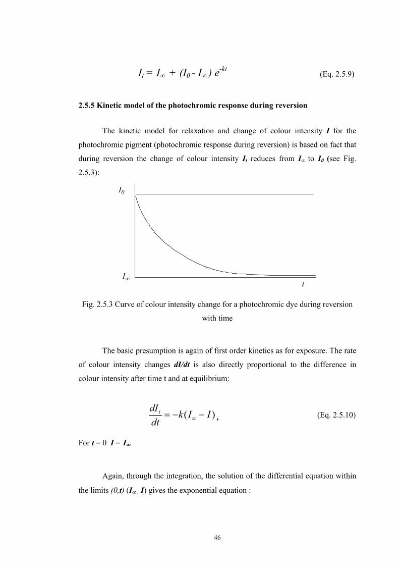
46

It = I∞ + (I0 - I∞ ) e-kt (Eq. 2.5.9)

2.5.5 Kinetic model of the photochromic response during reversion The kinetic model for relaxation and change of colour intensity I for the

photochromic pigment (photochromic response during reversion) is based on fact that

during reversion the change of colour intensity It reduces from I∞ to I0 (see Fig.

2.5.3):

I0

I∞t

Fig. 2.5.3 Curve of colour intensity change for a photochromic dye during reversion

with time

The basic presumption is again of first order kinetics as for exposure. The rate

of colour intensity changes dI/dt is also directly proportional to the difference in

colour intensity after time t and at equilibrium:

( )tdI k I Idt ∞= − − , (Eq. 2.5.10)

For t = 0 I = I∞

Again, through the integration, the solution of the differential equation within

the limits (0,t) (I∞ , I) gives the exponential equation :

47

I = I0 + ( I∞ -I0) e-kt (Eq. 2.5.11)

2.6 Colorimetric measurement of photochromic samples

Colorimetric instruments can be divided into three basic types, these being the

colorimeter, spectroradiometer and spectrophotometer, of which the most important is

the spectrophotometer. The spectrophotometer mainly measures reflectance,

transmittance, or absorbance at different wavelengths in the spectrum. The quantity of

reflectance measured is referred to as the reflectance factor RF. This factor is defined

as the reflectance of the sample at a specific wavelength, over a range of wavelengths,

compared to the reflectance of the perfectly reflecting diffuse white measured under

the same conditions. The mathematical expression is as follows

) whiteideal( standard

sample

)()(

)(λ

λλ

RR

RF = (Eq. 2.6.1)

2.6.1 Standard for the reflectance factor

The perfect reflecting diffuser was recommended as a reference standard in

1986 in the publication CIE Standard Colorimetric Observers [ISO/CIE 10527 –

1991: Colorimetric observers]. It is defined as the ideal isotropic diffuser with a

reflectance equal to unity. Because a perfect reflecting diffuser does not exist in

practice, durable reference standards must be calibrated by comparing the reflected

radiation with incident radiation directly. Such calibrations are difficult to do

accurately and, consequently, are usually performed only in selected national

metrology institutes. Until the 1959 CIE Session [89] the colorimetric measurements

of materials were referred not to the perfect reflecting diffuser but to smoked

magnesium oxide, and its reflectance value was taken to be 100% for all wavelengths.

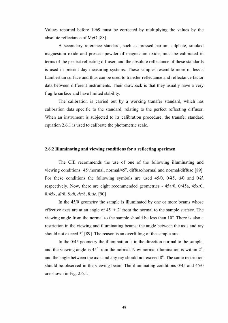
48

Values reported before 1969 must be corrected by multiplying the values by the

absolute reflectance of MgO [88].

A secondary reference standard, such as pressed barium sulphate, smoked

magnesium oxide and pressed powder of magnesium oxide, must be calibrated in

terms of the perfect reflecting diffuser, and the absolute reflectance of these standards

is used in present day measuring systems. These samples resemble more or less a

Lambertian surface and thus can be used to transfer reflectance and reflectance factor

data between different instruments. Their drawback is that they usually have a very

fragile surface and have limited stability.

The calibration is carried out by a working transfer standard, which has

calibration data specific to the standard, relating to the perfect reflecting diffuser.

When an instrument is subjected to its calibration procedure, the transfer standard

equation 2.6.1 is used to calibrate the photometric scale.

2.6.2 Illuminating and viewing conditions for a reflecting specimen

The CIE recommends the use of one of the following illuminating and

viewing conditions: 45o/normal, normal/45o, diffuse/normal and normal/diffuse [89].

For these conditions the following symbols are used 45/0, 0/45, d/0 and 0/d,

respectively. Now, there are eight recommended geometries - 45a:0, 0:45a, 45x:0,

0:45x, di:8, 8:di, de:8, 8:de. [90]

In the 45/0 geometry the sample is illuminated by one or more beams whose

effective axes are at an angle of 45o ± 2o

from the normal to the sample surface. The

viewing angle from the normal to the sample should be less than 10o. There is also a

restriction in the viewing and illuminating beams: the angle between the axis and ray

should not exceed 5o [89]. The reason is an overfilling of the sample area.

In the 0/45 geometry the illumination is in the direction normal to the sample,

and the viewing angle is 45o from the normal. Now normal illumination is within 2o,

and the angle between the axis and any ray should not exceed 8o. The same restriction

should be observed in the viewing beam. The illuminating conditions 0/45 and 45/0

are shown in Fig. 2.6.1.

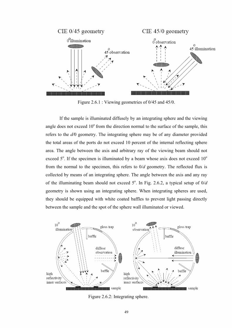
49

Figure 2.6.1 : Viewing geometries of 0/45 and 45/0.

If the sample is illuminated diffusely by an integrating sphere and the viewing

angle does not exceed 10o from the direction normal to the surface of the sample, this

refers to the d/0 geometry. The integrating sphere may be of any diameter provided

the total areas of the ports do not exceed 10 percent of the internal reflecting sphere

area. The angle between the axis and arbitrary ray of the viewing beam should not

exceed 5o. If the specimen is illuminated by a beam whose axis does not exceed 10o

from the normal to the specimen, this refers to 0/d geometry. The reflected flux is

collected by means of an integrating sphere. The angle between the axis and any ray

of the illuminating beam should not exceed 5o. In Fig. 2.6.2, a typical setup of 0/d

geometry is shown using an integrating sphere. When integrating spheres are used,

they should be equipped with white coated baffles to prevent light passing directly

between the sample and the spot of the sphere wall illuminated or viewed.

Figure 2.6.2: Integrating sphere.

50

In the 0/d and d/0 conditions, specular reflection can be excluded or included

by the use of a gloss trap. In the 0/d condition, the sample should not be measured

with a strictly normal axis of illumination if it is required to include the regular

component of reflection. It should be noted that only the 0/d geometry provides a

spectral reflectance. The other conditions d/0, 0/45 and 45/0 give a specific radiance

factor.

2.6.3 Illuminating and viewing conditions for transmitting specimens It is recommended that the colorimetric specification of transmitting species

corresponds to one of the following illuminating and viewing conditions:

normal/normal, normal/diffuse and diffuse/diffuse. The following symbols are used

0/0, 0/d and d/d, respectively [89].

In the normal/normal (0/0) condition, the specimen is illuminated by a beam

whose effective axis is at an angle not exceeding 5o from the normal to its surface and

with the angle between the axis and any ray of the illuminating beam not exceeding

5o. The geometric arrangement of the viewing beam is the same as that of the

illuminating beam. The specimen is positioned so that only the regularly transmitted

flux reaches the detector. This condition gives the regular transmittance, τr.

In the normal/diffuse (0/d) condition, the specimen is illuminated by a beam whose

effective axis is at an angle not exceeding 5o from the normal to its surface and with

the angle between the axis and any ray of the illuminating beam not exceeding 5o.

The hemispherical transmitted flux is usually measured with an integrating sphere.

The reflectance of the reflecting surface of a sphere or other material at the point of

impingement of the regularly transmitted beam, or at the point of impingement of the

illuminating beam in the absence of a specimen, must be identical to the reflectance

of the remainder of the internal reflecting sphere area. This condition gives the total

transmittance, τ.

If the regularly transmitted flux is excluded, for example by the use of a light

trap, it gives the diffuse transmittance, τ0/d. If the positions of the light source and

detector are interchanged, the method gives the equivalent diffuse/normal (d/0)

quantities. In the diffuse/diffuse (d/d) condition, the specimen is illuminated diffusely

51

with an integrating sphere and transmitted flux is collected using a second integrating

sphere. This condition gives the double transmittance, τ dd.

2.7. Conclusion

The principles of the photochromism of organic compounds, fundamental

optical concepts, spectral functions, optical models of translucent media and

colorimetric measurement of photochromic samples have been reviewed and

discussed in this chapter. In order to inform the respect into aspects of the

effectiveness of the production of photochromic textiles, which is the main subject in

this thesis, four equally important set of principles require to be understood and

considered:

1. The chemistry of photochromic colour change.

2. The use of the colorimetric values L*a*b* and the K/S function with colour change

intensity I for the description of photochromic colour change phenomena.

3. A description and understanding of the geometry of spectrophotometers, leading to

the possibility of spectrophotometer modification for the measurement of

photochromic reactions in reflectance mode.

4. Basic optical concepts included in Maxwell`s equations allow a description of the

relationships of electromagnetic radiation in the context of on photochromic

transitions. Consequently, these principles will be used to exploit the photochromic

system as a sensor of UV radiation.

The study of colour change phenomena of selected photochromic materials

allows to deep understanding of the conformation changes induced by UV radiation,

especially the pyrans and naphthooxazine dye types and their photochromic

heterolytic cleavage reactions, used in the experimental work described in this thesis.

There are also many limitations encountered during measurement of

photochromic materials in the application of the classical spectrophotometers.

Therefore it is necessary also to study the geometry of spectrophotometers, to select

52

the right configuration together with factor such as thermal stabilisation, time

sequenced individual measurements to allow a kinetic study of the photochromic

reaction, and to define the kinetic model of photochromic reaction, which is well

described by the Kubelka-Munk function.

53

Chapter 3 EXPERIMENTAL

In chapter 2 of this thesis, the important technical features of photochromic

materials have been reviewed. The review was particularly oriented towards various

features of transparent photochromic media (e.g., solution, glass, polymeric film etc.).

In the case of the measurement of photochromic textiles, consideration is required of

coloured surfaces with changeable features. This problem may be addressed with an

approach involving time sequence measurement and with simultaneous control of UV

exposure.

This experimental section contains two main parts: development of a

measuring system for the evaluation of the kinetics of colour change and the testing

of two types of photochromic textiles. Comparisons are made with photochromic

solutions where appropriate.

3.1. Instrumentation Humans can perceive two types of colour: the colour from a self-luminous

object is referred to as self-luminous colour, and the colour of an illuminated object,

referred to as object colour. A self-luminous object may be natural, such as the sun, or

artificial, such as computer displays, incandescent light bulbs, mercury lamps, and the

like. An object colour is the colour reflected from an illuminated object, and

comprises both the light reflected from the object's surface as well as any light

reflected and scattered from beneath the object's surface.

Instrumental colour measurement is now common practice in many situations

requiring colour quality control owing to the high variability in visual assessment and

the need for accurate colour assessment and communication. The interaction between

observer, light and object form the basis for all instrumental methods for

measurement of colour. Since direct measurement of colour perception is not

possible, the measurement of factors related to colour perception can be used to

numerically to describe colour. Colour measurement in practice does not necessarily

eliminate the need for a visual evaluation of the standard and batch.

Devices for colour measurement date from as early as 1900 when they were

originally known as absorptiometers. They were used to establish, by a visual

inspection, whether two coloured solutions were equal in shade [103]. The first

54

device designed for colour measurement of opaque materials was developed in the

period 1915-1920 and it was called a reflectometer. This device consisted of three

coloured filters and the apparatus was used to directly measure reflectance factors

relative to the amount of the three primaries contained in the measured sample.

Following the development of the CIE 1931 standard observer, the tristimulus

colorimeter was introduced. This device replaced the existing reflectometer [104].

The beginning of reflectance spectrophotometry dates back to 1928 when A.C.

Hardy, Professor of Optics at the Massachusetts Institute of Technology, initiated a

project to produce the first spectrophotometer specifically for the measurement of

reflectance. Commercialization of Hardy’s design began in 1935 when General

Electric introduced the General Electric Recording Spectrophotometer. This

instrument became the much needed reference spectrophotometer and provided the

basis for the development of modern industrial colour measurement [105, 106].

3.1.1 Tristimulus colorimeters and spectrocolorimeters

Early spectrophotometers were expensive and required skilled technicians to

run and maintain them. Colorimetric calculations had to be performed by hand or

with mechanical calculating machines. Industrial colour measurement eventually

became a common practice with the development of the colorimeter. Colorimeters

were developed in the 1940s and, because of their lower cost and simplicity of

operation, were in common use by the 1950s.

Colorimeters have been constructed using all eight CIE recommended

geometries [90]. They use three or four broad response filters to modify their light

source in an attempt to simulate a CIE illuminant and a standard observer

combination. Sample measurements did not result in spectral reflectance readings but

gave a direct conversion to either CIE tristimulus values or the coordinates of a

uniform colour space, such as CIELAB.

The main problem with colorimeters is their inability to measure metamerism.

Colorimeters generally allow for only one illuminant/observer combination and the

determination of metamerism requires a minimum of two such combinations.

Colorimeters using polychromatic illumination have been modified by filtering their

light sources to provide two illuminant/observer combinations. Another problem with

colorimeters is their lack of accuracy caused by the difficulty in finding filters

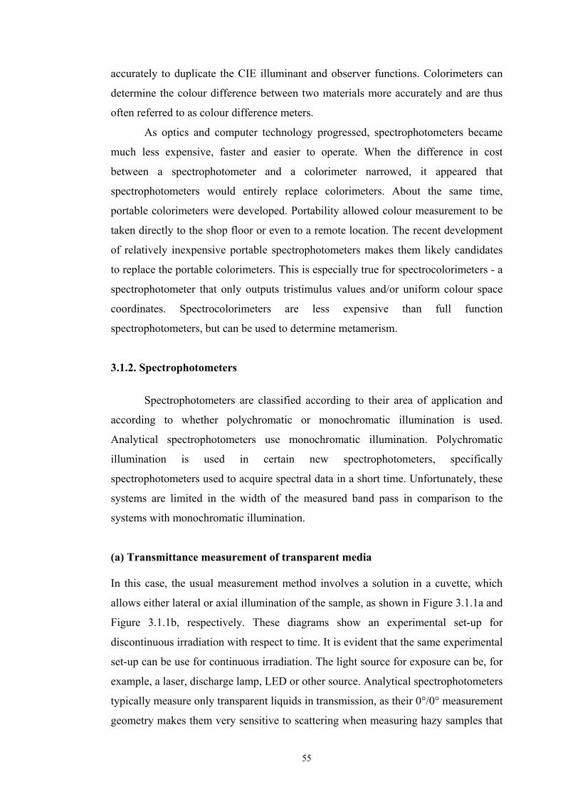
55

accurately to duplicate the CIE illuminant and observer functions. Colorimeters can

determine the colour difference between two materials more accurately and are thus

often referred to as colour difference meters.

As optics and computer technology progressed, spectrophotometers became

much less expensive, faster and easier to operate. When the difference in cost

between a spectrophotometer and a colorimeter narrowed, it appeared that

spectrophotometers would entirely replace colorimeters. About the same time,

portable colorimeters were developed. Portability allowed colour measurement to be

taken directly to the shop floor or even to a remote location. The recent development

of relatively inexpensive portable spectrophotometers makes them likely candidates

to replace the portable colorimeters. This is especially true for spectrocolorimeters - a

spectrophotometer that only outputs tristimulus values and/or uniform colour space

coordinates. Spectrocolorimeters are less expensive than full function

spectrophotometers, but can be used to determine metamerism.

3.1.2. Spectrophotometers

Spectrophotometers are classified according to their area of application and

according to whether polychromatic or monochromatic illumination is used.

Analytical spectrophotometers use monochromatic illumination. Polychromatic

illumination is used in certain new spectrophotometers, specifically

spectrophotometers used to acquire spectral data in a short time. Unfortunately, these

systems are limited in the width of the measured band pass in comparison to the

systems with monochromatic illumination.

(a) Transmittance measurement of transparent media In this case, the usual measurement method involves a solution in a cuvette, which

allows either lateral or axial illumination of the sample, as shown in Figure 3.1.1a and

Figure 3.1.1b, respectively. These diagrams show an experimental set-up for

discontinuous irradiation with respect to time. It is evident that the same experimental

set-up can be use for continuous irradiation. The light source for exposure can be, for

example, a laser, discharge lamp, LED or other source. Analytical spectrophotometers

typically measure only transparent liquids in transmission, as their 0°/0° measurement

geometry makes them very sensitive to scattering when measuring hazy samples that

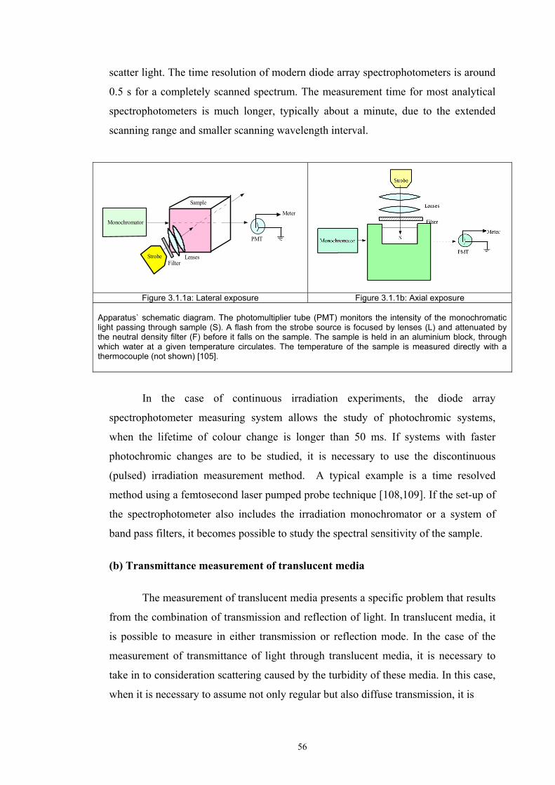
56

scatter light. The time resolution of modern diode array spectrophotometers is around

0.5 s for a completely scanned spectrum. The measurement time for most analytical

spectrophotometers is much longer, typically about a minute, due to the extended

scanning range and smaller scanning wavelength interval.

Monochromator

Strobe

Meter

PMT

Lenses

Sample

Filter

Figure 3.1.1a: Lateral exposure Figure 3.1.1b: Axial exposure Apparatus` schematic diagram. The photomultiplier tube (PMT) monitors the intensity of the monochromatic light passing through sample (S). A flash from the strobe source is focused by lenses (L) and attenuated by the neutral density filter (F) before it falls on the sample. The sample is held in an aluminium block, through which water at a given temperature circulates. The temperature of the sample is measured directly with a thermocouple (not shown) [105].

In the case of continuous irradiation experiments, the diode array

spectrophotometer measuring system allows the study of photochromic systems,

when the lifetime of colour change is longer than 50 ms. If systems with faster

photochromic changes are to be studied, it is necessary to use the discontinuous

(pulsed) irradiation measurement method. A typical example is a time resolved

method using a femtosecond laser pumped probe technique [108,109]. If the set-up of

the spectrophotometer also includes the irradiation monochromator or a system of

band pass filters, it becomes possible to study the spectral sensitivity of the sample.

(b) Transmittance measurement of translucent media

The measurement of translucent media presents a specific problem that results

from the combination of transmission and reflection of light. In translucent media, it

is possible to measure in either transmission or reflection mode. In the case of the

measurement of transmittance of light through translucent media, it is necessary to

take in to consideration scattering caused by the turbidity of these media. In this case,

when it is necessary to assume not only regular but also diffuse transmission, it is

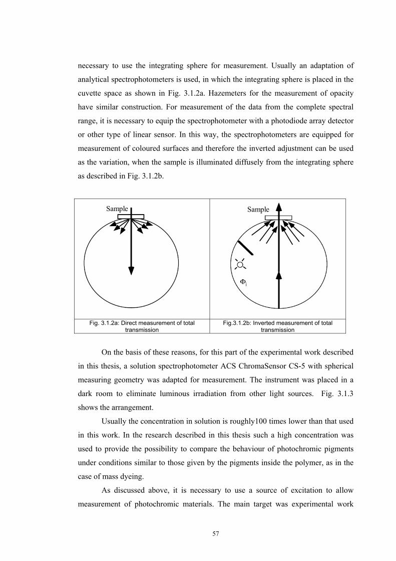
57

necessary to use the integrating sphere for measurement. Usually an adaptation of

analytical spectrophotometers is used, in which the integrating sphere is placed in the

cuvette space as shown in Fig. 3.1.2a. Hazemeters for the measurement of opacity

have similar construction. For measurement of the data from the complete spectral

range, it is necessary to equip the spectrophotometer with a photodiode array detector

or other type of linear sensor. In this way, the spectrophotometers are equipped for

measurement of coloured surfaces and therefore the inverted adjustment can be used

as the variation, when the sample is illuminated diffusely from the integrating sphere

as described in Fig. 3.1.2b.

Sample

Sample

Fig. 3.1.2a: Direct measurement of total

transmission Fig.3.1.2b: Inverted measurement of total

transmission

On the basis of these reasons, for this part of the experimental work described

in this thesis, a solution spectrophotometer ACS ChromaSensor CS-5 with spherical

measuring geometry was adapted for measurement. The instrument was placed in a

dark room to eliminate luminous irradiation from other light sources. Fig. 3.1.3

shows the arrangement.

Usually the concentration in solution is roughly100 times lower than that used

in this work. In the research described in this thesis such a high concentration was

used to provide the possibility to compare the behaviour of photochromic pigments

under conditions similar to those given by the pigments inside the polymer, as in the

case of mass dyeing.

As discussed above, it is necessary to use a source of excitation to allow

measurement of photochromic materials. The main target was experimental work

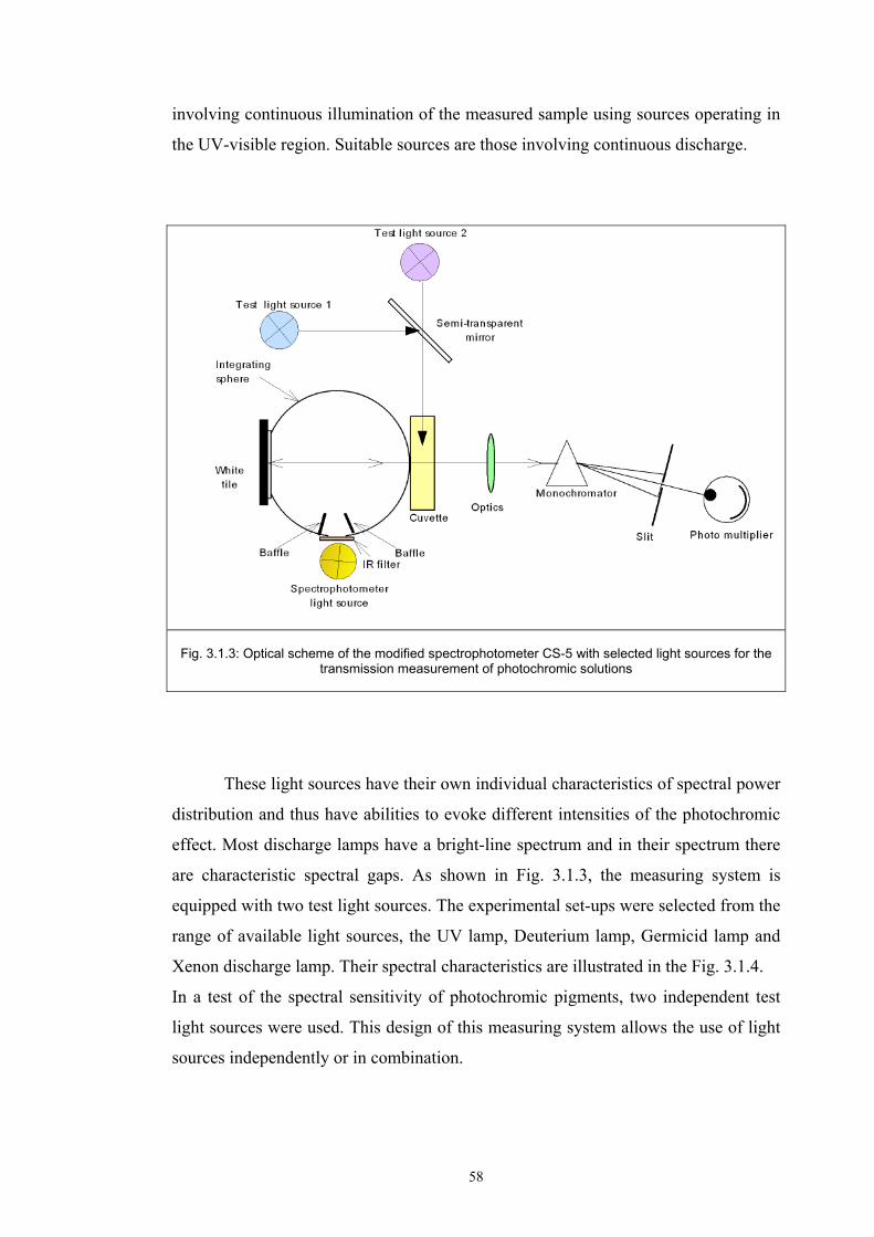
58

involving continuous illumination of the measured sample using sources operating in

the UV-visible region. Suitable sources are those involving continuous discharge.

Fig. 3.1.3: Optical scheme of the modified spectrophotometer CS-5 with selected light sources for the

transmission measurement of photochromic solutions

These light sources have their own individual characteristics of spectral power

distribution and thus have abilities to evoke different intensities of the photochromic

effect. Most discharge lamps have a bright-line spectrum and in their spectrum there

are characteristic spectral gaps. As shown in Fig. 3.1.3, the measuring system is

equipped with two test light sources. The experimental set-ups were selected from the

range of available light sources, the UV lamp, Deuterium lamp, Germicid lamp and

Xenon discharge lamp. Their spectral characteristics are illustrated in the Fig. 3.1.4.

In a test of the spectral sensitivity of photochromic pigments, two independent test

light sources were used. This design of this measuring system allows the use of light

sources independently or in combination.

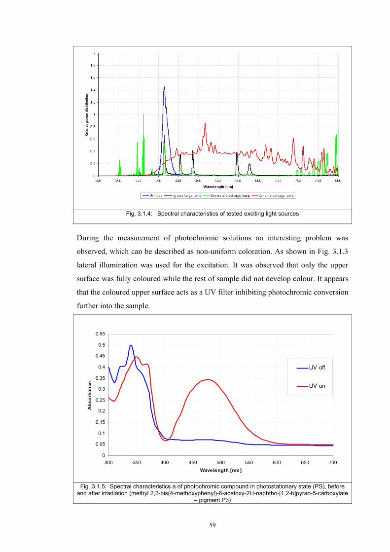
59

Fig. 3.1.4: Spectral characteristics of tested exciting light sources

During the measurement of photochromic solutions an interesting problem was

observed, which can be described as non-uniform coloration. As shown in Fig. 3.1.3

lateral illumination was used for the excitation. It was observed that only the upper

surface was fully coloured while the rest of sample did not develop colour. It appears

that the coloured upper surface acts as a UV filter inhibiting photochromic conversion

further into the sample.

0

0.05

0.1

0.15

0.2

0.25

0.3

0.35

0.4

0.45

0.5

0.55

300 350 400 450 500 550 600 650 700Wavelength [nm]

Abs

orba

nce

UV off

UV on

Fig. 3.1.5: Spectral characteristics a of photochromic compound in photostationary state (PS), before and after irradiation (methyl 2,2-bis(4-methoxyphenyl)-6-acetoxy-2H-naphtho-[1,2-b]pyran-5-carboxylate

– pigment P3)

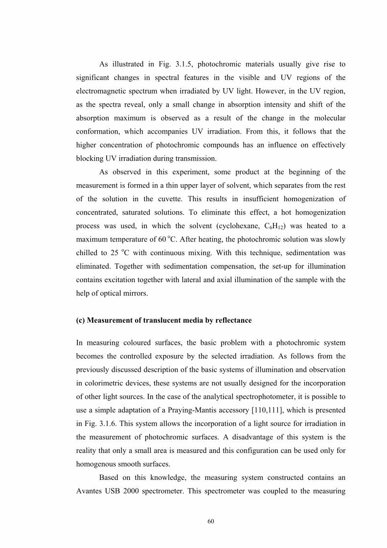
60

As illustrated in Fig. 3.1.5, photochromic materials usually give rise to

significant changes in spectral features in the visible and UV regions of the

electromagnetic spectrum when irradiated by UV light. However, in the UV region,

as the spectra reveal, only a small change in absorption intensity and shift of the

absorption maximum is observed as a result of the change in the molecular

conformation, which accompanies UV irradiation. From this, it follows that the

higher concentration of photochromic compounds has an influence on effectively

blocking UV irradiation during transmission.

As observed in this experiment, some product at the beginning of the

measurement is formed in a thin upper layer of solvent, which separates from the rest

of the solution in the cuvette. This results in insufficient homogenization of

concentrated, saturated solutions. To eliminate this effect, a hot homogenization

process was used, in which the solvent (cyclohexane, C6H12) was heated to a

maximum temperature of 60 oC. After heating, the photochromic solution was slowly

chilled to 25 oC with continuous mixing. With this technique, sedimentation was

eliminated. Together with sedimentation compensation, the set-up for illumination

contains excitation together with lateral and axial illumination of the sample with the

help of optical mirrors.

(c) Measurement of translucent media by reflectance

In measuring coloured surfaces, the basic problem with a photochromic system

becomes the controlled exposure by the selected irradiation. As follows from the

previously discussed description of the basic systems of illumination and observation

in colorimetric devices, these systems are not usually designed for the incorporation

of other light sources. In the case of the analytical spectrophotometer, it is possible to

use a simple adaptation of a Praying-Mantis accessory [110,111], which is presented

in Fig. 3.1.6. This system allows the incorporation of a light source for irradiation in

the measurement of photochromic surfaces. A disadvantage of this system is the

reality that only a small area is measured and this configuration can be used only for

homogenous smooth surfaces.

Based on this knowledge, the measuring system constructed contains an

Avantes USB 2000 spectrometer. This spectrometer was coupled to the measuring

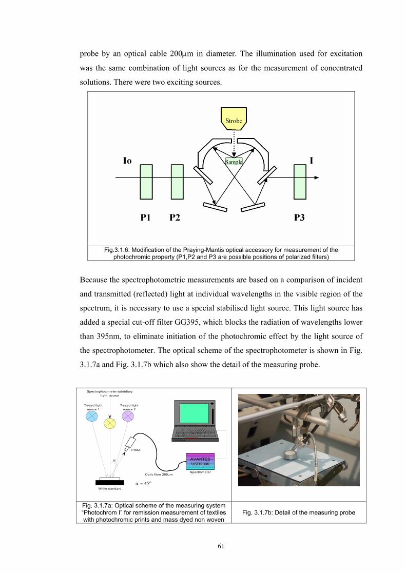
61

probe by an optical cable 200μm in diameter. The illumination used for excitation

was the same combination of light sources as for the measurement of concentrated

solutions. There were two exciting sources.

Sample

Fig.3.1.6: Modification of the Praying-Mantis optical accessory for measurement of the photochromic property (P1,P2 and P3 are possible positions of polarized filters)

Because the spectrophotometric measurements are based on a comparison of incident

and transmitted (reflected) light at individual wavelengths in the visible region of the

spectrum, it is necessary to use a special stabilised light source. This light source has

added a special cut-off filter GG395, which blocks the radiation of wavelengths lower

than 395nm, to eliminate initiation of the photochromic effect by the light source of

the spectrophotometer. The optical scheme of the spectrophotometer is shown in Fig.

3.1.7a and Fig. 3.1.7b which also show the detail of the measuring probe.

Tested l ightsource 2

Tested l ightsource 1

AVANTESUSB2000

Spectrophotometer subsidiarylight source

α

α = 45ο

Spectrometer

White standard

Optic fibre 200μm

Probe

Fig. 3.1.7a: Optical scheme of the measuring system “Photochrom I” for remission measurement of textiles with photochromic prints and mass dyed non woven

Fig. 3.1.7b: Detail of the measuring probe

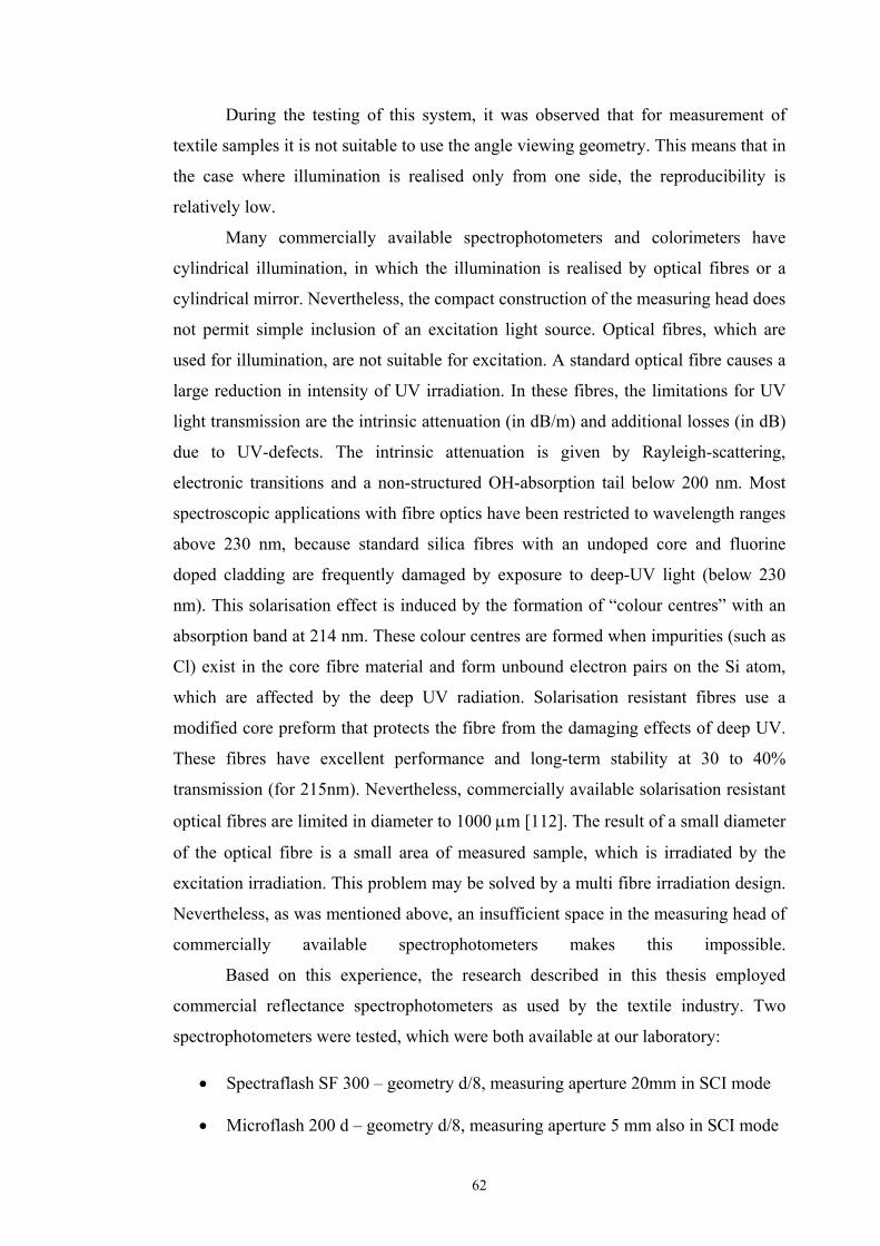
62

During the testing of this system, it was observed that for measurement of

textile samples it is not suitable to use the angle viewing geometry. This means that in

the case where illumination is realised only from one side, the reproducibility is

relatively low.

Many commercially available spectrophotometers and colorimeters have

cylindrical illumination, in which the illumination is realised by optical fibres or a

cylindrical mirror. Nevertheless, the compact construction of the measuring head does

not permit simple inclusion of an excitation light source. Optical fibres, which are

used for illumination, are not suitable for excitation. A standard optical fibre causes a

large reduction in intensity of UV irradiation. In these fibres, the limitations for UV

light transmission are the intrinsic attenuation (in dB/m) and additional losses (in dB)

due to UV-defects. The intrinsic attenuation is given by Rayleigh-scattering,

electronic transitions and a non-structured OH-absorption tail below 200 nm. Most

spectroscopic applications with fibre optics have been restricted to wavelength ranges

above 230 nm, because standard silica fibres with an undoped core and fluorine

doped cladding are frequently damaged by exposure to deep-UV light (below 230

nm). This solarisation effect is induced by the formation of “colour centres” with an

absorption band at 214 nm. These colour centres are formed when impurities (such as

Cl) exist in the core fibre material and form unbound electron pairs on the Si atom,

which are affected by the deep UV radiation. Solarisation resistant fibres use a

modified core preform that protects the fibre from the damaging effects of deep UV.

These fibres have excellent performance and long-term stability at 30 to 40%

transmission (for 215nm). Nevertheless, commercially available solarisation resistant

optical fibres are limited in diameter to 1000 μm [112]. The result of a small diameter

of the optical fibre is a small area of measured sample, which is irradiated by the

excitation irradiation. This problem may be solved by a multi fibre irradiation design.

Nevertheless, as was mentioned above, an insufficient space in the measuring head of

commercially available spectrophotometers makes this impossible.

Based on this experience, the research described in this thesis employed

commercial reflectance spectrophotometers as used by the textile industry. Two

spectrophotometers were tested, which were both available at our laboratory:

• Spectraflash SF 300 – geometry d/8, measuring aperture 20mm in SCI mode • Microflash 200 d – geometry d/8, measuring aperture 5 mm also in SCI mode

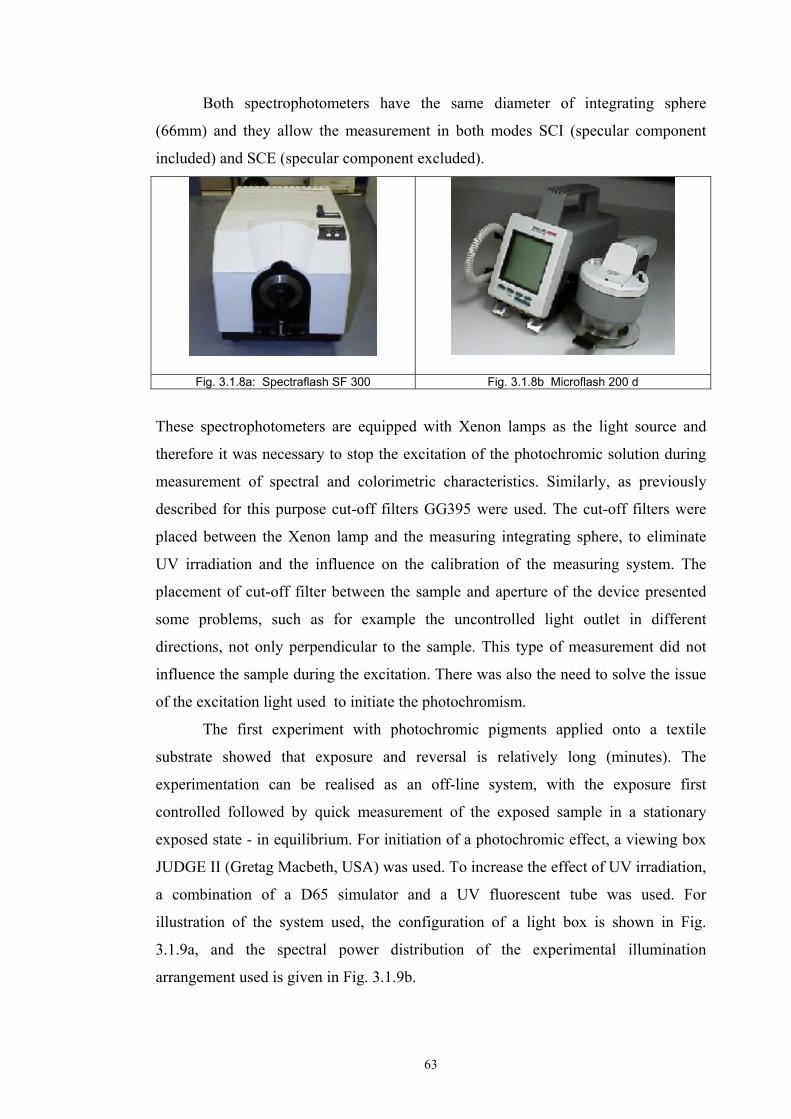
63

Both spectrophotometers have the same diameter of integrating sphere

(66mm) and they allow the measurement in both modes SCI (specular component

included) and SCE (specular component excluded).

These spectrophotometers are equipped with Xenon lamps as the light source and

therefore it was necessary to stop the excitation of the photochromic solution during

measurement of spectral and colorimetric characteristics. Similarly, as previously

described for this purpose cut-off filters GG395 were used. The cut-off filters were

placed between the Xenon lamp and the measuring integrating sphere, to eliminate

UV irradiation and the influence on the calibration of the measuring system. The

placement of cut-off filter between the sample and aperture of the device presented

some problems, such as for example the uncontrolled light outlet in different

directions, not only perpendicular to the sample. This type of measurement did not

influence the sample during the excitation. There was also the need to solve the issue

of the excitation light used to initiate the photochromism.

The first experiment with photochromic pigments applied onto a textile

substrate showed that exposure and reversal is relatively long (minutes). The

experimentation can be realised as an off-line system, with the exposure first

controlled followed by quick measurement of the exposed sample in a stationary

exposed state - in equilibrium. For initiation of a photochromic effect, a viewing box

JUDGE II (Gretag Macbeth, USA) was used. To increase the effect of UV irradiation,

a combination of a D65 simulator and a UV fluorescent tube was used. For

illustration of the system used, the configuration of a light box is shown in Fig.

3.1.9a, and the spectral power distribution of the experimental illumination

arrangement used is given in Fig. 3.1.9b.

Fig. 3.1.8a: Spectraflash SF 300 Fig. 3.1.8b Microflash 200 d

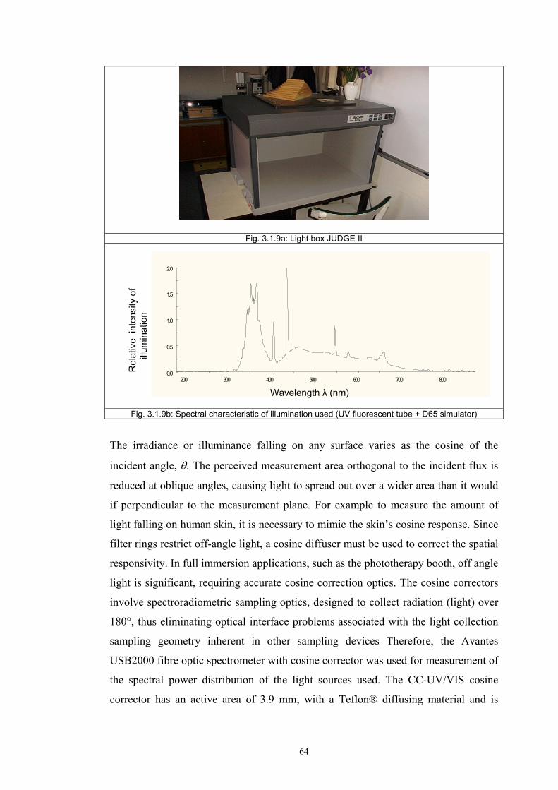
64

Fig. 3.1.9a: Light box JUDGE II

Fig. 3.1.9b: Spectral characteristic of illumination used (UV fluorescent tube + D65 simulator)

The irradiance or illuminance falling on any surface varies as the cosine of the

incident angle, θ. The perceived measurement area orthogonal to the incident flux is

reduced at oblique angles, causing light to spread out over a wider area than it would

if perpendicular to the measurement plane. For example to measure the amount of

light falling on human skin, it is necessary to mimic the skin’s cosine response. Since

filter rings restrict off-angle light, a cosine diffuser must be used to correct the spatial

responsivity. In full immersion applications, such as the phototherapy booth, off angle

light is significant, requiring accurate cosine correction optics. The cosine correctors

involve spectroradiometric sampling optics, designed to collect radiation (light) over

180°, thus eliminating optical interface problems associated with the light collection

sampling geometry inherent in other sampling devices Therefore, the Avantes

USB2000 fibre optic spectrometer with cosine corrector was used for measurement of

the spectral power distribution of the light sources used. The CC-UV/VIS cosine

corrector has an active area of 3.9 mm, with a Teflon® diffusing material and is

0.0

0.5

1.0

1.5

2.0

200 300 400 500 600 700 800

Rel

ativ

e in

tens

ity o

f

i

llum

inat

ion

Wavelength λ (nm)

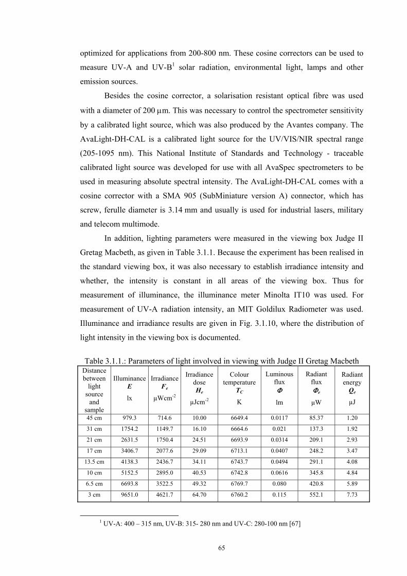
65

optimized for applications from 200-800 nm. These cosine correctors can be used to

measure UV-A and UV-B1 solar radiation, environmental light, lamps and other

emission sources.

Besides the cosine corrector, a solarisation resistant optical fibre was used

with a diameter of 200 μm. This was necessary to control the spectrometer sensitivity

by a calibrated light source, which was also produced by the Avantes company. The

AvaLight-DH-CAL is a calibrated light source for the UV/VIS/NIR spectral range

(205-1095 nm). This National Institute of Standards and Technology - traceable

calibrated light source was developed for use with all AvaSpec spectrometers to be

used in measuring absolute spectral intensity. The AvaLight-DH-CAL comes with a

cosine corrector with a SMA 905 (SubMiniature version A) connector, which has

screw, ferulle diameter is 3.14 mm and usually is used for industrial lasers, military

and telecom multimode.

In addition, lighting parameters were measured in the viewing box Judge II

Gretag Macbeth, as given in Table 3.1.1. Because the experiment has been realised in

the standard viewing box, it was also necessary to establish irradiance intensity and

whether, the intensity is constant in all areas of the viewing box. Thus for

measurement of illuminance, the illuminance meter Minolta IT10 was used. For

measurement of UV-A radiation intensity, an MIT Goldilux Radiometer was used.

Illuminance and irradiance results are given in Fig. 3.1.10, where the distribution of

light intensity in the viewing box is documented.

Table 3.1.1.: Parameters of light involved in viewing with Judge II Gretag Macbeth

Distance between

light source

and sample

Illuminance E

lx

IrradianceFe

µWcm-2

Irradiance dose He

µJcm-2

Colour temperature

TC

K

Luminous flux Φ

lm

Radiant flux Φe

µW

Radiant energy

Qe

µJ

45 cm 979.3 714.6 10.00 6649.4 0.0117 85.37 1.20

31 cm 1754.2 1149.7 16.10 6664.6 0.021 137.3 1.92

21 cm 2631.5 1750.4 24.51 6693.9 0.0314 209.1 2.93

17 cm 3406.7 2077.6 29.09 6713.1 0.0407 248.2 3.47

13.5 cm 4138.3 2436.7 34.11 6743.7 0.0494 291.1 4.08

10 cm 5152.5 2895.0 40.53 6742.8 0.0616 345.8 4.84

6.5 cm 6693.8 3522.5 49.32 6769.7 0.080 420.8 5.89

3 cm 9651.0 4621.7 64.70 6760.2 0.115 552.1 7.73

1 UV-A: 400 – 315 nm, UV-B: 315- 280 nm and UV-C: 280-100 nm [67]

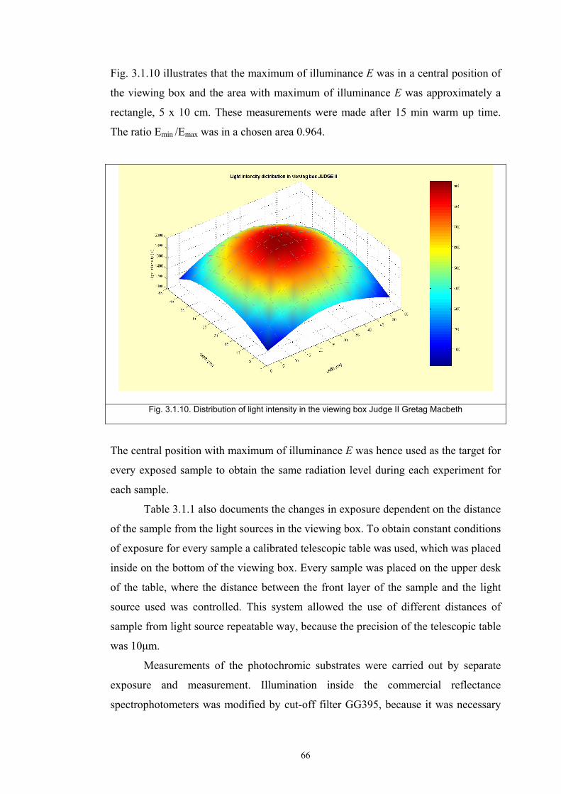
66

Fig. 3.1.10 illustrates that the maximum of illuminance E was in a central position of

the viewing box and the area with maximum of illuminance E was approximately a

rectangle, 5 x 10 cm. These measurements were made after 15 min warm up time.

The ratio Emin /Emax was in a chosen area 0.964.

Fig. 3.1.10. Distribution of light intensity in the viewing box Judge II Gretag Macbeth

The central position with maximum of illuminance E was hence used as the target for

every exposed sample to obtain the same radiation level during each experiment for

each sample.

Table 3.1.1 also documents the changes in exposure dependent on the distance

of the sample from the light sources in the viewing box. To obtain constant conditions

of exposure for every sample a calibrated telescopic table was used, which was placed

inside on the bottom of the viewing box. Every sample was placed on the upper desk

of the table, where the distance between the front layer of the sample and the light

source used was controlled. This system allowed the use of different distances of

sample from light source repeatable way, because the precision of the telescopic table

was 10μm.

Measurements of the photochromic substrates were carried out by separate

exposure and measurement. Illumination inside the commercial reflectance

spectrophotometers was modified by cut-off filter GG395, because it was necessary

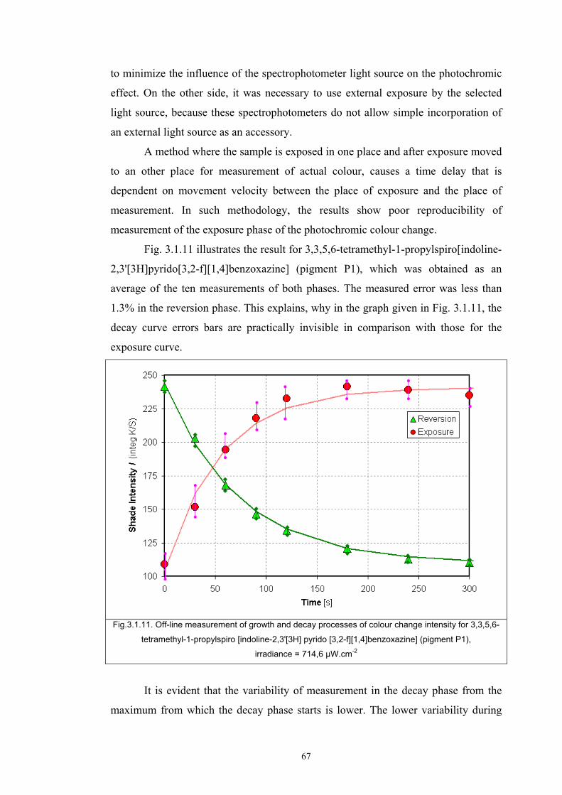
67

to minimize the influence of the spectrophotometer light source on the photochromic

effect. On the other side, it was necessary to use external exposure by the selected

light source, because these spectrophotometers do not allow simple incorporation of

an external light source as an accessory.

A method where the sample is exposed in one place and after exposure moved

to an other place for measurement of actual colour, causes a time delay that is

dependent on movement velocity between the place of exposure and the place of

measurement. In such methodology, the results show poor reproducibility of

measurement of the exposure phase of the photochromic colour change.

Fig. 3.1.11 illustrates the result for 3,3,5,6-tetramethyl-1-propylspiro[indoline-

2,3'[3H]pyrido[3,2-f][1,4]benzoxazine] (pigment P1), which was obtained as an

average of the ten measurements of both phases. The measured error was less than

1.3% in the reversion phase. This explains, why in the graph given in Fig. 3.1.11, the

decay curve errors bars are practically invisible in comparison with those for the

exposure curve.

Fig.3.1.11. Off-line measurement of growth and decay processes of colour change intensity for 3,3,5,6-

tetramethyl-1-propylspiro [indoline-2,3'[3H] pyrido [3,2-f][1,4]benzoxazine] (pigment P1),

irradiance = 714,6 µW.cm-2

It is evident that the variability of measurement in the decay phase from the

maximum from which the decay phase starts is lower. The lower variability during

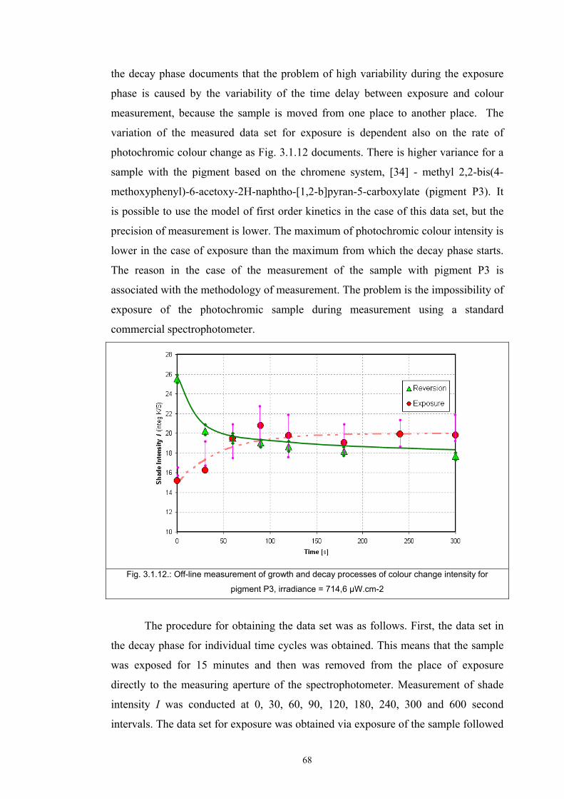
68

the decay phase documents that the problem of high variability during the exposure

phase is caused by the variability of the time delay between exposure and colour

measurement, because the sample is moved from one place to another place. The

variation of the measured data set for exposure is dependent also on the rate of

photochromic colour change as Fig. 3.1.12 documents. There is higher variance for a

sample with the pigment based on the chromene system, [34] - methyl 2,2-bis(4-

methoxyphenyl)-6-acetoxy-2H-naphtho-[1,2-b]pyran-5-carboxylate (pigment P3). It

is possible to use the model of first order kinetics in the case of this data set, but the

precision of measurement is lower. The maximum of photochromic colour intensity is

lower in the case of exposure than the maximum from which the decay phase starts.

The reason in the case of the measurement of the sample with pigment P3 is

associated with the methodology of measurement. The problem is the impossibility of

exposure of the photochromic sample during measurement using a standard

commercial spectrophotometer.

Fig. 3.1.12.: Off-line measurement of growth and decay processes of colour change intensity for

pigment P3, irradiance = 714,6 µW.cm-2

The procedure for obtaining the data set was as follows. First, the data set in

the decay phase for individual time cycles was obtained. This means that the sample

was exposed for 15 minutes and then was removed from the place of exposure

directly to the measuring aperture of the spectrophotometer. Measurement of shade

intensity I was conducted at 0, 30, 60, 90, 120, 180, 240, 300 and 600 second

intervals. The data set for exposure was obtained via exposure of the sample followed

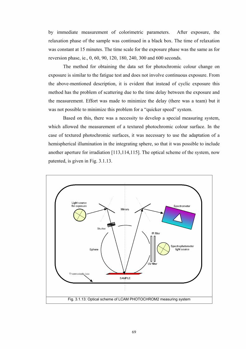
69

by immediate measurement of colorimetric parameters. After exposure, the

relaxation phase of the sample was continued in a black box. The time of relaxation

was constant at 15 minutes. The time scale for the exposure phase was the same as for

reversion phase, ie., 0, 60, 90, 120, 180, 240, 300 and 600 seconds.

The method for obtaining the data set for photochromic colour change on

exposure is similar to the fatigue test and does not involve continuous exposure. From

the above-mentioned description, it is evident that instead of cyclic exposure this

method has the problem of scattering due to the time delay between the exposure and

the measurement. Effort was made to minimize the delay (there was a team) but it

was not possible to minimize this problem for a “quicker speed” system.

Based on this, there was a necessity to develop a special measuring system,

which allowed the measurement of a textured photochromic colour surface. In the

case of textured photochromic surfaces, it was necessary to use the adaptation of a

hemispherical illumination in the integrating sphere, so that it was possible to include

another aperture for irradiation [113,114,115]. The optical scheme of the system, now

patented, is given in Fig. 3.1.13.

Fig. 3.1.13: Optical scheme of LCAM PHOTOCHROM2 measuring system

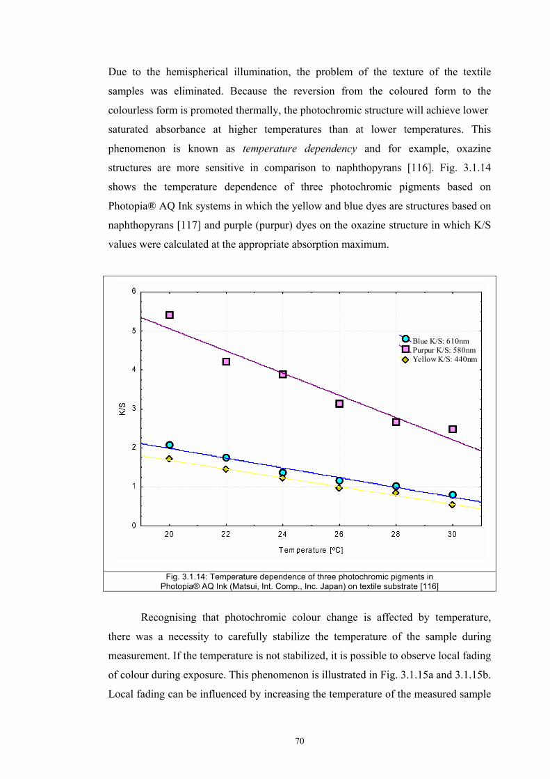
70

Due to the hemispherical illumination, the problem of the texture of the textile

samples was eliminated. Because the reversion from the coloured form to the

colourless form is promoted thermally, the photochromic structure will achieve lower

saturated absorbance at higher temperatures than at lower temperatures. This

phenomenon is known as temperature dependency and for example, oxazine

structures are more sensitive in comparison to naphthopyrans [116]. Fig. 3.1.14

shows the temperature dependence of three photochromic pigments based on

Photopia® AQ Ink systems in which the yellow and blue dyes are structures based on

naphthopyrans [117] and purple (purpur) dyes on the oxazine structure in which K/S

values were calculated at the appropriate absorption maximum.

Blue K/S:610 nmPurpur K/S:580 nm

Yellow K/S: 440 nm

Blue K/S: 610nmPurpur K/S: 580nmYellow K/S: 440nm

Fig. 3.1.14: Temperature dependence of three photochromic pigments in Photopia® AQ Ink (Matsui, Int. Comp., Inc. Japan) on textile substrate [116]

Recognising that photochromic colour change is affected by temperature,

there was a necessity to carefully stabilize the temperature of the sample during

measurement. If the temperature is not stabilized, it is possible to observe local fading

of colour during exposure. This phenomenon is illustrated in Fig. 3.1.15a and 3.1.15b.

Local fading can be influenced by increasing the temperature of the measured sample

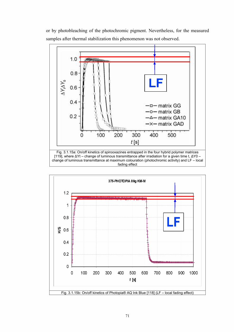
71

or by photobleaching of the photochromic pigment. Nevertheless, for the measured

samples after thermal stabilization this phenomenon was not observed.

Fig. 3.1.15a: On/off kinetics of spirooxazines entrapped in the four hybrid polymer matrices

[119], where ΔYt – change of luminous transmittance after irradiation for a given time t, ΔY0 – change of luminous transmittance at maximum colouration (photochromic activity) and LF – local

fading effect

Fig. 3.1.15b: On/off kinetics of Photopia® AQ Ink Blue [118] (LF – local fading effect)

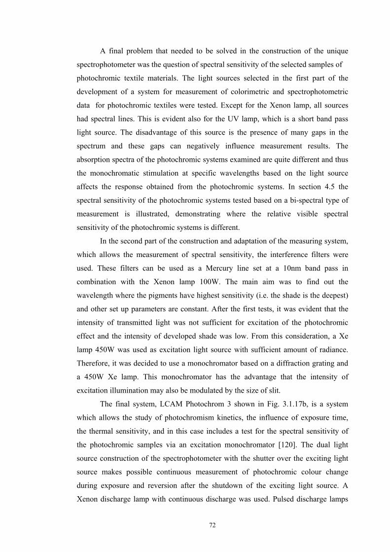
72

A final problem that needed to be solved in the construction of the unique

spectrophotometer was the question of spectral sensitivity of the selected samples of

photochromic textile materials. The light sources selected in the first part of the

development of a system for measurement of colorimetric and spectrophotometric

data for photochromic textiles were tested. Except for the Xenon lamp, all sources

had spectral lines. This is evident also for the UV lamp, which is a short band pass

light source. The disadvantage of this source is the presence of many gaps in the

spectrum and these gaps can negatively influence measurement results. The

absorption spectra of the photochromic systems examined are quite different and thus

the monochromatic stimulation at specific wavelengths based on the light source

affects the response obtained from the photochromic systems. In section 4.5 the

spectral sensitivity of the photochromic systems tested based on a bi-spectral type of

measurement is illustrated, demonstrating where the relative visible spectral

sensitivity of the photochromic systems is different.

In the second part of the construction and adaptation of the measuring system,

which allows the measurement of spectral sensitivity, the interference filters were

used. These filters can be used as a Mercury line set at a 10nm band pass in

combination with the Xenon lamp 100W. The main aim was to find out the

wavelength where the pigments have highest sensitivity (i.e. the shade is the deepest)

and other set up parameters are constant. After the first tests, it was evident that the

intensity of transmitted light was not sufficient for excitation of the photochromic

effect and the intensity of developed shade was low. From this consideration, a Xe

lamp 450W was used as excitation light source with sufficient amount of radiance.

Therefore, it was decided to use a monochromator based on a diffraction grating and

a 450W Xe lamp. This monochromator has the advantage that the intensity of

excitation illumination may also be modulated by the size of slit.

The final system, LCAM Photochrom 3 shown in Fig. 3.1.17b, is a system

which allows the study of photochromism kinetics, the influence of exposure time,

the thermal sensitivity, and in this case includes a test for the spectral sensitivity of

the photochromic samples via an excitation monochromator [120]. The dual light

source construction of the spectrophotometer with the shutter over the exciting light

source makes possible continuous measurement of photochromic colour change

during exposure and reversion after the shutdown of the exciting light source. A

Xenon discharge lamp with continuous discharge was used. Pulsed discharge lamps

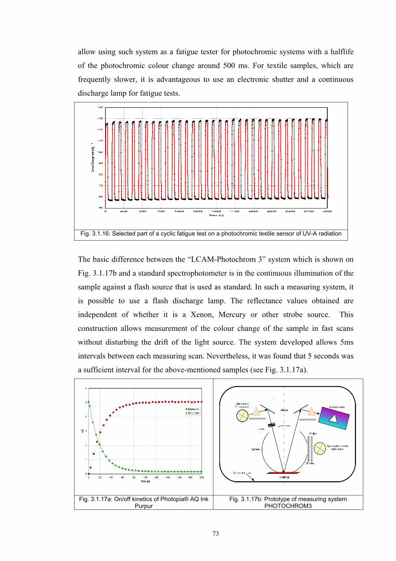
73

allow using such system as a fatigue tester for photochromic systems with a halflife

of the photochromic colour change around 500 ms. For textile samples, which are

frequently slower, it is advantageous to use an electronic shutter and a continuous

discharge lamp for fatigue tests.

Fig. 3.1.16: Selected part of a cyclic fatigue test on a photochromic textile sensor of UV-A radiation

The basic difference between the “LCAM-Photochrom 3” system which is shown on

Fig. 3.1.17b and a standard spectrophotometer is in the continuous illumination of the

sample against a flash source that is used as standard. In such a measuring system, it

is possible to use a flash discharge lamp. The reflectance values obtained are

independent of whether it is a Xenon, Mercury or other strobe source. This

construction allows measurement of the colour change of the sample in fast scans

without disturbing the drift of the light source. The system developed allows 5ms

intervals between each measuring scan. Nevertheless, it was found that 5 seconds was

a sufficient interval for the above-mentioned samples (see Fig. 3.1.17a).

Samplemonochromator monochromator

Fig. 3.1.17a: On/off kinetics of Photopia® AQ Ink Purpur

Fig. 3.1.17b: Prototype of measuring system PHOTOCHROM3

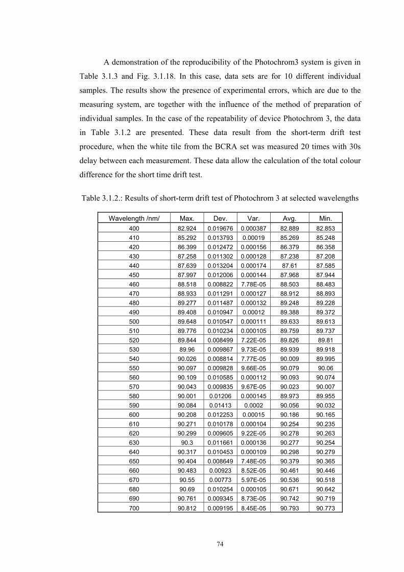
74

A demonstration of the reproducibility of the Photochrom3 system is given in

Table 3.1.3 and Fig. 3.1.18. In this case, data sets are for 10 different individual

samples. The results show the presence of experimental errors, which are due to the

measuring system, are together with the influence of the method of preparation of

individual samples. In the case of the repeatability of device Photochrom 3, the data

in Table 3.1.2 are presented. These data result from the short-term drift test

procedure, when the white tile from the BCRA set was measured 20 times with 30s

delay between each measurement. These data allow the calculation of the total colour

difference for the short time drift test.

Table 3.1.2.: Results of short-term drift test of Photochrom 3 at selected wavelengths

Wavelength /nm/ Max. Dev. Var. Avg. Min. 400 82.924 0.019676 0.000387 82.889 82.853 410 85.292 0.013793 0.00019 85.269 85.248 420 86.399 0.012472 0.000156 86.379 86.358 430 87.258 0.011302 0.000128 87.238 87.208 440 87.639 0.013204 0.000174 87.61 87.585 450 87.997 0.012006 0.000144 87.968 87.944 460 88.518 0.008822 7.78E-05 88.503 88.483 470 88.933 0.011291 0.000127 88.912 88.893 480 89.277 0.011487 0.000132 89.248 89.228 490 89.408 0.010947 0.00012 89.388 89.372 500 89.648 0.010547 0.000111 89.633 89.613 510 89.776 0.010234 0.000105 89.759 89.737 520 89.844 0.008499 7.22E-05 89.826 89.81 530 89.96 0.009867 9.73E-05 89.939 89.918 540 90.026 0.008814 7.77E-05 90.009 89.995 550 90.097 0.009828 9.66E-05 90.079 90.06 560 90.109 0.010585 0.000112 90.093 90.074 570 90.043 0.009835 9.67E-05 90.023 90.007 580 90.001 0.01206 0.000145 89.973 89.955 590 90.084 0.01413 0.0002 90.056 90.032 600 90.208 0.012253 0.00015 90.186 90.165 610 90.271 0.010178 0.000104 90.254 90.235 620 90.299 0.009605 9.22E-05 90.278 90.263 630 90.3 0.011661 0.000136 90.277 90.254 640 90.317 0.010453 0.000109 90.298 90.279 650 90.404 0.008649 7.48E-05 90.379 90.365 660 90.483 0.00923 8.52E-05 90.461 90.446 670 90.55 0.00773 5.97E-05 90.536 90.518 680 90.69 0.010254 0.000105 90.671 90.642 690 90.761 0.009345 8.73E-05 90.742 90.719 700 90.812 0.009195 8.45E-05 90.793 90.773

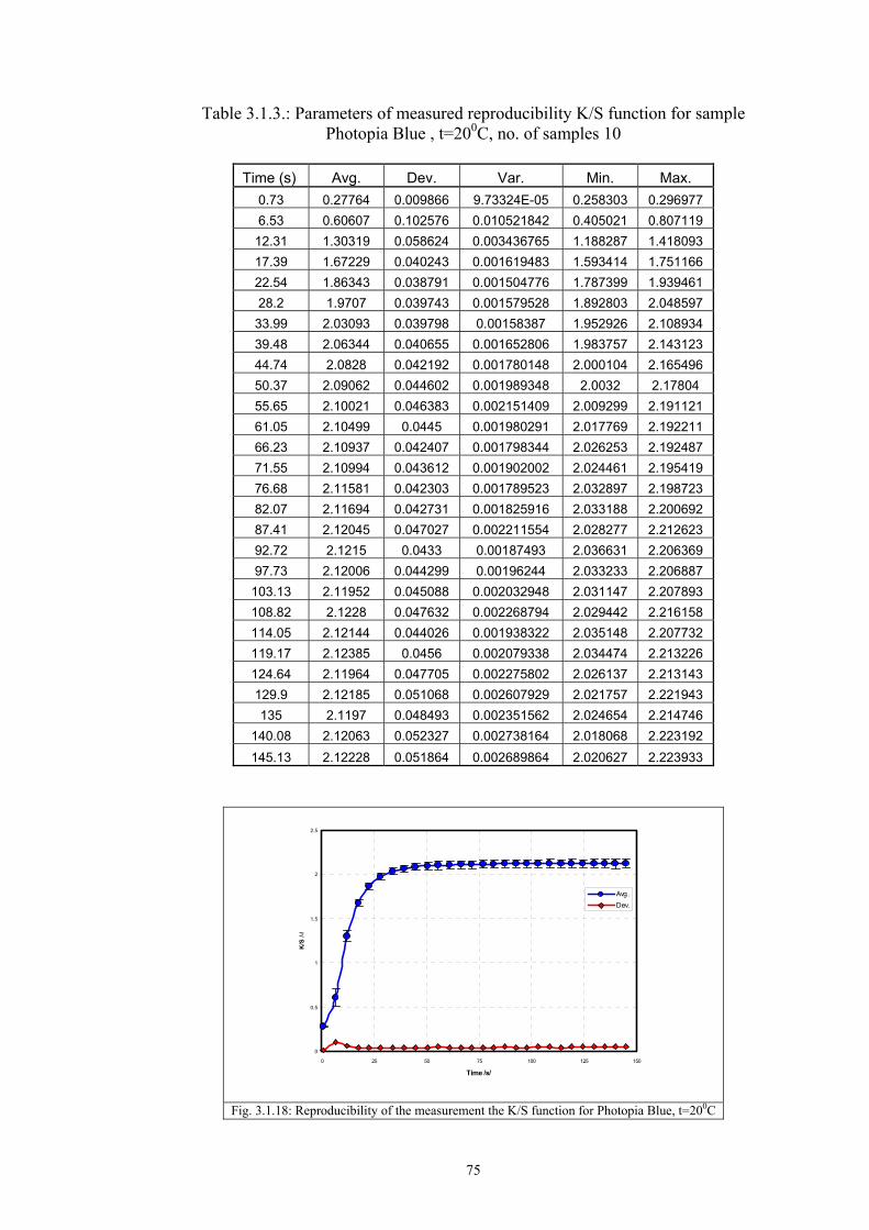
75

Table 3.1.3.: Parameters of measured reproducibility K/S function for sample Photopia Blue , t=200C, no. of samples 10

Time (s) Avg. Dev. Var. Min. Max.

0.73 0.27764 0.009866 9.73324E-05 0.258303 0.296977 6.53 0.60607 0.102576 0.010521842 0.405021 0.807119 12.31 1.30319 0.058624 0.003436765 1.188287 1.418093 17.39 1.67229 0.040243 0.001619483 1.593414 1.751166 22.54 1.86343 0.038791 0.001504776 1.787399 1.939461 28.2 1.9707 0.039743 0.001579528 1.892803 2.048597 33.99 2.03093 0.039798 0.00158387 1.952926 2.108934 39.48 2.06344 0.040655 0.001652806 1.983757 2.143123 44.74 2.0828 0.042192 0.001780148 2.000104 2.165496 50.37 2.09062 0.044602 0.001989348 2.0032 2.17804 55.65 2.10021 0.046383 0.002151409 2.009299 2.191121 61.05 2.10499 0.0445 0.001980291 2.017769 2.192211 66.23 2.10937 0.042407 0.001798344 2.026253 2.192487 71.55 2.10994 0.043612 0.001902002 2.024461 2.195419 76.68 2.11581 0.042303 0.001789523 2.032897 2.198723 82.07 2.11694 0.042731 0.001825916 2.033188 2.200692 87.41 2.12045 0.047027 0.002211554 2.028277 2.212623 92.72 2.1215 0.0433 0.00187493 2.036631 2.206369 97.73 2.12006 0.044299 0.00196244 2.033233 2.206887

103.13 2.11952 0.045088 0.002032948 2.031147 2.207893 108.82 2.1228 0.047632 0.002268794 2.029442 2.216158 114.05 2.12144 0.044026 0.001938322 2.035148 2.207732 119.17 2.12385 0.0456 0.002079338 2.034474 2.213226 124.64 2.11964 0.047705 0.002275802 2.026137 2.213143 129.9 2.12185 0.051068 0.002607929 2.021757 2.221943 135 2.1197 0.048493 0.002351562 2.024654 2.214746

140.08 2.12063 0.052327 0.002738164 2.018068 2.223192 145.13 2.12228 0.051864 0.002689864 2.020627 2.223933

0

0.5

1

1.5

2

2.5

0 25 50 75 100 125 150

Time /s/

K/S

/-/

Avg.Dev.

Fig. 3.1.18: Reproducibility of the measurement the K/S function for Photopia Blue, t=200C

76

3.1.3. Light fastness tests

In the case of photochromic materials, the assessment of lightfastness has its

own particular specificity. Standard light fastness tests have been devised for

traditional dyes and pigments. In the case of photochromic materials, because of their

dynamic colour change properties fatigue tests are relevant.

Standard light fastness tests may use outdoor exposure in selected locations or

exposure devices, which use artificial illumination. The standard ISO 105-B02

describes the test with artificial illumination [121]. In this thesis, a Xenotest 450 LF

test apparatus has been used modified to provide colorimetric measurement of

photochromic samples. The spectral response of photochromic samples is measured

before and after the light fastness test. Spectral properties were measured 15 minutes

after exposure in a viewing box. Based on the information it was possible to compare

two parameters – the colour change of photochromic samples after the lightfastness

test and the decrease of the extent of the photochromic colour change. Because

photochromic materials do not have high light fastness, the light fastness test was

arranged involving 10 cycles with 1 hour exposure in the Xenotest apparatus. It was

found that some of the samples have a stepwise reversion phase of the photochromic

cycle – the samples have a quick and slow part of the reversion phase. The total

number of exposure cycles was 10 with 24 hours relaxation before re-measurement.

After every hour the reflectance characteristics of all samples were measured by the

spectrophotometer. Because some pigments had a residual coloration from previous

illumination, similar measurements were also arranged after 24-hour relaxation. From

the observation, if the samples gave a photochromic response, the samples were

exposed and once again measured.

As discussed in the case of photochromic textiles, instead of the resistance

against continuous exposure to a light source containing UV irradiation, it is also

necessary to study the number of cycles, which the photochromic system can realize.

The number of possible cycles can theoretically be infinite. Therefore, the

limitation was used involving a 50% reduction in the photochromic response (50%

intensity of coloration).

Based on discussion with the dye manufacturer, the number of cycles was

limited to 200. The exposure was for 5 minutes and relaxation was for 10 minutes

before repetitions of exposure.

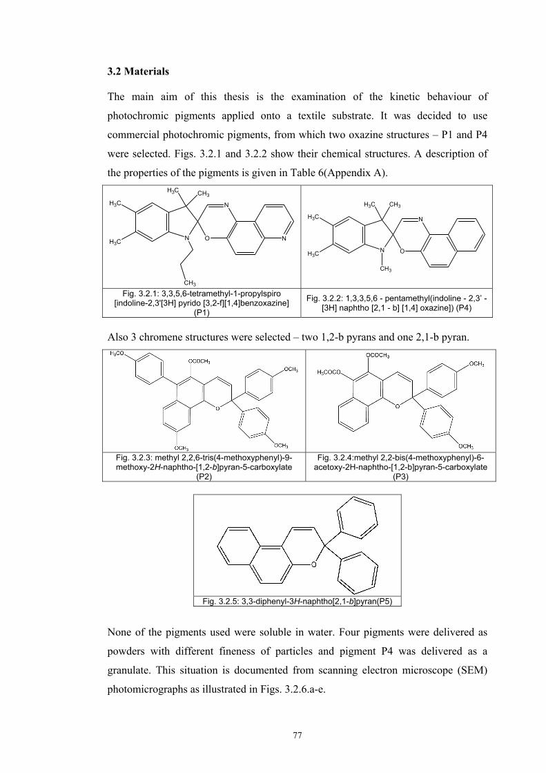
77

3.2 Materials

The main aim of this thesis is the examination of the kinetic behaviour of

photochromic pigments applied onto a textile substrate. It was decided to use

commercial photochromic pigments, from which two oxazine structures – P1 and P4

were selected. Figs. 3.2.1 and 3.2.2 show their chemical structures. A description of

the properties of the pigments is given in Table 6(Appendix A).

N

CH3

H3C CH3

H3C

H3C O

N

N

N O

N

CH3

CH3H3C

H3C

H3C

Fig. 3.2.1: 3,3,5,6-tetramethyl-1-propylspiro [indoline-2,3'[3H] pyrido [3,2-f][1,4]benzoxazine]

(P1)

Fig. 3.2.2: 1,3,3,5,6 - pentamethyl(indoline - 2,3’ - [3H] naphtho [2,1 - b] [1,4] oxazine]) (P4)

Also 3 chromene structures were selected – two 1,2-b pyrans and one 2,1-b pyran.

Fig. 3.2.3: methyl 2,2,6-tris(4-methoxyphenyl)-9-methoxy-2H-naphtho-[1,2-b]pyran-5-carboxylate

(P2)

Fig. 3.2.4:methyl 2,2-bis(4-methoxyphenyl)-6-acetoxy-2H-naphtho-[1,2-b]pyran-5-carboxylate

(P3)

Fig. 3.2.5: 3,3-diphenyl-3H-naphtho[2,1-b]pyran(P5)

None of the pigments used were soluble in water. Four pigments were delivered as

powders with different fineness of particles and pigment P4 was delivered as a

granulate. This situation is documented from scanning electron microscope (SEM)

photomicrographs as illustrated in Figs. 3.2.6.a-e.

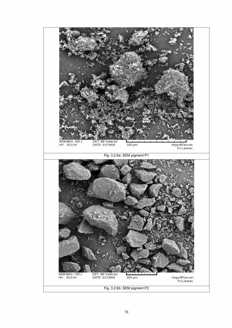
78

Fig. 3.2.6a: SEM pigment P1

Fig. 3.2.6b: SEM pigment P2

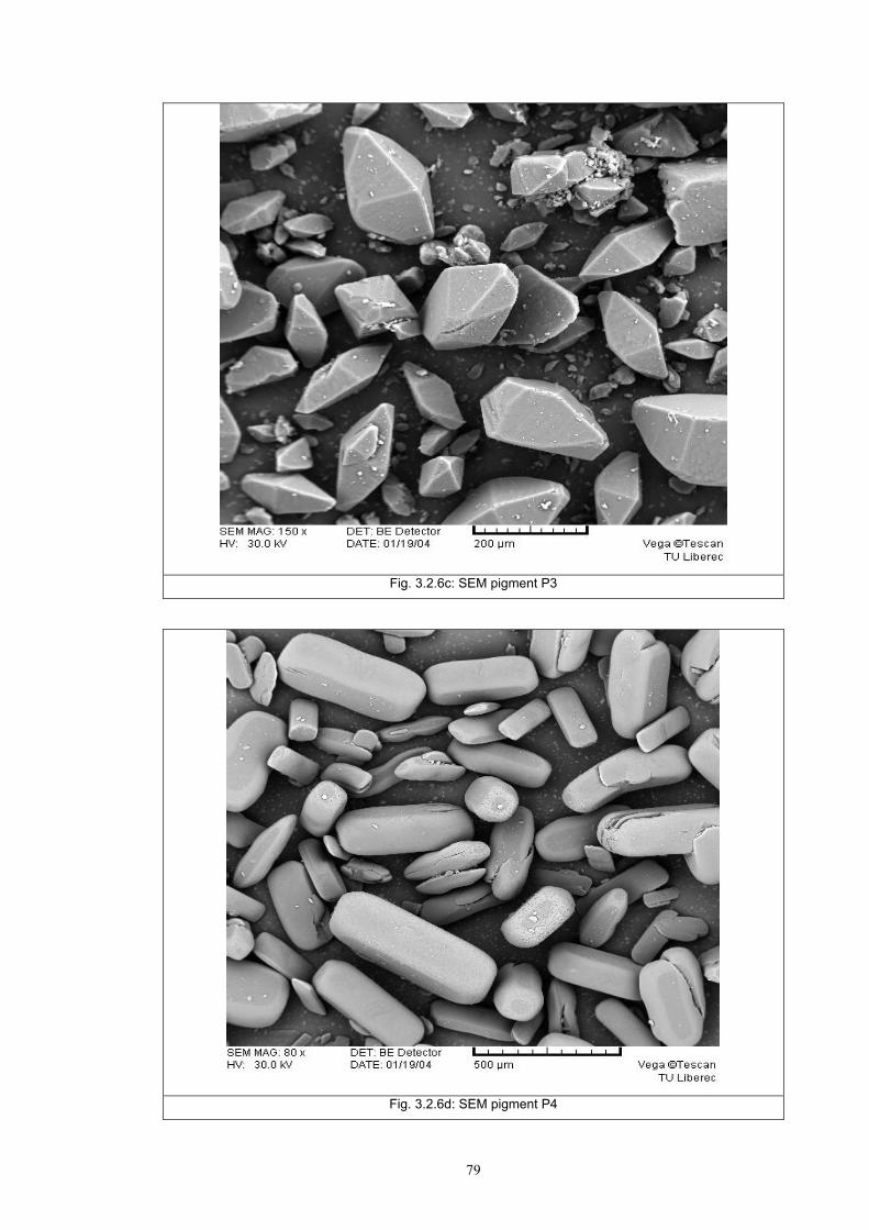
79

Fig. 3.2.6c: SEM pigment P3

Fig. 3.2.6d: SEM pigment P4

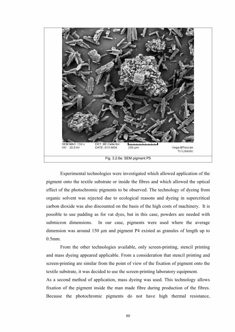
80

Fig. 3.2.6e: SEM pigment P5

Experimental technologies were investigated which allowed application of the

pigment onto the textile substrate or inside the fibres and which allowed the optical

effect of the photochromic pigments to be observed. The technology of dyeing from

organic solvent was rejected due to ecological reasons and dyeing in supercritical

carbon dioxide was also discounted on the basis of the high costs of machinery. It is

possible to use padding as for vat dyes, but in this case, powders are needed with

submicron dimensions. In our case, pigments were used where the average

dimension was around 150 μm and pigment P4 existed as granules of length up to

0.5mm.

From the other technologies available, only screen-printing, stencil printing

and mass dyeing appeared applicable. From a consideration that stencil printing and

screen-printing are similar from the point of view of the fixation of pigment onto the

textile substrate, it was decided to use the screen-printing laboratory equipment.

As a second method of application, mass dyeing was used. This technology allows

fixation of the pigment inside the man made fibre during production of the fibres.

Because the photochromic pigments do not have high thermal resistance,

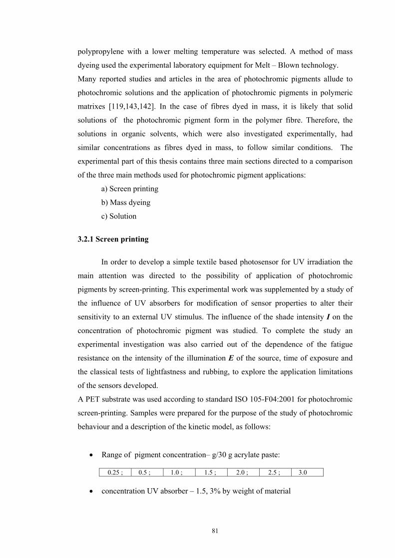
81

polypropylene with a lower melting temperature was selected. A method of mass

dyeing used the experimental laboratory equipment for Melt – Blown technology.

Many reported studies and articles in the area of photochromic pigments allude to

photochromic solutions and the application of photochromic pigments in polymeric

matrixes [119,143,142]. In the case of fibres dyed in mass, it is likely that solid

solutions of the photochromic pigment form in the polymer fibre. Therefore, the

solutions in organic solvents, which were also investigated experimentally, had

similar concentrations as fibres dyed in mass, to follow similar conditions. The

experimental part of this thesis contains three main sections directed to a comparison

of the three main methods used for photochromic pigment applications:

a) Screen printing

b) Mass dyeing

c) Solution

3.2.1 Screen printing

In order to develop a simple textile based photosensor for UV irradiation the

main attention was directed to the possibility of application of photochromic

pigments by screen-printing. This experimental work was supplemented by a study of

the influence of UV absorbers for modification of sensor properties to alter their

sensitivity to an external UV stimulus. The influence of the shade intensity I on the

concentration of photochromic pigment was studied. To complete the study an

experimental investigation was also carried out of the dependence of the fatigue

resistance on the intensity of the illumination E of the source, time of exposure and

the classical tests of lightfastness and rubbing, to explore the application limitations

of the sensors developed.

A PET substrate was used according to standard ISO 105-F04:2001 for photochromic

screen-printing. Samples were prepared for the purpose of the study of photochromic

behaviour and a description of the kinetic model, as follows:

• Range of pigment concentration– g/30 g acrylate paste:

0.25 ; 0.5 ; 1.0 ; 1.5 ; 2.0 ; 2.5 ; 3.0

• concentration UV absorber – 1.5, 3% by weight of material

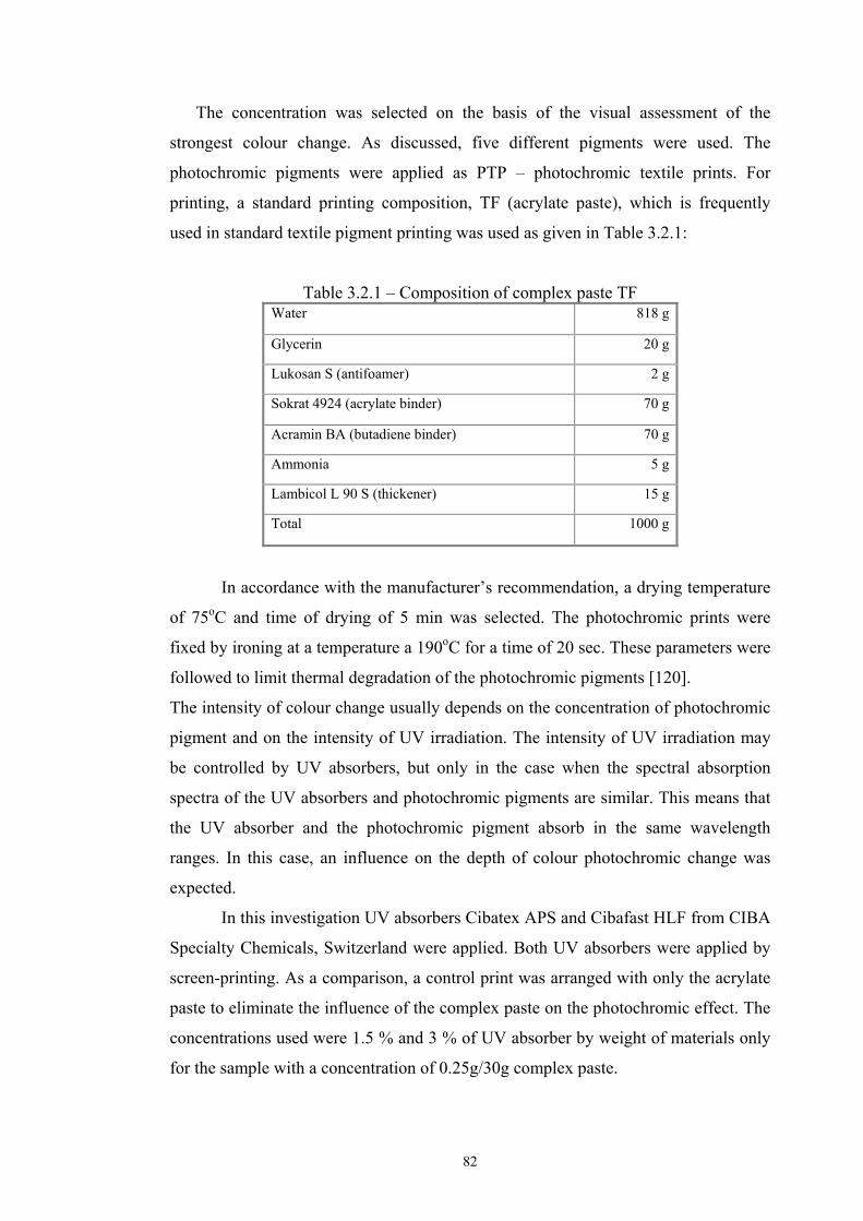
82

The concentration was selected on the basis of the visual assessment of the

strongest colour change. As discussed, five different pigments were used. The

photochromic pigments were applied as PTP – photochromic textile prints. For

printing, a standard printing composition, TF (acrylate paste), which is frequently

used in standard textile pigment printing was used as given in Table 3.2.1:

Table 3.2.1 – Composition of complex paste TF Water 818 g

Glycerin 20 g

Lukosan S (antifoamer) 2 g

Sokrat 4924 (acrylate binder) 70 g

Acramin BA (butadiene binder) 70 g

Ammonia 5 g

Lambicol L 90 S (thickener) 15 g

Total 1000 g

In accordance with the manufacturer’s recommendation, a drying temperature

of 75oC and time of drying of 5 min was selected. The photochromic prints were

fixed by ironing at a temperature a 190oC for a time of 20 sec. These parameters were

followed to limit thermal degradation of the photochromic pigments [120].

The intensity of colour change usually depends on the concentration of photochromic

pigment and on the intensity of UV irradiation. The intensity of UV irradiation may

be controlled by UV absorbers, but only in the case when the spectral absorption

spectra of the UV absorbers and photochromic pigments are similar. This means that

the UV absorber and the photochromic pigment absorb in the same wavelength

ranges. In this case, an influence on the depth of colour photochromic change was

expected.

In this investigation UV absorbers Cibatex APS and Cibafast HLF from CIBA

Specialty Chemicals, Switzerland were applied. Both UV absorbers were applied by

screen-printing. As a comparison, a control print was arranged with only the acrylate

paste to eliminate the influence of the complex paste on the photochromic effect. The

concentrations used were 1.5 % and 3 % of UV absorber by weight of materials only

for the sample with a concentration of 0.25g/30g complex paste.

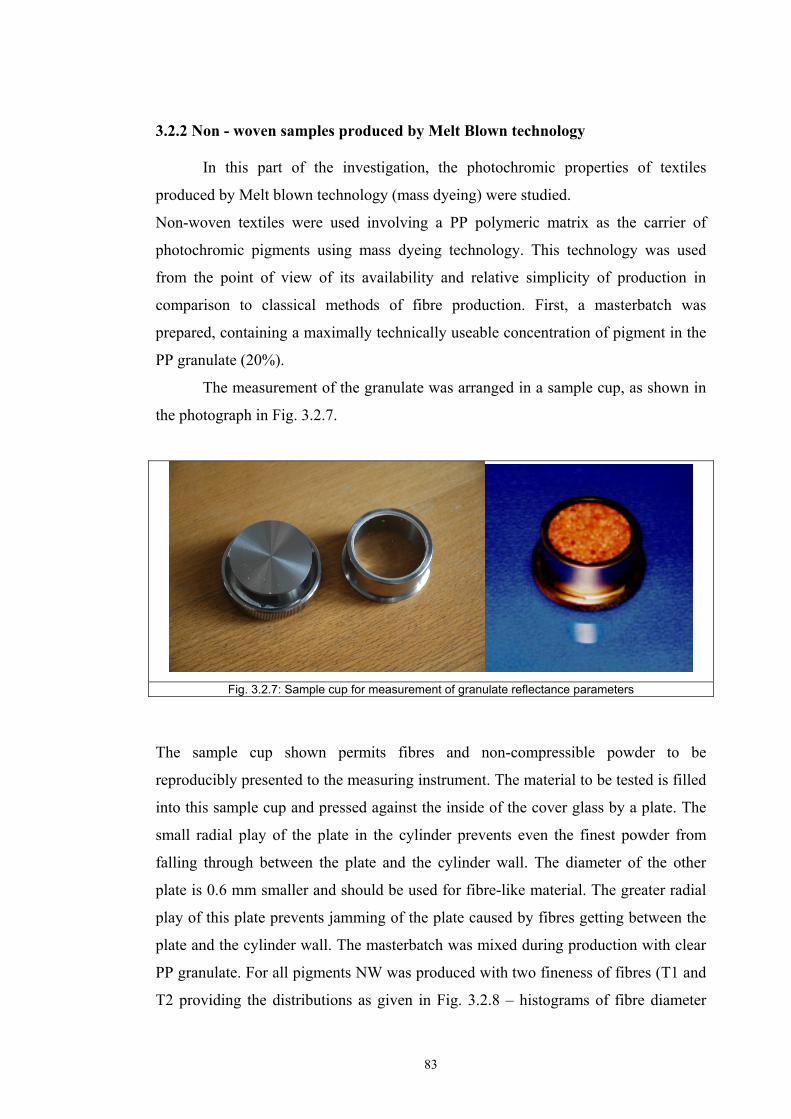
83

3.2.2 Non - woven samples produced by Melt Blown technology In this part of the investigation, the photochromic properties of textiles

produced by Melt blown technology (mass dyeing) were studied.

Non-woven textiles were used involving a PP polymeric matrix as the carrier of

photochromic pigments using mass dyeing technology. This technology was used

from the point of view of its availability and relative simplicity of production in

comparison to classical methods of fibre production. First, a masterbatch was

prepared, containing a maximally technically useable concentration of pigment in the

PP granulate (20%).

The measurement of the granulate was arranged in a sample cup, as shown in

the photograph in Fig. 3.2.7.

Fig. 3.2.7: Sample cup for measurement of granulate reflectance parameters

The sample cup shown permits fibres and non-compressible powder to be

reproducibly presented to the measuring instrument. The material to be tested is filled

into this sample cup and pressed against the inside of the cover glass by a plate. The

small radial play of the plate in the cylinder prevents even the finest powder from

falling through between the plate and the cylinder wall. The diameter of the other

plate is 0.6 mm smaller and should be used for fibre-like material. The greater radial

play of this plate prevents jamming of the plate caused by fibres getting between the

plate and the cylinder wall. The masterbatch was mixed during production with clear

PP granulate. For all pigments NW was produced with two fineness of fibres (T1 and

T2 providing the distributions as given in Fig. 3.2.8 – histograms of fibre diameter

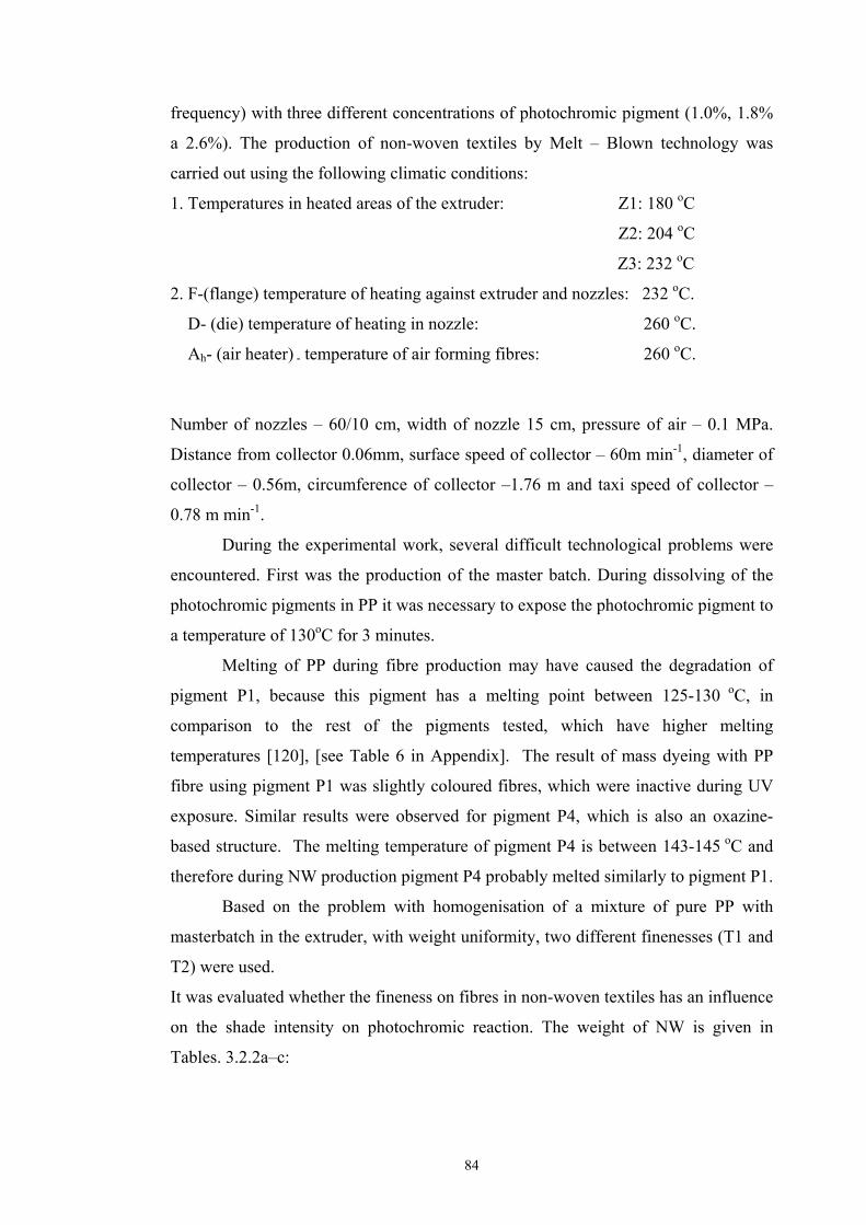
84

frequency) with three different concentrations of photochromic pigment (1.0%, 1.8%

a 2.6%). The production of non-woven textiles by Melt – Blown technology was

carried out using the following climatic conditions:

1. Temperatures in heated areas of the extruder: Z1: 180 oC

Z2: 204 oC

Z3: 232 oC

2. F-(flange) temperature of heating against extruder and nozzles: 232 oC.

D- (die) temperature of heating in nozzle: 260 oC.

Ah- (air heater) - temperature of air forming fibres: 260 oC.

Number of nozzles – 60/10 cm, width of nozzle 15 cm, pressure of air – 0.1 MPa.

Distance from collector 0.06mm, surface speed of collector – 60m min-1, diameter of

collector – 0.56m, circumference of collector –1.76 m and taxi speed of collector –

0.78 m min-1.

During the experimental work, several difficult technological problems were

encountered. First was the production of the master batch. During dissolving of the

photochromic pigments in PP it was necessary to expose the photochromic pigment to

a temperature of 130oC for 3 minutes.

Melting of PP during fibre production may have caused the degradation of

pigment P1, because this pigment has a melting point between 125-130 oC, in

comparison to the rest of the pigments tested, which have higher melting

temperatures [120], [see Table 6 in Appendix]. The result of mass dyeing with PP

fibre using pigment P1 was slightly coloured fibres, which were inactive during UV

exposure. Similar results were observed for pigment P4, which is also an oxazine-

based structure. The melting temperature of pigment P4 is between 143-145 oC and

therefore during NW production pigment P4 probably melted similarly to pigment P1.

Based on the problem with homogenisation of a mixture of pure PP with

masterbatch in the extruder, with weight uniformity, two different finenesses (T1 and

T2) were used.

It was evaluated whether the fineness on fibres in non-woven textiles has an influence

on the shade intensity on photochromic reaction. The weight of NW is given in

Tables. 3.2.2a–c:

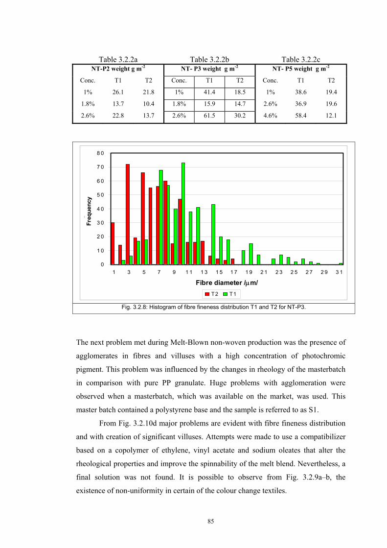
85

Table 3.2.2a Table 3.2.2b Table 3.2.2c

NT-P2 weight g m-2 NT- P3 weight g m-2 NT- P5 weight g m-2

Conc. T1 T2 Conc. T1 T2 Conc. T1 T2

1% 26.1 21.8 1% 41.4 18.5 1% 38.6 19.4

1.8% 13.7 10.4 1.8% 15.9 14.7 2.6% 36.9 19.6

2.6% 22.8 13.7 2.6% 61.5 30.2 4.6% 58.4 12.1

0

1 0

2 0

3 0

4 0

5 0

6 0

7 0

8 0

1 3 5 7 9 1 1 1 3 1 5 1 7 1 9 2 1 2 3 2 5 2 7 2 9 3 1

P rům ě r v lá k n a / Πm /

Če

tno

s

T2 T1

Fibre diameter /μm/

Freq

uenc

y

Fig. 3.2.8: Histogram of fibre fineness distribution T1 and T2 for NT-P3.

The next problem met during Melt-Blown non-woven production was the presence of

agglomerates in fibres and villuses with a high concentration of photochromic

pigment. This problem was influenced by the changes in rheology of the masterbatch

in comparison with pure PP granulate. Huge problems with agglomeration were

observed when a masterbatch, which was available on the market, was used. This

master batch contained a polystyrene base and the sample is referred to as S1.

From Fig. 3.2.10d major problems are evident with fibre fineness distribution

and with creation of significant villuses. Attempts were made to use a compatibilizer

based on a copolymer of ethylene, vinyl acetate and sodium oleates that alter the

rheological properties and improve the spinnability of the melt blend. Nevertheless, a

final solution was not found. It is possible to observe from Fig. 3.2.9a–b, the

existence of non-uniformity in certain of the colour change textiles.

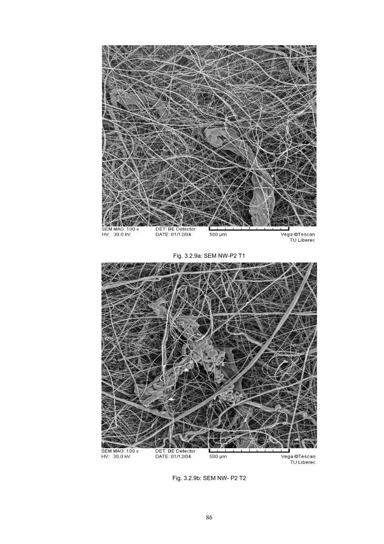
86

Fig. 3.2.9a: SEM NW-P2 T1

Fig. 3.2.9b: SEM NW- P2 T2

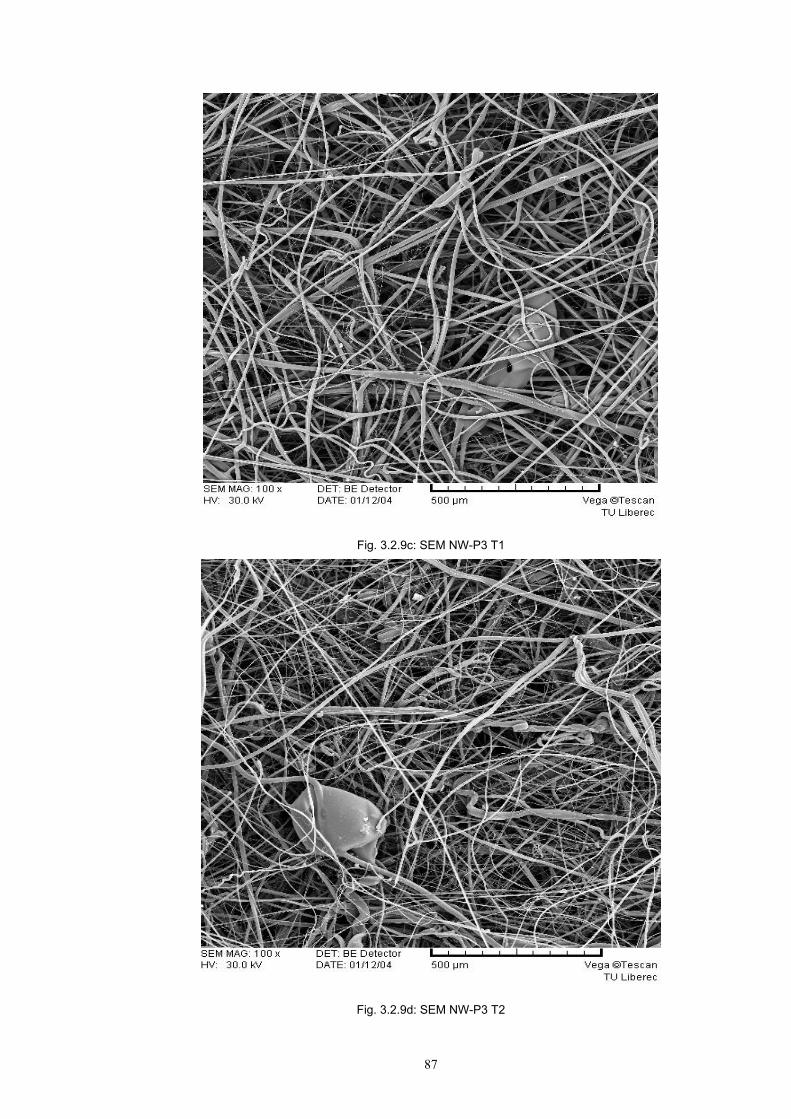
87

Fig. 3.2.9c: SEM NW-P3 T1

Fig. 3.2.9d: SEM NW-P3 T2

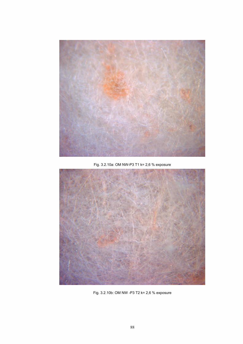
88

Fig. 3.2.10a: OM NW-P3 T1 k= 2,6 % exposure

Fig. 3.2.10b: OM NW -P3 T2 k= 2,6 % exposure

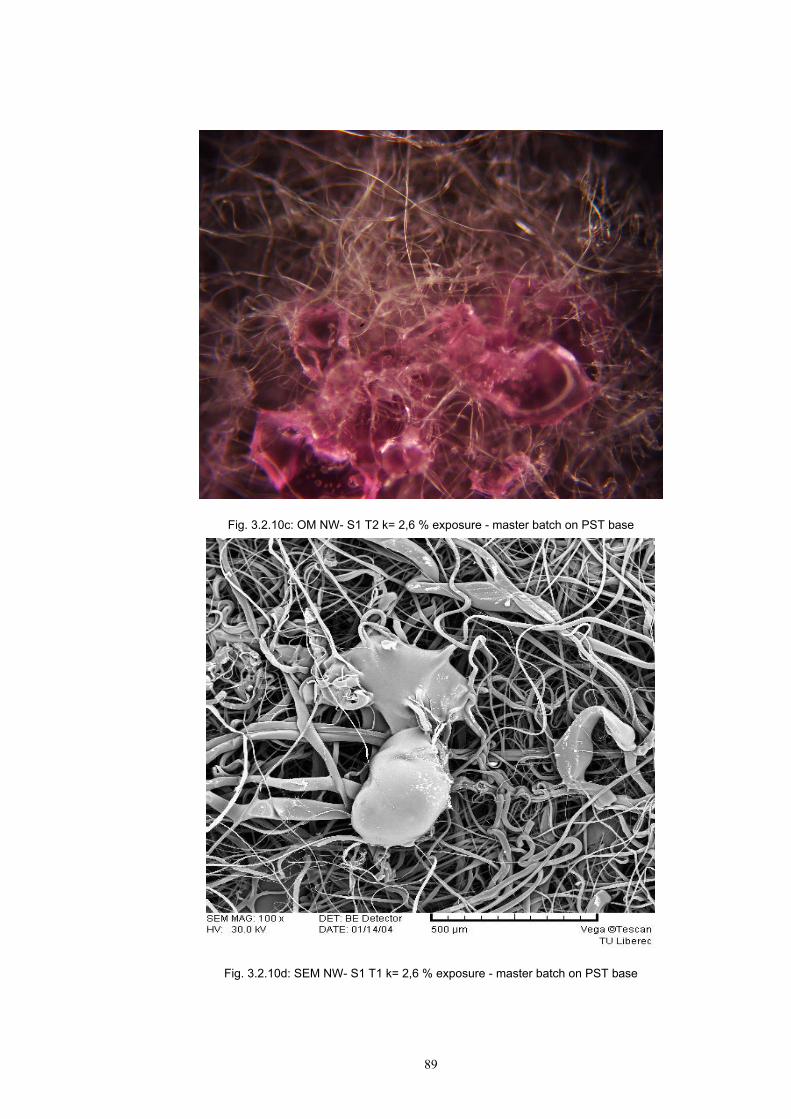
89

Fig. 3.2.10c: OM NW- S1 T2 k= 2,6 % exposure - master batch on PST base

Fig. 3.2.10d: SEM NW- S1 T1 k= 2,6 % exposure - master batch on PST base

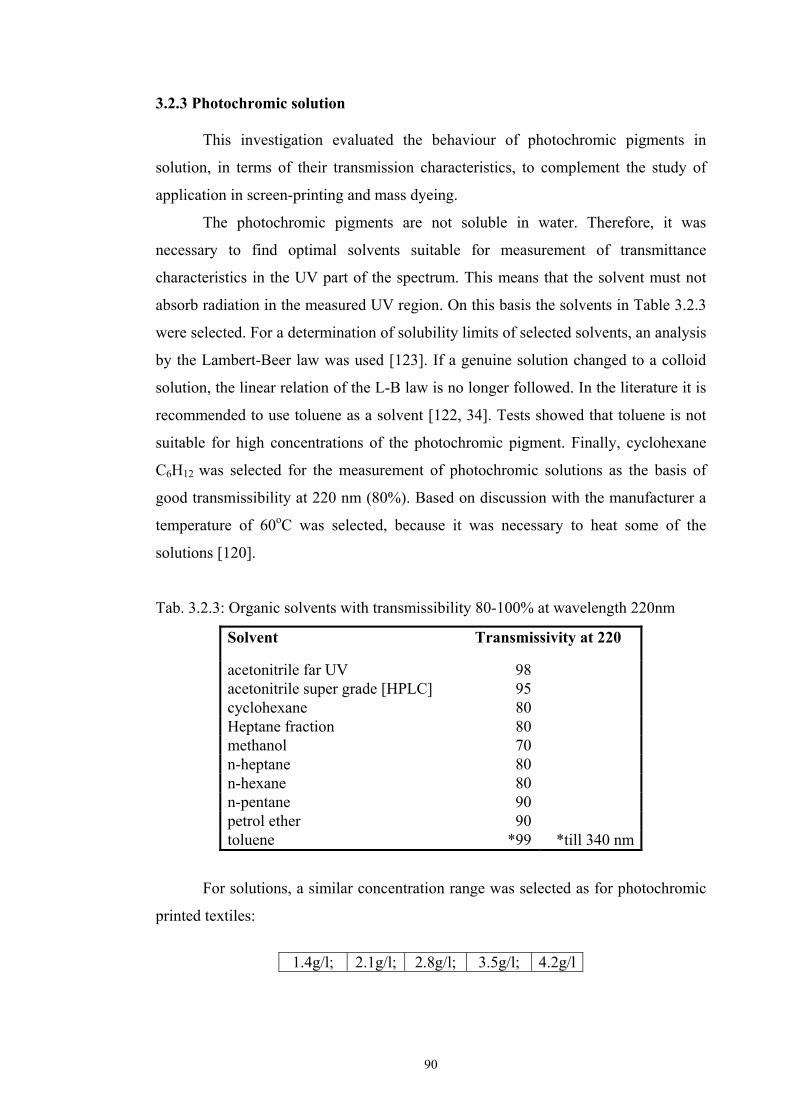
90

3.2.3 Photochromic solution This investigation evaluated the behaviour of photochromic pigments in

solution, in terms of their transmission characteristics, to complement the study of

application in screen-printing and mass dyeing.

The photochromic pigments are not soluble in water. Therefore, it was

necessary to find optimal solvents suitable for measurement of transmittance

characteristics in the UV part of the spectrum. This means that the solvent must not

absorb radiation in the measured UV region. On this basis the solvents in Table 3.2.3

were selected. For a determination of solubility limits of selected solvents, an analysis

by the Lambert-Beer law was used [123]. If a genuine solution changed to a colloid

solution, the linear relation of the L-B law is no longer followed. In the literature it is

recommended to use toluene as a solvent [122, 34]. Tests showed that toluene is not

suitable for high concentrations of the photochromic pigment. Finally, cyclohexane

C6H12 was selected for the measurement of photochromic solutions as the basis of

good transmissibility at 220 nm (80%). Based on discussion with the manufacturer a

temperature of 60oC was selected, because it was necessary to heat some of the

solutions [120].

Tab. 3.2.3: Organic solvents with transmissibility 80-100% at wavelength 220nm

Solvent Transmissivity at 220

acetonitrile far UV 98 acetonitrile super grade [HPLC] 95 cyclohexane 80 Heptane fraction 80 methanol 70 n-heptane 80 n-hexane 80 n-pentane 90 petrol ether 90 toluene *99 *till 340 nm

For solutions, a similar concentration range was selected as for photochromic

printed textiles:

1.4g/l; 2.1g/l; 2.8g/l; 3.5g/l; 4.2g/l

91

This concentration range was selected to compare differences in the

dependence of the photochromic reaction on the application medium of the

photochromic pigments. The solutions were prepared one or two days before

measurement in a dark room due to time demands on dissolving. The solutions were

stored in a dark box to prevent their exposure to UV irradiation. In section 3.1.2, it

was discussed that in the case of higher concentrations a separation of a thin layer

from the rest of the solution was visible. An electromagnetic mixer with controlled

heating solved the problem of photochromic solution non-homogeneity.

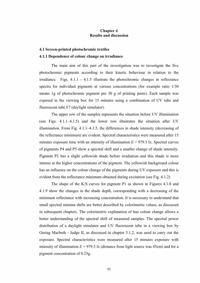
92

Chapter 4

Results and discussion 4.1 Screen-printed photochromic textiles

4.1.1 Dependence of colour change on irradiance

The main aim of this part of the investigation was to investigate the five

photochromic pigments according to their kinetic behaviour in relation to the

irradiance. Figs. 4.1.1 - 4.1.5 illustrate the photochromic changes in reflectance

spectra for individual pigments at various concentrations (for example ratio 1/30

means 1g of photochromic pigment per 30 g of printing paste). Each sample was

exposed in the viewing box for 15 minutes using a combination of UV tube and

fluorescent tube F7 (daylight simulator).

The upper row of the samples represents the situation before UV illumination

(see Figs. 4.1.1–4.1.5) and the lower row illustrates the situation after UV

illumination. From Fig. 4.1.1–4.1.5, the differences in shade intensity (decreasing of

the reflectance minimum) are evident. Spectral characteristics were measured after 15

minutes exposure time with an intensity of illumination E = 979.3 lx. Spectral curves

of pigments P4 and P5 show a spectral shift and a smaller change of shade intensity.

Pigment P2 has a slight yellowish shade before irradiation and this shade is more

intense at the higher concentrations of the pigment. The yellowish background colour

has an influence on the colour change of the pigments during UV exposure and this is

evident from the reflectance minimum obtained during excitation (see Fig. 4.1.2)

The shape of the K/S curves for pigment P1 as shown in Figures 4.1.8 and

4.1.9 show the changes in the shade depth, corresponding with a decreasing of the

minimum reflectance with increasing concentration. It is necessary to understand that

small spectral minima shifts are better described by colorimetric values, as discussed

in subsequent chapters. The colorimetric explanation of hue colour change allows a

better understanding of the spectral shift of measured samples. The spectral power

distribution of a daylight simulator and UV fluorescent tube in a viewing box by

Gretag Macbeth - Judge II, as discussed in chapter 3.1.2, was used to carry out the

exposure. Spectral characteristics were measured after 15 minutes exposure with

intensity of illumination E = 979.3 lx (distance from light source was 45cm) and for a

pigment concentration of 0.25g.

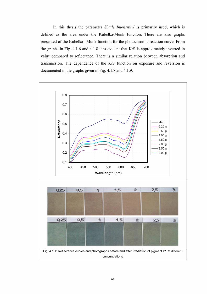
93

In this thesis the parameter Shade Intensity I is primarily used, which is

defined as the area under the Kubelka-Munk function. There are also graphs

presented of the Kubelka –Munk function for the photochromic reaction curve. From

the graphs in Fig. 4.1.6 and 4.1.8 it is evident that K/S is approximately inverted in

value compared to reflectance. There is a similar relation between absorption and

transmission. The dependence of the K/S function on exposure and reversion is

documented in the graphs given in Fig. 4.1.8 and 4.1.9.

0.1

0.2

0.3

0.4

0.5

0.6

0.7

0.8

400 450 500 550 600 650 700

Wavelength (nm)

Ref

lect

ance

start0.25 g0.50 g1.00 g1.50 g2.00 g2.50 g3.00 g

Fig. 4.1.1: Reflectance curves and photographs before and after irradiation of pigment P1 at different

concentrations

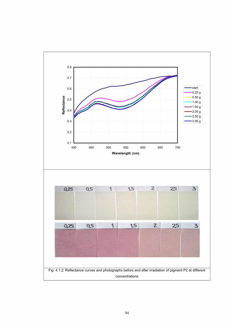
94

0.1

0.2

0.3

0.4

0.5

0.6

0.7

0.8

400 450 500 550 600 650 700

Wavelength (nm)

Ref

lect

ance

start0.25 g0.50 g1.00 g1.50 g2.00 g2.50 g3.00 g

Fig. 4.1.2: Reflectance curves and photographs before and after irradiation of pigment P2 at different

concentrations

95

0.1

0.2

0.3

0.4

0.5

0.6

0.7

0.8

400 450 500 550 600 650 700

Wavelength (nm)

Ref

lect

ance

start0.25 g0.50 g1.00 g1.50 g2.00 g2.50 g3.00 g

Fig. 4.1.3: Reflectance curves and photographs before and after irradiation of pigment P3 at different

concentrations

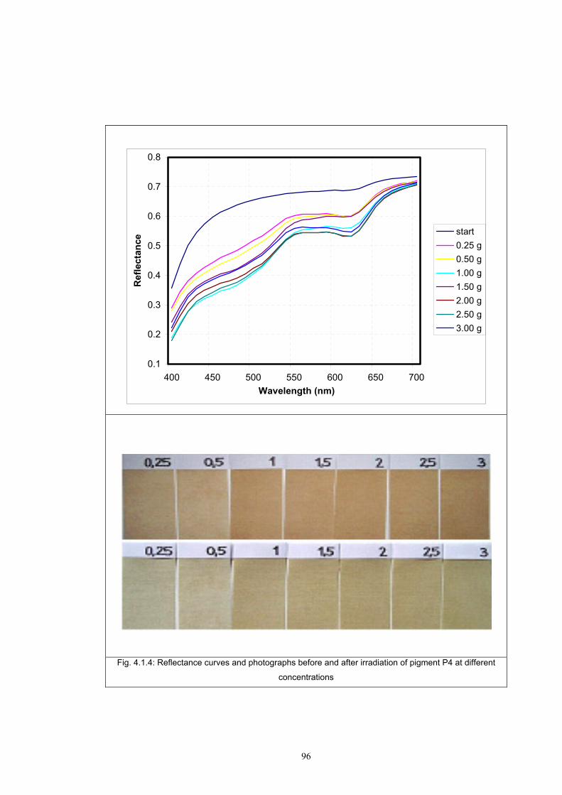
96

0.1

0.2

0.3

0.4

0.5

0.6

0.7

0.8

400 450 500 550 600 650 700Wavelength (nm)

Ref

lect

ance

start0.25 g0.50 g1.00 g1.50 g2.00 g2.50 g3.00 g

Fig. 4.1.4: Reflectance curves and photographs before and after irradiation of pigment P4 at different

concentrations

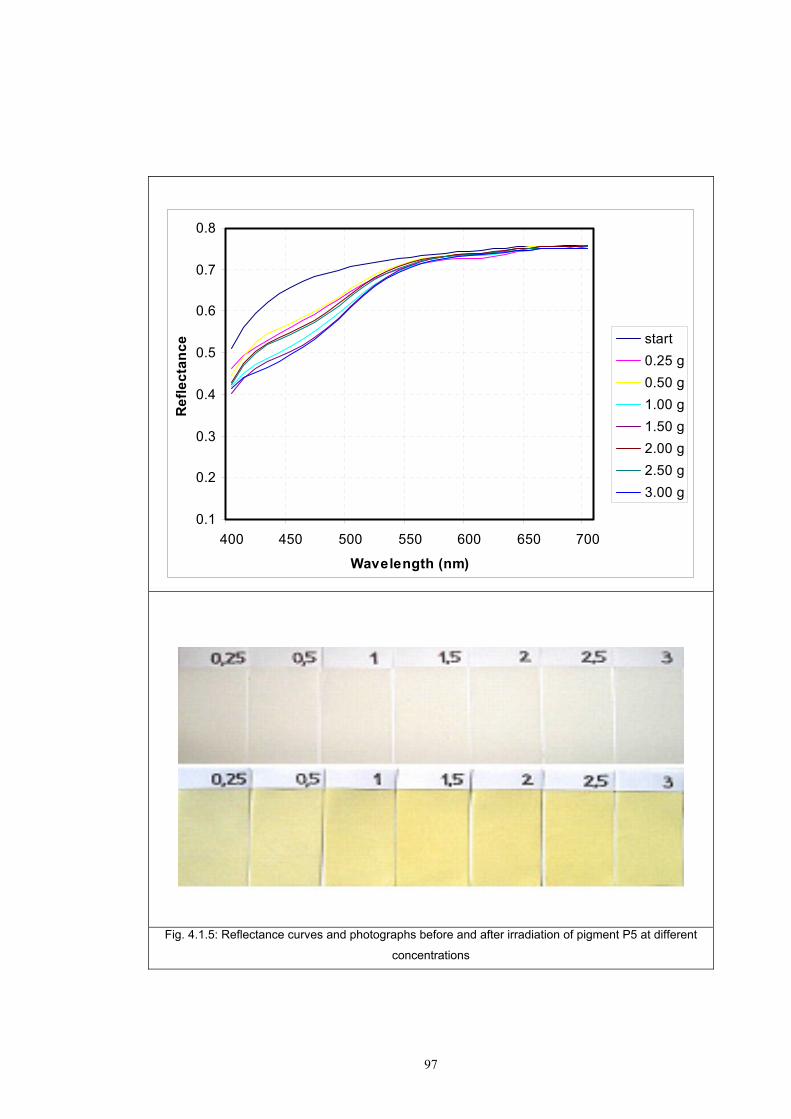
97

0.1

0.2

0.3

0.4

0.5

0.6

0.7

0.8

400 450 500 550 600 650 700

Wavelength (nm)

Ref

lect

ance start

0.25 g0.50 g1.00 g1.50 g2.00 g2.50 g3.00 g

Fig. 4.1.5: Reflectance curves and photographs before and after irradiation of pigment P5 at different

concentrations

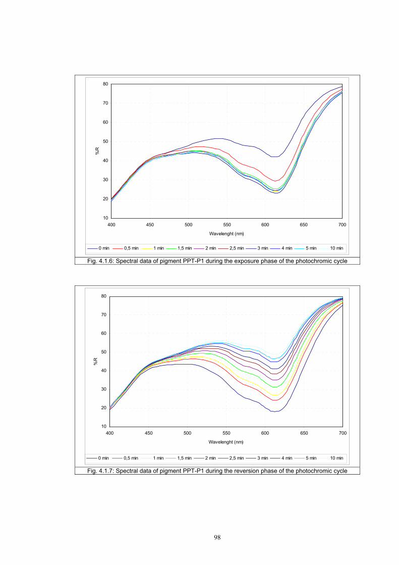
98

10

20

30

40

50

60

70

80

400 450 500 550 600 650 700

Wavelenght (nm)

%R

0 min 0,5 min 1 min 1,5 min 2 min 2,5 min 3 min 4 min 5 min 10 min

Fig. 4.1.6: Spectral data of pigment PPT-P1 during the exposure phase of the photochromic cycle

10

20

30

40

50

60

70

80

400 450 500 550 600 650 700

Wavelenght (nm)

%R

0 min 0,5 min 1 min 1,5 min 2 min 2,5 min 3 min 4 min 5 min 10 min

Fig. 4.1.7: Spectral data of pigment PPT-P1 during the reversion phase of the photochromic cycle

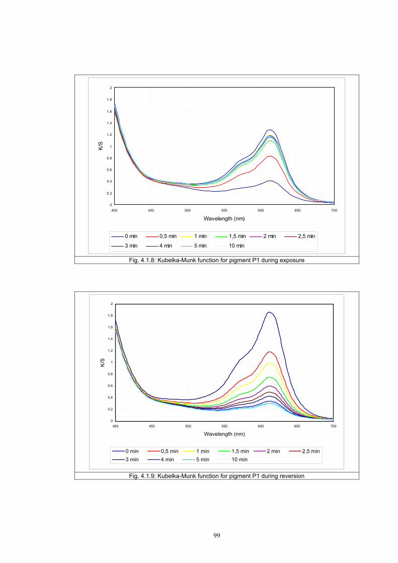
99

0

0.2

0.4

0.6

0.8

1

1.2

1.4

1.6

1.8

2

400 450 500 550 600 650 700

Wavelength (nm)

K/S

0 min 0,5 min 1 min 1,5 min 2 min 2,5 min

3 min 4 min 5 min 10 min

Fig. 4.1.8: Kubelka-Munk function for pigment P1 during exposure

0

0.2

0.4

0.6

0.8

1

1.2

1.4

1.6

1.8

2

400 450 500 550 600 650 700

Wavelength (nm)

K/S

0 min 0,5 min 1 min 1,5 min 2 min 2,5 min3 min 4 min 5 min 10 min

Fig. 4.1.9: Kubelka-Munk function for pigment P1 during reversion

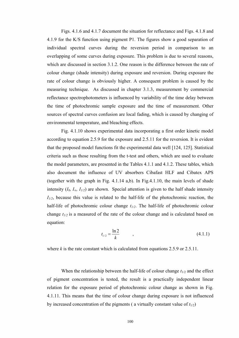
100

Figs. 4.1.6 and 4.1.7 document the situation for reflectance and Figs. 4.1.8 and

4.1.9 for the K/S function using pigment P1. The figures show a good separation of

individual spectral curves during the reversion period in comparison to an

overlapping of some curves during exposure. This problem is due to several reasons,

which are discussed in section 3.1.2. One reason is the difference between the rate of

colour change (shade intensity) during exposure and reversion. During exposure the

rate of colour change is obviously higher. A consequent problem is caused by the

measuring technique. As discussed in chapter 3.1.3, measurement by commercial

reflectance spectrophotometers is influenced by variability of the time delay between

the time of photochromic sample exposure and the time of measurement. Other

sources of spectral curves confusion are local fading, which is caused by changing of

environmental temperature, and bleaching effects.

Fig. 4.1.10 shows experimental data incorporating a first order kinetic model

according to equation 2.5.9 for the exposure and 2.5.11 for the reversion. It is evident

that the proposed model functions fit the experimental data well [124, 125]. Statistical

criteria such as those resulting from the t-test and others, which are used to evaluate

the model parameters, are presented in the Tables 4.1.1 and 4.1.2. These tables, which

also document the influence of UV absorbers Cibafast HLF and Cibatex APS

(together with the graph in Fig. 4.1.14 a,b). In Fig.4.1.10, the main levels of shade

intensity (I0, I∞, I1/2) are shown. Special attention is given to the half shade intensity

I1/2, because this value is related to the half-life of the photochromic reaction, the

half-life of photochromic colour change t1/2. The half-life of photochromic colour

change t1/2 is a measured of the rate of the colour change and is calculated based on

equation:

1/ 2ln 2tk

= , (4.1.1)

where k is the rate constant which is calculated from equations 2.5.9 or 2.5.11.

When the relationship between the half-life of colour change t1/2 and the effect

of pigment concentration is tested, the result is a practically independent linear

relation for the exposure period of photochromic colour change as shown in Fig.

4.1.11. This means that the time of colour change during exposure is not influenced

by increased concentration of the pigments ( a virtually constant value of t1/2)

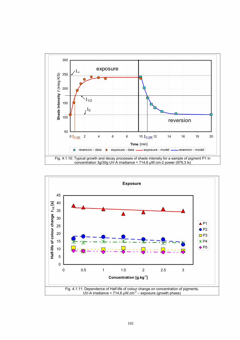
101

50

100

150

200

250

300

0 2 4 6 8 10 12 14 16 18 20

Time [min]

Shad

e In

tens

ity I

(inte

g K/

S)

reversion - data exposure - data exposure - model reversion - model

exposure

reversion

t1/2E

I0

I∞

I1/2

t1/2R

Fig. 4.1.10: Typical growth and decay processes of shade intensity for a sample of pigment P1 in concentration 3g/30g UV-A irradiance = 714,6 µW.cm-2 power (979,3 lx)

Exposure

0

5

10

15

20

25

30

35

40

45

0 0.5 1 1.5 2 2.5 3

Concentration [g.kg-1]

Hal

f-lif

e of

col

our c

hang

e t 1

/2 [s

]

P1P2P3P4P5

Fig. 4.1.11: Dependence of Half-life of colour change on concentration of pigments, UV-A irradiance = 714,6 µW.cm-2 – exposure (growth phase)

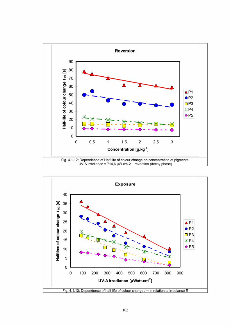
102

Reversion

0

10

20

30

40

50

60

70

80

90

0 0.5 1 1.5 2 2.5 3

Concentration [g.kg-1]

Hal

f-life

of c

olou

r cha

nge t 1

/2 [s

]

P1P2P3P4P5

Fig. 4.1.12: Dependence of Half-life of colour change on concentration of pigments, UV-A irradiance = 714,6 µW.cm-2 – reversion (decay phase)

Exposure

0

5

10

15

20

25

30

35

40

0 100 200 300 400 500 600 700 800 900

UV-A irradiance [µWatt.cm-2]

Hal

ftim

e of

col

our c

hang

e t 1

/2 [s

]

P1P2P3P4P5

Fig. 4.1.13: Dependence of half-life of colour change t1/2 in relation to irradiance E

103

It can be seen from Fig. 4.1.12 that the rate of the colour change during the

reversion phase is slightly dependent on pigment concentration, mainly for the two

pigments with a slow rate of colour change. Thus, it is possible to conclude that the

half-life of colour change is, for the exposure period of colour change, practically

independent of concentration. On the other hand, for the reversion period it can seen

that there is a decrease of t1/2 with increasing concentration. One explanation, which

may be proposed, is that this relationship is based on a faster reconversion to the

original chemical structure of the photochromic pigment at higher concentration. Fig.

4.1.13 shows that an increased intensity of illumination affects a linear decrease of t1/2

(halftime of colour change).

The optical yield Oy of photochromic colour change is calculated based on

equation (4.1.2).

( ) ( )1 2

1

, 0, , 0, , 0,0

e r

t tk t k t

y e e e r r rt

O I I I e dt I I I e dt− −∞ ∞ ∞= + − − + −∫ ∫ (4.1.2)

where I∞ is the intensity of coloration at infinite time, 0I is the intensity of

coloration at the start of experiment, ke is the rate constant during exposure and kr is

the rate constant during reversion for time t. For this purpose, exposure and reversion

are independent processes. The intensity of coloration at infinite time I∞ is described

by two values. For the meaning of shade intensity I subscripts (0,∞) are used, which

are related to the actual stage of the process. In the case of exposure, ,eI∞ is

practically the maximum intensity obtained and in the case of reversion. The shade

intensity ,rI∞ is equal to the shade intensity 0,eI from exposure, because reversion starts

at the shade intensity, when exposure is finished, and reversion ends ideally at the

same intensity of shade as exposure starts.

As observed from equation (4.1.2) it is evident that the Optical yield Oy is

based on the colour hysteresis area. Usually in the literature [126], this type of

equation involving a bi-exponential function is used to represent the photochromic

reaction. For the purpose of this work not only a bi-exponential function but also the

area under the bi-exponential function was used, where t1 is the time of maximal

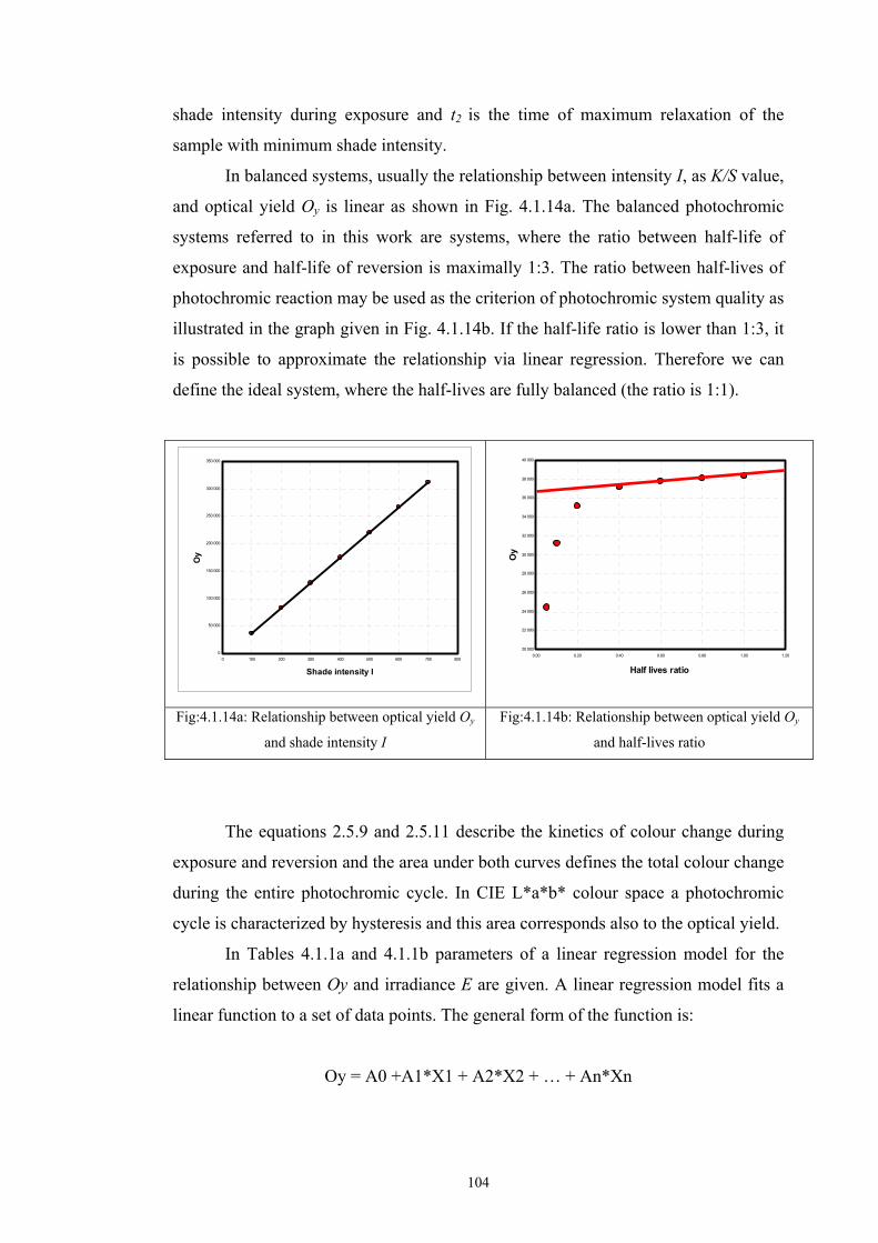
104

shade intensity during exposure and t2 is the time of maximum relaxation of the

sample with minimum shade intensity.

In balanced systems, usually the relationship between intensity I, as K/S value,

and optical yield Oy is linear as shown in Fig. 4.1.14a. The balanced photochromic

systems referred to in this work are systems, where the ratio between half-life of

exposure and half-life of reversion is maximally 1:3. The ratio between half-lives of

photochromic reaction may be used as the criterion of photochromic system quality as

illustrated in the graph given in Fig. 4.1.14b. If the half-life ratio is lower than 1:3, it

is possible to approximate the relationship via linear regression. Therefore we can

define the ideal system, where the half-lives are fully balanced (the ratio is 1:1).

0

50 000

100 000

150 000

200 000

250 000

300 000

350 000

0 100 200 300 400 500 600 700 800

Shade intensity I

Oy

20 000

22 000

24 000

26 000

28 000

30 000

32 000

34 000

36 000

38 000

40 000

0.00 0.20 0.40 0.60 0.80 1.00 1.20

Half lives ratio

Oy

Fig:4.1.14a: Relationship between optical yield Oy

and shade intensity I

Fig:4.1.14b: Relationship between optical yield Oy

and half-lives ratio

The equations 2.5.9 and 2.5.11 describe the kinetics of colour change during

exposure and reversion and the area under both curves defines the total colour change

during the entire photochromic cycle. In CIE L*a*b* colour space a photochromic

cycle is characterized by hysteresis and this area corresponds also to the optical yield.

In Tables 4.1.1a and 4.1.1b parameters of a linear regression model for the

relationship between Oy and irradiance E are given. A linear regression model fits a

linear function to a set of data points. The general form of the function is:

Oy = A0 +A1*X1 + A2*X2 + … + An*Xn

105

Where Oy is the target variable, X1, X2, … Xn are the predictor variables

(irradiance E), and A1, A2, … An are coefficients that multiply the predictor

variables. A0 is a constant. In this work a simplified variant of linear model is used:

Oy = A0 + A1*X.

Together with these regression model coefficients, “t” statistics are also

computed. The “t” statistic is computed by dividing the estimated value of the β

coefficient by its standard error. This statistic is a measure of the likelihood that the

actual value of the parameter is not zero. The larger the absolute value of t, the less

likely that the actual value of the parameter could be zero. The “t”statistic probability

is computed using a two-sided test.

From Fig. 4.1.15 a-b, it is evident that optical yield Oy depends on irradiance

E. This Figure also shows that a higher UV absorber concentration leads to a lower

optical yield of photochromic reaction Oy. Nevertheless, Tables 4.1.1 a-b shows that

the computed constant A0 of the regression model are insignificant in case when UV

absorbers are used. This result is affected by experimental errors, because in this

experiment a line method for measurement of colorimetric properties was used.

Table 4.1.1 a: Coefficients for model Oy=A0+A1*X for Cibafast HLF

Concentration of

UV absorber (%)

A0 standard deviation

t-criterion

Decision A1 standard deviation

t-criterion

Decision

0.0 849.658 216.731 3.920 significant 1.041 0.046 22.669 significant

1.5 190.334 194.905 0.561 insignificant 1.026 0.041 24.856 significant

3.0 109.324 157.070 1.212 insignificant 0.905 0.033 27.190 significant

Table 4.1.1 b: Coefficients for model Oy=A0+A1*X for Cibatex APS

Concentration of

UV absorber (%)

A0 standard deviation

t-criterion

Decision A1 standard deviation

t-criterion

Decision

0.0 849.658 216.731 3.920 significant 1.041 0.046 22.669 significant

1.5 177.764 199.640 0.890 insignificant 1.087 0.042 25.704 significant

3.0 173.313 202.833 0.854 insignificant 1.019 0.043 23.723 significant

106

0

1000

2000

3000

4000

5000

6000

7000

8000

9000

10000

0 100 200 300 400 500 600 700 800 900

UV-A irradiance [µWatt.cm-2]

Oy

0,0 g/l UV abs. 1,5 g/l UV abs. 3,0 g/l UV abs.

Fig. 4.1.15 a: Dependency of Oy on irradiance for different concentrations of UV absorber Cibafast HLF - pigment P1

0

1000

2000

3000

4000

5000

6000

7000

8000

9000

10000

0 100 200 300 400 500 600 700 800 900

UV-A irradiance [µWatt.cm-2]

Oy

0,0 g/l UV abs. 1,5 g/l UV abs. 3,0 g/l UV abs.

Fig.4.1.15 b: Dependency of Oy on irradiance for different concentrations of UV absorber Cibatex APS - pigment P1

107

The Tables 4.1.1c-d show the rate constants, half-life and the % extension of

half-life provided by the use of UV absorbers. From Tables 4.1.1c-d decrease of half-

life extension with increasing irradiance is evident.

Table 4.1.1 c: First order kinetic parameters for Cibafast HLF

Irradiance

E [μW.cm-2]

0% HLF

1.5% HLF

3.0% HLF

Rate constant

k

Half life t1/2

[s]

Rate constant

k

Half-life t1/2

[s]

Extension of Half-life

%

Rate constant

k

Half-life t1/2

[s]

Extension of Half-life

% 87.60 0.0191 36.09 0.0161 42.96 19.01 0.0136 50.77 40.66

143.43 0.0235 29.50 0.0203 33.96 15.12 0.0186 37.03 25.52229.11 0.0278 24.96 0.0255 27.18 8.89 0.0220 31.47 26.08358.10 0.0355 19.50 0.0320 21.65 11.00 0.0301 23.07 18.30605.50 0.0495 14.01 0.0470 14.72 5.06 0.0436 15.90 13.48814.39 0.0666 10.39 0.0606 11.43 10.06 0.0551 12.58 21.09

Table 4.1.1 d: First order kinetic parameters for Cibatex APS

Irradiance

E [μW.cm-2]

0% APS

1.5% APS

3.0% APS

Rate constant

k

Half life t1/2 [s]

Rate constant

k

Half-life t1/2 [s]

Extension of Half-

life %

Rate constant

k

Half-life t1/2 [s]

Extension of Half-life

%

87.60 0.0191 36.09 0.0140 49.52 37.20 0.0150 46.03 27.54143.43 0.0235 29.50 0.0201 34.28 16.19 0.0193 35.71 21.04229.11 0.0278 24.96 0.0233 29.66 18.82 0.0213 32.56 30.44358.10 0.0355 19.50 0.0340 20.41 4.65 0.0310 22.37 14.73605.50 0.0495 14.01 0.0473 14.65 4.52 0.0466 14.86 6.02814.39 0.0666 10.39 0.0636 10.90 4.94 0.0605 11.45 10.27

These values also demonstrate the UV absorber efficiency. The efficiency of

Cibatex APS is approximately a factor of two times lower in comparison to Cibafast

HLF. The reason for this phenomenon is probably associated with different

absorptions in the UV part of the spectrum and different absorbances at the same

concentration, as is documented in Fig. 4.1.16a. In Fig. 4.1.16b normalised absorption

curves are shown, where similar values of absorbance are obtained by the use of

different concentrations of UV absorbers. In the case of Cibatex APS it is necessary

to use double the concentration. This result correlates with the result obtained for UV

absorbers efficiency – the extension of half-life, as documented in Table. 4.1.1c-d. In

section 4.5 the influence of different wavelength of UV radiation on final shade

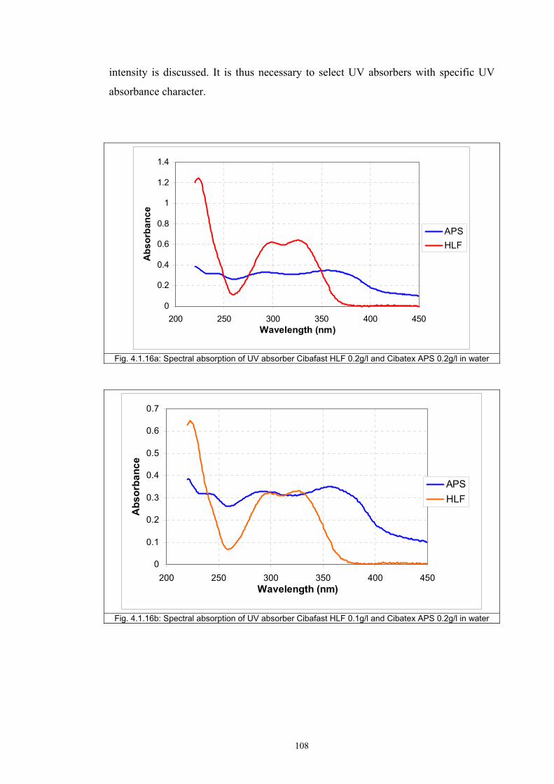
108

intensity is discussed. It is thus necessary to select UV absorbers with specific UV

absorbance character.

0

0.2

0.4

0.6

0.8

1

1.2

1.4

200 250 300 350 400 450Wavelength (nm)

Abs

orba

nce

APSHLF

Fig. 4.1.16a: Spectral absorption of UV absorber Cibafast HLF 0.2g/l and Cibatex APS 0.2g/l in water

0

0.1

0.2

0.3

0.4

0.5

0.6

0.7

200 250 300 350 400 450Wavelength (nm)

Abs

orba

nce

APSHLF

Fig. 4.1.16b: Spectral absorption of UV absorber Cibafast HLF 0.1g/l and Cibatex APS 0.2g/l in water

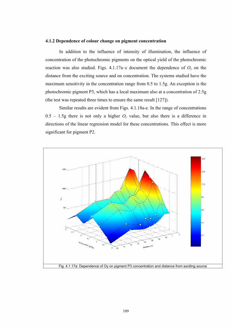
109

4.1.2 Dependence of colour change on pigment concentration

In addition to the influence of intensity of illumination, the influence of

concentration of the photochromic pigments on the optical yield of the photochromic

reaction was also studied. Figs. 4.1.17a–c document the dependence of Oy on the

distance from the exciting source and on concentration. The systems studied have the

maximum sensitivity in the concentration range from 0.5 to 1.5g. An exception is the

photochromic pigment P3, which has a local maximum also at a concentration of 2.5g

(the test was repeated three times to ensure the same result [127]).

Similar results are evident from Figs. 4.1.18a-e. In the range of concentrations

0.5 – 1.5g there is not only a higher Oy value, but also there is a difference in

directions of the linear regression model for these concentrations. This effect is more

significant for pigment P2.

Fig. 4.1.17a: Dependence of Oy on pigment P3 concentration and distance from exciting source

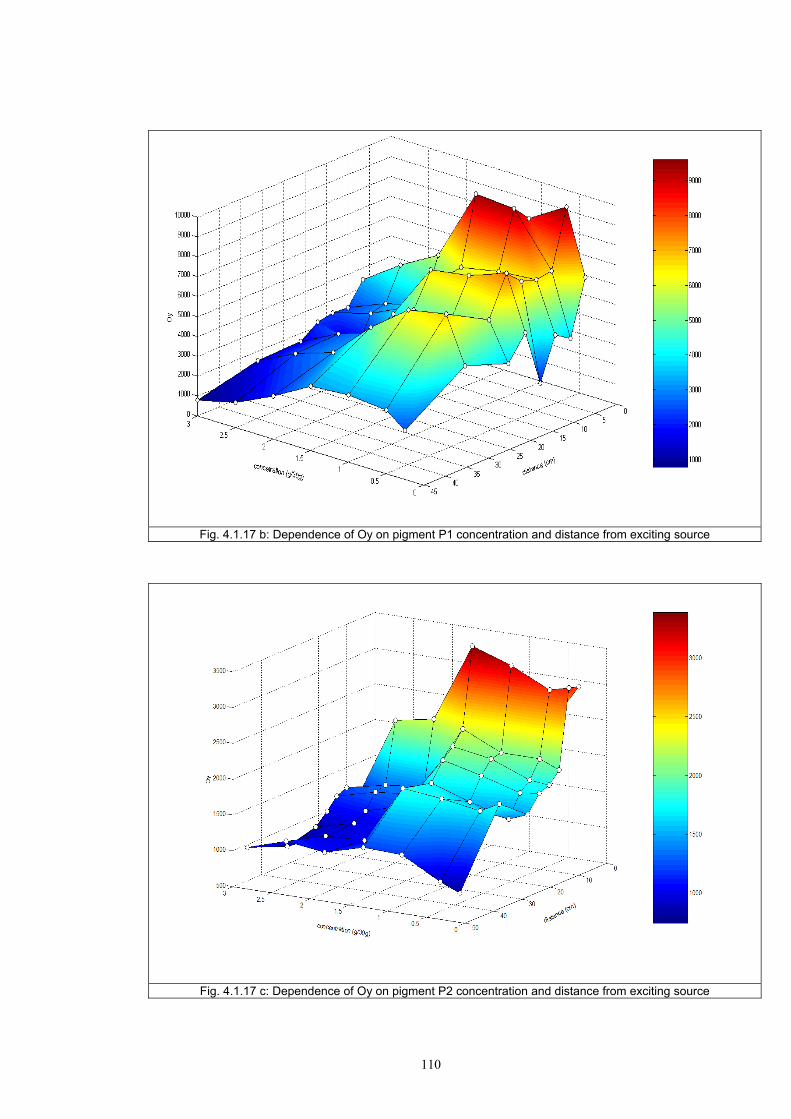
110

Fig. 4.1.17 b: Dependence of Oy on pigment P1 concentration and distance from exciting source

Fig. 4.1.17 c: Dependence of Oy on pigment P2 concentration and distance from exciting source

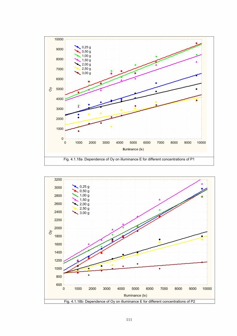
111

0 1000 2000 3000 4000 5000 6000 7000 8000 9000 10000

Illuminance (lx)

0

1000

2000

3000

4000

5000

6000

7000

8000

9000

10000

Oy

0,25 g 0,50 g 1,00 g 1,50 g 2,00 g 2,50 g 3,00 g

Fig. 4.1.18a :Dependence of Oy on illuminance E for different concentrations of P1

0 1000 2000 3000 4000 5000 6000 7000 8000 9000 10000

Illuminance (lx)

600

800

1000

1200

1400

1600

1800

2000

2200

2400

2600

2800

3000

3200

Oy

0,25 g 0,50 g 1,00 g 1,50 g 2,00 g 2,50 g 3,00 g

Fig. 4.1.18b: Dependence of Oy on illuminance E for different concentrations of P2

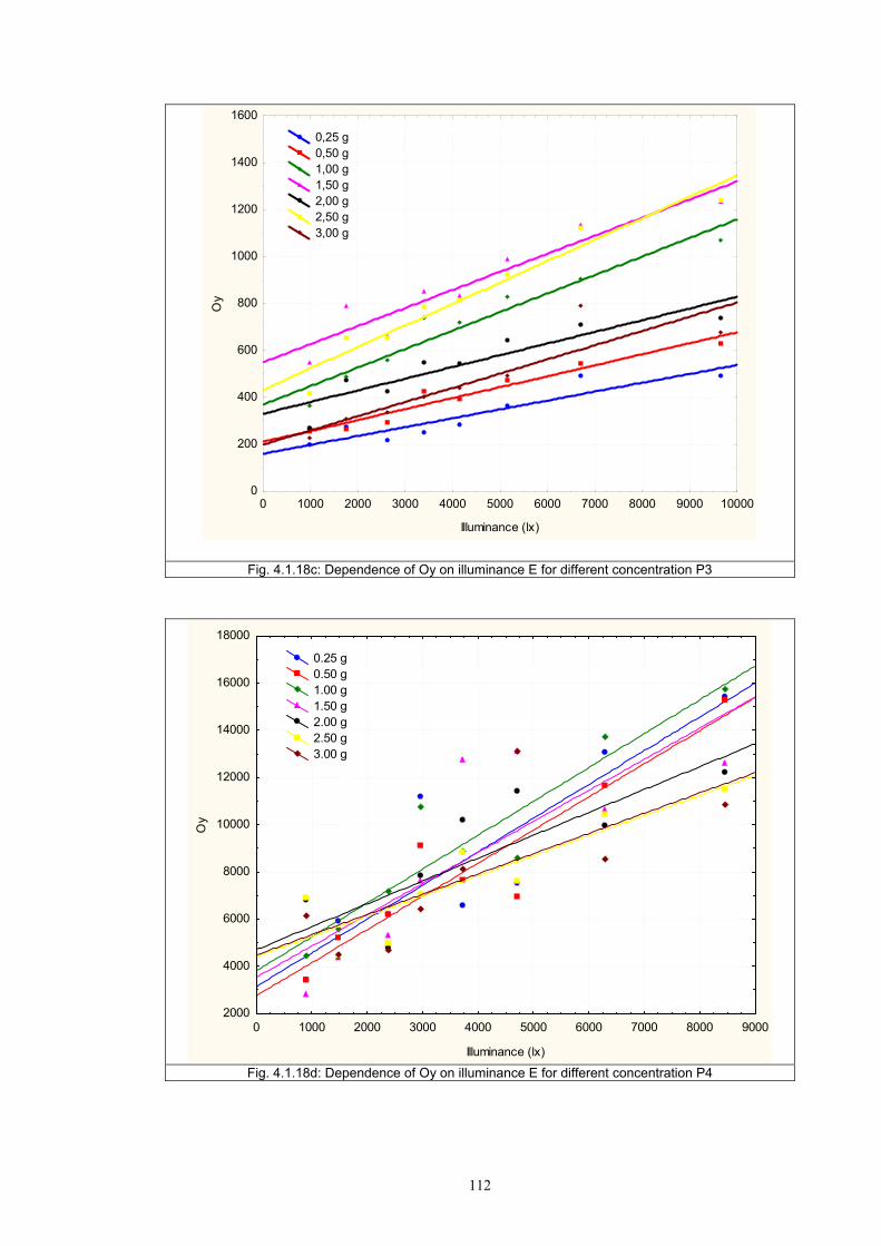
112

0 1000 2000 3000 4000 5000 6000 7000 8000 9000 10000

Illuminance (lx)

0

200

400

600

800

1000

1200

1400

1600

Oy

0,25 g 0,50 g 1,00 g 1,50 g 2,00 g 2,50 g 3,00 g

Fig. 4.1.18c: Dependence of Oy on illuminance E for different concentration P3

0 1000 2000 3000 4000 5000 6000 7000 8000 9000

Illuminance (lx)

2000

4000

6000

8000

10000

12000

14000

16000

18000

Oy

0.25 g 0.50 g 1.00 g 1.50 g 2.00 g 2.50 g 3.00 g

Fig. 4.1.18d: Dependence of Oy on illuminance E for different concentration P4

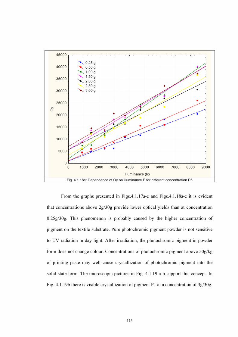
113

0 1000 2000 3000 4000 5000 6000 7000 8000 9000

Illuminance (lx)

0

5000

10000

15000

20000

25000

30000

35000

40000

45000O

y

0.25 g 0.50 g 1.00 g 1.50 g 2.00 g 2.50 g 3.00 g

Fig. 4.1.18e: Dependence of Oy on illuminance E for different concentration P5

From the graphs presented in Figs.4.1.17a-c and Figs.4.1.18a-e it is evident

that concentrations above 2g/30g provide lower optical yields than at concentration

0.25g/30g. This phenomenon is probably caused by the higher concentration of

pigment on the textile substrate. Pure photochromic pigment powder is not sensitive

to UV radiation in day light. After irradiation, the photochromic pigment in powder

form does not change colour. Concentrations of photochromic pigment above 50g/kg

of printing paste may well cause crystallization of photochromic pigment into the

solid-state form. The microscopic pictures in Fig. 4.1.19 a-b support this concept. In

Fig. 4.1.19b there is visible crystallization of pigment P1 at a concentration of 3g/30g.

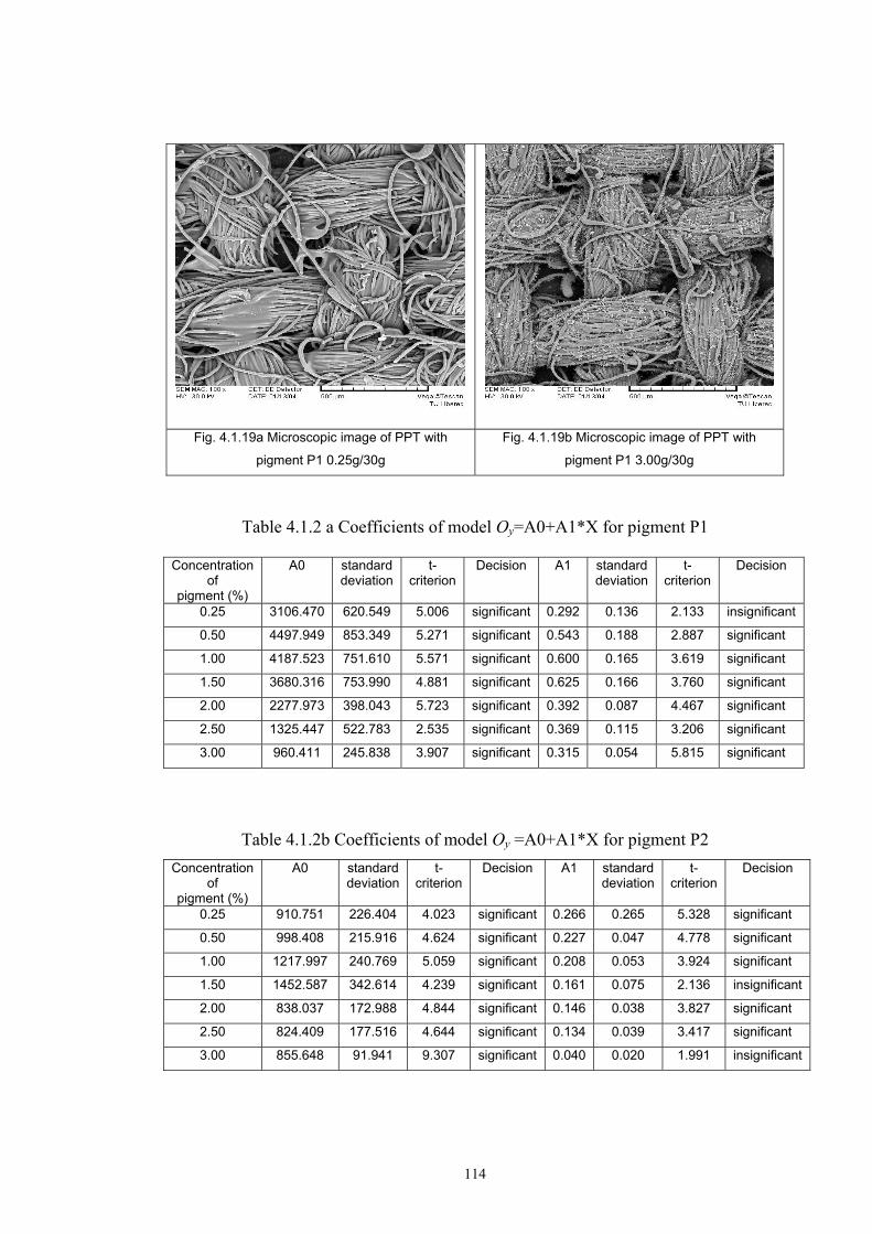
114

Fig. 4.1.19a Microscopic image of PPT with

pigment P1 0.25g/30g Fig. 4.1.19b Microscopic image of PPT with

pigment P1 3.00g/30g

Table 4.1.2 a Coefficients of model Oy=A0+A1*X for pigment P1

Concentration of

pigment (%)

A0 standard deviation

t-criterion

Decision A1 standard deviation

t-criterion

Decision

0.25 3106.470 620.549 5.006 significant 0.292 0.136 2.133 insignificant

0.50 4497.949 853.349 5.271 significant 0.543 0.188 2.887 significant

1.00 4187.523 751.610 5.571 significant 0.600 0.165 3.619 significant

1.50 3680.316 753.990 4.881 significant 0.625 0.166 3.760 significant

2.00 2277.973 398.043 5.723 significant 0.392 0.087 4.467 significant

2.50 1325.447 522.783 2.535 significant 0.369 0.115 3.206 significant

3.00 960.411 245.838 3.907 significant 0.315 0.054 5.815 significant

Table 4.1.2b Coefficients of model Oy =A0+A1*X for pigment P2 Concentration

of pigment (%)

A0 standard deviation

t-criterion

Decision A1 standard deviation

t-criterion

Decision

0.25 910.751 226.404 4.023 significant 0.266 0.265 5.328 significant

0.50 998.408 215.916 4.624 significant 0.227 0.047 4.778 significant

1.00 1217.997 240.769 5.059 significant 0.208 0.053 3.924 significant

1.50 1452.587 342.614 4.239 significant 0.161 0.075 2.136 insignificant

2.00 838.037 172.988 4.844 significant 0.146 0.038 3.827 significant

2.50 824.409 177.516 4.644 significant 0.134 0.039 3.417 significant

3.00 855.648 91.941 9.307 significant 0.040 0.020 1.991 insignificant

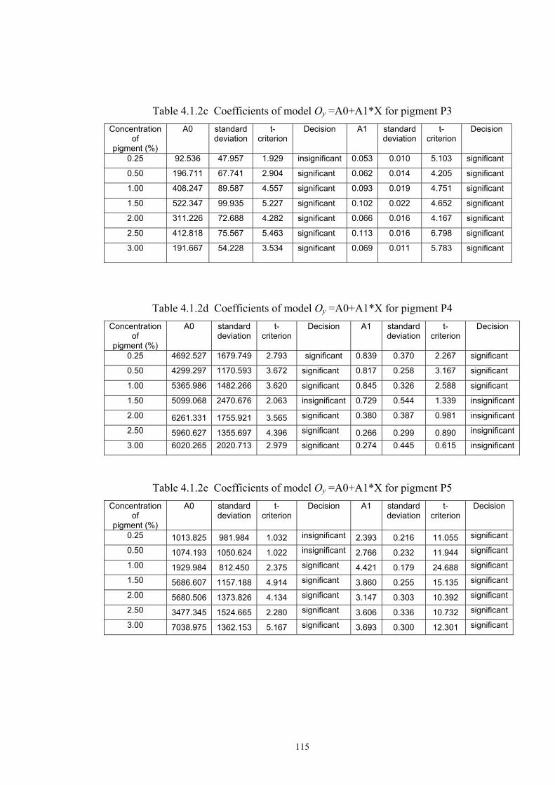
115

Table 4.1.2c Coefficients of model Oy =A0+A1*X for pigment P3 Concentration

of pigment (%)

A0 standard deviation

t-criterion

Decision A1 standard deviation

t-criterion

Decision

0.25 92.536 47.957 1.929 insignificant 0.053 0.010 5.103 significant

0.50 196.711 67.741 2.904 significant 0.062 0.014 4.205 significant

1.00 408.247 89.587 4.557 significant 0.093 0.019 4.751 significant

1.50 522.347 99.935 5.227 significant 0.102 0.022 4.652 significant

2.00 311.226 72.688 4.282 significant 0.066 0.016 4.167 significant

2.50 412.818 75.567 5.463 significant 0.113 0.016 6.798 significant

3.00 191.667 54.228 3.534 significant 0.069 0.011 5.783 significant

Table 4.1.2d Coefficients of model Oy =A0+A1*X for pigment P4 Concentration

of pigment (%)

A0 standard deviation

t-criterion

Decision A1 standard deviation

t-criterion

Decision

0.25 4692.527 1679.749 2.793 significant 0.839 0.370 2.267 significant

0.50 4299.297 1170.593 3.672 significant 0.817 0.258 3.167 significant

1.00 5365.986 1482.266 3.620 significant 0.845 0.326 2.588 significant

1.50 5099.068 2470.676 2.063 insignificant 0.729 0.544 1.339 insignificant

2.00 6261.331 1755.921 3.565 significant 0.380 0.387 0.981 insignificant

2.50 5960.627 1355.697 4.396 significant 0.266 0.299 0.890 insignificant

3.00 6020.265 2020.713 2.979 significant 0.274 0.445 0.615 insignificant

Table 4.1.2e Coefficients of model Oy =A0+A1*X for pigment P5 Concentration

of pigment (%)

A0 standard deviation

t-criterion

Decision A1 standard deviation

t-criterion

Decision

0.25 1013.825 981.984 1.032 insignificant 2.393 0.216 11.055 significant

0.50 1074.193 1050.624 1.022 insignificant 2.766 0.232 11.944 significant

1.00 1929.984 812.450 2.375 significant 4.421 0.179 24.688 significant

1.50 5686.607 1157.188 4.914 significant 3.860 0.255 15.135 significant

2.00 5680.506 1373.826 4.134 significant 3.147 0.303 10.392 significant

2.50 3477.345 1524.665 2.280 significant 3.606 0.336 10.732 significant

3.00 7038.975 1362.153 5.167 significant 3.693 0.300 12.301 significant

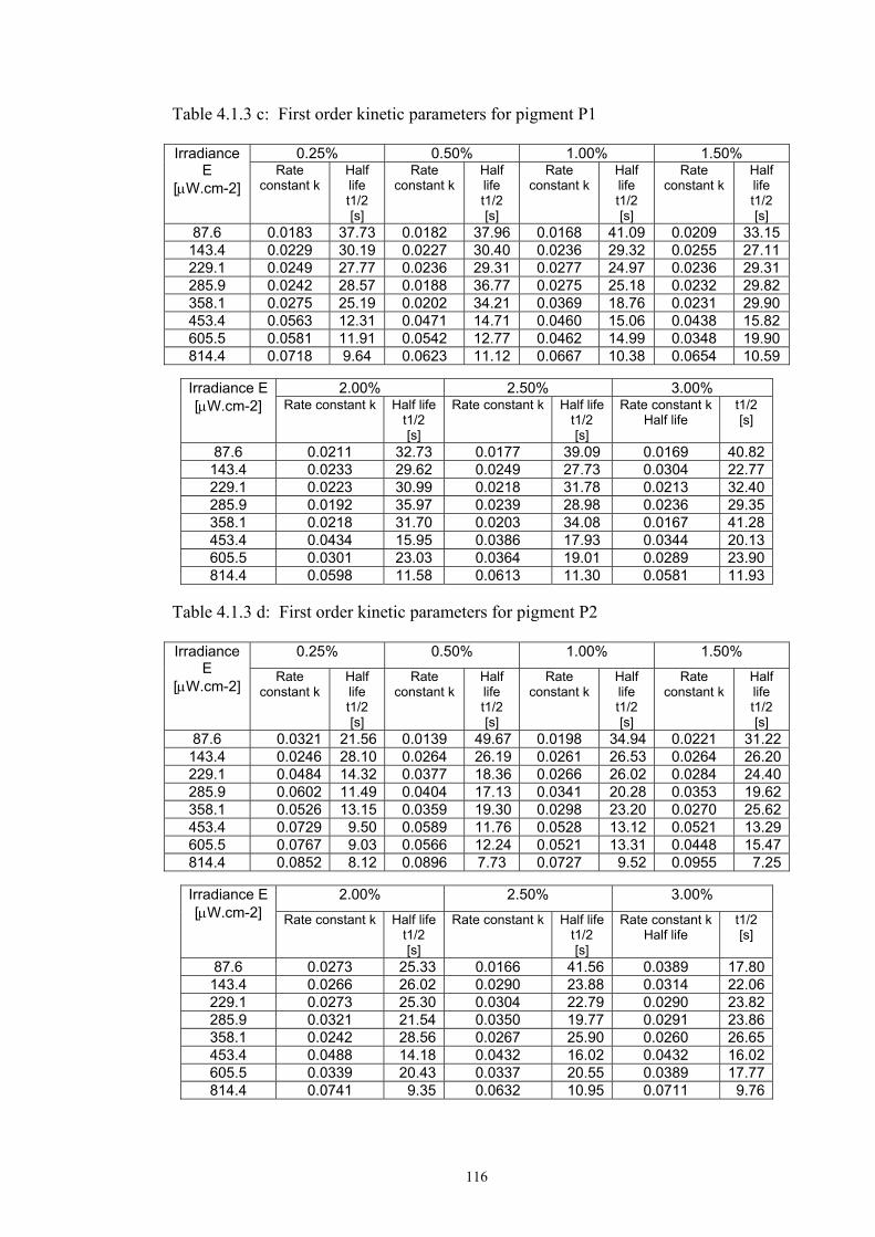
116

Table 4.1.3 c: First order kinetic parameters for pigment P1 Irradiance

E [μW.cm-2]

0.25% 0.50% 1.00% 1.50% Rate

constant k Half life t1/2 [s]

Rate constant k

Half life t1/2 [s]

Rate constant k

Half life t1/2 [s]

Rate constant k

Half life t1/2 [s]

87.6 0.0183 37.73 0.0182 37.96 0.0168 41.09 0.0209 33.15 143.4 0.0229 30.19 0.0227 30.40 0.0236 29.32 0.0255 27.11 229.1 0.0249 27.77 0.0236 29.31 0.0277 24.97 0.0236 29.31 285.9 0.0242 28.57 0.0188 36.77 0.0275 25.18 0.0232 29.82 358.1 0.0275 25.19 0.0202 34.21 0.0369 18.76 0.0231 29.90 453.4 0.0563 12.31 0.0471 14.71 0.0460 15.06 0.0438 15.82 605.5 0.0581 11.91 0.0542 12.77 0.0462 14.99 0.0348 19.90 814.4 0.0718 9.64 0.0623 11.12 0.0667 10.38 0.0654 10.59

Irradiance E[μW.cm-2]

2.00% 2.50% 3.00% Rate constant k Half life

t1/2 [s]

Rate constant k Half life t1/2 [s]

Rate constant k Half life

t1/2 [s]

87.6 0.0211 32.73 0.0177 39.09 0.0169 40.82143.4 0.0233 29.62 0.0249 27.73 0.0304 22.77229.1 0.0223 30.99 0.0218 31.78 0.0213 32.40285.9 0.0192 35.97 0.0239 28.98 0.0236 29.35358.1 0.0218 31.70 0.0203 34.08 0.0167 41.28453.4 0.0434 15.95 0.0386 17.93 0.0344 20.13605.5 0.0301 23.03 0.0364 19.01 0.0289 23.90814.4 0.0598 11.58 0.0613 11.30 0.0581 11.93

Table 4.1.3 d: First order kinetic parameters for pigment P2 Irradiance

E [μW.cm-2]

0.25% 0.50% 1.00% 1.50%

Rate constant k

Half life t1/2 [s]

Rate constant k

Half life t1/2 [s]

Rate constant k

Half life t1/2 [s]

Rate constant k

Half life t1/2 [s]

87.6 0.0321 21.56 0.0139 49.67 0.0198 34.94 0.0221 31.22143.4 0.0246 28.10 0.0264 26.19 0.0261 26.53 0.0264 26.20229.1 0.0484 14.32 0.0377 18.36 0.0266 26.02 0.0284 24.40285.9 0.0602 11.49 0.0404 17.13 0.0341 20.28 0.0353 19.62358.1 0.0526 13.15 0.0359 19.30 0.0298 23.20 0.0270 25.62453.4 0.0729 9.50 0.0589 11.76 0.0528 13.12 0.0521 13.29605.5 0.0767 9.03 0.0566 12.24 0.0521 13.31 0.0448 15.47814.4 0.0852 8.12 0.0896 7.73 0.0727 9.52 0.0955 7.25

Irradiance E[μW.cm-2]

2.00% 2.50% 3.00%

Rate constant k Half life t1/2 [s]

Rate constant k Half life t1/2 [s]

Rate constant k Half life

t1/2 [s]

87.6 0.0273 25.33 0.0166 41.56 0.0389 17.80143.4 0.0266 26.02 0.0290 23.88 0.0314 22.06229.1 0.0273 25.30 0.0304 22.79 0.0290 23.82285.9 0.0321 21.54 0.0350 19.77 0.0291 23.86358.1 0.0242 28.56 0.0267 25.90 0.0260 26.65453.4 0.0488 14.18 0.0432 16.02 0.0432 16.02605.5 0.0339 20.43 0.0337 20.55 0.0389 17.77814.4 0.0741 9.35 0.0632 10.95 0.0711 9.76

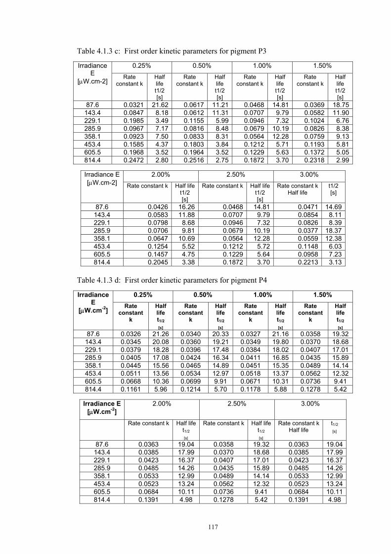
117

Table 4.1.3 c: First order kinetic parameters for pigment P3 Irradiance

E [μW.cm-2]

0.25% 0.50% 1.00% 1.50%

Rate constant k

Half life t1/2 [s]

Rate constant k

Half life t1/2 [s]

Rate constant k

Half life t1/2 [s]

Rate constant k

Half life t1/2 [s]

87.6 0.0321 21.62 0.0617 11.21 0.0468 14.81 0.0369 18.75143.4 0.0847 8.18 0.0612 11.31 0.0707 9.79 0.0582 11.90229.1 0.1985 3.49 0.1155 5.99 0.0946 7.32 0.1024 6.76285.9 0.0967 7.17 0.0816 8.48 0.0679 10.19 0.0826 8.38358.1 0.0923 7.50 0.0833 8.31 0.0564 12.28 0.0759 9.13453.4 0.1585 4.37 0.1803 3.84 0.1212 5.71 0.1193 5.81605.5 0.1968 3.52 0.1964 3.52 0.1229 5.63 0.1372 5.05814.4 0.2472 2.80 0.2516 2.75 0.1872 3.70 0.2318 2.99

Irradiance E[μW.cm-2]

2.00% 2.50% 3.00%

Rate constant k Half life t1/2 [s]

Rate constant k Half life t1/2 [s]

Rate constant k Half life

t1/2 [s]

87.6 0.0426 16.26 0.0468 14.81 0.0471 14.69143.4 0.0583 11.88 0.0707 9.79 0.0854 8.11229.1 0.0798 8.68 0.0946 7.32 0.0826 8.39285.9 0.0706 9.81 0.0679 10.19 0.0377 18.37358.1 0.0647 10.69 0.0564 12.28 0.0559 12.38453.4 0.1254 5.52 0.1212 5.72 0.1148 6.03605.5 0.1457 4.75 0.1229 5.64 0.0958 7.23814.4 0.2045 3.38 0.1872 3.70 0.2213 3.13

Table 4.1.3 d: First order kinetic parameters for pigment P4 Irradiance

E [μW.cm-2]

0.25% 0.50% 1.00% 1.50%Rate

constant k

Half life t1/2 [s]

Rate constant

k

Half life t1/2 [s]

Rate constant

k

Half life t1/2 [s]

Rate constant

k

Half life t1/2 [s]

87.6 0.0326 21.26 0.0340 20.33 0.0327 21.16 0.0358 19.32 143.4 0.0345 20.08 0.0360 19.21 0.0349 19.80 0.0370 18.68 229.1 0.0379 18.28 0.0396 17.48 0.0384 18.02 0.0407 17.01 285.9 0.0405 17.08 0.0424 16.34 0.0411 16.85 0.0435 15.89 358.1 0.0445 15.56 0.0465 14.89 0.0451 15.35 0.0489 14.14 453.4 0.0511 13.56 0.0534 12.97 0.0518 13.37 0.0562 12.32 605.5 0.0668 10.36 0.0699 9.91 0.0671 10.31 0.0736 9.41 814.4 0.1161 5.96 0.1214 5.70 0.1178 5.88 0.1278 5.42

Irradiance E

[μW.cm-2] 2.00% 2.50% 3.00%

Rate constant k Half life t1/2

[s]

Rate constant k Half life t1/2

[s]

Rate constant k Half life

t1/2

[s]

87.6 0.0363 19.04 0.0358 19.32 0.0363 19.04143.4 0.0385 17.99 0.0370 18.68 0.0385 17.99229.1 0.0423 16.37 0.0407 17.01 0.0423 16.37285.9 0.0485 14.26 0.0435 15.89 0.0485 14.26358.1 0.0533 12.99 0.0489 14.14 0.0533 12.99453.4 0.0523 13.24 0.0562 12.32 0.0523 13.24605.5 0.0684 10.11 0.0736 9.41 0.0684 10.11814.4 0.1391 4.98 0.1278 5.42 0.1391 4.98

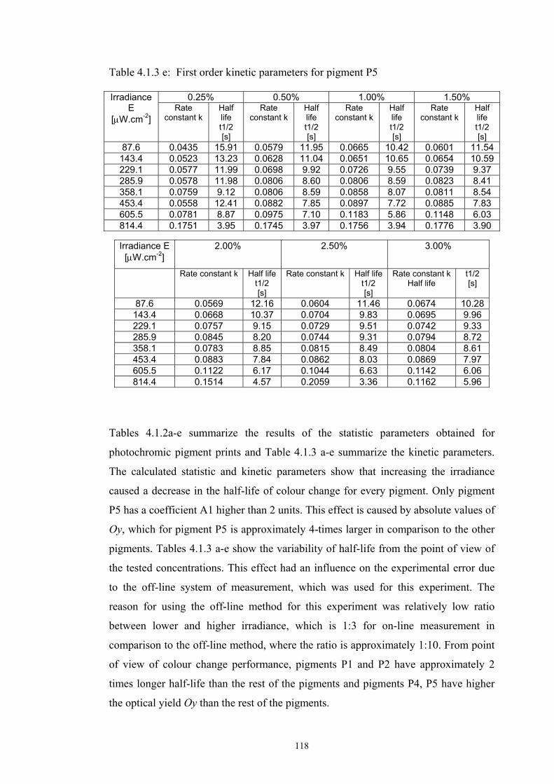
118

Table 4.1.3 e: First order kinetic parameters for pigment P5 Irradiance

E [μW.cm-2]

0.25% 0.50% 1.00% 1.50% Rate

constant k Half life t1/2 [s]

Rate constant k

Half life t1/2 [s]

Rate constant k

Half life t1/2 [s]

Rate constant k

Half life t1/2 [s]

87.6 0.0435 15.91 0.0579 11.95 0.0665 10.42 0.0601 11.54 143.4 0.0523 13.23 0.0628 11.04 0.0651 10.65 0.0654 10.59 229.1 0.0577 11.99 0.0698 9.92 0.0726 9.55 0.0739 9.37 285.9 0.0578 11.98 0.0806 8.60 0.0806 8.59 0.0823 8.41 358.1 0.0759 9.12 0.0806 8.59 0.0858 8.07 0.0811 8.54 453.4 0.0558 12.41 0.0882 7.85 0.0897 7.72 0.0885 7.83 605.5 0.0781 8.87 0.0975 7.10 0.1183 5.86 0.1148 6.03 814.4 0.1751 3.95 0.1745 3.97 0.1756 3.94 0.1776 3.90

Irradiance E

[μW.cm-2] 2.00% 2.50% 3.00%

Rate constant k Half life t1/2 [s]

Rate constant k Half life t1/2 [s]

Rate constant k Half life

t1/2 [s]

87.6 0.0569 12.16 0.0604 11.46 0.0674 10.28143.4 0.0668 10.37 0.0704 9.83 0.0695 9.96 229.1 0.0757 9.15 0.0729 9.51 0.0742 9.33 285.9 0.0845 8.20 0.0744 9.31 0.0794 8.72 358.1 0.0783 8.85 0.0815 8.49 0.0804 8.61 453.4 0.0883 7.84 0.0862 8.03 0.0869 7.97 605.5 0.1122 6.17 0.1044 6.63 0.1142 6.06 814.4 0.1514 4.57 0.2059 3.36 0.1162 5.96

Tables 4.1.2a-e summarize the results of the statistic parameters obtained for

photochromic pigment prints and Table 4.1.3 a-e summarize the kinetic parameters.

The calculated statistic and kinetic parameters show that increasing the irradiance

caused a decrease in the half-life of colour change for every pigment. Only pigment

P5 has a coefficient A1 higher than 2 units. This effect is caused by absolute values of

Oy, which for pigment P5 is approximately 4-times larger in comparison to the other

pigments. Tables 4.1.3 a-e show the variability of half-life from the point of view of

the tested concentrations. This effect had an influence on the experimental error due

to the off-line system of measurement, which was used for this experiment. The

reason for using the off-line method for this experiment was relatively low ratio

between lower and higher irradiance, which is 1:3 for on-line measurement in

comparison to the off-line method, where the ratio is approximately 1:10. From point

of view of colour change performance, pigments P1 and P2 have approximately 2

times longer half-life than the rest of the pigments and pigments P4, P5 have higher

the optical yield Oy than the rest of the pigments.

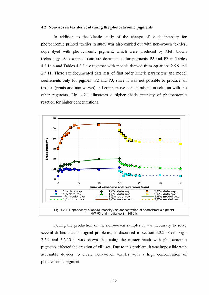
119

4.2 Non-woven textiles containing the photochromic pigments

In addition to the kinetic study of the change of shade intensity for

photochromic printed textiles, a study was also carried out with non-woven textiles,

dope dyed with photochromic pigment, which were produced by Melt blown

technology. As examples data are documented for pigments P2 and P3 in Tables

4.2.1a-e and Tables 4.2.2 a-e together with models derived from equations 2.5.9 and

2.5.11. There are documented data sets of first order kinetic parameters and model

coefficients only for pigment P2 and P3, since it was not possible to produce all

textiles (prints and non-woven) and comparative concentrations in solution with the

other pigments. Fig. 4.2.1 illustrates a higher shade intensity of photochromic

reaction for higher concentrations.

0

20

40

60

80

100

120

0 5 10 15 20 25 30Time of exposure and reversion (min)

Shad

e In

tens

ity I

1% data exp 1,8% data exp 2,6% data exp1% data rev 1,8% data rev 2,6% data rev1% model exp 1% model rev 1,8% model exp1,8 model rev 2,6% model exp 2,6% model rev

Fig. 4.2.1: Dependency of shade intensity I on concentration of photochromic pigment NW-P3 and irradiance E= 8460 lx

During the production of the non-woven samples it was necessary to solve

several difficult technological problems, as discussed in section 3.2.2. From Figs.

3.2.9 and 3.2.10 it was shown that using the master batch with photochromic

pigments effected the creation of villuses. Due to this problem, it was impossible with

accessible devices to create non-woven textiles with a high concentration of

photochromic pigment.

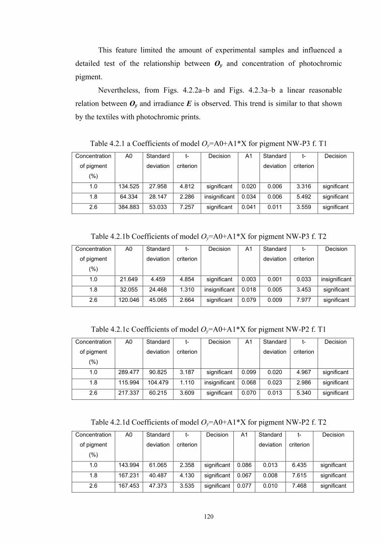
120

This feature limited the amount of experimental samples and influenced a

detailed test of the relationship between Oy and concentration of photochromic

pigment.

Nevertheless, from Figs. 4.2.2a–b and Figs. 4.2.3a–b a linear reasonable

relation between Oy and irradiance E is observed. This trend is similar to that shown

by the textiles with photochromic prints.

Table 4.2.1 a Coefficients of model Oy=A0+A1*X for pigment NW-P3 f. T1 Concentration

of pigment

(%)

A0 Standard

deviation

t-

criterion

Decision A1 Standard

deviation

t-

criterion

Decision

1.0 134.525 27.958 4.812 significant 0.020 0.006 3.316 significant

1.8 64.334 28.147 2.286 insignificant 0.034 0.006 5.492 significant

2.6 384.883 53.033 7.257 significant 0.041 0.011 3.559 significant

Table 4.2.1b Coefficients of model Oy=A0+A1*X for pigment NW-P3 f. T2 Concentration

of pigment

(%)

A0 Standard

deviation

t-

criterion

Decision A1 Standard

deviation

t-

criterion

Decision

1.0 21.649 4.459 4.854 significant 0.003 0.001 0.033 insignificant

1.8 32.055 24.468 1.310 insignificant 0.018 0.005 3.453 significant

2.6 120.046 45.065 2.664 significant 0.079 0.009 7.977 significant

Table 4.2.1c Coefficients of model Oy=A0+A1*X for pigment NW-P2 f. T1 Concentration

of pigment

(%)

A0 Standard

deviation

t-

criterion

Decision A1 Standard

deviation

t-

criterion

Decision

1.0 289.477 90.825 3.187 significant 0.099 0.020 4.967 significant

1.8 115.994 104.479 1.110 insignificant 0.068 0.023 2.986 significant

2.6 217.337 60.215 3.609 significant 0.070 0.013 5.340 significant

Table 4.2.1d Coefficients of model Oy=A0+A1*X for pigment NW-P2 f. T2 Concentration

of pigment

(%)

A0 Standard

deviation

t-

criterion

Decision A1 Standard

deviation

t-

criterion

Decision

1.0 143.994 61.065 2.358 significant 0.086 0.013 6.435 significant

1.8 167.231 40.487 4.130 significant 0.067 0.008 7.615 significant

2.6 167.453 47.373 3.535 significant 0.077 0.010 7.468 significant

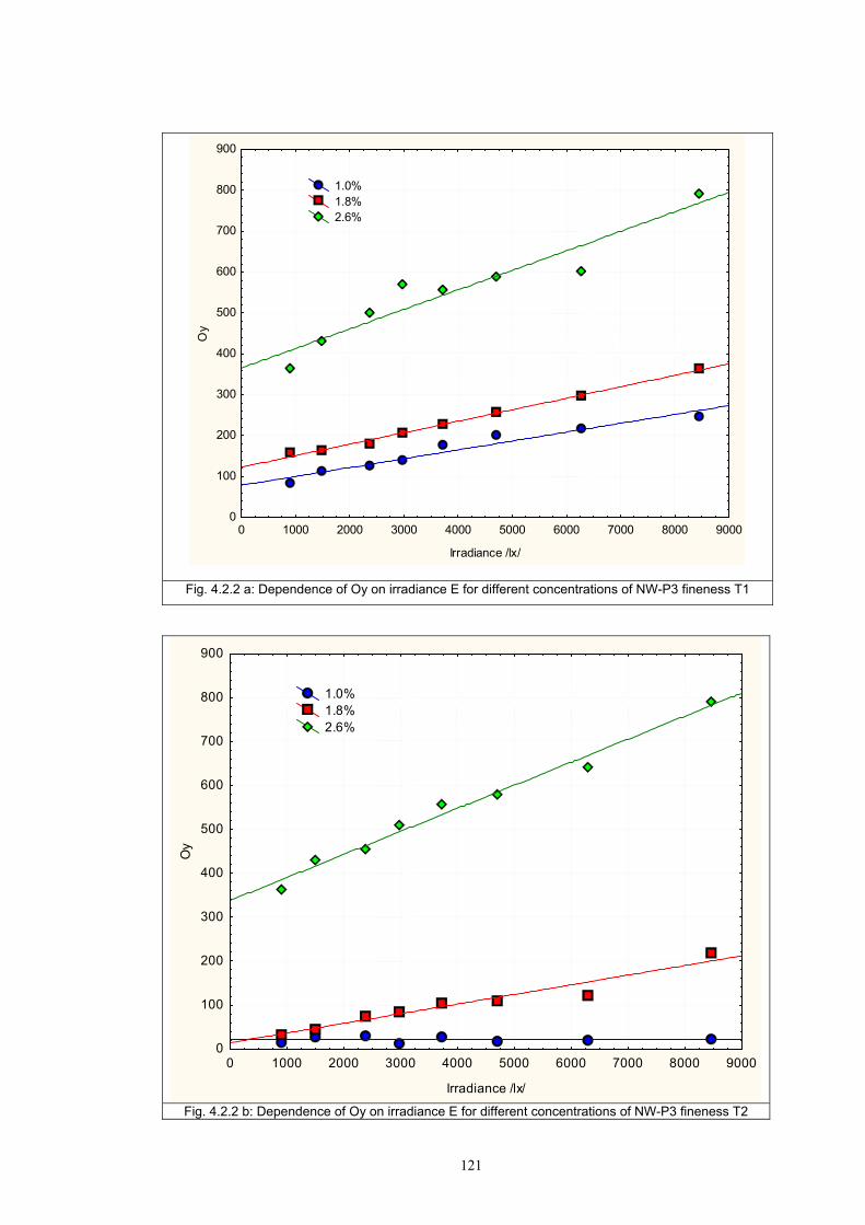
121

0 1000 2000 3000 4000 5000 6000 7000 8000 9000

Irradiance /lx/

0

100

200

300

400

500

600

700

800

900

Oy

1.0% 1.8% 2.6%

Fig. 4.2.2 a: Dependence of Oy on irradiance E for different concentrations of NW-P3 fineness T1

0 1000 2000 3000 4000 5000 6000 7000 8000 9000

Irradiance /lx/

0

100

200

300

400

500

600

700

800

900

Oy

1.0% 1.8% 2.6%

Fig. 4.2.2 b: Dependence of Oy on irradiance E for different concentrations of NW-P3 fineness T2

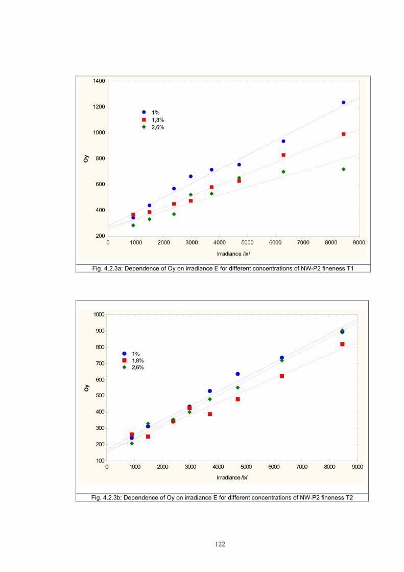
122

0 1000 2000 3000 4000 5000 6000 7000 8000 9000

Irradiance /lx/

200

400

600

800

1000

1200

1400O

y

1% 1,8% 2,6%

Fig. 4.2.3a: Dependence of Oy on irradiance E for different concentrations of NW-P2 fineness T1

Fig. 4.2.3b: Dependence of Oy on irradiance E for different concentrations of NW-P2 fineness T2

0 1000 2000 3000 4000 5000 6000 7000 8000 9000

Irradiance /lx/

100

200

300

400

500

600

700

800

900

1000

Oy

1% 1,8% 2,6%

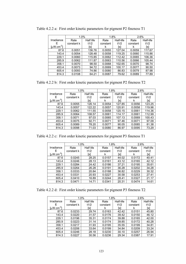
123

Table 4.2.2 a: First order kinetic parameters for pigment P2 fineness T1

Irradiance

E [μW.cm-2]

1.0% 1.8% 2.6% Rate

constant k Half life

t1/2 [s]

Rate constant

k

Half-life t1/2 [s]

Rate constant

k

Half-life t1/2 [s]

87.6 0.0051 136.76 0.0055 127.04 0.0059 117.67 143.4 0.0054 128.48 0.0058 119.25 0.0060 115.86 229.1 0.0060 115.85 0.0062 112.42 0.0065 106.36 285.9 0.0062 111.87 0.0063 110.56 0.0066 105.44 358.1 0.0070 98.50 0.0068 102.65 0.0070 98.74 453.4 0.0073 94.72 0.0069 100.17 0.0077 90.50 605.4 0.0093 74.86 0.0080 86.83 0.0079 87.98 814.3 0.0108 64.21 0.0087 79.62 0.0089 77.89

Table 4.2.2 b: First order kinetic parameters for pigment P2 fineness T2

Irradiance

E [μW.cm-2]

1.0% 1.8% 2.6% Rate

constant k Half life

t1/2 [s]

Rate constant

k

Half-life t1/2 [s]

Rate constant

k

Half-life t1/2 [s]

87.6 0.0055 126.14 0.0054 127.85 0.0056 123.25 143.4 0.0057 122.22 0.0057 120.91 0.0058 119.96 229.1 0.0062 111.55 0.0058 120.15 0.0061 114.36 285.9 0.0064 108.57 0.0061 114.17 0.0061 112.99 358.1 0.0071 97.03 0.0065 107.13 0.0069 100.43 453.4 0.0075 92.71 0.0071 97.46 0.0071 97.09 605.4 0.0089 78.20 0.0077 90.05 0.0085 81.38 814.3 0.0098 71.03 0.0080 86.97 0.0095 73.29

Table 4.2.2 c: First order kinetic parameters for pigment P3 fineness T1

Irradiance

E [μW.cm-2]

1.0% 1.8% 2.6% Rate

constant k Half life

t1/2 [s]

Rate constant

k

Half-life t1/2 [s]

Rate constant

k

Half-life t1/2 [s]

87.6 0.0245 28.25 0.0157 44.02 0.0172 40.41 143.4 0.0246 28.13 0.0161 43.12 0.0165 42.12 229.1 0.0284 24.42 0.0186 37.21 0.0195 35.61 285.9 0.0264 26.28 0.0191 36.28 0.0202 34.28 358.1 0.0333 20.84 0.0188 36.82 0.0229 30.32 453.4 0.0331 20.93 0.0227 30.58 0.0253 27.41 605.4 0.0410 16.89 0.0244 28.41 0.0327 21.17 814.3 0.0471 14.71 0.0341 20.31 0.0474 14.61

Table 4.2.2 d: First order kinetic parameters for pigment P3 fineness T2

Irradiance

E [μW.cm-2]

1.0% 1.8% 2.6% Rate

constant k Half life

t1/2 [s]

Rate constant

k

Half-life t1/2 [s]

Rate constant

k

Half-life t1/2 [s]

87.6 0.0233 29.74 0.0163 42.42 0.0151 45.80 143.4 0.0220 31.57 0.0176 39.42 0.0150 46.12 229.1 0.0196 35.31 0.0174 39.88 0.0165 42.00 285.9 0.0223 31.14 0.0174 39.85 0.0172 40.28 358.1 0.0217 31.93 0.0195 35.55 0.0199 34.81 453.4 0.0206 33.64 0.0199 34.84 0.0209 33.24 605.4 0.0246 28.18 0.0230 30.10 0.0257 26.94 814.3 0.0227 30.56 0.0236 29.34 0.0387 17.91

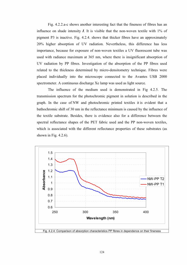
124

Fig. 4.2.2.a-c shows another interesting fact that the fineness of fibres has an

influence on shade intensity I. It is visible that the non-woven textile with 1% of

pigment P3 is inactive. Fig. 4.2.4. shows that thicker fibres have an approximately

20% higher absorption of UV radiation. Nevertheless, this difference has less

importance, because for exposure of non-woven textiles a UV fluorescent tube was

used with radiance maximum at 365 nm, where there is insignificant absorption of

UV radiation by PP fibres. Investigation of the absorption of the PP fibres used

related to the thickness determined by micro-densitometry technique. Fibres were

placed individually into the microscope connected to the Avantes USB 2000

spectrometer. A continuous discharge Xe lamp was used as light source.

The influence of the medium used is demonstrated in Fig 4.2.5. The

transmission spectrum for the photochromic pigment in solution is described in the

graph. In the case of NW and photochromic printed textiles it is evident that a

bathochromic shift of 30 nm in the reflectance minimum is caused by the influence of

the textile substrate. Besides, there is evidence also for a difference between the

spectral reflectance shapes of the PET fabric used and the PP non-woven textiles,

which is associated with the different reflectance properties of these substrates (as

shown in Fig. 4.2.6).

0.6

0.7

0.8

0.9

1

1.1

1.2

1.3

1.4

1.5

250 300 350 400

Wavelength (nm)

Abs

orba

nce

NW-PP T2NW-PP T1

Fig. 4.2.4: Comparison of absorption characteristics PP fibres in dependence on their fineness

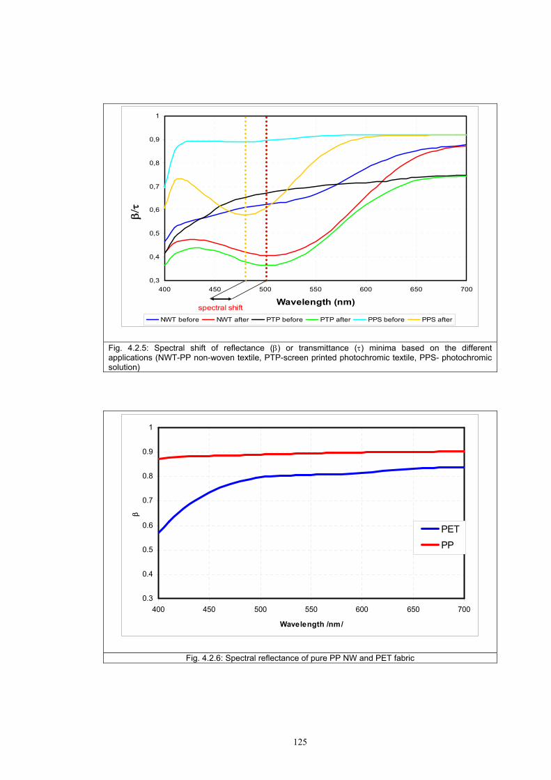
125

0,3

0,4

0,5

0,6

0,7

0,8

0,9

1

400 450 500 550 600 650 700

Wavelength (nm)

β/τ

NWT before NWT after PTP before PTP after PPS before PPS after

spectral shift

Fig. 4.2.5: Spectral shift of reflectance (β) or transmittance (τ) minima based on the different applications (NWT-PP non-woven textile, PTP-screen printed photochromic textile, PPS- photochromic solution)

0.3

0.4

0.5

0.6

0.7

0.8

0.9

1

400 450 500 550 600 650 700

Wavelength /nm/

β

PETPP

Fig. 4.2.6: Spectral reflectance of pure PP NW and PET fabric

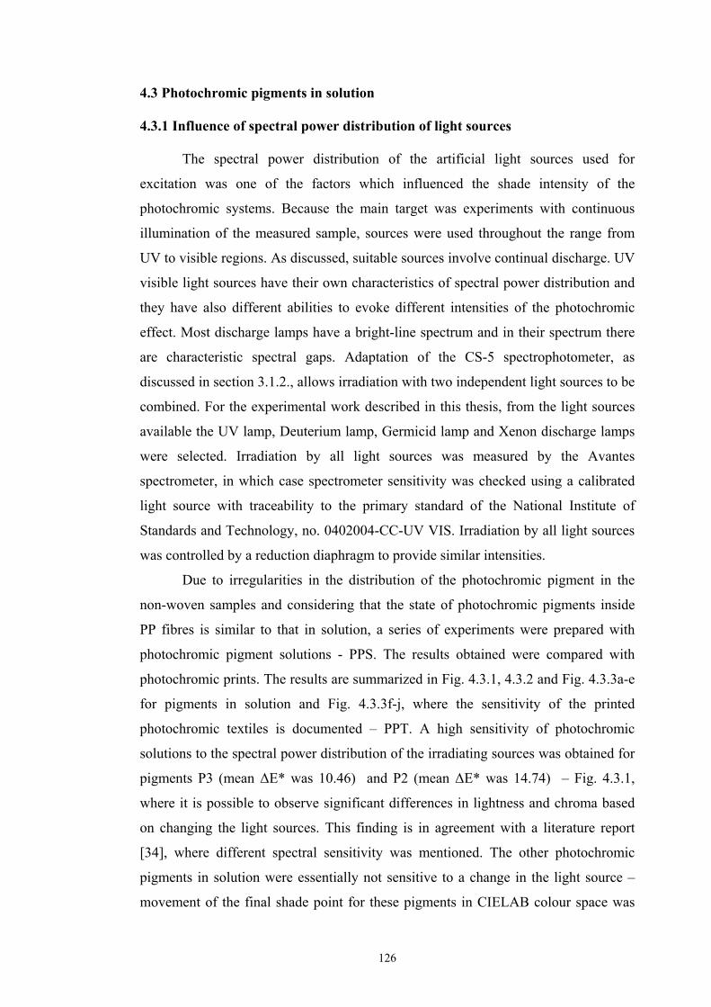
126

4.3 Photochromic pigments in solution

4.3.1 Influence of spectral power distribution of light sources

The spectral power distribution of the artificial light sources used for

excitation was one of the factors which influenced the shade intensity of the

photochromic systems. Because the main target was experiments with continuous

illumination of the measured sample, sources were used throughout the range from

UV to visible regions. As discussed, suitable sources involve continual discharge. UV

visible light sources have their own characteristics of spectral power distribution and

they have also different abilities to evoke different intensities of the photochromic

effect. Most discharge lamps have a bright-line spectrum and in their spectrum there

are characteristic spectral gaps. Adaptation of the CS-5 spectrophotometer, as

discussed in section 3.1.2., allows irradiation with two independent light sources to be

combined. For the experimental work described in this thesis, from the light sources

available the UV lamp, Deuterium lamp, Germicid lamp and Xenon discharge lamps

were selected. Irradiation by all light sources was measured by the Avantes

spectrometer, in which case spectrometer sensitivity was checked using a calibrated

light source with traceability to the primary standard of the National Institute of

Standards and Technology, no. 0402004-CC-UV VIS. Irradiation by all light sources

was controlled by a reduction diaphragm to provide similar intensities.

Due to irregularities in the distribution of the photochromic pigment in the

non-woven samples and considering that the state of photochromic pigments inside

PP fibres is similar to that in solution, a series of experiments were prepared with

photochromic pigment solutions - PPS. The results obtained were compared with

photochromic prints. The results are summarized in Fig. 4.3.1, 4.3.2 and Fig. 4.3.3a-e

for pigments in solution and Fig. 4.3.3f-j, where the sensitivity of the printed

photochromic textiles is documented – PPT. A high sensitivity of photochromic

solutions to the spectral power distribution of the irradiating sources was obtained for

pigments P3 (mean ΔE* was 10.46) and P2 (mean ΔE* was 14.74) – Fig. 4.3.1,

where it is possible to observe significant differences in lightness and chroma based

on changing the light sources. This finding is in agreement with a literature report

[34], where different spectral sensitivity was mentioned. The other photochromic

pigments in solution were essentially not sensitive to a change in the light source –

movement of the final shade point for these pigments in CIELAB colour space was

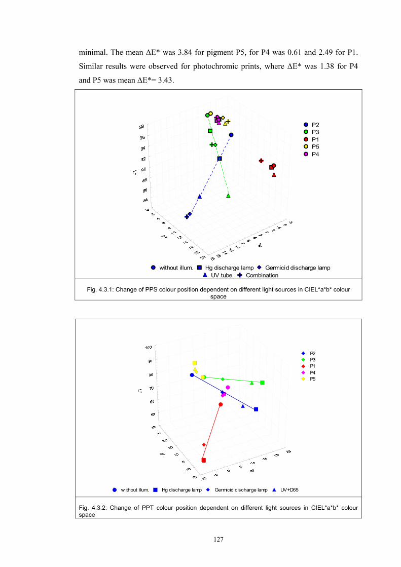
127

minimal. The mean ΔE* was 3.84 for pigment P5, for P4 was 0.61 and 2.49 for P1.

Similar results were observed for photochromic prints, where ΔE* was 1.38 for P4

and P5 was mean ΔE*= 3.43.

without illum. Hg discharge lamp Germicid discharge lamp UV tube Combination

P2P3P1P5P4

Fig. 4.3.1: Change of PPS colour position dependent on different light sources in CIEL*a*b* colour

space

P2 P3 P1 P4 P5

w ithout illum. Hg discharge lamp Germicid discharge lamp UV+D65

Fig. 4.3.2: Change of PPT colour position dependent on different light sources in CIEL*a*b* colour space

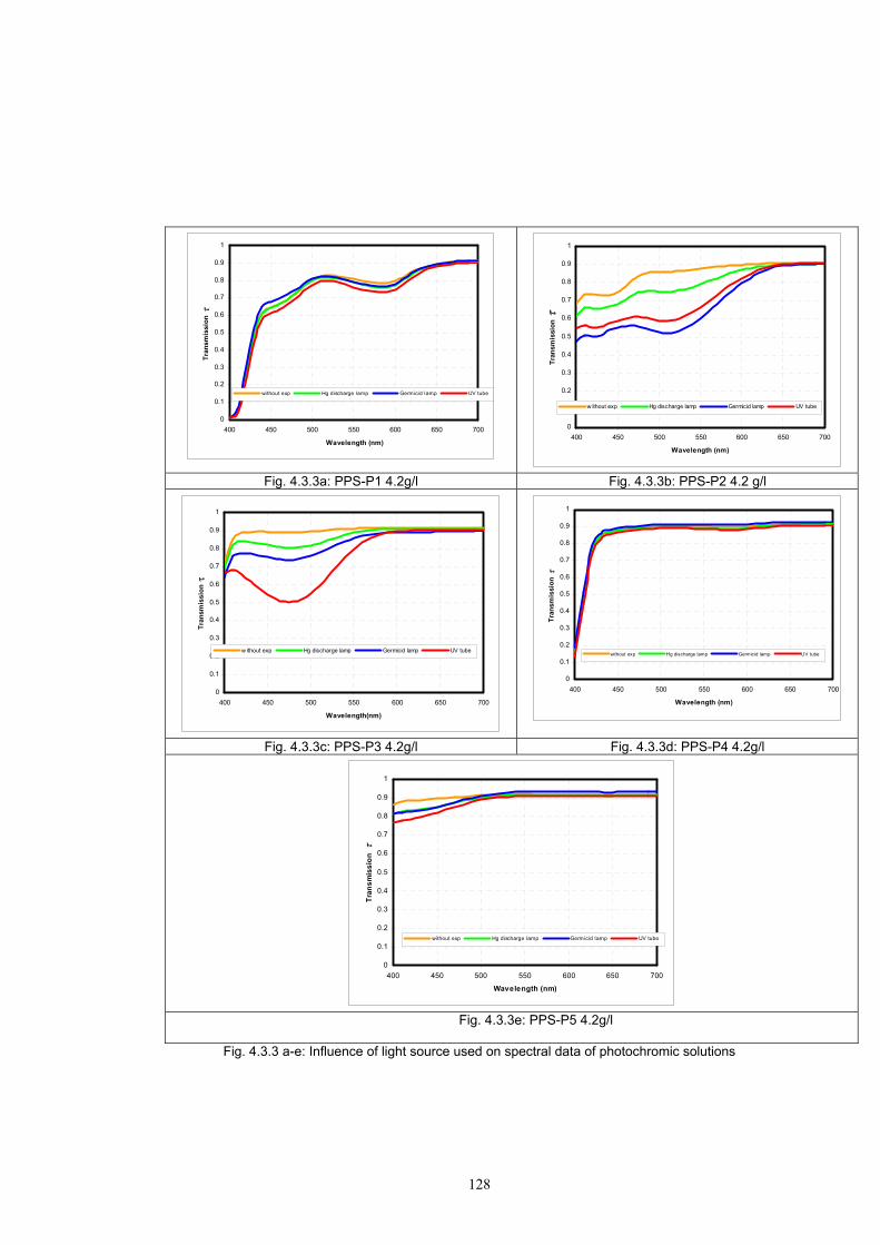
128

0

0.1

0.2

0.3

0.4

0.5

0.6

0.7

0.8

0.9

1

400 450 500 550 600 650 700

Wavelength (nm)

Tran

smis

sion

τ

without exp Hg discharge lamp Germicid lamp UV tube

0

0.1

0.2

0.3

0.4

0.5

0.6

0.7

0.8

0.9

1

400 450 500 550 600 650 700

Wavelength (nm)

Tran

smis

sion

τ

w ithout exp Hg discharge lamp Germicid lamp UV tube

Fig. 4.3.3a: PPS-P1 4.2g/l Fig. 4.3.3b: PPS-P2 4.2 g/l

0

0.1

0.2

0.3

0.4

0.5

0.6

0.7

0.8

0.9

1

400 450 500 550 600 650 700

Wavelength(nm)

Tran

smis

sion

τ

w ithout exp Hg discharge lamp Germicid lamp UV tube

0

0.1

0.2

0.3

0.4

0.5

0.6

0.7

0.8

0.9

1

400 450 500 550 600 650 700

Wavelength (nm)

Tran

smis

sion

τ

without exp Hg discharge lamp Germicid lamp UV tube

Fig. 4.3.3c: PPS-P3 4.2g/l Fig. 4.3.3d: PPS-P4 4.2g/l

0

0.1

0.2

0.3

0.4

0.5

0.6

0.7

0.8

0.9

1

400 450 500 550 600 650 700

Wavelength (nm)

Tran

smis

sion

τ

without exp Hg discharge lamp Germicid lamp UV tube

Fig. 4.3.3e: PPS-P5 4.2g/l

Fig. 4.3.3 a-e: Influence of light source used on spectral data of photochromic solutions

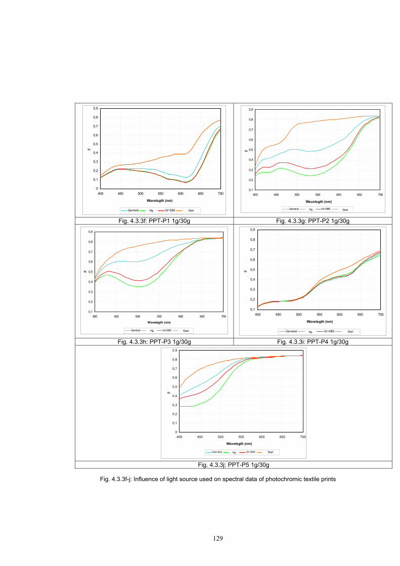
129

0

0,1

0,2

0,3

0,4

0,5

0,6

0,7

0,8

0,9

400 450 500 550 600 650 700

Vlnová délka (nm)

Stup

eň re

mis

e

Germicid Rtuťová UV+D65 před osvitem

Wavelegth (nm)

β

Hg Start

0,1

0,2

0,3

0,4

0,5

0,6

0,7

0,8

0,9

400 450 500 550 600 650 700

Vlnová délka (nm)

Stup

eň re

mis

e

Germicid Rtuťová UV+D65 před osvitem

Wavelegth (nm)

β

Hg Start Fig. 4.3.3f: PPT-P1 1g/30g Fig. 4.3.3g: PPT-P2 1g/30g

0,1

0,2

0,3

0,4

0,5

0,6

0,7

0,8

0,9

400 450 500 550 600 650 700

Vlnová délka (nm)

Stup

eň re

mis

e

Germicid Rtuťová UV+D65 před osvitem

Wavelegth (nm)

β

Hg Start

0,1

0,2

0,3

0,4

0,5

0,6

0,7

0,8

0,9

400 450 500 550 600 650 700

Vlnová délka (nm)

Stup

eň re

mis

e

Germicid Rtuťová UV+D65 před osvitem

Wavelegth (nm)

β

Hg Start

Fig. 4.3.3h: PPT-P3 1g/30g Fig. 4.3.3i: PPT-P4 1g/30g

0

0,1

0,2

0,3

0,4

0,5

0,6

0,7

0,8

0,9

400 450 500 550 600 650 700

Vlnová délka (nm)

Stup

eň re

mis

e

Germicid Rtuťová UV+D65 před osvitem

Wavelegth (nm)

β

Hg Start

Fig. 4.3.3j: PPT-P5 1g/30g

Fig. 4.3.3f-j: Influence of light source used on spectral data of photochromic textile prints

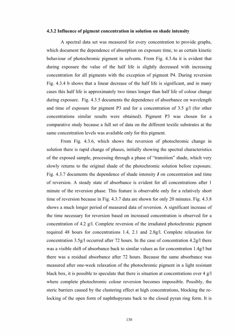
130

4.3.2 Influence of pigment concentration in solution on shade intensity

A spectral data set was measured for every concentration to provide graphs,

which document the dependence of absorption on exposure time, to as certain kinetic

behaviour of photochromic pigment in solvents. From Fig. 4.3.4a it is evident that

during exposure the value of the half life is slightly decreased with increasing

concentration for all pigments with the exception of pigment P4. During reversion

Fig. 4.3.4 b shows that a linear decrease of the half life is significant, and in many

cases this half life is approximately two times longer than half life of colour change

during exposure. Fig. 4.3.5 documents the dependence of absorbance on wavelength

and time of exposure for pigment P3 and for a concentration of 3.5 g/l (for other

concentrations similar results were obtained). Pigment P3 was chosen for a

comparative study because a full set of data on the different textile substrates at the

same concentration levels was available only for this pigment.

From Fig. 4.3.6, which shows the reversion of photochromic change in

solution there is rapid change of phases, initially showing the spectral characteristics

of the exposed sample, processing through a phase of “transition” shade, which very

slowly returns to the original shade of the photochromic solution before exposure.

Fig. 4.3.7 documents the dependence of shade intensity I on concentration and time

of reversion. A steady state of absorbance is evident for all concentrations after 1

minute of the reversion phase. This feature is observable only for a relatively short

time of reversion because in Fig. 4.3.7 data are shown for only 20 minutes. Fig. 4.3.8

shows a much longer period of measured data of reversion. A significant increase of

the time necessary for reversion based on increased concentration is observed for a

concentration of 4.2 g/l. Complete reversion of the irradiated photochromic pigment

required 48 hours for concentrations 1.4, 2.1 and 2.8g/l. Complete relaxation for

concentration 3.5g/l occurred after 72 hours. In the case of concentration 4.2g/l there

was a visible shift of absorbance back to similar values as for concentration 1.4g/l but

there was a residual absorbance after 72 hours. Because the same absorbance was

measured after one-week relaxation of the photochromic pigment in a light resistant

black box, it is possible to speculate that there is situation at concentrations over 4 g/l

where complete photochromic colour reversion becomes impossible. Possibly, the

steric barriers caused by the clustering effect at high concentrations, blocking the re-

locking of the open form of naphthopyrans back to the closed pyran ring form. It is

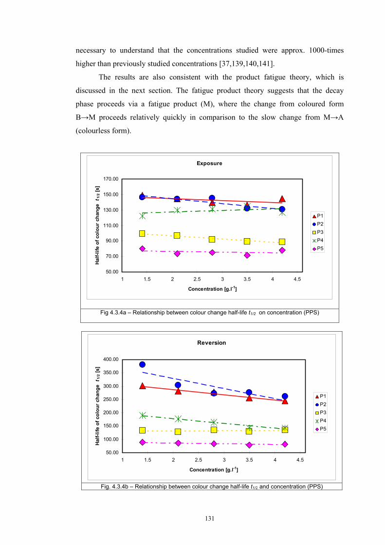
131

necessary to understand that the concentrations studied were approx. 1000-times

higher than previously studied concentrations [37,139,140,141].

The results are also consistent with the product fatigue theory, which is

discussed in the next section. The fatigue product theory suggests that the decay

phase proceeds via a fatigue product (M), where the change from coloured form

B→M proceeds relatively quickly in comparison to the slow change from M→A

(colourless form).

Exposure

50.00

70.00

90.00

110.00

130.00

150.00

170.00

1 1.5 2 2.5 3 3.5 4 4.5

Concentration [g.l-1]

Half-

life

of c

olou

r cha

nge t 1

/2 [s

]

P1P2P3P4P5

Fig 4.3.4a – Relationship between colour change half-life t1/2 on concentration (PPS)

Reversion

50.00

100.00

150.00

200.00

250.00

300.00

350.00

400.00

1 1.5 2 2.5 3 3.5 4 4.5

Concentration [g.l-1]

Half-

life

of c

olou

r cha

nge t 1

/2 [s

]

P1P2P3P4P5

Fig. 4.3.4b – Relationship between colour change half-life t1/2 and concentration (PPS)

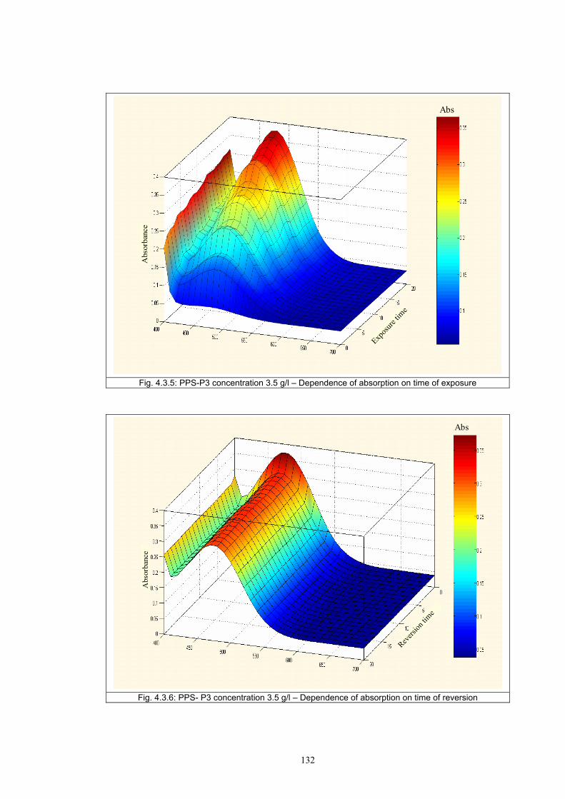
132

Abs

Abs

orba

nce

Exposu

re tim

e

Fig. 4.3.5: PPS-P3 concentration 3.5 g/l – Dependence of absorption on time of exposure

Abs

Abs

orba

nce

Revers

ion tim

e

Fig. 4.3.6: PPS- P3 concentration 3.5 g/l – Dependence of absorption on time of reversion

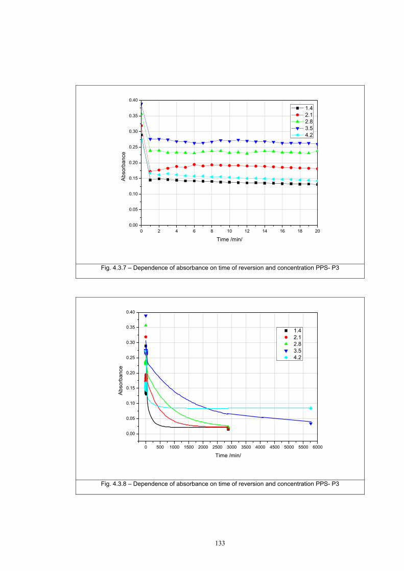
133

0 2 4 6 8 10 12 14 16 18 200.00

0.05

0.10

0.15

0.20

0.25

0.30

0.35

0.40

Abso

rban

ce

Time /min/

1.4 2.1 2.8 3.5 4.2

Fig. 4.3.7 – Dependence of absorbance on time of reversion and concentration PPS- P3

0 500 1000 1500 2000 2500 3000 3500 4000 4500 5000 5500 6000

0.00

0.05

0.10

0.15

0.20

0.25

0.30

0.35

0.40

Abso

rban

ce

Time /min/

1.4 2.1 2.8 3.5 4.2

Fig. 4.3.8 – Dependence of absorbance on time of reversion and concentration PPS- P3

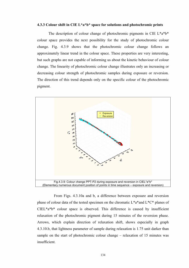
134

4.3.3 Colour shift in CIE L*a*b* space for solutions and photochromic prints

The description of colour change of photochromic pigments in CIE L*a*b*

colour space provides the next possibility for the study of photochromic colour

change. Fig. 4.3.9 shows that the photochromic colour change follows an

approximately linear trend in the colour space. These properties are very interesting,

but such graphs are not capable of informing us about the kinetic behaviour of colour

change. The linearity of photochromic colour change illustrates only an increasing or

decreasing colour strength of photochromic samples during exposure or reversion.

The direction of this trend depends only on the specific colour of the photochromic

pigment.

ExposureRev ersion

Fig.4.3.9: Colour change PPT-P2 during exposure and reversion in CIEL*a*b* (Elementary numerous document position of points in time sequence – exposure and reversion)

From Figs. 4.3.10a and b, a difference between exposure and reversion

phase of colour data of the tested specimen on the chromatic L*a*and L*C* planes of

CIEL*a*b* colour space is observed. This difference is caused by insufficient

relaxation of the photochromic pigment during 15 minutes of the reversion phase.

Arrows, which explain direction of relaxation shift, shows especially in graph

4.3.10.b, that lightness parameter of sample during relaxation is 1.75 unit darker than

sample on the start of photochromic colour change – relaxation of 15 minutes was

insufficient.

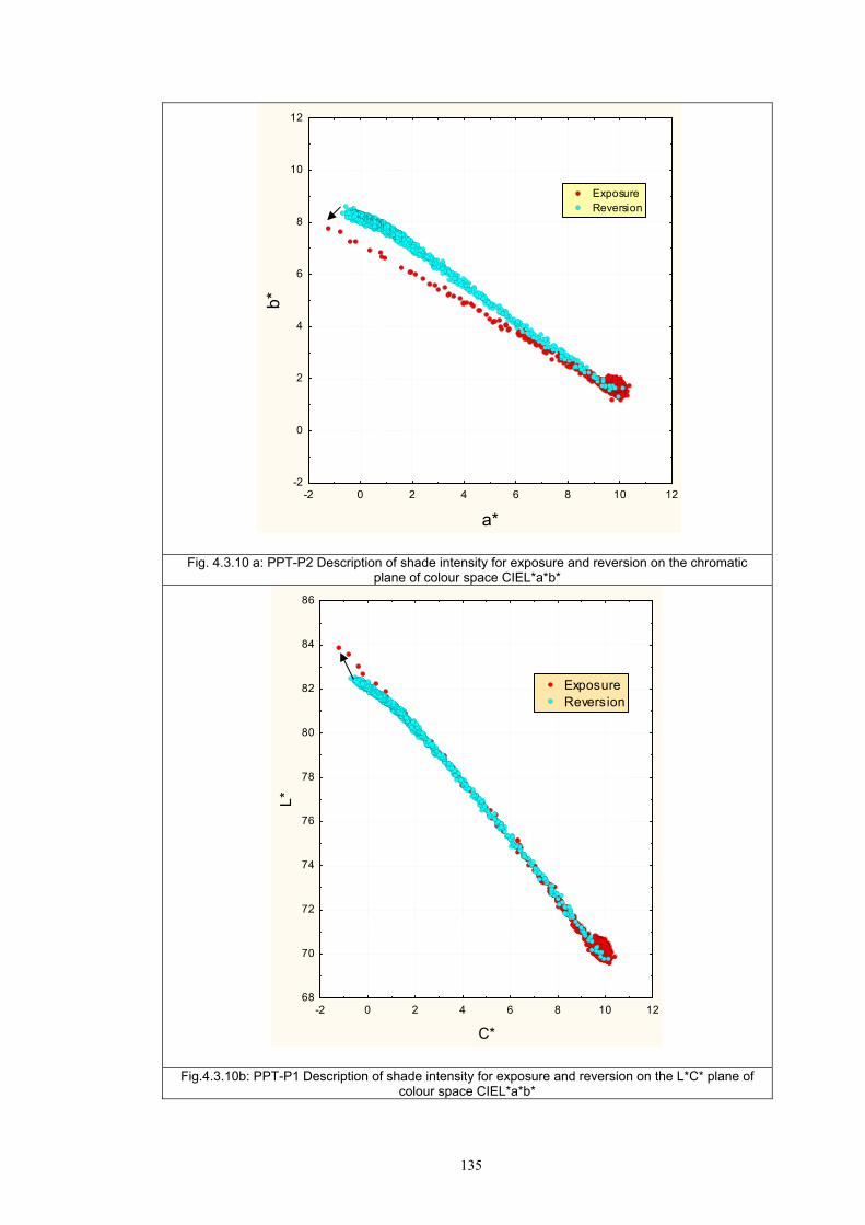
135

-2 0 2 4 6 8 10 12

a*

-2

0

2

4

6

8

10

12

b*

Exposure Reversion

Fig. 4.3.10 a: PPT-P2 Description of shade intensity for exposure and reversion on the chromatic plane of colour space CIEL*a*b*

-2 0 2 4 6 8 10 12

C*

68

70

72

74

76

78

80

82

84

86

L*

ExposureReversion

Fig.4.3.10b: PPT-P1 Description of shade intensity for exposure and reversion on the L*C* plane of colour space CIEL*a*b*

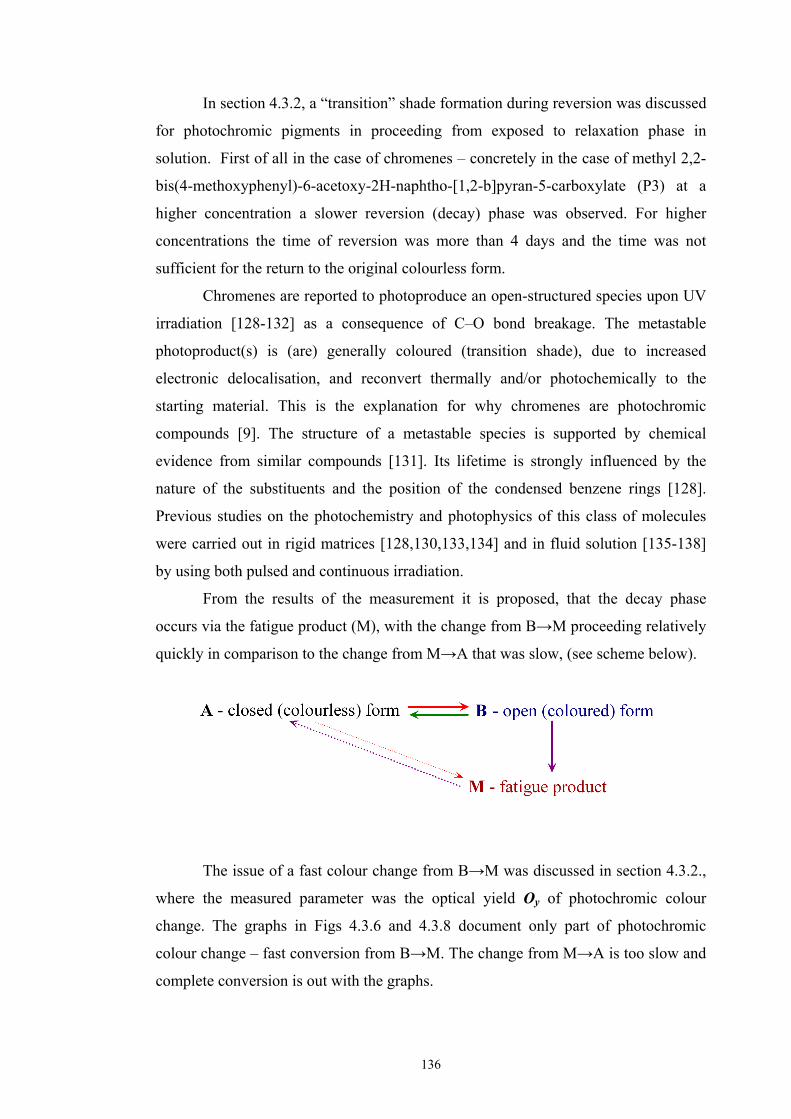
136

In section 4.3.2, a “transition” shade formation during reversion was discussed

for photochromic pigments in proceeding from exposed to relaxation phase in

solution. First of all in the case of chromenes – concretely in the case of methyl 2,2-

bis(4-methoxyphenyl)-6-acetoxy-2H-naphtho-[1,2-b]pyran-5-carboxylate (P3) at a

higher concentration a slower reversion (decay) phase was observed. For higher

concentrations the time of reversion was more than 4 days and the time was not

sufficient for the return to the original colourless form.

Chromenes are reported to photoproduce an open-structured species upon UV

irradiation [128-132] as a consequence of C–O bond breakage. The metastable

photoproduct(s) is (are) generally coloured (transition shade), due to increased

electronic delocalisation, and reconvert thermally and/or photochemically to the

starting material. This is the explanation for why chromenes are photochromic

compounds [9]. The structure of a metastable species is supported by chemical

evidence from similar compounds [131]. Its lifetime is strongly influenced by the

nature of the substituents and the position of the condensed benzene rings [128].

Previous studies on the photochemistry and photophysics of this class of molecules

were carried out in rigid matrices [128,130,133,134] and in fluid solution [135-138]

by using both pulsed and continuous irradiation.

From the results of the measurement it is proposed, that the decay phase

occurs via the fatigue product (M), with the change from B→M proceeding relatively

quickly in comparison to the change from M→A that was slow, (see scheme below).

The issue of a fast colour change from B→M was discussed in section 4.3.2.,

where the measured parameter was the optical yield Oy of photochromic colour

change. The graphs in Figs 4.3.6 and 4.3.8 document only part of photochromic

colour change – fast conversion from B→M. The change from M→A is too slow and

complete conversion is out with the graphs.

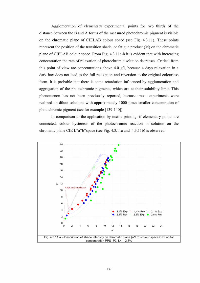
137

Agglomeration of elementary experimental points for two thirds of the

distance between the B and A forms of the measured photochromic pigment is visible

on the chromatic plane of CIELAB colour space (see Fig. 4.3.11). These points

represent the position of the transition shade, or fatigue product (M) on the chromatic

plane of CIELAB colour space. From Fig. 4.3.11a-b it is evident that with increasing

concentration the rate of relaxation of photochromic solution decreases. Critical from

this point of view are concentrations above 4.0 g/l, because 4 days relaxation in a

dark box does not lead to the full relaxation and reversion to the original colourless

form. It is probable that there is some retardation influenced by agglomeration and

aggregation of the photochromic pigments, which are at their solubility limit. This

phenomenon has not been previously reported, because most experiments were

realized on dilute solutions with approximately 1000 times smaller concentration of

photochromic pigment (see for example [139-140]).

In comparison to the application by textile printing, if elementary points are

connected, colour hysteresis of the photochromic reaction in solution on the

chromatic plane CIE L*a*b*space (see Fig. 4.3.11a and 4.3.11b) is observed.

0 2 4 6 8 10 12 14 16 18 20 22 24

a*

0

2

4

6

8

10

12

14

16

18

20

22

24

b*

1,4% Exp 1,4% Rev 2,1% Exp 2,1% Rev 2,8% Exp 2,8% Rev

After 2 days relaxation

Fig. 4.3.11 a – Description of shade intensity on chromatic plane (a*/ b*) colour space CIELab for

concentration PPS- P3 1.4 – 2.8%

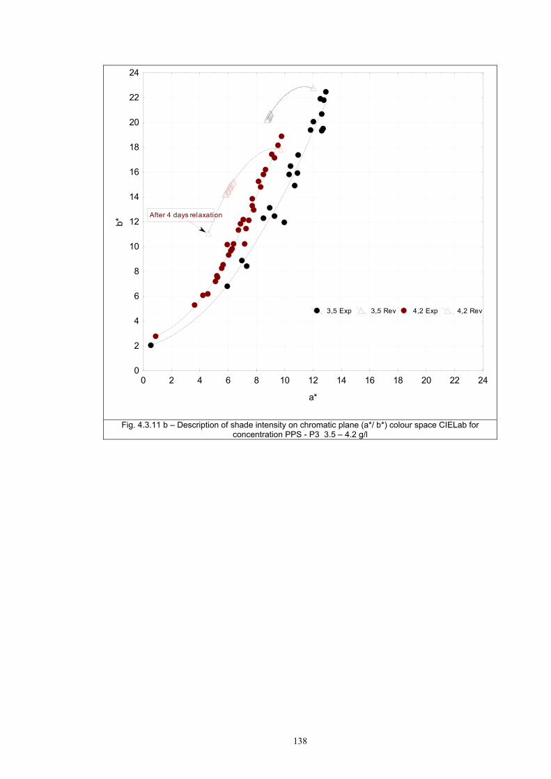
138

0 2 4 6 8 10 12 14 16 18 20 22 24

a*

0

2

4

6

8

10

12

14

16

18

20

22

24

b*

After 4 days relaxation

3,5 Exp 3,5 Rev 4,2 Exp 4,2 Rev

Fig. 4.3.11 b – Description of shade intensity on chromatic plane (a*/ b*) colour space CIELab for concentration PPS - P3 3.5 – 4.2 g/l

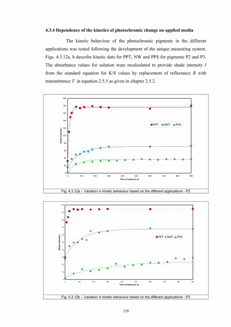
139

4.3.4 Dependence of the kinetics of photochromic change on applied media

The kinetic behaviour of the photochromic pigments in the different

applications was tested following the development of the unique measuring system.

Figs. 4.3.12a, b describe kinetic data for PPT, NW and PPS for pigments P2 and P3.

The absorbance values for solution were recalculated to provide shade intensity I

from the standard equation for K/S values by replacement of reflectance R with

transmittance T in equation 2.5.5 as given in chapter 2.5.2.

0

20

40

60

80

100

120

140

160

180

200

0 100 200 300 400 500 600 700 800 900

Time of exposure /s/

Shad

e In

tens

ity I

PPT NWT PPS

Fig. 4.3.12a – Variation in kinetic behaviour based on the different applications - P2

0

10

20

30

40

50

60

70

80

90

100

0 100 200 300 400 500 600 700 800 900

Time of exposure /s/

Shad

e in

tens

ity I

PPT NWT PPS

Fig. 4.3.12b – Variation in kinetic behaviour based on the different applications - P3

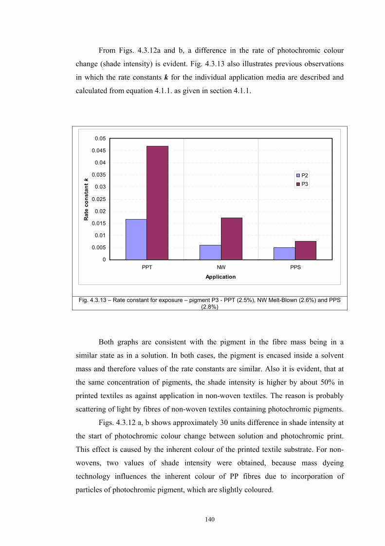
140

From Figs. 4.3.12a and b, a difference in the rate of photochromic colour

change (shade intensity) is evident. Fig. 4.3.13 also illustrates previous observations

in which the rate constants k for the individual application media are described and

calculated from equation 4.1.1. as given in section 4.1.1.

0

0.005

0.01

0.015

0.02

0.025

0.03

0.035

0.04

0.045

0.05

PPT NW PPS

Application

Rat

e co

nsta

nt k

P2P3

Fig. 4.3.13 – Rate constant for exposure – pigment P3 - PPT (2.5%), NW Melt-Blown (2.6%) and PPS (2.8%)

Both graphs are consistent with the pigment in the fibre mass being in a

similar state as in a solution. In both cases, the pigment is encased inside a solvent

mass and therefore values of the rate constants are similar. Also it is evident, that at

the same concentration of pigments, the shade intensity is higher by about 50% in

printed textiles as against application in non-woven textiles. The reason is probably

scattering of light by fibres of non-woven textiles containing photochromic pigments.

Figs. 4.3.12 a, b shows approximately 30 units difference in shade intensity at

the start of photochromic colour change between solution and photochromic print.

This effect is caused by the inherent colour of the printed textile substrate. For non-

wovens, two values of shade intensity were obtained, because mass dyeing

technology influences the inherent colour of PP fibres due to incorporation of

particles of photochromic pigment, which are slightly coloured.

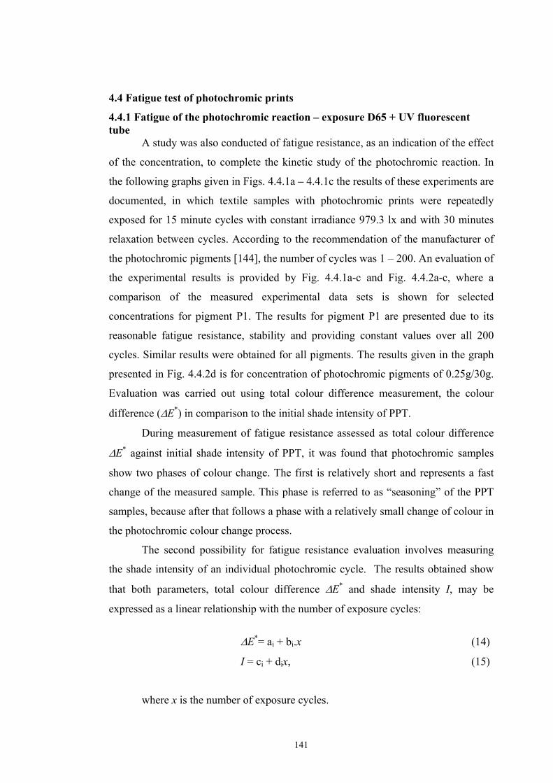
141

4.4 Fatigue test of photochromic prints

4.4.1 Fatigue of the photochromic reaction – exposure D65 + UV fluorescent tube A study was also conducted of fatigue resistance, as an indication of the effect

of the concentration, to complete the kinetic study of the photochromic reaction. In

the following graphs given in Figs. 4.4.1a – 4.4.1c the results of these experiments are

documented, in which textile samples with photochromic prints were repeatedly

exposed for 15 minute cycles with constant irradiance 979.3 lx and with 30 minutes

relaxation between cycles. According to the recommendation of the manufacturer of

the photochromic pigments [144], the number of cycles was 1 – 200. An evaluation of

the experimental results is provided by Fig. 4.4.1a-c and Fig. 4.4.2a-c, where a

comparison of the measured experimental data sets is shown for selected

concentrations for pigment P1. The results for pigment P1 are presented due to its

reasonable fatigue resistance, stability and providing constant values over all 200

cycles. Similar results were obtained for all pigments. The results given in the graph

presented in Fig. 4.4.2d is for concentration of photochromic pigments of 0.25g/30g.

Evaluation was carried out using total colour difference measurement, the colour

difference (ΔE*) in comparison to the initial shade intensity of PPT.

During measurement of fatigue resistance assessed as total colour difference

ΔE* against initial shade intensity of PPT, it was found that photochromic samples

show two phases of colour change. The first is relatively short and represents a fast

change of the measured sample. This phase is referred to as “seasoning” of the PPT

samples, because after that follows a phase with a relatively small change of colour in

the photochromic colour change process.

The second possibility for fatigue resistance evaluation involves measuring

the shade intensity of an individual photochromic cycle. The results obtained show

that both parameters, total colour difference ΔE* and shade intensity I, may be

expressed as a linear relationship with the number of exposure cycles:

ΔE*= ai + bi.x (14)

I = ci + dix, (15)

where x is the number of exposure cycles.

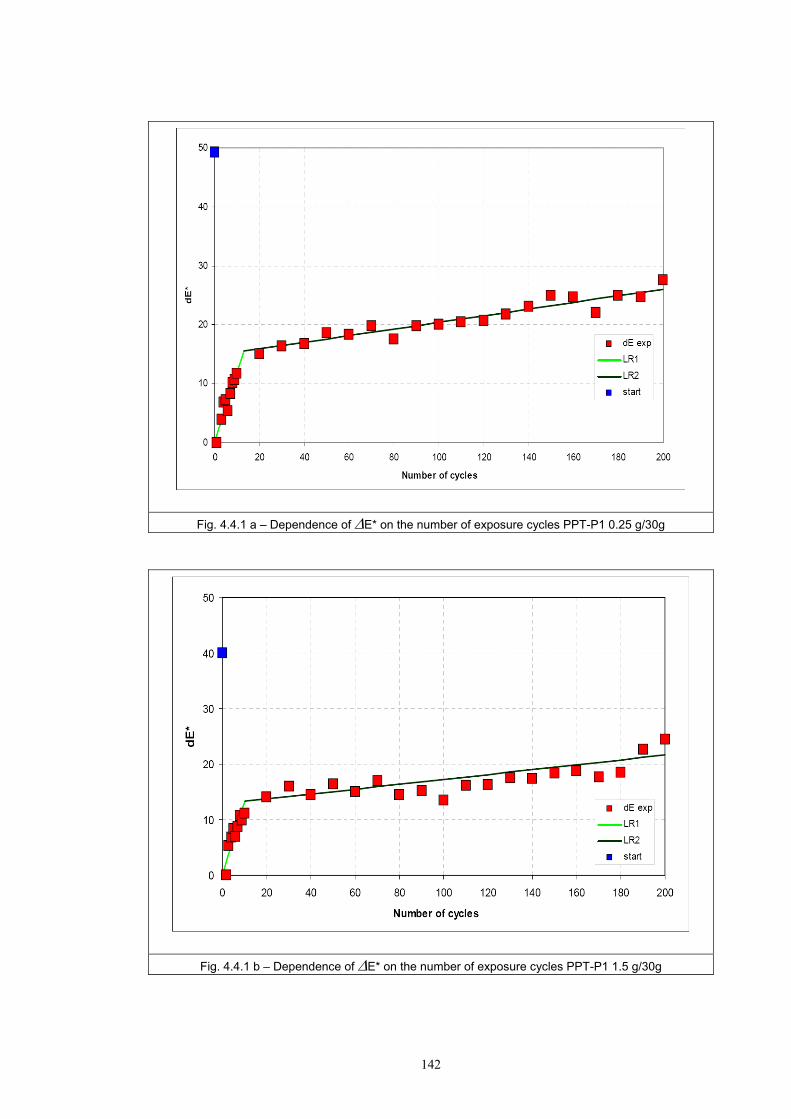
142

Fig. 4.4.1 a – Dependence of ΔE* on the number of exposure cycles PPT-P1 0.25 g/30g

Fig. 4.4.1 b – Dependence of ΔE* on the number of exposure cycles PPT-P1 1.5 g/30g

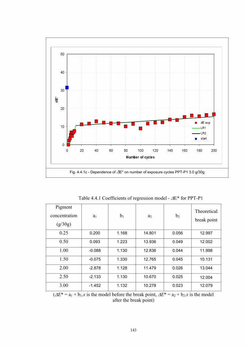
143

Fig. 4.4.1c - Dependence of ΔE* on number of exposure cycles PPT-P1 3.0 g/30g

Table 4.4.1 Coefficients of regression model - ΔE* for PPT-P1

Pigment

concentration

(g/30g)

a1 b1 a2 b2 Theoretical

break point

0.25 0.200 1.168 14.801 0.056 12.997

0.50 0.093 1.223 13.936 0.049 12.002

1.00 -0.088 1.130 12.836 0.044 11.998

1.50 -0.075 1.330 12.765 0.045 10.131

2.00 -2.878 1.128 11.479 0.026 13.044

2.50 -2.133 1.130 10.670 0.025 12.004 3.00 -1.452 1.132 10.278 0.023 12.079

(ΔE* = a1 + b1.x is the model before the break point, ΔE* = a2 + b2.x is the model after the break point)

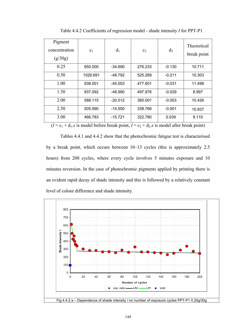
144

Table 4.4.2 Coefficients of regression model - shade intensity I for PPT-P1

Pigment

concentration

(g/30g)

c1 d1 c2 d2 Theoretical

break point

0.25 650.000 -34.690 276.233 -0.130 10.711

0.50 1026.691 -48.792 525.289 -0.211 10.303

1.00 938.001 -40.003 477.601 -0.031 11.498

1.50 937.092 -48.990 497.976 -0.029 8.997

2.00 588.115 -20.012 380.001 -0.003 10.426

2.50 505.990 -14.500 338.766 -0.001 10.937 3.00 466.783 -15.721 322.780 0.039 9.110

(I = c1 + d1.x is model before break point, I = c2 + d2.x is model after break point)

Tables 4.4.1 and 4.4.2 show that the photochromic fatigue test is characterised

by a break point, which occurs between 10–13 cycles (this is approximately 2.5

hours) from 200 cycles, where every cycle involves 5 minutes exposure and 10

minutes reversion. In the case of photochromic pigments applied by printing there is

an evident rapid decay of shade intensity and this is followed by a relatively constant

level of colour difference and shade intensity.

Fig.4.4.2 a – Dependence of shade intensity I on number of exposure cycles PPT-P1 0.25g/30g

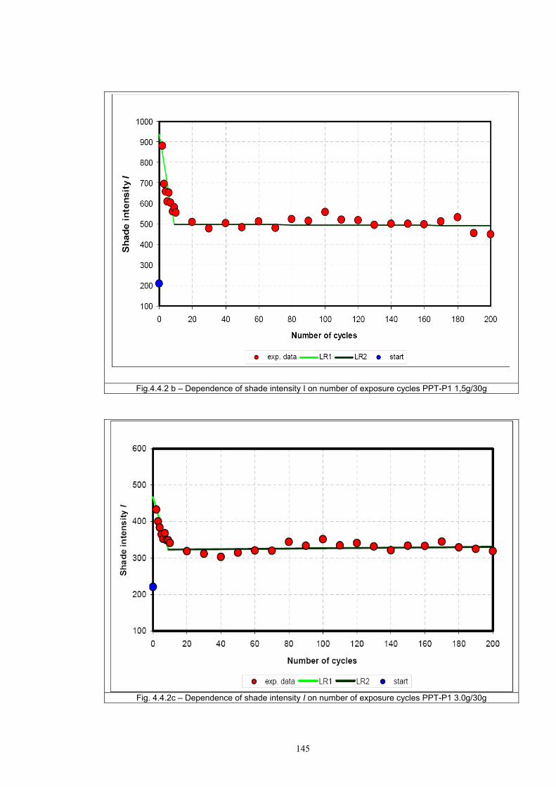
145

Fig.4.4.2 b – Dependence of shade intensity I on number of exposure cycles PPT-P1 1,5g/30g

Fig. 4.4.2c – Dependence of shade intensity I on number of exposure cycles PPT-P1 3.0g/30g

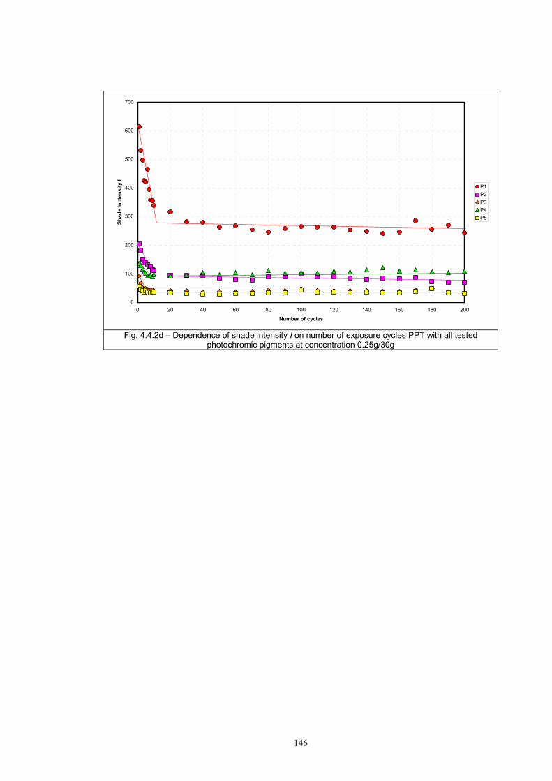
146

0

100

200

300

400

500

600

700

0 20 40 60 80 100 120 140 160 180 200

Number of cycles

Shad

e In

nten

sity

I

P1P2P3P4P5

Fig. 4.4.2d – Dependence of shade intensity I on number of exposure cycles PPT with all tested photochromic pigments at concentration 0.25g/30g

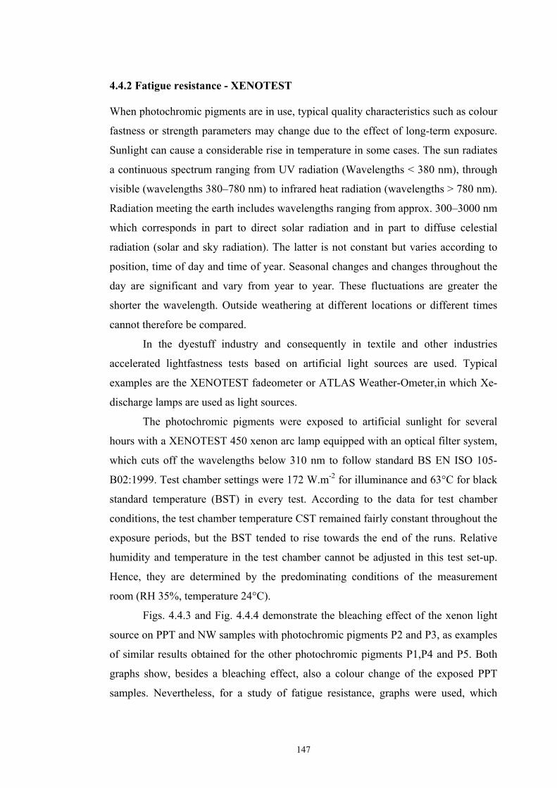
147

4.4.2 Fatigue resistance - XENOTEST

When photochromic pigments are in use, typical quality characteristics such as colour

fastness or strength parameters may change due to the effect of long-term exposure.

Sunlight can cause a considerable rise in temperature in some cases. The sun radiates

a continuous spectrum ranging from UV radiation (Wavelengths < 380 nm), through

visible (wavelengths 380–780 nm) to infrared heat radiation (wavelengths > 780 nm).

Radiation meeting the earth includes wavelengths ranging from approx. 300–3000 nm

which corresponds in part to direct solar radiation and in part to diffuse celestial

radiation (solar and sky radiation). The latter is not constant but varies according to

position, time of day and time of year. Seasonal changes and changes throughout the

day are significant and vary from year to year. These fluctuations are greater the

shorter the wavelength. Outside weathering at different locations or different times

cannot therefore be compared.

In the dyestuff industry and consequently in textile and other industries

accelerated lightfastness tests based on artificial light sources are used. Typical

examples are the XENOTEST fadeometer or ATLAS Weather-Ometer,in which Xe-

discharge lamps are used as light sources.

The photochromic pigments were exposed to artificial sunlight for several

hours with a XENOTEST 450 xenon arc lamp equipped with an optical filter system,

which cuts off the wavelengths below 310 nm to follow standard BS EN ISO 105-

B02:1999. Test chamber settings were 172 W.m-2 for illuminance and 63°C for black

standard temperature (BST) in every test. According to the data for test chamber

conditions, the test chamber temperature CST remained fairly constant throughout the

exposure periods, but the BST tended to rise towards the end of the runs. Relative

humidity and temperature in the test chamber cannot be adjusted in this test set-up.

Hence, they are determined by the predominating conditions of the measurement

room (RH 35%, temperature 24°C).

Figs. 4.4.3 and Fig. 4.4.4 demonstrate the bleaching effect of the xenon light

source on PPT and NW samples with photochromic pigments P2 and P3, as examples

of similar results obtained for the other photochromic pigments P1,P4 and P5. Both

graphs show, besides a bleaching effect, also a colour change of the exposed PPT

samples. Nevertheless, for a study of fatigue resistance, graphs were used, which

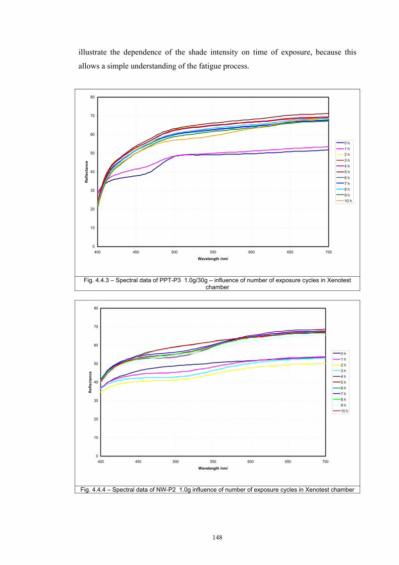
148

illustrate the dependence of the shade intensity on time of exposure, because this

allows a simple understanding of the fatigue process.

0

10

20

30

40

50

60

70

80

400 450 500 550 600 650 700

Wavelength /nm/

Ref

lect

ance

0 h1 h2 h3 h4 h5 h6 h7 h8 h9 h10 h

Fig. 4.4.3 – Spectral data of PPT-P3 1.0g/30g – influence of number of exposure cycles in Xenotest chamber

0

10

20

30

40

50

60

70

80

400 450 500 550 600 650 700

Wavelength /nm/

Ref

lect

ance

0 h1 h2 h3 h4 h5 h6 h7 h8 h9 h10 h

Fig. 4.4.4 – Spectral data of NW-P2 1.0g influence of number of exposure cycles in Xenotest chamber

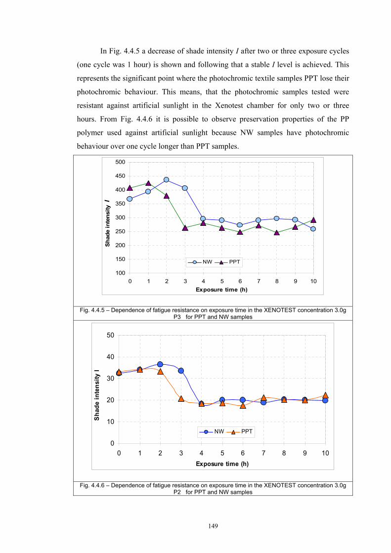
149

In Fig. 4.4.5 a decrease of shade intensity I after two or three exposure cycles

(one cycle was 1 hour) is shown and following that a stable I level is achieved. This

represents the significant point where the photochromic textile samples PPT lose their

photochromic behaviour. This means, that the photochromic samples tested were

resistant against artificial sunlight in the Xenotest chamber for only two or three

hours. From Fig. 4.4.6 it is possible to observe preservation properties of the PP

polymer used against artificial sunlight because NW samples have photochromic

behaviour over one cycle longer than PPT samples.

100

150

200

250

300

350

400

450

500

0 1 2 3 4 5 6 7 8 9 10Exposure time (h)

Shad

e in

tens

ity I

NW PPT

Fig. 4.4.5 – Dependence of fatigue resistance on exposure time in the XENOTEST concentration 3.0g P3 for PPT and NW samples

0

10

20

30

40

50

0 1 2 3 4 5 6 7 8 9 10Exposure time (h)

Shad

e in

tens

ity I

NW PPT

Fig. 4.4.6 – Dependence of fatigue resistance on exposure time in the XENOTEST concentration 3.0g P2 for PPT and NW samples

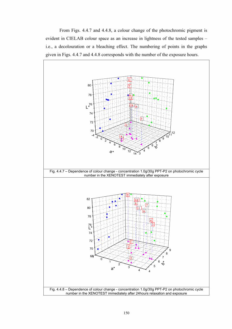
150

From Figs. 4.4.7 and 4.4.8, a colour change of the photochromic pigment is

evident in CIELAB colour space as an increase in lightness of the tested samples –

i.e., a decolouration or a bleaching effect. The numbering of points in the graphs

given in Figs. 4.4.7 and 4.4.8 corresponds with the number of the exposure hours.

-4 -2 0 2 46

810

1214 3

45

67

89

10111270

72

74

76

78

80

1

11

7

10

2

698

5

34

L*

b*a*

Fig. 4.4.7 – Dependence of colour change - concentration 1.0g/30g PPT-P2 on photochromic cycle number in the XENOTEST immediately after exposure

-10

12

34 4

56

78

9

68

70

72

74

76

78

80

829

10

11

87

6

1

45

3

2

L*

b*

a*

Fig. 4.4.8 – Dependence of colour change - concentration 1.0g/30g PPT-P2 on photochromic cycle number in the XENOTEST immediately after 24hours relaxation and exposure

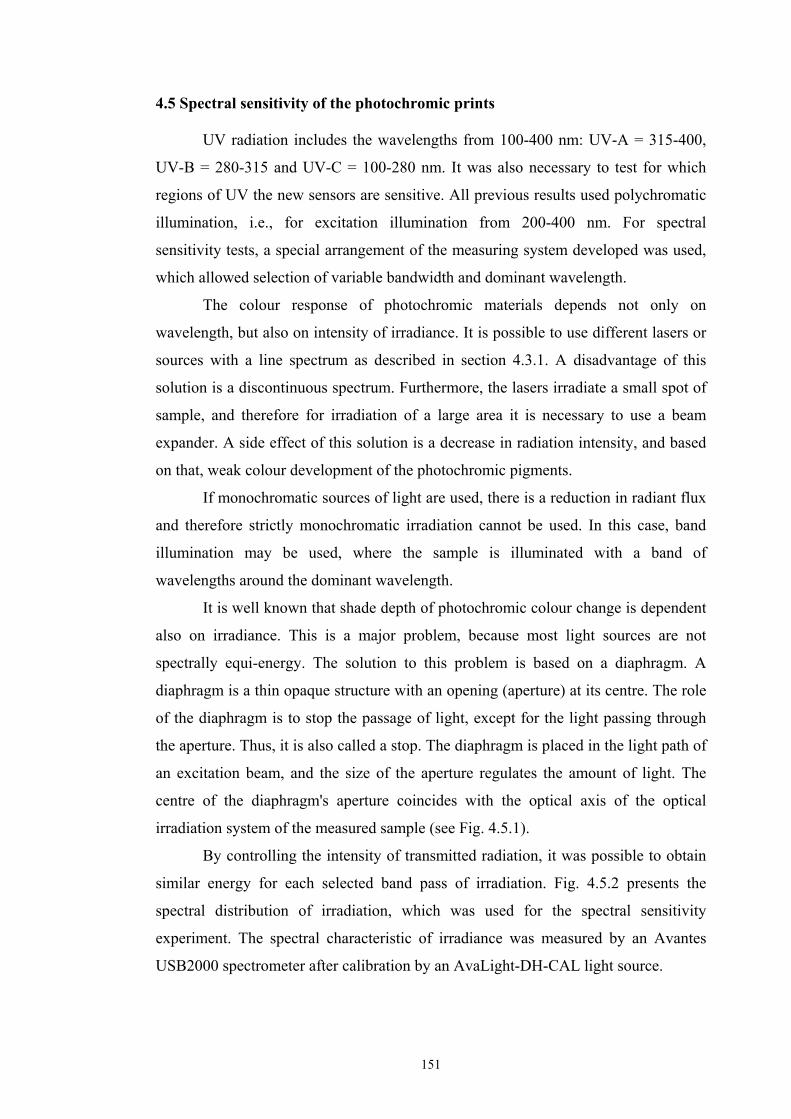
151

4.5 Spectral sensitivity of the photochromic prints

UV radiation includes the wavelengths from 100-400 nm: UV-A = 315-400,

UV-B = 280-315 and UV-C = 100-280 nm. It was also necessary to test for which

regions of UV the new sensors are sensitive. All previous results used polychromatic

illumination, i.e., for excitation illumination from 200-400 nm. For spectral

sensitivity tests, a special arrangement of the measuring system developed was used,

which allowed selection of variable bandwidth and dominant wavelength.

The colour response of photochromic materials depends not only on

wavelength, but also on intensity of irradiance. It is possible to use different lasers or

sources with a line spectrum as described in section 4.3.1. A disadvantage of this

solution is a discontinuous spectrum. Furthermore, the lasers irradiate a small spot of

sample, and therefore for irradiation of a large area it is necessary to use a beam

expander. A side effect of this solution is a decrease in radiation intensity, and based

on that, weak colour development of the photochromic pigments.

If monochromatic sources of light are used, there is a reduction in radiant flux

and therefore strictly monochromatic irradiation cannot be used. In this case, band

illumination may be used, where the sample is illuminated with a band of

wavelengths around the dominant wavelength.

It is well known that shade depth of photochromic colour change is dependent

also on irradiance. This is a major problem, because most light sources are not

spectrally equi-energy. The solution to this problem is based on a diaphragm. A

diaphragm is a thin opaque structure with an opening (aperture) at its centre. The role

of the diaphragm is to stop the passage of light, except for the light passing through

the aperture. Thus, it is also called a stop. The diaphragm is placed in the light path of

an excitation beam, and the size of the aperture regulates the amount of light. The

centre of the diaphragm's aperture coincides with the optical axis of the optical

irradiation system of the measured sample (see Fig. 4.5.1).

By controlling the intensity of transmitted radiation, it was possible to obtain

similar energy for each selected band pass of irradiation. Fig. 4.5.2 presents the

spectral distribution of irradiation, which was used for the spectral sensitivity

experiment. The spectral characteristic of irradiance was measured by an Avantes

USB2000 spectrometer after calibration by an AvaLight-DH-CAL light source.

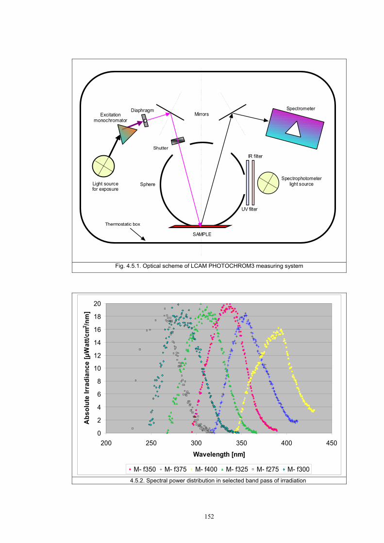
152

Shutter

Thermostatic box

Light sourcefor exposure

Spectrophotometerlight source

IR filter

SAMPLE

Sphere

SpectrometerMirrors

UV filter

Excitationmonochromator

Diaphragm

Fig. 4.5.1. Optical scheme of LCAM PHOTOCHROM3 measuring system

0

2

4

6

8

10

12

14

16

18

20

200 250 300 350 400 450

Wavelength [nm]

Abs

olut

e Irr

adia

nce

[µW

att/c

m2 /n

m]

M- f350 M- f375 M- f400 M- f325 M- f275 M- f300 4.5.2. Spectral power distribution in selected band pass of irradiation

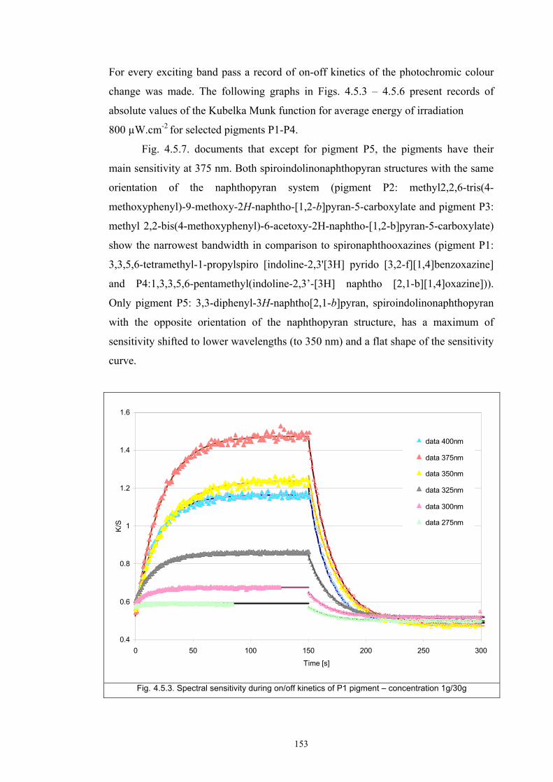
153

For every exciting band pass a record of on-off kinetics of the photochromic colour

change was made. The following graphs in Figs. 4.5.3 – 4.5.6 present records of

absolute values of the Kubelka Munk function for average energy of irradiation

800 µW.cm-2 for selected pigments P1-P4.

Fig. 4.5.7. documents that except for pigment P5, the pigments have their

main sensitivity at 375 nm. Both spiroindolinonaphthopyran structures with the same

orientation of the naphthopyran system (pigment P2: methyl2,2,6-tris(4-

methoxyphenyl)-9-methoxy-2H-naphtho-[1,2-b]pyran-5-carboxylate and pigment P3:

methyl 2,2-bis(4-methoxyphenyl)-6-acetoxy-2H-naphtho-[1,2-b]pyran-5-carboxylate)

show the narrowest bandwidth in comparison to spironaphthooxazines (pigment P1:

3,3,5,6-tetramethyl-1-propylspiro [indoline-2,3'[3H] pyrido [3,2-f][1,4]benzoxazine]

and P4:1,3,3,5,6-pentamethyl(indoline-2,3’-[3H] naphtho [2,1-b][1,4]oxazine])).

Only pigment P5: 3,3-diphenyl-3H-naphtho[2,1-b]pyran, spiroindolinonaphthopyran

with the opposite orientation of the naphthopyran structure, has a maximum of

sensitivity shifted to lower wavelengths (to 350 nm) and a flat shape of the sensitivity

curve.

0.4

0.6

0.8

1

1.2

1.4

1.6

0 50 100 150 200 250 300

Time [s]

K/S

data 400nm

data 375nm

data 350nm

data 325nm

data 300nm

data 275nm

Fig. 4.5.3. Spectral sensitivity during on/off kinetics of P1 pigment – concentration 1g/30g

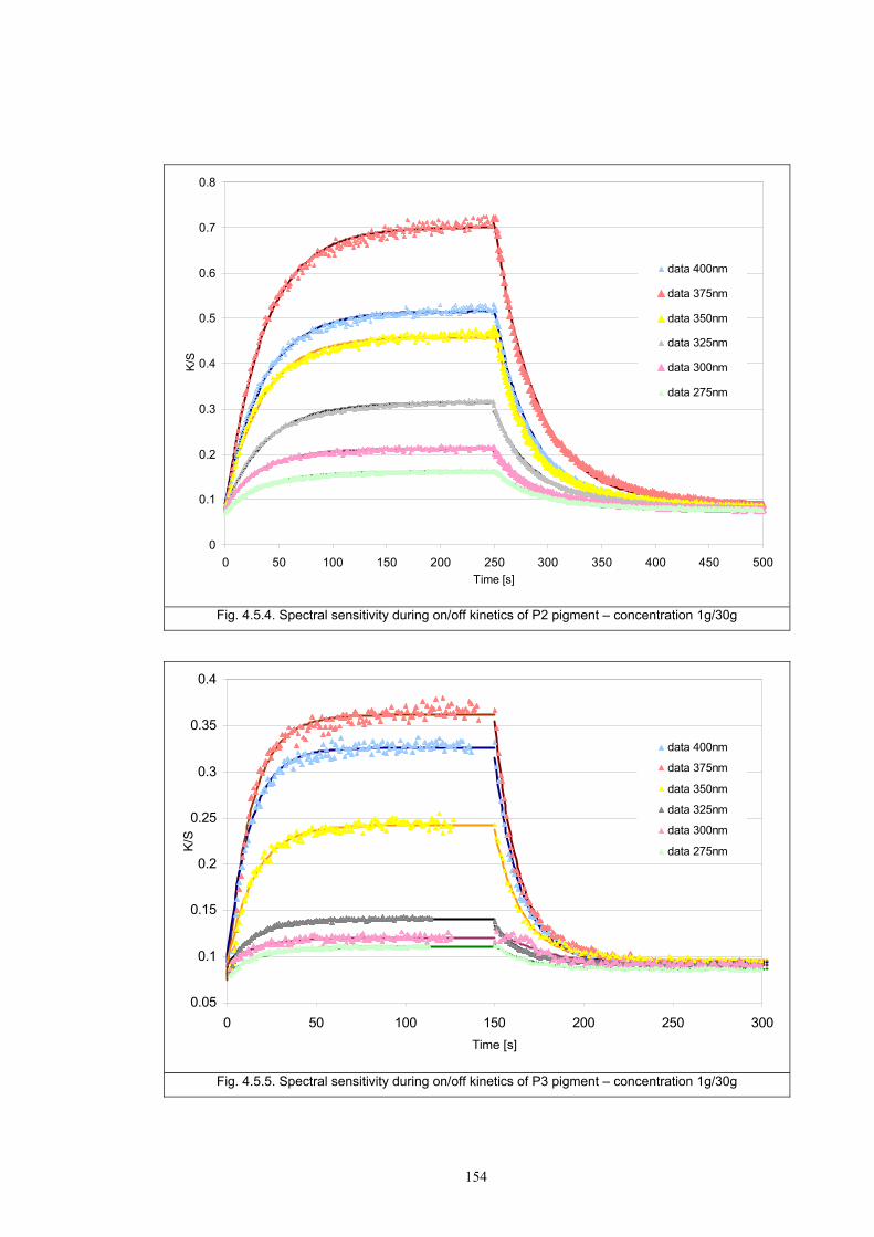
154

0

0.1

0.2

0.3

0.4

0.5

0.6

0.7

0.8

0 50 100 150 200 250 300 350 400 450 500Time [s]

K/S

data 400nm

data 375nm

data 350nm

data 325nm

data 300nm

data 275nm

Fig. 4.5.4. Spectral sensitivity during on/off kinetics of P2 pigment – concentration 1g/30g

0.05

0.1

0.15

0.2

0.25

0.3

0.35

0.4

0 50 100 150 200 250 300Time [s]

K/S

data 400nm

data 375nm

data 350nm

data 325nm

data 300nm

data 275nm

Fig. 4.5.5. Spectral sensitivity during on/off kinetics of P3 pigment – concentration 1g/30g

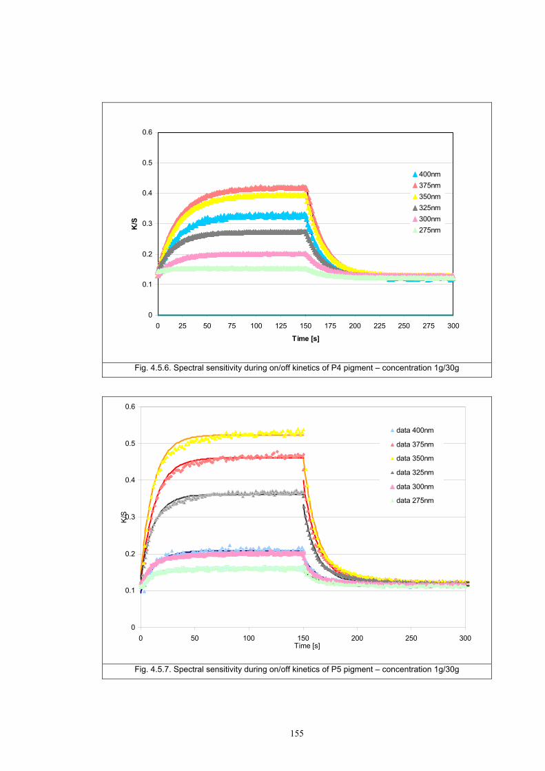
155

0

0.1

0.2

0.3

0.4

0.5

0.6

0 25 50 75 100 125 150 175 200 225 250 275 300

Time [s]

K/S

400nm375nm350nm325nm300nm275nm

Fig. 4.5.6. Spectral sensitivity during on/off kinetics of P4 pigment – concentration 1g/30g

0

0.1

0.2

0.3

0.4

0.5

0.6

0 50 100 150 200 250 300Time [s]

K/S

data 400nm

data 375nm

data 350nm

data 325nm

data 300nm

data 275nm

Fig. 4.5.7. Spectral sensitivity during on/off kinetics of P5 pigment – concentration 1g/30g

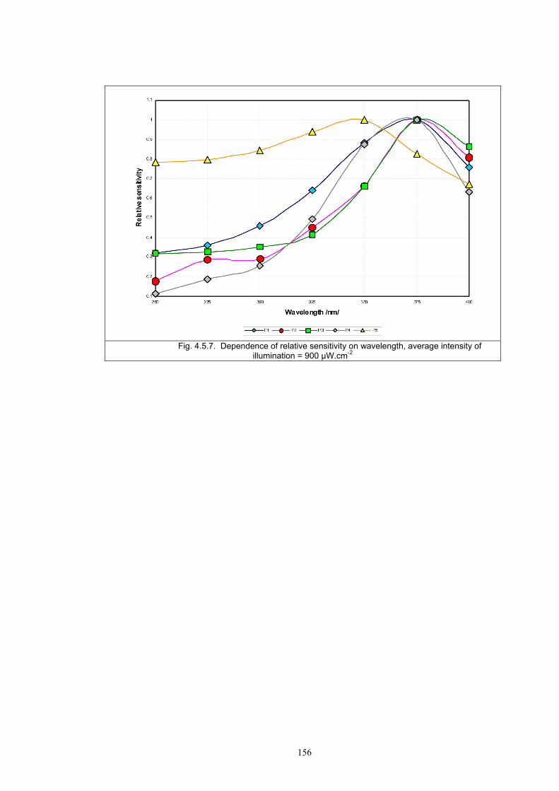
156

Fig. 4.5.7. Dependence of relative sensitivity on wavelength, average intensity of illumination = 900 µW.cm-2

157

Chapter 5 CONCLUSION

This chapter discusses how the individual aims of the project set out in

Chapter 1 have been addressed, as well as providing a summary of the main

conclusions and some suggestions for how the research might be progressed into the

future. The main goal of this PhD thesis was a kinetic study of the photochromic

colour change and a study of the dependence of colour change on the intensity of

illumination E. This study has included an evaluation of both exposure and reversion

of the photochromic reaction for selected pigments in different media. For this

research two spirooxazine and three naphthopyrans structures were selected. Their

structures are described in section 3.2 (materials). From the results obtained from the

on-line measurement method presented in section 4.1(screen –printed photochromic

textiles), section 4.2 (non woven textiles containing photochromic pigments) and

section 4.3 (photochromic solution), a first order kinetic model of photochromic

colour change was established. The basis of the first order kinetic model is described

in sections 2.5.4 and 2.5.5. The kinetic study and experimental data sets obtained

clearly verify the first order kinetic model for the all applications tested using

photochromic pigments (PPT, NW and PPS). Based on this kinetic model the

construction of an optical yield Oy formula for the reaction of photochromic textile

was proposed:

( ) ( )1 2

1

0 0 00

E R

t tk t k t

t

Oy I I I e dt I I I e dt− −∞ ∞ ∞= + − − + −∫ ∫

As a result of experimental observation and the calculation of the

dependence of optical yield, Oy, on intensity of illumination E, it was found that the

optical yield of the photochromic reaction Oy depends linearly on the intensity of

illumination E, as is documented in Figs. 4.1.14 a-b (for photochromic textile prints),

Figs. 4.2.2a-b and 4.2.3a-b (for non wovens).

Thus a major contribution of this research to the study of photochromism is

the discovery of a correlation between the optical yield of the photochromic reaction

Oy and irradiance – the intensity of illumination. This correlation has the potential to

be used for calibration of potential smart textile sensors with photochromic pigments

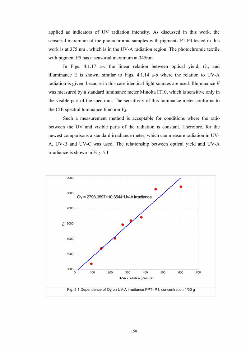
158

applied as indicators of UV radiation intensity. As discussed in this work, the

sensorial maximum of the photochromic samples with pigments P1-P4 tested in this

work is at 375 nm , which is in the UV-A radiation region. The photochromic textile

with pigment P5 has a sensorial maximum at 345nm.

In Figs. 4.1.17 a-c the linear relation between optical yield, Oy, and

illuminance E is shown, similar to Figs. 4.1.14 a-b where the relation to UV-A

radiation is given, because in this case identical light sources are used. Illuminance E

was measured by a standard luminance meter Minolta IT10, which is sensitive only in

the visible part of the spectrum. The sensitivity of this luminance meter conforms to

the CIE spectral luminance function Vλ.

Such a measurement method is acceptable for conditions where the ratio

between the UV and visible parts of the radiation is constant. Therefore, for the

newest comparisons a standard irradiance meter, which can measure radiation in UV-

A, UV-B and UV-C was used. The relationship between optical yield and UV-A

irradiance is shown in Fig. 5.1

0 100 200 300 400 500 600 700

UV-A irradiation (µW/cm2)

3000

4000

5000

6000

7000

8000

9000

Oy

Oy = 2793,0597+10,3544*UV-A irradiance

Fig. 5.1 Dependence of Oy on UV-A irradiance PPT- P1, concentration 1/30 g

159

The investigation of the kinetic behaviour of photochromic textiles, which is

discussed in section 4.1.1, show that for the exposure period the half-life of colour

change, t1/2, is practically independent of pigment concentration. This means that the

time of colour change during exposure is not influenced by increased concentration of

the pigments. During reversion of photochromic colour change a slight decrease of

half-life, t1/2, with increasing photochromic pigment concentration was found. A

strong negative linear relationship was found between half-life and irradiance for all

photochromic pigments.

Also in this research, large differences were observed between reversion rates

of the photochromic pigment applied by printing compared with solution. Differences

between solution and non-woven textiles are relatively small as illustrated graphically

in Fig. 4.3.13. This observation is consistent with the hypothesis that a photochromic

pigment incorporated in the mass of PP fibres is in a similar state as in a saturated

cyclohexane solution. The photochromic pigment is encased inside a solvent mass

and values of the rate constants are therefore similar.

In this work, observation of a “transition” shade during reversion of

photochromic pigments from exposed to relaxation phase in solution was discussed.

For higher concentrations the time of reversion was more than 4 days (96 hours) and

the time was not sufficient for the return to the original colourless form. Distribution

of experimental points on the chromatic plane a*b* of CIELAB colour space

represents the position of the transitional shade from the position of fully relaxed

photochromic solution. From Figs. 4.3.11a-b it is evident that with an increase in

concentration the extent of relaxation of the photochromic solution is reduced. A

critical feature from this point of view is a concentration above 4.0 g/l, because 4

days relaxation in a dark box does not lead to full relaxation and reversion to the

original colourless form. A possible explanation is that there may be a retardation

influenced by agglomeration and aggregation of the photochromic pigments, which

are at their limit of solubility. This phenomenon has not been reported previously,

because most experiments have been realized on dilute solutions with a 1000 times

smaller concentration of photochromic pigment. It was found that for formation of the

transition state in saturated photochromic solutions only one exposure cycle sufficed.

This phenomenon is referred to as “photochromic colour memory” - PCM.

Compared to the photochromic solutions tested the effect of PCM on PPT was

160

minimal and the time necessary for full colour recovery was under 12 minutes.

Nevertheless, during the experiments 24 hour relaxation was used.

Furthermore, it was shown that the application medium affects the colour of

photochromic samples. In the applied textile media, there is a bathochromic spectral

shift and the fibres or fabrics had a yellowish colour before irradiation compared with

the “ideal” colourless transmittance in solvents. Simultaneously, this work

demonstrates that producing photochromic textiles by melt blown technology brings

no advantage in comparison to photochromic prints. On the contrary, mass dyeing

technology is severely complicated and has only one benefit – marginally higher light

fastness.

It is evident that the intensity of the photochromic response depends on the

spectral power distribution of the exciting light source used and the absorption

characteristics of the media used. The light source sensitivity study documents

differences in response from the range of photochromic pigments tested. The

pigments based on substituted naphthopyrans (P2 and P3) were more sensitive as

illustrated in Figs. 4.3.1 and 4.3.2. These properties are believed to be due in part to

the stability (lack of steric interactions) of the trans-quinoidal open form. This result

is consistent with the influence of molecular orientation in the naphthopyran isomers

(P5) as discussed in the literature [10, 36]. The other pigments tested were essentially

insensitive to these factors.

The study of photochromic response modulation with the incorporation of UV

absorbers shows that the extension of half-life of photochromic colour change caused

by UV absorbers decreases with irradiance intensity. Also differences in the

efficiency of the UV absorbers used were found, which is probably associated by

different absorption properties.

The next main task was the study of the spectral sensitivity of photochromic

textiles which showed that, except for pigment P5, the pigments tested have their

main sensitivity at 375 nm as demonstrated in Fig. 4.5.8. Both [1,2-b] pyrans

(pigments P2, P3) show narrower bandwidths in comparison to spirooxazines

(pigments P1, P4). Pigment P5, which is a [2,1-b] pyran structure and which behaves

smoothly in terms of relative spectral sensitivity shows that the orientation of the

naphtho group has a strong effect. Replacement of methoxyphenyl group in pigment

P2 by an acetoxy group in pigment P3 caused a difference in developed colour, but

not in spectral sensitivity.

161

With respect to photostability, a further conclusion in this thesis is a stepwise

linear trend of photochromic response decrease during fatigue resistance tests found

for photochromic textile prints PPT, compared with a simple linear decrease of

photochromic response for solutions, as has been previously reported in some articles

[113-115]. During the first 10 cycles a large decrease in photochromic response was

measured. This period is called “burning” of the photochromic system. Subsequently,

the photochromic response is relatively stable (see Figs. 4.4.2 a-c.). One possible

explanation for this phenomenon is the problem of low spectral sensitivity of shade

intensity I compared with colour difference ΔE*. A main reason is that the parameter

of shade intensity is calculated as the integral value under the curve given by the K/S

function.

In addition, an important outcome of this work is the development of a unique

measuring system allowing the measurement of spectrophotometric and colorimetric

values. This system is now used as prototype for measurement of photochromic and

thermochromic behaviour of different materials. Due the control of excitation light

source using a shutter it is possible to measure photochromic properties for one or

multiple cycles. This system also allows the measurement of the thermal sensitivity

of photochromic samples.

Based on this result, the possibility has been demonstrated in principle that

photochromic textiles can be applied for the preparation of a sensorial system, which

allows simple visual assessment of the amount of UV radiation incident on the

sample. This system can be designed for example as a simple rule scale, where for

comparison there is a constant coloured part made from UV stable pigments or

dyestuffs. Individual parts of the constant scale can be judged as having the same

colour as the photochromic part at a specific intensity of UV radiation. The observer

will be able to estimate the level of UV radiation corresponding to a colour match

between the photochromic colour changeable part and visual stable part of the textile

UV sensor. From the point of view of future work in the photochromic textile field,

optimisation of the photochromic pigment used especially in terms of fatigue

resistance and spectral sensitivity criteria will be important. In this thesis, the

photochromic pigments tested were sensitive in the UV - A part of the spectrum. It is

well known that the UV – B part of electromagnetic spectrum is the main cause of

cancerous problems. Therefore, photochromic pigments sensitive in the UV - B part

will have in the near future an important role in this research field.

162

The development of a unique measuring system provides a starting point for

the standardisation process for the measurement of colorimetric parameters of

photochromic materials. Today, the situation means that the results of photochromic

material properties are incomparable, when different light sources with different

spectral power distribution and radiation intensity are used. Therefore, it will be

necessary to discuss the question of light source specification, which should be used

for excitation of photochromic materials in the future.

163

References

[1] Xiaoming T., Smart fibres, fabrics and clothing, The Textile Institute,

Cambridge England (2001)

[2] Viková, M., Vik, M., Some Problems in Measurement of UV Protective

Textiles, The 3rd China International Wool Textile Conference, Xi’an China

26-28 Sep. 2002, p.635-638,

[3] Vanicek, K., Frei, T., Litynska, Z., Schmalwieser, A., UV- Index for the

public, COST-713 Action 1999

[4] Bernhard, G., Seckmeyer, G., The uncertainty of measurements of spectral

solar UV irradiance, J. Geophys. Res. 104 14321–45, (1999)

[5] Kiedron, P. W., Michalsky, J. J., Berndt, J. L., Harrison, L. C., Comparison of

spectral irradiance standards used to calibrate shortwave radiometers and

spectroradiometers, Appl. Opt. 38 2432–9, (1999)

[6] Gardiner, B.G., P.J. Kirsch, editors, Second European Intercomparison of

Ultraviolet Spectroradiometers, Air Pollution Research Report no. 38,

Commission of European Communities, Brussels, Belgium, 1993, 38, 67

[7] Groebner, J., Blumthaler, M., Kazadzis, S., Bais, A., Webb, A., Schreder, J.,

Seckmayer, G., Rembges, D. , Traveling reference spectroradiometer for

routine quality assurance of spectral solar ultraviolet irradiance

measurements, Applied Optics, Vol. 44, Issue 25, pp. 5321-5331 (2005)

[8] Slaper, H., Reinen, H.A.J.M., Blumthater, M., Huber, M., Kuik, F.,

Comparison ground-level spectrally resolved solar UV measurements usin

various instruments: A technique resolving effects of wavelength shift and slit

width, Geophys. Res. Lett. 22 2721–4, (1995)

[9] Crano, J. C. & Guglielmetti, R. J., editors, Organic Photochromic and

Thermochromic compounds, Vol 1: Main photochromic families, Plenum

Press, New York (1999).

[10] Brown, G. H., editor, Techniques of Chemistry, Vol.III, Photochromism, John

Wiley & Sons, New York, First edition (1971).

[11] El'tsov, A.V., editor, Organic Photochromes, Plenum Publishing Corporation,

New York (1990).

[12] Stewart, J. J. P., editor, Semiempirical molecular orbital methods. In: Reviews

in Computational Chemistry, 1, VCH New York, 45-81 (1990).

164

[13] Mc Ardle C. B., editor, Applied Photochromic Polymer Systems, Blackie,

New York, (1992)

[14] Krongauz, V. , Weiss, V. , Berkovic, G., Spiropyrans and Spirooxazines for

Memories and Switches, Chem. Rev., 100 1741 (2000).

[15] Hurst, J. K., Giertz, K., Khairutdinov, R. F., Voloshina, E. N., Voloshina, N.

A., Minkin, V. I. , Photochromism of Spirooxazines in Homogeneous Solution

and Phospholipid Liposomes, J. Am. Chem. Soc., 1998, 120 (49), pp 12707–

12713 (1998).

[16] Bowen, C. M., Winkler, J. D., Michelet, V., Photodynamic Fluorescent Metal

Ion Sensors with Parts per Billion Sensitivity, J. Am. Chem. Soc., 1998, 120

(13), pp 3237–3242 (1998).

[17] Pearlman, R. S., editor, 3D Molecular Structures: Generation and use in 3D

searching In: 3DQSAR in Drug Design, Kubinyi, H. (Ed), Escom Science

Publishers: Leiden; 41-79 (1993).

[18] Hou, L., Schmidt, H., Effect of additives on the photostability of sol-gel-

derived organic-inorganic photochromic coatings, J. Mater. Sci. Lett, 16, 435

(1997).

[19] Kelly, J. M., Mc Ardle, C. B., Maunder, M. J., editors, Photochemistry and

polymeric systems, Royal Society of Chemistry, Cambridge (1993).

[20] Viková, M., Visual Assessment UV Radiation by Colour Changeable Textile

Sensors, AIC 2004, Color and Paints, the Interim Meeting of the International

Color Association, Porto Alegre 1-5. November 2004, Brasil

[21] Galston, A.W., Riboflavin, light, and the growth of plants, Science 111:619-

624. (1950)

[22] Bouas-Laurent, H., Dürr, H., Organic Photochromism, Pure Appl. Chem.,

Vol. 73, No. 4, pp. 639–665, (2001)

[23] Smets, G., Braeken, J., Irie, M., Photochemical Effects in Photochromic

Systems, Pure & Appi. Chem., Vol.50, pp. 845—856, (1978)

[24] Alfimov, M.V., O.A. Fedorova, and S.P. Gromov, Photoswitchable molecular

receptors, Journal of Photochemistry and Photobiology A: Chemistry, 158(2-

3): p. 183-198, (2003)

[25] Kelly, T.R., H. De Silva, and R.A. Silva, Unidirectional rotary motion in a

molecular system, Nature, 401(6749): p. 150-152, (1999)

165

[26] Ahmed, S.A., Photochromism of dihydroindolizines Part VI: synthesis and

photochromic behavior of a novel type of IR-absorbing photochromic

compounds based on highly conjugated dihydroindolizines, J. of Phys. Org.

Chem., 19: p. 402-414, (2006)

[27] Li, J., G. Speyer, and O.F. Sankey, Conduction Switching of Photochromic

Molecules. Physical Review Letters, 93: p. 248302, (2004)

[28] Janus, K., Koshets, I.A., S Sworakowski, J., Nespurek, S., An approximate

non-isothermal method to study kinetic processes controlled by a distribution

of rate constants: the case of a photochromic azobenzene derivative dissolved

in a polymer matrix, J. Mater. Chem., 12, 1657, (2002)

[29] Nespurek, S., Toman, P. Sworakowski, J., Charge carrier transport on

molecular wire controlled by dipolar species: Towards light-driven molecular

switch, Thin Solid Films, 438-439: p. 268-278, (2003)

[30] Christie, R.M., Colour Chemistry, The Royal Society of Chemistry (2001)

[31] Nassau, K., The Physics and chemistry of color, J. Wiley and Sons, Inc., 2nd

ed, New York (2001)

[32] Bordo, V.G., Rubahn, H.G., Optics and spectroscopy at surfaces and

interfaces, Wiley VCH, Weinheim, (2005)

[33] Dürr, H., Bouas-Laurent, H., Photochromism, Molecules and systems,

Elsevier, New York, (1990)

[34] Bamfield, P., Chromic phenomena, Technological Applications of Colour

Chemistry, The Royal Society of Chemistry, Cambridge, (2001)

[35] Gerhardt, G.E.,Township, W.: Single and Double Energy Transfer in Triplet-

Triplet Photochromic Composition, United States patent nu. 3,725, 292 (1973)

[36] Mancheva, I., Zhivkov, I., Nešpůrek, S., Kinetics of the Photochromic

Reaction in a Polymer Containing Azobenzene Groups, J. Opt. Adv.

Materials, Vol. 7, 253-256, (2005)

[37] Kühn, D., Balli, H., Steiner, U.E., Kinetic study of the photodecoloration

mechanism of an inversely photochromic class of compounds forming

spiropyran analogues, Journal of Photochemistry and Photobiology A:

Chemistry 61, 1, 99-112, (1991)

[38] Coelho, P.J., Salvador, M.A., Heron, B. M., Carvalho, L.M., Spectrokinetic

studies on new bi-photochromic molecules containing two naphthopyran

entities, Tetrahedron 61, 11730–11743, (2005)

166

[39] Delbaere, S., Luccioni-Houze, B., Bochu, Ch., Teral, Y., Campredon, M.,

Vermeersch, G., Kinetic and structural studies of the photochromic process of

3H-naphthopyrans by UV and NMR spectroscopy, J. Chem. Soc., Perkin

Trans. 2, 1153-1157, (1998)

[40] Liu, R.S.H., Hammond, G.S., Photochemical Reactivity of Polyenes. From

Dienes to Rhodopsin; from Microseconds to Femtoseconds, Photochem.

Photobiol. Sci., 2, 835 – 844, (2003)

[41] Ostrovskii, M. A., Fedorovich, I.B., Photochemical transformations of the

visual pigment rhodopsin, J. Quantum Electron. 8 1274-1278, (1978)

[42] Suzuki, T., Callender, R.H., Primary Photochemistry and Photoisomerization

of Retinal at 770K in Cattle and Squid Rhodopsins, Biophys. J. 34, 5, pp.

261-270, (1981)

[43] Nishioku, Y., Hirota, N., Nakagawa, M., Tsuda, M., Erazima, M., The energy

and dynamics of photoreaction intermediates of' Octopus rhodopsin studied

by the transient grating method, Anal. Sci, 17, 323-325, (2001)

[44] Kandori, H., Shichida, Y., Yoshizawa, T., Photoisomerization in Rhodopsin,

Biochemistry, Vol. 66, 11, 1197-1209, (2001)

[45] Yan, M., Manor, D., Weng, G., Chao, H., Rothberg, L., Jedju, T. M., Alfano,

R. R., Callender, R.H., Ultrafast spectroscopy of the visual pigment

rhodopsin, Proc. Natl. Acad. Sci. USA 88, 9809-9812, (1991)

[46] Liu, R.S.H., Colmenares, L.U., The molecular basis for the high photosensitivity of rhodopsin, PNAS 9, vol. 100, 25, 14639–14644, (2003)

[47] Han, M., Groesbeek, M., Sakmar, T.P., Smith, S.O., The C9 methyl group of

retinal interacts with glycine-121 in rhodopsin, Proc. Natl. Acad. Sci. Vol.

94, 13442–13447, (1997)

[48] Nakanishi, K., Photochemical studies of visual pigments, Pure & Appl.

Chem., Vol. 49, 333-339, (1977)

[49] Birge,R.R., Gillespie, N.B., Izaguirre, E.W., Kusnetzow, A., Lawrence, A.F.,

Singh, D., Song, Q.W., Schmidt, E., Stuart, J.A., Seetharaman, S., Wise, K.J.,

Biomolecular Electronics: Protein-based associative processors and

volumetric memories, J. Phys. Chem. B, 103, pp. 10746-10766, (1999)

[50] Lovrien, R., Waddington, J. C. B., Photoresponsive Systems I. Photochromic

Macromolecules, J. Amer. Chem. Soc. 86, pp. 2315-2322, (1964)

167

[51] Cojocariu, C., Rochon, P., Light-induced motions in azobenzenecontaining

polymers, Pure Appl. Chem., Vol. 76, No. 7–8, pp. 1479–1497, (2004)

[52] Maafi, M., Useful Spectrokinetic Methods for the Investigation of

Photochromic and Thermo-Photochromic Spiropyrans, Molecules 13, pp.

2260-2302, (2008)

[53] Tatewaki, H., Baden, N., Momotake, A., Arai, T., Erazima, M., Dynamics of

Water-Soluble Stilbene Dendrimers upon Photoisomerization, J. Phys. Chem.

B 108, 12784-12789, (2004)

[54] Wehrle, B., Limbach H.H., NMR study of Environment Modulated Proton

Tautomerism in Crystalline and Amourphous Phatlocyanine, Chem. Physics

136, pp.223-247 (1989)

[55] Dürr, H., A new photochromic system - potential limitatir and perspectives,

Pure &Appl. Chem., 62, 8, pp. 1477-1482, (1990)

[56] Cicogna, F., Ingrosso, G., Lodato, F., Marchetti, F., Zandomeneghi, M., 9-

anthroylacetone and its photodimer, Tetrahedron 60, pp. 11959–11968,

(2004)

[57] Born, M. and Wolf, E., Principles of Optics: Electromagnetic Theory of

Propagation, Interference and Diffraction of Light, Pergamon Press, Oxford,

(1975)

[58] Štoll, I., Tolar, J.: Teoretická fyzika (Theoretical Physics – in Czech), ČVUT

Press, Prague, (1994)

[59] Urbanova, M, Hofmann, J, Alexa, P., Fyzika II (Physics II – in Czech),

VŠCHT, Prague, (2000)

[60] Hecht, E., Optics, Third Edition, Addison-Wesley, Reading, Massachusetts,

(1998)

[61] Smith, W. J., “Modern Optical Engineering”, Mcgraw Hill, New York, (1990)

[62] Sillion, F. X., Peuch, C., Radiosity and Global Illumination, Morgan

Kaufmann, San Francisco, CA, (1994)

[63] Kaase, H., Fundamentals and Limitations of Optical Radiation Measurements,

Berlin VDI Verlag Düsseldorf, (1999)

[64] Bass, M, Van Stryland, E.W., Williams, D.R., Wolfe, W.L. editors, Handbook

of Optics: Devices, Measurements, & Properties, Volume II, Second Edition,

McGraw-Hall, New York, (1995)

168

[65] Boyd, R. W., Radiometry and the Detection of Optical Radiation, John Wiley

& Sons, New York, (1983)

[66] Walter G. Driscoll, Vaughan, W., Handbook of Optics, McGraw-Hill,

New York, (1978)

[67] Grum, Becherer, R.J., Optical Radiation Measurements (Volume 1):

Radiometry, Academic Press, New York, (1979)

[68] Wyszecki, G., Stiles, W., Color Science: Concepts and Methods, Quantitative

Data and Formulas, Second Edition, Wiley, New York, (1982)

[69] Richter, M., Einführung in die Farbmetrik, Verlag de Gruyter, Berlin, New

York, (1981)

[70] McCluney, W.R.: Introduction to Radiometry and Photometry, Artech House

Inc., Norwood (1994)

[71] Giorgianni, E.J., Madden, T.E., Digital Color Management, Addison-Wesley,

Reading, MA, (1998)

[72] Krinov, E. L., “Spectral Reflectance Properties of Natural Formations,”

National Research Council of Canada, Technical Translation TT-439,

translated by G. Belkov, (1953)

[73] MacAdam, D.L., Color Measurement Theme and Variations, Second Edition,

Springer-Verlag, Berlin, (1985)

[74] Shevell, S.K., Science of Color, Second Edition, Elsevier, Kidlington, Oxford,

(2003)

[75] Palik, E.D. ed., Handbook of Optical Constants of Solids I, Academic Press,

Boston, (1985)

[76] Palik, E.D. ed., Handbook of Optical Constants of Solids II, Academic Press,

Boston, (1985)

[77] Meyer, G.W., Wavelength Selection for Synthetic Image Generation,

Computer Vision, Graphics, and Image Processing, 41, pp. 57-79, (1988)

[78] Bass, M, Van Stryland, E.W., Williams, D.R., Wolfe, W.L. editors, Handbook

of Optics: Devices, Measurements, & Properties, Volume I, Second Edition,

McGraw-Hall, New York, (1995)

[79] Evans, R.M., An Introduction to Color, John Wiley & Sons, New York,

(1961)

[80] Fairchild, M.D., Color Appearance Models, Addison-Wesley, Reading, MA,

(1998)

169

[81] Judd, D.B., Contributions to Color Science, US Department of Commerce,

(1979)

[82] Wright, W. D., The Measurement of Colours, Fourth Edition, Van Nostrand

Reinhold, New York, (1969)

[83] Hall, A., Illumination and Color in Computer Generated Imagery, Springer-

Verlag, New York, (1989)

[84] CIE: Commission Internationale de l’Eclaire, “CIE Recomendations on

Uniform Colour Space – Colour Diference Equations, Psychometric Colour

Terms,” CIE Publication. Vol. 15, (1978)

[85] Levkowitz, H., Color Theory and Modeling for Computer Graphics,

Visualization, and Multimedia Applications, Kluwer Academic, Boston,

(1997)

[86] MacDonald, L. W., Luo, M.R., Colour imaging vision and technology, Wiley

and sons, Chichester, (1999)

[87] Westland, S. , Ripamonti, C., Computational Colour Science using MATLAB,

Wiley and sons, Chichester, (2004)

[88] Ohta, N., Robertson, A.R., Colorimetry Funamental and Applications, Wiley

and sons, Chichester, (2005)

[89] Schanda, J., Colorimetry Understanding the CIE system, Wiley and sons,

Hobokem, (2007)

[90] CIE: Commission Internationale de l’Eclaire, “Colourimetry 3-rd edition”,

CIE 15.3: (2007)

[91] Philips-Invernizzi, B., Dupont, D., Cazé, C., Bibliographical review for

reflectance of diffusing media, Optical Engineering, 40(6):1082–1092, (2001)

[92] Grum, F.C., Bartleson, C. J., Optical Radiation Measurements: Color

Measurement, Academic Press, (1980)

[93] Chandrasekhar, S., Radiative Transfer, Dover, New York, (1960)

[94] Mudgett, P.S., Richards, L.W., Multiple Scattering Calculations for

Technology, Journal of Applied Optics, 10(7):1485-1502, (1971)

[95] Schuster, A., Radiation through a Foggy Atmosphere, Astrophysics Journal,

21(1), (1905)

[96] Kubelka, P., Munk, F., Ein Beitrag zur Optik der Farbanstriche, Zeits. F.

techn. Physik, (12):593-601, (1931)

170

[97] Judd, D.B., Wyszecki, G., Color in Bussiness, Science, and Industry, Third

edition, John Wiley and Sons, New York, (1975)

[98] Green,P., MacDonald,L., Colour Enginering, John Wiley and Sons, (2002)

[99] Kubelka, B., New Contributions to the Optics of Intensely Light-Scattering

Materials. Part I, J.Opt.Soc.Am. 38, 448-457, (1948)

[100] Kubelka, B., New Contributions to the Optics of Intensely Light-Scattering

Materials. Part II, J.Opt.Soc.Am. 44, 330-335, (1954)

[101] McDonald, R., Colour Physics for Industry, Second edition, SDC Bradford,

(1997)

[102] Volz, H.G., Industrial Color Testing: Fundamentals and Techniques, Wiley-

VCH (2002)

[103] Randall, D. L.: COLOR TECHNOLOGY in the textile industry, Second

Edition, AATCC, (1997)

[104] Johnston, S.F., A History of Light and Colour Measurement, IOP Publishing

Ltd, (2001)

[105] Billmeyer, F.W. Jr., Hemmendinger, H., Instrumentation for Color

Measurement and its Performance, Golden Jubilee of Colour in the CIE,

Proceedings of a Symposium held by The Colour Group (Great Britain) at

Imperial College, London, England on 28 and 29 September 1981

[106] Nassau, K., Color for Science, Art and Technology, Elsevier, (1998)

[107] Williams, T.P., Photoreversal of Rhodopsin Bleaching, J. Gen. Physiol. Vol. 47, 679-689, (1964)

[108] Rullière, C., Amand, T. and Marie, X., Spectroscopic Methods for analyse of

sample dynamics (Femtosecond Laser Pulses), ed. Springer-Verlag, Berlin.

203-259, (1998)

[109] Ern, J., Petermann, M., Mrozek, T., Daub, J., Kuldov, K., Kryschi, C.,

Dihydroazulene/vinylheptafulvene photochromism: dynamics of the

photochemical ring-opening reaction, Chemical Physics 259, 331-337, (2000)

[110] Hogue, R., ‘Praying Mantis’ diffuse reflectance accessory for UV-Vis-NIR

spectroscopy, Fresenius J. Anal. Chem. 339, 68-69, (1991)

[111] Boroumand, F., Moser, J.E., van den Bergh, H.: Quantitative diffuse

reflectance and transmittance infrared spectroscopy of non-diluted powders,

Appl. Spectroscopy 46, 12, 1874-1886, (1992)

[112] Polymicro Technologies, available from: http://www.polymicro.com/products/

171

opticalfibers/products_opticalfibers_sr_uvmi_uvm_uvi.htm

[113] Vik, M., Viková, M., Equipment for monitoring of dynamism of irradiation

and decay phase photochromic substances (in Czech) Czech Patent no.: PV

2007- 858 PS3546CZ

[114] Viková, M., Selected problems of measurement of photochromic colorants,

Book of papers AIC Colour 05 - 10th Congress of the International Colour

Association, Granada, p.1135-1138, 2005

[115] Viková, M., Vik, M., Accurate measurement photochromic materials, 6th

International Conference - TEXSCI 2007, June 5-7, Liberec, 2007

[116] Van Gemert, B.; Kish, D.G., The Intricacies of Color Matching Organic

Photochromic Dyes, PPG informations, Vol. 5, No. 14, 53-61, (1999)

[117] Kamata, M., Suno, H., Maeda, T., Hosikawa, R., Reversible variable color

patterning composition for synthetic resin articles, US Patent 5431697

[118] Somani, P.R., editor, Chromic Materials, Phenomena and their Technological

Applications, Applied Science Innovations, New Delhi 2010, in chapter 13.

Methodology of measurement of photochromic materials - Viková, M., p.137

[119] Klukowska, A., Posset, U., Schottner, G., Jankowska-Frydel, A., Malatesta,

V., Photochromic sol-gel derived hybrid polymer coatings: the influence of

matrix properties on kinetics and photodegradation, Materilas Science-

Poland, 22, 3, 187- 199, (2004)

[120] Viková, M., Vik, M., Measurement of photochromic textiles, ISOP07,

Vancouver, Canada 7-10 Oct., 2007

[121] ISO 105-B02 Textiles - Tests for colour fastness - Part B02: Colour fastness to

artificial light: Xenon arc fading lamp test

[122] Bagdon, A.M., PPG Industries Inc. – photochromic pigments - technical

notes, fax 22 November 2002

[123] Czech Colourist no 43, 4, 5-37 (in Czech), (1989)

[124] Viková, M., UV sensible sensors based on textile fibres, International

Lighting and Colour conference, Cape Town, 2-5 November 2003, book of

papers 47-53, 2003

[125] Viková, M., Intelligent textiles – UV sensors, XXII. Course in lighting

technique (in Czech), Dlouhé Stráně 23.-24. September, s.70-74, 2003

[126] Ortyl, E., Kucharski, S., Kinetics of refractive index changes in polymeric

photochromic films, Macromol.Symp. 2004, 212, 321-326

172

[127] Viková,M., Contribution to development of textile based sensors – UV sensor,

7th Asian textile konference, New Delhi- India, Dec.1st – 3rd 2003

[128] Becker, R. S., Michl, J., The photochromic properties of 3H-naphthopyrans

(2H-benzochromenes), J. Am. Chem. Soc., 88, 5931–5933, (1966)

[129] Lenoble, C., Becker, R. S., Photophysics, photochemistry and kinetics of

photochromic 2H-pyrans and chromenes, J. Photochem., 33, 187–197, (1986)

[130] Kolc, J., Becker, R. S., The spectroscopy and photochemistry of naturally

occurring and synthetic chromenes, Photochem. Photobiol., 12, 383–393,

(1970)

[131] Kolc, J., Becker, R. S., Proofs of structure of the colored photoproducts of

chromenes and spiropyrans, J. Phys. Chem., 71, 4045–4047, (1967)

[132] Lukjanow, B. S., Knjazschanski, M. I. , Rewinski, J. W., Niworozschkin, L.

E., Minkin, W. I., Photo- und Thermochrome Spirane, III. Die Photochromie

von Selenochromene, Tetrahedron Lett., 22, 2007–2010, (1973)

[133] Becker, R. S., Dolan, E., Balke, D. E., Vibronic effects in photochemistry.

Competition between internal conversion and photochemistry, J. Chem. Phys.,

50, 239–245, (1969)

[134] Favaro, G., Romani, A., Becker, R.S., Competition between vibrational

relaxation and photochemistry: relevance of vibronic quantum effects,

Photochem. Photobiol., 74, 378–384, (2001)

[135] Becker, R. S., Pelliccioli, A. P., Romani, A., Favaro, G., Vibronic quantum

effects in fluorescence and photochemistry. Competition between vibrational

relaxation and photochemistry and consequences on photochemical control,

J. Am. Chem. Soc., 121, 2104–2109, (1999)

[136] Favaro, G., Mazzucato, U., Ottavi, G., Becker, R. S., Kinetic analysis of the

photochromic behaviour of a naturally occurring chromene (lapachenole)

under steady irradiation, Mol. Cryst. Liq. Cryst., 298, 137–144, (1997)

[137] Ottavi, G., Favaro, G., Malatesta, V., Spectrokinetic study of 2,2-diphenyl-5,6-

benzo(2H)chromene: a thermoreversible and photoreversible photochromic

system, J. Photochem. Photobiol., A, 115, 123–128, (1998)

[138] Favaro, G., Romani, A., Becker, R. S., Photochromic behavior of 2,2-spiro-

adamantylidene-2H-naphtho[1,2-b]pyran: a new thermoreversible and

photoreversible photochromic system, Photochem. Photobiol., 72, 632–638,

(2000)

173

[139] Prysztejn, H. E., Negri, R.M., An Experiment on Photochromism and Kinetics

for the Undergraduate Laboratory, J. Chem. Ed. 78, 5, 645-648, (2001)

[140] Misra, G. P., Lavabre,D., Micheau, J.C., Mechanistic Investigations Ans

Spectrokinetic Parameter Determination During Thermoreversible

Photochromism With Degradation : Example Of Application To The

Triphenylimidazolyl Dimer (Tpid) System, J. Photochem. Photobiol. A. :

Chem. 80, 251-256, (1994)

[141] Crano, J.C.; Flood, T.; Knowles, D., Kumar, A.; van Gemert, B.,

Photochromic compounds: Chemistry and application in ophthalmic lenses,

Pure and Appl. Chem., Vol. 68, No. 7; p. 1395-1398, (1996)

[142] Klukowska, A., Posset, U., Schottner, G., Frydel-Jankowska, A.,Malatesta,V.,

Photochromic sol-gel derived hybrid polymer coatings: the influence of

matrix properties on kinetics and photodegradation, Materials Science Poland

22, p. 187-199, (2004)

[143] Zayat, M., Levy, D., Photochromic naphthopyrans in sol–gel ormosil

coatings, J. Mater. Chem. Vol. 13, p. 727-730, (2003)

[144] Van Gemert, B., Knowles, D., Photochromism of Diarylnaphthopyrans, PPG

informations, Vol. 1, No. 1; p. 11-17, (1995)

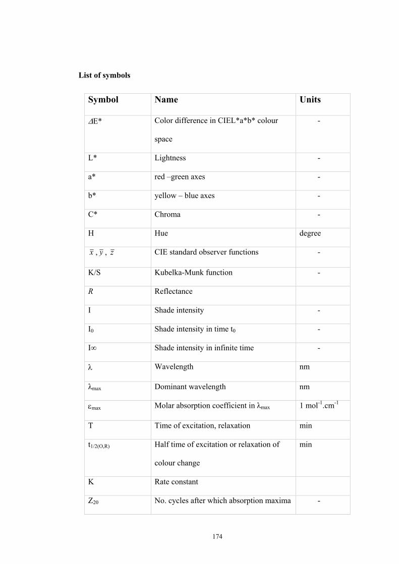
174

List of symbols

Symbol Name Units

ΔE* Color difference in CIEL*a*b* colour

space

-

L* Lightness -

a* red –green axes -

b* yellow – blue axes -

C* Chroma -

H Hue degree

x , y , z CIE standard observer functions -

K/S Kubelka-Munk function -

R Reflectance

I Shade intensity -

I0 Shade intensity in time t0 -

I∞ Shade intensity in infinite time -

λ Wavelength nm

λmax Dominant wavelength nm

εmax Molar absorption coefficient in λmax 1 mol-1.cm-1

T Time of excitation, relaxation min

t1/2(O,R) Half time of excitation or relaxation of

colour change

min

K Rate constant

Z20 No. cycles after which absorption maxima -

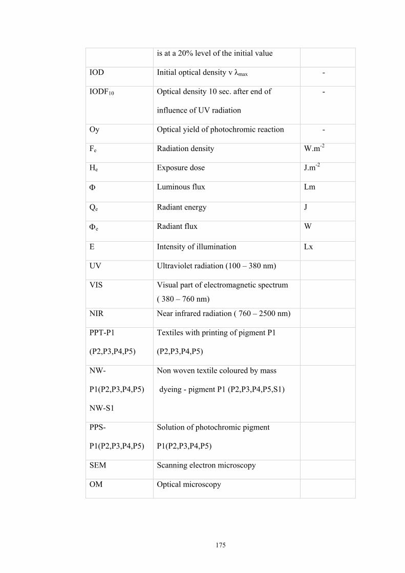
175

is at a 20% level of the initial value

IOD Initial optical density v λmax -

IODF10 Optical density 10 sec. after end of

influence of UV radiation

-

Oy Optical yield of photochromic reaction -

Fe Radiation density W.m-2

He Exposure dose J.m-2

Φ Luminous flux Lm

Qe Radiant energy J

Φe Radiant flux W

E Intensity of illumination Lx

UV Ultraviolet radiation (100 – 380 nm)

VIS Visual part of electromagnetic spectrum

( 380 – 760 nm)

NIR Near infrared radiation ( 760 – 2500 nm)

PPT-P1

(P2,P3,P4,P5)

Textiles with printing of pigment P1

(P2,P3,P4,P5)

NW-

P1(P2,P3,P4,P5)

NW-S1

Non woven textile coloured by mass

dyeing - pigment P1 (P2,P3,P4,P5,S1)

PPS-

P1(P2,P3,P4,P5)

Solution of photochromic pigment

P1(P2,P3,P4,P5)

SEM Scanning electron microscopy

OM Optical microscopy

176

Appendix A:

Selected measurement and their comparison with other authors

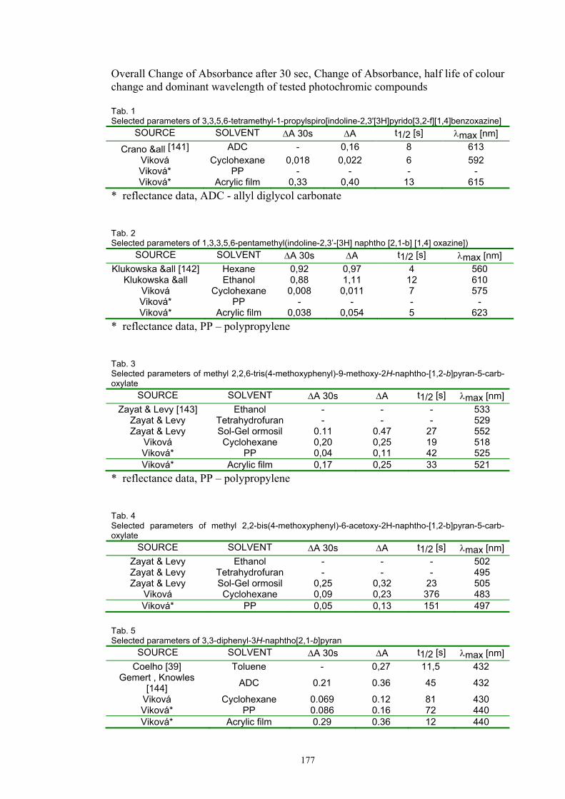
177

Overall Change of Absorbance after 30 sec, Change of Absorbance, half life of colour change and dominant wavelength of tested photochromic compounds

Tab. 1 Selected parameters of 3,3,5,6-tetramethyl-1-propylspiro[indoline-2,3'[3H]pyrido[3,2-f][1,4]benzoxazine]

SOURCE SOLVENT ΔA 30s ΔA t1/2 [s] λmax [nm]

Crano &all [141] ADC - 0,16 8 613 Viková Cyclohexane 0,018 0,022 6 592Viková* PP - - - - Viková* Acrylic film 0,33 0,40 13 615

* reflectance data, ADC - allyl diglycol carbonate Tab. 2 Selected parameters of 1,3,3,5,6-pentamethyl(indoline-2,3’-[3H] naphtho [2,1-b] [1,4] oxazine])

SOURCE SOLVENT ΔA 30s ΔA t1/2 [s] λmax [nm] Klukowska &all [142] Hexane 0,92 0,97 4 560

Klukowska &all Ethanol 0,88 1,11 12 610 Viková Cyclohexane 0,008 0,011 7 575 Viková* PP - - - - Viková* Acrylic film 0,038 0,054 5 623

* reflectance data, PP – polypropylene Tab. 3 Selected parameters of methyl 2,2,6-tris(4-methoxyphenyl)-9-methoxy-2H-naphtho-[1,2-b]pyran-5-carb-oxylate

SOURCE SOLVENT ΔA 30s ΔA t1/2 [s] λmax [nm] Zayat & Levy [143] Ethanol - - - 533

Zayat & Levy Tetrahydrofuran - - - 529 Zayat & Levy Sol-Gel ormosil 0.11 0.47 27 552

Viková Cyclohexane 0,20 0,25 19 518 Viková* PP 0,04 0,11 42 525 Viková* Acrylic film 0,17 0,25 33 521

* reflectance data, PP – polypropylene Tab. 4 Selected parameters of methyl 2,2-bis(4-methoxyphenyl)-6-acetoxy-2H-naphtho-[1,2-b]pyran-5-carb-oxylate

SOURCE SOLVENT ΔA 30s ΔA t1/2 [s] λmax [nm] Zayat & Levy Ethanol - - - 502 Zayat & Levy Tetrahydrofuran - - - 495 Zayat & Levy Sol-Gel ormosil 0,25 0,32 23 505

Viková Cyclohexane 0,09 0,23 376 483 Viková* PP 0,05 0,13 151 497

Tab. 5 Selected parameters of 3,3-diphenyl-3H-naphtho[2,1-b]pyran

SOURCE SOLVENT ΔA 30s ΔA t1/2 [s] λmax [nm] Coelho [39] Toluene - 0,27 11,5 432

Gemert , Knowles [144] ADC 0.21 0.36 45 432

Viková Cyclohexane 0.069 0.12 81 430 Viková* PP 0.086 0.16 72 440 Viková* Acrylic film 0.29 0.36 12 440

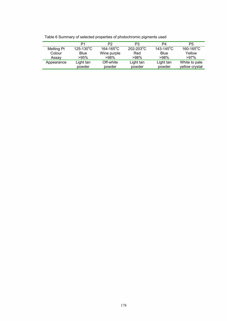
178

Table 6 Summary of selected properties of photochromic pigments used

P1 P2 P3 P4 P5 Melting Pt 125-130oC 164-165oC 202-203oC 143-145oC 160-165oC

Colour Blue Wine purple Red Blue Yellow Assay >95% >98% >98% >98% >97%

Appearance Light tan powder

Off-white powder

Light tan powder

Light tan powder

White to pale yellow crystal

179

Appendix B:

Author`s publications relating to the thesis

180

/1/ Viková, M., Vik, M.: Some Problems in Measurement of UV Protective Textiles,

The 3rd China International Wool Textile Conference, Xi’AN China 26-28 Sep.

2002, p.635-638, ISBN 7-5064-2373-1

/2/ Viková, M., Slabotinský, J., Musilová, M., Vik, M. Možnosti měření bariérových

vlastností ochranných textilií, II. Odborný seminář „Ochranné oděvy“ Prostějov, 23.

10. 2002

/3/ Viková, M., Slabotinský, J., Vik, M., Musilová, M.: Possibility of colorimetric

identification of dangerous gas penetration through protective clothes, TEXSCI 03,

16.- 18. 6. 2003, Liberec, Czech Republic, ISBN 80-7083-711-X

/4/ Viková,M.: Colorimetric identification of dangerous gas penetration through

protective clothes via inteligent underwear,83rd World Konference(83rd TIWC), May

23-27, 2004,Shanghai,China, p.772-774 ISBN 1870372611

/5/ Viková, M., Vik, M. : Smart textile based senzors, SUMMER SCHOOL

Intelligent Textile Structures - Application, Production and Testing, Center of

Excellence ITSAPT, Liberec Czech Republic, June 9 th -13 th 2003

/6/ Viková, M.: Textile photochromic sensors for protective textile, TEXSCI 03, 16.-

18. 6. 2003, Liberec, Czech Republic, 6p. on CD ROM, ISBN 80-7083-711-X

/7/ Viková, M., Vlákna a textil 10 (2), 82-85 (2003) ISSN 1335-0617

/8/ Viková, M., UV sensible sensors based on textile fibres, International Lighting

and Colour conference, Cape Town 2-5 November 2003, South Africa,book of papers

47-53

/9/ Viková, M. : Inteligentní textilie - senzory UV záření, XXII. Kurs osvětlovací

techniky, Dlouhé Stráně 23.-24. Září, s.70-74, ISBN 80-248 0446-8

/10/ Viková,M.: Contribution to development of textile based senzors – UV senzore,

7th Asian textile konference, New Delhi, India, Dec.1st – 3rd 2003, 6p. on CD ROM

/11/ Viková,M.: Možnosti využití pigmentů a barviv pro textilní senzory. Seminář:

Textilie v novém tisíciletí I. 24. 4. 2003 Výzkumné centrum textil, Technická

Universita v Liberci ISBN 55-022-03

/12/ Viková,M.: UV sensible sensors based on textile fibres. Seminář: Textilie

v novém tisíciletí II. 15.4 2004 Výzkumné centrum textil, Technická Universita

v Liberci ISBN 55-022-03

/13/ Viková, M., Vik,M.: Colour shift photochromic pigments in colour space CIE

L*a*b*, ISOP04, Arcachon 12.-15. 9. 2004, France

181

/14/ Viková, M., Vik, M. : Textile sensors based on color differences, 1 st Czech-

German Textile Workshop on Performance and Smart Fabrics, September 20th and

21th 2004, Dresden Germany

/15/ Viková, M. : Visual Assessment UV Radiation by Colour Changeable Textile

Sensors, AIC 2004, Color and Paints, the Interim Meeting of the International Color

Association, Porto Alegre 1-5. November 2004, Brasil

/16/ Viková, M.: Visual assesment UV radiation by colour changeable textile sensors,

2nd International Conference of Textile Research Division NRC, Cairo, Egypt, April

11-13, 2005

/17/ Viková, M.: SMART Textile Based Senzore - Theory and their Application,

Textile Processing: State of the Art & Future Developments, 2 (7) (2005) 507 – 511,

/18/ Viková, M. : Selected problems of measurement of photochromic colorants,

Book of papers AIC Colour 05 - 10th Congress of the International Colour

Association, Granada, p.1135-1138, 2005

/19/ Viková, M., Vik, M.: Colour shift photochromic pigments in colour space CIE

L*a*b*, Molecular Crystals and Liquid Crystals 431(2005), 103-116 [403-417]

/20/ Viková, M.: Colour change kinetic behavior of photochromic SMART textile

sensors, 4th Central European Conference 2005, 7-9 September 2005, Liberec, Czech

Republic

/21/ Viková, M., Vlach, P.*, Vik, M.: Textile based sensors – identification of

dangerous gases penetration, 4th Central European Conference 2005, 7-9 September

2005, Liberec, Czech Republic

/22/ Viková, M.: Photochromic pigments for SMART Textiles, ITSAPT project

seminar, Guimares 16. 11. 2005, Portugal

/23/ Viková, M, Vik, M.: Smart textile senzors for indication of UV radiation,

AUTEX 2006 World Textile Conference, 11-14 June Raleigh, USA

/24/ Vik, M., Viková, M.: Colorimetry of Color Changeable Materials, Micro-

symposium on Colour Research and Application, 8. September Kyoto, Japan

/25/ Viková, M., Vik, M.: Measurement of photochromic materials, BOLcolor 2006 -

II CONGRESO BOLIVIANO DEL COLOR - 25 al 27 de septiembre de 2006 La

Paz, Bolivia

/26/ Vik, M., Viková, M.: Spektrofotometrická měření v osvětlovací laboratoři, Kurz

osvětlovací techniky XXV, 16. -18. 10. 2006, Hotel Dlouhé Stráně, Kouty n. Desnou

182

/27/ Viková, M., Vik, M.: Accurate measurement photochromic materials, 6th

International Conference - TEXSCI 2007, June 5-7, Liberec

/28/ Viková, M., Vik, M.: Measurement of photochromic textiles, ISOP07, 7-10

October 2007, Vancouver, Canada

/29/ Vik, M., Viková, M.: Colorimetric Characterisation of color changeable

materials, 6th BAM-DIN-Workshop on Image Technology, 3. December,Berlin 2007

/30/ Viková, M. : Colour of changeable materials, invited paper on TU Granada –

Scientific Seminary, 6th February,2008

/31/ Viková, M. : Chameleonic textiles, Colour Emotion Research and Aplication,

National Yunlin University of Science and Technology, Taiwan, 22-24th July 2008

/32/ Viková, M., Vik, M. : Accurate measurement of photochromic materials, Colour

Emotion Research and Aplication, National Yunlin University of Science and

Technology, Taiwan, 22-24th July 2008

/33/ Viková, M.: Colorimetric Measurement of Photochromic Materials, 11th

Congress of the International Colour Association 2009, Sydney 27. 9-2.10. 2009,

Australia

183

Appendix C:

Selected author’s articles

184

Molecular Crystals and Liquid Crystals 431(2005), 103-116:

COLOUR SHIFT PHOTOCHROMIC PIGMENTS IN COLOUR SPACE CIE

L*a*b*

Martina Viková and Michal Vik LCAM – Department of Textile Materials, Technical University of Liberec, Hálkova

6, CZ-461 17 Liberec, Czech Republic, martina.vikova@vslib.cz

One of possibilities for protection of human body against acute and cumulative exposure to ultraviolet is the wearing of special protective clothes. Nevertheless on the other side the protective clothes have not the same barrier features against the UV light.

The aim of present research work in LCAM on the Technical University of Liberec is research and development of original method of measurement by flexible textile based sensors reacting on the UVA part of electromagnetic radiation. In this article is publicized information about testing above mentioned sensors with weave structure and non-woven textiles. Results show that produced sensors shows sensitivity as to time of exposition so also to intensity of irradiation and their response characteristics is same as for classical luxmeters.

Key words: Sensor, photochromism, colour space, colour hysteresion area, intensity of illumination

INTRODUCTION In present time become worse living conditions, increase harmful pollutants in

environment, which can irreversible damage our health, and jeopardize full quality

our life. Big attention is given in research area respectively in development and

perfection of protective clothes specially their barrier features. Protective barriers we

understand how the clothes or textiles protect wearer against above mentioned

dangerous conditions and if the protection is only partial or the protection is time

limited by ambient conditions. Most of protective clothes are not developed for long

time wearing. During development of these barrier structures we have to keep in our

mind full comfort of acting persons without limitation. Some of protective clothes are

equipped by electronics, respectively other sensors or devices, which monitoring and

quantify dangerous substances in environment. In present time is big attention given

to miniaturization of electronics and also flexibility their connection with computing

units [1].

185

Above mentioned describe concept of protective clothes we call as intelligent

structure. Disadvantage of this intelligent structure is no adequate response on the

external stimulus, there is only monitoring of external dangerous conditions. This

structure we call as passive intelligent textile structure.

Sensors and textile structures, which react adequate response and they are able

modulate protective degree in accordance on the external stimulus (change of

intensity UV, temperature, press, electrical field etc.) is called as SMART textile. As

example of passive intelligent textiles are optical fibres, which leading the not only

signal, but they are also sensitive on the deformation, concentration of substances,

press, electric power etc. As example of active intelligent textiles could be textiles

which react by change own colour in dependence on external stimulus (light,

temperature) and called as a chameleonic textiles or heat containing textiles, which

are able to store or slack energy according external temperature. Moreover textile

based sensors and active protective textiles has advantages that textile structure is

easy customizable by sewing, thermal bonding or gluing. Also there are advantages of

easy maintaining (washing, chemical drying) and low specific weight with good

strength, tensibility and elasticity. Good features are also workability without change

of technology of production and extremely large specific surface. Big advantages are

possible integration these types of sensors into system of protective clothes and also

their price availability. From these reason is this article directed to research of

textile-based sensors with photo chromic behaviour, respectively to study of dynamic

behaviour and modulation of sensitivity photo chromic sensors.

In this work is described new definition of colour reversible hysteresis, which

is described by hysteresis of colour change curve. This colour hysteresis curve is

described by kinetic model, which defines the speed of colour change initiated by

external stimulus – UV light. Kinetic model verification is done for textile sensors

with photo chromic pigment applied by textile printing, fibre mass dyeing.

MATERIALS AND USED METHODS

Our experiment was divided to 3 parts and every part is directed to special form of

application of photochromic pigments and study of photochromic behaviour from

point of kinetics and dynamics in different mediums:

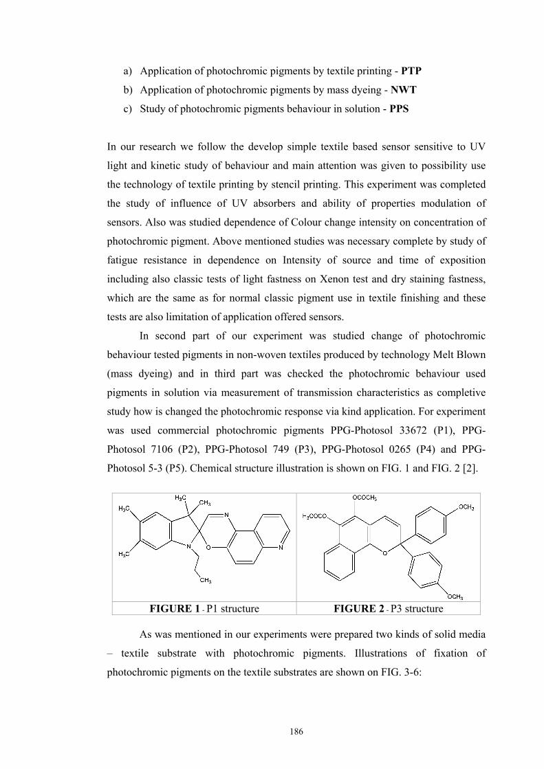
186

a) Application of photochromic pigments by textile printing - PTP

b) Application of photochromic pigments by mass dyeing - NWT

c) Study of photochromic pigments behaviour in solution - PPS

In our research we follow the develop simple textile based sensor sensitive to UV

light and kinetic study of behaviour and main attention was given to possibility use

the technology of textile printing by stencil printing. This experiment was completed

the study of influence of UV absorbers and ability of properties modulation of

sensors. Also was studied dependence of Colour change intensity on concentration of

photochromic pigment. Above mentioned studies was necessary complete by study of

fatigue resistance in dependence on Intensity of source and time of exposition

including also classic tests of light fastness on Xenon test and dry staining fastness,

which are the same as for normal classic pigment use in textile finishing and these

tests are also limitation of application offered sensors.

In second part of our experiment was studied change of photochromic

behaviour tested pigments in non-woven textiles produced by technology Melt Blown

(mass dyeing) and in third part was checked the photochromic behaviour used

pigments in solution via measurement of transmission characteristics as completive

study how is changed the photochromic response via kind application. For experiment

was used commercial photochromic pigments PPG-Photosol 33672 (P1), PPG-

Photosol 7106 (P2), PPG-Photosol 749 (P3), PPG-Photosol 0265 (P4) and PPG-

Photosol 5-3 (P5). Chemical structure illustration is shown on FIG. 1 and FIG. 2 [2].

FIGURE 1 - P1 structure FIGURE 2 - P3 structure

As was mentioned in our experiments were prepared two kinds of solid media

– textile substrate with photochromic pigments. Illustrations of fixation of

photochromic pigments on the textile substrates are shown on FIG. 3-6:

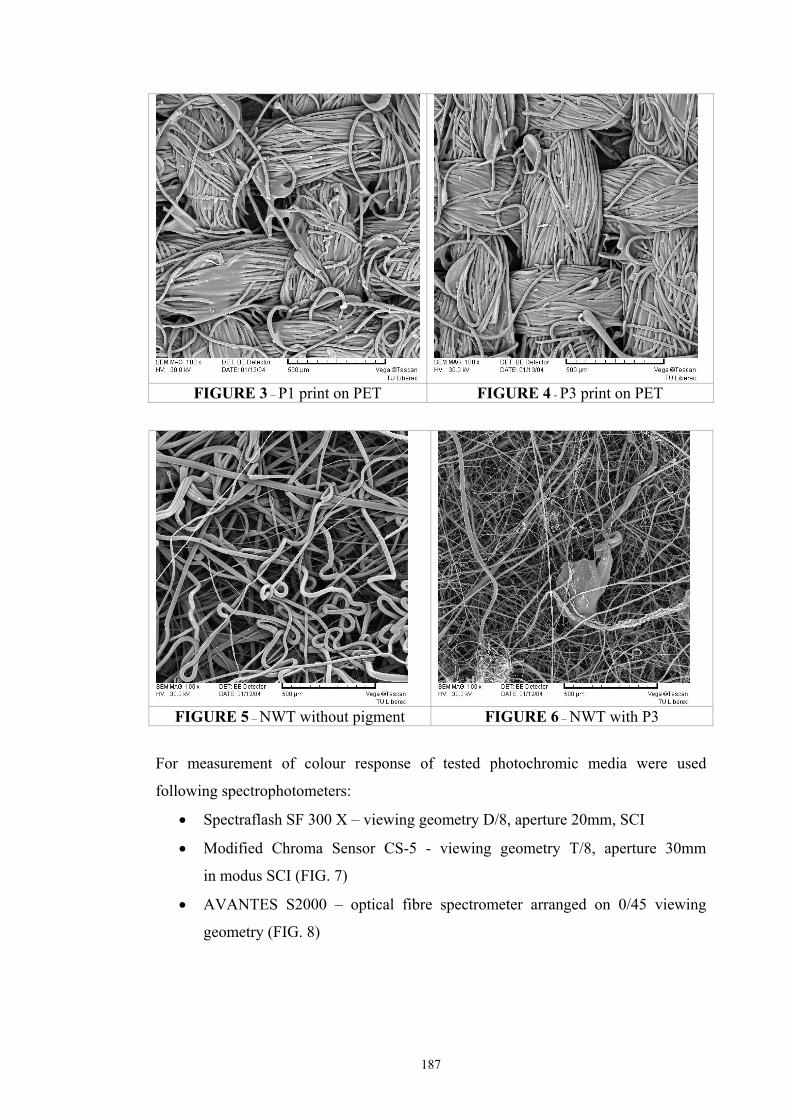
187

FIGURE 3 – P1 print on PET FIGURE 4 - P3 print on PET

FIGURE 5 – NWT without pigment FIGURE 6 – NWT with P3

For measurement of colour response of tested photochromic media were used

following spectrophotometers:

• Spectraflash SF 300 X – viewing geometry D/8, aperture 20mm, SCI

• Modified Chroma Sensor CS-5 - viewing geometry T/8, aperture 30mm

in modus SCI (FIG. 7)

• AVANTES S2000 – optical fibre spectrometer arranged on 0/45 viewing

geometry (FIG. 8)

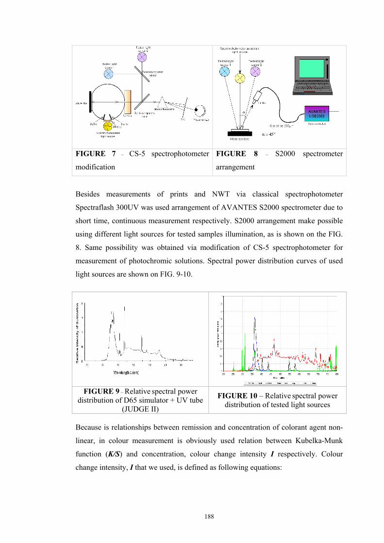
188

FIGURE 7 – CS-5 spectrophotometer

modification

FIGURE 8 – S2000 spectrometer

arrangement

Besides measurements of prints and NWT via classical spectrophotometer

Spectraflash 300UV was used arrangement of AVANTES S2000 spectrometer due to

short time, continuous measurement respectively. S2000 arrangement make possible

using different light sources for tested samples illumination, as is shown on the FIG.

8. Same possibility was obtained via modification of CS-5 spectrophotometer for

measurement of photochromic solutions. Spectral power distribution curves of used

light sources are shown on FIG. 9-10.

Because is relationships between remission and concentration of colorant agent non-

linear, in colour measurement is obviously used relation between Kubelka-Munk

function (K/S) and concentration, colour change intensity I respectively. Colour

change intensity, I that we used, is defined as following equations:

FIGURE 9 – Relative spectral power distribution of D65 simulator + UV tube

(JUDGE II)

FIGURE 10 – Relative spectral power distribution of tested light sources

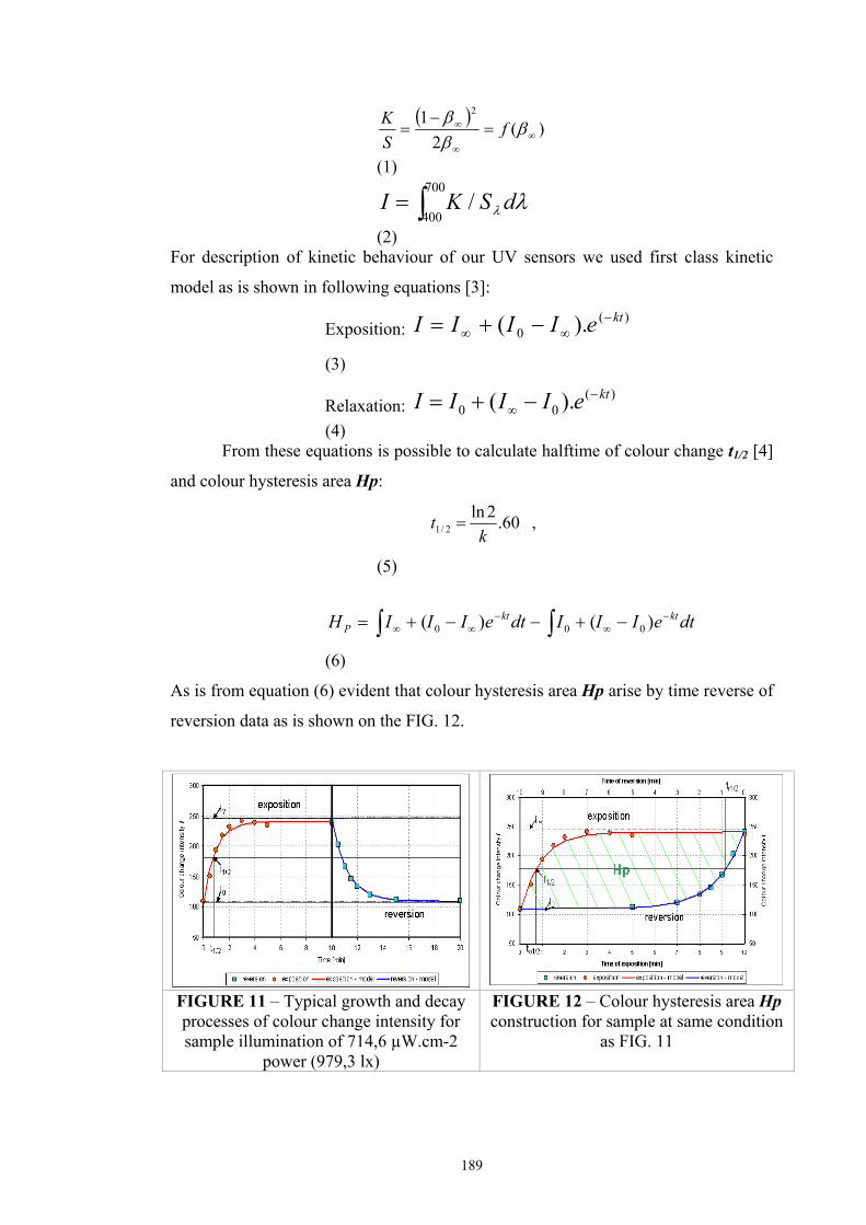
189

( ))(

21 2

∞∞

∞ =−

= βββ f

SK

(1)

∫=700

400/ λλ dSKI

(2)

For description of kinetic behaviour of our UV sensors we used first class kinetic

model as is shown in following equations [3]:

Exposition: )(

0 ).( kteIIII −∞∞ −+=

(3)

Relaxation: )(

00 ).( kteIIII −∞ −+=

(4) From these equations is possible to calculate halftime of colour change t1/2 [4]

and colour hysteresis area Hp:

60.2ln2/1 k

t = ,

(5)

dteIIIdteIIIH ktkt

P−

∞−

∞∞ −+−−+= ∫∫ )()( 000

(6)

As is from equation (6) evident that colour hysteresis area Hp arise by time reverse of

reversion data as is shown on the FIG. 12.

FIGURE 11 – Typical growth and decay processes of colour change intensity for sample illumination of 714,6 µW.cm-2

power (979,3 lx)

FIGURE 12 – Colour hysteresis area Hp construction for sample at same condition

as FIG. 11

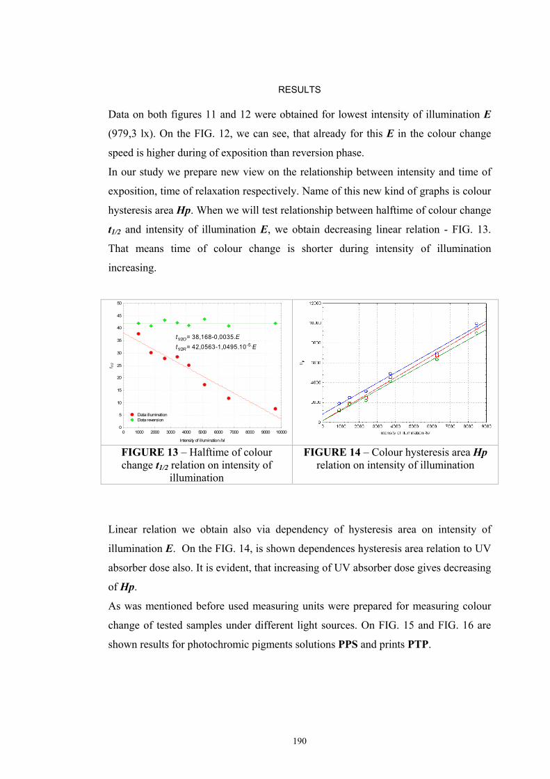
190

RESULTS

Data on both figures 11 and 12 were obtained for lowest intensity of illumination E

(979,3 lx). On the FIG. 12, we can see, that already for this E in the colour change

speed is higher during of exposition than reversion phase.

In our study we prepare new view on the relationship between intensity and time of

exposition, time of relaxation respectively. Name of this new kind of graphs is colour

hysteresis area Hp. When we will test relationship between halftime of colour change

t1/2 and intensity of illumination E, we obtain decreasing linear relation - FIG. 13.

That means time of colour change is shorter during intensity of illumination

increasing.

0 1000 2000 3000 4000 5000 6000 7000 8000 9000 10000

Intensity of illumination /lx/

0

5

10

15

20

25

30

35

40

45

50

t 1/2

t1/2O = 38,168-0,0035.Et1/2R = 42,0563-1,0495.10-5 .E

Data illumination Data reversion

FIGURE 13 – Halftime of colour change t1/2 relation on intensity of

illumination

FIGURE 14 – Colour hysteresis area Hp relation on intensity of illumination

Linear relation we obtain also via dependency of hysteresis area on intensity of

illumination E. On the FIG. 14, is shown dependences hysteresis area relation to UV

absorber dose also. It is evident, that increasing of UV absorber dose gives decreasing

of Hp.

As was mentioned before used measuring units were prepared for measuring colour

change of tested samples under different light sources. On FIG. 15 and FIG. 16 are

shown results for photochromic pigments solutions PPS and prints PTP.

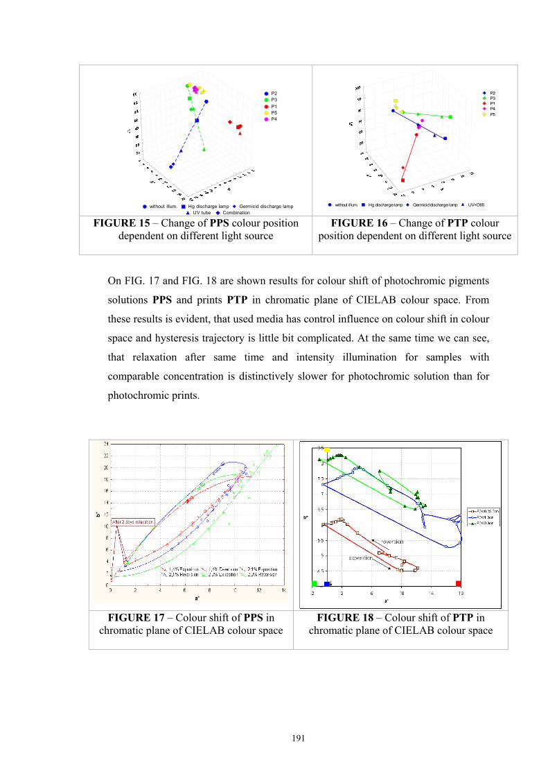
191

without illum. Hg discharge lamp Germicid discharge lamp UV tube Combination

P2P3P1P5P4

P2 P3 P1 P4 P5

without illum. Hg discharge lamp Germicid discharge lamp UV+D65

FIGURE 15 – Change of PPS colour position dependent on different light source

FIGURE 16 – Change of PTP colour position dependent on different light source

On FIG. 17 and FIG. 18 are shown results for colour shift of photochromic pigments

solutions PPS and prints PTP in chromatic plane of CIELAB colour space. From

these results is evident, that used media has control influence on colour shift in colour

space and hysteresis trajectory is little bit complicated. At the same time we can see,

that relaxation after same time and intensity illumination for samples with

comparable concentration is distinctively slower for photochromic solution than for

photochromic prints.

FIGURE 17 – Colour shift of PPS in chromatic plane of CIELAB colour space

FIGURE 18 – Colour shift of PTP in chromatic plane of CIELAB colour space

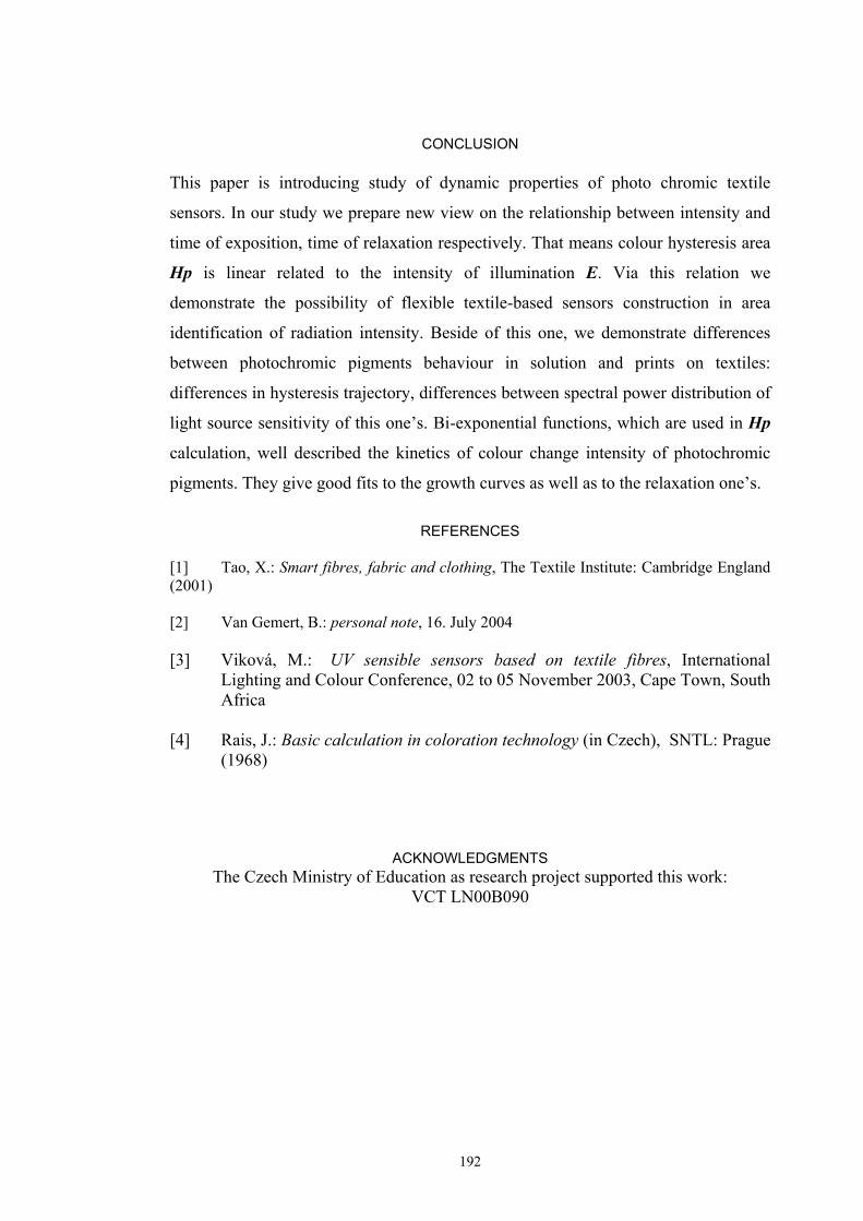
192

CONCLUSION This paper is introducing study of dynamic properties of photo chromic textile

sensors. In our study we prepare new view on the relationship between intensity and

time of exposition, time of relaxation respectively. That means colour hysteresis area

Hp is linear related to the intensity of illumination E. Via this relation we

demonstrate the possibility of flexible textile-based sensors construction in area

identification of radiation intensity. Beside of this one, we demonstrate differences

between photochromic pigments behaviour in solution and prints on textiles:

differences in hysteresis trajectory, differences between spectral power distribution of

light source sensitivity of this one’s. Bi-exponential functions, which are used in Hp

calculation, well described the kinetics of colour change intensity of photochromic

pigments. They give good fits to the growth curves as well as to the relaxation one’s.

REFERENCES

[1] Tao, X.: Smart fibres, fabric and clothing, The Textile Institute: Cambridge England (2001) [2] Van Gemert, B.: personal note, 16. July 2004 [3] Viková, M.: UV sensible sensors based on textile fibres, International

Lighting and Colour Conference, 02 to 05 November 2003, Cape Town, South Africa

[4] Rais, J.: Basic calculation in coloration technology (in Czech), SNTL: Prague

(1968)

ACKNOWLEDGMENTS The Czech Ministry of Education as research project supported this work:

VCT LN00B090

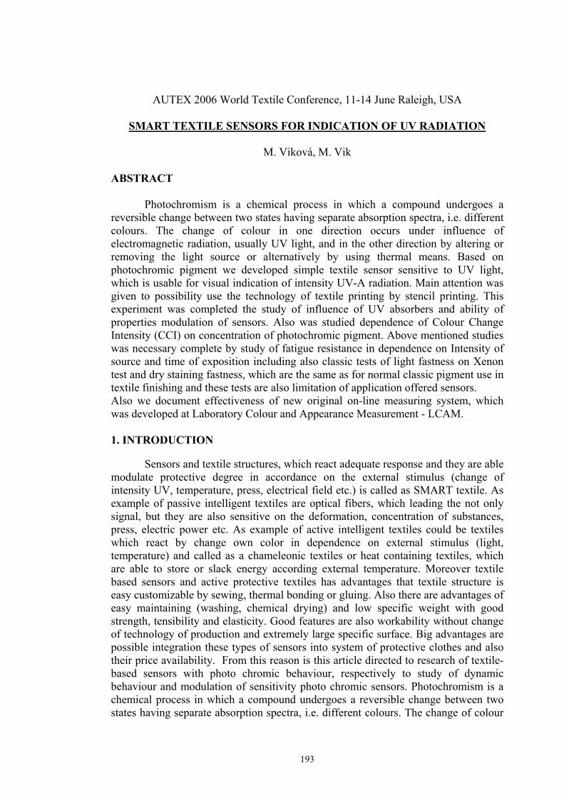
193

AUTEX 2006 World Textile Conference, 11-14 June Raleigh, USA

SMART TEXTILE SENSORS FOR INDICATION OF UV RADIATION

M. Viková, M. Vik ABSTRACT Photochromism is a chemical process in which a compound undergoes a reversible change between two states having separate absorption spectra, i.e. different colours. The change of colour in one direction occurs under influence of electromagnetic radiation, usually UV light, and in the other direction by altering or removing the light source or alternatively by using thermal means. Based on photochromic pigment we developed simple textile sensor sensitive to UV light, which is usable for visual indication of intensity UV-A radiation. Main attention was given to possibility use the technology of textile printing by stencil printing. This experiment was completed the study of influence of UV absorbers and ability of properties modulation of sensors. Also was studied dependence of Colour Change Intensity (CCI) on concentration of photochromic pigment. Above mentioned studies was necessary complete by study of fatigue resistance in dependence on Intensity of source and time of exposition including also classic tests of light fastness on Xenon test and dry staining fastness, which are the same as for normal classic pigment use in textile finishing and these tests are also limitation of application offered sensors. Also we document effectiveness of new original on-line measuring system, which was developed at Laboratory Colour and Appearance Measurement - LCAM. 1. INTRODUCTION Sensors and textile structures, which react adequate response and they are able modulate protective degree in accordance on the external stimulus (change of intensity UV, temperature, press, electrical field etc.) is called as SMART textile. As example of passive intelligent textiles are optical fibers, which leading the not only signal, but they are also sensitive on the deformation, concentration of substances, press, electric power etc. As example of active intelligent textiles could be textiles which react by change own color in dependence on external stimulus (light, temperature) and called as a chameleonic textiles or heat containing textiles, which are able to store or slack energy according external temperature. Moreover textile based sensors and active protective textiles has advantages that textile structure is easy customizable by sewing, thermal bonding or gluing. Also there are advantages of easy maintaining (washing, chemical drying) and low specific weight with good strength, tensibility and elasticity. Good features are also workability without change of technology of production and extremely large specific surface. Big advantages are possible integration these types of sensors into system of protective clothes and also their price availability. From this reason is this article directed to research of textile-based sensors with photo chromic behaviour, respectively to study of dynamic behaviour and modulation of sensitivity photo chromic sensors. Photochromism is a chemical process in which a compound undergoes a reversible change between two states having separate absorption spectra, i.e. different colours. The change of colour

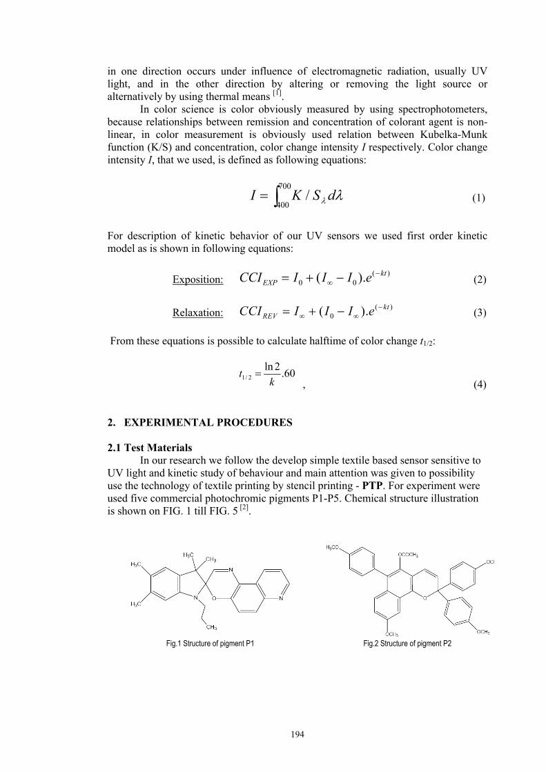
194

∫=700

400/ λλ dSKI

in one direction occurs under influence of electromagnetic radiation, usually UV light, and in the other direction by altering or removing the light source or alternatively by using thermal means [1].

In color science is color obviously measured by using spectrophotometers, because relationships between remission and concentration of colorant agent is non-linear, in color measurement is obviously used relation between Kubelka-Munk function (K/S) and concentration, color change intensity I respectively. Color change intensity I, that we used, is defined as following equations:

(1)

For description of kinetic behavior of our UV sensors we used first order kinetic model as is shown in following equations:

Exposition: ( )

0 0( ). ktEXPCCI I I I e −

∞= + − (2) Relaxation: ( )

0( ). ktREVCCI I I I e −

∞ ∞= + − (3) From these equations is possible to calculate halftime of color change t1/2:

60.2ln

2/1 kt =

, (4) 2. EXPERIMENTAL PROCEDURES 2.1 Test Materials In our research we follow the develop simple textile based sensor sensitive to UV light and kinetic study of behaviour and main attention was given to possibility use the technology of textile printing by stencil printing - PTP. For experiment were used five commercial photochromic pigments P1-P5. Chemical structure illustration is shown on FIG. 1 till FIG. 5 [2].

Fig.1 Structure of pigment P1 Fig.2 Structure of pigment P2

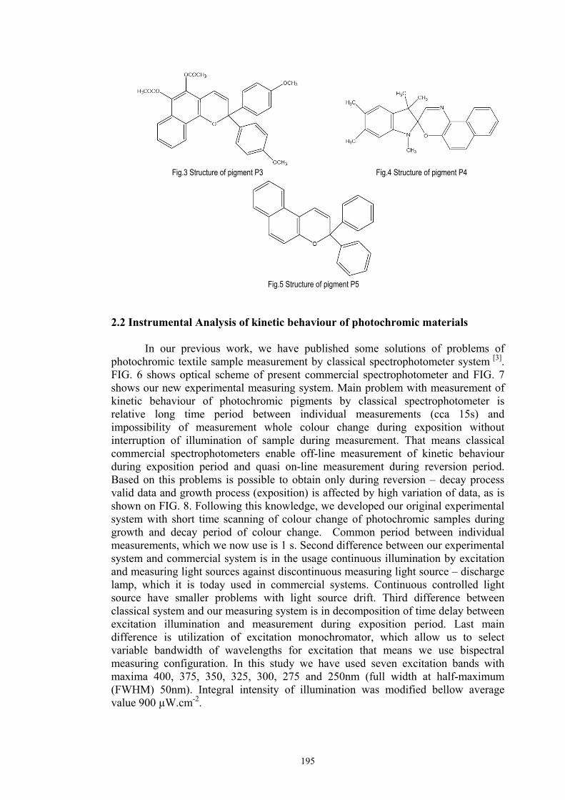
195

Fig.3 Structure of pigment P3 Fig.4 Structure of pigment P4

Fig.5 Structure of pigment P5

2.2 Instrumental Analysis of kinetic behaviour of photochromic materials In our previous work, we have published some solutions of problems of photochromic textile sample measurement by classical spectrophotometer system [3]. FIG. 6 shows optical scheme of present commercial spectrophotometer and FIG. 7 shows our new experimental measuring system. Main problem with measurement of kinetic behaviour of photochromic pigments by classical spectrophotometer is relative long time period between individual measurements (cca 15s) and impossibility of measurement whole colour change during exposition without interruption of illumination of sample during measurement. That means classical commercial spectrophotometers enable off-line measurement of kinetic behaviour during exposition period and quasi on-line measurement during reversion period. Based on this problems is possible to obtain only during reversion – decay process valid data and growth process (exposition) is affected by high variation of data, as is shown on FIG. 8. Following this knowledge, we developed our original experimental system with short time scanning of colour change of photochromic samples during growth and decay period of colour change. Common period between individual measurements, which we now use is 1 s. Second difference between our experimental system and commercial system is in the usage continuous illumination by excitation and measuring light sources against discontinuous measuring light source – discharge lamp, which it is today used in commercial systems. Continuous controlled light source have smaller problems with light source drift. Third difference between classical system and our measuring system is in decomposition of time delay between excitation illumination and measurement during exposition period. Last main difference is utilization of excitation monochromator, which allow us to select variable bandwidth of wavelengths for excitation that means we use bispectral measuring configuration. In this study we have used seven excitation bands with maxima 400, 375, 350, 325, 300, 275 and 250nm (full width at half-maximum (FWHM) 50nm). Integral intensity of illumination was modified bellow average value 900 µW.cm-2.

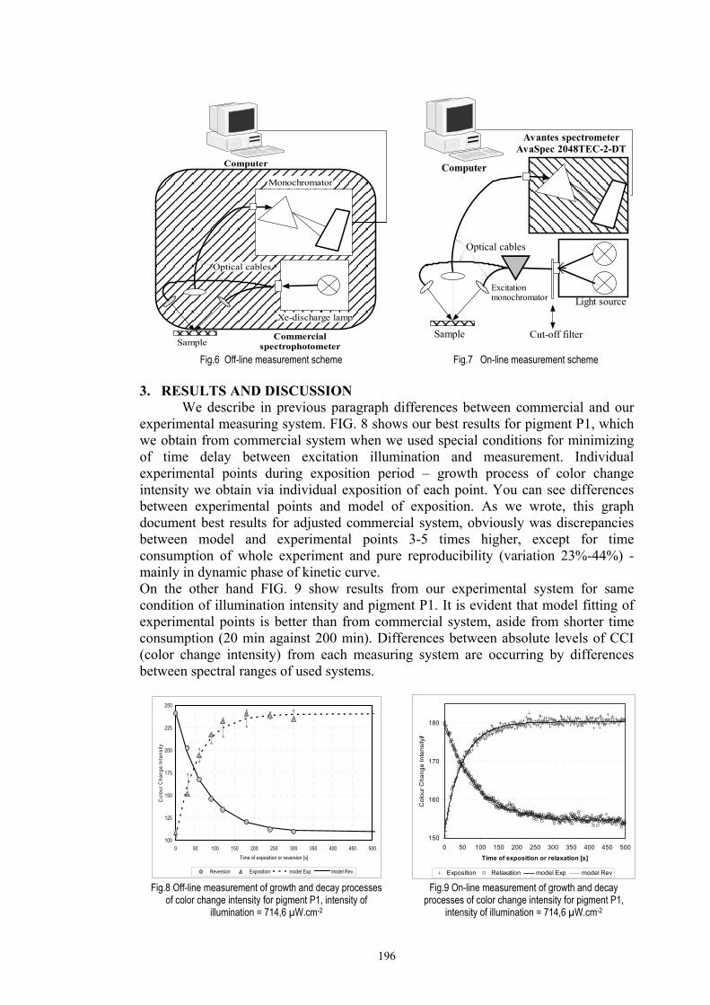
196

Computer

Sample

Xe-discharge lamp

Optical cables

Commercialspectrophotometer

MonochromatorComputer

Avantes spectrometerAvaSpec 2048TEC-2-DT

Sample

Light source

Cut-off filter

Optical cables

Excitationmonochromator

Fig.6 Off-line measurement scheme Fig.7 On-line measurement scheme 3. RESULTS AND DISCUSSION We describe in previous paragraph differences between commercial and our experimental measuring system. FIG. 8 shows our best results for pigment P1, which we obtain from commercial system when we used special conditions for minimizing of time delay between excitation illumination and measurement. Individual experimental points during exposition period – growth process of color change intensity we obtain via individual exposition of each point. You can see differences between experimental points and model of exposition. As we wrote, this graph document best results for adjusted commercial system, obviously was discrepancies between model and experimental points 3-5 times higher, except for time consumption of whole experiment and pure reproducibility (variation 23%-44%) - mainly in dynamic phase of kinetic curve. On the other hand FIG. 9 show results from our experimental system for same condition of illumination intensity and pigment P1. It is evident that model fitting of experimental points is better than from commercial system, aside from shorter time consumption (20 min against 200 min). Differences between absolute levels of CCI (color change intensity) from each measuring system are occurring by differences between spectral ranges of used systems.

100

125

150

175

200

225

250

0 50 100 150 200 250 300 350 400 450 500

Time of exposition or reversion [s]

Col

our C

hang

e In

tens

ity

Reversion Exposition model Exp. model Rev.

150

160

170

180

0 50 100 150 200 250 300 350 400 450 500

Time of exposition or relaxation [s]

Col

our C

hang

e In

tens

ity I

Exposition Relaxation model Exp model Rev

Fig.8 Off-line measurement of growth and decay processes of color change intensity for pigment P1, intensity of

illumination = 714,6 µW.cm-2

Fig.9 On-line measurement of growth and decay processes of color change intensity for pigment P1,

intensity of illumination = 714,6 µW.cm-2

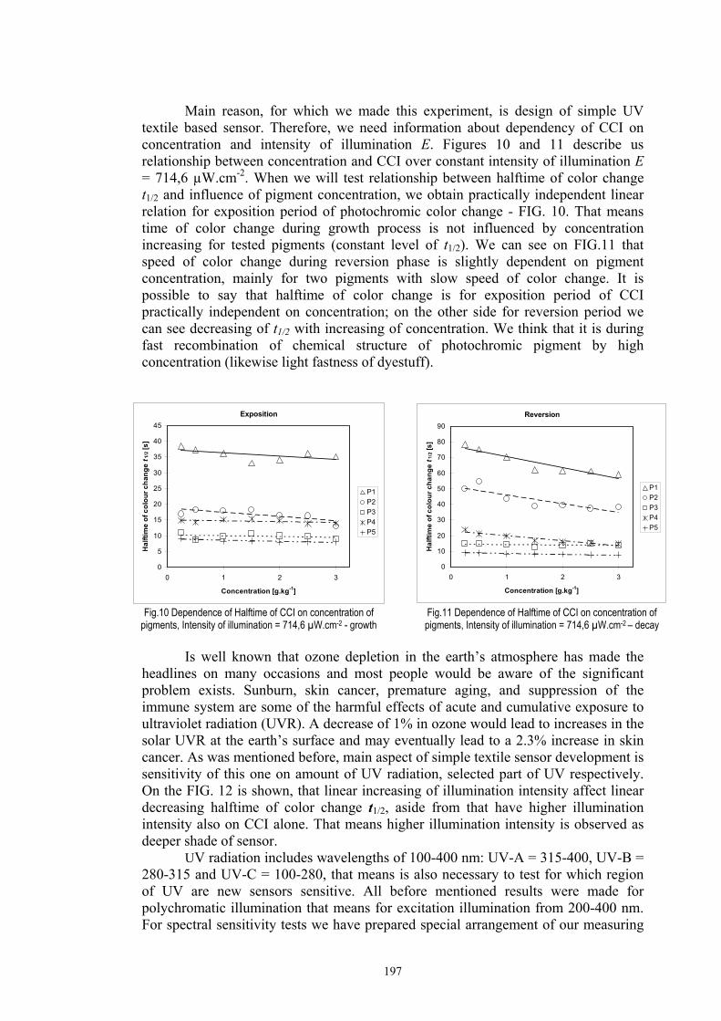
197

Main reason, for which we made this experiment, is design of simple UV

textile based sensor. Therefore, we need information about dependency of CCI on concentration and intensity of illumination E. Figures 10 and 11 describe us relationship between concentration and CCI over constant intensity of illumination E = 714,6 µW.cm-2. When we will test relationship between halftime of color change t1/2 and influence of pigment concentration, we obtain practically independent linear relation for exposition period of photochromic color change - FIG. 10. That means time of color change during growth process is not influenced by concentration increasing for tested pigments (constant level of t1/2). We can see on FIG.11 that speed of color change during reversion phase is slightly dependent on pigment concentration, mainly for two pigments with slow speed of color change. It is possible to say that halftime of color change is for exposition period of CCI practically independent on concentration; on the other side for reversion period we can see decreasing of t1/2 with increasing of concentration. We think that it is during fast recombination of chemical structure of photochromic pigment by high concentration (likewise light fastness of dyestuff).

Exposition

0

5

10

15

20

25

30

35

40

45

0 1 2 3

Concentration [g.kg-1]

Hal

ftim

e of

col

our c

hang

e t 1

/2 [s

]

P1P2P3P4P5

Reversion

0

10

20

30

40

50

60

70

80

90

0 1 2 3

Concentration [g.kg-1]

Hal

ftim

e of

col

our c

hang

e t 1

/2 [s

]

P1P2P3P4P5

Fig.10 Dependence of Halftime of CCI on concentration of pigments, Intensity of illumination = 714,6 µW.cm-2 - growth

Fig.11 Dependence of Halftime of CCI on concentration of pigments, Intensity of illumination = 714,6 µW.cm-2 – decay

Is well known that ozone depletion in the earth’s atmosphere has made the

headlines on many occasions and most people would be aware of the significant problem exists. Sunburn, skin cancer, premature aging, and suppression of the immune system are some of the harmful effects of acute and cumulative exposure to ultraviolet radiation (UVR). A decrease of 1% in ozone would lead to increases in the solar UVR at the earth’s surface and may eventually lead to a 2.3% increase in skin cancer. As was mentioned before, main aspect of simple textile sensor development is sensitivity of this one on amount of UV radiation, selected part of UV respectively. On the FIG. 12 is shown, that linear increasing of illumination intensity affect linear decreasing halftime of color change t1/2, aside from that have higher illumination intensity also on CCI alone. That means higher illumination intensity is observed as deeper shade of sensor.

UV radiation includes wavelengths of 100-400 nm: UV-A = 315-400, UV-B = 280-315 and UV-C = 100-280, that means is also necessary to test for which region of UV are new sensors sensitive. All before mentioned results were made for polychromatic illumination that means for excitation illumination from 200-400 nm. For spectral sensitivity tests we have prepared special arrangement of our measuring

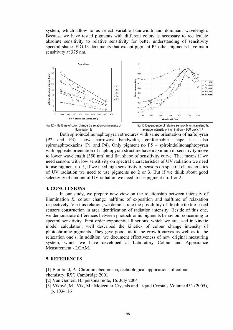
198

system, which allow to us select variable bandwidth and dominant wavelength. Because we have tested pigments with different colors is necessary to recalculate absolute sensitivity to relative sensitivity for better understanding of sensitivity spectral shape. FIG.13 documents that except pigment P5 other pigments have main sensitivity at 375 nm.

Exposition

0

5

10

15

20

25

30

35

40

0 100 200 300 400 500 600 700 800 900

UV-A irradiance [µWatt.cm-2]

Hal

ftim

e of

col

our c

hang

e t 1

/2 [s

]

P1P2P3P4P5

0.1

0.2

0.3

0.4

0.5

0.6

0.7

0.8

0.9

1

1.1

250 275 300 325 350 375 400

Wavelength /nm/

Rel

ativ

e se

nsiti

vity

P1P2P3P4P5

Fig.12 – Halftime of color change t1/2 relation on intensity of illumination E

Fig.13 Dependence of relative sensitivity on wavelength, average intensity of illumination = 900 µW.cm-2

Both spiroindolinonaphtopyran structures with same orientation of naftopyran (P2 and P3) show narrowest bandwidth, conformable shape has also spironaphtooxazins (P1 and P4). Only pigment no P5 – spiroindolinonaphtopyran with opposite orientation of naphtopyran structure have maximum of sensitivity move to lower wavelength (350 nm) and flat shape of sensitivity curve. That means if we need sensors with low sensitivity on spectral characteristics of UV radiation we need to use pigment no. 5, if we need high sensitivity of sensors on spectral characteristics of UV radiation we need to use pigments no 2 or 3. But if we think about good selectivity of amount of UV radiation we need to use pigment no. 1 or 2. 4. CONCLUSIONS

In our study, we prepare new view on the relationship between intensity of illumination E, colour change halftime of exposition and halftime of relaxation respectively. Via this relation, we demonstrate the possibility of flexible textile-based sensors construction in area identification of radiation intensity. Beside of this one, we demonstrate differences between photochromic pigments behaviour concerning to spectral sensitivity. First order exponential functions, which we are used in kinetic model calculation, well described the kinetics of colour change intensity of photochromic pigments. They give good fits to the growth curves as well as to the relaxation one’s. In addition, we document effectiveness of new original measuring system, which we have developed at Laboratory Colour and Appearance Measurement - LCAM. 5. REFERENCES [1] Bamfield, P.: Chromic phenomena, technological applications of colour chemistry, RSC Cambridge 2001 [2] Van Gemert, B.: personal note, 16. July 2004 [3] Viková, M., Vik, M.: Molecular Crystals and Liquid Crystals Volume 431 (2005),

p. 103-116

199

ACKNOWLEDGEMENTS The Czech Ministry of Education as research project 1M4674788501 supported this work. RESPONDENCE ADDRESS: Laboratory Color and Appearance Measurement Faculty of Textile Engineering, Technical University of Liberec, Hálkova 6, 461 17 Liberec, Czech Republic