eScholarship provides open access, scholarly publishingservices to the University of California and delivers a dynamicresearch platform to scholars worldwide.

University of California

Peer Reviewed

Title:Physiologically based synthetic models of hepatic disposition

Author:Hunt, C AnthonyRopella, Glen E PYan, LiHung, Daniel YRoberts, Michael S

Publication Date:12-01-2006

Publication Info:Postprints, Multi-Campus

Permalink:http://escholarship.org/uc/item/5r29n0mk

Additional Info:The original publication is available at http://www.springerlink.com/content/v082276440263046/?hl=u

Keywords:physiologically based, liver, modeling (modelling), simulation, discrete event, agent-based

Abstract:Current Physiologically based pharmacokinetic (PBPK) models are inductive. We present anadditional, different approach that is based on the synthetic rather than the inductive approach tomodeling and simulation. It relies on object-oriented programming A model of the referent systemin its experimental context is synthesized by assembling objects that represent components suchas molecules, cells, aspects of tissue architecture, catheters, etc. The single pass perfused ratliver has been well described in evaluating hepatic drug pharmacokinetics (PK) and is the systemon which we focus. In silico experiments begin with administration of objects representing actualcompounds. Data are collected in a manner analogous to that in the referent PK experiments.The synthetic modeling method allows for recognition and representation of discrete event anddiscrete time processes, as well as heterogeneity in organization, function, and spatial effects.An application is developed for sucrose and antipyrine, administered separately and togetherPBPK modeling has made extensive progress in characterizing abstracted PK properties but thishas also been its limitation. Now, other important questions and possible extensions emerge.How are these PK properties and the observed behaviors generated? The inherent heuristiclimitations of traditional models have hindered getting meaningful, detailed answers to suchquestions. Synthetic models of the type described here are specifically intended to help answersuch questions. Analogous to wet-lab experimental models, they retain their applicability evenwhen broken apart into sub-components. Having and applying this new class of models alongwith traditional PK modeling methods is expected to increase the productivity of pharmaceuticalresearch at all levels that make use of modeling and simulation.

Synthetic Models JPKPD: PMID 17051440

C.A. Hunt, et al. – 1 – UCSF BioSystems Group

Physiologically Based Synthetic Models of Hepatic Disposition

C. Anthony Hunt 1,2, Glen E.P. Ropella 2, Li Yan 1, Daniel Y. Hung 3,and Michael S. Roberts 3

1 The UCSF/UCB Joint Graduate Group in Bioengineering, University of California,Berkeley, CA, USA

2 The Department of Biopharmaceutical Sciences, Biosystems Group, University ofCalifornia, San Francisco, CA, USA

3 School of Medicine, Princess Alexandra Hospital, University of Queensland,Woolloongabba, Queensland, 4102, Australia

Abbreviations Used

CV: central veinISL(s): in silico liver(s)N1, N2, … : A set of experiments that explores sinusoidal network arrangementPBPK: physiologically based pharmacokineticPCs: properties and characteristicsPK: pharmacokineticPV: portal veinS1, S2, … : A set of experiments that explores spatial relationships within and between sinusoidsSA and SB: two classes of SSSD: standard deviationSM(s): similarity measure(s)SS(s): sinusoidal segment(s)

KEY WORDS: Physiologically based; liver; modeling (modelling); simulation; discrete event;agent-based, complex systems

Synthetic Models JPKPD: PMID 17051440

C.A. Hunt, et al. – 2 – UCSF BioSystems Group

ABSTRACT

Current physiologically based pharmacokinetic (PBPK) models are inductive. We presentan additional, different approach that is based on the synthetic rather than the inductiveapproach to modeling and simulation. It relies on object-oriented programming. A modelof the referent system in its experimental context is synthesized by assembling objects thatrepresent components such as molecules, cells, aspects of tissue architecture, catheters,etc. The single pass perfused rat liver has been well described in evaluating hepatic drugpharmacokinetics (PK) and is the system on which we focus. In silico experiments beginwith administration of objects representing actual compounds. Data is collected in amanner analogous to that in the referent PK experiments. The synthetic modeling methodallows for recognition and representation of discrete event and discrete time processes, aswell as heterogeneity in organization, function, and spatial effects. An application isdeveloped for sucrose and antipyrine, administered separately and together. PBPKmodeling has made extensive progress in characterizing abstracted PK properties but thishas also been its limitation. Now, other important questions and possible extensionsemerge. How are these PK properties and the observed behaviors generated? Theinherent heuristic limitations of traditional models have hindered getting meaningful,detailed answers to such questions. Synthetic models of the type described here arespecifically intended to help answer such questions. Having and applying this new classof models is expected to increase the productivity of pharmaceutical research at all levelsthat make use of modeling and simulation, by providing validated models that retain theirapplicability when broken apart into sub-components analogous to wet-lab experimentalmodels.

INTRODUCTIONA key goal in developing pharmacokinetic (PK) models is to use simulation to facilitate drug

development and clinical pharmacology. PK modeling has undergone considerable evolution inits efforts to achieve this goal. Nonparametric analysis makes no model assumptions about thebody but only provides moment data, which may be used to generate PK parameter values. Morecommonly, data is analyzed assuming the body may be described as an abstract series ofcompartments or, in physiologically based pharmacokinetics (PBPK), by representing organs ascompartments connected to represent a vascular system (1, 2). These and related model types areby nature inductive: they are a cognitive reduction of the biology to describe PK data, usingrepresentations of the hypothesized essential determinants governing the measured phenomena.Almost all of these models rely on systems of equations1 (typically differential equations) and/orprobabilistic networks to represent or describe essential features of PK data.

In this report, we introduce and demonstrate an additional approach (as distinct fromalternative) to PBPK modeling—one that is based on the synthetic, rather than the inductivemethod. A discretized analogue of the system that generated the data is constructed fromindependent components. It relies on object-oriented programming, and is constructed usingsoftware objects that are representations of body components. Design and construction is guidedby intended model uses, the problem being solved, and model requirements, as well as theavailable data. Different objects represent biological components that vary in size, type, andfunction. Some represent molecules, others represent cells, and still others represent aspects oftissue architecture, etc. The components are composed within a software environment thatincludes a representation of the experimental PK context (including the experimenters), and

1 Inductive models can take any form. Equations fit to data are just one example.

Synthetic Models JPKPD: PMID 17051440

C.A. Hunt, et al. – 3 – UCSF BioSystems Group

facilitates a cycle of creating, verifying, and changing models. Experiments are then conductedon the in silico analogue in the same ways that wet-lab PK experiments are conducted. In thisway, the analogue system reflects the entire experimental system of interest. Simulated PK datais collected and compared to referent PK data, when the latter are available. An acceptabledegree of similarity is taken as evidence supporting the hypothesis that the assembledcomponents have generative properties that mimic those of the corresponding biologicalcomponents: they are biomimetic. They exhibit their own phenotypic attributes. They can adapteasily to new situations, such as becoming a components of whole-body models. The envisionedanalogues are not alternatives to traditional PK models: the two classes of models serve differentpurposes and so can be synergistic.

Recognizing that the first goal in PK modeling has been to provide descriptions of theorgan (3), we have limited this report to representing aspects of the rat liver, as viewed from theperspective of sucrose administered together with antipyrine. This approach is consistent with thenotion that “an overall objective of physiological modeling is to simulate the complete systemthrough a fundamental study of its component parts” (1).

PHYSIOLOGICALLY BASED MODELINGThe Vision

PBPK models recognize anatomical and physiological realities, and attempt to account forthe role of differential distribution within and between organs as well as their varying blood flows(4). The expected heuristic value of PBPK modeling in research, drug development andregulatory science, and toxicological risk assessment is evident in the variety of envisioned modeluses discussed in several recent reviews (4, 5, 6). Several desired and anticipated advantages ofPBPK models have been cited (4, 5), but not yet realized, of which the following are just a few.It should be straightforward to reuse a parameterized PBPK model to explore the expectedbehaviors of different compounds. Models should be capable of reflecting whateverphysiological detail is relevant to the problem. Updating needs to be facile. One should be ableto replace low-resolution components with more detailed ones that will enable the simulation ofmechanistically based pharmacodynamics (4, 7) or to account for changes in rate-limiting steps orrelevant heterogeneity within tissues and cells (8, 9). Realization of these uses is expected to allowresearchers to answer important questions such as: can we predict the PK behavior of a new,unstudied compound by studying synthetic models validated against other compounds withdifferent PK behavior? Can we provide increasingly confident explanations of events withintarget sites, and can we adjust those events to take into account patient specific knowledge?

Inductive and Synthetic MethodsThe inductive method for creating models dominates the PK literature. Inductive models,

by definition, abstract away the very detail required by heuristic PBPK modeling. This has leadto top-down attempts to graft details onto the highly abstract inductive models. AugmentingPBPK modeling with the more flexible synthetic method provides a middle-out strategy with twoprimary benefits: 1) a deep physiological model–to–referent mapping and 2) access tounpredictable systemic phenomena in the model (e.g. those that may result from nonlinearities).Inductive methods, especially those dependent on continuum mathematics like ordinarydifferential equations, often rely on assumptions like linearity for their mathematical basis.Hence, any model developed with induction exhibits only the behaviors present, a priori, in themodel family used for induction. Synthetic PBPK modeling involves using independentcomponent to build a functioning analogue of the mechanisms (form and function; componentinteractions) of which an inductive PBPK model is an abstraction. Being composed of separatesub-models (10-14), synthetic models provide more flexibility in representation and underlying

Synthetic Models JPKPD: PMID 17051440

C.A. Hunt, et al. – 4 – UCSF BioSystems Group

assumptions2. We posit that this flexibility is critical to the satisfaction of the core requirementsof PBPK modeling and thereby achieving the vision.

APPLYING MODELING PRINCIPLESModels of Hepatic Elimination

How will changes in hepatic details alter the hepatic disposition of two compoundsadministered simultaneously? Traditionally, answers have been obtained using appropriatelydesigned in vitro and in vivo experiments. Sometimes they are not enough: the appropriateexperiment can be impossible, too challenging, too costly, take too long to set up and complete,or the researcher may be unable to uncover the precise intrahepatic events. It would be desirableto be able to conduct experiments in silico that would provide useful answers to questions,coupled with a useful measure of uncertainty. The following three questions are examples ofwhat can be addressed using in silico experimentation on synthetic models:

1. How might zonal differences in metabolizing enzymes influence the hepatic eliminationand metabolic profiles of compounds A and B when they are co-administered relative to beingadministered separately, especially when one pathway for metabolism is saturated?

2. How might hepatic elimination respond to a pharmacological or an inflammation-inducedreduction in sinusoid diameters, recognizing that vasoconstriction is often associated withischemia-reperfusion injury?

3. Can a significant difference in the ratio of metabolizing enzymes to various transporteractivities, within or between cells (in PK terms, the relative contributions of intrinsic clearanceand hepatic permeability clearance) account for some of the interindividual differences in thedose dependent hepatic clearance of some drug?

In this report, we provide a cornerstone for a solid foundation that can be built upon andextended to produce models that can answer such questions. It is envisioned that the ISL (insilico liver) will have many properties and behaviors that partially overlap those of the currentinductive models of hepatic elimination3. They will also be capable of exhibiting properties andbehaviors that are not achievable by those inductive models. During early development of a newclass of models, it is best to have trusted, successfully used models that, for overlappingbehaviors, can serve as standards, against which to contrast members the new class of models. Aprimary reason for focusing on the liver and hepatic elimination in this report is that the alreadyexisting rich literature provides multiple options for crossmodel validity.

Model Usage

The hepatic outflow profile of a compound is a phenotypic attribute. The greater thesimilarity between the measured behaviors of an ISL and known attributes of a liver, the moreuseful that ISL will become as a research tool and as an expression of the coalesced, relevantknowledge of the liver. In this report, we focus on hepatic outflow profiles of sucrose and a co-administered drug, antipyrine. To simulate the complete system through a fundamental study ofits component parts (1), this research will produce increasing overlap between ISL behaviors,properties, and characteristics, and measures of hepatic phenotypic attributes.

The long-term goal of this research is to produce increasing overlap between ISL behaviors,properties, and characteristics, and measures of hepatic phenotypic attributes. Achieving thatgoal depends on demonstrating models that achieve at least ten capabilities.1. The models are capable of accurately representing intrahepatic events.

2 We expand our ideas of inductive and synthetic modeling in Supplementary Material.3 Discussions of the variety of hepatic models used in PK can be found in (8) and (34).

Synthetic Models JPKPD: PMID 17051440

C.A. Hunt, et al. – 5 – UCSF BioSystems Group

2. There is clear physiological mapping between referent and model components because ISLobservables are designed to be consistent with those of the referent liver.

3. When dosed with a simulated compound, the ISL generates outflow data that are, to a domainexpert (in a type of Turing test), experimentally indistinguishable from the referent wet-labdata; this requires that the ISL and its framework must be suitable for experimentation.

4. To enable the above capabilities and support 6-9 below, the ISL and its framework must usediscrete interactions.

5. The ISL must be transparent: the details of the simulation, as it progresses, need to bevisualizable and measurable.

6. The components articulate: it must be easy to join, disconnect, and replace ISL components.7. The ISL components can be easily reconfigured to represent different histological,

physiological, or experimental conditions.8. It must be relatively simple to change usage and assumptions, or increase or decrease detail in

order to meet the particular needs of an experiment, without requiring significant re-engineering of the model.

9. The ISL must be reusable for simulating the disposition, clearance, and metabolic properties ofmultiple compounds in the same experiment, not just one each in separate experiments.

10. The ISL must be constructed so that it can eventually function as an organ component withina larger, synthetic, physiologically based, whole organism model.

Specification of an In Silico LiverTo enable achieving the ten capabilities, we discretize hepatic anatomy and physiology so

that important aspects of structure are mapped to directed graph structures. We specify only theminimum number of hepatic features needed to generate the required output and exhibit thespecified features. Features and functions that are currently not needed are not explicitlyspecified. Instead, they are conflated with other ISL components. When one these features orfunctions is needed, it can be brought back into focus and assigned to newly added componentswithout requiring significant re-engineering of the components already present.

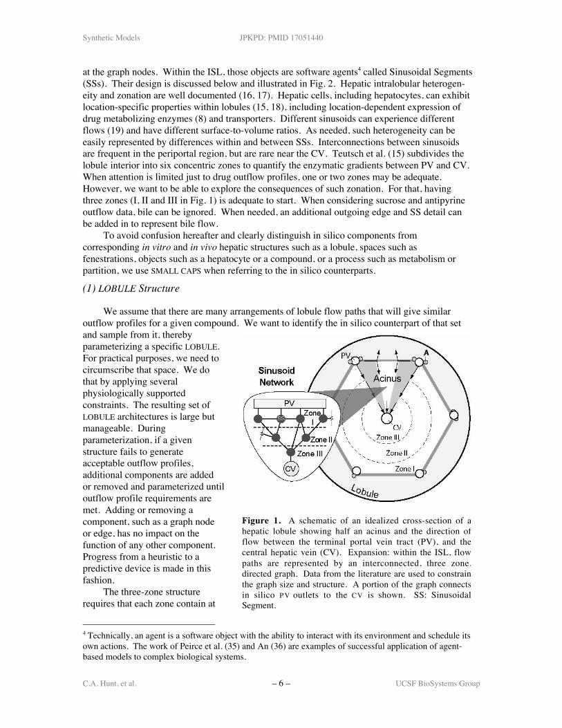
The hepatic parenchyma of the rat is organized as several polyhedral primaryunits—lobules—integrated into larger secondary units (15). We assume that secondary unitfunctions are similar throughout a normal liver, and that each has similar incoming and outgoingfluid flows. By making that assumption, we can collapse the graph that would be needed torepresent the entire liver into a directed graph of parallel single nodes, each representing asecondary unit. The integration of a dozen or so lobules into a secondary unit results from acommon drainage by its branches to form a central venular tree, and from the arrangement ofportal tracts and vascular septa that form a continuous vascular surface over the entire unit.Because of their structure, secondary units can be accurately represented as small networks ofprimary lobules. If we assume that all lobules in a secondary unit are similar in form andfunction, then we can collapse the secondary unit graph structure into a single node (a typicallobule) having one incoming and outgoing edge. The organization of this typical lobule ispictured in Fig. 1.

The arterial and portal vein (PV) blood supply for one lobule feeds into several dozensinusoids that merge in stages to only a small fraction of their original number as they feed intothe lobule’s outgoing central vein (CV). Those flow paths can also be represented by aninterconnected directed graph. Objects representing sinusoidal spaces and function can be placed

Synthetic Models JPKPD: PMID 17051440

C.A. Hunt, et al. – 6 – UCSF BioSystems Group

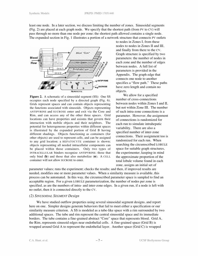
at the graph nodes. Within the ISL, those objects are software agents4 called Sinusoidal Segments(SSs). Their design is discussed below and illustrated in Fig. 2. Hepatic intralobular heterogen-eity and zonation are well documented (16, 17). Hepatic cells, including hepatocytes, can exhibitlocation-specific properties within lobules (15, 18), including location-dependent expression ofdrug metabolizing enzymes (8) and transporters. Different sinusoids can experience differentflows (19) and have different surface-to-volume ratios. As needed, such heterogeneity can beeasily represented by differences within and between SSs. Interconnections between sinusoidsare frequent in the periportal region, but are rare near the CV. Teutsch et al. (15) subdivides thelobule interior into six concentric zones to quantify the enzymatic gradients between PV and CV.When attention is limited just to drug outflow profiles, one or two zones may be adequate.However, we want to be able to explore the consequences of such zonation. For that, havingthree zones (I, II and III in Fig. 1) is adequate to start. When considering sucrose and antipyrineoutflow data, bile can be ignored. When needed, an additional outgoing edge and SS detail canbe added in to represent bile flow.

To avoid confusion hereafter and clearly distinguish in silico components fromcorresponding in vitro and in vivo hepatic structures such as a lobule, spaces such asfenestrations, objects such as a hepatocyte or a compound, or a process such as metabolism orpartition, we use SMALL CAPS when referring to the in silico counterparts.

(1) LOBULE Structure

We assume that there are many arrangements of lobule flow paths that will give similaroutflow profiles for a given compound. We want to identify the in silico counterpart of that setand sample from it, therebyparameterizing a specific LOBULE.For practical purposes, we need tocircumscribe that space. We dothat by applying severalphysiologically supportedconstraints. The resulting set ofLOBULE architectures is large butmanageable. Duringparameterization, if a givenstructure fails to generateacceptable outflow profiles,additional components are addedor removed and parameterized untiloutflow profile requirements aremet. Adding or removing acomponent, such as a graph nodeor edge, has no impact on thefunction of any other component.Progress from a heuristic to apredictive device is made in thisfashion.

The three-zone structurerequires that each zone contain at

4 Technically, an agent is a software object with the ability to interact with its environment and schedule itsown actions. The work of Peirce et al. (35) and An (36) are examples of successful application of agent-based models to complex biological systems.

Figure 1. A schematic of an idealized cross-section of ahepatic lobule showing half an acinus and the direction offlow between the terminal portal vein tract (PV), and thecentral hepatic vein (CV). Expansion: within the ISL, flowpaths are represented by an interconnected, three zone,directed graph. Data from the literature are used to constrainthe graph size and structure. A portion of the graph connectsin silico P V outlets to the CV is shown. SS: SinusoidalSegment.

Synthetic Models JPKPD: PMID 17051440

C.A. Hunt, et al. – 7 – UCSF BioSystems Group

least one node. In a later section, we discuss limiting the number of zones. Sinusoidal segments(Fig. 2) are placed at each graph node. We specify that the shortest path (from PV to CV) willpass through no more than one node per zone; the shortest path allowed contains a single node.The expanded section in Fig. 1 illustrates a portion of a network structure that connects PV outlets

to nodes in Zones I, from thesenodes to nodes in Zones II and III,and finally from there to the CV.Graph structure is specified by twoparameters: the number of nodes ineach zone and the number of edgesbetween nodes. A full list ofparameters is provided in theAppendix. The graph edge thatconnects one node to anotherspecifies a “flow path.” These pathshave zero length and contain noobjects.

We allow for a specifiednumber of cross-connectionsbetween nodes within Zones I and II,but not within Zone III. The numberof such intra-zone connections is aparameter. However, the assignmentof connections is randomized foreach run to simulate intrahepaticvariability. There are also aspecified number of inter-zoneconnections. Their assignment too israndomized for each run. Whensearching the circumscribed LOBULEspace for suitable graph structures,the experimenter, keeping in mindthe approximate proportion of thetotal lobule volume found in eachzone, assigns an initial set of

parameter values; runs the experiment; checks the results; and then, if improved results areneeded, modifies one or more parameter values. When a similarity measure is available, thisprocess can be automated. In this way, the circumscribed parameter space is sampled to find anacceptable region. For a given LOBULE parameterization, the number of nodes per zone isspecified, as are the numbers of intra- and inter-zone edges. In a given run, if a node is left withno outlet, then it is connected directly to the CV.

(2) SINUSOIDAL SEGMENT DesignWe have studied outflow properties using several sinusoidal segment designs, and report

here on one. Simpler designs generate behaviors that fail to meet either a specification or oursimilarity measure criterion. A SS is modeled as a tube-like space with a rim surrounded by twoadditional spaces. The tube and rim represent the central sinusoidal space and its immediateborders. The tube contains a fine-grained abstract “Core” space that represents blood. Grid A,the Rim, represents sinusoid edges near endothelial cells. A fine-grained space (Grid B) iswrapped around Grid A to represent the endothelial layer. Another space (Grid C) is wrapped

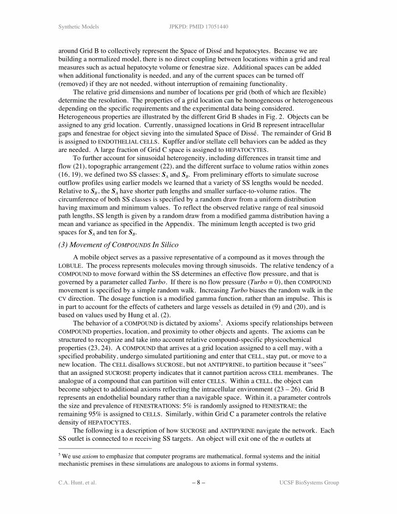
Figure 2. A schematic of a sinusoidal segment (SS): One SSoccupies each node specified by a directed graph (Fig. 6).Grids represent spaces and can contain objects representingthe functions associated with sinusoids. Objects representingANTIPYRINE and SUCROSE enter and exit via the Core andRim, and can access any of the other three spaces. Gridlocations can have properties and axioms that govern theirinteraction with mobile objects and their neighbors. Thepotential for heterogeneous properties within different spacesis illustrated by the expanded portion of Grid B havingdifferent shadings. Objects functioning as containers (forother objects) are used to represent cells, and can be assignedto any grid location; a HEPATOCYTE container is shown;objects representing all needed intracellular components canbe placed within those containers. Only two types ofINTRACELLULAR binders recognize ANTIPYRINE; those thatonly bind (b) and those that also metabolize (e). A CELLcontainer will not allow SUCROSE to enter.

Synthetic Models JPKPD: PMID 17051440

C.A. Hunt, et al. – 8 – UCSF BioSystems Group

around Grid B to collectively represent the Space of Dissé and hepatocytes. Because we arebuilding a normalized model, there is no direct coupling between locations within a grid and realmeasures such as actual hepatocyte volume or fenestrae size. Additional spaces can be addedwhen additional functionality is needed, and any of the current spaces can be turned off(removed) if they are not needed, without interruption of remaining functionality.

The relative grid dimensions and number of locations per grid (both of which are flexible)determine the resolution. The properties of a grid location can be homogeneous or heterogeneousdepending on the specific requirements and the experimental data being considered.Heterogeneous properties are illustrated by the different Grid B shades in Fig. 2. Objects can beassigned to any grid location. Currently, unassigned locations in Grid B represent intracellulargaps and fenestrae for object sieving into the simulated Space of Dissé. The remainder of Grid Bis assigned to ENDOTHELIAL CELLS. Kupffer and/or stellate cell behaviors can be added as theyare needed. A large fraction of Grid C space is assigned to HEPATOCYTES.

To further account for sinusoidal heterogeneity, including differences in transit time andflow (21), topographic arrangement (22), and the different surface to volume ratios within zones(16, 19), we defined two SS classes: SA and SB. From preliminary efforts to simulate sucroseoutflow profiles using earlier models we learned that a variety of SS lengths would be needed.Relative to SB , the SA have shorter path lengths and smaller surface-to-volume ratios. Thecircumference of both SS classes is specified by a random draw from a uniform distributionhaving maximum and minimum values. To reflect the observed relative range of real sinusoidpath lengths, SS length is given by a random draw from a modified gamma distribution having amean and variance as specified in the Appendix. The minimum length accepted is two gridspaces for SA and ten for SB.

(3) Movement of COMPOUNDS In SilicoA mobile object serves as a passive representative of a compound as it moves through the

LOBULE. The process represents molecules moving through sinusoids. The relative tendency of aCOMPOUND to move forward within the SS determines an effective flow pressure, and that isgoverned by a parameter called Turbo. If there is no flow pressure (Turbo = 0), then COMPOUNDmovement is specified by a simple random walk. Increasing Turbo biases the random walk in theCV direction. The dosage function is a modified gamma function, rather than an impulse. This isin part to account for the effects of catheters and large vessels as detailed in (9) and (20), and isbased on values used by Hung et al. (2).

The behavior of a COMPOUND is dictated by axioms5. Axioms specify relationships betweenCOMPOUND properties, location, and proximity to other objects and agents. The axioms can bestructured to recognize and take into account relative compound-specific physicochemicalproperties (23, 24). A COMPOUND that arrives at a grid location assigned to a cell may, with aspecified probability, undergo simulated partitioning and enter that CELL, stay put, or move to anew location. The CELL disallows SUCROSE, but not ANTIPYRINE, to partition because it “sees”that an assigned SUCROSE property indicates that it cannot partition across CELL membranes. Theanalogue of a compound that can partition will enter CELLS. Within a CELL, the object canbecome subject to additional axioms reflecting the intracellular environment (23 – 26). Grid Brepresents an endothelial boundary rather than a navigable space. Within it, a parameter controlsthe size and prevalence of FENESTRATIONS: 5% is randomly assigned to FENESTRAE; theremaining 95% is assigned to CELLS. Similarly, within Grid C a parameter controls the relativedensity of HEPATOCYTES.

The following is a description of how SUCROSE and ANTIPYRINE navigate the network. EachSS outlet is connected to n receiving SS targets. An object will exit one of the n outlets at 5 We use axiom to emphasize that computer programs are mathematical, formal systems and the initialmechanistic premises in these simulations are analogous to axioms in formal systems.

Synthetic Models JPKPD: PMID 17051440

C.A. Hunt, et al. – 9 – UCSF BioSystems Group

random. The probability of exit via a chosen outlet is a function of n, the available number of SSoutlets, ai, the inlet area, described below, of each SS (i = 1 … n), and ci, the “concentration” ofother solute objects just inside the target SS inlet. If the object does not exit, then a new outlet isselected from those remaining. If the SS cannot find a place for the COMPOUND (e.g., as aconsequence of crowding, as when “concentrations” are high) then the process is repeated up to10 times. The determinant for whether a SS can find a place in an output node is the estimate ofthe density of COMPOUND at the entrance of the SS. That density is estimated by the formula forthe area of a circle where the radius is derived from the circumference (r = C/2π); C is the widthof Grid A when laid flat. Flow and concentration come about, in part, due to this densitycalculation. If the simulated concentration is high at any part of the SS, flow out of that area willbe increased, resulting from the CONCENTRATION gradient and PRESSURE (more objects trying tomove creates a flow effect). Flow is also partly synthesized through adjustment of the Turbo andthe coreFlowRate parameters.

Both COMPOUNDS can enter a SS at either the Core or the Rim. Thereafter, until each iscollected at the CV they have several stochastic options, the aggregate properties of which aredetermined using Monte Carlo techniques. In the Rim or Core a COMPOUND can move withinthat space, jump from one space to the other, or exit the SS. When the COMPOUND jumps fromRim into Grid B, it can move within the space, or jump back to the Rim or on to Grid C. When itencounters a CELL, SUCROSE moves on. SUCROSE can move within the EXTRACELLULAR portionof Grid C or jump back to Grid B. After it exits a SS in Zone 3, it enters the CV; its passagethrough the CV is recorded (corresponding to being collected in the fraction collector).

The only subcellular functions needed to represent low clearance antipyrine are binding andmetabolism. All cellular components that bind or metabolize antipyrine are conflated into andrepresented by binding objects placed inside the containers representing CELLS. Metabolism ishandled as a special case of binding: enzyme objects bind ANTIPYRINE for some amount of timebefore either releasing or METABOLIZING it. Binding objects are assigned randomly to all CELLS.Enzyme objects are assigned randomly to HEPATOCYTES. Assignments are randomly drawn froma uniform distribution having a specified minimum and maximum. A binding parameter specifiesthe number of simulation cycles that ANTIPYRINE is bound. Enzyme objects are programmed torecognize substrates. They use an additional parameter, the probability of being metabolized.

ANTIPYRINE moves within a SS and LOBULE as does SUCROSE, but using its own parametervalues. When ANTIPYRINE encounters a CELL within Grid B or C it may partition into the CELL.Once inside it can move about, exit, bind or not bind, and possibly be METABOLIZED. For the

simulations that follow, all bindingobjects within a HEPATOCYTE alsoMETABOLIZE. The probability of anANTIPYRINE object beingMETABOLIZED is controlled by aparameter. Once METABOLIZED, thatANTIPYRINE is destroyed (unless wewish to track metabolites).

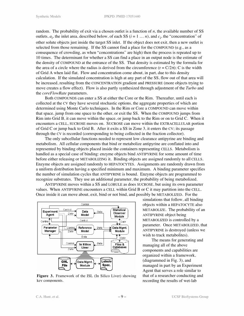
The means for generating andmanaging all of the abovecomponents and capabilities areorganized within a framework,(diagrammed in Fig. 3), andmanaged in part by an ExperimentAgent that serves a role similar tothat of a researcher conducting andrecording the results of wet-lab

Figure 3. Framework of the ISL (In Silico Liver) showingkey components.

Synthetic Models JPKPD: PMID 17051440

C.A. Hunt, et al. – 10 – UCSF BioSystems Group

experiments. Additional details are provided in the Supplementary Material.

The Stochastic Nature of In Silico Outflow ProfilesThe typical rat liver outflow profile is an account of on the order of 1015 or more drug

molecules percolating through hundreds of lobules. The typical in silico dose for one run withone LOBULE uses on the order of 5,000 objects, each representing a number (≥ 1) of molecules.An outflow profile for such a small number of objects is noisy and is inadequate to represent a PKprofile. At times following the outflow peak, it is increasingly possible to encounter an intervalduring which no objects are collected. A second independent run with that same LOBULE,parameter settings, and dose will produce a similar but uniquely different outflow profile. That isbecause a single experiment involves thousands of probabilistic events. For each independent run,the seed for the random number generator is changed, altering the specifics for all stochasticparameters. Several stochastic parameters control the ISL organizational and spatial architecture,specifically: the organization of the directed graph, assignment of SS type to each directed graphnode, the dimensions of the SS spaces, and how the edges are used to connect SSs. Together, foreach run, they provide a unique, individual version of the LOBULE where the relative differencesare analogous to the unique relative differences between lobules in the same liver. Differencesbetween runs also simulate some of the uncertainty that is built into the model. The varianceacross runs in the outflow fraction within a given time interval is neither constant nordeterministic. One ISL experiment combines the results from 10–50+ independent runs of thesame LOBULE.

To reduce outflow profile noise, we use a 70-point smoothing window. The resultingoutflow profile (Fig. 4 is an example) is sufficiently smooth for comparison with other profiles.An experimental result comprising 4-7 LOBULE runs6 is analogous to results one might obtain ifone could conduct a perfusion experiment on one hepatic lobule. Assuming the lobules within anormal liver are similar, the sum of the results from 10-50 runs can be used to represent theoutflow profile of one ISL.

Similarity MeasureWhen are two outflow profiles sufficiently similar to be considered experimentally

indistinguishable? The answer specifies when an in silico and an ISL outflow profile aresufficiently similar to be experimentally indistinguishable. For this study we decided that if mostof the values of an ISL outflow profile are within one standard deviation (SD) of mean valuesobtained from six repeated sucrose experiments, then the ISL data can be considered“experimentally indistinguishable” from that referent data.

For simplicity, we assume that the coefficients of variation of repeat observations withindifferent regions of referent outflow profiles are the same. In that way, we can use a similaritymeasure (SM) that is a simple, constant proportion interval. Specify a distance, d as the basis fora match. For each observation in reference profile P, create a lower, Pl, and an upper, Pu, boundby multiplying that observation by (1 – d) and (1 + d), respectively. The two curves Pl and Pu arethe lower and upper bounds of a band around P. The ISL outflow profile is deemed similar toreference outflow profile if, for example, 90% or more of the second profile stays within theband. In this study d is the standard deviation of the relative differences between each of sixreplicate sucrose experiments and the mean observations for that collection interval, pooled overall collection intervals. The data are from (2).

The SM score is the fraction of observations of the candidate time series (typically ≥ 100observations) that fall within the one SD envelope. Because the variability within any ISL run is

6 The coefficients of variation as a function of time for six repeated in silico experiments from (2) werecalculated. The values were higher at earlier and later times. Between 2 and 80 seconds values rangedfrom 1.2 to 54.4%, averaging 16.1%.

Synthetic Models JPKPD: PMID 17051440

C.A. Hunt, et al. – 11 – UCSF BioSystems Group

large, it is unlikely, even for one of the better matches, to have a SM score ≥ 0.97. For thesestudies, 0.8 is the lower limit of acceptable values. A value ≥ 0.9 is a quite reasonable match.For some future PBPK models more sophisticated SMs may be needed (as discussed in (27) and(28)).

RESULTSIn Silico ISL Outflow Profiles

In the referent wet-lab experiments, sucrose and antipyrine were co-administered. In the insilico experiments that follow, SUCROSE and ANTIPYRINE were both co-administered andadministered separately. Because ANTIPYRINE crosses into CELLS, whereas SUCROSE cannot, theoutflow profile for SUCROSE is much more sensitive to SS geometry than is the profile forANTIPYRINE, and that is a reason that it has been traditionally used as an extravascular marker(29, 30). Consequently, parameterizations were done as follows. Lobule and SS structure werefirst parameterized focusing on just on wet-lab sucrose profiles. Once acceptable SM values wereachieved, we held those values reasonably constant and then focused on adjusting the additionalparameter values that influenced only ANTIPYRINE. Antipyrine, rather than a more lipophilic,higher clearance drug was selected for assessing feasibility because its disposition properties aresimilar to those of sucrose. Several iterations of that procedure were needed to obtain acceptableSM values for both COMPOUNDS alone and administered together. Because of the key role ofwet-lab sucrose data in determining the in silico LOBULE structure, the sections that followfocuses mostly on SUCROSE.

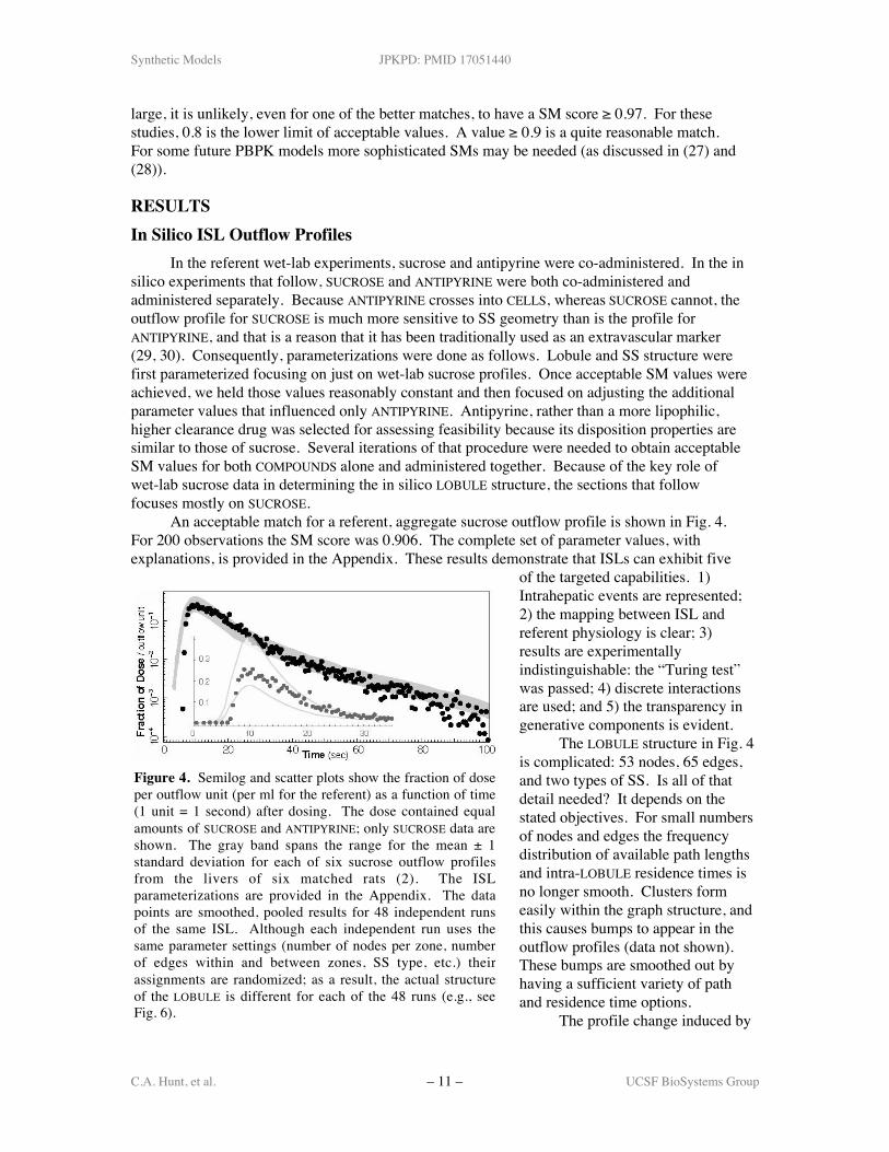
An acceptable match for a referent, aggregate sucrose outflow profile is shown in Fig. 4.For 200 observations the SM score was 0.906. The complete set of parameter values, withexplanations, is provided in the Appendix. These results demonstrate that ISLs can exhibit five

of the targeted capabilities. 1)Intrahepatic events are represented;2) the mapping between ISL andreferent physiology is clear; 3)results are experimentallyindistinguishable: the “Turing test”was passed; 4) discrete interactionsare used; and 5) the transparency ingenerative components is evident.

The LOBULE structure in Fig. 4is complicated: 53 nodes, 65 edges,and two types of SS. Is all of thatdetail needed? It depends on thestated objectives. For small numbersof nodes and edges the frequencydistribution of available path lengthsand intra-LOBULE residence times isno longer smooth. Clusters formeasily within the graph structure, andthis causes bumps to appear in theoutflow profiles (data not shown).These bumps are smoothed out byhaving a sufficient variety of pathand residence time options.

The profile change induced by

Figure 4. Semilog and scatter plots show the fraction of doseper outflow unit (per ml for the referent) as a function of time(1 unit = 1 second) after dosing. The dose contained equalamounts of SUCROSE and ANTIPYRINE; only SUCROSE data areshown. The gray band spans the range for the mean ± 1standard deviation for each of six sucrose outflow profilesfrom the livers of six matched rats (2). The ISLparameterizations are provided in the Appendix. The datapoints are smoothed, pooled results for 48 independent runsof the same ISL. Although each independent run uses thesame parameter settings (number of nodes per zone, numberof edges within and between zones, SS type, etc.) theirassignments are randomized; as a result, the actual structureof the LOBULE is different for each of the 48 runs (e.g., seeFig. 6).

Synthetic Models JPKPD: PMID 17051440

C.A. Hunt, et al. – 12 – UCSF BioSystems Group

a modest change in one parametercan be reasonably compensated forby adjustments in several of theother parameters. However, therelationships that produce thecompensations are highly nonlinear.As an illustration, to increasethroughput for sucrose one can:increase circumference of SSs;shorten the SSs; remove cycles fromthe graph; add more inter-zoneedges; remove intra-zone edges; orincrease the parameter Turbo.Overall, the parameters haveoverlapping influences and the mapbetween the parameters, their values,and the observables is nonlinear, aswould be the case if the analogousproperties in the actual liver weremodified, were it possible to makesuch modifications.

For the data in Fig. 4, the ISLparameters were tuned to generate a

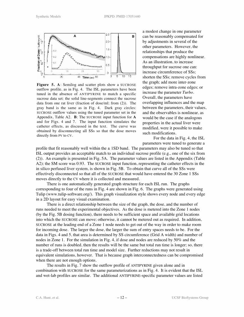
profile that fit reasonably well within the ± 1SD band. The parameters may also be tuned so thatISL output provides an acceptable match to an individual sucrose profile (e.g., one of the six from(2)). An example is presented in Fig. 5A. The parameter values are listed in the Appendix (TableA2); the SM score was 0.93. The SUCROSE input function, representing the catheter effects in thein silico perfused liver system, is shown in Fig. 5B. To obtain that curve all of the SSs wereeffectively disconnected so that all of the SUCROSE that would have entered the 30 Zone 1 SSsmoves directly to the CV where it is collected and measured.

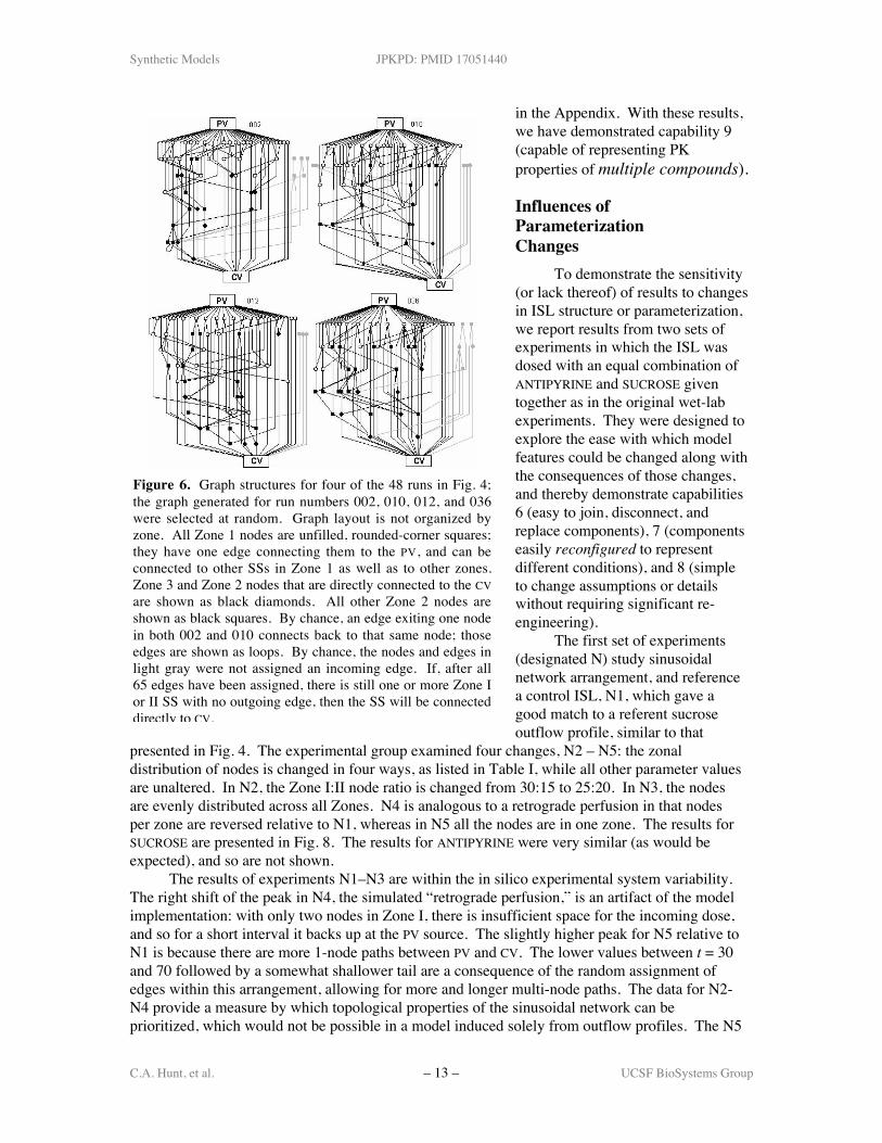
There is one automatically generated graph structure for each ISL run. The graphscorresponding to four of the runs in Fig. 4 are shown in Fig. 6. The graphs were generated usingTulip (www.tulip-software.org/). This graph visualization style shows every node and every edgein a 2D layout for easy visual examination.

There is a direct relationship between the size of the graph, the dose, and the number ofruns needed to meet the experimental objectives. As the dose is metered into the Zone 1 nodes(by the Fig. 5B dosing function), there needs to be sufficient space and available grid locationsinto which the SUCROSE can move; otherwise, it cannot be metered out as required. In addition,SUCROSE at the leading end of a Zone 1 node needs to get out of the way in order to make roomfor incoming dose. The larger the dose, the larger the sum of entry spaces needs to be. For thedata in Figs. 4 and 5, that area is determined by SS circumference (Grid A width) and number ofnodes in Zone 1. For the simulation in Fig. 4, if dose and nodes are reduced by 50% and thenumber of runs is doubled, then the results will be the same but total run time is longer; so, thereis a trade-off between total run time and model size. Further reductions may not result inequivalent simulations, however. That is because graph interconnectedness can be compromisedwhen there are not enough options.

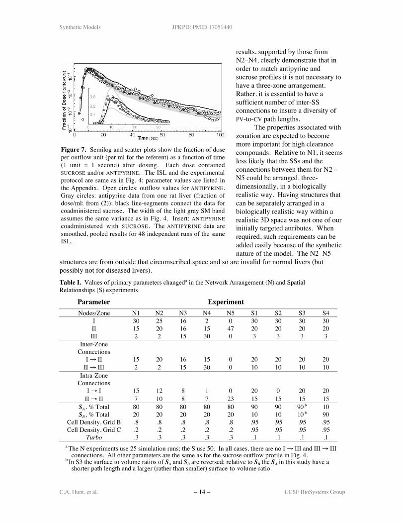
The results in Fig. 7 show the outflow profile of ANTIPYRINE given alone and incombination with SUCROSE for the same parameterizations as in Fig. 4. It is evident that the ISLand wet-lab profiles are similar. The additional ANTIPYRINE-specific parameter values are listed

Figure 5. A : Semilog and scatter plots show a SUCROSEoutflow profile, as in Fig. 4. The ISL parameters have beentuned in the absence of ANTIPYRINE to match a specificsucrose data set: the solid line-segments connect the sucrosedata from one rat liver (fraction of dose/ml; from (2)). Thegray band is the same as in Fig. 4. Dark gray circles:SUCROSE outflow values using the tuned parameter set in theAppendix, Table A2. B: The SUCROSE input function for Aand for Figs. 4 and 7. The input function simulates thecatheter effects, as discussed in the text. The curve wasobtained by disconnecting all SSs so that the dose movesdirectly from PV to CV.

Synthetic Models JPKPD: PMID 17051440

C.A. Hunt, et al. – 13 – UCSF BioSystems Group

in the Appendix. With these results,we have demonstrated capability 9(capable of representing PKproperties of multiple compounds).

Influences ofParameterizationChanges

To demonstrate the sensitivity(or lack thereof) of results to changesin ISL structure or parameterization,we report results from two sets ofexperiments in which the ISL wasdosed with an equal combination ofANTIPYRINE and SUCROSE giventogether as in the original wet-labexperiments. They were designed toexplore the ease with which modelfeatures could be changed along withthe consequences of those changes,and thereby demonstrate capabilities6 (easy to join, disconnect, andreplace components), 7 (componentseasily reconfigured to representdifferent conditions), and 8 (simpleto change assumptions or detailswithout requiring significant re-engineering).

The first set of experiments(designated N) study sinusoidalnetwork arrangement, and referencea control ISL, N1, which gave agood match to a referent sucroseoutflow profile, similar to that

presented in Fig. 4. The experimental group examined four changes, N2 – N5: the zonaldistribution of nodes is changed in four ways, as listed in Table I, while all other parameter valuesare unaltered. In N2, the Zone I:II node ratio is changed from 30:15 to 25:20. In N3, the nodesare evenly distributed across all Zones. N4 is analogous to a retrograde perfusion in that nodesper zone are reversed relative to N1, whereas in N5 all the nodes are in one zone. The results forSUCROSE are presented in Fig. 8. The results for ANTIPYRINE were very similar (as would beexpected), and so are not shown.

The results of experiments N1–N3 are within the in silico experimental system variability.The right shift of the peak in N4, the simulated “retrograde perfusion,” is an artifact of the modelimplementation: with only two nodes in Zone I, there is insufficient space for the incoming dose,and so for a short interval it backs up at the PV source. The slightly higher peak for N5 relative toN1 is because there are more 1-node paths between PV and CV. The lower values between t = 30and 70 followed by a somewhat shallower tail are a consequence of the random assignment ofedges within this arrangement, allowing for more and longer multi-node paths. The data for N2-N4 provide a measure by which topological properties of the sinusoidal network can beprioritized, which would not be possible in a model induced solely from outflow profiles. The N5

Figure 6. Graph structures for four of the 48 runs in Fig. 4;the graph generated for run numbers 002, 010, 012, and 036were selected at random. Graph layout is not organized byzone. All Zone 1 nodes are unfilled, rounded-corner squares;they have one edge connecting them to the PV, and can beconnected to other SSs in Zone 1 as well as to other zones.Zone 3 and Zone 2 nodes that are directly connected to the CVare shown as black diamonds. All other Zone 2 nodes areshown as black squares. By chance, an edge exiting one nodein both 002 and 010 connects back to that same node; thoseedges are shown as loops. By chance, the nodes and edges inlight gray were not assigned an incoming edge. If, after all65 edges have been assigned, there is still one or more Zone Ior II SS with no outgoing edge, then the SS will be connecteddirectly to CV.

Synthetic Models JPKPD: PMID 17051440

C.A. Hunt, et al. – 14 – UCSF BioSystems Group

results, supported by those fromN2–N4, clearly demonstrate that inorder to match antipyrine andsucrose profiles it is not necessary tohave a three-zone arrangement.Rather, it is essential to have asufficient number of inter-SSconnections to insure a diversity ofPV-to-CV path lengths.

The properties associated withzonation are expected to becomemore important for high clearancecompounds. Relative to N1, it seemsless likely that the SSs and theconnections between them for N2 –N5 could be arranged, three-dimensionally, in a biologicallyrealistic way. Having structures thatcan be separately arranged in abiologically realistic way within arealistic 3D space was not one of ourinitially targeted attributes. Whenrequired, such requirements can beadded easily because of the syntheticnature of the model. The N2–N5

structures are from outside that circumscribed space and so are invalid for normal livers (butpossibly not for diseased livers).Table I. Values of primary parameters changed a in the Network Arrangement (N) and SpatialRelationships (S) experiments

Parameter ExperimentNodes/Zone N1 N2 N3 N4 N5 S1 S2 S3 S4

I 30 25 16 2 0 30 30 30 30II 15 20 16 15 47 20 20 20 20III 2 2 15 30 0 3 3 3 3

Inter-ZoneConnections

I → II 15 20 16 15 0 20 20 20 20II → III 2 2 15 30 0 10 10 10 10

Intra-ZoneConnections

I → I 15 12 8 1 0 20 0 20 20II → II 7 10 8 7 23 15 15 15 15

SA , % Total 80 80 80 80 80 90 90 90 b 10SB , % Total 20 20 20 20 20 10 10 10 b 90

Cell Density, Grid B .8 .8 .8 .8 .8 .95 .95 .95 .95Cell Density, Grid C .2 .2 .2 .2 .2 .95 .95 .95 .95

Turbo .3 .3 .3 .3 .3 .1 .1 .1 .1a The N experiments use 25 simulation runs; the S use 50. In all cases, there are no I → III and III → III

connections. All other parameters are the same as for the sucrose outflow profile in Fig. 4.b In S3 the surface to volume ratios of SA and SB are reversed; relative to SB the SA in this study have a

shorter path length and a larger (rather than smaller) surface-to-volume ratio.

Figure 7. Semilog and scatter plots show the fraction of doseper outflow unit (per ml for the referent) as a function of time(1 unit = 1 second) after dosing. Each dose containedSUCROSE and/or ANTIPYRINE. The ISL and the experimentalprotocol are same as in Fig. 4; parameter values are listed inthe Appendix. Open circles: outflow values for ANTIPYRINE.Gray circles: antipyrine data from one rat liver (fraction ofdose/ml; from (2)); black line-segments connect the data forcoadministered sucrose. The width of the light gray SM bandassumes the same variance as in Fig. 4. Insert: ANTIPYRINEcoadministered with SUCROSE. The ANTIPYRINE data aresmoothed, pooled results for 48 independent runs of the sameISL.

Synthetic Models JPKPD: PMID 17051440

C.A. Hunt, et al. – 15 – UCSF BioSystems Group

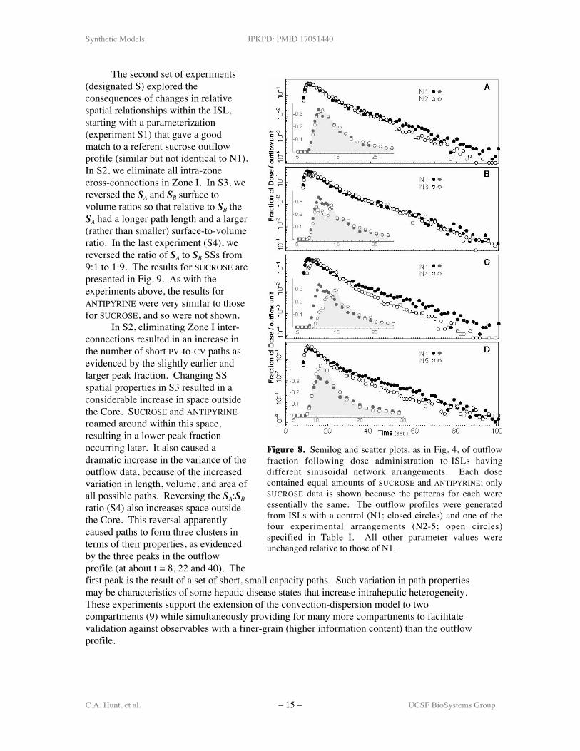
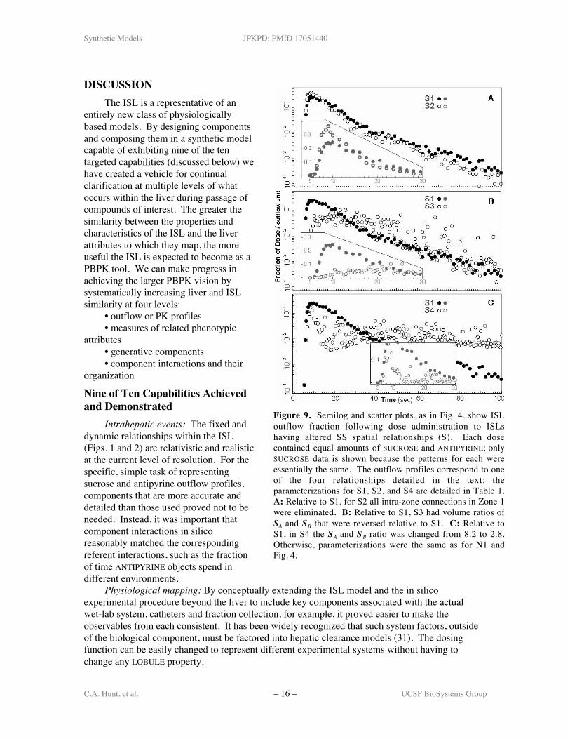
The second set of experiments(designated S) explored theconsequences of changes in relativespatial relationships within the ISL,starting with a parameterization(experiment S1) that gave a goodmatch to a referent sucrose outflowprofile (similar but not identical to N1).In S2, we eliminate all intra-zonecross-connections in Zone I. In S3, wereversed the SA and SB surface tovolume ratios so that relative to SB theSA had a longer path length and a larger(rather than smaller) surface-to-volumeratio. In the last experiment (S4), wereversed the ratio of SA to SB SSs from9:1 to 1:9. The results for SUCROSE arepresented in Fig. 9. As with theexperiments above, the results forANTIPYRINE were very similar to thosefor SUCROSE, and so were not shown.

In S2, eliminating Zone I inter-connections resulted in an increase inthe number of short PV-to-CV paths asevidenced by the slightly earlier andlarger peak fraction. Changing SSspatial properties in S3 resulted in aconsiderable increase in space outsidethe Core. SUCROSE and ANTIPYRINEroamed around within this space,resulting in a lower peak fractionoccurring later. It also caused adramatic increase in the variance of theoutflow data, because of the increasedvariation in length, volume, and area ofall possible paths. Reversing the SA:SB

ratio (S4) also increases space outsidethe Core. This reversal apparentlycaused paths to form three clusters interms of their properties, as evidencedby the three peaks in the outflowprofile (at about t = 8, 22 and 40). Thefirst peak is the result of a set of short, small capacity paths. Such variation in path propertiesmay be characteristics of some hepatic disease states that increase intrahepatic heterogeneity.These experiments support the extension of the convection-dispersion model to twocompartments (9) while simultaneously providing for many more compartments to facilitatevalidation against observables with a finer-grain (higher information content) than the outflowprofile.

Figure 8. Semilog and scatter plots, as in Fig. 4, of outflowfraction following dose administration to ISLs havingdifferent sinusoidal network arrangements. Each dosecontained equal amounts of SUCROSE and ANTIPYRINE; onlySUCROSE data is shown because the patterns for each wereessentially the same. The outflow profiles were generatedfrom ISLs with a control (N1; closed circles) and one of thefour experimental arrangements (N2-5; open circles)specified in Table I. All other parameter values wereunchanged relative to those of N1.

Synthetic Models JPKPD: PMID 17051440

C.A. Hunt, et al. – 16 – UCSF BioSystems Group

DISCUSSIONThe ISL is a representative of an

entirely new class of physiologicallybased models. By designing componentsand composing them in a synthetic modelcapable of exhibiting nine of the tentargeted capabilities (discussed below) wehave created a vehicle for continualclarification at multiple levels of whatoccurs within the liver during passage ofcompounds of interest. The greater thesimilarity between the properties andcharacteristics of the ISL and the liverattributes to which they map, the moreuseful the ISL is expected to become as aPBPK tool. We can make progress inachieving the larger PBPK vision bysystematically increasing liver and ISLsimilarity at four levels:

• outflow or PK profiles• measures of related phenotypic

attributes• generative components• component interactions and their

organization

Nine of Ten Capabilities Achievedand Demonstrated

Intrahepatic events: The fixed anddynamic relationships within the ISL(Figs. 1 and 2) are relativistic and realisticat the current level of resolution. For thespecific, simple task of representingsucrose and antipyrine outflow profiles,components that are more accurate anddetailed than those used proved not to beneeded. Instead, it was important thatcomponent interactions in silicoreasonably matched the correspondingreferent interactions, such as the fractionof time ANTIPYRINE objects spend indifferent environments.

Physiological mapping: By conceptually extending the ISL model and the in silicoexperimental procedure beyond the liver to include key components associated with the actualwet-lab system, catheters and fraction collection, for example, it proved easier to make theobservables from each consistent. It has been widely recognized that such system factors, outsideof the biological component, must be factored into hepatic clearance models (31). The dosingfunction can be easily changed to represent different experimental systems without having tochange any LOBULE property.

Figure 9. Semilog and scatter plots, as in Fig. 4, show ISLoutflow fraction following dose administration to ISLshaving altered SS spatial relationships (S). Each dosecontained equal amounts of SUCROSE and ANTIPYRINE; onlySUCROSE data is shown because the patterns for each wereessentially the same. The outflow profiles correspond to oneof the four relationships detailed in the text; theparameterizations for S1, S2, and S4 are detailed in Table 1.A: Relative to S1, for S2 all intra-zone connections in Zone 1were eliminated. B: Relative to S1, S3 had volume ratios ofSA and SB that were reversed relative to S1. C: Relative toS1, in S4 the SA and SB ratio was changed from 8:2 to 2:8.Otherwise, parameterizations were the same as for N1 andFig. 4.

Synthetic Models JPKPD: PMID 17051440

C.A. Hunt, et al. – 17 – UCSF BioSystems Group

Two classes of observables influenced physiological mappings: histological and dynamic.We used the former to set constraints: acceptable in silico components and relationships neededto fall within to be consistent. Where they fell, such as the number of graph nodes, theirinterconnections and SS properties, and number of ENZYMES per HEPATOCYTE, were controlledby the dynamic observable, of which we had one type: outflow profiles. By increasing thenumber of compounds that an ISL can represent (discussed below), we will be iterativelyimproving the physiological mapping along with the accuracy of the detail within.

Turing test: Because the many Monte Carlo controlled options at each cycle, each trek ofdose through the same lobule in unique and no two lobules are identical. By pooling results fromseveral simulations, we generated a unique outflow profile. In these ways, the ISL hasrepresented uncertainty in observations as well as in the biology and the outflow profiles. Usingan acceptably parameterized ISL, we demonstrated that once the SM criteria were satisfied, thenfrom data alone, the results from wet-lab and in silico experiments were experimentallyindistinguishable.

Transparency: Synthetic models transparency helps bring conceptual clarity to the opacityof biological systems. We can record where SUCROSE and ANTIPYRINE go and what they do. Wecan then visualize such detail as the simulation progresses7. We can, for example observe howany SS is connected to others or how many HEPATOCYTES an ANTIPYRINE visits before beingMETABOLIZED. From a modeling perspective, such capabilities provide a means of identifyingpotential flaws in the software, its assembly, and operation in ways that can feed back andinfluence the design of future experiments and how we think about the referent. Havingtransparency makes it possible to contrast visual and abstract features of the ISL and to observehow processes give rise to characteristic features. We can trace cause-effect relationships tospecific subcellular components.

Articulation: Articulation: To make model evolution facile, the PBPK modeler needs theability to easily explore an alternate sinusoidal topography, for example, or to alter the spatialarrangement of TRANSPORTERS and ENZYMES (23, 24). We have demonstrated that it isstraightforward to plug SS components together, later disconnect them, and replace some withnew components (Figs. 8 and 9). The same can be done within the SS functional unit: a grid orcells can be removed and modified. Cells can be added to or removed. The functions andinterrelations of the other components remain unaltered.

Reconfigurability: Internal and external factors can lead to important differences betweenlivers. The PBPK vision anticipates being able to explore the significance and consequences ofsuch differences. Using directed graphs to represent connectivity between units of function, oneof several possible approaches, enables us to manipulate the representation of both histology andphysiology. We have shown that it is easy to alter these representations and explore theconsequences. Although not demonstrated here, it is similarly easy to alter the experimentalcontext. The ISL represents an isolated, perfused liver. By altering the lobule input functions, wecan change the system to represent the liver in a living rat or within a different perfusion system.We can unplug HEPATOCYTES from the ISL and study their properties in simulated in vitroexperimental conditions (25, 26). Given appropriate in vitro data we can also refine,reparameterize and validate the HEPATOCYTES, and return them to the ISL to observe theconsequences within the whole-liver context.

Change usage: With traditional PBPK models, changing assumptions as we did for Fig. 8,can require a different set of differential equations where the mapping between the new and theoriginal parameters is not straightforward. This reality often hampers exploring the consequencesof alternative sets of assumptions. Consequently, some PBPK models can acquire a degree ofinertia. Researchers find it easier or more cost effective to adjust their requirements and model 7 A visualization of both SUCROSE and ANTIPYRINE moving within one SS is available at[http://biosystems.ucsf.edu/Researc/structure6/IL_Visualization.htm].

Synthetic Models JPKPD: PMID 17051440

C.A. Hunt, et al. – 18 – UCSF BioSystems Group

use to available models, thereby avoiding dealing with such challenges and forgoing the benefitsthey might have obtained. Elimination of such situations is the motivation for capability eight.

Multiple compounds: We have demonstrated a powerful, scientifically useful characteristicof the ISL. An ISL parameterized for one COMPOUND, SUCROSE in this case, can be used torepresent the outflow profile of a new compound, such as ANTIPYRINE, without compromising themodel’s ability to interact as before with the first compound. We need only change thoseparameters that are influenced differently by the new compound’s physicochemical properties.Should one or two new features be needed, they can be added without compromising existing ISLcapabilities. It remains to be demonstrated if a single ISL can be extended to a large set ofcompounds. The ISL exists and is capable of functioning whether or not it is dosed withSUCROSE and/or ANTIPYRINE. Each COMPOUND has properties that can be recognized by the ISLcomponents. They can even be given recognition algorithms so that after acquiring a mobileobject’s properties, the ISL components automatically adjust their responses according to aseparate or learned algorithm and the objects they encounter.

Discrete interactions: We demonstrated that adopting graphs (networks) as a fundamentalmodeling tool allows us to achieve the above nine capabilities. By restricting the model todiscrete interactions, it ensures that graphs can be used throughout the ISL, which ensures theabove nine capabilities and makes the resulting device more explorable.

Whole organism: Having the ISL become a component in a whole organism model is aspecial case of the articulation, reconfigurability, and change usage capabilities. Attaining it isessential to achieve the full PBPK vision and strengthen the case being made for this class ofmodels. Aspects of an ISL can be separately validated against in vitro data, for example, prior toinclusion within the whole organism model.

Detail, Accuracy, and RealismHow much detail does an ISL need; how accurate and realistic does it need to be? The

answers require having other information, such as a clear statement of why the model is needed.The PBPK vision is such a statement. We also need to state the uses to which the model will beput, such as to mimic specific aspects of hepatic functionality along with PCs of the referentsystem that we deem important for the analogue to possess. These PCs were a significantdeterminant of the detail reflected in Figs. 1 and 2. Depending on how PCs are specified, theywill circumscribe a space of allowable ISLs that can range from relatively simple to complex.The referent PCs are expected to have direct counterparts in the ISLs. For example, if at least50% of the sinusoids near the PV in the referent lobules are (or are assumed to be)interconnected, and this property is among the listed PCs, then at least 50% of the SSs near thePV in the ISL should be interconnected.

Most important are the measurable observables of the referent. They are used for modelvalidation (see Supplementary Material). They circumscribe the behavior space of each ISL. Thesimilarity measures used to compare referent and ISL observables provide an acceptance criterionfor the accuracy; and so, indirectly they are part of the ISL specification. They influence theISL’s detail and fidelity. For example, if we had decided to be satisfied with outflow profiles thatfit within a ± 2SD band about the target outflow data, and we had decided to tolerate a fewmodest bumps in the simulated outflow profile, then we could have accepted lobule graphstructures having significantly less detail.

Several ISL features can be cited as being realistic; others can be criticized as beingunrealistic. We have dealt with the former. Relative to the latter, here are three examples. 1) Ina lobule, only adjacent sinusoids are interconnected, whereas in the ISL, connections betweennodes are randomly assigned without consideration of relative location. 2) Because the SA and SB

are randomly assigned, the range of path lengths in terms of total grid length can beunrealistically broad. For example a one-node path could be as short as two grid spaces in length;

Synthetic Models JPKPD: PMID 17051440

C.A. Hunt, et al. – 19 – UCSF BioSystems Group

whereas, a three-node path could be 50 grid spaces or longer. It seems unlikely that the range inactual lobule path lengths will be that broad. To make relative path lengths more realistic, weneed to add a data-driven constraint to our list of targeted PCs. 3) The graph structures (Fig. 6)are intended to represent plausible paths, not actual measurable lengths. They are not intended tobe scale models of actual sinusoidal arrangements.

Because of the random assignment of edges, a Zone 1 or 2 node can be connected to itselfby a single edge (the loop in graphs 002 and 010 in Fig. 6) that forces some compound to revisitthe same region of functionality many times. We did not eliminate this feature because, eventhough it does not seem realistic, we did not have experimental evidence to rule out such pathoptions occurring at a low frequency. Should the evidence become available (or a convincingargument be offered) that no such paths exist in livers, a constraint can be added disallowingthem.

The ISL is complicated, and yet we are only dealing with antipyrine and sucrose. We donot yet address any of the potentially complex intracellular events encountered by some drugs. Isthis ISL too complicated? To achieve the PBPK vision will require a combination ofsophisticated knowledge, skills, and tools. The problems can have complex origins. Complicatedproblem solving and decision-making skills require complicated technology (or experiencedexperts or both). As the overlap between in silico and referent phenotypes increases, thecomplexity of ISLs and similar devices will approach that of their referents.

CONCLUSIONThere is increasing impetus for the inclusion of in silico PBPK modeling in defining

compound PK properties and their suitability for clinical use (33). To achieve these goals it isbecoming necessary to provide increasingly more useful predictions and detailed explanations forobserved PK behaviors and properties. Achieving the required detail is limited by the abstractivenature and inherent heuristic limitations of current inductive PBPK models. The synthetic ISL isan early example of a class of models specifically intended to help provide the required detail anddeliver improved insights.

ACKNOWLEDGEMENTSFor valuable technical assistance, we thank G. Cosmo Haun, and for theoretical, biological,

and practical advice, we thank Bernie Zeigler, Betty Hoener, and Zbigniew Kmiec. This work isreflected in the content of Li Yan’s Ph.D. dissertation. For their helpful advice and commentaryon the manuscript, along with helpful discussions and suggestions, we thank Jesse Engelberg,Pearl Johnson, Sunwoo Park, Shahab Sheikh-Bahaei, Teddy Lam, Suman Ganguli, Sean Kim,Mark Grant, and other members of the BioSystems Group along with Tom Robertson and NarelleWalker from UQ. CAH thanks Amina Qutub for her early efforts in agent-based modeling. Weare grateful for the financial support of the CDH Research Foundation (of which CAH is atrustee), the National Health and Medical Research Council of Australia, the Queensland andNew South Wales Lions Medical Research Foundation, and CAH. We are especially grateful tothe Swarm Development Group, Debian, and the Free Software Foundation for making all thetools. Earlier versions of the ISL were presented and discussed at the Computational Methods inSystems Biology, Second International Workshop, CMSB 2004, (32), and at the 26th AnnualInternational Conference of the Engineering in Medicine and Biology Society, September, 2004.

Synthetic Models JPKPD: PMID 17051440

C.A. Hunt, et al. – 20 – UCSF BioSystems Group

SUPPLEMENTARY MATERIAL

Visualizations of compounds moving within a SS and an entire LOBULE are available at[http://biosystems.ucsf.edu/Researc/structure6/IL_Visualization.htm]. The supplementarymaterial includes additional detail on the following eight topics. 1) The inductive and syntheticmethods; 2) contrasting inductive and synthetic models; 3) comparison of inductive and syntheticmodels; 4) validation of synthetic models; 5) in silico framework: technical detail; 6) in silicoexperimental method; 7) building an acceptable in silico liver model; and 8) higher and lowerlevels of resolution.

REFERENCES1. M. Rowland. Physiologic pharmacokinetic models: relevance, experience, and future trends. Drug

Metab. Rev. 15:55-74 (1984).2. D. Y. Hung, P. Chang, M. Weiss, and M. S. Roberts. Structure-hepatic disposition relationships for

cationic drugs in isolated perfused rat livers: transmembrane exchange and cytoplasmic bindingprocess. J. Pharmacol. Exper. Therap. 297:780–89 (2001).

3. J. B. Bassingthwaite. Blood flow and diffusion through mammalian organs. Science 167:1347-53(1970).

4. M. Rowland, L. Balant, and C. Peck. Physiologically based pharmacokinetics in drug developmentand regulatory science: a workshop report (Georgetown University, Washington, DC, May 29-30,2002). AAPS PharmSci. 6: article 6. DOI: 10.1208/ps060106 (2004).

5. M. E. Andersen. Toxicokinetic modeling and its applications in chemical risk assessment. Toxicol.Lett. 138(1-2):9-27 (2003).

6. D. E. Leahy. Progress in simulation modelling for pharmacokinetics. Curr. Top. Med. Chem. 3:1257-68 (2003).

7. R. A. Corley, T. J. Mast, E. W. Carney, J. M. Rogers, and G. P. Daston. Evaluation of physiologicallybased models of pregnancy and lactation for their application in children's health risk assessments.Crit. Rev. Toxicol. 33(2):137-211 (2003).

8. M. S. Roberts, B. M. Magnusson, F. J. Burczynski, and M. Weiss. Enterohepatic circulation:physiological, pharmacokinetic and clinical implications. Clin. Pharmacokinet. 41:751-90 (2002).

9. M. S. Roberts and Y. G. Anissimov. Modeling of hepatic elimination and organ distribution kineticswith the extended convection-dispersion model. J. Pharmacokin. Biopharm. 27:343-382 (1999).

10. B. P. Zeigler, H. Praehofer, and T. G. Kim. Theory of Modeling and Simulation: Integrating DiscreteEvent and Continuous Complex Dynamic Systems. Academic Press, California, 2000, pp. 3-36, 75-85,99-104, 137-147.

11. L. Steels and R. Brooks (eds.). The Artificial Life Route to Artificial Intelligence. Lawrence EarlbaumAssociates, Inc., New Jersey, 1995, pp. 83-121.

12. K. Czarnecki and U. Eisenecker. Generative Programming: Methods, Tools, and Applications.Addison-Wesley, New York, 2000, pp. 10, 251-254.

13. G. E. Ropella, C. A. Hunt, and D. A. Nag. Using heuristic models to bridge the gap between analyticand experimental models in biology. 2005 Spring Simulation Multiconference, The Society forModeling and Simulation International, April 2-8, 2005A, San Diego, CA.

14. G. E. Ropella, C. A. Hunt, and S. Sheikh-Bahaei. Methodological Considerations of HeuristicModeling of Biological Systems. The 9th World Multi-Conference on Systemics, Cybernetics andInformatics, July 10-13, 2005B, Orlando, Florida.

15. H. F. Teutsch, D. Schuerfeld, and E. Groezinger. Three-dimensional reconstruction of parenchymalunits in the liver of the rat. Hepatology 29:494-505 (1999).

16. J. J. Gumucio and D. L. Miller. Zonal hepatic function: solute-hepatocyte interactions within the liveracinus. Prog. Liver. Diseases. 7:17-30 (1982).

17. Y. Kato, J. Tanaka, and K. Koyama. Intralobular heterogeneity of oxidative stress and cell death inischemia-reperfused rat liver. J Surg. Res.95:99-106 (2001).

Synthetic Models JPKPD: PMID 17051440

C.A. Hunt, et al. – 21 – UCSF BioSystems Group

18. J. Y. Scoazec, L. Racine, A. Couvelard, J. F. Flejou, and G. Geldmann. Endothelial cell heterogeneityin the normal human liver acinus: in silico immunohistochemical demonstration. Liver 14:113-23(1994).

19. R. S. McCuskey. Morphological mechanisms for regulating blood flow through hepatic sinusoids.Liver 20:3-7 (2000).

20. K. Cheung, P. E. Hickman, J. M. Potter, N. Walker, M. Jericho, R. Haslam, and M. S. Roberts. Anoptimised model for rat liver perfusion studies. J. Surg. Res. 66:81–89 (1996).

21. A. Koo, I. Y. Liang, and K. K. Cheng. The terminal hepatic microcirculation in the rat. Quart. J. Exp.Physiol. Cogn. Med. 60:261-266 (1975).

22. D. L. Miller, C. S. Zanolli, and J. J. Gumucio. Quantitative morphology of the sinusoids of the hepaticacinus. Gastroenterology 76:965-969 (1979).

23. Y. Liu and C. A. Hunt. Studies of intestinal drug transport using an in silico epithelio-mimetic device.Biosystems 82(2):154-167 (2005).

24. Y. Liu and C. A. Hunt. Mechanistic study of the interplay of intestinal transport and metabolism usingthe synthetic modeling method. Pharm Res. 23(3):493-505 (2006).

25. S. Sheikh-Bahaei, G. E. P. Ropella, and C. A. Hunt. Agent-based simulation of in vitro hepatic drugmetabolism: in silico hepatic intrinsic clearance. 2005 Spring Simulation Multiconference, The Societyfor Modeling and Simulation International, April 2-8, San Diego, CA.

26. S. Sheikh-Bahaei, G. E. P. Ropella, and C. A. Hunt. In Silico Hepatocyte: Agent-Based Modeling ofthe Biliary Excretion of Drugs. 2006 Spring Simulation Multiconference, The Society for Modelingand Simulation International, April 2-6, Huntsville, AL.

27. S. Santini and R. Jain. Similarity Measures. IEEE Tran. Pattern Analysis and Machine Intelligence21(9):871-83 (1999).

28. D. A. Nag, G. E. P. Ropella, and C. A. Hunt. Similarity measures and validation in automatedmodeling. Huntsville Simulation Conference, Huntsville, AL, October 25-27, 2005.

29. C. A. Goresky. A linear method for determining liver sinusoidal and extravascular volumes. Am. J.Physiol. 204:626-40 (1963).

30. K. S. Pang, W.-F. Lee, W. F. Cherry, V. Yuen, J. Accaputo, S. Fayz, A. J. Schwab, and C. A. Goresky.Effects of perfusate flow rate on measured blood volume, Disse space, intracellular water space, anddrug extraction in the perfused rat liver preparation: characterization by the multiple indicator dilutiontechnique. J. Pharmacokinet. Biopharm. 16:595-632 (1988).

31. Y. G. Anissimov, A. J. Bracken, and M. S. Roberts. Catheter effects in organ perfusion experiments.J. theor. Biol. 214:263-73 (2002).

32. C. A. Hunt, G. E.P. Ropella, M. S. Roberts, and L. Yan. Biomimetic In Silico Devices. Lecture Notesin Bioinformatics 3082:35–43 (2005).

33. Food and Drug Administration. Innovation or Stagnation: Challenge and Opportunity on the CriticalPath to New Medical Products [online],<http://www.fda.gov/oc/initiatives/criticalpath/whitepaper.html> (2004).

34. D.E. Leahy. Progress in simulation modelling for pharmacokinetics. Curr. Top. Med. Chem.3(11):1257-68 (2003).

35. S.M. Peirce, E.J. van Gieson, and T.C. Skalak. Multicellular simulation predicts microvascularpatterning and in silico tissue assembly. FASEB J 18:731-33 (2004).

36. G. An. In-silico experiments of existing and hypothetical cytokine-directed clinical trials using agentbased modeling. Crit. Care Med. 32:2050-60 (2004).

APPENDIX

Synthetic Models JPKPD: PMID 17051440

C.A. Hunt, et al. – 22 – UCSF BioSystems Group

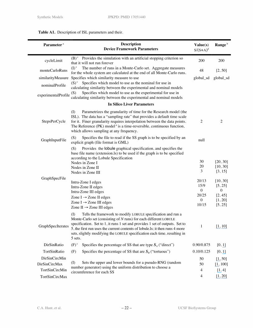
Table A1. Description of ISL parameters and their.

Parameter a DescriptionDevice Framework Parameters

Value(s)S/(S+A)d

Range b

cycleLimit (B) c Provides the simulation with an artificial stopping criterion sothat it will not run forever 200 200

monteCarloRuns (I) c The number of runs in a Monte-Carlo set. Aggregate measuresfor the whole system are calculated at the end of all Monte-Carlo runs. 48 [2, 50]

similarityMeasure Specifies which similarity measure to use global_sd global_sd

nominalProfile (S) c Specifies which model to use as the nominal for use incalculating similarity between the experimental and nominal models

experimentalProfile (S) Specifies which model to use as the experimental for use incalculating similarity between the experimental and nominal models

In Silico Liver Parameters

StepsPerCycle

(I) Parametrizes the granularity of time for the Research model (theISL). The data has a “sampling rate” that provides a default time scalefor it. Finer granularity requires interpolation between the data points.The Reference (PK) model a is a time-reversible, continuous function,which allows sampling at any frequency.

2 2

GraphInputFile (S) Specifies the file to read if the SS graph is to be specified by anexplicit graph (file format is GML) null

GraphSpecFile

(S) Provides the lobule graphical specification, and specifies thebase file name (extension.ls) to be used if the graph is to be specifiedaccording to the Lobule SpecificationNodes in Zone INodes in Zone IINodes in Zone III

Intra-Zone I edgesIntra-Zone II edgesIntra-Zone III edgesZone I → Zone II edgesZone I → Zone III edgesZone II → Zone III edges

30203

20/1315/9

020/25

010/15

[20, 30][10, 30][3, 15]

[10, 30][5, 25]

0[2, 45][1, 20][5, 25]

GraphSpecIterates

(I) Tells the framework to modify LOBULE specification and run aMonte-Carlo set (consisting of N runs) for each different LOBULEspecification. Set to 1, it runs 1 set and provides 1 set of outputs. Set to5, the first run uses the current contents of lobule.ls; it then runs 4 moresets, slightly modifying the LOBULE specification each time, resulting in5 sets.

1 [1, 10]

DirSinRatio (F) c Specifies the percentage of SS that are type SA (“direct”) 0.90/0.875 [0, 1]TortSinRatio (F) Specifies the percentage of SS that are SB (“tortuous”) 0.10/0.125 [0, 1]

DirSinCircMin 50 [1, 50]DirSinCircMax 50 [1, 100]

TortSinCircMin 4 [1, 4]TortSinCircMax

(I) Sets the upper and lower bounds for a pseudo-RNG (randomnumber generator) using the uniform distribution to choose acircumference for each SS

4 [1, 20]

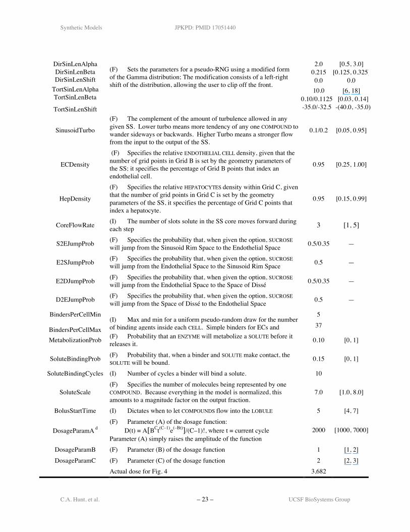
Synthetic Models JPKPD: PMID 17051440

C.A. Hunt, et al. – 23 – UCSF BioSystems Group

DirSinLenAlpha 2.0 [0.5, 3.0]DirSinLenBeta 0.215 [0.125, 0.325]DirSinLenShift 0.0 0.0

TortSinLenAlpha

(F) Sets the parameters for a pseudo-RNG using a modified formof the Gamma distribution; The modification consists of a left-rightshift of the distribution, allowing the user to clip off the front.

10.0 [6, 18]TortSinLenBeta 0.10/0.1125 [0.03, 0.14]TortSinLenShift -35.0/-32.5 -(40.0, -35.0)

SinusoidTurbo

(F) The complement of the amount of turbulence allowed in anygiven SS. Lower turbo means more tendency of any one COMPOUND towander sideways or backwards. Higher Turbo means a stronger flowfrom the input to the output of the SS.

0.1/0.2 [0.05, 0.95]

ECDensity

(F) Specifies the relative ENDOTHELIAL CELL density, given that thenumber of grid points in Grid B is set by the geometry parameters ofthe SS; it specifies the percentage of Grid B points that index anendothelial cell.

0.95 [0.25, 1.00]

HepDensity

(F) Specifies the relative HEPATOCYTES density within Grid C, giventhat the number of grid points in Grid C is set by the geometryparameters of the SS, it specifies the percentage of Grid C points thatindex a hepatocyte.

0.95 [0.15, 0.99]

CoreFlowRate (I) The number of slots solute in the SS core moves forward duringeach step 3 [1, 5]

S2EJumpProb (F) Specifies the probability that, when given the option, SUCROSEwill jump from the Sinusoid Rim Space to the Endothelial Space 0.5/0.35 —

E2SJumpProb (F) Specifies the probability that, when given the option, SUCROSEwill jump from the Endothelial Space to the Sinusoid Rim Space 0.5 —

E2DJumpProb (F) Specifies the probability that, when given the option, SUCROSEwill jump from the Endothelial Space to the Space of Dissé 0.5/0.35 —

D2EJumpProb (F) Specifies the probability that, when given the option, SUCROSEwill jump from the Space of Dissé to the Endothelial Space 0.5 —

BindersPerCellMin 5

BindersPerCellMax(I) Max and min for a uniform pseudo-random draw for the numberof binding agents inside each CELL. Simple binders for ECs andENZYMES for HEPATOCYTES.

37

MetabolizationProb (F) Probability that an ENZYME will metabolize a SOLUTE before itreleases it. 0.10 [0, 1]

SoluteBindingProb (F) Probability that, when a binder and SOLUTE make contact, theSOLUTE will be bound. 0.15 [0, 1]

SoluteBindingCycles (I) Number of cycles a binder will bind a solute. 10

SoluteScale(F) Specifies the number of molecules being represented by oneCOMPOUND. Because everything in the model is normalized, thisamounts to a magnitude factor on the output fraction.

7.0 [1.0, 8.0]

BolusStartTime (I) Dictates when to let COMPOUNDS flow into the LOBULE 5 [4, 7]

DosageParamA d(F) Parameter (A) of the dosage function: D(t) = A[BCt(C–1)e(–Bt)]/(C–1)!, where t = current cycleParameter (A) simply raises the amplitude of the function

2000 [1000, 7000]

DosageParamB (F) Parameter (B) of the dosage function 1 [1, 2]DosageParamC (F) Parameter (C) of the dosage function 2 [2, 3]

Actual dose for Fig. 4 3,682

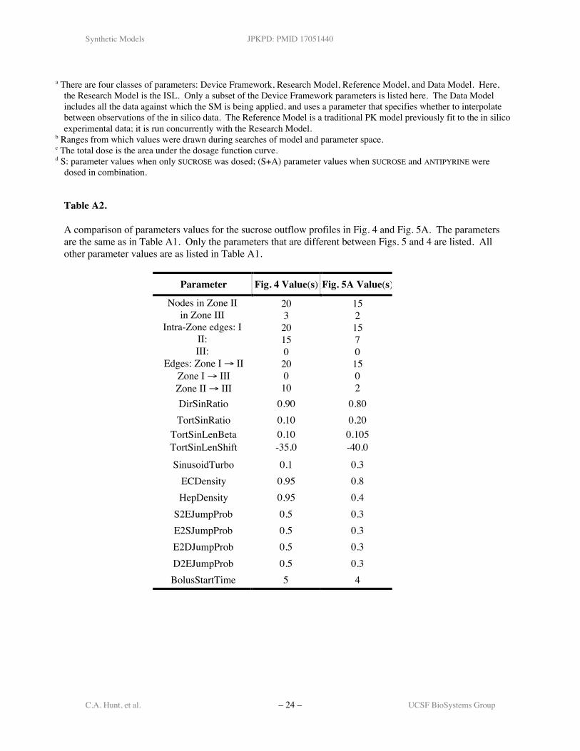
Synthetic Models JPKPD: PMID 17051440

C.A. Hunt, et al. – 24 – UCSF BioSystems Group

a There are four classes of parameters: Device Framework, Research Model, Reference Model, and Data Model. Here,the Research Model is the ISL. Only a subset of the Device Framework parameters is listed here. The Data Modelincludes all the data against which the SM is being applied, and uses a parameter that specifies whether to interpolatebetween observations of the in silico data. The Reference Model is a traditional PK model previously fit to the in silicoexperimental data; it is run concurrently with the Research Model.

b Ranges from which values were drawn during searches of model and parameter space.c The total dose is the area under the dosage function curve.d S: parameter values when only SUCROSE was dosed; (S+A) parameter values when SUCROSE and ANTIPYRINE were

dosed in combination.

Table A2.

A comparison of parameters values for the sucrose outflow profiles in Fig. 4 and Fig. 5A. The parametersare the same as in Table A1. Only the parameters that are different between Figs. 5 and 4 are listed. Allother parameter values are as listed in Table A1.

Parameter Fig. 4 Value(s) Fig. 5A Value(s)

Nodes in Zone IIin Zone III

Intra-Zone edges: III:III:

Edges: Zone I → IIZone I → IIIZone II → III

2032015020010

15215701502

DirSinRatio 0.90 0.80TortSinRatio 0.10 0.20

TortSinLenBeta 0.10 0.105TortSinLenShift -35.0 -40.0

SinusoidTurbo 0.1 0.3ECDensity 0.95 0.8HepDensity 0.95 0.4

S2EJumpProb 0.5 0.3E2SJumpProb 0.5 0.3E2DJumpProb 0.5 0.3D2EJumpProb 0.5 0.3BolusStartTime 5 4

Supplement: Physiologically Based Synthetic Models of Hepatic Disposition

C.A. Hunt, et al. – 1 – UCSF BioSystems Group

Supplementary Material

Physiologically Based Synthetic Models of Hepatic Disposition

C. Anthony Hunt 1,2, Glen E.P. Ropella 2, Li Yan 1, Daniel Y. Hung 3,and Michael S. Roberts 3

1 The UCSF/UCB Joint Graduate Group in Bioengineering, University of California,Berkeley, CA, USA

2 The Department of Biopharmaceutical Sciences, Biosystems Group, University ofCalifornia, San Francisco, CA, USA

3 School of Medicine, Princess Alexandra Hospital, University of Queensland,Woolloongabba, Queensland, 4102, Australia

Corresponding Author:

C. Anthony HuntDepartment of Biopharmaceutical Sciences513 Parnassus Ave., S-926University of CaliforniaSan Francisco, CA 94143-0446P: 415-476-2455F: 415-514-2008E: hunt@itsa.ucsf.edu

Supplement: Physiologically Based Synthetic Models of Hepatic Disposition

C.A. Hunt, et al. – 2 – UCSF BioSystems Group

1. Inductive and Synthetic Methods

Inductive models are usually built by analyzing data, creating a mapping between theenvisioned system structure and components of the data, and then representing the generation ofthose data components with mathematical equations. The method relies heavily on theresearcher’s knowledge combined with induction. When successful, it creates models thatextrapolate somewhat beyond the original data, making the method ideal for prediction.However, the models lack particulars. They are black boxes. The detail that is washed awaywhen an equation is induced contains heuristic value that is needed to achieve the PBPK vision.That detail may describe, for example, the mechanism by which the data were generated, whereasthe mathematics only describes the abstracted properties of the data.

Most PBPK modeling is equation based and, consequently, is limited by the complexity ofthe equations needed to describe intricate functional details. A challenge has been to add backdetail and thereby create models that more reliably describe desired and relevant features,including aspects of the very functional and spatial details that were abstracted away in equation-based models. The convection-dispersion model of the liver and its extension to twocompartments in the extended convection-dispersion model [paper: ref. 9] is an example.Logically, an even more detailed model would be based on an assembly of objects representingcells in a configuration that recognizes the heterogeneity in cell function. Such higher resolutionphenomena cannot easily be simulated within a larger system model using the continuous stateplus continuous time class of models to which most current PBPK models belong. Consequently,there is a need for additional modeling and simulation methods that are more responsive to thepreceding challenges.

There are now a variety of systems and behaviors emphasizing discrete events that arebeing simulated using object-oriented (OO) programming, with the extent of the modeling beingmore than what can be represented using the more mature continuous state, continuous timemodels [paper: ref. 10]. Discrete event, discrete space, discrete time models offer theoretical andpractical advantages because they allow, even facilitate, the composition (plugging togetherseparate components) and decomposition of models (e.g., removing components without breakingthe model). Moreover, in the case where a continuous model is desirable, a discrete model cansimulate or approximate it to arbitrary precision.

The constructivist or synthetic method [paper: ref. 10–14] consists of proposing andconstructing building blocks that can be assembled to create a transparent (easily understood orseen through), artificial system that functions in the real world. The experimental in vitro modelsthat are the mainstay of biomedical research (cell cultures, isolated, perfused organs and tissues,etc.) are synthetic models where some of the building blocks are laboratory items and others areliving parts. Using OO programming it is now feasible to build synthetic modelscomputationally. Synthetic PBPK modeling involves using component parts to build, in silico, afunctioning analogue of the mechanisms (form and function) of which an inductive PBPK modelis an abstraction. This approach is especially suitable for representing spatial and discrete event

Supplement: Physiologically Based Synthetic Models of Hepatic Disposition

C.A. Hunt, et al. – 3 – UCSF BioSystems Group

phenomena and has the potential to be developed and merged with the current PBPK modelingapproach. The resolution of the model dictates whether a mechanism is best modeled as discreteor continuous and a general discrete modeling approach allows the flexibility to choose theappropriate resolution according to the particular mechanism.

2. Contrasting Inductive and Synthetic Models

The advancements in OO programming make it easier to construct large system modelswhere the modular components are inductive models or synthetic models. What follows are briefdescriptions of examples of five different types of constructed, composite system models. In theparagraphs that follow, we draw on the second and third types to briefly compare and contrastinductive and synthetic PKPB models.

1. Synthetic models of engineered systems (e.g., a FedEx distribution center, a Boeing 787) thatare detailed and articulated: the underlying mechanisms are known. Each component is verywell understood and can be accurately represented in a number of ways including validatedabstract equations and more detailed, mechanistic, hierarchical representations. Thecomponents are integrated into a system model in order to study the referent system as a wholeand each component in its systemic context. The system model is transparent because at anylevel of resolution there is enough knowledge about the system to replace any component atany time with a more detailed, less abstract, representation, should that be needed.

2. Assembled, equational PBPK models (e.g., a physiologically based toxicokinetic model as in[Andersen ‘05]: there is incomplete knowledge about the underlying mechanisms.Consequently, aspects of system function are separately represented using equations that mapto abstract representations of known or hypothesized mechanistic components. The biologicalcomponents are not transparent because their underlying mechanisms (although basicallyunderstood) are not fully known, and/or because there is inadequate data on important deeperfeatures. Each PBPK model component is an equation; that equation is a black box because itis an induced abstraction (one can not look into the component to see how it works). Morerefined wet-lab experiments can supply additional detailed data to make the functioning of acomponent less opaque. However, inductive components in a PBPK model can never becometransparent, as in type 1, because making them so would require complete knowledge ofbiology. When each component of a system model is an inductive model of its biologicalcounterpart, the composite model, at its core, remains an inductive model: it is a large,composite inductive model. Robert Rosen [Rosen ‘83] eloquently details the dangers ofextrapolations that rely too strongly on the parameter values of such models.

3. Synthetic physiologically based models of mammalian systems of the type presented herein:there is incomplete knowledge about the underlying mechanisms. Nevertheless, a model isbuilt using OO analogues to recognizable components (as in the ISL). As in type 2, eachbiological component lacks transparency. However, unlike type 2, each component in thesynthetic model is transparent. The analogue components in the OO model, when they behave

Supplement: Physiologically Based Synthetic Models of Hepatic Disposition

C.A. Hunt, et al. – 4 – UCSF BioSystems Group

like those in the biological system, provide a specific instantiation for how the correspondingbiological components might actually work.

4. Of course, depending on intended use, hybrids of type 2 and 3 are feasible. Neither of themethods in 2 and 3 are superior. Both should be used when the particular strengths of both areneeded, which is the case for the PBPK vision.

5. To actually close the gap between both types of models and their biological referents,synthetic models will need the ability to fundamentally change during simulations. They mustbe able to evolve and undergo localized model morphogenesis in response to events within thesimulation.

We appreciate that all large, multi-component models have synthetic and inductive aspects,depending on the perspective from which they are viewed. At the bottom of every syntheticmodel lie inductively defined atomic components, and every inductively defined computer modelis synthetic at its highest systemic level.

Inductive models are induced from data and synthetic models are constructed from pre-existing components. Any component (like a LOBULE) could be an ODE model. As an example,we could replace one of the articulated ISL LOBULES with the two-phase stochastic kinetic model(2PSK model) in [paper: ref. 2]. The resulting hybrid ISL (1 [2PSK model] + 49 LOBULES)would be a synthetic model. In fact, we could replace all 50 LOBULES with varying instantiationsof the 2PSK model and the resulting ISL would still be a synthetic model because it is acomposite of 2PSK models and the result of executing all 50 together is not induced from anydata set (even though the 2PSK model is).

3. Comparing Inductive and Synthetic Models

Most current PBPK modeling methods have both inductive components and syntheticfeatures, as described above for type 2. Whereas the components themselves are inductivemodels, the combination of the components is synthetic. However, the combinations remainmathematical summaries of the component phenomena being modeled and, consequently, theirpredictive capabilities are limited to variants that preserve the induced parameterizations and I/Ocharacteristics of the components. The conditions under which such models can be used reliablyalso depend on the characteristics of the data from which the model components were induced.Combining the model components together raises the potential for component discordance,especially with an increase in the variety of components. Component discordance can arise frominconsistencies or lack of conformity between parameterized components at the model orsimulation level.

The components of the type 3 model described above are designed to be concordant (they interactsmoothly over the full range of conditions). Such a model is intended to be exercised (run) andmeasured in the same way as its referent in vitro or in vivo experimental system and data taken from itis validated against known details of, and the data taken from the referent. An essential differencebetween the methods in type 2 and type 3 lies in the fact that the inductive method explicitly uses theobserved phenomena (the data) as its input whereas the synthetic method starts with proposed

Supplement: Physiologically Based Synthetic Models of Hepatic Disposition

C.A. Hunt, et al. – 5 – UCSF BioSystems Group

building blocks and the relations between them [paper: ref. 13 & 14]. The inductive method takes theontology defined implicitly in the data as an inherent assumption whereas the synthetic method,employing cycles of creation, verification, and model change, attempts to construct an ontology (andan analogue that “lives” in that ontology) that can realize data of interest.

Differences between the two modeling methods can be seen in the mappings from the spaceof generator mechanisms to the space of phenomena. The inductive method starts with thephenomena, PK data, and works backward to the generators in an attempt to discover an inversemapping from range to domain. The criteria for success sit primarily in the range (the data). Thesynthetic method, in contrast, works forward from domain (components and generators) to range.Its constraints and criteria sit primarily in the domain. Induced models are ideally suited forexploiting discovered characteristics whereas synthetic models are ideally suited for exploring theconsequences of assembled components. Which type is used depends on what one is trying to do,to what ends one intends to use the model, and which elements of trade-off one needs or can take.Equation-based models lack that detail, yet all the heuristic value lies in the details. Theinductive model will likely provide a better fit to the data and a better extrapolation of that data ifthe same experimental conditions and protocol are retained. An inductive model allows one tomake claims about the data (on that model). The synthetic model allows one to make claimsabout mechanisms. The synthetic model can provide a hypothesis for the “machine” that isbelieved to generate the data. Liu and Hunt have shown that such hypotheses can be tested insilico (paper: ref. 24). Because of their greater detail, synthetic models can have a greaterheuristic value and a larger space of possible experimental conditions and system behaviors.

A strength of inductive, equation-based models is that they are purposefully removed fromthe specific, mechanistic, and causal particulars of the system being modeled. Consequently, theyare easily scaled. The only reason to use any other class of models is when one’s objectivedepends on knowledgeable use or understanding of those particulars. In that case, one mustrefuse to abstract away from the particulars. In the ISL, for example, we want to be able todistinguish ANTIPYRINE from SUCROSE within the same simulation, between sinusoidal segments,and between spaces such as the intra-endothelial-cell space, the Space of Dissé, and the intra-hepatocyte space. We want to be able to distinguish between normal and diseased sinusoidalsegments, etc.

Prior to the advent of OO programming it was difficult to build serious biological analoguesusing software. Consequently, effort and energy logically fixated where meaningful progresscould be made: inductive modeling and reliance on equations. The fundamental difficulty with thesynthetic method is establishing requirements for building an analogue that functions somewhatlike the referent. Synthetic modeling requires knowledge of the function and behavior of thereferent, of plausible mechanisms for that function, and of relevant observables by which theanalogue and the referent will be measured. For the ISL, considerable histological, physiologicaland pharmacokinetic (PK) knowledge is already available.

Supplement: Physiologically Based Synthetic Models of Hepatic Disposition

C.A. Hunt, et al. – 6 – UCSF BioSystems Group

4. Validation of Synthetic Models

How do PK researchers validate their experimental in vitro model systems? The question isrelevant because synthetic PBPK models are analogues of their wet-lab counterparts (for adiscussion of analogues, see [Rosen ‘83]). The validation of a model is defined in the (US DoD)Defense Modeling and Simulation Office’s glossary as “the process of determining the degree towhich a model or simulation is an accurate representation of the real world from the perspective ofthe intended uses of the model or simulation.” The concept of accuracy for a given purpose boilsdown to believability and usefulness on the part of domain experts. Experimental reproducibilitywithin and between laboratories is a key aspect of believability for wet-lab models [Thompson ‘02].Models are designed to meet specific requirements. If the requirements are taken from the referentbiological system, then a set of referent observables will guide evaluation of the model. Thoseobservables can be qualitative or quantitative, and in the latter case, it is feasible to have aquantitative measure of how well the observables are represented. In addition, equation basedmodels can be induced from the simulated data to facilitate validation. Validation can be achieved,for a model, by a direct, quantitative, or semi-quantitative comparison between model outputs andthe referent data. A synthetic model will not necessarily have a quantitatively precise mappingbetween its observables and those of the referent if model use requirements that were not based onquantitatively precise observables. When there is high uncertainty in a synthetic model, or whenquantitatively precise referent data with which to compare is not available, other forms of validationare required.

As in the case of in vitro models, weaker forms of validation can be established through anyprocess that increases the believability of the model, particularly to domain experts. Thesevalidation methods vary in their precision from precise but derived quantitative methods, to akind of Turing test, where the model observables are shown to an expert in an attempt to convincethe expert that s/he may be observing data from the referent system. Similar approaches can beused in validating synthetic in silico models. Ultimately, the techniques for validating syntheticmodels all descend from the basic process of measuring the model and the referent, and thencomparing the behaviors and outputs. The type of accuracy that can be obtained dependsfundamentally on the type of requirements for which the model is being developed.

5. In Silico Framework: Technical DetailThe primary computational tool is an experimental, small-scale Beowulf cluster, referred to

as the FURM cluster, configured as a test-bed for developing and testing the ISL. It consists of 8nodes and a Gigabit switch. To control and maintain the whole cluster system, one node isassigned as a system management node (head node). The other seven are dedicated to onlycomputational tasks (slave nodes). All eight processors are available for performingdistributed/parallel computational tasks.

Code is managed using CVS with a single HEAD branch and ChangeLogs for eachcommit. Experiments are conducted using the last stable version of the HEAD branch.Validation data is loaded using HDF5 (a Hierarchical Data Format product). As an experiment

Supplement: Physiologically Based Synthetic Models of Hepatic Disposition

C.A. Hunt, et al. – 7 – UCSF BioSystems Group

runs, simulation data is kept in memory (indexed by Scheme representation of the parametervector) until the end of the experiment, at which point it is written to comma separated filesindexed by filename. A “make” target is used to move all the relevant input, output, andparameter data into a dated directory, preserving the integrity of the relationships. A Pythonscript processes the raw output and prepares the data for analysis and plotting by R scripts. Foreach experimental milestone, data is archived to CD-ROM.

Development follows a loose and iterative specification, implementation, test, and commitprocess. The desired features are listed and the developers proposes a mechanism to implementthe features. When accepted, development begins. After each code change, the specific changesare documented in the ChangeLog. The code is tested against a brief experiment where inputs,parameters, and output are compared with prior experiments and examined for anomalies. Thechanges are then committed to CVS. A new, clean sandbox of the HEAD branch is checked out,built from scratch, and a new test experiment is run and the data checked for anomalies. Thedeveloper who made the changes then posts a high-level description of the changes, and thereasons for making them.

Coding standards follow typical Swarm patterns, using Objective-C and C++ (with ObjectOriented patterns). Development adheres to the architecture of the FURM method(http://furm.org). There is a single CVS module for the entire framework. There are seven sub-modules: one for the experimental data; one for the Reference model; one for the Researchmodels (ISLs); one for documentation; one for common modeling utilities (programminggenerics, graphs, and the statistics and data management classes); one for the input data; and onefor the set of data processing scripts and other tools.

6. In Silico Experimental MethodThe in silico experimental method is as follows. An experiment is set up by building the

software into an executable, creating/editing the parameter vector, and beginning the simulation.An experiment consists of several runs that comprise a Monte Carlo style simulation, the resultsof which are post-processed to arrive at a nominal data set that represents the result of theexperiment. The parameter vector also contains the limited capability to specify multipleexperiments by iterating over some of its values. The raw data is preserved, but this is typicallyused only for parameter sweeps and data matching. At the end of an experiment, the data isisolated with the “make” target and one of several data reduction scripts may be run to processand analyze the simulation result. Typically, this processing involves an external (to thesimulation) calculation of the similarity measure (SM) and plots made for examination by theexperimenter. A new parameter vector is then designed based on the quality of similarity and theprofile features as indicated by the data processing scripts.

7. Building an Acceptable In Silico Liver ModelEach molecule in an administered dose will experience similar but not identical interactions

with the environment that, collectively, can be described as a trek through a “typical” lobule.Therefore, a model representing that “typical” or average lobule, or even a portion thereof can be

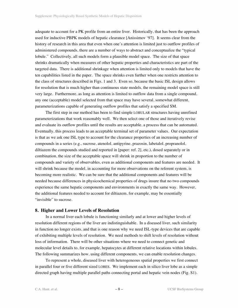
Supplement: Physiologically Based Synthetic Models of Hepatic Disposition

C.A. Hunt, et al. – 8 – UCSF BioSystems Group

adequate to account for a PK profile from an entire liver. Historically, that has been the approachused for inductive PBPK models of hepatic clearance [Anissimov ‘97]. It seems clear from thehistory of research in this area that even when one’s attention is limited just to outflow profiles ofadministered compounds, there are a number of ways to abstract and conceptualize the “typicallobule.” Collectively, all such models form a plausible model space. The size of that spaceshrinks dramatically when measures of other hepatic properties and characteristics are part of thetargeted data. There is additional shrinkage when attention is limited only to models that have theten capabilities listed in the paper. The space shrinks even further when one restricts attention tothe class of structures described in Figs. 1 and 3. Even so, because the basic ISL design allowsfor resolution that is much higher than continuous state models, the remaining model space is stillvery large. Furthermore, as long as attention is limited to outflow data from a single compound,any one (acceptable) model selected from that space may have several, somewhat different,parameterizations capable of generating outflow profiles that satisfy a specified SM.

The first step in our method has been to find simple LOBULAR structures having unrefinedparameterizations that work reasonably well. We then select one of those and iteratively reviseand evaluate its outflow profiles until the results are acceptable, a process that can be automated.Eventually, this process leads to an acceptable terminal set of parameter values. Our expectationis that as we ask one ISL type to account for the clearance properties of an increasing number ofcompounds in a series (e.g., sucrose, atenolol, antipyrine, prazosin, labetalol, propranolol,diltiazem the compounds studied and reported in [paper: ref. 2], etc.), dosed separately or incombination, the size of the acceptable space will shrink in proportion to the number ofcompounds and variety of observables, even as additional components and features are needed. Itwill shrink because the model, in accounting for more observations on the referent system, isbecoming more realistic. We can be sure that the additional components and features will beneeded because differences in physicochemical properties of drugs insure that no two compoundsexperience the same hepatic components and environments in exactly the same way. However,the additional features needed to account for diltiazem, for example, may be essentially“invisible” to sucrose.

8. Higher and Lower Levels of ResolutionIn a normal liver each lobule is functioning similarly and at lower and higher levels of

resolution different regions of the liver are indistinguishable. In a diseased liver, such similarityin function no longer exists, and that is one reason why we need ISL-type devices that are capableof exhibiting multiple levels of resolution. We need methods to shift levels of resolution withoutloss of information. There will be other situations where we need to connect genetic andmolecular level details to, for example, hepatocytes at different relative locations within lobules.The following summarizes how, using different components, we can enable resolution changes.

To represent a whole, diseased liver with heterogeneous spatial properties we first connectin parallel four or five different sized LOBES. We implement each in silico liver lobe as a simpledirected graph having multiple parallel paths connecting portal and hepatic vein nodes (Fig. S1).

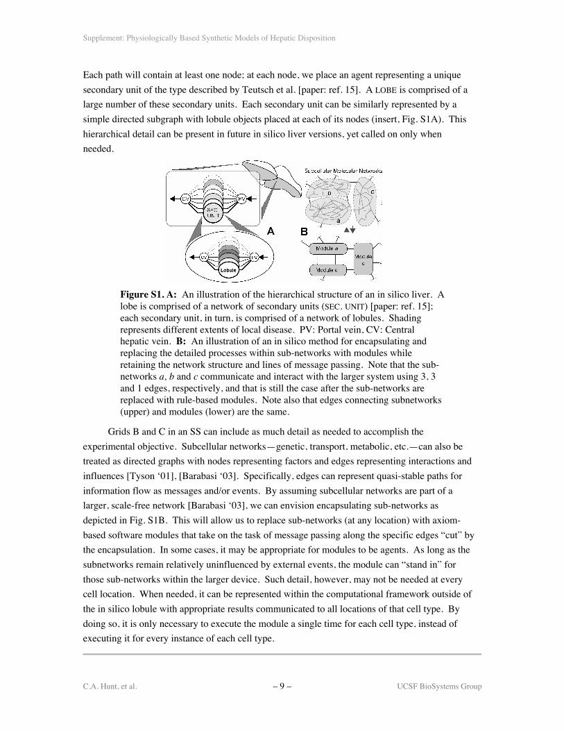
Supplement: Physiologically Based Synthetic Models of Hepatic Disposition

C.A. Hunt, et al. – 9 – UCSF BioSystems Group

Each path will contain at least one node; at each node, we place an agent representing a uniquesecondary unit of the type described by Teutsch et al. [paper: ref. 15]. A LOBE is comprised of alarge number of these secondary units. Each secondary unit can be similarly represented by asimple directed subgraph with lobule objects placed at each of its nodes (insert, Fig. S1A). Thishierarchical detail can be present in future in silico liver versions, yet called on only whenneeded.

Figure S1. A: An illustration of the hierarchical structure of an in silico liver. Alobe is comprised of a network of secondary units (SEC. UNIT) [paper: ref. 15];each secondary unit, in turn, is comprised of a network of lobules. Shadingrepresents different extents of local disease. PV: Portal vein, CV: Centralhepatic vein. B: An illustration of an in silico method for encapsulating andreplacing the detailed processes within sub-networks with modules whileretaining the network structure and lines of message passing. Note that the sub-networks a, b and c communicate and interact with the larger system using 3, 3and 1 edges, respectively, and that is still the case after the sub-networks arereplaced with rule-based modules. Note also that edges connecting subnetworks(upper) and modules (lower) are the same.

Grids B and C in an SS can include as much detail as needed to accomplish theexperimental objective. Subcellular networks—genetic, transport, metabolic, etc.—can also betreated as directed graphs with nodes representing factors and edges representing interactions andinfluences [Tyson ‘01], [Barabasi ‘03]. Specifically, edges can represent quasi-stable paths forinformation flow as messages and/or events. By assuming subcellular networks are part of alarger, scale-free network [Barabasi ‘03], we can envision encapsulating sub-networks asdepicted in Fig. S1B. This will allow us to replace sub-networks (at any location) with axiom-based software modules that take on the task of message passing along the specific edges “cut” bythe encapsulation. In some cases, it may be appropriate for modules to be agents. As long as thesubnetworks remain relatively uninfluenced by external events, the module can “stand in” forthose sub-networks within the larger device. Such detail, however, may not be needed at everycell location. When needed, it can be represented within the computational framework outside ofthe in silico lobule with appropriate results communicated to all locations of that cell type. Bydoing so, it is only necessary to execute the module a single time for each cell type, instead ofexecuting it for every instance of each cell type.

Supplement: Physiologically Based Synthetic Models of Hepatic Disposition

C.A. Hunt, et al. – 10 – UCSF BioSystems Group

M. E. Andersen, R. S. Thomas, K. W. Gaido, and R. B. Conolly. Dose-response modeling inreproductive toxicology in the systems biology era. Reprod. Toxicol. 19(3):327-37 (2005).

A. L. Barabasi and E. Bonabeau. Scale-free networks. Sci. Am. 288:60-9 (2003).R. Rosen. Role of similarity principles in data extrapolation. Am. J. Physiol. RICP 244:R591-99

(1983).H. F. Teutsch, D. Schuerfeld, and E. Groezinger. Three-dimensional reconstruction of

parenchymal units in the liver of the rat. Hepatology 29:494-505 (1999).M. Thompson, S. L. R. Ellison, and R. Wood. Harmonized guidelines for single-laboratory

validation of methods of analysis. Pure Appl. Chem. 74(5) 835–855 (2002).J. J. Tyson, K. Chen, and B. Novak. Network dynamics and cell physiology. Nat. Revs. Mol.

Cell Biol. 2:908-17 (2001).

Supplementary Material for Physiologically Based Synthetic Models of Hepatic Disposition

in the Journal of Pharmacokinetics and Pharmacodynamics, Volume 33, Number 6, December, 2006.

Screen Shots – First we present two screen shots of the visualization to help explain what the visualization shows.

Screen Shot 1: Lobule graph view.

Screen Shot 2: Sinusoidal segment (SS) view.

The visualization is implemented in Adobe's Director. If you have the Shockwave plugin for your browser, you can view it here.

Description

This movie is an interactive 3D visualization of two types of simulated compound, one that enters the in silico cells (modeling antipyrine) and one that does not (modeling sucrose), percolating through the In Silico Liver (ISL). The data driving the visualization is taken from the simulation through a combination of non-invasive instrumentation in the code as well as post-processing of simulation inputs and outputs. This visualization only shows the schematic structure of the ISL and how simulated solute travels through it. It does not show all the aspects of the model. In particular, The movie represents only a single Monte-Carlo trial through a single graph (modeling the lobule structure), whereas model results consist of many Monte-Carlo trials through several variant graphs. And it does not show the fine-grained spatial detail within each space. Metabolic events, for example, are not shown: the antipyrine simply vanishes.

The graph, shown in Screen Shot 1, is the primary component of the ISL. The nodes of the graph are called Sinusoidal Segments (SSes) and the edges are idealized connections between the SSes. The SSes are arranged at two levels: in 3 zones according to proximity to the input node (called the portalVein) and by the network's topology. The zonal assignment of the SSes is not shown here. Solute injected as a bolus (according to the Isolated Perfused Rat Liver experimental protocol) enters the portalVein, travels through the graph and exits the hepaticVein. An individual SS is shown in Screen Shot 2. The three grid spaces (pink: Grid A, yellow: Grid B, and blue: Grid C from Figure 2 in the paper) are rendered as concentric cylinders. Two views are provided of these cylinders. One is a side view (upper right) and the other is a head-on view (lower left). At the lower right the raw grid data is directly represented. Each grid point:

• is empty, that is, no in silico cell object is there, • contains an empty cell (rendered as mostly transparent white), • contains antipyrine or sucrose objects outside of a cell (red or green), • contains a cell with one or more free antipyrine objects within it, or • contains a cell with one or more bound antipyrine objects within it. For example: “3 bound”

means 3 bound antipyrine objects in a cell.

Controls

In the graph view, click on a SS to see the SS view. Then click on “View network Graph” in the bottom left hand part of the SS view to return to the graph view.

In the SS view, each “smooth” control on the upper left is used to distinguish the spaces; it causes the grid data to be blurred or not. The blurring is being applied as a texture to a cylinder and could be viewed as representing the likelihood that a compound of that type is actually in that location.

The “Show” control selects the space (Grid A + Core, Grid B, and Grid C) to be observed (or not).

Selecting “Rotate” causes the cylinder to rotate.

The “>||” and “||<” controls causes in silico time to move one step forward or backward.

Notes:

1. Compounds are injected into the In Silico Liver using a tight distribution function;

2. Antipyrine, but not sucrose, can enter cells;

3. There are objects within “cells” that can bind antipyrine;

4. Antipyrine bound within “hepatocytes” in the Disse layer can be metabolized.

5. Metabolites of antipyrine are not visualized;

6. In this movie there is no more than one free solute per cell.

For additional biological and pharmacokinetic detail see:

Hung DY, Chang P, Weiss M, Roberts MS.(2001) Structure-hepatic disposition relationships for cationic drugs in isolated perfused rat livers: transmembrane exchange and cytoplasmic binding process. J Pharmacol Exp Ther. 297:780-9.