A&A 536, A23 (2011)DOI: 10.1051/0004-6361/201116472c© ESO 2011

Astronomy&

AstrophysicsPlanck early results Special feature

Planck early results. XXIII. The first all-sky surveyof Galactic cold clumps�

Planck Collaboration: P. A. R. Ade72, N. Aghanim48, M. Arnaud59, M. Ashdown57,4, J. Aumont48, C. Baccigalupi70, A. Balbi29,A. J. Banday76,7,64, R. B. Barreiro54, J. G. Bartlett3,55, E. Battaner78, K. Benabed49, A. Benoît47, J.-P. Bernard76,7, M. Bersanelli26,42, R. Bhatia5,

J. J. Bock55,8, A. Bonaldi38, J. R. Bond6, J. Borrill63,73, F. R. Bouchet49, F. Boulanger48, M. Bucher3, C. Burigana41, P. Cabella29,C. M. Cantalupo63, J.-F. Cardoso60,3,49, A. Catalano3,58, L. Cayón19, A. Challinor51,57,9, A. Chamballu45, R.-R. Chary46, L.-Y Chiang50,

P. R. Christensen67,30, D. L. Clements45, S. Colombi49, F. Couchot62, A. Coulais58, B. P. Crill55,68, F. Cuttaia41, L. Danese70, R. D. Davies56,R. J. Davis56, P. de Bernardis25, G. de Gasperis29, A. de Rosa41, G. de Zotti38,70, J. Delabrouille3, J.-M. Delouis49, F.-X. Désert44, C. Dickinson56,

K. Dobashi15, S. Donzelli42,52, O. Doré55,8, U. Dörl64, M. Douspis48, X. Dupac34, G. Efstathiou51, T. A. Enßlin64, E. Falgarone58, F. Finelli41,O. Forni76,7, M. Frailis40, E. Franceschi41, S. Galeotta40, K. Ganga3,46, M. Giard76,7, G. Giardino35, Y. Giraud-Héraud3, J. González-Nuevo70,

K. M. Górski55,80, S. Gratton57,51, A. Gregorio27, A. Gruppuso41, F. K. Hansen52, D. Harrison51,57, G. Helou8, S. Henrot-Versillé62, D. Herranz54,S. R. Hildebrandt8,61,53, E. Hivon49, M. Hobson4, W. A. Holmes55, W. Hovest64, R. J. Hoyland53, K. M. Huffenberger79, A. H. Jaffe45, G. Joncas12,

W. C. Jones18, M. Juvela17, E. Keihänen17, R. Keskitalo55,17, T. S. Kisner63, R. Kneissl33,5, L. Knox21, H. Kurki-Suonio17,36, G. Lagache48,J.-M. Lamarre58, A. Lasenby4,57, R. J. Laureijs35, C. R. Lawrence55, S. Leach70, R. Leonardi34,35,22, C. Leroy48,76,7, M. Linden-Vørnle11,

M. López-Caniego54, P. M. Lubin22, J. F. Macías-Pérez61, C. J. MacTavish57, B. Maffei56, N. Mandolesi41, R. Mann71, M. Maris40,D. J. Marshall76,7, P. Martin6, E. Martínez-González54, G. Marton32, S. Masi25, S. Matarrese24, F. Matthai64, P. Mazzotta29, P. McGehee46,

A. Melchiorri25, L. Mendes34, A. Mennella26,40, S. Mitra55, M.-A. Miville-Deschênes48,6, A. Moneti49, L. Montier76,7, G. Morgante41,D. Mortlock45, D. Munshi72,51, A. Murphy66, P. Naselsky67,30, F. Nati25, P. Natoli28,2,41, C. B. Netterfield14, H. U. Nørgaard-Nielsen11,

F. Noviello48, D. Novikov45, I. Novikov67, S. Osborne75, F. Pajot48, R. Paladini74,8, F. Pasian40, G. Patanchon3, T. J. Pearson8,46, V.-M. Pelkonen46,O. Perdereau62, L. Perotto61, F. Perrotta70, F. Piacentini25, M. Piat3, S. Plaszczynski62, E. Pointecouteau76,7, G. Polenta2,39, N. Ponthieu48,

T. Poutanen36,17,1, G. Prézeau8,55, S. Prunet49, J.-L. Puget48, W. T. Reach77, R. Rebolo53,31, M. Reinecke64, C. Renault61, S. Ricciardi41, T. Riller64,I. Ristorcelli76,7, G. Rocha55,8, C. Rosset3, M. Rowan-Robinson45, J. A. Rubiño-Martín53,31, B. Rusholme46, M. Sandri41, D. Santos61, G. Savini69,

D. Scott16, M. D. Seiffert55,8, G. F. Smoot20,63,3, J.-L. Starck59,10, F. Stivoli43, V. Stolyarov4, R. Sudiwala72, J.-F. Sygnet49, J. A. Tauber35,L. Terenzi41, L. Toffolatti13, M. Tomasi26,42, J.-P. Torre48, V. Toth32, M. Tristram62, J. Tuovinen65, G. Umana37, L. Valenziano41, P. Vielva54,

F. Villa41, N. Vittorio29, L. A. Wade55, B. D. Wandelt49,23, N. Ysard17, D. Yvon10, A. Zacchei40, S. Zahorecz32, and A. Zonca22

(Affiliations can be found after the references)

Received 8 January 2011 / Accepted 30 August 2011

ABSTRACT

We present the statistical properties of the Cold Clump Catalogue of Planck Objects (C3PO), the first all-sky catalogue of cold objects, in termsof their spatial distribution, dust temperature, distance, mass, and morphology. We have combined Planck and IRAS data to extract 10 342 coldsources that stand out against a warmer environment. The sources are distributed over the whole sky, including in the Galactic plane, despite theconfusion, and up to high latitudes (>30◦). We find a strong spatial correlation of these sources with ancillary data tracing Galactic molecularstructures and infrared dark clouds where the latter have been catalogued. These cold clumps are not isolated but clustered in groups. Dusttemperature and emissivity spectral index values are derived from their spectral energy distributions using both Planck and IRAS data. Thetemperatures range from 7 K to 19 K, with a distribution peaking around 13 K. The data are inconsistent with a constant value of the associatedspectral index β over the whole temperature range: β varies from 1.4 to 2.8, with a mean value around 2.1. Distances are obtained for approximatelyone third of the objects. Most of the detections lie within 2 kpc of the Sun, but more distant sources are also detected, out to 7 kpc. The massestimates inferred from dust emission range from 0.4 M� to 2.4 × 105 M�. Their physical properties show that these cold sources trace a broadrange of objects, from low-mass dense cores to giant molecular clouds, hence the “cold clump” terminology. This first statistical analysis of theC3PO reveals at least two colder populations of special interest with temperatures in the range 7 to 12 K: cores that mostly lie close to the Sun;and massive cold clumps located in the inner Galaxy. We also describe the statistics of the early cold core (ECC) sample that is a subset of theC3PO, containing only the 915 most reliable detections. The ECC is delivered as a part of the Planck Early Release Compact Source Catalogue(ERCSC).

Key words. ISM: clouds – stars: formation – dust, extinction – submillimetre: ISM – ISM: general – catalogs

1. Introduction

With its unprecedented sensitivity and large spectral coverage inthe submm-to-mm range, the full-sky survey performed by the

� Corresponding author: L. Montier,e-mail: Ludovic.Montier@irap.omp.eu

Planck satellite (Tauber et al. 2010; Planck Collaboration 2011a)is providing an inventory of the cold condensations of interstel-lar matter in the Galaxy. The three highest frequency channelsof Planck cover the peak thermal emission frequencies of dustcolder than 14 K: a blackbody at T = 6 K, the coldest dust tem-perature found inside Galactic dense cores, peaks at 850 GHz.

Article published by EDP Sciences A23, page 1 of 33

A&A 536, A23 (2011)

Combined with far-IR data such as the InfraRed AstronomicalSatellite survey (IRAS; Neugebauer et al. 1984), the data en-able the determination of a temperature for the cold dust asso-ciated with the sources. This temperature will most certainly bean overestimate of the physical temperature, since some of the100μm (3 THz in the rest of the paper) emission may arise inwarm regions surrounding the coldest dust.

Investigating the distribution and physical properties of thecoldest regions in the Galaxy is critical for the study of the earlystages of star formation. In carrying this out, the main diffi-culty lies in the vast range of scales involved. While star for-mation itself is the outcome of gravitational instability occurringin cold and dense structures at scales less than a tenth of a par-sec, the characteristics of these structures (usually called “pre-stellar cores”) depend on their large-scale environment, up toGalactic scales. Indeed the formation and evolution of these sub-structures is driven by a complex coupling of self-gravity withcooling, turbulence and magnetic fields, to name a few processes(e.g. Falgarone & Puget 1985). To make progress in the under-standing of star formation, pre-stellar cores need to be observedin a variety of environments. More importantly, large surveys arerequired to address statistical issues and evolution. However, allthe investigations so far have been limited, for various reasons(atmospheric fluctuations, limited area, no temperature informa-tion), as described below.

Observations of thermal cold dust emission from the groundare limited by atmospheric fluctuations in the submillimetre do-main, restricting detections to sources smaller than a few ar-cminutes. The all sky surveys of IRAS and more recently WISE(Wright et al. 2010), in the mid- and far-IR have traced warmdust emission in regions already in an active phase of star for-mation. In and around these regions, peaks of cold dust emis-sion have been detected in several nearby molecular clouds withbolometer cameras such as SCUBA, MAMBO, SIMBA, andLABOCA (Motte et al. 1998; Curtis & Richer 2010; Hatchellet al. 2005; Enoch et al. 2006; Kauffmann et al. 2008; Hill et al.2005; Faúndez et al. 2004). Sub-arcminute resolution, combinedwith dedicated molecular line studies, has also provided infor-mation on the small-scale structure of the pre-stellar cores inthese clouds. The Bolocam Galactic Plane Survey at 1.1 mm re-veals dense regions within molecular clouds in the inner andouter Galaxy (Aguirre et al. 2011), although the survey has onlya small extension in latitude. Similarly the APEX TelescopeLarge Area Survey of the GALaxy (ATLASGAL, Schuller et al.2009) provides a survey of 95 square degree inside the Galacticplane, revealing thousands of bright and compact sources.

Opaque and dense regions are also detected as absorptionfeatures. Using the Two Micron All Sky Survey (2MASS), mapsof near-IR extinction have been produced for nearby molecularclouds (Lombardi & Alves 2001). A new population of thou-sands of massive dark clouds was discovered by observations ofmid-IR absorption towards the bright Galactic background (MSXand ISOGAL surveys; see Egan et al. 1998; Pérault et al. 1996).The mid-IR absorption studies are, however, strongly biased to-wards low latitudes where the Galactic background is bright, andthey do not provide information on the temperature of the dustcomponent.

Balloon-borne experiments allow observations that are freeof the modulation required to get rid of the atmospheric fluctua-tions, providing the first large unbiased surveys. The PRONAOSexperiment discovered massive cold condensations in cirrus-type clouds (Bernard et al. 1999; Dupac et al. 2003). Archeops(Désert et al. 2008) detected hundreds of sources with temper-atures down to 7 K. The latest balloon-borne survey is that of

the BLAST experiment which has located several hundred sub-millimetre sources in Vulpecula (Chapin et al. 2008) and Vela(Netterfield et al. 2009; Olmi et al. 2009), including a number ofcold and probably pre-stellar cores.

Space missions improve greatly the brightness sensitivity ofsuch continuum observations in the submillimetre range. TheSPIRE (Griffin et al. 2010) and PACS (Poglitsch et al. 2010)instruments aboard the Herschel satellite have already providedhundreds of new detections of both starless and protostellar cores(André et al. 2010; Bontemps et al. 2010; Könyves et al. 2010;Molinari et al. 2010; Ward-Thompson et al. 2010; Motte et al.2010; Hennemann et al. 2010). However, the sky areas mappedwill remain limited, even for surveys like HiGAL (Molinariet al. 2010) which covers the entire Galactic plane (but only for|b| < 1◦). One of the advantages of the Planck mission is that itprovides an all-sky census of cold sources, including those faraway from known star-forming regions.

Planck1 is the third generation mission to measure theanisotropy of the cosmic microwave (CMB). It observes the skyin nine frequency bands covering 30–857 GHz with high sensi-tivity and angular resolution from 31′ to 5′. The Low FrequencyInstrument LFI; (LFI; Mandolesi et al. 2010; Bersanelli et al.2010; Mennella et al. 2011) covers the 30, 44, and 70 GHz bandswith amplifiers cooled to 20 K. The High Frequency Instrument(HFI; Lamarre et al. 2010; Planck HFI Core Team 2011a) coversthe 100, 143, 217, 353, 545, and 857 GHz bands with bolome-ters cooled to 0.1 K. Polarization is measured in all but thehighest two bands (Leahy et al. 2010; Rosset et al. 2010). Acombination of radiative cooling and three mechanical cool-ers produces the temperatures needed for the detectors and op-tics (Planck Collaboration 2011b). Two data processing centres(DPCs) check and calibrate the data and make maps of the sky(Planck HFI Core Team 2011b; Zacchei et al. 2011). Planck’ssensitivity, angular resolution, and frequency coverage make it apowerful instrument for Galactic and extragalactic astrophysicsas well as cosmology. This paper is one of a series summarisingearly results (Planck Collaboration, 2011a–w) .

The Cold Clump Catalogue of Planck Objects (C3PO) willbe made public after splitting into homogeneous classes of as-trophysical objects and published in separate specific papers. Itwill reveal new locations where eventually the next generationof stars will form, and will provide an opportunity to addressa number of key questions related to Galactic star formationthat are difficult to answer without such an all-sky survey. Thecatalogue will prove invaluable for follow-up studies to inves-tigate in detail regions in the earliest stages of star formation,away from known star-forming regions. The cold nearby sourcesare of particular interest because they provide good pre-stellarcore candidates (with 0.2 pc resolution at a distance of 150 pc)and target regions in which to search for pre-stellar cores withhigher resolution follow-up programmes. This is demonstratedin Planck Collaboration (2011e, hereafter Paper II). Moreover,in this work we describe the statistics of the early cold cores(ECC) sample that is part of the recently published PlanckEarly Release Compact Source Catalogue2 (ERCSC; PlanckCollaboration 2011c). The ECC catalogue is a subset of the full

1 Planck (http://www.esa.int/Planck) is a project of theEuropean Space Agency (ESA) with instruments provided by two sci-entific consortia funded by ESA member states (in particular the leadcountries France and Italy), with contributions from NASA (USA) andtelescope reflectors provided by a collaboration between ESA and a sci-entific consortium led and funded by Denmark.2 The ERCSC is available here: http://www.sciops.esa.int/index.php?project=planck&page=Planck_Legacy_Archive).

A23, page 2 of 33

Planck Collaboration: Planck early results. XXIII.

C3PO catalogue and contains only the most secure detections ofall the sources with colour temperatures below 14 K. Finally, byproviding large maps of dust millimetre and submillimetre emis-sion, like those of the Herschel star-formation surveys (HiGAL,Gould Belt, HOBYS and Magellanic clouds surveys), Planck of-fers the possibility to map the total mass of star-forming inter-stellar clouds over the whole sky, independently of the state ofthe gas tracers (H i, H2 with or without CO). It provides in turnan estimate of the hierarchy of gravitational potential wells inwhich star formation occurs, through better mass estimates thatcan be made at higher frequencies.

In this paper we describe the general properties of the cur-rent cold sources catalogue that is based on data that the Plancksatellite has gathered during its first two surveys of the full sky.In the next section (Sect. 2) we detail the data processing andsource extraction methods that were used in the production ofthe catalogue. We then present the spatial distribution (Sect. 3)and the physical properties of the sample (Sect. 4). We finallydiscuss (Sect. 5) the nature of these cold sources, and we com-pare them with other well-known categories of pre-stellar or starforming objects.

2. Source extraction

2.1. Data set

As cold clumps are traced by their cold dust emission in the sub-millimetric bands, we use Planck channel maps of the HFI atthree frequencies, 353, 545 and 857 GHz, as described in de-tail in Planck HFI Core Team (2011b). The temperature mapsat these frequencies are based on the first two sky surveys ofPlanck, provided in Healpix format (Górski et al. 2005). Beamsare described by an elliptical Gaussian parameterisation lead-ing to FWHM θS given in Table 24 of Planck HFI Core Team(2011b), 4.42′, 4.72′ and 4.5′, at 857, 545 and 353 GHz, re-spectively. The noise in the channel maps is essentially whitewith a mean standard deviation of 1.4 × 10−3, 4.1 × 10−3

and 1.4 × 10−3 MJy sr−1 at 857, 545 and 353 GHz, respectively(Planck HFI Core Team 2011b). The photometric calibration isperformed using the CMB dipole for the 353 GHz channel, andusing FIRAS data (Fixsen et al. 1994) for the higher frequencychannels at 545 and 857 GHz. The absolute gain calibration ofHFI maps is known to better than 2% at 353 GHz and 7% at 545and 857 GHz (see Table 2 in Planck HFI Core Team 2011b). Forfurther details on the data reduction, see Planck HFI Core Team(2011b).

The detection algorithm requires the use of ancillary datato trace the warm component of the gas. Thus we combinePlanck data with the IRIS all-sky data (Miville-Deschênes &Lagache 2005), which is a reprocessed version of the IRAS data(Neugebauer et al. 1984). The choice of the IRIS 3 THz (100 μm)data as the template for the warm background (warm template)is motivated by the following: (i) 3 THz is very close to the peakfrequency of a blackbody at 20 K, and traces the warm com-ponent of the Galaxy; (ii) the fraction of small grains at this fre-quency remains very low and does not strongly alter the estimateof the emission from large grains that is extrapolated to shorterfrequencies; (iii) the IRIS survey covers almost the entire sky(only 2 bands of ∼2% of the whole sky are missing); and (iv) theresolution of the IRIS maps is closely matched to the resolutionof Planck in the high frequency bands, i.e., around 4.5′. Usingthe map at 3 THz as the warm template is, of course, not perfect,because a non-negligible fraction of the cold emission is stillpresent at this frequency. This lowers the intensity in the Planck

bands after subtraction of the extrapolated warm background.We will describe in detail, especially in Sect. 2.3, how we dealwith this issue for the photometry of the detected sources. AllPlanck and IRIS maps have been smoothed to the same resolu-tion, 4.5′, before source extraction and photometry processing.

2.2. Cold source extraction method

We have applied the detection method described in Montier et al.(2010), known as CoCoCoDeT (Cold Core Colour DetectionTool), on the combined IRIS plus Planck data set described inSect. 2.1. This algorithm uses the colour properties of the objectsto separate them from the background. In the case of this work,the method selects compact sources colder than the surround-ing Galactic background, that is at about 17 K (Boulanger et al.1996), but varies from one place to the other across the Galacticplane or at higher latitudes. This Warm Background Subtractionmethod is applied to each of the three highest frequency all-skyPlanck maps, and consists of six steps:

1. for each pixel i, the background colour Ciν at the Planck fre-

quency ν is estimated as the median value within a disc ofradius 15′ around the central pixel of the Planck map Mν

divided by the 3 THz map M3000,

Ciν =

⟨Mν

M3000

⟩i

15′; (1)

2. the contribution of the warm background Miν,warm in a pixel i

at Planck frequency ν is obtained by multiplying the estimateof the background colour with the value of the pixel in the3 THz intensity map Mi

3000,

Miν,warm = Mi

3000 ×Ciν = Mi

3000 ×⟨

Mν

M3000

⟩i

15′; (2)

3. the cold residual map Miν,cold in the pixel i at the Planck fre-

quency ν is computed by subtracting the warm backgroundmap from the Planck map,

Miν,cold = Mi

ν − Miν,warm = Mi

ν − M3000 ×⟨

Mν

M3000

⟩i

15′; (3)

4. the local noise level around each pixel in the cold resid-ual map is estimated in a radius of 30′ using the so-called “Median Absolute Deviation” that ensures robustnessagainst a high confusion level of the background and pres-ence of other point sources within the same area;

5. a thresholding detection method is applied in the cold resid-ual map to detect sources at a signal-to-noise ratio SNR> 4;

6. final detections are defined as local maxima of the SNR, con-strained so that there is a minimum distance of 5′ betweenthem.

This process is performed at each Planck band, yielding indi-vidual all-sky catalogues at 857, 545 and 353 GHz. The last stepof the source extraction consists of merging these three inde-pendent catalogues, by requiring a detection in all three bandsat SNR> 4. This step rejects spurious detections that are due tomap artifacts associated with a single frequency (e.g., stripesor under-sampled features). It increases the robustness of themerged catalogue, which contains 10 783 sources.

We stress that no any other a priori constraints are imposedon the size of the expected sources, other than the limited area on

A23, page 3 of 33

A&A 536, A23 (2011)

which the background colour is estimated. Thus we observe thatthe maximum scale of the C3PO objects is about 12′. Note alsothat this warm background subtraction method uses local esti-mates of the colour, identifying a relative rather than an absolutecolour excess. Thus cold condensations having a low tempera-ture contrast with an already cold background can be missed,while warm condensations colder than their environments willbe picked out by the algorithm. A more detailed analysis in tem-perature is thus required to assess the nature of the objects.

2.3. Photometry of the cold sources

We have developed a dedicated algorithm to derive the photom-etry of the cold source in each band. The flux densities are es-timated from the cold residual maps, instead of working on theinitial maps where the cold sources are embedded in their warmsurrounding background. As already stressed above, the main is-sue to deal with is how to perform photometry on the IRIS 3 THzmap when it also includes a fraction of the cold emission. Theflux density of the source at 3 THz has to be well determined fortwo reasons: (1) an accurate estimate of the flux density at thisfrequency is required because it constrains the rest of the anal-ysis in terms of spectral energy distribution (SED) and temper-ature; (2) an incorrect estimate of the flux density at 3 THz willpropagate through the Planck bands after subtraction of the in-terpolated contribution of the warm background. The main stepsof the photometry processing are described in the following sub-sections. An illustration of this process is provided in Fig. B.5 ofPaper II.

2.3.1. Step 1: elliptical Gaussian fit

An elliptical Gaussian fit is performed on the 1◦ × 1◦857 GHz/3 THz colour map centred on each C3PO object. Thisresults in estimates of three parameters: the major axis ex-tent σMaj; minor axis extent σMin; and position angle ψ. The re-lation between the Gaussian width σ and the FWHM θ is givenby σ = θ/

√8 ln(2). If the elliptical Gaussian fit is indetermi-

nate, a symmetrical Gaussian is assumed with a FWHM fixed toθ = 4.5′, and the flag Aper Forced is set to “on”. The source fluxdensities obtained on this “forced” aperture are often severelyunderestimated at all frequencies. This flagged population con-tains 978 sources which are rejected from the physical analysisof Sect. 4. However, they are included in the complete catalogue(defined in Sect. 2.7), which is used to assess the associationwith ancillary data and to study morphology at large scales (cf.Sect. 3).

2.3.2. Step 2: 3 THz photometry

The photometry on the 3 THz map is obtained by surface fitting,performed on local maps of size 1◦ × 1◦ centred on each candi-date. All components of the map are fitted as a whole, namely: apolynomial surface of order between three and six for the back-ground; a set of elliptical Gaussians when other point sources aredetected inside the local map; and a central elliptical Gaussiancorresponding to the cold source candidate for which the el-liptical shape is set by the parameters obtained during step 1.When the fit of the background is poor, i.e., a clear degener-acy is observed between the polynomial surface and the centralGaussian, we switch to performing simple aperture photometryon the local map. Note that this aperture photometry takes intoaccount the elliptical shape of the source provided by step 1. In

such cases (140 sources), the flag Bad Sfit 3 THz is set to “on”.Occasionally no counterpart at all is observed at 3 THz, when thecold source candidate is too faint or very cold, or the confusionof the Galactic background is too high. In such case, we are notable to derive any reliable estimate of the 3 THz flux density ofthe source, and only an upper limit can be provided. This upperlimit is defined as three times the standard deviation of the coldresidual map within a 25′ radius circle, and the flag Upper 3 THzis set to “on”. There are 2356 objects for which only an upperlimit is derived for the temperature. This population representsa very interesting sub-sample of the whole catalogue, probablythe coldest objects, but we do not have confidence in the physi-cal properties derived from the Planck data and so it is excludedfrom the physical analysis.

2.3.3. Step 3: 3 THz correction

Once an estimate of the flux density at 3 THz has been providedby steps 1 and 2, the warm template at 3 THz is corrected by re-moving an elliptical Gaussian corresponding to the flux densityof the central clump, yielding a corrected warm template. Thiscorrected warm template includes only the warm component ofthe signal. It is then extrapolated and subtracted at each Planckfrequency from the Planck maps to build the cold residual maps.When only an upper limit has been obtained at 3 THz, the warmtemplate is not changed.

2.3.4. Step 4: Planck bands photometry

Aperture photometry is performed on local cold residual mapscentred on each candidate in the Planck bands, at 857, 545 and353 GHz. This aperture photometry takes into account the realextent of each object by integrating the signal inside the ellipti-cal Gaussian constrained by the parameters obtained at step 1.The background is estimated by taking the median value in anannulus around the source. Nevertheless, in 229 cases, no pos-itive estimate of the flux density has been obtained, because ofthe presence of cold point sources that are too close or becausethe background is highly confused. These sources (for which theflag PS Neg is set to “on”) are simply removed from the physicalanalysis described in this paper.

2.4. SED modelling

The cold sources extracted by the above procedure are dis-tributed over the whole sky. Their flux densities at 857 GHzvaries by about 3 orders of magnitude, a broad range that pri-marily follows that of the source distances, although intrinsicvariations in source luminosity may contribute. The S 3000/S 857source colour also spans almost two orders of magnitude formost of the sources (Fig. 2).

We attempt in the following SED analysis to infer basicobservational properties of these sources. Given the large vari-ety of objects and environments represented in this catalogue,and the fact that the SEDs comprise only four bands (the IRIS3 THz and the three highest frequency Planck bands at 857, 545and 353 GHz), it has not been possible to carry out a complexmodelling of the sources, taking into account dust populationvariations or radiative transfer (e.g., Compiègne et al. 2011;Bernard et al. 2008; Doty & Leung 1994; Juvela & Padoan2003). Instead, we assume that the dust thermal emission atall frequencies is optically thin (this assumption is validated in

A23, page 4 of 33

Planck Collaboration: Planck early results. XXIII.

Fig. 1. Examples of SEDs and fits for four sources from our sample. Black diamonds with error bars are the IRIS 3 THz and Planck 857, 545 and353 GHz flux densities, expressed in the νIν = constant colour convention. Two fits have been performed, one with β = 2 (blue) and the otherwith β free (red). For comparison with the data (black diamonds), the expected flux densities for the two fits with the same colour convention arerepresented with blue squares and red plus signs. The quality of each fit can be judged by comparing the estimated flux densities in each band (i.e.,blue squares and red plus signs), with the actual measurements (i.e., black diamonds with error bars). Two envelopes are overlaid in the case of βfree: the (T + σT , β − σβ) modified blackbody emission model (red dotted curve), and the (T − σT , β + σβ) model (red dashed curve).

Sect. 4.4), and that the SED can be approximated by a singlemodified blackbody emission law:

S ν = ΩcκνBν (T ) NH2μmH, (4)

where S ν is the flux density at the frequency ν integrated overthe solid angle Ωc = πσMajσMin with σMaj and σMin the majorand minor axis of the Gaussian ellipse of the source, Bν(T ) isthe Planck function at temperature T , NH2 is the column density,μ = 2.33 is the mean molecular weight, and mH is the mass ofatomic hydrogen. The dust opacity κν is defined by

κν = κ0

(ν

ν0

)β, (5)

where κ0 is the value in cm2g−1 of the opacity at the referencefrequency ν0, and β is the dust emissivity spectral index. Thismodelling involves a maximum of three free parameters (T , βand normalisation) to fit four data points, yielding at least onedegree of freedom.

The fitting procedure is based on a reduced χ2 analysis, anduses the 1σ uncertainties on the input flux densities derived fromthe Monte Carlo analysis of Sect. 2.5, i.e., 40% in the IRIS 3 THzband and 8% in Planck bands. The χ2 minimisation is performedon a pre-calculated grid taking into account the colour correction

as defined in Planck HFI Core Team (2011b) and gives the exactminimum of χ2 in the (T , β, normalisation) space at the gridresolution, i.e., 0.01 K in T and 0.01 in β. It also provides theassociated 1σ uncertainty of the parameters by integrating thelikelihood over the grid. We try two alternative models, whichwe now describe.

Firstly, we fix the spectral index to β = 2 (Boulanger et al.1996). The χ2 minimisation is then performed on the T and nor-malisation parameters only, leading to two degrees of freedom.We provide a few examples of such SEDs and associated fitsin Fig. 1, for various cases of temperature and spectral index,with more examples given in Appendix D. However, the colour–colour diagram of Fig. 2 shows that single modified blackbodyemission models with β = 2 cannot explain the variety of casespresent in the data. Furthermore, the quality of the SED fits inthe case of β = 2 is illustrated in Fig. 3 which shows the distri-bution of the reduced χ2 as a function of temperature. In the caseof fixed β = 2 (dark solid contours), the lower the temperature,the poorer the quality of the χ2 fit.

Secondly, we perform a three parameter χ2 fit (on T , β andnormalisation). This introduces an additional degeneracy in thefit results that is discussed below. The impact on the fit qualityis illustrated in Fig. 3: in the case of β being free (red dashedcontours), the distribution of the reduced χ2 varies less over the

A23, page 5 of 33

A&A 536, A23 (2011)

Fig. 2. Colour–colour diagram of the photometrically reliable cata-logue: flux density ratio S 3000/S 857 versus S 353/S 857. The red lines showthe domain of the single modified blackbody emission models withfixed values of β. The blue lines show the domain of the single mod-ified blackbody emission models for fixed values of the temperature.The locus β = 2 (red solid line) appears to be insufficient to fit all theobservational data points (black dots) of the C3PO photometrically re-liable catalogue.

range of temperatures than when β is held fixed. The absolutevalue of χ2 is lower than in the case β = 2, as expected withthe introduction of an additional free parameter to the fit. In theframework of a single modified blackbody emission modellingof the SEDs, assuming a free β results in a better fit to the obser-vations although the best fit temperatures are nearly the same.

The known T −β degeneracy (e.g., Shetty et al. 2009b) couldaffect these determinations. Figure 4 shows the distribution ofthe fit parameters in relation to the colour ratios. For sourceswith S 3000/S 857 > 0.1, this ratio is a good tracer of the tempera-ture. Of special interest in our survey are the sources dominatedby intrinsically cold dust. For sources with S 3000/S 857 < 0.1,99% of them show a temperature below 12 K in the case of βfree, and 96% of them below 13 K in the case of β = 2, showingthat the T–β degeneracy is not significantly affecting the fractionof cold sources in this sample. This is illustrated in the two leftupper panels of Fig. 2. The lower left panel shows that they havea corresponding high dust emissivity spectral index β. Not sur-prisingly, the S 353/S 857 ratio is a tracer of β, but the fact that thecorrelation shows a large scatter is an indication that a fraction ofthe sources are cold enough not to be in the Rayleigh-Jeans do-main in that frequency range. On the contrary, the temperature isnot constrained by the S 353/S 857 ratio (right middle panel). Thedependence on temperature seen for the β = 2 case (right up-per panel) is an artifact imposed by the fixed value of β, leadingto a bad fit thus not a good temperature determination. Figure 2shows that for β = 2 (red solid line), a low S 353/S 857 ratio forcesthe solution to high temperatures, that may not be compatiblewith low S 3000/S 857 values (see two left panels of Fig. 4). For thecold sources selected with S 3000/S 857 < 0.1 and S 353/S 857 < 0.1(narrow SEDs), representing ≈7% of the photometrically reli-able sample, we are forced to keep β free in order to obtain rea-sonable fits; this is not the case for warm sources. If instead offitting with a single temperature, we assumed a temperature dis-tribution, then this would of course lead to even larger valuesof β.

We can see on the few SEDs shown in Fig. 1 that the IRISpoint at 3 THz plays a crucial role in modelling these SEDs, andobtaining the resulting temperature and spectral index estimates.

Fig. 3. 2D histogram of the reduced χ2 of the SED fitting as a functionof the temperature Tc (see Sect. 4.1) for the photometrically reliablecatalogue. The contours represent the 90%, 75%, 25%, 5% and 1% lev-els of the maximum of the 2D histogram over the (χ2, Tc) space. Case 1(black solid line): reduced χ2 obtained for β = 2 as a function of thetemperature inferred from the fit. When temperature becomes lower,more objects have a larger χ2. Case 2 (red dashed line): reduced χ2 as afunction of the temperature obtained with a free β. The threshold χ2 = 2(dash-dotted blue line) indicates the maximum level of χ2 that ensuresa reasonable fit.

Low estimates of the flux density at 3 THz lead to low temper-ature estimates and high β values. For this reason special carehas been taken to properly estimate the accuracy of the flux den-sity measurements in all bands (and especially at 3 THz) usingMonte Carlo analysis (see Sect. 2.5). More details on the dis-tribution of the temperature and β estimates are presented inSects. 4.1 and 4.2.

2.5. SED fitting quality assessment

To assess the accuracy of our photometry algorithm, we haveperformed Monte Carlo (MC) simulations. A total of 10 000simulated sources are randomly injected into the all-sky IRISand Planck maps. The simulated SEDs are assumed to followa modified blackbody form. The temperature T is randomlydistributed between 6 K and 20 K, The associated spectral in-dex β follows the Archeops distribution (Désert et al. 2008)β = (11.5 ± 3.8) × T−0.66±0.054. This gives values from β = 3.5at 6 K to β = 1.6 at 20 K, to which we add an additional ran-dom variation of 20%. As we will see later in Sect. 4.2, boththe functional form and the dispersion of the β values are sim-ilar to what is seen in Planck data and, therefore, provide anadequate starting point for the estimation of the uncertainties.The normalisation of the SEDs is constrained by the flux den-sity at 857 GHz, which is chosen to follow a logarithmic randomdistribution ranging from 10 to 500 Jy, covering 97% of the ob-served distribution. An elliptical Gaussian profile is assumed,with a FWHM spanning from 4.5′ to 7′ and an ellipticity rang-ing from 0 to 0.87. All simulated flux densities take into accountthe colour corrections. The complete process of photometry de-scribed in Sect. 2.3 is then applied on this set of simulated data,providing an estimate of all recovered quantities: flux densities;FWHM; and ellipticity. A distinction is made between the var-ious cases associated with the photometry flags introduced inSect. 2.3. Statistical bias and 1σ errors are derived and listed inTables 1 and 2, for all-sky and |b| < 25◦, respectively. A more

A23, page 6 of 33

Planck Collaboration: Planck early results. XXIII.

Fig. 4. Dependence of the temperature of the cold clumps and the dust emissivity spectral index β on the colours at low and high frequency around857 GHz. The temperature is obtained by performing an SED fit with a fixed β = 2 (upper panels) and a variable β (middle panels), while theassociated β is shown in the bottom panels. All quantities are given as a function of the S 3000/S 857 colour (left column) and of the S 353/S 857 colour(right column).

detailed description of these results is provided in Appendix Aand illustrated in Fig. A.1.

This Monte Carlo analysis confirms why sources with Aperforced set to “on” should be rejected from the physical study,since for these sources flux densities are systematically under-estimated by about 60%. For sources for which only an upperlimit at 3 THz has been provided by the algorithm (Upper 3 THzset to “on”), the flux density at 3 THz is over-estimated by a fac-tor of two. The discrepancy can reach a factor of three in regionsclose to the Galactic plane. This illustrates the limitations on anyphysical conclusions that could be drawn from this population of

sources. When a bad fit of the 3 THz background map has beenobtained (Bad Sfit 3 THz flag set to “on”), the main error comesfrom the highly biased estimate of the FWHM (+31%), lead-ing to an over-estimate of the flux densities in all bands. Thiscould happen when a strong source is embedded in a faint back-ground structure (e.g., at high latitude), introducing a degeneracybetween the fit of the central elliptical Gaussian and the polyno-mial fit of the background surface at 3 THz. Although the biasand 1σ values of flux densities are smaller than in the Normalcase, due to the strong signal of these sources, we reject this pop-ulation from the physical analysis, because they could introduce

A23, page 7 of 33

A&A 536, A23 (2011)

Table 1. Statistics of the Monte Carlo analysis performed to estimate the robustness of the photometry algorithm.

Normal Bad Sfit 3 THz Aper Forced Upper 3 THz

Quantity Bias [%] σ [%] Bias [%] σ [%] Bias [%] σ [%] Bias [%] σ [%]

S 3000 . . . . . . . . . . 1.4 31.7 1.0 4.7 −58.1 14.1 117.1 190.0S 857 . . . . . . . . . . −5.0 6.2 3.9 3.2 −56.3 13.8 −11.0 6.0S 545 . . . . . . . . . . −3.6 6.4 3.7 3.7 −55.8 14.4 −9.0 6.0S 353 . . . . . . . . . . −5.0 7.3 2.4 4.7 −58.9 14.8 −10.0 6.7FWHM . . . . . . . . −0.6 16.2 30.9 27.7 −25.2 16.3 −6.7 15.3Ellipticity . . . . . . 0.0 8.2 0.0 9.5 . . . . . . 0.0 9.0T . . . . . . . . . . . . −4.2 5.2 −4.1 1.6 −6.5 3.8 0.4 16.0β . . . . . . . . . . . . . 9.8 7.3 10.5 2.4 11.2 6.7 2.7 18.7

Notes. The bias (expressed as a percentage) is defined as the relative error between the median of the output distribution of the photometryalgorithm and the injected input. The 1σ uncertainty (also expressed as a percentage) represents the discrepancy around the most probable valueof the output distribution. Those quantities are given in the various cases corresponding to the output flags provided by the algorithm. Statistics ofthe temperature and spectral index are also given here, to show the impact of the observed error on flux densities.

Table 2. Same as Table 1 in the Galactic plane (|b| < 25◦).

Normal Bad Sfit 3 THz Aper Forced Upper 3 THz

Quantity Bias [%] σ [%] Bias [%] σ [%] Bias [%] σ [%] Bias [%] σ [%]

S 3000 . . . . . . . . . . 11.5 44.3 0.8 8.4 −51.6 21.1 204.5 278.2S 857 . . . . . . . . . . −4.0 8.1 2.1 4.7 −58.3 20.1 −10.4 7.1S 545 . . . . . . . . . . −2.5 8.0 2.4 4.9 −57.4 21.3 −7.8 7.0S 353 . . . . . . . . . . −3.4 8.7 1.9 5.5 −59.3 21.3 −8.7 7.4FWHM . . . . . . . . 0.0 18.1 31.0 31.1 −24.4 16.9 −5.2 17.6Ellipticity . . . . . . 0.0 9.3 −0.5 9.2 . . . . . . 0.1 10.4T . . . . . . . . . . . . −2.1 6.3 −3.2 1.8 −4.4 6.2 6.8 20.6β . . . . . . . . . . . . . 7.1 8.2 9.3 2.6 5.6 12.3 −4.9 20.4

erroneous estimates of the physical properties based on a highlybiased source extent.

If we focus now on the Normal case, when the photome-try algorithm has performed well, we first observe a slight biasof all flux estimates that is only due to the photometry algo-rithm and the process of warm background subtraction. The fluxdensity of the cold residual at 3 THz is over-estimated by 1.4%over the whole sky, and even more (+11.5%) in the Galacticplane. However, the flux densities in the Planck bands are under-estimated by 2–5%. The associated 1σ errors are about 6–7% onall-sky and 8–9% in the Galactic plane in the Planck bands andabout 40% in the 3 THz band. The impact of such a biased es-timate of the fluxes will be discussed together with the resultson the SED fitting in Sect. 4.1. Finally the FWHM estimates arebiased by less than 1% and have an accuracy of about ±18%,while the ellipticity does not present evidence of any bias, withan accuracy of ±9%.

The Monte Carlo simulations described here demonstrate therobustness of our photometry algorithm, and justify the rejectionof entire categories of objects using the photometry flags. Afterrejecting all sources that present at least one of the flags AperForced, PS Neg or Bad Sfit 3 THz, the remaining robust sampleconsists of 9465 objects, divided into two categories: 1840 ob-jects have only an upper limit estimate of the flux at 3 THz;and 7625 that have well defined photometry in IRIS and Planckbands. We will focus on this last category of 7625 sources forthe rest of the analysis on clump physical properties. Moreover,based on this MC analysis, we will adopt the following estimateof the 1σ uncertainty on flux densities: 40% for IRIS 3 THz;

and 8% for Planck bands. This error is much larger than the in-trinsic pixel noise and so instrumental errors are neglected.

We have used the same set of MC simulations to assessthe quality of the SED fitting procedure described in Sect. 2.4and the impact on the temperature and spectral index estimates.This analysis shows that the recovered temperature is slightlyunder-estimated (∼2% in the Galactic plane), while the associ-ated spectral index is over-estimated by about 7%. The statistical1σ uncertainties are about 6% and 8% for T and β, respectively.This will be discussed in more detail in Sect. 4.1.

2.6. Cross-correlation with existing catalogues

As one step of the validation of the Planck detections, we haveperformed an astrometric search on the SIMBAD database3 forall known sources within a 5′ radius of the C3PO sources. Thereare a large number of such objects in the SIMBAD database,which raises the question of chance alignments. This is espe-cially true for extragalactic objects, which have a reasonablyisotropic sky distribution. To judge the number of chance align-ments that can be expected by performing this kind of search, wehave also conducted a SIMBAD cross-check on the positions ofa set of 1000 MC simulated catalogues presented in Sect. 3.2.1.These MC realisations reproduce the object density of the Planckcatalogue per bin of longitude and latitude. The results presentedin Table 3 show that the number of coincidences in the ISM cate-gory (gathering the inter-stellar medium objects) is significantly

3 http://simbad.u-strasbg.fr/simbad/

A23, page 8 of 33

Planck Collaboration: Planck early results. XXIII.

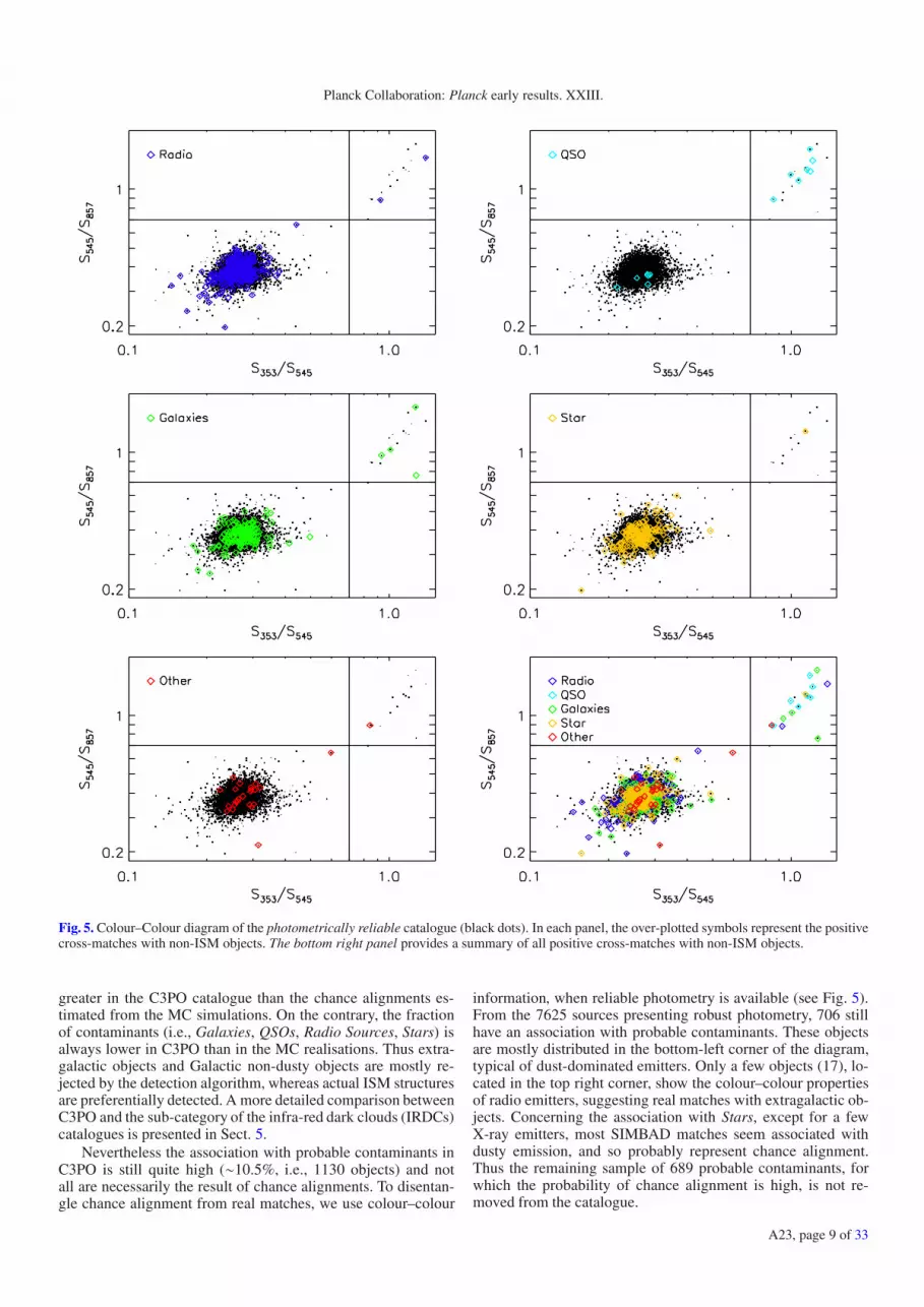
Fig. 5. Colour–Colour diagram of the photometrically reliable catalogue (black dots). In each panel, the over-plotted symbols represent the positivecross-matches with non-ISM objects. The bottom right panel provides a summary of all positive cross-matches with non-ISM objects.

greater in the C3PO catalogue than the chance alignments es-timated from the MC simulations. On the contrary, the fractionof contaminants (i.e., Galaxies, QSOs, Radio Sources, Stars) isalways lower in C3PO than in the MC realisations. Thus extra-galactic objects and Galactic non-dusty objects are mostly re-jected by the detection algorithm, whereas actual ISM structuresare preferentially detected. A more detailed comparison betweenC3PO and the sub-category of the infra-red dark clouds (IRDCs)catalogues is presented in Sect. 5.

Nevertheless the association with probable contaminants inC3PO is still quite high (∼10.5%, i.e., 1130 objects) and notall are necessarily the result of chance alignments. To disentan-gle chance alignment from real matches, we use colour–colour

information, when reliable photometry is available (see Fig. 5).From the 7625 sources presenting robust photometry, 706 stillhave an association with probable contaminants. These objectsare mostly distributed in the bottom-left corner of the diagram,typical of dust-dominated emitters. Only a few objects (17), lo-cated in the top right corner, show the colour–colour propertiesof radio emitters, suggesting real matches with extragalactic ob-jects. Concerning the association with Stars, except for a fewX-ray emitters, most SIMBAD matches seem associated withdusty emission, and so probably represent chance alignment.Thus the remaining sample of 689 probable contaminants, forwhich the probability of chance alignment is high, is not re-moved from the catalogue.

A23, page 9 of 33

A&A 536, A23 (2011)

Table 3. Cross-match with SIMBAD database for C3PO and simulatedcatalogues, for each category of SIMBAD type.

SIMBAD type C3PO MC[%] [%]

ISM . . . . . . . . . . 49.0 21.7Stars . . . . . . . . . . 2.4 4.9Galaxies . . . . . . . 2.1 7.4Radio Sources . . . 5.3 7.7QSOs . . . . . . . . . 0.2 0.3Others . . . . . . . . . 0.5 0.2New detections . . 40.4 57.8

Notes. The MC column gives an estimate of the probability of chancealignment found in the Monte Carlo simulations for each SIMBADtype.

A total of 441 objects are rejected from the initial C3PO cata-logue after this cross-correlation with ancillary data: 424 have noreliable photometry and are a priori rejected, due to a probableassociation with non-ISM objects; while the 17 others have reli-able photometry but are clearly identified as extragalactic objectsusing the colour–colour information.

2.7. Building the catalogues

Starting from the 10 783 source detections over the whole sky(see Sect. 2), two types of selection are applied. On the onehand, the cross-correlation with ancillary data identifies 441 sus-picious candidates which may be associated with contaminantslike extragalactic sources or stars (see Sect. 2.6). On the otherhand, the quality of the flux density extraction has been quan-tified (see Sect. 2.3), providing flags that allow the rejection ofentire categories of sources, because of their lack of robustnessor biases in estimates for at least one of the four IRIS plus Planckbands. Four flags are used to discard the photometrically unre-liable sources (see Sect. 2.5): Aper Forced (978); PSneg (229);Bad Sfit 3 THz (140); and Upper 3 THz (2356). We stress thatoverlap is possible between these flags. A total of 3158 objectshave at least one of the flags listed above.

Using all this information, we build two catalogues: a com-plete catalogue and a photometrically reliable catalogue. Thecomplete catalogue requires only the cross-check with ancillarydata, leading to 10 342 objects. The photometrically reliable cat-alogue requires both the cross-check with ancillary data, andthe absence of a photometric flag, ensuring the robustness ofthe photometry. This last catalogue contains 7608 objects. Outof the 7608 sources, 40% have no counterpart in the SIMBADdatabase. In addition, these new detections have a similar SNRdistribution as the complete catalogue (spanning from 4 to 30)and can be considered as reliable as those in the complete cata-logue.

The Planck ECC sample has been defined as a subset of theC3PO catalogue, following two criteria: a signal-to-noise ratiogreater than 15; and a temperature lower than 14 K. This selec-tion leads to 915 objects. Further details on the properties ofthis catalogue are given in Appendix C. The ECC has been in-cluded in the ERCSC (Planck Collaboration 2011c), as an auxil-iary product. The ERCSC has been built frequency by frequency,and so some overlap exists with the ECC. A schematic descrip-tion of these catalogues and the various sub-samples introducedin this work is given in Fig. 6.

Fig. 6. Partitioning of the two main C3PO samples: the complete (yel-low) catalogue; and the photometrically reliable (orange) catalogue.The overlap between the sample for which we have distance estimateswith those two catalogues is shown in brown. We finally overlay theECC catalogue (blue) to show its overlap with the other samples. Theproportional overlaps between samples are respected in this diagram.

3. Spatial distribution

We now study the spatial distribution of C3PO clumps at threedifferent scales, which we refer to as large, medium and smallscales. The large scale study consists of an all-sky analysis of thecorrelation between cold clumps and Galactic morphology. Themedium scale distribution handles shell- and loop-like Galacticobjects, covering areas from a few deg2 up to 150 deg2. Groupingproperties are finally analysed at small scales, i.e., about the de-gree scale. Furthermore we provide an estimate of the heliocen-tric distance for a sub-sample of such sources.

3.1. All-sky association with Galactic morphology

The all-sky distribution of the 10 342 sources of the completeC3PO catalogue is presented in the upper panel of Fig. 7. Mostlyconcentrated in the Galactic plane, the distribution clearly fol-lows Galactic structures between latitudes of −20◦ and +20◦.However, a few detections are observed at high Galactic lati-tude (|b| > 30◦) and after cross-correlation with external cata-logues have been confirmed not to be extragalactic in origin (seeSect. 2.6).

In the middle panel of Fig. 7, contours of the integrated in-tensity map of the CO J = 1→ 0 line are overlaid on the Planckcold clumps density all-sky map. This CO map is a combinationof data from Dame et al. (2001) and NANTEN data (Fukui et al.1999; Matsunaga et al. 2001; Mizuno & Fukui 2004), as definedin Planck Collaboration (2011d). The correlation between COand C3PO cold clumps is quite impressive and demonstrates therobustness of the detection process and the consistency of thephysical nature of these Planck cold objects. A detailed analysisshows that more than 95% of the clumps are associated with COstructures.

The lower panel of Fig. 7 shows the same kind of spatialcorrelation with the all-sky extinction, AV , map (Dobashi 2011).The AV map traces more diffuse regions of the Galaxy and ex-tends to higher latitudes, where cold clumps are also present.About 75% of the C3PO objects are associated with an extinc-tion greater than 1.

A23, page 10 of 33

Planck Collaboration: Planck early results. XXIII.

Cold Clump Density Map

CO contours on Cold Clump Density Map

AV contours on Cold Clump Density Map

Fig. 7. Upper panel: all-sky map of the number of C3PO Planck cold clumps per sky area (2◦ × 2◦). The ECC sources are overlaid as blue squares.Middle panel: contours of 12CO J=1→0) line emission (0.1, 1, 4, 10, 30 K km s−1) are over-plotted on the C3PO density map, which is set to zerowhere the CO map is not defined (limited by the blue contours). The resolution of the CO map is 2◦. Lower panel: visual extinction contours(AV = 0.1, 0.5, 1, 2, 3, 4, 5, 6, 7 mag) are over-plotted on the C3PO density map, which is set to zero where AV is lower than 0.1 mag (bluecontours). The AV map is also at a resolution of 2◦.

A23, page 11 of 33

A&A 536, A23 (2011)

Fig. 8. Planck-HFI map at 857 GHz (in MJy sr−1) of the Taurus cloudarea, showing the location and extent (at one FWHM) of the C3PO coldsources. C3PO cold sources are clearly distributed along the filamentsof submillimetre dust emission, also known to be the coldest regions inIRAS colours (Abergel et al. 1994).

3.2. Association with medium scale structures

Superimposed on the large-scale spiral structure of the Galaxyis a distribution of features known variously as shells, holes,loops, bubbles, arcs, filaments, superbubbles, supershells, etc.,which has been referred to as the “Cosmic Bubble Bath” (Brand& Zealey 1975) or the “Violent ISM” (McCray & Snow 1979).These structures are characterised by an underdensity or over-density of interstellar matter – either neutral or ionised – and arethought to be directly connected to the star-formation process(Blaauw 1991), forming loop-like, hole-like and filamentary-likestructures. The Taurus cloud illustrates the case (see Fig. 8). Thislow-mass star-formation complex has been subject to extensivestudies, due to its proximity (140 pc, Elias 1978). The far-IR datashow an intricate pattern of filaments, cavities and rings, which isalso visible in the 12CO and 13CO data (Goldsmith et al. 2008).The C3PO cold clumps in this field are predominantly foundalong the filaments and shells.

Shells and loops are structures characterised by a deficiencyof interstellar matter in their interior, accompanied by an over-density at the edges. They typically range in size from less than100 pc to more than 1000 pc. Some, but not all, are observedto expand (for expanding H i shells see e.g., Ehlerová & Palouš2005). These types of objects can be well represented by ellipti-cal rings. We provide here an overview of the distribution of theC3PO clumps with respect to the overall distribution of shells (asdefined in H i, see Heiles 1984) and loops (traced by far-IR data,see e.g., Schwartz 1987; Kiss et al. 2004). The cold clump sur-face density is remarkably high in the Taurus-Auriga-Perseus-Orion region (hereafter Taurus-Orion, see Fig. 9). Taurus-Orionis also characterised by a particular wealth of arcs, filaments andclustered sources, and we therefore use it as a special test casefor our analysis, that we compare to the all-sky distribution. Westress that we have removed the region centred on the Galacticplane (|b| < 5◦) from this analysis, due to the high confusionlevel.

In our discussion, we will refer to three selections: IN, thearea inside the fitted profile of the loops/shells; ON, coincidentwith the ring itself; and OFF, the area outside all rings. We firstcarry out the all-sky correlation between the C3PO cold clumpsand the different integrated areas relative to the shells/loops. Westudy this correlation shell-by-shell and loop-by-loop. For eachshell/loop i we calculate the C3PO surface density nON

i defined

Fig. 9. Surface density map of the C3PO sources in the Taurus-Orionregion, with the inner and outer boundaries of far-IR loops (Könyveset al. 2006) overlaid.

Table 4. Surface density (expressed in number per deg2) of C3POsources and Monte Carlo simulations for H i supershells in the threecases: IN shell; ON shell; and OFF areas.

Region Selection C3PO MC

IN 0.76 0.76 ± 0.02Taurus-Orion ON 0.91 0.85 ± 0.02

OFF 0.79 1.06 ± 0.05

IN 0.184 0.175± 0.002All-sky ON 0.322 0.238± 0.005

OFF 0.056 0.097± 0.002

Notes. Values for both the Taurus-Orion region and for all-sky are pre-sented. For Monte Carlo simulations, the mean value of the distributionis given along with the 1σ dispersion.

Table 5. Same as Table 4 for IRAS loops.

Region Selection C3PO MC

IN 0.65 1.02 ± 0.03Taurus-Orion ON 1.21 0.91 ± 0.03

OFF 0.56 0.60 ± 0.02

IN 0.119 0.135± 0.004All-sky ON 0.193 0.122± 0.003

OFF 0.144 0.173± 0.002

as the number of C3PO objects falling on the shell/loop dividedby the area of the ring of the shell/loop.

3.2.1. Simulated samples

In order to evaluate the reliability of the observed distributionof C3PO objects, we produce MC simulated samples (hereafterMC samples). In each of the 1000 MC samples the observednumber of sources (10 342) are randomly placed onto the skyfollowing the marginal distributions of the C3PO catalogue in(l, b) Galactic coordinates with a resolution of 5◦.

To test the all-sky correlation we calculate the surface den-sity values in each of the 1000 MC simulations for the differentintegrated areas (IN, ON, OFF). The mean values and standarddeviations are presented in column “MC” of Tables 4 and 5. Forthe shell-by-shell and loop-by-loop analysis, the surface densi-ties nON

i are defined for each shell/loop i as the average overthe 1000 MC realisations, with their associated standard devia-tion σON

i .

A23, page 12 of 33

Planck Collaboration: Planck early results. XXIII.

3.2.2. H i shells

We investigate the spatial correlation of the C3PO cold clumpswith the shells and supershells catalogued by Heiles (1984) us-ing the 21-cm line surveys by Weaver & Williams (1973) andHeiles & Habing (1974). Heiles (1984) listed objects only at|b| < 10◦, and physical sizes and distances are available for34 H i shells. The average diameter is 0.82 kpc, at an averagedistance of 6.1 kpc. We define a shell width individually for eachH i shell using the NASA LAMBDA4 H i column density fore-ground maps.

The results of the all-sky analysis are compiled in Table 4.The distribution of the C3PO surface density ON the studiedstructures shows a significant excess compared to the simula-tions. The excess in the Taurus-Orion region compared to theMC samples ON the H i shells is 2.6σ (respectively, 17σ for theall-sky case). On the contrary, the surface densities for OFF areslightly lower in the C3PO case compared to the simulated case.However, the surface density IN is not significantly different be-tween C3PO and simulations. Thus C3PO cold clumps seem tobe preferentially distributed ON the H i shells, whether in theTaurus-Orion region or over the whole sky.

3.2.3. IRAS loops

IRAS loops were identified by Könyves et al. (2006) in theframework of an investigation of the large-scale structure ofthe diffuse ISM, started by Kiss et al. (2004) using the 60 and100μm ISSA data (IRAS Sky Survey Atlas, Wheelock et al.1994). Galactic infrared loops (GIRLs, Könyves et al. 2006) bydefinition must show an excess far-IR intensity confined to anarc-like feature extending to at least 60% of a complete ellipse-shaped ring. The thicknesses of the rings are given in the cata-logue for all GIRLs. For about 20% of them a distance is alsoprovided, that gives an average diameter of 0.09 pc at an aver-age distance of 1.1 kpc. The potential role of the loops in thestar-formation process has first been discussed by Kiss et al.(2006) and Tóth & Kiss (2007). The catalogue of IRAS GIRLs(Könyves et al. 2006) contains 462 far-IR loops, but for this anal-ysis we only take into account the loops which are not com-pletely within the Galactic plane (|b| < 5◦), yielding 427 objects.

Figure 9 shows the surface density map of C3PO in theTaurus-Orion region with the far-IR loops overlaid. A first by-eye analysis already provides strong hints of a correlation be-tween these loops and the distribution of the cold clumps. Thestatistical analysis in Taurus-Orion and all-sky (see Table 5) con-firms these results, with, respectively, 11σ and 24σ excess of ONsurface densities, compared to simulations. In the Taurus-Orionregion the surface density ON the GIRLs is 6.3 times higher thanthe all-sky value. Moreover the all-sky surface density IN ap-pears to be lower than the ON and OFF surface densities. Thiscorresponds to the definition of the GIRLs, which says that theIN regions are “holes” in the interstellar medium.

When looking at the loop-per-loop analysis, over the total427 GIRLS, 180 are not empty, and as many as 68 loops showa clear excess (>3σ) of C3PO surface densities ON the loops.These regions are interesting candidates to be followed-up, inorder to study the correlation between the Planck cold clumpsand those medium scale loops.

4 http://lambd.gsfc.nasa.gov

3.3. Small scale clustering of C3PO sources

3.3.1. Method

Groups in the C3PO sample were identified using the MinimalSpanning Tree (MST) method of Cartwright & Whitworth(2004), as described in Gutermuth et al. (2009) and Beerer et al.(2010). The MST is the unique network of straight lines join-ing a set of points, such that: i) the total length of all the lines(hereafter “edges”) in the network is minimised; and ii) there areno closed loops. The construction of such a tree is describedby Gower & Ross (1969). Starting at any point, an edge iscreated joining that point to its nearest neighbour. The tree isthen extended by always constructing the shortest link betweenone of its nodes and an unconnected point, until all the pointshave been connected (Cartwright & Whitworth 2004). Withinthe MST structure, groups can be separated as having “small”branch lengths between all members, i.e., less than some cutoffbranch length.

We calculated the nearest neighbour distances for the C3POclumps. Following Gutermuth et al. (2009) we computed the cu-mulative number of nearest neighbour distances with length d orsmaller in the Taurus-Orion region, as a function of d. We de-rived the cutoff length as defined by the intersection between thetwo straight lines fitted on the two ends of the distribution. In ourcase, a cutoff length (i.e., maximum allowed distance between agroup member core and a given subgraph) of 25′ was adopted.We note that the definition of groups strongly depends on thevalue used as the critical MST branch length; larger values tendto increase the number of group members, while smaller valuestend to decrease the number of members (Kirk & Myers 2011).

3.3.2. Grouping properties

The results obtained with the MST method are compiled inTable 6. We first observe in the Taurus-Orion region that the av-erage number of groups in the MC samples and in C3PO aresimilar. For the all-sky data, the MC samples show 30% fewergroups (at 25σ) than in C3PO. We also investigate the propertiesof sub-samples of larger groups, containing at least four objects.Thus we define the fraction of groups with at least four memberscompared to the number of all groups as NG4+/NG. This fractionis 38% in the Taurus-Orion region and 28% over the whole-sky(see Table 6). These fractions are significantly higher than themean values derived from the MC simulations. We see here thesame behaviour for the Taurus-Orion region and for the wholesky. We also investigated the variation of NG and NG4+/NG as afunction of the cutoff length in the range 10′ to 30′ . For any cut-off length, the average NG and NG4+/NG in the MC samples were25–45% less than in the C3PO data. This analysis shows thatthe clustering of the C3PO cold clumps is real, and that largergroups are more common in C3PO than in random distributions.

The elongation of groups was analyzed for all those havingmore than three members. Figure 10 shows a group of C3POsources in the Taurus-Orion region. We used the Cartwright &Whitworth (2004) definition of cluster radius, Rc, as the distancebetween the mean position of all cluster members and the mostdistant sources. Following Schmeja & Klessen (2006) the area Aof the cluster was estimated using the convex hull (the minimalconvex set containing the set of points X in a real vector space V)of the data points. The convex hull radius, Rh, is defined as theradius of a circle with an area equal to the area A of the convexhull of the data points. Schmeja & Klessen (2006) describe theelongation measure ξ as: ξ = Rc/Rh.

A23, page 13 of 33

A&A 536, A23 (2011)

Table 6. Number and properties of identified groups in the C3PO dataand the Monte Carlo simulations for the Taurus-Orion and for the all-sky distribution.

Region C3PO MC

NG 248 259± 10Taurus-Orion NG4+/NG 0.38 0.16± 0.02

ξ 2.15 2.42± 0.94

NG 2119 1496± 25All-sky NG4+/NG 0.28 0.16± 0.02

ξ 2.54 2.5± 1.3

Notes. NG is the number of groups, NG4+ is the number of groups with atleast four members, and ξ denotes the average elongation of the groups.In the case of the MC results, the average over the 1000 realisations isprovided, with its associated standard deviation.

For a fully spherical group, the elongation measure wouldbe 1. If we approximate the shape of the groups with an el-lipse, then elongation measures 1.4, 1.7, 2 and 3.2 correspond toaxis ratios of 1:2, 1:3, 1:4 and 1:10, respectively. We calculatedthe elongation measure for all the 602 groups with N > 3. Wefound a mean elongation of ∼2.2 in the Taurus-Orion region, and∼2.5 in the all-sky distribution (see Table 6). These elongationscorrespond to an axis ratio of 1:4.8 in the Taurus-Orion regionand 1:6.3 in the all-sky sample. However, the mean elongation ofthe filaments in the MC samples (cf. Sect. 3.2.1) does not differfrom that in C3PO in these regions (see Table 6). We also inves-tigated the mean elongation in the C3PO data for different cutofflengths, and we found that the average elongation of the groupsis basically insensitive to this quantity. We actually do not seeany evidence for elongation of the largest groups (N > 3) in theC3PO catalogue using this analysis.

3.4. Distance estimation

Distance estimates are essential to properly analyse thepopulation of detected cold clumps. Four different methods arerequired to cover all the sources: association with IRDCs; associ-ation with known molecular complexes; a three dimensional ex-tinction method using the Two Micron All Sky Survey (2MASSSkrutskie et al. 2006); and using Sloan Digital Sky Survey(SDSS, Abazajian et al. 2003) data.

3.4.1. Distances to IRDCs

Simon et al. (2006b) and Jackson et al. (2008) provide kinematicdistance estimates for a total of 497 IRDCs extracted from theMSX catalogue (Simon et al. 2006a) that consists of 10 931 ob-jects. Kinematic distances are obtained via the observed radialvelocity of gas tracers in the plane of the Galaxy. By assumingthat the Galactic gas follows circular orbits and a Galactic rota-tion curve, an observed radial velocity at a given longitude corre-sponds to a unique Galactocentric radius. This means that in theinner Galaxy, two heliocentric distances are possible. This tech-nique is only applicable in the plane and requires the availabilityof appropriate molecular data. We find 127 Planck cold sources,over the complete catalogue, associated with IRDCs that alreadyhave a kinematic distance estimate. This number decreases to32 associations over the 7608 objects of the photometrically re-liable C3PO catalogue.

Fig. 10. A sample group of C3PO sources in the Taurus-Orion region,overlaid on the cold residual map in MJy sr−1. In this case, the elonga-tion measure is ξ = 3.4. Black asterisks show the C3PO cold sources,solid lines indicate the MST edges and black dashed lines indicate theconvex hull (defined in Sect. 3.3.2). The radius of the red dashed circledenotes Rc. Offset coordinates are used here, with the origin being thecentre of the group.

A more recent study by Marshall et al. (2009) uses an ex-tinction method, detailed in Sect. 3.4.3, on the same MSX cat-alogue of IRDCs, to derive the distance to 1259 objects. Thisyields 188 associations with C3PO clumps over the completecatalogue, and 47 over the photometrically reliable catalogue.

3.4.2. Distances to known molecular complexes

A simple inspection of the all-sky distribution of cold clumpssuggests that it follows known molecular complexes. Many ofthese molecular complexes have distance estimates in the liter-ature. To assign the distance of a complex to a particular coldclump we use the CO map of Dame et al. (2001) to trace thestructure of the molecular cloud above a given threshold, andtest for the presence of cold clumps inside this region. The as-sociation has been performed on 14 molecular complexes (seeTable 7) located outside the Galactic plane, to reduce the levelof confusion, leading to 1152 distance estimates over the com-plete catalogue and 947 on the photometric reliable catalogue.

3.4.3. Distances from extinction signature

Genetic forward modelling (using the pikaia code, Charbonneau1995) is used along with the 2MASS data and the BesançonGalactic model (Robin et al. 2003) to deduce the three dimen-sional distribution of interstellar extinction towards the coldclump detections. The derived dust distribution can then be usedto determine the distance of the sources, independently of kine-matic models of the Milky Way. Along a line of sight that crossesa cold clump, the extinction is seen to rise sharply at the distanceof the cloud. The method is fully explained in Marshall et al.(2006) and Marshall et al. (2009).

The distance, as determined by this technique, provides lineof sight information on the dust distribution. However, it doesnot have sufficient angular resolution to perform morphologi-cal matches on the cold clumps. To ensure that the extinctionrise detected along the line of sight is indeed related to the innerstructure we perform a consistency check on the column density

A23, page 14 of 33

Planck Collaboration: Planck early results. XXIII.

Table 7. Molecular complexes used to associate C3PO cold clumps towell-known Galactic structures, for which an estimate of the distance isavailable, as detailed in Sect. 3.4.2.

Name l b Area Distance No.[deg] [deg] [deg2] [pc]

Aquila Serpens . . 28 3 30 260 59Polaris Flare . . . . 123 24 134 150 55Camelopardalis . . 148 20 159 240 11Ursa Major . . . . . 148 35 44 240 13Taurus . . . . . . . . . 170 −15 883 140 393Taurus Perseus . . . 170 −15 883 350 227λ Ori . . . . . . . . . . 196 −13 113 400 66Orion . . . . . . . . . 212 −9 443 450 353Chamaeleon . . . . . 300 −16 27 150 114Ophiuchus . . . . . . 355 17 422 150 311Hercules . . . . . . . 45 9 35 300 16

derived from the extinction and from the source flux density, cor-rected for its temperature. Only detections where the two columndensities are in agreement within a factor of two are retained.This leads to distance estimates for 978 objects of the completeand photometrically reliable catalogue.

3.4.4. Distances from SDSS

Distances to cold clumps within 1 kpc are obtained by analysisof distance-reddening relations for late spectral type stars withinthe line of sight to each source (Mc Gehee, in prep.). M stars areused because they can be dereddened to their true spectral types,while the stellar loci of the earlier spectral types is almost paral-lel to the reddening vector and hence the true spectral type can-not be recovered. We determine the intrinsic g−i colour from themeasured Qgri = (g − r) − [

E(g − r)/E(r − i)](r − i) reddening-

invariant index using the median stellar locus of Covey et al.(2007). This is equivalent to dereddening to the M dwarf locusin the (g − r, r − i) colour–colour diagram. The reddening coef-ficients used are those of Schlafly et al. (2010) and photometricparallaxes are determined following Bochanski et al. (2010).

A simple profile model, consisting of a single step functionconvolved with a Gaussian (to model errors in the determina-tion of distance modulus), is fit to the derived E(B − V) anddistance values. Profiles with extreme fitted Gaussian widths, orwith poor fits as judged by high rms values, are considered unre-liable. Analysis of calibration fields containing the well-studiedOrion B Cloud, reveal that the recovered distance moduli areunderestimated by 0.35 mag, consistent with the bias expectedfrom the Mdwarf multiplicity fraction.

This processing yields 1452 distance estimates in the entirecatalogue, computed using stars within a 15′ radius of each po-sition. Of these, 349 profiles, primarily in regions of lower ex-tinction, are of acceptable quality.

3.4.5. Combined results

The number of sources for which distances could be recovereddepends on the method used (cf. Table 8). There is some over-lap, but each method has its distinct advantages according to thedistance range being considered.

The agreement between the estimates obtained with theSDSS extinction and the association to molecular complexesis good. While no bias is observed between these two distanceestimates, the discrepancy can reach 50% in some cases, which

Fig. 11. Distribution of C3PO cold clumps as seen from the NorthGalactic Pole. Colours stand for methods used to estimate distance:molecular Complex association (green); SDSS extinction (light blue);2MASS extinction (dark blue); IRDCs extinction (orange); and IRDCskinematic (red). The red dashed circle shows the 1 kpc radius aroundthe Sun. Black dashed lines represent the spiral arms and local bar. Theblack circles give the limits of the molecular ring.

gives an estimate of the uncertainty of those two methods. Theagreement between the distance estimates obtained with the as-sociation to IRDCs and the 2MASS extinction is also fairlygood, with about a 20% systematic over-estimate of the extinc-tion method compared to the kinetic method, and with a maxi-mum associated discrepancy of 50%. This study is in agreementwith the comparison performed by Peretto & Fuller (2010) be-tween the distance estimates of Marshall et al. (2009), Simonet al. (2006b) and Jackson et al. (2008) on IRDCs. On the otherhand no agreement is obtained between the SDSS extinction andthe 2MASS extinction methods on the fraction of objects (144)for which we have both estimates. The 2MASS distance esti-mates are about 2.5 times larger than the SDSS distance esti-mates on average, and can reach a factor of four in some cases.The 2MASS extinction method is not very sensitive to nearbyextinction features (D < 1 kpc), as there are not enough stars toaccurately determine the line of sight information. In contrast,the extinction method using SDSS is designed for nearby ob-jects. For objects within 1 kpc, we have preferably used SDSSdistances when available, or molecular complex distances oth-erwise. We finally estimate that the uncertainty of our distanceestimates is about a factor of two.

The number of objects for which we have a distance estimateis 2619, out of a total of 7608 objects in our photometrically re-liable subset, i.e., ∼34%. The distances of the cold clumps rangefrom 0.1 to 7 kpc, but they are mainly concentrated in the nearbySolar neighbourhood, as shown in Fig. 11. This type of dis-tribution has already been demonstrated using simulations (seeFig. 10 of Montier et al. 2010). The lack of detections at largedistances is mainly caused by the effects of confusion withinthe Galactic plane, which reduces the efficiency of the detectionmethod. Nevertheless, when comparing the distance distributionof the C3PO cold clumps associated with MSX IRDCs with thetotal sample of Simon et al. (2006b) in Fig. 12, we notice that the

A23, page 15 of 33

A&A 536, A23 (2011)

Table 8. Number of distance estimates available for the C3PO sourcesfor each method.

Method Complete C3PO Phot. reliable C3PO(Total in sample) (10 342) (7608)

IRDCs Kinematic . . . . . . . 127 32IRDCs Extinction . . . . . . . 188 472MASS Extinction . . . . . . 978 978SDSS Extinction . . . . . . . 1452 1004Molecular Complexes . . . . 1152 947Total . . . . . . . . . . . . . . . . 3411 2619

Notes. Notice that the total numbers are not equal to the sum of allmethods, due to overlap between them.

Fig. 12. Distance distribution of the MSX IRDCs (Simon et al. 2006b,solid blue line) and of the subset associated with the cold clumps of thecomplete C3PO catalogue (dash-dot-dot-dot red line) and the photomet-rically reliable subset of C3PO (dashed red line).

fraction of C3PO-IRDC matches does not depend on distanceand extends to 8 kpc.

Because the subset of C3PO cold clumps with a distance es-timate has been obtained using different methods, exploring var-ious regions and distances over the sky, this sample appears het-erogeneous. The completeness of the catalogue with respect todistances is quite difficult to assess. Thus we define two sub-sets for further analysis, for which we know that the sampleis more reliable and homogeneous: the first subset (1790 ob-jects) deals with local objects (D < 1 kpc) and uses only esti-mates from molecular complex associations and SDSS extinc-tion; the second subset (674 objects) focuses on more distantobjects (D > 1 kpc) and uses only 2MASS extinction estimatesand IRDC associations.

4. Physical properties

4.1. Temperature

The fitting procedure described in Sect. 2.4 has been appliedto the SEDs including four bands (IRIS 3 THz and Planck 857,545 and 353 GHz), to obtain temperature estimates. This processtakes into account the 1σ uncertainties on the input flux densitiesderived from the Monte Carlo analysis in Sect. 2.5, i.e., 40% forthe IRIS 3 THz band and 8% for Planck bands. For each source,two temperatures are derived: (1) the temperature of the coldclump Tc, based on the SED fits of the cold residuals (Sect. 2.3);and (2) the temperature of the warm background Tw obtainedfrom the SED fits performed on the warm background.

The resulting distributions of cold clump Tc and warm back-ground Tw temperatures are shown on Fig. 13 for β = 2 (dashed

Fig. 13. Distribution of the temperature of the cold clumps (blue) ofthe photometrically reliable catalogue and their associated warm back-ground (red) estimated inside the elliptical Gaussian of the clump itself,when using a fixed spectral index β = 2 (dashed line) or a variable β(solid line). The green curve gives the distribution of the temperature es-timates for the C3PO sources that present only an upper limit at 3 THz.This temperature is then only an upper limit estimate, associated with alower limit on the spectral index β.

lines) and for β free (solid lines). In the case where β is fixedat 2, the uncertainty on the temperature estimates is about 7%.The cold clump temperature Tc (blue dashed curve) distributionis shifted by a few degrees with respect to that of the warm back-ground Tw (red dashed curve). This is consistent with what isexpected from the extraction method of these cold sources. Thetemperatures of the cold clump and of the warm backgroundpeak at about 13 K and 15 K, respectively. The temperature dis-tribution of the warm background extends over the known rangein dust temperatures in the diffuse Galactic ISM. The temper-ature of the clumps Tc ranges from 9 K to 16 K, with a frac-tion 12% of them at Tc < 12K, as discussed in Sect. 2.4.

Treating β as a free parameter does not significantly af-fect these distributions. The associated spectral index β variesfrom 1.5 to 3, with an uncertainty of 21% and a mean value of 2.1for cold clumps and 1.8 for the total emission, consistent withother studies based on Planck data (Planck Collaboration 2011d;Planck Collaboration 2011t; Planck Collaboration 2011g). Thefraction of cold clumps with a temperature Tc < 12 K isnow 31%.

These results have to be corrected for two effects: the impactof the photometry algorithm itself; and the relative calibrationuncertainty between IRIS and Planck. We first recall that a biasof about −2% on T and 7% on β are induced by the photometryalgorithm itself (see Sect. 2.5). On the other hand, the calibrationuncertainty of flux densities (see Sect. B) does not introducedany bias on T or β, but generates an error of about 8% on βand from 3% to 5% on T , that should be added quadratically tothe uncertainty due to statistical errors. All these considerationslead to a final range of temperature of the clump Tc spanningthe range 7 K to 19 K, with an uncertainty of about 9%, and aspectral index β varying from 1.4 to 2.8, with an uncertainty ofabout 23%. The temperature of the clump Tc obtained in thecase β free is defined as the reference temperature of the source,especially in the physical analysis. This temperature is indica-tive of the average temperature of these sources over the Planckbeam.

In addition, 1805 sources from the complete cataloguepresent only an upper limit estimate for their flux densities at

A23, page 16 of 33

Planck Collaboration: Planck early results. XXIII.

Fig. 14. The temperature and spectral index values from the catalogueand the fitted β(T ) relations. The relation estimated from IRIS 3 THzand the three highest frequency HFI channels is shown as a blue linewith 1σ uncertainties denoted with dashed lines. The relation obtainedfrom the Archeops survey (Désert et al. 2008) is shown as a red solidline, within ±1σ red dashed curves.

3 THz (without any other photometric flag), which constrainseven better the dust temperature. The distribution of this upperlimit temperature, shown as a green line in Fig. 13, peaks at 11 Kand varies from 7 K to 19 K. This Upper 3 THz flag can be setwhen the confusion level is too high (in the Galactic plane), orwhen the sensitivity of IRAS (1 Jy) is reached. This populationof sources represents a very interesting sample of cold sources(another sub-sample of which is discussed in Sect. 5.2).

4.2. T – β relation

In order to examine the possible dependence between Tc and β,the values were fitted with a formula

β = (δ + ωT )−1, (6)

(see Dupac et al. 2003). The least squares fit gave parametersδ = 0.020 and ω = 0.035. Figure 14 shows the distribution ofthe C3PO sources (black dots) in the β−T space, and the best fitline (blue solid curve), with its associated 1σ errors. This fit is ina good agreement with the relation derived from Archeops coldsources (Désert et al. 2008), which is overlaid in red solid lines,with its associated 1σ errors in red dashed lines. Because Planckand Archeops have submillimetre bands in common, it is encour-aging to observe such an agreement between both populations ofcold sources, even although the noise level on Planck detectorshas been considerably reduced compared to the Archeops case,and the number of cold objects has been multiplied by about 30.

To estimate the uncertainties in the parameters, we carriedout Monte Carlo simulations starting with the observed sourceflux densities. The uncertainties of the flux density values weretaken to be 40% for the IRIS 3 THz band and 8% for the threePlanck bands. In each Monte Carlo realisation of the catalogue,we included additional variations in the calibration. The calibra-tion factors were generated from a normal distribution and weretaken to be 13.5% for the IRIS observations, 7% for the 545 GHzand 857 GHz data and 2% for the 353 GHz Planck band. Thesame calibration scaling was applied to the two highest fre-quency Planck bands, because their calibration is based on cor-relation with the same FIRAS template (see Appendix B). Withthe estimated statistical uncertainties, the result for the analysisof the four bands is δ = 0.020 ± 0.001 and ω = 0.035 ± 0.001.

Fig. 15. Monte Carlo analysis of the noise effects on the β(Tc) relation.The black dots correspond to a synthetic sample, where the source fluxdensities have been scaled to be consistent with a constant value of β.The green points show the Tc and β values extracted from data, wherewe have added to these flux densities the estimated observational noise.The red line is the fit to these points. The observed relation obtainedusing C3PO sources (blue line, cf. Fig. 14) is significantly steeper.

In the presence of observational errors, such as the uncertain-ties mentioned above, the T and β parameters become anticorre-lated (Schwartz 1982; Dupac et al. 2003; Shetty et al. 2009b).We used MC simulations to determine the degree of anticor-relation that in our case can be produced solely by the obser-vational noise. We started with the flux densities, temperatures,and spectral indices listed in the photometrically reliable C3POcatalogue. For each source, the flux densities were scaled withν2.2−β to produce a synthetic sample in which the spectral indexis approximately constant but the deviations from the modifiedblackbody emission curve are consistent with the observations.The resulting (T , β) points are plotted in Fig. 15 as black dots.In the MC study, noise was added to the flux densities and the Tand β values were estimated again. The observed relation is nolonger flat (green points and the red least squares line) becauseof the correlated errors in the determination of the two parame-ters. The scatter is larger than for the observed points (Fig. 14),suggesting that the noise in this MC test was at least not under-estimated. Nevertheless, the fitted β(T ) curve is flatter than therelation observed in the catalogue (blue curve) and the hypoth-esis of an intrinsically flat β(T ) relation can be excluded withmore than 99% confidence. We recall here that for the coldestsources both the temperature and β are well constrained by thecolours (see Sect. 2.4 and Fig. 4).

Moreover the process of integrating over the 5′ Planck beamcould mix components at various temperature. As studied byShetty et al. (2009a) in the case of mixing two temperature com-ponents and by Malinen et al. (2011) in the case of a simplecold core modelling with internal heating source, the effect oftemperature variations along the line-of-sight can produce sucha Tc–β anti-correlation. Notice that the scatter of the MC testperformed in this work (green points of Fig. 15) is compatiblewith the scatter obtained in Fig. 6 of Shetty et al. (2009a), giventhe uncertainties of Planck and IRIS data. However the observedspectral index β (>2) at low temperature (Tc < 12 K) cannot bereproduced by such temperature variations of individual compo-nents with β = 2.

Using PRONAOS data, Dupac et al. (2003) claimed tofind an anti-correlation between the dust spectral index and

A23, page 17 of 33

A&A 536, A23 (2011)

temperature. Since then similar results have been obtained instudies on Archeops cold cores (Désert et al. 2008), Boomerangdata (Veneziani et al. 2010) and recently Herschel data (Paradiset al. 2010). The temperature dependence of the spectral in-dex we recovered is steeper than that found in PRONAOS data(Dupac et al. 2003). It is also slightly steeper than the relationreported for Archeops cores (see Fig. 15; Désert et al. 2008), al-though the Archeops relation is clearly compatible with our re-sults given the uncertainties. Although a β(T ) relation similar tothat observed is expected for amorphous grains with disorderedstructure (Meny et al. 2007; Boudet et al. 2005) and for silicates,as shown more recently in laboratory experiments (Coupeaudet al. 2011), a robust physical interpretation cannot be inferredfrom our results because the clump sample is not a well-definedand homogeneous class of objects. Nevertheless, these studiessuggest caution when interpreting Tc–β relations for samplescontaining star-forming clouds.

4.3. Extension and ellipticity

The extension and ellipticity of the sources, derived during step 1of the photometry algorithm described in Sect. 2.3, have beencompared with the local point spread function (PSF) providedby the FEBeCoP tool (Mitra et al. 2011) at 857 GHz. This PSFtakes into account the impact of projection on the sky of theoptical beam of the instrument following the scanning strategy.Thus for each source, an elliptical Gaussian fit is applied on thePSF smoothed to 4.5′ to obtain the local FWHM θPSF, ellipticityεPSF and position angle ψPSF of the effective beam. The FWHMθ is defined as the geometric mean of the major and minor axiswidths:

θ =√(θMaj · θMin

), (7)

and the ellipticity is given by

ε =

√1 −

(θMin

θMaj

)2

· (8)

A few examples of FEBeCoP beams for Planck HFI detectorsare given in Fig. B.5 of Paper II. Figure 16 compares the statisti-cal distributions of the FWHM (upper panel), ellipticity (middle)and position angle (lower panel) between C3PO sources (solidline) and the local PSF at 857 GHz (dashed line).

Cold clumps are clearly extended, with an average value ofθc of 7.7′ compared to 4.3′ for the average PSF at 857 GHz overthe sky. Assuming that these compact sources are resolved bythe Planck beam, we can deconvolve them to derive the inferredintrinsic source size θi (dot-dashed line in Fig. 16) using

θi =

√θ2

c − θ2PSF, (9)

where θc is the extent of the source and θPSF is the PSF extent. Wefind that θi/θPSF ≈ 1.4, and can conclude that we have resolvedthe sources. Nevertheless, as pointed out by Enoch et al. (2007)and Netterfield et al. (2009), the fact that the cold sources aremostly extended compared to the PSF may be an indicator of thehierarchical structure of these objects. Netterfield et al. (2009)show that the BLAST sources present the same behaviour, witha ratio between the inferred source size and the BLAST beamequal to 1.1. Enoch et al. (2007) obtained a value of 1.5 for coldcores in Serpens, Perseus and Ophiucus observed with Bolocam.

Fig. 16. Upper panel: distribution of the FWHM of the Planck detec-tions compared to the distribution of the local PSF at 857 GHz (dashedline). Middle panel: distribution of the ellipticity of the cold clumps(solid line) and of the local PSF (dashed line). Lower panel: distribu-tion of the position angle of the elliptical Gaussian of the clumps (solidline), of the local PSF (dashed line), and the difference between them(dotted line).

Indeed these compact sources are associated with larger en-velopes, presenting radial density profiles described by powerlaws with an exponent in the range −2 to −1 (Young et al. 2003).

Cold clumps are also mostly elongated, with a distributionof the ellipticity extending to values as large as 0.98 and peakingat around 0.9, compared to the mean value of 0.6 for the localPSF. Nevertheless, it has been shown that the time response ofthe instrument could also have an impact on the elongation ofthe sources along the scanning strategy. The importance of thiseffect is still difficult to assess, and could be relevant in someregions of the sky. Thus caution has to be used concerning thisresult. However, the C3PO cold clumps are not preferentiallyaligned with the major axis of the PSF; the position angles ofthe elliptical clumps and of the PSF are uncorrelated. As alsostressed by Planck Collaboration (2011e), C3PO cold sourcesare often associated with filaments and parts of larger elongatedcold structures where star formation occurs (see also Fig. 8).This was noted a long time ago by Barnard (1907) for Taurus,and it has more recently been investigated by Herschel observa-tions in Polaris (Men’shchikov et al. 2010) and Aquila (Könyveset al. 2010).

When distances are available (see Sect. 3.4), we can derivethe physical size of the sources, defined as the FWHM in unitsof pc. Figure 17 presents the distribution of the size obtained for2619 sources. A distinction is made between local (D < 1 kpc,dashed line) and distant (D > 1 kpc, dot-dashed line) sources, asdefined in Sect. 3.4.5. The distribution of size ranges from 0.2 pcup to 20 pc, and is highly heterogeneous. Since the distribution

A23, page 18 of 33

Planck Collaboration: Planck early results. XXIII.

Fig. 17. Distribution of the physical size of the cold clumps in pc. Thedistinction is done between the local sample (D < 1 kpc, dashed line)and the distant sample (D > 1 kpc, dot-dashed line).

of the angular size is limited by the Planck resolution (i.e., ∼5′)and the maximum size of these compact sources (i.e., ∼12′), theassociated physical size is totally driven by the distance estimate.With such a wide range of sizes, the nature of these cold sourcescan vary appreciably, from cold and very compact sources tolarge clouds of a few pc. This will be discussed in more detail inSect. 5.

4.4. Column densities

We compute the column density values NcH2

averaged over theclump solid angle following Eq. (4), and using the integratedflux density S c

ν and temperature Tc of the cold clump. The mainsource of uncertainty here comes from the adopted value for κν.Large variations exist from one dust model to another, dependingon the dust properties considered: composition (with or withoutice mantles); structure (compact or fluffy aggregates); as wellas size (see reviews from Beckwith et al. 1990; Henning et al.1995). Dust models and observations show that κν values mayvary by factors of 3–4 (or higher) from diffuse to dense and coldregions (Ossenkopf & Henning 1994; Kruegel & Siebenmorgen1994; Stepnik et al. 2003; Juvela et al. 2010).

For this study, we have adopted the dust opacity fromBeckwith et al. (1990), in agreement with the recommenda-tion for dense clouds at intermediate densities, nH2 ≤ 105

(Preibisch et al. 1993; Henning et al. 1995; Motte et al. 1998),κν = 0.1(ν/1 THz) β cm2g−1, where we take a standard emis-sivity spectral index β = 2. The computation is performed atν = 857 GHz, which is close to the 1 THz of the formula, sothat the impact of variation of the spectral index β remains smallcompared to the uncertainty in κν. For β varying from 1 to 3, themaximum variation of κν around the value obtained with β = 2is 15%. The 857 GHz band also provides the best SNR and thedust emission here is optically thin, with an average dust opacityat 857 GHz of τ ∼ 5 × 10−4 � 1. We have checked that this isstill the case at 3 THz, with an average value of τ ∼ 10−2. Thisvalidates the initial assumption on opacity adopted for this work.

For the clumps which have no distance estimate, we havealso determined an approximate averaged volume density valuewith

ncH2= Nc

H2/σMin, (10)

where the third size dimension of the object is taken as equal tothe minimum value of the clump 2D size, σMin. The resultingnumber density ranges from 102 to 105 cm−3, with a mean valueof 2 × 103 cm−3 (see Table 9).

The distribution of the column density NcH2

as a functionof the other physical parameters derived is shown in Fig. 21.The values cover a wide range, from 1020 up to 1023 cm−2, andare centred around a few times 1021. In comparison with pre-vious studies, the peak of this distribution is lower than thetypical values of a few times 1022, inferred in cold cores ob-served from ground-based telescopes in nearby star-forming re-gions (Motte et al. 1998; Kauffmann et al. 2008; Enoch et al.2008; Curtis & Richer 2010; Belloche et al. 2011). This canbe explained by the Planck resolution, that preferentially se-lects quite extended objects, diluting sources smaller than the 5′beam. Nevertheless, we observe a few objects with column den-sity greater than 1023 cm−2, even at the Planck resolution. Thesefew objects could be precursors of massive stars, or high massstar-formation regions.

Finally, we observe that even the densest clumps (with highcolumn densities) cannot reach temperature lower than 7 K. Thisis in excellent agreement with recent observations of cold coresusing Herschel (e.g., Wilcock et al. 2011; Peretto et al. 2010).

4.5. Mass distribution

We can define the mass integrated over the clump by

M =S νΩcD2

κνBν(T ), (11)

where S ν is the integrated flux density at frequency ν =857 GHz, D is the distance, κν is the dust opacity (or mass ab-sorption coefficient) as defined in Sect. 4.4, and Bν(T ) is thePlanck function for dust temperature at T . The uncertainty in themass estimate can be quite high, due to the propagation of largeerrors on the dust opacity (that could reach 50%) and on the dis-tance estimate (about 100%) elevated by the square. These massestimates are therefore only accurate to within a factor of 4.

Figure 18 shows the distribution of the mass of the total sam-ple (solid line) and of the two subsets, D < 1 kpc (dashed line)and D > 1 kpc (dot-dashed line), as defined in Sect. 3.4.5. Therange of masses of the detected sources ranges from 0.4 M� up to2.4×105 M�, with a median value of 88 M�. It covers a broad va-riety of objects, from cores to giant molecular clouds, as will bediscussed in Sect. 5. The theoretical sensitivity limit of Planck tolow-mass cold cores is not reached. It would be about 0.03 M�,for a cold source located at 100 pc with a column density of1020 cm−2 (i.e., the lower limit of our sample, see Fig. 21) fill-ing the Planck beam of 4.5′. The lower mass limit in the C3POsample, i.e., 0.4 M�, is considerably larger because it is affectedby the confusion level and the extraction process from the warmbackground.

4.6. Luminosity

Bolometric luminosity is defined by

L = 4πD2∫ν

S νdν, (12)

where D is the distance, and S ν is the flux density for the clump.The bolometric luminosity, L, is integrated over the frequencyrange 300 GHz < ν < 10 THz, using the modelled SEDs derived

A23, page 19 of 33

A&A 536, A23 (2011)

Fig. 18. Mass distribution for the total sample (solid line), nearby sub-sample (D < 1 kpc, dashed line) and distant sub-sample (D > 1 kpc,dot-dashed line).

Fig. 19. Bolometric luminosity as a function of mass. The L = M limitis over-plotted as the red dashed line.

from temperature and spectral index fitting (see Sect. 4.1). TheL−M diagram is shown in Fig. 19. A large fraction of the objectsis located below the L = M line (red dashed line) over the wholerange of masses.

The quantity L/M has the advantage that it is independentof distance. Figure 20 shows the histogram of L/M for the pho-tometrically reliable C3PO catalogue (solid line), and for thesubset with distances (dashed line). The distributions of sourceswith and without distance estimates are very similar. This sug-gests that the methods used to estimate the distance do not intro-duce any strong distance-dependent selection bias in the samplecompared to the complete catalogue. The lack of angular resolu-tion prevents us from seeing internal sub-structures, so the pres-ence of objects at various stages of evolution cannot be rejected,as also discussed in Roy et al. (2011) for the BLAST popula-tion in CygX. Nevertheless the L/M ratio provides an indica-tion of the robustness of these sources as candidates for futurestar-forming regions, even at the Planck resolution. While 15%of the C3PO sources have a ratio L/M > 1 L�/M� and a tem-perature spanning from 13 K to 19 K, suggesting the presenceof already evolved objects, the remaining 85% should includea fair number of early stage objects, and offer valuable candi-dates to be followed-up at higher resolution (see for example the

Fig. 20. Histogram of the L/M ratio for the total C3PO catalogue (solidline) and the sub-sample of 2619 objects for which a distance estimatehas been obtained (dashed line).

Table 9. Statistical description of the distribution of physical propertiesof the Planck C3PO catalogue of cold clumps.

Quantity Min. Median Max.

Tc [K] . . . . . . . . . . . . . 7 13 19NH [cm−2] . . . . . . . . . . 1020 2 × 1021 2 × 1023

Size [pc] . . . . . . . . . . . 0.2 1.2 18Ellipticity . . . . . . . . . . 0.4 0.8 1Mass [M�] . . . . . . . . . . 0.4 88 2.4 × 105

Mean density [cm−3] . . 102 2 × 103 105

Notes. Notice that the minima and maxima of each quantity are not as-sociated with the same objects. See Fig. 21 to get a better understandingof the correlations between some of these physical quantities.

studies performed with Herschel on Planck sources, Paper II,Juvela et al. 2010).

5. Nature of the C3PO objects

5.1. A broad range of physical properties

As illustrated in Fig. 21 and summarised in Table 9, the C3POcatalogue contains cold sources covering a broad range of phys-ical properties. This is due to the fact that these sources aredetected as cold relatively to their environment, and that theirdistances cover more than an order of magnitude (note the D2

dependence of M in Fig. 21). It is therefore not surprising thatmost of the Planck cold sources, with sizes ranging from 0.2 pcto 18 pc and masses from less than 1 M� to several times 105 M�,are indeed a heterogeneous ensemble of objects. Only the small-est nearby Planck sources are likely to be cold cores accordingto the usual definition of being smaller than 0.2 pc, with a den-sity n > 104 cm−3 and mass M < 5 M� (cf. the categorization ofWilliams et al. 2000; Bergin & Tafalla 2007). Most of the otherstrace cold dust in large irregular structures up to the mass of giantmolecular complexes (GMCs). In addition to the intrinsic disper-sion of their properties, the background-foreground subtractioninduces uncertainties which have been estimated by MC simu-lations (Appendix A.1). These show that the properties of thebulk of the sources are not significantly affected. Neverthelessit should be kept in mind that a small fraction of the sources(typically 1 to 3%) in the Galactic plane where the density ofsources is of the order of 1 deg−2, might be superpositions of

A23, page 20 of 33

Planck Collaboration: Planck early results. XXIII.

Fig. 21. Correlation matrix between various physical properties of the Planck C3PO sources, specifically temperature Tc, H2 column density NcH2

,distance D, physical size FWHM and mass M. Red dots are the IRDC clumps of Simon et al. (2006b).

nearby and distant sources affecting by large factors the derivedphysical parameters. One should thus treat with care the outliersin Fig. 21 (or Fig. 4) which might result from this effect. We notethat a 4.5′ HFI beam leads to a resolution of 0.2 pc in the nearestmolecular complexes at 150 pc. Thus identifying more distantcores requires higher angular resolution than the Planck beam.

In Juvela et al. (2010, 2011) and our companion Paper II,we have conducted a preliminary analysis using Herschel ob-servations of a sample of ten cold clumps detected with Planck.These sources have been selected to sample different environ-ments, from high latitude cirrus to nearby and remote molecularcomplexes. The high angular resolution of the Herschel SPIREand PACS instruments has revealed rich and complex substruc-tures. A range of properties have been observed: generally thesubstructures have been found to be denser and colder (downto 7 K) than the Planck cold clump, except in two cases, wherewarmer sources have also been found in the Planck beam, in ad-dition to cold dust.

The temperatures derived for the sources in the cataloguecover a range (7–19 K) similar to previous estimates for anumber a cold condensations detected using multi-wavelengthsubmillimetre observations, for instance with the balloon-borne

experiments: PRONAOS, T ∼ 12 K in star-forming and cirrus re-gions (Stepnik et al. 2003; Dupac et al. 2003; Bernard et al.1999); Archeops, 7–18 K (Désert et al. 2008); and BLAST,9–14 K (Netterfield et al. 2009). The highest temperatures foundhere (T > 15–19 K) cannot realistically be called “cold clumps”,nevertheless they correspond to objects significantly colder thantheir observed environment. As a comparison, higher dust tem-peratures are obtained in the vicinity of H ii regions, even atPlanck resolution, with typically T ∼ 30 K (Leto et al. 2009).

Most of the Planck clumps are not “compact point sources”,i.e., the result of the detection of small cores diluted within thelarge beam of Planck. On the contrary, they are found to besignificantly extended and elongated. Independently of the an-gular resolution issue, it is difficult to distinguish here betweenthe core, clump and cloud terminology introduced by Williamset al. (2000). The specific method used to identify and extract thecore parameters should also to be considered (cf. for instanceCurtis & Richer 2010). Our method is based on a colour sig-nature of the objects, allowing the detection of the cold resid-ual after the removal of the warm background. As discussedin Paper II, this may result in the identification of a differentand more extended cold component than usually obtained with

A23, page 21 of 33

A&A 536, A23 (2011)

GLIMPSE 8μm Planck 857 GHz

Fig. 22. GLIMPSE 8 μm and Planck 857 GHz maps (in MJy sr−1) around the IRDC MSXDC G033.69−00.01 (green star). The contours show thecold residual map computed on the Planck 857 GHz map and using the IRIS 3 THz data. The positive contours (blue) are cold, while the negativecontours (red) are warm. The C3PO cold clump is also shown as the dashed black ellipse.

methods that identify structures on the basis of surface bright-ness (e.g., clumpfind, algorithms by Williams et al. 1994, ormulti-scale wavelet analysis).

5.2. Comparison with IRDC catalogue

The plots of Fig. 21 suggest an overlap between the propertiesof the IRDCs and the most massive Planck clumps. Interestingly,the mass distribution of the dust cores within IRDCs, reaching upto 103 M�, (Rathborne et al. 2010) suggests that the most mas-sive Planck clumps, like IRDCs as a whole, are ensembles ofcores arranged into larger structures similar to giant molecularcomplexes (GMCs).

Figure 22 provides an illustration of a common Planck andMSX detection in the case of MSXDC G033.69−00.01 (Simonet al. 2006a). The contours of the cold residual emission (in blue,light blue and red) are overplotted on the GLIMPSE 8 μm inten-sity maps. The ellipse showing the Planck clump (dashed line)extracted from our detection method encompasses the absorp-tion feature signature of the IRDC on the near-IR map. We notethat the Planck size is larger than the extent of the MSX absorp-tion. In the high-resolution map provided by GLIMPSE, sub-structures can be seen inside the extinction pattern.

This figure also illustrates the capability of the extractionmethod to isolate cold components in regions of bright emissioncontaining a high level of confusion. In this field, it is striking tosee how the brightest spots coincide with the warm component(traced in red), although the cold emission is mixed and hid-den inside an extended warmer background emission. The ob-ject with an average column density of 6.5 × 1022 cm−2, a massof 2.4 × 105 M� (at a distance of 7.1 kpc) and a temperature of12 K, is among the most extreme in the distributions shown inFig. 21. Eleven dense cores of mass ranging between 100 and1300 M� have been detected in this IRDC at 1.2 mm (Rathborneet al. 2006), and only three of them are associated with mid-IR emission. An IRAS source is also associated with one ofthese objects. This IRDC is therefore not among the youngestand coldest, that have not yet started to form stars. Neverthelessonly a few cores are warm, contributing about 2 × 103 M� ofwarm dust (Rathborne et al. 2006) out of the dust mass seen byPlanck, or only 1% of the total dust mass.

A cross-match between C3PO sources and the MSX cata-logue of 10 931 IRDCs (Simon et al. 2006a) leads to 469 (136 in

Fig. 23. Ratio of the angular extent of C3PO clumps and MSX IRDCs.

the photometrically reliable catalogue) Planck cold clumps asso-ciated with 1007 (296, respectively) MSX IRDCs. Less than 8%of the Planck clumps inside the region surveyed by MSX haveno directly association with an IRDC. Indeed a comparison ofthe angular size of these objects is presented in Fig. 23, andshows that the C3PO objects are more extended than the IRDCs.Part of this effect is due to the very different spatial resolutionof the MSX instrument at 8 μm (28′′ versus 5′ with Planck).Most of the IRDCs appear as elongated irregular structures oflength L and width L/a (a being the aspect ratio, a > 1); theirsize, defined as the geometric mean, is thus L/a0.5 (Simon et al.2006a). With its large beam, Planck does not resolve the IRDCsin width, but does so in length for the largest ones. Therefore,for the largest IRDCs, we have the ratio of C3PO size to IRDCsize being ∼a0.5 > 1, as seen in Fig. 22. The C3PO sizes, how-ever, may be genuinely larger than those of IRDCs detected inabsorption. In fact it appears that Planck is sensitive to dust col-umn densities smaller than 1021 cm−2 and colder than 15 K (cf.Fig. 21), while MSX (and Spitzer IRAC) absorption measure-ments have a sensitivity threshold of 3 × 1021 cm−2 (Peretto &Fuller 2010). Extended regions of cold dust with column densi-ties between 3 × 1020 cm−2 and 3 × 1021 cm−2 are therefore de-tectable by Planck with no absorption counterparts at 8 μm (asobserved in Fig. 22).

A23, page 22 of 33

Planck Collaboration: Planck early results. XXIII.

Fig. 24. Number of IRDCs found inside the Planck cold clumps when amatch has been obtained with the MSX catalogue (Simon et al. 2006a)and the Spitzer catalogue (Peretto & Fuller 2009).

We have also performed a cross-match with the Spitzer cat-alogue of IRDCs (Peretto & Fuller 2009), leading to 321 (78 inthe photometrically reliable catalogue) Planck cold clumps asso-ciated with 1382 (356, respectively) Spitzer IRDCs. It is shownin Fig. 24 that the C3PO clumps could contain up to eight MSXIRDCs and 15 Spitzer IRDCs. Furthermore, the median distancebetween IRDCs in the MSX and Spitzer catalogues are 2.9′ and1.7′, respectively, values which are lower than the C3PO typi-cal extent that is about 6′; this supports the presence of multi-ple IRDCs inside the C3PO clumps. However, projection effectshave to be taken into account when dealing with such Plancksources located in the Galactic plane, and caution has to be usedwhen considering the number of associated IRDCs.

6. Summary and perspectives

The three highest frequency channels of Planck, provide a cen-sus of cold dust sources in the Galaxy. To determine the prop-erties of the coldest sources, they have to be extracted from theemission of their warmer background. This is done with a ded-icated source extraction algorithm, CoCoCoDeT (Montier et al.2010) that operates on the Planck maps combined with thoseat 3 THz from the IRAS survey. The output, the Cold ClumpCatalogue of Planck Objects (C3PO), is the first such all-skycatalogue of cold dust sources. We stress that this method doesnot provide a complete sample of cold sources in the Galaxy,due in a large part to confusion in the Galactic plane, and thatit can only distinguish sources that are sufficiently colder thantheir background. The complete catalogue consists of 10 342 ob-jects, out of which the photometrically reliable catalogue com-prises 7608 sources, for which physical characteristics such asflux densities, temperatures, angular extents, ellipticities and col-umn densities are inferred from their SEDs. Among these asub-sample comprises 2619 sources with distance estimates, forwhich physical sizes, masses, and average densities can also beestimated. In this paper we have performed a statistical analy-sis of these samples of cold objects and analysed their physicalproperties.

The temperature of the Planck cold sources ranges from 7 Kto 19 K and its distribution peaks at about 13 K. The great valueof the C3PO catalogue is to provide a large number of very coldobjects for follow-up studies, about 600 having a temperatureTc < 10 K. Not only is this a large number compared to the al-ready known cold sources in the Galaxy, but they are distributed

over the whole sky, in the inner and outer Galaxy, and at highlatitude, both near and far away from known star-forming re-gions. The diversity of the environments probed, from nearbydiffuse molecular clouds to massive molecular complexes, andthe possibility to map the mass distribution in such hierarchicalenvironments opens new perspectives for understanding the evo-lution of molecular clouds towards star-formation activity in ourGalaxy.

Another output of the SED fitting procedure is the dust emis-sivity spectral index β. We show that the data are not consistentwith a constant value of β over the whole range of tempera-ture, and that it is anticorrelated with the dust temperature. Theanti-correlation observed for the coldest sources cannot be ex-plained by a fitting degeneracy, given the narrow range of SEDsobserved.

As expected, the Planck cold clump population is closely as-sociated with Galactic structures, especially the molecular com-ponent, and is mainly distributed within the Galactic plane.Nevertheless, since the detection of cold sources inside the thinGalactic plane is difficult (due to the high confusion level), mostof the detections are located within a few kpc of the Sun.

The mass of the cold sources for which the distance is knownvaries between 0.4 M� and 2.4 × 105 M�, and their size rangesfrom 0.2 to 18 pc, with average density between 102 cm−3 and105 cm−3. This broad range of properties makes the C3PO cat-alogue a heterogeneous ensemble of cold objects in the Galaxy.While a few appear as actual cold protostellar core candidates,most of the C3PO sources appear rather to be larger structures,ranging from interstellar clouds up to giant molecular complexesfor the most massive. A cross-match between C3PO sources andIRDCs from MSX and Spitzer shows that massive C3PO coldclumps contain up to 15 IRDCs, and that the C3PO sourcesare statistically more extended than IRDCs. The example of themassive IRDC MSXDC G033.69−00.01, detected in extinctionby MSX and in emission by Planck (see Fig. 22 in Sect. 5.2),shows Planck’s sensitivity to emission in the outskirts, whichare not detected in mid-IR absorption, and thus Planck comple-ment these extinction surveys when confusion is not too large.Furthermore, there is a subset of cold, extended (several pc) andmassive (>103 M�) C3PO sources that may have been revealedfor the first time by the Planck survey (see Fig. 22).

By studying the correlation between the cold clumps andlarge scale structures, such as the IRAS loops, we show thatthe cold clump population is preferably distributed on such largeshells. Another interesting property of the C3PO sources is theirdistribution along known filaments within molecular clouds, andthe associated degree of ellipticity of the sources.

In summary, because of the limited resolution (4.5′), theC3PO catalogue has assembled a large variety of objects in termsof physical properties, Galactic environment, and evolutionarystage, providing a wealth of new sources for follow-up and de-tailed investigations at higher angular resolution. With that per-spective, the Herschel follow-up key programme “Galactic ColdCores” is a unique tool to study the substructure and physics ofselected C3PO sources at the same frequencies (selection beingperformed on either their intrinsic properties or on their environ-ment). Such an analysis has already started (Juvela et al. 2010)on Herschel Science Demonstration Phase Data, and is contin-ued in Planck Collaboration (2011e).

Finally, a high reliability sub-sample of this large C3PO cata-logue has been delivered to the community: the Early Cold Core(ECC) sample. This is part of the ERCSC (Planck Collaboration2011c) and provides a list of 915 objects over the whole sky,with similar statistics at high flux densities to the C3PO sample

A23, page 23 of 33

A&A 536, A23 (2011)

but with temperatures less than 14 K. The ECC provides oppor-tunities for ground-based or Herschel follow-up of cold clumps.Specialised catalogues focused on homogeneous classes of as-trophysical objects will be published in subsequent papers. Inthese papers, a special effort will be made to improve the dis-tance estimates, to increase the volume explored in the Galaxy,and to provide better estimates of the physical parameters.

Acknowledgements. A description of the Planck Collaboration and a listof its members can be found at http://www.rssd.esa.int/index.php?project=PLANCK&page=Planck_Collaboration. We acknowledge the useof the Legacy Archive for Microwave Background Data Analysis (LAMBDA).Support for LAMBDA is provided by the NASA Office of Space Science. Thisresearch makes use of the SIMBAD database, operated at CDS, Strasbourg,France.

Appendix A: Monte Carlo quality assessmentof the photometry

As presented in Sect. 2.5, we have performed a Monte Carloanalysis to assess the robustness of the photometry algorithm de-scribed in Sect. 2.3. A set of 10 000 sources have been injectedinto Planck all-sky maps following a distribution of tempera-tures, dust spectral indices and flux densities in agreement withthe observations. Figure A.1 compiles the relative errors betweenoutput and input quantities (flux densities, FWHM, ellipticity,temperature and spectral index) for the complete set of simulatedsources as a function of the flags raised during the photometryestimate. Three flags have been investigated here: Aper Forced(blue); Bad Sfit 3 THz (red); and Upper 3 THz (green).

Appendix B: Impact of calibration uncertainty

The relative calibration uncertainty is known to be 13.5% forthe IRIS 3 THz data (Miville-Deschênes & Lagache 2005), andabout 7% for the Planck high frequency bands at 857 GHz and545 GHz, and 2% at 353 GHz (Planck HFI Core Team 2011a).Here we investigate the impact of this error on temperature andspectral index estimates, considering that the uncertainty is notindependent between all bands. The principle is to fix the twotop Planck bands (545 and 857 GHz) to follow the same relativecalibration error, while the 3 THz and the 353 GHz bands remainindependent. For a given temperature T and a dust spectral in-dex β, SEDs are simulated using a modified blackbody model,including colour corrections. A 13.5% relative level of Gaussiannoise is added on the 3 THz flux densities, then another 7% noiserealisation is added at 545 GHz and 857 GHz simultaneously,and a 2% noise realisation is added to the 353 GHz flux den-sities. We also study the combination of a calibration error plusan independent error band per band, set to 20% and 10% for the3 THz and Planck bands, respectively. A third set of data is de-fined as our reference case and does not include any calibrationerror, but only an independent error per band. The T, β fittingalgorithm described in Sect. 4.1 is applied on these three setsof SEDs, leading to an estimate of the bias and 1σ uncertaintyof the output distribution, for T ranging from 6 K to 25 K and βspanning from 1.75 to 2.5.

The results are shown in Fig. B.1. The impact of the calibra-tion uncertainty (in red) is very low compared to the size of themeasurement error only (in green). In all cases, the bias on tem-perature and β is negligible or significantly lower than 1%. Inboth cases the bias level remains independent of T and β. On theother hand the 1σ uncertainty on the temperature goes from 3%

to 8% at, respectively, 6 K and 25 K, due to calibration uncer-tainty only, and remains independent of β. The 1σ discrepancyon β is about 7–10% over this temperature range and it decreasesof 3% when β goes from 1.75 to 2.5. This error is larger andmuch more sensitive to β in the case of measurement uncertainty(green curves). Thus the impact of the calibration uncertaintyseems very small compared to the impact of the measurementerror coming from the flux densities. Moreover, in the case ofa combination of calibration and measurement uncertainties (inblue), both resulting uncertainties on T and β are found to addquadratically.

For this work, we consider separately the impact of the cal-ibration uncertainty, and simply add the quadratic errors at theend of the processing. The values of the calibration uncertaintiesfor T and β are provided in Tables B.1 and B.2 for a given setof T, β parameters.

Appendix C: The early cold core sub-sample

C.1. Selection criteria

The Early Release Compact Source Catalogue5 (ERCSC; PlanckCollaboration 2011c) was released in January 2011. It includesthe main ERCSC, where the point sources are detected in eachseparate channel map, but it also incorporates two specialisedcatalogues, the early Sunyaev-Zeldovich (ESZ) and the earlycold cores (ECC). The ECC is a sub-sample of the full C3POcatalogue, obtained by applying the following two criteria:

1. SNR > 15;2. TECC < 14 K.

Here SNR is the signal-to-noise ratio of the detection, and TECCis the temperature derived from aperture photometry. However,in the case of the ECC, this temperature is derived in a differentmanner than described here for the C3PO. In the ECC, the pho-tometry is carried out on the original Planck maps (i.e., maps thatstill retain the warm component of the diffuse dust emission), byplacing an aperture of 5′ radius on top of the detection. The back-ground is estimated using an annulus around the aperture with aninner radius of 5′ and an outer radius of 10′. Temperatures arederived from a fit to all four bands (IRIS 3 THz and Planck 857,545 and 353 GHz) used to obtain the detection. While the annu-lus is efficient in subtracting the diffuse warm background, thisestimate of the temperature does not take into account the realshape of the sources nor the subtraction of any warm envelopelinked to the clump. It does, however, provide a straightforwardestimate of the temperature that is provided in the ECC.

The signal-to-noise cut at SNR = 15 was selected based onthe Monte Carlo Quality Assessment (MCQA) results performedin the framework of the ERCSC. Three sets of 1000 sourceswere injected into the IRIS and Planck maps. These sourceswere defined by temperature, spectral index and flux density at857 GHz, and their associated SEDs followed a modified black-body model. Detection and photometry processing were thenapplied in these three sets of simulated maps, to find the pro-portion of detected sources and their recoveredflux densities. A

5 The ERCSC is available here: http://www.sciops.esa.int/index.php?project=planck&page=Planck_Legacy_Archive).

A23, page 24 of 33

Planck Collaboration: Planck early results. XXIII.

Fig. A.1. Comparison of the extracted and injected values of the Monte Carlo simulations performed to assess the quality of the photometryalgorithm. Black dots refer to the nominal case, when red, blue and green dots stand for various flags of the photometry algorithm: Bad Sfit 3 THz(red); Aper Forced (blue); and Upper 3 THz (green).

A23, page 25 of 33

A&A 536, A23 (2011)

Table B.1. Bias and 1σ error on the temperature due to the calibration uncertainty on flux densities in the IRIS 3 THz and Planck 857, 545 and353 GHz bands, shown for a range of (T, β).

β = 1.75 β = 2.00 β = 2.25 β = 2.50

T [K] Bias [%] σ [%] Bias [%] σ [%] Bias [%] σ [%] Bias [%] σ [%]

6 −0.2 2.7 0.0 2.6 0.0 2.7 0.4 2.77 0.2 3.2 0.3 3.0 0.0 3.0 −0.1 3.08 0.2 3.3 0.2 3.2 0.0 3.3 0.3 3.39 0.3 3.7 0.0 3.4 0.1 3.4 0.3 3.3

10 −0.2 3.8 0.3 3.9 0.0 4.1 −0.2 3.811 0.3 4.3 −0.1 4.2 −0.4 4.0 0.2 4.112 0.0 4.2 −0.3 4.3 0.1 4.3 0.1 4.313 −0.1 4.9 0.6 4.7 0.6 4.3 0.1 4.514 0.3 5.2 −0.2 5.3 0.4 5.2 0.4 4.815 0.0 5.2 −0.1 5.5 0.3 5.7 0.2 5.516 0.2 5.6 0.7 5.5 0.2 5.8 0.5 5.917 0.1 5.7 −0.1 6.0 0.2 5.8 0.2 5.718 0.2 6.1 0.6 6.6 0.1 6.2 0.3 6.219 0.2 6.5 0.5 6.3 −0.1 6.1 −0.5 6.420 0.3 7.2 0.4 7.0 1.0 7.1 0.2 6.721 0.6 7.5 0.7 7.2 0.2 7.2 0.0 7.322 0.2 7.5 0.5 7.9 0.3 7.5 0.6 7.123 0.4 7.6 1.0 8.4 0.5 8.0 0.6 8.324 0.2 8.5 0.6 8.3 0.9 8.2 0.5 8.625 0.2 8.1 0.3 8.2 0.3 8.3 0.5 8.3

Table B.2. Bias and 1σ error on the spectral index β due to the calibration uncertainty on flux densities in the IRIS 3 THz and Planck 857, 545 and353 GHz bands, shown for a range of (T, β).

β = 1.75 β = 2.00 β = 2.25 β = 2.50

T [K] Bias [%] σ [%] Bias [%] σ [%] Bias [%] σ [%] Bias [%] σ [%]

6 0.7 11.5 0.1 9.8 −0.1 9.0 −0.8 8.17 −0.6 11.4 −1.0 9.2 0.2 8.8 0.2 7.68 −0.5 10.5 −0.5 8.7 −0.1 8.2 −0.6 7.59 −0.8 10.8 0.0 8.6 0.3 7.8 −0.5 6.7

10 0.3 9.9 −0.6 8.9 0.1 8.2 0.3 6.611 −0.3 10.1 0.1 8.6 0.6 7.6 −0.2 6.712 0.2 9.0 0.7 8.2 −0.0 7.4 0.1 6.413 0.5 9.6 −1.0 8.2 −0.7 6.5 0.0 6.214 −0.3 9.7 0.5 8.4 −0.5 7.4 −0.5 6.115 0.5 8.7 0.4 8.1 −0.2 7.6 0.0 6.516 0.0 9.1 −0.5 7.5 0.1 7.3 −0.2 6.617 0.2 8.6 0.4 7.8 0.0 6.5 −0.2 6.018 0.2 8.5 −0.2 7.9 0.3 6.9 0.0 6.119 −0.2 8.7 −0.3 7.5 0.3 6.4 0.8 6.020 0.1 9.0 0.0 7.7 −0.8 6.8 0.1 6.021 −0.3 8.9 −0.2 7.3 0.0 6.6 0.3 6.022 0.3 8.7 −0.1 7.7 0.0 6.5 −0.2 5.623 0.1 8.1 −0.4 7.6 0.1 6.5 −0.1 6.124 0.7 8.7 0.0 7.3 −0.2 6.4 0.1 6.025 0.3 8.0 0.0 6.8 0.1 6.2 0.1 5.8

A23, page 26 of 33

Planck Collaboration: Planck early results. XXIII.

Fig. B.1. Bias and 1σ discrepancy of the temperature T and dust spectral index β estimates derived from a Monte Carlo analysis dedicated tostudying the impact of the calibration uncertainties. Three cases have been studied: calibration uncertainty only (red lines); independent fluxdensity errors (green); and calibration plus independent flux density errors (blue).

reliability of 90% was required, where reliability is here definedas the fraction of detected test sources with less than 30% errorin recovered flux density. The MCQA analysis showed that thechoice of SNR = 15 ensured a reliability of 90% over the temper-ature range TECC < 14 K in all three Planck bands (cf. Fig. 23 ofPlanck Collaboration 2011v). Hence, the ECC is 90% reliable,where the reliability is based on flux density, not detection.

C.2. Summary of the ECC

The above criteria lead to a sub-sample of 915 objects over thesky. Of these objects, 118 have no SIMBAD entry and are newdetections. Thus at least 13% are new sources.

Simply due to the selection criteria, the ECC is the high-SNRand the cold tail of the C3PO distribution. The spatial distribu-tion of the ECC objects is biased towards nearby, star-formationregions (e.g., Perseus, Taurus and Orion) where the SNR is high,while the Galactic disk is under-represented (see upper panel ofFig. 7). This is because of the higher confusion in the plane, sothat the SNR tends to be lower there, but also because the dusttemperatures in the plane tend to be higher. Not surprisingly, thederived column densities for the ECC objects are also biased to-wards the higher column densities in the C3PO distribution.

While the ECC does not contain this information, we haverecovered distance estimates for some of the ECC objects, us-ing the methods described in Sect. 3.4. Combining the distance

information with the flux densities of the dust emission, we canestimate the mass of the sources. We find that the ECC objectsare as varied in mass as the C3PO objects, ranging from whatmight be single cores (with a mass of a few M�, to clumps oftens and hundreds of M�, and even larger complexes of thou-sands of M�. Most of the objects for which we have mass esti-mates are in the range from 100 to 1000 M�. The spatial resolu-tion of Planck does not allow for a detailed morphological studyof these sources, so the users of the ECC need to be aware thatthey are not looking at single cores in most of the cases; onlyhigh-resolution follow-up studies will reveal the exact morphol-ogy of these clumps.

The ECC is an excellent resource for follow-up studies.Highly reliable, it contains coordinates, aperture photometry,and the derived temperature and spectral index for each object,which observers can use to estimate their own fluxes, or molec-ular lines brightnesses to look for. The simple aperture photom-etry procedure used the derive the flux densities makes it easyto combine the ECC information with follow-up observations toobtain composite SEDs.

Appendix D: Examples of SEDs

We provide here a few examples of SEDs of C3PO sourceswhich indicate temperatures: lower than 8 K (Fig. D.1); between8 K and 10 K (Fig. D.2); and between 10 K and 14 K (Fig. D.3).SED fits are plotted for both fixed β = 2 and β being free.

A23, page 27 of 33

A&A 536, A23 (2011)

Fig. D.1. SEDs of selected C3PO sources with temperatures Tc < 8 K. Black diamonds with error bars are the IRIS 3 THz and Planck 857, 545and 353 GHz data. Two fits have been performed: one with β = 2 (blue); and the other with β free (red). For comparison with the data (blackdiamonds), the expected flux densities for the two fits, with the same colour convention, are shown with blue squares and red plus signs. Thequality of each fit can be judged by comparing the estimated flux densities in each band, i.e., blue squares and red plus signs, with the actualmeasurements, i.e., black diamonds with error bars. Two models are overlaid to define an approximate error envelope in the case of β free: the(T + σT , β − σβ) modified blackbody emission model, in the red dotted curve; and the (T − σT , β + σβ) model in the red dashed curve.

A23, page 28 of 33

Planck Collaboration: Planck early results. XXIII.

Fig. D.2. SEDs of selected C3PO sources with temperatures in the range 8–10 K. See Fig. D.1 for details.

A23, page 29 of 33

A&A 536, A23 (2011)

Fig. D.3. SEDs of selected C3PO sources with temperatures in the range 10–14 K. See Fig. D.1 for details.

A23, page 30 of 33

Planck Collaboration: Planck early results. XXIII.

References

Abazajian, K., Adelman-McCarthy, J. K., Agüeros, M. A., et al. 2003, AJ, 126,2081

Abergel, A., Boulanger, F., Mizuno, A., & Fukui, Y. 1994, ApJ, 423, L59Aguirre, J. E., Ginsburg, A. G., Dunham, M. K., et al. 2011, ApJS, 192, 4André, P., Men’shchikov, A., Bontemps, S., et al. 2010, A&A, 518, L102Barnard, E. E. 1907, ApJ, 25, 218Beckwith, S. V. W., Sargent, A. I., Chini, R. S., & Guesten, R. 1990, AJ, 99,

924Beerer, I. M., Koenig, X. P., Hora, J. L., et al. 2010, ApJ, 720, 679Belloche, A., Schuller, F., Parise, B., et al. 2011, A&A, 527, A145Bergin, E. A., & Tafalla, M. 2007, ARA&A, 45, 339Bernard, J. P., Abergel, A., Ristorcelli, I., et al. 1999, A&A, 347, 640Bernard, J.-P., Reach, W. T., Paradis, D., et al. 2008, AJ, 136, 919Bersanelli, M., Mandolesi, N., Butler, R. C., et al. 2010, A&A, 520, A4Blaauw, A. 1991, in The Physics of Star Formation and Early Stellar Evolution,

ed. C. J. Lada, & N. D. Kylafis, NATO ASIC Proc., 342, 125Bochanski, J. J., Hawley, S. L., Covey, K. R., et al. 2010, AJ, 139, 2679Bontemps, S., André, P., Könyves, V., et al. 2010, A&A, 518, L85Boudet, N., Mutschke, H., Nayral, C., et al. 2005, ApJ, 633, 272Boulanger, F., Abergel, A., Bernard, J., et al. 1996, A&A, 312, 256Brand, P. W. J. L., & Zealey, W. J. 1975, A&A, 38, 363Cartwright, A., & Whitworth, A. P. 2004, MNRAS, 348, 589Chapin, E. L., Ade, P. A. R., Bock, J. J., et al. 2008, ApJ, 681, 428Charbonneau, P. 1995, ApJS, 101, 309Compiègne, M., Verstraete, L., Jones, A., et al. 2011, A&A, 525, A103Coupeaud, A., Demyk, K., Mény, C., & Nayral, C. 2011, A&A, 535, A124Covey, K. R., Ivezic, Ž., Schlegel, D., et al. 2007, AJ, 134, 2398Curtis, E. I., & Richer, J. S. 2010, MNRAS, 402, 603Dame, T., Hartmann, D., & Thaddeus, P. 2001, ApJ, 547, 792Désert, F., Macías-Pérez, J. F., Mayet, F., et al. 2008, A&A, 481, 411Dobashi, K. 2011, PASJ, 63, 1Doty, S. D., & Leung, C. M. 1994, ApJ, 424, 729Dupac, X., Bernard, J., Boudet, N., et al. 2003, A&A, 404, L11Egan, M. P., Shipman, R. F., Price, S. D., et al. 1998, ApJ, 494, L199Ehlerová, S., & Palouš, J. 2005, A&A, 437, 101Elias, J. H. 1978, ApJ, 224, 857Enoch, M. L., Young, K. E., Glenn, J., et al. 2006, ApJ, 638, 293Enoch, M. L., Glenn, J., Evans, II, N. J., et al. 2007, ApJ, 666, 982Enoch, M. L., Evans, II, N. J., Sargent, A. I., et al. 2008, ApJ, 684, 1240Falgarone, E., & Puget, J. L. 1985, A&A, 142, 157Faúndez, S., Bronfman, L., Garay, G., et al. 2004, A&A, 426, 97Fixsen, D. J., Cheng, E. S., Cottingham, D. A., et al. 1994, ApJ, 420, 457Fukui, Y., Mizuno, N., Yamaguchi, R., et al. 1999, PASJ, 51, 745Goldsmith, P. F., Heyer, M., Narayanan, G., et al. 2008, ApJ, 680, 428Górski, K. M., Hivon, E., Banday, A. J., et al. 2005, ApJ, 622, 759Gower, J. C., & Ross, G. J. S. 1969, Appl. Stat., 18, 54Griffin, M. J., Abergel, A., Abreu, A., et al. 2010, A&A, 518, L3Gutermuth, R. A., Megeath, S. T., Myers, P. C., et al. 2009, ApJS, 184, 18Hatchell, J., Richer, J. S., Fuller, G. A., et al. 2005, A&A, 440, 151Heiles, C. 1984, ApJS, 55, 585Heiles, C., & Habing, H. J. 1974, A&AS, 14, 1Hennemann, M., Motte, F., Bontemps, S., et al. 2010, A&A, 518, L84Henning, T., Michel, B., & Stognienko, R. 1995, Planet. Space Sci., 43, 1333Hill, T., Burton, M. G., Minier, V., et al. 2005, MNRAS, 363, 405Jackson, J., Finn, S., Rathborne, J., Chambers, E., & Simon, R. 2008, ApJ, 680,

349Juvela, M., & Padoan, P. 2003, A&A, 397, 201Juvela, M., Ristorcelli, I., Montier, L. A., et al. 2010, A&A, 518, L93Juvela, M., Ristorcelli, I., Pelkonen, V.-M., et al. 2011, A&A, 527, A111Kauffmann, J., Bertoldi, F., Bourke, T. L., Evans, II, N. J., & Lee, C. W. 2008,

A&A, 487, 993Kirk, H., & Myers, P. C. 2011, ApJ, 727, 64Kiss, C., Moór, A., & Tóth, L. V. 2004, A&A, 418, 131Kiss, Z. T., Tóth, L. V., Balázs, L. G., & Könyves, V. 2006, Publications of the

Astronomy Deparment of the Eotvos Lorand University, 17, 173Könyves, V., André, P., Men’shchikov, A., et al. 2010, A&A, 518, L106Könyves, V., Kiss, C., Moor, A., Kiss, Z. T., & Toth, L. V. 2006, VizieR Online

Data Catalog, 346, 31227Kruegel, E., & Siebenmorgen, R. 1994, A&A, 288, 929Lamarre, J., Puget, J., Ade, P. A. R., et al. 2010, A&A, 520, A9Leahy, J. P., Bersanelli, M., D’Arcangelo, O., et al. 2010, A&A, 520, A8Leto, P., Umana, G., Trigilio, C., et al. 2009, A&A, 507, 1467Lombardi, M., & Alves, J. 2001, A&A, 377, 1023Malinen, J., Juvela, M., Collins, D. C., Lunttila, T., & Padoan, P. 2011, A&A,

530, A101Mandolesi, N., Bersanelli, M., Butler, R. C., et al. 2010, A&A, 520, A3

Marshall, D. J., Robin, A. C., Reylé, C., Schultheis, M., & Picaud, S. 2006,A&A, 453, 635

Marshall, D. J., Joncas, G., & Jones, A. P. 2009, ApJ, 706, 727Matsunaga, K., Mizuno, N., Moriguchi, Y., et al. 2001, PASJ, 53, 1003McCray, R., & Snow, Jr., T. P. 1979, ARA&A, 17, 213Mennella, A., Butler, R. C., Curto, A., et al. 2011, A&A, 536, A3Men’shchikov, A., André, P., Didelon, P., et al. 2010, A&A, 518, L103Meny, C., Gromov, V., Boudet, N., et al. 2007, A&A, 468, 171Mitra, S., Rocha, G., Górski, K. M., et al. 2011, ApJS, 193, 5Miville-Deschênes, M., & Lagache, G. 2005, ApJS, 157, 302Mizuno, A., & Fukui, Y. 2004, in Milky Way Surveys: The Structure and

Evolution of our Galaxy, ed. D. Clemens, R. Shah, & T. Brainerd, ASP Conf.Ser., 317, 59

Molinari, S., Swinyard, B., Bally, J., et al. 2010, A&A, 518, L100Montier, L. A., Pelkonen, V., Juvela, M., Ristorcelli, I., & Marshall, D. J. 2010,

A&A, 522, A83Motte, F., Andre, P., & Neri, R. 1998, A&A, 336, 150Motte, F., Zavagno, A., Bontemps, S., et al. 2010, A&A, 518, L77Netterfield, C. B., Ade, P. A. R., Bock, J. J., et al. 2009, ApJ, 707, 1824Neugebauer, G., Habing, H. J., van Duinen, R., et al. 1984, ApJ, 278, L1Olmi, L., Ade, P. A. R., Anglés-Alcázar, D., et al. 2009, ApJ, 707, 1836Ossenkopf, V., & Henning, T. 1994, A&A, 291, 943Paradis, D., Veneziani, M., Noriega-Crespo, A., et al. 2010, A&A, 520, L8Pérault, M., Omont, A., Simon, G., et al. 1996, A&A, 315, L165Peretto, N., & Fuller, G. A. 2009, A&A, 505, 405Peretto, N., & Fuller, G. A. 2010, ApJ, 723, 555Peretto, N., Fuller, G. A., Plume, R., et al. 2010, A&A, 518, L98Planck Collaboration 2011a, A&A, 536, A1Planck Collaboration 2011b, A&A, 536, A2Planck Collaboration 2011c, A&A, 536, A7Planck Collaboration 2011d, A&A, 536, A8Planck Collaboration 2011e, A&A, 536, A9Planck Collaboration 2011f, A&A, 536, A10Planck Collaboration 2011g, A&A, 536, A11Planck Collaboration 2011h, A&A, 536, A12Planck Collaboration 2011i, A&A, 536, A13Planck Collaboration 2011j, A&A, 536, A14Planck Collaboration 2011k, A&A, 536, A15Planck Collaboration 2011l, A&A, 536, A16Planck Collaboration 2011m, A&A, 536, A17Planck Collaboration 2011n, A&A, 536, A18Planck Collaboration 2011o, A&A, 536, A19Planck Collaboration 2011p, A&A, 536, A20Planck Collaboration 2011q, A&A, 536, A21Planck Collaboration 2011r, A&A, 536, A22Planck Collaboration 2011s, A&A, 536, A23Planck Collaboration 2011t, A&A, 536, A24Planck Collaboration 2011u, A&A, 536, A25Planck Collaboration 2011v, The Explanatory Supplement to the Planck Early

Release Compact Source Catalogue (ESA)Planck Collaboration 2011w, A&A, 536, A26Planck HFI Core Team 2011a, A&A, 536, A4Planck HFI Core Team 2011b, A&A, 536, A6Poglitsch, A., Waelkens, C., Geis, N., et al. 2010, A&A, 518, L2Preibisch, T., Ossenkopf, V., Yorke, H. W., & Henning, T. 1993, A&A, 279,

577Rathborne, J. M., Jackson, J. M., & Simon, R. 2006, ApJ, 641, 389Rathborne, J. M., Jackson, J. M., Chambers, E. T., et al. 2010, ApJ, 715, 310Robin, A., Reylé, C., Derrière, S., & Picaud, S. 2003, A&A, 409, 523Rosset, C., Tristram, M., Ponthieu, N., et al. 2010, A&A, 520, A13Roy, A., Ade, P. A. R., Bock, J. J., et al. 2011, ApJ, 727, 114Schlafly, E. F., Finkbeiner, D. P., Schlegel, D. J., et al. 2010, ApJ, 725, 1175Schmeja, S., & Klessen, R. S. 2006, A&A, 449, 151Schuller, F., Menten, K. M., Contreras, Y., et al. 2009, A&A, 504, 415Schwartz, P. R. 1982, ApJ, 252, 589Schwartz, P. R. 1987, ApJ, 320, 258Shetty, R., Kauffmann, J., Schnee, S., & Goodman, A. A. 2009a, ApJ, 696, 676Shetty, R., Kauffmann, J., Schnee, S., Goodman, A. A., & Ercolano, B. 2009b,

ApJ, 696, 2234Simon, R., Jackson, J. M., Rathborne, J. M., & Chambers, E. T. 2006a, ApJ, 639,

227Simon, R., Rathborne, J. M., Shah, R. Y., Jackson, J. M., & Chambers, E. T.

2006b, ApJ, 653, 1325Skrutskie, M., Cutri, R., Stiening, R., et al. 2006, AJ, 131, 1163Stepnik, B., Abergel, A., Bernard, J., et al. 2003, A&A, 398, 551Tauber, J. A., Mandolesi, N., Puget, J., et al. 2010, A&A, 520, A1Tóth, L. V., & Kiss, Z. T. 2007, in IAU Symp. 237, ed. B. G. Elmegreen, &

J. Palous, 124

A23, page 31 of 33

A&A 536, A23 (2011)

Veneziani, M., Ade, P. A. R., Bock, J. J., et al. 2010, ApJ, 713, 959Ward-Thompson, D., Kirk, J. M., André, P., et al. 2010, A&A, 518, L92Weaver, H., & Williams, D. R. W. 1973, A&AS, 8, 1Wheelock, S. L., Gautier, T. N., Chillemi, J., et al. 1994, NASA STI/Recon

Technical Report N, 95, 22539Wilcock, L. A., Kirk, J. M., Stamatellos, D., et al. 2011, A&A, 526, A159Williams, J. P., de Geus, E. J., & Blitz, L. 1994, ApJ, 428, 693Williams, J. P., Blitz, L., & McKee, C. F. 2000, in Protostars and Planets IV, ed.

V. Mannings, A. P. Boss, & S. S. Russell (University of Arizona Press), 97Wright, E. L., Eisenhardt, P. R. M., Mainzer, A. K., et al. 2010, AJ, 140, 1868Young, C. H., Shirley, Y. L., Evans, II, N. J., & Rawlings, J. M. C. 2003, ApJS,

145, 111Zacchei, A., Maino, D., Baccigalupi, C., et al. 2011, A&A, 536, A5

1 Aalto University Metsähovi Radio Observatory, Metsähovintie 114,02540 Kylmälä, Finland

2 Agenzia Spaziale Italiana Science Data Center, c/o ESRIN, viaGalileo Galilei, Frascati, Italy

3 Astroparticule et Cosmologie, CNRS (UMR7164), Université DenisDiderot Paris 7, Bâtiment Condorcet, 10 rue A. Domon et LéonieDuquet, Paris, France

4 Astrophysics Group, Cavendish Laboratory, University ofCambridge, J J Thomson Avenue, Cambridge CB3 0HE, UK

5 Atacama Large Millimeter/submillimeter Array, ALMA SantiagoCentral Offices, Alonso de Cordova 3107, Vitacura, Casilla 7630355, Santiago, Chile

6 CITA, University of Toronto, 60 St. George St., Toronto, ON M5S3H8, Canada

7 CNRS, IRAP, 9 Av. colonel Roche, BP 44346, 31028 ToulouseCedex 4, France

8 California Institute of Technology, Pasadena, California, USA9 DAMTP, University of Cambridge, Centre for Mathematical

Sciences, Wilberforce Road, Cambridge CB3 0WA, UK10 DSM/Irfu/SPP, CEA-Saclay, 91191 Gif-sur-Yvette Cedex, France11 DTU Space, National Space Institute, Juliane Mariesvej 30,

Copenhagen, Denmark12 Département de physique, de génie physique et d’optique,

Université Laval, Québec, Canada13 Departamento de Física, Universidad de Oviedo, Avda. Calvo Sotelo

s/n, Oviedo, Spain14 Department of Astronomy and Astrophysics, University of Toronto,

50 Saint George Street, Toronto, Ontario, Canada15 Department of Astronomy and Earth Sciences, Tokyo Gakugei

University, Koganei, Tokyo 184-8501, Japan16 Department of Physics & Astronomy, University of British

Columbia, 6224 Agricultural Road, Vancouver, British Columbia,Canada

17 Department of Physics, Gustaf Hällströmin katu 2a, University ofHelsinki, Helsinki, Finland

18 Department of Physics, Princeton University, Princeton, New Jersey,USA

19 Department of Physics, Purdue University, 525 NorthwesternAvenue, West Lafayette, Indiana, USA

20 Department of Physics, University of California, Berkeley,California, USA

21 Department of Physics, University of California, One ShieldsAvenue, Davis, California, USA

22 Department of Physics, University of California, Santa Barbara,California, USA

23 Department of Physics, University of Illinois at Urbana-Champaign,1110 West Green Street, Urbana, Illinois, USA

24 Dipartimento di Fisica G. Galilei, Università degli Studi di Padova,via Marzolo 8, 35131 Padova, Italy

25 Dipartimento di Fisica, Università La Sapienza, P.le A. Moro 2,Roma, Italy

26 Dipartimento di Fisica, Università degli Studi di Milano, via Celoria16, Milano, Italy

27 Dipartimento di Fisica, Università degli Studi di Trieste, via A.Valerio 2, Trieste, Italy

28 Dipartimento di Fisica, Università di Ferrara, via Saragat 1, 44122Ferrara, Italy

29 Dipartimento di Fisica, Università di Roma Tor Vergata, via dellaRicerca Scientifica 1, Roma, Italy

30 Discovery Center, Niels Bohr Institute, Blegdamsvej 17,Copenhagen, Denmark

31 Dpto. Astrofísica, Universidad de La Laguna (ULL), 38206 LaLaguna, Tenerife, Spain

32 Eötvös Loránd University, Department of Astronomy, PázmányPéter sétány 1/A, 1117 Budapest, Hungary

33 European Southern Observatory, ESO Vitacura, Alonso de Cordova3107, Vitacura, Casilla 19001, Santiago, Chile

34 European Space Agency, ESAC, Planck Science Office, Caminobajo del Castillo s/n, Urbanización Villafranca del Castillo,Villanueva de la Cañada, Madrid, Spain

35 European Space Agency, ESTEC, Keplerlaan 1, 2201 AZNoordwijk, The Netherlands

36 Helsinki Institute of Physics, Gustaf Hällströmin katu 2, Universityof Helsinki, Helsinki, Finland

37 INAF - Osservatorio Astrofisico di Catania, via S. Sofia 78, Catania,Italy

38 INAF - Osservatorio Astronomico di Padova, Vicolodell’Osservatorio 5, Padova, Italy

39 INAF - Osservatorio Astronomico di Roma, via di Frascati 33,Monte Porzio Catone, Italy

40 INAF - Osservatorio Astronomico di Trieste, via G.B. Tiepolo 11,Trieste, Italy

41 INAF/IASF Bologna, via Gobetti 101, Bologna, Italy42 INAF/IASF Milano, via E. Bassini 15, Milano, Italy43 INRIA, Laboratoire de Recherche en Informatique, Université

Paris-Sud 11, Bâtiment 490, 91405 Orsay Cedex, France44 IPAG (Institut de Planétologie et d’Astrophysique de Grenoble),

Université Joseph Fourier, Grenoble 1/CNRS-INSU, UMR 5274,38041 Grenoble, France

45 Imperial College London, Astrophysics group, Blackett Laboratory,Prince Consort Road, London, SW7 2AZ, UK

46 Infrared Processing and Analysis Center, California Institute ofTechnology, Pasadena, CA 91125, USA

47 Institut Néel, CNRS, Université Joseph Fourier Grenoble I, 25 ruedes Martyrs, Grenoble, France

48 Institut d’Astrophysique Spatiale, CNRS (UMR8617) UniversitéParis-Sud 11, Bâtiment 121, Orsay, France

49 Institut d’Astrophysique de Paris, CNRS UMR7095, UniversitéPierre & Marie Curie, 98bis boulevard Arago, Paris, France

50 Institute of Astronomy and Astrophysics, Academia Sinica, Taipei,Taiwan

51 Institute of Astronomy, University of Cambridge, Madingley Road,Cambridge CB3 0HA, UK

52 Institute of Theoretical Astrophysics, University of Oslo, Blindern,Oslo, Norway

53 Instituto de Astrofísica de Canarias, C/Vía Láctea s/n, La Laguna,Tenerife, Spain

54 Instituto de Física de Cantabria (CSIC-Universidad de Cantabria),Avda. de los Castros s/n, Santander, Spain

55 Jet Propulsion Laboratory, California Institute of Technology, 4800Oak Grove Drive, Pasadena, California, USA

56 Jodrell Bank Centre for Astrophysics, Alan Turing Building, Schoolof Physics and Astronomy, The University of Manchester, OxfordRoad, Manchester, M13 9PL, UK

57 Kavli Institute for Cosmology Cambridge, Madingley Road,Cambridge CB3 0HA, UK

58 LERMA, CNRS, Observatoire de Paris, 61 Avenue del’Observatoire, Paris, France

59 Laboratoire AIM, IRFU/Service d’Astrophysique - CEA/DSM -CNRS - Université Paris Diderot, Bât. 709, CEA-Saclay, 91191 Gif-sur-Yvette Cedex, France

60 Laboratoire Traitement et Communication de l’Information, CNRS(UMR 5141) and Télécom ParisTech, 46 rue Barrault, 75634 ParisCedex 13, France

A23, page 32 of 33

Planck Collaboration: Planck early results. XXIII.

61 Laboratoire de Physique Subatomique et de Cosmologie,CNRS/IN2P3, Université Joseph Fourier Grenoble I, InstitutNational Polytechnique de Grenoble, 53 rue des Martyrs, 38026Grenoble Cedex, France

62 Laboratoire de l’Accélérateur Linéaire, Université Paris-Sud 11,CNRS/IN2P3, Orsay, France

63 Lawrence Berkeley National Laboratory, Berkeley, California, USA64 Max-Planck-Institut für Astrophysik, Karl-Schwarzschild-Str. 1,

85741 Garching, Germany65 MilliLab, VTT Technical Research Centre of Finland, Tietotie 3,

Espoo, Finland66 National University of Ireland, Department of Experimental

Physics, Maynooth, Co. Kildare, Ireland67 Niels Bohr Institute, Blegdamsvej 17, Copenhagen, Denmark68 Observational Cosmology, Mail Stop 367-17, California Institute of

Technology, Pasadena, CA, 91125, USA69 Optical Science Laboratory, University College London, Gower

Street, London, UK70 SISSA, Astrophysics Sector, via Bonomea 265, 34136 Trieste,

Italy

71 SUPA, Institute for Astronomy, University of Edinburgh, RoyalObservatory, Blackford Hill, Edinburgh EH9 3HJ, UK

72 School of Physics and Astronomy, Cardiff University, QueensBuildings, The Parade, Cardiff CF24 3AA, UK

73 Space Sciences Laboratory, University of California, Berkeley,California, USA

74 Spitzer Science Center, 1200 E. California Blvd., Pasadena,California, USA

75 Stanford University, Dept of Physics, Varian Physics Bldg, 382 viaPueblo Mall, Stanford, California, USA

76 Université de Toulouse, UPS-OMP, IRAP, 31028 Toulouse Cedex 4,France

77 Universities Space Research Association, Stratospheric Observatoryfor Infrared Astronomy, MS 211-3, Moffett Field, CA 94035, USA

78 University of Granada, Departamento de Física Teórica y delCosmos, Facultad de Ciencias, Granada, Spain

79 University of Miami, Knight Physics Building, 1320 Campo SanoDr., Coral Gables, Florida, USA

80 Warsaw University Observatory, Aleje Ujazdowskie 4, 00-478Warszawa, Poland

A23, page 33 of 33