Embed Size (px)
Citation preview
Revista Cientıfica Multidisciplinar
PLURALIDADENumero 1 2013
EDITOR-CHEFEDr. Odmir Andrade Aguiar
(Fundacao Plural, Sao Vicente, SP - Brasil)
EDITORES ASSISTENTESDr. Luis Fernando Marques Santos
(UFPB, Joao Pessoa, PB - Brasil)Dr. Ronald Stewart
(Projeto Exo-Scope, Gonzalez, TX - EUA)
EDITORES ASSOCIADOSDr. Chen Haoliang
(SMART, Create Tower - Singapura)Dr. Katia Naomi Kuroshima(UNIVALI, Itajaı, SC - Brasil)Dr. Marcos Paulo Bogossian
(Ministerio dos Transportes, Brasılia, DF - Brasil)Dr. Leandro Calado
(IEAPM, Arraial do Cabo, RJ - Brasil)Esp. Luciana Sacramento Aguiar
(Fundacao Plural, Sao Vicente, SP - Brasil)Esp. Luis F. Bensimon
(REPSOL, Houston, TX - EUA)Dr. Rafael Guarino Soutelino
(IEAPM, Arraial do Cabo, RJ - Brasil)Dr. Ramasamy Manivanan(CWPRS, Pune, MH - India)
Dr. Sergio Kleinfelder Rodriguez(SKLEIN Consultoria em Sustentabilidade, Sao Paulo, SP - Brasil)
Esp. Walter Trentadue(Colegio Harper, Brodhead, WI - EUA)
1
Copyright c© Fundacao Plural, 2013Capa: Glaciar Hubbard, AK - EUA, foto de Luciana Aguiar (www.luaguiar.com)Preparacao, Revisao e Editoracao: Conselho Editorial, utilizando LATEX
Revista Cientıfica Multidisciplinar
PLURALIDADEISSN 2318-2156
CONTATOS:Presidente do Conselho Executivo da Fundacao Plural
Eli Celice Dias, [email protected]
Odmir Andrade Aguiar, [email protected] de Arte e Programacao
Juliana Sacramento Aguiar, [email protected]
2013Todos os direitos de publicacao desta obra reservados aFUNDACAO PLURAL, Prefixo Editorial 66770Av. Presidente Wilson 1.033 - Itarare11320-001 - Sao Vicente - SPPublicacao on-line: www.pluralidade.info
2
SUMARIODEVELOPMENT OF ”L-TIP”: A NEW DELIVERY SYSTEMCOMPRISING MICROSPHERES, NANOSPHERES AND/ORPICOSPHERES MADE WITH BEESWAX AND NATURALFUMIGANT COMPOUNDS FOR FUNCTION AS A LOW-TOXICITY INTEGRATED PEST MANAGEMENT PRODUCT 1GLIESE 581G: A RE-EXAMINATION OF CURRENT DATAAND NEW EVIDENCE TO DETERMINE ITS EXISTENCE 6NEXT GENERATION MICRO-ENCAPSULED SUPERIORROCKET FUEL 53THEORETICAL OBSERVATIONS OF THE ICE FILLEDCRATERS ON MARTIAN MOON DEIMOS 56THEORETICAL COSMOLOGY-CELESTIAL MECHANICSCONSIDERING ECCENTRICITY OF THE PLANETARYMOTIONS, PATHS, OF PLANETS, AND EXOPLANETS ANDMERCURY’S PARTIAL IRREGULAR RETROGRADE-PATH 71THE (POSSIBLE) CONFIRMATION OF THE FIRSTEXO-OCEANS 82MOXIFLOXACIN HYDROCHLORIDE COMPOUNDIMPURITIES MICROSCOPIC IMAGING STUDY 96THEORETICAL IMPLICATIONS OF NANO-SCALE QUANTUMGRAVITO-MAGNETISM ON THE NATURE OF OUR STEADYSTATE UNIVERSE 101BOMBARDMENT OF METEORS FOR THE LAST 3.8 BILLIONYEARS 119HYDRODYNAMIC MODELING ANALYSIS OF THECIRCULATION OF THE BAY OF FUNDY 123SPINY DOGFISH SHARK SECRETION OPENINGS FORFLUOROAPATITE, FLUORIDE CONTENT IN THEENAMELOID OF THEIR TEETH 136
3
DEVELOPMENT OF ”L-TIP”: A NEWDELIVERY SYSTEM COMPRISINGMICROSPHERES, NANOSPHERES
AND/OR PICOSPHERES MADE WITHBEESWAX AND NATURAL FUMIGANTCOMPOUNDS FOR FUNCTION AS ALOW-TOXICITY INTEGRATED PEST
MANAGEMENT PRODUCT
Resnick, J.A.∗ Wahid, M.E.B.A.† Hahs, S.‡
Mann-Simmons, J.§
June, 2013
Abstract: Feral and commercial honey bee populations in the USA areat great risk of dying due to parasite infestations by trachea mites, varroamites, AFB/EFB (American/European Foul Brood Disease) and more re-cently in southeastern states, the (bee) Hive Beetle. Other risk factors, e.g.,exposure to neurotoxins found in man-made, chemical pesticides, present ad-ditional concerns. Recalcitrant problems for beekeepers is attack on bee hivesby large and small Wax Moths, rodentia and other consumers, resulting inthe loss of individuals (larvae) and decreases honey flows/output and har-vests. Current pesticide products, although marginally effective, are costlywith some containing chemicals and compounds that have been found to
∗PhD, MPH, Professor Emeritus, President and Chairman of the Board of Directorsat RMANNCO Inc. (Reno NV, USA) e-mail: [email protected]
†PhD, DVM, DAHP, Professor at University of Malaysia Terengganu (Terengganu,Malaysia)
‡Director of Beta-site Test Facilities at RMANNCO Inc. (Reno NV, USA)§Director of Global Logistics for Product Distribution at RMANNCO Inc. (Reno NV,
USA)
1
1
have migrated into the human food chain with additional concern that thesemay traverse blood-bell barriers and gain entry to the human genome. Too,these products may be lethal to other beneficial pollinators, to symbiotic in-sects, ants, for example, which also play a role in pollination. Some productsare found to be cumbersome, bulky, difficult to use, costly, and not readilyavailable in more remote regions of the USA. Expense of present productsto small/large producers, alike, is also a major consideration. Of furtherconcern is overburden/use of chemical pesticides to remedy honey bee in-festations resulting in possible negative genetic impact and consequences totargeted individuals, target-vectors and future apis phylogeny/ontogeny.
Key words: Bees, Americanized Bees, Bees of Malaysia, Pesticide, Resid-ual Affects
1 Introduction and Background
This paper discusses recent advancements in development of a novel deliv-ery system wherein conventional treatment modalities, e.g., bee cakes, wafer-type sheets and products placed on paper (strips), are replaced with micro-capsules configured to enable delivery of low-toxicity adjuvants at the macro,micro, nano and pico scales. Unique features of microsphere-manufactures,e.g., ability to configure new delivery modalities in the macro, micro, nanoand pico scales-ranges, is discussed with attention to affording the new de-livery modulus with specificity for:
1. Targeted treatment vectors;
2. Elimination of lethal chemical components and replacement with low-toxicity , natural, organic compounds; and
3. Reduction of physical, ergonomic and logistical stressors to the colonyby eliminating present treatment barriers, i.e., worker bees having to ac-cess present treatment products, e.g., densely-formed bee-cakes, wafersand wafer-strips.
A proposal to configure next-generation adjuvants for delivery at the pico-scale enabling delivery of low-toxicity countermeasure to residual neurotox-ins, e.g., nicotinomide, is presented.
2
2
2 The Problem
In November 2006 about Colony Collapse Disorder (CCD), a potentiallynew phenomenon described by sudden and widespread disappearances ofadult honey bees from beehives in the U.S., the CCD Steering Committeewas formed with the charge to help coordinate a federal response to addressthis problem. The CCD Steering Committee consists of scientists from theDepartment of Agriculture (USDA), Agricultural Research Service (ARS),National Institute of Food and Agriculture (NIFA), Animal Plant HealthInspection Service (APHIS). Who correspondingly combined their scientificand analytical resources together to bring about some of the finest mindsin these governmental and scientifically based organization to solve this evergrowing problem.
In addition to the aforementioned sources the Natural Resources Con-servation Service (NRCS), Office of Pest Management Policy (OPMP), theNational Agricultural Statistics Service (NASS), and also includes scientistsfrom the Environmental Protection Agency (EPA), further provided theirown forms of research to help try to find a solution to these problems. At thattime, the Committee requested input and recommendations from a broadrange of experts in apiculture about how to approach the problem. Out ofthis, the steering committee developed the CCD Action Plan [1]. Whichoutlined the main priorities for research and outreach to be conducted tocharacterize CCD and to develop measures to mitigate the problem. Sinceformation of the CCD Steering Committee early in 2007, the USDA, EPAand public and private partners have invested considerable resources to betteraddress CCD and other major factors adversely affecting bee health.
3 Intense Levels of Unresolved Research
Despite a remarkably intensive level of research effort towards understand-ing causes of managed honeybee colony losses in the United States, overalllosses continue to be high and pose a serious threat to meeting the pol-lination service demands for several commercial crops. Best ManagementPractice (BMP) guides have been developed for multiple stakeholders, butthere are numerous obstacles to widespread adoption of these practices. Inaddition, the needs of growers and other stakeholders must be taken intoconsideration before many practices can be implemented.
3
3
To address these needs, several individuals from the CCD Steering Com-mittee, along with Pennsylvania State University, organized and conveneda conference on October 1517, 2012, in Alexandria, Virginia that broughttogether stakeholders with expertise in honey bee health. Approximately175 individuals participated, including beekeepers, scientists from indus-try/academia/government, representatives of conservation groups, beekeep-ing supply manufacturers, commodity groups, pesticide manufacturers, andgovernment representatives from the U.S., Canada, and Europe.
4 Conclusion and Solution
Studies at UC-Davis in 2007 have demonstrated that parasitic infesta-tion(s) are a contributing factor in the onset of ”Colony Collapse Disorder”in honeybee populations, nationwide. According to the USDA, domestichoney production is off by 16% for the year 2012. CCD and recalcitrantinfestations by the varroa mite (V.destructor) have contributed to this de-creased production and has negatively impacted crop pollination/production,in general.
Our team has developed a new delivery system comprising 100% naturallow-toxicity components, called ”L-Tip” that has been shown to be effectivein treatment of colonies where V. destructor is present. Preliminary fieldstudies indicate effectiveness in treatment of Varroatosis and infestationsby the Parasitic Phorid Fly Apocephalus borealis as well. Ongoing studiesleading to Chapter 13 certification by the USDA are in progress in the statesof NC and CA. RMANNCO Labs, further initiated microscopic analysis andmicro-encapsulation denominators for introduction to eliminate the parasitescausing infestations. While Stewart Research and Consulting initiated andcompleted micro-imaging studies to help identify pesticide residual pre andpost pesticide residue pathologies within the American Bee population.
4.1 Acknowledgements
The Author and Co-Authors would like to thank all scientists and re-searchers involved with Feral and commercial honey bee populations in theUSA are at great risk of dying due to parasite infestations by trachea mites,varroa mites, AFB/EFB (American/European Foul Brood Disease).
4
4
4.2 Financial Stipulations
Financing of this research was made possible by RMANNCO Labs andThe Melstevia Corporation.
References
[1] AGRICULTURAL RESEARCH SERVICE (ARS).CCD Action Plan.Washington DC: USDA, 2007. Avaliable at:http://ars.usda.gov/is/br/ccd/ccd actionplan.pdf. Accessed in: Jun.04th, 2013.
5
5
GLIESE 581G: A RE-EXAMINATION OFCURRENT DATA AND NEW EVIDENCE
TO DETERMINE ITS EXISTENCE
Stewart, R.∗ Aguiar, O.A.† Robinett, R.‡
Trentadue, W.§
June, 2013
Abstract: Since 2007 to 2013 GJ-581d and GJ-581g have been two of themost controversial exoplanets known. In 2009 and in 2011 data was revisedon GJ-581d and it was estimated to be warmer than previously thought, andlikely had one or more oceans upon its surface. However, in 2012 the existenceof GJ-581d came into question, and the existence of especially GJ-581g wasconsidered to be just an illusion and new claims proposed that GJ-581g didnot exist. The aims are to re-examine some of the current known data onGJ-581d and GJ-581g and provide new data and evidence regarding not onlyregarding GJ-581d, but to also help determine if GJ-581g exists or not.
Key words: Gliese 581d, Gliese 581g, Radial Velocities, Exoplanets,Oceans.
1 Introduction and Background
1.1 Considering The Known Data About Gliese 581g
Gliese 581, is another known name for also the same star system knownas GJ-581. In 2005, Bonfils [6] published his paper proposing the detectionof Gliese 581b. In 2007, Udry [29] reported the detections of Gliese 581c of
∗PhD, CEO at Stewart Research, Founder of EXO-SCOPE Project (Gonzales TX,USA) e-mail: [email protected]
†DSc., Oceanographic Research Director at Plural Foundation (Sao Vicente SP, Brazil)‡Science Researcher at Orion Research Associates (Baltimore MD, USA)§Project Coordinator at EXO-SCOPE Project (Austin TX, USA)
1
6
5M⊕ and Gliese 581d at an estimated 5-6M⊕. In 2009, Mayor [16] reportedthe detection of Gliese 581e as the smallest exoplanet discovered as of yet.
All of these exoplanets were detected the radial velocity (RV) method usingthe famous HARPS spectrograph. It was determined the Gliese 581 star sys-tem consisted of four exoplanets being Gliese 581e, Gliese 581b, Gliese 581cand Gliese 581d. In 2010, Vogt [31] reported detecting two additional newexoplanets named Gliese 581g and Gliese 581f. Gliese 581g was estimatedto be equal to about 3M⊕. In the detection of Gliese 581g the HARPS andKeck data sets were both used to detect these potential exoplanets. However,greater debate and controversy arose when in 2011 Gregory [12] was uncer-tain and not clear if the Gliese 581g existed or not. His analysis seemed tohave diagnosing problems through his Bayesian amplitude noise harmonicsanalysis.
This seems to have occurred when implementing the determining red noiseamplitude measurements when applying the Bayesian methodology to thecircular orbital variations compared to those of eccentrically elliptical typeorbits, the analysis of noise could not be depended upon. This was especiallytrue when Gregory [12] applied the same on modeling applications as well.However, a comparison of a corrected filter to have the Bayesian method ofapplication was claimed to have made a difference. Based upon a previouspaper also written by this was modified in 2010 by Gregory and Fischer [13]was used on modeling. This filter was supposed to also been used to make theapplication of the Bayesian methodology more sensitive to noise harmonics,that would be sensitive to the low and high amplitude harmonics expressedin the orbits of either an exoplanet when it would either be in a low or higheccentricity orbit. However, this was strictly only applicable to occasionalmodeling conditions.
In the center of Figure 1 is a large star named HD-3651 that is about 36light years (LY) from Earth. In 2003 the ESO discovered that HD-3651 hadan exoplanet less massive than Saturn. However, in 2006 a brown dwarf star(shown within the circle) named HD-3651b was also shown to be orbitingHD-3651, in its own orbital path in this same solar system. Just like theprevious exoplanet a little smaller than Saturn. According to Shiga [20],three important discoveries were made concerning the HD-3651 star systemconditions. First, it was discovered that the orbit of HD-3651’s exoplanet didnot have a circular, near, circular, or elliptical type orbit. The exoplanetsorbit was irregular, stretched, and elongated. More egg-shaped. Second it
2
7
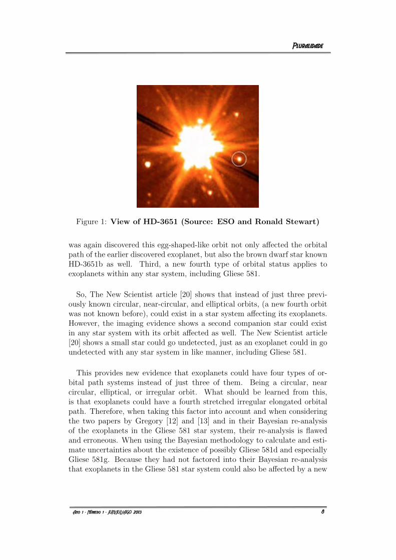
Figure 1: View of HD-3651 (Source: ESO and Ronald Stewart)
was again discovered this egg-shaped-like orbit not only affected the orbitalpath of the earlier discovered exoplanet, but also the brown dwarf star knownHD-3651b as well. Third, a new fourth type of orbital status applies toexoplanets within any star system, including Gliese 581.
So, The New Scientist article [20] shows that instead of just three previ-ously known circular, near-circular, and elliptical orbits, (a new fourth orbitwas not known before), could exist in a star system affecting its exoplanets.However, the imaging evidence shows a second companion star could existin any star system with its orbit affected as well. The New Scientist article[20] shows a small star could go undetected, just as an exoplanet could in goundetected with any star system in like manner, including Gliese 581.
This provides new evidence that exoplanets could have four types of or-bital path systems instead of just three of them. Being a circular, nearcircular, elliptical, or irregular orbit. What should be learned from this,is that exoplanets could have a fourth stretched irregular elongated orbitalpath. Therefore, when taking this factor into account and when consideringthe two papers by Gregory [12] and [13] and in their Bayesian re-analysisof the exoplanets in the Gliese 581 star system, their re-analysis is flawedand erroneous. When using the Bayesian methodology to calculate and esti-mate uncertainties about the existence of possibly Gliese 581d and especiallyGliese 581g. Because they had not factored into their Bayesian re-analysisthat exoplanets in the Gliese 581 star system could also be affected by a new
3
8

type of fourth orbit. Which could affect any of the exoplanets in Gliese 581star. This is especially important when considering a fourth type of orbitcould also affect Gliese 581d and Gliese 581g in the Habitable Zone (HZ).
1.2 Bayesian Re-Analysis of Gliese 581g
Other evidence within the papers by Gregory [12] [13] is that they discussin their papers is mentioned under subsection 4.3 entitled: ”Four PlanetModel”, and also according to Figure 121.
The paragraph continues to elaborate that the 4 planet model, Gliese 581dshows a very close 66.9 day orbital period. Which is very close to when Udry[29] corrected his original estimate of Gliese 581d having an 82 day orbital pe-riod down to a 67 day orbital period around its parent star instead. WhereasGliese 581g’s orbit was later estimated to be between a 34.0-36.0 day orbital.Again being consistent, and in extreme close estimations to Vogt’s [31], esti-mations reported in his paper. Therefore, Gregory [13] could not have suchclose estimations to Udry’s [29] estimations of Gliese 581d’s orbit being at a67.0 orbital cycle. When considering Gregory’s [12] estimate based upon hismodels that Gliese 581d had a 66.9 day orbit compared to Udry’s [29] revisedestimate that Gliese 581d had a 67.0 day orbit the measurements are almostidentical. The difference only being models 1/10th of 1.0%. On one hand,for the Bayesian methodology models to suggest uncertainty for Gliese 581d,and especially Gliese 581g based upon the Bayesian noise amplitude models,and than on the other hand for Gregory [12] to fully depend upon the ex-treme closeness of the estimated orbital paths for Gliese 581d and Gliese 581gexpressed in the papers by Udry [29] and Vogt [30], would seem to be con-tradictory to the Bayesian methodology model reanalysis of the entire Gliese581 star system. Especially when it would come to exoplanets Gliese 581d
1The 4th planet model is based upon the last and fourth planet of the Gliese 581 starsystem being Gliese 581d, they are giving admitted evidence to Gliese 581d. Whereas inFigure 14 of Gregory [12], the parameters for a: ”5 Planet Model” the 5th planet modelbeing Gliese 581g. As far as the amplitude is concerned the 5th planet, Gliese 581g ismore erratic. However, this does not necessarily mean that there is no existence for a 5thplanet, which would be applicable to Gliese 581g. Rather, it would mean just the opposite.In Figure 14 the orange colored perimeter and noise level could be: ”an accentuation ofGliese 581g’s close position in proximity to Gliese 581d, this could cause an extension ofadditional noise variations in the noise amplitude harmonics. This will be explained morein upcoming pages of this paper. However, additional evidence is supplied in Gregory [12]in paragraph 2 of the sub-heading entitled: ”6 Planet Model”. Gregory [12] states quote:”There is considerable agreement with the 4 and 5 planet model marginals shown”.
4
9
and Gliese 581g. Therefore, because of this type of inconsistencies and con-fusion on the part of the Gregory’s paper [12], it is evident that more doubtis created upon the paper written by Gregory [12] because of the discussionsin Gregory and Fischer’s earlier paper [13].
2 The 2012 Baluev Bayesian Research Paper
Dispute Casting Doubt On The Existence
of Gliese 581d
It is important to understand that if doubt can be put on the non-existenceof Gliese 581d as a previously confirmed exoplanet, than this would createeven more doubt for the existence of Gliese 581g. Therefore, much morediscussion for the existence of Gliese 581d is in order before Gliese 581g isdiscussed further.
In the paper by Baluev [4], the impact of red noise in radial velocity planetsearches: Only three planets orbiting Gliese 581? This proposes that becauseof the ”red noise levels” in the RV also known as Radial Velocity Method(RVM), which is the primary scientific technology and instrumentation usedfor attaining particular and specific data about an exoplanet and its identify-ing characteristics, like: ”mass”, etc..., may cast some doubt on the existenceof Gliese 581d. This was based upon the fact that in September 2012, Baluevfiltered out the ”red noise” from the Keck data and concluded that Gliese581d ’s existence is probable only to about a 3.0-4.0 standard deviations.Second, his paper reports that in the past, that because the: ”white levelof noise” was primarily studied and not the ”red noise”, than this is signif-icant new scientific evidence that Gliese 581d in Roman Baluev [4] reportsthat the red noise pertaining to the RVM significantly provides enough newadditional evidence that Gliese 581d does not exist. His paper further readsquote:
”We performed a detailed analysis of the latest HARPS and Keck radialvelocity data for the planet-hosting red dwarf GJ-581, which attracted a lotof attention in recent time. We show that this data contains important cor-related noise component (”red noise”) with the correlation timescale of theorder of 10 days. This red noise imposes a lot of misleading effects whilewe work in the traditional white-noise model. To eliminate these misleadingeffects, we propose a maximum-likelihood algorithm equipped by an extended
5
10
model of the noise structure. We treat the red noise as a Gaussian randomprocess with exponentially decaying correlation function.”.
This paper proposes that the: ”red noise levels” in any RV data (more orless) should be false positives or indicators of what is there in reality as far asexoplanets are concerned in the Gliese 581 star system. However, there area number of missed points and inconsistencies that when contemplated, andreasoned out with common-sense, and logical scientific deductive reasoning,these numerous points do not agree with what Baluev [4] is reporting for thenon-existence of Gliese 581d. This paper cannot list all of these reasons forlack of space in this paper that could be given that disagree with RomanBaluev [4]. However, in Stewart’s paper [24] from the top of page 1- the endof page 18 gives at least ten strong reasons as to why the paper by Baluev [4]has too many inconsistencies to be reliable for evidence against the existenceof Gliese 581d. Whereas on the other hand, these ten or more reasons onlygive that much more support in additional evidence for the existence of Gliese581d.
2.1 More Than Ten Strong Reasons Why BayesianStudy Re-Analysis of Gliese 581d and Gliese 581gIs Erroneous
In the recent paper by Vogt [30] reminds the reader that as far as a Bayesianre-analysis study of the Gliese 581 star system is concerned, that when consid-ering that Gliese 581d has an orbital cycle of about 67.0 days. The Bayesianre-analysis of Gliese 581d, is that exoplanets like Gliese 581g only about one-half of the 67 day orbital period of eccentricity like Gliese 581d. However,the Bayesian calculations have complications. Anglada-Escude & Dawson [2]continue to explain quote: ”If the modeler (who records the measurements),elects to allow the eccentricity of the 67 day planet to ”float”, least-squaresfitting routines will take advantage of this extra degree of freedom, allowingthe eccentricity of the 67 day to rise, and thereby largely masking any signalfrom a real fifth planet near half that period. Aliases from the unevenly-spacedsampling in the data set further complicate the behavior of peaks at or aroundhalf the period of the 67 day.”. Therefore, to correct this Anglada-Escude [2]used over 4,000 Monte Carlo simulations of the effects of both the eccentric-ity harmonics and its aliases to conclude that the presence of Gliese 581g.Providing that Gliese 581g is the fifth potential exoplanet in the Gliese 581star system. It also provides a significant amount of additional evidence thatis not only consistent with Vogt [31], but supports this paper as well. While
6
11
Bhattacharjee’s paper [5] supports all of the data for Gliese 581d and Gliese581g.
Mayor [16] data also brings out and discusses the Gliese 581d 67 day planetcircumstances and verifies the same. Which is also discussed in Vogt [30]points out that the HARPS and HIRES data sets just did not merge wellunder the assumption of an: ”all-floating-eccentricity”. Which when doneleaves larger numbers of peaks in the residuals and periodograms. By con-trast, models that assumed all-circular orbits allowed the two data sets tomeld much more closely, and produced much better equivalent quality withfewer parameters. Vogt [30] further explains that if a modeler allows theeccentricities of all four known planets to float, that this would add 8 ad-ditional parameters to the model. Also allowing more additional degrees offreedom than adding even two more planets on circular orbits. Therefore,when considering this extra data: ”The principle of parsimony” clearly favorscircular to near circular orbits for all of the planets in the Gliese 581 system.Vogt [30], and two Bayesian studies provided in Gregory [12] and Gregoryand Fischer [13], along with Vogt [30] discuss a fourth/fifth planet modelapplying to Gliese 581g. Which would have circular or at least near circularorbits around Gliese 581. Supporting this data and found, that by adding afifth planet at 32.1 days to the system, would account for an super-Earth-likeplanet in the middle of the HZ at about 2.2M⊕.
At the same time, the Tuomi study [28] explicitly concluded that the orbitsof the four confirmed planets were all consistent with circular to near circularorbits and cited 99% Bayesian credibility ranges of [0-0.67] for the 67 dayplanet Gliese 581d. The Bayesian analysis of Gregory [12] also lists uncer-tainties for 3 of 4 eccentricities in this system that are consistent with circularor near circular orbits around their star.The fact that neither Bayesian anal-ysis found sufficient evidence for more than four planets in the system alsodeserves further scrutiny. Tuomi [28] and Jenkins & Peacock [14] raised seri-ous doubts about the traditional threshold for the Bayesian Evidence Ratio.Therefore there is an additional amount of significant data and evidence tosupport the erroneous data of the Bayesian studies not supporting the exis-tence of Gliese 581d or Gliese 581g.
Contrary to the widespread impression that the Bayesian results rule outany more than 4 or 5 planets in the Gliese 581 system, the additional planetclaims of Vogt [31] are actually not in discord with these Bayesian analyses.How? Jenkins & Peacock [14] found the Bayesian evidence ratio to be a
7
12
noisy statistic, and cautioned that it may not be sensible to accept or rejecta model based solely on whether that evidence ratio reaches some thresholdnoise value. They conclude that the performance of such Bayesian tests issignificantly affected by the signal to noise ratio in the data.
3 Evidence That Gliese 581d and Gliese 581g
Exist In The Habitable Zone Next To Each
Other
Baluev [4] in their paper are confident that the existence of Gliese 581dis questionable and that Gliese 581g is an illusion as stated in their paper.What also proposes that the reliability of their paper should seriously bequestioned is because one of their subtitles states that: ”Red noise as adetection method can be a misleading agent”. Therefore, their paper againshows contradictory inconsistencies that keep proving their paper of BayesianStudies and re-examination of Gliese 581d and Gliese 581g cannot be reliedupon. What is truly surprising and confusing at the same time is the factthat in their paper they claim that while their technology and studies wereadequate enough to detect Gliese 581e, Gliese 581b and Gliese 581c, butwas not able to detect Gliese 581d or Gliese 581g. The laws of physics donot pick and choose to detect some exoplanets and then not others. Orpartially maybe suggest that Gliese 581d exists but should still be questionit’s existence. The technology is either going to detect all of the exoplanetsor not, especially if the technology or partial application of it is not sensitiveenough, or has not been attempted enough in measurements over a periodof time.
For example; Trentadue [27], Endl [9] and Wittenmyer [32] speaks thatwhen studying exoplanets the ones that should primarily be studied are theones that are closest to Earth’s own solar system, and especially if they havea possible HZ. However, all of these papers strongly suggest and were alsoin the study of the Proxima Centauri star system that after many years ofstudy using the RVM, that no exoplanets were found to be in the ProximaCentauri star system. Which is the closest star system to Earth. In additionto this Based upon Kasting [15] studied the same star system and found noexoplanets. However, again, Wittenmeyer [32] and Endl [9] determined thatonly when using the radial velocity method over numerous years and overmany attempts giving strong evidence that:
1. Proxima Centauri did not have a HZ; and
8
13
2. That no signal was able to be detected despite many attempts withthe RVM. No signals were picked up at all. Evidence, indicating notany exoplanets at all in orbit around Earth’s closest neighbor ProximaCentauri at just 4.22 LY away from Earth. This included any exoplan-ets that may equal the mass and size of Neptune and/or any gas giantslike Jupiter as well.
When considering that in the case of determining or not ”if” there wereany exoplanets in Proxima Centauri, this paper again needs to re-emphasizethat the ”only way” that RVM is going to work not only effectively, butalso accurately is when it is used ”over numerous years and over many at-tempts”. In Endl [10] presented their findings in looking for low density massexoplanets for example in Proxima Centauri and M. Endl and M. Kurster [9]determined that when using the radial velocity method and attest to the factthat as far as RVM is concerned as a scientific tool and instrumentation, itsaccuracy is solely dependent on the fact ”that since sensitivity is a functionof RVM accuracy and precision, that following up with as many additionalnumber of measurements and sampling as possible, adds more points to thecurrent data. Furthermore, this methodology allows an improvement of theRVM detection sensitivity over time”. Therefore, to be able to get a true sci-entific assessment if any exoplanet- (especially Gliese 581d and Gliese 581g)are there or not, the dependency of the accuracy of the RVM is very depen-dent on repetitious attempts and detections over a large amount of time. Inorder to truly get enough accumulative data to accurately determine if anexoplanet is in any star system or not. Especially Gliese 581d and Gliese581g.
This also proved true when in his paper by Dumusque [8]. An Earth massplanet orbiting Alpha Centauri B, spent over 3 years and numerous attemptsto be able to get enough data measurements to determine with any amountof accuracy as that there a mass sized Earth sized planet close to it’s parentstar in the Alpha Centauri B star system. In like manner, it is the sameconditions when determining if Gliese 581d and Gliese 581g are in the Gliese581 star system as well. However, this also applies to using the RVM in thisway. Because if it is not used in this way, than any use of this exoplanettechnology would not be accurate.
So, is the case when Gliese 581g was first announced by Vogt [31] whenhe revealed the probable existence of Gliese 581g that would reside in aboutthe middle of the habitable zone of the Gliese 581 star system. However,
9
14
new doubts about Gliese 581g’s existence were proposed in Pepe [18] and theGeneva Team used data from HARPS, or the High Accuracy Radial Velocityfor Planetary Searcher, a powerful spectrometer on a 3.6 m telescope inChile. It is well known that the HARPS spectrograph uses the radial velocitymethod, or measuring the gravitational tugs on stars by their planets bywatching the stars’ spectral lines ”wobble” back and forth due to the Dopplereffect. However, The Geneva Team, in Pepe [18], stated that they could notfind evidence of Gliese 581g. using the just HARPS technology by itself.
The Geneva Team gave further reasons as to why Gliese 581g did not exist.He stated in so many words ”Since Mayor’s announcement in 2009 of thelowest-mass planet Gliese 581e, we have gathered about 60 additional datapoints with the HARPS instrument for a total of 180 data points spanning 6.5years of observations”... ”From these data, we easily recover the 4 previouslyannounced planets Gliese 581b, Gliese 581c, Gliese 581d, and Gliese 581e.”,said Peppe. However, he then said ”We do not see any evidence for planet ’g’,the fifth planet in the system as announced by Vogt and his Team. The reasonfor that is that, despite the extreme accuracy of the HARPS instrument andthe many data points, the signal amplitude of this potential fifth planet isvery low and basically at the level of the measurement noise”.
3.1 What The Geneva Team Did Not Consider
However, in 2010 Vogt [31] stated that Gliese 581g existed. Vogt and Butlerused data from HARPS over a 4.3 year period and data from the HIRSEinstrumentation, over an 11 year period. It is important to remember thatearlier in this paper it was discussed how important it is when using the RVMfor detecting exoplanets, that like in the case as aforementioned in Trentadue[27], Endl [9] [10], Wittenmeyer [32], Kasting [15] and Dumusque [4], thatthe reliability, efficiency, proficiency, accuracy and sensitivity of the RVM tobe able to detect exoplanets in other star systems to its maximum capability,is solely dependent on the fact ”that since sensitivity is a function of RVMaccuracy and precision, that following up with as many additional number ofmeasurements and samplings as possible, adds more points to the current dataand that by this methodology, it allows for the best maximum improvement ofthe RVM detection sensitivity over time when using it to detect exoplanets”.In this case especially being applicable in detecting Gliese 581d and Gliese581g. The overall point here is that when the years that Vogt’s Team usedboth the HARPS data over 4.3 years and the HIRSE data over 11 moreyears what this mean is that very careful and exhausting efforts were putinto the RVM adding up to over 14.3 years that were spent using the RVM
10
15
to find exoplanet Gliese 581g. The HIRSE approach is the High ResolutionEchelle Spectrometer on one of the 10 m Keck Telescopes in Hawaii. Theiranalysis searches for planets in the Gliese 581 system using both sets of data,confirming the presence of planets Gliese 581b, Gliese 581c, Gliese 581d, andGliese 581e while showing evidence for the two new planets, Gliese 581f andespecially Gliese 581g. However, what is not known, and what the GenevaTeam did not think about or consider are several new areas of evidence thatmakes the case stronger for Gliese 581g. This comes down to four new areasof data as follows:
1. The Geneva Team use of only the HARPS instrumentation althoughwhile impressive was not precise enough by just this technology alonefor the 6.5 years to prove that this exoplanet does not exist;
2. The Geneva Team admitted ”The reason for that is that, despite theextreme accuracy of the HARPS instrument and the many data points,the signal amplitude of this potential fifth planet is very low and ba-sically at the level of the measurement noise” said Pepe. Therefore,since the ”Signal Amplitude” was at the same level of the ”Measure-ment Noise”, the reason The Geneva Team had a difficult time to dis-tinguish if Gliese 581g was there or not, does not provide any data orevidence that Gliese 581g was not there. Pepe and his Geneva Teamcannot determine with any scientific probability that Gliese 581g wasnot there, just because the precision of their RVM was not sensitiveenough to pick up enough of an RV signal to prove that the Gliese581g exoplanet does not exist. This contrasts with the work of Vogt,which argues that the false alarm probability for these six planets isextremely low.
3. Another important point missed is when a much closer reading of the”Vogt et al, (2010) preprint”, is done Vogt and his Team stated ”Thatboth sets of data from HARPS and HIRSE were needed to detect all 6planets in the Gliese 581 star system”. Which was done over a periodof time totaling over 14 years between the two HARPS and HIRSEdata sets. This would also mean:
(a) That The Geneva Team was evidently agreeable that HARPS andHIRSE did confirm the existence of exoplanets Gliese 581e, Gliese581b, Gliese 581c, and Gliese 581d, but were not willing to acceptthat the same scientific principle previously applied all of a suddenwas incapable of detecting Gliese 581g. That since both of theHARP and HIRSE technologies were needed to detect all the other
11
16
confirmed planets why didn’t the Geneva Team just simply ”Alsoduplicate” the use of both technologies just like the Vogt Teamdid to see if they could also detect Gliese 581g? Apparently theydid not and only chose the data that would support their conceptsinstead of looking at all of the data from A to Z.
(b) The total length of time and duration that the Vogt Team usedboth technologies to detect Gliese 581g was for a much longerperiod of time that the Geneva Team used only the HARPS tech-nology. The HIRSE technology secondly re-verified what the VogtTeam found with using the HARPS technology. Where the GenevaTeam did not re-verify their findings on an equal basis by using aback up technology to back up their HARPS findings, where theVogt Team did, and for a much longer period of time as well;
(c) Therefore it’s no surprise that the HARPS-only data set cannotconfirm the presence of exoplanet Gliese 581g. The fact that thescientific papers ”Gliese 581-Extra-Solar Imaging Survey” [22],”First View of Gliese 581d; A Preliminary Surface Survey (Part1)” [25], ”Gliese 581d; Views of Its Atmospheric, Topographi-cal, Geological, and Oceanic and Oceanic Conditions” [24] and”The (possible) confirmation of the first exo-oceans” [1], are pa-pers where conditions, circumstances, and observations were madein close to extremely close up images of an possible exoplanet fit-ting all of the descriptions in the Gliese 581 star system applicableto the exoplanet in this star system’s HZ known as Gliese 581dhave been intensely studied from numerous scientific disciplines.The fact that the research Team who intensely studied currentknown and new consistent areas of evidence pertaining to Gliese581d, which it was also observed numerous time to also be consis-tent orbital path for the currently known estimated orbital pathfor Gliese 581d also allowed the observation of another possibleexoplanet in the about the middle of the HZ of the Gliese 581star system that fits all of the known descriptions that could onlyapply to Gliese 581g.
In Figure 2 the estimated orbital path is seen for exoplanets c and b.However, the orange arrow points to the previously estimated orbitalpath made by Udry [29] at originally where Gliese 581d would have beenlocated on the outer edge of the HZ. However, later with many moremeasurements Udry [29] later revised the estimated orbital path for
12
17
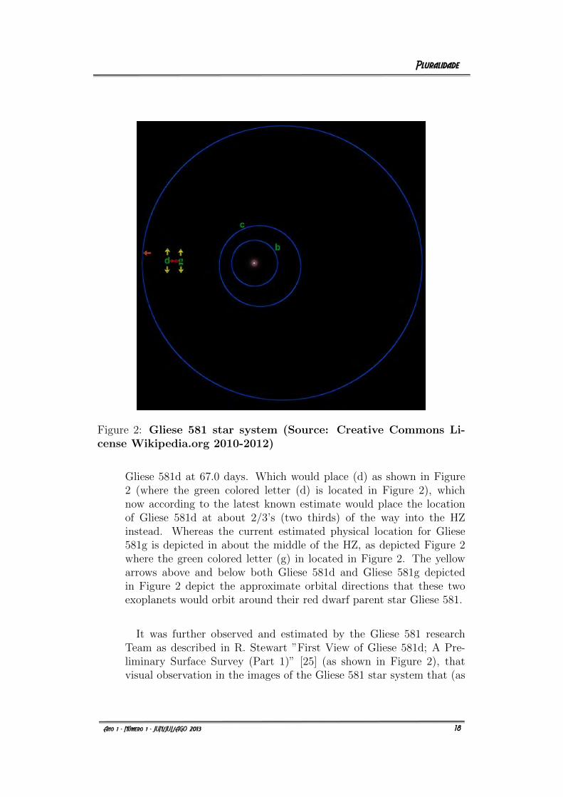
Figure 2: Gliese 581 star system (Source: Creative Commons Li-cense Wikipedia.org 2010-2012)
Gliese 581d at 67.0 days. Which would place (d) as shown in Figure2 (where the green colored letter (d) is located in Figure 2), whichnow according to the latest known estimate would place the locationof Gliese 581d at about 2/3’s (two thirds) of the way into the HZinstead. Whereas the current estimated physical location for Gliese581g is depicted in about the middle of the HZ, as depicted Figure 2where the green colored letter (g) in located in Figure 2. The yellowarrows above and below both Gliese 581d and Gliese 581g depictedin Figure 2 depict the approximate orbital directions that these twoexoplanets would orbit around their red dwarf parent star Gliese 581.
It was further observed and estimated by the Gliese 581 researchTeam as described in R. Stewart ”First View of Gliese 581d; A Pre-liminary Surface Survey (Part 1)” [25] (as shown in Figure 2), thatvisual observation in the images of the Gliese 581 star system that (as
13
18
shown in Figure 2), that the approximate locations and orbital pathrotations for Gliese 581d and Gliese 581g is consistent with the latestknown data.
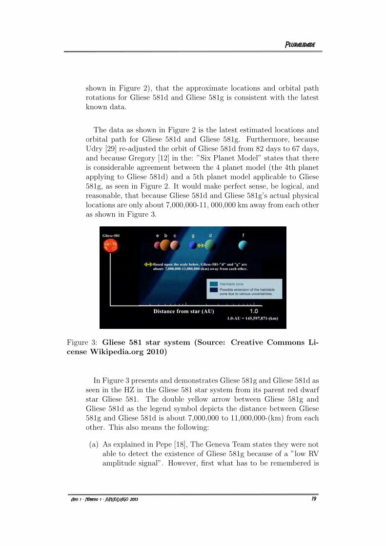
The data as shown in Figure 2 is the latest estimated locations andorbital path for Gliese 581d and Gliese 581g. Furthermore, becauseUdry [29] re-adjusted the orbit of Gliese 581d from 82 days to 67 days,and because Gregory [12] in the: ”Six Planet Model” states that thereis considerable agreement between the 4 planet model (the 4th planetapplying to Gliese 581d) and a 5th planet model applicable to Gliese581g, as seen in Figure 2. It would make perfect sense, be logical, andreasonable, that because Gliese 581d and Gliese 581g’s actual physicallocations are only about 7,000,000-11, 000,000 km away from each otheras shown in Figure 3.
Figure 3: Gliese 581 star system (Source: Creative Commons Li-cense Wikipedia.org 2010)
In Figure 3 presents and demonstrates Gliese 581g and Gliese 581d asseen in the HZ in the Gliese 581 star system from its parent red dwarfstar Gliese 581. The double yellow arrow between Gliese 581g andGliese 581d as the legend symbol depicts the distance between Gliese581g and Gliese 581d is about 7,000,000 to 11,000,000-(km) from eachother. This also means the following:
(a) As explained in Pepe [18], The Geneva Team states they were notable to detect the existence of Gliese 581g because of a ”low RVamplitude signal”. However, first what has to be remembered is
14
19
that in subheading #3. of item 3.1 of this paper that ”In Vogt(2010) preprint”, Vogt and his Team explicitly state ”That bothsets of data from HARPS and HIRSE were needed to detect all 6planets in the Gliese 581 star system”. Why is this another im-portant point?First of all Pepe and The Geneva Team did not use both of theHARPS and HIRES data sets as Vogt and his Team did. Vogtmade it very clear in his 2010 paper that both of the HARPS andHIRES data sets were needed in order to correctly detect theseexistence of Gliese 581g as an exoplanet. The primary point isthat apparently it was a well known fact that if it took both ofthe HARPS and HIRES data sets to detect the existence of Gliese581g. In other words, both of the HARPS and HIRES RV tech-nologies combined together would have made the RVM powerfuland sensitive enough to detect Gliese 581g’s signal harmonics sig-nature in order to give evidence that it existed.Therefore, because Pepe and his Team only used the HIRES dataset this instrumentation by itself was of course not strong enoughto pick up the signal it needed to in order to be able to detectGliese 581g. Second, it would have seemed that if Pepe and TheGeneva Team would really wanted to have determine if Gliese581g was there or not, all they had to be willing to do is simplyduplicate the same RVM that Vogt and his Team did with bothof the HARPS and HIRES data sets, for the same amount of timeduration as Vogt and his Team did. ”If” at that point they wereable to disprove by Vogt and his Team’s own methodologies thatthey were in error, ”then at that point in time”, they could havereported what their results showed Vogt to be in error. This wouldseem to be the appropriate way to disprove Vogt by exactly du-plicating his own scientific methodologies exactly by the way heand his Team had approached it. This could have helped provethe existence of Gliese 581g’s to a greater degree or not.
(b) Second, because the Gliese 581 star system is 20.3 LY from Earthit that when using just the HIRES instrumentation by itself maybarely be strong enough to pick up an amplitude signal as largeas Jupiter or larger gas giants within a solar system, includingthat of Gliese 581 in like manner. When exoplanets are moreEarth sized or just a little larger than Gliese 581g or Gliese 581d,by itself the HIRES instrumentation may not be strong enoughpick up the amplitude signal of smaller exoplanets larger that the
15
20
approximate 2.2-3.1M⊕ and about 1.3 to 1.5 times larger thanEarth according to Vogt [31].
(c) A third point to consider is that the Geneva Team only used theHIRES instrumentation. Considering that Gliese 581g and Gliese581d are likely only 7,000,000 to 11,000,000 km away from eachother, what also has not been considered is that it would havebeen possible that sometimes the signal amplitudes between de-tecting Gliese 581g and Gliese 581d became mixed up. By TheGeneva Team only using the HIRES instrumentation by itself, attimes Pepe and his Geneva Team may have believed they werepicking up signals from Gliese 581d, when in actuality they werereally picking up an amplitude signals from Gliese 581g instead,and vice-versa. Because of these two exoplanets locations, andorbital paths being too close together for the HIRES instrumenta-tion to detect correctly. Because by itself the HIRES instrumen-tation is not powerful and sensitive enough to pick up the signalof each exoplanet because their physical locations and/or orbitalpaths are just too close together. However, when considering themethodology that Vogt and his Team took it correctly measuredthe existence of Gliese 581g as he originally had reported in Vogt[31].
4. Therefore also when Anglada-Escude [2] present in his paper a detaileddiscussion when it comes to the orbits of both Gliese 581d and Gliese581g, when it first comes to the 67 day planet Gliese 581d orbital cycletheir paper shows that Gliese 581d produces a harmonic signal nearhalf that period of 33.5 days, relating to the orbital rotational cycle ofGliese 581g. The period of Gliese 581g reported by Vogt [31] is 36.56days, and one of its yearly aliases occurs near a period near 33.2 days.Because this yearly alias of planet Gliese 581g lies close to the eccen-tricity harmonic of the 67 day planet Gliese 581d, Anglada-Escude [2]present suggest that the signal from planet Gliese 581g can be partiallyor even totally absorbed by the eccentricity of planet Gliese 581d.2
Such consistency is verified again in Anglada-Escude [2] which showsthat they carried out statistical tests to quantify these interactionsand calculated False Alarm Probabilities (FAP) of 0.11% and 0.03%
2This would be consistent with the very close distance in physical location that Gliese581g and Gliese 581d are away from each other. In likely not only very close proximitylocation, but in their orbital paths as well.
16
21
for the signals associated with Gliese 581g. They also concluded thatthe presence of Gliese 581g is well supported by the data presentedby Mayor [16] and Vogt [30]. Vogt [31] also goes on to show that theadditional 60 HARPS measurements cited back in October 2010 byPepe [18], plus another full observing season of data were released inSeptember 2011 by Forveille [11], brought the total number of publishedHARPS velocities for Gliese 581 to 240. The release of Forveille’s data,essentially doubled the amount of high precision HARPS data publiclyavailable since Pepe [18] and Forveille [11] presented Keplerian modelsto that data set. Like Pepe [18], they also chose to exclude all HIRESdata from their analysis to avoid any risk of being misled by subtlelow-level systematics in one data set or the other.
Forveille [11] presented two multi-planet Keplerian models to this HARPSonly data set. The first was a four-planet model with the eccentricities ofall orbits allowed to float. These complications are described in detail byAnglada-Escude [2] and they also go into considerable detail that the eccen-tricity harmonics of a known exoplanet such as in the case of Gliese 581d cansometimes mask the signal of other planets near half of that planet’s periodlike Gliese 581g. Further describing how any fltting sequence for the Gliese581 system that proceeds sequentially in order of signal strength (as all previ-ous modelers, including the Bayesian studies have done) would be subjectedto the same principles and would produce the same results as aforementioned.
4 New Data by Vogt 2012 Supporting the Ex-
istence of Gliese 581g
Vogt [31] presents a significantly extended and goes into much deeper com-prehensive detail in a re-examination of he and his Teams original Vogt [31]analysis and very significantly expands their previous HARPS 2011 radialvelocity data set for Gliese 581 for the existence of Gliese 581g above andbeyond what Forveille [11] presented. Their analysis reaches substantiallydifferent conclusions regarding the evidence for a super and RMS values onlyafter removing some outliers from their models and refitting the trimmeddown RV set. They denote that after an additional 4,000 N-body simulationsof their Keplerian model all resulted in unstable systems in the methodologiesapproached by Forveille [11] and revealed that their reported 3.6 s detectionof e=0.32 for the eccentricity of Gliese 581e is manifestly incompatible withthe system’s dynamical stability. More evidence that Gliese 581g is in Gliese
17
22
581 star system.
However, Vogt [30] also reports duplicating the same type of model thatForveille [11] projects as a Keplerian Earth-mass planet in the star’s Habit-able Zone. In the paper by Vogt [30] reports being able to reproduce theirreported model. However, when it was integrated only over the time baselineof the observations, significantly increases and demonstrates the need for in-cluding non-Keplerian orbital precession when modeling the Gliese 581 starsystem.
Again Vogt [30] found that a four planet model with all of the planets oncircular or nearly circular orbits provides both an excellent self-consistent fitto their RV data and also results in a very stable configuration. In this paperthe Gliese 581 Research Team agrees with this and contends that Vogt’sexperimentation of the duplication of the periodogram of the residuals to a4 planet all circular, to near circular, orbit model reveals significant peaksthat suggest one or more additional planets in this system. In this paper wewould also like to report that in agreement with Vogt’s 2010 and 2012 papersthat the Gliese 581 Research Team observed in images to extreme close upimages what resembled circular, near circular, like orbits for Gliese 581d.
While Stewart [22] reports in his article that when first performing a rudi-mentary Gliese 581 survey in the summer to fall of 2011 observed that whathave the same strikingly close orbits for Gliese 581e, Gliese 581b, Gliese581c possible exoplanets he observed in similar images that these exoplanetsseemed to exhibit the same circular-near circular and/or combination circu-lar and some what elliptical orbit for these exoplanets in this star system.However would characterize more closely that the exoplanets in the Gliese581 system follow more closely a circular, near circular, orbital paths.
This paper also agrees with Vogt [30] with their re-evaluations with thetotal 240 point HARPS data set, that Gliese 581 has fully self-consistentstable orbits, by and of itself does offer significant support for a fifth signalin the data with a period near 32 days. This signal has a False AlarmProbability less than 4% and is consistent with a planet of minimum mass2.2M⊕ orbiting squarely in the star’s Habitable Zone at about 0.13 AU, whereliquid water on planetary surfaces is a real distinct possibility on Gliese 581g.
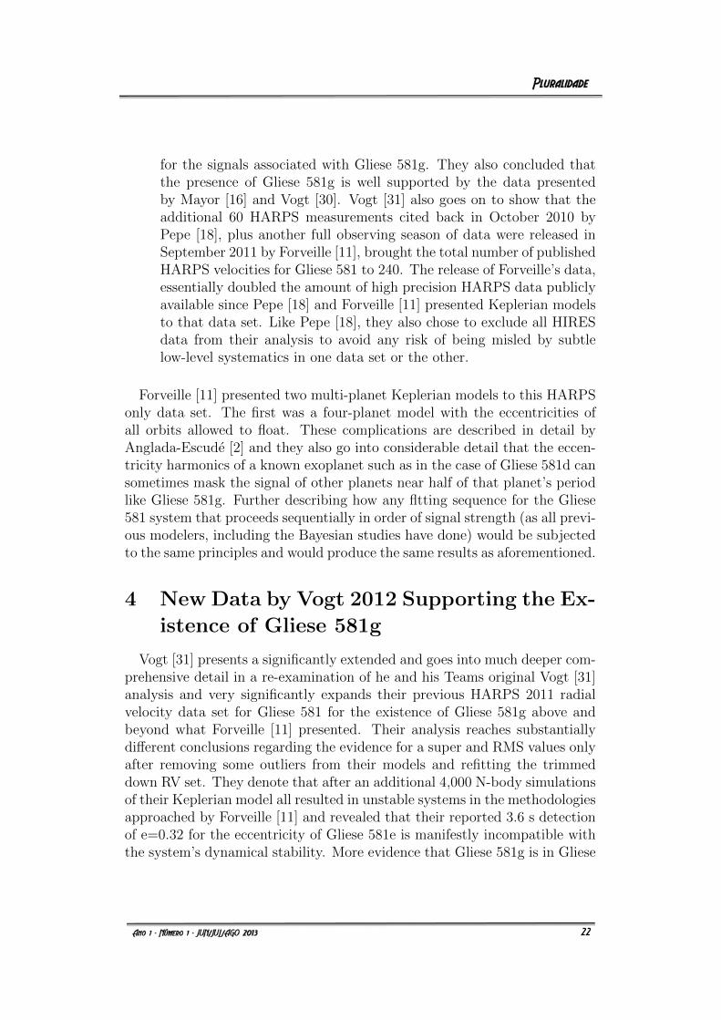
Figure 4 depicts a view of primarily Gliese 581d and Gliese 581g as seen inorbit around their parent red dwarf star Gliese 581. The yellow square is a
18
23
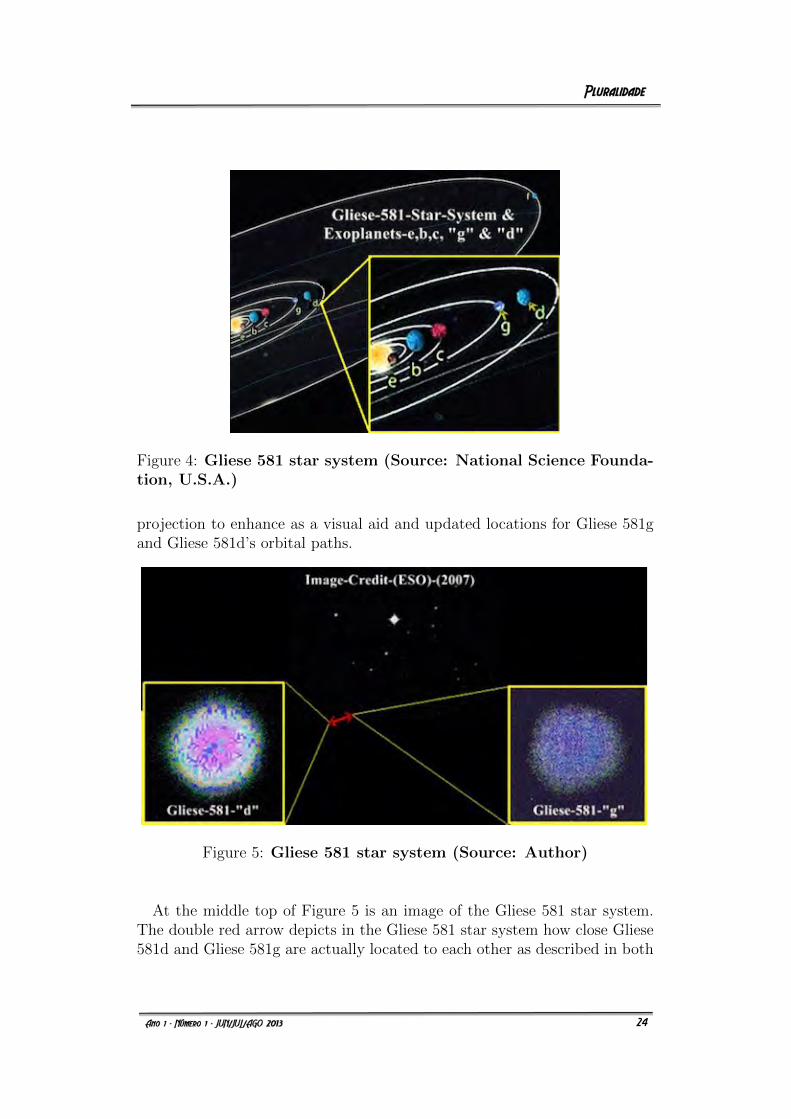
Figure 4: Gliese 581 star system (Source: National Science Founda-tion, U.S.A.)
projection to enhance as a visual aid and updated locations for Gliese 581gand Gliese 581d’s orbital paths.
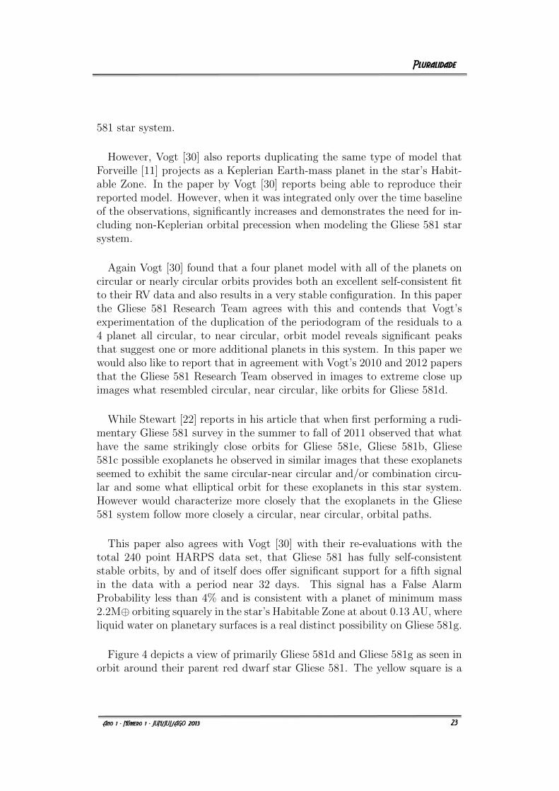
Figure 5: Gliese 581 star system (Source: Author)
At the middle top of Figure 5 is an image of the Gliese 581 star system.The double red arrow depicts in the Gliese 581 star system how close Gliese581d and Gliese 581g are actually located to each other as described in both
19
24
Stewart [25] [24]. Gliese 581g is projected in the left bottom corner of Figure5.
Figure 6: Moon and Gliese 581g (Source: Author)
Figure 6 (Left) depicts one of the last phases of Earth’s moon before itbecomes either a Full or New Moon. Trentadue [27] discusses that whenexamining exoplanets in other star systems, it is not that much differentthan how the Earth’s Moon transitions itself from about twenty-nine differentmoon phases every month. This is also true with planets, planetary bodiesin our solar system, and exoplanets. (Left) imaging evidence shows Earth’sMoon in its last phase before either becoming a full or new Moon. Rightimage is Gliese 581g also in its last phase before the full circular form ofGliese 581g can next be seen. In both images (in the upper top left corners),both Earth’s Moon and in Gliese 581g (both exhibit the same phases). Whichhave not quite yet reached their (Full and/or New Moon or planet phases)which in the next phase would develop into a full circle shape for eitherEarth’s Moon and Gliese 581g. Proved again in Figure 7. Earth’s mooncompared to Gliese 581-b’s moon.
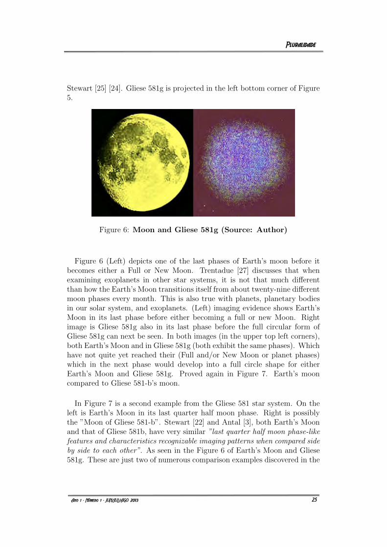
In Figure 7 is a second example from the Gliese 581 star system. On theleft is Earth’s Moon in its last quarter half moon phase. Right is possiblythe ”Moon of Gliese 581-b”. Stewart [22] and Antal [3], both Earth’s Moonand that of Gliese 581b, have very similar ”last quarter half moon phase-likefeatures and characteristics recognizable imaging patterns when compared sideby side to each other”. As seen in the Figure 6 of Earth’s Moon and Gliese581g. These are just two of numerous comparison examples discovered in the
20
25
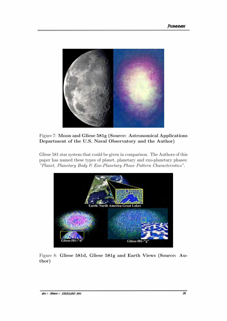
Figure 7: Moon and Gliese 581g (Source: Astronomical ApplicationsDepartment of the U.S. Naval Observatory and the Author)
Gliese 581 star system that could be given in comparison. The Authors of thispaper has named these types of planet, planetary and exo-planetary phases:”Planet, Planetary Body & Exo-Planetary Phase Pattern Characteristics”.
Figure 8: Gliese 581d, Gliese 581g and Earth Views (Source: Au-thor)
21
26
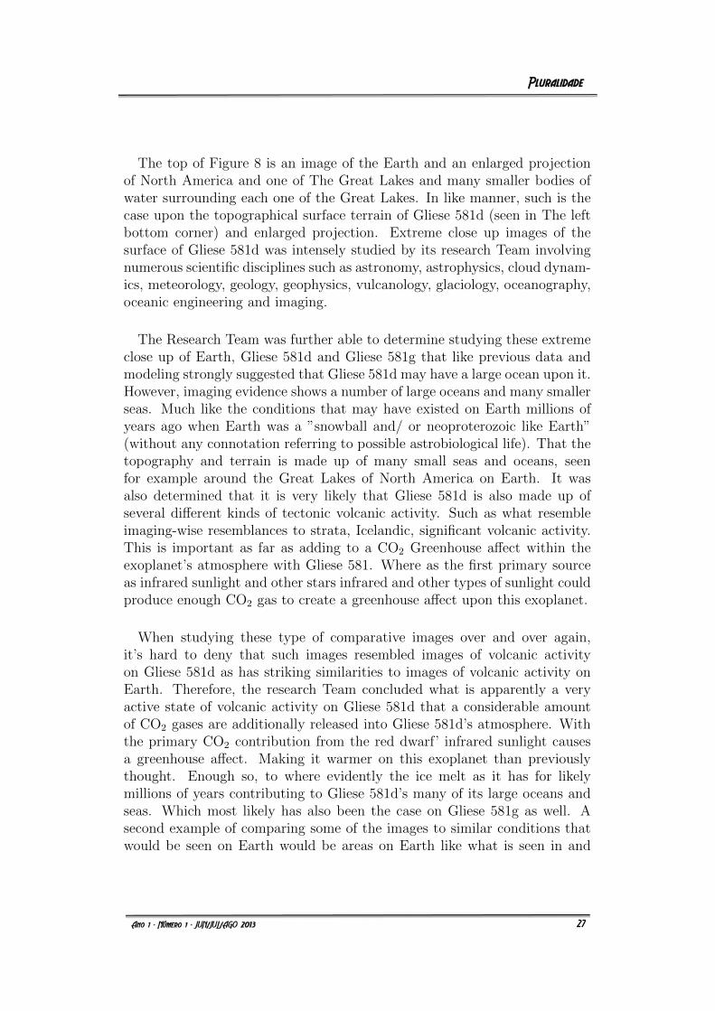
The top of Figure 8 is an image of the Earth and an enlarged projectionof North America and one of The Great Lakes and many smaller bodies ofwater surrounding each one of the Great Lakes. In like manner, such is thecase upon the topographical surface terrain of Gliese 581d (seen in The leftbottom corner) and enlarged projection. Extreme close up images of thesurface of Gliese 581d was intensely studied by its research Team involvingnumerous scientific disciplines such as astronomy, astrophysics, cloud dynam-ics, meteorology, geology, geophysics, vulcanology, glaciology, oceanography,oceanic engineering and imaging.
The Research Team was further able to determine studying these extremeclose up of Earth, Gliese 581d and Gliese 581g that like previous data andmodeling strongly suggested that Gliese 581d may have a large ocean upon it.However, imaging evidence shows a number of large oceans and many smallerseas. Much like the conditions that may have existed on Earth millions ofyears ago when Earth was a ”snowball and/ or neoproterozoic like Earth”(without any connotation referring to possible astrobiological life). That thetopography and terrain is made up of many small seas and oceans, seenfor example around the Great Lakes of North America on Earth. It wasalso determined that it is very likely that Gliese 581d is also made up ofseveral different kinds of tectonic volcanic activity. Such as what resembleimaging-wise resemblances to strata, Icelandic, significant volcanic activity.This is important as far as adding to a CO2 Greenhouse affect within theexoplanet’s atmosphere with Gliese 581. Where as the first primary sourceas infrared sunlight and other stars infrared and other types of sunlight couldproduce enough CO2 gas to create a greenhouse affect upon this exoplanet.
When studying these type of comparative images over and over again,it’s hard to deny that such images resembled images of volcanic activityon Gliese 581d as has striking similarities to images of volcanic activity onEarth. Therefore, the research Team concluded what is apparently a veryactive state of volcanic activity on Gliese 581d that a considerable amountof CO2 gases are additionally released into Gliese 581d’s atmosphere. Withthe primary CO2 contribution from the red dwarf’ infrared sunlight causesa greenhouse affect. Making it warmer on this exoplanet than previouslythought. Enough so, to where evidently the ice melt as it has for likelymillions of years contributing to Gliese 581d’s many of its large oceans andseas. Which most likely has also been the case on Gliese 581g as well. Asecond example of comparing some of the images to similar conditions thatwould be seen on Earth would be areas on Earth like what is seen in and
22
27
around the North pole and extreme far northern reaches of Canada. Whenthese extremely close images of the surface of Gliese 581d were comparedto cold environmental conditions on Earth, there were many similar andstrikingly similarities.
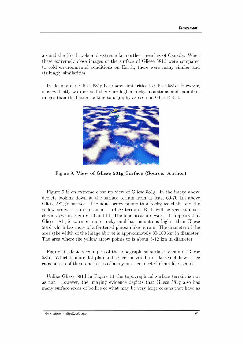
In like manner, Gliese 581g has many similarities to Gliese 581d. However,it is evidently warmer and there are higher rocky mountains and mountainranges than the flatter looking topography as seen on Gliese 581d.
Figure 9: View of Gliese 581g Surface (Source: Author)
Figure 9 is an extreme close up view of Gliese 581g. In the image abovedepicts looking down at the surface terrain from at least 60-70 km aboveGliese 581g’s surface. The aqua arrow points to a rocky ice shelf, and theyellow arrow is a mountainous surface terrain. Both will be seen at muchcloser views in Figures 10 and 11. The blue areas are water. It appears thatGliese 581g is warmer, more rocky, and has mountains higher than Gliese581d which has more of a flattened plateau like terrain. The diameter of thearea (the width of the image above) is approximately 80-100 km in diameter.The area where the yellow arrow points to is about 8-12 km in diameter.
Figure 10, depicts examples of the topographical surface terrain of Gliese581d. Which is more flat plateau like ice shelves, fjord-like sea cliffs with icecaps on top of them and series of many inter-connected chain-like islands.
Unlike Gliese 581d in Figure 11 the topographical surface terrain is notas flat. However, the imaging evidence depicts that Gliese 581g also hasmany surface areas of bodies of what may be very large oceans that have as
23
28
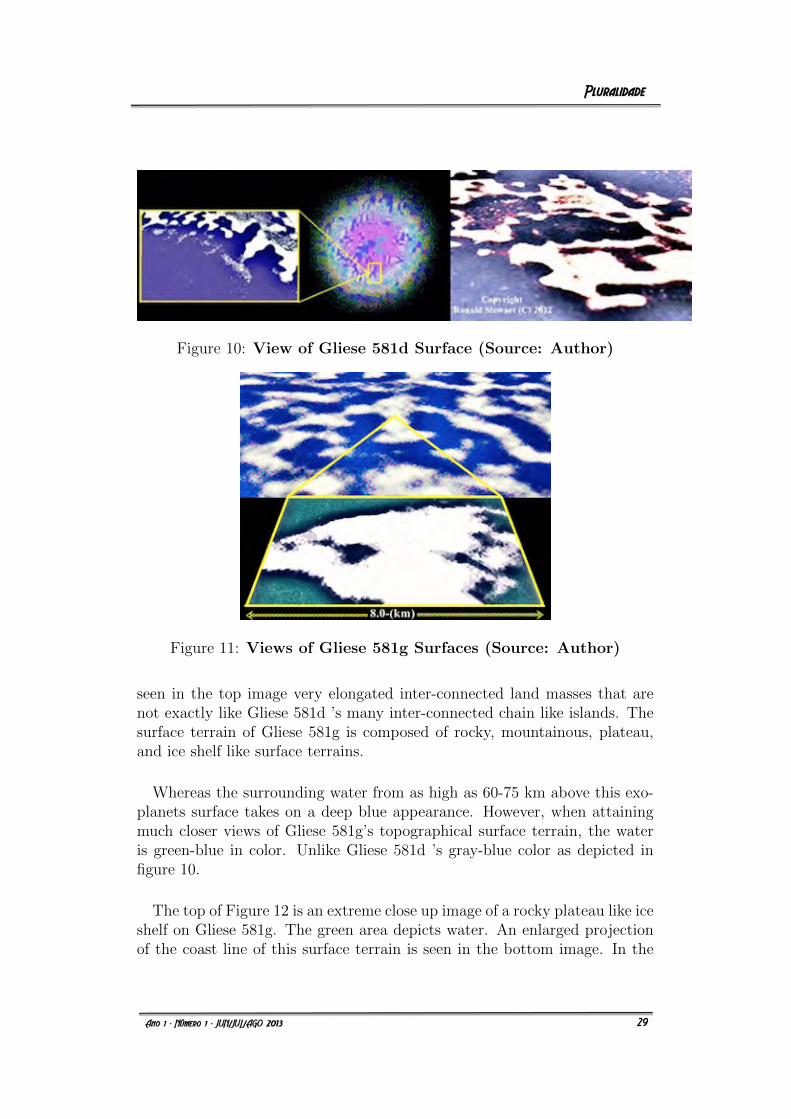
Figure 10: View of Gliese 581d Surface (Source: Author)
Figure 11: Views of Gliese 581g Surfaces (Source: Author)
seen in the top image very elongated inter-connected land masses that arenot exactly like Gliese 581d ’s many inter-connected chain like islands. Thesurface terrain of Gliese 581g is composed of rocky, mountainous, plateau,and ice shelf like surface terrains.
Whereas the surrounding water from as high as 60-75 km above this exo-planets surface takes on a deep blue appearance. However, when attainingmuch closer views of Gliese 581g’s topographical surface terrain, the wateris green-blue in color. Unlike Gliese 581d ’s gray-blue color as depicted infigure 10.
The top of Figure 12 is an extreme close up image of a rocky plateau like iceshelf on Gliese 581g. The green area depicts water. An enlarged projectionof the coast line of this surface terrain is seen in the bottom image. In the
24
29
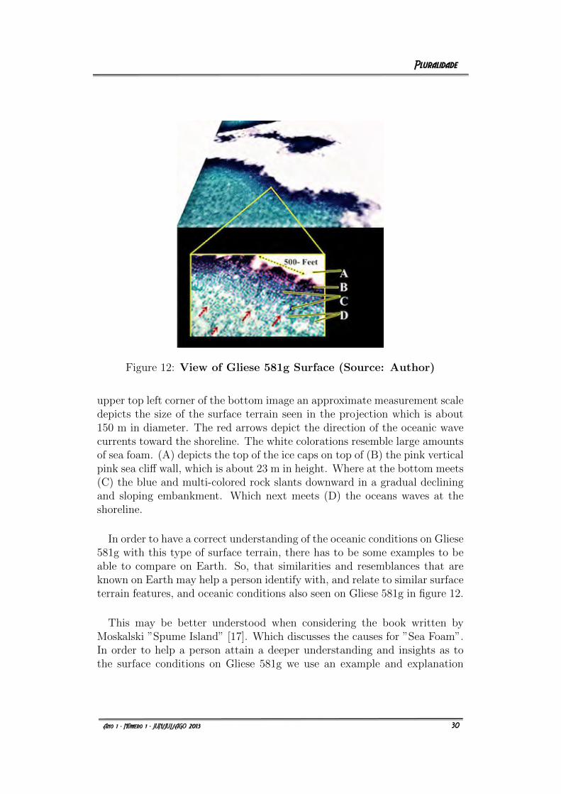
Figure 12: View of Gliese 581g Surface (Source: Author)
upper top left corner of the bottom image an approximate measurement scaledepicts the size of the surface terrain seen in the projection which is about150 m in diameter. The red arrows depict the direction of the oceanic wavecurrents toward the shoreline. The white colorations resemble large amountsof sea foam. (A) depicts the top of the ice caps on top of (B) the pink verticalpink sea cliff wall, which is about 23 m in height. Where at the bottom meets(C) the blue and multi-colored rock slants downward in a gradual decliningand sloping embankment. Which next meets (D) the oceans waves at theshoreline.
In order to have a correct understanding of the oceanic conditions on Gliese581g with this type of surface terrain, there has to be some examples to beable to compare on Earth. So, that similarities and resemblances that areknown on Earth may help a person identify with, and relate to similar surfaceterrain features, and oceanic conditions also seen on Gliese 581g in figure 12.
This may be better understood when considering the book written byMoskalski ”Spume Island” [17]. Which discusses the causes for ”Sea Foam”.In order to help a person attain a deeper understanding and insights as tothe surface conditions on Gliese 581g we use an example and explanation
25
30
from Moskalski’s book. So a comparison may be made on Earth, comparedto the surface conditions on Gliese 581g. There is an island that is very nearthe coastline of the Antarctic Peninsula named ”Spume Island/Sea-FoamIsland”. In 2009 NASA’s, satellite images included an orthographic pro-jection of NASA’s Blue Marble data set (1x1 km resolution global satellitecomposite). Scientific experiments and numerous oceanography and glaciol-ogy studies were accomplished over many years. This also included using”MODIS observations of polar sea ice which were combined with observa-tions of Antarctica made by the National Oceanic and Atmospheric Admin-istration’s AVHRR sensor (Advanced Very High Resolution Radiometer).”
Spume Island is a small, low, rocky island that consists of a sea cliff thatis ice capped on top. Which also has resemblances to the land mass andits descriptions of Gliese 581g as shown in Figure 12. At the bottom of thevertical sea cliff the coastline of the island slants downward until it meetsthe seashore. However, the unusual phenomenon is that when the averagehigh winds up to gale force winds blow against this island striking similaritiesas to what is seen on Gliese 581g (in the bottom of Figure 12), has manysimilarities to what happens to the oceanic conditions as seen at: ”SpumeIsland/Sea-Foam Island” 3.
Using this scale, average high winds up to gale force winds equaling anaverage high wind speeds of 14-17 m/s, would be the minimum wind speedneeded to create the same amount of sea foam at Spume/Foam Island as alsoseen on Gliese 581g. That would create oceanic wave heights of about 4-6 m,using the approximate measurement scale indicated in the bottom image ofFigure 12 the wave height for the waves seen in image recognition patternsalso measure about 4-6 m in height. Therefore, the imaging measurementrecognition patterns seen in the wave height in the bottom image of Figure12 involving Gliese 581g, is also consistent with the wave height neededat Spume/Foam Island in Earth’s oceans to also create the approximate
3There is a scientific methodology that measures wind speed on Earth known as: ”TheBeaufort Wind Force Scale”. When using this wind measurement methodology and sinceaverage high winds to gale force winds create similar conditions on ”Spume Island/Sea-Foam Island”, as also depicted, described, and explained in Figure 12, it is also importantto understand at what average high wind to gale force wind speeds would create enoughsea foam conditions at: ”Spume Foam Island” that if photographed would be equal toabout the amount of sea foam seen in the bottom image of Figure 12 on Gliese 581g. Theamount of sea form created by winds depends blowing over Spume/Foam Island on Earth,would be a determining factor exactly as to how much sea foam is created or not equal toFigure 12.
26
31
same amount of foam. Although Gale force winds do reach wind speedsat a maximum of 17-21 m/s, this would create even more sea foam. Asobserved in images of Gliese 581d the Gliese 581 Research Team did notnotice/observe (as of yet) any sea foam possibilities on Gliese 581d, comparedto the potential of this as seen most like in Figure 12 of the surface andoceanic conditions as seen in figure 12 of Gliese 581g. Which proposes a veryinteresting observation. Gale force winds as seen in the evidence of 15-18 min height on Gliese 581d have not yet been observed on Gliese 581g. Thisdoes not mean that sea foam does not exist on Gliese 581d, however is seenon Gliese 581g.
It is also important to note that Stewart [26] staring on subheading entitled”7.5 Scientific Team Observations Involving Likely-Oceanic Conditions andActivity On Gliese 581d”, brings up a question for the reader to contemplateon is: ”Does Gliese 581d have a climate?” The answer is, that it likely does.First analysis of many observations in the images of the surface of Gliese 581dshow very intensely active oceanic conditions and wave activity. A climatewould have to be present for the oceans to be active as they most likely are.
It mentions the oceanic currents maintain the distribution of heat andchemicals when a permanent cycle was established. The salinity of the largerbodies of water (seas and oceans) is assumed to be about 30% to 60% lowerthan 35 ppm, with a circulation determined by the rotation, of largest moonof Gliese 581d and its satellites, that may be in orbit around Gliese 581dabout a possible 12,500-18,000 km above this exoplanet’s surface. Whichmay be similar, and could be likened in example as seen in Earth’s solarsystem when it come to the Martian Moons above Mars named Phobos andDeimos. However, if such seas and oceans on Gliese 581d are dominated by ashort range of temperatures, than there would seem to be streams and rivers.However, as of yet there have not been any observations of streams or riverson Gliese 581d. However, this does not mean that they do not exist. Theycould elsewhere on this exoplanet not yet researched.
Therefore, what is observed and studied rather is most likely only con-centrations of chemical components and the high precipitation; so there is apossible existence of differentiation vertically in the masses of large bodies ofwater when it comes to the oceans and seas on Gliese 581d. However, underthe circumstances, it’s likely there are many ice-fluids that are also upon therock mixed with ice-like surface of Gliese 581d the rock-like surface. It isalso important to note that it that Gliese 581d had a large moon and other
27
32
satellite moon on the southeastern hemisphere of Gliese 581d and that thiswould also mean that Gliese 581d was not tidally locked. However, becausewe have not yet seen in this point of the investigation into Gliese 581g that itas of yet a large moon or other satellite moons have not been detected. Doesthis mean that Gliese 581g is tidally locked with one side of this exoplanethaving daylight all of the time and the opposite side would have no sunlightand permanent darkness with exceedingly cold temperatures? No it doesnot. Why? One strong reason is as this paper presents and demonstratesin the left image in Figure 6 depicts Earth’s Moon in one of its last phasesbefore becoming either a Full or New Moon. Again seen in Figure 7.
Stewart [26] also discusses that when examining exoplanets in other starsystems, it is not that much different than how the Earth’s Moon transitionsitself from about twenty-nine different moon phases every month. This alsotrue with all planets, planetary bodies in our solar system which includesother star systems as well. As depicted and described in Figure 6 and Figure7, in both images (in the upper top left corners), both Earth’s Moon andin Gliese 581g (these phases) have not quite yet reached their Full and /orNew Moon phases which in the next phase would develop into a full circle.This would mean that Gliese 581g is going through Moon-like/ planetary-likephases and that it has an axis and rotational movement. Which would not bethe case if this exoplanet was tidally locked. Just because (as of yet), therehas not been one of moons (or satellites) a moon for Gliese 581g does notmean that they are not there. Why? It could just be a matter that the oneor moons/ satellites for Gliese 581g could simply be hidden on the other sideof this exoplanet. Or, just a matter that as of yet the Gliese 581 ResearchTeam has not yet discovered any moon or satellites above the surface orGliese 581g and that could be discovered at some point into the future.
The next point is Stewart [26] discusses and shows some similarities in somesurface and oceanic conditions on Gliese 581g just like there is on Gliese 581d.However, Gliese 581g is another very unique exoplanet as a singularity in theGliese 581 star system and there may not be another unique exoplanet likeit anywhere in the Gliese 581 star system, and likely in the universe as well.At the writing of this paper it is theorized that Gliese 581d and especiallyGliese 581g may be the only two exoplanets in Gliese 581 that are likelyhabitable. At this point the impression about Gliese 581c is, that planetmay be a much warmer exoplanet that Gliese 581d or Gliese 581g and itpossibly could have some limited liquid water upon its surface. However,that it is much more teutonically/volcanically active than Gliese 581d or
28
33
Gliese 581g, and it is like a more diverse exoplanet to study geologically thanGliese 581d or Gliese 581g is. However, that will be in another subject ofdiscussion in another near future research paper.
Stewart [26] also discusses that ocean and sea wave heights were estimatedon Gliese 581d to be on an average of about 15-18 m. Further meaning;that the: ”Daily Average Wind Velocity” on Gliese 581d was estimated andcompared to wave height. That wind velocities on a daily basis would be atleast a have to be above gale force strength between 17-20 m/s. Which couldcreate waves in excess of 15-18 m in height. The gale force wind speeds onGliese 581d would most likely be considered Minimal Calm Wind Speeds OnA Day To day Basis On Gliese 581d. It may not be unusual for wind gustson an average day on Gliese 581d to reach speeds of 35-50 m/s. Whereas onGliese 581g, most likely average wind speeds as aforementioned before wouldbe about 14-17 m/s.Which this paper would like to re-emphasize, that thiswind speed is the minimum wind speed needed to create the same amountof sea foam at Spume/Foam Island on Earth (as also seen on Gliese 581g) asindicated Figure 12. Secondly, this would also create an approximate oceanand sea wave height of about 14-17 m/s instead. So, in simple terminologythe wind and ocean wave conditions on Gliese 581g are only about 1/3 (onethird) about what they are on Gliese 581d. Including that Gliese 581g is alsowarmer than Gliese 581d as well.
5 The Unique Emerald Colored Mountains of
Gliese 581g
Trentadue [27], Stewart [22] [25] [26] and Aguiar [1] papers bring to thereader’s attention that whether it be a star system close to Earth like ProximaCentauri, or where a recent exoplanet was discovered in Alpha Centauri B, orexoplanets in Gliese 581, the primary point is that each and every exoplanetthat exists anywhere in the universe is so unique in its own way, that no twoexoplanets anywhere in the universe may be the same. Figure 15 will presentand demonstrate that Gliese 581g is also very unique. For on this exoplanetthere are several mountains that look as though they are covered in emeraldcolor geophysical sedimentary strata that is simply breathtaking.
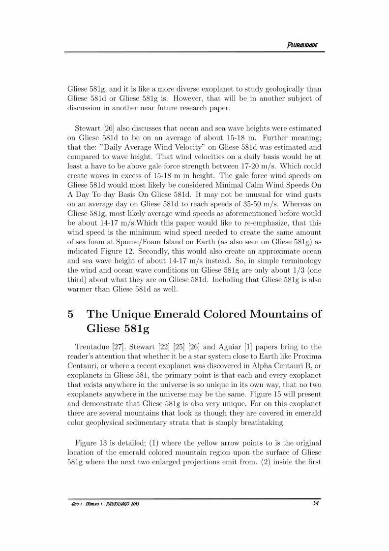
Figure 13 is detailed; (1) where the yellow arrow points to is the originallocation of the emerald colored mountain region upon the surface of Gliese581g where the next two enlarged projections emit from. (2) inside the first
29
34
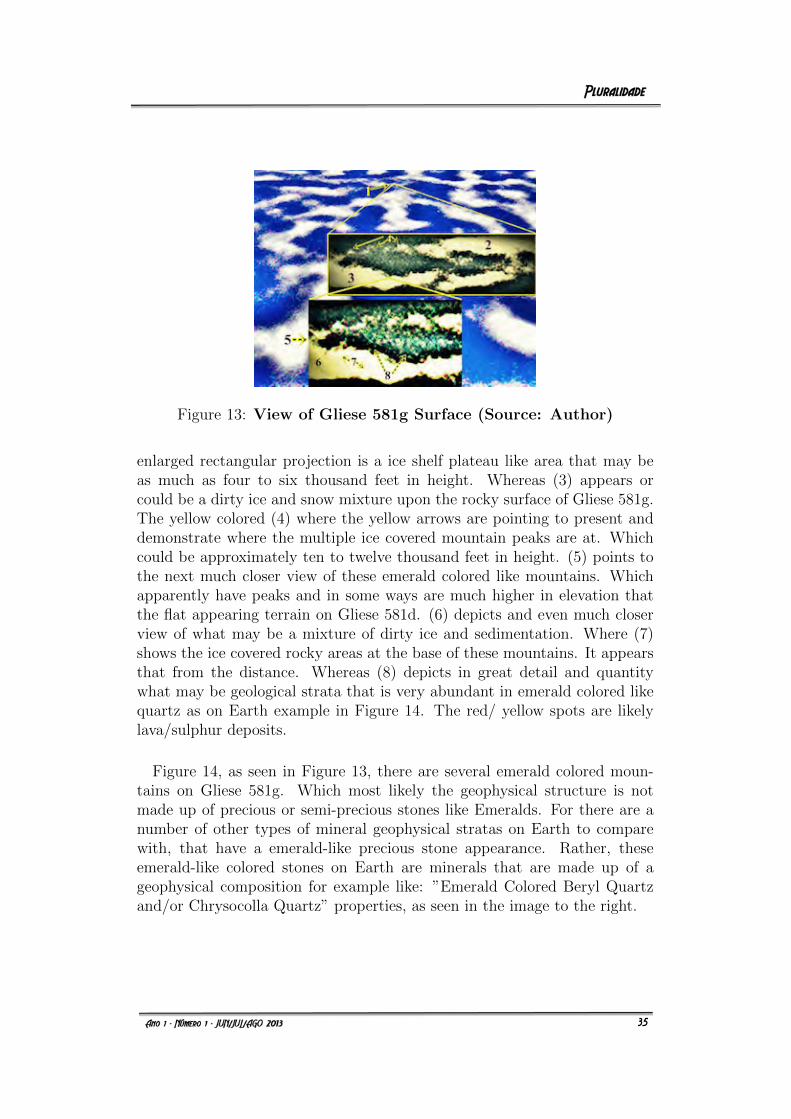
Figure 13: View of Gliese 581g Surface (Source: Author)
enlarged rectangular projection is a ice shelf plateau like area that may beas much as four to six thousand feet in height. Whereas (3) appears orcould be a dirty ice and snow mixture upon the rocky surface of Gliese 581g.The yellow colored (4) where the yellow arrows are pointing to present anddemonstrate where the multiple ice covered mountain peaks are at. Whichcould be approximately ten to twelve thousand feet in height. (5) points tothe next much closer view of these emerald colored like mountains. Whichapparently have peaks and in some ways are much higher in elevation thatthe flat appearing terrain on Gliese 581d. (6) depicts and even much closerview of what may be a mixture of dirty ice and sedimentation. Where (7)shows the ice covered rocky areas at the base of these mountains. It appearsthat from the distance. Whereas (8) depicts in great detail and quantitywhat may be geological strata that is very abundant in emerald colored likequartz as on Earth example in Figure 14. The red/ yellow spots are likelylava/sulphur deposits.
Figure 14, as seen in Figure 13, there are several emerald colored moun-tains on Gliese 581g. Which most likely the geophysical structure is notmade up of precious or semi-precious stones like Emeralds. For there are anumber of other types of mineral geophysical stratas on Earth to comparewith, that have a emerald-like precious stone appearance. Rather, theseemerald-like colored stones on Earth are minerals that are made up of ageophysical composition for example like: ”Emerald Colored Beryl Quartzand/or Chrysocolla Quartz” properties, as seen in the image to the right.
30
35
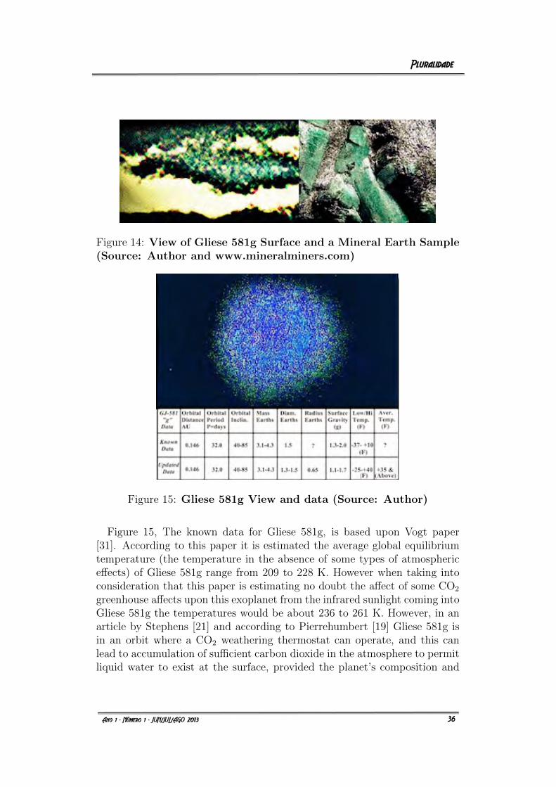
Figure 14: View of Gliese 581g Surface and a Mineral Earth Sample(Source: Author and www.mineralminers.com)
Figure 15: Gliese 581g View and data (Source: Author)
Figure 15, The known data for Gliese 581g, is based upon Vogt paper[31]. According to this paper it is estimated the average global equilibriumtemperature (the temperature in the absence of some types of atmosphericeffects) of Gliese 581g range from 209 to 228 K. However when taking intoconsideration that this paper is estimating no doubt the affect of some CO2
greenhouse affects upon this exoplanet from the infrared sunlight coming intoGliese 581g the temperatures would be about 236 to 261 K. However, in anarticle by Stephens [21] and according to Pierrehumbert [19] Gliese 581g isin an orbit where a CO2 weathering thermostat can operate, and this canlead to accumulation of sufficient carbon dioxide in the atmosphere to permitliquid water to exist at the surface, provided the planet’s composition and
31
36
tectonic behavior can support sustained out gassing.
In other words, the infrared contribution of the Gliese 581 red dwarf par-ent star provides some CO2 in the atmosphere of Gliese 581g. However,additional factors volcanic/teutonic activity would have to also be enough toprovide enough warmth to the Gliese 581g atmosphere for liquid water to beable to exist above 273 K. Or else the state of Gliese 581g would not haveliquid water but just ice. So, even at a certain point the temperature wouldhave to stay above freezing long enough to maintain a balance of maintain-ing liquid water upon Gliese 581g ’s surface. By comparison, Earth’s presentglobal equilibrium temperature is 255 K, which is raised to 288 K by green-house effects. However, the Sun’s energy output is thought to have beenonly about 75% of its current value, Two previously discovered planets inthe same system, Gliese 581c and Gliese 581d (inward and outward fromplanet Gliese 581g respectively), were also regarded as potentially habitablefollowing their discovery by Udry [29].
Whereas when Figure 8 is again re-examined it is known that some of thegreen colored areas on Earth (as seen a the top middle of the image) is vegeta-tion and that CO2 it provides in Earth’s atmosphere. However, when similargreen areas are seen in extreme close up views on the topographical surfaceterrain of both Gliese 581d and Gliese 581g, this is mostly different types ofice. Similar as would be seen in the colder environments of Earth. Whichcould also be likened to another Stewart paper [25]. Starting with Figure 5to Figure 8 in this paper describes how at one time Earth’s oceans may havetheoretically have formed from carbonaceous chrondrite meteors/meteoritesover billions of years and unlike Earth of today where as shown in Figure 8 ofthis paper where some of the green areas could be vegetation that allow theCO2 in Earth’s atmosphere to be absorbed by Earth vegetation and in turnexpel oxygen. However, in the left bottom corner Gliese 581d also has greencolored areas similar as also seen in the images of Earth. However, it is morelikely that on both Gliese 581d and Gliese 581g if there is any current oxygenin the atmosphere of either of these two exoplanets, as shown by Stewart [25],that Earth likely has greater quantities of oxygen than either Gliese 581d orGliese 581g. As explained before, Earth’s early developmental stages allowedoxygen to develop primarily by meteor/meteorite strikes on the Earth andeventually volcanic gas accumulation over time. Likely any additional oxy-gen in the atmospheres of either Gliese 581d or Gliese 581g developed overtime. Whereas Earth’s greater quantities of oxygen developed through thedischarge of oxygen through its vegetation, etc.
32
37
6 More Incoming Infrared (IR) Sunlight In
The Gliese 581d Star System Then Previ-
ously Thought
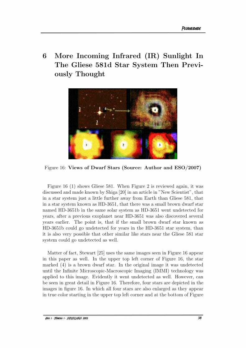
Figure 16: Views of Dwarf Stars (Source: Author and ESO/2007)
Figure 16 (1) shows Gliese 581. When Figure 2 is reviewed again, it wasdiscussed and made known by Shiga [20] in an article in ”New Scientist”, thatin a star system just a little further away from Earth than Gliese 581, thatin a star system known as HD-3651, that there was a small brown dwarf starnamed HD-3651b in the same solar system as HD-3651 went undetected foryears, after a previous exoplanet near HD-3651 was also discovered severalyears earlier. The point is, that if the small brown dwarf star known asHD-3651b could go undetected for years in the HD-3651 star system, thanit is also very possible that other similar like stars near the Gliese 581 starsystem could go undetected as well.
Matter of fact, Stewart [25] uses the same images seen in Figure 16 appearin this paper as well. In the upper top left corner of Figure 16, the starmarked (4) is a brown dwarf star. In the original image it was undetecteduntil the Infinite Microscopic-Macroscopic Imaging (IMMI) technology wasapplied to this image. Evidently it went undetected as well. However, canbe seen in great detail in Figure 16. Therefore, four stars are depicted in theimages in figure 16. In which all four stars are also enlarged as they appearin true color starting in the upper top left corner and at the bottom of Figure
33
38
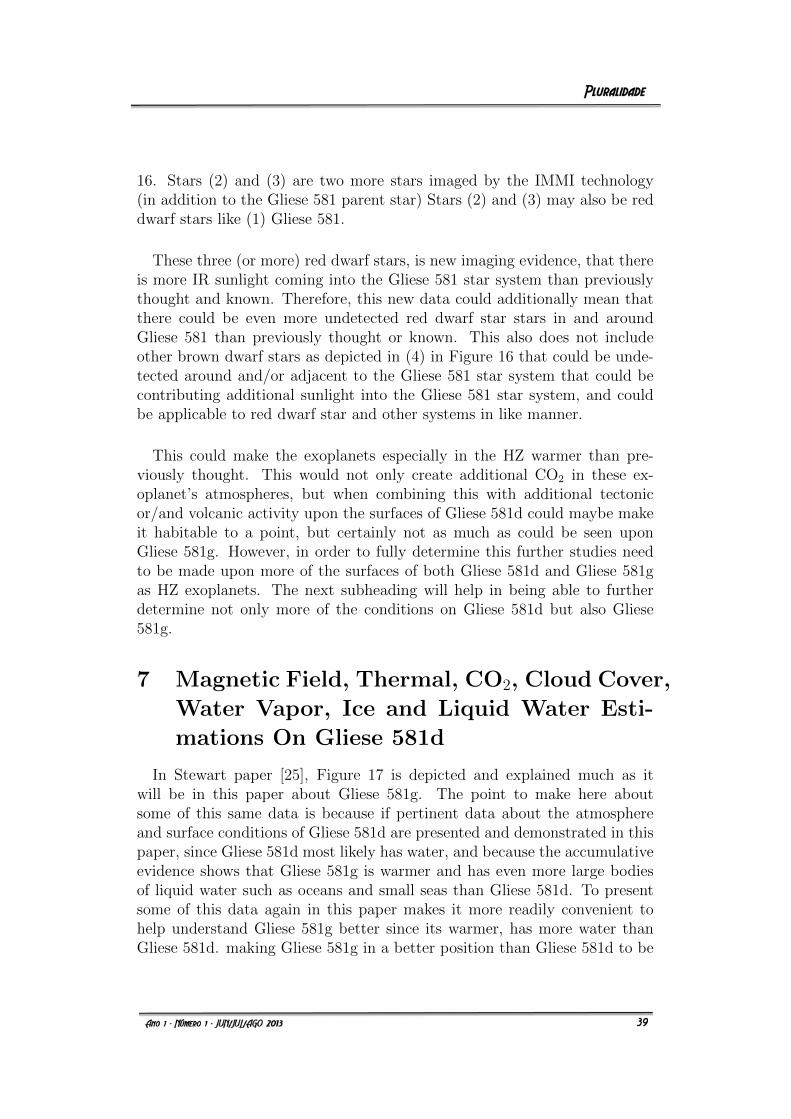
16. Stars (2) and (3) are two more stars imaged by the IMMI technology(in addition to the Gliese 581 parent star) Stars (2) and (3) may also be reddwarf stars like (1) Gliese 581.
These three (or more) red dwarf stars, is new imaging evidence, that thereis more IR sunlight coming into the Gliese 581 star system than previouslythought and known. Therefore, this new data could additionally mean thatthere could be even more undetected red dwarf star stars in and aroundGliese 581 than previously thought or known. This also does not includeother brown dwarf stars as depicted in (4) in Figure 16 that could be unde-tected around and/or adjacent to the Gliese 581 star system that could becontributing additional sunlight into the Gliese 581 star system, and couldbe applicable to red dwarf star and other systems in like manner.
This could make the exoplanets especially in the HZ warmer than pre-viously thought. This would not only create additional CO2 in these ex-oplanet’s atmospheres, but when combining this with additional tectonicor/and volcanic activity upon the surfaces of Gliese 581d could maybe makeit habitable to a point, but certainly not as much as could be seen uponGliese 581g. However, in order to fully determine this further studies needto be made upon more of the surfaces of both Gliese 581d and Gliese 581gas HZ exoplanets. The next subheading will help in being able to furtherdetermine not only more of the conditions on Gliese 581d but also Gliese581g.
7 Magnetic Field, Thermal, CO2, Cloud Cover,
Water Vapor, Ice and Liquid Water Esti-
mations On Gliese 581d
In Stewart paper [25], Figure 17 is depicted and explained much as itwill be in this paper about Gliese 581g. The point to make here aboutsome of this same data is because if pertinent data about the atmosphereand surface conditions of Gliese 581d are presented and demonstrated in thispaper, since Gliese 581d most likely has water, and because the accumulativeevidence shows that Gliese 581g is warmer and has even more large bodiesof liquid water such as oceans and small seas than Gliese 581d. To presentsome of this data again in this paper makes it more readily convenient tohelp understand Gliese 581g better since its warmer, has more water thanGliese 581d. making Gliese 581g in a better position than Gliese 581d to be
34
39
Figure 17: Views of Earth and Gliese 581d Surface (Source: Authorand NASA)
maybe be a more potentially habitable exoplanet, especially since it is aboutin the middle of Gliese 581’s HZ.
When Figure 17 is studied above it shows that the estimated magnetic fieldfor Gliese 581d (image to the far right), is compared to Earth (in the first twoimages to the left), presents and demonstrates a comparison of Earth takenby the NASA Geo-Stationary-Operational-Environmental Satellite (GOES),demonstrating in color coded sequences the thermal and CO2 levels on Earth.In like manner, the IMMI imaging technology uses its thermal, near-infrared,and infrared capabilities to determine the thermal and CO2 levels on Gliese581d as well. as shown in the far image to the right.
Just like the NASA GOES, the IMMI technology has the capability toduplicate in similar Raleigh scattering color spectrum sequences near-infraredand infrared, thermal and other to detect what the thermal, CO2, watervapor, ice, cloud cover, and limited magnetic field capabilities would be onGliese 581d as well. Which in some ways has similarities as seen in sometypes of LIDAR remote sensing and imaging technologies do in like manner.More discussion on the IMMI technology may be found in considerable detailnear the end of this paper.
In similar ways, just like the GOES satellite can calculate the Earth’s mag-netic field, CO2, cloud cover, water vapor and other atmospheric conditionsof the Earth, in like manner the IMMI technology has the capability of de-termining in an image of an exoplanet that uses ”Virtual Reality ModelingImages” to also diagnose the thermal, CO2, water vapor, ice, cloud cover,and limited magnetic field capabilities would be on Gliese 581d. Than asshown in Figure 17 a comparison is made with Earth in order to determine
35
40
in what similar kinds of ways Gliese 581d may resemble different aspects ofhabitability as would be seen on Earthy as well.
The IMMI capabilities show Gliese 581d’s surface areas such as (red) asthe hottest thermal surface areas, followed by (Rose) colored surfaces, while(Purple Areas) indicate surface water, (Gold) surface areas depict CO2 levels,(White) cloud cover or H2O as ice, and the (Black) surface areas mostlyindicated in these regions seen in black would represent the coldest regionsof this exoplanet.
Which are observed at being mostly in the North and South Pole regionsof this exoplanet. Estimations were given that the purple to blue primarilyrepresent water. As had been verified when making close observation investi-gations of these areas in extreme close ups of this exoplanet’s surface. This isthe first example where scientifically acceptable estimations have been madeon the surface of Gliese 581d. It is estimated by these comparisons betweenEarth and Gliese 581d being an: ”Earth-like to Water World like” exoplanethas approximately about 0.667% of similarities as may be seen of Earth whenit was in some where between its first and second snowball-like periods inEarth’s ancient history. However, at the same time the Gliese 581d ResearchTeam also believe that Gliese 581d is also going through a transitional climateperiod in its current similarities to Earth as well.
8 Other New Unknown Contributing Factors
That Contribute To The Warm of Earth,
Gliese 581d, and Gliese 581g In Similar
Cold Environments
Besides the Earth on both Gliese 581d and Gliese 581g due to the infraredsunlight coming into both Gliese 581d and especially Gliese 581g’s atmo-spheres creating CO2 and it being retained into both of these exoplanet’satmospheres, according to the original paper by Vogt [31], there are morereasons why both Gliese 581d and Gliese 581g are warmer. This paper hasdiscussed as shown in Figure 16 that there are more stars that may be lettingin additional sunlight into the Gliese 581 star system. This is new data notfound in other papers than the Gliese 581 Team has written together on thisas co-authors. Furthermore, since there could be more than just a total of 4stars letting infrared sunlight and/or additional other types of sunlight into
36
41
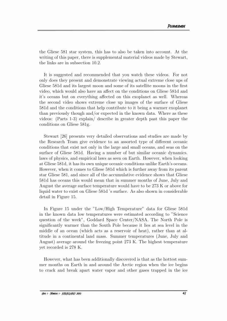
the Gliese 581 star system, this has to also be taken into account. At thewriting of this paper, there is supplemental material videos made by Stewart,the links are in subsection 10.2.
It is suggested and recommended that you watch these videos. For notonly does they present and demonstrate viewing actual extreme close ups ofGliese 581d and its largest moon and some of its satellite moons in the firstvideo, which would also have an affect on the conditions on Gliese 581d andit’s oceans but on everything affected on this exoplanet as well. Whereasthe second video shows extreme close up images of the surface of Gliese581d and the conditions that help contribute to it being a warmer exoplanetthan previously though and/or expected in the known data. Where as thesevideos: (Parts 1-3) explain/ describe in greater depth past this paper theconditions on Gliese 581g.
Stewart [26] presents very detailed observations and studies are made bythe Research Team give evidence to an assorted type of different oceanicconditions that exist not only in the large and small oceans, and seas on thesurface of Gliese 581d. Having a number of but similar oceanic dynamics.laws of physics, and empirical laws as seen on Earth. However, when lookingat Gliese 581d, it has its own unique oceanic conditions unlike Earth’s oceans.However, when it comes to Gliese 581d which is further away from its parentstar Gliese 581, and since all of the accumulative evidence shows that Gliese581d has oceans this would mean that in summer months of June, July andAugust the average surface temperature would have to be 273 K or above forliquid water to exist on Gliese 581d ’s surface. As also shown in considerabledetail in Figure 15.
In Figure 15 under the ”Low/High Temperature” data for Gliese 581din the known data low temperatures were estimated according to ”Sciencequestion of the week”, Goddard Space Center/NASA. The North Pole issignificantly warmer than the South Pole because it lies at sea level in themiddle of an ocean (which acts as a reservoir of heat), rather than at al-titude in a continental land mass. Summer temperatures (June, July andAugust) average around the freezing point 273 K. The highest temperatureyet recorded is 278 K.
However, what has been additionally discovered is that as the hottest sum-mer months on Earth in and around the Arctic region when the ice beginsto crack and break apart water vapor and other gases trapped in the ice
37
42
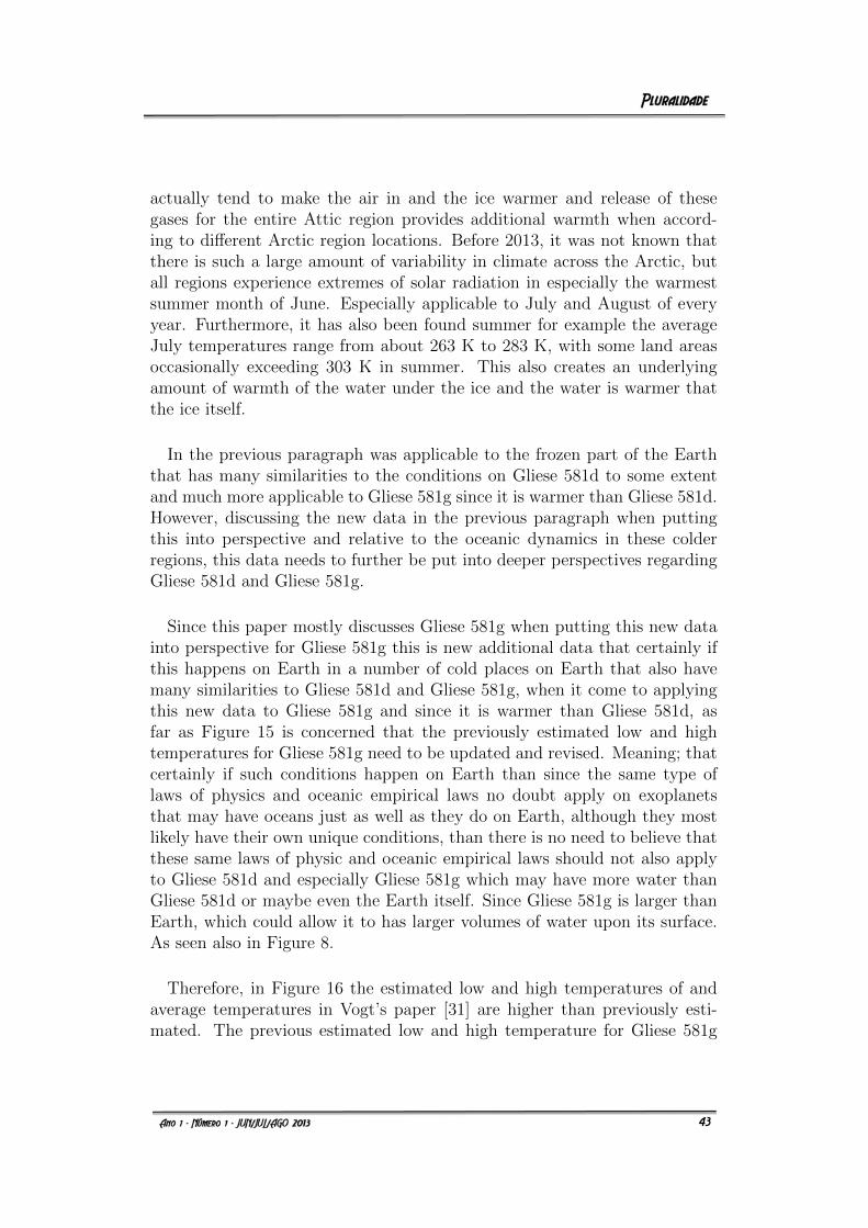
actually tend to make the air in and the ice warmer and release of thesegases for the entire Attic region provides additional warmth when accord-ing to different Arctic region locations. Before 2013, it was not known thatthere is such a large amount of variability in climate across the Arctic, butall regions experience extremes of solar radiation in especially the warmestsummer month of June. Especially applicable to July and August of everyyear. Furthermore, it has also been found summer for example the averageJuly temperatures range from about 263 K to 283 K, with some land areasoccasionally exceeding 303 K in summer. This also creates an underlyingamount of warmth of the water under the ice and the water is warmer thatthe ice itself.
In the previous paragraph was applicable to the frozen part of the Earththat has many similarities to the conditions on Gliese 581d to some extentand much more applicable to Gliese 581g since it is warmer than Gliese 581d.However, discussing the new data in the previous paragraph when puttingthis into perspective and relative to the oceanic dynamics in these colderregions, this data needs to further be put into deeper perspectives regardingGliese 581d and Gliese 581g.
Since this paper mostly discusses Gliese 581g when putting this new datainto perspective for Gliese 581g this is new additional data that certainly ifthis happens on Earth in a number of cold places on Earth that also havemany similarities to Gliese 581d and Gliese 581g, when it come to applyingthis new data to Gliese 581g and since it is warmer than Gliese 581d, asfar as Figure 15 is concerned that the previously estimated low and hightemperatures for Gliese 581g need to be updated and revised. Meaning; thatcertainly if such conditions happen on Earth than since the same type oflaws of physics and oceanic empirical laws no doubt apply on exoplanetsthat may have oceans just as well as they do on Earth, although they mostlikely have their own unique conditions, than there is no need to believe thatthese same laws of physic and oceanic empirical laws should not also applyto Gliese 581d and especially Gliese 581g which may have more water thanGliese 581d or maybe even the Earth itself. Since Gliese 581g is larger thanEarth, which could allow it to has larger volumes of water upon its surface.As seen also in Figure 8.
Therefore, in Figure 16 the estimated low and high temperatures of andaverage temperatures in Vogt’s paper [31] are higher than previously esti-mated. The previous estimated low and high temperature for Gliese 581g
38
43
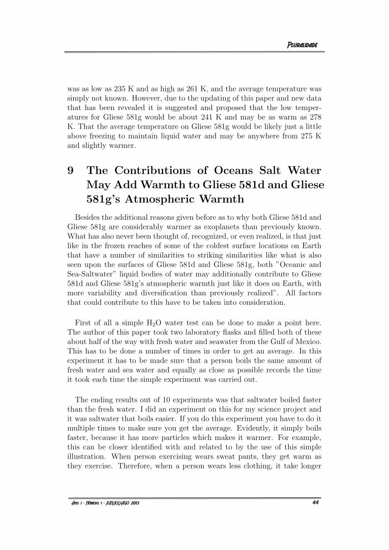
was as low as 235 K and as high as 261 K, and the average temperature wassimply not known. However, due to the updating of this paper and new datathat has been revealed it is suggested and proposed that the low temper-atures for Gliese 581g would be about 241 K and may be as warm as 278K. That the average temperature on Gliese 581g would be likely just a littleabove freezing to maintain liquid water and may be anywhere from 275 Kand slightly warmer.
9 The Contributions of Oceans Salt Water
May AddWarmth to Gliese 581d and Gliese
581g’s Atmospheric Warmth
Besides the additional reasons given before as to why both Gliese 581d andGliese 581g are considerably warmer as exoplanets than previously known.What has also never been thought of, recognized, or even realized, is that justlike in the frozen reaches of some of the coldest surface locations on Earththat have a number of similarities to striking similarities like what is alsoseen upon the surfaces of Gliese 581d and Gliese 581g, both ”Oceanic andSea-Saltwater” liquid bodies of water may additionally contribute to Gliese581d and Gliese 581g’s atmospheric warmth just like it does on Earth, withmore variability and diversification than previously realized”. All factorsthat could contribute to this have to be taken into consideration.
First of all a simple H2O water test can be done to make a point here.The author of this paper took two laboratory flasks and filled both of theseabout half of the way with fresh water and seawater from the Gulf of Mexico.This has to be done a number of times in order to get an average. In thisexperiment it has to be made sure that a person boils the same amount offresh water and sea water and equally as close as possible records the timeit took each time the simple experiment was carried out.
The ending results out of 10 experiments was that saltwater boiled fasterthan the fresh water. I did an experiment on this for my science project andit was saltwater that boils easier. If you do this experiment you have to do itmultiple times to make sure you get the average. Evidently, it simply boilsfaster, because it has more particles which makes it warmer. For example,this can be closer identified with and related to by the use of this simpleillustration. When person exercising wears sweat pants, they get warm asthey exercise. Therefore, when a person wears less clothing, it take longer
39
44
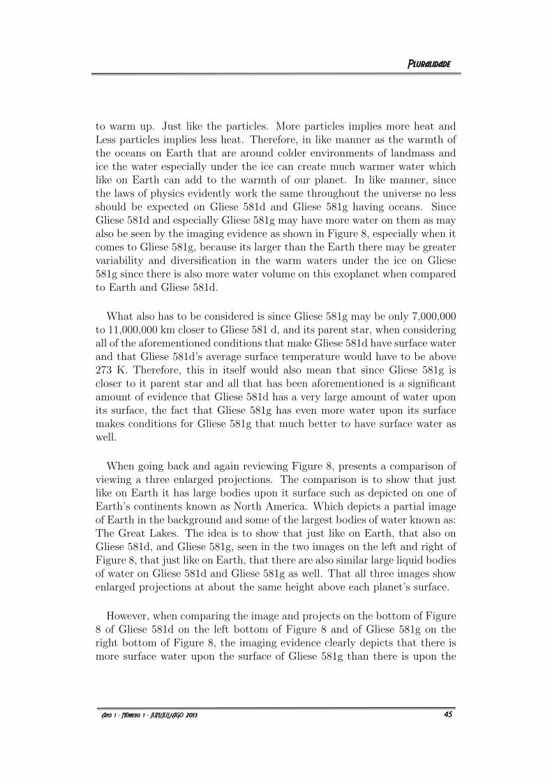
to warm up. Just like the particles. More particles implies more heat andLess particles implies less heat. Therefore, in like manner as the warmth ofthe oceans on Earth that are around colder environments of landmass andice the water especially under the ice can create much warmer water whichlike on Earth can add to the warmth of our planet. In like manner, sincethe laws of physics evidently work the same throughout the universe no lessshould be expected on Gliese 581d and Gliese 581g having oceans. SinceGliese 581d and especially Gliese 581g may have more water on them as mayalso be seen by the imaging evidence as shown in Figure 8, especially when itcomes to Gliese 581g, because its larger than the Earth there may be greatervariability and diversification in the warm waters under the ice on Gliese581g since there is also more water volume on this exoplanet when comparedto Earth and Gliese 581d.
What also has to be considered is since Gliese 581g may be only 7,000,000to 11,000,000 km closer to Gliese 581 d, and its parent star, when consideringall of the aforementioned conditions that make Gliese 581d have surface waterand that Gliese 581d’s average surface temperature would have to be above273 K. Therefore, this in itself would also mean that since Gliese 581g iscloser to it parent star and all that has been aforementioned is a significantamount of evidence that Gliese 581d has a very large amount of water uponits surface, the fact that Gliese 581g has even more water upon its surfacemakes conditions for Gliese 581g that much better to have surface water aswell.
When going back and again reviewing Figure 8, presents a comparison ofviewing a three enlarged projections. The comparison is to show that justlike on Earth it has large bodies upon it surface such as depicted on one ofEarth’s continents known as North America. Which depicts a partial imageof Earth in the background and some of the largest bodies of water known as:The Great Lakes. The idea is to show that just like on Earth, that also onGliese 581d, and Gliese 581g, seen in the two images on the left and right ofFigure 8, that just like on Earth, that there are also similar large liquid bodiesof water on Gliese 581d and Gliese 581g as well. That all three images showenlarged projections at about the same height above each planet’s surface.
However, when comparing the image and projects on the bottom of Figure8 of Gliese 581d on the left bottom of Figure 8 and of Gliese 581g on theright bottom of Figure 8, the imaging evidence clearly depicts that there ismore surface water upon the surface of Gliese 581g than there is upon the
40
45
surface of Gliese 581d. This is also consistent with the fact that such wouldbe the case, especially if Gliese 581g being closer to its parent star Gliese581 was warmer. The result being of course that more water would be uponits’ surface, most likely because whatever large amounts of ice that would beupon the surface would have melted in larger quantities of water that wouldbe upon the surface of Gliese 581g especially when compared to the surfacewater upon the surface of Gliese 581d. This would make Gliese 581g a bettersuited candidate for being more habitable as an exoplanet, especially sinceits location is in about the middle of the HZ.
10 Brief Concept On Re-Organizing Exoplanet
Methodologies For Greater Exoplanet De-
tection Capabilities
10.1 Conclusion
In the science of ”Exoplanetology” whenever a scientist, astronomer, as-trophysicist, decides to investigate any star system to look for exoplanetswhether it be either in or out of it’s HZ, they may only use one type ofexoplanet detection methodology. However, the question has to be asked:”Could there potentially be a better, more powerful, sensitive, accurate, pre-cise, scientific current methodology available for detecting and confirmingexoplanets in any star system with much less overall problems?” The Au-thors of this paper believe the answer to this question is: ”Yes”!
When it comes to current available exoplanet detection methodologies thebest way to explain this is by use of to illustration. We will use the exoplanetdetection methodology known as RVM as an example.
The first point is, when RVM by itself for detecting exoplanets in anotherstar system, and/ or if it also be with HARPS or HIRES data, the best wayto use it may best be explained, described, and understood when Dumusque[20] discusses this in his paper when he states ”that the reliability, efficiency,proficiency, accuracy, and sensitivity of the RVM to be able to detect exo-planets in other star systems to its maximum capability, is solely dependenton the fact that since sensitivity is a function of RVM accuracy and pre-cision, that following up with as many additional number of measurementsand samplings as possible, adds more points to the current data and that by
41
46
this methodology, it allows for the best maximum improvement of the RVMdetection sensitivity over time when using it to detect exoplanets”.
The previous quote only pertains to one methodology used when it comesto detecting exoplanets. So, the second question is: ”How may this method-ology for exoplanets be improved upon?” It is not so much a matter that theindividual exoplanet RVM needs to be improved upon. Except as a singu-lar scientific methodology the sensitivity of the technology could be and oneday will be improved upon. Rather as far as the preent and current way ofdetecting exoplanets it could be potentially greatly improved upon that ifinstead of just using one scientific methodology to look for exoplanets in astar system, why not use as many as possible instead?
In other words for instance, suppose a scientist wants to do a deeper in-vestigation into the Alpha Centauri B star system to determine if there maybe one or more exoplanets in its HZ? The immediate thought and approachmay be to want to only use the RVM. However, why do this when thereare also other additional current available exoplanet detection technologiesavailable that could be used in addition to just the RVM that could greatlyenhance the prospect of greater detection of exoplanets in the Alpha CentauriB habitable zone?
In addition to just using the RVM just by itself a scientist could prudentlychoose to also use any and all of the additional methods of exoplanet detec-tion to make a much stronger case for the detection of exoplanets if thet alsoused in addition to the RVM in this example, if they also used: ”AstrometricMeasurement, Gravitational Microlensing, Transit Method”, and any othertechnology and instrumentation available, in order to provide a much greaterscientific approach in the detection and confirmation of any exoplanets in theHZ of Alpha Centauri B example this paper has just aforementioned”. Evenif a research facility only has one exoplanet detection methodology avail-able to them, they could still collaborate with another facility, university orscientist(s) that has any of these other exoplanet detection methods, whichwould only enhance the detection and confirmation of suchlike exoplanets.Especially, when it comes to exoplanets in any star systems’ HZ. However,since this concept was originally thought of by the Author of this paper,this concept and it’s use falls under copyright and intellectual property andproprietary rights under the scientific research consortium known as: Inter-national Consortium On Microscopic To Macroscopic Research (ICOMMR)if anyone wishes to use this concept please contact the first author of this
42
47
paper.
This paper has also presented and demonstrated new data never thoughtof before, and imaging evidence that is consistent, that in the Gliese 581 starsystem all of the accumulative evidence revises and updates, that not only isthere a exoplanet in the HZ named Gliese 581d, but especially an exoplanetin the middle of the HZ Gliese 581 star system also known by the name ofGliese 581g.
10.2 Supplemental Material Videos
For more data, images and accumulative evidence regarding Gliese 581dand especially Gliese 581g, that due to space restrictions was not able to bepresented and demonstrated in this paper please go to the following URLsand watch these videos as follows:
http://www.stewart-research-consulting.com/2—exo-scope.html
http://www.stewart-research-consulting.com/4-other-star-systems.html
http://www.stewart-research-consulting.com/gliese-581-d.html
http://www.stewart-research-consulting.com/gliese-581-g.html
10.3 Acknowledgements
The authors of this paper would like to thank all of the researchers over theyears that have contributed to the exploration of the Gliese 581 star system.
References
[1] AGUIAR, O.A., STEWART, R., ARTUSO, G., SAMADI, A., ARISTIZ-ABAL, C.I.O., ACKERMAN, J.R., TRENTADUE, W. The (possible)confirmation of the first exo-oceans. Pluralidade 1: 82-95, 2013.
[2] ANGLADA-ESCUDE, G., DAWSON, R.I. Aliases of the first eccen-tric harmonic: Is GJ 581g a genuine planet candidate? arXiv:1011.0186 [astro-ph.EP], 2011.
43
48
[3] ANTAL, S., STEWART, R. Alpha Centauri B and re-cent exoplanet discovery. Journal of the International Soci-ety of Peer Reviewers. Available at: http://www.stewart-research-consulting.com/5-astronomy.html. Accessed in: Jun. 5th, 2013.
[4] BALUEV, R. The impact of red noise in radial velocity planetsearches: Only three planets orbiting GJ581?. arXiv: 1209.3154[astro-ph.EP], 2012.
[5] BHATTACHARJEE, Y.Data dispute revives exoplanet claim. Sci-ence 337:398, 2012.
[6] BONFILS, X., FORVEILLE, T., DEFOSSE, X., UDRY, S., MAYOR,M., PERRIER, C., BOUCHY, F., PEPE, F., QUELOZ, D. andBERTAUX, J-L. The HARPS search for southern extra-solarplanets VI. A Neptune-mass planet around the nearby M dwarfGl 581. A&A 443: L15-L18, 2005.
[7] COLE, S., HANSEN, K. NASA study projects warming-drivenchanges in global rainfall. NASA News, Release 13-119. Availableat: http://www.nasa.gov/topics/Earth/features/wetter-wet.html. Pub-lished in: May 3rd, 2013.
[8] DUMUSQUE, X., PEPE, F., LOVIS, C., SEGRANSAN, D.,SAHLMANN, J., BENZ, W., BOUCHY, F., MAYOR, M., QUELOZ,D., SANTOS, N. and others. An Earth mass planet orbiting AlphaCentauri B. Nature 491:207-211, 2012.
[9] ENDL, M., KURSTER, M. Toward detection of terrestrial planetsin the habitable zone of our closest neighbor: Proxima Cen-tauri. arXiv: 0807.1452 [astro-ph], 2008.
[10] ENDL, M., KURSTER, M., ROUESNEL, F., ELS, S., HATZES, A.P.,COCHRAN, W.D. Scientific frontiers in research on extrasolarplanets. San Francisco: D.Deming and S.Seager. Conference Series, v.294, pp. 75-78.
[11] FORVEILLE, T., BONFILS, X., DEFOSSE, X., ALONSO, R., UDRY,S., BOUCHY, F., GILLION, M., LOVIS, C., NEVES, V., MAYOR, M.and others. The HARPS search for southern extra-solar planetsXXXII. Only 4 planets in the Gl 581 system. arXiv: 1109.2505[astro-ph.EP], 2011.
44
49
[12] GREGORY, P.C. (2011). Bayesian re-analysis of the Gliese 581exoplanet system. arXiv: 1101.0800 [astro-ph.SR], 2011.
[13] GREGORY, P.C., FISCHER, D.A. A bayesian periodogram findseEvidence for three planets in 47 Ursae Majoris. MNRAS403:701, 2010.
[14] JENKINS, C.R., PEACOCK, J.A. The power of bayesian evidencein astronomy. MNRAS, 413:2895, 2011.
[15] KASTING J.F., WHITMIRE, D.P., REYNOLDS, R.T. Habitablezones around main sequence stars. Icarus 101:108-128, 1993.
[16] MAYOR M., BONFILS, X., FORVEILLE, T., DEFOSSE, X.,BERTAUX, J-L., BEUST, H., BOUCHY, F., LOVIS, C., PEPE F.,PERRIER, C. and others. The HARPS search for southern extra-solar planets XVIII. A Earth-mass planet in the GJ 581 plan-etary system. A&A 507: 487-494, 2009.
[17] MOSKALSKI, N. Nocturne opus 1: Sea Foam. Bear, DE: DivinityPress, 2012. ISBN 978-0-988-38117-9.
[18] PEPE, F., MAYOR, M., LOVIS, C., BENZ, W., BOUCHY, F., DU-MUSQUE, X., QUELOZ, D, SANTOS, N., SEGRANSAN, D., UDRY,S. Hunting for the lowest-mass exoplanets. International Astro-nomical Union Simposium #276, 2010. Torino: A.Sozzetti, M.G.Lat-tanzi & P.Boss, 2011.
[19] PIERREHUMBERT, R.T. A Palette of climates for Gliese 581g.The Astrophysical Journal Letters 726:L8 (5pp), 2011.
[20] SHIGA, D. Brown dwarfs may stretch out exoplanets’ orbits.New Scientist e-Magazine. Available at: http://www.newscien-tist.com/article/dn10111-brown-dwarfs-may-stretch-out-exoplanets-orbits.html. Published in: Sep. 20th, 2006.
[21] STEPHENS, T. Newly discovered planet may be first truly hab-itable exoplanet. University News & Events, University of California,Santa Cruz. Available at:http://news.ucsc.edu/2010/09/planet.html.Published in: Sep. 29th, 2010.
[22] STEWART, R. Gliese 581-extra-solar imaging survey. Jour-nal of the International Society of Peer Reviewers. Available at:http://www.stewart-research-consulting.com/6-astronomy.html. Ac-cessed in Jun. 5th, 2013.
45
50
[23] STEWART, R., AGUIAR, O.A., ARTUSO, G., ARISTIZABAL,C.I.O., ACKERMAN, J.R., TRENTADUE, W., ROBINETT, R.Earth’s oceans; A theoretical approach how interconnectedcontinents and high altitude mountain glaciers formedthem. Journal of the International Society of Peer Reviewers.Available at: http://www.stewart-research-consulting.com/up-loads/6/4/5/4/6454783/earths oceans -a theorectical approachhow earths high altitude continent mountains formed them.pdf. Ac-cessed in Jun. 5th, 2013.
[24] STEWART, R., CELEBONOVIC, V., AGUIAR, O.A.,CHATZITHEODORIDIS, E., ACKERMAN, J., ROMAN, M.,ARTUSO, G., TRENTADUE, W., SAMADI, A., ARISTI-ZABAL, C.I.O. and others. Gliese 581d; Views of Itsatmospheric, topographical, geological, and oceanicconditions (Part 2). Journal of The International Soci-ety of Peer Reviewers. Available at: http://www.stewart-research-consulting.com/uploads/6/4/5/4/6454783/gliese-581- d-views of its atmosphere geology topography and oceanicconditions-part-2.pdf. Accessed in: Jun. 5th, 2013.
[25] STEWART, R., CELEBONOVIC, V., AGUIAR, O.A.,CHATZITHEODORIDIS, E., ARTUSO, G., SAMADI, A., ARIS-TIZABAL, C.I.O., BINGHAM, M., TRENTADUE, W., ROBINETT,R. and others. First view of Gliese 581d; A preliminarysurface survey (Part 1). Journal of the International Societyof Peer Reviewers. Available at: http://www.stewart-research-consulting.com/7-astronomy.html. Accessed in: Jun. 5th, 2013.
[26] STEWART, R., CELEBONOVIC, V., AGUIAR, O.A.,CHATZITHEODORIDIS, E., ARTUSO, G., SAMADI, A., ARIS-TIZABAL, C.I.O., BINGHAM, M., TRENTADUE, W., ROBINETT,R. and others. First view of Gliese 581d; A preliminarysurface survey (Part 2). Journal of the International Societyof Peer Reviewers. Available at: http://www.stewart-research-consulting.com/8-astronomy.html. Accessed in Jun. 5th, 2013.
[27] TRENTADUE, W. Proxima Centauri has no exoplanets.Journal of the International Society of Peer Reviewers. Availableat: http://www.stewart-research-consulting.com/4-astronomy.html.Published in: Apr. 10th, 2013.
46
51
[28] TUOMI, M. Bayesian re-analysis of the radial velocities of Gliese581. A&A 528: L5, 2011.
[29] UDRY, S., BONFILS, X., DEFOSSE, X., FORVEILLE, T., MAYOR,M., PERRIER, C., BOUCHY, F., LOVIS, C., PEPE, F., QUELOZ, D.and others. The HARPS search for southern extra-solar planetsXI. Super-Earths (5 and 8M⊕) in a 3-planet system. A&A 469:L43-L47, 2007.
[30] VOGT, S.S., BUTLER, R.P., HAGHIGHIPOUR, N. GJ 581 update:Additional evidence for a super-earth in the habitable zone.arXiv: 1207.4515 [astro-ph.EP], 2012.
[31] VOGT, S.S., BUTLER, R.P., RIVERA, E.J., HAGHIGHIPOUR, N.,HENRY, G.W., WILLIAMSON, M.H. The lick-carnegie exoplanetsurvey: A 3.1 M Earth Planet in the Habitable Zone of theNearby M3V Star Gliese 581. arXiv: 1009.5733 [astro-ph.EP], 2010.
[32] WITTENMYER, R.A., ENDL, M., COCHRAN, W.D., HATZES, A.P.,WALKER, G.A.H., YANG, S.L.S., PAULSON, D.B. Detection limitsfrom the McDonald observatory planet search program. TheAstronomical Journal 132:177-188, 2006.
47
52
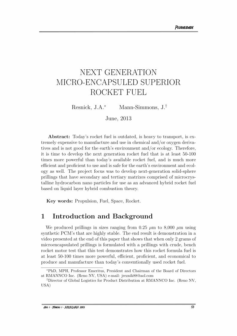
NEXT GENERATIONMICRO-ENCAPSULED SUPERIOR
ROCKET FUEL
Resnick, J.A.∗ Mann-Simmons, J.†
June, 2013
Abstract: Today’s rocket fuel is outdated, is heavy to transport, is ex-tremely expensive to manufacture and use in chemical and/or oxygen deriva-tives and is not good for the earth’s environment and/or ecology. Therefore,it is time to develop the next generation rocket fuel that is at least 50-100times more powerful than today’s available rocket fuel, and is much moreefficient and proficient to use and is safe for the earth’s environment and ecol-ogy as well. The project focus was to develop next-generation solid-sphereprillings that have secondary and tertiary matrixes comprised of microcrys-talline hydrocarbon nano particles for use as an advanced hybrid rocket fuelbased on liquid layer hybrid combustion theory.
Key words: Propulsion, Fuel, Space, Rocket.
1 Introduction and Background
We produced prillings in sizes ranging from 0.25 µm to 8,000 µm usingsynthetic PCM’s that are highly stable. The end result is demonstration in avideo presented at the end of this paper that shows that when only 2 grams ofmicroencapsulated prillings is formulated with a prillings with crude, benchrocket motor test that this test demonstrates how this rocket formula fuel isat least 50-100 times more powerful, efficient, proficient, and economical toproduce and manufacture than today’s conventionally used rocket fuel.
∗PhD, MPH, Professor Emeritus, President and Chairman of the Board of Directorsat RMANNCO Inc. (Reno NV, USA) e-mail: [email protected]
†Director of Global Logistics for Product Distribution at RMANNCO Inc. (Reno NV,USA)
1
53
1.1 Basic Testing and Microencapsulation Processes
Our microencapsulation process [1] and instrument is a NASA Spinofftechnology first used to produce glass microbeads in space on STS-41 andSTS-43 and later to spawn creation of an arsenal of oilspill cleanup, medical,pharmaceutic and food products.
The project focus was to develop next-generation solid-sphere prillings thathave secondary and tertiary matrixes comprised of microcrystalline hydrocar-bon nano particles for use as an advanced hybrid rocket fuel based on liquidlayer hybrid combustion theory. We produced prillings in sizes ranging from0.25 µm to 8,000 µm using synthetic PCM’s that are highly stable.
1.2 Spin-off NASA Technology and Applicable To OtherProducts
The video demo [2] shows small scale static test (burn) using just 2 gramsof prilling product that is 250 µm in size and encapsulated in a polypropy-lene sheath comprising the solid rocket fuel component. The oxidizer is O2
(gas). This technology is representative of next-generation ’future fuels’ thatproduce a very thin, low viscosity, low surface tension liquid layer on the fuelsurface when it burns. Driven by the oxidizer, lift off and entrainment ofPCM, droplets and secondary nanoparticle hydrocarbon components greatlyincrease the overall fuel mass transfer rate simulating a continuous spray in-jection system with the fuel-components vaporization occurring around thedroplets convecting between the melt layer and flame-front resulting in higherregression rates and exponential increase in thrust.
2 Conclusion
Is simple that this paper provides a new breakthrough in the productionof a superior next generation rock fuel. Which will also compliment the nextgeneration in space exploration in our solar system as well.
2.1 Acknowledgements
The authors of this paper would like to thank all scientists and researchersfor their research, and would like to thank Stewart Research 1.0-nm-(nano-meter) imaging studies.
2
54
2.2 Financing
Financing for the research behind this paper was provided by theRMANNCO Corporation.
References
[1] RMANNCO Laboratories. Microencapsulation prilling process toproduce rocket fuel. Reno: RMANNCO, 2013.
[2] . Short run showing test with 2 gramsof RMANNCO’s prillings with crude, benchrocket motor. Available at: www.youtube.com/watch?fea-ture=player embedded&v=GfFkXxXYYaY. Accessed in: Jun. 7th,2013.
3
55
THEORICAL OBSERVATIONS OF THEICE FILLED CRATERS ON MARTIAN
MOON DEIMOS
Baziotis, I.P.∗
June, 2013
Abstract: For decades mankind has envisioned a manned mission toMars. Some plans initiated the concept that using Martian Moon Deimos asa possible stepping stone to Mars. However, within the last several decadesone of the questions that has evaded scientists is: ”Does Deimos have any iceupon it’s surface and/ or in it’s craters?” Why? Because ice is a form of water,and water as far as outer space is concerned in the number one most preciousresource. Not only because water is a fundamental essential for sustaininglife, but it is also necessary for producing rocket fuel. However, one of theforemost problems in being able to ascertain if there is any water on Deimosis the fact that the closest images ever taken of Deimos last occurred whenthe Voyager 2 Orbiter mission was able to take some images of the surfaceof Deimos as close as 30 km. However, at even this close a distance to thesurface of Deimos these images were still not close enough to determine if icewas upon the surface of Deimos or in its craters. In order to provide enoughice so that a manned mission to Deimos is feasible. Therefore, at this point intime in 2013 there is still not enough data to seriously determine if a mannedmission to Deimos as a stepping stone to Mars is a practical viability or not.
Key words: Mars, Deimos, Mission.
∗PhD, Department of Mineralogy, Petrology and Economic Geology, School of Geologyat Aristotle University of Thessaloniki (Thessaloniki, Greece) and Department of EarthSciences at University of Perugia (Perugia, Italy), e-mail: [email protected]
1
56
1 The Availability of Water Throughout The
Universe Increasing The Likeli-hood of Wa-
ter On Deimos
Bradford [2] brings to the reader’s attention that a vaster entire quasarin outer space was discovered by astronomers that provides new data andevidence that water is abundant in outer space.
This discovery occurred in 2011 and according to researchers this discoveryshows that water has been prevalent in the universe for nearly its entireexistence. Therefore, it would also exist in abundant amounts in our solarsystem and on planetary bodies such as upon the surface of Mars MoonDeimos as well.
In a new hypothesis and theory when Earth’s solar system and sun werefirst formed billions of years ago the most abundant components were hydro-gen and oxygen. In like manner, when Earth’s solar system formed water indifferent forms such as ice would also be available.
However, two questions are: ”Where”? and: ”In what amounts”? Includ-ing, is there any water at all in the form of ice on Mars Moon Deimos?
2 What Types of Craters Would Likely Hold
The Most Water OnMartian Moon Deimos
What was known about Deimos and Phobos before the 1990’s? From 1877when Deimos was first discovered until the 1990’s for the most part telescopic,radar telescopes, and spectroscopy were used in addition to a few images ofDeimos up until that period of time existed and as far as the origin of theMartian moons has still controversial as discussed in Burns’ paper [3]. Theprimary hypotheses are that they formed either by capture or by accretion.Because of the similarity to the composition of C-type or D-type asteroids,one hypothesis is that the moons may be objects captured into martianorbit from the asteroid belt, with orbits that have been circularized either byatmospheric drag or tidal forces. While Cazenave [4] further discusses andproposes that Deimos was captured by Mars in the beginning in the formationof Mars when energy creating the Mars, Deimos, and Phobos system. Whileotherwise, Landis [9] stipulates that the current Mars atmosphere is too thin
2
57
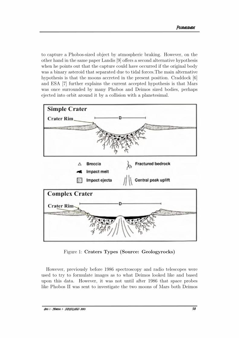
to capture a Phobos-sized object by atmospheric braking. However, on theother hand in the same paper Landis [9] offers a second alternative hypothesiswhen he points out that the capture could have occurred if the original bodywas a binary asteroid that separated due to tidal forces.The main alternativehypothesis is that the moons accreted in the present position. Craddock [6]and ESA [7] further explains the current accepted hypothesis is that Marswas once surrounded by many Phobos and Deimos sized bodies, perhapsejected into orbit around it by a collision with a planetesimal.
Figure 1: Craters Types (Source: Geologyrocks)
However, previously before 1986 spectroscopy and radio telescopes wereused to try to formulate images as to what Deimos looked like and basedupon this data. However, it was not until after 1986 that space probeslike Phobos II was sent to investigate the two moons of Mars both Deimos
3
58
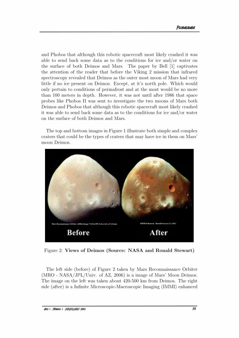
and Phobos that although this robotic spacecraft most likely crashed it wasable to send back some data as to the conditions for ice and/or water onthe surface of both Deimos and Mars. The paper by Bell [1] captivatesthe attention of the reader that before the Viking 2 mission that infraredspectroscopy revealed that Deimos as the outer most moon of Mars had verylittle if no ice present on Deimos. Except, at it’s north pole. Which wouldonly pertain to conditions of permafrost and at the most would be no morethan 100 meters in depth. However, it was not until after 1986 that spaceprobes like Phobos II was sent to investigate the two moons of Mars bothDeimos and Phobos that although this robotic spacecraft most likely crashedit was able to send back some data as to the conditions for ice and/or wateron the surface of both Deimos and Mars.
The top and bottom images in Figure 1 illustrate both simple and complexcraters that could be the types of craters that may have ice in them on Mars’moon Deimos.
Figure 2: Views of Deimos (Source: NASA and Ronald Stewart)
The left side (before) of Figure 2 taken by Mars Reconnaissance Orbiter(MRO - NASA/JPL/Univ. of AZ, 2006) is a image of Mars’ Moon Deimos.The image on the left was taken about 420-500 km from Deimos. The rightside (after) is a Infinite Microscopic-Macroscopic Imaging (IMMI) enhanced
4
59
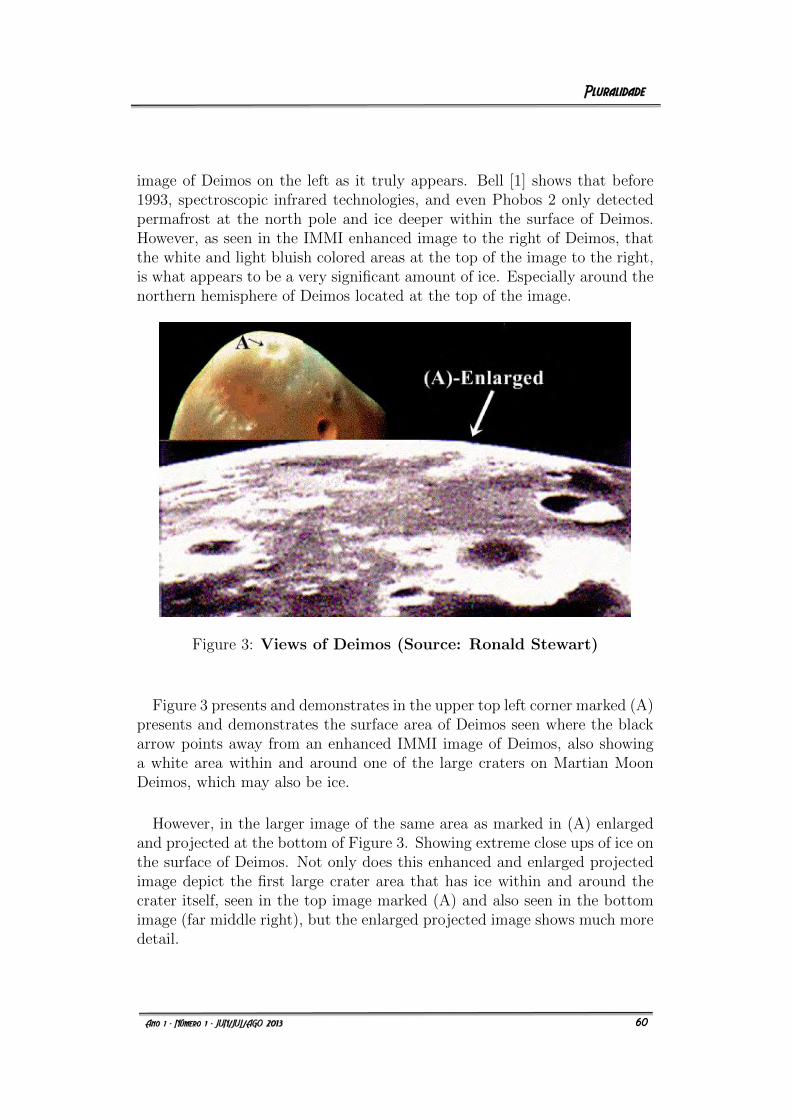
image of Deimos on the left as it truly appears. Bell [1] shows that before1993, spectroscopic infrared technologies, and even Phobos 2 only detectedpermafrost at the north pole and ice deeper within the surface of Deimos.However, as seen in the IMMI enhanced image to the right of Deimos, thatthe white and light bluish colored areas at the top of the image to the right,is what appears to be a very significant amount of ice. Especially around thenorthern hemisphere of Deimos located at the top of the image.
Figure 3: Views of Deimos (Source: Ronald Stewart)
Figure 3 presents and demonstrates in the upper top left corner marked (A)presents and demonstrates the surface area of Deimos seen where the blackarrow points away from an enhanced IMMI image of Deimos, also showinga white area within and around one of the large craters on Martian MoonDeimos, which may also be ice.
However, in the larger image of the same area as marked in (A) enlargedand projected at the bottom of Figure 3. Showing extreme close ups of ice onthe surface of Deimos. Not only does this enhanced and enlarged projectedimage depict the first large crater area that has ice within and around thecrater itself, seen in the top image marked (A) and also seen in the bottomimage (far middle right), but the enlarged projected image shows much moredetail.
5
60
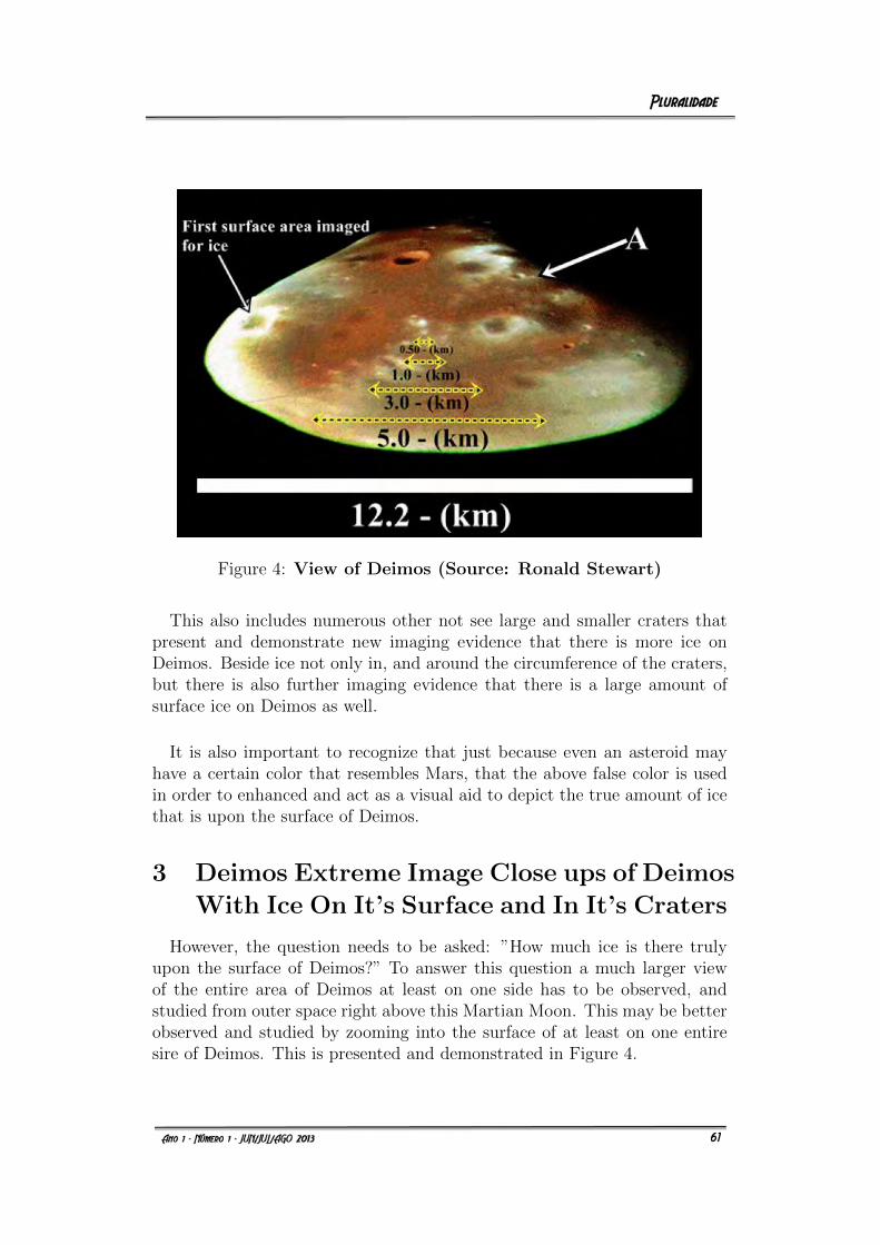
Figure 4: View of Deimos (Source: Ronald Stewart)
This also includes numerous other not see large and smaller craters thatpresent and demonstrate new imaging evidence that there is more ice onDeimos. Beside ice not only in, and around the circumference of the craters,but there is also further imaging evidence that there is a large amount ofsurface ice on Deimos as well.
It is also important to recognize that just because even an asteroid mayhave a certain color that resembles Mars, that the above false color is usedin order to enhanced and act as a visual aid to depict the true amount of icethat is upon the surface of Deimos.
3 Deimos Extreme Image Close ups of Deimos
With Ice On It’s Surface and In It’s Craters
However, the question needs to be asked: ”How much ice is there trulyupon the surface of Deimos?” To answer this question a much larger viewof the entire area of Deimos at least on one side has to be observed, andstudied from outer space right above this Martian Moon. This may be betterobserved and studied by zooming into the surface of at least on one entiresire of Deimos. This is presented and demonstrated in Figure 4.
6
61
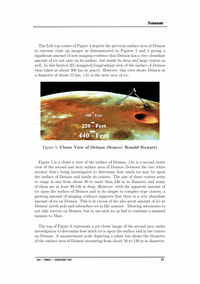
The Left top corner of Figure 4 depicts the previous surface area of Deimosin extreme close up images as demonstrated in Figures 2 and 3 giving asignificant amount of new imaging evidence that Deimos has a very abundantamount of ice not only on its surface, but inside its deep and large craters aswell. In this limited 3D elongated/longitudinal view of the surface of Deimos(was taken at about 300 km in space). However, this view shows Deimos ata diameter of about 12 km. (A) is the next area of ice.
Figure 5: Closer View of Deimos (Source: Ronald Stewart)
Figure 5 is a closer a view of the surface of Deimos. (A) is a second closerview of the second and next surface area of Deimos (between the two whitearrows) that’s being investigated to determine how much ice may be uponthe surface of Deimos and inside its craters. The size of these craters seemto range in size from about 30 to more than 240 m in diameter and manyof them are at least 90-120 m deep. However, with the apparent amount ofice upon the surface of Deimos and in its simple to complex type craters, agrowing amount of imaging evidence supports that there is a very abundantamount of ice on Deimos. This is in excess of the also great amount of ice atDeimos’ north pole and subsurface ice in like manner. Allowing astronauts tonot only survive on Deimos, but to use such ice as fuel to continue a mannedmission to Mars.
The top of Figure 6 represents a yet closer image of the second area underinvestigation to determine how much ice is upon the surface and in the craterson Deimos. A measurement scale depicting a white bar shows the diameterof the surface area of Deimos measuring from about 30 to 120 m in diameter.
7
62
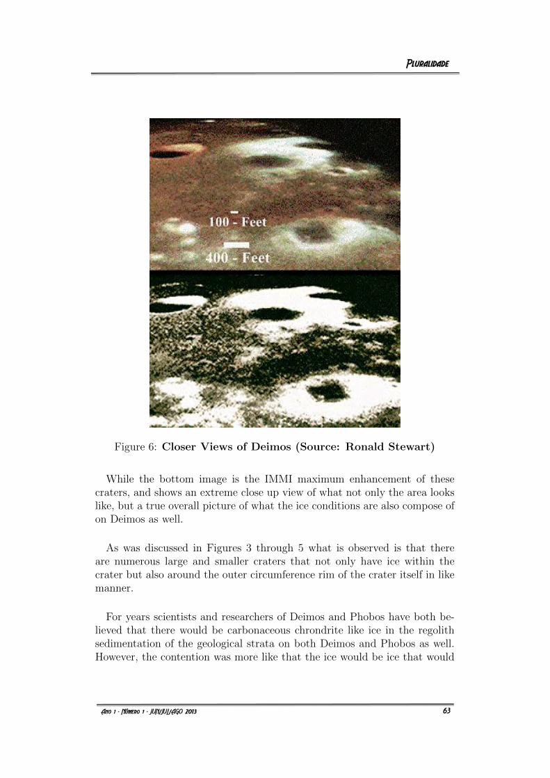
Figure 6: Closer Views of Deimos (Source: Ronald Stewart)
While the bottom image is the IMMI maximum enhancement of thesecraters, and shows an extreme close up view of what not only the area lookslike, but a true overall picture of what the ice conditions are also compose ofon Deimos as well.
As was discussed in Figures 3 through 5 what is observed is that thereare numerous large and smaller craters that not only have ice within thecrater but also around the outer circumference rim of the crater itself in likemanner.
For years scientists and researchers of Deimos and Phobos have both be-lieved that there would be carbonaceous chrondrite like ice in the regolithsedimentation of the geological strata on both Deimos and Phobos as well.However, the contention was more like that the ice would be ice that would
8
63
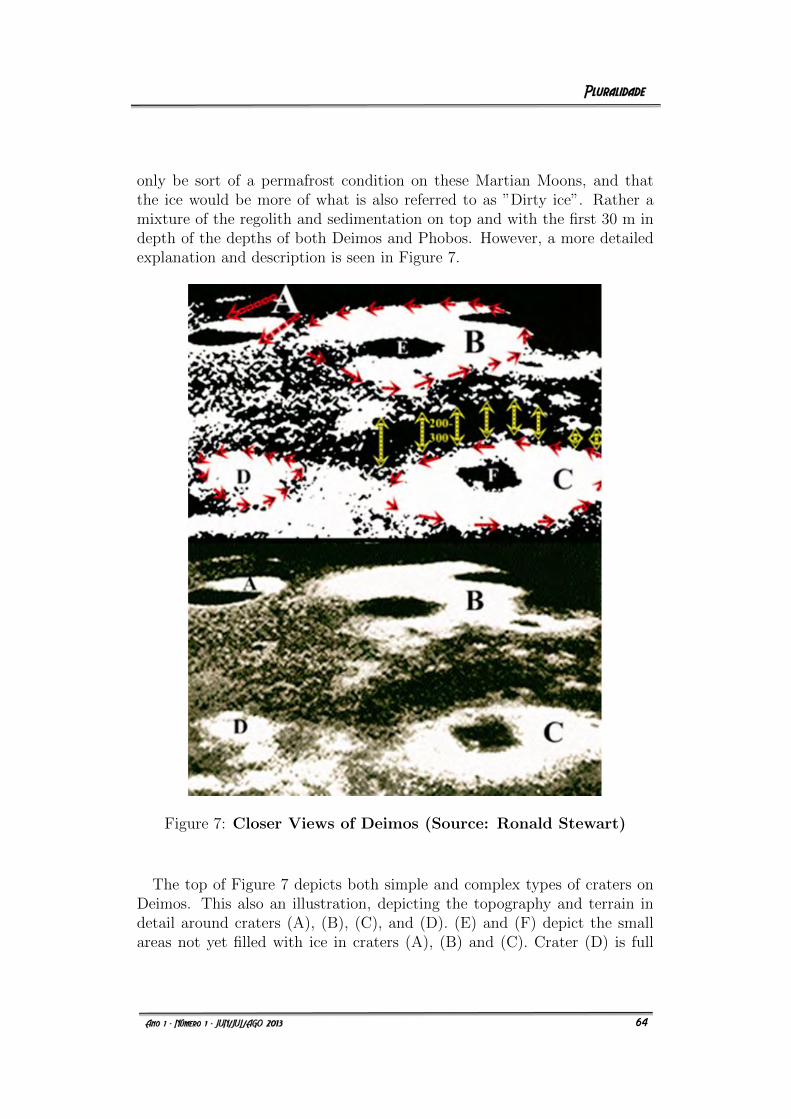
only be sort of a permafrost condition on these Martian Moons, and thatthe ice would be more of what is also referred to as ”Dirty ice”. Rather amixture of the regolith and sedimentation on top and with the first 30 m indepth of the depths of both Deimos and Phobos. However, a more detailedexplanation and description is seen in Figure 7.
Figure 7: Closer Views of Deimos (Source: Ronald Stewart)
The top of Figure 7 depicts both simple and complex types of craters onDeimos. This also an illustration, depicting the topography and terrain indetail around craters (A), (B), (C), and (D). (E) and (F) depict the smallareas not yet filled with ice in craters (A), (B) and (C). Crater (D) is full
9
64
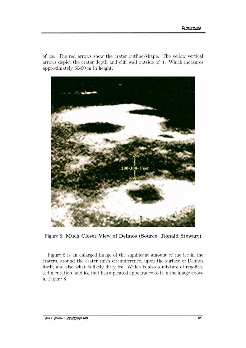
of ice. The red arrows show the crater outline/shape. The yellow verticalarrows depict the crater depth and cliff wall outside of it. Which measuresapproximately 60-90 m in height.
Figure 8: Much Closer View of Deimos (Source: Ronald Stewart)
Figure 8 is an enlarged image of the significant amount of the ice in thecraters, around the crater rim’s circumference, upon the surface of Deimositself, and also what is likely dirty ice. Which is also a mixture of regolith,sedimentation, and ice that has a pleated appearance to it in the image abovein Figure 8.
10
65
4 Why At Least A Robotic Or Manned Mis-
sion To Deimos
Landis [8] discusses that in the 1990’s the political and economic conditionswould have been a good timing prospect for a manned mission to Mars.However, one of the reasons this did not happen was because of what somerefer to as ”Moon Mission Lag”. Meaning; some people believe mankindhad enough space exploration from the Apollo Lunar Missions. That anyadditional venture to Mars would not have been accepted with open arms.However, today in 2013 a manned mission to Mars is taking on a new senseof invigoration. NASA’s series of rover missions has kept the spark alive. Onthe other hand and other space agencies around the world and the privateindustry sector has become much more involved. Some private venturingaspects talking about putting a manned mission around Mars by sometimebetween 2018 and 2023.
With an the announcement by President Barrack Obama to put a mannedmission on an asteroid and private enterprise of companies like PlanetaryResources and Deep Space Industries in an apparent race for mining asteroidshas also made many persons regain new invigorated belief that the wealth ofspace resources, could be good for both mankind in opportunity for wealthand technology as well. However, at this time there is a considerable amountof discussion as to how all of this should be approached. Asking: ”Is it feasibleto send a manned mission directly to Mars?” Or should there be a much morepractical approach that could accomplish several space exploration missionsall at one time?
Making a case to use Deimos as a potential stepping stone for a mannedmission to Mars not only makes sense, it is logical, practical, and reasonable,but it is also the most cost effective as well. How?
Since President Barrack Obama announced a goal to put an man on anasteroid by no later than 2035 this could fit in well by sending a man to Mars’Moon Deimos. Why? Since some scientists may consider Deimos an asteroidlike moon of Mars, and since sending a manned mission to an asteroid willbe out of the confines of earth’s orbit, which would be millions of km intoouter space, what has to be considered is that since Deimos is also millionsof km away from Earth, why not just make the trip to Deimos? At the sametime it would also accomplish several goals at the same time such as:
11
66
1. Using Deimos as a stepping stone to a Mars manned mission;
2. Deimos could be studied as an asteroid like moon of Mars. Answeringquestions of it’s primordial origins;
3. Deimos could be looked at in the context that it may also offer theadvancement of new knowledge, understandings, enlightenment, andinsights and the development of new technologies that could be usedto mine asteroids; and
4. More could be learned about Deimos as to whether or not it was formedabout the time Mars was or at the beginning of our solar system.
Deimos is the smallest and outermost moon of Mars, and hence the near-Mars target that is most accessible in terms of required delta V. A Deimoslanding would be the first manned landing on celestial body outside Earth’sorbit.
5 Conclusion
Deimos is easier, far less costly, safer, and can be done much sooner. In thepaper by Singer [13] proposes that because Deimos is in near-synchronousorbit, with the entire Mars surface (except for extreme polar latitudes) com-ing in view over a period of about 125 days, that coordinating a first mannedmission to Deimos would create a perfect opportunity either for a rover-likerobotic mission and/or hopefully a manned mission to take place on Deimos,Cordell [5].
Cordell [5], O’Leary [10] and Thomas [14] explore that if Deimos wouldhave ice that it would be extremely important and useful as a resource forin-space propellant production.”Water is rocket-fuel ore”.
These papers further discuss that since Deimos and Phobos are spectro-scopically similar to carbonaceous chondrites (as previous and current evi-dence has also strongly suggested) it had been highly suspected that Deimoshad permafrost at it’s north pole. However, although the past and currentevidence is re-affirmed and confirmed with the new imaging evidence in thispaper, besides just being able to confirm the past and current evidence muchmore data now comes to light. that just besides having permafrost dirty iceconditions where ice does exist, there is now additional imaging evidence thatan abundant amount of ice exists not only within the craters, in and around
12
67
the crater rim, but also exists upon the surface of Deimos as well. Therefore,in addition to all of this, previous evidence also indicated that the subsurfaceof Deimos contained sub-surface chemically bound water, and that Deimoswas also thought to be anhydrous as also strongly suggested by Bell [1] andPalmer [12]. That Deimos would also have in it’s sub-surface sedimentol-ogy carbonaceous-chondrite-like assemblages of anhydrous silicates, carbon,organic compounds, and ice.
Since this paper has provided strong new data and imaging evidence thatDeimos not only has a very abundant amount of ice upon it’s surface anddeep large craters, is that much more of a reason for a manned mission toDeimos as a stepping stone to Mars.
5.1 Acknowledgements
The author of this paper would like to extend their gratitude for the manyyears of work that has gone into researching any an all papers written byresearchers and scientists alike, and the ongoing research on Martian moonsDeimos and Phobos, and Mars as a planet. For without such dedicationpapers like this one would not be possible, and also like to thank Dr. RonaldStewart for the IMMI/EXO-SCOPE technologies that made the images inthis paper possible.
5.2 Supplementary Reference Materials
For additional reference videos in addition to the references made in thecontext of this paper on Mars’ Moon Deimos, please refer to videos numbers11 to 14 at http://www.stewart-research-consulting.com/2—exo-scope.html.
References
[1] BELL, J.F., FANALE, F., CRUIKSHANK, D.P. Chemical and phys-ical properties of the martian satellites. Resources of Near-EarthSpace, pp. 887-901, 1993.
[2] BRADFORD, C.M., BOLATTO, A.D., MALONEY, P.R., AGUIRRE,J.E., BOCK, J.J., GLEN, J., KAMENETZKY, J., LUPU, R., MAT-SUHARA, H., MURPHY, E.J. and others. The Water Vapor Spec-trum of APM 08279+5255: X-Ray Heating and InfraredPumping over Hundreds of Parsecs. arXiv: 1106.4301 [astro-ph.CO], 2011.
13
68
[3] BURNS, J.A. Contradictory Clues as to the Origin of the Mar-tian Moons in Mars. Mars A93-27852:1283-1301, 1991.
[4] CAZENAVE, A., DOBROVOLSKIS, A., LAGO, B. Orbital historyof the martian satellites with inferences on their origin. Icarus44(3):730-744, 1980.
[5] CORDELL, B.M.Manned Mars Mission Overview,. AIAA 89:2766,1989.
[6] CRADDOCK, R. A. The Origin of Phobos and Deimos. 25th An-nual Lunar and Planetary Science Conference. Houston TX: LPSC XXV,1994.
[7] EUROPEAN SPACE AGENCY (ESA). Martian moons: Phobos.Available at: http://sci.esa.int/science-e/www/object/index.cfm?fob-jectid=31031. Published in: Sep. 25th, 2012.
[8] LANDIS, G.A. Footsteps to Mars: An incremental approachto Mars exploration. Journal of the British Interplanetary Society48:367-342, 1995.
[9] LANDIS, G. A., Origin of Martian Moons from Binary AsteroidDissociation. arXiV: 0903.3434 [astro-ph.EP], 2009.
[10] O’LEARY, B. Mars 1999: A Concept for Low-Cost Near TermHuman Exploration and Propulsion Processing on Phobos andDeimos in Case for Mars III. AAS 204, 1989.
[11] O’LEARY, B., Rationales for Early Human Missions to Phobosand Deimos in Lunar Bases and Space Activities of the 21st Century.Houston TX: LPI, pp. 801-808, 1985.
[12] PALMER, S. remarks at Case for Mars V. Boulder CO,1993.
[13] SINGER, S.F. A Manned Mission to Phobos and Deimos. AAS81:231, v.57, pp. 39-65, 1984.
[14] THOMAS P. et al., Satellites of Mars: Geologic History. MarsA93-27852:1257-1282, 1991.
14
69
THEORETICALCOSMOLOGY-CELESTIAL MECHANICSCONSIDERING ECCENTRICITY OF THE
PLANETARY MOTIONS, PATHS, OFPLANETS, AND EXOPLANETS ANDMERCURY’S PARTIAL IRREGULAR
RETROGRADE-PATH
Majstor, N.M.∗
June, 2013
Abstract: Context- In the current formulas for astronomical applica-tion to the movement and orbital paths of not only planets and planets inour own solar system is based upon concept of circular motion, and Kepler’sthree Laws of Planetary Motion. Therefore a new theory is needed to im-prove the current understanding of kepeler’s Laws and how they truly apply,not only in Earth’s own solar system, but across the universe in like man-ner. Aims/Goals/Results- However, little thought is given to a relation ofthe circular orbits in relation to the theoretical elliptical motion of celestialbodies and the wider analysis of the known laws which govern the move-ments of celestial bodies around not only Earth’s sun, but in theory wouldbe applicablke to other stars, in other star systems across the universe aswell. Which demands that this be taken into consideration when consideringany type of astronomical phenomenon and that a derived theoretical formulafor calculating the eccentricities of a planet, planetary body, in our own so-lar system, or beyond applies equally as well pertaining to all star systems.Within each star system there is also the theoretical probability that at leastone planet/exoplanet could have a partial irregular retrograde path as is also
∗MSc, Independent Researcher In Theoretical Cosmology and Celestial Mechanics(Podgorica, Crna Gora) , e-mail: [email protected]
1
70
seen within our own solar system when it comes to the displaced irregularmovements of the planet Mercury. Therefore, theoretically such will be dis-cussed in existing and new theoretical and mathematical formulas of suchprocesses as an astronomical invariant with respect to the planets, in ourown solar system and application in theory to exoplanets in other star sys-tems in like manner in which evidence is also made in current bibliographicalreferences as well.
Key words: Cosmology, Solar System, Planetary Bodies, Mercury, Exo-planets.
1 Introduction
An introductory path in understanding connection concerning this pa-per may well be best explained in ”Theoretical Celestial Mechanics” [1],”which gives both theoretical and mathematical computations, and biblio-graphical references, as to why there possibly exists numerous star systemsthat could have at least one planet and/or planetary body (such as a minorplanet),which in theory could have a partia and/or fulll irregular retrogradepath as is also seen within our own solar system, when it comes to the dis-placed irregular movements of the planet Mercury. This is explained furtherin this logic line:
PLANETARY MOTION
1. a is the major semi-axis (velika poluosa ellipse)
2. b is the minor semi-axis (mala poluosa)
3. c is the focal distance (fokusna udaljenost)
4. p is the focal parameter (fokusni parameter)
5. t is the orbit tangent line (tangenta)
6. n is the orbit normal (normala)
7. ϕ is the polar angle of of the radius vector r, mesure from the axisx in counter-clockwise direction ro the radius vector r (polarni ugaoradiusvektora r, mjeren od ose x u suprotnom smjeru kazaljke na satudo radiusvektora r)
8. ε is the numerical eccentricity (numericki ekscentricitet)
2
71
From the kinematics of the point M in Fig.1 and Fig.2 can be writtenfollowing relations:
p =b2
a= a(1− ε2) (1)
r1 = a+ εx (2)
r = a− εx (3)
r + r1 = 2a (4)
r =p
1 + εcosϕ= a(1− εcosu) (5)
S = πab (6)
x2
a2+y2
b2= 1 (7)
tg(ϕ
2) =
√1 + ε
1− εtg(
u
2) (8)
tg(γ) =1 + εcos(ϕ)
εsin(ϕ)(9)
vr = pεω0sin(ϕ) (10)
vϕ = pω0(1 + εcos(ϕ)) (11)
v = pω0
√1 + ε2 + 2εcos(ϕ)) (12)
ωϕ =dϕ
dt= ω0(1 + εcos(ϕ))2 (13)
ω0 =C2
p2=
√kM
p3(14)
C2 =√kpM (15)
cos(γ) =εsin(ϕ)√
1 + ε2 + 2εcos(ϕ)(16)
sin(γ) =1 + εcos(ϕ)√
1 + ε2 + 2εcos(ϕ)(17)
From derived is (Iz izvedenog je):
ωϕ =dϕ
dt= ω0(1 + εcos(ϕ))2 (18)
There is (Odavde se nalazi) tϕ = f (ϕ)
3
72
tϕ =1
ω0
∫ ϕ
0
dϕ
(1 + εcos(ϕ))2(19)
tϕ =1
ω0
[2√
(1− ε2)3arctg(
(1− ε)tg(ϕ2)√
1− ε2)− εsin(ϕ)
(1− ε2)(1 + εcos(ϕ))] (20)
If we take (Ako se uzme da je)
1− ε√1− ε2
=
√1− ε1 + ε
(21)
will be obtained (dobice se):
tϕ =1
ω0(1− ε2)[
2√1− ε2
arctg(
√1− ε1 + ε
tg(ϕ
2))− εsin(ϕ)
1 + εcos(ϕ)] (22)
From equations (13) and (14) (Iz (13) i (14) je):
ω0 =kM
p3=
√√√√ 4π2a3
T 2a3(1− ε2)3=
2π
T (1− ε2)√
1− ε2=
2π√
1− ε2T (1− ε2)2
(23)
2 Planets, Planetary Bodies, Affected By Our
Sun, and Exoplanets Affected By Their Par-
ent Stars
In astronomy, Kepler’s Laws of planetary motion are three scientific lawsdescribing orbital motion, originally formulated to describe the motion ofplanets around Earth’s Sun.
Kepler’s laws are:
1). The orbit of every planet is an ellipse with the Sun at one of the twofoci. 2). A line joining a planet and the Sun sweeps out equal areas duringequal intervals of time.] 3). The square of the orbital period of a planet isproportional to the cube of the semi-major axis of its orbit. Kepler’s Lawsand his analysis of the observations on which they were based challengedthe long-accepted geocentric models of Aristotle and Ptolemy, and gener-ally supported the heliocentric theory of Nicolaus Copernicus . Althoughthe implementation of Kepler’s Laws continued to support the fundamentalgeneralized theories of Nicolaus Copernicus.
4
73
For example; in relation to and what is consistent with the (original paperpaper written by this author in both Serbian and in a limited translation ofEnglish),the original paper’s theoretical calculations are also consitent withthe laws of physics, and of the currently understood explanations, and de-scriptions, expressed in detailed calculations regarding the orbit of the planetMars. Which was first indicated to Kepler its elliptical shape, and he inferredthat other heavenly bodies, including those farther away from the Sun, haveelliptical orbits too. It was in such like assertions of Kepler’s laws and hisanalysis of the observations on which they were based, challenged the long-accepted geocentric models of Aristotle and Ptolemy. However, Kepler’s lawsalso did away with Copernicus’s circular orbits and epicycles), by assertingthat the Earth orbited the Sun, proving that the planets’ speeds varied, andusing elliptical orbits rather than circular orbits with epicycles.
Since bibliographical references are needed in any scientific research paper,in order to comapre and show the difference between the knowledge on asubject that is currently known and how the new paper-(like the one youare now reading) in the English language textual explanation may be able toexplain as best as possible in written text how the new theories may applyas an improvement past the current theories and knowledge. In correlationwith this in a previous paper [1], by Gregory and Fischer (2010), when thispaper also considers the current thinking on planetary motion the authors ofthis paper propose that when considering the aspect of planetary motion theeccentricity from this equation cannot calculate the true value of eccentricitybecause it is an equation with two unknown factors. However, this paper anew in theory proposes that the calculations may find important relationshipsfor calculating the surface segment of the ellipse corresponding to the angleof a planet and/or planetary body when it is in motion in rotational orbitaround its sun. However, a second variant is applicable when pertainingto the eccentric rotation and movement of planets, and planetary bodiesespecially in our own solar system. In theory, this may also include exoplanetsin other star systems in our universe as well. When the formulas are furtherstudied beyond this paper, what is revealed is in theory that when the Sunis intensely involved in its function of movement the angle of a planet’smovement is in relation to its direct influence by its sun, and the closestplanets to the sun most likely (in theory) like Mercury’s partial irregularretrograde path is directly related to it being the closest planet to our sun.
5
74
3 Radial Velocity and Circulating Components
Follow The Relationship To Kepler’s Law
However, when it comes to Kepler’s second law for example; a planet wouldmove faster near the Sun so the same area is swept out in a given time as atlarger distances. This would also mean; that where the planet moves moreslowly, would be a representation of the planet’s proposed velocity and theforce on the planet as well. This would be consistent with the first existence inconjuction with the laws of physics. Especially, in relation to the technologyknown as (RV). Or the radial velocity method which is also used as a primarytechnology in the detection of exoplanets.
For the angled orbital rotational path for planets in our own solar systemand for exoplanets in other star systems as well, the relationship for theangle for the orbital rotational path for a planet or planetary body in anystar system is conducive and obeys Kepler’s Law in also in relation to itsradial velocity and circulating component velocities in relation to its parentstar.
As expressed before [1], as also discussed in the paper by Gregory and Fis-cher,(2010) although this paper primarily discusses this same type of subjectin relation to exoplanets However, this paper proposes that the evidence isseen in our own solar system as it could be in other star systems involviungexoplanets as well. The evidence is in the fact, how this also applies in ev-idence to Earth’s own solar system. Where the planet Mercury’s irregularplanetary movement is also a good example of that. Current thinking hascome to the conclusion the first two of Kepler’s Laws relate to an ellipse ,and claims to be the path of a celestial body mass. However, not only doesthis paper propose evidencein theory that is somewhat different. This paperalso proposes that the center of mass also includes all satellites. Such asminor planets, asteroids, and moons. Whether they are either stationary orrevolving in orbit around their larger centers of mass like a planet/ exoplanetas well. This applies whether it be in our own solar system and/or anotherstar system.
Isaac Newton also gave evidence to kepler’s law in:”Principle Mathemat-ics”. Further meaning; ” That if an instantaneous force is considered on theplanet during its orbit, the area of the triangles defined by the path of theplanet will be the same, for any fixed time interval. When the interval tendsto zero, the force can be considered continuous”.
6
75
Whereas in this paper in theory it is proposed that an angle of a planetin motion to its star that the angle of the ellipse is one-quarter to that of itseccentricity as well.
Therefore the author of this paper, and especially in the original paperwritten in the Serbian language as well emphasizes the strong use of calcula-tions to propose that the center of mass in planetary systems is its barycen-ter. That a planet has completely different actual path. This range gives themean radius of inertia of the body, measured from that barycenter and/ orfrom the rotation of all masses around a planet or in a planetary system, thecurrent value of the radius of inertia or radius of movement of the planetsbeing around their center. Equating to our sola system’s sun.
The planetary system radius of inertia, and movement around its parentstar/ sun could also be expressed in the following abbreviations. This is asfollows: ts is own time rotation; T is the time of revolution; a is the majoraxis of the ellipse; ε is the eccentricity of orbit and φ is the right anomaly-angle between the alignment of its parent star; in relation to its planets/exoplanets.
4 Planetary Mass Moving In An Ellipse In A
Clockwise Directional Motion
Therefore, accordingly the Center of this radius the ellipse of a planet/exoplanet moving in an elliptical orbit around its own parent star/sun, movesin a clockwise direction.
For example: in theory in our own solar system in relation to how theplanet Mercury revolves in an irregular orbit and round our own sun. In likemanner, elliptical orbits of exoplanets around their parent star/sun couldhave some similar irregular movements around their parent stars as well.Just like Mercury in our own solar system moves around our sun in also anirregular orbit in like manner.
In this theoretical case whether it be mercury in our own solar system, oran exoplanet in another star system, both of these situations could both alsohave retrograde motion around their stars/suns in like manner.
7
76
However,some forms of orbital rotation cannot be calculated because of atleast two or more unknown factors. However, what may also find importantrelationships for calculating the surface segment of the ellipse correspondingto its angle. This also is consistent and corresponds to the circulation move-ment. Which also involves moves from the radius of this angle in proportionto the movement of the body. Coming from the fact that the orientation andthat the velocity is circumferential in relation to also the product vector.
This possibly could also mean that while Einstein’s theory of relativity,is correct, it also applies to other variable orbits as we see for most of theplanetary/sun orbit relationships in our own solar system. That is; except forMercury and how it likely also has an irregular retrograde orbit around ourown sun as well. Einstein’s theory may have similar applications regardingthis in other star systems and their exoplanets in the universe as well.
However, when the concept of Mercury’s partial irregular movements aretaken into consideration what conclusion can be drawn from the paper [1] byGregory and Fischer, (2010) involving: ”Theoretical Celestial Mechanics”?
The discussion derived from the theoretical proposals drawn from that pa-per conclude that planet, planetary bodies, exoplanets in other star systemsand likely much of other astronomical phenomenon in our own solar sys-tem and other star systems propose that the these terms can be calculatedeccentricity using the gradual approach , and for the known value of theeccentricity of the Earth.
However what this paper does not also take into consideration is, that theknown value than is calculated within an equation and the accuracy of theseequations may be projected to an accuracy within five decimal places. Beingz equal to 0.0167112.
This may also be expressed in the elliptical eccentricity orbit of a either aplanet in our solar system and/or an exoplanet in another solar system.
Research papers have to relate to and promote new hypotheses and theoriesbased upon previous research . Therefore when considering the eccentricity ofplanetary motion and bodies in our own solar system, this is best expressedin being able to relate the new theory to curent/ recent discoveries wherethe previous current scientific thinking in a one tailed hypotheses can be im-proved upon in a new two tailed theory which presents and demonstrates new
8
77
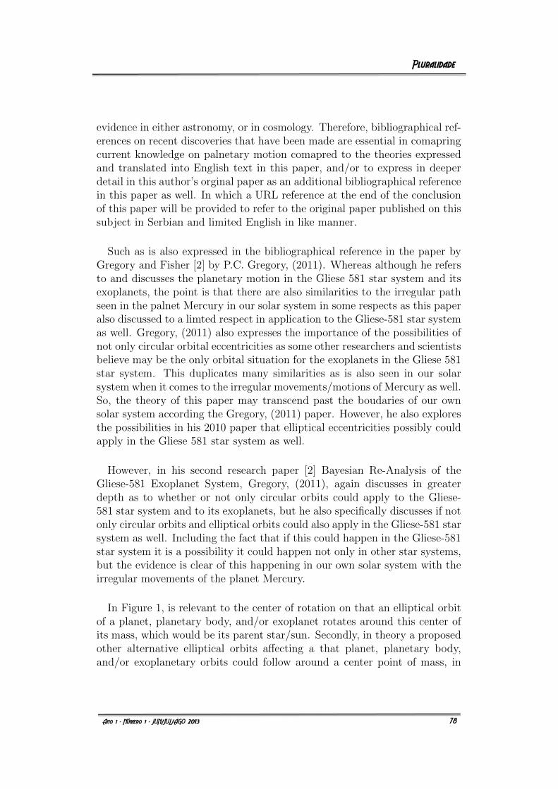
evidence in either astronomy, or in cosmology. Therefore, bibliographical ref-erences on recent discoveries that have been made are essential in comapringcurrent knowledge on palnetary motion comapred to the theories expressedand translated into English text in this paper, and/or to express in deeperdetail in this author’s orginal paper as an additional bibliographical referencein this paper as well. In which a URL reference at the end of the conclusionof this paper will be provided to refer to the original paper published on thissubject in Serbian and limited English in like manner.
Such as is also expressed in the bibliographical reference in the paper byGregory and Fisher [2] by P.C. Gregory, (2011). Whereas although he refersto and discusses the planetary motion in the Gliese 581 star system and itsexoplanets, the point is that there are also similarities to the irregular pathseen in the palnet Mercury in our solar system in some respects as this paperalso discussed to a limted respect in application to the Gliese-581 star systemas well. Gregory, (2011) also expresses the importance of the possibilities ofnot only circular orbital eccentricities as some other researchers and scientistsbelieve may be the only orbital situation for the exoplanets in the Gliese 581star system. This duplicates many similarities as is also seen in our solarsystem when it comes to the irregular movements/motions of Mercury as well.So, the theory of this paper may transcend past the boudaries of our ownsolar system according the Gregory, (2011) paper. However, he also exploresthe possibilities in his 2010 paper that elliptical eccentricities possibly couldapply in the Gliese 581 star system as well.
However, in his second research paper [2] Bayesian Re-Analysis of theGliese-581 Exoplanet System, Gregory, (2011), again discusses in greaterdepth as to whether or not only circular orbits could apply to the Gliese-581 star system and to its exoplanets, but he also specifically discusses if notonly circular orbits and elliptical orbits could also apply in the Gliese-581 starsystem as well. Including the fact that if this could happen in the Gliese-581star system it is a possibility it could happen not only in other star systems,but the evidence is clear of this happening in our own solar system with theirregular movements of the planet Mercury.
In Figure 1, is relevant to the center of rotation on that an elliptical orbitof a planet, planetary body, and/or exoplanet rotates around this center ofits mass, which would be its parent star/sun. Secondly, in theory a proposedother alternative elliptical orbits affecting a that planet, planetary body,and/or exoplanetary orbits could follow around a center point of mass, in
9
78
Figure 1: Planetary Motion (Source: Author)
similar ways how the planet Mercury revolves in orbit around Earth’s sun.Another example has to do with an exoplanet about the size of Saturn dis-covered in 2003 and in 2006 a brown dwarf star was also discovered to havevery oblong and irregular egg shaped like elliptical eccentric orbits in a starsystem 33 light years from Earth known as: ”HD 3651”.
5 Conclusion
In conclusion from the standpoints of theoretical cosmology, astronomy,and astrophysics, this paper has considered that current known thinkingstipulates that some current formulas for astronomical applications pertain-ing to the orbital rotational paths of either planets, planetary bodies, andsatellites that have to do with any and all other astronomical phenomenonin Earth’s solar system and/or in other star systems primarily should haveonly circular orbital paths to the movement and application in the universe.However, because in earth’s own solar system the planet mercury is unlikeany other planetary orbital rotational path as a planet around the sun thatthis paper proposed and contended that if such irregular movements accord-ing to the retrograde orbital path of Mercury exists in Earth’s solar system
10
79
where mankind also lives, than such like retrograde elliptical orbital pathscould exist else where in other star systems with the exoplanets as well.
Therefore, this paper has presented an demonstrated not only theoreticalmathematical equations that propose and offer additional explanations thatboth circular and elliptical retrograde orbits more likely than not exist notonly pertaining to the planet Mercury in not only Earth’s solar system, but inalso other star systems as well. Therefore, the current mode of understandingthat circular orbit are not the only orbits that exist not only in earth’s solarsystem and not only other star systems in the our Milky way galaxy, butmost like throughout the entire universe instead.
5.1 Exceptions to this paper
The original paper was written in both the Serbian and English languages.However, there are some Serbian mathematical formula symbols in the Ser-bian language that will not allow some of these mathematical formulas tobe translated into English with the correct interpretations. Therefore, a fullinterpretation of the author’s original paper and mathematical formulas can-not be fully interpreted into the ultimate goal of my the author’s researchand work. Which in theory the author the author’s original paper in theoryhas a goal of correcting Kepler’s laws, and perhaps that which is also relatedto the theory of relativity. In theoretical terminology that specifically relatesto, and explains and describes the irregular movement not only concerningMercury, but also all the planets (less than that of the Mercury). Therefore,in this paper although an English translation is made to explain as best aspossible how the author’s original theories may be better understood in En-glish, this paper does not an cannot fully express in the English language howthe author’s theories original paper makes these theories and mathematicalformula equations fully known.
5.2 Observation
The author also does not delete/ eliminate any of the Serbian language ex-planations and/or descriptions from the original paper sketches, illustrations,or diagrams, so that the full interpretation of both the author’s theories andmathematical formula equations do not invalidate real understandings andinsights into the evidence.
11
80
5.3 Important Reference to Full Original Paper
You may find the original version of this paper in both the Serbian and En-glish languages at http://www.stewart-research-consulting.com/2-cosmology.html.
5.4 Acknowledgements
The author this paper would like to thank any and all researchers in thesciences of theoretics, cosmology, astronomy, astrophysics, and in physics forall of their tireless research throughout the years. For without such researchpapers like this one would not have been possible.
5.5 Financial Statement
The author for this paper would also like to thank Stewart Research forhelping to also financially make this paper a reality, and providing some ofthe research funds for the implementation of such a paper as well,a nd for thispaper’s translation into English text to explain this authors original paperas much as currently possible.
References
[1] GREGORY, P.C., FISCHER, D.A. A Bayesian Periodogram FindsEvidence for Three Planets in 47 Ursae Majoris. MNRAS403:701, 2010.
[2] GREGORY, P.C. (2011). Bayesian Re-Analysis of the Gliese 581Exoplanet System. arXiv: 1101.0800 [astro-ph.SR], 2011.
[3] MAJSTOR, N.M. Diplomirani masinski inzenjer-smjer-energetski u penzji. Translated by the author. Journal of the Inter-national Society of Peer Reviewers. Available at: http://www.stewart-research-consulting.com/2-cosmology.html. Accessed in: Jun. 11th,2013.
[4] SHIGA, D. Brown dwarfs may stretch out exo-planets’ orbits. NewScientist e-Magazine. Available at:http://www.newscientist.com/article/dn10111-brown-dwarfs-may-stretch-out-exoplanets-orbits.html. Published in: Sep. 20th, 2006.
12
81
THE (POSSIBLE) CONFIRMATION OFTHE FIRST EXO-OCEANS
Aguiar, O.A. ∗ Stewart, R. † Artuso, G.‡ Samadi, A.§
Aristizabal, C.I.O. ¶ Ackerman, J.R. ‖ Trentadue, W.∗∗
Robinett, R.††
February, 2013
Abstract
Current capabilities of telescopy and imaging at best are capable ofimaging another solar system. Only a few images exist of exoplanetsthat have been imaged in another star system. Current aforemen-tioned technologies are incapable of not only not being able to viewand image exoplanets up close, but it is next to impossible to attainextreme close up images of the potential exoplanet’s surface. Sincecurrent technological capabilities are lacking in these astronomical in-vestigations new technologies are needed in order to not only imageother extra-solar systems, but to also image their potential exoplanetsup close. In order to determine exoplanets had one or more oceans onit’s surface. The ”IMMI/EXO-SCOPE Technologies” have been usedto draw a possible map, find one or more oceans on Gliese 581d andmake theoretical assumptions of the oceanographic conditions.
Key words: Oceanography, Astro-oceanography, Astrophysics,Gliese 581d
∗DSc, Oceanographic Research Director at Plural Foundation (Sao Vicente, Brazil)e-mail: [email protected]
†PhD, CEO at Stewart Research (Gonzales TX, USA)‡PhD, Geologist at Agenzia Regionale Campana Difesa Suolo Localita (Napoli, Italia)§MSc, Doctoral Student and Lecturer at Tabriz University (Tabriz, Iran)¶MSc., Doctoral Student at Federal Fluminense University (Niteroi, Brazil)‖PG, Principal Geologist at Twin Oaks Consulting, LLC (Hazelton PA, USA)
∗∗Project-Coordinator of EXO-SCOPE (Austin TX, USA)††Science Researcher at Orion Research Associates (Baltimore MD, USA)
1
82
1 Introduction
1998 was The International Oceans Year, in 2008 the ONU establishedJune 8th as a World Ocean Day, and August 2012 the scientific team , leadedby Dr. Ronald Stewart, agreed that there was just not one possible ocean,but many more oceans upon the exoplanet’s surface known as Gliese 581d inthe constellation of Libra.
Plagiarizing Dr. Joshua Lederberg [3], who first used the ”exo-” prefixin an academic paper: ”The imminence of interplanetary traffic calls forsystematic criticism of the theoretical basis and operational methods of exo-oceanography, the initial search for and continual investigation of water bod-ies it might encounter”. Besides the difficulty to confirm an ocean usingspecular reflection, the IMMI Technology in a elegant way give us imagesthat corroborate the oceans hypothesis that some researchers have about thesurface of Gliese 581d.
IMMI is the acronym for (Infinite Microscopic - Macroscopic-Imaging) andEXO-SCOPE is the acronym for (Exoplanetary-Telescope), each is a separatetechnology and piece of technological hardware. Invented and developed byone of the fellow co-authors of this scientific paper, Dr. Ronald Stewart. Alook at http://www.stewart-research-consulting.com provides much deepercomprehensive instructional detail how these two technologies work.
Besides the difficulty to confirm an ocean using specular reflection [1] theIMMI Technology [5] in an elegant way gave us images that corroborate theoceans hypothesis that some researchers have about Gliese 581d’s surface.
2 The Scientific Data of Gliese 581d
The current known scientific data has revised itself and has changed threetimes since 2007; originally [10] it was thought that Gliese 581d was justoutside the edge of the Habitable Zone (HZ), and that it would be too coldto be a candidate to possibly be favorable to some sort of extraterrestrial life.However, Mayor in this paper [4] (who was on the original discovery team),revised its original estimate of the planet’s orbital perimeters, finding that itorbits closer to its star than originally believed, concluding that the planetwas inside the HZ instead. This was further corroborated by an article bythe ESO [2] that Gliese 581d was the lightest exoplanet yet discovered.
2
83
In 2011 new findings concluded now that there was a good possibility thateven liquid water could exist upon this exoplanet surface, this was furtherconsistent with a Gliese 581d climate study by Wordsworth [11], which gavefurther new evidence that Gliese 581d was likely covered by a ”large and deepocean”. The paper by Wordsworth [11] in the study model also presents anddemonstrates that an average estimation the light that Gliese 581d receivesfrom its star has about 30% of the intensity of sunlight on Earth.
However, this model goes on to determine that ”if” an atmospheric green-house effect was produced on this exoplanet due to the increased infrared(IR) radiation sunlight that would be coming into Gliese 581d, that thiscould significantly raise planetary temperatures, which would be caused bya Greenhouse effect upon the planet’s surface. Volcanic activity could raisethis even higher.
In the research paper [7] entitled ”Vegetation’s Red Edge: A Possible Spec-troscopic Bio-signature of Extraterrestrial Plants” refers to the to the leafreflectance of light between 700 and 750nm wavelength. This paper is usesa concept that light reflectance of vegetation would produce a strong-lightreflection variance, that could be used on exoplanets to try to determine ifan exoplanet had some form of extraterrestrial vegetational life on it or not;such a futuristic technology would certainly have a considerable amount ofscientific worth.
The technology mentioned in Seager’s article [7] is feasible. However,Cowan [1] refers in his research to a proposed new future technology andrefers to it as: ”Specular Reflection”, in which it is currently estimated thatabout ten years into the future will be able to try to find water vapor, ice,or liquid water on a exoplanet. This technology would be based upon beingable to use a spectrum of scattered light from a spatially unresolved extrasolar terrestrial planet; the light would be reflected off of the exoplanet whenit would be in its various moon phases. especially in regard to a conceptof ”Specular Reflection”, which is designed to be used to try to find watervapor, ice, or liquid water on an exoplanet. This technology would be basedupon being able to using a spectrum of scattered light from a spatially un-resolved extra solar terrestrial planet; the light would be reflected off of theexoplanet when it would be in almost moon type phases.
Seager [7] permeates the concept that a red colored spectrum color variancewould be indicative of possible vegetation on an extra solar planet, the use of
3
84
this concept in color spectrum identification (not necessarily in this paper)for the detection of some sort of alien vegetation. However, the ”red edge”concept is a light variance that has the potential for locating possible vegeta-tion on an exoplanet that would be in a star system as reported in Stewart’spaper [8] what is particularly interesting is that when the ”red edge” conceptaccording to him is coupled and combined with what Cowan [1] describes inhis paper entitled: ”Spectrography Specular Reflection Method”, could the-oretically be used in this extra variance, in finding oceans on an exoplanetas well.
Stewart explained [8] what some of the priorities are when making a surveyof another star system; one of these priorities would be to determine if thestar system has a HZ. In many cases, known science has already determinedthe area of space that is not too close to the center of the star system, andnot too far away where it would be too cold- to possibly support some formof extraterrestrial form of life.
The IMMI technology has a number of capabilities that could be usedfor the detection of water vapor in the exoplanets atmosphere, ice, or liquidwater that could be upon an exoplanet’s surface, these capabilities is entitled”IMMI Blue Dot Exoplanet Technology”.
The IMMI technology capability is based upon similar methodologies ofnear IR band with color spectrum wave variance which is in the spectrum ofEarthshine (i.e., the spatially integrated scattered light spectrum of Earth),this is similar to the same technology used in the ”Earthshine Project” andobservations made from the Apache Point Observatory (New Mexico) toemphasize that time variability is key to detecting weak surface bio signaturessuch as the vegetation red edge that Seager [7] describes. Whereas the :”IMMI Blue Dot Exoplanet Technology” is based upon the true genius ofDr. Carl Sagan, in his book entitled ”Pale Blue Dot: A Vision of the HumanFuture in Space” [6] Here are two partial quotes from his book affecting theIMMI Blue Dot Exoplanet Technology.
”The Earth is the only world known so far to harbor life. There is nowhereelse, at least in the near future, to which our species could migrate. Visit,yes. Settle, not yet. Like it or not, for the moment the Earth is wherewe make our stand. ... It has been said that astronomy is a humbling andcharacter-building experience. There is perhaps no better demonstration ofthe folly of human conceits than this distant image of our tiny world. To me,
4
85
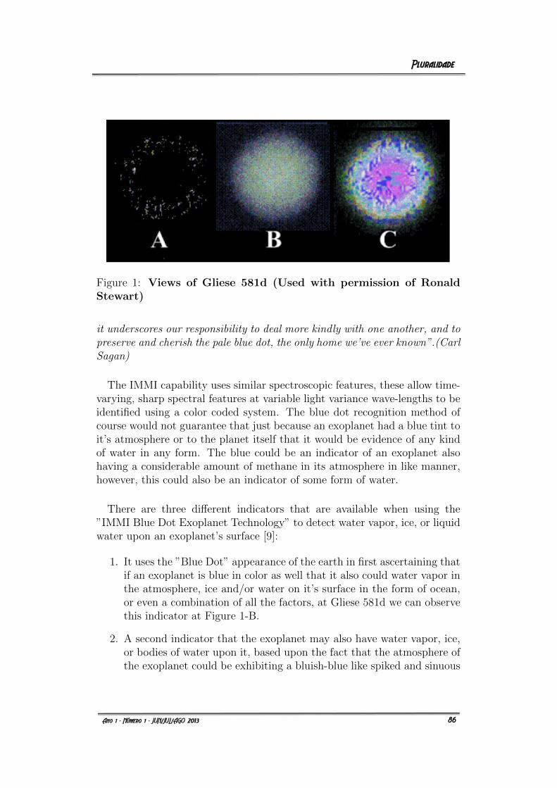
Figure 1: Views of Gliese 581d (Used with permission of RonaldStewart)
it underscores our responsibility to deal more kindly with one another, and topreserve and cherish the pale blue dot, the only home we’ve ever known”.(CarlSagan)
The IMMI capability uses similar spectroscopic features, these allow time-varying, sharp spectral features at variable light variance wave-lengths to beidentified using a color coded system. The blue dot recognition method ofcourse would not guarantee that just because an exoplanet had a blue tint toit’s atmosphere or to the planet itself that it would be evidence of any kindof water in any form. The blue could be an indicator of an exoplanet alsohaving a considerable amount of methane in its atmosphere in like manner,however, this could also be an indicator of some form of water.
There are three different indicators that are available when using the”IMMI Blue Dot Exoplanet Technology” to detect water vapor, ice, or liquidwater upon an exoplanet’s surface [9]:
1. It uses the ”Blue Dot” appearance of the earth in first ascertaining thatif an exoplanet is blue in color as well that it also could water vapor inthe atmosphere, ice and/or water on it’s surface in the form of ocean,or even a combination of all the factors, at Gliese 581d we can observethis indicator at Figure 1-B.
2. A second indicator that the exoplanet may also have water vapor, ice,or bodies of water upon it, based upon the fact that the atmosphere ofthe exoplanet could be exhibiting a bluish-blue like spiked and sinuous
5
86
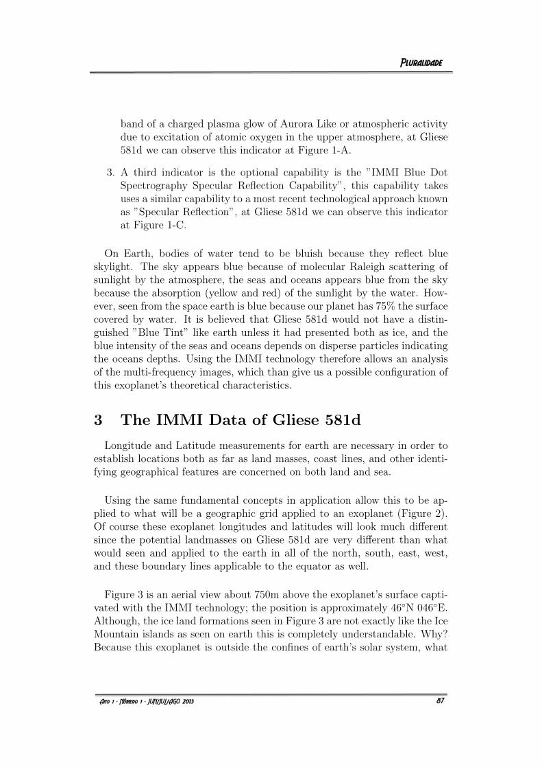
band of a charged plasma glow of Aurora Like or atmospheric activitydue to excitation of atomic oxygen in the upper atmosphere, at Gliese581d we can observe this indicator at Figure 1-A.
3. A third indicator is the optional capability is the ”IMMI Blue DotSpectrography Specular Reflection Capability”, this capability takesuses a similar capability to a most recent technological approach knownas ”Specular Reflection”, at Gliese 581d we can observe this indicatorat Figure 1-C.
On Earth, bodies of water tend to be bluish because they reflect blueskylight. The sky appears blue because of molecular Raleigh scattering ofsunlight by the atmosphere, the seas and oceans appears blue from the skybecause the absorption (yellow and red) of the sunlight by the water. How-ever, seen from the space earth is blue because our planet has 75% the surfacecovered by water. It is believed that Gliese 581d would not have a distin-guished ”Blue Tint” like earth unless it had presented both as ice, and theblue intensity of the seas and oceans depends on disperse particles indicatingthe oceans depths. Using the IMMI technology therefore allows an analysisof the multi-frequency images, which than give us a possible configuration ofthis exoplanet’s theoretical characteristics.
3 The IMMI Data of Gliese 581d
Longitude and Latitude measurements for earth are necessary in order toestablish locations both as far as land masses, coast lines, and other identi-fying geographical features are concerned on both land and sea.
Using the same fundamental concepts in application allow this to be ap-plied to what will be a geographic grid applied to an exoplanet (Figure 2).Of course these exoplanet longitudes and latitudes will look much differentsince the potential landmasses on Gliese 581d are very different than whatwould seen and applied to the earth in all of the north, south, east, west,and these boundary lines applicable to the equator as well.
Figure 3 is an aerial view about 750m above the exoplanet’s surface capti-vated with the IMMI technology; the position is approximately 46◦N 046◦E.Although, the ice land formations seen in Figure 3 are not exactly like the IceMountain islands as seen on earth this is completely understandable. Why?Because this exoplanet is outside the confines of earth’s solar system, what
6
87
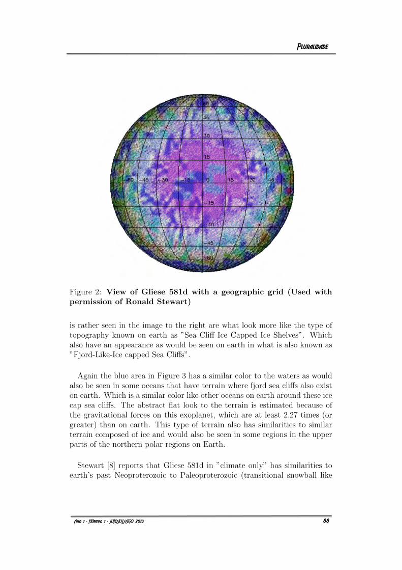
Figure 2: View of Gliese 581d with a geographic grid (Used withpermission of Ronald Stewart)
is rather seen in the image to the right are what look more like the type oftopography known on earth as ”Sea Cliff Ice Capped Ice Shelves”. Whichalso have an appearance as would be seen on earth in what is also known as”Fjord-Like-Ice capped Sea Cliffs”.
Again the blue area in Figure 3 has a similar color to the waters as wouldalso be seen in some oceans that have terrain where fjord sea cliffs also existon earth. Which is a similar color like other oceans on earth around these icecap sea cliffs. The abstract flat look to the terrain is estimated because ofthe gravitational forces on this exoplanet, which are at least 2.27 times (orgreater) than on earth. This type of terrain also has similarities to similarterrain composed of ice and would also be seen in some regions in the upperparts of the northern polar regions on Earth.
Stewart [8] reports that Gliese 581d in ”climate only” has similarities toearth’s past Neoproterozoic to Paleoproterozoic (transitional snowball like
7
88
Figure 3: A Gliese 581d sea cliff ice capped ice shelves (Used withpermission of Ronald Stewart)
earth) as it most likely existed millions of years ago1.
The analysis of many observations in the images of the surface of Gliese581d show very intensely active oceanic conditions and wave activity, a cli-mate would have to be present for the oceans to be active as they most likelyare. Observations in images and videos determine that there are likely ahundred seas and at least a dozen oceans upon the surface of Gliese 581 d.There are likely hundreds of small bodies of water on land and each is aseparate body of water without obvious connections, the melting ice basinsmaybe make the largest group of bodies of water.
When analyzing these facts and observations from the astronomical sense,concerning the exoplanet’s albedo, the ratio of the light reflected by a planetor satellite to that received by it, is only about one-third or a little morethan on earth. However, from an imaging standpoint the dark blue areas onthis exoplanet are big deep bodies of water, or in the last analysis, Oceans.
The review and analysis of the IMMI images allow us to draw a possibleconfiguration of Gliese 581d (Figure 4) showing a lot of water bodies andland masses, more IMMI images are needed to make a whole planisphere.There have been many numerous observations made of not only Gliese 581das not only an exoplanet itself, but especially of it’s surface from a number
1Note: It needs to be made perfectly clear, that this scientific paper is only likeningthese conditions these conditions ”in climate; not the biological means that are associatedwith such descriptions”.
8
89
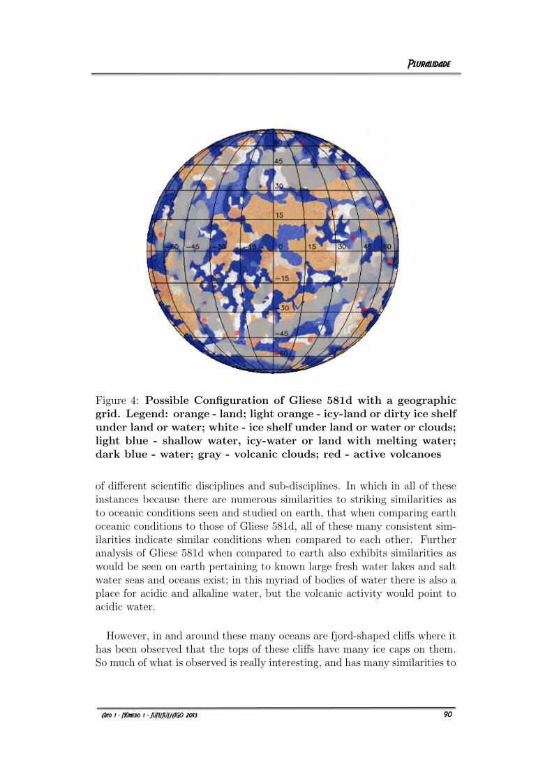
Figure 4: Possible Configuration of Gliese 581d with a geographicgrid. Legend: orange - land; light orange - icy-land or dirty ice shelfunder land or water; white - ice shelf under land or water or clouds;light blue - shallow water, icy-water or land with melting water;dark blue - water; gray - volcanic clouds; red - active volcanoes
of different scientific disciplines and sub-disciplines. In which in all of theseinstances because there are numerous similarities to striking similarities asto oceanic conditions seen and studied on earth, that when comparing earthoceanic conditions to those of Gliese 581d, all of these many consistent sim-ilarities indicate similar conditions when compared to each other. Furtheranalysis of Gliese 581d when compared to earth also exhibits similarities aswould be seen on earth pertaining to known large fresh water lakes and saltwater seas and oceans exist; in this myriad of bodies of water there is also aplace for acidic and alkaline water, but the volcanic activity would point toacidic water.
However, in and around these many oceans are fjord-shaped cliffs where ithas been observed that the tops of these cliffs have many ice caps on them.So much of what is observed is really interesting, and has many similarities to
9
90
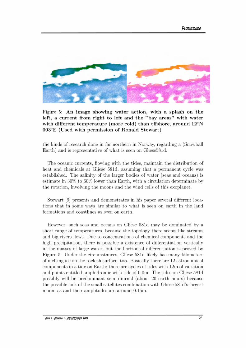
Figure 5: An image showing water action, with a splash on theleft, a current from right to left and the ”bay areas” with waterwith different temperature (more cold) than offshore, around 12◦N003◦E (Used with permission of Ronald Stewart)
the kinds of research done in far northern in Norway, regarding a (SnowballEarth) and is representative of what is seen on Gliese581d.
The oceanic currents, flowing with the tides, maintain the distribution ofheat and chemicals at Gliese 581d, assuming that a permanent cycle wasestablished. The salinity of the larger bodies of water (seas and oceans) isestimate in 30% to 60% lower than Earth, with a circulation determinate bythe rotation, involving the moons and the wind cells of this exoplanet.
Stewart [9] presents and demonstrates in his paper several different loca-tions that in some ways are similar to what is seen on earth in the landformations and coastlines as seen on earth.
However, such seas and oceans on Gliese 581d may be dominated by ashort range of temperatures, because the topology there seems like streamsand big rivers flows. Due to concentrations of chemical components and thehigh precipitation, there is possible a existence of differentiation verticallyin the masses of large water, but the horizontal differentiation is proved byFigure 5. Under the circumstances, Gliese 581d likely has many kilometersof melting ice on the rockish surface, too. Basically there are 12 astronomicalcomponents in a tide on Earth; there are cycles of tides with 12m of variationand points entitled amphidromic with tide of 0.0m. The tides on Gliese 581dpossibly will be predominant semi-diurnal (about 20 earth hours) becausethe possible lock of the small satellites combination with Gliese 581d’s largestmoon, as and their amplitudes are around 0.15m.
10
91
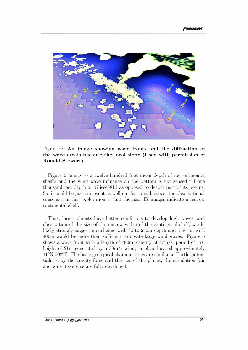
Figure 6: An image showing wave fronts and the diffraction ofthe wave crests because the local slope (Used with permission ofRonald Stewart)
Figure 6 points to a twelve hundred foot mean depth of its continentalshelf’s and the wind wave influence on the bottom is not sensed till onethousand feet depth on Gliese581d as opposed to deeper part of its oceans.So, it could be just one event as well our last one, however the observationalconsensus in this exploration is that the near IR images indicate a narrowcontinental shelf.
Thus, larger planets have better conditions to develop high waves, andobservation of the size of the narrow width of the continental shelf, wouldlikely strongly suggest a surf zone with 30 to 250m depth and a ocean with400m would be more than sufficient to create large wind waves. Figure 6shows a wave front with a length of 780m, celerity of 47m/s, period of 17s,height of 21m generated by a 30m/s wind, in place located approximately11◦N 002◦E. The basic geological characteristics are similar to Earth, poten-tialities by the gravity force and the size of the planet; the circulation (airand water) systems are fully developed.
11
92
4 Conclusion
Gliese581d has very strong wind and wave actions causing the impressionof an exoplanet that is in a state of continuous inclement weather, all oceano-graphic conditions would likely be more intense than on earth, similar as towhat would be seen on earth during an intense tropical storm on an ongoingcontinuous basis.
Waves are larger and the coastal currents are more intense because of thetopography. Different from earth having two large landmasses, and/or severalcontinents, whereas Gliese 581d has a myriad of land masses that consistof chain-like-interconnected-continental-islands, which affects and causes adifferent dynamics of the water mass, with possible water circulation underthe ice caps.
While other effects, too few at this point to determine what other type ofinteractive oceanic conditions and dynamics may be present on Gliese 581d,indicates the need for further investigative images and study to help establishand complete a hypothesis. However, it is unquestionable that the existenceof oceans and seas are upon this exoplanet in the Gliese 581 star system inits HZ known as Gliese 581d. The author and co-authors of this paper planmore research and papers pertaining to Gliese 581d.
In all of the accumulative previously known and new data, imaging evi-dence, videos, and other supplemental materials to this research paper, andthe many numerous observations made from several or more applicable sci-entific disciplines and sub-disciplines, it has been determined that all of thisdata and evidence is consistent. Secondly, all of the data and images ob-served and studied is also consistent with the laws of physics and empiricallaws.
It could also be said that there are many similarities to Gliese 581d as wouldhave also been seen in a snowball-like-earth, but how the characteristics ofearth developed compared as a planet, compared to Gliese 581d as seen noware not similar.
Gliese 581d is in the HZ in its system, the estimated average temperature is20◦C, the estimated lowest temperature is around 0◦C, have all three indica-tors of water of the ”IMMI Blue Dot Exoplanet Technology” and the imagesof the surface show interaction ocean-atmosphere with wind generated waves.
12
93
References
[1] COWAN, N.B., ABBOT, D.S. & VOIGT, A. A False PositiveFor Ocean Glint on Exoplanets The Latitude Albedo Effect.arXiv:1205.1058v1 [astro-ph.EP], 2012.
[2] EUROPEAN SOUTHERN OBSERVATORY (ESO). Lightest exo-planet yet discovered. Science Release eso0915. Garching: ESO, 2009.
[3] LEDERGERG, J. Signs of Life, Criterion-System of Exobiology.Nature 207:4992, 1965.
[4] MAYOR, M., BONFILS, X., FORVEILLE, T., DEFOSSE, X. UDRY,S., BERTAUX, J-L., BEUST, H., BOUCHY, F., LOVIS, C., PEPE, F.,and others. The HARPS search for southern extra-solar planetsXVIII: An Earth-mass planet in the GJ 581 planetary system.Astronomy and Astrophysics, arXiv:0906.2780 [astro-ph.EP], 2009.
[5] RESNICK, J., STEWART, R. IMMI - Micro - Ordersof Magnitude Basics in Microscopy. Journals of Sci-ence. Available at: http://www.journals-of-science.com/up-loads/6/8/9/3/6893524/immi - micro - orders - of - magnitudebasics in microscopy.pdf. Accessed in: Jan. 20th, 2013.
[6] SAGAN, C. Pale Blue Dot: A Vision of the Human Future inSpace. New York: Random House, 1994.
[7] SEAGER, S., TURNER, E.L., SCHAFER, J., FORD, E.B. Vegeta-tion’s Red Edge A Possible Spectroscopic Bio-signature of Ex-traterrestrial Plants. arXiv:050.3302, [astro-PH], 2005.
[8] STEWART, R., AGUIAR, O., ARTUSO, G., ARISTIZABAL, C.,ACKERMAN, J., TRENTADUE, W., ROBINETT, R. Earth’sOceans: A Theoretical Approach How Interconnected Con-tinents and High Altitude Mountain Glaciers Formed Them.International Journal of Geology and Paleontology. Available at:http://www.journals-of-sciences.com ijgp-geology–paleontology.html.Accessed in: Jan. 20th, 2013.
[9] STEWART, R., CELEBONOVIC, V., AGUIAR, O.A.,CHATZITHEODORIDIS, E., ACKERMAN, J.R., ROMAN, M., AR-TUSO, G., TRENTADUE, W., SAMADI, A., ARISTIZABAL, C.I.O.and others. First View of Gliese 581d: A Preliminary Surface
13
94
Survey. International Journal of Astronomy and Astrophysics Re-search. Available at: http://www.journals-of-sciences.com/-ijaar.html.Accessed in: Jan. 20th, 2013.
[10] UDRY, S., BONFILS, X., DEFOSSE, X., FORVEILLE, T., MAYOR,M., PERRIER, C., BOUCHY, F., LOVIS, C., PEPE, F., QUELOZ,D., and others. The HARPS search for southern extra-solarplanets XI. Super-Earths (5 & 8M⊕) in a 3-Planet System.arXiv:0704.3841 [astro-PH], 2007.
[11] WORDSWORTH, R., FORGET, F., SELSIS, F., MILLOUR, E.,CHARNAY, B., MADELEINE, J-B. Gliese 581d is the first dis-covered terrestrial-mass exoplanet in the habitable zone.arXiv:1105.1031v1 [astro-ph.EP], 2011.
14
95
MOXIFLOXACIN HYDROCHLORIDECOMPOUND IMPURITIES MICROSCOPIC
IMAGING STUDY
Spaulding, V.E. ∗
June, 2013
Abstract: The methodology and formula for producing moxifloxacin hy-drochloride compounds and having very low levels of impurities are providedin Pharmaceutical US Patent # 20130059880. Which initiates claims thatthe impurities in and ending result when produced is less than 0.1%, pertotal volume of this pharmaceutical when in its moxifloxacin tosylate crys-tal powder form. We contend that moxofloxacin related impurities not onlypose some of the already known side affects such as rash, and slight fever,but that these impurities may have other deficiencies, however, may alsohave unknown other benefits deep within the compound properties as well.However, the problem is that whether it be an optical, electron, and even theworld’s most powerful Atomic Force Microscope (AFM), they all have limi-tations in being able to attain deep enough microscopic measurement scalelevels, in order to determine what other impurities, deficiencies, and benefitsthis drug may have. Therefore, a much deeper microscopic imaging study isneeded to see if other important discoveries could be made.
Key words: Moxifloxacin, Hydrochloride, Pharmaceutics, Infection.
1 Introduction and Background
The methodology used is to start with a micrograph, depicting a sample ofmoxifloxacin tosylate crystal powder at approximately 200 µm in diameter.Two microscopic imaging technologies known as IMMI [4] and will attain one
∗PhD, Member of the Board of Directors at International Consortium on Microscopicand Macroscopic Research (Gonzales TX, USA) e-mail: [email protected]
1
96
continuous microscopic imaging view starting at 200 µm, attaining a continu-ous microscopic imaging video view of much deeper and smaller microscopicmeasurement scale sizes into this pharmaceutical. Eventually attaining a mi-croscopic measurement scale size of approximately 1.0 nm or smaller. Whichwill expose this drug at its atomic level or even smaller. The ending result(to one degree or another) will be to find similarities, resemblances, outlines,connections, or microscopic imaging recognition patterns in the drug. Be-tween the known and unknown impurities, deficiencies, and benefits that thispharmaceutical may yet have to offer by the discoveries made within it. Sec-ondly, the video made will take up where this paper leaves off at. Therefore,it is not only important to read this paper to watch the video to it as well.
This paper’s foundation is based upon aspects of moxifloxacin is an an-tibacterial medication used to treat patients with certain types of bacterialinfections, such as pneumonia, bronchitis, and also has been an alterna-tive pharmaceutical in the treatment in other types of infections such asMycoplasma gentialium. However, a concise, deeper, comprehensive and de-tailed micro-imaging study is needed to determine not only attain new data,but to also help scientists, researchers, and the pharmaceutical industry toattain deeper understandings and insights into the compositional aspects ofthis pharmaceutical. Which would also add new enlightenment as to whatadditional possible impurities, deficiencies, and benefits this drug may have.This medication is part of a class of drugs called fluroroquinolones, whichwork by destroying bacterial pathogens in the body. However, as with anydrug, side affects may occur as well. Therefore, the intent and purpose ofthis paper is to discuss some of the side affects caused by this drug, and thenintroduce the microscopic imaging/video study. Looking at this pharmaceu-tical starting at a diameter of about 200 µm eventually attain a microscopicmeasurement of 1.0 nm Which should reveal new data that will provide newdata. proving new knowledge, understandings, insights, and enlightenmentinto this drug never attained before.
2 Headache and Dizziness
Treatment with this antibiotic can cause headache or dizziness in patients,health reports [5] at PDR Health. Which is a, a medical information website associated with the Physicians’ Desktop Reference. Headache pain orsensations of dizziness can affect a patient’s ability to remain alert and at-tentive while at work or school. Patients can manage headache side effects byusing an over-the-counter pain medication, such as acetaminophen. During
2
97
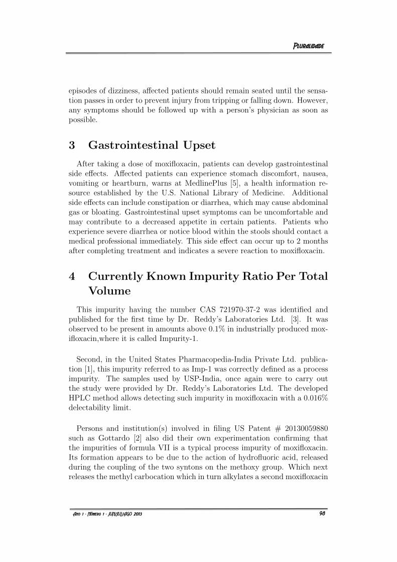
episodes of dizziness, affected patients should remain seated until the sensa-tion passes in order to prevent injury from tripping or falling down. However,any symptoms should be followed up with a person’s physician as soon aspossible.
3 Gastrointestinal Upset
After taking a dose of moxifloxacin, patients can develop gastrointestinalside effects. Affected patients can experience stomach discomfort, nausea,vomiting or heartburn, warns at MedlinePlus [5], a health information re-source established by the U.S. National Library of Medicine. Additionalside effects can include constipation or diarrhea, which may cause abdominalgas or bloating. Gastrointestinal upset symptoms can be uncomfortable andmay contribute to a decreased appetite in certain patients. Patients whoexperience severe diarrhea or notice blood within the stools should contact amedical professional immediately. This side effect can occur up to 2 monthsafter completing treatment and indicates a severe reaction to moxifloxacin.
4 Currently Known Impurity Ratio Per Total
Volume
This impurity having the number CAS 721970-37-2 was identified andpublished for the first time by Dr. Reddy’s Laboratories Ltd. [3]. It wasobserved to be present in amounts above 0.1% in industrially produced mox-ifloxacin,where it is called Impurity-1.
Second, in the United States Pharmacopedia-India Private Ltd. publica-tion [1], this impurity referred to as Imp-1 was correctly defined as a processimpurity. The samples used by USP-India, once again were to carry outthe study were provided by Dr. Reddy’s Laboratories Ltd. The developedHPLC method allows detecting such impurity in moxifloxacin with a 0.016%delectability limit.
Persons and institution(s) involved in filing US Patent # 20130059880such as Gottardo [2] also did their own experimentation confirming thatthe impurities of formula VII is a typical process impurity of moxifloxacin.Its formation appears to be due to the action of hydrofluoric acid, releasedduring the coupling of the two syntons on the methoxy group. Which nextreleases the methyl carbocation which in turn alkylates a second moxifloxacin
3
98
molecule. This impurity is particularly difficult to remove from the productusing conventional re-crystallization methods. Therefore, this molecule alsoneeds to be looked for as well.
Figure 1: Visualization of moxifloxacin (Source: Fabbrica ItalianaSintetici S.p.A [2])
Based upon US Patent # 20130059880 shows an image acquired with anoptical microscope of moxifloxacin tosylate crystal powder and indicativeimpurities at an approximate microscopic measurement scale level of 200 µm(Figure 1).
5 Supplemental Material
Available at: http://www.stewart-research-consulting.com/medical-r–d.html.
6 Acknowledgements
The author of this paper would like to thank all researchers and scientistsinvolved in the study of medical diseases and the pharmaceutical industry.Who for without their research papers like this one would not be possible,and also like to thank the Stewart Research and Consulting for the pharma-ceutical video..
4
99
References
[1] DEVI, M.L., CHANDRASEKHAR, K.B. A validated, specificstability-indicating RP-LC method for moxifloxacin and its re-lated substances. Chromatographia 69:933-999, 2009.
[2] GOTTARDO, G., PADOVAN, P. OSTI, S. Moxifloxacin hydrochlo-ride compounds and intermediates and methods for makingsame. US Patent # 20130059880. Available at: http://patents.jus-tia.com/patent/20130059880. Accessed in: Jun. 28th, 2013.
[3] KUMAR, Y.R., RAJU, V.V.N.K.V., KUMAR, R.R., ESWARAIAH, S.,MUKKANTI, K., SURYANARAYANA, M.V., REDDY, M.S. Struc-tural identification and characterization of impurities in mox-ifloxacin. Journal of Pharmaceutical and Biomedical Analysis 34-5:1125-1129, 2004.
[4] RESNICK, J., STEWART, R. IMMI - Micro - Or-ders of Magnitude Basics in Microscopy. Jour-nals of Science. Available at: http://www.journals-of-science.com/uploads/6/8/9/3/6893524/immi - micro - orders - of -magnitude basics in microscopy.pdf. Accessed in: Jun. 28th, 2013.
[5] UDDIN, R. Side effects of roxithromycim. Live Strong site. Avail-able at: http://www.livestrong.com/article/133587-moxifloxacin-side-effects/#ixzz2VwcuHYKL. Published in: Jul. 08th, 2010.
5
100
THEORETICAL IMPLICATIONS OFNANO-SCALE QUANTUM
GRAVITO-MAGNETISM ON THE NATUREOF OUR STEADY STATE UNIVERSE
Boyd, M.E. ∗
July, 2013
Abstract: The Big Bang Theory has come in to question because sur-rounding galaxies accelerate apart faster than predicted by the theory. Thishas been referred to by some physicists as ”inflation theory”. Recent dis-coveries of the presence of gravitational lensing rings observed in the cosmicbackground of the known observable universe (Figure 1) coupled with thequantum relationship of gravity to electromagnetism (Figure 2) supports thepremise for ”eternal inflation” upon which some inflation theories are based,undermining the Big Bang Theory’s premise that at some time in the distantpast a finite temporal event occurred creating the universe of today.
Key words: Gravitational, Einstein Rings, Black Hole, Quantum Time,Big Bang.
1 Highlights
In particle physics, the ADD model, also known as the model with largeextra dimensions, offers an alternative scenario to explain the weakness ofgravity relative to the other forces. This theory requires that the fields of thestandard model are confined to a four-dimensional membrane, while gravitypropagates in several additional spatial dimensions that are large comparedto the Planck scale.
∗President at Californians for Renewable Energy, Inc. (CARE) (Soquel CA, USA)e-mail: [email protected]
1
101
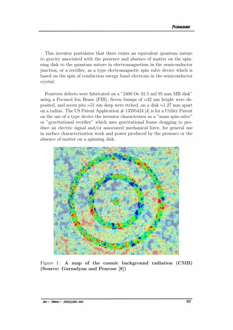
This inventor postulates that there exists an equivalent quantum natureto gravity associated with the presence and absence of matter on the spin-ning disk to the quantum nature in electromagnetism in the semiconductorjunction, or a rectifier, as a type electromagnetic spin valve device which isbased on the spin of conduction energy band electrons in the semiconductorcrystal.
Fourteen defects were fabricated on a ”2400 Oe 31.5 mil 95 mm MR disk”using a Focused Ion Beam (FIB). Seven bumps of ≈32 nm height were de-posited, and seven pits ≈51 nm deep were etched, on a disk ≈1.27 mm aparton a radius. The US Patent Application # 13595424 [4] is for a Utility Patenton the use of a type device the inventor characterizes as a ”mass spin-valve”or ”gravitational rectifier” which uses gravitational frame dragging to pro-duce an electric signal and/or associated mechanical force, for general usein surface characterization work and power produced by the presence or theabsence of matter on a spinning disk.
Figure 1: A map of the cosmic background radiation (CMB)(Source: Gurzadyan and Penrose [8])
2
102
Recently observed gravitational lensing rings in the cosmic background ra-diation shown in Figure 1 where ”the observable effect, in our CMB sky, offamilies of concentric circles over which the temperature variance is anoma-lously low, the centre of each such family representing the point of ’I’ atwhich the cluster converges. These centers appear as fairly randomly dis-tributed fixed points in our CMB sky. The analysis of Wilkinson MicrowaveBackground Probe’s (WMAP) cosmic microwave background 7 years maps[3] [10] does indeed reveal such concentric circles, of up to 6σ significance” asreported by Gurzadyan and Penrose in 2010 [8]. These concentric rings arepredicted by Albert Einstein’s theory of general relativity. Instead of lightfrom a source traveling in a straight line in three dimension, it is bent bythe presence of a massive body, like a super massive black hole which dis-torts space-time. An Einstein Ring is a special case of gravitational lensing,caused by the exact alignment of the source, lens and observer. This resultsfrom symmetry around the lens, causing a ring-like structure. The size of anEinstein ring is given by the Einstein radius. This author postulates theysuggest the presence of a super massive black hole.
In radians, it is:
θE =
√4GM
c2dLSdLdS
(1)
where:G is the gravitational constant,M is the mass of the lens,c is the speed of light,dL is the angular diameter distance to the lens,dS is the angular diameter distance to the source, anddLS is the angular diameter distance between the lens and the source.
Note that, over cosmological distances dLS 6= dS - dL, in general.
2 Theory of Quantum Gravitation
Einstein’s problem was he only understood the universe from the side ofelectrons not the holes side that dominates it. If you think of empty space asa high density of holes and matter as regions where electron density is higherthen you see Einstein Dirac etc..., where blinded by the light produced by
3
103

electrons..., that’s why they couldn’t see the holes in the universe all aroundthem.
Magnetism is a property of electromagnetism produced by electron statesin matter; gravity is produced by the mass of the matter which mass comesfrom the mass of the neutrons and protons of the element of matter as de-scribed in the periodic table of the elements of matter.
Table 1: Particle mass
Name Mass
proton 1.6726 x 10⁻²⁷ kgneutron 1.6749 x 10⁻²⁷ kgelectron 0.00091x10⁻²⁷ kg
The mass of a neutron is greater than the mass of a proton because theneutron contains a proton, contains an electron with some subatomic parti-cles.
Neutron stars are collapsed matter leaving only neutrons at the atomicscale that makes up the neutron star and black holes are nearly identical butmade of protons [holes] instead.
Black holes are black not because light doesn’t escape but because blackholes are made of holes [collapsed protons] where light is not present becausethere are no electrons to absorb the light for re-emission of the light.
Holes are the mechanism for quantum tunneling in the semiconductor; aswell as superconductivity. To understand how ”holes” work it is useful toexamine the Hall effect in semiconductors. The Hall effect is due to thenature of the current in a conductor. Current consists of the movement ofmany small charge carriers, typically electrons, holes, what are called mobileions or all three. When a magnetic field is present that is not parallel tothe direction of motion of moving charges, these charges experience a force,called the Lorentz force. When such a magnetic field is absent, the chargesfollow approximately straight, ’line of sight’ paths between collisions withimpurities, phonons, etc. However, when a magnetic field with a perpendic-ular component is applied, their paths between collisions are curved so that
4
104
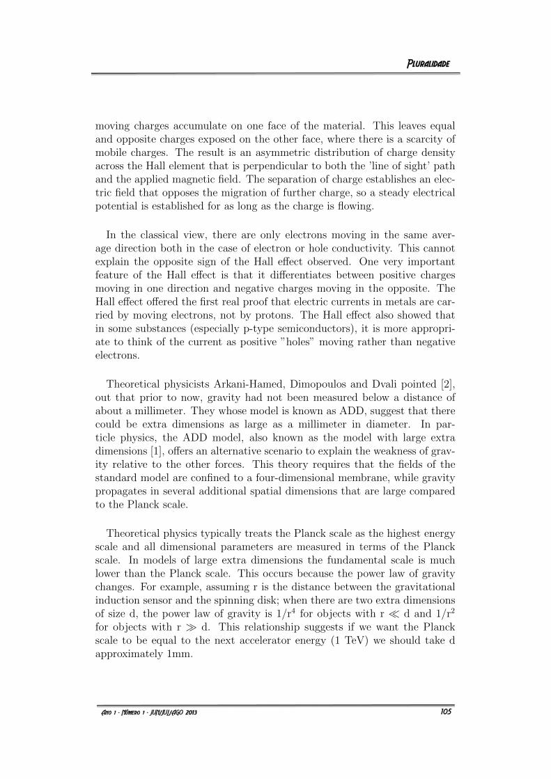
moving charges accumulate on one face of the material. This leaves equaland opposite charges exposed on the other face, where there is a scarcity ofmobile charges. The result is an asymmetric distribution of charge densityacross the Hall element that is perpendicular to both the ’line of sight’ pathand the applied magnetic field. The separation of charge establishes an elec-tric field that opposes the migration of further charge, so a steady electricalpotential is established for as long as the charge is flowing.
In the classical view, there are only electrons moving in the same aver-age direction both in the case of electron or hole conductivity. This cannotexplain the opposite sign of the Hall effect observed. One very importantfeature of the Hall effect is that it differentiates between positive chargesmoving in one direction and negative charges moving in the opposite. TheHall effect offered the first real proof that electric currents in metals are car-ried by moving electrons, not by protons. The Hall effect also showed thatin some substances (especially p-type semiconductors), it is more appropri-ate to think of the current as positive ”holes” moving rather than negativeelectrons.
Theoretical physicists Arkani-Hamed, Dimopoulos and Dvali pointed [2],out that prior to now, gravity had not been measured below a distance ofabout a millimeter. They whose model is known as ADD, suggest that therecould be extra dimensions as large as a millimeter in diameter. In par-ticle physics, the ADD model, also known as the model with large extradimensions [1], offers an alternative scenario to explain the weakness of grav-ity relative to the other forces. This theory requires that the fields of thestandard model are confined to a four-dimensional membrane, while gravitypropagates in several additional spatial dimensions that are large comparedto the Planck scale.
Theoretical physics typically treats the Planck scale as the highest energyscale and all dimensional parameters are measured in terms of the Planckscale. In models of large extra dimensions the fundamental scale is muchlower than the Planck scale. This occurs because the power law of gravitychanges. For example, assuming r is the distance between the gravitationalinduction sensor and the spinning disk; when there are two extra dimensionsof size d, the power law of gravity is 1/r4 for objects with r � d and 1/r2
for objects with r � d. This relationship suggests if we want the Planckscale to be equal to the next accelerator energy (1 TeV) we should take dapproximately 1mm.
5
105
As suggested by ADD, gravity could be just as strong as the other forcesbut only felt strongly at short distances. Scientists funded by the EuropeanSpace Agency have measured the gravitational equivalent of a magnetic fieldfor the first time in a laboratory. Just as a moving electrical charge cre-ates a magnetic field, so a moving mass generates a gravitomagnetic field.According to Einstein’s Theory of General Relativity, the effect is virtuallynegligible. However Tajmar [11] have measured the effect in a laboratory.Their experiment involves a ring of superconducting material rotating up to6,500 times a minute. The volume Pit & Bump Volume is expressed again inthe mathematical equation that would be the theoretical mechanisms for theinflux possible for a black hole. Which may be expressed by equation (1).
Figure 2: Gravitational induction equivalent of the semiconductorrectifier (Source: Author)
This author postulates that there exists an equivalent quantum natureto gravity associated with the presence and absence of matter on the spin-ning disk to the quantum nature in electromagnetism in the semiconductorjunction (or a rectifier) as a type electromagnetic spin valve device which isbased on the spin of conduction energy band electrons in the semiconductorcrystal. Figure 2 shows the gravitational induction equivalent of the semi-conductor; as a gravitational rectifier in the mass spin valve device; whereby
6
106
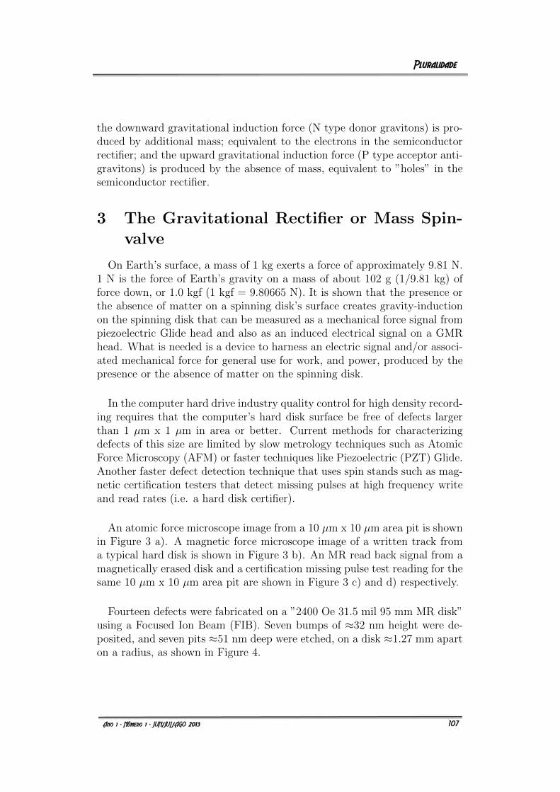
the downward gravitational induction force (N type donor gravitons) is pro-duced by additional mass; equivalent to the electrons in the semiconductorrectifier; and the upward gravitational induction force (P type acceptor anti-gravitons) is produced by the absence of mass, equivalent to ”holes” in thesemiconductor rectifier.
3 The Gravitational Rectifier or Mass Spin-
valve
On Earth’s surface, a mass of 1 kg exerts a force of approximately 9.81 N.1 N is the force of Earth’s gravity on a mass of about 102 g (1/9.81 kg) offorce down, or 1.0 kgf (1 kgf = 9.80665 N). It is shown that the presence orthe absence of matter on a spinning disk’s surface creates gravity-inductionon the spinning disk that can be measured as a mechanical force signal frompiezoelectric Glide head and also as an induced electrical signal on a GMRhead. What is needed is a device to harness an electric signal and/or associ-ated mechanical force for general use for work, and power, produced by thepresence or the absence of matter on the spinning disk.
In the computer hard drive industry quality control for high density record-ing requires that the computer’s hard disk surface be free of defects largerthan 1 µm x 1 µm in area or better. Current methods for characterizingdefects of this size are limited by slow metrology techniques such as AtomicForce Microscopy (AFM) or faster techniques like Piezoelectric (PZT) Glide.Another faster defect detection technique that uses spin stands such as mag-netic certification testers that detect missing pulses at high frequency writeand read rates (i.e. a hard disk certifier).
An atomic force microscope image from a 10 µm x 10 µm area pit is shownin Figure 3 a). A magnetic force microscope image of a written track froma typical hard disk is shown in Figure 3 b). An MR read back signal from amagnetically erased disk and a certification missing pulse test reading for thesame 10 µm x 10 µm area pit are shown in Figure 3 c) and d) respectively.
Fourteen defects were fabricated on a ”2400 Oe 31.5 mil 95 mm MR disk”using a Focused Ion Beam (FIB). Seven bumps of ≈32 nm height were de-posited, and seven pits ≈51 nm deep were etched, on a disk ≈1.27 mm aparton a radius, as shown in Figure 4.
7
107
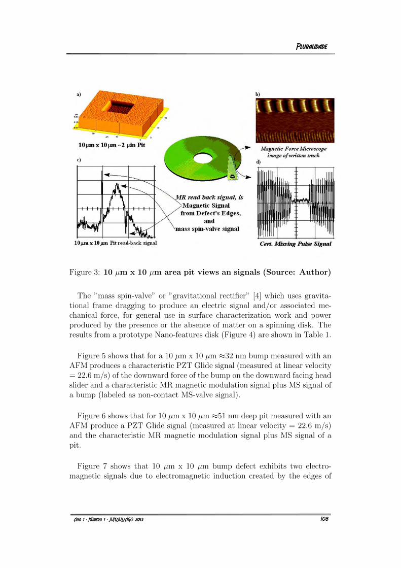
Figure 3: 10 µm x 10 µm area pit views an signals (Source: Author)
The ”mass spin-valve” or ”gravitational rectifier” [4] which uses gravita-tional frame dragging to produce an electric signal and/or associated me-chanical force, for general use in surface characterization work and powerproduced by the presence or the absence of matter on a spinning disk. Theresults from a prototype Nano-features disk (Figure 4) are shown in Table 1.
Figure 5 shows that for a 10 µm x 10 µm ≈32 nm bump measured with anAFM produces a characteristic PZT Glide signal (measured at linear velocity= 22.6 m/s) of the downward force of the bump on the downward facing headslider and a characteristic MR magnetic modulation signal plus MS signal ofa bump (labeled as non-contact MS-valve signal).
Figure 6 shows that for 10 µm x 10 µm ≈51 nm deep pit measured with anAFM produce a PZT Glide signal (measured at linear velocity = 22.6 m/s)and the characteristic MR magnetic modulation signal plus MS signal of apit.
Figure 7 shows that 10 µm x 10 µm bump defect exhibits two electro-magnetic signals due to electromagnetic induction created by the edges of
8
108
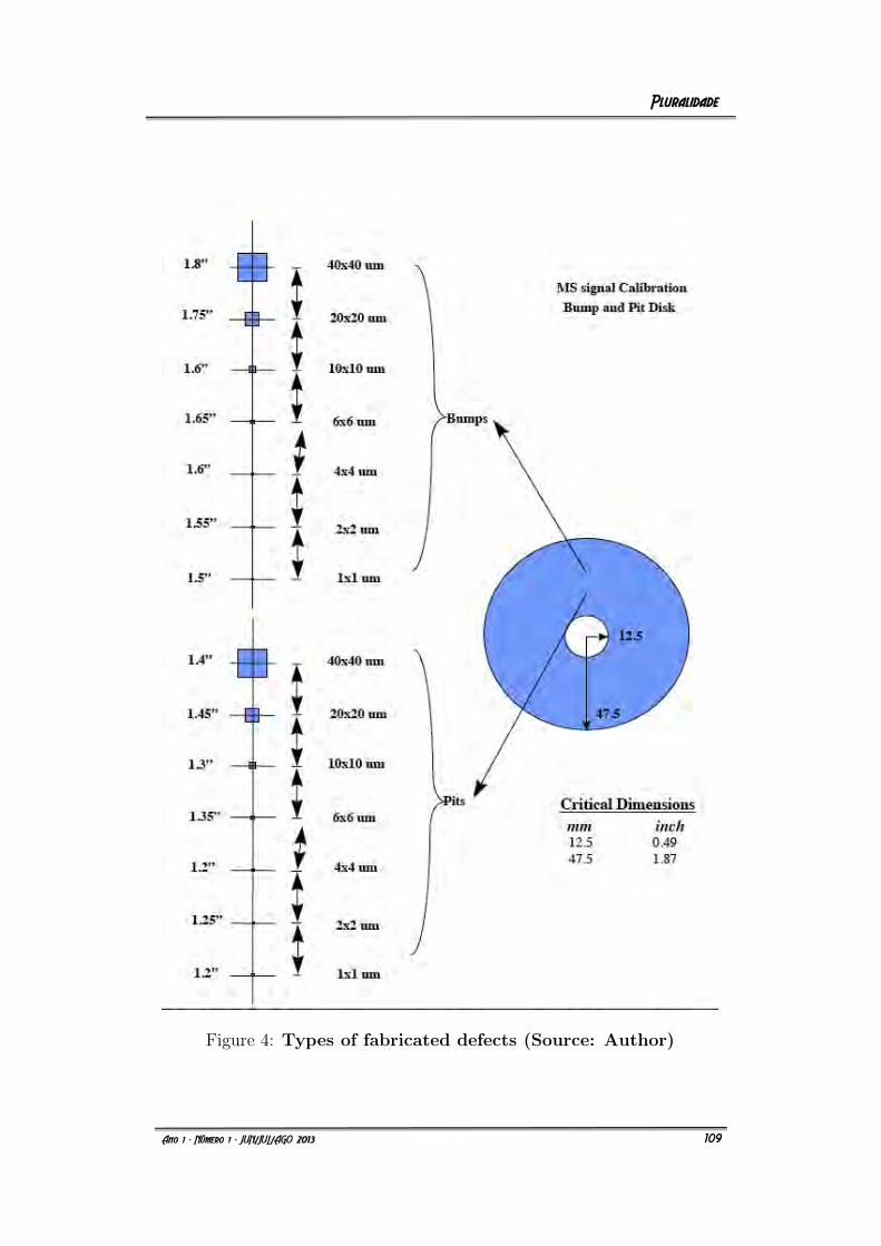
Figure 4: Types of fabricated defects (Source: Author)
9
109
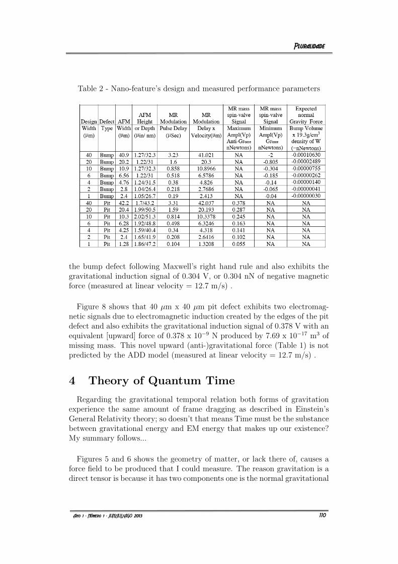
Table 2 - Nano-feature’s design and measured performance parameters
the bump defect following Maxwell’s right hand rule and also exhibits thegravitational induction signal of 0.304 V, or 0.304 nN of negative magneticforce (measured at linear velocity = 12.7 m/s) .
Figure 8 shows that 40 µm x 40 µm pit defect exhibits two electromag-netic signals due to electromagnetic induction created by the edges of the pitdefect and also exhibits the gravitational induction signal of 0.378 V with anequivalent [upward] force of 0.378 x 10⁻⁹ N produced by 7.69 x 10⁻¹⁷ m3 ofmissing mass. This novel upward (anti-)gravitational force (Table 1) is notpredicted by the ADD model (measured at linear velocity = 12.7 m/s) .
4 Theory of Quantum Time
Regarding the gravitational temporal relation both forms of gravitationexperience the same amount of frame dragging as described in Einstein’sGeneral Relativity theory; so doesn’t that means Time must be the substancebetween gravitational energy and EM energy that makes up our existence?My summary follows...
Figures 5 and 6 shows the geometry of matter, or lack there of, causes aforce field to be produced that I could measure. The reason gravitation is adirect tensor is because it has two components one is the normal gravitational
10
110
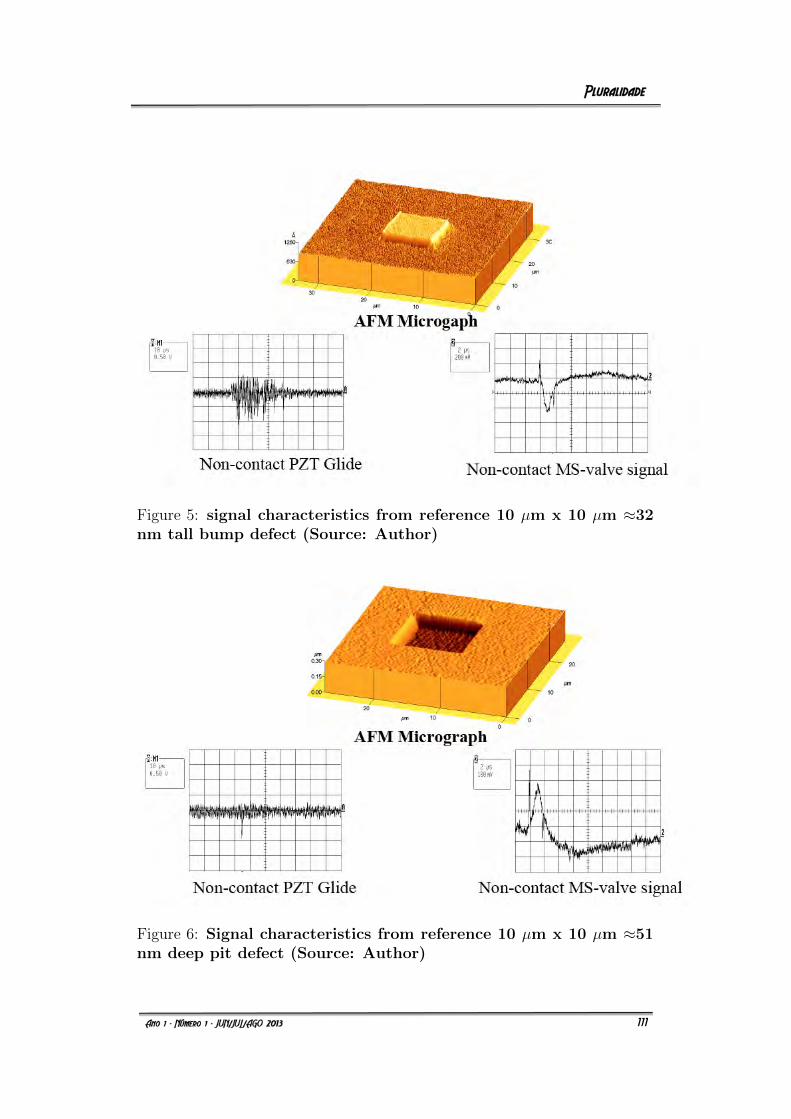
Figure 5: signal characteristics from reference 10 µm x 10 µm ≈32nm tall bump defect (Source: Author)
Figure 6: Signal characteristics from reference 10 µm x 10 µm ≈51nm deep pit defect (Source: Author)
11
111
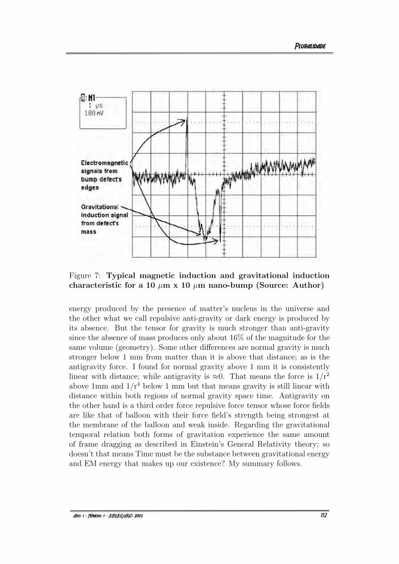
Figure 7: Typical magnetic induction and gravitational inductioncharacteristic for a 10 µm x 10 µm nano-bump (Source: Author)
energy produced by the presence of matter’s nucleus in the universe andthe other what we call repulsive anti-gravity or dark energy is produced byits absence. But the tensor for gravity is much stronger than anti-gravitysince the absence of mass produces only about 16% of the magnitude for thesame volume (geometry). Some other differences are normal gravity is muchstronger below 1 mm from matter than it is above that distance; as is theantigravity force. I found for normal gravity above 1 mm it is consistentlylinear with distance; while antigravity is ≈0. That means the force is 1/r2
above 1mm and 1/r4 below 1 mm but that means gravity is still linear withdistance within both regions of normal gravity space time. Antigravity onthe other hand is a third order force repulsive force tensor whose force fieldsare like that of balloon with their force field’s strength being strongest atthe membrane of the balloon and weak inside. Regarding the gravitationaltemporal relation both forms of gravitation experience the same amountof frame dragging as described in Einstein’s General Relativity theory; sodoesn’t that means Time must be the substance between gravitational energyand EM energy that makes up our existence? My summary follows.
12
112
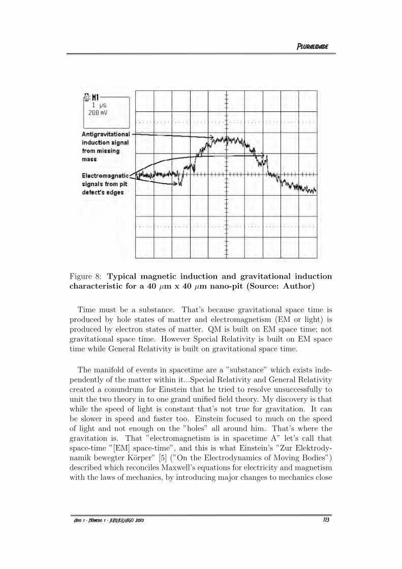
Figure 8: Typical magnetic induction and gravitational inductioncharacteristic for a 40 µm x 40 µm nano-pit (Source: Author)
Time must be a substance. That’s because gravitational space time isproduced by hole states of matter and electromagnetism (EM or light) isproduced by electron states of matter. QM is built on EM space time; notgravitational space time. However Special Relativity is built on EM spacetime while General Relativity is built on gravitational space time.
The manifold of events in spacetime are a ”substance” which exists inde-pendently of the matter within it...Special Relativity and General Relativitycreated a conundrum for Einstein that he tried to resolve unsuccessfully tounit the two theory in to one grand unified field theory. My discovery is thatwhile the speed of light is constant that’s not true for gravitation. It canbe slower in speed and faster too. Einstein focused to much on the speedof light and not enough on the ”holes” all around him. That’s where thegravitation is. That ”electromagnetism is in spacetime A” let’s call thatspace-time ”[EM] space-time”, and this is what Einstein’s ”Zur Elektrody-namik bewegter Korper” [5] (”On the Electrodynamics of Moving Bodies”)described which reconciles Maxwell’s equations for electricity and magnetismwith the laws of mechanics, by introducing major changes to mechanics close
13
113

to the speed of light. This later became known as Einstein’s special theoryof relativity (SR) [6] [7] That ”gravitation is in spacetime B” let’s call thatspace-time ”[G]space-time” and this is what Einstein’s General relativity(GR) describes. According to general relativity [9] , the observed gravita-tional attraction between masses results from the ”warping of space and timeby those masses”. When I write about this ”manifold of events in spacetimeare a ”substance” which exists independently of the matter within it” this”manifold of events in spacetime” is this property that makes Time; as wemeasure it; the emergent [positive arrow of time]. Therefore time is a vectorwhich direction depends on your position in our universe which is created bya change of energy states between gravitation to electromagnetism; and visaversa.
Figure 9: Time band gap between gravity and electromagnetism inthe mass spin-valve device (Source: Author)
Figure 9 shows that in our local universe; the time band gap between grav-ity and electromagnetism; is about 22 µs. In this region time stops due to thenon-renormalizability of gravity. Based on empirical measurements (Figure9) this inventor postulates that time itself exists in two simultaneous space-time continuum; one based on electro-magnetism, and one based on gravity.The Wall of Planck only applies in the electromagnetic ”energy” universe;not the one based on gravity. In the gravity universe; ”mass-energy”, or
14
114
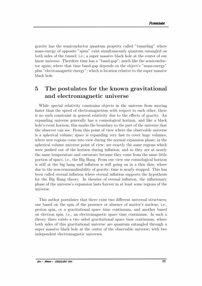
gravity has the semiconductor quantum property called ”tunneling” wheremass-energy of opposite ”spins” exist simultaneously quantum entangled onboth sides of the tunnel; i.e.; a super massive black hole at the center of ourknow universe. Therefore time has a ”band-gap”; much like the semiconduc-tor again; where that time band-gap depends on the object’s ”mass-energy”plus ”electromagnetic energy”; which is location relative to the super massiveblack hole.
5 The postulates for the known gravitational
and electromagnetic universe
While special relativity constrains objects in the universe from movingfaster than the speed of electromagnetism with respect to each other, thereis no such constraint in general relativity due to the effects of gravity. Anexpanding universe generally has a cosmological horizon, and like a blackhole’s event horizon, this marks the boundary to the part of the universe thatthe observer can see. From this point of view where the observable universeis a spherical volume; space is expanding very fast to cover huge volumes,where new regions come into view during the normal expansion phase; in thespherical volume universe point of view; are exactly the same regions whichwere pushed out of the horizon during inflation; and so they are at nearlythe same temperature and curvature because they come from the same littleportion of space, i.e., the Big Bang. From our view our cosmological horizonis still at the big bang and inflation is still going on in a thin skin; wheredue to the non-renormalizability of gravity; time is nearly stopped. This hasbeen called eternal inflation where eternal inflation supports the hypothesisfor the Big Bang theory. In theories of eternal inflation, the inflationaryphase of the universe’s expansion lasts forever in at least some regions of theuniverse.
This author postulates that there exist two different universal structures;one based on the spin of the presence or absence of matter’s nucleus, i.e.,proton spin, or a gravitational space time continuum, and another basedon electron spin, i.e., an electromagnetic space time continuum. In such atheory there exists a two sided gravitational space time continuum; whereboth sides of this gravitational universe are quantum entangled through asuper massive black hole at the center of the observable universe; with twoindependent electromagnetic universes.
15
115
The fact that the gravity force has been measured to be as strong as theelectromagnetic forces; below one millimeter distance, and gravity propagatesat a slower speed than electromagnetism; implies, the universe is steady-stateand the electromagnetic image of the cosmic background shown in Figure 1suggests that fact. The observed rings are visible because there are two sidesto the universe that are quantum entangled through the force of gravity;our normal 4-D universe with x, y, z, and time (Planck’s Universe whichfollows the Standard Model); and another dimensional domain for gravitywhere gravity propagates in several additional spatial dimensions that arelarge compared to the Planck scale, i.e. the ADD Universe.
With a two sided universe our 4-D universe exists in a parabolic universewhere depending on your position relative to the super massive black holeat the center of the universe (the focal point) you will be accelerating ordecelerating; where at our position the relationship of mass to normal gravityis described by the relationship (additional mass) bump volume, in [µm3], isequal to:
Vbump = 6(−Gf )2 − 7(−Gf )− 0.4 (2)
where Gf is the ”negative” attractive force of Gravity which is a parabolicfunction which has two mathematically real factors (Figure 2). Assuming theGravitational induction force (-Gf ) is variable x and the volume of additionalmass is y. Solving for y = 0, by simplifying the equation gives two real factorsx1 and x2; where x1 = 1.221255 and x2 = -0.054589.
In the anti-universe quantum entangled through the force of gravity asmeasured from our 4-D universe; where repulsive ”+” anti-gravity exists inhyperbolic space with one real part and two imaginary factors, relative to us,described by the relationship (missing mass) pit volume, in [µm3], is equalto:
Vpit = −3000Gf3 + 1000Gf
2 − 200Gf + 8 (3)
Assuming the anti-gravitational induction force (Gf ) is variable x and thevolume of missing mass is y, then y = -3000x3 + 1000x2 - 200x + 8, assumingy = 0 the roots are : x1 = 0.0510251 x2 = 0.141154 + 0.179826i x3 = 0.141154- 0.179826i.
16
116
6 Conclusion
Recent discoveries of the presence of gravitational lensing rings observed inthe cosmic background coupled with a new understanding of the relationshipof gravity to electromagnetism suggest the existence of an eternal inflationgravitational universe decoupled from our local electromagnetic universe andthat the Big Bang Theory is just plain wrong.
6.1 Acknowledgements
I would like to thank Gedeon Heinrich, Heiner Sussner, Blasius Brezoczky,George Burt, Dave Ferry, Veronica Munro, Brian-Tinh Vu, and Mike Ro-gowski for their support in the initial research and subsequent co-authoringby Xipung Xo of the paper ”MR glide inspection for hard disk defect de-tection”, Proc. SPIE 3619, 53 (1999); http://dx.doi.org/10.1117/12.343712without which the authors subsequent patent application and this paperwould not be possible.
References
[1] ANTONIADIS, N., ARKANI-HAMED, N., DIMOPOULOS, S.,DVALI, G. New dimensions at a millimeter to a Fermi and su-perstrings at a TeV. arXiv: hep-ph/9804398, 1998.
[2] ARKANI-HAMED, N., DIMOPOULOS, S., DVALI, G. The Hierar-chy problem and new dimensions at a millimeter. arXiv: hep-ph/9803315, 1998.
[3] BENNETT, C.L., HILL, R.S., HINSHAW, G., LARSON, D., SMITH,K.M., DUNKLEY, J., GOLD, B., HALPERN, M., Jarosik, N., et al.Seven-year Wilkinson microwave anisotropy probe (WMAP)observations: Are There Cosmic Microwave BackgraoundAnomalies? arXiv: 1001.4758 [astro-ph.CO], 2010.
[4] BOYD, M.E. A device and method to produce gravitomag-netic induction, mass spin-valve or gravitational rectifier.US Patent Application # 13595424. Available at: http://www.cal-free.com/13595424.pdf. Accessed in: Jun. 30th, 2013.
[5] EINSTEIN, A. Zur Elektrodynamik bewegter Korper. Annalender Physik 17: 891-921, 1905.
17
117
[6] EINSTEIN, A.; GROSSMANN, M. Entwurf einer verallgemein-erten Relativitatstheorie und einer Theorie der Gravitation.Zeitschrift fur Mathematik und Physik 62: 225-261, 1913.
[7] EINSTEIN, A. Die Grundlage der allgemeinen Rela-tivitatstheorie. Annalen der Physik, 49, 1916.
[8] GURZADYAN, V.G., PENROSE, R. Concentric circles in WMAPdata may provide evidence of violent pre-Big-Bang activity.arXiv: 1011.3706 [astro-ph.CO], 2010.
[9] HILBERT, D., Die Grundlagen der Physik. Mathematische An-nalen, 92, 1924.
[10] KOMATSU, E., SMITH. K.M., DUNKLEY, J., BENNETT, C.L., HIN-SHAW, G., JAROSIK, N., LARSON, D.,MOTAL, M.R., et al. Seven-year Wilkinson microwave anisotropy probe (WMAP) obser-vations: Cosmological interpretation. arXiv: 1001.4538 [astro-ph.CO], 2010.
[11] TAJMAR, M., MATOS, C.J. Gravitomagnetic Fields in RotatingSuperconductors to Solve Tate’s Cooper Pair Mass Anomaly.arXiv: gr-qc/060786, 2006.
18
118
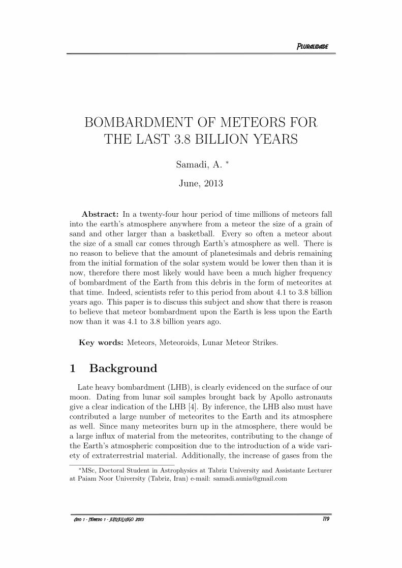
BOMBARDMENT OF METEORS FORTHE LAST 3.8 BILLION YEARS
Samadi, A. ∗
June, 2013
Abstract: In a twenty-four hour period of time millions of meteors fallinto the earth’s atmosphere anywhere from a meteor the size of a grain ofsand and other larger than a basketball. Every so often a meteor aboutthe size of a small car comes through Earth’s atmosphere as well. There isno reason to believe that the amount of planetesimals and debris remainingfrom the initial formation of the solar system would be lower then than it isnow, therefore there most likely would have been a much higher frequencyof bombardment of the Earth from this debris in the form of meteorites atthat time. Indeed, scientists refer to this period from about 4.1 to 3.8 billionyears ago. This paper is to discuss this subject and show that there is reasonto believe that meteor bombardment upon the Earth is less upon the Earthnow than it was 4.1 to 3.8 billion years ago.
Key words: Meteors, Meteoroids, Lunar Meteor Strikes.
1 Background
Late heavy bombardment (LHB), is clearly evidenced on the surface of ourmoon. Dating from lunar soil samples brought back by Apollo astronautsgive a clear indication of the LHB [4]. By inference, the LHB also must havecontributed a large number of meteorites to the Earth and its atmosphereas well. Since many meteorites burn up in the atmosphere, there would bea large influx of material from the meteorites, contributing to the change ofthe Earth’s atmospheric composition due to the introduction of a wide vari-ety of extraterrestrial material. Additionally, the increase of gases from the
∗MSc, Doctoral Student in Astrophysics at Tabriz University and Assistante Lecturerat Paiam Noor University (Tabriz, Iran) e-mail: [email protected]
1
119
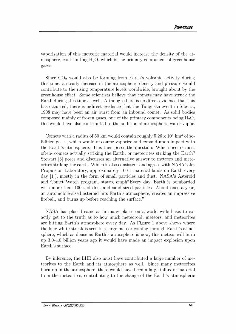
vaporization of this meteoric material would increase the density of the at-mosphere, contributing H2O, which is the primary component of greenhousegases.
Since CO2 would also be forming from Earth’s volcanic activity duringthis time, a steady increase in the atmospheric density and pressure wouldcontribute to the rising temperature levels worldwide, brought about by thegreenhouse effect. Some scientists believe that comets may have struck theEarth during this time as well. Although there is no direct evidence that thishas occurred, there is indirect evidence that the Tunguska event in Siberia,1908 may have been an air burst from an inbound comet. As solid bodiescomposed mainly of frozen gases, one of the primary components being H2O,this would have also contributed to the addition of atmospheric water vapor.
Comets with a radius of 50 km would contain roughly 5.26 x 10⁵ km3 of so-lidified gases, which would of course vaporize and expand upon impact withthe Earth’s atmosphere. This then poses the question: Which occurs mostoften- comets actually striking the Earth, or meteorites striking the Earth?Stewart [3] poses and discusses an alternative answer to meteors and mete-orites striking the earth. Which is also consistent and agrees with NASA’s JetPropulsion Laboratory, approximately 100 t material lands on Earth everyday [1]), mostly in the form of small particles and dust. NASA’s Asteroidand Comet Watch program, states, emph”Every day, Earth is bombardedwith more than 100 t of dust and sand-sized particles. About once a year,an automobile-sized asteroid hits Earth’s atmosphere, creates an impressivefireball, and burns up before reaching the surface.”
NASA has placed cameras in many places on a world wide basis to ex-actly get to the truth as to how much meteoroid, meteors, and meteoritesare hitting Earth’s atmosphere every day. As Figure 1 above shows wherethe long white streak is seen is a large meteor coming through Earth’s atmo-sphere, which as dense as Earth’s atmosphere is now, this meteor will burnup 3.0-4.0 billion years ago it would have made an impact explosion uponEarth’s surface.
By inference, the LHB also must have contributed a large number of me-teorites to the Earth and its atmosphere as well. Since many meteoritesburn up in the atmosphere, there would have been a large influx of materialfrom the meteorites, contributing to the change of the Earth’s atmospheric
2
120
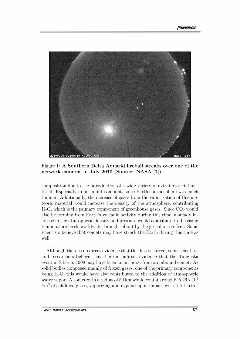
Figure 1: A Southern Delta Aquarid fireball streaks over one of thenetwork cameras in July 2010 (Source: NASA [1])
composition due to the introduction of a wide variety of extraterrestrial ma-terial. Especially in an infinite amount, since Earth’s atmosphere was muchthinner. Additionally, the increase of gases from the vaporization of this me-teoric material would increase the density of the atmosphere, contributingH2O, which is the primary component of greenhouse gases. Since CO2 wouldalso be forming from Earth’s volcanic activity during this time, a steady in-crease in the atmospheric density and pressure would contribute to the risingtemperature levels worldwide, brought about by the greenhouse effect. Somescientists believe that comets may have struck the Earth during this time aswell.
Although there is no direct evidence that this has occurred, some scientistsand researchers believe that there is indirect evidence that the Tunguskaevent in Siberia, 1908 may have been an air burst from an inbound comet. Assolid bodies composed mainly of frozen gases, one of the primary componentsbeing H2O, this would have also contributed to the addition of atmosphericwater vapor. A comet with a radius of 50 km would contain roughly 5.26 x 10⁵
km3 of solidified gases, vaporizing and expand upon impact with the Earth’s
3
121
atmosphere. This then poses the question: Which occurs most often- cometsactually striking the Earth, or meteorites striking the Earth? According toNASA’s Jet Propulsion Laboratory [1], approximately 100 t material landson Earth every day, mostly in the form of small particles and dust. Consistentwith Short and French [2] as well.
2 Evidence
In relation than to the recent large The Chelyabinsk Russia MeteoroidImpact in Chelyabinsk, Russia would seem to give considerable evidence, thatinstead of a comet blast occurring in Siberia in 1908, that in all likelihood,it was due to a large meteoroid that impacted Siberia instead. By what hasbeen discussed in this paper because of the amount of meteors and meteoritesthat strike the earth’s atmosphere literally millions of time per day in atwenty-four hour period of time, it would make more scientific sense, anddeductably logical that when the Earth has just formed and its atmospherewas either very thin or did not exist at all, that the earth was impacted withmuch more intense severity from meteors and/ or meteorites in much greaterquantities per twenty-four hour period of time 4.1 to 3.8 billion years ago inEarth’s infancy, compared to the current day and time in Earth’s history.
References
[1] NATIONAL AERONAUTICS AND SPACE ADMINISTRA-TION (NASA). What’s Hitting The Earth?. Science news.Available at: http://science.nasa.gov/science-news/science-at-nasa/2011/01mar meteornetwork/. Published in: Mar. 1st, 2011.
[2] SHORT, N.M., FRENCH, B.M. Shock Metamorphism of NaturalMaterials. Baltimore: Mono Book Corp., 1968.
[3] STEWART, R., AGUIAR, O., ARTUSO, G., ARISTIZABAL, C.,ACKERMAN, J., TRENTADUE, W., ROBINETT, R. Earth’sOceans: A Theoretical Approach How Interconnected Con-tinents and High Altitude Mountain Glaciers Formed Them.International Journal of Geology and Paleontology. Available at:http://www.journals-of-sciences.com/ijgp-geology–paleontology.html.Accessed in: Jan. 20th, 2013.
[4] TAYLOR, S.R. Planetary science: A lunar perspective. Houston:LPI/USRA, 1982.
4
122
HYDRODYNAMIC MODELING ANALYSISOF THE CIRCULATION OF THE BAY OF
FUNDY
Edinger, J.E. ∗
June, 2013
Abstract:The purposes of the Bay of Fundy Simulations are or back-ground information for a field trip to Acadia University in Wolfville, NSdealing with different aspects of the Bay of Fundy. To apply the IntrogllvhtWater Quality and Hydrodynamic model [1] to a large enough water bodyfor which the Coriolis acceleration could be significant. To examine how theIntrogllvht model sets up and performs for another case. (Alpha testing ofthe model software). The study investigates the following aspects of theBayof Fundy. Its general surface and bottom circulation patterns. The surfacedistribution of the Saint John and Saint Croix River outflows to show howthey might distribute eggs and larvae spawned within their shoreline embay-ments. The flushing time of water from different locations within the bayto estimate how fast exchange takes place within it and as an indication ofpossible water quality problems. The study covers: A general description ofthe processes driving circulation within the Bay, and the data required forsetting up a hydrodynamic and transport model of the bay. The tidal, fresh-water inflow and bathymetric data available from the internet for setting upthe model. Development of the model grid.The model setup Input Data forthe simulations Graphical descriptions of the circulation, spreading of theSaint John and Saint Croix Rivers.Surface and bottom water flushing times.The possible role of Coriolis Acceleration. Tides at different locations. Tidalvelocities at the mouth for comparison to available data.
Key words: Bay of Fundy, Hydrology, Hydrodynamic Modeling, Oceanog-raphy, Tidal Circulation.
∗PhD, Independent Consultant in Environmental Hydrology (Wayne PA, USA) e-mail:[email protected]
1
123
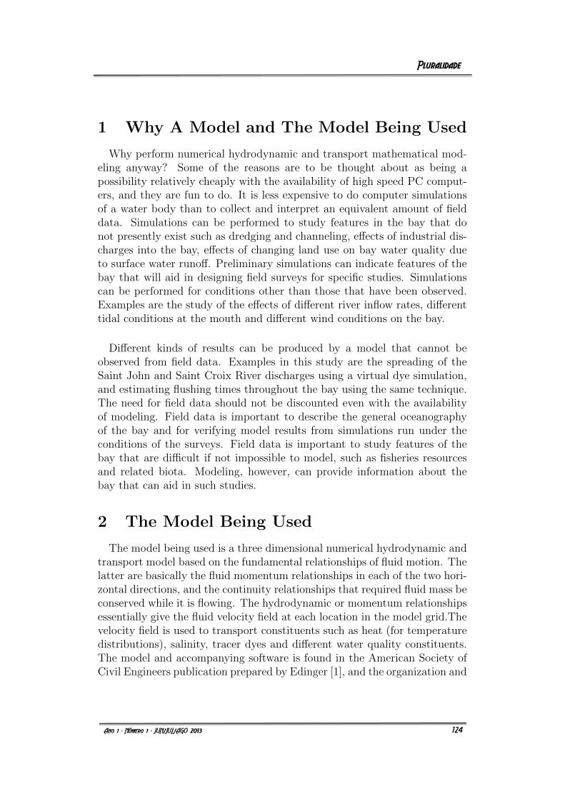
1 Why A Model and The Model Being Used
Why perform numerical hydrodynamic and transport mathematical mod-eling anyway? Some of the reasons are to be thought about as being apossibility relatively cheaply with the availability of high speed PC comput-ers, and they are fun to do. It is less expensive to do computer simulationsof a water body than to collect and interpret an equivalent amount of fielddata. Simulations can be performed to study features in the bay that donot presently exist such as dredging and channeling, effects of industrial dis-charges into the bay, effects of changing land use on bay water quality dueto surface water runoff. Preliminary simulations can indicate features of thebay that will aid in designing field surveys for specific studies. Simulationscan be performed for conditions other than those that have been observed.Examples are the study of the effects of different river inflow rates, differenttidal conditions at the mouth and different wind conditions on the bay.
Different kinds of results can be produced by a model that cannot beobserved from field data. Examples in this study are the spreading of theSaint John and Saint Croix River discharges using a virtual dye simulation,and estimating flushing times throughout the bay using the same technique.The need for field data should not be discounted even with the availabilityof modeling. Field data is important to describe the general oceanographyof the bay and for verifying model results from simulations run under theconditions of the surveys. Field data is important to study features of thebay that are difficult if not impossible to model, such as fisheries resourcesand related biota. Modeling, however, can provide information about thebay that can aid in such studies.
2 The Model Being Used
The model being used is a three dimensional numerical hydrodynamic andtransport model based on the fundamental relationships of fluid motion. Thelatter are basically the fluid momentum relationships in each of the two hori-zontal directions, and the continuity relationships that required fluid mass beconserved while it is flowing. The hydrodynamic or momentum relationshipsessentially give the fluid velocity field at each location in the model grid.Thevelocity field is used to transport constituents such as heat (for temperaturedistributions), salinity, tracer dyes and different water quality constituents.The model and accompanying software is found in the American Society ofCivil Engineers publication prepared by Edinger [1], and the organization and
2
124
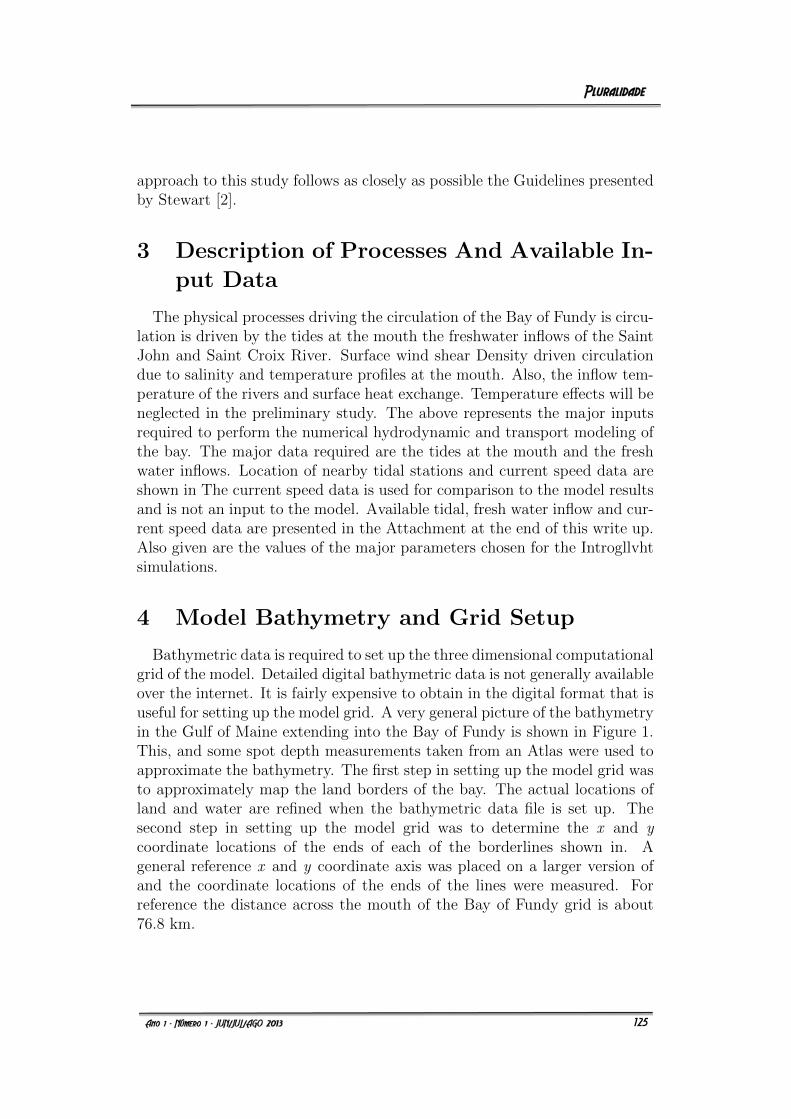
approach to this study follows as closely as possible the Guidelines presentedby Stewart [2].
3 Description of Processes And Available In-
put Data
The physical processes driving the circulation of the Bay of Fundy is circu-lation is driven by the tides at the mouth the freshwater inflows of the SaintJohn and Saint Croix River. Surface wind shear Density driven circulationdue to salinity and temperature profiles at the mouth. Also, the inflow tem-perature of the rivers and surface heat exchange. Temperature effects will beneglected in the preliminary study. The above represents the major inputsrequired to perform the numerical hydrodynamic and transport modeling ofthe bay. The major data required are the tides at the mouth and the freshwater inflows. Location of nearby tidal stations and current speed data areshown in The current speed data is used for comparison to the model resultsand is not an input to the model. Available tidal, fresh water inflow and cur-rent speed data are presented in the Attachment at the end of this write up.Also given are the values of the major parameters chosen for the Introgllvhtsimulations.
4 Model Bathymetry and Grid Setup
Bathymetric data is required to set up the three dimensional computationalgrid of the model. Detailed digital bathymetric data is not generally availableover the internet. It is fairly expensive to obtain in the digital format that isuseful for setting up the model grid. A very general picture of the bathymetryin the Gulf of Maine extending into the Bay of Fundy is shown in Figure 1.This, and some spot depth measurements taken from an Atlas were used toapproximate the bathymetry. The first step in setting up the model grid wasto approximately map the land borders of the bay. The actual locations ofland and water are refined when the bathymetric data file is set up. Thesecond step in setting up the model grid was to determine the x and ycoordinate locations of the ends of each of the borderlines shown in. Ageneral reference x and y coordinate axis was placed on a larger version ofand the coordinate locations of the ends of the lines were measured. Forreference the distance across the mouth of the Bay of Fundy grid is about76.8 km.
3
125
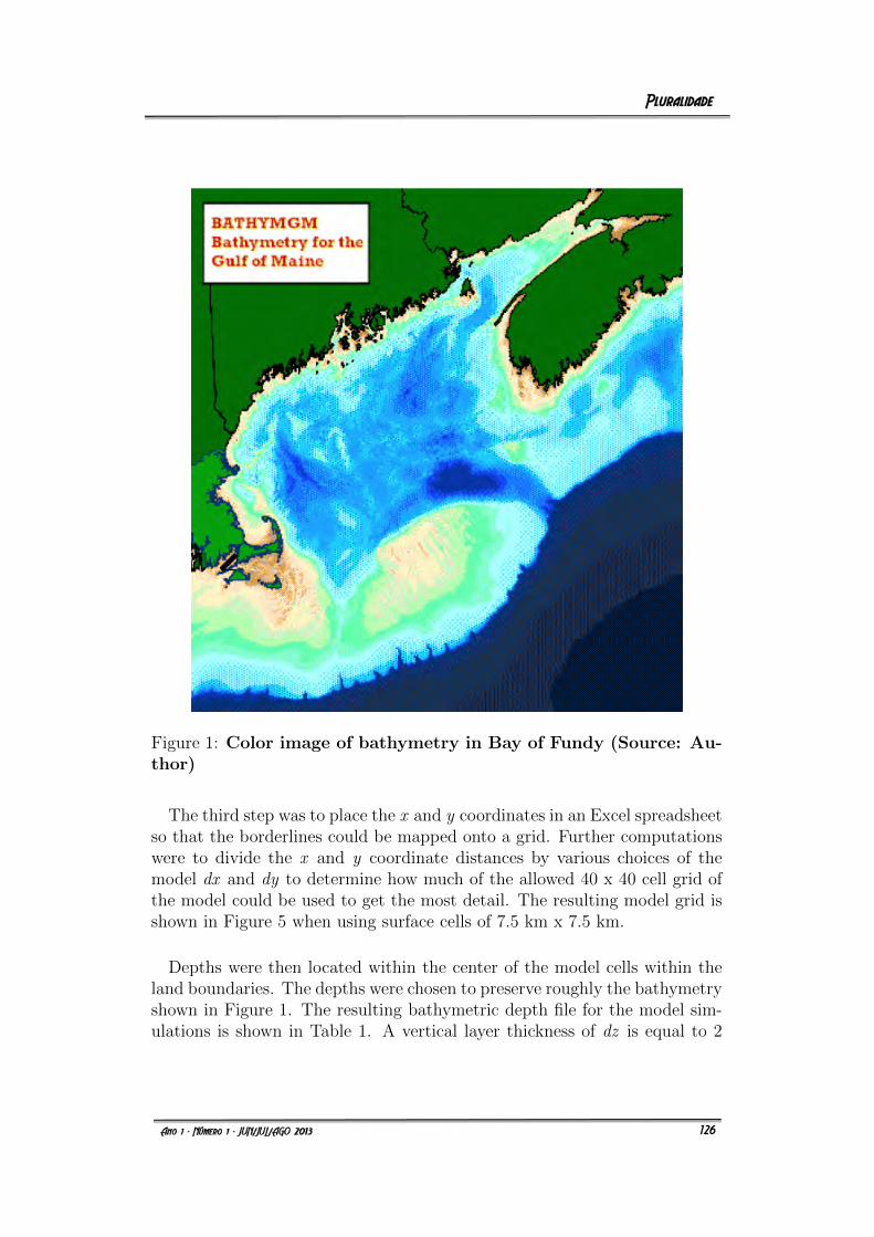
Figure 1: Color image of bathymetry in Bay of Fundy (Source: Au-thor)
The third step was to place the x and y coordinates in an Excel spreadsheetso that the borderlines could be mapped onto a grid. Further computationswere to divide the x and y coordinate distances by various choices of themodel dx and dy to determine how much of the allowed 40 x 40 cell grid ofthe model could be used to get the most detail. The resulting model grid isshown in Figure 5 when using surface cells of 7.5 km x 7.5 km.
Depths were then located within the center of the model cells within theland boundaries. The depths were chosen to preserve roughly the bathymetryshown in Figure 1. The resulting bathymetric depth file for the model sim-ulations is shown in Table 1. A vertical layer thickness of dz is equal to 2
4
126
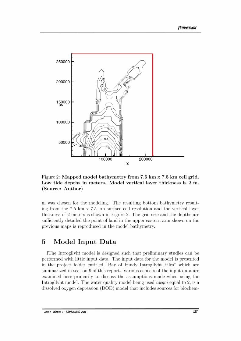
Figure 2: Mapped model bathymetry from 7.5 km x 7.5 km cell grid.Low tide depths in meters. Model vertical layer thickness is 2 m.(Source: Author)
m was chosen for the modeling. The resulting bottom bathymetry result-ing from the 7.5 km x 7.5 km surface cell resolution and the vertical layerthickness of 2 meters is shown in Figure 2. The grid size and the depths aresufficiently detailed the point of land in the upper eastern arm shown on theprevious maps is reproduced in the model bathymetry.
5 Model Input Data
IThe Introgllvht model is designed such that preliminary studies can beperformed with little input data. The input data for the model is presentedin the project folder entitled ”Bay of Fundy Introgllvht Files” which aresummarized in section 9 of this report. Various aspects of the input data areexamined here primarily to discuss the assumptions made when using theIntrogllvht model. The water quality model being used nwqm equal to 2, is adissolved oxygen depression (DOD) model that includes sources for biochem-
5
127
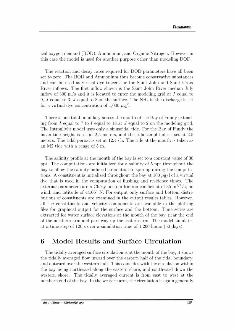
ical oxygen demand (BOD), Ammonium, and Organic Nitrogen. However inthis case the model is used for another purpose other than modeling DOD.
The reaction and decay rates required for DOD parameters have all beenset to zero. The BOD and Ammonium thus become conservative substancesand can be used as virtual dye tracers for the Saint John and Saint CroixRiver inflows. The first inflow shown is the Saint John River median Julyinflow of 300 m/s and it is located to enter the modeling grid at I equal to9, J equal to 3, J equal to 8 on the surface. The NH3 in the discharge is setfor a virtual dye concentration of 1,000 µg/l.
There is one tidal boundary across the mouth of the Bay of Fundy extend-ing from I equal to 7 to I equal to 18 at J equal to 2 on the modeling grid.The Introgllvht model uses only a sinusoidal tide. For the Bay of Fundy themean tide height is set at 2.5 meters, and the tidal amplitude is set at 2.5meters. The tidal period is set at 12.45 h. The tide at the mouth is taken asan M2 tide with a range of 5 m.
The salinity profile at the mouth of the bay is set to a constant value of 30ppt. The computations are initialized for a salinity of 5 ppt throughout thebay to allow the salinity induced circulation to spin up during the computa-tions. A constituent is initialized throughout the bay at 100 µg/l of a virtualdye that is used in the computation of flushing and residence times. Theexternal parameters are a Chezy bottom friction coefficient of 35 m1/2/s, nowind, and latitude of 44.66o N. For output only surface and bottom distri-butions of constituents are examined in the output results tables. However,all the constituents and velocity components are available in the plottingfiles for graphical output for the surface and the bottom. Time series areextracted for water surface elevations at the mouth of the bay, near the endof the northern arm and part way up the eastern arm. The model simulatesat a time step of 120 s over a simulation time of 1,200 hours (50 days).
6 Model Results and Surface Circulation
The tidally averaged surface circulation is at the mouth of the bay, it showsthe tidally averaged flow inward over the eastern half of the tidal boundary,and outward over the western half. This coincides with the circulation withinthe bay being northward along the eastern shore, and southward down thewestern shore. The tidally averaged current is from east to west at thenorthern end of the bay. In the western arm, the circulation is again generally
6
128
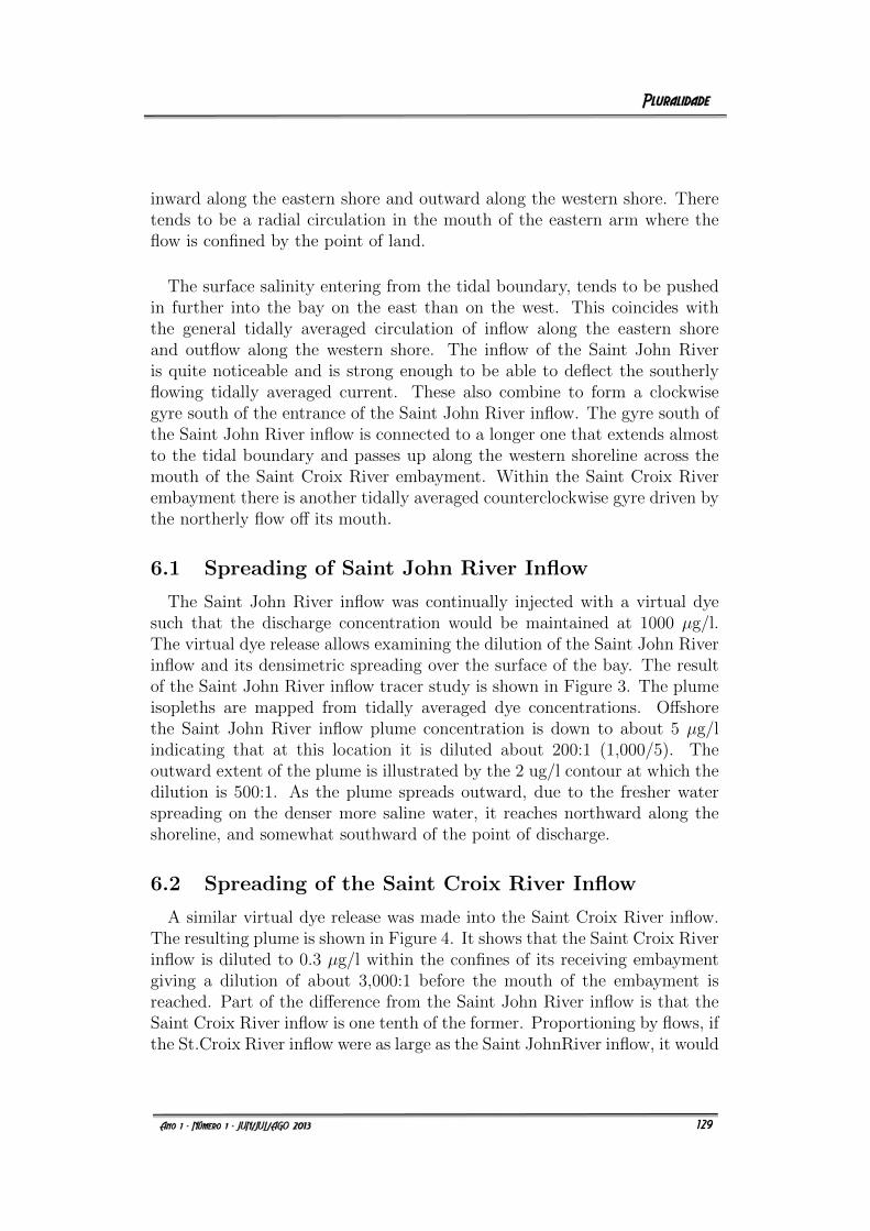
inward along the eastern shore and outward along the western shore. Theretends to be a radial circulation in the mouth of the eastern arm where theflow is confined by the point of land.
The surface salinity entering from the tidal boundary, tends to be pushedin further into the bay on the east than on the west. This coincides withthe general tidally averaged circulation of inflow along the eastern shoreand outflow along the western shore. The inflow of the Saint John Riveris quite noticeable and is strong enough to be able to deflect the southerlyflowing tidally averaged current. These also combine to form a clockwisegyre south of the entrance of the Saint John River inflow. The gyre south ofthe Saint John River inflow is connected to a longer one that extends almostto the tidal boundary and passes up along the western shoreline across themouth of the Saint Croix River embayment. Within the Saint Croix Riverembayment there is another tidally averaged counterclockwise gyre driven bythe northerly flow off its mouth.
6.1 Spreading of Saint John River Inflow
The Saint John River inflow was continually injected with a virtual dyesuch that the discharge concentration would be maintained at 1000 µg/l.The virtual dye release allows examining the dilution of the Saint John Riverinflow and its densimetric spreading over the surface of the bay. The resultof the Saint John River inflow tracer study is shown in Figure 3. The plumeisopleths are mapped from tidally averaged dye concentrations. Offshorethe Saint John River inflow plume concentration is down to about 5 µg/lindicating that at this location it is diluted about 200:1 (1,000/5). Theoutward extent of the plume is illustrated by the 2 ug/l contour at which thedilution is 500:1. As the plume spreads outward, due to the fresher waterspreading on the denser more saline water, it reaches northward along theshoreline, and somewhat southward of the point of discharge.
6.2 Spreading of the Saint Croix River Inflow
A similar virtual dye release was made into the Saint Croix River inflow.The resulting plume is shown in Figure 4. It shows that the Saint Croix Riverinflow is diluted to 0.3 µg/l within the confines of its receiving embaymentgiving a dilution of about 3,000:1 before the mouth of the embayment isreached. Part of the difference from the Saint John River inflow is that theSaint Croix River inflow is one tenth of the former. Proportioning by flows, ifthe St.Croix River inflow were as large as the Saint JohnRiver inflow, it would
7
129
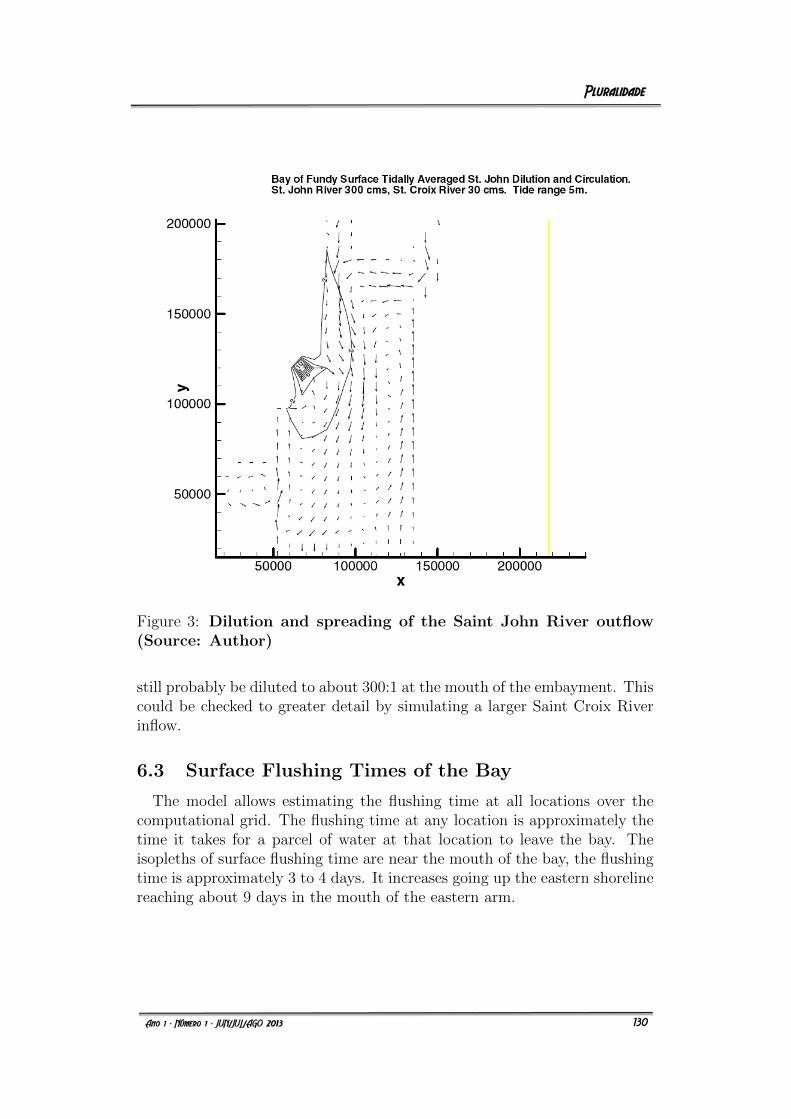
Figure 3: Dilution and spreading of the Saint John River outflow(Source: Author)
still probably be diluted to about 300:1 at the mouth of the embayment. Thiscould be checked to greater detail by simulating a larger Saint Croix Riverinflow.
6.3 Surface Flushing Times of the Bay
The model allows estimating the flushing time at all locations over thecomputational grid. The flushing time at any location is approximately thetime it takes for a parcel of water at that location to leave the bay. Theisopleths of surface flushing time are near the mouth of the bay, the flushingtime is approximately 3 to 4 days. It increases going up the eastern shorelinereaching about 9 days in the mouth of the eastern arm.
8
130
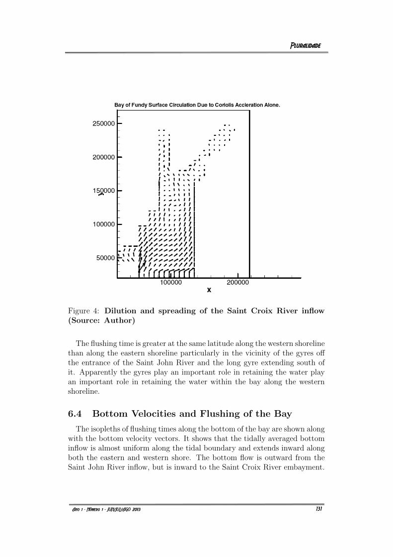
Figure 4: Dilution and spreading of the Saint Croix River inflow(Source: Author)
The flushing time is greater at the same latitude along the western shorelinethan along the eastern shoreline particularly in the vicinity of the gyres offthe entrance of the Saint John River and the long gyre extending south ofit. Apparently the gyres play an important role in retaining the water playan important role in retaining the water within the bay along the westernshoreline.
6.4 Bottom Velocities and Flushing of the Bay
The isopleths of flushing times along the bottom of the bay are shown alongwith the bottom velocity vectors. It shows that the tidally averaged bottominflow is almost uniform along the tidal boundary and extends inward alongboth the eastern and western shore. The bottom flow is outward from theSaint John River inflow, but is inward to the Saint Croix River embayment.
9
131
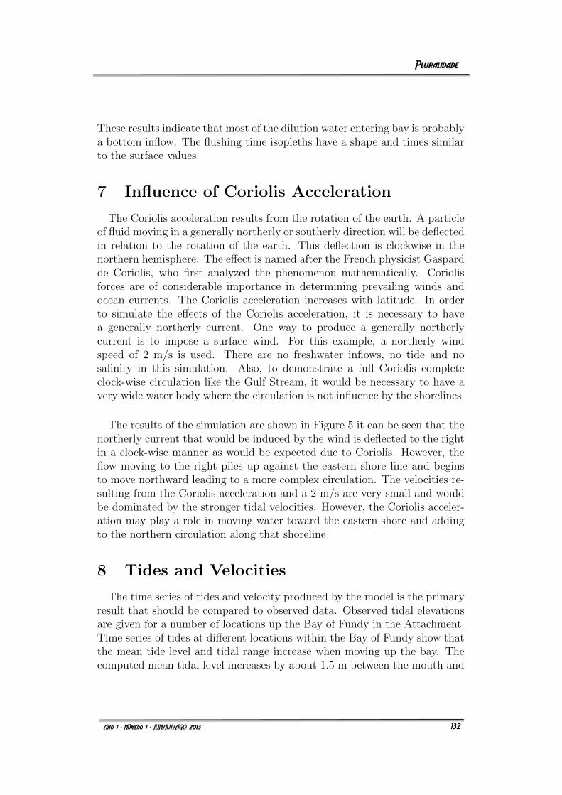
These results indicate that most of the dilution water entering bay is probablya bottom inflow. The flushing time isopleths have a shape and times similarto the surface values.
7 Influence of Coriolis Acceleration
The Coriolis acceleration results from the rotation of the earth. A particleof fluid moving in a generally northerly or southerly direction will be deflectedin relation to the rotation of the earth. This deflection is clockwise in thenorthern hemisphere. The effect is named after the French physicist Gaspardde Coriolis, who first analyzed the phenomenon mathematically. Coriolisforces are of considerable importance in determining prevailing winds andocean currents. The Coriolis acceleration increases with latitude. In orderto simulate the effects of the Coriolis acceleration, it is necessary to havea generally northerly current. One way to produce a generally northerlycurrent is to impose a surface wind. For this example, a northerly windspeed of 2 m/s is used. There are no freshwater inflows, no tide and nosalinity in this simulation. Also, to demonstrate a full Coriolis completeclock-wise circulation like the Gulf Stream, it would be necessary to have avery wide water body where the circulation is not influence by the shorelines.
The results of the simulation are shown in Figure 5 it can be seen that thenortherly current that would be induced by the wind is deflected to the rightin a clock-wise manner as would be expected due to Coriolis. However, theflow moving to the right piles up against the eastern shore line and beginsto move northward leading to a more complex circulation. The velocities re-sulting from the Coriolis acceleration and a 2 m/s are very small and wouldbe dominated by the stronger tidal velocities. However, the Coriolis acceler-ation may play a role in moving water toward the eastern shore and addingto the northern circulation along that shoreline
8 Tides and Velocities
The time series of tides and velocity produced by the model is the primaryresult that should be compared to observed data. Observed tidal elevationsare given for a number of locations up the Bay of Fundy in the Attachment.Time series of tides at different locations within the Bay of Fundy show thatthe mean tide level and tidal range increase when moving up the bay. Thecomputed mean tidal level increases by about 1.5 m between the mouth and
10
132
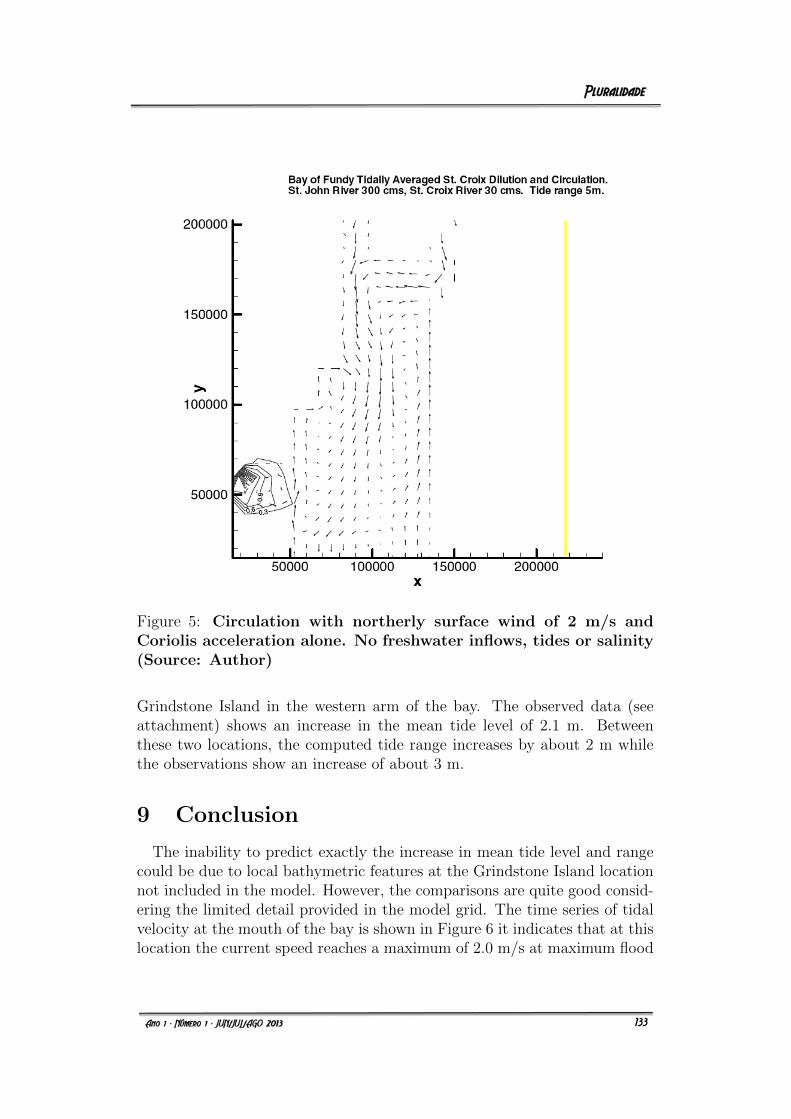
Figure 5: Circulation with northerly surface wind of 2 m/s andCoriolis acceleration alone. No freshwater inflows, tides or salinity(Source: Author)
Grindstone Island in the western arm of the bay. The observed data (seeattachment) shows an increase in the mean tide level of 2.1 m. Betweenthese two locations, the computed tide range increases by about 2 m whilethe observations show an increase of about 3 m.
9 Conclusion
The inability to predict exactly the increase in mean tide level and rangecould be due to local bathymetric features at the Grindstone Island locationnot included in the model. However, the comparisons are quite good consid-ering the limited detail provided in the model grid. The time series of tidalvelocity at the mouth of the bay is shown in Figure 6 it indicates that at thislocation the current speed reaches a maximum of 2.0 m/s at maximum flood
11
133
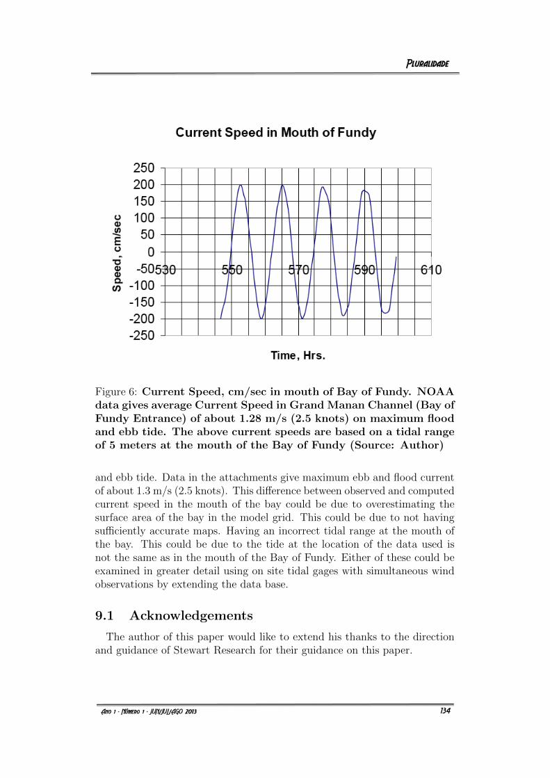
Figure 6: Current Speed, cm/sec in mouth of Bay of Fundy. NOAAdata gives average Current Speed in Grand Manan Channel (Bay ofFundy Entrance) of about 1.28 m/s (2.5 knots) on maximum floodand ebb tide. The above current speeds are based on a tidal rangeof 5 meters at the mouth of the Bay of Fundy (Source: Author)
and ebb tide. Data in the attachments give maximum ebb and flood currentof about 1.3 m/s (2.5 knots). This difference between observed and computedcurrent speed in the mouth of the bay could be due to overestimating thesurface area of the bay in the model grid. This could be due to not havingsufficiently accurate maps. Having an incorrect tidal range at the mouth ofthe bay. This could be due to the tide at the location of the data used isnot the same as in the mouth of the Bay of Fundy. Either of these could beexamined in greater detail using on site tidal gages with simultaneous windobservations by extending the data base.
9.1 Acknowledgements
The author of this paper would like to extend his thanks to the directionand guidance of Stewart Research for their guidance on this paper.
12
134
References
[1] EDINGER, J.E. Waterbody Hydrodynamic and Water QualityModeling. An Introductory Workbook and CD-ROM on ThreeDimensional Waterbody Modeling. Reston VA: ASCE Press, 2002.
[2] STEWART, R., AGUIAR, O.A., ARTUSO, G., ARISTIZABAL,C.I.O., ACKERMAN, J.R., TRENTADUE, W., ROBINETT, R.Earth’s oceans; A theoretical approach how interconnectedcontinents and high altitude mountain glaciers formedthem. Journal of the International Society of Peer Reviewers.Available at: http://www.stewart-research-consulting.com/up-loads/6/4/5/4/6454783/earths oceans -a theorectical approachhow earths high altitude continent mountains formed them.pdf. Ac-cessed in Jul. 2nd, 2013.
13
135
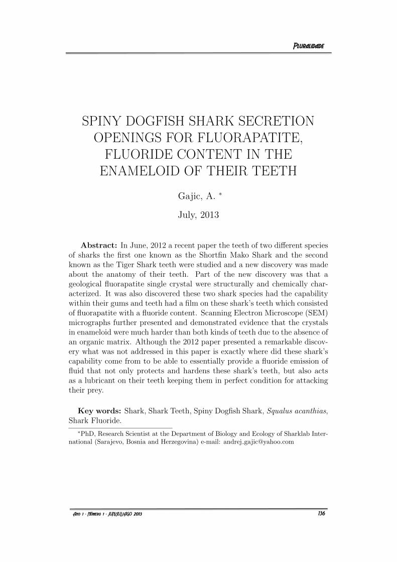
SPINY DOGFISH SHARK SECRETIONOPENINGS FOR FLUORAPATITE,FLUORIDE CONTENT IN THEENAMELOID OF THEIR TEETH
Gajic, A. ∗
July, 2013
Abstract: In June, 2012 a recent paper the teeth of two different speciesof sharks the first one known as the Shortfin Mako Shark and the secondknown as the Tiger Shark teeth were studied and a new discovery was madeabout the anatomy of their teeth. Part of the new discovery was that ageological fluorapatite single crystal were structurally and chemically char-acterized. It was also discovered these two shark species had the capabilitywithin their gums and teeth had a film on these shark’s teeth which consistedof fluorapatite with a fluoride content. Scanning Electron Microscope (SEM)micrographs further presented and demonstrated evidence that the crystalsin enameloid were much harder than both kinds of teeth due to the absence ofan organic matrix. Although the 2012 paper presented a remarkable discov-ery what was not addressed in this paper is exactly where did these shark’scapability come from to be able to essentially provide a fluoride emission offluid that not only protects and hardens these shark’s teeth, but also actsas a lubricant on their teeth keeping them in perfect condition for attackingtheir prey.
Key words: Shark, Shark Teeth, Spiny Dogfish Shark, Squalus acanthias,Shark Fluoride.
∗PhD, Research Scientist at the Department of Biology and Ecology of Sharklab Inter-national (Sarajevo, Bosnia and Herzegovina) e-mail: andrej [email protected]
1
136
1 The Spiny Dogfish Shark (Squalus acan-
thias)
Figure 1: In the upper top image is of the shark species known asSpiny Dogfish Shark (Squalus acanthias). This image was origi-nally presented in the paper of Bigelow and Schroeder [1]. Thatshows the upper and lower jaw teeth as depicted in (A). Where theyellow arrow points away from (A) to an example tooth of SpinyDogfish Shark. Where as a horizontal artist rendition is presentedand depicted in (B), which is depicted and projected in a larger sideview (3D) box, as seen in (C). Which B and C are used as visualaids present and demonstrate how these sporadic secretion open-ings for the fluroapatitie fluoride content to seep out of on to theshark’s teeth. Providing not only a fluoride-like film on their teethprotecting them, but which also provides a lubricant on the sharksteeth as well. The above illustration marked (A) first appeared inGarman [4]. (Source: Author, [1], [4])
Enax [3] and his team presents the significant discovery in their paper asaforementioned in the abstract of this paper that the Shortfin Mako Shark(Isurus oxyrinchus) and the Tiger Shark (Galeocerdo cuvier) teeth were stud-ied in 2012. The new anatomical discovery on these two species of shark
2
137
characterized that a single geological fluorapatite crystal was structurallyand chemically responsible for producing a film on these shark’s teeth whichconsisted of fluorapatite with a fluoride content. The evidence provided inthis paper and study were SEM micrographs, which gave evidence that thecrystals in enameloid were much harder than both kinds of teeth in bothshark species, because of the absence of an organic matrix. However, wehave discovered where the fluoride like secreted film comes from. That thereare special openings in the Spiny Dogfish Shark (Squalus acanthias) teethwhere this secretion originates from.
2 Secretion Openings For The Diet of Spiny
Dogfish Shark (Squalus acanthias)
The authors of this paper also propose that it is not just the Spiny DogfishShark species that has these secretion openings in its teeth. We further pro-pose by our study of the aforementioned shark species that the previous sharkspecies Shortfin Mako Shark and the Tiger Shark, have these fluoride-like se-cretion openings sporadically located in certain teeth within their upper andlower jaw teeth in like manner just like the Spiny Dogfish Shark as discussedand presented in this paper. This is essentially how Enax [3] and his teamwere able to discover the ”Resulting fluoride-like secreted film” on the Short-fin Mako and the Tiger Sharks species teeth. However, we contend havingdiscovered the ”cause” from where where this secretion originates. It wasfurther found that for the Shortfin Mako and the Tiger Sharks species filmwas indigenous diet, as it is with the Spiny Dogfish Shark.
3 Conclusion
By being able to study the Spiny Dogfish Shark (Squalus acanthias), it hasenabled the author of this paper to make a connection between the fluoridelike secretion discovered by Enax [3]) and his team. It has also provided adeeper understanding to the data and sources of additional reference to SteveKemper studies of different shark species at the Smithsonian Institution.Which also include the studies conducted by Clark [2], Kenney [5], Lemonick[6] and facts and details of sharks history, characteristics, senses, behavior,feeding and sex online references as well.
3
138
3.1 Acknowledgements
The author of this paper would like to thank any and all scientists, re-searchers, and science disciplines related to the science of Oceanography andMarine Sciences for all of their research and international cooperation. Forwithout their dedication such papers as this one would not have been possi-ble.
References
[1] BIGELOW, H.B., SCHROEDER, W.C.. Fishes of the western northatlantic, Part One, Lancelets, Cyclostomes, Sharks. MemoirSears Foundation for marine research, Number 1. New Haven: YaleUniversity. 1948.
[2] CLARK, E. Sharks: Magnificent and misunderstood. NationalGeographic, August 1981.
[3] ENAX, J., PRYMAK, O., RAABE, D., EPPLE, M. Structure, com-position and mechanical properties of shark teeth. Journal ofStructural Biology 178-3: 290-299, 2012.
[4] GARMAN, S. The Plagiostomia (Sharks, Skates and Rays). Mem-oirs of the museum of comparative zoology. Cambridge: Harvard Col-lege, 1913.
[5] KENNEY, N.T.. Sharks: Wolves of the sea. National Geographic,February 1968,
[6] LEMONICK, M.D. Under Attack. Time, September 1997.
4
139


![Colec]ia PLURAL](https://img.pdfslide.net/doc/110x75/63590fd068c5ffb421045d28/colecia-plural.jpg)


