Pointwise Estimates and Exponential Laws in Metastable Systems Via Coupling Methods

Alessandra Bianchi, Anton Bovier, Dmitry Ioffe

no. 461

Diese Arbeit ist mit Unterstützung des von der Deutschen Forschungs-

gemeinschaft getragenen Sonderforschungsbereichs 611 an der Universität

Bonn entstanden und als Manuskript vervielfältigt worden.

Bonn, November 2009

POINTWISE ESTIMATES AND EXPONENTIAL LAWS IN METASTABLESYSTEMS VIA COUPLING METHODS

ALESSANDRA BIANCHI, ANTON BOVIER, AND DMITRY IOFFE

ABSTRACT. We show how coupling techniques can be used in some metastablesystems to prove that mean metastable exit times are almost constant as functionsof the starting microscopic configuration within a “metastable set”. In the exampleof the Random Field Curie Weiss model, we show that these ideas can also be usedto prove asymptotic exponentiality of normalized metastable escape times.

1. INTRODUCTION

1.1. The problem. Over the last years, potential theoretic methods were systemat-ically developed to rigorously derive sharp estimates for characteristic quantities inMarkov processes exhibiting so-called metastable behavior [4, 2]. Roughly speak-ing, metastable systems are characterized by the fact that the state space can bedecomposed into several disjoint subsets, with the property that transition timesbetween subspaces are long compared to characteristic mixing times within eachsubspace. In simple situations, in particular when the state space is sufficientlydiscrete (e.g. fixed finite state space), mixing could be effectively characterizedthrough return probabilities to some specific atoms (see [4]).

A key idea of the potential theoretic approach is to express quantities of physicalinterest in terms of capacities and to use variational principles to compute the latter.A fundamental identity used systematically in this approach is a representationformula for the Green’s function, gB(x, y), with Dirichlet conditions in a set B, thatreads (in the context of arbitrary discrete state space)

gB(x, y) = µ(y)hx,B(y)

cap(x,B), (1.1)

where B is a subset of the configuration space, hx,B(y) is the equilibrium potential,i.e.

hx,B(y) =

1, if y = x

0, if y ∈ BPy (τx < τB) , otherwise.

(1.2)

cap(x,B) is the capacity between the set B and the point x.

Date: September 7, 2009.2000 Mathematics Subject Classification. 82C44,60tK35,60G70.Key words and phrases. Disordered system, random field Curie-Weiss model, Glauber dynamics,

metastability, potential theory, coupling, exponential law.This research was supported in part through a grant by the German-Israeli Foundation (GIF).

A. Bovier is supported in par by the DFG in the SFB 611 and the Hausdorff Center for Mathe-matics. The kind hospitality of the Technion, Haifa, the Weierstrass-Institute for Applied Anal-ysis and Stochastics, and the Institute of Applied Mathematics at Bonn University is gratefullyacknowledged.

1

COUPLING 2

This formula (which gives immediately a formula for the mean hitting time of B,for the process starting in x) is useful as long as the ratio appearing in (1.1) is notseriously of the form 0/0, or, more precisely, if the capacity is essentially invariantif the point x is replaced by a “fat” neighborhood of x. 1 Examples where thisis not the case are diffusion processes in d > 1, Glauber dynamics in the case offinite temperature, etc.. In such cases a useful version can be extracted by suitableaveraging. E.g., ifA ≡ Ax is a neighborhood of x, we can readily derive the formula

EνAτB =1

cap(A,B)

∑y

hA,B(y)µ(y), (1.3)

where νA is a specific probability distribution on A. The right-hand side can beevaluated in many cases of interest when formula (1.1) makes no sense. This hasbeen demonstrated recently in two examples, the Glauber dynamics of the randomfield Curie-Weiss model at finite temperature [1], and the Kawasaki dynamics inthe zero temperature limit on volumes that diverge exponentially with the inversetemperature [6].

An obvious question is whether the mean hitting time of B really depends on thespecific initial distribution νA or whether, for all z ∈ A, EzτB ∼ EνAτB. A relatedquestion is whether the distribution of this hitting times is typically exponential, asone would expect. This problem arises already in the case of diffusion processes onRd, d > 1. In that case, however, the issue is readily resolved by the use of ellipticregularity theory, which provides a priori bounds on the Holder continuity of therelevant functions [3]. In the case of stochastic Ising models, however, we are notaware of comparable results.

In the present paper we will present a method that allows to prove such re-sults at least in some cases. It is based on coupling techniques and allows to turnthe following simple heuristic argument into a rigorous proof: The Markov chainshould mix quickly before it leaves a substantial neighborhood of the starting pointx; since the mixing time is short compared to the hitting time τB, the mean of τBshould be the same for all starting configuration in A. Moreover, the chain willreturn many times to A before reaching B; by rapid mixing, the return times willbe i.i.d., hence the number of returns will be geometric, and the scaled hitting timewill be exponential.

To demonstrate the usefulness of this approach, our key example will be the Ran-dom Field Curie-Weiss model with continuous distribution of the random fields. Inthat sense, the present result is also a completion of our previous paper [1]. How-ever, the basic ideas are more general and will be of relevance for the treatment ofmetastable systems at large.

1.2. Setting. In this subsection we describe a general setting in which our meth-ods can be applied.

In the sequel N will be a large parameter. We consider (families of) Markovprocesses, σ(t), with finite state space, SN ≡ −1, 1N , and transition probabilitiespN that are reversible w.r.t. a (Gibbs) measure, µN . Transition probabilities pN

1To be more precise, it may happen that hx,B(y) = f(A)hA,B(y)and cap(x,B) = f(A)cap(A,B),for “macroscopic” sets A 3 x, where f(A) cap(A,B). Then hx,B(y)

cap(x,B) = hA,B(y)cap(A,B) , but except in

cases where this is manifest by some symmetry, it will be very hard to establish this fact by a directestimation of numerator and denominator in (1.1).

COUPLING 3

always have the following structure: At each step a site x ∈ Λ is chosen withuniform probability 1/N . Then the spin at x is set to ±1 with probabilities p±x (σ);p+x (σ) + p−x (σ) ≡ 1. In the sequel we shall assume that there exists α ∈ [1/2, 1) such

thatmaxx,σ,±

p±x (σ) ≤ α. (1.4)

A key hypothesis is the existence of a family of “good” mesoscopic approximationsof our processes. By this we mean the following: There is a sequence of disjointpartitions, Λn

1 , . . . ,Λnkn, of Λ ≡ 1, . . . , N, and a family of maps, m(n) : SN →

Γn ⊂ Rn, given by

mni (σ) =

1

N

∑x∈Λni

σx. (1.5)

We will always think of these partitions as nested, i.e.

Λn+11 , . . . ,Λn+1

kn+1

is a re-

finement of Λn1 , . . . ,Λ

nkn. On the other hand, to lighten the notation, we will

mostly drop the superscript and identify kn = n, and refer to the generic partitionΛ1, . . . ,Λn. It will be convenient to introduce the notation Sn[m] ≡ (mn)−1(m) forthe set-valued inverse images of mn. We think of the maps mn as some block aver-ages of our ‘microscopic variables σi over blocks of decreasing (in n) “mesoscopic”sizes.

As it is well known, the image process, mn(σ(t)), is in general not Markovian.However, there is a canonical Markov process, mn(t), with state space Γn and re-versible measure Qn ≡ µN (mn)−1, that is a “best” approximation of mn(σ(t)),in the sense that if mn(σ(t)) is Markov, then mn(t) = mn(σ(t)) (in law). For allm,m′ ∈ Γn, the transition probabilities of this chain are given by

rN(m,m′) ≡ 1

Qn(m)

∑σ∈Sn[m]

σ′∈Sn[m′]

µN(σ)pN(σ, σ′). (1.6)

By “good approximations” we will mean that the following two conditions hold:(A.1) the sequence of chains mn(t) approximates mn(σ(t)) in the strong sense

that that there exists ε(n) ↓ 0, as n ↑ ∞, such that 2 for any m,m′ ∈ Γn,

maxσ∈Sn[m],σ′∈Sn[m′]

rN (m,m′)>0

∣∣∣∣pN(σ, σ′)|Sn[m′]|rN(m,m′)

− 1

∣∣∣∣ ≤ ε(n). (1.7)

(A.2) The microscopic flip rates satisfy: If mn(σ) = mn(η) and σx = ηx, thenp±x (σ) = p±x (η).

Finally, we need to place us in a “metastable” situation. Specifically, we willassume that there exist two disjoint sets A = σ ∈ SN : mn0(σ) ∈ A and B =σ ∈ SN : mn0(σ) ∈ B, for some n0 and sets A,B ∈ Γn0, a constant C > 0 and asequence an <∞, such that, for all n ≥ n0 large enough and for all σ, σ′ ∈ A,

Pσ′[τB < τmn(σ)

]≤ ane−CN , (1.8)

2Note that our assumption is indeed much stronger then the maybe more natural looking

maxσ∈Sn[m]

∣∣∣∣∣∑σ′∈Sn[m′] p(σ, σ

′)

rN (m,m′)− 1

∣∣∣∣∣ ≤ ε(n).

COUPLING 4

where, with a little abuse of notation, we denoted by τmn(σ) the first hitting time ofthe set Sn[mn(σ)].

In this setting we will prove the following theorem.

Theorem 1.1. Consider a Markov process as described above, and let A,B be suchthat (1.8) holds. Then,

maxσ,σ′∈A

∣∣∣∣ EστBEσ′τB

− 1

∣∣∣∣ ≤ e−CN/2. (1.9)

The strategy of the proof of Theorem 1.1 will be as follows:Consider an auxiliary Markov chain on the state space SN for which the rates

p(n)N (σ, σ′) = rN(mn(σ),mn(σ′))/Sn[mn(σ′)]. (1.10)

For such chains we can adopt a coupling mechanism constructed by Levin et al.[8] in the case of the Curie-Weiss model. Then we show that for the original chain,one can construct a coupling that will succeed with a probability that is not toosmall; finally, due to the strong recurrence property (1.8), we will be able to retrythe coupling in the case of failure until final success. The details of this procedureare somewhat intricate, as we must make sure to avoid conditioning that couldmodify the mean hitting times.

Remark. We formulate the assumptions here in the context in which we will actu-ally prove our results. The restriction to the state space −1, 1N is mainly donebecause we need to construct an explicit coupling. It is rather straightforward togeneralize everything to the case of Potts spins (SN ≡ 1, . . . , qN) and maps mn

whose components are permutation invariant functions of the spin variables onΛ

(n)i .

A second and related problem that tends to arise in the situation that we areinterested in is the breakdown of strict renewal properties. This is a well-knownissue in the theory of continuous space Markov processes where methods suchas Nummelin splitting [9] were devised to prove e.g. ergodic theorem in Harrisrecurrent chains. Here we would like to use renewal arguments e.g. to proveasymptotic exponentiality of the law of τB, for instance. We will show that againcoupling arguments can be used to solve such problems.

As an example we will prove the following theorem.

Theorem 1.2. In the random field Curie-Weiss model, for A and B chosen to satisfythe hypothesis of Theorem 1.1,

Pσ (τB/EστB > t)→ e−t, as N ↑ ∞, (1.11)

for all σ ∈ A and for all t ∈ R+.

The proof of this theorem will be a little involved. The basic idea is to derive arenewal equation for the Laplace transform of τB. This will require, again, the useof analogous coupling techniques.

1.3. The random field Curie-Weiss model. The results of this paper are moti-vated by the study of the Glauber dynamics of the random field Curie-Weiss model(RFCW). We will show that the assumptions of the two theorems above can beverified in that model. We briefly recall results for this model obtained recently in[1].

COUPLING 5

In the RFCW model the state space is SN ≡ −1, 1N , the Gibbs measure is givenby

µN(σ) = Z−1N exp (−βHN(σ)) , (1.12)

and the random Hamiltonian, HN , is defined as

HN(σ) ≡ −N2

(1

N

∑i∈Λ

σi

)2

−∑i∈Λ

hiσi, (1.13)

where Λ ≡ 1, . . . , N and hi, i ∈ Λ, are i.i.d. random variables on some probabilityspace (Ω,F ,Ph).

The total magnetization,

mN(σ) ≡ 1

N

∑i∈Λ

σi, (1.14)

is an effective order parameter of the model, and the sets of configurations wherethe magnetization takes particular values, play the role of metastable states. Morespecifically, we introduce the law of mN through

Qβ,N ≡ µβ,N m−1N , (1.15)

on the set of possible values ΓN ≡ −1,−1 + 2/N, . . . , 1. Qβ,N satisfies a largedeviation property, in particular

Zβ,NQβ,N(m) =

√2I′′N (m)

Nπexp (−NβFβ,N(m)) (1 + o(1)) , (1.16)

with IN being the Legendre transform of

t 7→ 1

N

∑i∈Λ

log cosh (t+ βhi) , (1.17)

and with a fairly explicit form for the rate function (“free energy”), Fβ,N . Themetastable states correspond to local minima of Fβ,N , whenever they exist.

A crucial feature of the model is that we can introduce a family of mesoscopicvariables in such a way that the dynamics on these mesoscopic variables is wellapproximated by a Markov process. Let us briefly describe these mesoscopic vari-ables.Coarse graining. Let I denote the support of the distribution of the random fields.Let I`, with ` ∈ 1, . . . , n, be a partition of I such that, for some C < ∞ and forall `, |I`| ≤ C/n ≡ ε.

Each realization of the random field hii∈N induces a random partition of theset Λ ≡ 1, . . . , N into subsets

Λk ≡ i ∈ Λ : hi ∈ Ik. (1.18)

We may introduce n order parameters

mk(σ) ≡ 1

N

∑i∈Λk

σi. (1.19)

We denote by m the n-dimensional vector (m1, . . . ,mn). m takes values in the set

ΓnN ≡ ×nk=1

−ρN,k,−ρN,k + 2

N, . . . , ρN,k − 2

N, ρN,k

, (1.20)

where

ρk ≡ ρN,k ≡|Λk|N

. (1.21)

COUPLING 6

Note that the random variables ρN,k concentrate exponentially (in N) aroundtheir mean value EhρN,k = Ph[hi ∈ Ik] ≡ pk.

The Hamiltonian can be written as

HN(σ) = −NE(m(σ)) +n∑`=1

∑i∈Λ`

σihi, (1.22)

where E : Rn → R is the function

E(x) ≡ 1

2

(n∑k=1

xk

)2

+n∑k=1

hkxk, (1.23)

with

h` ≡1

|Λ`|∑i∈Λ`

hi, and hi ≡ hi − h`. (1.24)

The equilibrium distribution of the variables m(σ) is given by

Qβ,N(x) ≡ µβ,N(m(σ) = x) (1.25)

=1

ZNeβNE(x)Eσ1m(σ)=xe

Pn`=1

Pi∈Λ`

σi(hi−h`).

For a mesoscopic subset A ⊆ ΓnN , we define its microscopic counterpart,

A = Sn[A] = σ ∈ SN : m(σ) ∈ A . (1.26)

Note that, as in the one-dimensional case, we can express the right-hand side of(1.26) as

Zβ,NQβ,N(x) =n∏`=1

√(I′′N,`(x`/ρ`)/ρ`)

Nπ/2exp (−NβFβ,N(x)) (1 + O(1)) , (1.27)

with a rather explicit expression for the function Fβ,N ,

Fβ,N(x) ≡ −1

2

(n∑`=1

x`

)2

−n∑`=1

x`h` +1

β

n∑`=1

ρ`IN,`(x`/ρ`). (1.28)

The key point of the construction above is that it places the RFCW model in thecontext described in Section 1.2. Namely, defining the mesoscopic rates rN(m,m′)in (1.6) for the functions m defined in (1.19), one can easily verify that the es-timates (1.7) hold, as was exploited in [1]. That also the recurrence hypothesis(1.8) holds in this model, will be shown in the next subsection.

In [1] we proved the following:

Theorem 1.3. Assume that β and the distribution of the magnetic field are such thatthere exist more than one local minimum of Fβ,N . Let m∗ be a local minimum of Fβ,N ,M ≡ M(m∗) be the set of minima of Fβ,N such that Fβ,N(m) < Fβ,N(m∗), and z∗ bethe minimax between m and M , i.e. the lower of the highest maxima separating mfrom M to the left respectively right. Then, Ph-almost surely,

EνS[m∗],S[M ]τS[M ] = C(β,m∗,M)N exp (βN [Fβ,N(z∗)− Fβ,N(m∗)]) (1 + o(1)) (1.29)

where C(β,m∗,M) are constants that are computed explicitly in [1].

COUPLING 7

Here the initial measure, νS[m∗],S[M ], is the so-called last exit biased distributionon the set S[m∗] ≡ σ ∈ SN : mN(σ) = m∗, given by the formula

νA,B(σ) =µβ,N(σ)Pσ[τB < τA]∑σ∈A µβ,N(σ)Pσ[τB < τA]

. (1.30)

Although the theorem is states in [1] for the starting measure in a set definedwith respect to the one-dimensional order parameter, the estimates given thereimmediately imply that the same formulas hold for EνS[m∗],S[M ]

τS[M ], with m∗ a localminimum in the n-dimensional order parameter space.

The results of the present paper will allow to show that the same estimates holdpointwise even in a neighborhood of S[m∗], for n large enough.

1.4. Local recurrence in the RFCW model. Before starting the proof of 1.9, let usverify hypothesis 1.8 for the RFCW model. Specifically, let us define the metastableset Aδ ⊂ ΓnN as the ball, with respect to the Hamming distance, of fixed radius δN ,δ > 0, centered on a local minimum m∗ of Fβ,N . Let Aδ ⊂ SN be the correspondingmicroscopic metastable and denote by τm the first hitting time of the set Sn[m].With this notation we have:

Lemma 1.4. There exist δ > 0 and c1 > 0 such that, for all n large enough, σ, σ′ ∈ Aδ,

Pσ[τB < τm(σ′)

]≤ e−c1N . (1.31)

Proof. We first notice that, if σ′ ∈ Sn[m∗], then the lemma is true for all n suffi-ciently large and with a constant c0 independent of n , as it has been proved in [1](see Prop. 6.12).

Moreover, for all σ, σ′ ∈ Aδ,

Pσ[τm(σ′) < τm∗

]≥ e−cδN , (1.32)

for some finite and positive constant c. To see this, notice that due to the propertyof Aδ, it is possible to construct a mesoscopic path from m(σ) to m(σ′) with lengthat most δN . Implementing the argument that it is used in the proof of Lemma 6.11of [1], one gets (1.32).

To prove (1.31), we then use a renewal argument. Let us consider a configura-tion σ ∈ Sn[m∗] and a generic σ′ ∈ Aδ, and set for simplicity m ≡ m(σ′). Then

Pσ(τB < τm) ≤ Pσ(τB < τm ∧ τm∗) +∑

η∈Sn[m∗]

Pσ(τm∗ < τB < τm , σ(τm∗) = η)

≤ Pσ(τB < τm∗) + maxη∈Sn[m∗]

Pη(τB < τm)Pσ(τm∗ < τm)

≤ e−c0N + maxη∈Sn[m∗]

Pη(τB < τm)(1− e−cδN

), (1.33)

where in the second line we used the Markov property, and in the last line we usedinequality (1.31) and (1.32). Taking the maximum over σ ∈ Sn[m∗] on both sidesof (1.33) and rearranging the summation, we get inequality (1.31) for σ ∈ Sn[m∗],with a constant c1 = c0 − cδ which is positive for any δ small enough.

COUPLING 8

Then, let us consider the general case of σ, σ′ ∈ Aδ and set again m ≡ m(σ′). Asbefore, we have

Pσ(τB < τm) ≤ Pσ(τB < τm ∧ τm∗) +∑

η∈Sn[m∗]

Pσ(τm∗ < τB < τm , σ(τm∗) = η)

≤ Pσ(τB < τm∗) + maxη∈Sn[m∗]

Pη(τB < τm)Pσ(τm∗ < τB)

≤ e−c0N + e−c1N = e−c1N(1 + o(1)), (1.34)

where in the third line we used the inequality (1.31) for η ∈ Sn[m∗], for which it isalready proven. This concludes the proof of the Lemma.

Lemma 1.4 shows that, for all n large enough, the RFCW model parametrized bythe variables m ∈ ΓnN satisfies the hypothesis 1.8 with A = Aδ as defined above.

Acknowledgement: We thank Malwina Luczak for stimulating discussions on Ref.[8] and coupling methods in general.

2. CONSTRUCTION OF THE COUPLING

2.1. The coupling by Levin, Luczak, and Peres. We begin by explaining a cou-pling that was used by Levin et al. [8] in the usual Curie-Weiss model. We firstshow how the same idea can be implemented in our setting when the transitionrates are given by pN defined in (1.10). We consider a partition, Λ1, . . . ,Λn, ofΛ ≡ 1, . . . , N and let mn = (m1(σ), . . . ,mn(σ)) be the vector of partial magne-tizations as defined in (1.19). In the sequel we drop the superscript n and setm ≡ mn.

We continue to employ the notation p±x (σ),

p−σxx (σ) ≡ NpN(σ, σ(x)) and p+x (σ) + p−x (σ) = 1 (2.1)

where as usual σx is the configuration obtained from σ be setting σxx = −σx andleaving all other components of σ unchanged.

The coupling of Levin et al is constructed as follows. Let σ and η be two initialconditions such that m(σ) = m(η). Let It, t = 0, 1, 2, . . . , be a family of indepen-dent random variables that are uniformly distributed on Λ. Assume that at time t,m(σ(t)) = m(η(t)), and do the following:

(O1) Draw the random variable It;(O2) Set ηIt(t + 1) = ±1 with probability p±N(ηIt(t)) and set ηx(t + 1) = ηx(t) for

all x 6= It;(A) Do the following:

(i) If σIt(t) = ηIt(t), then set∗ ηIt(t+ 1) = σIt(t+ 1);∗ σx(t+ 1) = σx(t), for all x 6= It.

(ii) If σIt(t) 6= ηIt(t), then let Λk be the element of the partition such thatIt ∈ Λk and choose y uniformly at random on the set z ∈ Λk : σz(t) 6=ηz(t) 6= ηIt(t). Note that this set is not empty, since m(σ(t)) = m(η(t))and σ(t) and η(t) differ in one site of Λk. Then set∗ ηIt(t+ 1) = σy(t+ 1);∗ σx(t+ 1) = σx(t), for all x 6= y.

COUPLING 9

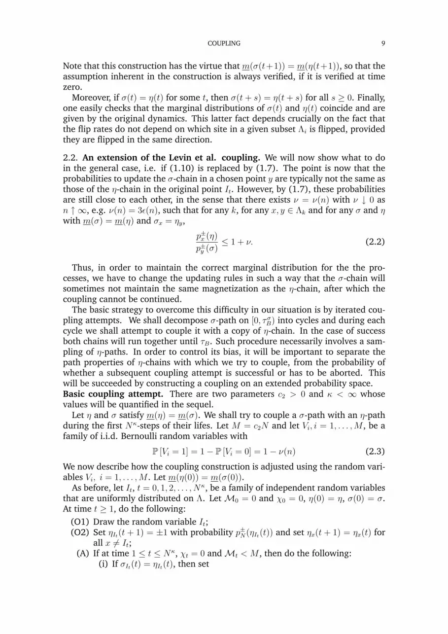
Note that this construction has the virtue that m(σ(t+1)) = m(η(t+1)), so that theassumption inherent in the construction is always verified, if it is verified at timezero.

Moreover, if σ(t) = η(t) for some t, then σ(t+ s) = η(t+ s) for all s ≥ 0. Finally,one easily checks that the marginal distributions of σ(t) and η(t) coincide and aregiven by the original dynamics. This latter fact depends crucially on the fact thatthe flip rates do not depend on which site in a given subset Λi is flipped, providedthey are flipped in the same direction.

2.2. An extension of the Levin et al. coupling. We will now show what to doin the general case, i.e. if (1.10) is replaced by (1.7). The point is now that theprobabilities to update the σ-chain in a chosen point y are typically not the same asthose of the η-chain in the original point It. However, by (1.7), these probabilitiesare still close to each other, in the sense that there exists ν = ν(n) with ν ↓ 0 asn ↑ ∞, e.g. ν(n) = 3ε(n), such that for any k, for any x, y ∈ Λk and for any σ and ηwith m(σ) = m(η) and σx = ηy,

p±x (η)

p±y (σ)≤ 1 + ν. (2.2)

Thus, in order to maintain the correct marginal distribution for the the pro-cesses, we have to change the updating rules in such a way that the σ-chain willsometimes not maintain the same magnetization as the η-chain, after which thecoupling cannot be continued.

The basic strategy to overcome this difficulty in our situation is by iterated cou-pling attempts. We shall decompose σ-path on [0, τσB) into cycles and during eachcycle we shall attempt to couple it with a copy of η-chain. In the case of successboth chains will run together until τB. Such procedure necessarily involves a sam-pling of η-paths. In order to control its bias, it will be important to separate thepath properties of η-chains with which we try to couple, from the probability ofwhether a subsequent coupling attempt is successful or has to be aborted. Thiswill be succeeded by constructing a coupling on an extended probability space.Basic coupling attempt. There are two parameters c2 > 0 and κ < ∞ whosevalues will be quantified in the sequel.

Let η and σ satisfy m(η) = m(σ). We shall try to couple a σ-path with an η-pathduring the first Nκ-steps of their lifes. Let M = c2N and let Vi, i = 1, . . . ,M , be afamily of i.i.d. Bernoulli random variables with

P [Vi = 1] = 1− P [Vi = 0] = 1− ν(n) (2.3)

We now describe how the coupling construction is adjusted using the random vari-ables Vi, i = 1, . . . ,M . Let m(η(0)) = m(σ(0)).

As before, let It, t = 0, 1, 2, . . . , Nκ, be a family of independent random variablesthat are uniformly distributed on Λ. LetM0 = 0 and χ0 = 0, η(0) = η, σ(0) = σ.At time t ≥ 1, do the following:

(O1) Draw the random variable It;(O2) Set ηIt(t + 1) = ±1 with probability p±N(ηIt(t)) and set ηx(t + 1) = ηx(t) for

all x 6= It;(A) If at time 1 ≤ t ≤ Nκ, χt = 0 andMt < M , then do the following:

(i) If σIt(t) = ηIt(t), then set

COUPLING 10

∗ ηIt(t+ 1) = σIt(t+ 1);∗ σx(t+ 1) = σx(t), for all x 6= It;∗ Mt+1 =Mt.

(ii) If σIt(t) 6= ηIt(t), let Λk be the element of the partition such that It ∈ Λk

and, as before, choose y uniformly at random on the set z ∈ Λk :σz(t) 6= ηz(t) 6= ηIt(t). Then set∗ σy(t+ 1) = ηIt(t+ 1) with probability1 if VMt = 1

p±It(η(t))∧p±y (σ(t))−(1−ν)p±It

(η(t))

νp±It(η(t))

, if VMt = 0,(2.4)

and σy(t+ 1) = −ηIt(t+ 1) with probability0 if VMt = 1p±It

(η(t))−p±It (η(t))∧p±y (σ(t))

νp±It(η(t))

if VMt = 0(2.5)

∗ σx(t+ 1) = σx(t), for all x 6= y.∗ If VMt = 0, then set χs = 1 for s = t + 1, . . . , Nκ, otherwise setχt+1 = χt.∗ SetMt+1 =Mt + 1;

(B) If at time t, either χt = 1 orMt = M , then update σ independently of η,i.e.

(i) draw I ′t independently with the same law as It, and(ii) set σI′t(t+ 1) = ±1 with probability p±N(σ(t)), and σx(t+ 1) = σx(t), for

all x 6= I ′t.The processMt is a counter that increases by one each time a new coin Vi is usedby the coupling. The value χt = 1 of the variable χt indicates that that a zero coinwas used by time t.

The following lemma collects the basic properties of the process constructedabove.

Lemma 2.1. Let P denote the joint distribution of the processes σ, η, V defined above.Then the above is a good coupling in the sense that the marginal distributions of bothη(t), t ≤ Nκ and σ(t), t ≤ Nκ under the law P are Pσ(0) and Pη(0), respectively.

Proof. The assertion is obvious for the process η(t). It is also clear for the σ(t)process if updates are done according to case B. Therefore, we only need to checkthat it holds for process σ(t) at such times t ≤ Nκ when χt is still 0 andMt is stillless than M = c2N . In other words, we need to compute

P[σ(t+ 1) = σ+

x (t)|σ(t);χt = 0;Mt < c2N], (2.6)

where σ+x

∆= (σ1, . . . , σx−1,+1, . . . σN). First it is cleat that, given that It = x and

σIt(t) = ηIt(t), we get the desired result, i.e.

P[σ(t+ 1) = σ+

x (t)|It = x;σx(t) = ηx(t);σ(t);χt = 0;Mt < c2N)

= p+x (η(t)) = p+

x (σ(t)). (2.7)

In the case It = y 6= x, we get a contribution to (2.6) only if(i) x, y are in the same set Λi,

(ii) σy(t) 6= ηy(t),

COUPLING 11

(iii) σx(t) 6= ηx(t), and(iv) σx(t) = ηy(t).

If these conditions are satisfied, the probability to flip σx to +1 is then

(1− ν)p+y (η(t)) + νp+

x (η(t)p+y (η(t)) ∧ p+

x (σ(t))− (1− ν)p+y (η(t))

νp+y (η(t))

(2.8)

+ νp−yp−y (η(t))− p−y (η(t)) ∧ p−x (σ(t))

νp−y (η(t))

= p+y (η(t)) ∧ p+

x (σ(t)) + p−y (η(t))− p−y (η(t)) ∧ p−x (σ(t))

= p+x (σ(t)).

The last line is easily verified by distinguishing cases. It now follows easily that theprobability in (2.6) is equal to N−1p+

x (σ(t)), as desired. This proves the lemma.

The construction above tries to merge the processes η(t) and σ(t) only as long asχt = 0 andMt < M . Note that if for some t < Nκ both these conditions still holdand, in addition, η(t) = σ(t), then the two dynamics automatically stay togetheruntil Nκ and, indeed, may stay coupled forever. It would be tempting to try toclassify such situation as “successful coupling”. However, this would involve animplicit sampling of η-trajectories which may lead to distortion of their statisticalproperties. For example, it is not clear whether the correct value of EητB wouldsurvive such procedure.

In order to go around these possible obstacles we will in fact employ a morestringent point of view on what “successful coupling” should be. Namely, we shallsay that our Basic Coupling Attempt is successful if the following two independentevents A and B simultaneously happen on the enlarged probability space:

(1) The eventA ≡

∀Mi=1 Vi = 1

, (2.9)

is the event that all M random variables Vi should be equal to 1 .(2) The event B will only depend on the random variables η(t), t ≤ Nκ. To

define it, we introduce two stopping times, S and N . Let

Sx = inf t : ηx(t+ 1) = −ηx(0) (2.10)

and set S ≡ max1≤x≤N Sx. Clearly, Sx is the first time the spin at site x hasbeen flipped and S is the first time all coordinates of η have been flipped.N is defined as

N ≡S∑t=0

N∑x=1

1It=x1t≤Sx. (2.11)

which is the total number of flipping attempts until time S. Finally,

B ≡ τ ηB ≥ Nκ ∩ S < Nκ ∩ N ≤M . (2.12)

The important observation is the following.

Lemma 2.2. On A ∩ B, the coupling is successful in the sense that

A ∩ B ⊂ η(Nκ) = σ(Nκ). (2.13)

COUPLING 12

Proof. On the event B ∩ A, by time Nk η(t) has not reached B, all spins have beenflipped once, and each flip that involved a site where η(t) 6= σ(t) was done whenthe coin Vi took the value +1. Therefore on each first flip the corresponding η andσ spins became aligned, hence η(Nκ) = σ(Nκ).

Remark. Note that the inclusion (2.13) is in general strict. The rational for theintroduction of the events A and B is that the unlikely event A does not affectthe η-chain at all and that the (likely) event B does not distort the hitting times ofthe η-chain in the sense that Eη (τB1B) ≥ EητB

(1− e−cN

). This will be part of the

content of Lemma 2.3 which we formulate and prove below.

2.3. Construction of a cycle and cycle decomposition of σ-paths. We have seenthat B∩A indicates that our coupling is successful and η(t) and σ(t) arrive togetherin B. However, the probability ofA∪B is very small, essentially due to the fact thatthe probability of A is small, namely P(A) = (1 − ν)M . What will be essential isthat the probability of B is otherwise close to one, and therefore the η-paths (whichare independent of the Vi) will be affected very little by the occurrence of A ∩ B.

We then have to decide what to do on (A ∪ B)c at time Nκ. Define the stoppingtime

∆ = min t > Nκ : σ(t) ∈ Sn[m(η)] . (2.14)

IfD = ∆ < τσB ∩ (A ∩ B)c (2.15)

happens, than we shall initiate a new basic coupling attempt at time ∆ for a newindependent copy of η-chain and a chain starting from σ(∆). Otherwise, on theevent Dc ∪ (Ac ∩ Bc), the process stops and coupling has not occurred.

The cycle decomposition of σ[0, τσB) is based on a collectionη`[0, τ `,ηB )

of in-

dependent copies of η-chains and on a collectionV ` =

(V `

0 , . . . , V`Nκ

)of i.i.d.

stacks of coins. The eventsA`,B`

are well defined and independent. The events

D`

are defined iteratively as follows: The event D0 is simply the above eventD defined with respect the coupling attempt based on

η0, V 0

. If it happens we

denote by θ0 = ∆0 the random time at which the first cycle ends. Assume now that∩k−1

0 D` happened and that the (k − 1)-st cycle was finished at a random time θk−1

and at some random microscopic point σ(θk−1) ∈ Sn[m(η)]. Let us initiate a newbasic coupling attempt using a new independent copy

ηk, V k

for a chain starting

at η and a chain starting from σ(θk−1). The event Dk, and accordingly the cyclelength ∆k, are then defined appropriately. If Dk happens then θk ≡ θk−1 + ∆k,σ(θk) ∈ Sn[m(η)] is well defined as well, and the iterative procedure goes on.

In the light of the above definitions, the enlarged probability space Ω has thefollowing disjoint decomposition,

1 =∞∑k=0

1Ak1Bk

k−1∏`=0

(1− 1A`1B`)1D` (2.16)

+∞∑k=0

(1− 1Ak1Bk) (1− 1Dk)k−1∏`=0

(1− 1A`1B`)1D`

COUPLING 13

As a consequence, we arrive to the following decomposition of the hitting time τσBin terms of the (independent ) hitting times

τ k,ηB

,

τσB =∞∑k=0

k−1∏`=0

1D(`) (1− 1A(`)1B(`))

(θk−1 + τ k,ηB

)1A(k)1B(k)

+ τσB

∞∑k=0

k−1∏`=0

1D(`) (1− 1A(`)1B(`))

(1− 1D(k)) (1− 1A(k)1B(k))

(2.17)

(In both formulas above we use the convention that products with a negative num-ber of terms are equal to 1 and set θ−1 ≡ 0). Note that the first terms in (2.16) and(2.17) correspond to the cases when the iterative coupling eventually succeeds,whereas the second term corresponds to the case when it eventually fails.

2.4. Upper bounds on probabilities and proof of Theorem 1.1.

Lemma 2.3. The following estimates hold uniformly in σ, η ∈ A:(i) There is a constant c > 0, independent of n, such that, for N large enough,

P (Bc) ≤ e−cN , (2.18)

andEη (τB1B) ≥ EητB

(1− e−cN

). (2.19)

(ii) If N is large enough,

Pσ (D) ≥ 1− e−cN . (2.20)

Proof. Item (ii) follows from Lemma 1.4 with e.g. c = c1/2. To prove item (i), wewrite Bc = τ ηB ≤ Nκ ∪ S ≥ Nκ ∪ N > M. Thus,

1Bc = 1τηB≤Nκ + 1τηB>Nκ1S≥Nκ + 1τηB>Nκ1S<Nκ1N>M. (2.21)

Inserting this into Equations (2.18) resp. (2.19), there are three terms to bound.The first term is easy:

Pη (τB < Nκ) ≤ Nκ maxσ′:m(σ′)=m

Pσ′ (τB < τm) ≤ Nκe−c1N , (2.22)

The first inequality used the fact that in order to reach B, the process has to makeone final excursion to B without return to the starting set m, and that there are atmostNκ attempts to do so. The last inequality then uses (1.31). The correspondingterm for (2.19) is then

Eη

(τ ηB1τηB<Nκ

)≤ N2κe−c1N . (2.23)

The second term is also easy: First,

Pη (τB > Nκ ∩ S ≥ Nκ) ≤ Pη (S ≥ Nκ) (2.24)

and

Eη

(τB1τB>Nκ1S≥Nκ

)≤

∑σ′

(Nκ + Eσ′τB) Pη(ηNκ = σ′;S ≥ Nk

)≤

(Nκ + max

σ′Eσ′τB

)Pη (S ≥ Nκ) . (2.25)

COUPLING 14

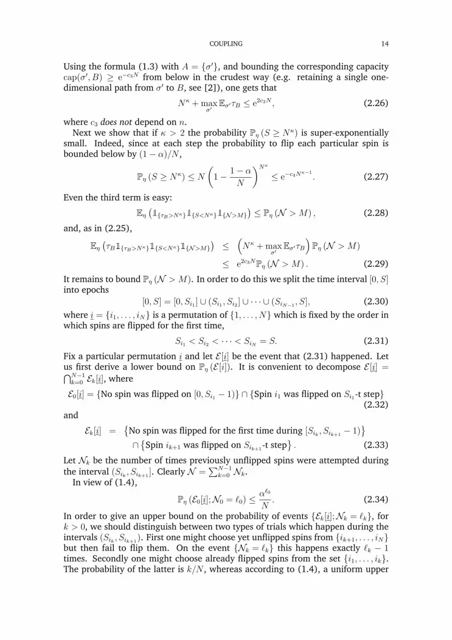
Using the formula (1.3) with A = σ′, and bounding the corresponding capacitycap(σ′, B) ≥ e−c3N from below in the crudest way (e.g. retaining a single one-dimensional path from σ′ to B, see [2]), one gets that

Nκ + maxσ′

Eσ′τB ≤ e2c3N , (2.26)

where c3 does not depend on n.Next we show that if κ > 2 the probability Pη (S ≥ Nκ) is super-exponentially

small. Indeed, since at each step the probability to flip each particular spin isbounded below by (1− α)/N ,

Pη (S ≥ Nκ) ≤ N

(1− 1− α

N

)Nκ

≤ e−c4Nκ−1

. (2.27)

Even the third term is easy:

Eη

(1τB>Nκ1S<Nκ1N>M

)≤ Pη (N > M) , (2.28)

and, as in (2.25),

Eη

(τB1τB>Nκ1S<Nκ1N>M

)≤

(Nκ + max

σ′Eσ′τB

)Pη (N > M)

≤ e2c3NPη (N > M) . (2.29)

It remains to bound Pη (N > M). In order to do this we split the time interval [0, S]into epochs

[0, S] = [0, Si1 ] ∪ (Si1 , Si2 ] ∪ · · · ∪ (SiN−1, S], (2.30)

where i = i1, . . . , iN is a permutation of 1, . . . , N which is fixed by the order inwhich spins are flipped for the first time,

Si1 < Si2 < · · · < SiN = S. (2.31)

Fix a particular permutation i and let E [i] be the event that (2.31) happened. Letus first derive a lower bound on Pη (E [i]). It is convenient to decompose E [i] =⋂N−1k=0 Ek[i], where

E0[i] = No spin was flipped on [0, Si1 − 1) ∩ Spin i1 was flipped on Si1-t step(2.32)

and

Ek[i] =

No spin was flipped for the first time during [Sik , Sik+1− 1)

∩

Spin ik+1 was flipped on Sik+1-t step

. (2.33)

Let Nk be the number of times previously unflipped spins were attempted duringthe interval (Sik , Sik+1

]. Clearly N =∑N−1

k=0 Nk.In view of (1.4),

Pη (E0[i];N0 = `0) ≤ α`0

N. (2.34)

In order to give an upper bound on the probability of events Ek[i];Nk = `k, fork > 0, we should distinguish between two types of trials which happen during theintervals (Sik , Sik+1

). First one might choose yet unflipped spins from ik+1, . . . , iNbut then fail to flip them. On the event Nk = `k this happens exactly `k − 1times. Secondly one might choose already flipped spins from the set i1, . . . , ik.The probability of the latter is k/N , whereas according to (1.4), a uniform upper

COUPLING 15

bound for the probability of the former option is α(N − k)/N . Thus, if Gk is theσ-field generated by η[0,Sk], then

Pη(Ek;Nk = `k

∣∣∣ Gk) ≤ α

N

(α(N − k)

N

)`k−1(∞∑j=0

(k

N

)j)`k

(2.35)

=α`k

N − k.

Therefore,

Eη

(k∏`=0

1E`1Nk=`k

∣∣∣Gk) ≤ α`k

N − k

k−1∏`=0

1E`[i], (2.36)

and, consequently,

Pη (E [i] ; N0 = `0; . . . ;NN−1 = `N−1) ≤ 1

N !α

P`k (2.37)

As a result we get that

Pη (N > M) ≤∑L>M

αL(N + L

L

)≤∑L>M

e− ln(1/α)LeN(ln(1+L/N)+1). (2.38)

For M ≡ c2N , and providing that c2 is large enough, we finally obtain that

Pη (N > M) ≤ e−c5N , (2.39)

for a constant c5 increasing linearly with c2. Putting all estimates together con-cludes the proof of the lemma.

Notice that if A ∩ B happens, then m(ηt) ≡ m(σt). In particular, A ∩ B ⊂τσB ≥ Nκ and hence τσB = τ ηB on A ∩ B.

Let us go back to the cycle decomposition (2.17). Using E for the expectation onthe enlarged probability space,

EτσB ≥∞∑k=0

E

k−1∏`=0

1D(`) (1− 1A(`)1B(`))

τ k,ηB 1A(k)1B(k) (2.40)

LetFθk be the σ-algebra generated by all the events and trajectoriesA(`),B(`),D(`),η` and σ(θ`−1, θ`], ` ≤ k. Then, in view of the independence of copies

η`, V `

,

E(τ ηB1A(k)1B(k)

∣∣Fθk−1

)= P (A) Eη (τB1B) = (1− ν)MEη (τB1B) (2.41)

On the other hand,

E(1D(`) (1− 1A(`)1B(`))

∣∣∣Fθ`−1

)≥ E (1− 1A(`)1B(`))− max

σ′∈Sn[m](1− Pσ′(D))

≥ 1− (1− ν)M − e−cN . (2.42)

Altogether (recall that M = c2N),

EστB ≥ Eη (τB1B) (1− ν)c2N∞∑k=0

(1− (1− ν)c2N − e−cN

)k≥ EητB

1− e−cN

1 + (1− ν)−c2Ne−cN(2.43)

which tends to EητB if ν < c/c2. This concludes the proof of Theorem 1.1

COUPLING 16

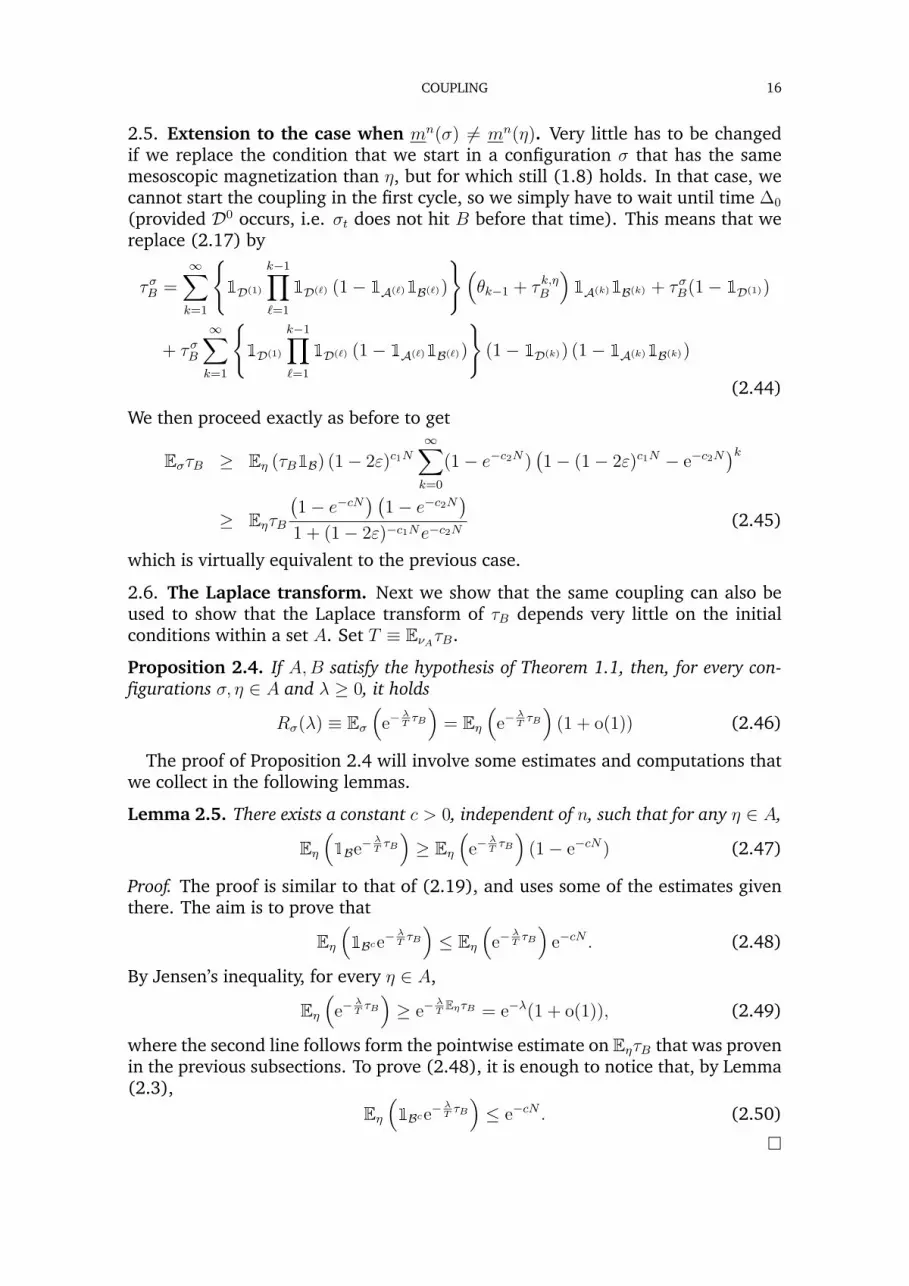
2.5. Extension to the case when mn(σ) 6= mn(η). Very little has to be changedif we replace the condition that we start in a configuration σ that has the samemesoscopic magnetization than η, but for which still (1.8) holds. In that case, wecannot start the coupling in the first cycle, so we simply have to wait until time ∆0

(provided D0 occurs, i.e. σt does not hit B before that time). This means that wereplace (2.17) by

τσB =∞∑k=1

1D(1)

k−1∏`=1

1D(`) (1− 1A(`)1B(`))

(θk−1 + τ k,ηB

)1A(k)1B(k) + τσB(1− 1D(1))

+ τσB

∞∑k=1

1D(1)

k−1∏`=1

1D(`) (1− 1A(`)1B(`))

(1− 1D(k)) (1− 1A(k)1B(k))

(2.44)

We then proceed exactly as before to get

EστB ≥ Eη (τB1B) (1− 2ε)c1N∞∑k=0

(1− e−c2N)(1− (1− 2ε)c1N − e−c2N

)k≥ EητB

(1− e−cN

) (1− e−c2N

)1 + (1− 2ε)−c1Ne−c2N

(2.45)

which is virtually equivalent to the previous case.

2.6. The Laplace transform. Next we show that the same coupling can also beused to show that the Laplace transform of τB depends very little on the initialconditions within a set A. Set T ≡ EνAτB.

Proposition 2.4. If A,B satisfy the hypothesis of Theorem 1.1, then, for every con-figurations σ, η ∈ A and λ ≥ 0, it holds

Rσ(λ) ≡ Eσ

(e−

λTτB)

= Eη

(e−

λTτB)

(1 + o(1)) (2.46)

The proof of Proposition 2.4 will involve some estimates and computations thatwe collect in the following lemmas.

Lemma 2.5. There exists a constant c > 0, independent of n, such that for any η ∈ A,

Eη

(1Be−

λTτB)≥ Eη

(e−

λTτB)

(1− e−cN) (2.47)

Proof. The proof is similar to that of (2.19), and uses some of the estimates giventhere. The aim is to prove that

Eη

(1Bce

− λTτB)≤ Eη

(e−

λTτB)

e−cN . (2.48)

By Jensen’s inequality, for every η ∈ A,

Eη

(e−

λTτB)≥ e−

λT

EητB = e−λ(1 + o(1)), (2.49)

where the second line follows form the pointwise estimate on EητB that was provenin the previous subsections. To prove (2.48), it is enough to notice that, by Lemma(2.3),

Eη

(1Bce

− λTτB)≤ e−cN . (2.50)

COUPLING 17

Proof of Prop. 2.4. For simplicity consider the case when mn(σ) = mn(η) ≡ m.Analogously to Eq. (2.17) we obtain

Eσ

(e−

λTτB)

= E

(∞∑k=0

e−λT

(θk−1+τk,ηB )1A(k)1B(k)

k−1∏`=0

1D(`) (1− 1A(`)1B(`))

)(2.51)

+ E

(e−

λTτσB

∞∑k=0

(1− 1D(k)) (1− 1A(k)1B(k))k−1∏`=0

1D(`) (1− 1A(`)1B(`))

)

≤∞∑k=0

E

(e−

λTτk,ηB 1A(k)1B(k)

k−1∏`=0

1D(`) (1− 1A(`)1B(`))

)

+∞∑k=0

E

((1− 1D(k)) (1− 1A(k)1B(k))

k−1∏`=0

1D(`) (1− 1A(`)1B(`))

).

Now, for every k, ` ≥ 0, as in (2.41),

E(1A(k)1B(k)e−

λTτk,ηB∣∣Fθk−1

)≤ (1− ν)MEη

(e−

λTτB). (2.52)

Moreover, as in (2.42),

E(1D(`) (1− 1A(`)1B(`))

∣∣∣Fθ`−1

)≤ E

(1− 1A(`)1B(`)

∣∣∣Fθ`−1

)= 1− P(A)P(B)

≤ 1− (1− ν)M(1− e−cN). (2.53)

This last estimate, together with result (2.20) of Lemma 2.3, shows that the lastline in (2.51) is smaller than

∞∑k=0

e−cN(1− (1− ν)M(1− e−cN)

)k ≤ 2e−N(c−c2ν) (2.54)

Combining these estimates, we get

Eσ

(e−

λTτB)≤ Eη

(e−

λTτB)

(1− ν)c2N∞∑k=0

(1− (1− ν)c2N(1− e−cN)

)k≤ Eη

(e−

λTτB) (

1− e−cN)

+ 2e−N(c−c2ν)

= Eη

(e−

λTτB) (

1 + 3e−N(c−c2ν))

(2.55)

which tends to Eη

(e−

λTτB

)if ν < c/c2.

3. RENEWAL AND THE EXPONENTIAL DISTRIBUTION FOR THE RFCW

We will use the results of Subsections 1.3-1.4 and the notation introduced therein.In particular, for each n fixed, we set A = Sn[m∗] and Aδ = Sn[Aδ], where Aδ is themesoscopic δ-neighborhood of m8. In the sequel we shall choose n appropriatelylarge and δ appropriately small.

In the case of the RFCW model we will prove the convergence of the law of thenormalized metastable time, τB, to an exponential distribution, via convergenceof the Laplace transform, Rσ(λ), defined in (2.46). The proof of the latter will bebased on renewal arguments.

COUPLING 18

3.1. Renewal equations. By Proposition 2.4, instead of studying the process start-ing in a given point σ, for which no exact renewal equation will hold, it is enoughto study the process starting on a suitable measure on A, for which such a relationwill be shown to hold. For λ ≥ 0, let ρλ denote the probability measure on A thatsatisfies the equation,∑

σ∈A

ρλ(σ)Eσ

(e−

λTτA1τA<τB1σ(τA)=σ′

)= C(λ)ρλ(σ

′), (3.1)

for all σ′ ∈ A, where

C(λ) = Eρλ

(e−

λTτA1τA<τB

). (3.2)

Existence and uniqueness of such a measure follows from the Perron-Frobeniustheorem in a standard way.

The usefulness of this definition comes from the fact that the Laplace transformof τB started in this measure satisfies an exact renewal equation.

Lemma 3.1. Let Rρλ(λ) =∑

σ ρλ(σ)Rσ(λ). Then

Rρλ(λ) =Eρλ

(e−

λTτB1τB<τA

)1− Eρλ

(e−

λTτA1τA<τB

) (3.3)

Proof. Using that 1 = 1τB<τA + 1τA<τB and the strong Markov property, we see that

Rρλ(λ) = Eρλ

(e−

λTτB1τB<τA

)(3.4)

+∑σ′∈A

Eρλ

(e−

λTτA1τA<τB1σ(τA)=σ′

)Eσ′e

− λTτB

= Eρλ

(e−

λTτB1τB<τA

)+∑σ′∈A

C(λ)ρλ(σ′)Eσ′e

− λTτB

Equation (3.3) is now immediate.

3.2. Convergence. As a result of the representation (3.3), Theorem 1.2 will followfrom (2.46) once we prove the following lemma.

Lemma 3.2. With the notation from Lemma 3.1, for any λ ≥ 0,

limN→∞

Eρλ

(e−

λTτB1τB<τA

)1− Eρλ

(e−

λTτA1τA<τB

) =1

1 + λ. (3.5)

Proof of Lemma 3.2. The proof of this lemma comprises nine steps.

STEP 1. Here is the crucial pointwise bound which is an application of the UphillLemma that will be established in the next subsection:

Lemma 3.3. There exists c7 > 0 such that

Eσ

(τB1τB<τA

)≤ e−c7NEσ

(τA1τA<τB

), (3.6)

uniformly in σ ∈ A.

COUPLING 19

We shall proceed with the proof assuming that (3.6) holds. In particular,

Eρλ

(τB1τB<τA

)≤ e−c7NEρλτA1τA<τB. (3.7)

STEP 2. (3.7) implies that

Tλ ≡ EρλτB = Eρλ

(τB1τB<τA

)+ Eρλ

(τB1τA<τB

)(3.8)

= Eρλ

(τA1τA<τB

) (1 + o(e−c7N)

)+ Eρλ

(1τA<τBEσ(τA)τB

)= TλPρλ (τA < τB) + Eρλ

(τA1τA<τB

) (1 + o(e−c7N)

)+ Eρλ

(1τA<τB

(Eσ(τA)τB − Tλ

)).

However, by the invariance of ρλ,

Eρλ

(1τA<τBe

− λTτA(Eσ(τA)τB − Tλ

))= 0. (3.9)

It follows that the absolute value of the last term in (3.8) is bounded above as,

Eρλ

((1− e−

λTτA

)1τA<τB

)maxσ∈A|EστB − Tλ| (3.10)

≤ λmaxσ∈A

∣∣∣∣EστB − TλT

∣∣∣∣Eρλ

(τA1τA<τB

)= o(e−CN/2)Eρλ

(τA1τA<τB

),

where we used (1.9) in the last step. This implies the following lemma.

Lemma 3.4. There exists c8 > 0, such that, for any λ ≥ 0 fixed,

Tλ =EρλτA1τA<τBPρλ (τB < τA)

(1 + o(e−c8N)

). (3.11)

In view of (3.11), a look at (3.7) reveals that the conditional expectation,

Eρλ [τB | τB < τA]

T= o(e−c7N). (3.12)

Using that, for x ≥ 0, 1 ≥ e−x ≥ 1 − x, it follows that the numerator in (3.3)satisfies

Eρλ

(e−

λTτB1τB<τA

)= Pρλ (τB < τA)

(1 + o(e−c7N)

). (3.13)

STEP 3. Let us turn now to the denominator in (3.3). We rewrite it as

Pρλ (τB < τA)

1 + λ

Eρλ

((1− e−

λTτA

)1τA<τB

)λPρλ (τB < τA)

. (3.14)

Using (3.11) for 1/Pρλ (τB < τA), we are left with a computation of

T

λEρλ

(τA1τA<τB

)Eρλ

((1− e−

λTτA

)1τA<τB

). (3.15)

Since,

Eρλ

((1− e−

λTτA

)1τA<τB

)=λ

T

∫ 1

0

Eρλ

(e−

sλTτAτA1τA<τB

)ds, (3.16)

COUPLING 20

we deduce that the expression in (3.15) belongs to the intervalEρλe−λTτAτA1τA<τB

EρλτA1τA<τB, 1

(3.17)

The target (3.5) follows once we show that

limN→∞

Eρλe−λTτAτA1τA<τB

EρλτA1τA<τB= 1. (3.18)

It is clear that (3.17) follows once we show that there exists a sequence αN ↓ 0,such that

limN→∞

EρλτA1τA<τB1τA<αNTEρλτA1τA<τB

= 1. (3.19)

This will be our next goal.

STEP 4. Let Bδ = SN \Aδ. Our proof of (3.19) is based on the following decompo-sition,

EρλτA1τA<τB1τA>αNT ≤ EρλτA1τA<τBδ1τA>αNT + EρλτA1τBδ<τA<τB≡ Iδ + IIδ.

(3.20)

The logic behind the above splitting should be transparent: The conditional (onτA < τB) landscape should have the global mesoscopic minima at A. The term Iδis a local one and should be small since the dynamics cannot spend too much timeinside a local well Aδ without hitting A. On the other hand, the term IIδ should besmall because of the price paid for the uphill run towards Bδ before hitting A. Weclaim that there exists αN ↓ 0 and c > 0 such that

max Iδ, IIδ ≤ e−cN . (3.21)

Evidently, (3.19) is a consequence of (3.21).

STEP 5. Bound on Iδ. The term Iδ is bounded above as

Iδ ≤ maxσ∈A

EστA∪Bδ1τA∪Bδ>αNT. (3.22)

The right hand side of (3.22) depends on the dynamics in a δ-neighbourhood of anon-degenerate local minimum A = Sn[m∗]. We try to formalize an intuitive ideathat such dynamics mixes up on time scale much shorter than T and cannot affordspending αNT units of time without hitting A ∪ Bδ. This is a somewhat coarseestimate. Let us start with estimating hitting times from equilibrium measure overmesoscopic slots:

Lemma 3.5. Let Aδ and Bδ be as defined above. Then there exists c(δ) satisfyingc(δ) ↓ 0, as δ ↓ 0, such that, for all m′ ∈ Aδ \m∗,

Eνm′τA∪Bδ ≤ ec(δ)N , (3.23)

where νm′ is the probability measure on Sn[m′], which we referred to in Eq. (1.3).

COUPLING 21

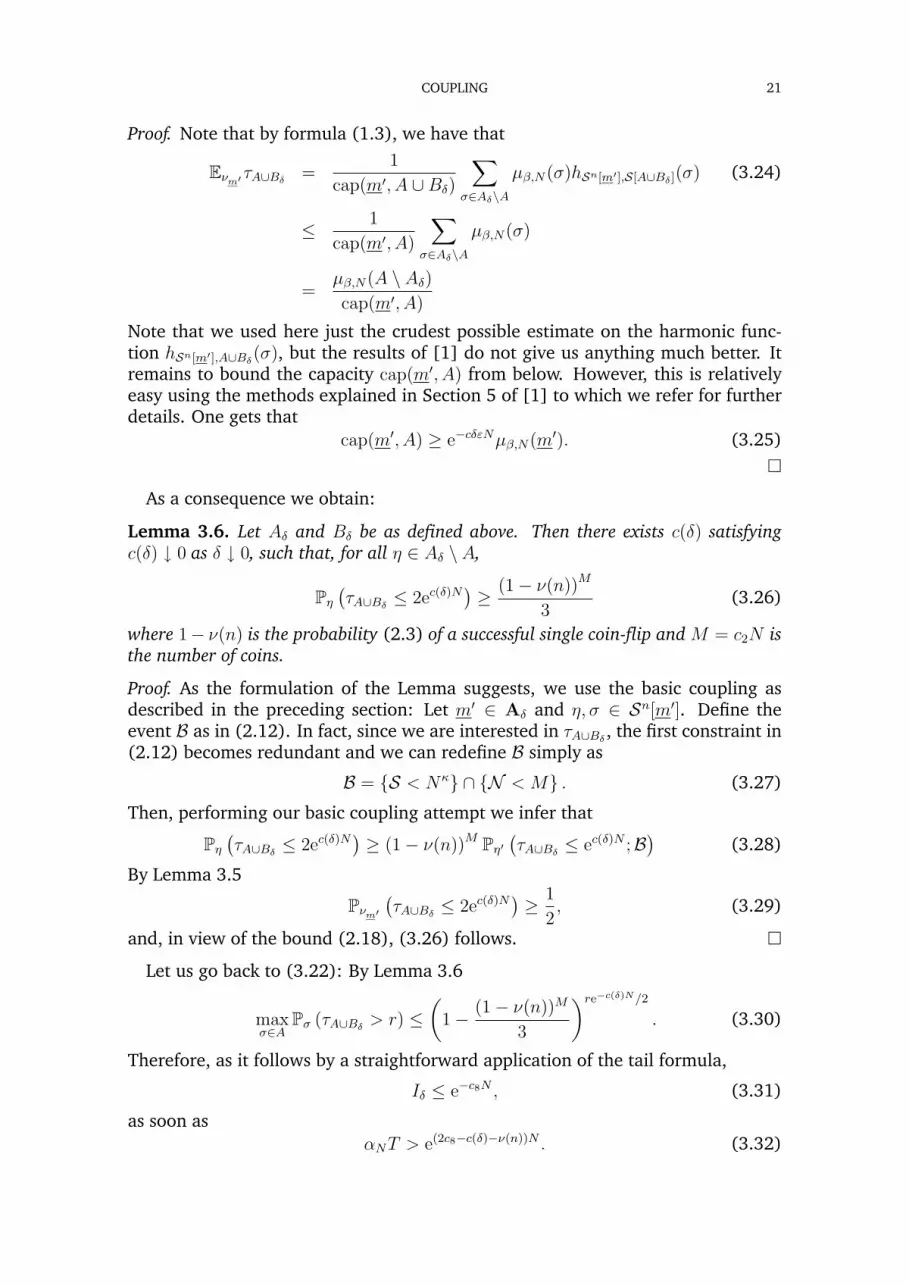
Proof. Note that by formula (1.3), we have that

Eνm′τA∪Bδ =

1

cap(m′, A ∪Bδ)

∑σ∈Aδ\A

µβ,N(σ)hSn[m′],S[A∪Bδ](σ) (3.24)

≤ 1

cap(m′, A)

∑σ∈Aδ\A

µβ,N(σ)

=µβ,N(A \ Aδ)cap(m′, A)

Note that we used here just the crudest possible estimate on the harmonic func-tion hSn[m′],A∪Bδ(σ), but the results of [1] do not give us anything much better. Itremains to bound the capacity cap(m′, A) from below. However, this is relativelyeasy using the methods explained in Section 5 of [1] to which we refer for furtherdetails. One gets that

cap(m′, A) ≥ e−cδεNµβ,N(m′). (3.25)

As a consequence we obtain:

Lemma 3.6. Let Aδ and Bδ be as defined above. Then there exists c(δ) satisfyingc(δ) ↓ 0 as δ ↓ 0, such that, for all η ∈ Aδ \ A,

Pη(τA∪Bδ ≤ 2ec(δ)N

)≥ (1− ν(n))M

3(3.26)

where 1− ν(n) is the probability (2.3) of a successful single coin-flip and M = c2N isthe number of coins.

Proof. As the formulation of the Lemma suggests, we use the basic coupling asdescribed in the preceding section: Let m′ ∈ Aδ and η, σ ∈ Sn[m′]. Define theevent B as in (2.12). In fact, since we are interested in τA∪Bδ , the first constraint in(2.12) becomes redundant and we can redefine B simply as

B = S < Nκ ∩ N < M . (3.27)

Then, performing our basic coupling attempt we infer that

Pη(τA∪Bδ ≤ 2ec(δ)N

)≥ (1− ν(n))M Pη′

(τA∪Bδ ≤ ec(δ)N ;B

)(3.28)

By Lemma 3.5

Pνm′(τA∪Bδ ≤ 2ec(δ)N

)≥ 1

2, (3.29)

and, in view of the bound (2.18), (3.26) follows.

Let us go back to (3.22): By Lemma 3.6

maxσ∈A

Pσ (τA∪Bδ > r) ≤(

1− (1− ν(n))M

3

)re−c(δ)N/2. (3.30)

Therefore, as it follows by a straightforward application of the tail formula,

Iδ ≤ e−c8N , (3.31)

as soon asαNT > e(2c8−c(δ)−ν(n))N . (3.32)

COUPLING 22

Since T ∼ eCN with C > 0 being, of course, independent of our choice of δ andn, it is always possible to tune the parameters δ, n and αN ↓ 0 in such a way that(3.32) holds.

STEP 6. Bound on IIδ. Note that

Eρλ

(τA1τBδ<τA<τB

)= Eρλ

(τBδ1τBδ<τA

)+ Eρλ

(1τBδ<τAEσ(τBδ )τA1τA<τB

).

(3.33)By the Uphill Lemma (see (3.51) below) the first term in (3.33) is negligible withrespect to EρλτA1τA<τBδ. Therefore, the bulk of the remaining work is to find anappropriate upper bound on the second term in (3.33).

By the Downhill Lemma (see (3.60) below) we would be in a good shape ifwe would have the original reversible measure µ instead of the ρλ eigen-measuredefined in (3.1). Namely, (3.60) implies that, independently of n, there existscδ > 0 such that

1

µ(A)

∑σ∈A

µ(σ)Eσ

(1τBδ<τAEσ(τBδ )τA1τA<τB

)≤ e−cδN , (3.34)

as soon as N is large enough. Consequently, it would be enough to prove thefollowing uniform upper bound: There exists c9 < ∞, such that for any n (andhence ε = ε(n)) fixed,

maxσ∈A

ρλ(σ)

µ(σ)/µ(A)≤ ec9εN , (3.35)

as soon as N is large enough.

STEP 7. In order to check (3.35) first of all note that by reversibility,∑σ′∈A

µ(σ′)Pσ′ (τ rA < τB;σ(τ rA) = σ) = µ(σ)Pσ (τ rA < τB) , (3.36)

where τ rA is the r-th hitting time of A. Assume now that we are able to prove thatthere exists r and M such that

Pη (τ rA < τB;σ(τ rA) = σ) ≤ (1− ε)−M Pσ′ (τ rA < τB;σ(τ rA) = σ) , (3.37)

uniformly in η, σ, σ′ ∈ A. In view of (3.1) this would imply,

ρλ(σ) ≤ 1

C(λ)r

∑η

ρλ(η)Pη (τ rA < τB;σ(τ rA) = σ)

≤ (1− ε)−M

C(λ)rPσ′ (τ rA < τB;σ(τ rA) = σ) .

(3.38)

Multiplying both sides above by µ(σ′) and applying (3.36), we conclude that (3.37)implies that

ρ(σ) ≤ (1− ε)−M

C(λ)rµ(σ)

µ(A)Pσ (τ rA < τB) , (3.39)

uniformly in σ ∈ A. The target (3.35), therefore, would be a consequence of thefollowing two claims: There exists c > 0, such that, independently of the coarsegraining parameter n,

C(λ) ≥ 1− e−cN , (3.40)as soon as N is sufficiently large. Furthermore, for sufficiently large c2 and κ,(3.37) holds with M = c2N and r = Nκ.

COUPLING 23

STEP 8. Proof of (3.40). By the uniform bound (1.32) and Jensen’s inequality, itfollows

C(λ) ≥((1− e−cN

)∑σ

ρλ(σ)Eσ

(e−

λTτA

∣∣∣τA < τB

)≥(1− e−cN

)exp

− λT

∑σ

ρλ(σ)Eσ

(τA

∣∣∣τA < τB

)

≥(1− e−cN

)exp

−λEρλ

(τA1τA<τB

)T (1− e−cN)

(3.41)

By (3.11),

Eρλ

(τA1τA<τB

)=TλPρλ (τB < τA)

1 + o (e−c8N), (3.42)

and (3.40) follows by (1.32) and (1.9).

STEP 9. Proof of (3.37). First of all note that there exists c10 <∞ such that

Pη(τ rA < τB ; στrA = σ

)≥ e−c10NPη (τ rA < τB) , (3.43)

uniformly in σ, η ∈ A. This is a rough estimate: by Markov property,

Pη(τ rA < τB ; στrA = σ

)≥ Pη (τ rA < τB) min

η′∈APη′ (τA < τB ; στA = σ) . (3.44)

Let η′ ∈ A and let the Hamming distance between σ and η′ be K. Then we canreach σ from η′ by flipping exactly K spins; since this can be done in K! orders,and each flip has probability at least ((1− α)/N) by (1.4), we see that

Pη′ (τA < τB ; στA = σ) ≥ K!

NK(1− αK), (3.45)

and (3.43) follows.Next, let η ∈ A and consider a dynamics starting from η. We shall try to couple it

with a dynamics starting from σ′ using just one basic coupling attempt. Employingthe same notation as in Subsection 2.2, we know (see (2.27) and (2.39)) that forκ > 2 and M = c2N ,

Pη (S > Nκ,N > M) ≤ e−c6N , (3.46)

where c6 grows linearly with c2. In the sequel we choose c2 so large that c6 becomeslarger than the constant c10 in (3.43).

Let us redefine the event B in (2.12) as B = S ≤ Nκ ∩ N ≤M. The coinsV1, . . . , VM and the event A =

∀Mi=1Vi = 1

remain the same. Consider the en-

larged probability space(

Ω, P)

which corresponds to a single basic coupling at-tempt to couple a dynamics σ(t) from σ′ to the dynamics η(t) which starts at η.

The coupling is successful if and only if the event A ∩ B, which depends on atmost Nκ steps, happens. Therefore,

Pσ′ (τ rA < τB ; σ(τ rA) = σ) ≥ P (Nκ ≤ τ rA < τB; η(τ rA) = σ;A;B) (3.47)

= Pη (Nκ ≤ τ rA < τB; η(τ rA) = σ;B) P(A)

= Pη (Nκ ≤ τ rA < τB; η(τ rA) = σ;B) (1− ε)M .

COUPLING 24

Now, let us choose r = Nκ. In particular, the constraint Nκ ≤ τ rA becomes redun-dant. By (1.32) and in view of (3.43) and our choice of M which leads to a largec6 in (3.46), there exists c11 > 0 such that,

Pη (τ rA < τB; η(τ rA) = σ;B) ≥ Pη (τ rA < τB; η(τ rA) = σ)− Pη(Bc) (3.48)

≥ Pη (τ rA < τB; η(τ rA) = σ)(1− e−c11N

).

(3.37) follows.

3.3. Uphill and Downhill Lemmas. In this subsection we shall prove (3.6) and(3.34). Most of the computation is done in the general context of irreduciblereversible Markov chains on a finite state space Σ. Let p(σ, σ′) be the transitionprobabilities, µ the invariant measure, and A,B two disjoint subsets of Σ. Wewrite

∂A = σ′ 6∈ A : ∃σ ∈ A s.t. p(σ, σ′) > 0 = σ′ 6∈ A : ∃σ ∈ A s.t. p(σ′, σ) > 0 .(3.49)

In the sequel we shall assume that B ∩ ∂A = ∅. As usual, for a set C ⊂ Σ, τC =min n > 0 : σ(n) ∈ C.

Lemma 3.7. [Uphill Lemma] For any A and B disjoint subsets of Σ such that, inaddition, B ∩ ∂A = ∅,

Eσ

(τA1τA<τB

)≥ min

σ′∈∂APσ′ (τA < τB) EστA∪B (3.50)

for any σ ∈ A. Consequently,

Eσ

(τB1τB<τA

)≤ max

σ′∈∂A

1− Pσ′ (τA < τB)

Pσ′ (τA < τB)Eσ

(τA1τA<τB

). (3.51)

Proof. Given σ ∈ A let us compute,

EστA∪B − 1 =∑σ′∈∂A

p(σ, σ′)Eσ′τA∪B

=∑σ′∈∂A

µ(σ′)p(σ′, σ)

µ(σ)Eσ′τA∪B

=1

µ(σ)

∑σ′∈∂A

∑δ 6∈A∪B

µ(σ′)p(σ′, σ)GA∪B(σ′, δ)

=1

µ(σ)

∑σ′∈∂A

∑δ 6∈A∪B

µ(δ)GA∪B(δ, σ′)p(σ′, σ)

=∑

δ 6∈A∪B

µ(δ)

µ(σ)

∑σ′∈∂A

GA∪B(δ, σ′)p(σ′, σ). (3.52)

Next, observe that for every δ 6∈ A ∪B,∑σ′∈∂A

GA∪B(δ, σ′)p(σ′, σ) = Pδ (τA < τB;στA = σ) ≡ gσ(δ). (3.53)

Indeed, all we need to check is that (I − PA∪B) gσ(δ) = p(δ, σ), where PA∪B is the(sub-probability) transition kernel for the chain killed upon reaching A ∪ B. The

COUPLING 25

latter is straightforward: For δ 6∈ A ∪B,

gσ(δ) = p(δ, σ) +∑

δ′ 6∈A∪B

p(δ, δ′)Pδ′ (τA < τB;στA = σ) = p(δ, σ) + PA∪Bgσ(δ) (3.54)

Therefore we conclude that

EστA∪B = 1 +∑

δ 6∈A∪B

µ(δ)

µ(σ)Pδ (τA < τB;στA = σ) (3.55)

= 1 +∑

δ 6∈A∪B

µh(δ)

µ(σ)Phδ (στA = σ) ,

where, on the last step, we have introduced the Doob’s h-transform with the har-monic function h(δ) ≡ hA,B(δ), the transition probabilities ph(·, ·) on (Σ \ (A ∪B))×Σ given by

ph(σ, σ′) =1

h(σ)p(σ, σ′)h(σ′), (3.56)

and the measure µh(δ) = h(δ)µ(δ). By construction, µh(δ)ph(δ, δ′) = µh(δ′)ph(δ′, δ)whenever both δ and δ′ are in Σ \ (A ∪ B). Hence, µh(δ)Gh

A(δ, δ′) = µh(δ′)GhA(δ′, δ)

for the Green’s functions of the h-process killed upon reaching A.With the above in mind we obtain,

Eσ

(τA1τA<τB

)= Pσ (τA < τB) +

∑σ′∈∂A

p(σ, σ′)Eσ′τA1τA<τB (3.57)

= Pσ (τA < τB) +∑σ′∈∂A

p(σ, σ′)h(σ′)Ehσ′τA

= Pσ (τA < τB) +1

µ(σ)

∑σ′∈∂A

p(σ, σ′)µh(σ′)Ehσ′τA

= Pσ (τA < τB) +∑

δ 6∈A∪B

µh(δ)

µ(σ)

∑σ′∈∂A

GhA(δ, σ′)p(σ′, σ).

Let us compare the expression above with the last line in (3.52) and, accordingly,with (3.55). The h-transformed counterpart of (3.53) reads as: ∀δ 6∈ A ∪B,∑

σ′∈∂A

GhA(δ, σ′)ph(σ′, σ) = Phδ (στA = σ). (3.58)

Since for σ′ ∈ ∂A and σ ∈ A, ph(σ′, σ) = p(σ′, σ)/h(σ′) we infer from (3.57),

Eσ

(τA1τA<τB

)≥ Pσ (τA < τB) + min

σ′∈∂Ah(σ′)

∑δ 6∈A∪B

µh(δ)

µ(σ)Phδ (στA = σ) (3.59)

We have proved the lemma.

We can now derive Lemma (3.3). Since in the particular case of A and B weconsider here, (1.8) holds, the estimate (3.6) follows.

Let us go back to (3.34). By our basic estimate on the microscopic harmonicfunction h(σ) = Pσ (τA < τB), (3.34) would follow once we prove the followingDownhill Lemma:

COUPLING 26

Lemma 3.8. [Downhill Lemma] With the notation introduced before,∑σ∈ A

µ(σ)Eσ

(1τBδ<τAEσ(τBδ )τA1τA<τB

)≤(1 + e−cN

) ∑σ′∈Aδ\A

µh(σ′)Phσ′ (τBδ < τA) .

(3.60)

Proof. By reversibility,

µ(σ)Eσ

(1τBδ<τA1σ(τBδ )=η

)= µ(η)Eη

(1τA<τBδ1σ(τA)=σ

). (3.61)

Hence,∑σ∈A

µ(σ)Eσ

(1τBδ<τAEσ(τBδ )τA1τA<τB

)=∑η∈Bδ

µ(η)Pη (τA < τBδ) Eη

(τA1τA<τB

).

(3.62)Since the only non-zero contribution to the latter sum comes from η ∈ ∂Aδ, we canbound it above in terms of the h-transformed quantities as(

1 + e−cN) ∑η∈Bδ

µh(η)Phη (τA < τBδ) EhητA. (3.63)

Applying the representation formula (1.3) for hitting times for the h-transformeddynamics, we can represent the above sum as∑

σ′∈Aδ\A

µ(σ′)h(σ′)Phσ′ (τBδ < τA) , (3.64)

and (3.60) follows.

Notice that using an estimate completely analogous to Lemma 1.4, one sees that∑σ′∈Aδ\A

µ(σ′)h(σ′)Phσ′ (τBδ < τA) ≤ µ(Aδ \ A)e−cδN , (3.65)

for some cδ > 0. This allows to deduce (3.34) from (3.60).

REFERENCES

[1] A. Bianchi, A. Bovier, and D. Ioffe, Sharp asymptotics for metastability in the Random FieldCurie-Weiss model, Elect. J. Probab. 14, 1541-1603 (2009).

[2] A. Bovier, Metastability, in Methods of Contemporary Mathematical Statistical Mechanics (R.Kotecky, ed.), 177–221, Lecture Notes in Mathematics 1970, Springer, Berlin, 2009.

[3] A. Bovier, M. Eckhoff, V. Gayrard and M. Klein, Metastability in stochastic dynamics of disor-dered mean-field models, Probab. Theory Rel. Fields 119 (2001) 99–161.

[4] A. Bovier, M. Eckhoff, V. Gayrard and M. Klein, Metastability and low lying spectra in re-versible Markov chains, Commun. Math. Phys. 228 (2002) 219–255.

[5] A. Bovier, M. Eckhoff, V. Gayrard and M. Klein, Metastability in reversible diffusion processesI. Sharp asymptotics for capacities and exit times, J. Europ. Math. Soc. (JEMS) 6, 399-424(2004)

[6] A. Bovier, F. den Hollander, and C. Spitoni, Homogeneous nucleation for Glauber andKawasaki dynamics in large volumes and low temperature, WIAS preprint 1331, to appearin Ann. Probab. (2008)

[7] M.D. Donsker and S.R.S. Varadhan, On the principle eigenvalue of second order elliptic dif-ferential operators, Commun. Pure Appl. Math. 29 (1976) 595–621.

[8] D.A. Levin, M. Luczak, and Y. Peres, Glauber dynamics for the mean field Ising model: cut-off,critical power law, and metastability, Probab. Theory. Rel. Fields, DOI 007/s00440-008-0189-z, 2008.

COUPLING 27

[9] E. Nummelin, A splitting technique for Harris recurrent Markov chains, Z. Wahrscheinlichkeit-stheorie verw. Geb. 43, 309-318 (1978).

A. BIANCHI, WEIERSTRASS-INSTITUT FUR ANGEWANDTE ANALYSIS UND STOCHASTIK, MOHREN-STRASSE 39, 10117 BERLIN, GERMANY

E-mail address: bianchi@wias-berlin.de

A. BOVIER, INSTITUT FUR ANGEWANDTE MATHEMATIK, RHEINISCHE FRIEDRICH-WILHELMS-UNI-VERSITAT BONN, ENDENICHER ALLEE 60, 53115 BONN, GERMANY

E-mail address: bovier@uni-bonn.de

D. IOFFE, WILLIAM DAVIDSON FACULTY OF INDUSTRIAL ENGINEERING AND MANAGEMENT, TECH-NION, HAIFA 32000, ISRAEL

E-mail address: ieioffe@technion.ac.il

Bestellungen nimmt entgegen: Sonderforschungsbereich 611 der Universität Bonn Poppelsdorfer Allee 82 D - 53115 Bonn Telefon: 0228/73 4882 Telefax: 0228/73 7864 E-Mail: astrid.link@ins.uni-bonn.de http://www.sfb611.iam.uni-bonn.de/

Verzeichnis der erschienenen Preprints ab No. 445

445. Frehse, Jens; Specovius-Neugebauer, Maria: Existence of Regular Solutions to a Class of Parabolic Systems in Two Space Dimensions with Critical Growth Behaviour 446. Bartels, Sören; Müller, Rüdiger: Optimal and Robust A Posteriori Error Estimates in

L∞

(L2) for the Approximation of Allen-Cahn Equations Past Singularities

447. Bartels, Sören; Müller, Rüdiger; Ortner, Christoph: Robust A Priori and A Posteriori Error Analysis for the Approximation of Allen-Cahn and Ginzburg-Landau Equations Past Topological Changes 448. Gloria, Antoine; Otto, Felix: An Optimal Variance Estimate in Stochastic Homogenization of Discrete Elliptic Equations 449. Kurzke, Matthias; Melcher, Christof; Moser, Roger; Spirn, Daniel: Ginzburg-Landau Vortices Driven by the Landau-Lifshitz-Gilbert Equation 450. Kurzke, Matthias; Spirn, Daniel: Gamma-Stability and Vortex Motion in Type II Superconductors 451. Conti, Sergio; Dolzmann, Georg; Müller, Stefan: The Div–Curl Lemma for Sequences whose Divergence and Curl are Compact in W

−1,1

452. Barret, Florent; Bovier, Anton; Méléard, Sylvie: Uniform Estimates for Metastable Transition Times in a Coupled Bistable System 453. Bebendorf, Mario: Adaptive Cross Approximation of Multivariate Functions 454. Albeverio, Sergio; Hryniv, Rostyslav; Mykytyuk, Yaroslav: Scattering Theory for Schrödinger Operators with Bessel-Type Potentials 455. Weber, Hendrik: Sharp Interface Limit for Invariant Measures of a Stochastic Allen-Cahn Equation 456. Harbrecht, Helmut: Finite Element Based Second Moment Analysis for Elliptic Problems in Stochastic Domains 457. Harbrecht, Helmut; Schneider, Reinhold: On Error Estimation in Finite Element Methods without Having Galerkin Orthogonality 458. Albeverio, S.; Ayupov, Sh. A.; Rakhimov, A. A.; Dadakhodjaev, R. A.: Index for Finite Real Factors

459. Albeverio, Sergio; Pratsiovytyi, Mykola; Pratsiovyta, Iryna; Torbin, Grygoriy: On Bernoulli Convolutions Generated by Second Ostrogradsky Series and their Fine Fractal Properties 460. Brenier, Yann; Otto, Felix; Seis, Christian: Upper Bounds on Coarsening Rates in Demixing Binary Viscous Liquids 461. Bianchi, Alessandra; Bovier, Anton; Ioffe, Dmitry: Pointwise Estimates and Exponential Laws in Metastable Systems Via Coupling Methods