POLENET/LAPNET teleseismic P wave travel time

Solid Earth, 7, 425–439, 2016

www.solid-earth.net/7/425/2016/

doi:10.5194/se-7-425-2016

© Author(s) 2016. CC Attribution 3.0 License.

POLENET/LAPNET teleseismic P wave travel time tomography

model of the upper mantle beneath northern Fennoscandia

Hanna Silvennoinen1, Elena Kozlovskaya2,1, and Eduard Kissling3

1Sodankylä Geophysical Observatory, University of Oulu, P.O. Box 3000, 90014 Oulu, Finland2Oulu Mining School, University of Oulu, P.O. Box 3000, 90014 Oulu, Finland3Institute of Geophysics, ETH Zürich, Sonneggstrasse 5, 8092 Zürich, Switzerland

Correspondence to: H. Silvennoinen ([email protected])

Received: 22 August 2015 – Published in Solid Earth Discuss.: 10 September 2015

Revised: 26 February 2016 – Accepted: 29 February 2016 – Published: 24 March 2016

Abstract. The POLENET/LAPNET (Polar Earth Observ-

ing Network) broadband seismic network was deployed in

northern Fennoscandia (Finland, Sweden, Norway, and Rus-

sia) during the third International Polar Year 2007–2009.

The array consisted of roughly 60 seismic stations. In our

study, we estimate the 3-D architecture of the upper man-

tle beneath the northern Fennoscandian Shield using high-

resolution teleseismic P wave tomography. The P wave to-

mography method can complement previous studies in the

area by efficiently mapping lateral velocity variations in the

mantle. For this purpose 111 clearly recorded teleseismic

events were selected and the data from the stations hand-

picked and analysed. Our study reveals a highly heteroge-

neous lithospheric mantle beneath the northern Fennoscan-

dian Shield though without any large high P wave velocity

area that may indicate the presence of thick depleted litho-

spheric “keel”. The most significant feature seen in the ve-

locity model is a large elongated negative velocity anomaly

(up to − 3.5 %) in depth range 100–150 km in the central

part of our study area that can be followed down to a depth

of 200 km in some local areas. This low-velocity area sep-

arates three high-velocity regions corresponding to the cra-

tonic units forming the area.

1 Introduction

Recently, dense two-dimensional (2-D) networks of broad-

band seismic instruments have proved to be a most effec-

tive means to study the three-dimensional (3-D) structure

of the lithosphere (Trampert and Van der Hilst, 2005). One

such network was the POLENET/LAPNET broadband seis-

mic network (http://www.oulu.fi/sgo-oty/lapnet) deployed in

northern Fennoscandia (Finland, Sweden, Norway, and Rus-

sia) during the third International Polar Year 2007–2009.

The project was a part of the POLENET (Polar Earth Ob-

serving Network, http://www.polenet.org) consortium. The

network consisted of 37 temporary and 21 permanent seis-

mic stations (Fig. 1). All the stations, except two tempo-

rary stations, were broadband with flat frequency response at

least between 0.01 and 25 Hz. The network registered wave-

forms from teleseismic, regional, and local events during

May 2007–September 2009. The average distance between

the stations was 70 km.

One of the main targets of POLENET/LAPNET was to

obtain a 3-D seismic model of the upper mantle in the north-

ern Fennoscandian Shield, in particular, beneath its Archaean

domain (Fig. 1), as the area has not been studied previously

by dense broadband seismic networks. Since 1980–1990, af-

ter the discovery of two large diamond deposits in its north-

eastern margin (close to the city Arkhangelsk in Russia), the

area has been considered to be worth further investigating for

diamondiferous kimberlitic rocks. This supposition is based

on three empirically established factors necessary for dia-

mond preservation: Archaean bedrock, a low geothermal gra-

dient, and a thick lithosphere (Clifford, 1966).

As shown by Snyder et al. (2004), recordings of teleseis-

mic events can be used to explore the mantle lithosphere to

depths of several hundred kilometres, and through geological

interpretations, to assess its potential as a diamond reservoir.

Generally, such modelling of the upper mantle needs to in-

clude P and S wave velocity models estimated by teleseis-

Published by Copernicus Publications on behalf of the European Geosciences Union.

http://www.oulu.fi/sgo-oty/lapnet

http://www.polenet.org

426 H. Silvennoinen et al.: POLENET/LAPNET teleseismic P wave travel time tomography model

(a)

(b)

Caledonides (510 - 410 Ma)

Granitoid complexis (1860 - 1750 Ma)

Schists, migmatites, vulcanites (1880 - 1900 Ma)

Metavolcanic rocks, metasediments (1880 - 1900 Ma)

Norbotten Craton (1860 - 1750 Ma)

Lapland granulite terraine (1880 - 1900 Ma)

Archaean greenstones (> 2500 Ma)

Archaean gneisses and migmatites (> 2500 Ma)

Sandstone and shale (ca. 1400 Ma)

Archaean gneisses and migmatites with Svecokarelian overprint (1880 - 1900 Ma)

Archaean greenstones with Svecokarelian overprint (1880 - 1900 Ma)

POLENET/LAPNET broadband station POLENET/LAPNET short period stationSVEKALAPKO broadband station included into this study from Plomerova et al. (2010)

5° 10° 15° 20° 25° 30° 35° 40°

56°

58°

60°

62°

64°

66°

68°

70°

72°

5° 10° 15° 20° 25° 30° 35° 40°

56°

58°

60°

62°

64°

66°

68°

70°

72°

Svecofennian orogeny

Lapland-Kola orogeny

18˚ 20˚ 22˚ 24˚ 26˚ 28˚ 30˚

64˚

66˚

68˚

70˚

18˚ 20˚ 22˚ 24˚ 26˚ 28˚ 30˚18˚ 20˚ 22˚ 24˚ 26˚ 28˚ 30˚

Nor

rbot

ten

Cra

ton

ao

s

Cle

dnid

e

Kola Province

li n Province

Karea

Belomorian Mobile Belt

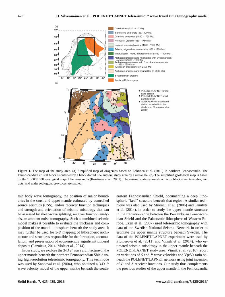
Figure 1. The map of the study area. (a) Simplified map of orogenies based on Lahtinen et al. (2015) in northern Fennoscandia. The

Fennoscandian crustal block is outlined by a black dotted line and our study area by a rectangle. (b) The simplified geological map is based

on the 1 : 2 000 000 geological map of Fennoscandia (Koistinen et al., 2001). The seismic stations are shown with black stars, triangles, and

dots, and main geological provinces are named.

mic body wave tomography, the position of major bound-

aries in the crust and upper mantle estimated by controlled

source seismics (CSS), and/or receiver function techniques

and strength and orientation of seismic anisotropy that can

be assessed by shear-wave splitting, receiver function analy-

sis, or ambient noise tomography. Such a combined seismic

model makes it possible to evaluate the thickness and com-

position of the mantle lithosphere beneath the study area. It

may further be used for 3-D mapping of lithospheric archi-

tecture and structures responsible for the formation, accumu-

lation, and preservation of economically significant mineral

deposits (Laznicka, 2014; Mole et al., 2014).

In our study, we explore the 3-D P wave architecture of the

upper mantle beneath the northern Fennoscandian Shield us-

ing high-resolution teleseismic tomography. This technique

was used by Sandoval et al. (2004), who obtained a 3-D P

wave velocity model of the upper mantle beneath the south-

eastern Fennoscandian Shield, documenting a deep litho-

spheric “keel” structure beneath that region. A similar tech-

nique was also used by Shomali et al. (2006) and Janutyte

et al. (2014), in order to study the upper mantle structure

in the transition zone between the Precambrian Fennoscan-

dian Shield and the Palaeozoic lithosphere of Western Eu-

rope. Eken et al. (2007) used teleseismic tomography with

data of the Swedish National Seismic Network in order to

estimate the upper mantle structure beneath Sweden. The

data of the POLENET/LAPNET experiment were used by

Plomerová et al. (2011) and Vinnik et al. (2014), who es-

timated seismic anisotropy in the upper mantle beneath the

POLENET/LAPNET study area. Vinnik et al. (2016) report

on variations of S and P wave velocities and Vp/Vs ratio be-

neath the POLENET/LAPNET network using joint inversion

of P and S receiver functions. Our study thus complements

the previous studies of the upper mantle in the Fennoscandia

Solid Earth, 7, 425–439, 2016 www.solid-earth.net/7/425/2016/

H. Silvennoinen et al.: POLENET/LAPNET teleseismic P wave travel time tomography model 427

by the body-wave tomography technique. It is also a valu-

able contribution to the combined seismic model of the upper

mantle beneath the northern Fennoscandian Shield.

2 Tectonic setting

Our study area is located in the Fennoscandian Shield in the

northern part of the East European Craton. The area consists

of the Archaean Karelian craton in the eastern part of the

study area, subdivided into Karelian and Kola provinces and

the Belomorian Mobile Belt in between, the Svecofennian

Norrbotten craton in the western part, and the Caledonides in

the north-western corner (Fig. 1b).

The Karelian craton started rifting in the Palaeoprotero-

zoic era some 2.5–2.1 Ga ago. Rifting began in the north-east

and led to a separation of cratonic components by oceans

around 2.1 Ga (Daly et al., 2006). The rifting event was fol-

lowed by two orogenies: the Lapland–Kola orogeny (1.94–

1.86 Ga, Daly et al., 2006) and the northern part of the

Svecofennian orogeny (1.92–1.89 Ga, Lahtinen et al., 2008)

(Fig. 1a).

The Lapland-Kola orogeny was preceded by subduction

of the new oceanic crust and by island arc accretion at

1.95–1.91 Ga. The orogeny was a transpressional continent-

continent collision between Kola province and Karelian

province and produced only a minimal amount of juvenile

crust (Lahtinen et al., 2008). The juvenile material seems

to be dominated by Archaean crustal origin though man-

tle contribution cannot be ruled out (Heilimo et al., 2014).

Although in general, the Svecofennian orogeny formed a

large unit of new Palaeoproterozoic crust, similarly to the

Lapland–Kola orogeny, its northern part is mainly comprised

of reworked Archaean material. The orogeny began from the

north, where the Karelian craton and Norrbotten Craton col-

lided at ca. 1.92 Ga (Lahtinen et al., 2008, 2015).

After these two orogenies, there have been no major tec-

tonic events in our study area, but there is still some smaller

volume magmatism with ages from Palaeoproterozoic to De-

vonian (Downes et al., 2005). These rocks are often from rel-

atively deep sources and, though quite diverse in rock types,

are some of the most important carriers of mantle xenoliths

(Woodard, 2010).

3 Data set

The main data set used in this study is the data of the

POLENET/LAPNET network that was recorded during

May 2007–September 2009 (Kozlovskaya et al., 2007). For

this study, we selected 96 teleseismic events that were located

at epicentral distances between 30◦ and 90◦ from our station

network and were clearly recorded by most of the stations. In

addition to the new data set from the POLENET/LAPNET

network, we included previous data from the northern part

of the SVEKALAPKO network (Hjelt et al., 2006) located

30°

60°

90°

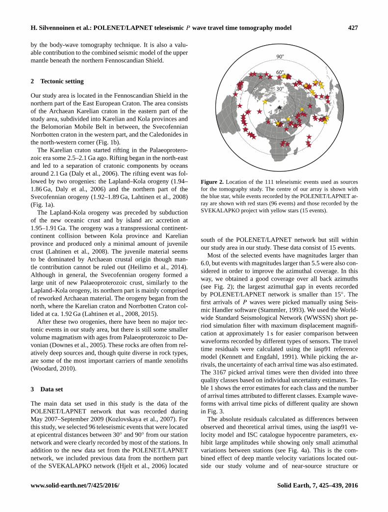
Figure 2. Location of the 111 teleseismic events used as sources

for the tomography study. The centre of our array is shown with

the blue star, while events recorded by the POLENET/LAPNET ar-

ray are shown with red stars (96 events) and those recorded by the

SVEKALAPKO project with yellow stars (15 events).

south of the POLENET/LAPNET network but still within

our study area in our study. These data consist of 15 events.

Most of the selected events have magnitudes larger than

6.0, but events with magnitudes larger than 5.5 were also con-

sidered in order to improve the azimuthal coverage. In this

way, we obtained a good coverage over all back azimuths

(see Fig. 2); the largest azimuthal gap in events recorded

by POLENET/LAPNET network is smaller than 15◦. The

first arrivals of P waves were picked manually using Seis-

mic Handler software (Stammler, 1993). We used the World-

wide Standard Seismological Network (WWSSN) short pe-

riod simulation filter with maximum displacement magnifi-

cation at approximately 1 s for easier comparison between

waveforms recorded by different types of sensors. The travel

time residuals were calculated using the iasp91 reference

model (Kennett and Engdahl, 1991). While picking the ar-

rivals, the uncertainty of each arrival time was also estimated.

The 3167 picked arrival times were then divided into three

quality classes based on individual uncertainty estimates. Ta-

ble 1 shows the error estimates for each class and the number

of arrival times attributed to different classes. Example wave-

forms with arrival time picks of different quality are shown

in Fig. 3.

The absolute residuals calculated as differences between

observed and theoretical arrival times, using the iasp91 ve-

locity model and ISC catalogue hypocentre parameters, ex-

hibit large amplitudes while showing only small azimuthal

variations between stations (see Fig. 4a). This is the com-

bined effect of deep mantle velocity variations located out-

side our study volume and of near-source structure or

www.solid-earth.net/7/425/2016/ Solid Earth, 7, 425–439, 2016


SGFquality class 3+/- 0.4 s

LP62quality class 2+/- 0.2 s

OULquality class 1+/- 0.1 s

06:34:15 06:34:25 06:34:35

P_absP

P

P

Time in UTC

Figure 3. Example travel time picks of different quality from the same event observed at three different stations. The recorded waveforms

have been filtered with the WWSSN short period simulation filter. The travel time observation from the station OUL was attributed a quality

class 1, the one from station LP62 a quality class 2, and from station SGF a quality class 3. For OUL, the absolute travel time (Pabs) was

picked as well as the relative travel time (P ). For each pick, the timing uncertainty estimate of the quality class is shown with a grey rectangle.

Table 1. The travel time data quality classes. The table shows the data quality classes, the corresponding error estimates, and the number of

travel time residual in the quality class for POLENET/LAPNET data, SVEKALAPKO data, and the total. The bottom row shows the total

number of travel time residuals over all quality classes for both projects, and finally the total number of travel time residuals in our database.

Quality Error Number of Number of Total number

class estimate (s) POLENET/LAPNET SVEKALAPKO of residuals

residuals residuals

1 ±0.1 2572 239 2811

2 ±0.2 430 85 515

3 ±0.4 165 35 200

Total 3167 359 3526

teleseismic hypocentre parameter uncertainties. To separate

these effects from our observations, the average travel time

residual over all stations was calculated for each event and

subtracted from all corresponding residuals. The resulting

relative residuals contain the effects of the velocity variations

within our study volume with reference to the iasp91 model.

Figure 4b shows the azimuthal distributions of the residu-

als for three selected stations representing different regions

within our study area.

The additional data recorded by SVEKALAPKO network

included 15 events recorded at 31 stations yielding 360 P

wave residual times (Plomerová et al., 2006). To ascertain

the compatibility of the two data sets, we compared the

residuals recorded at four seismic stations operational during

both SVEKALAPKO and POLENET/LAPNET projects and

found no significant difference in residual amplitudes or dis-

tribution. The comparison figures are available in the Supple-

ment. The quality class distribution of the SVEKALAPKO

data is shown in Table 1. All seismic stations included in this

study are shown in Fig. 1b and the event distribution is shown

in Fig. 2.

4 The inversion method

In seismic tomography, the basic system of equations relating

velocity perturbations inside the study volume to travel time

residuals is

d =Gm, (1)

where d is a data vector composed of travel time resid-

uals, m is a model parameter vector composed of veloc-

ity perturbations in each cell of the velocity model, and G

is a matrix of partial derivatives defining the coupling be-

tween data and model parameters (e.g. Kissling, 1988). The

method searches the velocity perturbations inside a defined



KIFKIF

LP62

MSF

LP62

MSF18˚20˚22˚24˚26˚28˚30˚

64˚

65˚

66˚

67˚

68˚

69˚

70˚

-2.0 -0.8 -0.4 0.0 0.4 0.8 2.0

30°

60°

90°

30°

60°

90°

30°

60°

90°

30°

60°

90°

30°

60°

90°

30°

60°

90°

Traveltime residual [s]

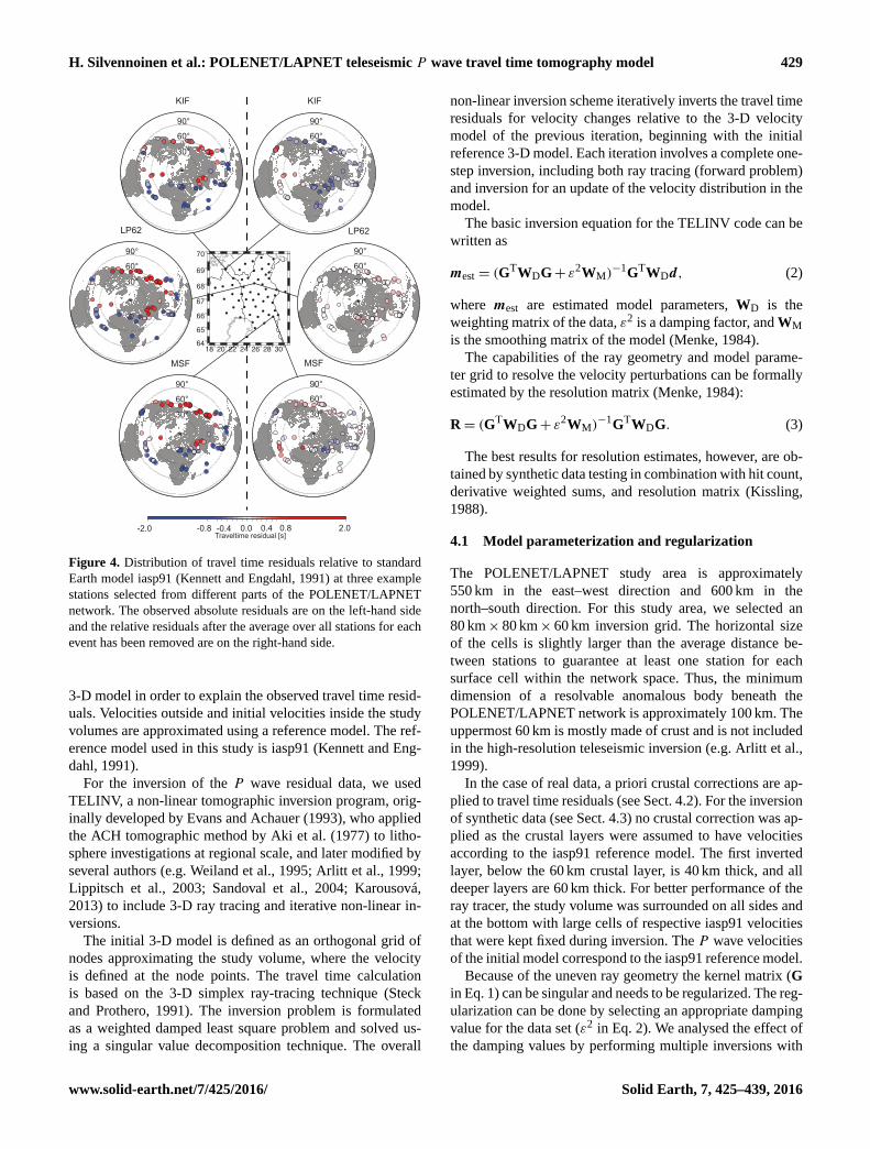
Figure 4. Distribution of travel time residuals relative to standard

Earth model iasp91 (Kennett and Engdahl, 1991) at three example

stations selected from different parts of the POLENET/LAPNET

network. The observed absolute residuals are on the left-hand side

and the relative residuals after the average over all stations for each

event has been removed are on the right-hand side.

3-D model in order to explain the observed travel time resid-

uals. Velocities outside and initial velocities inside the study

volumes are approximated using a reference model. The ref-

erence model used in this study is iasp91 (Kennett and Eng-

dahl, 1991).

For the inversion of the P wave residual data, we used

TELINV, a non-linear tomographic inversion program, orig-

inally developed by Evans and Achauer (1993), who applied

the ACH tomographic method by Aki et al. (1977) to litho-

sphere investigations at regional scale, and later modified by

several authors (e.g. Weiland et al., 1995; Arlitt et al., 1999;

Lippitsch et al., 2003; Sandoval et al., 2004; Karousová,

2013) to include 3-D ray tracing and iterative non-linear in-

versions.

The initial 3-D model is defined as an orthogonal grid of

nodes approximating the study volume, where the velocity

is defined at the node points. The travel time calculation

is based on the 3-D simplex ray-tracing technique (Steck

and Prothero, 1991). The inversion problem is formulated

as a weighted damped least square problem and solved us-

ing a singular value decomposition technique. The overall

non-linear inversion scheme iteratively inverts the travel time

residuals for velocity changes relative to the 3-D velocity

model of the previous iteration, beginning with the initial

reference 3-D model. Each iteration involves a complete one-

step inversion, including both ray tracing (forward problem)

and inversion for an update of the velocity distribution in the

model.

The basic inversion equation for the TELINV code can be

written as

mest = (GTWDG+ ε2WM)−1GTWDd, (2)

where mest are estimated model parameters, WD is the

weighting matrix of the data, ε2 is a damping factor, and WM

is the smoothing matrix of the model (Menke, 1984).

The capabilities of the ray geometry and model parame-

ter grid to resolve the velocity perturbations can be formally

estimated by the resolution matrix (Menke, 1984):

R= (GTWDG+ ε2WM)−1GTWDG. (3)

The best results for resolution estimates, however, are ob-

tained by synthetic data testing in combination with hit count,

derivative weighted sums, and resolution matrix (Kissling,

1988).

4.1 Model parameterization and regularization

The POLENET/LAPNET study area is approximately

550 km in the east–west direction and 600 km in the

north–south direction. For this study area, we selected an

80 km× 80 km× 60 km inversion grid. The horizontal size

of the cells is slightly larger than the average distance be-

tween stations to guarantee at least one station for each

surface cell within the network space. Thus, the minimum

dimension of a resolvable anomalous body beneath the

POLENET/LAPNET network is approximately 100 km. The

uppermost 60 km is mostly made of crust and is not included

in the high-resolution teleseismic inversion (e.g. Arlitt et al.,

1999).

In the case of real data, a priori crustal corrections are ap-

plied to travel time residuals (see Sect. 4.2). For the inversion

of synthetic data (see Sect. 4.3) no crustal correction was ap-

plied as the crustal layers were assumed to have velocities

according to the iasp91 reference model. The first inverted

layer, below the 60 km crustal layer, is 40 km thick, and all

deeper layers are 60 km thick. For better performance of the

ray tracer, the study volume was surrounded on all sides and

at the bottom with large cells of respective iasp91 velocities

that were kept fixed during inversion. The P wave velocities

of the initial model correspond to the iasp91 reference model.

Because of the uneven ray geometry the kernel matrix (G

in Eq. 1) can be singular and needs to be regularized. The reg-

ularization can be done by selecting an appropriate damping

value for the data set (ε2 in Eq. 2). We analysed the effect of

the damping values by performing multiple inversions with



25

0.020

0.022

0.024

0.026

0.028

0.018

0.016

0.0140.002 0.004 0.006 0.007 0.010

Model variance [km 2 s ]

Dat

a va

rianc

e [s

2 ]

Inversion variances using real data

Inversion variances of the checkerboard test shown in �gure 9

0.017 s2

The initial data variance = 0.049 s2

400

200

100

50

1

2

3

45

6

25

400

200

1001

234 56

50

–1

Figure 5. A comparison between data and model variance with dif-

ferent damping values. The selected damping value was first found

using one inversion round only and the results are shown with dia-

monds with the damping value used shown on the right side of the

symbols. The number of iterations was also optimized (dots with

the number of iterations marked to their left side) for the selected

damping value of 100. The final number of iterations, 4, is marked

with a red circle. The grey line denotes the overall data uncertainty,

0.017 s2, calculated as the average uncertainty of all observations.

different damping values both with synthetic data and real

data to find the best damping value for our data set. The fi-

nal damping value of 100 was selected by investigating the

trade-off curve between model and data variance (see Fig. 5

for the trade-off curve of the real data and Fig. 6 for exam-

ples of the crustal corrected residuals). At the same time, the

smallest singular value to be used (minSV) was estimated us-

ing a similar method that was used with damping. Finally, a

value of 70 was selected.

4.2 Crustal correction model

Due to steep incidence angles and subsequent near-lack of

cross firing, teleseismic rays are largely incapable of resolv-

ing upper lithosphere structure such as Moho topography and

3-D crustal velocity variations. Lateral variation of crustal

structure, however, may significantly affect travel times of

teleseismic rays (Arlitt et al., 1999). Hence, when illuminat-

18˚ 20˚ 22˚ 24˚ 26˚ 28˚ 30˚64˚

65˚

66˚

67˚

68˚

69˚

70˚

18˚ 20˚ 22˚ 24˚ 26˚ 28˚ 30˚64˚

65˚

66˚

67˚

68˚

69˚

70˚

−0.3 −0.2 −0.1 0.0 s

0 40 80 100

-0.1

-0.2

-0.3

Trav

eltim

e [s

]

A

A’

A A’

Distance [km]

(a)

(b)

Figure 6. Crustal correction map. Panel (a) shows crustal correction

values for all of the stations. The values are based on a travel time

of a vertical seismic ray travelling through the crustal correction

model described in Sect. 4.2. Panel (b) shows the comparison of

the travel times through a vertical section of the pseudo-3-D crustal

correction model used in this study (black line) and the southern

part of the POLAR wide-angle reflection and refraction profile (red

line, Janik et al., 2009). The location of the comparison is shown

by a black line in (a).

ing the structures at upper mantle depths with high-resolution

teleseismic tomography, it is necessary to correct the data a

priori for the effect of crustal structures as documented for

southern Finland by Sandoval et al. (2003). A new map of

the crustal thickness was established by Silvennoinen et al.

(2014) based on previous and new controlled source seismic

and receiver function results in our study area. This map in

combination with an averaged 1-D velocity–depth function

is used in this study to construct a 3-D crustal model for the

purpose of correcting travel times for crustal effects.

The 3-D crustal model used in this study was estab-

lished by using Bloxer software (https://wiki.oulu.fi/display/

~mpi/Block+model+maintenance). Bloxer is a piece of soft-

ware designed to build 3-D block models with different pa-

rameters (density, seismic velocity, magnetization etc.). The

Moho depth map by Silvennoinen et al. (2014) was im-

ported to Bloxer. All blocks below the Moho to a maximum


https://wiki.oulu.fi/display/~mpi/Block+model+maintenance

https://wiki.oulu.fi/display/~mpi/Block+model+maintenance


model depth of 60 km were given a P wave velocity value

8.05 km s−1 that is the P wave velocity of the uppermost

mantle of the iasp91 reference model.

As our study area does not have enough P wave veloc-

ity information available to estimate a true 3-D distribu-

tion of seismic velocities in the crust between CSS profiles,

we used an average P wave velocity for crustal depths de-

fined from major refraction seismic profiles, namely FEN-

NOLORA (Guggisberg, 1986; Guggisberg et al., 1991; Lu-

osto and Korhonen, 1986) in Sweden, POLAR (Luosto et al.,

1989; Janik et al., 2009) in Finland, and PECHENGA-

KOSTOMUKSHA (Azbel et al., 1989, 1991; Azbel and

Ionkis, 1991) in Russia. A map of crustal correction times

for vertical incident rays arriving at each station is shown

in Fig. 6a. The crustal effect established by Sandoval et

al. (2003) for southern and central Finland has an almost

perfect fit with the crustal effect established in this study

for the overlapping southern part of our study area (south

of 65.5◦ N).

To evaluate the travel time through this pseudo-3-D model

with averaged velocity–depth function and locally variable

Moho depths in comparison to the travel time through a lo-

cal 2-D velocity distribution, derived from a wide-angle re-

flection and refraction profile, we calculated the travel times

trough our model to the depth of 70 km along the POLAR

profile (Janik et al., 2009). This profile is located near the

centre of our study area. From the comparison of travel times

through our crustal correction model and the 2-D model

by Janik et al. (2009), we found the effect of local crustal

velocity–depth variations to be minor compared to the effect

of the variation in Moho depth (see Fig. 6b).

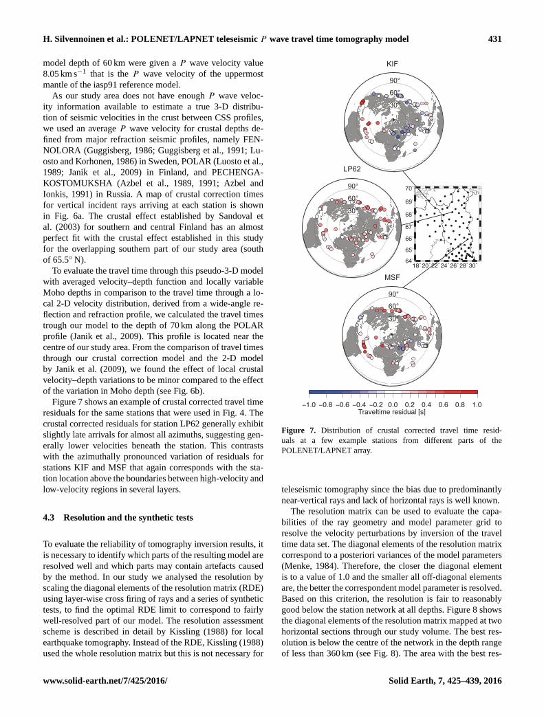
Figure 7 shows an example of crustal corrected travel time

residuals for the same stations that were used in Fig. 4. The

crustal corrected residuals for station LP62 generally exhibit

slightly late arrivals for almost all azimuths, suggesting gen-

erally lower velocities beneath the station. This contrasts

with the azimuthally pronounced variation of residuals for

stations KIF and MSF that again corresponds with the sta-

tion location above the boundaries between high-velocity and

low-velocity regions in several layers.

4.3 Resolution and the synthetic tests

To evaluate the reliability of tomography inversion results, it

is necessary to identify which parts of the resulting model are

resolved well and which parts may contain artefacts caused

by the method. In our study we analysed the resolution by

scaling the diagonal elements of the resolution matrix (RDE)

using layer-wise cross firing of rays and a series of synthetic

tests, to find the optimal RDE limit to correspond to fairly

well-resolved part of our model. The resolution assessment

scheme is described in detail by Kissling (1988) for local

earthquake tomography. Instead of the RDE, Kissling (1988)

used the whole resolution matrix but this is not necessary for

LP62

MSF18˚20˚22˚24˚26˚28˚30˚

64˚

65˚

66˚

67˚

68˚

69˚

70˚

0.0−0.2−0.4−1.0 −0.8 −0.6 0.2 0.4 0.6 0.8 1.0Traveltime residual [s]

KIF

30°

60°

90°

30°

60°

90°

30°

60°

90°

Figure 7. Distribution of crustal corrected travel time resid-

uals at a few example stations from different parts of the

POLENET/LAPNET array.

teleseismic tomography since the bias due to predominantly

near-vertical rays and lack of horizontal rays is well known.

The resolution matrix can be used to evaluate the capa-

bilities of the ray geometry and model parameter grid to

resolve the velocity perturbations by inversion of the travel

time data set. The diagonal elements of the resolution matrix

correspond to a posteriori variances of the model parameters

(Menke, 1984). Therefore, the closer the diagonal element

is to a value of 1.0 and the smaller all off-diagonal elements

are, the better the correspondent model parameter is resolved.

Based on this criterion, the resolution is fair to reasonably

good below the station network at all depths. Figure 8 shows

the diagonal elements of the resolution matrix mapped at two

horizontal sections through our study volume. The best res-

olution is below the centre of the network in the depth range

of less than 360 km (see Fig. 8). The area with the best res-



-3%

360 km

ST 1

ST 2

ST 3

ST 1

ST 2

ST 3

SYNTHETIC MODEL RESULT

-4%

120 km

24˚ 28˚ 32˚

65˚

67˚

69˚

71˚

16˚ 20˚

65˚

67˚

69˚

71˚

63˚

65˚

67˚

69˚

71˚

0.0 0.3 0.6 0 180 360

+3%

SYNTHETIC MODEL RESULT

+4%

+3%

velo

city

per

turb

atio

n [%

]−4

−20

24

RDE back-azimuth[˚]

24˚ 28˚ 32˚16˚ 20˚

65˚

67˚

69˚

71˚

24˚ 28˚ 32˚16˚ 20˚

65˚

67˚

69˚

71˚

63˚

63˚24˚ 28˚ 32˚16˚ 20˚

65˚

67˚

69˚

71˚

0.0 0.3 0.6 RDE

63˚

0 180 360back-azimuth[˚]

24˚ 28˚ 32˚16˚ 20˚

65˚

67˚

69˚

71˚

63˚

24˚ 28˚ 32˚16˚ 20˚

65˚

67˚

69˚

71˚

63˚

24˚ 28˚ 32˚16˚ 20˚

65˚

67˚

69˚

71˚

63˚24˚ 28˚ 32˚16˚ 20˚

65˚

67˚

69˚

71˚

63˚

24˚ 28˚ 32˚16˚ 20˚

65˚

67˚

69˚

71˚

63˚24˚ 28˚ 32˚16˚ 20˚

65˚

67˚

69˚

71˚

63˚

24˚ 28˚ 32˚16˚ 20˚

65˚

67˚

69˚

71˚

63˚24˚ 28˚ 32˚16˚ 20˚

65˚

67˚

69˚

71˚

63˚

24˚ 28˚ 32˚16˚ 20˚

65˚

67˚

69˚

71˚

63˚24˚ 28˚ 32˚16˚ 20˚

65˚

67˚

69˚

71˚

63˚

24˚ 28˚ 32˚16˚ 20˚

65˚

67˚

69˚

71˚

63˚24˚ 28˚ 32˚16˚ 20˚

65˚

67˚

69˚

71˚

63˚

500400300200100

0

−300 −100 100 300

500400300200100

0

−300 −100 100 300

500400300200100

0

−300 −100 100 300

ST 1

ST 2

ST 3

+4%

+4%

+3%

-4%

-4%

-3%

km

Dep

th [k

m]

km

Dep

th [k

m]

km

Dep

th [k

m]

W E

W E

W E

(a) (b)

Figure 8. Two examples of data used to evaluate the lateral resolution of the inversion results with our data set at depths of (a) 120 km and

(b) 360 km. The evaluation was based on diagonal elements of the resolution matrix (RDE) in the upper left corner of both subplots but also

on ray coverage, shown in the upper right corner of both subplots, and the three synthetic test ST1, ST2, and ST3. Red dots and triangles in

RDE plots show the locations of the POLENET/LAPNET and SVEKALAPKO stations, respectively, and the yellow line shows the boundary

of the fairly well-resolved area. The boundary mostly follows a 0.3 RDE line but has occasionally been adjusted based on ray coverage and

synthetic test results. In the right side of the figure, west–east vertical sections through the three synthetic models are shown, clarifying the

location of the anomalous bodies in the vertical direction. The resolution analysis figures at all depths can be found in the Supplement.

olution moves eastward at larger depths, corresponding with

the region of most cross firing from events in the NE, E, and

SE (see Fig. 8b). This is understandable as the stations in the

western part of the network belong to the permanent Swedish

National Seismic Network (SNSN) in Sweden, which was

being updated during the POLENET/LAPNET data acquisi-

tion period. Additionally, the most common recorded back

azimuth direction pointed towards east. As a consequence,

the number of rays crossing the cells in the western part of

the study area, especially from south to north, was smaller

and the ray coverage sparser.

The sensitivity of our data set to velocity heterogeneities

in the upper mantle was tested with the “chequerboard” test.

We constructed a model consisting of alternating positive

and negative anomalies placed regularly through the study

area in both vertical and horizontal directions. The magni-

tudes of the P wave velocity anomalies were ±2 % com-

pared to the iasp91 reference model and the anomaly size

was 160 km× 160 km× 120 km or 2× 2× 2 cells in the in-

version grid. Between the anomalies, we left layers with no

velocity perturbations as suggested by Sandoval et al. (2004).

Examples of the model at two depths (120 and 360 km) are

shown in Fig. 9.

A synthetic data set was calculated using this model and

the ray parameters of the real data set, and the resulting syn-

thetic data set was inverted back to a velocity model. In the

horizontal direction, the anomalies were generally well re-

covered below the station network at all depths. Also, in the

vertical direction the recovery was good in the central and

eastern parts of the study area. In the western part, however,

there was some smearing especially in the north–south di-

rection. Figure 9 compares the model used for computing the

synthetic data set and the results after inversion with our se-

lected damping value at selected depths of 120 and 360 km

as well as through two vertical sections.

Additionally, the resolution was evaluated using synthetic

tests with different structures simulating large-scale anoma-

lies in the upper mantle. We speculated that there could be

such structure in the upper mantle roughly below the Belo-

morian Mobile Belt (see Fig. 1). Hence, all three tests have

an anomalous body there and an additional body crossing

it diagonally to help us visualize how anomalies can affect

each other. The synthetic test models and results are shown



SYNTHETIC MODEL RESULTSYNTHETIC MODEL RESULT

SYNTHETIC MODEL RESULT360 kmSYNTHETIC MODEL RESULT120 km

500 400 300 200 100

0

−200 0 200

S N

Dep

th [k

m]

500 400 300 200 100

0

−200 0 200

S N

500 400 300 200 100

0

−200 0 200

W E

500 400 300 200 100

0

−200 0 200Distance [km]

W E

Distance [km]Distance [km]Distance [km]

Dep

th [k

m]

Dep

th [k

m]

Dep

th [k

m]

18˚ 20˚ 22˚ 24˚ 26˚ 28˚ 30˚64˚

65˚

66˚

67˚

68˚

69˚

70˚

18˚ 20˚ 22˚ 24˚ 26˚ 28˚ 30˚64˚

65˚

66˚

67˚

68˚

69˚

70˚

18˚ 20˚ 22˚ 24˚ 26˚ 28˚ 30˚64˚

65˚

66˚

67˚

68˚

69˚

70˚

18˚ 20˚ 22˚ 24˚ 26˚ 28˚ 30˚64˚

65˚

66˚

67˚

68˚

69˚

70˚

velocity perturbation [%]−4 −2 0 2 4

+2%

+2%

-2%

-2%

-2%

-2%+2%

+2%

(a) (b)

(d)(c)

Figure 9. Chequerboard test results. Two horizontal sections are shown at the depths of 120 (a) and 360 km (b) as well as two vertical

sections, one in SN direction (c) and one in EW direction (d). For each section, both the model used to compute the synthetic data set and the

result after inversion are shown. The model plot of subplot (a) shows the grid used and the locations of the vertical and horizontal sections

with thicker lines, respectively. The locations of the anomalies are bordered with rectangles. The areas that were not inverted are marked

with grey blocks.

in Fig. 8. From the results, we can see that while the anoma-

lies are recovered quite well, there is some leakage both up-

and downward. Similarly to chequerboard tests, we see that

the resolution in the western part of the study area is not as

good as in the eastern part. In the areas with fairly good res-

olution, leakage may generally extend into the next layer up

or down from the anomalous body (i.e. up to 60 km), while

in areas with poor resolution, the leakage can extend to two

layers (up to 120 km). From the test (Fig. 8) we can also see

that we obtain slight positive anomalies around the negative

anomalous body and vice versa, marking an “overswinging”

effect (Kissling et al., 2001).

The fairly well-resolved regions for each layer of our study

area are denoted in Fig. 8. The regions are mainly based on

an RDE value of 0.3, which was selected as the optimal RDE

limit of our model based on ray coverage and synthetic test

results. The regions may have slight deviations from the RDE

based on contracting information from ray coverage and syn-

thetic tests. Similar analysis for the rest of the depth layers

can be found in the Supplement.

Synthetic tests were used to derive the damping param-

eter and singular value cut-off appropriate for data error

and model parameterization. Results of those tests yielded

a damping parameter of 100 and a minSV of 70 as the best

choice for our data set.

5 Results

The main results of inversion with the real data are shown

in Figs. 10 and 11. Our study revealed a highly heteroge-

neous lithospheric mantle beneath the northern Fennoscan-

dian Shield, without any large high P wave velocity area

that might indicate the presence of thick depleted lithospheric

keel revealed beneath the southern part of the shield in Swe-

den (Shomali et al., 2006) and beneath the SVEKALAPKO

study area (Sandoval et al., 2004), as well as in some other

shield areas (e.g. Pasyanos and Nyblade, 2007; Priestley

et al., 2008; Villemaire et al., 2012). The anomalies in the

well-resolved part of our study area are concentrated in the

upper part of the model volume, especially in the layer at

120 km depth (see Fig. 10).

While teleseismic tomography is not effective in resolv-

ing vertical variations of seismic velocities, the recent re-

sult of joint analysis of P and S wave receiver functions by

Vinnik et al. (2016) revealed velocities close to those in the

iasp91 model at upper mantle depths. Additionally, their re-

sults show that absolute average values of seismic velocities

in the lithospheric mantle beneath southern Finland are gen-

erally higher than those beneath the northern Finland.

In our model, we can recognize several anomalies with

higher velocities in the upper part of the lithospheric mantle

(down to depths of about 120–200 km) that spatially correlate

with the Karelian, Kola, and Norrbotten cratons (anomalies

I, II, and III, respectively, in Fig. 10b). While only anomaly

I is clearly located within the fairly well-resolved part of



16˚ 18˚ 20˚ 22˚ 24˚ 26˚ 28˚ 30˚ 32˚ 363˚

64˚

65˚

66˚

67˚

68˚

69˚

70˚

71˚

16˚ 18˚ 20˚ 22˚ 24˚ 26˚ 28˚ 30˚ 32˚ 34˚63˚

64˚

65˚

66˚

67˚

68˚

69˚

70˚

71˚240 km

360 km

16˚ 18˚ 20˚ 22˚ 24˚ 26˚ 28˚ 30˚ 32˚ 363˚

64˚

65˚

66˚

67˚

68˚

69˚

70˚

71˚

16˚ 18˚ 20˚ 22˚ 24˚ 26˚ 28˚ 30˚ 32˚ 34˚63˚

64˚

65˚

66˚

67˚

68˚

69˚

70˚

71˚180 km

16˚ 18˚ 20˚ 22˚ 24˚ 26˚ 28˚ 30˚ 32˚ 363˚

64˚

65˚

66˚

67˚

68˚

69˚

70˚

71˚

16˚ 18˚ 20˚ 22˚ 24˚ 26˚ 28˚ 30˚ 32˚ 34˚63˚

64˚

65˚

66˚

67˚

68˚

69˚

70˚

71˚

120 km

16˚ 18˚ 20˚ 22˚ 24˚ 26˚ 28˚ 30˚ 32˚ 363˚

64˚

65˚

66˚

67˚

68˚

69˚

70˚

71˚

16˚ 18˚ 20˚ 22˚ 24˚ 26˚ 28˚ 30˚ 32˚ 34˚63˚

64˚

65˚

66˚

67˚

68˚

69˚

70˚

71˚300 km

16˚ 18˚ 20˚ 22˚ 24˚ 26˚ 28˚ 30˚ 32˚ 363˚

64˚

65˚

66˚

67˚

68˚

69˚

70˚

71˚

16˚ 18˚ 20˚ 22˚ 24˚ 26˚ 28˚ 30˚ 32˚ 34˚63˚

64˚

65˚

66˚

67˚

68˚

69˚

70˚

71˚

16˚ 18˚ 32˚ 34˚63˚

64˚

65˚

66˚

67˚

68˚

69˚

70˚

71˚

20˚

22˚ 24˚ 26˚ 28˚ 30˚

80 km

Velocity perturbation [%]−4 −2 0 2 4

~

II

III

I

IV

(a)

(b)

(c)

(d)

(e)

( f )

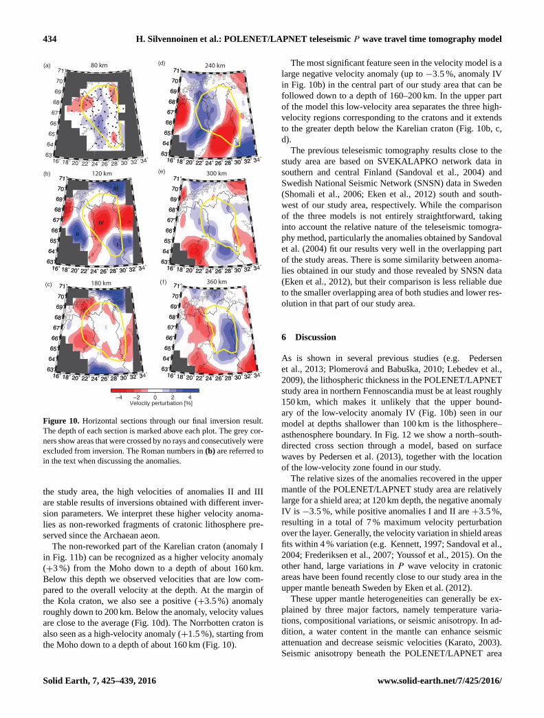
Figure 10. Horizontal sections through our final inversion result.

The depth of each section is marked above each plot. The grey cor-

ners show areas that were crossed by no rays and consecutively were

excluded from inversion. The Roman numbers in (b) are referred to

in the text when discussing the anomalies.

the study area, the high velocities of anomalies II and III

are stable results of inversions obtained with different inver-

sion parameters. We interpret these higher velocity anoma-

lies as non-reworked fragments of cratonic lithosphere pre-

served since the Archaean aeon.

The non-reworked part of the Karelian craton (anomaly I

in Fig. 11b) can be recognized as a higher velocity anomaly

(+3 %) from the Moho down to a depth of about 160 km.

Below this depth we observed velocities that are low com-

pared to the overall velocity at the depth. At the margin of

the Kola craton, we also see a positive (+3.5 %) anomaly

roughly down to 200 km. Below the anomaly, velocity values

are close to the average (Fig. 10d). The Norrbotten craton is

also seen as a high-velocity anomaly (+1.5 %), starting from

the Moho down to a depth of about 160 km (Fig. 10).

The most significant feature seen in the velocity model is a

large negative velocity anomaly (up to −3.5 %, anomaly IV

in Fig. 10b) in the central part of our study area that can be

followed down to a depth of 160–200 km. In the upper part

of the model this low-velocity area separates the three high-

velocity regions corresponding to the cratons and it extends

to the greater depth below the Karelian craton (Fig. 10b, c,

d).

The previous teleseismic tomography results close to the

study area are based on SVEKALAPKO network data in

southern and central Finland (Sandoval et al., 2004) and

Swedish National Seismic Network (SNSN) data in Sweden

(Shomali et al., 2006; Eken et al., 2012) south and south-

west of our study area, respectively. While the comparison

of the three models is not entirely straightforward, taking

into account the relative nature of the teleseismic tomogra-

phy method, particularly the anomalies obtained by Sandoval

et al. (2004) fit our results very well in the overlapping part

of the study areas. There is some similarity between anoma-

lies obtained in our study and those revealed by SNSN data

(Eken et al., 2012), but their comparison is less reliable due

to the smaller overlapping area of both studies and lower res-

olution in that part of our study area.

6 Discussion

As is shown in several previous studies (e.g. Pedersen

et al., 2013; Plomerová and Babuška, 2010; Lebedev et al.,

2009), the lithospheric thickness in the POLENET/LAPNET

study area in northern Fennoscandia must be at least roughly

150 km, which makes it unlikely that the upper bound-

ary of the low-velocity anomaly IV (Fig. 10b) seen in our

model at depths shallower than 100 km is the lithosphere–

asthenosphere boundary. In Fig. 12 we show a north–south-

directed cross section through a model, based on surface

waves by Pedersen et al. (2013), together with the location

of the low-velocity zone found in our study.

The relative sizes of the anomalies recovered in the upper

mantle of the POLENET/LAPNET study area are relatively

large for a shield area; at 120 km depth, the negative anomaly

IV is −3.5 %, while positive anomalies I and II are +3.5 %,

resulting in a total of 7 % maximum velocity perturbation

over the layer. Generally, the velocity variation in shield areas

fits within 4 % variation (e.g. Kennett, 1997; Sandoval et al.,

2004; Frederiksen et al., 2007; Youssof et al., 2015). On the

other hand, large variations in P wave velocity in cratonic

areas have been found recently close to our study area in the

upper mantle beneath Sweden by Eken et al. (2012).

These upper mantle heterogeneities can generally be ex-

plained by three major factors, namely temperature varia-

tions, compositional variations, or seismic anisotropy. In ad-

dition, a water content in the mantle can enhance seismic

attenuation and decrease seismic velocities (Karato, 2003).

Seismic anisotropy beneath the POLENET/LAPNET area



(a) A’

A A’

B

B’

C

C’

Dep

th (k

m)

km

(c) C’

18˚ 20˚ 22˚ 24˚ 26˚ 28˚ 30˚64˚

65˚

66˚

67˚

68˚

69˚

70˚

500

400

300

200

100

0

−300 −200 −100 0 100 200 300(b) B’

Dep

th (k

m)

500

400

300

200

100

0

km−300 −200 −100 0 100 200 300

km−300 −200 −100 0 100 200 300

Dep

th (k

m)

500

400

300

200

100

0

Velocity perturbation [%]−4 −2 0 2 4

III IV

IIV

II IVIII

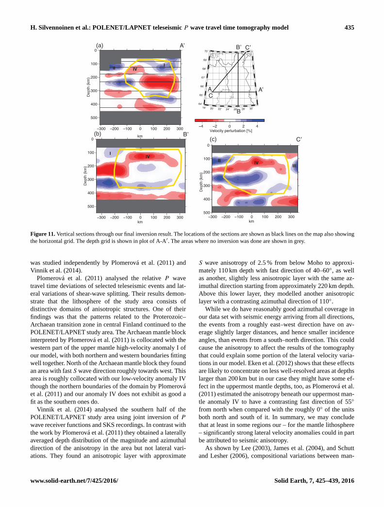
Figure 11. Vertical sections through our final inversion result. The locations of the sections are shown as black lines on the map also showing

the horizontal grid. The depth grid is shown in plot of A-A′. The areas where no inversion was done are shown in grey.

was studied independently by Plomerová et al. (2011) and

Vinnik et al. (2014).

Plomerová et al. (2011) analysed the relative P wave

travel time deviations of selected teleseismic events and lat-

eral variations of shear-wave splitting. Their results demon-

strate that the lithosphere of the study area consists of

distinctive domains of anisotropic structures. One of their

findings was that the patterns related to the Proterozoic–

Archaean transition zone in central Finland continued to the

POLENET/LAPNET study area. The Archaean mantle block

interpreted by Plomerová et al. (2011) is collocated with the

western part of the upper mantle high-velocity anomaly I of

our model, with both northern and western boundaries fitting

well together. North of the Archaean mantle block they found

an area with fast S wave direction roughly towards west. This

area is roughly collocated with our low-velocity anomaly IV

though the northern boundaries of the domain by Plomerová

et al. (2011) and our anomaly IV does not exhibit as good a

fit as the southern ones do.

Vinnik et al. (2014) analysed the southern half of the

POLENET/LAPNET study area using joint inversion of P

wave receiver functions and SKS recordings. In contrast with

the work by Plomerová et al. (2011) they obtained a laterally

averaged depth distribution of the magnitude and azimuthal

direction of the anisotropy in the area but not lateral vari-

ations. They found an anisotropic layer with approximate

S wave anisotropy of 2.5 % from below Moho to approxi-

mately 110 km depth with fast direction of 40–60◦, as well

as another, slightly less anisotropic layer with the same az-

imuthal direction starting from approximately 220 km depth.

Above this lower layer, they modelled another anisotropic

layer with a contrasting azimuthal direction of 110◦.

While we do have reasonably good azimuthal coverage in

our data set with seismic energy arriving from all directions,

the events from a roughly east–west direction have on av-

erage slightly larger distances, and hence smaller incidence

angles, than events from a south–north direction. This could

cause the anisotropy to affect the results of the tomography

that could explain some portion of the lateral velocity varia-

tions in our model. Eken et al. (2012) shows that these effects

are likely to concentrate on less well-resolved areas at depths

larger than 200 km but in our case they might have some ef-

fect in the uppermost mantle depths, too, as Plomerová et al.

(2011) estimated the anisotropy beneath our uppermost man-

tle anomaly IV to have a contrasting fast direction of 55◦

from north when compared with the roughly 0◦ of the units

both north and south of it. In summary, we may conclude

that at least in some regions our – for the mantle lithosphere

– significantly strong lateral velocity anomalies could in part

be attributed to seismic anisotropy.

As shown by Lee (2003), James et al. (2004), and Schutt

and Lesher (2006), compositional variations between man-



low P wave velocity anomaly mapped in this study

%

approx. 200km thick lithosphereof Fennoscandian shield in study region

S-wave velocity perturbation

Figure 12. Comparison to previous lithosphere thickness results.

The figure has been modified from Pedersen et al. (2013) and it

shows the S wave velocity structure obtained in that study in com-

parison to the global S wave velocity model by Debayle and Ri-

card (2012). The area outlined with the yellow line shows the well-

resolved part of our model at the depth of the low-velocity anomaly

found in the upper mantle.

tle peridotites that are depleted in Fe and more fertile can

explain up to 1–2 % velocity anomalies of P wave veloci-

ties. In order to explain larger anomalies, one would need

the combined effect of major element chemistry and temper-

ature as shown by Hieronymus and Goes (2010). That is why

the lowered seismic velocities in the lithospheric mantle of

the central part of our study area (anomaly IV compared to

anomalies I, II and III) are probably most due to the com-

bined effect of anisotropy, a more fertile composition, and a

generally higher temperature.

The low-velocity zone spatially overlaps in the east with

the Kola alkaline province (see Fig. 13), in which alkaline

magmas have intruded the crust (Downes et al., 2005) during

several metasomatic events. Kempton et al. (1995) proposed

that at least one of them was ancient while the latest occurred

in the Devonian. The same events would also result in exten-

sive reworking and refertilization of the originally depleted

NBC Norbotten CratonKaC Karelian CratonKoC Kola Craton Kola alkaline province (Downes et al., 2005) Upper mantle slow velocity anomaly from Bruneton et al. (2004) Low velocity anomaly in depth range 100 km to 200 km from Sandoval et al. (2004) Outline of the fairly well resolved region in our model Baltic-Bothnia megashear based on Berthelsen and Marker (1986)

Velocity perturbation [%]-4 -2 0 2 4

NBC

18˚ 20˚ 22˚ 24˚ 26˚ 28˚ 30˚

60˚

62˚

64˚

66˚

68˚

70˚KoC

KaC

Figure 13. Our results at the depth of 120 km together with cratonic

units in our study area and locations of the Kola alkaline province,

an upper mantle low-velocity anomaly found in SVEKALAPKO

data by Bruneton et al. (2004) and Sandoval et al. (2004), and

Baltic-Bothnia megashear.

Archaean mantle keel while the latest Devonian magmatism

would also explain higher mantle temperatures.

On the other hand, the area of low seismic velocities in the

central part of the network separates Norrbotten, Kola and

Karelian cratons from each other and is spatially correlating

with the northern part of the 1.9–1.8 Ga N–S trending Baltic-

Bothnia Megashear (BBMS) stretching below the Baltic Sea

and the Gulf of Bothnia and continuing to the Caledonides

in Norway (Berthelsen and Marker, 1986, see Fig. 13). The

northern part of the BBMS was later named Pajala shear

zone by Kärki et al. (1993). This shear zone is about 40 km

wide, represented by a complex set of N–S striking shear and

thrust zones. Lahtinen et al. (2015) proposed that the Pajala

shear zone originated as a divergent plate boundary due to

the collision of two Archaean continental units (Norrbotten

and Karelian), and it was multiply reactivated after the con-

tinental collision with both lateral and vertical movements

before 1.83 Ga. As the horizontal sections in the upper man-

tle obtained in our modelling suggest a depth distribution of

the velocity perturbations beneath the megashear similar to

that revealed by Bruneton et al. (2004) and Sandoval et al.

(2004) (see Fig. 13), we suggest that the Pajala shear zone

may continue to the south beneath the Gulf of Bothnia as

was originally proposed by Berthelsen and Marker (1986).

However, the metasomatic processes and refertilization of

the upper mantle in the Palaeoproterozoic alone would not

produce such low seismic velocities as we observed in our

model and combined effect of temperature and composition

would be necessary (Hieronymus and Goes, 2010). Thus,



we may speculate that since the Palaeoproterozoic the whole

BBMS was reactivated by a later tectonothermal event (or

multiple events), during which the cratonic lithosphere was

partly destroyed. The time of those events is not clear, but

they could have occurred the same time with the Paleo-

zoic post-collisional alkaline magmatism in the Kola alka-

line province caused by plume activity (Marty et al., 1998;

Downes et al., 2005; Kogarko et al., 2010).

The Supplement related to this article is available online

at doi:10.5194/se-7-425-2016-supplement.

Acknowledgements. The authors would like to thank the staff of

the Sodankylä geophysical observatory, Institute of Geophysics

of ETH Zürich, and the Institute of Geophysics of the Academy

of Sciences of the Czech Republic for all technical help during

this study. Special thanks to Helena Munzarova, who provided

us the ray distribution plots of Fig. 8. Hanna Silvennoinen

would also like to thank the Finnish Academy of Science and

Letters and Apteekin rahasto for funding her during her part

of this study. The reviews of J. R. R. Ritter and an anonymous

referee led to substantial improvements in this manuscript. The

POLENET/LAPNET project is part of the International Polar Year

2007–2009 and a part of the POLENET consortium. Equipment

for the temporary deployment was provided by RESIF-SISMOB,

FOSFORE, EOST-IPG Strasbourg Equipe seismologie (France),

Seismic pool (MOBNET) of the Geophysical Institute of the

Czech Academy of Sciences (Czech Republic), the Sodankylä

Geophysical Observatory (Finland), the Institute of Geosphere

Dynamics of RAS (Russia), the Institute of Geophysics ETH

Zürich (Switzerland), the Institute of Geodesy and Geophysics, the

Vienna University of Technology (Austria), and the University of

Leeds (UK). The study was financed by the Academy of Finland

(grant no. 122762), University of Oulu (Finland), FBEGDY

program of the Agence Nationale de la Recherche, Institut Paul

Emil Victor (France), ILP (International Lithosphere Program)

task force VIII, grant no. IAA300120709 of the Grant Agency

of the Czech Academy of Sciences, and the Russian Academy of

Sciences (programs no. 5 and no. 9). The POLENET/LAPNET

working group members are Elena Kozlovskaya, Helle Ped-

ersen, Jaroslava Plomerová, Ulrich Achauer, Eduard Kissling,

Irina Sanina, Teppo Jämsén, Hanna Silvennoinen, Catherine Pe-

quegnat, Riitta Hurskainen, Robert Guiguet, Helmut Hausmann,

Petr Jedlicka, Igor Aleshin, Ekaterina Bourova, Reynir Bodvarsson,

Evald Brückl, Tuna Eken, Pekka Heikkinen, Gregory House-

man, Helge Johnsen, Elena Kremenetskaya, Kari Komminaho,

Helena Munzarova, Roland Roberts, Bohuslav Ruzek, Hos-

sein Shomali, Johannes Schweitzer, Artem Shaumyan, Ludek Vec-

sey, and Sergei Volosov.

Edited by: J. Plomerova

References

Aki, K., Christoffersson, A., and Husebye, E.: Determination of the

three-dimensional seismic structure of the lithosphere, J. Geo-

phys. Res., 82, 277–296, 1977.

Arlitt, R., Kissling, E., and Ansorge, J.: Three-dimensional crustal

structure beneath the TOR array and effects on teleseismic wave-

fronts, Tectonophysics, 314, 309–319, 1999.

Azbel, I. and Ionkis, V.: The analysis and interpretation of wave

fields on Soviet and Finnish DSS profiles, in: Structure and

dynamics of the Fennoscandian lithosphere, edited by: Korho-

nen, H. and Lipponen, A., Institut of Seismology, University of

Helsinki, Helsinki, Finland, 21–30, 1991.

Azbel, I., Buyanov, A., Ionkis, V., Sharov, N., and Sharova, V.:

Crustal structure of the Kola-Peninsula from inversion of deep

seismic-sounding data, Tectonophysics, 162, 78–99, 1989.

Azbel, I., Yegorkin, A., Ionkis, V., and Kagaloval, L.: Pecularities

of the Earth’s crust deep structure along the Nikel-Umbozero-

Ruchýi profile, Investigation of the Earth’s continental litho-

sphere with complex seismic methods, Institut of Mines, St. Pe-

tersburg, Russia, 1991.

Berthelsen, A. and Marker, M.: 1.9–1.8 Ga old strike-slip megas-

hear in the Baltic Shield, and their plate tectonic implications,

Tectonophysics, 128, 163–181, 1986.

Bruneton, M., Pedersen, H., Farra, V., Arndt, N., Vacher, P., and

SVEKALAPKO Seismic Tomography Working Group: Com-

plex lithospheric structure under the central Baltic Shield from

surface wave tomography, J. Geophys. Res., 109, B10303,

doi:10.1029/2003JB002947, 2004.

Clifford, T.: Tectono-metallogenic units and metallogenic provinces

of Africa, Earth Planet Sci. Lett., 1, 421–434, 1966.

Daly, J. S., Balagansky, V. V., Timmerman, M. J., and Whitehouse,

M. J.: The Lapland-Kola orogen: Palaeoproterozoic collision and

accretion of the northern Fennoscandian lithosphere, in: Euro-

pean Lithosphere Dynamics, edited by: Gee, D. G. and Stephen-

son, R. A., Geol. Soc. London, 32, 579–598, 2006.

Debayle, E. and Ricard, Y.: A global shear velocity model of

the upper mantle from fundamental and higher Rayleigh

mode measurements, J. Geophys. Res., 117, B10308,

doi:10.1029/2012JB009288, 2012.

Downes, H., Balaganskaya, E., Beard, A., Liferovich, R., and De-

maiffe, D.: Petrogenetic processes in the ultramafic, alkaline and

carbonatitic magmatism in the Kola Alkaline Province: A review,

Lithos, 85, 48–75, 2005.

Eken, T., Shomali, H., Roberts, R., and Bodvarsson, R.: Upper man-

tle structure of the Baltic Shield below the Swedish National

Seismological Networks (SNSN) resolved by teleseismic tomog-

raphy, Geophys. J. Int., 169, 617–630, 2007.

Eken, T., Plomerová, J., Vecsey, L., Babuška, V., Roberts, R.,

Shomali, H., and Bodvarsson, R.: Effects of seismic anisotropy

on P-velocity tomography of the Baltic Shield, Geophys. J. Int.,

188, 600–612, 2012.

Evans, J. and Achauer, U.: Teleseismic velocity tomography us-

ing the ACH method: theory and application to continental scale

studies, in: Seismic Tomography, edited by: Iyer, H., Hirahara,

K., Chapman and Hall, London, UK, 319–360, 1993.

Frederiksen, A. W., Miong, S.-K., Darbyshire, F. A., Eaton, D. W.,

Rondenay, R., and Sol, S.: Lithospheric variations across the

Superior Province, Ontario, Canada: Evidence from tomogra-


http://dx.doi.org/10.5194/se-7-425-2016-supplement

http://dx.doi.org/10.1029/2003JB002947

http://dx.doi.org/10.1029/2012JB009288


phy and shear wave splitting, J. Geophys. Res., 112, B07318,

doi:10.1029/2006JB004861, 2007.

Guggisberg, B.: Eine zweidimensionale refraktionseismische In-

terpretation der Geschwindigkeits-Tiefen-Struktur des oberen

Erdmantels unter dem Fennoskandischen Schild (Projekt FEN-

NOLORA), PhD thesis, ETH, Zürich, Switzerland, 1986.

Guggisberg, B., Kaminski, W., and Prodehl, C.: Crustal structure

of the fennoscandian shield – a traveltime interpretation of the

long-range Fennolora seismic refraction profile, Tectonophysics,

195, 105–137, 1991.

Heilimo, E., Elburg, M., and Andersen, T.: Crustal growth and re-

working during Lapland–Kola orogeny in northern Fennoscan-

dia: U–Pb and Lu–Hf data from the Nattanen and Litsa–Aragub-

type granites, Lithos, 205, 112–126, 2014.

Hieronymus, C. and Goes, S.: Complex cratonic seismic structure

from thermal models of the lithosphere: effects of variations in

deep radiogenic heating, Geophys. J. Int., 180, 999–1012, 2010.

Hjelt, S.-E., Korja, T., Kozlovskaya, E., Lahti, I., Yliniemi, J., and

BEAR and SVEKALAPKO Working Groups: Electrical conduc-

tivity and seismic velocity structures of the lithosphere beneath

the Fennoscandian Shield, in: European Lithosphere Dynamics,

edited by: Gee, D. and Stephenson, R., Geol. Soc. London, Mem.

Ser., 32, 541–559, 2006.

James, D., Boyd, F., Schutt, D., Bell, D., and Carlson, R.: Xeno-

lith constraints on seismic velocities in the upper mantle be-

neath southern Africa, Geochem. Geophys. Geosyst., 5, Q01002,

doi:10.1029/2003GC000551, 2004.

Janik, T., Kozlovskaya, E., Heikkinen, P., Yliniemi, J., and Silven-

noinen, H.: Evidence for preservation of crustal root beneath

the Proterozoic Lapland-Kola orogen (northern Fennoscandian

shield) derived from P and S wave velocity models of PO-

LAR and HUKKA wide-angle reflection and refraction profiles

and FIRE4 reflection transect, J. Geophys. Res.-Sol. Ea., 114,

B06308, doi:10.1029/2008JB005689, 2009.

Janutyte, I., Kozlovskaya, E., Majdanski, M., Voss, P. H., Budraitis,

M., and PASSEQWorking Group: Traces of the crustal units

and the upper-mantle structure in the southwestern part of the

East European Craton, Solid Earth, 5, 821–836, doi:10.5194/se-

5-821-2014, 2014.

Karato, S.-I.: Mapping Water Content in the Upper Mantle, Inside

the Subduction Factory, Geophysical Monograph 138, Americal

Geophysical Union, 2003.

Kärki, A., Laajoki, K., and Luukas, J.: Major Palaeoproterozoic

shear zones of the central Fennoscandian Shield, Precambrian

Res., 64, 207–223, 1993.

Karousová, H.: TELINV2012 – User’s Guide, Prague, Czech Re-

public, 2013.

Kempton, P., Downes, H., Sharkov, E., Vetrin, V., Ionov, D., Car-

swell, D., and Beard, A.: Petrology and geochemistry of xeno-

liths from the Northern Baltic shield: evidence for partial melt-

ing and metasomatism in the lower crust beneath an Archaean

terrane, Lithos, 36, 157–184, 1995.

Kennett, B.: The mantle beneath Australia, AGSO J. Austr. Geol.

Geoph., 17, 49–54, 1997.

Kennett, B. and Engdahl, E.: Traveltimes for global earthquake lo-

cation and phase identification, Geophys. J. Int., 105, 429–465,

1991.

Kissling, E.: Geotomography with local earthquake data, Rev.

Gephysics, 26, 659–698, 1988.

Kissling, E., Husen, S., and Haslinger, F.: Model parameterization

in seismic tomography: a choice of consequence for the solution

quality, Phys. Earth Planet. Int., 123, 89–101, 2001.

Kogarko, L., Lahaye, Y., and Brey, G.: Plume-related mantle source

of super-large rare metal deposits from the Lovozero and Khibina

massifs on the Kola Peninsula, Eastern part of Baltic shield: Sr,

Nd and Hf isotope systematics, Mineral. Petrol., 98, 197–208,

2010.

Koistinen, T., Stephens, M. B., Bogatchev, V., Nordgulen, Ø., Wen-

nerström, M., and Korhonen, J.: Geological map of Fennoscan-

dian shield, scale 1 : 2 000 000, Geological Surveys of Finland,

Norway and Sweden and the North-West Department of Natural

Resources of Russia, 2001.

Kozlovskaya, E. and POLENET/LAPNET working group: Seis-

mic network XK:LAPNET/POLENET seismic temporary array

(RESIF-SISMOB), RESIF – Réseau Sismologique et géodésique

Français, doi:10.15778/RESIF.XK2007, 2007.

Lahtinen, R., Garde, A. A., and Melezhik, V. A.: Paleoproterozoic

evolution of Fennoscandia and Greenland, Episodes, 31, 1–9,

2008.

Lahtinen, R., Huhma, H., Lahaye, Y., Jonsson, E., Manninen, T.,

Lauri, L., Bergman, S., Hellström, F., Niiranen, T., and Nironen,

M.: New geochronological and Sm-Nd constraints across the Pa-

jala shear zone of northern Fennoscandia: Reactivation of a Pa-

leoproterozoic suture, Precambrian Res., 256, 102–119, 2015.

Laznicka, P.: Giant metallic deposits – A century of progress, Ore

Geol. Rev., 62, 259–314, 2014.

Lebedev, S., Boonen, J., and Trampert, J.: Seismic structure of Pre-

cambrian lithosphere: New constraints from broad-band surface-

wave dispersion, Lithos, 109, 96–111, 2009.

Lee, C.-T.: Compositional variation of density and seismic veloci-

ties in natural peridotites at STP conditions: implications for seis-

mic imaging of compositional heterogeneities in the upper man-

tle, J. Geophys. Res., 108, 2441, doi:10.1029/2003JB002413,

2003.

Lippitsch, R., Kissling, E., and Ansorge, J.: Upper mantle

structure beneath the Alpine orogen from high-resolution

teleseismic tomography, J. Geophys. Res., 108, 2376,

doi:10.1029/2002JB002016, 2003.

Luosto, U. and Korhonen, H.: Crustal structure of the baltic shield

based on off – Fennolora refraction data, Tectonophysics, 128,

183–208, 1986.

Luosto, U., Flueh, E., Lund, C.-E., and POLAR Working group:

The crustal structure along the POLAR profile from seismic re-

fraction investigation., Tectonophysics, 162, 51–85, 1989.

Marty, B., Tolstikhin, I., Kamensky, I., Nivin, V., Balaganskaya, E.,

and Zimmerman, J.-L.: Plume-derived rare gases in 380 Ma car-

bonatites from the Kola region (Russia) and the argon isotopic

composition in the deep mantle, Earth Planet Sci. Lett., 164, 179–

192, 1998.

Menke, W.: Geophysical Data Analysis: Discrete Inverse Theory,

International Geophysical Series, Academic Press, London, UK,

45 pp., 1984.

Mole, D., Fiorentini, M. L., Cassidy, K. F., Kirkland, C. L., The-

baud, N., McCuaig, T. C., Doublier, M. P., Duuring, P., Romano,

S. S., Maas, R., Belousova, E. A., Barnes, S. J., and Miller, J.:

Crustal evolution, intra-cratonic architecture and the metallogeny

of an Archaean craton, Special Publications, Geol. Soc. London,

393, 23–80, 2014.


http://dx.doi.org/10.1029/2006JB004861

http://dx.doi.org/10.1029/2003GC000551

http://dx.doi.org/10.1029/2008JB005689

http://dx.doi.org/10.5194/se-5-821-2014

http://dx.doi.org/10.5194/se-5-821-2014

http://dx.doi.org/10.15778/RESIF.XK2007

http://dx.doi.org/10.1029/2003JB002413

http://dx.doi.org/10.1029/2002JB002016


Pasyanos, M. and Nyblade, A.: A top to bottom lithospheric study

of Africa and Arabia, Tectonophysics, 444, 27–44, 2007.

Pedersen, H., Debayle, E., Maupin, V., and the

POLENET/LAPNET Working Group: Strong lateral varia-

tions of lithospheric mantle beneath cratons – Example from the

Baltic Shield, Earth Planet Sci. Lett., 383, 164–172, 2013.

Plomerová, J. and Babuška, V.: Long memory of mantle lithosphere

fabric – European LAB constrained from seismic anisotropy,

Lithos, 120, 131–143, 2010.

Plomerová, J., Babuška, V., Vecsey, L., Kozlovskaya, E., Raita, T.,

and SSTWG: Proterozoic-Archean boundary in the upper mantle

of eastern Fennoscandia as seen by seismic anisotropy, J. Geo-

dyn., 41, 400–410, 2006.

Plomerová, J., Vecsey, L., Babuška, V., and LAPNET Working

Group: Domains of Archean mantle lithosphere deciphered by

seismic anisotropy – inferences from the LAPNET array in

northern Fennoscandia, Solid Earth, 2, 303–313, doi:10.5194/se-

2-303-2011, 2011.

Priestley, K., McKenzie, D., Debayle, E., and Pilidou, S.: The

African upper mantle and its relationship to tectonics and sur-

face geology, Geophys. J. Int., 175, 1105–1126, 2008.

Sandoval, S., Kissling, E., Ansorge, J., and the SVEKALAPKO

Seismic Tomography Working Group: High-resolution body

wave tomography beneath the SVEKALAPKO array – Part I: A

priori three-dimensional crustal model and associated traveltime

effects on teleseismic wave fronts, Geophys. J. Int., 153, 75–87,

2003.

Sandoval, S., Kissling, E., Ansorge, J., and SVEKALAPKO

STWG: High-resolution body wave tomography beneath the

SVEKALAPKO array: II. Anomalous upper mantle structure be-

neath the central Baltic Shield, Geophys. J. Int., 157, 200–214,

2004.

Schutt, D. and Lesher, C.: The effects of melt depletion on the den-

sity and seismic velocity of garnet and spinel lherzolite, J. Geo-

phys. Res., 111, B05401, doi:10.1029/2003JB002950, 2006.

Shomali, Z., Roberts, R., Pedersen, L., and TOR Working Group:

Lithospheric structure of the Tornquist Zone resolved by non-

linear P and S teleseismic tomography along the TOR array,

Tectonophysics, 416, 133–149, 2006.

Silvennoinen, H., Kozlovskaya, E., Kissling, E., Kosarev, G., and

POLENET/LAPNET working group: A new Moho boundary

map for northern Fennoscandian shield based on combined

controlled-source seismic and receiver function data, Geo. Res.

J., 1/2, 19–32, 2014.

Snyder, D., Rondenay, S., Bostock, M., and Lockhart, G.: Mapping

the mantle lithosphere for diamond potential using teleseismic

methods, Lithos, 77, 859–872, 2004.

Stammler, K.: SeismicHandler – programmable multichannel data

handler for interactive and automatic processing of seismological

analyses, Comput. Geosci., 19, 135–140, 1993.

Steck, L. K. and Prothero, W.: A 3-D ray-tracer for teleseismic

body-wave arrival-times, B. Seismol. Soc. Am., 81, 1332–1339,

1991.

Trampert, J. and Van der Hilst, R.: Towards a quantitative interpre-

tation of global seismic tomography, Geophysical Monograph,

American Geophysical Union, 160 pp., 2005.

Villemaire, M., Darbyshire, F., and Bastow, I.: Evolution of

the mantle from Archean to Phanerozoic and its modifica-

tion during subsequent hotspot tectonism : seismic evidence

from eastern North America, J. Geophys. Res., 117, B12302,

doi:10.1029/2012JB009639, 2012.

Vinnik, L., Oreshin, S., Makeyeva, L., Peregoudov, D., Ko-

zlovskaya, E., and POLENET/LAPNET Working Group:

Anisotropic lithosphere under the Fennoscandian shield

from P receiver functions and SKS waveforms of the

POLENET/LAPNET array, Tectonophysics, 628, 45–54,

2014.

Vinnik, L., Kozlovskaya, E., Oreshin, S., Kosarev, G., Piiponen, K.,

and Silvennoinen, H.: The lithosphere, LAB, LVZ and Lehmann

discontinuity under central Fennoscandia from receiver func-

tions, Tectonophysics, 667, 189–198, 2016.

Weiland, C., Steck, L., Dawson, P., and Korneev, V.: Nonlinear

teleseismic tomography at Long Valley caldera, using three-

dimensional minimum travel time ray tracing, J. Geophys. Res.,

100, 20379–20390, 1995.

Woodard, J.: Genesis and Emplacement of Carbonatites and Lam-

prophyres in the Svecofennian Domain, PhD thesis, University

of Turku, Turku, Finland, 2010.

Youssof, M., Thybo, H., Artemieva, I. M., and Levander, A.: Upper

mantle structure beneath southern African cratons from seismic

finite-frequency P- and S-body wave tomography, Earth Planet.

Sci. Lett., 420, 174–186, doi:10.1016/j.epsl.2015.01.034, 2015.


http://dx.doi.org/10.5194/se-2-303-2011

http://dx.doi.org/10.5194/se-2-303-2011

http://dx.doi.org/10.1029/2003JB002950

http://dx.doi.org/10.1029/2012JB009639

http://dx.doi.org/10.1016/j.epsl.2015.01.034

Documents

POLENET/LAPNET teleseismic P wave travel time