Embed Size (px)
Citation preview

P E R S P E C T I V E S O N
I N T E G R A T E D C O A S T A L
Z O N E M A N A G E M E N T
I N SOUTHAMERICA~~~~
Eds.RAMIRO NEVES
JOB BARETTA
MARCOS MATEUS
~~
miolo projecto euro. 12/11/08 12:05 PM Page 1

T I T L E
Perspectives on Integrated Coastal Zone Management in South America
E D I T O R SRamiro Neves, Job Baretta, Marcos Mateus
I S B N978-972-8469-74-0
L E G A L R E G I S T R AT I O N286710/08
D E S I G NGolpe de Estado – Produções Criativas, Lda.
PA G I N AT I O NPaulo Tribolet Abreu
G R A P H I C A R T P R O D U C T I O NManuela Morais
P R I N T E D A N D B O U N D B YGuide – Artes Gráficas
P U B L I S H E D A N D D I S T R I B U T E D B YIST Press
E D I T O R I A L C O O R D I N AT I O N
IST PRESS
D I R E C T O R Joaquim J. Moura Ramos
Eduardo Borges Pires
Instituto Superior Técnico Av. Rovisco Pais 1049-001 Lisboa Portugal www.istpress.ist.utl.pt
FIRST PUBLISHED IN PORTUGAL IN 2008 BY IST PRESS • COPYRIGHT © 2008 BY IST PRESS
All rights reserved. No part of this book may be reproduced or transmitted in any form or by any means,electronic or mechanical, including photocopying, recording or by any information storage and retrieval system, without permission in writing from the publisher.
PERSPECTIVES ON INTEGRATED COASTAL ZONE MANAGEMENT IN SOUTH AMERICA R. NEVES, J.W. BARETTA AND M. MATEUS (EDS.), IST PRESS, 2008
III
CONTENTS
EDITORS VII
CONTRIBUTORS VIII
PREFACE XV
PART A: INTRODUCTION 1
Basic concepts of Estuarine Ecology ............................................................... 3
The continuous challenge of managing Estuarine Ecosystems ..................... 15
The DPSIR framework applied to the Integrated Management of Coastal Areas ............................................................................................................... 29
Coastal zone management in South America with a look at three distinct Estuarine Systems .......................................................................................... 43
PART B: THE METHODOLOGICAL COMPONENTS 59
A PHES-system approach to coastal zone management .............................. 61
Definition of state indicators for the management of interactions between inland and estuarine systems ......................................................................... 71
Modelling coastal systems: the MOHID Water numerical lab ........................ 77
Modelling pollution: oil spills and faecal contamination ................................. 89
Load and flow estimation: HARP-NUT guidelines and SWAT model description ...................................................................................................... 97
Groundwater recharge assessment .............................................................. 103
Groundwater vulnerability to pollution and to sea water intrusion in coastal aquifers ............................................................................................. 113
MATEDIT: a software tool to integrate information in decision making processes ...................................................................................................... 123
Spatial Decision Support System (SDSS) for Integrated Coastal Zone Management (ICZM) ..................................................................................... 129

CONTENTS IV
PART C: FROM SHALLOW WATER TO THE DEEP FJORD: THE STUDY SITES 137
Occupation history of the Santos Estuary .................................................... 139
Climatology and hydrography of Santos estuary ......................................... 147
Primary producers in Santos Estuarine System ........................................... 161
Zoobenthos of the Santos Estuarine System ............................................... 175
Ecological status of the Santos Estuary water column ................................ 183
Sediment quality of the Santos Estuarine System ........................................ 195
Socio-economic issues in Santos estuary .................................................... 205
The Bahía Blanca Estuary: an integrated overview of its geomorphology and dynamics ................................................................................................ 219
Climatological features of the Bahía Blanca estuary .................................... 231
Water chemistry and nutrients of the Bahía Blanca Estuary ........................ 241
Composition and dynamics of phytoplankton and aloricate ciliate communities in the Bahía Blanca estuary ..................................................... 255
Composition and dynamics of mesozooplankton assemblages in the Bahía Blanca estuary .................................................................................... 271
Salt-marshes: role within the Bahía Blanca estuary ..................................... 277
Socio-economic issues in the Bahía Blanca estuary .................................... 287
Pollution processes in Bahía Blanca estuarine environment ........................ 301
Characterization of Bahía Blanca main existing pressures and their effects on the state indicators for surface and groundwater quality ............ 315
The estuarine system of the Aysén Fjord ...................................................... 333
The ecological and cultural landscape of the Aysén River basin ................. 341
Socio-economy of the Aysén area ................................................................ 357

CONTENTS V
PART D: SITE APPLICATIONS: INTEGRATING THE COMPONENTS 365
Land cover analysis of ECOMANAGE study areas as basis for DPSIR framework applications ................................................................................. 367
Groundwater assessment of Santos Estuary ............................................... 377
Contaminant transport in the sedimentary aquifer of Alemoa ...................... 389
Load and flow estimation in Santos watersheds .......................................... 393
An ecological Model application to the Santos Estuary, Brazil: testing and validation ................................................................................................ 401
A modelling approach to the study of faecal pollution in the Santos Estuary .......................................................................................................... 425
Assessing the impact of several development scenarios on the water quality of Santos Estuary ............................................................................. 435
Potential use of ecological tools to lead public policies: an integrative approach in the Santos Estuarine System .................................................... 445
Building of the Decision Support System in the Santos Estuarine System... 457
Difficulties and opportunities found during the implementation of the ECOMANAGE Project in the Santos Estuarine System ...................... 465
Effect of the flowrate variations of Sauce Chico and Napostá Grande rivers over the inner part of Bahía Blanca estuary ........................................ 471
Hydrodynamics and sediments in Bahía Blanca Estuary: Data analysis and modelling ............................................................................................... 483
Evolution of salinity and temperature in Bahía Blanca estuary, Argentina ... 505
The application of MOHID to assess the potential effect of sewage discharge system at Bahía Blanca estuary (Argentina) ................................ 515
MOHID oil spills modelling in coastal zones: A study case on Bahía Blanca estuary (Argentina) ............................................................................ 523
Groundwater flow components to the global estuary model of the Aysén fjord .......................................................................................... 529
Estimation of loads in the Aysén Basin of the Chilean Patagonia: SWAT model and Harp-Nut guidelines ......................................................... 539

CONTENTS VI
Hydrodynamical vertical 2D model for the Aysén fjord ................................ 555
Ecological Conceptual Model for a Southern Chilean fjord: the Aysén Fjord case study .......................................................................... 567
Conceptual, PHES-system, models of the Aysén Fjord: the case of salmon farming ......................................................................................... 581
A management tool for salmon aquaculture: integrating MOHID and GIS applications for local waste management .................................................... 585
The Aysén Fjord tsunami of April 2007: unexpected uses of circulation models .......................................................................................................... 597
FINAL REMARKS 603

PERSPECTIVES ON INTEGRATED COASTAL ZONE MANAGEMENT IN SOUTH AMERICA R. NEVES, J.W. BARETTA AND M. MATEUS (EDS.), IST PRESS, 2008
VII
EDITORS
NEVES, RAMIRO J. MARETEC Instituto Superior Técnico (IST) Secção de Ambiente e Energia - Departamento de Mecânica Av. Rovisco País 1049-001 Lisboa, Portugal E-mail: [email protected]
BARETTA, JOB van Polanenpark 212 2241RX Wassenaar ZH Netherlands Email: [email protected]
MATEUS, MARCOS D. MARETEC Instituto Superior Técnico (IST) Secção de Ambiente e Energia - Departamento de Mecânica Av. Rovisco País 1049-001 Lisboa, Portugal E-mail: [email protected]

CONTRIBUTORS VIII
CONTRIBUTORS
ABALO PABLO Laboratorio de Hidraulica Universidad Nacional del Sur Av. Alem 1253 - Primer Piso 8000 Bahía Blanca, Argentina E-mail: [email protected]
ALBERDI, ERNESTO Instituto Argentino de Oceanografía (IADO) Area Oceanografía Física Complejo CCT-CONICET-Bahía Blanca, C.C. 804 8000 Bahía Blanca, Argentina E-mail: [email protected]
ALBUQUERQUE FILHO, JOSÉ LUIZ Instituto de Pesquisas Tecnológicas do Estado de São Paulo - IPT Centro de Tecnologias Ambientais e Energéticas - CETAE Laboratório de Recursos Hídricos e Avaliação GeoAmbiental - LabGeo Av. Prof. Almeida Prado, 532 05508-901 - São Paulo - SP - Brasil E-Mail: [email protected]
ALMEIDA, PAOLA B. Departamento de Ciencias del Mar y Médio Ambiente ESPOL Campus Prosperina, FIMCM, Ecuador E-mail: [email protected]
ANDRADE, SANTIAGO J. Pontificia Universidad Católica de Chile Departamento de Ecología Centro de Estudios Avanzados en Ecología y Biodiversidad Alameda 340, Santiago, Chile E-mail: [email protected]
ARIAS, ANDRÉS H. CONICET Instituto Argentino de Oceanografía (IADO) Area Oceanografía Química Complejo CCT-CONICET-Bahía Blanca, C.C. 804 8000 Bahía Blanca, Argentina E-mail: [email protected]
ASTEASUAIN, RAÚL O. CONICET Instituto Argentino de Oceanografía (IADO) Area Oceanografía Química Complejo CCT-CONICET-Bahía Blanca, C.C. 804 8000 Bahía Blanca, Argentina E-mail: [email protected]
ARGENTINO-SANTOS, RAQUEL C. Instituto Oceanográfico da Universidade de São Paulo (IOUSP) Laboratório de Ecotoxicologia Marinha - LEcotox Praça do Oceanográfico, 191 05508-120 São Paulo, Brasil E-mail: [email protected]
BACHMANN, PAMELA L. Laboratorio de Modelación Ecológica Departamento de Ciencias Ecológicas, Facultad de Ciencias, Universidad de Chile Las Palmeras 3425, Ñuñoa, Santiago Chile E-mail: [email protected]
BELCHIOR, CONSTANÇA C. PROCAM – Programa de Pós-Graduação em Ciência Ambiental Universidade São Paulo (USP) Rua do Anfiteatro 181 Colmeia Favo 14 05508-900 Cidade Universitária, S. Paulo, Brasil E-mail: [email protected]
BERASATEGUI, ANABELA A. CONICET Instituto Argentino de Oceanografía (IADO) Area Oceanografía Biológica Complejo CCT-CONICET-Bahía Blanca, C.C. 804 8000 Bahía Blanca, Argentina E-mail: [email protected]
BERGMANN FILHO, TULLUS U. Instituto Oceanográfico da Universidade de São Paulo Depto. de Biologia Laboratório de Ecotoxicologia Marinha Praça do Oceanográfico, 191. Cidade Universitária 05508-120 São Paulo, Brasil E-mail: [email protected]

CONTRIBUTORS
IX
BERZIN, GILBERTO Núcleo de Pesquisas Hidrodinâmicas (NPH) Universidade Santa Cecília (UNISANTA) Faculdade de Engenharia Civil Rua Oswaldo Cruz, 277 11045-907 Santos, SP - Brasil E-mail: [email protected]
BIANCALANA, FLORENCIA CONICET Instituto Argentino de Oceanografía (IADO) Area Oceanografía Biológica Complejo CCT-CONICET-Bahía Blanca, C.C. 804 8000 Bahía Blanca, Argentina E-mail: [email protected]
BORGES, ROBERTO P. Universidade Santa Cecília (UNISANTA) Faculdade de Ciências e Tecnologia Rua Oswaldo Cruz, 266 11045-907 Santos, SP - Brasil E-mail: [email protected]
BOTTÉ, SANDRA E. CONICET Instituto Argentino de Oceanografía (IADO) Area Oceanografía Química Complejo CCT-CONICET-Bahía Blanca, C.C. 804 8000 Bahía Blanca, Argentina E-mail: [email protected]
BRAUNSCHWEIG, FRANK Action Modulers Rua Cidade De Frehel, Bloco B, Nº12 A 2640-469 Mafra, Portugal E-mail: [email protected]
BURBA, NICOLETTA Dipartimento di Biologia, Laboratorio di Ecologia Quantitativa Università degli Studi di Trieste, Via Weiss 2 34100 Trieste, Italia E-mail: [email protected]
CAMARGO, R Instituto de Astronomia, Geofísica e Ciências Atmosféricas (IAGUSP) Departamento de Ciências Atmosféricas Rua do Matão, 1226 Cidade Universitária 05508 – 090 São Paulo, SP, Brasil E-mail: [email protected]
CAMPUZANO, FRANCISCO J. MARETEC Instituto Superior Técnico (IST) Secção de Ambiente e Energia Departamento de Mecânica Av. Rovisco País 1049-001 Lisboa, Portugal E-mail: [email protected]
CARBONE, ELIZABETH. Instituto Argentino de Oceanografía (IADO) Area Hidrología y Limnología Complejo CCT-CONICET-Bahía Blanca, C.C. 804 8000 Bahía Blanca, Argentina E-mail: [email protected]
CESAR, AUGUSTO Departamento de Ecotoxicologia Universidade Santa Cecília (UNISANTA) Faculdade de Ciências e Tecnologia Rua Oswaldo Cruz, 266 11045-907 Santos, SP - Brasil E-mail: [email protected]
CHAMBEL, PEDRO MARETEC Instituto Superior Técnico (IST) Secção de Ambiente e Energia Departamento de Mecânica Av. Rovisco País 1049-001 Lisboa, Portugal E-mail: [email protected]
DELGADO, LUISA E. Laboratorio de Modelación Ecológica Departamento de Ciencias Ecológicas, Facultad de Ciencias, Universidad de Chile Las Palmeras 3425, Ñuñoa, Santiago Chile E-mail: [email protected]
DELUCCHI, FEDERICO CONICET Instituto Argentino de Oceanografía (IADO) Area Oceanografía Química Complejo CCT-CONICET-Bahía Blanca, C.C. 804 8000 Bahía Blanca, Argentina E-mail: [email protected]
DE MARCO, SILVIA G. Universidad Nacional de Mar del Plata (UNMdP) Facultad de Ciencias Exactas y Naturales Departamento de Biología Dean Funes 3350, 3º piso 7600 Mar del Plata, Argentina E-mail: [email protected]

CONTRIBUTORS X
FEOLI, ENRICO Dipartimento di Biologia, Laboratorio di Ecologia Quantitativa Università degli Studi di Trieste, Via Weiss 2 34100 Trieste, Itália E-mail: [email protected]
FERNANDES, LUIS MARETEC Instituto Superior Técnico (IST) Secção de Ambiente e Energia Departamento de Mecânica Av. Rovisco País 1049-001 Lisboa, Portugal E-mail: [email protected]
FERNANDES, RODRIGO MARETEC Instituto Superior Técnico (IST) Secção de Ambiente e Energia Departamento de Mecânica Av. Rovisco País 1049-001 Lisboa, Portugal E-mail: [email protected]
FERNÁNDEZ SEVERINI, MELISA D. CONICET Instituto Argentino de Oceanografía (IADO) Area Oceanografía Biológica Complejo CCT-CONICET-Bahía Blanca, C.C. 804 8000 Bahía Blanca, Argentina E-mail: [email protected]
FERRER, LAURA D. Universidad de las Islas Baleares Departamento de Química Cra.Valldemossa km 7.5 07122 Palma de Mallorca, Spain. E-mail: [email protected]
FIORI, EVELYN F. Universidade Santa Cecília (UNISANTA) Faculdade de Ciências e Tecnologia Rua Oswaldo Cruz, 266 11045-907 Santos, SP – Brasil E-mail: [email protected]
FRANÇA, CARLOS A. S. Instituto Oceanográfico da Universidade de São Paulo (IOUSP) Departamento de Oceanografia Física, Química e Geológica Praça do Oceanográfico, 191 Cidade Universitária 05508 – 120 São Paulo, SP, Brasil E-mail: [email protected]
FREIJE, RUBÉN H. Universidad Nacional del Sur (UNS) Departamento de Química Av. Alem 1253 8000 Bahía Blanca, Argentina E-mail: [email protected]
GASPARRO, MARCIA R. Instituto Oceanográfico da Universidade de São Paulo (IOUSP) Laboratório de Ecotoxicologia Marinha - LEcotox Praça do Oceanográfico, 191 05508-120 São Paulo Brasil E-mail: [email protected]
GIANESELLA, SÔNIA M. F. Instituto Oceanográfico da Universidade de São Paulo Departamento de Oceanografia Biológica Pça do Oceanográfico, 191 Cidade Universitária, 05508-900, São Paulo, Brasil E-mail:[email protected]
GIORDANO, FABIO Universidade Santa Cecília (UNISANTA) Faculdade de Ciências e Tecnologia Rua Oswaldo Cruz, 266 11045-907 Santos, SP - Brasil E-mail: [email protected]
GUINDER, VALERIA A. CONICET Instituto Argentino de Oceanografía (IADO) Area Oceanografía Biológica Complejo CCT-CONICET-Bahía Blanca, C.C. 804 8000 Bahía Blanca, Argentina E-mail: [email protected]

CONTRIBUTORS
XI
GONZALEZ TRILLA, GABRIELA Universidad de Buenos Aires (UBA) Facultad de Ciencias Exactas y Naturales Lab.Ecología Regional Grupo de Ecología de Humedales Pabellón II, Ciudad Universitaria 1428 Buenos Aires, Argentina E-mail: [email protected]
HARARI, JOSEPH Instituto Oceanográfico da Universidade de São Paulo (IOUSP) Departamento de Oceanografia Física, Química e Geológica Praça do Oceanográfico, 191 Cidade Universitária 05508 – 120 São Paulo, SP, Brasil E-mail: [email protected]
HOFFMEYER, MÓNICA S. CONICET Instituto Argentino de Oceanografía (IADO) Area Oceanografía Biológica Complejo CCT-CONICET-Bahía Blanca, C.C. 804 8000 Bahía Blanca, Argentina E-mail: [email protected]
KODAMA, LEANDRO K. Universidade Santa Cecília (UNISANTA) Faculdade de Ciências e Tecnologia Rua Oswaldo Cruz, 266 11045-907 Santos, SP - Brasil E-mail: [email protected]
LEITÃO, JOSÉ HIDROMOD Av. Manuel da Maia, nº36, 3ºEsq 1000-2001 Lisboa, Portugal E-mail: [email protected]
LEITÃO, PAULO C. HIDROMOD Av. Manuel da Maia, nº36, 3ºEsq 1000-2001 Lisboa, Portugal E-mail: [email protected]
LEITÃO, TERESA E. Groundwater Division Hydraulics and Environment Department Laboratório Nacional de Engenharia Civil (LNEC) Av. do Brasil, 101 1700-066 Lisboa, Portugal E-mail: [email protected]
LEITE, CLÁUDIO B.B. Instituto de Pesquisas Tecnológicas do Estado de São Paulo - IPT Centro de Tecnologias Ambientais e Energéticas - CETAE Laboratório de Resíduos e Áreas Contaminadas - Larac Av. Prof. Almeida Prado, 532 05508-901 - São Paulo - SP - Brasil E-Mail: [email protected]
LIMBOZZI, FABIANA Instituto Argentino de Oceanografía (IADO) Area Oceanografía Química Complejo CCT-CONICET-Bahía Blanca, C.C. 804 8000 Bahía Blanca, Argentina E-mail: [email protected]
LOBO-FERREIRA, JOÃO PAULO Groundwater Division Hydraulics and Environment Department Laboratório Nacional de Engenharia Civil Av. do Brasil 101 1700-066 Lisboa, Portugal E-mail: [email protected]
MALARODA, MASSIMO Dipartimento di Biologia, Laboratorio di Ecologia Quantitativa Università degli Studi di Trieste, Via Weiss 2 34100 Trieste, Italia E-mail: [email protected]
MANCUSO, MALVA A. Instituto de Pesquisas Tecnológicas do Estado de São Paulo - IPT Centro de Tecnologias Ambientais e Energéticas - CETAE Laboratório de Recursos Hídricos e Avaliação GeoAmbiental - LabGeo Av. Prof. Almeida Prado, 532 05508-901 - São Paulo,SP, Brasil E-mail: [email protected]
MARCOVECCHIO, JORGE E. CONICET Instituto Argentino de Oceanografía (IADO) Area Oceanografía Química Complejo CCT-CONICET-Bahía Blanca, C.C. 804 8000 Bahía Blanca, Argentina E-mail: [email protected]

CONTRIBUTORS XII
MARÍN, VICTOR H. Laboratorio de Modelación Ecológica Departamento de Ciencias Ecológicas, Facultad de Ciencias, Universidad de Chile Las Palmeras 3425, Ñuñoa, Santiago Chile E-mail: [email protected]
MATEUS, SANDRA P. MARETEC Instituto Superior Técnico (IST) Secção de Ambiente e Energia Departamento de Mecânica Av. Rovisco País 1049-001 Lisboa, Portugal E-mail: [email protected]
MELO, WALTER D. CONICET Instituto Argentino de Oceanografía (IADO) Gabinete de Cartografía y SIG Complejo CCT-CONICET-Bahía Blanca, C.C. 804 8000 Bahía Blanca, Argentina E-mail: [email protected]
MENÉNDEZ, MARÍA C. CONICET Instituto Argentino de Oceanografía (IADO) Area Oceanografía Biológica Complejo CCT-CONICET-Bahía Blanca, C.C. 804 8000 Bahía Blanca, Argentina E-mail: [email protected]
MOYA, GUSTAVO C. Universidade Santa Cecília (UNISANTA) Faculdade de Ciências e Tecnologia Rua Oswaldo Cruz, 266 11045-907 Santos, SP - Brasil
NAPOLITANO, ROSSELLA Dipartimento di Biologia, Laboratorio di Ecologia Quantitativa Università degli Studi di Trieste, Via Weiss 2 34100 Trieste, Italia E-mail: [email protected]
NEGRÍN, VANESA L. CONICET Instituto Argentino de Oceanografía (IADO) Area Oceanografía Química Complejo CCT-CONICET-Bahía Blanca, C.C. 804 8000 Bahía Blanca, Argentina E-mail: [email protected]
OLIVEIRA, MANUEL MENDES Groundwater Division Hydraulics and Environment Department Laboratório Nacional de Engenharia Civil Av. do Brasil 101 1700-066 Lisboa, Portugal E-mail: [email protected]
PAREDES, MARÍA A. Laboratorio de Modelación Ecológica Departamento de Ciencias Ecológicas, Facultad de Ciencias, Universidad de Chile Las Palmeras 3425, Ñuñoa, Santiago Chile E-mail: [email protected]
PATROLONGO, PAULA CONICET Instituto Argentino de Oceanografía (IADO) Area Oceanografía Biológica Complejo CCT-CONICET-Bahía Blanca, C.C. 804 8000 Bahía Blanca, Argentina E-mail: [email protected]
PEREIRA, CAMILO D. S. Departamento de Ecotoxicologia Universidade Santa Cecília (UNISANTA) Faculdade de Ciências e Tecnologia Rua Oswaldo Cruz, 266 11045-907 Santos, SP - Brasil E-mail: [email protected]
PERILLO, GERARDO M.E. CONICET Instituto Argentino de Oceanografía (IADO) Area Oceanografía Física Complejo CCT-CONICET-Bahía Blanca, C.C. 804 8000 Bahía Blanca, Argentina E-mail: [email protected]
PETTIGROSSO, ROSA E. Universidad Nacional del Sur (UNS) Departamento de Biología, Bioquímica y Farmacia San Juan 670 8000 Bahía Blanca, Argentina E-mail: [email protected]
PICCOLO, MARÍA CINTIA CONICET Instituto Argentino de Oceanografía (IADO) Area Meteorología Complejo CCT-CONICET-Bahía Blanca, C.C. 804 8000 Bahía Blanca, Argentina E-mail: [email protected]

CONTRIBUTORS
XIII
PIERINI, JORGE O. Instituto Argentino de Oceanografía (IADO) Area Oceanografía Física Complejo CCT-CONICET-Bahía Blanca, C.C. 804 8000 Bahía Blanca, Argentina E-mail: [email protected]
PIZARRO, NORA Universidad Nacional del Sur (UNS) Departamento de Geografía y Turismo 12 de Octubre y San Juan 8000 Bahía Blanca, Argentina E-mail: [email protected]
POPOVICH, CECILIA A. Universidad Nacional del Sur (UNS) Departamento de Biología, Bioquímica y Farmacia San Juan 670 8000 Bahía Blanca, Argentina E-mail: [email protected]
RIBEIRO, RENAN B. Núcleo de Pesquisas Hidrodinâmicas (NPH) Universidade Santa Cecília (UNISANTA) Faculdade de Engenharia Civil Rua Oswaldo Cruz, 277 11045-907 Santos, SP - Brasil E-mail: [email protected]
ROSSO, SÉRGIO Instituto de Biociências Departamento de Ecologia Universidade de São Paulo Cidade Universitária, 05508-900, São Paulo, SP – Brasil Email: [email protected]
SALDANHA-CORRÊA, FLÁVIA M.P. Instituto Oceanográfico da Universidade de São Paulo Departamento de Oceanografia Biológica Pça do Oceanográfico, 191 Cidade Universitária, 05508-900, São Paulo, Brasil E-mail:[email protected]
SAMPAIO, ALEXANDRA F. P. Núcleo de Pesquisas Hidrodinâmicas (NPH) Universidade Santa Cecília (UNISANTA) Faculdade de Engenharia Civil Rua Oswaldo Cruz, 277 11045-907 Santos, SP - Brasil E-mail: [email protected]
SANTOS, JOÃO A. P. Universidade Santa Cecília (UNISANTA) Faculdade de Ciências e Tecnologia Rua Oswaldo Cruz, 266 11045-907 Santos, SP - Brasil E-mail: [email protected]
SANTOS, MAURÍCIO P. Universidade Santa Cecília (UNISANTA) Faculdade de Ciências e Tecnologia Rua Oswaldo Cruz, 266 11045-907 Santos, SP - Brasil E-mail: [email protected]
SCIMONE, MAURO Dipartimento di Biologia, Laboratorio di Ecologia Quantitativa Università degli Studi di Trieste, Via Weiss 2 34100 Trieste, Italia E-mail: [email protected]
SCHMIEGELOW, JOÃO M. M. Universidade Santa Cecília (UNISANTA) Faculdade de Ciências e Tecnologia Rua Oswaldo Cruz, 266 11045-907 Santos, SP - Brasil E-mail: [email protected]
SIMONETTI, CRISTINA ERM Brasil Avenida dos Carinás, 635 04086-011 São Paulo, SP - Brasil E-mail: [email protected]
SOUSA, EDUINETTY CECI P. M. Instituto Oceanográfico da Universidade de São Paulo (IOUSP) Laboratório de Ecotoxicologia Marinha - LEcotox Praça do Oceanográfico, 191 05508-120 São Paulo Brasil E-mail: [email protected]
SPETTER, CARLA V. CONICET Instituto Argentino de Oceanografía (IADO) Area Oceanografía Química Complejo CCT-CONICET-Bahía Blanca, C.C. 804 8000 Bahía Blanca, Argentina E-mail: [email protected]

CONTRIBUTORS XIV
TIRONI, ANTONIO Laboratorio de Modelación Ecológica Departamento de Ciencias Ecológicas, Facultad de Ciencias, Universidad de Chile Las Palmeras 3425, Ñuñoa, Santiago Chile E-mail: [email protected]
TOMBESI, NORMA B. Universidad Nacional del Sur (UNS) Departamento de Química Av. Alem 1253 8000 Bahía Blanca, Argentina E-mail: [email protected]
TOPOROVSKI, CLAUDIA Z. Instituto de Pesquisas Tecnológicas do Estado de São Paulo - IPT Centro de Tecnologias Ambientais e Energéticas – CETAE Laboratório de Resíduos e Áreas Contaminadas - Larac Av. Prof. Almeida Prado, 532 05508-901 - São Paulo - SP - Brasil E-mail: [email protected]
TORRES, MARCELA A. Laboratorio de Modelación Ecológica Departamento de Ciencias Ecológicas, Facultad de Ciencias, Universidad de Chile Las Palmeras 3425, Ñuñoa, Santiago Chile E-mail: [email protected]
YARROW, MATTHEW M. Laboratorio de Modelación Ecológica Departamento de Ciencias Ecológicas Facultad de Ciencias, Universidad de Chile Las Palmeras 3425, Ñuñoa, Santiago Chile E-mail: [email protected]

PERSPECTIVES ON INTEGRATED COASTAL ZONE MANAGEMENT IN SOUTH AMERICA R. NEVES, J.W. BARETTA AND M. MATEUS (EDS.), IST PRESS, 2008
XV
PREFACE
From a human history perspective, the intrinsic characteristics of estuaries have made them preferable sites of occupation and, consequently, intense areas of development. A direct consequence of human occupation of these coastal areas is that estuaries rank among the environments most affected by human presence and activities. The fast expansion of socio-economic activities on coastal and estuarine areas over the last decades, such as tourism, nature conservation, coastal fisheries and industrial and urban development has expanded and complicated the management tasks. In recent years, there has been a growing concern to maintain a steady growth in economical activities and social development in estuarine areas, while preserving their natural features and ecological services.
Given the acceptance by governments of the goal of sustainable development, a more sustainable coastal management strategy requires a more interdisciplinary and integrated management process. There are no easy answers to the question of what is best for a particular system from a resource’s management point of view. It is the task of scientists from different disciplines to present as complete a picture as possible to those who make decisions. The ECOMANAGE (Integrated Ecological Coastal Zone Management System) project described here, funded by the European Commission’s Sixth Framework Programme (Contract nº INCO-CT-2004-003715), aims to provide coastal authorities with the knowledge and tools for such an integrated management approach. The common goal was to work towards a social and environmental sustainable estuarine system management in three distinct transitional waters systems in South America: Santos Estuary in Brazil, Bahía Blanca Estuary in Argentina and Fjord Aysén in Chile. Besides their geographical location, these coastal systems cover a wide spectrum of management challenges because they vary significantly in their ecological state and human pressures, in a gradient that goes from a more pristine state of Fjord Aysén, to the heavily occupied and degraded system in Santos Estuary.
The South American continent is endowed with a unique and valuable marine heritage, which enclose several of the world’s largest and most productive estuaries. The accelerated development in most Latin American countries is posing demanding challenges in the management of natural resources, especially in coastal areas. Integrated coastal management approaches are required, combining all aspects of the human, physical and biological aspects of the coastal zone within a single management framework. Integrated coastal management is presented here as a broad, multi-purpose endeavor aimed at improving the quality of life of communities dependent on estuarine resources and helping local

PREFACE
XVI
decision maker attaining sustainable development of estuarine areas, from the headwaters of coastal watersheds to the outer marine areas. The work presented in this volume is a step in that direction. Hopefully, the knowledge, experience, tools and results presented here will be used in other places with similar conflicting uses of natural resources.
Interdisciplinary and integration was the major thrust of ECOMANAGE. The project was originally assembled from scientifically promising and socially relevant research fields, with physical modelling and eutrophication as the core. The social sciences, human ecology and management oriented subjects were included to provide the project with the integrative principle. The work developed during the project formed the knowledge pool for this book. The volume is a collection of writings selected on the basis of novelty, relevance in a water resource management framework, and insightfulness. Contributions have also been included in order to survey the strengths and limitations of a range of existing coastal zone management practices operating in different local environmental and socio-economic contexts. The core message that is highlighted is that the management challenges posed are complex and multifaceted, encompassing physical forcing, natural hazard and variability and vulnerability, together with socio-cultural vulnerability problems.
Being the result of a multidisciplinary scientific endeavor, the book will have an audience that range across a wide spectrum of environmental and social disciplines. The book should be of interest for anyone working in the field of ICZM (Integrated Coastal Zone Management), from scientists to decision makers. Dealing with examples from South America, the book has a strong local interest. However, the kind of approach developed in the project and portrayed in the book enables this work to be used as a benchmark for scientists working worldwide in related areas or facing the same challenges.
The book addresses costal zone management in an integrative way, with particular focus on water resources. As such, we hope it will be of interest for scientists working in fields such as aquatic ecology, ecohydrology, ground water, marine sciences in general, water quality, coastal zone management, etc. In addition, the strong component of the modelling approach will target the modelling community, from ecosystem to ground water modelers.
The Editors September, 2008

INTRODUCTION
PART A
miolo projecto euro. 12/11/07 4:33 PM Page 4


PERSPECTIVES ON INTEGRATED COASTAL ZONE MANAGEMENT IN SOUTH AMERICAR. NEVES, J.W. BARETTA AND M. MATEUS (EDS.), IST PRESS, 2008
BASIC CONCEPTS OF ESTUARINE ECOLOGY
M. MATEUS, S. MATEUS AND J.W. BARETTA
1 ESTUARINE SYSTEMS: THE LAND-OCEAN LINK
Estuaries are highly dynamic environments with their physical, chemical and biological struc-ture characterized by high spatial and temporal variability. The temporal fluctuations and spa-tial gradients in these systems induce large variability in chemical and biological propertiesof the water and sediment. Estuaries are subject to continuous variations in wind, irradiance,rainfall, water level and freshwater runoff. Moreover, estuaries are very often heavily utilisedand impacted by mankind, being used as (natural) harbours, for fish farming, recreation, aswaste water recipient, etc. There are many ways to define what an estuary is. Probablythe simplest definition is that an estuary is a partially enclosed coastal embayment wherefresh water and sea water meet and mix. The estuary can have the simple morphology of ariver entering the sea or a complex and lengthy one, like in fjords. Estuaries are among themost productive environments on earth and they are important ecotones, i.e., transition zonesbetween different ecosystems. Ecotones are boundaries between resource patches in thelandscape, regulating energy, nutrient and mineral sediment flow between adjacent patches(Naiman et al. 1995, Schiemer et al. 1995). Estuaries and their frequently associated fringesof tidal flats, salt marshes and mangrove forests are the transition zones between one environ-ment and another - tidal flats, salt marshes and mangrove forests are the transition betweenland and sea, and estuaries the transition between fresh and sea water. Being the transitionsbetween very different environments, all estuaries share significant physical, chemical andbiological features. Thus, we can state that an estuary is a transition system governed bycomplex interacting elements which vary in space and time.
Usually, estuaries have more similarities with the marine than with the freshwater environment,but in all aquatic systems the throphodynamic structure and functions are very similar, with theexception of gelatinous plankton, which does not occur in freshwater systems. Nevertheless,in each and every aquatic system, the local mix of interactions between the abiotic and bioticenvironment results in different system behaviour and a different response to anthropogenicpressures, making it impossible to use simple rules of thumb to predict ecosystem responsesto such pressures.
2 PHYSICAL AND CHEMICAL CHARACTERISTICS OF ESTUARIES
Estuaries and the adjacent coastal areas have a specific size, shape and bathymetry, a spe-cific tidal influence, fresh water inflow, turbidity and residence times, sediment properties,carbon-to-nutrients ratios, water-column turbidity, etc. Together, all these characteristics, to-gether with human-influenced environment make each estuary unique. Estuaries possess aunique combination of characteristics, frequently expressed in steep physical, chemical andbiological gradients. Because it is where fresh and salt water meets, estuaries are influenced
3
M. MATEUS, S. MATEUS AND J.W. BARETTA
by processes affecting both these types of water, such as tides, coastal hydrodynamics, vari-ations in the river, etc. These factors not only govern much of the physical and chemicalcharacteristics of the estuaries but also its ecological dynamics. Extreme salinity and tem-perature fluctuations, muddy substrates, and other physical factors like light availability andresidence time help make estuaries challenging ecosystems for aquatic organisms.
The shape of the estuary and its sediment, the wind, evaporation of water from the surfaceand river flow influences temperature and salinity in estuaries. The water temperature inestuaries varies markedly because of their shallow water and large surface area. Fjords arethe exception because of their greater water depth. Water temperature affects the dynamics ofa system because it regulates all biological rates. Therefore, a clear seasonality in biologicalactivity is seen in estuaries at mid- to high latitudes. Generally, salinity decreases movingupstream but it fluctuates dramatically both from place to place and time to time. Salinity mayalso vary with depth in the estuary, as well as across the estuary due to the Coriolis effect.
2.1 Water circulation and stratification
Water circulation inside an estuary can change the conditions of the ecosystem over a muchsmaller temporal scale, when compared with neritic or oceanic areas. The hydrodynamics in-side an estuary are driven by a complex interplay of mechanisms, all with a strong influence onbiological processes. Water circulation is conditioned by tidal currents, river discharges, windand local topography. The resulting circulation patterns may have a large effect on the abun-dance and production of the microbial community by controlling the supply of allochthonousorganic matter, concentrating and retaining locally produced organic matter inside the system.They also produce conditions for long-term coupling of bacterial production and autochthonssources of organic matter. Because an estuary is not a closed system, tidal currents act asan oscillating conveyor belt with the coastal zone, moving plankton, organic and inorganicmaterials, and sediments back and forth, creating complex distribution patterns.
Estuaries can be classified according to their mean tidal range as microtidal (mean tidal range< 2m), mesotidal (mean tidal range between 2 and 4 m), macrotidal (mean tidal range be-tween 4 and 6 m), and hypertidal (mean tidal range > 6m) (Dyer 1997). The difference in thetidal range confers distinct characteristics to the estuarine dynamics. As an example, macroti-dal estuaries, which are characterized by high tidal energy, generally exhibit lower levels ofchlorophyll a (Chla) than systems with lower tidal energy. They also exhibit a tolerance to highnutrient loadings from freshwater outflows (Monbet 1992). Estuaries are usually divided in twoclasses defined by their vertical density profile. When the currents of riverine fresh water in-flow and tide are similar, turbulence is the major mixing agent. This process is induced by theperiodicity of tidal action. In this case the vertical salinity profile is less variable because mostof the energy dissipates in the vertical mixing, producing a rather complex set of layers andwater masses. Under these conditions, estuaries are considered partially mixed or moderatelystratified. In completely mixed and vertically homogeneous estuaries, however, the tidal action
4

BASIC CONCEPTS OF ESTUARINE ECOLOGY
is strongly dominant and the water column is well mixed. Together with the shallowness in thistype of estuaries, the balance between fresh and sea water, controlled daily by strong tidalcurrents and modulated seasonally by the river flow, contributes to the absence of a verticalstratification. Major salinity and temperature changes are more frequently observed horizon-tally rather than vertically and this spatial heterogeneity is thought to affect nearly every aspectof population dynamics, species interactions, and community structure.
2.2 Residence time
With the influence of tidal currents and river flow, the entire estuary experiences fluxes thatinterfere with the transport and expression of biological activities and with the distribution ofbiomass in the water column. The residence (or flushing) time of water depends stronglyon tides, freshwater runoff and morphological size, especially length. Other processes canmodify the residence time in an individual estuary, such as currents driven by a difference indensity between fresh and salt water - this is particularly important in deep fjords, bays andsemi-enclosed seas where the bottom waters can be nearly stagnant and where water qualitycan be degraded severely. Another key process is water storage and buffering by intertidalwetlands, mainly salt marsh or mangrove vegetation that flank the main estuary and resultsin drag to the flow and temporary storage of waters. The residence time reflects the rate atwhich dissolved and planktonic components in the water are flushed out to the sea. As such,it controls many of the elements that provide information on the health of the estuary. As such,the residence time of an estuary is an important parameter because it expresses its robust-ness and ability to cope with human-induced stress; Well-flushed estuaries are intrinsicallymore robust than poorly flushed systems. Environmental degradation is usually intensifiedduring periods of reduced freshwater inflows, for example, during drought or when human ac-tivities in the catchment cause significant reductions in dissolved oxygen, for example througheutrophication. The residence time is usually more critical in areas where contaminant ac-cumulation and increased turbidity from human influences are most likely to occur. This isusually the case in the upper reaches of the estuary and in confined areas in estuaries withintricate morphologies.
2.3 Nutrient availability
Nutrients can be present in two major forms: inorganic (or mineral) and organic (both living anddetrital). Nitrogen and phosphorus are the most significant nutrients, and their main speciesinclude dissolved (nitrate, nitrite, ammonium, organic N, phosphate, organic P) and particulate(organic N, organic P) components. Particulate species tend to be dominant in the river loadsreaching the estuaries, but nitrate and phosphate become more important in populous regions.The dynamics of nutrients depend on a number of physical, biological and chemical processesand their fate after entering the estuary varies as a function of turbidity, water flow and biota.Physical processes include mixing, flushing and sedimentation. Chemical processes includeabsorption and desorption. Biological processes include fixation of dissolved and particulatenutrients, primarily by bacteria and phytoplankton, and release of inorganic nutrients through
5

M. MATEUS, S. MATEUS AND J.W. BARETTA
mineralization, mostly by bacterioplankton (decomposers). Biological and chemical transfor-mation processes increase in importance with increasing residence time because, when theresidence time is large, there is more time for these processes to occur.
Systems with very long residence times can export much less of these nutrients to the coastalzone than systems with very short residence times. When the residence time is high the nu-trients can end up being consumed while still in the estuary or lost by chemical processeslike denitrification (i.e., loss of nitrogen to the atmosphere). There are no general rules topredict what nutrients limit estuarine primary producers, and when. Instead, the norm is thatestuarine seasonal cycles depend on the temporal occurrence of deliveries of nutrients, therelative magnitudes of the sources of nutrients, and the biological demands. Each estuarymay have its own combination of these three types of conditions, resulting in a seasonal cyclewith reasonably well-understood control mechanisms (Valiela 1995). In some estuaries tidalmixing may be the major mechanism providing nutrients. In fjords for example, nutrients areregenerated by the benthos and the advection induced by tidal movements, together with tur-bulence, supplies phytoplankton with nutrients. River and estuarine waters are often enrichedwith phosphate from urban and industrial wastewater and from land runoff and they receivesilicate from tributary river inflows via rock weathering and soil leaching. In pristine environ-ments, the transport of nutrients from the drainage basin to its watercourses is dependent onthe chemical and mechanical weathering of soil minerals, whereas in cultivated environmentsagriculture is considered to be the largest contributor to river nutrient loads (Tappin 2002).
2.4 Oxygen concentrations
In estuaries, salt marshes and mangrove forests, oxygen concentration is highly variable andoften reaches extreme levels. Dissolved oxygen is an important chemical variable becauseof the metabolic requirement of aerobic organisms. Decomposition of the large quantitiesof organic matter produced in these environments or introduced as sewage or waste inputsmay deplete dissolved oxygen to hypoxic and anoxic levels. Nitrogenous compounds maycreate a significant extra oxygen demand in estuaries through microbially mediated nitrogentransformations. Ammonia utilizes dissolved oxygen during nitrification to produce nitrate, vianitrite. Ammonia is usually a by-product of most biological processes and additional ammoniais input to estuaries via tributary rivers and wastewater discharges.
At the same time, high rates of photosynthesis may increase dissolved oxygen concentrationto super-saturated levels. High nutrient inputs to estuaries and the associated eutrophicationcan lead to algal blooms and this, in turn, can result in the consumption of dissolved oxygenby decaying algae once the nutrients become depleted. Dead phytoplankton is further decom-posed by bacteria, thus enhancing the oxygen demand. The residence time plays a major rolein this process because it determines whether excessive nutrient inputs are likely to lead toalgal blooms and oxygen sags. Low dissolved oxygen levels in estuarine waters are gener-ally attributed to direct effluent discharges, sewage treatment plants and industrial pollution.
6

BASIC CONCEPTS OF ESTUARINE ECOLOGY
However, high oxygen demand and anoxia can also be associated with natural processes,especially with the increase of organic material in the estuary turbidity maximum. Consider-ing the influence of varying residence times and other environmental factors, such as watertemperature and wind intensity, there is usually no simple relationship between the oxygendemand of waste effluents and reductions in oxygen concentrations. The oxygen deficit de-pends on water flow, turbidity, and oxygen supply and demand, and this varies among andwithin estuaries (Owens et al. 1997).
2.5 Underwater light climate
Many estuaries are relatively shallow and one would expect an optimum underwater lightclimate for primary production, both in the water column and on the sediment. However,high concentrations of suspended sediment are common, which greatly reduces water clarity.This permits very little light to penetrate through the water column. The resuspension of finesediments induced by tidal currents determines the underwater light climate. Tidally drivenresuspension, and riverine sources of sediments influence suspended matter concentration,determining the photic depth in the water column. Mean annual chlorophyll a levels are signif-icantly lower in strongly tidal than in weakly tidal estuaries with similar nutrient levels (Monbet1992). Larger and more energetic tides ensure that accumulated sediment is systematicallysuspended, leading to high turbidity and low light levels with less potential for bloom condi-tions, regardless of nutrient levels. The result is that in many estuarine systems, light is a keylimiting factor for pelagic primary production (Cloern 1999, 2001). Estuaries with marked tidesgenerally exhibit a tolerance to eutrophication, being insensitive to some degree to the nutrientloading in their inflowing rivers.
3 TYPES OF ESTUARINE COMMUNITIES
Estuarine ecosystems include several distinct communities, each with their own characteristicassemblage of plants and animals. Some of these communities are permanent parts of thesystem, while others like plankton and nekton come in and leave with the tide. To betterunderstand the role of the different estuarine communities, it is important to have a closer lookat the main compartments of these systems.
3.1 Water column or pelagic communities
Typical features of oceanic pelagic systems are the dominance of locally-produced (autochtho-nous) organic material and the oligotrophic conditions with characteristically small phytoplank-ton cells. A rather different situation is found in estuarine ecosystems, where a high content ofallochthonous material is present, as well as high levels of nutrients (indicating mesotrophic,eutrophic and even hypertrophic conditions), larger phytoplankton cells like centric diatoms,and intense bacterial activity. The type and density of plankton inhabiting estuaries variesimmensely with the currents, salinity, and temperature. Most of the phytoplankton and zoo-
7

M. MATEUS, S. MATEUS AND J.W. BARETTA
plankton in small estuaries are marine species flushed in and out by the tides, while largerestuaries with longer residence times may also have their own, strictly estuarine species. Themajor distinction between estuaries and lakes, apart from salinity, is the tidal energy in estua-ries, which ranges from small (the Baltic) to enormous (Bay of Fundy, Nova Scotia) in directproportion to the local tidal range. The tide generates tidal currents, which in turn generateturbulent mixing, which leads to resuspension of sediments and hence to turbid water wherethe sunlight cannot penetrate very deeply, which reduces the thickness of the euphotic zone,strongly reducing the growth potential for phytoplankton. In a more general way the controllingmechanisms on the production of estuarine and coastal systems are usually summarized infive major conditions: ambient light, nutrient availability, temperature, grazing, and transport.
River inflow, reflecting climate variability, affects biomass through fluctuations in flushing, butalso induces changes in the growth rates through fluctuations in total suspended solids. Inwell mixed estuaries, phytoplankton populations may have to adapt to continuously changingirradiance conditions ranging from complete darkness to saturating light. The result is thatthere may be several regulatory mechanisms acting at the same time or with particular spa-tial/temporal relevance. The specific mechanisms and timing by which light, nutrients, grazingand predation interact may differ, but the major variables are near-universal. Although estua-ries may appear very distinctive environments at first sight, the seasonal cycle is determinedby the same limiting factors that are prominent elsewhere in the sea, but modified to an extentby the seasonal input of fresh water (Valiela 1995).
The formation of blooms in the estuary is controlled by local conditions and transport-relatedmechanisms that govern biomass distributions (Lucas et al. 1999a, Lucas et al. 1999b). Localphytoplankton population growth rates may vary significantly in the horizontal due to variationsin water column height, as well as differences in turbidity, nutrient availability, grazing pressure,and time scales for vertical transport through the water column. Biomass abundance at anyparticular place and time is a function of: (1) spatial variability of population dynamics, and (2)spatially variable transport of water. Several processes will determine if local high phytoplank-ton growth rates are the same as the bloom formation areas (biomass accumulation). The firstcontrol can be defined by the local combinations of both biotic and abiotic parameters respon-sible for the balance between production and loss (turbidity, nutrients, grazing pressure, etc.).Therefore, local conditions control net population growth at a particular location. The secondmajor control - transport - determines biomass concentration and distribution, thus controllingif and where a bloom actually occurs (favorable conditions for patchiness vs. dispersion ofmass through the domain, etc.). The transport inside the estuary determines the residencetime of the water in different parts of the system, determining whether phytoplankton remainfor the time necessary to generate a bloom, but also conditioning the exchanges between sedi-ment and water column. Also with respect to bloom development, well-mixed shallow subtidalareas are much more dynamic environments than deep channel regions, exhibiting a broaderrange of effective growth rates over tidal time scales and potentially acting as a significantsource and sink for phytoplankton biomass (Lucas et al. 1999a).
8

BASIC CONCEPTS OF ESTUARINE ECOLOGY
The relation between freshwater flow and accumulation of phytoplankton biomass in estuariesis complex. In estuaries where the processes of material transport are mostly tidally driven,tidal variability dominates seasonal effects. River discharges are particularly relevant in wintermonths characterized by high flow values. While high freshwater inputs can stimulate pri-mary production by importing nutrients into the system, the development of blooms is onlypossible when the net rate of biomass accumulation exceeds the losses (either by biotic orabiotic means). Therefore, also low river inputs causing longer residence times may allow theaccumulation of phytoplankton and may trigger a bloom.
3.2 Benthic communities in tidal flats
Sediment areas exposed at low tide are called tidal flats and, if they have a clay content ofmore than 10%, mud flats. Mud flats are particularly extensive in estuaries with a large tidalrange. Estuaries with a high tidal range usually have large tidal flat areas, and sizable naturalmicrophytobenthic communities, which play an important role in carbon fixation and nutrientremoval in shallow waters (Gao and Mckinley 1994, Simas et al. 2001). Benthic primary pro-ductivity in shallow waters is strongly dependent on the regulation of underwater light climateby suspended particulate matter (Schild and Prochnow 2001). If an excess of nutrients exists,light availability will be the key limitation. In intertidal areas, the combination of shallow watersand strong tidal currents creates a complex pattern of SPM transport, deposition, and resus-pension dynamics. Sub-tidal benthic primary production will probably be low due to naturalturbidity.
In temperate climates the mudflats are often fringed by salt marshes that are inundated atspring tides or, in the tropics, by mangroves. These vegetated mudflats play a critical role indetermining the robustness of the estuary, by trapping fine sediments, sequestering nutrientsand pollutants, influencing the water residence time, and converting nutrients in the watercolumn into plant biomass. Mudflats are home to a wide range of organisms that toleratethe changing conditions induced by the tidal movements. Almost always large numbers ofbenthic diatoms grow on the mud and frequently produce extensive blooms. Bacteria are alsoextremely abundant in the tidal flats where they decompose the organic matter brought in byrivers and tides.
3.3 Salt marshes
Salt marshes are buffer areas that link land and sea. Salt marshes generally start at the level ofthe average neap tide and extend upward to and beyond the height of the highest tides. Theyare one of the few examples of a community of higher plants that can tolerate saltwater andsurvive in the marine environment. In total there are about 500 species of plants belonging to18 families of angiosperms found in salt marshes worldwide (e.g. Spartina). Many species areperennial grasses. The salt marshes are dominated by grasses such as Spartina spp., and byrushes, Juncus spp. The duration of exposure and inundation during the tidal cycle determines
9

M. MATEUS, S. MATEUS AND J.W. BARETTA
the species zonation. Even though salt marsh plants tolerate full strength seawater, they growfaster in low salinities because salts of seawater are an osmotic stress, with a metabolic costimposed on plants.
Salt marshes occur in the alluvial plains associated with an estuary and generally includechannels, called tidal creeks that fill and empty with the motion of the tides. These meanderingcreeks usually form an intricate network of drainage channels across a salt marsh. Besideshaving drainage creeks, salt marshes also have mud flat areas (called pans) and tidal flats.Salt pans are circular to elliptical depressions, which are flooded at high tide and remain filledwith salt water at low tide. Salt marshes stabilize the sediments, thus promoting their owngrowth. The roots and stems tend to capture the suspended sediments carried by currents andwaves. Few animals feed on the salt marsh directly, most of the energy captured by the marshin photosynthesis being slowly released to the adjacent water and sediments as the vegetationdecays. Terrestrial animals including insects, birds and mammals, account for about 50%of the fauna found in salt marshes. Marine animals, mostly invertebrates, include bivalves,gastropod snails and crabs. The salt marsh is a detrital system where grazing herbivores playa minor role. Most of the detrital material from Spartina of the low marsh is washed out by thetide; that of the high marsh is decomposed in place by bacteria.
3.3.1 Nutrient dynamics
The growth and development of salt marsh communities is influenced by the concentrations ofnutrients and these, in turn, by groundwater flows. As such, salt marsh nutrient fluxes can beaffected by the hydrological conditions, particularly the magnitude and status of groundwaterflows (Sutula et al. 2001). The concentration of nutrients in salt marsh creeks depends on thebalance between the supply (from inside and outside) and the rate of uptake by the growth ofsalt marsh vegetation. Where adequate levels of both phosphorus and nitrogen occur, otherelements, such as silicon, can become limiting (Jacobsen et al. 1995). The importance of saltmarshes as a nutrient source and sink for the estuary is an open question. The amount ofnitrogen cycled depends on tidal input, physical and chemical exchanges with air and water,and biological fluxes. Salt marshes are characterized by their large nutrient storage capaci-ties that under certain circumstances can become ’leaky’ with subsequent nutrient releases(Turner 1993). The release of nitrogen and phosphorus from the salt marsh occurs generallyduring the process of the decomposition of organic matter, but direct losses by the leachingof nitrogen, phosphorus and also carbon, from live plant tissues can also take place. The fluxof released nutrients can be high enough to account for significant increases in the activity ofthe estuarine phytoplankton community and, consequently, of potential significance for manyother estuarine communities.
3.3.2 Fluxes of organic matter
Primary production and decomposition rates are high within the salt marsh, usually compara-ble to those of tropical rain forests. The behaviour of DOM and POM is essentially similar to
10

BASIC CONCEPTS OF ESTUARINE ECOLOGY
suspended sediment and is based on the flux of the tidal water flow. The fate of excess carbonproduction within these systems is not well understood. Some salt marshes are dependenton tidal exchanges and import more than they export, whereas others export more than theyimport. Excess production may end up in the sediments, being transformed by microbes inwater in the marsh and tidal creeks, or exported to the estuary physically as detritus, as bacte-ria, or as fish, crabs, and intertidal organisms in the food web. The possibilities for the exportof organic matter to adjoining marine ecosystems have also been widely recognized. The ba-sic model of salt-marsh estuaries as exporting systems usually referred to as the “OutwellingHypothesis” (Dame et al. 1986), developed from the notion that marsh productivity may be“outwelled ”as organisms rather than as organic matter and nutrients (Odum 2000).
3.4 Mangroves
Mangrove forests are important coastal ecosystems that provide a variety of ecological and so-cietal services. At tropical and subtropical latitudes the herb-dominated salt marsh is replacedby mangrove forests. These are concentrated along low lying coasts with sandy shores andin estuaries. They stand as a transition between two environments (land and sea), usually inestuaries where they act as an interface between river and sea. Mangroves are associatedwith the terrestrial climates of the tropical rain forest, tropical dry forest, savanna and desert,due mainly to the sensitivity of mangrove to frost.
Mangroves are forests of trees and shrubs that are rooted in soft sediment in the upper inter-tidal zone where wave action is absent, sediments accumulate and the mud is anoxic. Theyextend landward to the spring tide high water line, where they are only rarely flooded. Theterm ”mangrove” refers to a variety of trees and shrubs belonging to some 12 genera and upto 80 species of flowering terrestrial plants (angiosperms) found world-wide. Mangrove treesof different species are usually distributed relative to elevation within the intertidal zone. Themost frequent are the Genus Rhizophora near the water (intertidal zone, inundation by aver-age high tides), Avicennia (flooded by average spring tides) and Laguncularia (only reachedby the highest tides). One of the most widely distributed is the red mangrove Rhizophora.The dominant genera (Rhizophora, Avicennia) share some common features: they are salt-tolerant and ecologically restricted to tidal swamps, and possess both aerial and shallow rootsthat interlink and spread widely over muddy substrate.
These forests are a unique marine system, having aerial storage of plant biomass, harboringboth marine and terrestrial species. The forest comprises euryhaline plants, tolerant to awide range of salinities, found in fully saline waters and well up into estuaries. Immersion ofroots in seawater up to 1m in depth is common. The roots of mangroves are morphologicallyspecialized for anchoring and nutrient transport. Mangroves and salt marshes have manysimilarities in physical and biological processes. These include their role in trapping sedimentand pollution, converting nutrients to plant biomass and serving as a habitat for numerousorganisms like fish and crustaceans.
11

M. MATEUS, S. MATEUS AND J.W. BARETTA
Mangrove trees have special physiological adaptations that exclude salt from entering theirtissue, or that allow the excretion of salt in excess. Many species are viviparous, producingseeds that germinate on the tree. Mangroves harbor a rich fauna where birds, monkeys,snakes, frogs and insects are common inhabitants. Barnacles, snails, fiddler crabs and landcrabs are also found around mangroves.
3.4.1 Mangrove forest components and abiotic conditions
Ecologically, a mangrove community can be divided into: (1) Above-water forest. A studyof Florida mangroves showed that about 5% of the total leaf production was consumed byterrestrial grazers, the rest entering the aquatic system as debris and becoming available formarine detritivores, either fish or invertebrates (Twilley et al. 1986); (2) Intertidal swamp. Leaflitter is a major source of nutrients and energy in the mangrove swamp, and many residentsare detritivores; (3) Submerged subtidal habitat. High organic content in the fine-grained mud;burrowing animals (crabs, shrimps, worms, etc.) are common, and their burrows facilitateoxygen penetration into the mud and thus ameliorate anoxic conditions.
Mangrove systems occupy the full tidal range, and as a consequence, the organisms in theseenvironments are exposed to highly variable light conditions, ranging from full sunlight at lowtide to very little light at high tide. Penetration of light and water movement varies over shortdistances and in the course of a day. This physical variability is reflected in highly variablechemical conditions. Complex tidal currents flow in mangrove forests, where they are involvedin ecological processes. In addition, these currents also fragment and transport the litterproduced by mangrove vegetation. Temperature is also highly variable: because it is a shallowwater system (particularly at low tide), water temperature varies with air temperature, seawaterand river water temperature may be different inside the estuary, so temperature may changewith each tidal cycle (shallow areas in these environments can heat up to 40 °C). Oxygenconcentration is highly variable and often reaches extreme levels. While decomposition oflarge quantities of organic matter can deplete dissolved oxygen, high rates of photosynthesiscan increase its concentrations to super-saturated levels.
3.4.2 Production
Mangrove ecosystems rank amongst the most productive communities in the world, with theirnet primary production estimated at 1.1 x10¹⁵ g yr−1 worldwide (Duarte and Cebrian 1996).Most of the plant material is not eaten directly, but decays and enriches the adjacent watersthrough detritus food chains. Mangrove forests export a considerable portion of their produc-tion to the surrounding waters, largely as leaf fall and other detrital material. Concentration ofdissolved inorganic P in mangroves is generally low. A close microbe-nutrient plant connectionmay serve as a path to conserve scarce nutrients necessary for the existence of these forests(Alongi et al. 1993). Numerous studies have shown that the influence of mangrove forestson the adjacent lagoonal and near-coastal ecosystems is variable in terms of matter transferbalances. Whether mangroves act as a source or sink of organic matter depends on factorssuch as topography, forest types, and tidal regime.
12

BASIC CONCEPTS OF ESTUARINE ECOLOGY
Tidal inundation generates a nutrient exchange between sediment and estuarine waters. Wa-ter exchange transports nutrients into mangrove areas, and exports organic material out. Butmangroves are rich in recycled nutrients because the roots trap detritus which are mineralisedin the sediments. The recycled nutrients then become available for uptake by the roots of themangroves. As such, the mangroves are not solely dependent on dissolved nutrients in thesurrounding (oligotrophic) seawater. Other typical features of mangrove sediments are rela-tively low concentrations of dissolved inorganic nutrients, for example, nitrate, ammonium andphosphate in porewater, and the presence of tannins derived from leaching and decomposingroots and litter. Ammonium is the main form of inorganic N in mangrove sediments becausenitrification is prevented due to the lack of oxygen in the sediment.
3.4.3 Interaction with sediments
Mangrove forests tend to accumulate sediment by creating conditions for the fine particlestrapped in the root system to become permanently deposited. This sediment trapping capacityof mangroves is essential for the ecosystem. Mangroves form protective barriers against winddamage and erosion in regions that are subjected to severe tropical storms. In some areasthey may facilitate the conversion of intertidal regions into semi-terrestrial habitats by trappingand accumulating sediment. The intertwined roots further reduce water velocities, trappingsuspended sediments and organic material (particularly leaves).
3.5 Sea Grass Meadows
Other communities that thrive in the shallow and well lighted areas in some estuaries, coastallagoons and coastal areas are the sea grass meadows. These are among the few higherplants that are totally adapted to the marine environment, with about 50 species that can livetotally submerged in seawater. In temperate waters, the most common genus is Zostera (eel-grass), while in tropical waters it is Thalassia (turtle grass). These plants absorb nutrientsdirectly from the water across the leaf surface and from the sediment by their roots. Sea grassmeadows are rich biological communities with high rates of primary production. Few animalseat sea grass directly: manatee, green turtles, parrot fish and surgeon fish are the principalvertebrate herbivores in the tropics. Sea urchins are the only invertebrates feeding on theseplants. Sea grass meadows serve as host to epiphytes including micro- and macroalgae suchas benthic diatoms and filamentous red algae. Between 25-30% of total photosynthesis maybe due to epiphytic algae. Invertebrate species feeding within the sea grass meadows onepiphytic algae include gastropods, nudibranchs, isopods, amphipods and shrimp. A consid-erable fraction of the leaves are sloughed off and may float considerable distances, breakingdown, sinking and becoming part of the sediment, eventually entering the detritus food chain.During this breakdown process, the leaves become floating bacterial cultures. These in turnare used as a food source by filter and deposit feeders. Sea grass meadows stabilize the sed-iments in which they grow because the leaves deflect and reduce the water movements fromwaves and currents. Suspended material tends to settle in the quiet waters in the meadowand is bound by the network of rhizomes and roots.
13

M. MATEUS, S. MATEUS AND J.W. BARETTA
REFERENCES
Alongi D M, Christoffersen P, Tirendi F (1993) The Influence of Forest Type on Microbial-Nutrient Rela-tionships in Tropical Mangrove Sediments. Journal of Experimental Marine Biology and Ecology 171:201-223
Cloern J E (1999) The relative importance of light and nutrient. Aquatic Ecology 33: 3-15
Cloern J E (2001) Our evolving conceptual model of the coastal eutrophication problem. Marine Ecology-Progress Series 210: 223-253
Dame R, Chrzanowski T, Bildstein K, Kjerfve B, Mckellar H, Nelson D, Spurrier J, Stancyk S, StevensonH, Vernberg J, Zingmark R (1986) The Outwelling Hypothesis and North Inlet, South-Carolina. MarineEcology-Progress Series 33: 217-229
Duarte C M, Cebrian J (1996) The fate of marine autotrophic production. Limnology and Oceanography41: 1758-1766
Dyer K R (1997) Estuary - A Physical Introduction, 2nd edition. Wiley. 195p
Gao K, Mckinley K R (1994) Use of Macroalgae for Marine Biomass Production and Co2 Remediation - aReview. Journal of Applied Phycology 6: 45-60
Jacobsen A, Egge J K, Heimdal B R (1995) Effects of Increased Concentration of Nitrate and PhosphateDuring a Springbloom Experiment in Mesocosm. Journal of Experimental Marine Biology and Ecology187: 239-251
Lucas L V, Koseff J R, Cloern J E, Monismith S G, Thompson J K (1999a) Processes governing phyto-plankton blooms in estuaries. I: The local production-loss balance. Marine Ecology-Progress Series187: 1-15
Lucas L V, Koseff J R, Monismith S G, Cloern J E, Thompson J K (1999b) Processes governing phyto-plankton blooms in estuaries. II: The role of horizontal transport. Marine Ecology-Progress Series187: 17-30
Monbet Y (1992) Control of Phytoplankton Biomass in Estuaries - a Comparative-Analysis of Microtidaland Macrotidal Estuaries. Estuaries 15: 563-571
Naiman R J, Magnuson J J, Mcknight D M, Stanford J A, Karr J R (1995) Fresh-Water Ecosystems andTheir Management - a National Initiative. Science 270: 584-585
Odum E P (2000) Tidal marshes as outwelling/pulsing systems. In: Weinstein M P, Kreeger D (eds)Concepts and controversies in tidal marsh ecology. Kluwer Academic Publishers, Dordrecht,
Owens R E, Balls P W, Price N B (1997) Physicochemical processes and their effects on the compositionof suspended particulate material in estuaries: Implications for monitoring and modelling. MarinePollution Bulletin 34: 51-60
Schiemer F, Zalewski M, Thorpe J E (1995) Land Inland Water Ecotones - Intermediate Habitats Criticalfor Conservation and Management. Hydrobiologia 303: 259-264
Schild R, Prochnow D (2001) Coupling of biomass production and sedimentation of suspended sedimentsin eutrophic rivers. Ecological Modelling 145: 263-274
Simas T, Nunes J P, Ferreira J G (2001) Effects of global climate change on coastal salt marshes. Eco-logical Modelling 139: 1-15
Sutula M, Day J W, Cable J, Rudnick D (2001) Hydrological and nutrient budgets of freshwater and estua-rine wetlands of Taylor Slough in Southern Everglades, Florida (USA). Biogeochemistry 56: 287-310
Tappin A D (2002) An examination of the fluxes of nitrogen and phosphorus in temperate and tropicalestuaries: Current estimates and uncertainties. Estuarine Coastal and Shelf Science 55: 885-901
Turner R E (1993) Carbon, Nitrogen, and Phosphorus Leaching Rates from Spartina-Alterniflora SaltMarshes. Marine Ecology-Progress Series 92: 135-140
Twilley R R, Lugo A E, Patterson-Zucca C (1986) Litter Production and Turnover in Basin MangroveForests in Southwest Florida. Ecology 67: 670-683
Valiela I (1995) Marine ecological processes, Second edition. Springer-Verlag, New York. 686p.
14

PERSPECTIVES ON INTEGRATED COASTAL ZONE MANAGEMENT IN SOUTH AMERICAR. NEVES, J.W. BARETTA AND M. MATEUS (EDS.), IST PRESS, 2008
THE CONTINUOUS CHALLENGE OF MANAGING ESTUARINE ECOSYSTEMS
M. MATEUS, J.W. BARETTA AND R. NEVES
1 THE SIGNIFICANCE OF ESTUARIES IN HUMAN AFFAIRS
In the course of human history, the coastal plains and river valleys have usually been the mostpopulated areas over the world. Proximity to water bodies has been an incentive for the loca-tion of human settlements for millennia. Presently, about 60% of the world’s population livesalong the estuaries and the coast (Lindeboom 2002). Located at the interface between landand the sea, estuaries are sites of significant biotic diversity and human development. Estua-ries provide many goods and services including coastal protection, tourism, water purification,breeding and nursing grounds for commercial fish species, etc. The biological productivitysustaining a high level of food production in these areas has been a major attraction for hu-man settlement, as well as the use of the rivers and estuaries as transport routes, fundamentalfor economic and social development.
From a human history perspective the function of estuaries as natural harbors and provider ofabundant natural resources made them the location of some of the world’s greatest cities. Adirect consequence of human occupation of these coastal areas is that estuaries rank amongthe environments most impacted by human activities. In many cases the consequence ofhuman intrusion has been disastrous. Human actions also have resulted in worldwide mani-pulation of the hydrological, chemical, and biological factors that regulate estuaries ecologicaldynamics (Strayer et al. 1999, Council 2000, Cloern 2001).
Human modification of marine environments, especially coastlines, estuaries and wetlandshas gone hand in hand with social and economic development. As such, any analysis of thewater resources and their conflictive management policies of these areas must be based onawareness of environmental and economical fundamentals (Allan 2005). Management effortsof marine living resources are increasingly shifting towards ecosystem-based management(Pikitch et al. 2004), and estuaries are no exception. Ecosystems are complex adaptive sys-tems that require a flexible governance with the capacity to respond to environmental feedback(Levin 1998, Dietz et al. 2003). There is a need to deal with scientific insights, economic andsocial factors in making natural resource management decisions. These decisions, in turn,have ecological, economic, social and political ramifications. The inevitable result is that itbecomes difficult sometimes to isolate the key elements that affect decisions about environ-mental impacts and the management of such resources. In addition, changing human valuesand social priorities also form part of the context for resource management. This facet ofsocietal change, together with environmental stochasticity, makes management a dynamicendeavor.
15

M. MATEUS, J.W. BARETTA AND R. NEVES
2 CONFLICTING INTERESTS
The oceans cover 75% of the earth’s surface, accounting for 90% of the planet’s water sup-ply. Marine ecosystems provide a wide variety of goods and services, including vital foodresources for millions of people (Holmlund and Hammer 1999). Man’s utilization of coastalareas sea can basically be reduced to three aspects: (1) exploitation of marine organismsfor food and other purposes, (2) use of the sea as a dumping ground, and (3) land reclama-tion. Together with environmental functions or services provided by estuaries, such as foodproduction, mineralization of organic wastes, and aesthetic value, there are other servicesand amenities that are crucial for human activity like transport function, recreational activi-ties, tourism, etc (Figure 1). This explains why estuaries, when compared to other marineareas, have the highest mean financial value per hectare per year (Figure 1). However, therapid degradation of estuarine systems reveals the conflicting nature of human interest inthese coastal areas. Maintenance or expansion of a regional economy is a major, usuallyeven the primary, objective. While exploiting its resources, human activities also contribute tothe destruction of other resources. Sometimes this apparent paradox denotes unsustainablepractices and management shortcomings. It also can be the symptom of conflicting interestsbetween development and conservation. But a conflict of interests can also arise in the conflictbetween human needs. As an example, the changes in river flows due to irrigation, dammingand water diversion can modify the entire food web up to the level of fisheries, with significantnegative consequences (Wolanski et al. 2006). Aquaculture is also an example of an enter-prise with social and economical impact, but at the same time with the potential to degradethe environment.
A large and still increasing proportion of the human population lives close to the coast; thusthe loss of services such as flood control and waste detoxification can have disastrous con-sequences (Adger et al. 2005). Changes in marine biodiversity are directly caused by over-exploitation, pollution, and habitat destruction, or indirectly through climate change and re-lated perturbations of ocean biogeochemistry. Among several irremediable problems, regionalecosystems such as estuaries (Lotze et al. 2006), and coastal communities (Jackson et al.2001) are rapidly losing populations, species, or entire functional groups. Human-dominatedmarine ecosystems are experiencing accelerating loss of populations and species, with largelyunknown consequences. Marine biodiversity loss is increasingly impairing the ocean’s capa-city to provide food, maintain water quality, and recover from perturbations (Worm et al. 2006).Ultimately, since flows from natural systems are limited, a conflict between human objectivesand conservation of resources is inevitable, unless the rate at which humans extract resourcesfrom the marine environment are also limited (Ludwig 1993, Ludwig et al. 1993).
3 HUMAN INFLUENCE: ESTUARINE DEGRADATION THROUGH TRANSFORMATION
Coastal ecosystems have suffered multiple pressures, sometimes undergoing degradation insmall, incremental steps that are difficult to recognize, while other in fast and huge steps. The
16

THE CONTINUOUS CHALLENGE OF MANAGING ESTUARINE ECOSYSTEMS
increase of human populations in the river basins, by natural growth and internal migration,has resulted in a doubling of the population along many coasts over the last 20 years. Humanactivity affects ecosystem structure and functions through the disruption of the pattern andrate of matter as well as energy flow through ecosystems (Ohl et al. 2007). Transport andtransformation and removal of resources driven by societal and economic pressures changethe landscape and influence biodiversity, redefine the ecological state of ecosystems and therate of delivering goods and services.
General analyses and reviews over the past two decades have identified a range of pressuresthat cause undesirable change in coastal ecosystems (Burke et al. 2001, Redman et al. 2004).Physical alteration, habitat degradation and destruction, pollution, water withdrawal, overex-ploitation, and the introduction of non-native species are the leading causes of ecosystemdegradation. When compared with other marine systems, estuaries are under more intensedegradation (Figure 2). Direct human impacts on estuaries have different origins, ranging fromthe consequences of engineering works (e.g., harbor construction, land claim, etc.) on the es-tuarine water residence time and change in sediment patterns, to the effects of wastewaterdischarges on the health of the biota. Liquid discharges and solid dumping with anthropogenicorigins include an array of chemical contaminants, such as metals, organometals, petroleumhydrocarbons, organic compounds from pesticides, industrial wastes products and nutrients.
3.1 Modification and destruction of habitats
Most of the human activities related with the occupation and development of estuarine areascauses problems by habitat modification or destruction. Estuaries are dredged or filled andtransformed into marinas, seaports, industrial parks, cities, and garbage dumps. Historically,most reclamation has been mainly related with flood protection and the production of agri-culturally valuable land. A more recent trend is the reclamation to create land for residentialhousing, industry (petrochemical and oil refineries installations, etc.), and port, dock and air-port facilities. Numerous estuaries have been transformed and even completely destructedthrough landfill to build urban or industrial infrastructures. A warning example comes from theUnited States where about one third of the estuaries have disappeared altogether.
Dredging and maintenance dredging of navigation channels may have several impacts on themarine environments. Estuaries are particularly sensitive areas, and any artificial deepeningmay result in permanent modifications in the ecological functioning of the system, even withpermanent loss of environmental services. As an example, the land-building function of man-grove vegetation has very important implications in coastal management because it works asa natural barrier to protect adjacent land by enhancing sedimentation and reducing erosionby wave action, tides, and river flow. This is important for shallow estuaries that are prone toflooding, especially where the land is below sea level.
17

M. MATEUS, J.W. BARETTA AND R. NEVES
FIGURE 1: Several activities generate significant revenues in coastal and marine areas. This graphic
illustrates the economic benefits of coastal tourism, trade and shipping, offshore oil and gas, and fisheries.
It also illustrates an estimation of the financial value of selected marine biomes (UNEP/GRID-Arendal
2002a).
3.2 Port activities
Port activities are among the main driving forces in many estuaries around the world. They ac-count for a number of known environmental pressures and have been responsible for changesin the state of the systems. There has been a continuous process of change in internationaltransport management over the last 10 years, from a segmented modal approach towardsa much more integrated transport concept tailored to better meet the pressing needs of cus-tomer industries. This, in turn, is resulting in an increasing pressure on ports to adapt their roleand function to this more demanding operational environment (Juhel 2001). The interactionbetween the port and the city often surrounding it, in terms of transport network requirements,environmental protection, and overall safety, is a prerequisite for effective delivery of integrated
18

THE CONTINUOUS CHALLENGE OF MANAGING ESTUARINE ECOSYSTEMS
logistics services. This means that the expansion of port activities, either by physical expan-sion or intensification of its use, or both, is always made in conjunction with the developmentof other supporting infrastructure. The overall consideration is that port development does notnecessarily means new and better equipment; it means new and/or wider roads, larger areasfor container storage and transport, traffic intensification, both in water and on land, etc.
A major problem associated with port activity in estuaries (which are shallow by nature) is theamount of dredging, both to expand the port or simply to maintain and improve navigability,as most estuarine channels require almost continuous dredging to keep them at the requireddepth. The disposal of thousands, if not millions of tons of sediment is a common problemwhich results directly from the maintenance-dredging activity. This is particularly problematicwhen sediments are dredged from polluted areas. Heavy metals and other pollutants thatare adsorbed to the sediment and buried can still be remobilized, by a number of processessuch as bioturbation, natural erosion and dredging. The disposal of dredged sediments re-quires an integrated management approach because they can contain potentially hazardoussubstances. If a system is degraded because of multiple anthropogenic pressures, as manyestuaries in developing countries,as well as most estuaries in the developed world, effectivemanagement programs must be implemented to achieve sustainability. Consequently, thedevelopment of a Coastal Management Program as a management tool for port authoritiesshould be a priority in order to prevent or minimize negative impacts of dredging activities.
3.3 Eutrophication
The increase in human occupation of both the estuarine and watershed is seen as the ma-jor cause of nutrient enrichment of estuarine and coastal areas. Fluxes of mineral nutrients,such as phosphate and nitrate, into the sea have world-wide more than doubled in the lastdecades (Meybeck 1998). The industrial and urban expansion in most developed countrieshas been pushing the natural state of estuarine systems to a state in which there is an artificialacceleration of nutrient-enrichment processes. Nutrient loads in many rivers have increasedmarkedly over the last decades and this increase is thought to be at least partly responsible forthe changed eutrophic status of a number of estuaries and coastal seas. This has become asignificant problem in many estuaries and coastal zones, manifesting itself in symptoms suchas high levels of chlorophyll a, excessive occurrence of macroalgae and epiphyte blooms, oc-currence of anoxia and hypoxia, and harmful and toxic algal blooms (Bricker et al. 2003). Insome ecosystems, the amount of extra nutrients is small enough that it may generate an in-crease of biological productivity without dramatic modification of biodiversity (Zalewski 2002).More commonly, however, the load of nutrients is so high that it degrades water quality, com-promising ecological services, biodiversity, and productivity.
Estuarine ecosystems usually have a high content of allochthonous material and high concen-trations of nutrients (comprising mesotrophic and eutrophic conditions), supporting high ratesof phytoplankton and bacterial production. The increase of both organic material and nutrients
19

M. MATEUS, J.W. BARETTA AND R. NEVES
in the system above background levels, as a result of eutrophication, poses serious threats.Physical characteristics of the estuary such as turbidity and the residence time control avai-lability of nutrients and light in the system (Monbet 1992). To a certain extent, the residencetime of an estuary determines the risk of degradation or eutrophication in the adjacent coastalareas. This depends on whether estuaries and coastal wetlands have sufficient time to de-plete the nutrient reservoir, or whether nutrients make their way to the shelf without significantloss.
Cultural eutrophication reflects the enrichment of catchments areas like estuaries induced byhuman activities with nutrients like N and P, but not with silica. For some time now this un-balanced nutrient enrichment has been hypothesized as the cause of the shift from diatomdominance to non diatom dominance in the phytoplankton composition (Officer and Ryther1980). Eutrophication conditions, with an increase in nitrogen and phosphorus and not insilica, forces a change in N:Si and P:Si ratios that is favorable to flagellate blooms and un-favorable to diatoms. The transition from diatom-based to non-diatom based phytoplanktoncommunities has been associated with a degradation of the water quality (Turner and Raba-lais 1994). Because Harmful Algal Blooms (HAB) occurrences are frequent near shore, localnutrient inputs are usually thought to be a causative factor. Nutrient enrichment of coastalareas may have other far-reaching consequences, such as loss or degradation of sea grassbeds, fish-kills, interdiction of shellfish and other types of aquaculture and smothering of bi-valves and other benthic organisms. Irrespective of the type and magnitude of the impacts, themodifications in the system induced by nutrient enrichment usually have significant economicand social costs, some of which may be readily identified (e.g. direct costs such as productivitylosses), whilst others (e.g. indirect and non-use values) are more difficult to determine andtend to be ignored (Turner et al. 1999).
3.4 Oxygen depletion
Oxygen depletion is among the most serious threats that coastal systems such as estuariescan face (NRC 2000), and environmental degradation problems associated with the occur-rence of low oxygen are increasing on a global scale. There is no other environmental variableof such ecological importance to coastal marine ecosystems that has changed so drasticallydue to human influences in recent decades (Diaz and Rosenberg 1995). Anoxia is most oftenassociated with inputs of sewage and other organic materials. In estuaries and coastal areasnear major population centers, the low dissolved oxygen levels are usually attributed to indus-trial and direct effluent discharges, especially from sewage treatment plants. The dischargeof organic waste depletes oxygen directly as it decomposes, and the addition of nutrients canlead to oxygen depletion by stimulating primary production. There is a link between eutrophi-cation and problematic oxygen levels because the boost in primary production promoted bynutrient enrichment leads to an increase in organic matter to be degraded by bacteria lateron. The anthropogenic nutrient loading has increased the frequency and severity of hypoxiain estuaries and semi-enclosed seas (Rabalais and Turner 2001).
20
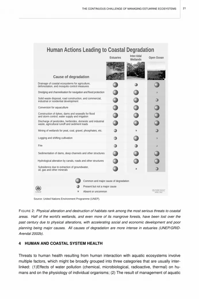
THE CONTINUOUS CHALLENGE OF MANAGING ESTUARINE ECOSYSTEMS
Dredging and channelisation for navigation and flood protection
Solid waste disposal, road construction, and commercial, industrial or residential development
Conversion for aquaculture
Construction of dykes, dams and seawalls for floodand storm control, water supply and irrigation
Discharge of pesticides, herbicides, domestic and industrial waste, agricultural runoff and sediment loads
Mining of wetlands for peat, coal, gravel, phosphates, etc.
Logging and shifting cultivation
Fire
Sedimentation of dams, deep channels and other structures
Hydrological alteration by canals, roads and other structures
Human Actions Leading to Coastal Degradation
Source: United Nations Environment Programme (UNEP).
Estuaries Inter-tidalWetlands Open Ocean
Cause of degradation
Subsidence due to extraction of groundwater,oil, gas and other minerals
Drainage of coastal ecosystems for agriculture,deforestation, and mosquito control measures
Source: United Nations Environment Programme (UNEP).
Common and major cause of degradation
Present but not a major cause
Absent or uncommon APRIL 2002DELPHINE DIGOUT
UNEP
FIGURE 2: Physical alteration and destruction of habitats rank among the most serious threats to coastal
areas. Half of the world’s wetlands, and even more of its mangrove forests, have been lost over the
past century due to physical alterations, with accelerating social and economic development and poor
planning being major causes. All causes of degradation are more intense in estuaries (UNEP/GRID-
Arendal 2002b).
4 HUMAN AND COASTAL SYSTEM HEALTH
Threats to human health resulting from human interaction with aquatic ecosystems involvemultiple factors, which might be broadly grouped into three categories that are usually inter-linked: (1)Effects of water pollution (chemical, microbiological, radioactive, thermal) on hu-mans and on the physiology of individual organisms; (2) The result of management of aquatic
21

M. MATEUS, J.W. BARETTA AND R. NEVES
resources (e.g., wetland drainage, land reclamation, dredging, aquaculture, etc.); (3) Effectsof global change affecting climate and the hydrological cycle (e.g., habitat degradation, war-ming, increased rainfall, storms). It is obvious that the role of humans in decreasing the qualityof life in the marine environment has been enormous. The detrimental effects of pollution candirectly or indirectly affect all forms of life in estuaries and this, in turn, can similarly presenta hazard to human health when marine organisms are used as food or by direct contact withthe water and sediments. A significant number of human activities contribute to the release ofpollutants to the estuary by rivers and tributaries, run-off, groundwater and the atmosphere.Considerable amounts of these contaminants remain inside the estuary or adjacent coastalzone, particularly in poorly flushed areas.
5 MANAGING COASTAL WATER RESOURCES: A SHARED RESPONSIBILITY
In simple terms, the great challenge of this century is to find the means to develop humancapital (socio-economically, culturally and equitably), while at the same time preserving andprotecting natural capital. The socio-economic dimension, with its focus on human concerns,is a crucial component of the approach, taking full account of:
1. Stakeholders having input in the planning and management of the resource, ensuringespecially that the interests of all quadrants of society, as well as natural interests, arefully represented;
2. The multiple uses of the resources and the range of people’s needs;
3. Integrating water plans and strategies into the national planning process and environ-mental concerns into all government policies and priorities, as well as considering theimplications of proposed and adopted actions;
4. The essential needs of the ecosystems so that they are properly protected.
Summarizing, coastal management embraces the principles of participation and transparencyto attain social equality and good governance. This reaffirms that governments are the ste-wards of valuable assets such as their coastal waters and ecosystems, and with effectivecooperative management, these common resources can contribute to sustainable economicgrowth.
6 THE ECONOMICAL AND ECOLOGICAL CONTEXT OF NATURAL RESOURCE MAN-AGEMENT
Management decisions based purely on economical considerations always compare the cur-rent market value of the natural resources against an ill-defined ecological value. However, inmaking decisions, relevant factors must include such things as the relative value of ecologicalprocesses, conservation priorities, and alternative land use practices. Because of the uncer-tainty in forecasting the economic value of alternatives, and the difficulties inherent in defining
22

THE CONTINUOUS CHALLENGE OF MANAGING ESTUARINE ECOSYSTEMS
very different values in the same currency, decisions end up being taken mostly by politicaland social forces on short term economical considerations The concept of intergenerationalequity is usually part of definitions of sustainability but this concept is intractable from a man-ager’s perspective. Also, management decisions usually rely on dealing with the resource asit is now (e.g., available space, fish populations, etc.), instead of on the basis of their sustaina-bility. From the perspective of developing procedures for sustainable resource use practices,there is more at stake than simply the particular interests of the resource owners or managers.A number of general principles have been suggested for the discussion of sustainability andresource use (Ludwig et al. 1993):
• Human motivations and responses should be included as part of the system to be stu-died and managed;
• Past examples show that resource exploitation has seldom been sustainable, and fre-quently scientific advice is ignored;
• Resources should be managed explicitly for uncertainty by considering a variety of dif-ferent strategies, favoring actions that are informative, reversible and that are robust touncertainty;
• Management strategies should be adaptive, considering uncertainty and surprise as anintegral part of anticipated response;
• Policies and actions are required that involve not only social objectives, but that continueto improve understanding and provide for flexibility in the event of unexpected events;
• Trial-and-error must be seen as an integral part of adaptive management;
• Such an approach should be interdisciplinary and combine historical, comparative andexperimental approaches to resource use.
7 ECOSYSTEM-BASED MANAGEMENT: THE SUSTAINABLE USE OF ESTUARINE RE-SOURCES
Sustainability is both an ecological and an economic concept. Achieving adequate sustaina-bility practices must be a priority to maintain or restore these environments and the ecologicalservices they provide. This, in turn, will be translated in economic benefits. Sustainable use ofestuarine systems and the goods and services they support depends on: (1) efficient couplingbetween advances in the environmental sciences and their application for the public good,and (2) our understanding of the interdependency of ecological and socio-economic systems.Today, there are unacceptable disconnects between these processes on both counts (Bowenand Riley 2003). Ecosystem-based strategies consider the effects of human activities in thecontext of natural variability and change. Ecosystem-based management is emerging as a uni-fying approach to secure and efficient marine operations, environmental protection, resourcemanagement, land-use planning and environmental engineering (Sherman and Duda 1999,Cicin-Sain et al. 2000). This is especially significant in estuaries where the combined effects
23

M. MATEUS, J.W. BARETTA AND R. NEVES
of habitat alterations, land sources of pollution, over fishing, harmful algal blooms, and invasivespecies are most severe (Botsford et al. 1997). Implementing a strategy of ecosystem-basedmanagement requires the capability to engage in adaptive management and a decision ma-king process that depends on routine and rapid detection of changes in the state of the system.Although the challenges are many, the coordinated development of a multidisciplinary scien-tific effort may provide an important means to bridge the gap between science and manage-ment by the routine and repeated provision of scientifically credible, quantitative assessmentsof the status of estuarine ecosystems across the land-sea interface.
8 MEETING SOCIAL NEEDS
Estuaries and other coastal systems are experiencing unprecedented changes that makethem more susceptible to natural hazards and less able to support living resources. A broadspectrum of phenomena from global warming and sea level rise to harmful algal blooms(HABs) and losses of biodiversity are exhibiting troubling trends in their magnitude or fre-quency. These trends are related to both natural processes and increasing human demandson coastal ecosystems to support commerce, living resources, recreation, and living space.
One of the major challenges in coastal zone management, and particularly in estuarine man-agement, is to balance the environmental constraints with social needs. This is a rather de-manding task because it starts with a fairly consensual identification of major social goalsfollowed sometimes by a not so obvious definition of particular social needs for any specificsystem. Because of their nature, societal goals can only be achieved with the developmentof an integrated and holistic approach. They can be broadly summarized in the following list(UNESCO 2005): (1) Improve the safety and efficiency of marine operations; (2) Mitigate andmore effectively control the effects of natural hazards; (3) Minimize public health risks; (4) Pro-tect and restore healthy ecosystems in a more effective way; (5) Improve the capacity to detectand predict the effects of global climate change on coastal ecosystems; (6) More effectivelyrestore and sustain living marine resources.
To achieve these goals, an informed management for sustainable use of estuarine servicesrequires the capability to routinely and rapidly assess their state and health, detect changeson a broad spectrum of time and space scales, and provide timely predictions of likely futurestates. Relevant and informed decisions, whether they are concerned with ship routing, beachclosures, fisheries management, dredging disposal, or mitigating the effects of an oil spillcaused by an accident, require the provision of useful marine data and information at ratestuned to the time scales at which decisions must or should be made. This begs for an integralapproach to achieve an appropriate set of priorities in the estuarine zone management thatequilibrates ecological and social and economical needs. For the time being this capacity isstill in an embryonic stage in most countries.
24

THE CONTINUOUS CHALLENGE OF MANAGING ESTUARINE ECOSYSTEMS
9 INTEGRATED APPROACHES TO ESTUARINE ECOSYSTEM MANAGEMENT
Estuarine areas, with their overlapping economic interests competing for the same commonproperty resources, are where integrated approaches are most urgently needed. Integratedcoastal management usually focuses on three major goals: (1) overcoming the conflicts asso-ciated with the sectoral management, (2) preserving the productivity and biological diversityof coastal systems, and (3) promoting and equitable and sustainable allocation of coastal re-sources (Post and Lundin 1996). The forms of integration required by coastal managementhave many dimensions. An example is the combination of good science with governance.Being complex systems under significant human pressures, estuaries cannot be managed inthe absence of the best available information of both biophysical and social sciences. Ma-rine sciences help characterize problems over time, distinguishing natural and human-relatedcauses of environmental change. When combined with the results of economic and social re-search, these efforts contribute to innovative management solutions. Another example is theintegration among sectors and disciplines. The complex overlay of processes and institutionsin estuarine areas makes it impossible for a single agency or entity to meet the challenges ofmanagement alone. Success lies in forging partnership among institutions meaning, amongother things, to develop an interdisciplinary dialog to achieve a holistic approach to the man-agement of the system.
9.1 The interdisciplinary and cross-sectoral dialog
Decisions concerning water related resources management are too often taken without suf-ficient scientific and empirical background, addressing only short term and single goals, andignoring the complexity of processes in aquatic ecosystems (Naiman et al. 1995). Man-agement of socioeconomic interests and associated environmental issues requires practicalassessment techniques that should be based on an interdisciplinary approach. An effectivemanagement tool should always consider the development of protection policies to reduceimpacts on the environment. Developing a fully integrated, multi-disciplinary system for estua-rine management has been a particularly challenging task because: (1) it requires systematicmonitoring and research activities and these are usually non-existent or primitive at best, and(2) the operational capacity for detecting, assessing and predicting changes in ecosystemhealth, the sustainability of natural resource and public health risks, is poorly developed.
9.2 A holistic approach to the study of estuarine systems
The recent cooperation between ecologists and water managers has led to attempts to in-tegrate an ecosystem approach into Integrated Water Resources Management (IWRM). Therationale in this approach has been to conceptualize a catchment- or basin-based holistic ap-proach, which takes into consideration the multiple roles of water both in ecosystems and inhuman socio-economic systems. This involves consideration of terrestrial and aquatic ecosys-tems and the water links between them, requiring from water managers an understanding ofthe linkages between water circulation and ecosystems.
25

M. MATEUS, J.W. BARETTA AND R. NEVES
Fundamentally, this is a response to the much-criticized fragmented sector-by-sector approachto water-related resource management (aquaculture, sewage disposal, fishing, recreation,etc.). The new paradigm highlights instead the benefits that an integrated, overall approach towater management, on a catchment or basin basis, can deliver. IWRM promotes not just thecooperation across sectors, but also the coordinated management and development of landand water (both surface water and groundwater), so as to maximize the resulting social andeconomic benefits in an equitable manner, without compromising ecosystem sustainability.It is imperative to address the ecological and socio-economic links in the management ofdynamic systems such as estuaries and coastal areas. The Driver-Pressure-State-Impact-Response (DPSIR) model (Bowen and Riley 2003) provides a framework for achieving this.This methodology will be addressed in the next chapter.
10 FINAL REMARKS
Estuarine areas have been and remain in close association with humans. This relation ofhuman dependence on the natural characteristics of estuarine systems implies that these re-sources have to be managed in ways that guarantee their sustainability, but also in such away that social and economical structures have viable development targets. Considering thescale of the multiple resource demands imposed on estuaries they, rank among the ecosys-tems under heaviest (and increasing) pressure. The multiple usage of the goods and servicesprovided by estuarine systems reflects the variety of stakeholder interests and perceptions.To attain a sustainable utilization of estuarine areas and resources requires a far more com-plicated approach of social, economic and environmental issues, than is the case for purelymarine or purely terrestrial environments. The effective use of available information in deve-lopment planning and management for estuaries depends on an Integrated Water ResourcesManagement strategy. Resource sustainability cannot be detached from the sustainability ofhuman economies, natural communities and ecosystems. Sustainability is a moving targetbecause ecosystems change over time and so do the economic, social and political climatesin which decisions are made change. The rate of development of estuarine areas and the re-sulting environmental impact may largely be determined by the efforts that are devoted to theearly detection of environmental problems. Hence, the successful management of estuariesand coastal waters requires a basin-wide management, which considers the river basin as thefundamental unit of territorial management (Zalewski 2002). To pursue this goal means thatpresent practices by official institutions based on municipalities or counties as an administra-tive unit, or based on managing specific activities must be changed or abandoned altogether.Without these changes and a holistic approach towards the management of these systems,estuaries and coastal waters will continue to be degraded.
REFERENCES
Adam J A (2003) Mathematics in nature: modeling patterns in the natural world. Princeton UniversityPress, Princeton and Oxford. 360p.
26

THE CONTINUOUS CHALLENGE OF MANAGING ESTUARINE ECOSYSTEMS
Adger W N, Hughes T P, Folke C, Carpenter S R, Rockstrom J (2005) Social-ecological resilience tocoastal disasters. Science 309: 1036-1039
Allan J A (2005) Water in the Environment/Socio-Economic Development Discourse: Sustainability, Chang-ing Management Paradigms and Policy Responses in a Global System. Government and Opposition40: 181-199
Balls P W (1994) Nutrient Inputs to Estuaries from 9 Scottish East-Coast Rivers - Influence of EstuarineProcesses on Inputs to the North-Sea. Estuarine Coastal and Shelf Science 39: 329-352
Botsford L W, Castilla J C, Peterson C H (1997) The management of fisheries and marine ecosystems.Science 277: 509-515
Bowen R E, Riley C (2003) Socio-economic indicators and integrated coastal management. Ocean &Coastal Management 46: 299-312
Bricker S B, Ferreira J G, Simas T (2003) An integrated methodology for assessment of estuarine trophicstatus. Ecological Modelling 169: 39-60
Burke L, Kura Y, Kassem K, Revenga C, Spalding M, McAllister D (2001) Pilot Analysis of Global Ecosys-tems: Coastal Ecosystems. World Resources Institute., Washington, D.C.
Cicin-Sain B, Knecht R W, Vallega A, Harakunarak A (2000) Education and training in integrated coastalmanagement: lessons from the international arena. Ocean and Coastal Management 43: 291-330
Cloern J E (2001) Our evolving conceptual model of the coastal eutrophication problem. Marine Ecology-Progress Series 210: 223-253
Council N R (2000) Clean coastal waters: understanding and reducing the effects of nutrient pollution.National Academy Press, Washington. 405p.
Diaz R J, Rosenberg R (1995) Marine benthic hypoxia: A review of its ecological effects and the be-havioural responses of benthic macrofauna. Oceanography and Marine Biology - an Annual Review,Vol 33 33: 245-303
Dietz T, Ostrom E, Stern P C (2003) The struggle to govern the commons. Science 302: 1907-1912
Epstein P R (1999) Perspectives: Medicine - Climate and health. Science 285: 347-348
EU (2000). Directive 2000/60 of the European Parliament and of the Council of 23 October 2000 estab-lishing a framework for community action in the field of water policy. EU
Holmlund C M, Hammer M (1999) Ecosystem services generated by fish populations. Ecological Eco-nomics 29: 253-268
Jackson J B C, Kirby M X, Berger W H, Bjorndal K A, Botsford L W, Bourque B J, Bradbury R H, Cooke R,Erlandson J, Estes J A, Hughes T P, Kidwell S, Lange C B, Lenihan H S, Pandolfi J M, Peterson C H,Steneck R S, Tegner M J, Warner R R (2001) Historical overfishing and the recent collapse of coastalecosystems. Science 293: 629-638
Juhel M (2001) Globalisation, Privatisation and Restructuring of Ports. International Journal of MaritimeEconomics 3: 139-174
Levin S A (1998) Ecosystems and the biosphere as complex adaptive systems. Ecosystems 1: 431-436
Lindeboom H (2002) The coastal zone: an ecosystem under pressure. In: Field J G, Hempel G, Summer-hayes C P (eds) Oceans 2020: Science, Trends, and the Challenge of Sustainability. Island Press,Washington, pp 49-84
Lotze H K, Lenihan H S, Bourque B J, Bradbury R H, Cooke R G, Kay M C, Kidwell S M, Kirby M X,Peterson C H, Jackson J B C (2006) Depletion, degradation, and recovery potential of estuaries andcoastal seas. Science 312: 1806-1809
Ludwig D (1993) Environmental Sustainability - Magic, Science, and Religion in Natural-Resource Man-agement. Ecological Applications 3: 555-558
Ludwig D, Hilborn R, Walters C (1993) Uncertainty, Resource Exploitation, and Conservation - Lessonsfrom History. Science 260: 17
27

M. MATEUS, J.W. BARETTA AND R. NEVES
Meybeck M (1998) Man and river interface: multiple impacts on water and particulates chemistry illustratedin the Seine river basin. Hydrobiologia 374: 1-20
Monbet Y (1992) Control of Phytoplankton Biomass in Estuaries - a Comparative-Analysis of Microtidaland Macrotidal Estuaries. Estuaries 15: 563-571
Naeem S, Thompson L J, Lawler S P, Lawton J H, Woodfin R M (1994) Declining Biodiversity Can Alterthe Performance of Ecosystems. Nature 368: 734-737
Naiman R J, Magnuson J J, Mcknight D M, Stanford J A, Karr J R (1995) Fresh-Water Ecosystems andTheir Management - a National Initiative. Science 270: 584-585
NRC (2000) Clean coastal waters: understanding and reducing the effects of nutrient pollution. NationalResearch Council. National Academy Press, Washington. 405p.
Officer C B, Ryther J H (1980) The Possible Importance of Silicon in Marine Eutrophication. MarineEcology-Progress Series 3: 83-91
Ohl C, Krauze K, Grunbuhel C (2007) Towards an understanding of long-term ecosystem dynamics bymerging socio-economic and environmental research Criteria for long-term socio-ecological researchsites selection. Ecological Economics 63: 383-391
Pikitch E K, Santora C, Babcock E A, Bakun A, Bonfil R, Conover D O, Dayton P, Doukakis P, FluhartyD, Heneman B, Houde E D, Link J, Livingston P A, Mangel M, McAllister M K, Pope J, Sainsbury K J(2004) Ecosystem-based fishery management. Science 305: 346-347
Post J, Lundin C (1996) Guidelines for integrated coastal zone management. Environmentally SustainableDevelopment Studies and Monograph Series no. 9. The World Bank, Washington, D.C.
Rabalais N N, Turner R E (2001) Coastal Hypoxia: Consequences for Living Resources and Ecosystems.American Geophysical Union, Washington, D.C.
Redman C L, Grove J M, Kuby L H (2004) Integrating social science into the long-term ecological research(LTER) network: Social dimensions of ecological change and ecological dimensions of social change.Ecosystems 7: 161-171
Sherman K, Duda A M (1999) An ecosystem approach to global assessment and management of coastalwaters. Marine Ecology-Progress Series 190: 271-287
Strayer D L, Caraco N F, Cole J J, Findlay S, Pace M L (1999) Transformation of freshwater ecosystemsby bivalves - A case study of zebra mussels in the Hudson River. Bioscience 49: 19-27
Turner R E, Rabalais N N (1994) Coastal Eutrophication near the Mississippi River Delta. Nature 368:619-621
Turner R K, Georgiou S, Gren I M, Wulff F, Scott B, Soderqvist T, Bateman I J, Folke C, Langaas S,Zylicz T, Maler K G, Markowska A (1999) Managing nutrient fluxes and pollution in the Baltic: aninterdisciplinary simulation study. Ecological Economics 30: 333-352
UNEP/GRID-Arendal (2002a). Benefits from marine and coastal ecosystems and activities. UNEP/GRID-Arendal Maps and Graphics Library. Retrieved 15:55, December 17, 2007 (http://maps.grida.no/go/graphic/benefits-from-marine-and-coastal-ecosystems-and-activities)
UNEP/GRID-Arendal (2002b). Human activities leading to coastal degradation. UNEP/GRID-ArendalMaps and Graphics Library. Retrieved 10:55, December 17, 2007 (http://maps.grida.no/go/graphic/human_activities_leading_to_coastal_degradation)
UNESCO (2005). An implementation strategy for the coastal module of the Global Ocean ObservingSystem. IOC Information Documents Series N°1217
Wolanski E, Chicharo L, Chicharo M A, Morais P (2006) An ecohydrology model of the Guadiana Estuary(South Portugal). Estuarine Coastal and Shelf Science 70: 132-143
Worm B, Barbier E B, Beaumont N, Duffy J E, Folke C, Halpern B S, Jackson J B C, Lotze H K, MicheliF, Palumbi S R, Sala E, Selkoe K A, Stachowicz J J, Watson R (2006) Impacts of biodiversity loss onocean ecosystem services. Science 314: 787-790
Zalewski M (2002) Ecohydrology - the use of ecological and hydrological processes for sustainable man-agement of water resources. Hydrological Sciences Journal 47: 823-832
28

PERSPECTIVES ON INTEGRATED COASTAL ZONE MANAGEMENT IN SOUTH AMERICAR. NEVES, J.W. BARETTA AND M. MATEUS (EDS.), IST PRESS, 2008
THE DPSIR FRAMEWORK APPLIED TO THE INTEGRATED MANAGEMENT OFCOASTAL AREAS
M. MATEUS AND F.J. CAMPUZANO
1 INTRODUCTION
Over the last decades numerous and diverse problems with ecological implications have chal-lenged both environmental scientists and decision-makers. These problems have rangedin scale and magnitude: global climate change, loss of habitat and biodiversity, habitat de-struction, and effects of multiple anthropogenic chemicals on ecological systems. Extant andemerging problems have highlighted the need for flexible approaches to deal efficiently withthe problems by establishing a link between ecological data with the needs of decision-makingenvironmental managers. Several methodologies and tools have been developed and usedto face the multifaceted challenges posed by the management of resources where apparentconflicts of interest exist. Ecosystem function is affected by human activities through the dis-turbance of energy and matter flow (Ohl et al. 2007). These changes in ecosystem processesinfluence biodiversity, change the ecological state of ecosystems and impact both on societyand the economy. Thus the inclusion of socio-economic dimensions into standard ecologicalresearch has been identified as a challenge in the new paradigm of sustainable developmentand management of natural resources. Efforts to expand the understanding of these interde-pendencies have led to improvements over the last decade Bowen and Riley 2003), mainly byusing socio-economic indicators that link the changes in environment to social and economicdrivers, and political responses. The challenge has been to understand the relationships be-tween social/economic interests and associated environmental issues, which require practicalevaluation techniques based on an interdisciplinary approach.
Together with the multidisciplinary approach required by the new demands on the manage-ment of resources with a holistic perspective, a multi-sectoral approach must also be consid-ered. The parties involved in the process: scientists, civil servants and stakeholders all speakdifferent languages, function in response to different reward systems, and work on differenttime scales. The realization of the magnitude of these problems led to the development ofintegrative approaches able to deal with these diverse requirements and still provide realisticsolutions. The DPSIR (Drivers-Pressures-State-Impact-Responses) framework is such a tool(Figure 1), allowing the description of environmental problems by defining the relationships be-tween anthropogenic activities and the environment. The framework provides a better contextin which to integrate different types of indicators, opening the possibility of taking into accountnot only the environmental but also the socio-economic impacts that result from changes inthe state of coastal systems. Also, it places side-by-side environmental and socio-economicinterests. The DPSIR framework helps to allow sustained and routine provision of qualityenvironmental data and information and the availability of sound scientific advice to enableresponsive government decisions and to enhance the effectiveness of management actions.
29

M. MATEUS AND F.J. CAMPUZANO
2 THE BACKGROUND OF THE DPSIR FRAMEWORK
The origins of the DPSIR framework go back to the Stress-Response framework developed byStatistics Canada in the late 1970s (Rapport and Friend 1979). This first framework was laterextended in the 1990s by, among others, the Organization for Economic Co-operation and De-velopment (OECD 1991, 1993) and the United Nations (UN 1996, 2001), resulting in the PSR(Pressures, States and Responses) framework. Also during the 1990s, this paradigm wasfurther extended to its present form of the DPSIR framework, originally in two studies by theEuropean Environmental Agency (EEA 1995, Holten-Andersen et al. 1995). The objective ofthese frameworks has been to clarify multi-sectoral relationships and to highlight the dynamiccharacteristics of the ecosystems and socioeconomic changes (Elliott 2002). All these frame-works share the distinction between (i) forces that act on the environment, (ii) changes that, asa consequence, take place in the environment and (iii) the societal reaction to those changes.The DPSIR framework follows the same general model as previous frameworks but divergesin the sense that it distinguishes more steps in the process (Niemeijer and de Groot 2008). Sowhile there are some differences between these frameworks in terms of terminology and thedegree of detail, they are all based on the causal chain concept.
The DPSIR Framework is an instrument for analyzing environmental problems, with regards tosustainable development (Borja et al. 2006). The basic aims of its approach are: (i) to be ableprovide relevant information on the different elements of the DPSIR sequence, (ii) to clarifythe ways in which they are connected and related to each other and (iii) to estimate the effec-tiveness of responses. The DPSIR framework provides helpful insights on the relationshipsbetween the origins and consequences of environmental problems and, at the same time,helps to understand their dynamics by addressing the links between DPSIR elements. Thisintegrative approach presupposes substantial understanding of the underlying causal relation-ships between human activities and the resultant impacts on ecosystems, coastal economiesand communities, and human response mechanisms. Nevertheless, the integrative nature ofthe framework leads to its wide use, especially by the European Environmental Agency, inselecting indicators for evaluating the implementation of EU environmental policies.
The DPSIR framework has rapidly become popular among researchers and policy makersalike as a conceptual framework for structuring and communicating relevant environmentalpolicy research (Svarstad et al. 2008). For this reason it has been successfully implementedin different kinds of coastal management issues, and its contribution to highlight the dynamiccharacteristics of ecosystem and socio-economical changes has been validated (Turner etal. 1998). A presumed strength of the DPSIR framework lies in its simplicity to capture keyrelationships between factors in society and the environment. While simple in concept, theframework is flexible enough to be conceptually valid over a range of spatial scales (von Bo-dungen and Turner 2001). Consequently, it can be used as a communication tool betweenscientists from different disciplines as well as between researchers, on the one hand, andpolicy makers and stakeholders on the other.
30

THE DPSIR FRAMEWORK APPLIED TO THE INTEGRATED MANAGEMENT OF COASTAL AREAS
Driving Forces Pressures
State ofthe Environment
(SoE)
Impacts
Responses
Source : Global International Water Assessment (GIWA), 2001; European Environment Agency (EEA), Copenhagen.
Socio-economic and socio-culturalforces driving human activities,which increase or mitigatepressures on the environment.
The condition of the environment(eg. the assessment
of air or water quality)
Effects of environmental degradation(eg. biodiversity loss, economic damage).
Responses by society to theenvironmental situation (eg. cleanerproduction, regulations).
MARCH 2002DELPHINE DIGOUT
The DPSIR Framework(Driving forces-Pressures-State-Impacts-Responses)
Stresses that human activitiesplace on the environment (eg.wastewater)
UNEP
FIGURE 1: DPSIR framework for State of Environment Reporting (UNEP/GRID-Arendal 2002).
3 THE HEURISTIC DPSIR-CONCEPT
The Driving forces-Pressure-State-Impact-Response concept (DPSIR) provides a heuristicframework for the analysis of cause-effect relationships in complex systems which are subjectto human action (Brandt 2000). The general idea behind the DPSIR concept is that human ac-tivities, i.e. the drivers, exert a certain pressure on a particular part of the natural environmentcausing a change in its components and/or in its overall state. The outcome of this process isan environmental impact, which usually results in certain responses by society. The responsecan run across different segments of society, from the political arena, to socio-economic andpurely economic sectors. Eventually, responses can modify the nature of the driving forces(thus mitigating or even enhancing the actual pressure) and/or compensate for the impact.Finally, the driving forces may also be altered directly by the impact.
31

M. MATEUS AND F.J. CAMPUZANO
A clear example in many estuaries relates to sewage discharges in the system. The increaseddemand for housing (Driving force) can lead to the intensification of direct discharges of un-treated sewage in the waters, resulting in the increase of nutrient loads and faecal contami-nation of nearby streams (Pressure), leading to the eutrophication of water bodies (State) andsubsequent changes in aquatic life and biodiversity and contamination of food resources (Im-pact). One way to address this situation (Response) would be to improve the sanitary system;another would be to require changes in occupation practices and even to ban the consumptionof contaminated marine organisms such as shellfish.
3.1 Drivers of (environmental) change
The first step in the DPSIR framework is the definition of the driving-forces that lead to en-vironmental pressures. For this first step it is important to identify the major stakeholders,their values and interests, and also the potential conflicts between them. A driving force, alsotermed a driver, is an established social need that represents a factor and social force thatmay induce changes in the state of the environment. This social need usually arises from theeconomical sphere, which means that drivers are frequently linked to the financial system. Assuch, drivers are usually considered to be economic and social goals of those involved in theindustry, as well as economic and social policies of governments. In coastal areas, shipping,fisheries, tourism and aquaculture are among the most commonly mentioned drivers of DPSIRmodels.
3.2 Pressures (on the environment)
Pressures can broadly be described as the means through which drivers are actually ex-pressed, i.e, in the way they interfere and perturb the system. Inside the framework, pressuresare the link between socioeconomic activities and the natural system. In a sense, all humanactivities end up by generating pressures on the environment, to a lesser or greater degree.The existing pressures on estuarine and coastal areas can be divided into four groups: (i) pol-lution, comprising urban, industrial, agricultural and aquaculture discharges; (ii) alteration ofthe hydrological regime, including water abstraction, flow regulation and restoration activities;(iii) changes in the morphology, including land reclamation and infrastructures; and (iv) biologyand its uses, including all kind of resource exploitation, changes in biodiversity and recreation(Borja et al. 2006). As such, pressures fall into three general categories that range from sim-ple interference to inducing changes in the natural functioning of ecosystems: (a) fluxes intowater bodies, (b) excessive usage of natural resources, and (c) changes in the food web.
3.3 The state of the environment
The combination of physical, chemical and biological conditions defines the state of the en-vironment in a given area. This state is affected by the pressures and eventually modified inits environmental conditions. The result of this induced change may be expressed as a loss
32
THE DPSIR FRAMEWORK APPLIED TO THE INTEGRATED MANAGEMENT OF COASTAL AREAS
of ecosystem services. So, if the state is changed, human dependence on the system mayalso be compromised (e.g., loss of fish stocks, bathing areas, etc.). Although there is a linkbetween pressure and state, the relationship between them in estuaries is strongly influencedby geomorphology and hydrodynamics: estuaries subject to similar nutrient-related pressureoften exhibit totally different eutrophication symptoms, and in some cases no symptoms at all.Factors such as flushing time, tidal range, and turbidity play a major role in determining thenature and magnitude of symptom expression.
3.4 Environmental and societal impacts
The state of the system needs to be assessed in terms of its physical, chemical and biolog-ical conditions, and this leads to the definition of impact on each component. Thus, impactscorrespond to the effects resulting from the change in the state of the ecosystem. Usuallythese effects are studied by identifying changes in bio-physical-chemical conditions that leadto changes in the components of the environment (e.g. water quality, biodiversity etc.). How-ever, this has also impacts on society. Hence, environmental impacts are related to the healthof the ecosystem, while social impacts are linked to effects on human health and to the ef-fects and resources that society identifies as valuable. An assessment of the impacts requiresmonitoring procedures and the definition and use of indicators of change.
3.5 Societal responses
The DPSIR model assumes that all pressures degrade the ecosystem, and that this negativeimpact can only be reverted through subsequent responses. This means that the magnitudeof the impacts may lead to a re-evaluation of current management policies and may eventu-ally lead to the realization of the need of different management responses. In this sense, aresponse is a societal action related to an actual environmental problem or perceived risk.This action, often moved by public policies of governmental actors, can also be stimulated byother sectors of civil society such as NGOs, universities, etc. A response can be describedas a reaction to the negative effects of impacts. The responses vary according to the scaleof the impacts, becoming an attempt to mitigate the impacts or reverse them in an attempt toreestablish the ”normal” state of the system, if possible. If preventive measures are taken toeradicate or ameliorate the impacts of pressures in the system, then it will change the originaldrivers.
The human or societal response to the changes resulting from our activities has to be estab-lished to meet what we may call six tenets for environmental management (Elliott 2002). Someof these tenets are well-known in national and international strategies (the first three), whileothers need to be considered to guarantee that solutions to environmental change sit withinour developed systems. Accordingly, our actions (Responses) have to be: (1) Environmentallysustainable (i.e. nature-friendly in the present and in the future); (2) Technologically feasible(i.e. with adequate methods and equipment); (3) Economically viable (i.e. at a reasonable and
33

M. MATEUS AND F.J. CAMPUZANO
supportable cost); (4) Socially desirable (i.e. wanted by our societies); (5) Legally permissible(i.e. in compliance with national and international legislation); (6) Administratively achievable(i.e. carried out and enforced by our system of departments, agencies and governments).
4 METHODOLOGIES USED IN THE DPSIR ANALYSES
The integrative nature of the DPSIR framework in the study of human-ecosystem interactionsmeans that a significant range of techniques, methodologies and tools must be used to achievethat end. The temporal scope of the framework, with processes spanning across different timescales, and addressing present and future states, requires these methodologies and tools todiagnose and predict. Some of the procedures are of a descriptive and static nature, i.e. theygive a snapshot of the actual state of the system (e.g., environmental indicators, conceptualmodels), while others are dynamic, meaning that they can describe the temporal evolution ofthe system to some degree (e.g. mathematical models).
4.1 Environmental indicators
The use of indicators is fundamental in the DPSIR framework because they provide an objec-tive system of information and evaluation. An indicator can be described as something thatprovides a clue to a matter of larger significance or makes perceptible a trend or phenomenonthat is not immediately detectable (Hammond et al. 1995). In the DPSIR context, the Euro-pean Environment Agency (EEA Glossary, 2007) describes an environmental indicator as ”aparameter or a value derived from parameters that describe the state of the environment andits impact on human beings, ecosystems and materials, the pressures on the environment, thedriving forces and the responses steering that system.” As such, an environmental indicatoris a qualitative or quantitative parameter characterizing the current condition of an elementof the environment or its change over time. Such environmental indicators have three basicfunctions (Aubry and Elliott 2006):
• To simplify, considering that only a few indicators are selected according to their per-ceived relevance for characterizing the overall state of the ecosystem.
• To quantify, because the value of an indicator is compared with reference values con-sidered to be characteristic of the state of the ecosystems, thus quantifying the shiftsfrom reference or expected conditions.
• To communicate, by facilitating the transmission of meaningful information on environ-mental issues to stakeholders and policy makers, by promoting information exchangeand comparison of spatial and temporal patterns.
Indicators are increasingly being developed and used as management tools to address en-vironmental issues. Over the last years, environmental indicators have taken on such impor-tance because they provide a signal that communicates a complex message in a simplified
34

THE DPSIR FRAMEWORK APPLIED TO THE INTEGRATED MANAGEMENT OF COASTAL AREAS
and useful manner (Jackson et al. 2000). Also, environmental indicators provide an importantsource of information for policy makers and help to guide decision-making as well as moni-toring and evaluation, because they can provide valuable information on complex issues in arelatively accessible way.
Environmental indicators have come to play a vital role in environmental reporting as primeassessors of pressures on the environment, of the evolving state of the environment, and ofthe appropriateness of policy measures (Niemeijer and de Groot 2008). But because theyare so important, it is a major challenge to determine which set of parameters and values ofecological systems characterize the entire system and still are simple enough to be effectivelyand efficiently monitored and modelled (Dale and Beyeler 2001). Indicators, therefore, need tobe properly selected and the methodology of their calculation specified if the dynamic parts ofa given system are to be understood and appear compelling to the user communities (Bowenand Riley 2003).
4.2 Environmental modelling
Environmental modelling is an explicit treatment of our understanding of the deterministic andstochastic mechanisms that affect our studied object (Akcakaya et al. 1997). Numerical mod-els stand as a way to look at real systems and to translate them into compartments, identifyingthe connection between them. They are versatile tools that enable an in-depth look at naturalsystems which cannot be achieved by the simple combination of analytical methods. The useof models makes it possible to explain cause and effect in environmental processes, distin-guish between anthropogenic and natural contaminant sources and their respective impact,etc.. Modelling results are also important to complement and interpolate data from traditionalobservational research methods. Because models have the capability to bridge the gap be-tween small scale and large scale processes, they become an essential tool for understandingcomplex processes that link different compartments of the system (e.g., benthic and pelagicsystems) and run across the land-sea interface by linking catchment and estuarine processes.This is particularly relevant in eutrophication-related studies, where nutrient dynamics can beaddressed in the vast context of major biogeochemical cycles (Harrison 1992).
Models are increasingly becoming indispensable tools in environmental studies and manage-ment decisions (Neves 2007). In the DPSIR framework, models are commonly used to eluci-date each component and the relation between the different components (e.g., the pressureswith the state). Combining the DPSIR with numerical models allows the generation of pre-dictions on potential levels of selected impacts, making responses actions ”prior” to the fullmanifestation of those impacts in the environment. However, it is obvious that no model willever be able to address all problems and answer all questions. For this reason there are somany types of models. Water quality models, ecological models, hydrodynamic and ground-water models are just a few examples.
35

M. MATEUS AND F.J. CAMPUZANO
Most models address specific disciplines of knowledge but can be coupled to other models toachieve an integrated model approach to the study of natural systems. The use of models indecision making must have the main objective of improving communication and understandingof the nature of the problems. If they achieve this goal, the results they produce will be inte-grated quite naturally with value judgments and political constraints. This will result in betterdecisions than would have been made if the models had not been used. To produce this out-come, models must be carefully and thoroughly documented, and limitations, sensitivities andassumptions must be explicitly stated. In addition, modelers must be sensitive to the needsand limitations of the people who intend to use them. It is as important, if not more important,for the ecologist to communicate the uncertainties and assumptions underlying the model, asit is to communicate the set of predictions. Ultimately, the relevance of models for environ-mental decision-making is in the mind of the policy maker, and not in the expert opinion of themodeler.
4.3 The role of conceptual models
It is questionable whether we will ever have fully validated numerical models that can ad-equately predict the ecological effects of human activities. Even so, models can be seenas serious attempts, and probably the most adequate, to relate human drivers with ecologicalstates. The first step towards creating such models is to have some knowledge on the physicaland biological features of the system and the definition of the problem, hence the productionof conceptual models. Considering trends in marine environmental management, it is in factfundamental to develop conceptual models. For simplicity, these can be regarded as diagramswhich bring together and summarise information from many areas.
The schematic approach of conceptual models confer them the simplicity that lengthy and de-tailed descriptions cannot. As such, they have an educational significance and at the sametime provide the basis for communicating the main message to managers and developers.Conceptual models are usually a good starting point for developing quantitative and dynamicnumerical models, or to point to the limitation of such models and the available scientific knowl-edge. They also have the advantage of exposing gaps in knowledge, thus helping to definefurther field and laboratory studies to fill these gaps. In particular, they allow a problem to bedeconstructed as a precursor to each aspect being assessed, prioritized and addressed (El-liott 2002). Under the DPSIR framework it is essential to be aware of the spatial and temporallinks in the marine system. This, in turn, has to be coupled with the diverse nature of stressorson the systems which requires conceptual models to be linked together and further developedtowards numerical and predictive models.
4.4 Stakeholder’s involvement through participation
”Environmental issues are best handled with participation of all concerned citizens, at therelevant level”. This is the introductory statement of Principle 10 of the Rio Declaration on
36

THE DPSIR FRAMEWORK APPLIED TO THE INTEGRATED MANAGEMENT OF COASTAL AREAS
Environment and Development (1992). This principle states that individuals must have theopportunity to participate in decision-making processes and that States shall promote andencourage public awareness and participation by making information widely available. Coastalmanagement programs must ensure strong public involvement of stakeholders, because theyrepresent the people who are most affected by the coastal development process. This is bestachieved by making public education and consensus-building important components of anyinitiative. The responsibility of stakeholders must go well beyond the awareness to participatein the decision making process; they must also be held accountable for such task.
A way of incorporating stakeholders’ opinions into the decision-making process has beenthrough the methodology of participative experts’ model (Failing et al. 2004). In this strat-egy, the model of the system, irrespective of the complexity, starts by being generated with theparticipation of some stakeholders or social actors. As a rule, the chosen stakeholders arethose that the group of experts identifies as more relevant to the potentially analyzed problem.This degree of involvement confers common sense to the modelling exercise by keeping theaims of scientists at realistic levels, and assures that the model is not socially naive. An opendialogue between scientists and stakeholders is necessary in order to make decisions regard-ing what can be done and what shall be left either to other scientists or other modelling tools,or both. As addressed before, the most important feature about models is that they must berelevant to decision-makers. This means that if models do not include stakeholders in theirdevelopment, the study on the availability of significant societal resources might be doomedto failure. If the process of model building is collaborative and iterative, and if it involves rep-resentatives of all stakeholders, it has a chance of being realistic, hence useful, i.e., will havethe ability to answer the right questions.
A well-structured decision process involving stakeholders can typically be summarized in threekey steps Keeney 1992, Clemen and Winkler 1999):
• Setting objectives and indicators for each of them. These indicators (also known asperformance measures) become the criteria for evaluating and comparing policy alter-natives. Since setting objectives is a deliberative and value-based activity, it demandsinput from a broad range of stakeholders. Defining indicators is both deliberative andanalytical, requiring involvement from both technical specialists and stakeholders.
• Identifying policy alternatives and assessing their impact on the objectives. The impactof the policy alternatives is measured by the indicators. The description of impactsshould explicitly characterize the uncertainty associated with the estimate. This is ananalytical activity, conducted largely by technical experts, with input from stakeholdersin the form of selecting the experts and defining their terms of reference.
• Evaluating and choosing a preferred policy alternative. Choices will most likely involvetrade-offs among competing objectives and methods for making choices should allowstakeholders to state their preferences (value-based information) for different outcomes,based on good information (factual or technical information). This again is a deliberativetask involving both scientific and stakeholder participation.
37
M. MATEUS AND F.J. CAMPUZANO
5 THE DPSIR FRAMEWORK AND THE INTEGRATED COASTAL ZONE MANAGEMENT
Integrated Coastal Zone Management (ICZM) promotes sustainable management of coastalareas in a dynamic, multidisciplinary and iterative process. It includes all the processes in-volved in this task, from information collection, planning, decision making, management andmonitoring of implementation. It is also a process that involves the informed participation andcooperation of all relevant actors to evaluate the societal goals in a given coastal area, andto take actions towards meeting these objectives. In the long term, ICZM tries to achieve abalance between environmental, social, economic and cultural goals, always keeping withinthe limits set by natural dynamics. The integrative nature of this approach is in its range of ob-jectives, but also in the integration of the many instruments needed to meet these objectives,as well as the integration of the terrestrial and marine components of the target territory, inboth time and space.
In recent times, a few new concepts have come out related to coastal managemen, whose ap-plication has been encouraged by institutions (i.e. EU Parliament and council 2002/413/EC),and the DPSIR framework as a tool for the former. The ICZM concept is based on a holis-tic approach to manage conflicts between different coastal uses and interests (aquaculture,resource extraction, tourism, housing, etc.) and to facilitate the use and dissemination of in-formation, especially between society, managers and scientists. Today, DPSIR is increasinglyused as a framework for structuring case studies in relation to issues of human interferencesin an effort to manage landscapes and seascapes (Elliott 2002, La Jeunesse et al. 2003,Scheren et al. 2004, Holman et al. 2005). The DPSIR approach has become increasinglyaccepted and applied to different case studies to solve problems involving a range of coastalmarine environments: coastal areas, coastal lagoons, deltaic systems, estuaries, river basins.A summary of applications of the DPSIR framework to marine environments is presented inTable 1. In this sense, the DPSIR framework has received much attention and use in ICZMstrategies and programs.
ICZM efforts worldwide face major challenges. This is particularly evident in estuarine man-agement, where the goal is to balance environmental constraints with social needs, whilemaintaining the habitual fragile balance between ecosystem performance and human-relatedactivities. Because of their nature, societal goals can only be achieved together with envi-ronmental goals with the development of an integrated and holistic approach. The DPSIRframework is an effective way to deal with complex issues, such as the management of nutri-ent fluxes (Smith et al. 1999) and the impact of development in catchment areas (Cave et al.2003), inside the broader scope of the ICZM programs.
6 FUTURE PERSPECTIVES
There are no straightforward answers to the question of what is best for a particular systemwhen there are potential conflicts between natural and economic interests. It is the task ofscientists from different disciplines to present as complete as possible a picture to those who
38

THE DPSIR FRAMEWORK APPLIED TO THE INTEGRATED MANAGEMENT OF COASTAL AREAS
make decisions or have the capacity for lobbying in the decision-making process. To achievea holistic view of these systems and fully incorporate the needs of policy-makers, frameworkssuch as the DPSIR framework are essential. In complex ecosystems like estuaries, where thehuman presence and activity is growing at an alarming pace, there is an urgent need to linkscience (the knowledge on the system functioning) to the causes of change in its state and tothe social, economic and legal responses by Man to that change. This necessity is behind theincreasing use of the DPSIR approach (Elliott 2002).
TABLE 1: A summary of applications of the DPSIR framework in ICZM strategies.
Study site Area Subject Reference
Guanabara Bay basin (Brazil) River Basin Sustainable Development Bidone and Lacerda (2004)
Thermaikos Gulf (Greece) River Basin Hindcasting coastal evolution Karageorgis et al. (2006)
Po Catchment-Adriatic Sea (Italy) River Basin & Coastal area ICZM Pirrone et al. (2005)
Aixos River catchment and Thermaikos Gulf (Greece) River Basin & Coastal area Eutrophication Karageorgis et al. (2005)
Southern European Coastal Lagoons Coastal Lagoons ICZM Aliaume et al. (2007)
Sacca di Goro (Northern Adriatic Sea, Italy) Coastal Lagoon Aquaculture impacts Marinov et al. (2007)
UK Coast Coastal area Offshore wind power Elliott (2002)
Nestos Delta (Greece) Coastal area Environmental status indicators Karakos et al. (2003)
Italian Coast Coastal area Coastal environment assessment Casazza et al. (2002)
Ria Formosa (Portugal) Coastal Area Dredging activities Pacheco et al. (2007)
Ria Formosa (Portugal) Coastal Area Eutrophication Newton et al. (2003)
Bay of Gdansk (Poland-Russia) Coastal Area Eutrophication Kannen et al. (2004)
German Coast Coastal Area Future Planning Kannen (2004)
DPSIR was projected to explicitly relate environmental changes driven by socio-economicpressures with the required socio-economic measures to mitigate adverse impacts of changecaused by human actions. For estuaries and coastal areas in general, the DPSIR analysis hasthe ability to link large-scale human drivers of change and their impacts on the systems, withmanagement responses (e.g., sewage treatment, preservation of mangrove areas, modifyingdredging activities, etc.). A major advantage of the framework lies in its capacity to integratesocio-economic aspects with ecological impacts, addressing not only the consequences ofhuman activities on the system, but also its feedback.
The DPSIR framework works well at simplifying the complexity of natural systems manage-ment, such as estuarine areas, at the same time informing policy makers, scientists and thegeneral public on the actions that can cause changes in the status of the system and the na-ture and consequences of those changes. Several shortcomings have been ascribed to theDPSIR framework as a tool for establishing effective communication between environmentalscientists of different disciplines, and between stakeholders and policy makers. One of theseshortcomings seems to be the lack of efforts to find a satisfactory way of dealing with themultiple attitudes and definitions of issues by stakeholders and the general public (Svarstad
39

M. MATEUS AND F.J. CAMPUZANO
et al. 2008). Nevertheless, this framework has proven to be an effective way to deal withthe complex task of managing natural system when real conflicts exist in regard to their useand transformation and, most important, a central methodology for establishing cause-effectrelationships in the use and exploitation of natural resources and their status. The DPSIRframework is a practical tool for testing observations and hypotheses. It is being used suc-cessfully and increasingly as a research aid to interpret ecological relationships in ongoingevaluations of management alternatives and to develop effective ecological and societal tar-gets for a meaningful, conflict-free, sustained and sustainable development.
REFERENCES
Akcakaya H R, Burgman M A, Ginzburg L R (1997) Applied population ecology. Applied Biomathematics,New York. 255p.
Aliaume C, Do Chi T, Viaroli P, Zaldıvar J M (2007) Coastal lagoons of Southern Europe: recent changesand future scenarios. Transitional Waters Monographs 1: 1-12
Aubry A, Elliott M (2006) The use of environmental integrative indicators to assess seabed disturbance inestuaries and coasts: Application to the Humber Estuary, UK. Marine Pollution Bulletin 53: 175-185
Bidone E D, Lacerda L D (2004) The use of DPSIR framework to evaluate sustainability in coastal areas.Case study: Guanabara Bay basin, Rio de Janeiro, Brazil. Regional Environmental Change 4: 5-16
Borja A, Galparsoro I, Solaun O, Muxika I, Tello E, Uriarte A, Valencia V (2006) The European WaterFramework Directive and the DPSIR, a methodological approach to assess the risk of failing to achievegood ecological status. Estuarine, Coastal and Shelf Science 66: 84-96
Bowen R E, Riley C (2003) Socio-economic indicators and integrated coastal management. Ocean andCoastal Management 46: 299-312
Brandt J (2000) Monitoring multi-functional terrestrial landscapes. In: Brandt J, Tress G, Tress B (eds)Multi-Functional Landscapes. University of Roskilde, Roskilde, pp 157-161
Casazza G, Silvestri C, Spada E, Melley A (2002) Coastal environment in Italy: preliminary approachusing the DPSIR scheme of indicators. Littoral: 541-549
Cave R R, Ledoux L, Turner K, Jickells T, Andrews J E, Davies H (2003) The Humber catchment andits coastal area: from UK to European perspectives. The Science of the Total Environment 314-316:31-52
Clemen R T, Winkler R L (1999) Combining probability distributions from experts in risk analysis. RiskAnalysis 19: 187-203
Dale V H, Beyeler S C (2001) Challenges in the development and use of ecological indicators. EcologicalIndicators 1: 3-10
EEA (1995) Europe’s Environment: the Dobris Assessment. European Environment Agency, Copenhagen
Elliott M (2002) The role of the DPSIR approach and conceptual models in marine environmental man-agement: an example for offshore wind power. Marine Pollution Bulletin 44: Iii-Vii
Failing L, Horn G, Higgins P (2004) Using expert judgment and stakeholder values to evaluate adaptivemanagement options. Ecology and Society 9: -
Hammond A, Adriaanse A, Rodenburg E, Bryant D, Woodward R (1995) Environmental Indicators: A Sys-tematic Approach to Measuring and Reporting on Environmental Policy Performance in the Context ofSustainable Development. World Resources Institute, Washington, DC. 50p.
Harrison W G (1992) Regeneration of nutrients. In: Falkowski P G, Woodhead A D (eds) Primary produc-tivity and biogeochemical cycles in the sea. Plenum Press, New York, pp 385-407
40

THE DPSIR FRAMEWORK APPLIED TO THE INTEGRATED MANAGEMENT OF COASTAL AREAS
Holman I P, Rounsevell M A, Shackley S, Harrison P A, Nicholls R J, Berry P M, Audsley E (2005) A re-gional, multi-sectoral and integrated assessment of the impacts of climate and socio-economic changein the UK. Climate Change 71: 9-41
Holten-Andersen J, Paalby H, Christensen N, Wier M, Andersen F M (1995) Recommendations on strate-gies for integrated assessment of broad environmental problems. Report submitted to the EuropeanEnvironment Agency (EEA) by the National Environmental Research Institute (NERI), Denmark.
Jackson L E, Kurtz J C, Fisher W S (2000). Evaluation Guidelines for Ecological Indicators. Report No.EPA/620/R-99/005. Environmental Protection Agency, Washington, DC.
Kannen A (2004) Holistic system analysis for ICZM: The coastal futures approach. Coastline Reports 1:177-181
Kannen A, Jedrasik J, Kowalewski M, Oldakowski B, Nowacki J (2004) Assessing catchment-coast inter-actions for the Bay of Gdansk. Coastline Reports 2: 155-165
Karageorgis A P, Kapsimalis V, Kontogianni A, Skourtos M, Turner K R, Salomons W (2006) Impact of100-year human interventions on the deltaic coastal zone of the Inner Thermaikos Gulf (Greece): ADPSIR framework analysis. Environmental Management 38: 304-315
Karageorgis A P, Skourtos M S, Kapsimalis V, Kontogianni A D, Skoulikidis N T, Pagou K, Nikolaidis N P,Drakopoulou P, Zanou B, Karamanos H, Levkov Z, Anagnostou C (2005) An integrated approach towatershed management within the DPSIR framework: Axios River catchment and Thermaikos Gulf.Regional Environmental Change 5: 138-160
Karakos A, Skoulikaris X, Monget J-M, Jerrentrup H (2003) The broadcasting on internet of water DPSIRindicators. Experiment on the Nestos delta, Greece. Global Nest 5: 81-87
Keeney R L (1992) Value-focused thinking: a path to creative decision-making. Harvard University Press,Boston, Massachussetts, USA.
La Jeunesse I, Rounsevell M, Vanclooster M (2003) Delivering a decision support system tool to a rivercontract: a way to implement the participatory approach principle at the catchment scale? Physicsand Chemistry of the Earth 28: 547-554
Marinov D, Galbiati L, Giordani G, Viaroji P, Norro A, Bencivelli S, Zaldivar J M (2007) An integratedmodelling approach for the management of clam fanning in coastal lagoons. Aquaculture 269: 306-320
Neves R (2007) Numerical models as decision support tools in coastal areas. In: Gonenc I E, KoutitonskyV, Wolflin J P (eds) Assessment of the Fate and Effects of Toxic Agents on Water Resources. Springer/ NATO Public Diplomacy Division, pp 173-197
Newton A, Icely J D, Falcao M, Nobre A, Nunes J P, Ferreira J G, Vale C (2003) Evaluation of eutrophica-tion in the Ria Formosa coastal lagoon, Portugal. Continental Shelf Research 23: 1945-1961
Niemeijer D, de Groot R (2008) A conceptual framework for selecting environmental indicator sets. Eco-logical Indicators 8: 14-25
OECD (1991) Environmental Indicators, a Preliminary Set. OECD, Paris.
OECD (1993) OECD core set of indicators for environmental performance reviews. Environmental Direc-torate Monographs No.83
Ohl C, Krauze K, Grunbuhel C (2007) Towards an understanding of long-term ecosystem dynamics bymerging socio-economic and environmental research Criteria for long-term socio-ecological researchsites selection. Ecological Economics 63: 383-391
Pacheco A, Carrasco A R, Vila-Concejo A, Ferreira O, Dias J A (2007) A coastal management programfor channels located in backbarrier systems. Ocean & Coastal Management 50: 119-143
Pirrone N, Trombino G, Cinnirella S, Algieri A, Bendoricchio G, Palmeri L (2005) The Driver-Pressure-State-Impact-Response (DPSIR) approach for integrated catchment-coastal zone management: pre-liminary application to the Po catchment-Adriatic Sea coastal zone system. Regional EnvironmentalChange 5: 111-137
41

M. MATEUS AND F.J. CAMPUZANO
Rapport D, Friend A (1979). Towards a Comprehensive Framework for Environmental Statistics: a Stress-response Approach. Statistics Canada Catalogue 11-510. Minister of Supply and Services Canada,Ottawa.
Scheren P A G M, Kroeze C, Janssen F J J G, Hordijk L, Ptasinski K J (2004) Integrated water pollutionassessment of the Ebrie Lagoon, Ivory Coast, West Africa. Journal of Marine Systems 44: 1-17
Smith V H, Tilman G D, Nekola J C (1999) Eutrophication: impacts of excess nutrient inputs on freshwater,marine, and terrestrial ecosystems. Environmental Pollution 100: 179-196
Svarstad H, Petersen L, Rothman D, Siepel H, Watzold F (2008) Discursive biases of the environmentalresearch framework DPSIR. Land Use Policy 25: 116-125
Turner R K, Lorenzoni I, Beaumont N, Bateman I J, Langford I H, McDonald A L (1998) Coastal manage-ment for sustainable development: analysing environmental and socio-economic changes on the UKcoast. Geographical Journal 164: 269-281
UN (1996) Indicators of sustainable development. Division for Sustainable Development. United Nations
UN (2001) Indicators of sustainable development: framework and methodologies. Background Paper No.3, Commission on Sustainable Development, Division for Sustainable Development, Department ofEconomic and Social Affairs. United Nations, New York.
UNEP/GRID-Arendal (2002). The DPSIR Framework. UNEP/GRID-Arendal Maps and Graphics Library.Retrieved 15:22, December 17, 2007 (http://maps.grida.no/go/graphic/the_dpsir_framework)
von Bodungen B, Turner R K (2001) Science and integrated coastal management. An Introduction. DalhenUniversity Press, Berlin. 378p.
42

PERSPECTIVES ON INTEGRATED COASTAL ZONE MANAGEMENT IN SOUTH AMERICAR. NEVES, J.W. BARETTA AND M. MATEUS (EDS.), IST PRESS, 2008
COASTAL ZONE MANAGEMENT IN SOUTH AMERICA WITH A LOOK ATTHREE DISTINCT ESTUARINE SYSTEMS
M. MATEUS, F. GIORDANO, V.H. MARIN AND J. MARCOVECCHIO
1 INTRODUCTION
Estuaries and adjacent coastal areas can be characterized by several variables such as: size,shape and bathymetry, tidal influence, fresh water inflow, turbidity, residence times, sedimentproperties, and water-column turbidity. Also of great importance are the geographical location(mainly the latitude) and human pressures. In combination, all these characteristics shape theecology of an estuary, conferring singularity to each system. The ECOMANAGE project fo-cused on three estuarine systems in South America: Santos Estuary (24o S) and Bahıa Blanca(39o S) in the Atlantic coast, and Aysen Fjord (45◦ S) in the Pacific coast. These estuaries,in terms of their ecology, differ in features like the role of the benthic system, anthropogenicnutrient inputs, presence/absence of tidal flats. The main purpose of this chapter is to des-cribe in general terms the backdrop of the South American coastal zone management reality,highlighting the major features of these three system. Together, they represent key coastalzones regarding their integrated management. All show conflicting interests between urban,industrial and agricultural development and environmental conservation. Thus, beyond theirdifferences, they share some of the major regional environmental concerns in South America,namely, the transformation of the landscape and seascape with the loss of natural patrimony,increased human waste and industrial disposal (UNEP 1999).
2 THE SOUTH AMERICAN REALITY
The South American region is characterized by a remarkable heterogeneity in climate, ecosys-tems, human population distribution and economic development. The combination of the pre-vailing atmospheric and oceanic circulation defines the climate and the land and sea producti-vity of the region. This partly explains the distribution of human settlements and the availabilityof basic services (e.g., water supply). According to the medium prospect of the United Nations(Nawata 1999), an increase in population to 838 million is expected for South America by theyear 2050. The growth rate of coastal populations in almost every Latin American countryis greater than its national growth rate. Nearly 75% of the region’s inhabitants live in cities,and 60% of the largest 77 cities are in the coastal zone. As a result, over the last decadesSouth America has become more urban and also much more coastal (Hinrichsen 1997). Thisconcentration along the coast is accompanied by a similarly disproportionate share of the re-gion’s infrastructure and economic activity, some of which requires proximity to the waterfront.Land-use changes have become a major force driving ecosystem changes. Up to 19% of thetotal area of Latin America is used as agricultural lands (excluding pastures). The waters ofPeru and Chile support one of the top five commercial fisheries and, until recently, the world’sfastest growing fishery thrived off the coasts of Argentina and Uruguay (IDB 1995).
43

M. MATEUS, F. GIORDANO, V.H. MARIN AND J. MARCOVECCHIO
Santos Estuary24º S 46º W
Bahía Blanca39º S 62º W
Aysén Fjord45º S 73º W
FIGURE 1: The three ECOMANAGE study sites in South America: Santos Estuary in Brazil, Bahıa Blanca
in Argentina and Aysen Fjord in Chile.
2.1 Biodiversity of the Region
South America hosts a significant percentage of the world’s biodiversity in terrestrial and ma-rine habitats (Heywood and Watson 1995). For example, there is a large variety of coastalwetlands. The unique location of the region, its extreme climatic variations, tidal patterns,and geological features, make these coastal wetlands rank among the most productive of theworld. However, a significant part of them endure the impact of population growth, expan-sion of the agricultural activity, and land-use changes. However, considering that seven of theworld’s most diverse and threatened areas are in Latin America and the Caribbean (Myers etal. 2000), the continent faces today serious challenges in natural resources management.
2.2 Socioeconomic factors
From an historical perspective, the use of ocean and maritime access has been at the heartof the southern hemisphere’s economic and political development. The ports of South Ame-rica are important nodes in the flow of goods brought into and exported from the Region.For example, the Region’s industrial ports are the second leading destination for containeri-zed U.S. exports. Expanding ports and maritime trade are often accompanied by intensified
44

COASTAL ZONE MANAGEMENT IN SOUTH AMERICA WITH A LOOK AT THREE DISTINCT ESTUARINE SYSTEMS
transportation corridors in coastal ocean areas, as is happening off Argentina, Brazil, Ecuadorand Uruguay. The ports of South America are also a significant factor in land use changesin the coastal zone. Most commodity ports serve as development poles for manufacturingand processing activities, often contributing to both the urbanization and increasing industrialcharacter of coastal areas. South American economies are increasingly dependent on tradeagreements like the Mercosur that has Argentina, Brazil, Paraguay, and Uruguay as partici-pating countries, and Bolivia and Chile as associate members. These have developed withthe main purpose of speeding up socioeconomic development, and have important effects onthe economy and, indirectly, on the environment of the region. Even with a strong economicperspective at its core, much of these agreements are gradually considering environmentalissues. Indeed, a growing environmental awareness is evident in local legislations in the re-gion. Furthermore, a large percent of coastal populations, especially those with low income,still depends on natural resources exploitation (e.g. artisan fisheries, small-scale aquacultureand farming). As a result, sustainable development strategies and integrated managementare rather timely in order to decrease conflicts.
2.3 Environmental awareness
Over the last decades, and especially after Rıo 1992, South American countries have beendeveloping a strong environmental awareness. This is evident in the ratification of internationaland regional conventions and agreements, and in the adaptation into the national legislationof many countries to reflect the need of a sustainable development. Two major steps of SouthAmerican government have initiated a path for preventive actions regarding the use of naturalresources: the ratification of the recommendations of the United Nations Conference on En-vironment and Development (UNCED 1992), and the incorporation of recommendations fromthe Agenda 21 into national legislation.
As environmental concerns become more pressing, they are receiving more attention on theinternational political agenda. South America is no exception to this. In line with United NationsResolution A/52/629 calling for cooperation to incorporate sustainable development programsat national, regional and global levels, countries in South America have been engaged in ac-complishing the objectives of such development programs. The large majority of countries fol-low the recommendations made by the United Nations Commission for Sustainable Develop-ment (UNCSD), and the Economic Commission for Latin America and the Caribbean (ECLAC)is assisting them in the integration process of relevant disciplines and sectors. There are alsoa significant number of regional agreements and a vast body of laws, rules, and regulationsto ensure systematic and coordinated actions for protecting the environment and promotingsustainable development (Bertucci et al. 1996, Solano 1997). Most South American gov-ernments have developed and implemented comprehensive environmental legal frameworkswith relevant laws and procedures for specific resources and activities like marine resources,coastal areas, tourism, etc. However, local empowered stakeholder participation is still in anearly stage (Bachmann et al. 2007).
45

M. MATEUS, F. GIORDANO, V.H. MARIN AND J. MARCOVECCHIO
2.4 Challenges in integrated coastal zone management
Habitat transformation (for infrastructure expansion, aquaculture, agriculture, etc.), and sewageand garbage disposal are among the most recurrent problems in South American coastalzones. Water resource management has been identified as a guiding objective by SouthAmerican countries, with the following subdivisions: (1) Water Supply; (2) Watershed Man-agement; Management of marine coast and related resources; and (3) improved quality ofgroundwater (UNEP 2003). The legal frameworks for coastal management are being revisedin many countries and in some cases modified to change the sectorial focus to a more inte-grated management approach. This is being pursued having in mind the multiple uses of re-sources by different sectors like agriculture, fishing, aquaculture, industry, domestic consump-tion, energy and recreational use. From this perspective, the challenge of coastal ecosystemmanagement in South America can be address with common and shared methods.
3 DRIVERS OF CHANGE IN COASTAL AREAS
Coastal and marine areas of South America undergo fast and frequently drastic transforma-tion. Many of these changes, typical of coastal areas, are experienced as environmental,economic and social problems. For the region, these can be summarized in the followingtopics, with their relative importance varying from one location to another (Lemay 1998).
3.1 Degradation of coastal ecosystems
Degradation of coastal systems occurs mainly by the combination of land conversion and theexpansion of coastal infrastructures. The loss of mangrove areas is a clear example. It hasbeen estimated that 55% of the entire mangrove coast of Latin America and Caribbean wasclassified as either critical or endangered, 30% vulnerable and only 15% as stable (Olson etal. 1995). In the tropical Americas, the loss of coastal forests, mainly mangroves, occurs ata rate of approximately 1% year (Ellison and Farnsworth 1996). In some parts of the regionthis poses a threat to local subsistence because most commercial shellfish and finfish usemangrove forests for nurseries and refuge, and so the fisheries in mangrove regions are de-clining at a similar rate as mangrove communities (Ewell and Twilley 1998). Many areas areexperiencing a rapid and often drastic transformation and degradation to coastal and marineareas. Land conversion is causing degradation of coastal habitats, including mangroves, es-tuaries and coral reefs. Mangroves, for example, have been disappearing at an alarming rateover the past 20 years. Coastal water quality has been declining throughout the region, dueto increasing discharges of untreated municipal waste.
3.2 Depletion of commercial fisheries stock
Depletion of stocks, overcapitalization and plant closures, habitat degradation, non-compliancewith management regulations and illegal practices, are among the main problems that the fish-
46

COASTAL ZONE MANAGEMENT IN SOUTH AMERICA WITH A LOOK AT THREE DISTINCT ESTUARINE SYSTEMS
eries sector faces in the Region. The expansion of aquaculture, which often depends on wildfisheries stocks for seeding and food, also contributes to enhance pressure on natural stocks.
3.3 Land use and resource allocation conflicts
Land reclamation for residential, industrial, agricultural and tourism purposes has caused thedegradation of coastal and marine ecosystems of the sub-region. The massive and largelyunplanned investments in sectors like aquaculture, port and industrial facilities expansion, andtourism is coastal and estuarine areas has been pointed out as the reasons of acceleratedland use changes and associated conflicts. Frequently new activities compete for the sameresource upon which traditional communities depend. When compared to other tropical re-gions such as Southeast Asia, the importance of aquaculture in South America is relativelysmall. Nonetheless its importance is growing in countries such as Ecuador, where a sig-nificant shrimp mariculture industry has developed mostly in mangrove converted areas andsalt ponds. More recently important breakthroughs have taken place in aquaculture in Chile(mostly salmon), induced by attractive export markets and made possible by favorable environ-mental conditions for their growth (Lemay 1998). This activity has been steadily growing at animpressive rate of 30% a year, when compared with 9.5% worldwide. Indeed salmon farming,induced by favorable export markets, is generating around US$450 million a year in exportearnings. The environmental impact of this activity has been generating growing concerns,especially because of the habitat losses; eutrophication associated with effluent discharges,other changes is estuarine water quality and the introduction of exotic species.
Tourism investments represent an important catalyst of land use change in coastal areas, andthe South American continent is no exception. Tourism has increased in the last decades andthis may lead to important environmental impact when it takes place in estuaries and man-groves (Garreta-Harkot 2003). In addition to generating employment, tourism investmentslead to important land use changes in coastal areas. Many rural coastal areas are experien-cing a gradual shift from dependence on local fisheries and agriculture towards the provisionof tourism services and related activities (WTTC 1993). The development of the tourism sec-tor implies a demand for improved access along the coast in places that until recently hadno basic services. Improvements in access, energy distribution and communications neededfor resort development or other infrastructures, as well as prospects for employment, attractnew residents to the coast. A frequent outcome is the transformation of natural (ecosystemscomposition) and human landscape (e.g., traditional fishing villages). These changes triggerrising prices for land, competition for resources, conflicts with sectors such as fisheries andagriculture, and may hinder the development of proper management policies.
3.4 Degradation of coastal water quality induced by land-based sources
Estuarine and coastal habitats are receiving waters for significant volumes of municipal andindustrial wastewater discharges, combined with urban and agricultural runoff, and other point
47

M. MATEUS, F. GIORDANO, V.H. MARIN AND J. MARCOVECCHIO
and non-point sources. In many estuaries there are signs that the natural dilution capacity isbeing exceeded by the volumes and concentration levels of effluents. Also in the estuaries,the raising levels of pollution represent an increasing public health hazard. For instance,The Global Programme of Action for the Protection of the Marine Environment from Land-based Activities from UNEP has summarized the environmental priorities for the Region as:(1) Inadequate discharge of liquid urban effluents; (2) Industrial effluents pollution; (3) Pollutionrelated to inadequate use of agrochemical products; (4) Degradation of aquatic environmentsdue to expansion of urban limits; (5) Inadequate disposal of urban solid residues; and (6)Activities related to extraction, transport and storage of oil or derivates (Marcovecchio 2000).
Industries dealing with horticulture and aquaculture, oil, lumber, chemicals, textiles, vehiclerepairs and ship building have all added large quantities of hazardous materials to rivers,estuaries, wetlands and coastal areas, and have had major impacts on the aquatic and marineenvironments (Davidson 1990). The disposal of more than 87% of Municipal Wastewater inrivers, lakes, and seas create serious damage to aquatic ecosystems and implies a significantimpact to public health; the enormous lack of minimum facilities for the disposal of wastewatercontributes significantly to the deterioration of underground water systems, rivers and coastalenvironments (UNEP 2003).
3.5 Increasing coastal erosion
Deforestation, dredging and filling, poorly designed coastal structures and illegal sand mininghas contributed to the increase of coastal erosion and often intensify the risk associated withcoastal hazards.
4 A LOOK AT THREE CONTRASTING SITES IN SOUTH AMERICA
A significant number of estuarine areas in South America have been affected by human in-fluence to some degree. Many of these systems show conflicting interests between urban,industrial and agricultural pressures and environmental maintenance. From heavily popu-lated area of Santos Estuary to the near-pristine water conditions of Aysen Fjord, the sitesaddressed here cover a wide range of ecological and socio-economical conditions, and theirinevitable conflicts and challenges in management, which can be found in South America.These systems share some similarities and also some conspicuous differences, but togetherthey face many of the main challenges discussed above. Tables 1 and 2 contain a brief sum-mary of the major features of each system and Figures 2 to 4 bring additional information byadding visual insights.
4.1 Santos estuary
Located at the Southern Brazilian Coast, the estuarine system of Santos comprises threemajor estuarine channels, namely Sao Vicente, Santos and Bertioga, interconnected in its
48

COASTAL ZONE MANAGEMENT IN SOUTH AMERICA WITH A LOOK AT THREE DISTINCT ESTUARINE SYSTEMS
inner area. Santos and Sao Vicente channels comprise an approximate area of 44,100 m2,with an average depth of 15 m in the central dredged channel of Santos and 8 m in Sao Vicentechannel. Six main rivers discharge in Santos estuary: Piacaguera, Boturoca, Cubatao, Mogi,Quilombo e Jurubatuba. There are also many tributaries and artificial channels that collectrain drainage water and clandestine domestic waste. The tropical and subtropical climatecauses high rainfall in the summer period. The Santos Estuary can be classified as a typicalsub-tropical mangrove system under significant anthropogenic pressure. After hundreds ofyears of urban, industrial and port development, the estuary is a highly changed ecosystem.Its extensive areas of mangrove, with associated fauna and flora have been destroyed overtime and are now partially degraded. The estuarine water column can be stratified, mainlydue to vertical gradients of temperature. The estuarine system has a considerable ecologicalimportance because it has a natural high productivity and is a natural habitat for many animalslike birds, mammals, fish and numerous kinds of invertebrates.
The phytoplankton is dominated by diatom communities from the Genus Skeletonema spp.and Thalassiosira spp. Nanoplanktonic phytoflagellates share the dominance (alternate) withdiatoms because of the adaptation to the changing light and nutrients conditions induced bythe spring-neap tide cycles. Red tides caused by Mesodinium rubrum in the inner shelf ofSantos have been reported (Moser et al. 2005), a species that is not toxic but can causeoxygen depletion problems at the end of the bloom. Other primary producer groups found inthe region are the seaweeds, conspicuous in many areas in the soft substratum of mangroveforests, and Spartina spp, which occupy many mangrove fringe areas.
The Santos estuarine system holds the larger Brazilian harbor as well as the most impor-tant industrial complex of the Brazilian coast. The Santos estuarine complex, regarded as apolluted area (de Sousa et al. 1998), is an area heavily occupied by urban, industrial andport activities. The construction of an underground generating plant by the Light Companyin the late fifties lead to the amplification of the capacity of generating energy in this area,turning possible the installation of a petroleum refinery, a petrochemical complex and, later, ametallurgical complex. These development have modified significantly the environmental andhydrodynamic conditions of the estuary. This period of fast growth during the 1950s-1960s,required amplification of the port area, and the need for continuous dredging of the mainchannels to allow the circulation of heavy ships in the harbor and access to areas of the upperestuary where major industries are located.
The main socio-economic drivers for the Santos estuary are the industrial and port activities,and the resident population. Currently, there are nearly 400,000 people living in this area,but the Santos, Cubatao and S. Vicente cities and adjoining region account for ∼1,000,000inhabitants (almost doubled in the vacation period). The Baixada Santista region is, at thesame time, a tourism, industrial and port center. Cubatao city has a remarkable industrial polewith different kinds of industries but mainly associated with the petroleum products, fertilizerproduction and a very remarkable steel production. The main sources of pollution at this regionare: the Santos port and ships which are involved in the spillage and loss of shipped products,
49

M. MATEUS, F. GIORDANO, V.H. MARIN AND J. MARCOVECCHIO
the industrial pole of Cubatao, the domestic waste of Sao Vicente and Santos cities (which aremainly discharged through an emissary), the garbage dump of the Baixada Santista region,besides the discharge of waters from the Billings water reservoir which receives used waterfrom some parts of Sao Paulo City. The population accounts for the high levels of pollutantsdischarged in the system through sewage water. The discharges of domestic waste watersare scattered, due to the existence of only 3 WWTPs. Clandestine domestic sewage disposalarises from slum quarters at the channel margins and make up a significant contribution to theeutrophication of the system. Several industrial effluents are discharged in the inner areas ofthe estuary and port activities act as another anthropogenic impact in the system.
Some kinds of hazardous compounds are dispensed into the estuary such as nutrient salts,heavy metals, organic compounds and petroleum hydrocarbons. These pressures in the es-tuary have impacts not only in the estuary, by inducing changes in the ecologic dynamics, butalso in Santos Bay and adjacent beaches. Water quality is a public health problem in thiscoastal zone. The main stakeholders in Santos include local government, university and edu-cational system, industrial and harbour consortiums and NGOs (environmental protection).All the uses of the estuary make this a place of conflictive interests and uses, adding seriousdifficulties to its management and governance.
4.2 Bahıa Blanca estuary
Bahıa Blanca is a mesotidal coastal plain estuary in the southwest of the Buenos AiresProvince. The main channel of this estuary has a total length of 60 km, varying in widthfrom about 3-4 km at the mouth (22 m depth) to 200 m at the head (3 m depth). This channelis partly closed by a modified ebb delta. Three freshwater tributaries enter the estuary: thesauce Chico River (with a drainage area of about 1,620 km2), discharging into the principalchannel about 3km downstream from the head of the estuary, Saladillo (with a drainage areaof 830 km2) and the Naposta Grande Creek (with a drainage area of about 1,260 km2) thatreaches the estuary about 1km downstream of Ingeniero White Port. Both Sauce Chico andNaposta Grande rivers are originated in ”Serra de la Ventana” in the top part of the watershed.
The Bahıa Blanca estuarine system shows some striking similarities with Santos estuary. Thesimilarities are related to the intensive anthropogenic pressure and some ecological featuressuch as the dominance of diatoms. However, there are some major differences, especially inthe vertical physical structure and in the tidal range. Unlike Santos, the Bahıa Blanca estu-ary is not stratified and has a larger tidal range. Unlike most southern hemisphere temperatesystems, phytoplankton bloom takes place in winter months reaching 70 mg Chla m−3. Thebloom is dominated by diatoms (especially Thalassiosira curviseriata) with flagellates appear-ing only near the end of the bloom episodes. The typical phytoplankton succession starts withlarge diatoms, followed by dinoflagellates and ends with small diatoms. This succession sug-gests a complex nutrient control on primary production. Nutrient concentrations are alwayshigh inside the estuary all year round, yet there are no signs of eutrophication in the system.
50

COASTAL ZONE MANAGEMENT IN SOUTH AMERICA WITH A LOOK AT THREE DISTINCT ESTUARINE SYSTEMS
The inner estuarine area receives high loads of organic matter from WWTPs, limiting lightpenetration in the vicinity of the discharge points and they can have a significant contributionto nutrient budgets in the upper estuary. The estuary has extensive intertidal areas with highhalophytes coverage.
The main identified socio-economic drivers for the Bahıa Blanca are the agricultural activityand population growth. This population growth generates a pressure over land use, impactingthe water quality of the estuary, and also affecting the coastal zone. To augment production,soil fertility has been increased over the last year by fertilization. Consequently, agriculturepractices have contributed to the eutrophication of the estuary through soil leaching and runoff.The city of Bahıa Blanca has rapidly expanded to a total of 350,000 inhabitants over the lasttwo decades and still has a large potential for growth.
The demographic growth has been fuelled by a large petrochemical park, fertilizer and ther-moelectric plants, as well as expanding port activities since much of Argentina’s export movesthrough Ingeniero White Port (Perillo et al. 2001). As a consequence, the discharge of in-dustrial wastes and untreated or partially treated domestic sewage has generated increasingproblems of contamination. Dredging of the Principal Channel from 9.5- to 13.5 m depthshas generated over 35 x106 m3 of sediments, dumped on tidal flats and in off-shore locations.Dredging and deposition has introduced major changes of circulation patterns in the estuary.
4.3 Aysen fjord
The Aysen Fjord stands in striking contrast with the previous estuarine systems. Aysen isthe eleventh administrative Chilean region; located between 45◦ and 46◦ S. The region ischaracterized by a significant oceanic climate range and vast diversity of ecosystems. Thereare an insular part and a continental part, with a total territory of 108,000 km2. It is the leastpopulated of the fourteen political regions of Chile (around 90,000 habitants) with a density of0.8 habitants km−2. Commercial activities have been primarily based on the exploitation of theregion’s natural resources and include: fishing and aquaculture, mining, livestock productionand ranching, sawmills, agriculture and forestry.
As any fjord system, Aysen fjord has an extremely high residence time (>200 days) and is per-manently stratified. There is a strong seasonal signal in the freshwater inputs, resulting mostlyfrom the ice melting in the watershed and seasonal rain pattern. Aysen River is the main fresh-water water input into Aysen Fjord, having a total watershed area of about 12000 km2. Freshwater only affects the upper layer (less than 10 m deep) of the system. Primary production inthe water column is dominated by diatoms and dinoflagelates. The strong oxygen productionof the upper layer contrasts with the low oxygen conditions of the bottom (around 2.5 ml l−1)resulting from the bacterial degradation of organic matter in the sediment. Aysen is a 300 mdeep fjord and consequently the sediment is exclusively a mineralization compartment.
51

M. MATEUS, F. GIORDANO, V.H. MARIN AND J. MARCOVECCHIO
Given the late colonization of this area (mainly during the first half of the XX century), Aysen isstill a low population region with a large governmental organization, given its geopolitical im-portance. Consequently, many key stakeholders correspond to governmental organizations.Salmon farmers are also key stakeholders and have been identified as the main actors of thefuture economic development of the area. Other primary stakeholders correspond to artisanfishermen, tourism companies, agricultures and mining companies. Although the Aysen re-gion is often seen as a pristine and undisturbed zone in southern Chile, it has a past record ofdevastating human impact. Colonization during last century was accomplished using fire asa management tool; the fires were started intentionally by settlers (and supported by govern-ment policies of the time) to clear areas for cattle and sheep. Wildfires that burned throughoutthe 1940s have left a long-lasting mark on the watershed by changing the physical and chem-ical characteristics of the soils.
Nowadays, the region still holds its almost pristine state, but the estuarine system is slowingbeing enriched with organic matter originated in the numerous mariculture units scattered inthe Fjord. Salmon farming industry is the main socio-economic driver in the Aysen Fjord. Thisactivity, strongly supported by foreign capital investment, is characterized by having some ofits industries ranking on the top ten industries nationwide and two of them worldwide. Recentinvestment initiatives indicate that aquaculture production in the area is in a process of expan-sion: by 2010 it is projected that the XI region (and Aysen county in particular) will produce42% of the national salmonid production (up from 20% today). Besides salmon farming, thesystem has been used for other purposes such as mollusk harvesting and, more recently, in-dustrial development. About 80% of the population in Aysen watershed is concentrated in theurban areas (Coyhaique, Puerto Aysen, Puerto Chacabuco). In the region of Aysen, 70% ofthe total habitants are connected to sewer system. This fjord receives the liquid residues ofPuerto Aisen (a town of 37,000 people, located close to its head). Its also home of the onlyseaport for the region (Puerto Chacabuco).
5 FUTURE TRENDS
The environmental costs of regional economic expansion have been extremely high, and seemto be growing. The major issues are the accelerating over-exploitation of land and marine re-sources, increasing conflict over access to and use of water, loss of biodiversity and habitatdegradation, urban waste disposal problems. South America interest in a solid economicaldevelopment in pace with sustainable natural resource usage is expected to increase over thenext few decades, stimulated mostly by new trade opportunities, changing markets, height-ened awareness of coastal hazards and natural resources conflicts, and the participation ininternational agreements (Lemay 1998). Undoubtedly, a key challenge for the Region overthe next decades will be to cope with rates of change in coastal areas, especially in estuarinesystems, recognizing shortcomings of traditional approaches and building on the lessons ofemerging policy reforms for integrated coastal zone management.
52

COASTAL ZONE MANAGEMENT IN SOUTH AMERICA WITH A LOOK AT THREE DISTINCT ESTUARINE SYSTEMS
TABLE 1: Major biotic and abiotic features of the three estuarine systems (see text for details).
Feature Santos Estuary Bahía Blanca Aysén Fjord
Zone Sub-tropical Warm temperate Cold temperate Mixing characteristics Partly mixed Well mixed Permanently stratified Dilution potential Moderate High Low Vegetation Mangrove swamps
High emergent vegetation Tidal flats
Spartina fringes Tidal flats Relatively low emergent
vegetation
No marine vegetation
Nutrients Nutrient exporter Nutrient exporter Nutrient importing from
the sea Production Strongly heterotrophic
system (mineralizing system)
Neutral (varying from auto to heterotrophic)
Strongly autotrophic system
TABLE 2: Major socio-economical features of the three estuarine systems (see text for details).
Feature Santos Estuary Bahía Blanca Aysén Fjord Drivers Industrial and port
activities Population growth
Agricultural activity Industrial and port activities
Population growth
Salmon Farming
Population (in the area) 1,000,000 350,000 90,000 Economic activities Petrochemical park
Refineries and terminals Fertilizer plants Thermoelectric plant Metal industries Port activities
Petrochemical park Refineries and terminals Fertilizer plants Thermoelectric plant Several industries (meat and fish factories, leather and textile plants, etc.)
Port activities
Salmon fish farming Artisan fishing Forestry
Pressures Urban and industrial
pollution (wastewater effluents discharges with and without treatment)
Dredging
Urban and industrial pollution (wastewater effluents discharges with and without treatment)
Dredging
Organic inputs (associated with fish feed and faecal pallets), sediments from terrestrial systems
Major impacts Eutrophication
Habitat degradation (loss) Eutrophication
Local bottom modification
Human utilization of the system
Occupation (housing) Recreation (bathing in the bay area)
Food source
Food source Habitat Food source Tourism
Overall State Highly modified
Heavily Polluted Modified Polluted
Near pristine, unpolluted
Key stakeholders Regional government
Industrial consortiums Port authorities NGOs
Regional government Industrial consortiums Port authorities
Regional and national government
Salmon farmers
53

M. MATEUS, F. GIORDANO, V.H. MARIN AND J. MARCOVECCHIO
FIGURE 2: The Santos Estuary is a highly changed system after decades of occupation and development.
These snapshots show different areas of the estuary depicting some of the main drivers: urban pressure
with an example of occupation in the frontline of the bay area (top), an industrial plant in Cubatao area
(middle), located in the inner part of the estuary, and port activities (bottom). (Photos by M. Mateus)
54

COASTAL ZONE MANAGEMENT IN SOUTH AMERICA WITH A LOOK AT THREE DISTINCT ESTUARINE SYSTEMS
FIGURE 3: The large industrial pole of Bahıa Blanca (top, partial view) is a major driver in this system.
Water pollution is among its most significant impacts, as seen in the middle plate, where a sign warns
against toxic residues. Fishing is also a main economic activity in Bahıa Blanca and the industrial port
is also an harbor for both the fishing fleet (bottom) and cereal and oil/gas exportations. (Photos by M.
Mateus)
55

M. MATEUS, F. GIORDANO, V.H. MARIN AND J. MARCOVECCHIO
FIGURE 4: The Aysen Fjord is in almost pristine state, maintaining much of its landscape (top) and system
functioning unchanged over the recent decades of human settlement and growth in the area. The main
drives in the system are the tourism, justified by the search for its esthetic value (top), fishing (middle) and
salmon farming (bottom). (Photos by M. Mateus)
56

COASTAL ZONE MANAGEMENT IN SOUTH AMERICA WITH A LOOK AT THREE DISTINCT ESTUARINE SYSTEMS
A commitment towards sustainable development of the Region’s estuarine resources is grad-ually emerging. Unreasonable demands from society in the past led to a general decline ofthe resources and irreversible changes in the nature of many ecosystems. Many of the nat-ural assets of the Region have been undervalued but this trend is now being reversed. Thecontribution of coastal and marine areas to sustainable development is increasingly gainingrecognition among public, private and political sectors in coastal states. Combined with this in-creasing recognition of importance is an emerging awareness of the need to manage coastaland marine resources hand-in-hand with the optimization of allocation of its uses. The re-gion’s central challenge is now to build a political consensus that will maintain stability andeconomic growth while addressing the growing social and environmental problems (UNEP1999). Clearly, careful planning and management of all sectoral activities simultaneously willresult in greater overall benefits than pursuing sectoral development plans independently ofone another. Integrated coastal management approaches are required, combining all aspectsof the human, physical and biological aspects of the coastal zone within a single managementframework.
The main challenges in estuarine and coastal zone management faced by South Americannations have been identified in the three study sites presented here. The remaining of thisvolume will deal with the work done for each site during the ECOMANAGE project and theresults obtained. The research effort undertaken will be used to assist local stakeholdersand decision making entities to implement adequate management strategies. This will lead,eventually, to achieve satisfactory results for the improvement of the ecological status of eachsite, and at the same time helping their steady and sustainable socio-economic development.
REFERENCES
Bachmann P, Delgado L E, Marin V H (2007) Aanalysis of the citizen’s participation concept used by localdecision makers: the case of the Aysen watershed in southern Chile. Int. J. Sustainable Development10: 251-266
Bertucci R, Cunha E, Devia L, Figueria M, Ruiz R, Diaz Labrano F, Vidal Perera R (1996) Mercosur yMedio Ambienta. Edicion Ciudad, Argentina.
Davidson L (1990). Environmental Assessment of the Wider Caribbean Region. UNEP Regional SeasReports and Studies No. 121. Nairobi, Kenya.
Ellison A M, Farnsworth E J (1996) Anthropogenic disturbance of Caribbean mangrove ecosystems: Pastimpacts, present trends, and future predictions. Biotropica 28: 549-565
Ewell K C, Twilley R R (1998) Different kinds of mangrove forests provide different goods and services.Global Ecology and Biogeography Letters 7: 83-94
Garreta-Harkot P F (2003) The Brazilian National Plan of Coastal Management, the health and the envi-ronment. MD Thesis. Faculdade de Saude Publica da Universidade de Sao Paulo, Sao Paulo.
Heywood V H, Watson R T (1995) Global Biodiversity Assessment. Cambridge University Press, Cam-bridge, United Kingdom and New York, USA. 1140p
Hinrichsen D (1997) Living on the Edge: Managing Coasts in Crisis. Island Press.
IDB (1995) Coastal and Marine Resources Management: Strategy Profile. Inter-American DevelopmentBank, Washington DC, United States.
57

M. MATEUS, F. GIORDANO, V.H. MARIN AND J. MARCOVECCHIO
Lemay M H (1998) Coastal and Marine Resources Management in Latin America and the Caribbean -Technical Study. Inter-American Development Bank, Washington, D. C. 57p.
Marcovecchio J E (2000). UNEP: Overview of Land-Based Sources and Activities Affecting the Marine,Coastal and Associated Freshwater Environment in the Upper Southwest Atlantic Ocean. UNEP/GPACoordination Office, Regional Seas Report and Studies Series No170, 57pp.
Moser G A O, Belem A L, Soares J A, Carbeiro M A. 2005. Descricao de uma mare vermelha, causadapor Mesodinium rubrum (Lohmann, 1908), na plataforma interna de Santos (SP, Brasil). In: XXVCongreso de Ciencias del Mar / XI Congreso Latino Americano de Ciencias del Mar. COLACMARXXI.
Myers N, Mittermeler R, Mittermeler C, da Fonseca G, Kent J (2000) Biodiversity hotspots for conservationpriorities. Nature 403: 21-26
Nawata K (1999) ”Society” in 2050: Choice for Global Sustainability. In: Nawata K. Global Industrial andSocial Progress Research Institute. Asahi Glass Foundation, Japan, pp 15-49
Olson D, Dinerstein E, Cintron G, Iolster P (1995) A Conservation Assessment of Mangrove Ecosystemsof Latin America and the Caribbean. World Wildlife Fund, Washington, D.C.
Perillo G M E, Piccolo M C, Parodi E, Freije R H (2001) The Bahıa Blanca Estuary, Argentina. In: SeeligerU, Kjerve B (eds) Coastal Marine Ecosystems of Latin America. Springer-Verlag Berlin Heidelberg,pp 205-217
Solano P (1997) Legislacion Ambiental Suramericana Aplicable a los Humedales. UICN, Wetlands Inter-national SPDA. 204p.
Sousa E C P M, Tommasi L R, David C J (1998) Microphytobenthic primary production, biomass, nutrientsand pollutants of Santos Estuary (24 degrees S,46 degrees 20 ’ W). Sao Paulo, Brazil. BrazilianArchives of Biology and Technology 41: 27-36
UNCED (1992) Earth Summit, Rio de Janeiro. United Nations Conference on Environment and Develop-ment. London Regency Press, London, United Kingdom.
UNEP (1999) Global Environmental Outlook 2000. United Nations Environment Programme, Nairobi,Kenya.
UNEP (2003). Water Resources Management in Latin America and the Caribbean. Fourteenth Meetingof the Forum of Ministers of the Environment of Latin America and the Caribbean. Panama City,Panama.
WTTC (1993) Travel and Tourism: A New Economic Perspective. The 1993 WTTC Report, ResearchEdition. World Travel and Tourism Council, London, United Kingdom.
58

THE METHODOLOGICAL COMPONENTS
PART B
miolo projecto euro. 12/11/07 4:33 PM Page 4


PERSPECTIVES ON INTEGRATED COASTAL ZONE MANAGEMENT IN SOUTH AMERICAR. NEVES, J.W. BARETTA AND M. MATEUS (EDS.), IST PRESS, 2008
A PHES-SYSTEM APPROACH TO COASTAL ZONE MANAGEMENT
V.H. MARIN AND L.E. DELGADO
1 INTRODUCTION
In the past, ecological systems and human societies were analyzed independently from eachother. However, in the words of Redman et al. (2004): ”The isolated study of ecological andsocial systems is no longer defensible”. The main reason for this is that societies and theirdevelopment have influenced and modified most, if not all, ecological systems of the planet.This, in turn, has affected human societies and their development (Meadows et al. 2004).Thus, we can more properly describe today’s nature as an interacting set of ecological-socialsystems.
For this reason, it is essential to consider human societies as reflexive components of theecological systems upon which we depend. However, in order to apply this conceptualizationa change in the dominant scientific paradigm is required. This change is necessary becausein its normal way of functioning, science does not, and indeed it does not have the mecha-nisms to, incorporate social perception. Post-normal science is an emerging paradigm thatincorporates both scientific knowledge and social perception as a requisite to understand aninter-subjective reality. Post-normal constructivism (Von Glasersfeld 1984, Jones 2002, Del-gado and Marın 2005, Marın et al. 2007) proposes that knowledge cannot be understood asthe image or representation of an ontologically objective reality, but rather as the organizationand ordination of worlds constituted and generated in our experience. Thus, diverse socialactors (including scientists) confronting the same environmental landscape will perceive dif-ferent components and interactions depending on the mental models or frameworks used inthe process of perception (Kolkman et al. 2005).
The present condition in South America, in relation to environmental themes, is that relevantdefinitions, delimitations, analysis and strategies are generated by groups of experts (tech-nocrats), based on their investigations, publications in scientific journals and previous work onthe same topic. The social context in which ecological or environmental problems are studiedis seldom considered, including the way in which such problems are perceived by local actors.As a consequence, scientists tend not to be involved in a real or effective way of communi-cating with the socio-cultural components that impact and interact with ecological systems.Despite this technocratic dominance, important changes are taking place in the manner inwhich environmental problems and integrated management are perceived and analyzed. Thisis facilitated through the development of holistic, multidisciplinary and participative visions ofscience (Costanza and Jørgensen 2002, Kangas and Store 2003, Marın et al. 2007, Marınand Delgado 2007).
In this chapter we develop the concept of Physical-Ecological-Social (PHES) system as apost-normal alternative to the classical, indeed Kuhnian, ecosystem concept. We propose it
61

V.H. MARIN AND L.E. DELGADO
as a tool to improve the communication between scientists and other social actors in relationto integrated coastal zone management.
2 ECOSYSTEMS AND PHES-SYSTEMS
Arthur Tansley proposed in 1935 a new term for the ecological sciences: the ecosystem (Tans-ley 1935). Whether due to a need of ecologists to find a term that would unite them below oneconceptual umbrella or, as Golley (1993) proposes, the postwar enchantment with systemicsciences, the literature shows that ’the ecosystem’ has been one of the most utilized ecolo-gical concepts, both inside and outside the discipline of ecology. An uncountable number ofscientific articles exists that utilize the term as a geographic reference, a replacement for oth-ers ill-defined terms (e.g. region, place, space, landscape, etc.). Other articles use the termas a descriptor of an ’object’. Perhaps given the vagueness of the concept at this momentin history, some contemporary ecologists have seriously questioned its use (O’Neill 2001).The widespread use of the ecosystem concept (Golley 1993) and its multidimensional char-acter (Pickett and Cadenasso 2002, Jax and Rozzi 2004) have resulted in a great gamma ofdefinitions from objects in the ’real world’ to abstract concepts.
The ecosystem concept, in its original formulation, only makes reference to the ”system froma physical point of view”; emphasizing the interaction between biotic and abiotic components(Pickett and Cadenasso 2002). In this sense, Tansley’s ecosystem is not a place on the faceof the planet, but rather a non-dimensional conceptual framework. Or in the words of O’Neill(2001): ”a way to observe nature”. If this is the case, the ecosystem is certainly a constructivistconcept where the observer plays a fundamental role. The ecosystem is generated when anobserver distinguishes differences in the observed world (Haag and Kaupenjohan 2001). Thisprocess is not only dependent on the individuals involved, but also, in its most elaborated form(e.g. scientific observations), on the school to which the observer belongs. For example, ecol-ogists trained as population-community experts will tend to observe ecosystems as comprisedby interacting organisms. Ecologists trained in system approaches are likely to describe themin terms of quality and quantity of energy without a single reference to organisms.
Despite the fact that the original ecosystem concept is constructivist in nature, its use by theacademy has transformed it into an object independent of the perception of the observer;one that can be defined without ambiguities (Jax and Rozzi 2004). For us, one of the mostimportant implications of the work of Tansley (1935) is that dividing planet Earth into smallparts (and labeling each part as an ecosystem) is a necessary exercise only because of ourinability to study the whole interconnected totality. This continues to be true, even after morethan seventy years since 1935 and the work of global scientific programs.
However, How do scientists define and delimit ecosystems? When ecological systems arethe subject of study (or study units), work groups normally define components and borderconditions according to the formulated questions. The system defined in this manner, whichfor simplicity we shall call the ”agreed ecosystem” may or may not have the properties that
62

A PHES-SYSTEM APPROACH TO COASTAL ZONE MANAGEMENT
theoreticians have attributed to the theoretical ecosystem (e.g. Jørgensen and Muller 2000,Likens 1992). For example, Likens (1992) proposed one of the most influential ecosystem con-ceptualizations so far, where all components and all interactions should be considered. Theagreed ecosystem almost never contains (nor in practice could contain) all of the organismsand abiotic components in a certain area; rather it contains only those necessary to answerthe questions at hand. It is for this reason, that it appears naive to think that in its current use,the ecosystem concept can provide a ’non-ambiguous’ definition (sensu Jax and Rozzi 2004)to delineate an ecological-social entity that could be the basis for integrated, participative, en-vironmental management. This motivated us to generate a new concept, one that would takeinto account post-normal conditions of integrated management (where: facts are uncertain,values in dispute, stakes high, and decisions urgent; Funtowicz and Ravetz 2000), theabsence of which make the old ecosystem concept one of dubious use at the society andnature crossroad.
Based in a large part on the literature on perception and delimitation of systems (Muller andLeupelt 1998, Kay et al. 1999, Jørgensen and Muller 2000), on the analysis of the ecosystemconcept (O’Neill 2001, Picket and Cadenasso 2002) and on discussions about post-normalscience and the environment (Guba 1990, Lal et al. 2001, Marın and Delgado 2005), wepropose that the social-ecological analysis of the environment, especially as it relates to itsmanagement, should be carried out on the basis of the Physical-Ecological-Social System(PHES-system) concept. A PHES-system is an observer-dependent, spatially explicit, con-ceptual model of an ecological system where its components and boundaries depend on thequestions being addressed, the observers who formulate them and the social context in whichthey were proposed (Fig. 1). Thus, a PHES-system is a socially dependent conceptual modelon the society-nature relations that arise as part of an integrated approach to analyzing adefined region of the planet. This concept incorporates two new characteristics in relation toprevious system concepts used in environmental management: 1) human societies are explic-itly incorporated as reflexive components of the system (socio-ecological component); and 2)the bio-ecological components (other species in the defined area) are only those necessaryto deal with the proposed questions.
One of the main differences between the use of the ecosystem concept and the PHES-systemis the methodology by which these distinctions are generated. The definition of a PHES-system begins with a series of meetings in which different visions of the environmental prob-lem are shared, the effect of these visions on the eco-social structure of the system and itscomponents and the valuation of the different components or processes by the actors or stake-holders; that is, an intensive process of citizen participation. This participation, in order to beeffective, should improve the communication among social actors, in such a way that theymay share and understand each other’s visions (or PHES-systems) of the ecological systembeing managed. Since a PHES-system is, above all, a conceptual model, we have designed aparticipative methodology for their generation. This method is presented below (item 4.) andan example shown in Part D (Outcomes of the project).
63

V.H. MARIN AND L.E. DELGADO
FIGURE 1: Relationships between the contemporaneous ecosystem concept (Likens, 1992), human soci-
eties and the physical structure of the system with the PHES-system. All the information obtained about
the system is filtered by the observers in relation to the questions being asked and the proposed methods
and approaches to deal with them.
3 PHES-SYSTEMS AND INTEGRATED COASTAL ZONE MANAGEMENT
Coastal zones, and the watersheds that discharge into them, are among the world’s regionswith greatest anthropogenic influence. It is estimated that over 50% of the global humanpopulation lives within 200 km of the oceans’ coasts. This dominant and multifaceted pres-ence of human activity has stimulated the development of concepts and strategies aimed atthe integrated and harmonic management of these areas. Integrated Coastal Zone Mana-gement (ICZM) has been defined as: ”A dynamic process in which a coordinated strategy isdeveloped and implemented in order to establish multiple environmental, socio-cultural, andsustainable uses of the coastal zone” (CAMPNET 1989). Afterward, the World Bank, in adocument entitled ”Guidelines for Integrated Coastal Zone Management” (Post and Lundin1996), emphasized that the ICZM should consider the activities of all sectors that affect thecoast, including economic, social, environmental, and ecological aspects. Other approaches(e.g. DPSIR) reduce society only to economic impacts, without considering other interactionsbetween them and the environment. Incorporating the perception of other social actors (non-scientists) the description of pressures and effects can, for example, incorporate the historicalrelationships between societal and ecosystem changes (Saez et al., submitted).
The inclusion of ICZM as one of the main recommendations of Agenda 21, generated duringthe Rio Earth Summit (United Nations Conference on Environment and Development, Rıo deJaneiro, 1992), prompted the international acceptation and political prominence of the con-cept.
64

A PHES-SYSTEM APPROACH TO COASTAL ZONE MANAGEMENT
One of the requisites for the development of ICZM is integrated economic, social, and eco-logical knowledge of the coastal zone, and identification of the main components of the cor-responding sub-systems, as well as the interactions between them. From an ecological per-spective, this form of generating knowledge is an integral part of the ecosystem managementapproach. This approach emphasizes the analysis of biotic and abiotic components of eco-logical systems and their interactions. However, in its classical form, this approach does notconsider humans as components (O’Neill 2001). Furthermore, since ecosystems definitionand delimitation are based only on expert’s advice, it does not fulfill one of the main recom-mendations of Agenda 21: that ”the best way to deal with environmental issues is with theparticipation of all concerned citizens, at its appropriate level”. Consequently, we proposethat the PHES-system concept and its related participatory approaches facilitate several ofthe requirements of the ICZM such as: the inclusion of human societies as components ofcoastal zones, the integrated analysis of eco-social components and the use of conceptualmodels as the basis of narration of the distinct visions held by the social actors that participatein management.
Integrated management is based on a series of elements that have the objective of gatheringand articulating a diversity of facets such as plans and programs for economic development.This process considers the coordination, from a multidisciplinary perspective, of conservationand management activities as well as the use of ecosystem services in a spatially defined area(watershed, fjord, forest) with the objective of maximizing the social and economic benefits inthe most equitable way. The focus is on the integration of the responsibilities of different levelsof government (local, regional, and national), between the private and public sector, incorpo-rating all of the actors in the diverse array of aspects of management (Salomons et al. 1999).This management should include an adaptive vision, that is, the policies, plans, and programsshould be evaluated and modified periodically, in a gradual way according to the reality of thesituation in which they are being applied. In this way, the management programs can be un-dertaken and incorporated by all of the actors of the ecosystem, with the goal of achieving abetter and more efficient development of the programs applied to the sustainable use of theecosystems (Sabine et al. 2004). However, if the involved actors do not share the same modelof the ecological system, then its integrated management (especially if citizen’s participationis empowered) is very difficult. If we accept that each group of social actors involved in themanagement of an ecological system has its own perspective of it (several PHES-systems ofone ecological system), then it is necessary to be able to share these visions in order to arriveat a consensual and integrated management that has a chance of success. Conceptual par-ticipative modelling is one of the ways in which such visualization can be carried out (Redmanet al. 2004, Marın et al. 2007). This is especially appropriate if the goal is to incorporatemodels derived from local non-scientific knowledge. Both the techniques of cognitive map-ping (Ozesmi and Ozesmi 2004) and participative modelling (Heemskerk et al. 2003, Marınet al. 2007) have been used successfully in the generation of ecological-social models. ThePHES-systemic vision of ICZM is, therefore, an invitation to incorporate human societies ascomponents of that which we manage. Furthermore, it is a proposal to consider as relevant
65

V.H. MARIN AND L.E. DELGADO
the diverse visions of distinct social actors and that these visions are considered at the timeof implementing environmental management plans. Otherwise, we may end up caught in the”parable of the elephant” (Marın and Delgado, in press).
4 PARTICIPATIVE MODELLING
4.1 On the need of social actor’s participation
Participative modelling, within the context of a PHES-system approach to integrated mana-gement, is a way to make explicit the perception that a group of social actors has on theecological system being managed. Why is this necessary? Because as Waltner-Toews et al.(2003) argue: ”perspective changes everything” and thus, ecosystems should be managed”inside out”. However, in order to do that: societies have to be incorporated within the sys-tem and we should be able to share all visions. One of the problems we have encountered,when using other conceptual modelling approaches (e.g. focus groups), is that models endup having the imprint of the ”dominant scientist” (sensu Bordieu 2003). Thus, we generatedan approach to the conceptual modelling of ecological system named: A brainstorming stra-tegy to conceptual PHES-system modelling (Marın et al. 2007). In what follows we describethis approach. Its main objective is to generate an uncritical environment in order to reduceinhibitions so people may express their points of view in a more open manner.
4.2 A brainstorming strategy for conceptual modelling
Conceptual models have proved to be effective communication tools, especially when dealingwith complex systems (Heemskerk et al. 2003, Marın and Delgado 2007, van den Belt 2004).However, in highly hierarchical settings (e.g. students-professors, landowners-peasants, ge-neral managers-employees) inhibition is highly likely. Nicolson et al. (2002), working to de-velop heuristics for interdisciplinary modelling, point out that the task of communicating withstakeholders or social actors is vastly underrepresented in many scientific projects. ECOMAN-AGE was a project based on a strong interaction between scientists and local stakeholders.Thus, from the beginning there was a need to generate innovative participatory methods sowe could build the conceptual model of the studied ecosystems incorporating the perceptionsof all people involved.
Figure 2 shows a flow diagram of the main steps followed to generate conceptual modelsin interdisciplinary, hierarchical, experts/non-experts settings. Although the interested readermay find many books on the subject, we would recommend two Internet sites that ended upbeing very useful in designing our sessions. The process is initiated by sending questionsto the potential participants of the modelling session. The development of these questionsshould be based on: (a) analysis of current private and state development projects which mayhave an impact on the ecosystems being modelled, (b) current environmental national, local,legislation, and (c) the state of the ecological systems. Although workshop conveners may
66

A PHES-SYSTEM APPROACH TO COASTAL ZONE MANAGEMENT
restrict themselves to the use of the submitted questions during the brainstorming session,their main aim is to provide participants with a global idea of the reason why they have beeninvited.
In a brainstorming session, narrators play a very specific role: recording all statements ofparticipants without making comments or including extra material. Furthermore, since the ulti-mate goal is to generate a PHES-system, an extra requirement is to have working knowledgeof an iconographic modelling software that may be used to generate the conceptual models(e.g. Stella or Vensim).
FIGURE 2: Sequential steps for the generation of conceptual PHES-system models using brainstorming
techniques.
There are several ways to develop a brainstorming session, most of which are fully describedin the web pages cited above. Among the alternatives (unstructured or free flow, silence-written, structured or in circle), we recommend the later. The reason for this is simple, mostof the time the invitees will be new to this sort of sessions; thus, any other format could inhibitthe participation of some of the members (in the case of unstructured format) or prevent thebuilding of ideas based on other member’s comments (in the case of silence format). Although
67
V.H. MARIN AND L.E. DELGADO
all the details given in the previous paragraphs are important to take into consideration in aPHES-system modelling session, there is one which is of the utmost importance: At the be-ginning of the session the convener should explicitly read the four basic rules of brainstorming:
1. Postpone and withhold judgment of ideas
2. Concentrate on quantity rather than quality
3. Encourage the building upon ideas put forward by other participants
4. Every person and every idea has equal worth
The first rule, out of the four, is by far the most important. Brainstorming techniques are suc-cessful only to the extent that through them it is possible to generate the necessary uncriticalenvironment, which should encourage an open exchange of ideas.
Once the brainstorming session is over, which should take between 1.5 to 2.0 hours maxi-mum, the convener and narrators should end with a full record of the ideas of all stakeholdersinvolved. The next step is then to generate the conceptual model based on the ideas gatheredduring the brainstorming session. Although is not necessary to use iconographic modellingsoftware (see for example Heemskerk et al. 2003), experience show that it is a useful ap-proach to modelling (van den Belt 2004, Marın et al. 2007).
The result of the previously described process should be a conceptual model of the ecosystem(a PHES-system) from the point of view of a group of stakeholders. If analyzed along with thenotes and transcripts of the brainstorming session, ecosystem managers will have a betterperspective of the way stakeholders see and interact with the ecological system. When manyPHES-systems are generated, modelers may attempt to join them into a single model thatrepresents the common ecosystem perception of the stakeholders. This can then be used asa powerful management tool. However, there may be some cases where one or two PHES-systems will simply be non-compatible. That is, perceptions may be so divergent that it is notpossible to put them together. In those cases modelers should warn managers that they maybe facing potential conflicts among stakeholders and act accordingly.
Integrated coastal zone management should be, above all, a coordinated effort to allocatemultiple uses in areas close to the coastline. In order to attain this goal, it is necessary toincorporate the visions and perceptions of social actors. The PHES-system approach wehave described here was conceived with that objective in mind. Further along this book weshow examples of its use within the context of the ECOMANAGE project.
REFERENCES
Bourdieu P (2003). El oficio de cientıfico. Ciencia de la ciencia y reflexividad. Editorial Anagrama S.A.,Barcelona, Espana. 212pp.
CAMPNET (1989). The Status of Integrated Coastal Zone Management: A Global Assessment. SummaryReport of the Workshop convened at Charleston, South Carolina, July 4-9. Coastal Area Managementand Planning Network, Rosenstiel School of Marine Science, University of Miami.
68

A PHES-SYSTEM APPROACH TO COASTAL ZONE MANAGEMENT
Costanza R, Jorgensen S (2002). Understanding and solving environmental problems in the 21st century.Toward a new, integrated hard problem science. Elsevier, New York.
Delgado LE, Marın VH (2005). FES-sistema: un concepto para la incorporacion de las sociedades hu-manas en el analisis medioambiental en Chile. Revista Ambiente y Desarrollo 21: 18-22
Funtowicz SO, Ravetz JR (2000) La ciencia posnormal. Ciencias con la gente. Icaria Editorial S. A.,Barcelona, 109 pp.
Golley FB (1993). A history of the ecosystem concept in ecology. Yale Univ. Press.
Guba EG (1990). The paradigm dialog. Sage, London.
Heemskerk M,Wilson K, Pavao-Zuckerman M (2003). Conceptual models as tools for communicationacross disciplines. Conser vation Ecology 7 (3): 8 (http://www.consecol.org/vol7/iss3/art8)
Jax K, Rozzi R (2004). Ecological theory and values in the determination of conservation goals: examplesfrom temperate regions of Germany, United States of America, and Chile. Rev. Chil. Hist. Nat. 77:349-366
Jones S (2002). Social constructionism and the environment: through the quagmire. Global Environmen-tal Change 12: 247-251
Jorgensen SE, Muller F (2000). Handbook of ecosystem theories and management. Lewis Publishers,Washington D.C.
Kangas J, Store R (2003). Internet and teledemocracy in participatory planning of natural resourcesmanagement. Landscape and Urban Planning 62: 89-101
Kay JJ, Regier HA, Boyle M, Francis G (1999). An ecosystem approach to sustainability: addressing thechallenge of complexity. Futures 31: 721- 734
Kolkman MJ, Kok M,Van Der Veen A (2005). Mental model mapping as a new tool to analyse the use ofinformation in decisionmaking in integrated water management. Physics and Chemistry of the Earth30: 317-332
Lal P, Lim-Applegate H, Scoccimarro M (2001). The adaptive decision-making process as a tool forintegrated natural resource management: focus, attitudes, and approach. Cons. Ecology 5 (2):11(http://www.consecol.org/vol5/iss2/art11)
Likens GE (1992). The ecosystem approach: its use and abuse. Ecology Institute, Luhe. 166p.
Marın V H, Delgado LE, Bachmann P (2007). conceptual PHES-system models of the Aysen watershedand fjord (Southern Chile): testing a brainstorming strategy. Journal of Environmental Management.doi:10.1016/j.jenvman.2007.05.012
Marın VH, Delgado LE (2005). ”El manejo ecosistemico de los recursos marinos vivos: Un desafıo eco-social”; pp. 555-570. En: E. Figueroa (editor). Biodiversidad marina: valoracion, usos y perspectivas.Editorial Universitaria, Santiago.
Marın VH, Delgado LE (2007). Elaboracion de un modelo conceptual del ecosistema del humedal de rıoCruces. Informe de Avance. Universidad de Chile, 183 pp. (http://ecosistemas.uchile.cl)
Marın VH, Delgado LE (in press). Modelos conceptuales en ecologıa de ecosistemas: descubriendo alelefante. Revista chilena de Historia Natural.
Muller F, Leupelt M (1998). Eco targets, goal functions, and orientors. Springer Verlag, Berlın.
Nicolson CR, Starfield AM, Kofinas GP, Kuse JA (2002). Ten heuristics for interdisciplinary modelingprojects. Ecosystems 5,376-384
O’Neill R (2001). Is it time to bury the ecosystem concept? (With full military honors, of course!). Ecology82: 3275 - 3284.
Ozesmi U, Ozesmi SL (2004) Ecological models based on people’s knowledge: a multi-fuzzy cognitivemapping approach. Ecol. Modelling 176: 43-64
Pickett STA, Cadenasso ML (2002). The ecosystem as a multidimensional concept: meaning, model, andmetaphor. Ecosystems 5: 1-10
69

V.H. MARIN AND L.E. DELGADO
Post J, Lundin C (1996). Guidelines for Integrated Coastal Zone Management. Environmentally Sus-tainable Development Studies and Monographs Series No. 9, The World Bank, Washington, D. C.USA.
Redman CHL, Grove JM, Kuby LH (2004). Integrating social science into the Long-Term Ecological Re-search (LTER) Network: social dimensions of ecological change and ecological dimensions of socialchange. Ecosystems 7: 161-171
Sabine E et al. (2004). Adaptative management : a synthesis of current understanding and effectiveapplication. Ecological Management and Restoration, 5 (3), 177-182.
Saez A, Delgado LE, Marin VH (manuscript). The SEES framework: rethinking socio-environmentalconcepts. Submitted to the Journal of Environmental Management.
Salomons W, Turner R, de Lacerda L, Ramachandran S (1999). Perspectives on Integrated Coastal ZoneManagement. Germany. Springer-Verlag Berlin Heidelberg.
Tansley A (1935).The use and abuse of vegetational concepts and term. Ecology 57: 720-727
Van den Belt M (2004) Mediated modelling. A system dynamics approach to environmental consensusbuilding. Island Press, Washington D.C. 339pp.
Von Glasersfeld E (1984). ”An introduction to radical constructivism”. En: P. Watzlawick (Ed.). Theinvented reality. New York: Norton.
Waltner-Toews DJ,.Kay J, Neudoerffer C, Gitau Th (2003) Perspective changes everything: managingecosystems from inside out. Frontiers in ecology and the environment. 1: 23-30
70

PERSPECTIVES ON INTEGRATED COASTAL ZONE MANAGEMENT IN SOUTH AMERICAR. NEVES, J.W. BARETTA AND M. MATEUS (EDS.), IST PRESS, 2008
DEFINITION OF STATE INDICATORS FOR THE MANAGEMENT OFINTERACTIONS BETWEEN INLAND AND ESTUARINE SYSTEMS
T.E. LEITAO
1 INTRODUCTION
This chapter briefly describes the methodology used to define State indicators used in themanagement of estuarine systems during the course of the ECOMANAGE project.
An indicator is defined as ”a statistic or measure, which facilitates interpretation and judg-ment about the condition or an element of the world or society in relation to a standard orgoal” (USEPA 1995). ”Indicators help to reflect and communicate a complex idea [. . . ]. Weuse them to observe, describe, and evaluate actual states, to formulate desired states or tocompare an actual with a desired state. These simple numbers, descriptive or normativestatements can condense the enormous complexity of the world around us into a manageableamount of meaningful information. [. . . ] It aims to communicate information on the system orprocess. The dominant criterion behind an indicator’s specification is scientific knowledge andjudgment” (WWDR 2003). Within the water-related field, indicators must be used to manageand systemize information due to the large amount of data available and the increasing com-plexity of policy problems, providing information for political decision-making processes, andalso information for the public.
The type of indicators hereinafter proposed for ECOMANAGE project are ”basic indicators”,defined in Chapter 1 of the WWDR (2006) as to ”provide fundamental information not directlylinked to policy goals (e.g. water resources, GNP and population), well established, widelyused and corresponding to data generally widely available around the world”. The use ofan indicator depends on the objectives for which they are used. In the following sections,a proposal for ECOMANAGE indicators will be explained based on the 3 project case-studyareas needs.
2 OBJECTIVES
The use of indicators within ECOMANAGE Project has the objective of connecting the drivingforces of the watershed activities to the state of coastal ecosystems and resources, throughpressures and pathways, using the conceptual index framework of DPSIR (driver-pressure-state-impact-response) initially proposed by OECD (1993).The indicators proposed serve twomain purposes within the Project: (1) reflect the present state of waters (inland and estuary)due to the existing pressures; and (2) evaluate effects deriving from new scenarios to bemodelled regarding various environmental management measures of land use - land coverchanges. Their final purpose is to help choosing the watershed scenarios that better contributeto a sustainability integrated management of the selected coastal zones.
71

T.E. LEITAO
The indicators in this project are ’state’ indicators (DPSIR), meaning indicators that describethe actual State conditions of the systems. These indicators are divided in quantity and quality,and are proposed for the 3 media studied: groundwater, surface water and estuary water.Sonak et al. (2003) refer a set of other type of indicators for coastal ecosystems analysis, alsousing the DPSIR framework such as: ’Pressure’ indicators, which refer to the stresses createdby different drivers on the coastal area; and ’Impact’ indicators which can be described by theeffect on coastal ecosystems and resources as reflected by changes in the characteristics ofthe ecosystem. However, this type of indicators - ’Pressure’ and ’Impact’ - is not envisaged tobe used for ECOMANAGE project.
Since ECOMANAGE project scenarios are centered in land use - land cover changes, ’state’indicators directly attempt to reflect the main effects of these changes, both in the watershed(groundwater and surface water) and the estuary waters:
• In the case of Santos estuary (Brazil), these aspects concern essentially the socialchanges: movement, increase and density of population and their effects in water de-mand, water pollution, and the sustainability of mangrove.
• In the case of Bahıa Blanca estuary (Argentina), the analysis is focused on the changesin land use for agriculture and for livestock, as well as on the placement of the citysewage treatment plant.
• In the case of fiord Aysen (Chile), the analysis is centred on the effects of intensifyingand extending the salmon fish farming for several scenarios.
3 INDICATORS PROPOSAL
3.1 Quantity indicators
’State’ quantity indicators are defined only for inland waters, as the changes in pressures arenot expected to be reflected in the quantity of the water in the estuary (although their effectscan be reflected in the quality aspects, e.g. changes in the salinity due to freshwater dischargedecrease caused by higher freshwater demand, as later referred to in the quality indicators).Quantity indicators will assess the changes in water amount due to the different scenarios ofpressures for each case-study.
For groundwater, the quantity ’state’ indicator proposed is the piezometric level. Additionalpumping, either due to scenarios of growth of population consumption or to agriculture de-mands, will result in a decrease in this level. Note that if the source for irrigation water comesfrom surface water, it is possible that an increase in the groundwater level is observed.
A more complex form of assessing the changes in the equilibrium between groundwater andsea-water due to new pressures caused by water demand, i.e. aquifer vulnerability to sea-water intrusion in coastal aquifers (that may affect the some mangrove health due to changes
72

DEFINITION OF STATE INDICATORS FOR THE MANAGEMENT OF INTERACTIONS BETWEENINLAND AND ESTUARINE SYSTEMS
in the salinity) is GALDIT index (originally done in the framework of the EU-India INCO-DEVCOASTIN project, Chachadi and Lobo Ferreira 2005). The indexes congregate a set of indi-cators which describe the most important factors controlling seawater intrusion: Groundwateroccurrence (aquifer type; unconfined, confined and leaky confined); Aquifer hydraulic conduc-tivity; Depth to groundwater Level above the sea; Distance from the shore (distance inlandperpendicular from shoreline); Impact of existing status of sea water intrusion in the area; andThickness of the aquifer, which is being mapped. The acronym GALDIT is formed from thehighlighted letters of the parameters for ease of reference. These factors, in combination, aredetermined to include the basic requirements needed to assess the general seawater intrusionpotential of each hydrogeologic setting. GALDIT factors represent measurable parameters forwhich data are generally available from a variety of sources without detailed examination. Anumerical ranking system to assess seawater intrusion potential in hydrogeologic settings hasbeen devised using GALDIT factors. The system contains three significant parts: weights,ranges, and ratings. Each GALDIT factor has been evaluated with respect to the other todetermine the relative importance of each factor.
For surface water, the chosen indicator for ECOMANAGE project is the flowrate dischargeof rivers into the estuaries. Flowrate changes reflect the seasonal availability, the climaticchanges and also reflect the extra demands (Pressures) due to urban and agriculture acti-vities. A decrease in the flowrate will be expected in scenarios of population and agriculturegrowth. Moreover, the water quality is expected to be worsening due to these activities, as canbe seen in the next section. Salt water intrusion can also affect the possibility of using surfacefresh water of upstream reservoirs.
3.2 Quality indicators
A ’State’ quality indicator helps assessing the current status of water quality (due to existingpressures) and to further weigh up the effects of the different scenarios that are modelled.As stated before, the scenarios for the 3 case-study areas are focused on changes due topopulation changes, to land use changes due to agriculture and livestock, and to changes infish farming. All these activities have analogous effects in what concerns the main type ofpollutants associated to them. Therefore, the selection of common indicators is possible and,therefore, hereinafter proposed. The main types of pollutants expected are described in Table1, based on some indications by Chapman (1996).
From the main type of pollutants referred, the following indicators are proposed:
• Faecal and other pathogens coming from livestock and human waste; Indicator: Es-cherichia coli (E. Coli).
• Nutrients such as nitrogen and phosphorus coming from fertilizers, manures, and sewage;Indicator: nitrate ( NO−3 ), ammonium ( NH+
4) and phosphate ( PO3−4 ).
• Organic wastes coming from slurries, silage liquor, surplus crops, and sewage sludge.
73

T.E. LEITAO
Indicator: chemical oxygen demand (COD) or biological oxygen demand (BOD) or dis-solved oxygen (DO) or oxygen ( O2%).
• Heavy metals have little expression in this type of pollution, and therefore no indicatorsare proposed.
• Salinity indicates the freshwater and salt water interactions; Indicator: electrical con-ductivity (EC) or salinity and clorinity ( Cl−).
• Total suspended solids (TSS) is also an important indicator of loads, i.e. soil particles(resulting in suspended solids) coming from farming, upland erosion, forestry, urbanareas and construction and demolition sites.
• Other indicators of the water quality status: pH, Silica (Si), Chlorophyll-a (Chl-a), benthicoxygen demand, Secchi depth (the depth of the water where the disk vanishes andreappears).
Urban, agriculture and livestock can also led to other important indicators that were not cho-sen for this project since their analyses are frequently unavailable. They refer to pesticides,veterinary medicines, biocides, and endocrine-disrupting substances (particularly estrogenicsteroids deriving from human contraceptive pills, linked to feminization of male fish).
TABLE 1: ECOMANAGE project activities potentially causing water pollution and main type of pollutants
associated. Category legend: P - Point, D - Diffuse and L - Line. Main type of pollutants
Activity Category Faecal pathogens Nutrients Organic
micropollutants Heavy metals Salinity
Urbanisation Unsewered sanitation P-D x x x x Land discharge of sewage P-D x x x x Stream discharge of sewage P-L x x x x Sewage oxidation lagoons P x x x x Sewer leakage P-L x x x x Landfill, solid waste disposal P x x x x Highway drainage soak-aways P-L x x x* Wellhead contamination P x x x
Agricultural Fertilisers D x x Irrigation D x x x Sludge and slurry D x x x x Wastewater irrigation D x x x x
Livestock rearing/crop processing Unlined effluent lagoons P x x x Land discharge of effluent P-D x x x x Fish farming P-D x x x x Stream discharge of effluent P-L x x x
*In countries where de-icing procedures are applied.
3.3 Synthesis of the State indicators proposed
Table 2 presents a synthesis of the ’state’ indicators proposed for ECOMANAGE project, basedon the ’pressure’ scenarios that will be modelled for each case-study site, as referred in previ-ous sections.
74

DEFINITION OF STATE INDICATORS FOR THE MANAGEMENT OF INTERACTIONS BETWEENINLAND AND ESTUARINE SYSTEMS
As can be seen in Table 2, when feasible, ECOMANAGE indicators are the same in the threemedia: groundwater, surface water and estuary. Common indicators between inland and es-tuary are essential to help integrating the effects of the different watershed pressure scenariosin the estuary water quality and quantity. However, in same cases it is not reasonable to havethe same indicators: TSS is a meaningless measure in groundwater since the geological ma-terial acts as a natural filter that reduces its value; phosphorus and ammonia are usually not aproblem in groundwater quality due to its strong retention into the soil particles; etc. Also themeasurement of oxygen content in water is typically different for each media; so the indicatorsproposed for each media reflect the most common expression used, corresponding to the datamore widely available.
The indicators referred in Table 2 must be measured in different temporal and spatial scalesto supply useful information. So, for example surface flow discharges must be given in termsof seasonal and annual discharges, as well as groundwater discharge rates; oxygen and mostother quality parameters must be measured for the different seasons, considering not onlyseveral points in the area but also their profile in the water, especially for the case of estuaries.
TABLE 2: Synthesis of the ’state’ indicators for ECOMANAGE project.
‘State’ quantity indicators ‘State’ quality indicators Case study Pressure
Groundwater Surface fresh water Estuary Groundwater Surface
fresh water Estuary
Aysén Fjord Fish farming - Flowrate -
Bahía Blanca
Agriculture + population
Piezometric level Flowrate -
Santos Estuary
Population + sewage
Piezometric level Flowrate -
pH, E. Coli, NO3
-, DO, COD, EC, Cl-
E. Coli, NO3-,
NH4+, PO4
3-, BOD, O2, EC,
Cl, TSS, Si
E. Coli, NO3-, NH4
+, PO4
3-, O2, salinity,TSS, Si, Chl-a, Benthic oxygen demand, Secchi
depth
REFERENCES
Chapman D (1996) Water Quality Assessments - A guide to Use of Biota, Sediments and Water in En-vironmental Monitoring (2ed), World Health Organization, United Nations Environment Programme,609 pp. (http://www.who.int/water_sanitation_health/resourcesquality/wqabegin.pdf)
Chachadi A G, Lobo Ferreira J P (2005) Assessing aquifer vulnerability to sea-water intrusion using GalditMethod: Part 2 - GALDIT indicators description. Proceedings of the 4th Interceltic ”Water in CelticCountries: Quantity, Quality and Climate Variability”, Lobo Ferreira J P and Vieira J (eds).
OECD (1993) Towards sustainable development: environmental indicators. Organisation for EconomicCo-operation and Development, Paris.
Sonak S, Noronha L, Abraham M (2003) Driving force, pressure, and impact indicators for a tourismdestination. In: Noronha L, Lourenco N, Lobo-Ferreira J P, Lleopart A, Feoli E, Sawkar K, Chachadi AG (eds) Coastal tourism, environment, and sustainable local development, TERI (India), 464 pp.
WWDR (2003) Water for People, Water for Life. The United Nations World Water Development Report,36 pp. (http://unesdoc.unesco.org/images/0012/001295/129556e.pdf)
WWDR (2006) Water, a Shared Responsibility. The United Nations World Water.
75


PERSPECTIVES ON INTEGRATED COASTAL ZONE MANAGEMENT IN SOUTH AMERICAR. NEVES, J.W. BARETTA AND M. MATEUS (EDS.), IST PRESS, 2008
MODELLING COASTAL SYSTEMS: THE MOHID WATER NUMERICAL LAB
P.C. LEITAO, M. MATEUS, F. BRAUNSCHWEIG, L. FERNANDES AND R. NEVES
1 THE MOHID MODELLING SYSTEM
MOHID Water is a numerical model included in MOHID Water Modelling System (Braun-schweig et al. 2004), an integrated water modelling software that can be used to simulatewater bodies, porous media flow and infiltration, and watersheds (http://www.mohid.com).Over the past years MOHID Water has been used to simulate a variety of processes andscales in marine systems. This chapter presents a brief record of these applications, alongwith a description of the transport processes simulated by the MOHID system and its mod-elling philosophy. MOHID Water is the latest version of MOHID long set of evolutions whichstarted back in 1985. Since then, a continuous development effort of new features has beenmaintained. Model updates and improvements have been made available on a regular basisand used in the framework of many research and engineering projects. Initially, MOHID wasa two-dimensional tidal model written in FORTRAN 77 (Neves 1985). This version also gavethe present name to the model, which derives from the Portuguese abbreviation of ”MOdeloHIDrodinamico” (Hydrodynamic Model). Traditionally known as a hydrodynamic model, it wasfirst used to study estuaries and coastal areas using a classical finite-differences approach.Further developments included a 3D setup and the addition of baroclinic effects (Santos 1995),and full discretization to a finite volumes approach, allowing the use of generic vertical coordi-nates (Martins 2000).
A substantial increase in the number of users has occurred since the model was made avail-able on Internet, backed up by an online user forum. Model robustness in hydrodynamics setthe basis for the development and coupling of a transport model, including fine sediment trans-port (Cancino and Neves 1999). This development also allowed the coupling of a water quality(eutrophication) module (Portela 1996, Miranda 1999, Pina 2001, Saraiva et al. 2007) whichincreased the variety of model applications and transformed the model into a fully integratedtool. In time, the increase of MOHID programmers and users proved to be unsustainable dueto the multidisciplinary nature of the endeavour and to FORTRAN 77 language limitations. Soit was necessary to establish a methodology which allowed reusing the code systematicallyand improving its robustness. The model was restructured and converted to ANSI FORTRAN95, profiting from its new features such as the ability to use object oriented programmingmethods. This migration began in 1998, implementing object oriented features as describedby Decyk et al. (1997) with significant changes in code organization (Miranda et al 2000),leading to an object oriented model for surface water bodies which integrates different scalesand processes (Leitao 2003). The object oriented strategy proved to be reliable and robust,though it has increased the code and the execution time twofold or threefold, depending onthe nature of the applications (Miranda et al. 2000). Presently the MOHID development is arelatively straightforward task due to the use of this philosophy.
77

P.C. LEITAO, M. MATEUS, F. BRAUNSCHWEIG, L. FERNANDES AND R. NEVES
2 APPLICATION EXAMPLES
MOHID Water has been applied in numerous studies, integrating a wide variety of processesand scales. Among the recent applications to marine systems we find:
• Estuaries: Sado estuary, Portugal (Martins et al. 2001); Tagus estuary, Portugal (Leitaoet al. 2003, Braunschweig et al. 2003, Mateus 2006); Guadiana, Portugal (Saraiva etal. 2007);
• Coastal lagoons: Ria de Aveiro (Trancoso et al. 2005, Vaz et al. 2007); Ria Formosa(Silva et al. 2002), Obidos (Silva et al. 2005);
• Coastal areas: Ria de Pontevedra; Spain (Villarreal et al. 2002), Brazilian Coast (Leitaoet al. 2004), Nazare Canyon, Portugal; Galician coast (Carracedo et al. 2006, Fig. 1);
• Oceans: Cadiz Gulf, Spain (Leitao et al. 2005), Iberian West Coast (Coelho et al. 2002,Santos et al. 2005).
Some of these modelling studies focused only on hydrodynamic processes: Cadiz gulf circu-lation (Leitao et al. 2005); Poleward current (Coelho et al. 2002); Barotropic 3D flows in anestuary (Martins et al. 2001) and in a costal lagoon (Silva et al. 2002); Baroclinic 3D flow inan estuary (Leitao 2003) and in a Galician Ria (Villarreal et al. 2002); Waves and currentsinteraction effect on the sea level in a coastal lagoon (Silva et al. 2005); Non hydrostatic pro-cesses associated with internal waves (Theias 2005). Some studies were also focused on thedynamics of fine sediment: In the Western Scheldt and Gironde estuaries (Cancino and Neves1999); Dredge material contaminated with release in a coastal area off-shore of the Santos es-tuary (Leitao et al. 2004); The effect of internal tides on fine sediment transports in the NazareCanyon, located on the Portuguese coast. Other studies focused on water quality issues: ThePrestige oil spill (Carracedo et al. 2006); Influence of nutrient loads in Portuguese estuaries(Saraiva et al. 2007); Modelling of Macroalgae in a shallow temperate estuary (Trancoso etal. 2005); Modelling phytoplankton dynamics in the Tagus estuary, Portugal (Mateus 2006); Amethodology to estimate renewal time scales in estuaries applied to the Tagus Estuary case(Braunschweig et al. 2003).
3 TRANSPORT PROCESSES
Transport processes play a key role in marine environments and so one main goal of MOHIDis to simulate them accurately. This modelling system simulates the transport processes ofmomentum, mass and heat in the water column, and the vertical transport of mass in thesediment column. Mass can be transported in the dissolved phase and the particulate phase,both in the water and the sediment columns (Figure 2). The particulate matter tends to beadsorbed to the fine sediments. The fine sediments settle at the water-sediment interface(fluff layer). They can be eroded or undergo a consolidation process; if they are consolidatedthe adsorbed particulate matter can be transferred to the dissolved phase and be dispersed in
78

MODELLING COASTAL SYSTEMS: THE MOHID WATER NUMERICAL LAB
the sediment column by diffusion processes (Figure 2). The accurate simulation of hydrody-namic and fine sediments dynamics is critical for modelling the transport of water properties(e.g. primary producers, particulate and dissolved organic matter, oxygen, etc.) controlling ina relevant way the biogeochemical variability of the marine systems. MOHID simulates the hy-drodynamic processes in the water column using a eulerian referential. However, the transportof mass and heat can be done using a eulerian or a lagrangian referential. The fine sedimentsdynamic can be divided into two major compartments: the water column and the sedimentcolumn. In the first the transport is highly 3D in nature, while in the second the transport ismainly in the vertical direction.
FIGURE 1: Lagrangian particles are released at different depths: surface particles (dark grey), 1 m depth
particles (light grey). Surface particles are directly dragged by wind with a velocity proportional to the wind
velocity in a percentage of (b) 1.5%, (c) 2.5%, (d) 3.3%. Results are compared with an ENVISAT satellite
image (a) taken on November 17th (adapted from Carracedo et al. 2006).
3.1 Eulerian referential
MOHID is able to simulate in an Eulerian referential (fixed grid) the transport processes ofmomentum, mass and heat in the water column. The evolution of the non-turbulent flowproperties (hydrodynamics) is computed using the Navier-Stokes equations for a rotating fluid.The geophysical fluid is constrained to the hydrostatic and the Boussinesq approximations, asa practical result of dimensional analysis. The spatial discretization is done using a finite-
79
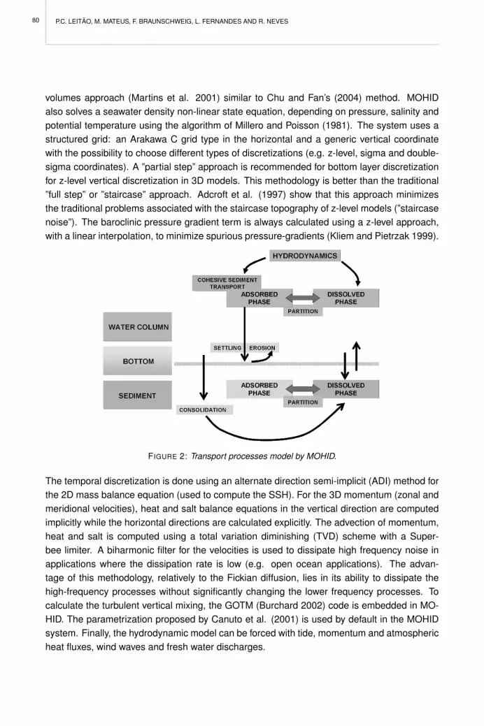
P.C. LEITAO, M. MATEUS, F. BRAUNSCHWEIG, L. FERNANDES AND R. NEVES
volumes approach (Martins et al. 2001) similar to Chu and Fan’s (2004) method. MOHIDalso solves a seawater density non-linear state equation, depending on pressure, salinity andpotential temperature using the algorithm of Millero and Poisson (1981). The system uses astructured grid: an Arakawa C grid type in the horizontal and a generic vertical coordinatewith the possibility to choose different types of discretizations (e.g. z-level, sigma and double-sigma coordinates). A ”partial step” approach is recommended for bottom layer discretizationfor z-level vertical discretization in 3D models. This methodology is better than the traditional”full step” or ”staircase” approach. Adcroft et al. (1997) show that this approach minimizesthe traditional problems associated with the staircase topography of z-level models (”staircasenoise”). The baroclinic pressure gradient term is always calculated using a z-level approach,with a linear interpolation, to minimize spurious pressure-gradients (Kliem and Pietrzak 1999).
FIGURE 2: Transport processes model by MOHID.
The temporal discretization is done using an alternate direction semi-implicit (ADI) method forthe 2D mass balance equation (used to compute the SSH). For the 3D momentum (zonal andmeridional velocities), heat and salt balance equations in the vertical direction are computedimplicitly while the horizontal directions are calculated explicitly. The advection of momentum,heat and salt is computed using a total variation diminishing (TVD) scheme with a Super-bee limiter. A biharmonic filter for the velocities is used to dissipate high frequency noise inapplications where the dissipation rate is low (e.g. open ocean applications). The advan-tage of this methodology, relatively to the Fickian diffusion, lies in its ability to dissipate thehigh-frequency processes without significantly changing the lower frequency processes. Tocalculate the turbulent vertical mixing, the GOTM (Burchard 2002) code is embedded in MO-HID. The parametrization proposed by Canuto et al. (2001) is used by default in the MOHIDsystem. Finally, the hydrodynamic model can be forced with tide, momentum and atmosphericheat fluxes, wind waves and fresh water discharges.
80

MODELLING COASTAL SYSTEMS: THE MOHID WATER NUMERICAL LAB
3.2 Open boundary
To prescribe coherent open boundary conditions (OBC), good external data are mandatory(Blayo and Debreu 2005). There are several sources of external solutions for coastal applica-tions. Several global tidal solutions became very common approximately 15 years ago (e.g.CSR4, FES2004, GOT00.2, NAO. 99b, TPXO6.2). The MOHID system has the necessarysoftware tools to generate the external solution from the FES2004 tidal SSH atlases (Lyard etal. 2006). Pre-operational models have been made available over the last years (Mercator,HYCOM-US, Topaz and FOAM), providing a best estimate on the current state of the oceanlow frequency processes. The MOHID system also has the necessary software to use theMercator and HYCOM-US for external solutions and initial conditions (Leitao et al. 2005).The MOHID system allows the user to construct a tree of one-way nested models with nolimitations on the number of nesting levels from a software perspective (Braunschweig et al.2004). By default, for each nesting level the external data for the OBC is the upper level inthe MOHID nesting system. However, the user can add another solution linearly to the uppernesting levels. This nesting capability allows overlapping different scales in an efficient way tostudy local processes.
3.3 Lagrangian referential
Mohid can simulate the transport of mass (dissolved and particulate) in the water column us-ing a lagrangian approach (Leitao 1996). The velocities of lagrangian particles at any pointin space are calculated with a linear interpolation between the points of the hydrodynamicmodel grid. Turbulent transport is responsible for dispersion. The effect of eddies on parti-cles depends on the ratio between eddies and particle size. Eddies bigger than the particlesmake them move at random. On the other hand, eddies smaller than the particles causeentrainment of matter into the particle, increasing its volume and mass according to the envi-ronment concentration. The random movement is calculated following the procedure proposedby Allen (1982). The random displacement is calculated using the mixing length and the stan-dard deviation of the turbulent velocity component, as given by the turbulence closure of thehydrodynamic model. Particles retain the velocity during the necessary time to perform therandom movement, which is dependent on the local turbulent mixing length (Leitao 1996). It isalso possible to associate to the particle the main processes of the fine sediments dynamicsdescribed below: settling velocity, adsorption/desorption, deposition and erosion.
3.4 Fine sediments in the water column
Particulate properties transported in the water column are governed by a 3D advection-diffusionequation where the vertical advection includes the particle settling velocity. Two different ap-proaches are followed to compute settling: a constant settling velocity and a settling velocitydependent of fine sediment concentration. In the first case, each particulate can have itsspecific and constant settling velocity, which can be derived from literature (depending on its
81

P.C. LEITAO, M. MATEUS, F. BRAUNSCHWEIG, L. FERNANDES AND R. NEVES
size and biogeochemical characteristics). The latter approach, however, needs some con-siderations. Since the settling velocity algorithm was developed for fine sediment modelling,it raises the question of how the settling velocity of particulates with other properties can becomputed. The model assumes the same velocity as for the fine sediment settling velocity,therefore reinforcing the importance of fine sediments in the distribution and fate of the ad-sorbed contaminants fraction. The algorithm follows a formulation widely used in literature(e.g. Mehta 1988), where the general correlations for the settling velocity in the flocculationrange are:
WS = K1Cm for C < CHS (1)
and in the hindered settling range:
WS = K1CmHS [1.0− K2 (C − CHS)]m1 for C > CHS (2)
where WS ( m s−1) is the settling velocity, C ( kg m−3) is the concentration, and the subscriptHS refers to the onset of the hindered settling (of about 2 to 5 kg m−3). The coefficients K1
( m4 kg−1 s−1) and K2 ( m3 kg−1) depend on the mineralogy of the mud and the exponents mand m1 depend on particle size and shape.
3.4.1 Adsorption/Desorption
Adsorption and desorption are considered as a reaction process, that can be included in thesinks and sources terms of the transport equation. This reaction involves the dissolved andthe particulate phases of the contaminant being simulated, where the two phases tend to anequilibrium, which is given by a partition coefficient. The equilibrium can be described by thefollowing system of equations (Hayter and Pakala 1989):
∂Cd
∂t= k (D%× Cp − P%× Cd ) (3)
∂Cp
∂t= k (P%× Cd − D%× Cp) (4)
where Cp and Cd are the particulate and dissolved contaminant concentrations respectively;k ( s−1) is the equilibrium kinetic rate for adsorption-desorption between dissolved and partic-ulate phase; D% is the dissolved contaminant fraction; and P% the particulate contaminantfraction. The kinetic constant defines the rate at which the two phases tend to equilibrium. Toaccount for the fact that, in the presence of low suspended matter concentrations, the adsorp-tion process is less likely to occur (the probability of a contaminant ion to collide with a particleis lower), a direct relation between the kinetic rate and the suspended particulate matter wasimplemented: (
k = kref · CSPMCSPMreference
for CSPMCSPMreference
< 1k = kref for CSPM
CSPMreference≥ 1
(5)
where CSPM is the concentration of the suspended particulate matter approximately equal tothe fine sediment concentration. The kref is the kinetic rate for a CSPM of reference ( CSPMreference).
82
MODELLING COASTAL SYSTEMS: THE MOHID WATER NUMERICAL LAB
3.5 Water-sediment interface model
The water sediment interface model also known as fluff layer computes and manages bound-ary conditions for the water column and sediment compartments.
3.5.1 Fine sediments fluxes
For fine sediments at the bottom, a flux term, Fb (mass of sediment per unit bed area per unittime) can be defined, corresponding to a source or sink for the suspended particulate matterin conditions of erosion or deposition, respectively. Consequently, at the bottom:
Fb = FE − FD (6)
where FE and FD are respectively the erosion and deposition fluxes. It is assumed that, whenbottom shear stress is smaller than a critical value for deposition, there is addition of matterto the bottom, and, when the bottom shear is higher than a critical value, erosion occurs.Between those values, erosion and deposition balance each other. The erosion algorithmused is based on the classical approach of Partheniades (1965). Erosion occurs when thebottom shear stress exceeds the threshold of erosion. The flux of eroded matter is given by:(
FE = E“ττE− 1”
for τb > τCSE
FE = 0 for τb < τCSE
(7)
where τ is the bed shear stress, τCSE is a critical shear stress for erosion and E is the erosionparameter ( kg m−2 s−1). This erosion algorithm is computed at the sediment-water interface.If this layer is eroded, erosion occurs from the underlying sediment layer, which has a higherlevel of compaction, therefore increasing the erosion shear stress thresholds. This is obtainedby defining τCSE as depth dependent, reflecting the increasing resistance of the sediment to beeroded as scouring reaches deeper layers. Wave induced shear stress can also be computedby the model by a linear wave theory, given wave characteristics such as wave period and wavesignificant height. Estuarine local waves can be important in terms of sediment resuspension,especially in shallow water where the wave stresses effect reaches the sediment bed. Pina(2001) presents a detailed description on the formulation implemented in the model. On theother hand, the deposition flux can be defined as:
FD = −p(WSC)b (8)
where p is the probability of sediment particles to settle down on the bed; WS is near-bed thesettling velocity; and C the near-bed fine sediment concentration. The probability of deposition(Krone 1962), can be defined as:
p = (1− τb
τCSD) (9)
where τb (Pa) and τCSD (Pa) are the bottom shear stress and the critical shear stress fordeposition respectively. This concept reflects the fact that the deposition of flocks is controlledby near-bed turbulence. For a flock to stick to the bed, gravitational forces must be strong
83

P.C. LEITAO, M. MATEUS, F. BRAUNSCHWEIG, L. FERNANDES AND R. NEVES
enough to withstand the near bed shear stress. The deposition algorithm (Krone 1962), likethe erosion algorithm, is based on the assumption that deposition and erosion never occursimultaneously, i.e., a particle reaching the bottom has a probability of remaining there thatranges from 0 to 1 as the bottom shear stress varies between its upper limit for deposition andzero respectively. Deposition is calculated as the product of the settling flux and the probabilityof a particle to remain on the bed:(
FD = (CWS)B(1− ττCSD
) for τb < τCSD
FD = 0 for τb > τCSD(10)
The critical shear stress for deposition depends mainly on the size of the flocks. Bigger flockshave a higher probability of remaining on the bed than smaller flocks. As only a single char-acteristic class of fine sediment is considered in the model, parameters must be calibrated,starting from reference values found in literature, in order to achieve good approximations inthe final results. Consolidation is considered to occur in recently deposited sediments at thesediment-water interface and is modelled as a sediment flux, Fconsolidation ( kgsed m−2 s−1), be-tween the fluff layer and the first sediment layer at a certain rate, kconsolidation ( s−1), dependenton the sediment mass per unit of surface area deposited at the fluff layer. It is assumed thatconsolidation only occurs when shear stress (τb) is lower than the critical shear stress fordeposition (τCSD): (
Fconsolidation = 0 for τb > τCSD
Fconsolidation = Msediment · kconsolidation for τb < τCSD(11)
This consolidation flux is one of the governing processes for particulate contaminant fractionsto enter the sediment compartment.
3.5.2 Particulate properties fluxes
Particulate properties fluxes at the sediment-water interface depend on erosion and on con-solidation processes. As the erosion algorithm was developed specifically for fine sedimentmodelling, when computing other particulate properties fluxes at the bed, the erosion rate pa-rameter cannot be the same. Thus, a specific proportionality factor for the erosion constant iscomputed, Eprop, for each property, relating the quantity of property ( Mproperty in kgproperty m−2)to the quantity of fine sediment deposited in the bed ( Msediment in kgsed m−2). The particulateproperty erosion flux is then computed similarly to fine sediments but with a specific Eprop:
Eprop = E„
Mproperty
Msediment
«(12)
In this way, critical shear stress values are considered equal for all particulate properties, withthe specific erosion constant being the differentiating factor. When consolidation occurs asimilar algorithm is followed, relating the sediment consolidation flux to the particulate prop-erty deposited mass. Thus, the property consolidation flux ( Fprop) can be computed with thefollowing expression:
F propconsolidation = F sediment
consolidation
„Mproperty
Msediment
«(13)
84

MODELLING COASTAL SYSTEMS: THE MOHID WATER NUMERICAL LAB
3.5.3 Dissolved properties
Dissolved properties fluxes across the water-sediment interface depend both on erosion / con-solidation processes and on concentration gradients between the water column lower layerand on the interstitial water of the sediment upper layer. As stated before, when the fluff layeris active (i.e. there are recently deposited sediments on the bed), interstitial water betweenthose sediment particles is not considered. Thus, when erosion occurs there is no dissolvedproperties influx from the fluff layer to the water column. The interstitial water in the sedimentsupper layers (containing solutes such as dissolved contaminant fractions, nutrients, etc) isflushed to the water column when consolidated sediment is eroded (upper sediment compart-ment layer). On the other hand, when consolidation occurs, water overlying the sediment bedbecomes part of the sediment interstitial water. These processes constitute an additional fluxof solutes to and from the water and sediment columns. Thus, a water flux ( Fwater in m3 s−1)can be computed, corresponding to the amount of porewater dragged along with the erodedsediments or to the amount of overlying water captured in the consolidation process:
F watererosion/consolidation = Ferosion/consolidation · A · φk ·
1ρsed · (1− φkn)
(14)
where, Ferosion/consolidation is the fine sediment flux ( kgsed m−2 s−1) between the sediment-waterinterface and the sediments’ upper layer, φkn is the porosity in the upper (k=n) sediment layer,ρsed is the sediment dry density ( kgsed m−3
sed) and A is the area ( m2) of the sediment-waterinterface. Respectively, solute fluxes are given by:
F soluteerosion/consolidation =
F watererosion/consolidation · Csolute
A(15)
where C is solutes’ concentration ( kg m−3water) in the sediment upper layer or in the water column
bottom layer, depending on the type of flux (erosion or consolidation). As mentioned above,the concentration gradients between the water column bottom layer and the sediment surfacelayer can also produce a mass flux through the sediment-water interface. Solutes in a turbulentflow can be transported by a mean advective flux, turbulent diffusion and molecular diffusion. Itis usually considered that solutes diffusion coefficient is equal to the fluids turbulent viscosity,which are usually several orders of magnitude higher. Nonetheless, when approaching thesediment bed water flow is reduced, and the same is true of turbulent motion, leading toan increase in the importance of molecular diffusion relative to the turbulent one. Thus, asub-diffusive layer (Boudreau 1997) is formed, where a linear concentration gradient can beconsidered, and a diffusive flux, Fdiffusive ( kgsolute m−2 s−1), can be computed representing therate at which this gradient tends to be eliminated:
Fdiffusive =Dmolecular
δ· A · (Cwater − Cintertidal ) (16)
in which Dmolecular is the molecular diffusion coefficient ( m2 s−1), and δ (m) is the sub-diffusiveboundary layer thickness, which is dependent on near-bed turbulence:
δ =2 · νwater
u+(17)
where νwater is the water kinematic viscosity ( m2 s−1) and u+ is near-bed shear velocity ( m s−1).
85
P.C. LEITAO, M. MATEUS, F. BRAUNSCHWEIG, L. FERNANDES AND R. NEVES
4 SEDIMENT COLUMN MODEL
The sediment compartment consists of saturated porous media, formed by sediments and bywater that fills the interstices between the sediments. Properties in this compartment can ei-ther be dissolved (in the porewater), or particulate (adsorbed on to sediments). The sediment-water interface handles processes occurring between the water and the sediment column.Since it is very difficult to define physically, this interface really is an abstraction. In the modelit can be seen as a thin sediment layer (fluff-layer) with transient characteristics, depending ba-sically on temporal scales associated with hydrodynamics and transport in the water column,namely erosion and deposition. This layer has a separation function, which allows dissociatingprocesses that occur on the sediment deposit, at a very slow scale, ”filtering” the high frequen-cies of erosion/deposition fluxes that shape it, therefore leading to consolidation. Dissolvedproperties can be produced in the interface but their mass is not part of it, becoming part ofthe water column by means of a boundary condition flux. Contrastingly, particulate propertiesare part of the sediment-water interface. This can be the case when sediment deposition oc-curs but the sediment is not yet consolidated. Thus, a particulate property deposited mass istracked in order to know how much of is available when erosion conditions occur. Followingthis concept, it is considered that dissolved properties can exchange fluxes directly betweenthe water column and the sediment interstitial water. In erosion conditions, if this transientlayer is completely eroded, then scouring takes place from the sediment compartment upperlayer, where consolidated sediment is present. When this happens, interstitial water is en-trained along with the sediment, constituting a flux to the water column. In the same way,when the fluff-layer consolidates and becomes part of the sediment column there is an inputof overlying water (and its properties) to the sediment compartment. The sediment columnmodel is a set of 1D vertical models defined below the 3D water column model (Figure 3).Both models share the same horizontal discretization, but compute independent vertical coor-dinates. Adsorption and desorption processes are simulated with a similar approach as in thewater column.
FIGURE 3: Sediment compartment discretization.
86

MODELLING COASTAL SYSTEMS: THE MOHID WATER NUMERICAL LAB
REFERENCES
Adcroft A, Hill C, Marshall J (1997) Representation of Topography by Shaved Cells in a Height CoordinateOcean Model, Monthly Weather Review 125: 2293-2315
Allen C M (1982) Numerical simulation of contaminant dispersion in estuary flows, Proc. R. Soc. London.A 381: 179-194
Blayo E, Debreu L (2005) Revisiting open boundary conditions from the point of view of characteristicvariables. Ocean Modelling 9: 231-252
Boudreau B P (1997) A one dimensional model for bed-boundary layer particle exchange, Journal ofMarine Systems 11: 279-303
Braunschweig F, Martins F, Leitao P, Neves R (2003) A methodology to estimate renewal time scales inestuaries: the Tagus Estuary case, Ocean Dynamics 53: 137-145
Braunschweig F, Chambel P, Fernandes L, Pina P, Neves R (2004) The object-oriented design of theintegrated modelling system MOHID, Computational Methods in Water Resources International Con-ference, Chapel Hill, North Carolina, USA.
Burchard H (2002) Applied turbulence modelling in marine waters, Vol. 100 of Lecture Notes in EarthSciences, Springer, 229 pp.
Cancino L, Neves R (1999) Hydrodynamic and sediment suspension modelling in estuarine systems, PartII: Application to the Western Scheldt and Gironde estuaries, Journal of Marine Systems 22: 117-131
Canuto V M, Howard A, Cheng Y, Dubovikov M S (2001) Ocean Turbulence. Part I: One-Point ClosureModel Momentum and Heat Vertical Diffusivities. Journal of Physical Oceanography 31: 1413-1426
Carracedo P S, Torres-Lopez S, Barreiro M, Montero P, Balseiro C F, Penabad E, Leitao P C, Perez-Munuzuri V (2006) Improvement of pollutant drift forecast system applied to the Prestige oil spills inGalicia Coast (NW of Spain): Development of an operational system, Marine Pollution Bulletin 53:350-360
Chu P C, Fan C (2004) Finite volume ocean circulation modelA Terrain-Following Crystal Grid FiniteVolume Ocean Circulation Model, Journal of Oceanography 60: 945-952
Coelho H S, Neves R J, White M, Leitao P C, Santos A J (2002) A model for ocean circulation on theIberian coast, Journal of Marine Systems 32: 153-179
Decyk V K, Norton C D, Szymanski B K (1997) Introduction to Object-Oriented Concepts using Fortran90,Unpublished.
Hayter E J, Pakala C V (1989) Transport of inorganic contaminants in estuarial waters, Journal of CoastalResearch, Special Issue 5: 217-230
Kliem N, Pietrzak JD (1999) On the pressure gradient error in sigma coordinate ocean models: A com-parison with a laboratory experiment. Journal of Geophysical Research 104: 29781-29800
Krone R (1962) Flume Studies of the Transport in Estuaries Shoaling Processes, Hydr. Eng. Lab., Uni-versity of Berkeley, California, USA.
Leitao P, Coelho H, Santos A, Neves R (2005) Modelling the main features of the Algarve coastal cir-culation during July 2004: A downscaling approach. Journal of Atmospheric & Ocean Science 10.421-462
Leitao P, Leitao J, Neves R, Berzin G, Silva A (2004) Hydrodynamics And Transport In The Coastal ZoneOf Sao Paulo - Brazil. Proceedings 29th International Conference of Coastal Engineering 3: 3316-3328
Leitao P C (2003) Integracao de escalas e de processos na modelacao do ambiente marinho. Tese deDoutoramento. Universidade Tecnica de Lisboa, Instituto Superior Tecnico, Lisboa..
Leitao P C (1996) Modelo de dispersao lagrangeano tridimensional, Dissertacao para a obtencao dograu de Mestre em Ecologia, Gestao e Modelacao de Recursos Marinhos, Instituto Superior Tecnico,Lisboa.
87

P.C. LEITAO, M. MATEUS, F. BRAUNSCHWEIG, L. FERNANDES AND R. NEVES
Lyard F, Lefevre F, Letellier T, Francis O (2006) Modelling the global ocean tides: modern insights fromfes2004. Ocean Dynamics 56: 394-415
Martins F (2000) Modelacao matematica tridimensional de escoamentos costeiros e estuarinos usandouma abordagem de coordenada vertical generica. Tese de Doutoramento. Universidade Tecnica deLisboa, Instituto Superior Tecnico, Lisboa.
Martins F, Leitao P, Silva A, Neves R (2001) 3D modelling in the Sado estuary using a new generic verticaldiscretization approach. Oceanologica Acta 24: S51-S62
Mateus M (2006) A process-oriented biogeochemical model for marine ecosystems: development, nu-merical study, and application. PhD. Instituto Superior Tecnico, Lisbon, Portugal.
Mehta A J (1988) Laboratory Studies on Cohesive Sediment Deposition and Erosion, Physical Processesin Estuaries, Job Dronkers and Wim van Leussen (Editors), Springer-Verlag.
Millero F J, Poisson A (1981) International one-atmosphere equation of state of seawater. Deep-Sea Res28: 625-629
Miranda, R., 1999, Nitrogen Biogeochemical Cycle Modeling in the North Atlantic Ocean, Dissertacaopara a obtencao do grau de Mestre em Ecologia, Gestao e Modelacao de Recursos Marinhos, InstitutoSuperior Tecnico, Lisboa
Miranda R, Braunschweig F, Leitao P, Neves R, Martins F, Santos A (2000) MOHID 2000, A Coastalintegrated object oriented model. Hydraulic Engineering Software VIII, WIT Press.
Neves R J (1985) etude experimentale et modelisation des circulations transitoire et residuelle dansl’estuaire du Sado. Ph.D. Thesis. Univ. Liege, Liege.
Partheniades E (1965) Erosion and Deposition of Cohesive Soils, J. Hydr. Div. 91: 105-139
Pina P (2001) An Integrated Approach to Study The Tagus Estuary Water Quality. Dissertacao para aobtencao do Grau de Mestre em Ecologia, Gestao e Modelacao dos Recursos Marinhos. SuperiorTecnico, Universidade Tecnica de Lisboa, Lisbon.
Portela L I (1996) Mathematical modelling of hydrodynamic processes and water quality in Tagus estuary.Ph.D. thesis. Universidade Tecnica de Lisboa, Instituto Superior Tecnico, Lisboa.
Santos A (1995) Modelo hidrodinamico tridimensional de circulacao oceanica e estuarina. Tese deDoutoramento. Universidade Tecnica de Lisboa, Instituto Superior Tecnico, Lisboa.
Santos A, Nogueira J, Martins H (2005) Survival of sardine larvae off the Atlantic Portuguese coast: apreliminary numerical study. ICES Journal of Marine Science: Journal du Conseil 62: 634-644
Saraiva S, Pina P, Martins F, Santos M, Braunschweig F, Neves R (2007) Modelling the influence of nutrientloads in Portuguese estuaries. Hydrobiologia 587: 5-18
Silva A, Leitao P C, Leitao J C, Braunschweig F, Neves R (2002) Ria Formosa 3D hydrodynamic model.A contribution for the understanding of the Faro-Olhao inlet processes, Littoral 2002, Porto, Portugal.
Silva A, Leitao P C (2005) A contribution to the understanding of the Obidos lagoon dynamics, Proc. ofCoastal Dynamics 2005, International Conference on Coastal Dynamics, Barcelona.
Theias H (2005) Numerical Modeling of Non-Hydrostatic Processes in Estuarine and Coastal Regions.Mater Thesis in Hydraulics. Universidade Tecnica de Lisboa, Instituto Superior Tecnico.
Trancoso A R, Saraiva S, Fernandes L, Pina P, Leitao P, Neves R (2005) Modelling macroalgae using a 3Dhydrodynamic-ecological model in a shallow, temperate estuary. Ecological Modelling 187: 232-246
Vaz N, Dias J M, Leitao P C, Nolasco R (2007) Application of the Mohid-2D model to a mesotidal temperatecoastal lagoon. Computers & Geosciences 33: 1204-1209
Villarreal M R, Montero P, Tabuada J J, Prego R, Leitao P C, Perez-Villar V (2002) Hydrodynamic modelstudy of the Ria de Pontevedra under estuarine conditions, Estuarine, Coastal and Shelf Science 54:101-113
88

PERSPECTIVES ON INTEGRATED COASTAL ZONE MANAGEMENT IN SOUTH AMERICAR. NEVES, J.W. BARETTA AND M. MATEUS (EDS.), IST PRESS, 2008
MODELLING POLLUTION: OIL SPILLS AND FAECAL CONTAMINATION
M. MATEUS AND R. FERNANDES
1 INTRODUCTION
Human activities in coastal areas degrade biota and affect human health. Pollution causedby oil spills and sewage disposal are among the most obvious examples of this reality. Bothhave clear detrimental effects, with obvious socio-economic consequences and, over the lastdecades, have been at the top of the list of estuarine management concerns. Public healthrisks posed by sewage discharge to sea led the United Nations Group of Experts on the Scien-tific Aspects of Marine Pollution (GESAMP) to place this threat on the top of its list of concerns,in 1990. While not harming the environment in the same way as oil pollution, sewage impairshuman health by the transmission of enteric diseases. Human sewage contains enteric bac-teria, pathogens and viruses, and the eggs of intestinal parasites. Contamination of food ordrinking and bathing waters may therefore pose a public health hazard. There have beensome instances of hepatic and enteric diseases contracted through bathing in contaminatedwaters (Clark 1992). In most developing countries, discharge of raw sewage in coastal areasand estuaries is still common practice, posing serious threats for the population that makesuse of the waters.
Faecal and oil pollution assessment requires descriptive and predictive tools, such as nu-merical simulation models, that are able to reproduce the dynamics of the systems in study,and simulate the fate of the pollutants under a broad range of scenarios (Bach et al. 1995,Christodoulou et al. 1995, Rodriguez et al. 1995, Garvey et al. 1998, Mahajan et al. 1999,Noutsopoulos et al. 1999). This chapter presents synthetic description of the oil and faecal co-liform modules of the MOHID modelling system. They have been applied in the ECOMANAGEstudy sites to study the influence of the hydrodynamic regime on the fate of these pollutants,their impact on the system, and in some cases, to test different management options.
2 MODELLING FRAMEWORK
Attaining an adequate description of the dynamics of contamination is imperative to definewater quality management strategies and to develop realistic contingency plans to deal withpotential threats. This is frequently achieved through the use of numerical model simulations.A major advantage of the use of models in pollution studies is that they can be used as adiagnostic tool (identifying and studying actual problems) and as a prognostic tool (testing dif-ferent scenarios). In addition, numerical tools can be implemented to render forecast capacityto pollution assessments. The numerical tool must be able to achieve basic goals such as (1)an accurate assessment of the dispersion of the pollutant, and (2) a reproduction of the basicprocesses that affect the state and fate of the pollutant in the environment.
89

M. MATEUS AND R. FERNANDES
Contrary to oil spills that usually have a tremendous visual impact, feacal pollution can beunnoticed. A striking difference between these two forms of pollution is their residence time inthe water; hydrocarbons can last for long periods of time when compared with faecal agents.Faecal bacteria are bioindicators, meaning that their residence time in aquatic systems iscomparatively low, usually ranging from less than an hour to a few hours, and occasionallyup to some days. However, from a modelling perspective, oil spills and faecal pollution sharesame basic requirements in respect to the underlying physical mechanisms of transport inwater. Hydrodynamic processes govern the dispersion of contaminants in the receiving area.So, by coupling general hydrodynamic processes and pollutant-specific processes, modelscan determine the plume evolution, enabling the prediction of affected areas and ambientconcentrations over time. In summary, models enable the assessment of the magnitude of thepollution.
The effects that transport, ambient conditions, domain geometry and bathymetry, and othervariables have on the dynamics of these pollutants in aquatic environments, require that mod-els have the ability to reproduce their contribution to the dynamics of the system. The MOHIDnumerical platform (more details in the previous chapter) is such a tool because of the widerange of processes it simulates. Within this modelling framework there are independent mo-dules that deal with the dynamics of these pollutants. This chapter deals with these modules,addressing in a brief way the processes they simulate and the baseline modelling philosophy.
3 THE LAGRANGIAN MODULE
Lagrangian transport models are very useful to simulate localized processes with sharp gradi-ents (submarine outfalls, sediment erosion due to dredging works, hydrodynamic calibration,oil dispersion, etc.). The MOHID model uses the concept of lagrangian tracers to assess thespatial-temporal evolution of the contamination plume, determined by tidal regime and localcirculation. Tracers are transported by currents calculated by hydrodynamic model and eachtracer has the ability to be associated with one or more properties (physical, chemical or bio-logical). This model is a subset of the MOHID modelling system and has been used in otherinstances also to study pollutant dispersion (Gomez-Gesteira et al. 1999). At the presentstage the model is able to simulate oil dispersion, water quality evolution and sediment trans-port. The lagrangian module interacts with other modules such as the oil dispersion moduleto simulate oil dispersion and the Escherichia coli decay module. Sediment transport can beassociated directly to tracers using the concept of settling velocity.
3.1 Tracer concept
Tracers are characterized by their spatial coordinates, volume and a list of properties, eachwith a given concentration. The most important property of a tracer is its position in space(x,y,z). The tracer can be a water mass, a sediment particle or group of particles, a moleculeor group of molecules, or even a phytoplankton cell. The movement of tracers can be in-
90

MODELLING POLLUTION: OIL SPILLS AND FAECAL CONTAMINATION
fluenced by the velocity field from the hydrodynamic module, by the wind from the interfacewater-air module, by the spreading velocity from oil dispersion module and by random velocity.Both volume and properties concentration of each tracer vary in time in response to differentparameters and ambient conditions. For E. coli, for example, volume is affected by turbulentmixing while fecal concentration depends on environmental factors like irradiance, tempera-ture and salinity. Tracers belonging to the same origin have the same list of properties and usethe same parameters for random walk, E. coli decay, etc. Origins can differ in the way theyemit tracers. There are three different ways to define origins in space: (1) Point Origins - emitstracers at a given point; (2) Box Origins - emits tracers over a given area; (3) Accident Origins- emit tracers in a circular form around a point. Origins, in turn, emit tracers in two differentways: (i) Continuous - emits tracers during a period of time; (ii) Instantaneous - emits tracersat one instant.
3.2 Tracer Movement
The major factor responsible for particle movement is generally the mean velocity. Spatialcoordinates are given by the definition of velocity:
dxi
dt= ui (xi , t) (1)
where u is the mean velocity and x the particle position. This equation is solved using a simpleexplicit method:
x t+∆ti = x t
i + ∆t · uti (2)
Higher order accuracy requires the use of an iterative procedure. For most natural flows,the explicit method is sufficiently accurate. Velocity at any point in space is calculated usinga linear interpolation between the points of the hydrodynamic model grid. The lagrangianmodule allows splitting the calculation of the trajectory of the tracers into sub-steps of thehydrodynamic time step.
3.3 Turbulent Diffusion
Turbulent transport is responsible for dispersion. The effect of eddies over particles dependson the ratio between eddies and particle size. Eddies bigger than the particles make themmove at random, while eddies smaller than the particles cause entrainment of matter into theparticle, increasing its volume and mass according to the environment concentration. Ran-dom movement is calculated following the procedure proposed by Allen (1982). The randomdisplacement is calculated using the mixing length and the standard deviation of the turbulentvelocity component, as given by the turbulence closure of the hydrodynamic model. Parti-cles retain that velocity during the necessary time to perform the random movement, whichis dependent on the local turbulent mixing length. The increase in volume is associated withsmall-scale turbulence and is reasonable to assume it as isotropic. Under these conditions,small particles keep their initial form and their increase in volume is a function of the volumeitself.
91

M. MATEUS AND R. FERNANDES
4 OIL SPILLS
The prediction and simulation of the trajectory and weathering of oil spills are essential to thedevelopment of pollution response and contingency plans, as well as to the evaluation of en-vironmental impact assessments. In order to predict the fate of oil products spilled in coastalzones, the oil weathering model predicts the evolution and behavior of the processes (trans-port, spreading, evaporation, etc.) and properties (density, viscosity, etc) of the oil products.
Oil density and viscosity, and many different processes such as oil spreading, evaporation,dispersion, sedimentation, dissolution, emulsification and oil beaching have been included inthe oil module. Depending on the characteristics of the computational mesh or the magnitudeof the spill, the model considers different alternative methods to simulate some of these pro-cesses. The oil weathering module (OWM) uses mainly the hydrodynamics and lagrangiantransport modules. The hydrodynamic module simulates the velocity field necessary for thelagrangian module to calculate oil trajectories. These oil trajectories are computed assumingthat oil can be idealized as a large number of particles that independently move in water.
Water properties and atmospheric conditions are introduced in the lagrangian module andused by the oil module to determine oil processes and properties. Except for the spreadingand oil-beaching, all weathering processes and properties are assumed to be uniform for alltracers, like water properties and atmospheric conditions. These are assumed to be equalto the environmental conditions at the accident’s origin. Oil temperature is assumed equal towater temperature, neglecting solar radiation or any other energy transfer process that mayinfluence oil temperature. In its current setup MOHID OWM is not a 3D application. It simulatesthe amount of oil that leaves the water surface (by different processes like evaporation, ordispersion in water), without simulating the evolution at the subsurface and variations in thewater column.
4.1 Modelled processes
Only a description of the modelled processes is presented here, since detailed informationon the governing equations and model parameterization is available in the form of a User’sManual for download at the MOHID’s model website (http://www.mohid.com).
4.1.1 Spreading
For an instant spill accident, the initial area of spilled oil is calculated according to Fay’s for-mulation (Fay 1969). Two different algorithms are available to estimate oil spreading. One ofthe algorithms determines random velocities assuming a uniform distribution inside a range(in directions x and y ), proportional to diffusion coefficients, which are calculated assumingthat lagrangian tracers spreading is equivalent to Fay’s formulas solution (Fay 1969). The onlyphase simulated in spreading is the gravity-viscous phase, from solutions proposed by Fay.
The other algorithm proposed for oil spreading is based in thickness differences inside theoil slick, presuming that the existence of a thickness gradient generates a ”spreading force”
92

MODELLING POLLUTION: OIL SPILLS AND FAECAL CONTAMINATION
in the direction of minor thickness. Therefore, a tracer will move from the computational cellwith larger oil thickness to the thinner one. This formulation uses a coefficient to approach thesolution to the Fay solution, in order to make results sensible to some factors, like differentoil densities, originating different behaviors. In the oil module, velocities are calculated in thefaces of cells where oil is present, in directions x and y. Subsequently, in the lagrangianmodule tracer velocities are interpolated based on cell faces velocities and tracer position.If the average oil thickness becomes too thin (less than a value between 0.1 and 0.01 mm,depending of product viscosity), oil spreading is stopped.
4.1.2 Density and viscosity
Oil density is estimated considering the density of the emulsion at ambient temperature, thedensity of fresh oil at a reference temperature and the water temperature. The oil’s initialdensity is obtained from the algorithm proposed by the American Petroleum Institute (API).Only oil products with lower density than water are modelled, because higher density productswill sink. In the model the oil viscosity is controlled by three major factors: temperature,evaporation and emulsification.
4.1.3 Evaporation and emulsification
In MOHID the oil evaporation process can be estimated by two different methods: an analyticalmethod, also known as the evaporative exposure method (Stiver and Mackay 1984), and by amore recent methodology proposed by Fingas (1998), where the relevant factors are time andtemperature. Square root equations can also be used in some refined oils and in short termsimulations (1-2 days). The emulsification process consists in the incorporation of water in oil,usually starts after a certain amount of oil has evaporated. An emulsification constant is used,which means the percentage of oil evaporated before emulsification starts. By default, thisconstant is 0%. When emulsification starts, incorporation of water in oil can be simulated bytwo different algorithms: the widely used equation of Mackay et al. (1980) and the Rasmussenequation (Rasmussen 1985).
4.1.4 Dispersion
This is the process where oil droplets entrain the water column. Two different methods areavailable to predict this weathering process, based on the formulations proposed by Delvigneand Sweeney (1998), and Mackay et al. (1980). The latter method is a simplified algorithmdeveloped for vertical dispersion as a function of squared wind velocity, for conditions whereturbulent energy is difficult to determine.
4.1.5 Dissolution
Dissolution is quantified through the Cohen method, considering the analytical solution for thesolubility of typical oil proposed by Huang and Monastero (1982).
93

M. MATEUS AND R. FERNANDES
4.1.6 Sedimentation
Although the process of oil sedimentation is relatively difficult to estimate, the MOHID modeluses a formulation developed by Science Applications International (Payne et al. 1987) for thispurpose. Only droplets greater than 70 microns and smaller than 200 microns are consideredfor sedimentation. Bigger droplets are less likely to stick to sediment particulate matter, andthose smaller than 70 microns are already estimated in the dispersion process.
4.1.7 Oil-Beaching
When oil reaches a coastal zone, it might become beached. This model estimates the amountof beached oil when the model user predefines a beaching probability (or different beachingprobabilities for different coastal zones).
5 FAECAL CONTAMINATION
The reduction of faecal contaminant loads in the water is achieved by a combination of threemain factors: initial dilution, dispersion and bacterial decay. Dynamic models usually takeinto consideration the physical processes of dilution and dispersion but frequently ignore theinfluence of abiotic effects on bacteria mortality by assuming a fixed mortality rate. Undercertain conditions, this limitation hinders the results. For the specific case of the decline infaecal indicator bacteria, several studies have shown a particularly relevant role of abioticfactors like temperature, salinity and irradiance (Pereira and Alcantara 1993, Sarikaya andSaatci 1995, Serrano et al. 1998). A more realistic assessment of temporal and spatialfaecal contamination can be achieved by using a feacal decay model with a dynamic T90 asa function of instant solar radiation, water temperature and salinity. Faecal dispersion can besimulated using both the lagrangian and the eulerian transport schemes.
5.1 Faecal decay model
TC and FC groups have similar decay rates (Marais 1974) and have been commonly usedas indicators to assess water quality state. The die-off rate of this class of organisms isrepresented by a first-order equation (Chick’s Law for disinfection), which states that the rateof loss is proportional to the concentration:
∂N∂t
= −kN (3)
where N is the initial bacterial concentration in the effluent and k, the first-order decay rate( day−1) or die-off coefficient, usually described in the form of a sum of individual parameters:
k = kb + ki + ks + kp (4)
where kb is the base mortality - a function of temperature and salinity - ki is the death rate dueto solar radiation, ks is the net loss/gain due to settling/resuspension, and kp is the mortality
94

MODELLING POLLUTION: OIL SPILLS AND FAECAL CONTAMINATION
rate induced by predation. In the MOHID framework the fecal mortality model accounts forthe impacts of temperature, salinity and ambient light in the decay of fecal indicators. It isderived from in situ and laboratory studies of mortality rates of E. coli made in the CantabrianSea (Canteras et al. 1995). The contribution of settling/suspension and grazing were notconsidered. As such, the simultaneous combination of all factors considered is expressed as:
k = 2.533 × 1.04(T−20) × 1.012S + 0.113iz (5)
where S and T are the surrounding water salinity and temperature (oC), respectively, and izis the irradiance ( watt m−2) at depth z (m). Irradiance levels in the water environment areestimated by the hydrodynamic model where the light extinction is already parameterized andthe irradiance is known for each vertical layer (depth integrated). This implies that for 2D-horizontal settings a mean value is calculated from irradiance levels at surface, consideringthe light attenuation effect of water molecules over the height of the water column. Bacterialdecay is usually expressed as T90, the time in which 90% of population is no longer de-tectable, meaning 1 log reduction in number of pathogens. Assuming a first-order loss, the90% mortality time is obtained by:
T90 = 2.303k−1 (6)
Together with FC concentrations, the model also outputs T90 values since these can be usedto explain the underlying dynamics of the contamination patterns. This is particularly useful issystems with a high spatial and temporal changes in ambient conditions.
5.2 The influence of abiotic parameters
Fixed T90 values are still widely used in modelling studies to assess the impact of bacterialinputs in water bodies (Kashefipour et al. 2002). However, when this methodology is appliedto areas with strong daily fluctuations of irradiance, usually associated with tidal movementsressuspending sediments and blocking light, it may fail to consider the major influence of lightin bacterial decay. The explicit modelling of abiotic effects on FC decay, on the other hand,accounts for the variation in ambient conditions. The wide range of T90 values over a dailycycle is obvious when we consider a typical diel period in late spring and summer at midlatitudes. It has been pointed that impact studies of FC contamination usually consider T90values lower than the values measured in culture experiments (Guillaud et al. 1997). Thisassumption can compromise the quality of model predictions, limiting the role of models haspredictive tools. This is further aggravated because static values are used from the entiresimulation period.
REFERENCES
Allen C M (1982) Numerical-Simulation of Contaminant Dispersion in Estuary Flows. Proceedings of theRoyal Society of London Series a-Mathematical Physical and Engineering Sciences 381: 179-194
Bach H K, Orhon D, Jensen O K, Hansen I S (1995) Environmental-Model Studies for the Istanbul Master-Plan .2. Water-Quality and Eutrophication. Water Science and Technology 32: 149-158
95
M. MATEUS AND R. FERNANDES
Canteras J C, Juanes J A, Perez L, Koev K N (1995) Modeling the Coliforms Inactivation Rates in theCantabrian-Sea (Bay-of-Biscay) from in-Situ and Laboratory Determinations of T-90. Water Scienceand Technology 32: 37-44
Christodoulou G C, Ioakeim I, Ioannou K (1995) Modeling of pollution from the wastewater discharge ofthe city of Limassol. Water Science and Technology 32: 197-204
Clark R B (1992) Marine Pollution. Clarendon Press, Oxford. 172p.
Delvigne G A L, Sweeney C E (1998) Natural Dispersion of Oil. Oil & Chemical Pollution 4: 281-310
Fay J A (1969) The spread of oil slicks on a calm sea. In: (eds) Oil on the Sea. Plenum Press, New York,pp 53-63
Fingas M. 1998. The evaporation of oil spills: development and implementation of new prediction method-ology. In: Marine Environmental Modelling Seminar ’98. Lillehammer, Norway.
Garvey E, Tobiason J E, Hayes M, Wolfram E, Reckhow D A, Male J W (1998) Coliform transport in apristine reservoir: Modeling and field studies. Water Science and Technology 37: 137-144
Gomez-Gesteira M, Montero P, Prego R, Taboada J J, Leitao P, Ruiz-Villarreal M, Neves R, Perez-Villar V(1999) A two-dimensional particle tracking model for pollution dispersion in A Coruna and Vigo Rias(NW Spain). Oceanologica Acta 22: 167-177
Guillaud J F, Derrien A, Gourmelon M, Pommepuy M (1997) T90 as a tool for engineers: Interest andlimits. Water Science and Technology 35: 277-281
Huang J C, Monastero F C (1982). Review of the state-of-the-art of oil spill simulation models - FinalReport. American Petroleum Institute.
Kashefipour S M, Lin B, Harris E, Falconer R A (2002) Hydro-environmental modelling for bathing watercompliance of an estuarine basin. Water Research 36: 1854-1868
Mackay D, Buistt I A, Mascarenhas R, Paterson S (1980). Oil spill processes and models., EnvironmentCanada Manuscript Report No. EE-8, Ottawa, Ontario.
Mahajan A U, Chalapatirao C V, Gadkari S K (1999) Mathematical modeling - A tool for coastal waterquality management. Water Science and Technology 40: 151-157
Marais G R (1974) Fecal Bacterial Kinetics in Stabilization Ponds. Journal of the Environmental Engineer-ing Division-Asce 100: 119-139
Noutsopoulos C, Gavalaki E, Andreadakis A (1999) Evaluation of the impact from the discharge of treatedsewage on the south-east Saronicos Gulf through mathematical water quality modelling. Water Sci-ence and Technology 39: 63-70
Payne J R, Kirstein B E, Clayton J R, Clary C, Redding R, McNabb D, Farmer G (1987). Integration ofSuspended Particulate Matter and Oil Transportation Study. Final Report, Report to Minerals Man-agement Service, MMS 87-0083
Pereira M G, Alcantara F (1993) Culturability of Escherichia-Coli and Streptococcus-Faecalis in BatchCulture and in-Situ in Estuarine Water (Portugal). Water Research 27: 1351-1360
Rasmussen D. 1985. Oil Spill Modelling - A tool for cleanup operations. In: Oil Spill Conference, AmericanPetroleum Institute. pp243-249
Rodriguez A, SanchezArcilla A, Redondo J M, Bahia E, Sierra J P (1995) Pollutant dispersion in thenearshore region: Modelling and measurements. Water Science and Technology 32: 169-178
Sarikaya H Z, Saatci A M (1995) Bacterial Die-Away Rates in Red-Sea Waters. Water Science andTechnology 32: 45-52
Serrano E, Moreno B, Solaun M, Aurrekoetxea J J, Ibarluzea J (1998) The influence of environmentalfactors on microbiological indicators of coastal water pollution. Water Science and Technology 38:195-199
Stiver W, Mackay D (1984) Evaporation Rate of Spills of Hydrocarbons and Petroleum Mixtures. Environ-mental Science & Technology 18: 834-840
96

PERSPECTIVES ON INTEGRATED COASTAL ZONE MANAGEMENT IN SOUTH AMERICAR. NEVES, J.W. BARETTA AND M. MATEUS (EDS.), IST PRESS, 2008
LOAD AND FLOW ESTIMATION: HARP-NUT GUIDELINES AND SWAT MODELDESCRIPTION
P. CHAMBEL-LEITAO
1 INTRODUCTION
When eutrophication is considered an important process to control it can be accomplishedreducing nitrogen and phosphorus losses from both point and nonpoint sources and helpingto assess the effectiveness of the pollution reduction strategy. HARP-NUT guidelines (Guide-lines on Harmonized Quantification and Reporting Procedures for Nutrients) are presentedby OSPAR as the best common quantification and reporting procedures for calculating thereduction of nutrient inputs. In 2000, OSPAR adopted the Harmonized Quantification and Re-porting Procedures for Nutrients (HARP-NUT guidelines) on a trial basis. They were intendedto serve as a tool for OSPAR Contracting Parties to report, in a harmonized manner, their dif-ferent commitments, present or future, with regard to nutrients under the OSPAR Convention,in particular the ”Strategy to Combat Eutrophication”.
OSPAR 2000 adopted HARP-NUT guidelines number 1-9, except for number 6 on diffusesources. OSPAR 2000 agreed that the further development of draft Guideline 6 within OSPARshould only start when the results of the EC Fifth Framework Programme Euroharp projecton an intercomparison of quantification models for losses from diffuse anthropogenic sourceswere available. OSPAR 2004 adopted revised versions of HARP-NUT guidelines 1,3,4,5,7,8and 9 and noted a report on progress on the euroharp project, indicating that the outputfrom this project was expected to become available at the end of 2004 for use in the furtherdevelopment of HARP-NUT Guideline 6. OSPAR 2007 adopted the HARP-NUT GL 6 on atrial basis for the 2007/2008 and 2009/2010 implementation reporting rounds under PARCOMRecommendation 88/2.
There is no such approach to quantify loads of nutrients specific for all South America, which iswhy HARP-NUT guidelines were used in ECOMANAGE. The use of a standard methodologylike the one of HARP-NUT guidelines is a first iteration to study the eutrophication in SouthAmerica. As such, this application could be the first step in the development of HARP-NUTguidelines for South America. In this chapter the methodology and application of HARP-NUTguidelines is described with special emphasis in: i) HARP-NUT description ii) SWAT model;iii) Applicability of HARP-NUT and SWAT to South America.
2 HARP-NUT GUIDELINES GENERAL DESCRIPTION
HARP-NUT Guidelines (Borgvang and Selvik 2000, Schoumans 2003) were developed toquantify and report on the individual sources of nitrogen and phosphorus discharges/losses tosurface waters (Source Orientated Approach). These results can be compared to nitrogen and
97
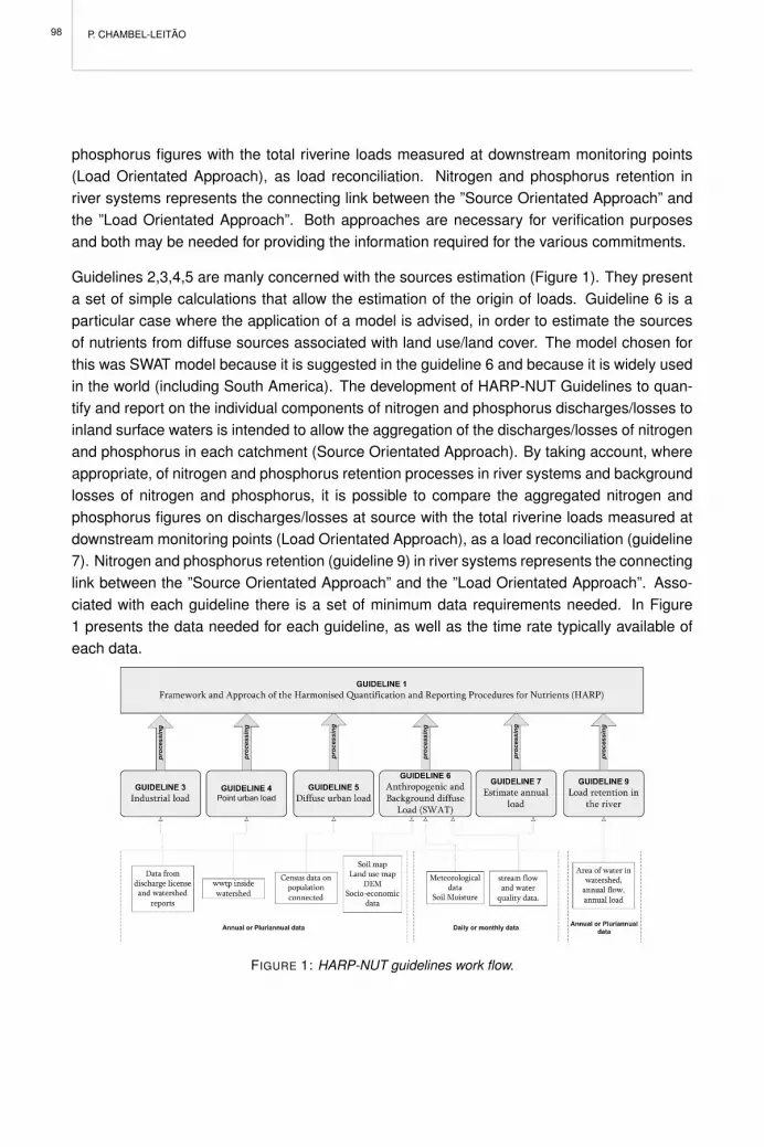
P. CHAMBEL-LEITAO
phosphorus figures with the total riverine loads measured at downstream monitoring points(Load Orientated Approach), as load reconciliation. Nitrogen and phosphorus retention inriver systems represents the connecting link between the ”Source Orientated Approach” andthe ”Load Orientated Approach”. Both approaches are necessary for verification purposesand both may be needed for providing the information required for the various commitments.
Guidelines 2,3,4,5 are manly concerned with the sources estimation (Figure 1). They presenta set of simple calculations that allow the estimation of the origin of loads. Guideline 6 is aparticular case where the application of a model is advised, in order to estimate the sourcesof nutrients from diffuse sources associated with land use/land cover. The model chosen forthis was SWAT model because it is suggested in the guideline 6 and because it is widely usedin the world (including South America). The development of HARP-NUT Guidelines to quan-tify and report on the individual components of nitrogen and phosphorus discharges/losses toinland surface waters is intended to allow the aggregation of the discharges/losses of nitrogenand phosphorus in each catchment (Source Orientated Approach). By taking account, whereappropriate, of nitrogen and phosphorus retention processes in river systems and backgroundlosses of nitrogen and phosphorus, it is possible to compare the aggregated nitrogen andphosphorus figures on discharges/losses at source with the total riverine loads measured atdownstream monitoring points (Load Orientated Approach), as a load reconciliation (guideline7). Nitrogen and phosphorus retention (guideline 9) in river systems represents the connectinglink between the ”Source Orientated Approach” and the ”Load Orientated Approach”. Asso-ciated with each guideline there is a set of minimum data requirements needed. In Figure1 presents the data needed for each guideline, as well as the time rate typically available ofeach data.
FIGURE 1: HARP-NUT guidelines work flow.
98

LOAD AND FLOW ESTIMATION: HARP-NUT GUIDELINES AND SWAT MODEL DESCRIPTION
3 SWAT MODEL
In SWAT simulated basin is divided in several sub-basins. Each sub-basin can be divided inmany HRU (Hidrologic Response Units - units with the same land use and soil type) or it canbe only one HRU. Each HRU has as superior boundary soil surface, and as inferior boundarythe aquifer (Figure 2). It receives for the superior boundary precipitation, of which part is con-verted into run-off and another part is converted in infiltration. The part that is converted intorun-off is directed to the sub-basin channel. The part that infiltrates is carried along the soilprofile, being able to evapotranspirate, to be percolated to the aquifer or carried laterally alongthe soil profile until it reaches the channel. The water that reaches the aquifer is lost for thechannel or the deep aquifer or finally for the atmosphere (the effect of capillary rise is simu-lated like this because SWAT soil hydrodynamics is one way: only allows water to percolateand no capillary rise). Because the evapotranspiration rate is strongly influenced by a numberof vegetative surface characteristics, PET is the rate at which evapotranspiration would occurfrom a large area uniformly covered with growing grass, completely shading the ground, ofuniform height and never short of water. Penman-Monteith method describes the equationto estimate PET (Monteith 1965, Allen 1986, Allen et al. 1989). Once total potential evapo-transpiration is determined, actual evaporation must be calculated. SWAT first evaporates anyrainfall intercepted by the plant canopy. Next, SWAT calculates the maximum amount of tran-spiration and the maximum amount of sublimation/soil evaporation based on Richtie’s (1972)method.
FIGURE 2: Example of the Hidrologic Response Units (HRU).
Plant growth in SWAT is estimated using the heat unit theory. This theory postulates thatplants have heat requirements that can be quantified and linked to time to maturity. Becausea plant will not grow when the mean temperature falls below its base temperature, the onlyportion of the mean daily temperature that contributes towards the plant’s development is theamount that exceeds the base temperature. To measure the total heat requirements of aplant, the accumulation of daily mean air temperatures above the plant’s base temperature is
99

P. CHAMBEL-LEITAO
recorded over the period of the plant’s growth and expressed in terms of heat units (Barnard1948, Phillips 1950). Run-Off in SWAT is based on the SCS runoff equation, which is anempirical model that was the product of more than 20 years of studies involving rainfall-runoffrelationships from small rural watersheds across the U.S. The model was developed to providea consistent basis for estimating the amounts of runoff under varying land use and soil types(SCS 1972, Rallison and Miller 1981).
Manning’s equation for uniform flow in a channel is used to calculate the rate and velocityof flow in a reach segment and also to estimate overland flow. Percolation is calculated foreach soil layer in the profile. Water is allowed to percolate if the water content exceeds thefield capacity water content for that layer. Water that percolates out of the lowest soil layerenters the vadose zone. The vadose zone is the unsaturated zone between the bottom ofthe soil profile and the top of the aquifer. An exponential decay weighting function proposedby Venetis (1969) and used by Sangrey et al. (1984) in a precipitation/groundwater responsemodel is utilized in SWAT to account for the time delay in aquifer recharge once the waterexits the soil profile. The baseflow recession constant is a direct index of groundwater flowresponse to changes in recharge (Smedema and Rycroft 1983). Values vary from 0.1-0.3 forland with slow response to recharge to 0.9-1.0 for land with a rapid response. Although thebaseflow recession constant may be calculated, the best estimates are obtained by analyzingmeasured streamflow during periods of no recharge in the watershed.
4 HARP-NUT AND SWAT APPLICABILITY TO SOUTH AMERICA
For the application of Source Orientated Approach of HARP-NUT guidelines, a great amountof data is needed because a study of a catchment is complex and needs the use of manysources of data in order to represent and clarify the various aspects that affect water quality.For the Source oriented approach (guidelines 2, 3, 4, 5) data was obtained in the three sitesfrom national census, environmental agencies and agriculture agencies. For guideline 6 inputdata are the ones needed by SWAT model: topography, land use/land cover, soil type and me-teorology. The digital elevation model (DEM) was obtained from the Shuttle Radar TopographyMission (SRTM) DEM data (Hounam and Werner 1999). This mission covered the entire SouthAmerica. Land Use/Land Cover maps were obtained for Argentina and Brasil from Landsatsatellite images (ETM+) downloaded from the free site http://glcf.umiacs.imd.edu.data.The type of classification applied was Supervised Classification. For Chile maps of Land usewere already available, and they were the ones used for watershed modelling. Often there isno available data on soil properties like porosity, wilting point, hydraulic conductivity and fieldcapacity. This was the case in all study sites. However some data like texture was available.Soil properties were derived in ECOMANAGE study sites using pedotransfer functions. Thesefunctions consist in predictive functions of certain soil properties from other more available,easily, routinely, or cheaply measured properties like texture. Many studies have developedstatistical correlations between soil texture and selected soil potentials (versus water content)using a large data base, and also between selected soil textures and hydraulic conductivity.
100

LOAD AND FLOW ESTIMATION: HARP-NUT GUIDELINES AND SWAT MODEL DESCRIPTION
Saxton et al. (1986) developed a procedure to estimate soil-water characteristics from readilyavailable inputs using results of previous statistical analyses of a large data base.
Climate Information obtained from national meteorology institute as well as water institutesincluded: i) average maximum air temperature for month, ii) average minimum air temperaturefor month, iii) standard deviation for maximum air temperature in month, iv) standard deviationfor minimum air temperature in month, v) average daily solar radiation in month, vi) averagedew point temperature in month, vii) average wind speed in month and finally daily precipita-tion. For the load oriented approach water quality and quantity was obtained. For water qualitymonthly values of concentration of nutrients were obtained for basin and sub basins. For wa-ter quantity daily flows were obtained. Retention of Nitrogen and phosphorus in river systemsrepresents the connecting link between the ”Source Orientated Approach” and the ”Load Ori-entated Approach”. Retention depends manly on: i) The portion of lakes, river stretches andwetland in each catchment; ii) The hydrological and morphological conditions within the riversystem. Nitrogen and phosphorus retention used in ECOMANAGE were quantified on the ba-sis of the mass balance of investigated lakes and rivers in Europe. In future studies retentionresults should be complemented with local studies of retention.
The applicability of HARP-NUT and SWAT can also be evaluated by the quality and usefulnessof the results. In the case of Aysen and Santos flows and the load of nutrients estimated wereused for the calibration of the MOHID estuary model, which produced reasonable results. ForBahıa Blanca, the estimated flow values confirmed the limited effect on the Bahıa Blancaestuary. Moreover data on rivers and on meteorology was very poor, but a set of data fromthe forties allowed calibrating flow in SWAT for Naposta watershed. Less than 10% of theprecipitation was transformed in flow. This fact associated with the relative small scale ofthe watersheds resulted in an insignificant influence of flows and loads of nutrients on theBahıa Blanca estuary. In Santos estuary main sources are industries. It’s difficult to make theanalysis of industries effluents. However major contributors to nutrient loads were identifiedby using the source and load reconciliation strategy of HARP-NUT. In Aysen most pollutionis diffuse, and there was available data to run and calibrate SWAT model. However, changesto SWAT code had to be made (within this project) in order to adapt it to South Americaparticularities. One of the most important changes was to include organic nitrogen in the rain.This change decreased the differences between ”Source Orientated Approach” and the ”LoadOrientated Approach”. One of the strong aspects of HARP-NUT guidelines is the integratedapproach to the eutrophication problem in coastal areas, which prove to produce reasonableresults which were used as an input for the MOHID estuary model in ECOMANAGE studysites. This application implied the application of SWAT model which generated flows that werealso used has input for MOHID.
5 FUTURE WORK
Application of HARP-NUT in ECOMANAGE consisted in an overall nutrient budget that hasto be confirmed and improve with new data and more detailed studies. In the case o Santos
101

P. CHAMBEL-LEITAO
main improvements include the monitoring of main potential sources of nutrients which arelocated in Moji and Piacaguera. In the case of Aysen one of the main improvements sug-gested is the understanding of soil organic matter distribution in the watershed, as well hasthe mineralization rate. The reason for this is the importance of soil organic matter in over-all budget. As discussed before, the watersheds that drain to Bahıa Blanca (Sauce Chico,Saladillo and Naposta) are irrelevant for global studies of estuary hydrodynamics and eutro-phycation. They could be relevant for local studies of areas adjacent to river mouths in theestuary, especially in terms of fecal coliforms. The application of HARP-NUT guidelines andthe application of SWAT contributed for estimating the global budget of water and nutrients. Toobtain this, SWAT model had to be calibrated for the watershed. The implementation of thismodel could be a valuable tool for future management plans of the watershed.
REFERENCES
Allen RG (1986) A Penman for all seasons. J. Irrig. and Drain Engng., ASCE, 112: 348-368
Allen RG, Jensen ME, Wright JL, Burman RD (1989) Operational estimates of evapotranspiration. Agron.J. 81: 650-662
Barnard JD (1948) Heat units as a measure of canning crop maturity. The Canner 106: 28
Borgvang SA, Selvik JS (eds) (2000) Development of HARP Guidelines - Harmonised Quantification andReporting Procedure for Nutrients. SFT Report 1759/2000. 179pp.
Hounam D, Werner M (1999) The Shuttle Radar Topography Mission (SRTM) In: Proceedings of ISPRS-Workshop ”Sensors and Mapping from Space 1999”, Hannover, Germany, CD-ROM. (http://www.ipi.uni-hannover.de/html/publikationen/1999/isprs-workshop/cd/pdf-papers/hounam.pdf)
Monteith JL (1965) Evaporation and the environment. In The state and movement of water in livingorganisms, XIXth Symposium. Soc. for Exp. Biol., Swansea, Cambridge University Press. p. 205-234
OSPAR (2003) Strategies of the OSPAR Commission for the Protection of the Marine Environment of theNorth-East Atlantic, (Reference number: 2003-21) Part II. OSPAR (2003) Annual report, 2002-2003,Volume 1
OSPAR (2006) Nutrients in the Convention Area including Assessments of Implementation of PARCOMRecommendations 88/2, 89/4 and 92/7. OSPAR report No 257
Phillips EE (1950) Heat summation theory as applied to canning crops. The Canner 27: 13-15
Rallison RE, Miller N (1981) Past, present and future SCS runoff procedure. In V.P. Singh (ed.). Rainfallrunoff relationship. Water Resources Publication, Littleton, CO. p. 353-364
Ritchie JT (1972) Model for predicting evaporation from a row crop with incomplete cover. Water Resour.Res. 8: 1204-1213
Sangrey DA, Harrop-Williams KO, Klaiber JA (1984) Predicting groundwater response to precipitation.ASCE J. Geotech. Eng. 110: 957-975
Saxton KE, Rawls WJ, Romberger JS, Papendick RI (1986) Estimating generalized soil-water character-istics from texture. Soil Sci. Soc. Am. J. 50: 1031-1036
Schoumans OF, Silgram M (eds.) (2003) Review and literature evaluation of Quantification Tools for theassessment of nutrient losses at catchment scale. EUROHARP report 1-2003, NIVA report SNO4739-2003
Smedema LK, Rycroft DW (1983) Land drainage-planning and design of agricultural drainage systems,Cornell University Press, Ithica, N.Y.
SCS - Soil Conservation Service (1972) Section 4: Hydrology In National Engineering Handbook.
Venetis C (1969) A study of the recession of unconfined aquifers. Bull. Int. Assoc. Sci. Hydrol. 14:119-125
102
PERSPECTIVES ON INTEGRATED COASTAL ZONE MANAGEMENT IN SOUTH AMERICAR. NEVES, J.W. BARETTA AND M. MATEUS (EDS.), IST PRESS, 2008
GROUNDWATER RECHARGE ASSESSMENT
M.M. OLIVEIRA, J.P. LOBO FERREIRA AND M. YARROW
1 INTRODUCTION
The choice of a model or method to compute recharge derives from the conceptualizationof the recharge process of a study area. This conceptualization is based on the physicalsystem, its geometry, all the inputs and outputs of water and its locations. The computation ofrecharge is based on mass balances between water entering, leaving or being stored in thewater system. These mass balances are generally water-mass balances but can also be anysubstance-mass balance diluted in water. Models to compute recharge may be grouped intomass balances above saturated zone and mass balances in the saturated zone.
The water mass balances above the saturated zone are predictive models as they quantifyrecharge by computing the processes prior to recharge occurrence (precipitation, infiltration,water stored in the surface and in the vadose zone). The soil daily sequential water bal-ance is an appropriate method to estimate deep percolation that, in some conditions may beassumed to be equal to recharge. This method requires knowledge of the climatic data tocharacterize precipitation and reference evapotranspiration, and knowledge of medium char-acteristic parameters, that depend on the complexity of the selected model. These modelsallow for estimation of distributed recharge in a region, produce results by recharge episodeand may be applied to any geological medium (intergranular, fissured, karstic or more thanone type). However, the more general application is for intergranular, as the soil storage ismore easily quantified, and preferential pathways are less important.
The water mass balances in the saturated zone are response models as they represent thereaction of the groundwater medium to the recharge process. Several methods are availabledepending on the hydrogeological setting, for instance: (1) surface flow hydrograph separa-tion, (2) spring discharge quantification, (3) flow quantification in aquifer sections, (4) saturatedzone storage change (water level change), (5) combination of these methods, also includinghuman water abstractions. These methods are integrative for a region and may computerecharge by episode. In the surface flow hydrograph separation method baseflow and di-rect runoff are separated. Baseflow is an estimate of recharge that occurs in the area definedby a watershed when all groundwater flow inside the watershed discharges to the surface wa-ter streams inside that watershed (i.e. there is a coincidence between the watershed and thehydrogeological basin). The hydrogeological settings more favourable to observe this requisiteare local systems of metamorphic and igneous rocks, with intergranular or fissured porosity.In some cases of sedimentary rocks with intergranular porosity, even if stratified, this requisitemay still be found. The surface flow hydrograph separation method is probably the easiestrecharge calculation method to use, as it does not require medium characteristic parameters,and only requires knowledge of daily precipitation and flow series.
103

M.M. OLIVEIRA, J.P. LOBO FERREIRA AND M. YARROW
The spring discharge method provides a direct measurement of the amount of water thatrecharged the system. It requires the knowledge of the area drained by the spring, whichis not an easy value to obtain. Due to the structure of the groundwater flow paths and thesprings’ significant water volumes this method is mainly applicable for karstic hydrogeologi-cal settings. For the other hydrogeological media, despite the possible occurrence of largeflow springs, it is likely that it exists diffuse discharge in important amounts that difficult thequantification of discharge. The flow quantification in aquifer sections is applicable to anyhydrogeological medium requiring the knowledge of the recharge area upgradient the mea-suring section, the constant monitoring of the piezometric level in both sides of the sectionand the aquifer transmissivity along the measuring section. These requirements turn the ap-plication of the method more difficult. The water level change method is based on the directconsequences of recharge. The time step for the application of this method is very short. Forthe application of this method the difference between groundwater flow entering and leavingthe system should be negligible in relation to the water level rise. This method also requiresthe characterization of effective porosity in the depth of water level oscillation.
Among the methods referred to above, two of them are applied in the case study areas: thesoil daily sequential water balance and the surface flow hydrograph separation method.These methods are described in more detail in the next sections.
2 SOIL DAILY SEQUENTIAL WATER BALANCE
For the conceptual case of an area where there is no artificial recharge, no surface flow en-tering the area, and the groundwater level is always below the soil zone, the water balanceequation for the soil of that area can be expressed by (Figure 1):
P − RET −∆Al − Sr − Dp = ε (1)
where P is the precipitation, RET is the effective evapotranspiration, ∆Al is the variation (final- initial) of the water stored in the soil, Sr is the surface runoff, Dp is the deep percolation andε is the calculation error of the balance. The sequential mass balance approach intends tomeasure or estimate and compute P, RET, Sr and ∆Al processes, computing Dp by solvingequation (1) considering ε = 0. The sequential water balance is carried out in a determinedtime step, for instance the daily time step. Recharge (R) is then assumed to be equal to Dp:
R = Dp = P − RET −∆Al − Sr (2)
The soil daily sequential water balance method is a good method to forecast differences ontotal recharge in response to changing daily precipitation pattern. Moreover as a generalcharacteristic of the method it allows for the determination of seasonal recharge. However itmust be taken into account that the presented method provides a value of the water availablefor deep percolation, and that this deep percolation will take some time to reach the aquifer. Asoil daily sequential water balance methodology was implemented in the BALSEQ numerical
104

GROUNDWATER RECHARGE ASSESSMENT
model (Lobo Ferreira 1981, Lobo Ferreira and Delgado Rodrigues 1988), originally writtenin Fortran. Figure 2 shows the flowchart of the BALSEQ model. In this model the runoffcurve number (NC) that depends on soil hydraulic conductivity and on land use, is used inthe process of estimating surface runoff. NC values vary between 0 (corresponds to an areawith infinite permeability, where all water infiltrates into the soil), and 100 (corresponds to acompletely impermeable zone).
The effective evapotranspiration is calculated using the potential evapotranspiration (the eva-potranspiration that would occur if the water available in the soil was not a limiting factor) andthe amount of water available in the soil. This water available in the soil is calculated by a se-quential water balance that daily updates the water stored in the soil. The computation of deeppercolation depends on the maximum amount of water available in the soil for evapotranspi-ration (AGUT = (sr - wp) . rd) in which sr is the specific retention (or field capacity), wp is thewilting point and rd is the depth of the plant roots. If after the process of evapotranspirationthe water stored in the soil is above the AGUT value, the water in excess of AGUT becomesdeep percolation.
The BALSEQ numerical model has been subject to changes and new methods have been im-plemented to calculate surface infiltration, effective evapotranspiration and deep percolation.These methods, developed in Oliveira (2004a) have all been included in the BALSEQ MODnumerical model, written in Visual Basic. The surface infiltration is computed using formulasobtained to generalize the results of the Philip infiltration model (Philip 1957, in Lencastre andFranco 1984, Rawls and Brakensiek 1989) applied to several situations that depend on thewater content of the soil, the soil texture, the daily precipitation and its distribution. Theseformulas depend on the daily precipitation and on two tabulated coefficients (Oliveira 2004a,Oliveira et al. 2008) that depend on the textural soil class and on the initial soil moisture.
The effective evapotranspiration is estimated based on the formulation presented in Allen etal. (1998):
RET = (Ka.Kcb + Ke).ETo (3)
where ETo is the reference evapotranspiration, Kcb is the basal crop coefficient, Ke is thesoil water evaporation coefficient and Ka is the water stress coefficient. The procedures tocharacterize the parameters in equation (3) are presented originally in Allen et al. (1998). TheETo represents the evaporation from a hypothetical reference crop under determined weatherconditions. The Kcb and Ke terms of the equation integrate the physical and physiologicaldifferences between the specific field crop and the reference crop, hence their values varywith time (depending on the vegetative stage). The use of the two different coefficients, Kcb
and Ke, constitutes the dual crop coefficient approach. The Ka term is related to the stressconditions in which the crop develops and depends on the water available in the soil duringthe crop growth. Also the Ke term is dependent on the soil moisture in the bare soil part.The computation of the soil moisture, on which Ka and Ke depend, is achieved by a dailysequential water balance.
105

M.M. OLIVEIRA, J.P. LOBO FERREIRA AND M. YARROW
FIGURE 1: Soil water balance of an area with no discharge of groundwater and no surface flow entering
in the system.
FIGURE 2: Flow chart of BALSEQ model for daily sequential water balance in the soil.
106

GROUNDWATER RECHARGE ASSESSMENT
The methodology that was implemented in BALSEQ MOD allows for the existence of up totwo land covers and a bare soil surface. The area occupied by each cover may vary in time.For instance, in the case of two different vegetation covers, the area occupied by each covercan change according to the vegetation development period. These features required the soilarea to be divided in up to three parts. For each soil part, a daily sequential water balance iscarried out. The water balance of one part is dependent on the water balance of the other twoparts. So the sequential water balance must be performed simultaneously.
The following information is required to estimate effective evapotranspiration: (1) daily surfaceinfiltration; (2) daily reference evapotranspiration; (3) the fraction of the area occupied by eachland cover; in the case of vegetation cover it is necessary to know the area fraction occupiedby the vegetation during mid-season and late-season stages, and the area fraction occupiedby vegetation during the initial stage of the development; for static land covers these fractionsare equal; (4) the soil depth subject to evapotranspiration; for the vegetation cover, two soildepths are defined accordingly to the development stage of the vegetation: the initial stageand the mid-season and late season crop development stage; for bare soil a depth of 15cm subject to evaporation is assumed; (5) the basal crop coefficients, for initial, middle andlate seasons of the vegetation cover; these depend on the vegetation height, the air relativehumidity, the wind speed, and the fraction of land surface covered by the vegetation; (6) thefirst day of the initial stage, and the length of each crop growth stage: initial stage length, cropdevelopment length, mid-season length and late-season length; (7) threshold values for theminimum amount of water stored in the soil that allow the effective evapotranspiration to occurat the maximum rate, both for the vegetation cover and for the bare soil.
The deep percolation is calculated depending on the soil saturated hydraulic conductivity andon the water that exists in the soil that can drain under the force of gravity. This aspectalso depends on the sequential water balance in the soil, which is different depending on thevegetation cover. Details about the methods to compute each one of the referred to processesmay be consulted in Oliveira (2004a) and in Oliveira et al. (2008). Surface or total flow (F ) of ariver is mainly composed of (1) direct runoff or overland flow (Fd), produced in the watershedabove the place where it is measured, resulting from precipitation that does not infiltrate intothe soil surface and that is not retained (for example in the plants canopy, buildings, dams,etc.), and (2) baseflow (Fb), resulting from water that infiltrates into the soil, goes through thesubsurface and eventually comes to the surface, being the discharge of groundwater to thewatershed:
F = Fd + Fb (4)
The hydrograph represents surface flow against time (Figure 3). The two large flow compo-nents of surface flow (Fd and Fb) may be separated in the hydrograph. Several methods exist(cf. e.g. Linsley et al. 1975). One of these consists in connecting total flow that exists in thebeginning of the rising limb of a new direct runoff episode due to the occurrence of precipita-tion to the total flow that exists in the end of this direct runoff episode. Linsley et al. (1975)present the following equation to estimate time from the hydrograph peak to a point located in
107

M.M. OLIVEIRA, J.P. LOBO FERREIRA AND M. YARROW
the end of the recession curve that reflects the end of direct runoff (A is watershed area abovethe measuring station in km2 and n is number of days):
n = 0.8A0.2 (5)
The hydrograph separation (HS) method, using a daily basis, was initially developed and pro-grammed in the QuickBasic computer code DECHIDR (Oliveira et al. 1997) and later updatedto Visual Basic 6.0 in DECHIDR VB program (Oliveira 2001, Oliveira 2004a). It was developedfor the estimation of groundwater recharge in the fractured massifs of Portugal, since knowl-edge about recharge in these regions was scarce, and data was available on surface flow andprecipitation daily time series. The applications of DECHIDR VB have been disseminated inseveral papers, for instance Oliveira (2004b) and Oliveira (2006).
The general technique for the separation followed the method represented in Figure 4. Themethod consists of plotting a straight line linking the hydrograph origin of the precipitation/totalflow (P/F) episode under analysis with total flow calculated in the beginning of day n + 1.Day n [computed with equation (5)] refers to the number of days with direct runoff after thehydrograph peak (Figure 4A) or the end of the precipitation if this exceeds the hydrograph peak(Figure 4B).The area above the line represents direct runoff of the episode under analysiswhile the area below the line represents its baseflow.
The HS turns out to be a more complex process due to the occurrence of different super-imposed episodes, which can result in the recession of several P/F episodes in the sameday. To deal with this situation, a set of procedures was developed in order to isolate distinctP/F episodes. The separation is carried out sequentially considering the input data series:date, total flow and precipitation. Oliveira (2004a) and Oliveira et al. (2008) describe theseprocedures.
The advantages of the HS method in estimating recharge are: (1) it is easy to apply with com-monly available precipitation and flow data; (2) it only requires the definition of two parameters(1- the number of days in which there is direct runoff, and 2- the precipitation threshold - ifthis parameter is considered); (3) it is not constrained to fixed parameters of the watershedbecause each P/F episode is considered separately; (4) it is able to control and maintain themass balance between precipitation and the produced total flow; (5) it integrates all the pro-cesses of the hydrological cycle that take place in the watershed, measuring the response ofthe system to those processes; (6) it is applicable to the whole watershed, not requiring thedefinition of recharge and discharge areas of the groundwater medium.
The following limitations are referred to: (1) it is vulnerable to errors in the determination of totalflow; (2) it is dependent on the quality of the estimation of precipitation in the watershed, mainlyif the balance between precipitation and total flow is used; (3) it considers that streams areonly receiving bodies (does not consider bank storage) and that all groundwater dischargesto those streams derive from inside the watershed; (4) it may not be used directly if there aredams that inhibit natural flow.
108

GROUNDWATER RECHARGE ASSESSMENT
FIGURE 3: Surface flow hydrograph and separation of surface flow into direct runoff and baseflow.
FIGURE 4: Example of the hydrograph separation process, for n = 2 day, using as criterion (A) the day of
the hydrograph peak, (B) the last precipitation day.
Baseflow is an estimator of the recharge that occurs in the area defined by a watershed. Inbetween the occurrence of the recharge process and the subsequent baseflow, the process ofdischarge from the saturated groundwater medium to the surface medium must be considered.Baseflow is a measure of the groundwater medium discharge to the surface medium if: (1)there is no storage of surface water; (2) there is no evaporation of surface water; and (3) thereis no abstraction of surface water. On the other hand, groundwater discharge may translatethe groundwater recharge if: (1) recharge is the only water source of the saturated medium;(2) there is no abstraction of groundwater; (3) all the water that leaves the saturated zoneflows to the surface medium; and (4) there is no evapo(transpi)ration from groundwater.
109

M.M. OLIVEIRA, J.P. LOBO FERREIRA AND M. YARROW
3 SNOWMELT
In many temperate regions of the world, snowmelt represents an important source of waterand can, to varying degrees, change the patterns observed in hydrographs. Moreover, thechemical properties of meltwater change over the snowmelt period. Tracer studies are oftenused to illuminate the origin and principal flow paths of water in a basin (Sueker et al. 2000). Inthe case where information on chemical tracers is not available, simple energy-budget equa-tions may be used to predict the quantity and timing of snowmelt in specific watersheds. Thesnowmelt model calculates precipitation as rain, new snow, snowpack, and ultimately meltwa-ter. The water available for movement as baseflow or surface flow (meltwater plus precipitationas rain) is calculated on a daily basis and imported into DECHIDR VB in order to obtain valuesfor baseflow.
Snowmelt depends on the balance of a series of energy sources and sinks, including short-wave and longwave radiation, convection from the air (sensible energy), vapour condensation(latent energy), conduction from the ground, and the energy contained in rain (USACE 1998).Once snow melts, it can follow the same flow paths as rain. Thus, snowmelt calculations caneffectively be separated from the processes related to the movement of the snowmelt into theriver network.
The generalized energy-balance snowmelt equations are often simplified based on certainmeteorological or forest-cover conditions. In general, snowmelt can be divided into two types:rain-free and rain-on-snow. Equations for rain-on-snowmelt can be greatly simplified becausesolar radiation can be considered a relatively minor energy input. Snowmelt equations dependon the categories of forest density. These equations can be consulted in USACE (1998), andare also reproduced in Yarrow and Oliveira (2006).
The snowmelt model follows the flowchart in Figure 5. It is important to note that snow ismeasured in units of water equivalent (mm) so as not to introduce further uncertainty as tosnow depths and snowpack dynamics. Using information about temperature and precipitation,new snow is calculated daily. A daily snow balance equation is used to calculate the evolutionof the snowpack over time.
To run the hydrograph separation method, the daily snowmelt and the precipitation as rainare summed to get the daily water available for infiltration (eventually baseflow) and directrunoff. In basins where snow represents an important percentage of the annual precipitation,the unmodified use of the hydrograph separation method could lead to erroneous conclusions.Thus, it is important to consider how snowmelt might influence the hydrographs of the associ-ated river and how to account for this process in the hydrograph separation method. Withoutaccounting for snowmelt, in periods without precipitation, baseflow would be overestimatedbecause total flow would be considered as baseflow originating from the last precipitationepisode (Yarrow and Oliveira 2006). During the spring snowmelt season, one could expecthydrograph peaks due only to snowmelt.
110
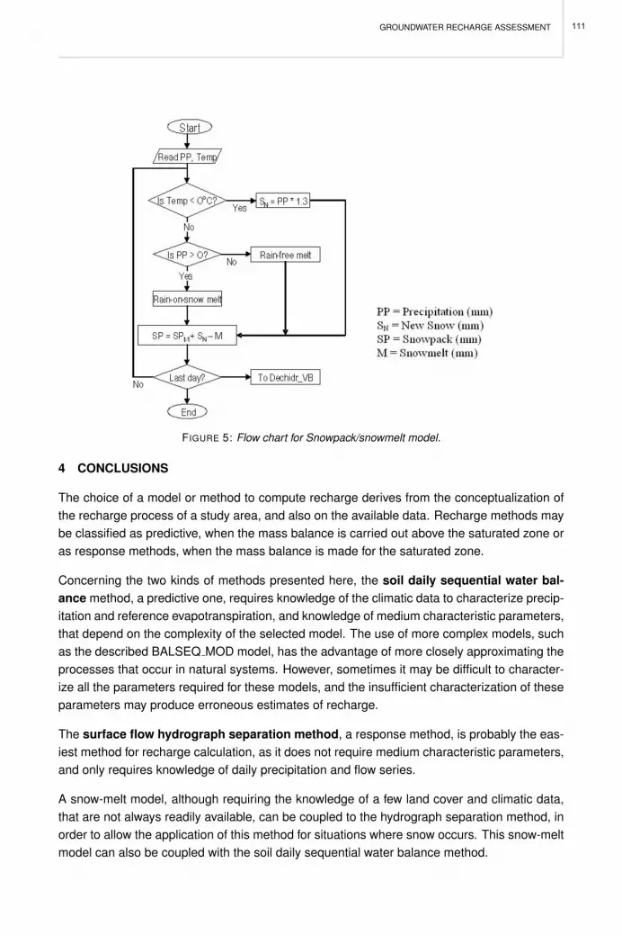
GROUNDWATER RECHARGE ASSESSMENT
FIGURE 5: Flow chart for Snowpack/snowmelt model.
4 CONCLUSIONS
The choice of a model or method to compute recharge derives from the conceptualization ofthe recharge process of a study area, and also on the available data. Recharge methods maybe classified as predictive, when the mass balance is carried out above the saturated zone oras response methods, when the mass balance is made for the saturated zone.
Concerning the two kinds of methods presented here, the soil daily sequential water bal-ance method, a predictive one, requires knowledge of the climatic data to characterize precip-itation and reference evapotranspiration, and knowledge of medium characteristic parameters,that depend on the complexity of the selected model. The use of more complex models, suchas the described BALSEQ MOD model, has the advantage of more closely approximating theprocesses that occur in natural systems. However, sometimes it may be difficult to character-ize all the parameters required for these models, and the insufficient characterization of theseparameters may produce erroneous estimates of recharge.
The surface flow hydrograph separation method, a response method, is probably the eas-iest method for recharge calculation, as it does not require medium characteristic parameters,and only requires knowledge of daily precipitation and flow series.
A snow-melt model, although requiring the knowledge of a few land cover and climatic data,that are not always readily available, can be coupled to the hydrograph separation method, inorder to allow the application of this method for situations where snow occurs. This snow-meltmodel can also be coupled with the soil daily sequential water balance method.
111

M.M. OLIVEIRA, J.P. LOBO FERREIRA AND M. YARROW
REFERENCES
Allen RG, Pereira LS, Raes D, Smith M (1998) Crop evapotranspiration - Guidelines for computing cropwater requirements, FAO, Irrigation and Drainage Paper, nr. 56
Linsley Jr RK, Kohler MA and Paulhus JLH (1975) Hydrology for Engineers. 2nd edn. McGraw HillKogakusha, Ltd.
Lencastre A, Franco FM (1984) Licoes de Hidrologia. Lisboa, Universidade Nova de Lisboa, Faculdadede Ciencias e Tecnologia. 451 pp.
Lobo Ferreira JP (1981) Mathematical Model for the Evaluation of the Recharge of Aquifers in SemiaridRegions with Scarce (Lack) Hydrogeological Data. In: Verruijt A, Barends FBJ (eds) Proceedings ofEuromech 143/2-4 Setp. 1981, Rotterdam, A.A. Balkema. Also published: 1982, Lisboa, LaboratorioNacional de Engenharia Civil, Memoria No 582
Lobo Ferreira JP, Delgado Rodrigues J (1988) BALSEQ - A Model for the Estimation of Water Balances,Including Aquifer Recharge, Requiring Scarce Hydrogeological Data. In: Simmers (ed) Estimation ofNatural Groundwater Recharge. Dordrecht, D. Reidel, NATO ASI Series, Vol. 222
Oliveira MM, Moinante MJ and Lobo Ferreira JP (1997) Cartografia Automatica da Vulnerabilidade deAquıferos com base na Aplicacao do Metodo DRASTIC. Relatorio 60/97-GIAS, LNEC (in Portuguese).
Oliveira MM (2001) A Estimativa da Recarga das Aguas Subterraneas a Partir da Decomposicao deHidrogramas de Escoamento Superficial - O Programa de Computador DECHIDR VB.VBP. Seminariosobre ”A Hidroinformatica em Portugal”, Publicacao em CD-ROM, LNEC, Lisboa, 15-16 November (inPortuguese).
Oliveira MM (2004a) Recarga de aguas subterraneas: Metodos de avaliacao. Ph.D. Thesis on Geology(Hydrogeology), University of Lisbon, Faculty of Sciences, Geology Departament, 440 pp (in Por-tuguese).
Oliveira MM (2004b) Recharge Estimation of a Gneissic Area in Ponte de Panasco (Portugal) using aDaily Surface Flow Hydrograph Separation Technique. XXXIII Congress of the IAH ”GroundwaterFlow Understanding from local to regional scales”, Zacatecas, Mexico, 11-15 October.
Oliveira MM (2006) The estimation of groundwater recharge of fractured rocks in Portugal using surfaceflow measurements. In: Chambel A (ed) Proceedings of the 2nd Workshop of the IAH Iberian RegionalWorking Group on Hard Rock Hydrogeology. Universidade de Evora, Associacao Internacional deHidrogeologos - Grupo Portugues, pp. 221-233
Oliveira MM, Limbozzi F, Leitao TE, Carrica JC, Albouy ER, Lobo Ferreira JP (2008) Deliverable 2.6 - SIGmapping of hydrogeologic parameters, including groundwater recharge assessment and vulnerabilityto pollution - 2nd Part: Bahıa Blanca Estuary. Report - NAS, LNEC, under preparation.
Rawls WJ, Brakensiek DL (1989) Estimation of soil water retention and hydraulic properties. In: Morel-Seytoux, H.J. (ed.) Unsaturated flow in hydrologic modeling. Fort Collins, USA. p 275-300
Sueker JK, Ryan JN, Kendall C, Jarrett RD (2000) Determination of hydrologic pathways during snowmeltfor alpine/subalpine basins, Rocky Mountain National Park, Colorado. Water Resources Research,36: 63-75
USACE (1998) Engineering and Design: Runoff from Snowmelt. Manual EM 1110-2-1406. 142p. U.S.Army Corps of Engineers.(http://www.usace.army.mil/publications/eng-manuals/em1110-2-1406/toc.htm)
Yarrow M, Oliveira MM (2006) ECOMANAGE - Integrated Ecological Coastal Zone Management System.Deliverables 2.6 & 2.8 - CHILE. D2.6 - SIG mapping of hydrogeologic parameters, including ground-water recharge assessment and vulnerability to pollution & D2.8 - Groundwater flow and transportcomponents of the global estuary model. LNEC, Relatorio 379/2006 - NAS, Lisboa, 42 pp.
112

PERSPECTIVES ON INTEGRATED COASTAL ZONE MANAGEMENT IN SOUTH AMERICAR. NEVES, J.W. BARETTA AND M. MATEUS (EDS.), IST PRESS, 2008
GROUNDWATER VULNERABILITY TO POLLUTION AND TO SEA WATERINTRUSION IN COASTAL AQUIFERS
J.P. LOBO FERREIRA AND M.M. OLIVEIRA
1 INTRODUCTION
In integrated coastal zone management, groundwater plays an important role as it dischargesto the rivers, estuaries, and sea, contributing with fresh water to these systems and transport-ing dissolved substances. These substances may be natural, due to the chemical reactions ofthe water with the underground medium, or may result from man-originated pollutants. Thesepollutants exist on the land surface, and are transported to the groundwater medium by theinfiltrating surface water (including rainfall) that recharges the aquifer medium and, after flow-ing in the aquifer, during a period that may range from days to thousands of years, dischargesto the surface medium. In the underground medium, the pollutant load may be reduced, dueto the underground medium properties that react with the polluted groundwater, and the dis-charged groundwater may present better chemical characteristics. Also, the opposite directionmay be considered, i.e. when instead of groundwater discharging to the surface water bodies,it is the surface water bodies that infiltrate or move into the groundwater body. This is the caseof the marine salt-water intrusion due to the equilibrium between the groundwater medium andthe sea-water medium. This equilibrium may be affected by the pumping of groundwater thatinduces saline water flow from the sea into the aquifer.
The groundwater vulnerability may be considered an indication of the likelihood that a ground-water body may be contaminated either by surface water infiltration or by the movement ofthe sea-water intrusion interface. On the other hand it gives an indication of the likelihoodthat a pollutant may be retained in the groundwater medium, thus influencing the quality ofthe groundwater discharged to the surface medium. Thus, groundwater vulnerability assess-ment is a measure to protect groundwater. Several works have been made in order to accessmainly groundwater vulnerability to pollution. This chapter gives a general overview of somegroundwater vulnerability assessment methodologies, presents the concepts and describeswith more detail some techniques, one of which was applied in the ECOMANAGE Project.
2 CONCEPT OF VULNERABILITY TO POLLUTION
According to Lobo Ferreira and Cabral (1991) it is believed that the most useful definition ofvulnerability is one that refers to the intrinsic characteristics of the aquifer, which are relativelystatic and mostly beyond human control. It is proposed therefore that the groundwater vul-nerability to pollution be defined, in agreement with the conclusions and recommendationsof the international conference on ”Vulnerability of Soil and Groundwater to Pollutants”, heldin 1987 in The Netherlands, as (Duijvenbooden et al. 1987): ”the sensitivity of groundwaterquality to an imposed contaminant load, which is determined by the intrinsic characteristics of
113
J.P. LOBO FERREIRA AND M.M. OLIVEIRA
the aquifer ”. Thus defined, vulnerability is distinct from pollution risk. Pollution risk dependsnot only on vulnerability but also on the existence of significant pollutant loading entering thesubsurface environment. It is possible to have high aquifer vulnerability but no risk of pollu-tion, if there is no significant pollutant loading; and to have high pollution risk in spite of lowvulnerability, if the pollutant loading is exceptional. It is important to make clear the distinctionbetween vulnerability and risk. This because risk of pollution is determined not only by theintrinsic characteristics of the aquifer, which are relatively static and hardly changeable, butalso on the existence of potentially polluting activities, which are dynamic factors which can inprinciple be changed and controlled.
Considerations on whether a groundwater pollution episode will result in serious threat togroundwater quality and thus to its (already developed, or designated) water supply are notincluded in the proposed definition of vulnerability. The seriousness of the impact on wateruse will depend not only on aquifer vulnerability to pollution but also on the magnitude of thepollution episode, and the value of the groundwater resource. Given the definition of vulnera-bility proposed as above, it is important to recognise that the vulnerability of an aquifer will bedifferent for different pollutants. For example, groundwater quality may be highly vulnerableto the loading of nitrates at the surface, originated in agricultural practices, and yet be littlevulnerable to the loading of pathogens.
In view of this reality, it is scientifically most sound to evaluate vulnerability to pollution in re-lation to a particular class of pollutant, such as nutrients, organics, heavy metals, pathogens,etc., i.e. to create specific vulnerability maps. This point of view has been expressed by otherauthors (e.g. Foster 1987), and some work has been done in specific vulnerability mapping.An example is the work of Canter et al. (1987) for nitrate pollution of agricultural origin. Alter-natively, vulnerability mapping could be performed in relation to groups of polluting activities(Foster 1987), such as unsewered sanitation, agriculture, and particular groups of industries.This has been attempted for some activities. An example is the work of Le Grand (1983) forwaste disposal. Although it is recognised that this specific vulnerability mapping is scientifi-cally sounder, one must realise that there will generally be insufficient available data to performspecific vulnerability mapping. Therefore, it is necessary to adopt a mapping system that issimple enough to apply using the data generally available, and yet is capable of making bestuse of those data in a technically valid and useful way. Various such systems of vulnerabilityevaluation and ranking have been developed and applied in the past. Examples are Albinetand Margat (1970), Haertl (1983), Aller et al. (1987), and Foster (1987). Some of the sys-tems for vulnerability evaluation and ranking include a vulnerability index which is computedfrom hydrogeological, morphological and other aquifer characteristics in some well-definedway. The adoption of an index has the advantage of, in principle, eliminating or minimisingsubjectivity in the ranking process.
The same definition provided to the aquifer system may be given to a groundwater pumpingwell. In the case of the exploitation of an aquifer system, one may be interested on knowinghow vulnerable a well in terms of water pollution is. The vulnerability of a producing well to
114

GROUNDWATER VULNERABILITY TO POLLUTION AND TO SEA WATER INTRUSION IN COASTAL AQUIFERS
pollution could be defined as ”the sensitivity of the pumped groundwater quality to an imposedcontaminant load, which is determined by the intrinsic characteristics of the aquifer that con-tribute with flow to the well”. A well corresponds to a 1D part of the aquifer system where it isinstalled, and hence the same methodology for the aquifer system could be applied. Howevera well is pumping water only at specific depths. Hence, it is important to define the part of thewell which is screened and is pumping the water. In the case of coastal aquifers the sea-watermay be regarded as a contaminant load that, in the case of aquifer exploitation, may con-tribute with non-fresh water to a pumping well. Chachadi and Lobo Ferreira (2001) handledthis situation and presented the concept of groundwater vulnerability to sea water intrusion as”the sensitivity of groundwater quality to an imposed groundwater pumpage or sea level riseor both in the coastal belt, which is determined by the intrinsic characteristics of the aquifer ”.
3 METHODS FOR VULNERABILITY ASSESSMENT
3.1 Introduction
The pumping well vulnerability may be regarded as wellhead protection zoning, i.e. the vul-nerable area directly depends on the travel time of water towards the pumping well, being thistravel time a function of the hydraulic properties of the aquifer. On the other hand, the traveltime could also be defined for a pollutant as a function of the retardation properties of thehydrogeological medium in relation to the pollutant or the decay properties of the pollutant.Often, the travel time is a defined value in legislation, and the need to know the retardationproperties is disregarded. When the travel time is a defined value, several kinds of approachesmay be considered, depending on the consideration of two or three dimensions of the domain.These approaches are based on the groundwater numerical modelling or on approximationsthat require hydrogeological data.
The simpler approach is the calculated fixed radius method. A more elaborated approach, re-quiring the hydraulic head knowledge was developed by Krijgsman and Lobo Ferreira (2001).These approaches are applicable in two dimensions horizontal domain. More elaboratedapproaches depend on numerical modelling, that allow two or three dimensional ground-water flow modelling with particle tracking (dependent on the numerical flow models). TheWELLFLOW mathematical model allows the computation of travel time distances in a radialcross-section (vertical 2D, cf. Feseker and Lobo Ferreira 2001). These methodologies canalso be found in Lobo Ferreira et al. (2004).
The aquifer vulnerability may be characterised as a function of the physical system propertiesin terms of more or less favourable conditions in the system for a pollutant load to contaminatethe aquifer. Or it may be characterised using numerical flow modelling. The first approach maybe considered a parametric one, in which different variables are characterised and put togetherto produce an index, as is the case of the DRASTIC index for a pollutant load occurring in theground surface (cf. Aller et al. 1987) or the GALDIT index for the case of coastal aquifersin relation with marine water (cf. Chachadi and Lobo Ferreira 2001). The second approach,
115

J.P. LOBO FERREIRA AND M.M. OLIVEIRA
which may inclusively consider the flow in the unsaturated (vadose) zone, rely on the numericalflow models, and is related to the travel time of groundwater flow. This modelling may becoupled with the attenuation conditions of the medium that dictate the pollutant concentrationon the aquifer system. In the next sections parametric methods are described in more detail:the DRASTIC index and the GALDIT index.
3.2 The DRASTIC index for the assessment of groundwater vulnerability to pollution
The index of vulnerability DRASTIC (Aller et al., 1987) was created for the following conditions:(1) the contaminant is introduced at the ground surface; (2) the contaminant is flushed into theground water by precipitation; (3) the contaminant has the mobility of water; and (4) the areaevaluated with DRASTIC is 100 acres (0.4 km2) or larger. The index of vulnerability DRASTICcorresponds to the weighted addition of seven values corresponding to seven parameters thatcharacterise the subsurface medium and its specificity: (1) Depth to the water (D); (2) NetRecharge (R); (3) Aquifer material (A); (4) Soil type (S); (5) Topography (T); (6) Impact of theunsaturated zone (I); (7) Hydraulic Conductivity (C).
A value between 1 and 10 to each parameter, except R for which the value ranges between 1and 9, is attributed, depending on local conditions. High values correspond to high vulnerabil-ity. The attributed values are generally obtained from tables, which give the correspondencebetween local hydrogeologic characteristics and the parameter value. DRASTIC index is com-puted by:
DRASTIC = DRDW + RRRW + ARAW + SRSW + TRTW + IR IW + CRCW (1)
where R = rating and W = weight. Thus, each parameter has a predetermined, fixed, relativeweight that reflects its relative importance to vulnerability. The most significant factors haveweights of 5 and the least significant a weight of 1. A second weight has been assigned toreflect the agricultural usage of pesticides. Table 1 shows the ratings to be assigned to eachDRASTIC parameter and the weights for standard DRASTIC applications and for DRASTICpesticide applications. In some cases a rating interval and a typical rating (in brackets) isshown, which represents, in the case of the rating interval, the values that the parameter canassume, depending for instance on the clay content, the weathering conditions, or the fissuringin the case of the aquifer media. The minimum value of the standard DRASTIC index is 23and the maximum value is 226. Such extreme values are very rare, the most common valuesbeing within the range 50 to 200. Whereas the corresponding minimum and maximum valuesfor pesticide DRASTIC index are 26 and 256 respectively.
Depth to the water (D) refers to the distance from the ground surface to the top of the aquifer.In the case of a non-confined aquifer, the top of the aquifer is given by the water table. In thecase of a confined aquifer it is given by the base of the confining layer. The depth to water isan important factor in the evaluation of groundwater pollution vulnerability primarily becauseit determines the thickness of material through which a contaminant must travel before reach-ing the aquifer. The depth to water is also important because it provides an opportunity for
116

GROUNDWATER VULNERABILITY TO POLLUTION AND TO SEA WATER INTRUSION IN COASTAL AQUIFERS
oxidation and it may help to determine the contact time of pollutant with the surrounding me-dia. In general, there is a greater chance for attenuation of pollutants to occur as the depthto the water increases because deeper aquifer tops imply longer travel times in the vadosezone with an exception that if the vadose media is fractured or karstified then the travel timeis independent of the depth of the aquifer. The quantity of net recharge (R) represents theamount of water per unit area of land, which penetrates the ground surface and reaches thewater table. This recharged water is thus available to disperse, dilute and transport a contam-inant vertically into the vadose zone to the water table and horizontally within the aquifer. Thegreater the recharge, the greater the potential for groundwater pollution. However, at certainquantity of recharge the pollution event may in turn decrease due to dilution of the contami-nant. Aquifer media (A) refers to a lithological unit that serves as an aquifer. Aquifer mediaplays an important role in dissipation and transportation of the pollutants once introduced intothem. The parameters like effective porosity, grain size, clay contents and aquifer thicknessare the four main characteristics that control dissemination and transportation of the contami-nants in the aquifer. Soil media (S) refers to that uppermost portion of the vadose zone whichis characterised by significant biological activity. In the DRASTIC classification, the soil mediais referred to be the upper weathered zone of the earth which averages to a depth of twometres or less from ground surface. Eleven different soil types which were given ratings ofbetween 1 and 10 were defined by Aller at al. (1987). The parameter topography (T) refersto the slope and slope variability of the land surface. Topography has an influence on the soildevelopment and therefore has an effect on contaminant attenuation. The topography also de-termines the contact time of contaminants with the soil and in case of unconfined aquifers thetopography can provide information about the groundwater gradients and velocities. Smallerground slopes are always potential for groundwater pollution compared to steep slopes. InDRASTIC method percent slope is considered for rating topography. Impact of the vadosezone media (I): By definition, the vadose zone includes all the unsaturated media below theground and above the water table, including the soil zone. As the soil was already consideredin the S parameter, the I parameter of the DRASTIC method will refer only to the unsaturatedmedia below the bottom of the soil layer and above the water table in case of unconfinedaquifer. When evaluating a confined aquifer, the ”confining layer” must be treated as a vadosezone and be always assigned a rating of 1. The type of vadose zone media determines theattenuation characteristics of the material below the soil horizon and above the water table.Biodegradation, neutralisation, mechanical filtration, chemical reactions, volatilisation and dis-persion are the processes that may occur within the vadose zone. The media also controlsthe path length and routing, thus affecting the time available for attenuation and the quantityof material found. The routing is strongly influenced by any fracturing present in the vadosemedia. Hydraulic Conductivity of the aquifer (C): The rate of contaminant movement inthe saturated zone is also controlled by the rate of groundwater movement. This parameter isused to measure the rate of water flow in the aquifer. By definition the aquifer hydraulic con-ductivity is the ability of the aquifer to transmit water. The higher the conductivity the higherthe rate of contaminant movement.
117

J.P. LOBO FERREIRA AND M.M. OLIVEIRA
The relation between DRASTIC index and aquifer system vulnerability may be considered as:Very high vulnerability (>199); High vulnerability (160-199); Moderate vulnerability (120-159);Low vulnerability (<120). The DRASTIC index was applied to the Santos estuary area (Figure1, Oliveira et al. 2005).
FIGURE 1: Characterization of the DRASTIC vulnerability of groundwater to pollution in the Santos estuary
area.
3.3 The GALDIT index for the assessment of the coastal aquifer vulnerability to seawater intrusion
The description of the GALDIT index methodology is based on the work of Chachadi and LoboFerreira (2005, 2007), where more in detail information may be found. Inherent in each hydro-geologic setting is the physical characteristics that affect the seawater intrusion potential. Afterextensive discussions and consultations with the experts, academicians etc., the most impor-tant mapable factors that control the seawater intrusion were found to be: (1) Groundwateroccurrence (aquifer type) (G); (2) Aquifer hydraulic conductivity (A); (3) Height of groundwa-ter level above sea level (L); (4) Distance from the shore (D); (5) Impact of existing status ofseawater intrusion (I); (6) Thickness of aquifer being mapped (T).
These factors, in combination, give the acronym GALDIT. They are determined to include thebasic requirements needed to assess the general seawater intrusion potential of each hydro-geologic setting. GALDIT factors represent measurable parameters for which data are gener-ally available from a variety of sources without detailed reconnaissance. The GALDIT systemcontains three significant parts: weights, ranges and importance ratings. Each GALDIT factor
118

GROUNDWATER VULNERABILITY TO POLLUTION AND TO SEA WATER INTRUSION IN COASTAL AQUIFERS
has been evaluated with respect to the other to determine the relative importance of eachfactor. The basic assumption made in the development of the tool is that the bottom of theaquifer(s) lies below the mean sea level. The GALDIT index is computed through the mul-tiplication of the rating attributed to each parameter by its relative weight, adding up the sixproducts and dividing the result by the sum of the weights (which is 15):
GALDIT = (GRGW +ARAW +LRLW +DRDW + IR IW +TRTW ) / (GW +AW +LW +DW + IW +TW ) (2)
where R = rating and W = weight. The indicator weights depict the relative importance of theindicator to the process of seawater intrusion. After identifying the indicators, a group of peopleconsisting of geologists, hydrogeologists, environmentalists, students, in-house experts wasasked to weigh these indicators in the order of importance to the process of seawater intrusion.The feedbacks from all such interactions were analysed statistically and the final consensuslist of indicators weights was prepared. The most significant indicators have weights of 4 andthe least a weight of 1 indicating parameter of less significance in the process of seawaterintrusion. The indicators must be considered as constants and may not be changed undernormal circumstances.
Each of the indicators is subdivided into variables according to the specified attributes to deter-mine the relative significance of the variable in question on the process of seawater intrusion.The importance ratings may assume the values: 2.5, 5, 7.5 or 10. Higher importance ratingindicate higher vulnerability to seawater intrusion. Table 2 shows the classes and the ratingsto assign to each parameter.
Groundwater occurrence (Aquifer type) (G): The extent of the seawater intrusion dependson the basic nature of groundwater occurrence. Aquifer hydraulic conductivity (A): Thisparameter is used to measure the rate of flow of water in the aquifer and hence to the sea. Itis similar to parameter C of DRASTIC index. The magnitude of seawater front movement is in-fluenced by the hydraulic conductivity of the aquifer. The higher the hydraulic conductivity thegreater the inland movement of the seawater front. Height of groundwater level above sealevel (L): This indicator determines the hydraulic pressure availability to push back the seawa-ter front. The higher the water level in relation to sea level the lower the rating. Distance fromthe shore (D): The impact of seawater intrusion generally decreases as one moves inland atright angles to the shore. The maximum impact is witnessed close to the coast. ParameterD is measured in relation to the high tide. Impact status of existing seawater intrusion (I):The ratio Cl−/[ HCO−3 + CO2−
3 ] was recommended by Chachadi and Lobo Ferreira (2001)as a criterion to evaluate seawater intrusion into coastal aquifers. Chloride is the dominantion in the seawater and it is only available in small quantities in groundwater, while bicarbon-ate, which is available in large quantities in groundwater, occurs only in very small quantities inseawater. Thickness of aquifer being mapped (T): Aquifer thickness plays an important rolein determining the extent and magnitude of seawater intrusion in coastal areas. The larger theaquifer thickness the larger the extent of seawater intrusion.
119

J.P. LOBO FERREIRA AND M.M. OLIVEIRA
TABLE 1: Ranges and ratings for the DRASTIC parameters (adapted from Aller et al. 1987).
D - Depth to water (m) R - net Recharge (mm yr-1)
(Weight - standard: 5; - pesticide: 5) Rating (Weight - standard: 4; - pesticide: 4) Rating < 1.5 10 < 51 1
1.5 - 4.6 9 51 - 102 3 4.6 - 9.1 7 102 - 178 6
9.1 - 15.2 5 178 - 254 8 15.2 - 22.9 3 > 254 9 22.9 - 30.5 2 S - Soil media (texture)
> 30.5 1 (Weight - standard: 2; - pesticide: 5) Rating A - Aquifer media Thin or Absent, Gravel 10
(Weight - standard: 3; - pesticide: 3) Rating Sand 9 Massive Shale 1-3 (2) Peat 8
Metamorphic/Igneous 2-5 (3) Shrinking and/or Aggregated Clay 7 Weathered Metamorphic/Igneous 3-5 (4) Sandy Loam 6
Glacial Till 4-6 (5) Loam 5 Silty Loam 4 Bedded Sandstone, Limestone and Shale
Sequence 5-9 (6) Clay Loam 3 Massive Sandstone or Massive Limestone 4-9 (6) Muck 2
Sand and Gravel 4-9 (8) Nonshrinking and Nonaggregated Clay 1 Basalt 2-10 (9) T - Topography (slope in %)
Karst Limestone 9-10 (10) (Weight - standard: 1; - pesticide: 3) Rating I - Impact of the vadose zone media < 2 10
(Weight - standard: 5; - pesticide: 4) Rating 2-6 9 Confining Layer 1 6-12 5
Silt/Clay 2-6 (3) 12-18 3 Shale 2-5 (3) > 18 1
Limestone 2-7 (6) C - Hydraulic conductivity (m d-1) Sandstone 4-8 (6) (Weight - standard: 3; - pesticide: 2) Rating
Bedded Limestone, Sandstone, Shale 4-8 (6) < 4.1 1 Sand and Gravel with significant Silt and Clay 4-8 (6) 4.1 - 12.2 2
Metamorphic/Igneous 2-8 (4) 12.2 - 28.5 4 Sand and Gravel 6-9 (8) 28.5 - 40.7 6
Basalt 2-10 (9) 40.7 - 81.5 8 Karst Limestone 8-10 (10) > 81.5 10
TABLE 2: Ratings for the GALDIT parameters (Chachadi and Lobo Ferreira 2005, 2007).
G - Groundwater occurrence (Aquifer type) A - Aquifer hydraulic conductivity (m d-1)
(Weight: 1) Rating (Weight: 3) Rating Confined Aquifer 10 High >40 10
Unconfined Aquifer 7.5 Medium 10-40 7.5 Leaky confined Aquifer 5 Low 5-10 5
Bounded Aquifer (recharge and/or impervious boundary aligned parallel to the coast) 2.5 Very low <5 2.5
L - Height of groundwater level above sea level (m) D - Distance from the shore (high tide) (m) (Weight: 4) Rating (Weight: 4) Rating
High <1.0 10 Very small <500 10 Medium 1.0-1.5 7.5 Small 500-750 7.5
Low 1.5-2.0 5 Medium 750-1000 5 Very low >2.0 2.5 Far >1000 2.5
I - Impact status of existing seawater intrusion - Range of Cl- / [HCO3
- + CO32-], ratio in epm in ground water
T - Aquifer thickness (saturated) (m)
(Weight: 1) Rating (Weight: 2) Rating High >2 10 Large >10 10
Medium 1.5-2.0 7.5 Medium 7.5-10 7.5 Low 1-1.5 5 Small 5-7.5 5
Very low <1 2.5 Very small <5 2.5
120

GROUNDWATER VULNERABILITY TO POLLUTION AND TO SEA WATER INTRUSION IN COASTAL AQUIFERS
FIGURE 2: Computed GALDIT index for today’s sea level (left) and for sea level rise of 0.5 m (right).
Once the GALDIT index has been computed it is possible to classify the coastal areas intocategories of seawater intrusion vulnerability as follows (Chachadi and Lobo Ferreira 2005,2007): High vulnerability (≥7.5), Moderate vulnerability (5 to 7.5), Low vulnerability (<5). TheGALDIT index methodology was firstly applied to the Bardez aquifer in Goa, India, first using aformer methodology, with weights and importance ratings different from the actual, (Chachadiand Lobo Ferreira 2001, 2002), and with the actual methodology (Chachadi and Lobo Ferreira2005, 2007).
This methodology was also applied to the Monte Gordo aquifer system in South-eastern Por-tugal Algarve region, considering three different scenarios regarding the parameter L: today’ssea level, sea level rise of 0.25 m, and sea level rise of 0.5 m. Figure 2 shows the computedGALDIT index for the today’s sea level scenario and for the sea level rise of 0.5 m scenario.The three scenarios application show how important it is to assess on due time the impactof sea water level rise due to climate changes. These results are also important to observethe negative effects of overexploitation of aquifers, which affects regional groundwater level,causing in coastal zone salt water intrusion. The same study considering the effects of seawater rise in the Bardez aquifer in Goa, India is available in Chachadi et al. (2002).
4 CONCLUSIONS
The vulnerability mapping can be used as a tool for the management of the land use in termsof groundwater protection (DRASTIC index) or for the management of the coastal groundwaterresources (GALDIT index). The GALDIT applications can also be made for the island aquifersso that optimal management practices can be evolved for groundwater use. The maps canbe prepared using GIS or if the area is small, point values of the vulnerability indices can beobtained and then contoured using a contour drawing program to get a vulnerability scoremap. The point values of GALDIT index can be used in ascertaining the wellhead protectionareas in the coastal belts to prevent seawater mixing.
121

J.P. LOBO FERREIRA AND M.M. OLIVEIRA
REFERENCES
Albinet M, Margat J (1970) Cartographie de la vulnerabilite a la pollution des nappes d’eau souterraine,Bull. BRGM 2me Series 3 (4)
Aller L, Bennet T, Lehr JH, Petty RJ (1987) DRASTIC: a standardized system for evaluating groundwaterpollution potential using hydrogeologic settings, U.S. EPA Report 600/2-85/018
Canter L, Knox R, Fairchield D (1987) Ground Water Quality Protection, Lewis Publishers, Inc., Chelsea,Mi.
Chachadi AG, Lobo Ferreira JP (2001) Sea water intrusion vulnerability mapping of aquifers isung GALDITmethod. Proc. Workshop on modeling in hydrogeology, Anna University, Chennai, pp.143-156, andin Coastin - A Coastal Policy Research Newsletter, Number 4, pp. 7-9 (http://www.teriin.org/teri-wr/coastin/newslett/coastin4.pdf).
Chachadi AG, Lobo Ferreira JP, Noronha L, Choudri BS (2002) Assessing the impact of sea-level riseon salt water intrusion in coastal aquifers using GALDIT model. Coastin, A Coastal Policy ResearchNewsletter, Number 7, New Delhi, TERI, pp. 27-32 (http://www.teriin.org/teri-wr/coastin/newslett/coastin7.pdf).
Chachadi AG, Lobo Ferreira JP (2005, 2007) Assessing aquifer vulnerability to sea-water intrusion usingGaldit Method: Part 2 - GALDIT indicators description. In 4th Interceltic ”Water in Celtic Countries:Quantity, Quality and Climate Variability”, Guimaraes, 11-14 July 2005. And in: Lobo Ferreira JP,Vieira, JMP (eds) Water in Celtic Countries: Quantity, Quality and Climate Variability, IAHS Publication310, pp. 172-180
Duijvenbooden W van, Waegeningh HG van (1987) Vulnerability of Soil and Groundwater to Pollutants,Proceedings and Information No. 38 of the International Conference held in the Netherlands, in 1987,TNO Committee on Hydrological Research, Delft, The Netherlands.
Feseker T, Lobo Ferreira JP (2001) Delineation of wellhead protection zones - a simplified approach.Coastin, A Coastal Policy Research Newsletter (5) (http://www.teriin.org/teri-wr/coastin/newslett/coastin5.pdf).
Foster SSD (1987) Fundamental concepts in aquifer vulnerability, pollution risk and protection strategy,in W. van Duijvanbooden and H.G. van Waegeningh (eds.), Vulnerability of Soil and Groundwater toPollution, Proceedings and Information No. 38 of the International Conference held in the Netherlands,in 1987, TNO Committee on Hydrological Research, Delft, The Netherlands.
Haertle A (1983) Method of working and employment of EDP during the preparation of groundwater vul-nerability maps, IAHS Publ. 142(2)
Krijgsman B, Lobo Ferreira JP (2001) A methodology for delineating wellhead protection areas. Lisboa,Laboratorio Nacional de Engenharia Civil, Informacao Tecnica de Hidraulica, INCH 7
Le Grand HE (1983) A standardized system for evaluating waste disposal sites, NWWA, Worthington,Ohio.
Lobo Ferreira JP, Cabral M (1991) Proposal for an Operational Definition of Vulnerability for the Euro-pean Community’s Atlas of Groundwater Resources, in Meeting of the European Institute for Water,Groundwater Work Group Brussels.
Lobo Ferreira JP, Krijgsman B, Feseker T (2004) Models for Delineating Wellhead Protection Areas forRegional Unconfined Aquifers and for Stratified Aquifers. Geofısica Internacional (2004), Vol. 43,Num. 4, pp. 651-659
Lobo Ferreira JP, Chachadi AG, Diamantino C, Henriques MJ (2005, 2007) Assessing Aquifer Vulnera-bility to Sea-Water Intrusion Using Galdit Method: Part 1 - Application to the Portuguese Aquifer ofMonte Gordo. In 4th Interceltic ”Water in Celtic Countries: Quantity, Quality and Climate Variability”,Guimaraes, 11-14 July 2005. And in: Lobo Ferreira JP, Vieira, JMP (eds) Water in Celtic Countries:Quantity, Quality and Climate Variability, IAHS Publication 310, pp. 161-171
Oliveira MM, Henriques MJ, Lobo Ferreira JP (2005). SIG mapping of hydrogeologic parameters, includinggroundwater recharge assessment and vulnerability to pollution (1st Version - The Santos Estuaryarea) - EcoManage Project, Deliverable 2.6. Relatorio 413/05 - NAS, LNEC, 63 pp.
122

PERSPECTIVES ON INTEGRATED COASTAL ZONE MANAGEMENT IN SOUTH AMERICAR. NEVES, J.W. BARETTA AND M. MATEUS (EDS.), IST PRESS, 2008
MATEDIT: A SOFTWARE TOOL TO INTEGRATE INFORMATION IN DECISIONMAKING PROCESSES
N. BURBA, E. FEOLI AND M. MALARODA
1 INTRODUCTION
In this era of omnipresent Information and Communication Technology (ICT), the availabilityof software tools is immense, however to find the one tailored to satisfy all our specific needsis almost impossible. This is the reason why, instead of spending time in searching for the”perfect software”, it is better to spend time to write directly the software that does exactlywhat we want it to do. MATEDIT is a product of this philosophy. It is non-commercial softwarethat extracts information from data matrices. The acronym stands for MATrix and EDITing;while the term matrix is obvious, the term editing deserves an explanation. It is there to copethe idea that the matrices of ecological data have information that has to be enlighten in aprocess that is analogous to that of the editor of a book (or a paper) when she/he is keepingthe decision to publish or not the book (or the paper).
The current version of MATEDIT was mainly developed as a free software tool within theproject ECOMANAGE as a mathematical tool of general applicability suitable both for Inte-grated Assessment (IA) and for transdisciplinary actions (TA). IA and TA are considered todaythe fundamental steps in decision making processes. Rotmans and van Asselt (2001) definedIA as ”an interdisciplinary process of structuring knowledge elements from various scientificdisciplines in such a manner that all relevant aspects of a complex societal problem are con-sidered in their mutual coherence for the benefit of decision-making”, while Ahern (2005) con-siders TA (which he calls transdisciplinary modelling), as the process that integrates planningwith research, ”enabling the multidimensional challenge of sustainability to be understoodmore rigorously with many disciplines involved, and with the involvement of the public (i.e.stakeholders, elected officials)”. Ahern (2005) also stresses that the level of TA has become akey indicator of rigorous sustainability.
2 MATEDIT
MATEDIT was designed to structure data matrices (or data tables) in order to show relation-ships between objects and variables. Structuring data matrices, also called block clustering,may be achieved in different ways and it is the basis to classify simultaneously variables andobjects (Podani and Feoli 1991, Miklos et al. 2005). MATEDIT is an expanded WINDOWSversion of an old one written for DOS. The first version is the only officially published (Burbaet al. 1992), the current one has been submitted (Burba et al. 2007) to the international jour-nal ”Community Ecology”. MATEDIT is based on similarity theory, a theory that is emergingindependently within different disciplines and it is considered under different perspectives byseveral authors, also within the Artificial Intelligence (AI) research framework (e.g. Stull 1988,Rusthon 1988, Zilitinkevich et al.1998, Janowicz 2006, Jia-Rong et al. 2007).
123
N. BURBA, E. FEOLI AND M. MALARODA
MATEDIT is based on fuzzy set theory (Zadeh 1965, Zimmerman 1996), whose fundamentalaxiom is that ”any element, of a universe real or imaginary, may be considered as belongingto several sets with a degree of belonging to each set”. MATEDIT produces fuzzy sets once aset of data elements (objects or variables) are grouped in classes. The degrees of belongingof the elements are calculated on the basis of the similarity they have with the classes de-fined in a classification process. MATEDIT compares and tests with permutation techniques(Good 1994, Manly 1997, Pillar 1996) the significance of similarity between objects and/orvariables and the sharpness of classifications of the same sets of elements (objects or vari-ables) based on different sets of characters (in case of objects) or objects (in case of variables)and/or different similarity functions and clustering methods. MATEDIT compares also differentclassifications of the same objects or variables by continency tables according to the methodsuggested by Estabrook and Estabrook (1989).
MATEDIT implements only few similarity functions among those most commonly used, but in-cludes some similarity functions that are rarely found in other software tools, such as the indexof Gower (Gower 1971) and the probabilistic similarity index of Goodall (Goodall 1964, Goodall1966, Goodall et al. 1991, Goodall 1993). All the functions are adapted to consider missingvalues. MATEDIT can import matrices from OpenOffice Calc and Microsoft Excel and canexport data directly to Excel or in free format. MATEDIT performs hierarchical cluster analysiswith the three fundamental criteria: single, average and complete linkage (Sneath and Sokal1973) and extracts eigenvalues and eigenvectors from squared matrices. It performs othersimple matrix operations such as matrix sum, differences and multiplication, and also it per-forms product of the elements of a matrix by the corresponding elements of other matrices ofthe same size. This is useful for weighting variables or criteria both for comparisons betweenobjects and for multicriteria evaluation (Saaty 1980, Saaty 1999). MATEDIT produces den-drograms and scattergrams and allows to produce subsets of the data matrices by clicking onthe dendrogram branches and by delimiting clusters drawing closed lines around points withthe cursor in the scattergrams. It rearranges rows and columns of a data matrix accordingto the dendrogram sequences or other sequences given by the user, so it is very useful forstructuring data tables and to obtain concentration values in the ”blocks” corresponding to thesub-matrices of structured tables (Feoli and Orloci, 1979). It standardises and transforms vari-ables by many ways and normalises rows and column vectors. It also gives ranks to variablesby the sum of squares criterion. It reduces the data matrix by grouping column and row vectorsaccording to a specified dendrogram classification or clusters isolated from the scattergramsor by other external grouping criteria.
The scoring in the groups can be done in several ways (sum, average, minimal value, maximalvalue, deviation from expectation), to produce degrees of belonging of objects or variablesto sets. MATEDIT includes options for identification purposes (supervised classification) byassigning new objects or variables to clusters already established using the available similarityfunctions and all the three criteria implemented in the program namely single, average andcomplete linkage) or by using the neural network algorithms of the public domain software tool
124

MATEDIT: A SOFTWARE TOOL TO INTEGRATE INFORMATION IN DECISION MAKING PROCESSES
SNNS (Java/Stuttgart Neural Network Simulator) to which it is interfaced (http://www-ra.informatik.uni-tuebingen.de/SNNS/). MATEDIT has also the possibility to use a scriptlanguage in format XML that allows making in one run different procedures of data analysis.Based on the capabilities listed above MATEDIT can be considered a flexible decision supportsystem with many capabilities not present in other (commercial) software for DSS and SDSS(e.g. DEFINITE, Janssen and Herwijnen 1994).
3 MATEDIT FOR MULTICRITERIA EVALUATION
MATEDIT can be used to build the matrix ALTERNATIVES/EFFECTS in a participatory ap-proach that can accomodate discussions and brainstorming with stakeholders. Once thematrix is obtained on the basis of consensus among different ”participants” in the decisionprocess, MATEDIT ranks the alternatives according to their similarity to the alternative that isconsidered the best in terms of the effects (Malczewski 1999).
Several options are available, the easiest to understand is the one based on the transformationof the scores of the effects according to the formula (xi-xmin)/(xmax-xmin) and on the compar-ison of the alternatives with the vectors representing the worst and best alternatives by scoringthe effects as zero or one depending on whether they represent costs or benefits. Many dif-ferent tables can be obtained introducing the uncertainty values and weights according to theinteraction among the stakeholders involved in the decision making process.
4 CONCLUSION
Integrated Coastal Zone Management (ICZM) requires multidisciplinary data collection, inter-disciplinary data analysis and transdisciplinary knowledge integration. MATEDIT is a mathe-matical software tool that can help in all the three phases. It can be used to manipulatethe data stored in matrices by applying the matrix algebra, useful for representing the mul-tidimensional spaces as defined by matrices describing landscape states or alternatives interms of the effects (Multicriteria analysis). These spaces may be represented both in termsof eigenvectors (e.g. Principal component analysis, Orloci 1978) and/or fuzzy sets (Feoli andZuccarello 1986, 1988).
ICZM can be seen in the perspective of ”deliberation matrices” (O’ Connor 2000, 2004). Inthis context MATEDIT can be used to compare the matrices produced in the deliberation pro-cedure, being capable to compare the matrices of the ”deliberation cube” in all the three di-mensions. These dimensions are: the classes of stakeholders (one dimension of the cube)judging a set of scenarios, the set of scenarios (second dimension of the cube) described by aset of key governance or decision issues (third dimension of the cube). MATEDIT is a tool thatcan help the development and the application of the concept of increasing policy integrationin ICZM since the tabular (matrix) rearrangement and the ordination scattergrams producedby MATEDIT can be easily understood by the stakeholders in participative planning activities(Cundill et al. 2005).
125

N. BURBA, E. FEOLI AND M. MALARODA
REFERENCES
Ahern J (2005). Theories, methods and strategies for sustainable landscape planning, In: Tress B, TressG, Fry G, Opdam P (eds.) Landscape research to landscape planning: Aspects of integration, educa-tion and application. Sprinter.
APHA American Public Health Association (1995) Standard Methods for the Examination of Water andWastewater (AWWA, WPCF). 19a Ed. Washington.
Asselt M, van Rijkens-Klomp N (2002) A look in the mirror: reflection on participation in Integrated As-sessment from a methodological perspective. Global Environmental Change 12(3): 167-184
ASTM American Society for Testing and Materials (1996) Elements in Water by ICP-MS, D-5673/96.Philadelphia.
Bonn B (1998) Polychlorinated dibenzo-p-dioxin and dibenzofuran concentration profiles in sediment andfish tissue of the Willamette Basin, Oregon. Environmental Science and Technology 32: 729-735
Burba N, Feoli E, Malaroda M, Zuccarello V (1992) Un sistema informativo per la vegetazione. Softwareper l’archiviazione della vegetazione italiana e per l’elaborazione di tabelle. Manuale di utilizzo deiprogrammi. Quad. CETA 2, pp. 78
Burba N, Feoli E, Malaroda, M, Zuccarello V (2007) MATEDIT: a software tool supporting the applicationof similarity theory in community ecology. Submitted to Community Ecology.
Cundill G, Fabricius C, Marti N (2005) Foghorns to the future: using knowledge and transdisciplinarity tonavigate complex systems. Ecology and Society 10 (2): 8 (http://www.ecologyandsociety.org/)
Estabrook C, Estabrook G (1989) Actus: a solution to the problem of small samples in the analyses oftwo-way contingency tables. Historical Methods 82: 5-8
Feoli E, Orloci L (1979) Analysis of concentration and detection of underlying factors in structured tables.Vegetation 40:49-54
Feoli E, Zuccarello V (1986) Ordination based on classification: yet another solution?! Abstracta Botanica10: 203-219
Feoli E, Zuccarello V (1988) Syntaxonomy, a source of useful fuzzy sets for environmental analysis?.Coenoses 3: 65-70
Good P (1994) Permutation Tests. Springer-Verlag, New York.
Goodall D (1964) A probabilistic similarity index. Nature 203: 1098
Goodall D (1966) A new similarity index based on probability. Biometrics 22: 882-907
Goodall D, Ganis P, Feoli E (1991) Probabilistic methods in classification: A manual for seven computerprograms. In: Feoli E, Orloci L (eds) Computer assisted vegetation analysis. Kluwer Academic Pub-lisher, pp 453-467
Goodall D (1993) Probabilistic indices for classification - Some extensions. Abstracta Botanica 17: 125-132
Governo do Estado de Sao Paulo, Segreteria de Estado do Meio Ambiente, CETESB- Companhia de Tec-nologia de Saneamento Ambiental, Diretoria de Controle da Poluicao, Diretoriade Desenvolvimentoe Transferencia de Tecnologia e Diretoria de Recursos Hidircos e Engenharia Ambiental (2001) Sis-tema Estuarino de Santos e Sao Vicente. PROCOP, PROGRAMA DE CONTROLE DE POLUICAO,PROGRAMA DE ASSISTENCIA TECNICA, S. Paulo, Brazil.
Gower J (1971) A general coefficient of similarity and some of its properties. Biometrics 27: 857-871
Jia-Rong Y, Tzu-Yu L, Jiann-Shing S, Yun C (2007) Applying similarity theory and Hilbert Huang transformfor estimating the differences of pig’s blood pressure signals between situations of intestinal arteryblocking and unblocking. International Journal of Biomedical Sciences 2: 113-118
Janowicz K (2006) Sim-DL: Towards a semantic similarity measurement theory for the description logicALCNR in geographic information retrieval. In: Meersman Z, Tari P, Herrero et al. (eds.) SeBGIS OTMWorkshops 2006, LNCS 4278, pp. 1681-1692
126

MATEDIT: A SOFTWARE TOOL TO INTEGRATE INFORMATION IN DECISION MAKING PROCESSES
Janssen R, Herwijnen M (1994) DEFINITE: a system in support decisions on a finite set of alternatives,user manual. Kluwer, Dordrecht.
Malczewiski J. (1999) GIS and multicriteria decision analysis. In: Wily & Sons (eds). New York, pp392
Manly B (1997) Randomization, Bootstrap and Monte Carlo methods in biology. In: Chapman and Hall(eds), 2nd edition, London.
Miklos I, Somodi I, Podani J (2005) Rearrangement of ecological data matrices via Markov chain MonteCarlo simulation. Ecology 86(12): 3398-3410
O’Connor M (2004) The KerBabel indicator dialogue box: Generic design specifications for the ”IndicatorDialogue Box” - Version 3. In : Rapport de Recherche du C3ED, UniversitA c© de Versailles St-Quentin-en-Yvelines, Guyancourt, pp50
O’Connor M (2000) Pathways for environmental valuation: A walk in the (Hanging) Gardens of Babylon.Ecological Economics 34(2): 175-194
Orloci L (1978) Multivariate analysis in vegetation research. Junk, The Hague.
Pillar, V.D. 1996. A randomization-based solution for vegetation classification and homogeneity testing.Coenoses 11: 29-36
Pillar V, Orloci L (1996) On randomization testing in vegetation science: multifactor comparisons of relevegroups. Journal of Vegetation Science 7: 585-592
Podani J, Feoli E (1991) A general strategy for the simultaneous classification of variables and objects inecological data tables. Journal of Vegetation Science 2: 435-444
Rotmans J, van Asselt M (2001) Integrated Assessment: Current Practices and Challenges for the Future.In: Costanza R, Tognetti S (eds) Ecological Economics and Integrated Assessment: A participatoryprocess for including equity, efficiency and scale in decision making for sustainability. SCOPE, Paris,USA.
Rushton J, Nicholson I (1988) Genetic similarity theory, intelligence, and human mate choice. Ethologyand Sociobiology 9: 45-57
Saaty T (1977) A scaling method for priorities in hierarchical structures. Journal of Mathematical Psychol-ogy 15: 234-281
Saaty T (1999) Decision Making for Leaders. RWS Publications, Pittsburg.
Sneath P, Sokal R (1973) Numerical Taxonomy. Freeman, San Francisco.
Stull R (1988) An Introduction to Boundary Layer Meteorology, 666 pp. Kluwer Academic Publisher.
Zadeh L (1965) Fuzzy sets. Inform. Control 8: 338-353
Zilitinkevich S, Johansson P, Mironovc D, Baklanov A (1998) A similarity-theory model for wind profileand resistance law in stably stratified planetary boundary layers. Journal of Wind Engineering andIndustrial Aerodynamics 74-76: 209-218
Zimmerman H (1996) Fuzzy set theory and its applications. 3rd edition, Kluwer Academic Publisher,Dordrecht.
127


PERSPECTIVES ON INTEGRATED COASTAL ZONE MANAGEMENT IN SOUTH AMERICAR. NEVES, J.W. BARETTA AND M. MATEUS (EDS.), IST PRESS, 2008
SPATIAL DECISION SUPPORT SYSTEM (SDSS) FOR INTEGRATED COASTALZONE MANAGEMENT (ICZM)
E. FEOLI AND M. SCIMONE
1 INTRODUCTION
Coastal zones are among the most complex spatial systems where to take decisions. To copewith problems related to conflicts and/or find optimal solutions, Fedra and Feoli (1998) proposethe integration of Geographic Information Systems (GIS), Image Processing Systems (IPS),Remote Sensing (RS), with Data Management, Data Analysis and Modelling, as a necessaryexercise. Definitions of decision support systems (DSS) range from: ”interactive computerbased systems that decision makers utilize with data and models to solve unstructured prob-lems” (Gorry and Morton 1971) ”or semi-structured problems” (Malczewski 1999), to ”any sys-tem that makes some contribution to decision making” (Sprague and Watson 1986). We cansay that decision support systems are the results of the ”approaches for applying informationsystems technology to increase the effectiveness of decision makers in situations where thecomputer can support and enhance human judgement in the performance of tasks that haveelements which cannot be specified in advance” (Sol 1983). Spatial decision support systems(SDSS) are special cases of DSS. They are meant to optimally locate in space human activ-ities (e.g. cropping, logging, selling, etc.) and manufactures (buildings, infrastructures etc.)that can be called for brevity ”land uses” according to some specific objectives. The applica-tion of SDSS should follow a decision making process that already selects the type of landuse among different alternatives.
The concept of suitability is central in DSS and SDSS applications. According to this concept,the choice done is not the best in absolute terms, but just the best in the relative contextin which DSS and SDSS are applied. For this reason, the ultimate objective of a computerbased decision support system (DSS or SDSS) is merely to improve the decision makingprocesses by providing useful and scientifically sound information to the actors involved inthese processes, and tools that can flexibly and easily deal with such information in iterativeand recursive way. DSS and SDSS belong to the ”domain of decision making” that is givenby a network of actors (stakeholders) whose main nodes are: decision and policy makers,investors, entrepreneurs, the ”general public” and the scientific/ technical institutions that canoffer knowledge and tools to support the decision making. According to Fedra and Feoli (1998)in this network where ”problem owners and various actors in the decision making processhave a central role; supporting their respective tasks requires man-machine interfaces thatare easy to use and easy to understand: the paradigm of the thematic map offered by GIS is apowerful tool for this purpose. . . ” an effective decision support system must first of all providea common, shared information basis, framework and language for dialogue and negotiation.Fedra and Feoli (1998) stated also that ”an information system that can cater to all these needsmust be based on more than good science and solid engineering. The need for better tools to
129
E. FEOLI AND M. SCIMONE
handle ever more critical environmental and resource management problems is obvious, andthe rapidly developing field of information technology can provide the necessary machinery.The biggest challenge, however, seems to be the integration of new information technologiesand more or less mature formal methods of analysis into institutional structures and societalprocesses, that is, putting these tools to work in practice”. This contribution is in line withthese sentences suggesting a unifying view of DSS and SDSS under the perspective of MultiCriteria Evaluation (MCE).
2 A UNIFIED VIEW OF DSS AND SDSS
The theoretical and technical description of DSS and SDSS have been extensively and ad-equately covered in the literature (Geoffrion 1983, Craig and David, 1991, Densham, 1991,Goodchild and Densham, 1990, Moon, 1992, NCGIA 1992, Paruccini, 1994, Malczewski 1999and references therein). Concerning the technical aspects, DSS and SDSS have in commonthe following components: Data bases, Data analysis, Modelling and Expert systems, Sim-ulation and Optimisation, Multicriteria Evaluation (MCE) and User Interface. However SDSSrequires one more component that is known as Geographic Information System (GIS).
2.1 DSS and definition of alternatives
The word ”alternative” is the key word in the domain of decision making. A decision may bedefined as a choice between alternatives. The alternatives may represent different optionsof action following different hypotheses among which a choice is desirable based on somespecific criteria. To establish alternatives is the first step in a decision making process. Evenif a scenario of socio-economic development is delineated the scenario may present a set ofpossible alternatives that are difficult to be objectively evaluated and ranked according to theneeds of the people. The ranking of alternatives is a procedure that requires comparativeanalysis in terms of costs and benefits. The questions: who pays the costs and who receivethe benefits are fundamental to be answered within the ”domain of decision making”. The eval-uation and ranking the alternatives follows always a hierarchical process that can be logicallyand scientifically codified (Saaty 1980, 1999). An example of a hierarchical process is given inTable 1. Different scenarios can be built to describe the possible socio-economic developmentof a given area on the basis of different alternatives: e.g. development based on industrialsector or development based on tourism. A first application of DSS could be done in order torank the scenarios as alternatives. Once a rank is obtained for ”industry ” or ”tourism”, a set ofalternatives considered within each scenario (e.g. converting existing industries, building newindustry etc.) have to be ranked .
2.2 DSS and definition of criteria
In any DSS application criteria are the factors that act positively or negatively in favour of aspecific alternative. The ranking of alternatives is conditioned by the choice of criteria and by
130

SPATIAL DECISION SUPPORT SYSTEM (SDSS) FOR INTEGRATED COASTAL ZONE MANAGEMENT (ICZM)
the weight given to them. For that reason the participatory approach is necessary to ensurethe democratic discussion and the respect of the equity principle. It is obvious that the criteriaare determined on the basis of the objectives to be achieved. If for example the objectiveis sustainable development, criteria are to be chosen within socio-economic and ecologicalparameters (indicators). In theory, there is no limit for the choice of the criteria. In terms ofthe DPSIR model the criteria are based on the State - Impact indicators. They are alwaysdetermined by experts who act on the basis of their experience with or without the analysis ofavailable data and/ or modelling and in consultation with stakeholders and interested public.Also the choice of the criteria is always based on cost-benefit considerations and has alwaysa strong component of subjectivity.
2.3 DSS and the effects/alternatives matrix
Once a set of criteria is defined, they have to be evaluated or measured in terms of the ef-fects the different alternatives have on the state of the corresponding indicators (variables).For example, if biodiversity is a criterion to be used, the effects, negative or positive (costsand benefits) the alternatives may have on it, have to be measured. The estimated numberof species lost can be a measure of the effect (cost) of the alternatives on biodiversity. Whenscientific/technical reports, databases, indicator tables, etc. are available, or when it is possi-ble to apply models (e.g. predicting soil erosion, biomass productivity, etc.), for some criteriathe effects may be measured by ratio/interval scale, however for the majority of the effectsexpert judgement in ordinal scale is the only possibility. The first step in any decision processis the construction of the matrix effects/alternatives. This matrix should be built once all thealternatives and effects have been well defined. The matrix consists of m effects and n alter-natives, where the x(i,j) scores represent the effects of the j-th alternative on the i-th criterion(variable). Table 2 represents such a matrix. This is the basis to compare the alternatives andthe effects using matrix algebra.
TABLE 1: Example of a hierarchical structure to be submitted to DSS in order to rank the different alterna-
tives. Scenario level Industry Tourism
Alternatives (1) Converting existing industries (2) Building new industries (3) Improving infrastructures
etc…
(1) Improving existing resorts (2) Building new resorts (3) Improving infrastructures
etc…
TABLE 2: The matrix effects/alternatives for three alternatives. Alternative 1 Alternative 2 Alternative 3
Effect a X(a,1) X(a,2) X(a,3)
Effect b X(b,1) X(b,2) X(b,3)
Effect c X(c,1) X(c,2) X(c,3)
etc… … … …
131

E. FEOLI AND M. SCIMONE
2.4 SDSS and definition of the alternatives (Operational Geographic Units, OGUs)
Once chosen the best scenario the question to answer with SDSS is: Where to optimally locatethe selected ”land uses” (that were alternatives defined and selected in a previous DSS). Forthis, it is essential to use a geographic information system (GIS) where all the necessary car-tographic information are stored. The first step in the use of GIS for the SDSS is the definitionof the operational geographic units (OGU) where to locate the selected ”land uses” (industries,markets, roads, airports, harbours, hotels etc.). The OGUs are the alternatives to be ranked inSDSS. According Feoli and Zuccarello (1996) OGUs can be of different nature and size: pixelsof remote sensing images (Landsat, SPOT etc.), administrative units, land cover patches orarbitrary cells of a net (grid, triangulated network, quadtree pattern, hexagonal mesh, thiessenpolygons, etc., (see Peuquet 1984, Skole et al. 1993) that are superimposed to a map of agiven territory.
2.5 SDSS and definition of the criteria
In SDSS the criteria are factors that act in favour of suitability of a given OGU to host theselected ”land use” and constraints that deny the suitability. The most important key-word inSDSS is suitability and the most important tool is the suitability map. The GIS component ofSDSS is essential to produce suitability maps. Factors on which to rank the OGUs are spatialvariables: topographical, geo-morphological, geographical, ecological etc. measured by val-ues of distances (e.g. distance by the rivers, by the roads, by urban areas etc.), degrees ofinclination of slopes, aspect, by meters above the sea level etc. or by the quality of the position(e.g. within a valley, on the top of a mountain etc.), or by measures of risks of various nature(soil erosion, water flooding, fire, etc.). It follows that SDSS deals with matrices describing theOGUs with spatial variables representing the factors. Table 3 is such an example.
2.6 Multi Criteria Evaluation (MCE)
Multicriteria Evaluation (MCE) is applied both in DSS and SDSS on the basis of the same the-oretical background, it can be defined as a set of techniques that can be used to combine a setof criteria to achieve a single composite basis to select among alternatives according to spe-cific objectives (Eastman 2001, Munda 1995, Nijkamp et al. 1990). After having obtained thematrix effects/alternatives or the matrix factors/OGUs (X), that we can call criteria/alternativesmatrix, the following are the steps in a decision making procedure of MCE.
2.6.1 Normalisation / standardisation
Both in DSS and in SDSS, the criteria are variables measured in different scales: rationa/interval(temperature, inhabitants of a city, concentration of pollutants in air, water, etc.); ordinal (rel-ative impact of an intervention, classes of risk for a certain factor, etc.); binary (violation ornon-violation of a standard, occurring or non-occurring of an event, etc.); nominal (negative,positive, no effect, etc.). To make alternatives comparable, standardisation or normalisation
132

SPATIAL DECISION SUPPORT SYSTEM (SDSS) FOR INTEGRATED COASTAL ZONE MANAGEMENT (ICZM)
of rational/interval and ordinal variables is required, in order to set the range of the variablesrepresenting the criteria between 0 and 1 (dimensionless). Among the most common, thereare:
Standardisation to maximum: x’(i,j) = x(i,j) / max (i)
Standardisation within interval: x’(i,j) = (x(i,j) - min (i)) (max(i)-min(i))
Standardisation to goal (i.e. in case of having to respect some standards or to achieve a goal,above or below which the score is considered 0 or 1): x’(i,j) = [x(i,j)- min (i)) / (goal(i)-min(i)]
Standardisation by non-linear functions: x(i,j) = x(i,j) / f(x) [where f(x) could be exp, log, S-shape, etc.]
2.6.2 Giving weight to each criterion
To each criterion (or groups of similar criteria) a weight should be given for defining its rela-tive importance in composing the multicriteria index. Weights of criteria depend on differentpriorities of objectives or strategic scenarios, finally based on decision-makers choices. Dif-ferent techniques are used to assign weights. Direct assessment: to each criterion a weightis attributed giving an arbitrary score based on judgement (e.g. from 0 to 10). Weights arethen normalised to the sum of scores; Pairwise comparison: weights are given based on therelative importance of the criteria in pairwise comparisons (e.g. A is 2 times important thanB, B is 1/2 times important than C, etc). The scores are reported in a symmetric matrix andthe weight of each criterion computed according to the sum of the factor importance scoreswith regard to all the others; Expected value (direct ranking criterion): criteria are directlyranked based on an assigned scale of importance given by the experts. Weights are assignedproportionally to the rank fitting a chosen function (e.g. negative exp).
2.6.3 Ranking alternatives based on the multicriteria index
A multicriteria index (ranging 0-1) is calculated for each alternative summing the weightedcontribution of each criterion:
Ij =X
x(i , j) ∗ Wi (1)
where x(i,j) is the score of the variable corresponding to the i-th criterion and wi is the weightgiven to it. The alternatives are ranked from the highest (best solution) to the lowest (worst)index.
2.6.4 Uncertainty estimation and sensitivity analysis
Uncertainty and Sensitivity analysis are useful techniques to estimate the stability of the ranksof the alternatives in function of magnitude of changes in weights and scores of the criteria.They can be performed by several techniques, the most suitable looks to be the one based onrandomization.
133

E. FEOLI AND M. SCIMONE
2.7 Suitability maps and sustainable land use
The above described procedure for MCE has the same steps in DSS and SDSS. The rankin SDSS expresses a measure of suitability of OGUs to host a given land use. The map-ping of the suitability indices produces the suitability maps for each land use. The selectionof the criteria on which the suitability maps are based is depending on many factors relatedto the knowledge and perception of the stakeholders about their landscape and to their eco-nomic interests. The criteria may be considered arbitrary: different sets of criteria may beused and their weights can be changed. Of course changing criteria and weights may haveeffects on suitability maps (sensitivity analysis). It follows that suitability maps are more thana methodological issues since they drive the planners to shift from multidisciplinary model tointerdisciplinary and transdisciplinary models requiring the participation of all the interestedstakeholders in defining the criteria and their weights. The suitability is a not absolute con-cept, but relative to the context. For example, a piece of land may be suitable for rice cultivationeven if it is in a dry area provided there is a system for irrigation that can supply the necessarywater quantity for a ”convenient” cost.
If the criteria are chosen in function of a sustainable development, the suitability maps willshow the optimal allocation of the selected land use according to sustainability criteria. Itfollows that suitability maps can be very useful for a cartographic presentation of different sce-narios of sustainable development (e.g. Altobelli et al. 2001). It may happen that decisionsare needed that satisfy several objectives at the same time. These objectives may be com-plementary or conflicting in nature (Rosenthal 1985, Carver 1991). In case of complementaryobjectives, multi-objective decisions can be solved through a hierarchical extension of themulticriteria evaluation process (Saaty 1999). More difficult is to afford conflicting objectives.These must be ranked and discussed in a participatory approach where different perspectivesand scenarios should be discussed in a transdisciplinary approach (Rotmans and van Asselt2001, Asselt and Rijkens-Klomp 2002). In SDSS the problem is more complicated than inDSS because the same OGU can be suitable for all the conflicting objectives and it has to bechosen only for one of them. In this case the ranks of the objectives obtained in DSS shouldbe followed and used to combine the suitability maps into a single suitability map indicatingthe degree to which the OGUs meet all of the objectives considered (see Voogd 1983). Withconflicting objectives, it is often not possible to find a unique solution in SDSS and the mostcommon one is the development of a compromise solution according to the percentage of landallotment given to the different alternatives (Eastman 2001).
3 CONCLUSIONS
Both DSS and SDSS are semi-structured procedures because they have two main phases:the unstructured one dedicated to obtain the matrix effects/alternatives or factors/OGUs (ma-trices X) and the structured one that can follows well established mathematical proceduresonce the matrix X is given. The most important phase is to obtain the matrix X. It requires a
134

SPATIAL DECISION SUPPORT SYSTEM (SDSS) FOR INTEGRATED COASTAL ZONE MANAGEMENT (ICZM)
participatory approach of stakeholders of the ”decision making domain” in a democratic andequity environment. The method of giving weight to the criteria by pairwise comparison is onethat it is easily applicable in the participatory approach and that stimulate the active participa-tion of the involved stakeholders. According to the experiences made, stakeholders are verycurious to know how much consistent is the matrix they have generated, and they are alwayskeen to work and try to give different weights till the consistency is reached. The methodbased on the similarity with the ”ideal point” (e.g. Burba et al. 2008) is also well understoodby stakeholders since, the ordination graphs can show the mutual position of the alternatives(and /or OGUs) with respect what the stakeholders define as the best and the worst alternative(situation) in terms of the effects on the chosen criteria (see Burba et al., Belchior et al., thisvolume). Both the approaches allow the application of sensitivity and uncertainty analysis andwould be able to implement at any stage expert knowledge. The use of public domain softwareand simple procedures such as the approximate method of weighting is strongly suggestedas best practice since the stakeholders may have an easy control on what is going on withoutgetting lost in the black boxes of commercial software.
TABLE 3: The matrix factors/OGUs as n alternatives. OGU 1 OGU 2 OGU 3 OGU j OGU n
Factor a X(a,1) X(a,2) X(a,3) …………. X(a,n)
Factor b X(b,1) X(b,2) X(b,3) …………. X(b,n)
Factor c X(c,1) X(c,2) X(c,3) …………. X(c,n)
etc… … … … …………..
REFERENCES
Altobelli A, Feoli E, Gallizia Vuerich L, Zerihun W (2001) Data integration and scenario simulation in adegraded and degrading area of East Africa (Tigray, Ethiopia). In: Enne G, Peter D, Pottier D (eds)Desertification Convention: Data and Information Requirements for Interdisciplinary Research. Proc.Int. Workshop, 9th -11th October 1999, Alghero (Sardinia), European Commission, pp.69-77
Asselt MBA, van Rijkens-Klomp N (2002) A look in the mirror: reflection on participation in IntegratedAssessment from a methodological perspective. Global Environmental Change 12: 167-184
Belchior et al. (2008) Building of the Decision Support System in the Santos Estuarine System, thisvolume.
Burba N, Feoli E, Malaroda M, Zuccarello V (2008). MATEDIT: a software tool supporting the applicationof similarity theory in community ecology. Submitted to Community Ecology.
Burba N, Feoli E, Malaroda M (2008) MATEDIT: a software tool to integrate information in decision makingprocesses, this volume.
Carver SJ (1991) Integrating Multicriteria Evaluation with Geographical Information Systems. InternationalJournal of Geographical Information Systems 5: 321-339
Craig WJ, David MD (1991) Progress on the Research Agenda: URISA ’90. URISA Journal 3: 90-96
Densham PJ (1991) Spatial Decision Support Systems. In: Maguire DJ, Goodchild MF, Rhind DW, (eds)Geographical Information Systems: Principles and Applications. London, Longman 1: 403-412
Eastman JR (2001) Idrisi 32 (rel.2) Guide to GIS and Image Processing, vol.2. ClarkLabs, Worcester,USA.
Fedra K, Feoli E (1998) GIS Technology and Spatial Analysis in Coastal Zone Management. EEZ Tech-nology 3: 171-179
135

E. FEOLI AND M. SCIMONE
Feoli E, Zuccarello V (1996) Spatial pattern of ecological processes: the role of similarity in GIS applica-tions for landscape analysis. In Fisher M, Scholten HJ, Unwin D (eds) Spatial Analytical Perspectiveson GIS. Taylor and Francis, London. pp.175-185
Gabriel KR (1971) The biplot graphic display of matrices with application to principal component analysis.Biometrika 58: 453-467
Goodall DW (1964) A probabilistic similarity index. Nature 203: 1098
Gower JC (1971) A general coefficient of similarity and some of its properties. Biometrics 27: 857-871
Geoffrion AM (1983) Can OR/MS Evolve Fast Enough? Interfaces 13: 10-25
Goodchild MF, Densham PJ (1990) Spatial Decision Support Systems: Scientific Report for the SpecialistMeeting, technical Report 90-5, National Centre for Geographic Information and Analysis.
Gorry A, Morton MSS (1971) A framework for information systems. Sloan Management Review 13: 55-77
Malczewski J (1999) GIS and Multicriteria Decision Analysis. John Wiley and Sons, New York.
Moon G (1992) Capabilities Needed in Spatial Decision Support Systems. GIS/LIS ’92 2: 594-600
Munda G (1995) Multicriteria Evaluation in a Fuzzy Environment, Physica-Verlag, Heidelberg, 255pp.
NCGIA (1992) A Research Agenda of The National Centre for Geographic Information and Analysis.Technical Report 92-7
Nijkamp P, Rietveld P, Voogt H (1990) Multicriteria Evaluation in Physical Planning. North-Holland.
Peuquet DJ (1984) A conceptual framework and comparison of spatial data models. Cartographica 21:66-113
Paruccini M (1994) Applying Multicriteria Aid for Decision to Environmental Management. Kluwer.
Rosenthal RE (1985) Concepts, theory and techniques: Principles of multi-objective optimisation. Deci-sion Sciences 16: 133-152
Rotmans J, van Asselt MBA (2001) Integrated Assessment: Current Practices and Challenges for theFuture. In: Costanza R, Tognetti S (eds) Ecological Economics and Integrated Assessment: A partici-patory process for including equity, efficiency and scale in decision making for sustainability. SCOPE,USA.
Saaty TL (1977) A Scaling Method for Priorities in Hierarchical Structures. J. of Mathematical Psychology15: 234-281
Saaty TL (1980) The Analytical Hierarchy Process. McGraw Hill, New York.
Saaty TL (1999) Decision Making for Leaders. RWS Publications, Pittsburgh.
Skole DL, Moore III B, Chomentowski WH (1993) Global Geographic Information Systems and Databasesfor Vegetation Change Studies. In: Solomon AM, Shugart HH (eds) Vegetation Dynamics and GlobalChange, Chapman & Hall, New York, London, pp.168-189
Sol HG (1983) Processes and tools for decision support: Inferences for future developments. In: Sol HG(ed) Processes and Tools for Decision Support, North Holland, Amsterdam, the Netherlands, pp 1-6
Sprague RH, Watson HJ (1986) Decision Support Systems: Putting Theory into Practice. Prentice Hall.
Voogd H (1983) Multicriteria Evaluation for urban and regional planning. PION, London.
136

FROM SHALLOW WATER TO THE DEEP FJORD:THE STUDY SITES
PART C
miolo projecto euro. 12/11/07 4:33 PM Page 5


PERSPECTIVES ON INTEGRATED COASTAL ZONE MANAGEMENT IN SOUTH AMERICAR. NEVES, J.W. BARETTA AND M. MATEUS (EDS.), IST PRESS, 2008
OCCUPATION HISTORY OF THE SANTOS ESTUARY
M.R. GASPARRO, E.C.P.M. SOUSA, F. GIORDANO AND R.C. ARGENTINO-SANTOS
1 SETTLEMENT HISTORY
Nowadays, the Santos Estuarine System is considered one of the most critical areas in SaoPaulo State, concerning the degradation level of the different compartments which integratethe aquatic system and the seven Conservation Units due to the presence of the petrochem-ical industry pole in Cubatao city, the Santos Harbor, and also due to the irregular use andoccupation of the lands favoring the dissemination of diffuse sources of contamination, com-plicating the monitoring and the integrated management of the environment. To evaluate sucha variety of aspects of the ”Baixada Santista”, the study focus of ECOMANAGE Project, thedetailed characterization of the area in a variety of aspects of knowledge is important. A suc-cinct review of the history, focusing the industrialization process and its benefits and costsshould help to learn about the importance of a development planning to minimize economic,social and environmental conflicts.
2 EARLY OCCUPATION
In 1508, a Port of slaves (”Temiuru”) was settled in the region controlled by the PortugueseJoao Ramalho. Few years later, in 1532, Martim Afonso de Souza founded the first villageof Brazil, in the Southern part of Sao Vicente Island. Some time later, in 1536, the Villageof Santos started to grow, in a place called ”Iguaguassupe” (big ”lagamar”). In a naturalsedimentation area bordered by the Sao Vicente and Santo Amaro Islands, a harbor with alittle movement of ships was settled. It was the beginning of the history of Santos Harbor(Figure 1). In 1830 Santos Harbor started to export coffee (Figure 2). In 1867 the arrival ofthe trains of the Railway Company linking the Santos Port to the coffee farms in the Centralpart of the State of Sao Paulo brought a great increase in the activities in the region and,consequently, richness. But, on the other hand, the environmental problems in the estuaryalso increased. In 1895, the first industry (”Companhia Curtidora Fomex”) was established inCubatao City, located at the estuarine head. This industry produced tannin extracted from theblack mangrove trees in order to tan animal skins.
During the decade of 1910 the first chemistry industries were settled down in the region andin the decade of 1920 the Sao Paulo road linking Santos to Sao Paulo cities was inaugurated.Also hydroelectric power plant Henry Borden started to capture the water from the area ofSao Paulo City and deposited it in the Estuary of Santos. The Baixada Santista is located onthe mid-southern coast of Sao Paulo State enclosing the municipalities of Bertioga, CubataoGuaruja, Itanhaem, Mongagua, Peruıbe, Praia Grande, Santos and Sao Vicente. The highestpopulation density is in Sao Vicente Island in the municipalities of Santos and Sao Vicente,
139

M.R. GASPARRO, E.C.P.M. SOUSA, F. GIORDANO AND R.C. ARGENTINO-SANTOS
occupying a territorial area of 271 km2, of which 39.4 km2 are in the insular domain and thegreater portion (231.6 km2) is located on the mainland.
The Santos - Sao Vicente estuarine System receives the discharge of important rivers whichintegrate the ”Unidade de Gerenciamento de Recursos Hıdricos (UGRHI)” (the HydrologicalResources Management Unit) of the Baixada Santista. These rivers are Cubatao, Pereque,Moji, Quilombo and Itapanhau, besides other rivers, which come from other seven differentConservation Units, e.g. the State Parks of Serra do Mar and Xixova. The Baixada San-tista region possesses a well established and developed social economic complex in whichthe Santos Harbor, the siderurgic-petrochemical pole in Cubatao, the commercial and servicecentre in Santos and the tourism exploitation are the more important factors.
FIGURE 1: Picture of the Santos Harbor in the 18th Century from a famous artist from Benedito Calixto
(Porto do Bispo, Santos Colonial - Oleo sobre tela Benedito Calixto, c. 1765-1775. Source: Biblioteca
Nacional).
FIGURE 2: Picture from the Coffee Loading Zone at Port of Santos during the XIX Century (Source:
Fundacao Arquivo e Memoria de Santos).
140

OCCUPATION HISTORY OF THE SANTOS ESTUARY
The geomorphological characteristics of Santos Bay, widely open to the sea and the depthof the Santos channel were decisive factors to the harbor settlement and increase. With theincrease of the coffee trading, Santos had an intensive development, mainly in the secondpart of the XIX century. This process continued until the decade of 1940, when the housingboom started due to tourist demand (Goldenstein 1992). Until the 1940s, the Santos industrialpark was not important. It consisted of industries linked to harbor activities and some othersof consumption of goods.
Santos Harbor is the most important Brazilian harbor responsible for the traffic of the productsfrom the biggest industrial park in Brazil comprising the States of Sao Paulo, Minas Gerais,Mato Grosso do Sul e Goias (Silva Filho 1992). Santos Harbor is responsible for 30% of thetotal national export and for 60% of the total container shipments in the country. Nowadays theannual transport volume is approximately 60 million tons of a variety of products, contrastingwith the 125 thousand tons transported in 1892. Santos Harbor possesses 12 km of piers onboth sides of the Santos channel. However, it is still growing by the acquisition of new lands inthe neighboring areas (www.portodesantos.com.br/historia).
During the Second World War, Brazil went through many difficulties related to petroleumderivates, which could not be imported. At that time the country had a minimal capacity ofpetroleum refining, so the industrial and transport sectors were deeply affected. Such situationfavored the decision to create a pole composed by petrochemical and siderurgical industriesnear the Serra do Mar slopes, in Baixada Santista. It was a political and economic decisionbased on strategic reasons, which met the demand of economic groups from Sao Paulo. Thisdecision did not take into account spatial planning criteria neither the theories of best locationsfor industry (Lineu 1992).
The chosen area was in the Cubatao municipality, located 14 km from Santos, covering anarea of 160 km2 in Serra do Mar slopes and in estuarine lands; the former utilisation wasbased on modest agricultural exploitation. Until the creation of the Anchieta road, in 1948,this place did not have any importance to the region; it was only a space between Sao Pauloand Baixada Santista beaches. The area became more and more attractive to the industriesas the conditions for their settlement were improved. As a result, in the late 1970´s and early1980´s, Cubatao became worldwide recognized as the ”most polluted city in the world” or asthe ”death valley” due to problems related to pollution and environmental degradation causedby the disorganized and heavy occupation of the industries and population linked to them.Alonso (1992) states that the Cubatao development, before the environmental limit capacitywas surpassed, was the clearest example of the unique prevalence of the economic criterialeading the decisions in the organization of spaces and in the management of the productiveactivities. As a consequence of the great loads of pollutants discharged into the system, in1983 the Sao Paulo State government and the local industries elaborated a program aiming atgradually reducing the atmospheric pollutants emissions (Ab’ Saber 1982 in Milare and Magri1992). This program was executed by the government environmental protection agency, theCETESB (Lamparelli et al. 2001).
141

M.R. GASPARRO, E.C.P.M. SOUSA, F. GIORDANO AND R.C. ARGENTINO-SANTOS
In a macro-regional analysis the proximity to the Sao Paulo metropolis, the good circulationaxis previously built, e.g. Santos-Jundiaı Railway, Anchieta road and Santos Harbor consti-tuted important factors in the potential of industrialization in Cubatao (Afonso 2006). Severalother factors were not considered, such as:
• Limited space with strait stripes of soft soil, sandy and swampy lands with low supportcapacity, which are receivers of enormous freshwater sources mainly from the Serra doMar slopes forming a complex net of channels with the hydraulic system which is verydifficult to understand and control;
• The mangrove area rich in meandering rivers next to the Serra do Mar highlands in-terferes in the moist and warm climate, subject to atmospheric currents favoring themaintenance of the atmospheric thermal inversions which have a drastic effect againstthe dispersion of pollutants;
• The proximity of the Serra do Mar with its steep slopes in association with the level of airpollution increases the risk of soil slides, as the pollutants destroy the natural vegetationdestabilizing the soil (Goldenstein 1992, Lineu 1992).
Cubatao city is different from other suburban centers once its organization was based on thenecessity of a link between Santos Harbor and Sao Paulo city. In the absence of one ofthese elements: harbor and metropolis, Cubatao would not exist. The binomial Sao Paulo-Baixada Santista can be understood as a complex. Cubatao settlement occurred in a verydynamic phase of the Brazilian economy when the average growth rate of industrial productionwas 10.5% (between 1955 and 1960). In this period, the government assistance favored thedevelopment of industries with focus on the production of goods that used to be imported(Goldenstein 1992).
3 MAJOR INDUSTRIAL DRIVERS
Based on Alonso (1992) and Goldstein (1992), the unguided settlement process of the indus-tries in Cubatao had as main participants the following industries.
3.1 Henry Borden Hydroeletric power plant
The Riacho Grande retention and the forced reversion of its waters towards the Serra do Mar,where the power plant was built, occurred independent of any geomorphologic evaluation.The enormous elevation gradient of the land in Santos side and the low gradient of the RioGrande tributaries called the attention of the engineers of the Light and Power Company,which decided the water pumping downhill would occur in a single jet up to Cubatao (Mortonne1935).
142

OCCUPATION HISTORY OF THE SANTOS ESTUARY
3.2 Refinery
The idea of building a refinery in the Southern part of the country appeared around 1948 andits inauguration was in 1955. The process of choosing the place for its settlement is not wellknown: Rio de Janeiro and Sao Paulo States were competitors. The decision was political, inthe name of the national security, and was also based on the proximity of the Santos Harborto be the petroleum receiver and on the energy availability from Henry Borden. Pipelines totransport the oil from Santos Harbor to the refinery were built. Another set of pipelines wouldbe built to transport the oil products uphill to Sao Paulo, in the plateau. If the refinery had beenbuilt in the plateau only a set of ducts to transport the crude oil would have been enough.The waste of money did not stop: in a short time Santos Harbor became an oil terminaland the neighboring area turned into an industrial center, changing also the course of theurban development. A refinery represents one of the most powerful manifestations of moderncapitalism. The great petroleum companies in the world- and among them is PETROBRAS -constitute an enormous capital concentration, mostly based on the commercial and industrialintegration, including research, exploitation, transport, refinement, and the distribution of thefinal products.
3.3 Petrochemistry
An example of the choices made about the location of the industries in Cubatao is the UltrafertilCompany, which was constituted by mixed funds of which the majority belonged to PhilipsPetroleum Company, the greatest ammonium distributor in the world. The Ultrafertil projectwas the production of nitrogen nutrients from naphtha and phosphoric nutrients. Such prod-ucts were imported and the government gave guarantees to keep their supply. PETROBRASwas created in 1953, as a mixed economy society, with the function of ruling the nationalpetroleum politics and defining the attributions of the National Petroleum. The PresidenteBernardes Refinery in Cubatao was a new component of its patrimony. This refinery had amultiplier effect: several petrochemical industries became interested in using the advantagesof such location. Generally these industries were subsidiaries of big North-American compa-nies as Copebras, Union Carbide and Estireno, among others. These companies remainedrelatively small for ten years, waiting for solutions of the political problems related to petroleumderivates. In 1965, when the access of the private companies to this sector was opened, thepetrochemical industry and the PETROBRAS (through its subsidiary, the PETROQUISA) hada great increase and new petrochemical industries were settled in Baixada Santista and in theplateau as well.
The ”Companhia Brasileira de Estireno” began to operate in 1957, using gaseous ethylenefrom PETROBRA?S. The Union Carbide of Brasil S/A (polyethylene producer) started its pro-duction in 1958, also using the ethylene produced in the Arthur Bernardes refinery. The Brazil-ian Petrochemical Company (Copebras) started its operations in Baixada Santista in 1958.Another company, the Ultrafertil, was created in 1967 by the merger of the Brazilian group
143

M.R. GASPARRO, E.C.P.M. SOUSA, F. GIORDANO AND R.C. ARGENTINO-SANTOS
Ultra Gas with the great American petrochemical Philips Petroleum Company. The Ultrafertilwas settled in this region because 58% of the fertilizers consumption in the country was fromthe Central and Southern regions.
3.4 Siderurgic
The COSIPA is the great private siderurgical complex created in Baixada Santista in 1951.This company was settled in a creek linked to Santos estuary, in a swampy ground. Thepreparation of the ground for its purposes was expensive and time-consuming, requiring manylandfills. The area occupied by COSIPA is ≈7.9 km2 (Gutberlet 1996). The state governmententered as a minority partner in 1956 to guarantee the continuation of COSIPA activities. Thisindustry had an important role in the regional development, and also for the country devel-opment. Nevertheless, it generated many environmental problems. The cement companyCIMERITA (Cimento Santa Maria) was created to use the coal furnace slag generated byCOSIPA, since this material represents 60% of the bulk matter to produce this kind of cement.Nowadays, Cubatao (Figure 3) is among the first state municipalities in production values andoccupies the 3rd position in the contribution to state per number of inhabitants. Its industries,with few exceptions, are big and modern enterprises, with the participation of foreign wealthattracted by the opportunity of participation in this pioneer activity in the country.
FIGURE 3: Cubatao siderurgy park (source: ECOMANAGE photo by Renan B. Ribeiro).
4 ECONOMIC AND ENVIRONMENTAL CONFLICTS
The growth of the global economy during the decade of 1990 led Cubatao to a big industrialproduction representing up to 54% of the petrochemical industry, 21% of fertilizers industry,15% of the Metallurgy and 9% of the chemistry industry of Brazil. According to Ab Saber
144

OCCUPATION HISTORY OF THE SANTOS ESTUARY
(1982) the case of Cubatao can be taken as a desolate example of an imperfect organizationof human occupation of the land in the third world. The excellent macro location (betweenSantos Harbor and Sao Paulo) was not able to surpass the negative aspects imposed by itsmicro location (in a swampy area). The city has available old and modern structures builtalong the time in the region, still represents the pathway linking the biggest and most impor-tant Brazilian harbor to the biggest and most important city in the country. The estuary is alsoused as private harbors to the local industries. However, there is little available space in themargins of the steep Serra do Mar slopes, covered by tropical rain forest. Thus, the industries,commercial and residential areas have to occupy the small parts of flat ground surrounded bythe slopes and the labyrinthine tidal flat dominated by mangroves (Gutberlet 1996, Ab Saber1982). It is important to note that since the beginning of the industrial pole settlement in Cu-batao environmental legislation is not effective, until the present days (Afonso 2006).
”Fora de seus proprios limites, o municıpio era notorio apenas para os taumaturgosdo ”milagre brasileiro”, cujo brilho efemero entao deslumbrava os espıritos acrıticos.Ali se instalavam - diriam - um polo industrial de base, que bem poderia simbolizare resumir a arrancada brasileira para o desenvolvimento: o lugarejo estagnado deha pouco transmutava-se em pujante complexo sıdero-quımico; os manguezais bo-chornosos e improdutivos cediam lugar aos altos-fornos e as torres de craking, for-nalhas de dolares que em breve metamorfozeariam o tropico indolente em potenciado Primeiro Mundo....” Melo Filho (1972)
REFERENCES
Ab’ Saber AN (1982) Um exemplo a nao ser seguido. In: Cubatao: uma tragedia Ecologica. Ciencia Hoje1: 20-21
Afonso, CM (2006) A paisagem da Baixada Santista: Urbanizacao e conservacao. Sao Paulo: Editora daUniversidade de Sao Paulo: FAPESP, 309p.
Almeida, FFM de (1974) Fundamentos geologicos do relevo paulista. IGEOG. Sao Paulo, n°14
Biblioteca Nacional (c.1765-1775) Porto do Bispo, Santos Colonial - Oleo sobre Tela Benedito Calixto.Fundacao Arquivo e Memoria de Santos - Fotografia do Porto de Santos.
Goldenstein L (1992) O assentamento industrial na Baixada Santista. In: Questoes Ambientais Litoraneas(Um Seminario Interuniversitario). Anais. Sao Paulo. 19-25 de outubro de 1992. Universidade de SaoPaulo/Universidade de Dublin/Universidade Tecnica; p. 24-29
Gutberlet J (1996) Cubatao: Desenvolvimento, Exclusao Social e Degradacao Ambiental/ Jutta Gutberlet;traducao de Kay-Uwe Gutberlet - Sao Paulo: Editora da Universidade de Sao Paulo, FAPESP, 244p.
Lamparelli ML, Costa MP, Prosperi VA, Bevilacqua JE, Araujo RPA, Eysink GGL, Pompeia S (2001) Sis-tema Estuarino de Santos e Sao Vicente. Relatorio Tecnico CETESB. Sao Paulo, SP. 178p.
Melo Filho M (1972) O Milagre Brasileiro. 8°edicao. Rio de Janeiro. Bloch Editores. 188p.
Milare E, Magri RVR (1992) CUBATAO um modelo de desenvolvimento nao-sustentavel. Sao Paulo emPerspectiva 6(1-2): 99-105
145


PERSPECTIVES ON INTEGRATED COASTAL ZONE MANAGEMENT IN SOUTH AMERICAR. NEVES, J.W. BARETTA AND M. MATEUS (EDS.), IST PRESS, 2008
CLIMATOLOGY AND HYDROGRAPHY OF SANTOS ESTUARY
J. HARARI, C.A.S. FRANCA AND R. CAMARGO
The atmospheric conditions at the surface have great influence on the dynamic and biolog-ical characteristics of the ocean. In this chapter, initially meteorological data produced bythe global atmospheric model of the National Center for Environmental Prediction / NationalCenter for Atmospheric Research (NCEP/NCAR) (Kalnay et al. 1996) were used to analyzethe climatology of the South Eastern Brazilian coastal area, in which the estuary of Santos isenclosed. Although some local time series are available in the coastal region of Sao PauloState, NCEP / NCAR data are very suitable for climatological and meteorological studies, dueto their homogeneity, quality and number of variables, besides the fact that the atmosphericmodel already incorporates local observations.
Data from the period 1980 to 2004 were considered in the climatology analysis of the oceanicregion, where the mean surface winds are mainly from NE, weakening and turning from Eat the platform and continental area. Normal monthly mean values of the most importantmeteorological variables at the position 22°30’S 45°W, the nearest grid point of NCEP / NCARmodel to Santos Estuary, are presented in Figure 1, with their respective standard deviations(above and below the central lines), as computed for the 25 years period (normal monthlymeans are the mean values of all months of January, February, etc). Near to the estuary, theannual variations are significant, as for example for the air temperature, which ranges from17.33 ± 3.89 °C in July to 21.77 ± 1.89 °C in February, having a mean value over the wholeperiod 1980-2004 of 19.72 ± 3.39 °C; the rates of precipitation and evaporation also displaylarge annual variations (Figure 1).
Precipitation computations agree fairly well with data from the rain gauge stations on the coast;for example, the annual mean given by NCEP / NCAR model is 0.55± 0.96 e-07 m s−1, whichcorresponds to 1734.45 ± 3027.50 mm yr−1, while the rain gauge located at Guaruja, 24°00’S 46°17’ W, measured 2131.22 mm yr−1 (SIGRHI - Information System for Water ResourcesManagement of Sao Paulo State - DAEE site, access in 2006 - http://www.sigrh.sp.gov.br). The atmospheric circulation at the surface, in Baixada Santista region, depends on theSubtropical High Pressure Center of the South Atlantic and its interactions with the Sub PolarLow Pressures (Moscati et al. 2000); considering typical conditions, winds from the East aredominant in all seasons, having a mean value of 1.49 ± 3.77 m s−1, with mean sea levelpressure of 1015.59 ± 4.33 hPa (Figure 1). However, in the limit of the sub tropical and subpolar regions, strong western winds occur, developing instabilities with scales of several daysand thousands of kilometers; as a consequence, in the Brazilian southeastern area cold frontsmodify the typical atmospheric conditions, leading to a rotating wind from East to North andWest, with atmospheric pressure falling about 10 hPa, followed by winds from the South, airtemperature decreasing about 5 °C and atmospheric pressure rising; in the sequence, thewinds turn East again, and the temperature and pressure increase up to their typical values.The intensity and duration of the instabilities vary over the year, being more frequent and
147

J. HARARI, C.A.S. FRANCA AND R. CAMARGO
stronger in winter than in summer; in general, eastern winds are weak (less than 3 m s−1)of long duration (5 to 10 days) while the wind gyre (from East to North and West) takes afew hours, producing strong wind intensities (up to 10 m s−1), characterizing the cold front’sarrival, which is followed by strong Southern winds (between 5 and 10 m s−1) during 1 to 3days.
FIGURE 1: Normal monthly mean sea level pressure, air temperature, surface winds, precipitation and
evaporation (upper to lower), with standard deviations, as computed by NCEP / NCAR model for the
period 1980 - 2004, at the position 22°30’S 45°W.
The influence of cold fronts in generating Southern winds may be observed in the normalmonthly means, which display a shift of the mean winds to NW, especially in the months ofAugust to October (Figure 1). The meteorological conditions at the surface for 22°30’ S 45°W,in the months of the physical measurements in Santos estuarine region, September 2005and March 2006, are presented in Figures 2 and 3 (winter) and 4 and 5 (summer), as timeseries of sea level pressure, air temperature, winds, precipitation and evaporation rates, as
148

CLIMATOLOGY AND HYDROGRAPHY OF SANTOS ESTUARY
extracted from the NCEP/NCAR global atmospheric model (Kalnay et al. 1996). Figures 2and 3 show that during the month of September 2005 six cold fronts reached the BrazilianSoutheastern region (Moscati et al. 2000), causing several periods of strong Southern winds,but only one significantly rainy period (days 26-28); however, the hydrographic and currentmeasurements in Santos estuarine region were done under good meteorological conditions,between two successive cold fronts, in September 16th (winds from the East). On the otherhand, in the month of March 2006, only three weak cold fronts were observed with severalrainy days (Figures 4 and 5), and the first front occurred during the winter hydrographic andcurrent meter survey, on days 13th and 14th of that month, causing significant winds fromSouth.
Tides within Santos Estuary are regularly recorded in Torre Grande tidal station, 23°56.95’ S46°18.50’ W, and analyzed through the harmonic method (Franco 1988, Franco and Harari1987). The main tidal components amplitudes and phases are presented in Table 1 (Harariand Camargo 1995), showing a semi-diurnal tide with daily inequalities; the ratio of the sumof the amplitudes of the two main diurnal components to the sum of the amplitudes of the twomain semi-diurnal components is F = 0.30. The tides in Santos have amplitudes of 0.60 m and0.14 m, for spring and neap tides, respectively. Considering the tidal records of 2005-2006,daily, monthly, seasonal and annual mean sea levels were computed by applying a low-passfilter based on running means: denoting A24 as the mean value of 24 hourly observations, thesea level heights were submitted to the A24 A25 A25 filter, in order to remove tidal oscillations(Godin 1972). Values of the normal mean sea level for the analyzed period are presentedin Figure 6. The normal monthly mean sea levels have a maximum in April - May and a sec-ondary maximum in August - September, which are related to steric effects in summer (volumeincrease) and cold fronts in winter, respectively (Harari and Camargo 1995). Observed seasurface levels and computed mean sea levels in Torre Grande, in September 2005 and March2006, are displayed in Figures 7 and 8.
TABLE 1: Principal tidal components in Santos Estuary: components, angular velocity (degrees/h), ampli-
tude and standard deviation (cm), Greenwich phase and standard deviation (degrees).
3
Components Angular Velocity (°/h) H (cm) ± (cm) Gw (°) ± (°)
Q1 13.3986609 3.19 0.31 101.94 6.55
O1 13.9430356 11.69 0.31 124.22 1.78
P1 14.9589314 2.03 0.31 182.34 8.68
K1 15.0410686 6.44 0.31 187.63 3.01
N2 28.4397295 5.23 0.53 231.09 5.69
M2 28.9841042 37.32 0.53 173.36 0.79
S2 30.0000000 23.91 0.53 179.27 1.27
K2 30.0821373 8.01 0.53 170.26 4.75
M3 43.4761560 6.11 0.33 349.96 2.99
The most important features of the sea level and mean sea level plots (Figures 7 and 8) arethe tidal amplitude variations between spring and neap tides (0.60 and 0.14 m, respectively)
149

J. HARARI, C.A.S. FRANCA AND R. CAMARGO
and the mean sea level oscillations associated to cold front incursions (Harari and Camargo1995); measurements on 16th September 2005 were performed after the passage of a strongmeteorological system that raised the mean sea level from -0.4 to +0.5 m, while the 13-14thMarch 2006 observations were done under the influence of a weak cold front, which raisedthe mean sea level to about 0.3 m above the annual mean. Besides sea level, another impor-tant characterization of the estuary is related to currents and temperature - salinity fields. Arepresentative sampling of the estuary was done by FUNDESPA (2002), in a section locatedat 23°53.99’ S 46°22.64’ W, near to the port of Companhia Siderurgica Paulista (COSIPA),in front of Cubatao, sampled in the period from 21 June to 11 July 2001. In this period, asmall temperature interval was observed, 20.0 to 22.9 °C, and a larger one for salinity, 23.7 to30.8; as a consequence, density varied with salinity, presenting values between 1015.4 and1021.4 kg m−3. Smaller salinities were estimated at the surface, due to river discharges, andlarger values near to the bottom, related to the intrusion of haline waters coming from theadjacent coast, transported by flooding tides and gravitational circulation. Maximum ebbingand flooding currents of the longitudinal (N-S) component in COSIPA section reached -0.63and 0.50 m s−1, respectively. In the complete analyzed tidal cycles, extreme ebbing currentswere stronger than the correspondent flooding ones, due to river flows; the transversal (E-W)current component is much smaller in COSIPA area. Based on these data, time series ofvertical profiles of currents, salinity and density are presented on Figure 9, representing fourtidal cycles, starting on 05 July, 2001 - during spring tides. The configuration of isohalinesand isopycnals indicate that, in the estuary, temperature and pressure have smaller effect indensity while salinity is the dominant factor. According to the vertical stratification of salinity,the estuary, near to its head, is partially mixed and weakly stratified, indicating that part of thetidal energy is responsible for the vertical mixing in the water column.
Comparing neap and spring tidal periods, in the former surface currents reached extremevalues of -0.27 and 0.32 m s−1 at the surface, -0.22 and 0.26 m s−1 at 5 m depth, finally -0.15and 0.25 m s−1 at 10 m; the bigger asymmetry at the bottom (flooding currents towards thecontinent, >0) indicates the prevailing density currents (baroclinic effect) and the possibilityof substances transport from the adjacent coast. On the other hand, during spring tides,stronger currents occur, reaching -0.45 m s−1 and 0.35 m s−1 at the surface, -0.35 m s−1
and 0.30 m s−1 at 5 m depth, -0.26 m s−1 and 0.25 m s−1 near to the bottom (10 m). Thelayered Richardson Number and the Stratification - Circulation Diagram (Miranda et al. 2002)show that 95% of the salt transport within the estuary is due to eddy diffusion and only 5%by advection; the weak vertical stability allows the transport of nutrients to the euphotic zone,provided their availability in deeper layers.
The measurements in ECOMANAGE Project of physical and hydrodynamic properties repre-senting winter and summer conditions were taken across sections in the estuary channels axiswith 2 or 3 stations each (Figure 10); on each station, 1 to 6 levels were sampled, dependingon the maximum depth; the surveys comprised a total of 9 sections, with 25 stations in thewinter campaign and 28 in the summer one.
150

CLIMATOLOGY AND HYDROGRAPHY OF SANTOS ESTUARY
FIGURE 2: Surface sea level pressure (upper), air temperature (middle) and winds (lower) computed by
the NCEP / NCAR model in the position 22°30’ S 45°W, for September 2005.
FIGURE 3: Precipitation (upper) and evaporation (lower) computed by the NCEP / NCAR model in the
position 22°30’ S 45°W, for September 2005.
151

J. HARARI, C.A.S. FRANCA AND R. CAMARGO
FIGURE 4: Surface sea level pressure (upper), air temperature (middle) and winds (lower) computed by
the NCEP / NCAR model in the position 22°30’ S 45°W, for March 2006.
FIGURE 5: Precipitation (upper) and evaporation (lower) computed by the NCEP/NCAR model in the
position 22°30’ S 45°W, for March 2006.
152

CLIMATOLOGY AND HYDROGRAPHY OF SANTOS ESTUARY
FIGURE 6: Normal monthly mean sea levels in Santos (m), with standard deviations, considering the
period 2005-2006.
FIGURE 7: Sea surface and mean sea level in Santos Estuary - Torre Grande tidal station, in September
2005.
153
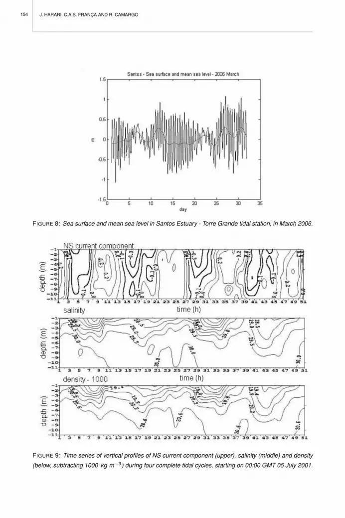
J. HARARI, C.A.S. FRANCA AND R. CAMARGO
FIGURE 8: Sea surface and mean sea level in Santos Estuary - Torre Grande tidal station, in March 2006.
FIGURE 9: Time series of vertical profiles of NS current component (upper), salinity (middle) and density
(below, subtracting 1000 kg m−3) during four complete tidal cycles, starting on 00:00 GMT 05 July 2001.
154

CLIMATOLOGY AND HYDROGRAPHY OF SANTOS ESTUARY
On September 2005, stations were taken in a clockwise sense in the estuary, starting atsection 8 in the western entrance, from 12:30 UTC to 17:40 UTC; this period corresponds, ap-proximately, to flood-tide (from low-water at 10:30 UTC to high-water at 17:53 UTC), in springtide conditions. Mean temperatures were, everywhere in the estuary, close to 21 °C, with verysmall regional variability, within a range of 0.3 °C, close to the measurement precision. Sur-face and bottom temperatures show the same behavior, having very small stratification (warmwater overlying cold water), but again within the measurement errors.
Salinity varies from 15 (fresh) to 35 psu (haline ocean water) in the estuary. Lowest valuesare found in the area close to where tidal waves meet, in the inner section of the estuary, alsodue to the sampling schedule. Differences between west (fresh) and east (saltier) estuary en-trances should be attributed to the tidal phase. Although smaller than the horizontal variability,there is a noticeable increase in salinity with the depth everywhere in the estuary, up to 4 psu.
Dissolved oxygen concentrations displayed larger values at the channels entrances (especiallyat the surface) and smaller ones inside the estuary (at the bottom), with maximum value atthe surface of station 1A (7.68 ml l−1) and minimum at the bottom of station 5A (4.58 ml l−1).Figure 11 presents selected vertical profiles of temperature, salinity and dissolved oxygen, atthe entrance of the Port Channel (section 1) in the innermost station (5) and at the entrance ofSao Vicente Channel (section 8). As stated before, the temperature variations are very small,while salinity and dissolved oxygen exhibit significant gradients along the Channels and strongvertical stratification in the inner region.
The observed current vectors for each station in the winter survey produced Figures 12 and 13,for surface and depth-mean currents. Mean currents reach up to 0.50 m s−1 in the estuary;the tidal flooding during the observation period implied sea-to-estuary currents everywhere;these measurements show that the tidal waves, coming from both estuarine entrances, meetsomewhere between sections 6 and 4 (west of Casqueiro Island). Surface currents followquite close to the mean currents, eventually reaching more than 0.50 m s−1.
On 2006, the summer samplings were taken in two consecutive days, 13th and 14th March,for the Port of Santos and Sao Vicente Channel, again with flooding currents in spring tideconditions; on 13th March low water occurred at 11:08 UTC and high water at 17:08 UTC,with measurements between 12:24 UTC and 18:13 UTC; and on 14th March, the times of lowand high waters were 11:39 UTC and 17:38 UTC, with samplings between 14:50 UTC and17:29 UTC.
In March the temperatures were significantly higher than in September, ranging between 26.92°C and 29.12 °C, but again displaying small vertical variations; on the other hand, salinityvalues range over a larger interval, from 16.7 to 28.8 psu, with significant stratification in somestations, of about 4 psu; dissolved oxygen also has significant gradients along the channels,with a maximum at the surface of station 1 (8.81 ml l−1) and a minimum at the bottom ofstation 5 (3.56 ml l−1). These characteristics may be observed in the selected profiles shownon Figure 14, in the same sections of Figure 11.
155

J. HARARI, C.A.S. FRANCA AND R. CAMARGO
FIGURE 10: Positions of the hydrographic and current meter sections (1 - 9).
FIGURE 11: Vertical profiles of physical properties (temperature above, salinity middle and dissolved
oxygen below) in selected stations of September 2005 sampling - stations on sections 1 (left), 5 (middle)
and 8 (right).
156

CLIMATOLOGY AND HYDROGRAPHY OF SANTOS ESTUARY
FIGURE 12: Surface currents measured on September 2005.
FIGURE 13: Depth mean currents based on measurements at several depths on September 2005.
157

J. HARARI, C.A.S. FRANCA AND R. CAMARGO
FIGURE 14: Vertical profiles of physical properties (temperature above, salinity middle and dissolved
oxygen below) in selected stations of March 2006 sampling - stations on sections 1 (left), 5 (middle) and
8 (right).
FIGURE 15: Surface currents measured on March 2006.
158

CLIMATOLOGY AND HYDROGRAPHY OF SANTOS ESTUARY
The current patterns in summer were not much different from winter (Figures 15 and 16), dueto the large influence of the tidal currents, considering that both campaigns were done duringspring tides with flooding currents (Harari et al. 1999, Harari and Gordon 2001). Again max-imum currents are about 0.50 m s−1, with small variations between the surface and deepervalues.
Temperature and salinity fields measured in the ECOMANAGE Project have the same fea-tures of observations of previous campaigns; the current measurements also have the samestandards, although the characteristics of residual surface currents towards the sea and bot-tom currents towards the continent, in the inner part of the estuary, may only be detected inlonger time series.
Physical data presented here, a systematic observation of Santos Estuary waters, appear tobe reliable and representative of the winter and summer conditions. These data, together withother previous observations, are used to validate the hydrodynamic numerical models.
FIGURE 16: Depth mean currents based on measurements at several depths on March 2006.
REFERENCES
FUNDESPA - Fundacao de Estudos e Pesquisas Aquaticas (2002) Relatorio Complementar do ProjetoEstudo e Projeto Ambiental para viabilizacao da obra de dragagem do canal de acesso e baıa deevolucao dos terminais marıtimos privativos e de uso misto de Cubatao. Julho de 2002
Franco AS (1988) Tides - fundamentals, analysis and prediction. 2nd. Ed, FCTH, S. Paulo, 249p.
Franco AS, Harari J (1987) Computer programs for tidal data checking, correction, analysis and prediction
159

J. HARARI, C.A.S. FRANCA AND R. CAMARGO
by the harmonic method. Relatorio Interno do Instituto Oceanografico da Universidade de Sao Paulo,16:1-65
Godin G (1972) The analysis of tides. Liverpool University Press, 246p.
Harari J, Camargo R (1995) Tides and mean sea level variabilities in Santos (SP), 1944 TO 1989. Re-latorio Interno do Instituto Oceanografico da USP, 36:15p.
Harari J, Camargo R, Cacciari PL (1999) Implantacao de um sistema de previsao de mares e de cor-rentes de mare na Baixada Santista atraves de modelo numerico tridimensional - Relatorio Tecnicodo Instituto Oceanografico da USP, 45:21p.
Harari J, Gordon M (2001) Simulacoes numericas da dispersao de substancias no Porto e Baıa de Santos,sob a acao alatorio de mares e ventos - Revista Brasileira de Recursos Hıdricos, 6(4):115-131
Kalnay E, Knamitsu M, Klister R, Collins W, Deaven D, Gandin I, Iredell M, Saha S, White G, WoollenJ, Zhu Y, Chelliah M, Ebisuzaki W, Higgins W, Janowisk J, Mo K, Ropelewski C, Wang J, Leetma A,Reynolds R, Jenne R, Joseph D (1996) The ncep/ncar 40-year reanalysis project. Bulletin AmericanMeteorology Society, 77:437-470
Miranda LB, Castro BM, Kjerfve B (2002) Princıpios de Oceanografia Fısica de Estuarios. Sao Paulo:Editora da Universidade de Sao Paulo, 424p.
Moscati MCL et al. (2000) Estudo climatologico sobre a costa sul - sudeste do Brasil (Partes I, II e III). XICongresso Brasileiro de Meteorologia, Rio de Janeiro.
160

PERSPECTIVES ON INTEGRATED COASTAL ZONE MANAGEMENT IN SOUTH AMERICAR. NEVES, J.W. BARETTA AND M. MATEUS (EDS.), IST PRESS, 2008
PRIMARY PRODUCERS IN SANTOS ESTUARINE SYSTEM
J.M.M. SCHMIEGELOW, S.M.F. GIANESELLA, C. SIMONETTI, F.M.P. SALDANHA-CORREA, E. FEOLI, J.A.P.SANTOS, M.P. SANTOS, R.B. RIBEIRO AND A.F.P. SAMPAIO
1 ATLANTIC RAIN FOREST
Baixada Santista lies in the Atlantic Rain Forest area, which originally comprised a complexof broad-leaved evergreen forests that once dominated the Brazilian Eastern border, alongan almost continuous belt from the state of Rio Grande do Norte (6°S) to Rio Grande doSul (30°S). In the South-eastern and Southern parts, the Atlantic forest is characterized by aremarkable altitudinal gradient and its most typical physiognomy is associated with the Serrado Mar. The distinct physical conditions combined with the past influence of different florasresulted in an exceptionally high floristic and physiognomic diversity, in all the three levels:within-habitats (alfa), along environmental gradients or among different communities (beta),and diversity of the landscape (gamma). Nowadays, however, only little remains of the forests’original complexity. As the main setting of Brazilian history, the Atlantic rain forest has beendrastically reduced since the discovery. The remnants of the forest currently cover no morethan 7% of its original extent. Continuous remnants are presently restricted to two separateregions: Southern Bahia state, up in the Northeast, and Southeastern Brazil.
In the study area, as in other parts of the Southeast, the dense evergreen forest still coversmost of the scarps of the Serra do Mar, where it was preserved to a large extent due tothe natural limits of the environment - the steeply dissected relief, the dense drainage, thehigh atmospheric humidity and rainfall rates, and the pronounced surface processes. Figure1 presents the distribution of the Atlantic forests’ remnants. Most of the remaining naturalvegetation is or has been somehow disturbed by the anthropogenic occupation, intense useof natural resources and, at least during the last half-century, by high levels of air, water andsoil pollution, which was not controlled until 1983. In 1962 the forests of the Serra do Marwere not severely degraded by air pollution. Primary and secondary forests covered 53% and30% of the Cubatao area, respectively. In the following years, the unfavorable conditions forthe atmospheric dispersion of industrial emissions and the increasing levels of atmosphericpollutants promoted drastic changes in the composition and structure of the natural forests,which soon lost most of their emergent and canopy trees, for they were not able to survive insuch a highly polluted environment. By the end of the seventies, virtually all the natural forestsof the Serra do Mar surrounding the Baixada Santista were strongly affected by air pollution(Pompeia 1997).
The conditions have been slowly changing since the mid eighties, when the State Environmentdepartment started to control the industrial emissions. In spite of some recovery of the canopy,the forest diversity, however, is not being restored, since even the lower levels of atmosphericpollution still restrict the establishment or hamper the development of most native species,
161

J.M.M. SCHMIEGELOW, S.M.F. GIANESELLA, C. SIMONETTI, F.M.P. SALDANHA-CORREA, E. FEOLI, J.A.P. SANTOS,M.P. SANTOS, R.B. RIBEIRO AND A.F.P. SAMPAIO
FIGURE 1: Distribution of the forests’ remnants in Baixada Santista.
favoring the proliferation of a few tolerant pioneer species (Pompeia 1997). Intermediate seralstage secondary forests along slightly polluted areas have closed canopies, but lack mosthardwood species and adult forms of Euterpe edulis, a palm tree intensively exploited due toits commercial value, a clear evidence of disturbance. Myrtaceae, Rubiaceae, Euphorbiaceae,Sapotaceae, and Melastomataceae are usually the richest and most abundant families. Val-ues of alpha diversity vary from 3.4 to 3.9, similar to those of other developed secondaryforests (e.g. Silva and Leitao Filho 1982, Mantovani et al. 1990, Mantovani 1993, Melo andMantovani 1994), and densities vary from 2300 to 2500 individuals per hectare (Leitao Filhoet al. 1989, Leitao Filho et al. 1993, Pompeia 1997).
In the heavily polluted areas, forests have open canopies and lack bromeliads, orchids, ges-neriaceans and other epiphytes, which are remarkably diverse and abundant in undisturbedforests. Under storey tree ferns, caespitose palms and several Piperaceae are fairly common,especially in forest gaps. Myrtaceae, Melastomataceae, Palmae, Rubiaceae, and Fabaceaeare the richest and most abundant families. Pioneer species, such as Tibouchina pulchra, T.mutabilis and Miconia cinnamomifolia (Melastomataceae), Bactris setosa and Syagrus roman-zoffiana (Arecaceae), and Cecropia glaziouii (Cecropiaceae), are abundant. Alpha diversity,otherwise, is low, varying from 2.14 to 3.09 (Leitao Filho et al. 1993, Pompeia 1997). A consid-erable number of trees belonging to the most common species develop an abnormal number
162

PRIMARY PRODUCERS IN SANTOS ESTUARINE SYSTEM
of additional trunks, suggesting the premature death of the main trunk and basal branching.These species are able to grow relatively well until they reach the canopy, when they becomemore vulnerable to the phytotoxic effects of the atmospheric pollutants. At this stage, mostof the typical canopy and emergent trees die and are replaced by tolerant and fast-growingpioneer species (Pompeia 1997).
2 MANGROVE FOREST
Besides the rain forest remnants, the area still preserves quite extensive mangrove wetlands(Figure 2). Mangrove forests are the usual vegetation in large parts of tropical and equatorialsheltered areas. It is well known that mangrove forests represent an important detritus sourceto adjacent estuarine and coastal systems (Odum and Heald 1975). They hold great intrinsicecological value providing various kinds of goods and services.
In Brazil, mangroves are usual structures along its coastal areas, from the Northern frontier(4°30’ N) to Laguna, in Santa Catarina state (28°30’ S). The total area of Brazilian mangrovesis estimated from 10,000 km2 (Herz 1987) to 25,000 km2 (Saenger et al. 1983), depending onthe methodology employed for the quantification. The Brazilian mangroves present a typicalvegetal formation constituted by six species [Rhizophora mangle L., R. racemosa G. F. Mayer,R. harrisonii Leechman, Avicennia schaueriana Stapf. and Leech, A. germinans (L.) andLaguncularia racemosa (L.)]. Only three of these species occur in Sao Paulo state: R. mangle,A. schaueriana and L. racemosa (Lamparelli and Moura 1998). According to Herz (1991), themangrove area in the coast of Sao Paulo State encompasses 231 km2 and 42.5% is locatedin the Baixada Santista. However, according to Lamparelli and Moura (1998), this area isslightly larger, with 120.2 km2 or 52% of Sao Paulo state mangroves forests. Santos, SaoVicente and Cubatao are the main municipalities that shelter the Santos estuarine systemand are covered by 69.7 km2 of mangrove forests (Lamparelli and Moura 1998). Accordingto CETESB (1991), 16% of the original mangrove areas in the Baixada Santista have beenconverted to urban and industrial uses, 40% of the forests are well preserved, mainly thoselocated in the Bertioga region and some in the Sao Vicente region; the degraded mangrovestotal 44%, mainly in the Santos/Cubatao region, which is clearly related to industrial pollution.
The main sources of degradation in this region have been oil spills and the industrial and urbaneffluents that enter the system through the Cubatao and Mogi Rivers, including the waters ofthe Billings Reservoir (Sao Paulo municipality), discharged through the Henry Borden powerplant (CETESB 1990) into the Cubatao river. In spite of its ecological importance, there is littleinformation about the mangroves structure and production in the Santos estuarine system,and most of it was obtained in studies developed in small distinct areas like those by Comelliet al. (1994), Menezes (2000), Pozzi-Neto (2000), Menguini (2004) and Fruehauf (2005).
Comelli et al. (1994) studied the phytosociological characteristics of a small mangrove area inCubatao. An attempt to restore degraded mangrove areas was performed by Menezes (2000)through the planting of mangrove species in a bare area previously occupied by mangrove in
163

J.M.M. SCHMIEGELOW, S.M.F. GIANESELLA, C. SIMONETTI, F.M.P. SALDANHA-CORREA, E. FEOLI, J.A.P. SANTOS,M.P. SANTOS, R.B. RIBEIRO AND A.F.P. SAMPAIO
FIGURE 2: A typical mangrove forest in the Santos estuarine system (photo ECOMANAGE by Joao A. P.
dos Santos).
Cubatao. The author also made an attempt to gain the commitment of the local fishing commu-nity in projects of environmental restoration/conservation and concluded that the restorationof degraded mangroves is feasible in the area, provided some care is exercised and the localcommunities are involved in the establishment of conservation policies. Pozzi-Neto (2000)studied some mangrove sites on the Santos estuarine system aiming at applying economicassessment techniques to obtain the partial economic value of those mangroves forests. Men-guini (2004) studied the mangrove area at Barnabe Island (Santos Estuarine System), a siteimpacted in 1998 by a DCPD (dicyclopentadiene) spill that was followed by a fire, in orderto assess residual impacts and to follow the natural restoration processes. Fruehauf (2005)assessed the contamination by heavy metals in the soil, water, vegetation and organisms inthree areas in the Santos estuarine system. The worst environmental conditions were foundat the Cosipa channel (= Piacaguera channel), followed by the Cascalho River mangrove andMariana River. It was verified that metal contamination was the cause of the decreasing es-tablishment of R. mangle.
There was one large study in the region done by CETESB (1988), that analyzed 33 sites inthe mangrove system, including Bertioga channel which used to receive less contaminants.This study described the forest height ranging from 4.5 m to 13.2 m (average of about 8 m),density ranging from 600 to 3800 trees ha−1 and with 900 to 5800 stems ha−1. The diameterat breast-height (DBH) ranged from 3.6 to 12.8 cm with the basal area between 3.59 to 31.13m2 ha−1. The seedling and sapling density ranged from 0 to 23200 ha−1 and from 0 to 5200ha−1, respectively. With regard to the leaf size, the average in the different sites ranged from20.7 to 36.5 cm2 for R. mangle, 12.5 to 27.9 cm2 for L. racemosa and 10.5 to 18.8 cm2 for A.schaueriana.
164

PRIMARY PRODUCERS IN SANTOS ESTUARINE SYSTEM
In order to obtain recent information about the mangrove system, a new estimate of the man-grove area was performed using the satellite image mosaic of Google Earth Plusr (obtainedin October and November, 2005) and the aerial photos from the Santos municipality carto-graphic basis (year of 2002). Field confirmation was done using GPS, and a new map of themangrove forest area was developed comprising the area inside the limits of ECOMANAGEProject, that is Sao Vicente, Cubatao and parts of those from Guaruja, Praia Grande andSantos (the eastern limit was the Largo do Candinho - Bertioga channel).
To obtain information about the structure and litter production of the mangrove forests, monthlydata were obtained based on 20 belt-transects in the estuarine area named Bertioga Channel(BERT), Diana River (RDIN), Jurubatuba River (JURB), Barnabe Island (BARB), Nossa Sen-hora das Neves Stream (NEVE), Quilombo River (QULM), Piacaguera Channel (CPCG), Pe-dreira River (RPDR), Duas Barras Island (IDBS), Cubatao River (RCUB), Cascalho de CimaRiver (RCSC), Cascalho de Baixo River (RCSB), Mariana River (RMRN), Piacabucu River(RPCB), Queirozes River (RQRZ), Maranhos River (RMRH), Santana River (RSTN), BrancoRiver (RBRC), Largo da Pompeba (LPPB) and Barreiros Channel (CBRR) (Figure 3). Thebelt-transects were placed randomly in each area and were divided in four 10x10 m parcelslocated at the fringe portion, the end portion and two others located at equitable distancebetween the extreme points.
The phytosociological characteristics were evaluated according to Schaeffer-Novelli and Cintron(1986) using the tree density, height and diameter at breast-height (DBH) as structural mea-surements from the mangrove trees according to the formulae given by Curtis and McIntosh(1950). From these data the Importance Value Index of Curtis (IVI) (Curtis 1959) was ob-tained, which is the sum of the relative density, relative dominance (based on the basal area)and relative frequency for each one of the mangrove tree species. This index expresses therelative importance of each species in the system.
The biomass production was evaluated at all the sudy sites according to the Brown (1984)methodology. For this purpose, we placed 240 baskets (2 mm mesh size) under the mangrovetrees positioned at random, three baskets in each stratum, and using 3 m intervals as units.The litter production was collected monthly. The material was dried in stove and weighed.The dry weight was converted to biomass m2 from the area of basket aperture and the dailyproduction was calculated from the number of days between sampling.
Using Arcviewr software the total mangrove coverage in the study area was calculated as71.3 km2, distributed over the municipalities as follows: Santos, 31%, Sao Vicente, 23%,Cubatao, 22%, Guaruja, 14% and Praia Grande, 10%. These values are very similar to thoseobtained by Lamparelli and Moura (1998) - in their case the value was a bit lower becausethey did not include the end portion of the Bertioga channel, which was done in the presentstudy. Among the 20 studied sites, 10 of them presented A. schaueriana with the highest IVI(R. mangle presented a small difference, with 9 sites); and L. racemosa presented the highestIVI only in one of the sites (Piacaguera channel) (Figure 4).
165

J.M.M. SCHMIEGELOW, S.M.F. GIANESELLA, C. SIMONETTI, F.M.P. SALDANHA-CORREA, E. FEOLI, J.A.P. SANTOS,M.P. SANTOS, R.B. RIBEIRO AND A.F.P. SAMPAIO
The litter production ranged from 432.9 g m−2 y−1 (Piacabucu River) to 945.7 g m−2 y−1 (Cu-batao River) (Figure 5). The highest litter production was observed for R. mangle in QueirozesRiver (628.7 g m−2 y−1), followed by A. schaueriana (541.7 g m−2 y−1 in Mariana river) andL. racemosa (284.0 g m−2 y−1 in Barreiros channel. The mean litter production for the studysites was equal to 675.8 g m−2 y−1. The leaves represented 80% of the total litter production.The seasonal litter production was lowest at the end of the winter (September with 35.5 g m−2)and the highest in the summer (February, with 84.3 g m−2) (Figure 6). Maximum productionfor R. mangle (40.7 g m−2) and L. racemosa (17.8 g m−2) were also observed in September,but for A. schaueriana the largest production was observed in November (30.1 g m−2).
2.1 Saltmarsh
The Baixada Santista estuarine area also comprises several saltmarsh areas (Figure 7). Salt-marshes provide large amounts of organic matter to estuarine and coastal food chains. Thisorganic matter usually cannot be used directly by estuarine consumers. The large amounts ofcellulose and lignin in its plant material make the digestion by most of the organisms difficult,except for microorganisms that possess special enzymes for that. Therefore, a large part ofthe saltmarsh primary production is consumed in the form of debris generated by the slowmicrobial decomposition. Lima et al. (1987) showed that 50% of the organic matter of theestuarine sediment in Alagado de Pedra de Guaratiba (Rio de Janeiro State, Brazil) consistedof salt marsh debris.
The salt marsh community is considered essential to coastal environment (Wiegert and Po-meroy 1981) for the creation of refuge area to mating, nursery, home and food for many birds,rodents, reptiles, fishes and crustaceans (Day et al. 1989, Darby 2006). One important groupof saltmarsh plants belongs to the Family Poaceae, genus Spartina. In Brazil, Adaime (1976)observed the excellent adaptation of this genus to estuarine conditions, which allows it to tol-erate climatic variations, salinity fluctuations as well as long exposition and flooding periods,forming dense banks in the intertidal region.
Many aspects of saltmarsh plants in Sao Paulo state were studied in the Cananeia area byAdaime (1976), Takeda (1988), Tararam et al. (1991), Flynn (1994), Tararam (1994), Attoliniet al. (1997), Cunha-Lignon (2001, 2005), Cunha-Lignon et al. (2005), Esposito et al. (2006)and Oliveira et al. (2006), and in Itanhaem by Biudes and Camargo (2006). However, despitethe importance of the Santos estuarine system on the Sao Paulo coast, no data was reportedon its saltmarsh banks. The saltmarsh banks from the Santos estuarine system area mostlycomprise Spartina from the species S. alterniflora and S. densiflora. Both the settlement areaof the saltmarsh and its density were measured in situ for the whole estuarine system exceptin a small area nearby Cubatao, where its characteristics were evaluated by random samples.The total area occupied by S. alterniflora banks was 167,742 m2 with a mean density of 77.4individuals m−2 (Table 1; Figure 8). S. densiflora, occurred in an area of 14,786 m2 with amean density of 568.5 individuals m−2 (Table 1).
166

PRIMARY PRODUCERS IN SANTOS ESTUARINE SYSTEM
FIGURE 3: Mangrove covered area and the location of the 20 transects for phytosociology and litter
studies. See text for explanation of the abbreviations.
FIGURE 4: Importance Value Index of the mangrove trees in the studied places.
167

J.M.M. SCHMIEGELOW, S.M.F. GIANESELLA, C. SIMONETTI, F.M.P. SALDANHA-CORREA, E. FEOLI, J.A.P. SANTOS,M.P. SANTOS, R.B. RIBEIRO AND A.F.P. SAMPAIO
FIGURE 5: Mean weight of the mangrove litter in the studied places.
FIGURE 6: Mangrove mean monthly litter production.
TABLE 1: Total area covered by Spartina ssp ).
Spartina alterniflora Spartina densiflora
Area (m2) 167,742 14,786
Mean density (individuals m-2) 77.4 ± 59.3 568.5 ± 259.9
168

PRIMARY PRODUCERS IN SANTOS ESTUARINE SYSTEM
Three S. alterniflora banks were sampled to estimate live and dead biomass and above-groundnet primary production (ANPP). Five random samples from each bank were obtained duringeight months (March to November, 2007) using a 35x35 cm quadrat. The individuals weresubmitted to a close-cut to the soil, separated in alive and dead components by coloration andthe living ones were counted. The plants were sorted by color difference into alive and deadcomponents and dried in a stove for biomass evaluation. There was a tendency for a biomassreduction of both living and dead fractions from March to November with a small increase inAugust and September (Figure 9), which may be due to the small seasonal variation found insubtropical regions. It was also verified that the mean dead biomass weight was always largerthan the live one and that the standard deviation was much higher for the dead biomass. Theabove-ground net primary production (ANPP) of the Spartina alterniflora banks was estimatedduring a period of eight months by the Smalley method (Long and Mason 1983). The meanvalue of the three banks for this period was 1481.7 g m−2.
3 PHYTOPLANKTON
The phytoplankton community may be an important contributor to primary production evenin estuarine systems where other producers are quite relevant. The phytoplankton commu-nity in Santos estuarine system is dominated by phytoflagellates although diatom blooms arealso a common feature. Gianesella-Galvao (1978) reported Skeletonema costatum bloomsreaching up to 99% of the bulk phytoplankton density during the summer in the Bay of Santos.This author considers other phytoplankton genera also important: Cyclotella, Thalassiosira,Chaetoceros, Coscinodiscus, Asterionella, Leptocylindrus and Nitzschia. At that time, at theend of the 1970´s, high mercury levels were detected in the Santos estuarine system, andseveral species of phytoplankton presented morphological abnormalities.
FIGURE 7: A typical Spartina alterniflora bank in the Santos estuarine system (photo ECOMANAGE by
Mauricio P. dos Santos).
169

J.M.M. SCHMIEGELOW, S.M.F. GIANESELLA, C. SIMONETTI, F.M.P. SALDANHA-CORREA, E. FEOLI, J.A.P. SANTOS,M.P. SANTOS, R.B. RIBEIRO AND A.F.P. SAMPAIO
FIGURE 8: Spatial distribution of S. alterniflora banks in the Santos estuarine system. Circles indicate
occurrence of the banks.
FUNDESPA (1998) reported nanophytoplankton densities ranging between 2.88 to 5.87 x10⁶
cells l−1 in Santos bay. The community was composed mainly by phytoflagellates smallerthan 6µm, Thalassiosira sp, pennate diatoms and coccolithophorids. The microplankton frac-tion was dominated by Chaetoceros compressus, C. curvisetus, C. socialis, Guinardia sp,Pseudo-nitzschia sp and Leptocylindrus sp, with densities ranging from 1.89 to 3.73 x10⁵
cells l−1. Moser (2002) identified the species Skeletonema costatum and Skeletonema spas the main components of the nanoplankton in Santos and Sao Vicente channels. Otherimportant genera were Chaetoceros, Thalassiosira and Cyclotella. Among the microplank-ton forms the more abundant genera found by this author were Navicula, Thalassionema,Pseudo-nitzschia, Nitzschia, Rhizosolenia, Coscinodiscus, Asterionellopsis, Guinardia, Lep-tocylindrus, Hemiaulus and Rhaphoneis. Cyanobacteria were also important in the summer,in the inner portions of Sao Vicente Channel and Largo do Caneu. In this place the dinoflage-lates Prorocentrum gracile and P. scutellum were also important.
More recently, Ancona (2007) observed the nanoplankton (largely represented by phytoflag-ellates and some cyanobacteria) as the dominating phytoplankton community. The followingdiatom genera were the main components of the microplankton of Santos Channel and Bay:Actinoptychus, Chaetoceros, Corethron, Coscinodiscus, Cyclotella, Dactyliosolen, Guinar-dia, Hemiaulus, Leptocylindrus, Melosira, Meuniera, Odontella, Skeletonema, Stephanopyxis,Thalassiosira, Triceratium, Asterionellopsis, Cymbela, Cylindroteca, Diploneis, Fragilariop-sis, Navicula, Nitzschia, Pleurosigma, Pseudo-nitzschia, Rhizososolenia and Thalassionema.Among the dinoflagellates the main genera found were: Ceratium, Gonyaulax, Oxytoxum,Peridinium, Prorocentrum and Protoperidinium.
170

PRIMARY PRODUCERS IN SANTOS ESTUARINE SYSTEM
The occurrence of harmful algal blooms in coastal areas under intense anthropogenic pres-sures has been an increasing concern especially due to its consequences for the public health.According to Hallegraeff et al. (2003), phytoplankton blooms have become more frequentsince the 70´s. In Brazil there are few studies focusing on this problem (Owen et al. 1992,Gianesella-Galvao et al. 1996, Proenca 2004, Carvalho et al. 2007). In the Santos estuar-ine system, Skeletonema costatum blooms were reported by Gianesella-Galvao (1978) andMoser (2002). Despite the fact that these species do not produce toxins, Hallegraeff et al.(2003) warned about their potential harmful effect, whatever that might be. Another matterof concern is the relative increase of dinoflagellates in the phytoplankton community recentlyobserved in Baixada Santista (Moser 2002, CETESB 2004), since a great number of speciesin this group are potential toxin-producers. Gianesella and Saldanha-Correa (2003) observedthe occurrence of the genus Alexandrium near the sewage outfall in Guaruja, besides thecyanobacteria of the genus Anabaena, typical of polluted waters. Carvalho et al. (2007)reported a Trichodesmium erythraea bloom along a broad area of the Baixada Santista offshore.
FIGURE 9: Alive (left) and dead (right) biomass variation of the S. alterniflora for the eight studied months.
Gianesella-Galvao (1982) reported primary production rates as high as 488.4 mg C m−3 h−1,pointing out this system as one of the most productive tropical estuaries indicating the effect ofthe urban and industrial effluents on phytoplankton biomass development in Santos estuary.The Chla concentration was also high (maximum of 55.32 mg m−3). Further studies (FUN-DESPA 1998, CETESB 2001) corroborate the high eutrophication level in this area. Recently,Moser (2002) computed the instantaneous transport rates from Sao Vicente and Santos Chan-nels inlets to Santos Bay and observed that the nutrient inputs via these channels were themain sources of the eutrophication of such water body, and the inputs from the submarineoutfall were responsible for a small fraction of this total input.
Several studies since 1975 (Gianesella-Galvao 1982, Moser 2002, CETESB 2005) have demon-strated an increase in Chla concentrations in the estuary through the last 30 years. Moser etal. (2005) recorded a maximum of 97.4 mg Chla m−3. Ancona (2007), based on monthlyobservations during a year in Santos Channel and Bay, found phytoplankton biomass rangingfrom 0.85 to 28.08 mg m−3 in the bay and from 1.93 to 65.28 mg m−3 in Santos Channel.Primary productivity in channel waters ranged between 1.34 to 48.75 mg C m−3 h−1 and from0.09 to 24.91 mg C m−3 h−1 in bay waters. The lowest biomass and production rates were
171

J.M.M. SCHMIEGELOW, S.M.F. GIANESELLA, C. SIMONETTI, F.M.P. SALDANHA-CORREA, E. FEOLI, J.A.P. SANTOS,M.P. SANTOS, R.B. RIBEIRO AND A.F.P. SAMPAIO
detected in the winter period. According to this author, light and water column stability are themain factors for phytoplankton development in Santos estuary. The highest Chla values re-ported for Santos Estuary by the several authors cited above, are in the range of hypertrophicenvironments as stated by Smith et al. (1999).
REFERENCES
Adaime R R (1976) Estudo da Variacao Estacional do ”Standing-Crop” e do Repovoamento em um Bancode Spartina alterniflora Loiseleur, 1807 no Complexo Estuarino Lagunar de Cananeia. Dissertacaode Mestrado. Universidade de Sao Paulo, Instituto Oceanografico, 72p.
Ancona C M (2007) Aspectos da variacao espacial e temporal da biomassa e producao fitoplanctonica eparametros correlatos no estuario e baıa de Santos. Dissertacao de Mestrado. Universidade de SaoPaulo, Instituto Oceanografico, 229p.
Attolini F S, Flynn M N, Tararam A S (1997) Influence of Spartina alterniflora and tide level on the struc-ture of polychaete associations in an euryhaline salt marsh in Cananeia lagoon estuarine region (SEBrazil). Rev. bras. Oceanogr. 45(1/2): 25-34
Biudes J F V, Camargo A F M (2006) Changes in biomass, chemical composition and nutritive value ofSpartina alterniflora due to organic pollution in the Itanhaem river basin (SP, Brasil). Braz. J. Biol.66(3): 781-789
Brown MS (1984) Mangrove litter production and dynamics In: SC Snedaker, JG Snedaker (eds) (1984)The mangrove ecosystem: research methods. UNESCO, Bungay, United Kingdom. 251p.
Carvalho M, Gianesella S M F, Saldanha-Correa F M P (2007) Trichodesmium erythraea bloom in thecontinental shelf off Santos, Southeast Brazil. BDUA Journal of Biology 2: 219
CETESB (1978) Poluicao nas aguas do estuario e Baıa de Santos. Vols I e II.
CETESB (1988) Estudo dos manguezais da Baixada Santista - Relatorio Final. Sao Paulo: CETESB. 70p
CETESB (1990) Contaminantes na bacia do rio Cubatao e seus reflexos na biota aquatica. RelatorioTecnico.CETESB. Sao Paulo. 81p + apendices.
CETESB (1991) Avaliacao do estado de degradacao dos ecossistemas da Baixada Santista - SP. Re-latorio Tecnico CETESB. Sao Paulo, SP. 45p.
CETESB (2001) Sistema estuarino de Santos e Sao Vicente. Sao Paulo, 141p. http://www.cetesb.sp.gov.br/Agua/praias/relatorios.asp, visited in 4/3/08
CETESB (2004) Relatorio de Qualidade das Aguas Litorıneas do Estado de Sao Paulo- Balneabilidadedas Praias. 331p. http://www.cetesb.sp.gov.br/Agua/praias/relatorios.asp, visited in 4/3/08
CETESB (2005) Relatorio de Qualidade de Aguas Interiores no Estado de Sao Paulo. Sao Paulo, 488p.http://www.cetesb.sp.gov.br/Agua/praias/relatorios.asp, visited in 4/3/08
Comelli F A M, Ponte A C E, Claro S M C A (1994) Aspectos estruturais de um manguezal em Cubatao,SP, Brasil. In: Anais do III Simposio de ecossistemas da costa brasileira, Serra Negra, Sao Paulo.ACIESP, Serra Negra. Vol. I, pp. 97-103
Cunha-Lignon M (2001) Dinamica do manguezal no sistema de Cananeia-Iguape, Estado de Sao Paulo- Brasil. Dissertacao de Mestrado. Universidade de Sao Paulo. Instituto Oceanografico, 57p.
Cunha-Lignon M (2005) Ecologia de manguezais: desenvolvimento espaco-temporal no sistema costeiroCananeia-Iguape, Sao Paulo, Brasil. Tese de doutorado. Universidade de Sao Paulo. InstitutoOceanografico. 198p.
Cunha-Lignon M, Almeida R, Menghini R P, Schaeffer-Novelli Y (2005) Monitoramento de plantulas,jovens de mangue e cobertura de Spartina alterniflora em manguezais no sistema costeiro Cananeia-Iguape, Litoral Sul de Sao Paulo. II Congresso Brasileiro de Oceanografia, Vitoria/ES.
Curtis J T (1959) Vegetation of Wisconsin: An Ordination of Plant Communities. University of WisconsinPress, Madison, WI. 657 p.
172

PRIMARY PRODUCERS IN SANTOS ESTUARINE SYSTEM
Curtis J T, McIntosh R P (1950) The interrelation of certain analytic and synthetic phytosociological char-acters. Ecology 31(3): 434-455
Darby F A (2006) Belowground biomass of Spartina alterniflora: seasonal variability and response tonutrients. Dissertation. The Department of Oceanography and Coastal Sciences B. S. Our Lady ofHoly Cross College. Faculty of the Louisiana State University. 99p.
Day J W, Hall C A, Kemp W M, Yanez-Arancibia A (1989) Estuarine Ecology. John Wiley & Sons, NewYork. 558p.
Esposito T, Souza D B, Rossini D, Santos R, Fernandes S, Flynn M N (2006) Marismas, fluxo energeticoe piramide de biomassa. Environmental and Health World Congress. Santos. Brasil.
Flynn M N (1994) Aspectos ecologicos das associacoes de especies e avaliacao do efeito da predacaosobre a estrutura da macrofauna bentonica de bancos de Spartina (Cananeia, SP, Brasil). Tese dedoutorado. Instituto Oceanografico da Universidade de Sao Paulo. 169p.
Fruehauf S P (2005) Rhizophora mangle (Mangue vermelho) em areas contaminadas de manguezal naBaixada Santista. Tese de Doutorado. Piracicaba. 223p.
FUNDESPA (1998) Levantamento oceanografico da area diretamente afetada por efluentes dos emissariossubmarinos de esgotos da SABESP, entre os municıpios de Sao Sebastiao e Mongagua, estado deSao Paulo (Projeto LOESS). Relatorio final, vol. IV, 49p.
Gianesella-Galvao S M F (1978) Producao primaria da baıa de Santos, estado de Sao Paulo. Aspectossobre a eficiencia fotossintetica num ambiente marinho poluıdo. Dissertacao de Mestrado. Universi-dade de Sao Paulo, Instituto Oceanografico, 53p.
Gianesella-Galvao S M F (1982) Standing-stock and potential production of phytoplankton in the Bay ofSantos, Brasil. Bolm. Inst.oceanogr. 31(2): 85-94
Gianesella S M F, Saldanha-Correa F M P (2003) Avaliacao da comunidade fitoplanctonica na area ad-jacente ao emissario submarino de esgotos na Praia da Enseada, Guaruja (SP), em Janeiro e Julhode 2002. III Congresso Brasileiro de Pesquisas Ambientais e Saude- Meio Ambiente e Saude. 21 a23 de Julho de 2003, Santos, Sao Paulo. CD-rom pp. 18 a 21
Gianesella-Galvao S M F, Costa M P de F., Kutner M B B (1996) Bloom of Oscillatoria (Trichodesmium)erytraea (Ehr.) Kutz. in coastal waters of Southeast Atlantic. Publ. esp. Inst. oceanogr. 11: 133-140
Hallegraeff G M, Anderson D M, Cembella A , Enevoldsen H O (2003) Manual on harmful marine microal-gae. UNESCO, Paris. 793p.
Herz R (1987) Estrutura fısica dos manguezais da costa do estado de Sao Paulo, p. 117-126. In: ACIESP(ed.). Anais do Simposio sobre Ecossistemas da Costa Sul e Sudeste Brasileira: Sıntese dos con-hecimentos. ACIESP, Cananeia (SP).
Herz R (1991) Manguezais do Brasil. Sao Paulo, Instituto Oceanografico, USP, 247p.
Lamparelli C C, Moura D O (1998) Mapeamento dos ecossistemas costeiros do Estado de Sao Paulo.Sao Paulo: Secretaria do Meio Ambiente, CETESB. 108p.
Leitao-Filho H F, Cesar O, Pagano S N, Timoni J L (1989) Composicao florıstica do estado arboreo daMata Atlantica no municıpio de Cubatao (SP). Comparacao de areas preservadas e areas submetidasa poluicao. In: Congresso Nacional de Botanica, 40, Cuiaba, MT. Abstracts, v. 11, p. 437
Leitao-Filho H F, Pagano S N, Cesar O, Timoni J L, Rueda J J (1993) Ecologia da Mata Atlantica emCubatao. Sao Paulo: Editora da Universidade Estadual Paulista; Campinas: Editora da Universidadede Campinas, 184p.
Lima N R W, Martinellii L A, Victoria R L, Mozeto A A (1987) Contribuicao de materia organica de Spartinaalterniflora para o sedimento do Alagado de Pedra Guaratiba (RJ): Uso de 13C como Tracador. Rev.Brasil. Biol. 47(4): 487-491
Long S P, Mason C F (1983) Saltmarsh Ecology. Glasgow, Blackie & Son Ltd., 160p.
Mantovani W (1993) Estrutura e dinamica da Floresta Atlantica na Jureia, Iguape - SP. 1993. 126 p.Thesis (Livre Docencia) - Instituto de Biociencias, Universidade de Sao Paulo.
173

J.M.M. SCHMIEGELOW, S.M.F. GIANESELLA, C. SIMONETTI, F.M.P. SALDANHA-CORREA, E. FEOLI, J.A.P. SANTOS,M.P. SANTOS, R.B. RIBEIRO AND A.F.P. SAMPAIO
Mantovani W, Rodrigues RR, Rossi L, Romaniuc Neto S, Catharino ELM, Cordeiro I (1990) A vegetacaona Serra do Mar em Salesopolis, SP. In: Simposio de Ecossistemas da Costa Sul e Sudeste Brasileira,2., 1990, Aguas de Lindoia. Anais... Sao Paulo: ACIESP, 1990. V. 1, p. 348-384 (Publicacao n. 70-1).
Melo M M R F, Mantovani W (1994) Composicao florıstica e estrutura de um trecho de Mata Atlantica deencosta, na Ilha do Cardoso (Cananeia, SP, Brasil). Bol. Inst. Bot., Sao Paulo, n. 9, p. 107-158
Menezes G V (2000) Recuperacao de manguezais: um estudo de caso na Baixada Santista, Estado deSao Paulo, Brasil. Tese de Doutorado, Instituto Oceanografico, Universidade de Sao Paulo, 164p. +Anexos com figuras e tabelas.
Menguini R P (2004) Ecologia de Manguezais: Grau de Perturbacao e Processos Regenerativos emBosque de Mangue da Ilha Barnabe, Baixada Santista, Sao Paulo, Brasil. Dissertacao de Mestrado,Universidade de Sao Paulo, Instituto Oceanografico. 96p.
Moser G A O (2002) Aspectos da eutrofizacao no sistema estuarino de Santos: distribuicao espaco-temporal da biomassa e produtividade primaria fitoplanctonica e transporte instantaneo de sal, clorofila-a, material em suspensao e nutrientes. Tese de Doutorado. Universidade de Sao Paulo, InstitutoOceanografico. 2 vol.
Moser G A O, Gianesella S M F, Barrera-Alba J J, Bergamo A L, Saldanha-Correa F M P, Miranda L B,Harari J (2005) Instantaneous transport of salt, nutrients, suspended matter and chlorophyll-a in thetropical estuarine system of Santos. Bras. J. Oceanogr. 53(3/4): 115-127
Odum W E, Heald E J (1975) The detritus-based food web of an estuarine mangrove community. In L ECronin (ed.) Estuarine Research. New York, Academic Press, Inc. p.265-286
Oliveira S C S, Neto J S, Godoi A, Cassiano C S, Oliveira M I, Flynn M N (2006) Fluxo de energia emmarisma na regiao de Cananeia. Environmental and Health World Congress. Santos, Brazil. 679-681p.
Owen R W, Gianesella-Galvao S M F, Kutner M B B (1992) Discrete, subsurface layers of the autotrophicciliate Mesodinium rubrum off Brazil. J. Plank. Res. 14(1): 97-105
Pompeia S L (1997) Sucessao secundaria da Mata Atlantica em areas afetadas pela poluicao atmosferica.Cubatao, SP. Tese de doutorado. Universidade de Sao Paulo., 125p.
Pozzi-Neto D (2000) Baixada Santista, manguezal e vazamento de oleo: uma valoracao economica-ecologica. Dissertacao de Mestrado. Programa de Pos-Graduacao em Ciencia Ambiental. Universi-dade de Sao Paulo. 114p.
Proenca L A O (2004) A red water caused by Mesodinium rubrum on the coast of Santa Catarina, South-ern Brazil. Brazilian Journal of Oceanography 52(2): 153-161
Saenger P E J, Hegerl, E J, Davie, J D S (1983) Global status of mangrove ecosystems. Commission onEcology Paper n 3, International Union for Conservation of Nature. The Environmentalist 3(3): 1-88
Schaeffer-Novelli Y, Cintron G (1986) Guia para estudos de areas de manguezal - estrutura, funcao eflora. Caribbean Ecological Research. Sao Paulo. 150p + 3 apendices.
Silva AF, Leitao Filho HF (1982) Composicao florıstica e estrutura de um trecho de mata atlantica deencosta no municıpio de Ubatuba (Sao Paulo, Brasil). Rev. Bras. Bot. Sao Paulo, n. 5, p. 43-52
Smith VH, Tilman GD, Nekola JC (1999) Eutrophication: impacts of excess nutrient inputs on freshwater,marine, and terrestrial ecosystems. Environmental Pollution 100: 179-196
Takeda A M (1988) Estrutura de associacao macrobenticas da Spartina alterniflora Loiseleur, 1807 nocomplexo estuarino-Lagunar de Cananeia. Tese de doutorado. Universidade de Sao Paulo. InstitutoOceanografico. 70p.
Tararam A S (1994) Distribuicao espacial e temporal da macrofauna bentopelagica em marismas daregiao de Cananeia (SP, Brasil). Tese de doutorado. Universidade de Sao Paulo. Instituto Oceanografico.169p.
Tararam A S, Schaeffer-Novelli Y, Gallerrani G, Miyagi V K (1991) Fauna associada a folhas de Spartinaalterniflora Loiseleur, 1807, em experimento de decomposicao realizado em Cananeia, Estado deSao Paulo. II Simposio sobre Oceanografia, Instituto Oceanografico, Sao Paulo/SP.
Wiegert R G, Pomeroy L R (1981) The ecology of a saltmarsh. New York, Springer-Verlag.
174

PERSPECTIVES ON INTEGRATED COASTAL ZONE MANAGEMENT IN SOUTH AMERICAR. NEVES, J.W. BARETTA AND M. MATEUS (EDS.), IST PRESS, 2008
ZOOBENTHOS OF THE SANTOS ESTUARINE SYSTEM
R.P. BORGES, E.F. FIORI, J.A.P. SANTOS, L.P. ZARONI,F. GIORDANO, L.K. KODAMA, G.C. MOYA, S. ROSSO AND R.B. RIBEIRO
1 INTRODUCTION
ECOMANAGE, which applies the DPSIR methodology, has identified a number of human ac-tivities in the Santos Estuarine system which lead to a high level of pressures on this ecosys-tem. Benthic fauna has been shown to be a very good indicator of such pressures, since itis directly exposed to the constant changes of state suffered by the estuary. Although theobjectives of the project did not include a zoological survey of the area, the ECOMANAGEdata field campaigns on benthic fauna and its respective detailed measures of diversity andbiomass, were very useful to indicate the state of both water and sediment.
2 SOFT-SEDIMENT SUBLITTORAL ZOOBENTHOS
The study of soft-sediment benthos communities within the Santos Estuarine System was de-veloped owing to the scarcity of available data. For these reasons, it was decided that thecollection and analysis of the macro-benthic organisms inhabiting the soft sediments in theestuarine channels should be included, looking for determining communities’ basic character-istics and their specific composition along the estuary. It was made with samples from eightstations regarded as strategic in terms of impacts, water flow and nutrient drainage (figure1). One expects, also, to identify the possibly most sensitive areas to human activities. Inthis work soft-sediment macrobenthos on eight stations in the Santos Estuarine System weresampled, both in winter (August, 2005) and summer (February, 2006) campaigns.
Twenty-eight taxonomic groups were registered in all of the samples (Table 1). These groupscomprised 11 phyla or subphyla of benthic animals: Cnidaria, Platyhelminthes, Nemertea, Ne-matoda, Mollusca, Annelida, Sipuncula, Echiura, Arthropoda (Subphyla Cheliceriformes andCrustacea) and Chordata (Subphyla Cephalochordata). Among those groups, some individ-ual organisms could not be identified to a lower level owing to fragmentation of the specimensduring the sampling procedure; The relative abundance of major groups in all samples pooledcan be seen in Figure 2.
The faunistic composition was similar to that observed in other surveys in estuarine regions,particularly comparing with the results obtained by Abessa (2002) in the Santos EstuarineSystem, and by Hostin (2007) in the Paranagua Estuarine Complex (Parana state, BR), whichalso is an important port terminal complex. Polychaeta was the main group in general, followedby Gastropoda (Figure 2). A predominance of annelids was reported before by Heitor (2000)in the Santos Bay and by Abessa (2002) in the Santos estuary. Along the port of Santosand Cubatao channel sites (i.e. 2 and 5) the number of individuals in the main groups was
175

R.P. BORGES, E.F. FIORI, J.A.P. SANTOS, L.P. ZARONI,F. GIORDANO, L.K. KODAMA, G.C. MOYA, S. ROSSO AND R.B. RIBEIRO
much higher in winter than in summer, particularly Polychaeta, Gastropoda and Crustacea insite 2, and Polychaeta in site 5. However, the opposite was observed in the sites deeper inthe estuarine system like the Sao Vicente internal area (on site 6 of Pompeba for instance,Polychaeta was more than three times more abundant in the summer than in the winter) andin Santos site 4 (Caneu), Polychaeta was almost four times more abundant in the summerthan in the winter.
The two sites that showed the highest contrast in species richness were those located alongthe port of Santos and Cubatao channel (sites 2 and 5, respectively). Site 2 was the richest inboth seasons and site 5 was the poorest in species in both seasons (Figures 3 and 4, Table2). The Shannon-Wienner diversity index (H’ in bits) follows the richness, with site 2 the mostdiverse and site 5 the least diverse (Table 2). It is remarkable that the number of groups washigher in site 2 than in the other sites studied. Other works reported high toxicity near this sitein the recent past (Abessa 2002); the same was detected in site 5 area (Sousa et al. 2007).The other sites suffer more impact of domestic sewage.
FIGURE 1: Sampling points of the estuarine Benthos.
In only one site Polychaeta was not the most abundant group: the site 8 (Gonzaguinha), whereGastropoda was many times as abundant as the other groups, probably related with sediment(sand with grain size larger than in other sites) and relative position in the estuary (Figure 5).
176

ZOOBENTHOS OF THE SANTOS ESTUARINE SYSTEM
FIGURE 2: Relative abundance of the main groups; data of both seasons and all sites is pooled.
TABLE 1: Taxonomic groups and total abundance in both seasons.
6
Groups Abundance Groups Abundance
Annelida 1 12 N2* 4 Polychaeta 1080 N7* 1 Oligochaeta 25 N8* 2 Gastropoda 926 N11* 1
Bivalvia 125 N13* 5 Nematoda 190 N14* 8 Crustacea 78 N15* 1 Nemertea 37 N16* 2 Sipuncula 25 N20* 1 Anthozoa 9 N21* 2
Cephalochordata 11 N23* 3 Echiura 4 N24* 1
Hidrozoa 2 N25* 0 Hirudinea 1
Platyhelminthes 1
* Groups which were not identified but safely isolated from the identified ones.
TABLE 2: Extreme values of species richness and diversity (Shannon-Wienner H’ - bits) found along the
estuary’s studied sites: 2 (TECON) and 5 (Piacaguera Channel).
8
Site 2 (TECON) Site 5 (Piaçaguera)
Index Winter Summer Winter Summer
Richness 10 18 4 2
Shannon (H’) 2.082 2.861 0.666 0.890
177

R.P. BORGES, E.F. FIORI, J.A.P. SANTOS, L.P. ZARONI,F. GIORDANO, L.K. KODAMA, G.C. MOYA, S. ROSSO AND R.B. RIBEIRO
FIGURE 3: Relative abundance of the main groups in site 2 (TECON) in the winter (left) and in the summer
(right).
FIGURE 4: Relative abundance of the main groups in site 5 (Piacaguera Channel) in the winter (left) and
in the summer (right).
FIGURE 5: Relative abundance of the main groups in site 8 (Gonzaguinha) in the winter (left) and in the
summer (right).
178

ZOOBENTHOS OF THE SANTOS ESTUARINE SYSTEM
The number of major groups didn’t show a clear correlation to either season or organic mattercontent of the sediment. The same was observed in relation to sediment grain size, becausein almost all sites the sediment was sand-silt ( 70% fine sand), typically mud. These resultswere not surprising and were reported in other works performed in estuaries around the world.Sediment analyses showed no direct relation between grain size and organic matter content.It’s established that, for coastal waters, this kind of relation is commonly direct (Levinton 2001,Nybakken 2001). However, in estuarine systems, particularly those with mangrove forests, thelarge amount of organic matter that comes to the bottom may be more significant than otherfactors to determine the content of this matter in the sediment.
The Santos Estuarine System is affected by human occupation and it, perhaps, determinesthe amount of mineral particles that comes to the water mass. An area that receives a largeamount of sewage, as revealed by socio-economic survey and also observed by Bonetti (2000)was Largo da Pompeba (6), which contained a high number of major groups and a greatabundance of organisms. The large number of factors affecting soft benthos communities inthe Santos Estuarine System, from natural complexity of the system to human interferences,makes it very difficult to reveal and understand how the main forces work. These factorschange in kind and intensity along the estuary and perhaps only with integrated studies, likeECOMANAGE program, a general understanding of this kind of system will be possible.
3 HARD SUBSTRATE SUBLITTORAL ZOOBENTHOS (FOULING COMMUNITIES)
The ECOMANAGE project conducted several experimental studies in order to find ways tocharacterize Santos’ estuarine ecosystems in an integrated way, according to the DPSIR(Drive, Pressure, State, Impact and Response) methodology. The Fouling Project, developedas a sub-item of the estuarine biological community fauna studies, evaluates the communityof encrusting marine sessile organisms in the indicative search of pressures to the functioningstate of the estuarine ecosystem.
The community of these encrusting invertebrates has been regarded as a pressure to thesystem in the whole world for its importance to shipping, mainly due to the economic problemsthat are caused by encrustation in boats and ships, piers, floating buoys and submarine cables.The structure of ”fouling” in the estuarine region of Santos and Sao Vicente was observedduring summer and winter seasons at four distinct points in the estuary (Figure 6). In eachone of them, four ceramic plates were used as fouling collectors during a period of threemonths. The analyses were carried out through the analysis of diversity, biomass and volumeof the collected organisms, in order to obtain a qualitative and quantitative set of data for hardsubstrate sessile organism distribution along the different sites according to Giordano (2001)and Borges (2002).
179

R.P. BORGES, E.F. FIORI, J.A.P. SANTOS, L.P. ZARONI,F. GIORDANO, L.K. KODAMA, G.C. MOYA, S. ROSSO AND R.B. RIBEIRO
FIGURE 6: Site studies where ceramic tiles were used as fouling fauna samplers.
The results show values of the diversity indexes to be higher during the winter season andvalues of biomass and volume to be higher during the summer season. It was also verifiedthat approximately 65% of the taxonomic groups found had been observed in both seasons ofthe year (Figure 7 showing the plates with different taxonomic groups among them sea-squirt,bryozoans, barnacles, sea worms and mussels were the most abundant groups). The resultsof richness and diversity indexes obtained in Sao Vicente were very low, probably due to agreat ousting of sewers, coming from the palafittes, sub-houses from which sewage directlypours into the estuary and prevents the settlement of more sensitive members of the foulingcommunity. However, in this same region, the biggest growth rates of the fouling community’sbiomass occurred, mostly due to the incredible rates of bivalves’ filter feeders growth (up to11 g of dry weight of organic matter a day per plate!). Fouling, as well as other bio-indicators,demonstrates that the greatest pressures in the estuarine system come from sewage and sub-normal residences at the edge of the estuary whereas along the port channel the shippingactivities played the important role of new species introduction by ballast water discharges.
180

ZOOBENTHOS OF THE SANTOS ESTUARINE SYSTEM
FIGURE 7: Ceramic tile used for fouling community recruitment (source: ECOMANAGE photos by Leandro
Kodama).
4 FINAL CONSIDERATIONS ON BENTHOS
As the fouling community fauna depends much more on water column conditions while soft-sediment fauna is more frequently related to sediment quality we can conclude that:
• In Cubatao and Santos Estuarine areas (Northern and Eastern part of the estuary) thegrowth of the fouling fauna was not as high, but instead, higher diversity indexes seemedto be explained by the relative lower levels of sewage discharges in these waters;
• Instead, it seemed to be related to a high growth of fouling fauna, the negative effectsof waters contaminated with sewage discharges, noticed in Sao Vicente estuarine area(western area of the estuary) also supported by the results of the water column qualitytests obtained by ecotoxicology procedures;
• Soft-sediment Benthic Fauna biodiversity reflects the high levels of sediment contami-nation, historically reported in the estuary as a major pressure for the ecosystem. Thiscould be confirmed with the ECOMANAGE field data analysis, by the very poor indexesobtained on diversity and the high dominance obtained of these values whenever thesite studied was on the Santos Cubatao side of the estuary (places subjected to formerdredging activities) such as the Piacaguera Channel;
• The benthos survey was an important tool in order to evaluate the environmental ”status”as affected by two factors: the suspended organic load and the sediment organic mattercontent. The abundance of the first factor showed a close relation to high levels offouling communities’ biomass increase; nevertheless, the abundance of the secondfactor showed no close relation to the number of individuals and taxa in all sites.
REFERENCES
Abessa DMS (2002) Avaliacao da qualidade de sedimentos do Sistema Estuarino de Santos, SP, Brasil.Tese de Doutorado. Universidade de Sao Paulo Instituto Oceanografico. 290p.
Anderson MJ, Underwood AJ (1994) Effects of substratum on the recruitment and development of anintertidal estuarine fouling assemblage. Journal of Experimental Marine Biology and Ecology 184(2):217-236
181

R.P. BORGES, E.F. FIORI, J.A.P. SANTOS, L.P. ZARONI,F. GIORDANO, L.K. KODAMA, G.C. MOYA, S. ROSSO AND R.B. RIBEIRO
Bonetti C (2000) Foraminıferos como bioindicadores do gradiente de estresse ecologico em ambientescosteiros poluıdos. Estudo aplicado ao Sistema Estuarino de Santos - Sao Vicente (SP, Brasil). ThesisTese de Doutorado. Universidade de Sao Paulo Instituto Oceanografico. 229p.
Borges RP (2002) Recrutamento em substrato artificial consolidado no estuario de Santos (Santos - SP):um estudo em medio prazo. Sao Paulo. Tese de Doutorado. Universidade de Sao Paulo. Instituto deBiociencias. 92p.
Diegues AC (1987) Conservacao e desenvolvimento sustentado de ecossistemas litoraneos no Brasil. In:I Simposio de Ecossistemas da Costa Sul e Sudeste Brasileira. Cananeia, Sao Paulo. Publ. ACIESP3: 196-243
Eston VR (1981) Recobrimento primario de substratos artificiais submersos no estuario de Santos (SaoPaulo, Brasil). Sao Paulo. Dissertacao de Mestrado. Universidade de Sao Paulo. Instituto Oceanografico.116p.
Giordano F (2001) Colonizacao de placas de ”fouling” no estuario de Santos (Santos-SP): Analises tran-sicional e de sensibilidade complementando a abordagem baseada em recobrimentos especıficos ediversidade. Sao Paulo. Tese de Doutorado. Universidade de Sao Paulo. Instituto de Biociencias.141p.
Haag WR, Berd DJ. Garton DW (1993) Reduced survival and fitness in native bivalves in response tofouling by the introduced zebra mussel (Dreissena polymorpha) in Western Lake Erie. CanadianJournal Fisheries and Aquatic Science, 50: 13-19
Heitor SR (2000) Composicao e distribuicao da macrofauna bentonica em areas sob influencia da disposicaooceanica de esgotos municipais na Baixada Santista e no Canal de Sao Sebastiao, Sao Paulo, BrasilTese de Doutorado. Universidade de Sao Paulo. 245p.
Hostin LM (2007) Estrutura da macrofauna bentica nos canais de acesso aos terminais portuarios docomplexo estuarino de Paranagua (Parana) sujeitos a dragagem. In: XII Congresso Latino-Americanode Ciencias do Mar. Florianopolis. CD-ROM.
Levinton JS (2001) Marine Biology: function, biodiversity, ecology. 2th ed. Oxford: University Press. 560p.
Lindegarth M, Hoskin M (2001) Patterns of distribution of macro-fauna in different types of estuarine, softsediment habitats adjacent to urban and non-urban areas. Estuarine, Coastal and Shelf Science,52:237-247
Menge BA (1991) Relative importance of recruitment and other causes of variation in rocky intertidalcommunity structure. Journal of Experimental Marine Biology and Ecology, 146: 69-100
Migotto AE (2000) Avaliacao do estado do conhecimento da diversidade de invertebrados marinhos noBrasil. Avaliacao do Estado do Conhecimento da Diversidade Biologica do Brasil. MMA - GTB/CNPq- NEPAM/Unicamp. 65p.
Nybakken JW (2001) Marine Biology: an ecological approach. 2nd. ed. New York: Harper and Row,Publishers Inc. 514p.
Rajagopal S, Nair KVK, Van der Velde G, Jenner HA (1997) Seasonal settlement and succession of foulingcommunities in Kalpakkam, east coast of India. Journal of Aquatic Ecology, 30(4): 309-325
Shin PKS, Ellingsen KE (2004) Spatial patterns of soft-sediment benthic diversity in subtropical HongKong waters. Marine Ecology Progress Series, 276: 25-35
Sousa ECPM, Abessa DMS, Rachid BRF, Gasparro MR, Zaroni LP (2007) Ecotoxicological assesmentof sediments from the port of Santos and the disposal sites of dredged material. Brazilian Journal ofOceanography, 55(2): 75-81
Sutherland JP, Karlson RH (1977) Development and Stability of the Fouling Community at Beaufort, NorthCarolina. Ecological Monographs, 47: 425-446
182

PERSPECTIVES ON INTEGRATED COASTAL ZONE MANAGEMENT IN SOUTH AMERICAR. NEVES, J.W. BARETTA AND M. MATEUS (EDS.), IST PRESS, 2008
ECOLOGICAL STATUS OF THE SANTOS ESTUARY WATER COLUMN
S.M.F GIANESELLA, F.M.P. SALDANHA-CORREA, E.C.P.M. SOUSA AND M.R. GASPARRO
1 INTRODUCTION
The Santos Estuary, in Sao Paulo State, Brazil, is known for its high pollution levels related toport, industrial and urban uses. Despite its importance and strategic location in the nationalcontext, few systematic studies have been conducted aiming to determine the ecological sta-tus of the system. There is no available data on the Santos Estuary’s pristine conditions, i.e.before the occupational boom occurring in this area at the end of the 1960s and early 1970s,with the development of the Cubatao industrial park and Santos port expansion, besides theurban center.
The first extensive survey in Santos Bay was carried out between 1974-1977 to establishthe original environmental conditions before the construction of the Santos submarine out-fall (CETESB 1978, Gianesella-Galvao 1978, 1982), regarding the future management of thearea. The findings indicated that the environment was heavily impacted: phosphate valuesvaried from 1.44 to 4.22 µM and mean total inorganic nitrogen varied from 10.84 to 21.53 µM,with nitrate concentrations attaining 19.28 µM. However N:P ratio never exceeded 10. At thattime, Hg was also detected in high concentrations, with values attaining 3.64 µM, 10 times themaximum detected by Fitzgerald and Lions (1973) in the seawater. The highest nutrient con-centrations were detected in the inner estuary portions, decreasing towards Santos Bay. Suchgradient were consistent with the circulation model suggested by Garcia-Ochipinti (1972). Ac-cording to this author, during high tide, the seawater enters the estuary through the bottomlayers, whereas brackish water flows downwards through surface layers (0-1 m). This is thepredominant pattern about 85% of the time.
The Cananeia Estuary (25°04 ’S), south of the Santos Estuary, was chosen as a comparativemodel since it is relatively near the Santos Estuary (located at neighboring latitudes and geo-graphically at the same embayment) and displayed similar climate, soil and mangrove vegeta-tion, despite that each estuary presents their particular characteristics. Kato (1966) reported3.0 µM nitrate and 0.7 µM phosphate as maximum concentrations in Cananeia Estuary. Suchvalues are a clear indication of the eutrophication process that the Santos Estuary underwentfrom 1974-1977. By the mid 1970s, domestic and industrial effluents had begun to be gov-ernmentally regulated. In the 1980s, the state environmental protection agency (CETESB)initiated a program for controlling the main sources of pollution in the Santos harbor and in-dustrial park of Cubatao. An effort was also made by the authorities to control clandestinesewage disposal. However, subsequent studies (FUNDESPA 1998, Braga et al. 2000, Frazao2001, CETESB 2001, Moser 2002, Ancona 2007) indicate that eutrophic conditions still per-sist. Braga et al. (2000) verified nitrate and phosphate concentrations higher than 90 and24 µM, respectively, near Cubatao city. These authors affirm that the concentration declines
183

S.M.F GIANESELLA, F.M.P. SALDANHA-CORREA, E.C.P.M. SOUSA AND M.R. GASPARRO
towards Santos Bay; nevertheless, low concentrations are not attained for both elements inbay waters. Frazao (2001), comparing the trophic state of waters of Ubatuba, Santos andPraia Grande, concluded that Santos is the most eutrophic of the three. CETESB (2001)verified high levels of heavy metals in the sediments and biota from Santos and Sao Vicenteestuaries. Moser (2002) verified nitrate and phosphate concentrations higher than 12 and 4.0µM, respectively, in Santos and Sao Vicente Channels pointing out that the nutrient input fromthese channels into Santos Bay are much more relevant than the discharge of the sewagesubmarine outfall (located at the middle of Santos Bay).
Ancona (2007) studied the time-space variability of nutrients, chlorophyll-a (Chl-a) and otherrelated variables in Santos Channel and Bay, based on monthly samplings from November2004 to December 2005. This work represents the best data set available to characterize thisregion, also notably referring to a very recent period. The author reports dissolved inorganicnitrogen attaining values up to 41.1 µM in Santos Channel and up to 35.1 µM in Santos Bay.Ammonium was the main inorganic nitrogen form (maximum of 32.5 µM in Santos Channeland 21.5 µM in the Bay). Ammonium availability was negatively correlated to salinity, indicatingthat its source is the brackish waters, being more important in rainy periods. On the other hand,nitrate concentrations were higher in the driest periods. Phosphate maximum concentrationswere 11.31 µM in the bay and 8.38 µM in the channel waters. The source of phosphate for thesystem is also the inner channel waters, as attested by negative correlations between salinityand phosphate. The low N:P ratio is still observed in the area, due to the phosphate overload,and not to low nitrogen availability. In terms of silicate, the mean value in channel waters wasnearly 15 µM, while in the bay waters the mean was lower, approximately 10 µM. Such silicatelevels are high denoting an environment under the influence of great land drainage.
The current status of the estuarine system was evaluated by samplings performed in 8 stationsdistributed throughout the estuarine region (Figure 1) in winter (August, 2005) and summer(March, 2006).
2 MATERIAL AND METHODS
In situ vertical profiles of physical properties (T, Salinity, pH) were performed using a HORIBAmulti-parameter sensor. Secchi disk readings were used to estimate the euphotic zone thick-ness (Zeu), according to Poole and Atkins (1929). Discrete water samples for chemical vari-ables were taken with van Dorn bottles at three depths: surface, mid-water and 1 m above thebottom. Dissolved oxygen (DO) and alkalinity analyses were processed in the field laboratory,within 6 h after sampling. DO samples were analyzed by Winkler’s method (Grasshoff et al.1983) and oxygen saturation (DOS) was computed according to UNESCO (1973). Alkalinitydeterminations were performed by titration using HCl 0.05 M (Gran 1952) and the data wereused to estimate the dissolved CO2 concentrations based on Carmouze (1994) computations.Aliquots of water were filtered through AP-40 Milliporer glass fiber filters for photosyntheticpigment analyses (Saldanha-Correa et al. 2004) and seston determination. The filtered waterwas frozen for the dissolved inorganic nutrient analysis.
184

ECOLOGICAL STATUS OF THE SANTOS ESTUARY WATER COLUMN
Inorganic nutrients were analyzed by spectrophotometric methods: nitrite, nitrate and ammo-nium according to Aminot and Chaussepied (1983) and phosphate and silicate following themethods described in Grasshoff et al. (1983). Chlorophyll-a (Chl-a) was determined accordingto Jeffrey and Humphrey (1975) equations, active chlorophyll-a (Act Chl-a) and pheopigments-a by Lorenzen (1967) and carotenes according to Parsons et al. (1984). Seston analyses wereperformed by the gravimetric method discriminating inorganic and organic fractions (APHA1985) using pre-combusted and pre-weighed AP-40 Milliporer filters. The phytoplankton in-ternal nutrient status was also evaluated using the ratio between the optical density at 480 and665 nm of the samples used for pigment determinations (Heath et al. 1990).
Primary productivity rates (PP) were determined in surface and bottom samples of stations1, 2, 3, 5, 6 and 8 in winter and 1, 3, 5, 6 and 8 in summer, through incubations using 14C(Steemann-Nielsen 1952) in photosyntetron-like chambers. The 14C assimilated was con-verted to units of mg C m−3 h−1, according to the equations described in Teixeira (1973).Aliquots of the same samples submitted to primary productivity experiments from stations 1, 2and 3 in winter and 1, 3, 5, 6 and 8 in summer were taken to determine the bacterial secondaryproductivity (BSP) following the method proposed by Smith and Azam (1992), using 3H− Thyinstead of 3H− Leucine. The number of disintegrations per minute of each sample was con-verted to moles of incorporated 3H− Thy L−1 h−1 according to the equation proposed by Bell(1993). The conversion of moles incorporated to cells produced per unit time was done byapplying the thymidine conversion factor (TCF) of 0.52 x10¹⁸ cells per mol of thymidine de-termined by Barrera-Alba et al. (2004) in Cananeia Estuary. A second conversion, from cellproduction to productivity in units of carbon was done assuming the factor of 20 fg C cell−1
(Lee and Fuhrman 1987).
Considering the complex composition of the industrial and urban sewage discharged in San-tos Estuary due to several types of pollutants, ecotoxicologic tests were also performed inorder to gain complementary information. These bioassays are useful for evaluating the en-vironmental degradation process since they determine the synergistic effect of the chemicalaction of the toxic agents, the physiology of the test organism and the environmental conditions(FUNDESPA 2007, Rachid 2002).
Toxicity tests with surface water were conducted using non-diluted water samples. The em-bryolarval development test with L.variegatus followed the ABNT (2006a). Chronic toxicitytests were conducted for 24 h, after this period the percentage of normal pluteus larvae wasevaluated. For the acute toxicity tests with the surface water, the bacteria Vibrio fischeri wasused according to ABNT (2006b). This bioassay consisted of determination of the inhibitoryeffect of water samples on the light emission of these luminescent bacteria, for 5, 15 and 30min. The ecotoxicity data were compared statistically using the MSD (Minimum SignificantDifference) method and analysis of variance followed by the Dunnett’s test for detection of sig-nificant differences and determination of the toxic samples (ASTM 1992, Swartz et al. 1985,USEPA 1991).
185

S.M.F GIANESELLA, F.M.P. SALDANHA-CORREA, E.C.P.M. SOUSA AND M.R. GASPARRO
3 RESULTS AND DISCUSSION
The Santos Estuary is a partially stratified system, with sharper stratification in Sao VicenteChannel and the inner estuarine areas. During winter samplings, water temperature was near22 °C and salinity ranged from 25.7 in station 6 up to 33.7 in the channel inlets. During sum-mer samplings, water temperature was nearly 6 °C higher than during winter, with a meanvalue of 28 °C. Due to the higher summer rainfall, which increases the freshwater contributionin the estuarine head, salinity mean value was 23.07, i.e. about 8 units lower than in winter.Water density in summer was much lower than in winter as a result of the high temperaturesand low salinities (Table 1).
TABLE 1: Mean (±SD), maximum and minimum values of the physical and chemical variables obtained in
winter and summer sampling cruises in the 8 stations distributed throughout the Santos estuarine system.
(Sigma-t in kg m−3 and dissolved inorganic nutrients in µM).
Aug/05 T (ºC) Sal Sigma-t pH OD
(ml l-1) DOS (%)
CO2 (%)
CO2/DO NH4
+ NO3- NO2
- DIN (µM) PO4-3 N:P Si(OH)4
Mean 22.04 31.25 21.33 8.63 4.45 87.32 307.81 3.47 12.85 6.15 1.45 20.44 4.89 5.07 15.07 SD 0.46 2.63 2.18 0.12 0.68 14.07 158.47 3.07 11.28 8.27 1.03 15.13 4.39 2.69 5.04
max. 23.10 34.90 25.00 8.70 5.77 114.90 621.40 10.17 51.31 41.84 4.93 58.07 22.40 12.56 28.54 min. 21.40 23.70 16.00 8.30 2.69 52.00 135.74 0.00 0.66 1.20 0.15 6.96 0.55 1.65 7.41
Mar/06 T (ºC) Sal Sigma-t pH DO
(ml l-1) DOS (%)
CO2 (%)
CO2/DO NH4
+ NO3- NO2
- DIN PO4-3 N:P Si(OH)4
Mean 27.99 23.07 13.61 7.29 3.85 80.38 721.13 9.35 20.12 5.18 1.12 26.42 3.81 8.51 24.21 SD 0.60 3.71 2.79 0.28 1.06 24.49 446.16 7.52 16.40 5.37 0.77 19.33 2.27 8.96 11.84
max. 29.12 28.80 18.00 7.80 6.17 134.28 1835.33 26.52 69.76 23.93 3.29 78.04 8.33 44.35 46.65 min. 27.03 16.70 8.00 6.91 2.52 51.66 189.09 0.00 0.33 0.71 0.21 3.72 0.81 2.45 5.99
Dissolved oxygen (DO) mean concentrations and DO saturation percentage (DOS) were higherduring the winter than in summer (Table 1). DO levels were always lower in the inner brack-ish waters (with the minimum at station 6) tending to increase towards the channel mouths.DO levels were above the minimum recommended limit by Brazilian environmental legislation(CONAMA 2005) but in stations 6 and 7, the averages were very close to this limit. The DOsaturation levels were mostly below 100% indicating a deficit in O2 production related to itsconsumption, mainly in summer.
Mean pH value in winter was more than one unit higher than the summer mean. The averageconcentrations of dissolved CO2 in the water column were also higher in summer than inwinter but in terms of percentage of CO2 saturation, the estuarine waters always presentedCO2 over saturation (Table 1), indicating an intense heterotrophic activity. Summer valueswere twice as high as winter ones, and attained more than 1500% saturation at stations 4and 6. An estimate of the balance between heterotrophic and autotrophic processes wasobtained using the ratio CO2/ O2 saturation. Results indicate strong heterotrophic behavior inthis system with a significant increase during summer.
The inorganic nutrient concentrations detected throughout the estuary in summer and winterconfirmed the eutrophic characteristics (Table 1). Some points, such as station 6 site, dis-
186

ECOLOGICAL STATUS OF THE SANTOS ESTUARY WATER COLUMN
played worse conditions: in summer, the maximum ammonium concentration obtained (69.7µM) was within the limit of acceptance for brackish waters according to the environmental leg-islation (CONAMA 2005). The region’s nearby station 6 is shallow and receives the runoff of agarbage disposal on the island side with high loads of ammonium, phosphate and many othertoxic components, not quantified in this study. Ammonium was the main inorganic nitrogenform in both sampling periods but mainly in winter, corresponding to almost 90% of the totaldissolved inorganic nitrogen. Ammonium and silicate were clearly associated with waters ofcontinental origin since the highest values were detected at the inner stations (4 to 7) whereammonium ranged from 21.57 to 51.52 µM in summer, whereas the maximum silicate con-centration (Table 1) was attained at the innermost station (st. 5). Ammonium is also producedby organic matter decomposition and the high summer temperatures certainly contributed tothe increase of this activity.
Inorganic phosphate, otherwise, seems to have an inner local source, relatively independentof rain contribution, since higher concentrations were detected during winter (Table 1). Cur-rently, there are several possible sources of nutrients in the inner areas, including domesticand industrial effluents, and these sources are relevant, as indicated by the absolute nutrientconcentrations. The silicate and phosphate concentrations observed were a bit higher thanthose observed by Braga et al. (2004) in the inner estuarine regions. On the other hand, thenitrate values were much lower than those reported by these authors, who did not evaluatethe ammonium contribution to the system. Despite the high concentrations of total inorganicnitrogen verified in both periods, the N:P ratios (Redfield 1934) were always below 10, due tothe high phosphate loads.
Seston distribution presented the same pattern in summer and winter, with higher concentra-tions in Santos Channel, almost 5 times higher than the mean values obtained in Sao Vicenteand inner estuary stations. The organic fraction (OS) corresponded to around 30% of thebulk (Table 2). The high seston load is an important factor in reducing the euphotic zonethickness. Indeed, light penetration was usually low, between 2 and 5m, and may be limitingphytoplankton growth in the subsurface layers, as Santos Channel can reach up to 15 m indepth.
The estuary is characterized by its high phytoplankton biomass. Chl-a levels are compatibleto the observed in eutrophic system as stated by Smith et al. (1999), with mean concentrationaround 10 mg m−3. Phytoplankton biomass was slightly more elevated during winter thansummer (Table 2). During summer, the spatial Chl-a distribution tended to be more homoge-neous. In winter, Chl-a concentration tended to increase from Santos Channel towards theinner estuary with a maximum value at station 7. Conversely, station 7 presented the lowestbiomass in summer. The lower Chl-a values observed in the upper reaches may be ascribedto the smaller retention time of the waters at this period, due to the larger contribution offreshwater into the system. The main vertical differences were observed in the inner stations,principally in station 5, where the highest values occurred in surface waters.
187

S.M.F GIANESELLA, F.M.P. SALDANHA-CORREA, E.C.P.M. SOUSA AND M.R. GASPARRO
TABLE 2: Mean (±SD), maximum and minimum values of the variables: euphotic zone thickness (Zeu), to-
tal seston (TS), percentage of organic seston (% OS), photosynthetic pigments (in mg m−3) PP and BSP
(in mg C m−3 h−1), PP/Chl-a ( mg C (mg Chl)−1 h−1) and the ratio BSP/PP on a daily basis, obtained
in winter and summer sampling cruises in Santos Estuary.
Aug/05 Zeu TS OS Chl-a Chl-a act Chl-c Carotene 480/665 PP PP/Cl-a BSP BSP/PP
Mean 2.80 179.02 31.65 9.73 6.55 2.15 5.57 1.21 21.72 2.68 0.31 0.06 SD 0.80 250.07 32.44 6.96 5.66 1.25 4.93 0.14 18.22 1.06 0.09 0.03
max. 4.20 766.20 94.07 30.30 27.07 5.76 22.42 1.59 60.80 4.43 0.41 0.10 min. 2.10 36.60 9.84 2.95 0.00 0.75 0.43 1.02 2.36 1.03 0.10 0.04
March/06 Zeu TS OS Chl-a Chl-a act Chl-c Carotene 480/665 PP PP/Cl-a BSP BSP/PP
Mean 3.40 179.10 26.20 8.09 4.98 1.48 5.36 1.22 60.00 7.98 1.17 0.12 SD 1.50 258.65 35.31 2.82 2.12 0.56 1.97 0.23 75.00 12.39 0.95 0.14
max. 6.10 889.40 90.35 12.16 9.11 2.58 9.49 1.72 230.31 42.10 3.45 0.49 min. 1.90 32.50 0.00 2.78 1.09 0.53 2.60 0.95 3.87 0.55 0.37 0.01
Total carotene concentrations followed the same temporal distribution pattern of Chl-a, withmean concentration values slightly higher during winter than summer. The active Chl-a gen-erally represented more than 50% of total Chl-a, which indicates a healthy state for the phy-toplankton. The ratio 480/665 (Table 2) corroborates this assumption since all the values forthis ratio were below 2, indicating a good intracellular nutritional status (Heath et al. 1990) inboth studied periods.
The mean primary productivity ratio (PP) obtained in summer was higher than winter one(Table 2). PP rates obtained from surface waters were generally higher than those from bottomsamples, except in st. 8 and 1 in summer. The highest rate was attained from the surface waterof st. 6 (230.31 mg C m−3 h−1) and the PP observed values in Santos Channel were alwaysbelow those from the other stations, indicating that Santos Channel is the less productiveportion of the system. This feature can be attributed to the higher depths verified in thisportion of the estuary which restricts phytoplankton cells to remain light limited in this coursethroughout the mixing layer. Also, this channel shelters the Santos port, experiencing intensetraffic of large ships, which increases the water instability and turbidity, negatively affecting thephytoplankton growth.
In terms of PP/Chl-a ratios, Santos inlet station presented the lowest value in both periods.In winter, mean ratio was 2.68 mg C mg Chl−1 h−1, whereas the mean ratio in summer wasalmost four times this value (Table 2). These results may be ascribed to the high water tem-peratures observed in summer favoring the phytoplankton development in nutrient rich watersand at more stable conditions than those verified at the channel mouths. The highest PP/Chl-aratio considering both sampling periods was 42.2 mg C mg Chl−1 h−1, verified at surface ofstation 6 in summer.
The BSP rates observed in summer were almost twice those observed in winter (Table 2). Asimilar spatial pattern of PP/Chl-a ratios was observed for BSP in summer, with the highest
188

ECOLOGICAL STATUS OF THE SANTOS ESTUARY WATER COLUMN
value in station 6 (3.45 mg C m−3 h−1) and the higher ratios near the surface. However, interms of BSP, the differences between surface and bottom samples were usually small. Con-sidering the results on a daily basis, the values observed in the Santos system ranged from2.35 to 82.76 mg C m−3 d−1, or 14.4 to 114.2 mg C m−2 d−1 in area terms. The BSP rateswere higher than those obtained by De Souza et al. (2003) in the Zuari estuary, India, wherethe authors report mean rates of 70 mg C m−3 d−1 in the surface and 35 mg C m−3 d−1 inthe bottom waters.
This environment shows physical similarities with Santos estuary as the temperature ranges,depth, mixing conditions, and mangroves in the surroundings. Another example of a tropi-cal environment was the lowland rivers of Orinoco basin (Castillo et al. 2004) that presentedvalues between 4.8 to 6.24 mg C m−3 d−1, rates significantly lower than those observed inSantos estuary. If one considers the bacterial productivity rates in terms of area, the re-sults obtained were extremely low compared to the ranges reported by Barrera-Alba (2004)in Cananeia-Iguape estuary (in summer: 459.0 to 12730.0 and in winter: 182.5 to 1354.5mg C m−2 h−1). However, the BSP rates obtained in Santos estuary are in the same rangeas those obtained by Hock and Kirshman (1993) in the Delaware estuary, with also similarvalues for Chl-a and PP rates, by Shiah et al. (2003) in the continental shelf of East ChinaSea BSP (6 to 179 mg C m−2 h−1) and higher than those of Almeida et al. (2002) in the Riade Aveiro system (1.5 to 36.8 mg C m−2 h−1). Both PP and BSP rates were highest at station6, demonstrating that this is an important place for the evaluation of the estuarine dynam-ics, which is producing and probably exporting materials toward the bay through Sao VicenteChannel (stations 7 and 8) favoring eutrophication processes in the bay.
The BSP/PP results indicate the dominance of phytoplankton autotrophic processes over thebacterial heterotrophic ones. According to these results, the ratio CO2/ O2 was expected tobe quite low. However, the CO2/ O2 ratios clearly indicate the predominance of heterotrophicprocesses over autotrophic ones, mainly in the inner estuarine portions. Such differencesmay be ascribed to the heterotrophic activities not related to water column process. Oneof particular importance, not analyzed in the present study, is the bacterial decompositionactivity in the mangrove sediments: certainly a great part of the CO2 produced is dissolvedin the water as the high tides invade the mangrove. Additionally, the heterotrophic activity inthe estuarine sediment is possibly high, removing O2 from and introducing CO2 into the watercolumn.
Seston analysis showed phytoplankton as a less important component of the organic fraction.This means that a great load of the organic material comes from the terrestrial or aquaticvegetation and also from domestic and industrial effluents discharged throughout the estuary,which decompose on the way to the open sea. Consequently, the BSP/PP ratios indicate thephytoplankton primary productivity is able to support the water column heterotrophic demand;nevertheless, other CO2 sources determine the heterotrophic characteristics of the SantosEstuary.
189
S.M.F GIANESELLA, F.M.P. SALDANHA-CORREA, E.C.P.M. SOUSA AND M.R. GASPARRO
The maintenance of high productivity rates and the dominant water column mixed conditionsobserved in the inner areas of the system during the summer prevented anoxic conditions.Acute toxicologic tests with Vibrio fischeri presented negative results for both sampling pe-riods. However, the Lytechinus variegatus tests indicated chronic toxic effect on the embry-olarval development in the sample of station 6 (at Largo da Pompeba) for the winter sample.In summer, samples from stations 2, 3 and 4 were also considered toxic. The sample fromstation 3 (Largo Santa Rita) showed the lowest embryolarval development rate, about 7%.Samples from stations 2 and 4 presented rates of approximately 60 and 70%, respectively(Figure 2). The larval development in winter samples was generally higher than those ob-served in summer tests.
4 CONCLUSIONS
The comparison of these recent data with those of thirty years ago clearly shows the escalatingof nutrient input into the area, despite the environmental programs applied, increasing scrutinyand reduction of the legal limit of contaminants discharge in industrial effluents. The verifiedincrease in concentrations was due to population growth in the metropolitan Santos area be-yond the limit of the support capacity of the estuarine system, revealing both the enormouspressure to which the area has been submitted over the last 3-4 decades and the necessity ofintegrated management of the area.
The huge loads of nutrient and seston received by Santos and Sao Vicente Estuaries sig-nificantly impact the phytoplankton biomass and productivity and also the balance betweenautotrophic and heterotrophic processes. Nutrients are not limiting phytoplankton growth, andthe main forcing agents related to phytoplankton productivity were temperature and light. Wa-ter column depth and dynamic stability seem to be the main forces causing the differencesbetween Sao Vicente and Santos Channels concerning phytoplankton biomass and produc-tion rates.
The biomass concentration allows for characterizing the inner region as eutrophic (based onSmith et al. 1999). The high percentage of active Chl-a and the 480/665 ratio indicated goodphysiological conditions of the phytoplankton cells. DO concentrations in the system werenever under the minimum legally accepted limit, due to the high phytoplankton productivityand prevailing mixed conditions of the environment, despite the strong heterotrophic activityindicated by CO2/ O2 ratios.
Ecotoxicity tests with water samples did not indicate acute toxicity for the entire area. Never-theless, the results of chronic toxicity tests revealed critical areas in the estuary. The resultsobserved in terms of chronic toxicity provide significant insight into the ecological impact onthe area, even though the advective processes in the water column tend to dilute the toxicagents.
190

ECOLOGICAL STATUS OF THE SANTOS ESTUARY WATER COLUMN
FIGURE 1: Map of the Santos estuarine system (Southeast Brazil) and the location of the 8 sampling
stations visited in August 2005 and March 2006.
FIGURE 2: Medium percentage of normal larvae and standard deviation obtained at the test with water
column samples collected in winter and summer.
191
S.M.F GIANESELLA, F.M.P. SALDANHA-CORREA, E.C.P.M. SOUSA AND M.R. GASPARRO
REFERENCES
ABNT- Associacao Brasileira de Normas Tecnicas (2006a) Ecotoxicologia Aquatica - Toxicidade cronicade curta duracao- Metodo de ensaio com ourico-do-mar (Echinodermata: Echinoidea). ABNT/NBR15350:2006, 17p.
ABNT (2006b) Ecotoxicologia Aquatica - Determinacao do efeito inibitorio de amostras de agua sobrea emissao de luz de Vibrio fischeri (Ensaio de bacteria luminescente) - Parte 3: Metodo utilizandobacterias liofilizadas. ABNT/NBR 15411-3:2006, 15p.
ASTM - American Society for Testing and Materials (1992) Standard guide for conducting 10 days staticsediment toxicity tests with marine and estuarine amphipods. In: Annual Book of ASTM Standards-section 11: Water and environmental technology, E 1367-90. Philadelphia, American Society forTesting and Materials, p.1083-1115
Almeida MA, Cunha MA, Alcantara F (2002) Seasonal change in the proportion of bacterial and phyto-plankton production along gradient in a shallow estuary. Hydrobiologia, 475/476:251-262
Aminot A, Chaussepied M (1983) Manuel des analyses chimiques en milieu marin. Brest, C.N.E.X.O.,376pp.
Ancona CM (2007) Aspectos da variacao espacial e temporal da biomassa e producao fitoplanctonica eparametros correlatos no estuario e baıa de Santos. Dissertacao de Mestrado. Universidade de SaoPaulo, Instituto Oceanografico, 229p.
APHA - American Public Health Association, Inc. (1985) Standard Methods for the Examination of Waterand Wastewater, 16th ed., Washington, D.C.
Barrera-Alba JJ (2004) Dinamica metabolica e transporte de propriedades no sistema estuarino-lagunarde Cananeia-Iguape. Tese de doutorado. Universidade de Sao Paulo, Instituto Oceanografico, 376p.
Barrera-Alba JJ, Gianesella SMF, Saldanha-Correa FMP, Moser GAO (2004) On the determination of aconversion factor from labeled thymidine incorporation by bacteria to cell production in a Sub-tropicalestuary: preliminary results. Brazilian Journal of Oceanography 52(3): 239-243
Bell RT (1993) Estimating production of heterotrophic bacterioplankton via incorporation of tritiated thymi-dine. In: Kemp P; Sherr B; Sherr E and Cole J (eds.). Handbook of methods in aquatic microbialecology. Lewis Publishers, Inc. p. 495-503
Braga ES, Bonetti CVDH, Burone L, Bonetti Fo J (2000) Eutrophication and bacterial pollution caused byindustrial and domestic wastes at Baixada Santista estuarine system - Brazil. Marine Pollution Bulletin40(2): 165-173
Castillo MM, Allan JD, Sinsabaugh RL, Kling GW (2004) Seazonal and interannual variation of bacterialproduction in low lands rivers of Orinoco Basin. Freshwater Biology. 49: 1400-1414
Carmouze JP (1994) O Metabolismo dos Ecossistemas Aquaticos. Fundamentos teoricos, metodos deestudo e analises quımicas. Ed. FAPESP, 253p.
CETESB - Companhia de Tecnologia e Saneamento Ambiental (1978) Poluicao nas aguas do estuario eBaıa de Santos. Vols I e II, 71p.
CETESB (2001) Sistema estuarino de Santos e Sao Vicente. Sao Paulo, 141p.
CONAMA - Conselho Nacional do Meio Ambiente (2005) Resolucao 357 de 17 de marco de 2005. Min-isterio do Meio Ambiente. Brasil.
De Souza MJBD, Nair S, Loka Bjarathi PA, Chandranmohan D (2003) Particle associated bacterial dy-namics in a tropical tidal plain (Zuary estuary, India) Aquatic Microbiol Ecology 33:29-40
Fitzgerald WF, Lions WB (1973) Organic mercury compounds in coastal waters. Nature 242(5398): 452-453
Frazao LR (2001) Eutrofizacao por esgotos domesticos e sua relacao com a ecologia e fisiologia dofitoplancton marinho no litoral do Estado de Sao Paulo: Ubatuba, Praia Grande e Santos. Dissertacaode Mestrado, Universidade de Sao Paulo. Instituto Oceanografico, Sao Paulo, 152p.
192

ECOLOGICAL STATUS OF THE SANTOS ESTUARY WATER COLUMN
FUNDESPA - Fundacao de Estudos e Pesquisas Aquaticas (1998) Levantamento oceanografico da areadiretamente afetada por efluentes dos emissarios submarinos de esgotos da SABESP, entre os mu-nicıpios de Sao Sebastiao e Mongagua, estado de Sao Paulo (Projeto LOESS). Relatorio Final, vol.IV, 49p.
FUNDESPA (2007) Monitoramento ambiental do Canal de Sao Sebastiao, estado de Sao Paulo (ProjetoTEBAR). Relatorio Integrado 1998-2007, CD l
Garcia Occhipinti A (1972) Estudos para o sistema de disposicao oceanica de esgotos de Santos e SaoVicente. Revista do Departamento de Aguas e Esgotos 86: 155-176
Gianesella-Galvao SMF (1978) Producao primaria da baıa de Santos, estado de Sao Paulo. Aspectos so-bre a eficiencia fotossintetica num ambiente marinho poluıdo. Dissertacao de Mestrado. Universidadede Sao Paulo, Instituto Oceanografico, 53p. +tabs and figs.
Gianesella-Galvao SMF (1982) Standing -stock and potential production of phytoplankton in the Bay ofSantos. Brazil. Boletim do Instituto Oceanografico 31(2): 85-94
Gran G (1952) Determination of the equivalence point in potenciometric titrations, part II. Analyst 77:661-671
Grasshoff K, Ehrhardt M, Kremling K (1983) Methods of Seawater Analysis. 2nd revised and extendeded. Basel, Verlag Chemie, 419p.
Heath MR, Richardson K, Kjorboe T (1990) Optical assessment of phytoplankton nutrient depletion. Jour-nal Plankton Research 12(2): 381-396
Hock MP, Kirchman DL 91993) Seasonal and inter-annual variability in bacterial production and biomassin a temperate estuary. Marine Ecology Progress Series 98: 283-295
Jeffrey SW, Humphrey GF (1975) New espectrofotometric equations for determining chlorophylls a, b, c1and c2 in higher plants, algal and natural phytoplankton. Biochemestry Physiology Planzen (BPP)Bd.167 S 191-194
Kato K (1966) Chemical investigations on the hydrographical system of Cananeia Lagoon. Boletim doInstituto Oceanografico 15(1): 1-12
Lee S, Fuhrman JA (1987) Relationships between biovolume and biomass of naturally derived marinebacterioplankton. Appl. Environment Microbiology 53: 1298-1303
Lorenzen CJ (19670 Determination of chlorophyll and phaeopigment: espectrophotometric equations.Limnology and Oceanography 12: 343-346
Moser GAO (2002) Aspectos da eutrofizacao no sistema estuarino de Santos: distribuicao espaco-temporal da biomassa e produtividade primaria fitoplanctonica e transporte instantaneo de sal, clorofila-a, material em suspensao e nutrientes. Tese de Doutorado. Universidade de Sao Paulo, InstitutoOceanografico. 2 vol.
Parsons TR, Takahashi M Hargrave B (1984) Biological oceanographic processes. Oxford, PergamonPress.
Poole HH, Atkins WRG (1929) Photo-electric measurements of submarine illumination throughout theyear. Journal of Marine Biological Association 16: 297-324
Rachid BRF (2002) Avaliacao ecotoxicologica dos efluentes domesticos lancados pelos sistemas dedisposicao oceanica da Baixada Santista. Tese de Doutorado. Universidade de Sao Paulo, Insti-tuto Oceanografico. Sao Paulo, SP. 286p.
Redfield AC (1934) On the proportions of organic derivatives in sea water and their relation to the compo-sition of plankton. In: Daniel RJ (ed.). Liverpool, Liverpool University Press. p. 176-192
Saldanha-Correa FMP, Gianesella SMF, Barrera-Alba JJ (2004) A comparison of the retention capabil-ity among three different glass-fiber filters used for chlorophyll determinations. Brazilian Journal ofOceanography 52(3/4): 245-249
Shiah FK, Gong GC, Chen cc (2003) Seasonal and spatial variation of bacterial production in the con-tinental shelf of the East China Sea: possible controlling mechanisms and potential roles in carboncycling. Deep-Sea Research II 50: 1295-1309
193

S.M.F GIANESELLA, F.M.P. SALDANHA-CORREA, E.C.P.M. SOUSA AND M.R. GASPARRO
Smith DC, Azam F (1992) A simple, economical method for measuring bacterial protein synthesis rates inseawater using 3H-leucine. Marine Microbiological Food Webs 6(2): 107-114
Smith VH, Tilman GD, Nekola JC (1999) Eutrophication: impacts of excess nutrient inputs on freshwater,marine, and terrestrial ecosystems. Environmental Pollution 100: 179-196
Steemann-Nielsen E (1952) The use of radio-active carbon ( 14C) for measuring organic production in thesea. Journal du Conseil International pour l’Exploration de la Mer, 18: 117-140
Swartz RC, DeBen WA, Jones JKP, Lamberson JO, Cole FA (1985) Phoxocephalid amphipod bioassay formarine sediment toxicity. In: Symposium on Aquatic Toxicology and Hazard Assessment, 7, Philadel-phia, ASTM, p.284-307
Teixeira C (1973) Introducao aos metodos para medir a producao primaria do fitoplancton marinho. Bole-tim do Instituto Oceanografico, S Paulo, 22: 59-92
UNESCO - United Nations Educational, Scientific and Cultural Organization (1973) International Oceano-graphic Tables. Tables of oxygen. National Institute of Oceanography of Great Britain and UNESCO.Vol. 2
USEPA - United State Environmental Protection Agency (1991) Short-term methods for estimating thechronic toxicity of effluents and receiving waters to marine and estuarine organisms. Klemm D, GEMorrison, TJ Norberg-King, WH Peltier, MA Heber (eds.). U.S. Environmental Protect Agency ReportEPA/600/4-91/003. Ohio, Cincinnati, 579p.
194

PERSPECTIVES ON INTEGRATED COASTAL ZONE MANAGEMENT IN SOUTH AMERICAR. NEVES, J.W. BARETTA AND M. MATEUS (EDS.), IST PRESS, 2008
SEDIMENT QUALITY OF THE SANTOS ESTUARINE SYSTEM
E.C.P.M. SOUSA, A. CESAR, M.R. GASPARRO, R.C. ARGENTINO-SANTOS, L.P. ZARONI,C.D.S. PEREIRA, T.U. BERGMANN FILHO AND L.F.J. OLIVEIRA
1 INTRODUCTION
Besides water column conditions already described in Chapter Ecological status of the SantosEstuary water column, especial attention should be given to the estuarine sediment quality,considering that sediments accumulate contaminants in concentrations higher than those ob-served in the water column, producing harmful effects on the benthic biota and the organismsthat feed on the benthos or the sediment. Due to benthos’ ecological importance and thepersistence of pollutants in this environmental compartment, the sediment is adequate forenvironmental evaluations (Swartz et al. 1982).
Santos Estuary is regarded as a highly disturbed and polluted environment. The high inhab-itant density and the intense industrial and port activities have been induced environmentalperturbations in the area. The physical and chemical characteristics of the sediment in this re-gion have been extensively studied (Boldrini and Navas Pereira 1987, Bonetti 2000, CETESB1981, 1985, Fulfaro et al. 1983, Lamparelli et al. 2001, Medeiros 2000, Montone 1987, Pros-peri et al. 1998, Tommasi 1979, 1985, Weber 1981) and pollutants in concentrations able toproduce biological adverse effects have been observed.
Ecotoxicological studies were recently applied as another tool for the estuary’s environmentalassessment. Such approach includes biological information about the effects of xenobioticsin aquatic organisms (Abessa et al. 1998, 2001, Cesar et al. 2006, Rachid 2002, Sousa etal. 2007) and a new advance has focused on the ”weight of evidence” (Chapman 1992), inte-grating physical, chemical and biological data to perform a synoptic view of the environmentalquality of this estuary (Abessa 2002, Abessa et al. 2005, Cesar et al. 2007). The aim of thisstudy was to verify the sediment quality in the Santos Estuarine System affected by differentsources of contamination through ecotoxicological assays.
2 MATERIALS AND METHODS
The sampling area (Figure 1) is comprised on Santos Bay and Estuary. The east side ofthe estuary comprises stations 1, 2, 3 and 5. That area receives high influence of domesticwaste, industrial effluents and dredging interference from port activity. The west side of the es-tuary is influenced particularly by domestic waste from slums at the border of the Sao VicenteChannel (stations 6, 7 and 8). Reference samples were collected from Ilhabela City, situ-ated in Sao Sebastiao Island, Sao Paulo (23º48’ S, 45º23’ W) and in Itapanha and Candinho,both situated on the Bertioga Channel. Ecotoxicological analyses consisted of toxicity testswith water-sediment interface, elutriate, porewater and whole sediment, according to Table 1.
195

E.C.P.M. SOUSA, A. CESAR, M.R. GASPARRO, R.C. ARGENTINO-SANTOS, L.P. ZARONI,C.D.S. PEREIRA, T.U. BERGMANN FILHO AND L.F.J. OLIVEIRA
Toxicity of the sediment-water interface was determined following the procedures describedby Cesar et al. (2004) and in accordance with accepted guidelines (ABNT 2006b, CETESB1999, Environment Canada 1992, USEPA 1995, 2002).
Elutriate can be defined as a liquid phase extracted from fine particles, obtained after re-suspension of sediments in water (Oxford Reference 1990). Toxicity tests with elutriates weredeveloped specifically to evaluate the effects caused by disposal of dredged material on waterquality, simulating, in short-scale, the transference of the toxic capacity from sediments towater as a consequence of such disposal. Elutriate samples were prepared according toLamberson et al. (1992).
FIGURE 1: Map of the Santos Estuarine System (Southeastern Brazil) and the location of the 8 sampling
stations in the visited area in August 2005 and March 2006.
TABLE 1: Ecotoxicological tests.
Sample Endpoint Organism
Water –sediment Interface
Embryolarval development
Lytechinus variegatus
Elutriate Embryolarval development Lytechinus variegatus
Porewater Embryolarval development Offspring
Lytechinus variegates Nitocra sp
Whole sediment
Survival Offspring
Tiburonella viscana Nitocra sp
196

SEDIMENT QUALITY OF THE SANTOS ESTUARINE SYSTEM
Porewater is the liquid phase of the sediment and was extracted by suction using the method-ology proposed by Winger and Lasier (1991). The following porewater dilutions were preparedin filtered seawater: 25%, 50% and 100%. For liquid samples (water-sediment interface, elu-triate and porewater), an embryolarval development test with Lytechinus variegatus followingABNT (2006b) methodology was used.
According to this methodology, chronic toxicity tests were conducted for 24hours and, afterthis period, the percentage of normal pluteus larvae was evaluated. Nitocra sp was also usedto test porewater toxicity through the methodology described by Lotufo and Abessa (2002). Astatic 96 hours test was conducted. The chronic effect was measured through reproductionrate, considering the amount of live offspring (nauplii and copepodites) in each concentration.
Toxicity of whole sediment was assessed using the method described by Swartz et al. (1985)and adapted by Melo and Abessa (2002) for Tiburonella viscana. A static acute 10-day testwas conducted and the mortality rate was evaluated. The chronic test with whole sedimentwas performed with Nitocra sp as well during 96 hours. The offspring rates were evalu-ated (Lotufo and Abessa 2002). All the data was analyzed by one-way analysis of variance(ANOVA) followed by Dunnett’s test (ASTM 1992, Swartz et al. 1985, USEPA 1991). Theresults were compared statistically using the MSD (Minimum Significant Difference) methodand analysis of variance followed by the Dunnet’s test for detection of significant differencesand determination of the toxic samples.
3 RESULTS AND DISCUSSION
3.1 Interface water-sediment L. variegatus
In relation to interface water-sediment tests conducted in the winter, only the samples of sta-tions 7 and 8 (situated at Garganta do Diabo and Portinho) showed toxic effect to the embry-olarval development of Lytechinus variegatus. During the summer, the stations consideredtoxic were 1, 2, 3, 4, 5, 6, 7 and 8. During this period the stations 1, 2, 6, 7 and 8 exhibited thelow development of L. variegatus embryos, as observed in Figure 2.
It is possible to observe that interface water-sediment samples, collected in summer, pre-sented lower development than samples collected in winter. This pattern is not observed atstations 5 and 8.
3.2 Elutriate L. variegatus
Taking into account the low development of L. variegatus embryos exposed to elutriate, allsamples collected in summer showed adverse effects at the concentrations 100%, while inwinter the toxic samples were 2, 4, in Itapanhau and Candinho. The results are presented inFigure 3.
197
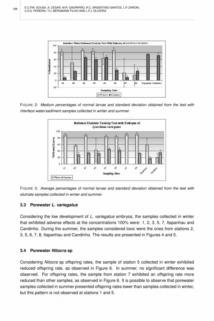
E.C.P.M. SOUSA, A. CESAR, M.R. GASPARRO, R.C. ARGENTINO-SANTOS, L.P. ZARONI,C.D.S. PEREIRA, T.U. BERGMANN FILHO AND L.F.J. OLIVEIRA
FIGURE 2: Medium percentages of normal larvae and standard deviation obtained from the test with
interface water/sediment samples collected in winter and summer.
FIGURE 3: Average percentages of normal larvae and standard deviation obtained from the test with
elutriate samples collected in winter and summer.
3.3 Porewater L. variegatus
Considering the low development of L. variegatus embryos, the samples collected in winterthat exhibited adverse effects at the concentrations 100% were: 1, 2, 3, 5, 7, Itapanhau andCandinho. During the summer, the samples considered toxic were the ones from stations 2,3, 5, 6, 7, 8, Itapanhau and Candinho. The results are presented in Figures 4 and 5.
3.4 Porewater Nitocra sp
Considering Nitocra sp offspring rates, the sample of station 5 collected in winter exhibitedreduced offspring rate, as observed in Figure 6. In summer, no significant difference wasobserved. For offspring rates, the sample from station 7 exhibited an offspring rate morereduced than other samples, as observed in Figure 6. It is possible to observe that porewatersamples collected in summer presented offspring rates lower than samples collected in winter,but this pattern is not observed at stations 1 and 5.
198

SEDIMENT QUALITY OF THE SANTOS ESTUARINE SYSTEM
FIGURE 4: Average percentages of normal larvae and standard deviation obtained from the test with
porewater samples collected in winter.
FIGURE 5: Average percentages of normal larvae and standard deviation obtained from the test with
porewater samples collected in summer.
FIGURE 6: Medium tax of offspring and respective pattern deviations obtained from the test with porewater
samplesin winter and summer.
199

E.C.P.M. SOUSA, A. CESAR, M.R. GASPARRO, R.C. ARGENTINO-SANTOS, L.P. ZARONI,C.D.S. PEREIRA, T.U. BERGMANN FILHO AND L.F.J. OLIVEIRA
3.5 Whole sediment Tiburonella viscana
The acute test with the amphipod T. viscana exhibited toxicity at station 7 and reduced survivalat station 4, collected in winter, and stations 3 and 5, collected in summer. The results obtainedin both seasons are presented in Figure 7. According to these results, the survival percentageof adults amphipod in relation to the sediment evaluated was higher in samples collected inwinter than samples collected in summer.
FIGURE 7: Medium survivor for amphipod T. viscana and standard deviation in sampling stations collected
in winter and summer.
3.6 Whole sediment Nitocra sp
The chronic test with Nitocra sp exhibited reduced offspring rates in samples of stations 2, 3and 6 in relation to other samples collected in winter, although no significant difference was ob-served between samples collected in summer. The results obtained in this test are presentedin Figure 8. Regarding the adverse effects presented for Nitocra sp test, it is possible to verifytoxicity in all stations, with variations on the exposure routes, end points and organisms tested.
FIGURE 8: Medium taxes of offspring and respective standard deviations obtained in whole sediment test,
winter and summer.
200

SEDIMENT QUALITY OF THE SANTOS ESTUARINE SYSTEM
3.7 Toxicity frequencies
Figure 9 shows the frequency of each studied area. Toxicity was more often verified at sta-tions 2, 3, and 5. These stations are situated near the container terminal at Porto Channel;at Largo Santa Rita, between Bagre and Barnabe Islands and COSIPA Channel, respectively(Figure 9). According to Abessa (2002), higher concentrations of Cd, Hg and Zn were de-tected in samples of sediment from station in region 3. The region of station 2, according toNishigima 2001, presents PAHs concentrations between 1.38 and 2.91 µg g−1 and some aro-matic compounds presenting values higher than PEL (Probably Effect Level), such as Criseno,Fluoranteno and Pireno.
FIGURE 9: Toxicity frequencies in samples from studied areas.
According to Lamparelli et al. 2001, in the region of station 3, Largo de Santa Rita, higherlevels of Hg were detected in samples of sediment and the total PCBs incorporated to fishwere above the established limit for human consumption. The regions of stations 4 and 5 areareas influenced by industrial discharges, and are highly contaminated by PAHs and metals(Cesar et al. 2006). Station 6, located in Largo da Pompeba, presented moderate toxicityfrequency. However, the chemical contaminant level, except for Cd, is not high. However,according to Lamparelli et al. 2001, this area receives a significant amount of drainage watercontaminated by sewage, which could explain the higher frequency of toxicity.
According to Medeiros (2000), Medeiros and Bicego (2004), who quantified biochemical in-dicators at sewage in estuary and Santos bay, the Largo do Pompeba region presents LABs
201

E.C.P.M. SOUSA, A. CESAR, M.R. GASPARRO, R.C. ARGENTINO-SANTOS, L.P. ZARONI,C.D.S. PEREIRA, T.U. BERGMANN FILHO AND L.F.J. OLIVEIRA
(Linear aquilbenzeno) values similar to the values observed at the end of the outfall in SantosBay. This value was attributed to the introduction of domestic sewage in natura from slumand wood stacks at the margin of the entire region and from the garbage deposit of Alemoa.Although that compounds might not be to blame, many others could be responsible for thetoxicity found in that region. The samples from stations 1, 7 and 8 in external areas of theestuarine system present lower frequency of toxicity and, according to Abessa and Sousa(2001), these areas presented moderate or inexistent levels of degradation.
Our results were in accordance to Abessa (2002), Cesar et al. (2006) and Sousa et al. (2007)that considered the superior portion of the estuarine system critical. In the present study,the area with higher toxicity was found at stations 2, 3 and 5. Those areas were considereddegraded while stations 6 and 7 presented moderate degradation. The seasonal variationon toxicity results could be explained in part by the terrestrial drainage runoff in summer,which caused the increasing uptake of contaminants. In the estuary, the salinity is anotherfactor that controls the availability of contaminants between sediment, interstitial water andoverlying water, and the time of balance between these compartments varies due to the type ofsediment and the time of overlying water remain. The rise of salinity intensifies the removal oforganic matter dissolved in the sediment, forming the particulate organic matter that probablyintensifies the sorption of hydrophobic chemicals from water to sediment.
Metals like Cd and Zn could diminish the sorption process with the organic particulate matterin higher salinities, increasing the availability in the water phase (Chapman and Wang 2001).The distribution of chemicals in sediment can also be related to the type of grain. Localhydrodynamics conducts the distribution of superficial particles in sediment, and, therefore,the distribution of contaminants and the bioavailability of them inside the estuary.
4 CONCLUSIONS
The higher incidence of toxicity was observed in the tests carried out with sediment samplesfrom Santos and Piacaguera Channels due to the accumulated contaminants in concentra-tions higher than those observed in the water column, which produced negative acute andchronic effects as mortality and reduced offspring.
Considering the previous pollution in this compartment and the variations on terrestrial drai-nage runoff, industrial and domestic sewage inputs, hydrodynamics and dredged process, thebioavailability and effects of contaminants in the sediment of this estuary could be considereda dynamic process, that should be monitored constantly as part of an integrated costal zonemanagement.
REFERENCES
Abessa DMS (2002) Avaliacao da qualidade de sedimentos do Sistema Estuarino de Santos, SP, Brasil.Tese de Doutorado. Universidade de Sao Paulo Instituto Oceanografico. 290p.
202

SEDIMENT QUALITY OF THE SANTOS ESTUARINE SYSTEM
Abessa DMS, Sousa ECPM (2001) Preliminary studies on the acute toxicity of marine sediments collectedclose to the sewage outfalls from Baixada Santista, SP, Brazil. In: Anais do 1º Congresso Brasileirode Pesquisas Ambientais. 03 de setembro de 2001. Santos, SP. CD-Rom, pp.59-61
Abessa DMS, Sousa ECPM, Tommasi LR (1998) Algumas consideracoes sobre o emprego da Trıade deQualidade de Sedimento no estudo da contaminacao marinha. Relatorio Tecnico da Revista Brasileirade Oceanografia 42: 1-12
Abessa DMS, Scott Carr R, Rachid BRF, Sousa ECPM, Hortelani MA, Sarkis JE (2005) Influence of aBrazilian sewage outfall on the toxicity and contamination of adjacent sediments. Marine PollutionBulletin 50: 875-885
Abessa DMS, Sousa ECPM, Rachid BRF, Mastroti RR (2001) Sediment toxicity in Santos estuary, SP-Brazil: preliminary results. Ecotoxicological Environmental Restoration 4: 6-9
ABNT (2006b) Ecotoxicologia Aquatica - Toxicidade cronica de curta duracao - Metodo de ensaio comourico-do-mar (Echinodermata: Echinoidea). ABNT/NBR 15350:2006, 17p.
ASTM - American Society for Testing and Materials (1992) Standard guide for conducting 10 days staticsediment toxicity tests with marine and estuarine amphipods. In: Annual Book of ASTM Standards-section 11: water and environmental technology, E 1367-90. Philadelphia, ASTM, p.1083-1115
Boldrini CV, Navas-Pereira D (1987) Metais pesados na Baıa de Santos e Estuarios de Santos e SaoVicente: Bioacumulacao. Ambiente 1: 118-127
Bonetti C (2000) Foraminıferos como bioindicadores do gradiente de estresse ecologico em ambientescosteiros poluıdos. Estudo aplicado ao sistema estuarino de Santos - Sao Vicente (SP, Brasil). Tesede Doutorado. Universidade de Sao Paulo, Instituto Oceanografico. Sao Paulo. 229p + anexos.
Cesar A, Choueri RB, Riba I, Morales-Caselles C, Pereira CDS, Santos AR, Abessa DMS, DelValls TA(2007) Comparative sediment quality assessment in different littoral ecosystems from Spain (Gulf ofCadiz) and Brazil (Santos and Sao Vicente estuarine system). Environmental International 33: 429-435
Cesar A, Pereira CDS, Santos AR, Abessa DMSA, Fernandez N, Choueri RB, Del Valls TA (2006) Eco-toxicological assessment of sediments from the Santos and Sao Vicente estuarine system - Brazil.Brazilian Journal of Oceanography 54: 55-63
Cesar A, Marın A, Marin-Guirao L, Vita R (2004) Amphipod and sea urchin testes to assess the toxicity ofMediterranean sediments: the case of Portman Bay. Scientia Marina, 68: 205-213
CETESB (1981) Metais pesados na Baıa de Santos e Estuarios de Santos e Sao Vicente. RelatorioTecnico CETESB. Sao Paulo, SP. 231p.
CETESB (1985) Baixada Santista - Memorial Descritivo. Carta do Meio Ambiente e de sua dinamica.Relatorio Tecnico CETESB. Sao Paulo, SP. 33p.
CETESB (1999) Agua do mar - Teste de toxicidade cronica de curta duracao com Lytechinus variegatusLamarck, 1816 (Echinodermata: Echinoidea). Norma Tecnica L5.250. Sao Paulo, CETESB, 16p.
Chapman PM (1992) Pollution status of North Sea sediments - an international integrative study. MarineEcology Progress Series 91: 313-322
Chapman P, Wang F (2001) Assessing sediment contamination in estuaries. Annual Review. Environ-mental Toxicology and Chemistry 20: 3-22
Environment Canada (1992) Biological test method: Fertilization assay using echinoids (sea urchins andsand dollars), amended November 1997. EPS 1/RM/27. North Vancouver, BC.
Fulfaro VJ, Requejo CS, Landim PMB, Fulfaro R (1983) Distribuicao de elementos metalicos nos sedi-mentos da Baıa de Santos, SP. In: Simposio Regional de Geologia, 4. 1983. Atas. Sao Paulo/SP,Sociedade Brasileira de Geologia, p.275-289
Lamberson JO, Dewitt TH, Swartz RC (1992) Assessment of sediment toxicity to marine benthos. In:Burton GA (ed.) Sediment Toxicity Assessment. Chelsea: Lewis Publishers. P.183-211
Lamparelli ML, Costa MP, Prosperi VA, Bevilacqua JE, Araujo RPA, Eysink GGL, Pompeia S (2001) Sis-tema Estuarino de Santos e Sao Vicente. Relatorio Tecnico CETESB. Sao Paulo. 178p.
203

E.C.P.M. SOUSA, A. CESAR, M.R. GASPARRO, R.C. ARGENTINO-SANTOS, L.P. ZARONI,C.D.S. PEREIRA, T.U. BERGMANN FILHO AND L.F.J. OLIVEIRA
Lotufo GR, Abessa DMS (2002) Testes de toxicidade de sedimento total e agua intersticial estuarinosutilizando copepodes bentonicos In: Nascimento IA, ECPM Sousa, MG Nipper (eds). Metodos emEcotoxicologia Marinha: Aplicacoes no Brasil. Ed. Artes Graficas e Ind. Ltda. 262p.
Medeiros PM (2000) Avaliacao da origem de hidrocarbonetos em sedimentos marinhos de Santos eSao Sebastiao, utilizando-se hidrocarbonetos marcadores geoquımicos. Dissertacao de Mestrado.Universidade de Sao Paulo, Instituto Oceanografico. Sao Paulo. 102p.
Medeiros P, Bıcego MC (2004) Investigation of natural and anthropogenic hydrocarbons inputs in sedi-ments using geochemical markers. I. Santos, SP - Brazil. Marine Pollution Bulletin 49: 761-769
Melo S, Abessa DMS (2002) Testes de toxicidade com sedimentos marinhos utilizando amphipodosbentonicos. In: Nascimento IA, ECPM Sousa, MG Nipper (eds). Metodos em Ecotoxicologia Mar-inha: Aplicacoes no Brasil. Ed. Artes Graficas e Ind. Ltda. 163-178p.
Montone RC (1987) Hidrocarbonetos clorados no litoral do Estado de Sao Paulo. Dissertacao de Mestra-do. Universidade de Sao Paulo, Instituto Oceanografico. Sao Paulo, SP. 102p.
Nishigima FN, Weber RR, Bıcego MC (2001) Aliphatic and aromatic hydrocarbons in sediments of Santosand Cananeia, SP, Brazil. Marine Pollution Bulletin 42: 1064-1072
Oxford References (1990) A concise dictionary of chemistry. New York: Oxford University Press, 111p.
Prosperi VA, Eysink GGJ, Saito LM (1998) Avaliacao do grau de contaminacao do sedimento ao longo docanal de navegacao do porto de Santos. Relatorio Tecnico CETESB. Sao Paulo, SP. 33p + anexos.
Rachid BRF (2002) Avaliacao ecotoxicologica dos efluentes domesticos lancados pelos sistemas dedisposicao oceanica da Baixada Santista. Tese de Doutorado. Universidade de Sao Paulo, Insti-tuto Oceanografico. Sao Paulo, SP. 286p.
Sousa ECPM, Abessa DMS, Rachid BRF, Gasparro MR, Zaroni LP (2007) Ecological assessment ofsediments from the Port of Santos and the disposal sites of dredge material. Brazilian Journal ofOceanography 55:75-81
Swartz RC, DeBen WA, Jones JKP, Lamberson JO, Cole FA (1985) Phoxocephalid amphipod bioassay formarine sediment toxicity. In: Symposium on Aquatic Toxicology and Hazard Assessment, 7, Philadel-phia, ASTM, p.284-307
Swartz RC, DeBen WA, Sercu, KA, Lamberson JO (1982) Sediment toxicity and the distribution of theamphipods in Commencement Bay, Washington, USA. Marine Pollution Bulletin 13:359-364
Tommasi LR (1979) Consideracoes ecologicas sobre o Sistema Estuarino de Santos, Sao Paulo. Tesede Livre Docencia. Universidade de Sao Paulo, Instituto Oceanografico. Sao Paulo. 2vols.
Tommasi LR (1985) Resıduos de praguicidas em aguas e sedimentos de fundo do sistema estuarino deSantos (SP). Ciencia e Cultura 37: 1001-1012
USEPA - United State Environmental Protection Agency 1991. Short-term methods for estimating thechronic toxicity of effluents and receiving waters to marine and estuarine organisms. Klemm D, GEMorrison, TJ Norberg-King, WH Peltier, MA Heber (eds.). U.S.EPA Report EPA/600/4-91/003. Ohio,Cincinnati, 579p.
USEPA (1995) Short-term methods for estimating the chronic toxicity of effluents and receiving waters towest coast marine and estuarine organisms. EPA/600/R-95-136. Cincinatti, Ohio.
USEPA (2002) Methods for Measuring the AcuteToxicity of Effluents and Receiving Waters to Freshwaterand Marine Organisms. Fifth Edition. October 2002
Weber RR (1981) Hidrocarbonetos no ambiente marinho - aspectos analıticos ambientais. Tese deDoutorado. Universidade de Sao Paulo, Instituto Oceanografico. Sao Paulo. 178p.
Winger PV, Lasier PJ (1991) A vacuum-operated pore-water extractor for estuarine and freshwater sedi-ments. Archives of Environmental Contamination and Toxicology 21: 321-324
204

PERSPECTIVES ON INTEGRATED COASTAL ZONE MANAGEMENT IN SOUTH AMERICAR. NEVES, J.W. BARETTA AND M. MATEUS (EDS.), IST PRESS, 2008
SOCIO-ECONOMIC ISSUES IN THE SANTOS ESTUARY
A.F.P. SAMPAIO AND J.M.S. FERREIRA
1 INTRODUCTION
This chapter presents the main aspects of the socioeconomic issues in the Santos and SaoVicente estuarine systems which have been addressed in the Ecomanage project. In closecooperation with the stakeholders two socioeconomic issues were selected for implementa-tion with the analysis methodologies developed in this project. In light of the fact that highpopulation density and ”urban sprawl” in metropolitan areas are usually the consequence ofnumerous drivers, this work sought to identify indicators that could mirror the basis of thesemetropolitan socio-economic conditions and identify the pressures associated with them. Thus,information was sought on population growth rate and density, economic activities in the regionand the characteristics of its sanitation infrastructure for water and sewage.
2 STUDY REGION
The study area encompasses five municipalities that comprise the Baixada Santista metropoli-tan region, formed by nine coastal municipalities, whose socioeconomic activities take place inthe Santos and Sao Vicente estuarine systems (Figure 1). The municipalities of Santos, SaoVicente, Cubatao, Praia Grande and Guaruja all fall in the study area; the two latter munici-palities have only part of their territory in this drainage basin. At the continental rise of Serrado Mar, the cities of Santo Andre and Sao Bernardo do Campo, two cities of the metropolitanregion of Sao Paulo, also fall within this drainage basin. However, as this area lies in the Serrado Mar State Park, where any development activity is forbidden, these cities were excludedfrom the socioeconomic analyses presented here.
3 METHODOLOGY
A wide-ranging literature search was carried out and an analysis of secondary data from cen-sus surveys was completed by an extensive information and data gathering campaign with themunicipal administrations of all five municipalities. All the information obtained was convertedinto a GIS format at a scale of 1:50,000. A year-long preliminary study comprised successivefield visits, along with participation in countless regional and state discussion fora, such asenvironmental councils, public hearings, regional and health development seminars and par-ticipation in meetings with representatives of the various sectors active in the region, amongthem industry representatives, hydrographic basin committees, port management, Agenda 21,coastal management, among others. This work helped in the identification of stakeholders andin the holding of consultative meetings by the project’s staff with these stakeholders to dissem-inate the DPSIR approach. These meetings, described by Belchior et al. (this volume) from
205

A.F.P. SAMPAIO AND J.M.S. FERREIRA
the first turned out to be effective for making an informed choice from the many socioeconomicissues existing in the region and in obtaining clear answers from the stakeholders concerningtheir management needs and -weaknesses in tackling these issues. This approach providedthe project with the much needed support to focus on two important socioeconomic driversassociated with the lack of urban infrastructure which were chosen for the implementationof the Ecomanage methodologies of integrated coastal analysis and the management toolsdeveloped in the project.
The second step was to perform a prospective analysis of socio-economic development forthese two drivers based on historical trends and on an assessment of the current trend in theprivate as well as in the public sector. To that effect, demographic projections were made forthe five cities. Also an analysis was carried out of the main projects foreseen by private andgovernmental organisations.
FIGURE 1: The Santos study area.
4 SOCIO-ECONOMIC DRIVERS OF CHANGE
Due to the presence of a large industrial agglomeration around the largest Brazilian port andthe existing high rate of urbanization, there is a huge variety of issues with environmentalaspects that could be studied in the region; however, the preliminary studies and the existingsecondary data, reinforced by the needs of the stakeholders, expressed during the forums in
206

SOCIO-ECONOMIC ISSUES IN THE SANTOS ESTUARY
the second year of the project, indicated two high-priority study subjects: (1) Housing issuesrelated to the existence of a large number of illegal and ramshackle dwellings on river banksand along estuarine channels, and (2) sanitation issues related to the diffuse discharge ofdomestic sewage.
In order to correctly forecast the development of these problem areas, other drivers of changesuch as population growth and urban, industrial and port development were taken into accountso that local actors could eventually be provided with comprehensive information on the futuredevelopment of these scenarios. The following sections describe the history of urban develop-ment in the region up to the present, the current demographic profile as population growth rate,demographic density, urban infrastructure and prospective analysis of the selected scenarios.
4.1 Historic evolution of urban development in Santos
Marked socioeconomic development of the region started in the late nineteenth century, drivenby the growth of the coffee economy linked to the Port of Santos. The expansion of the coffeetrade - in the early twentieth century - made the Port of Santos the largest port exporting thisproduct. Thus, the city of Santos had an important role as broker of this operation’s financialand commercial activities. This greatly stimulated the urbanization and development of Santosearly in the twentieth century and the city needed improvements in infrastructure. Immigrationat this time was important too, because a good number of the immigrants that arrived in thecountry via the Port of Santos settled there, enhancing population growth (Figure 2), but alsoworsening the environmental conditions on account of the scarcity of sanitation infrastructureand -services (Silveira 1994).
The historical landmark of sanitary investment at that time was Saturnino de Brito’s projectwith the construction of drainage channels all over the insular area of Santos, started in 1910.This system, still in working condition today, was projected to cater for a resident populationof 150,000 inhabitants (AGEM 2001), that suffered from the lack of basic sanitation as well asfrom the health and death problems associated with it.
In 1947, with the construction of a highway connecting the coast with the highlands of SaoPaulo, followed by the implementation of the car industry in the sixties, Santos started beingstrongly pressed by the leisure and tourism industry. This momentum was a change for theentire region, making it a tourist center for the capital and the whole state of Sao Paulo. Thetourism industry accounted for changing dramatically - and in a very short period of time - thewhole spatial and urban configuration of the region. The city started experiencing increasingdemands for vacation housing, services and associated commerce. This occurred with suchintensity in Santos that in the late sixties the city lived through urban saturation phenomenathat would make for a change in the demographic, economic and social patterns in the seven-ties (AGEM/EMPLASA 2002). At that time the degree of urbanization of Santos was already95% (Young and Fusco 2006) and its population over 260,000 people (Jakob 2003).
207

A.F.P. SAMPAIO AND J.M.S. FERREIRA
FIGURE 2: Population growth in Santos (1940 to 2000).
Simultaneously, between 1953 and 1954, the city of Cubatao, the only city in the region nothaving beaches and therefore not counting on the benefits of the tourism industry, startedattracting industry thanks to the proximity of the estuary, of the Port of Santos but mainlythanks to the abundance of water and electricity provided by the Henry Borden hydroelectricplant opened in 1933 and expanded in 1955. With the decision of building the PresidenteBernardes refinery, the supply of raw materials produced by that company induced the set-tlement of a series of other industries, making the region a strongly integrated petrochemicalcomplex, followed later on by the construction of Companhia Siderurgica Paulista (Cosipa)and industries of the chemical sector, including fertilizers. Thus, the development and theexpansion of industrial activities accounted for economic growth and increasing job supply,attracting a large number of migrants in search of job opportunities from other regions of thecountry, chiefly Bahia, Minas Gerais and Sao Paulo’s countryside. Therefore, Cubatao’s ur-ban population which was only 1,887 inhabitants strong in 1940, grew to 78,327 inhabitantsin 1980. However, after some time, the serious effects of air and water pollution by theseheavy industries, unencumbered by pollution control policies at the time - worsened by thetopographical and climate characteristics of Cubatao - turned this scenario of economic de-velopment into one of the most serious environmental problems of the Southern Hemisphere.Cubatao came to be regarded as the most polluted city in the world in the eighties.
From 1950 - with the beginning of industrialization in Cubatao and the increase of tourism,made possible by the construction of the Anchieta highway - to the eighties, population growthstrongly changed the region. Housing went high-rise, following in the footsteps of the demo-graphic growth in the insular part of Santos and Sao Vicente and consequently the saturationof available areas, causing a great urban agglomeration to emerge, mainly in the up-marketareas close by the sea. Due to the city of Santos’ physical limits in its insular portion, to thehigh costs close to the beach avenue and the weakness of the land on the city’s hills, thelow-income population migrated to the peripheral zones of the city and to the neighboringmunicipalities (Jakob 2004). This characteristic of the urban consolidation of Santos, driven
208

SOCIO-ECONOMIC ISSUES IN THE SANTOS ESTUARY
by the scarcity and consequent increase in the cost of land, made young families look else-where for places more within their means. This natural flow, characteristic of many big citiesin development produced three migratory vectors surging from Santos, still going on today.
The first is toward insular and continental Sao Vicente and its closest neighbor, Praia Grande,the second is toward Cubatao and the third toward the district of Vicente de Carvalho inGuaruja. These migratory vectors were identified by Jakob (2003) as having occurred since1980. However, the urban expansion in the region was also accompanied by the developmentof countless low-grade (slums) and clandestine lot division. The places chosen for this kind ofoccupation were the environmentally weakest areas such as mangrove areas and river banks,difficult to access and completely lacking infrastructure. The growth of these clandestine set-tlements occurred in a haphazard way and worsened even more in the following decades,during periods of economic recession and unemployment that occurred all over the BaixadaSantista metropolitan region.
From the second half of the seventies a new process of expanding demand for both portand port-associated services - concentrated in Baixada Santista - was stimulated by the eco-nomic expansion occurring in the state of Sao Paulo, making the Port of Santos undergo deepchanges and become the largest port for commercial cargo in the country. However, into theeighties, despite the improvement in road access with the construction of a new highway, in-dustrial development lagged behind. The negative economic impacts of the crisis and theeconomic policy of that period caused a remarkable reduction in economic growth. The highdegree of environmental pollution - forcing environmental protection agencies to tighten con-trol over the industries - made the petrochemical complex lose new investments, (shifted toother parts of the country) despite its excellent location. These events directly affected thewhole of the region, causing unemployment and underemployment with strong impacts in theregional urban space (AGEM/EMPLASA 2002).
The conjunction of all of these factors at the time made the cities suffer a tremendous pro-cess of environmental degradation and loss of quality of life owing to industrial and domesticpollution, the latter caused by the great urban agglomeration in the insular area and the ap-pearance of several low-grade settlements in the peripheral zones. Consequently, a greatnumber of tourists went on to look for other coastal regions as holiday destinations. Thisforced the state government and the city of Santos to start an improvement program aimedat recovering the tourist potential that the city was losing. Following local political pressure,a state sanitation program was started in the peripheral zones that host the largest numberof low-grade settlements; however this action was not enough to serve all of the existing low-income nuclei that were settled between the seventies and nineties (Young and Fusco 2006),and that still subsist today.
Studies carried out by Jakob (2003) show that currently the region goes through a period ofgreat change in its population dynamics, marked by a deceleration in the growth rate and bythe emergence of an urban metropolitan structure, in a phase of consolidation on the insular
209

A.F.P. SAMPAIO AND J.M.S. FERREIRA
portion of the cities of Santos and Sao Vicente (Young and Fusco 2006). These trends how-ever can be slightly altered or accelerated since there is evidence of a resurgence in economicgrowth, both country-wide and regional, marked by significant investments in real estate, har-bour development and industry, all known to be urban growth and development fosterers.However, it is also extremely difficult to predict with any degree of certainty what the impactsof this new age of investments will be. Therefore, what has been done was to make someconsiderations and inferences based upon historical trends that have affected this region.
From this point of view, based on the process of occupation and development marked by the in-sular area’s urban consolidation, peripherization of the region and this new economic momen-tum, qualitative and quantitative analyses of the agents, current and future socio-economicpressures on the environment were carried out. Besides, a drive to design prospective sce-narios on regional development took place including demographic projections for the five cities,along with an analysis of public and private projects related to existing low-grade settlementsand the expansion of basic sanitation services in the region. Both analyses were performedfor a time horizon up to 2015, the year in which some of these cities prepare to present the re-sults of the actions towards reaching the goals set out in the ”Millennium Development Goals”,a UN program for sustainable development of cities (SEADE 2005).
4.2 Demographic Profile
Among the five towns of the estuary region, Santos is the town with the largest number ofinhabitants and with the largest territorial area, followed by Sao Vicente, that holds the greatestpopulation density per square kilometer, according to the last Census in 2000 (Fig.3). Thesefive cities, according to the demographic census, house 72% of total about 1,500,000 peoplefrom the entire Baixada Santista metropolitan region and all of them have over 100,000 andfewer than 500,000 inhabitants (Table 1).
The fact that these cities are completely urbanized, only separated by natural barriers, suchas rivers, hills, mangrove areas and estuarine channels indicates that the insular area of San-tos and Sao Vicente, characterized by high demographic density (Figure 3) due to the hugeexisting population agglomeration, cannot grow significantly any more. Nevertheless, in thecase of Sao Vicente, while in the insular part the population only went from 221,296 inhabi-tants in 1991 to 225,873 inhabitants in 2000, in the continental area, the population had anextraordinary growth, jumping from 47,322 inhabitants in 1991 to 77,678 inhabitants in 2000,thus growing at a 5.66% annual rate. This rate far surpasses the region’s average growthrate, explaining the great expansion observed in the urban area of Vicente, located on thecontinental side and showing the region’s heterogeneity.
4.3 Slum-housing
A great number of illegal low-grade human settlements (slums) exist in the region. Thereis a significant portion of people living on palafittes and many of them have settled on the
210

SOCIO-ECONOMIC ISSUES IN THE SANTOS ESTUARY
river banks and in extensive mangrove areas (PRIMAHD 2005, IBGE 2000) of the coast plainwithout any control from the public office. According to census data (IBGE 2000) along withthe most recent municipal surveys, 20% ofthe population in the Santos - Sao Vicente estuarydrainage basin lives in illegal housing (Table 2). Most of these illegal human settlements haveover 1,000 inhabitants (Figure 4). In the city of Santos, 60% of low-grade settlements havethis characteristic and in Sao Vicente, 100% can be found like this (Young and Fusco 2006).
Due to the fact that they are illegal, and thus officially do not exist these settlements haveno proper water and sewerage servicing and due to the fact that they are found in mangroveareas and river banks, considerable volumes of domestic effluents are being drained directlyinto the estuary (Table 3). Thus, the in-natura dumping of this domestic sewage into channels,rivers and the sea of the region is a (potential) source of estuarine pollution (CETESB 2001)and consequently very likely of health problems for people, especially for children from 1 to 10years old who use the estuarine water for leisure and recreation (Figure 5).
FIGURE 3: Demographic density of Santos - Sao Vicente estuary (Source: IBGE 2000)
4.4 Health
Child mortality is one of the most used indices to evaluate the health conditions of a population.The five towns lowered their child mortality rate between 1995 and 2000 (Figure 6); however,all the towns with the exception of Santos had higher child mortality rates than the averagerate in the whole state of Sao Paulo (RMBS 2007). It was also observed that the child mortalityrates of the five cities showed large fluctuations which deserve special attention in the treat-
211

A.F.P. SAMPAIO AND J.M.S. FERREIRA
ment of this issue. Although the figures fluctuate without showing a clear trend, they do showthat the situation has worsened visibly in Santos and Sao Vicente in CETEC/CETAM (2000).Adding to this all, the results of microbiological water analyses carried out twice a year byCETESB corroborate a contamination scenario, since the quantity of coliforms found in thesesamples has not only exceeded the maximum limits but has also progressively increased inrecent years, making the prevalence of domestic sewage discharges evident (CETESB 2006,2005). Besides, two analyses of colimetric data performed all over the estuary in 2006/2007,summer and winter have also confirmed this type of estuarine contamination.
FIGURE 4: Inhabitants of illegal settlements slums/low-grade dwellings. Source: municipal data.
FIGURE 5: Children playing in the Santos estuary channel.
212

SOCIO-ECONOMIC ISSUES IN THE SANTOS ESTUARY
The abundance of faecal coliforms indicates that the estuarine waters used for leisure by apart of the population may also be contaminated by pathogens responsible for the transmis-sion of (infectious) diseases, putting this population’s health at risk. Likewise, no data fromepidemiologic research in the region was found that was associated to the current scenario ofmicrobiological contamination encountered. Consequently, it is necessary to prioritize futureworks of this nature to identify what the impact of this increasing deterioration of estuarinewater quality is on the health of these populations that frequently use these waters for leisureand may therefore run the risk of contracting diseases.
FIGURE 6: Child mortality rate (per 1,000 born alive) from 1995 to 2000.
TABLE 1: Population by city (Source: IBGE 2000).
Town Population
Santos 417,983
São Vicente 303,551
Guarujá 264,812
Praia Grande 193,582
Cubatão 108,309
Total 1,087,273
TABLE 2: People in illegal housing (slum). Source: municipal data.
City Inhabitants
Cubatão 52,863
Santos 30,724
São Vicente 86,909
Praia Grande 14,592
Guarujá 43,869
Total 228.957
213

A.F.P. SAMPAIO AND J.M.S. FERREIRA
TABLE 3: People serviced by sewerage services (Source: IBGE 2000 and SABESP)
SANITARY CHARACTERISTICS POPULATION
NOT TREATED 457,067
TREATED (ETE) 81,451
TREATED (SANTOS OUTFALL) 520,688
TREATED (PG AND GJÁ OUTFALL) 28,037
TOTAL 1,087,273
4.5 Sanitary Infrastructure
As the fast process of urban expansion in these cities was not followed by the supply of basicsanitation service, there is nowadays a great deficit of sewerage collecting network (Figure7). Through the crossing of data from the last demographic census (IBGE 2000) and fromthe Companhia de Saneamento Basico do Estado de Sao Paulo - SABESP it was possibleto estimate quantitatively and with more precision the number of people yearly attended andnot attended by domestic effluent drainage and treatment services. Thus, except for the cityof Santos, that now has 98% serviced (CETEC/CETAM 2000), from the total population ofthe five cities, 42% has no sewerage collecting network. If we consider the submarine outfallsystem in the region (where there is no primary treatment) as a final effluent disposal system,this number will account for about only 8% of the population upon counting the number ofpeople that have their effluents treated before dumping into the estuary. This data corroboratethe scenario of water contamination by domestic sewage, which seems to be one of the majorproblems for the Santos Estuarine System. The subsequent hyper-eutrophication could causegreat harm to the flora and fauna, besides being a permanent danger to public health, espe-cially for those living alongside these estuarine waters. Bringing the Santos Estuarine Systemto good sanitary conditions should therefore be a priority for local management.
5 PROSPECTIVE ANALYSIS
Prospective analyses for 2010 and 2015 were carried out to define the scenarios for urbanarea expansion and for domestic effluent sanitation services. Demographic projections of thestatus-quo were made from the history of socioeconomic development over the last decades,also taking into account the possible influence on the urban scenarios from the implementationof large industrial and harbour projects as well as from urban infrastructure projects in thisperiod.
In this sense, integration with the social actors was fundamental to learn about the currentlyexisting efforts to safeguard the socioeconomic development of the region. Projects of basicsanitation service expansion, slum urbanization as well as those from the port and industrialzone were assessed. This analysis helped to associate the current demographic trends withthose of economic development. The main projects that have already started or are in the plan-ning stage were identified, even those which are still under public discussion/analysis. Large
214

SOCIO-ECONOMIC ISSUES IN THE SANTOS ESTUARY
construction projects - as, for example, industrial plant expansion and real estate projects -were identified in the region and associated to demographic growth through the spontaneousstimulus of migratory phenomena, which are usually associated with such undertakings. Thus,this analysis aims to provide elements for some prognostics on the impact from these regionaldevelopment trends on the future quality of hydric resources in the coastal environment.
FIGURE 7: Sewerage collecting network in the Santos area.
5.1 Demographic Trends
Population growth (Table 4) in the region shows a decreasing trend with annual values below2.0% and the process of urbanization driven by the intra and inter-metropolitan migratory flowalso is slowing due to the urban consolidation of the central municipalities, Santos and SaoVicente. Hence, we can formulate two hypotheses for the population evolution in the region:
• Decrease of population growth rate and relative control of migratory flows, higher pop-ulation densities in the peripheral cities, owing to a more moderate expansion of theurban area and/or implementation of measures to restrict building on environmentally-protected areas as Serra do Mar slopes, mangrove areas and river banks.
• (Slight) increase of population growth rate due to an increase in migratory flows, fol-lowed by a process of increasing population in the peripheral cities and mainly in thecontinental area of Santos and Sao Vicente, owing to the lack of measures for controllingbuilding in environmentally-protected areas, as exemplified by past events, stimulatedby the ease of traffic access.
215

A.F.P. SAMPAIO AND J.M.S. FERREIRA
In the light of these hypotheses and of an infrastructure investment boom in the region fos-tered mostly by the growth of the national economy, some considerations could be formulated.Countless industrial and port expansion works - many of them underway now - have beenaltering the regional socioeconomic situation. Thus, it was found that the probability of thesecond hypothesis coming true is much higher than that of the first. As such, it is recom-mended to implement the measures proposed in the Coastal Management Program and itsimportant management tool, the Economic Ecological Zone Division. It is also recommendedto promote integrated solutions creating new urban designs for existing natural and urban ar-eas (Afonso 2006), since these urban areas have irregularly expanded over natural areas.Finally, demographic data show that this problem is prone to occur more strongly in the con-tinental areas of Santos and Sao Vicente, with Sao Vicente, due to the greater ease of roadaccess and the existing urban infrastructure, being the most vulnerable.
TABLE 4: Demographic projections for 2015.
Santos São Vicente Cubatão Praia Grande Guarujá total
2000 415,922 303,413 110,378 105,950 151,580 1,087,243
2015 419,681 371,563 144,954 180,678 211,737 1,328,613
balance 3,759 73,120 34,576 74,728 60,157 241,370
5.2 Sanitary infrastructure
The 2010 and 2015 scenarios of the evolution of sanitary infrastructure (Figure 8) were pro-jected based on the current and planned interventions of governmental projects and demo-graphic estimates. The 2015 scenario considers a broad project of sanitary upgrading de-veloped with the aim of eradicating the actual deficit in sewerage drainage and treatment,and improve the microbiological quality of the region’s beaches. Health indices have beenconsidered in this analysis. According to Sabesp - Companhia de Saneamento Basico doEstado de Sao Paulo - an increase in the treatment service is foreseen for the urban areasof the nine cities of Baixada Santista, among them, the study region, through the ”Projeto deRecuperacao da Qualidade Ambiental da Baixada Santista (Baixada Santista’s EnvironmentalQuality Recovery Project)” (DIARIO DO SENADO FEDERAL 2004).
The study areas of ECOMANAGE in the Santos estuary were assessed in order to estimatethe percentage of the population with and without sewerage facilities, as well as the sewagetreatment. However, it was found that in spite of the large investment, extension and impor-tance of the project for the entire region of Baixada Santista, the population that irregularlyoccupies the banks of rivers and estuary channels is not part of the population that will beaddressed in this program, but the part of the population that, while living in the urbanizedareas, have no sewerage drainage network. Therefore, actions that could address these in-formal communities were undertaken. Thus, it was also possible to identify the urbanization
216

SOCIO-ECONOMIC ISSUES IN THE SANTOS ESTUARY
processes foreseen for these illegal areas from information provided by governmental projectsand programs. Conditions for the 2010 scenario were inferred from this data (Figure 8). Fromthe population projections for the five municipalities and considering the implantation of envi-ronmental sanitation projects foreseen for the region, it was found that until 2010, the regionwill increase the percentage having access to sewerage drainage network service from 58%to 67% and for the 2015 scenario the level of servicing grows to be 89% of the population.
FIGURE 8: Evolution of sanitary infrastructure scenario for 2010 and 2015.
6 FINAL CONSIDERATIONS
Historically, the unevenness of interests created by the lack of public policies - that can setmechanisms to guarantee social welfare - associated to the region’s economic developmentresulted in the loss of precious spaces and consequently of the opportunity of offering a sig-nificant portion of the population the possibility of integrating to urban spaces where urbanservice supply is established. Thus, the approach adopted in this study is justified for set-ting a knowledge base through spatial, demographic and sanitary characterization, capable ofhelping in the understanding about the estuary’s contamination sources.
An existing deficit in sanitary service coverage is found, estimated in 42% of lack of seweragedrainage network service that includes the illegal houses and also the lack of drainage inregular urban areas. Therefore, considering the final realization of all interventions foreseenby governamental organs currently under way and demographic projections, the evolution ofthese scenarios was designed, projecting them for 2010 and 2015. It is expected that theseresults - along with the contaminant dispersion numerical modelling technique - are useful forthe understanding and the forecast of its effects and impacts on the coastal zone of the region.
217

A.F.P. SAMPAIO AND J.M.S. FERREIRA
REFERENCES
AGEM (2001) Plano Diretor de Turismo da Baixada Santista, 202p.
AGEM/EMPLASA (2002) Plano de desenvolvimento Integrado: regiao Metropolitana da Baixada Santista,91p.
Afonso C M (2006) A paisagem da Baixada Santista: urbanizacao, transformacao e conservacao. EDUSP,305p.
Belchior C, Gianesella S M F, Sampaio A (2008) Difficulties and Opportunities found during the Imple-mentation of the ECOMANAGE Project in the Santos Estuarine System, this volume.
CETEC/CETAM (2000) (Centro Tecnologico de Lins - SP / Centro Tecnico de Engenharia Ambiental).Minuta Preliminar do Relatorio de Situacao dos Recursos Hıdricos da UGRHI7. Comite da BaciaHidrografica da Baixada Santista, Relatorio Zero, 238p.
CETESB (2001) Relatorio do Programa de Controle da Poluicao no Sistema Estuarino de Santos e SaoVicente (PROCOP). Companhia de Tecnologia de Saneamento Ambiental, Sao Paulo. 178p.
CETESB (2005) Relatorio de Qualidade de aguas litorıneas. Companhia de Tecnologia de SaneamentoAmbiental, Sao Paulo. 254p.
Diario do Senado Federal. ”Resolucao 09, de 2004”. Republica Federativa do Brasil, ano LIX, n°.095,junho, 2004, pp. 17840-14841
IBGE Censo Demografico (2000) Agregado de Setores Censitorios dos Resultados do Universo, InstitutoBrasileiro de Geografia e Estatıstica-IBGE, 2000
Jakob A A E (2003) Analise Socio-Demografica da Constituicao do Espaco Urbano da Regiao Metropoli-tana da Baixada Santista no perıodo 1960-2000. Tese de Doutorado apresentada ao Programa deDoutorado em Demografia do Instituto de Filosofia e Ciencias Humanas da Universidade Estadual deCampinas sob a orientacao do Prof. Dr. Jose Marcos Pinto da Cunha. Campinas, SP: [s.n.].
Jakob A A E (2004) As mudancas socio-espaciais na Ilha de Sao Vicente nos anos 1990 e a possibilidadede novas regionalizacoes por meio de analises intra-urbanas. XIV Encontro Nacional de EstudosPopulacionais, ABEP, MG, Brasil.
PRIMAHD (2005) Programa Regional de Identificacao e Monitoramento de Areas de Habitacao Descon-forme da R.M.B.S. AGEM. Relatorio Final. 565p.
RMBS (2007) Regiao Metropolitana da Baixada Santista. ” Levantamento de Informacoes” desenvolvidopela Coordenadoria de Planejamento e Avaliacao (CPA) e pela Unidade de Assessoria Economica(UAE) com a colaboracao da Agencia Metropolitana da Baixada Santista (AGEM), a partir do trabalhosobre Economia Regional Paulista elaborado pela UAE. (www.planejamento.sp.gov.br
SEADE (2005) Relatorio Estadual de Acompanhamento dos Objetivos de Desenvolvimento do Milenio -2005. Imprensa Oficial de Sao Paulo. 61p.
Silveira D (1994) Valorizacao do centro historico de Santos. Santos: UNISANTOS, 1994. Trabalho Finalde Graduacao Apresentado na Faculdade de Arquitetura Urbanismo.
Young A.F., Fusco W. (2006) Espacos de Vulnerabilidade Socio-Ambiental para a populacao da BaixadaSantista: identificacao e analise de areas crıticas. XV Encontro Nacional de estudos Populacionais,Caxambu, MG.
218

PERSPECTIVES ON INTEGRATED COASTAL ZONE MANAGEMENT IN SOUTH AMERICAR. NEVES, J.W. BARETTA AND M. MATEUS (EDS.), IST PRESS, 2008
THE BAHIA BLANCA ESTUARY: AN INTEGRATED OVERVIEW OF ITSGEOMORPHOLOGY AND DYNAMICS
M.C. PICCOLO, G.M.E. PERILLO AND W.D. MELO
1 INTRODUCTION
Estuarine dynamics are dependent on the geomorphology, freshwater input, tides and me-teorological conditions predominant in the system (Perillo 1995a,b). Based on the geomor-phological features, tidal propagation into the estuary is strongly modified and can producevariations of the tidal range along the channel and in the resulting tidal currents and resid-ual transport of salt, sediment, nutrients and contaminants. The large intertidal areas of theBahıa Blanca Estuary (Figure 1) play a major role on the physical processes that are observedin this environment. On the other hand, these same morphological features make the stan-dard measurement methodologies inadequate to control the whole system (Perillo and Piccolo1998). The objective of this chapter is to provide a general and integrated description of thegeomorphology and the physical oceanography of the Bahıa Blanca Estuary as a basis forunderstanding the biogeochemical and modelling efforts presented in other chapters of thisbook. It is based on previous reviews by Perillo and Piccolo (1999), Perillo et al. (2000, 2004),Cuadrado et al. (2004) and on data gathered since then.
2 GEOMORPHOLOGY
Argentine estuaries are concentrated along the temperate Southwestern Atlantic coast andrange from microtidal (e.g., Rio de la Plata) to macrotidal (e.g., Gallegos, Santa Cruz) (Piccoloand Perillo 1999). The Bahıa Blanca Estuary (BBE) together with Anegada Bay (Figure 1) area nearly unique case as they are atypical estuaries. They are part of the partly submergedLate Pleistocene-Early Holocene delta of the Colorado River and smaller tributaries that eitherno longer flow into the system or have disappeared altogether (Melo et al. 2003). An exampleof the historical evolution during the last 20,000 years is given in Figure 2.
BBE (Figure 1) corresponds to the northern portion of the former delta with a general triangularshape. The base of the triangle is the mouth having a width of 53 km while the length alongthe Canal Principal (the largest tidal channel) is 60 km. The modern Bahıa Blanca Estuaryextends over about 2,300 km2 andcomprises several tidal channels, extensive tidal flats (1,150km2) with patches of low salt marshes, and islands (410 km2). Owing to marked differencesin surface morphology, the area can be divided along the northern shore of Falsa Bay intoa funnel-shaped northern sector, characterized by the Canal Principal and many small tidalchannels, and a southern sector, dominated by the Falsa, Verde and Brightman bays (Perilloand Piccolo 1999).
219

M.C. PICCOLO, G.M.E. PERILLO AND W.D. MELO
FIGURE 1: Location map of the Bahıa Blanca Estuary and its relationship with Anegada Bay.
As indicated, the Canal Principal has a total length of 60 km and varies in width from about 3-4km at the mouth (22 m depth) to 200 m at the head (3 m depth); both depth and width increasealmost an order of magnitude from head to mouth (Perillo and Piccolo 1991). Like other majorchannels (bays) that flow towards the inner shelf, the Canal Principal is partly closed by amodified ebb delta (Cuadrado and Perillo 1997). The channel cross section is steep on thesides, with a U-shaped bottom having a small asymmetry to the right. Upstream of PuertoGalvan (Figure 2) the channel narrows and becomes more V-shaped with the asymmetryfollowing the meandering pattern headward (Gomez et al. 1997). At the confluence with theCanal Principal, the funnel-shaped mouth of tributary channels is turned seawards, due to theebb dominance, and up to 25-m-deep scour holes may develop (Ginsberg and Perillo 2004).
Most ebb deltas at the mouth of major channels have undergone changes (Gomez and Perillo1992); however, the original delta shape and southward orientation of the ebb channel andassociated shoals in the Canal Principal are still preserved despite strong marine dynamics.This is due to its stable connection to the northern shore and its position on top of a sill(Chasico Formation), which has reduced sediment transport and served as an anchor for theebb delta (Cuadrado and Perillo 1997). The mobility of delta shoals depends on the approachangle of tidal currents (Perillo and Cuadrado 1991), while 3D dunes in the Canal Principal andtributary channels are formed due to high current velocity and geomorphological ”traps” which
220

THE BAHIA BLANCA ESTUARY: AN INTEGRATED OVERVIEW OF ITS GEOMORPHOLOGY AND DYNAMICS
favor sedimentation (Aliotta and Perillo 1987, Gomez et al. 1997). Except for bed forms inflood-dominated channels, all 3D dunes and shoals in the BBE have ebb dominance. Sincesediment runoff from rivers is virtually absent and ebb delta characteristics impede sedimentinput from the shelf, the high concentration of suspended sediments in the estuary is due toerosion of tidal flats and island shores (Ginsberg and Perillo 1990).
The southern coast of the Canal Principal across Ingeniero White Harbour has retreated up to50 m between 1980 and 1986 and 1.5 million m3 were exported from an 8-km stretch in themid-reach of the channel (Perillo and Sequeira 1989). However, the dredging of the harbourand navigation channel to a nominal depth of 45’ (13.5 m) in 1989-1990 affected most of thetidal flats located along large portions of the southern coast of the Canal Principal. The tidalflats have become Spartina marshes in about 3 years time after the dredging. At the presenttime, there are indications that the Spartina marshes are now in an incipient erosional stage,probably due to lack of sediment input.
Because most sediment in the estuary are silts and clays (Gelos et al. 2004), strong currentsand short slack water intervals impede their deposition in channels and on the tidal flats, whileshort, locally generated waves erode old sediments and prevent any accumulation of newones. These conditions explain the erosional stage of most of the estuary and the prevalenceof sediments from the deltaic deposition period. Furthermore, the biological and physicalinteractions in the system are rather important in the development of tidal creeks (Perillo andIribarne 2003) and play a role in the erosional processes. For instance, Minkoff et al. (2005)and Minkoff (2007) have demonstrated that crabs and plants acting together were responsiblefor eroding over 2200 m3 of sediments of a 270 Ha high marsh in 45 yrs.
3 PHYSICAL OCEANOGRAPHY
3.1 Freshwater Input
Two freshwater tributaries enter the estuary from the northern shore. The Sauce Chico River(drainage area of 1,600 km2) discharges into the Canal Principal about 3 km downstreamfrom the head of the estuary and the Naposta Grande Creek (drainage area of 1240 km2)reaches the estuary about 1 km downstream of Ingeniero White Harbour (Figure 1). Bothtributaries behave similarly in spring and summer during maximum mean rainfall but they areout of phase in autumn when the Sauce Chico River has a secondary mode (Piccolo andPerillo 1990). Although mean annual runoff flows of the Sauce Chico River and the NapostaGrande Creek are low (1.5-1.9 and 0.5-0.9 m3 s−1, respectively), runoff from the Sauce ChicoRiver may peak between 10 and 50 m3 s−1, with a recorded maximum of 106 m3 s−1 in1977, although there are other sources that indicate a maximum of 200 m3 s−1. Besidesthese major freshwater inputs, the inflows from other, smaller tributaries into the estuary areintermittent and only significant during periods of high local precipitation. However, the largestinput of freshwater, nutrients and contaminants is provided by the sewage discharges fromBahıa Blanca, Punta Alta and Ing. White cities.
221

M.C. PICCOLO, G.M.E. PERILLO AND W.D. MELO
FIGURE 2: Historical evolution of the Bahıa Blanca Estuary during the last 20,000 years.
3.2 Tides and Tidal Currents
The principal energy input into the Bahıa Blanca system is produced by a quasi-stationary,semidiurnal tidal wave. The mean tidal amplitude varies between 3.5 and 2.2 m at the headand mouth of the estuary, respectively. The amplitude to depth ratio is large in the innerreach varying from 0.09 to 1.39. Although, this ratio may appear small for the outer reachstations, it is caused by a geomorphologic difference. There is a tendency for the semidiurnalconstituents to increase from the mouth to the head of the estuary. M2 is the most impor-tant tidal component, followed by N2, S2, and K1, at Ingeniero White, Puerto Belgrano andOceanographic Tower, respectively. At the Oceanographic Tower the tide is predominantlymixed semidiurnal, but along the Canal Principal it is purely semidiurnal.
222

THE BAHIA BLANCA ESTUARY: AN INTEGRATED OVERVIEW OF ITS GEOMORPHOLOGY AND DYNAMICS
The propagation of the wave is affected by the geometry of the channels and intertidal en-vironments and islands. Reflection on the channel flanks and the head convert the originalprogressive form into a standing wave, while bottom and wall friction drain energy from thewave. The amplitude of the tidal wave increases with a decrease in depth and/or breadth of thechannel; therefore, the actual amplitude of the tide along the estuary is directly related to thebalance between friction and convergence. Thus, the Bahıa Blanca is a hypersynchronous-type estuary, where the amplitude increases steadily from the mouth to the head, implying thatthe convergence effect on the tidal wave is larger than the friction effect.
A strong reduction occurs along the Sauce Chico River, due to a frictional effect associatedwith dampening produced by river flow on one side and spreading over salt flats at the otherside. The average rate of tidal energy dissipation per unit mass of fluid due to friction is0.0017 m2 s−1 (Perillo and Piccolo 1991). Large negative dissipation rates in the outer reachof the estuary are due to differences in amplitude between the mouth (Bermejo Island) andthe head. Differences in duration between flood and ebb indicate that depth mean longitudinalcurrent velocities in the Canal Principal and other major channels are asymmetrical and largelycaused by the extensive tidal flats bordering the Canal Principal (Piccolo and Perillo 1990).The peak ebb current is about twice the maximum flood current in the upper reaches; however,the flood usually has a longer duration.
Typical velocity profiles over a tidal cycle for two stations located on a cross-section of theCanal Principal near the Ing.White Harbor are shown in Figure 3. Those profiles clearlyshow examples of flow acceleration and deceleration and the reversing condition of the flow.When tidal records are compared with the predicted astronomical tide, large differences bothin height and time are encountered. In general, winds blowing from the NW sector producea set down of the water level by pushing the surface water out. SE winds generate the op-posite effect. However, the predominant winds from the NW and N produce the greatest tidalvariations by: (a) advancing the time of low water, (b) delaying the time of high water, and (c)reducing the predicted water levels at both high and low tide (Perillo and Piccolo 1991).
Storm surges or tidal perturbations were studied employing two years (October 1983-1985) ofhourly tidal records measured at Ingeniero White and the Oceanographic Tower (Perillo andPiccolo 1991). Ingeniero White has the largest number of cases with no perturbation; however,it presents the highest deviations from the predicted tides. In 24 cases the surges were largerthan 2 m, with negative and positive peaks of - 4.01 m at low tide and 2.39 m during a fallingtide, respectively. At the Oceanographic Tower station, peak values were - 1.51 m (high tide)and 1.87 m (rising tide). In both stations the maximum negative surges coincide with windsblowing from the NW and maximum positive ones with SW winds. The latter are very intensivewinds that act over the intertidal flats as they are covered inducing a set-up against the coast.
Northern winds produce a set down of the tide while southern winds produce a set up. Whenthe wind blew from the N-NNW it caused negative mean deviations of -22 and -12 cm, mean-while WSW winds generated positive deviations of 52 and 17 cm. A simple analysis relating
223

M.C. PICCOLO, G.M.E. PERILLO AND W.D. MELO
the azimuth of the Canal Principal at Ingeniero White (129°) to the wind direction during highand low water conditions indicates that for winds blowing from the south, the storm surgeshould be positive, and negative for the northern winds. This result holds for all cases but theSE one. For SE winds, the storm surge was positive about half of the time during high tidesand unknown circumstances may have generated a modification of the behaviour.
FIGURE 3: Velocity profiles along a tidal cycle at two stations located across the Canal Principal of Bahıa
Blanca Estuary near Ing. White Harbor. a) northern station, b) southern station.
A significant relationship was also found between positive and negative time (∆t) and height(∆H) differences and the stage of the tide (Figure 4a). Considering all cases, the coincidencewas over 90%. On the other hand, if the relationship between wind and channel orientation istaken into account, for northern winds positive time differences (delay) should be associatedwith high water and negative ones (advance) with low water. The opposite occurs for thesouthern winds. However, the observations show no coincidence with the previous reasoningfor the first three groups (0 h < time < 432 h) and complete coincidence for the last one (606h < time < 668 h). In the fourth group (438 h < time < 600 h) the agreement is relative sinceonly one low tide value was negative.
Long-term changes (time scales > 10 days) of the wind over the sea level are predominant forshorter scales, the spectra (not shown here) have common energy peaks at 6.4, 4, 2.9 and 2.1days. The phase propagation from the inner estuary to the mouth for periods shorter than 16days has an average time lag of 2.5 h. The sea level fluctuations, for periods between 2.2 and
224

THE BAHIA BLANCA ESTUARY: AN INTEGRATED OVERVIEW OF ITS GEOMORPHOLOGY AND DYNAMICS
5.6 days and larger than 10 days, are normally driven by the NW and W winds, respectively.Therefore, the continental winds play a major role in generating long period variations withinthe estuary. Although both stations have similar responses to wind forcing, the wind effectis greater in the inner estuary. The differences may be associated with their particular geo-morphologic setting. The Oceanographic Tower is located in an almost open ocean situation;therefore, only when the extensive tidal flats are covered by water both stations can show sim-ilar characteristics. Nevertheless, the analysis of coherence and wind direction points out thatthe subtidal fluctuations at the Oceanographic Tower are associated with the regional windpattern at periods shorter than 7 days.
FIGURE 4: a) relationships between wind direction and height (H) and time (t) differences between real
and b) predicted tide at Ing. White Harbor.
On the other hand, at high frequencies, the wind produces two types of waves in the estuary:(a) wind waves, and (b) waves formed by the interaction of wind and tidal currents (Perillo andSequeira 1989). Small waves of about 5 to 10 cm in height, maximum wavelengths of 1 to 3m and periods of 1 to 3 s characterize the Canal Principal and the intertidal flats during hightide. Oceanic waves are only important on the coast outside the estuary and on the outerbanks. Waves generated within the channels by the interaction of the incoming tide with thewind blowing from the northern sector are extremely steep, up to 1.5 m high, with wavelengthsof the order of 10 to 30 m.
225

M.C. PICCOLO, G.M.E. PERILLO AND W.D. MELO
3.3 Salinity and Temperature
Mean annual temperature based on continuous data gathered between 2000 and 2007 atPuerto Cuatreros and Ing. White stations is 15.6 °C , with maximum and minimum regis-tered values of 29.2 °C and 3.6 °C , respectively. Longitudinal temperature distributions varybetween rainy periods in spring/summer and low runoff in winter, when the vertical thermalstructure of the estuary is homogeneous and longitudinal variations are less than 3 °CMeansurface salinity increases exponentially from the head to the middle reach of the estuary. De-pending on runoff conditions, salinity differences between the mouth and head of the estuarymay reach 17 and more than 4 between surface and bottom. At low water, haline stratifi-cation (halocline 1-3 m) may occur in areas of freshwater inflow, while salinity tends to behomogeneous in the outer estuary (Figure 5).
Salinity and temperature distribution therefore characterize the Bahıa Blanca Estuary as typela (Hansen and Rattray 1966). During normal runoff, the partially mixed inner region betweenthe mouth of the Sauce Chico River and Ingeniero White Port tends to become vertically ho-mogeneous at low runoff, while salinity patterns in the outer homogeneous region are similarto the adjacent continental shelf. The boundary between these regions depends on river dis-charge (Martos and Piccolo 1988, Piccolo and Perillo 1990).
FIGURE 5: Examples of salinity profiles at two stations of the Canal Principal of the Bahıa Blanca Estuary.
3.4 Residual Fluxes
Examples of cross-section residual fluxes at the Canal Principal near Ing. White Harbor aregiven in Figure 6 (based on the methodology developed by Perillo and Piccolo 1993, 1998).The new field and data reduction methodology insures an error-free calculation of the fluxeseven with complex cross-section morphologies. The estuary behaves mostly as vertically ho-mogeneous with residual flows directed in opposing directions. On the southern portion of the
226

THE BAHIA BLANCA ESTUARY: AN INTEGRATED OVERVIEW OF ITS GEOMORPHOLOGY AND DYNAMICS
channel the flow is headward whereas on the northern portion the flow has two layers similarto a partly mixed estuary. However, the flows are reversed as the upper layer is headward andthe lower layer seaward. Therefore, the residual circulation shows a significant difference inthe direction of mass transport, causing salt concentrations in the inner portion of the estuaryoften exceeding those of the inner continental shelf.
Figure 6 clearly shows two layers: an upper one where the residual flux is seaward (positivevalues) and a lower one with headward flux (negative values). The upper layer becomesdeeper from x = 0.6 northward indicating the influence of the center of the channel and thehigher ebb velocities found at the stations measured there. Meanwhile, the effect of the tidalflats is well demonstrated by the smaller thickness of the upper layer southward of x = 0.4.
4 DISCUSSION AND CONCLUSIONS
Bahıa Blanca Estuary displays one of the most complex sets of geomorphological and dy-namic conditions to be found on the Argentine coastline. There are major differences with thetypical river mouth estuary because of the geological conditions that created this environment.First of all, the estuary is only a part of what once was the largest delta in the country beingalmost 200 km wide at the distal point. For the sake of comparison, the Parana Delta locatedwithin the Rio de la Plata Estuary is only 45 km wide, the Nile Delta is 250 km and the NigerDelta is 400 km wide. During its geological evolution (Figure 2), it went through full fluvial andsubaerial conditions to a shallow bay-shelf with depths up to 7-10 m over the tidal flats todayand depths of more than 30 m in the outer reaches of the channels. The Flandrian transgres-sion retreated at a much slower pace than the transgression; the coast moved progressively,leaving sand bars and spits. Although there are no definitive paleontological features that canprovide hard evidence, we believe that the climatic conditions during the retreating period werealready as dry as the present one. Therefore, very little input of sediment was provided by therivers coming into the receding bay.
This supposition is derived from a comparative geomorphological analysis of Anegada Bay.After its formation, this southern portion of the Colorado Delta had very few fluvial (if any)tributaries coming into it, thus its evolution was dependent only on the input of sedimentsfrom the shelf. However, both Anegada and Bahıa Blanca have very similar geomorphologicalproperties. Normally, sediment from the shelf does not enter the estuary (most probably thesame is true for Anegada Bay, although there are no studies dealing with this subject there).
Based on the salinity and temperature distribution alone, the Bahıa Blanca Estuary is dividedin two. The inner part, from the mouth of the Sauce Chico River to Ingeniero White, is classifiedas a partially mixed estuary during normal runoff conditions, but with a strong tendency tobecome vertically and even sectionally homogeneous during low runoff. The outer part issectionally homogeneous. The boundary between both parts is transitory and depends on theriver discharge. According to the classification of Hansen and Rattray (1966), the estuary maybe characterized as Type la.
227

M.C. PICCOLO, G.M.E. PERILLO AND W.D. MELO
FIGURE 6: a) Mass and b) salt residual flux distributions at a cross-section near Ing. White Harbor on
spring tide.
The mixing regime is characterized by Ri < 2 and it is associated to strong turbulent processesduring maximum ebb and flood conditions, in particular on the northern flank of the estuary.Therefore, fully developed mixing is found almost throughout the tidal period. Stratificationis established at the beginning of the ebb cycle, being generated by the combined outflowof the river and the ebbing tide, producing a seaward tilt of the isohalines. The process isenhanced by low turbulence levels due to the small currents. As the current velocity increases,turbulent mixing also increases. During the flooding stage, the possibilities of developingany stratification are very low since the flood is driving well-mixed water from down-estuary.Turbulent mixing at midflood is high and practically constant resulting in low Ri.
The residual circulation shows a significant difference in the direction of the mass transport.On the deeper parts of the sections (northern flank) the flow reverses with depth, being head-ward near the bottom. The net transport is completely landward in the shallower parts. Thisbehaviour, added to the washing of the back estuary saline, produce a concentration of salt inthe inner portion of the estuary, resulting in salinities larger than those observed in the innercontinental shelf. Analysis by Piccolo and Perillo (1990) of the current stations located on thesouthern flank of the Canal Principal may indicate that the asymmetry of the tidal current ismainly caused by the presence of the extensive tidal flats along the channel.
REFERENCES
Aliotta S, Perillo GME (1987) A sand wave field in the entrance to the Bahıa Blanca Estuary, Argentina.Marine Geology 76: 1-14
228

THE BAHIA BLANCA ESTUARY: AN INTEGRATED OVERVIEW OF ITS GEOMORPHOLOGY AND DYNAMICS
Cuadrado DG, Perillo GME (1997) Migration of intertidal sand banks at the entrance of the Bahia BlancaEstuary, Argentina. Journal of Coastal Research 13: 139-147
Cuadrado DG, Ginsberg SS, Gomez EA (2004) Geomorfologıa. In: Piccolo MC, Hoffmeyer MS (eds), ElEcosistema del Estuario de Bahıa Blanca. Instituto Argentino de Oceanografıa, Bahıa Blanca, 29-38
Gelos EM, Marcos AO, Spagnuolo JO, Schillizzi RA (2004) Textura y mineralogıa de sedimentos. In:Piccolo MC, Hoffmeyer MS (eds), El Ecosistema del Estuario de Bahıa Blanca. Instituto Argentino deOceanografıa, Bahıa Blanca, 43-50
Ginsberg SS, Perillo GME (1990) Channel bank recession in the Bahıa Blanca Estuary, Argentina. Journalof Coastal Research 6: 999-1010
Ginsberg SS, Perillo GME (2004) Characteristics of tidal channels in a mesotidal estuary of Argentina.Journal of Coastal Research 20: 489-497
Gomez EA, Perillo GME (1992) Largo Bank: a shoreface-connected linear shoal at the Bahıa BlancaEstuary entrance, Argentina. Marine Geology 104: 193-204
Gomez EA, Ginsberg SS, Perillo GME (1996). Geomorfologıa y sedimentologıa de la zona interior delCanal Principal del Estuario de Bahıa Blanca. Revista de la Asociacion Argentina de Sedimentologıa3: 55-61
Hansen DV, Rattray M (1966) New dimensions in estuary classification. Limnology and Oceanography11: 319-326
Martos P, Piccolo MC (1988) Hydrography of the Argentine continental shelf between 38 and 42° S. Con-tinental Shelf Research 8: 1043-1056
Melo WD, Schillizzi R, Perillo GME, Piccolo MC (2003) Influencia del area continental pampeana so-bre el origen y la morfologıa del estuario de Bahıa Blanca. Revista de la Asociacion Argentina deSedimentologıa 10: 65-72
Minkoff DR, Escapa CM, Ferramola FE, Maraschin S,Pierini JO, Perillo GME, Delrieux C (2006) Effectsof crab-halophytic plant interactions on creek growth in a S.W. Atlantic salt marsh: A cellular automatamodel. Estuarine Coastal and Shelf Science 69: 403-413
Minkoff DR (2007) Geomorfologıa y dinamica de canales de marea en ambientes intermareales. Tesis deDoctorado, Departamento de Ingenierıa, Universidad Nacional del Sur, 175pp.
Perillo GME (1995a) Geomorphology and sedimentology of estuaries: an introduction. In: Perillo GME(ed), Geomorphology and Sedimentology of Estuaries. Development in Sedimentology Vol. 53, Else-vier Science BV, Amsterdam, 1-16
Perillo GME (1995b) Definition and geomorphologic classifications of estuaries. In: Perillo GME (ed),Geomorphology and Sedimentology of Estuaries. Development in Sedimentology Vol. 53, ElsevierScience BV, Amsterdam, 17-47
Perillo GME, Sequeira ME (1989) Geomorphologic and sediment transport characteristics of the middlereach of the Bahıa Blanca estuary, Argentina. Journal of Geophysical Research-Oceans 94: 14351-14362
Perillo GME, Piccolo MC (1991) Tidal response in the Bahıa Blanca Estuary. Journal of Coastal Research7: 437-449
Perillo GME, Piccolo MC (1993) Methodology to study estuarine cross-section. Revista Geofısica 38:189-206
Perillo GME, Piccolo MC, Parodi E, Freije RH (2000) The Bahıa Blanca Estuary, Argentina. In: SeeligerU, Kjerfve B (eds), Coastal Marine Ecosystems of Latin America. Environmental Science Series,Springler Verlag, Berlin 205-217
Perillo GME, Piccolo MC, Palma E, Pierini JO, Perez DE (2004) Oceanografıa Fısica del estuario de BahıaBlanca. In: Piccolo MC, Hoffmeyer MS (eds), El Ecosistema del Estuario de Bahıa Blanca. InstitutoArgentino de Oceanografıa, Bahıa Blanca, 61-67
Piccolo MC, Perillo GME, Arango JM (1987) Hidrografıa del estuario de Bahıa Blanca, Argentina. RevistaGeofisica 26: 75-89
Piccolo MC, Perillo GME (1999) Estuaries of Argentina: a review. In: Perillo GME, Piccolo MC, PinoQuivira M (eds), Estuaries of South America: their geomorphology and dynamics. EnvironmentalScience Series, Springer-Verlag, Berlin: 101-132
229


PERSPECTIVES ON INTEGRATED COASTAL ZONE MANAGEMENT IN SOUTH AMERICAR. NEVES, J.W. BARETTA AND M. MATEUS (EDS.), IST PRESS, 2008
CLIMATOLOGICAL FEATURES OF THE BAHIA BLANCA ESTUARY
M.C. PICCOLO
1 INTRODUCTION
Climate variations have significant economic and social consequences, particularly in regionswith important agricultural production, such as the Buenos Aires province. The Bahıa Blancaestuary is located in the temperate climate zone, with well-defined seasons. This implies thatthe summers and winters are rigorous and the intermediate seasons more benign. Significantspatial variations in temperatures and precipitation characterize the region. They relate toexposure to dominant air flows, orientation of the coast and presence of ocean currents. Inthe study area, there is a continuous flow of different types of air masses, which cause asignificant variability in weather conditions (Capelli de Steffens and Campo 1994).
The southwestern region of the Buenos Aires province is under the influence of semi-permanentanticyclone centers located in the Atlantic and Pacific Ocean (Figure 1a). These two majorsystems generate typical air masses and determine the dominant synoptic conditions of thearea. The Subtropical Anticyclone center of the South Atlantic originates a warm and humidflow of air from the North that affects the Argentine coast in particular in the Buenos Airesprovince. This movement is responsible for most of the rainfall in the coastal plain which char-acterizes the Bahıa Blanca estuary. The Northern flow returns to the ocean after downloadingthe rainfall in the Ventania hills and in the coastal plain south of Buenos Aires. That is whythe winds that reach the estuary from the N and NW have continental characteristics. On theother hand, the South Pacific anticyclone originates air masses that enter the Patagonia regionwith a SW-NE direction. The winds from the SW sector are always dry. Cyclonic centers flowfrom the S and SW across the Andes and then through Patagonia towards the estuary. Theconvergence of all the air masses from the Atlantic and Pacific oceans drives the formation offronts that often cause heavy rainfall. Another weather system that sometimes has influenceon the region is a low pressure center located in the NW of Argentina. This low pressurecenter reinforces the Northern circulation, causing a significant instability in the study region.
The typical climatological features and weather systems of the area are described in thischapter. The Bahıa Blanca meteorological data (38° 44’ S - 62° 10’ W) represent the weatherconditions in the inner part of the estuary and the Coronel Rosales data the outer ones. Un-fortunately, the time series are not of equal length. The Bahıa Blanca data is a time series ofalmost 100 years, but the Coronel Rosales of only 5 years (2000-2004). Significant differencesin the synoptic conditions between the internal and external sectors of the estuary were thereasons for the installation of a meteorological station in the Coronel Rosales harbor (Piccoloand Galındez 1984).
231

M.C. PICCOLO
FIGURE 1: a) Mean location of the ocean anticyclones that generate typical synoptic weather conditions
in the Bahıa Blanca estuary; b) Typical synoptic conditions during the Pampero; c) synoptic conditions for
Southeast Winds and d) Typical weather conditions for North Winds (Modified from Capelli de Steffens
and Campo 2004).
2 TYPICAL SYNOPTIC WEATHER SYSTEMS
Weather conditions are crucial for the success of numerous activities (economic, strategic,research, entertainment, etc.) carried out from the harbors. The Bahıa Blanca estuary isaffected by various synoptic weather systems which depending on their origin present differentcharacteristics. Three main weather systems are characteristic in the estuary: the Pampero(wind from the Pampas), Southeast winds (Sudestada) and the North Wind. These flows havedifferent directions and a great influence on wave height and the amplitude of the tides in theestuary.
232

CLIMATOLOGICAL FEATURES OF THE BAHIA BLANCA ESTUARY
2.1 Pampero
It is a synoptic condition that develops in the course of approximately a week, strong windsblow from the South. It is a cold, fresh or temperate wind according to the season but alwaysdry. Its speed exceeds 40 km h−1. In its initial phase precipitation frequently occurs and itis then called Wet Pampero, otherwise it is called Dry Pampero. In which case dust stormsoccur particularly in arid regions and it is characterized by the presence of fine dust, whichsignificantly affects visibility and even the health of the population. The beginning of a Pamperocoincides with the passage of a cold front.
The front is generated by two air masses. One is generated by the South Pacific anticyclone.The air mass crosses the Andes Mountains and downloads its moisture on their windwardslopes. The other air mass is originated by the South Atlantic anticyclone that dominates theArgentine plains (Figure 1b). It is a warm and wet flow from the North. In a second phase, thecold front moves toward the NE. In its flow across the southern Buenos Aires province, theatmospheric pressure increases and the relative humidity decreases. In its final stage the skyis clear, calm, and the air temperature drops significantly.
2.2 Southeast Wind (Sudestada)
Continuous precipitation and wind from the SE and E characterize this weather condition thataffects the coast of the province. Regular to strong winds from the Southeast sector blow withspeeds over 35 km h−1. It is accompanied by persistent rains and relatively low temperatures.The air mass that generates this synoptic system is a detachment from the South Pacificanticyclone that travels across the Patagonian region, favored by a high pressure systemespecially during winter and spring. The trajectory of the anticyclone is W-E and when locatedin the Atlantic Ocean off the coast of Buenos Aires province it causes serious damage (Figure1c). The strongest flows are found in the month of October with approximately one week ofcold weather and rain. The devastating effect on inhabited coastal areas is great. Coastalinundations occur, boats and buildings located on the beach are usually damaged, etc.
2.3 The North Wind
The North wind prevails in the southern Buenos Aires province. It blows more frequentlyin spring and summer, generating high temperatures, changes in atmospheric pressure anddryness in the environment. It is usually accompanied by clouds of dust and smoke fromthe fires that frequently occur in the summer in the plain regions of the province. A directconsequence is the reduction in visibility due to particulate matter, which may affect groundand air transportation. The western edge of the South Atlantic anticyclone originates thisairflow and discharges its humidity on the coast, center of the country and the pampas plain.Consequently, the South of the Buenos Aires province receives a mass of dry and warm airfrom the North that produces irritability in the population due to the excessive concentration ofpositive ions (Figure 1c).
233

M.C. PICCOLO
3 MEAN METEOROLOGICAL FIELDS
Climatological Data from the Argentine National Weather Service (S.M.N. 1992) were ana-lyzed to study the mean meteorological parameters. Rainfall shows a gradual eastward in-crease at the estuary latitude. From a total of 300 mm in Viedma - Patagones (40° 50’ S -63° 00’ W), it increases to 530 mm in Hilario Ascasubi (39° 22’ S - 62° 39’ W), 613 mm inBahıa Blanca and 841 mm in Tres Arroyos (38° 33’ S - 60° 25’ W). The distribution of rainfallreveals the influence of the Westerly winds regime that imposes characteristics of dryness onthe entire Patagonian coast. Towards the Southwest an arid continental climate is typical. Oneexample is presented in Table 1 with climatic information pertaining to El Rincon Lighthousestation located on the eastern tip of the Verde peninsula where the mean annual precipitationis 498 mm in a distinctly maritime area typical of the Bahıa Blanca estuary (S.M.N. 1941-1990).
In the estuary, the maximum rainfall values come in the months of March (90.9 mm) andOctober (80.9 mm). The minimum rainfall occurs during the winter. As a rule, June is thedriest month (16.5 mm) (Figure 2). This fact is reflected in the landscape and vegetablefarming characteristic of the region. The humidity is high for the region due to the proximity ofthe estuary. The annual average atmospheric pressure is normal, 1013.1 hPa, although 1037hPa maximum and 977.1 hPa minimum have been measured in July 2002 and in March 2001,respectively.
The thermal regime in the area shows a large difference between winter and summer, whilespring and fall present great similarity in temperature. The mean annual temperature is15.1°C with thermal annual amplitudes evidencing the moderating effect exerted by the oceanin the coastal areas (Campo and Capelli de Steffens 2000). The beginning and end of thesummers present significant rainfall and high temperatures. Winters are cold and frost occurson average about 8 days a month in June and July, dropping to 7 in August. Snowfall andfog are exceptional in the region. On average, fog may occur about 16 days a year with thehighest occurrence in winter.
The spatial and temporal variability in the precipitation is large. The precipitation is closelyrelated to increasing temperature. The thermal amplitudes decrease toward the East showinga transition from continental to ocean climate. The presence of the estuary originates lowtemperatures in its vicinity. Simultaneously, the heat island phenomenon which characterizesBahıa Blanca city causes higher temperatures inside the city. As a consequence, there aresignificant differences in temperature between Bahıa Blanca city and its periphery. The aver-age annual temperature of Bahıa Blanca is 2 °C higher than in Ing. White and 0.5 °C higherthan that obtained in the adjacent rural environment (airport station). Broadly this can be at-tributed to the influence of man-made heat generated by the city of Bahıa Blanca through itsmultiple activities (Capelli de Steffens and Piccolo 1987).
The last 100 year of temperature and precipitation analysis is presented in Table 2. Averageannual temperatures decreased up to 1950. In the following two decades, a slight increase of0.2 °C in the average temperature was found and in 1980 the temperatures increased another
234

CLIMATOLOGICAL FEATURES OF THE BAHIA BLANCA ESTUARY
0.2 °C. The seasonal distribution of temperature and precipitation show that summer andspring follow the trend of annual increases in temperature and decreases in precipitation. Therain in the summer during the 1981-90 decade only reached 70% of the total rainfall of theprevious period, but in the last decade it reached the values of the 1971-80 one once more.The mean temperatures are uniform in general but in the last decade a significant increase intemperature and precipitation was recorded.
Several singularly extreme temperatures were recorded last century. On January 21, 1980,43.8 °C was reached. This value was the absolute maximum temperature in the century, whilethe absolute minimum was recorded on July 4, 1988 at -11.8 °C during a so called ”cold wave”which lasted for thirteen consecutive days.
Another important theme is the variability of the precipitation observed in different sectorsof the estuary. The monthly rainfall varies substantially at only a few miles distance. As anexample, Figure 3 shows the monthly rainfall for the year 2001 in three locations near theestuary: Ing White harbor, Puerto Rosales harbor and Malaver lagoon located approximately8 km from Puerto Rosales harbour. In Malaver lagoon it rains more than in the other twostations and in Puerto Rosales more than in Ing. White. The analysis of the 2000-2004 periodpresented the same results (Piccolo and Diez 2004).
3.1 Winds
The winds are persistent all year round. Their annual mean velocity is 22.5 km h−1. The num-ber of days a year with strong winds is significant (196), always over 43 km h−1. An analysisof the wind speed in different periods shows a great variation (Figure 4). The decade 1971-1980 presented the highest mean values all along. The minimum mean values registered inthe period 1901-1950 can be explained by several reasons. One is the change of location ofthe weather station. It is now 83 m above mean sea level (MSL); it used to be 20 m. Obviously,this timeseries thus has a serious methodological flaw.
FIGURE 2: Relationship between Precipitation (Pp) and temperature (T). (Period 1981-1990) (Modified
from Capelli de Steffens and Campo 2004).
235

M.C. PICCOLO
FIGURE 3: Precipitation in three locations near the Bahıa Blanca estuary during the year 2001.
FIGURE 4: Wind velocities in the Bahıa Blanca estuary in different decades. (Modified from Capelli de
Steffens and Campo 2004).
Autumn is the season that presents the lowest wind velocities, whereas the end of the springand the summer present the highest. This could partly explain the disparity in records such asthe value of the beginning of the century with an annual average of 9 km h−1 which contrastsdramatically with subsequent registrations. Another reason is that the average velocity wastaken from 50 years of records, therefore the result can be affected by smoothing.
236

CLIMATOLOGICAL FEATURES OF THE BAHIA BLANCA ESTUARY
Storms are also frequent in the region. The maximum record of the century was obtained onMarch 21, 1981. West and Northwest winds reached a maximum intensity of 160 km h−1.The damage in the city was noticeable. Figure 5 shows the annual wind rose for Bahıa Blancafor the period 1981-1990 where the predominance of the Western, North, and Northwest di-rections is emphasized. Calm days only reach 10% of total registrations. Along the year theprevailing wind is from the North during all seasons. In the summer winds from the East,Southeast and South are frequent and the number of calm days is low. In autumn the fre-quency of winds increases especially from the Northwest and West with the highest velocitiesin winter. In the spring winds diminish and the prevailing directions are from the West andNorthwest.
On the other hand, the average wind speed for Puerto Rosales is 22.6 km h−1. The highestgust observed was from the SSW with 132.5 km h−1 in the year 2002. Figure 6 shows thehighest gusts recorded in the 1999 and 2002. They represent the years in which the minorand major gusts, respectively were observed. The more intense gusts correspond to windsfrom the SSW, SW, NNW and NW directions. The gusts in Puerto Rosales were greater thanthose in Ing. White for the 2000-2004 period. In both places the highest gusts were from theSW direction. Although the measurement period in the Puerto Rosales station is very short toestablish general climatic characteristics of the area however, comparison with other stationslocated in the hinterland of the estuary, made it possible to determine that Puerto Rosalespresents synoptic conditions which are much more exposed to the marine action and to themoderating effect of the sea (Piccolo 1985). The minimum Puerto Rosales temperatures weregreater than those recorded in the hinterland of the estuary and the maximum temperatureswere lower. However, the wind speed was higher than in the inner estuary region (Piccolo etal. 1989). There is similar variation in the other meteorological parameters.
4 CONCLUSION
A synthesis of the most important features of the Bahıa Blanca estuary weather conditionsis presented in this chapter. The estuary is located in a temperate climate. In the last 100years mean temperatures oscillated around 15 °C. Annual precipitation varied between 540mm and 712 mm. The spatial and seasonal variability of the precipitation is significant. Fewstudies were performed on the subject (Piccolo and Diez 2004). The winds are persistent allyear round. Their annual mean velocity is 22,5 km h−1. Strong winds, over 43 km h−1, blowover the estuary 54% of the whole year. The estuary is affected by strong winds associated todistinct synoptic weather conditions. The characteristic wind from the South, from the pampas,is called Pampero. It is associated with a cold front which crosses the estuary. The pamperois usually a dry airflow. The Southeastern wind, denominated ”Sudestada” brings rain, fog andcauses many problems to the population due to its bad weather conditions. Finally, the mostfrequent wind direction is from the North / Northwest.
237

M.C. PICCOLO
FIGURE 5: Wind Rose at Bahıa Blanca station (1981-1990). (Modified from Capelli de Steffens and
Campo 2004).
FIGURE 6: Puerto Rosales gust wind rose ( km h−1) a) in 1999; b) 2002 (Piccolo and Diez 2004).
TABLE 1: Mean annual parameters in El Rincon Lighthouse station (Capelli de Steffens and Campo 2004).
Parameter Annual Mean Values
Atmospheric Pressure (hPa) 1013.3
Temperature (ºC) 14.4
Relative Humidity (%) 73
Mean Wind velocity (km/h) 15.8
Precipitation (mm) 498.0
238

CLIMATOLOGICAL FEATURES OF THE BAHIA BLANCA ESTUARY
TABLE 2: Mean seasonal temperature and precipitation (National Meteorological Service Statistics).
Summer
Autumn
Winter
Spring
Anual
Period T
(ºC) Pp
(mm) T
(ºC) Pp
(mm) T
(ºC) Pp
(mm) T
(ºC) Pp
(mm) T
(ºC) Pp
(mm)
1901- 50 22.8 156 15.3 165 8.5 61 15.2 158 15.5 540
1951- 60 21.8 157 14.5 177 7.9 86 14.3 138 14.7 558
1961- 70 21.7 185 14.9 164 8.4 84 14.6 141 14.9 604
1971- 80 21.9 240 14.7 205 8.1 78 14.7 189 14.9 712
1981- 90 22.7 168 14.6 188 8.1 86 14.9 174 15.1 614
1990- 00 22.3 237.6 16.6 173 9.2 115.4 15.4 158.8 15.7 684.9
REFERENCES
Capelli de Steffens A, Pıccolo MC (1987) Incidencia de factores geograficos locales en las temperaturasmaximas del area de Bahıa Blanca. Revista Universitaria de Geografıa. U.N.S. 3: 1-19
Capelli de Steffens A, Campo de Ferreras A (1994) La transicion climatica en el sudoeste bonaerense.SIGEO 5. Depto. de Geog. U.N.S.
Capelli de Steffens A, Campo de Ferreras A (2004) Climatologia. En: Piccolo MC, Hoffmeyer M (eds),Ecosistema del estuario de Bahıa Blanca, Instituto Argentino de Oceanografia, pp.79-86
Campo A, Capelli de Steffens A (2000) Variaciones ombrotermicas en el Sur de la provincia de BuenosAires. GAEA. Contribuciones Cientıficas, pp.63-68
La Nueva Provincia (2001) La lluvia golpeo muy duro a Bahıa Blanca, 19 de abril.
La Nueva Provincia (2002a). Serios inconvenientes y mas de cien evacuados por el agua. 14 de octubre.
La Nueva Provincia (2002b). Nieve en las sierras, 21 de octubre.
Piccolo MC (1985) Estudio climatico de la ria en Ing. White. La Nueva Provincia 8
Piccolo MC, Galindez DE (1984) Determinacion de temperatura del aire y del agua mediante analisis deregresion. Actas XII Coloquio Argentino de Estadıstica 1: 64-70
Piccolo MC, Diez PG (2004) Meteorologia del puerto Coronel Rosales. En: Piccolo MC, Hoffmeyer M(eds), Ecosistema del estuario de Bahıa Blanca, Instituto Argentino de Oceanografia, pp. 87-90
Piccolo MC, Capelli de Steffens A, Campo de Ferreras A (1989) Variacion espacial del viento en el areade Bahıa Blanca. Revista Geofısica, IPGH (Mexico) 31: 205-220
Sanchez RM, Pezzola N, Cepeda J (1998) Caracterizacion edafo-climatica del area de influencia de laINTA EEA Hilario Ascasubi. Partidos de Villarino y Patagones, provincia de Buenos Aires. Boletın dedivulgacion N°18
Servicio Meteorologico Nacional. S/f. Estacion Sinoptica Faro El Rincon, Perıodo 1941-1990
Servicio Meteorologico Nacional. Estadısticas Climatologicas. 1981-1990 Serie B- N°37. Bs. As. 1992
239


PERSPECTIVES ON INTEGRATED COASTAL ZONE MANAGEMENT IN SOUTH AMERICAR. NEVES, J.W. BARETTA AND M. MATEUS (EDS.), IST PRESS, 2008
WATER CHEMISTRY AND NUTRIENTS OF THE BAHIA BLANCA ESTUARY
R.H. FREIJE, C.V. SPETTER, J.E. MARCOVECCHIO, C.A. POPOVICH,S.E. BOTTE, V. NEGRIN, A. ARIAS, F. DELUCCHI AND R.O. ASTEASUAIN
1 INTRODUCTION
Different characteristics of the estuarine environments (i.e. geo-morphological, hydrographi-cal, climatic or chemical ones) strongly condition the biodiversity within those systems (Harri-son 2004). So, the range of values of the different parameters involved (temperature, salinity,pH, dissolved oxygen, inorganic nutrients, organic matter, etc) as well as their correspondingseasonality or anomalies would directly determine the scenario where the whole biologicalprocesses will occur also including populations movement along different spatial gradientsdue to physiological problems (Laprise and Dodson 1994). In addition, the distribution andavailability of non-conservative constituents such as oxygen, nutrients or organic carbon de-termine the potential primary production of the system, and consequently the potential transferof energy to higher trophic levels (Cantoni et al. 2003, Rydberg et al. 2006).
Bahıa Blanca estuary has been the object of a large number of environmental studies over thelast 30 years. From these studies, a large time-series database on physicochemical parame-ters has been assembled for the inner part of the estuary (Pto.Cuatreros and Pto.Ing.White;Figure 1). This database is a very useful tool to diagnose the environmental condition of thesystem considering that the inner part of the estuary includes not only the entry points of themain rivers from the region but also the largest human activities such as cities, industries andharbours, with their consequent impacts on the estuary. In addition, information has also beenrecorded through cruises along the Main Navigation Channel, as well as from many coastalstudies on the tidal flats at Villa del Mar, Puerto Galvan and Puerto Cuatreros (Fig. 1).
The main goal of the present chapter is to summarize the available information on the physico-chemical condition of Bahıa Blanca estuary, including the corresponding range of values of theconsidered parameters (temperature, salinity, turbidity, dissolved oxygen, inorganic nutrients(DIN, Dissolved Inorganic Nitrogen; DIP, Dissolved Inorganic Phosphorous and DSi, DissolvedSilicates), particulate organic matter and photosynthetic pigments (Chl-a and phaeopigments),and to identify seasonal variations, as well as the influence of external sources.
2 MAIN PHYSICAL-CHEMICAL CHARACTERISTICS WITHIN THE ESTUARY
2.1 Temperature
The analysis of the obtained data has shown a very stable behavior of this parameter alongthe Main Navigation Channel, from the head of the estuary and up to its mouth. In fact,non significant differences have been observed between the considered areas of the estuary(inner, middle and outer), which allows to sustain that both the ocean water temperature as
241

R.H. FREIJE, C.V. SPETTER, J.E. MARCOVECCHIO, C.A. POPOVICH,S.E. BOTTE, V. NEGRIN, A. ARIAS, F. DELUCCHI AND R.O. ASTEASUAIN
well as the air one are the main responsible for the variations of this parameter within theestuary. Water temperature measured in the inner zone has demonstrated to be stronglyregulated by the air temperature of the region, and their corresponding curves of measuredvalues have shown quite similar trend in their distribution of values (Figure 2).
Extreme values recorded for temperature along the 1996-2006 period within the estuary variedbetween 5.1 °C and 26.4 °C , which have been measured on July’02 (winter) and January’04(summer) respectively. The distribution of temperature values has followed a sinusoidal curve,which indicates the occurrence of a thermic cycle characteristic of the estuarine conditions(Newton and Mudge 2003, Harrison and Whitfield 2006).
FIGURE 1: Location of Bahıa Blanca estuary and Villa del Mar, Puerto Galvan and Puerto Cuatreros.
FIGURE 2: Mean water temperature at Pto.Cuatreros (-◦-) and Pto.Ing.White (- -◦- -) (in 1974 - 2003)
related to mean air temperature at Bahıa Blanca (-•-) for the 1860-1990 period.
242

WATER CHEMISTRY AND NUTRIENTS OF THE BAHIA BLANCA ESTUARY
2.2 Salinity
The distribution of salinity does not present a sharp gradient along the main channel of theestuary, as can be observed in many of these systems (Brockway et al. 2006, O’Callaghanet al. 2007). Even though a clear variation in salinity could be observed in the inner estu-ary, where a range from 17.9 psu to 41.3 psu has been recorded (Freije and Marcovecchio2004). The very important fact that the estuary becomes ”hypersaline” in almost every sum-mer transforms it in a negative one during that period, allowing an inwards flux. The observeddistribution of salinity values fully agrees with previous reports by other authors on differentestuarine systems (Ahel et al. 1996, Ysebaert et al. 2003).
2.3 pH
The distribution of pH values along the estuary has presented low differences, usually linkedto seasonal changes and related to biological processes. So, the highest pH values havebeen recorded just after the occurrence of large phytoplankton blooms (winter and summer),reaching up to levels of ∼9 (Popovich et al. 2008). This seasonal distribution pattern aswell as the importance of this parameter has been highlighted by several authors for differentestuarine systems (Jin et al. 2006, Melville and Pulkownik 2006).
2.4 Turbidity
Turbidity in the inner area of the estuary seems to decrease seawards, considering that nearthe head it ranges between 50 and 300 NTU, while seawards it decreases to less than 200NTU in the middle area of the estuary, and at the open ocean observed values close to themouth of the estuary are lower than 30 NTU. This fact can be related with both the occurringof the main sediment sources in the inner area (streams, rivers, sewage outfalls, harbours)as well as the increasing depth from the head to the mouth of the estuary which generateslower sediment resuspension (Cuadrado et al. 1994, Perillo et al. 2005). The analysis ofPto,Cuatreros and Pto.Ing White time series has shown a slightly lower mean values at IWthan at PC, and in both cases the maximum values have been recorded during stormy winters.This distribution trend agreed with the reports from other authors for different estuaries at otherlatitudes, not only obtained from field work (Irigoien et al. 1999) but also from remote sensingones (Chen et al. 2007).
2.5 Dissolved oxygen
The distribution of dissolved oxygen within Bahıa Blanca estuary has shown adequate val-ues to support a significant biological production, with average levels close to 7 mg l−1, andreaching up to approximately 13 mg l−1 during the highest productive periods (winter and latesummer) (Popovich and Marcovecchio 2008). The highest concentrations of dissolved oxygenwere always recorded in the inner area of the estuary; the spatial distribution trend of this pa-
243
R.H. FREIJE, C.V. SPETTER, J.E. MARCOVECCHIO, C.A. POPOVICH,S.E. BOTTE, V. NEGRIN, A. ARIAS, F. DELUCCHI AND R.O. ASTEASUAIN
rameter has shown a very stable level along the whole estuary (Popovich and Marcovecchio2008). This observation has also agreed with the corresponding distribution of the oxygensaturation percentage that also reached the highest values in the inner region of up to 130%during phytoplankton blooms (Popovich and Marcovecchio 2008).
2.6 Dissolved Nutrients
Bahıa Blanca estuary has been recognized as a nutrient-enriched environment, maintainingsignificant levels of these inorganic compounds during most of the year (Freije and Marcovec-chio 2004). A typical spatial pattern for nutrients has to decrease from the inner zone of theestuary to the mouth (Figure 3). Thus, the mean levels of NO−2 + NO−3 , PO3−
4 and Silicateshave varied from 7.76 ± 6.13 µM, 1.85 ± 1.07 µM and 80.22 ± 27.53 µM, respectively, at theinner area; and 1.36 ± 1.61 µM, 1.30 ± 0.32 µM and 20.22 ± 9.62 µM respectively, at themouth (Popovich and Marcovecchio 2008). On the other hand, a very high stock of ammoniumis usually available within the system, mainly also in the inner area, with mean values of 32.32± 25.78 µM, and reaching up to a peak of 102.8 µM registered in Jun’02 (Figure 4) (Freije andMarcovecchio 2004, Popovich et al. 2008). This is a very important point, considering that thisspecies has never been completely depleted, and so represents a permanent potential stockof nitrogen for the estuary.
2.6.1 Dissolved Nutrients on the Villa del Mar tidal flat
Villa del Mar is a small resort town located on the middle Bahıa Blanca estuary, ∼5 km fromPunta Alta city ; it is a small dock where an intense sport fishery activity exist. This estuarinearea shows predominant distribution of different fin-fish species, while the halophyte vegeta-tion is dominated by Spartina alterniflora Loisel (Negrin et al. 2007).
Preliminary studies carried out in the tidal flat of Villa del Mar during 2006 and 2007, showthat the concentration of DIN, DIP and DSi in surface estuarine water (SEW) (23.12 ± 10.46µM, 2.91 ± 0.99 µM and 84.9 ± 7.3 µM, respectively) was lower than those determinedin porewater of the usually flooded tidal flat ( PWI) (59.90 ± 49.22 µM, 16.96 ± 10.44 µMand 361.1 ± 66.1 µM, respectively) and in the occasionally flooded tidal flat ( PWII) (54.04 ±8.97 µM, 20.40 ± 8.47 µM and 417.3 ± 37.20 µM, respectively) (Table 1). In these studiesthe occasionally flooded tidal flat was considered as the flat that only floods under certainclimatic conditions, especially when strong winds came from the southern region. NH+
4 wasthe dominant fraction of the DIN. In PWI the concentration of NH+
4 was significantly greaterthan in PWII; meanwhile this one had the highest concentration of NO−3 , especially during thespringtime and the summer, which is being related to processes of nitrification.
The analysis of these results compared to the zones with vegetation showed a higher con-centration of DIN (especially ammonium and nitrate) in flats without vegetation than in thevegetated ones. This fact has been related with the use by the vegetation (Negrın et al.2008).
244

WATER CHEMISTRY AND NUTRIENTS OF THE BAHIA BLANCA ESTUARY
FIGURE 3: Variation of nutrient concentrations (nitrate, nitrite, phosphate, silicate ; µM) along the Main
Navigation Channel from Bahıa Blanca estuary.
245

R.H. FREIJE, C.V. SPETTER, J.E. MARCOVECCHIO, C.A. POPOVICH,S.E. BOTTE, V. NEGRIN, A. ARIAS, F. DELUCCHI AND R.O. ASTEASUAIN
FIGURE 4: Seasonal distribution of ammonium (mean value ± standard deviation ; µM) at the inner area
of the estuary.
2.6.2 Dissolved Nutrients in Puerto Galvan tidal flat
Puerto Galvan at the inner area of the estuary has a reduced surface due to the continuousincreasing industries located within the area over the last decades. This site is surrounded bya large petrochemical nucleus, refineries and fertilizer plants, as well as deep water harbours.This means that periodical dredging, artisanal and commercial fisheries, and oil and cerealcargo vessel traffic usually affect this area, as well as the direct impact of both Bahıa Blancaand Ing. White cities. The occurrence of both Spartina alterniflora and the benthic macroalgaeEnteromorpha sp. characterize its higher intertidal area (Botte 2005).
TABLE 1: Dissolved Inorganic Nitrogen, Dissolved Inorganic Phosphorus and Dissolved Silicates Con-
centrations (in µM) in Surface Estuarine Water (SEW), Porewater in usually flooded tidal flat ( PWI ) and
Porewater in occasionally flooded tidal flat ( PWII ) in Villa del Mar.
winter spring summer autumn
SEW 28.78 13.80 14.89 35.02
PWI 110.91 9.61 26.85 92.25 DIN
PWII 48.15 64.36 49.60
SEW 3.54 3.57 1.63 2.89
PWI 38.46 1.79 5.99 21.60 DIP
PWII 46.45 10.76 26.63 23.82
SEW 85.88 81.40 79.92 93.28
PWI 1025.84 437.20 328.71 317.47 DSi
PWII 470.59 459.15 404.63 388.03
246

WATER CHEMISTRY AND NUTRIENTS OF THE BAHIA BLANCA ESTUARY
According to the data compilation of dissolved inorganic nutrients in Surface estuarine water(SEW) and Pore water (PW) in the tidal flats of Puerto Galvan from 2000 to 2002, obtainedby Botte (2005), the concentrations of DIN, DIP and DSi were higher in PW than in SEW. Inautumn 2001 (El Nino year), both in SEW and in PW were recorded the highest concentrationsof DIN (150.57 ± 31.88 µM and 321.59 ± 29.80 µM, respectively) and DSi (113.1 ± 17.9 µMand 193.6± 54.5 µM, respectively); thus showing an important contribution from the terrestrialdrainage due to the water-sediment interaction. Then, the concentration of DSi was stablearound values of 90.5 ± 7.9 µM in SEW and 150.9 ± 13.7 µM in PW.
DIP did not show great variations in SEW (2.54 ± 1.18 µM), meanwhile in PW the highestconcentrations were recorded in autumn (8.84 ± 2.80 µM) and winter (8.48 ± 3.20 µM). Inwinter the values of DIN were low (44.44 ± 0.24 µM in SEW) with minimum values in PW(74.20 ± 25.46 µM). In spring and summer the concentrations were 66.58 ± 8.82 µM and44.91 ± 6.96 µM in SEW, and 133.90 ± 79.47 µM and 114.52 ± 50.03 µM.
Botte (2005) has made a comparison between concentrations of NH+4 in porewater of Puerto
Cuatreros, Puerto Galvan and Maldonado (a resort area placed between both harbours)where Puerto Galvan highlighted with a total mean of ∼72 µM. In the above mentioned workit has been suggested that the tidal flat of Puerto Galvan would act as a source of nutrients,without considering the important anthropogenic load that this place could be receivng.
2.6.3 Dissolved Nutrients in Puerto Cuatreros tidal flat
Puerto Cuatreros is a good representative example of the inner zone of the system, withscarce vegetation on the tidal flats, high nutrient concentrations, and high phytoplanktonbiomass (Gayoso 1998, Spetter 2006, Popovich et al. 2008). This area has an averagedepth of 7 m, with a vertically homogeneous and highly turbid water column (Pıccolo and Per-illo 1990). The Sauce Chico River, whose watershed comprises highly agriculture and cattlebreeding lands, is the main freshwater source for the study area, with a mean annual runoff of1.9 m3 s−1, which can increase up to 10 to 106 m3 s−1 with the autumn rainfall (Pıccolo et al.1990).
Puerto Cuatreros is the more evaluated site about nutrients dynamics in the inner zone of theBahıa Blanca estuary. Freije and Marcovecchio (2004) summarized the recorded informationover more than 20 years of nutrient data compilation in surface estuarine water of this place.They concluded that the nutrient dynamics in Puerto Cuatreros has a typical behaviour in sum-mer, when short duration pulses of growth of small phytoplankton species take place and theyusually decrease the concentration of dissolved inorganic nutrients for some days; in autumn,when the maximum nutrient concentrations connected with the mode of rains of this place canbe found; in the bloom period (a phase that recurs every year) when the concentration of nu-trients abruptly falls, usually reaching its annual minima and therefore constituting a limitationto the bloom; and, at the end, a phase called ”recuperation” when the concentration of eachnutrient increases and which occurs usually in springtime.
247

R.H. FREIJE, C.V. SPETTER, J.E. MARCOVECCHIO, C.A. POPOVICH,S.E. BOTTE, V. NEGRIN, A. ARIAS, F. DELUCCHI AND R.O. ASTEASUAIN
The distribution analysis of DIN, DIP and DSi in Puerto Cuatreros from 2001 to 2003 showedthe previously depicted dynamics (Figure 5). However, Spetter (2006) observed during theyears 2004 and 2005 some changes in the expected dynamics. The distribution of concentra-tion of DIN in Puerto Cuatreros, in 2001 and 2002, presented a typical behaviour, with highvalues in autumn (92.04 ± 30.23 µM) and spring (57.91 ± 18.87 µM), coinciding with rainyperiods (Spetter et al. 2008); and a large decrease in winter (28.72 µM, July 2001; 17.38 µM,July 2002), and summer (21.74 µM, Dec. 2001; 36.13 µM, Dec. 2002) (Figure 5). In contrast,lower concentrations than in previous years were observed from March 2003 to November2005 (31.68 ± 13.43 µM) (Spetter et al. 2008).
The winter diatom bloom has been recognized as the most important event in the phytoplank-ton annual cycle in the Bahıa Blanca estuary (Gayoso 1998, Popovich 2004). DIN -unlike Pand Si- has been responsible for the highest primary production in this area (Popovich et al.2008). Recent studies have demonstrated that the winter/early spring phytoplankton bloom(diatoms dominated by Thalassiosira spp. and Chaetoceros spp.) in the inner zone of theBahıa Blanca estuary starts in June consuming NO−3 as first source of Nitrogen and depletingall dissolved inorganic nutrients until August (Popovich et al. 2008). The NH+
4 seemed to bethe main source of nitrogen (Spetter et al. 2008).
Small forms of phytoflagellates (10 - 20 µm) occurred year-round with maximal abundancein summer (Gayoso 1999); this suggests that they would be responsible for the strong DINdecrease (Spetter et al. 2008); however, in summer of years 2004 and 2005 other groupswhich could be responsible for the large decrease of nutrient concentrations were found (CAPopovich, personal communication). According to Perillo et al. (2004) the Sauce Chico Riveris the main freshwater input to the inner area of the Bahıa Blanca estuary, in agreement withLara and Pucci (1983) who have highlighted the influence of the above mentioned river in thestudied area.
Seven years of historical data for DIN in Sauce Chico River give a mean concentration in theorder of 60 µM. This high concentration of DIN compounds was related to the anthropogenicactivities in the corresponding watershed, which cross trough an area intensively used forboth agricultural and livestock farming activities. Spetter (2006), Spetter et al. (2008) havedemonstrated that the Sauce Chico River is an important source of DIN in the inner zone ofthe estuary, especially during heavy rain periods.
Popovich et al. (2008) have considered Phosphorus as the main potential limiting nutrient forthe winter diatom bloom such as it had been reported in many coastal and estuarine systems(Benitez Nelson 2000, Ehrenhauss 2004). Figure 5 shows that the distribution of DIP concen-tration from 2001 to 2005 followed the expected tendency, with high values in autumn (2.72 ±0.54 µM) and spring (2.47 ± 1.49 µM), minima in winter (1.58 ± 0.72 µM) and values of 2.19± 0.78 µM in summer. It should be noted that the authors found, during this study, the mini-mum concentration of DIN and DIP (6.71 and 0.72 µM respectively) in January 2004, insteadof in winter as it was previously depicted.
248

WATER CHEMISTRY AND NUTRIENTS OF THE BAHIA BLANCA ESTUARY
FIGURE 5: Monthly distribution of DIN, DIP and DSi in surface estuarine water in Puerto Cuatreros.
(Extracted from Spetter 2006, Spetter et al. 2008).
The concentration of DSi showed minima in winter (104.1 ± 33.5 µM) and an increase inspring and summer (118.1 ± 33.0 µM) (Figure 5). In 2004, the highest concentrations of thewhole studied period were observed (158.4 ± 28.9 µM) and they were related to the influenceof the Sauce Chico River (956.0 ± 300.6 µM). During the year 2005 the concentrations of DSiwere the lowest (84.4± 21.6 µM) of the whole analysed period. Those variations on the typicaldynamics of the dissolved inorganic nutrients in surface estuarine water of Puerto Cuatrerosare being connected with changes in the environmental factors such as lower precipitationsand increase or decrease of temperature (Spetter et al. 2008). Studies carried out by DelBlanco (2007) show that the concentration of nutrients in the tidal flat of Puerto Cuatreros isnot affected by the advance of tides.
During the years 2003 and 2004, the dynamics of dissolved inorganic nutrients in surfaceestuarine water (SEW) was analysed with respect to the observed dynamics in pore water(PW) (Figure 6) and the results showed that NO−2 in SEW (1.30 ± 1.06 µM) was higher thanin the PW (0.26± 0.19 µM); NO−3 showed a similar trend (8.87± 6.46 µM and 0.99± 1.10 µMrespectively). Unlike this, NH+
4 presented an inverse trend, with higher levels in the PW (22.15± 13.50 µM) than in the SEW (14.37 ± 8.99 µM) (Spetter et al. 2007a). The nitrification, thebiological process which transforms reduced forms of nitrogen to nitrate (Herbert 1999, Koopsand Pommerening-Roser 2001), seemed to occur at the end of spring within sediments dueto the presence of NO−3 in PW. The ammonification, the release of NH+
4 from the nitrogenousorganic matter supplied to the sediments (Herbert 1999), would develop throughout the wholeyear, although nitrate reduction process would only be present in later summer (Spetter et al.2008). Both processes take part in the stage of ”recuperation” of nutrients described earlier.
249

R.H. FREIJE, C.V. SPETTER, J.E. MARCOVECCHIO, C.A. POPOVICH,S.E. BOTTE, V. NEGRIN, A. ARIAS, F. DELUCCHI AND R.O. ASTEASUAIN
In the case of DIP in surface estuarine water and porewater, it has not shown great differ-ences (Figure 5 and 6) and its concentration in SEW was 1.99 ± 0.90 µM and in PW 1.57± 0.89 µM (Spetter 2006). With respect to the concentration of DSi, it was higher in pore-water (207.9 ± 90.7 µM) than in SEW (144.9 ± 47.0 µM) (Figure 5 and 6). The comparisonof the concentration of DSi in porewater extracted from the innermost fractions of sedimentpresented a marked tendency to increase with deeper sediments. It was suggested that thisphenomenon is a consequence of the dissolution of biogenic silica in the sediments (Spetter2006), according to Ehrenhauss et al. (2004).
2.7 Chlorophyll a
Simultaneously with the occurrence of these nutrient distribution processes within the estuary,the one for the corresponding photosynthetical pigments (i.e. chlorophyll a) have also beenidentified for this system (Figure 7). Thus, a clear decreasing trend of chlorophyll concen-tration from the inner area (mean value 10.77 ± 4.97 µg l−1 with values reaching up to 18µg l−1 down to the outer one (mean value 3.19 ± 1.74 µg l−1) has been observed (Figure7). Nevertheless, it is important to highlight that the Chl-a levels within the estuary has neverbeen null, which indicates that the system is a permanently productive estuary, and its lowervalues are similar to those usually recorded in coastal marine waters from the Argentine Sea(Marcovecchio 2000). In addition, during the last three decades Chl-a values of approximately42 µg l−1 have been recorded in different years (Gayoso 1998, Popovich and Marcovecchio2008). Simultaneously with this pigment distribution and concentrations, the values of net pri-mary production (NPP) determined at the inner area of the estuary have reached up to ∼300mg C m−3 h−1, which could be mentioned as being among the highest records reviewed inthe international literature (Marcovecchio and Freije 2004).
2.8 Particulate Organic Matter
The high primary production levels determine the occurrence of high concentrations of organicmatter within the system (mean values ∼2000 mg C m−3 for both Pto.Cuatreros and Pto.IngWhite), with the maximum levels coinciding with the peaks of chlorophyll a. The depletion ofnitrate, nitrite and silicate together with the increase in dissolved oxygen levels, indicate thatmost of the determined POM originates from primary production. In addition, different organicmatter sources occur within the system, including sewage outfalls, rivers and streams, etc.,which could significantly modify the OM available stock for the system.
3 CONCLUDING COMMENTS
Bahıa Blanca estuary is a very large system, whose functioning is clearly characterized byseveral processes that on the whole determine the extent of the biological production occur-ring there. The distribution of the structural parameters within the system is very stable, mainlyin terms of temperature, pH and turbidity. Salinity presents a relative stability, though signifi-
250

WATER CHEMISTRY AND NUTRIENTS OF THE BAHIA BLANCA ESTUARY
cant variations occur at the inner area, where it could alternatively be increased or decreasedaccording to the season. The estuary is usually nutrient enriched, and compounds of nitro-gen (especially ammonium) are always available, even though the concentration of oxidizednitrogen compounds ( NO−2 and NO−3 ) and phosphorus used to be fully depleted during theperiodical phytoplankton blooms. In addition, high levels of silicate are usually available in theestuary, mainly in the inner area, which is roughly adequate to support the biological demandwithin the system.
FIGURE 6: Concentration of nitrite, nitrate, ammonium, DIP and DSi in porewater (PW) at Puerto Cua-
treros during May 2003 - May 2004. All concentrations are in µM. (Extracted from Spetter 2006, Spetter
et al. 2008).
251

R.H. FREIJE, C.V. SPETTER, J.E. MARCOVECCHIO, C.A. POPOVICH,S.E. BOTTE, V. NEGRIN, A. ARIAS, F. DELUCCHI AND R.O. ASTEASUAIN
FIGURE 7: Chl-a concentration along the Main Navigation Channel.
Concerning primary production, the most important annual period is late winter - early spring,when the highest phytoplankton blooms have historically occurred. It is developed so, be-cause during this time the nutrients (N, P and Si) are largely available, and both the temper-ature and light intensity are sufficiently low (∼5 to 7 °C , and 400-700 µE m−2 s−1 respec-tively; after Popovich et al., this volume) as required by the dominant diatom species (Thalas-siosira curviseriata) responsible for this bloom. Thus, very high levels of Chl-a were detectedduring this phenomenon (with values reaching up to 55 mg m−3), representing densities of∼13x 106 cells l−1 or net primary production of ∼300 mg C m−3 h−1.
The very high amounts of organic matter generated by these biological processes ensurethe regenerated nutrients production, through mineralization processes occurring within theestuary (Spetter 2006). The obtained results seemed to indicate that a predominant liberationof ammonium was observed from the estuarine sediments in the inner estuary, even significantamounts of oxidized nitrogen compounds ( NO−2 and NO−3 ) were eventually also produced(Spetter 2006). In addition, these are the first nitrogen nutrients to be consumed during thephytoplankton bloom, and just when both NO−2 and NO−3 were depleted the NH+
4 started to beconsumed (Popovich et al. 2008). This productive cycle, regulated through bio-geochemicaljoint processes has functioned well for a long time (at least during the past 30 years, whenthese studies first started). Consequently, this is a very good scenario to control the evolutionand progress of the estuary chemical processes, as well as to monitor the potential occurrenceof changes within the identified trends.
REFERENCES
Ahel M, Barlow RG, Mantoura RFC (1996) Effect of salinity gradients on the distribution of phytoplanktonpigments in a stratified estuary. Mar. Ecol. Progr. Ser. 143: 289-295
Benitez - Nelson CR (2000) The biogeochemical cycling of phosphorus in marine systems. Earth - Sci-ence Reviews 51: 109-135
Botte SE (2005) El rol de la vegetacion en el ciclo biogeoquımico de metales pesados en humedalesdel estuario de Bahıa Blanca. Doctoral Thesis, Universidad Nacional del Sur (UNS), Bahıa Blanca(Argentina), 317 pp
252

WATER CHEMISTRY AND NUTRIENTS OF THE BAHIA BLANCA ESTUARY
Brockway R, Bowers D, Hoguane A, Dove V, Vassele V (2006) A note on salt intrusion in funnel-shapedestuaries: Application to the Incomati estuary, Mozambique. Estuarine Coastal and Shelf Science 66:1-5
Cantoni C, Cozzi S, Pecchiar I, Cabrini M, Mozeti? P, Catalano G, Fonda Umani S (2003) Variabilite a courtterme de la production primaire et de l’assimilation d’azote inorganique en liaison avec l’environnementdans une aire cotiere de faible profondeur (golfe de Trieste, Adriatique Nord). Oceanol. Acta 26: 565-575
Cuadrado D, Perillo GME, Marcos A (1994) Analisis preliminar del transporte del sedimento en suspensionen Puerto Rosales. V Reunion Arg.Sedimentologıa.: 229-234
Chen Z, Hu C, Muller-Karger F (2007) Monitoring turbidity in Tampa Bay using MODIS/Aqua 250-m im-agery. Remote Sens. Environ. 109: 207-220
Del Blanco L (2007) El efecto de la marea sobre la distribucion de nutrientes y materia organica enplanicies costeras. Doctoral Thesis, Universidad Nacional del Sur (UNS), Bahıa Blanca (Argentina),287 pp
Ehrenhauss S, Witte U, Janssen F, Huettel M (2004) Decomposition of diatoms and nutrient dynamic inpermeable North Sea sediments. Continental Shelf Research 24: 721-737
Freije RH, Marcovecchio JE (2004) Oceanografıa quımica del estuario de Bahıa Blanca. In: Piccolo MC,Hoffmeyer MS (eds) El ecosistema del estuario de Bahıa Blanca, IADO, Bahıa Blanca (Argentina), pp69-78
Gayoso A M (1998) Long - term phytoplankton studies in the Bahıa Blanca estuary, Argentina. ICESJournal of Marine Science 55: 1-6
Gayoso A M (1999) Seasonal Succession Patterns of Phytoplankton in the Bahıa Blanca Estuary (Ar-gentina). Botanica Marina 42: 367-375
Harrison TD (2004) Physico-chemical characteristics of South-African estuaries in relation to the zoo-geography of the region. Estuarine Coastal and Shelf Science 61: 73-87
Harrison TD, Whitfield AK (2006) Temperature and salinity as primary determinants influencing the bio-geography of fishes in South African estuaries. Estuarine Coastal and Shelf Science 66: 335-345
Herbert R A (1999) Nitrogen cycling in coastal marine ecosystems. FEMS Microbiology Reviews 23:563-590
Irigoien X, Post J, Castel J, Pfeiffer KF, Hellmann B (1999) Nycthemeral variations of the dissolved oxygenconcentration in the turbidity maximum of three European estuaries: biological vs. physical processes.Journal of Marine System 22: 173-177
Jin X, Wang S, Pang Y, Wu F-C (2006) Phosphorus fractions and the effect of pH on the phosphorusrelease of the sediments from different trophic areas in Taihu Lake, China. Environmental Pollution139: 288-295
Koops H-P, Pommerening-Roser A (2001) Distribution and ecophysiology of the nitrifying bacteria empha-sizing cultured species. FEMS Microbiology Ecology 37: 1-9
Laprice R, Dodson JJ (1994) Environmental variability as a factor controlling spatial patterns in distributionand species diversity of zooplankton in the St.Lawrence estuary. Mar. Ecol. Progr. Ser. 107: 67-81
Lara R J, Pucci A E (1983) Distribucion espacio-temporal de nutrientes en la Bahıa Blanca. Acta Oceano-grafica Argentina 3: 113-134
Marcovecchio JE (2000) Land-based sources and activities affecting the marine environment at the UpperSouthwestern Atlantic Ocean: an overview. UNEP Regional Seas Reports & Studies N° 170: 67pp.
Marcovecchio JE, Freije RH (2004) Efectos de la intervencion antropica sobre sistemas marinos cos-teros: el estuario de Bahıa Blanca. Anales de la Academia Nacional de Ciencias Exactas, Fısicas yNaturales (ANCEFN), Buenos Aires (Argentina) 56: 115-132
Melville F, Pulkownik A (2006) Investigation of mangrove macroalgae as bioindicators of estuarine con-tamination. Marine Pollution Bulletin 52: 1260-1269
253

R.H. FREIJE, C.V. SPETTER, J.E. MARCOVECCHIO, C.A. POPOVICH,S.E. BOTTE, V. NEGRIN, A. ARIAS, F. DELUCCHI AND R.O. ASTEASUAIN
Negrin V, de Villalobos A, Asteasuain R, Arlenghi J, Marcovecchio J E (2008) Efecto de la marea y lavegetacion en la concentracion de nutrientes y materia organica en humedales del estuario de BahıaBlanca. V Congreso Iberoamericano de Fısica y Quımica Ambiental, Mar del Plata, Argentina.
Newton A, Mudge SM (2003) Temperature and salinity regimes in a shallow, mesotidal lagoon, the RiaFormosa, Portugal. Estuarine Coastal and Shelf Science 57: 73-85
O’Callaghan J, Pattiaratchi C, Hamilton D (2007) The response of circulation and salinity in a micro-tidalestuary to sub-tidal oscillations in coastal sea surface elevation. Continental Shelf Research 27: 1947-1965
Perillo GME, Piccolo MC, Parodi E, Freije RH (2001) The Bahıa Blanca estuary, Argentina. In: SeeligerU, Kjerfve B (eds) Coastal Marine Ecosystems of Latin America. Springer-Verlag, Heidelberg, pp205-217
Perillo G M E, Pıccolo M C, Palma E D, Perez D E, Pierini J O (2004) Oceanografıa Fısica. In: PıccoloM C and Hoffmeyer M S (Eds.), Ecosistema del estuario de Bahıa Blanca, Instituto Argentino deOceanografıa, Bahıa Blanca, Argentina, pp. 61-67
Perillo GME, Pierini JO, Perez DE, Piccolo MC (2005) Suspended sediment fluxes in the middle reach ofthe Bahia Blanca estuary, Argentina. In: FitzGerald DM, Knight J (eds) High Resolution Morphody-namics and Sedimentary Evolulion of Estuaries. Springer Sci.Publ., Netherlands, pp 101-114
Popovich CA, Spetter CV, Marcovecchio JE, Freije RH (2008) Dissolved nutrient availability during winterdiatom bloom in a turbid and shallow estuary (Bahıa Blanca, Argentina). Journal of Coastal Research24 (1): 95-102 (DOI:10.2112/06-0656.1)
Popovich CA, Marcovecchio JE (2008) Spatial and temporal variability of phytoplankton and environmen-tal factors in a temperate estuary of South America (Atlantic coast, Argentina). Continental ShelfResearch (doi:10.1016/j.csr.2007.08.001)
Rydberg L, Ærtebjerg G, Edler L (2006) Fifty years of primary production measurements in the Balticentrance region, trends and variability in relation to land-based input of nutrients. Journal of SeaResearch 56: 1-16
Spetter CV (2006) Ciclo biogeoquımico de nutrientes inorganicos de nitrogeno en los humedales delestuario de Bahıa Blanca. Doctoral Thesis, Universidad Nacional del Sur (UNS), Bahıa Blanca (Ar-gentina), 158 pp
Spetter CV, Popovich CA, Asteasuain RO, Freije RH, Marcovecchio JE (2008) Cambios en la concen-tracion de DIN, DIP y DSi en la zona interna del estuario de Bahıa Blanca y su relacion con losfactores ambientales. V Congreso Iberoamericano de Fısica y Quımica Ambiental, Mar del Plata,Argentina, 2008 (in press)
Ysebaert T, Herman PMJ, Meire P, Craeymeersch J, Verbeek H, Heip CHR (2003) Large-scale spatialpatterns in estuaries: estuarine macrobenthic communities in the Schelde estuary, NW Europe. Estu-arine Coastal and Shelf Science 57: 335-355
254

PERSPECTIVES ON INTEGRATED COASTAL ZONE MANAGEMENT IN SOUTH AMERICAR. NEVES, J.W. BARETTA AND M. MATEUS (EDS.), IST PRESS, 2008
COMPOSITION AND DYNAMICS OF PHYTOPLANKTON AND ALORICATECILIATE COMMUNITIES IN THE BAHIA BLANCA ESTUARY
C.A. POPOVICH, V.A. GUINDER AND R.E. PETTIGROSSO
1 PHYTOPLANKTON
1.1 Introduction
Estuaries are extremely heterogeneous systems where physical, chemical, geological and bi-ological factors interact closely. These heterogeneous conditions cause seasonal and spatialvariation in the estuarine environment and therefore on phytoplankton dynamics. Short-termvariability (daily, monthly, seasonal) and long-term variability (annual, decadal) in phytoplank-ton community structure may be induced by tides, light availability, stratification, advection,precipitation, nutrient loading, zooplankton grazing as well as climatic changes, among others(e.g. Cloern 1996, Smayda 1998). In addition, the floristic composition of estuarine phyto-plankton communities varies according to biogeographical aspects on both regional and localscales.
Documenting phytoplankton dynamics is an essential step in assessing the role of estuaries inbiogeochemical cycles, as well as in determining the long-term responses of coastal ecosys-tems to anthropogenic stress. One of the most relevant features of long-time phytoplanktonstudies is that they allow the detection of potential changes in the successional annual patternand interannual variations. Water assessments of the inner zone of the Bahıa Blanca estuaryare available for a 28 year period (1978-2007). This data set (probably the most extensivecontinuous record from South America) describes the variations and changes observed inphytoplankton biomass, abundance, composition, and environmental variables. Specifically,the phytoplankton abundance and composition were studied during the periods: 1978-1981,1988-1994, 2002-2003 and 2006-2007. Besides this intensive long-term monitoring at thehead of the estuary, other studies have been carried out along the longitudinal gradient of thePrincipal Channel (Popovich 1997, Guinder et al. 2007c, Popovich and Marcovecchio 2008),in the outer zone of the estuary (Sabatini 1982) and within the inner shelf offshore from theBahıa Blanca estuary (Gayoso et al. 1994).
This chapter summarizes all the available historical information about the phytoplankton com-munity in the Bahıa Blanca estuary, with emphasis on timing, magnitude, triggering and com-position of the phytoplankton winter-early spring bloom, in order to evaluate their role as a keyevent in this environment. It is recognized that phytoplankton composition is a natural bioindi-cator because of its complex and rapid responses to fluctuations of environmental conditions.The long-term monitoring of dominant species and their relationships with environmental con-ditions in the Bahıa Blanca estuary provides motivation to investigate many questions: Canchanging bloom dynamics (frequency, duration, magnitude, species composition) represent atool to evaluate an element of anthropogenic impact? Are the changes observed since 2000
255

C.A. POPOVICH, V.A. GUINDER AND R.E. PETTIGROSSO
in the phytoplankton community an effect of the increasing human activity in the Bahıa Blancaestuary? A 28-yr period is a time scale over which we must separate anthropogenic influencesfrom natural variability. Thus, in this context, this chapter provides an ecological baseline toevaluate changes in the water quality in the Bahıa Blanca estuary.
1.2 Seasonal patterns of the most representative species
Phytoplankton seasonal patterns of temperate coastal environments are characterized bygreat variability, but they usually include major blooms during spring and summer and mi-nor ones in early autumn (Smayda 1980, Hallegraeff and Jeffrey 1993). In the Bahıa Blancaestuary, the occurrence of a winter-early spring diatom bloom is the most important event inthe phytoplankton annual cycle (Figure 1). Similar behaviours have been observed in Nar-ragensett Bay, USA (Pratt 1965), Peel-Harvey estuary, Australia (McComb et al. 1981) andMalaga Bay, Spain (Jimenez et al. 1987).
The genus Thalassiosira is the most conspicuous component of phytoplankton in the area.The species described are: Thalassiosira curviseriata Takano (Figure 2, a and b), T. anguste-lineata Fryxell et Hasle, T. pacifica Gran et Angst (Figure 2, e, f and g), T. rotula Meunier, T.eccentrica (Ehrenberg) Cleve (Figure 2, h), T. hibernalis Gayoso, T. hendeyi Hasle et Fryxell,and T. minima Gaarder (Figure 3, a and b) (Gayoso 1981a 1989, Popovich 1997). T. curvis-eriata is clearly the most abundant species in the phytoplankton annual cycle (Popovich andGayoso 1999, Popovich et al. 2008); it is observed year-round with a very strong peak inwinter. This species accounted for 60-90% of the total number of cells in the annual bloom(Figures 4 and 5). Its greatest densities vary from 2.8x 10⁶ cells l−1 to 12.7x 10⁶ cells l−1.Other abundant species during the winter bloom are: T. anguste-lineata, T. rotula, T. pacifica,T. eccentrica and T. hibernalis (Figure 4). Thalassiosira minima is usually more abundantduring spring and summer and T. hendeyi appears almost all year-round but does not bloom.
FIGURE 1: Seasonal variation of the phytoplankton and Thalassiosira curviseriata abundance and Chl-a
( µg l−1) in the Bahıa Blanca estuary during 1991-1993. W (winter) and S (spring). (Graph adapted from
Popovich and Gayoso 1999)
256

COMPOSITION AND DYNAMICS OF PHYTOPLANKTON AND ALORICATE CILIATE COMMUNITIESIN THE BAHIA BLANCA ESTUARY
FIGURE 2: Blooming species: Thalassiosira curviseriata (a and b), Skeletonema costatum (c), Chaeto-
ceros ceratosporus (d), Thalassiosira pacifica (e, f and g), T. eccentrica (h) Thalassiosira sp. (i and j),
Chaetoceros debilis (k and l) and C. diadema with resting spores (m). Scale bar = 10 µm.
257

C.A. POPOVICH, V.A. GUINDER AND R.E. PETTIGROSSO
Chaetoceros Ehrenberg, is the second most important genus in the annual cycle in termsof cell density and number of species (Figure 5). The species described in the area are:Chaetoceros ceratosporus var. brachysetus Rines et Hargraves (Figure 2, d) , C. debilis Cleve(Figure 2, k and l), C. diadema (Ehrenberg) Gran (Figure 2, m), C. similis Cleve, C. subtilisCleve and its variety C. subtilis var. abnormis Proschinka-Lavrenko (Gayoso 1988, 1999) anda small Chaetoceros sp. characterized by delicate setae. Chaetoceros subtilis tends to bepresent in summer and autumn whereas the other Chaetoceros spp. are frequent during thewinter bloom.
Skeletonema costatum (Greville) Cleve (Figure 2, c) and Asterionellopsis glacialis (Castra-cane) Round are of secondary importance during the winter bloom, however their occurrenceshows conspicuous interannual variations. Ditylum brightwelli (West) Grunow (Figure 3, d) isvery variable in abundance throughout the year whereas Leptocylindrus minimus Gran (Figure2, e), Guinardia delicatula (Cleve) Hasle (Figure 3, f) and Cerataulina pelagica (Cleve) Hendeytend to become dominant in spring and summer. Thalassiosira hendeyi and Paralia sulcata(Ehrenberg) Cleve (Figure 3, g and h) and the tychopelagic species Cylindrotheca closterium(Ehrenberg) Reimann and Lewin (Figure 3, j) are present most of the year. The tychopelagicspecies Gyrosigma attenuatum (Kutz.) Rab. is present in the water column associated withturbulence processes.
Small phytoflagellates (10-20 µm) are present throughout the year with maximum abundanceduring summer. The dinoflagellates Scrippsiella trochoidea (Stein) Loeblich III (Figure 3, l),Prorocentrum sp. and Protoperidinium punctulatum (Pauls) Balech, are important in late-spring and early summer. The abundance of S. trochoidea ranges between 80x 103 cells l−1
(Popovich et al. 2008) and 2.7x 10⁶ cells l−1 (Gayoso 1999). During the summer unidenti-fied species of gymnodinians and Cryptophyceae are dominant with a maximum peak up to1.5x 106 cells l−1 (Popovich 1997, Gayoso 1999). Conspicuous interannual variations in theabundance of phytoflagellates were found in the estuary. Some aspects of these groups, suchas biomass and zooplankton relationship, have been considered by Sabatini (1987). The Xan-tophyceae Ophiocytium sp. is an important phytoplankter in the estuary during spring when itreaches densities up to 105 cells l−1.
1.3 Winter-spring diatom bloom: timing, magnitude, trigger and succession
Weekly sampling at the fixed station over a long time period has shown that the typical winterbloom in the Bahıa Blanca estuary usually begins in July and finishes in early September. Max-imum abundance has ranged between 3x 10⁶ cells l−11 and 12.74x 10⁶ cells l−1 with maximalChl-a values ranging up to 54 µg l−1 and primary production determinations reaching up to300 mg C m−3 d−1 (Freije and Gayoso 1988). Factors regulating bloom inception and declineshow seasonal and interannual variations. In the Bahıa Blanca estuary a decrease of tem-perature, high nutrient concentrations in autumn (Popovich 1997, Popovich et al. 2008) anda relaxation in zooplankton grazing pressure may indeed trigger the inception of the bloom.
258

COMPOSITION AND DYNAMICS OF PHYTOPLANKTON AND ALORICATE CILIATE COMMUNITIESIN THE BAHIA BLANCA ESTUARY
On the other hand, the collapse of the winter-spring bloom in August or September appearsto result from a combination of intensive copepod grazing and nutrient limitation (Popovich etal. 2008).
FIGURE 3: Non blooming species. Thalassiosira minima (a and b), Podosira stelliger (c), Dytilum
brightwellii (d), Leptocylindrus minimus (e), Guinardia delicatula (f), Paralia sulcata (g and h), Actinocyclus
sp. (i), Cylindrotheca closterium (j), Actynoptychus adriaticus (k), Scrippsiella trochoidea (j). Scale bar =
10 µm.
259

C.A. POPOVICH, V.A. GUINDER AND R.E. PETTIGROSSO
At the species level, the phytoplankton community is dominated by an assemblage of bloom-ing species (Thalassiosira spp. and Chaetoceros spp.) in winter, which show a recurrent an-nual pattern (Figure 4). Some non-blooming species (other diatoms and dinoflagellates) alsoappear during the blooming season but they are less recurrent and show large interannualvariations. According to Popovich et al. (2008), the early phase of the winter bloom is charac-terized by a marked dominance of T. curviseriata (i.e relative dominance >60%), whereas thelater phase is characterized by the coexistence (i.e. single-species relative dominance <35%)of different blooming species.
Biogeographical considerations of the most important species have been discussed by Po-povich and Gayoso (1999) and Gayoso (1999) who state that the assembly of Thalassiosiraspecies characteristic of the winter-early spring bloom in the Bahıa Blanca estuary differs fromthose found in other temperate estuaries. In Narragansett Bay, the winter-spring diatom bloomwas dominated by Thalassiosira nordenskioeldii and Detonula confervaceae (Smayda 1980);in a Scottish sea-loch, the spring bloom was caused by Thalassiosira angulata, T. anguste-lineata, T. gravida, T. nordenskioeldii and T. rotula (Harris et al. 1995). T. curviseriata, thedominant species in the Bahıa Blanca estuary, has a distribution restricted to eutrophic coastalwaters. It was found in the Bay of Tokyo in Japan, associated with diatom blooms and waterdiscoloration process (Takano 1981); and in coastal waters of Australia (Hallegraeff 1984) andSkagerrak, North Atlantic (Lange et al. 1992).
1.4 Relationships between winter diatom bloom and environmental factors
Spatial and temporal studies along the longitudinal gradient of the Principal Channel of theBahıa Blanca estuary (80 km) showed that Chl-a concentrations, phytoplankton abundanceand nutrient levels tend to decrease from the head to the mouth of the estuary (Popovich1997, Guinder et al. 2007c, Popovich and Marcovecchio 2008). Indirect evidence (e.g. higherlevels of biomass and favourable growth conditions, such as elevated euphotic to mixing depthratios and nutrient levels) supports the idea that the most important primary production in theestuary occurs in the inner zone during the winter diatom bloom. Thus, knowledge of theregulatory mechanisms of the winter bloom is a necessary step to predict possible changes inthe water quality in the inner zone.
The seasonal pattern and interannual variations of phytoplankton are currently interpretedas being the result of changing environmental conditions, considered as selective factors ondifferent species assemblages. In nutrient-rich and highly turbid systems, such as the BahıaBlanca estuary, the phytoplankton growth rate is usually limited by light. Interestingly, thestart of the bloom, usually during June-July, coincides with the minimum annual temperatures(around 5 °C), shortest daylengths (9h light, 15 h dark) and lowest incident irradiances (400-700 µE m−2 s−1). As previously mentioned, T. curviseriata is a key species in the winter-earlyspring diatom bloom (Popovich and Gayoso 1999). Therefore, its behaviour can be used, forinstance, to analyze bloom dynamics and environmental factor relationships.
260

COMPOSITION AND DYNAMICS OF PHYTOPLANKTON AND ALORICATE CILIATE COMMUNITIESIN THE BAHIA BLANCA ESTUARY
The increase in abundance of this species in the inner zone of the estuary was negativelycorrelated with temperature (Popovich 1997). Autoecological studies of T. curviseriata showedthat this species grows well at relatively low temperatures (up to 1 doubling per day at 5-10 °C)and relatively low light intensity (maximum rate of growth between 70 and 80 muE m−2 s−1),its optimal range of growth being between 5 to 20 °C and 25 to 40 salinity values (Popovich andGayoso 1999). These characteristics may explain the ability of this species to flourish duringwinter when light and temperature conditions are apparently limiting, and its presence almostall year round under variable temperature and salinity conditions. The species response totemperature could be a reference for detecting the effects of long-term climatological changeson phytoplankton dynamics.
Phytoplankton blooms in estuaries have been recorded as being associated with increasingnutrient loads. The inner zone of the Bahıa Blanca estuary is considered to be highly eutrophic(Marcovecchio and Freije 2004). The Sauce Chico River, at the head of the Bahıa Blancaestuary, appears to be an important potential source of N for new production (sensu, Dugdaleand Goering 1967). In addition, nutrient regeneration processes resulting from water-sedimentinteractions, increase of zooplankton activity during the post-bloom period (Hoffmeyer 1994,Pettigrosso et al. 1997) and presumably other factors, such as adjacent salt marshes, maycontribute to the nutrient increase that occurs during spring and summer.
The rates and pathways through which blooms act as agents of geochemical change arehighly dependent on the species abundance and composition of the bloom communities (Clo-ern 1996). In the Bahıa Blanca estuary during the winter bloom, high levels of phytoplanktonbiomass were associated with depletion of nitrate, as well as minimum values of phosphateand silicate. The increase of biomass (Chl-a up to 44.3 µg l−1), which characterized thebeginning of the bloom in 2002, was almost entirely due to T. curviseriata (64.5-81.8%). Itsgrowth, mainly concurrent with dissolved inorganic nitrogen (DIN) decrease, was related tonew production in this area. According to the observed trends of the DIN sources, preferentialutilization of the nitrogen pool components might occur gradually, shifting the utilization of ni-trate to ammonium. This unusual situation has been seen in many studies on nitrate uptake byphytoplankton at high ammonium levels, especially from coastal and estuarine environments(Comin and Valiela 1993, Kudela and Dugdale 2000).
Although this mechanism has not been fully understood, both cultivated and natural phy-toplankton communities have shown an optimum nitrate uptake under low light conditions(Leonardos and Geider 2004). On the other hand, the observations in the Bahıa Blanca es-tuary suggest that low phosphate concentrations contributed to the diatom bloom collapsemore than DIN and silicate. Coincidently, a field-research from 1991 to 1993 reported a sig-nificant negative coefficient of a multiple regression analysis for phosphate concentrationsand T. curviseriata (Popovich 1997). Phosphate limitation has already been reported in manycoastal and estuarine systems (Benitez-Nelson 2000) and its largest effect was linked to thelimitation of winter and spring production (Conley 2000 and references therein). The evidencefrom these studies strongly suggests that T. curviseriata plays an important role in the flux ofdissolved inorganic nutrients in the inner zone of the estuary.
261

C.A. POPOVICH, V.A. GUINDER AND R.E. PETTIGROSSO
FIGURE 4: Winter bloom succession during 2002. Abundance (cells x 103 l−1) of Thalassiosira spp. (a)
and Chaetoceros spp (b). (Graph adapted from Popovich et al. 2008).
1.5 Changes in phytoplankton community structure and seasonality
The winter-early spring diatom bloom in the Bahıa Blanca estuary has recurred throughout the1978-2002 period and in 2007 (Gayoso, 1999, Popovich et al. 2007). Changes in the seasonalsuccession pattern of phytoplankton have been observed from 2003 until the present (Popo-vich et al. 2007, Guinder et al. 2007b). The main discrepancies in the seasonal pattern thatmake the period 2003-2007 conspicuously abnormal are: 1) the diminution or even absenceof the winter-early spring diatom bloom, 2) a clear trend of decreasing abundance or even thedisappearance of some of the typical blooming species, 3) the occurrence of short biomasspeaks throughout the year and 4) the presence of a few uncommon diatom species in thesystem that become most abundant in summer and autumn (Guinder et al. 2006, 2007b).
In 2006 the absence of the winter-spring bloom (Guinder et al. 2006, 2007a, b) was responsi-ble for a low annual mean Chl-a concentration (5.8 µg l−1) compared to previous years whichwere characterized by a uni-modal phytoplankton pattern. During the past five years T. curvis-eriata was no longer the dominant species in winter as it had been for more than two decades.Moreover, it used to be a main part of the planktonic assemblage year-round, but since 2003it has only appeared in short discrete periods and in low abundance (72.7x 10⁴ cells l−1 inJune 2006). The abundance of other diatoms, considered as blooming species in the estuary,was negligible or even absent, e.g. Thalassiosira hibernalis, T. rotula, T. anguste-lineata andChaetoceros similis. Also, some non blooming species that used to be present in moderateabundance during the winter season (e.g. A. glacialis) have almost disappeared.
262

COMPOSITION AND DYNAMICS OF PHYTOPLANKTON AND ALORICATE CILIATE COMMUNITIESIN THE BAHIA BLANCA ESTUARY
Conspicuous shifts in the seasonal pattern of phytoplankton were recorded in 2006, sincebiomass peaks occurred in mid summer, late autumn-early winter and late winter. Thesethree abundance peaks were of similar magnitude and duration (Figure 5), but they werecharacterized by different species composition. The episodes of chlorophyll increase werealso episodes of increasing phytoplankton cell number and were restricted to the upper part ofthe estuary (Guinder et al. 2007b, 2007c). The increasing frequency of phytoplankton peakshas been associated with nutrient enrichment in shallow estuaries and coastal waters (Cloern2001). In recent years, the summer peak has been composed of diatom species that seemto gradually reach greater magnitudes year after year (Popovich et al. 2007, Guinder et al.2007b). Moreover, in 2005 the annual maximum chlorophyll (20.94 µg l−1) was in summerrather than in winter (12.21 µg l−1) (Popovich et al. 2007).
For the past five years some novel species have become frequent in the estuary all year-roundand have been responsible for the maximum biomass in summer and autumn. These diatomsare Cyclotella spp. (6-15 µm), Thalassiosira sp. (9-36 µm) (Figure 2, i and j), T. minima (Figure3, a and b) and Minidiscus chilensis. Similar novel appearances followed by persistence,perennial predominance, or even establishment as keystone species, have been increasinglydocumented in other environments (Smayda 1998). The intensive proliferation and elevatedbiomass reached by these species in 2006 could be due to the absence or low densities of thetypically dominant ones (e.g. T. curviseriata, T. rotula, T. anguste-lineata, T. hibernalis), whichwere probably competitively superior. In the Bahıa Blanca estuary, interannual variability hasbeen associated with changes in the relative abundances of some species, such as in 1981and 1990 (Gayoso 1998, 1999), but the typical blooming species were also present in thoseyears. For instance, the seasonal pattern of phytoplankton that has been observed since 2003is totally abnormal compared with historical data.
For the past five years the seasonal behaviour of dissolved nutrients also has deviated fromthe characteristic pattern (Popovich et al. 2007). On the other hand, during the past threedecades a gradual increase in surface water temperature has been perceived (Marcovecchioand Freije 2004). As previously explained, the start of the winter bloom takes place when thewater temperature is markedly diminished and remains around 5 °C for a relatively long period.The minimum temperature recorded in winter 2006 was 7.6 °C, while it was over 8°C duringthe rest of the year (Guinder et al. 2007b). The cooler water seems to not only trigger thebloom inception and its permanence for more than two months but also promotes the growthof the typical diatom blooming species. Considering this, there is certainly strong evidence tosuggest that large structural changes in phytoplankton seasonality could be explained by themild winters and the consequently higher water temperatures.
Another factor that could be regulating the annual phytoplankton dynamics in the estuary isgrazing by the mesozooplankton, which is usually lower in winter (Hoffmeyer 2004, Barrıade Cao et al. 2005). The possible effect of grazing as a changing mechanism is uncertain,but it might be of some importance, taking into account the level of secondary production inthe system (Pettigrosso et al. 1997). Quantitative studies of the phytoplankton communityresponse to these variables are needed to interpret the observed community changes.
263

C.A. POPOVICH, V.A. GUINDER AND R.E. PETTIGROSSO
As well as internal forces of biological, chemical and physical variability, there might be exter-nal events (e.g. meteorological, climatological) that drive changes in the phytoplankton com-munity structure in the Bahıa Blanca estuary. Further studies should be carried out in order toascertain which are the principal factors regulating the phytoplankton seasonality. The last fiveyears might just have been an atypical period for the Bahıa Blanca estuary or they could beindicating the beginning of gradual and directional changes that are occurring in the system.This temperate estuary is the only one in South America that has multidecadal data, so aswell as being locally relevant, it also provides an invaluable database for relating conspicuousecosystem shifts with trends in atmospheric oscillations or anthropogenic perturbations.
2 PLANKTONIC CILIATES
2.1 Introduction
Planktonic ciliates constitute a diverse group from a trophic and taxonomic point of view. Theyare often dominant components of the microzooplankton community in the 20-200 µm sizerange. They are key grazers within the ”microbial loop” which is responsible for the rapid rem-ineralization of organic matter in the water column (Finlay 2001) and they play a key role intransferring energy from primary production to higher trophic levels. Some planktonic ciliates,such as tintinnids, have a lorica constructed by themselves, but they are only a small percent-age of the entire ciliate biota. The most common ciliates are ”aloricate” forms, without a lor-ica. Although aloricate planktonic ciliates are usually found in high numbers in coastal waters(Pierce and Turner 1992), their distribution, taxonomic composition and ecological character-istics in estuaries in the South Atlantic Ocean, and Argentina in particular, are poorly known(Pettigrosso 2001, 2003, Pettigrosso et al. 1997, Pettigrosso and Barrıa de Cao 2004). Thestudy of species composition and seasonal variation of the aloricate planktonic ciliates fromthe Bahıa Blanca estuary was carried out in Puerto Cuatreros which was considered repre-sentative of the inner zone of the estuary and was characterised by variable temperature andsalinity. The objective of this section is to examine information concerning the taxonomy andecology of the aloricate planktonic ciliates, with emphasis on the phytoplankton bloom, in orderto evaluate their role as a link between phytoplankton and higher trophic levels.
2.2 Species composition and geographical distribution
The Protargol staining technique, following Tuffau (1967), Lee et al. (1985) and Foissner(1991) was used to determine the taxonomic composition. Most of the ciliates recorded inPuerto Cuatreros belonged to the orders: Choreotrichida Small & Lynn and Strombidiida Petz& Foissner. These groups are commonly found in other coastal areas of the world with asimilar range of temperature and salinity (Pettigrosso 2003) (Table 1). However, the samespecies, e.g. Strombidium emergens, have also been recorded at geographically differentsites and quite different water temperatures (Weddell Sea; Gulf of Maine, USA and PuertoCuatreros) (Pettigrosso 2003). Altogether, seven species of aloricate planktonic ciliates were
264

COMPOSITION AND DYNAMICS OF PHYTOPLANKTON AND ALORICATE CILIATE COMMUNITIESIN THE BAHIA BLANCA ESTUARY
recorded: Strombidinopsis elongata Song & Bradbury, S. epacrum Lynn & Montagnes, S.capitatum (Leegaard) Kahl, S. acutum Leegaard, S. emergens (Leegaard) Kahl, S. dalumLynn, Montagnes & Small and Cyrtostrombidium longisomum Lynn & Gilron (Table 1) andthey are all new records for the coastal waters of Argentina (Pettigrosso 2003).
2.3 Aloricate planktonic ciliates during the phytoplankton bloom
The studies carried out on aloricate planktonic ciliates during the phytoplankton bloom from10 June to 22 September 1994, showed the presence of two peaks of total ciliate biomassand two peaks of total Chl-a (Figure 6). More than 60% of the first peak of ciliate biomasswas formed by individuals of 103-104 µ m3 in size and was observed three weeks after theChl-a peak corresponding to the <25 µm phytoplankton fraction. The second peak of ciliatebiomass was produced at a low abundance of the largest species. It was constituted principallyof ciliates 105 and >105 µ m3 in size and occurred two weeks after the second peak of Chl-a,which was formed by the >25 µm phytoplankton fraction (Pettigrosso et al. 1997).
The correlation test performed between ciliates of different (volume) size classes and the twofractions of Chl-a revealed that the <25 µ mchlorophyll a fraction showed a significant pos-itive correlation with all size classes of the aloricate ciliates, except the smallest ones. Thissuggests that ––although a correlation analysis cannot prove a cause-effect relationship ––thesmallest fraction of Chl-a was the main food source of the ciliates during the bloom period;however, their grazing impact on the phytoplankton was not relevant. The peaks of the cil-iate biomass were mostly due to a reduction of the grazing pressure on the largest ciliates(top-down control) at high phytoplankton abundance, as occurs during the bloom period (Pet-tigrosso et al. 1997).
2.4 Abundance and species composition of aloricate planktonic ciliates from the wastew-ater discharge zone in the Bahıa Blanca estuary
One of the main sources of organic pollution of coastal waters in the world is domestic sewage.The subject of planktonic ciliates in relation to organic pollution has not been studied in Ar-gentine coasts, with the exception of the Rıo de La Plata coast (Rives 1997). In this contextthe variation in composition and abundance of the aloricate planktonic ciliate community in thewastewater discharge zone of the Bahıa Blanca estuary was carried out in relation to physico-chemical and biochemical parameters from 16 June 1995 to 20 May 1996. In order to compareresults, sampling was carried out at two fixed stations, one in the wastewater discharge zone(WWDS) and the other (Boya 31) in the Principal Channel (Barria de Cao et al. 2003).
The aloricate ciliates recorded at the two stations were represented by the genera: Strom-bidium, Strombidinopsis, Cyrtostrombidium, Strobilidium, Lohmmanniella Leegaard 1915 andTontonia Faure-Fremiet. In general, the total abundance of aloricate ciliates was higher inBoya 31 than in WWDS and showed significant positive correlation with salinity and negativecorrelation with POM and phosphate. Strombidinopsis and Strombidium were the most con-
265

C.A. POPOVICH, V.A. GUINDER AND R.E. PETTIGROSSO
spicuous genera at both stations indicating a certain tolerance to high levels of organic matterand salinity variations. Meanwhile Strobilidium, Lohmmanniella, and Tontonia also appear tobe tolerant even though they were represented by a smaller abundance. The exception wasCyrtostrombidium genus which was 50% lower in number at WWDS, demonstrating a certaindegree of sensitivity to high organic matter levels and low salinity values.
FIGURE 5: Seasonal variation of phytoplankton abundance and Chl-a ( µg l−1) in the Bahıa Blanca estu-
ary during 2006-2007 (Graph adapted from Guinder et al. 2006).
FIGURE 6: Biomass of phytoplankton ( µg Chlal−1) and aloricate ciliates ( µg C l−1) during the 1994
phytoplankton bloom.
3 CONCLUSIONS AND FUTURE WORK
Phytoplankton is an excellent indicator of ecological change. The structure of the phytoplank-ton community and related environmental factors has been observed in the Bahıa Blancaestuary since 1978. The long-term patterns of the annual (winter-early spring) diatom bloom
266

COMPOSITION AND DYNAMICS OF PHYTOPLANKTON AND ALORICATE CILIATE COMMUNITIESIN THE BAHIA BLANCA ESTUARY
behaviour, the key species and their environmental tolerance ranges have been identified.A modest increasing trend has been observed in phytoplankton abundance and compositionsince 2000. Secondary diatom blooms during summer-autumn have been more frequent. Inaddition, both a lower magnitude and duration of the winter diatom bloom has been recorded.
The specific causes of these changes in the bloom dynamics have not been established;however it is possible to hypothesize that changes in nutrient dynamics and environmentalconditions, particularly temperature, may play major roles in the observed changes in the phy-toplankton. The dynamic nature of the phytoplankton coupled with multiple scenarios (temper-ature increase, nutrient input, anthropogenic influences, light availability, level of suspendedsediment) and the resultant impacts on biogeochemical and habitat conditions, trophic stateand food web structure should be studied in a prognostic model in order to evaluate and helpmanage ecological change in this coastal ecosystem.
TABLE 1: Species composition, occurrence and geographical distribution of aloricate planktonic ciliates
from the Bahıa Blanca estuary, Argentina. (1) (Song and Bradbury 1998), (2) (Pettigrosso, 2003), (3)
(Lynn and Montagnes, 1988), (4) (Montagnes et al. 1988), (5) (Lynn et al. 1988), (6) (Lynn and Gilron
1993), (7) (Leakey et al. 1994).
Species Occurrence Salinity TºC Geographic distribution
Strombidinopsis elongate Winter 29.6-35.7 8.8 -11 (1) Yellow Sea, China
(2) Puerto Cuatreros, Bahía Blanca estuary, Argentina.
Strobilidium epacrum Spring 30-38 12 -18 (3) Isles of Shoals, Gulf of Maine.
(2) Puerto Cuatreros, Bahía Blanca estuary, Argentina.
Strombidium capitatum
Spring-Summer 29-30 12-21 (4) Great Harbor, Woods Hole, Massachusetts, USA.
(2) Puerto Cuatreros, Bahía Blanca estuary, Argentina.
Strombidium acutum
Spring-Summer 30-35 12-19
(3) Isles of Shoals, Gulf of Maine, USA. (5) Perch Pond, Falmouth, Massachusetts, USA (2) Puerto Cuatreros, Bahía Blanca estuary, Argentina.
Strombidium emergens Winter 30-33 9-12
(3) Isles of Shoals, Gulf of Maine, USA. (5) Weddell Sea (69º46'-70º21'S, 08º53'-11º00'W). (2) Puerto Cuatreros, Bahía Blanca estuary, Argentina.
Strombidium dalum Spring 30-31 9-13
(3)Isles of Shoals, Gulf of Maine, USA. (6) Coastal waters near Kingston Harbour, Jamaica; (2) Puerto Cuatreros, Bahía Blanca estuary, Argentina.
Cyrtostrombidium longisomum Spring 29-35.5 11-22
(6) Coastal waters near Kingston Harbour, Jamaica. (7) Plymouth Sound, Southampton waters. (2) Puerto Cuatreros, Bahía Blanca estuary, Argentina.
REFERENCES
Barrıa de Cao MS, Pettigrosso RE, Parodi E, Freije RH (2003) Abundance and species composition ofplanktonic Ciliophora from the wastewater discharge zone in the Bahıa Blanca Estuary, Argentina.Iheringia, Serie Zoologica 93: 229-236
Barrıa de Cao MS, Beigt D, Piccolo MC (2005). Temporal variability of diversity and biomasa of tintinnids(Ciliophora) in a southwestern Atlantic temperate estuary. Journal of Plankton Research 27: 1103-1111
267

C.A. POPOVICH, V.A. GUINDER AND R.E. PETTIGROSSO
Benitez-Nelson CR (2000) The biogeochemical cycling of phosphorus in marine systems. Earth-ScienceReviews 51: 109-135
Carstensen J, Henriksen P, Heiskanen AS (2007) Summer algal blooms in shallow estuaries: Definition,mechanisms, and link to eutrophication. Limnology and Oceanography, 52(1): 370-384
Cloern JE (1996) Phytoplankton bloom dynamics in coastal ecosystems: a review with some generallessons from sustained investigation of San Francisco Bay, California. Reviews of Geophysics 34:127-168
Cloern JE (2001) Our evolving conceptual model of the coastal eutrophication problem. Marine EcologyProgress Series 210: 223-253
Comin FA, Valiela I (1993) On the controls of phytoplankton abundance and production in coastal lagoons.Journal of Coastal Research 9: 895-906
Conley DJ (2000) Biogeochemical nutrient cycles and nutrient management strategies. Hydrobiologia.410: 87-96
Dugdale RC, Goering JJ (1967) Uptake of new and regenerated forms of nitrogen in primary productivity.Limnology and Oceanography 24: 483-494
Finlay BJ (2001) Protozoa. Encyclopedia of Biodiversity 4: 901-915
Foissner W (1991) Basic light and scanning electron microscopic methods for taxonomic studies of ciliatedprotozoa. European Journal of Protistology 27: 313-330
Freije RH, Gayoso AM (1988) Produccion primaria del estuario de Bahıa Blanca. Informes UNESCO,Ciencias del Mar, Uruguay, 47: 112-114
Gayoso AM (1981a) Estudio de las diatomeas del estuario de Bahıa Blanca. Tesis Doctoral, UniversidadNacional de la Plata, Argentina, 100pp.
Gayoso AM (1981b) Estudio del fitoplancton del estuario de Bahıa Blanca. (Pcia. de Bs. As, Argentina).Zona Interna. Puerto Cuatreros. Contribucion Cientıfica IADO. Bahıa Blanca, Argentina, 60: 1-29
Gayoso AM (1983) Estudio del fitoplancton del estuario de Bahıa Blanca (Buenos Aires, Argentina). Stu-dia Oecologica 2: 73-88
Gayoso AM (1988) Variacion estacional del fitoplancton en la zona mas interna del estuario de BahıaBlanca (Argentina). Gayana Botanica 45: 241-248
Gayoso AM (1989) Species of the Diatom Genus Thalassiosira from a coastal Zone of the South Atlantic(Argentina). Botanica Marina 32: 331-337
Gayoso AM (1998) Long-term phytoplankton studies in the Bahıa Blanca estuary, Argentina. ICES Journalof Marine Science 55: 655-660
Gayoso AM (1999) Seasonal succession patterns of phytoplankton in the Bahıa Blanca estuary (Ar-gentina). Botanica Marina 42: 367-375
Gayoso AM, Popovich CA, Tumini L (1994) Fitoplancton. In: Perillo GME (ed), Estudio oceanografico dela plataforma interior frente al estuario de Bahıa Blanca (Campana AU02/93). Contribucion CientıficaIADO, Bahıa Blanca, Argentina, 311: 36-39
Guinder VA, Popovich CA, Perillo GME (2006). Relacion entre zona eufotica, capa superficial de mezclay fitoplancton en la parte interna del estuario de Bahıa Blanca. VI Jornadas Nacionales de Cienciasdel Mar. Pto Madryn, Argentina. Abstract: 218p.
Guinder VA, Popovich CA, Perillo GME, Helbling WE (2007a) Phytoplankton dynamics during sunlighthours in a winter day, Bahıa Blanca Estuary, Argentina. Plankton Symposium IV. Joao Pessoa, Brasil.Journal of Biology 2, Abstract: 74p.
Guinder VA, Popovich CA, Perillo GME (2007b) Variacion en la dinamica estacional del fitoplancton en elEstuario de Bahıa Blanca. XXXI Jornadas Argentinas de Botanica. Corrientes, Argentina. Abstract:184p.
Guinder VA, Popovich CA, Perillo GME (2008) Phytoplankton biomass distribution along a turbid estu-ary, Argentina, in relation to environmental variables. I Congreso Ibero-Americano de Oceanografıa.Fortaleza, Brasil. Accepted abstract
268

COMPOSITION AND DYNAMICS OF PHYTOPLANKTON AND ALORICATE CILIATE COMMUNITIESIN THE BAHIA BLANCA ESTUARY
Hallegraef GM (1984) Species of the Diatom Genus Thalassiosira in Australian Waters. Botanica Marina25: 495-513.
Hallegraeff GM, Jeffrey SW (1993) Annually recurrent diatom blooms in spring along the New South Walescoast of Australia. Australian Journal Marine and Freshwater Research 44:325-34
Harris ASD, Medlin LK, Lewis J, Jones KJ (1995) Thalassiosira species (Bacillariophyceae) from a Scot-tish sea-loch. European Journal of Phycology 30: 117-131
Hoffmeyer MS (1994) Seasonal succession of Copepoda in the Bahıa blanca estuary. In: Ferrari, F.D. and Bradley B. P. (Eds.), Ecology and Morphology of Copepods, Developments on hydrobiology.Hydrobiologia 292/293: 303-308
Hoffmeyer, MS (2004). Meso-Zooplancton. In: Piccolo, MC and MS Hoffmeyer (Eds), El ecosistema delestuario de Bahıa Blanca. Bahıa Blanca: 133-141
Jimenez F, Rodriguez J, Bautista B, Rodriguez V (1987) Relations between Chlorophyll, phytoplanktoncell abundance and biovolume during a winter bloom in Mediterranean coastal waters. Journal Exper-imental Marine Biology and Ecology 105: 161-173
Kudela RM, Dugdale RC (2000) Regulation of phytoplankton new production as determined by enclosureexperiments with nutrient additions in Monterey Bay, California. Deep-Sea Research 2 (47): 1023-1053
Lange CB, Hasle GR, Syvertsen EE (1992) Seasonal cycle of diatoms in the Skagerrak, North Atlantic,with emphasis on the period 1980-1990. Sarsia 77: 173-187
Leakey RJG, Burkill PH, Sleigh MA (1994) A comparison of fixatives for the estimation of abundance andbiovolumen of marine planktonic ciliate populations. Journal of Plankton Research 16: 375-389
Lee JJ, Small EB, Lynn DH, Bovee EC (1985) Some techniques for collecting, cultivating and observingprotozoa. In: Lee JJ, Hutner SH, Bovee EC (eds) An illustrated guide to the Protozoa. Lawrence,Society of Protozoologists Special Publ., Allen Press, 629p.
Leonardos N, Geider RJ (2004) Responses of elemental and biochemical compositions of Chaetocerosmuelleri to growth under varying light and nitrate: phosphate supply ratios and their influence oncritical N:P. Limnolology and Oceanography 49: 2105-2114
Lynn DH, Gilron LG (1993) Strombidiid ciliates from coastal waters near Kingston Harbour, Jamaica (Cil-iophora, Oligotrichia, Strombiidae). Journal of Marine Biology Association UK 73: 47-65
Lynn DH, Montagnes DJS (1988) Taxonomic descriptions of some conspicuous species of strobilidiineciliates (Ciliophora: Choreotrichida) from the Isles of Shoals, Gulf of Maine. Journal of Marine BiologyAssociation UK 68: 639-658
Marcovecchio JE, Freije RH (2004). Efectos de la intervencion antropica sobre sistemas marinos cos-teros: el estuario de Bahıa Blanca. Anales Academia Nacional de Ciencias Exactas, Fısicas y Natu-rales 56: 115-132
McComb AJ, Atkins R, Birch P, Gordon D, Lukatelich R (1981) Eutrophication in the Peel-Harvey estuarinesystem, Western Australia. In: Neilson BJ, Cronin LE (ed), Estuaries and Nutrients. Humana Press,Clifton, NJ (USA): 323-343 pp.
Montagnes JSD, Lynn DH, Stoeker DK, Small EB (1988) Taxonomic descriptions of one new speciesand redescription of four species in the family Strombiidae (Ciliophora, Oligotrichida). Journal ofProtozoology, Lawrence, 35:189-197
Pettigrosso RE, Barria de Cao MS, Popovich CA (1997) Planktonic ciliates during diatom bloom in BahıaBlanca estuary, Argentina. I. Aloricated ciliates 1. Oebalia 23: 3-19
Pettigrosso RE (2001). Estudio Taxonomico y Ecologico de Ciliados Planctonicos (Ciliophora Choreotrichiday Strombidiida) del Estuario de Bahıa Blanca, Argentina. PhD Thesis,, Universidad Nacional del Sur,Bahıa Blanca, Argentina 173pp.
Pettigrosso RE (2003). Planktonic ciliates Choreotrichida and Strombidiida from the inner zone of theBahıa Blanca estuary, Argentina. Iheringia 93: 117-126
Pettigrosso RE, Barrıa de Cao MS (2004). Ciliados planctonicos. In: Piccolo MC, Hoffmeyer MS (eds), Elecosistema del estuario de Bahıa Blanca: 121-131
269

C.A. POPOVICH, V.A. GUINDER AND R.E. PETTIGROSSO
Petz W, Song W, Wilbert N (1995) Taxonomy and ecology of the ciliate fauna (Protozoa, Ciliophora) in theendopelagial and pelagial of the Weddell Sea (Antarctica). Stapfia Linz 40: 1-223
Pierce WR, Turner JT (1992) Ecology of planktonic ciliates in marine food webs. Reviews on AquaticSciences 6: 139-181
Popovich CA (1997) Autoecologıa de Thalassiosira curviseriata Takano (Bacillariophyceae) y su impor-tancia en el entendimiento de la floracion anual de diatomeas en el estuario de Bahıa Blanca (Pcia.Bs. As., Argentina). PhD Thesis, Universidad Nacional del Sur, Bahıa Blanca, Argentina 222pp.
Popovich CA (2004) Fitoplancton. In: Piccolo MC, Hoffmeyer MS (eds), El ecosistema del estuario deBahıa Blanca: 91-100
Popovich CA, Gayoso AM (1999) Effect of irradiance and temperature on the growth rate of Thalassiosiracurviseriata Takano (Bacillariophyceae), a bloom diatom in Bahıa Blanca estuary (Argentina). Journalof Plankton Research 21: 1101-1110
Popovich CA, Asteasuain RO, Spetter CV, Marcovecchio JE, Freije RH (2007) Long-term Phytoplank-ton and Environmental Variables Observations in the Bahıa Blanca Estuary, Argentina. ChapmanConference on Long Time-Series Observations in Coastal Ecosystems: Comparative Analyses ofPhytoplankton Dynamics on Regional to Global Scales, Croacia. Abstract, 33
Popovich CA, Marcovecchio JE (2008) Spatial and Temporal Variability of Phytoplankton and Environmen-tal Factors in a Temperate Estuary of South America (Atlanthic Coast, Argentina). Continental ShelfResearch 28 (2): 236-244
Popovich CA, Spetter CV, Marcovecchio JE, Freije RH (2008) Nutrient availability during winter diatombloom in a shallow and well-mixed estuary (Bahıa Blanca, Argentina). Journal of Coastal Research24 (1): 95:102
Pratt D (1965) The winter-spring diatom flowering in Narragansett Bay. Limnology and Oceanography 10:173-184
Rives CV (1997) Protozoos como indicadores de contaminacion. In: Calidad de las aguas de la franjacostera sur del Rıo de La Plata (San Fernando-Magdalena). Buenos Aires, Secretarıa de ObrasPublicas: 113-119
Sabatini ME (1982) Estudio preliminar del fitoplancton del estuario de Bahıa Blanca. Zona externa. Tesisde Licenciatura en Oceanografıa. Universidad Nacional del Sur, Bahıa Blanca, 39pp.
Sabatini ME (1987) Fito y zooplancton de un sector de la Bahıa Blanca: especies dominantes, standingstock y estimacion de la produccion, con particular referencia a Acartia tonsa Dana, 1849 (Copepoda:Calanoida). PhD Thesis, Universidad Nacional del Sur, Bahıa Blanca, 164pp.
Smayda TJ (1980) Phytoplankton species succession. In: Morris I (ed) The Physiological Ecology ofPhytoplankton. University of California Press: 493-563
Smayda TJ (1998) Patterns of variability characterizing marine phytoplankton, with examples from Narra-gansett Bay. ICES Journal Marine Science 55: 562-573
Song W, Bradbury CP (1998) Studies on some new and rare reported marine Planktonic ciliates (Cilio-phora: Oligotrichida) from coastal waters in north China. Journal of Marine Biology Association UK78: 767-794
Takano H (1981) New and Rare Diatoms from Japanese Marine Waters. VI. Bulletin Tokai RegionalFisheries Research Laboratory 105: 31-41
Tuffrau M (1967) Perfectionnements et practique de la technique d’impregnation au protargol des infu-soires cilies. Protistologica 3: 91-98
270

PERSPECTIVES ON INTEGRATED COASTAL ZONE MANAGEMENT IN SOUTH AMERICAR. NEVES, J.W. BARETTA AND M. MATEUS (EDS.), IST PRESS, 2008
COMPOSITION AND DYNAMICS OF MESOZOOPLANKTON ASSEMBLAGES INTHE BAHIA BLANCA ESTUARY
M. S. HOFFMEYER, M. FERNANDEZ SEVERINI, M. C. MENENDEZ, A. A. BERASATEGUI AND F. BIANCALANA
1 INTRODUCTION
In addition to its role in the cycling of nutrients and pollutants in estuaries and other aquaticecosystems, zooplankton produces a large fraction of the total secondary production support-ing the higher trophic levels. This community thus constitutes the structural and functional linkbetween primary producers and the larger benthic and pelagic organisms (Cushing 1975).In estuaries, these heterotrophic organisms are successfully adapted to highly variable con-ditions and tolerate a wide range of environmental stressors. Estuarine zooplankton is alsomuch more tolerant to higher perturbation levels (pollution by toxic chemicals, dredging, eu-trophication) than that from continental shelf waters (Uye et al. 1992, Esteves et al. 1997).
Research on the biology, ecology and biodiversity of mesozooplankton assemblages in theBahıa Blanca estuary dates back to approximately 30 years ago, providing a large databaseof accumulated information (Guerrero et al. 1976, Hoffmeyer 1983, 1986, 1990, 1994, Mi-anzan and Sabatini 1985, Sabatini 1988, 1989, 1990, Hoffmeyer and Prado Figueroa 1997,Hoffmeyer and Torres 2001, Piccolo and Hoffmeyer 2004). More studies have been carriedout on zooplankton of the Main Channel and the inner zone of the Bahıa Blanca estuary thanof the outer zone. The inner zone is the area that has suffered most modification as a con-sequence of a combination of anthropogenic pressures including those of an industrial nature(oil refineries, petrochemical industries) and those related to domestic sewage, dredging andshipping. This chapter provides information on the state of the mesozooplankton assemblagesin the Bahıa Blanca estuary and the changes that have occurred over the last decades.
2 SPATIAL AND TEMPORAL DYNAMICS
The mesozooplankton of the inner zone of the Bahıa Blanca estuary was first studied during1974-1976 by Guerrero et al. (1976). The holoplankton fraction was made up of Calanoidea,Harpacticoidea, Cyclopoidea and Monstrilloidea, all copepods, and the meroplankton of de-capod larvae from the Grapsidae family, polychaetes, gastropods, bivalves and the cirripedsBalanus amphitrite and B. venustus niveus (Valentinuzzi de Santos 1971). Zooplankton abun-dance increased during November 1974, reaching its maximum value in the warm season,with approximately 90,000 ind m−3. Calanoid copepods appeared throughout the entire studyzone, whereas harpacticoids were more abundant in the innermost stations. Brachyuranzoeae were the most abundant larvae in all the sampling stations, with a major dominancein spring and summer, whereas barnacle larvae dominated only in the innermost zone.
271

M. S. HOFFMEYER, M. FERNANDEZ SEVERINI, M. C. MENENDEZ, A. A. BERASATEGUI AND F. BIANCALANA
Hoffmeyer (1983) performed a characterization of mesozooplankton from the mouth to thehead of the estuary during 1979 - 1981. The holoplankton was made up mainly of copepodspecies such as Acartia tonsa, Paracalanus parvus, Labidocera fluviatilis, Calanoides carina-tus, Oithona nana, Monstrilla sp., Monstrilla helgolandica, Tisbe varians, Harpacticus chelifer,Nannopus palustris, Robertsonia propinqua, Dactylopodia tisboides, Heterolaophonte sp. (affpauciseta) and Euterpina acutifrons.
P. parvus and the large calanoid copepods C. carinatus and L. fluviatilis were only present inthe outer zone of the estuary. In contrast, A. tonsa occurred in the whole study area through-out the year (Hoffmeyer 2004a, Hoffmeyer unpub.). Its abundance showed a bimodal curvewith maxima in early autumn and spring and a minimum in early winter. This species was con-sidered a key taxon whose numerical significance impacted heavily on total mesozooplanktonabundance (Sabatini 1989).
In terms of meroplankton, Hoffmeyer (1983) reported larvae of Tubularia crocea, Ciona in-testinalis, Conopeum sp, Spionidae sp, Balanus sp, Mollusca and Grapsidae, the main taxonduring 1979-1981 being Grapsidae larvae, which appeared in spring and increased in abun-dance in summer in response to increasing temperatures (Hoffmeyer 2004a). Subsequentstudies conducted by Cervellini (1986, 1988) in the same study area from 1983 to 1985 re-vealed high larvae densities of two species of Grapsidae: Chasmagnathus granulatus (84%of total abundance) and Cyrtograpsus altimanus (60% of total abundance) in the inner zoneof the estuary.
3 CHANGES IN MESOZOOPLANKTON STRUCTURE AND DYNAMICS
Seasonal zooplankton succession in the inner zone of the estuary during 1990-1991 was com-pared to that from 1979-1980. The results showed the presence of Eurytemora americana,a new copepod species, and a noticeable increase in B. glandula larvae (Hoffmeyer 2004a).According to Hoffmeyer (1994), E. americana was accidentally introduced via ballast waterfrom ships. Since its arrival, this species has increased in density over the years, co-existingwith A. tonsa during June-July to October and producing a slight exclusion of this copepod. E.americana remains in the plankton for around 4 months and then disappears, a phenomenonrelated to the strategy of diapause egg production (Hoffmeyer et al. in press).
Nauplius and cypris larvae of Balanus glandula were first recorded during the 1990-1991 pe-riod by Wagner et al. (1993). This new immigrant was first registered for Mar del Plata coasts(Spivak and L´Hoste 1976) and its distribution subsequently expanded southward along thecoasts of Buenos Aires province and Patagonia (Rico et al. 2001, Orensanz et al. 2002,Hoffmeyer 2004a, 2004b). Since its arrival in the Bahıa Blanca estuary, the population hasgrown rapidly, competing successfully for space with B. amphitrite, the other cirriped species.During the annual cycle 1996-1997, the plankton showed a similar seasonal succession com-pared to historical data (IADO, 1997), though a lower specific richness and abundance wasdetected.
272

COMPOSITION AND DYNAMICS OF MESOZOOPLANKTON ASSEMBLAGES IN THE BAHIA BLANCA ESTUARY
Recent studies performed during 2006-2007 showed the presence of various developmentalstages of L. fluviatilis and C. carinatus in the inner zone of the estuary (Hoffmeyer, 2008).An increase in P. parvus abundance was also recorded in the same zone. The presence ofthese species here, as opposed to the shelf waters adjacent to the estuary where it is usuallyfound, can be explained by a zooplankton translocation caused by the exchange of ballastwater between the outer and the inner zone of the estuary. Comparison of these resultswith those of 1979-1981 indicates an enhancement of the distributional range of L. fluviatilisand C. carinatus and an increase of P. parvus in the inner zone of the estuary. In the samestudy a higher abundance peak of the invader E. americana and a lower abundance peak ofA. tonsa were observed than previously reported. Obviously, these peaks affected the totalmesozooplankton abundance (Figure 1).
FIGURE 1: Mesozooplankton abundance (ind m−3) and number of taxa in the inner zone of the Bahıa
Blanca estuary, during 2007 annual cycle (extracted from Hoffmeyer 2008
4 LOCAL IMPACTS ON THE MESOZOOPLANKTON ASSEMBLAGES
4.1 Effect of wastewater discharge on mesozooplankton diversity
Wastewater from the city of Bahıa Blanca is discharged into the estuary after only primarytreatment. To analyze the effect of this effluent on mesozooplankton diversity, a samplingprogramme was carried out from June to November 1995. Four stations were sampled, onein the wastewater discharge zone and the others in the Main Channel (Biancalana 2003). Thepolluted area exhibited high values of particulate organic matter and nutrients, particularlyphosphates. In general, diversity (Shannon-Wiener index) decreased towards the wastewaterdischarge site, revealing a decrease in mesozooplankton total abundance and a low number oftaxa in the discharge zone. These taxa are probably more resistant to the particular features ofthis site. Two zones were differentiated by cluster analysis, one at the point of discharge of theeffluent and the other, far from this site. The results indicated changes in the mesozooplanktonassemblages due to the effluent effect.
273

M. S. HOFFMEYER, M. FERNANDEZ SEVERINI, M. C. MENENDEZ, A. A. BERASATEGUI AND F. BIANCALANA
4.2 Effect of a power plant cooling system on mesozooplankton survival
The impact of the power plant cooling system (Comandante Luis Piedrabuena) in the BahıaBlanca estuary on the survival of mesozooplanktonic organisms was evaluated during the1990-1992 period (Hoffmeyer et al. 2005). Mortality rates were calculated for juveniles andadults of A. tonsa and E. americana, and for larvae of the crab Chasmagnathus granulata andthe cirriped Balanus glandula. Mean total mortality values were up to four times higher at thewater discharge site than at intake, though for all species, significant differences were onlyregistered in post-capture mortality. No evidence of greater larval sensitivity was found. Thesharpest decrease in overall mesozooplankton abundance was found in areas close to heatedwater discharge.
5 CONCLUSIONS
The present work shows the changes in the structure of mesozooplanktonic assemblages inthe Bahıa Blanca estuary over the last 30 years. Such changes include the invasion of newspecies, the spatial and temporal variation of abundance patterns, a decrease in biodiver-sity and the extension of the distributional range of allochtonous species. The anthropogenicpressures caused by industrial and harbor development could partly explain the variation inthe mesozooplankton assemblages. The continuous monitoring of this ecosystem will pro-vide valuable information to document temporal variability and understand how anthropogenicfactors interact with natural conditions. This ecological information will help to explain thecause-effect relationships between environmental changes and the biotic communities of theBahıa Blanca estuary.
REFERENCES
Biancalana F (2003). Efecto del vertido de aguas cloacales sobre la composicion, estructura y diversidaddel meso-zooplancton en el estuario de Bahıa Blanca. Tesis de Licenciatura, Universidad Nacionaldel Sur, Bahıa Blanca, Argentina.
Cervellini P.M (1986). Larvas y postlarvas de crustaceos Decapodos del estuario de Bahıa Blanca.I.Aspectos Cualitativos. Spheniscus 3: 1-23
Cervellini P.M (1988). Las larvas y postlarvas de los crustaceos Decapoda en el estuario de Bahıa Blanca.Variaciones estacionales y su relacion con los factores ambientales. Tesis Doctoral, UniversidadNacional del Sur, Bahıa Blanca, Argentina.
Cushing D.H (1975). Marine Ecology and Fisheries. Cambridge University Press, Cambridge, 278pp.
Esteves J. L, Solıs M, Gil M, Santinelli N, Sastre V, Gonzalez Raies C, Hoffmeyer M, Commendatore M(1997). Evaluacion de la contaminacion urbana de la Bahıa Nueva (Provincia del Chubut). InformesTecnicos del Plan de Manejo Integrado de la Zona Costera Patagonica (Fundacion Patagonia Natural,Puerto Madryn, Argentina), pp 31-32
Guerrero M.A, Izquierdo M, Canelo S (1976). Observaciones mensuales sobre algunos aspectos biologicosde la rıa de Bahıa Blanca entre Pto. Ing. White y Pto. Cuatreros. Contribucion Cientifica. IADO 36:1-7
Hoffmeyer M.S (1983). Zooplancton del area interna de la Bahıa Blanca (Buenos Aires, Argentina) I-Composicion faunıstica. Historia Natural 3: 73-94
274

COMPOSITION AND DYNAMICS OF MESOZOOPLANKTON ASSEMBLAGES IN THE BAHIA BLANCA ESTUARY
Hoffmeyer M.S (1986). Estudios relativos a la alimentacion del copepodo planctonico Acartia tonsa Danaen el estuario de Bahıa Blanca. Tesis Doctoral. Universidad Nacional de La Plata. Argentina.
Hoffmeyer M.S (1990). The occurrence of Neomysis americana in two new localities of the South Ameri-can coast (Mysidacea). Crustaceana 58: 186-192
Hoffmeyer M.S (1994). Seasonal succession of Copepoda in the Bahıa Blanca estuary. In: Ferrari,F.D., Bradley, B.P (eds). Ecology and Morphology of Copepods, Developments on Hydrobiology.Hydrobiologia, pp. 303-308
Hoffmeyer M.S (2004a). Decadal change in zooplankton seasonal succession in the Bahıa Blanca estu-ary, Argentina, following introduction of two zooplankton species. Journal of Plankton Research 26:181-189
Hoffmeyer M.S (2004b). Meso-zooplancton. In: Piccolo, M.C. y Hoffmeyer, M.S. (eds.). Ecosistema delestuario de Bahıa Blanca, pp 133-141
Hoffmeyer M.S (2008). Convenio especıfico MBB - UNS. Programa de monitoreo de la calidad ambientalde la zona interior del estuario de Bahıa Blanca. Anexo III: Estudio del fitoplancton, micro, meso ymacrozooplancton. Informe final, 2007
Hoffmeyer M.S, Prado Figueroa M (1997). Oral field integumental structures of the copepods Eurytemoraaffinis and Acartia tonsa related with their trophic habits. Crustaceana 70: 257-271
Hoffmeyer M.S, Torres E (2001). Morphometric variables and individual volume of Eurytemora americanaand Acartia tonsa females from the Bahıa Blanca estuary, Argentina. Hidrobiologıa 459: 73-82
Hoffmeyer M.S, Biancalana F, Berasategui A.A (2005). Impact of a power plant cooling system on copepodand meroplankton survival (Bahıa Blanca estuary, Argentina). Iheringia, 95: 311-318
Hoffmeyer M.S, Berasategui A.A, Beigt D, Piccolo M.C In press. Environmental regulation of the estuarinecopepods Acartia tonsa and Eurytemora americana during coexistence period. Journal of the Marinebiological Association of the United Kingdom.
Mianzan H.W, Sabatini M.E (1985). Estudio preliminar sobre distribucion y abundancia de Mnemiopsismaccradyi en el estuario de Bahıa Blanca (Ctenophora). Spheniscus 1: 53- 68
Orensanz J.M, Schwindt E, Pastorino G, Bortolus A, Casas G, Darrigran G, Elıas R, Lopez Gappa J. J,Obenat S, Pascual M, Penchaszadeh P, Pıriz M. L, Scarabino F, Spivak E. D, Vallarino E.A (2002). Nolonger the pristine confines of the world ocean: A survey of exotic marine species in the southwesternAtlantic. Biological Invasion 4: 115-143
Piccolo M.C, Hoffmeyer M.S (2004). Ecosistema del estuario de Bahıa Blanca. Especial publication ofInstituto Argentino de Oceanografıa (CONICET-UNS). Bahıa Blanca. Argentina.
Rico A, Lanas P, Lopez Gappa J.J (2001). Temporal and spatial patterns in the recruitment of Balanusglandula and Balanus laevis (Crustacea, Cirripedia) in Comodoro Rivadavia harbour (Chubut, Ar-gentina). Rev. Mus. Argentino de Cien. Nat, N. S. Buenos Aires, 3: 175-179
Sabatini M. E (1988). Fito y zooplancton de un sector de la Bahıa Blanca: especies dominantes, standingstock y estimacion de la produccion, con particular referencia a Acartia tonsa Dana, 1849 (Copepoda:Calanoida). Tesis Doctoral. Departamento de Biologıa. Universidad Nacional del Sur. Bahıa Blanca.Argentina.
Sabatini M.E (1989). Ciclo anual del copepodo Acartia tonsa Dana, 1849 en la zona interna de la BahıaBlanca (Pcia. de Buenos Aires, Argentina). Scientia Marina 53: 847-856
Sabatini M.E (1990). The developmental stages (copepodids I to VI) of Acartia tonsa Dana, 1849 (Cope-poda, Calanoida). Crustaceana 59: 53-61
Spivak E.D, L’Hoste S.G (1976). Presencia de cuatro especies de Balanus en la costa de la Provincia deBuenos Aires. (Manuscrito) Distribucion y aspectos ecologicos.
Uye S, Ayaki Y, Onbe T (1992). Seasonal geographical distribution of zooplankton in Hiroshima Bay andits adjacent waters, the inland Sea of Japan. J. Fac. Appl. Biol. Sci. Hiroshima Univ 31: 99-119
Valentinuzzi de Santos S (1971). Estudio preliminar sobre las comunidades intercotidales del pto de IngWhite (Pcia. De Bs. Aires). Physis 30: 407-417
Wagner J.M, Hoffmeyer M.S, Tejera L.A, Nizovoy A.M (1993). Variacion estacional de larvas y adultos deBalanus en el puerto de Ingeniero White (estuario de Bahıa Blanca, Argentina). In: Actas JornadasNacionales de Ciencias del Mar´91. Puerto Madryn (Chubut).Argentina, pp.79-86
275


PERSPECTIVES ON INTEGRATED COASTAL ZONE MANAGEMENT IN SOUTH AMERICAR. NEVES, J.W. BARETTA AND M. MATEUS (EDS.), IST PRESS, 2008
SALT-MARSHES: ROLE WITHIN THE BAHIA BLANCA ESTUARY
S. BOTTE, V. NEGRIN, P. PRATOLONGO AND G. GONZALEZ TRILLA
1 INTRODUCTION
Two important plant communities exist within estuarine environments: salt-marshes in tem-perate and warm temperate latitudes, and mangrove swamps on tropical and sub-tropicalcoastlines (Dawes 1991, Cagnoni 1999). These wetlands develop in the intertidal zone, ageomorphic environment that permits both the deposition of fine sediments and the estab-lishment of vegetation (Luternauer et al. 1995, Davidson-Arnott et al. 2002), making them ofparticular interest from a biogeochemical point of view.
Salt-marshes are the main sites for the dynamic exchange of water, sediment and organicmatter between uplands and coastal waters (Gordon et al. 1985). They can either act as asource or a sink of nutrients and contaminants (Weis and Weis 2004, Botte 2005, Hempel etal., submitted) depending on the current biogeochemical characteristics. Macrophytes havealso been shown to play important roles in marsh biogeochemistry through their active andpassive circulation of elements (Weis and Weis 2004). The production of organic matter inthese environments is also of great interest because of the formation of detritus by halophyticplants, which may be an important component in the food chain in coastal waters due to highprimary production and frequent tidal connection (Chalmers et al. 1985).
The Bahıa Blanca estuary in Argentina, on the northern limits of Patagonia (situated between38° and 39° S), is a good case study for evaluating the transfer of nutrients, metals and or-ganic matter between the coastal zone and the open sea, because stands of halophytic plantsare present, as described in others coastal salt-marshes (Luternauer et al. 1995, Mitsch andGosselink 2000), which are normally dense and varied. A study of the biogeochemical bal-ances of nutrients, metals and other contaminants which can be modified by an increase ordecrease in load would provide an important data base that could be included in dynamicmodels such as MOHID. Moreover, ecological studies of the role of salt-marshes would pro-vide information that would assist decision makers in land use planning within these systems,when considering future development (e.g., industrial locations, port facilities, fishery fleet, oiltransport, processing and storage, etc).
Research on the production of Spartina alterniflora and Sarcocornia perennis is being car-ried out, as salt marshes are considered to be one of the more productive systems in theworld (Gosselink 1980, Dawes 1991, Brewer 1994) and they cover large areas in this estuary.Studies of the function of macrophytes in nutrient and metal cycles are relatively recent. So,this chapter offers a brief overview of the biological and chemical characteristics of the saltmarshes in the Bahıa Blanca estuary in order to assess current knowledge.
277

S. BOTTE, V. NEGRIN, P. PRATOLONGO AND G. GONZALEZ TRILLA
2 STRUCTURE AND FUNCTIONS OF SALT-MARSHES
Salt-marshes are found along all the margins of the Bahıa Blanca estuary except on the north-ern margin where various human activities have been developed (e.g. cities, ports and indus-tries; Figure 1), as well as on all the tidal flats in this system. Salt marshes comprise a varietyof plants: rushes, sedges and grasses, and they can be divided into two zones. The upperor high marsh is flooded irregularly and its upper limit is dependent on the extent of flood-ing caused by extremely high tides. The low marsh is flooded twice a day and its extent isdelimited by the high and low water contour lines. The dominant salt marsh species in theBahıa Blanca estuary (Figure 2) include: Spartina alterniflora (Smooth cord grass) in the low-est areas that are most frequently flooded, Spartina densiflora (Dense-flowered cord grass)occurring along the higher marsh areas that are occasionally flooded, and Sarcocornia peren-nis (”jume”) which grows under water-saturated soil conditions with high salinity. Beyond thereach of the ordinary tides, some shrubs grow e.g. Atriplex undulata, Cyclolepis genistoides,Lycium chilense, Heterostachys ritteriana, Allenrolfea patagonica and Geoffroea decorticans,and more or less extensive natural grassland develops where Distichlis spicata and Distichlisscoparia are dominant (Verettoni 1961, Lamberto et al. 1997, Nebbia and Zalba 2003, Nebbia2005).
The distribution of species tends to be regulated by competition at the higher elevations,whereas at the lower sites it is governed by physiological tolerance to salt content. Only afew isolated shrub species are observed on the shoreline of the inner Bahıa Blanca estuarywhere the soils contain a large amount of salt, but, as the land rises and the salinity dimin-ishes, the percentage of bare ground decreases and less tolerant species are found (Verettoni1961, Nebbia 2005). On the outer area of the estuary, Spartina alterniflora marshes developas discontinuous patches near to the limits of normal high tides (Figure 3).
A comparison of the data of the last census (2002-2003) with that of 1961 shows an importantsimilarity in both the dominant species and their abundance, although several species showsignificant increases in the area covered (e.g. S. densiflora and A. undulate) (Nebbia andZalba 2003). The surface coverage in the Bahıa Blanca salt-marshes (based on satelliteimage analysis between 2002-2004) by the three dominant species is: 9,193 ha of Spartinaalterniflora, 65 ha of Spartina densiflora and 20,376 ha of Sarcocornia perennis (Isacch et al.2006).
As a result of human activities in the Bahıa Blanca estuary in the last 25 years, several salt-marshes have been drained or filled with silt, sand or municipal waste, so they can no longersurvive and finally disappear. The percentage of estuarine habitat which has been lost dueto dredging or land fill activities has not been quantified. However, the Argentine Institute ofOceanography has been studying changes in the coastal habitats of the Bahıa Blanca estuaryfor many years and scientists have evaluated changes in certain areas, such as the PuertoRosales area, by comparing aerial photographs obtained between 1936 and 2000, as well asusing LANDSAT images of the coast from 1998, 2000 and 2003. The changes observed show
278

SALT-MARSHES: ROLE WITHIN THE BAHIA BLANCA ESTUARY
an expansion of Spartina alterniflora habitats, especially in the last 10 years (Federici et al.2003).
3 CHARACTERIZATION OF DIFFERENT SCENARIOS
3.1 Middle area of the estuary
The salt marshes at Villa del Mar, a small village near to Punta Alta, approximately in themiddle of the Bahıa Blanca estuary, have particular characteristics. Differences have beenfound in plant height and in the patterns of standing and exported biomass in the S. alternifloramarsh, which can be attributed to topographical factors associated with differences in theexposure to tidal water. The water would be acting as a stress and forcing factor that is also avehicle for the exportation of dry material (Gonzalez Trilla et al. 2007).
Net Primary Production (NPP) represents the real production rate of new biomass (Begon etal. 2006). NPP is a key function of ecosystems and plays a main role in the carbon cycle andenergy balances. Primary production in the S. alterniflora marsh at Villa del Mar was mea-sured using clipped-plot techniques which gave values of 969 g m−2 yr−1 in the low marshand 745 g m−2 yr−1 in the high marsh (Gonzalez Trilla et al. 2007), showing the importance ofexposure to tidal water in this system. On the other hand, the net production, measured by har-vesting methods, was greater in the high marsh than in the low marsh, which was observed inevery season, as well as for the whole year. The accumulated average (above-ground tissuesonly) in one year were 1,496.1 ± 51.8 g m−2 and 351 ± 15.4 g m−2, respectively (Negrinet al. 2007, Figure 4). This might indicate that this species prefers unsaturated soils, eventhough it is adapted to flooding, which could be due to the reduced rate of nutrient absorptionin saturated conditions (Cagnoni 1999).
Another important characteristic of the marshes is the detritus that is generated from the de-composition of dead plant tissue (Tenore 1977, Currin et al. 1995, Weis et al. 2002). Nutrients,organic matter and metals are removed from the sediment through the detritus and put intothe surface substrate and then released into the sea water and so it plays an important rolein the cycling of elements (Hopkinson and Schubauer 1984, Quan et al. 2007). The inputof nutrients to the system by decomposition, which is being evaluated in this area using thelitter- bag technique (Bocock and Gilbert 1957, Odum and de la Cruz 1967), depends on theelemental composition of the tissues and the biomass production. The biomass of S. alterni-flora at the Villa del Mar site is mainly found in underground tissues and they seem to showa higher phosphorus concentration than the aerial parts, so the input of this element by thisspecies could be of great importance (Negrin et al. 2006). On the other hand, as mentionedin the previous paragraph, the above-ground biomass of the high marsh is abundant, so theinput of nitrogen and phosphorus from this source should be also considered. The amount ofelement input can be estimated by multiplying the biomass with the corresponding fractionalconcentration of each element, as was done for the S. alterniflora marsh in Villa del Mar (Table1, from Negrin et al. 2007).
279

S. BOTTE, V. NEGRIN, P. PRATOLONGO AND G. GONZALEZ TRILLA
FIGURE 1: Different human activities in the middle part of the estuary (Puerto Galvan and Cargill, respec-
tively); each one showing relict patches of S. alterniflora.
FIGURE 2: Examples of salt-marsh plants in the Bahıa Blanca estuary. a) Spartina alterniflora, b) Spartina
densiflora, c) Sarcocornia perennis.
TABLE 1: An evaluation of the seasonality of nitrogen and phosphate inputs from above-ground tissues of
S. alterniflora.
280

SALT-MARSHES: ROLE WITHIN THE BAHIA BLANCA ESTUARY
FIGURE 3: Patches of Spartina alterniflora in the outer areas in Bahıa Blanca estuary.
FIGURE 4: Seasonal changes in above-ground biomass in zones with different degrees of exposure to
tidal water. Differences in all seasons between both sites were significant but seasonal changes within
each zone were not significant (n=4 for winter and spring, and n=8 for summer and autumn; values are
means with one SE bar) (from Negrin et al. 2007).
281

S. BOTTE, V. NEGRIN, P. PRATOLONGO AND G. GONZALEZ TRILLA
Furthermore, the amount of detritus generated by S. alterniflora in respect to the green tissuesis relevant information. Recent studies have shown that live/dead ratios were greater in thelow marsh than in the high marsh throughout the whole year, indicating a greater loss of deadtissues due to greater influence of tidal water and, as a consequence, a lesser importance ofthe detritus as a source of food in this zone (Negrin et al. 2007, Figure 5). In addition, otherpotentially harmful elements, such as heavy metals, can also be passed into the environmentthrough detritus and finally to consumers (Weis and Weis 2002, Botte 2005, Hempel et al.,submitted).
Marsh macrophytes are also very important in biogeochemical cycles when the concentrationof nutrients and organic matter in areas with vegetation and bare ground are compared. Inthe Spartina marshes at Villa del Mar, the unvegetated areas show a greater concentration ofnitrogen nutrients than the vegetated ones, with an annual mean of 41.20 vs. 2.28 µM, and54.29 vs. 27.33 µM for nitrate and ammonium, respectively. These are the more abundantnitrogen species and therefore the main source of this element to the plants (Negrin et al., inpress). In addition, high concentrations of particulate organic matter (POM) occur within thisestuary (Freije et al., this volume), with even higher levels in the porewater from vegetatedareas, with annual mean values at the Villa del Mar site of up to 20 mg C l−1 and without anysignificant differences with respect to the bare tidal flats (Negrin et al., in press),
3.1.1 Phytoremediation
Salt-marshes are often considered strategic for the retention of contaminants. Several authorshave reported that Spartina alterniflora can accumulate metals from sediments via the rootsand translocate some portion to the above-ground tissues (Weis and Weis 2002, Botte 2005).So, S. alterniflora, and also other typical macrophytes such as Sarcocornia perennis, could beused to immobilize metals and store them in roots under the ground and/or in the soil (”phy-tostabilization”), preventing the movement of pollutants from sediments into the food webs ofmarshes and waters near to the shore (Weis and Weis 2004, Botte 2005). The discovery ofmetal hyper-accumulating properties in certain plants has suggested that it may be feasible touse these plants for environmental restoration (”phytoremediation”), especially those speciesthat have a high biomass production, such as S. alterniflora (Ensley 2000). These plants canalso export different elements to the system, regulating their concentration and transferencebetween matrixes.
The S. alterniflora near to Villa del Mar does not show any clear differences in the distributionof metals between the medium and high salt-marshes, but there are some differences in theconcentrations within tissues. Greater values have been shown in underground tissues in themedium as well as in the high salt-marshes (Hempel et al., submitted). Moreover, differenceswere found in the distribution of metals in the sediments: they are more concentrated in tidalflats (and also nitrogen nutrients show a similar distribution, Negrin et al., in press) than invegetated areas, in sites where human activity is greater, whereas in areas with less impact thesediments linked to underground parts of S. alterniflora have a higher metal content (Hempelet al., submitted).
282

SALT-MARSHES: ROLE WITHIN THE BAHIA BLANCA ESTUARY
FIGURE 5: Seasonal changes in live/dead ratios in zones with different degrees of exposure to tidal water.
Only differences between both sites in summer and autumn were significant. (n=4 for winter and spring,
and n=8 for summer and autumn; values are means with one S.E bar) (from Negrin et al. 2007).
3.2 Inner area of the estuary
In the inner part of the estuary, between Puerto Galvan and Puerto Cuatreros, the organicmatter concentrations in the porewater show the same tendency. The levels are much higherin the interstitial water from tidal flats (mean values up to 34 mg C l−1 for Puerto Cuatreros,Maldonado and Puerto Galvan) than in the subsurface sea water (Botte 2005).
3.2.1 Phytoremediation
Sarcocornia perennis has been found together with or replacing Spartina alterniflora, espe-cially in the inner marshes of the Bahıa Blanca estuary. Its expansion can alter edaphic condi-tions because S. perennis is physiologically and morphologically different from Spartina spp.(Lamberto et al 1997) as well as metal and nutrient cycling processes (Windham et al. 2003,Botte 2005). Comparative studies of the metal dynamics between S. perennis and S. alterni-flora species have been carried out in the inner zone of the estuary. The Spartina marshesshowed higher values of essential metals whereas Sarcocornia marshes mainly accumulatetoxic elements e.g. cadmium or lead. Moreover, S. perennis, which is the main species in thePuerto Cuatreros area, sequesters more metals in above-ground tissues than S. alterniflora,whereas the latter species has shown that it retains more metals in underground structures(Botte 2005).
The sediments associated with the underground parts of the plants have shown higher con-centrations than those from the bare flats for most of the studied metals (Botte 2005). Thissuggests an important role of salt-marshes, because elements such as metals would be lessavailable in the environment as a whole if they are stored in plant tissues.
283

S. BOTTE, V. NEGRIN, P. PRATOLONGO AND G. GONZALEZ TRILLA
4 CONCLUSIONS
The results obtained so far show that salt-marsh macrophytes function as regulators in shal-low and highly variable ecosystems, such as the Bahıa Blanca estuary. Salt-marshes are ofparticular interest because of their vulnerability to different human activities and a better under-standing is needed of the way they respond to environmental changes. The densely vegetatedsalt-marshes in the Bahıa Blanca estuary may influence the nutrient, organic matter and metalfluxes between the tidal flats and the water body. The way in which the metals and nutrientsare distributed within plants and the associated sediment and the extent of uptake can haveimportant effects on their residence time in plants and in wetlands, and their potential transferto the sea.
Salt-marshes are capable of exporting materials that are stored in the underground tissuesof macrophytes to the surrounding ecosystem via detritus, and they act as good regulatorsin the biogeochemical balance of nutrients, organic matter and metals. All this informationwill have implications for the Coastal Management of the Bahıa Blanca estuary, providing anappropriate scenario for use of models, which might help to give an integrated image of thisenvironment.
REFERENCES
Begon M, Townsend C, Harper J (2006) Ecology. From individuals to ecosystems. 4th Edition. BlackwellPublishing. United Kingdom, 738 pp
Botte S (2005) El rol de la vegetacion en el ciclo biogeoquımico de metales pesados, en humedales delestuario de Bahıa Blanca. Ph.D. Thesis, UNS, Bahıa Blanca, Argentina
Bocock K, Gilbert O (1957) The disappearance of leaf litter under different woodland conditions. PlantSoil 9:179-185
Brewer R (1994) The Science of Ecology. 2nd Edition, Saunders Collegue Publishing, 773pp
Cagnoni M (1999) Espartillares de la costa bonaerense de la Republica Argentina. Un caso de humedalesCosteros. In: Malvarez A (ed) Topicos sobre humedales subtropicales y templados de Sudamerica.UNESCO Press, Montevideo, Uruguay, pp 51-67
Currin C, Newell S, Paerl H (1995) The role of standing dead Spartina alterniflora and benthic microalgaein salt marsh food webs: considerations based on multiple stable isotope analysis. Marine EcologyProgress Series 121: 99-116
Chalmers G, Wiegert R, Wolf P (1985) Carbon balance in a salt marsh: Interactions of diffusive export,tidal deposition and rainfall-caused erosion. Estuarine Coastal and Shelf Sciences 21: 757-771
Davidson-Arnott R, van Proosdij D, Ollerhead J, Schostak L (2002) Hydrodynamics and sedimentation insalt marshes: examples from a macrotidal marsh, Bay of Fundy. Geomorphology 48: 209-231
Dawes C (1991) Botanica Marina. LIMUSA, Mexico, 652 pp.
Ensley B (2000) Rationale for use of phytoremediation. In: Raskin I, Ensley BD (eds) Phytoremediationof toxic metals: using plants to clean up the environment, Wiley-Interscience Publication, New York,USA, pp 3-11
Federici G, Gomez E, Cuadrado D, Borges M (2003) Influencia de la Spartina alterniflora en la sedi-mentacion en Puerto Rosales. Resumenes V Jornadas Nacionales Ciencias del Mar - XIII ColoquioArgentino de Oceanografıa, Mar el Plata, Argentina
284

SALT-MARSHES: ROLE WITHIN THE BAHIA BLANCA ESTUARY
Freije RH, Spetter CV, Marcovecchio JE, Popovich CA, Botte CA, Negrın V, Arias A, Delucchi F, AsteasuainRO (2008) Water chemistry and nutrients of the Bahıa Blanca Estuary, this volume.
Gonzalez Trilla G, Vicari R, Marcovecchio J, Kandus P (2007) Estimacion de Productividad Primaria deSpartina alterniflora a partir de metodos no destructivos en marismas de Bahıa Blanca, Argentina. XIICOLACMAR. Florianopolis, Brasil.
Gordon D, Cranford P, Desplanque C (1985) Observations on the ecological importance of salt marshesin the Cumberland Basin, a macrotidal estuary in the Bay of Fundy. Estuarine Coastal and ShelfSciences 20:205-227
Gosselink J (1980) Tidal Marshes- The boundary between land and ocean. U. S. Fish and Wildl. Serv.,FWS/OBS-80/15. Washington, D.C., USA, 13 pp
Hempel M, Botte S, Negrin V, Chiarello M, Marcovecchio J (submitted) The role of smooth cordgrassSpartina alterniflora and associated sediments in heavy metals biogeochemical cycle within BahıaBlanca estuary salt-marshes. Journal of Soils and Sediments.
Hopkinson C, Schubauer J (1984) Static and dynamic aspects of nitrogen cycling in the salt marshgraminoid Spartina alterniflora. Ecology 65 (3): 961-969
Isacch J, Costa C, Rodriguez-Gallego L, Conde D, Escapa M, Gagliardini D, Iribarne O (2006) Distributionof salt marsh plant communities associated with environmental factors along a latitudinal gradient onthe south-west Atlantic coast. Journal of Biogeography 33:888-900
Lamberto S, Valle A, Aramayo E, Andrada A (1997) Manual ilustrado de las plantas silvestres de la regionde Bahıa Blanca. Dpto. de Agronomıa, Universidad Nacional del Sur Press, Bahıa Blanca, Argentina,548 pp
Luternauer J, Atkins R, Moody A, Williams H, Gibson J (1995) Salt Marshes. In: Perillo G (ed) Geomor-phology and Sedimentology of Estuaries, Developments in sedimentology 53. Elsevier, Amsterdam,The Netherlands, pp 307-332
Mitsch W, Gosselink J (2000) Wetlands, 3rd edition. Van Nostrand Reinhold. New York, NY, USA
Nebbia A (2005) Evaluacion del potencial de distintos sectores del Partido de Bahıa Blanca para el es-tablecimiento de areas naturales protegidas. Ph. D. Thesis, UNS, Bahıa Blanca, Argentina.
Nebbia A, Zalba S (2003) Comunidades vegetales de la costa del Partido de Bahıa Blanca: cuarenta decambios. Resumenes XXIX Jornadas Argentinas de Botanica y XV Reunion Anual de la SociedadBotanica de Chile, Cordoba, Argentina. In: Boletın Soc. Argent. Botanica 38 (Supl.),
Negrin V, Botte S, Spetter C, de Villalobos A, Asteasuain R, Marcovecchio J, Perillo G (2006) Estudiopreliminar de la dinamica de nutrientes y materia organica en las marismas del estuario de BahıaBlanca. Resumenes VI Jornadas Nacionales de Ciencias del Mar y XIV Coloquio de Oceanografıa.Puerto Madryn
Negrin V, de Villalobos A, Marcovecchio J (2007) Spartina alterniflora: biomasa aerea y aporte de nutri-entes en una marisma del estuario de Bahıa Blanca. Resumenes XXIV Jornadas Cientıficas de laAsociacion de Biologıa de Tucuman
Negrin V, de Villalobos A, Asteasuain R, Arlengui J, Marcovecchio J (2008, in press) Efecto de la mareay la vegetacion en la concentracion de nutrientes y materia organica en humedales del estuario deBahıa Blanca. Resumen ampliado V Congreso Iberoamericano de Fısica y Quımica Ambiental. Mardel Plata, Argentina.
Odum E, de la Cruz A (1967) Particulate organic detritus in a Georgia salt marsh estuarine ecosystem.In: Lauff G (ed.) Estuaries. Am. Assoc. Advanc. Sci. Washington, DC, pp 383-388
Quan W, Han J, Shen A, Ping X, Qian P, Li C, Shi L, Chen Y (2007) Uptake and distribution of N, P andheavy metals in three dominant salt-marsh macrophytes from Yangtze River estuary, China. MarineEnvironmental Research 64: 21-37
Tenore K (1977) Growth of Capitella capitata cultured on various levels of detritus derived from differentsources. Limnology and Oceanography 22: 936-941
Verettoni H (1961) Las asociaciones halofilas del Partido de Bahıa Blanca. Universidad Nacional del Sur,Talleres Graficos Panzini Hnos. S.R.L. Press, Bahıa Blanca, Argentina, 105 pp.
285

S. BOTTE, V. NEGRIN, P. PRATOLONGO AND G. GONZALEZ TRILLA
Weis J, Weis P (2002) Contamination of saltmarsh sediments and biota by CCA treated wood walkways.Marine Pollution Bulletin 44: 504-510
Weis J, Weis P (2004) Metal uptake, transport and release by wetland plants: implications for phytoreme-diation and restoration. Environment International 30: 685-700
Weis J, Windham L, Santiago-Bass C, Weis P (2002) Growth, survival, and metal content of marsh inver-tebrates fed diets of detritus from Spartina alterniflora Loisel. and Phragmites australis Cav. Trin. exSteud. from metal-contaminated and clean sites. Wetlands Ecology and Management 10: 71-84
Windham L, Weis J, Weis P (2003) Uptake and distribution of metals in two dominants salt marsh macro-phytes, Spartina alterniflora (cordgrass) and Phragmites australis (common reed). Estuarine, Coastaland Shelf Science 56: 63-72
286

PERSPECTIVES ON INTEGRATED COASTAL ZONE MANAGEMENT IN SOUTH AMERICAR. NEVES, J. BARETTA AND M. MATEUS (EDS.), IST PRESS, 2008
SOCIO-ECONOMIC ISSUES IN THE BAHIA BLANCA ESTUARY
N. PIZARRO AND M.C. PICCOLO
1 INTRODUCTION
The Bahıa Blanca estuary is situated in the south-west of the Buenos Aires province sur-rounded by the Coronel de Marina Leonardo Rosales (Coronel Rosales), Bahıa Blanca andVillarino districts (Figure 1). Each of them present special demographic features, among whichBahıa Blanca stands out because of it demographic influence and economic and educationalsignificance. Many anthropogenic activities are carried out on the coastline. Figure 2 showsthe main industrial sites located in the coastal area. The most important one is a Petrochemi-cal Complex located at Ing. White in the Bahıa Blanca district (Figure 1). The harbour area isincluded in the regulation policy of the Environmental Law No12350. The aim of this law is toprotect the environment and its main objective is to create a Special Programme for Preser-vation and Optimization of the Environment Quality by monitoring and controlling the gaseousemissions and the liquid effluents originated at the industries. However there are sites of theestuary that are not protected by this law. Examples are the presence of a refinery, an effluenttreatment plant, etc. very close to the city.
The main socio-economic problems identified at the Bahıa Blanca estuary, after numerousmeetings and surveys with stakeholders related to the estuary activities, are: (1) the unequalgrowth of the population at the three districts which surrounds de estuary; (2) the continuousloss of the fishing resources which create serious problems for the local fishing community;and, (3) the quality of the Bahıa Blanca estuary waters for recreational purposes. Due to thedifferent themes, in this chapter these subjects are separately developed.
2 DEMOGRAPHIC DYNAMICS OF THE DISTRICTS OF THE BAHIA BLANCA ESTUARY
The evolution of the population of the three districts that surround the Bahıa Blanca estuary(Bahıa Blanca, Coronel Rosales and Villarino) was analyzed with the data from the NationalPopulation and Housing Census of the National Institute of Statistic and Census (INDEC)over the last four decades (1960-1990). The result of the population data (age, density andactivities) was related to the evolution of the industry in the area and the activities of the threemajor ports located on its coasts. They are Cuatreros, Ingeniero White and Puerto Belgranoharbours (Figure 1).
The population density of the districts did not show significant variations. According to thelast population census Bahıa Blanca presented a density of 118.3 inhab km−2 in 1991 and123.8 inhab km−2 in 2001. At the Coronel Rosales district the density varied from 45.4 inhabkm−2 in 1991 to 46.4 inhab km−2 in 2001 and in Villarino, the district with a bigger area buta lesser population, showed 2.1 inhab km−2 in 1991 and 2.3 inhab km−2 on the last census.
287

N. PIZARRO AND M.C. PICCOLO
FIGURE 1: Surrounding districts location of the Bahıa Blanca estuary.
An analysis of the total population data of Bahıa Blanca for the years 1960-1970-1980-1991and 2001, compared to the data of the Buenos Aires province and the whole country, showsthat Bahıa Blanca has a moderate intercensus growth with a marked decrease up to 1991.The Villarino district differs substantially from the others, presenting a low growth during thefirst periods and a small recovery during the last ones (Figure 3).
The Bahıa Blanca district showed a gradual demographic growth during the periods 1970-1980 and 1991-2001, however the growth is small compared with the whole Buenos Airesprovince in the other intercensus periods values were similar. The situation is different whenthe growth is considered at national level because the population growth of the district is fasterduring the periods 1960-1970 and 1970-1980, is the same in 1980-1991 and decreases duringthe last period. The Coronel Rosales district shows a greater population growth in the period1960-1970, but noticeable decreases in the two following intercensus periods and slightlyincreases in the last one. This situation may be influenced by the elimination of compulsorymilitary service and a severe restructuration of the Navy, which had a strong impact becauseof the range of influence of the Puerto Belgrano Navy Base. Villarino, mainly a rural district,presents a very low growth up to 1980, a situation that changes during the 1980-1991 period,and coincides with the national and province growth during the last period, which indicates astable growth. The decrease observed may well be caused by the agricultural crisis and theincrease by the boom of horticulture, mainly onion crop.
288

SOCIO-ECONOMIC ISSUES IN THE BAHIA BLANCA ESTUARY
FIGURE 2: Localization of the main industrial sites at the petrochemical complex in the Bahıa Blanca
district.
2.1 Sex ratio
This parameter is defined as the proportion of males to females in a given population, usuallyexpressed as the number of males per 100 females. In the Bahıa Blanca district a small valueis found due to the higher life expectancy of women compared with that of men (Figure 4). Thisis particularly true for people over 65 (Figure 4d). In the Coronel Rosales district, because ofthe presence of the Navy Base, the population is characterized by more males than females,situation that is similar in the Villarino district, where men are needed to perform typical ruralactivities
2.2 Age population analysis
The three districts surrounding the estuary present different age ratios (calculated as the num-ber of persons 65 years old or over per hundred persons under age 15). Bahıa Blanca standsout with the biggest index, which is increasing. In fact, the ratio changes from 33.8 people in1980, to 52.3 in 2001. The index shows the increase of the aged population. The CoronelRosales district also shows an important ageing index (from 31 in 1980 to 39.8 in 2001), whileVillarino is the district that has the lowest, based on a bigger birth rate.
Bahıa Blanca is the district with the most demographic weight. According to the 2001 census ithad 284.776 inhabitants, with an increase of 4.62%. In former census the growth was bigger.From 1970 to 1980 it rose 18.65%; between 1980 and 1991 it rose 16.30%. As stated by
289

N. PIZARRO AND M.C. PICCOLO
the latest census (Figure 5a), a remarkable decrease of the birth rate is observed, especiallyduring 2001 (-10.46%) A slight increase of the active population (mainly in groups from 15 to19 and from 20 to 24) is noticeable. The main reason is the number of students that come fromthe nearby cities to study at the National University (Universidad National del Sur) located inBahıa Blanca city. The figures show an important increase of the passive population (over 65years old, 21.44%).
The Coronel Rosales district has 60.892 inhabitants according to the 2001 census (Figure5b). A slight increase of 2.27% with regard to the former census (1991-2001) was found.In the period 1980-1991 there is a decrease of 0.53 in the 15 to 19 year olds because ofthe elimination of the compulsory military service on the Puerto Belgrano Navy Base. Asin the rest of the country, in this district the birth rate shows an evident decrease (-6.78%)and the over 65 year old group presents the biggest increase (20.91%). The Villarino districthad, according to the 2001 census, 26.517 inhabitants (Figure 5c). This district presents thebiggest population increase, reaching 6.56% between 1991 and 2001. The over 65 year oldgroup increases the most (23.76%). A slight decrease in birth rate was found, an increase inmales from 5 to 29 year olds and in females, from 5 year olds to the top of the pyramid.
2.3 Urban and rural population
The urbanization and the rural area of the three districts are very different. As mentionedbefore, Bahıa Blanca has a mainly urban population (98.7%), Coronel Rosales shows a slightlysmaller proportion (94.1%) and in Villarino only 61.5% of the population is urban (Figure 6).According to the data of the latest census the scarce rural populations of the Bahıa Blanca andCoronel Rosales districts have slightly decreased. Villarino shows more significant changesin 1980 the rural population was up to 50%, in 1990 48%, and according to data of the 2001census, this figure decreases to 38% (Figure 6). Summarizing, the population of the districtsthat limit the Bahıa Blanca estuary is decreasing significantly. Nevertheless, over the past 20years the number of industries that have settled in the Petrochemical Complex and ports hasgrown rapidly. Therefore, in the coming years, the authorities should take steps to generate asuccessful development of the region.
3 FISHERIES
The coastal regions are transition and interaction spaces between land and marine environ-ments. Fisheries which develop in these areas are characterised by an environmental com-plexity (different oceanographic conditions, contamination problems because of the spilling ofwaste and contaminants from urban and industrial areas); biological complexity (great varietyof species, breeding areas, reproductive areas, shelter areas for young stages); and finallysocial complexity (a lot of manpower employment, allows the survival of important coastalcommunities). The study of these regions must be focuses from a multidisciplinary and inte-gral point of view, to make decisions for a sustainable development (Perrotta et al. 2007).
290

SOCIO-ECONOMIC ISSUES IN THE BAHIA BLANCA ESTUARY
FIGURE 3: Population growth by decades (Source: INDEC National Census of Population and Housing
1960, 1970, 1980 and 1991, National Census of Population, Home and Housing 2001).
FIGURE 4: a) Sex ratio, c) Sex ratio, under 15 years old, c) Sex ratio, 15 to 64 years old and d) Sex ratio
over 65 years old.
291

N. PIZARRO AND M.C. PICCOLO
FIGURE 5: a) Bahıa Blanca; b) Coronel Rosales and c) Villarino population pyramids.
As a fishery, the Bahıa Blanca harbour has little national relevance. The harbour at the cityof Mar del Plata monopolises this activity in the Buenos Aires province, receiving about 95%of the fish captures, including species from the Bahıa Blanca estuary. To the south of ourcountry, the main harbours of Chubut and Santa Cruz provinces receive quantities similar tothose Mar del Plata does. The unloading at Bahıa Blanca is about 40.000 tons, whereas Mardel Plata unloads 450.000 tons, Chubut 400.000 tons and Santa Cruz 300.000 tons. On theother hand, the unloading at the local harbour consists of species from deep waters, at opensea, mainly from the south. Among these species are Patagonian tooth fish, Patagonian cod,longtail hake, southern blue whiting and grenadier.
292

SOCIO-ECONOMIC ISSUES IN THE BAHIA BLANCA ESTUARY
Artisanal fishing is important for the Ing White community located at the Bahıa Blanca districtbecause many families depend on this activity for their livelihood. According to data from theCommercial Exploitation Department of the Subsecretariat for Fishing Activities of the BuenosAires Province there are 114 fishing ships operating in Ingeniero White and Coronel Rosalesharbours (Figure 7). Only 10 of them are more than 13 meters long (GBA 1996a, b). The mainspecies captured at the estuary are striped weakfish (15% of the annual catch), Patagoniansmooth hound (15% of the annual catch), white croaker (10% of the annual catch), silver side(3% of the annual catch) and flounder (2% of the annual catch). The latter, although it has alow percentage compared to the other species, has a very high commercial value and makes agood profit (GBA 1998a,b; Suquele y Colautti 2004). The fishing period at the estuary extendsfrom September to May, depending on the species (Pizarro et al. 2007). On the other hand,crustaceans like Argentine stiletto shrimp and Argentine red shrimp, are very important for thefishermen in Bahıa Blanca, although most of the catches are made in Riacho Azul, a naturalreserve of the San Blas and Anegada bays, located at the south of the estuary (Figure 1).
Sport fishing is another important activity in the estuary. During the first week of May the SharkWeek takes place. It is an eagerly awaited competition in which many fishermen compete forthe best shark capture. Another fishing event occurs every year during six four-hour days offishing at the Punta Ancla beach on the northern coast of the estuary. This annual competitionis for bed silver side fish.
3.1 Historic evolution of the fishing activities at the Bahıa Blanca estuary
The Bahıa Blanca estuary is an area for fish feeding and breeding. The same as other pro-tected areas like lagoons and coastal zones it fulfills an important role for marine speciesconservation. This estuary is one of the most important protected areas of the Buenos Airesprovince coastline. Previous studies of the region concern taxonomy (Berg 1895, Ringueletand Aramburu 1960, Menni et al. 1984) of a very small number of species. Lopez Cazorla(1987, 2004) made a detail study of the fish fauna of the estuary in order to determine itsspatial and temporary distribution and the level of utilization of the environment at the differentstages of each species (young and adult).
The seasonal fluctuations of the fish populations in this type of environment are due to numer-ous reasons, temperature being the main factor. The increase of the number of species andindividuals is directly connected with the increase of the water temperature; a high number ofspecies is recorded in summer and a lower number in winter. Although most of the speciesare suitable for human consumption, only five present a significant economical interest. Theseare: striped weakfish (Cynoscion guatucupa), white croaker (Micropogonias furnieri), Patag-onian smoothhound (Mustelus schmitti), flounder (Paralichthys orbignyanus) and silver side(Odonthestes argentinensis) (Lopez Cazorla 2004).
Artisanal fishing is the activity carried out by one or more fishermen, using small ships, onareas near the seaside (Fernandez 1999). According to the Federal Fishing Council of the
293

N. PIZARRO AND M.C. PICCOLO
Buenos Aires province, artisanal fishing is defined as an activity involving catching and ex-tracting sea products like fish, crustaceans, molluscs and seaweeds; done in a direct, per-sonal and regular way by fishermen at 12 miles from seashore, by means of simple extractiontechniques with direct involvement of fishermen. Beach nets, gillnets, fish traps and differenttypes of hooks can be employed from the seaside, with or without the assistance of smallboats. Artisanal fishing can be performed in geographic areas that differ in the characteristicsof water and environment. Artisanal fishing must be differentiated from the industrial, sinceartisanal fishing is an activity that constitutes the main support of many families, which is whythere is a great concern (La Nueva Provincia 2004).
During the last 20 years artisanal fishermen have been complaining about the continuous lossof the fishing resources at the estuary. Important governmental institutions reported the exter-mination of many marine species. During the year 2002 the fishermen pointed out that whitecroaker had disappeared and that other species of the estuary, such as striped weakfish andPatagonian smoothhound were facing extinction (La Nueva Provincia 2002). Nevertheless,studies on the evolution of this resource at the estuary are scarce. In 2001 a law for fishingemergency was passed. Therefore, the main objective of this item is to discuss the evolution ofthe artisanal fishing in the Bahıa Blanca estuary related to changes in the fisheries legislation,fishing equipment and the commercialization of the product in the different estuary harbourslocated at the Bahıa Blanca estuary.
The decline of the fishing industry since 1980 has caused a change in the fishery legislation.To preserve the resource, the fishing equipment used by fishermen was modified (Pizarro et al.2007). A cooperative institution used to concentrate all the fishing information and the numberof captures from the estuary. Because of the fishing activity crisis, this cooperative was closedand replaced by private companies. Later, the legislation and the ways of reporting the fishingcapture change. Nowadays the Subsecretariat for Fishing Activities of the Agricultural AffairsMinistry of the Buenos Aires Province is in charge of gathering the information.
The artisanal fishing volume and its corresponding income have been decreasing for thelast 25 years. According to artisanal fishermen, the period 1978-1981 was when the activ-ity reached its maximum captures (CedePesca 2004). During those times the total amountof extractions was only an extremely low portion of the resource. The quantity and capacityof the boats set the limit of the captures. There were more than fifty 12 meters long boats.Depending on the season they fished flounder, white croaker, striped weakfish, Patagoniansmoothhound and silver side, among other species. The analysis of the capture data providedby fishermen for the period under study confirms the decrease of the resource at the BahıaBlanca estuary. The decrease of the captures is significant and gradual year by year for allspecies.
The most important resource in the Bahıa Blanca area was the striped weakfish. This specieshistorically represents between 45 and 70% of the total captures. During the year the adultstage presents two peaks of abundance: the first in April - May and the second, and more
294
SOCIO-ECONOMIC ISSUES IN THE BAHIA BLANCA ESTUARY
important in August - September. The adult stage of the fish enters the region to feed andrecover after reproduction (Lopez Cazorla 2004). Figure 8a shows the reported captures onchosen years. The decrease of the capture is noticeable. Similar results can be observed forall the species, with significant annual variations, as is common for this type of resource.
Another example is the white croaker (Figure 8b). At the seashore of the Buenos Airesprovince, the white croaker is fished during the whole year, but not at the Bahıa Blanca estu-ary, where the young stages appear in autumn whereas the adult stages are fished in springand summer. The latter are more abundant during the period between November and March(Lopez Cazorla 2004). Annual variations are very significant during the period under study, butthe decrease of the resource is an undeniable fact. Other species show similar fluctuations.
3.2 Future fishery resource
To study the commercial fishing activity, capture, production and commercialization processesmust be considered. All over the world these activities are in charge of different economicpartners, but in Argentina different economic groups have developed them. The analysis ofthe resource sustainability is essential, since it is one of the greatest problems that arise fromthe sector’s crisis. This is a new issue in the country, because the national exploitation wasalways under de maximum sustainable capture level for each species.
All partners involved in artisanal fishing agree about two important issues. The first one isthat the activity is undergoing a profound crisis, mainly due to a lack of an integrated coastalmanagement. The second is that there is consensus to define the main problem, i.e. thescarcity of the resource inside de estuary. The decrease of the resource has many causes.One is the rise of the harbour activity at the Bahıa Blanca estuary. The continuous dredgingand the water contamination due to waste spilling have harmed the food for fish, and as aconsequence the quantity of fish coming into the estuary is smaller since the food is notenough (CedePesca 2004).
Other opinions indicate that the main reason for the scarcity is bad management of the re-source out of the estuary, which causes more captures, and as a consequence fewer fishcoming into the estuary. In the mid-eighties the artisanal Mar del Plata fleet was restruc-tured into nearby and faraway fleets and started fishing further south. It was then that thedecrease of fish captures started. The new fishing area where the Mar del Plata fleet wasfishing (Claromeco, Monte Hermoso) is where many species lay eggs. Their fishing impactson the resource evolution (CedePesca 2004). According to Lopez Cazorla (2004) this is thecase with striped weakfish. The origin of the changes observed in the region may be relatedto the extensive fishing of this species, both in the Uruguay-Argentine common fishing areaand in the Rincon area, which is located to the south of the Buenos Aires province, close tothe mouth of the estuary.
This last factor is closed related to the modifications of the fishing legislation in force in theBuenos Aires province. These laws allow artisanal fishing from Mar del Plata to move to the
295
N. PIZARRO AND M.C. PICCOLO
south. Unfortunately modifications of the law were late and affect breeding areas of these ma-rine species. Faced with different sector pressure because of the almost exhaustion of certainspecies and social unrest, the government passed a new law. This law resizes the sector,considering the decrease of captures, establishes a different way of distribution of the fish-ing rights through a share system, indicates a precise control mechanism on the exploitationof the resource and greater scientific accuracy in decision making regarding the ecosystem(Rodrıguez et al. 1999).
4 MALDONADO RESORT AREA: UTILIZATION BY THE LOCAL COMMUNITY
Among the tourist attractions of Bahıa Blanca, the Maldonado resort area, located at theestuary, is the most important recreational area of the city. By the end of XIX century therewas a small harbour favoured by fishermen because of its proximity to the urban area. It wasnamed ”Puerto Maldonado” and had a small inn and accommodation services. Around theyear 1885 the residents of the city started going there during summer. By 1898 tents hadbeen installed, there was a small restaurant and people could rent bathing suits. During thesummer there was also a transportation service eight times a day.
The first important modification of the environment took place in 1918, when Mr Pedro So-maruga, the new owner, inaugurated the ”Bahıa Blanca Great Resort”, although in the courseof time, the place returned to its original name. At that time the resort had a 500 m diameterswimming pool with access ramps and stairs on either side, 140 single booths and 40 biggerbooths for families” ”The water in the swimming pool changed at every tide, and accordingto customs of that time, the pool was divided into two separate sectors: one for women andthe other for men” (Rimondi 1977). The features of the place remained almost unchangeduntil recent times. Due to the growing popularity of the resort, the Bahıa Blanca Municipalityissued a permit to Pedro Somaruga to build and exploit an economical tram for the next 10years. The tram was narrow type rail (600 mm), powered by gasoline, and had open coachesfor 28 seated passengers and a maximum of 6 coaches.
In December 1923 the tram service started with a total travelling distance of 4122 meters.The tram runs during summer, at 30 minutes intervals. It was very popular among the citizensdue to its low cost, but because the starting point was in the outskirts (Malvinas street), formost people it was time consuming and costly to reach” (Rimondi 1977). This was why peoplestarted using other means of transportation, such as buses ”As early as 1925 the tram stoppedits service” On February 1942 a strong storm completely destroyed the resort devastating allthe booths. One year later a new owner rebuilt it, including a lodging house and a restaurant.On October 12, 1949 the government of the province expropriates it (until that time it hadalways been privately). Due to the progressive damage, the Municipality started taking chargeof maintenance and finally in October 1964 the resort was placed under Municipal control.
At present, it has a salt water swimming pool for adults and one for children. Water comes fromthe Bahıa Blanca estuary through specially built lock gates. They are opened once a day tochange the water of the pool. There is a leisure activity sector with grills, tables and benches,
296

SOCIO-ECONOMIC ISSUES IN THE BAHIA BLANCA ESTUARY
FIGURE 6: Percentage of total urban and rural population of Bahıa Blanca (BB), Coronel Rosales (CR)
and Villarino. Period 1981-2001.
FIGURE 7: Fishing fleet at the estuary (after GBA 1998a)
FIGURE 8: Reported captures on chosen years of a) striped weakfish and b) white croaker (Pizarro et al.
2007)
297

N. PIZARRO AND M.C. PICCOLO
umbrellas, tents, mini-market and a sanitary building with bathrooms, showers, lockers andexternal showers, among other facilities. A mobile first aid facility, in charge of Red Crosspersonnel is available during the whole season, from December to mid of March (Piccolo et al.2006). During 2004 some changes were made: 120 tents and several umbrellas were added;repair of the infirmary sector adding new medical services; renovation of the sanitary sector;construction of a cement pavement on part of the swimming pool bottom; repair of the stairsand lock gates; construction of concrete paths inside the resort, renovation of the restaurantand repair of the grills.
Because of the importance to the population of the Maldonado pool and considering the pol-lution problems of the Bahıa Blanca estuary it was decided to study the quality of its water.Several meetings were carried out with the authorities of the Social and Human DevelopmentSecretary of the Municipal Government. Their main concern was to have pollution- free watersand their archives have given us useful information.
4.1 Visitors
Data provided by the Bahıa Blanca Municipality show an important number of persons attend-ing the resort during all the seasons particularly the 2002-2003 one with 67380 visitors. Themonth with the most visitors is always January, with values oscillating between 25344 (2001-2002 season) and 34667 (2002-2003 season, Table 1). The day with the most visitors of eachseason is Christmas day (December 25). Season 2004-2005 was an exception because ofthe unfavourable weather conditions, with low temperatures, 19 mm of rain and winds over100 km h−1 (with gusts reaching 180 km h−1) (Piccolo et al. 2007).
In January, Sunday is the day with the biggest crowd except those days with bad weatherconditions. January 1st is one of the days with the largest number of visitors. Season 2004-2005 is the one that shows the biggest crowd on Sundays, with a total of 11610 persons and arecord of 3895 attendances on Sunday 16. January 2003 has the biggest attendance (34667persons). During the 2000-2001 season, characterized by high temperatures the quantity ofpeople attending the resort was not massive. For example, on January 15 (Monday), withmore than 37 oC only 951 persons attended. On the previous day, when the temperaturereached only 28 oC, the visitors were 2195. These figures show that the resort is mainly usedon Sundays (Figure 20). These characteristics are the same for all seasons, with a gradualdecrease of visitors starting in February and more noticeable in March, when most of thepopulation ends their holidays and the school year starts.
4.2 Swimming pool waters quality
Maldonado resort is one of the few places where the inhabitants can be near the sea with theirfamilies. It shows an important number of visitors during summer and it is also used as a sum-mer camp for children. Therefore, the resort infrastructure and the quality of the water must bewell preserved. Adequate maintenance is necessary. Water quality controls are sporadic, and
298

SOCIO-ECONOMIC ISSUES IN THE BAHIA BLANCA ESTUARY
some samples have had values unfit for human use. When this happens, the floodgates areopened to change the water in the pool. The Bromatology Department of the Bahıa BlancaMunicipality carries out microbiologic controls on the waters of the swimming pool. The datasupplied by the Department shows that for the 2000-2001 season, one analysis was madebefore the bbeginning of the activities (December 14). Its value was 40 CFU/100 ml of En-terococci (whereas the maximum limit is 35 CFU/100 ml). Later 13 controls were carried outshowing values under the mentioned limit (Piccolo et al. 2007). On December 17 and 29(2003) values were under the limit. However, 21 days later (January 19) a new control showed99 CFU/100 ml and another one on January 26 indicated 100 CFU/100 ml. As these valuesare not suitable for human use, a frequent replacement of the pool water is recommended.
TABLE 1: Visitors to the Maldonado resort by season and month (Source: Data provided by the Bahıa
Blanca Municipality)
5 CONCLUSION
Different socio-economic aspects of the districts surrounding the Bahıa Blanca estuary wereanalyzed. Three main themes arise: 1) the unequal population growth of the three districtsaround the estuary; 2) the continuous loss of the fishing resource, which generates seriousproblems for the local fishing community; and 3) the quality of the waters of the estuary forrecreational activities. In regards to population, the Bahıa Blanca district presents a moderateintercensus growth but with a marked decrease, following the national and provincial trends.On the other hand, the Coronel Rosales district shows a notorious decrease until 1991; andVillarino, unlike the others, presents a scarce growth during the first periods and a slight re-covery in the last ones.
The continuous decrease of fish captures arise as one of the main problems for the coastalcommunity. After an analysis of the evolution of the fishing laws of the Buenos Aires provinceand the decrease in the fishing of the main species at the Bahıa Blanca estuary, we mayinfer that the main cause for the scarcity of the resource was bad management. Outside theestuary an indiscriminate capture of all species was found. This is the main reason for themarked fishery decrease inside the estuary in the last two decades. The Maldonado resort isunique in the Bahıa Blanca city. Its pool es filled with waters from the Bahıa Blanca estuary. Ingeneral, the bacteriological data indicated that the water is apt for public use, except on somedays when the attendance was high. Therefore, a more frequent change of the pool water isrecommended.
299

N. PIZARRO AND M.C. PICCOLO
In summary, many socio economic issues were analyzed in the estuary area. Only the mostsignificant socio-economic problems of the communities surrounding the Bahıa Blanca estu-ary were described in this chapter. There still are many issues to be studied to help thosecommunities. The area is developing very fast, for this reason research should continue. Oneof problems to analize is what will happen to the Maldonado resort when the new dischargeof liquid sewage from a neighborhood under construction near the area will start to work.
REFERENCES
Berg C (1895) Enumeracion sistematica y sinonımica de los peces de las costas argentinas y uruguayas.Anales Museo Nacional Bs As, Serie II, 4: 1-120
CedePesca (2004) La pesca artesanal en la rıa de Bahıa Blanca. Estudios Especiales Indicadores deActividad Economica No 56: 20-26
Fernandez S (1999) La pesca artesanal en el Uruguay (http://wwwpesfveteduuy/publicaciones/pescarthtml)
GBA (1996a) URL: http://www.maa.gba.gov.ar/pesca/leg_archivos/D421-96.pdfGBA (1996b) URL: http://www.maa.gba.gov.ar/pesca/leg_archivos/D8-96.pdfGBA (1998a) URL: http://www.maa.gba.gov.ar/pesca/leg_archivos/disp1173-98.pdfGBA (1998b) URL: http://www.maa.gba.gov.ar/pesca/leg_archivos/ley\%2024922.pdfGBA (1998c) URL: http://www.maa.gba.gov.ar/pesca/leg_archivos/Ley\%2011477.pdfLa Nueva Provincia (2002) Oposicion al accionar de lanchas marplatenses Bahıa Blanca, martes 26 de
febrero.La Nueva Provincia (2004) 22 de diciembre de 2004. (http://www.lanueva.com.ar/04/12/22/4cm026.
sht)Lopez Cazorla A (1997) Pesca comercial en el area de Bahıa Blanca. En: Errazu AF, Lopez Cazorla A,
Sanchez OR, Miguel V, Savoretti A (eds), Estudio de Pesca y Acuicultura en la zona de Bahıa Blancay Punta Alta. Informe Cientıfico-Tecnologico Secretarıa de Extension, Universidad Nacional del Sur -Bahıa Blanca: 141pp.
Lopez Cazorla A (2004) Peces. En: Piccolo MC, Hoffmeyer MS (eds), Ecosistema del estuario de BahıaBlanca. Instituto Argentino de Oceanografia, 191-201
Menni RC, Ringuelet RA, Aramburu RH (1984) Peces marinos de la Argentina y Uruguay Editorial Hem-isferio Sur: 359pp.
Perrotta RG, Ruarte C, Carozza C (2007) La pesca costera en al Argentina. Ciencia Hoy Vol 17, No 97Piccolo, M.C. Pizarro, N., Conde, A, Baldini, M., Cubitto, M.A. y Chiarello, N., 2007. El balneario Maldon-
ado para uso recreativo. GEOACTA 32: 139-144Pizarro, N. Piccolo, M.C. Conde, A. A. Quiroga, G.R.A., 2007. La evolucion historica de la actividad
pesquera en el estuario de Bahıa Blanca. Perıodo 1982-1998. Contribuciones Cientificas. CongresoNacional de Geografia, 339-348.
Rimondi O (1977) Requiem Para El Balneario Maldonado. La Nueva Provincia, 12 de noviembre de 1997Ringuelet RA, Aramburu RH (1960) Peces marinos de la Republica Argentina Clave de familias y generos
y catalogo crıtico abreviado. Agro, 2: 1-141Rodrıguez A, Borras G, Bucci I, Bucci L, Ruiz M (1999) El sector pesquero marplatense: una aproximacion
diagnostica del actual y futuro escenario ante la emergencia de la ley de pesca. Instituto Nacional dela Administracion Publica Direccion Nacional de Estudios y Documentacion, 83pp.
Suquele PN, Colautti DC (2004) La pesca artesanal y comercial en los puertos de la zona de la Rıade Bahıa Blanca, Buenos Aires. Analisis de los partes de pesca correspondientes a los anos 2000,2001, 2002, 2003 y enero-marzo 2004. Boletın No 2, Subsecretaria de Actividades pesqueras de laProvincia de Buenos Aires, pp14.
300

PERSPECTIVES ON INTEGRATED COASTAL ZONE MANAGEMENT IN SOUTH AMERICAR. NEVES, J.W. BARETTA AND M. MATEUS (EDS.), IST PRESS, 2008
POLLUTION PROCESSES IN BAHIA BLANCA ESTUARINE ENVIRONMENT
J. MARCOVECCHIO, S. BOTTE, F. DELUCCHI, A. ARIAS, M. FERNANDEZ SEVERINI,S. DE MARCO, N. TOMBESI, S. ANDRADE, L. FERRER AND R.H. FREIJE
1 INTRODUCTION
Natural systems dynamics, relationships and equilibrium can be significantly affected due tohuman interventions which alter (either eventually or structurally) their activities imbalance.Each environment has its own characteristics which determine the response against thesechanges. Main human processes generating the strongest effects on coastal marine systemsare: non adequate use of soils (including unplanned urbanization), untreated domestic orindustrial sewage discharge, harbour activities, and incorrect solid waste disposal. Simultane-ous occurrence of these processes can generate different kind of impacts on natural systems,and their magnitudes will depend not only on phenomena intensity but also response ability ofthe considered environment.
Bahıa Blanca estuary, at the southern Buenos Aires Province Atlantic littoral, is an excellentstudy case, because it is a large transitional environment with a great Human activity within itsinner area, including most of the above mentioned processes. This environment has been par-ticularly studied since the 1970s, including its water physico-chemical parameters, associatedbiological processes and pollutants occurrence. These studies allow to characterize the po-tential effects on the system, as well as to recognize its response ability. The present chapterincludes a brief overview on the occurrence, levels and distribution trends of the main pollu-tants determined within Bahıa Blanca estuary (i.e. heavy metals, hydrocarbons) in both theabiotic and the biological compartments. The identified trends are analyzed within an historicalviewpoint, which allows pointing out evolutive processes on the estuarine environmental qual-ity. This information is largely useful to make concrete monitoring and management programswithin the estuary.
2 HEAVY METALS
The studies on heavy metals at Bahıa Blanca estuary started on the early 80’s, includingthe corresponding data on sediments, suspended particulate matter (SPM), estuarine wa-ter and biota. All these data have been obtained through the application of internationallystandardized methodologies (wet acid mineralization processes followed by atomic absorp-tion spectroscopy -AAS-) opportunely described and compiled by Botte (2005), Marcovecchioand Ferrer (2005), and De Marco et al. (2006). Most of these results were obtained within theinner area of the estuary, even additional information exist on other regions along the system(Figure 1). In all cases, the analytical quality (AQ) of the developed analysis were checkedagainst internationally certified reference materials, provided by the National Institute for En-vironmental Sciences (NIES) from Tsukuba (Japan) (mussel and pepperbush tissues, marine
301

J. MARCOVECCHIO, S. BOTTE, F. DELUCCHI, A. ARIAS, M. FERNANDEZ SEVERINI,S. DE MARCO, N. TOMBESI, S. ANDRADE, L. FERRER AND R.H. FREIJE
and estuarine sediments), as well as by the National Institute of Standards & Technology(NIST) from Boulder, Colorado (USA) (mussel tissue, marine sediments). Statistical compar-isons were developed using analysis of variance (ANOVA), mean values assessment (Tukey’stest), correlation analysis and single linear regression analysis (Sokal and Rohlf 1979).
FIGURE 1: Location of sampling stations within Bahıa Blanca estuary.
2.1 Total content of heavy metals in sediments
Mean values of the studied metals (Cd, Cr, Cu, Fe, Pb, Zn) in surface sediments from theinner area of the estuary are presented in Table 1. It is possible to observe that -even withquite different magnitudes- most of metals concentrations show decreasing trends from thehead of the estuary (station #1) down to the outer area (station #8) (Figure 2). In the studiedgrid it was determined the highest concentrations of most metals in the inner area, betweenstation #1 and #5, corresponding to the inner area where drain a channel receiving the indus-trial effluents, two harbors (Pto. Galvan, Pto. Ing.White), and the Bahıa Blanca city sewageoutfall discharge receiving channel, respectively. These facts are reflecting the anthropogenicimpact at the inner system. Interestingly, both discharges (the industrial and the sewer ones)presented similar contents of heavy metals, and consequently were pointed out as the mostimportant sources of these pollutants in the system. Furthermore, the differences recorded be-tween metals concentrations on inner sediments and those from the outer zones were highlysignificant (p < 0.01), indicated that a strong dilution effect was occurring within the systemand pointed out that the tidal energy influence along time (twice a day) clearly redistributethe introduced metals, modifying the background level and also homogenizing the estuarysediment concentrations.
302

POLLUTION PROCESSES IN BAHIA BLANCA ESTUARINE ENVIRONMENT
TABLE 1: Heavy metal concentrations ( µg g−1, d.w.) in surface sediments within Bahıa Blanca estuary.
(concentrations in µg g−1, d.w., except Fe in mg g−1, d.w.) (mean value ± standard deviation).
Sampling stations located on the southern coast of the estuary (station #9 to #13; Figure 2)presented, in every cases, extremely low concentrations of the studied metals (Table 1). Thisoccurred as expected, considering their distance from the recognized anthropogenic sourcesof metals. In this sense, it can be pointed out that station #9 behavior appeared to be influ-enced by the closer stations at the Main Navigation Channel, while the other ones representedthe background levels of the studied metals at the estuary (Ferrer et al. 1996, Andrade et al.1996).
In addition, metals geochemical fractioning within Bahıa Blanca finest sediments (<63 µmfraction) were studied at the inner area of the estuary, applying a sequential extraction methoddescribed by Lacerda et al.(1988) and Maddock and Lopes (1988). This methodology hasprovided information about the metal content of five geochemical fractions: (i) F1, exchange-able adsorbed metals; (ii) F2, oxidisable metal complexes; (iii) F3, metals in carbonates; (iv)F4, metals in reducible compounds; and, (v) F5, residual metals. The obtained information isquite trascendent in terms of environmental management, considering it allows to forecast po-tential effects of metals by quantification of the potentially bioavailable fraction (PBF = F1 + F2)(Marcovecchio et al. 1998), which indicates the percentage of metal which could be assimi-lated by the organisms within this environment. Furthermore, clearly identify the percentageof non-mobile ( F5) or more mobile ( F3 or F4) metals fractions. These results are quite inter-esting for the Environmental plannification, considering they provide a good approach of thereal circulation of metals within the systems.
303

J. MARCOVECCHIO, S. BOTTE, F. DELUCCHI, A. ARIAS, M. FERNANDEZ SEVERINI,S. DE MARCO, N. TOMBESI, S. ANDRADE, L. FERRER AND R.H. FREIJE
FIGURE 2: Heavy metal concentrations ( µg g−1, d.w.) in surface sediments from the Main Navigation
Channel within Bahıa Blanca estuary (mean value ± standard deviation).
304

POLLUTION PROCESSES IN BAHIA BLANCA ESTUARINE ENVIRONMENT
In the case of Bahıa Blanca estuary PBF ∼13% - 40% for Cd, ∼3% - 25% for Zn, ∼19% - 59%for Cu, < 3% for Cr, 4.5% - 15% for Pb, and percentages close to zero for Fe were opportunelydetermined (Marcovecchio and Ferrer, 2005). According to Salomons and Forstner (1984) orBaisch and Wasserman (1998) the assessment of geochemical partitioning is an excellent toolto identify the influence of human activities on trace metal distribution within natural systems.Increased values of Me- F1 and Me- F2, as recorded in the present study, are environmentallysignificant because they comprise the potentially bioavailable fraction (PBF), which indicatesmetals that can be assimilated by organisms (Marcovecchio et al. 1998). In the same way,increasing values of Me- F3 (in carbonates) and Me- F4 (reducible compounds) indicate greatermobility and reactivity within the system (Baisch and Wasserman 1998). In the present caseof study the results showed that most of the considered metals are in bioavailable or mobileforms, an only a limited fraction is non-mobile ones. This point is of great interest in terms ofMOHID application to study de distribution of these pollutants within the estuary.
2.2 Metal distribution within estuarine zooplankton
Zooplankton plays an important role within estuarine food webs as well as in the correspondingtrace metals biogeochemical cycles, transferring them up to higher trophic levels, functioningas a link from primary producers to higher order consumers. Due to this feature and theirlarge biomass, worldwide distribution, rapid turnover, potential role as indicators of the minimallethal concentration of metals, and ability to accumulate heavy metals, zooplankton organismsare increasingly used as biomonitors in marine systems. The first studies on heavy metalsconcentration in the zooplankton from Bahıa Blanca estuary started in 2004, and its aim isto detect areas affected by heavy metals through analyses of metals in zooplankton. So,macrozooplanktonic (> 500 µm) and mesozooplanktonic (< 200 µm) species were collectedfor metals determinations and quantitative / qualitative analysis at the inner area of the estuary(from V.Viejo to Ing.White). Besides, water samples were taken for metals determinations insuspended particulate matter (SPM) and physico-chemical parameters were considered todetect possible effects on metal contents.
The results on metal concentrations in zooplankton are shown in Figure 3, where importantseasonal variations as well as differences among the sampling stations can be observed. Onthe other hand, spatial and temporal heterogeneity could be related either to changing in metalbioavailability and/or to the species involved with differences in diets and metal accumulationstrategies. The results of zooplankton abundance and composition were in agreement withhistorical data (Hoffmeyer 2004). The highest abundances of mesozooplankton and macro-zooplancton were recorded in spring and summer. Within the first fraction, Eurytemora amer-icana and Acartia tonsa were the dominant copepods respectively. In the macrozooplanctonthe main taxa were Decapoda larvae (summer) and the mysids Arthromysis magellanica andNeomysis americana (spring). Presently, toxicity bioassays with Cd and Pb (dissolved andparticulate) are being carried out in copepods. These studies comprise lethal and sublethaleffects in adults of A. tonsa and E. americana through 96 hs semi-static acute assays. Prelim-inary results show that Cd is more toxic than Pb at the assay conditions.
305

J. MARCOVECCHIO, S. BOTTE, F. DELUCCHI, A. ARIAS, M. FERNANDEZ SEVERINI,S. DE MARCO, N. TOMBESI, S. ANDRADE, L. FERRER AND R.H. FREIJE
3 MERCURY
According to Marcovecchio et al. (1986), Marcovecchio and Ferrer (1999) and Ferrer et al.(2000) the surface sediments of Bahıa Blanca estuary have presented mercury levels reachingup to 1700 ng g−1 (d.w.), and a clear distribution trend could be demonstrated: sediments ofthe outer area of the estuary have shown significantly lower mercury contents than thosefrom the inner one (Table 2). Moreover it is important to emphasise that a highly significantdecrease of Hg concentration within the studied estuarine sediments has occurred during thestudy period (1982-2005) (De Marco et al. 2006). Also the levels in suspended particulatematter (SPM) reached up to 9958 ng g−1 (d.w.), according to reports from the area, with thesame previously described decreasing trend over time (Table 2).
Finally, when mercury was analyzed in typical organisms of the estuary (i.e., fish species)residues of this metal were recorded in most of the analyzed specimens, though at very lowconcentrations. This fact has been observed during the last 20 years, even though mercuryvalues within the analyzed fish tissues have significantly decreased (p < 0.01) over this sameperiod (Figure 4) (De Marco et al. 2006).
Estuarine sediments and SPM mercury values were shown to be highest during the 1980s,and these levels were related to the use of this area for the dumping of industrial effluents aswell as to the proximity of the former landfill zone of Bahıa Blanca city domestic solid wasteat that time (Marcovecchio et al. 1986). Hg concentrations in organisms from Bahıa Blancaestuary (including edible species) were also higher than those recorded in the same speciesfrom the marine coastal zone (De Marco et al. 2006). This coherence among mercury con-tents in abiotic and biological compartments during this period suggest that physico-chemicalconditions of the system (i.e. pH, redox potential -pE-, salinity, dissolved oxygen concen-tration, etc) were adequate to assure the transference and circulation of this metal along itsbiogeochemical cycle.
The change in mercury levels within Bahıa Blanca estuarine system cannot be connectedwith simultaneous changes in its hydrographical and chemical conditions, keeping in mindthat physico-chemical properties of the estuary have remained stable within their historicalrange of variation (Freije and Marcovecchio, 2004). Consequently, the occurrence of otherkind of scenarios must be considered, and in this way different hypotheses could be takeninto account (i.e., decrease of inputs, dredging and removal of sediments, etc.) and could betested through MOHID application to check potential areas of accumulation of mercury withinthe estuary.
4 ORGANOTIN COMPOUNDS
Bio-fouling is the undesirable growth of biological organisms which may cause several prob-lems to the shipping industry. In order to prevent this phenomenon, antifouling measures havebeen used since the Middle Ages. In the 1970s, the chemical industry developed a highly
306

POLLUTION PROCESSES IN BAHIA BLANCA ESTUARINE ENVIRONMENT
efficient antifouling coating based on organotin compounds, especially Tributyltin Oxide (OMI1999). A few years later researchers found that TBT was highly toxic not only for the foulingorganisms but also for others, such as gastropods and oysters.
The occurrence of organotin pollution in sediments from Bahıa Blanca estuary has been stud-ied applying a reference method published by UNEP (1994) and modified by Delucchi et al.(2007). This study concerns the inner area of the estuary, mainly close to the harbours (twolarge commercial ports and the largest harbour of the Argentinean Army, including dry dockfacilities). The results of DBT and TBT concentration (expressed as ng Sn g−1 on dry weight)obtained in the sediment samples are presented in Table 3. On the other hand, the occur-rence of DBT and TBT compounds on suspended particulate matter (SPM) has also beendetermined, keeping in mind this compartment is one of the major sinks for pollutants in themarine environment. In this way the contaminants can be transported and distributed all overthe estuary adsorbed to the SPM until environmental conditions become favorable for sedi-mentation as part of the fine fraction in bottom sediment.
The results show that both DBT and TBT were adsorbed to SPM all over the evaluated sites(Figure 5). The highest levels of TBT were recorded at Puerto Ingeniero White and near theNavy Base Puerto Belgrano, with values ranging between 165.8 and 389.7 ng Sn g−1. Thefirst results of studies on the occurrence of DBT/TBT within biota from Bahıa Blanca estuarywere obtained in specimens of the fine snail Zidona dufresnei and sole fish Paralichthys sp.,collected on the inner area of the Main Navigation Channel (Table 4). In those specimenswhere TBT was detected, concentrations were higher than in sediments of the same area,which led to hypothesize the occurrence of a bioaccumulation process of these compounds.
The high adsorption and octanol:water coefficients of TBT produce its association to SPMand sediments mostly. This process, which was verified in the Bahıa Blanca estuary, is re-versible and these matrices could act as a source of dissolved TBT. The spatial distribution ofTBT demonstrates that its concentration decreases rapidly as we move further from the mainsource, in this case the dry docks and main ports. The broad distribution of DBT may be dueto an important degradation process and its redistribution adsorbed to sediments along theBahıa Blanca estuary.
5 HYDROCARBONS
5.1 Total Petroleum Hydrocarbons (TPHs)
Total Hydrocarbons are a mix of alkanes, alkenes and alkyne-based compounds and aromatichydrocarbons or arenes, composed entirely of carbon or hydrogen. The majority of hydrocar-bon sources are crude oil, natural gas and coal (fossil fuels). Several contaminants input path-ways are well known at the Bahıa Blanca estuarine system: air transportation and subsequentatmospheric (dry/wet) depositions, punctual discharges to the unified collector channel of thePetrochemical pole, diffuse spills to Saladillo de Garcıa and Maldonado river, direct releases
307

J. MARCOVECCHIO, S. BOTTE, F. DELUCCHI, A. ARIAS, M. FERNANDEZ SEVERINI,S. DE MARCO, N. TOMBESI, S. ANDRADE, L. FERRER AND R.H. FREIJE
to the Main Channel and indirect discharges to the wastewater network. At present, there isa lack of historical records on this kind of pollutants. Available information includes continu-ous studies on Total Petroleum Hydrocarbons (TPHs) for the last ten years (Lara et al. 1995,Marcovecchio et al. 1997, 2000, 2004, 2006) on subsurface water (dissolved/dispersed) andsediments. A few records exist from the beginning of the 1980’s (Sericano and Pucci 1984)on organochlorine hydrocarbon levels.
An overview of the average levels of dissolved/dispersed TPHs in seawater for the period1996-2000 shows low values, including several records below the analytic detection limit indi-cating, on average, low levels of hydrocarbon pollution (Marcovecchio et al. 1997, 2000). Thedistribution was homogeneous, with maximum values at the outer zone of the estuary (0.20-0.30 mg l−1). Subsequent studies (Marcovecchio et al. 2004, 2006) reported one magnitudeorder higher values for particular stations, indicating the presence of acute pollution eventsadded to the chronic background of hydrocarbons previously registered. The registered TPHsvalues in sediments were low -on average- (with many values below the detection limit) (Mar-covecchio et al. 1997, 2000). Subsequent values (Marcovecchio et al. 2004, 2006) recordedpunctual up raises of two magnitude order, following the seawater trend level for that period.
5.2 Polycyclic Aromatic Hydrocarbons (PAHs)
Polycyclic aromatic hydrocarbons (PAHs) are ubiquitous contaminants in the marine and coastalenvironments. Chemically, the PAHs group belongs to the aromatic or arene hydrocarbon fam-ily. Anthropogenic activities are generally recognised to be the most important source of PAHsrelease into the environment. At present, there are no previously published data on hydrocar-bon contents such as PAHs on estuarine waters and sediments in Bahıa Blanca.
Since April 2004, a wide range of sediment PAHs concentrations was measured for PAHs(Arias et al., 2008, submitted) ranging from less than 20 ng g−1 to more than 10000 ng g−1(dryweight) -
PPAHs which includes 17 PAHs ranging from two to six condensed rings- (Figure
6). The highest levels for PAHs were observed within the sediments collected near industrialwaste discharges and harbours, ranging from 1200 ng g−1 to more than 10200 ng g−1, withan average concentration of 3571±987 ng g−1; for the off-shore sampling PAHs levels rangedfrom 15 ng g−1 to 1550 ng g−1, indicating Bahıa Blanca estuary area to be an industrializedcoastal one with chronic pollution (Baumard et al., 1998, Ponce-Velez et al., 2006).
Mussels PAHs content were assessed in the zone as part of the International Mussel WatchProject (Farrington and Tripp, 1995), the levels found in that study for the outer zone of theestuary were moderate to high, corresponding to sites located near Navy/commercial portsand/or large urban centers. Recent studies (Arias, personal communication) support previ-ously published data recording moderate PAHs levels for local mussels from the inner indus-trialized zone of the estuary.
308

POLLUTION PROCESSES IN BAHIA BLANCA ESTUARINE ENVIRONMENT
FIGURE 3: Seasonal metal concentrations ( µg g−1, d.w.) in mesozooplankton along the sampling sta-
tions.
FIGURE 4: Total mercury concentrations ( ng g−1, wet weight) in muscle of the Whitemouth Croaker
(Micropogonias furnieri) from Bahıa Blanca estuary (after De Marco et al. 2006).
309

J. MARCOVECCHIO, S. BOTTE, F. DELUCCHI, A. ARIAS, M. FERNANDEZ SEVERINI,S. DE MARCO, N. TOMBESI, S. ANDRADE, L. FERRER AND R.H. FREIJE
FIGURE 5: TBT levels ( ng Sn g−1, dw) in suspended particulate matter and estuarine water pH from the
study area (after Delucchi et al. 2007).
FIGURE 6: PAH levels in Bahıa Blanca estuary surface sediments over a two-years period (after Arias et
al. 2008, submitted).
310

POLLUTION PROCESSES IN BAHIA BLANCA ESTUARINE ENVIRONMENT
TABLE 2: Total mercury concentrations ( ng g−1, d.w.) in surface sediments from Bahıa Blanca estuary.
TOTAL MERCURY (ng g-1, d.w.)
Surface Sediments Suspended Particulate Matter Period of
study Outer Area
Inner Area
Period of study
Outer Area
Inner Area
1982 – 1988
236 ± 84
1040 ± 388
1989 - 2000
174 ± 90
557 ± 182
2001 - 2005
39 ± 20
98 ± 33
1982 – 1990
1995 - 2002
3350 ± 1050
1090 ± 330
8320 ± 3620
4210 ± 2520
TABLE 3: DBT and TBT concentrations ( ng Sn g−1, d.w.) at the sites along the Main Navigation Channel
in Bahıa Blanca estuary (after Delucchi et al. 2007).
ORGANOTIN CONCENTRATION (ng Sn g-1)
DBT TBT
Sampling Station Median Range Median Range
Villarino Viejo
9.3
0 – 75.2
0
0 – 1.7
Puerto Cuatreros
17.0
0 – 74.6
0
0 – 2.0
Maldonado
14.2
0 – 67.1
0.6
0 – 35
Puerto Galván
13.8
2.1 – 67.1
1.9
0 – 170
Puerto Ing. White
13.6
3.2 - 33
1.8
0 – 11.6
Puerto Belgrano
Site 1
Site 2
63.8
1645.0
21.9
3288
3056 - 3227
TABLE 4: DBT and TBT concentration ( ng Sn g−1, d.w.) in lyophilized tissue of estuarine organisms from
Bahıa Blanca.
ORGANOTIN CONCENTRATION (ng Sn g-1)
Studied species DBT TBT
Zidonia dufresnei (fine snail) 0.3 – 78.0 0 – 55.6
Paralichthys sp. (flat fish) 0.2 – 5.3 0 – 25.7
311

J. MARCOVECCHIO, S. BOTTE, F. DELUCCHI, A. ARIAS, M. FERNANDEZ SEVERINI,S. DE MARCO, N. TOMBESI, S. ANDRADE, L. FERRER AND R.H. FREIJE
6 CONCLUDING COMMENTS
1. Heavy metals were found in all the analyzed compartments, including both abiotic andbiotic ones.
2. Bahıa Blanca estuarine sediments have low to medium heavy metal concentrations.
3. Suspended particulate matter is the main heavy metals carrier in this estuary.
4. Organisms from the estuary (i.e. zooplankton) accumulate heavy metals, indicating thata transfer process of these elements from abiotic to biotic compartments exists.
5. Mercury has also been detected in all compartments in the estuary, but a highly signifi-cant decrease of its concentration has been recorded during the last decades.
6. Organotin compounds were also found in both abiotic and biotic compartments of theestuary, with harbour areas showing the highest concentrations.
7. Both TPHs and PAHs have been found in sediments from the estuary, at medium tohigh levels (this last case at point focus sites).
8. The pollution studies support the idea that the Bahıa Blanca estuary is a system im-pacted by anthropogenic activities, and the institution of a permanent monitoring pro-gram in order to assess pollution problems is strongly recommended.
9. The use of numerical models (such as MOHID) would be a nice tool to forecast thepotentiality of the identified processes within new scenarios, which could be generatedfrom modified base conditions of the estuary.
REFERENCES
Andrade JS, JE Marcovecchio, AE Pucci (1996) Dissolved and particulated trace metals in sub-surfacewaters from the southern area of Bahıa Blanca estuary, in Argentina. In: JE Marcovecchio (ed),Pollution Processes in Coastal Environments, Univ.Nac.de Mar del Plata, Mar del Plata (Argentina),Ch.III: pp. 267-270
Arias AH, Vazquez-Botello A, Tombesi NB, Freije RH, Marcovecchio JE Presence, distribution and ori-gins of PAHs in sediments from Bahıa Blanca Estuary, Argentina. Arch. Environ. Contam. Toxicol.(submited for publication)
Baisch PR, Wasserman JC (1998 Chemistry and distribution of trace elements in the Patos Lagoon, SouthBrazil. In: Wasserman JC, Silva Filho EV, Villas-Boas R (eds), Environmental Geochemistry in theTropics, Springer-Verlag, Heidelberg (Germany), Chapter 8: 105-117
Baumard P, Budzinski H, Michon Q, Garrigues T, Burgeot T, Bellocq J. (1998) Origin and bioavailabilityof PAHs in the Mediterranean Sea from mussel and sediment records. Estuarine Coastal and ShelfScience 47: 77-90
Botte SE (2005) El rol de la vegetacion en el ciclo biogeoquımico de metales pesados en humedalesdel estuario de Bahıa Blanca. Doctoral Thesis, Universidad Nacional del Sur (UNS), Bahıa Blanca(Argentina), 317pp.
Calmano W, Forstner U (1983) Chemical extraction of heavy metals of polluted river sediments in centralEurope. Science of the Total Environment 28: 77-90
Delucchi F, Tombesi NB, Freije RH, Marcovecchio JE (2007) Butyltin Compounds in Sediments of theBahıa Blanca Estuary, Argentina. Environmental Monitoring and Assessment 132: 445-451
312

POLLUTION PROCESSES IN BAHIA BLANCA ESTUARINE ENVIRONMENT
De Marco SG, SE Botte, JE Marcovecchio (2006) Mercury distribution in abiotic and biological com-partments within several estuarine systems from Argentina: 1980 - 2005 period. Chemosphere 65:213-233
Farrington JW, Tripp BW (eds) (1995) International Mussel Watch Project, Initial Implementation Phase.Final Report, NOAA Technical Memorandum NOS ORCA 95, 63pp.
Ferrer LD, JE Marcovecchio, AE Pucci (1996) Geochemical partitioning of chromium, zinc and manganesein surface sediments from Bahıa Blanca estuary, in Argentina. In: JE Marcovecchio (ed), PollutionProcesses in Coastal Environments, Univ.Nac.de Mar del Plata, Mar del Plata (Argentina), Ch. II: pp.238-242
Ferrer LD, Andrade S, Asteasuain R, Marcovecchio J, Pucci A (2000) Heavy metals distribution in the es-tuarine ecosystem of Bahıa Blanca, Argentina. In: Nriagu JO (Ed), Heavy Metals in the Environment,Contrib. No1120, University of Michigan, School of Public Health, Ann Arbor, MI (USA), (CD-ROM).
Forstner U, Wittmann GT (eds) (1983) Metal pollution in the aquatic environment, Springer- Verlag, Hei-delberg (Germany): 486pp.
Freije RH, Marcovecchio JE (2004) Oceanografıa Quımica. In: Ecosistema del estuario de Bahıa Blanca.Piccolo MC, Hoffmeyer MS (Eds), IADO, Bahıa Blanca (Argentina), Ch.8: 69-78. (ISBN 987-9281-96-9)
Hoch M, Alonso-Azcarate J, Lischick M (2002) Adsorption behavior of toxic tributyltin to clay-rich sedi-ments under various environmental conditions. Environmental Toxicology and Chemistry 21: 1390-1397
Hoffmeyer MS (2004) Decadal change in zooplankton seasonal succession in the Bahia Blanca Estuary,Argentina, following introduction of two zooplankton species. Journal of Plankton Research 26:1-9
Lacerda LD, Souza CM, Pestana MHD (1988) Geochemical distribution of Cd, Cu, Cr, and Pb in sedimentsof estuarine areas along the Southeastern Brazilian coast. In: Seelinger U, Lacerda LD, PatchineelamSR (eds), Metals in Coastal Environments of Latin America, Heidelberg (Germany), Springer-Verlag,pp. 86-99
Langston WJ, Pope ND (1995) Determinants of TBT adsorption and desorption in estuarine sediments.Marine Pollution Bulletin 31: 32-43
Lara RJ, Asteasuain A, Rusansky C, Asteasuain A (1995) Distribution of petroleum hydrocarbons in watersof the Bahıa Blanca bay, Argentina. Marine Pollution Bulletin 30: 281-283
Maddock JEL, Lopes CEA (1988) Behaviour of pollutant metals in aquatic sediments. In: Seelinger U,Lacerda LD, Patchineelam SR (eds), Metals in Coastal Environments of Latin America, Heidelberg(Germany), Springer-Verlag, pp.100-105
Marcovecchio JE, Lara RJ, Gomez EA (1986) Total mercury in marine sediments near a sewage outfall.Relation with organic matter. Environmental Technology Letters 7: 501-507
Marcovecchio JE, Asteasuain RO, Rusansky CN, Ferrer LD, Andrade JS, Asteasuain AA (1997) Estudiode la calidad de agua en el estuario de Bahıa Blanca. I. Quımica Marina. Informe Tecnico del IADOpara la Camara Regional de la Industria (Bahıa Blanca), 65pp.
Marcovecchio JE, Ferrer LD, Barral AO, Scagliola MO, Pucci AE (1998) A model for geochemical parti-tioning of heavy metals in the Mar del Plata coastal ecosystem, Argentina. In: Wasserman JC, SilvaFilho EV, Villas-Boas R (eds), Environmental Geochemistry in the Tropics, Springer-Verlag, Heidel-berg (Germany), Ch.10: 139-149
Marcovecchio JE, Ferrer LD (1999) Trace metal distribution and geochemical partitioning in Bahıa Blancaestuary sediments: an overview. In: Abrao JJ, Santelli RE (Eds), Environmental Geochemistry inTropical Countries, Univ. Fed. Fluminense, Brasil, pp. 169-175 (CD-ROM).
Marcovecchio JE, Asteasuain RO, Ferrer LD, Andrade JS, Asteasuain AA, Contardi ET (2000) Estudio dela calidad de agua en el estuario de Bahıa Blanca (2a. Etapa) - Informe Final. Informe Tecnico delIADO para la Camara Regional de la Industria (Bahıa Blanca), 68pp.
Marcovecchio JE, Asteasuain RO, Freije RH, Botte SE, Chiarello MN, Arlenghi JH, Moratto A (2004)Estudio del impacto de la descarga cloacal de la ciudad sobre el estuario de Bahıa Blanca. InformeTecnico del IADO para la Municipalidad de Bahıa Blanca, 105pp.
313

J. MARCOVECCHIO, S. BOTTE, F. DELUCCHI, A. ARIAS, M. FERNANDEZ SEVERINI,S. DE MARCO, N. TOMBESI, S. ANDRADE, L. FERRER AND R.H. FREIJE
Marcovecchio JE, LD Ferrer (2005) Distribution and geochemical partitioning of heavy metals in sedimentsof the Bahıa Blanca estuary, Argentina. J.Coast.Res.21: 826-834
Marcovecchio JE, Asteasuain RO, Freije RH, Botte SE, Chiarello MN, Arlenghi JH, Martınez AM (2006)Programa de Monitoreo de la Calidad Ambiental de la Zona Interior del Estuario de Bahıa Blanca.Informe Final. Informe Tecnico del IADO para el CTE de la Municipalidad de Bahıa Blanca, 82pp.
OMI (1999) Sistemas antiincrustantes: hacia una solucion no toxica. La OMI al Dıa. OrganizacionMarıtima Internacional. London, United Kingdom. May 1999: 32pp.
Ponce-Velez G, Botello AV, Dıaz-Gonzalez G (2006) Organic and inorganic pollutants in marine sedi-ments from northern and southern continental shelf of the Gulf of Mexico. International Journal onEnvironment and Pollution 26: 156-171
Salomons W (1995) Long-term strategies for handling contaminated sites and large-scale areas. In: Sa-lomons W, Stigliani WM (eds), Biogeodynamics of pollutants in soils and sediments.Risk assessmentof delayed and non-linear responses, Heidelberg (Germany), Springer-Verlag: pp. 1-30
Salomons W, Forstner U (eds) (1984) Metals in the Hydrocycle, Springer-Verlag, Heidelberg (Germany):349pp.
Sericano JL, Pucci AE (1984) Chlorinated hydrocarbons in the seawater and surface sediments of BlancaBay, Argentina. Estuarine, Coastal and Shelf Science 19: 27-51
Sokal RR, FJ Rohlf (1979) Biometrıa: Principios y metodos estadısticos en la investigacion biologica.Madrid, Spain: Blume Ediciones, 832p.
UNEP/IOC/IAEA (1994) Determination of organotins in environmental samples. Reference Methods forMarine Pollution Studies N° 59: 38pp.
314

PERSPECTIVES ON INTEGRATED COASTAL ZONE MANAGEMENT IN SOUTH AMERICAR. NEVES, J.W. BARETTA AND M. MATEUS (EDS.), IST PRESS, 2008
CHARACTERIZATION OF BAHIA BLANCA MAIN EXISTING PRESSURES ANDTHEIR EFFECTS ON THE STATE INDICATORS FOR SURFACE ANDGROUNDWATER QUALITY
F. LIMBOZZI AND T.E. LEITAO
1 INTRODUCTION
Coastal zone water quality depends directly on existing local pressures but also on pressuresoriginated in the drainage watershed basins, which effects are transported to the estuarymostly by rivers and by groundwater. This chapter characterizes the pressures originated fromthe watershed upgradient to the coastal area of Bahıa Blanca estuary, in terms of quantity andquality. The state indicators characterization allowed a diagnosis of the reference situationin what concerns the surface water and groundwater quality that can potentially contributeto the estuary (Leitao et al. 2007). For this aim, the DPSIR (Driver-Pressure-State-Impact-Responses) methodology is applied. The state indicators used reflect the present situationof the inland waters due to the existing pressures and the actual conditions of the systems.Quantity indicators assess the changes in water amount due to changes in the pressures. Forgroundwater, the quantity ’state’ indicator proposed is the piezometric level, while for surfacewater the chosen indicator is the flowrate discharge of rivers into the estuary. The changesin land use for agriculture and for livestock, as well as the placement of city sewage treat-ment plant are the selected scenarios for the case of Bahıa Blanca estuary, being the qualityindicators chosen in order to reflect the effects of these pressures.
2 STUDY AREA CHARACTERIZATION
The area considered for the watersheds characterization encompasses the northern boundaryof the Bahıa Blanca estuary, from the Sauce Chico river until the city of Punta Alta. This arealies in the pampean plain and includes the districts of Tornquist, Bahıa Blanca and CoronelRosales. It is characterized by two distinct drainage sectors: one with perennial and intermit-tent watercourses and the other only with temporary streams. The first occupies the totality ofBahıa Blanca district and the western portion of Tornquist, while the latter corresponds to theCoronel Rosales district.
2.1 Climate
The climate of Bahıa Blanca region is temperate, with annual mean temperatures between 14°Cand 20 °Cand well differentiated seasons. In spite of the proximity to the Atlantic Ocean, thecontinental influence is evidenced by clear annual temperature oscillations. The precipitationregime confers a sub-humid or transition climatic character. The predominant winds comefrom northwestern quadrant, being the annual average wind speed 24 km h−1 for the period
315

F. LIMBOZZI AND T.E. LEITAO
of 1971-1990. The annual average temperature for the same period was of 15 °C, beingthe average temperature in the warmest month (January) 23.2 °C, and 7.5 °Cin the coldestmonth (July). The minimum absolute temperature was of -11.8 °Cand the maximum abso-lute was 43.8 °C. According to the Thornthwaite climate classification, the weather in BahıaBlanca lies in the Dry-Subhumid group, with null or low water excess. In accordance withthe Kopen climate classification, weather fits in the BS climatic type, semi-arid. The averageannual precipitation for the period 1896-2000 obtained for Bahıa Blanca is 584.6 mm with apredominance of rains in autumn.
2.2 Geology, soils, geomorphology and tectonics
2.2.1 Geology and soils
The study area of Bahıa Blanca is included in the Colorado basin which is, in a very simplifiedway, characterized by faulted bedrock partially covered by a Paleozoic substratum. Since theTertiary, no significant faults occurred and the overlying sediments were smoothly depositedtowards the centre of the basin in a synclinal-like structure. Besides the quartzite outcropsfrom Paleozoic, the sediments from the upper tertiary and quaternary ages are the ones out-cropping mostly in the study area (Bonorino 1988, Albouy 1994, Carrica 1998). From the baseto the top, the stratigraphy of the region is composed by: an igneous-metamorphic complex ofPrecambrian-Paleozoic inferior age with depths between 1,430 and 1,920 m; quartzite rocksfrom Paleozoic age that form the mountain nucleus of the region; a complex set of layers ofsedimentary origin, from Ceno-Mesozoic age, with different lithology and thickness, and otherquaternary formations of small geographic expression and low hydrogeologic interest (Fidalgoet al. 1975, Bonorino 1988, De Francesco 1992). Soil characterization was carried out byPena Zubiate and Maldonado Pinedo (1980), based on the soil taxonomy developed by theUnited States Department of Agriculture, who have found Mollisols, Entisols and Aridisols.Furthermore, the Soil Map of the Buenos Aires Province (INTA-CIRN 1989) identifies twelvesoil types in the study area with Haplustolls, Argiustolls and Argiudolls being the main groupsin the region.
2.2.2 Geomorphology and tectonics
In the study area, there are two main geomorphologic units: the mountains to the NE and theplain in the medium and low watershed areas. The structure of the sedimentary basin startedto be shaped in Paleozoic age with the quartzite formations that, in the Permic Superior, werefolded forming the present Sierras Australes de la provincia de Buenos Aires. Only in thehilly area, the Paleozoic formations outcrop, forming a positive core that is the main sourceof continental sediments of the region. Later, during Upper Jurassic and Medium Cretaceoustimes, this hydrogeologic basement was fractured and fragmented in blocs. The processwas probably connected with the Atlantic Ocean opening and it resulted in an extensive faultsystem N-S and E-W that gave rise to gradients of 100-300 m between blocks that can evenreach 1,000 m, accordingly to seismic information (Bonorino 1988).
316

CHARACTERIZATION OF BAHIA BLANCA MAIN EXISTING PRESSURES AND THEIR EFFECTS ON THE STATEINDICATORS FOR SURFACE AND GROUNDWATER QUALITY
The thick sedimentary cover started during Mesozoic times. By then, the basin was subsidingwith no special orogenic period, but having some bedrock faults responsible for the slope ofthe sediments deposited. The main subsiding period happened during Miocene period when asea transgression occurred. The basin filling occurred in the upper Miocene age, representedby the continental deposits, and in the Pleistocene there were a set of sea transgressionsand regressions sediments that covered the wide valleys. During the Holocene there was alift in the continental area due to a marine regression that allowed the outcrop of the Pleisto-Holocene marine sediments and the deepening of the rivers due to the decrease of its baselevel. From a geomorphologic point of view, the coastal zone is a platform of marine abrasionbuilt over the plio-pleistocenic sediments carried in the last transgression in the Holoceneperiod (Sala et al. 1985). The upper tertiary and quaternary formations form the phreaticaquifer of post-Pliocene age studied and presented in this chapter.
2.3 Hydrology
The study area is characterized by a hydrologic year that starts in the end of summer, inFebruary, when the maximum precipitation occurs. Before this period the water reserves havereached a minimum and the drainage network in the upper watershed is partially inactive withthe evapotranspiration processes being responsible for important losses of water. The smallfraction of water not subject to evapotranspiration constitutes the soil water with diminutivedrainage. Winter is the season with less rainfall. Nevertheless, the humidity in the water-shed is high due to the low evapotranspiration rate and to the effect of aquifer recharge thatalso feeds the rivers, producing a rather high flowrate. Spring is the second rainiest season.The watershed has good water storage allowing a rapid surface runoff. The end of springis marked by rare precipitation events that are summed up to a high evapotranspiration ratewhich are responsible for the decrease in water reserves, clearly seen in the river flowrate.This phenomenon has its clearest expression in summer.
The hydrodynamic conceptual model of the regional phreatic aquifer was defined by Bonorino(1988), Albouy (1994), Carrica (1998) and Bonorino et al. (1996), and synthesized in Bonorinoet al. (2001). The recharge is done with the precipitation surplus in the entire watershed, beingthe most important sector the hill area and decreasing towards the coastal area. It is likely thatsome lateral and vertical circulation to the deeper aquifers also occurs. Therefore, the regionalcirculation scheme considers one preferential area of recharge close to the hills (between 7and 8.5% of the rain, according to Carrica and Lexow 2004), one circulation area in the plainsand a discharge area in the coastal area.
2.4 Hydrogeology
The main hydrogeological formation is ”La Norma”, which belongs to the Miocene superior-Pliocene (De Francesco 1992). This is the most interesting system in terms of continuityin water transmission, constituting the studied phreatic aquifer of this region (Carrica et al.
317
F. LIMBOZZI AND T.E. LEITAO
2003). It forms the lower limit of the system in the study area and outcrops in several parts ofthe basin. Its lithology is mainly fine sand to clay with a calcium carbonated cement as well ascalcareous levels, known as ”Sedimentos Pampeanos” (Fidalgo et al. 1975). The mineralog-ical composition of these sediments is quartz and alkaline feldspars and volcanic sediments,with the smaller fraction composed of calcite, illite, and montmorillonite (Bonorino et al. 2001).This is a multi-layer system with aquifer-aquitard levels that is regionally considered with ahomogeneous transmissivity. In some parts of the coastal area, from 5 m above the sea leveluntil the bottom of the Bahıa Blanca estuary, the pampean sediments are covered by sand,limes and clay formations of marine environment denominated ”Maldonado Formation” (Fi-dalgo 1983), a Pleistocene superior formation also known as post-pampean. Its thicknesscan reach 15-20 m close to the main channels and decreases towards the continent until itdisappears some 4 to 5 km from the coast. This formation has very low hydraulic gradient anda hydrodynamic where vertical movements dominate.
The maximum thickness of the overall aquifer formation is less than 200 m, decreasing towardsthe hill side of the Sierras Australes (Bonorino et al. 2001). Regionally it is difficult to define itsbase and the continuity of the different sedimentary layers. This aquifer is considered in closehydraulic connection with the surface water of the valley above due to the rapid changes in thepiezometric levels after rain events as well as to the low salinity of its waters. The hydraulicgradients are very different throughout the watershed: the higher values are closer to the hillsaround 13 per thousand, lowering to the medium area of the watershed to values of the orderof 2 to 6 per thousand, and in the south values in some parts to less than 1 per thousand.The permeability of this system is attributed to a secondary porosity from macropores andmicrofissures and, in agreement with the quoted authors, the estimated values are between 1and 3 m day−1. Transmissivity values vary between 100 and 180 m2 day−1.
2.5 Main inland water contribution
The studied area covers the following main set of watercourses: Sauce Chico, NapostaGrande, Maldonado channel (from a natural drainage), Saladillo de Garcıa and Dulce, thetwo latter converging to Maldonado Stream. Sauce Chico and Naposta Grande rivers arethe only permanent streams of the Bahıa Blanca estuary region (Garcıa and Garcıa 1964)and form a hierarchized drainage network of third order (Strahler 1952). According to Heffner(2003), the surface water input to the estuary is mainly coming from Naposta Grande andSauce Chico rivers with respectively 33 and 62% of the total flowing water. The drainage ar-eas of Naposta Grande and Sauce Chico rivers cover 1,237 km2 and 1,600 km2 respectivelyand their surface water flowrate to the estuary is approximately 263,000 m3 day−1. Hence,these are the watersheds mainly analyzed in this work. However, due to the importance ofthe organic matter contribution of Saladillo de Garcıa stream to the estuary, the data from itsdischarge is also appraised. The estimated groundwater discharge to the estuary is about2,000 m3 day−1 representing 0.6% of the total water flowing to the estuary. Sewer dischargesand industrial wastewater discharges represent 23.3% and 3.2% of the total flow respectively.
318

CHARACTERIZATION OF BAHIA BLANCA MAIN EXISTING PRESSURES AND THEIR EFFECTS ON THE STATEINDICATORS FOR SURFACE AND GROUNDWATER QUALITY
3 MAIN PRESSURES: SOURCES OF DIFFUSE AND POINT POLLUTION
3.1 Urban
The main sources of point pollution in the study area are located in the urban areas of BahıaBlanca district (where 92.3% of its population is in Bahıa Blanca city, with 284,776 inhabitants,and 5.4% in the towns of Ingeniero White and General Cerri) (Figure 1) and Coronel Ros-ales district located southeast (Punta Alta city, with a total population of 57,277 inhabitants,represents main urban centre of the district). At present, the principal sources of urban dis-charges to the estuary at Bahıa Blanca district are the sewage treatment plant of Bahıa Blancacity and the sewer of Ingeniero White town. In summer, the Maldonado Resort Area (Baln-eario Maldonado), close to the Maldonado Channel mouth, can also be considered a pollutionsource. The sewer system at General Cerri is presently under development. At the presentonly a small sector of this town has a sewer network which discharges to the Saladillo stream.The main sources of urban pollution of Coronel Rosales district are the sewage discharges ofPunta Alta city, done through a deactivated treatment plant.
FIGURE 1: Sampling points for groundwater (G - Naposta and GS - Sauce Chico) and surface water (S -
Naposta and SS - Sauce Chico), and limnimeters location in the two main watersheds.
3.2 Industrial
The industrial discharges concern mainly the harbour area of Bahıa Blanca including the petro-chemical center. Within Ingeniero White harbour, according to the type of products handled,two areas can be distinguished. The first area is designed for loading grain. The other area is
319

F. LIMBOZZI AND T.E. LEITAO
designed to store general merchandise. Also the harbour has a dock for coastal fishing boatsand harbour tugs. Finally, in the lower area of the harbour, the Terminal Glencore -Toepferhandles grain and fuel oil for a thermoelectric power plant. At Coronel Rosales district themost important spills are originated by the activities of the Puerto Belgrano Naval Station andthe oil tanker operations near Puerto Rosales. According to their receiving bodies, four groupsof industrial effluent discharges can be differentiated:
1. Discharges to the unified collector channel of the Petrochemical Pole (PetroquımicaBahıa Blanca (PBB) - Polisur; Solvay-Indupa) mainly consisting in water with mercury,brines, chlorinated organic compounds, treatment plant and laboratory discharge wa-ters with muds rich in mercury and zinc, particulate polyvinyl, Hg, HgOH and smokeparticles;
2. Discharges to Saladillo de Garcıa river (TGS - Gral.Cerri) containing waste water fromthe treatment plant and laboratory discharges;
3. Direct releases to the Principal Channel (Petrobras; Mega; Profertil; Oil Tanking - EBYTEM)of hydrocarbons, muds with heavy hydrocarbon fractions, treatment plant and laboratorydischarge waters, particulate urea and crude oil;
4. Discharges to the cloacae network (Cargill and Air Liquide) with treatment plant andlaboratory discharge waters, sunflower pellets and smoke.
3.3 Livestock-agriculture
Besides the urban and industrial sectors referred to above, there is the main socioeconomicactivity in the region: a mixed livestock-agriculture production system. In a large part of thestudy area, raising cattle is the pillar of the productive system. The production is mainly bovinein rotation with cultures climatically adapted and resistant to the soil limitations. Wheat is themain culture, followed by oats and brewing barley to a minor extent. The summer cultures areless significant with sunflower and forager sorghum prevailing. One of the zones with greatercattle-agricultural activity is located at the upper part of Naposta Grande watershed whilethe horticultural land use in this basin is small and there are only two horticultural producerslocated in two neighboring areas of Bahıa Blanca.
The upper part of Sauce Chico watershed is also occupied by a large livestock development; inthe middle basin there are extensive horticultural lands while in the lower basin, near GeneralCerri and Villarino Viejo towns, there are smaller farms, 75 horticultural farms with 45 produc-ers managing them (Albaladejo et al. 2000). The existing information about the use and typeof agrochemical applied in cultivated soils is scarce for pesticides as well as for for fertilizers.Data obtained at the upper part of Naposta Grande watershed through personal communica-tion with producers show that fertilizer application ranges from 40-100 kg culture−1 of urea orPDA and pesticides are applied circumstantially for Lepidoptera. In the lower part of SauceChico basin values that range from 9 to 84 kg yr−1 of organophosphor pesticides, carba-mates, benzimidazole and pyrethroids, among others, are utilized. Horticultural producers of
320

CHARACTERIZATION OF BAHIA BLANCA MAIN EXISTING PRESSURES AND THEIR EFFECTS ON THE STATEINDICATORS FOR SURFACE AND GROUNDWATER QUALITY
Naposta Grande make use of approximately 4 kg yr−1 of pesticides (courtesy of Eng. Agr.Jorge Lusto). At the moment, a monitoring programme to assess the agrochemicals used inhorticulture is being carried out through the ”Programa de Promocion y Desarrollo del CinturonHortıcola de Bahıa Blanca” implemented by the Bahıa Blanca Municipality in collaboration withthe Department of Agronomy of the Universidad Nacional del Sur of Bahıa Blanca.
4 WATER QUALITY STATUS IN THE MAIN WATERSHEDS
4.1 Methodology
The water composition is a result of a set of factors that influence its quality, e.g. climate,topography, geology, type of soils and vegetation, land cover and land use. The latter causespressures that are responsible for the specific state of water quality. Surface direct runoff,especially in the case of high intensity rain events, has a composition close to that of the rain,or can result in infiltration through the fractures with some interconnection and appear againat the surface in springs enabling infiltration into the phreatic aquifer. The water compositiondepends on the paths of circulation, as well as on the time of residence in the aquifer or theriver. As a result of this, water quality varies in time and space.
Data of several previous studies in the region were gathered, including some unpublisheddata from Autoridad del Agua (ADA- Water Authority), the organism that manages the watersources of the Buenos Aires province, and Universidad Nacional del Sur that were kindlymade available to this project by their authors. The existing data were complemented withnew data collected during recent monitoring campaigns which were outlined by the InstitutoArgentino de Oceanografıa (IADO) of Argentina and the Laboratorio Nacional de EngenhariaCivil (LNEC) of Portugal allowing updating the available information in terms of time, spaceand new elements, and obtaining a diagnosis of the present situation for groundwater andsurface water state indicators (Figure 1). The overall data refer mainly to both surface andgroundwater of the most important regional watersheds contributing to the estuary: NapostaGrande and Sauce Chico, and are presented in the form of the State indicators (Table 1).Furthermore additional information about other discharges is included.
4.2 Existing information and new data gathered
Table 2 presents a synthesis of the existing records about state indicators and the corre-sponding dates of sampling. Table 3 and Figure 1 present the statistic results of the new datarecently gathered in the ECOMANAGE project. In the next sections, both a hydrologic anda hydrogeologic characterization of the reference situation is made for these watersheds interms of the state indicators.
321

F. LIMBOZZI AND T.E. LEITAO
TABLE 1: Quantity and quality ”State” indicators proposed for groundwater and surface water in the case
of Bahıa Blanca estuary.
PressureGroundwater S urface fresh water Groundwater S urface fresh water
Agriculture + population
'S tate' quantity indicators 'S tate' quality indicators
pH, E-Coli, NO3-, DO
BOD, EC, Cl-
E-Coli, NO3-, NH4
+, PO43,
BOD, DO, EC, Cl-, TSS, SiFlowratePiezometric level
TABLE 2: Existing state indicators data for surface and groundwater of Naposta Grande and Sauce Chico
watersheds.
S ource Date Indicators S ource Date Indicators
C. López and O. Bisiuk (AGOSBA-Autoridad el Agua)
1993-1994 1999-2000
R.H. Freije and R. Asteasuain (Química Ambiental -UNS Química M arina -IADO )
F. Limbozzi (Química Ambiental -UNS)
Flow rate EC, TDS, COD, OD, Cl-,
NO3-, NH4
+, PO43-, Si
Piezometric level pH, EC, Cl-
Piezometric level pH, EC, Cl-
Piezometric level pH, EC, Cl-
Flow rate BOD, COD, DO, F-Coli,
N-TK, NH4+, P-tot
EC, TDS, Cl-, NO3-, NH4
+,
PO43-, Si
2005-2006Piezometric level
EC, TDS, DO, Cl-, NO3-,
NH4+, PO4
3-
Flow rate
Flow rate 1988-1990
1997-2006
S AUCE CHICO
Flow rate EC, TDS, COD, DO, Cl-,
NO3-, NH4
+, PO43-, Si
Dirección General de Agua y Energía Eléctrica
1952-1978
Piezometric level EC, TDS, DO, Cl-, NO3
-, NH4
+, PO43-
C. López and O. Bisiuk (AGOSBA-Autoridad el Agua)
R.H. Freije and R. Asteasuain (Química Ambiental -UNS Química M arina -IADO )
E.R. Albouy (Hidrogeología - UNS)
1993-1994 1999-2000
1997-2006
F. Limbozzi (UNS-CONICET)
2000-2002
1986-1989
2005-2006
NAPOS TÁ GRANDE
S urface water Groundwater
J.C. Carrica (Hidrogeología - UNS)
Dirección General de Agua y Energía Eléctrica
1952-1970
F. Limbozzi, J. M arcovecchio (IADO) and T. Leitão (LNEC)
2005-2006Flow rate
EC, TDS, DO, Cl-, NO3-,
NH4+, PO4
3-
F. Limbozzi, J. M arcovecchio (IADO) and T. Leitão (LNEC)
F. Limbozzi, J. M arcovecchio (IADO) and T. Leitão (LNEC)
F. Limbozzi, J. M arcovecchio (IADO) and T. Leitão (LNEC)
2005-2006Flow rate
EC, TDS, DO, Cl-, NO3-,
NH4+, PO4
3-
1992-1994
Flow rate BOD, COD, OD, F-Coli,
N-TK, NH4+, P-tot
TABLE 3: Synthesis of quality and quantity state indicators for surface and groundwater at Naposta Grande
and Sauce Chico watersheds.
Minimum Maximum Average Median TSS [mg.L-1] 194 2,673 1,003 951 Cl- [mg.L-1] 15 780 196 155 Cond [µS.cm-1] 343 4,250 1,174 839 pH pH units 7.3 9.5 8.3 8.3 Turb [NTU] 0 72 14 4 DO [mg.L-1] 2.6 12.0 7.2 7.5 DO [%] 27 114 70 66
NO2- [mg.L-1] 0.001 0.320 0.042 0.016
NO3- [mg.L-1] 1.23 72.97 15.29 8.82
PO43- [mg.L-1] 0.019 0.296 0.110 0.075
NH4+ [mg.L-1] 0.00 0.52 0.17 0.16
Water depth [m] 3.4 28.4 12.2 9.6
322

CHARACTERIZATION OF BAHIA BLANCA MAIN EXISTING PRESSURES AND THEIR EFFECTS ON THE STATEINDICATORS FOR SURFACE AND GROUNDWATER QUALITY
TABLE 4: Main flowrate data for Naposta Grande and Sauce Chico rivers.
Average Flowrate Minimum Flowrate Maximum Flowrate
[m3.s-1] [m3.s-1] [m3.s-1]
0,03 18,3
13,5
- 38.72857 - 62.45240
- 38.72857 - 62.45240
- 38.08953 - 62.28248
S AUCE CHICO
0,31
3,030 0,72
1,9 -38.59059 - 62.08764
2,5
Saladero 1,050 0,30 167,1
1988-1990
0,967 0,73
1936-1944
F. Limbozzi and J. M arcovecchio (IADO)
2005-2007 1,720
0,904
F. Limbozzi and J. M arcovecchio (IADO)
2005-2007 - 38.76995 - 62.23323
1963-1968
Paso Bower
Puente Canesa
S ource DateLat - Long Location
NAPOS TÁ GRANDE
220,0
Dirección General de Agua y Energía Eléctrica
1990
- 38.20771 - 62.11302 0,06
0,06
0,10
0,425Cerro del Águila
R.H. Freije and R. Asteasuain (UNS-IADO)
1997-2002 4,530 0,32
Dirección General de Agua y Energía Eléctrica
1940-1945
SaladeroR.H. Freije and R. Asteasuain
(UNS-IADO)
Villarino Viejo
Villarino Viejo
4,6
1,504
28,3
570,0
1997-2002 - 38.76995 - 62.23323
0,333
4.3 State quantity indicators
4.3.1 Surface freshwater
Table 4 presents a synthesis of the main flowrate overall data available for Sauce Chico andNaposta Grande rivers. The last available records agree with DGAyEE’s historical registers(DGAyEE 1950, Carrica 1998) for the lower basin of Naposta Grande river (between Saladeroand Puente Canesa flow gauge stations respectively). Equivalent relationships cannot beestablished in the case of Sauce Chico river because there is no past flowrate record closeto its mouth. In both watercourses, data of Freije and Asteasuain correspond to registersmeasured monthly; therefore they have great divergences with the other records (the staff inthe installation of IADO’s flow gauge stations of the Hydraulics Laboratory of UNS and thekind cooperation of Eng. Juan Carlos Schefer, member of the Directory of the Water Authorityof Buenos Aires province, are acknowledged). The absence of significant flowrate changes,except for seasonal and climatic variations, would indicate that pressures due to urban andagricultural activities have not increased in the last years.
4.3.2 Groundwater
Hydrogeologic observations of Naposta Grande allow inferring that in the piedmont, the phreaticaquifer presents a predominant NE-SW axis where the watercourses have an influent behaviorwith respect to the watertable. Southward, at the plain, the courses change their character toeffluent although at short intervals this condition can change in one or both margins. Probablythis is due to the general landscape rejuvenation and the differential erosion of the riverbeds.The groundwater flow at the middle part of the watershed has an N-S predominant path. Thedominant type of piezometric surface has convergent radial characteristics towards the watercourses and divergent feature in the watershed boundaries with parabolic depression profileswhereas inside the valley within sediments of greater permeability, hyperbolic profiles predom-inate.
323

F. LIMBOZZI AND T.E. LEITAO
The groundwater flow behavior at the low basin allows subdividing it in three sectors. South-eastward, an irregular piezometric surface’s morphology is typical due to the presence of localzones of recharge (sandy bodies) and discharge (topographic gaps) while the northwesternarea is a zone topographically depressed where the water table frequently outcrops in therainy months and the phreatic surface has a radial morphology converging on the drainagepaths, with groundwater divides of local order which separate the contributions that the riverreceives. Inside Bahıa Blanca urban zone, the groundwater flow has been modified by engi-neering works, including the river canalization. Finally, the third sector lies in the area closerto the river mouth, where the water table is shallow and sometimes outcropping and its mor-phology has been anthropogenically modified. A series of recharge sectors with divergentradial pattern and convergent sectors of local discharges is observed and there is a predom-inance of vertical movements (evapotranspiration, infiltration and recharge) over the surfaceand groundwater runoff (Carrica 1998).
At the upper part of Sauce Chico watershed, according to Albouy (1994), the groundwaterflux in the water table has a general southward direction and is characterized by a flow ofshort path with tendency to converge towards the watercourses that drain the aquifer. Thewatercourses are effluent except in the head of the ephemeral tributaries at the hilly sector,where they are influents. The morphology of the water table is radial with compartments inthe watershed boundaries; in the piedmont the flow lines are divergent in the flux axis and theconcavity of the piezometric isolines is oriented to the higher part of the terrain. The networkof groundwater flow reveals that the hilly sector behaves like a preferential recharge area whilethe base level, or aquifer discharge level, is constituted by the perennial drainage of the basin.
According to Carrica (1998), in the Naposta Grande basin pluriannual and cyclic phreatic leveloscillations have been observed with differences up to 25 m depth in the watershed boundarieswhile in the discharge zones, closer to the course, no appreciable differences were found. Asimilar behavior was observed by Albouy in the Sauce Chico basin. According to his work,there is no uniformity in the groundwater level variations for the watershed area, showing largerfluctuations at piedmont sectors.
Data of piezometric levels of Sauce Chico and Naposta Grande watersheds obtained by theIADO-LNEC team during 2006 display no significant variations with respect to those obtainedat the end of the 80’s. The possible pressures from additional pumping, either attributable tothe growth of the population or to agriculture demands, seem to have no significant effect onthe piezometry state quantity indicator.
4.4 State quality indicators
4.4.1 Surface water
The average values of quality indicators close to the mouths of the main watercourses wereobtained by Dr. R.H. Freije and Lic. R. Asteasuain (UNS-IADO team) from 1997 to 2006 and
324

CHARACTERIZATION OF BAHIA BLANCA MAIN EXISTING PRESSURES AND THEIR EFFECTS ON THE STATEINDICATORS FOR SURFACE AND GROUNDWATER QUALITY
can be found in Table 5 by their courtesy. The influence of the urban pressures identified insection 3 can be seen in the water quality of Naposta, in the samples taken monthly in theriver since 1997, upstream and downstream of the city of Bahıa Blanca such as in the currentdata. While it is possible to observe slight differences for the electrical conductivity before andafter the city, the contrast is clear in the nitrate content, with the concentration of this stateindicator being higher after the city (although the values are below the guideline of 50 mg l−1
defined by WHO (2006) for drinking water).
TABLE 5: Average values of quality state indicators (collected by Freije and Asteasuain).
IndicatorConductivity
[µS .cm-1]
TDS
[mg.L-1]
DO
[mg.L-1]
pH
[upH-]Cl-
[mg.L-1]
COD
[mg.L-1]NO3
-
[mg.L-1]
NH4+
[mg.L-1]
S iO44-
[mg.L-1]
PO43-
[mg.L-1]
Flow rate
[m3.s-1]
Before city 1,323 846 9.5 8.8 155 11.1 2.96 0.43 71 0.207 3.52
After city 1,420 895 9.4 8.6 178 17.0 8.32 0.50 58 0.274 3.03
Sauce Chico Western branch 959 617 10.1 9.0 105 10.0 2.45 0.41 62 0.078 4.53
Napostá Grande
For Sauce Chico the existing information is more limited; unpublished data collected by Freijeand Asteasuain indicate no significant changes in the pattern of electrical conductivity, nitrateand phosphorous since 1997. The values of electrical conductivity even show a slight ten-dency to decrease over the past decade. Concerning the nitrogen content in water, the dataavailable allow observing that the nitrate and ammonium levels are low even in the lower basin,where the horticultural activity is intense.
The spatial distribution of the water electrical conductivity median values along the basin forthe 90’s and 2000 decades is shown in Figure 2. It is possible to detect a general trendfor an increase in the water electrical conductivity downgradient. No significant changes areobserved comparing the current situation to the results obtained in the Naposta Grande riverby Carrica (1998) between 1986 and 1988 and by Limbozzi (1998) in the 90 decade, and atthe upper part of Sauce Chico river by Albouy (1994) in the 80’s, although the sampling pointsare not exactly the same.
According to Limbozzi (1998) silicate levels in Naposta Grande river oscillate between 15 and68 mg l−1. The values start to increase downstream until the middle basin end, but after thatarea they show a slight decrease probably due to a dilution by means of freshwater flowingfrom boundary farms. A similar trend can be appreciated in Table 5 before and after the city.Though equivalent information for Sauce Chico river is not available, an analogous behaviouris expected since the sediment composition in both watersheds is similar, with the weatheringof its minerals the main source of silicates.
Dissolved oxygen exists in both watersheds in normal concentrations for surface water. Lowersaturation percentages correspond to the hilly sectors where greater biological activity takesplace; downstream values above 70% are frequent indicating the autodepuration capacity ofthe watercourses. Despite of the importance of the quality indicators BOD and E. Coli to re-flect changes in the different scenarios of pressures, mainly those due to urban, agricultural
325

F. LIMBOZZI AND T.E. LEITAO
and livestock activities, the existing information about these parameters is scarce and dis-continuous. Monitoring for their assessment is a work in progress. Data gathered by Freijeand Asteasuain about COD indicate no significant changes in both watercourses during thelast decade. However, according to the average values for the obtained series, a significantincrease can be observed in this quality indicator for Naposta Grande river downstream fromthe city, demonstrating the effects of the anthropogenic influence (Table 5). The informationcollected by the official authorities (Table 2) in sites near the mouth of the main streams,Sauce Chico and Naposta Grande, in the Maldonado Channel and in the Saladillo streamis presented in Table 6. According to these parameters, the main pressures to the estuarywould be the sewage treatment plant of Bahıa Blanca discharges, followed by Sauce Chicoand Saladillo streams contributions.
TABLE 6: Main streams water quality flowing to the Bahıa Blanca estuary (AGOSBA).
S OURCE Lat [S ] Long [W] BOD COD Q BOD COD UNLOADINGmg.L-1 mg.L-1 m3.h-1 Kg.d-1 Kg.d-1 %
Sauce Chico-RN3 38.702087 62.456778 24 55 5,490 3,162 7,243 15.8Sauce Chico-Aguará 38.714188 62.412677 60 173 1,250 1,800 5,190 11.3
Saladillo 38.688448 62.388439 75 201 970 1,746 4,679 10.2M aldonado Channel 38.729022 62.310933 44 112 330 348 887 1.9
Napostá Grande 38.770512 62.232741 26 80 1,510 942 2,899 6.3Sewer- I. White 38.779488 62.249626 176 457 120 506 1,300 2.8
Sewer- Punta Alta 38.908806 62.063637 101 225 400 970 2,160 4.7Sewer- Ba Bca 38.764990 62.228290 183 390 2,000 8,780 18,700 40.7
Isaura 38.754264 62.305618 100 295 80 192 566 1.2Pole Collector Channel 38.762642 62.300887 86 324 290 598 2,255 4.9
ESEBA Neutralization Channel 38.789140 62.249936 65 180 10.4 16 45 0.1
During the years 1993 and 1994, the Sauce Chico river was monitored both in an area con-tiguous to a papermill, in a resort area named Balneario Parque Norte, and in the dischargezone of the sewage treatment plant of Tornquist town, all sites located in the upper part ofthe watershed. Although the watershed water quality in this zone has no direct influence onthe estuary, it has great importance for several touristic and recreational activities. Data ofthat monitoring are displayed in the Table 7 representing average values of nine samplingcampaigns. Furthermore, during the years 1999 and 2000, the ADA has monitored the waterquality of the main courses and the Maldonado channel and also the effluents of the collectorchannel of Petrochemical Pole and Tornquist sewer discharge.
Previous studies about faecal Coliforms (Escherichia coli) in water and sediments of the BahıaBlanca estuary (Cabezalı et al. 2004) made evident an accentuated spatial variability accord-ing to the impact of both urban and industrial discharges and the slaughterhouse discharges;however no seasonal variability was found. On the other hand, faecal indicators persist inshallow sediments, raising the risk of contamination. Moreover, bacteria strains from freshwa-ter (Sauce Chico river) are less resistant to antibiotics than others coming from crude sewerunloads.
In the context of industrial pressure, focusing on the state indicators, levels of total and ammo-niacal nitrogen, BOD, COD, DO and suspended solids for the liquid effluents of the companiesplaced in the Industrial Park and the Petrochemical Pole have been appraised. Also pH,electric conductivity and flowrate values were assessed. Data shown reveals that suspended
326

CHARACTERIZATION OF BAHIA BLANCA MAIN EXISTING PRESSURES AND THEIR EFFECTS ON THE STATEINDICATORS FOR SURFACE AND GROUNDWATER QUALITY
solids discharge from the Polo collector channel and DQO values of TGS and Solvay-Indupacompanies occasionally exceed the maximum allowed levels according to provincial legisla-tion, while indicators of organic matter discharge and nitrogen species are regularly belowthem. Flow rates and electric conductivity are variable according to each company and theyhave no established limits, while pH values are always within recommended values (MBB2007). Although the industrial area is only 7.7 km2 large, the pressures originated in this zoneare of great concern for the regional stakeholders, since they can have great influence on thelocal environment and on fishing practices.
TABLE 7: Surface water state quality indicators analyzed by AGOSBA at upper part of Sauce Chico
watershed. S ampling S ite Lat [S ] Long [W] BOD COD Tot. Coli Fec. Coli
[mg.L-1] [mg.L-1] [NMP/100] [NMP/100]38.05202 62.25212 23 61 2,033 10,66538.08957 62.28286 40 81 1.59E+08 7.93E+07
Sewer- Tornquist 38.08915 62.23047 71 215 3.34E+04 16,714
Sauce Chico
4.4.2 Groundwater
The electrical conductivity of the groundwater at Naposta Grande watershed has an averagevalue of 1,174 µS cm−1. Carrica (1998) describes for 80 decade values from 151 up to7,200 µS cm−1, the latter near the coastal area. Figure 2 shows the values registered in the90 decade making evident the increase of salinity downgradient. Also, the present situationconcerning groundwater values for electrical conductivity is presented for the whole studyarea. No big changes are observed relating to the values or the trend of higher values close tothe estuary, although the sampling points are not exactly the same. The ionic concentrationstend to increase towards the estuary due to the ionic enrichment along the aquifer, from therecharge to the discharge area. The higher salinity and electrical conductivity in the dischargearea are also related to the high piezometric levels found, the very low hydraulic gradientsas well as the lower sediment permeability, which favors the evapotranspiration and verticalinfiltration in comparison to groundwater horizontal flow (Sala et al. 1985).
Concerning chloride ion concentrations of Naposta Grande groundwater, in the 80 decadeCarrica (1998) found levels from 8 mg l−1 at the hilly zone up to more of 1,000 mg l−1 closerto estuary. More recently, for a smaller data series, Limbozzi et al. (2005) reported an averagevalue of 131 mg l−1 with the same trend to increase from the hilly zone to the estuary. Latestdata ranges from 15 to 780 mg l−1 with an average value of 196 mg l−1, sustaining the sametrend. According to Comite Tecnico Ejecutivo of Municipalidad de Bahıa Blanca (CTE), at thecoastal zone chloride levels as high as 27,500 mg l−1 can be found (MBB 2007).
There are no previous studies for groundwater in relation to nitrate levels in the main water-sheds, except for an analysis in the hilly sector of the Sierras Australes where the naturalaverage concentration of nitrate in groundwater was 12.6 mg l−1 (Bonorino et al. 1999) andthe cited CTE’s report on shallow and deep wells where values lower than 27 mg l−1 werefound. Concerning the data gathered by the IADO-LNEC team, the higher nitrate contents,
327

F. LIMBOZZI AND T.E. LEITAO
up to 89.2 mg l−1, are observed in the upper part of the watershed possibly connected toagricultural practices. For Sauce Chico watershed, the evaluated upper and middle parts ofthe basin show low values (Figure 3).
Additional data of the other species of nitrogen and phosphate levels have been collectedin the phreatic aquifer of the region and they are displayed in Table 2 and 3. Furthermore,CTE has carried out a monitoring program on several wells placed inside of Profertil landswith ammonium the only state quality indicator analyzed. The average value obtained was2,858 mg l−1 with a maximum value of 9,300 mg l−1. Low dissolved oxygen levels are usualin both watersheds. Lower saturation percentages correspond to the hilly sectors though thevalues have no regular pattern in whole area. Groundwater has often low vulnerability topathogenic contamination due to a barrier effect provided by the overlying soil and its un-saturated zone. Nevertheless, pathogenic contamination may occur through contaminatedwells or underground pollution sources, such as latrines and sewer lines or intensive livestockzones; therefore, E. coli monitoring in locations connected to pollution sources is currently inprogress.
5 SUMMARY AND CONCLUSIONS
As a result of the analysis and interpretation of the state quality indicators, in connection withthe sources of pollution (Pressures) in the region, the following conclusions can be drawn. Theinfluence of the pressures identified can be seen in the water quality of Naposta Grande river,namely in the samples taken before and after the city of Bahıa Blanca. While it is possibleto observe slight differences for the electrical conductivity, the nitrate content is clearly higherafter the city. Yet, their values are below the guideline of 50 mg l−1 defined by WHO (2006)for drinking water.
For the groundwater in Naposta Grande watershed, there is an increase of salinity downgra-dient, due to an enrichment of salts from evaporation and the water circulation in the aquiferalong the watershed reaching a maximum in the coastal discharge area. Concerning electri-cal conductivity, it shows no big changes from the 90’s to the present situation. However, highvalues in terms of electrical conductivity conferring to most waters a high risk of salinization forpotential agriculture activities. Also the nitrate content is high in the area, with the highest val-ues in the upper part of the watershed, possibly as a result of pressures caused by agriculturepractices.
For the water of Sauce Chico river no significant changes are observed in the water pat-tern since 1997 for electrical conductivity, nitrate and phosphorus. All of them have normalconcentrations for surface water. Groundwater in the Sauce Chico watershed shows ionicconcentrations that tend to increase towards the estuary due to the ionic enrichment alongthe aquifer, from the recharge to the discharge area in Bahıa Blanca estuary; very low hy-draulic gradients and lower sediment permeability favors the evapotranspiration and verticalinfiltration in comparison to groundwater horizontal flow.
328

CHARACTERIZATION OF BAHIA BLANCA MAIN EXISTING PRESSURES AND THEIR EFFECTS ON THE STATEINDICATORS FOR SURFACE AND GROUNDWATER QUALITY
FIGURE 2: Electrical conductivity values ( µS cm−1) for surface (dots) and groundwater (squares): in the
90’s (left) and in the decade 2000 (right).
FIGURE 3: Nitrate values ( mg l−1) for Naposta Grande and Sauce Chico watersheds: surface water in
the 90’s (left) and surface (dots) and groundwater (squares) in 2006 (right).
329

F. LIMBOZZI AND T.E. LEITAO
At the present time piezometric levels for both watersheds show no variations with respect tothose obtained at the end of the 80 decade. The effects of the pressures identified can, tosome extent, be detected in the quality status of both surface and groundwater in the area.Therefore, it is advisable to carry out environmental management measures regarding inlandwaters protection from those identified sources and to develop monitoring in the area in orderto assess the beneficial effects of those measures.
Following this work, the coastal zone is being monitored through four piezometers installedclose to Sauce Chico and Maldonado Channel mouths. Also, with the aim of establishingthe direct incidence that the watersheds might have in the estuary, it is proposed to continueassessing DOB, E. Coli and silicate levels in new and already existing monitoring sites, intheir lower parts. Moreover, monitoring of some points upstream and downstream from sitesof regional concern such as a paper mill, a private cemetery, a slaughterhouse and a landfillis ongoing at the moment.
REFERENCES
Albaladejo C, Lorda A, Duvernoy I (2000) Proximidad a la ciudad y/o proximidad a los mercados: doscontextos de oportunidades muy diferentes para la pequena agricultura. El caso de los horticultoresdel SW bonaerense, Argentina. 16th Symposium of the International Farming Systems Associationand 4th Latin American Farming Systems Research and Extension Symposium.
Albouy R (1994) Hidrogeologıa de la cuenca superior del rıo Sauce Chico, Sierras Australes, provincia deBuenos Aires. Tesis doctoral. Biblioteca Central de la Universidad Nacional del Sur.
Bonorino A, Albouy E, Lexow C, Carrica J (1999) Nitratos en el acuıfero de la zona periserrana de lasSierras Australes. Serie de Correlacion Geologica 13: 231-240
Bonorino G (1988) Geohidrologıa del sistema hidrotermal profundo de la region de Bahıa Blanca. Tesisdoctoral. Biblioteca Central de la Universidad Nacional del Sur.
Bonorino G, Albouy R, Carrica J (2001) Hidroquımica de un acuıfero loessico. Geoacta, 26: 33-45
Bonorino G, Panarello H, Carrica J, Albouy R (1996) Isotopos estables y dinamica del acuıfero freatico dela vertiente occidental de las Sierras Australes.
Cabezalı C, Baldini M, Cubito M (2004) Estudios microbiologicos. Bacterias indicadoras de contami-nacion. In: Ecosistema del Estuario de Bahıa Blanca. Ed. M.C. Pıccolo and M.S. Hoffmeyer. InstitutoArgentino de Oceanografıa, Bahıa Blanca, Argentina. 233pp.
Carrica J (1998) Hidrogeologıa de la cuenca del arroyo Naposta Grande, provincia de Buenos Aires. TesisDoctoral. Biblioteca Central de la Universidad Nacional del Sur.
Carrica J, Lexow C (2004) Evaluacion de la recarga natural al acuıfero freatico de la cuenca superiordel Arroyo Naposta Grande, Argentina. Revista de la Asociacion Geologica Argentina, Vol. 59 N°2(281-290) Buenos Aires.
Carrica J, Albouy R, Bonorino G (2003) Modificaciones hidrodinamicas en el acuıfero costero del area in-dustrial de Bahıa Blanca. III Congreso Argentino de Hidrogeologıa y I Seminario Hispano-Latinoameri-cano sobre temas actuales de la hidrologıa subterranea. Memorias (1): 113-122
De Francesco F (1992) Estratigrafıa del cenozoico en el flanco occidental de las sierras de Curamalal.Sierras Australes Bonaerenses. III Jorn. Geologicas Bonaerenses. Actas: 3-12. La Plata.
DGAyEE (1950) Anuario Hidrologico 1945-1946. Direccion General de Agua y Energıa Electrica. Minis-terio de Industria y Comercio de la Nacion. Publicacion Oficial. Buenos Aires, 237pp.
Fidalgo F (1983) Geologıa y geomorfologıa del area White-Cerri y los alrededores de Bahıa Blanca.Comision Estudio Suelos White-Cerri. MOP de la provincia de Bs.As.Informe Final (inedito). La Plata.
330

CHARACTERIZATION OF BAHIA BLANCA MAIN EXISTING PRESSURES AND THEIR EFFECTS ON THE STATEINDICATORS FOR SURFACE AND GROUNDWATER QUALITY
Fidalgo F, De Francesco F, Pascual R (1975) Geologıa superficial de la llanura bonaerense. VI CongresoGeologico Argentino. Bahıa Blanca. Relatorio: 103-138
Garcıa J, de Garcıa O (1964) Hidrogeologıa de la Region de Bahıa Blanca. Direccion Nacional de Ge-ologıa y Minerıa. Boletın N°96
Heffner M (2003) Aportes de Agua a la Rıa de Bahıa Blanca. Comite Tecnico Ejecutivo Secretarıa dePolıtica Urbano Ambiental. Municipalidad de Bahıa Blanca, Noviembre, 2003
INTA-CIRN (1989) Mapa de suelos de la provincia de Buenos Aires. Esc. 1:500.000 Buenos Aires. 525pp.
Leitao T, Limbozzi F, Melo W, Oliveira M., Carrica J, Albouy E (2007) - ECOMANAGE - Integrated Ecolog-ical Coastal Zone Management. Deliverable 2.7 - Diagnosis of the reference Situation and Definitionof a Target Situation related to Groundwater Bahıa Blanca Estuary. Relatorio 237/07 - NAS, LNEC,69pp.
Limbozzi F, Bonorino A, Avena M (2005) Aspectos geoquımicas de Fluor y Arsenico en un acuıferoloessico. Cuenca del Arroyo Naposta Grande, Bahıa Blanca. IV Congreso Argentino de Hidroge-ologıa, Rıo Cuarto, Argentina, pp 113-123
Limbozzi F (1998) Variaciones fısicas y quımicas de las aguas del arroyo Naposta Grande. LaboratorioAvanzado de Licenciatura en Quımica. Quımica Ambiental, Universidad Nacional del Sur, BahıaBlanca, Argentina. 59pp.
MBB (2007) Programa Integral de Monitoreo- Polo Petroquımico y area Portuaria del Distrito de BahıaBlanca (2006-2007). Septima Auditorıa. Municipalidad de Bahıa Blanca- Comite Tecnico Ejecutivo(http://www.bahiablanca.gov.ar/cte)
Pena Zubiate C, Maldonado Pinedo D (1980) Inventario Integrado de los recursos naturales de la provinciade La Pampa, INTA-UNLP. In Cano E. (Eds.): Buenos Aires, pp 71-76
Sala J., Bonorino A, Carrica J (1985) Aspectos hidroquımicos del acuıfero libre en los alrededores deIng. White, provincia de Buenos Aires. Primeras Jornadas Geologicas Bonaerenses. Tandil. Actas:505-529
Strahler A (1952) Hypsometric (area-altitude) analysis of erosional topography. Geological Society Amer-ican 63: 1117-1142
WHO (2006) Guidelines for Drinking-water Quality. First addendum to third edition, (http://www.who.int/water_sanitation_health/dwq/guidelines/en/index.html)
331


PERSPECTIVES ON INTEGRATED COASTAL ZONE MANAGEMENT IN SOUTH AMERICAR. NEVES, J.W. BARETTA AND M. MATEUS (EDS.), IST PRESS, 2008
THE ESTUARINE SYSTEM OF THE AYSEN FJORD
V.H. MARIN, A. TIRONI, M.A. PAREDES, F. CAMPUZANO
1 INTRODUCTION
Chile’s austral region from 41◦S to 55◦S corresponds to one of the planet’s most complexsystem of fjords and channels, forming some of the largest estuarine systems of the world(Palma, 2004). In Chile, this system has a length of over 1600 km, and a surface area ofnearly 240,000 km2, with a high degree of geomorphologic and hydrographic complexity.
The coastline of southern Chile (below 41◦S) is comprised of a continuous series of deepbasins, channels and islands formed by glacial erosion during the Quaternary and tectonicsinking of the Central Chilean Valley. This area extends from Puerto Montt City (42◦30’S)to Cape Horn (55◦58’S), in a rugged region composed by a myriad of islands, fjords andchannels with a relief ranging from 500 to 2000 m (Silva 2002). The bottom topography ofthe inlets is made irregular by frequent sills, which act as barriers for the circulation of bottomwaters, favoring high sedimentation and a depression in dissolved oxygen, although anoxiais never attained (Silva, 2002). These factors, plus highly variable climatic conditions andminimal anthropogenic influence (Silva 2002), produce ecosystems that can be consideredstructurally and functionally unique (Palma 2004).
The Aysen fjord is located in the middle of this exceptional territory (45◦12’S), with a length of65 km, and an average width of 6.5 km (Fig. 1). The fjord was formed during the Holoceneby glacial erosion, it’s western part connect with the ocean through the Costa and Moraledachannels, with a median depth of 217 m and a maximum inner depth of 350 m. The fjordmouth opens in a ”v” shape that contains a group of small islands. The inner part is almostisolated from direct oceanic influence, with the exception of the ocean driven deep flow (seebelow); its surface waters receive freshwater discharges from the Condor (50 m s−1), Cuervo(100 m s−1) and Aysen (500-1000 m s−1) rivers (Guzman, 2004). Its main circulation forcingsare: coastal ocean semidiurnal tides, local wind stress and river discharges.
The Aysen climate is influenced by polar and sub-polar winds year round, generating thehumid (oceanic) characteristic of the western side of the Andes at these latitudes. The annualprecipitation pattern shows a strong meridional gradient with 4000 mm yr−1 on the west sideof the fjords to less than 600 mm yr−1 in the east side, along the border with Argentina. Theaverage atmospheric annual temperature of the area is between 7◦C and 9◦C, with maximumvalues in January (≈18◦C) and minimum (≈2◦C) in July.
The physical, chemical and biological oceanography of the Chilean fjord system has been, andcontinue to be, the main focus of the CIMAR-Fiordos program, coordinated by the Chilean Na-tional Oceanographic Committee (Silva and Palma 2005). This research program organizedand deployed 8 scientific cruises to the Chilean fjords between 1995 and 2004, five of which
333

V.H. MARIN, A. TIRONI, M.A. PAREDES, F. CAMPUZANO
collected information in the area of the Aysen fjord. All CIMAR-Fiordos data can be requestedonline (free of charge) at the website of the Hydrographic and Oceanographic Service of theChilean navy (http://www.shoa.cl). Most scientific articles related to this area have beenpublished (in spanish) in the scientific journal ”Ciencia y Tecnologıa del Mar, Chile” (availableonline at: http://www.cona.cl).
2 HYDRODYNAMICS
The overall dynamics of an estuary, and its steady state salinity distribution, depend on twovariables: R, the volume of freshwater that enter from the rivers during one tidal period andV, the tidal prism which corresponds to the volume brought into the estuary by the tide andremoved over each tidal cycle. Depending upon the relationship between these two variables,estuaries can be grouped into classes (e.g. salt wedge, inverse, intermittent, highly stratified,etc.). Fjords correspond to highly stratified estuaries, where the R/V ratio fluctuates between0.1 and 1.0. The Aysen fjord is characterized by a slow circulation, with a surface outflow layer,less than 10 m thick, of 0.03 m s−1 and an interior compensatory flow of 0.05 m s−1 (Cacereset al. 2002). These characteristics generate residence times inside the fjord in excess of 500days (Guzman, 2004). Indeed, other authors have suggested residence time of the order of 10months at the entrance of the Aysen fjord (Salinas and Hormazabal, 2004). Although the clas-sical estuarine circulation is a two-layer system, Caceres et al. (2002) have proposed that theAysen fjord may behave as a three-layer system depending on wind conditions. Coastal tidesrepresent one of the most important forcings in the area. The tidal wave is mixed semidiurnal,with minimum difference (<2 m) between high and low tides (Fierro et al. 2000).
The fjord, in terms of conservative variables such as salinity and temperature, can be dividedin two layers separated by a halocline (vertical gradient of 6 psu/10m) that in its inner partreaches down to 25 m. Below the halocline salinity increases up to 31.4 psu (Silva et al. 1997,Guzman and Silva 2002). Temperature in the fjord fluctuates between 9◦C and 11◦C, but atany given time it may be vertically homogeneous.
3 WATER QUALITY: OXYGEN AND NUTRIENTS DYNAMICS
Fjords’ surface waters are well oxygenated through the year (6.0-8.2 ml l−1), with maximumvalues in spring near the head of the fjord, mainly caused by the seasonal increase in primaryproduction (see below). Consequently, nutrients (nitrate and phosphate) are low through theyear with minima during spring. In deeper waters, oxygen doesn’t show significant seasonalvariability, even though the sub-surface minimum changes from 50 m during summer to morethan 100 m in spring (Guzman 2004). Below 100 m dissolved oxygen shows a stable behaviorthrough the year (Guzman and Silva 2002). Nutrients also show seasonal variations in thelocation of sub-surface maxima following the oxygen dynamics.
Along its main axis the Aysen fjord shows important deep water quality differences. For ex-ample, deep water oxygen can be higher than 5 ml l−1 at the fjord’s mouth and lower than 3
334

THE ESTUARINE SYSTEM OF THE AYSEN FJORD
ml l−1 at its head (Guzman and Silva 2002). Nevertheless, deep waters near the head of thefjord have not been reported as anoxic.
Nutrient studies show that some of them have higher concentrations at inland fjords compareto those closer to the ocean. For example, Prado-Fiedler (2000) has shown that ammoniumcan reach subsurface (10 m) values above 2 µmmol l−1 near the head of the Aysen fjord.However, other nutrients such as nitrate and phosphate do not show large horizontal differ-ences but a clear vertical structure. In the case of the Aysen fjord, nitrate and phosphate arelocated mostly below the halocline with a clear oceanic origin (Guzman and Silva 2002). Thishas been corroborated by studies of the Aysen watershed that shows that the Aysen River canbe classified as oligotrophic (Oyarzo 2006).
Aysen Fjord’s water profiles show very steep vertical gradients for the main nutrients: phos-phate, nitrate, nitrite and silicate. While deep waters remain with relative constant valuesthrough the year, upper layers (>20 m) show large variations between seasons, been mainlymodulated by phytoplankton blooms during spring and by freshwater discharges in winter sea-son (Guzman and Silva 2002).
4 FJORD’S ECOLOGY
Based on available information from the oceanographic cruises Cimar- Fiordo 1, 4 and 7,Aysen Fjord’s phytoplankton present different characteristics compared to other channels andfjords in the area, being mainly represented by small size species with low biomass values(Paredes 2005, Avaria et al. 1997). Its composition seems to be affected mainly by watertemperature and nutrient concentrations (Avaria et al. 1997). Nonetheless, chlorophyll andsize diversity is often modulated by a dynamic combination of several environmental variables(Paredes 2005). The Aysen Fjord present low biodiversity values, with a small increase nearthe head, where freshwater species like Rhizosolenia eriensis and Melosira pseudogranulatacan be found (Avaria et al. 1999). In general, there is a good relationship between biomass(measured as chlorophyll a), cell density (Avaria et al. 1997) and size diversity (Paredes 2005)in the fjord’s head. This suggests that most cells are photosintetically active and most specieshave similar size (Paredes 2005).
Phytoplankton communities are dominated through the year by microphytoplankton (20 to 200µm), specially Skeletonema costatum, a small diatom with high growth rates attaining highdensities during spring season (Avaria et al. 1997, 1999, 2004). After the spring maximum,diatoms abundance suffer a reduction during summer and winter, with smaller phytoplanktonspecies [nano (2-20 µm) and picoplankton (0.2-2 µm)] increase their contribution. This causethe winter reduction of chlorophyll biomass, reaching values almost 10 times lower than spring(Fig. 2). Accordingly, as primary production is determined by the biomass and size structuresof phytoplankton in southern fjords, productivity rates also follow this trend, with spring valueseven 10 times higher than winter (Pizarro et al. 2005a).
335

V.H. MARIN, A. TIRONI, M.A. PAREDES, F. CAMPUZANO
The region shows strong seasonal variations in the light climate Daily mean surface valuesof photosynthetically active radiation (PAR) in Aysen spring season reach 473 µM m−2 s−1
(≈112.62 W m−2 according Luning 1981), with a 19 m deep euphotic zone at the mouth and 10m at the head. Summer values are close to 405 405 µM m−2 s−1 (≈96.43 W m−2) with a eu-photic zone of 21 m at the fjord body (Pizarro et al. 2005a). Phytoplankton biomass influenceover the optical conditions of the fjord waters could be larger in spring season, when biomassvalues reach 9.9 mg Chla m−2 integrated up to 50 m and with a euphotic zone 28 m deep atthe fjord head, and the greater transparency of the water in summer, towards the interior of thefiord reflects already mentioned diminution of the biomass of the phytoplankton (Pizarro et al.2005b). Moreover, the winter chlorophyll values decrease to 1.6-1.9 mg Chla m−2 integratedup to 50 m at the fjord mouth and to 3.5 mg Chla m−2 at the head, but the euphotic zoneincreases (i.e. 46 m at the fjord mouth).
Phytoplankton biomass variability is also explained by the intensity of herbivorous micro zoo-plankton grazing, which is dominated by copepods and crustaceous larvae, been abundantespecially during summer and spring seasons (Avaria et al. 1999). The information aboutzooplankton in the Aysen Fjord is scanty, with studies focused only in one taxonomic group ata time, without ecosystemic or trophic considerations. Most of the time considering the pres-ence, abundance and distribution of crustaceous larvae (Zama and Cardenas 1984, Mujicaand Medina 1997, Mujica 2003), fisheries (Pequeno 1981, Balbontın and Bernal 1997, 1999),mollusks (Vega et al. 2000) and gelatinous zooplankton (Palma y Rosales 1997, Palma andAravena 2002). In general, all taxa show low diversity, which is explained by large salinityvariations through the water column and high stratification, producing physical barriers on thedaily vertical migration of larvae in feeding and anti-predatory behavior. Therefore, speciesfound in the inner parts of the fjord must be adapted to this estuarine environment (Balbontınand Bernal 1997, Palma and Aravena 2002). The most abundant and widely distributed crus-taceous decapods larvae belong to the infraorder Brachyura. Another important member ofzooplankton communitiy is Munida subrrugosa (Mujica and Medina 1997, Mujica 2003), asmall galatheid crab founded in large stocks that is an important source of food to marineinvertebrates (Mattehews 1932).
Within zooplankton carnivorous, the greater predators of the copepods are quetognats (Al-varino 1985, Stuart and Verheye 1991, Casanova 1999), Aysen Fjord shows large densitiesbut low species richness of quetognats during the summer and spring season, mainly influ-enced by salinity and temperature (Palma and Rosales 1995). The species of quetognatspresents agree with the description their description of organisms strongly influenced by thesalinity and the water temperature (Gasca et al. 1996, Marazzo and Nogueira 1996). Adition-ally, Aysen Fjord’s head has been pointed out as an important reproductive zone for southernfisheries in summer, with lower significance in spring season). Nevertheless fish larvae di-versity is bigger than other taxa (Balbontın and Bernal 1999). Microbiological studies on thefjord’s waters have focused on bacteria and fungi identification, especially those involved onthe nitrogen cycle (Aguilera et al. 2002).
336

THE ESTUARINE SYSTEM OF THE AYSEN FJORD
FIGURE 1: Map of the Chile Southern Coastline, with details for the Aysen Fjord (lower map). (1) Cha-
cabuco bay, (2) Constriccion de Meninea.
Chlorophyll-a profiles in the Aysén fjord head
0
2
4
6
8
10
12
14
16
0 0,5 1 1,5
Chlorophyll (mg m-3)
Dep
th (m
)
Winter
Spring
FIGURE 2: Chlorophyll profiles of the Aysen fjord.
337

V.H. MARIN, A. TIRONI, M.A. PAREDES, F. CAMPUZANO
The main results of these studies show bacteria getting maximum values during spring sea-son, with values almost 100 times larger than winter concentrations for some functional groups.Samples also show that the area of the Fjord’s head presents higher bacteria concentrationsfor almost every functional group -of the nitrogen cycle- compared with the oceanic area (Aguil-era et al. 2002).
REFERENCES
Aguilera A, E Valenzuela, H Palma and J Castellano (2002) Produccion y emision de oxido nitrosoen la zona de fiordos y canales de la IX region de Chile. Resultados crucero CIMAR-FIORDO 7.Resumenes ampliados. 67-76.
Alvarino A (1985). Predation in the plankton realm, mainly with reference to fish larvae. Invest. Mar.Cicimar 2: 107- 123
Avaria S, C Caceres and P Munoz (2004) Distribucion del microfitoplancton entre el golfo Corcovado y elestero Elefantes en la primavera de 1998 y en el verano de 1999. (Crucero CIMAR 4 Fiordos). Cienc.Tecnol. Mar 27: 17-47
Avaria S., P. Munoz, C. Caceres y P. Vera (1999) Variaciones en la composicion y abundancia del microfi-toplancton en el area oceanica, canal Moraleda y boca de fiordos al norte y al sur de la constricciondel Meninea. Resultados crucero CIMAR-FIORDO 4. Resumenes ampliados. 47-51
Avaria S., D. Cassis, P. Munoz and P. Vera (1997) Distribucion del microfitoplancton marino en aguasinteriores del sur de Chile en octubre de 1995 (crucero CIMAR-FIORDO 1). Cienc. Tecnol. Mar 20:107-123
Balbontın F. and R. Bernal (1999) Cambios estacionales en la composicion del ictioplancton de loscanales australes entre el golfo Corcovado y golfo Elefantes. Resultados crucero CIMAR-FIORDO4. Resumenes ampliados. 74-76. Comite Oceanografico nacional. Chile.
Balbontın F. and R. Bernal (1997) Distribucion y abundancia del ictioplancton en la zona austral de Chile.Cienc. Tecnol. Mar 20: 155-163
Casanova J.P (1999) Chaetognatha. En: D. Boltovskoy (ed.). South Atlantic Zooplankton. BackhuysPubl., Leiden, pp. 1353-1374
Fierro C, Bravo M, Castillo M (2000) Caracterizacion del regimen de mareas y corrientes a lo largo delCanal Moraleda (43◦ 54’ S - 45◦ 17’ S). Cienc. Tecnol. Mar 23: 3-14
Gasca R., J.N. Alvarez-Cadena and E. Suarez-Morales (1996) Chaetognath assemblages in the MexicanCaribbean Sea (1991). Carib. Mar. Stud. 5: 41-50
Guzman D. and N. Silva (2002) Caracterizacion fısica y quımica y masas de agua en los canales australesde Chile entre boca del Guafo y golfo Elefantes (Crucero Cimar-Fiordo 4). Cienc. Tecnol. Mar 25:45-76
Luning K (1981) Photobiology of seaweeds: ecophysiological aspects. In: T. Levring (ed.). Proc. 10thInternat. Seaweed Symposium. Walter de Gruyter, Berlin.
Marazzo A. and C. Nogueira (1996) Composition, spatial and temporal variations of Chaetognatha inGuanabara bay, Brazil. J. Plankton Res. 18: 2367-2376
Mattehews L (1932) Lobster-Krill, Anomuran Crustacea that are the food of whales. Discovery Reps. 5:467- 487
Mujica A (2003) Larvas de crustaceos decapodos de los fiordos de la zona de Aysen. Cienc. Tecnol. Mar26: 109-121
Mujica A. and M Medina (1997) larvas de crustaceos decapodos de los canales australes de chile (41o
30’ -46o 40’ S). Cienc. Tecnol. Mar 20: 147-154
Munoz P. and S. Avaria (1997) Fenomenos de marea roja y otras floraciones algales en Chile. Cienc.Tecnol. Mar 20: 175-192
338

THE ESTUARINE SYSTEM OF THE AYSEN FJORD
Oyarzo P (2006) Distribucion espacial de la carga de nutrientes en la cuenca hidrografica del rio Aysen.Seminario de tıtulo para optar al Tıtulo del Biologo con mencion en Medio Ambiente. Facultad deCiencias, Universidad de Chile, Santiago 63pp.
Palma S, Silva N (2004) Distribution of siphonophores, chaetognaths, euphausiids and oceanographicconditions in the fjords and channels of southern Chile Deep-Sea Research II 51: 513-535
Palma S and Aravena G (2002) Distribucion vertical y horizontal de los quetognatos capturados entre elgolfo Corcovado y el estero Elefantes. Cienc. Tecnol. Mar 25: 87-104
Palma S. and S. Rosales (1997) Sifonoforos de los canales australes chilenos (41o 30’-46o 40’ S). Cienc.Tecnol. Mar 20: 125-145
Palma S. and S. Rosales (1995) Composicion. Distribucion y abundancia estacional del macroplanctonde la bahıa de Valparaıso. Invest. Mar. 23: 49-66
Paredes M A (2005) Alteraciones ambientales moduladoras de la diversidad alometrica del fitoplanctonen fiordos y canales australes. Tesis de Magıster en Ciencias Biologicas con mencion en Ecologıa yBiologıa Evolutiva. Universidad de Chile.
Pequeno G (1981) Peces de las riberas estuariales del rıo Lingue, Chile, Canh. Biol. Mar., Roscoff., 22:141-163
Pizarro G, Astoreca R, Montecino V, Paredes M A, Alarcon G, Uribe P and Guzman L (2005a). Patronesespaciales de la abundancia de la clorofila, su relacion con la productividad primaria y la estructurade tamanos del fitoplancton en julio y noviembre de 2001 en la region de Aysen (43o- 46o S). Cienc.Tecnol. Mar 28: 27-42
Pizarro G, Astoreca R, Montecino V, Paredes MA, Alarcon G,Uribe P, Guzman L (2005b). Patronesespaciales de la abundancia de la clorofila, su relacion con la productividad primaria y la estructurade tamanos del fitoplancton en julio y noviembre de 2001 en la region de Aysen (43o- 46o S). Cienc.Tecnol. Mar 28: 27-42
Sievers H, Vega A (1996) Distribucion de caracterısticas fısico- quımicas del agua de mar en canales yfiordos de las regiones X y XI. Resultados del Crucero Ciamr- Fiordo1, Resumenes ampliados, pags.28-30, Comite Oceanografico nacional. Chile.
Silva N, Palma S (2005) Programa CIMAR. Memoria Gestion 1995-2004. Comite Oceanografico Nacional-Chile. Printed by SHOA, Chile 85 pp (http://www.cona.cl)
Stuart V, Verheye HM (1991) Diel migration and feeding patterns of the chaetognath, Sagitta friederici, offthe west coast of South Africa. J. Mar. Res. 49: 493-515
Vega MA, Rocha FJ, Osorio C (2000) Variaciones espaciales y temporales de paralarvas de cefalopodosen el canal Moraleda (43o S), sur de Chile. Cienc. Tecnol. Mar 23: 69-82
Salinas S, Hormazabal S (2004) Capacidad de transporte de la constriccion de Meninea para un flujo dedos capas y el efecto de la corriente de marea. Cienc. Tecnol. Mar 27: 5-15
Silva N, Calvete C, Sievers H (1997) caracterısticas oceanograficas fısicas y quımicas de los canalesaustrales entre Puerto Montt y Laguna San Rafael (Crucero CIMAR-FIORDO 1). Ceienc. Tecnol. Mar20: 23-106
Silva N, Prego R (2002) Carbon and Nitrogen Spatial Segregation and Stoichiometry in the Surface Sed-iments of Southern Chilean Inlets (41-56S). Estuarine, Coastal and Shelf Science 55: 763-775
Zama A, Cardenas E (1984)Illustrations of planktonic animals found in Aysen fiord and Moraleda channel,the XI region, Chile. JICA Informational Brief 6, 20pp.
339


PERSPECTIVES ON INTEGRATED COASTAL ZONE MANAGEMENT IN SOUTH AMERICAR. NEVES, J.W. BARETTA AND M. MATEUS (EDS.), IST PRESS, 2008
THE ECOLOGICAL AND CULTURAL LANDSCAPE OF THE AYSEN RIVERBASIN
M.M. YARROW AND M.A. TORRES
1 INTRODUCTION
The Aysen River basin is located in southern Chile (between 45o and 46o S) and covers anarea of 11,456 km2 (Figure 1). The western part of the basin contains a series of steep, highlydissected subwatersheds. The Aysen basin is somewhat unusual for Chile in that severalof the main tributaries have their origin in the dry plateaus to the east of the main Andesrange. Given consistent prevailing winds off the southern Pacific, the spatial distribution ofprecipitation within the basin is highly heterogeneous. The basin’s patterns of precipitation,soil genesis, vegetation and human management and extraction all affect the nutrient cyclesand export.
The vegetation of this part of the Chilean Patagonia is characterized by temperate evergreenand deciduous forest dominated by Southern Beech (Nothofagus sp.). Because over 46%of the basin is still forested, the area is often considered one of the most pristine regions ofChile. However, the landscape has been changed significantly by human activities since theend of the 19th century (see also Delgado and Bachmann, this volume). Colonizers to thearea brought with them their cattle and cultural valuations of landscape. Spurred on by theirgovernment, these settlers cleared pastures through the deliberate setting of fires, resultingin the loss of approximately 60% of the original old-growth forest throughout the region. Cur-rently, the landscape shows a consistent pattern of settlement and modification to the rivervalleys.
This chapter provides a description and analysis of the rugged and fascinating landscapefound in the Aysen River basin and how historic changes in the basin are connected to thesocio-political context of 20th century Chile. We base our analysis on current geographicaldata but also environmental and social history using a S-DPSIR framework. Given that stake-holder narratives and scenario evaluations have become a central part of ecological modelingfor decision support and management purposes (see Marın and Delgado, this volume), it iscritical to understand historic patterns of change.
2 GEOLOGY, TOPOGRAPHY, PEGOGENOSIS
The Andes chain in the XI Region of Chile is dominated by the Patagonian Batholith whichextends about 1000 km from 41◦S to 52◦S and is about 200 km wide from east to west. Thisbatholith was formed during different subduction-related volcanic episodes from the Creta-ceous to the Neogene (Late Miocene). The Aysen basin is located northeast of the ChileTriple Junction, a point of convergence between the South American plate, the Nazca plate,
341

M.M. YARROW AND M.A. TORRES
and the Antarctic plate. Subduction along the margin of the South American plate has givenrise to several volcanoes in the vicinity of the Aysen basin which have greatly influenced itsgeology and soils. It is worth mentioning the Maca Volcano near the headwaters of the CuervoRiver and the Hudson Volcano on the southwest border of the Aysen basin. The Hudson hasbeen recently active, with three eruptions in the last 40 years (Gutierrez et al. 2005). Thishigh level of activity might be explained by the relatively rapid rate of tectonic convergencenear the Triple Junction during the Holocene (9 mm yr−1) (Stern 2008). The materials origi-nating from volcanic activity in the southern Andean volcanic zone are typically calc-alkaline.A striking feature of the current topography in the Aysen basin (Figure 2) is that the landscapeis dominated by glacial and periglacial landforms.
FIGURE 1: Geographic location of the Fiordo Aysen PHES-system. The red area corresponds to Aysen
river watershed.
342

THE ECOLOGICAL AND CULTURAL LANDSCAPE OF THE AYSEN RIVER BASIN
FIGURE 2: Topography of the Aysen River Basin.
Glaciation has been such an important process in the basin that it has masked discontinuitiesbetween different lithographic blocks (Thomson 2002). Fluvial processes are important inshaping the landscape, especially in the western part of the basin where annual rainfall canreach 5000 mm yr−1 (DGA). These processes have created a series of steep-sided, highlydissected valleys to the west of Coyhaique and more open plateau lands to the east. Thiscan be demonstrated by comparing the mean percent slope for the mountainous area in thewestern part of the basin (45% mean slope to the west of 72◦10’ W) and in the easternpart (12.3% mean slope to the east of 71◦50’ W). The river network in the Aysen basin issomewhat unusual for Chile in that several of the main tributaries have their origin in the drierplateaus to the east of the main Andes range then flow west, essentially through the bulk ofthe Andes range and discharge into the Aysen fjord. This unique topography underlies theheterogeneous spatial distribution of precipitation and the diversity of vegetation communitiesfound in the basin.
343

M.M. YARROW AND M.A. TORRES
Soils of the Aysen basin are fairly young, with slow rates of soil formation. Temperaturesare quite cool and, in the western part of the basin, show very moderate seasonal extremes.Puerto Aysen has a mean annual temperature of 9 ◦C, while in Coyhaique it is just 7.7 ◦C.This makes for low levels of soil flora activity. Furthermore, the erosion and mass wastingprocesses that occur in the mountainous western part of the basin also mean that manyupland forest soils are thin and undeveloped. Consequently, deep soils are almost exclusivelyfound in the valley bottoms. However, it may have been these deeper soils that have beenmost affected by fires set by the inhabitants during the early decades of the 20th century,principally in the valleys. Such extensive and long-burning fires have undoubtedly impactedthe basin’s soils. Although no empirical studies were done at the time, research shows thatfire reduces soil organic matter and can alter nutrient cycles in the soil (Alauzis et al. 2004).In the eastern part of the basin where the topography is more open and the vegetation lessdense, wind erosion affected many denuded soils after burning. According to a soil survey ofthe Aysen basin (IREN-CORFO 1979), the majority of soils as classified by textural class havea high percentage of sand. Some minor areas, where low velocity fluvial deposits (such asthe area near the outlet of the Aysen river), have finer textures. Other areas associated withwetlands or lakes have hydric and, in some cases, organic (peat) soils. The organic materialcontent of the basin’s soils can be quite high, above 20% in many cases (Silva et al. 1999).Soils throughout the Aysen basin have been influenced by volcanism and in some areas thishas lead to problems with soil acidity (Hepp 1996).
3 ORIGINAL VEGETATION
According to Gajardo (1994), in the Aysen River basin there are six native vegetation associa-tions. This classification is based on known ecologic, geologic, geomorphologic, climatic andedaphic constraints to the occurrence of each vegetation association. Assuming that theselimits were not substantially modified by pre-settlement fires or other events, we can take Ga-jardo’s vegetation associations as a reasonable hypothesis of the composition and distributionof forests in Aysen before colonization. The following are more detailed descriptions of eachassociation found in the basin:
• Aysen deciduous forest: the main species is Nothofagus pumilio (Lenga). This forest isrelatively homogeneous both in floristic composition and structure. It is found in areaswith large precipitation and altitude gradients.
• Puyuhuapi evergreen forest: This forest is found on gentle slopes and valleys bothin continental Patagonia and the Chronos archipelago. The most frequent species isPilgerodendron uvifera (Guaitecas cypress).
• Montane evergreen forest: It is found at intermediate altitudes, in mountains areas withrelatively gentle slopes and in valleys. In the valleys of the Aysen basin, however, ithas been practically eliminated due to ranching. The dominant species is Nothofagusbetuloides (Magellan Coigue).
344

THE ECOLOGICAL AND CULTURAL LANDSCAPE OF THE AYSEN RIVER BASIN
• Patagonian steppe of Aysen: an association that occurs on gentle terrain and wheretussock grasses such as (Stipa neaei) are predominant and are at times interrupted byshrublike patches of Nothofagus Antarctica (Nirre).
• Deciduous high-elevation shrubland: This association occurs along the vegetation limitof the mountainous western part of the basin. It is composed principally of NothofagusAntarctica (Nirre) in its shrub-like growth form.
• Periglacial shrubland: This association is formed by shrub and short trees communitiesthat are found near glaciers. The dominant species are Nothofagus Antarctica (Nirre)and Nothofagus betuloides (Magellan Coigue). This association is mostly localized inthe southern part of the watershed.
4 HUMAN SETTLEMENT AND LANDSCAPE CHANGE IN THE AYSEN BASIN
The modification of the landscape in Aysen, as in the rest of Chile, began to accelerate withcolonization. During the 19th Century, after a series of struggles for independence from Spain,the newly liberated countries of Latin America became preoccupied with establishing theiradministrative boundaries. In Chile, the area south of the 38th parallel had been only lightlyexplored by the time of independence in 1810. The first Chilean colonizers to arrive in Aysenmight be considered repatriates - they were from communities that were expelled from theArgentine Patagonia during the conflict over the political boundary at the end of the 19thcentury.
In the first decades of the 20th century, the Chilean government began to actively encouragethe colonization of its southernmost territories by providing land grants to companies with thecondition that they bring Chilean or foreign workers. This might be seen as a desperate acton the part of the government to secure its national sovereignty, given that the population ofthe entire region in the first decade of the 20th century was on the order of a few hundredpeople. Timber and cattle companies that were thus attracted to the Aysen region began torapidly clear land in order to construct their own facilities, towns for their employees and createpastures for cattle and sheep. The tool used to clear land was fire, and vast stretches of theforested landscape were intentionally burned (Ortega and Bruning 2004, Otero 2006). Duringthis period of colonization, no government policies dealt with land management or appropriatetechniques for natural resources extraction. The idea that nature existed to be tamed byhumans was culturally dominant at the time. Forests were actually seen as an obstacle tothe growth of an economy based on ranching and agriculture. In the most isolated areas ofsouthern Chile, the government would only grant land if the colonists were able to remove70% of the forest in a period of 5 years (Otero 2006). This type of government incentiveand the desire of large cattle companies to extent their production created the conditions forlarge-scale environmental change. Between 1933 and 1952, close to 2.8 million hectares offorest were burned in the Aysen region; this included more than 50% of the region’s lenga(Nothofagus pumilio) forests (Quintanilla 2007).
345

M.M. YARROW AND M.A. TORRES
Despite such an effort to prepare the land for ranching, the majority of the concessions grantedby the government went broke due to an overestimation of the capacity of the soil to sustainproductive pasture lands. Another unexpected consequence of clearing the forests was theresultant water and wind erosion - estimated at 5 tons per hectare per year (Otero 2006),that removed thousands of tons of soil from a zone characterized by slow pedogenesis. Thiserosion impacted rivers and lakes of the Aysen basin. An example is the sedimentation ofthe port that provided the livelihood for the former regional capital - Puerto Aysen. The portwas forced to move to Puerto Chacabuco and the city of Coyhaique eventually became theregional capital and most populous and prosperous city in the region (Figure 3). Erosion alsotook its toll on cattle companies.
FIGURE 3: This map can be seen the location of the most important populated places in the basin. Also,
you can see how these places and roads built to connect them have been installed in the valleys and lower
areas, which coincide with the burned areas.
346

THE ECOLOGICAL AND CULTURAL LANDSCAPE OF THE AYSEN RIVER BASIN
After leaving the region for greener pastures, their lands were spontaneously occupied byArgentine settlers who have since raised cattle and sheep in subsistence manner. This briefhistory of the colonization of the Aysen River basin shows how the political and cultural contextof the day determined the way settlers viewed and ’managed’ their land. Ultimately, the impactof colonization by fire was so large that it is clearly seen in the basin’s current landscapecomposition and configuration (MINVU 2005).
A conceptual model often used to study environmental problems is the DPSIR model (Mateusand Campuzano, this volume). One of the key aspects of this model is its holistic approachbased on the assumption that economic activities and societal behavior affect environmentalhealth. The model simplifies this complex relationship in order to promote an understand-ing of the origin and consequences of environmental problems and how societies respondto them (Gobin et al 2004). Although the model has been widely used, the social variablesthat it incorporates are not always clear or complete - only social indicators from a naturalscience perspective are included, i.e. simplifying society to its economy. The model alsomakes no reference to temporal scales. Given that change in the landscape configuration ofthe Aysen River basin has been driven by socio-economic factors occurring in a particularhistoric context, we used a transformed version of the DPSIR model to describe the princi-pal physical-ecological and socio-economic transformations that occurred in the Aysen basinduring its colonization: the S-DPSIR (Social-DPSIR) or SEES model (Society - Economy -Environment - Society).
According to the SEES model, landscape change drivers not only include the patterns ofproduction and consumption but also the social structure that contains them. Thus, for theAysen River basin, the following drivers were identified (Figure 4): (1) Historical: Chileanindependence and territorial struggles; (2) Socio-political: Colonization of frontier areas; (3)Organizational: the most viable productive activities, ranching and agriculture; (4) Cultural:Valuation of the natural World.
The main pressure identified is the use of natural resources, specifically the intention to ar-rive at a profitable use of the landscape through ranching and agriculture. The ”State” ofthe environment, after drivers and pressures had acted, was a heavily modified landscape.Over 30% of the Aysen basin was burned, erosion became a serious problem on the hillsides,and the sedimentation of the rivers, lakes and estuaries occurred. Impacts were both eco-logical and socio-economic: (A) Ecological impacts: changes in the physical-chemical andecological characteristics of the basin and in the ecosystem processes and functions; (B)Socio-economic impacts: changes in the mentality of the inhabitants and their valuation of theforests. Large economic losses after cattle companies went broke.
Responses, on the other hand, occurred at distinct levels and can be divided according tothe historic moment that they occurred: (A) Immediate responses: change in the economicactivities carried out by the inhabitants of the basin, change in the spatial distribution of theprimary populated areas, failure of the cattle companies and their subsequent abandonment
347

M.M. YARROW AND M.A. TORRES
FIGURE 4: Conceptual model of historic change in the structure of the landscape in the Aysen river basin
based on the S-DPSIR framework.
of the land; (B) Posterior (after 1938): the creation of policies to protect against soil erosion,the creation of reserves for the conservation of the native forest, and a push to reforest thehillsides. Only during 2004, these ideas were incorporated into a regional land use planningdocument with a goal of sustainable distributing different land uses throughout the region.
This history of the colonization and transformation of the Aysen watershed is best understoodin the political context of the day and in terms of the cultural identity and worldview of the firstEuropean and Chilean settlers. This history also shows how the drivers of change (generatedby society) return as negative feedback when analysis or reflections about consequencesof management actions are not incorporated into the decision-making process. Landscapechanges occurred in the Aysen basin can be seen by comparing the maps of the originalvegetation associations and the current land use (Figure 5).
5 CURRENT CONFIGURATION OF THE LANDSCAPE
When the fires in Aysen had burned out, it was clear that the landscape had been dramaticallychanged. Valleys had been converted into extensive grasslands with occasional patches ofbushes or small trees. The remaining forests were located almost exclusively on the sides ofthe mountains and the high altitude zones of the basin. The fires created a particular land-scape that persists until today - the presence of burned trees trunks scattered throughoutthe pastures of the basin. These trunks impede a more active management of these pas-tures because large machinery cannot effectively operate and thus the regional governmentis sponsoring the removal of these trunks (Figure 6).
348

THE ECOLOGICAL AND CULTURAL LANDSCAPE OF THE AYSEN RIVER BASIN
FIGURE 5: (a) vegetation association proposed by Gajardo (1994), we take this vegetation associations
as a reasonable hypothesis of the composition and distribution of forests in Aysen before colonization. (b)
Actual land use cover. Comparing this figure with the number 3 we can see that areas having greater
intervention are in the valleys and areas with low slope.
By: Mathew Yarrow, 2006
FIGURE 6: Map of the extension of the areas with dead trunks in the Aysen basin (close to 10% of the
surface area) and a picture of how these landscapes look.
349

M.M. YARROW AND M.A. TORRES
5.1 Landuse within Aysen basin
The cartographic data set used for this analysis was obtained from the national inventory ofnative forests (1997) (Scale 1:50,000). From the information on current land use (Figure 5,right), it is clear that the main economic activities are physically located in the valleys andsteppe. As a result, the riparian and lowland forests of the Aysen basin have been signifi-cantly altered. The area of most extensive land cover change is located in the eastern partof the basin, principally in the upper Simpson River, the Coyhaique River and the EmperadorGuillermo River valleys. When the percent coverage of the different land uses is calculatedfor burned and un-burned areas, an important difference in the amount of native vegetationcoverage is detected (Figure 7). Currently, 46.4% of the watershed corresponds to forests.However, only 13.5% of the watershed is protected as part of the national system of wild pro-tected areas. The rest of the forests can be harvested after the regional governmental officeapproves a management plan. The main vegetation types in the Aysen basin correspond tonative forest associations:
• Lenga forest : represents 63.4% of the native forest cover in the watershed.
• Evergreen forest : As a mono-specific forest, this represents 4.2% of the forest water-shed; when associated with other species the evergreen forest reaches 32.2%.
• Puyuhuapi evergreen forest. This forest represents only 0.2% of the forest area withinthe watershed.
Grasslands and pastures, used mostly for cattle, comprise 29.3% of the watershed surfacefollowed by areas with snow and glaciers (14%) and areas with no vegetation (7.3%). Asmaller fraction of the watershed corresponds to water bodies (1.6%), wetlands (1.2%), urbanareas (0.1%) and agriculture land (0.1%). Figure 8 shows the allocation of the gross domesticproduct by the year 2002 in the Aysen region. The contribution of agriculture, cattle farmingand forestry is only 3.9% (Chilecalifica program 2004).
5.2 Landscape analysis
When using landscape metrics to quantify landscape pattern, it is essential to have a centralquestion in mind to help guide decisions about the scale and type of metrics used (Lauschand Herzog 2002, McGarigal and Marks 1994). In the context of ECOMANAGE, a central ob-jective was to link the hydrodynamics, nutrient cycles, and human activities in the river basins.Underlying the landscape patterns of vegetation are precipitation gradients, geomorphologyand soils. These patterns can be captured in certain landscape indices. In order to studythe configuration of the landscape, analysis plots were established along east-west transectsseparated by 25 km. To aid comparisons, plots were centered on isohyets intersecting thetransects (Figure 9). The seventeen landscape plots are 10 km per side; sixteen were used inthe analysis, while the seventeenth was placed to capture a specific area in the east basin.
350

THE ECOLOGICAL AND CULTURAL LANDSCAPE OF THE AYSEN RIVER BASIN
FIGURE 7: Comparison of the proportion of land use classes in the burned and unburned areas of the
Aysen basin.
FIGURE 8: Gross domestic product in the Aysen region, 2002.
A GIS layer that contained information about forest structure was used in the following analy-sis. Land cover classes such as urban, agriculture, pasture were lumped together and consid-ered the ’matrix’. Each plot was converted to an ArcGrid format with a resolution of 250x250pixels (40m) and introduced into the FRAGSTATS 3.3 software. The coverage of native forestin the plots between the isohyets 1000-2000 mm H2O yr−1 is quite low, reflecting the exten-sive human use of this area. The area between 600-1000 mm H2O yr−1 shows more forest
351

M.M. YARROW AND M.A. TORRES
cover because it includes areas that are drier, and often colder that the area between iso-hyets 2000-3000 mm H2O yr−1, and therefore not as adequate for ranching activities. Furtheranalysis revealed some notable patterns. First, and not surprisingly, the number of patchesof forest in the landscapes is highly correlated to the edge density (r = 0.799, n = 16, p <
0.0002). Second, there is a significant negative correlation between the percent of each plotburned by forest fires and the percent of forest cover (r = -0.61, n = 16, p < 0.0123). Othernoteworthy findings are listed below:
• There is a significant and positive correlation between the length of roads and the areaof forest burned within 16 plots established in the Aysen basin. (Linear model: y = 18.57+ 1.482x; p < 0.0034; r2 = 0.44);
• Valleys, at a basin scale, tend to concentrate human disturbance and activity, effectivelyfragmenting the basin into several large mountain islands mostly covered by forests,and snow/glaciers;
• The eastern side of the Aysen basin, with less dramatic topography, has generally ex-perienced more human impact than the western side.
The above analysis points to several ideas worthy of further investigation. First, valleys of theAysen basin tend to be the most altered areas. This indicates a spatial proximity of majorhuman landuse and the fluvial network. The steep topography of the basin creates high flowrates and short hydrological trajectories. This fact, in conjunction with low water temperatures,suggests that rivers act more as conduits of nutrient than major processors. Thus, the con-nectivity of nutrient cycles in the Aysen basin and fjord is estimated to be quite high. Anothercorollary of the spatial proximity of human land use and the river network is that riparian areashave been some of the most altered systems within the Aysen basin.
6 NITROGEN AND PHOSPHORUS CYCLES
The isolated nature of the Aysen River basin extends to its nutrient cycles. Here, prevailingwinds blow in from the south Pacific, passing over mostly uninhabited islands, fjords, andforested mountains before arriving at the basin. Thus, exogenous pollution from upwind ar-eas (a common occurrence in the northern hemisphere) is virtually non-existent in the basin(Godoy et al. 2003, Oyarzun et al. 2004). Given that external input via dry and wet depositionis low, forests in the basin would be expected to have high internal nutrient cycling resulting inlow nutrient loading to rivers. Currently, the water quality of the basin’s rivers does not presentany substantial problems and their waters have been classified as oligotrophic (Oyarzo 2006).However, the creation of pastures by burning and the subsequent introduction of cattle andsheep into many areas (especially valleys), have altered watershed dynamics in ways that arenot yet fully understood.
Because extensive studies of nutrient cycles are not currently available for the Aysen basin,we used information from similar areas, especially Chiloe Island to generate a hypothesis of
352

THE ECOLOGICAL AND CULTURAL LANDSCAPE OF THE AYSEN RIVER BASIN
what is likely occurring in Aysen. The dissolved inorganic N ( NO3 and NH4) in wet depositionto forested ecosystems in Puyehue Park averaged 0.059 mg l−1 and contrasts sharply toDIN concentrations of 0.49 mg l−1 in New England USA (Oyarzun et al. 2004, Campbellet al. 2000). While the Nothofagus genus, the dominant trees in the Aysen, does not havesymbiotic N-fixation, non-symbiotic N-fixation takes place in the woody debris and litter on theforest floor. Perez and colleagues (2003a) report that nonsymbiotic fixation in Chiloe rangesbetween 1.5-3.6 kg N ha−1 yr−1. In general, natural N inputs to the Aysen basin are low.
Net N mineralization has also been studied in Patagonia; values between 12 to 37 kg N ha−1
yr−1 have been reported, significantly less than forested systems with anthropogenic N inputs(Perez et al. 1998, Perez et al. 2003a). Perez and colleagues (2003a) show that denitrificationin temperate forests of Chiloe Island are very low: roughly 0.2 kg N ha−1 yr−1. Althoughmeasured data are not available for the Aysen Basin, it is hypothesized that denitrificationmaybe higher in the western fringe where precipitation can surpass 4m yr-1, or in specificpatches of wetland soils in the eastern part of the basin. Denitrification is likely limited bythe fact that inorganic N is taken up rapidly by microbes and vegetation (Perakis and Hedin2001, Perakis and Hedin 2005). Due to low available N, turnover rates of canopy foliage inPatagonian forest tend to be low: on the order of 5 years for broad leaf evergreen forests and15 years for conifer-dominated forests (Perez et al. 2003b).
FIGURE 9: Sampling design used in landscape pattern analysis, Isohyets in mm H2O yr−1. Transect
number at left to the watershed.
353
M.M. YARROW AND M.A. TORRES
Dissolved organic nitrogen makes up the bulk of exported N in forested watersheds and ap-pears to be controlled by hydrological factors instead of by microbial processes or plant uptake(Perakis and Hedin 2001). Unfortunately, the importance of DON in the basin’s rivers cannotbe evaluated because this variable is not measured by the local governmental agencies. Whatis known about the phosphorus cycle in Nothofagus forests come from outside the Aysenbasin. In Chiloe one study found that the amount labile P in the soil was fairly even amongdifferent vegetation communities (Thomas et al. 1999). Several studies have found that labileP in forest soils in Patagonia is greater than the annual demand for P by the vegetation. Forexample, in an evergreen Nothofagus-dominated forest in Chiloe, the annual P uptake was21.7 kg ha−1 while the available soil P measured 103 kg ha−1 (Vann et al. 2002). However,in the Aysen basin, P is a limiting factor in the pastures. One study reported in Hepp (1996)showed that pasture production increased 35% when P was added in the autumn (and allother nutrients where added in excess) and 43% when P was added in the spring. Additionalinformation about the modeling of nutrient cycles in the Aysen basin can be found in Part C ofthis book.
7 DISCUSSION AND CONCLUSION
The history of the Aysen River basin is a textbook case of how decisions taken in a specific po-litical, economic and cultural context can affect all aspects of a physical-ecological-social sys-tem (PHES-system) and become the catalyst of permanent changes. Six to seven decadessince intentionally set fires wiped out most of the original forests in the valleys of the Aysenbasin, the overwhelming majority of these areas remain deforested. Although, ranching ispracticed on many of these deforested lands, effectively suppressing forest re-growth, erosionand other changes to the soils during this time appear to have made this denudation of thevalleys an irreversible change. However, cultural change has occurred since the original col-onization of the basin and this underlies a new set of changes that affect the landscape indifferent ways. For example, measures are now being taken to protect the remaining nativeforest, such as the creation of public and private reserves. This has allowed the regenerationof some forested areas and kept erosion in check. Today, as land available for forestry in re-gions to the north becomes scarce, reforestation with exotic species such (e.g. Pseudotsugamenziessi and Pinus ponderosa) has taken place. Such activity is justified in the public sphereby claims that erosion will be reduced. It is also an indication that as new productive activi-ties become profitable in this still isolated region, the landscape will continue to be changed,creating new patterns.
Another important aspect that can strongly determine landscape structure is the regional plan-ning documents that define the desirable development scenarios (Lausch and Herzog 2002,Herzog et al. 2001, SERPLAC 2005). This political tool attempts to determine at a regionalscale the way the landscape will be organized and structured in the future. One of the mainplanning goals is to distribute productive activities through the territory so that secondary ef-fects of exploiting particular resources, such as water pollution, do not negatively affect other
354
THE ECOLOGICAL AND CULTURAL LANDSCAPE OF THE AYSEN RIVER BASIN
economic activities. Although the lessons of past disaster in Aysen have to some extent beenlearned by the public planning agencies, the complexity of PHES-systems and the increasingneeds of a growing population for a diverse array of ecosystem services make it very difficultto estimate the consequences of landuse decisions. This observation underlines why it is im-portant to (1) take the social and environmental history of a PHES-system into considerationin decision-making process and (2) connect various parts of complex systems through mod-eling and scenario analysis. Decisions will ultimately be political in nature, but they should bebased on the best possible input from social actors and scientists. This will go a long waytoward avoiding the same dramatic pitfalls of past decisions taken in the Aysen basin.
REFERENCES
Alauzis MV, Mazzarino MJ, Raffaele E, Roselli L (2004) Wildfires in NW Patagonia: long-term effects ona Nothofagus forest soil. Forest Ecology and Management 192: 131-142
Campbell JL, Hornbeck JW, Mcdowell WH, Buso DC, Shanley JB, Likens GE (2000) Dissolved organicnitrogen budgets for upland, forested ecosystems in New England. Biogeochemistry 49: 123-142
Chilecalifica (2004) Caracterizacion del Mercado laboral de la region de Aysen. Ministerio de Economıa,ministerio de educacion y ministerio de trabajo y prevision social. Gobierno de Chile. (www.mintrab.gob.cl/descargar/empleo_estad/XI_region_251_272.pdf, consulted 3/31/2008)
De Miguel J, Casado M, Acosta B, Del Pozo A, Ovalle C, Hepp C, Helizalde H, Zagal E, Gerding M,Barrera J Finot L (2005) Caracterizacion ecologica y agronomica de la interaccion bosque - praderapara la elaboracion de un modelo sostenible de explotacion silvopastoral en la region patagonica deAysen (Chile). (http://www.inia.cl/geam/Proyectos/Biodiversidad.pdf#search=\%22\%22de\%20miguel\%22\%20aysen\%22, consulted 4/6/06)
Delgado LE, Bachmann P (2008) Socio-economy of the Aysen area, this volume.
Gajardo R (1994) La vegetacion natural de Chile. Clasificacion y distribucion geografica, Editorial Univer-sitaria, Santiago, Chile.
Gasto J, Cosio F, Canario D (1993) Clasificacion de ecorregiones y determinacion de sitio y condicion.Manual de aplicacion de municipios y predios rurales. Red de Pastizales Andinos. Quito Ecuador.
Gutierrez F, Gioncada A, Gonzalez Ferran O, Lahsen A, Mazzuoli R (2005) The Hudson Volcano and sur-rounding monogenetic centres (Chilean Patagonia): An example of volcanism associated with ridge-trench collision environment. Journal of Volcanology and Geothermal Research 145: 207- 233
Gobin A, Jones A, Kirkby M, Campling P, Govers G, Kosmas C, Gentile AR (2004) Indicators for pan-European assessment and monitoring of soil erosion by water. Environmental Science & Policy 7:25-38
Hepp C (1996) Praderas en la zona austral: XI Region (Aysen). In: INIA, Praderas para Chile. EditorialRuiz.
Herzog F, Lausch A, Muller E, Thulke H, Steinhardt U, Lehmann S (2001) Landscape Metrics for Assess-ment of Landscape Destruction and Rehabilitation. Environmental Management 27: 91-107
IREN-CORFO (1979) Suelos y erosion. M. Peralta, S. Gonzalez, A. Carpinelli y A. Kuhne (eds.). Per-spectivas de desarrollo de los recursos de la Region Aysen del General Carlos Ibanez del Campo.Publicacion N◦ 26, Tomos I y II. Santiago, Chile.
Lausch A, Herzog F (2002) Applicability of landscape metrics for the monitoring of landscape change:issues of scale, resolution and interpretability. Ecological Indicators 2: 3-15
Marin V, Delgado L (2008) A PHES-system approach to coastal zone management, this volume.
Mateus M, Campuzano F (2008) The DPSIR framework in the Integrated Management of Coastal Areas,this volume.
355

M.M. YARROW AND M.A. TORRES
McGarigal K, Marks BJ (1994) Fragstats: Spatial Pattern Analysis Program For Quantifying LandscapeStructure, Version 2.0
MINVU (Secretaria Regional Ministerial de Vivienda y Urbanismo) XI Region, Habiterra S.A. DiagnosticoPlan Regulador Comunal de Aysen. Gobierno de Chile.
Murdie RE, Styles P, Prior DJ, Daniel AJ (2000) A new gravity map of southern Chile and its preliminaryinterpretation. Rev. geol. Chile 27
Newbold J (2004) Balancing economic considerations and the rights of indigenous people: the Mapuchepeople of Chile. Sustainable Development 12: 175-182
Ortega H, Bruning A (2004) Aysen, panorama historico y cultural, XI region. (http://www.aisenpanorama.cl, consulted 5/5/06)
Otero L (2006) La huella del fuego. Historia de los bosques nativos, poblamiento y cambios en el paisajedel sur de Chile. Pehuen editores, Chile.
SERPLAC - Secretarıa Regional Ministerial de Planificacion y Coordinacion, XI Region de Aysen (2005)Plan Regional de Ordenamiento Territorial. Coyhaique, Chile. (http://serplac11.serplac.cl/link.cgi/Publicaciones/278, consulted 12/10/05)
Stern CR (2008) Holocene tephrochronology record of large explosive eruptions in the southernmostPatagonian Andes. Bull Volcano 70: 435-454
Thomas SM, Johnson AH, Frizano J, Vann DR, Zarin DJ, Joshi A (1999) Phosphorus fractions in montaneforest soils of the Cordillera de Piuchue, Chile: biogeochemical implications. Plant Soil 211: 139-148
Thomson, SN (2002) Late Cenozoic geomorphic and tectonic evolution of the Patagonian Andes betweenlatitudes 42◦S and 46◦S: An appraisal based on fission-track results from the transpressional intra-arcLiquine-Ofqui fault zone. GSA Bulletin 114: 1159-1173
Vann DR, Amishi J, Perez C, Johnson AH, Frizano J, Zarin DJ, Armesto JJ (2002) Distribution and cyclingof C, N, Ca, Mg, K and P in three pristine, old-growth forests in the Cordillera de Piuchue, Chile.Biogeochemistry 60: 25-47
356

PERSPECTIVES ON INTEGRATED COASTAL ZONE MANAGEMENT IN SOUTH AMERICAR. NEVES, J.W. BARETTA AND M. MATEUS (EDS.), IST PRESS, 2008
SOCIO-ECONOMY OF THE AYSEN AREA
L.E. DELGADO AND P. BACHMANN
1 GENERAL CHARACTERIZATION OF AYSEN SOCIO-ECONOMY
Human settlements in the Aysen region are known since the XVI and XVII centuries, whenthe area was discovered by Hernando de Magallanes on 1520, who called this area the ”Tra-pananda province” (CONAF-SERNATUR 2005). The area was then inhabited by two aborig-inal groups: Tehuelches (or Patagones) and Alacalufes (or Kaweshkar). The former locatedin the ”pampas” and the later in coastal zones. Contemporaneously, those two groups left nodescendents in the Aysen population.
The current Chilean political-administrative division of the territory was generated in the year1979. The Aysen region was divided in four provinces, with Coyhaique and Aysen being themost developed among the four. The late immigration processes can be divided in two pe-riods: (1) the colonization from the end of the 19th century through the first half of the 20thcentury. During this period there were two waves of immigration. The first, spontaneous innature, included settlers from Argentina and the achipelago of Chiloe; the second had its ori-gin in land concessions given to commercial enterprises and private citizens by the Chileangovernment with the objective of incorporating these far-flung regions into the national econ-omy. (2) Growth of commercial activity in the second half of the 20th century. The commercialactivities of this period have been primarily based on the exploitation of the region’s naturalresources and include: fishing and aquaculture, mining, livestock production and ranching,sawmills and agriculture.
Aysen is the third political region in terms of surface area and at the same time the less pop-ulated. Its population was of only 197 inhabitants in 1907 and of 91,492 in 2002 (INE 2002).Its average density today reaches only 0.8 inhabitants km−2. Eighty percent of that popula-tion lives in urban areas, mostly in Puerto Aysen and Coyhaique counties, located within theAysen river watershed (Fig. 1 in Yarrow and Torres, this volume). Both counties show impor-tant differences in terms of demographic and socio-economic variables. Consequently, eachcounty has been is analyzed separately. The capital city, Coyhaique, was founded in 1929 toprovide support to the settlers who had been arriving since the end of the 19th century to raiselivestock. Puerto Aysen was established in 1914 as a small port and as regional capital. How-ever, at that time the habilitation of new territory for colonization was drove by a ”fire strategy”resulting in more than 3 x 10⁶ hectares of native Nothofagus forest completely burned (Fig.3 in Yarrow and Torres, this volume). Between the multiple environmental impacts caused bythe fires, erosion and run-off of huge amounts of soil through the Aysen watershed provokedthe embankment of the main river, making necessary the relocation of the main port and re-gional capital, from Puerto Aysen to Puerto Chacabuco, and from Puerto Aysen to Coyhaique(1976) respectively. At the front of these administrative changes, caused by the ecological
357

L.E. DELGADO AND P. BACHMANN
disaster occurring hundreds of kilometers away in the upper region of the watershed, PuertoAysen started a socio-economic deterioration process that is perceived until today (Ortegaand Brunning 2000). Puerto Chacabuco, 14 km from Puerto Aysen, is now the major portin the fjord for tourist routes, and sustaining the major concentration of salmon and seafoodprocessing factories. The majority of the salmon concessions are located along the fjord.
2 DEMOGRAPHY
2.1 Aysen County
The population of Aysen County in 1992 was of 19,090 habitants with 53% of males. In thedecade between 1992 and 2002, total Aysen population increased by about 3000 people,reaching 11,853 residents (Fig. 1A). Figure 1B shows the percentages of male and femalesin rural and urban areas in Aysen County. The percentage of male residents is greater thanthe percentage of female residents in both areas, but more notably in the rural areas. Thistendency is mainly due to the type of economic activity carried out in Aysen (e.g. small-scale,artisan, fishing and aquaculture), that require physical labor customarily done by men. Campson islands and remote coastal areas, which are frequently visited by fishermen, have beendubbed by the local residents as ’islands of men’. Age class distribution in Aysen Countyshows the following patterns: (A) The age group between 15 and 19 years in rural areas issignificantly reduced compared to neighboring age classes. This pattern is not seen the urbanareas and it is likely to represent the emigration of young people to find work in other areas;(B) Contrary to what is observed in the rural areas, the urban area presents a sex ratio closeto 1:1, with some age classes having more women than men.
2.2 Coyhaique County
The county of Coyhaique has a larger population than Aysen. In 1992, the total populationwas 43,209 inhabitants, this figure grew by about 7,000 people to a total population of just over50,000 in 2002 (Fig. 1C). In contrast to Aysen County, the sex ratio is closer to a 1:1. Urbanpopulation is divided equally between sexes; however, in rural areas the male population isgreater than the female population (Fig. 1D). The rural population in Coyhaique County showsthe following patterns with respect to age and sex: (A) The age group between 15 and 19years is primarily composed by men; (B) Male: female ratio is similar to rural areas of Aysen,but distinct from the urban zone, where the female and male populations are similar in size.
3 REGIONAL MIGRATION
The Aysen region-like other outlying regions of Chile-has among the highest rates of immigra-tion and emigration. The rate of regional annual immigration is 2.3%. Available date showsthat those females ages 15 to 19 from both Coyhaique and Aysen emigrate from the regionlooking for better educational and employment opportunities. According to the 1992 Census,
358

SOCIO-ECONOMY OF THE AYSEN AREA
a total of 9,067 people in region declared themselves to be immigrants from other regions ofChile or other countries. A total of 2,782 people had emigrated from the X Region (borderingthe region of Aysen to the North) with 2,220 people originating in the Metropolitan Region(Santiago) and 1,425 from other countries.
4 EDUCATION
The education levels measured by the Census in the Aysen region are as follows: kindergartenand preschool, elementary and middle school (primary school), high school, humanities (re-ferred as high school level before ∼1965), vocational high school, technical school (1-3 yearspost-high school), professional school (2-4 years post high-school), university (> 5 years),and the special category ”never attended an educational establishment”. Kindergarten andpreschool level corresponds to ages 0-6; primary or elementary and middle level to ages 6-13; normal high school and vocational high school to ages 14-18.
4.1 Aysen County
According to the 2002 Census, fifty-one percent of the total population of Aysen had achievedprimary or elementary/middle school level, 27% had finished high school (31% if humanitiesand vocational high school are included). In 2002 only 9% of the population had a highereducation (technical, professional, or university). This might be partly due to the lack of uni-versities or professional institutes in the region as well as the income distribution of the countyof Aysen.
4.2 Coyhaique County
According to the 2002 Census, 46% percent of the total population of Coyhaique had achievedprimary or elementary/middle school level, 29% had finished high school (34% if humanitiesand vocational high school are included). Thirteen percent of the population of Coyhaiquehas a higher education degree (technical, professional, or university). In the last three years,there has been an increase in the number of private and state-funded establishments of higheducation in the region. This is likely to reduce the emigration of certain age groups and anoverall improvement in quality of life indicators.
5 ECONOMY
5.1 Employment
According to the results of the 1992 census, the economically active population of the XIregion of Chile was of 27,839 people. The sectors that employed most people were agricul-ture (4,185 people) and commerce (3,377 people), concentrating between them 27% of theregion’s workforce.
359

L.E. DELGADO AND P. BACHMANN
FIGURE 1: Main demographic characteristics of the Aysen fjord population. 1A: The population of Aysen
county in 1992 and 2002, total population and by sex. 1B: Percentage of male and female inhabitants of
urban and rural zones in Aysen county (2002 Census). 1C: The population of Coyhaique county in 1992
and 2002, total population and by sex. 1D: Percentage of male and female inhabitants of urban and rural
zones in Coyhaique county (2002 Census).
5.1.1 Aysen County
Of the 8,733 people of working age (<15 years) in Aysen County (2002 Census), 75% aresalaried employees, 17% unskilled workers, 13% are workers involved in agriculture, fishing,livestock raising, and 11 % skilled labor (machine and plant operators). However, only 3% ofthe workforce is classified as employer or manager. This fits with the relatively low educationallevels and the income distribution in the county.
5.1.2 Coyhaique County
In Coyhaique County, there are 18,970 people of working age, of whom 73% are salariedworkers. As in Aysen only about 3% of the workforce are bosses/managers or employers.The category with the largest percentage of the workforce is ’unskilled worker’, followed bytechnicians and mid-level professional (representing 13% of the population). The next groupis made up of officials, machine operators, craftsmen, and workers in other trades. Serviceworkers and salespeople make up 10% of the workforce, while office employees correspondto 9%.
360
SOCIO-ECONOMY OF THE AYSEN AREA
5.2 Distribution of the workforce among economic activities
The counties of Aysen and Coyhaique have very different local economies and provide differ-ent job opportunities to their residents. Aysen County’s economy is mainly based on aquacul-ture and fishing and the services related to these activities. However, 19% of Aysen County’srural population works in land-based productive activities (agriculture, cattle ranching, andforestry). Coyhaique County’s economy, on the other hand, is essentially service-oriented,especially public administration and services related to the city’s status as regional capital. Inthe rural areas of Coyhaique County, 57% of the populace works in farming, ranching, andmining.
5.3 Recent evolution of the economy
From a long-term perspective, the most notable change in the economy of the Aysen regionhas been a shift from forestry, agriculture, and cattle grazing to fishing and aquaculture. Figure2 shows that in 2002 fishing generated close to 25% of the GDP. Another remarkable aspectis that transportation and communication have risen in the past decade-a trend that is likelyrelated to the growth and requirements of the aquaculture industry. Although services cur-rently contribute less percentage-wise to the GDP than in the early 1990s, they continue tobe a fundamental sector in the regional economy. In fact, the economy of the regional capitalof Coyhaique is fundamentally based on the service sector. The category that includes com-merce, restaurants and hotels is also important at the regional level and is directly related totourism.
5.4 Economic projections by sectors
5.4.1 Aquaculture
Industrial salmon farming in Chile has grown spectacularly over the last 15 years. Indeed, be-tween 1990 and 2005 the value of exports grew by almost 1,000%. Fishing and aquaculturerepresent more than 13% of the gross regional product and provide employment to more than18% of Aysen labour force. Indicators of this are the statistics on the number of investment ini-tiatives registered with the SEIA (the Environmental Impact Evaluation System administratedby the National Environmental Commission or CONAMA). In 2002, the registered initiatives inaquaculture and fishing represented a potential investment of 466 million dollars; in 2003 theregistered initiatives represented 153 million dollars.
The majority of these initiatives correspond to the final ’fattening’ phase of salmon productionthat would occur in the saline waters of Aysen Fjord. These initiatives indicate that aquacultureproduction in the XI region is in a process of expansion: by 2010 it is projected that the XIregion (and Aysen County in particular) will produce 42% of the national salmon production(from a 20% today). This growth would be the result of an expected investment of 1400 milliondollars in the region.
361

L.E. DELGADO AND P. BACHMANN
FIGURE 2: Contributions to the regional GDP by economic sector (Silvoagropecuario = agriculture,
forestry, cattle ranching).
The production of salmon species for export occurs in several distinct phases, each requiringspecific environmental conditions or ecosystem services. First, fish hatcheries involved insmolt production require contaminant-free fresh water with temperatures below 12 oC. Theraising of salmon from smolt to adults require estuarine or protected coastal zones wheresalmons can adapt to salt water conditions and achieve a size sufficient for harvesting. Theconditions exist in the Aysen watershed and Fjord to support the growth of both of thesephases. Finally, with an increase in production and a desire within the industry to improvethe quality of its products, it will be necessary to increase the concentration and production ofprocessing plants. This trend in salmon production is creating a significant cluster of salmonproduction and processing enterprises in the area in and around Puerto Aysen and PuertoChacabuco.
5.4.2 Tourism
The regional tourism industry has shown positive growth recently in terms of both the numberof tourists arriving in the region and the number of tourist-related business and available hotelbeds. In general terms, Aysen county and Puerto Chacabuco in particular, serve as a portof entry for tourists arriving by boat. Balmaceda, a small village come 60 km east from Coy-haique, has the only airport in the watershed serviced by major carriers. Most of the servicesand established tourist attractions are located in the Eastern part of the watershed, with Coy-haique as the main tourist hub. Aysen County doesn’t lack scenery or attractions for tourists,
362

SOCIO-ECONOMY OF THE AYSEN AREA
but they are less developed than Coyhaique in terms of infrastructure and the access is lim-ited. Regional planners are hoping to change this in the future. In both counties there arenumerous lakes and rivers suitable for sport and recreational fishing (trout and salmon are themain target species). Different kinds of boating activities are available, including rafting andkayaking.
5.4.3 Agribusiness and Forestry
This sector has traditionally been small-scale and oriented toward local markets, although thisis gradually changing. The cold climate restricts agriculture to certain areas of the watershed.Forestry activities include the production of firewood for home heating during winter. Har-vested firewood consists of native southern beech species (Nothofagus spp.). The productionof lumber is based on the introduction of non-native conifer species. Although this representsonly 0.6% of the national lumber and pulp production, the number of hectares planted withpine is increasing. Cattle ranching have only recently been gaining access to markets outsideof the region and country. Although about 1 million hectares are currently used for this activity,the production has been limited by soil erosion and nutrient leaching. Several governmentalagencies have programs to boost cattle production in the watershed.
6 CONCLUSIONS
Currently, Aysen is confronted with the enormous challenge of improving the quality of lifethrough economic growth and generation of jobs, maintaining the cultural and ecological in-tegrity of the region. Its fast growth and immigration rates and the ubiquity of national newsand cultural media have effectively pushed the local cultural patrimony into a secondary role.On the other hand, in 2005 Aysen Regional Government drafted the Regional Land Use Plan(Plan de Ordenamiento Territorial ; PROT 2005) of Aysen Region in which the future devel-opment scenarios for the region were identified. The plan foresees that salmon farming willreceive a strong impulse. The coastal area of Aysen region is expected to hold 70% of thefuture expansion of Chilean salmon aquaculture. Hydropower is the other strategic sectorexpected to rapidly develop in the next decade. Industry and commerce are classified as ac-tivities in expansion, while primary natural resources exploitation activities, like cattle, mining,agriculture and fishing as activities in decline. The main basis (almost 90%) for the develop-ment and subsistence of this region is still the utilization of natural resources. Consequently,there is a lot a pressure for the commercial use of the natural elements (e.g. native forest aswood, prairies for grazing) of the Aysen watershed. Indeed, salmon farming both within thewatershed (production of juveniles) and within the fjord is the second largest in the country.On top of those activities, eco-tourism and artisan fisheries also contribute to the utilization ofnatural resources. It is easy to anticipate, given the variety of commercial activities and usesof resources, the emergence of conflicts of interest among social actors. However, althoughintegrated watershed management is urgent, including the effective participation of all socialactors involved, it has not yet been implemented.
363

L.E. DELGADO AND P. BACHMANN
REFERENCES
CONAF-SERNATUR (2005). Corporacion Nacional Forestal & Servicio Nacional de Turismo, Region deAysen. Almanaque Patagonia XI, Areas Silvestres Protegidas, Region de Aysen. Chile.
INE (2002) Instituto Nacional de Estadısticas (INE). Base de datos CENSO 1992-2002, [CD-ROM], Chile.
Ortega P, Brunning A (2000). Aisen. Panorama historico y cultural de la XI region. Ediciones LOM.
PROT (2005) Secretarıa Regional Ministerial de Planificacion y Coordinacion XI Region de Aysen. PlanRegional de Ordenamiento Territorial, Coyhaique, Chile. Available from: http://serplac11.serplac.cl/link.cgi/Publicaciones/278.
Yarrow M M, Torres M A (2008) The ecological and cultural landscape of the Aysen River basin, thisvolume.
364

PART D
miolo projecto euro. 12/11/07 4:33 PM Page 6
SITE APPLICATIONS:INTEGRATING THE COMPONENTS


PERSPECTIVES ON INTEGRATED COASTAL ZONE MANAGEMENT IN SOUTH AMERICAR. NEVES, J.W. BARETTA AND M. MATEUS (EDS.), IST PRESS, 2008
LAND COVER ANALYSIS OF ECOMANAGE STUDY AREAS AS BASIS FORDPSIR FRAMEWORK APPLICATIONS
P. ALMEIDA-GUERRA, E. FEOLI AND R. NAPOLITANO
1 INTRODUCTION
Considering that the SEA (Strategic Environmental Assessment) is based on the DPSIRframework (Therivel 2004, Dalal-Clayton and Sadler 2005) it is possible to say that the landcover pattern of a given area is the result (STATE) of the choices made between differentappropriate alternatives of land use considered good enough to reach an income growth(DRIVING FORCES). Nowadays, the choice among the many land use alternatives are al-most always and everywhere mediated and/or supported by local, national and internationalpolicies (Nijkamp and Vindigni 2003) although the final decision is always in the hand of theland owners. As a matter of fact, after the conference Earth Summit held in Rio de Janeiro(Brazil) in 1992, the implementation of the Agenda 21 for sustainable development is con-sidered in almost all the countries of the world (Filho 2002) at all administrative levels. It isobvious that sustainable development depends on the choices of land use; therefore there isa need of appropriate tools to support spatial decisions for ”sustainable land use” planning.
Land cover maps are the most important tools among all. These types of maps are able toshow land cover patterns (spatial patterns) of specific areas at a given time and may offermore information on the state of the environment when an appropriate ecological descriptionis available for each land cover type. The ecological description may be based on severalenvironmental quality indicators; one of the most relevant is vegetation cover since it conditionsall the ecosystem functionality. The same land use can produce different land cover typesdepending on several factors such as the type of ecosystems involved and their reaction toimpacts, the way in which a land use is implemented and the intensity of land use. At this levelland cover maps are valuable tools used to measure the divergence between the current landuse locations and the most suitable ones as suggested by Dragan et al. (2008). Therefore,to define the land cover type and to measure the vegetation cover within each land covertype, remote sensing data are commonly used within GIS (Geographic Information System)technology (see Malczewski 2004 for a critical review on the use of GIS for planning purposes).
This chapter provides a summary of land cover analysis carried out at the three study areas ofECOMANAGE: Santos Estuary (Brazil), Bahıa Blanca Estuary (Argentina), and Fiordo Aysen(Chile). Here land cover is analysed under the perspectives of the DPSIR framework to un-derstand the environmental situation of the different land components of the three estuarinesystems. Land cover maps have been produced for each area both for implementing soilerosion models in order to estimate the rate of sediments that can flow in the water, and to es-tablish a monitoring system to register land cover change as consequence of socio-economicand climate change.
367

P. ALMEIDA-GUERRA, E. FEOLI AND R. NAPOLITANO
2 MATERIALS AND METHODS
LANDSAT images were the main source of land cover analysis to produce land cover mapsand to calculate the Normalized Differential Vegetation Index (NDVI) for each land cover typeand its corrections according to Brown et al. (2000) and Chen et al. (2002). Based on theconsiderable number of images available and their spatial and spectral resolution acceptablefor an accurate vegetation cover classification (i.e. a variety of bands covering almost allelectromagnetic spectrum from visible to infrared, the ones corresponding to photosyntheticactivity), Landsat images were the best option for land cover analysis. Another importantaspect taken into consideration and very much significant to support this choice was the factthat LANDSAT images can be downloaded free of charge at http://glcf.umiacs.umd.edu/index.shtml.
To obtain the land cover maps of the three study areas, supervised classification was appliedbased on the maximum likelihood algorithm (ENVI 2003). Training samples were selectedduring field campaigns (Brazil during April 2005 and March 2006, Argentina and Chile duringMarch 2006) with the help of GPS technology. Maps of the areas, bibliographical data, aerialphotographs, and other information provided by the partners were also essential for the defi-nition of training samples and for field and laboratory verification. Specific land cover classeswere defined for each study area based on the main land uses relevant to the economic activ-ities of these areas (DRIVING FORCES).
Among the several parameters that can be obtained from remote sensing data (spectralbands) the NDVI is one of the most important, furthermore recognized as a very sensitiveindicator of vegetation cover and land degradation (Dregne 1983, Tucker et al. 1983, Box etal. 1989, Price 1992, Davenport and Nicholson 1993, De Jong 1994, Hill et al. 1994, Lacaze1994, Pickup and Chewings 1994, Gamon et al. 1995, Duncan 1997, Penuelas and Filella1998, Purevdorj et al. 1998, Hurcom and Harrison 1998, Lyon et al. 1998, Azzali and Menenti2000, Hill and Peter 1996, Thornes 1996). The NDVI is widely used since it is easily obtainedfor different time and seasonal periods from images that can be downloaded free of chargefrom internet (NOAA, LANDSAT, MODIS, etc). However, its use in tropical areas has somedrawbacks that can be overcome by some indices that ”correct” the traditional NDVI (Brownet al. 2000, Chen et al. 2002). Therefore for the three sites of the ECOMANAGE project, theleaf area index (LAI) was preferred.
The LAI was obtained by indirect ground measurements with two instruments, the LAI-2000of Licor (Anonymous 1992) and the hemispheric photographs (Baret and Weiss 2004). Themeasured LAI was used as the independent variable and the corrected NDVI obtained fromthe LANDSAT images as the dependent variable in the inversion of the empirical relationshipas suggested by Chen et al. (2002) to obtain the LAI maps from the corrected NDVI maps. Asa result, a-dimensional character of vegetation cover ( m2 of leaves over m2 of soil) that has amore structural meaning than NDVI and that is less affected by the high temporal variation ofNDVI is obtained.
368
LAND COVER ANALYSIS OF ECOMANAGE STUDY AREAS AS BASIS FOR DPSIR FRAMEWORK APPLICATIONS
3 SHORT DESCRIPTION OF THE THREE AREAS
3.1 Santos Bay
The study area is part of Baixada Santista, located in South America in the southeastern partof Brazil within the southern limit of the tropical zone. The mean temperature is about 22 ◦C,and the average rainfall about 2500 mm yr−1. The area belongs to Sao Paulo State, whichis one of the most important states of Brazil with a total area of 248,176.7 km2, a populationof 40,404,010 inh (estimated for May 2006), representing 21.5% of Brazil’s population with adensity of 149.2 inh km2. The study are, Santos, is approximately at 70 km distant from thecity of Sao Paulo, the capital of the state and one of the most crowded cities of the world. SaoPaulo state is responsible for approximately one-third of the Brazilian GDP (Gross DomesticProduct). The state’s GDP (Purchasing Power Parity-PPP) consists of 550 billion dollars,making it also one of the biggest economies in Latin America.
The economy is based on machinery, automobile and aviation industries, services, financialcompanies, commerce, textiles, orange cultivation, sugar cane and coffee production, amongthe most important ones. Baixada Santista has a total area of 2373 km2, Santos about 2000km2. The economy of Santos is based on its port, tourism, some important industries (i.e.copper, chemical), commerce, banks and other services. The port is the most importantin Brazil and at the same time the biggest one in Latin America: it traded over 72 millionstons in 2006. It faces large industrial complexes and shipping centres that handle a largeportion of the world’s coffee exports; as well as a number of other Brazilian exports includingoranges, bananas and cotton. The population of Santos is about 480,000 concentrated almostexclusively in the urban areas.
The estuarine system is characterized by a flat area surrounded by scarps of the plateau ofSerra do Mar. The sedimentation in the estuary was always high requiring continuous dredgingactivities. Taking into consideration the ecological point of view the most important character-istics of the area are: the ”Mata Atlantica” tropical forest that covers almost completely thescarps and the extensive mangrove forests covering almost all the flat humid areas. Currently,the Brazilian legislation considers mangroves and ”Mata Atlantica” as permanent preserva-tion areas, as a result much more control and attention is given to these natural ecosystems,protecting them from urban and industrial development.
3.2 Bahıa Blanca
Bahıa Blanca is located in the eastern side of Argentina, in Buenos Aires Province, due to itsposition, Bahıa Blanca belongs to a Temperate Climatic Zone, with average yearly tempera-tures between 14 ◦C and 20 ◦C and thermal seasons very well differentiated. Bahıa Blanca ischaracterized by hot summers and cold winters, while spring and autumn seasons are mildlyand pleasant. Winds are, generally, moderated with an average of 25 km h−1, however dur-ing spring and summer (December, January and February) wind speed can increase up to
369

P. ALMEIDA-GUERRA, E. FEOLI AND R. NAPOLITANO
60 km h−1 and more, coming from the north and north-west in summer and from the southand south-east in winter. The yearly rainfall range fluctuates between 500 mm and 600 mm,with high monthly variability. Rains are more frequent and abundant at the end of spring andbeginning of summer.
The economy of the area is mainly based on the intense agricultural and cattle activitiesthat strongly influenced the land cover pattern and the reduction of natural vegetation cover.However, also industries like oil refineries (ESSO, Shell, Petrobras), chemical (INDUPA, DowQuimica) and oil tanking activities and artisan fisheries are highly relevant for the area. BahıaBlanca is an important transhipping and commercial centre thanks to its location betweenthe important regions of the ”Pampas” and ”Patagonia”. It handles the large export trade ofBuenos Aires and neighbour provinces. Bahıa Blanca estuary system hosts several sea portsespecially on the north-eastern shore of the bay. The most important are: Puerto IngenieroWhite, mainly used for grains and containers, it concentrates a large percentage of Argentina’sexportation of cereal and oil, and Puerto Galvan specialized in sunflower, soy oil and chemi-cals such as urea. The population is about 340,000 inh for an area of 6000 km2. Urbanizationlevel is quite high, about 98.5% of the population is concentrated in urban areas.
Completely flat areas characterize the estuarine system as well as significant intertidal flatsall along the estuary, consequently producing a very high tidal excursion (almost 4 m). Fromthe ecological point of view the coastal humid area is quite different from the one of Santos,Bahıa Blanca has large extensions of salt marshes and sand vegetation.
3.3 Fiordo Aysen
Aysen, the eleventh administrative region is located in southern Chile, between 45◦ and 46◦
S and from 71o E to the Pacıfic ocean. The limits of this region are: the lakes in the north,Argentina in the east, the Strait of Magellan and Chilean Antarctica to the south, and the PacificOcean to the west. The region has fresh oceanic and humid climate. There are an insular partand a continental part, with a total territory of 108.000 km2. It is the least populated of thethirteen regions of Chile (91492 inh) with a density of 0.8 inh km2. The study area includesthe watershed of Fiordo Aysen (Aysen). The total area of the watershed is 11456 km2. Theannual precipitation pattern shows a strong meridional gradient between 4000 mm yr−1 onthe west side of the basin to less than 600 mm yr−1 on the east side, along the border withArgentina (Delgado and Yarrow 2005).
The economy that was mainly based on forestry, breeding and agriculture, is today shiftingtowards an economy based on aquaculture (salmon breeding) and tourism. This will have apositive effect on forest cover that was drastically reduced during the past decades by a strongdeforestation. From the ecological point of view the watershed of Aysen is very heteroge-neous; including cold steppe, intermediate humid temperate, humid boreal, humid temperate,glaciers-snow and tundra.
370

LAND COVER ANALYSIS OF ECOMANAGE STUDY AREAS AS BASIS FOR DPSIR FRAMEWORK APPLICATIONS
4 RESULTS: A SCHEMATIC COMPARISON OF THE STUDY AREAS ON THE BASIS OFDPSIR FRAMEWORK
Delimitation of study areas was based on the limits of the three watersheds related to thecorresponding estuarine systems. The areas of Santos, Bahıa Blanca, and Aysen are: 2,000km2, 6,000 km2 and 11,000 km2 respectively. The comparison between the three areas interms of land cover types and LAI were summarized in Table 1. The accuracy of the three landcover classifications range between 88 to 91%, the lowest for Bahıa Blanca and the highestfor Santos. The main reason for this difference is related to the fact that Santos has a moreuniform and extensive vegetation cover of forest (on scarps) and mangroves (at sea level),whereas the land cover of Bahıa Blanca is very fragmented by ”patches” of different types ofcrops, pastures, estuarine vegetation and the estuary itself which are much more difficult toclassify.
The uncertainty of mapping Aysen’s land cover is due to the heterogeneity of the landscapeand the high variation in the digital elevation model (from 0 to 2600 m). The comparison ofthe three study areas in terms of DPSIR framework is presented in Table 2. The scale ofevaluation ranges from 0 to 5, where 5 represent the maximum intensity. The areas may beconsidered quite different in terms of the driving forces and pressures. The fact that Santos’seconomy is evidently oriented to port and urban activities (commerce, services) and industrieshas lead to an intensive land use of flat areas for urbanisation, industrial settlements and portinfrastructures and to a relatively good preservation of forest on the scarps and on highlands.
TABLE 1: Percentage of land cover types in the three study areas and average (avg) and standard devia-
tion (std) of their leaf area index (LAI). The maximum values for each variable of the two sets of data are
indicated in bold to show the differences between the three areas.
Land cover types Santos Bahía
Blanca Aysén
LAI Santos
avg std
LAI B. Blanca
avg std
LAI Aysén
avg std Urban areas 0.15 0.023 0.001 0.4 0.6 0.8 1.5 1.2 1.5 Industrial areas 0.03 0.001 1E-04 0.1 0.3 0.1 0.6 ? ? Agricultural areas and grasslands 0 0.226 0.219 0 0 5.5 1.5 2.7 2 Pastures and prairies 0 0.392 0.146 0 0 2.4 1.0 1.2 0.87 Bare soil or very sparse vegetation 0.015 0.236 0.097 1.3 2.6 0.3 1.1 0.2 0.8 Mata atlantica initial secondary stage 0.203 0 0 5.5 1.1 0.0 0.0 0.0 0.0 Mata atlantica advanced stage 0.411 0 0 6.1 1.1 0.0 0.0 0.0 0.0 Degraded vegetation 0.081 0.025 0 4.6 1.8 1.7 0.9 2.4 2.0 Shrublands 3.84 1.94 Open forests 0 0 0.187 0.0 0.0 0.0 0.0 4.4 3.5 Broad leaved evergreen 0 0 0.18 0.0 0.0 0.0 0.0 4.1 2 Dense decidous mixed forest and coniferous 0 0 0.17 0.0 0.0 0.0 0.0 5.8 3 Intertidal flats 0 0.023 0 0.0 0.0 0.0 0.3 0.0 0.0 Saltmarshes (spartina, sarcococornia) 0 0.049 0 0.0 0.0 0.2 0.7 0.0 0.0 Sand bars, sand banks, sand pl 0 0.025 0 0.0 0.0 0.1 0.5 0.0 0.0 Mangrove 0.083 0 0 3.3 0.8 0.0 0.0 0.0 0.0 Sparse mangrove 0.027 0 0 1.0 0.6 0.0 0.0 0.0 0.0
371

P. ALMEIDA-GUERRA, E. FEOLI AND R. NAPOLITANO
TABLE 2: Comparison between the three study areas in terms of DPSIR related only to vegetation cover
as state variable. The values range between 0 and 5 (maximal intensity). The scores of Driving forces (D)
reflect a judgement of intensity based of the economy of the areas, the scores on Pressures (P) reflect
the data of population growth, the scores on vegetation cover (S) reflect the data in Table 1, the scores
of impacts (I): loss of vegetation cover reflects the distance from the maximal natural vegetation cover,
the risk of soil erosion, land slides and sedimentation reflect the combination of the land cover with the
digital elevation model. As a result it is expected that low vegetation cover and steep slopes have a higher
risk of soil erosion and slides, and represent a condition to produce more sedimentation in the estuarine
systems.
DPSIR comparison
Santos Bahía Aysén
Urbanisation 5 4 1 D
industrialisation 4 5 2 D
agriculture 0 5 3 D
breeding 0 2 4 D
forestry 0 0 3 D
mining 0 0 3 D
infrastructures 5 5 4 D
commerce 5 5 3 D
tourism 3 2 3 D
port activities 5 5 2 D
fisheries 0 2 4 D
aquaculture 0 0 5 D
population 5 3 1 P
space demand 5 4 1 P
dredging 5 ? 0 P
vegetation cover 3 2 4 S
loss of vegetation cover (deforestation) 2 3 4 I
Risk of soil erosion 3 1 3 I
risk of land slides 3 0 3 I
sedimentation 3 3 2 I
conservation initiatives - % protected areas 30 ? 13 R
The pressure of urbanisation is so high that in some parts of the scarps, near industrial sites,some ”favelas” are developing, thus increasing the risk of slides. Furthermore, several inves-tigations (CETESB 1980, 1986, 1989, 1990, Domingos et al. 1998, Fialho 1997, Klump et al.1994, 1996, 2002, Moraes et al. 2000, Pinto 2000, Silva Filho 1987, Szabo et al. 2003) haveshown negative effects from air pollution on the forest remnants surrounding the industrialsettlements.
According to LAI data collected by ECOMANAGE there is a significant decrement of the value,which is below the average up to a distance of 1,5 Km from industrial sites (Napolitano andFeoli in prep.). On flat areas facing the sea forests were completely destroyed while mangrovessuffered a strong reduction. Nowadays, mangroves are still at risk due to soil reclamation forport infrastructures, urbanisation and dredging, despite having been declared protected areas.In the watersheds of Bahıa Blanca estuarine system the original vegetation, mainly prairieswith sparse trees and shrubs, has practically disappeared. Crops occupy more than 20% of
372

LAND COVER ANALYSIS OF ECOMANAGE STUDY AREAS AS BASIS FOR DPSIR FRAMEWORK APPLICATIONS
the watershed areas, while controlled pastures (over the original prairies) reach about 40%of the area. The space for urban development is higher than in Santos study area, so thepressure for space is lower in Bahıa Blanca, which is reflected by a higher LAI in urban areas(Table 2).
The intensive agricultural and pasture activities might increase the risk of high nutrient loadsin the estuary with eutrophication consequences. The fact that bare soil has a high covervalue depends mainly on crops ploughing activities. Generally, agricultural activities leavesoil unprotected for some period of time and exposed to wind erosion during that period.The geomorphology of Aysen’s watershed is more complicated than the geomorphology ofSantos and Bahıa Blanca watersheds. The watershed is much larger than the other twoand shows several valleys and mountain ranges with strong variability in elevation causinga high variability of vegetation cover distributed in vegetation belts. The land cover reflectsan economy mainly based on forestry and cattle and sheep farming. The area suffered astrong deforestation process that has increased the risk of soil erosion, slides and sedimentflow towards the sea. However, nowadays Aysen’s economy is shifting towards aquaculture(salmon farming) and tourism which alleviates the pressure on forests.
5 CONCLUSIONS
The interaction between economy, geomorphology and environmental and ecological featuresof the three study areas has strongly influenced their land cover pattern. Considering thewater condition of the three estuarine systems it is possible to say that this pattern has beeninfluenced mainly by urban and industrial pollutants in Santos, by industrial and agriculturalpollutants in Bahıa Blanca and by sediments and aquaculture pollutants in Aysen. Planningactivities, as RESPONSES in the DPSIR framework are required. These RESPONSES shouldbe based on policies that will reduce the risk of losing ecosystem functions of the estuarinesystems, hence maintaining a high level of the ecosystem services in the watersheds of thestudy areas. Protection measures of the natural ecosystems are applied in Santos and Aysen,however a development policy which integrates the ecosystem functionality of the watershedswith the ecosystem functionality of the estuarine systems is needed for a better integrationbetween the economy related to land use and the economy related to the use of coastalwaters and ecosystems.
REFERENCES
Anonymous (1992), LAI-2000 Plant Canopy Analyser, Operating Manual, LI-COR, Inc Lincoln, Nebraska.
Azzali S, Menenti M (2000). Mapping vegetation-soil-climate complexes in southern Africa using temporalFourier analysis of NOAA-AVHRR data. International Journal of Remote Sensing 21(5): 973-996
Baret F, Weiss M (2004). Can-Eye: processing digital photographs for canopy structure characterization.Tutorial. Avignon. (http://www.avignon.inra.fr/can_eye/page2.htm)
Box E, Holben B, Kalb V (1989). Accuracy of the AVHRR Vegetation Index as a predictor of biomass,primary productivity and net CO2 flux. Vegetation 80: 71-89
373

P. ALMEIDA-GUERRA, E. FEOLI AND R. NAPOLITANO
Brown L, Chen J, Leblanc S, Cihlar J (2000). Short wave infrared correction to the simple ratio: an imageand model analysis. Remote Sensing of Environment 71: 16- 25
CETESB (1980). Companhia de Tecnologia de Saneamento Ambiental. Catalogo de plantas resistentesa poluicao atmosferica de Cubatao, SP. Sao Paulo, pp 57
CETESB (1986). Companhia de Tecnologia de Saneamento Ambiental. Degradacao da vegetacao daSerra do Mar em Cubatao. Avaliacao preliminar. Sao Paulo, pp 104
CETESB (1989). Companhia de Tecnologia de Saneamento Ambiental. Recomposicao da vegetacao daSerra do Mar em Cubatao (Serie Pesquisa). Sao Paulo, pp 68
CETESB (1990). Companhia de Tecnologia de Saneamento Ambiental. Serra do Mar: degradacao eRecuperacao (Serie Documentos). Sao Paulo, pp 56
Chen J, Pavlic G, Brown L, Cilhar J, Leblanc S, White H, Hall R, Peddle D, King D, Tropfymow J, Swift E.,Van der Sanden J, Pellikka P (2002). Derivation and validation of Canada-wide coarse-resolution leafarea index maps using high-resolution satellite imagery and ground measurements. Remote sensingof Environment 80: 165-184
Dalal-Clayton B, Sadler B (2005). Strategic Environmental Assessment. A sourcebook and referenceguide to international experience. Earthscan, London.
Davenport M, Nicholson S (1993). On the relation between rainfall and the Normalized Difference Vege-tation Index for diverse vegetation types in East Africa. International Journal of Remote Sensing 14:2369-2389
De Jong S (1994). Applications of reflective remote sensing for land degradation studies in a Mediter-ranean environment. Nederlandse Geografische Studies: 177
Delgado L, Yarrow M (2005). Deliverable 1.4. Report on maps on land use and vegetation cover. In:Ecomanage project documents (http://www.ecomanage.info)
Domingos M, Klump A, Klump G (1998). Air pollution impact on the Atlantic forest in the Cubatao region,SP, Brazil. Ciencia e Cultura 50: 230-236
Dragan M, Duriavig M, Feoli E, Fernetti M, Lourenco N, Machado C (2008). Order and chaos in landscape:the role of suitability maps to plan sustainable development. Ecological Questions 8 (in press).
Dregne H (1983). Desertification of arid lands. London, Paris, New York, Harwood Academic Publishers.
Duncan D (1997). Analysis and comparison of two AVHRR NDVI time series. In: Aerospace Engineeringand Engineering Mechanics. Austin, University of Austin.
ENVI (2003). ENVI Version 4.0 User’s Guide. Research Systems Inc.(RSI). September 2003 Edition:563-564
Fialho R (1997). Acumulacao foliar de fluoretos e seu significado ecologico em especies arboreas daMata Atlantica, Cubatao, SP. Master thesis. Instituto de Biociencias, Universidade de Sao Paulo, SaoPaulo, pp 123
Filho W (2002). International experiences on sustainability. Peter Lang Scientific Publishers, Frank-furt/New York.
Gamon J, Field C, Goulden M, Griffin K, Hartley A, Joel G, Penuelas J, Valentini R (1995). Relationshipsbetween NDVI, canopy structure, and photosynthesis in three Californian vegetation types. EcologicalApplications 5(1): 28-41
Hill J, Peter D (1996). The use of remote sensing for land degradation and desertification monitoring inthe Mediterranean Basin - state of the art and future research. Luxembourg, European Commission:235
Hill J, Sommer S, Mehl W, Megier J (1994). A conceptual framework for mapping and monitoring thedegradation of Mediterranean ecosystems with remote sensing. In: Hill J, Peter D (eds) The use ofremote sensing for land degradation and desertification monitoring in the Mediterranean Basin - stateof the art and future research. Luxembourg, European Commission, pp 23-40
Hurcom S, Harrison A (1998). The NDVI and spectral decomposition for semi-arid vegetation abundanceestimation. International Journal of Remote Sensing 19(16): 3109-3125
374

LAND COVER ANALYSIS OF ECOMANAGE STUDY AREAS AS BASIS FOR DPSIR FRAMEWORK APPLICATIONS
Klump A, Klump G, Domingos M (1994). Plants as bioindicators of air pollution at the Serra do Mar nearthe industrial complex of Cubatao, Brazil. Environmental Pollution 85: 109-116
Klump A, Klump G, Domingos M, Silva M (1996). Fluoride impact on native tree species of the AtlanticForest near Cubatao, Brazil. Water, Air and Soil Pollution 87: 57-71
Klump G, Furlan C, Domingos M, Klump A (2000). Response of stress indicators and growth parametersof Tibouchina pulchra Cogn. exposed to air and soil pollution near the industrial complex of Cubatao,Brazil. The Science of the Total Environment 246: 79-91
Lacaze B (1994). Spectral characterization of vegetation communities and practical approaches to vege-tation cover changes monitoring. In: Hill J, Peter D. (eds) The use of remote sensing for land degra-dation and desertification monitoring in the Mediterranean Basin - state of the art and future research.Luxembourg, European Commission, pp 23-40
Lyon J, Yuan D, Lunetta R, Elvidge C (1998). A change detection experiment using vegetation indices.Photogrammetric Engineering and Remote Sensing 64(2): 143-150
Malczewski J (2004). GIS-based land use suitability analysis: a critical overview. Progress in Planning62: 3-65
Moraes J, Donzelli P, Lombardi Neto F, Prado H, Melo A (2000). Land planning for sustainable develop-ment in watersheds using geographical information system. International Archives of Photogrammetryand remote sensing. Amsterdam, v. XXXII, n. B7: 895-900
Nijkamp P, Vindigni G (2003). Impact assessment of qualitative policy scenarios. A comparative casestudy on land use in Sicily. Management of Environmental Quality: An International Journal 14: 108-133
Penuelas J, Filella I (1998). Visible and near-infrared reflectance techniques for diagnosing plant physio-logical status. Trends in Plant Science 3(4): 151-156
Pickup G, Chewings V (1994). Identifying and measuring land degradation processes using remote sens-ing. In: Hill J, Peter D (eds) The use of remote sensing for land degradation and desertificationmonitoring in the Mediterranean Basin - state of the art and future research. Luxembourg, EuropeanCommission: 135-145
Pinto R (2000). Dados radiometricos (0,400 a 0,900 ?m) na avaliacao de efeitos da poluicao atmosfericaem folhas de especies da Mata Atlantica em Cubatao (SP). Instituto de Pesquisas Espaciais, SaoJose dos Campos, pp 146
Price J (1992). Estimating vegetation amount from visible and near infrared reflectances. Remote Sensingof the Environment 41: 29-34
Purevdorj T, Tateishi R, Ishiyama T, Honda Y (1998). Relationships between percent vegetation cover andvegetation indices. International Journal of Remote Sensing 19(18):3519-3535
Silva Filho N (1987). Ensaios de recomposicao da vegetacao das encostas da Serra do Mar, Cubatao,SP. In: Congresso Nacional de Botanica, 37, Campos do Jordao. Anais, pp 23-24
Szabo A, Domingos M, Rinaldi M, Delitti W (2003). Acumulo foliar de enxofre e suas relacoes comalteracoes no crescimento de plantas jovens de Tibouchina pulchra Cogn.(Melastomataceae) ex-postas nas proximidades do polo industrial de Cubatao, SP. Revista Brasileira de Botanica 26(3):379-390
Therivel R (2004). Strategic Environmental Assessment in Action, Earthscan, London.
Thornes J (1996). Introduction, In: Brandt C, Thornes J (eds.) Mediterranean desertification and landuse. John Wiley & Son, Inc., New York, pp 1
Tucker C, Vanpraet C, Boerwinkel E, Gastn A (1983). Satellite remote sensing of total dry matter produc-tion in the Senegalese Sahel. Remote Sensing of the Environment 13: 461-474
375


PERSPECTIVES ON INTEGRATED COASTAL ZONE MANAGEMENT IN SOUTH AMERICAR. NEVES, J.W. BARETTA AND M. MATEUS (EDS.), IST PRESS, 2008
GROUNDWATER ASSESSMENT OF SANTOS ESTUARY
M.A. MANCUSO, J.P. LOBO-FERREIRA AND J.L. ALBUQUERQUE FILHO
1 INTRODUCTION
Groundwater studies were developed for a better understanding the fresh water dynamic onthe basin. A groundwater flow model was developed to simulate the contribution of fresh waterfrom the sedimentary aquifer to Santos Estuary, based on Anderson and Woessner (1992)protocol. The conceptualization was based on the physical system, its geometry, geologyand hydrogeology. The conceptual model also comprises groundwater recharge estimationand water budget understanding. For groundwater studies the subject area was the land thatcontributes in surface and underground with fresh water to Santos Estuary. Only the westernpart of the Santo Amaro Island and Cabucu basin contributes with fresh water to the Santosestuary. The water flows directly to the Bertioga channel, which separates the Santo AmaroIsland from mainland. So the study area is about 835 km2 large.
2 GEOLOGY
The geological description is based on CETEC (1999) and the geological map based on theSuguio and Martin (1978, in DAEE, 1979, scale 1:100.000), to delimitate the Cenozoic sedi-ments, and Perrota et al. (2004) (scale 1:750.000), IPT (1981) (1:500.000) and DAEE (1979)for the geological characterization of this formations (Figure 1). The geology of the area maybe grouped into the basement formations (Paleozoic and Pre-Cambrian) and cenozoic cover(alluvium, marine and mixed sediments, undifferentiated continental sediments and Cananeiaformation) (Figure 1). The basement formations are the result of several tectonic phases, re-sponsible for deformation, faulting, foliation, besides metamorphism and magmatic processes,combined with variations of sea level and climate. Inland, several faulting and epeirogenesishave produced the escarpment of the actual Serra do Mar.
In the Cenozoic, the main events may be summarized in topography modelling, tropical humidclimate, sea transgression and deposition of the sedimentary sequences. The geologicaldescription of the Cenozoic formations is summarized in Table 1. The sedimentary cenozoiccoverage is formed of unconsolidated sediments, located in the plain and low areas of theCoastal Plain and in the foot of the hills. They are represented by four geological units: Qa- alluvium sediments; Qm - marine and mixed sediments; Qi - undifferentiated continentalsediments; and Qc - Cananeia formation.
The Cananeia formation (Qc) is composed of old marine sandy deposits (thin sands) withsparse clayey layers, often limonited, with average thickness of 30 m. Externally to theCananeia formation, extensive portions of Marine and Mixed Sediments (Qm), include sandsfrom beaches, marine deposits locally subject to fluvial and/or eolic action, sandy-silted-clayey
377

M.A. MANCUSO, J.P. LOBO-FERREIRA AND J.L. ALBUQUERQUE FILHO
terms from fluvio-marine-lacustrine deposition and mangroves deposits. The thickness ofthese sediments (sandy to clayey, mud with high content of biodetritical organics from man-grove) may be more than 50 m deep. The detrital deposits mainly located in the basal portionof the hills and half hillside (Undifferentiated continental sediments - Qi), are mainly composedof immature sediments, poorly sorted and often coarse material from colluvium’s material.They are formed of gravels, sands and clays in variable proportions sometimes comprisingnumerous blocks.
The alluvium sediments (Qa) comprise unconsolidated sands of variable granulometry, as wellas clay and fluvial gravels, also found in terraces. In the Paleozoic and Pre-Cambrian rocks thesoils cover the basement, having been produced from the weathering of bedrock, and whosegranulometry, mineralogy and thickness vary accordingly with the basement rock lithology.
The characterization of the bottom of the sedimentary aquifer and the sediments stratificationis based on the following data:
• geological maps: Suguio and Martin (1978), Perrota et al. (2004) and IPT (1981);
• 4 geological cross sections (DAEE, 1979);
• 42 well logs (DAEE, 1979);
• 10 geophysical logs (DAEE, 1979).
According to the collected information, the bottom of the aquifer (top of crystalline rock) variesfrom -25 m close to the hard rock, disappearing where the hard rock formations outcrop, andincreasing up to -230 m in the southwest part of the basin, close to the ocean and up to -125southeast of Sao Vicente Island. In the Santos Estuary channel the bottom of the aquifervaries mostly from -50 to -75 m, with the higher levels north of the island are up to -25 m(Figure 2). The sediment thickness in Praia Grande, close to the ocean, is mostly around100 m, increasing to 230 m southwest. North of Santos the thickness decreases to 30 m butsoutheast it is around 150 m (Figure 2).
3 HYDROGEOLOGY
The geological approach was used to study the aquifer geometry and hydraulic characteriza-tion. In Santos basin there are two main groundwater systems, the fracture and the sedimen-tary aquifer. In this case study, considering the purpose of the hydrogeological studies on theidentification of the fresh water discharge to the estuary, we focus on the sedimentary aquifersystem. The hydraulic characterisation of this aquifer media was based on the 3D geologicalmap (Figure 3), elaborated on the basis of Suguio and Martin (1978), Perrota et al. (2004),IPT (1981), well logs, geophysical logs, geological cross sections and hydrogeological datafrom DAEE (1979). The hydraulic conductivity (K) parameter for each geological formation ofthe sedimentary aquifer was a function of the lithology and, also, based on recovery test ofmonitoring wells performed by Consultoria Paulista (2004) and MKR (2003).
378

GROUNDWATER ASSESSMENT OF SANTOS ESTUARY
FIGURE 1: Geology of the sedimentary formation of the Land Santos Estuary area (Source: Perrota et al.
2004, Suguio and Martin 1978).
FIGURE 2: Bedrock elevation and thickness of the sediments in the porous aquifer (Source: Bedrock
elevation modified from DAEE 1979).
379
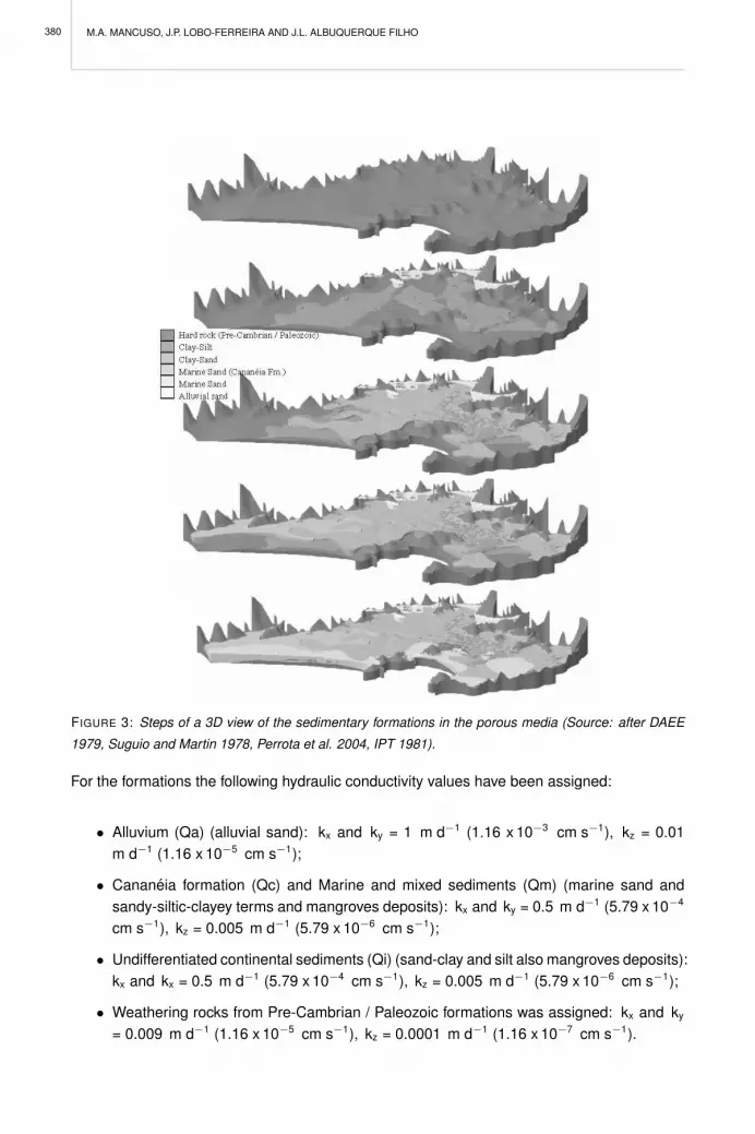
M.A. MANCUSO, J.P. LOBO-FERREIRA AND J.L. ALBUQUERQUE FILHO
FIGURE 3: Steps of a 3D view of the sedimentary formations in the porous media (Source: after DAEE
1979, Suguio and Martin 1978, Perrota et al. 2004, IPT 1981).
For the formations the following hydraulic conductivity values have been assigned:
• Alluvium (Qa) (alluvial sand): kx and ky = 1 m d−1 (1.16 x 10⁻³ cm s−1), kz = 0.01m d−1 (1.16 x 10⁻⁵ cm s−1);
• Cananeia formation (Qc) and Marine and mixed sediments (Qm) (marine sand andsandy-siltic-clayey terms and mangroves deposits): kx and ky = 0.5 m d−1 (5.79 x 10⁻⁴
cm s−1), kz = 0.005 m d−1 (5.79 x 10⁻⁶ cm s−1);
• Undifferentiated continental sediments (Qi) (sand-clay and silt also mangroves deposits):kx and kx = 0.5 m d−1 (5.79 x 10⁻⁴ cm s−1), kz = 0.005 m d−1 (5.79 x 10⁻⁶ cm s−1);
• Weathering rocks from Pre-Cambrian / Paleozoic formations was assigned: kx and ky
= 0.009 m d−1 (1.16 x 10⁻⁵ cm s−1), kz = 0.0001 m d−1 (1.16 x 10⁻⁷ cm s−1).
380
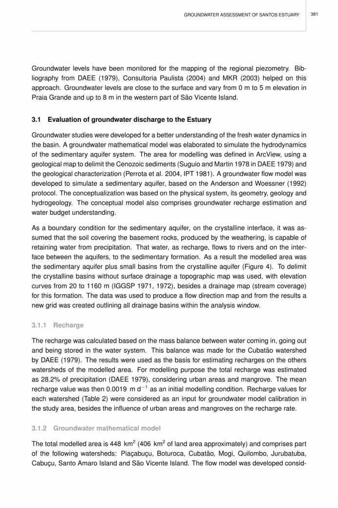
GROUNDWATER ASSESSMENT OF SANTOS ESTUARY
Groundwater levels have been monitored for the mapping of the regional piezometry. Bib-liography from DAEE (1979), Consultoria Paulista (2004) and MKR (2003) helped on thisapproach. Groundwater levels are close to the surface and vary from 0 m to 5 m elevation inPraia Grande and up to 8 m in the western part of Sao Vicente Island.
3.1 Evaluation of groundwater discharge to the Estuary
Groundwater studies were developed for a better understanding of the fresh water dynamics inthe basin. A groundwater mathematical model was elaborated to simulate the hydrodynamicsof the sedimentary aquifer system. The area for modelling was defined in ArcView, using ageological map to delimit the Cenozoic sediments (Suguio and Martin 1978 in DAEE 1979) andthe geological characterization (Perrota et al. 2004, IPT 1981). A groundwater flow model wasdeveloped to simulate a sedimentary aquifer, based on the Anderson and Woessner (1992)protocol. The conceptualization was based on the physical system, its geometry, geology andhydrogeology. The conceptual model also comprises groundwater recharge estimation andwater budget understanding.
As a boundary condition for the sedimentary aquifer, on the crystalline interface, it was as-sumed that the soil covering the basement rocks, produced by the weathering, is capable ofretaining water from precipitation. That water, as recharge, flows to rivers and on the inter-face between the aquifers, to the sedimentary formation. As a result the modelled area wasthe sedimentary aquifer plus small basins from the crystalline aquifer (Figure 4). To delimitthe crystalline basins without surface drainage a topographic map was used, with elevationcurves from 20 to 1160 m (IGGSP 1971, 1972), besides a drainage map (stream coverage)for this formation. The data was used to produce a flow direction map and from the results anew grid was created outlining all drainage basins within the analysis window.
3.1.1 Recharge
The recharge was calculated based on the mass balance between water coming in, going outand being stored in the water system. This balance was made for the Cubatao watershedby DAEE (1979). The results were used as the basis for estimating recharges on the otherswatersheds of the modelled area. For modelling purpose the total recharge was estimatedas 28.2% of precipitation (DAEE 1979), considering urban areas and mangrove. The meanrecharge value was then 0.0019 m d−1 as an initial modelling condition. Recharge values foreach watershed (Table 2) were considered as an input for groundwater model calibration inthe study area, besides the influence of urban areas and mangroves on the recharge rate.
3.1.2 Groundwater mathematical model
The total modelled area is 448 km2 (406 km2 of land area approximately) and comprises partof the following watersheds: Piacabucu, Boturoca, Cubatao, Mogi, Quilombo, Jurubatuba,Cabucu, Santo Amaro Island and Sao Vicente Island. The flow model was developed consid-
381

M.A. MANCUSO, J.P. LOBO-FERREIRA AND J.L. ALBUQUERQUE FILHO
ering flow as a steady state, with lakes and the channel considered as constant head cells.Rivers were simulated as drains. A two layer model of the porous aquifer was elaborated, withthe first being an unconfined layer and the second a confined/unconfined layer. This divisionintended to evaluate the real groundwater flow rate discharge to the estuary, considering atotal penetrating channel on the first layer. The first layer has a mean thickness of 25 m, andthe second layer has variable thickness according to the bedrock elevation.
The 3D model grid starts at the World Coordinates X = 337,080 m, Y = 7,336,560 m and Z= -230 m, ending at X = 377,080 m, Y = 7,365,560 m and Z = 1,070 m. The model has twolayers subdivided into 116 rows by 160 columns. Each cell is 250 m by 250 m along the xxand yy directions. The zz direction varies according to the layer to which each cell belongsand to the x and y coordinates of that cell. The thickness for the first layer was calculated as30% of total thickness of the sediments, between topographic level and hard rock, specifyinga minimum thickness of 20 m. Total thickness was calculated from topographic grid and hardrock top elevation grid (-230 m), base for the sedimentary aquifer system (Figure 5). Surfacewater from rivers, drains, Santos estuary and the Atlantic Ocean were represented as drainsand constant head on Modflow software. On the first layer (Figure 6) were represented therivers, drains and channels, as a partially penetrating water system. The Atlantic Ocean hasbeen represented as a constant head and a full interception system for groundwater flow. Con-sidering the purpose of this work, groundwater and sea water interaction was not simulated. The constant head boundary at 0 m allowed quantifying mean groundwater discharge fromthe sedimentary aquifer.
FIGURE 4: Sedimentary aquifer and basins from crystalline aquifer that contribute with groundwater flow
to the porous aquifer (Source: Cenozoic formation limit after Suguio and Martin 1978).
382

GROUNDWATER ASSESSMENT OF SANTOS ESTUARY
3.2 Model calibration results and conclusions
Model calibration target was the piezometric surface to be compatible with DAEE (1979). Table3 shows range values used for calibration. The objective of the model calibration is to obtainpiezometric surface compatible with observed heads, or the piezometric surface of DAEE(1979). In a general way, at Santos Estuary sedimentary aquifer groundwater flows locallytowards the rivers, and the drains opened according to the urban development. Regionallygroundwater flows towards the sea as may be observed from piezometric maps shown inFigure 7.
Water budget shows that flows in and out from the system are almost the same, with a dis-crepancy of 1%. Results show that total discharge from groundwater is 877 x 103 m3 d−1,208 x 103 m3 d−1 (24%) flows to the Estuary and 493 x 103 m3 d−1 (56%) to the drains, partof groundwater flows to the Atlantic Ocean (20%) (Table 4). Total discharge from precipitationthrough the sedimentary aquifer to the Estuary is about 8%. Flow depends on the water-shed location, area and land use, but mean flow from groundwater to the Estuary boundaryis around 1 m2 m−1 d−1. Table 4 and Figure 8 show the groundwater discharge from thesedimentary aquifer to the Estuary System.
According to the groundwater model developed in this work, the discharge from the sedimen-tary aquifer directly to the Estuary is approximately 8% of the precipitation. Discharge fromfractures of the crystalline aquifer (hard rock) has not been considered. From the resultsit can be concluded that groundwater discharge to Santos Estuary depends on the water-shed location, area and land use. Flow discharge is lower on a well drainage basin, becausegroundwater contributions are mainly to the drains. This base flow discharge is counted onthe rivers flow rate. There is a high fresh water discharge to the Atlantic Ocean, from PraiaGrande and Santos area. Lower values are related with crystalline rock outcrop and smallislands. Monthly recharge values for each watershed were considered as an input for modelsimulation in the study area, as well as the influence of urban areas and mangroves on therecharge rate.
One can observe differences between groundwater recharge rates on forest land use for theCubatao watershed, and groundwater recharge on urban areas, as calculated for Santos andSao Vicente. The computation didn’t consider losses from water supply pipes. From thesimulation it can be conclude that Boturoca watershed, Sao Vicente and Santo Amaro Islandare the main contributors of fresh water from the sedimentary aquifer to the estuary. Lowerdischarges to the estuary were observed in drains and, afterwards as surface water, to theestuary. It’s important to collect new groundwater data to improve this first modelling approach.The physiography of the area, the land use and mainly the large amount of rainfall, increasingthe availability of water, at least in quantity terms, may be responsible for the non-existence ofgroundwater studies.
383
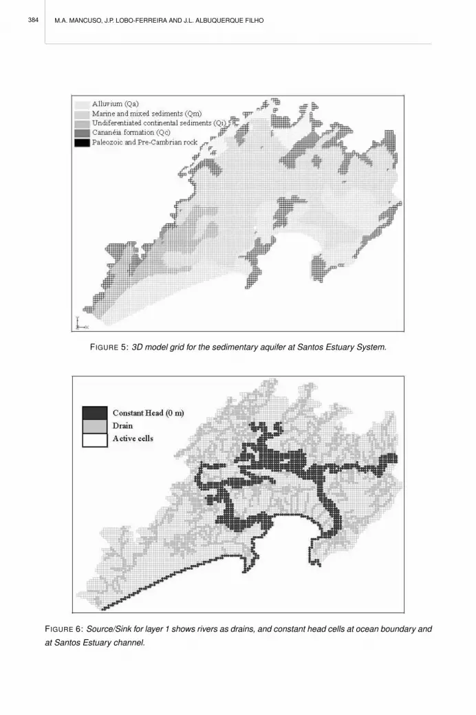
M.A. MANCUSO, J.P. LOBO-FERREIRA AND J.L. ALBUQUERQUE FILHO
FIGURE 5: 3D model grid for the sedimentary aquifer at Santos Estuary System.
FIGURE 6: Source/Sink for layer 1 shows rivers as drains, and constant head cells at ocean boundary and
at Santos Estuary channel.
384

GROUNDWATER ASSESSMENT OF SANTOS ESTUARY
FIGURE 7: Piezometric head for Land Santos Estuary sedimentary aquifer resulted from Modflow model.
FIGURE 8: Groundwater flow discharge from the sedimentary aquifer to Santos Estuary.
385

M.A. MANCUSO, J.P. LOBO-FERREIRA AND J.L. ALBUQUERQUE FILHO
TABLE 1: Geology of the sediment formations of Land Santos Estuary area (Source: Geological Map of
Sao Paulo State, in IPT 1981). Period (Age) Geological formation Lithology
Qa - Alluvium Unconsolidated sands of variable texture, associated clays and gravels
Qm – Marine and mixed sediments Sands, marine, sandy-siltic-clayey terms and mangroves deposits
Qi – Undifferentiated continental sediments Continental deposits
Cenozoic
Qc – Cananéia formation Unconsolidated thin marine sands
TABLE 2: Recharge in Santos Estuary watersheds.
Watershed Modelled Area (km2)
P (mm year-1)
Potential Recharge2 (m3 d-1)
Boturoca stream 128.1 2640 261,282 Cubatão stream 21.0 2863 46,451 Piaçabuçu stream 57.1 2405 106,098 S. Vicente island 58.5 2291 103,547 Mogi stream 20.5 2704 42,827 Santo Amaro island 68.6 2376 125,929 Cabuçu stream 28.4 2771 60,801 Jurubatuba stream 36.3 2539 71,207 Quilombo stream 25.0 2619 50,586 Islands 4.9 2410
Total 448.3 868,728 2 28,2% from precipitation, considering urban areas and mangrove (DAEE 1979)
TABLE 3: Range values used to calibrate the model.
Parameter Initial Condition
Hydraulic Conductivity (k) kxx and kyy = 0.009 m d-1 to 1 m d-1 ; kzz = 0.005 m d-1 to 0.0001 m d-1
Drain Conductance 0,2 to 2 L (m)
Recharge 1,8 x 10⁻³ m d-1 to 2,2 x 10⁻³ m d-1
Initial head 0 m to 10 m
386

GROUNDWATER ASSESSMENT OF SANTOS ESTUARY
TABLE 4: Estimated groundwater discharge to the Estuary System resulting from a year groundwater
simulation.
Discharge Flow (m3 d-1) Watershed Discharge
Boundary (m) Estuary Drains Atlantic Ocean Total
Boturoca stream 43,971 -43,816 -147,098 -58,805 -249,719 Cubatão stream 5,804 -4,600 -45,890 - -50,490 Piaçabuçu stream 10,697 -13,910 -38,002 -68,044 -119,956 S. Vicente island 40,878 -40,092 -23,798 -45,648 -109,538 Mogi stream 10,449 -8,580 -30,283 - -38,863 Santo Amaro island (*) 25,202 -25,825 -74,350 -2,826 -103,001 Cabuçu stream (*) 13,866 -24,164 -43,302 - -67,466 Jurubatuba stream 14,183 -21,717 -56,260 - -77,977 Quilombo stream 9,224 -19,941 -33,604 - -53,544 Islands 29,544 -5,036 - -5,036 Santos Estuary - Ocean -1,531 -1,531
Total -207,681 -492,587 -176,855 -877,122
REFERENCES
Anderson MP, Woessner WW (1992) Applied groundwater modeling: simulation of flow and advectivetransport. Academic Press. San Diego. 381 pp.
BcDaee2000 (2000) Banco Pluviometrico, Fluviometrico e Regionalizacao Hidrologica do Estado de SaoPaulo, v1.0. (http://www.sigrh.sp.gov.br Cited 20 Jun 2006)
CETEC (1999) Minuta Preliminar do Relatorio de Situacao dos Recursos Hıdricos da UGRHI 7. Comiteda Bacia Hidrografica da Baixada Santista, 238 pp.
Consultoria Paulista (2004) Estudo de Impacto Ambiental - EIA. Dragagem do Canal de Piacaguera eGerenciamento dos passivos ambientais. Sao Paulo.
DAEE - Departamento de Aguas e Energia Eletrica do Estado de Sao Paulo (1979) Estudo de AguasSubteraneas. Regiao Administrativa 2. Santos. Sao Paulo.
IGGSP - Instituto Geografico e Geologico de Sao Paulo (1971) Folha de Mongagua. Folha SG-23-V-A-III-2. Regiao Sul do Brasil. Escala: 1:50.000
IGGSP - Instituto Geografico e Geologico de Sao Paulo (1972) Folha de Santos. Folhas SF-23-Y-D-IV-3e SG-23-V-B-I-1. Escala: 1:50.000
IPT - Instituto de Pesquisas Tecnologicas do Estado de Sao Paulo - IPT (1981) Mapa Geologico do Estadode Sao Paulo. Escala 1: 500.000. Sao Paulo: IPT, 1981a. 2 v. (Monografias, 6; Publicacao, 1 184).
MKR (2003) Estudo de Impacto Ambiental - EIA. Terminal portuario Embraport. Capıtulo 8 - DiagnosticoAmbiental das areas de influencia. Meio Fısico. Sao Paulo.
Perrota, MM et al. (2004) Folha SG.22 - Curitiba. In: Schobbenhaus, C. et al. (Ed.). Carta geologicado Brasil ao milionesimo, Sistema de Informacoes Geograficas. Brasılia: CPRM, 2004. (ProgramaGeologia do Brasil). CD-ROM.
Suguio K, Martin L (1978) Mapa geologico das formacoes quaternarias marinhas do litoral Paulista e SulFluminense, escala 1:100.000. IG-USP and ORSTOM. France.
387


PERSPECTIVES ON INTEGRATED COASTAL ZONE MANAGEMENT IN SOUTH AMERICAR. NEVES, J.W. BARETTA AND M. MATEUS (EDS.), IST PRESS, 2008
CONTAMINANT TRANSPORT IN THE SEDIMENTARY AQUIFER OF ALEMOA
C.B.B. LEITE, C.Z. TOPOROVSKI AND M.A. MANCUSO
ECOMANAGE project aims to push the capacity of assisting managers to join horizontallyknowledge from ecological and socio-economic disciplines. The three key aspects of ECO-MANAGE are (1) the consideration that a coastal zone depends on local pressures, but alsoon pressures originated in the drainage basin, transported mostly by rivers and by groundwa-ter, (2) that socio-economic activities are the driving forces of those pressures and that theirimpacts on the ecosystem have feedback on socio-economics and (3) the impacts depend onphysical characteristics of the ecosystem that together with the loads determine its ecologicalstate. The project is destined to develop a management integrated system for the coastal zoneand apply it in the Santos Estuary - SP - Brazil. The research was developed using mathemat-ical models to quantify the pollution loads transported by groundwater from Alemoa’s dump tothe Santos Estuary.
Alemoa quarter is one of the oldest used areas of Santos city. It’s located at the northwest partof the island. This area is inside the limits of Santos Port, where today is located an importantindustrial complex, with patios and deposits of containers used to transport loads to and fromthe port. Alemoa area was used for more than 50 years as a disposal for solid waste from theoperation of the Santos Port. Also, domestic waste was illegally dumped in the area. Beyondthese activities, the area was used to store and move explosives on the access bridge andmaterial dragged during the installation activities of Petrobras´ terminal.
This work presents the first approach for assessing the evaluation of contaminant dischargefrom the illegal waste dumped at Alemoa area into Santos Estuary, based on existing data.It presents the conceptual model, the mathematical model and the computed results thatallowed the quantification and mapping of the contaminant flow discharge. The physical dataof the Alemoa area was presented in terms of geology, hydrogeology, altimetry, evaporationand precipitation. The total modeled area is 0,917 km2 and comprises part of the Sao VicenteIsland (Figure 1).
The model was developed using the software: Ground Water Modeling System - GMSr, withthe modules MAP, MODFLOW, PEST, MODPATH, and MT3D. MODFLOW was first publishedby McDonald and Harbaugh (1988). The flow model was developed considering flow as asteady state, with lakes and the channel considered as constant head cells. Rivers weresimulated as drains. The conceptualization was based on the physical system, its geome-try, geology and hydrogeology. The conceptual model also comprises groundwater rechargeestimation and water budget understanding.
The area for modeling was defined in AutoCADr, using lithologics and hydrogeologics infor-mation of 35 boreholes. As a boundary condition for the sedimentary aquifer, it was consideredthe crystalline interface at -25 m deep. To delimitate this area was used a topographic map(AGEM, 1:1 000). These data was used to produce a grid with 10 m x 10 m cell representing
389

C.B.B. LEITE, C.Z. TOPOROVSKI AND M.A. MANCUSO
the elevation surface. Considering the lithology two layers were defined, both layers on porousaquifer. The bottom elevation of the first layer is -3.5 m and the bottom elevation of the secondis -25 m, so the first layer has a thickness of 4 to 10 m.
FIGURE 1: Alemoa’s dump in Santos Estuary.
The mathematical model used to represent the contamination plume was MT3D. The modelwas published by Zheng and Wang (1999) and it is used to calculate the transport of a con-tamination plume by resolving transport equations. Four transport models were built to deter-minate the contaminations plume of benzene, cadmium, lead and toluene. The income dataused by MT3D model had followed the same parameters used for Modflow model. For the de-termination of the contamination plume were considered the concentrations of contaminantsobtained in each of the 35 boreholes (observation wells) as a constant load launched into theaquifer.
Considering these data, the contaminant transport model allowed the simulation of advectionand dispersion in the aquifer sedimentary system. The final aim was to quantify the diffusepollution loads discharging to the Santos Estuary. Figures 2 to 5 present the contaminationplumes in Alemoa area in a period of 100 years, and Table 1 presents the contaminant dis-charge to Santos Estuary.
From the results, presented in Figures 2 to 5 and Table 1, it can be concluded that the con-taminant discharge of the Alemoa’s dump are mainly directed to drains, and then to SantosEstuary. Also, underground discharge direct to the Santos Estuary is lower. The total contam-inant discharge of Alemoa’s dump to the Santos Estuary, considering a period of 100 years,was calculated in 175,048.91 mg to benzene, 53,310.1 mg to toluene, 824,704.21 mg to leadand 64,602.64 mg to cadmium.
390

CONTAMINANT TRANSPORT IN THE SEDIMENTARY AQUIFER OF ALEMOA
FIGURE 2: Contamination plume for Benzene ( C6H6).
FIGURE 3: Contamination plume for Cadmium (Cd).
TABLE 1: Contaminant discharge to Santos Estuary.
Compounds Drains (mg)
Drains (mg y-1)
Santos Estuary (mg)
Santos Estuary (mg y-1)
Total Discharge (mg)
Total Discharge (mg y-1)
Benzene (C6H6) 130,443.00 1304.43 44,605.91 446.06 175,048.91 1750.49
Cadmium (Cd) 59,247.54 592.48 5,355.097 53.55 64,602.637 646.03
Lead (Pb) 494,854.80 4948.55 329,849.90 3298.50 824,704.70 8247.05
Toluene (C7H8) 51,095.49 510.95 2,214.61 22.15 53,310.10 553.10
391

C.B.B. LEITE, C.Z. TOPOROVSKI AND M.A. MANCUSO
FIGURE 4: Contamination plume for Lead (Pb).
FIGURE 5: Contamination plume for Toluene ( C7H8).
REFERENCES
AGEM - Agencia Metropolitana da Baixada Santista (2003) - Sistema Cartografico Metropolitano daBaixada Santista. Folhas SF-23-Y-D-IV-3-SE-C-I-2-A, SF-23-Y-D-IV-3-SE-C-I-2-B, SF-23-Y-D-IV-3-SE-C-I-3-A, SF-23-Y-D-IV-3-SE-C-I-3-B, SF-23-Y-D-IV-3-SE-C-I-2-C, SF-23-Y-D-IV-3-SE-C-I-2-D, SF-23-Y-D-IV-3-SE-C-I-3-C, SF-23-Y-D-IV-3-SE-C-I-3-D, SF-23-Y-D-IV-3-SE-C-I-5-A, SF-23-Y-D-IV-3-SE-C-I-5-B, SF-23-Y-D-IV-3-SE-C-I-6-A and SF-23-Y-D-IV-3-SE-C-I-6-B. Scale: 1: 1.000.
McDonald M G and Harbaugh A W (1988) ”MODFLOW - A Modular Three-Dimensional Finite DifferenceGround Water Flow Model”. Washington D.C., U.S. Geological Survey. Waterloo Hydrologic Inc.
Zheng C and Wang P (1999) MT3DMS: A modular three-dimensional multispecies model for simulation ofadvection, dispersion and chemical reactions of contaminants in groundwater systems; Documenta-tion and User’s Guide, Contract Report SERDP-99-1, U.S. Army Engineer Research and DevelopmentCenter, Vicksburg, MS.
392

PERSPECTIVES ON INTEGRATED COASTAL ZONE MANAGEMENT IN SOUTH AMERICAR. NEVES, J.W. BARETTA AND M. MATEUS (EDS.), IST PRESS, 2008
LOAD AND FLOW ESTIMATION IN SANTOS WATERSHEDS
P. CHAMBEL-LEITAO, A.F.P. SAMPAIO AND P. ALMEIDA
1 INTRODUCTION
The basin of the Santos estuary, due to its high rate of urbanization has a very diversified use,designed especially for public and industrial services, reception of domestic and industrial ef-fluents, fishing for sustenance, recreation, navigation and generation of electricity (CETESB,2005). The estuary has an important basin designed for the supply of one of the great in-dustrial centers of the country, the largest port of Latin America and a population of over amillion people distributed over five towns that make up the estuary of Santos. Historicallysome rivers received in the past a huge load of industrial effluents without any treatment frompetrochemical, chemical and fertilizer plants as well as from a steelworks. In the last decade,the quality of the effluents improved significantly thanks to regulatory actions taken by envi-ronmental institutions which forced industries to invest in treatment systems, but some riversstill suffer high rates of BOD. Besides, the basin suffers large pressures from irregular humanoccupation on the river banks and from urban discharges without treatment.
This paper presents the application of SWAT to estimate de effluent flows to the estuary andthe application of HARP-NUT guidelines to estimate the loads of nutrients to the estuary. Boththe flows and nutrients estimated were used as boundary conditions to the MOHID estuarymodel.
2 THE SWAT MODEL
During the ECOMANAGE project a Landsat satellite image of April 30, 2000 was used for theelaboration of vegetation cover maps for the Santos estuary watersheds. The results obtainedwere then used as the Landcover input for the SWAT model. The soil map included in CETEC(1999) was used as input for SWAT. Information referring to the analytic, grain and chemistrycharacteristics associated with these types of soils were collected from Rossi (1999). Thetopography used was obtained by NASA in the Shuttle Radar Topographic Mission (SRTM)and that was available for download from the Internet.
The precipitation used was from Paranapiacaba (code: E3-037) Latitude -46.28 and Longitude-23.77 which lies at an elevation of 820 m. This station was chosen for four reasons: i) it has analmost complete time series; ii) it has a long period of data which includes the flow measuresdata (from 01-01-1936 to 30-06-1998); iii) it has an average annual precipitation of 2000 mmwhich, according to the average annual precipitation maps, is the average precipitation inthe region; iv) it is the most representative for Quilombo river which is the watershed withmost measurements of flow. Fluviometric, meteorological, and water quality data was madeavailable through BcDaee2000. There are 3 fluviometric stations in the watersheds around
393

P. CHAMBEL-LEITAO, A.F.P. SAMPAIO AND P. ALMEIDA
Santos estuary (Figure 1). Unfortunately, only data for a short historical period are availablefor Cubatao and Moji stations (three and two years respectively), while for Quilombo we have15 years of data. The main conclusion was that Cubatao measured and modelled flow had thebest fit (Table 1). On the other hand Quilombo modelled flows were higher than the measuredones. This might be due to an under estimation of evapotranspiration or an excess input ofprecipitation to the model.
Evapotranspiration estimated by the model is around 20-30% which is similar to values esti-mated by Lopes (2001). To obtain the measured values, 50% evapotranspiration would haveto be calculated with the model. But this wouldn’t be consistent with flow measures for Cu-batao and Moji which indicate evapotranspiration of 20-30%. On the other hand precipitationis expected to be representative for Quilombo river because it’s the closest to Quilombo andit has an average annual precipitation of 2000 mm which, according to the average annualprecipitation maps, is the average precipitation in the region. This means that probably theflow measurements (which in fact are based on river level measurements) in Quilombo wereunderestimates. Finally, Moji has few values and half of them are not concordant with themodel while the other half shows a very good fit.
3 HARP-NUT GUIDELINES
The application of the OSPAR HARP Guidelines to the Santos Basin has helped to elucidatesome of the gaps in the data available for this basin. Nevertheless, we have proceeded toapply the guidelines, indicating in the following text the assumptions made for each guideline.Based on CETESB monitoring stations, four monitored areas were evaluated using OSPARHARP Guidelines. The name of the water quality station is shown in Table 2 as well as thearea of the associated drainage basin. The distribution of these drainage basins is displayed inFigure 1. The remaining area that drains to the estuary and is not included in these monitoredwatersheds is called the unmonitored area, and its delineation is shown in Figure 2.
No data was found on aquaculture in the area of Santos Estuary. Due to the high degree ofindustrialization of the region and to the level of pollution in the area it is expected that there isno aquaculture in the area. Loads estimated for Henry Borden using CETESB data were 446ton N yr−1 and 43 ton P yr−1. For the drainage area of the monitoring station Cuba27 (in theupper part of Cubatao watershed), no industries were identified, and the diffuse loads comingfrom this area were used as an input to the Cuba39 monitored area.
The following industrial discharges are included in the drainage area of monitoring stationCuba39: Ultrafertil-CCB, Ripasa, Petrobras-RPBC, CBE, Dow Quımica, Petrocoque and Car-bocloro. From those, there were available data for outflow and BOD only for Ultrafertil-CCB,Ripasa, Petrobras-RPBC, Petrocoque and Carbocloro; additionally, there were data on Nitro-gen and Phosphorus and outflow for Ultrafertil - CCB. The Henry Borden Power Plant alsodischarges in the Cuba39 monitoring station, and was also considered an industry.
394

LOAD AND FLOW ESTIMATION IN SANTOS WATERSHEDS
FIGURE 1: Drainage area of CETESB monitoring stations.
FIGURE 2: Unmonitored area draining to the estuary.
TABLE 1: Comparison of observed and modelled average monthly flows. Calibration period Observed flow
[m3 s-1] Modeled
flow [m3 s-1] R2 Model Efficiency
Cubatão Oct ‘66–Jul ‘69 10.4 11.6 0.68 0.67 Moji Aug ‘72 –Sep‘74 2.35 2.61 0.34 0.19 Quilombo Oct ‘71–Nov ‘87 3.02 4.50 0.63 0.01 Dailly Cubatão Oct ‘66–Jul ‘69 10.4 11.6 0.56 0.55 Moji Aug ’72 –Sep’74 2.35 2.61 0.33 -0.97 Quilombo Oct ‘71–Nov ‘87 3.02 4.50 0.33 -0.67
395

P. CHAMBEL-LEITAO, A.F.P. SAMPAIO AND P. ALMEIDA
TABLE 2: Monitored area delineated based in monitoring stations.
Watershed Code Area [km2]
Cubatão CUBA 27 135 Cubatão CUBA 39 45
Moji MOJI 46 Piaçaguera PIAC 9
For Moji four main industries were identified in the drainage basin: Ultrafertil-CPG, Manah,Serrana which are part of Bunge Fertilizantes S/A. Only for the first industry was found dataon BOD, nitrogen and outflow. Even with those values the estimated loads originating fromindustry are almost irrelevant. However in a load oriented approach it is shown that loads inthe rivers are very high and that they are probably originating from these industries. Accordingto Santos (2001), it is estimated that in Cubatao, in the state of Sao Paulo, there are about 20million tons of phosphorus cast, dumped into two open-air piles referring to the production ofUltrafertil (Moji, Cubatao, Estuary) and Copebras (Piacaguera).
According to data from 2006 provided by CETESB, Cosipa is responsible for most of indus-trial load with 352.71 ton N yr−1 of nitrogen and Ultrafertil CPG is responsible for most of theindustrial phosphorus load (35.85 ton P yr−1). For guideline 4 data from effluents were in-ferred from statistics on the population from the Instituto Brasileiro de Geografia e Estatıstica(IBGE 2000). Population values were obtained at the level of the smallest administrative unit:”Bairro”. Data available included population, total households and households connected topublic sewerage. Households include also slums improvised houses.
First the percentage was estimated of each ”Bairro” inside each watershed. Assuming that thehouseholds are uniformly distributed in the ”Bairro”, population, total households and house-holds connected to public sewerage were multiplied by that fraction, obtaining in this way theamounts inside each watershed. Then the average size of a household was estimated. Mul-tiplying this value by the number of households connected to public sewerage, the number ofpeople connected to public sewerage was estimated. Assuming that there was no treatmentof the wastewater, and that each person produced 12 g N day−1 and 2.5 g P day−1, an an-nual value of N and P in sewerage was estimated. These per capita values are proposed byguideline 4. As a first approximation (taking in consideration we do not know the percentageof the population in the unmonitored area which is connected to the outfall) it was assumedthat all discharge directly into the estuary.
Using a similar approach as the one mentioned in guideline 4 (Sewage Treatment Worksand Sewerage) it was estimated the value of nutrient loads from households not connected topublic sewerage. The only difference from the previous approach was that the per capita loadswere: 8.5 g N and 1.2 g P per person and per day. These values are proposed by guideline 5.These values are smaller than the ones in untreated public sewerage basically because thesewage that is not connected to the public collectors can take more time to reach the waterbodies allowing for retention during the travel time. This hypothesis is not correct for examplefor systems discharging directly to the estuary or the main rivers.
396

LOAD AND FLOW ESTIMATION IN SANTOS WATERSHEDS
The Harp guideline 6 provides example methodologies from several signatory countries asto how to quantify nitrogen and phosphorus from diffuse anthropogenic sources and naturalbackground losses. The use of the SWAT model is one of the proposed methodologies andwas the one used in this approach. Loads in the river (”load oriented approach”) were es-timated based on 5 years of measurements of CETESB in the monitoring places defined inFigure 1. For the period of water quality data, average monthly values of SWAT flows wereused, because there were no measured flows in that period. As seen before SWAT was cali-brated based on historical measurements in the watershed gauge stations.
MOJI and PIAC present N/P ratios of about two, which is high considering that the urban ef-fluents have a N/P ratio of 5. This is probably related with the industrial effluents released withhigh concentrations of phosphorus in these sub basins. Retention is a function of temperature,physical characteristics of rivers and lakes, such as residence time (lakes) and specific runoff,hydraulic load and bottom characteristics (rivers). Many of these parameters are difficult tomeasure, and therefore difficult to implement in calculation procedures. In general, nitrogenretention is more influenced by biological processes than the phosphorus retention, whereasthe phosphorus retention is more influenced by sedimentation processes than the nitrogenretention.
In order to arrive at nutrient retention estimates, the German approach described in OSPARguideline 9 was used. In order to estimate the surface area of water in the monitored water-sheds an empirical relation suggested in guideline 9 was used. This relation allows estimatingthe area of the watershed occupied by rivers. It was assumed that the area of lakes in thiswatershed was irrelevant. Additionally flow results from SWAT were used to calculate reten-tion using the equations described in this guideline (the same flow results as the ones used inGuideline 7). The parameters in said equation were derived empirically from 100 river basinsin Europe. The guideline does not indicate the variability and uncertainty associated withthese parameters. Keeping in mind the steep topography, these are fast-flowing rivers andthus it is likely that retention is relatively low.
The application of the HARP Guidelines shows that Load Oriented Approach and SourceOriented Approach gave similar values for CUBA39 station, while for MOJI and PICA stationsthe values were completely different (Table 3). The main reason for the major discrepanciesin MOJI and PIACA are related to the high measured loads in the rivers in combination withthe absence of effluent concentrations from the industries in the watersheds. Table 4 showsthat urban effluents have an important contribution to loads of nutrients. However this value isprobably overestimated, because part of the population is directly connected to the outfall.
4 DISCUSSION AND CONCLUSIONS
SWAT model was calibrated to generate flows for Santos watersheds. This allowed to pro-duce two types of flow as boundary conditions for the estuary model: i) the main discharges offresh water if possible associated with the water quality gauge stations ii) the total discharge of
397

P. CHAMBEL-LEITAO, A.F.P. SAMPAIO AND P. ALMEIDA
fresh water to the estuary. The difference between both these flows is that the drainage areaassociated with the first one is roughly half of the total drainage area of the estuary. This kindof result is important to improve estuary model results. In fact it only makes sense to imposea discharge in a region where the tide does not influence river flow. Only there we can guar-antee a point discharge. Below that point water arrives at the estuary (in high tide) in a diffuseway. It does not make sense to define in the model thousands of diffuse discharges. It is alsocontroversial to combine all the diffuse discharges into only one point discharge. However allthese scenarios can be tested with estuary model.
TABLE 3: Results of the application of HARP Guidelines for the Santos basin.
Santos Basin Total Nitrogen (tons yr-1) Total Phosphorus (tons yr-1)
Discharges and losses of N and P GL
C27 C39 Moji Pica C27 C39 Moji Pica
+ Upstream inputs 408 33
+ Losses from aquaculture 2 0 0 0 0 0 0 0 0
+ Discharge from industry 3 0 535 0 1 0 101 0 0
+ Discharges from sewage treatment plants
4 5 42 0 0 1 9 0 0
+ Losses households not connected WWTP
5 54 17 3 0 7 2 0 0
+ Diffuse nitrogen losses 6 169 93 100 23 10 6 3 1
= Sum of all losses/discharges (from Source Orientated Approach)
227 1080 103 24 18 152 3 1
- Nutrient retention in surface waters 9 15 11 31 3 1 1 5 1
= Total estimated nutrients at the monitoring point (Source Orientated
Approach)
212 1069 73 21 17 151 -2 0
To be compared with:
Total (from Load Orientated Approach) 7 408 1558 997 177 33 184 245 220
TABLE 4: Results of the application of HARP Guidelines to the unmonitored area of the Santos basin -
Source oriented approach.
Santos Basin Total N (tons yr-1)
Total P (tons yr-1)
Discharges and losses of N and P GL
UnMonitored
+ Upstream inputs 0 0
+ Losses from aquaculture 2 0 0
+ Discharge from industry 3 19 4
+ Discharges from sewage treatment plants 4 4674 974
+ Losses households not connected WWTP 5 0 0
+ Diffuse nitrogen losses 6 753 63
= Sum of all losses/discharges (from Source Orientated Approach) 5446 1040
398

LOAD AND FLOW ESTIMATION IN SANTOS WATERSHEDS
In terms of load in the estuary we can discern 4 different main sources: i) load from therivers in the industrial area; ii) Load from Cosipa; iii) Load from urban origin; iv) Diffuse loadfrom forested watersheds estimated with SWAT. The first source is located in the watershedmonitored area, while the remaining three sources are located in the unmonitored area.
Average monthly concentrations were estimated from CETESB measurements of concentra-tion in the river. These values were compared with the known loads in the respective water-shed. For Cubatao load, the origins of the loads were justified. For Moji and Piacaguera theorigin of the loads in the river was not justified, but they probably originated from the fertilizerindustries located on these watersheds, from which there are no data available on effluents.
REFERENCES
BcDaee2000 (2000) Banco Pluviometrico, Fluviometrico e Regionalizacao Hidrologica do Estado de SaoPaulo, v. 1.0
CETEC (1999) Minuta Preliminar do Relatorio de Situacao dos Recursos Hıdricos da UGRHI 7. Comiteda Bacia Hidrografica da Baixada Santista, 238 pp.
Cetesb-Companhia de Tecnologia de Saneamento Ambiental (2005) Relatorio de Qualidade das AguasInteriores do Estado de Sao Paulo. (http://www.cetesb.sp.gov.br/Agua/rios/relatorios.asp)
Cetesb-Companhia de Tecnologia de Saneamento Ambiental (2006) Relatorio de Qualidade das AguasInteriores do Estado de Sao Paulo. (http://www.cetesb.sp.gov.br/Agua/rios/relatorios.asp)
IBGE (2000) Statistics on the population from the Instituto Brasileiro de Geografia e Estatıstica. (www.ibge.gov.br)
Rossi M (1999) Fatores formadores da paisagem litoranea: A Bacia do Guaratuba, Sao Paulo, Brasil.PhD thesis. Universidade de Sao Paulo. Faculdade de Filosofia, Letras e Ciencias Humanas, Depar-tamento de Geografia (FFLCH-USP). Sao Paulo, Brazil. 55-99pp.
399


PERSPECTIVES ON INTEGRATED COASTAL ZONE MANAGEMENT IN SOUTH AMERICAR. NEVES, J.W. BARETTA AND M. MATEUS (EDS.), IST PRESS, 2008
AN ECOLOGICAL MODEL APPLICATION TO THE SANTOS ESTUARY, BRAZIL:TESTING AND VALIDATION
M. MATEUS, A.F.P. SAMPAIO AND S. MATEUS
1 WHY MODEL ECOLOGICAL PROCESSES IN SANTOS ESTUARY?
Over the past decades an intense research program has been carried out at the Santos Es-tuary to study the ecological dynamics of the system. Much of this work has been field dataacquisition in monitoring programs and subsequent interpretation. Modelling approaches havebeen scarce and generally devoted to the study of hydrodynamics in the bay area or sedimenttransport in the system (Harari and de Camargo 2003). Until now there has been a lack ofintegrative modelling approaches in the Santos estuary. This is the first attempt at simulat-ing the hydrodynamics of the system coupled to some of its ecological processes. Since theSantos estuary is a highly impacted system (Braga et al. 2000, Medeiros and Bicego 2004a,b, Abessa et al. 2005, Cesar et al. 2007), the need for such a tool is emphasized by thenecessity to link human pressures known in the area with the ecological state of the systemaccording to the DPSIR framework (Mateus and Campuzano, this volume). Among the mostrelevant aspects that such a tool can address, there are: (1) The insights that it can provideinto the major physical-ecological interactions in the estuary; (2) Assessing the contribution ofisolated Pressures such as the sewage outfall or industrial effluent to the State of the system;(3) Provide a numerical tool to help in the management of the system (Response) by allowingthe testing of different scenarios of human Pressures.
This work presents the application of a coupled physical-ecological model within the MOHIDsystem (Leitao et al., this volume) to the Santos estuary. The ecological model, the MOHIDWQ model, is an adaptation of the NPZ modelling paradigm (Fasham et al. 1990). Detaileddescription of the model implementation is provided, with particular emphasis on the charac-terization of the forcing and modelling options. Model results are compared against field datato assess model performance and validate the results. This model application relies on theassumption that the model correctly reproduces the hydrodynamics of the Santos estuary.
In the DPSIR framework, this work describes the state of the system based on some ecologicaland water quality parameters. The model is forced with values previously quantified for thePressures, namely, nutrient and organic matter concentrations in the rivers, the submarineoutfall in the bay, the absent sewage drainage networks in the quarters and direct raw sewageinputs from slum quarters around the margins of the estuary. These Pressures, which fall inone of the major groups of estuarine and coastal area pressures, namely pollution, includingurban, industrial, agricultural and aquaculture discharges (Borja et al. 2006), express theforcing from the major drivers: human occupation and industry. The outcome of this numericalstudy is a benchmark model application which can be further developed to study differentscenarios of development or actions prompted by responses. Also, the results presented
401

M. MATEUS, A.F.P. SAMPAIO AND S. MATEUS
here will enable the quantification of changes induced by responses, when compared with theresults from the model runs for different scenarios.
2 MODEL IMPLEMENTATION
The ecological model is coupled with the hydrodynamic model previously described, and sothe same assumptions for the physical features of the system apply here. These are: (1) thewater-column is homogeneous, i.e., non-stratified over the modelled domain (2D horizontal);(2) the hydrodynamics in the bay are controlled by the tide and the water flow from the mainchannels, i.e., there are no shelf water currents. The model domain is the same as for thehydrodynamic application and to reduce the run time, the coarse grid was adopted for thepresent study. The external conditions include river discharges, forcing functions (for exampleirradiance, air temperature), and boundary conditions (concentrations of each state variable onthe open Atlantic boundary). Whenever possible, these values have been taken from availablefield data. The ecological model runs with a time step of 1 hr. A constant value for eachproperty was defined as the open boundary condition (Table 1).
2.1 Atmospheric forcing
Climatological irradiance levels were calculated by the model for the domain geographicalcoordinates from the solar constant corrected for cloudiness with mean monthly cloud coverdata. Air temperature and relative humidity were also used to force the model over the entiredomain (Figure 1), with monthly values taken from field observations made by CODESP me-teorological station at Alemoa during 1997 and cloud cover was taken from field observationsmade at the Ilha da Moela meteorological station at Guaruja during 1999.
2.2 River inputs
The model considers six river inputs inside the model domain. When considering the eco-logical dynamics of the system, river discharges also need to be characterized by valuesof nutrients, organic matter components, and other biogenic constituents. For simulationswith the ecological model, the discharge of Cubatao+Henry Borden and Mogi+Piacaguera arecharacterized by mean monthly concentrations of ammonium, nitrate, nitrite, phosphate anddissolved oxygen (Figure 2) calculated from data collected by CETESB between 2000 and2005. The COSIPA industrial effluent is characterized by high nutrient loads and a significantflow for an effluent of this kind. According to Gragnani (1996) most of Moji/Picaguera flow iscaught by Cosipa and dumped in the Cosipa channel. Therefore we have modelled a joint dis-charge of Moji/Piacaguera and the Cosipa effluent. The Cosipa, contribution is a flow of 2.38m3 s−1 and a concentration of 23 mg l−1 of ammonium and DON, and 4.6 mg l−1 of bothphosphate and DOP. These values have been estimated from field observations and avail-able monitoring studies from Cetesb-Cubatao. The remaining values as well as the valuesassumed for the other discharges are summarized in Table 2.
402

AN ECOLOGICAL MODEL APPLICATION TO THE SANTOS ESTUARY, BRAZIL: TESTING AND VALIDATION
FIGURE 1: Monthly mean values for air temperature and relative humidity used to force the model.
FIGURE 2: Monthly mean values of water quality parameters assumed for the major river discharges: the
joint discharges of Moji + Piacaguera and Cubatao + Henry Borden.
403

M. MATEUS, A.F.P. SAMPAIO AND S. MATEUS
TABLE 1: Initial conditions, river inputs and boundary conditions defined for each variable in the model
simulations (unless noted otherwise).
Properties Units Initial conditions Boundary conditions
Nitrate 0.09 0.095
Nitrite 0.003 0.001
Ammonium 0.002 0.002
Refractory DON 0.2 0.02
Labile DON 0.02 0.002
PON
mg N l-1
0.37 0.0009
Inorganic phosphorus 0.03 0.03
Refractory DOP 0.028 0.002
Labile DOP 0.0028 0.00028
POP
mg P l-1
0.05 0.005
Oxygen mg O2 l-1 8 9.56
Phytoplankton 0.05 0.02
Zooplankton mg C l-1
0.03 0.01
Temperature ºC 20 20
Salinity PSU 20 36
Cohesive sediments mg l-1 100 25
2.3 Sewage nutrient input
As already mentioned, the Santos estuarine system is heavily impacted by human occupationand activities. A significant part of the anthropogenic pressure is in the form of diffuse sewagedischarges in several places scattered inside the estuary (Braga et al. 2000, CETESB 2001).Most of these discharges are associated with the slum quarters near (and sometimes over)the water line, and often with absent or provisional sewage drainage systems. Together withthe faecal contamination, the discharges into the system also have an associated load of nu-trients, both in a mineral and an organic form. To account for this source of eutrophication,the model considers 29 sewage discharge points inside the estuary (Figure 3, left). Thesecomprise the submarine outfall, sewage treatment plants and direct inputs from slum quar-ters. Each discharge is characterized by flow rate, associated nutrients and dissolved organicmatter concentrations. The flow and concentration of sewage treatment plants were calcu-lated from data obtained from SABESP (Sao Paulo State Basic Sanitation Company) anddirect discharges were estimated from the population number calculated for each district bythe Brazilian Institute of Geography and Statistics (IBGE 2000), in the municipal data on peo-ple living in slums and in measured values of water consumption by neighborhoods (Table 2).This number stands as an estimate based on the households not connected to the municipalsewage system.
Reference flow and concentrations for areas where data were not available were taken fromMetcalf and Eddy (2005) values for high-strength wastewater (Table 3). The partition betweenthe different pools of nutrients (organic and mineral) was also based on Metcalf and Eddy
404

AN ECOLOGICAL MODEL APPLICATION TO THE SANTOS ESTUARY, BRAZIL: TESTING AND VALIDATION
(2005). All discharges are characterized by a cohesive sediment concentration of 120 mg l−1,a salinity of 0.5 and a temperature of 24 oC. Together with the sewage discharges originatingfrom the poor or non-existent sewage system in some areas of Santos, the submarine outfall inthe bay is another large source of nutrients. The effluent characteristics used in this simulationare presented in Figure 4.
FIGURE 3: Left: Sewage discharge points associated with the outfall, sewage treatment plants, and the
slum quarters and absent sewage drainage networks. The model domain is divided in seven integration
boxes to allow the calculation of the exchange fluxes of properties inside the estuarine area between the
boxes. Legend for the boxes: Sao Vicente Channel and Piacabucu river (1), Santos channel (2), Boturoca
and Mariana river and Pompeba large (3), Largo do Caneu or Cubatao area (4), Lower Sao Vicente
Channel (5), Bagres and Barnabe Island area (6), and Santos bay (7). Right: Mangrove areas used in the
model to account for the shading effect.
2.4 Mangrove shading effect
Considering the large mangrove areas inside the estuaries, the model accounts for the shad-ing effect of mangrove trees. Because a considerable fraction of the mangrove forest is inpermanently flooded areas, they strongly reduce the amount of light reaching the water sur-face. The spatial distribution of mangrove areas (Figure 3, right) was taken from aerial surveyphotographs and satellite images. This model feature is based on three simple assumptions:(i) the shading effect is quantified as a 50% reduction of the irradiance that reaches the sur-face, (ii) the mangrove is a climax community, implying that the shading effect is constant,and (iii) there are no net nutrient fluxes between mangrove and water column. The latterassumption is based on studies made in the nearby mangrove forest at Cananeia, where itwas observed that the mangrove forest does not export significant amounts of nitrogen to theadjacent lagoon (Carmouze et al. 1998). Apparently, the simultaneous processes of releaseand incorporation of ammonium explains this occurrence. The explicit modelling of mangrovedynamics would require a complex biochemical reaction model. This, in turn, would make themodelling exercise computationally heavy and compromise the simplicity that managementmodels aim for.
405

M. MATEUS, A.F.P. SAMPAIO AND S. MATEUS
TABLE 2: Sewage discharge areas and characterization of the respective effluent. Discharges include
the outfall, sewage treatment plants (STP), slum quarters and quarters beyond sewage drainage. Values
calculated according to measured mean concentrations of N and P of the effluent marked with *. The
remaining values were estimated.
Sewage discharge area Inhabitants Flow (m3 s-1)
N (kg day-1)
P (kg day-1)
Quietude and Vila Nova 36006 0.057 310.4 44.8 Antartica and Ponte Nova 38120 0.060 356.6 57.8 Sítio Campo 10533 0.011 89.5 12.6 Jd Rio Branco, Mangue Seco and Quarentenário 12356 0.011 148.3 30.9 STP Humaitá* 23018 0.040 97.1 17.5 Trevo* 21522 0.020 258.3 53.8 STP Samaritá 26940 0.040 78.7 8.1 Vale verde and Vl Esperança 7792 0.007 66.2 9.4 Vl Esperança e Vl Natal 8557 0.008 72.7 10.3 Nova Republica e Bolsão 5583 0.005 67.0 14.0 São José e Vila Nova 9555 0.009 81.2 11.5 Vila Pescadores 8340 0.008 100.1 20.9 Vila Criadores 800 0.001 9.6 2.0 Caneleira/Butantã/ Jd São Manoel/Alemoa 9751 0.009 117.0 24.4 Vila Gilda / Sá Catarina / Joquey (Sambaiatuba) 34239 0.032 410.9 85.6 Pompeba / Piçarros / Caxeta and Joquey 13950 0.013 167.4 34.9 Vl Pantanal 3600 0.003 43.2 9.0 Explanada do Barreiros 9215 0.009 78.3 11.1 México 70 28980 0.027 347.8 72.5 Bitaru (Rio d`avó) 15300 0.018 183.6 38.3 Morro José Menino 1233 0.001 14.8 3.1 Ilha diana 175 0.000 2.1 0.4 V. Carvalho (Caixao/ Acaraú/Sta Madalena) and V. Carvalho c/ rede 90242 0.084 1082.9 225.6 Prainha 7552 0.007 90.6 18.9 V. Carvalho (Conceiçãozinha) 7774 0.007 93.3 19.4 Sto Antonio / Sta Clara / Engenho / Flores / Cachoeira / Mangue Seco e Primavera 20782 0.019 249.4 52.0 Sta Cruz 5018 0.003 60.2 12.5 Goes 300 0.000 3.6 0.8 Sta rosa e Vl Ligia 7359 0.007 88.3 18.4 STP Cubatao * 31493 0.200 546.5 113.8 Santos outfall* 520950 2.500 12313.7 1883.5 TOTAL 1,017,035 3.22 16,151 2,673
2.5 The role of benthonic OM mineralization
A simple benthic model is coupled to the pelagic model to account for nutrient diagenesisin the sediment. A fixed mineralization rate of 0.1 d−1 is assumed and PON and POP areconverted to ammonium and phosphate, respectively, and released to the water column. Thestoichiometric balance of oxygen consumption is considered in this process.
2.6 Spin-up
The model is run for a period of one year (July 2004 - July 2005) as a spin up period. Giventhe control of suspended sediment concentration on the ambient light, special attention waspaid to the description of cohesive sediments, both in the water column and in the sedimentsof the estuary. The methodology adopted for modelling cohesive sediment dynamics con-sisted of starting the simulations with a layer of 10 kg m−2 of cohesive sediments in the entiredomain and a constant concentration of 100 mg l−1 in the water column. Based on previousmodelling experiments, a one year spin-up was considered a reasonable time to achieve areasonable cohesive sediment pattern inside the estuary with deposition and erosion areasalready defined.
406

AN ECOLOGICAL MODEL APPLICATION TO THE SANTOS ESTUARY, BRAZIL: TESTING AND VALIDATION
FIGURE 4: Monthly mean values used to characterize the outfall effluent discharge in Santos bay.
2.7 Model calibration and validation
Models can be calibrated with field data by adjusting model parameter values until an ac-ceptable simulation is achieved, i.e., reproduce the main features of the modelled system asreflected in the data. Once this is achieved, another simulation is performed and validatedwith an independent set of data (Thomann and Muller 1982, 1987). If the second simulationis also acceptable then the model is considered valid. This approach has been used in thismodel application.
The model has been previously calibrated with available data (Braga et al. 2000, Bosquilha2002, Lima 2003). Due to the scarcity of available field data, the calibration process focusedon reproducing the major features of the system and the range of variability as inferred from insitu data. Once this was achieved, the model was then validated with data from two monitoringcampaigns in the estuary made during the Ecomanage project. The monitoring program wasdesigned to quantify the spatial. differences in the estuary (eight stations distributed all overthe estuary) as well as the seasonal differences by running a campaign in winter (August 2005)and summer (March 2006). The model was validated using the field data for temperature,dissolved oxygen, nutrients (ammonia and phosphate), and chlorophyll.
407

M. MATEUS, A.F.P. SAMPAIO AND S. MATEUS
3 MODEL RESULTS
Any ecological model, irrespective of the level of detail and complexity, produces a consider-able volume of results that may vary in relevance depending on the objectives of the modelimplementation. For the sake of clarity, we have focused on a few state variables (phytoplank-ton biomass, oxygen concentration, nitrate, phosphate and organic matter),on rates in theform of mass fluxes and on some dimensionless variables such as limitation factors To reducethe bulk of results, only some stations will be discussed. These have been chosen such asto represent distinct areas of the estuary. Also, the model domain has been aggregated intoseven regions, or boxes (Figure 3, box labels in the legend). Integration boxes try to captureareas in the system with similar conditions (both biotic and abiotic). This concept is used toallow the assessment of the temporal evolution over larger areas of the system and to calcu-late net mass fluxes between adjacent boxes, averaging out temporal and spatial variability.These results are then used to plot annual budgets.
3.1 Temperature
Model results for water temperature show the typical seasonal pattern of tropical estuarinesystems, namely, high temperatures during the entire year with an increase in the australsummer months (Figure 5 and Figure 6), reaching 32 oC in some areas. A spatial patterncan also be seen in the results (Figure 6), with higher temperatures in shallow areas insidethe estuary, and lower temperatures in the coastal areas. Only the influence of the CubataoRiver and Henry Borden is noticeable by the cool water plume associated with the discharge.Spatial differences are not noticeable when comparing the stations (Figure 5) because theyare located in the main (deeper) channels where the residence time of water is significantlylower than in the inner, more stagnant and shallower areas.
3.2 Cohesive sediments
The concentration of cohesive sediments in the water column shows a large spatial and tempo-ral variation. The significant difference between the inner areas and the mouth of the estuaryis evident in Figure 5, with concentration at P5 (innermost station) peaking above 100 mg l−1,while barely reaching 20 mg l−1 at P1. Higher values are observed during the rainy summermonths (Figure 6), while in the drier winter months lower concentrations are observed in theentire system. The timing and level of the higher values of suspended sediment in the watercolumn agree with field data where SST maximum values of around 180 mg l−1 are reportedin January (Moser et al. 2002).
As the major source of sediment input into the system, river discharges have a significantinfluence on the horizontal patterns. Sediment concentrations are usually higher in the innerparts of the estuary, where rivers are located (Figure 6). This is particularly evident in summermonths near Cubatao River, the largest contributor of sediments to the system. Sedimentresuspension also contributes to the concentration in the water column, especially in shallow
408

AN ECOLOGICAL MODEL APPLICATION TO THE SANTOS ESTUARY, BRAZIL: TESTING AND VALIDATION
areas where the currents are more intense, i.e., higher bottom stress. This contribution is seenin the marked spring and neap tide cycles in the model results (time series).
3.3 Light
Suspended matter determines the underwater light climate in the water column by reducingdown welling light. As a consequence, available light for photosynthesis is mostly controlled bythe amount of cohesive sediments in the water column. This implies that the general pattern ofirradiance in the water-column closely follows the pattern of cohesive sediment distribution, asshown in Figure 6. Despite the higher concentration of sediments in the water column duringsummer, irradiance levels are still higher because the irradiance reaching the surface is alsohigher during this period. In some places the values are >250 watt m−2. Because the modelis a 2D application, light is integrated over the entire water column, meaning that in deeperareas less light is available. This explains why in some areas the irradiance is quite low, evenwhen cohesive sediment concentration is also low, and vice-versa. This effect is seen in thebay area (lower irradiance, lower sediment concentrations) and in the inner shallow areas(higher irradiance, higher sediment concentrations), both with values ranging from 0 and 100watt m−2.
3.4 Nutrients
Model output for ammonium and phosphate concentrations at all stations is plotted in Figure 7.The results show a similar spatial and temporal pattern characterized by: (1) slight seasonalfluctuations, (2) a marked fortnightly frequency induced by the spring-neap cycle, (3) a stronghorizontal gradient caused by high concentrations in the inner estuarine area (e.g., stationsP4 and P5) where ammonium and phosphate reach the highest levels, ∼1.1 mg l−1 and∼0.8 mg l−1, respectively. At the outer stations (P1 and P8) these values are always <0.3mg l−1. These patterns can in part be explained by the river inputs (especially Cubatao) andtheir seasonality mostly driven by the presence of a rainy season. The rivers account foran increase in the nutrient loads to the system, thus, enriching the inner areas where riverdischarges are located.
Nutrients are consumed and converted by primary producers as soon as the light conditionsallow it, which is possible in inner areas of the estuary close to the nutrient sources. Sincethere are no outside sources of nutrients as relevant as rivers (the influence of the oceanicboundary conditions is negligible), nutrient concentrations decrease from the inner areas tothe oceanic area by consumption and dilution (Figure 9). Nutrient concentrations are slightlyhigher in the Sao Vicente channel (when compared to the Santos channel), probably as a re-sult of the many direct sewage discharges in this channel and the less energetic hydrodynamicregime which reduces the dilution, when compared to the Santos channel. The influence ofthe submarine outfall is noticeable in the spatial distribution of the ammonium concentration,demonstrating the contribution of this nutrient input to the nutrient levels in the bay.
409
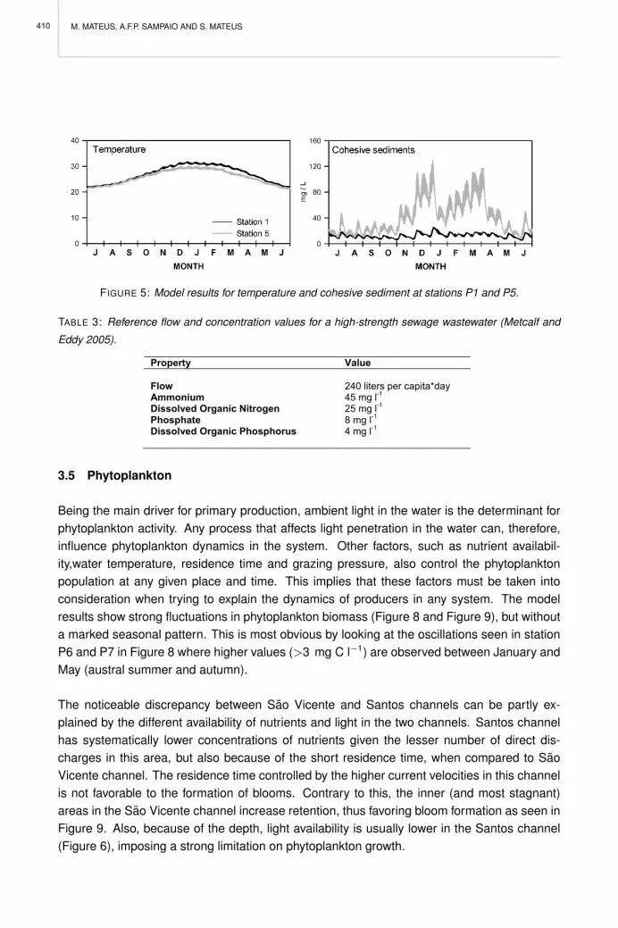
M. MATEUS, A.F.P. SAMPAIO AND S. MATEUS
FIGURE 5: Model results for temperature and cohesive sediment at stations P1 and P5.
TABLE 3: Reference flow and concentration values for a high-strength sewage wastewater (Metcalf and
Eddy 2005).
Property Value Flow 240 liters per capita*day Ammonium 45 mg l-1 Dissolved Organic Nitrogen 25 mg l-1 Phosphate 8 mg l-1 Dissolved Organic Phosphorus 4 mg l-1
3.5 Phytoplankton
Being the main driver for primary production, ambient light in the water is the determinant forphytoplankton activity. Any process that affects light penetration in the water can, therefore,influence phytoplankton dynamics in the system. Other factors, such as nutrient availabil-ity,water temperature, residence time and grazing pressure, also control the phytoplanktonpopulation at any given place and time. This implies that these factors must be taken intoconsideration when trying to explain the dynamics of producers in any system. The modelresults show strong fluctuations in phytoplankton biomass (Figure 8 and Figure 9), but withouta marked seasonal pattern. This is most obvious by looking at the oscillations seen in stationP6 and P7 in Figure 8 where higher values (>3 mg C l−1) are observed between January andMay (austral summer and autumn).
The noticeable discrepancy between Sao Vicente and Santos channels can be partly ex-plained by the different availability of nutrients and light in the two channels. Santos channelhas systematically lower concentrations of nutrients given the lesser number of direct dis-charges in this area, but also because of the short residence time, when compared to SaoVicente channel. The residence time controlled by the higher current velocities in this channelis not favorable to the formation of blooms. Contrary to this, the inner (and most stagnant)areas in the Sao Vicente channel increase retention, thus favoring bloom formation as seen inFigure 9. Also, because of the depth, light availability is usually lower in the Santos channel(Figure 6), imposing a strong limitation on phytoplankton growth.
410

AN ECOLOGICAL MODEL APPLICATION TO THE SANTOS ESTUARY, BRAZIL: TESTING AND VALIDATION
FIGURE 6: Model results for temperature, cohesive sediments, and irradiance in the water column. Some
scales have been expanded to enhance the spatial pattern.
411

M. MATEUS, A.F.P. SAMPAIO AND S. MATEUS
FIGURE 7: Model results for temperature, cohesive sediments, and irradiance in the water column. Some
scales have been expanded to enhance the spatial pattern.
FIGURE 8: Model results phytoplankton concentration at the monitoring points.
412

AN ECOLOGICAL MODEL APPLICATION TO THE SANTOS ESTUARY, BRAZIL: TESTING AND VALIDATION
FIGURE 9: Model results for ammonium, phosphate, phytoplankton biomass, particulate organic nitrogen
(PON), and dissolved oxygen saturation.
413

M. MATEUS, A.F.P. SAMPAIO AND S. MATEUS
Model output allows a detailed assessment of the temporal variation in resource limitation.Overall, the major limitation in the estuary is imposed by light, as seen in Figure 10 for threeintegration boxes, followed by temperature to a much lesser degree. This limitation is mainlyattributed to the high concentrations of cohesive sediments in the inner shallow areas of theestuary and to the depth of the deeper channels and outer area. Despite the high sedimentconcentrations in the water-column observed in some inner areas, light limitation is lower inthese areas when compared with the outer areas. This is illustrated in Figure 10, where Santoschannel (box 2) shows a higher limitation by light than the Cubatao area (box 4) located in theupper estuary. No limitation occurs for nutrients and the strong nutrient gradient in the estuarydoes not translate into an increase in nutrient limitation towards the nutrient-poor outer areas.
Due to the large freshwater contribution, the highest concentrations of dissolved inorganic nu-trients are found in the inner areas of the estuary. However, these more eutrophic conditionsdo not necessarily result in higher phytoplankton biomass since the high sediment concen-tration in the water and the consequent high light attenuation lead to light limitation of theprimary production. A similar mechanism has been reported for the nearby estuarine systemof Cananea-Iguape (Berrera-Alba et al. 2007).
Temperature limitation is almost horizontally homogeneous. Higher limitation is seen in winterand limitation also increases in high summer. This happens because ambient water tem-perature goes below or above the optimal temperature range. Finally, the model results forzooplankton biomass (Figure 11) suggest that grazing pressure may play a significant role inthe control of phytoplankton populations in the more inner areas. As seen for Stations P4and P5, zooplankton biomass is sometimes higher than phytoplankton biomass. Despite thehigh concentration of zooplankton at these stations (when compared to phytoplankton), thephytoplankton does not seem to be affected, suggesting high production rates.
3.6 Organic matter
In the present model setting, resuspension from the sediments, detrital material and riverdischarges are the sources of organic matter. So, in areas where resuspension is frequent(assuming there is PON in the sediments), where biological activity is more intense and un-der the influence of river discharges, OM concentrations are expected to be higher. Modelresults for PON (Figure 9 and Figure 12) illustrate this relation, with higher values, peakingat 0.2 mg l−1, observed in inner areas of the estuary where biological activity is intense andthe influence of rivers is maximal. This is also true for the Sao Vicente channel area whencompared with Santos channel. A small seasonal variation is observed in the results. Thelink to resuspension of PON is not so obvious because places under strong erosion do notnecessarily lead to an increase of resuspension of PON. The rationale is that in some areas,PON may be absent from the sediments.
414

AN ECOLOGICAL MODEL APPLICATION TO THE SANTOS ESTUARY, BRAZIL: TESTING AND VALIDATION
FIGURE 10: Limitation factors calculate by the model for some integration boxes. Note that values in the
Y axis stand for the inverse of limitation, i.e., the higher the value, the lower the limitation (total limitation
= 0; no limitation = 1).
3.7 Dissolved oxygen
Dissolved oxygen in the water is linked with biological activity and also dependent on watertemperature. Areas with high phytoplankton biomass are expected to have higher saturationsof oxygen (at least during daytime) as a result of photosynthesis. This oxygen production isbalanced by the mineralization of organic matter which requires oxygen and produces carbondioxide. So it is expected that oxygen concentrations and saturation values in the water trackthe dynamics of phytoplankton and organic matter closely. The interplay of these processesis seen in the horizontal fields of dissolved oxygen saturation (Figure 9). As an example, it ispossible to see that saturation values vary considerably inside the estuary, especially near theinfluence area of the rivers Botoroca, Cubatao, Pereque, and the direct sewage discharges.In this particular case, oxygen consumption may exceed production and the high loads oforganic matter at this time of year linked with decreased light availability may be the cause forunder-saturation values.
415

M. MATEUS, A.F.P. SAMPAIO AND S. MATEUS
FIGURE 11: Model results phytoplankton and zooplankton concentration at three monitoring points. Sam-
pling points were selected to consider the inner areas (P4 and P5) and a channel (P6).
FIGURE 12: Model results for particulate organic nitrogen (PON) at the monitoring points.
416

AN ECOLOGICAL MODEL APPLICATION TO THE SANTOS ESTUARY, BRAZIL: TESTING AND VALIDATION
Supersaturation values are observed in the bay and outer oceanic area, but also in some ar-eas inside the estuary where local conditions cause production to exceed consumption. Thispattern has also been observed in the nearby system of Cananeia which shares many physi-cal and biological features with the Santos estuary (Berrera-Alba et al. 2007). This occurrencemeans that despite the eutrophic state of these systems, oxygen production in the water col-umn can still compensate for the consumption caused by organic matter degradation. Theresults show that the system can be highly heterotrophic at some places (saturation valuesbelow 50%), due to the high loads of allochthonous organic matter, as seen in Figure 9. Thereis a slight decrease in oxygen concentrations in summer months observed at all stations.
4 MASS FLUXES IN THE ESTUARY
The model results for mass fluxes between different regions in the estuary (integration boxesin Figure 3) of some selected properties are listed in Table 4 and presented in Figure 13. Thevalues were integrated for a period of one year and account for net fluxes across the boundarybetween adjacent boxes. Considering the boundary of the bay area (box 7) to the open oceanas a hypothetical limit of the estuary, it is possible to look at the model results as an estimateof the export-import of mass from the estuary to the coastal area. The net balance betweenthese two areas is seen in Table 4 in the column 7 to 0. The results show that all describedstate-variables except oxygen are exported from the estuary to the coastal area. Under theseconditions, the model shows that the estuary is exporting nutrients and organic matter (bothliving and non-living) and importing oxygen. These results suggest that the nutrients thatenter in the system via rivers fuel local production but exceed the local needs, thus enrichingthe system and coastal areas. The oxygen dynamics need further attention because theestuary exports oxygen to the bay via Sao Vicente channel (∼27 ton yr−1) and much of thisproduction enters the estuary again via Santos channel (∼20 ton yr−1). Because oxygencan be introduced in the system from the atmosphere, no simple inference can be madefrom the results about the dynamics of the system. However, it can be speculated that theproduction in some areas can be surpassed by respiration (mineralization of autochthonousand allochthonous organic matter that enters via rivers).
There are other interesting patterns that can be found by looking at some distinct areas of thesystems. A striking feature of the system is the net balance between the bay area and bothchannels (box 7 to box 5 and to box 1). Apparently, the channels have distinct flux dynamics.There is a net positive balance from Sao Vicente channel (box 5) to the bay (box 7) for all themonitored state-variables. The opposite situation is observed for the fluxes between Santoschannel and the bay, where the net fluxes are negative towards the bay, meaning that Santoschannel is an entrance route for matter in the estuary. Curiously, a fraction of what is beingexported by the Sao Vicente channel enters the estuary again by Santos channel.
According to model results, Santos channel is a sink for phytoplankton, because only 106ton yr−1 transit from box 2 to 6, whereas 965 ton yr−1 transit from box 7 to 2. This sink of
417

M. MATEUS, A.F.P. SAMPAIO AND S. MATEUS
phytoplankton explains why the fluxes from Santos channel to Bagres island area (box 2 to 6)of all other variables increase (detrital matter, mineralized nutrients, oxygen consumption). Incontrast, Pombeba large area (box 3) is a source of phytoplankton, where the amount that isexported to Sao Vicente channel (box 1) is more than double the imported quantity from theCubatao area (box 4). Model results for the fluxes point to an eutrophication of the system.
5 CALIBRATION AND VALIDATION
The calibration and validation exercise was carried out with the aim of qualitatively assessingthe model performance. The main purpose was to test the ability of the model to reproducethe overall dynamics of the system and its adequacy as a tool for the prediction of the conse-quences of different (reduction) scenarios for effluent flow, nutrient loads, etc. To assess theperformance of the model, i.e., whether it is able to reproduce the observed spatial and tempo-ral patterns and their variability, model results were compared with observational data. Muchof the available data for calibration (Braga et al. 2000, Bosquilha 2002, Moser et al. 2002,Lima 2003) provided significant information on the patterns and variability in nutrient concen-trations and organic matter components. After calibration, the model was able to reproducesome of the patterns in the dynamics of the system as presented in these studies.
Validation was made by matching simulated values with field data for the respective proper-ties, as shown in Figure 14. Simulated dynamics correspond well with data from the eightmonitoring sites in the estuary. In general, the model produced realistic estimates for temper-ature, oxygen and nutrients. The magnitude and timing of the phytoplankton peak in in themodel reproduced field measurements satisfactorily. A match in values has been regularlyachieved, but sometimes not at the same station, as seen in the Chla values for August 2005.The largest mismatches are found regularly at stations 3 and 7. Despite these divergencesbetween model results and data, the model matched validation data with a fair degree of ac-curacy. The noted discrepancies between modelled and measured values may be due at leastpartially to our simplification of the dynamics of system components such as the mangrovesand inaccurate estimates of the nutrient loads to the system.
6 MODEL PERFORMANCE EVALUATION
The model was able to reproduce the major features of a typical tropical estuarine ecosystemsuch as Santos Estuary: large temperature variation along the salinity gradient, high meanwater temperatures, low light penetration, and variability in the flushing times and sedimentand nutrient discharges caused by marked temporal variability in fresh water discharges (Eyreand Balls 1999). The model results reveal a complex interaction of these factors. The seasonalcycle is evident in the results, mostly governed by river discharge associated with the rainyseason, and by the light regime (with both temporal and spatial variation). Also, the resultsshow a marked (fortnightly) spring-neap cycle, evident in the time series plots for all properties.
418

AN ECOLOGICAL MODEL APPLICATION TO THE SANTOS ESTUARY, BRAZIL: TESTING AND VALIDATION
308
275
72
864
510 486
1431
597
Ammonium
213
270
504
963
919 935
1081
954
Phosphate
11219
8531
13902
15223
1815115486
1322
0
16438
Oxygen
1022
177
76567054
1420
5477
767192
Phytoplankton
FIGURE 13: Model estimates for the fluxes of nutrients, phytoplankton biomass and oxygen between
different areas of the estuary. All values in metric tones per year.
TABLE 4: Mass fluxes between adjacent boxes integrated for one year at the boundary of each box.
Positive values mean a net positive balance from one box to the other, while negative values express a
negative balance. Column 7 to 0 is relative to fluxes at the boundary of box 7 with the coastal area.
mass fluxes between boxes (ton yr-1) 1 to 5 2 to 6 3 to 1 3 to 4 4 to 6 5 to 7 7 to 0 7 to 2
Ammonium 510 275 597 -864 -72 486 1431 308 Nitrate 2067 742 2332 -2907 -1673 2115 2482 464
Phosphate 919 270 954 -963 -504 935 1081 213 Oxygen 18151 8531 16438 -15223 -13902 15486 -13220 11219
Phytoplankton 7656 177 5477 767 192 7054 1427 1022 PON 407 81 324 -88 16 467 287 92
The organic matter and nutrient concentrations calculated in this study generally fall in thesame range as the field data. However, the modelled phosphorus values appear to be higherthan the corresponding field data. This suggests that P loads can be overestimated or that theboundary conditions may be too high. From this, we can conclude that a correct characteri-zation of inputs to the system is a prerequisite for a successful calibration effort. The modelreproduces the spatial pattern for the properties, where higher values occur in inner estuarineareas, with a limited circulation, and lower values in the main channels with shorter residencetimes.
419
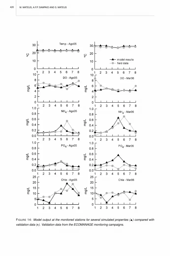
M. MATEUS, A.F.P. SAMPAIO AND S. MATEUS
FIGURE 14: Model output at the monitored stations for several simulated properties (N) compared with
validation data (•). Validation data from the ECOMANAGE monitoring campaigns.
420

AN ECOLOGICAL MODEL APPLICATION TO THE SANTOS ESTUARY, BRAZIL: TESTING AND VALIDATION
The model results suggest that Sao Vicente channel is the main exit route of materials fromthe estuary, a part of which enters the estuary again via the Santos channel. The modelshows a distinct dynamic between these two channels, controlled mainly by the residencetime (controlled by physical factors) and the presence of nutrient sources. The residence timein Sao Vicente channel is higher than in Santos channel, a difference that controls much ofthe dynamics of material between the channel and the bay. The fast renewal time of water inSantos estuary means that much of the water comes from the bay, which explains the importof material exported from the Sao Vicente channel.
Although the recycling of nutrients in the system appears to be important, there is a clearcontrol by allochthonous nutrients. Much of the behavior of the system is determined by thelarge amounts of nutrients (mineral and organic) that are discharged via sewage and rivers.A striking pattern to notice is the oxygen demand in the system, most obvious in the importa-tion of oxygen from the bay (Figure 13). This behavior of the system (as a large bioreactor)poses a challenging demand its management, considering the large anthropogenic pressureexpressed in the marked eutrophication of the estuary. In contrast to oxygen, the estuaryexports nutrients and organic matter to the coastal area. These results strongly suggest thatthe Santos estuary is in a highly eutrophic condition, compromising the water quality in theadjacent coastal areas.
Overall, the model is able to reproduce much of the features from the conceptual model de-rived from field data. The most significant features where the model agrees with data can besummarized in:
• A general pattern in dissolved nutrient concentrations with higher values in the direc-tion of the estuary’s head waters, especially in the areas of industrial effluents (e.g.,Piacaguera channel and Largo do Caneu), and with relatively low values in the outer ar-eas close to the open sea. This pattern is shaped mostly by physical mixing processes.Some increases are found near densely populated urban areas where sewage is di-rectly discharged into the estuary. A clear gradient of dilution from the estuary’s interiorto its mouth is seen along the natural channels (Braga et al. 2000).
• The relation between the spring-neap cycle and the nutrient and phytoplankton con-centrations. Phytoplankton has marked variations during neap-tide when nutrient, lightavailability and residence time all reach maximal values (Moser et al. 2005). Light isusually the limiting factor for phytoplankton growth in estuaries (Cloern et al. 1995, Clo-ern 1999). The oscillations in light and nutrient conditions between spring and neaptides shape phytoplankton growth. Neap tide conditions enhance the stability in thewater column, decreasing the suspended sediments that block the light, and createbloom conditions by increasing the residence time. This pattern has been observed inBertioga channel, a channel connected to the upper Santos channel (Gianesella et al.2000), suggesting that the Santos Estuary also shares this feature. Changes in lightconditions and flushing ultimately control phytoplankton distribution in the estuary.
421

M. MATEUS, A.F.P. SAMPAIO AND S. MATEUS
• Export of organic matter, inorganic nutrients and phytoplankton to the bay highlightingthe contribution of the estuary to the eutrophication of Santos bay, especially during therainy season when river flow is higher (Moser et al. 2005).
• The increase in particulate matter is mostly from allochthonous sources, not from localphytoplankton production.
• Nutrient limitation does not play a significant role in phytoplankton dynamics. While inthe inner parts of the estuary this pattern is explained by the nutrient inputs from riversand direct sewage discharges, in the bay area this can be explained by the inorganicnutrients contributed by the submarine outfall (Moser et al. 2002, Moser et al. 2004).
7 THE MODEL AS A MANAGEMENT TOOL
For a model to be useful as a management tool it must reproduce the main features of thesystem under study. This implies that the model must capture the significant processes andinteractions between compartments. In short, the model must be able to reproduce the basicelements of the conceptual model of the system.
Under a DPSIR framework, the model establishes a clear relation between anthropogenic nu-trient sources (Pressures), the cycling of carbon biomass in the system and oxygen-relatedproblems (State). The outfall emission, river discharges, storm drains and sewage dischargesall contribute to its enrichment with nutrients. At the same time, the emissions have a clearimpact on oxygen dynamics by increasing the organic matter concentrations, enhancing het-erotrophic activity, which in turn contributes still more nutrients to the system. The more com-plex the system is the more difficult is the task to model it. This is particularly true in caseswhere the anthropogenic influences are many-faceted, as they are in the Santos estuary.There is always a degree of uncertainty in the load estimates used in the model because ofthe impossibility to quantify the loads accurately, and this uncertainty negatively affects themodelling exercise. Despite all the uncertainty, the model has the capability to reproduce ma-jor features of the ecological conceptual model of Santos and the links between environmentalState and human Drivers.
REFERENCES
Abessa D M S, Carr R S, Rachid B R F, Sousa E C P M, Hortelani M A, Sarkis J E (2005) Influence ofa Brazilian sewage outfall on the toxicity and contamination of adjacent sediments. Marine PollutionBulletin 50: 875-885
Berrera-Alba J J, Gianesella S M, Moser G A, Saldanha-Correa F M P (2007) Bacterial and phytoplanktondynamics in a sub-tropical estuary. Hydrobiologia (in press): DOI 10.1007/s10750-10007-19156-10754
Borja A, Galparsoro I, Solaun O, Muxika I, Tello E, Uriarte A, Valencia V (2006) The European WaterFramework Directive and the DPSIR, a methodological approach to assess the risk of failing to achievegood ecological status. Estuarine, Coastal and Shelf Science 66: 84-96
422

AN ECOLOGICAL MODEL APPLICATION TO THE SANTOS ESTUARY, BRAZIL: TESTING AND VALIDATION
Bosquilha G E (2002) Estudo da distribuicao de surfactantes anionicos e de polifosfatos no Sistema Es-tuarino de Santos/Sao Vicente e Baıa de Santos (SP, Brasil) e Avaliacao de metodologias aplicadas.Master Degree. Universidade de Sao Paulo. Instituto Oceanografico, S Paulo.
Braga E S, Bonetti C V D H, Burone L, Bonetti J (2000) Eutrophication and bacterial pollution caused byindustrial and domestic wastes at the Baixada Santista estuarine system - Brazil. Marine PollutionBulletin 40: 165-173
Carmouze J P, Galvao S G, Nishiara L, Mesquita S L (1998) Modelling chemical changes of tidal watersemerging from a mangrove forest at Cananeia, Brazil. Mangroves and Salt Marshes 2: 43-49
Cesar A, Choueri R B, Riba I, Morales-Caselles C, Pereira C D S, Santos A R, Abessa D M S, DelValls TA (2007) Comparative sediment quality assessment in different littoral ecosystems from Spain (Gulf ofCadiz) and Brazil (Santos and Sao Vicente estuarine system). Environment International 33: 429-435
CETESB (2001) Relatorio do Programa de Controle da Poluicao no Sistema Estuarino de Santos e SaoVicente (PROCOP). Companhia de Tecnologia de Saneamento Ambiental, Sao Paulo. 178p.
Cloern J E (1999) The relative importance of light and nutrient. Aquatic Ecology 33: 3-15
Cloern J E, Grenz C, Vidergar-Lucas L (1995) An empirical model of the phytoplankton chlorophyll : car-bon ratio - the conversion factor between productivity and growth rate. Limnology and Oceanography40: 1313-1321
Eyre B, Balls P W (1999) A comparative study of nutrient behavior along the salinity gradient of tropicaland temperate estuaries. Estuaries 22: 313-326
Fasham M J R, Ducklow H W, Mckelvie S M (1990) A Nitrogen-Based Model of Plankton Dynamics in theOceanic Mixed Layer. Journal of Marine Research 48: 591-639
Gianesella S M, Saldanha-Correa F P, Teixeira C (2000) Tidal effects on nutrients and phytoplanktondistribution in Bertioga Channel, Sao Paulo, Brazil. Aquatic Ecosystem Health and Managment 3:533-544
Gragnani M (1996) Dinamica hidraulico-salina e seu controle: O caso do Baixo Cubatao - Sao Paulo. MDThesis. Escola Politecnica da Universidade de Sao Paulo, Sao Paulo.
Harari J, de Camargo R (2003) Numerical simulation of the tidal propagation in the coastal region ofSantos (Brazil, 24 degrees S 46 degrees W). Continental Shelf Research 23: 1597-1613
IBGE (2000). Instituto Brasileiro de Geografia e Estatıstica.
Leitao P C, Mateus M, Braunschweig F, Fernandes L, Neves R (2008) Modelling coastal systems: theMOHID Water numerical lab, this volume.
Lima C A (2003) Estudo de indicadores biologicos de poluicao (coliformes totais e coliformes fecais) ede suas relacoes com os teores de nitrogenio amoniacal, ureia e oxigenio dissolvidos, no SistemaEstuarino de Santos/Sao Vicente e Baıa de Santos. Master Degree. Universidade de Sao Paulo.Instituto Oceanografico, S Paulo.
Mateus M, Campuzano F (2008) The DPSIR framework in the Integrated Management of Coastal Areas,this volume.
Medeiros P M, Bicego M C (2004a) Investigation of natural and anthropogenic hydrocarbon inputs insediments using geochemical markers. I. Santos, SP - Brazil. Marine Pollution Bulletin 49: 761-769
Medeiros P M, Bicego M C (2004b) Investigation of natural and anthropogenic hydrocarbon inputs insediments using geochemical markers. II. Sao Sebastido, SP - Brazil. Marine Pollution Bulletin 49:892-899
Metcalf (2005) Wastewater Engineering: Treatment and Reuse, Fourth edition. McGraw Hill. 1819p.
Moser G A, Sigaud-Kutner T C, Cattena C O, Gianesella S M, Braga E S, Schinke K P, Aidar E (2004)Algal growth potential as an indicator of eutrophication degree in coastal areas under sewage disposalinfluence. Aquatic Ecosystem Health and Managment 7: 115-126
Moser G A O, Gianesella S M, Alba J J, Bergamo A L, Saldanha-Correa F M P, Miranda L B, Harari J(2005) Instantaneous transport of salt, nutrients, suspended matter and chlorophyll-a in the tropicalestuarine sustem of Santos. Brazilian Journal of Oceanography 53: 115-127
423

M. MATEUS, A.F.P. SAMPAIO AND S. MATEUS
Moser G A O, Gianesella S M F, Cattena C O, David C J, Barrera-Alba J J, Saldanha-Correa F M P, BragaE S. 2002. Influencia das mares sobre o fitoplancton no sistema estuarino de Sao Vicente e Santos.In: Anais do Congresso Brasileiro de Pesquisas Ambientais. Congresso Brasileiro de PesquisasAmbientais
Thomann R V, Muller J A (1982) Verification of water quality models. Journal of Environmental Engineering108: 923-940
Thomann R V, Muller J A (1987) Principles of surface water quality modelling and control. Harper andRow, New York.
424

PERSPECTIVES ON INTEGRATED COASTAL ZONE MANAGEMENT IN SOUTH AMERICAR. NEVES, J.W. BARETTA AND M. MATEUS (EDS.), IST PRESS, 2008
A MODELLING APPROACH TO THE STUDY OF FAECAL POLLUTION IN THESANTOS ESTUARY
A.F.P. SAMPAIO, M. MATEUS, R.B. RIBEIRO AND G. BERZIN
1 INTRODUCTION
The need for adequate disposal techniques and sites for urban wastewater has long been rec-ognized. The most convenient place to discharge wastewater, whether treated or untreated,is usually into any nearby body of water. Communities located in estuarine and coastal areashave several alternatives for disposal their wastewater: direct discharge into the sea throughsubmarine outfalls, in the watercourses and tributaries feeding the estuary, and directly in theestuarine waters. The availability of a nearby water body leads many communities to dis-charge untreated or partially treated wastewater into estuarine and coastal waters. A basicassumption is made that dilution can lessen pollution-related problems. However, mixing incoastal waters is far from complete and in estuaries even less complete, thus leading some-times to the presence of plumes with high concentration of polluting agents. In more stagnantareas the wastewaters can promote the formation of ”hotspots” in the immediate vicinity of thedischarge point, where concentrations rise to significant levels.
Domestic wastewater contains a large number of pathogenic organisms originating from hu-mans who are infected with disease or who are carriers of a particular disease. The mostcommon pathogens found in sewage are those that cause typhoid fever, dysentery, gastroen-teritis, diarrhea and cholera. The faecal coliform group of bacteria is usually used as a proxyfor pathogenic agents in wastewater. On average, each person discharges from 100 to 400billion coliform organisms per day, along with many other potential harmful bacteria and virus.The number of viable coliforms in fresh domestic sewage ranges from 108 to 109 MPN (MostProbable Number) per 100ml (Bishop 1983).
2 FAECAL POLLUTION IN THE SANTOS ESTUARINE SYSTEM
Until recently in Brazil less than 13% of Municipal Wastewater was treated before disposalin a river, lake or ocean (UNEP 2003). As such, the faecal pollution in the Santos area isa common challenge shared with many other Brazilian coastal systems. The main healthproblems observed in coastal populations in Brazil include the increase and re-emergency ofdiseases like yellow fever, dengue, malaria, water borne disease (diarrhea, hepatitis, typhoidfever, cholera) and virus diseases (Garreta-Harkot 2003).
This chapter focuses on a model application to assess the health of the marine water bodiesalong the Santos - Sao Vicente estuary, with special attention to a specific indicator of faecalcontamination, Escherichia coli. The need of this analysis was based on the fact that theregion - as other coastal metropolitan areas - has densely populated urban areas without
425

A.F.P. SAMPAIO, M. MATEUS, R.B. RIBEIRO AND G. BERZIN
a sewage drainage network or sewage treatment and a high number of irregular dwellings.Because of their location close to the mangrove and river banks, a significant part of thesehousing nuclei drain considerable loads of domestic effluents directly to the estuary. This typeof pollution has not been as intensively studied as other research lines developed in the region(which were more frequently associated to the history of chemical pollution of the sedimentsand the water by industrial activities). However, some works have pointed out the need forthese analyses due to the high and increasing rate of faecal coliforms found in the waters ofthe estuary (Cetesb 2005, 2006). The presence of many slum quarters and quarters withoutsewage network or treatment, as well as the three sewage treatment plants and the submarineoutfall, create a considerable anthropogenic pressure on the aquatic environment, affectingthe biota as well as human health in the Santos - Sao Vicente estuarine system (Braga et al.2000, Abessa et al. 2005).
The in-natura domestic sewage dumping in estuarine channels and rivers has been classifiedas a potential source of pollution in Santos - Sao Vicente estuarine system (Braga et al. 2000,Cetesb 2001, Lima 2003, Gianesella 2006). The extent and the degree of contamination aswell as the resilience of this environment to the increase of microbiological contamination is stillunknown. Numerical models are very useful to estimate contaminant dispersion, particularlyfaecal coliforms, because they can combine hydrodynamic and water quality processes (Fricket al. 2001). This work presents such an application, based on the MOHID model system(Leitao et al., Mateus and Fernandes, this volume), aiming to validate a faecal decay modelfor the Santos Estuary so it can be used as a management and predictive tool.
3 MODEL IMPLEMENTATION
The water quality model is coupled with the hydrodynamic model previously described (Leitaoet al., this volume) and so the same assumptions for the physical features of the system arevalid here. These are: (1) the water-column is not stratified (2D horizontal); (2) the hydrody-namics in the bay are not affected by shelf water circulation. The external conditions includeriver discharges, forcing functions, like solar radiation and air temperature, and boundary con-ditions. The simulations were performed with variable T90 decay model for E. coli (see Mateusand Fernandes, this volume).
3.1 Atmospheric forcing
Climatological radiation levels were calculated by the model for the domain geographical coor-dinates. Air temperature, relative humidity and cloud cover (Figure 1) were also used to forcethe model, with monthly values taken from field observations made at CODESP meteorolog-ical station at Alemoa during 1997. For cloud cover the only complete historical series foundis from 1999, obtained by observation at the Brazilian Navy’s meteorological station locatedon Moela Island, at a zone adjacent to Santos bay, about 17 km away from the CODESPmeteorological station at Alemoa.
426

A MODELLING APPROACH TO THE STUDY OF FAECAL POLLUTION IN THE SANTOS ESTUARY
3.2 Initial and boundary conditions
The boundary conditions (temperature, salinity, cohesive sediments and E. coli concentra-tions) considered for open Atlantic boundaries and the initial conditions for the model are givenin table 1. The model considers six river inputs inside the domain. In two of these rivers (Cu-batao + Henry Borden and Moji + Piacaguera) a monthly mean faecal coliforms concentrationwas considered (Figure 2) according to a bimonthly value average between 2000 and 2005obtained from CETESB’s monitored points. The pollution point sources used in the modelwere determined based on current information on the sanitary conditions of the basin, so thatthe development of a numerical reference scenario for the current situation could therefore beestablished. The model considers 31 sewage discharge points, three sewage treatment plants(STP) and the submarine outfall in the bay (Figure 3 and table 2). All discharges are charac-terized by a cohesive sediment concentration of 120 mg l−1, a salinity of 0.5, a temperatureof 24 oC.
TABLE 1: Initial conditions and boundary conditions defined for each property in model simulations.
Properties Units Initial conditions
Boundary conditions
Temperature ºC 20 20
Salinity psu 20 36
Cohesive sediments mg l-1 100 25
E. coli MPN/100ml 0 0
TABLE 2: Sewage discharge areas, E. coli concentration and the respective effluent flow ( m3 s−1). Dis-
charges include the outfall, sewage treatment plants (STP), slum quarters and quarters out of sewage
drainage (Not treated).
Sewage discharge points MPN/100ml Flow m3 s-1
Not treated 1.00 x 10⁸ 0.436 STP Cubatão 3.72 x 10⁵ 0.200 STP Humaitá 5.30 x 10⁵ 0.040 STP Samaritá 2.30 x 10⁵ 0.040 Santos submarine outfall 7.48 x 10⁶ 2.500
Total
3.216
3.3 Model validation
The model results were validated with E. coli field data from two ECOMANAGE campaignscarried out in August 2006 and in April 2007 (Figure 4). These analyses allowed the identifi-cation of the degree of microbiological contamination in the water, especially in the interior ofthe Santos Estuarine System where data of this nature are scarce. The sampling campaignswere carried out by means of a cooperation regime between UNISANTA through ECOMAN-AGE Project and SABESP - Sao Paulo State Basic Sanitation Company: the field samplingwas carried out by the UNISANTA team and the analyses by the SABESP team.
427

A.F.P. SAMPAIO, M. MATEUS, R.B. RIBEIRO AND G. BERZIN
FIGURE 1: Monthly mean values for air temperature, cloud cover and relative humidity used to force the
model.
FIGURE 2: Monthly mean values of E. coli assumed for the major river discharges: the joint discharges of
Moji + Piacaguera and Cubatao + Henry Borden.
4 MODEL RESULTS
Considering the objective of this work, an analysis of faecal contamination in the Santos Es-tuarine system, only the model results for faecal coliforms are discussed here. Eight pointsinside the Santos Estuary (Figure 5) were chosen for the output of model results in order tosimplify the analyses. Field data from these stations was used to perform the validation.
The faecal coliform concentration in the water column shows a greater spatial variation (Fig-ure 6 and 7). In the Largo da Pompeba (P6) and Barreiros channel (P7) values above 103
MPN/100ml are observed (Figure 6), being the point 6 the most critical in terms of concen-tration. This higher concentration can be associated with the amount of slum quarters andquarters out without sewage network. Although the Cubatao, Mogi and Piacaguera riversdischarges contributed with higher concentration of E.coli, the Piacaguera channel (P5) andLargo do Caneu (P4) areas show concentrations below 100 MPN/100ml.
428

A MODELLING APPROACH TO THE STUDY OF FAECAL POLLUTION IN THE SANTOS ESTUARY
FIGURE 3: Sewage discharge points defined for the model simulation.
FIGURE 4: Results from the E. coli data sampling campaign (MPN/100ml) in the summer and winter.
A reason for this result can be related to the fact that these areas, being shallower, have highersolar radiation levels in the water column, the main agent that controls the survival of entericbacteria in the water (Sarikaya and Saatci 1995, Serrano et al. 1998). Besides, these pointsare far from the sources of dumping, so dilution also contributes to the low concentration. AtSantos channel (P2) the model shows concentrations below 103 MPN/100ml, slightly lowerthan the measured data. This discrepancy can be related to the discharges of untreatedsewage of Vicente de Carvalho besides the slum quarters. Spring and neap tide cycles causegreat variation on E. coli concentrations, as seen in the model results (Figure 7). A greatervariability is seen in the monitored points located in the Santos (P1) and Sao Vicente (P8)channels, Sao Vicente having higher concentrations. The concentrations in these areas are
429

A.F.P. SAMPAIO, M. MATEUS, R.B. RIBEIRO AND G. BERZIN
regulated by hydrodynamic conditions. During a spring ebb tide the model shows that thesechannels contribute to increase the faecal contamination at Santos bay (Figure 7), mainlyclose to the Sao Vicente channel.
The influence of the submarine outfall at the Santos Bay is clearly noted, but the high concen-tration of E. coli from this source does not seem to reach Santos and Sao Vicente beaches,as seen in Figure 4. However, it is worth pointing out that the simulated conditions refer to a2D model integrated in vertical, representing patterns of circulation in Santos forced only byastronomical tide and without the influence of wind.
5 MODEL VALIDATION
Validation was performed by matching simulated values with field data, as illustrated in Fig-ure 8. The model performed very well for the winter, producing realistic estimates for E. coliconcentrations in most of eight points. Only the results for points 3 and 5 were not so wellreproduced. The model estimates for summer did not match results as well as for winter. Inthe summer only point 2 matched the campaign result. This difference between model re-sults for summer and winter conditions can be attributed to the fact that an elevation in thedischarges by urban drainage was not considered for the summer in the model, except forthe river flow. Historical data on total and faecal coliform samplings carried out at Santos bayshows a significant elevation in microbiological contamination rates in the rain season coinci-dent with the summer in the region (Sartor 2000, Lima 2003). Besides, one has to consideran increase in sewage generation incurred by the population growth in this season too. Themeasure campaign performed within the project corroborates this scenario, considering thatthe number of samples that exceeded the 103 MPN/100ml in summer was 5 times higher thanwinter samples (from a total 57 samples). This variation was observed all over the estuary.Another point that must be considered is that the data used to validate the model has beenfrom surface samples and the model presents the water column average results.
6 FINAL CONSIDERATION AND FUTURE WORK
E. coli concentrations were used in this study as indicators of aquatic pollution and anthropicinterference in Santos - Sao Vicente estuarine system originated from urban residual waterdumping on the superficial water bodies. Two microbiological data sampling campaigns per-formed during the project showed a marked faecal coliform fluctuation between the summerand the winter when compared to each other - where the summer analyses showed a numberof points (45) over 103 MPN/100ml. The results clearly reveal a seasonal variability within theestuary. The results corroborate the existing literature related to the contribution of urban plu-vial drainage to microbiological contamination (Sartor 2000, Lima 2003). Still, in this estuarythese simulations tend to become even more complex owing to the need of considering an in-crease in tourist population, as well as a greater contribution of diffuse loads from pluviometricprecipitations, both being a typical summer phenomena in the region.
430

A MODELLING APPROACH TO THE STUDY OF FAECAL POLLUTION IN THE SANTOS ESTUARY
FIGURE 5: Sampling stations for the data survey campaigns.
FIGURE 6: Model output results for E. coli concentration (MPN/100ml) at the eight monitored points.
431

A.F.P. SAMPAIO, M. MATEUS, R.B. RIBEIRO AND G. BERZIN
FIGURE 7: Model output results for E. coli concentration (MPN/100ml) in different tide conditions.
The model captures the spatial-temporal patterns of E. coli dynamics in the system. However,the summer results showed the importance of considering the affluent discharges of pluvialorigin typical of this season in future works for a better reproduction of the coliform behaviorin this period. Therefore, it is recommended that more research be done to achieve an ef-fective assessment of the role of this contribution in modelling simulations. Even though thesolution of the model is integrated for the water column, the comparisons between measuresand model results were satisfactory, especially in Santos and Sao Vicente channels, bothcharacterized by a stronger natural hydrodynamic regime when compared to other areas.
The validation outcome for the dispersion of microbiological plumes has been positive, but theneed for a more advanced validation process, based on a broader and systematic field mon-itoring is evident. Although this sort of ongoing monitoring is an expensive effort, the results
432

A MODELLING APPROACH TO THE STUDY OF FAECAL POLLUTION IN THE SANTOS ESTUARY
are fundamental for a proper understanding of the system’s functioning, therefore fundamentalfor a correct calibration and validation of the numerical models. Together, more field data andmodelling simulations will increase the knowledge of the seasonal microbiological behavior inthe interior of the estuary. This is of paramount importance to determine spatial-temporal vari-ation in faecal concentrations with more precision and, consequently, perfecting the forecastcapability of the modelling system. Such a system is required for a proper management of theSantos bay water quality, given that the source of much of its contamination is located insidethe estuary, as suggested by field data and supported by model results.
FIGURE 8: Comparison between model output (black bar) and data field (gray bar) at the monitored
sample points.
REFERENCES
Abessa DMS, Carr RS, Rachid BRF, Sousa ECPM, Hortelani MA, Sarkis JE (2005) Influence of a Braziliansewage outfall on the toxicity and contamination of adjacent sediments. Marine Pollution Bulletin 50:875-885
Bishop PL (1983) Marine pollution and its control. McGraw-Hill. 357p.Braga E S, Bonetti C V D H, Burone L, Bonetti J (2000) Eutrophication and bacterial pollution caused by
industrial and domestic wastes at the Baixada Santista estuarine system - Brazil. Marine PollutionBulletin 40: 165-173
CETESB (2001). Relatorio do Programa de Controle da Poluicao no Sistema Estuarino de Santos e SaoVicente (PROCOP). Companhia de Tecnologia de Saneamento Ambiental, Sao Paulo. 178p.
CETESB (2005). Relatorio do Qualidade de aguas litoraneas. Companhia de Tecnologia de SaneamentoAmbiental, Sao Paulo. 254p.
CONAMA (2005). Conselho Nacional de Meio Ambiente. Resolucao 357/2005. Diario do Senado Federal(2004). ”Resolucao 09”. Republica Federativa do Brasil, ano LIX, n◦.095, junho, 2004, pp. 17840-14841
Frick W, Roberts LPJW, Davis J, Keyes D, Baumgartner K G (2001) Dilution model for effluent discharges,(visual plumes). Environmental Research Division, NERL, ORD - U.S. Environmental ProtectionAgency - Standarts and Applied Division Office of Science and Technology, 2001, July, n. 4
Garreta-Harkot PF (2003) The Brazilian National Plan of Coastal Management, the health and the envi-ronment. MD Thesis. Faculdade de Saude Publica da Universidade de Sao Paulo, Sao Paulo.
Gianesella SM, Saldanha-Correa FP, Teixeira C (2006) Tidal effects on nutrients and phytoplankton distri-bution in Bertioga Channel, Sao Paulo, Brazil. Aquatic Ecosystem Health and Managment 3: 533-544
433

A.F.P. SAMPAIO, M. MATEUS, R.B. RIBEIRO AND G. BERZIN
Gianesella SMF, Ricci FP, Moser GAO , Saldanha-Correa FMP, Toma AEF (2006) Distribuicao do materialem suspensao nos canais de Santos e Sao Vicente. In: Environmental and Health World Congress:642-645
IBGE (2000)Censo Demografico. Instituto Brasileiro de Geografia e Estatıstica.
Leitao PC, Mateus M, Braunschweig F, Fernandes L, Neves R (2008) Modelling coastal systems: theMOHID Water numerical lab, this volume.
Lima CA (2003) Estudo de indicadores biologicos de poluicao (coliformes totais e coliformes fecais) ede suas relacoes com os teores de nitrogenio amoniacal, ureia e oxigenio dissolvidos, no SistemaEstuarino de Santos/Sao Vicente e Baıa de Santos. Master Degree. Universidade de Sao Paulo.Instituto Oceanografico, S Paulo.
Mateus M, Fernandes R (2008) Modeling Pollution: Oil Spills and Faecal Contamination, this volume.
Moser GA, Sigaud-Kutner TC, Cattena CO, Gianesella SM, Braga ES, Schinke KP, Aidar E (2004) Algalgrowth potential as an indicator of eutrophication degree in coastal areas under sewage disposalinfluence. Aquatic Ecosystem Health and Managment 7: 115-126
Sarikaya HZ, Saatci AM (1995) Bacterial Die-Away Rates in Red-Sea Waters. Water Science and Tech-nology 32: 45-52
Sartor SM, Degaspari F (2000) A balneabilidade das praias de Santos - Discussao dos criterios oficiaisde avaliacao. 27◦ Congresso Interamericano de Engenharia Sanitaria e Ambiental.
Serrano E, Moreno B, Solaun M, Aurrekoetxea JJ, Ibarluzea J (1998) The influence of environmentalfactors on microbiological indicators of coastal water pollution. Water Science and Technology 38:195-199
UNEP (2003) Water Resources Management in Latin America and the Caribbean. Fourteenth Meetingof the Forum of Ministers of the Environment of Latin America and the Caribbean. Panama City,Panama.
434

PERSPECTIVES ON INTEGRATED COASTAL ZONE MANAGEMENT IN SOUTH AMERICAR. NEVES, J.W. BARETTA AND M. MATEUS (EDS.), IST PRESS, 2008
ASSESSING THE IMPACT OF SEVERAL DEVELOPMENT SCENARIOS ON THEWATER QUALITY IN SANTOS ESTUARY
A.F.P. SAMPAIO, M. MATEUS AND R.B. RIBEIRO
1 INTRODUCTION
Growing human populations and associated infrastructures in coastal areas have been grad-ually destroying the balance between terrestrial and marine environments. Among these hu-man pressures, the impact of sewage inputs and urban runoff has been highlighted as a majorglobal problem requiring urgent action. Faecal pollution is a consequence with serious impli-cations for human health. Eutrophication is another symptom with direct consequences forthe ecosystem. Eutrophication is usually recognized as an undesirable effect, a fact that ex-plains the numerous recommendations regarding reduction of nutrient inputs from wastewatertreatment issued over the past decades (e.g., Helsinki Comission - HELCOM).
The Santos area faces the same basic problems experienced by many developing countries,such as shortage of adequate housing and lack of sewerage system (Garreta-Harkot 2003).There is growing anthropogenic pressure on the coastal zone resulting from the main socio-economic Drivers that include the rapid increase in the coastal population, industrial develop-ment, etc. Input of domestic sewage and estuarine discharge has been pointed out as themain source of eutrophication in this system (Moser et al. 2004), and studies have estab-lished a link between the contribution of Santos and Sao Vicente estuaries as the major causeof eutrophication of Santos bay (Moser et al. 2005).
The development of management policies for the Santos estuary has to deal with faecal pol-lution and eutrophication-related problems. An informed management for a sustainable useof estuarine services requires the capacity to assess their state, and to predict future statesin the face of different development perspectives and choices. The definition of developmentstrategies must consider that the existing Pressures can be mitigated or additional ones canappear. In addition, the overall Impact on the environment must be forecast. Part of this effortcan be achieved by testing the result of different development scenarios with numerical modelsimulations. Models are increasingly becoming indispensable tools in environmental studiesand management decisions. In the DPSIR framework models are commonly used to eluci-date each component and the relation between different the different components (e.g., thepressures with the state). Combining the DPSIR with numerical models allows the generationof predictions on the potential levels of selected impacts, allowing policy makers to promoteresponsive remedial or mitigating actions before the predicted impacts manifest themselves inthe environment.
This chapter describes such a modelling study, made to assess and forecast the result offour different management scenarios for wastewater disposal in the Santos Estuary. Thestudy aimed to characterize the extension and degree of microbiological contamination and
435

A.F.P. SAMPAIO, M. MATEUS AND R.B. RIBEIRO
changes in the eutrophic state in the estuarine waters of Santos under different input scenariosof urban discharges and temporal and spatial evolution. This study does not address thefeedback implications that each development scenario has on the socioeconomic activities inthe Santos area.
2 DEVELOPMENT SCENARIOS
The simulated scenarios include a number of possible scenarios within the field of probable.The conditions that range from the ”business as usual” scenario, i.e., no changes to the ac-tual conditions, meaning that no actions are taken or management policies implemented toimprove the sewage treatment and disposal, to an ”optimum case” scenario (hypothetical). Inthis last scenario the population growth and its impact is minimized by adequate managementprocedures that significantly reduce untreated domestic sewage discharges into the estuary.The ”business as usual” scenario is used as the reference condition.
Two intermediate scenarios have been projected having in mind the changes that are expectedto occur in the estuary as a result of projected improvements in the sewage drainage system,such as the implementation of drainage systems in some slum quarters already urbanized, theconstruction and extension of the actual system in other areas, and the treatment of sewageeffluent prior to disposal inside the estuary. These scenarios result from a prospective analysisthat was made considering the main Drivers in the system. Finally, the fourth scenario, the”optimum case”, is based on hypothesized desirable conditions.
The sewage input for all scenarios was estimated according to current sanitary conditions,future projects in basic sanitation foreseen for the region and one hypothetic scenario. A qual-itative and quantitative secondary data survey on urban discharges was carried out on themodel’s land boundary, that is, all over the estuary’s drainage basin, in order to characterizeand estimate the pressures resulting from current urban occupation. This estimate was basedon the data survey of a group of socioeconomic components related to the homes’ sanitarycharacteristics described by Sampaio and Ferreira (this volume). Their data were obtainedfrom the last demographic census (IBGE 2000) and from internal data from the Companhiade Saneamento Basico do Estado de Sao Paulo (Sao Paulo State Basic Sanitation Com-pany - SABESP). By cross-checking these sources of information, it was possible to estimatequantitatively and more accurately the volumes drained to the estuary without treatment fromthe homes without a connection to the sewage drainage network and the loads of domesticeffluents from the sewage treatment stations and the submarine outfall.
The discharge points defined in the simulations (Figure 1) were set based on current infor-mation on the sanitary conditions of the basin, so that a numerical reference scenario for thecurrent situation could be established. Once this stage - consisting of the implementation,calibration and validation of a water quality model - had been accomplished, it was possible toprospect future development conditions. Thus, the aspects that involve the lack of coverage ofurban sanitary services were also analyzed in a projection towards 2010 and 2015, to assess
436

ASSESSING THE IMPACT OF SEVERAL DEVELOPMENT SCENARIOS ON THE WATER QUALITY IN SANTOS ESTUARY
the impact of population growth and the possible advancements of public policies foreseen inthis temporal window. Besides, the simulation of a hypothetical scenario - where all the loadsthat were not addressed by sanitary projects until 2015 were directed to treatment stations orto the existing outfall - was included in order to verify what the results achieved were.
FIGURE 1: Sewage discharge points for each scenario.
2.1 Scenario 1: ”business as usual”
This scenario can be seen as the ”worst case scenario” since it implies that the actual situationis not improved by remedial actions. This scenario considers 31 sewage discharge points,three sewage treatment plants (STP) and the submarine outfall. This is considered as thereference scenario and has been addresses by Sampaio et al. (this volume) for the faecalpollution and by Mateus et al. (this volume) for the ecology.
2.2 Scenario 2
This scenario (2010 scenario) considers 27 sewage discharge points that include the improve-ments in the sewage drainage systems provided by the works announced for the region by thefederal government and also an increase in sewage generation incurred by the estimated pop-
437

A.F.P. SAMPAIO, M. MATEUS AND R.B. RIBEIRO
ulational growth. Among the major changes from the reference scenario (Scenario 1) is thediversion of some sewage discharges from Piacabucu River to the Praia Grande outfall, partof the sewage diverted to the Santos outfall in the bay, the increase in the loads at Site 8 asa result of urban development in the surrounding area, and an increase in the discharges atPompeba area.
2.3 Scenario 3
This scenario is based on predictions for the year 2015 for population growth and the sewagesystem improvement work that will be developed from 2010 to 2015. It considers 21 sewagedischarge points. Compared to the reference situation, in this scenario the water treatmentplan (WTP) flow at Cubatao is over three times higher, there is a new WTP at Santos channel,the diversion of some sewage discharges from Santos channel to the Guaruja outfall. Also,the sewage outfall flow in the bay was increased by 0.5 m3 s−1 and its point of disposal moved400 meters seawards. Improvements from ”Onda Limpa”, a great sanitary project (Diario doSenado Federal 2004) were included in addition to the previous works already foreseen in the2010 scenario. Scenarios 2 and 3 were designed according to data provided by stakeholders,and existing chronograms being that analysis based upon the dates predicted for the end ofthe works.
2.4 Scenario 4: ”optimum case”
This is a fictitious scenario where all but three of the remaining slum quarters are connectedto the sewage drainage network and directed to the submarine outfall or to sewage treatmentplants. The loads have been calculated for the expected population in 2015.
3 MODEL SIMULATIONS
The water quality model used here to simulate the ecological dynamics and faecal pollutionhave been previously calibrated and validated (see Mateus et al., Sampaio et al., this volume)and the results presented in these previous modelling studies used to characterize the refer-ence state. As such, the modelling settings used in the present study (forcing functions, initialconditions, assumptions, etc.) are the same as defined in these chapters. The only differencesbetween scenarios are the discharge points inside the estuary and the loads.
Unlike the majority of water quality indicators, faecal contamination is a bioindicator. Thismeans that it’s persistence time in aquatic systems is short, usually ranging from less than anhour to a day, and occasionally up to a few days days. Thus, even in intense hydrodynamicregimes, the range of their spreading is limited. The short life span of these organisms meansthat modelling fecal decay in aquatic systems can be done with small-scale applications andshort-time runs. As such, the simulations to assess faecal pollution were made for a periodof one month to comprise a full spring-neap cycle. The period of simulation for the ecological
438

ASSESSING THE IMPACT OF SEVERAL DEVELOPMENT SCENARIOS ON THE WATER QUALITY IN SANTOS ESTUARY
model, on the other hand, was set to 10 years to allow the system to stabilize under the newforcing conditions imposed in each scenario. The nutrient loads for each scenario were calcu-lated based on the population growth estimate and according to the methodology previouslydescribed by Mateus et al. (this volume). In Table 1 are the sewage inputs of faecal coliformsconcentration for the Submarine outfall, sewage treatment plant (STP), slum quarters andquarters out of sewage drainage (not treated) and the respective effluent flow for the sewagedischarge, both used for all scenarios.
TABLE 1: Sewage discharge points, the fecal coliform concentration and the respective effluent flow
( m3 s−1) for all scenarios. Discharges include the outfall, sewage treatment plants (STP), slum quar-
ters and quarters beyond sewage drainage (Not treated). (*) Estimated value for new STP.
Sewage discharge points MPN/100ml Reference 2010 2015 Fictitious
Not treated 1.00 x 10⁸ 0.436 0.361 0.134 0.012
STP Cubatão 3.72 x 10⁵ 0.200 0.210 0.322 0.347
STP Humaitá 5.30 x 10⁵ 0.040 0.042 0.049 0.061
STP Samaritá 2.30 x 10⁵ 0.040 0.046 0.049 0.094
Santos submarine outfall 7.48 x 10⁶ 2.500 2.674 3.003 3.271
STP Vicente de Carvalho 5.00 x 10⁵ * --- --- 0.267 0.273
Total 3.216 3.333 3.824 4.058
4 MODEL RESULTS FOR THE DEVELOPMENT SCENARIOS
4.1 Faecal pollution
Regarding scenario 2 (2010 scenario), although some changes were made compared to thereference scenario, such as reducing the in-natura sewer contribution in the estuary, the modelshowed that there was an increase in faecal contamination in many places (Figure 2), mainlyin the areas previously described as critical, like point 6. This was due to population growth,resulting in an increase of the discharges (flows and loads). Therefore, in general, the al-terations attributed to this scenario showed that there was no significant improvement in thequality of the water of the estuary, as a consequence of population growth.
Results for scenario 3 (2015 scenario) show a significant reduction on E. coli concentrationswhen compared to the previous scenarios (Figure 1 and 2). The main reduction was observedin the Santos channel (P1 and P2), with the sewage treatment from Vicente de Carvalho quar-ters through the implementation of a new STP and the removal of three discharge sourcesassociated to irregular dwellings in Guaruja to the outside of the basin. In Sao Vicente, theJockey Club quarter link in the sewer line only caused a small improvement of water quality atLargo da Pompeba area (P6), probably due to the significant number of slum quarters in thisarea. E. coli concentrations are still close to 103 MPN/100ml. Concentrations at Sao Vicentechannel are still high, more likely due to Mexico 70 slum quarter contribution (a densely pop-ulated slum quarter). This sewage input has a great impact on the water quality of the place.
439

A.F.P. SAMPAIO, M. MATEUS AND R.B. RIBEIRO
However, the influence of Sao Vicente channel at Santos - Sao Vicente bay has been greatlyreduced (Figure 3), compared to the reference scenario.
Finally, for scenario 4 (fictional) it is obvious that the connection of untreated sewage areaswith the sewer line (thus assuming that the whole population has basic sanitation) causes agreat improvement in water quality at the Santos estuarine system, as the model results forthis scenario clearly corroborate. (Figure 2 and 3).
FIGURE 2: Model results for E. coli concentration (MPN/100ml) at the monitored points for each scenario.
440
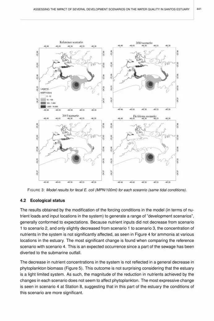
ASSESSING THE IMPACT OF SEVERAL DEVELOPMENT SCENARIOS ON THE WATER QUALITY IN SANTOS ESTUARY
FIGURE 3: Model results for fecal E. coli (MPN/100ml) for each sceanrio (same tidal conditions).
4.2 Ecological status
The results obtained by the modification of the forcing conditions in the model (in terms of nu-trient loads and input locations in the system) to generate a range of ”development scenarios”,generally conformed to expectations. Because nutrient inputs did not decrease from scenario1 to scenario 2, and only slightly decreased from scenario 1 to scenario 3, the concentration ofnutrients in the system is not significantly affected, as seen in Figure 4 for ammonia at variouslocations in the estuary. The most significant change is found when comparing the referencescenario with scenario 4. This is an expected occurrence since a part of the sewage has beendiverted to the submarine outfall.
The decrease in nutrient concentrations in the system is not reflected in a general decrease inphytoplankton biomass (Figure 5). This outcome is not surprising considering that the estuaryis a light limited system. As such, the magnitude of the reduction in nutrients achieved by thechanges in each scenario does not seem to affect phytoplankton. The most expressive changeis seen in scenario 4 at Station 8, suggesting that in this part of the estuary the conditions ofthis scenario are more significant.
441

A.F.P. SAMPAIO, M. MATEUS AND R.B. RIBEIRO
FIGURE 4: Model results for ammonia at Stations P1, P4 and P8. Last three years of the 10-year simula-
tion run.
FIGURE 5: Model results for phytoplankton at Stations P1, P4 and P8. Last three years of the 10-year
simulation run.
Dissolved oxygen concentration is one of the most important water quality parameters giventhe role of oxygen in the dynamics of aquatic systems. So, the health of a system can beassessed by looking at oxygen saturation in the water. The scenarios 3 and 4 tested in thisstudy imply a reduction of nutrient loads to the system. Since a fraction of that nutrient loadcorresponds to particulate material, reductions in these inputs mean less bacterial activity,thus lower oxygen demand. The result of reducing organic matter inputs to the system isclearly seen in the results for dissolved oxygen concentrations (Figure 6). There are no ap-parent changes between scenario 1 and 2 but, as the reduction becomes more relevant in theother scenarios, the increase in oxygen levels becomes more significant. Hence, the largestchanges are found when comparing the reference scenario with the fictitious scenario.
442

ASSESSING THE IMPACT OF SEVERAL DEVELOPMENT SCENARIOS ON THE WATER QUALITY IN SANTOS ESTUARY
FIGURE 6: Model results for dissolved oxygen at Stations P1, P4 and P8. Last three years of the 10-year
simulation run.
5 DEVELOPMENT SCENARIOS AND THEIR IMPLICATIONS
Results of future scenario analysis have suggested, as expected, that the treatment of do-mestic sewage effluents in the basin for the 2015 and fictitious scenarios reflected significantimprovements in water quality, except for some points where critical zones remain due to thepermanence of effluent discharges from the housing nuclei not included in these projects. Thecurrent and 2010 scenario analysis showed how the disorderly occupation of territorial spacealong with insufficient proper sanitary infrastructure can pose great threats for the riversidecommunities and other populations that use these waters for recreation, leisure and food. E.coli concentrations were some orders of magnitude above the level allowed for water bodiesof Class 1, according to Resolution 357/05 from CONAMA (2005) which sets a mandatorymaximum limit of 103 MPN/100 ml for brackish water. These values were estimated by themodel under different tidal conditions and also obtained in laboratory analysis. Higher valuesimply human health risks in use of these waters by the population.
The estuary is subjected to intense anthropogenic impact from urban activities, manifestedmainly in high loads of organic matter and nutrients discharged in the system. These pres-sures not only affect the (eu)trophic state of some parts of the estuary, but may also contributeto alter the ecologic dynamics of the system as a whole. The increase of both organic matterand nutrients in the system above background levels, as a result of eutrophication, poses seri-ous threats. Oxygen depletion is one of the most serious threats that coastal systems such asestuaries can face (NRC 2000). If the enrichment occurs via the addition of organic material,then an increase in bacterial activity may be expected, leading to potential oxygen depletion,both in the water column and in the sediment. So, while not significantly changing the nu-trient concentrations in the estuary, the decrease in nutrient loads from human occupationcontributes to the increase in the oxygen concentration, as seen in the scenarios that havebeen tested. This is particularly relevant in a system like Santos estuary where the physicaland biological characteristics can lead to anoxic conditions in the inner areas and in places
443

A.F.P. SAMPAIO, M. MATEUS AND R.B. RIBEIRO
where the water column may become stratified, or to less extreme conditions such as oxygensags in places where residence time is long.
6 FINAL CONSIDERATIONS AND FUTURE WORK
Models are increasingly becoming indispensable tools in environmental studies and manage-ment decisions. This work shows the relevance of water quality modelling in the importantand difficult task of integrated analysis of components responsible for the alteration of state ina dynamic environment under strong anthropogenic influence, such as densely populated es-tuaries. This study shows that even mild improvement of sanitary conditions (e.g. scenario 2)can already lead to situations where people, especially children, have free access to the waterand may use it safely as a playground. From an ecological perspective, the results suggestthat inappropriate management practices which result in an increase in nutrient inputs to thesystem, especially in the form of organic matter, inevitably contribute to its degradation.
This work represents the first step in the development of a water quality forecast system for theregion, which can be used to improve the quality of future decision-making. Also, this studypoints to the benefit for the human and system’s health if proper management practices areimplemented with regard to the nutrient loads that reach the system in sewage. The resultswill provide relevant information to stakeholders for an effective management of issues relatedto the region’s environmental sanitation, and to public health problems and further ecosystemdegradation that might occur if appropriate management practices are not adopted.
REFERENCES
CONAMA (2005). Conselho Nacional de Meio Ambiente. Resolucao 357/2005
Diario do Senado Federal (2004). ”Resolucao 09”. Republica Federativa do Brasil, ano LIX, n◦.095,junho, 2004, pp.17840-14841
Garreta-Harkot P F (2003) The Brazilian National Plan of Coastal Management, the health and the envi-ronment. MD Thesis. Faculdade de Saude Publica da Universidade de Sao Paulo, Sao Paulo.
IBGE (2000). Instituto Brasileiro de Geografia e Estatıstica (http://www.ibge.gov.br)
Mateus M, Sampaio AF, Mateus S (2008) An ecological Model application to the Santos Estuary, Brazil:testing and validation, this volume.
Moser G A, Sigaud-Kutner T C, Cattena C O, Gianesella S M, Braga E S, Schinke K P, Aidar E (2004)Algal growth potential as an indicator of eutrophication degree in coastal areas under sewage disposalinfluence. Aquatic Ecosystem Health and Managment 7: 115-126
Moser G A O, Gianesella S M, Alba J J, Bergamo A L, Saldanha-Correa F M P, Miranda L B, Harari J(2005) Instantaneous transport of salt, nutrients, suspended matter and chlorophyll-a in the tropicalestuarine sustem of Santos. Brazilian Journal of Oceanography 53: 115-127
NRC (2000) Clean coastal waters: understanding and reducing the effects of nutrient pollution. NationalResearch Council. National Academy Press, Washington. 405p
Sampaio AF, Mateus M, Ribeiro RB, Berzin G (2008) A modelling approach to the study of faecal pollutionin the Santos Estuary, this volume.
Sampaio AF, Ferreira JMS (2008) Socio-economic issues in Santos estuary, this volume.
444

PERSPECTIVES ON INTEGRATED COASTAL ZONE MANAGEMENT IN SOUTH AMERICAR. NEVES, J.W. BARETTA AND M. MATEUS (EDS.), IST PRESS, 2008
POTENTIAL USE OF ECOLOGICAL TOOLS TO DIRECT PUBLIC POLICIES: ANINTEGRATIVE APPROACH IN THE SANTOS ESTUARINE SYSTEM
C.D.S. PEREIRA, A. CESAR, R.P. BORGES, S.M.F. GIANESELLA, E.C.P.M. SOUSA,F.M. SALDANHA-CORREA, M.R. GASPARRO, G. BERZIN, R.B. RIBEIRO AND E.F. FIORI
1 WHY AN INTEGRATIVE APPROACH?
The integration of environmental data (physical, chemical, biological, ecotoxicological and eco-logical descriptors) can be performed through multivariate analyses, resulting in a wider andmore robust interpretation of the data set. Principal Components Analysis (PCA) is one of themost common methods to integrate data from different nature and it has been successfullyused in environmental quality assessments (Cesar et al. 2007, Riba et al. 2004, Del Valls etal. 2002, Del Valls and Chapman 1998).
Physical, chemical, biological and ecotoxicological data obtained in surveys conducted dur-ing August 2005 and March 2006 in the Santos estuarine system were used to assess thewater and sediment quality (see chapter on Santos Estuary, Part B). Such approaches, whenapplied alone, may result in a lack of realism and/or large uncertainties; but when they areused in an integrative manner, more reliable information about the environmental condition isprovided. The complex nature of the water and sediment data matrices makes it difficult toidentify the components that cause biological effects and their correlations. In this context, thePCA (Factor analysis) is an interesting tool due to the fact that: (1) it provides an ecologicalinterpretation of the environmental properties; (2) it integrates different lines of evidence; (3) itsupports conclusions based on a weight-of-evidence approach.
The objective of this chapter is to establish water and sediment quality in different areas af-fected by different sources of contamination by using an integrative method, providing a betterunderstanding of the real impact of human activities on this estuarine environment.
2 THE MULTIVARIATE ANALYSIS
Physical, chemical, biological and ecotoxicological data were integrated by factor analysisusing a principal components analysis as the extraction procedure. This is a multivariatetechnique to explore variable distributions. The original data set used in the analysis wasdivided in two main matrices: one referring to water and another to sediment data. After that,each main matrix was divided in two, based on the sampling period. They were named: WaterColumn (winter), Water Column (summer), Sediment (winter) and Sediment (summer).
Water matrices included the results of toxicological analysis evaluating sea-urchin embryolar-val development (SUED), microbiological parameters (total coliforms (TC) and Escherichia coli(EC)), local depth (LD), euphotic zone depth (Zeu), chlorophyll-a concentration integrated overthe water column (Cl int), salinity (SAL), dissolved oxygen saturation (DOS), concentration of
445

C.D.S. PEREIRA, A. CESAR, R.P. BORGES, S.M.F. GIANESELLA, E.C.P.M. SOUSA,F.M. SALDANHA-CORREA, M.R. GASPARRO, G. BERZIN, R.B. RIBEIRO AND E.F. FIORI
ammonium ( NH+4), nitrate ( NO−3 ), nitrite ( NO−2 ) total inorganic nitrogen (N total), inorganic
phosphate ( PO−34 ), silicate ( Si(OH)4), Chlorophyll-a concentration (Chl-a), Chlorophyll-c con-
centration (Chl-c), Carotenes (Carot.), percentage of active Chlorophyll -a in relation to thesum of Chlorophyll-a plus phaeopigments (% Chl-a act), and total suspended matter or ses-ton (Se).
Sediment matrices included the results of sea-urchin embryolarval development in interstitialwater (SUEDI), sea-urchin embryolarval development in elutriate (SUEDE), sea-urchin em-bryolarval development in sediment-water interface (SUEDSW), Nitocra sp. offspring rates ininterstitial water (ORIN), Nitocra sp. offspring rates in sediment (ORSN), Tiburonella viscanasurvival in sediment (SSA), analyses of sediment composition as percentage of fine particles(%F), organic matter (OM), salinity (SAL), and several ecological indexes such as number ofspecies (S), number of individuals (N), Margalef´s species richness (d), Pielou´s evenness(J’), Shannon’s diversity (H’), and Simpson’s dominance (D).
Factor analysis was performed on the correlation matrix, which means that the variables wereauto scaled (standardized) so as to be treated with equal importance. All the analyses wereperformed using the PCA option for the multivariate exploratory techniques procedure, fol-lowed by the basic set-up for factor analysis procedure from the STATISTICA software tool(Stat Soft Inc 2001 version 6). The eigenvalues obtained that were higher than 1 (Kaiser’scriteria) and the factor loadings higher than ±0.40 were considered as significant, accordingto Tabachinic and Fidell (1996). Besides the analysis of the variables aggregated by PCA, arepresentation of factor scores from each sampling point to the centroid of all cases for theoriginal data was made; the factor scores quantify the prevalence of every component for thesampling points and are used to confirm the factor description.
3 RESULTS AND DISCUSSION
3.1 Water column (winter)
Results of the factor analysis applied to the Water Column (winter) matrix are summarized inTable 1. The three principal factors explained 82.04% of the original data set bulk variance.The loadings following varimax rotation for the three factors are presented. Each factor is de-scribed according to the dominant group of variables. The first principal factor (F1) accountsfor the majority of the variance (44.43%), and it was positively associated to high concentra-tions of total coliforms and E. coli, as well as to nutrients as ammonium, nitrite, total inorganicnitrogen, phosphate and silicate. Negatively related to F1 are the embryolarval developmentof sea-urchins, salinity and oxygen saturation. Such association of variables indicates thatF1 represents nutrient rich estuarine water undergoing nitrification process and high bacterialactivity decreasing the oxygen levels in the water column, due to the predominance of het-erotrophic process over the autotrophic ones. Factor 2 (24.03%) is related to phytoplanktonbiomass (integrated chlorophyll-a in water column and average values of chlorophyll-a, c andcarotenes) and to availability of light in the water column, indicated by positive correlation to
446

POTENTIAL USE OF ECOLOGICAL TOOLS TO DIRECT PUBLIC POLICIES: AN INTEGRATIVE APPROACH IN THESANTOS ESTUARINE SYSTEM
euphotic zone and negatively related to total seston, which means low water turbidity. Fac-tor 2 can be ascribed as favorable conditions to phytoplankton development, once light is theprimary limiting factor for phytoplankton growth in estuarine waters (Ancona 2007). Factor 3explained 13.58% of the variance related to nitrate, total nitrogen availability and high pro-portions of active chlorophyll-a, indicating a new production process or a less intense grazingpressure.
Besides the analysis of the variables aggregated by PCA, a representation of estimated factorscores from each station to the centroid of all cases of the original data was made in order toconfirm the factor descriptions and to characterize the water quality at each sampling station(Figure 1). Factor 1 was very important only at point 6, at Largo da Pompeba in Sao VicenteChannel, which means this site presented unique characteristics related to the other samplingpoints, namely, the worst environmental conditions. Foremost, the low oxygen availability, andthe bad development of the sea-urchins embryos in the ecotoxicological tests attest the heavycontamination of the inner estuary. The winter represents the less rainy season in the area,which results in small loads of sediment transported by runoff, as indicated by the negativeassociation to seston. The significant contribution of domestic sewage at this site is pointedout by the high concentrations of total coliforms and E. coli. The sampling points located inSantos Channel (P1 to P3) do not correlate to any factor (Figure 1). This feature is due tothe lower nutrients and phytoplankton biomass (i.e. chlorophylls) concentrations found in thisregion compared to the ones observed at the inner estuary (P4 and P5) and in Sao VicenteChannel (P6 to P8). Indeed, P4 and P5 presented positive factor scores to F3 suggesting newbiomass production (high percentage of active Chl-a) supported by nitrate.
Factor 2, representative in points 5, 7 and 8, indicates eutrophic conditions in terms of phyto-plankton biomass. According to the data presented in Ecological status of the Santos Estuarywater column chapter (Gianesella et al., this volume) nutrient availability is also high at thesesites. The present analysis indicates point 6 as the place under heaviest sewage contam-ination. Nevertheless, this effect is diminished towards inner estuary and towards the SaoVicente Channel downstream. Moreover, Sao Vicente Channel presents more eutrophic char-acteristics in terms of phytoplankton biomass and nutrients than Santos Channel.
3.2 Water column (summer)
The PCA analysis applied to the Water Column (summer) matrix distinguished four principalfactors. The loadings following varimax rotation for the four factors are presented in Table 2.The four factors explained 87.36% of the variance in the original data set. The first principalfactor (F1) accounted for 41.04 % of the variance. This factor was positively related to thehigh levels of dissolved CO2 and inorganic nutrient concentrations (ammonium, nitrate, nitrite,phosphate and silicate). Negatively related to the factor thereof are salinity, the percentage ofoxygen saturation and seston concentration. Similar to the Water Column (winter) data, theF1 represents the estuarine waters rich in nutrients under higher heterotrophic activity. The
447

C.D.S. PEREIRA, A. CESAR, R.P. BORGES, S.M.F. GIANESELLA, E.C.P.M. SOUSA,F.M. SALDANHA-CORREA, M.R. GASPARRO, G. BERZIN, R.B. RIBEIRO AND E.F. FIORI
F2 (20.01% of the variance) was associated to photosynthetic pigments (chlorophylls a, c andcarotenes) and inversely related to phosphate and seston. Again, as in the winter matrix,F2 represented phytoplankton biomass abundance. The third factor explained 16.26% of thevariance and associated local depth, euphotic zone thickness (Zeu) and high percentage ofactive chlorophyll-a. Inversely correlated to F3 were chlorophyll-a by area unit (Int. Chl.)and seston. Therefore, F3 represents the light availability at the sampling points. Factor 4(10.05%) was related to positive sea-urchin embryolarval development, high values of totalcoliforms and E. coli, besides reduced nitrogen forms (ammonium and nitrite). This factorindicates the relation between the presence of coliforms and high ammonium levels in thewater due to the nitrification processes.
Considering the factor scores at each sampling point along the Santos Estuarine System(Figure 2) the relation of factor 1 with the inner estuarine sites is evidenced. F1 became morerepresentative from P3 to P5 and decreased from this point to P7. This factor separated theregions under more intense salt water influence from the ones dominated by brackish water.The F2 was representative in the sampling points P1, P3 to P5 and P8. This factor basicallyrepresented the sites with high phytoplankton biomass: the channels inlets (P1 and P8) andthe inner channel stations with low seston concentrations allowing the phytoplankton growth.Factor three (F3), representative in Santos Channel stations (P1 to P3), P4 and P6, wasrelated to the availability of light in the deepest layers of the water column. In these pointslight could reach the bottom layer, in opposition to the points 7 and 8, for instance, wherethe euphotic zone occupied less than a half of the total depth. This is an important factor forphytoplankton growth, once cells can be light limited during a great part of the day throughthis course along the mixing layer, and this is what was probably happening in Sao Vicentedownstream.
Finally, factor 4, related to high coliforms and ammonium levels, indicative of domestic sewagecontamination, was more representative in point 6, as observed in winter data. However, theweight of such variables in summer were smaller than those observed in winter, probably dueto the more intense rainfall in summer, which enhances the dilution and dispersion of con-taminants, decreasing the impact observed in winter scenario. In summer, the highest ratesof bacterial secondary productivity and primary productivity were detected at this place, con-ferring to P6 a unique characteristic in relation to the other portions of the estuary. Factor 4was also representative in point 1, in the Santos Channel inlet. This result can be a conse-quence of clandestine domestic sewage disposals from Vicente de Carvalho, a neighboringarea which is growing faster and disorderly.
3.3 Sediment (winter)
Physical, chemical, ecological and ecotoxicological data of sediment samples collected inwinter were associated by PCA resulting in three principal factors (Table 3). The loadingsfollowing varimax rotation for the three factors are found in Figure 3. Such factors explained
448
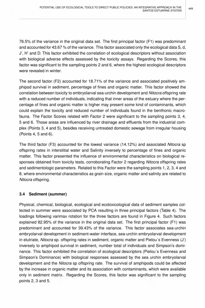
POTENTIAL USE OF ECOLOGICAL TOOLS TO DIRECT PUBLIC POLICIES: AN INTEGRATIVE APPROACH IN THESANTOS ESTUARINE SYSTEM
76.5% of the variance in the original data set. The first principal factor (F1) was predominantand accounted for 43.67 % of the variance. This factor associated only the ecological data S, d,J’, H’ and D. This factor exhibited the correlation of ecological descriptors without associationwith biological adverse effects assessed by the toxicity assays. Regarding the Scores, thisfactor was significant to the sampling points 2 and 6, where the highest ecological descriptorswere revealed in winter.
The second factor (F2) accounted for 18.71% of the variance and associated positively am-phipod survival in sediment, percentage of fines and organic matter. This factor showed thecorrelation between toxicity to embryolarval sea-urchin development and Nitocra offspring ratewith a reduced number of individuals, indicating that inner areas of the estuary where the per-centage of fines and organic matter is higher may present some kind of contaminants, whichcould explain the toxicity and reduced number of individuals found in the benthonic macro-fauna. The Factor Scores related with Factor 2 were significant to the sampling points 3, 4,5 and 6. Those areas are influenced by river drainage and effluents from the industrial com-plex (Points 3, 4 and 5), besides receiving untreated domestic sewage from irregular housing(Points 4, 5 and 6).
The third factor (F3) accounted for the lowest variance (14.12%) and associated Nitocra spoffspring rates in interstitial water and Salinity inversely to percentage of fines and organicmatter. This factor presented the influence of environmental characteristics on biological re-sponses obtained from toxicity tests, corroborating Factor 2 regarding Nitocra offspring ratesand sedimentologic parameters. Related to this Factor were the sampling points 1, 2, 3, 4 and8, where environmental characteristics as grain size, organic matter and salinity are related toNitocra offspring.
3.4 Sediment (summer)
Physical, chemical, biological, ecological and ecotoxicological data of sediment samples col-lected in summer were associated by PCA resulting in three principal factors (Table 4). Theloadings following varimax rotation for the three factors are found in Figure 4. Such factorsexplained 82.95% of the variance in the original data set. The first principal factor (F1) waspredominant and accounted for 39.43% of the variance. This factor associates sea-urchinembryolarval development in sediment-water interface, sea-urchin embryolarval developmentin elutriate, Nitocra sp. offspring rates in sediment, organic matter and Pielou´s Evenness (J’)inversely to amphipod survival in sediment, number total of individuals and Simpson’s domi-nance. This factor exhibited the correlation of ecological descriptors (Pielou´s Evenness andSimpson’s Dominance) with biological responses assessed by the sea urchin embryolarvaldevelopment and the Nitocra sp offspring rate. The survival of amphipods could be affectedby the increase in organic matter and its association with contaminants, which were availableonly in sediment matrix. Regarding the Scores, this factor was significant to the samplingpoints 2, 3 and 5.
449

C.D.S. PEREIRA, A. CESAR, R.P. BORGES, S.M.F. GIANESELLA, E.C.P.M. SOUSA,F.M. SALDANHA-CORREA, M.R. GASPARRO, G. BERZIN, R.B. RIBEIRO AND E.F. FIORI
FIGURE 1: Estimated factor scores (F1 to F3) to the eight sampling points along the Santos Estuarine
System considering data of the winter water column matrix. The factor scores quantify the prevalence of
every component for each station and are used to confirm the factor description.
450

POTENTIAL USE OF ECOLOGICAL TOOLS TO DIRECT PUBLIC POLICIES: AN INTEGRATIVE APPROACH IN THESANTOS ESTUARINE SYSTEM
FIGURE 2: Estimated factor scores (F1 to F4) for the eight sampling points along the Santos Estuarine
System considering data of the summer water column matrix. The factor scores quantify the prevalence
of every component for each station and are used to confirm the factor description.
451

C.D.S. PEREIRA, A. CESAR, R.P. BORGES, S.M.F. GIANESELLA, E.C.P.M. SOUSA,F.M. SALDANHA-CORREA, M.R. GASPARRO, G. BERZIN, R.B. RIBEIRO AND E.F. FIORI
FIGURE 3: Factor scores (F1 to F3) from eight sample points (P1 to P8 referred to sites 1 to 8 from Santos
ECOMANAGE data field campaigns) considered for the winter sediment.
452

POTENTIAL USE OF ECOLOGICAL TOOLS TO DIRECT PUBLIC POLICIES: AN INTEGRATIVE APPROACH IN THESANTOS ESTUARINE SYSTEM
FIGURE 4: Factor scores (F1 to F3) from eight sample points (P1 to P8 referred to sites 1 to 8 from Santos
ECOMANAGE data field campaigns) considered for the summer sediment.
453

C.D.S. PEREIRA, A. CESAR, R.P. BORGES, S.M.F. GIANESELLA, E.C.P.M. SOUSA,F.M. SALDANHA-CORREA, M.R. GASPARRO, G. BERZIN, R.B. RIBEIRO AND E.F. FIORI
TABLE 1: Sorted rotated factor loadings of the original 19 variables on the three principal factors of winter
water column data from Santos Estuarine System.
Parameter Factor 1 Factor 2 Factor 3
% Variance 44.43 24.03 13.58 SUED -0.94 --- ---
TC 0.89 --- --- EC 0.92 --- ---
Depth --- -0.79 --- Zeu --- 0.53 ---
Int. Chl --- 0.76 --- Salinity -0.94 --- --- % DOS -0.82 --- ---
NH4+ 0.96 --- ---
NO3- --- --- 0.92
NO2- 0.76 0.42 ---
N Total 0.84 --- 0.49 PO4
-3 0.43 --- 0.62 Si(OH)4 0.77 0.41 --- Chl-a --- 0.88 --- Chl-c --- 0.95 ---
Carotene --- 0.90 --- % Active Chl --- --- 0.89 Total seston --- -0.57 -0.60
TABLE 2: Sorted rotated factor loadings of the original 19 variables on the three principal factors of summer
water column data from Santos Estuarine System.
Parameter Factor 1 Factor 2 Factor 3 Factor 4
% Variance 41.04 20.01 16.26 10.05
SUED --- --- --- 0.61
Total Colimetry --- --- --- 0.85
E. coli --- --- --- 0.86
Depth --- --- 0.96 ---
Zeu --- --- 0.96 ---
Int. Chl --- 0.48 -0.77 ---
Salinity -0.93 --- --- ---
% DOS -0.94 --- --- ---
% CO2 0.74 --- --- ---
NH4+ 0.76 --- --- 0.62
NO3- 0.77 --- --- ---
NO2- 0.57 --- --- 0.65
N Total 0.82 --- --- 0.54
PO4-3 0.57 -0.41 --- ---
Si(OH)4 0.81 --- --- ---
Chl-a --- 0.95 --- ---
Chl-c --- 0.92 --- ---
Carotene --- 0.97 --- ---
% Active Chl --- --- 0.96 ---
Total seston -0.60 -0.51 -0.57 ---
454

POTENTIAL USE OF ECOLOGICAL TOOLS TO DIRECT PUBLIC POLICIES: AN INTEGRATIVE APPROACH IN THESANTOS ESTUARINE SYSTEM
TABLE 3: Sorted rotated factor loadings of the original 15 variables on the three principal factors of winter
sediment data from Santos Estuarine System.
Parameter Factor 1 Factor 2 Factor 3
% Variance 43.67 18.71 14.12 SUEDI --- --- --- SUEDE --- -0.57 -0.58
SUEDSW --- 0.74 --- ORIN --- --- 0.94 ORSN --- -0.95 --- SSA --- --- --- % F --- 0.62 -0.58 OM --- 0.57 -0.78
Salinity --- --- 0.59 S 0.91 --- --- N --- -0.86 --- d 0.93 --- --- J' 0.87 --- --- H' 0.97 --- --- D -0.95 --- ---
TABLE 4: Sorted rotated factor loadings of the original 15 variables on the three principal factors of summer
sediment data from Santos Estuarine System.
Parameter Factor 1 Factor 2 Factor 3
% Variance 39.43 29.37 14.15 SUEDSW 0.74 --- --- SUEDE 0.68 --- 0.45 SUEDI --- --- -0.96 ORIN --- --- -0.93 ORSN 0.69 --- --- SSA -0.57 -0.52 --- OM 0.93 --- --- S --- -0.91 --- N -0.76 --- --- d --- -0.99 --- J' 0.92 --- --- H' --- -0.96 --- D -0.54 0.72 ---
The second factor (F2) accounted for 29.37% of the variance and associated Simpson’s Dom-inance inversely to amphipod survival in sediment, number of species, Margalef’s speciesRichness and Shannon’s Diversity. This factor exhibited the direct association of ecologi-cal descriptors with effects on amphipod survival, probably related with contamination and/orsedimentological parameters. Significantly related to this Factor were the sampling points 1,3, 5 and 8. Finally, the third factor (F3) accounted for the lowest variance (14.15%) and as-sociated sea-urchin embryolarval development in interstitial water, sea-urchin embryolarvaldevelopment in elutriate and Nitocra sp. offspring rates in interstitial water. This factor exhib-ited association of toxicity responses in interstitial water. Significantly related to this Factorwere the sampling points 3, 4, 6, 7 and 8.
455

C.D.S. PEREIRA, A. CESAR, R.P. BORGES, S.M.F. GIANESELLA, E.C.P.M. SOUSA,F.M. SALDANHA-CORREA, M.R. GASPARRO, G. BERZIN, R.B. RIBEIRO AND E.F. FIORI
4 CONCLUSIONS
This integrative analysis applied to the whole estuarine area clearly indicates that the innerportion is more intensively affected by the anthropogenic impacts at the present time. Theworst water conditions were found in Largo da Pompeba (P6), especially during the winter,when rainfall is less intense and the dilution or renewal rates of the estuarine water are smaller.Another important aspect to be taken into account is the small water volume in Sao VicenteChannel due to its shallowness, preventing a quick and efficient dispersion of the dissolvedand particulate material which enters in the water column, opposed to the observed at SantosChannel. Despite the high ammonium levels which were detected in most parts of the estuar-ine system, the integrative analysis of nutrients, toxicity tests and colimetry data was able topoint out the more critical pollution sites, discriminating them from those where phytoplanktoncan develop in a healthy condition.
Regarding sediment conditions, it was possible to identify worse quality in Piacaguera andSantos Channels, which exhibited more significant alterations probably related to the previ-ous intensive industrial discharges that occurred in this area, suggesting that the persistenceof pollutants in this environmental compartment are still producing toxicity and consequentlynegative effects to the benthic biota. Apparently, the input of contaminants in the SantosEstuarine System water bodies from industrial discharges is relatively under a better controlthan the untreated domestic sewage discharges, which affect mostly the Sao Vicente Chan-nel. These results demonstrate how good the decision made by the researchers was to focuson the urban occupation and sewage disposal, among so many others, as the pressures forthe DSS study model. The present results strongly indicate the collection and treatment ofdomestic sewage, especially in the Sao Vicente Channel, as priorities for the improvement ofthe estuarine environmental condition.
REFERENCES
Ancona CM (2007) Aspectos da variacao espacial e temporal da biomassa e producao fitoplanctonica eparametros correlatos no estuario e baıa de Santos. Dissertacao de Mestrado. Universidade de SaoPaulo, Instituto Oceanografico, 229p.
Cesar A, Choueri RB, Riba I, Morales-Caselles C, Pereira CDS, Santos AR, Abessa DMS, DelValls TA(2007) Comparative sediment quality assessment in different littoral ecosystems from Spain (Gulf ofCadiz) and Brazil (Santos and Sao Vicente estuarine system). Environmental International, 33: 429-435
DelValls TA, Chapman PM (1998) Site-specific sediment quality values for the Gulf of Cadiz (Spain) andSan Francisco Bay (USA), using the sediment quality triad and multivariate analysis. Ciencias Mari-nas, 24: 313-36
DelValls TA, Forja JM, Gomez-Parra A (2002) Seasonality of contamination, toxicity, and quality values insediments from littoral ecosystems in the Gulf of Cadiz (SW Spain). Chemosphere, 46: 1033-43
Gianesella S M F, Saldanha-Correa F M P, Sousa E C P M and Gasparro M R (2008) Ecological status ofthe Santos Estuary water column, this volume.
Riba I, Casado-Martınez C, Forja JM, DelValls TA (2004) Sediment quality in the Atlantic coast of Spain.Environmental Toxicology and Chemistry, 85: 141-56
Tabachinic BG, Fidell LS (1996) Using multivariate statistics. Hasper Collins, College Publishers, NY,USA.
456
PERSPECTIVES ON INTEGRATED COASTAL ZONE MANAGEMENT IN SOUTH AMERICAR. NEVES, J.W. BARETTA AND M. MATEUS (EDS.), IST PRESS, 2008
BUILDING OF THE DECISION SUPPORT SYSTEM IN THE SANTOSESTUARINE SYSTEM
C. BELCHIOR, A.F.P. SAMPAIO, F. GIORDANO, M.R. GASPARRO, R.C. ARGENTINO-SANTOS,E.C.P.M. SOUSA, E. FEOLI, S.M.F. GIANESELLA, F.M.P. SALDANHA-CORREA AND G. BERZIN
1 INTRODUCTION
This chapter is intended to present the work done by the ECOMANAGE project in applyingthe information gathered during the project to the pressing environmental problems whichare threatening the Santos Estuarine System and are therefore urgently in need of effectivemanagement responses. As described before, this region is marked by several conflicts whoseassociated complexity made it inevitable to make a choice for a problem that could be tackledwithin the project’s time frame. Thus, after carefully reviewing the magnitude of the impactsthat these existing conflicts were having on both human health and water quality, as well asthe associated political will to discuss each problem, two issues where selected: the housingand domestic sewage scenarios. In the next sections both problems will be briefly illustrated,followed by a description of the work developed to implement the Decision Support System,which was built together with the local stakeholders in order to draw up possible responses forthese problems.
2 SCENARIOS ADDRESSED IN THE DSS DEVELOPED FOR THE SANTOS ESTUARINESYSTEM
The choice of the scenarios that were going to be analyzed for application in the DSS wasbased on the difficulties exposed by stakeholders both from the local and state public ad-ministration, which were mainly related to issues regarding the urban development that hasoccurred in this region, as well as on the state analysis of the estuarine system made by theECOMANAGE project. From these, three main issues were identified: (1) the lack of availablespaces near urban centers where basic infrastructure was already established; (2) the highcosts of projects related to housing demand and basic sanitation services; and (3) the amountand resulting impacts of diffuse pollution originated from both urban drainages of the neighbor-hoods without a sewerage drainage network and sub-normal housing nuclei. Consequently,two main problems were selected: the housing demand for the resettlement of populations inunder-developed housing and the respective supply of basic sanitation services.
Most of the populations that live in under-developed housing are occupying ecologically sen-sitive or risky areas such as riverbanks, mangrove areas and hill slopes, which are classifiedas permanent preservation areas by the Brazilian legislation and therefore, cannot be occu-pied. This situation is a result of the disorderly urban expansion that occurred in the past,and whose consequences last up to these days and has led to a high demand for appropriatespace for resettlement. Since this pitfall of finding urban spaces adequate to this demand has
457

C. BELCHIOR, A.F.P. SAMPAIO, F. GIORDANO, M.R. GASPARRO, R.C. ARGENTINO-SANTOS,E.C.P.M. SOUSA, E. FEOLI, S.M.F. GIANESELLA, F.M.P. SALDANHA-CORREA AND G. BERZIN
actually been aggravated over the last decades, the issues associated with the urbanizationof sub-normal human settlements were chosen as the first scenario, called Housing scenariofor the application of the multiple tools developed within the project, namely the DSS.
The second scenario evaluated in the project equally derives from the form of urban devel-opment that has established itself in the region and is related to the supply of basic sanita-tion services and its features. Because this urban expansion was not adequately planned orguided, neither was the supply of these services, areas with serious insufficiencies of basicsanitation were originated, where the sewage ends up being dumped directly into the estuarinewaters, without any kind of treatment. Thus, the second scenario selected by the ECOMAN-AGE project was related to the aspects involved around the dumping of residual waters intothe estuary and was called Sewage scenario.
2.1 Main Aspects of the Assessed Scenarios
According to PRIMAHD (2005), IBGE (2000) and more recent municipal surveys, about200,000 people live in irregular housing in the Santos - Sao Vicente Estuary drainage basinthat have insufficient or no basic urban infrastructure such as water supply, electricity orgarbage and sewage disposal. Municipal surveys further show that most of these irregularsettlements correspond to population agglomerations that surpass 1,000 inhabitants. This isactually the case for 60% of the sub-normal occupations located in Santos and of all occupa-tions in Sao Vicente (Young 2006).
The lack of adequate areas for housing is one of the main problems in the region and resultsfrom three factors. The first is a direct consequence of the natural characteristics of the coastalplain where the study area is located, since the urban center of the region is situated in theinsular portion of the estuary where there is limited space for any kind of construction. This partof the estuary is in fact already undergoing under a major process of population densification.The second aspect derives from the fact that the peripheral urban areas, though less dense,also have their expansion limited for they are surrounded by Atlantic rainforest and mangrovevegetation whose ecosystem services, described in previous chapters, are fundamental to theoverall maintenance of the region and its quality of life and therefore should not be disturbed.Also, the further destruction of remaining vegetation areas that are in intermediate and latesuccession stages was recently prohibited by means of a state resolution (SMA 2007). Thisis all the more valid since the areas that have had their vegetation altered but have no longerbeen disturbed ever since can be found nowadays in an advanced state of regeneration. Andlast, the third aspect is related to the existence of a great number of areas with contaminatedsoils in the region (CETESB 2001) that compromise their use by society and are still waitingfor an appropriate solution.
One of the attempted solutions to this problem has been the acquisition by the government ofareas that are prone to receive populations from sub-normal housing. In this sense, the use ofthe available spaces in already urbanized areas or those adjacent to them for such purposes
458

BUILDING OF THE DECISION SUPPORT SYSTEM IN THE SANTOS ESTUARINE SYSTEM
would be ideal, since they already have the necessary urban basic infrastructure and thiswould allow for easier integration with the urban centers. Nevertheless, the lack of space inthe region has resulted in an increase in land value and has made this solution too costly andmany times not feasible. This phenomenon of rise of urban land values, already detailed in thechapter related to socio-economy of the Santos Estuarine Region has been intensified over thelast decade by the increasing interest of private companies for these areas. This process hasbeen mainly powered by the resumption of the real estate sector and growth of the port sector,whose expansion in activities has elevated the demand for useful areas, valuing not only thescarce urban lots found in upmarket areas but also peripheral urban areas, especially thosein good environmental state. This is particularly the case for retroportuary areas because theelevation of container cargo trading that has been taking place in the Port of Santos since 2000has dramatically increased the demand for low-cost areas usually located in the outskirts ofthe urban area and consequently speculated their price.
This already complex scenario made up by the increasing demand for retroportuary areas,the strong activity in the real estate market and the high degree of urban densification willprobably be worsened by industrial expansion, as revealed in some municipal urban occupa-tion plans from 2007 where incentives to this end can be found. This setting has thereforeled to a situation of fierce competition among the economic sectors to the detriment of theunderprivileged, whose basic necessities have been left aside. This is all the more true tothose communities situated in fragile and environmentally risky areas that have no conditionsof hygiene and safety and should therefore be transferred to other areas that have adequateurban infrastructure.
To cope with this situation, another solution that has been tried in the region to solve the prob-lem of sub-housing has been to maximize the re-urbanization of the areas already degradedby these settlements, only providing for the relocation of these populations when absolutelynecessary and to the smallest possible percentage of people. However this solution also hasserious hindrances, as pointed out by a World Bank report (IBAM 2004), which together withBrazilian institutions, analyzed several Brazilian experiences in land urbanization and regular-ization of human irregular settlements. These include financial constraints, related to securing,managing and applying the necessary financial resources; technical constraints, related to thegeomorphologic and environmental characteristics of the area, as well as those related to thekind of occupation that is in place; and constraints related to the lack of judicial and institutionalcapacity and political willingness. This work has also pointed out that the absence of effectivecontrol over further growth and expansion of settlements after re-urbanization is completed isanother factor that threatens the continuity and sustainability of programs of this nature in thelong term.
Some slum re-urbanization experiences were actually followed during the ECOMANAGEproject and it was possible to witness the difficulty that exists in effectively carrying out projectsof this nature. Among them, is the case of irregular settlements that existed in the insularportion of Sao Vicente and where re-urbanization of slum quarters that extended into man-
459

C. BELCHIOR, A.F.P. SAMPAIO, F. GIORDANO, M.R. GASPARRO, R.C. ARGENTINO-SANTOS,E.C.P.M. SOUSA, E. FEOLI, S.M.F. GIANESELLA, F.M.P. SALDANHA-CORREA AND G. BERZIN
grove area was in fact accomplished but due to the lack of adequate inspection and controlmechanisms, allowed for the establishment of new sub-housing settlements, forcing the publicadministration to take extreme measures in order to limit its proliferation. This was done bybuilding a road between the estuary channel and the area that had been re-urbanized andtransferring the new sub-houses situated over the water, only leaving mangrove after the roadin order to effectively avoid new occupations. Finally, vertical construction has also been at-tempted in order to maximize space but the pedological characteristics of the region makethis kind of construction expensive, which again complicates its implementation for a popularhousing end.
Chosen as the second scenario, the urban discharges were acknowledged by the stakehold-ers as also one of the main problems of the region, since a solution to the issue of sub-normalhousing regularization has still not been found making the estuary the main direct receiverof this organic load. This situation is aggravated by the fact that these sub-normal housesare illegal, therefore preventing the public administration from providing the necessary infras-tructure that would mitigate the impacts originated by this situation. This, of course, will onlyhappen once these areas have been properly regularized by the State. There is actually a ma-jor sanitary project currently under way in the region, whose aim is to raise the actual sewagecollection levels up to 95% of the total Baixada Santista population (Diario do Senado Federal2004). However, this project does not consider the inhabitants that are occupying the illegalareas, which represent about 20% of the total population of the region. So even though thisproject will improve the quality of life and to a certain extent the environmental state of theestuary, it will still leave the most needed uncared for.
The lack of appropriate responses and the worrisome status of the Housing and Sewagesituation in the Santos Estuarine System are consequently issues that were considered toneed urgent attention and were therefore prioritized in the ECOMANAGE project.
3 METHODOLOGY APPLIED IN THE DSS AND MAIN RESULTS FOR THE HOUSINGAND SEWAGE SCENARIOS
3.1 Assembling a stakeholder group
The Decision Support System (DSS) was the main tool developed by the ECOMANAGEproject to assess the stakeholders view on the Housing and Sewage issues and jointly find thebest answer to these problems. The first step then was to build a stakeholder group amongstthe several institutions (governmental and non-governmental) and interested parties that weredirectly involved with these problems and willing to collaborate. Actually, a constituency wasquickly built soon after the beginning of the project since there were over a hundred entitiesshowing a strong interest to participate in the project, which allowed for the establishment ofa consultative council. The stakeholders that belonged to this council represented the partiesthat wanted to collaborate with the ECOMANAGE project and so, they were also the onesthat were invited to form a more technical group, whose objective was to participate in the
460

BUILDING OF THE DECISION SUPPORT SYSTEM IN THE SANTOS ESTUARINE SYSTEM
development of the DSS. A quite diverse stakeholder group was therefore assembled withmore then thirty representatives of state and local government agencies, academia and localNGOs, whose work dealt directly or indirectly with the Housing and Sewage drivers.
3.2 Filling in the decision matrixes
The next step was to set up a series of meetings with this group in order to build a decision-matrix for the DSS, which consists of an alternative/effects matrix, as explained in the method-ology part of this book. In this way, the first meeting was intended to explain what a DSSconsisted of and how it could help the stakeholders to evaluate different management alterna-tives for the selected issues, as well as to outline what was expected from their participation.Also, a brief consideration was made regarding the housing and sewage state of the region,mainly to present the findings that the ECOMANAGE project had assembled and to bring ev-eryone to the same level of information. The Housing state was therefore considered in viewof the actual distribution of slums and urbanized areas, as well as the projections of populationgrowth for the next 10-15 years for the five municipalities. As for the sewage state, a diagnosticof critical areas, the sewage treatment level and the existing management measures were laidout.
In the second meeting, a matrix that had already some alternatives and effects filled in by theteam was handled to the stakeholders as means to guide them, since none of them had everparticipated in such work and debate was open to find more alternatives and effects for theHousing and Sewage problems. The alternatives and effects filled out by the team were doneby considering all the information gathered by the project to evaluate the state of the region, aswell as from experts’ knowledge. This was done over several internal meetings that took placeat UNISANTA and IO-USP and where some of the pressures and impacts of housing andurban discharges were defined, particularly regarding the biological aspects of such issues.
After noticing that participation had dramatically fallen from the first to the second meeting,fact that is explored later on in this chapter when the difficulties and opportunities of the im-plementation of the ECOMANAGE are assessed, a strategy change had to be made. Thus,after carefully considering time constraints and the difficulties that were occurring to gatherand sustain such a diverse and numerous group to work together, the initial plan, which con-sisted of filling in the matrixes during the meetings so that consensus could be achieved bydiscussing issues together, was dropped and it was determined that the matrixes were to becompleted by each stakeholder in their working environment and then sent over by email.
In the end, six alternatives for the Sewage scenario and four alternatives for the Housing sce-nario were jointly put forward by the team and the stakeholders, as well as several biologicaland socio-economical effects. The stakeholders also gave a score to each alternative/effectoption, which was sent by email and the result was processed with the Matheditr softwarein order to find the best alternative for each scenario. A final third meeting was then madeto present the findings to the stakeholders and discuss the results. Again, this meeting had
461

C. BELCHIOR, A.F.P. SAMPAIO, F. GIORDANO, M.R. GASPARRO, R.C. ARGENTINO-SANTOS,E.C.P.M. SOUSA, E. FEOLI, S.M.F. GIANESELLA, F.M.P. SALDANHA-CORREA AND G. BERZIN
very little attendance when compared to the initial meeting, which corroborated the change ofstrategy that was made in the beginning of this process.
3.3 Finding the best alternative for each scenario
The results obtained for Housing showed that none of the proposed alternatives could be con-sidered appropriate to deal with the actual situation since even the ones that got higher scoresstill remained quite far from the best (b) option, as it can be seen in Figure 1. Nevertheless,out of the four alternatives considered, the removal of slums into newly horizontally built areaswas the best-placed alternative, closely followed by removal of slums into newly vertically builtareas. This is actually consistent with the data gathered by the ECOMANAGE project, whichshows that there are several unoccupied areas that are suited for relocation projects, oncethese are better planned.
As for Sewage, the best alternative was to build concrete cesspits followed by treated subma-rine outfall, as shown in Figure 2. Stakeholders therefore considered that concrete cesspitscould be a good solution for the current sewage situation since the majority of the people thatare not attended by municipal sewage services live in slum quarters. This general concep-tion that concrete cesspits could attenuate the problem of having a deficient sewerage systemexists amongst most stakeholders but is also in fact the general public opinion, who believesthat this could be a solution in many other different areas in Brazil that are missing appropriatesanitary conditions. This is due to the fact that cesspits are a low technology and low cost op-tion, which would make them ideal solutions when obtaining the necessary funding to install afully operating sanitation system is a problem.
However, from a technical point of view, concrete cesspits are not considered a good solutionin areas where the groundwater level is close to the surface, such as in the Santos EstuarineSystem, because this prohibits its construction. Furthermore, concrete cesspits only retainthe solid part of the sewage. As a result of this, the contaminant elements (i.e. bacteria) arenot removed from the effluent, meaning it will eventually reach the estuary and contaminateit, unless it is treated by chloride (ABNT-NBR7229/1993). Having put this, the best alternativeshould then be considered the expansion in number and capacity of the wastewater treatmentplants and the construction of new submarine outfalls.
In conclusion, the DSS developed within the ECOMANAGE project showed great potential-ity to back up environmental decision-making in the Santos Estuarine System. It must beacknowledged that the management alternatives considered for the Housing and Sewagescenarios were not very specific and so the results obtained were not surprising and wereeven expected. This was in part due to the lack of some crucial information that was neces-sary to further detail the alternatives and that could not be retrieved in time. Nevertheless,this was the first time that most of these stakeholders and even local project team membersused a DSS to analyze environmental problems and consequently evaluated managementalternatives depending on their cumulative social, economical and environmental effects.
462

BUILDING OF THE DECISION SUPPORT SYSTEM IN THE SANTOS ESTUARINE SYSTEM
Also, the DSS brought together stakeholders that have an important role in the management ofthe Santos region so that these alternatives could be jointly discussed and thought over. Thiswas later recognized by these stakeholders to be quite gratifying and that it had helped themto consider other standpoints, showing them aspects that they were not aware of or that theydid not realize that had any association with the tackled scenarios. In fact, one of the partici-pating stakeholders, who represented the state environmental control and regulation agency,even showed its interest to apply the DSS on a particular issue related to the environmentaland social impacts of a relocation project that they were handling at the time, recognizing inthis way the potentiality of this tool. Consequently, the development of the DSS in the SantosEstuarine System, although it did not serve to help choosing a real management response tothe problems of Housing and Sewage, it aroused awareness among the stakeholders involvedthat integrated decision-making by promoting an analysis of both natural and socioeconomicaspects of an issue, can help to build sound, sustainable environmental decisions and aboveall, can be a powerful tool to reach consensus in this highly conflicted area.
FIGURE 1: Ranking results for Housing: w - worst alternative; b - best alternative; A1 - Slum expan-
sion (”Business As Usual”); A2 - Removal of slums for vertical constructions; A3 - Removal of slums for
horizontal constructions; A4 - Urbanization of former slum area (X and Y axes refer to relative spatial
distribution of the alternatives).
FIGURE 2: Ranking results for Sewage alternatives: w - worst alternative; b - best alternative; A1 - Direct
Sewage Discharge (”Business As Usual”); A2 - Untreated Outfall; A3 - Primary Treated Outfall; A4 - Pre-
treated Submarine Outfall; A5 - Treated Submarine Outfall; A6 - Concrete Cesspit (X and Y axes refer to
relative spatial distribution of the alternatives).
463

C. BELCHIOR, A.F.P. SAMPAIO, F. GIORDANO, M.R. GASPARRO, R.C. ARGENTINO-SANTOS,E.C.P.M. SOUSA, E. FEOLI, S.M.F. GIANESELLA, F.M.P. SALDANHA-CORREA AND G. BERZIN
REFERENCES
ABNT - Associacao Brasileira de Normas Tecnicas (1993) Resumo sobre o funcionamento de fossassepticas dimensionadas e construıdas segundo a NBR 7229/93. Disponıvel em www.fibrasil.com/fossas.htm, acessado em 3/12/2007
CETESB - Companhia de Tecnologia de Saneamento Ambiental (2001) Sistema estuarino de Santos eSao Vicente, 141p.
Diario do Senado Federal. 2004. Resolucao 09 de Junho de 2004. Republica Federativa do Brasil, anoLIX, n. 095, pp 17840-14841
IBAM - Instituto Brasileiro de Administracao Municipal (2004) Estudo da avaliacao da experiencia brasilei-ra sobre urbanizacao de favelas e regularizacao fundiaria. Assessoria Internacional, projeto n◦17.408. Relatorio Final: Vol. 1, 125p. e Vol. 2, 20p.
IBGE - Instituto Brasileiro de Geografia e Estatıstica (2000) Censo demografico 2000, Agregado de Se-tores Censitarios dos Resultados do Universo. IBGE.
Jakob AE (2003) Analise sociodemografica da constituicao do espaco urbano da regiao metropolitana daBaixada Santista no perıodo 1960-2000. Tese doutorado. Programa de doutorado em demografia doInstituto de Filosofia e Ciencias Humanas da Universidade Estadual de Campinas. 220p.
Matheditr(2000) Software for Windows.
PRIMAHD (2005) Programa regional de identificacao e monitoramento de areas de habitacao descon-forme da R.M.B.S. AGEM. Relatorio Final. 565p.
SMA - Secretaria do Meio Ambiente do Estado de Sao Paulo (2007) Resolucao SMA 40 de 21 Setembrode 2007. 3p.
Young AF (2006) Espacos de vulnerabilidade socioambiental para a populacao da Baixada Santista:Identificacao e analise de areas crıticas. XV Encontro Nacional de estudos Populacionais, Caxambu,MG.
464

PERSPECTIVES ON INTEGRATED COASTAL ZONE MANAGEMENT IN SOUTH AMERICAR. NEVES, J.W. BARETTA AND M. MATEUS (EDS.), IST PRESS, 2008
DIFFICULTIES AND OPPORTUNITIES FOUND DURING THE IMPLEMENTATIONOF THE ECOMANAGE PROJECT IN THE SANTOS ESTUARINE SYSTEM
C. BELCHIOR, S.M.F. GIANESELLA AND A.F.P. SAMPAIO
The purpose of this chapter is to present the main obstacles encountered to develop andimplement a project such as ECOMANAGE in the Santos Estuarine System, but also to putforward some of the main opportunities that were revealed to the team during the projectimplementation. This outcome evaluation was preferred to a performance evaluation since thiskind of evaluation is unusual in Brazil and by actually reporting on the existing difficulties andopportunities to implement an ICM project rather then just doing a simple output evaluation, itis believed that one can better contribute and improve the process of coastal management inthe region or elsewhere, as discussed before. But foremost, it is necessary to briefly sketchthe context of coastal management in Brazil with regard to what has been achieved up to nowand what the existing constraints are to the implementation of the national programme.
The National Programme of Coastal Management (GERCO) in Brazil was first established in1985 by the Interministerial Commission for Marine Resources (CIRM), with the first nationalcoastal management law being published in 1988 (law no 7.661/88). This law establisheda National Coastal Management Plan (PNGC) aimed at proposing rational uses of coastalresources for the benefit of the local population and conservation of coastal ecosystems. Ittook a while to start implementing the PNGC´s instruments and working towards its specificobjectives on promoting the sustainable development of Brazilian coastal zones (Asmus andKitzmann 2004), although it represented a hallmark for ICM in the country.
Progress was made over the years, especially powered by a growing awareness of the na-tional population of environmental issues, which added to the pressure imposed by interna-tional convention commitments and led to the development of legal and institutional conditionsthat allowed for ICM evolution and strengthening in the country. Thus, currently Brazil hasa well developed coastal management programme, with specific coastal management plansdeveloped in all its 17 coastal states, several technical and regulating tools set in motion anda central unit to coordinate all these efforts. Nevertheless, even though important advanceshave been made at the legal and administrative levels, there are still serious obstacles in theway of ICM in Brazil.
Several political, institutional, technical and sociocultural constraints have been identified (Die-gues 1999, Asmus and Kitzmann 2004, Polette and Vieira 2005), with the main ones as fol-lows: lack of political will to truly implement the National Coastal Management Programme,especially by local governments; decisions strongly influenced by economic interests, withexistence of powerful lobbies from sectors such as the very state, tourism or the industry;lack of institutional integration, resulting in uncoordinated public policies that are related tocoastal environmental issues; lack of a truly decentralized governance, leaving the crucialdecisions in the hands of the federal government; significant differences between the states
465

C. BELCHIOR, S.M.F. GIANESELLA AND A.F.P. SAMPAIO
in the institutional and technical capacity to implement the National Programme, resulting instrong asymmetries in the country concerning achieved results; poorly capacitated and toofew technicians in governmental coastal management teams, as well as inadequate funding;lack of involvement of specialists such as members from academia or consultants that haveextensive experience in environmental, coastal and marine sciences; continuous changes ingovernment institutions and positions, which ngatively affect the consistency and outcomes ofcoastal management actions; insufficient public participation in decision-making and last, butnot least, the lack of effective social mobilization of local communities in support of coastalmanagement measures.
Due to these constraints and although coastal management in Brazil is supported by a stronglegal framework as well as other pertinent institutional arrangements, it has been consideredthat it remains a technocratic exercise, without so far having had a significant impact on thepromotion of sustainable development of coastal zones (Diegues 1999, Polette and Vieira2005).
Many of the above obstacles were also felt during the implementation of the ECOMANAGEproject in the Santos Estuarine System, which was divided in two periods in order to success-fully complete the different steps of the DPSIR model: a first one, which corresponded to thefirst two years of the project, where the focus was on collecting data and information to feedand validate the numerical models to be applied in the estuarine region but also to build a so-cial and environmental diagnosis of the area, as a result of which the problem of Housing andSewage in the region was identified as the core problem. In this phase, Drivers, Pressures andState were determined. The second and last period was marked by the development of theDecision Support System, which was carried out in order to build and evaluate managementalternatives for both the Housing and Sewage problems, as previously described, determiningin this way the possible Impacts and Responses for these selected problems that would resultfrom the implementation of different public policy alternatives.
These two phases also corresponded to different degrees of stakeholder participation. Par-ticipatory management was a central tenet of the ECOMANAGE project so one of the mainconcerns was to constitute right from the beginning of the project a diverse group of stake-holders that would adequately represent all the interested parties in coastal management inthe region. This was done by sending invitations to government agencies (local, regional andstate) and representatives of local governments, private sector (industry, port, etc), as well aslocal NGOs to form a consultative council of the project.
During the first phase, these stakeholders were only asked to participate in consultative meet-ings where they were informed of the main goals, ongoing work and the next steps of theproject. In these meetings, they were encouraged to express their opinions and make sug-gestions, without further commitment. In the second phase, a more active participation wasrequested and their views were incorporated into the Decision Support System that was builttogether with the team experts.
466

DIFFICULTIES AND OPPORTUNITIES FOUND DURING THE IMPLEMENTATION OF THE ECOMANAGE PROJECTIN THE SANTOS ESTUARINE SYSTEM
Since the work developed by the ECOMANAGE project was so diverse, several technical, in-stitutional, political and sociocultural obstacles were also perceived. As stated before, thesewere similar to those reported by other authors along the whole country. In this way, themain technical obstacles were not so much in the lack of crucial information, but rather itsunavailability or inconsistency. There exist many universities and other research institutionsin the area, as well as in nearby Sao Paulo that have been studying various environmentaland socioeconomic aspects of the region for quite a long time. Also, there already is a signif-icant amount of official data, available to be used. The problem remained in the difficulty ofactually obtaining that information, which is highly dispersed through several institutions andpoorly disseminated or even of a classified nature. Due to their distinct institutional origin,the available data were also heterogeneous in respect to the methodology of obtainment andtime-series frequently lacked continuity.
Some political and institutional obstacles were felt during the project development and sincethey pose a serious difficulty for the implementation of projects related to coastal and envi-ronmental management, they deserve to be outlined. These consist basically in the lack ofpolitical motivation to tackle environmental problems and the existence of important pressureson local government from lobby groups, mainly from industry, port and even some state sec-tors. Some municipalities took concrete action trying to solve some of the most serious andurgent socio-environmental conflicts in their jurisdiction with measures such as reallocatingpeople that live in slum quarters or environmental rehabilitation but generally there is a lack ofreal commitment and interest in solving these conflicts, with economic development still beingthe main priority for local decision-makers.
Another serious institutional constraint found was the weak cooperation between institutionsresponsible for backing up decision-making or for its enforcement, compromising an effectivedialog between the actors involved in local coastal management. It is interesting to note thatthere already exist some institutional arrangements in the region that should be promoting anintegrated view of the area and a holistic course of action. These include an official sectorialgroup of coastal management, made up by governmental and societal stakeholders that wasformed as a council to discuss and assist coastal management in the region; a hydrographicalbasin committee, also made up by governmental and societal parties, where issues relatedto the management of the watershed are discussed; a metropolitan agency, which was con-stituted to integrate the planning and organize the execution of governmental actions in theregion; and a council for development of the metropolitan region, made up by representativesof the different municipalities and of the state government, where common issues to the re-gion are discussed. Yet, these institutions or councils remain too often isolated from eachother, when their work could and should be intertwined in order to combine efforts to buildconsensual measures and thus, improving decision-making.
The environmental offices of the local municipalities are also working separately, which resultsin actions that are only aimed at solving issues inside their own jurisdictional boundaries. Al-though some issues might originate only in one municipality, their direct or indirect impacts
467

C. BELCHIOR, S.M.F. GIANESELLA AND A.F.P. SAMPAIO
are almost never limited to that municipality, which makes these local measures ineffective toimprove the state of the whole estuarine region. The municipalities also lack clear public en-vironmental policies. Thus, local governments are not viewing problems from an ecosystem’sperspective, their actions remaining strongly sectorial and the intergovernmental institutionsor decision-aid councils that should be promoting or assisting this integrative vision are notfulfilling this role.
In respect to socio-cultural constraints, these were associated with the lack of willingness andtrue commitment from local stakeholders to participate in environmental decision-making. Al-though a formal participatory structure already exists in this region, with official councils andcommittees such as those mentioned above, where society is given a place to actively partic-ipate in the decision-making process, the main outcome of this participation has been quitedisappointing so far, particularly to the social participants. Since their views and wishes aremost of the time not taken into consideration, due to the tripartite (1/3 state government, 1/3local government, 1/3 civil society) system of participation or due to the prevailing economics-driven course of action, this has led to a disbelief in this kind of management and therefore alack of motivation to embrace participatory actions.
This was particularly felt during the second phase of the project, when a truly participatory ap-proach was undertaken. In the first phase, the project had hoped to build the necessary con-stituency by gradually showing the potentialities of the developed tools for the environmentalmanagement of the Santos Estuarine System and also by demonstrating that this was a reallydemocratic exercise, where all parties would be equally important and equally heard. How-ever, when those stakeholders were invited to participate in the more technical meetings ofthe second phase, this time to get actively involved in the project, the attendance dramaticallydecreased over those meetings. Moreover, the social stakeholders were also those that par-ticipated least, when compared to governmental actors, which reveals their lack of enthusiasmfor this kind of process. In fact, the determination to participate demonstrated by governmen-tal actors, especially from agencies that weren’t directly involved in decision-making (such asthe agency responsible for the environmental regulation and the one responsible for the waterand sewage planning) was somewhat surprising since, as mentioned before, governmentalinterests in the region are still strongly associated to economical issues and in this case, wewere dealing with social and environmental problems. This fact may be attributed to a higherdegree of environmental conscientiousness by the governmental technicians.
The ineffective participatory management currently taking place in the Santos estuarine regioncan also be explained by the fact that although there are several NGOs, whose activities areconcerned with social welfare and environmental protection and awareness, as well as severalprojects of the same nature led by local universities, these actions remain disjointed. Civilsociety has still not succeeded in organizing itself to have a strong and unified voice, whichwould most certainly improve the effectiveness of their actions and their role in environmentalmanagement.
468

DIFFICULTIES AND OPPORTUNITIES FOUND DURING THE IMPLEMENTATION OF THE ECOMANAGE PROJECTIN THE SANTOS ESTUARINE SYSTEM
Although there were several obstacles that caused difficulties for the work developed by theECOMANAGE team, many opportunities and potentialities were also revealed during theproject period, which indicate that important steps have been taken to show the importanceof integrated coastal management in finding sound and democratic responses to the localenvironmental problems and, therefore, suggesting that the work initiated by the ECOMAN-AGE project will be carried on independently, after its completion. First, although stakeholderparticipation was not as expected, important cooperation relationships could still be estab-lished with those that did participate, which may indicate that there are good opportunities toestablish further relations of this nature. Furthermore, successful participation experiences,as small as they may seem, are an achievement that must be appropriately acknowledged inorder to promote future actions in this course. This is particularly important in regions suchas the Santos Estuarine System, where there is a background of poor social participation inenvironmental decision-making, which has created an image that participatory managementis pointless in face of the power of economic interests.
In fact, the reasons behind the decrease in participation during the project development werenot fully ascertained. It is a reality that there is a true difficulty in maintaining discussion withcommitted actors to debate the socio-environmental conflicts in the region and that the powerof participation has fallen into disbelief but external factors might also have contributed to thelack of commitment. One suggested explanation is lack of agenda, that is, participants werealready overworked and didn’t have any more time or will to engage in volunteer activities.Another possibility could be a misunderstanding of what was being asked of the stakeholders,in this case representing a project team failure, since several authors emphasize the necessityof specialists in communication to make the interface between science and society (Beckerset al. 2007) and the project team had little experience as a whole on this subject. Therefore,the fact that they did succeed in forming a small but dedicated group of stakeholders thatcommitted in such a way to the project and interacted actively with the team incorporating aproposed tool, must be considered the most favorable outcome of the ECOMANAGE project.
It was also clear to the stakeholders that this kind of forum where everyone could express theirviews, as well as listen to each other and work with integrated tools that allowed to structureproblems from both their envronmental and socio-economical sides as well as from a water-shed perspective (and not from the jurisdictional boundaries) was something innovative in theregion and something that helped them to fully grasp the complexity of these issues and of thenecessary responses. This positive feedback has in fact led to the continuation of partnershipsbetween the Brazilian Institutions that comprised the local ECOMANAGE team and participat-ing governmental institutions that have seized the potential and adequacy of the offered tools.In addition, another partnership has been formed at the end of the project with a metropolitanagency that did not participate during the project due to legal constraints, but after realizing thepotentialities and applicability of the project’s tools, has decided to overcome those constraintsand show its willingness to work together. Therefore, these concrete partnerships that weregenerated indicate that the work initiated by the ECOMANAGE project has great possibilitiesto be continued, fulfilling the knowledge transfer objective of the project.
469

C. BELCHIOR, S.M.F. GIANESELLA AND A.F.P. SAMPAIO
Since these relationships were formed between governmental institutions and universities,they might also indicate the possibility for other future cooperation partnerships between theseentities in such a way that the scientific and technical capacity that exists in the many univer-sities of the Santos region will be used to support and improve decision-making. This is in factanother achievement since the potential of academia to assist in coastal management in Brazilhas been systematically underexploited. Finally, a data bank has been built over the Internetwith free access that centralizes all the data and information gathered during the ECOMAN-AGE project, making these easily accessible to all interested parties. This will undoubtedlyfacilitate future projects and assist local governments and thus contribute to the developmentof further coastal management actions.
In conclusion, in spite of all difficulties encountered by the research team of the ECOMAN-AGE project in attaining its objectives, the efforts allowed major breakthroughs in the Santosestuarine region. It represented a relevant opportunity to consider complex issues such asHousing or Sewage that directly affect the well-being of local populations and the environmen-tal integrity of the estuary, from a holistic point of view, gathering different and often conflictingstakeholders to discuss these matters in a democratic way and using integrated managementtools to back-up decision-making. This pilot project resulted in the establishment of importantpartnerships between governmental institutions and universities, which have expressed theirtrust in the developed tools and their wish to carry on the work initiated, showing that in spite ofthe complexity of the existing social-environmental problems of the region, progress towardsmore sustainable forms of coastal management can be achieved if the appropriate course ofaction is taken.
REFERENCES
Asmus M and Kitzmann D (2004) Gestao costeira no Brasil: estado atual e perspectivas. In: ECOPLATA- Programa de apoyo a la gestion integrada en la zona costera Uruguaya. Montevideo, Uruguai.
Beckers T, Woodrow P E, Gianesella S M F, Klenner L G, Klink C A, Tourrand J F and Weingart P (2007)Communicating science to the media, decision makers and the public. In: Tiessen, H.; Brklacich, M.;Breulmann, G. and Menezes, R. S. C. (eds). Communicating global change science to society - Anassessment and case studies. Scope Island Press, Washington. 68p.
Diegues A (1999) Human populations and coastal wetlands: conservation and management in Brazil.Ocean & Coastal Management 42: 187-210
Polette M and Vieira P F (2005) Avaliacao do processo de gerenciamento costeiro no Brasil: bases paradiscussao. UFSC, Florianopolis. 285p.
470

PERSPECTIVES ON INTEGRATED COASTAL ZONE MANAGEMENT IN SOUTH AMERICAR. NEVES, J.W. BARETTA AND M. MATEUS (EDS.), IST PRESS, 2008
THE EFFECT OF FLOWRATE VARIATIONS OF THE SAUCE CHICO ANDNAPOSTA GRANDE RIVERS ON THE INNER PART OF THE BAHIA BLANCAESTUARY
M.E. CARBONE, F. LIMBOZZI, E. ALBERDI AND P. ABALO
1 INTRODUCTION
Transition zones between fluvial and marine environments represent complex regions of highimportance to man. The interface between fresh and sea water has a significant role in de-termining the dynamic of the estuaries and the sediment transport, as well as the boundaryconditions for coastal river plumes and their chemical and biological properties. Hence theneed to study the linkage between these two dynamical systems connecting the driving forcesof the watershed activities to the coastal ecosystems and resources. To this purpose, in theconceptual index framework of DPSIR, the use of the flowrate discharge of rivers into the es-tuary (Leitao, this volume) was proposed as quantity state indicator for surface water. Theriver flowrate is the most important parameter to determine the possibilities of hydric resourcemanagement; it depends basically on three factors: the climate, the vegetation and the soil -substrate complex. In addition to these factors, some associated processes that directly in-fluence the flowrate are: precipitation, evaporation, interception, transpiration, infiltration andstorage (Pedraza Gilsanz 1996). Moreover, this indicator also reflects the extra demands(pressures) due to urban and agriculture activities.
This chapter presents an analysis of the hydrological behavior of Sauce Chico and NapostaGrande rivers in the lower part of their watersheds, particularly at their mouths, and the rela-tionship between their flowrates and rainfall events. In addition, both their incidence on andtheir interaction with the hydrodynamics of the marine environment in the inner area of BahıaBlanca estuary are evaluated. It is shown how a significant flowrate increase produced by onestorm event of a single exceptional rainfall affects this section of the estuary. To this purposea preliminary hydrodynamic model based on the MOHID Water Modelling System has beendeveloped.
2 STUDY AREA
The Bahıa Blanca estuary is a mesotidal system conformed by an important network of chan-nels of diverse dimensions oriented in a NW-SE direction. These channels have sinusoidalcourses separated by islands and extensive tidal flats usually composed of silty clay sedi-ments. The tidal regime is semidiurnal, the average tidal amplitude at the ports of IngenieroWhite and Galvan (inner zone) being 3.8 and 2.7 m in spring tide and neap tide respectively(Perillo and Piccolo 1999). Sauce Chico and Naposta Grande are part of the Atlantic basinsand are the only permanent tributaries of the Bahıa Blanca estuary (Garcıa and Garcıa 1964)which form a hierarchized drainage network of third order (Strahler 1952). The Sauce Chico
471
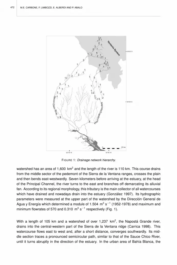
M.E. CARBONE, F. LIMBOZZI, E. ALBERDI AND P. ABALO
FIGURE 1: Drainage network hierarchy.
watershed has an area of 1,600 km2 and the length of the river is 110 km. This course drainsfrom the middle sector of the pedemont of the Sierra de la Ventana ranges, crosses the plainand then bends east-westwardly. Seven kilometers before arriving at the estuary, at the headof the Principal Channel, the river turns to the east and branches off demarcating its alluvialfan. According to its regional morphology, this tributary is the main collector of all watercourseswhich have drained and nowadays drain into the estuary (Gonzalez 1997). Its hydrographicparameters were measured at the upper part of the watershed by the Direccion General deAgua y Energıa which determined a module of 1.504 m3 s−1 (1952-1978) and maximum andminimum flowrates of 570 and 0.310 m3 s−1 respectively (Fig. 1).
With a length of 105 km and a watershed of over 1,237 km2, the Naposta Grande river,drains into the central-western part of the Sierra de la Ventana ridge (Carrica 1998). Thiswatercourse flows east to west and, after a short distance, converges southwardly. Its mid-dle section traces a pronounced semicircular path, similar to that of the Sauce Chico River,until it turns abruptly in the direction of the estuary. In the urban area of Bahıa Blanca, the
472

THE EFFECT OF FLOWRATE VARIATIONS OF THE SAUCE CHICO AND NAPOSTA GRANDE RIVERS ON THE INNERPART OF THE BAHIA BLANCA ESTUARY
Naposta Grande has been canalized and runs through an underground pipe during part of itscourse. Ten kilometers before its mouth the stream bifurcates into the main course and theMaldonado channel. The morphology of the basin is characteristic of a plain environment witha smooth slope towards the south (Carrica 1998). Its drainage network is made up of perma-nent and temporary watercourses with low to moderate density. Its hydrographic parameterswere measured by the Direccion General de Agua y Energıa, which determined maximum andminimum flowrates of 220 m3 s−1 and 0.061 m3 s−1 respectively, with an annual average of0.425 m3 s−1 (1952-1970) at the upper basin and 0.904 m3 s−1 (1963-1968) in the end of themiddle basin (Carica 1998).
Besides the urban and industrial activities, the main socioeconomic activity in the region is amixed livestock-agriculture production system. One of the zones with greater activity is locatedat the upper part of Naposta Grande watershed. The upper part of Sauce Chico watershed isalso occupied by a large livestock development; in the middle basin there are extensive horti-cultural lands while in the lower basin, close to the river mouth, there are numerous farms ofsmaller size. In Naposta Grande watershed, the horticultural land use area is small and thereare only two horticultural producers located in the lower basin. The water of both rivers is usedfor irrigation throughout their watersheds and particularly in the lower basins, on horticulturecrops.
3 METHODOLOGY
In order to calculate the flowrates of the Sauce Chico and the Naposta Grande rivers a tech-nique of indirect gauging in natural channels was used (Chow 1982).The depth of the waterwas continuously measured in both watercourses using a limnimeter-phreatimeter Mod. LF-325 provided by Genica Ingenierıa (Bahıa Blanca, Argentina). This data enabled the calcula-tion of the flowrates using the rating curve obtained by a working team of the Instituto Argentinode Oceanografıa (IADO) thanks to the qualified support of the staff of the Hydraulics Labora-tory of Universidad Nacional del Sur (UNS), both institutions of Bahıa Blanca. The measuresections were selected considering their accessibility conditions and making sure that theirflow regimes were continuous in the lower part of the watersheds near both mouths (Figure2). To get a comprehensive view of a heavy rainfall event, a dense network of precipitationand stream gauges is necessary. However the rainfall data available for this study area isscarce and is provided by two rainfall gauge stations located in the middle and the lower partof Naposta Grande watershed. The first one, a Davis GroWeather Station is placed in a townnamed Tres Picos (38o17´26.2” S and 62o10´16.6” W) and the other one is situated in theComandante Espora Aerometeorologic Station (38o43´47.8” S and 62o09´5.9” W).
The analysis of the precipitations registered between November of 2005 and September of2007 in the middle and lower basins of the Naposta Grande river helped establish the rela-tion between the rainfall and the flowrates obtained for that period. Although the data seriescorresponds only to three years, it is enough to make a preliminary characterization of the
473

M.E. CARBONE, F. LIMBOZZI, E. ALBERDI AND P. ABALO
region studied. In addition, a study was carried out based on the hydrograms showing theprecipitation events of a single heavy rain and their relation with the flowrate increase at themouths of both courses. In order to analyse the interaction between fluvial and marine envi-ronments in the inner part of Bahıa Blanca estuary, a preliminary hydrodynamic model usingMOHID Water Modelling System was developed. This application allowed the simulation ofthe effects of exceptional flowrates upon the estuary according to the rainfall events above re-ferred. The grid used was 200x200 with 5 layers and the geometry was of the sigma type.Theparameters incorporated for the MOHID execution were: bathymetry of the internal zone of theestuary, salinity and temperature data of its waters and flowrates higher than 90 m3 s−1 regis-tered for their main tributary watercourses. Other information considered included level curvesand speed and direction of local winds. The estuary bathymetry was provided by Doctors Su-sana Ginsberg, Eduardo Gomez and Gerardo Perillo from Instituto Argentino de Oceanografıa(IADO). Wind and estuary water parameters were obtained from gauge stations by personnelof the same institute.
FIGURE 2: Location of the limnimeters at the head of Bahıa Blanca estuary.
4 FLOWRATE VARIATIONS OF SAUCE CHICO AND NAPOSTA GRANDE RIVERS
For the period of November 3, 2005 to October 31, 2007, the average flowrate of the SauceChico was 1.72 m3 s−1. Due to a damage suffered by the limnimeter sensor, no data wasgathered from February 21 to March 31, 2006. The highest value was recorded in spring timewith a peak of 18.32 m3 s−1 in October 2006 while the minimum flowrate was registered insummer time, with a value 0.03 m3 s−1 in January 2007. The seasonal average flowrates forthis period are shown in figure 3. The average monthly flowrates of the analysed series pre-sented their highest levels in the months of October 2006 and March, September and October2007. The periods of low water for the Sauce Chico occurred during the months of December
474
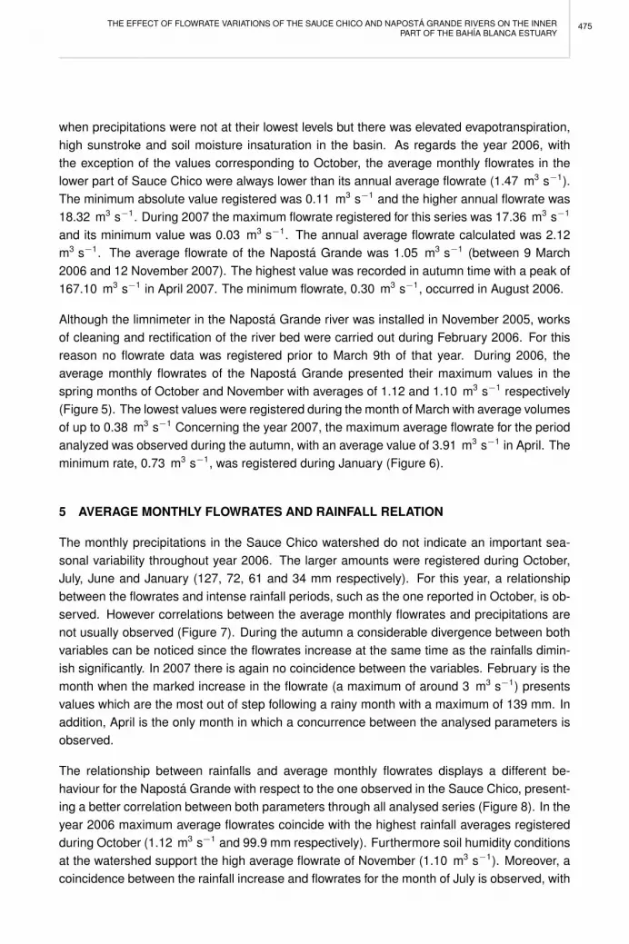
THE EFFECT OF FLOWRATE VARIATIONS OF THE SAUCE CHICO AND NAPOSTA GRANDE RIVERS ON THE INNERPART OF THE BAHIA BLANCA ESTUARY
when precipitations were not at their lowest levels but there was elevated evapotranspiration,high sunstroke and soil moisture insaturation in the basin. As regards the year 2006, withthe exception of the values corresponding to October, the average monthly flowrates in thelower part of Sauce Chico were always lower than its annual average flowrate (1.47 m3 s−1).The minimum absolute value registered was 0.11 m3 s−1 and the higher annual flowrate was18.32 m3 s−1. During 2007 the maximum flowrate registered for this series was 17.36 m3 s−1
and its minimum value was 0.03 m3 s−1. The annual average flowrate calculated was 2.12m3 s−1. The average flowrate of the Naposta Grande was 1.05 m3 s−1 (between 9 March2006 and 12 November 2007). The highest value was recorded in autumn time with a peak of167.10 m3 s−1 in April 2007. The minimum flowrate, 0.30 m3 s−1, occurred in August 2006.
Although the limnimeter in the Naposta Grande river was installed in November 2005, worksof cleaning and rectification of the river bed were carried out during February 2006. For thisreason no flowrate data was registered prior to March 9th of that year. During 2006, theaverage monthly flowrates of the Naposta Grande presented their maximum values in thespring months of October and November with averages of 1.12 and 1.10 m3 s−1 respectively(Figure 5). The lowest values were registered during the month of March with average volumesof up to 0.38 m3 s−1 Concerning the year 2007, the maximum average flowrate for the periodanalyzed was observed during the autumn, with an average value of 3.91 m3 s−1 in April. Theminimum rate, 0.73 m3 s−1, was registered during January (Figure 6).
5 AVERAGE MONTHLY FLOWRATES AND RAINFALL RELATION
The monthly precipitations in the Sauce Chico watershed do not indicate an important sea-sonal variability throughout year 2006. The larger amounts were registered during October,July, June and January (127, 72, 61 and 34 mm respectively). For this year, a relationshipbetween the flowrates and intense rainfall periods, such as the one reported in October, is ob-served. However correlations between the average monthly flowrates and precipitations arenot usually observed (Figure 7). During the autumn a considerable divergence between bothvariables can be noticed since the flowrates increase at the same time as the rainfalls dimin-ish significantly. In 2007 there is again no coincidence between the variables. February is themonth when the marked increase in the flowrate (a maximum of around 3 m3 s−1) presentsvalues which are the most out of step following a rainy month with a maximum of 139 mm. Inaddition, April is the only month in which a concurrence between the analysed parameters isobserved.
The relationship between rainfalls and average monthly flowrates displays a different be-haviour for the Naposta Grande with respect to the one observed in the Sauce Chico, present-ing a better correlation between both parameters through all analysed series (Figure 8). In theyear 2006 maximum average flowrates coincide with the highest rainfall averages registeredduring October (1.12 m3 s−1 and 99.9 mm respectively). Furthermore soil humidity conditionsat the watershed support the high average flowrate of November (1.10 m3 s−1). Moreover, acoincidence between the rainfall increase and flowrates for the month of July is observed, with
475
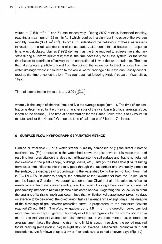
M.E. CARBONE, F. LIMBOZZI, E. ALBERDI AND P. ABALO
values of (0.54) m3 s−1 and 51 mm respectively. During 2007 rainfalls increased monthly,reaching a maximum of 132 mm in April which resulted in a significant increase of the averagemonthly flowrate (3.91 m3 s−1). In order to understand the behaviour of these watershedsin relation to the rainfalls the time of concentration, also denominated balance or responsetime, was calculated. Llamas (1993) defines it as the time required to achieve the stationarystate during a uniform heavy rain; that is, the time necessary for all the system (for the wholeriver basin) to contribute effectively to the generation of flow in the water-drainage. The timethat takes a water particle to travel from the point of the watershed furthest removed from thewater-drainage where it has fallen to the actual water-drainage site is the one usually consid-ered as the time of concentration. This was obtained following Kirpich’ equation (Wainelista,1997):
Time of concentration (minutes): tc = 3.97“
L0.77
S0.385
”
where L is the length of channel (km) and S is the average slope ( mm−1). The time of concen-tration is determined by the physical characteristics of the river basin (surface, average slope,length of the channel). The time of concentration for the Sauce Chico river is of 17 hours 20minutes and for the Naposta Grande the time of balance is of 7 hours 17 minutes.
6 SURFACE FLOW HYDROGRAPH SEPARATION METHOD
Surface or total flow (F) of a water stream is mainly composed of (1) the direct runoff oroverland flow (Fd), produced in the watershed above the place where it is measured, andresulting from precipitation that does not infiltrate into the soil surface and that is not retained(for example in the plant canopy, buildings, dams, etc.), and (2) the base flow (Fb), resultingfrom water that infiltrates into the soil, goes through the subsurface and eventually comes tothe surface, the discharge of groundwater to the watershed being the sum of both flows, thatis F = Fd + Fb. In order to analyze the behavior of the flowrates for both the Sauce Chicoand the Naposta Grande a hydrograph was done (see Oliveira et al., this volume), reflectingevents where the watercourses swelling was the result of a single heavy rain which was notpreceded by immediate rainfalls (for the considered series). Regarding the Sauce Chico, fromthe analysis of its rising limb it was determined that, while the hydrograph peak takes five dayson average to be perceived, the direct runoff lasts an average time of eight days. The durationof the discharge of groundwater (depletion curve) is proportional to the maximum flowratereached (Chow 1982). Therefore for gauges up to 4,5 m3 s−1 the depletion curve can lastmore than twelve days (Figure 9). An analysis of the hydrographs for the storms occurred inthe area of the Naposta Grande was also carried out. It was determined that, whereas theaverage time it takes the stream to rise (rising limb) is about three days, the period requiredfor its draining (recession curve) is eight days on average. Meanwhile, groundwater runoff(depletion curve) for flows of up to 3 m3 s−1 extends over a period of seven days (Fig. 10).
476

THE EFFECT OF FLOWRATE VARIATIONS OF THE SAUCE CHICO AND NAPOSTA GRANDE RIVERS ON THE INNERPART OF THE BAHIA BLANCA ESTUARY
0.0
0.2
0.4
0.6
0.8
1.0
1.2
1.4
1.6
1.8
2.0
Q [m
3 .s-1
]
SPRING SUMMER AUTUMM WINTER Nov 05-Oct 07
FIGURE 3: Seasonal average flowrates and general average for the evaluated series (November 2005-
October 2007) in the lower part of Sauce Chico River.
0.0
0.5
1.0
1.5
2.0
2.5
3.0
3.5
N2005
D J F M A M J J A S O N D J F M A M J J A S O2007
Monthly average Series average
FIGURE 4: Average monthly and series average flowrates at Sauce Chico lower basin.
0.0
0.2
0.4
0.6
0.8
1.0
1.2
1.4
Q [m
3 .s-1
]
SPRING SUMMER AUTUMM WINTER Mar 06 -Nov 07
FIGURE 5: Seasonal average flowrates and general average for the evaluated series (March 2006-
November 2007) in the lower part of the Naposta Grande watershed.
477
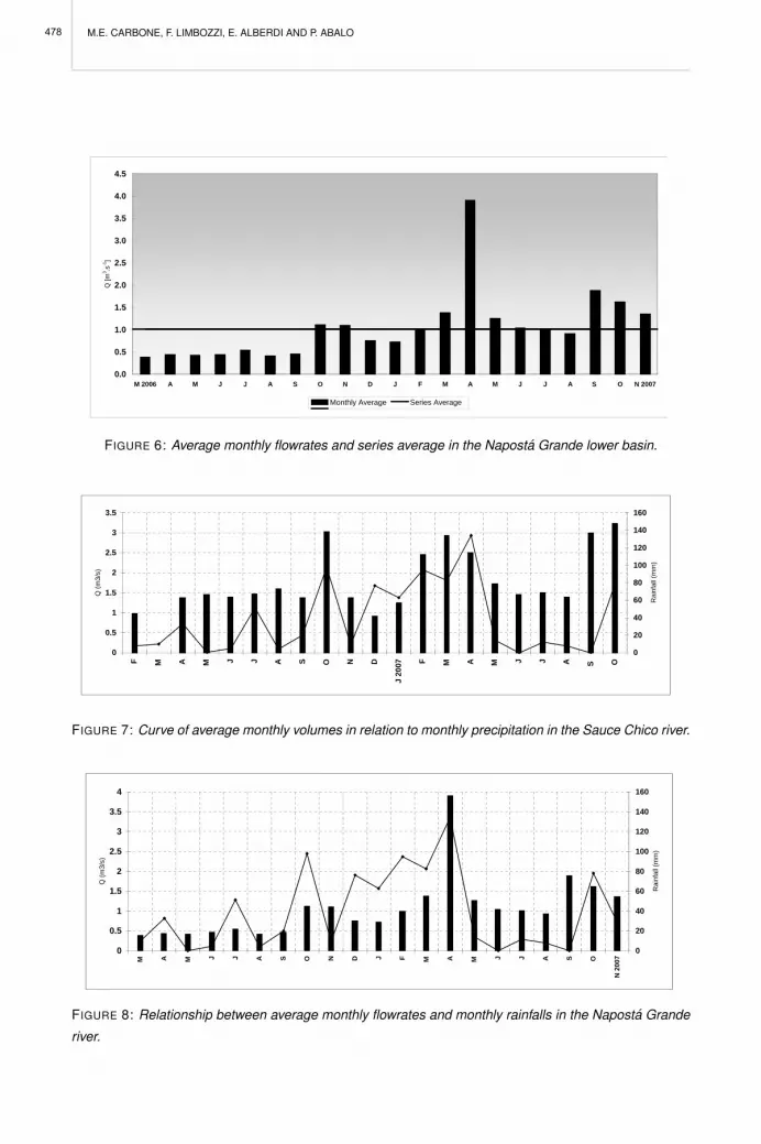
M.E. CARBONE, F. LIMBOZZI, E. ALBERDI AND P. ABALO
0.0
0.5
1.0
1.5
2.0
2.5
3.0
3.5
4.0
4.5
M 2006 A M J J A S O N D J F M A M J J A S O N 2007
Q [m
3 .s-1
]
Monthly Average Series Average
FIGURE 6: Average monthly flowrates and series average in the Naposta Grande lower basin.
0
0.5
1
1.5
2
2.5
3
3.5
F M A M J J A S O N D
J 20
07 F M A M J J A S O
Q (m
3/s)
0
20
40
60
80
100
120
140
160
Rai
nfal
l (m
m)
FIGURE 7: Curve of average monthly volumes in relation to monthly precipitation in the Sauce Chico river.
0
0.5
1
1.5
2
2.5
3
3.5
4
M A M J J A S O N D J F M A M J J A S O
N 2
007
Q (m
3/s)
0
20
40
60
80
100
120
140
160
Rai
nfal
l (m
m)
FIGURE 8: Relationship between average monthly flowrates and monthly rainfalls in the Naposta Grande
river.
478

THE EFFECT OF FLOWRATE VARIATIONS OF THE SAUCE CHICO AND NAPOSTA GRANDE RIVERS ON THE INNERPART OF THE BAHIA BLANCA ESTUARY
7 APPLICATION OF THE MOHID WATER MODELLING SYSTEM
The simulation of the discharge of both the Sauce Chico and the Naposta Grande waters intothe estuary enabled the observation of a significant difference in the hydrodynamical behaviorat its head. The mouth of the Sauce Chico is located in a mesotidal zone with a gentleslope and an important network of medium-depth channels. Therefore, its flow is constantlyconditioned by the characteristics of the sector. The morphology of the islands, which are nohigher than 2.10 m, and the complex network of tidal channels result in a significant run-offat low tide in exceptional rainfall events. The maximum depths range from 6 m to 1 m in theinnermost part of the head and sediments are predominantly sandy (Gomez et al. 1996).
1.5
2.5
3.5
4.5
5.5
18-0
4-07
20-0
4-07
22-0
4-07
24-0
4-07
26-0
4-07
28-0
4-07
30-0
4-07
FIGURE 9: Hydrograph of the Sauce Chico river.
1
2
3
4
5
6
7
11-3
-07
12-3
-07
13-3
-07
14-3
-07
15-3
-07
16-3
-07
17-3
-07
18-3
-07
19-3
-07
20-3
-07
21-3
-07
22-3
-07
23-3
-07
FIGURE 10: Hydrograph of the Naposta Grande river.
479

M.E. CARBONE, F. LIMBOZZI, E. ALBERDI AND P. ABALO
Based on measurements taken on the site, the simulation showed a maximum dischargespeed of 0.5 m s−1 and an exceptional flowrate of 67 m3 s−1 resulting from an extreme pre-cipitation event of a single heavy rain (Figure 11). The Naposta Grande presents a slightdischarge at its mouth, which immediately interacts with the morphology of the area- in otherwords, its waters are channelled, reaching a speed no higher than 1 m s−1. The maximumflowrate in this simulation is 90 m3 s−1. The depths in the inner sector of the estuary rangefrom 5 to 15 m, being about 20 m at high tide and the wind blows predominantly from thenorth-west (Figure 12).
FIGURE 11: Simulation of the discharge of the Sauce Chico river.
8 CONCLUSIONS
This preliminary study on the behaviour of the Sauce Chico and the Naposta Grande riversshows that, although they are both part of Atlantic basins, they present singular characteristics.From a hydromorphological point of view, for instance, both watercourses flow across landswith different gradients and determinants. The characteristics of both the use of the landand the productive activities carried out in the area could modify the flowrates registered bythe stations located in the lower basins; nevertheless, the absence of data upstream anddownstream of sectors with great productivity precludes verifying this supposition. Despitethe lack of a more extensive precipitation database over the November 2005 - September2007 period the series analysed has helped establish a preliminary characterisation of theflowrates over the last two years and their direct correspondence with rainfall events. Oncethe flowrates of both watercourses have been characterised, the data obtained can be usedin the construction of a hydrodynamical model. The simulation of the discharge of the Sauce
480

THE EFFECT OF FLOWRATE VARIATIONS OF THE SAUCE CHICO AND NAPOSTA GRANDE RIVERS ON THE INNERPART OF THE BAHIA BLANCA ESTUARY
Chico and the Naposta Grande not only aided in determining the differences presented bythe hydrodynamical behaviour in the inner sector of Bahıa Blanca estuary, it also showed howthese features influence the runoff in both watercourses. The speeds registered were 0.5 and1 m s−1 and the flowrates ranged between 67 and 90 m3 s−1 for the Sauce Chico and theNaposta Grande, respectively.
FIGURE 12: Simulation of the discharge of the Naposta Grande river.
REFERENCES
Carrica J (1998) Hidrogeologıa de la cuenca del arroyo Naposta Grande, provincia de Buenos Aires. Tesisdoctoral. Biblioteca Central, Universidad Nacional del Sur, 215pp.
Chow VT (1982) Hidraulica de los canales abiertos. Editorial Diana. Mexico, 633pp.
Garcıa J, de Garcıa OME (1964) Hidrogeologıa de la region de Bahıa Blanca (Prov Bs As y la Pampa).Direccion Nacional de Geologıa y Minerıa. Boletin N 96: 1-94 Buenos Aires.
Gomez EA, Ginsberg SS, Perillo GME (1996) Geomorfologıa y sedimentologıa de la zona interior delCanal Principal del Estuario de Bahıa Blanca. AAS Revista, 3/2: 55-61
Gonzalez M (1997) Diagnostico ambiental de la Provincia de Buenos Aires. Tomo I Ediciones BancoProvincia, Buenos Aires, 245pp.
Leitao T (2008) Definition of state indicators for the management of interactions between inland andestuarine, this volume.
Llamas J (1993) Hidrologıa general: principios y aplicaciones. Universidad del Paıs.
481

M.E. CARBONE, F. LIMBOZZI, E. ALBERDI AND P. ABALO
Oliveira MM, Lobo Ferreira JP, Yarrow M (2008) Groundwater recharge assessment, this volume.
Pedraza Gilsanz J (1996) Geomorfologıa, principios, metodos y aplicaciones. Ed Rueda. Madrid. 414pp.
Perillo GME, Piccolo MC (1999) Geomorphologic and physical characteristics of the Bahıa Blanca Estuary.Argentina. En: Perillo GME, Piccolo MC, Pino Quivira M (eds.), Estuaries of South America: theirgeomorphology and dynamics. Environmental Science Series, Springer-Verlag, Berlın: 195-216.
Piccolo MC, Perillo GME, Arango JM (1987) Hidrografıa del estuario de Bahıa Blanca, Argentina. RevistaGeofısica 26: 75-89
Strahler A (1952) Hypsometric (area-altitude) analysis of erosional topography. Geological Society Amer-ican 63: 1117-1142
Wanielista MP (1997) Hydrology and Water quality Control. Wiley, 2nd edition, 567pp.
482

PERSPECTIVES ON INTEGRATED COASTAL ZONE MANAGEMENT IN SOUTH AMERICAR. NEVES, J.W. BARETTA AND M. MATEUS (EDS.), IST PRESS, 2008
HYDRODYNAMICS AND SEDIMENTS IN BAHIA BLANCA ESTUARY: DATAANALYSIS AND MODELLING
F.J. CAMPUZANO, J.O. PIERINI AND P.C. LEITAO
1 INTRODUCTION
The Bahıa Blanca estuary, as indicated by its name, is a bay or rather collection of bayslocated on the Southern part of Buenos Aires Province (Argentina) on the uppermost terraceof the Argentinean Continental Shelf (ACS), according to the bathymetric division proposedby Parker et al. (1997). The channels and bays with North-West to South-East orientationrun through extensive tidal areas, namely from North to South: Principal Channel, where themain human settlements are located, Falsa Bay and Verde Bay. On the Principal Channel oneof the most important deep water ports of Argentina is located, and though the harbours andthe navigation channel are dredged to a nominal depth of 13 m, a tidal prediction model ”isurgently required” for navigational security (Perillo and Piccolo 1991).
The Principal channel has an elongated shape with a total length of 68 km, being 200 m and3-4 km wide near its head and mouth, respectively (Aliotta and Perillo, 1987). The PrincipalChannel ends inland in a salt flat known as Salitral de la Vidriera. Falsa and Verde bays arealso funnel shaped with total lengths of around 30 km and around 4 and 6 km wide respec-tively. In the study area (Figure 1), average depth is around 10 m with a maximum value ofaround 22 m. Intertidal areas account for about 40% of the domain represented in Figure 1and have a concomitantly large influence both on water and sediment dynamics. In the nearbycoastal area the isobaths have a NE-SW orientation (Pierini 2007).
FIGURE 1: Bahıa Blanca model domain bathymetry and elevation of intertidal areas.
483

F.J. CAMPUZANO, J.O. PIERINI AND P.C. LEITAO
Water circulation in Bahıa Blanca estuary is mainly driven by tides, though it complex geometryand the prevailing winds produce deviations from the astronomical tides (Perillo and Piccolo1991, Palma 1995, Etala 2000). Though it traditionally has been considered as an estuary(Piccolo and Perillo 1990), nowadays the only natural fresh water sources discharge into theBahıa Blanca bay innermost area (Heffner et al. 2003) at low flowrates. As such, only thisinner area might be considered a true estuary.
2 GEOMORPHOLOGY
The Bahıa Blanca estuary is a dynamically active system in which the main driving force thatcontributed to its formation is no longer present. Melo et al. (2003) described the evolutionof the Bahıa Blanca area from 20000 years BP when the study area was a coastal plain thatthe Colorado River traversed on its way to the open ocean. The freshwater inputs began togrow a deltaic front that, together with the increase in river flow and sea level rise, by 6000years BP created the system of channels. From 5000 years BP on, the partial decrease ofthe mean sea level, along with the progressive migration to the South of the Colorado Riverand the migration North of other creeks decreased fresh water inputs into the Bahıa Blancasystem. Those losses were compensated by the entry of oceanic water that led the systemto the present situation. The Colorado River discharges nowadays South to the Bahıa Blancaestuary with an average flow of 138 m3 s−1. However, it appears to have almost no influenceon hydrodynamics or in sediments input into the system anymore (Cuadrado et al. 2002).Currently, the only natural fresh water sources in Bahıa Blanca estuary are Sauce Chico River,Naposta Grande creek and Maldonado creek, which is formed by the junction of Saladillo deGarcıa and Dulce creeks (Heffner et al. 2003).
At present, the Bahıa Blanca estuary comprises three large interconnected parallel tidal chan-nels with a NW-SE orientation, namely from South to North: Verde Bay, Falsa Bay and Prin-cipal Channel. To these bays arrive channels of all types and dimensions, from large straighttidal channels to meandering creeks and gullies (Ginsberg and Perillo 2004). The PrincipalChannel is the only bay that receives freshwater discharges and near its mouth shifts from thefunnel shape to a meandering channel. This main channel is connected mainly at its southernmargin to other minor tidal channels. On the other hand, Verde and Falsa bays´ head actlike a basin catchment where the different tidal creeks join. Nevertheless, the system is inpermanent evolution as was observed by Ginsberg and Perillo (2004) who detected a lateralmigration on some tidal channels at a rate of 25 m yr−1.
3 HYDRODYNAMIC DATA DESCRIPTION AND ANALYSIS
3.1 Tides
In the Bahıa Blanca estuary, tidal data are collected in three different stations (Table 1, Figure2) from the open ocean to the inner area of the Principal Channel: Torre Mareografica (here-
484

HYDRODYNAMICS AND SEDIMENTS IN BAHIA BLANCA ESTUARY: DATA ANALYSIS AND MODELLING
after TM), Puerto Belgrano Harbour (hereafter PB) and Ingeniero White Harbour (hereafterIW). Ten-minute water level timeseries for the three permanent tidal gauges were provided bythe Bahıa Blanca Port Consortium (CGPBB) for more than three years. The Bahıa Blancaestuary is a mesotidal estuary (Piccolo and Perillo 1990, Cuadrado et al. 2002, Ginsberg andPerillo 2004), with a tidal range of 2-4 m. Averages performed on each tidal gauge water leveldata for the year 2000 show that the tidal range increases along the Principal channel frommesotidal to nearly macrotidal.
FIGURE 2: Location of the tidal (circles), current (diamond) and meteorological (square) observation
stations in the Bahıa Blanca estuary.
Harmonic analyses performed on the water level time series using the POL/PSMSL TidalAnalysis Software Kit 2000 (TASK-2000) resulted in 62 tidal components for each tidal gauge.Observed and predicted with the tidal components, water levels for each tidal gauge presenta high coefficient of determination ( R2) from 0.87 for TM station to 0.91 for IW station.
Mean water level ( Z0) for the three permanent tidal stations shows a difference of 0.70 mbetween the two most widely separated stations (55 Km). This difference will be addressedlater in the modelling chapter. The tidal components of greater amplitude are given in Table2, the list is led in all the stations by the semidiurnal components, followed by the diurnalcomponents whose influence decreases headwards. The Formzahl coefficient (F) provides aquantification of the degree of influence of the semidiurnal and diurnal components. It consistsof the division of the sum of the two main diurnal tidal components ( K1 and O1) by the sumof the two main semidiurnal components ( M2 and S2). According to the result of the F ratio,tides can be considered diurnal (F>3), semidiurnal (F<0.25) or mixed (0.25<F<3). In BahıaBlanca the F ratio decreases as the tidal wave progresses up the estuary, being 0.26 at TMstation and 0.19 at IW station. Tides in the Bahıa Blanca estuary can thus be classified assemidiurnal. As the tide heads inland, the weight of the so-called compound tides or overtides
485

F.J. CAMPUZANO, J.O. PIERINI AND P.C. LEITAO
( M4, MS4 and MN4), generated by nonlinear interactions of primary constituents, increases.This effect takes place in shallow water areas, also increasing the tidal range. These newconstituents are important for turbulence, tidal asymmetry and mean water level (Wang et al.2002).
According to Wang et al. (2002), tidal asymmetry can be assessed as a comparison of theamplitudes and phases of the dominant M2 component with the overtide M4. A relative phase(phi = 2φ2 − φ4) between 0o and 180o indicates longer duration of the flood than ebb (flood-dominant) and vice versa. After analysing the data for the three tidal gauges in Bahıa Blanca,an evolution from the flood-dominated coast to the ebb-dominated head can be observed. InTable 3 the values obtained for the years 2000-2003 analysis are summarised. The α param-eter calculated as division of the M4 amplitude by the M2 amplitude indicates the degree ofasymmetry, this parameter increases headwards due to a larger increase of the M4 compo-nent than the M2.
TABLE 1: Location, observation period and source of hydrodynamic and atmospheric data.
Station Longitude Latitude Period Source
TM 61º43'12" W 39º08'56" S 23/08/99 - 31/12/03 CGPBB PB 62º06'15" W 38º53'48" S 23/08/99 - 31/12/03 CGPBB IW 62º16'08" W 38º47'26" S 23/08/99 - 31/12/03 CGPBB PR 62º04'00" W 38º53'00" S 01/01/01- 01/12/01 IADO
PC 62°03'09" W 38°56'40 "S 17/03/97 – 21/04/97 SHN
TABLE 2: Principal tidal components for each tidal gauge (H=amplitude; ϕ=phase).
Puerto Ing. White Puerto Belgrano Torre Mareográfica Tidal Component
Speed (deg/hr) H (cm) φ (º) H (cm) φ (º) H (cm) φ (º)
ZO 0.000 263.544 0.000 245.635 0.000 193.273 0.000 M2 28.984 169.123 186.072 153.523 177.906 115.864 157.094 L2 29.528 25.475 255.364 22.471 245.987 15.977 220.692 N2 28.440 23.983 103.593 21.080 95.833 15.239 76.690 M4 57.968 22.764 178.277 16.141 184.234 6.396 171.968 S2 30.000 21.589 307.350 20.632 298.669 16.843 274.215 K1 15.041 21.151 61.178 21.481 54.527 20.345 45.066 O1 13.943 15.528 0.701 16.186 355.431 15.426 344.967 MU2 27.968 14.523 291.531 14.015 282.016 12.590 264.735 NU2 28.513 10.954 137.915 9.637 130.029 7.632 113.261
3.2 Currents
The dataset collected at the Punta Ciguenas oil pipe monobuoy (Figure 2, Table 1) by the NavyHydrographical Service (SHN), consisting of current speed and direction every 15 minutesduring 35 days, was the most representative dataset available in the Bahıa Blanca estuary.The average value for the whole series is 0.64 m s−1 with a maximum of 1.33 m s−1 and
486

HYDRODYNAMICS AND SEDIMENTS IN BAHIA BLANCA ESTUARY: DATA ANALYSIS AND MODELLING
the directions are practically opposite pointing to 295o and 115o respectively (Figure 3). Ebbtide maximum velocities are slightly higher. In order to validate and calibrate the model fordifferent periods, the harmonic components of the dataset were obtained for each componentof the velocity using the TASK-2000 software. Component U intensity of the velocity is almostdouble the V component, due to the orientation of the Principal Channel. The most importantharmonic component for velocity is the M2 which is responsible for more than 40% of tidalvelocity, followed by the N2 component that represents an 8% of the intensity of the currents.The tidal components are able to explain 82% of the total variability of the currents measuredduring the sampling period, the remainder of the variability may be due to variations in meansea level and to atmospheric effects.
TABLE 3: Principal tidal components for each tidal gauge (H=amplitude; ϕ= phase).
Puerto Ing. White Puerto Belgrano Torre Mareográfica
M2 H (cm) 169.123 153.523 115.864 M2 φ (º) 186.072 177.906 157.094 M4 H (cm) 22.764 16.141 6.396 M4 φ (º) 178.277 184.234 171.968 α 0.135 0.105 0.055 Phi 193.867 171.578 142.22
FIGURE 3: Current intensities and directions observed and obtained through harmonic analysis for the
same period (Left) and observed current values analysis (Right).
3.3 Freshwater inputs
Main natural fresh water inputs in the Bahıa Blanca estuary are located at the innermost partof the Principal Channel. Basically, only Sauce Chico River and Naposta Grande creeks havea considerable discharge in the study site (Heffner et al. 2003) with average annual flows of5.80 and 2.68 m3 s−1 respectively. Nevertheless, high runoff peaks have been registered,
487

F.J. CAMPUZANO, J.O. PIERINI AND P.C. LEITAO
for instance in the Sauce Chico River several times discharges over 50 m s−1 have been ob-served (Perillo and Piccolo 1991). Although the source of both rivers is located in the Sierrasde la Ventana mountain range, both catchment areas are not subjected to the same processesand present different discharge peaks during the year. Sauce Chico River has two main peaks,one in autumn (Feb-Jun) and a stronger one during spring (Aug-Dec). However, the NapostaGrande Creek flow shows peaks in winter (Apr-Aug) and spring (Aug-Dec), both with similarintensities. The spring peak in both rivers corresponds to the rainiest period in the BahıaBlanca region. Sauce Chico presents a flow pattern very influenced by the local rain patternon Bahıa Blanca region while Naposta is more influenced by the precipitation near the Sier-ras de la Ventana (Piccolo et al. 1987). Figure 4 shows the monthly average flow from datacollected during the 1993-1999 period provided by Aguas Bonaerenses Sociedad Anonima(ABSA). There are other creeks flowing into the Bahıa Blanca estuary, such as Galvan, Sal-adillo de Garcıa and Maldonado creeks with an overall flow lower than the Naposta Grandecreek (Piccolo et al. 1987).
FIGURE 4: Naposta Grande Creek and Sauce Chico rivers monthly average flow.
3.4 Atmospheric influence
The SMN (National Meteorological Service, 1985) in Capelli and Campo (2004) describedthe study area as dominated by the pressure systems from the West and Southwest and thepresence of a semi permanent high pressure over the South-western Atlantic centred at 30o.The circulation around the Western edge of the anticyclone results in strong winds from theNW and N. When winds blow from NW, they produce lower water levels than those predictedby the astronomical tides; on the other hand, when wind blows from SE water is piled upin the inner areas of the bay increasing the water level. This phenomenon is locally knownas sudestadas. According to Perillo and Piccolo (1991) and Piccolo and Diez (2004) thepredominant winds from N and NW produced an advance of the low water time, a delay onthe high water time and reduced the predicted levels both for high and low tide.
488

HYDRODYNAMICS AND SEDIMENTS IN BAHIA BLANCA ESTUARY: DATA ANALYSIS AND MODELLING
Thirty minute data observed at Puerto Rosales meteorological station (Table 1, Figure 2)by the IADO for the period January-November 2001 showed prevailing winds blowing fromNorthern sectors, mainly from the North and Northeast. Maximum intensity recorded on thisperiod was 23.2 m s−1 and an average value of 6.2 m s−1. During most of the time intensitiesdo not surpass 10 m s−1.
4 HYDRODYNAMIC MODEL: SETUP AND RESULTS
The implementation of a validated hydrodynamic model would serve for applications thatwould aid in coastal management and would serve as a part of the DPSIR approach. TheMOHID hydrodynamic model (http://www.mohid.com/) was used to force a Bahıa Blanca2-Dimensional domain model covering the study site. The most relevant characteristic is theorder of magnitude of the horizontal and vertical dimensions. In our case study the horizontalextent is 70 km, while the average depth is 10m.
4.1 Modelling grids
To study the different hydrodynamic processes involved in Bahıa Blanca, two different spa-tial scales covering the main area of interest were adopted with different resolutions: 0.01o
and 0.002o horizontal step covering from the coordinates -61.41W, -39.38S to the inner es-tuary (Pierini 2007), hereafter referred as LoRes grid and HiRes grid, respectively. The maininterests in developing different resolutions have been, on the one hand, to study differentprocesses in diverse detail according to the available data and, on the other, to maximise themodel runtime. Bathymetric data used for composing the different model domains came fromthe GEBCO digital atlas, a one minute global bathymetric grid database (IOC, IHO and BODC2003) and from CGPBB data with a waterline obtained after evaluating 6 sets of Landsat 5 TMand Landsat 7 ETM data resulting in a high density bathymetry (50 m x 50 m) (Pierini 2007).
4.2 Tides
Tide enters each bay of the Bahıa Blanca estuarine system by its Southern margin findingall the channels reduced in width and most of the intertidal areas emerged. As the tide ad-vances, water starts to cover the intertidal area amplifying the submerged area. As a result ofthe interaction of the tidal wave with the shallow depths of the channels, overtides importanceincreases. Maximum tidal amplitudes are thus found at the innermost areas for each of thethree different channels, and the absolute maximum was found in Principal Channel. Dur-ing high tides, the connections between the three different bays reach their maximum widthfavouring water exchange between bays. When the tidal wave retreats, water scours from theinundated intertidal areas through tidal channels into the main channels, the time to evacuatethose waters is long and so this process is still going on when a new tidal wave is alreadyentering the system, as can be appreciated on the last image of the sequence (Figure 5). Dueto the vicinity of the TM tidal gauge to the boundary of the Bahıa Blanca domain, the modelforcing consisted of imposing those tidal components along the entire coastal open boundary.
489

F.J. CAMPUZANO, J.O. PIERINI AND P.C. LEITAO
FIGURE 5: Water levels for the HiRes domain during a period of 12 hours.
The Bahıa Blanca Estuary Principal Channel mean sea level, as stated in the data analysis,presented a permanent sea level difference of 70 cm between the most distant tidal gauges.That tidal amplification could not be explained by the increase of mean sea level due to tidaldumping. Using simultaneous validation of the water levels and the current intensities at PuntaCiguenas (PC) station, it was concluded that using the mean sea level of the outermost station,TM, the right quantity of water was not entering the system, as the obtained currents at thatstation were reduced compared to the observations. On the contrary, when adding these 70cm to the mean sea level of the TM station, both water levels and current intensities at PCstation presented a high coefficient of determination.
Applying these conditions to the model, correlations between the expected water levels dueto astronomical tides and model results obtained were performed obtaining correlation coef-ficients above 0.93 (Table 4). To further evaluate the comparison between the observed tidallevels obtained through harmonic analysis with the predicted levels obtained through mod-elling, the additional indicators suggested by Willmott (1982) were assessed (Table 4).
490

HYDRODYNAMICS AND SEDIMENTS IN BAHIA BLANCA ESTUARY: DATA ANALYSIS AND MODELLING
TABLE 4: Model performance indicators at each tidal gauge.
Station Torre Mareográfica Puerto Belgrano Puerto Ing. White
Correlation (r) 0.985 0.987 0.966 Coef. Determination (r2) 0.971 0.974 0.933 MB -0.048 0.104 -0.054 RMSE 0.162 0.220 0.369 Skill 0.992 0.991 0.981
Mean bias (MB) indicates the average difference between the observed and predicted values.Predicted amplitudes vary in (bias/total amplitude*100) 1.37, 2.35 and 1.08% of the total am-plitude at TM, PB, and IW stations, respectively. Root Mean Square Error (RMSE), or standarddeviation, is the square root of the variance which represents that 95% of the model predictionsdo not differ (in absolute value) from the observations by more than 2xRMSE. The skill indexis intended as a descriptive measure, and is both a relative and bounded measure which canbe widely applied to make cross-comparisons between models. It provides similar informationto the coefficient of determination, in the sense that it gives a measure of model performance,but it penalises models with greater bias. If the skill index is 1, the model presents an optimalpredictive skill. Skill values for each station are close to 1, indicating a high degree of modelperformance.
4.3 Currents
Currents on Bahıa Blanca estuary are mainly caused by tides. In addition, the importance ofthe geomorphology for the tidal asymmetry is reflected in the residual currents. Tidal currentsat the mouth of the estuary are the result of the cumulative processes of the outer generalcirculation and the distortion produced by the estuary hydrodynamics. Flood velocities aregenerally larger than the ebb velocities outside the estuary due to the direct relationship be-tween velocity and depth.
4.3.1 Instantaneous currents
The Principal channel, according to Piccolo et al. (1987), is dominated by ebb currents, max-imum surface values are 0.80 m s−1 and 1.40 m s−1 for flow and ebb currents, respectively.Very similar values were obtained by Gomez et al (1996) integrating vertically the observa-tions, with values of 1.05 m s−1 and 1.30 m s−1 for flow and ebb respectively. In the coastalarea, measurements obtained during the Austral campaign in 1993 observed maximum ve-locities of 0.6 m s−1 with velocities over 0.3 m s−1 being exceeded for more than 30% of thetime (Cuadrado et al. 2002).
Model results (Figure 6) present an ebb-dominated inner estuary in opposition to a flood-dominated coastal area in agreement to both the relative phase values (phi) obtained in Sec-tion 3.1 and Cuadrado et al. (2002). In Verde Bay maximum values are found near its mouthdue to the channelling of the ebbing waters; in Falsa Bay, in addition to the mouth, it presents
491

F.J. CAMPUZANO, J.O. PIERINI AND P.C. LEITAO
maximum values near its head in the region where water from the surrounding intertidal areascours and in the Principal Channel values are high along the main axis of the channel.
During flood, the high intensities on the three bays are located along each main channelslowly covering the intertidal areas where velocities relax. During ebb along the main axis ofthe Principal Channel values range between 0.7 m s−1 and 1.4 m s−1, the maximum valuesbeing found near the upper reaches; maximum values of similar intensity are observed inFalsa Bay near its head and near the mouth of Verde Bay. On the three bays, velocities duringebb tide are higher than during flood. Low intensities are mainly found in the higher reachesof the intertidal areas. During flood, water piles up in the entry of the channels, with speeds ofnearly 1 m s−1 being observed in the mouth and average speeds along the channel axis of 0.4m s−1 on average. Peak velocities observed in the model on the intertidal areas during floware generally below 0.3 m s−1. It can be concluded that the model reproduces the principalfeatures described in the literature.
FIGURE 6: Instant velocities for a 12 hour period in the Bahıa Blanca estuary HiRes domain.
492

HYDRODYNAMICS AND SEDIMENTS IN BAHIA BLANCA ESTUARY: DATA ANALYSIS AND MODELLING
4.3.2 Residual currents
The residual currents are a significant factor regarding the import and export of dissolved andparticulate substances of the estuarine system. Two different residuals are relevant in terms ofcharacterising the estuary, namely residual flux velocity and residual velocity. The residual fluxvelocity is calculated by the vertical integration of the specific residual water fluxes occurringduring a defined period and is expressed in m s−1 and influences the transport of dissolvedproperties in the water column (i.e. nutrients). Figure 7 Top presents results corresponding toa month simulation average. As was pointed out by Perillo et al. (1987) and Pierini (2007) forthe head of the Principal Channel, net transport in deeper areas is seawards while in shallowerwaters is landwards. The model reproduces this pattern. In the mouth of the Principal Channeldue to its particular geomorphology with channels crossing intertidal areas, a recirculationpattern can be observed. As a consequence, the dissolved components would be transportedinto the intertidal areas and recirculated in the Principal Channel mouth retarding their exportto the open ocean.
FIGURE 7: Residual flux velocity (Top) and Residual velocity (Bottom) in the inner (Left) and the outer
(Right) area of the Bahıa Blanca estuary.
The residual velocities are the net velocities obtained after balancing currents in different di-rections and they are of particular importance regarding particulate matter transport such assediments. The most remarkable results (Figure 7 Bottom) are the net transport from the in-tertidal areas into the main channels. A recirculation pattern can also be found at the mouth ofthe Principal Channel. According to these results, the intertidal channels would be exportingsediments and other particulate matter into the main channels favouring erosion processes inthe intertidal areas, although some recirculation at the Principal Channel mouth would slowdown the sediments release into the coastal area (Pierini 2007).
493

F.J. CAMPUZANO, J.O. PIERINI AND P.C. LEITAO
FIGURE 8: Intensities and direction/s of the currents in Punta Ciguenas stations obtained through har-
monic analysis (dots) and modelling (diamonds) for LoRes and HiRes domains.
4.3.3 Currents Validation
The main tidal current validation has been performed in the centre of the Principal Channel inthe vicinity of the Punta Ciguenas (PC) buoy (Figure 2, Table 1). After adding 70 cm to themean sea level observed in TM station, it has been found that the model is able to reproducethe current intensities and directions (Figure 8). The coefficient of determination obtainedwhen comparing both intensities is 0.72. In the HiRes domain this value increases to 80%.Model results and observed values present maximum peaks of intensity around 1.30 m s−1
during ebb conditions and nearly 1 m s−1 during flood conditions.
4.4 Wind effect
In order to study the effect of wind over the water levels observed, a month was simulatedwith different wind conditions. According to data analysis performed by Cuadrado et al (2005),predominant directions are NW, NNW and SE with a velocity range between 5 and 10 m s−1.A reference simulation with no wind was used to compare with simulations forced with constantwind conditions of 10 m s−1 coming from different directions (N, NW, S & SE). Maximumdifferences occur at the higher reaches of the estuary when winds blow along the PrincipalChannel axis, piling up water when it blows from the South and decreasing water levels whenit blows from the North. In Table 5, mean sea levels are summarised for the three tidal stationsanalysed in this study.
5 SUSPENDED SEDIMENT DATA ANALYSIS
Despite the relevance of sediments accretion-erosion processes in the evolution of the geo-morphology and hydrodynamics, suspended sediment data for the Bahıa Blanca estuary arescarce and the origin of the sediments in the water column is not well-established. From the
494

HYDRODYNAMICS AND SEDIMENTS IN BAHIA BLANCA ESTUARY: DATA ANALYSIS AND MODELLING
socio-economic point of view, the importance hinges on the need to maintain a nominal depthof 13.7 m for harbours and navigational channels (Perillo and Sequeira 1989). The Port Con-struction and Navigational Ways National Direction (DNCPVN, its Spanish acronym) dredgesaround 300,000 m3 yr−1 in a 2 km stretch of El Toro Channel to maintain a 10 m nominaldepth.
TABLE 5: Wind direction and resulting mean sea level for each tidal gauge.
Wind Direction Torre Mareográfica Puerto Belgrano Puerto Ing. White No Wind 1.93 1.93 1.94 North 1.84 1.64 1.62 Northwest 1.83 1.67 1.54 South 2.03 2.22 2.34 Southeast 2.01 2.25 2.44
Sediment balance is related to accumulation or erosion processes, also connected to theresidual velocities. In the same sense, Ginsberg and Perillo (2004) concluded that the du-ration of asymmetry controls the trend of erosion in the channel system while the velocityasymmetry is responsible for the net sediment transport. Flow asymmetries characterized byshorter flood duration and higher flood current maximum (flood dominance) induces landwarddirected sediment transport while shorter ebb periods and greater ebb current maximum (ebbdominance) cause net outward sediment transport (Lanzoni and Seminara 2002).
The lack of major sediment point sources in the system, due to the reduced river flow, and thesmall contribution of sediments from the open ocean implies that the channel margins and in-tertidal areas should be regarded as the main source of sediments (Perillo and Sequeira 1989,Ginsberg and Perillo 2004). They considered sediment transport controlled by the degree oftidal asymmetry and trends on erosion governed by the degree of time asymmetry. Accordingto Perillo and Cuadrado (1990) an erosion process is ongoing in the study area, sedimentsare eroded from the channel margins and eventually exported to the continental shelf. Thematerials affected are mainly very fine sand (38%), silt (37%) and clay (25%); with the sandtransported as bedload and the other fractions in suspension (Aliotta et al. 2004).
As occurs with hydrodynamics, wind direction and intensity has an effect on suspended sedi-ments in the estuary. Perillo and Cuadrado (1990) found in the nearby coastal area, Northeastof Bahıa Blanca estuary mouth, homogeneous sediment concentrations between 70 and 90mg l−1 with North wind that decreased to 10 to 20 mg l−1 when the wind shifted to a SSEdirection. The origin of those sediments was found related to the Bahıa Blanca sedimentplume.
The Austral campaign on November 1993 covered the coastal vicinity of the Bahıa Blancashowing a clear sediment front along the coastal area of the Bahıa Blanca estuary (Figure9, left), also observed in recent satellite pictures (Figure 9 right). In the Austral campaign,maximum concentrations of over 60 mg l−1 are related to the Principal Channel while coastalvalues are between 20 and 25 mg l−1 in agreement with the values estimated by Cuadrado
495

F.J. CAMPUZANO, J.O. PIERINI AND P.C. LEITAO
et al. (2002). According to determinations done by NEDECO-ARCONSULT (1983) referred toin Perillo and Sequeira (1989), mean values for the middle reach of the estuary are around 90mg l−1. In the vertical, sediment concentrations present a nearly homogeneous distribution,with distance from the coast being the main factor determining the observed concentrations.This implied that a 2D model could be used to simulate the sediment transport and to testdifferent hypotheses of the origin and fate of the cohesive sediments.
FIGURE 9: Total suspended matter observed on the outer area of Bahıa Blanca estuary measured during
the Austral campaign at the surface in mg l−1 (left) and MERIS satellite image dated on 10/08/2004
(right).
6 BAHIA BLANCA ESTUARY COHESIVE SEDIMENTS CONCEPTUAL MODEL
Based on model tests, historical data and a bibliographic survey, the conceptual model to betested assumes that water column sediments are resuspended during the high tides on thetidal flats and transported to each bay’s main channel (Figure 10). In this manner, erosionis taking place due to the sediment loss into the open ocean although the erosion processis a slow process. This theory would also explain the wide ranges of values for turbidity andsediments in the inner areas of the system where tidal flats occupy larger areas in comparisonwith the main channel. Thus, depending on the stage of the tidal cycle when the data arecollected and on the wind conditions, data would vary considerably on the inner stations withmaximum values which may be up to six times larger than the minimum values observed.
The 0.01o resolution grid was forced by the TM station tidal components taking into accountthe difference in the mean sea level. In the seabed, two different sources for the cohesivesediment layer were initially assumed. The intertidal area is considered as the main contributorof sediments to the water column, with a total thickness of available sediment of 0.2 m, onthe other hand sediments in the channels and deeper areas were considered with a totalthickness of 0.05 m that might undergo erosion and deposition processes. The sediments
496

HYDRODYNAMICS AND SEDIMENTS IN BAHIA BLANCA ESTUARY: DATA ANALYSIS AND MODELLING
were also divided into a total of 15 layers; the first 8 were defined empty to allow consolidationof sediments, the next five represented each a 15% of the total sediments and the last twoconsisted of the 12.5% of the total sediments.
FIGURE 10: Sediments loads from the intertidal areas into the Principal Channel of the Bahıa Blanca
estuary (Google Earth Captures).
In addition, different critical shear stress profiles were considered on the intertidal and sub-merged areas. Sediments on the bottom of the channels were considered to be harder andalso requiring higher stress intensity for resuspension. For the submerged area, an exponen-tial increase of critical shear stress from 60 to 125 Pa was considered, while for the intertidal,a homogeneous value of 1.35 Pa was considered. The equations governing the erosion anddeposition processes that would modify the original values are described in Chapter 5 of thisvolume.
The values assigned to the erosion and depositon parameters have been taken from thosepublished by Perillo and Sequeira (1989) to model the cohesive sediment transport in themiddle reach of the Bahıa Blanca Estuary (Table 6). The settling velocity was computed byNEDECO-ARCONSULT (1983) as 1.25x10⁻³ m s−1. Perillo and Sequeira, based on thework of Hayter (1985), calculated a value for the first centimetre of newly deposited mud of0.225 N m−2. The same authors assumed that mud characteristics were similar to those inSan Francisco Bay where Mehta (1985) obtained a value of 0.1 N m−2. In this study a drydensity for the sediment of 2300 kg m−3 was used. To calibrate our model, different values forthe erosion rate parameter have been evaluated, finally choosing a value of 10−5 kg m−2 s−1.
Those conditions are defined for the interface of the sediment with the water, also knownas the fluff layer. Under this layer, a 3D sediment model that would provide this layer ofsediments when they are eroded was deployed. The model boundaries are forced by the tworivers Naposta Creek and Sauce Chico River as the unique land source of sediments with aconstant concentration of 25 mg l−1, and a constant value for the ocean boundary of 21.6mg l−1 (Cuadrado et al. 2002). Also, an initial value of 50 mg l−1 was considered as theconcentration in the water column for the entire system.
497

F.J. CAMPUZANO, J.O. PIERINI AND P.C. LEITAO
TABLE 6: Parameters used to model the erosion and deposition of cohesive sediments.
Parameter Symbol Value Source Critical shear erosion τE 0.225 N m-2 Perillo and Sequeira 1989 Erosion rate E 1·10-5 kg m-2 s-1 Critical shear deposition τcd 0.1 N m-2 Perillo and Sequeira 1989 Constant settling velocity ws 1.25·10-3 m s-1 Perillo and Sequeira 1989 Manning coefficient 0.020
7 SEDIMENT MODEL RESULTS
The Bahıa Blanca model, using the assumptions described above, was run for a period of fiveyears until the bottom sediments and the water column concentrations stabilised, followed bya four year model run. A series of stations (Figure 11) running along the Principal Channelof Bahıa Blanca Estuary was selected to evaluate the defined sediment model reaction to theforced hydrodynamics.
FIGURE 11: Location of the monitoring stations in the Bahıa Blanca estuary model.
The model results show a decrease in suspended sediments from the head to mouth of eachbay. Sediments are resuspended during the flood and transported through the intertidal chan-nels into the main channels of each bay during the ebb tide. During the ebb tide, maximumconcentrations are reached in the water column. During spring tides, the range of sedimentconcentrations on the water column is wider than during neap tides. The influence of springand neap tides is detected even in the most distanced station Buoy 2. The transport of thesesediments off each channel produces a sediment front along the Bahia Blanca coast (Fig-ure 12). This feature was noticed in the MERIS satellite image (Figure 9, right) with similarconcentrations to the observed in the model results.
The average values for the three year simulation depicted in Figure 13 follow a spatial dis-tribution in which the innermost estuarine area cohesive sediment concentrations are stable,
498
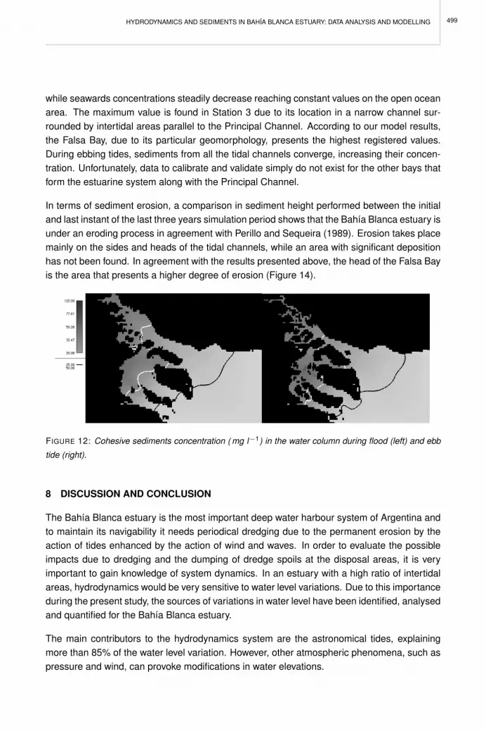
HYDRODYNAMICS AND SEDIMENTS IN BAHIA BLANCA ESTUARY: DATA ANALYSIS AND MODELLING
while seawards concentrations steadily decrease reaching constant values on the open oceanarea. The maximum value is found in Station 3 due to its location in a narrow channel sur-rounded by intertidal areas parallel to the Principal Channel. According to our model results,the Falsa Bay, due to its particular geomorphology, presents the highest registered values.During ebbing tides, sediments from all the tidal channels converge, increasing their concen-tration. Unfortunately, data to calibrate and validate simply do not exist for the other bays thatform the estuarine system along with the Principal Channel.
In terms of sediment erosion, a comparison in sediment height performed between the initialand last instant of the last three years simulation period shows that the Bahıa Blanca estuary isunder an eroding process in agreement with Perillo and Sequeira (1989). Erosion takes placemainly on the sides and heads of the tidal channels, while an area with significant depositionhas not been found. In agreement with the results presented above, the head of the Falsa Bayis the area that presents a higher degree of erosion (Figure 14).
FIGURE 12: Cohesive sediments concentration ( mg l−1) in the water column during flood (left) and ebb
tide (right).
8 DISCUSSION AND CONCLUSION
The Bahıa Blanca estuary is the most important deep water harbour system of Argentina andto maintain its navigability it needs periodical dredging due to the permanent erosion by theaction of tides enhanced by the action of wind and waves. In order to evaluate the possibleimpacts due to dredging and the dumping of dredge spoils at the disposal areas, it is veryimportant to gain knowledge of system dynamics. In an estuary with a high ratio of intertidalareas, hydrodynamics would be very sensitive to water level variations. Due to this importanceduring the present study, the sources of variations in water level have been identified, analysedand quantified for the Bahıa Blanca estuary.
The main contributors to the hydrodynamics system are the astronomical tides, explainingmore than 85% of the water level variation. However, other atmospheric phenomena, such aspressure and wind, can provoke modifications in water elevations.
499

F.J. CAMPUZANO, J.O. PIERINI AND P.C. LEITAO
FIGURE 13: Average values for four years simulation in each of the model monitored stations along the
Principal Channel main axis.
FIGURE 14: Sediment height difference between the last three years simulated with an erosion rate of
10−5 kg m−2 s−1.
The circulation in the Bahıa Blanca estuary has been described as dominated by a semidiur-nal, quasi-stationary tidal wave (Perillo and Piccolo 1991) and this makes it a tide-governedestuary. The tidal wave travels from the South and enters each of the bays by the Southernmargin. The particular geomorphology of the Bahıa Blanca estuary produces the increaseof the overtides components which produce the tidal amplitude increase. As an effect, tidesevolve from the outer ocean from flood dominated to ebb dominated increasing this domi-nance with the distance from the mouth. As a result, higher current speeds are found during
500

HYDRODYNAMICS AND SEDIMENTS IN BAHIA BLANCA ESTUARY: DATA ANALYSIS AND MODELLING
ebb for each of the bays. Maximum values during ebb tide are found near the mouth of theestuary where waters collected by the system of channels meet, and along the main axis ofthe channel. During flood, maximum values are found near the mouth of the bays where waterentering piles up. On the other hand, minimum values are found on the elevated intertidalareas.
One of the great advantages of using modelling tools in integrated coastal zone managementis that datasets collected at different periods and sampling intervals can all be integratedinto one tool to reproduce periodical phenomena, i.e. tides, currents. Also, modelling allowsisolating and discriminating single processes from all the available information. Data modifythe conditions of the model, and model results can provide a feedback for the accuracy andconsistency of the data. For these reasons, models should not be regarded as data ”sink”tools only, as they are also able to test the available data consistence.
In the Bahıa Blanca case, modelling served to confirm an inconsistency on the MSL usedfor the TM station. In this case, the simultaneous use of observed water levels and currents,although they were not from the same period, and the posterior mathematical analysis andvalidation through a hydrodynamical model resulted in the conclusion that mean sea levelsfor the tidal gauge stations needed (re)calibration. This is one of the major outcomes of thepresent work.
The model hydrodynamics indicates a residual circulation into the head of the tidal channelof dissolved properties; on the contrary, tidal channels export particulated matter. This fact isrelevant for water quality and sediment studies. Dissolved properties would tend to accumulatein the innermost areas of the channels while sediments would be washed away. The latterphenomena would be less in the Principal Channel, due to the recirculation pattern found atits mouth. These features are also in agreement with the lagrangian test performed wheretracers located in the innermost area of the Principal Channel present longer residence times.
Although more detailed work should be performed on this matter, the model appears to re-spond to wind forcing as the literature has described. Water levels increase in the inner areaswhen winds blow from the South-Southeast sector and decrease on average when they blowfrom the opposite direction. This effect is more intense when the wind blows along the baysmain axis.
In this chapter, a conceptual sediment model has been established, in which due to the ab-sence of external sources of sediments, the sediments found in the water column have theirorigin in the Bahıa Blanca estuarine system. Tidal currents transport the eroded sedimentsfrom the channel flanks into the Principal channels (Perillo and Sequeira 1989). These sedi-ments would be transported by the ebb currents and exported into the adjacent coastal shelfforming a sediment front along the Bahıa Blanca coast along with the exported sediment fromthe other bays of the Bahıa Blanca estuarine system.
501

F.J. CAMPUZANO, J.O. PIERINI AND P.C. LEITAO
Some assumptions were made in order to achieve the present results. The intertidal areaswere considered the main source of sediments into the system with a higher resuspensionpotential of sediments than in the subtidal areas. The subtidal areas were a residual sourceof more compacted sediments that would need higher stresses to be eroded, while in theintertidal areas, the stress needed would be lesser and constant with sediment depth. This3-dimensional geomorphological model was forced by a 2-dimensional vertically averagedhydrodynamical model with a resolution of 0.01o.
The results obtained through the simulations agree in general with the conceptual model andthe analysed data. The model has been validated mainly in the Principal Channel of the BahıaBlanca due to the lack of data for the rest of the system. Cohesive sediment concentrationsdecrease steadily from the innermost area of the channel to the open ocean. The decreasein sediment concentration is mainly due to the higher proportion of intertidal areas in the innerareas of the system while the proportion of these areas is lesser mouthwards. In its mouth,the Principal Channel, Falsa Bay and Verde Bay formed a sediment and hydrodynamic frontthat is more intense during ebb tides and enhanced during spring tides which indicates neterosion in the system.
REFERENCES
Aliotta S, Perillo G M E (1987). A sand wave field in the entrance to Bahıa Blanca Estuary, Argentina.Marine Geology, 76:1-14
Aliotta S, Lizasoain G O, Ginsberg S S (2004). Dinamica sedimentaria y evolucion morfologica de unprofundo canal del estuario de Bahıa Blanca. Revista de la Asociacion Geologica Argentina, 59:14-28
Capelli de Steffens A, Campo de Ferreras A M (2004). Climatologıa. In: Piccolo, M.C. y m. S. Hoffmeyer,(Eds.) Ecosistema del Estuario de Bahıa Blanca, pp.79-86
Cuadrado D G, Piccolo M C, Perillo G M E (2002). Hydrography of the inner shelf offshore Bahıa BlancaEstuary, Argentina. Thalassas, 18:45-56
Cuadrado D G, Gomez E A, Ginsberg S S (2005). Tidal and longshore sediment transport associated toa coastal structure. Estuarine, Coastal and Shelf Science, 62:291-300
Etala P (2000). Modelos hidrodinamicos anidados para el calculo de la onda de tormenta en el estuariode Bahıa Blanca. PhD Thesis, Universidad de Buenos Aires, 131p.
Ginsberg S S, Perillo G M E (2004). Characteristics of tidal channels in a mesotidal estuary of Argentina.Journal of Coastal Research, 20:489-497
Gomez E A, Ginsberg S S, Perillo G M E (1996). Geomorfologıa y sedimentologıa de la zona interior delcanal principal del estuario de Bahıa Blanca. AAS Revista , 3:55-61
Hayter E J (1985). Estuarial sediment bed model, in Estuarine Cohesive Sediment Dynamics, edited byA J Mehta. Springer-Verlag, New York: pp326-359
Heffner M, Bodnariuk P, Lopez F, Vaschetti G (2003). ”Aportes de agua a la Rıa de Bahıa Blanca.” Ed.Comite Tecnico Ejecutivo Municipalidad de Bahıa Blanca, 9p.
IOC, IHO, BODC (2003). Centenary Edition of the GEBCO Digital Atlas. Published on CD-ROM on behalfof the Intergovernmental Oceanographic Commission and the International Hydrographic Organiza-tion as part of the General Bathymetric Chart of the Oceans; British Oceanographic Data Centre,Liverpool. (http://www.ngdc.noaa.gov/mgg/gebco/gebco.html)
502

HYDRODYNAMICS AND SEDIMENTS IN BAHIA BLANCA ESTUARY: DATA ANALYSIS AND MODELLING
Lanzoni S, Seminara G (2002). Long-term evolution and morphodynamic equilibrium of tidal channels.Journal of Geophysical Research, 107:1-13
Mehta A J (1985). Characterization of cohesive sediment properties and transport in estuaries, in Estuar-ine Cohesive Sediment Dynamics, edited by A J Mehta. Springer-Verlag, New York: 290-325.
Melo W D, Schillizzi R, Perillo G M E, Piccolo M C (2003). Influencia del area continental pampeana en laevolucion morfologica del Estuario de Bahıa Blanca. AAS Revista, 10:39-52
NEDECO-ARCONSULT (1983). Estudio de dragado del canal de acceso al Puerto de Bahıa Blanca,informe final (technical report), 3 volumes, Buenos Aires.
Palma E D (1995). Modelo matematico hidrodinamico de circulacion con contorno variable. Desarrollo yaplicaciones. PhD Thesis, Universidad Nacional del Sur, (inedited), 178p.
Parker G, Paterlini M C, Violante R A (1997). The sea floor. In: E. Boschi, (Ed.), El mar argentino ysus recursos pesqueros. Instituto Nacional de Investigacion y Desarrollo Pesquero. Mar de Plata,Republica Argentina: 65-88.
Perillo G M E, Piccolo M C, Arango JM, Sequeira M E (1987). Hidrografıa y circulacion del estuario deBahıa Blanca (Argentina) en condiciones de baja descarga. 2o Congreso Latinoamericano sobreCiencias del Mar. 95-104
Perillo G M E, Sequeira M E (1989). Geomorphologic and sediment transport characteristics of the middlereach of the Bahıa Blanca Estuary (Argentina). Journal of Geophysical Research, 94:14351-14362
Perillo G M E, Cuadrado DG (1990). Nearsurface suspended sediments at Monte Hermoso Beach, Ar-gentina: I. Descriptive characteristics. Journal of Coastal Research, 6:981-990
Perillo G M E, Piccolo M C (1991). Tidal response in the Bahıa Blanca Estuary, Argentina. Journal ofCoastal Research, 7:437-449
Piccolo M C, Perillo G M E, Arango J M (1987). Hidrografıa del estuario de Bahıa Blanca, Argentina.Revista Geofısica, 26:75-89
Piccolo M C, Perillo G M E (1990). Physical Characteristics of the Bahıa Blanca Estuary (Argentina).Estuarine, Coastal and Shelf Science, 31:303-317
Piccolo M C, Diez P G (2004). Meteorologıa del Puerto Coronel Rosales. In: Piccolo, M. C. y M. S.Hoffmeyer, (Eds.) Ecosistema del Estuario de Bahıa Blanca, pp.87-90
Pierini J O (2007). Circulacion y transporte en zonas costeras del estuario de Bahıa Blanca. PhD Thesis,Universidad de Buenos Aires, (unedited), 225p.
Wang, Z B, Jeuken M C J L, Gerritsen H, de Vriend H J, Kornman B A (2002). Morphology and asymmetryof the vertical tide in the Westerschelde estuary. Continental Shelf Research, 22:2599-2609
Willmott, C J (1982). Some comments on the evaluation of model performance. Bulletin of the AmericanMeteorological Society, 63(11):1309-1369
503


PERSPECTIVES ON INTEGRATED COASTAL ZONE MANAGEMENT IN SOUTH AMERICAR. NEVES, J.W. BARETTA AND M. MATEUS (EDS.), IST PRESS, 2008
EVOLUTION OF SALINITY AND TEMPERATURE IN BAHIA BLANCA ESTUARY,ARGENTINA
J.O. PIERINI, J. MARCOVECCHIO, F. CAMPUZANO AND G.M.E. PERILLO
1 INTRODUCTION
The main driving forces of circulation in a large number of estuaries are river flow at thehead of the estuary and changes in the sea level at the mouth of the estuary, which in turndetermine the distribution of water properties like salinity and temperature, as well as thedistribution of any other tracer. In Bahıa Blanca estuary there are other forcing actions likewind stress and surface heat balance and they respond differently to these forcing actions.Bahıa Blanca estuary is in Argentina and the most dynamic in terms of physical and biogeo-chemical processes. It is a very important ecosystem in the region where it is situated dueto the intense human activity in its waters and along its margins. In the last 30-40 years theestuary was studied mainly from a biological and geological point of view.
There are not many studies or publications regarding the hydrology and physical processesof the estuary. Despite this fact, a prior physical process study (Perillo et al. 1987, Piccoloand Perillo 1990) reveals some of the main features of Bahıa Blanca. Observations of waterlevel, current velocity, temperature and salinity properties were made at several stations inthe estuary during the last years. It was determined that the type of tide at the mouth ofthe estuary is semidiurnal and it was observed that the astronomical tide is the main forcingdriving water circulation in Bahıa Blanca estuary. The tidal wave propagation in the study areahas the characteristics of a damped progressive wave. According to this study Bahıa Blancaestuary was found to be a vertically homogeneous estuary. Nevertheless, some channels mayexhibit the characteristics of a partially mixed estuary, depending on the freshwater input.
The importance of the freshwater sources in the estuary dynamics and of its seasonal effectsremained a subject of study until now. The estuary has also been studied through numericalmodelling. These studies were performed to investigate topics such as the tidal propagationin the estuary (Palma 1995, Etala 2000, Pierini 2007), the Lagrangian transport of particles(Pierini 2007) and studies of residual suspended sediment (Perez and Perillo 1998). Theestuary has several freshwater sources, Sauce Grande River being the most important andNaposta Creek. This last freshwater source is connected to the Atlantic through a channellocated in the central area of the estuary, Principal channel. This channel is only partiallyknown in terms of temperature and salinity processes, even though it is ideal to perform thiskind of studies in Bahıa Blanca estuary. The description of salinity patterns provides a basisfor predicting the behaviour of other soluble substances, being suitable to study since the saltis a natural tracer.
This study takes a first step to better comprehend the interaction between seawater, fresh-water and temperature within this system and to the understanding of its dynamics. These
505

J.O. PIERINI, J. MARCOVECCHIO, F. CAMPUZANO AND G.M.E. PERILLO
studies require a large amount of field data, of salinity and water temperature, as well as theimplementation of numerical models that combine hydrodynamic and transport modules. Thiscontribution uses two complementary and interconnected approaches to study the water tem-perature and salinity patterns in Bahıa Blanca estuary, combining field measurements withnumerical modelling results.
The main purpose of this chapter is to determine the horizontal patterns of salt and watertemperature in two stations along the Principal channel and to evaluate the importance ofthe main forcing mechanisms: tides and incoming river flow. To achieve this objective, ashort description of the first annual observational program of the hydrological properties inBahıa Blanca estuary will be given. Salinity and water temperature data were measuredin (Cuatreros Harbour) the harbour of Puerto Cuatreros and Ingeniero White Harbour alongthe Principal Channel in the inner part of estuary. These measurements have been takenweekly since 1974 to the present day. An estimation of the river flow for the survey periodswas also performed. Results will be presented and discussed, that reflect the influence ofsuperficial heat transfer and tidal forcing on the spatial and temporal distribution of the referredhydrological properties.
Another aim of this work is to implement a transport model in a 2D mode for the entire area ofthe estuary, with a closer look at its inner area. The model used was Mohid-Water ModellingSystem, a finite volume model that combines hydrodynamic and transport modules, describingits assessment through calibration and validation against several different data sets.
Due to the estuary´s complex geometry and the number of calibration stations used, this goalconstitutes a very challenging task. The model was calibrated using as a first approach aqualitative comparison of the temporal evolution of sea surface elevation (SSE) data mea-sured in 1999/2003 at three locations. When a good match is obtained for all stations, themodel’s accuracy is evaluated through the determination of the root mean square (RMS) errorand also through the comparison between amplitude and phase of the main tidal constituentsdetermined from harmonic analysis of the observed and computed data. The validation proce-dure was performed using two independent data sets, which includes observations of currentvelocities (1997 data) and SSE values.
A mathematical model is by definition an attempt to approximate and reproduce real phe-nomena. The approximations and parameterizations used for the synthesis of the model leadto discrepancies and deviations of model results from observations. The optimization of themodel performance is a complicated task and before using a model for operational applicationsthe model should be verified, calibrated and validated. However, there is no widely acceptedprocedure for carrying out these tasks. Model calibration and validation appears in variousforms, dependent on data availability, characteristics of water body, and most of all, the per-ceptions and opinions of modellers (Hsu et al. 1999). The aim of this paper is to present thecalibration and validation of the salt and the temperature for Bahıa Blanca estuary.
506

EVOLUTION OF SALINITY AND TEMPERATURE IN BAHIA BLANCA ESTUARY, ARGENTINA
2 STUDY AREA
A map of the Bahıa Blanca estuary location is shown in Figure 1. Principal channel is lo-cated in the middle of complex area of Bahıa Blanca estuary, a mesotidal and shallow (meandepth of about 1 m relative to the local datum) estuary situated in the southeast of the BuenosAires province, in Argentina. The study area from the mouth of the estuary to the head isapproximately 79 km long, has an average width of about 200 m and a mean depth, alongits longitudinal axis, of about 10 m. The tides are semidiurnal, with M2 as the most impor-tant constituent, representing more than 90% of the tidal energy. The estimated tidal prismfor the estuary head at extreme neap and extreme spring is 6,5 x10⁹ m3 and 1,0 x10¹⁰ m3,respectively, with an average value of 8,4 x10⁹ m3. The total estimated freshwater input for theestuary is very small (about 4,4 x10⁴ m3 during a complete tidal cycle) when compared to thetidal prism both at the mouth or at the beginning of Principal channel.
In spite of the small contribution of the rivers in terms of water input, when compared to thetidal prism, they may have a long-term influence on the residual transport. Previous studiesby Perillo and Piccolo (1991) and Pierini (2007) revealed that the tide is strongly distortedas it progresses upstream from the mouth towards the end of the channels of the estuary,due to changes in channel’s geometry and bathymetry. The general characteristics of thetidal wave are those of a damped progressive wave. Nevertheless, in shallow areas the tidalwave assumes the main characteristics of a standing wave. From a dynamical point of view,Principal Channel may be considered the most important area of the estuary, because thestrongest currents are observed here, reaching values higher than 2 m s−1. The estuary’sother channels are mainly shallow and tidal flat areas, contributing to a strong damping ofcurrents.
3 MODEL CONFIGURATION
The MOHID - Water Modelling System (Leitao et al., ReferencesMOHID) is a barotropic fi-nite volume model, designed for coastal and estuarine shallow water applications, like BahıaBlanca estuary where flow over complex topography, flooding and drying of intertidal areas,changing mixing conditions are all important. MOHID allows an integrated modelling approachof physical and biogeochemical processes. A complete description of the model’s physics canbe found in several works by Martins et al. (2001) or Leitao (2003).
MOHID has been configured for the Bahıa Blanca estuary. The bathymetry of the estuary isextracted from data obtained by the Bahıa Blanca Port Consortium. More recent bathymetricdata, obtained from recent dredging operations in several channels and remote sensor im-ages, were also used (Pierini 2007). Bathymetry is probably the most important among manyfactors that affect the flow properties in shallow systems like Bahıa Blanca estuary. Previousmodelling experience indicates that bathymetry controls the spatial variability of current magni-tude and direction. Thus, an accurate bathymetric representation is one of the most importantand fundamental requirements for successful modelling (Pierini 2007). This is particularly true
507

J.O. PIERINI, J. MARCOVECCHIO, F. CAMPUZANO AND G.M.E. PERILLO
FIGURE 1: Bathymetry, location of the tidal gauges and discharges within the estuary.
for the Bahıa Blanca estuary, where the bathymetry is very complex. Furthermore, the gridmust accurately represent the bathymetric characteristics of the estuary and guarantee modelstability.
The task of defining the grid-depth relations for the computational grid points can be extremelytime consuming and tedious. The flow simulation in this complex domain requires the use ofa high resolution grid. The model grid must be sufficiently refined to resolve the essentialfeatures of the depth and the geometry variations, but as the grid resolution is refined the totalnumber of grid points and the computation time both increase geometrically. For this domainthe ideal cell dimension would be around 50m, but the compromise solution was to develop agrid with dimensions of 200m, resulting in 119 cells in the x-direction (eastward) and 68 cellsin the y-direction (northward) (Figure 1). In this case the narrowest channels had their widthexaggerated, but by decreasing their depth it was guaranteed that they maintained their watervolume.
Changes in the bathymetry may be expected due to sediment dynamics and to the dredgingoperations performed last years. The domain was designed to resolve the estuary’s dynamicsand not the dynamics of the near coastal ocean. Bahıa Blanca estuary is an estuary where thetidal prism spreads toward the main channels and extensive tidal flats. This causes a decreaseof the tidal prism through the channel affecting the dynamics of the whole study area. The RioSauce Chico river and Arroyo Naposta creek (Figure 1) supply fresh-water to the system.Thus, in order to simulate this inflow/outflow, the model uses as boundary conditions waterflow, salinity and water temperature time series computed using a two-dimensional (depth-integrated) application of the model for all the study area.
The 2D application uses a variable spatial step Cartesian grid with higher resolution in thestudy area, calculating time-varying discharge, salinity and water temperature time series. The
508

EVOLUTION OF SALINITY AND TEMPERATURE IN BAHIA BLANCA ESTUARY, ARGENTINA
model was forced using tides (ocean open boundary) and the landward boundary was forcedusing river flow values typical for each run. At the oceanic and landward boundaries, the watertemperature and salinity are fixed in each simulation, with typical values for each period. Atthe surface, heat fluxes were imposed. The model uses the heat fluxes parameterizationsdescribed by Chappra (1997). Time step is 60 seconds and the horizontal eddy viscosity is50 m2 s−1. For the transport model the initial conditions are salinity and water temperaturefields, obtained by interpolation of data collected in the study area. A value of 50 m2 s−1 wasadopted for both salt and heat diffusion coefficients. The two-dimensional application is fullydescribed in Campuzano et al. (2008). Coefficients of horizontal viscosity and diffusivity areset to 50 m2 s−1. Initial conditions for the hydrodynamic model are null free surface gradientsand null velocity in all grid points. Initial conditions for the transport model are mean monthlyvalues of salinity and water temperature (typical values for each run).
As a first approach, a model covering the Argentina Continental Shelves to whole estuary andsurroundings (”grandfather model”, Figure 2) and forced with tidal components provided by thegeneric tidal FES95.2 model (Le Provost et al. 1998). In order to simulate water level at theboundaries a network of ”imaginary” tidal gauges fringing the model boundary is set as shownin Figure 2 for the primary model. The model automatically performs triangulations betweenthe different ”imaginary” tidal gauges to impose the tide on every cell of the boundary. At thelandward boundary freshwater inflow was imposed water inflow/outflow, salinity and temper-ature fluxes were also prescribed. On the offshore open boundary and at the river boundaryconstant values of salinity and water temperature were prescribed ( Ssea = 35 and Sriver = 0.5,water temperature varies from run to run). The hydrodynamic was spun up from rest over 4days (∼8 tidal cycles). This is considered a fair adjustment period for the hydrodynamics. Thespin-up period is not included in the results and the initial state of a run refers to the end of thespin-up period.
3.1 Temperature and Salt transport models
In most estuaries with a significant freshwater discharge, salinity may serve as an ideal nat-ural tracer for calibration of transport processes. In these environments the tidal current, thefreshwater discharge, the density circulation, as well as the turbulent mixing processes af-fect salinity distribution. Therefore, the salinity distribution reflects the combined results of allthese processes, and in turn it controls the density circulation and modifies the transport pro-cesses. Assuming that the barotropic flows (tidal and freshwater flows) have been calibratedand validated, the procedure to calibrate the salinity transport model is to match the observedand the computed salinity time series in Puerto Cuatreros and Puerto Ingeniero White. Inthis calibration procedure, the analysis of predicted distributions of salinity is used to guidethe adjustment of calibration constants through comparison with the typical horizontal salinitydistribution observed in Bahıa Blanca estuary. Once the salinity transport model is consideredcalibrated, the transport processes may be considered well represented by the model. There-fore, the calibration of the heat transport model is related only to the heat and radiative fluxesparameterization.
509

J.O. PIERINI, J. MARCOVECCHIO, F. CAMPUZANO AND G.M.E. PERILLO
A set of salinity and water temperature data measured between 1/4/2003 and 1/8/2004 isavailable for comparison with model results. These data include long time series of salinityand water temperature measured weekly at Puerto Cuatreros and Puerto Ingeniero White.The freshwater continuous inflows through the upstream boundaries are not known. Theimposed flowrates at the rivers boundaries resulting from mean monthly value procedure werethe following (Table 1)
The freshwater was specified with salinity equal to 0.5, freshwater temperature for the Na-posta Creek and Sauce Chico River as 10 oC. In the calibration of the heat transport modelthe sensible and the latent heat fluxes coefficients are also used as calibration parametersand were considered constant in all the simulations. It was found that the agreement betweenthe predicted and the observed temperature is good. Figures 3 and 4 show the comparisonbetween the predicted and observed salinity and water temperature, respectively, for 2 sta-tions (Puerto Cuatreros and Puerto Ingeniero White). The patterns observed are essentiallydependent on the tidal transport. The RMS values were computed for each station, and arepresented in each plot.
The agreement between the predicted and the observed salinity may be considered good forall the stations, the salinity time evolution and amplitude variation being well represented bythe model. The maximum absolute RMS value was determined for station Puerto Cuatreros,with a value of 0.125, which represents about 12% of the local salinity amplitude. The RMSvalue for the other station is also around 10% of the local salinity amplitude. In general there isa good agreement between the predicted and the observed water temperature values (Figure3 and 4). The RMS values are typically about 21% of the local water temperature amplitude.From these results it may be considered that the transport processes in the Bahıa Blancaestuary are well represented by the transport models. And the heat exchanges between theatmosphere and the water surface are very important processes too.
4 CONCLUSIONS
The transport models of heat and salt were successfully implemented for the Bahıa Blancaestuary. Results show that the calibration of the models was successfully carried out, showinga good agreement between measurements and model results. The validation tests showedthat the models can reproduce an independent observed data set. The developed and appliedmodels to the study area appear to use an adequate bathymetry. However, differences stilldo exist, and they might be the result of several factors, including: inaccurate definition of thebathymetry in the model for that region; very narrow channels not well resolved by the modelhorizontal grid; and uncertainties in the field data. The results show that the models can ac-curately reproduce the barotropic flows and simulate adequately the salt and heat transport inBahıa Blanca estuary, even in conditions of freshwater inputs from the rivers and heat transferbetween the atmosphere and the water surface. The models can, therefore, be considered asa new important tool for future studies of Bahıa Blanca estuary dynamics and water quality.
510

EVOLUTION OF SALINITY AND TEMPERATURE IN BAHIA BLANCA ESTUARY, ARGENTINA
FIGURE 2: Nested models used for Bahıa Blanca Model. On the left is the primary model (Argentina
model), on the right above is the secondary model (El Rincon model) and lower right is the tertiary model
(Bahıa Blanca model).
TABLE 1: Monthly mean freshwater flows
Month Arroyo Napostá creek (m3s-1)
Río Sauce Chico river (m3s-1)
January 2.25 4.35
February 1.80 4.40
March 2.20 6.50
April 1.85 6.55
May 2.70 6.40
June 3.60 5.15
July 3.60 4.80
August 2.00 4.60
September 2.55 6.80
October 3.60 8.45
November 3.15 6.25
December 2.80 5.30
Average 2.68 5.80
511

J.O. PIERINI, J. MARCOVECCHIO, F. CAMPUZANO AND G.M.E. PERILLO
FIGURE 3: Puerto Cuatreros salinity and temperature representation: observed (grey line) and modelled
(circles).
FIGURE 4: Puerto Ingeniero White salinity and temperature representation: observed (grey line) and
modelled (circles)
512
EVOLUTION OF SALINITY AND TEMPERATURE IN BAHIA BLANCA ESTUARY, ARGENTINA
REFERENCES
Campuzano FJ, Pierini JO, Leitao P (2008) Hydrodynamics and Sediments in Bahıa Blanca Estuary: Dataanalysis and modelling, this volume.
Chapra S (1997) Surface water-quality modelling McGraw-Hill, New York, pp: 784
Etala P (2000) Modelos hidrodinamicos anidados para el calculo de la onda de tormenta en el estuariode Bahıa Blanca. Tesis Doctoral, Universidad de Buenos Aires, 131pp.
Hsu MH, Kuo AY, Kuo JT, Liu WC (1999) Procedure to calibrate and verify numerical models of estuarinehydrodynamics. Journal of Hydraulic Engineering 166-182
Leitao PC (2003) Integration of Scales and Processes in the marine Environment Modelling. Doctoralthesis, Technical Superior Institute, Lisbon, 2003. (in Portuguese)
Leitao PC, Mateus M, Braunschweig F, Fernandes L, Neves R (2008) Modelling coastal systems: theMOHID Water numerical lab, this volume.
Martins F, Leitao P, Silva A, Neves R (2001) 3D modelling in the Sado estuary using a new generic verticaldiscretization approach. Oceanologica Acta 24: 1-12
Palma ED (1995) Modelo matematico hidrodinamico de circulacion con contorno variable. Desarrollo yaplicaciones. Tesis Doctoral, Universidad Nacional del Sur, 178pp.
Perez DE, Perillo GME (1998) Residual fluxes of mass, salt and suspended sediment through a sectionof the Bahıa Blanca estuary. Geoacta, 23: 51-65
Perillo GME, Piccolo MC, Arango JM, Sequeira ME (1987) Hidrografıa y circulacion del estuario de BahıaBlanca (Argentina) en condiciones de baja descarga. 2 Congreso Latinoamericano sobre Cienciasdel Mar, II, 95-104pp.
Perillo GME, Piccolo MC (1991) Tidal response in Bahia Blanca estuary, Argentina. Journal of CoastalResearch 7: 437-449
Piccolo MC, Perillo GME (1990) Physical Characteristics of the Bahıa Blanca Estuary (Argentine). Estu-arine, Coastal and Shelf Science 31: 303-317
Pierini JO (2007) Circulacion y transporte en zonas costeras del estuario de Bahıa Blanca. Tesis Doctoral,Universidad de Buenos Aires, 225pp.
Provost C, Lyard F, Molines JM, Genco ML, Rabilloud F (1998) A hydrodynamic ocean tide model improvedby assimilating a satellite altimeter-derived data set. Journal of Geophysical Research 103(C3): 5513-5529
513


PERSPECTIVES ON INTEGRATED COASTAL ZONE MANAGEMENT IN SOUTH AMERICAR. NEVES, J.W. BARETTA AND M. MATEUS (EDS.), IST PRESS, 2008
THE APPLICATION OF MOHID TO ASSESS THE POTENTIAL EFFECT OFSEWAGE DISCHARGE SYSTEM AT BAHIA BLANCA ESTUARY (ARGENTINA)
J.O. PIERINI, F. CAMPUZANO, J. MARCOVECCHIO AND G.M.E. PERILLO
1 INTRODUCTION
The Bahıa Blanca urban wastewater treatment plant (UWWTP) discharges the wastewaterfrom the city into the Bahıa Blanca Estuary through a tidal channel located 4 km south fromthe closest city, Ingeniero White, and 1.7 km south from the mouth of the Naposta Creek.There are four UWWTPs discharging in the Bahıa Blanca Estuary, with the highest flow fromthe Bahıa Blanca UWWTP at 65000 m3 d−1, corresponding to 77% of the total (Heffner etal. 2003). Wastewater is an important source of freshwater in the Bahıa Blanca estuarycomprising 23.3% of the overall freshwater, with contributions of a similar magnitude as thefreshwater inputs from the Naposta Grande Creek, 86400 m3 d−1 (Carrica 1998) and theSauce Chico creek, 164000 m3 d−1.
Sewerage systems in Bahıa Blanca city are designed with overflow structures that dischargeinto local waterways when the capacity of the system is exceeded. Overflows occur whenthe hydraulic capacity of the system is exceeded due to heavy rains. During dry periods,overflow can also take place due to blockages or pump failures. Aguas Bonaerenses SociedadAnonima (ABSA) manages the main network. The aim of this research was to analyze thepotential risks of sewage in the estuary and the installation of a new UWWTP on the coast inthe inner Bahıa Blanca estuary near bathing waters, i.e. the Maldonado Municipal pool.
2 STUDY APPROACH
The problems associated with wastewater discharges in estuarine and riverine areas are ofgrowing engineering interest, since the increase of pollutant loads in the last decades may leadto serious environmental impacts. In order to quantify river and estuary pollution problems itis necessary to predict the concentration distribution of the pollutant loads in the area understudy under different conditions. Numerical models constitute a powerful tool for the studyof diffusion and dispersion of pollutants. Model simulations reproduced two different sewagedischarges (West and East UWWTPs) in the inner part of Bahıa Blanca estuary (Figure 1).The actual UWWTP discharges into a tidal channel, located 5 km away from Puerto IngenieroWhite (Latitude: 38◦48’34.51” S Longitude: 62◦13’19.70” W) in the vicinity of the NapostaRiver mouth (Figure 1). Official data made available by ABSA estimate an UWWTP dischargeof 0.575 m3 s−1 on average, although on the other hand Piccolo and Perillo (1990) estimated adischarge of 10 m3 s−1 and sometimes higher than this value. Maldonado Channel is a water-way mainly used when the Naposta River reaches flows over 30 m3 s−1, preventing floodingsby deviation of part of the water. This channel is used during torrential rains, maximum flowunder average conditions is 3.6 m3 s−1.
515

J.O. PIERINI, F. CAMPUZANO, J. MARCOVECCHIO AND G.M.E. PERILLO
Samples were collected from five sites along the principal channel of the Bahıa Blanca Estu-ary. Pollutants were characterized in the sewage of Bahıa Blanca to determine its physical,chemical, toxicological and microbiological character (MBB 2004). The analyses included: or-ganic and inorganic nutrients, microbial faecal indicators and toxicants. Although the projectwas not a study of the stormwater impacts, we looked for the pollutants common to both todistinguish the impacts of the overflow during rain events. During the ECOMANAGE Projectwe simulated the potential impact of sewage discharges and the installation of a new primarytreatment plant in the inner estuary. But for the new location of a Treatment Plant there are nodata or knowledge of the environmental impact. The next stage of the ECOMANAGE projectwill be to determine the environmental water-quality of Bahıa Blanca estuary in relation to thepollutants found in the untreated sewage. We found that the most cost-effective approach wasto test samples for faecal coliform contamination during the event at all locations and times.Faecal coliform (thermo-tolerant coliform) tests were completed in 2003 to identify areas ofgreatest contamination. The more expensive and time-consuming analyses were then usedas confirmation tests for the presence of human faecal contamination.
FIGURE 1: Location of the Sewage Treatment Plant (West and East STP), water discharge and tidal
gauges within Bahıa Blanca estuary.
Knowing the environmental water-quality in the recipıent, we were able to compare environ-mental impact caused by the two treatment plants. Human faecal contamination in the wa-terway was used to assess the public health hazard and potential risk assessment based onpathogenic indicators (Escherichia coli). The Escherichia coli abundance was then used inthe risk assessment model to determine potential human public health risks over the innerpart of estuary. Risk assessment requires knowledge of the extent of human exposure, suchas recreational waters (Maldonado pools). While we observed children as well as complete
516

THE APPLICATION OF MOHID TO ASSESS THE POTENTIAL EFFECT OF SEWAGE DISCHARGE SYSTEMAT BAHIA BLANCA ESTUARY (ARGENTINA)
families swimming within the study area, a quantitative assessment of the use (exposure tohazard) of the waterway was beyond the scope of this study.
This study took into account the two treatment plants focusing on the potential impacts andhazards over the inner part of Bahıa Blanca estuary as well as the feasibility of using a hydro-dynamic model to interpret the pathogenic contamination due to sewage inputs.
3 MATERIAL AND METHODS
3.1 Study Area
The selected area (Figure 1) is located in the southwest of Buenos Aires Province (Argentina).This area is a hydrographic basin of 19000 km2. It is a mesotidal estuary characterizedby a complex tidal channel network separated by islands, wide low marshes and tidal flats.Furthermore, the tidal flats are covered by dense nets of minor tidal channels and creeks. Allmajor channels open to the inner continental shelf form ebb deltas, some of which are largelymodified by present day dynamic conditions. The study is concentrated on a sector of the mainchannel (Figure 1) located in the northern part of the estuary. This channel is approximately70 km long and 3 km wide in its lower reaches. The average depth of the channel is 10 mand the circulation is dominated by a quasi stationary tidal wave (Perillo et al. 2004). Meantidal range varies from 2 m at an offshore Oceanographic Tower to 3.5 m at Puerto IngenieroWhite (Figure 1). Prevalent winds for the area are mainly from the Northwest and North.These continental winds are strong and flow approximately parallel to the axis of the channel,thus affecting the circulation and vertical mixing in the estuary. The main pathogenic inputswere two sewage treatment plants, located in the northern part of the estuary, equipped withactivated sludge treatments (Figure 1). Treated wastewater was monthly sampled at the fivesampling stations of the outfall near Naposta Creek. These sites were selected based on theirlevels of bacterial contamination or hydrodynamic circulation. Water samples were stored at 4oC during shipment and analysed within 36 h.
3.2 Hydrodynamic Model
The MOHID hydrodynamic model (Coelho et al. 2002, Santos et al. 2002) was used to force amodel covering the study site (from the coordinates (-61.41W, -39.38S) to the inner estuary).In order to study the different hydrodynamic processes involved in Bahıa Blanca it was neededto adopt different spatial scales. As a result, the model of Bahıa Blanca consists of a set ofthree nested grids: (1) Level Argentina: covers the Atlantic coast of South America (-70W-40W, -60S -20S) with a resolution of 0.06o; (2) Level Rincon: a secondary model coveringthe area known as El Rincon with 0.02o resolution (-62.6W -60.5W, -42.8S -38.68S); (3) LevelBahıa Blanca: a third submodel covering the main area of interest, the Bahıa Blanca with0.005o resolution (covering from the coordinates (-61.41W, -39.38S) to the inner estuary. Themain interest in developing different resolutions has been to study different process in more
517
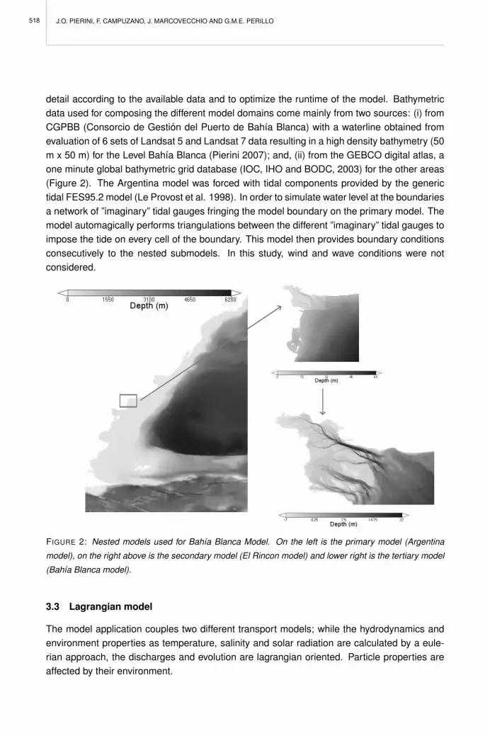
J.O. PIERINI, F. CAMPUZANO, J. MARCOVECCHIO AND G.M.E. PERILLO
detail according to the available data and to optimize the runtime of the model. Bathymetricdata used for composing the different model domains come mainly from two sources: (i) fromCGPBB (Consorcio de Gestion del Puerto de Bahıa Blanca) with a waterline obtained fromevaluation of 6 sets of Landsat 5 and Landsat 7 data resulting in a high density bathymetry (50m x 50 m) for the Level Bahıa Blanca (Pierini 2007); and, (ii) from the GEBCO digital atlas, aone minute global bathymetric grid database (IOC, IHO and BODC, 2003) for the other areas(Figure 2). The Argentina model was forced with tidal components provided by the generictidal FES95.2 model (Le Provost et al. 1998). In order to simulate water level at the boundariesa network of ”imaginary” tidal gauges fringing the model boundary on the primary model. Themodel automagically performs triangulations between the different ”imaginary” tidal gauges toimpose the tide on every cell of the boundary. This model then provides boundary conditionsconsecutively to the nested submodels. In this study, wind and wave conditions were notconsidered.
FIGURE 2: Nested models used for Bahıa Blanca Model. On the left is the primary model (Argentina
model), on the right above is the secondary model (El Rincon model) and lower right is the tertiary model
(Bahıa Blanca model).
3.3 Lagrangian model
The model application couples two different transport models; while the hydrodynamics andenvironment properties as temperature, salinity and solar radiation are calculated by a eule-rian approach, the discharges and evolution are lagrangian oriented. Particle properties areaffected by their environment.
518

THE APPLICATION OF MOHID TO ASSESS THE POTENTIAL EFFECT OF SEWAGE DISCHARGE SYSTEMAT BAHIA BLANCA ESTUARY (ARGENTINA)
4 RESULTS
The variation of E. coli concentration from day 0 (starting date of the outbreak) to day 90(when the simulation was stopped) is reported in Figure 3 for all sample sites. An increaseof the contamination was observed during the first days corresponding to the dispersion inthe estuary. After 90 days concentrations were well established and were only dependent onthe tide and decay rate. The effect of the semidiurnal tide was well modelled. The maximalconcentration was observed every 12 h at high tide. The E. coli water concentration washighly variable, depending on the tide. In this simulation, the maximal water concentrationat 17-7-2003 was equivalent to 105 CFU/100 ml (St 4, Figure 3 and 4), after 90 days, thespatial distribution was observed in the other samples sites. The model indicated minimaland maximal concentration of E. coli for the five sites. For example, at St 3, all the E. coliresults obtained by analysis were in accordance with the model, as no sample was found tobe contaminated by more than 4560 CFU/100 ml except at the discharge station (Table 1). Allthe results obtained fitted the values calculated with the model.
TABLE 1: Escherichia coli observed and modelled with MOHID.
E. Coli concentration (CFU/100 ml)
17 – Jun – 2003 30 – Jul – 2003 10 – Sept - 2003
St Obs Mod Obs Mod Obs Mod 1 2300 2200 4400 4560 1000 1500
2 400 320 1700 1780 1400 1510
3 1700 1700 2100 2212 3600 3655
4 100000 100000 180000 184000 240000 243000
5 2500 2500 2300 2300 2000 1922
5 DISCUSSION AND CONCLUSION
For the integration of the wastewater issue in the coastal management in Bahıa Blanca es-tuary, and more widely in all sensitive coastal ecosystems a systemic methodology basedon modelling and simulations can allow the investigation of several different technical solu-tions which are evaluated using environmental and health criteria. Coastal management forsustainable development requires the investigation of alternative strategies which should op-timize: resource preservation, water quality, technical aspects and human uses. Once theurban wastewater has been discharged it is diluted by the estuarine water. The resulting mix-ture flows towards the main channel of the estuary, a further dilution gradually occurring as aresult of mixing with the estuarine water.
The modelling approach embedded in an ecosystem approach is designed to provide to thepublic a physical and environmental understanding of the processes, as well as to help deci-
519

J.O. PIERINI, F. CAMPUZANO, J. MARCOVECCHIO AND G.M.E. PERILLO
sion makers to analyze the public demands and to evaluate the environmental investments.The narrow application of a modelling system and production of the results is not sufficientbecause of the complexity of the situations and the nature of the challenges. The use of op-timizing models for systems analysis as linear programming could be used to evaluate andvalidate some technical solution. This form of numerical approach will only work if everyoneinvolved in the process understands the benefits and limitations of its application and agreeswith its uses.
FIGURE 3: Location of the E. coli samples near STP East and temporary evolution in St 4 and St 3.
Mathematical models were previously shown to be efficient to evaluate sewage impact onbacterial contamination (Kashefipour et al. 2002, Pierini 2007). The use of mathematicalmodelling could help to interpret the large Escherichia coli variations observed along the es-tuary, principally from the new sewage discharge in the inner part of estuary, near Maldonado
520

THE APPLICATION OF MOHID TO ASSESS THE POTENTIAL EFFECT OF SEWAGE DISCHARGE SYSTEMAT BAHIA BLANCA ESTUARY (ARGENTINA)
Municipal pool. Moreover, this location requires the construction of a very efficient, sensi-tive and expensive tertiary process in the treatment plant. In case of malfunctioning - 105
CFU/100 ml - the effluent could generate a large polluted area. Consequently, the outflowmust be (re)located to an always submerged point, several meters below the low tide levelwhere the currents are continuous as in the main channel.
The model was capable of predicting complex two dimensional flow features and provided arational tool for environmental decision making. The Estuarine impact assessment using atwo-dimensional circulation and transport model has been implemented. The MOHID modeldescribed herein is expected to be a useful tool in the efforts to reduce the pollution in theBahıa Blanca estuary. Several projects may have strategic options which are not amenableto simple comparative analysis. In these cases, analytical techniques must help the decision-maker by showing the implications of the various options with the necessary multi-disciplinaryperspective, rather than presenting a prescription for action. This recognizes that such com-plex investment decisions are inherently political. The strategy is then based on the decisionmaker’s capacity to understand the environmental challenge and the human uses and also, toaccept the results of the modelling approach which might deeply modify the initial project.
FIGURE 4: Spatial distribution of E. coli with STP West and East discharges in Bahıa Blanca Estuary.
REFERENCES
Canteras JC, Juanes JA, Perez L, Koev KN (1995) Modeling the coliforms inactivation rates in the CantabrianSea (Bay of Biscay) from in situ and laboratory determinations of T90. Water Science and Technology32: 37-44
Carrica JC (1998) Hidrogeologıa de la cuenca del Arroyo Naposta Grande, Provincia de Buenos Aires.PhD Thesis. Universidad Nacional del Sur. Bahıa Blanca. Argentina. pp: 215 and annexes.
Coelho HS, Neves RJ, White M, Leitao PC, Santos AJ (2002) A model for ocean circulation on the Iberian
521

J.O. PIERINI, F. CAMPUZANO, J. MARCOVECCHIO AND G.M.E. PERILLO
coast. Journal of Marine Systems 32: 153-179
Heffner M, Bodnariuk P, Lopez F, Vaschetti G (2003) Aportes de agua a la Rıa de Bahıa Blanca. InformesMedioambientales. Comite Tecnico Ejecutivo de la municipalidad de Bahıa Blanca. (in Spanish)
IOC, IHO, BODC (2003) Centenary Edition of the GEBCO Digital Atlas. Published on CD-ROM on behalfof the Intergovernmental Oceanographic Commission and the International Hydrographic Organiza-tion as part of the General Bathymetric Chart of the Oceans; British Oceanographic Data Centre,Liverpool.
Kashefipour SM, Falconer RA (2002) Longitudinal dispersion coefficients in natural channels. Water Re-search 36: 1596-1608
Le Provost C, Lyard F, Molines JM, Genco ML, Rabilloud F (1998) A hydrodynamic ocean tide modelimproved by assimilating a satellite altimeter-derived data set. Journal of Geophysical Research 103:5513-5529
Municipalidad de Bahıa Blanca (2004) Estudio Bacteriologicos realizados en aguas y sedimentos delEstuario de Bahıa Blanca. Informe Final. pp:11 (in Spanish)
Perillo GM, Piccolo MC, Arango JM, Sequeira ME (1987) Hidrografıa y circulacion del estuario de BahıaBlanca (Argentina) en condiciones de baja descarga. 2 Congreso Latinoamericano sobre Cienciasdel Mar, II, pp.95-104 (in Spanish)
Perillo GME, Piccolo MC, Palma ED, Perez DE, Pierini JO (2004) Oceanografıa Fısica. En: Piccolo MC,Hoffmeyer MS (eds) Ecosistema del Estuario de Bahıa Blanca, pp.61-67 (in Spanish)
Piccolo MC, GME Perillo (1990) Physical Characteristics of the Bahıa Blanca Estuary (Argentine). Estu-arine, Coastal and Shelf Science 31: 303-317
Pierini JO (2007) Circulacion y transporte en zonas costeras del estuario de Bahıa Blanca. PhD Thesis,Universidad de Buenos Aires, pp: 225 (in Spanish)
Santos A, Martins H, Coelho H, Leitao PC, Neves R (2002) A circulation model for the European oceanmargin. Applied Mathematical Modelling 26: 563-582
522

PERSPECTIVES ON INTEGRATED COASTAL ZONE MANAGEMENT IN SOUTH AMERICAR. NEVES, J.W. BARETTA AND M. MATEUS (EDS.), IST PRESS, 2008
MOHID OIL SPILL MODELLING IN COASTAL ZONES: A CASE STUDY INBAHIA BLANCA ESTUARY (ARGENTINA)
J.O. PIERINI, J. MARCOVECCHIO, F. CAMPUZANO AND G.M.E. PERILLO
1 INTRODUCTION
Half the world’s production of crude oil is transported by sea (Clark 1992). A significant amountof oil is spilled into the sea from operational discharges, collision and grounding of tankers,well blow-outs and pipeline-breaks. Forty-eight percent of marine oil pollution is due to refinedproducts and 29% to crude oil. Tanker accidents contribute 5% of marine pollution (Fingas2001). Due to global economic growth, the demand for petroleum products is on the rise;hence one might also expect an increase in oil spills, especially along tanker routes. In BahıaBlanca estuary there are two monobuoys near the coast to discharge or load oil tankers. Inrecent years the international community has become increasingly aware of the risks due tomajor accidents occurring near populated and environmentally sensitive areas (i.e. the Pres-tige oil spill in 2002 (Galicia, Spain), the Hebei Spirit oil spill in 2007 (Taean, South Korea).There is also a growing need to ensure that health, environmental and safety issues are ad-dressed as an integral part of social and financial development. Petroleum products that enterthe marine environment have distinct effects, depending on their composition, concentrationand the elements in the environment that are taken into consideration. Some effects can berelated to transformations of the chemical composition of the environment and alterations inits physical properties, the destruction of the nutritional capital of the marine biomass, dangerto human health, and changes in the environmental biological equilibrium.
The Bahıa Blanca estuary coastal waters are noted for their heavy oil tanker traffic and, asa consequence, the risk of an oil spill occurring in these coastal waters is very real. ThePresidente ILLIA oil tanker accident, in the middle part of Bahıa Blanca estuary on May 19th,1992, when the vessel due to strong SE wind spilled about 700 m3 of crude oil over the seawater, is just one recent example of an accident with serious environmental consequences forthe Bahıa Blanca estuary coastal zone (Figure 1).
Numerical models are in principle able to predict the evolution and behavior of oil spilledin coastal zones, regardless of the atmospheric conditions, hence the vast interest in them.Mathematical modelling thus is a very powerful tool for management assessment after an oilspill accident, particularly for determining mitigating measures and to help monitor accidentevolution. The latest information technologies have provided us with new tools that are ca-pable of efficiently processing the great quantity of information needed to support accidentalhydrocarbon spill management. These modelling tools are indispensable in the forecasting ofoil slick evolution at coastal areas, as they allow measures to mitigate the negative impactsassociated with hydrocarbon spills to be put in place. When integrated with other geographicinformation tools, the information provided by the model results can be analyzed easily andaid decision making.
523

J.O. PIERINI, J. MARCOVECCHIO, F. CAMPUZANO AND G.M.E. PERILLO
Spill modelling is important to predict the trajectories and oil fate for devising suitable combat-ing mechanisms. Hypothetical spill trajectories for different scenarios should be hindcast forthe Bahıa Blanca estuary, but as no real spill data exist to validate the model, results wouldstill be uncertain. Concern exists about the 300 km2 Bahıa Blanca, Bahıa Falsa and BahıaVerde natural reserve being hit by an oil spill event because of its sensitivity and ecologicaland economical importance (i.e. tourism).
Measurements of tides, currents, winds and hydrography close to the spill location were madeavailable in order to validate and calibrate a hydrodynamical model for Bahıa Blanca estuary.MOHID model was used to simulate trajectories (Leitao et al., Mateus and Fernandes, thisvolume). The present work is the first modelling study for a hypothetical oil spill in the coastalwaters of Bahıa Blanca estuary. The objectives of this study were: (i) to simulate hydrodynam-ics of the coastal waters; (ii) to generate a trajectory for a potential spill; and, (iii) to generatea training system to provide an oil spill response in Argentinian harbors and make decisionsupport available in a short time to be applied to the contingency plans.
2 IMPACTS OF OIL SPILLS
The petroleum products that enter the marine environment have distinct effects, depending ontheir physical and chemical composition, and the environmental elements that are considered.The mechanisms of toxic action depend on the petroleum’s characteristics. The toxicity of thevarious fractions of the pollutants is directly related to the distilled products, on a short-termbasis, and related to the slow-action products, on a long-term basis. It is also related secon-darily to the products degraded either biologically, through the action of bacteria, or throughphysical-chemical processes. Petroleum pollution can be detected through the modification ofthe environmental conditions and can be described by transformations of the chemical compo-sition of the environment and alterations in its physical properties, destruction of the biomassnutritional budget or changes in the environmental biological equilibrium.
From the physical point of view, oil directly influences the marine environment, since gastransfer mechanisms are impaired by the presence of a pollutant layer on the surface. Self-purification processes are thus reduced. These processes can worsen by the increased oxy-gen consumption by growing micro-organisms, depending on the quantity of biodegradableorganic matter present. This oxygen deficit could even create conditions for anaerobic life,giving rise to the death and disappearance of certain species and permitting the fermentationof organic residues.
From a biological point of view, the environmental effects of oil are varied and complex. Whilesome are immediately obvious, others only manifest themselves after a long period. The de-gree of the effect is therefore different, whether in the animal or in the plant kingdom. In thecase of crude oil, the volatile components and the aromatic compounds are the most toxic. Inaddition to possible direct intoxication resulting from the inhalation or ingestion of petroleumproducts, there is an indirect risk to humans from the consumption of certain marine animals
524

MOHID OIL SPILL MODELLING IN COASTAL ZONES: A CASE STUDY IN BAHIA BLANCA ESTUARY (ARGENTINA)
(fish, crustaceans, etc.) that have been in close contact with the oil. The pollution’s noxiouseffects can also be felt indirectly through its environmental and economic impacts; damage tobiological resources (flora and fauna), affecting biodiversity; deterioration in seawater; shore-line quality and recreational waters, with negative effects on human and economic activities.
FIGURE 1: Location of Punta Ciguena and Punta Ancla monobuoys, tidal gauges, bathymetry and single-
point mooring system for Bahıa Blanca estuary.
3 CASE STUDY: MONOBUOY ACCIDENT MODELLING
In the middle of Bahıa Blanca estuary, there are two monobuoys (Punta Ciguenas and PuntaAncla) where crude oil is loaded and discharged. The MOHID model was used to evaluate thefate of spilled oil under different wind conditions (NNO, SSO, NNE and SSE).
525

J.O. PIERINI, J. MARCOVECCHIO, F. CAMPUZANO AND G.M.E. PERILLO
It is the first time that a simulation of these characteristics is performed in Bahıa Blanca estuaryand the results provide useful information to implement contingency plans and areas to guidethe oil booms to another area could be considered, but require a discussion on the acceptanceto sacrifice another area. The oil characteristics for the simulations were obtained from thetypical NRN (Neuquen Rio Negro) oil composition, which is the type of oil loaded to the shipsat the buoys (Table 1). For this experience it has been simulated an accidental discharge of45 m3 of oil type NRN (Table 1). The accident simulation starts at Punta Ciguena monobuoy(38◦56’40.30” S and 62◦ 03’8.99” W) being subject to estuarine hydrodynamics and windfields that play an important role in the oil transport processes. This accident simulation wasperformed to analyse their influence and also to test the surface oil slick transport model. TheMOHID 2DH hydrodynamic model was used to quantify the current velocities in the coastalzone during the accident. Figure 1 shows the geographical extent, and the bottom topography(Pierini 2007).
The same hydrodynamical model configuration as applied in the case of bacterial pollutionwas employed. Figure 2 displays the instantaneous maximum tidal current velocities (duringebb and flood) at the accident area, produced by the calibrated and validated hydrodynamicalmodel. The hydrodynamical model was used to calculate the tidal current velocities during thehypothetical accident period with the different wind scenarios. The wind directions (NNO, SSO,NNE, SSE) and intensities (average 10 m s−1) used in the simulations were representativeof the study area (Piccolo and Diez 2004). Figure 3 presents the spatial distribution of the oilwith different wind directions. The wind clearly appears to have a significant influence on theoil transport process. The oil spill in Figure 3 can be seen floating along and over the coast,and out along to Principal channel. The coastal city of Punta Alta and Puerto Rosales harbor,lie near the oil spill.
• The region of Puerto Rosales Harbor, especially between the monobuoys, as well asthe inner part of Bahıa Blanca estuary, run a high degree of risk that increases duringdischarge or loading of tankers.
• The whole northern coast of the Bahıa Blanca estuary, and especially the area to theeast of Principal channel, including the Natural Reserve of Bahıa Blanca, Bahıa Falsaand Bahıa Verde runs a high degree of risk.
• The Puerto Rosales area (near Punta Ciguena monobuoy) runs a high degree of riskwith increasing winds from a SSE direction.
• The areas of Southern coast runs a low degree of risk which increases during periodswith prevailing Northerly winds.
modelling could be taken a further step with the development of operational models that inte-grate meteorological models and wave models to force hydrodynamical models thus forecast-ing the hydrodynamical conditions during a possible event.
526

MOHID OIL SPILL MODELLING IN COASTAL ZONES: A CASE STUDY IN BAHIA BLANCA ESTUARY (ARGENTINA)
FIGURE 2: Maximum tidal current velocities (during ebb and flood) at the accident area (Punta Ciguena).
TABLE 1: Properties of the oil type NRN (Source: OiltankingEbytem S.A., personal communication).
Property Value
Density (15 ºC) 844 kg m-3
API 36.06
Water 0.05 %
Salts 35 grm-3
Sulphur 0.40 gr %
Vapour Tension 2.91 lbm-2
Viscosity (37.8º) 710 St
Pour Point -9
In a precautionary approach, the MOHID model oil application for Bahıa Blanca could help indefining management responses to an oil slick incident by identifying the areas where collec-tion and protection operations would be most urgent. Moreover, in combination with socioeco-nomic information it could help defining a future integrated coastal zone management. It wouldbe necessary in the future to improve the monitoring of the spills and to improve access to me-teorological data in addition to an evaluation of a possible increase in the coastal observationalnetwork, to cover data gaps. Last but not least, we are greatly indebted to OiltankingEbytemS.A for their kind collaboration in this work.
527

J.O. PIERINI, J. MARCOVECCHIO, F. CAMPUZANO AND G.M.E. PERILLO
FIGURE 3: Spatial oil spill distribution with different wind directions at the accident area (Punta Ciguena)
and impact zones.
REFERENCES
Carracedo P, Torres-Lopez S, Barreiro M, Montero P, Balseiro CF, Penabad E, Leitao PC, Perez-MunuzuriV (2006) Improvement of pollutant drift forecast system applied to the Prestige oil spills in GaliciaCoast (NW of Spain): Development of an operational system. Marine Pollution Bulletin 53: 350-360
Clark RB (1992) Marine Pollution. 3rd ed., Gookcraft Ltd., London, UK, 248pp.
Fernandes R (2001) Modelacao de derrames de hidrocarbonetos. Final year project dissertations, Insti-tuto Superior Tecnico, Lisbon, pp: 67
Fingas M (2001) The Basics of Oil Spill Cleanup. Lewis Publishers, London (UK), 233pp.
Leitao PC, Mateus M, Braunschweig F, Fernandes L, Neves R (2008) Modelling coastal systems: theMOHID Water numerical lab, this volume.
Mateus M, Fernandes R (2008) Modelling Pollution: Oil Spills and Faecal Contamination, this volume.
Montero P, Blanco J, Cabanas JM, Maneiro J, Pazos Y, Moronom A, Balseiro CF, Carracedo P, Gomez P,Penabad E, Perez-Munuzuri V, Braunschweig F, Fernandes P, Leitao PC, Neves RJ (2003) Oil SpillMonitoring and Forecasting on the Prestige-Nassau Accident, Proceedings of the 26th. Arctic andMarine Oilspill Program (AMOP), Volume 2
Piccolo MC, Diez P (2004) Meteorologıa del Puerto Coronel Rosales. In: Piccolo MC, Hoffmeyer MS(eds), Ecosistema del Estuario de Bahıa Blanca: 87-90 (in Spanish)
Pierini JO (2007) Circulacion y transporte en zonas costeras del estuario de Bahıa Blanca. PhD Thesis,Universidad de Buenos Aires, 225pp. (in Spanish)
528

PERSPECTIVES ON INTEGRATED COASTAL ZONE MANAGEMENT IN SOUTH AMERICAR. NEVES, J.W. BARETTA AND M. MATEUS (EDS.), IST PRESS, 2008
GROUNDWATER FLOW COMPONENTS TO THE GLOBAL ESTUARY MODELOF THE AYSEN FJORD
M. YARROW AND M.M. OLIVEIRA
1 INTRODUCTION
The Aysen Fjord receives freshwater mainly from the Aysen river watershed (Q∼ 545 m3 s−1).A key goal of ECOMANAGE was to study the importance of the groundwater medium in thesystem, its recharge and the contribution of the groundwater medium to the river flow. Toachieve this goal the surface flow hydrograph separation method is used in order to separatebaseflow and direct runoff. Because of the high latitude and mountainous terrain of the AysenBasin, it is important to consider the impact of snowfall and snowmelt on hydrographs and ongroundwater recharge. The applied techniques have been presented in Oliveira et al. (thisvolume).
Two watersheds within the Aysen basin were chosen for application of the snowmelt model andthe hydrograph separation method because they are gauged rivers and are close to weatherstations. An additional consideration was a significant elevation range. Weather stations inthe Aysen basin are generally located below 700 m elevation and in order to fully understandhydrographs in the basin it is necessary to consider the dynamics of snowfall and snowmeltat higher elevations. Each watershed was divided into three elevation bands of approximately500 m each. This elevation range was suggested in the documentation for the SnowmeltRunoff Model (Martinec, 1994). Furthermore, each watershed was divided into zones accord-ing to the dominant gradient in annual precipitation. For the Coyhaique watershed, the annualprecipitation decreases from the fluviometric station, eastward toward Argentina. The RioClaro watershed receives higher overall precipitation, decreasing from the headwater to thefluviometric station. Using routines in ArcView GIS 3.3, the area of each of these precipitation-elevation zones was calculated, as well as an estimation of the percent areal forest coverage.Table 1 and Table 2 characterize the snowmelt zones created for each watershed.
2 SNOWMELT MODEL INFORMATION
Table 3 lists parameters and variables required by the snowmelt equations and gives informa-tion about their sources and values. These equations can be found in USACE (1998)), and arealso reproduced in Yarrow and Oliveira (2006). In the watersheds modelled, the equations forforested and partially forested areas were used. In the case of zone F (>1200 m; >1500 mmannual precipitation) in the Rio Claro watershed, the rain-free, open area equation should beused. However, the use of this equation requires two additional variables that are unavailablefor this area; furthermore, because the zone only misses the canopy cover threshold by 2 per-cent, it is deemed that the equation for partially forested areas will suffice. Forest cover datacame from the spatially-explicit ’Catastro del Bosque Nativo’ database generated by CONAF-
529

M. YARROW AND M.M. OLIVEIRA
CONAMA in 1997 and provided to ECOMANAGE project by SERPLAC. Information aboutthe physiognomy of the vegetation in the watersheds was quantified using the Table 4 andeach vegetation type was weighted by its area within each zone. Canopy cover is importantin the calculation of long-wave radiation, short-wave radiation, and convection melt. Table 5shows the categories of forest density used to determine which of the simplified energy-budgetequations can be used.
TABLE 1: Snowmelt model zones based on elevation and annual precipitation for Rio Claro watershed.
The percent forest cover within each zone is indicated in parentheses.
Elevation Zone (altitude m) 1000-1500 1500-2000
1 (226-699) A (11.5%) B (39.3%) 2 (700-1199) C (74%) D (68.9%)
3 (1200-1722) F (8.4%)
TABLE 2: Snowmelt model zones based on elevation and annual precipitation for Coyhaique watershed.
The percent forest cover within each zone is indicated in parentheses.
Precipitation (mm yr-1) Elevation Zone (altitude m) >800 400-800 <400
1 (282-799) A (22.4%) B (31.2%) C (68%)
2 (800-1249) D (75.3%) E (30.6%) F (34.4%)
3 (1250-1697) G (10.9%) H (10.3%) I (12.5%)
3 DETERMINATION OF THE SNOW COVERED AREA
MODIS satellite images were classified in ENVI 4.2, using the middle infrared (mir) and bluebands (the bands used for the normalized difference snow index). A maximum likelihoodsupervised classification routine was used; the regions of interest for the supervised classifi-cation were based on a GIS coverage from SERPLAC indicating areas of permanent snow.Three MODIS images were used, representing winter (July 12 to 28, 2005), spring (Novem-ber 12-28, 2005), and summer (March 6-21, 2006) (Figure 1). A sinusoidal curve was fit tothese few data points using the snow coverage for each elevation zone in the two watersheds.Using the equations thus produced, an attempt was made to use the daily proportion of eachelevation zone covered by snow and a weighting factor for snowmelt. This makes intuitivesense: as the area covered by snow in each zone decreases during the spring, the productionof snowmelt water should decrease even as the rate of melt increases. However, the imple-mentation of this snow-cover-area weighting factor was problematic. On one hand, Figure2A and B indicate that significant inter-annual variation can occur in these basins, thus theacquisition and analysis of MODIS images becomes labor-intensive. On the other hand, useof a weighting factor was shown to lead to significant snow accumulation between years inthe Rio Claro watershed. In the absence of information indicating that there is net snow andice accumulation in this watershed, it appeared judicious to not apply the snow-cover-areaweighting factor until more information is available.
530

GROUNDWATER FLOW COMPONENTS TO THE GLOBAL ESTUARY MODEL OF THE AYSEN FJORD
FIGURE 1: Snow cover winter - summer 2005-2006 (From MODIS imagery).
As recorded data were not available on snowfall, snow depth, and snow melting rates for theAysen region, the snowmelt model could not verified. A rudimentary calibration was under-taken by (1) comparing the snow-covered area generated from the MODIS images with thepresence of snowpack in the elevation bands and (2) modifying the precipitation adjustmentfactors so that long-term precipitation was greater than the streamflow of the given watershed.The lack of a rigorous calibration of the snowmelt model should be taken into considerationwhen interpreting the final results. A comparison of Figure 2A and B shows that snow accu-mulation should be a more important process in the Rio Claro watershed, where up to 1800mm of precipitation fell as snow in the highest elevation band. This significant accumulationof snow in the Rio Claro watershed also meant that snow remained on the ground longerinto the summer than in the Coyhaique watershed, where the snowpack had melted betweenmid-October and early December.
531

M. YARROW AND M.M. OLIVEIRA
FIGURE 2: Modeled snowpack, (A) Coyhaique watershed. (B) Rio Claro watershed. Three vertical bands
are shown; values are in mm of water equivalent.
4 CONSIDERING SNOWMELT IN THE HYDROGRAPH SEPARATION METHODOLOGY
The hydrograph separation model, DECHIDR VB, described in Oliveira et al. (this volume),was run with the following settings: number of days from hydrograph peak until end of directrunoff (n) = 2 d; Minimum precipitation required to begin new recharge episode = 0.1 mm d−1;no control over balance between precipitation and runoff; model considers precipitation in or-der to start a new episode. In order to allow a comparison between dynamics with and withoutsnowmelt, two runs were made for each period, using data on Rio Claro watershed. A visualcomparison of Figure 3A and B indicates that with the calculation of snowmelt, the interpre-tation of the hydrograph changes. In Figure 3A there is a steady contribution of snowmelt,with peaks of precipitation. It is likely that the daily snowmelt is not so constant. However,the snowmelt model uses monthly instead of daily radiation and thus differences betweendaily melt rates are probably less than what would be observed in the field. Nonetheless, thepresence of this snowmelt water informs the hydrograph separation model that new runoff-recharge episodes should begin. Without this snowmelt signal (Figure 3B), the peaks in thehydrograph are considered to be come from baseflow - due to the fact that there is no pre-cipitation as rain. Thus, the inclusion of snowmelt can (1) help explain the high streamflowsand hydrograph peaks that occur in the absence of rain events and (2) help avoid the overestimation of baseflow when using the hydrograph separation method.
532

GROUNDWATER FLOW COMPONENTS TO THE GLOBAL ESTUARY MODEL OF THE AYSEN FJORD
TABLE 3: Source of parameters and variables used in snowmelt model.
Parameter or variable Source or References
Value (if applicable) Considerations
Daily mean air temperature, ºC DGA Average of daily min and max values
Dewpoint Temperature, ºC Relative humidity, temperature (DGA) Relative humidity for the Coyhaique Alto
station, taken from the Ñirehuao station
Precipitation, mm DGA
Snowfall often underestimated in rain gages: if precipitation falls as snow, it is multiplied by a factor of 1.3 (Larson and Peck, 1974)
Temperature – Elevation Adjustment factor
SRM User Manual 1998 -0.65 °C/ 100m Average temp for elevation zones is
adjusted from nearest weather station
Precipitation adjustment factor SERPLAC
Precipitation isohyets used to adjust the precipitation falling at nearest station. Number of rain days unchanged.
Wind (v) DGA Daily wind from Ñirehuao used for the Coyhaique watershed, average monthly values used for the R. Claro watershed
Solar radiation Monthly average hours of sun (DGA)
Solar radiation calculated on a monthly basis using Excel worksheet provided by IST.
Snow albedo (α) Tague & Band 2004
α = 0.85* (0.94Age^0.58)
Albedo decay function based on the number of days since last snowfall
Mean elevations DEM (SERPLAC) Watershed divided into 3 elevation zones; mean elevation calculated in ArcView
Forest cover (F) Land use GIS theme (SERPLAC)
Vegetation structural classes converted to forest cover categories with the weighting factors found in Table 4
Basin convection-condensation melt factor (k) USACE 1998 0.5
Range is 0.3 to 1. A low value was used because of high forest and mattoral cover in study watersheds.
Basin shortwave radiation melt factor (k’) USACE 1998 1
Range of parameter 0.9 to 1.1: a central value was used because aspects are evenly distributed in study watersheds
5 RESULTS FOR RIO CLARO WATERSHED
The Rio Claro watershed covers 108 km2 to the west of the town of Coyhaique. The RioClaro flows toward the east, emptying into the Rio Simpson. With its headwaters coming fromthe central Andean range, this watershed has higher pluviosity and generally steeper slopesthan the larger Coyhaique watershed. For the purpose of the snowmelt model, the watershedwas divided into five zones, as seen in Table 1. The available data allowed for the snowmeltmodel and DECHIDR VB to be run for the following periods: May 1985 to December 1986and December 2003 to August 2005.
The results obtained (Table 6 and Figure 4) show that the average baseflow for this periodrepresents close to 2/3 of the total streamflow. This is perhaps a surprisingly high value fora watershed that has relatively steep slopes and thus a large potential for high runoff rates.However, it must be considered that almost 40% of this watershed is covered by forest andthat, in general, the soils are quite sandy (average of 88% sand in forest soils) (Cruces etal. 1999). Furthermore, the soils in the Aysen basin are often thin and underlain by weath-ered bedrock or glacial deposits (Hepp 1996), thus it makes intuitive sense that much of the
533

M. YARROW AND M.M. OLIVEIRA
streamflow in the Rio Claro watershed is contributed by shallow groundwater. However, it isimportant that the results be interpreted with caution as there is uncertainty associated withthe snowmelt model and the hydrograph separation method has the limitations described inOliveira et al. (this volume).
The results obtained also indicate that snowmelt is an important component of runoff andbaseflow. It appears that snowmelt regularly makes up between 50% and 70% of the wateravailable for transport to the river system during the spring months. This is important becauseit represents a significant time lag in watershed-level hydrodynamics that could ultimately playa role in the chemistry and sediment loads of the river water. Sueker et al. (2000) indicate thatduring the snowmelt season in the Rocky Mountains, 42-57% of streamflow was provided bysnowmelt runoff.
FIGURE 3: Rio Claro watershed hydrograph separation detail (A) considering snowmelt (B) not consider-
ing snowmelt. Units: mm d−1. The shaded areas represent baseflow discharge, while the solid colors
represent surface runoff.
534

GROUNDWATER FLOW COMPONENTS TO THE GLOBAL ESTUARY MODEL OF THE AYSEN FJORD
6 RESULTS FOR COYHAIQUE WATERSHED
The Rio Coyhaique watershed covers 616 km2 to the east of the town of Coyhaique, whereit flows into the Rio Simpson. The eastern margin of the Coyhaique watershed borders withArgentina and includes areas classified as Patagonian steppe. The eastern part of the wa-tershed is quite dry (average annual precipitation of 325 mm yr−1) and it receives higherprecipitation between May and August (winter). For the purpose of the snowmelt model, thewatershed was divided into nine zones, as seen in the Table 1. The available data allowed forthe snowmelt model and DECHIDR VB to be run for the following periods: January 1985 toApril 1986 and January 2000-February 2003.
Table 7 and Figure 5 show that streamflow in the Coyhaique River is comprised of 80% base-flow discharge. This is higher than the Rio Claro watershed and indicates that there is relativelylittle runoff. Again, it is worth mentioning the high permeability of the soils in the Aysen basin.This fact, coupled with the flatter topography and low precipitation of the Coyhaique water-shed could explain this high baseflow value. The snowmelt appears to make up a relativelysmall portion of the streamflow, about 26%. Snowmelt still influences the hydrograph of theCoyhaique river, but this influence is more temporally limited as compared to the Rio Clarowatershed. In general, it is apparent that the Coyhaique watershed exhibits a strongly sea-sonal pattern where monthly streamflow and snowmelt rates are highly correlated (r = 0.77, n= 32). On the other hand, the monthly precipitation as rain calculated by the snowmelt modelis not significantly correlated with streamflow (r = -0.08, n = 32). This is an interesting anomalyand likely has to do with high evapotranspiration during the summer and the fact that muchprecipitation falls as snow during the winter.
7 CONCLUSIONS
The surface flow hydrograph separation method (requiring precipitation and streamflow data)coupled with a daily snowmelt model that accounts for the time lag and distinct pattern in whichsnow becomes available for runoff or groundwater recharge, was developed and applied in theAysen basin. This model was based on available information about the topography, vegeta-tion cover, and several meteorological and climatic variables. It is assumed that calculatedbaseflow is an estimation of the recharge that occurred in the system. Groundwater rechargeestimates varied between the Rio Claro watershed (average baseflow is 3.65 mm d−1) andthe Coyhaique watershed (average baseflow is 1.15 mm d−1). This reflects the steep gradientin precipitation caused by an orographic effect as prevailing winds pass across the Andes. Inall likelihood, this difference also reflects differences in topography and vegetation cover. Thepresented results allow hydrologists (and others) to obtain a good estimate in the absence ofsolid, local data on snowfall and groundwater.
535

M. YARROW AND M.M. OLIVEIRA
FIGURE 4: Monthly values for total stream flow, precipitation and associated values in Rio Claro water-
shed.
FIGURE 5: Monthly values for total stream flow, precipitation and associated values in Coyahaique water-
shed.
536

GROUNDWATER FLOW COMPONENTS TO THE GLOBAL ESTUARY MODEL OF THE AYSEN FJORD
TABLE 4: Weighting factors for structural vegetation classes.
Structural vegetation class
Dense forest
Semidense forest
Open forest
Pine plantation
Semidense mattoral
Open mattoral
Rock outcroppings, pasture
Weighting factor 1 0.7 0.4 0.8 0.3 0.2 0
TABLE 5: Categories of forest density (Source: USACE 1998).
Descriptive category Heavily forested Forested Partly forested Open
Mean canopy cover (%) >80 60-80 10-60 <10
TABLE 6: Average monthly values ( mm month−1), Rio Claro watershed.
Total
Streamflow (F) Baseflow
(Fb) Runoff
(Fd) Rain+snowmelt
(Tw) Rain (R) Snowmelt (Sm) Fb/F Sm/Tw
166 107 58 204 131 73 68% 35%
TABLE 7: Average monthly values ( mm month−1), Coyhaique watershed
Total Streamflow (F)
Baseflow (Fb)
Runoff (Fd)
Rain+snowmelt (Tw) Rain (R) Snowmelt
(Sm) Fb/F (%) Sm/Tw(%)
45 35 10 50 35 15 80% 26%
REFERENCES
Cruces P, Ahumada C, Cerda C, Silva L. (1999) Guıa descriptiva de sitios miscelaneos para la conser-vacion y menor valor forrajero de la region de Aysen. Gobierno Regional de Aysen. Ministerio deAgricultura Servicio Agrıcola y Ganadero (SAG). Departamento de Proteccion de los Recursos Natu-rales Renovables. Proyecto FNDR - SAG XI Region de Aysen: ”Levantamiento Para el Ordenamientode los Ecosistemas De Aysen”.
Hepp C (1996) Praderas en la zona austral: XI Region (Aysen). In: INIA, Praderas para Chile. EditorialRuiz.
Larson LL, Peck EL (1974) Accuracy of precipitation measurements for hydrologic modeling. Water Re-sources Research 10:857-863
Linsley Jr RK, Kohler MA, Paulhus JLH (1975) Hydrology for Engineers. 2nd edn. McGraw Hill Kogakusha,Ltd.
Martinec J, Rango A, Roberts R (1994) The Snowmelt-Runoff Model (SRM) Users Manual, UpdatedEdition 1994, Version 3.2, Department of Geography - University of Bern.
Oliveira MM, Lobo Ferreira JP, Yarrow M (2008) Groundwater recharge assessment, this volume.Sueker JK, Ryan JN, Kendall C, Jarrett RD (2000) Determination of hydrologic pathways during snowmelt
for alpine/subalpine basins, Rocky Mountain National Park, Colorado. Water Resources Research,36: 63-75
Tague CL, Band LE (2004) RHESSys: Regional Hydro-Ecologic Simulation System - An Object-OrientedApproach to Spatially Distributed Modeling of Carbon, Water, and Nutrient Cycling. Earth Interactions:8:1-42
USACE (1998) Engineering and Design: Runoff from Snowmelt. Manual EM 1110-2-1406. U.S. ArmyCorps of Engineers, 142p.(http://www.usace.army.mil/publications/eng-manuals/em1110-2-1406/toc.htm)
Yarrow M, Oliveira MM (2006) ECOMANAGE - Integrated Ecological Coastal Zone Management System.Deliverables 2.6 & 2.8 - CHILE. D2.6 SIG mapping of hydrogeologic parameters, including groundwa-ter recharge assessment and vulnerability to pollution & D2.8 Groundwater flow and transport compo-nents of the global estuary model. LNEC, Relatorio 379/2006 - NAS, Lisboa, 42 pp.
537


PERSPECTIVES ON INTEGRATED COASTAL ZONE MANAGEMENT IN SOUTH AMERICAR. NEVES, J.W. BARETTA AND M. MATEUS (EDS.), IST PRESS, 2008
ESTIMATION OF LOADS IN THE AYSEN BASIN OF THE CHILEAN PATAGONIA:SWAT MODEL AND HARP-NUT GUIDELINES
M. YARROW AND P. CHAMBEL-LEITAO
1 INTRODUCTION
The Aysen Basin presents a fascinating and challenging case for determining nutrient loadsand understanding the ecohydrological processes that influence these loads. Three principalchallenges were faced by the ECOMANAGE team in calculating nutrient loads: 1) nutrientcycling in the Chilean Patagonia differs significantly from temperate systems in the NorthernHemisphere, 2) the Aysen Basin has complex topographic, climatic, edaphic, and ecologicalcharacteristics that can not necessarily be easily modeled with current watershed models, 3)although ECOMANAGE was able to obtain all relevant existing data for the basin, certain ’dataholes’ persist. This chapter delves into the approach taken to confront these challenges andpresents the results obtained and lessons learned in the process. Although the basin is oftenconsidered ’pristine’, the nutrient loads calculated here show an important impact from humanactivities. The combination of a nutrient accounting and balance tool (Harp-Nut guidelines)with a semi-distributed watershed simulation model (SWAT2005) provides an integrated andflexible approach for estimating nutrient loads and allowing the simulation of possible futurescenarios.
The main results of this work have been: (1) export estimation of Nitrogen and phosphorous tothe Aysen Fjord using SWAT model and Harp-Nut guidelines, (2) comparison of SWAT modeland bibliographic values on nitrogen cycling, (3) the development of associated tools to SWATmodel facilitated the evaluation of nitrogen cycle, and (4) organic nitrogen in the rain is animportant input in this basin.
2 DESCRIPTION OF AYSEN BASIN
The Aysen River basin is located between 45o - 46o16’ S and has a surface area of 11,456km2. The topography of the basin and the spatial distribution of precipitation within the basinare quite heterogeneous. Soils tend to be thin and are largely composed of volcanic ash (Hepp1996). More detail about the geography, ecology and social history can be found in Yarrowand Torres (this volume).
Currently, the water quality of the basin’s rivers does not present any marked problems andthe waters have been classified as oligotrophic (Oyarzo 2006). However, as salmon aqua-culture in Southern Chile grows by leaps and bounds, the Technological Salmon Institute hasprojected that the number of hatcheries in the basin will grow from about 18 to 114 (CONAMA2006). Furthermore, the regional Agriculture and Livestock Service (SAG) has supported anintensification of livestock production in the basin - one estimate is that cattle will double within
539

M. YARROW AND P. CHAMBEL-LEITAO
a decade. Thus, for regional planners to understand the implications of economic drivers onthe water quality of the basin, it is important to develop tools and apply models to the basin forthe calculation of nutrient loads.
3 NUTRIENT DYNAMICS IN PATAGONIAN FORESTS AND STREAMS
Perhaps the most outstanding feature of the Southern Patagonian forests is their isolation.Currently, a major effect of isolation is that rates of wet and dry nutrient deposition remainsimilar to historic rates, while in the northern hemisphere these rates have been severelyaltered. Inorganic N wet deposition to forested ecosystems in Southern Chile is limited; con-centrations range from 0.015 to 0.071 mg l−1 (Hedin et al. 1995, Perez et al. 1998, Godoyet al. 2003). On the other hand, organic N in rainwater and especially cloudwater can con-tribute significantly to the total N deposition (Godoy et al. 2003). Net N mineralization hasalso been studied in Patagonia and reported values of between 12 to 37 kg N ha−1 yr−1 havebeen reported, significantly less than forested systems with anthropogenic N inputs (Perez etal. 2003a). Denitrification can be generally characterized as low in well-drained forested soilsand higher in wetter floodplain areas. Perez and colleagues (2003a) show that denitrificationin temperate forests of Chiloe Island are low: roughly 0.2 kg N ha−1 yr−1. Volatilization ofnitrogen does not appear to be important in the nutrient cycle of Patagonian forests, accordingto an N tracer study by Perakis and Hedin (2001). To synthesize the above: tight N cycleshave been documented in several Patagonian temperate forests and would be expected in theAysen Basin as well. This would result in low nutrient loading in the river network. However,the introduction of cattle and sheep into the basin has altered watershed dynamics in waysthat are not yet fully understood. Figure 1 summarizes what is known about the fluxes andpools of the N cycle in Patagonian forests.
4 APPLICATION OF HARP-NUT GUIDELINES
Harp-Nut guidelines were developed to quantify and report on the individual sources of ni-trogen and phosphorus discharges/losses to surface waters (Source Orientated Approach).These results can be compared to nitrogen and phosphorus figures with the total riverineloads measured at downstream monitoring points (Load Orientated Approach), as load rec-onciliation. Figure 2 shows, for the Aysen Basin, the delineation of monitored area and thenon-monitored area. This delineation was made using the Aysen River gage station. TheSWAT model will be the main tool that will be used to estimate diffuse loads.
4.1 Data Used
In general, there is little major industry within the Aysen Basin. Within the monitored part ofthe basin, the main point sources include mining, two small slaughterhouses, numerous gravelextraction sites, fish processing plants, fish hatcheries, and wastewater treatment plants. To
540
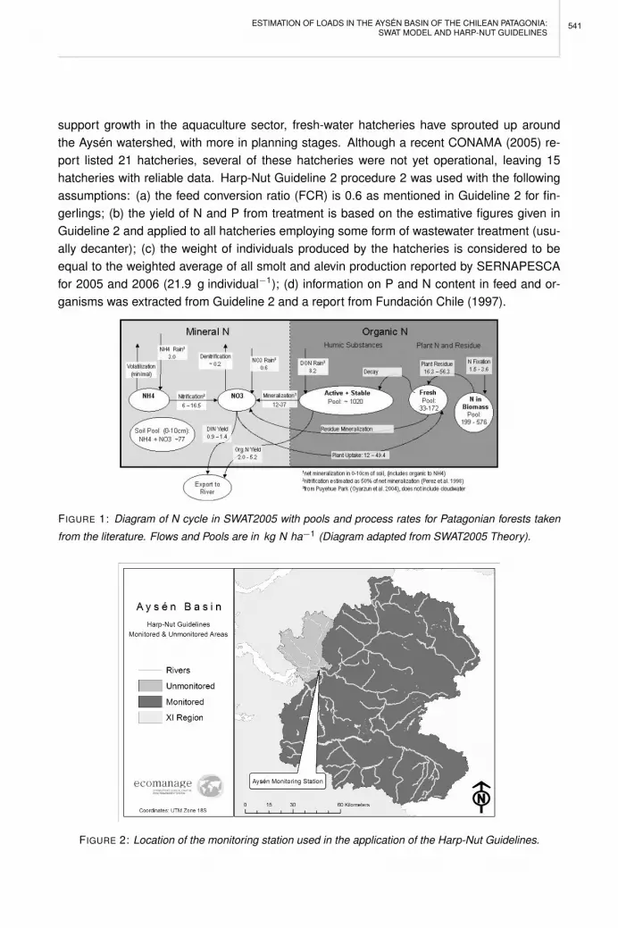
ESTIMATION OF LOADS IN THE AYSEN BASIN OF THE CHILEAN PATAGONIA:SWAT MODEL AND HARP-NUT GUIDELINES
support growth in the aquaculture sector, fresh-water hatcheries have sprouted up aroundthe Aysen watershed, with more in planning stages. Although a recent CONAMA (2005) re-port listed 21 hatcheries, several of these hatcheries were not yet operational, leaving 15hatcheries with reliable data. Harp-Nut Guideline 2 procedure 2 was used with the followingassumptions: (a) the feed conversion ratio (FCR) is 0.6 as mentioned in Guideline 2 for fin-gerlings; (b) the yield of N and P from treatment is based on the estimative figures given inGuideline 2 and applied to all hatcheries employing some form of wastewater treatment (usu-ally decanter); (c) the weight of individuals produced by the hatcheries is considered to beequal to the weighted average of all smolt and alevin production reported by SERNAPESCAfor 2005 and 2006 (21.9 g individual−1); (d) information on P and N content in feed and or-ganisms was extracted from Guideline 2 and a report from Fundacion Chile (1997).
FIGURE 1: Diagram of N cycle in SWAT2005 with pools and process rates for Patagonian forests taken
from the literature. Flows and Pools are in kg N ha−1 (Diagram adapted from SWAT2005 Theory).
FIGURE 2: Location of the monitoring station used in the application of the Harp-Nut Guidelines.
541

M. YARROW AND P. CHAMBEL-LEITAO
CONAMA provided four composite samples of effluent from Comercial Manihuales (a foodprocessing plant) as well as average monthly effluent flow rates. Salmones Antartica has twoplants that are considered here. Calculations were based on method 3 of Guideline 3, howeverdue to few data points the effluent flows and nutrient concentrations were averaged and thenmultiplied by 365 to get annual loads.
Harp-Nut Guidelines 4 & 5 deal with sewage treatment. There are five waste water treatmentplants (WWTP) in operation in the Aysen watershed. Only about 4% of the population in theAysen watershed is not hooked up to a municipal waste treatment system. For the two mainWWTPs Coyhaique and Puerto Aysen, information about the average daily discharge andmonthly quarter quality monitoring was available (CADE-IDEPE 2004). Nutrient loads for thethree other plants were estimated via person equivalency information found in the OSPARguidelines. A 50% treatment efficiency was used for these three smaller plants in absence ofconcrete local information. Information about rural and urban population sizes in the AysenBasin was taken from the 2002 National Census. OSPAR population equivalency informationwas used to calculate N and P loads from rural households.
Harp-Nut Guideline 7 deals with the measured nitrogen and phosphorus loads in a givenbasin. A primary problem encountered in the application of this guideline is the lack of im-portant variables (N-total, Organic N and P-total) and the sparse temporal resolution (at bestseasonal). Additionally, some of the data points represent outliers with no further informationabout why they may have originated. As a way to deal with the uncertainty introduced by thisdata set, we have consulted several other sources about nutrient concentrations in the riversof southern Chile. A study by Oyarzun et al. (2004) found that in a micro-watershed in theX Region of Chile, nitrogen exported via runoff was made up of close to 89% organic nitro-gen, while the nitrate fraction contains only 6% of exported N. The work of Perakis and Hedin(2002) agrees with Oyarzun et al. (2004) in that nitrogen export from 100 first-order streamsin unpolluted temperate South American forests is mainly in the dissolved organic form. Giventhe large geographical coverage of the Perakis and Hedin study, it is highly likely that smallstreams in the forested areas of the Aysen Basin conform to this pattern.
On the other hand, two other studies indicate that the small ratio of nitrate: total N exportmentioned above cannot be simply extrapolated to larger bodies of water or watersheds withnon-forested landuses. A study by Oyarzun and Huber (2003) compared stream nutrientconcentrations in forested and pasture-covered watersheds in the X region of Chile. This studyindicated that NO3 makes up a higher proportion of the total N in watersheds dominated bylivestock activities. Finally, water quality data collected for a MOP-DGA study (1996) in theinlets and outlets of Lake Riesco and Lake Elizalde (located within the Aysen Basin) indicatedthat on average, nitrate made up 40% of the total-N, and orthophosphate made up 37.5% ofthe total-P. Because the MOP-DGA sampling was focused on lacustrine systems and includeda relatively short time series, the authors have decided to combine this data set with resultsfrom the three other publications mentioned previously. For nitrogen, a ratio of nitrate:totalN of 0.219 was used while a ratio of phosphate:total P of 0.375 was used for Phosphorus.
542

ESTIMATION OF LOADS IN THE AYSEN BASIN OF THE CHILEAN PATAGONIA:SWAT MODEL AND HARP-NUT GUIDELINES
These ratios were then used to convert the measured concentrations NO3 − N and PO4 − Pinto Total-N and Total-P, respectively. This conversion represents a major assumption as tothe relative proportions of the different N fractions within the Aysen River, values that are likelyto change seasonally and through time, as different productive activities are undertaken in thewatershed. However, this is the only way forward using the currently available data.
In order to arrive at nutrient retention estimates, the German approach described in Harp-Nutguideline 9 was used. The area of the areas of lakes and reservoirs with the Aysen Basin wascalculated in ArcViewr 3.3 to be 164 km2. Additionally, fluviometric data from Guideline 7 wasused to calculate retention using the equations described in this guideline. The parameters insaid equation were derived empirically from 100 river basins in Europe.
4.2 Results of Harp-Nut Application
Due to uncertainty associated with the measured values of N and P for the Aysen monitoringstation, the values of the Harp-Nut ”load-oriented” approach should be interpreted with caution(Table 1). Nevertheless, the correspondence between the load-oriented and source-orientedapproaches indicates that despite challenges with data completeness, the general patternsand magnitudes of nutrient loading in the Aysen Basin have been correctly identified. By usinga nitrate: total N ratio that represents a range of studies approximating the different conditionsfound in the Aysen Basin, the load-oriented estimate is 3438 tons N yr−1, which is only 8%higher than the source-oriented estimate. The inclusion of N loads from the un-monitored partof the basin brings the total annual N load to the Aysen fjord to 3641 tons yr−1. The sourceoriented approach quantifies N loading by sector. Table 1 shows that point sources of nitrogenare relatively low in the Aysen Basin - on the order of 4.5% of the total N loads. Diffuse Nloads from ranching and land-use change are estimated to be 15% of total N loads. Thus,according to the application of the Harp-Nut guidelines, just under 20% of all N reaching theAysen Fjord is of human origin.
Because less literature on P loads in Patagonia was encountered, the load-oriented estimateis based on a PO4 − P: Total-P ratio from the MOP-DGA study (1996). The correspondencebetween the source-oriented and load-oriented approaches is lower for P than for N. A morerepresentative sample of P fraction in the basin would likely provided improved results. Nev-ertheless, general patterns emerge. The phosphorus loads showed more human influenceas compared to nitrogen, with 38% of P loading deriving from human sources. Again, pointsources of P are low, totaling 7.3% of total P export. This indicates that diffuse sources of P,such as ranching and landuse change comprise just under one third of P loading to the AysenFjord. It is interesting that the SWAT model indicates that P is lost much more readily than Nto the river network when considering grazing. More needs to be done to verify this pattern,but given that P is often a limiting nutrient for agricultural activities in the basin, this finding isof some interest (Hepp 2004).
543

M. YARROW AND P. CHAMBEL-LEITAO
TABLE 1: Results of the application of the Harp-Nut Guidelines to the Aysen Basin.
5 SWAT MODEL APPLICATION
The SWAT model was used to: (a) estimate the background levels of N and P loads in theAysen Basin (b) estimating diffuse N and P loading by changing landuse to reflect currentconditions and utilizing a SWAT grazing routine reflecting recent stocking rates. These modelruns were used in the application of the Harp-Nut Guidelines. Additionally, work was done toadjust the SWAT nutrient modules so that they would reproduce patterns of nutrient cyclingfound in the Chilean Patagonia.
5.1 Data Used
The landuse information used in the Aysen SWAT model came from two sources. First, forthe current landuse the Registry of Native Forest (CONAF-CONAMA 1999) was utilized. Thisdatabase includes a large number of land cover classes, subdivided by physiognomy in thecase of forest classes. This information was converted (and simplified) into a format usableby SWAT. Built-in SWAT land cover classes were used for agricultural areas, pastures andrangeland, pine plantations, and urban areas. It was not clear how to simulate the nativeforest communities of southern Chile using the limited array of SWAT tree classes. Thus, fivenew SWAT classes were created based on an extensive literature review and expert opinion.Finally, due to the large proportion of the basin that is either above the vegetation limit or is
544
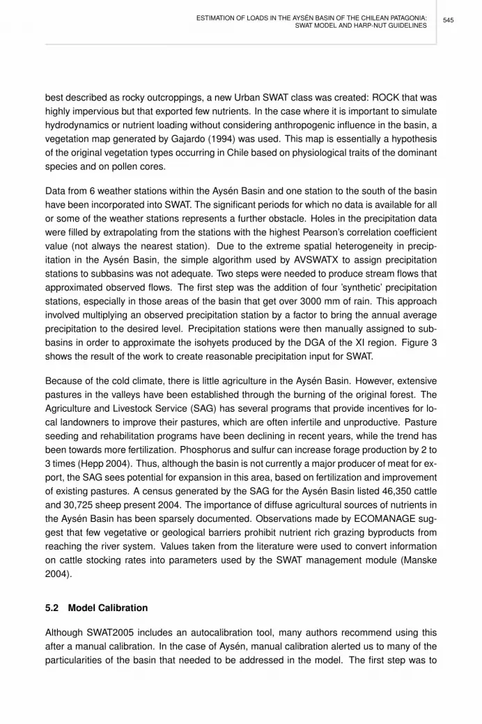
ESTIMATION OF LOADS IN THE AYSEN BASIN OF THE CHILEAN PATAGONIA:SWAT MODEL AND HARP-NUT GUIDELINES
best described as rocky outcroppings, a new Urban SWAT class was created: ROCK that washighly impervious but that exported few nutrients. In the case where it is important to simulatehydrodynamics or nutrient loading without considering anthropogenic influence in the basin, avegetation map generated by Gajardo (1994) was used. This map is essentially a hypothesisof the original vegetation types occurring in Chile based on physiological traits of the dominantspecies and on pollen cores.
Data from 6 weather stations within the Aysen Basin and one station to the south of the basinhave been incorporated into SWAT. The significant periods for which no data is available for allor some of the weather stations represents a further obstacle. Holes in the precipitation datawere filled by extrapolating from the stations with the highest Pearson’s correlation coefficientvalue (not always the nearest station). Due to the extreme spatial heterogeneity in precip-itation in the Aysen Basin, the simple algorithm used by AVSWATX to assign precipitationstations to subbasins was not adequate. Two steps were needed to produce stream flows thatapproximated observed flows. The first step was the addition of four ’synthetic’ precipitationstations, especially in those areas of the basin that get over 3000 mm of rain. This approachinvolved multiplying an observed precipitation station by a factor to bring the annual averageprecipitation to the desired level. Precipitation stations were then manually assigned to sub-basins in order to approximate the isohyets produced by the DGA of the XI region. Figure 3shows the result of the work to create reasonable precipitation input for SWAT.
Because of the cold climate, there is little agriculture in the Aysen Basin. However, extensivepastures in the valleys have been established through the burning of the original forest. TheAgriculture and Livestock Service (SAG) has several programs that provide incentives for lo-cal landowners to improve their pastures, which are often infertile and unproductive. Pastureseeding and rehabilitation programs have been declining in recent years, while the trend hasbeen towards more fertilization. Phosphorus and sulfur can increase forage production by 2 to3 times (Hepp 2004). Thus, although the basin is not currently a major producer of meat for ex-port, the SAG sees potential for expansion in this area, based on fertilization and improvementof existing pastures. A census generated by the SAG for the Aysen Basin listed 46,350 cattleand 30,725 sheep present 2004. The importance of diffuse agricultural sources of nutrients inthe Aysen Basin has been sparsely documented. Observations made by ECOMANAGE sug-gest that few vegetative or geological barriers prohibit nutrient rich grazing byproducts fromreaching the river system. Values taken from the literature were used to convert informationon cattle stocking rates into parameters used by the SWAT management module (Manske2004).
5.2 Model Calibration
Although SWAT2005 includes an autocalibration tool, many authors recommend using thisafter a manual calibration. In the case of Aysen, manual calibration alerted us to many of theparticularities of the basin that needed to be addressed in the model. The first step was to
545

M. YARROW AND P. CHAMBEL-LEITAO
run the SWAT model with the data described previously. This served as a baseline run, towhich subsequent modifications were compared. Calibration for river flows was carried outusing four fluviometric stations: (1) Simpson River (2) Manihuales River, (3) Blanco River, andfinally (4) Aysen River. An issue that became readily apparent was that the algorithm used bythe AVSWAT-X interface to assign precipitation stations to subbasins was not optimal. For theperiod between 1996 and 2002, the measured average streamflow at the Aysen River was 537m3 s−1. This contrasts with a value of 375 m3 s−1 with automatic assignment of precipitationstations and 531 m3 s−1 with manual assignment.
A second issue that affects streamflow in this mountainous basin is snowfall. Because theDGA’s weather stations in the basin are at low elevations where winter temperatures are tem-pered by prevailing winds off the Pacific Ocean, snow occurs infrequently in SWAT under thebaseline setup. In order to enhance this key hydrologic process, we calculated 10 elevationbands for each subbasin allowing the temperature of the higher bands to fall below freezingfor a longer period of time. This has the effect of increasing snow as a percentage of total pre-cipitation from 0.5% in the baseline run, to between 15-40% in the runs with elevation bands(Figure 4). Although there is no empirical data about the percent of precipitation that falls assnow in the Aysen Basin, this range is reasonable given that a) a maritime climate on theleeward side of the Andes range produces heavy precipitation, much of it as rain and b) snowis common in the higher mountains and eastern plateaus but areas east of the main Andesrange are significantly drier. The strength of a snowmelt signal in the flow data of the AysenRiver varies interanually. Manipulating the TLAPS parameter (the temperature lapse rate -◦Ckm−1) can produce more snowfall in the model, but this often reduces the quality of hydro-dynamic results unless measured temperature and radiation data is available to accuratelycalculate snowmelt pulses.
It is important to note that the Blanco River subbasin is the largest contributor to the stream-flows at the Aysen fluviometric station. This subbasin is very mountainous, has the highestprecipitation in the basin, contains several major lakes and does not benefit from having pre-cipitation or weather stations. Thus, it represents a challenge in the process of model setup.We found the best approach under these circumstances is to link changes the parameteri-zation with physical processes that are known to be occurring in the subbasin. On the otherhand, the Manihuales subbasin has three precipitation and weather stations and consequentlyproduced better model results.
5.3 Hydrodynamic results
The results from the autocalibration analysis were used as the basis for the final hydrody-namic setup of the Aysen SWAT model. Because the autocalibration minimizes the sum of thesquares of the residuals for daily streamflow, the daily statistics improved significantly. How-ever, in order to strike a balance between daily and monthly hydrodynamic results, some ofthe best values from the autocalibration were changed. Thus, the CN2 parameters were mul-
546

ESTIMATION OF LOADS IN THE AYSEN BASIN OF THE CHILEAN PATAGONIA:SWAT MODEL AND HARP-NUT GUIDELINES
tiplied by 1.3 instead of 1.5, and the canmx parameter was increased to 10 in forested HRUs.The value of Lat time in the final calibration was 3.5. According to a recent paper on modelevaluation guidelines, NSE values greater than 0.5 indicate satisfactory model performancewhile values above 0.65 indicate good performance (Moriasi et al. 2007). Table 2 shows thatduring the calibration phase, the Aysen SWAT model had good performance at all stationsexcept Blanco River. The difficulty in modeling the Blanco subbasin is evident by looking atthe validation statistics. Poor model performance in this subbasin can affect the Aysen stationdownstream. Nevertheless, the monthly performance of the model at the Aysen station for theperiod 1996 to 2005 is satisfactory.
FIGURE 3: Isohyets and the assignation of precipitation stations among subbasins.
FIGURE 4: Breakdown of terrestrial hydrological process (percent of total precipitation). The baseline
run (no elevation bands/WATR landuse class) and the final run (elevation bands/RNGB instead of WATR
landuse class) are shown.
547

M. YARROW AND P. CHAMBEL-LEITAO
5.4 Nutrient dynamics in SWAT
The SWAT model was used to calculate annual nitrogen and phosphorus loads from diffusesources. An initial comparison of the measured inorganic nutrient concentrations from theAysen monitoring station and the annual nutrient loads estimated with SWAT led to the con-clusion that diffuse loads were being significantly overestimated. This led to a more detailedexamination of the nitrogen cycle used in SWAT and the inferences that can be drawn aboutN cycling in the Aysen Basin.
5.4.1 Wet deposition of nitrogen
As mentioned previously, wet deposition of nitrogen in Southern Chile differs from most ar-eas of the Northern Hemisphere. It was found that the RCN parameter (concentration of N inprecipitation) in SWAT2005 was code was fixed at 1 mg l−1, significantly higher than measure-ments from Southern Chile (Godoy et al. 2003). Furthermore, the literature from Patagoniaindicates that dissolved organic nitrogen (DON) can make up two thirds of wet deposition(Oyarzun et al. 2004). Thus, SWAT source code was changed to allow DON to be added as acomponent of wet N deposition (as well as NO3 and NH4).
After a spin-up period of 2 years, we compared the average daily NO3 concentration at thesubbasin that corresponds to the Aysen River monitoring station with 28 measurements ofNO3 − N taken between 1997 and 2004 by the local authorities. The average measured valuewas 0.0475 mg l−1 while SWAT NO3 output for the corresponding reach was 0.0453 mg l−1.The difference between modeled and measured values was not statistically significant (t= 0.40,p=0.69, gl=27 ). The same simulation set up, run with RCN = 1 gives a NO3 concentration inthe reach of 0.74 mg l−1, which is higher than even the highest measured value.
5.4.2 Tree growth and residue production
SWAT outputs the biomass generated in each HRU, and though for agricultural landuses thisfigure may be directly compared to crop growth and harvest, the situation for forests is morecomplex. In SWAT2005, the default tree parameter sets (e.g. PINE) lead to a large fractionof annual biomass production removed as yield or converted to residue, resulting in minimalgrowth of persistent biomass such as trunks and large roots. If the primary objective forcalibrating biomass is to achieve realistic nutrient cycling, then the total biomass of a forestsystem can be ignored and the focus can be placed on residue production. In Table 3, theranges of litterfall for the three principal forest types in the Aysen Basin were gathered fromthe literature and compared to SWAT output after calibration. The most sensitive parametermodified was BIO LEAF which controls the fraction of biomass converted to residue at the endof each season. Other parameters changed-according to values found in the literature-werethe nitrogen and phosphorus uptake parameters, LAI, canopy height, rooting depth, and theharvest index.
548

ESTIMATION OF LOADS IN THE AYSEN BASIN OF THE CHILEAN PATAGONIA:SWAT MODEL AND HARP-NUT GUIDELINES
TABLE 2: Results for the calibration and validation phases of the final Aysen SWAT setup. Statistics: Root
Mean Square Error/Coef. of Determination (R2)/ Nash-Sutcliffe Efficiency (NSE).
Station Time period Observed/ modeled
flow (m3 s-1) RMSE
Day/Month R2
Day/Month NSE
Day/Month
Aysén Jan ‘96–Dec ‘99 531 / 535 321 / 136 0.48 / 0.75 0.47 / 0.70
Mañihuales Jan ‘96–Dec ‘99 176 /176 141 / 70 0.47 / 0.67 0.46 / 0.67
Simpson Jan ‘96–Dec ‘99 48 / 56 31 / 19 0.60 / 0.81 0.55 / 0.72
Calibration
Blanco Nov ‘98-Dec ‘00 230 / 220 131/78 0.38 / 0.41 0.07 / 0.27
Aysén Jan ’01-Jul ‘05 579 / 513 278 / 189 0.45 / 0.53 0.35 / 0.42
Mañihuales Jan ’01-Jun’05 180 / 161 122 / 71 0.50 / 0.69 0.48 / 0.62
Simpson Jan ’01-Jun’05 62 / 52 37 / 25 0.48 / 0.66 0.42 / 0.55
Validation
Blanco Jan ’01-Jun’05 284 / 234 145 / 112 0.38 / 0.36 0.00 / 0.02
TABLE 3: New SWAT Land Cover Classes Used in Aysen SWAT Model.
SWAT Code Vegetation Type Main Species Range of litterfall
(mg ha-1 yr-1) Simulated residue, range and mean (mg ha-1 yr-1)
BCAY Deciduous forest of Aysén Nothfagus pumilio 2.0 - 3.6 1.9 - 4.2; 2.93 MCAM Montane deciduous forest N. Antarctica, N. pumilio,
Berberis spp. 1.4 - 2.5 1.2 – 2.8; 1.94
BSNB Montane evergreen forest Nothfagus Betuloides, Laurelia philippiana 2.8 - 3.8
2.3 – 3.82; 3.19 Sources: Caldentey et al. 2001, Austin and Sala 2002, Vann et al. 2002, Pérez et al. 2003b
5.4.3 New nutrient output for SWAT/MOHID
One obstacle for the rapid exploration of nutrient cycling in SWAT is the absence of a com-prehensive output file that includes all processes and pools for a given land cover class. Itis possible to look at individual HRUs, but this is tedious when a SWAT setup has severalhundred HRUs. SWAT2005 output also provides basin-wide yearly averages for some nutrientforms and processes, but this output does not allow the examination of a certain land cover.Using the MOHID programming philosophy and making use of MOHID post-processing tools,the source code of SWAT2005 was modified to create an output file for each landuse class thatwas the average of all HRUs of that class (Chambel-Leitao et al. 2007). In order to condensethe large amount of data in these new *.ldu files, we created a macro in Microsoft Excel thatcalculates the average values over a user-specified time period for all the pools and processesin the SWAT model. These average values are then placed in a diagram as a way to facilitatethe visualization and analysis of nutrient cycles.
The deciduous forest of Aysen cover class (BCAY) was used as an example of this new out-put (Figure 5). Without changing SWAT source code, we were able to replicate the relativemagnitude of some of the nitrogen processes and pools such as denitrification, volatilization,mineralization and plant uptake. However, some others were difficult to calibrate effectively.For one thing, it is difficult to limit NO3 export via lateral flow and groundwater flow, even low-ering the NPERCO parameter to a very low parameter allows significant export of NO3. Asthis model has been used primarily in areas where NO3 is the most important form of N ex-ported, certain equations should probably be modified. Furthermore, the stable organic pool
549

M. YARROW AND P. CHAMBEL-LEITAO
of nitrogen is high. The equation that initializes soil N content from organic carbon might over-estimate the N in humus. However, this also indicates that more data is required to understandpatterns of soil organic matter in the Aysen Basin. One result of calibrating the nitrogen cyclein SWAT was that the cycle became tighter, showing a low ratio of external: internal N flows.
6 DISCUSSION AND CONCLUSION
The concurrent use of the SWAT model and Harp-Nut Guidelines is a good approach in theface of uncertainty and in the current case-study, has produced good results. We concludethat roughly 20% of N loads in the monitored part of basin appear to come from anthropogenicactivities, while 38% of P loads come from anthropogenic activities. Although this analysis in-dicates that aquaculture in the form of salmon hatcheries is currently contributing less than4% of the total N and P in the basin, it is clear that a dramatic increase in the number ofhatcheries could have an important impact on nutrient loads. Our analysis indicates that dif-fuse anthropogenic activities of N and P are very important in the Aysen Basin. Any increase inlivestock production intensity should be accompanied by the implementation of best manage-ment practices (BMPs). The HARP-NUT results can be confirmed and improved by increasingthe sampling frequency of water quality in the rivers to a monthly basis.
The work represented by this chapter and previously papers (Yarrow and Chambel-Leitao2007a, 2007b) is useful in synthesizing current information about hydrodynamics and nutrientdynamics in the Aysen Basin and providing a basis for further work in the area. We haveemphasized the terrestrial nitrogen cycle, because (1) diffuse nutrient sources appear to bevery important in this basin, (2) local authorities have limited information on terrestrial nitrogenpathways and nitrogen species concentrations in freshwater systems. Further work could (1)examine denitrification rates in the pluvious western part of the Aysen. (2) study mineralizationin situ; given high measured organic soil content in the basin, mineralization of organic nitro-gen can greatly affect availability of inorganic N for vegetation., and (3) map patterns of soilorganic content throughout the basin (currently this has been limited to productive areas). Thiswork would improve SWAT results given that nutrient export in SWAT is relatively sensitive tosoil organic matter.
We have taken steps to improve the modeling of watersheds dominated by relatively unpol-luted temperate forests with SWAT2005. Our strategy has been to make small modificationinstead of adding more complex routines requiring additional parameterization or input data.We have seen results improve: the ratio of organic N to inorganic N in river water has de-creased as we have calibrated and then modified the model. Apart from a few processes,the annual fluxes in the SWAT N cycle for the BCAY cover class corresponded to what weregleaned from the literature. A macro created in Excel allows diagrams (such as Figure 5) tobe rapidly produced. SWAT results indicate that the internal N cycling in the basin is highcompared to either inputs via precipitation or exports to the river system. This is consistentwith published work in temperate forests of southern Chile (e.g. Perez et al. 2003).
550

ESTIMATION OF LOADS IN THE AYSEN BASIN OF THE CHILEAN PATAGONIA:SWAT MODEL AND HARP-NUT GUIDELINES
FIGURE 5: Output of SWAT2005 after calibration and changes for BCAY forest type ( kg N ha−1 yr−1).
It is important to mention the utility of using SWAT with the three wet deposition compartments( NH4, NO3, and DON) in (1) approximating the N cycle in remote areas of the Chilean Patag-onia and (2) studying the potential effects of increasing anthropogenic N emissions worldwideand the interactions between climate change and biogeochemical cycles. We strongly en-courage regional authorities to measure the different forms of N deposition within the AysenBasin to confirm assumptions made in the current work and as a way to detect changes in theN cycle over time. Additionally, monitoring can confirm the importance of DON export fromsubwatersheds that have different levels of anthropogenic activities. In concluding, the resultsof the modeling and analysis in this chapter provide several concrete suggestions for futureresearch and monitoring in the Aysen Basin. Furthermore, they suggest that rapid develop-ment of different economic sectors such as aquiculture and animal production could have anotable impact on nutrient exports. We recommend that management approaches and con-tinued data collection be integrated among the regional authorities. As management plans arerefined, they can be evaluated with the SWAT model and the kind of detailed analysis of thenutrient cycles undertaken in this chapter.
REFERENCES
Austin AT, Sala OE (2002) Carbon and nitrogen dynamics across a natural pecipitation gradient in Patag-onia. Argentina Journal Vegetation Science 13: 351-360
Caldentey J, Ibarra M, Hernandez J (2001) Litter fluxes and decomposition in Nothofagus pumilio standsin the region of Magallanes, Chile. Forest Ecology and Management 148: 145-157
Chambel-Leitao P, Braunschweig F, Fernandes L, Neves R, Galvao P (2007) Integration of MOHID modeland tools with SWAT model, 4th International SWAT Conference Delfi, The Netherlands.
CONAF - Corporacion Nacional Forestal, CL, CONAMA - Comision Nacional del Medio Ambiente, CL(1999) Proyecto catastro y evaluacion de los recursos vegetacionales nativos de Chile. Santiago,Chile. 87p.
551

M. YARROW AND P. CHAMBEL-LEITAO
CONAMA (2005) Anteproyecto de normas secundarias de calidad ambiental para la proteccion de lasaguas continentales superficiales de la cuenca del rıo Aysen. Comision Nacional de Medio Ambiente(National Environmental Commission). (http://www.sinia.cl/1292/articles-34169_Aysen.pdf,Cited 10 Dec 2006)
CONAMA (2006) Direct comunication between CONAMA, XI Region de Chile and Laboratorio de Mod-elacion Ecologica, Santiago de Chile. DGA - Direccion General de Aguas - Departamento de Estudiosy Planificacion (1996) Estudios Limnologicos de Los Lagos Elizalde y Riesco.
DGA - Direccion General de Aguas - Departamento de Estudios y Planificacion (2005) Analisis Ba-timetrico y Morfometrico en la Cuenca del rıo Aysen.
ECOMANAGE (2005) Deliverable 1.4 Maps of landuse and vegetation cover. (http://antar.uchile.cl/proyectos/ECOMANAGE/resultados/vegetacion_suelo_aisen.pdf, Cited 10 Dec 2006)
ECOMANAGE (2005) GIS coverages obtained by the ECOMANAGE Project from SERPLAC - XI Region,Chile.
Fundacion Chile (1997) Evaluacion de Impacto Ambiental del Fosforo Proviniente de los AmilmentosUtilizados en Salmonicultura.
Gajardo R (1994) La vegetacion natural de Chile: Clasificacion y distribucion geografica. Santiago deChile: Editorial Universitaria. 199p.
Godoy R, Paulino L, Oyarzun C, Boeck P (2003) Atmospheric N deposition in central and southern Chile:an overview. Gayana Bot. 60: 47-53
Hedin LO, Armesto JJ, Johnson AH (1995) Patterns of nutrient loss from unpolluted, old-growth temperateforests: evaluation of biogeochemical theory. Ecology 76: 493-509
Hepp C (1996) Praderas en la zona austral: XI Region (Aysen). In: Ruiz I (ed) Praderas para Chile.Santiago, Chile.
Hepp C (2004) Sistemas productivos de carne bovina y ovina. TierraAdentro. Septiembre-Octubre 22-25
IREN-CORFO (1979) Perspectivas de desarrollo de los recursos de la Region de Aysen. Pub. N◦ 26
Manske LL (2004) A Method of determining stocking rate based on monthly standing herbage biomasa.NDSU Dickenson Research Extension Center 2004 Annual Report. (http://www.ag.ndsu.nodak.edu/dickinso/research/2003/tocweb.htm)
Moriasi DN, Arnold JG, Van Liew MW, Bingner RL, Harmel RD, Veith TL (2007) Model evaluation guide-lines for systematic quantification of accuracy in watershed simulations. Transactions of the ASABE50: 885-900
Neitsch SL, Arnold JG, Kiniry JR, Williams JR, King KW (2000) SWAT2000: Theoretical Documentation.Grassland, Soil and water Research Laboratory Agricultural Research Service.
Perakis SS, Hedin LO (2001) Fluxes and fates of nitrogen in soil of an unpolluted old-growth temperateforest, southern Chile. Ecology 82: 2245-2260
Perakis SS, Hedin LO (2002) Nitrogen loss from unpolluted South American forests mainly via dissolvedorganic compounds. Nature 415: 416-419
Perez CA, Carmona MR, Armesto JJ (2003a) Non-symbiotic nitrogen fixation, net nitrogen mineralizationand denitrification in evergreen forests of Chiloe island, Chile: a comparison with other temperateforests. Gayana Bot. 60: 25-33
Perez CA, Armesto JJ, Torrealba C, Carmona MR (2003b) Litterfall dynamics and nitrogen use efficiencyin two evergreen temperate rainforests of southern Chile. Austral Ecology 28: 591-600
Oyarzo PA (2006) Distribucion Espacial De La Carga De Nutrientes En La Cuenca Hidrografica Del RioAysen. Seminario de Tıtulo, Tıtulo de Biologo con Mencion en Medio Ambiente, Universidad de Chile.
Oyarzun CE, Huber A (2003) Exportacion de nitrogeno en cuencas boscosas y agrıcolas en el sur deChile. Gayana Bot. 60: 63-68
Oyarzun CE, Godoy R, Schrijver AD, Staelens J, Lust NL (2004) Water chemistry and nutrient budgets inan undisturbed evergreen rainforest of southern Chile. Biogeochemistry 71: 107-123
552

ESTIMATION OF LOADS IN THE AYSEN BASIN OF THE CHILEAN PATAGONIA:SWAT MODEL AND HARP-NUT GUIDELINES
SERNAPESCA (2006) Personal communication. 20 Nov 2006.
Vann DR, Amishi J, Perez C, Johnson AH, Frizano J, Zarin DJ, Armesto JJ (2002) Distribution and cyclingof C, N, Ca, Mg, K and P in three pristine, old-growth forests in the Cordillera de Piuchue, Chile.Biogeochemistry 60: 25-47
Yarrow M, P Chambel-Leitao (2007a) Chilean Patagonia: Challenges and Lessons. Fourth Conferenceon Watershed Management to Meet Water Quality Standards and TMDLs. Crowne Plaza Riverwalk,San Antonio, Texas.
Yarrow M, Chambel-Leitao P (2007b) Simulating Nothfagus forests in the Chilean Patagonia: a test andanalysis of tree growth and nutrient cycling in SWAT. 4th International SWAT Conference. Delfi, TheNetherlands.
Yarrow M, Torres M (2008) The ecological and cultural landscape of the Aysen River basin, this volume.
van Griensven A, Meixner T, Grunwald S, Bishop T, Diluzio M, Srinivasan R (2006b) A global sensitivityanalysis tool for the parameters of multi-variable catchment models. J. Hydrol. 324: 10-23
553


PERSPECTIVES ON INTEGRATED COASTAL ZONE MANAGEMENT IN SOUTH AMERICAR. NEVES, J.W. BARETTA AND M. MATEUS (EDS.), IST PRESS, 2008
HYDRODYNAMICAL VERTICAL 2D MODEL FOR THE AYSEN FJORD
F.J. CAMPUZANO, P.C. LEITAO, M.I. GONCALVES, V. MARIN AND A. TIRONI
1 INTRODUCTION
As a first approach to model the hydrodynamics and ecological evolution of a fjord, a 2Dvertical model was implemented to evaluate the sharp gradients that occur on fjords with a highriver discharge. The Aysen Fjord located on Region XI on the Chilean Patagonia is one of thestudy sites of the ECOMANAGE Project, along with Bahıa Blanca and Santos estuaries. TheAysen fjord is one of the natural connections between the Andean mountains and the systemof islands and fjords in southern Chile, called the Chilean Inland Sea. In this fjord, severalextreme events take place which make it special from an oceanographic point of view: verylarge river discharges fed by rain and by melt water from the Andes glaciers accompaniedby low temperatures provoking a very sharp gradient in the vertical density structure of thesystem. This feature is very important for the functioning of the system from the hydrodynamicand the ecological point of view.
2 NUMERICAL MODEL IMPLEMENTATION
The Mohid modelling system (Leitao et al., this volume), has been employed to simulate thebaroclinic hydrodynamics of the Aysen fjord. Turbulent vertical mixing has been reproducedusing the embedded GOTM model (Burchard 2002) using the parameterisation proposed byCanuto et al (2001) with the exception of the minimum Turbulent Kinetic Energy (k min) valuefor the Mellor-Yamada turbulence model, most satisfactory results were obtained with a valueof 5x10⁻⁵.
2.1 Domain discretisation
The Aysen 2D vertical model domain was obtained from a previous 2D horizontal domainobtained through interpolation of the digitalised nautical charts from the Chilean Navy’s Hy-drographic and Oceanographic Service (SHOA, its Spanish acronym). A transect followingthe main axis of the fjord was defined and the extracted depths were converted into a regulargrid that covers the major bathymetric features of the fjord seabed, i.e. sea mounts and seaterraces (Figure 1). The horizontal distance covered by the domain was divided into a regularhorizontal grid with 64 cells (Figure 2). The first 47 cells correspond to smoothed bathymetricdata to avoid numerical problems and the last 17 were added for numerical stability with theimposed boundary conditions. Vertically the discretisation consisted of 30 layers divided intotwo vertical domains: a cartesian domain consisting of 16 layers from the bottom to a depth of32 m; above which was defined a sigma domain with 14 layers up to the free surface (Figure2). Both domains been have defined taking into consideration the known vertical stratification
555

F.J. CAMPUZANO, P.C. LEITAO, M.I. GONCALVES, V. MARIN AND A. TIRONI
and in order for the model to be able to reproduce cell heights decrease from bottom to top(Table 1).
TABLE 1: Layer thicknesses of the two domains in the 2D vertical model in meters. Mohid layers are
numbered from bottom to top.
Layer 1 2 3 4 5 6 7 8 9 10 11 12 13 14 15 16 Cart. 50 50 20 20 20 20 20 10 10 10 10 8 5 5 5 5 Sigma 5 5 3 3 2 2 2 2 2 2 1 1 1 1
2.2 Hydrodynamical forcing
On each of the sides of the model domain a different hydrodynamical forcing was imposed:tides on the open boundary and river discharge on the inland area. On the ocean boundarywere imposed the tidal components obtained from the Chacabuco Harbour tidal gauge recordsfor the years 2003-2004. Tidal analysis performed on the water level series using the TASK-2000 Software (Tidal Analysis Software Kit 2000, POL/PSMSL) was used to obtain 63 tidalcomponents.
The Aysen River, the largest river discharging into the fjord by volume, located at the head ofthe fjord is the only one considered to force the model thus the influence of the lateral fresh-water inputs from other rivers are neglected in this model. In order to force river dischargeswith realistic flow values despite the lack of observed data, the Soil and Water AssessmentTool (SWAT) model (Arnold and Fohrer 2005) has been applied to the Aysen River catchment.An application of the SWAT model to the Aysen catchment (Yarrow and Leitao 2007) producedthe monthly flow values summarised in Table 2. The river discharge has been implementeddividing its flow over the top six cells at the land boundary. Monthly river temperatures wereobtained by adjustment into a curve of the temperature data collected by CADE-IDEPE (2004)and it was also assumed that the water discharged was pure freshwater (0.01 PSU).
To characterise the Aysen area atmospheric conditions, monthly values for air temperature,relative humidity and cloud cover data from Meteorological Annals of Chile colleted at PuertoAysen for the years 1968-1969 (Ministry of Defence, Table 2) were imposed in the model Atmo-sphere Module. Additionally, winds measured at Mitahue Island (45o24’05.94” S, 73o44’25.22”W, Figure 3), located in the Moraleda Channel near the mouth of the Aysen fjord, during theCIMAR 7 campaign in 2002 were imposed only to calculate atmosphere-sea heat exchangesdue to wind. Wind forcing was not taken into consideration for hydrodynamical forcing. Thoughthe Mitahue Island is not located in the Aysen fjord, this dataset represents wind speeds anddirections registered in the vicinity of the fjord, and could be considered as a typical channellocation record. Recorded data show that the wind blows predominantly from the third andfourth quadrant, from North to Southwest, and during most of the time wind speeds do notexceed 5 m s−1.
556

HYDRODYNAMICAL VERTICAL 2D MODEL FOR THE AYSEN FJORD
TABLE 2: Monthly averaged values for river properties (flow and temperature) and atmospheric properties
(temperature, relative humidity and cloud coverage).
Month River Flow (m3 s-1) River Temp (ºC) Air Temp (ºC) R Humidity (%) Cloud Cover (%) 1 325.86 11.01 14.15 88.2 79.2 2 249.45 11.88 12.30 89.3 87.9 3 336.82 11.37 11.50 88.3 69.2 4 475.12 9.60 9.35 92.3 81.0 5 655.63 7.05 7.65 93.0 88.8 6 731.80 4.40 4.75 92.2 79.0 7 729.44 2.37 4.55 93.0 85.8 8 814.96 1.49 5.60 91.0 79.4 9 636.33 2.01 7.00 85.8 84.8 10 542.83 3.78 8.00 88.2 79.6 11 436.88 6.33 11.30 86.2 84.2 12 439.44 8.97 12.85 85.0 77.5
FIGURE 1: Aysen fjord domain bathymetry with a transect along the main axis (Top) and the depth contour
of this transect (Bottom).
FIGURE 2: Aysen Fjord 2D vertical model discretisation.
557

F.J. CAMPUZANO, P.C. LEITAO, M.I. GONCALVES, V. MARIN AND A. TIRONI
FIGURE 3: Mitahue Island geographical location (Left) and wind speeds and directions (Right).
3 MODEL RESULTS
3.1 Hydrodynamics
The residual velocities are the net velocities obtained after averaging currents. The residualcurrents presented in Figure 4 were obtained from one year simulations. The residual currentspresent a clear three layer structure similar to the one described in the literature (Caceres et al.2002, Valle-Levinson et al. 2002). At the surface there is a strong seaward current immediatelybelow there is landward. Below these two superficial layers there is a much thicker third layerwhere the residual current does not have a clear pattern. The two layers superficial flow isclearly induced by the density gradients caused by the input of fresh water at the head of thefjord. The fresh river water tends to lie on top of the denser sea water. This induces a seawardsea surface height gradient. This gradient generates a superficial seaward residual current,with the landward density gradient generating an undercurrent.
When the relative scale between the horizontal and vertical components of the vector is en-larged it can be seen how the interaction of the barotropic tide with the bottom topographycreates internal tides. The main area of internal wave generation would be in the pinningpoints and the sill found at the entrance of the Aysen fjord. The irregularities on the seabedare mainly reflected in the vertical velocities as can be observed in Figure 5. This result showsthat below the surface layers the model presents residual velocities with a turbulent structurehighly conditioned by the internal tide. It should be kept in mind that the model was onlyforced with river discharge and tide. The residual current structure may be affected by otherprocesses not considered in this implementation like wind forcing or interaction of the fjordcirculation with the large scale circulation.
Instant maximum currents values are observed on the surface layer depending on the river dis-charge. In this surface layer velocities according to the model are comprised mainly between0.1 and 0.3 m s−1 (Figure 6).
558

HYDRODYNAMICAL VERTICAL 2D MODEL FOR THE AYSEN FJORD
FIGURE 4: Residual currents after one year simulation (arrows) and horizontal velocity (grey scale) show-
ing the three layer circulation. The vertical vector component scale is 500 times the horizontal vector
component.
FIGURE 5: Residual currents after one year simulation (arrows) and vertical velocity (grey scale) vertical
vector component 1000 times the horizontal vector component.
FIGURE 6: Instantaneous currents during flood (Left) and ebb conditions (Right).
559

F.J. CAMPUZANO, P.C. LEITAO, M.I. GONCALVES, V. MARIN AND A. TIRONI
3.2 Salinity and Temperature
Most of the data used for the Aysen study area come from the different CIMAR-FIORDOSoceanographic cruises (hereafter, CIMAR) that cover the whole system of southern Chileanfjords funded by the Chilean Navy’s Hydrographic and Oceanographic Service (SHOA, itsSpanish acronym). In addition to the CIMAR cruises, the Salmon Technological Institute (IN-TESAL, its Spanish acronym) which is part of the Salmon Industry Association, SalmonChile(http://www.salmonchile.cl/), made available temperature, salinity, density and oxygenvertical profiles data collected on the 10th of February 2007 on nine stations along the AysenFjord. Further descriptions of these datasets can be found on the chapter ”Ecological Con-ceptual Model for a Southern Chilean fjord: the Aysen Fjord case study”.
Vertical salinity gradients in the Aysen fjord are sharp due to the high amount of water col-lected by the fringing watersheds that reach the surface of the waterbody by their respectivewatercourses. River flow characterisation is not sufficiently defined due to the lack of obser-vations in many of the watercourses. The largest one in discharge volume is the Aysen Riverlocated at the innermost part of the fjord. The other rivers for which discharge information isavailable are located in the vicinity of the Aysen River.
Haline stratification occurs in the first meters where values decrease from surface values be-tween 2.70 and 10.60 PSU (inner and outer station values) to stable deep values of around31 PSU at 80 meters (Figure 7), though the strong halocline is in the first few meters, i.e. theinner stations go from 2.7 to 25 PSU in 3 meters. Salinity values increase steadily seawards,this stratification is also maintained by the inputs from the lateral entrance of freshwater alongthe whole length of the fjord, with relatively low values of salinity at the mouth of the fjord.This intense halocline extends through all the fjord from 10 to 25 m deep; however its intensityvaries in time due to the variability of the river discharge and tidal variability (Guzman andSilva 2002).
The salinity on the fjord presents a nearly steady situation during the whole year due to thehigh river discharges. The surficial low salinities are found also in the outer reaches of thefjord because due to the strong stratification mixing with deep water is minimal (Figure 8).Deep waters permanently maintain salinity values typical of the Chilean Inland Sea of around31 PSU. In the horizontal, the interseasonal difference would consist in the extension of thefresh water plume seawards. Model results agree with the features described for the salinity;these features are shown in Figure 9.
Temperature in the fjord also shows a steep gradient in the surface waters. Below the thermo-cline typical values for the fjord along the year are around 10-11 oC. On the other hand, surfacewaters present a seasonal range due to atmospheric heating and cooling, of 4 to 14 oC, andthe rivers temperature, between 1.5 and 12 oC (Table 2). This wide range of temperatureswould be important for the ecological diversity and the appearance of HABs as is describedin the chapter ”Ecological Conceptual Model for a Southern Chilean fjord: the Aysen Fjord”.Below the thermocline near the head of the estuary at around 25 m depth a temperature inver-
560

HYDRODYNAMICAL VERTICAL 2D MODEL FOR THE AYSEN FJORD
sion is present . This phenomenon is more common during spring-summer conditions thoughit can also be observed in winter. In the innermost stations during spring-summer conditionsthe typical decreasing profile is disrupted at 25 m by a mass of colder water. Also in the datacollected by SalmonChile on the 10th of February of 2007, under summer conditions, whenthe river discharge is lower than during wintertime show this watermass with different temper-ature trapped in the subsurface (Figure 10). The seasonal variation in surface temperatures islarger in the fjord water than in the nearby coastal water as can be seen in Figure 11. Duringsummer temperatures are relatively similar over the study area whereas during winter a cleargradient occurs between the fjord waters and coastal water with differences of 5 oC.
Model results are quite in agreement with the observations (Figure 12) with different temper-atures and inversions also observed in the model results. During summer (Figure 12 Right)subsurface water would correspond to warmer water that enters forced by the tide underneaththe surface freshwaters. During winter (Figure 12 Top), water with higher temperature thanthe defined range, around 0.1 oC over the surrounded water, and this water mass would beflowing seawards. The mechanism proposed for this characteristic is that during winter dueto the low temperatures on the surface and of the river discharge a cold thin layer is formedthat covers a warmer water that maintains the heat due to the high stratification and as wascommented with regard the residual currents their exit would be through the bottom layer ofcirculation loosing its temperature as travels through colder waters. However, this temperatureminimum seems to not influence the density profile; in fact the Aysen fjord could be regardedas a nearly uniformly stratified watermass (Figure 13). The proposed explanation for this isthe contrary effect that the salinity profile has on density.
4 DISCUSSION AND CONCLUSIONS
The occurrence of harmful algal blooms (HABs) has been related to years that presentedtemperatures higher than the average for the Aysen fjord. Three species found in the area arerelated to the production of toxins: Alexandrium catenella (PSP- paralytic shellfish poisoning),Dinophysis acuta and D. acuminata (DSP- diarrhetic shellfish poisoning). During warm yearsthe proportion of toxic and harmful microalgae increases in the total phytoplankton population.
Toxic dinoflagellates appeared in temperature ranges between 10.5 and 14.5 oC. (Cassis etal. 2002). For this reason, it is relevant to characterise the hydrodynamics and processesregulating temperature and salinity. Model results and analysed data suggest a three-layeredcirculation with a top layer dominated by river discharges that presents temperatures andsalinities different from the surrounding coastal waters with the differences being more in-tense during winter when river flows are larger. Under this thin top layer appears an incomingcurrent that penetrates the system mainly tidally forced, providing waters with temperaturesand salinities typical for the Chilean Inland Sea. The entrance of these waters results duringwinter in a tongue of warmer water that is trapped between colder layers and that during sum-mer, as the surface is heated, flows outside as part of the third layer of circulation which ismainly seawards.
561

F.J. CAMPUZANO, P.C. LEITAO, M.I. GONCALVES, V. MARIN AND A. TIRONI
FIGURE 7: Salinity profiles along the Aysen Fjord for the CIMAR spring-summer cruises (Top), winter
cruises (Middle) and Intesal campaign in February 2007 (Bottom). Distance is measured seawards from
the innermost station.
FIGURE 8: Surface salinity in the Aysen Fjord and the adjacent part of the Moraleda Channel during the
campaigns carried out in spring-summer (Top) and winter (Bottom) conditions.
562

HYDRODYNAMICAL VERTICAL 2D MODEL FOR THE AYSEN FJORD
FIGURE 9: Modelled salinities for the months of July (Top) and January (Bottom).
FIGURE 10: Temperature profiles along the Aysen Fjord for the CIMAR spring-summer campaigns (Top),
winter campaigns (Middle) and Intesal Campaign in February 2007 (Bottom). Distance is measured sea-
wards from the innermost station.
563

F.J. CAMPUZANO, P.C. LEITAO, M.I. GONCALVES, V. MARIN AND A. TIRONI
FIGURE 11: Surface temperatures in the Aysen Fjord and the adjacent part of the Moraleda Channel for
the campaigns carried out during spring-summer (Top) and winter (Bottom) conditions.
FIGURE 12: Surface modelled temperatures for the months of July (Top) and January (Bottom).
564
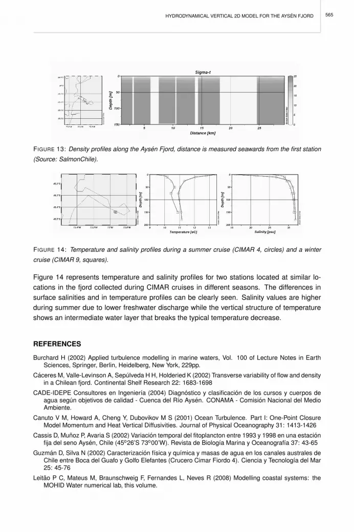
HYDRODYNAMICAL VERTICAL 2D MODEL FOR THE AYSEN FJORD
FIGURE 13: Density profiles along the Aysen Fjord, distance is measured seawards from the first station
(Source: SalmonChile).
FIGURE 14: Temperature and salinity profiles during a summer cruise (CIMAR 4, circles) and a winter
cruise (CIMAR 9, squares).
Figure 14 represents temperature and salinity profiles for two stations located at similar lo-cations in the fjord collected during CIMAR cruises in different seasons. The differences insurface salinities and in temperature profiles can be clearly seen. Salinity values are higherduring summer due to lower freshwater discharge while the vertical structure of temperatureshows an intermediate water layer that breaks the typical temperature decrease.
REFERENCES
Burchard H (2002) Applied turbulence modelling in marine waters, Vol. 100 of Lecture Notes in EarthSciences, Springer, Berlin, Heidelberg, New York, 229pp.
Caceres M, Valle-Levinson A, Sepulveda H H, Holderied K (2002) Transverse variability of flow and densityin a Chilean fjord. Continental Shelf Research 22: 1683-1698
CADE-IDEPE Consultores en Ingenierıa (2004) Diagnostico y clasificacion de los cursos y cuerpos deagua segun objetivos de calidad - Cuenca del Rıo Aysen. CONAMA - Comision Nacional del MedioAmbiente.
Canuto V M, Howard A, Cheng Y, Dubovikov M S (2001) Ocean Turbulence. Part I: One-Point ClosureModel Momentum and Heat Vertical Diffusivities. Journal of Physical Oceanography 31: 1413-1426
Cassis D, Munoz P, Avaria S (2002) Variacion temporal del fitoplancton entre 1993 y 1998 en una estacionfija del seno Aysen, Chile (45o26’S 73o00’W). Revista de Biologıa Marina y Oceanografıa 37: 43-65
Guzman D, Silva N (2002) Caracterizacion fısica y quımica y masas de agua en los canales australes deChile entre Boca del Guafo y Golfo Elefantes (Crucero Cimar Fiordo 4). Ciencia y Tecnologıa del Mar25: 45-76
Leitao P C, Mateus M, Braunschweig F, Fernandes L, Neves R (2008) Modelling coastal systems: theMOHID Water numerical lab, this volume.
565

F.J. CAMPUZANO, P.C. LEITAO, M.I. GONCALVES, V. MARIN AND A. TIRONI
Valle-Levinson A, Caceres M, Sepulveda H H, Holderied K (2002) Patrones de flujo en los canales asoci-ados a la boca del Seno Aysen. Ciencia y Tecnologıa del Mar 25: 5-16
Yarrow M, Leitao P C (2007) Simulating Nothofagus forests in the Chilean Patagonia: a test and analysisof tree growth and nutrient cycling in SWAT- 4th International SWAT Conference July 2-6 2007
566

PERSPECTIVES ON INTEGRATED COASTAL ZONE MANAGEMENT IN SOUTH AMERICAR. NEVES, J.W. BARETTA AND M. MATEUS (EDS.), IST PRESS, 2008
ECOLOGICAL CONCEPTUAL MODEL FOR A SOUTHERN CHILEAN FJORD:THE AYSEN FJORD CASE STUDY
F.J. CAMPUZANO, V. MARIN, A. TIRONI AND P. CHAMBEL-LEITAO
1 INTRODUCTION
The geographical location of each fjord conditions the ecological processes taking place inthe system because the factors involved such as river discharges, including their origin andassociated loads, and atmospheric conditions act locally converting them into singular studysites. In this paper we describe a conceptual and numerical ecological model for the Aysenfjord (Southern Chile), one of the study sites of the ECOMANAGE Project. The Aysen fjord iswhere the main human settlements of the XI Region of Chile are located and thus is a targetof possible ecological perturbations including harmful algal blooms (HABs) by phytoplanktonspecies harmful to salmon farming such as toxic dinoflagellates, which have been increasingtheir presence and distribution range in recent years (Munoz et al. 1992).
2 MATERIAL AND METHODS
Most of the data used for the Aysen study area come from the different CIMAR-FIORDOScampaigns (hereafter, CIMAR). These campaigns consist of oceanographic cruises alongthe whole system of southern Chilean fjords funded by the Chilean Navy’s Hydrographic andOceanographic Service (SHOA, its Spanish acronym). The CIMAR campaigns are focusedon different studies of the Chilean southern fjord system; the Aysen fjord was included in fivedifferent CIMAR campaigns. Most of these campaigns were divided in two cruises (E1 andE2).Table 1 summarises the period when each campaign took place and Table 2 the vari-ables measured in each campaign. Due to the scarcity of data those data have to be groupedinto spring-summer conditions and winter conditions. In addition to the CIMAR cruises, theSalmon Technological Institute (INTESAL, its Spanish acronym) which is part of the SalmonIndustry Association, SalmonChile (http://www.salmonchile.cl/), made available temper-ature, salinity, density and oxygen vertical profile data collected on the 10th of February 2007on nine stations along the Aysen Fjord ((http://pronosticos.salmonchile.cl/) (Figure 1).
2.1 Modelling efforts
The MOHID water modelling system Module Water Quality has been coupled to the hydro-dynamical model described in the Chapter ”Hydrodynamical vertical 2D model for the Aysenfjord” in order to sketch the ecological processes taking place in the Aysen fjord. The WaterQuality Module is based on an eutrophication model developed by the EPA (U.S. Environmen-tal Protection Agency) (Bowie et al. 1985). Initially, the model simulated the oxygen, nitrogenand phosphorus biogeochemical cycles, including both inorganic and organic forms, but re-
567

F.J. CAMPUZANO, V. MARIN, A. TIRONI AND P. CHAMBEL-LEITAO
cently the silica cycle has also been included. The concentrations of these nutrients alongwith other environmental factors such as light availability and temperature would determinethe dynamics of the primary producers, in this case phytoplankton and diatoms, and indirectlythe zooplankton dynamics as well. In order to model the ecological processes taking placein the Aysen fjord, it was to characterise the Aysen waterbody with two open boundaries cor-responding to the Aysen River loads and the open entrance that connects the fjord with theMoraleda Channel in the Chilean Inland Sea. In order to force river discharges with realisticlocal values despite the lack of observed data, the Soil and Water Assessment Tool (SWAT)model (Arnold and Fohrer 2005) has been applied to the Aysen River catchment. As definedby their creators, the model consists of a river basin scale model developed to quantify theimpact of land management practices in large, complex watersheds. An application of theSWAT model, on the Aysen catchment (Yarrow and Leitao 2007), produced the monthly nu-trient values summarised in Table 3. The oxygen concentrations presented in the same tablewere obtained from seasonal data presented in CADE-IDEPE (2004). The river discharge hasbeen implemented dividing its flow over the top six cells of the land boundary.
Cohesive sediment loads from the river were included on the model though observed data areabsent. A constant concentration of 25 mg l−1 was assumed for the river discharge. Concen-trations along the fjord strongly depend on river flow, with the river plume presenting higherconcentrations and extending further during winter, coinciding with high river discharges. TheAysen fjord initial conditions and for its coastal open boundary have been characterised by us-ing vertical profiles from station 77 of the campaign CIMAR 1 (table 4). This station has beenchosen because of its location near the mouth of the Aysen fjord and also because duringthe CIMAR 1 campaign were collected simultaneously more water properties. The boundarycells would be reading the boundary conditions from the interior, obtaining at each momentthe immediate values resulting from the interaction of the initial values and the forcing.
The Mohid model atmospheric module has a global model of radiation that changes the emit-ting radiation from the high atmosphere that can be modulated by the local climatology. Inthe case of Aysen, relative humidity, air temperature and cloud cover was obtained from theMeteorological Annals of Chile for the years 1968-1969 at Puerto Aysen (Table 5) to charac-terise the Aysen fjord climatology. To favour the exchange of heat and gases taking place atthe air-water interface also it was included winds collected during the CIMAR 7 campaign in2002, as explained in the Hydrodynamical chapter. The model was previously run for a periodof a year to adjust the initial values to the atmospheric, river and boundary forcing. The modelresults shown in this chapter correspond to the subsequent year of simulation.
3 DATA AND MODELLING RESULTS
3.1 Abiotic variables
Oxygen concentrations present their maximum values, close to 12 mg/l, at the surface due toexchange with the atmosphere favoured by the wind interaction and the entry of oxygenated
568

ECOLOGICAL CONCEPTUAL MODEL FOR A SOUTHERN CHILEAN FJORD: THE AYSEN FJORD CASE STUDY
river waters (Table 3). Though a minimum appears around 100 m, this could be explainedby the deposition at the bottom near the river mouth of the organic loads at the head of thefjord where a platform stops at around 100 m. Through remineralisation processes oxygenis consumed nearly to depletion levels, under 2 mg l−1. This mass of water with low oxygenlevels is transported to the rest of the estuary at the same depth (Figure 2). Also is in the headof the fjord where material allochtonous coming from land is mainly deposited thus consumingoxygen near the bottom. As was observed on the residual flux velocities there are waterexports from this area to the fjord waters which can be observed on Figure 2 as a plumewith low oxygen concentrations. This process is permanent though during winter, levels theextension of this plume can be greater because of the increase of loads into the system, asthe model results show (Figure 3).Oxygen concentrations are higher on the superficial fjordswater than in the vicinity coastal waters due to the entry of more oxygenated fresh waters.
TABLE 1: Cruises of the CIMAR program in the study area.
Cruise Initial Date End Date Season
CIMAR 1 08-10-1995 11-11-1995 Spring CIMAR 4 E1 26-09-1998 09-10-1998 Spring CIMAR 4 E2 25-02-1999 08-03-1999 Summer CIMAR 7 E1 07-07-2001 21-07-2001 Winter CIMAR 7 E2 12-11-2001 27-11-2001 Spring CIMAR 8 E1 01-07-2002 26-07-2002 Winter CIMAR 8 E2 15-11-2002 28-11-2002 Spring CIMAR 9 E1 05-08-2003 25-08-2003 Winter CIMAR 9 E2 03-11-2003 21-11-2003 Spring
TABLE 2: Variables collected during each campaign.
Campaign Temp Sal Oxygen Ammonia Nitrite Nitrate Phosphate Silicate Chl a CIMAR 1 X X X X X X X X X
CIMAR 4 E1 X X X X X X X CIMAR 4 E2 X X X X X X X CIMAR 7 E1 X X X X X X X X CIMAR 7 E2 X X X X X X X X CIMAR 8 E1 X X X X X X X CIMAR 8 E2 X X X X X X X CIMAR 9 E1 X X X X X X X CIMAR 9 E2 X X X X X X X
SalmonChile X X X
TABLE 3: Monthly values of nutrients and oxygen imposed on the Aysen River discharge.
Month Flow
(m3s-1) Oxygen (mg l-1)
Nitrate (mg l-1)
Nitrite (mg l-1)
Ammonia (mg l-1)
Organic N (mg l-1)
Phosphate (mg l-1)
Organic P (mg l-1)
January 325.86 12.2 0.1262 0.0044 0.0113 0.0042 0.0076 0.0003 February 249.45 12.2 0.0808 0.0052 0.0128 0.0049 0.0080 0.0003 March 336.82 12.2 0.0885 0.0052 0.0142 0.0061 0.0073 0.0004 April 475.12 13.1 0.0856 0.0071 0.0230 0.0155 0.0096 0.0010 May 655.63 13.1 0.0916 0.0111 0.0437 0.0379 0.0152 0.0028 June 731.80 13.1 0.1089 0.0104 0.0409 0.0354 0.0150 0.0026 July 729.44 11.9 0.1385 0.0267 0.0972 0.0779 0.0347 0.0051 August 814.96 11.9 0.1136 0.0197 0.0700 0.0537 0.0268 0.0034 September 636.33 11.9 0.0877 0.0101 0.0345 0.0274 0.0144 0.0019 October 542.83 10.8 0.0752 0.0071 0.0227 0.0155 0.0104 0.0010 November 436.88 10.8 0.0623 0.0048 0.0135 0.0068 0.0075 0.0004 December 439.44 10.8 0.0578 0.0043 0.0114 0.0049 0.0066 0.0003
569

F.J. CAMPUZANO, V. MARIN, A. TIRONI AND P. CHAMBEL-LEITAO
TABLE 4: Vertical profiles of station 77 of CIMAR 1 used for characterising the Aysen fjord watercolumn.
Depth
(m) Salinity (PSU)
Temperature (ºC)
Oxygen (mg l-1)
Nitrate (mg l-1)
Nitrite (mg l-1)
Ammonia (mg l-1)
Phosphate (mg l-1)
Silicate (mg l-1)
2 13.4558 10.8477 10.6957 0.0056 0.0018 0.0017 0.0016 2.4435 5 25.8857 10.1496 8.9678 0.1555 0.0028 0.0038 0.0375 0.5617 10 29.1555 9.5800 8.1110 0.1765 0.0045 0.0063 0.0443 0.4775 15 29.4397 9.4941 8.4395 0.0094 20 29.5993 9.4922 8.2396 0.0074 25 29.6338 9.5059 7.9682 0.2045 0.0014 0.0060 0.0480 0.4494 50 30.4125 9.8220 6.8544 0.0021 75 30.7126 9.7861 7.0686 0.2395 0.0028 0.0021 0.0566 0.5536
100 30.9620 9.8179 7.5256 0.2283 0.0024 0.0021 0.0560 0.5617 150 31.0517 9.5745 7.9972 0.2255 0.0015 0.0021 0.0560 0.6741 200 31.0791 9.5326 7.6112 0.2003 0.0017 0.0021 0.0529 0.4775
On the other hand, nitrogen species on surface waters are nearly depleted for nitrate, nitriteand ammonia. In the case of nitrate, it appears to be nearly absent from the surface waterof the fjord (Figure 4), mainly consumed by primary producers where light conditions favourtheir growth. Nitrate concentrations on the surface are higher during winter due to a higherriver flow and slightly higher concentrations of this compound on river water, along with theadverse conditions for primary producers. Under the pycnocline, organic particulate mattertends to accumulate and to undergo remineralisation processes where nitrate is released andtransformed into ammonia, nitrite being an intermediate in the process. The presence of nitriteindicates that transformation between nitrate and ammonia is taking place. In this sense,surface waters of the fjord present lower values of nitrate when compared with the watersof the Moraleda Channel nearby. Model results (Figure 5) reproduce the same pattern ofconcentrations and show that during summer the layer where nitrate concentrations are nearlydepleted increases maybe due to better light conditions. Prado-Fielder (2000) considers thatnitrite concentrations are, however, due to nitrification processes that would convert ammoniainto nitrite.
FIGURE 1: Location of Intesal-SalmonChile vertical profiles.
In the case of ammonia, only near the fjords head where several rivers discharge, this nutrientis present in the surface waters (Figure 6). Ammonia concentrations in the surface extendfurther due to higher river discharges during winter. Padro-Fielder (2000) also considered thatdifferences in ammonia concentration between the continental fjords and the open channelscorrespond to a higher terrestrial input of organic nitrogen and the limited water exchange inthese channels closed on one of its sides. Ammonia concentrations present a similar verticaldistribution as the nitrate with subsurface maximum values due to remineralisation processes(Figure 7). However, the number of available ammonia observations is too small to reach adefinitive conclusion.
570

ECOLOGICAL CONCEPTUAL MODEL FOR A SOUTHERN CHILEAN FJORD: THE AYSEN FJORD CASE STUDY
FIGURE 2: Oxygen concentration profiles along the Aysen Fjord for the CIMAR spring-summer campaigns
(Top), winter campaigns (Middle) and Intesal Campaign on February 2007 (Bottom). Distance is measured
seawards from the innermost station.
FIGURE 3: Modelled oxygen concentrations for the months of July (Left) and January (Right).
As in the case of nitrate, inorganic phosphorus concentrations are higher near the bottom ofthe fjord (Figure 8) due to remineralisation processes taking place on the sediment and tothe low loads from the river. During spring/summer conditions phosphate is depleted in thefjords head, while during winter low levels are present in the top layer and concentrationsare higher than in summer conditions. The fjord would act as a whole as a net exporter ofphosphorus to the adjacent coastal waters. Model results (Figure 9) reproduce this samepattern of concentrations.
On the other hand, silica concentrations reach their maximum concentrations on the surfacedue to the river being the main source (Figure 10). Thus the maximum concentrations are
571

F.J. CAMPUZANO, V. MARIN, A. TIRONI AND P. CHAMBEL-LEITAO
found near the river mouth and decrease along the fjord and the value would be modulated byriver flow. In the model a second maximum appears near the bottom due to remineralisation(Figure 11).
FIGURE 4: Nitrate concentration profiles along the Aysen Fjord for the campaigns carried out during
spring-summer (Top) and winter conditions (Bottom). Distance is measured seawards from the innermost
station.
FIGURE 5: Modelled nitrate concentrations for the months of July (Left) and January (Right).
TABLE 5: Monthly averaged atmospheric conditions from the Meteorological Annals of Chile (1968-1969).
Month Temperature (ºC) Relative Humidity (%) Cloud Cover (0-1)
January 14.15 88.17 0.792 February 12.30 89.33 0.879 March 11.50 88.33 0.692 April 9.35 92.33 0.810 May 7.65 93.00 0.888 June 4.75 92.17 0.790 July 4.55 93.00 0.858 August 5.60 91.00 0.794 September 7.00 85.83 0.848 October 8.00 88.17 0.796 November 11.30 86.17 0.842 December 12.85 85.00 0.775
572
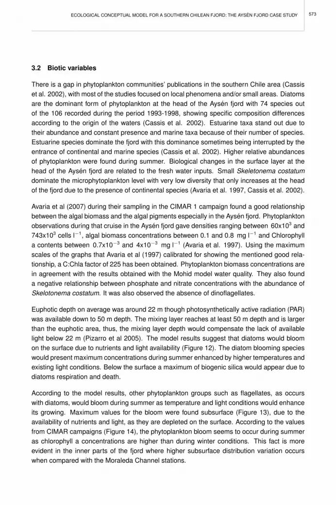
ECOLOGICAL CONCEPTUAL MODEL FOR A SOUTHERN CHILEAN FJORD: THE AYSEN FJORD CASE STUDY
3.2 Biotic variables
There is a gap in phytoplankton communities’ publications in the southern Chile area (Cassiset al. 2002), with most of the studies focused on local phenomena and/or small areas. Diatomsare the dominant form of phytoplankton at the head of the Aysen fjord with 74 species outof the 106 recorded during the period 1993-1998, showing specific composition differencesaccording to the origin of the waters (Cassis et al. 2002). Estuarine taxa stand out due totheir abundance and constant presence and marine taxa because of their number of species.Estuarine species dominate the fjord with this dominance sometimes being interrupted by theentrance of continental and marine species (Cassis et al. 2002). Higher relative abundancesof phytoplankton were found during summer. Biological changes in the surface layer at thehead of the Aysen fjord are related to the fresh water inputs. Small Skeletonema costatumdominate the microphytoplankton level with very low diversity that only increases at the headof the fjord due to the presence of continental species (Avaria et al. 1997, Cassis et al. 2002).
Avaria et al (2007) during their sampling in the CIMAR 1 campaign found a good relationshipbetween the algal biomass and the algal pigments especially in the Aysen fjord. Phytoplanktonobservations during that cruise in the Aysen fjord gave densities ranging between 60x103 and743x103 cells l−1, algal biomass concentrations between 0.1 and 0.8 mg l−1 and Chlorophylla contents between 0.7x10⁻³ and 4x10⁻³ mg l−1 (Avaria et al. 1997). Using the maximumscales of the graphs that Avaria et al (1997) calibrated for showing the mentioned good rela-tionship, a C:Chla factor of 225 has been obtained. Phytoplankton biomass concentrations arein agreement with the results obtained with the Mohid model water quality. They also founda negative relationship between phosphate and nitrate concentrations with the abundance ofSkelotonema costatum. It was also observed the absence of dinoflagellates.
Euphotic depth on average was around 22 m though photosynthetically active radiation (PAR)was available down to 50 m depth. The mixing layer reaches at least 50 m depth and is largerthan the euphotic area, thus, the mixing layer depth would compensate the lack of availablelight below 22 m (Pizarro et al 2005). The model results suggest that diatoms would bloomon the surface due to nutrients and light availability (Figure 12). The diatom blooming specieswould present maximum concentrations during summer enhanced by higher temperatures andexisting light conditions. Below the surface a maximum of biogenic silica would appear due todiatoms respiration and death.
According to the model results, other phytoplankton groups such as flagellates, as occurswith diatoms, would bloom during summer as temperature and light conditions would enhanceits growing. Maximum values for the bloom were found subsurface (Figure 13), due to theavailability of nutrients and light, as they are depleted on the surface. According to the valuesfrom CIMAR campaigns (Figure 14), the phytoplankton bloom seems to occur during summeras chlorophyll a concentrations are higher than during winter conditions. This fact is moreevident in the inner parts of the fjord where higher subsurface distribution variation occurswhen compared with the Moraleda Channel stations.
573

F.J. CAMPUZANO, V. MARIN, A. TIRONI AND P. CHAMBEL-LEITAO
FIGURE 6: Ammonia concentration profiles along the Aysen Fjord for the campaigns carried out during
spring-summer (Top) and winter conditions (Bottom). Distance is measured seawards from the innermost
station.
FIGURE 7: Modelled ammonia concentrations for the months of July (Left) and January (Right).
FIGURE 8: Phosphate concentration profiles along the Aysen Fjord for the campaigns carried out during
spring-summer (Top) and winter conditions (Bottom). Distance is measured seawards from the innermost
station.
574

ECOLOGICAL CONCEPTUAL MODEL FOR A SOUTHERN CHILEAN FJORD: THE AYSEN FJORD CASE STUDY
FIGURE 9: Modelled phosphate concentrations for the months of July (Left) and January (Right).
FIGURE 10: Silicate concentration profiles along the Aysen Fjord for the campaigns carried out during
spring-summer (Top) and winter conditions (Bottom). Distance is measured seawards from the innermost
station.
FIGURE 11: Modelled inorganic silica concentrations for the months of July (Left) and January (Right).
575

F.J. CAMPUZANO, V. MARIN, A. TIRONI AND P. CHAMBEL-LEITAO
The Aysen fjord is located in one of the main areas of accumulation of zooplankton restrictedto the Aysen fjord along with neighbouring Moraleda and Darwin channels (Palma and Silva2004). However, this biomass abundance is not translated into species richness due to thespatial and temporal heterogeneity with marked gradients. Only few zooplanktonic specieshave been successfully adapted to the extreme oceanographic temperature, salinity and oxy-gen ranges (Palma and Silva 2004). During the CIMAR 8 campaign, zooplankton biomassmainly comprised copepods, chaetognaths and euphausids and highest biomass values inthe system were found in the Guafo Mouth, the main connection between the Moraleda Chan-nel and the open ocean, and the lowest values were observed in the Chile Inland Sea wherethe Aysen fjord is located (Palma and Apablaza 2005).
Though zooplankton is present in the model it is not controlling the phytoplankton biomass withthe present parameterisation. Basically, its concentration is depending on the river dischargevalues that later is transported to the boundary where due to the boundary conditions theyaccumulate. As no data about zooplankton dynamics are available the function on regulatingthe primary producers’ biomass is unknown.
4 DISCUSSION AND CONCLUSIONS
The model simulation reproduces the main physical-chemical features of the observed data.The sharp pycnocline acts as a barrier between the upper and bottom layers preventing mixingof water unless due to highly energetic processes. Surface waters are mainly dominated byatmospheric and river discharge processes while bottom water processes are related to sed-iment processes and coastal boundary processes. The main interaction between both layersconsists of the particulate matter that the upper layer exports to deep waters. Surface watersare well oxygenated as the rivers discharging into the fjord present high concentrations of oxy-gen (Table 3). The nutrient loads from the Aysen River are of the same order of magnitudeas the receiving environment, though slightly higher. In this sense, the Aysen River can beregarded as an oligotrophic river.
Perhaps, the most important effect would be the deposit of particulate matter in the adjacentfjord beds, also because the inner area would be the section of the fjord with the highest pri-mary production. These deposits would consume oxygen through remineralisation, producinga plume of nearly anoxic waters and rich in inorganic nutrients that would extend trough thefjord transported by the deep water circulation. Oxygen is depleted near the bottom due toremineralisation of organic matter. In Figure 15 can be seen how nitrate concentrations in-crease landwards while oxygen concentrations decrease. Also in the inner stations can beappreciated higher concentrations of nitrite which is considered as an intermediate form of thewhole process that goes from ammonia to nitrate; only the presence of nitrite concentrationsindicates the active production of nitrate (Sverdrup et al. 1942).
According to the values from the CIMAR campaigns and model results the phytoplanktonbloom seems to take place during summer with higher chlorophyll a concentrations than duringwinter, especially in the inner parts of the fjord. In this sense, also the production of the system
576

ECOLOGICAL CONCEPTUAL MODEL FOR A SOUTHERN CHILEAN FJORD: THE AYSEN FJORD CASE STUDY
would be conditioned by the river discharges, more due to the nutrient loads than to its flowand to light availability. Very little is known about zooplankton dynamics in the system so thecontrol that can apply to the primary producers is practically unknown.
FIGURE 12: Modelled diatoms concentrations for the months of July (Top) and January (Bottom).
FIGURE 13: Modelled phytoplankton concentrations for the months of July (Top) and January (Bottom).
577

F.J. CAMPUZANO, V. MARIN, A. TIRONI AND P. CHAMBEL-LEITAO
FIGURE 14: Chlorophyll concentration profiles along the Aysen Fjord for the campaigns carried out during
spring-summer (Top) and winter conditions (Bottom). Distance is measured seawards from the innermost
station.
FIGURE 15: Nutrient profiles obtained during the CIMAR1 campaign for the inner fjord (circles), middle
fiord (squares) and near the Aysen fjord mouth (diamonds).
578

ECOLOGICAL CONCEPTUAL MODEL FOR A SOUTHERN CHILEAN FJORD: THE AYSEN FJORD CASE STUDY
In spite of the scarce data, knowledge of the system and model assumptions made it possibleto establish a simple 2D vertical model that mainly reproduces the processes described by thebibliography and the general trends of the data. This model could serve as a first step to studythe possible effects of modifying the entrance of organic matter as a product of a differentmanagement of the river catchment or other entrances of organic matter into the system.
REFERENCES
Antezana T (1999) Plankton of Southern Chilean fjords: trends and linkages. Scientia Marina, 63: 69-80
Arnold J G, Fohrer N (2005) SWAT2000: current capabilities and research opportunities in applied water-shed modelling. Hydrological Processes 19: 563-572
Avaria S, Cassis D, Munoz P, Vera P (1997) Distribucion del microfitoplancton marino en aguas interioresdel Sur de Chile en octubre de 1995 (Crucero Cimar-1). Ciencia y Tecnologıa del Mar 20: 107-123
Bowie G L, Mills W B, Porcella D B, Cambell C L, Pagendorf J R, Rupp G L, Johnson K M, Chan P W,Gherini S A, Chamberlin C E (1985) Rates, Constants and Kinetic Formulations in Surface WaterQuality Modelling. U.S. Environmental Protection Agency.
Cassis D, Munoz P, Avaria S (2002) Variacion temporal del fitoplancton entre 1993 y 1998 en una estacionfija del seno Aysen, Chile (45o26’S 73o00’W). Revista de Biologıa Marina y Oceanografıa, 37: 43-65
Munoz P, Avaria S, Sievers H, Prado R (1992) Presencia de dinoflagelados toxicos del genero Dinophysisen el seno Aysen, Chile. Revista de Biologıa Marina, 27: 187-212
Palma S, Apablaza P (2005) Distribucion geografica de la biomasa zooplanctonica y de los sifonoforosepipelagicos capturados entre la Boca del Guafo y el Canal Pulluche (CIMAR 8 FIORDOS)
Palma S, Silva N (2004) Distribution of siphonophores, chaetognaths, euphausiids and oceanographicconditions in the fjords and channels of southern Chile. Deep-Sea Research II 51: 513-535
Pizarro G, Montecino V, Guzman L, Munoz V, Chacon V, Pacheco H, Frangopulos M, Retamal L, AlarconC (2005). Patrones locales recurrentes del fitoplancton en fiordos y canales australes (43o- 56o S) enprimavera y verano. Ciencia y Tecnologıa del Mar 28: 63-83
Prado-Fiedler R (2000) Distribucion espacial del amonio en fiordos y canales comprendidos entre PuertoMontt y Laguna San Rafael en perıodo de primavera. Ciencia y Tecnologıa del Mar 23: 15-24
Silva N, Guzman D, Valdenegro A (1999) Balance de agua y sal para el Seno Aysen, Chile. In: ComiteOceanografico Nacional-Chile (ed.) Resultados crucero CIMAR-FIORDO 4. Extended abstracts: 18-24
Sverdrup H U, Johnson M W, Fleming R H (1942). The oceans, their physics, chemistry, and generalbiology. Prentice-Hall.
Yarrow M, Leitao PC (2007) Simulating Nothfagus forests in the Chilean Patagonia: a test and analysis oftree growth and nutrient cycling in SWAT- 4th International SWAT Conference July 2-6, 2007
579

PERSPECTIVES ON INTEGRATED COASTAL ZONE MANAGEMENT IN SOUTH AMERICAR. NEVES, J.W. BARETTA AND M. MATEUS (EDS.), IST PRESS, 2008
CONCEPTUAL, PHES-SYSTEM, MODELS OF THE AYSEN FJORD: THE CASEOF SALMON FARMING
L.E. DELGADO, V.H. MARIN, A. TIRONI AND P. BACHMANN
1 INTRODUCTION
In a previous chapter we have argued that the integrated management of coastal zones shouldbe sensitive to the variety of perceptions that different social actors or stakeholders have onthe ecological system being managed (Marın and Delgado, this volume). Our analysis of theeconomy and social conditions of Aysen suggested us that the main actors, in relation to theAysen fjord, are: the local government and salmon farmers (Delgado and Bachmann, this vo-lume; Bachmann et al. 2007). Consequently we studied the perception of these stakeholdersby means of conceptual PHES-systems models of the Aysen fjord. Since they interact fre-quently on issues related to its management, we found that it was timely and indeed beneficialfor them to know each other’s perception of the ecosystem that generates the services theyaffect.
The basis and general description of the PHES-system approach can be found in the chapterby Marın and Delgado in this volume, on Marın et al. (2008) and Delgado and Marın (2005).The generation of conceptual models started by sending, two weeks in advance, a short list ofquestions that would be the basis of the brainstorming sessions. Several questions (e.g. theeffects of fish hatcheries on the water quality of the fjord, the system components of salmonfarming, and the effects of salmon on the fjord) were common to both groups for comparativepurposes.
Conceptual models, coded using STELLA Research 9.0, were built after the brainstormingsessions. In the case of government experts, two models were built owing to the rather largenumber of people involved and then merged. In the case of salmon farmers one model wasbuilt. In all cases participants were encouraged to use the information generated during theprevious session. Most results from the government stakeholder session have been reportedby Marın et al. (2008) and the interested reader is encourage to read it. Here we analyzeresults only as they relate to the subsequent conceptual models of the Aysen fjord.
2 BRAINSTORMING SESSION RESULTS
The results of the brainstorming sessions showed that: while the local government perceivesthe fjord as an interactive ecological system, salmon farmers sees it as a market place wherethe ”natural environment” only exists at the beginning of the market study. For example, whenanswering on the effect of hatcheries, government officers proposed two components (fishfood and fecal material) and one process (excretion) as dominant. They further stated thatalthough today there are only 14 hatcheries in the Aysen watershed, the salmon market has
581

L.E. DELGADO, V.H. MARIN, A. TIRONI AND P. BACHMANN
established that their number should grow up to 110 within the next 10 years. Furthermore,participants suggested that loosing fish food from hatcheries is not a problem (current lossesare near 5-7% by mass), since this represents a cost that companies intend to decrease. Theyexpressed concern over the fact that other components of the fish diet (e.g. zinc, antibiotics)are currently not regulated and that this may represent a problem in the near future. Salmonfarmers, on the other hand, answered that the effect of hatcheries on environmental variablesis unknown, that current legislation is unclear and that treating hatcheries as sources of pollu-tants is unjustified given that high value of the river flow/residues ratio. Finally they added thatgiven these uncertainties, there is a clear need for more studies.
When confronted to the issue of salmon farming within the fjord, government officers iden-tified several variables and processes that should be considered. Most government expertsemphasized the potential negative effects of escaped salmons on the biological diversity of thefjord. Salmon farmers stated that since salmons have been in the area since 1969, when theChilean government authorized its farming, they should be considered now (25 years later)as native fauna. Furthermore, they stated that most escaped salmons remain in the vicinity ofthe broken cages. They finally stated that the main causes for the escape of salmons are sealions and robbery. The different perceptions of these two key stakeholders on the fjord wereeven clearer during the building of conceptual models.
3 CONCEPTUAL MODELS OF THE AYSEN FJORD IN RELATION TO SALMON FARM-ING
Figures 1 and 2 show the conceptual models generated by government experts and by salmonfarmers respectively. The first model divided the fjord in sections: head, center and mouth.Since salmon farming is developed mostly near the head, we have concentrated our modellingefforts in this part of the model. The government model (Fig. 1) shows the different processesrelated to the fate of nutrients in the system. From their point of view, salmon farming contributewith nutrients through salmon excretion and the waste of salmon food (see also Tironi etal., this volume). However, they also postulate that the government can influence these twoprocesses by means of coastal zone management schemes. Thus, government proposes thatthey can have an impact on the two most important human nutrient sources: salmon farmingand urban activity. Potential regulatory mechanisms are: secondary water quality norms andwaste disposal legislation.
The environment, for salmon farmers, which represents a large portion of the government’smodel, is confined to one single converter inside one process: market study (Fig. 2). Italso appears influencing the production process through the environmental norms set by thegovernment1. Once the market study is over, and they have decided the location for thefarming of salmons, the environment ”disappears” with the exception of governmental water
1An example is the Supreme Decree 90 which regulates water quality for industrial residues (http://www.ist.cl/archivos/ds90.pdf).
582

CONCEPTUAL, PHES-SYSTEM, MODELS OF THE AYSEN FJORD: THE CASE OF SALMON FARMING
quality rules and regulations. The rest of the processes and variables in the salmon farmer’smodel are related to two main processes: production and exports which in turn affect and willbe affected by two main state variables: salmon biomass and markets (mostly international).
It is worth noting that the urban environment appears twice in the model. On one hand,the production process is affected by the urban environment in the sense of providing skillfulmanpower and their necessary education (Urban environment II, Fig. 2). On the other, thehigh water quality requirements of salmon farming makes the urban environment an unwantedvariable (urban environment I, fig. 2), which then affects the production process both throughthe logistics necessary to stay ”neither too close, nor too near” and, in turn, affecting the spatialdistribution of the farming centers. Sea lions and salmon robbery appears in their model asaffecting the export process.
FIGURE 1: Stella coded conceptual model (government PHES-system) of the Aysen fjord in relation to
salmon farming. See text for details.
4 LESSONS FROM AYSEN FJORD PHES-SYSTEM MODELLING
We have shown, both through the development of brainstorming sessions as through the sub-sequent conceptual models, that the perceptions of the Aysen fjord ecosystem by two of thekey stakeholder’s related to salmon farming are very different. In one case (local government)the fjord is viewed as an interactive system composed of biotic and abiotic components andfluxes, one of them being salmon farming. In the other case (salmon farmers) the system iscloser to a ”market place” where most variables are related to the export process. Is it possi-ble to link the two models? In this case the answer is positive, although we do not show themerged models for reasons of page space only. However, the interested reader can down-
583

L.E. DELGADO, V.H. MARIN, A. TIRONI AND P. BACHMANN
load it from the internet (http://ecosistemas.uchile.cl). In essence both views of the fjordecosystem (or PHES-systems) are complementary. The government model lacks all ”mar-ket variables” and the salmon farmers model lack all ”ecosystem variables”. Thus merging inthis case is simple. However, in order to use the merged product for integrated managementboth key stakeholders will have to learn from each other perspectives. This is indeed oneof the most important findings from other groups generating frameworks for interdisciplinarymodelling: the major problem when integrating and coordinating different stakeholders seemsto be communication (e.g. Heemskerk et al. 2003). In this regard, the PHES-system ap-proach can effectively be used as a communication tool among stakeholders for the benefit onintegrated ecosystem management.
FIGURE 2: Stella coded conceptual model (salmon farmers PHES-system) of the Aysen fjord in relation
to salmon farming. See text for details.
REFERENCES
Bachmann P, Delgado LE, Marın VH (2007) Analysis of the citizen’s participation concept used by localdecision makers: the case of the Aysen watershed in southern Chile. Int. J. Sustainable Development10:251-266
Delgado LE, Bachmann P (2008) Socio-economy of the Aysen area, this volume.
Delgado LE, Marın VH (2005) FES-sistema: un concepto para la incorporacion de las sociedades hu-manas en el analisis medioambiental en Chile. Revista Ambiente y Desarrollo 21: 18-22
Heemskerk M,Wilson K, Pavao-Zuckerman M (2003) Conceptual models as tools for communicationacross disciplines. Conservation Ecology 7 (3): 8
Marın V H, Delgado LE, Bachmann P (2008) Conceptual PHES-system models of the Aysen watershedand fjord (Southern Chile): testing a brainstorming strategy. Journal of Environmental Management88:1109-1118
Marın VH, Delgado LE (2008) A PHES-system approach to coastal zone management, this volume.
584

PERSPECTIVES ON INTEGRATED COASTAL ZONE MANAGEMENT IN SOUTH AMERICAR. NEVES, J.W. BARETTA AND M. MATEUS (EDS.), IST PRESS, 2008
A MANAGEMENT TOOL FOR SALMON AQUACULTURE: INTEGRATING MOHIDAND GIS APPLICATIONS FOR LOCAL WASTE MANAGEMENT
A. TIRONI, V.H. MARIN AND F. CAMPUZANO
1 INTRODUCTION
Contemporary human pressures over world marine ecosystems could be unsustainable. Over75% of the world natural fish stocks are considered fully exploited or over-exploited (FAO2007). Direct impacts over biodiversity, habitat destruction, waste disposal and climate changeindirect effects -and a possible synergy between these factors- (Harley and Hughes 2006)allow predicting the collapse of all harvested taxa by the year 2048, if we sustain today’s trendof use and extraction (Worm et al. 2006). However, fish consumption has duplicated since1960 and now it’s the fastest growing food industry worldwide (FAO 2007).
In this context, fish farming -responsible of more than 70% of this growth- appears as a properway to reduce human pressure over world natural fisheries. But, is this true for all typesof aquaculture? Unfortunately no, farming of carnivorous species requires large food inputsand produces a series of local impacts on marine ecosystems, converting them in a mixedblessing for world fisheries (Naylor et al. 2000). Fish farming reduces the pressure overnatural fisheries used for human consumption, but at the same time it raises the demand forsome pelagic species (e.g Chilean mackerel) used for fish oil and flour, used in the elaborationof fish pellets. One of these forms of aquaculture is salmon farming (Naylor et al. 2000, 2003,2005).
In general terms, the marine stage of salmon farming productive cycle consist of an accel-erated and controlled growth of juvenile individuals, until they obtain an appropriated weightfor their processing and commercialization. Fish are maintained in floating cages, settled inprotected areas (like fjords, channels and inner seas), and fed with pellets made of a variablefraction of marine fish flour and oil. Aside from the pressure over pelagic fisheries, salmonfarming produces a series of environmental impacts over marine ecosystems where the cagesare installed. They are, in a short summary: (1) waste disposal over the water column andbottom, like food pellets, fish feces and antibiotics, (2) invasion by exotic fish species andpathogens every time fish escape from cages and, as a result of these processes, (3) habitatdestruction (Naylor et al. 2003, 2005, Miranda and Zemelman 2002, Cabello 2006). Theseimpacts could obscure salmon farming’s contribution to reduce pressures on natural fisheriesresources. In this context, it could be argued that salmon farming is now in a crossroad be-tween been against or in favor of sustainable development of world fisheries. The path it shalltake will depend on their fish flour and oil use policies (Naylor et al. 2000), and how it willmanage local impacts related to their activities. It is toward the later that we have focused thiswork.
585

A. TIRONI, V.H. MARIN AND F. CAMPUZANO
2 LAGRANGIAN MODELS AND THEIR USE IN SALMON FARMING MANAGEMENT
A common cause of most salmon farming local environmental impacts is particulate wastedisposal in the form of food pellet and feces- to the water column and bottom. These particlesusually deposit in the vicinity of cages, distressing the system in various ways: (a) artificialinputs of organic carbon, nitrogen and phosphorous, (b) increase in primary productivity, mod-ifying bottom’s community structure, (c) negative impacts over benthos biodiversity and (d) theformation of an anoxic layer in the sediments under the cages (Corner et al. 2006, Cromey etal. 2002, Findlay et al. 1995, Soto and Norambuena 2004)
A widely adopted management tool for this kind of particulate wastes is their dynamic sim-ulation by means of lagrangian particle-tracking models (Cromey et al. 2002, Cromey andBlack 2005). These models simulate the dispersion and sedimentation of particles in ocean’sbottom. Coupling these with other numerical models, involving additional physical, biogeo-chemical and ecological process, could contribute to a more integral assessment of salmonfarming local impacts (Corner et al. 2006, Cromey et al. 2002, Cromey and Black 2005, Pan-chang et al. 1997, Perez et al. 2002) . We implemented, as one of ECOMANAGE activities, athree-level nested, coupled circulation-lagrangian model to assess the fate of particles gener-ated at salmon farming sites, one of the main economic drivers of the Aysen fjord region. Wehave applied this tool to the Chacabuco bay area inside the fjord.
3 METHODS
3.1 Hydrodynamic models
Hydrodynamic models utilized were developed with the open-source software MOHID WaterModeling System (Leitao et al., this volume). A 3-level nested modeling structure was chosenin order to simulate the complex tide signal of the fjord system, reduce numerical errors andto enhance model stability (Fig. 1). The first level, Fjords, is a barotropic, single-layer sigmamodel covering the northern part of Chilean fjords, between 41◦S and 46◦S, with a definitionof 2.2 km. The main purpose of this level was to generate the tidal components, obtained fromthe FES2004 model (Lyard et al. 2006), for the lower level models. The second level in thenested structure (Aysen) is a model covering the area of the Aysen Fjord. It is also barotropic,but aside from incorporating tides from the Fjords model, it includes the three most importantfresh water discharges (rivers) of the fjord. These two models have been described in detailby Marin and Campuzano (in press).
The third level, Chacabuco, covered the inner area of the Aysen Fjord. It is a baroclinic model,with a cartesian geometry of 11 vertical layers. Its resolution is approximately of 100 m, andit was over this level that the lagrangian particle-tracking sub-model was implemented. Thenumerical grid was generated using bathymetric data from Armada de Chile (Chilean Navy),using geo-statistic methods in order to generate a smooth bathymetry in areas where the pointcoverage was not accurate enough.
586

A MANAGEMENT TOOL FOR SALMON AQUACULTURE: INTEGRATING MOHID AND GIS APPLICATIONSFOR LOCAL WASTE MANAGEMENT
FIGURE 1: Geographic area covered by the 3 level nested modeling structure in southern Chile. Grayscale
areas represent each of the model grids. Chacabuco bay, where the particle-tracking model was mounted,
is marked with an asterisk.
The three models were initialized for 10 days with the purpose of stabilizing Aysen’s Fjordwater level, followed by a 25 days run to initialize water properties (temperature and salinity).Finally, with tide signal, temperature and salinity stabilized, a third 16-day run was imple-mented to simulate pellets dispersion in the bay area. Table 1 shows the main characteristicsof each of the three models.
3.2 Lagrangian Particle Tracking Module
In what follows we describe the parameterization and assumptions used in relation to salmonfarming loads and their dispersal in the water column.
Discharge volume: A fish density of 10 kg m−3, for every 6000 m−3 cage, was considered forpellets output with a food/biomass ratio of 1.2. Only 5% of this load was considered to passcage’s depth and fall through the water column. We have further assumed that half of thesewasted pellets were eaten by local marine fauna (Cromey et al. 2002). This pellet mass (in Kg)was then converted to particles assuming a caliber 2500 pellet (0.9 g per pellet, taken fromEwos Chile website, http://www.ewos.com/cl/, visited on 07/23/2007). The final number ofparticles was calculated as 450 particles per cage every two hours.
587

A. TIRONI, V.H. MARIN AND F. CAMPUZANO
Sedimentation Velocity: Previous work has shown that sedimentation velocity depends onparticle size (Perez et al. 2002) and that pellets suffer changes in their size as they descendthrough the water column (Chen et al. 1999). Here we have simplified this process applying aconstant sedimentation velocity. The main purpose of this simplification was reducing calcula-tion time and hardware requirements, given the rather large number of particles tracked in oursimulation ( > 109).
Salmon Production Cycle: Salmon farming involves different fish densities for each stage ofthe production cycle. For the purposes of this model we chose a fixed density (10 kg m−3)corresponding to a high production stage. We subsequently tracked their discharges every 2hours.
Consolidation: The model does not consider pellets consolidating in the sediments. Thereis no enough available information about sediments in the study area. A no-resuspensionscenario was added to the sensitivity analysis to test for this assumption.
3.3 Sensitivity Analysis
Sensitivity analysis was done defining default values for every parameter tested (default run),and then adjusting them within the range found in literature to create sensitivity scenarios(Cromey et al. 2002, Panchang et al. 1997, Perez et al. 2002, Chen et al. 1999, Wiberg2004). Seven scenarios were defined as shown in Table 2. The variable over which weperform the sensitivity test was the number of particles on day sixteen of simulation ( N16) ina specified area. The area was chosen after sampling the model for number of particles ina series of boxes over the whole bay. We chose the one showing greater variation betweensensitivity scenarios. Model sensitivity (Sx) was evaluated as the change in ” N16” relative tochanges in a model parameter ”P” (Huntley et al. 1987), using equation (1).
Sx =(N16s,x − N16def )/N16def
(Ps,x − Pdef )/Pdef(1)
Where N16s,x is the value for N16 for the x scenario in the sensitivity analysis, and N16def isthe value for N16 on the default run. Ps,x correspond to the value of parameter P for a givensensitivity scenario x, while Ndef is the default value of the parameter.
3.4 Management tool
The management tool generated is a modified ArcViewr 3.3 (ESRI Inc.) interface (pro-grammed using AVENUE scripts) that shows, in a simple and user-friendly way, the combinedresults of the hydrodynamic and particle-tracking model in a Geographic Information System(GIS) environment. Custom buttons were added to show pellets dispersal, relevant hydro-dynamic data and GIS coverage. Help text and button information were translated to locallanguage (spanish) to improve user experience. During the development of the tool, localmanager’s capabilities and requirements were checked to improve its usage and to fulfill theirinformation requirements.
588
A MANAGEMENT TOOL FOR SALMON AQUACULTURE: INTEGRATING MOHID AND GIS APPLICATIONSFOR LOCAL WASTE MANAGEMENT
4 RESULTS
The Chacabuco hydrodynamic model was validated with respect to salinity and water level.The model is capable of reproducing the typical halocline of the Aysen fjord, with the riverflowing seaward through the upper level of the water column (Fig. 2). When comparing wa-ter levels given by the model with real values taken from mareographic station located insidethe model, the results shows a good fit, with an r2 of 0.94 (Marin and Campuzano, in press).Thus, the model is able to simulate the main characteristics of the estuarine system in the Cha-cabuco bay area. Therefore, the validated model was used to study the spatial dispersion ofparticulate wastes coming from salmon farming activities in the bay, using MOHID lagrangianmodule.
The results of the lagrangian particle tracking module (pellets dispersal after 16 days of sim-ulation of five cages throwing 450 particles every 2 hour) is shown in Figure 3. The ma-jority of the origins showed pellets dispersing mostly beneath the cages or in distances be-tween 100 m and 500 m from the cage’s center. The greater dispersal in our simulationreached 1100 m, not including isolated particles. In total, pellets covered between 17%and 27% of the Chacabuco bay area. Results for the sensitivity analysis, grouped by sce-narios, are shown in Table 3. The most sensitive variables were those defining resuspen-sion; specifically erosion and deposition shear stress. The management tool was deliveredto local decision makers. Additionally, there is an online version of the tool (mapserver for-mat: http://ecosistemas.uchile.cl/ecomanage/resultados). The tool has already beenused in the process of generating new environmental regulations for the Aysen region (DGA,CONAMA, personal communication).
5 COMPARISON WITH OTHER MODELS
We have shown the development of a lagrangian particle tracking model that can be used bysalmon farmers and local decision makers. When comparing model’s output with previouswork with lagrangian approaches (Cromey et al. 2002, Cromey and Black 2005), the resultsare qualitatively similar. DEPOMOD is the only model with its dispersion module validated,showing between 13% and 22% of difference between modeled and observed values (Cromeyet al. 2002). Thus, we have used it as a reference in this comparison.
There are some important differences between MOHID and DEPOMOD that should be takeninto account before comparing them. First, MOHID sedimentation velocity was fixed during thewhole simulation ( 1.28x10⁻¹ m s−1), while DEPOMOD uses random generated rates takenfrom a given range of values. The amount of particles simulated with MOHID ( 4x10⁹) isfive orders of magnitude above DEPOMOD ( 7x10⁴). In fact, our volumes were close to realproduction values for particulate wastes discharges from Chilean salmon cages (EIA reportsfrom salmon farmers POCH, 2004). Another important difference is the spatial and time scaleof both models. While Cromey et al. (2002) used a grid definition of 10x10 m, covering anarea of 0.25 km2, here we used a grid of 100x100 m, covering an area of 147 km2.
589

A. TIRONI, V.H. MARIN AND F. CAMPUZANO
TABLE 1: Main properties of the 3 nested model system.
Model Nesting Level
Grid Definition (km) Geometry Type Discharges Tides
Fjord 1 2.2 Sigma, 1 layer Barotropic No FES2004
Aysén 2 0.5 Cartesian, 1 layer Barotropic Yes Fjord Model
Chacabuco 3 0.1 Cartesian, 11 layers Baroclinic Yes Aysén Model
TABLE 2: Default values and sensitivity analysis scenarios. For every scenario, defaults parameters were
modified to fit a range of values founded in literature.
Resuspension Sedimentation Random movement
Parameters Default values E1 E2 E3 E4 E5 E6 E7
VARVELHX* 0.02 - - - - 0.04 0.01
VARVELH* 0.02 - - - - 0.04 0.01
Critical Shear Stress of Erosion 0.02 0.01 0.04 1 x 10⁻⁵ - - - -
Critical Shear Stress of Deposition 0.004 0.002 0.008 1 x 10⁻⁵ - - - -
Erosion Rate 0.005 0.0025 0.01 1 x 10⁻¹⁰ - - - -
Sedimentation velocity 0.128 - - 0.096 0.064 - -
*varvelhx y varvelh are both model parameters determining particle random movement
TABLE 3: Results from the sensitivity analysis. Each scenario is represented by the relative amount of
variation of a given parameter from their default values. Sensitivity was calculated based on Huntley
(1986).
Sensitivity (x 103) as particle number Sensitivity Scenario
200% -75% -50% -200000%
Resuspension (E 1-3) -664.3 335.5 982.8
Sedimentation Velocity (E 4-5) -1.8 107.1
Random Movement (E 6-7) 90.5 128.6
590

A MANAGEMENT TOOL FOR SALMON AQUACULTURE: INTEGRATING MOHID AND GIS APPLICATIONSFOR LOCAL WASTE MANAGEMENT
FIGURE 2: Salinity values for model results (◦) and available field data (•). The dotted lines represent
standard deviation of model results.
The time span of both simulations is also very different. Our model ran for sixteen days, withparticle discharges every two hours for five origins, while Cromey et al. (2002) shows a 24 hoursimulation with a single discharge. Despite the differences just mentioned, DEPOMOD andMOHID show similar results in their pellets’ dispersal simulation. Cromey et al. (2002) showedthat pellets dispersal occurred mainly beneath the cages (0-100 m), reaching a maximumdistance for pellets dispersal of 200-300 m from the cage center. Our results, for comparabledepths, show the same pattern, but with maximum dispersal distances of 300-400 m. Thus,the simulation of salmon farming particulate waste dispersal using MOHID lagrangian moduleshows congruent results when compared with previous experiences with similar approaches(Cromey et al. 2002) and in general, with previous simulations of particulate waste dispersal(Corner et al. 2006, Panchang et al. 1997, Perez et al. 2002).
591

A. TIRONI, V.H. MARIN AND F. CAMPUZANO
FIGURE 3: Final spatial distribution of our 16-days simulation. Darker particles represent the results
from the default simulation, while grayscale particles symbolize particle dispersion from the sensitivity
scenarios. White circles shows each cage location.
6 A BROADER CONTEXT
Models, like the one we have developed here, do not gain enough relevance until they are con-sider as part of a wider strategy, thus allowing the application of their results outside academiccircles. A management framework we think is able to provide this wider context is IntegratedCoastal Zone Management (ICZM; Turner 1999, 2000) is one strategy where models can beused. This management framework understand the relationship between nature and societyas a process where perturbations generated from the former alter some ecosystem functions,eventually affecting the flux of ecosystem services to society, generating negative impacts overit, in a cycle called Driver-Pressure-State-Impact-Response. ICZM also provides a good sup-port for stakeholder involvement in any of the multiple stages of project development (Christieet al. 2005, de Araujo et al. 1999).
In this work we understand stakeholders involvement as a continuum from partial involvement,or cooperative research (e.g. information exchange agreements), to collaborative research,where scientist and stakeholders jointly develop research projects. In any point of this spec-trum, recent studies show that participatory research is able to contribute to scientists andstakeholders more informed about each other and better engaged in projects’ objectives andoutcomes (Hartley et al. 2006). Furthermore, stakeholder involvement has the potential to in-crease their self-reliance and awareness of the issues being investigated, facilitating more eq-
592

A MANAGEMENT TOOL FOR SALMON AQUACULTURE: INTEGRATING MOHID AND GIS APPLICATIONSFOR LOCAL WASTE MANAGEMENT
uitable trade-offs between stakeholders with competing interests (de Araujo et al. 1999). Fromthis point of view, our experience during the development of this work showed that stakehold-ers’ involvement in the research process brings a series of benefits: (1) Considering the largefield data required to set model’s initial/boundaries conditions and for the validation process,government stakeholders participation -and their data bases- were a key element in the datagathering period, (2) the working relationship generated with local stakeholders allowed usto identify each of their administrative, technical and institutional capabilities, key informationwhen generating public research reports and decision support systems to final users (Peder-sen et al. 2005) and (3) the creation and definition of modeling scenarios was facilitated duringthis interaction, linking research objectives with stakeholders’ specific interests (Hanson et al.2006).
However, there’s a huge distance between the theory and practice of ICZM, especially in thecontext of developing countries. ICZM requires an integrated approach to natural resourcemanagement, and strong institutions able to guarantee an equitable distribution of projectsbenefits among stakeholders, with the ability to resolve conflicts between partners, super-vising the realization of conflict-solving agreements and assuring stakeholders participation(Oracion et al. 2005, Pollnac and Pomeroy 2005). None of these conditions are satisfiedin Chile. First of all, Garces (2005) proposes that Integrated Management (IM) would notbe possible given the reductionist approach taken by Chilean environmental institutions andlegal framework. Furthermore, Chilean economic orthodoxy, based on a neoliberal economywith small-state, free-market priorities, sustained on raw material exports, privileges economicgrowth -measured as GDP increase- over other aspects of economic welfare, even showing ahostile attitude over more sustainable initiatives (Carruthers 2001).
On a potential scenario of ICZM, this historical predilection towards the generators of this eco-nomic growth on a national level (private companies, multinationals, sometimes the govern-ment itself) (Saez and Cerda 2007) over other more sustainable aspects has produced unevenrelationships between stakeholders on the local (regional) and central (national) level, limitinggovernment institution’s capacity to solve potential conflicts. Finally, participatory processesare seriously constrained, mostly explained by; (1) stakeholder’s apathy towards participa-tory measures and proceeding given recent historical and political developments (Carruthers2001) and (2) a fragmentary, merely informative ”top-down” approach by government institu-tions towards stakeholders participation (Bachmann 2007, Fraser et al. 2006). It’s under thissocio-political context that this work was meant to improve local decision-making processesinvolving salmon farming particulate waste management, strengthening regional environmen-tal institutions. In the context of a developing country like Chile, we expect this to be one steptowards ICZM.
REFERENCES
Bachmann P (2007) Citizen participation and integrated management of the Aysen river basin. Towardthe integrated ecological management of coastal zones in Chile: Contributions of the ECOManage
593
A. TIRONI, V.H. MARIN AND F. CAMPUZANO
project. P. Bachmann, L. Delgado and V. Marin. Santiago: 66-75
Cabello FC (2006) Heavy use of prophylactic antibiotics in aquaculture: a growing problem for human andanimal health and for the environment. Environmental Microbiology 8: 1137-1144
Carruthers D (2001) Environmental politics in Chile: legacies of dictatorship and democracy. Third WorldQuarterly 22: 343-358
Chen YS, Beveridge MCM, Telfer TC (1999) Settling rate characteristics and nutrient content of the fae-ces of Atlantic salmon, Salmo salar L., and the implications for modelling of solid waste dispersion.Aquaculture Research 30: 395-398
Christie P, Lowry K, White AT, Oracion EG, Sievanen L, Pomeroy RS, Pollnac RB, Patlis JM, Eisma RLV(2005) Key findings from a multidisciplinary examination of integrated coastal management processsustainability. Ocean & Coastal Management 48: 468-483
Corner RA, Brooker AJ, Telfer TC, Ross LG (2006) A fully integrated GIS-based model of particulate wastedistribution from marine fish-cage sites. Aquaculture 258: 299-311
Cromey CJ, Black KD (2005) Modelling the Impacts of Finfish Aquaculture. Handbook of EnvironmentalChemistry. O. Hutzinger. Berlin, Springer-Verlag. 5: 129
Cromey CJ, Nickell TD, Black KD (2002) DEPOMOD-modelling the deposition and biological effects ofwaste solids from marine cage farms. Aquaculture 214: 211-239
de Araujo LM, Bramwell B (1999) Stakeholder Assessment and Collaborative Tourism Planning: The Caseof Brazil’s Costa Dourada Project. Journal of Sustainable Tourism 7: 356
Findlay RH, Watling L, Mayer LM (1995) Environmental Impact of Salmon Net-Pen Culture on MarineBenthic Communities in Maine: A Case Study. Estuaries 18: 145-179
Food and Agricultural Organization (2007) The State of World Fisheries and Aquaculture F. a. A. Organi-zation. Rome, Food and Agricultural Organization
Fraser EDG, Dougill AJ, Mabee WE, Reed M, McAlpine P (2006) Bottom up and top down: Analysisof participatory processes for sustainability indicator identification as a pathway to community em-powerment and sustainable environmental management. Journal of Environmental Management 78:114-127
Garces J (2005) Gestion de Recursos Naturales en Chile: Proposicion de un modelo de gestion integradapara la cuenca Maipu Mapocho. Santiago, Universidad de Chile. Msc in Environmental Planning andManagement
Hanson CE, Palutikof JP, Dlugolecki A, Giannakopoulos C (2006) Bridging the gap between science andthe stakeholder: the case of climate change research. Clim Res 31: 121-133
Harley CDG, Hughes R (2006) The impacts of climate change in coastal marine systems. Ecology Letters9: 228-241
Hartley TW, Robertson RA (2006) Stakeholder Engagement, Cooperative Fisheries Research and Demo-cratic Science: The Case of the Northeast Consortium. Human Ecology Review 13: 161
Huntley ME, Marin V, Escritor F (1987) Zooplankton grazers as transformers of ocean optics: A dynamicmodel. Journal of Marine Research 45: 911-945
Leitao PC, Mateus M, Lemos R, Braunschweig F, Fernandes L, Neves R (2008) Modelling coastal sys-tems: the MOHID Water numerical lab, this volume.
Lyard F, Lefevre F, Letellier T, Francis O (2006) Modelling the global ocean tides: modern insights fromFES2004. Ocean Dynamics 56: 394-415
Marin V, Campuzano F (2006). Un modelo hidrodinamico-barotropico para los fiordos australes de Chileentre los 41oS y los 46oS. Ciencia y Tecnologıa del Mar.
Miranda CD, Zemelman R (2002) Antimicrobial multiresistance in bacteria isolated from freshwater Chileansalmon farms. The Science of The Total Environment 293: 207-218
Miranda CD, Zemelman R (2002) Bacterial resistance to oxytetracycline in Chilean salmon farming. Aqua-culture 212: 31-47
594

A MANAGEMENT TOOL FOR SALMON AQUACULTURE: INTEGRATING MOHID AND GIS APPLICATIONSFOR LOCAL WASTE MANAGEMENT
Naylor R, Burke M (2005) Aquaculture and Ocean Resources: Raising Tigers of the Sea. Annual Reviewof Environment and Resources 30: 185-218
Naylor RL, Eagle J, Smith WL (2003) Salmon Aquaculture in the Pacific Northwest: A Global Industry withLocal Impacts. Environment(Washington DC) 45: 18-39
Naylor RL, Goldburg RJ, Primavera JH, Kautsky N, Beveridge MCM, Clay J, Folke C, Lubchenco J,Mooney H, Troell M (2000) Effect of aquaculture on world fish supplies. Nature 405: 1017-1024
Oracion EG, Miller ML, Christie P (2005) Marine protected areas for whom? Fisheries, tourism, andsolidarity in a Philippine community. Ocean & coastal management 48: 393-410
Panchang V, Cheng G, Newell C (1997) Modeling Hydrodynamics and Aquaculture Waste Transport inCoastal Maine. Estuaries 20: 14-41
Pedersen JD, Beck S, Johansen HB, Jensen HB (2005) Capacity Development in Integrated Coastal ZoneManagement: Some Lessons Learned from Malaysia. Coastal Management 33: 353-372
Perez OM, Telfer TC, Beveridge MC, Ross LG (2002) Geographical Information Systems(GIS) as a SimpleTool to Aid Modelling of Particulate Waste Distribution at Marine Fish Cage Sites. Estuarine, Coastaland Shelf Science 54: 761-768
POCH consultores (2004) Declaracion de Impacto Ambiental, Centro Engorda Salmonideos, Canal Kinglado nor-este isla Gertrudis, Pert no 203111106, 2004, Comision Nacional de Medio Ambiente
Pollnac RB, Pomeroy RS (2005) Factors influencing the sustainability of integrated coastal managementprojects in the Philippines and Indonesia. Ocean & coastal management 48: 233-251
Saez A, Cerda M (2007) An environmental field analysis of salmon farming in the Aysen region. Towardthe integrated ecological management of coastal zones in Chile: Contributions of the ECOManageproject. P. Bachmann, L. Delgado and V. Marin. Santiago: 77-85
Secretaria Regional Ministerial de Vivienda y Urbanismo XI Region, Habiterra S.A (2004) Plan Regionalde Desarrollo Urbano Aysen. Coyhaique, Ministerio de Vivienda y Urbanismo
Soto D, Norambuena F (2004) Evaluation of salmon farming effects on marine systems in the inner seasof southern Chile: a large-scale mensurative experiment. Journal of Applied Ichthyology 20: 493-501
Turner RK (2000) Integrating natural and socio-economic science in coastal management. Journal ofMarine Systems 25: 447-460
Turner RK, Salomons W (1999) Coastal management principles and practice; introduction and overview.Perspectives on Integrated Coastal Zone Management,. W. Salomons, Turner, RK, de Lacerda, LDand Ramachandran, S. Berlin, Springer-Verlag: 1-10
Wiberg P (2004) Modeling Sediment Erosion and Redistribution in Fine-Grained Shelf Environments.EuroSTRATAFORM Program report. D. o. E. Sciences, University of Virginia.
Worm B, Barbier EB, Beaumont N, Duffy JE, Folke C, Halpern BS, Jackson JBC, Lotze HK, Micheli F,Palumbi SR (2006) Impacts of Biodiversity Loss on Ocean Ecosystem Services. Science 314: 787
595


PERSPECTIVES ON INTEGRATED COASTAL ZONE MANAGEMENT IN SOUTH AMERICAR. NEVES, J.W. BARETTA AND M. MATEUS (EDS.), IST PRESS, 2008
THE AYSEN FJORD TSUNAMI OF APRIL 2007: UNEXPECTED USES OFCIRCULATION MODELS
V.H. MARIN, L.E. DELGADO AND A. TIRONI
1 INTRODUCTION
One characteristic of the Chilean territory is its high frequency of earthquakes. The responsi-bility for the coordination of responses and management in case of natural disasters in Chilerests with the National Emergency Office (ONEMI, http://www.onemi.cl). When dealingwith specific disasters, ONEMI seeks advice from experts and scientists through ScientificTechnical Committees (STC). On January 22nd, 2007 a seismic crisis started in the Aysenfjord area. A series of earthquakes, sometimes referred as earthquake’s swarms, occurredduring a period of approximately four months. Given the steepness of the fjord’s topographyand the possibility of landslides that could in turn generate tidal waves within the fjord, ECO-MANAGE scientists were invited to join ONEMI’s STC for Aysen. On April 21st, 2007 a majorearthquake (6.2 on the Richter scale) affected the Aysen region. This earthquake triggered a7 x106 m3 landslide, mostly rocks, which, in turn, generated a 14 m tidal wave (SHOA 2007).Although the tsunami did not reach populated areas, it resulted in the dead of people which,at the moment of its triggering, were onboard small vessels within the fjord. Both national andlocal governments started a desperate search for the victims, in order to relief the pain of theaffected families. At that point, ONEMI turned to ECOMANAGE posing a specific question:Was it possible to use the results of Aysen’s circulation model as an aid in searching for thetsunami’s victims? The remainder of this chapter is a summary our response.
2 MODELLING THE THREE-DIMENSIONAL CIRCULATION OF THE AYSEN FJORD
The circulation of deep estuaries like fjords is highly three-dimensional (see Marın et al., thisvolume). In the specific case of the Aysen fjord, both data (Caceres et al. 2002) and modelsshow that there may be more than two layers which are influenced by the wind and the tidalcycle. Beyond this local complexity, the tidal signal that arrives in the fjord has to cross a sin-gular seascape full of islands and small channels (Marın and Campuzano, in press). In orderto model this complex signal a 3-level nested circulation model was implemented. Most detailsabout the first level (FJORD), have been explained by Tironi et al. (this volume) and by Marınand Campuzano (in press). Since our main objective in ECOMANAGE was to understandand model the inner Chacabuco bay, we developed a second level nesting model which wetermed AYSEN (Tironi et al., this volume). This second level would normally be 2D barotropic,since its only purpose would be to bring the tidal signal from the previous level (FJORD) intothe target model (CHACABUCO). However, when ONEMI’s request arrived it was clear thata three-dimensional model of the whole Aysen fjord was necessary. The reason for this wasthe processes that undergo a dead human body when falls in the water (explained to us by
597
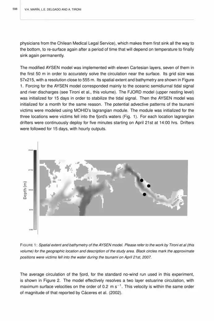
V.H. MARIN, L.E. DELGADO AND A. TIRONI
physicians from the Chilean Medical Legal Service), which makes them first sink all the way tothe bottom, to re-surface again after a period of time that will depend on temperature to finallysink again permanently.
The modified AYSEN model was implemented with eleven Cartesian layers, seven of them inthe first 50 m in order to accurately solve the circulation near the surface. Its grid size was57x215, with a resolution close to 555 m. Its spatial extent and bathymetry are shown in Figure1. Forcing for the AYSEN model corresponded mainly to the oceanic semidiurnal tidal signaland river discharges (see Tironi et al., this volume). The FJORD model (upper nesting level)was initialized for 15 days in order to stabilize the tidal signal. Then the AYSEN model wasinitialized for a month for the same reason. The potential advective patterns of the tsunamivictims were modeled using MOHID’s lagrangian module. The module was initialized for thethree locations were victims fell into the fjord’s waters (Fig. 1). For each location lagrangiandrifters were continuously deploy for five minutes starting on April 21st at 14:00 hrs. Drifterswere followed for 15 days, with hourly outputs.
FIGURE 1: Spatial extent and bathymetry of the AYSEN model. Please refer to the work by Tironi et al (this
volume) for the geographic location and description of the study area. Black circles mark the approximate
positions were victims fell into the water during the tsunami on April 21st, 2007.
The average circulation of the fjord, for the standard no-wind run used in this experiment,is shown in Figure 2. The model effectively resolves a two layer estuarine circulation, withmaximum surface velocities on the order of 0.2 m s−1. This velocity is within the same orderof magnitude of that reported by Caceres et al. (2002).
598
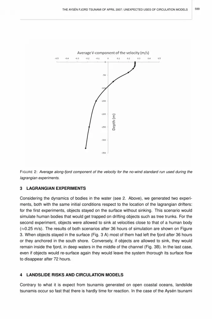
THE AYSEN FJORD TSUNAMI OF APRIL 2007: UNEXPECTED USES OF CIRCULATION MODELS
FIGURE 2: Average along-fjord component of the velocity for the no-wind standard run used during the
lagrangian experiments.
3 LAGRANGIAN EXPERIMENTS
Considering the dynamics of bodies in the water (see 2. Above), we generated two experi-ments, both with the same initial conditions respect to the location of the lagrangian drifters:for the first experiments, objects stayed on the surface without sinking. This scenario wouldsimulate human bodies that would get trapped on drifting objects such as tree trunks. For thesecond experiment, objects were allowed to sink at velocities close to that of a human body(≈0.25 m/s). The results of both scenarios after 36 hours of simulation are shown on Figure3. When objects stayed in the surface (Fig. 3 A) most of them had left the fjord after 36 hoursor they anchored in the south shore. Conversely, if objects are allowed to sink, they wouldremain inside the fjord, in deep waters in the middle of the channel (Fig. 3B). In the last case,even if objects would re-surface again they would leave the system thorough its surface flowto disappear after 72 hours.
4 LANDSLIDE RISKS AND CIRCULATION MODELS
Contrary to what it is expect from tsunamis generated on open coastal oceans, landslidetsunamis occur so fast that there is hardly time for reaction. In the case of the Aysen tsunami
599

V.H. MARIN, L.E. DELGADO AND A. TIRONI
A
B
FIGURE 3: Spatial distribution of lagrangian drifters for the first experiment, non-sinking drifters (A) and
the second experiment (sinking drifters) after 36 hours of simulation.
it took only 6 minutes for the waves to arrive at populated areas (SHOA 2007). Given thelocation of the landslide and the distribution of populated areas, victims were reduced only tothose standing on boats during the event. Although the Chilean government deployed a rathercostly operation in search of victims, none were found. Our lagrangian model results suggestthat the main reason for this is that just 36 hours after falling I the fjord’s waters, victims werealready far away from the main event sector.
Risk prevention seems to be the only solution in the face of landslide tsunamis, given its fastdynamics. After the April event, the Chilean government organized a group of experts onnumerical modelling, including ECOMANAGE scientists. The main task of this group was togenerate a prediction model to assess risk potential and likely responses in other sectors ofthe Aysen fjord. The results of that work were delivered to the government on August 2007(SHOA 2007). As a result of the studies conducted by ECOMANAGE and by other membersof ONEMI’s STC for Aysen, most parts of the inner fjord were declared as dangerous for
600

THE AYSEN FJORD TSUNAMI OF APRIL 2007: UNEXPECTED USES OF CIRCULATION MODELS
aquaculture. However, although human lives and whole farming facilities were lost, salmonfarmers soon started a lobby to reverse the decision of fjord closure for salmon farming.1
Thus, the main lesson from this experience is that numerical models, such as the ones devel-oped by ECOMANAGE on the Aysen fjord, may be important tools for risk assessment andto suggest strategies for local governments. Specially when confronted to decisions that mayaffect human lives. However, in the end these tools will be only one component in a complexset of components related to the development and security of coastal areas. Final decisionswill always be political!
REFERENCES
Caceres M, Valle-Levinson A, Sepulveda HH, Holderied K (2002) Transverse variability of flow and densityin a Chilean fjord. Continental Shelf Research 22: 1683-1698
Marın VH, Campuzano F (In press) Un modelo hidrodinamico-barotropico para los fiordos australes deChile entre los 41◦S y los 46◦S. Ciencia y Tecnologıa del Mar.
Marın VH, Tironi A, Paredes MA, Campuzano F (2008) The estuarine system of the Aysen fjord. Thisvolume.
SHOA (2007) Puerto Aysen, Puerto Chacabuco. Cartas de Inundacion por tsunami generado por remo-ciones en masa. Servicio Hidrografico y Oceanografico de la Armada de Chile. Valparaıso, Chile.60pp.
Tironi A, Marin VH, Campuzano F (2008) A management tool for salmon aquaculture: integrating MOHIDand GIS applications for local waste management. This volume.
1http://www.nuestromar.org/noticias/pesca_y_acuicultura10512_092007_chile_lobby_salmonero_intenta_reabrir_zona_sismica_del_fiordo_aysen
601


PERSPECTIVES ON INTEGRATED COASTAL ZONE MANAGEMENT IN SOUTH AMERICAR. NEVES, J.W. BARETTA AND M. MATEUS (EDS.), IST PRESS, 2008
FINAL REMARKS
M. MATEUS, J.W. BARETTA AND R. NEVES
This volume has drawn together contributions from a range of disciplines to address the chal-lenges and explore the opportunities for managing three very different coastal systems inSouth America: the Santos Estuary (Brazil), the Bahıa Blanca (Argentina) and the AysenFjord (Chile). We have looked at a wide range of coastal management scenarios in the var-ious geographical settings. But for all the differences, there are similar developments and acommon recognition of the conflicting uses of the coastal area. This was the main theme atall sites, and hence, the principal focus of this volume.
A range of views emerges from this volume on managing coastal zones. Coastal managersgenerally agree that a broad and integrated view of coastal systems is necessary to capturetheir complexity. However this perspective sometimes is in conflict with a more reductionistapproach to coastal sciences, which tends to concentrate on individual system componentsas such. While this approach can be very useful, if the component(s) studied are criticalto system function, integration most of the time is the key to understand the link betweensystem components and overall system function. Both approaches have been followed in thework developed during the ECOMANAGE project. Individual compartments of each systemwere studied and the knowledge gained was then used to gain a deeper understanding ofthe overall picture, where the complex feedbacks between man (socioeconomic features) andnature (ecological features) manifested themselves. The DPSIR framework has paved theway for this integrative approach.
A simple, yet fundamental lesson emerges from this book, connecting the local interest of de-velopment and economic growth with adequate management of the coastal resources. Socialwellbeing means achieving the equilibrium between physical as well as socioeconomic stabil-ity, which makes the management task all the more difficult. Attaining such demanding goalimplies minimizing the impacts of human occupation because they diminish or even destroyproductive uses of coastal areas, undermining their ability to provide human populations witha healthy natural environment. As we have shown, the functioning of ecosystems may be dis-turbed by a wide range of impacts and these, in turn, have direct and indirect repercussionson the socioeconomic structure of the area. Through a series of responses and/or adaptivemeasures, which may range from changing social habits, laws and policies to technologicalsolutions, humans attempt to prevent or lessen potentially destructive processes.
Despite the intrinsic complexity of these efforts, it is obvious that an assessment of the impactsof human activities on the system and the feedback mechanisms to the socioeconomy remainscentral to planning the use and development of coastal zones. And this is why the plans andpolitics for land use and for the management of the water is a shared responsibility betweenscientists, civil servants, politicians, stakeholders and NGO’s. Coastal management is anintegrating concept. The diverse group of people involved in this project has embraced the
603

M. MATEUS, J.W. BARETTA AND R. NEVES
concept of a multidisciplinary approach, its value to society, and especially as a way of makingtheir knowledge more relevant to coastal managers and stakeholders.
Hard decisions need to be made in both short- and long-term management of the three sys-tems addressed in this volume. The complex interactions between the various subsystems ineach case make such decisions particularly difficult. In face of this complexity, those involvedin the management of these areas need to promote a continuing vision of the coast againstwhich to plan both the immediate and the gradual development of the system. Certainly thiswill lead to difficult but fundamental choices and decisions in order to achieve the sustainablephysical, social and economic development of the region.
This volume suggests that a critical lesson to be drawn for ICZM is that management decisionsmust be based on the understanding of the coastal system in a dynamic and holistic frame-work. It has been important to us to ensure that scientific approaches and models contributeto understand the integrated nature of coastal areas at multiple scales, and are available tosupport all levels of decision making for integrated management. This is the rationale behindthe major effort devoted to the modelling of the three systems.
Fundamental understanding of the behavior of many components of each study site has beenput forward in this volume by both physical and social scientists. However, integrating thisdisparate knowledge into understanding of the dynamics of each system and to apply it toachieve tangible outcomes for coastal management are still major challenges. Assuming thatgood decisions in coastal zone management emerge from detailed knowledge on the func-tioning of those areas, our goal has been encapsulating this knowledge in an integrative andcomprehensive way. Achieving proper management policies is a moving target because thedrivers change and, consequently, the pressures, state and impacts. As such, a continuousadaptation of management strategies is a necessity in order to optimize responses to thesechanges. While this also requires a continuous research effort and long-term study programs,we hope to have kick-started this on-going process with the work developed during the 3-yearECOMANAGE project.


