Porosity and permeability prediction from wireline logs using artificial neural networks: a North Sea case study

Geophysical Prospecting, 2001, 49, 431±444

Porosity and permeability prediction from wireline logs using artificial

neural networks: a North Sea case study

Hans B. Helle,1* Alpana Bhatt1,2 and Bjùrn Ursin2

1Hydro E&P Research Centre Bergen, Sandsliveien 90, 5049 Sandsli, Norway, and 2Norwegian University of Science and Technology,Department of Petroleum Engineering and Applied Geophysics, 7491 Trondheim, Norway

Received June 2000, revision accepted March 2001

A B S T R A C T

Estimations of porosity and permeability from well logs are important yet difficult

tasks encountered in geophysical formation evaluation and reservoir engineering.

Motivated by recent results of artificial neural network (ANN) modelling offshore

eastern Canada, we have developed neural nets for converting well logs in the North

Sea to porosity and permeability. We use two separate back-propagation ANNs (BP-

ANNs) to model porosity and permeability. The porosity ANN is a simple three-

layer network using sonic, density and resistivity logs for input. The permeability

ANN is slightly more complex with four inputs (density, gamma ray, neutron

porosity and sonic) and more neurons in the hidden layer to account for the increased

complexity in the relationships. The networks, initially developed for basin-scale

problems, perform sufficiently accurately to meet normal requirements in reservoir

engineering when applied to Jurassic reservoirs in the Viking Graben area. The mean

difference between the predicted porosity and helium porosity from core plugs is less

than 0.01 fractional units. For the permeability network a mean difference of

approximately 400 mD is mainly due to minor core-log depth mismatch in the

heterogeneous parts of the reservoir and lack of adequate overburden corrections to

the core permeability. A major advantage is that no a priori knowledge of the rock

material and pore fluids is required. Real-time conversion based on measurements

while drilling (MWD) is thus an obvious application.

I N T R O D U C T I O N

Porosity and permeability are the key variables in character-

izing a reservoir and in determining flow patterns in order to

optimize the production of a field. Reliable predictions of

porosity and permeability are also crucial for evaluating

hydrocarbon accumulations in a basin-scale fluid-migration

analysis and to map potential pressure seals in order to

reduce drilling hazards.

Several relationships have been offered which can relate

porosity to wireline readings, such as the sonic transit time

and density logs. However, the conversion from density and

transit time to equivalent porosity values is not trivial. The

common conversion formulae contain terms and factors that

depend on the individual location and lithology, e.g. clay

content, pore-fluid type, grain density and grain transit time

for the conversion from density and sonic logs, respectively,

that in general are unknowns and thus must be determined

from rock sample analysis.

Permeability is also recognized as a complex function of

several interrelated factors such as lithology, pore-fluid

composition and porosity. Thus, permeability estimates

from well logs often rely upon porosity, e.g. through the

Kozeny±Carman equation, which also contains adjustable

factors such as the Kozeny constant, which varies within the

range 5±100 depending on the reservoir rock and grain

q 2001 European Association of Geoscientists & Engineers 431

Paper presented at the 61st EAGE Conference ± GeophysicalDivision, Helsinki, Finland, June 1999.*E-mail: [email protected]

geometry (Rose and Bruce 1949). Nelson (1994) has given a

detailed review of these problems.

Motivated by recent results of artificial neural network

(ANN) modelling by Huang et al. (1996) and Huang and

Williamson (1997) applied to porosity and permeability

prediction from offshore Canada wireline data, we applied a

similar approach to data from the North Sea. The objective

here is thus not to propose a new method, but to develop

networks that are applicable to the area at hand. In this case

study we have developed networks using data from wells in

the Viking Graben. The networks were initially developed for

basin-scale pressure analysis in the northern Viking Graben,

which is an active area of exploration and production with

several producing fields implying access to core and wireline

data relevant for a basin-scale flow study.

While testing our networks on available core data from

hydrocarbon reservoirs in the area, we realized that the

prediction accuracy was sufficient to meet normal requirements

in reservoir engineering. Thus, to improve the capability of

the network to account for variations in reservoir fluid, we

added a few training facts from the gas- and oil-bearing

sections to the original training data set. We find that our

modified general Viking Graben neural nets display a better

performance for the main reservoir interval of an oilfield than

the specialized networks based only on local core data.

T H E L O G C O N V E R S I O N P R O B L E M

Geophysical well logs generally provide a better representa-

tion of in situ conditions in a lithological unit than laboratory

measurements because they sample a larger volume of rock

around the well and provide a continuous record. However,

as with most well-logging measurements, the sonic log does

not directly measure the parameter with which it has become

associated, i.e. the porosity, given by

fDt �Dtg ÿ Dt

Dtg ÿ Dtf; �1�

where Dtg and Dtf are the sonic transit times of the grain

material and pore fluid, respectively, and Dt is the bulk transit

time (Wyllie, Gregory and Gardner 1956).

Similarly, the porosity from bulk density log values r

requires that the grain density rg and fluid density r f be

known quantities, i.e.

fr ��rg ÿ r��rg ÿ rf�

´ �2�

As demonstrated in studies by, for example, Vernik (1997) of

the compressional-wave velocity in consolidated siliciclastics,

these can be subdivided into a number of major petrophysical

groups according to their clay content, and a consistent

velocity±porosity transform can be established for each

group. From ultrasonic measurements on brine-saturated

samples, Klimentos (1991) has provided an empirical formula

relating the compressional velocity to porosity f (volume

fraction) and clay content Cl (volume fraction) by

V P �in km=s� � 5:87 2 6:99f ÿ 3:33Cl: �3�

It thus seems obvious that no single log measurement is

sufficient to obtain reliable values of porosity. Additional

data would be required from the pore fluid and grain

material, which normally are not at hand except for special

studies in cored reservoir intervals. This is shown in Fig. 1

where we have combined wireline readings of sonic velocity

Figure 1 (a) Empirical velocity-to-porosity transform obtained from

linear regression by combining logs (sonic, density) and laboratory

data (grain density, clay content and total organic carbon) from the

northern Viking Graben. The porosity is obtained from the density

using equation (2). A change of 50% (vol.) in the clay content Cl has

approximately the same effect on VP as a change of 10% (vol.) in the

total organic content TOC as indicated by the arrow. (b) By

accounting for Cl and TOC the velocity±porosity transform may be

significantly improved. The result from equation (3) of Klimentos

(1991) is shown for comparison.

432 H.B. Helle et al:

q 2001 European Association of Geoscientists & Engineers, Geophysical Prospecting, 49, 431±444

and laboratory data of grain density rg. A more consistent

velocity±porosity transform can clearly be obtained if the

clay content is taken into account. Moreover, by including the

total organic content TOC as the third independent variable

we have demonstrated that the linear least-squares fit can be

further improved. However, these relationships are of limited

practical value because they require the clay content and

organic content to be accurately estimated, which is hard to

do in practice, given the limitations in the semi-empirical

relationships based on the gamma-ray and resistivity logs.

The example of an extended laboratory analysis of samples

from core plugs and cuttings shown in Fig. 2 demonstrates

the sensitivity of the gamma-ray log readings to variations in

the total organic content TOC in a North Sea well. A

correlation between clay content and the gamma ray is clearly

seen. On the other hand, a pronounced peak in the gamma

ray coincides with the peak values of the TOC in the

Kimmeridge Clay Formation, showing that the gamma ray

also has a strong response to petrophysical variables other

than the clay content. Again, this demonstrates that a single

log cannot by itself resolve a petrophysical property.

Alternatively, a suite of different logs in combination may

be used to quantify a given petrophysical property provided

its relationship to the log readings can be established. Except

for the unknown values of grain material and fluid proper-

ties, the porosity can be expressed by linear functions of sonic

transit time (equation (1)) and bulk density (equation (2)).

Because the sonic and density logs respond differently to the

fluid and grain material, and since they constitute indepen-

dent measurements of the same property, a combination of

the two may improve the accuracy compared with that of the

log-to-porosity transform based on sonic or density alone.

Moreover, by adding the resistivity to the suite of logs, the

accuracy of the porosity transform may be further improved

since resistivity is normally the best indicator for the type of

pore fluid. In the following sections we demonstrate that the

sonic, density and resistivity combined into an artificial

neural network provide accurate porosity estimates for any

combination of grain material and pore fluid.

While porosity is fairly linearly related to the sonic and

density readings, the common permeability transforms

indicate non-linear relationships between permeability and the

same physical measurements. As predicted from the Kozeny±

Carman relationship, the permeability can be expressed by

k � Bf3d2

t; �4�

where B is a geometrical factor, d denotes a characteristic

grain or pore diameter and t denotes the tortuosity. The

additional dependence on the rock texture, the pore shape

and its distribution, along with the clay content, indicates

that the relationship between log readings and permeability is

more complicated than that for porosity and, moreover, that

additional physical measurements are required to represent

its value. Because permeability of natural sediments is a

tensor rather than a scalar property, anisotropy may further

complicate the permeability transform in boreholes that are

not normal to the bedding.

Commonly used empirically derived equations are of the

form (Wyllie and Rose 1950),

k � Bf x

Syv

; �5�

which is similar to the Kozeny±Carman relationship (4),

where Sv is the irreducible water saturation and the

parameters B, x and y are determined from data, usually

Figure 2 A typical set of laboratory data used in this study. To some

extent the gamma ray reflects the clay content. Notice, however, the

strong response in the gamma ray to high values of TOC in the

Kimmeridge Clay Formation (a) and the large range of grain density

variations (b) due to the mixture of the light kerogen (rk < 1.4 g/

cm3) and the heavier clay material (rm < 2.77 g/cm3).

Pore±perm prediction by neural nets 433


from a log(k)±f diagram. In many cases relationships

between permeability and porosity may exist. Schlumberger

(1989) provided various published forms of (5).

In the following sections we show that accurate conversion

from well logs to permeability can be obtained by using the

neural network alternative rather than the semi-empirical

transforms. As is apparent from the above discussion, a more

complex network may be required for permeability compared

to that of the porosity network.

B A C K - P R O PA G AT I O N N E U R A L N E T W O R K S

The back-propagation artificial neural network (BP-ANN) is

a relatively new tool in petroleum geoscience, which is

gradually being introduced into several practical applications

including seismic analysis. It simulates the cognitive process

of the human brain and is well suited for solving difficult

problems, such as character recognition, which are not

amenable to conventional numerical methods (Lawrence

1994; Patterson 1996; Haykin 1999). The ANN functions

as a non-linear dynamic system that learns to recognize

patterns through training. The network (Fig. 3) has two

major components: nodes (or neurons) and connections

(which are weighted links between the neurons). Upon

exposure to training examples (patterns), the neurons in an

ANN compute the activation values and transmit these values

to each other in a manner that depends on the learning

algorithm being used.

The learning process of the BP-ANN involves sending

the input values forward through the network, and then

computing the difference between the calculated output and

the corresponding desired output from the training data set.

This error information is propagated backwards through the

ANN and the weights are adjusted. After a number of

iterations the training stops when the calculated output

values best approximate the desired values. The similarities

between BP-ANN and the common geophysical inversion

techniques are obvious.

The ANN approach has several advantages over conven-

tional statistical and deterministic approaches. The most

important one is that it is free from the constraints of a

certain function form. Here, we do not consider procedures,

rules or formulae, only what kinds of input data the neural

network can use to make an association with the desired

output. Moreover, in contrast to linear regression models, the

ANN approach does not force predicted values to lie near the

mean values and thus it preserves the actual variability in the

data (Rogers et al. 1995). A detailed comparison by Huang

et al. (1996) of permeability prediction by BP-ANN with

those of conventional multiple linear regression (MLR) and

multiple non-linear regression (MNLR) techniques clearly

favours the BP-ANN approach.

There are two questions in neural network design that have

no precise answer because they are application-dependent:

1 How much data do we need to train the network?

2 What is the best number of hidden neurons to use?

In general, the more facts and the fewer hidden neurons

there are, the better. There is, however, a subtle relationship

between the number of facts and the number of hidden

neurons. Too few facts or too many hidden neurons can cause

the network to memorize, implying that it performs well

during training, but tests poorly and fails to generalize.

There are no rigorous rules to guide the choice of the

number of hidden layers and the number of neurons in the

hidden layers. However, more layers are not better than few,

and it is generally known that a network containing few

hidden neurons generalizes better than one with many

neurons (Lawrence 1994). For instance, if the relationship

between input and output is known to be almost linear, we

may emulate the linear regression by choosing the number of

independent connections, i.e. neuron weights, equal to the

number of independent coefficients in the regression equa-

tion. Then, a few neurons may be added to the hidden layer in

order to account for non-linearity between input and output.

On the other hand, the optimal combination can only be

achieved by testing and by learning through experience with

the data and problems at hand.

Figure 3 Architecture of a BP-ANN with four nodes in the input

layer, seven nodes in the hidden layer and only one node in the output

layer. The symbols W1i,2j and W2k,3l are the weights connecting the

input and hidden layers, and the output and hidden layers,

respectively. The two networks used in this study have the same

architecture but differ in the number of hidden neurons, i.e. seven

neurons in the porosity network and 12 in the permeability network.



T H E P O R O S I T Y N E T W O R K

For the porosity network we used the architecture as shown

in Fig. 3 but with only three neurons in the input layer, i.e.

density, sonic and resistivity. A single hidden layer has seven

neurons and the output layer has only one neuron (porosity).

The sources of training data for the porosity network are

summarized in Table 1. Training facts are dominated by non-

reservoir intervals from Tertiary to Jurassic levels. The

majority of the porosity values are based on grain density

laboratory measurements and bulk densities from wireline

data (Lucas 1998). These data were carefully selected to

obtain a range of values appropriate for most sediments in

the Viking Graben (Bhatt 1998) for use in a basin-scale fluid-

flow analysis. Tests of this network reveal excellent overall

characteristics when applied to the entire geological section

(Fig. 4) as well as in the fine details of a water-bearing

reservoir (Fig. 5).

The main advantage of using porosity derived from the

density measurements is the fact that these are the best

possible estimates of in situ porosity values since the

compressibility of the pure grain material is likely to be

small compared with that of the matrix. The grain density in

the laboratory is thus not very different from in situ values,

and hence the porosity estimates are less prone to pressure

corrections than those based on core plugs (Fig. 6a). On the

other hand, the comparison made between predictions and

core helium porosity reveals striking similarities (Fig. 5),

indicating that core and well data may be fairly consistent.

For the initial network the pore fluid was assumed to be

brine of density 1.03 g/cm3 since no samples were taken from

hydrocarbon-bearing sections. In order to adjust the initial

network to account for the various pore fluids, we added a

few data points taken from hydrocarbon reservoirs. The

training patterns cover the porosity range 0.02±0.55

(Fig. 7a). From a total of 81 facts only 14 facts are taken

from the main test area (Q-field). The capability of the

resulting modified network to account for different pore

fluids can be appreciated in Figs 8 and 9. Here we compare

the porosity predicted by ANN with those predicted by the

density±porosity transform (equation (2)) using a constant

grain density rg � 2.64 g/cm3 and with fluid densities r f of

0.25, 0.75 and 1.03 g/cm3 for gas, oil and brine, respectively.

The corresponding porosity transforms fr as shown in Fig. 8

reveal strong sensitivity to the pore-fluid density, with

differences of 0.1±0.15 fractional units between the results

of assuming brine- versus gas-filled rock. Because of the

strong response to pore fluid in fr the common procedure

Table 1 Selection of facts for the porosity network

Well No. of facts Porosity range (%) Comments

T-1 23 5±46 Grain and bulk density (Lucas 1998)

T-2 42 25±43 Grain and bulk density (Lucas 1998)

F-4 2 49±55 Grain and bulk density (Bhatt 1998)

Q-20 10 24±27 From the gas zone. Core helium porosity

Q-22 1 23 High resistivity data. Core helium porosity

Q-23 3 24±26 High resistivity data. Core helium porosity

Figure 4 (a) A test of porosity prediction by ANN in well S and (b) a

cross-plot of measured (from bulk and grain density) versus predicted

porosity reveal consistent results. The test data are unknown to the

network. Density, resistivity and sonic logs are the inputs.



implies correction for mixed saturation of pore fluids. An

additional correction term for clay content (Schlumberger

1989) and a variable rg are normally included to improve the

accuracy of the transform, implying the need for additional core

data and input from log interpretation to obtain a measure

of shaliness from the gamma-ray log. However, in the neural

net approach, only log data are required once the network

has been properly tuned to the area and reservoir at hand.

In general, there is a good fit between the porosity

predicted by ANN (fANN) and the corresponding fr . For

the water-bearing reservoir (Figs 8a and 9a), the two

predictions are practically coincident and comply very well

with the helium core porosity within a mean difference

Figure 5 The porosity network trained for basin-scale prediction

(Fig. 4) also performs excellently in details when tested against

helium core porosity data from a reservoir.

Figure 6 Relative changes in (a) helium porosity and (b) water

permeability as a function of confining pressure for a selection of

rock samples from a special core analysis study of well Q-0. Values of

helium core porosity and Klinkenberg-corrected air permeability at

atmospheric pressure are provided.

Figure 7 Histograms displaying the distri-

bution of facts for (a) the porosity and (b)

the permeability networks used in this study

(see Tables 1 and 2). The porosity facts are

based on grain density measurements and

hence are independent of pressure. Klinken-

berg corrections have been applied to the

permeability data.



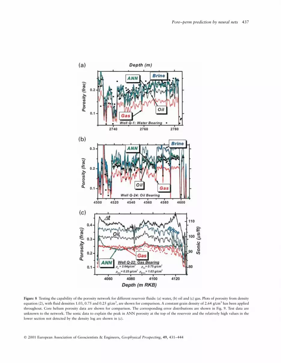
Figure 8 Testing the capability of the porosity network for different reservoir fluids: (a) water, (b) oil and (c) gas. Plots of porosity from density

equation (2), with fluid densities 1.03, 0.75 and 0.25 g/cm3, are shown for comparison. A constant grain density of 2.64 g/cm3 has been applied

throughout. Core helium porosity data are shown for comparison. The corresponding error distributions are shown in Fig. 9. Test data are

unknown to the network. The sonic data to explain the peak in ANN porosity at the top of the reservoir and the relatively high values in the

lower section not detected by the density log are shown in (c).



(fcore 2 fANN) of approximately 0.01 and a standard

deviation of approximately 0.015 based on the 155 core

samples from well Q-1. Similar conclusions are valid for the

oil-bearing reservoir (Figs 8b and 9b) using 96 core samples

from well Q-24. In the gas-bearing reservoir (Figs 8c and 9c),

particularly near the shale±sand transition at the top of the

reservoir interval, there is peak in fANN, which is not present

in the core or the density porosity. While the density is

virtually constant, the sonic reveals distinct peaks at the top

and bottom of the reservoir. This feature has been observed in

several of the wells in the Q-field and is thus considered to be

a real low-velocity event. In most cases observed, the density

log responds to this transition and, moreover, core plugs from

the zone normally reflect its high porosity. Thus, in this case,

Figure 9 As Fig. 8, with plots of the differ-

ence between helium core porosity and the

porosity values predicted from the neural

network (fcore 2 fANN). The difference

(fr 2 fANN) between the porosity pre-

dicted from the density equation (2) and

the neural net is shown for comparison. The

mean error is approximately 0.01 with a

standard deviation of less than 0.02 porosity

fractions. Test data are unknown to the

network.



the ANN prediction based on input from three logs compares

less favourably with the helium core porosity than that from

density alone.

T H E P E R M E A B I L I T Y N E T W O R K

While porosity is a scalar quantity, the rock permeability is a

tensor owing to the directional alignment of the pore

structure of natural sediments. Even in the reservoir rocks

at hand, we find that the ratio of in-bedding to normal-

bedding permeability may be one to two orders of magnitude.

Since logging tools are confined to the direction of the drill

bore, it is expected that the log readings are affected by

anisotropy to various degrees, depending on the drilling

angle.

The permeability of the core plugs is normally measured at

atmospheric pressure using air, and the Klinkenberg correc-

tion is subsequently applied to convert to equivalent fluid

permeability. Standard core permeability data thus represent

values at the surface while logs are obtained at in situ

conditions in the reservoir, where the confining pressures are

more than 200 bars. Compression of the rock changes the

pore and the pore-throat-size distribution. Changes in the

pores may increase the tortuosity and close some of the fluid-

flow paths. At the surface the permeability of a core sample

may be overestimated by a factor of two compared with its

in situ value.

In the initial study we attempted to overcome the problems

of permeability anisotropy by restricting the selection to

vertical wells and in-bedding permeability (kh). However, we

find that the variations in the permeability anisotropy are

confined to a much smaller scale (,0.1 m) than the spatial

resolution of the logging tools (,1 m) and thus anisotropy

variations appear to have less impact on the log readings than

expected.

Correction for the pressure effects is a more difficult

problem, which cannot be solved within the present industry

practice where only a small number of core samples from a

field is used for investigating the effect of overburden

pressure. Moreover, there is no obvious procedure to convert

air-permeability data at atmospheric pressure to fluid-

permeability data at in situ conditions. The results of a

special core analysis study shown in Figs 6 and 10 may

be indicative of the general trend, but they cannot be used

to establish a generally valid function to convert air±water

permeability at the surface to fluid permeability at

depth. While the porosity at low effective pressure may be

overestimated by 5±15% (Fig. 6a), the corresponding perme-

ability data may have errors of 20±100% (Fig. 6b) depending

on the rock texture and history of the individual sample.

For the permeability network we used the same general

Figure 10 Water permeability for a range of confining pressures

versus Klinkenberg-corrected air permeability at atmospheric pres-

sure, based on the special core analysis data on 11 core plugs from

well Q-0.

Table 2 Selection of facts for the permeability network

Well No. of facts Porosity range (%) Permeability range (kh) Comments

Q-11 44 3±34 34 mD212 D Air permeability. Core plugs

P-10 140 5±32 35 mD21.7 D Air permeability. Core plugs

H7-1 1 8.5 5 nD Water permeability (Krooss et al. 1998)




H3-1 2 2.5 0.5 nD20.8 nD Water permeability (Krooss et al. 1998)

Q-20 5 24±27 1.6 D26.3 D From the gas zone. Air permeability. Core plugs



architecture as above, with four input neurons (density,

gamma ray, neutron porosity and sonic), 12 neurons in a

single hidden layer and a single neuron (permeability) in the

output layer. The sources of training data for the permeability

network are summarized in Table 2. Most of the training

facts are conventional Klinkenberg-corrected air-permeability

measurements on core plugs. In order to tune the initial

network for basin-scale applications (Bhatt 1998), a few

samples of low-permeability shale data taken from the study

of Krooss, Burkhardt and SchloÈmer (1998) were added.

While the porosity network is based on samples from both

the Tertiary and the Jurassic, all training facts for the

permeability network are confined to cored sections from the

upper Jurassic. As can be seen from Table 2, the permeability

data are dominated by wells outside the test field (Q-field),

and the majority of facts (70%) are from a different field in

the same area (P-field).

By adding the six low-permeability shale points in the

range 0.5±39 nD to the standard core analysis permeability

Figure 11 Comparison of (a) porosity and (b) permeability predic-

tions with core data in well Q-4. Depths of large scatter in the core

data coincide with a fine-layering sequence seen in the cores but not

properly resolved by the logging tools. The reservoir is oil-bearing.

The hole deviation is 0±18. Fine-layering heterogeneity in the lower

part of the reservoir is clearly expressed in the core data and partly

expressed by the variability in the sonic (c) which has best spatial

resolution (1±2 ft). The corresponding variability in the density log is

less pronounced. Grain density is shown for comparison.


tions with core data in well Q-2. Calcite-cemented layers are well

expressed by low values of porosity and permeability. The reservoir is

oil-bearing and the hole deviation is 1±28.



in the range 34 mD212 D (Fig. 7b), we have covered most

sediments within the prospective depths in the Viking

Graben. Since most of the facts included in the initial

network were taken from water- and oil-bearing rocks, we

added a few points from a gas-bearing interval (of Q-20) to

cover the complete range of reservoir fluids.

E R R O R S I N C O R E D ATA

Enforcing the same measurement conditions for laboratory

and log data requires core data obtained under simulated

reservoir conditions. The industry practice, however, is to use

core data measured at ambient conditions to calibrate log

data measured in situ. This practice, which is sometimes

necessary for financial reasons or because of technical

shortcomings, is scientifically unsatisfactory.

When core and wireline data are combined to establish the

networks for quantitative prediction of petrophysical quan-

tities such as porosity and permeability, we should keep in

mind possible errors in the data. While the wireline tools

measure properties in situ at elevated temperature and

pressure, the core data are normally obtained in the

laboratory at room conditions. In particular, cores collected

at great depths are exposed to mechanical deformation and

microcracking that significantly increases the surface values

of permeability and porosity compared with those in situ. We

may also expect significant scatter in the porosity and

permeability data since the mechanical impact may differ

for individual rock samples due to different composition and

sampling history of the core plug. As shown in Fig. 6, the

changes with pressure are particularly strong at pressures

approaching atmospheric pressure when the microcracks

tend to open. The porosity and permeability versus pressure

curves are similar for the majority of the core samples while a

few are highly offset from the average curve, indicating that

the large amount of scatter in surface values of porosity and


tions with core data in well Q-24. The reservoir is oil-bearing and the

hole deviation is 54±608.


tions with core data in well Q-20. There is a gas/oil contact at

3198 m. The hole deviation is 38±428.



permeability may be due to the different pressure effects on

the individual core plugs. While the general trend for

permeability (Fig. 10) reveals that highly permeable rocks

are more prone to pressure effects than less permeable rocks,

one of the samples shown in Fig. 6(b) demonstrates the

opposite behaviour. A local or generally valid pressure

correction formula is thus not easy to establish. On the

other hand, since the air-to-water-permeability conversion

seems to be a strong function of permeability itself, some of

the scatter observed in the permeability data could obviously

be removed by presenting water permeability at reservoir

pressure instead of air permeability at atmospheric pressure.

From the results in Fig. 10 we find, for example, that an air

permeability of 10 D at atmospheric pressure reduces by

40% to a water permeability of 6 D at 200 bars, while for a

100 mD sample the corresponding reduction amounts to only

15% (85 mD). The scatter in the data, however, is too high to

accept the corresponding empirical formula for pressure

Figure 15 Histograms and cross-plots dis-

playing the difference between values

obtained from core measurements and the

output from the neural nets for well Q-20

(Fig. 14).

Table 3 Summary of core±ANN comparison of porosity and permeability

f core ± fANN Kcore ± KANN

Well Mean s Mean s (mD) Hole angle (8) Pore fluid Comments

Q-1 0.007 0.015 2454 1038 1±2 W

Q-2 20.011 0.065 2222 769 1±2 O

Q-4 20.001 0.027 116 2414 1±2 O

Q-22 20.011 0.019 1311 1426 63 G 1 training fact porosity

Q-23 20.001 0.024 79 780 29±30 O 3 training facts porosity

Q-20 0.002 0.018 2578 2192 38±42 G/O 10 porosity, 5 permeability

Q-24 20.014 0.015 2318 816 54±60 O



corrections. Thus, to avoid introducing erroneous overburden

corrections to the core data we have, in this study, used

the raw Klinkenberg permeability supplied by the core

laboratory. However, the problem is of significant practical

importance and hence should be investigated further.

E R R O R S D U E T O R E S O L U T I O N A N D

S PAT I A L S A M P L I N G

Worthington (1991) provided a review of the problems

encountered when comparing downhole and core measure-

ments. As with any attempt at combining well logs and core

data, shifts between recorded well-log depths and sample

depths are possible for a number of reasons. While every

attempt is made to remove these depth shifts, undetected

depth shifts could cause significant errors in porosity and

particularly in the permeability predictions.

The spatial scale of the well-log measurements is not

equivalent to that of the rock sample measurements. Well-log

measurements are more spatially averaged than core data.

Permeability and porosity measured from cores are repre-

sentative of only a small rockmass, while a single well-log

reading is a composite result of petrophysical properties

within a radius of a few centimetres to several metres,

depending on which tool is being used. Small-scale hetero-

geneity between core samples a few centimetres apart may

not be resolved at all by well logs.

Due to strong heterogeneity in petrophysical properties,

and the anisotropic nature of permeability in most natural

rocks, it is often difficult to define a characteristic volume

that is suitable for numerical calculations. We must keep in

mind that a measured value can serve as an estimate of the

property over a small interval. Errors in well-log data are

caused by poor borehole conditions. Washout, caving,

abnormal mudcake, etc. are all capable of adversely affecting

well-log responses.

N E U R A L N E T P R E D I C T I O N S A N D

C O M PA R I S O N W I T H C O R E D ATA

While most of the data used for the network design are taken

from various wells in an extended area of the northern Viking

Graben, we tested the networks on conventional data from

an oilfield. The results of the neural network predictions in

the cored reservoir intervals are presented below. Results for

a selection of wells are displayed in Figs 11±15, and a

summary of the error analysis for seven wells with various

reservoir fluids and hole deviations is given in Table 3.

In general the error distribution fits the normal distribu-

tion. Therefore, the mean values and the standard deviations

presented here are those of the Gaussian model. Cross-plots

(Fig. 15) are less meaningful since the data in the present

situation are dominated by samples in the good reservoir

section, with only a few values from low-porosity and low-

permeability rocks. For the seven wells listed in Table 3, the

average mean porosity difference (fcore 2 fANN) between

the core data and the predictions is less than 1% porosity

units, with a minimum of 0.1% for well Q-4 (Fig. 11) and

maximum of 1.4% for well Q-24 (Fig. 13; see also Figs 8b

and 9b). The average standard deviation in porosity is 2.7%,

with a minimum of 1.5% in Q-1 and Q-24 and maximum of

6.5% in Q-2 (Fig. 12).

For permeability the differences (Kcore 2 KANN) are more

significant, with a minimum of 79 mD for Q-23 and a

maximum of 1311 mD for well Q-22. The average standard

deviation in the permeability of about 1350 mD reflects the

large amount of scatter in the core permeability data and the

limited spatial resolution of the logging tools as discussed

above. In particular, there is significant small-scale hetero-

geneity in the lower section of the reservoir as can be seen

from the scatter in the core data. However, this feature is less

apparent in log data, except for the sonic and density logs as

shown in Fig. 11, where a marked increase in the amplitude

of short-length variations coincides with intervals where core

data exhibit maximum scattering.

While the main reservoirs of the wells Q-4 and Q-20

(Figs 11 and 14) look fairly homogeneous in terms of log

responses, the corresponding intervals of Q-2 and Q-24

(Figs 12 and 13) are clearly interbedded by calcite-cemented

layers of detectable thickness, where the predictions repro-

duce the core data with reasonable accuracy. Thinner beds

not detected by the logs are also present in the well as

indicated by the presence of core plugs with low values of

porosity and permeability. Obviously, these core plugs taken

near the bed boundaries contribute most to the errors given in

Table 3.

C O N C L U S I O N

The neural network approach to porosity and permeability

conversion has a number of advantages over conventional

methods. These include empirical formulae based on linear

regression models or the common semi-empirical formulae,

such as Wyllie's equation and the density equation for

porosity conversion, and the Kozeny±Carman equation for

permeability conversion. The neural net method represents a



pragmatic approach to the classical log conversion problem

that over the years has caused problems to generations of

geoscientists and petroleum engineers. Instead of searching

for complicated interrelationships between geological/

geophysical properties, the neural net approach requires no

underlying mathematical model and no assumption of

linearity among the variables.

The main drawback of the method is the amount of effort

required to select a representative collection of training facts,

which is common for all models relying on real data, and

the time to train and test the network. On the other hand,

once established the application of the network requires a

minimum of computing time.

For the porosity network we find that porosity values from

grain density and in situ bulk density data give more

consistent results than using standard helium core porosity

data. For the permeability network we normally have no

other alternatives than air permeability from core plugs and

the network will thus inherit the limitations embedded in the

method.

Our porosity predictions are sufficiently accurate to satisfy

most practical needs. Their accuracy is comparable with that

obtained from the density equation. The network approach,

on the other hand, requires no a priori knowledge of the grain

material and pore fluid, and can thus equally well be applied

while drilling without prior petrophysical evaluation.

In addition, our permeability predictions are sufficiently

accurate for most practical purposes, given the limitations

due to the spatial resolution of the logging instruments

and the expanded range covered by the permeability values.

Application to real-time data (MWD) is the obvious

extension of this technique.

A C K N O W L E D G E M E N T S

The work leading to the neural networks used in this study

was partly supported by the European Union under the

project `Detection of overpressure zones by seismic and well

data'. We thank S. Hansen, B. Farrelly and J. Okkerman for

important technical comments. We are particularly grateful

to the two anonymous reviewers for many detailed correc-

tions and comments that improved the clarity of the

manuscript.

R E F E R E N C E S

Bhatt A. 1998. Porosity, permeability and TOC prediction from well

logs using a neural network approach. MSc thesis, NTNU,

Trondheim.

Haykin S. 1999. Neural Networks: A Comprehensive Foundation.

Prentice-Hall, Inc.

Huang Z., Shimeld J., Williamson M. and Katsube J. 1996.

Permeability prediction with artificial neural network modelling

in the Venture gas field, offshore eastern Canada. Geophysics 61,

422±436.

Huang Z. and Williamson M.A. 1997. Determination of porosity and

permeability in reservoir intervals by artificial neural network

modelling, offshore eastern Canada. Petroleum Geoscience 3,

245±258.

Klimentos T. 1991. The effect of porosity±permeability±clay content

on the velocity of compressional waves. Geophysics 56, 1930±

1939.

Krooss B.M., Burkhardt M. and SchloÈmer S. 1998. Permeability

and petrophysical properties of mudrocks from Haltenbanken

area offshore Norway. Report 501398, Institut fuÈ r ErdoÈ l und

Organische Geochemie, JuÈ lich, Germany.

Lawrence J. 1994. Introduction to Neural Networks: Design, Theory

and Applications. California Scientific Software Press.

Lucas A. 1998. An assessment of linear regression and neural

network methods of porosity prediction from well logs. MSc thesis,

University of Reading.

Nelson P.H. 1994. Permeability±porosity relationships in sedimen-

tary rocks. Log Analyst 3, 38±62.

Patterson D.W. 1996. Artificial Neural Networks: Theory and

Applications. Prentice-Hall, Inc.

Rogers S.J., Chen H.C., Kopaska-Merkel D.C. and Fang J.H. 1995.

Predicting permeability from porosity using artificial neural

networks. AAPG Bulletin 79, 1786±1797.

Rose W. and Bruce W.A. 1949. Evaluation of capillary character in

petroleum reservoir rock. Petroleum Transactions, AIME 186,

127±142.

Schlumberger 1989. Log Interpretation: Principles and Applications.

Schlumberger Educational Services, Houston.

Vernik L. 1997. Predicting porosity from acoustic velocities in

siliciclastics: a new look. Geophysics 62, 118±128.

Worthington P.F. 1991. Reservoir characterization at the mesoscopic

scale. In: Reservoir Characterization II (eds L.W. Lake et al.), pp.

123±165. Academic Press, Inc.

Wyllie M.R.J., Gregory A.R. and Gardner L.W. 1956. Elastic wave

velocities in heterogeneous and porous media. Geophysics 21, 41±

70.

Wyllie M.R.J. and Rose W.D. 1950. Some theoretical considerations

related to the quantitative evaluation of the physical characteristics

of reservoir rock from electrical log data. Journal of Petroleum

Technology 189, 105±118.



Documents

Porosity and permeability prediction from wireline logs using artificial neural networks: a North Sea case study