poverty alleviation versus social insurance systems: a

POVERTY ALLEVIATION VERSUSSOCIAL INSURANCE SYSTEMS:

A COMPARISON OFLIFETIME REDISTRIBUTION

Jane Falkinghamand

Ann Harding

Discussion Paper No. 12

April 1996

National Centre for Social and Economic Modelling

• Faculty of Management • University of Canberra •

The National Centre for Social and Economic Modellingwas established on 1 January 1993, following a contractbetween the University of Canberra and the then federalDepartment of Health, Housing, Local Government andCommunity Services (now Health and Family Services).

NATSEM aims to enhance social and economic policydebate and analysis by developing high quality models,

applying them in relevant research and supplyingconsultancy services.

NATSEM’s key area of expertise lies in developing andusing microdata and microsimulation models for a rangeof purposes, including analysing the distributional impactof social and economic policy. The NATSEM models are

usually based on individual records of real (butunidentifiable) Australians. This base produces great

flexibility, as results can be derived for small subgroupsof the population or for all of Australia.

NATSEM ensures that the results of its work are madewidely available by publishing details of its products andresearch findings. Its technical and discussion papers areproduced by NATSEM’s research staff or visitors to thecentre, are the product of collaborative efforts with other

organisations and individuals, or arise fromcommissioned research (such as conferences). Discussionpapers present preliminary research findings and are only

lightly refereed.

It must be emphasised that NATSEM does not haveviews on policy and that all opinions are

the authors’ own.

Director: Ann Harding

National Centre for Social and Economic Modelling• Faculty of Management • University of Canberra •

POVERTY ALLEVIATION VERSUS

SOCIAL INSURANCE SYSTEMS:

A COMPARISON OF

LIFETIME REDISTRIBUTION

Jane Falkingham

and

Ann Harding

Discussion Paper No. 12

April 1996

iii

ISSN 1320 3398ISBN 0 85889 508 0

© NATSEM, University of Canberra 1996

National Centre for Social and Economic Modelling,GPO Box 563Canberra ACT 2601Australia

Phone: +61 6 275 4900 Fax: +61 6 275 4875E-mail: Client services [email protected]

General [email protected]

Core funding for NATSEM is provided by the federal Department ofHealth and Family Services.

iii

Abstract

Among other objectives, modern social security and taxation systemsseek to redistribute income from those with high to those with lowincomes and to reallocate income across the life cycle of individuals.While there are numerous studies of the extent to which these aims areachieved during a short period, such as a week or a year, there arealmost no studies of the lifetime redistributional impact of tax andtransfer systems.

In this paper, two broadly comparable dynamic cohort microsimulationmodels are used to assess the lifetime redistributional impact of theBritish and Australian social security and direct taxation systems. Theanalysis suggests that the Australian system, with its emphasis onpoverty alleviation, results in greater lifetime interpersonalredistribution than the British social insurance-based system.

iv

Authors’ note

Jane Falkingham is a lecturer in population studies in the Department ofSocial Policy at the London School of Economics and a ResearchAssociate of the Welfare State Program at the London School ofEconomics. Ann Harding is Professor of Applied Economics and SocialPolicy at the University of Canberra and inaugural Director of theUniversity’s National Centre for Social and Economic Modelling.

Acknowledgments

The authors would like to thank Steve Gribble of Statistics Canada fordetailed helpful comments on an earlier version of this paper. This is arevised version of a paper presented at the December 1993 InternationalAssociation for Research in Income and Wealth Special Conference onMicrosimulation and Public Policy in Canberra, and the authors wouldalso like to thank participants at that conference for their comments.

General caveat

NATSEM research findings are generally based on estimatedcharacteristics of the population. Such estimates are usually derivedfrom the application of microsimulation modelling techniques tomicrodata based on sample surveys.

These estimates may be different from the actual characteristics of thepopulation because of sampling and non-sampling errors in themicrodata and because of the assumptions underlying the modellingtechniques.

The microdata do not contain any information that enables identificationof the individuals or families to which they refer.

v

Contents

Abstract ....................iiiAuthors’ note .................... ivAcknowledgments .................... ivGeneral caveat .................... iv

1. Introduction ......................1

2. The models ......................32.1 Similarities ..........................3

2.2 Differences ..........................5

2.3 Caveats and qualifications ..........................6

3. The systems ......................83.1 The British social insurance system ..........................8

3.2 The Australian social assistance model ........................11

4. Lifetime redistribution: social insurance versuspoverty alleviation systems ....................13

5. Intrapersonal versus interpersonal redistribution ....................235.1 Financing from direct taxes ........................24

5.2 Financing from all taxes ........................28

6. Summary ....................29

References ....................34

1

1. Introduction

All modern social security systems serve two linked, but distinct, aims.On the one hand, they are an updated ‘Robin Hood’ mechanism fortransferring resources raised through taxation from those with highincomes to those with low incomes — termed interpersonal redistribution.On the other hand, they are also intended to transfer resources from thetime in life when incomes are relatively high to other times when theincomes of the same individuals are low — intrapersonal redistribution.

To date, most distributional analyses have focused on the first of theseaims, largely consisting of studies of the annual net fiscal incidence oftaxes and cash transfers (Central Statistical Office (UK) 1992; Harding1984; Saunders 1984). These studies thus examine the redistributionalimpact of government during a short period such as a week or a year.However, a very different distributional picture emerges when theeffects of social security and taxation are examined over lifetimes(Falkingham and Hills 1995; Harding 1993a; Nelissen 1993).

Social security systems can be broadly classified as:• social insurance-based systems, where individuals secure

entitlements to a range of income support payments because of theiridentifiable social insurance contributions while in the labourmarket; and

• social assistance systems, where entitlement to a benefit is based oncitizenship rather than contribution, but where entitlement is subjectto the imposition of income and assets tests and, frequently for thoseof working age, requirements to engage in job search and trainingactivities.

In reality, few social security systems are purely insurance-based, mosthaving some elements of social assistance to cover individuals who failto meet the contributory requirements.

One might predict that a primarily social insurance-based system wouldlead to a higher degree of intrapersonal redistribution of resources overa lifetime and that a primarily social assistance-based system, with itsemphasis on poverty alleviation, would result in a greater degree ofinterpersonal redistribution. However, some degree of convergence inthe redistributional impact of different systems when looked at from a

2 Discussion Paper No. 12

lifetime perspective might also be expected. The ‘insurance’ principleleads, after the event, to interpersonal redistribution, as some will sufferthe contingencies insured, such as sickness and unemployment, whileothers will not. Similarly, the length of retirement will vary because ofdifferent life spans. The ‘social’ insurance principle that contributionsshould not reflect risk, that ‘none should claim to pay less because he ishealthier or in more regular employment’, also leads to interpersonalredistribution (Beveridge 1942, p. 13).

Likewise, recipients of income support payments under a povertyalleviation system may, when viewed across the life cycle, simply bereceiving the taxes they had paid earlier. At any point in time, a largeproportion of those with low incomes are retirees who might haveenjoyed higher incomes in the past, or students who will probably earnmuch higher incomes in the future. Social assistance schemes thereforeimplicitly reallocate income over the life cycle, introducing an element ofintrapersonal distribution.

To examine whether a poverty alleviation system results in greaterlifetime interpersonal redistribution requires data for complete lifetimes,which are exceedingly rare. Given this lack of data, an alternative is toexamine what Summers (1956) referred to as the ‘latent lifetime incomedistribution’ — that is, the lifetime distribution that would result ifcurrent conditions continued indefinitely. Economists and economet-ricians have used a number of techniques to simulate lifetime incomeprofiles, but these have not allowed for the real life continual changes inthe circumstances of individuals. The relatively recent technique ofdynamic microsimulation, in contrast, allows the characteristics ofindividuals within the model to change constantly so that individualsmay, for example, enter or leave the labour force, get married ordivorced, and bear children (see Harding 1993a). One of the moststriking findings from longitudinal data is how much diversity peopleexperience over their lifetimes. Thus, dynamic microsimulation modelsare potentially a significant improvement on the static models used byeconometricians in the past.

This paper investigates the hypothesis using data from two dynamiccohort microsimulation models developed in parallel for Australia(HARDING) and Great Britain (LIFEMOD). The examples of Australiaand Britain are particularly germane to the question at hand. In the1980s Australia undertook a radical reform of its social security system

Poverty Alleviation versus Social Insurance Systems 3

that left it with perhaps the ‘purest’ social assistance system in theindustrialised world. The British system, in turn, still has its foundationsin the Beveridge report and remains the epitome of a social insurance-based system.

Chapter 2 discusses the construction of the two dynamic cohort models,focusing on their similarities and differences. Although developed inparallel and sharing a similar modular structure, the two models are notidentical, perhaps more akin to ‘kissing cousins’ than sisters. Therefore,it is important to highlight where differences may be due to methodol-ogy rather than the operation of the respective social security systems.Chapter 3 summarises the social security systems in Australia andBritain, as modelled in HARDING and LIFEMOD. Chapters 4 and 5contrast how these examples of social insurance and poverty alleviationsystems perform in the lifetime income redistribution stakes. Thechapters seek to provide answers to such questions as: how redistri-butional overall are the systems; what balance between intrapersonaland interpersonal redistribution do they produce; how far do the twosystems converge in outcomes when compared over the lifetime; and,finally, is a poverty alleviation system really just that or does it, over thelifetime, imitate a social insurance system? Finally, chapter 6summarises the main findings.

2. The models

The construction of both of the dynamic cohort models employed in thispaper has been usefully described elsewhere (for HARDING seeHarding 1993a; for LIFEMOD see Falkingham and Lessof 1991, 1992).Nevertheless, it is instructive to briefly describe their development,pointing out their similarities and differences.

2.1 Similarities

Both models simulate complete life histories for a pseudocohort of 2000males and 2000 females. These individuals are dynamically aged frombirth to death and experience major life events such as schooling,marriage, childbirth, children leaving home, employment and


retirement. At this stage, the cohort experiences no immigration oremigration; the only way in which the cohort changes size is fromattrition due to mortality.

It is important to point out that the microunit that both HARDING andLIFEMOD simulates is the individual rather than the family or thehousehold. Therefore it is only the characteristics of the cohortindividuals that are modelled. For example, there is no comprehensiveinformation on the children of each cohort member, but simply their age,parity, and whether they are participating in full-time education (that is,whether they are classified as dependent children). HARDING andLIFEMOD do not contain detailed information about the householdcomposition of cohort members, unlike other microsimulation modelssuch as that developed at Tilburg University (Nelissen 1993). However,since cohort members are selected to marry each other, the character-istics of an individual’s spouse are available at each stage during theirunion. This is of particular importance in the labour market, income taxand social security modules, where these characteristics interact and thecharacteristics of both partners in the preceding period determine thecharacteristics of the present period. Specification of an individual’sincome also depends on the spouse’s income.

The simulation process requires transition probabilities or behaviouralequations as input for every variable generated. The various prob-abilities of demographic and other events occurring to people areestimated in the two models from a variety of sources (most notablypublished official statistics and secondary analysis of large sample socialsurveys such as the Australian income distribution survey and the UKgeneral household and family expenditure surveys).

Given the uncertainty surrounding future changes in marriage and birthrates, labour force participation rates and so on, both models assume asteady state world and, as far as possible, all input data are calculatedfor a specific year. Therefore, the HARDING cohort is ‘born’ into andlives in a world that looks like Australia in 1986. Unfortunately, becauseof data availability, the two models were not constructed on the samebase year. The LIFEMOD cohort lives in a world that looks like Britain in1985. Although the steady state assumption results in a highly stylised‘population’, it has been found to provide a useful benchmark againstwhich current government policies and changes to those policies can beevaluated. Both the Canadian DEMOGEN and German SFB3 dynamic


cohort models also assume a steady state world when evaluating theimpact of existing and potential government policies (Wolfson 1988,p. 233; Hain and Helberger 1986, p. 63).

2.2 Differences

Apart from the transition probabilities to which each cohort member isexposed, and the institutional structure of taxes and benefits of theAustralian and British social security systems, there are several key pro-gramming differences that should be highlighted. The two models usecommon core code for the initial modules, particularly those concernedwith family formation and dissolution. However, the models diverge inthe approach taken to simulate labour force participation and earnings.HARDING models the number of hours spent in paid employment, self-employment or unemployment at a given age, whereas LIFEMODmodels the number of weeks spent in any given state during the year.HARDING also uses techniques to generate the inequality apparentwithin the labour market, such as the existence of concentrated longterm unemployment. LIFEMOD, like the DEMOGEN and SFB3 models,uses econometric techniques to simulate the decision to enter or leavethe workforce, while the HARDING model follows the DYNASIMapproach of using simple matrices of probabilities of participation(Orcutt, Caldwell and Wertheimer 1976). However, the HARDINGmatrices include most of the dependent variables in the LIFEMODequations and both studies found educational attainment and workforceparticipation in the previous year to be among the main explanatoryvariables.

Because of data limitations, female labour force participation wasmodelled independently of spouse’s employment patterns inHARDING. In LIFEMOD, however, the employment and earnings ofmarried women are dependent on their husband’s employment statusand income. This might create more ‘double-unemployed’ couples inBritain than in Australia, given the well known disincentive effect of ahusband’s unemployment on a wife’s labour supply. However, there islittle evidence of such an effect when the lifetime distribution of earningsis examined.

Another difference is in the treatment of maintenance income. BothHARDING and LIFEMOD model the receipt of maintenance income by


sole mothers following divorce. However, in LIFEMOD payment ofmaintenance income by ex-husbands was also modelled. This is taken tobe ‘negative’ income and thus depresses men’s original income. Thismay account for the somewhat flatter distribution of original income inBritain than in Australia. However, this paper compares the change inthe distribution between original and gross income (that is, the role ofcash benefits) and between gross income and net income (that is, the roleof taxes) rather than examining the shape of the original incomedistribution. Consequently, differences in modelling methodology arenot expected to greatly influence the overall results.

2.3 Caveats and qualifications

The use of HARDING and LIFEMOD in distributional analysis of thekind presented in this paper involves a number of difficulties whosesignificance should be fully appreciated when interpreting the sub-sequent results. The problems apply equally to HARDING andLIFEMOD and a common approach has been taken to their resolution.Thus, if biases exist, they should apply equally to the two models.

Indirect and local government taxes

Both models currently ignore indirect taxes and are limited to the majorcash transfers and income taxes administered by the central govern-ments. Neither HARDING or LIFEMOD include taxes levied by otherlevels of government1, the inclusion of which could (along with expendi-ture taxes) make a substantial difference to the findings. In the UnitedKingdom in 1985, income taxes and national insurance contributionsamounted to 52 per cent of total central government revenue. InAustralia in 1986, income taxes amounted to 51 per cent of all federalgovernment revenue. During the 1980s the British government pursueda policy of shifting the tax burden from one of ‘tax as you earn’ to ‘tax asyou spend’, and this has obvious implications for redistribution now.

1 In Britain in 1985 this was local authority rates, which were replaced by the

infamous ‘poll tax’ in 1989-90 and succeeded by the council tax in 1993-94. InAustralia, all three levels of government levy taxes or rates that are not included inthis analysis.


Benefits in kind from other government funded services also affectlifetime income redistribution. Le Grand (1982) identified the educationsystem as being particularly regressive over the course of life, with themiddle classes benefiting disproportionately from expenditure oneducation (particularly higher education), although this conclusion isdisputed by Harding using Australian data (1993a, p. 72). Both modelsdo allow for the allocation of expenditure on education and, in the caseof LIFEMOD, on the national health service; however, these expendi-tures are not included in this particular analysis (for a discussion ofeducation transfers, see Harding 1995 and Barr and Falkingham 1993).

The counterfactual

In assessing the impact of the social security system on the distributionof income, the distribution after intervention necessarily has to becompared with the distribution before intervention. This immediatelyraises the question of what is the most appropriate ‘before’ benchmarkor counterfactual. This study follows convention and measures theredistributional effect of the taxation and transfer systems against theoriginal distribution of pre-tax and pre-transfer income. While it isclearly invalid to assume that the pattern of factor incomes wouldremain the same if there were no government, such an assumption isimplicit in this study, as there are no data available indicating how thelifetime distribution of factor incomes in Australia or Britain wouldchange if their governments were to disappear.

Assumed incidence of cash transfers and income taxes

The benefit of cash transfers is assumed to be fully incident on those towhom the transfers are paid. This assumption is controversial. It can beargued that the benefit of family allowances is incident equally on ahusband and wife, or indeed on the children, rather than solely on themother who is the formal recipient. Yet alternative assumptions are alsonot straightforward. Both governments have explicitly made the motherthe recipient of child benefits (family allowances) because of doubts as towho received the benefits when it was paid to the husband. Similarly itis not clear that the benefits are fully incident on children (Barro 1974).

Likewise, the burden of taxation is assumed to be fully incident on thoselegally liable to pay the taxes. Those with such liabilities are also


assumed to pay them in full and no account is taken of possible taxevasion or of the ‘underground’ economy. However, full compliance isnot mirrored in the case of benefit receipt, and both models incorporateassumptions of take-up rates. In LIFEMOD take-up of means-testedbenefits is related to the size of entitlement (the higher the entitlementthe greater the likelihood of an individual claiming it). In HARDING,take-up of the family income supplement is affected by self-employmentstatus, the number of children and the size of the entitlement.

Real economic growth

A fourth issue is whether and how to allow for real economic growth.The ‘unit of account’ in both models is based on current earnings levels.Allowance could be made for real earnings growth as well as careerprogression in earnings as people become older, but then there wouldneed to be a discount for the lower value of later receipts. Implicitly theapproach adopted assumes that the effects of overall real economicgrowth and a real discount rate cancel each other out. In LIFEMOD, thismeans that, once in payment, benefits that are indexed to prices ratherthan earnings (such as public sector pensions or State Earnings RelatedPension Scheme rights in retirement) are assumed to slip back each yearat the rate of real earnings growth.

3. The systems

3.1 The British social insurance system

In LIFEMOD the individuals in the model live their entire lives in thedemographic and economic environment of Britain as it was in 1985.Therefore, the social security benefits they receive and their direct taxliabilities are calculated under the rules of the taxation and benefitsystems as they were in April 1985. The simulation of the systems isdescribed in detail in Hills and Lessof (1993).

Entitlement to the majority of benefits within the British social securitysystem depends on an individual’s national insurance contributionrecord. The contribution in any year depends on earnings levels and thenumber of weeks of employment or self-employment. In 1985, employee


contributions had a ‘slab structure’, with reduced rates payable incertain earnings bands. Earnings above the upper earnings limit wereexempt. The social security module of LIFEMOD follows this bandedstructure in modelling contribution liabilities.

In addition to the national insurance contribution, contributions to theState Earnings Related Pension Scheme (SERPS) and, where applicable,contributions to occupational pensions were also modelled. In 1985 itwas possible for a (legally) married couple to choose betweenassessment of their joint income or assessment of individual incomes. InLIFEMOD the tax liabilities under both options are calculated. It isassumed that couples choose the option giving the lowest total liability:tax calculated jointly or tax on the part of a wife’s income that is deemedto be part of her husband’s income for tax purposes is then apportionedbetween the husband and wife.

Old age pensions constitute by far the largest cash transfer program onan annual basis and are the most significant cash benefit when viewedover a lifetime. Income support in old age in Britain takes the form of atwo-tier pension. The first tier is provided by a universal flat rate basicstate pension for which an individual must have sufficient qualifyingyears — that is, years in which a given amount of national insurancecontribution is paid. People with home care responsibilities may becredited with contribution years toward the basic state pension even if inthose years they paid insufficient national insurance contributions eitherbecause of low or no earnings. This is known as home responsibilityprotection. Receipt of this protection does not affect income in the year itis received but may affect future income streams.

The second tier is furnished by earnings-related pensions, which can beprovided under SERPS or by an employer under an occupationalpension scheme. In 1985 the number of private personal pensions werelow, both in payment and in accumulation, and so these were notincluded in the modelling process. The majority of occupational pensionschemes in Britain are defined benefit schemes with the pension linkedto the level of final salary, whereas personal pensions pay a definedcontribution. The latter are much more difficult to calculate in a steadystate world. In LIFEMOD, pension rights are simulated along withSERPS and other pension entitlements as the cohort individuals age. Thepension rights accumulated may be transferred to an individual’s


spouse in the event of them dying before pensionable age. Widows canalso inherit occupational pensions.

As well as old age support there is a range of contingent benefits inBritain that are not subject to a means test — child benefit (whichdepends simply on the number of children and which is assumed inLIFEMOD to be incident on the mother except in the case of widowers);one parent benefit paid to lone parents; unemployment benefit paid for amaximum of 52 weeks in any two years to those who are unemployedand who have a good enough recent employment history; and invaliditybenefit, severe disablement allowance, mobility allowance, attendanceallowance and invalid care allowance, all of which depend on the degreeof disability and age of original receipt. Income from all of these benefits,and tax liabilities, are modelled prior to calculating any eligibility formeans-tested support.

Means-tested benefits include the supplementary benefit (now incomesupport) or family income supplement (now family credit). The latterapplies only to those who have children and have worked full-time for aperiod in the year. The amount received depends on the number and theages of the children and on weekly income in relation to particularthresholds. Income support is available for individuals or couples withperiods without full-time work during a year. The entitlement dependson family circumstances, age, previous receipt of income support,income and capital. Family credit is assumed to be received by womenexcept in the case of widowed fathers. Where a couple is entitled tofamily credit, the amount received is taken to be part of the man’sincome. Additions to family credit for housing costs, along with otherhousing-related cash transfers such as housing benefit and rent and raterebates, were not modelled in this version of LIFEMOD. Similarlysubsidies available to owner occupiers through mortgage interest taxrelief were also not included.

Means-tested benefits are assessed on a weekly rather than an annualbasis. Where income varies over the year (for instance, because of aperiod of unemployment) benefit entitlement would generally beunderestimated if receipt were calculated on the basis of average incomeover the whole year. Thus, annual income in LIFEMOD is dividedbetween two periods — the period in which someone is employed full-time and the rest. Assessment for means-tested benefits is on a joint basisfor couples (including those cohabiting but not married).


Student grants were simulated, but were treated as part of originalincome rather than as a social security type of cash benefit. This isdifferent from the approach adopted in the Australian model.

3.2 The Australian social assistance model

The Australian social security system principally consists of a range ofincome-tested payments that are available to those with particularcharacteristics (the simulation of the system is described in detail inHarding 1993a). The social security cash transfers simulated in themodel, with 1986 payment rates and income tests, are the age pension,invalid pension, wife’s pension, carer’s pension, widow’s pension,supporting parent’s benefit, unemployment benefit, sickness benefit andspecial benefit. All of these transfers were income tested on the incomeof the individual (or husband and wife for married or de facto couples),and bore no relation to previous periods in the labour force or previousearnings. In addition to the basic rates, all of those receiving the abovepayments could receive a number of additional allowances, of whichadditional pension and benefit (paid for dependent children) and themother’s or guardian’s allowance (paid to those receiving the widow’spension or the supporting parent’s benefit) were included in the model.Rent assistance, which was paid to pensioners and beneficiaries whowere private renters, was not included in the model because of the lackof housing data from the 1986 income distribution survey.

Family income supplement was payable to low income families withdependent children who were not receiving any other form of incomesupport from the federal government — that is, effectively those whowere in the labour force. Only two payments in 1986 were not incometested and included in the model. One was the family allowance, whichwas payable monthly to people with dependent children aged less than16 years, full-time dependent students aged 16 and 17 years notreceiving education transfers, or similar students aged 18–24 years invery low income families. The multiple birth payment to the parents oftriplets or quads aged under 6 years was also modelled.

All benefits and supplements for couples were paid by the Departmentof Social Security to the husband, while pensions were split equallybetween partners but any additional payments for the children ofpensioners were paid to the wife. The family allowance, multiple birth


payment and family income supplement were all expressly paid to themother in married couples. All of these provisions were fullyincorporated within the simulation.

The simulation of social security transfers was very comprehensive. Asmall number of payments were not modelled but, overall, 97 per cent ofthe outlays on pensions, 99 per cent of the outlays on benefits and 98 percent of the outlays on child transfers were captured in the simulation.Apart from waiting periods and a few special provisions, eligibility forsocial security cash transfers was essentially based on weekly income.Consequently, eligibility for most payments was based on the incomeand circumstances of each family during each week of each year in themodel.

In 1986 all pensions and the supporting parent’s benefit were bothincome and asset tested. It was not possible to model the assets testadequately because of the lack of data about assets in Australia. Anumber of techniques were therefore used to produce an appropriatedegree of take-up for the age pension, sickness and special benefit andthe family income supplement. (The age pension was the principalsource of income for most retirees in Australia, with 79 per cent of thepopulation of age pension age receiving the age pension in 1986. Othersreceived occupational pensions from their employers, which weregenerally linked to final average salary and length of service.)

The Department of Education also provided two major transfers in 1986,income tested on the income of both parents and students — theSecondary Allowances Scheme (SAS) and the Tertiary EducationAssistance Scheme (TEAS). Both of these were simulated in the model,as was the Postgraduate Awards Scheme. These payments were countedas part of the cash transfer system when assessing the redistributionalimpact of government (in contrast to the British methodology, whichcounted them as original income).

Moving to the income tax system, the tax unit in Australia is theindividual, although those with particular family circumstances canclaim a number of special deductions or rebates. The 1985-86 Australianincome tax scales were modelled, as were the dependent spouse rebate,the sole parent rebate, and the pensioner and beneficiary rebates forsocial security recipients. The Medicare levy, which was a special taxsupplement set at 1 per cent of taxable income, was also modelled. The


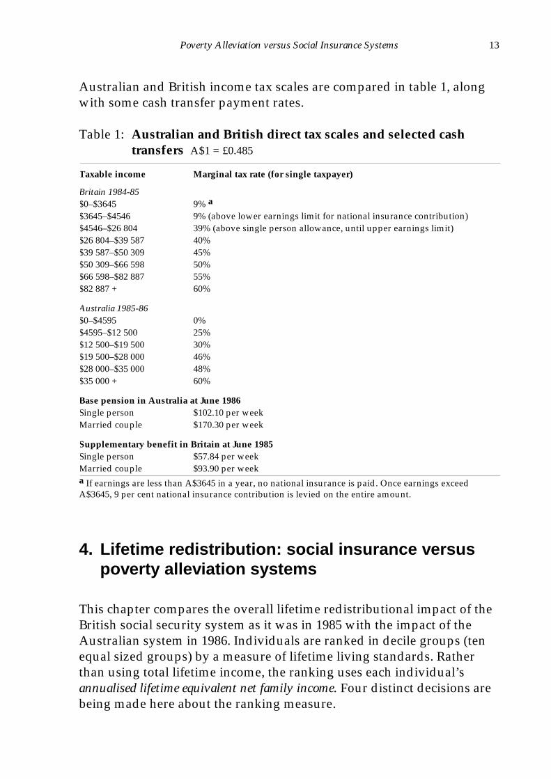
Australian and British income tax scales are compared in table 1, alongwith some cash transfer payment rates.

Table 1: Australian and British direct tax scales and selected cashtransfers A$1 = £0.485

Taxable income Marginal tax rate (for single taxpayer)

Britain 1984-85$0–$3645 9% a

$3645–$4546 9% (above lower earnings limit for national insurance contribution)$4546–$26 804 39% (above single person allowance, until upper earnings limit)$26 804–$39 587 40%$39 587–$50 309 45%$50 309–$66 598 50%$66 598–$82 887 55%$82 887 + 60%

Australia 1985-86$0–$4595 0%$4595–$12 500 25%$12 500–$19 500 30%$19 500–$28 000 46%$28 000–$35 000 48%$35 000 + 60%

Base pension in Australia at June 1986Single person $102.10 per weekMarried couple $170.30 per week

Supplementary benefit in Britain at June 1985Single person $57.84 per weekMarried couple $93.90 per weeka If earnings are less than A$3645 in a year, no national insurance is paid. Once earnings exceedA$3645, 9 per cent national insurance contribution is levied on the entire amount.

4. Lifetime redistribution: social insurance versuspoverty alleviation systems

This chapter compares the overall lifetime redistributional impact of theBritish social security system as it was in 1985 with the impact of theAustralian system in 1986. Individuals are ranked in decile groups (tenequal sized groups) by a measure of lifetime living standards. Ratherthan using total lifetime income, the ranking uses each individual’sannualised lifetime equivalent net family income. Four distinct decisions arebeing made here about the ranking measure.


First, lifetime income is annualised by averaging total lifetime net incomeover each year of life from the age of 16 years. This has the advantage ofavoiding locating people in the upper part of the income distributionjust because they have a long life and have the longest time toaccumulate total income. Conversely, if annualised income were notused, those who died in their 20s and 30s would appear to have a lowlifetime income and thus a low standard of living, whereas their incomeswhile they were alive might have been very high. Cohort individualswho die before the age of 17 years are excluded from the analysis, as themajority of this group would not have entered the labour force and thuswould have zero annualised income. Annualised income measures canbe viewed as the average amount of income received during each year ofadult life.

Second, net or disposable ‘after-tax’ income is used in preference to grossincome as it provides a more accurate measure of the living standardsattained by individuals and families.

Third, income is equivalised to allow for different family circumstances ofcohort individuals. If equivalent income were not used, a person with anannualised income of half a million dollars and no dependants, forexample, would be regarded as having experienced the same lifetimestandard of living as another person with the same annualised incomewho supported a spouse and three children.

Fourth, although it is the individual who is the unit of analysis, when acohort member is living with other adults the equivalent income of thefamily is attributed to them. This assumes that each person in a familyexperiences the same standard of living — that is, the income is sharedequally within the family. Research by Edwards (1981) and Pahl (1990)suggests that this is not always the case. In other work the sensitivity ofvarying this assumption of equal sharing has been explored(Falkingham and Hills 1995; Harding 1993a), but here analysis is limitedto this central case.

There are numerous difficulties with equivalence scales and it is notclear which scale is the most appropriate — especially for internationalcomparative analysis (see Coulter, Cowell and Jenkins 1992 for a fulldiscussion of the problems). The equivalence scale used in both theAustralian and British results is that implicit in the British social securitysystem in 1985 — the so-called ‘McClements scale’ — but it has been


rescaled so that a single adult is given the value of 1.00 (that is, to givefamily income per equivalent adult). (Additional adults are given thevalue of 0.64, children aged under 2 years 0.15, aged 5–7 years 0.34, aged8–10 years 0.38, aged 11–12 years 0.41, aged 13–15 years 0.44 and aged16–17 years 0.59.)

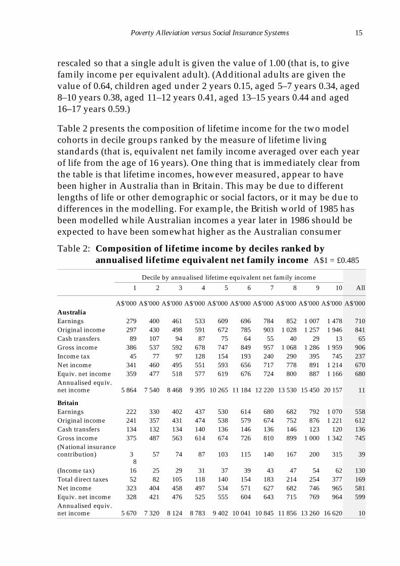
Table 2 presents the composition of lifetime income for the two modelcohorts in decile groups ranked by the measure of lifetime livingstandards (that is, equivalent net family income averaged over each yearof life from the age of 16 years). One thing that is immediately clear fromthe table is that lifetime incomes, however measured, appear to havebeen higher in Australia than in Britain. This may be due to differentlengths of life or other demographic or social factors, or it may be due todifferences in the modelling. For example, the British world of 1985 hasbeen modelled while Australian incomes a year later in 1986 should beexpected to have been somewhat higher as the Australian consumer

Table 2: Composition of lifetime income by deciles ranked byannualised lifetime equivalent net family income A$1 = £0.485

Decile by annualised lifetime equivalent net family income

1 2 3 4 5 6 7 8 9 10 All

A$’000 A$’000 A$’000 A$’000 A$’000 A$’000 A$’000 A$’000 A$’000 A$’000 A$’000AustraliaEarnings 279 400 461 533 609 696 784 852 1 007 1 478 710Original income 297 430 498 591 672 785 903 1 028 1 257 1 946 841Cash transfers 89 107 94 87 75 64 55 40 29 13 65Gross income 386 537 592 678 747 849 957 1 068 1 286 1 959 906Income tax 45 77 97 128 154 193 240 290 395 745 237Net income 341 460 495 551 593 656 717 778 891 1 214 670Equiv. net income 359 477 518 577 619 676 724 800 887 1 166 680Annualised equiv.net income 5 864 7 540 8 468 9 395 10 265 11 184 12 220 13 530 15 450 20 157 11

BritainEarnings 222 330 402 437 530 614 680 682 792 1 070 558Original income 241 357 431 474 538 579 674 752 876 1 221 612Cash transfers 134 132 134 140 136 146 136 146 123 120 136Gross income 375 487 563 614 674 726 810 899 1 000 1 342 745(National insurancecontribution) 3

857 74 87 103 115 140 167 200 315 39

(Income tax) 16 25 29 31 37 39 43 47 54 62 130Total direct taxes 52 82 105 118 140 154 183 214 254 377 169Net income 323 404 458 497 534 571 627 682 746 965 581Equiv. net income 328 421 476 525 555 604 643 715 769 964 599Annualised equiv.net income 5 670 7 320 8 124 8 783 9 402 10 041 10 845 11 856 13 260 16 620 10


price index, for example, increased by 8.4 per cent between June 1985and June 1986. The difference may also be due to the exchange rate usedto convert the pound sterling to dollars (the average rate during theAustralian financial year 1985-86 — the best that could be achieved in acomparison of Australia in 1986 with Britain in 1985). The absoluteamounts are very sensitive to the exact rate and so direct comparisons ofabsolute amounts between the two countries should be treated withsome caution. Of more interest is the pattern of income composition withindeciles and the distribution of income.

In contrast to traditional cross-sectional or annual distributional studies,the distribution of lifetime income appears to be more equitable. Mostnotably, even the lowest income deciles have significant amounts ofincome from earnings, constituting over half of total lifetime grossincome. Higher lifetime original incomes are the product of higherearnings and greater investment income and increased access tooccupational superannuation (pensions). Although not shown in thetable, the distribution of private pension income is highly skewedtowards those in the top three deciles of lifetime income.

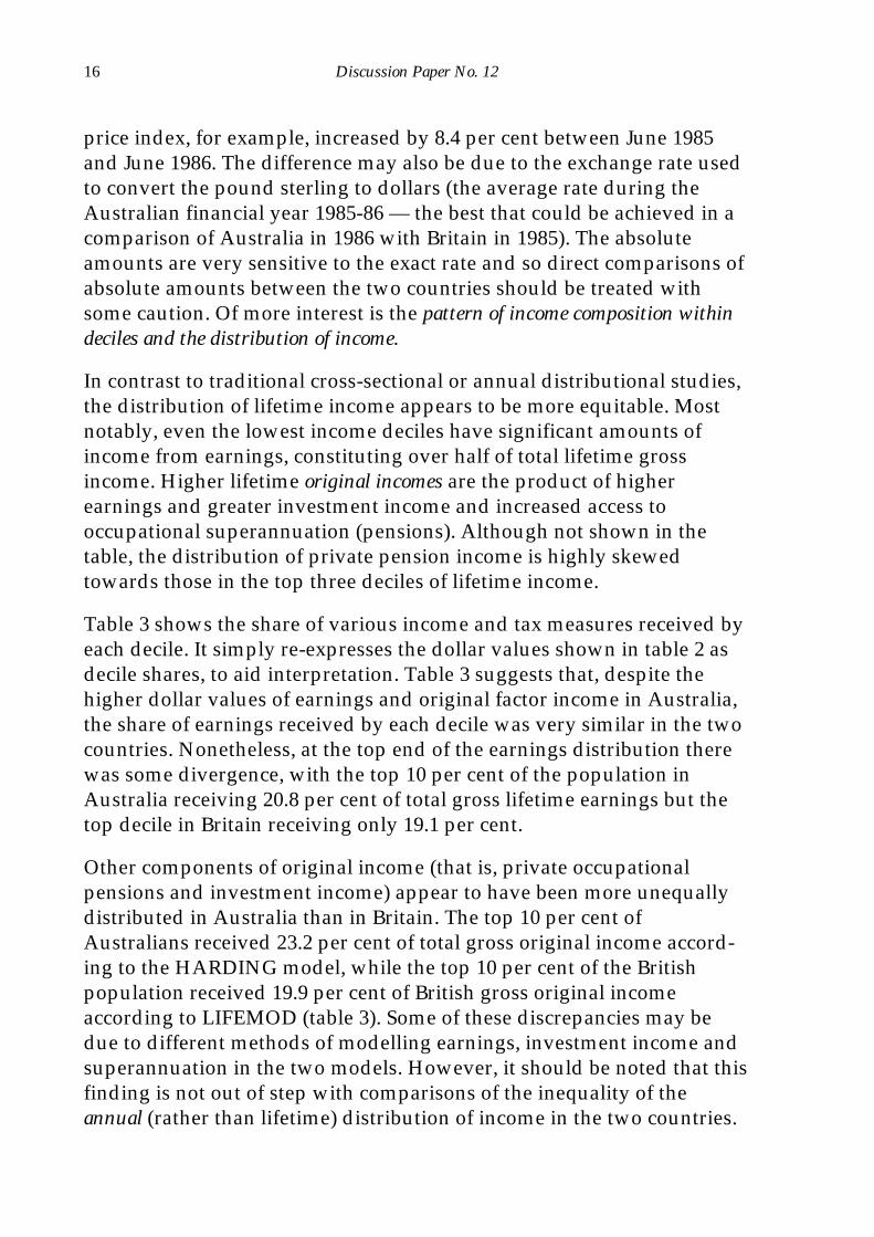
Table 3 shows the share of various income and tax measures received byeach decile. It simply re-expresses the dollar values shown in table 2 asdecile shares, to aid interpretation. Table 3 suggests that, despite thehigher dollar values of earnings and original factor income in Australia,the share of earnings received by each decile was very similar in the twocountries. Nonetheless, at the top end of the earnings distribution therewas some divergence, with the top 10 per cent of the population inAustralia receiving 20.8 per cent of total gross lifetime earnings but thetop decile in Britain receiving only 19.1 per cent.

Other components of original income (that is, private occupationalpensions and investment income) appear to have been more unequallydistributed in Australia than in Britain. The top 10 per cent ofAustralians received 23.2 per cent of total gross original income accord-ing to the HARDING model, while the top 10 per cent of the Britishpopulation received 19.9 per cent of British gross original incomeaccording to LIFEMOD (table 3). Some of these discrepancies may bedue to different methods of modelling earnings, investment income andsuperannuation in the two models. However, it should be noted that thisfinding is not out of step with comparisons of the inequality of theannual (rather than lifetime) distribution of income in the two countries.


For example, Mitchell (1991, p. 123) found that the distribution oforiginal income in Australia was more unequal than the distribution oforiginal income in the United Kingdom.

Cash transfers were much more important in Britain than in Australiafor every decile. As table 2 shows, the 10 per cent of the Australianpopulation with the lowest lifetime incomes received on averageA$89 000 in cash transfers during their lives. This compares with theA$134 000 received by the poorest 10 per cent of the British population.In Australia, cash transfers generally declined in absolute value asincome increased. In contrast, in Britain the absolute value of lifetimetotal cash benefits was relatively flat across the whole incomedistribution (with a slight rise in the middle, followed by a slight dip).Thus, while the top decile of Australians received on average onlyA$13 000 of cash transfers during their lifetimes, the top decile of theBritish population averaged A$120 000 of benefits. And the bottom

Table 3: Shares of lifetime income by deciles ranked by annualisedlifetime equivalent net family income


1 2 3 4 5 6 7 8 9 10 All

% % % % % % % % % % %AustraliaEarnings 3.9 5.6 6.5 7.5 8.6 9.8 11.1 12.0 14.2 20.8 100Original income 3.5 5.1 5.9 7.0 8.0 9.3 10.7 12.2 14.9 23.2 100Cash transfers 13.6 16.4 14.4 13.4 11.4 9.8 8.4 6.1 4.4 2.0 100Gross income 4.3 5.9 6.5 7.5 8.2 9.4 10.6 11.8 14.2 21.7 100Income tax 1.9 3.2 4.1 5.4 6.5 8.2 10.2 12.2 16.7 31.5 100Net income 5.0 6.8 7.4 8.2 8.8 9.7 10.7 11.6 13.2 18.2 100Equiv. net income 5.2 7.0 7.6 8.5 9.1 9.9 10.7 11.8 13.0 17.1 100Annualised equiv.net income 5.1 6.6 7.4 8.2 9.0 9.8 10.7 11.8 13.5 17.7 100

BritainEarnings 4.0 5.9 7.2 7.8 8.9 9.5 11.0 12.2 14.2 19.1 100Original income 3.9 5.7 7.0 7.7 8.8 9.4 10.9 12.2 14.2 19.9 100Cash transfers 10.0 9.7 9.9 10.4 10.0 10.8 10.1 10.8 9.2 8.9 100Gross income 5.0 6.5 7.5 8.2 9.0 9.7 10.8 12.0 13.3 17.9 100National insurancecontribution 4.1 6.2 7.8 8.3 9.4 10.0 11.3 12.6 14.0 16.1 100Income tax 2.3 4.5 5.8 6.7 8.0 8.9 10.8 12.9 15.4 24.2 100Total direct taxes 3.0 4.9 6.2 7.0 8.3 9.2 10.9 12.9 15.1 22.4 100Net income 5.6 7.0 7.9 8.5 9.2 9.8 10.8 11.8 12.8 16.6 100Equiv. net income 5.5 7.0 8.0 8.7 9.2 10.1 10.7 11.9 12.8 16.1 100Annualised equiv.net income 5.7 7.1 7.9 8.4 9.2 9.7 10.7 11.5 13.0 16.8 100


decile in Australia received almost 600 per cent more in cash transfersthan the top decile — in sharp contrast to the bottom decile in Britain,which received only 12 per cent more than the top decile.

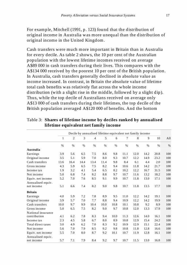
Nonetheless, cash transfers in Britain were still progressive, amountingto a higher proportion of the income of the lifetime poor than of thelifetime rich. Figure 1 shows the average amounts of cash transfersreceived by deciles, ranked by annualised lifetime equivalent net familyincome, expressed as a percentage of their lifetime average gross income.In Britain the lifetime cash transfers received by the bottom decileamounted to just over 35 per cent of the group’s lifetime gross income,while the comparable figure in Australia was about 23 per cent. For thetop income decile, cash transfers in Britain amounted to 9 per cent oflifetime gross income while, in Australia, the comparable figure was lessthan 1 per cent.

What about direct taxes? For Australia, federal income tax was includedin the simulation and for Britain the comparable taxes were income taxesplus national insurance contributions. Direct taxes amounted to a higherproportion of lifetime gross income in Australia than in Britain — 26 percent on average in Australia compared with 23 per cent in Britain (table2). For the poorest 10 per cent of the Australian cohort, total lifetimedirect taxes amounted to A$45 000 on average, compared with A$52 000

Figure 1: Total lifetime cash transfers received as percentage of totallifetime gross income by deciles ranked by annualisedlifetime equivalent net family income

0

5

10

15

20

25

30

35

40

1 2 3 4 5 6 7 8 9 10Deciles by annualised lifetime equivalent net family income

%

Australia

Britain


for the British cohort. For the top decile in Australia, direct taxesaveraged just under A$750 000 while for the top decile in Britain totallifetime direct taxes totalled only A$377 000.

The poorest 10 per cent of the Australian cohort contributed 1.9 per centof total lifetime direct taxes, compared with 3 per cent for the bottomBritish decile (table 3). The top decile shouldered a larger proportion ofthe lifetime direct tax burden in Australia than in Britain — 31.5 per centcompared with 22.4 per cent. (This is in part a product of the interactionof higher incomes of the top decile in Australia, but is also due to a muchmore progressive income tax scale.)

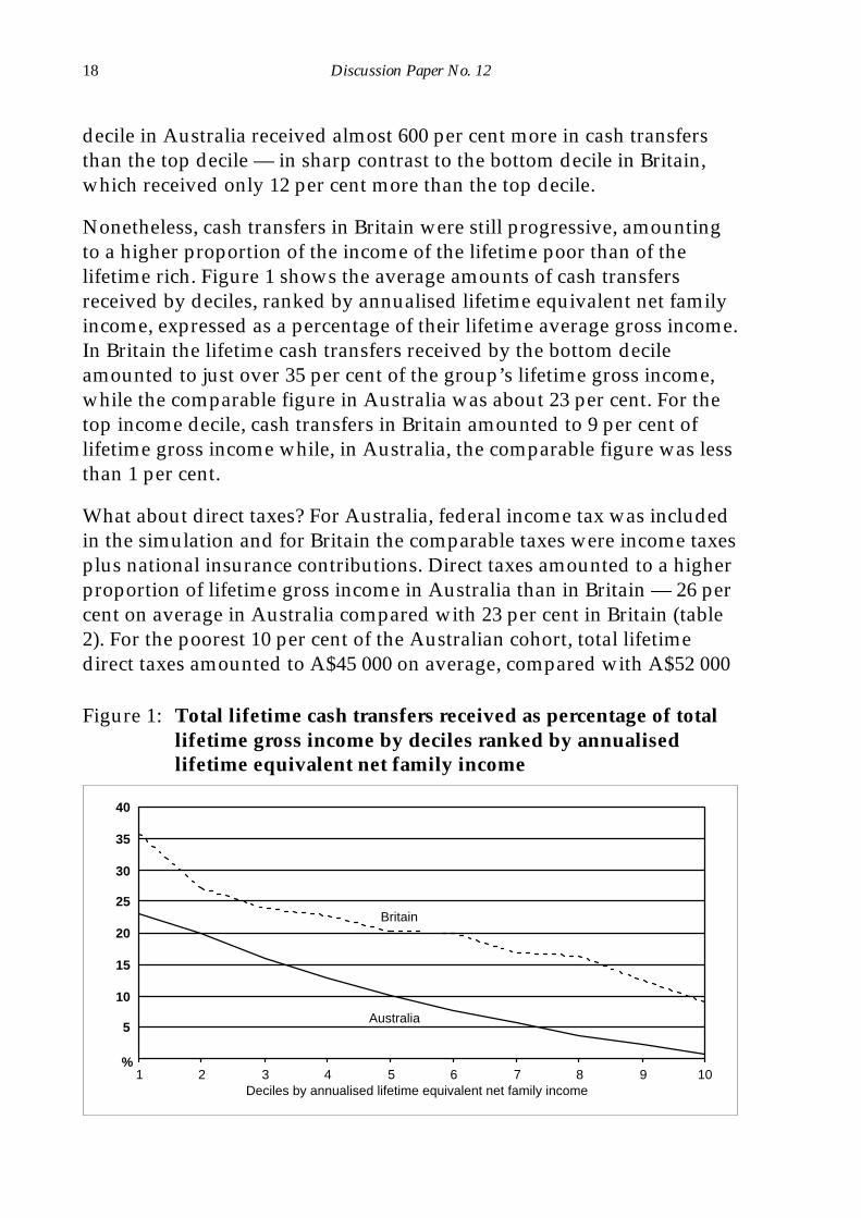
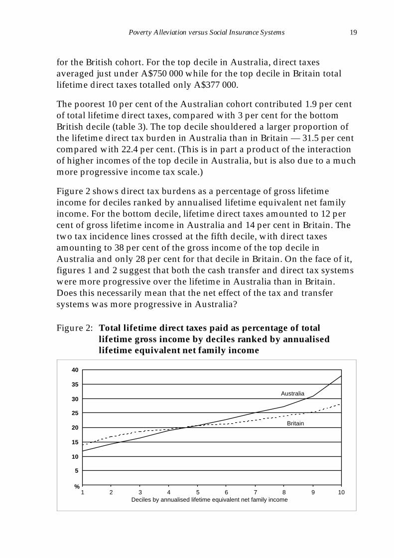
Figure 2 shows direct tax burdens as a percentage of gross lifetimeincome for deciles ranked by annualised lifetime equivalent net familyincome. For the bottom decile, lifetime direct taxes amounted to 12 percent of gross lifetime income in Australia and 14 per cent in Britain. Thetwo tax incidence lines crossed at the fifth decile, with direct taxesamounting to 38 per cent of the gross income of the top decile inAustralia and only 28 per cent for that decile in Britain. On the face of it,figures 1 and 2 suggest that both the cash transfer and direct tax systemswere more progressive over the lifetime in Australia than in Britain.Does this necessarily mean that the net effect of the tax and transfersystems was more progressive in Australia?

Figure 2: Total lifetime direct taxes paid as percentage of totallifetime gross income by deciles ranked by annualisedlifetime equivalent net family income

0

5

10

15

20

25

30

35

40

1 2 3 4 5 6 7 8 9 10Deciles by annualised lifetime equivalent net family income

%

Australia

Britain


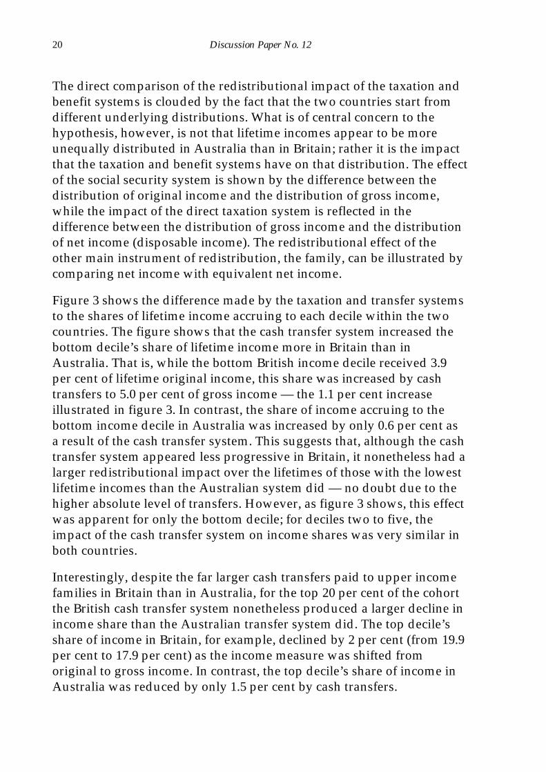
The direct comparison of the redistributional impact of the taxation andbenefit systems is clouded by the fact that the two countries start fromdifferent underlying distributions. What is of central concern to thehypothesis, however, is not that lifetime incomes appear to be moreunequally distributed in Australia than in Britain; rather it is the impactthat the taxation and benefit systems have on that distribution. The effectof the social security system is shown by the difference between thedistribution of original income and the distribution of gross income,while the impact of the direct taxation system is reflected in thedifference between the distribution of gross income and the distributionof net income (disposable income). The redistributional effect of theother main instrument of redistribution, the family, can be illustrated bycomparing net income with equivalent net income.

Figure 3 shows the difference made by the taxation and transfer systemsto the shares of lifetime income accruing to each decile within the twocountries. The figure shows that the cash transfer system increased thebottom decile’s share of lifetime income more in Britain than inAustralia. That is, while the bottom British income decile received 3.9per cent of lifetime original income, this share was increased by cashtransfers to 5.0 per cent of gross income — the 1.1 per cent increaseillustrated in figure 3. In contrast, the share of income accruing to thebottom income decile in Australia was increased by only 0.6 per cent asa result of the cash transfer system. This suggests that, although the cashtransfer system appeared less progressive in Britain, it nonetheless had alarger redistributional impact over the lifetimes of those with the lowestlifetime incomes than the Australian system did — no doubt due to thehigher absolute level of transfers. However, as figure 3 shows, this effectwas apparent for only the bottom decile; for deciles two to five, theimpact of the cash transfer system on income shares was very similar inboth countries.

Interestingly, despite the far larger cash transfers paid to upper incomefamilies in Britain than in Australia, for the top 20 per cent of the cohortthe British cash transfer system nonetheless produced a larger decline inincome share than the Australian transfer system did. The top decile’sshare of income in Britain, for example, declined by 2 per cent (from 19.9per cent to 17.9 per cent) as the income measure was shifted fromoriginal to gross income. In contrast, the top decile’s share of income inAustralia was reduced by only 1.5 per cent by cash transfers.


Moving to the taxation system, the Australian taxation system appearsto have changed net income shares to a greater extent than the Britishsystem does, except for the lowest income decile. Consequently, the neteffect of the Australian taxation and transfer systems was to increase theincome share accruing to deciles two to five by more than the taxationand transfer systems in Britain did. Similarly, the more progressiveAustralian direct tax structure resulted in the income share of the top 30per cent of the cohort being reduced by more as a result of the taxationand transfer systems than was the case with the British systems. It isnotable that in both countries the crossover point between net gain andnet loss occurs at the seventh decile.

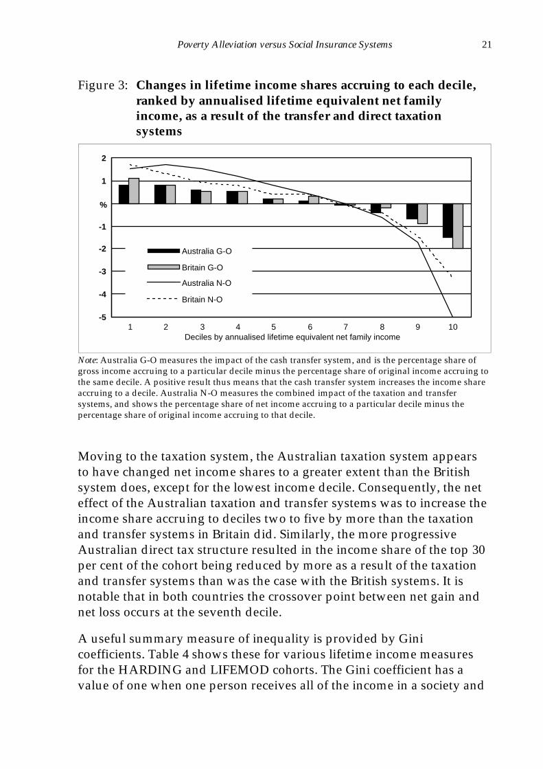
A useful summary measure of inequality is provided by Ginicoefficients. Table 4 shows these for various lifetime income measuresfor the HARDING and LIFEMOD cohorts. The Gini coefficient has avalue of one when one person receives all of the income in a society and

Figure 3: Changes in lifetime income shares accruing to each decile,ranked by annualised lifetime equivalent net familyincome, as a result of the transfer and direct taxationsystems

-5

-4

-3

-2

-1

0

1

2

1 2 3 4 5 6 7 8 9 10

Australia G-O

Britain G-O

Australia N-O

Britain N-O

Deciles by annualised lifetime equivalent net family income

%

Note: Australia G-O measures the impact of the cash transfer system, and is the percentage share ofgross income accruing to a particular decile minus the percentage share of original income accruing tothe same decile. A positive result thus means that the cash transfer system increases the income shareaccruing to a decile. Australia N-O measures the combined impact of the taxation and transfersystems, and shows the percentage share of net income accruing to a particular decile minus thepercentage share of original income accruing to that decile.


a value of zero if income is equally distributed among all persons. Thehigher the Gini coefficient, the more unequal the distribution of incomebeing measured.

The cash transfer system in Australia reduced the Gini coefficient (fromoriginal income to gross income) by 0.038. In Britain, although theabsolute amounts of cash benefits in table 2 were much more evenlyspread across the deciles, the Gini coefficient was reduced by 0.055.Thus, the cash transfer system had a greater equalising effect in Britainthan in Australia.

The direct taxation system further reduced the Gini coefficients. Theadditional reduction in Britain was relatively small — only 0.027, eventhough the absolute amounts of direct taxes paid exceeded cash transfersreceived. In Australia, however, the reduction was larger — 0.059.Overall, the net effect of the tax and transfer systems in Britain, reflectedin the difference between the disposable and original incomedistributions, was a reduction in the Gini coefficient of 0.082. InAustralia the net effect was greater — 0.097. Nonetheless, the lifetimedistribution of disposable income — as measured by the Gini coefficient— remained more equal in Britain than in Australia.

All of the preceding analysis simply shows the income personallyreceived by cohort individuals within the two models. In many casesthis would not provide an accurate indicator of the standard of livingachieved by individuals. This is because those with a low originalincome of their own might have lived in a family where they shared, forexample, the earnings of their spouse. To examine the redistributionalimpact of the family, the difference between the distribution of thedisposable incomes of individuals is compared with the distribution of

Table 4: Gini coefficients for lifetime income measures

Income measure Australia Britain

Original income 0.370 0.327Gross income 0.332 0.272Net (disposable) income 0.273 0.245Equivalent net family income 0.220 0.204

DifferencesGross income minus original income -0.038 -0.055Net income minus gross income -0.059 -0.027Net income minus original income -0.097 -0.082Equivalent net income minus net income -0.053 -0.041


the disposable incomes of the families in which those individuals lived.Table 4 suggests that the role played by families in redistributinglifetime income was as great as that of the taxation system in Australia.Thus, while the Australian taxation system reduced the Gini coefficientby 0.059 the impact of the family on disposable income reduced the Ginicoefficient by 0.053. In Britain the family played less of a role but wasstill very influential, reducing the Gini coefficient by 0.041. One reasonfor this is that the LIFEMOD cohort experienced a higher incidence ofmarital dissolution than did the HARDING cohort and thus spent agreater proportion of their lifetimes in single adult households wherethere was no opportunity to benefit from income sharing.

5. Intrapersonal versus interpersonal redistribution

From the models it is possible to identify receipts of cash benefits thatwere ‘paid for’ at another stage in an individual’s life (intrapersonalredistribution) and those that represent net transfers from others(interpersonal redistribution). To separate the net transfers within themodel populations, it was necessary to make an assumption about thetaxes allocated to pay for them. This can be done in two ways:

• assuming only direct taxes were used to finance benefits — thus, it isassumed that in Britain cash benefits were financed by all of thenational insurance contributions and 58 per cent of the income taxpaid by each group and that in Australia 27.6 per cent of all incometaxes paid by the cohort financed all cash transfers received by thecohort; and

• assuming that a proportion of both direct and indirect taxes was used.Indirect taxes are not modelled in the original versions of HARDINGand LIFEMOD (although see Harding 1993b) but in recent years thecombined effect of direct and indirect taxes in Britain has come closeto being proportional to gross income2. The combination of directand indirect taxes is therefore proxied by assuming financing from

2 For instance, for the United Kingdom the Central Statistical Office (1992, appendix

4, table 2) shows the Gini coefficients of equivalised gross income and equivalisedpost-tax income (that is, after both direct and indirect taxes) as equal — 0.32 in1985.


the percentage of each individual’s gross income required to pay forbenefits in aggregate. In HARDING 7.2 per cent of the lifetime grossincome received by all cohort members would finance all cashtransfers received by the cohort. In Britain the corresponding figurewas 16.3 per cent.

Two possible financing scenarios are thus tested. By adopting such anapproach, the counterfactual assumptions used are that, in the absenceof cash transfers from the welfare state, individuals would have to paycorrespondingly less tax :

• in proportion to their direct tax liabilities; or• in proportion to their gross income.

Thus it is hoped that systemic differences in taxation structures betweenthe two countries are controlled for.

5.1 Financing from direct taxes

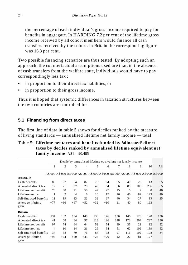
The first line of data in table 5 shows for deciles ranked by the measureof living standards — annualised lifetime net family income — total

Table 5: Lifetime net taxes and benefits funded by ‘allocated’ directtaxes by deciles ranked by annualised lifetime equivalent netfamily income A$1 = £0.485


1 2 3 4 5 6 7 8 9 10 All

A$’000 A$’000 A$’000 A$’000 A$’000 A$’000 A$’000 A$’000 A$’000 A$’000 A$’000AustraliaCash benefits 89 107 94 87 75 64 55 40 29 13 65Allocated direct tax 12 21 27 29 43 54 66 80 109 206 65Lifetime net benefit 78 88 71 58 42 27 15 6 2 0 40Lifetime net tax 1 2 4 6 10 17 26 46 82 193 40Self-financed benefits 11 19 23 23 33 37 40 34 27 13 25Average lifetimegain

+77 +86 +67 +52 +32 +10 -11 -40 -80 -193

BritainCash benefits 134 132 134 140 136 146 136 146 123 120 136Allocated direct tax 41 68 84 97 113 126 148 173 204 297 136Lifetime net benefit 97 74 64 64 52 54 39 35 21 12 52Lifetime net tax 4 10 14 21 29 34 51 62 102 189 52Self-financed benefits 37 58 70 76 84 92 97 111 102 108 84Average lifetimegain

+93 +64 +50 +43 +23 +20 -12 -27 -81 -177


lifetime cash benefit receipts. The following line shows what each groupwould contribute in direct taxes to finance the cash benefits of the entirecohort. The calculations in the remainder of the table show net receiptsand payments using these ‘allocated’ tax payments.

During each year of life individuals might pay tax, receive cash benefitsor (for perfectly good reasons) both. In the last case, some or all of thebenefits they received in a year would be paid for by their own direct taxin the same year — that is, there would be intrapersonal redistributionwithin the same year (sometimes known as ‘churning’). For example, somepeople would receive:

• taxable benefits (such as the state pension);

• non-taxable benefits but pay tax on other income (for instance,women with earnings receiving child benefit); or

• benefits because they are out of work for part of a year, but pay taxon earnings in the rest of it.

People might also pay for their own benefits in other years of their lives.Over their whole lives, individuals are either net lifetime taxpayers ornet lifetime benefit recipients (or, conceivably, neither if they breakeven).3

3 Algebraically the various measures can be expressed as follows. Let Bi be the gross

cash benefits received by individual i in year t, and Ti be the gross (allocated) taxpaid by them in that year. Then the aggregate gross cash benefits, G, for the modelpopulation over its entire lifetime is given by:G = ∑ i Bi = ∑ i Ti.

Self-financed benefits, SFB, are given by:SFBi = Ti (if Bi > Ti)

= Bi (if Bi < Ti).

An individual’s net lifetime gain, Ni, is:Ni = Bi – Ti.

Total interpersonal redistribution, IR, is the sum of positive net lifetime gains and isgiven by:IR = ∑ i (Ni Ni > 0).Total intrapersonal redistribution, IA, is the sum of self-financed benefits:IA = ∑ i SFBi (and by construction, G = IR + IA).


Table 5 illustrates the scale of such ‘self-financing’ of benefits (intra-personal redistribution), together with the net lifetime taxes or benefitsof individuals in excess of self-financed benefits (interpersonalredistribution). For example, the bottom income decile in Australiareceived a total of A$89 000 in cash transfers during their lifetimes.About 28 per cent of the total income tax that they paid during theirlifetimes financed all cash transfers, so that their allocated direct taxburden was about 28 per cent of the A$45 000 of lifetime direct taxshown in table 2 (that is, about A$12 000). In other words, out of all thecash transfers paid to the entire cohort during their lifetimes, the bottomdecile contributed on average A$12 000 of the direct taxes that financedthose cash transfers.

Of this A$12 000 allocated tax burden, A$11 000 was paid back in theform of cash transfers. The bottom Australian decile thus financedA$11 000 of the A$89 000 of cash transfers that were paid to them. Mostindividuals in the bottom Australian decile were net lifetime benefici-aries after taking account of cash transfers received and allocated taxespaid — the average lifetime net benefit for the entire decile beingA$78 000. However, a few individuals within this decile were netlifetime taxpayers. In other words, a few individuals in the bottom decilepaid out more in allocated taxes during their lifetimes than they receivedin cash transfers. For the decile as a whole, the lifetime allocated tax thatthey paid out and that financed the benefits of others averaged aboutA$1000. Consequently, the average lifetime gain for this group wasA$77 000. Therefore, the ‘self-financed benefits’ rows in table 5 show thescale of intrapersonal redistribution and the ‘average lifetime gain’ rowsshow the scale of interpersonal redistribution.

The bottom decile in Britain received much more in cash transfers thanthe bottom Australian decile did, but they also paid much moreallocated direct tax. The poorest decile in Britain paid for about 28 percent of the cash transfers that they received (in contrast to only 12 percent for the bottom Australian decile). However, the bottom decile inBritain still received an average lifetime gain of A$93 000 — muchhigher than the average lifetime gain of A$77 000 received by the bottomAustralian decile. For deciles two to five, however, the Australian taxand transfer systems delivered more interpersonal redistribution. Theaverage lifetime gain for those in the bottom half of the lifetime incomedistribution averaged A$63 000 in Australia but A$55 000 in Britain.


The proportion of gross benefits received by each decile that representedintrapersonal rather than interpersonal redistribution grew rapidly asincomes increased. In Britain, by the third decile the majority of thegroup’s gross receipts were self-financed; the same was true by the sixthdecile in Australia. For the top group, A$108 000 out of the A$120 000received on average in Britain was self-financed and the net taxpayerswithin the group paid out A$189 000 (averaged over the whole group).The pattern for the entire cohort is shown in the final column of table 5.On average, HARDING model individuals received A$65 000 in cashtransfers over their lifetimes — A$25 000 or 38 per cent representingbenefits that individuals effectively paid for themselves. In Britain,individuals averaged A$136 000 in lifetime cash transfers — A$84 000 or62 per cent financed from their own taxes.

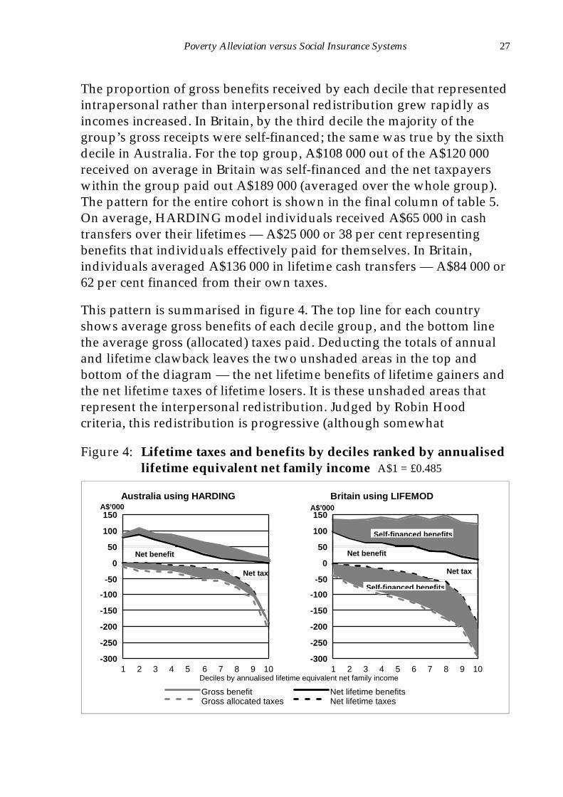
This pattern is summarised in figure 4. The top line for each countryshows average gross benefits of each decile group, and the bottom linethe average gross (allocated) taxes paid. Deducting the totals of annualand lifetime clawback leaves the two unshaded areas in the top andbottom of the diagram — the net lifetime benefits of lifetime gainers andthe net lifetime taxes of lifetime losers. It is these unshaded areas thatrepresent the interpersonal redistribution. Judged by Robin Hoodcriteria, this redistribution is progressive (although somewhat

Figure 4: Lifetime taxes and benefits by deciles ranked by annualisedlifetime equivalent net family income A$1 = £0.485

Australia using HARDING Britain using LIFEMOD

-300

-250

-200

-150

-100

-50

0

50

100

150

1 2 3 4 5 6 7 8 9 10

Gross benefit Net lifetime benefitsGross allocated taxes Net lifetime taxes

Net tax

Net benefit

-300

-250

-200

-150

-100

-50

0

50

100

150

1 2 3 4 5 6 7 8 9 10

Net tax

Net benefit

Self -financed benefits

Self -financed benefits

Deciles by annualised lifetime equivalent net family income

A$’000 A$’000


approximate, with some net lifetime taxpayers at the bottom and arather larger number of net lifetime gainers at the top), and is muchmore so in Australia than in Britain.

The shaded areas (of equal size for each group at the top and the bottomof the diagram) show the intrapersonal redistribution. In the Australiansystem, on average 38 per cent (A$25 000) of lifetime benefits were paidfor by the same individual at another stage in their life while 62 per centwere paid for by others. By coincidence, the proportions are reversed inBritain, with 62 per cent of benefits constituting intrapersonalredistribution and 38 per cent interpersonal redistribution. So far, thenull hypothesis seems unequivocally unrejected.

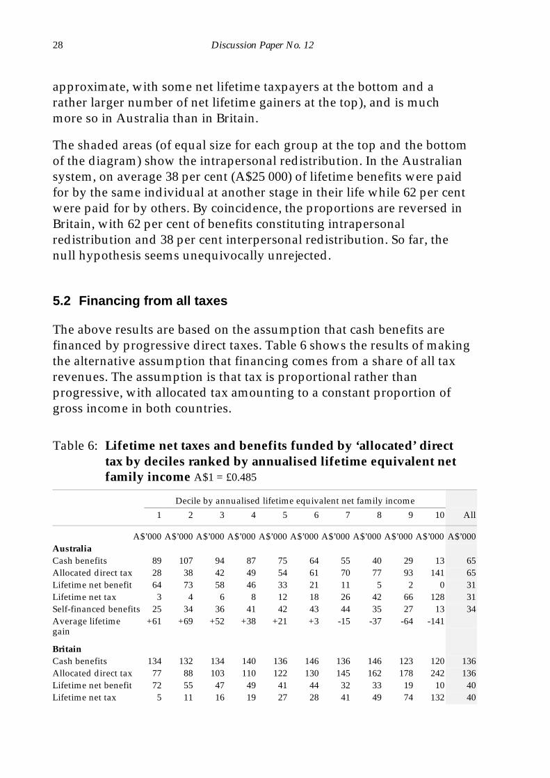
5.2 Financing from all taxes

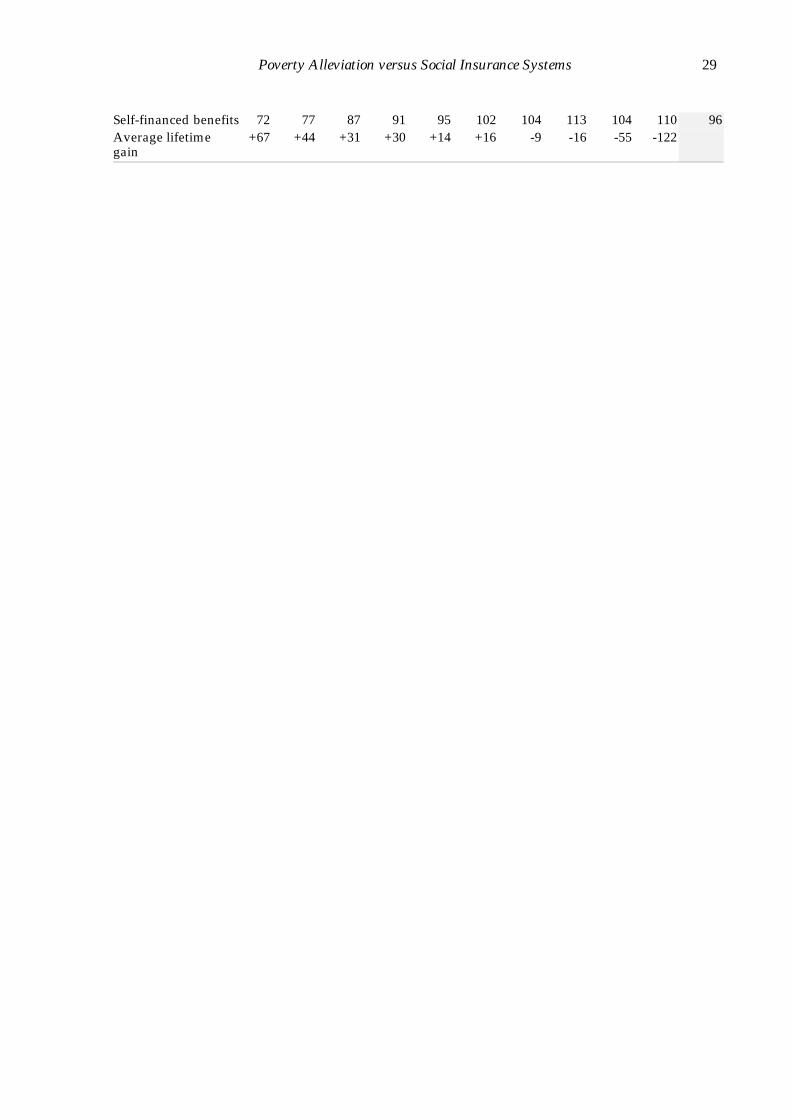
The above results are based on the assumption that cash benefits arefinanced by progressive direct taxes. Table 6 shows the results of makingthe alternative assumption that financing comes from a share of all taxrevenues. The assumption is that tax is proportional rather thanprogressive, with allocated tax amounting to a constant proportion ofgross income in both countries.

Table 6: Lifetime net taxes and benefits funded by ‘allocated’ directtax by deciles ranked by annualised lifetime equivalent netfamily income A$1 = £0.485


1 2 3 4 5 6 7 8 9 10 All

A$’000 A$’000 A$’000 A$’000 A$’000 A$’000 A$’000 A$’000 A$’000 A$’000 A$’000AustraliaCash benefits 89 107 94 87 75 64 55 40 29 13 65Allocated direct tax 28 38 42 49 54 61 70 77 93 141 65Lifetime net benefit 64 73 58 46 33 21 11 5 2 0 31Lifetime net tax 3 4 6 8 12 18 26 42 66 128 31Self-financed benefits 25 34 36 41 42 43 44 35 27 13 34Average lifetimegain

+61 +69 +52 +38 +21 +3 -15 -37 -64 -141

BritainCash benefits 134 132 134 140 136 146 136 146 123 120 136Allocated direct tax 77 88 103 110 122 130 145 162 178 242 136Lifetime net benefit 72 55 47 49 41 44 32 33 19 10 40Lifetime net tax 5 11 16 19 27 28 41 49 74 132 40


Self-financed benefits 72 77 87 91 95 102 104 113 104 110 96Average lifetimegain

+67 +44 +31 +30 +14 +16 -9 -16 -55 -122


Four differences from earlier results stand out.

• The proportion of intrapersonal redistribution rises from 38 per centto 52 per cent in Australia and from 62 per cent to 71 per cent inBritain.

• The average net gains to the bottom deciles are reduced and,symmetrically, the net loss of the top groups are decreased. Thus,there is less interpersonal redistribution.

• The interpersonal redistribution involved, while of a smaller scalethan when direct taxes are assumed to be the source of finance, isnonetheless progressive.

• Even controlling for the finance mechanism, the British socialsecurity system results in more intrapersonal redistribution than theAustralian system does and less interpersonal redistribution.

6. Summary

All social security and income tax systems are intended to generate bothinterpersonal redistribution of income (from those with high to thosewith low incomes) and intrapersonal redistribution (from one period ofan individual’s life cycle to another). Until now, most analyses of theredistributional impact of the taxation and transfer systems have beenlimited to the interpersonal redistribution generated at a single point intime. The lack of lifetime data has limited the capacity to answerquestions about the intrapersonal and interpersonal redistributionalimpact of the modern welfare state over a longer period. This paperrepresents a first attempt to undertake international comparative workabout the lifetime redistributional effects of social systems thatemphasise social insurance goals and those that emphasise povertyalleviation goals.

The work was based on two dynamic cohort microsimulation modelsthat put 4000 simulated British individuals and 4000 simulated


Australian individuals through their life cycles — from birth to death.Although some aspects of life have been modelled differently, themodels are in many respects unusually comparable, having beingdeveloped with a high degree of cooperation.

The Australian lifetime income distribution appeared more unequalthan the British distribution, and average gross lifetime incomes inAustralia, at A$906 000, were substantially higher than in Britain(A$745 000). This seemed to be due to a multitude of factors, includingan earlier base year for Britain (1985 as opposed to 1986 for Australia),higher unemployment and lower education levels in Britain, andsociodemographic differences, including higher mortality, divorce andsole-parenthood rates in Britain. It is important to keep these differencesin the original income distribution in mind when assessing the followingresults. For example, because the top 10 per cent of the Australian cohort(the group with the highest incomes) had original incomes that were 40per cent higher than the top 10 per cent of the British cohort, it would beexpected that their income tax contributions would have beensubstantially higher (because of the progressive taxation system). Theseunderlying differences complicate the comparison, and only broadconclusions can be drawn about how the two welfare states appear to beredistributing lifetime income.

Some broad conclusions did, however, emerge. Total lifetime cashtransfers seemed to be much greater in Britain than in Australia,amounting to A$136 000 on average in Britain but only A$65 000 inAustralia. The absolute value of lifetime cash transfers received declinedconsiderably as Australian incomes increased. In contrast, the absolutevalue remained relatively stable across the whole income distribution inBritain.

Cash transfers amounted to a higher proportion of gross income inBritain than in Australia for every decile. For example, cash transfersamounted to about 35 per cent of the gross income of the bottom decilein Britain and 23 per cent in Australia. For the top decile, the comparablefigures were 9 per cent in Britain and less than 1 per cent in Australia.According to Gini coefficients, the British cash transfer system reducedthe inequality of the original income distribution by more than theAustralian system did.


Average lifetime income taxes in Australia amounted to A$237 000,compared with an average A$169 000 in Britain. Interestingly, in bothcountries income taxes (plus national insurance contributions in Britain)amounted to half of total tax revenue. The Australian direct taxationsystem looked more progressive, with average tax rates being lower forthe Australian bottom decile than for the corresponding British decilebut higher for the top decile. However, to some extent this apparentdifference was due to discrepancies in the original income distributionagainst which progressivity was assessed. The direct taxation systemreduced the Australian Gini coefficient by 0.059, more than double the0.027 reduction achieved by the British direct taxation system.

It was possible to look at the extent to which receipts of cash benefits byan individual were paid for by that person at another stage in their life(lifetime intrapersonal redistribution) and the extent of net transfersfrom other people (interpersonal redistribution). Assuming that all cashbenefits were financed from direct taxes, on average out of the A$65 000each Australian received in cash transfers over their lifetimes, 38 percent were effectively paid for by the individuals themselves, whereas 68per cent were paid for by others. These proportions were reversed inBritain.

The proportion of cash transfers that represented intrapersonalredistribution increased as incomes increased. In Britain, by the thirddecile, the majority of the group’s gross receipts were self-financed overthe lifetime; the same was true by the sixth decile in Australia.Alternatively, if it was assumed that cash transfers were financed by aproportional rather than a progressive tax, the proportion of transfersthat were self-financed increased from 38 per cent to 52 per cent inAustralia and from 62 per cent to 71 per cent in Britain.

Thus, controlling for the greater redistributional effect of the moreprogressive Australian taxation system does not alter the finding that aprimarily social assistance-based system (such as Australia’s), with itsemphasis on poverty alleviation, results in a greater degree of inter-personal redistribution of income. Conversely, a primarily socialinsurance-based system (such as Britain’s), with its emphasis on the linkbetween contributions and benefits, results in a greater degree ofintrapersonal redistribution.


Finally, it must be acknowledged that this study examines theredistributional impact of the British and Australian systems bycomparing the post-tax and transfer income distribution with theoriginal income distribution prevailing in each country. An alternativemethod would be to simulate the rules of the taxation and transfersystems of both countries against the same original income distribution(that is, run the rules for both taxation and transfer systems againsteither the Australian or the British original income distributions). Suchan exercise would provide a very interesting complement to the studypresented here. However, it would not necessarily provide moredefinitive answers about the lifetime redistributional impact of eachcountry’s systems, as this would depend on the extent to which theprevailing taxation and transfer rules had already affected behaviour —and thus the ‘original’ income distribution — within each country.


References

Barr, N. and Falkingham, J. 1993, Paying for learning, Welfare State Programme,Discussion Paper WSP/94, London School of Economics.

Barro, R. 1974, ‘Are government bonds net wealth?’, Journal of PoliticalEconomy, vol. 82, pp. 1095–117.

Beveridge, W. 1942, Social Insurance and Allied Services, Cmd. 6404, HMSO,London.

Central Statistical Office (UK) 1992, ‘The effects of taxes and benefits onhousehold income 1989’, Economic Trends, no. 459, pp. 127–65.

Coulter, F., Cowell, F.A. and Jenkins, S.P. 1992, ‘Differences in needs andassessment of income distributions’, Bulletin of Economic Research, vol. 44,no. 2, pp. 77–124.

Edwards, M. 1981, Financial Arrangements within Families, National Women’sAdvisory Council, Canberra.

Falkingham, J. and Lessof, C. 1991, LIFEMOD — The Formative Years, WelfareState Programme Research Note WSP/RN/24, London School ofEconomics.

—— and ——1992, ‘Playing god: the construction of LIFEMOD, a dynamiccohort microsimulation model’, in Hancock, R. and Sutherland, H. (eds),Microsimulation Models for Public Policy Analysis: New Frontiers, STICERDOccasional Paper no. 17, London School of Economics.

—— and Hills, J. (eds) 1995, The Dynamic of Welfare, Harvester-Wheatsheaf,London.

Hain, W. and Helberger, C. 1986, ‘Longitudinal microsimulation of lifetimeincome’ in Orcutt, G., Merz, J. and Quinke, H. (eds), MicroanalyticSimulation Models to Support Social and Financial Policy, North Holland,New York.

Harding, A. 1984, Who Benefits: The Welfare State and Redistribution, SocialWelfare Research Centre Reports and Proceedings no. 45, University ofNew South Wales, Sydney.

—— 1993a, Lifetime Income Distribution and Redistribution: Applications of aDynamic Cohort Microsimulation Model, North Holland, Amsterdam.


—— 1993b, ‘The lifetime incidence of indirect taxes: wholesale sales tax andexcises’, in Head, J. (ed.), Fightback: An Economic Analysis, Australian TaxResearch Foundation, Sydney.

—— 1995, ‘Financing higher education: an assessment of income-contingentloan options and repayment patterns over the life cycle’, EducationEconomics, vol. 3, no. 2, pp. 173–203.

Hills, J. and Lessof, C. 1993, Modelling Direct Tax and Social Security over theLifetime, Welfare State Programme Research Note WSP/RN/25, LondonSchool of Economics.

Le Grand, J. 1982, The Strategy of Equality: Redistribution and the Social Services,Allen & Unwin, London.

Mitchell, D. 1991, Income Transfers in Ten Welfare States, Avebury, Aldershot.

Nelissen, J.H.M. 1993, The Redistributive Impact of Social Security Schemes onLifetime Labour Income, Report no. 22, Tilburg University.

Orcutt, G., Caldwell, S. and Wertheimer, R. 1976, Policy Exploration ThroughMicroanalytic Simulation, Urban Institute Press, Washington, DC.

Pahl, J. 1990, ‘Household spending, personal spending and the control ofmoney in marriage’, Sociology, vol. 24, part 1, pp. 119–38.

Saunders, P. 1984, Evidence on Income Redistribution by Governments, OECDEconomics and Statistics Department Working Paper no. 11, Paris.

Summers, R. 1956, An Econometric Investigation of the Size Distribution of LifetimeAverage Income, Department of Economics Technical Report no. 31,Stanford University.

Winter, D. 1994, Modelling lifetime earnings, London School of Economics,mimeograph.

Wolfson, M. 1988, ‘Homemaker pensions and lifetime redistribution’, Review ofIncome and Wealth, vol. 34, no. 3, pp. 221–50.

NATSEM publications

Copies of NATSEM publications and information about NATSEM maybe obtained from:

Ms Kirrilie NordsvanPublications OfficerNational Centre for Social and Economic ModellingUniversity of CanberraGPO Box 563Canberra City ACT 2601Australia

Ph: + 61 6 275 4900 Fax: + 61 6 275 4875E-mail: [email protected]

Periodic publications

NATSEM News keeps the general community up to date with thedevelopments and activities at NATSEM, including product andpublication releases, staffing and major events such as conferences. Thisnewsletter is produced twice a year.

The Income Distribution Report (IDR), which is also produced twice ayear, provides information and comment on the average incomes ofAustralian families, covering the incidence of taxation for differentfamily types, the income support provided by the government and howdifferent family groups are faring. The IDR, which is available onsubscription, presents this information in a simple, easy-to-followformat.

NATSEM’s Annual Report gives the reader an historical perspective ofthe centre and its achievements for the year.

STINMOD/95

STINMOD is an easy-to-use microsimulation model for betterunderstanding the impact of social and economic change on Australianfamilies. It is a cutting edge tool for exploring the distributional impactof possible government policy changes. Microsimulation models arebuilt from the bottom up, using samples of microdata based on realAustralians. From such a foundation, projections can then be made forthe wider community.

The third release of STINMOD is now available. This releaseincorporates changes to social security payments announced in the1995-96 budget, more flexible output specifications, online benchmarkresults and context-sensitive help screens, and enables users to savepolicy options so that they can be reused at a later date.

STINMOD Technical Paper series

No. Authors Title

1 Lambert, S., Percival, R.,Schofield, D. and Paul, S.

An Introduction to STINMOD: A StaticMicrosimulation Model, October 1994

2 Percival, R. Building STINMOD’s Base Population,November 1994

3 Schofield, D. and Paul, S. Modelling Social Security and Veterans’Payments, December 1994

4 Lambert, S. Modelling Income Tax and the Medicare Levy,December 1994

5 Percival, R. Modelling AUSTUDY, December 1994

6 Landt, J. Modelling Housing Costs and Benefits, December1994

7 Schofield, D. Designing a User Interface for a MicrosimulationModel, March 1995

8 Percival, R. andSchofield, D.

Modelling Australian Public Health Expenditure,May 1995

9 Paul, S. Modelling Government Education Outlays,September 1995

10 Schofield, D., Polette, J.and Hardin, A.

Modelling Child Care Services and Subsidies,January 1996

DYNAMOD Technical Paper series

No. Authors Title

1 Antcliff, S. An Introduction to DYNAMOD: A DynamicMicrosimulation Model, September 1993

Discussion Paper series

No. Authors Title

1 Harding, A. Lifetime Repayment Patterns for HECS andAUSTUDY Loans, July 1993

2 Mitchell, D. andHarding, A.

Changes in Poverty among Families during the1980s: Poverty Gap Versus Poverty Head-countApproaches, October 1993

3 Landt, J., Harding, A.,Percival, R. andSadkowsky, K.

Reweighting a Base Population for aMicrosimulation Model, January 1994

4 Harding, A. Income Inequality in Australia from 1982 to 1993:An Assessment of the Impact of Family,Demographic and Labour Force Change,November 1994

5 Landt, J., Percival, R.,Schofield, D. andWilson, D.

Income Inequality in Australia: The Impact ofNon-Cash Subsidies for Health and Housing,March 1995

6 Polette, J. Distribution of Effective Marginal Tax RatesAcross the Australian Labour Force, August 1995

7 Harding, A. The Impact of Health, Education and HousingOutlays on Income Distribution in Australia inthe 1990s, August 1995

8 Beer, G. Impact of Changes in the Personal Income Taxand Family Payment Systems on AustralianFamilies: 1964 to 1994, September 1995

9 Paul, S. and Percival, R. Distribution of Non-Cash Education Subsidies inAustralia in 1994, September 1995

10 Schofield, D., Polette, J.and Hardin, A.

Australia’s Child Care Subsidies: A DistributionalAnalysis, January 1996

11 Schofield, D. The Impact of Employment and Hours of Workon Health Status and Health Service Use,March 1996

Documents

poverty alleviation versus social insurance systems: a