Discussion PapersCollana di

E-papers del Dipartimento di Scienze Economiche – Università di Pisa

Luciano Fanti and Luca Spataro

Poverty traps and intergenerational transfers

Discussion Paper n. 66

2007

Discussion Paper n. 66, presentato: marzo 2007

Indirizzi dell’Autore: Luciano Fanti: Tel. +39 050 2216369, fax +39 050 2216384. Email: lfanti@ec.unipi.it.Luca Spataro: Tel. +39 050 2216217, fax +39 050 2216384. Email: l.spataro@ec.unipi.it

© Luciano Fanti and Luca Spataro

La presente pubblicazione ottempera agli obblighi previsti dall’art. 1 del decreto legislativo luogotenenziale 31 agosto1945, n. 660.

Si prega di citare così: Luciano Fanti and Luca Spataro, Poverty traps and intergenerational transfers, Discussion Papersdel Dipartimento di Scienze Economiche – Università di Pisa, n. 66 (http://www-dse.ec.unipi.it/ricerca/discussion-papers.htm).

1

Poverty traps and intergenerational transfers

Abstract In this paper, by adopting an OLG neoclassical growth model we show that intergenerational transfers may trigger the take off of an economy entrapped into poverty in a twofold way: 1) by eliminating the zero equilibrium -which, under technology with low factor substitutability, is always a “catching” point- so that the economy might start converging to a positive equilibrium. In this case the appropriate instrument turns out to be a transfer from the old to the young, while there is no room for policies redistributing in the opposite direction (i.e. a pay-as you-go-pension scheme); 2) when the rich equilibrium is unstable -which can be the case under high intertemporal substitution of individuals- the introduction of transfers may stabilize such an equilibrium, so that the economy starts converging to it. In the latter case both policy programs such as pay-as-you-go pension schemes or subsidies to the young may help escaping from poverty. However, we point out that in either circumstances, the “size” of transfers should be sufficiently large (and, as for pensions not even too large), in order to avoid ineffective and useless burden on the taxpayers without triggering the take off. Keywords: poverty traps, intergenerational transfers, OLG. JEL codes: D31, D50, O11, O23 1. Introduction

The recent literature on economic growth has highlighted the role of multiple equilibria and poverty traps1 in explaining the different long run performances of rich and poor countries2.

Within the neoclassical growth model (e.g. Solow (1956) and Diamond (1965)), which has been a basic frame for studying the issue of poverty traps, at least three canonical models have been largely discussed: 1) models with non-constant returns to scale in technology, due for example to externality such as learning-by doing (e.g. Cazzavillan et al. (1998)) or, from a historical point of view, due to the passage from an agricultural era at diminishing returns to an industrial era at increasing returns (e.g. Prskawetz et al. (2000)) ; 2) models with a non-constant rate of population growth, for instance corresponding to the “stylized fact” of the so-called demographic transition (e.g. Strulik (1997), Manfredi and Fanti (2003)); 3) models with non constant saving rates (e.g. Strulik (1999)). All these models entail a S-shaped relationship, sometimes postulated “ad hoc”, between either technology or population growth or saving rate on the one hand and growth on the other hand. Likewise, in all these models a positive shock in the technical progress or in the saving rate or, alternatively, a negative shock in the population growth rate may lead to escape from the poverty trap3.

However, up to now the role of intergenerational transfers in affecting the poverty trap problem has been overlooked by this stream of literature. In the present work we tackle this issue, within the OLG framework a la Diamond (1965), by focusing on two possible sources of poverty entrapment: the first one is the existence of multiple equilibria with a “catching” zero equilibrium point, arising when the production function is of CES type: this case provides a micro-foundation for the S-shaped relation between production and accumulation above mentioned. The second origin of the poverty trap that we consider here, and rather overlooked so far, is the possible instability of the 1 We recall that a loose definition of a poverty trap concerns the existence of a stable “poor” steady state equilibrium (low levels of per capita output and capital stock) which assumes the feature to be a trap in that, notwithstanding the efforts of the agents to escape from it, the economy shows a tendency to return to such a poor equilibrium. 2 For recent surveys and works on poverty traps see Galor (1996), Azariadis (1996) and (2004), Hoff (2000), Hoff and Sen (2004), Matsuyama (1995) and (1997), Easterly (2001), Bowles, Durlauf and Hoff (2004) and Mookherjee and Ray (2001). 3 For a recent example, Sachs et al. (2004) adopt these models to provide a theory for Africa’s poverty.

2

“rich” equilibrium arising in presence of high intertemporal elasticity of substitution in agents’ preferences. To our knowledge this is the first study, dealing with poverty traps, enlightening the role of both low factor substitutability and high intertemporal elasticity in providing a micro-foundation of the occurrence of such traps.

In these cases we address the following question: are there any policy tools solving the poverty trap problem? We argue that intergenerational transfers may be an effective instrument in a twofold way: 1) firstly, eliminating the zero catching point and so, triggering the take off of the economy 2) secondly, and more interestingly, through the stabilization of the rich equilibrium so that the economy can start converging to it. As regards the first point, we argue that the appropriate policy instrument is a transfer from the old to the young; as for the second point, we show that both transfer policies may work for stabilization and, moreover, that the “size” of such transfers, in either direction, does matter, since it should be sufficiently large (although, as for pensions, not even too large).

The economic intuition of our results can be posed as follows: as for results sub 1), since in this case the poverty trap is originated by insufficient capital accumulation, a policy redistributing from the old (consumers) to the young (savers) will enhance such an accumulation and then will help the economy undertaking a higher growth path. Otherwise, policies redistributing in the opposite direction through the well known “crowding out effect” would discourage savings even more, hence impeding the taking off of the economy. As for results sub 2): the competitive equilibrium, without public intervention is not able to reach a long run stable rich balanced growth path, because private savings are too reactive to the interest rate, due to a high IES (thus, in this case the economy is condemned either to extinction or to “wild” fluctuations around the unstable rich equilibrium).

In this case any policy, redistributing in either direction, can work for stability to the extent that it is successful in reducing such a reactivity of savings to the market yield.

It turns out that the stabilizing effect of the public intervention occurs only if the tax/transfers are sufficiently high; moreover, the direction of the redistribution depends on the difference between n and r.

In the light of these results, our paper is a further contribution to the micro-foundation of the causes of poverty traps as well as to the analysis of the possible policy remedies to this problem in the strand of the OLG neoclassical growth theory. The value added of our results consists, on the one hand, in finding a role, indeed rather complex, of pure redistributive taxes among generations, for triggering the take off of the economy; on the other hand, to stress the crucial role played not only by the direction, but also by the magnitude of such transfers.

The work is organized as follows: after the introduction, in sections 2 and 3 we lay out the setup of the model without and in presence of the State intervention, respectively. In the latter case we discuss the effects of such intervention on the long run equilibria. In section 4 we present the main results of the comparative dynamics analysis with respect to the tax policy parameter and provide a numerical simulation. Concluding remarks will end the paper. 2. The model setup

The economy is populated by two-period living individuals, who maximize a utility function U, defined over c1 and c2, that is consumption in the first and second period of life; hence, in their youth the Nt agents born in period t must choose how much to save out of their income, which is comprised of the wages received from their fixed labor supply (which is normalized to 1). The population Pt grows at a constant growth rate, n, so that Nt=Nt-1(1+n).

Moreover, in this closed-production economy perfect competition is assumed. As a consequence, firms, owning an CRS technology, can hire capital and labor by remunerating them at their marginal productivities.

3

2.1 Households By assuming a CIES utility function, individuals solve the following problem:

Max Ut=u(c1t)+βu(c2t+1)

sub c1t+ ( )( )1

12

1 +

+

+ tt

t

rEc =wt,

where u=

σ

σ

11

11

−

−c , with 0>σ and 1≠σ and Et is the expectation operator as for time t. We assume

myopic expectations, so that: ( )1+tt rE =rt. First order conditions deliver the following results:

c1t= ( ) 111 −++ σσβ t

t

rw [1]

( )( ) 112 11

1−+

++

+= σσ

σσ

ββ

t

ttt r

wrc [2]

st tt cw 1−≡ =( )

( ) ( ) σσσσ

σσ

βββ

−−−

−

++=

++

+11

1

11111

t

t

t

tt

rw

rwr

, [3]

c1t, c2t+1, st>0.

Note that ( ) ( )( )[ ] 1011

11 21 <

>⇔

<>

++

+−=

∂∂

−−

−−

σβ

βσ

σσ

σσ

t

tt

t

t

r

wrrs

.

As known, when the IES parameter -σ - is lower (higher) than 1, the substitution effect is dominated by (dominates) the income effect, and therefore, a rise in the rate of interest has a negative (positive) effect on savings: a rise of the remuneration of savings leads to more (less) consumption today. In the case of logarithmic preferences ( 1=σ ), income and substitution effect cancel each other out, so that interest rate changes do not affect the intertemporal allocation of resources. 2.2 The production sector

We assume a competitive market with identical firms: thus, firms hire capital and labor by remunerating them according to their marginal productivity. Moreover, due to the homogeneity of

degree one of the aggregate production function F(K,L) and defining LKk ≡ and

( ) ( ) ( )1,, kFL

LKFkf =≡ , it follows that:

tkK rfF =≡ '' and ttkL wkffF =−≡ '' , [4]

4

where rt and wt are the interest rate and the wage in period t, and the subscript of the derivative functions 'F and 'f indicates the derivation variable.

In the present work we use a CES production function of the following type:

( ) ( )[ ] ,1,1ρρρ αα −−− −+= LKALKF ρ>-1, ρ≠0, A>0, α∈ (0,1) [5]

which, in per worker terms, has the form:

( ) ( )[ ] ,11ρρ αα −− −+= kAkf [5’]

with ( )ρ

ρα+

−

=

1'

kfAfk and ( ) ( )ρρα +−−=− 1' 1 fAkff tk . [6]

Precisely, in the analysis that follows we will assume low degree of substitutability between labor and capital inputs, i.e. ρ>04. 2.3 Market clearing condition The equation providing the market clearing condition is:

kt+1=( )

( ) ( )( )1

1

1111

−

−

++++

σσ

σσ

ββ

t

tt

rnwr [7]

or

kt+1= ==+

)(1 t

ttt kn

),r(wsφ

( ) ( )( )σσβ −− +++ 1111 t

t

rnw

, [7’]

which is also the equation resuming the entire dynamics of the model. The existence and the

number of the steady states emerge from the analysis of the implicit equation

( ) ( )( )( ) ( )( ) ( )[ ]kwkrkrn

k 11 1

1111 −

− ++++

− σσσσ

ββ

=0. [8]

The case of an OLG economy with Cobb-Douglas production function and a CIES utility

function has been discussed by de La Croix and Michel (2002, par. 1.81, pp. 45/51 and Figure 1.16). The feature of this economy is that there are two equilibria, the zero one, which is always 4 The discussion on whether the actual value of the elasticity of substitution (θ=1/(1+ρ)) between labor and capital is lower than 1 or not is a long debated one. The case of θ<1 has been recognized of significant empirical relevance since long time. For example, Solow (1958) argued for a θ around 2/3 and Lucas (1969) around 0.6. Finally Rowthorn (1999a) reports the estimates of θ from 33 econometric studies, according to which the overall median of the summary values (median of the medians) is equals to 0.58 (and only in 7 cases the elasticity is greater than 0.8). Rowthorn (1999b) estimates in indirect way the elasticity of substitution (based on some empirical values of the labor demand elasticity, profit share and price elasticity), generating the following examples for the parameter ρ.

Italy UK France Germany Sweden Japan USA

ρ 13.3 3.95 15.6 1.63 24 5.25 13.2

5

unstable, and a positive equilibrium may be either stable or unstable, depending on the IES parameter value. Moreover, also the case with CES production function and Cobb Douglas utility function has been discussed in de La Croix and Michel (2002, par. 1.6, p. 32-33, Figs. 1.10-1.11). The feature of the latter economy, with low substitutability between labor and capital, is that three equilibria can exist, and the lowest one, the zero equilibrium, is a catching point.

Here we build a model which combines a CES production function with a CIES utility function; such a model presents the same structure of the two cases mentioned above, as regards the existence and multiplicity of equilibria. However, in our model we are able to encompass both multiple equilibria and possible instability of the “rich” equilibrium in a single framework.

In particular, we illustrate some features of our model which are essential for the investigation of the poverty trap problem. First of all, we show that, also in our model, when the substitutability between labor and capital is low, the zero equilibrium is a “catching point”5. Furthermore, it is shown that the accumulation locus can be backward bending when the IES is sufficiently high ( 1>σ )6.

The finding on the possible negativity of the slope of the capital accumulation locus can be explained as follows: when the IES is sufficiently high, the derivative of saving with respect to the interest rate is positive and higher than the derivative of savings with respect to wage. As a 5 In the latter case: 1) f(0)=0, which is an equilibrium point, in contrast with the case of high substitutability where f(0)>0, which is not an equilibrium; 2) since 0)('lim

0>

→kf

k and finite and 0)(''lim

0=

→kf

k, and, under

CIES preferences it can be shown that ( ) 01

lim ''10

=

+−

−=+

→ nssk

fdk

dk rtwttkt

t

tk

, which means that, if the initial

capital/labor ratio is low enough, the economy will converge to the trivial steady state with zero capital. In other words, the economy will be entrapped into the poverty trap. Note that the violation of one of the Inada conditions (whereby ∞=

→)('lim

0kf

k) implied by the low substitutability is a crucial ingredient for the existence

of a poverty trap. 6 Assume depreciation is equal to 1 for simplicity, such that 1+r=f’, then by derivating eq. [7’], with respect to k, we can write the following

φ ’(kt)= ( ) ( )( ) ( ) ( )( ) ( )( )

( ) ( )( )( ) ( ) =+++

+−+=

+++

+−−

++++

−−

−+−

+−−

−−

−−t

t

t

tt

t

t

t

tt

t

t

rkf

rr

kww

rn

fwrrn

w1

''11

11

'

111

''11

111' 1

1

1

1211 σσ

σσ

σσ

σσ

σσ β

βσ

β

βσ

β

( ) ( ) ( ) ( ) ( )( )

( ) ( ) ( )

+

+−+=

+

+−+= −+−

+

+++

−+−+ σσσσ βσεε

εεβσε 1

,1

,1,1,1

1,

1 111111 tt

tkr

kw

t

tkrkrt

ttkw

t

t rw

nkk

kr

wnk

kk

tt

tt

ttttrt

where tt kw ,ε and ( ) tt kr ,1+ε are the elasticity of w and (1+rt) with respect to kt, respectively. By substituting the

expressions for (1+rt) and wt from [6], by reckoning that tt kw ,ε / ( ) tt kr ,1+ε =- ρ−

tk α/(1-α) and manipulating further, we get

'φ (kt)( ) ( ) ( )

( )

( )[ ]

−

+−+−

−= ++−

−+−

−+

++

11

11

1,1

1 )1(11

1ρ

ρρ

σρρ

σρ α

α

βσααε

tt

t

t

krt k

fA

kkfA

nk

k tt = ( ) ( ) ( )( )( )( )

Ω−Γ+

−− +

++

+ρσ

ρ σα

αε 11

,11 1

1 tt

krt k

kk tt

, where ( ) [ ][ ]ρ

σρσ

ααβ −

−−−

−+=Γ

AAn

)1(1

1

and ( ) ( )t

tt kf

kk =Ω .

Note that, since ( ) tt kr ,1+ε <0, necessary (although not sufficient) condition for having 'φ <0 is that 1>σ . Moreover, by inspection of ( )tkΩ it emerges that the latter function is increasing in k; therefore, under realistic parameter values, 'φ is positive up to a certain level of k, beyond which it becomes a decreasing function of kt.

6

consequence, an increase of current capital intensity, by reducing the interest rate (and even increasing the wage rate), generates a reduction of saving and, thus, of the next period capital intensity, in such a way that the capital accumulation locus turns out to be backward bending. Moreover, in the latter case the “rich” stationary state, if it does exist, may be locally unstable. For this occurrence the value of the IES parameter turns out to be crucial. The econometric evidence on its value is rather controversial. For example, Hall (1988) for the US founded that there is no strong evidence that the elasticity is positive. In contrast with Hall, other studies have suggested a much higher values of the IES. The estimate obtained by Hansen and Singleton (1982, 1983), for instance, lies between 0.5 and 2, while the estimate obtained by Eichenbaum et al. (1986) can be as high as 10 depending on the data set used. Finally more recent and accurate studies estimate a rather high IES (about 2 by Gruber (2006) or over 2 by Mulligan (2003 and 2004)). Hence, a backward bending accumulation locus in many cases may be considered an empirically founded assumption.

As regards the dynamical and steady state investigation of the CIES-CES OLG economy, our results can summarized as follows7. Result 1 The economy can present the following four equilibrium configurations, depending on the values of the parameters underlying the model:

1. one equilibrium: the trivial one (k=0), locally stable; 2. two equilibria: k=0 (locally stable) and one tangent equilibrium point (this is obviously a

very special case); 3.1.three equilibria: k=0 (stable), one positive intermediate locally unstable and one high

locally stable (forσ sufficiently low). 3.2. three equilibria: k=0 (stable), one positive intermediate locally unstable and one high

locally unstable, but, due to the strong nonlinearity of the model, potentially surrounded by a stable (attractive) region (forσ sufficiently high)8.

When the economy is entrapped into poverty, we argue that there is room for policy intervention, whose effectiveness, however, depends on the origin of the entrapment. In what follows we investigate the role of redistributive policies as a device for escaping from poverty. 3. Redistributive policies

Consider now an economy in which the government can use intergenerational transfers of the form:

0121 =+ −tt NN ττ [9]

and, in per worker terms ( ) 01 21 =++ ττ n [9’]

7 For economy of space we do not provide here the conditions for the existence of multiple equilibria, which can be obtained straightforwardly by investigating the properties of both [11’] and [13]. 8 As known, the condition for local stability of the capital intensity equilibrium is the following:

( )nssk

fdk

dk rtwttkt

t

t

+−

−=+

1''1 <1. When such expression is less than -1, then the rich equilibrium shows a local

instability of oscillatory type. For a review of the stability conditions for a non-linear first-order difference equation see de la Croix-Michel (2002), p. 317.

7

where 1τ and 2τ are the lump sum tax/transfers on the young and on the old, respectively. Hence, the first order conditions deliver the following results

c1t= ( ) 1111

−++ σσβ tr

+

−−t

t rw

12

1ττ and ( )

( ) 112 111

−+ +++

= σσ

σσ

ββ

t

tt r

rc

+

−−t

t rw

12

1ττ

st tt cw 11 −−≡ τ = ( )( ) 1

1

111

−

−

+++

σσ

σσ

ββ

t

t

rr ( )1τ−tw +

( )( )12

111 −+++ σσβ tt r)r(τ , [10]

c1t, c2t+1, 1τ−tw , st>0. Finally, by using eq. [9’], eqs. [7] become

kt+1= ( ) ( )( ) ( ) ( ) ( )( )

+

+++−+

+++−

−t

ttt

t rnrwr

rn 1111

1111

11

1

σσσσ

σσ

βτββ

[11]

or

kt+1= ==+

),(1 2

2 τφ tttt kn

),τ,r(ws

( ) ( )( ) ( ) ( ) ( )( )( )

++

+++++

+++−

−t

ttt

t rnnrwr

rn 11111

1111

21

1

σσσσ

σσ

βτββ

. [11’]

Finally, the analysis of the existence and of the number of the equilibria can be carried out analytically by studying the implicit equation:

(1+n)k-s(w,r,τ2)=0 [12] that is

( ) ( )( )( ) ( )( ) ( ) ( )( ) ( )( ) ( )( ) 0

11111

1111

21

1 =

++

+++++

+++− −

− krnnkrkwkr

krnk

σσσσ

σσ

βτββ

. [12’]

Note that, with lump sum taxes, when τ1 is positive (that is τ2 is negative), the existence of an intertemporal equilibrium, that is a sequence of temporary equilibria satisfying the optimality conditions of the agents and the market equilibrium conditions, is no longer warranted9. In fact, the condition kt+1>0 for any initial capital stock is not necessarily satisfied and, in such a case savings are negative as well. Hence, we derive the conditions assuring: a) wt-τ1>0 (which is a necessary condition for st≥0), as shown in the following frame:

wt-τ1>0 ⇒ ( ) ( )ρρα +−− 11 fA -τ1>0 ⇒ ( )1τTkt > , where ( ) ( )ρ

ρρ

αατ

αα

τ

1

1

11 1111)(

−

+

−−

−=

AT

(note that ( ) 0' 1 >τT ). and b) st≥0 (that is w-τ1-c1≥0), which from eqs. [9’] and [10], can be written as follows

9 We thank an anonymous referee to have pointed out the issue.

8

st≥0 ( ) ( ) ( )( )

++++

−+⇔ −

t

ttt r

nrwr

111

1 11

σσσσ β

τβ ≥0, implying that ( )kE<1τ , where

( ) ( )( ) ( )( )( ) ( )nkr

kwkrkE+++

+=

111

σσ

σσ

ββ .

It can be shown that E is inverse-U shaped with respect to k, such that, for plausible values of the parameters, the above condition binds for low values of k or for high values of k.

Therefore, we can see that, in order to guarantee the existence of the intertemporal equilibrium, the higher the tax on the young is, the higher the initial capital stock must be.

In the remainder of the analysis we will assume that such conditions are satisfied and in the graphical analysis we will always control for the existence of the intertemporal equilibrium10. The effects of intergenerational transfers on the existence and multiplicity of the steady state capital equilibria are summarized in the following: Proposition 1 1) An intergenerational transfer (in whatever direction) eliminates the trapping (zero) equilibrium; 2) A subsidy on the old increases the ex-intermediate11, always locally unstable, equilibrium, while a tax on the old reduces or eliminates it. 3) A subsidy on the old decreases the rich equilibrium, a tax on the old increases it. Proof: As for point 1), for ρ>0, f(0)=0, r(0)=Aα-1/ρ>0 and w(0)=0; by looking at eq. [11’], it emerges that when τ2 ≠0, kt=0 implies kt+1 ≠ kt so that zero in no longer an equilibrium. The proof of points 2) and 3) is articulated in two parts. First, recall that when σ ≤ (>)1, then sr≤(>)0; given that sw and ''

ktf− are always positive, then the sign of the slope of the accumulation locus

( )

+−

−=+

nsskf

dkdk rtwtt

ktt

t

1''1 [13]

is: i ) always positive if σ ≤1 ii) ambiguous if σ >1. In particular, in the case ii) the sign of [13] is negative if σ >1 and the substitution effect is sufficiently higher than the income effect (i.e. 0≤− rtwtt ssk ). Second, the effect of a tax on the old, is given by the following:

( ) wkrk ksfsfns

ddk

''''2 1

2

+−+= τ

τ [14]

10 For example, the subsequent Fig. 1 shows that, in some cases, when young are taxed, there exist threshold values of the initial capital stock below which the intertemporal equilibrium does not exist. 11 Since, after the introduction of the intergenerational transfer the low zero equilibrium is lost, then the former intermediate equilibrium (in the economy without transfers), becomes now the low equilibrium (in the economy with transfers).

9

Since sτ2>0, the effect of a change in the tax on the old on the steady state capital intensity depends on the sign of the denominator of [14]. In particular, by recognizing that such denominator is

( )

−+ +

t

t

dkdkn 111 evaluated at the steady state, we have the following possible outcomes:

a) if [ [1,01 ∈+

t

t

dkdk (case of monotonically convergent high long run equilibrium), then

2τddk >0;

b) if [ ]∞∈+ ,11

t

t

dkdk , (case of monotonically divergent low long run equilibrium) then

2τddk <0;

c) if [ [0,1 ∞−∈+

t

t

dkdk (case of oscillating - either convergent or divergent- high long run

equilibrium), then 2τd

dk >0.

Points a) and c) prove point 3) of Proposition 1, while point b) proves point 2) of Proposition 1. Moreover from Proposition 1 it descends that a sufficiently high subsidy to the old can make

both the ex-intermediate equilibrium and the high one collapse in an unique equilibrium (a tangent bifurcation occurs), such that further increases in the level of τ2 lead to the disappearance of both equilibria. On the hand, a sufficiently high subsidy to the young may eliminate the ustable ex-intermediate equilibrium. For these reasons we point out that the “size” of the redistribution does matter as for both the existence and the number of the long run equilibria.

We will see in the next section that the size of the public intervention also matters for the stability of the rich equilibrium, because the parametric window for which the instability of the latter occurs is rather large. Hence, in order to stabilize this equilibrium it is necessary to introduce a sufficiently “strong” redistributive policy, which, rather interestingly, could be either a tax on old or a pension, depending both on socio-political preferences and on the difference between n and r.

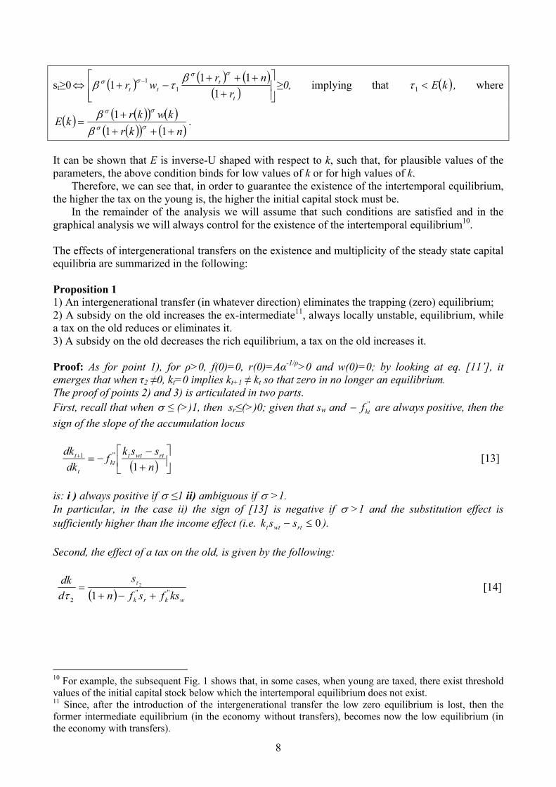
The content of Proposition 1 and the possible disappearance of all the equilibria are both illustrated in Fig.1, for the following parameter set: A=6, β=0.8, α=0.7, ρ=2.5, σ=5, n=0.3. This set, which is purely illustrative, implies that the accumulation locus is backward bending. The curve B is the benchmark case without tax/transfer and shows three equilibria: a zero stable equilibrium, both unstable intermediate and high equilibria. Furthermore, Fig. 1 shows how the level of high equilibrium is reduced when τ2 decreases from τ2 =3.5 to τ2=-3.5 and, furthermore, the disappearance of such an equilibrium when τ2=-4.5 (a more detailed discussion of Figure 1 is postponed to the following section).

10

Fig. 1. Capital accumulation loci (A-E curves) when τ2 varies, (r-n) and f’’ functions12. Legend: Curve A: τ2=3.5; B: τ2=0; C: τ2 = -1; D: τ2= -3.5; E: τ2=-4.5. Parameter set: A=6, β=0.8, α=0.7, ρ=2.5, σ=5, n=0.3. The effects of the two alternative policies, either tax on the old (that subsidy to the young) or tax on the young (that is pension transfer) on the long run steady states are summarized in the following remark: Remark 1. A policy favoring the old (pension transfers) eliminates the trapping (zero) equilibrium, increases the intermediate one and reduces the rich equilibrium. However, unfortunately, an excessive transfer (too high pension benefits) may lead to the disappearance of the equilibrium so that the economy eventually collapses. Conversely, a sufficiently high subsidy to the young causes the disappearance of the trapping (zero) equilibrium (although a trapping low equilibrium may exist for sufficiently low subsidies), the reduction and, possibly, the disappearance of the intermediate (unstable) equilibrium and, finally, the increase of the rich equilibrium.

12 Note that, for τ2≤0, the Figure shows the values of initial kt, below which the existence of the intertemporal equilibrium is not warranted, as we have pointed out in the analysis of the of main text of the this section.

11

From the above analysis, it emerges that not only the direction of the transfers, but also their magnitude is crucial for escaping from poverty. A numerical evaluation of this cruciality will be pursued in the following section, where a comparative dynamics analysis with respect to τ2 will be performed as well. 4. Policy transfers and taking off After having discussed the shift of equilibrium loci and thus, the existence of the long run equilibria, as a consequence of intergenerational transfers policy, we now perform a comparative dynamics analysis. By assuming that the economy is initially entrapped into poverty we distinguish two sub-cases according to the origin of the entrapment: 1) the rich equilibrium exists and is stable, but the economy is poor of capital and so cannot escape from the basin of attraction of the poor equilibrium. Note that in such a case, however, an external factor – e.g. capital donations, etc. – increasing the capital stock beyond the unstable intermediate equilibrium would permit the escape and the convergence towards the rich equilibrium. 2) the rich equilibrium exists but is unstable. If this is the case, in contrast with the previous one, for whatever policy increasing the capital stock (for instance, due to an external factor such as donation or international transfer), the economy will be always attracted again by the equilibrium with low capital. Therefore, in this case, even in the presence of external donation, the only device for escaping from poverty is that to create economic conditions rendering the high equilibrium attractive. Below, we will show that such an instrument, rather unexpectedly, can be an appropriate redistributive scheme among generations. Hence, in the analysis that follows, for both cases 1) and 2), we discuss the effectiveness of the introduction of intergenerational transfers for the taking off13. We now focus on case 1). The following remarks summarize our findings: Remark 2. When a country is entrapped at the zero equilibrium, the introduction of the intergenerational transfers can cause the taking off. The reason is the following: the zero equilibrium (which is a “catching” point) always disappears in presence of transfers, so that the economy may start converging to the “high” equilibrium, provided that the unstable intermediate equilibrium is eliminated by this policy or, alternatively, the capital stock at the time of the introduction of the transfers is pushed sufficiently beyond the unstable equilibrium. What is the economic comment to Remark 2? In case 1) the appropriate instrument is the introduction of a transfer from old to young. It is easy to see that this policy would permit to escape from poverty, by using either a smaller external capital donation than that needed in the absence of the policy or, without any necessity of such an external aid, provided that the tax transfer is sufficiently large such that the intermediate equilibrium is eliminated. Moreover, as expected, this policy enhances also the level of long run income via transfers to the generation that saves and accumulates. Therefore, in case 1), there is no room for implementing a transfer mechanism from the young to the old (i.e. a pay as you go –PAYG- pension scheme), because, through the well known crowding out effect which shifts the accumulation locus downwards, it would result in either a decrease of the long run income, or, more dangerously, to the disappearance of the economy in the long run. We now turn to analyze the case 2) (in which the rich equilibrium exists but is unstable).

In such a case, it is crucial to analyze the stability of the rich equilibrium rather than the existence of multiple equilibria, in that the effectiveness of the transfers policy for escaping from poverty depends crucially on the effects of the policy on the stability of the rich equilibrium.

13 Here we focus on the poverty trap problem, while we do not address the issue of optimality of the intergenerational transfers in the presence of poverty traps.

12

Indeed, as regards the level of the positive steady state capital stock, while the effect of an intergenerational transfer is clearcut (that is transfers from old to young always raise long run capital and income while transfers in the opposite directions reduce them), as for the stability of such a rich equilibrium, the analysis of the redistributive policies is much more complex and rich of outcomes, as it is summarized in the following remark and proposition. Remark 3. When a country is entrapped at the zero equilibrium, because the existing “high” equilibrium is unstable (recall that this entrapment persists even when the capital stock is temporarily increased up to the “high” equilibrium) the introduction of the intergenerational transfers can cause the taking off if and only if the rich equilibrium, formerly unstable, becomes stable, so that the economy starts converging to it. The reason of the Remark is self evident: if, after the introduction of the policy, no stable equilibrium does exist, the economy will never converge to a high equilibrium balanced growth path. The effects of the policy on the stability of the high equilibrium is summarized in the proposition below: Proposition 2 The role played by the transfers on the stability of the “high” equilibrium is as follows: 1) when n>r, an increase of τ2 stabilizes the high rich equilibrium; 2) when n<r, an increase of τ2 may be either stabilizing or destabilizing. Proof: The effects of a tax change on the stability of the “rich” equilibrium, summarized in Proposition 2, can be investigated through the following derivative of eq. [13] with respect to τ2.

( ) ( )

∂∂

−∂∂

−

∂∂

∂∂

−∂∂

+−−−+

=∂

∂ +

22

''

2

'''''

2

1

11

ττττrw

krw

wkrwk

SS

t

t

sskfkks

ksksfsksf

ndk

dk

.

Now, recalling that:

ws

rs rw

∂∂

=∂∂ ,

rw

ws

rs rr

∂∂

∂∂

=∂∂ , ''

kkfkw

−=∂∂ , and 0

2

=∂∂τ

ws, we can write as follows:

( ) ( )

∂∂

−+∂∂

∂∂

++−+

−=∂

∂

+−−

+

32144 344 2143421

43421

?

2

''

2

?

''''

?

'''

2

1

31

1τττ

rk

rwkrwk

SS

t

t

sfk

ws

kfsfsksfn

dkdk

.

Note that the sign of the overall derivative depends on the sign of three ambiguous components at the RHS of the equation above. Despite such ambiguities, with further assumptions we are able to

show some clearcut results. Note that ( )kswr

w ws

wskfs ,

'' 313 ε−=∂∂

+ , where ksw ,ε >0 is the elasticity

13

of sw with respect to capital and ( ) ( ) ( )

( )( ) ( ) ( )( )211

2 1111

1111

σσσσ

σσ

ββ

βσ

τ −−+ ++++

++

++−−

=∂∂

rrn

rnrnr

st

r ; since, we assume that

both f’’’ and ( )ksw ,31 ε− are positive14, we have that:

1) when n≥r, since ''kf is negative, an increase of τ2 is always stabilizing15.

2) When n<r, the sign of an increase of τ2 is ambiguous. In particular, a sufficiently high value

of σ makes the sign of 2τ∂

∂ rs negative, which is a necessary condition for the mentioned

ambiguity.

These findings unveil the existence of an interesting, possibly not-monotonous relationship between stability of the rich equilibrium and transfers scheme. Let us explain with a benchmark case in which large pension benefits are provided (τ2<<0) and the rich equilibrium is stable: given that higher PAYG pension benefits imply lower capital accumulation and higher interest rate, then it is very likely that, in this case, r>>n. Proposition 2 predicts that, in this situation, a reduction of pension benefits (that is an increase of τ2) may be destabilizing; however, further reductions of pensions (or even a transformation of pensions in net taxes on the old), by allowing higher accumulation and, thus, lowering r, can reduce the inequality between n and r and, sooner or later can revert it (i.e. n>r). In the latter case, further reductions of τ2 turn to be stabilizing.

In the next section we resort to numerical simulations to investigate whether increases of τ2 are

stabilizing or destabilizing, depending on the relation between the underlying parameters of the economy shown above.

4.1. A numerical illustration and some policy implications

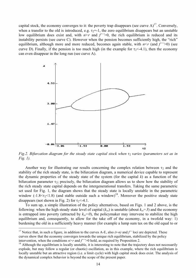
Since further analytical insights are too cumbersome, the surprisingly complicated relation between stability and intergenerational transfers is illustrated now via numerical simulations by using both a graphical analysis and a dynamical simulative analysis. As regards the graphical tool, Figure 1 is again useful for illustrating the content of Proposition 2: let us observe for sake of illustration that the rich equilibrium is unstable when transfers are absent (τ2=0), that is the case of poverty trap with unstable rich equilibrium (see curve B)16. Then, when a transfer to the young (tax on the old) is introduced, such that, for example, τ2=3.5, the rich equilibrium becomes the unique equilibrium and is not only increased but also stabilized, such that, for whatever existing level of

14 Simulations show that for a wide set of parameters f’’’ and ( )ksw ,31 ε− are positive in the proximity of the steady state. Recall that f’’’ can be negative when the technology is of the CES type; on the contrary, it is unambiguously positive in the case of a Cobb-Douglas production function. 15 Indeed in this case

( ) ( ) ( )

031(1

1

2

''

2

'''''

2

1

>

∂∂

−+∂∂

−+−

+−=

∂

∂

+++−+

+

3214342143421 ττε

τr

kkswkrwk

SS

t

t

sfksfsksfn

dkdk

w

16 In order to facilitate the comparison of the slopes of the curves, we have depicted the line y=-X+constant, whose slope represents the local instability bifurcation value for the rich equilibrium.

14

capital stock, the economy converges to it: the poverty trap disappears (see curve A)17. Conversely, when a transfer to the old is introduced, e.g. τ2=-1, the zero equilibrium disappears but an unstable low equilibrium does exist and, with n>r and f’’’>0, the rich equilibrium is reduced and its instability persists (see curve C). However when the pension becomes sufficiently high, the “rich” equilibrium, although more and more reduced, becomes again stable, with n<r (and f’’’>0) (see curve D). Finally, if the pension is too much high (in the example for τ2<-4.1), then the economy can even disappear in the long run (see curve A).

Fig.2. Bifurcation diagram for the steady state capital stock when τ2 varies (parameters set as in Fig. 1).

Another way for illustrating our results concerning the complex relation between τ2 and the

stability of the rich steady state, is the bifurcation diagram, a numerical device capable to represent the dynamic properties of the steady state of the system (for the capital k) as a function of the bifurcation parameter τ2; precisely, the bifurcation diagram allows us to show how the stability of the rich steady state capital depends on the intergenerational transfers. Taking the same parametric set used for Fig. 1, the diagram shows that the steady state is locally unstable in the parametric window (-1.8<τ2<1.8) (and stable outside such a window)18. Moreover the positive steady state disappears (not shown in Fig. 2) for τ2<-4.1.

To sum up, a simple illustration of the policy alternatives, based on Figs. 1 and 2 above, is the following: when the high steady state level of capital (kss) is unstable (about kss=3) and the economy is entrapped into poverty (attracted by kss=0), the policymaker may intervene to stabilize the high equilibrium and, consequently, to allow for the take off of the economy, in a twofold way: 1) burdening the old in a sufficiently heavy manner (for example a lump sum tax on the old equal to or 17 Notice that, in such a figure, in addition to the curves A-E, also (r-n) and f’’ loci are depicted. These curves show that the economy converges towards the unique rich equilibrium, stabilized by the policy intervention, when the conditions n>r and f’’’>0 hold, as required by Proposition 2. 18 Although the equilibrium is locally unstable, it is interesting to note that the trajectory does not necessarily explode, but may follow a regular (or chaotic) oscillation, as in this example, where the rich equilibrium is locally unstable but an attractive region (i.e. a limit cycle) with high capital stock does exist. The analysis of the dynamical complex behavior is beyond the scope of the present paper.

15

greater than 1.8) to stabilize the rich equilibrium (at τ2=1.8 kss is about 3.2); notice that a tax of the old less than 1.8 would be ineffective and uselessly painful for the old (in that the rich equilibrium would remain ustable); 2) introducing a tax on the young (i.e. a PAYG pension scheme) insuring a pension equal to or higher than 1.8, to stabilize the rich equilibrium ((at τ2=-1.8 kss is about 2.9)19; symmetrically, note that a pension transfer lower than 1.8 would be ineffective and uselessly painful for the young in that the rich equilibrium would be still unstable).

Hence, a country can escape from poverty by introducing either a pension scheme or a tax on the old; as expected, the introduction of the former would obtain a lower long run capital intensity. However, especially in the cases in which the difference in the long run capital intensities brought about by the two redistributive mechanisms is not dramatic, as in the case illustrated in our example (kss=3.2 with tax on the old versus kss=2.9 with PAYG scheme), the choice of the instrument to be adopted can be led by social preferences or political arguments. Indeed, our analysis shows that the policymaker should calibrate attentively the “size” of such intervention, which in any case should be sufficiently large (and, as for pensions not even too large).

As far as Social Security is concerned, the results explained above can be summarized in the following remark:

Remark 4. If the policymaker can only but introduce a pension transfer (because for social reasons a tax on the old is undesirable), then the escape from poverty needs a sufficiently strong pension transfer, in such a way that the positive equilibrium becomes attractive. However, if the implemented pension transfer is too high, such a positive equilibrium may disappear because the disincentive to save due to the high pension impedes the capital accumulation necessary for the existence of the economy.

Thus, we argue that there is room for tax policies for escaping from poverty trap but we have evidenced the difficulty to implement it.

Finally, some other policy implications follow from our analysis (in particular from Proposition 2). We distinguish two cases: 1) n≥r and 2) n<r.

As regards the former case, we recall that Samuelson (1958) and Diamond (1965) have shown that redistributive policies favoring the old (i.e. a PAYG scheme) are Pareto improving. However, such well known result appears suitable for rich countries only: in fact, when an economy is struggling against poverty, of the kind analyzed in this paper, our analysis shows that a policy redistributing in favor of the old is likely to be less effective, while one favoring the active generations appears to be more effective for triggering the take off. In fact, although being welfare worsening in the short run (due to the burden exerted on the old generation alive at the moment of the phasing in of the transfer policy), nevertheless the latter policy allows for the taking off the economy (and hence, is welfare improving in the long run).

As for the latter case, when n<r, whether redistributing in favor of the old or of the young is detrimental/effective for the solution of the poverty trap problem is an empirical matter, depending on the parameters underlying the economy. 5. Concluding remarks

In this work we extend the neoclassical growth literature on poverty traps by analyzing the role of intergenerational transfers. By using CIES preferences and a CES technology with low factor 19 Note that the introduction of the pension should be accompanied by a positive shock on the existing capital stock– e.g. a capital donation- sufficient to push the economy towards the basin of attraction of the stabilized rich equilibrium, if the economy, at the moment of the transfers introduction, was in proximity of zero equilibrium.

16

substitution in a standard OLG economy, we show that when the economy is entrapped at the zero equilibrium, the introduction of the intergenerational transfers can cause the taking off in a twofold manner: 1) in one case the zero equilibrium (which is a “catching” point) always disappears in presence of transfers, so that the economy may start converging to the “high” equilibrium; in this case the appropriate instrument comes out to be a transfer from the old to the young, while there is no room for a policy transfer redistributing in the opposite direction (i.e. a pay-as-you-go pension scheme); 2) in the second case, when the rich equilibrium is unstable, the introduction of transfers may stabilize such an equilibrium, so that the economy starts converging to it. Interestingly, in the latter case, we have shown that: i) a country can escape from poverty by introducing either a pension scheme or a tax on the old and the choice of the instrument to be used, although the introduction of the pension would obtain a lower long run capital intensity, can be led by social preferences or political arguments; ii) the policymaker should calibrate attentively the “size” of such intervention, which in any case should be sufficiently large (and, as for pensions not even too large): for instance too small pensions could be ineffective and uselessly painful for the young, but too large pensions could even cause the extinction of the economy. References

Azariadis C., (1996): “The economics of poverty traps-part one: complete markets”, Journal of Economic Growth, 1(4), 449-86.

Azariadis, C. (2004): “The theory of poverty traps: what have we learned?” in Poverty Traps, (S. Bowles, S. Durlauf and K. Hoff, eds), in press.

Bowles, S., S. N. Durlauf and K. Hoff, eds. (2004): Poverty Traps, in press. Cazzavillan G., Lloyd-Braga T. and Pintus P. A. (1998): “Multiple Steady States and Endogenous

Fluctuations with Increasing Return to Scale in Production”, Journal f Economic Theory, 80, 60-107. De La Croix D., Michel P. (2002): A theory of Economic Growth, Cambridge University Press,

Cambridge, UK. Diamond P. (1965): “National Debt in a neoclassical growth model”, American Economic Review 41,

1126-50. Easterly, W. (2001): The Elusive Quest for Growth: Economists’ Adventures and Misadventures in the

Tropics, The MIT Press, Cambridge, Massachusetts. Eichenbaum, M.S., Hansen, L.P. and Singleton, K.J. (1986): “A Time Series Analysis of

Representative Agent Models of Consumption and Leisure Choice Under Uncertainty.” Working Paper No. 1981. National Bureau of Economic Research.

Galor O. (1996): “Convergence? Inferences from theoretical models”, The Economic Journal, 106 (437), 1056-69.

Gruber J. (2006), A Tax-Based Estimate of The Elasticity Intertemporal Substitution, NBER Working Paper, no. 11945, January.

Hall, R. (1988): “Intertemporal Substitution in Consumption”. The Journal of Political Economy, Vol. 96, No. 2. (Apr., 1988), pp. 339-357.

Hansen, L.P., Singleton, K.J. (1983): “Stochastic Consumption, Risk Aversion, and the Temporal Behavior of Asset Returns”. The Journal of Political Economy, 91(2), 249-65.

Hansen, L.P., Singleton, K.J. (1982): “Generalized Instrumental Variables Estimation of Nonlinear Rational Expectations Models.” Econometrica 50: 1269-86.

Hoff, K. (2000): “Beyond Rosenstein-Rodan: the modern theory of coordination problems in development,” Proceedings of the World Bank Annual Conference on Development Economics.

Hoff, K., Sen, A. (2004): “The kin system as a poverty trap,” in Poverty Traps, (S. Bowles, S. Durlauf and K. Hoff, eds), in press.

Lucas, R.E, .Jr. (1969): “Labor Capital Substitution in U.S. Manufacturing”, in A. Harberger and M. Bailey, eds., Taxation of Income From Capital, Washington, DC: Brookings Institution.

Manfredi, P., Fanti, L. (2003): “The demographic transition and neoclassical models of balanced growth” in N. Salvadori (ed.) “The Theory of Economic Growth: a “classical perspective”, Edward Elgar, Cheltenham, U.K..

Matsuyama, K. (1995): “Complementarities and cumulative processes in models of monopolistic competition”, Journal of Economic Literature, 33, 701–729.

17

Matsuyama, K. (1997): “Complementarity, instability and multiplicity,” Japanese Economic Review, 48 (3), 240–266.

Mookherjee, D., Ray, D. (2001) Readings in the Theory of Economic Development, Blackwell Publishing, New York.

Mulligan, C. (2003): “Capital, Interest, and Aggregate Intertemporal Substitution”. Working paper, University of Chicago.

Mulligan, C. (2004): “What do Aggregate Consumption Euler Equations Say about the Capital Income Tax Burden?”. The American Economic Review: Papers and Proceedings, May 2004.

Prskawetz, A., Steinmann, G. and Feichtinger, G. (2000): “Human capital, technological progess and the demographic transition”, Mathematical Population Studies, 7(4), 343-63.

Rowthorn, R.E. (1999a): “Unemployment, Wage Bargaining and Capital-Labour Substitution”, Cambridge Journal of Economics, July.

Rowthorn, R.E. (1999b): “Unemployment, Capital-Labor Substitution, and Economic Growth”, IMF Working Paper No. 99/43, March 1.

Sachs, J.D., McArthur, J.W.,Schmidt-Traub, G., Kruk M., Bahadur C., Faye M., McCord G. (2004): “Ending Africa’s Poverty Trap”, Brookings Papers on Economic Activity, 1, pp. 117-216

Samuelson, P.A. (1958): “An exact consumption-loan model of interest with or without the social contrivance of money”, Journal of Political Economy 66, 467-82.

Solow, R. (1956): “A Contribution to the Theory of Economic Growth”, Quarterly Journal of Economics, 70 (1), 65-94.

Solow, R. (1958): “A Sceptical Note on the Constancy of Relative Share”. American Economic Review, 48, 618-31.

Strulik, H. (1997): “Learning by doing, population pressure, and the theory of demographic transition”, Journal of Population Economics, 10, 285-98.

Strulik, H. (1999): “Demographic transition, stagnation, and demoeconomic cycles in a model for the less developed economy”, Journal of Macroeconomics, 21(2), 397-413.

Discussion Papers - Dipartimento Scienze Economiche – Università di Pisa

1. Luca Spataro, Social Security And Retirement Decisions In Italy, (luglio 2003)

2. Andrea Mario Lavezzi, Complex Dynamics in a Simple Model of Economic Specialization, (luglio2003)

3. Nicola Meccheri, Performance-related-pay nel pubblico impiego: un'analisi economica, (luglio 2003)

4. Paolo Mariti, The BC and AC Economics of the Firm, (luglio- dicembre 2003)

5. Pompeo Della Posta, Vecchie e nuove teorie delle aree monetarie ottimali, (luglio 2003)

6. Giuseppe Conti, Institutions locales et banques dans la formation et le développement des districts industrielsen Italie, (luglio 2003)

7. F. Bulckaen - A. Pench - M. Stampini, Evaluating Tax Reforms without utility measures : the performance ofRevenue Potentialities, (settembre 2003, revised June 2005)

8. Luciano Fanti - Piero Manfredi, The Solow’s model with endogenous population: a neoclassical growth cyclemodel (settembre 2003)

9. Piero Manfredi - Luciano Fanti, Cycles in dynamic economic modelling (settembre 2003)

10. Gaetano Alfredo Minerva, Location and Horizontal Differentiation under Duopoly with MarshallianExternalities (settembre 2003)

11. Luciano Fanti - Piero Manfredi, Progressive Income Taxation and Economic Cycles: a Multiplier-AcceleratorModel (settembre 2003)

12. Pompeo Della Posta, Optimal Monetary Instruments and Policy Games Reconsidered (settembre 2003)

13. Davide Fiaschi - Pier Mario Pacini, Growth and coalition formation (settembre 2003)

14. Davide Fiaschi - Andre Mario Lavezzi, Nonlinear economic growth; some theory and cross-country evidence(settembre 2003)

15. Luciano Fanti , Fiscal policy and tax collection lags: stability, cycles and chaos (settembre 2003)

16. Rodolfo Signorino- Davide Fiaschi, Come scrivere un saggio scientifico:regole formali e consigli pratici(settembre 2003)

17. Luciano Fanti, The growth cycle and labour contract lenght (settembre 2003)

18. Davide Fiaschi , Fiscal Policy and Welfare in an Endogenous Growth Model with Heterogeneous Endowments(ottobre 2003)

19. Luciano Fanti, Notes on Keynesian models of recession and depression (ottobre 2003)

20. Luciano Fanti, Technological Diffusion and Cyclical Growth (ottobre 2003)

21. Luciano Fanti - Piero Manfredi, Neo-classical labour market dynamics, chaos and the Phillips Curve (ottobre2003)

22. Luciano Fanti - Luca Spataro, Endogenous labour supply and Diamond's (1965) model: a reconsideration ofthe debt role (ottobre 2003)

23. Giuseppe Conti, Strategie di speculazione, di sopravvivenza e frodi bancarie prima della grande crisi(novembre 2003)

24. Alga D. Foschi, The maritime container transport structure in the Mediterranean and Italy (dicembre 2003)

25. Davide Fiaschi - Andrea Mario Lavezzi, On the Determinants of Growth Volatility: a NonparametricApproach (dicembre 2003)

26. Alga D. Foschi, Industria portuale marittima e sviluppo economico negli Stati Uniti (dicembre 2003)

27. Giuseppe Conti - Alessandro Polsi, Elites bancarie durante il fascismo tra economia regolata edautonomia (gennaio 2004)

28. Annetta Maria Binotti - Enrico Ghiani, Interpreting reduced form cointegrating vectors of incomplete systems.A labour market application (febbraio 2004)

29. Giuseppe Freni - Fausto Gozzi - Neri Salvadori, Existence of Optimal Strategies in linear Multisector Models(marzo 2004)

30. Paolo Mariti, Costi di transazione e sviluppi dell’economia d’impresa (giugno 2004)

31. Domenico Delli Gatti - Mauro Gallegati - Alberto Russo, Technological Innovation, Financial Fragility andComplex Dynamics (agosto 2004)

32. Francesco Drago, Redistributing opportunities in a job search model: the role of self-confidence and socialnorms (settembre 2004)

33. Paolo Di Martino, Was the Bank of England responsible for inflation during the Napoleonic wars (1897-1815)? Some preliminary evidence from old data and new econometric techniques (settembre 2004)

34. Luciano Fanti, Neo-classical labour market dynamics and uniform expectations: chaos and the “resurrection”of the Phillips Curve (settembre 2004)

35. Luciano Fanti – Luca Spataro, Welfare implications of national debt in a OLG model with endogenous fertility(settembre 2004)

36. Luciano Fanti – Luca Spataro, The optimal fiscal policy in a OLG model with endogenous fertility (settembre2004)

37. Piero Manfredi – Luciano Fanti, Age distribution and age heterogeneities in economic profiles as sources ofconflict between efficiency and equity in the Solow-Stiglitz framework (settembre 2004)

38. Luciano Fanti – Luca Spataro, Dynamic inefficiency, public debt and endogenous fertility (settembre 2004)

39. Luciano Fanti – Luca Spataro, Economic growth, poverty traps and intergenerational transfers (ottobre 2004)

40. Gaetano Alfredo Minerva, How Do Cost (or Demand) Asymmetries and Competitive Pressure Shape TradePatterns and Location? (ottobre 2004)

41. Nicola Meccheri, Wages Behaviour and Unemployment in Keynes and New Keynesians Views. AComparison (ottobre 2004)

42. Andrea Mario Lavezzi - Nicola Meccheri, Job Contact Networks, Inequality and Aggregate Output (ottobre2004)

43. Lorenzo Corsini - Marco Guerrazzi, Searching for Long Run Equilibrium Relationships in the Italian LabourMarket: a Cointegrated VAR Approach (ottobre 2004)

44. Fabrizio Bulckaen - Marco Stampini, Commodity Tax Reforms In A Many Consumers Economy: A ViableDecision-Making Procedure (novembre 2004)

45. Luzzati T. - Franco A. (2004), “Idrogeno fonti rinnovabili ed eco-efficienza: quale approccio alla questioneenergetica?”

46. Alga D. Foschi , “The coast port industry in the U.S.A: a key factor in the process of economic growth”(dicembre 2004)

47. Alga D. Foschi , “A cost – transit time choice model: monomodality vs. intermodality” (dicembre 2004)

48. Alga D. Foschi , “Politiques communautaires de soutien au short sea shipping (SSS)” (dicembre 2004)

49. Marco Guerrazzi, Intertemporal Preferences, Distributive Shares, and Local Dynamics (dicembre 2004)

50. Valeria Pinchera, “Consumo d’arte a Firenze in età moderna. Le collezioni Martelli, Riccardi e Salviati nelXVII e XVIII secolo” (dicembre 2004)

51. Carlo Casarosa e Luca Spataro, “Propensione aggregata al risparmio, rapporto ricchezza-reddito edistribuzione della ricchezza nel modello del ciclo di vita "egualitario": il ruolo delle variabilidemografiche” (aprile 2005)

52. Alga D. Foschi – Xavier Peraldi – Michel Rombaldi, “Inter – island links in Mediterranean Short Sea ShippingNetworks” (aprile 2005)

53. Alga D. Foschi (2005), “Lo shipping, la cantieristica ed i porti nell’industria marittima” (aprile 2005)

54. Marco Guerrazzi, “Notes on Continuous Dynamic Models: the Benhabib-Farmer Condition for Indeterminacy”(settembre 2005)

55. Annetta Binotti e Enrico Ghiani, "Changes of the aggregate supply conditions in Italy: a small econometricmodel of wages and prices dynamics" (settembre 2005)

56. Tommaso Luzzati, “Leggere Karl William Kapp (1910-1976) per una visione unitaria di economia, società eambiente” (dicembre 2005)

57. Lorenzo Corsini (2006), “Firm's Entry, Imperfect Competition and Regulation”

58. Mario Morroni (2006), “Complementarities among capability, transaction and scale-scope considerations indetermining organisational boundaries”

59. Mario Morroni (2006), “Innovative activity, substantive uncertainty and the theory of the firm”

60. Akos Dombi (2006), "Scale Effects in Idea-Based Growth Models: a Critical Survey"

61. Binotti Annetta Maria e Ghiani Enrico (2006), “La politica economica di breve periodo e lo sviluppo dei primimodelli mocroeconometrici in Italia: dalla vicenda ciclica degli anni ’60 alla prima crisi petrolifera”

62. Fioroni Tamara (2006), “Life Expectancy, Health Spending and Saving”

63. Alga D. Foschi (2006), “La concentrazione industriale per i sistemi di trasporto sostenibile: un caso disuccesso nel Mediterraneo orientale”

64. Alga D. Foschi (2006), “La concentrazione industriale per i sistemi di trasporto sostenibile

65. Maurizio Lisciandra (2007), “The Role of Reciprocating Behaviour in Contract Choice”

Redazione:Giuseppe Conti

Luciano Fanti (Coordinatore Responsabile)Davide Fiaschi

Paolo ScapparoneE-mail della Redazione: papers-SE@ec.unipi.it