Predicting CO2 Minimum Miscibility Pressure (MMP) Using Alternating

Conditional Expectation (ACE) Algorithm

O. A. Al-omair1, A. Malallah1, A. Elsharkawy1, and M. Iqbal1*

1 Petroleum Engineering Department, College of Engineering & Petroleum,

Kuwait University, P.O. Box 5969, Safat, Kuwait.

osamah@dr-alomair.com - malallahq80@hotmail.com - adel.elsharkawy@ku.edu.kw

maqsoodqp@hotmail.com

* Corresponding author

Résumé - Prédire CO2 pression de miscibilité minimale (MMP) en alternant espérance

conditionnelle (ACE) Algorithme injection de gaz miscible est l'un des plus importants amélioré

de récupération du pétrole (EOR) approches pour la récupération du pétrole augmente. En raison

de l'énorme coût associé à cette approche, un haut degré de précision est nécessaire pour prédire

l'issue du processus. Une telle précision inclut les paramètres de présélection pour le déplacement

de gaz miscible; le "pression de miscibilité minimale" (MMP) et la disponibilité du gaz. Tous les

classiques et stat-of-the-art des méthodes de mesure de MMP sont soit de temps ou de coûts

décidément processus exigeant. Par conséquent, afin d'aborder l'industrie immédiate exige une

approche non paramétrique, alternant espérance conditionnelle (ACE), est employé dans cette

étude pour estimer les MMP. Cet algorithme transforme en corrélation optimale d'un ensemble de

prédicteurs (C1, C2, C3, C4, C5, C6, C7 +, CO2, H2S, N2, MW5 +, MW7 + et T) avec une

réponse optimale (MMP) transformer. Le modèle proposé a produit un effet maximal linéaire entre

ces variables transformées. Cent treize de données MMP points sont considérés à la fois de la

littérature pertinente publiée et les travaux expérimentaux. Cinq mesures pour la MMP pétrole

koweïtiens sont inclus comme une partie des données de test. Le modèle proposé est validé en

utilisant une analyse statistique détaillée; une valeur raisonnablement bonne de 0,956 coefficient

de corrélation est obtenu comme comparer aux corrélations existant. De même, l'écart type et la

moyenne des valeurs absolues d'erreur sont au plus bas que 139 psia et 4,68% respectivement.

Ainsi, elle révèle que les résultats sont plus fiables que les corrélations existantes pour l'injection

du CO2 pur pour améliorer la récupération du pétrole. En plus de sa précision, l'approche de l'ECA

est plus puissant, rapide et peut traiter un ensemble de données énorme.

Abstract - Predicting CO2 Minimum Miscibility Pressure (MMP) Using Alternating

Conditional Expectation (ACE) Algorithm - Miscible gas injection is one of the most important

enhanced oil recovery (EOR) approaches for increasing oil recovery. Due to the massive cost

associated with this approach a high degree of accuracy is required for predicting the outcome of

the process. Such accuracy includes, the preliminary screening parameters for gas miscible

displacement; the ―minimum miscibility pressure‖ (MMP) and the availability of gas.

All conventional and stat-of-the-art MMP measurement methods are either time consuming or

decidedly cost demanding processes. Therefore, in order to address the immediate industry

demands a nonparametric approach, Alternating Conditional Expectation (ACE), is employed in

this study to estimate MMP. This algorithm correlates optimal transforms of a set of predictors

(C1, C2, C3, C4, C5, C6, C7+, CO2, H2S, N2, Mw5+, Mw7+ and T) with an optimal response (MMP)

transform. The proposed model has produced a maximum linear effect between these transformed

variables. One hundred thirteen MMP data points are considered both from the relevant published

literature and the experimental work. Five MMP measurements for Kuwaiti Oil are included as a

part of the testing data. The proposed model is validated using detailed statistical analysis; a

reasonably good value of correlation coefficient 0.956 is obtained as compare to the existing

correlations. Similarly, standard deviation and average absolute error values are at the lowest as

139 psia and 4.68 % respectively. Hence, it reveals that the results are more reliable than the

existing correlations for pure CO2 injection to enhance oil recovery. In addition to its accuracy,

the ACE approach is more powerful, quick and can handle a huge data.

INTRODUCTION

Miscible gas injection into an oil reservoir is among the most widely used enhanced oil recovery

techniques, and its applications are increasingly visible in oil production worldwide. An important

concept associated with the description of miscible gas injection processes is the minimum

miscibility pressure (MMP). MMP is the lowest pressure at which gas and oil become miscible at

a fixed temperature and the displacement process becomes very efficient. It is considered as one

of the most important factors in the selection of candidate reservoirs for gas injection at which

miscible recovery takes place and it determines the efficiency of oil displacement by gas.

Determination of MMP lies under two categories; experimental and non-experimental. The

experimental methods are; slim tube, rising bubble apparatus, multi-contact experiment, pressure-

composition diagram, vanishing interfacial tension, vapour density, and high pressure visual

sapphire cell. The non-experimental methods consist of both analytical and numerical approaches.

All correlations and EOS also belong to the analytical techniques. Non-experimental

computational methods are fast and convenient alternatives to otherwise slow and expensive

experimental procedures. This research focuses on the analytical aspect of MMP estimation. It

introduces a non parametric model to improve the MMP estimation.

1. EXPERIMENTAL TECHNIQUES FOR MEASURING MMP

Several experimental methods have been developed for measuring MMP for an oil-solvent system.

Slim-tube experiments (Yellig et al., 1980, and Huang et al., 1994) are widely accepted as the

industry standard experimental procedure to estimate the MMP. P-X diagram, multi contact, core

flooding tests, and vapour density experiments of injected gas versus pressure at low temperatures

are additional experiments for MMP measurements (Thomas et al., 1994, and Harmon and Grigg,

1986). These experiments are generally reliable because they use real fluids and can capture the

complex interactions between fluid flow and phase behaviour in a porous medium. These

experiments, however, are also slow and expensive to conduct, and thus, in practice, few MMPs

are obtained this way. Several researchers stated that no standard has been agreed on for the

apparatus and testing procedure used for MMP measurements (Orr et. al., 1982, Nouar and Flock,

1984, and Kechut, et al., 1999).

Other experimental MMP methods, such as rising bubble apparatus (RBA) experiments

(Christianson and Haines 1987) and vanishing interfacial tension (VIT) tests (Rao 1997) are

unlikely to provide good MMP predictions because they fail to reproduce the interaction of fluid

flow and phase behaviour in Condensing-Vaporizing floods (Jessen and Orr 2008). The RBA test

is a fast way to estimate the MMP during vaporizing gas drive injection study. The test involves

direct visual observation of the behaviour of a bubble of injection gas as it rises through a column

of reservoir oil contained in the RBA cell. A comparison of the two measurement techniques

(Slim Tube and RBA) has been discussed by many investigators (Novosad et al., 1989,

Elsharkway et. al., 1992, Huang and Dyer; 1993, and Srivastava et al., 1994). Although the VIT

experimental set up is quite elaborated, the technique itself is quite simple in terms of its

principles. This method is based on the concept that, at miscibility, the value of IFT between the

two phases is zero. In this method, the IFT is measured between the injected gas and crude oil at

reservoir temperature at varying pressures or enrichment levels of gas phase. The MMP is then

determined by extrapolating the plot between IFT and pressure to zero interfacial tension.

Other researchers investigated the modification of existing experimental methods; Srivastava and

Huang (1998) suggested a single bubble injection technique to extend the applicability of RBA for

determining MMP for solvent gases exhibiting enriched gas drive behaviour. Kechut et al. (1999)

proposed the vapour liquid equilibrium-interfacial tension test (VLE-IT) approach that measures

the IFT between the injected gas and the oil at reservoir temperature and varying pressures using

proto type equipment.

2. NON-EXPERIMENTAL METHODS FOR MMP DETERMINATION

Non-Experimental computational methods provide fast and cheap alternatives to MMP

experimental approaches. They are also indispensable tools in tuning equations of state (EOS) to

MMP for compositional simulations. Incorporating the MMP in the process of tuning can improve

the accuracy of EOS in gas displacement simulations (Jessen and Stenby 2007, Yuan et. al. 2005).

The non experimental methods for MMP determination are classified into; numerical methods and

analytical methods.

2.1 Numerical Methods can be used to calculate MMP numerically, assuming that appropriate

equation of state (EOS) based fluid phase behaviour characterization is available. EOS‘s

reliability depends on the quality of the data used and the oil composition. Wang and Peck

(2000) have reported that among the numerical MMP calculation approaches, one-

dimensional compositional simulation is shown to be able to predict MMPs that are

consistent with slim-tube test data, provided that appropriate fluid phase behaviour

characterization is available and care is taken to account for the effect of numerical

dispersion. Alternatively, 2D or 3D compositional simulation models can also be used to

calculate MMPs accurately, assuming that enough number of cells is used to mitigate the

effect of numerical dispersion. No doubt, selecting a large number of grid blocks will limit

the effect of numerical dispersion but these types of simulation approaches are generally

time-consuming. In addition, when the number of pressure points at which simulations are

performed is not large enough to obtain a reasonably well defined recovery curve, the

numerically calculated MMPs are subject to the visual interpretation of the recovery curve.

Conclusions from (Wang and Peck, 2000, Zick, 1986, and Stalkup, 1982 and 1987) and

others indicate that numerical simulation and 1D Slim-tube simulation give excellent

matching to the experimental data.

2.2 Analytical Methods are another method to determine MMP. These methods are based on

the analytical theory of multi component gas injection processes. Because of their

improved speed, analytical methods offer significant promise for developing improved

fluid correlations and for use in compositional streamline simulations. Correlations for

predicting MMP have been proposed by a number of investigators, and are important tools

for rapid and accurate MMP calculation. Enich et al. (1988) pointed out that, ideally, any

correlation should account for each parameter known to affect the MMP, should be based

on thermodynamic or physical principles that affect the miscibility of fluids, and should be

directly related to the multiple contact miscibility process. For an initial and quick

estimate, operators use correlation currently available in the literature. For screening

purposes, correlations gave a fair first guess depending on the data used. However, the

success of the correlations is usually limited to the composition range in which these

correlations were developed. The CO2 MMP correlations fall into two categories: the pure

and impure CO2; while the other category treats MMP‘s of other gases. Benham et al.

(1960) presented empirical curves for predicting MMP for reservoir oils that are displaced

by rich gas. Further, he proposed equations that have been derived from graphical

correlations, based on calculated critical point compositions of selected multi-component

systems which were simplified into three pseudo-components. Cronquist (1978) used the

temperature and C5+ molecular weight as correlation parameters in addition to the volatile

mole percentage (C1 and N2). Yellig and Metcalfe (1980) from their experimental study

proposed a correlation for predicting the CO2 MMP‘s that uses the temperature ―T‖ as the

only correlating parameter. Alston et al., (1985) presented an empirically derived

correlation for estimating the MMP of live oil systems by pure and impure CO2 streams.

MMP has been correlated with temperature, oil C5+ molecular weight, volatile oil fraction,

intermediate oil fraction and composition of CO2 streams. Glaso (1985) presented a

generalized correlation for predicting the MMP required for multi-contact miscible

displacement of reservoir fluids by hydrocarbon, CO2 or N2 gas. The equations are derived

from graphical correlations given by Benham et al. (1960) and give MMP as a function of

reservoir temperature, C7+ molecular weight, mole percent methane in the injection gas, and

the molecular weight of the intermediates (C2 through C6) in the gas. Orr and Jensen

(1986) suggested that the vapour pressure curve of CO2 can be extrapolated and equated

with the MMP to estimate the MMP for low temperature reservoirs. However, none of

these correlations gives adequate emphasis to oil properties and composition and all fail to

accurately predict the miscibility pressure for variety of crude oil types.

3. ANALYTICAL METHODS REGRESSION TECHNIQUES

Regression analysis is a statistical tool for the investigation of relationships between variables.

Usually, the investigator seeks to ascertain the causal effect of one variable upon another—the

effect of a price increase upon demand, for example, or the effect of changes in the money supply

upon the inflation rate. To explore such issues, the investigator assembles data on the underlying

variables of interest and employs regression to estimate the quantitative effect of the causal

variables upon the variable that they influence. The investigator also typically assesses the

―statistical significance‖ of the estimated relationships, that is, the degree of confidence that the

true relationship is close to the estimated relationship. Broadly speaking there are two types of

regression techniques, explained in the following paragraphs.

3.1 Parametric Regression Analysis addresses the effect of one or more independent

variables (predictors or covariates) on a dependent variable (response). The initial stages

of data analysis often involve exploratory analysis. Unfortunately traditional multiple

regression techniques are limited, since they usually require a priori assumptions about the

functional forms that relate the response and predictor variables. When the relationship

between the response and the predictor variable is unknown or inexact, linear parametric

regression can yield erroneous and even misleading results. This is the primary motivation

for the use of non-parametric regression techniques, which make few assumptions about

the regression surface (Friedman and Stuetzle, 1981).

3.2 Non-Parametric Regression Analysis The objective of fully exploring and explaining the

effect of covariates on a response variable in regression analysis is facilitated by properly

transforming the independent variables. There are number of parametric transformations

for continuous variables in regression analysis. Estimating the optimal transformation is

the primary motivation for the use of non-parametric regression techniques, which make

few assumptions about the regression surface (Breiman and Friedman, 1985). Non-

parametric regression techniques are based on successive refinements by attempting to

define the regression surfaces in an iterative fashion while remaining ‗data driven‘ as

opposed to ‗model driven‘. The advantage of the non-parametric regression is easy to use

and can quickly provides results that reveal the dominant independent variables and

relative characteristics of the relationships (Wu et al., 2000). There are many non-

parametric tests (Sign test, Wilcoxon Signed-Ranks test, Mann-Whitney U test, Kruskal-

Wallis H-test, Jonckheere test, Friedman ANOVA, etc.) being used for the analysis

purposes. In this particular study we have considered an approach called Alternating

Conditional Expectations (ACE).

3.3 Alternating Conditional Expectations (ACE) Non-parametric regression methods can be

broadly classified into those which do not transform the response variable (such as

generalised additive models) and those which do (such as Alternating Conditional

Expectations, ACE). Moreover, the ACE algorithm can handle variables other than

continuous predictors such as categorical (ordered or unordered), integer and indicator

variables (Wang and Murphy, 2004).

The present approach to estimate MMP is guided by the view that statistical methods for dealing

with data that exhibit strong linear associations are well developed; consequently, many non-

standard problems are best addressed by transforming the data to achieve increased linear

association. The analysis given here also serves to illustrate the exploratory use of the ACE

algorithm to suggest expressions, and the use of R2 from the ACE transformed variables as a

benchmark. The ACE-Transformed variables exhibit substantially greater linear association than

the untransformed variables. One of the principal benefits of the ACE algorithm is that it provides

a theoretical standard against which more analytically appealing transformation can be judged

(Veaux, et al., 1989). The power of the ACE approach lies in its ability to recover the functional

forms of variables and to uncover complicated relationships (Wang and Murphy, 2004). It can be

applied both bivariate and multivariate cases and it yields maximum correlations in transformed

space (Malallah et al., 2005). A modification of ACE algorithm with graphical (GRACE) interface

was later proposed by Xue et al. (1997).

4. DEVELOPMENT OF ACE MMP MODEL

This study uses an algorithm (ACE) of Brieman and Friedman (1985) for estimating the

transformations of a response and a set of predictor variables in multiple regression problems in

enhanced oil recovery. The name ‗alternating conditional expectations‘ refers to the algorithm

used to compute optimum transforms (viz. those that minimize the summation of squares of the

error). The mathematical expectation is the mean of the distribution of a population and is denoted

by μ or E(Z), where Z is the variable that describes the experiment. μ is mostly used mostly in uni-

variate statistics. The word ‗conditional‘ in ACE is meant to indicate that the means of Z/Q

variables (i.e., the conditional variables) are determined. The conditions in ACE are the values of

the dependent variable or those of an independent variable. Conditional expectations can be

expressed as:

Y

XE ii and

i

ii

X

XE

(1)

The proposed nonparametric approach can be applied easily for estimating the optimal

transformation of different gas injection data to obtain maximum correlation between observed

variables. An ACE regression model can be expressed as:

p

i

ii XY1

(2)

Where θ is a function of the response (dependent) variable Y, Φi are functions of the predictors

(independent) variables Xi , i =1,2,3,……..p. Thus, the ACE model replaces the problem of

estimating a linear function of a p-dimensional variable X = (X1, X2, X3, X4, ………………. Xp)

by estimating p separate one-dimensional functions, Φi, and θ using an iterative method. These

transformations are achieved by minimizing the unexplained variance of a linear relationship

between the transformed response variable and the sum of transformed predictor variables.

For a given dataset consisting of a response variable Y and predictor variables X1, X2, X3,

X4,………. Xp, the ACE algorithm starts out by defining arbitrary measurable mean

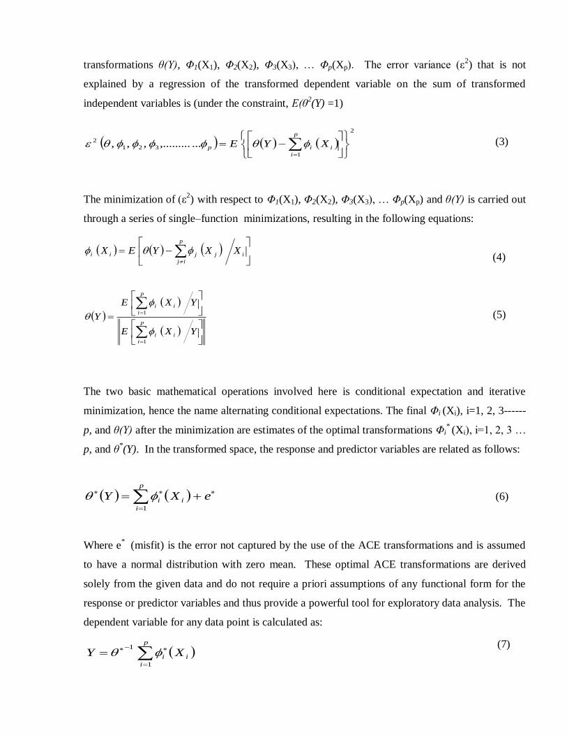
transformations θ(Y), Φ1(X1), Φ2(X2), Φ3(X3), … Φp(Xp). The error variance (ε2) that is not

explained by a regression of the transformed dependent variable on the sum of transformed

independent variables is (under the constraint, E(θ2(Y) =1)

(3)

The minimization of (ε2) with respect to Φ1(X1), Φ2(X2), Φ3(X3), … Φp(Xp) and θ(Y) is carried out

through a series of single–function minimizations, resulting in the following equations:

(4)

(5)

The two basic mathematical operations involved here is conditional expectation and iterative

minimization, hence the name alternating conditional expectations. The final Φi (Xi), i=1, 2, 3------

p, and θ(Y) after the minimization are estimates of the optimal transformations Φi*

(Xi), i=1, 2, 3 …

p, and θ*(Y). In the transformed space, the response and predictor variables are related as follows:

eXYp

i

ii

1

(6)

Where e*

(misfit) is the error not captured by the use of the ACE transformations and is assumed

to have a normal distribution with zero mean. These optimal ACE transformations are derived

solely from the given data and do not require a priori assumptions of any functional form for the

response or predictor variables and thus provide a powerful tool for exploratory data analysis. The

dependent variable for any data point is calculated as:

(7)

2

1

321

2 ...,.........,,,

p

i

iip XYE

i

p

ij

jjii XXYEX

YXE

YXE

Yp

i

ii

p

i

ii

1

1

p

i

ii XY1

1

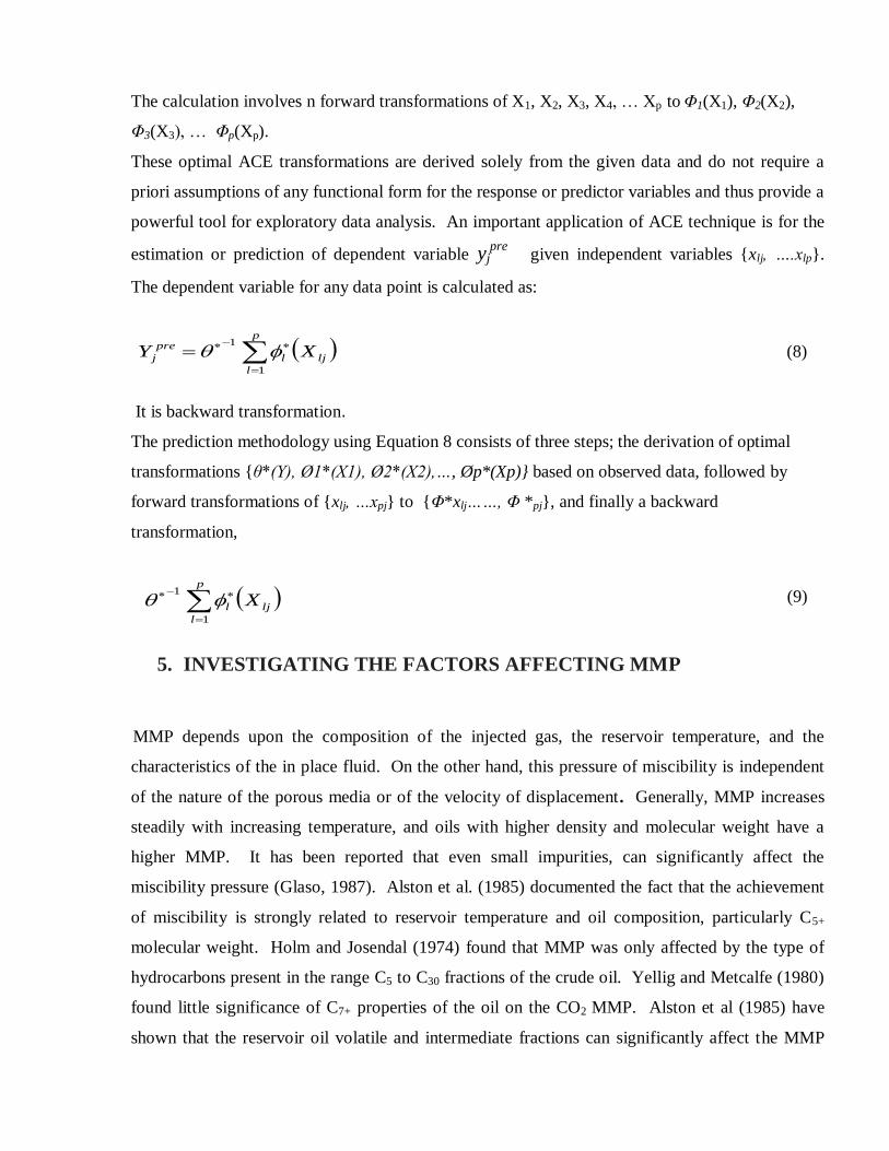
The calculation involves n forward transformations of X1, X2, X3, X4, … Xp to Φ1(X1), Φ2(X2),

Φ3(X3), … Φp(Xp).

These optimal ACE transformations are derived solely from the given data and do not require a

priori assumptions of any functional form for the response or predictor variables and thus provide a

powerful tool for exploratory data analysis. An important application of ACE technique is for the

estimation or prediction of dependent variable yjpre

given independent variables {xlj, ….xlp}.

The dependent variable for any data point is calculated as:

(8)

It is backward transformation.

The prediction methodology using Equation 8 consists of three steps; the derivation of optimal

transformations {θ*(Y), Ø1*(X1), Ø2*(X2),…, Øp*(Xp)} based on observed data, followed by

forward transformations of {xlj, …xpj} to {Φ*xlj……, Φ *pj}, and finally a backward

transformation,

(9)

5. INVESTIGATING THE FACTORS AFFECTING MMP

MMP depends upon the composition of the injected gas, the reservoir temperature, and the

characteristics of the in place fluid. On the other hand, this pressure of miscibility is independent

of the nature of the porous media or of the velocity of displacement. Generally, MMP increases

steadily with increasing temperature, and oils with higher density and molecular weight have a

higher MMP. It has been reported that even small impurities, can significantly affect the

miscibility pressure (Glaso, 1987). Alston et al. (1985) documented the fact that the achievement

of miscibility is strongly related to reservoir temperature and oil composition, particularly C5+

molecular weight. Holm and Josendal (1974) found that MMP was only affected by the type of

hydrocarbons present in the range C5 to C30 fractions of the crude oil. Yellig and Metcalfe (1980)

found little significance of C7+ properties of the oil on the CO2 MMP. Alston et al (1985) have

shown that the reservoir oil volatile and intermediate fractions can significantly affect the MMP

p

l

ljl

pre

j XY1

1

p

l

ljl X1

1

when their ratios depart from unity. This also explained the effects of both solution gas (live oil

systems) and impurity of CO2 sources (Alston, et al., 1985). James et al (1981) presented an

empirical correlation which predicted the MMP for a wide variety of live oils and stock oils with

both pure and diluted CO2. This correlation, requiring only the oil gravity, molecular weight,

reservoir temperature and injection gas composition, showed substantially better agreement with

experiment. Many correlations relating the MMP to the physical properties of the oil and the

displacing gas have been proposed to facilitate screening procedures and to gain insight into the

miscible displacement process (Alston et al., 1985; Orr and Silva, 1987; Rathmell et al.; 1971).

To study the effect of these parameters on tested data, several sensitivity analyses were conducted.

Figure 1 shows the relationship between the independent variables and MMP for the data used in

this study. The correlation coefficient of each independent variable is shown. It is clear that the

temperature is the most dominant factor. The parameters C1, C2, C5, and MwC5+ have the same

proportional effect with C5, and MwC5+ having insignificant roles. On the other side, intermediate

components (C3, & C4) and heavy ends (C6, & C7+) are showing inverse effects. Addition to this,

all the non-hydrocarbon gases (CO2, N2 & H2S) showing inverse relationship with a considerable

role.

6. PROPOSED CO2 MMP MODEL FORMULATION

As discussed earlier, MMP is a function of temperature, crude oil composition and composition of

the solvent. To understand the in-situ crude oil composition impact on MMP, the functional form

of MMP Model is:

75 ,,,, MCMCTNHCHCfMMP COMPCOMP (10)

HCCOMP = Mole Fraction of hydrocarbons (C1, C2, -------- C7+)

NHCCOMP = Mole Fraction of non-hydrocarbons (H2S, CO2, N2)

T = Temperature

MC5+ = Molecular weight of Pentane Plus

MC7+ = Molecular weight of Heptane Plus

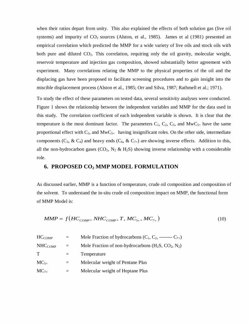
6.1 Data Distribution

The data set used in this study consisted of 113 MMP measurements (pure CO2) taken from

worldwide gas injection projects from the published literature. The ranges of variables and MMPs

used for this study are shown in Table 1. The collected data cover a wide range of API gravities

(13 to 48 oAPI) and reservoir temperatures (71 to 265

oF). The data were divided into two sets.

The training set consisted of 96 MMP measurements and a testing set of 17, which were randomly

selected from the total set of data. Out of 17 testing set, 5 were taken from MMP measurements of

Kuwait oil fields studied in Kuwait University PVT Lab. Both, the detailed compositional

analyses and minimum miscibility pressure measurements were experimentally determined.

6.2 Optimal ACE Regression

The proposed ACE algorithm provides a nonparametric optimization of the dependent (MMP) and

independent variables (HCCOMP, NHCCOMP, T, MC5+, MC7+), it does not provide a computational

model for these variables. However, the optimal data transforms can be fitted by simple

polynomials that can be used to predict the dependent variable. The default polynomial is of

degree two but for any improvement the degree can be increased. To find the maximum/optimal

correlation, the ACE algorithm has the capability of using the independent and dependent variables

in their actual space or in the logarithmic space. After testing all possible combinations of the

independent and dependent variables in either logarithmic or actual space, the complete suite of

fitting polynomials is listed in Table 2. Coefficients of this fitted polynomial will be incorporated

in the final SUM equation to estimate MMP.

In the proposed nonparametric ACE model for MMP estimation, there are 13 predictors. The sum

of all these optimal transformed independent variables is;

13

1i

ipSUM

(11)

ACE predicted / calculated MMP will be:

SUMpMMP O

1 (12)

A thorough investigation and detailed scrutiny of several scenarios for different transforms of

predicting variables (both in real and logarithmic space) was executed. This yields the best

combination, that has the highest correlation coefficient (R2

= 0.956), the lowest average absolute

relative error (AARE = 4.68 %), the lowest average relative error (ARE = -0.66 %), and the lowest

standard deviation (SD = 139) is;

0

1

1

2

2 aSUMaSUMaMMP

(13)

7. RESULTS AND DISCUSSION

7.1 Optimal Transforms Predictions

The nonparametric independent variables proposed in this study (HCCOMP, NHCCOMP, T, MC5+,

MC7+) were investigated thoroughly to find their optimal transforms using ACE. Similarly, the

nonparametric dependent variable (MMP) was investigated.

In case of hydrocarbon transforms all mole fractions are found more optimal to their respective

transforms in the logarithmic space instead of real space. These optimal transforms defined by

ACE are explained in Figures 2 through 8. The default polynomial interpreted by GRACE is of

degree 2 like in case of C1 & C7+, however there are some higher degrees polynomials; C2 & C4

with degree 6, C6 with degree 5 and C3 & C5 with degree 4. Each ACE defined transform shows a

specific pattern.

The non-hydrocarbon transforms of all mole fractions are found more optimal to their respective

transforms in the logarithmic space instead of real space. These optimal transforms defined by

ACE are explained in Figures 9 through 11. In this group we have higher degrees of fitting

polynomials; CO2 with degree 6 and H2S & N2 both with degree 4.

The real space optimal transforms for both plus fraction molecular weights (Mw5+ and Mw7+) and

temperature transforms are more optimal to their respective transforms in the real space. These

optimal transforms defined by ACE are explained in Figures 12 through 14.

Both Mw7+ & T transforms are fitted at default polynomials of degree 2, whereas Mw5+ transform

is fitted at degree 4.

Finally, the real space of dependent variable (MMP) optimal transform is shown in Figure 15.

This transform has a fitting polynomial of default degree 2. Coefficients of this fit polynomial will

be incorporated in the final SUM equation to estimate MMP.

All transformed independent variables (predictors) are found numerically, finally they are added

up and correlate with the transform of MMP. It is shown in Figure 16 that an excellent correlation

is obtained and this match is modelled by an equation 14, as shown below. The correlation

coefficient for this optimized regression is 0.98014. This proves the power of ACE algorithm.

MMP= 25.923 SUMTr2 + 651.360 SUMTr + 2009.7 (14)

7.2 Comparison of Proposed Model with Existing Correlations

A detailed comparison study was conducted between the proposed CO2 MMP model and the

existing published and well acknowledged CO2 MMP correlations. Table 2 presents the statistical

analysis between the results predicted by ACE model and that by published correlations. It is

inferred from the analysis that ACE is a powerful tool and shows high accuracy as compared to

other correlations.

All statistical tools; AARE, ARE, SD, SSE and r2 are depicting good commitment. Therefore, it is

inferred from the statistical analysis that ACE is a powerful tool and shows high accuracy as

compared to other available predicting correlations.

7.3 Validation of Proposed ACE Model for CO2 MMP

To check the validity/credibility of ACE model and to check its predictive capability for MMP, all

the derived polynomials of variables (both predictors and Response) were examined using testing

data of 17 points. Five of these are the experimental measurements made for Kuwaiti oil fields.

Hence, a good match between the experimentally measured and ACE estimated values for MMP is

observed in Figure 17. This proves the validity of our proposed ACE model.

Once again a detailed comparison study was conducted for theses 17 data points between the

proposed CO2 MMP model and the existing published and well acknowledged CO2 MMP

correlations. A detailed statistical analysis with different statistical tools is explained in Table 3.

Once again, statistical tools; SD and SSE are proving good commitment as compared to the other

predicting methods. Hence, the overall performance of ACE for predicting CO2 MMP is better

and acceptable.

CONCLUSIONS

A nonparametric model to predict MMP is developed based on 96 measurements. The proposed

ACE model is shown to be more accurate than the existing conventional regression correlations.

This model is able to predict MMP for pure CO2 as a function of temperature and composition (all

possible factors affecting MMP). The model has certain advantages:

The approach solves the general problem of establishing the linearity assumption required in

regression analysis, so that the relationship between response and independent variables can be

best described and existence of non-linear relationship can be explored and uncovered.

An examination of these results can give the data analyst insight into the relationships between

these variables, and suggest if transformations are required.

The ACE plot is very useful for understanding complicated relationships and it is an

indispensable tool for effective use of the ACE results.

It provides a straightforward method for identifying functional relationships between

dependent and independent variables.

ACKNOWLEDGEMENT

The authors gratefully acknowledged the facilities and resources provided for this study by the

Petroleum Engineering Department, Kuwait University, General Facility Project GE 01/07,

(Petroleum Fluid Research Centre – PFRC).

NOMENCLATURE

AARE = average absolute relative error, %

ARE = average relative error, %

C1 = methane mole fraction

C2 = ethane mole fraction

C3 = propane mole fraction

C4 = butane mole fraction

C5 = pentane mole fraction

C6 = hexane mole fraction

C7+ = heptane plus mole fraction

CO2 = carbon dioxide mole fraction

E = mathematical expectation

e* = misfit (error)

f = function

HCCOMP = a group, mole fractions of hydrocarbon composition

H2S = hydrogen sulphide mole fraction

Ln = natural log

MC5+ = Molecular wt of Pentane Plus

MC7+ = Molecular wt of Heptane Plus

MMP = minimum miscibility pressure (psig)

NHCCOMP = a group, mole fractions of non-hydrocarbon composition

N2 = nitrogen mole fraction

R = correlation coefficient, %

RE = relative error

R2 = ratio of data variability

RMSE = Root Mean Square Error

SD = standard deviation of the errors

SSE = sum of squares of the errors

SSR = regression sum of squares

SST = total sum of squares

T = temperature (F)

Tr = transform

REFERENCES

Malallah, A., Gharbi, R. and Algharaib, M. (2006) Accurate Estimation of the World Crude Oil

Properties Using Graphical Alternating Conditional Expectations, Energy Fuels 20, 2, 688–698.

Alston, R. B., Kokolis, G. P. and James, C. F. (1985) CO2 Minimum Miscibility Pressure: a

Correlation for Impure CO2 and live oil systems, SPEJ. Apr., 268-274.

Benham, A. L., Dowden, W. E., and Kunzman, W. J. (1960) Miscible Fluid Displacement –

Prediction of Miscibility Pressure, J. Pet. Tech., Trans. AIME, 219., 229-237.

Brieman, L. and Friedman, J. H. (1985) Estimating optimal transformations for multiple

regressions and correlation, Journal of the American Statistical Association 80, 391, 580-619.

Wu, C. H. Soto, R. D. Valko, P. P. and Bubela, A. M. (2000) Non-Parametric regression and

neural-network infill drilling recovery models for carbonate reservoirs, Computers & Geosciences

26, 9, 975-987.

Christiansen, R. L. and Haines, H. K. (1987) Rapid Measurement of Minimum Miscibility

Pressure with the Rising-Bubble Apparatus, SPE Res. Eng. ; Trans., AIME, 283, 523-527.

Cook, A. B., Walter, C. J., and Spencer, G. C. (1969) Realistic K-values of C7+ Hydrocarbons for

Calculating Oil Vaporization during Gas Cycling at High Pressure, J. Pet. Technol., 901-915.

Cronquist, C. (1978) Carbon Dioxide Dynamic Miscibility with Light Reservoir Oils, Paper

presented at the, Fourth Annual U. S. DOE Symposium, Tulsa, Vol. lb-Oil, 28-30 Aug.

Deffrenne, P., Marle, C., Pacsirszki, J., and Jeantet, M. (1961) The determination of pressures of

miscibility, SPE Paper 116 presented at the SPE Annual Fall Meeting, Dallas, Texas, 8-11 Oct.

Wang, D. and Murphy, M. J. (2004) Estimating Optimal Transformations for multiple Regression

Using the ACE Algorithm, Journal of Data Science, 2, 4, 329-346.

Elsharkawy, A.M., Poettmann, F.H. and Christiansen, R.L. (1992) Measuring Minimum

Miscibility Pressure: Slim-Tube or Rising-Bubble Method? SPE/DOE Paper 24114 presented at

SPE/DOE Enhanced Oil Recovery Symposium, Tulsa, Oklahoma, 22-24 Apr.

Enich, R.M., Holder, G. D. and Mosri, B. I. (1988) A thermodynamic correlation for the MMP in

CO2 flooding of petroleum reservoirs, SPE Reserv. Eng. 3, 1, 81-92.

Gasem, K.A.M., Dickson, K.B., Shaver, R.D. and Robinson Jr. R.L. (1993) Experimental phase

densities and interfacial tensions for a CO2/Synthetic-oil and a CO2/reservoir-oil system, SPE

Reserv. Eng. 8, 3, Aug., 170–174.

Glaso, O. (1985) Generalized Minimum Miscibility Pressure Correlation, SPE J 25, 6, Dec., 927-

934.

Glaso, O. (1987) Miscible Displacement: Recovery Tests with Nitrogen, SPE Reserv. Eng. 5, 1,

Feb., 61-68.

Harmon, R. A. and Grigg, R. B. (1988) Vapour Density Measurement for Estimating Minimum

Miscibility Pressure, SPE Reserv. Eng. 11, 1215-1220.

Holm, L. W. and Josendal, V. A., (1974) Mechanisms of Oil Displacement by Carbon Dioxide, J.

Pet. Technol. ; Trans. AIME, 257, Dec., 1427-1436.

Huang, S. S. and Dyer S. B. (1993) Miscible Displacement in the Weyburn Reservoir; A

Laboratory Study, J. Can. Petrol. Technol. 32, 7, 42-50.

Jessen, K., Stenby, E. and Orr, F. (2004) Interplay of Phase Behavior and Numerical Dispersion in

Finite-Difference Compositional Simulation. SPE J. 9, 2, 193-201.

Chaback, J. (1989) Discussion of Vapour-Density Measurement for Estimating Minimum

Miscibility Pressure, SPE Reserv. Eng., May, 253-256.

Johnson, J.P. and Pollin, J.S. (1981) Measurement and Correlation of CO2 Miscibility Pressures

SPE Paper 9790 presented at the SPE/DOE Enhanced Oil recovery Symposium, Tulsa, 5-8 Apr.

Kechut, N. I., Zain, Z. M., Ahmad, N. and Raja D. M. I. (1999) New Experimental Approaches in

Minimum Miscibility Pressure (MMP) Determination. SPE Paper 57286 Presented in the SPE

Asia Pacific Improved Oil Recovery Conference, Kuala Lumpur, Malaysia, 25-26 Oct.

Koch, H. A. Jr. and Hutchinson, C. A. Jr. 1958 Miscible Displacements of Reservoir Oil using

Flue Gas, J. Pet. Technol.; Trans., AIME, 213, 7-19.

Kuo, S. S. (1985) Prediction of Miscibility for the Enriched-Gas Drive Process, SPE Paper 14152

presented at the 60th

SPE Technical Conference, Las Vegas, Nevada, 22-26 Sept.

Blanco, M., Coello, J., Maspoch, S. and Puigdomènech, A. R. (1999) Modelling of an

environmental parameter by use of the alternating conditional expectation method, Chemometrics

and Intelligent Laboratory Systems 46, 31-39.

McNeese, C.R. (1963) The High Pressure Gas Process and the Use of Flue Gas, Symposium on

Production and Exploration, Chemistry, Los Angeles, Mar.

Meltzer, B. D., Hurdle. J. M. and Cassingham, R. W. (1965) An Efficient Gas Displacement

Project-Raleigh Field, Mississippi, J. Pet. Technol., May, 509-514.

Nouar, A. and Flock, D. (1984) Parametric Analysis on the Determination of the Minimum

Miscibility Pressure in Slim Tube Displacements, J. Can. Petrol. Technol. 23, 5, 80-88.

Novosad, Z., Sibbald, L. R. and Costain, T. G. (1989) Design of miscible solvents for a rich gas

drive-comparison of slim tube tests with rising bubble tests, paper presented at CIM 40th

Annual

Technical Meeting, Banff.

Orr, F. M., Jr., Silva, M. K., Lien, C. L. and Pelletier, M. T. (1982) Laboratory experiments to

evaluate field prospects for CO2 flooding, J. Petrol. Technol, 34, 888-898.

Orr, F.M. and Jensen, C.M. (1986) Interpretation of Pressure Composition Phase Diagram for

CO2/Crude-Oil Systems, SPE J. 10, Oct., 485–497.

Orr, F. M. and Silva, M. K. (1987) Effect of Oil Composition on Minimum Miscibility Pressure-

Part 2: Correlation, SPE Reserv. Eng., 27, 6, 479-491.

Pedersen, K. S., Fjellerup J., Thomassen, P., and Fredenslund, A. (1986) Studies of Gas Injection

into Oil Reservoirs by a Cell to Cell Simulation Model, SPE Paper 15599 presented at Annual

Technical Conference and Exhibition, New Orleans, Louisiana, 5-8 Oct.

Rao, D.N. (1997) A New Technique of Vanishing Interfacial Tension for Miscibility

Determination, Fluids Phase Equilibria, 139, 311-324.

Rathmell, J.J., Stalkup, F. I., and Hassinger, R. C. (1971) A laboratory investigation of miscible

displacement by CO2, SPE Paper 3483 presented at Annual Fall Meeting of SPE, New Orleans,

Louisiana, 3-6 Oct.

Richard D. Veaux, De. and Steele, J. M. (1989) ACE Guided Transformation method for

estimation of the coefficient of soil-water diffusivity, Techno-metrics, 31, 1.

Srivastava, R. K. and Huang, S. S. (1998) New Interpretation Technique for Determining

Minimum Miscibility Pressure by Rising Bubble Apparatus for Enriched-Gas Drives, SPE Paper

39566 at SPE India Oil and Gas Conference and Exhibition, New Delhi, India, 17-19 Feb.

Stalkup, F. I. (1987) Displacement Behavior of the Condensing/ Vaporizing Gas Drive Process,

SPE Paper 16715 presented at SPE Annual Technical Conference and Exhibition, 171-182, Dallas,

Texas, 27-30 Sep.

Thomas, F. B., Zhou, D. B., Bennion, D. B., and Bennion, D. W. (1994) A Comparative Study of

RBA, P-X, Multi-contact and Slim Tube Results, J. Can. Petrol. Technol, 33, 2.

Wang, Y. and Orr, F.M. Jr. (1997) Analytical Calculation of Minimum Miscibility Pressure, Fluid

Phase Equilibria, 139, 53, 101-124.

Xue, G., Datta-Gupta, A., Valko, P., and Blasingame, T. (1997) Optimal Transformations for

Multiple Regression: Application to Permeability Estimation from Well Logs, SPE Reserv. Eval.

Eng. 12, 2, 85-94.

Yellig, W. F. and Metcalfe, R. S. (1980) Determination and Prediction of CO2 Minimum

Miscibility Pressures, J. Petrol. Technol. Jan., 160-168.

Yuan, H., Johns, R. T., Egwuenu, A.M., and Dindoruk, B. (2004) Improved MMP Correlations for

CO2 Floods Using Analytical Gas Flooding Theory, SPE Paper 89359 presented at SPE/DOE

Symposium on Improved Oil Recovery, Tulsa, Oklahoma, 17-21 Apr.

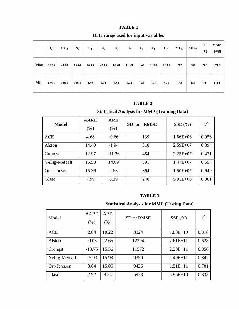
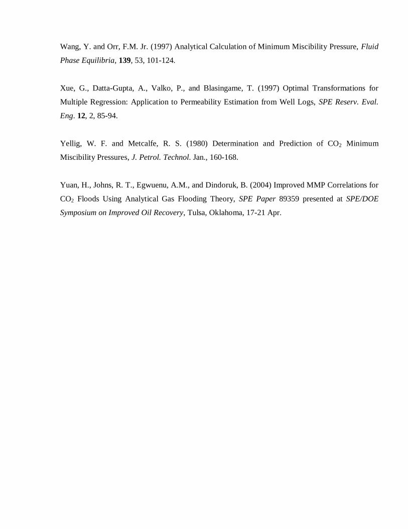
TABLE 1

Data range used for input variables

H2S CO2 N2 C1 C2 C3 C4 C5 C6 C7+ MC5+ MC7+ T

(F)

MMP

(psig)

Max 17.56 24.00 16.44 76.43 23.16 18.40 11.23 9.49 16.00 73.61 262 286 265 3705

Min 0.001 0.001 0.001 2.56 0.01 0.89 0.28 0.25 0.79 5.70 132 151 71 1101

TABLE 2

Statistical Analysis for MMP (Training Data)

Model AARE

(%)

ARE

(%) SD or RMSE SSE (%) r

2

ACE 4.68 -0.66 139 1.86E+06 0.956

Alston 14.40 -1.94 518 2.59E+07 0.394

Cronqst 12.97 -11.26 484 2.25E+07 0.471

Yellig-Metcalf 15.58 14.89 391 1.47E+07 0.654

Orr-Jennsen 15.36 2.63 394 1.50E+07 0.649

Glaso 7.99 5.39 248 5.91E+06 0.861

TABLE 3

Statistical Analysis for MMP (Testing Data)

Model AARE

(%)

ARE

(%) SD or RMSE SSE (%) r

2

ACE 2.84 10.22 3324 1.88E+10 0.818

Alston -0.03 22.65 12394 2.61E+11 0.628

Cronqst -13.75 15.56 11572 2.28E+11 0.858

Yellig-Metcalf 15.93 15.93 9359 1.49E+11 0.842

Orr-Jennsen 3.84 15.06 9426 1.51E+11 0.781

Glaso 2.92 8.54 5923 5.96E+10 0.833

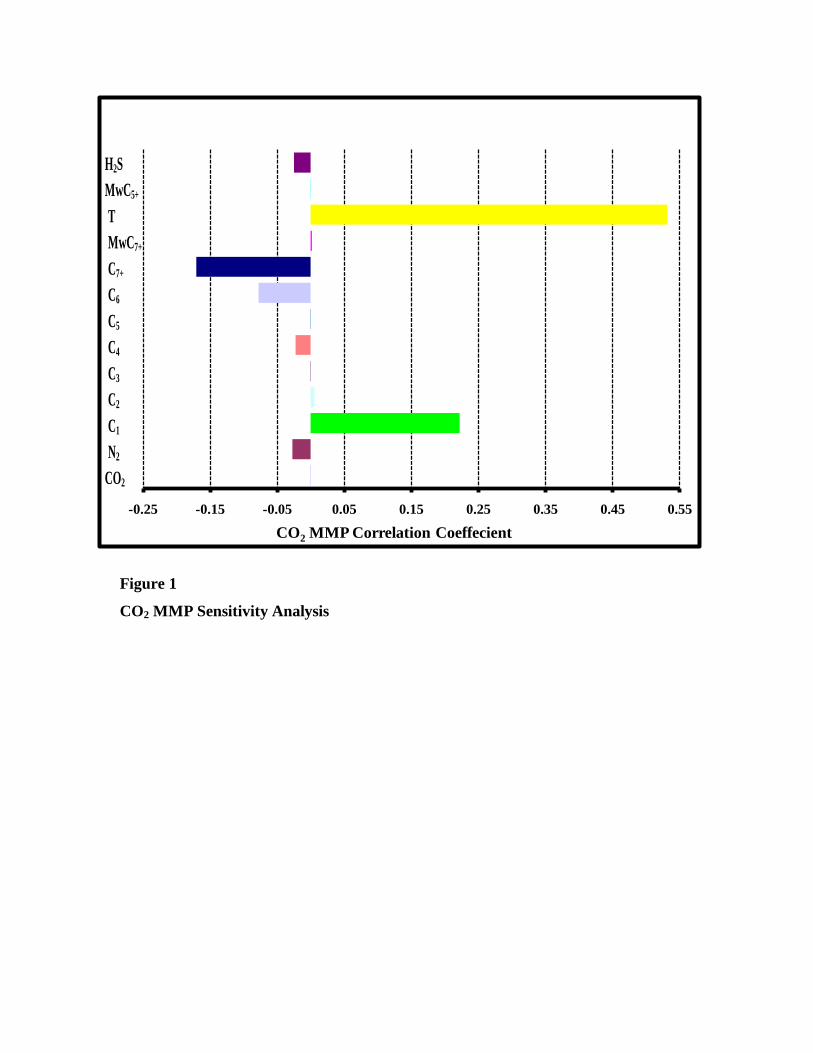
Figure 1

CO2 MMP Sensitivity Analysis

-0.25 -0.15 -0.05 0.05 0.15 0.25 0.35 0.45 0.55

CO2 MMP Correlation Coeffecient

H2S

MwC5+

T

MwC7+

C7+

C6

C5

C4

C3

C2

C1

N2

CO2

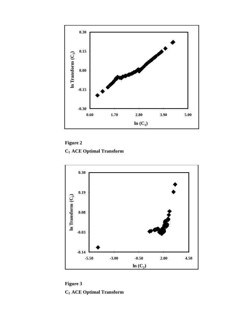
Figure 2

C1 ACE Optimal Transform

Figure 3

C2 ACE Optimal Transform

-0.30

-0.15

0.00

0.15

0.30

0.60 1.70 2.80 3.90 5.00

ln T

ran

sform

(C

1)

ln (C1)

-0.14

-0.03

0.08

0.19

0.30

-5.50 -3.00 -0.50 2.00 4.50

ln T

ran

sform

(C

2)

ln (C2)

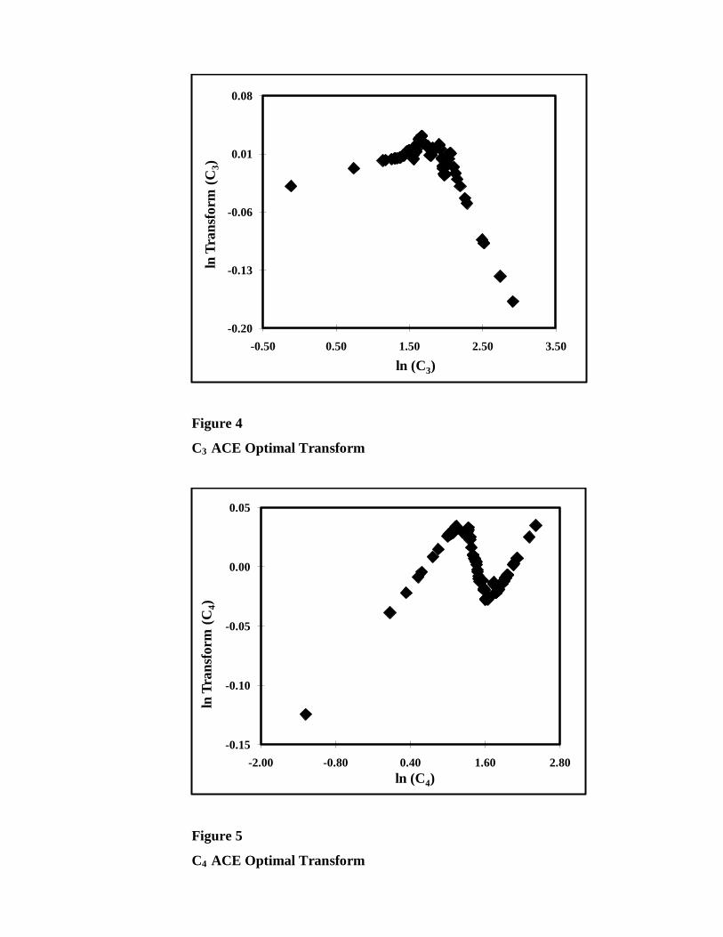
Figure 4

C3 ACE Optimal Transform

Figure 5

C4 ACE Optimal Transform

-0.20

-0.13

-0.06

0.01

0.08

-0.50 0.50 1.50 2.50 3.50

ln T

ran

sform

(C

3)

ln (C3)

-0.15

-0.10

-0.05

0.00

0.05

-2.00 -0.80 0.40 1.60 2.80

ln T

ran

sform

(C

4)

ln (C4)

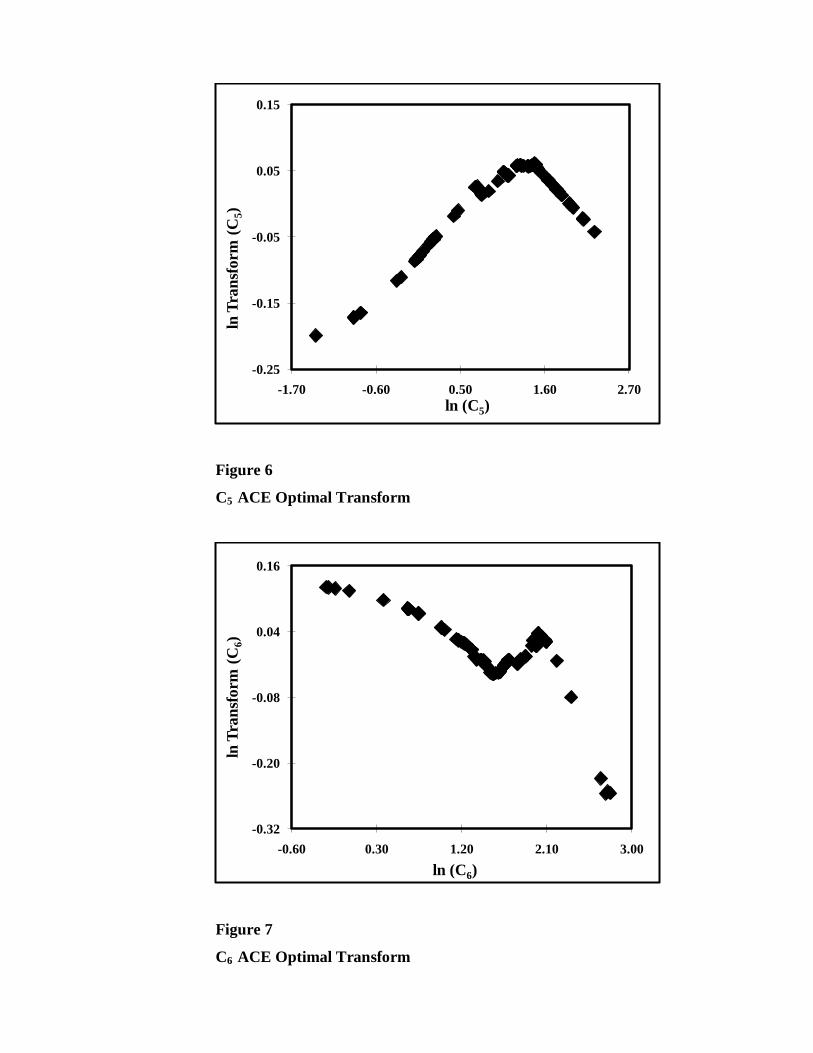
Figure 6

C5 ACE Optimal Transform

Figure 7

C6 ACE Optimal Transform

-0.25

-0.15

-0.05

0.05

0.15

-1.70 -0.60 0.50 1.60 2.70

ln T

ran

sform

(C

5)

ln (C5)

-0.32

-0.20

-0.08

0.04

0.16

-0.60 0.30 1.20 2.10 3.00

ln T

ran

sform

(C

6)

ln (C6)

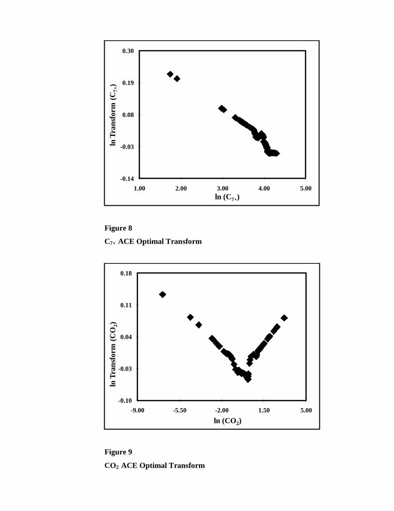
Figure 8

C7+ ACE Optimal Transform

Figure 9

CO2 ACE Optimal Transform

-0.14

-0.03

0.08

0.19

0.30

1.00 2.00 3.00 4.00 5.00

ln T

ran

sform

(C

7+)

ln (C7+)

-0.10

-0.03

0.04

0.11

0.18

-9.00 -5.50 -2.00 1.50 5.00

ln T

ran

sform

(C

O2)

ln (CO2)

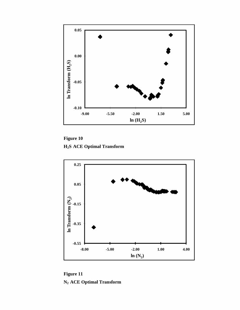
Figure 10

H2S ACE Optimal Transform

Figure 11

N2 ACE Optimal Transform

-0.10

-0.05

0.00

0.05

-9.00 -5.50 -2.00 1.50 5.00

ln T

ran

sform

(H

2S

)

ln (H2S)

-0.55

-0.35

-0.15

0.05

0.25

-8.00 -5.00 -2.00 1.00 4.00

ln T

ran

sform

(N

2)

ln (N2)

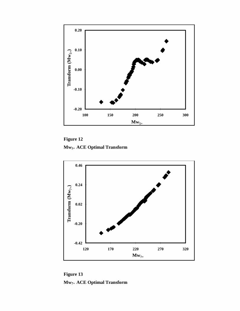
Figure 12

Mw5+ ACE Optimal Transform

Figure 13

Mw7+ ACE Optimal Transform

-0.20

-0.10

0.00

0.10

0.20

100 150 200 250 300

Tra

nsf

orm

(M

w5

+)

Mw5+

-0.42

-0.20

0.02

0.24

0.46

120 170 220 270 320

Tra

nsf

orm

(M

w7

+)

Mw7+

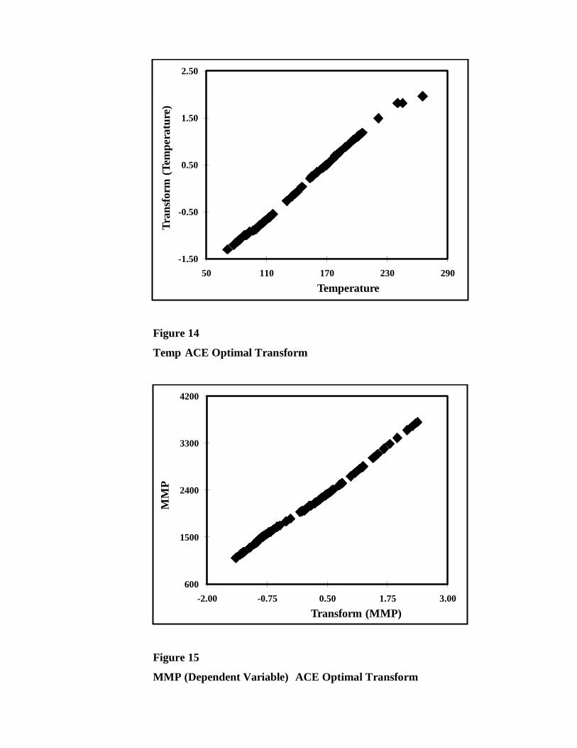
Figure 14

Temp ACE Optimal Transform

Figure 15

MMP (Dependent Variable) ACE Optimal Transform

-1.50

-0.50

0.50

1.50

2.50

50 110 170 230 290

Tra

nsf

orm

(T

emp

era

ture

)

Temperature

600

1500

2400

3300

4200

-2.00 -0.75 0.50 1.75 3.00

MM

P

Transform (MMP)

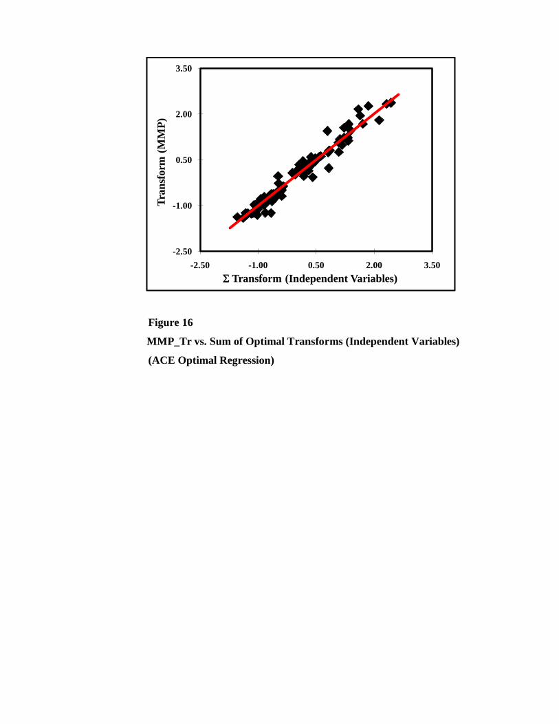
Figure 16

MMP_Tr vs. Sum of Optimal Transforms (Independent Variables)

(ACE Optimal Regression)

-2.50

-1.00

0.50

2.00

3.50

-2.50 -1.00 0.50 2.00 3.50

Tra

nsf

orm

(M

MP

)

S Transform (Independent Variables)

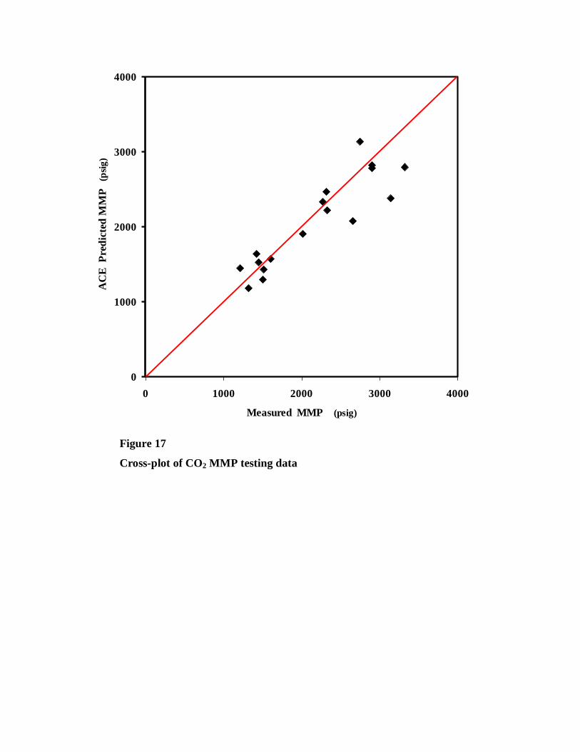
Figure 17

Cross-plot of CO2 MMP testing data

0

1000

2000

3000

4000

0 1000 2000 3000 4000

Measured MMP (psig)

A

CE

P

red

icte

d M

MP

(

psi

g)