Predicting cone-in-cone blender efficiencies from key material properties

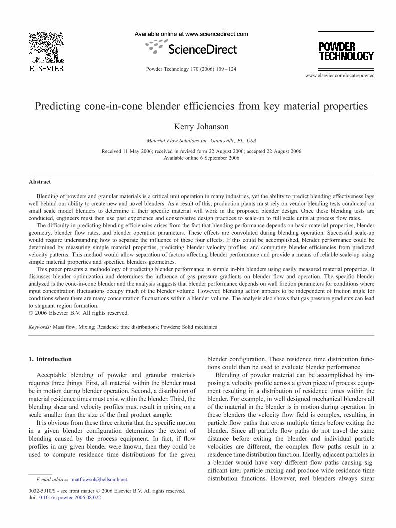
(2006) 109–124www.elsevier.com/locate/powtec

Powder Technology 170

Predicting cone-in-cone blender efficiencies from key material properties

Kerry Johanson

Material Flow Solutions Inc. Gainesville, FL, USA

Received 11 May 2006; received in revised form 22 August 2006; accepted 22 August 2006Available online 6 September 2006

Abstract

Blending of powders and granular materials is a critical unit operation in many industries, yet the ability to predict blending effectiveness lagswell behind our ability to create new and novel blenders. As a result of this, production plants must rely on vendor blending tests conducted onsmall scale model blenders to determine if their specific material will work in the proposed blender design. Once these blending tests areconducted, engineers must then use past experience and conservative design practices to scale-up to full scale units at process flow rates.

The difficulty in predicting blending efficiencies arises from the fact that blending performance depends on basic material properties, blendergeometry, blender flow rates, and blender operation parameters. These effects are convoluted during blending operation. Successful scale-upwould require understanding how to separate the influence of these four effects. If this could be accomplished, blender performance could bedetermined by measuring simple material properties, predicting blender velocity profiles, and computing blender efficiencies from predictedvelocity patterns. This method would allow separation of factors affecting blender performance and provide a means of reliable scale-up usingsimple material properties and specified blenders geometries.

This paper presents a methodology of predicting blender performance in simple in-bin blenders using easily measured material properties. Itdiscusses blender optimization and determines the influence of gas pressure gradients on blender flow and operation. The specific blenderanalyzed is the cone-in-cone blender and the analysis suggests that blender performance depends on wall friction parameters for conditions whereinput concentration fluctuations occupy much of the blender volume. However, blending action appears to be independent of friction angle forconditions where there are many concentration fluctuations within a blender volume. The analysis also shows that gas pressure gradients can leadto stagnant region formation.© 2006 Elsevier B.V. All rights reserved.

Keywords: Mass flow; Mixing; Residence time distributions; Powders; Solid mechanics

1. Introduction

Acceptable blending of powder and granular materialsrequires three things. First, all material within the blender mustbe in motion during blender operation. Second, a distribution ofmaterial residence times must exist within the blender. Third, theblending shear and velocity profiles must result in mixing on ascale smaller than the size of the final product sample.

It is obvious from these three criteria that the specific motionin a given blender configuration determines the extent ofblending caused by the process equipment. In fact, if flowprofiles in any given blender were known, then they could beused to compute residence time distributions for the given

E-mail address: [email protected].

0032-5910/$ - see front matter © 2006 Elsevier B.V. All rights reserved.doi:10.1016/j.powtec.2006.08.022

blender configuration. These residence time distribution func-tions could then be used to evaluate blender performance.

Blending of powder material can be accomplished by im-posing a velocity profile across a given piece of process equip-ment resulting in a distribution of residence times within theblender. For example, in well designed mechanical blenders allof the material in the blender is in motion during operation. Inthese blenders the velocity flow field is complex, resulting inparticle flow paths that cross multiple times before exiting theblender. Since all particle flow paths do not travel the samedistance before exiting the blender and individual particlevelocities are different, the complex flow paths result in aresidence time distribution function. Ideally, adjacent particles ina blender would have very different flow paths causing sig-nificant inter-particle mixing and produce wide residence timedistribution functions. However, real blenders always shear

mailto:[email protected]

http://dx.doi.org/10.1016/j.powtec.2006.08.022

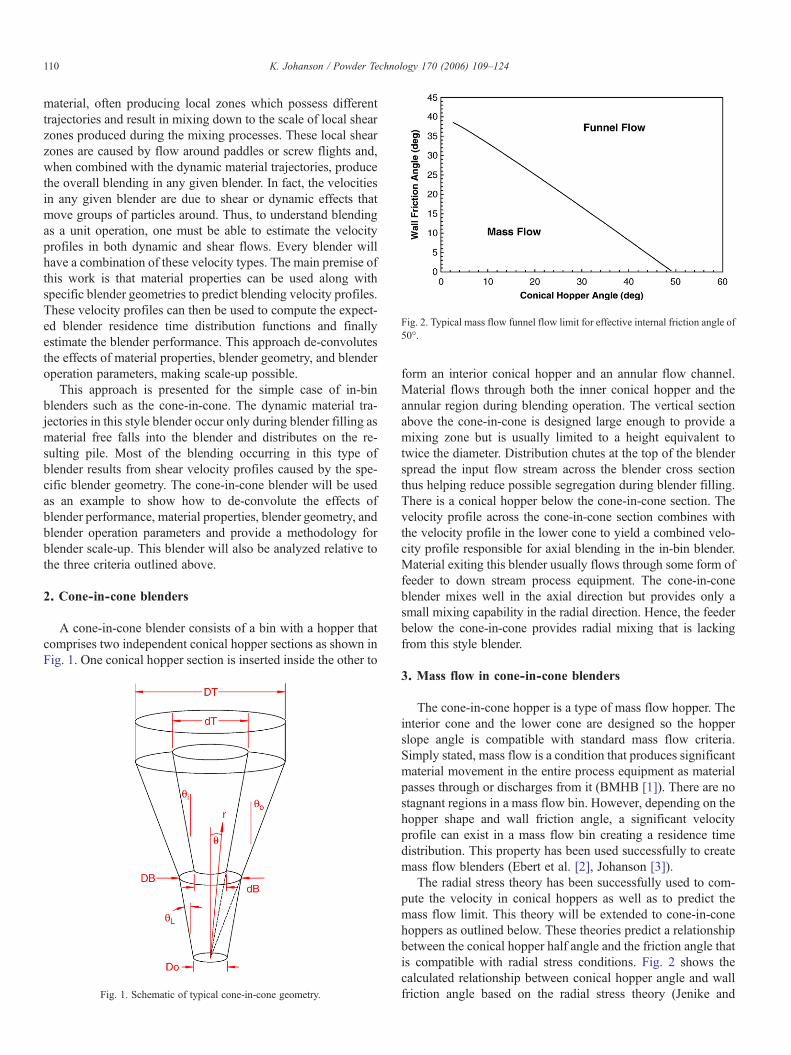
Fig. 2. Typical mass flow funnel flow limit for effective internal friction angle of50°.

110 K. Johanson / Powder Technology 170 (2006) 109–124

material, often producing local zones which possess differenttrajectories and result in mixing down to the scale of local shearzones produced during the mixing processes. These local shearzones are caused by flow around paddles or screw flights and,when combined with the dynamic material trajectories, producethe overall blending in any given blender. In fact, the velocitiesin any given blender are due to shear or dynamic effects thatmove groups of particles around. Thus, to understand blendingas a unit operation, one must be able to estimate the velocityprofiles in both dynamic and shear flows. Every blender willhave a combination of these velocity types. The main premise ofthis work is that material properties can be used along withspecific blender geometries to predict blending velocity profiles.These velocity profiles can then be used to compute the expect-ed blender residence time distribution functions and finallyestimate the blender performance. This approach de-convolutesthe effects of material properties, blender geometry, and blenderoperation parameters, making scale-up possible.

This approach is presented for the simple case of in-binblenders such as the cone-in-cone. The dynamic material tra-jectories in this style blender occur only during blender filling asmaterial free falls into the blender and distributes on the re-sulting pile. Most of the blending occurring in this type ofblender results from shear velocity profiles caused by the spe-cific blender geometry. The cone-in-cone blender will be usedas an example to show how to de-convolute the effects ofblender performance, material properties, blender geometry, andblender operation parameters and provide a methodology forblender scale-up. This blender will also be analyzed relative tothe three criteria outlined above.

2. Cone-in-cone blenders

A cone-in-cone blender consists of a bin with a hopper thatcomprises two independent conical hopper sections as shown inFig. 1. One conical hopper section is inserted inside the other to

Fig. 1. Schematic of typical cone-in-cone geometry.

form an interior conical hopper and an annular flow channel.Material flows through both the inner conical hopper and theannular region during blending operation. The vertical sectionabove the cone-in-cone is designed large enough to provide amixing zone but is usually limited to a height equivalent totwice the diameter. Distribution chutes at the top of the blenderspread the input flow stream across the blender cross sectionthus helping reduce possible segregation during blender filling.There is a conical hopper below the cone-in-cone section. Thevelocity profile across the cone-in-cone section combines withthe velocity profile in the lower cone to yield a combined velo-city profile responsible for axial blending in the in-bin blender.Material exiting this blender usually flows through some form offeeder to down stream process equipment. The cone-in-coneblender mixes well in the axial direction but provides only asmall mixing capability in the radial direction. Hence, the feederbelow the cone-in-cone provides radial mixing that is lackingfrom this style blender.

3. Mass flow in cone-in-cone blenders

The cone-in-cone hopper is a type of mass flow hopper. Theinterior cone and the lower cone are designed so the hopperslope angle is compatible with standard mass flow criteria.Simply stated, mass flow is a condition that produces significantmaterial movement in the entire process equipment as materialpasses through or discharges from it (BMHB [1]). There are nostagnant regions in a mass flow bin. However, depending on thehopper shape and wall friction angle, a significant velocityprofile can exist in a mass flow bin creating a residence timedistribution. This property has been used successfully to createmass flow blenders (Ebert et al. [2], Johanson [3]).

The radial stress theory has been successfully used to com-pute the velocity in conical hoppers as well as to predict themass flow limit. This theory will be extended to cone-in-conehoppers as outlined below. These theories predict a relationshipbetween the conical hopper half angle and the friction angle thatis compatible with radial stress conditions. Fig. 2 shows thecalculated relationship between conical hopper angle and wallfriction angle based on the radial stress theory (Jenike and

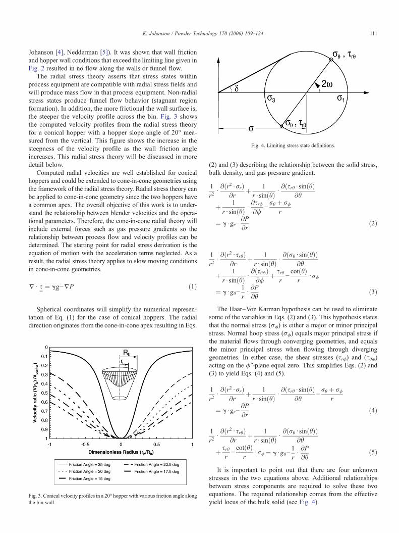
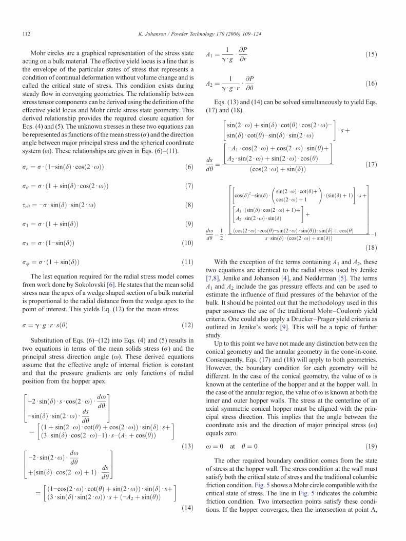
Fig. 4. Limiting stress state definitions.

111K. Johanson / Powder Technology 170 (2006) 109–124

Johanson [4], Nedderman [5]). It was shown that wall frictionand hopper wall conditions that exceed the limiting line given inFig. 2 resulted in no flow along the walls or funnel flow.

The radial stress theory asserts that stress states withinprocess equipment are compatible with radial stress fields andwill produce mass flow in that process equipment. Non-radialstress states produce funnel flow behavior (stagnant regionformation). In addition, the more frictional the wall surface is,the steeper the velocity profile across the bin. Fig. 3 showsthe computed velocity profiles from the radial stress theoryfor a conical hopper with a hopper slope angle of 20° mea-sured from the vertical. This figure shows the increase in thesteepness of the velocity profile as the wall friction angleincreases. This radial stress theory will be discussed in moredetail below.

Computed radial velocities are well established for conicalhoppers and could be extended to cone-in-cone geometries usingthe framework of the radial stress theory. Radial stress theory canbe applied to cone-in-cone geometry since the two hoppers havea common apex. The overall objective of this work is to under-stand the relationship between blender velocities and the opera-tional parameters. Therefore, the cone-in-cone radial theory willinclude external forces such as gas pressure gradients so therelationship between process flow and velocity profiles can bedetermined. The starting point for radial stress derivation is theequation of motion with the acceleration terms neglected. As aresult, the radial stress theory applies to slow moving conditionsin cone-in-cone geometries.

jd s¼ ¼ gPg−jP ð1Þ

Spherical coordinates will simplify the numerical represen-tation of Eq. (1) for the case of conical hoppers. The radialdirection originates from the cone-in-cone apex resulting in Eqs.

Fig. 3. Conical velocity profiles in a 20° hopper with various friction angle alongthe bin wall.

(2) and (3) describing the relationship between the solid stress,bulk density, and gas pressure gradient.

1r2d@ðr2d rrÞ

@rþ 1rd sinðhÞ d

@ðsrhd sinðhÞ@h

þ 1rd sinðhÞ d

@sr/@/

−rh þ r/

r

¼ gd gr−@P@r

ð2Þ

1r2d@ðr2d srhÞ

@rþ 1rd sinðhÞ d

@ðrhd sinðhÞÞ@h

þ 1rd sinðhÞ d

@ðsh/Þ@/

þ srhr−cotðhÞ

rd r/

¼ gd gh−1

rd@P

@hð3Þ

The Haar–Von Karman hypothesis can be used to eliminatesome of the variables in Eqs. (2) and (3). This hypothesis statesthat the normal stress (σϕ) is either a major or minor principalstress. Normal hoop stress (σϕ) equals major principal stress ifthe material flows through converging geometries, and equalsthe minor principal stress when flowing through diverginggeometries. In either case, the shear stresses (τrϕ) and (τθϕ)acting on the ϕ˜-plane equal zero. This simplifies Eqs. (2) and(3) to yield Eqs. (4) and (5).

1r2d@ðr2d rrÞ

@rþ 1rd sinðhÞ d

@ðsrhd sinðhÞ@h

−rh þ r/

r

¼ gd gr−@P@r

ð4Þ

1r2d@ðr2d srhÞ

@rþ 1rd sinðhÞ d

@ðrhd sinðhÞÞ@h

þ srhr−cotðhÞ

rd r/ ¼ gd gh−

1rd@P@h

ð5Þ

It is important to point out that there are four unknownstresses in the two equations above. Additional relationshipsbetween stress components are required to solve these twoequations. The required relationship comes from the effectiveyield locus of the bulk solid (see Fig. 4).


Mohr circles are a graphical representation of the stress stateacting on a bulk material. The effective yield locus is a line that isthe envelope of the particular states of stress that represents acondition of continual deformation without volume change and iscalled the critical state of stress. This condition exists duringsteady flow in converging geometries. The relationship betweenstress tensor components can be derived using the definition of theeffective yield locus and Mohr circle stress state geometry. Thisderived relationship provides the required closure equation forEqs. (4) and (5). The unknown stresses in these two equations canbe represented as functions of themean stress (σ) and the directionangle between major principal stress and the spherical coordinatesystem (ω). These relationships are given in Eqs. (6)–(11).

rr ¼ rd ð1−sinðdÞd cosð2d xÞÞ ð6Þ

rh ¼ rd ð1þ sinðdÞd cosð2d xÞÞ ð7Þ

srh ¼ −rd sinðdÞd sinð2d xÞ ð8Þ

r1 ¼ rd ð1þ sinðdÞÞ ð9Þ

r3 ¼ rd ð1−sinðdÞÞ ð10Þ

r/ ¼ rd ð1þ sinðdÞÞ ð11ÞThe last equation required for the radial stress model comes

from work done by Sokolovski [6]. He states that the mean solidstress near the apex of a wedge shaped section of a bulk materialis proportional to the radial distance from the wedge apex to thepoint of interest. This yields Eq. (12) for the mean stress.

r ¼ gd gd rd sðhÞ ð12Þ

Substitution of Eqs. (6)–(12) into Eqs. (4) and (5) results intwo equations in terms of the mean solids stress (σ) and theprincipal stress direction angle (ω). These derived equationsassume that the effective angle of internal friction is constantand that the pressure gradients are only functions of radialposition from the hopper apex.

−2d sinðdÞd sd cosð2d xÞd dxdh

−sinðdÞd sinð2d xÞd dsdh

264

375

¼ 1þ sinð2d xÞd cotðhÞ þ cosð2d xÞð Þd sinðdÞd sþð3d sinðdÞd cosð2d xÞ−1Þd s−ðA1 þ cosðhÞÞ� �

ð13Þ−2d sinð2d xÞd dx

dh

þðsinðdÞd cosð2d xÞ þ 1Þd dsdh

264

375

¼ ð1−cosð2d xÞd cotðhÞ þ sinð2d xÞÞd sinðdÞd sþð3d sinðdÞd sinð2d xÞÞd sþ ð−A2 þ sinðhÞÞ� �

ð14Þ

A1 ¼ 1gd g

d@P@r

ð15Þ

A2 ¼ 1gd gd r

d@P@h

ð16Þ

Eqs. (13) and (14) can be solved simultaneously to yield Eqs.(17) and (18).

dsdh

¼

sinð2d xÞ þ sinðdÞd cotðhÞd cosð2d xÞ−sinðdÞd cotðhÞ−sinðdÞd sinð2d xÞ

" #d sþ

−A1d cosð2d xÞ þ cosð2d xÞd sinðhÞþA2d sinð2d xÞ þ sinð2d xÞd cosðhÞ

" #

ðcosð2d xÞ þ sinðdÞÞ ð17Þ

dxdh

¼ 12d

cosðdÞ2−sinðdÞd sinð2d xÞd cotðhÞþcosð2d xÞ þ 1

!d ðsinðdÞ þ 1Þ

#"d sþ

A1d ðsinðdÞd cosð2d xÞ þ 1ÞþA2d sinð2d xÞd sinðdÞ

" #þ

ðcosð2d xÞd cosðhÞ−sinð2d xÞd sinðhÞÞd sinðdÞ þ cosðhÞ

26666666664

37777777775

sd sinðdÞd ðcosð2d xÞ þ sinðdÞÞ −1

ð18ÞWith the exception of the terms containing A1 and A2, these

two equations are identical to the radial stress used by Jenike[7,8], Jenike and Johanson [4], and Nedderman [5]. The termsA1 and A2 include the gas pressure effects and can be used toestimate the influence of fluid pressures of the behavior of thebulk. It should be pointed out that the methodology used in thispaper assumes the use of the traditional Mohr–Coulomb yieldcriteria. One could also apply a Drucker–Prager yield criteria asoutlined in Jenike's work [9]. This will be a topic of furtherstudy.

Up to this point we have not made any distinction between theconical geometry and the annular geometry in the cone-in-cone.Consequently, Eqs. (17) and (18) will apply to both geometries.However, the boundary condition for each geometry will bedifferent. In the case of the conical geometry, the value of ω isknown at the centerline of the hopper and at the hopper wall. Inthe case of the annular region, the value ofω is known at both theinner and outer hopper walls. The stress at the centerline of anaxial symmetric conical hopper must be aligned with the prin-cipal stress direction. This implies that the angle between thecoordinate axis and the direction of major principal stress (ω)equals zero.

x ¼ 0 at h ¼ 0 ð19ÞThe other required boundary condition comes from the state

of stress at the hopper wall. The stress condition at the wall mustsatisfy both the critical state of stress and the traditional columbicfriction condition. Fig. 5 shows aMohr circle compatible with thecritical state of stress. The line in Fig. 5 indicates the columbicfriction condition. Two intersection points satisfy these condi-tions. If the hopper converges, then the intersection at point A,

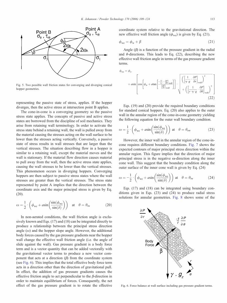
Fig. 5. Two possible wall friction states for converging and diverging conicalhopper geometries.

Fig. 6. Force balance at wall surface including gas pressure gradient terms.


representing the passive state of stress, applies. If the hopperdiverges, then the active stress at intersection point B applies.

The cone-in-cone is a converging geometry so the passivestress state applies. The concepts of passive and active stressstates are borrowed from the discipline of soil mechanics. Theyarise from retaining wall terminology. In order to activate thestress state behind a retaining wall, the wall is pulled away fromthe material causing the stresses acting on the wall surface to belower than the stresses acting vertically. Conversely, a passivestate of stress results in wall stresses that are larger than thevertical stresses. The situation describing flow in a hopper issimilar to a retaining wall, except the material moves and thewall is stationary. If the material flow direction causes materialto pull away from the wall, then the active stress state applies,causing the wall stresses to be lower than the vertical stresses.This phenomenon occurs in diverging hoppers. Converginghoppers are then subject to passive stress states where the wallstresses are greater than the vertical stresses. The stress staterepresented by point A implies that the direction between thecoordinate axis and the major principal stress is given by Eq.(20).

x ¼ 12d /we þ asin

sinð/we

sinðdÞ� ��

at h ¼ hiw ð20Þ

In non-aerated conditions, the wall friction angle is exclu-sively known and Eqs. (17) and (18) can be integrated directly toproduce a relationship between the principal stress directionangle (ω) and the hopper slope angle. However, the additionalbody forces caused by the gas pressure gradients near the hopperwall change the effective wall friction angle (i.e. the angle ofslide against the wall). Gas pressure gradient is a body forceterm and is a vector quantity that can be added vectorally withthe gravitational vector terms to produce a new vector com-ponent that acts at a direction (β) from the coordinate system(see Fig. 6). This implies that the total effective body force termacts in a direction other than the direction of gravitational pull.In effect, the addition of gas pressure gradients causes theeffective friction angle to act perpendicular to the β-direction inorder to maintain equilibrium of forces. Consequently, the neteffect of the gas pressure gradient is to rotate the effective

coordinate system relative to the gravitational direction. Thenew effective wall friction angle (ϕwe) is given by Eq. (21).

/we ¼ /w þ b ð21ÞAngle (β) is a function of the pressure gradient in the radial

and θ-directions. This leads to Eq. (22), describing the neweffective wall friction angle in terms of the gas pressure gradientterms.

/we ¼ /w

þ asin cos /w þ atan− 1

r d@P@h

� �wall

@P@r

� �wall

" #" #d

ffiffiffiffiffiffiffiffiffiffiffiffiffiffiffiffiffiffiffiffiffiffiffiffiffiffiffiffiffiffiffiffiffiffiffiffiffiffiffiffiffiffiffiffiffiffiffiffiffiffi1

gd gd@P@r

� �wall

� �2

þ 1rd gd g

d@P@h

� �wall

� �2

vuuuuuuut

3777775

2666664

ð22ÞEqs. (19) and (20) provide the required boundary conditions

for standard conical hoppers. Eq. (20) also applies to the outerwall in the annular region of the cone-in-cone geometry yieldingthe following equation for the outer wall boundary condition.

x ¼ 12d /we þ asin

sinð/we

sinðdÞ� ��

at h ¼ how ð23Þ

However, the inner wall in the annular region of the cone-in-cone requires different boundary conditions. Fig. 7 shows theexpected contours of major principal stress direction within theannular region. This figure implies that the direction of majorprincipal stress is in the negative ω-direction along the innercone wall. This suggest that the boundary condition along theouter surface of the inner cone wall is given by Eq. (24)

x ¼ −12d /we þ asin

sinð/we

sinðdÞ� ��

at h ¼ hiw ð24Þ

Eqs. (17) and (18) can be integrated using boundary con-ditions given in Eqs. (23) and (24) to produce radial stresssolutions for annular geometries. Fig. 8 shows some of the

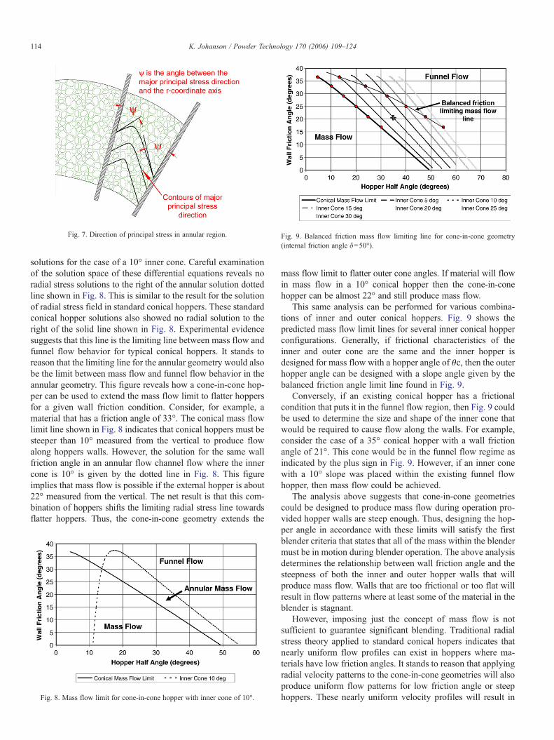
Fig. 7. Direction of principal stress in annular region. Fig. 9. Balanced friction mass flow limiting line for cone-in-cone geometry(internal friction angle δ=50°).


solutions for the case of a 10° inner cone. Careful examinationof the solution space of these differential equations reveals noradial stress solutions to the right of the annular solution dottedline shown in Fig. 8. This is similar to the result for the solutionof radial stress field in standard conical hoppers. These standardconical hopper solutions also showed no radial solution to theright of the solid line shown in Fig. 8. Experimental evidencesuggests that this line is the limiting line between mass flow andfunnel flow behavior for typical conical hoppers. It stands toreason that the limiting line for the annular geometry would alsobe the limit between mass flow and funnel flow behavior in theannular geometry. This figure reveals how a cone-in-cone hop-per can be used to extend the mass flow limit to flatter hoppersfor a given wall friction condition. Consider, for example, amaterial that has a friction angle of 33°. The conical mass flowlimit line shown in Fig. 8 indicates that conical hoppers must besteeper than 10° measured from the vertical to produce flowalong hoppers walls. However, the solution for the same wallfriction angle in an annular flow channel flow where the innercone is 10° is given by the dotted line in Fig. 8. This figureimplies that mass flow is possible if the external hopper is about22° measured from the vertical. The net result is that this com-bination of hoppers shifts the limiting radial stress line towardsflatter hoppers. Thus, the cone-in-cone geometry extends the

Fig. 8. Mass flow limit for cone-in-cone hopper with inner cone of 10°.

mass flow limit to flatter outer cone angles. If material will flowin mass flow in a 10° conical hopper then the cone-in-conehopper can be almost 22° and still produce mass flow.

This same analysis can be performed for various combina-tions of inner and outer conical hoppers. Fig. 9 shows thepredicted mass flow limit lines for several inner conical hopperconfigurations. Generally, if frictional characteristics of theinner and outer cone are the same and the inner hopper isdesigned for mass flow with a hopper angle of θc, then the outerhopper angle can be designed with a slope angle given by thebalanced friction angle limit line found in Fig. 9.

Conversely, if an existing conical hopper has a frictionalcondition that puts it in the funnel flow region, then Fig. 9 couldbe used to determine the size and shape of the inner cone thatwould be required to cause flow along the walls. For example,consider the case of a 35° conical hopper with a wall frictionangle of 21°. This cone would be in the funnel flow regime asindicated by the plus sign in Fig. 9. However, if an inner conewith a 10° slope was placed within the existing funnel flowhopper, then mass flow could be achieved.

The analysis above suggests that cone-in-cone geometriescould be designed to produce mass flow during operation pro-vided hopper walls are steep enough. Thus, designing the hop-per angle in accordance with these limits will satisfy the firstblender criteria that states that all of the mass within the blendermust be in motion during blender operation. The above analysisdetermines the relationship between wall friction angle and thesteepness of both the inner and outer hopper walls that willproduce mass flow. Walls that are too frictional or too flat willresult in flow patterns where at least some of the material in theblender is stagnant.

However, imposing just the concept of mass flow is notsufficient to guarantee significant blending. Traditional radialstress theory applied to standard conical hopers indicates thatnearly uniform flow profiles can exist in hoppers where ma-terials have low friction angles. It stands to reason that applyingradial velocity patterns to the cone-in-cone geometries will alsoproduce uniform flow patterns for low friction angle or steephoppers. These nearly uniform velocity profiles will result in

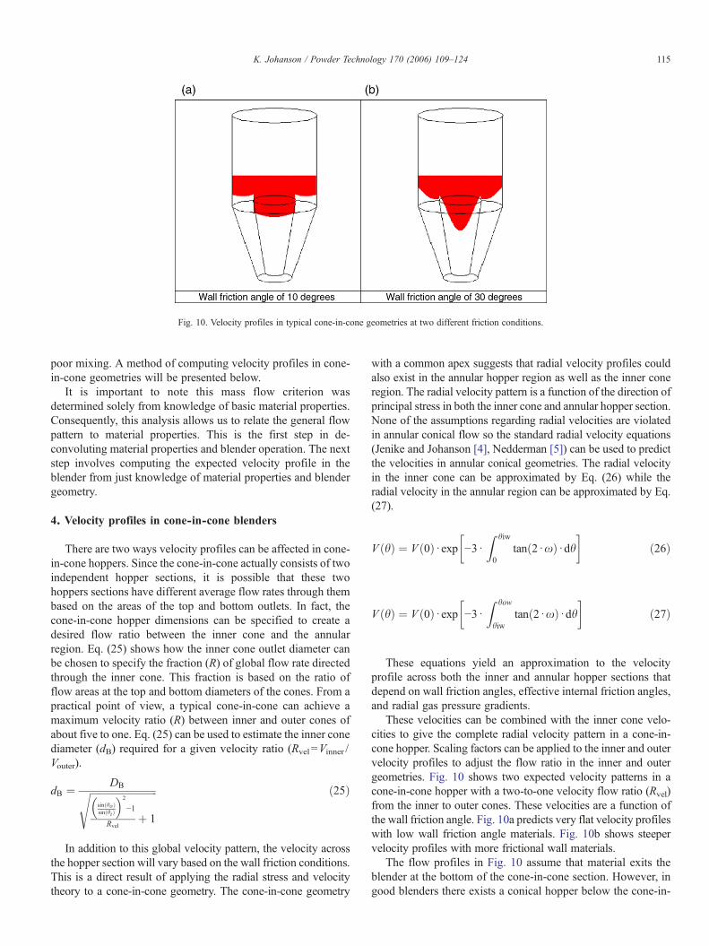
Fig. 10. Velocity profiles in typical cone-in-cone geometries at two different friction conditions.


poor mixing. A method of computing velocity profiles in cone-in-cone geometries will be presented below.

It is important to note this mass flow criterion wasdetermined solely from knowledge of basic material properties.Consequently, this analysis allows us to relate the general flowpattern to material properties. This is the first step in de-convoluting material properties and blender operation. The nextstep involves computing the expected velocity profile in theblender from just knowledge of material properties and blendergeometry.

4. Velocity profiles in cone-in-cone blenders

There are two ways velocity profiles can be affected in cone-in-cone hoppers. Since the cone-in-cone actually consists of twoindependent hopper sections, it is possible that these twohoppers sections have different average flow rates through thembased on the areas of the top and bottom outlets. In fact, thecone-in-cone hopper dimensions can be specified to create adesired flow ratio between the inner cone and the annularregion. Eq. (25) shows how the inner cone outlet diameter canbe chosen to specify the fraction (R) of global flow rate directedthrough the inner cone. This fraction is based on the ratio offlow areas at the top and bottom diameters of the cones. From apractical point of view, a typical cone-in-cone can achieve amaximum velocity ratio (R) between inner and outer cones ofabout five to one. Eq. (25) can be used to estimate the inner conediameter (dB) required for a given velocity ratio (Rvel=Vinner /Vouter).

dB ¼ DBffiffiffiffiffiffiffiffiffiffiffiffiffiffiffiffiffiffiffiffiffiffiffiffiffiffiffisinðhoÞsinðhiÞ

2

−1

Rvelþ 1

s ð25Þ

In addition to this global velocity pattern, the velocity acrossthe hopper section will vary based on the wall friction conditions.This is a direct result of applying the radial stress and velocitytheory to a cone-in-cone geometry. The cone-in-cone geometry

with a common apex suggests that radial velocity profiles couldalso exist in the annular hopper region as well as the inner coneregion. The radial velocity pattern is a function of the direction ofprincipal stress in both the inner cone and annular hopper section.None of the assumptions regarding radial velocities are violatedin annular conical flow so the standard radial velocity equations(Jenike and Johanson [4], Nedderman [5]) can be used to predictthe velocities in annular conical geometries. The radial velocityin the inner cone can be approximated by Eq. (26) while theradial velocity in the annular region can be approximated by Eq.(27).

V ðhÞ ¼ V ð0Þd exp −3dZ hiw

0tanð2d xÞd dh

� �ð26Þ

V ðhÞ ¼ V ð0Þd exp −3dZ how

hiwtanð2d xÞd dh

� �ð27Þ

These equations yield an approximation to the velocityprofile across both the inner and annular hopper sections thatdepend on wall friction angles, effective internal friction angles,and radial gas pressure gradients.

These velocities can be combined with the inner cone velo-cities to give the complete radial velocity pattern in a cone-in-cone hopper. Scaling factors can be applied to the inner and outervelocity profiles to adjust the flow ratio in the inner and outergeometries. Fig. 10 shows two expected velocity patterns in acone-in-cone hopper with a two-to-one velocity flow ratio (Rvel)from the inner to outer cones. These velocities are a function ofthe wall friction angle. Fig. 10a predicts very flat velocity profileswith low wall friction angle materials. Fig. 10b shows steepervelocity profiles with more frictional wall materials.

The flow profiles in Fig. 10 assume that material exits theblender at the bottom of the cone-in-cone section. However, ingood blenders there exists a conical hopper below the cone-in-

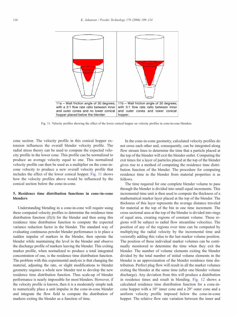
Fig. 11. Velocity profiles showing the effect of the lower conical hopper on velocity profiles in cone-in-cone blenders.


cone section. The velocity profile in this conical hopper ex-tension influences the overall blender velocity profile. Theradial stress theory can be used to compute the expected velo-city profile in the lower cone. This profile can be normalized toproduce an average velocity equal to one. This normalizedvelocity profile can then be used as a multiplier on the cone-in-cone velocity to produce a new overall velocity profile thatincludes the effect of the lower conical hopper. Fig. 11 showshow the velocity profiles above would be influenced by theconical section below the cone-in-cone.

5. Residence time distribution functions in cone-in-coneblenders

Understanding blending in a cone-in-cone will require usingthese computed velocity profiles to determine the residence timedistribution function (E(t)) for the blender and then using thisresidence time distribution function to compute the expectedvariance reduction factor in the blender. The standard way ofevaluating continuous powder blender performance is to place asudden impulse of markers in the blender, then operate theblender while maintaining the level in the blender and observethe discharge profile of markers leaving the blender. This exitingmarker profile, when normalized to produce a total integratedconcentration of one, is the residence time distribution function.The problem with this experimental analysis is that changing thematerial, adjusting the rate, or slight modifications to blendergeometry requires a whole new blender test to develop the newresidence time distribution function. Thus scale-up of blenderperformance is nearly impossible for most blenders. However, ifthe velocity profile is known, then it is a moderately simple taskto numerically place a unit impulse in the cone-in-cone blenderand integrate the flow field to compute the distribution ofmarkers exiting the blender as a function of time.

In the cone-in-cone geometry, calculated velocity profiles donot cross each other and, consequently, can be integrated alongflow stream lines to determine the time that a particle placed atthe top of the blender will exit the blender outlet. Computing theexit times for a layer of particles placed at the top of the blendergives rise to a method of computing the residence time distri-bution function of the blender. The procedure for computingresidence time in the blender from material properties is asfollows.

The time required for one complete blender volume to passthrough the blender is divided into small equal increments. Thisincremental time unit is then used to compute the thickness of amathematical marker layer placed at the top of the blender. Thethickness of this layer represents the average distance traveledfor material at the top of the bin in one time increment. Thecross sectional area at the top of the blender is divided into ringsof equal area, creating regions of constant volume. These re-gions will be subject to radial flow streamline velocities. Theposition of any of the regions over time can be computed bymultiplying the radial velocity by the incremental time andvectorally adding this value to the last marker volume position.The position of these individual marker volumes can be conti-nually monitored to determine the time when they exit theblender. The number of volume elements exiting the blenderdivided by the total number of initial volume elements in theblender is an approximation of the blender residence time dis-tribution. Perfect plug flow will result in all the marker volumesexiting the blender at the same time (after one blender volumedischarge). Any deviation from this will produce a distributionin residence times and result in blending. Fig. 12 shows acalculated residence time distribution function for a cone-in-cone hopper with a 10° inner cone and a 20° outer cone and auniform velocity profile imposed below the cone-in-conehopper. The relative flow rate variation between the inner and

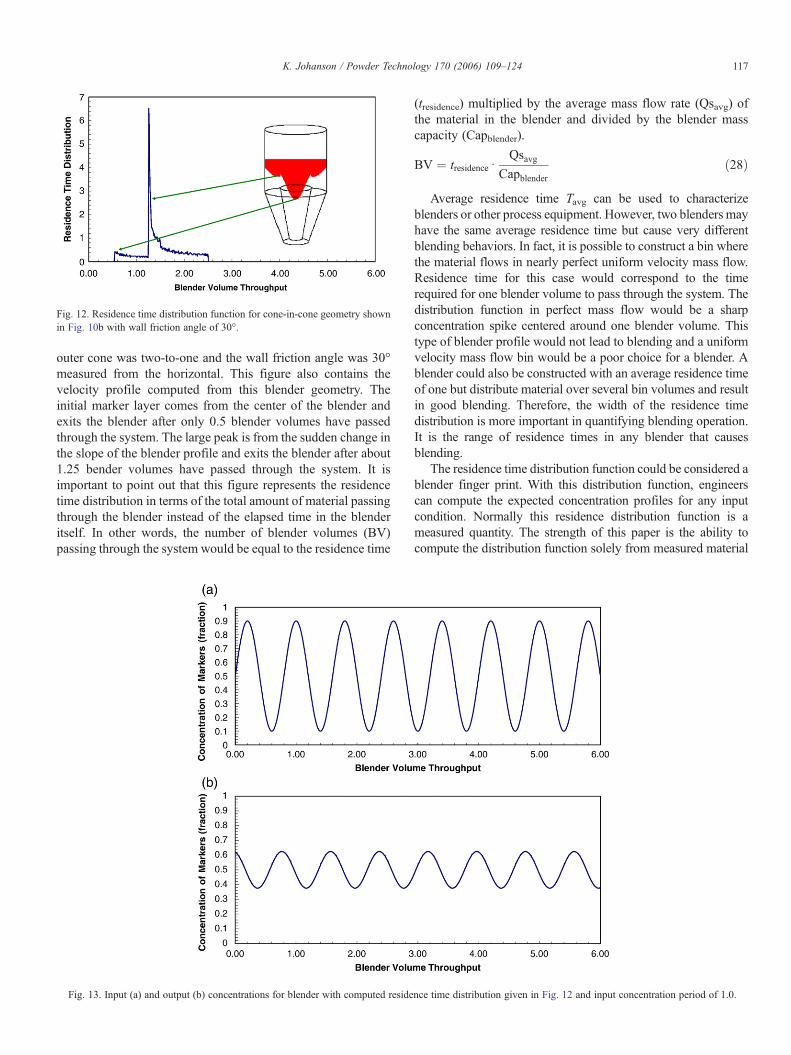
Fig. 12. Residence time distribution function for cone-in-cone geometry shownin Fig. 10b with wall friction angle of 30°.


outer cone was two-to-one and the wall friction angle was 30°measured from the horizontal. This figure also contains thevelocity profile computed from this blender geometry. Theinitial marker layer comes from the center of the blender andexits the blender after only 0.5 blender volumes have passedthrough the system. The large peak is from the sudden change inthe slope of the blender profile and exits the blender after about1.25 bender volumes have passed through the system. It isimportant to point out that this figure represents the residencetime distribution in terms of the total amount of material passingthrough the blender instead of the elapsed time in the blenderitself. In other words, the number of blender volumes (BV)passing through the system would be equal to the residence time

Fig. 13. Input (a) and output (b) concentrations for blender with computed reside

(tresidence) multiplied by the average mass flow rate (Qsavg) ofthe material in the blender and divided by the blender masscapacity (Capblender).

BV ¼ tresidencedQsavg

Capblenderð28Þ

Average residence time Tavg can be used to characterizeblenders or other process equipment. However, two blenders mayhave the same average residence time but cause very differentblending behaviors. In fact, it is possible to construct a bin wherethe material flows in nearly perfect uniform velocity mass flow.Residence time for this case would correspond to the timerequired for one blender volume to pass through the system. Thedistribution function in perfect mass flow would be a sharpconcentration spike centered around one blender volume. Thistype of blender profile would not lead to blending and a uniformvelocity mass flow bin would be a poor choice for a blender. Ablender could also be constructed with an average residence timeof one but distribute material over several bin volumes and resultin good blending. Therefore, the width of the residence timedistribution is more important in quantifying blending operation.It is the range of residence times in any blender that causesblending.

The residence time distribution function could be considered ablender finger print. With this distribution function, engineerscan compute the expected concentration profiles for any inputcondition. Normally this residence distribution function is ameasured quantity. The strength of this paper is the ability tocompute the distribution function solely from measured material

nce time distribution given in Fig. 12 and input concentration period of 1.0.

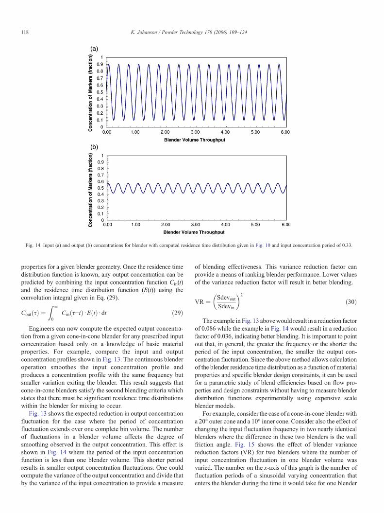
Fig. 14. Input (a) and output (b) concentrations for blender with computed residence time distribution given in Fig. 10 and input concentration period of 0.33.


properties for a given blender geometry. Once the residence timedistribution function is known, any output concentration can bepredicted by combining the input concentration function Cin(t)and the residence time distribution function (E(t)) using theconvolution integral given in Eq. (29).

CoutðsÞ ¼Z l

0Cinðs−tÞd EðtÞd dt ð29Þ

Engineers can now compute the expected output concentra-tion from a given cone-in-cone blender for any prescribed inputconcentration based only on a knowledge of basic materialproperties. For example, compare the input and outputconcentration profiles shown in Fig. 13. The continuous blenderoperation smoothes the input concentration profile andproduces a concentration profile with the same frequency butsmaller variation exiting the blender. This result suggests thatcone-in-cone blenders satisfy the second blending criteria whichstates that there must be significant residence time distributionswithin the blender for mixing to occur.

Fig. 13 shows the expected reduction in output concentrationfluctuation for the case where the period of concentrationfluctuation extends over one complete bin volume. The numberof fluctuations in a blender volume affects the degree ofsmoothing observed in the output concentration. This effect isshown in Fig. 14 where the period of the input concentrationfunction is less than one blender volume. This shorter periodresults in smaller output concentration fluctuations. One couldcompute the variance of the output concentration and divide thatby the variance of the input concentration to provide a measure

of blending effectiveness. This variance reduction factor canprovide a means of ranking blender performance. Lower valuesof the variance reduction factor will result in better blending.

VR ¼ SdevoutSdevin

� �2

ð30Þ

The example in Fig. 13 abovewould result in a reduction factorof 0.086 while the example in Fig. 14 would result in a reductionfactor of 0.036, indicating better blending. It is important to pointout that, in general, the greater the frequency or the shorter theperiod of the input concentration, the smaller the output con-centration fluctuation. Since the above method allows calculationof the blender residence time distribution as a function of materialproperties and specific blender design constraints, it can be usedfor a parametric study of blend efficiencies based on flow pro-perties and design constraints without having to measure blenderdistribution functions experimentally using expensive scaleblender models.

For example, consider the case of a cone-in-cone blender witha 20° outer cone and a 10° inner cone. Consider also the effect ofchanging the input fluctuation frequency in two nearly identicalblenders where the difference in these two blenders is the wallfriction angle. Fig. 15 shows the effect of blender variancereduction factors (VR) for two blenders where the number ofinput concentration fluctuation in one blender volume wasvaried. The number on the x-axis of this graph is the number offluctuation periods of a sinusoidal varying concentration thatenters the blender during the time it would take for one blender

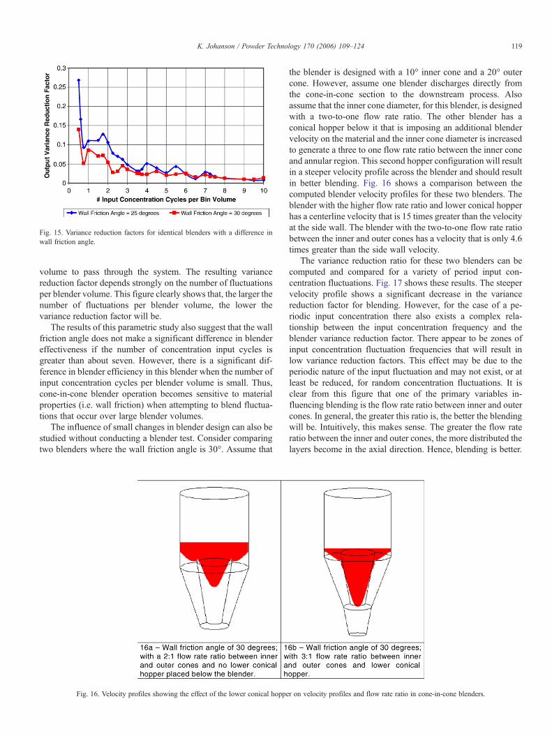
Fig. 15. Variance reduction factors for identical blenders with a difference inwall friction angle.


volume to pass through the system. The resulting variancereduction factor depends strongly on the number of fluctuationsper blender volume. This figure clearly shows that, the larger thenumber of fluctuations per blender volume, the lower thevariance reduction factor will be.

The results of this parametric study also suggest that the wallfriction angle does not make a significant difference in blendereffectiveness if the number of concentration input cycles isgreater than about seven. However, there is a significant dif-ference in blender efficiency in this blender when the number ofinput concentration cycles per blender volume is small. Thus,cone-in-cone blender operation becomes sensitive to materialproperties (i.e. wall friction) when attempting to blend fluctua-tions that occur over large blender volumes.

The influence of small changes in blender design can also bestudied without conducting a blender test. Consider comparingtwo blenders where the wall friction angle is 30°. Assume that

Fig. 16. Velocity profiles showing the effect of the lower conical hoppe

the blender is designed with a 10° inner cone and a 20° outercone. However, assume one blender discharges directly fromthe cone-in-cone section to the downstream process. Alsoassume that the inner cone diameter, for this blender, is designedwith a two-to-one flow rate ratio. The other blender has aconical hopper below it that is imposing an additional blendervelocity on the material and the inner cone diameter is increasedto generate a three to one flow rate ratio between the inner coneand annular region. This second hopper configuration will resultin a steeper velocity profile across the blender and should resultin better blending. Fig. 16 shows a comparison between thecomputed blender velocity profiles for these two blenders. Theblender with the higher flow rate ratio and lower conical hopperhas a centerline velocity that is 15 times greater than the velocityat the side wall. The blender with the two-to-one flow rate ratiobetween the inner and outer cones has a velocity that is only 4.6times greater than the side wall velocity.

The variance reduction ratio for these two blenders can becomputed and compared for a variety of period input con-centration fluctuations. Fig. 17 shows these results. The steepervelocity profile shows a significant decrease in the variancereduction factor for blending. However, for the case of a pe-riodic input concentration there also exists a complex rela-tionship between the input concentration frequency and theblender variance reduction factor. There appear to be zones ofinput concentration fluctuation frequencies that will result inlow variance reduction factors. This effect may be due to theperiodic nature of the input fluctuation and may not exist, or atleast be reduced, for random concentration fluctuations. It isclear from this figure that one of the primary variables in-fluencing blending is the flow rate ratio between inner and outercones. In general, the greater this ratio is, the better the blendingwill be. Intuitively, this makes sense. The greater the flow rateratio between the inner and outer cones, the more distributed thelayers become in the axial direction. Hence, blending is better.

r on velocity profiles and flow rate ratio in cone-in-cone blenders.

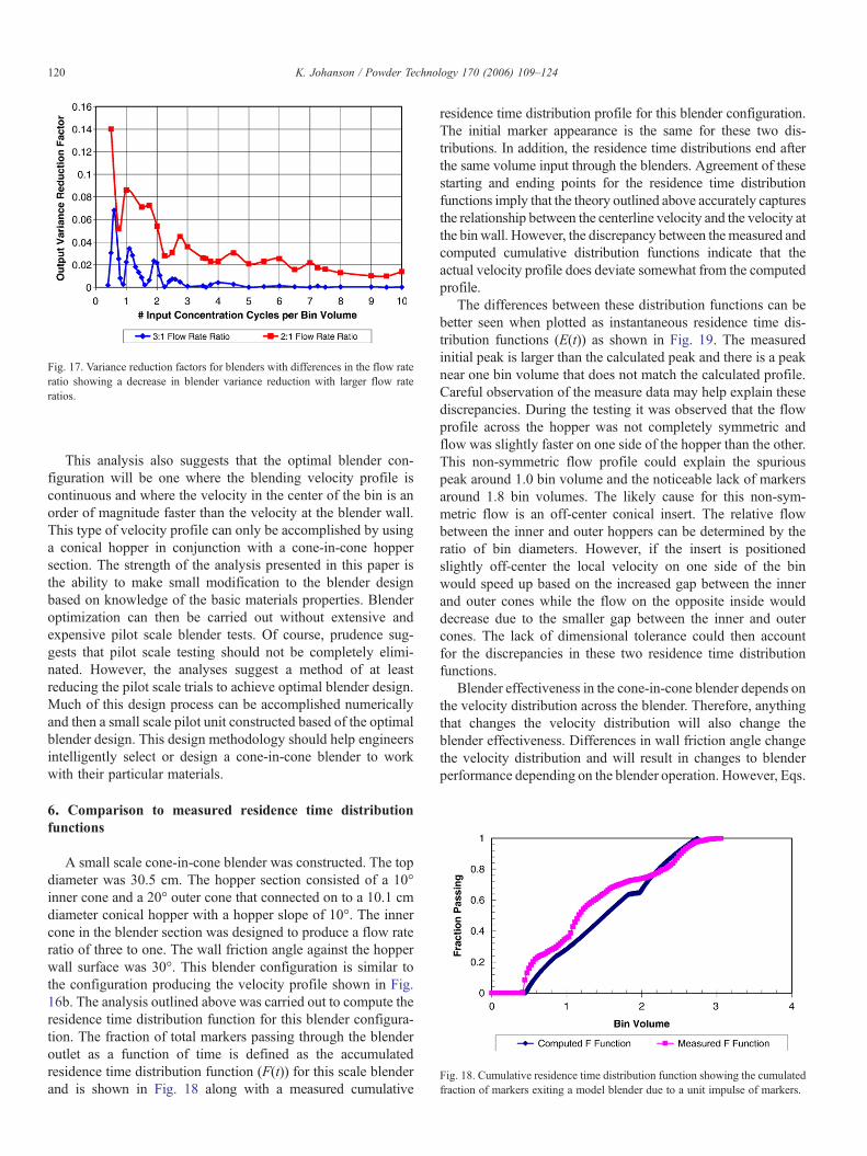
Fig. 17. Variance reduction factors for blenders with differences in the flow rateratio showing a decrease in blender variance reduction with larger flow rateratios.

Fig. 18. Cumulative residence time distribution function showing the cumulatedfraction of markers exiting a model blender due to a unit impulse of markers.


This analysis also suggests that the optimal blender con-figuration will be one where the blending velocity profile iscontinuous and where the velocity in the center of the bin is anorder of magnitude faster than the velocity at the blender wall.This type of velocity profile can only be accomplished by usinga conical hopper in conjunction with a cone-in-cone hoppersection. The strength of the analysis presented in this paper isthe ability to make small modification to the blender designbased on knowledge of the basic materials properties. Blenderoptimization can then be carried out without extensive andexpensive pilot scale blender tests. Of course, prudence sug-gests that pilot scale testing should not be completely elimi-nated. However, the analyses suggest a method of at leastreducing the pilot scale trials to achieve optimal blender design.Much of this design process can be accomplished numericallyand then a small scale pilot unit constructed based of the optimalblender design. This design methodology should help engineersintelligently select or design a cone-in-cone blender to workwith their particular materials.

6. Comparison to measured residence time distributionfunctions

A small scale cone-in-cone blender was constructed. The topdiameter was 30.5 cm. The hopper section consisted of a 10°inner cone and a 20° outer cone that connected on to a 10.1 cmdiameter conical hopper with a hopper slope of 10°. The innercone in the blender section was designed to produce a flow rateratio of three to one. The wall friction angle against the hopperwall surface was 30°. This blender configuration is similar tothe configuration producing the velocity profile shown in Fig.16b. The analysis outlined above was carried out to compute theresidence time distribution function for this blender configura-tion. The fraction of total markers passing through the blenderoutlet as a function of time is defined as the accumulatedresidence time distribution function (F(t)) for this scale blenderand is shown in Fig. 18 along with a measured cumulative

residence time distribution profile for this blender configuration.The initial marker appearance is the same for these two dis-tributions. In addition, the residence time distributions end afterthe same volume input through the blenders. Agreement of thesestarting and ending points for the residence time distributionfunctions imply that the theory outlined above accurately capturesthe relationship between the centerline velocity and the velocity atthe bin wall. However, the discrepancy between themeasured andcomputed cumulative distribution functions indicate that theactual velocity profile does deviate somewhat from the computedprofile.

The differences between these distribution functions can bebetter seen when plotted as instantaneous residence time dis-tribution functions (E(t)) as shown in Fig. 19. The measuredinitial peak is larger than the calculated peak and there is a peaknear one bin volume that does not match the calculated profile.Careful observation of the measure data may help explain thesediscrepancies. During the testing it was observed that the flowprofile across the hopper was not completely symmetric andflow was slightly faster on one side of the hopper than the other.This non-symmetric flow profile could explain the spuriouspeak around 1.0 bin volume and the noticeable lack of markersaround 1.8 bin volumes. The likely cause for this non-sym-metric flow is an off-center conical insert. The relative flowbetween the inner and outer hoppers can be determined by theratio of bin diameters. However, if the insert is positionedslightly off-center the local velocity on one side of the binwould speed up based on the increased gap between the innerand outer cones while the flow on the opposite inside woulddecrease due to the smaller gap between the inner and outercones. The lack of dimensional tolerance could then accountfor the discrepancies in these two residence time distributionfunctions.

Blender effectiveness in the cone-in-cone blender depends onthe velocity distribution across the blender. Therefore, anythingthat changes the velocity distribution will also change theblender effectiveness. Differences in wall friction angle changethe velocity distribution and will result in changes to blenderperformance depending on the blender operation. However, Eqs.

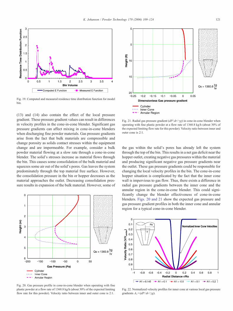
Fig. 19. Computed and measured residence time distribution function for modelbin.

Fig. 21. Radial gas pressure gradient (dP /dr /γg) in cone-in-cone blender whenoperating with fine plastic powder at a flow rate of 1360.8 kg/h (about 30% ofthe expected limiting flow rate for this powder). Velocity ratio between inner andouter cone is 2:1.


(13) and (14) also contain the effect of the local pressuregradient. These pressure gradient values can result in differencesin velocity profiles in the cone-in-cone blender. Significant gaspressure gradients can affect mixing in cone-in-cone blenderswhen discharging fine powder materials. Gas pressure gradientsarise from the fact that bulk materials are compressible andchange porosity as solids contact stresses within the equipmentchange and are impermeable. For example, consider a bulkpowder material flowing at a slow rate through a cone-in-coneblender. The solid's stresses increase as material flows throughthe bin. This causes some consolidation of the bulk material andsqueezes some air out of the solid's pores. Gas leaves the systempredominately through the top material free surface. However,the consolidation pressure in the bin or hopper decreases as thematerial approaches the outlet. Decreasing consolidation pres-sure results in expansion of the bulk material. However, some of

Fig. 20. Gas pressure profile in cone-in-cone blender when operating with fineplastic powder at a flow rate of 1360.8 kg/h (about 30% of the expected limitingflow rate for this powder). Velocity ratio between inner and outer cone is 2:1.

the gas within the solid's pores has already left the systemthrough the top of the bin. This results in a net gas deficit near thehopper outlet, creating negative gas pressures within thematerialand producing significant negative gas pressure gradients nearthe outlet. These gas pressure gradients could be responsible forchanging the local velocity profiles in the bin. The cone-in-conehopper situation is complicated by the fact that the inner conewall is impervious to gas flow. Thus, there exists a difference inradial gas pressure gradients between the inner cone and theannular region in the cone-in-cone blender. This could signi-ficantly change the blender effectiveness of cone-in-coneblenders. Figs. 20 and 21 show the expected gas pressure andgas pressure gradient profiles in both the inner cone and annularregion for a typical cone-in-cone blender.

Fig. 22. Normalized velocity profiles for inner cone at various local gas pressuregradients A1= (dP /dr /γg).

Fig. 23. Normalized velocity profiles in annular section of cone-in-cone hopperas a function of local gas pressure gradient A1= (dP /dr /γg).


Once the local gas pressure gradients are known, the radialvelocity analysis outlined above can be implemented to com-pute the expected velocity profiles for the case of the local radialpressure gradients given in Fig. 22. This analysis can be appliedto both the inner cone and the annular region to determine thevelocity profiles at various local gas pressure gradients. Fig. 22shows the expected velocity profiles in the 10° inner cone atdifferent radial gas pressure gradients. Note that the negativegas pressure gradient at the bottom of the inner cone is largeenough to result in a funnel-flow velocity pattern. If this high gaspressure gradient persisted throughout the inner cone section, itwould induce a funnel flow velocity pattern in the blender andresult in a preferred flow channel. Luckily the gradients in otherhopper elevations are smaller than this value. Likewise, Fig. 23indicates that if gas pressure gradients in the annular section havelarge enough negative values, then preferred flow channelswould develop along the outer wall of the inner cone. Each of thevelocity profiles in these figures has been normalized so thevelocity at the centerline equals one.

Fig. 24. Velocity profiles in cone-in-cone blender at various locations in the blender.between the inner cone and the annular section.

However, local velocity profiles at any elevation in theblender can be computed by assuming a two-to-one velocitydifference between the inner and outer cone and computing thevelocity profile from the local gas pressure gradient given inFig. 20. Fig. 24 shows several of these velocity profiles in thehopper section of the cone-in-cone blender. This figure indicatesthat the steep funnel flow velocity pattern persists only near thehopper outlet. Velocity profiles near the top of the cone sectionare actually flatter than those expected for normal mass flowwithout gas pressure effects. It is not likely that the small zoneof steep velocity profiles near the inner hopper outlet willpromote complete funnel-flow behavior in the entire hoppersection. However, increasing the solids flow rate will increasethe magnitude of these negative gas pressure gradients in thelower hopper and increase the positive gas pressure gradients inthe upper hopper section. This suggests that one should expectto see a flow rate condition that may induce a preferred flowchannel formation in the center of the blender during operationat high flow rates. Conversely, the higher gas pressure gradientat the top of the hopper would likely result in overall averagevelocity profiles flatter than typical velocities in mass flowblenders without gas pressure gradient effects. This suggeststhat the blending action of the blender may diminish as the flowrate of fine powder increases until the very steep profile in thelower hopper section occupies a significant portion of the bin, atwhich point the blender velocity profile produces funnel flowbehavior. The whole matter of the influence of local gas pressuregradient in cone-in-cone blenders is an interesting area forfurther study. However, this theoretical analysis suggests thatfine powders may be susceptible to preferred flow channelformation in cone-in-cone blenders if conditions are right.

7. Conclusions

The strength of this paper is the ability to compute theresidence time distribution function just from knowledge of

The mass flow rate in this blender is 1360.8 kg/h with a two to one velocity ratio


material properties. The properties induce a unique velocitypattern in a given cone-in-cone geometry that can be approx-imated using limiting states of stress in the blender. The radialvelocity assumption allows radial velocity fields to be extendedto annular flow channels. The analysis in this paper suggeststhat the blender design is somewhat independent of wall frictionangle for conditions where there are several input concentrationfluctuations in a single blender volume. However, friction angledoes play a role in blender performance for conditions where theblender must mix large-period input fluctuations. Radial velocityprofiles in cone-in-cone blenders can be extended to include theeffect of local gas pressure gradients. There is some evidence thatthese gas pressure gradients can induce funnel-flow behavior inthe blender, depending on the operation flow rate, and may resultin preferred flow channels during operation. This is an area forfurther research. It is the contention of the author that the methodof blender evaluation outlined above could be used with otherblender configurations to develop a bridge between blendereffectiveness and the material properties which control thevelocity profiles in the blender. This general methodology, ifsuccessfully implemented, will allow scale-up of blenders. Thiswill likely require solving complex 3D differential equations withfree boundaries to obtain an approximation to the local velocitypatterns. Even though this is a formidable task, the author sug-gests this road as the way forward. Advances in volume of fluidfinite element methods or a combination of DEM and FEMapproaches may provide the necessary computational power toaccomplish this task.

NomenclatureA1 Dimensionless radial pressure gradient body force ratioA2 Dimensionless θ˜-direction pressure gradient body force

ratioBV Bin volumeCapblender Blender capacityCin Input concentrationCout Output concentrationDT Top diameter of outer cone (m)dT Top diameter of inner cone (m)DB Bottom diameter of outer cone (m)DB Bottom diameter of inner cone (m)DO Outlet diameter of cone-in-cone hopper (m)E(t) Residence time distribution function E(t)=dF(t)/dtF(t) Cumulative residence time distribution functionP Gas pressure (KPa)Qs Solids flow rate (kg/hr)r Radial coordinate (m)Rvel Ratio of inner and outer velocities in cone-in-cone hopperrb Distance from the hopper centerline to hopper radial

coordinate (m)Rb Distance from the hopper centerline to the hopper wall

(m)s θ-dependence function for radial stressSdevin Standard deviation of input streamSdevout Standard deviation of output streamV(θ) Radial velocity (m/s)V(0) Velocity at hopper centerline (m/s)

V(rb) Radial velocity in terms of distance from centerline(m/s)

Vcenter Velocity at hopper centerline (m/s)VR Variance reduction factorγ Powder bulk density (kg/m3)β Angle between the effective wall body force and the

gravitational vector direction (deg)δ Effective Internal friction angle (deg)ϕw Wall friction angle (deg)ϕwe Effective wall friction angle including gas pressure

gradient trems (deg)σr Normal stress on the plane perpendicular to the radial

direction in a spherical coordinate system (KPa)σθ Normal stress on the plane perpendicular to the θ-

direction in a spherical coordinate system (KPa)σϕ Normal stress on the plane perpendicular to the ϕ-

direction in a spherical coordinate system (KPa)σ Mean stress (KPa)σ1 Major principal stress (KPa)σ3 Minor principal stressθw Half angle of conical hopper measured from the

vertical (deg)θi Half angle of inner conical hopper measured from the

vertical (deg)θo Half angle of outer conical hopper measured from the

vertical (deg)θL Half angle of conical hopper at bottom of cone-in-cone

(deg)θ θ-direction coordinate (deg)ϕ ϕ-direction coordinate (deg)ϕw Wall friction angle (deg)ϕwe Effective wall friction angle (deg)τrϕ Shear stress on the plane perpendicular to the radial

direction acting in the ϕ-direction in a cylindricalcoordinate system (KPa)

τrθ Shear stress on the plane perpendicular to the radialdirection acting in the θ-direction in a cylindricalcoordinate system (KPa)

τθϕ Shear stress on the plane perpendicular to the θ-direction acting in the ϕ-direction in a cylindricalcoordinate system (KPa)

ω Angle between the major principal stress and the r-coordinate direction (deg)

Acknowledgment

The author would also like to acknowledge the financialsupport of the Engineering Research Center (PERC) for Par-ticle Science and Technology at the University of Florida,Material Flow Solutions Inc, the National Science FoundationNSF Grant #EEC-94-02989, and the Industrial Partners of thePERC.

References

[1] B.M.H.B. Silos, Draft Design Code for Silos, Bin, Bunkers and Hoppers,1987.


[2] F. Ebert, G. Dau, V. Durr, Blending performance of cone-in-cone blenders—experimental results and theoretical predictions, Proceedings of the 4thInternational Conference for Conveying and Handling of Particulate Solids,2003.

[3] J.R. Johanson, Controlling flow patterns in bins by use of an insert, BulkSolids Handling 2 (3) (Sept 1982).

[4] A.W. Jenike, J.R. Johanson, Stress and Velocity Fields in Gravity Flow ofBulk Solids, Bulletin, vol. 116, Utah Engineering Station, 1967.

[5] R.M. Nedderman, Statics and Kinematics of Granular Materials, CambridgeUniversity Press, 1992.

[6] V.V. Sokolovskii, Statics of Granular Media, Pergamon Press, Oxford, 1965.[7] A.W. Jenike, Gravity Flow of Bulk Solids, Bulletin, vol. 108, Utah

Engineering Station, 1961.[8] A.W. Jenike, Flow and Storage of Bulk Solids, Bulletin, vol. 123, Utah

Engineering Station, 1967.[9] A.W. Jenike, Powder Technology 50 (1987) 229.

Documents

Predicting cone-in-cone blender efficiencies from key material properties