NBER WORKING PAPER SERIES

PREDICTING CRIMINAL RECIDIVISMUSING "SPLIT POPULATION"SURVIVAL TIME MODELS

Peter Schmidt

Ann Dryden Witte

Working Paper No. 2445

NATIONAL BUREAU OF ECONOMIC RESEARCH1050 Massachusetts Avenue

Cambridge, MA 02138November 1987

This research was supported by the National Institute of Justice, U.S. Departmentof Justice. The Institute's support does not indicate their concurrence withour methods or conclusions. The research reported here is part of the NBER'sresearch program in Labor Studies. Any opinions expressed are those of the authorsand not those of the National Bureau of Economic Research.

NBER Working Paper #2445November 1987

Predicting Criminal Recidivism Using"Split Population" Survival Time Models

ABSTRACT

In this paper we develop a survival time model in which the probability of

eventual failure is less than one1 and in which both the probability of eventual

failure and the timing of failure depend (separately) on individual

characteristics. We apply this model to data on the timing of return to prison for

a sample of prison releasees4 and we use it to make predictions of whether or not

individuals return to prison. Our predictions are more accurate than previous

predictions of criminal recidivism. The model we develop has potential

applications in economics; for example it could be used to model the probability

of default and the timing of default on loans,

Peter SchmidtDepartment of Economics

Michigan State UniversityEast Lansing, MI 48824-1038

Ann Dryderi WitteDepartment of Economics

Wellesley CollegeWellesley, MA 02181

1. Introduction

Durin the 1970's and early 1980s; eVidence accLimulated indicating that a

relatively small group of offenders committed most serious offenses. These

findings4 coupled with increasinQ pressures on the budgets of criminal justice

agencies, led to calls for more effective use of the public expenditures for crime

control by identifying and incarcerating the most serious arid persistent offenders.

The extremely influential work of Greenwood (1982) is a good example of the

research promoting a policy of "selective incapacitation." However4 the success of

such a policy clearly depends an the ability to predict accurately xante (at the

time a sentencing or parole decision is to be made) which individuals would return

to crime if released. Thus there has been a resurgence of interest in the question

of how well one can predict criminality at the individual level. A good survey of

recent work on prediction in criminology is given by Farrington (1987). who

concludes that predictive ability to date is rather disappointing4 with most

predictive models yielding false positive and false negative rates both in excess

of 0Y,.

In this paper, we generate predictions of whether or not an individual will

return to prison using survival time (or "failure time") models. Surprisingly,

survival models have not been used much in crimimirsology, and explanatory variables

have almost never been included in those survival models that have been used. Our

predictions are therefore based on a more sophisticated statistical model than

previous researchers have considered. Encouragingly4 we predict return to prison

more accurately than has been done in the past. However4 the accuracy of our

predictions is (in our opinion) still not sufficient to justify a policy of

Sel ective incapacitation.

2

Such a predictive exercise is of substantial interest to criminologists, but

probably not to most economists. However, the model which we develop to make our

predictions is novel and has potential applications in a number of areas of

economics. Specifically, we consider a 'split population model" in which it is

assumed that some fraction of the sample would never return to prison1 so that the

distribution of time until return is relevant only for the remaining fraction of

the sample who would eventually return. Spilt models tend to imply very rapidly

decreasing hazard rates (because the surviving population is implicitly made up

increasingly of individuals who will never fail)1 and they are very useful in our

application because our hazard rate does indeed fall very rapidly. Furthermore; we

parameterize both the probability of eventual return and the timing of return; so

that we can make separate statements about the effects of explanatory variables on

these two conceptually different aspects of recidivism. For example1 we find that

race and sex affect the probability of eventual recidivism but not its timing1

while two indicators of the nature of the previous offense affect the timing of

recidivism (for the eventual red dlvi sts) but not the probability of eventual

reci divi sm.

It is not hard to think of potential economic applications of our model. For

example1 in the credit—scaring problem considered by Boyes, Hoffman and Low (1988),

we might wish to estimate separately the effect; of individual characteristics or

of features of the loan itself on the probability cf eventual default and on the

timing of default for those individuals who will eventually default. split model

may be very reasonable for this application because many individuals would in fact

never default, no matter how long they were observed. Furthermore, while most

credit—scoring analyses focus c'nly on the probability of eventual default, the

likely timing of default is also relevant to the expected profitability of a

potential loan1 and therefore should also be of use in deciding whether to grant

credit. A traditional creditscoring analysis that focuses only on the probability

of default may fail to give proper weight to individual characteristics that affect

the timing of default (conditional on eventual default), but that do not affect the

probability of eventual default.

More generally4 our model may be useful in the analysis of the timin9 of any

event which does not occur for a substantial fraction of the sample. For example4

if we are interested in the duration of spells of employment, it should be

recognized that a substantial proportion of individuals will never be unemployed.

Models which fail to recognize this point will almost surely umisspecify the

distribution of survival times. They will underpredict the proportion of always—

employed individuals and (because they are misspecified) they may give misleading

estimates of the effects of explanatory variables.

2. Data

The data used in this paper consist of information on a cohort of releasees

from the North Carolina prison system. This cohort consists of all individuals

released from North Carolina prisons from July 1, 1977 through June 30, 1978.

There were 94Z7 such individuals. This data set is far larger and more timely than

is usual in criminal justice research, and it is clear what population it

represents.

We also obtained and analyzed data on a second similar cohort of releasees,

but to save space we will not report these results here. Further details an the

results for our second cohort (and4 indeed, on all aspects of our research project)

can be found in Schmidt and Witte (1987, 1988).

4

There were 130 observations in our data that were obviously defective and had

to be discarded. In almost all cases the defect in the data leading to

elimination of the observation 15 that the individual was in fact not released from

prison during the time period which defined the data set. It is important note

that the number of defective cases was only slightly more than one perce of the

original number of cases. This is a very low discaro rate for release cohort data

and attests to the high quality of the Not h Carolina record keeping system.

A more serious problem is that marty observations lacked information on one or

more variaus which we used in our analyses. Only 4618 observations contained

informaion on all variables of interestq while the other 4709 observations lacked

some information. The most commonly missing piece of data was information on

alcohol or drug abuses which turns out to be a very significant predictor of post—

release criminality 4287 of the 4709 incomplete observations lacked this

information. We discarded the incomplete observations entirely and analyzed only

those which were complete. Clearly this raises the possibility of selectivity

bias in our results but we preferred this to the omission of a very important

explanatory variable.

Having discarded the incomplete observations we split the sample of complete

observations randomly into an "estimation sample" (or "analysis sample) of 1540

observations arid a 'validation sample" of 3078 observations.2 We fit our

statistical models to the estimation samples and then used the validation sample to

check the predictive accuracy of these models. This procedure reflects the

generally accepted view that the predictive accuracy of a model can be checked

validly only on data riot used to estimate the model.

We will now define the variables used in our study. The dependent variable

which we seek to explain is the length of time from an individuaFs release from

C

prison jr North Carolina until his or her return to prison there. Therefore the

outcome variables which we define are an indicator of whether the individual

returned to prison within the followup period and the length of time until return

for those individuals who did return, while the explanatory variables are

demographic characteristics and measures of the past criminal and correctional

histories of the individuals.

To be more specifics recall that our data set was defined by date of release

from prison. The sentence from which the individuals were released will be called

the sample sentence, and the conviction which resulted in the sample sentence will

correspondingly be called the sample conviction. All explanatory variables are

defined either as of the time of entry or as of the time of release from the sample

sentence. The outcome variables were defined as the result of a search of North

Carolina Department of Correction records in April, 1984, Thus the fcllowup period

ranged from 70 to 81 months. This followup period is quite long for a study of

recidivism; most studies follow releasees for three years or less.

We define the following outcome variables; for each individual

FOLLOW, the length of the foilowup period, in months.

RECID, a dummy variable equal to one if the individual returned to a North

Carolina prison during the foilowup period and equal to zero otherwise.

rIME, the length of time from release from prison until return to prison;

rounded to the nearest month for individuals for whom RECID 1. TIME is

undefined for individuals for whom RECID 0.

We now define the Following explanatory variables, for each individual:

TSERVD, the time served (in months) for the sample sentence

AGE, age (in months) at time of release.

6

PRIORS the number of previous incarcerations, not including the sample

sentence at the time of entry into the prison system for the sample sentence.

RULE, the number of prison rule violations reported during the sample

sentence.

SCHOOL the number of years of formal schooling completed at the time of entry

into the prison system for the sample sentence.

WHITE, a dummy variable equal to zero if the individual is black, and equal to

one otherwise.

MALE, a dummy variable equal to one if the individual is male, and equal to

zero if female.

ALCHY, a dummy variable equal to one if the individual's record indicates a

serious problem with alcohol (before entry into the prison system) and equal to

zero otherwise.

JUNKY, a dummy variable equal to one if the individual's record indicates use

of hard drugs (before entry into the prison system) and equal to zero otherwise.

MARRIED, a dummy individual equal to one if the individual was married at the

time of entry into prison for the sample sentence, and equal to zero otherwise.

SUPER, a dummy variable equal to one if the individual's release from the

sample sentence was supervised (e.g., parole), arid equal to zero otherwise.

WORKREL, a dummy variable equal to one if the individual participated in the

North Carolina prisoner work release program during the sample sentence, and equal

to zero otherwise.

FELON, a dummy variable equal to one if the sample sentence was for a felony,

and equal to zero if it was for a misdemeanor.

PERSON, a dummy variable equal to one if the sample sentence was for a crime

against a person, and equal to zero otherwise.

7

PROPTY, a dummy variable equal to one if the sample sentence was for a crime

against property, and equal to zero otherwise.4

3. Models Without ExlanatoVariab1es

We begin our analysis by fitting various parametric models to our estimation

sample, and checking how well the models fit the estimation sample and how well

they predict the actual outcomes in our validation sample. This is a standard

exercise in the criminological literature (see, for example, Maltz (1984) and the

references therein), but there has not been sufficient attention given to the

question of how well commonly—used distributions fit the data.

A useful first step is to have a look at the nature of the empirical

distribution of time until recidivism. The solid line in Figure 1 gives the

empirical (actual) density for the validation sample, and the density for the

estimation sample would look more or less the same. Similarly, a graph of the

hazard rate would again reveal more or less the same pattern. Specifically, it is

important to note two important features of the hazard rate in our data. First, it

is non—monotonic; the hazard first rises and then falls.' Second, once it begins

to fall, the hazard rate falls very quickly. These features of the data are common

in applications involving recidivism, and perhaps in economics as well, but they

are not common in the biological or reliability applications typically discussed in

the statistical literature on survival times. As a result, distributions typically

found in standard texts like Kalbfleisch and Prentice (1980) or Lawless (1982) do

not fit our data well.

We fit five different distributions to the data, by maximum likelihood

exponential, Weibull, lognarmal, laglogistic and LaGuerre. The exponential and

Weibull distributions are commonly found in the survival time literature, but they

8

should nøt be expected to do well here because they can not generate a non—

monotonic hazard rate. The lognormal and loglogistic distributions, on the other

harid imply a hazard that first rises and then falls, just as in our data. The

LaGuerre model (Cox and Oates (1984, p. 20), Kiefer (1985)) has a density which is

the product of an exponential function and a polynomial; this is known as a

LaGuerre polynomial in the mathematical literature. It is intended to give a

flexible approximation to an arbitrary density.' We use a second—degree LaGuerre

distribution (that is, it contains a second—degree polynomial).

None of these distributions fits our data adequately. In each case they

overpredicted recidivism for the first few months after release and they

underpredicted it during the intermediate period of roughly one to three years

after release. Furthermore, all of the distributions except the La6uerre

overpredicted recidivism in the tail of the distribution. The lognormal and

loglagistic distributions fit noticably better than the exponential or Weibull, as

expected, but they still did not generate a sufficiently rapid increase in the

hazard at first or a sufficiently rapid decrease in the hazard in the tail of the

distribution. The LaGuerre model fit better than any of the others, especially in

the tail, but it still was quite inadequate for the first two years after release.

The superiority of the LaGuerre model is evident from the likelihood values

achieved, which were —3431, —3405, —3370, —3390 and —3356, for the exponential,

Weibull, lognormal, loglogistic and LaGuerre distributions, respectively. It is

also clear from any reasonable measure of the quality of the predictions generated

for the validation sample. For example, if we measure the quality of these

predictions by the maximum difference between the predicted and the actual cdf, the

value for the LaGuerre distribution is .020, compared to .079, .049, .037, and .040

for the other four distributions.

9

The dashed line in Figure 1 displays the density of time until recidivism

predicted by the LaSuerre distribution. The inadequacy of the fit is evident.

While we could continue to experiment with other distributions, one lesson that

should be clear is that "off—the—shelf" models from the biostatistical or

operations research literatures are not necessarily adequate for applications in

other fields.

4. Split Models

The parametric models considered in the last section all assumed some form of

the cumulative distribution function for the time until recidivism. Any such

cumulative distribution function approaches one as time at risk becomes

sufficiently large. In the present context1 this implies that every individual

would eventually return to prison1 and this implicit assumption can be argued to be

unreasonable. In this section, we will consider "split population models" (or

simply "split models") in which the probability of eventual recidivism is an

additional parameter to be estimated, and may be less than one. A distribution of

failure times is also specified, as before1 but this is understood to apply only to

those individuals who will eventually fail. Split models were introduced to the

criminological literature by Maltz and McCleary (1977), with previous treatments in

the statistical literature dating back to Anscombe (1961), and they have been

further developed in a line of research well summarized by Maltz (1984) or Schmidt

and Witte (1988, chapter 5). They do not appear to have been used in economics,

but in our opinion they are likely to be useful there as well.

Using the notation of Schmidt and Witte (1984, section 6.4), we can express a

split model as follows. First, let F be arc unobservable variable indicating

whether an individual would or would not eventually fail. Specifically, let F

l0

equal one for individuals who would eventually fail, and zero far individuals who

would never fails Then we assume

(1) NE = 1) = S ,F(F = 0) = 1 — S

The parameter S is of course the eventual recidivism rate. Second, we assume some

cumulative distribution function G(tF1) for the individuals who would ultimately

fail, and we let g(tF1) be the corresponding density. We note explicitly that

such a distribution is defined conditional on Fl, and is irrelevant fur

individuals for whom F0.

Now let I be the length of the followup period, and let C be the observable

dummy variable indicating whether or not the individual has returned to prison by

the end of the followup period. For the recidivists in the sample, we observe C

1 and the failure time t, and of course we know that F = 1. The appropriate

density is therefore

(2) P(F1) g(tF1) = S g(tF=1).

On the other hand, for the rion—recidivists in the sample we observe only C0, and

the probability of this event is

(3) P(C=0) = P(F=0) + P(F=1)P(t>TF1)

1 — S + S El — 6(T{F1)].

The likelihood is then made up of terms like (2) for recidivists and (3) for non—

recidivists (individuals who have not returned to prison by the end of the followup

period).

We fit split models to our data using the same five distributions as were

considered in the previous section (exponential, Weibull, lognormal, luglogistic

and LaGuerre). The likelihood ViUCS achieved were —335B —3346, —3342, —3341, arid

—3349, respectively, while the maximum differences between the actual and the

predicted cdf in the validation sample were .024, .017 .005, .011 arid .021. The

11

loglogistic model fits the estimation sample slightly better than the lognormal

model, while the lognormal model generates slightly better predictions for the

validation samples but there is in fact little basis on which to choose between the

two distributions, ard either of them dominates the other three distributions

considered. However1 what is more striking is the extent to which the split models

dominate the simple (not split) models of the previous section. In terms of

likelihood value or quality of predictions the worst of our split models (split

exponential) is comparable to the best of our simple models (LaGuerre)1 even though

it contains fewer parameters. The best of our split models say the split

lognormal, is much better than any of the models of the last section. Introduction

of the splitting parameter into the logniormal model increases the likelihood value

by approximately 50, and reduces the maximum difference between the predicted and

the actual cdf from .037 to .005; these are certainly impressive improvements in

the model to be achieved by the introduction of a single parameter.7

The dotted line in Figure 1 gives the predicted density for the split

lognormal model. The Fit of the model to the data appears to be quite adequate,

and this conclusion is confirmed by more formal tests reported in Schmidt and Witte

(1988 section 5.3).

The value of the "splitting parameter" 8 generated by the split lognormal

model is 0.45. This is the long—run (eventual) recidivism rate. By way of

contrast, the long—run recidivism rate is by definition equal to one in non—split

models, and this is reflected in very large implied recidivism rates for long but

finite followups. For example, the 25—year recidivism rates implied by our models

of the last section were 0.94, 0.89, 0.78, 0.78, and 0.52 for the exponential,

Weibull, lognormal. loglogistic and La8uerre distributions, respectively. Based on

a limited number of studies with very long followup periods1 such as PicCord (1978)

12

and Kitchener, Schmidt and Glaser (1977), a long—run failure rate of approximately

0.5 appears to be reasonable for our data and definition of recidivism.

5. Models With Explanatory Variables

We now consider models with explanatory variables. This is obviously

necessary if we are to make predictions for individuals, or even if we are to make

potentially accurate predictions for groups which differ systematically from our

original sample (for example4 to evaluate the effectiveness of a correctional

program which is applied to a non—random sample of the population of releasees).

Furthermore, in many applications in economics or criminology the coefficients of

the explanatory variables may be of obvious interest.

We begin by fitting the proportional hazards model to our data. The point of

this exercise is to see which explantory variables are worth including, without

making a specific distributional assumption. The estimates are based on the usual

'partial MLE" method; the ties in the data are handled using the approximation of

Peto (1972), as reported also by Kalbfleisch and Prentice (19804 equation (4.8)).

Our estimates are given in Table 1 using the 15 explanatory variables defined in

section 2. (Note that a few variables have been rescaled, to make the coefficients

of a more conveniently magnitude.) The "t ratios" reported are the asymptotic

standard normal statistics used to test the hypothesis that the coefficient is

zero.

Looking under the heading "ORIGINAL SPECIFICATION," we see that six

coefficients are individually insignificant at the 57. level. They are also jointly

insignificant4 as judged by the likelihood ratio test; and we dropped the

corresponding six variables (RULE, MARRIED, SCHOOL, WDRKREL, PERSON, and SUPER)

from the model. Interestingly, an exponential model with the log of the mean

13

depending linearly on the explanatory variables led to exactly the same decision

about which variables to drop5 and indeed to almost exactly the same t ratios and

likelihood ratio statistic. Our results indicate that the type of individual most

likely to have a small value of time until recidivism is a young black male with a

larqe number of previous incarcerations, who is a drug addict and/or alcoholic4 and

whose previous incarceraticrr was lerthy arid was for a crime aQainst property.

These findings., with the possible exception of the findings on race, are consistent

with the conclusions of one of the two most comprehensive surveys available (Wilson

and Herrnstein (1985)), with most of the conclusions of the second such survey

(Biumsteiri et ml. (1986)), arid with our own previous work (Schmidt and Witte

(1984))

We now turn to a parametric model based on the lognormal distribution. As

noted above, we also considered the exponential distribution, but it did not fit

the data as well as the logriormal, so we will not discuss it here. The model in

its most general form is a split model in which the probability of eventual

recidivism follows a logit model4 while the distribution of time until recidivism

(conditional on eventual recidivism) is lognoruial4 with its mean depending on

explanatory variables.

To be more explicit, we follow the notation of section 4 For individual i,

there is an unobservable variable F1 which indicates whether or not individual i

will eventually return to prison. The probability of eventual failure for

individual i will be denoted , so that P(F 1) = &. Let X1 be a (row) vector

of individual characteristics (explanatory variables), and let be the

corresponding vector of parameters. Then we assume a logit model for eventual

reci di vi sm:

(4) = 1 / Cl 4 eXi0]

14

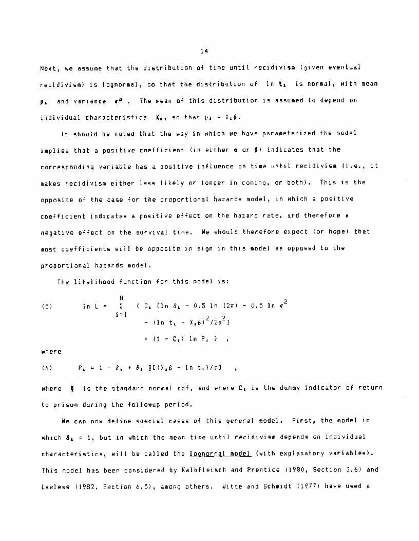
Next, we assume that the distribution of time until recidivism (given eventual

recidivism) is lognormal, so that the distribution of In t1 is normal, with mean

p and variance r2 . The mean of this distribution is assumed to depend on

individual characteristics X, so that XdI.

it should be noted that the way in which we have parameterized the model

implies that a positive coefficient (in either a or ) indicates that the

corresponding variable has a positive in+luence on time until recidivism (i.e. it

makes recidivism either less likely or longer in coming, or both). This is the

opposite of the case for the proportional hazards rnodel in which a positive

coefficient indicates a positive effect on the hazard rate, and therefore a

negative effect on the survival time. We should therefore expect (or hope> that

most coefficients will be opposite in sign in this model as opposed to the

proportional hazards model.

The likelihood function for this model is

N

(5) in L = E C C tin 8 — 0.5 in (2ir) — 0.5 in

i=12 '

— (in t — Xd'l) /2wi

+ (1 — Ca) In P1 }

where

(6) P = 1 - j + [(X1i - in t1)/ff]

where * is the standard normal cdF, and where C is the dummy indicator of return

to prison during the followup period.

We can now define special cases of this general model. First, the model in

which = 1, hut in which the mean time until recidivism depends on individual

characteristics, will be called the lonormal model (with explanatory variables).

This model has been considered by Kalbfleisch and Prentice (1980, Section 3.6) and

Lawless (1982, Section 6,5), among others. Witte and Schmidt (1977) have used a

very similar model to analyze recidivism. It is not a split model. Second1 the

model in which & is replaced by a single parameter & will be referred to as the

split lognorinal model (with explanatory variables). In this model the probability

of eventual recidivism is a constant1 though not necessarily equal to one, while

the mean of the distribution of time until recidivism varies over individuals.

Third1 the model in which p is replaced by a single parameter p will be called the

logit lognortnal model. In this model the probability of eventual recidivism varies

over individuals1 while the distribution of time until recidivism (for the eventual

recidivists) does not depend on individual characteristics. Finally, the general

model as presented above will be called the iggjt/individual_1alinodel. In

this model both the probability of eventual recidivism and the distribution of time

until recidivism vary over individuals.

In the lognormal, split lognormal and logit lognormal models, only one aspect

of recidivism (probability or timing) depends on explanatory variables.

Interestingly, these three models generate very similar results. Table 2 gives the

results for the split lognormal model and the logit lognormal model. The results

from these two models are very similar1 as is evident at a glance1 and are in turn

very similar to those from the proportional hazards model (Table I>. In fact, this

robustness of results goes beyond what is displayed in this paper. Essentially the

same results are obtained from the lognormal model, and also from models like these

three models but based on the exponential distribution.

However, while the choice of model does not have much effect on the estimated

coefficients, there is considerable variation in the quality of the fit and the

predictions which are generated. In both respects the lognormal models dominate

the exponential models, and the logit lognorinal model dominates the lognormal and

split lognormal models. For example, the likelihood value of —3265 for the logit

16

lognormal model is noticably higher than the values for the lognormal and split

lognormal models (-3273 and —3256>. The maximum difference between the predicted

and the actual cdf is also smaller (.006 versus .030 and .034).

We now turn to the logit/individual lognormal models in which both the

probability of eventual recidivism and the distribution of time until recidivism

vary according to individual characteristics. These parameter estimates are given

in Table 3. They are somewhat more complicated to discuss than the results from

our other models in part because there are simply more parameters and some of

them turn out to be statistically insignificant. However, every coefficient that

is statistically significantly different from zero has the expected sign (the same

sign as in our previous models), and in that sense the results are still

essentially the same as before.

In Table 3, we can see that four variables have statistically significant

effects on both the probability of eventual recidivism and on the mean time until

recidivism: TSERVD, ABE, PRIORS and ALCHY. Three variables have statistically

significant effects on the probability but not the timing of recidivism: WHITE,

JUNKY, and MALE. The remaining two variables, FELON and PROPTY, have statistically

significant effects on the timing of recidivism but not on the probability of

eventual recidivism. Thus it appears that we are indeed able to separate out the

effects of individual characteristics on the probability of eventual failure from

their effects on the timing of failure (for those who will ultimately fail), an

optimistic result.

Furthermore, these results are reasonably similar to the results we obtained

using a logit/individual exponential model; see Table 4. The difference is that

AGE, PRIORS, and ALCHY did not have significant effects on the mean time until

recidivism, in the exponential case, while they did in the lognormal case. Thus

17

our results are reasonably robust to our distributional assumptions. Perhaps not

surprisingly, however, they are less robust in this model than they were in the

simpler models previously considered.

The extent to which our results are sensitive to distributional assumptions is

an important issue, because there is seldom much reason to believe strongly in

one's distributional assumptions. However, a counterargument is that this simply

indicates that one should take care in investigating the adequacy of such

assumptions, which we have done.

6. Predictions for Individuals

We now return to the problem of prediction at the individual level, using the

models estimated in section 5. This is a fairly standard use of such models for

example, the studies included in Farrington and Tarling (1985) include predictions

of failure on parole, of recidivism, and of absconding from institutions for young

offenders. The desire to make predictions for individuals undoubtedly derives from

a desire to use such predictions as the basis for differential treatments for

individuals. Because our data are on length of time until recidivism, it is

natural for us to regard recidivism as the event to be predicted, and to ask how

well our models predict it.

Recidivism is a discrete event, while our models yield a probability of this

event for each individual. This immediately raises the question of how to

summarize the accuracy of the models predictions. One possibility is to use

statistical measures (akin to correlations) of the degree of association between

the models' probabilities and the observed binary outcome. While Kendall's tau has

often been suggested for this purpose in the criminological literature, a more

standard statistical measure would be the biserial correlation coefficient, which

18

is a form of the correlation coefficient used when one variable is continous and

the other is binary. However we will not pursue such measures here1 since they

are not of obvious practical use.

A more readily interpreted summary of predictive success, in the present

context, is simply to predict that individuals with probabilities above some chosen

level will return to prison (and that individuals with probabilities below that

level will not), and to calculate the error rate of these predictions. This seems

to us to be reasonable because it evaluates the accuracy of exactly the procedure

which would be followed in a practical application of these models.

Following the usual practice in the criminological literature (e.g., see

Wilbanks (1985)), we begin by predicting the 'carrect" proportion of failures, and

evaluate the extent to which we have correctly predicted which individuals will

fail. The failure rate in the estimation sample is 0.366, and so we predict

recidivism for the 36.67. of the validation sample who have the highest

probabilities of recidivism (regardless of the absolute magnitudes of these

probabilites). Basing our predictions on the proportional hazards model, we

predict recidivism for 1127 individuals (36.67. of the 3078 individuals in the 1978

validation sample>, of whom 595 actually returnded to prison and 532 did not; and

we predict 1951 individuals riot to return to prison, of whom 540 returned to prison

and 1411 did not. We therefore have a false positive rate of 532 / 1127 0.472,

and a false negative rate of 540 / 1951 = 0.277. Although we do not report the

results here, the logit lognormal model and the logit/individual lognormal model

generate more or less the same error rates.8

The predictive accuracy of our models compares quite favorably with the

accuracy of the models recently surveyed by Farrington (1987). He reports that

Greenwood (1982) had a false positive rate of 56% and a false negative rate of 467.

19

for his estimation sample. (Greenwood had no validation sample.) Janus' (1985)

predictions resulted in an even poorer record1 with a 627. false positive rate and a

647. false negative rate. Blumsteiri, Farrington arid Moitra's (1985> false negative

rate of 357. is lower than that of either Greenwood or Janus, although more than ten

percentage points higher than our own1 and their false positive rate is higher than

either we or Greenwood obtain. However! while we are able to predict more

accurately than the studies surveyed by Farrington, our false positive rate is in

our opinion still much too high to justify using our models to implement a policy

of selective incapacitation.

On the other hand, riot all potential users of prediction need to predict

recidivism for the "correct' proportion of the sample. Far example, a policy of

selective incapacitation might be considered viable if we could predict recidivism

with considerable assurance even for a very limited proportion of the sample.

Similarly1 models like ours might be useful in deciding on candidates for early

release if they could predict success (non—recidivism) with assurance, for some

proportion of the sample.

In Table 5, we rank individuals by their predicted probabilities of recidivism

(generated by the logit lognormal model) and then report the actual proportions of

recidivists in groups representing various percentiles of the "distribution' of

predicted probabilities of recidivism. For example, we can see in Table 5 that the

20'!. of the sample (616 individuals> with the highest predicted probabilities of

recidivism had an actual recidivism rate of 59.97., whereas the remaining 807. of the

sample (2462 individuals) had a recidivism rate of 31.17.. Obviously our models

have at least some predictive power, since individuals with higher predicted

probabilities of failure do indeed fail more often than individuals with lower

probabi I ites.

20

In considering a policy of selective incapacitation, it is important that

there be some group of individuals whom we can predict to fail with near certainty.

Using this model, any such group would have to be very small. For example, our

predicted "worst" 17. of the sample has a recidivism rate of 83.97., but it is a

group of only 31 individuals. The recidivism rate falls to 70.17. if we include the

154 individuals in the upper 57. of the probability ranking. These probabilities of

a false positive error seem rather high. A public official who is considering

selective incapacitation for the "worst' 17. of a potential release cohort would

probably not like to think that over 157. of those "worst" individuals would in fact

riot return to prison after a four—year followup.

We are much mare successful in predicting individuals who will not fail. For

example, in the group of 31 individuals who represent the predicted 'best" 17. of

the sample, the failure rate is only 6.57.. Even if we enlarge the group

considerably to include 308 individuals (the 107. of the sample with the lowest

predicted probabilities of recidivism), the failure rate is only 13.07., and this

false negative rate is much lower than the corresponding false positive rate

(32.57.) far the corresponding upper 107. of the sample. The fact that it is easier

for us to identify individuals who are likely to succeed than it is for us to

identify individuals who are likely to fail is natural because in our data less

than half of all individuals fail.

7, Conclusions

One purpose of this paper is to interest econometricians and economists in

'split—population' models which have been used in criminology. These are failure

time models in which it is explicitly recognized that some individuals will never

fail. Split models tend to imply a very rapidly falling hazard rate, and they will

1.

tend to fit well data with this characteristic. They tend to avoid the

overprediction of the long—run failure rate, a major problem with more traditional

failure time models in criminology. Furthermore we can allow explanatory

variables to affect both the probability of eventual, failure and the timing of

failure for those who will ultimately fail1 so that we can separate out the effects

of the explanatory variables on these two conceptually different features of

behavior.

second purpose of the paper is to make a contribution to the criminological

literature on prediction of recidivism, There is substantial interest in the

question of how well we can predict the future criminal behavior of individuals.

Previous attempts to predict individual outcomes using statistical models have had

somewhat mixed success statistical methods have consistently outperformed

clinical or judgemental methods of prediction1 but have still suffered from high

error rates. Most previous attempts at prediction in criminology have relied on

rather simple models, and our analysis is an attempt to see whether we can improve

the accuracy of such predictions by using a more sophisticated statistical model.

We succeed in predicting recidivism more accurately than others have done.

However it is still not clear that predictions of the accuracy that we attain are

useful in a practical sense. Unsurprisingly, there is still a need for better

models and better data.

REFERENCES

Anscombe, F. II. (1961), '1Estimating a Mixed—Exponential Response Law,' Journal ofthe American Statistical Association1 56, 493—502.

Blumstein, A,, D. Farrington and S. Moitra (1985), &Delinquency Careers:Innocents, Desisters and Persisters,& Crime and Justice: An Annual Review ofResearch L 187-220.

22

Blumstein, A., 3. Cohen! 3. A. Roth and C. 4. Visher (1986), i.jal_Careersjnd"Career Criminals", Washington, D.C.: National Academy Press.

Boyas, W. 3., D. L. Hoffman and S. A. Low (1989), "An Econometric Analysis of theBank Credit Scoring Problem," Journal of Econometrics, this issue.

Burgess, E. W. (1928)! "Factors Determining Success or Failure on Parole," in A. A.Bruce, E. W. Burgess and A. 3. Harno, The Workings of the Indeterminate SentenceLaw and the Parole Syitem in Illinois, Springfield: Illinois State Board ofParole.

Cox, D. R. and D. Dates (1984), Analysis of Survival Data, London: Chapman andHal 1.

Farrington, 9. P. (1987), "Predicting Individual Crime Rates," in Prediction andClassification Criminal__Justice Decision Makzg (Crime and j_iLw ofResearch), 9, 53—101.

Farrinqton, 9. P. and R. Tarling (1985), Prediction in Criminology, Albany: StateUniversity of New York Press.

Goldfeld, S. M. and P. E. Ouandt (1981), "Econometric Modelling with Non-NormalDisturbances!" Journal of Econometrics, 17, 41—156.

Greenwood. P. (1982), Selective_Incapacitation, Santa Monica, California: RandCorporation.

Hoffman, P. B. and B. Store—Meierhoefer (1979), "Post Release Arrest Experiences ofFederal Prisoners: 4 Six—year Follow—up," Journal_of Criminal_Justicg., 7, 193—216.

Janus, M. C. (1985), "Selective Incapacitation: Have We Tried It? Does It Work?"Journal of Criminal Justic.e, LL 117-129.

Kalbfleisch, 3. D. and R. L. Prentice (1980). The Statistical Analysis of FailureTime Data, New York: Wiley.

Kiefer, N. M. (1985), "Specification Diagnostics Based on LaGuerre Alternatives forEconometric Models of Duration," f_çonometric, B, 135—154.

Kitchener, H., A. K. Schmidt and D. Glaser (1977), "How Persistent is Post-prisonSuccess?' Federal Protection, 41, 9-15.

Lawless, 3. F. (1982). Statistical Models and Mghods_fo_jfetime_Dat, New York:Wiley.

Lutkepohl. H. (1980), 'Approximation of Arbitrary Distributed Lag Structures by aModified Polynomial Lag: An Extension," Journal j the American StatisticaLAssociation, 75, 428—430.

tlaltz, M. D. (1984), Recidivism, Orlando, Florida: Academic Press.

Maltz, 11. 0. arid R. McCleary (1977); 'The Mathematics of Behavioral Change:Recidivism arid Construct Validity," Evaluation Quarterly, , 421—438.

McCord, J. (1978); "A Thirty Year Follow—up of Treatment Effects;" AmericanPsychologjst, 284-289.

Peto, 8. (1972), "Contribution to the Discussion of Paper by D. R. Cox," Journal ofthe Royal Statistical Society! Series, 34, 472—475.

Schmidt, P. arid W. 8. Mann (1977), "A Note on the Approximation of ArbitraryDistributed Lag Structures by a Modified Almon Lag;" Journal of the AmericanStatistical Association1 72, 442—443.

Schmidt, P. and A. D. Witte (1984), An Economic Analysis of Crime and Justice:Theory! Methods, and Applications1 Orlando, Florida: Academic Press,

Schmidt, P. and A. D. Witte (1987); How L _WiU They Survive? PredictingRecidivism using Survival Models, Report to the National Institute of Justice.

Schmidt, P. and A. D, Witte (1988), Prejçfln Rcidivism using Survival Models1New York: Springer—Verlag.

Wilbanks, W. L. (1985), "Predicting Failure Oh Parole," in Prediction inCriminolqy, D1 P. Farrington and R. Tarling, editors, Albany: State University ofNew York Press.

Wilson, J. Q. and R. J. Herrnstein (1985), Crime and Human Nature, New York: Simonand Schuster.

Witte, A. 0. and P. Schmidt (1977), "An Analysis of Recidivism, Using the Truncated

Lognormal Distribution," Applied Statistics1 , 302—311.

FOOTNOTES

1. A discussion of the extent to which selection into the sample correlates withour explanatory variables can be found in Schmidt and Witte (1987, chapter 2).

2. We placed approximately one third of the sample of complete observations intoour analysis sample because this yielded a sample size large enough to yieldprecise results, but not so large as to exhaust our computer budget prematurely.

3. Note that our data contain information only on return to prison in NorthCarolina. While this is the variable of interest to the North Carolina Departmentof Correction, it is certainly not ideal. In particular, some of our releaseescertainly must have returned to prison elsewhere than in North Carolina. A similarproblem is that some of the releasees will have died during the followup period.Variables which correlate positively with geographical mobility or with mortalitywill have a spurious correlation with our dependent variable. However, given thenature of our data, there is nothing we can do about this. There is some priorevidence suggesting that relatively few individuals should be expected to return to

24

prison outside of North Carolina, but that the death rate is considerably higherthan in the general population; see Witte (1975).

4. Some convictions are for crimes not classified as crimes against a person orcrimes against property, so that PROPTY and PERSON do contain independent information.

5. An interesting question is whether the non—monotonicity of the density of time

until reimprisonment is due solely to procedural delays between the commission of acriminal offense and return to prison. Unfortunately, our data do not allow us to

answer this question.

6. For a sufficiently high degree of polynomial, the LaGuerre distribution canapproximate y_ survival time distribution arbitrarily well. See Schmidt and Mann(1977) and Lutkepohl (1980).

7. The change in the likelihood value of 50 would generate a likelihood ratio teststatistic of 100, for a test of the restriction (8 = 1) that reduces the splitlognormal model to the simple lognormal model of section 3. While the likelihoodratio test statistic does not have its usual chi—squared distribution here (therestriction is on the boundary of the parameter space), there can be little ioubtthat this restriction is soundly rejected by the data.

8. The logit lognormal and logit/individual l;normal models generate ratherdifferent probabilities of recidivism than the proportional hazards model, but therank ing of ind1duals are very similar for all three models. If we fix the

proportion f the sample for whom we will predict recidivism, only the rankings arerelevant.

d

e

n

5

ity

.005

.0025

Figure 1

Predicted versus actual recidivism

number of months since release

Legend: = actual

predicted by split lognormal modelfit to 1978 analysis sample

predicted by LaGuerre model fitto 1978 analysis sample

.020

0175

.015

.0125

.0075

0

0 10 20 30 40 50 60 70

TABLE 1

PRQPOiTIONAL HAZARDS MODEL

Final Specification Original Specification

YARB.L COEFFICIENT tJATIQ. C OE FF1 CI EN T t_RATIO

TSERVD/100AGE/ 1000PRIORS/lOWHITEF EL ON

ALCHYJUNKYPROPTYHALErr1T T' /1 C£ULiJ1/ i_UMARRIEDSCH()OL/10WoR K RELPERSONSUPE H

in L

1.3712—3.4969

• 89883— .44041— .57342

• 41250.31512• 40483• 7 0252

8. 15

-7 . 096.75

—5.07—4. 10

3.983.283. 022 . 92

1620-3.3445

.836 C) 2— .44475

57866.4285 C)28204

.39012

.67569r Qi• uuui.

—. 15290— .25082

086048

5.92-6.43

6 . 09—5.07-3.544.112.912.472.781.83

-1.42-1.29

96.31

- . 09

SPLIT LOGNORNAL MODEL LOGIT LOGNORNAL MODEL

YARJ ABLE COEFFICIENT t RATIO) C OH F F I CI H NT

TSERVD/ 100AGE/ 10 C) C)

PRIORS/i 0WHITEFE LO N

ALCHYJUNKYP ROPTYHALECNST

—1 . 975 Ci

3.5721—1.4551

4840094958

.61275— .31317—.66631-.796564. 0828

-5 . 967. 48

-6 . 664. 104.73

-4.21-2. 18—3 .55-3. 1413.33

—2.871.34 . 3424

-1.9857.66509

1. (>043—.63419- .44104- .55841— .88252

067918

-5. 036.74

-5 . 264.794. Cli

-3.6 C)—2.73-2 . 35-2.96

19

o = .70852a = 1.4901

In L = -3265.1

p 3.2159a = 1.2C)0i

in L = —3256.5

-397 C). 7

075544—. C)087688

—3967.0

TABLE 2

TABLE 3

LOE4IT/INDIVIDUAL LUGNuRNAL MODEL

Equation forP(Never Fail)

Eciuaton for DurationGiven Eventual Failure

VARIABLE COEFFICIENT t RATIO CO ER F I C 1 EN T t RATIO

TSERVD/ 10 C)AGE111 000PRIORS/lOWHITEFE LONAL CH YJUNKYPEOPTYMALECNST

—1 58413.7653

-1. 1543648184636344280

- 454552042288117

— .001198

4.635.12

-4.714.341.71

—2.49-2.60

792.27— .00

—1. 15321 2498- .66517

0 17C) 90.68911- . 3128C) 04483

— .56749- .0978353.2381

-3.892. 08

-4. 011 :

3. 06-2. U/

03—2.85

—. 175. 43

= 1.1212in L = —3239.3

TABLE 4

LOGIT/INDIVIDUAL EXPONENTIAL MODEL

Equation forP(Never Fail)

Equation for Duration.Given Eventual Failure

I ABLE 0 E FF1 C IE1I tBATIQ CUE F F IC I EN T t RATIO

TSEEVD/ 100AGE/lOU0PRIOES/1 C)

WHITEF EL oN

ALCHYJUNKYPR OPT Y

MALECNST

—1.31053. 7754

—1. 98687409435430

—.4657 1- .37281-.11487- .93485

12416

—3.784.34

-4.914.671 . 30

-2. 55-2. 23—.46

-2.6728

-1.44411.4229039529

—.13145.79184

- .24999-.11489- .67599.13731

3.3319

-4.751. 56

20—.823.39

—1. 48— .72

-3.7125

5.29

in L = —3255.4