Embed Size (px)
Citation preview
PREDICTION OF TIRE GRIP
A new method for measurement of rubber friction under laboratory conditions
Marzieh Salehi

PREDICTION OF TIRE GRIP
A new method for measurement of rubber friction under laboratory conditions
Marzieh Salehi
The present research was sponsored by Apollo Tyres Global R&D B.V., VMI Holland
B.V., Evonik Resource Efficiency GmbH, respectively by order of contribution.
Graduation Committee:
Chairman: Prof. Dr. Ir. H.F.J.M. Koopman University of Twente, ET
Promoter: Prof. Dr. A. Blume University of Twente, ET/ETE
Co-promoter: Prof. Dr. Ir. J.W.M. Noordermeer University of Twente, ET/ETE
Internal members: Prof. Dr. Ir. R. Akkerman University of Twente, ET/PT
Prof. Dr. Ir. M.B. de Rooij University of Twente, ET/STT
External members: Dr. Ir. I.J.M. Besselink Eindhoven University of Technology
Prof. Dr. M.J. Carré The University of Sheffield
Special experts: Dr. B. Persson Jülich Forschungszentrum,
Dr. M. Heinz Evonik Resource Efficiency GmbH
Referent Dr. L.A.E.M. Reuvekamp Apollo Tyres Global R&D
PREDICTION OF TIRE GRIP
A new method for measurement of rubber friction under laboratory conditions
DISSERTATION
to obtain the degree of doctor at the University of Twente,
on the authority of the rector magnificus, prof. dr. T. T.M. Palstra
on account of the decision of the Doctorate Board, to be publicly defended
on Friday the 6th of November 2020 at 14.45 hours
by
Marzieh Salehi
This dissertation has been approved by the supervisors:
Prof. Dr. A. Blume Prof. Dr. Ir. J. W. M. Noordermeer
Cover design: Marzieh Salehi
Printed by: Gildeprint, Enschede
Lay-out: Marzieh Salehi
ISBN: 978-90-365-5063-5
DOI: 10.3990/1.9789036550635
© 2020 Marzieh Salehi, the Netherlands. All rights reserved. No parts of this thesis may be reproduced, stored in a retrieval system or transmitted in any form or by any means without permission of the author.
Alle rechten voorbehouden. Niets uit deze uitgave mag worden vermenigvuldigd, in enige vorm of op enige wijze, zonder voorafgaande schriftelijke toestemming van de auteur.

To my beautiful mother,
The fact that I am missing you every single day, doesn’t get old by the time!
This is for you and because of you!
مادر مهربانمتقدیم به
دل من تشنه یک لحظه دیدار تو است

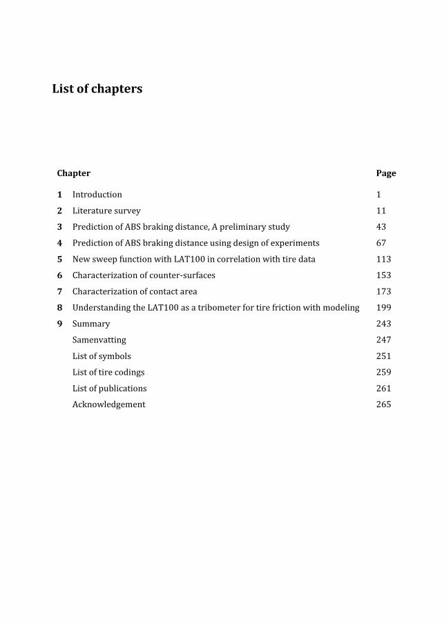
List of chapters
Chapter Page
1 Introduction 1
2 Literature survey 11
3 Prediction of ABS braking distance, A preliminary study 43
4 Prediction of ABS braking distance using design of experiments 67
5 New sweep function with LAT100 in correlation with tire data 113
6 Characterization of counter-surfaces 153
7 Characterization of contact area 173
8 Understanding the LAT100 as a tribometer for tire friction with modeling 199
9 Summary 243
Samenvatting 247
List of symbols 251
List of tire codings 259
List of publications 261
Acknowledgement 265
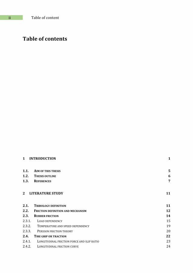
ii Table of content
Table of contents
1 INTRODUCTION 1
1.1. AIM OF THIS THESIS 5
1.2. THESIS OUTLINE 6
1.3. REFERENCES 7
2 LITERATURE STUDY 11
2.1. TRIBOLOGY DEFINITION 11
2.2. FRICTION DEFINITION AND MECHANISM 12
2.3. RUBBER FRICTION 14
2.3.1. LOAD DEPENDENCY 15
2.3.2. TEMPERATURE AND SPEED DEPENDENCY 19
2.3.3. PERSSON FRICTION THEORY 20
2.4. TIRE GRIP OR TRACTION 22
2.4.1. LONGITUDINAL FRICTION FORCE AND SLIP RATIO 23
2.4.2. LONGITUDINAL FRICTION CURVE 24
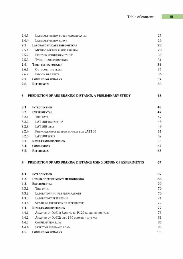
iii Table of content
2.4.3. LATERAL FRICTION FORCE AND SLIP ANGLE 25
2.4.4. LATERAL FRICTION CURVE 26
2.5. LABORATORY SCALE TRIBOMETERS 28
2.5.1. METHODS OF MEASURING FRICTION 28
2.5.2. FRICTION STANDARD METHODS 30
2.5.3. TYPES OF ABRASION TESTS 31
2.6. TIRE TESTING FOR GRIP 34
2.6.1. OUTDOOR TIRE TESTS 35
2.6.2. INDOOR TIRE TESTS 36
2.7. CONCLUDING REMARKS 37
2.8. REFERENCES 38
3 PREDICTION OF ABS BRAKING DISTANCE, A PRELIMINARY STUDY 43
3.1. INTRODUCTION 43
3.2. EXPERIMENTAL 47
3.2.1. TIRE DATA 47
3.2.2. LAT100 TEST SET-UP 48
3.2.3. LAT100 DISCS 49
3.2.4. PREPARATION OF RUBBER SAMPLES FOR LAT100 51
3.2.5. LAT100 TESTS 52
3.3. RESULTS AND DISCUSSION 53
3.4. CONCLUSIONS 62
3.5. REFERENCES 63
4 PREDICTION OF ABS BRAKING DISTANCE USING DESIGN OF EXPERIMENTS 67
4.1. INTRODUCTION 67
4.2. DESIGN OF EXPERIMENTS METHODOLOGY 68
4.3. EXPERIMENTAL 70
4.3.1. TIRE DATA 70
4.3.2. LABORATORY SAMPLE PREPARATIONS 70
4.3.3. LABORATORY TEST SET-UP 71
4.3.4. SET-UP OF THE DESIGN OF EXPERIMENTS 72
4.4. RESULTS AND DISCUSSION 77
4.4.1. ANALYSIS OF DOE 1: SANDPAPER P120 COUNTER-SURFACE 78
4.4.2. ANALYSIS OF DOE 2: DISC 180 COUNTER-SURFACE 81
4.4.3. CONFIRMATION RUNS 88
4.4.4. EFFECT OF SPEED AND LOAD 90
4.5. CONCLUDING REMARKS 95
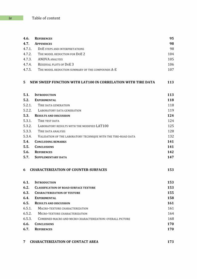
iv Table of content
4.6. REFERENCES 95
4.7. APPENDICES 98
4.7.1. DOE STEPS AND INTERPRETATIONS 98
4.7.2. THE MODEL REDUCTION FOR DOE 2 104
4.7.3. ANOVA ANALYSIS 105
4.7.4. RESIDUAL PLOTS OF DOE 3 106
4.7.5. THE MODEL REDUCTION SUMMARY OF THE COMPOUNDS A-E 107
5 NEW SWEEP FUNCTION WITH LAT100 IN CORRELATION WITH TIRE DATA 113
5.1. INTRODUCTION 113
5.2. EXPERIMENTAL 118
5.2.1. TIRE DATA GENERATION 118
5.2.2. LABORATORY DATA GENERATION 119
5.3. RESULTS AND DISCUSSION 124
5.3.1. TIRE TEST DATA 124
5.3.2. LABORATORY RESULTS WITH THE MODIFIED LAT100 125
5.3.3. TIRE DATA ANALYSIS 128
5.3.4. VALIDATION OF THE LABORATORY TECHNIQUE WITH THE TIRE-ROAD DATA 132
5.4. CONCLUDING REMARKS 141
5.5. CONCLUSIONS 141
5.6. REFERENCES 142
5.7. SUPPLEMENTARY DATA 147
6 CHARACTERIZATION OF COUNTER-SURFACES 153
6.1. INTRODUCTION 153
6.2. CLASSIFICATION OF ROAD SURFACE TEXTURE 153
6.3. CHARACTERIZATION OF TEXTURE 155
6.4. EXPERIMENTAL 158
6.5. RESULTS AND DISCUSSION 161
6.5.1. MACRO-TEXTURE CHARACTERIZATION 161
6.5.2. MICRO-TEXTURE CHARACTERIZATION 164
6.5.3. COMBINED MACRO AND MICRO CHARACTERIZATION: OVERALL PICTURE 168
6.6. CONCLUSIONS 170
6.7. REFERENCES 170
7 CHARACTERIZATION OF CONTACT AREA 173
v Table of content
7.1. INTRODUCTION 173
7.2. BACKGROUND 174
7.3. EXPERIMENTAL 174
7.3.1. SAMPLE PREPARATIONS AND RUBBER PROPERTIES 174
7.3.2. MEASUREMENT CONDITIONS 176
7.3.3. THE MEASUREMENT METHOD 176
7.4. RESULTS AND DISCUSSIONS 179
7.4.1. EVALUATION METHOD 179
7.4.2. COMPARISON WITH THE REAL AREA OF CONTACT IN PERSSON THEORY 182
7.4.3. COMPARISON BETWEEN THE TIRES AND GROSCH TEST WHEELS IN PRESSURE HISTOGRAMS 191
7.4.4. EFFECT OF IN-RUBBER PROPERTIES AND SURFACE ROUGHNESS 192
7.5. SUMMARY AND CONCLUDING REMARKS 194
7.6. REFERENCES 195
8 UNDERSTANDING THE LAT100 AS A TRIBOMETER FOR TIRE FRICTION WITH
MODELING 199
8.1. LAT100 TEST SET-UP 200
8.1.1. THE LAT100 AS A ROLLING FRICTION TESTER 200
8.1.2. EFFECT OF DISC CURVATURE 201
8.1.3. WHEEL DEFLECTION 203
8.2. ROLLING FRICTION OF A TIRE 204
8.2.1. THE TIRE BRUSH MODEL 206
8.2.2. PURE LATERAL (SIDE) SLIP 210
8.2.3. PURE LONGITUDINAL SLIP 214
8.2.4. ACCURACY OF THE MODEL 215
8.3. IMPLEMENTATION OF THE BRUSH MODEL 215
8.3.1. MODEL INPUTS 215
8.3.2. MODEL OUTPUTS 218
8.3.3. POTENTIAL MODEL IMPROVEMENTS 222
8.3.4. ATTRIBUTION OF FRICTION COMPONENTS 223
8.3.5. COMPARISON OF Α AND Κ SWEEP TESTS 224
8.3.6. COMPARISON OF Α SWEEP TEST OF GROSCH WHEEL AND TIRE 229
8.4. CONCLUSIONS 235
8.5. REFERENCES 236
8.6. APPENDIX: TREAD COMPOUND CHARACTERIZATIONS 240
9 SUMMARY 243
SAMENVATTING 247

vi Table of content
LIST OF SYMBOLS 251
LIST OF TIRE CODINGS 259
LIST OF PUBLICATIONS 261
ACKNOWLEDGMENT 265
1 Introduction
The ingenious invention of the wheel had a major impact on human lives. It
tremendously improved the lifestyle of ancients because of the low resistance to motion
compared to dragging sleighs with high friction to the ground. This is due to a simple
physical fact that the relative speed of the wheel contact point to the ground is zero,
considering a planar movement of the wheel without slipping on a linear road. It is not
so long ago that tires with the current look came into use. The very first built cars had
wooden wheels covered with leather [1]. The abrasion resistance of these tires was
poor and they lasted for just a limited amount of kilometers. Probably excellent rolling
resistance and skid resistance of these tires were not so much an issue on the dirt/mud
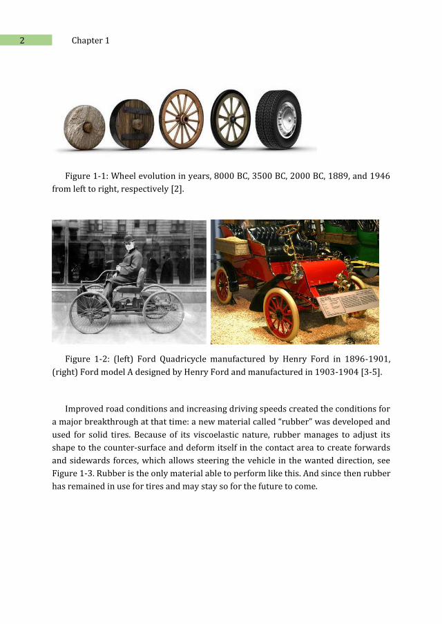
roads of those times. Figure 1-1 shows the wheel revolution over the years and Figure
1-2 the first automobiles designed by Henry Ford.
2 Chapter 1
Figure 1-1: Wheel evolution in years, 8000 BC, 3500 BC, 2000 BC, 1889, and 1946
from left to right, respectively [2].
Figure 1-2: (left) Ford Quadricycle manufactured by Henry Ford in 1896-1901,
(right) Ford model A designed by Henry Ford and manufactured in 1903-1904 [3-5].
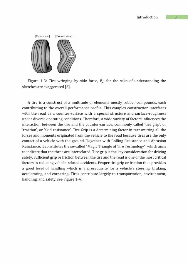
Improved road conditions and increasing driving speeds created the conditions for
a major breakthrough at that time: a new material called “rubber” was developed and
used for solid tires. Because of its viscoelastic nature, rubber manages to adjust its
shape to the counter-surface and deform itself in the contact area to create forwards
and sidewards forces, which allows steering the vehicle in the wanted direction, see
Figure 1-3. Rubber is the only material able to perform like this. And since then rubber
has remained in use for tires and may stay so for the future to come.
3 Introduction
Figure 1-3: Tire wringing by side force, 𝐹𝑦; for the sake of understanding the
sketches are exaggerated [6].
A tire is a construct of a multitude of elements mostly rubber compounds, each
contributing to the overall performance profile. This complex construction interfaces
with the road as a counter-surface with a special structure and surface-roughness
under diverse operating conditions. Therefore, a wide variety of factors influences the
interaction between the tire and the counter-surface, commonly called ‘tire grip’, or
‘traction’, or ‘skid resistance’. Tire Grip is a determining factor in transmitting all the
forces and moments originated from the vehicle to the road because tires are the only
contact of a vehicle with the ground. Together with Rolling Resistance and Abrasion
Resistance, it constitutes the so-called “Magic Triangle of Tire Technology”, which aims
to indicate that the three are interrelated. Tire grip is the key consideration for driving
safety. Sufficient grip or friction between the tire and the road is one of the most critical
factors in reducing vehicle-related accidents. Proper tire grip or friction thus provides
a good level of handling which is a prerequisite for a vehicle’s steering, braking,
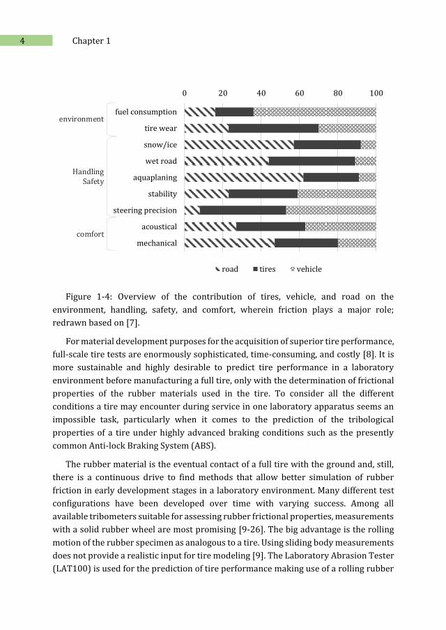
accelerating, and cornering. Tires contribute largely to transportation, environment,
handling, and safety, see Figure 1-4.
4 Chapter 1
environment
HandlingSafety
comfort
0 20 40 60 80 100
fuel consumption
tire wear
snow/ice
wet road
aquaplaning
stability
steering precision
acoustical
mechanical
road tires vehicle
Figure 1-4: Overview of the contribution of tires, vehicle, and road on the
environment, handling, safety, and comfort, wherein friction plays a major role;
redrawn based on [7].
For material development purposes for the acquisition of superior tire performance,
full-scale tire tests are enormously sophisticated, time-consuming, and costly [8]. It is
more sustainable and highly desirable to predict tire performance in a laboratory
environment before manufacturing a full tire, only with the determination of frictional
properties of the rubber materials used in the tire. To consider all the different
conditions a tire may encounter during service in one laboratory apparatus seems an
impossible task, particularly when it comes to the prediction of the tribological
properties of a tire under highly advanced braking conditions such as the presently
common Anti-lock Braking System (ABS).
The rubber material is the eventual contact of a full tire with the ground and, still,
there is a continuous drive to find methods that allow better simulation of rubber
friction in early development stages in a laboratory environment. Many different test
configurations have been developed over time with varying success. Among all
available tribometers suitable for assessing rubber frictional properties, measurements
with a solid rubber wheel are most promising [9-26]. The big advantage is the rolling
motion of the rubber specimen as analogous to a tire. Using sliding body measurements
does not provide a realistic input for tire modeling [9]. The Laboratory Abrasion Tester
(LAT100) is used for the prediction of tire performance making use of a rolling rubber
5 Introduction
wheel known as the Grosch wheel, named after the original developer of the equipment:
Dr. Karl Alfred Grosch. The equipment is designed to simulate a wide range of tire
service conditions to measure abrasion loss and the frictional forces as a function of
various tire-road service conditions such as slip, load, and speed on different counter-
surfaces. Furthermore, the evaluated friction properties of the tire tread compounds
can thus be employed as input data for models and simulations for tire characteristics.
The quality and parametrization of the tire models and simulations strongly depend on
the correct input of rubber friction properties [9, 10, 12, 13, 25].
The LAT100 is a laboratory apparatus. The first purpose for which it was developed
was to measure rubber abrasion; therefore, its designation is “Laboratory Abrasion
Tester”. Gradually it was realized that the apparatus could also be used as a tribometer
to characterize friction properties. Consequently, there is a steadily increasing interest
to develop this concept further, which was the main purpose of the research presented
in this thesis.
1.1. Aim of this thesis
In previous studies by Grosch and Heinz [19], it has been demonstrated that the wet
grip, abrasion, and rolling resistance can be characterized by the LAT100, provided the
right conditions for testing are employed. The question has been raised whether testing
of various tire compounds under dry conditions could also be employed to predict tire
frictional properties in longitudinal as well as lateral conditions. This was taken as the
original objective of the present work, to include different tire tread formulations, as
well as different counter surfaces. The results of LAT100 tests were to be correlated
with actual tire tests on standardized roads, under ABS-conditions, and different test
modalities for the tires on the real roads.
Later on in the project, a new test configuration was designed and further developed
by introducing a dynamic interface to the LAT100. This was set as an additional
objective to understand the machine as a tribometer because it already provided tire
operating conditions with a wheel-shaped specimen. This similarity provides a high
potential for mimicking tire grip in a laboratory environment. Therefore, to predict tire
grip with the evaluation of rubber friction using LAT100, the thesis is structured as
explained in the next section. Therewith, two main characteristic friction components:
adhesion between the rubber and the counter-surface and deformation related to the
viscoelastic nature of the rubber, can be attributed to the tire or wheel specimen rolling
friction.
6 Chapter 1
The development outlined in the present thesis was based on real tire testing in
comparison with LAT100 experiments. In the course of the project, three types of real
tire tests were executed with different tire sizes and tread compositions. The tire tests
were to evaluate dry grip in three different test modalities: ABS braking distance, the
lateral and longitudinal test modalities so-called α-sweep, and κ-sweep, respectively.
The LAT100 measurements were to be performed in two test modes, locked wheel as a
sliding friction tester and sweep test with a rolling wheel. The actual tire data and
compound formulations were considered proprietary by Apollo Tyres. However, the
point was to compare and rank the tire data and laboratory results to be similar. Thus,
the ratings provided by normalized tire data are still comparable with the absolute
values and the results of correlations remain the same. Therefore, the chapters were
designed as stand-alone texts based on the wide range of tire data, types, and test
modalities.
1.2. Thesis outline
The outline of the present thesis is built on six main pillars, in which a strong cross-
disciplinary approach for the research is being employed. Chapter 2 is a survey of the
literature on friction and tire grip concepts and a short introduction to the Persson’s
contact theory. Also, the available laboratory tribometers and tire testing methods are
introduced and compared. Chapter 3 presents mainly preliminary studies on the
LAT100 to discover the apparatus possibilities and limitations to be exploited for dry
tire friction evaluations. In this chapter, the frictional forces of four different tread
compounds are determined by collecting individual measurement points at defined test
conditions. The results are correlated with tire ABS braking ratings. In Chapter 4, the
LAT100 is further employed as a sliding friction tester with blocked wheels for the
prediction of dry ABS braking distance by deriving a mathematical model using Design
of Experiments for the input factors. The mutual interactions of factors on tire friction
are quantified, where the effects of factors alone are not adequate. In Chapter 5, the
LAT100 is re-designed and a new dynamic interface is developed by which it is possible
to perform and mimic tire test modalities in a laboratory environment for a small
rubber wheel. Comprehensive tire testing is performed to provide sufficient data for
the method validation. Strong correlations are obtained between LAT100 results and
the lateral tire test modality called α-sweep, but not for the longitudinal or so-called κ-
sweep. In Chapters 6 and 7, counter-surface and contact area are analyzed using power
spectral density and Persson’s friction theory to obtain a better explanation for the
acquired correlations. And finally, Chapter 8 is dedicated to understanding the
dynamics and physics of a rolling rubber wheel on a counter-surface disc of the LAT100
7 Introduction
test set-up utilizing the renowned physical “brush model” for tires. Therewith, the
behavior of the rolling wheel in lateral and longitudinal movements is investigated in
comparison to a real tire. A better comprehension of the intricate differences between
the 𝛼 and 𝜅 sweep test configurations is obtained in association with rubber friction
components.
1.3. References
1. Type of the tire for the very first cars, personal communication with Prof. Dr. Jacques Noordermeer, based on his visit to Henry Ford Museum, Dearborn, Detroit, USA, 2020.
2. Greatest invention: wheel evolution, in Stories of science, Date of access: 2020 July; Available from https://www.quora.com/q/stories-of-science/Greatest-invention.
3. A visit to the Henry Ford Museum, in MODEL T FORD FIX, Date of access: 2020 July; Available from https://modeltfordfix.com/a-visit-to-the-henry-ford-museum/.
4. Ford Quadricycle, in the pioneering automobile, Date of access: 2020 July; Available from https://en.wikipedia.org/wiki/Ford_Quadricycle.
5. Ford Model A (1903–04), in From Wikipedia, the free encyclopedia, Date of access: 2020 July; Available from https://en.wikipedia.org/wiki/Ford_Model_A_(1903-04).
6. Kabe, K. and N. Miyashita, A study of the cornering power by use of the analytical tyre model. Vehicle System Dynamics, 2005. 43(sup1): p. 113-122.
7. Salminen, H., Parametrizing tyre wear using a brush tyre model. 2014, Royal Institute of Technology, Stockholm, Sweden.
8. Salehi, M., J.W.M. Noordermeer, L.A.E.M. Reuvekamp, T. Tolpekina, and A. Blume, A New Horizon for Evaluating Tire Grip Within a Laboratory Environment. Tribology Letters, 2020. 68(1): p. 37.
9. Riehm, P., H.-J. Unrau, and F. Gauterin, A model based method to determine rubber friction data based on rubber sample measurements. Tribology International, 2018. 127: p. 37-46.
10. Gutzeit, F. and M. Kröger, Experimental and Theoretical Investigations on the Dynamic Contact Behavior of Rolling Rubber Wheels, in Book 'Elastomere Friction: Theory, Experiment and Simulation', D. Besdo, B. Heimann, M. Klüppel, M. Kröger, P. Wriggers, and U. Nackenhorst, Editors. 2010, Springer Berlin Heidelberg: Berlin, Heidelberg. p. 221-249.
8 Chapter 1
11. Steen, R.v.d., I. Lopez, and H. Nijmeijer, Experimental and numerical study of friction and .giffness characteristics of small rolling tires. Tire Science and Technology, 2011. 39(1): p. 5-19.
12. Dorsch, V., A. Becker, and L. Vossen, Enhanced rubber friction model for finite element simulations of rolling tyres. Plastics, Rubber and Composites, 2002. 31(10): p. 458-464.
13. Bouzid, N., B. Heimann, and A. Trabelsi, Empirical friction coefficient modeling for the Grosch-wheel-road system, in VDI Berichte. 2005. p. 291-307.
14. Nguyen, V.H., D. Zheng, F. Schmerwitz, and P. Wriggers, An advanced abrasion model for tire wear. Wear, 2018. 396-397: p. 75-85.
15. Wu, J., C. Zhang, Y. Wang, and B. Su, Wear Predicted Model of Tread Rubber Based on Experimental and Numerical Method. Experimental Techniques, 2018. 42(2): p. 191-198.
16. Grosch, K.A., Correlation Between Road Wear of Tires and Computer Road Wear Simulation Using Laboratory Abrasion Data. Rubber Chemistry and Technology, 2004. 77(5): p. 791-814.
17. Grosch, K.A., Goodyear Medalist Lecture. Rubber Friction and its Relation to Tire Traction. Rubber Chemistry and Technology, 2007. 80(3): p. 379-411.
18. Grosch, K.A., Rubber Abrasion and Tire Wear. Rubber Chemistry and Technology, 2008. 81(3): p. 470-505.
19. Heinz, M. and K.A. Grosch, A Laboratory Method to Comprehensively Evaluate Abrasion, Traction and Rolling Resistance of Tire Tread Compounds. Rubber Chemistry and Technology, 2007. 80(4): p. 580-607.
20. Grosch, K.A., A new way to evaluate traction-and wear properties of tire tread compounds, in Rubber Division, American Chemical Society. 1997: Cleveland, Ohio.
21. Heinz, M., A laboratory abrasion testing method for use in the development of filler systems. Technical report rubber reinforcement systems, 2015, Evonik Industries GmbH, Essen, Germany.
22. Heinz, M., A Universal Method to Predict Wet Traction Behaviour of Tyre Tread Compounds in the Laboratory. Journal of Rubber Research, 2010. 13(2): p. 91-102.
23. Salehi, M., LAT100, Prediction of tire dry grip. 2017, University of Twente: Enschede: Ipskamp Printing.
24. Salehi, M., J.W.M. Noordermeer, L.A.E.M. Reuvekamp, W.K. Dierkes, and A. Blume, Measuring rubber friction using a Laboratory Abrasion Tester (LAT100) to predict car tire dry ABS braking. Tribology International, 2019. 131: p. 191-199.

9 Introduction
25. Bouzid, N. and B. Heimann, Micro Texture Characterization and Prognosis of the Maximum Traction between Grosch Wheel and Asphalt Surfaces under Wet Conditions, in Book 'Elastomere Friction: Theory, Experiment and Simulation', D. Besdo, B. Heimann, M. Klüppel, M. Kröger, P. Wriggers, and U. Nackenhorst, Editors. 2010, Springer Berlin Heidelberg: Berlin, Heidelberg. p. 201-220.
26. RTM Friction and Lambourn Abrasion Testers in Physical testing equipment (for rubber and plastics), Date of access: 2020 July; Available from https://www.ueshima-seisakusho.co.jp/product/product_gum/gum_ichiran_en.html

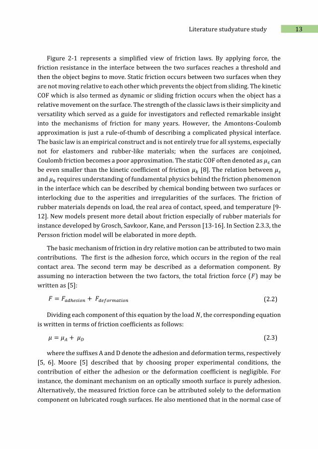
2 Literature study
2.1. Tribology definition
Tribology is the “λογοσ” (logos) or science of “τρίβω” (tribo) or slide/rub. An exact
translation defines tribology as the study of sliding or rubbing. The modern and
broadest meaning is the study of friction, lubrication, and wear [1].
Tribology of elastomers can be defined as "the science and technology for
investigating the regularities of the emergence, change and development of various
tribological phenomena in rubber and rubber-like materials and their tribological
applications". Tribological phenomena concern the combination of interactions
between surfaces in relative motion and the environment, including all of the following
interactions: mechanical, physical, chemical, thermo-chemical, mechano-chemical, and
tribo-chemical [2].
12 Chapter 2
2.2. Friction definition and mechanism
Friction can be simply described as: “We need to overcome friction to move one
material against another, a common phenomenon in our everyday world. Nails hold
because of friction. We couldn't walk or even crawl without friction [3]’’.
Probably Leonardo da Vinci (1452-1519) was the first who developed the basic
concepts of friction and Amontons (1699) was inspired by his drawings and sketches.
“Amontons’ law” showed the proportionality between the frictional force and the
normal force [4]. A mathematical form of the friction law was described by Charles
Augustin Coulomb who conducted a set of experiments to analyze the magnitude of the
Coefficient Of Friction (COF) during sliding as follows:
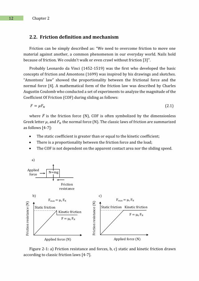
𝐹 = 𝜇𝐹𝑁 (2.1)
where 𝐹 is the friction force (N), COF is often symbolized by the dimensionless
Greek letter 𝜇, and 𝐹𝑁 the normal force (N). The classic laws of friction are summarized
as follows [4-7]:
The static coefficient is greater than or equal to the kinetic coefficient;
There is a proportionality between the friction force and the load;
The COF is not dependent on the apparent contact area nor the sliding speed.
Applied force
N=mg
Friction resistance
a)
Applied force (N)
Fric
tio
n re
sist
ance
(N
)
Kinetic friction
Fmax = µs FN
F = µk FN
Static friction
Applied force (N)
Fric
tio
n re
sist
ance
(N
)
Kinetic friction
Fmax = µs FN
F = µk FN
Static friction
b) c)
Figure 2-1: a) Friction resistance and forces, b, c) static and kinetic friction drawn
according to classic friction laws [4-7].
13 Literature studyature study
Figure 2-1 represents a simplified view of friction laws. By applying force, the
friction resistance in the interface between the two surfaces reaches a threshold and
then the object begins to move. Static friction occurs between two surfaces when they
are not moving relative to each other which prevents the object from sliding. The kinetic
COF which is also termed as dynamic or sliding friction occurs when the object has a
relative movement on the surface. The strength of the classic laws is their simplicity and
versatility which served as a guide for investigators and reflected remarkable insight
into the mechanisms of friction for many years. However, the Amontons-Coulomb
approximation is just a rule-of-thumb of describing a complicated physical interface.
The basic law is an empirical construct and is not entirely true for all systems, especially
not for elastomers and rubber-like materials; when the surfaces are conjoined,
Coulomb friction becomes a poor approximation. The static COF often denoted as 𝜇𝑠 can
be even smaller than the kinetic coefficient of friction 𝜇𝑘 [8]. The relation between 𝜇𝑠
and 𝜇𝑘 requires understanding of fundamental physics behind the friction phenomenon
in the interface which can be described by chemical bonding between two surfaces or
interlocking due to the asperities and irregularities of the surfaces. The friction of
rubber materials depends on load, the real area of contact, speed, and temperature [9-
12]. New models present more detail about friction especially of rubber materials for
instance developed by Grosch, Savkoor, Kane, and Persson [13-16]. In Section 2.3.3, the
Persson friction model will be elaborated in more depth.
The basic mechanism of friction in dry relative motion can be attributed to two main
contributions. The first is the adhesion force, which occurs in the region of the real
contact area. The second term may be described as a deformation component. By
assuming no interaction between the two factors, the total friction force (𝐹) may be
written as [5]:
𝐹 = 𝐹𝑎𝑑ℎ𝑒𝑠𝑖𝑜𝑛 + 𝐹𝑑𝑒𝑓𝑜𝑟𝑚𝑎𝑡𝑖𝑜𝑛 (2.2)
Dividing each component of this equation by the load 𝑁, the corresponding equation
is written in terms of friction coefficients as follows:
𝜇 = 𝜇𝐴 + 𝜇𝐷 (2.3)
where the suffixes A and D denote the adhesion and deformation terms, respectively
[5, 6]. Moore [5] described that by choosing proper experimental conditions, the
contribution of either the adhesion or the deformation coefficient is negligible. For
instance, the dominant mechanism on an optically smooth surface is purely adhesion.
Alternatively, the measured friction force can be attributed solely to the deformation
component on lubricated rough surfaces. He also mentioned that in the normal case of

14 Chapter 2
dry sliding between rough surfaces, the coefficient of adhesional friction is generally at
least twice as high as the deformation contribution [5]. However, the contribution of
the attributed friction mechanism is still debatable.
2.3. Rubber friction
In the contact area between an elastomer and a rough surface in relative motion, the
adhesion component of the friction force is referred to as molecular interaction
between the rubber and the substrate. The deformation term is due to a delayed
recovery of the elastomer after indentation by a particular asperity, which is generally
termed the hysteresis component of friction [5].
Figure 2-2: Principal components of elastomeric friction on a dry surface [5].
Figure 2-2 shows how the total friction force develops in sliding over a single
asperity, separated into an adhesion and a deformation part [5]. Therefore:
𝐹𝑑𝑒𝑓𝑜𝑟𝑚𝑎𝑡𝑖𝑜𝑛 = 𝐹ℎ𝑦𝑠𝑡𝑒𝑟𝑒𝑠𝑖𝑠 (2.4)
𝐹 = 𝐹𝑎𝑑ℎ𝑒𝑠𝑖𝑜𝑛 + 𝐹ℎ𝑦𝑠𝑡𝑒𝑟𝑒𝑠𝑖𝑠 (2.5)
𝜇 = 𝜇𝐴 + 𝜇𝐻 (2.6)
where 𝜇𝐻 designates the term due to hysteresis. Moore [5] also described the
adhesion as a surface effect, whereas hysteresis is a bulk phenomenon that depends on
the viscoelastic properties of the elastomer.
15 Literature studyature study
A disruptive stick-slip process at a molecular level is fundamentally responsible for
adhesion and several theories exist to explain the phenomenon. However, both
adhesion and hysteresis can be attributed to the viscoelastic properties of rubber at the
macroscopic level [5].
2.3.1. Load dependency
In earlier work, Schallamach [11] presented some experimental evidence that the
load dependency of rubber friction can be explained by the proportionality of the
frictional force to the true area of contact between rubber and track. He deduced the
real area of contact and contact pressure by considering elastic deformation of the
rubber surface on spherical asperities using a simple model. For soft rubber on smooth
surfaces, the real or actual contact area 𝐴 (m2) increases with the nominal or apparent
pressure 𝑃 (Pa) as follows:
𝐴 ∝ 𝑃2/3 (2.7)
This outcome is in agreement with a theoretical expression derived by Hertz from
the classical elasticity theory for spherical contacts, which leads to the following
relation for COF:
𝜇 ∝ 𝑃−1/3 (2.8)
Schallamach carried out extensive experiments with several hard tire tread
compounds on surfaces with various asperity shapes and coarseness and showed that
the exponent in Eq. (2.8) changes to the value -1/9; therefore the load dependency may
be neglected in the case of rough surfaces [11, 13]. He explained that the true area of
contact and frictional force under low load is smaller since the rubber is in contact with
the “tallest asperities” and the “smaller asperities” will gradually come into contact with
the counter-surface as the load increases [11].
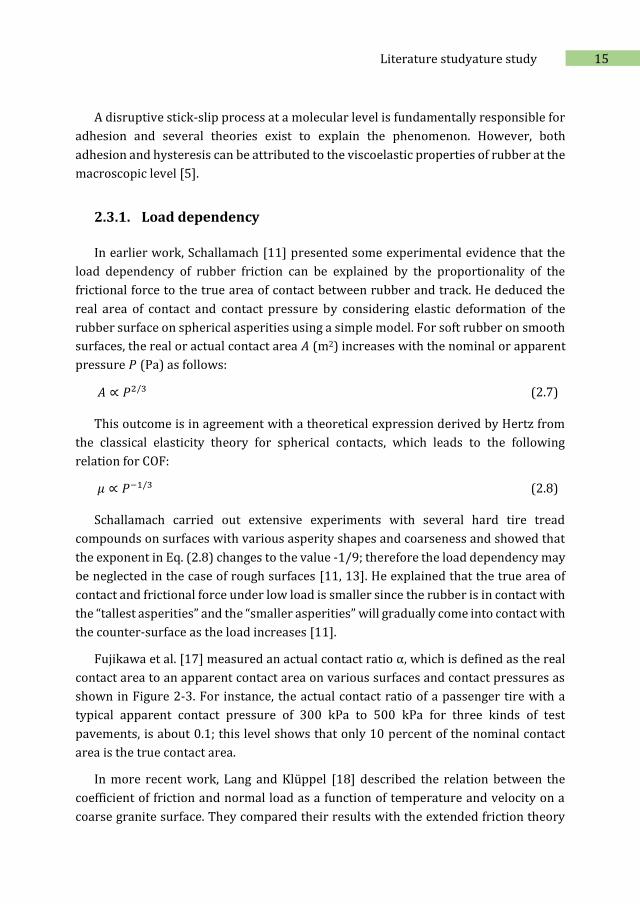
Fujikawa et al. [17] measured an actual contact ratio α, which is defined as the real
contact area to an apparent contact area on various surfaces and contact pressures as
shown in Figure 2-3. For instance, the actual contact ratio of a passenger tire with a
typical apparent contact pressure of 300 kPa to 500 kPa for three kinds of test
pavements, is about 0.1; this level shows that only 10 percent of the nominal contact
area is the true contact area.
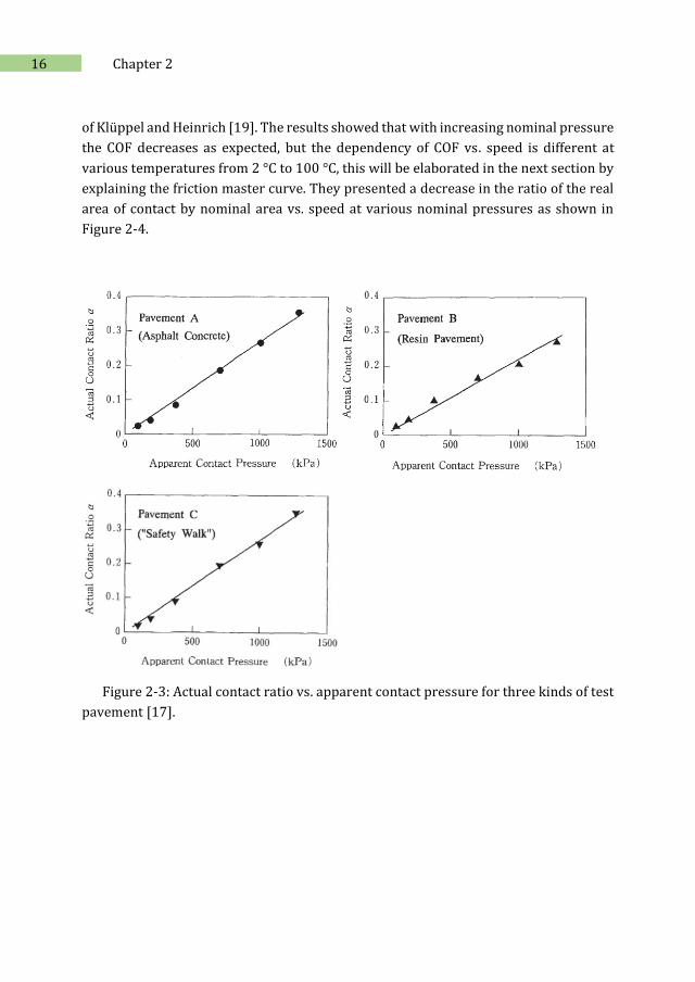
In more recent work, Lang and Klüppel [18] described the relation between the
coefficient of friction and normal load as a function of temperature and velocity on a
coarse granite surface. They compared their results with the extended friction theory
16 Chapter 2
of Klüppel and Heinrich [19]. The results showed that with increasing nominal pressure
the COF decreases as expected, but the dependency of COF vs. speed is different at
various temperatures from 2 °C to 100 °C, this will be elaborated in the next section by
explaining the friction master curve. They presented a decrease in the ratio of the real
area of contact by nominal area vs. speed at various nominal pressures as shown in
Figure 2-4.
Figure 2-3: Actual contact ratio vs. apparent contact pressure for three kinds of test
pavement [17].
17 Literature studyature study
Figure 2-4: The real area of contact/nominal area (𝐴𝑐/𝐴0) vs. velocity v (m/s) at
various nominal pressure (bar) and 70 °C temperature, taken from ref. [18].
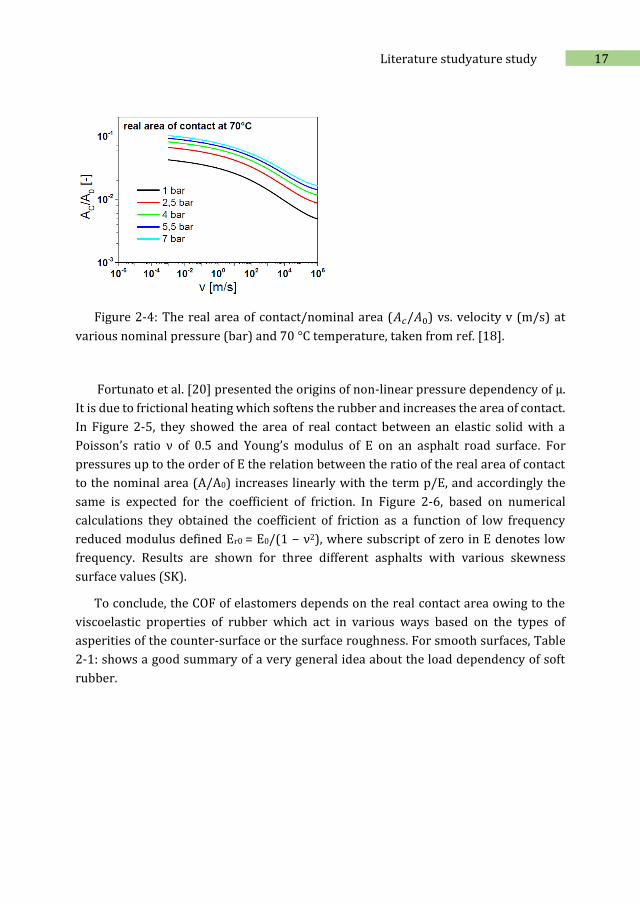
Fortunato et al. [20] presented the origins of non-linear pressure dependency of μ.
It is due to frictional heating which softens the rubber and increases the area of contact.
In Figure 2-5, they showed the area of real contact between an elastic solid with a
Poisson’s ratio ν of 0.5 and Young’s modulus of E on an asphalt road surface. For
pressures up to the order of E the relation between the ratio of the real area of contact
to the nominal area (A/A0) increases linearly with the term p/E, and accordingly the
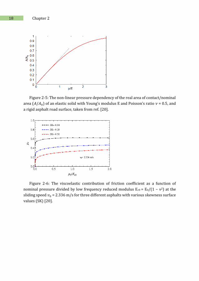
same is expected for the coefficient of friction. In Figure 2-6, based on numerical
calculations they obtained the coefficient of friction as a function of low frequency
reduced modulus defined Er0 = E0/(1 − ν2), where subscript of zero in E denotes low
frequency. Results are shown for three different asphalts with various skewness
surface values (SK).
To conclude, the COF of elastomers depends on the real contact area owing to the
viscoelastic properties of rubber which act in various ways based on the types of
asperities of the counter-surface or the surface roughness. For smooth surfaces, Table
2-1: shows a good summary of a very general idea about the load dependency of soft
rubber.
18 Chapter 2
Figure 2-5: The non-linear pressure dependency of the real area of contact/nominal
area (𝐴/𝐴0) of an elastic solid with Young’s modulus E and Poisson’s ratio 𝜈 = 0.5, and
a rigid asphalt road surface, taken from ref. [20].
Figure 2-6: The viscoelastic contribution of friction coefficient as a function of
nominal pressure divided by low frequency reduced modulus Er0 = E0/(1 − ν2) at the
sliding speed 𝑣0 = 2.336 m/s for three different asphalts with various skewness surface
values (SK) [20].
19 Literature studyature study
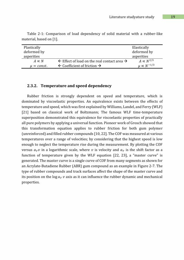
Table 2-1: Comparison of load dependency of solid material with a rubber-like
material, based on [1].
Plastically deformed by asperities
Elastically deformed by asperities
𝐴 ∝ 𝑁 Effect of load on the real contact area 𝐴 ∝ 𝑁2/3 𝜇 = 𝑐𝑜𝑛𝑠𝑡. Coefficient of friction 𝜇 ∝ 𝑁−1/3
2.3.2. Temperature and speed dependency
Rubber friction is strongly dependent on speed and temperature, which is
dominated by viscoelastic properties. An equivalence exists between the effects of
temperature and speed, which was first explained by Williams, Landel, and Ferry (WLF)
[21] based on classical work of Boltzmann; The famous WLF time-temperature
superposition demonstrated this equivalence for viscoelastic properties of practically
all pure polymers by applying a universal function. Pioneer work of Grosch showed that
this transformation equation applies to rubber friction for both gum polymer
(unreinforced) and filled rubber compounds [10, 22]. The COF was measured at various
temperatures over a range of velocities; by considering that the highest speed is low
enough to neglect the temperature rise during the measurement. By plotting the COF
versus 𝑎𝑇𝑣 in a logarithmic scale, where 𝑣 is velocity and 𝑎𝑇 is the shift factor as a
function of temperature given by the WLF equation [22, 23], a “master curve” is
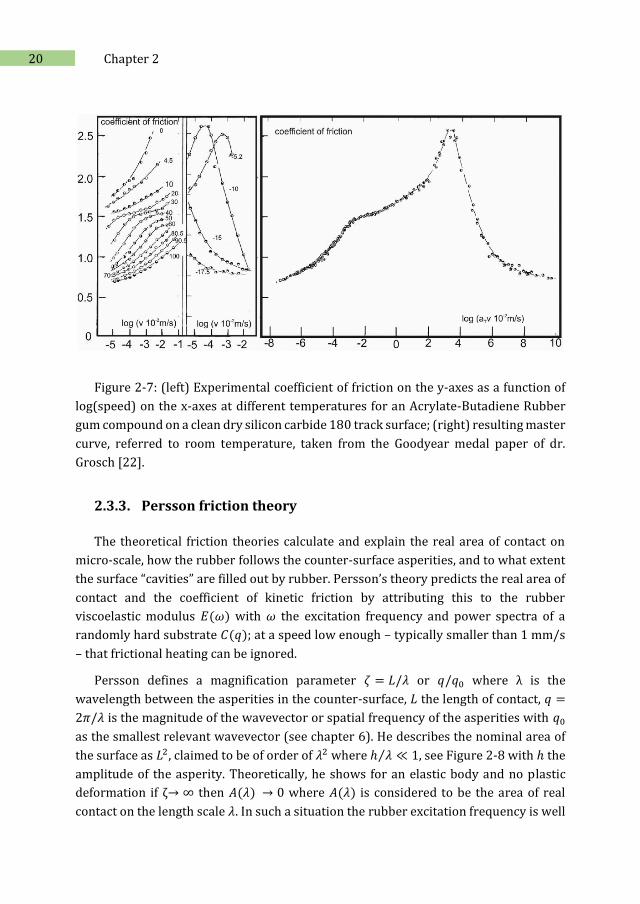
generated. The master curve is a single curve of COF from many segments as shown for
an Acrylate-Butadiene Rubber (ABR) gum compound as an example in Figure 2-7. The
type of rubber compounds and track surfaces affect the shape of the master curve and
its position on the log 𝑎𝑇 𝑣 axis as it can influence the rubber dynamic and mechanical
properties.
20 Chapter 2
Figure 2-7: (left) Experimental coefficient of friction on the y-axes as a function of
log(speed) on the x-axes at different temperatures for an Acrylate-Butadiene Rubber
gum compound on a clean dry silicon carbide 180 track surface; (right) resulting master
curve, referred to room temperature, taken from the Goodyear medal paper of dr.
Grosch [22].
2.3.3. Persson friction theory
The theoretical friction theories calculate and explain the real area of contact on
micro-scale, how the rubber follows the counter-surface asperities, and to what extent
the surface “cavities” are filled out by rubber. Persson’s theory predicts the real area of
contact and the coefficient of kinetic friction by attributing this to the rubber
viscoelastic modulus 𝐸(𝜔) with 𝜔 the excitation frequency and power spectra of a
randomly hard substrate 𝐶(𝑞); at a speed low enough – typically smaller than 1 mm/s
– that frictional heating can be ignored.
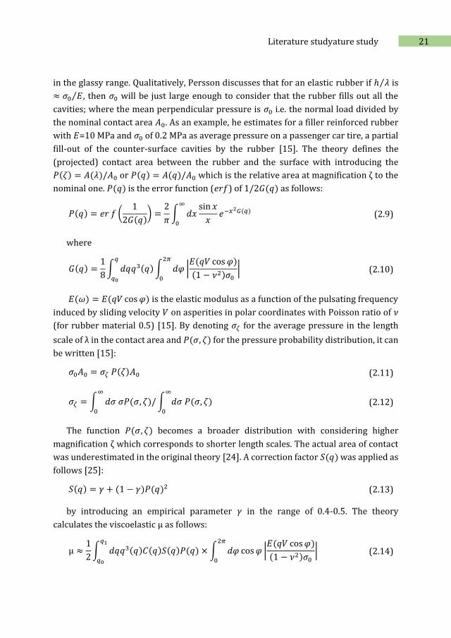
Persson defines a magnification parameter 휁 = 𝐿/𝜆 or 𝑞/𝑞0 where λ is the
wavelength between the asperities in the counter-surface, 𝐿 the length of contact, 𝑞 =
2𝜋/𝜆 is the magnitude of the wavevector or spatial frequency of the asperities with 𝑞0
as the smallest relevant wavevector (see chapter 6). He describes the nominal area of
the surface as 𝐿2, claimed to be of order of 𝜆2 where ℎ 𝜆 ≪ 1⁄ , see Figure 2-8 with ℎ the
amplitude of the asperity. Theoretically, he shows for an elastic body and no plastic
deformation if ζ→ ∞ then 𝐴(𝜆) → 0 where 𝐴(𝜆) is considered to be the area of real
contact on the length scale 𝜆. In such a situation the rubber excitation frequency is well
21 Literature studyature study
in the glassy range. Qualitatively, Persson discusses that for an elastic rubber if ℎ 𝜆⁄ is
≈ 𝜎0 𝐸⁄ , then 𝜎0 will be just large enough to consider that the rubber fills out all the
cavities; where the mean perpendicular pressure is 𝜎0 i.e. the normal load divided by
the nominal contact area 𝐴0. As an example, he estimates for a filler reinforced rubber
with 𝐸=10 MPa and 𝜎0 of 0.2 MPa as average pressure on a passenger car tire, a partial
fill-out of the counter-surface cavities by the rubber [15]. The theory defines the
(projected) contact area between the rubber and the surface with introducing the
𝑃(휁) = 𝐴(𝜆)/𝐴0 or 𝑃(𝑞) = 𝐴(𝑞)/𝐴0 which is the relative area at magnification ζ to the
nominal one. 𝑃(𝑞) is the error function (𝑒𝑟𝑓) of 1/2𝐺(𝑞) as follows:
𝑃(𝑞) = 𝑒𝑟 𝑓 (1
2𝐺(𝑞)) =
2
𝜋∫ 𝑑𝑥
sin 𝑥
𝑥𝑒−𝑥2𝐺(𝑞)
∞
0
(2.9)
where
𝐺(𝑞) =1
8∫ 𝑑𝑞𝑞3(𝑞) ∫ 𝑑𝜑 |
𝐸(𝑞𝑉 cos 𝜑)
(1 − 𝜈2)𝜎0
|2𝜋
0
𝑞
𝑞0
(2.10)
𝐸(𝜔) = 𝐸(𝑞𝑉 cos 𝜑) is the elastic modulus as a function of the pulsating frequency
induced by sliding velocity 𝑉 on asperities in polar coordinates with Poisson ratio of 𝜈
(for rubber material 0.5) [15]. By denoting 𝜎𝜁 for the average pressure in the length
scale of λ in the contact area and 𝑃(𝜎, 휁) for the pressure probability distribution, it can
be written [15]:
𝜎0𝐴0 = 𝜎𝜁 𝑃(휁)𝐴0 (2.11)
𝜎𝜁 = ∫ 𝑑𝜎 𝜎𝑃(𝜎, 휁)/ ∫ 𝑑𝜎 𝑃(𝜎, 휁)∞
0
∞
0
(2.12)
The function 𝑃(𝜎, 휁) becomes a broader distribution with considering higher
magnification ζ which corresponds to shorter length scales. The actual area of contact
was underestimated in the original theory [24]. A correction factor 𝑆(𝑞) was applied as
follows [25]:
𝑆(𝑞) = 𝛾 + (1 − 𝛾)𝑃(𝑞)2 (2.13)
by introducing an empirical parameter 𝛾 in the range of 0.4-0.5. The theory
calculates the viscoelastic μ as follows:
μ ≈1
2∫ 𝑑𝑞𝑞3(𝑞)𝐶(𝑞)𝑆(𝑞)𝑃(𝑞) × ∫ 𝑑𝜑 cos 𝜑 |
𝐸(𝑞𝑉 cos 𝜑)
(1 − 𝜈2)𝜎0
|2𝜋
0
𝑞1
𝑞0
(2.14)
22 Chapter 2
C(q) is the spectral density which represents the surface roughness, see Chapter 6.
Figure 2-8: A schematic view of the contact between the rubber and a hard substrate
at a different magnification of ζ according to Persson’s theory [15].
2.4. Tire grip or traction
Tires are built up of a multitude of different elements such as the tread, sidewall,
bead, shoulder, and various plies, which mostly comprise of rubber compounds; each
contributing to the overall tire performance profile. Tires support and transmit all types
of loads or forces such as vertical, longitudinal braking, driving, cornering forces, and
camber thrust. All forces are necessary for the directional control of the vehicle. The
best compromise in tire construction regarding carcass stiffness, tread pattern and
compound is to engineer the tire in such a way to meet the requirement of the “vehicle
suspension”.
Tire grip is a concept that describes the interaction between the tire and the road. A
tire with better grip provides e.g. a shorter stopping distance which is the distance that
the vehicle needs to come to a full stop. A proper tire grip provides a good level of
handling. To describe the tire grip of various tire constructions on the road with a
variety of surface textures, the tire-road interface has great importance. Some of the
important features of tire behavior at the interface are:
Normal force distribution
Actual slip velocity at various points in the contact area
Shape of the contact area
Deformation of the tread blocks at a range of speeds as a function of tire
geometry.
23 Literature studyature study
Tire grip or traction is generated by the frictional forces which are created by the
relative movement of these tread blocks on the ground. This relative movement is
known as the slippage which occurs only during cornering, braking, and accelerating
when the tread block has a displacement; otherwise, the relative speed of the tire in the
contact line would be zero. To achieve a better understanding of the tire grip, it is
essential to have a closer look into the tire forces acting during the braking
(accelerating) and cornering states and their corresponding slippage [26].
2.4.1. Longitudinal friction force and slip ratio
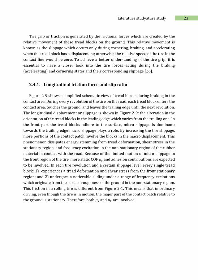
Figure 2-9 shows a simplified schematic view of tread blocks during braking in the
contact area. During every revolution of the tire on the road, each tread block enters the
contact area, touches the ground, and leaves the trailing edge until the next revolution.
The longitudinal displacement or slippage is shown in Figure 2-9: the alteration in the
orientation of the tread blocks in the leading edge which varies from the trailing one. In
the front part the tread blocks adhere to the surface, micro slippage is dominant;
towards the trailing edge macro slippage plays a role. By increasing the tire slippage,
more portions of the contact patch involve the blocks in the macro displacement. This
phenomenon dissipates energy stemming from tread deformation, shear stress in the
stationary region, and frequency excitation in the non-stationary region of the rubber
material in contact with the road. Because of the limited motion of micro-slippage in
the front region of the tire, more static COF 𝜇𝑠 and adhesion contributions are expected
to be involved. In each tire revolution and a certain slippage level, every single tread
block: 1) experiences a tread deformation and shear stress from the front stationary
region; and 2) undergoes a noticeable sliding under a range of frequency excitations
which originate from the surface roughness of the ground in the non-stationary region.
This friction in a rolling tire is different from Figure 2-1. This means that in ordinary
driving, even though the tire is in motion, the major part of the contact patch relative to
the ground is stationary. Therefore, both 𝜇𝑠 and 𝜇𝑘 are involved.
24 Chapter 2
Rω
V vehicle Belt
Road Stationary region
Micro slippageNon-stationary region
Macro-slippage
Energy dissipation due to
Tread deformation & shear streass
Frequency excitation
displacement
Figure 2-9: Tire tread blocks in the contact area in the longitudinal direction.
2.4.2. Longitudinal friction curve
The difference between the longitudinal driving speed 𝑉𝑥 (m/s) and the equivalent
circumferential velocity of the wheel (𝑅𝑒Ω) is the longitudinal slip, where Ω (rad/s) is
the rotational velocity of the wheel [27, 28]. According to the SAE1, the longitudinal slip
ratio is defined as:
𝜅 = − 𝑉𝑥 − 𝑅𝑒Ω
𝑉𝑥
(2.15)
where 𝑅𝑒 (m) is the effective tire radius which can be measured during the
experiment. It is defined as the radius of the tire when rolling with no external torque
applied to the spin axis. Since the tire flattens in the contact patch, this value lies
between the tire’s un-deformed radius and static loaded radius [29].
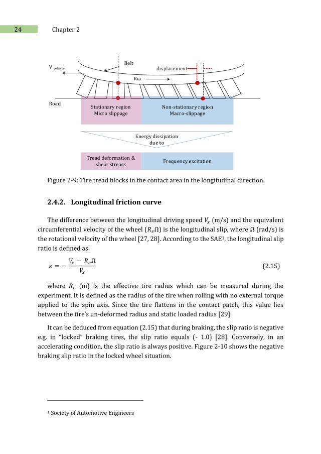
It can be deduced from equation (2.15) that during braking, the slip ratio is negative
e.g. in “locked” braking tires, the slip ratio equals (- 1.0) [28]. Conversely, in an
accelerating condition, the slip ratio is always positive. Figure 2-10 shows the negative
braking slip ratio in the locked wheel situation.
1 Society of Automotive Engineers
25 Literature studyature study
Slidingcoefficientof friction
Braking slip-ratio
Max. longitudinal force
-0.5 -1.0 -1.5
Lo
ngi
tud
ina
l fo
rce
(a.u
.)
Locked Wheel
Figure 2-10: Longitudinal force in arbitrary units (a.u.) vs. braking slip ratio,
redrawn from [28].
2.4.3. Lateral friction force and slip angle
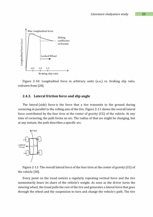
The lateral (side) force is the force that a tire transmits to the ground during
cornering in parallel to the rolling axis of the tire. Figure 2-11 shows the overall lateral
force contributed by the four tires at the center of gravity (CG) of the vehicle. At any
time of cornering, the path forms an arc. The radius of that arc might be changing, but
at any instant, the path describes a specific arc.
Figure 2-11: The overall lateral force of the four tires at the center of gravity (CG) of
the vehicle [30].
Every point on the tread notices a regularly repeating vertical force and the tire
momentarily bears its share of the vehicle’s weight. As soon as the driver turns the
steering wheel, the tread pulls the rest of the tire and generates a lateral force that goes
through the wheel and the suspension to turn and change the vehicle's path. The tire
26 Chapter 2
tread deforms as it passes the contact patch area. It is the tire's resistance to this
deflection that creates the lateral force that turns the vehicle [30].
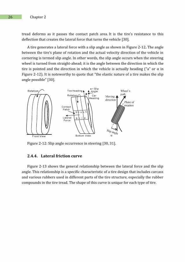
A tire generates a lateral force with a slip angle as shown in Figure 2-12. The angle
between the tire’s plane of rotation and the actual velocity direction of the vehicle in
cornering is termed slip angle. In other words, the slip angle occurs when the steering
wheel is turned from straight-ahead; it is the angle between the direction in which the
tire is pointed and the direction in which the vehicle is actually heading ("a" or α in
Figure 2-12). It is noteworthy to quote that “the elastic nature of a tire makes the slip
angle possible” [30].
Figure 2-12: Slip angle occurrence in steering [30, 31].
2.4.4. Lateral friction curve
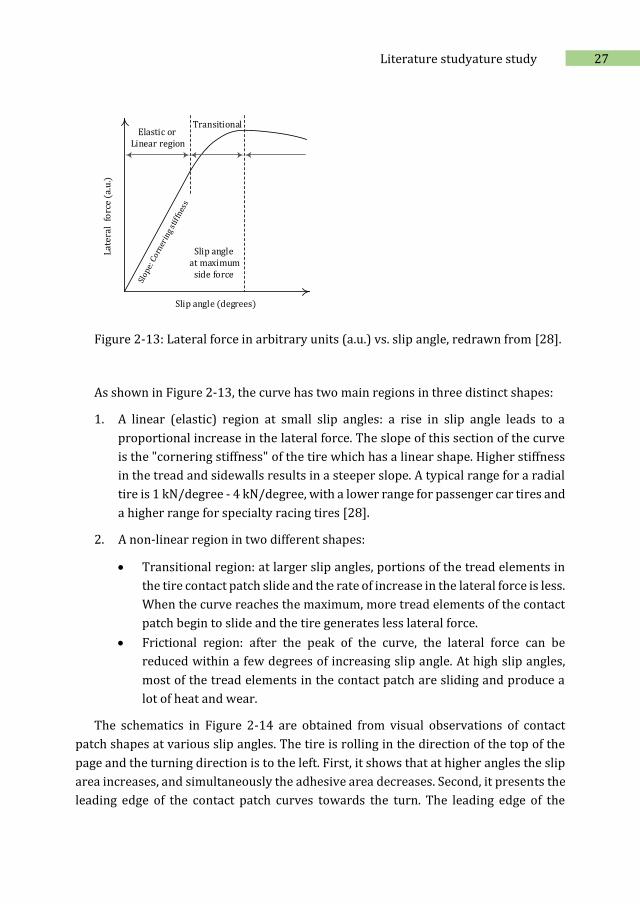
Figure 2-13 shows the general relationship between the lateral force and the slip
angle. This relationship is a specific characteristic of a tire design that includes carcass
and various rubbers used in different parts of the tire structure, especially the rubber
compounds in the tire tread. The shape of this curve is unique for each type of tire.
27 Literature studyature study
Slip angle (degrees)
Elastic or Linear region
Transitional
Slip angle at maximum
side force
La
tera
l f
orc
e (
a.u
.)
Figure 2-13: Lateral force in arbitrary units (a.u.) vs. slip angle, redrawn from [28].
As shown in Figure 2-13, the curve has two main regions in three distinct shapes:
1. A linear (elastic) region at small slip angles: a rise in slip angle leads to a
proportional increase in the lateral force. The slope of this section of the curve
is the "cornering stiffness" of the tire which has a linear shape. Higher stiffness
in the tread and sidewalls results in a steeper slope. A typical range for a radial
tire is 1 kN/degree - 4 kN/degree, with a lower range for passenger car tires and
a higher range for specialty racing tires [28].
2. A non-linear region in two different shapes:
Transitional region: at larger slip angles, portions of the tread elements in
the tire contact patch slide and the rate of increase in the lateral force is less.
When the curve reaches the maximum, more tread elements of the contact
patch begin to slide and the tire generates less lateral force.
Frictional region: after the peak of the curve, the lateral force can be
reduced within a few degrees of increasing slip angle. At high slip angles,
most of the tread elements in the contact patch are sliding and produce a
lot of heat and wear.
The schematics in Figure 2-14 are obtained from visual observations of contact
patch shapes at various slip angles. The tire is rolling in the direction of the top of the
page and the turning direction is to the left. First, it shows that at higher angles the slip
area increases, and simultaneously the adhesive area decreases. Second, it presents the
leading edge of the contact patch curves towards the turn. The leading edge of the
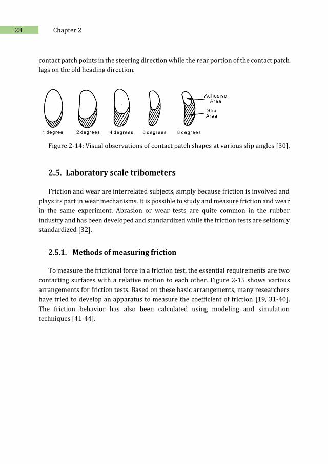
28 Chapter 2
contact patch points in the steering direction while the rear portion of the contact patch
lags on the old heading direction.
Figure 2-14: Visual observations of contact patch shapes at various slip angles [30].
2.5. Laboratory scale tribometers
Friction and wear are interrelated subjects, simply because friction is involved and
plays its part in wear mechanisms. It is possible to study and measure friction and wear
in the same experiment. Abrasion or wear tests are quite common in the rubber
industry and has been developed and standardized while the friction tests are seldomly
standardized [32].
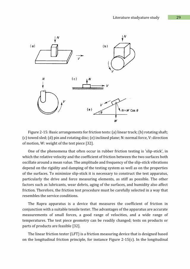
2.5.1. Methods of measuring friction
To measure the frictional force in a friction test, the essential requirements are two
contacting surfaces with a relative motion to each other. Figure 2-15 shows various
arrangements for friction tests. Based on these basic arrangements, many researchers
have tried to develop an apparatus to measure the coefficient of friction [19, 31-40].
The friction behavior has also been calculated using modeling and simulation
techniques [41-44].
29 Literature studyature study
Figure 2-15: Basic arrangements for friction tests: (a) linear track; (b) rotating shaft;
(c) towed sled; (d) pin and rotating disc; (e) inclined plane; N: normal force, V: direction
of motion, W: weight of the test piece [32].
One of the phenomena that often occur in rubber friction testing is 'slip-stick', in
which the relative velocity and the coefficient of friction between the two surfaces both
oscillate around a mean value. The amplitude and frequency of the slip-stick vibrations
depend on the rigidity and damping of the testing system as well as on the properties
of the surfaces. To minimize slip-stick it is necessary to construct the test apparatus,
particularly the drive and force measuring elements, as stiff as possible. The other
factors such as lubricants, wear debris, aging of the surfaces, and humidity also affect
friction. Therefore, the friction test procedure must be carefully selected in a way that
resembles the service conditions.
The Rapra apparatus is a device that measures the coefficient of friction in
conjunction with a suitable tensile tester. The advantages of the apparatus are accurate
measurements of small forces, a good range of velocities, and a wide range of
temperatures. The test piece geometry can be readily changed; tests on products or
parts of products are feasible [32].
The linear friction tester (LFT) is a friction measuring device that is designed based
on the longitudinal friction principle, for instance Figure 2-15(c). In the longitudinal
(
d)
30 Chapter 2
friction principle at a 100% slip ratio (𝜅 = 1), there is no need to use a whole tire as a
test object a rubber sample or tire tread block can represent the whole tire friction [26].
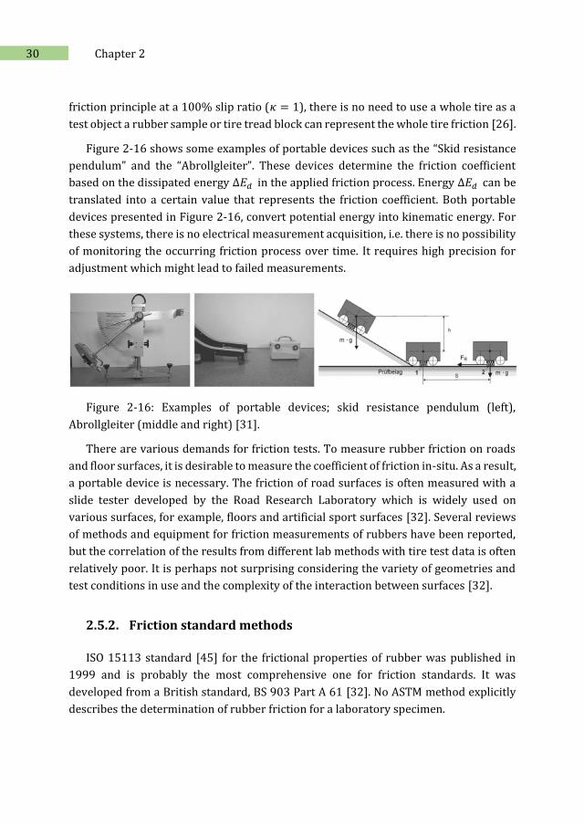
Figure 2-16 shows some examples of portable devices such as the “Skid resistance
pendulum” and the “Abrollgleiter”. These devices determine the friction coefficient
based on the dissipated energy ∆𝐸𝑑 in the applied friction process. Energy ∆𝐸𝑑 can be
translated into a certain value that represents the friction coefficient. Both portable
devices presented in Figure 2-16, convert potential energy into kinematic energy. For
these systems, there is no electrical measurement acquisition, i.e. there is no possibility
of monitoring the occurring friction process over time. It requires high precision for
adjustment which might lead to failed measurements.
Figure 2-16: Examples of portable devices; skid resistance pendulum (left),
Abrollgleiter (middle and right) [31].
There are various demands for friction tests. To measure rubber friction on roads
and floor surfaces, it is desirable to measure the coefficient of friction in-situ. As a result,
a portable device is necessary. The friction of road surfaces is often measured with a
slide tester developed by the Road Research Laboratory which is widely used on
various surfaces, for example, floors and artificial sport surfaces [32]. Several reviews
of methods and equipment for friction measurements of rubbers have been reported,
but the correlation of the results from different lab methods with tire test data is often
relatively poor. It is perhaps not surprising considering the variety of geometries and
test conditions in use and the complexity of the interaction between surfaces [32].
2.5.2. Friction standard methods
ISO 15113 standard [45] for the frictional properties of rubber was published in
1999 and is probably the most comprehensive one for friction standards. It was
developed from a British standard, BS 903 Part A 61 [32]. No ASTM method explicitly
describes the determination of rubber friction for a laboratory specimen.
31 Literature studyature study
The standard methods do not describe a specific apparatus but explain the
importance of tight control of the parameters and indicate remarkable guidance both
in the text and annexes on factors to be considered in obtaining friction measurements.
Three procedures for determining dynamic friction are given: the initial friction,
friction after repeated movement between the surfaces, and friction in the presence of
lubricants or contaminants. Some procedures are indicated for preparing the sliding
surfaces.
In most test procedures, the objective is to provide the best correlation with service
conditions together with good reproducibility between laboratories. Regarding the
aforementioned statement that friction and wear are interrelated and test
configurations are similar, an overview of different abraders is summarized in the next
section which might be opted for the friction measurements.
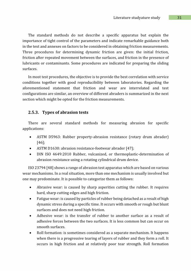
2.5.3. Types of abrasion tests
There are several standard methods for measuring abrasion for specific
applications:
ASTM D5963: Rubber property-abrasion resistance (rotary drum abrader)
[46];
ASTM D1630: abrasion resistance-footwear abrader [47];
DIN ISO 4649:2010 Rubber, vulcanized, or thermoplastic-determination of
abrasion resistance using a rotating cylindrical drum device.
ISO 23794 [48] shows a range of abrasion test apparatus which are based on various
wear mechanisms. In a real situation, more than one mechanism is usually involved but
one may predominate. It is possible to categorize them as follows:
Abrasive wear: is caused by sharp asperities cutting the rubber. It requires
hard, sharp cutting edges and high friction.
Fatigue wear: is caused by particles of rubber being detached as a result of high
dynamic stress during a specific time. It occurs with smooth or rough but blunt
surfaces and does not need high friction.
Adhesive wear: is the transfer of rubber to another surface as a result of
adhesive forces between the two surfaces. It is less common but can occur on
smooth surfaces.
Roll formation: is sometimes considered as a separate mechanism. It happens
when there is a progressive tearing of layers of rubber and they form a roll. It
occurs in high friction and at relatively poor tear strength. Roll formation
32 Chapter 2
results in a characteristic abrasion pattern of ridges and grooves at right angles
to the direction of movement (often called Schallamach waves).
Corrosive wear: is due to a direct chemical attack on the surface.
Erosive wear: is sometimes used for the action of particles in a liquid stream.
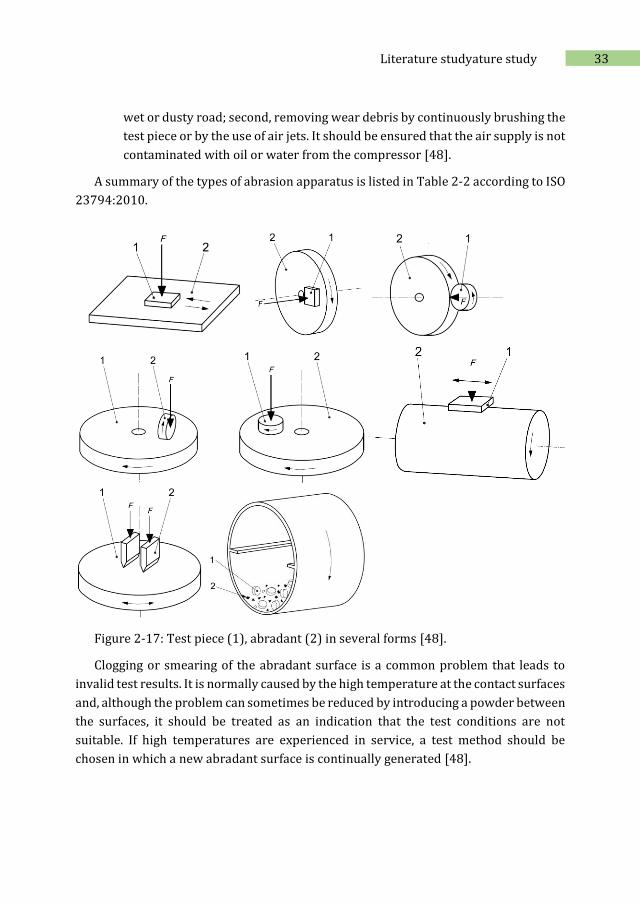
Another distinction between various tests is related to the test specimen geometry
and abradant. Some common combinations are shown in Figure 2-17. Abradants can be
classified into the following types:
Abrasive wheels;
Papers and clothes;
Metal knives;
Smooth surfaces;
Loose abradants.
The proper test method should be selected based on the service conditions of the
real application. Every category has its pros and cons, but reproducibility and
availability in a convenient form are a necessity.
The operating and test conditions can be summarized as follows:
Temperature: controlling the temperature of the contact surfaces during the
test is very difficult, although the tests are carried out at ambient temperature;
it has a huge impact on the correlation between laboratory and service
conditions.
Degree and rate of slip: the relative movement or slip is crucial in determining
the wear rate. The higher slip also gives a higher heat generation.
Contact pressure: under some conditions, if the abrasion mechanism changes,
a large rise in temperature occurs dependent on the friction between the
surfaces.
Continuous contact: when the test piece is continuously in contact with the
abradant and there is no chance for the generated heat at the contact surfaces
to be dissipated.
Intermittent contact: the contact occurs in a regular interval not continuously.
Lubricants and contamination: the interface between surfaces is important
because any change in the nature of the contact surface creates a big difference
in the final results. Two arguments arise regarding the lubricants and
contamination; first, deliberately applying another material or media between
surfaces to simulate service condition, for instance, lubricants such as water or
introduction of particulate material to a surface to simulate tire running on a
33 Literature studyature study
wet or dusty road; second, removing wear debris by continuously brushing the
test piece or by the use of air jets. It should be ensured that the air supply is not
contaminated with oil or water from the compressor [48].
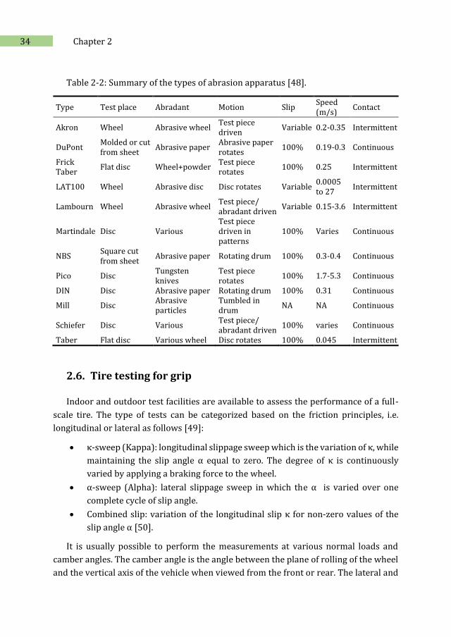
A summary of the types of abrasion apparatus is listed in Table 2-2 according to ISO
23794:2010.
Figure 2-17: Test piece (1), abradant (2) in several forms [48].
Clogging or smearing of the abradant surface is a common problem that leads to
invalid test results. It is normally caused by the high temperature at the contact surfaces
and, although the problem can sometimes be reduced by introducing a powder between
the surfaces, it should be treated as an indication that the test conditions are not
suitable. If high temperatures are experienced in service, a test method should be
chosen in which a new abradant surface is continually generated [48].
34 Chapter 2
Table 2-2: Summary of the types of abrasion apparatus [48].
Type Test place Abradant Motion Slip Speed (m/s)
Contact
Akron Wheel Abrasive wheel Test piece driven
Variable 0.2-0.35 Intermittent
DuPont Molded or cut from sheet
Abrasive paper Abrasive paper rotates
100% 0.19-0.3 Continuous
Frick Taber
Flat disc Wheel+powder Test piece rotates
100% 0.25 Intermittent
LAT100 Wheel Abrasive disc Disc rotates Variable 0.0005 to 27
Intermittent
Lambourn Wheel Abrasive wheel Test piece/ abradant driven
Variable 0.15-3.6 Intermittent
Martindale Disc Various Test piece driven in patterns
100% Varies Continuous
NBS Square cut from sheet
Abrasive paper Rotating drum 100% 0.3-0.4 Continuous
Pico Disc Tungsten knives
Test piece rotates
100% 1.7-5.3 Continuous
DIN Disc Abrasive paper Rotating drum 100% 0.31 Continuous
Mill Disc Abrasive particles
Tumbled in drum
NA NA Continuous
Schiefer Disc Various Test piece/ abradant driven
100% varies Continuous
Taber Flat disc Various wheel Disc rotates 100% 0.045 Intermittent
2.6. Tire testing for grip
Indoor and outdoor test facilities are available to assess the performance of a full-
scale tire. The type of tests can be categorized based on the friction principles, i.e.
longitudinal or lateral as follows [49]:
κ-sweep (Kappa): longitudinal slippage sweep which is the variation of κ, while
maintaining the slip angle α equal to zero. The degree of κ is continuously
varied by applying a braking force to the wheel.
α-sweep (Alpha): lateral slippage sweep in which the α is varied over one
complete cycle of slip angle.
Combined slip: variation of the longitudinal slip κ for non-zero values of the
slip angle α [50].
It is usually possible to perform the measurements at various normal loads and
camber angles. The camber angle is the angle between the plane of rolling of the wheel
and the vertical axis of the vehicle when viewed from the front or rear. The lateral and
35 Literature studyature study
vertical forces and self-aligning torques are measured and by employing tire models
e.g. the Magic Formula (MF) of Pacejka [43] the data are presented in the typical friction
curves as illustrated in Figure 2-10 and Figure 2-13.
2.6.1. Outdoor tire tests
The outdoor tests being employed for measuring tire grip are vehicle-based or
trailer tests carried out on real test tracks. A vehicle test is conducted on a commercial
car equipped with Anti-lock Braking System (ABS) to evaluate the stopping distance
under specified test conditions. The distance that the car reaches from a specified high
speed to nearly a full stop is the stopping or braking distance. A test procedure in ASTM
F1649 exists for the wet braking traction performance of passenger car tires.
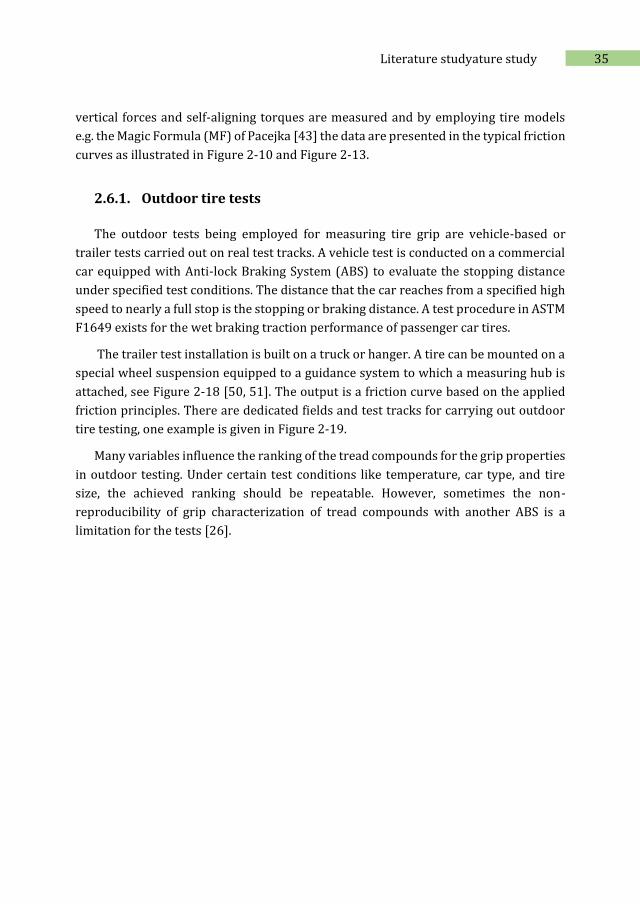
The trailer test installation is built on a truck or hanger. A tire can be mounted on a
special wheel suspension equipped to a guidance system to which a measuring hub is
attached, see Figure 2-18 [50, 51]. The output is a friction curve based on the applied
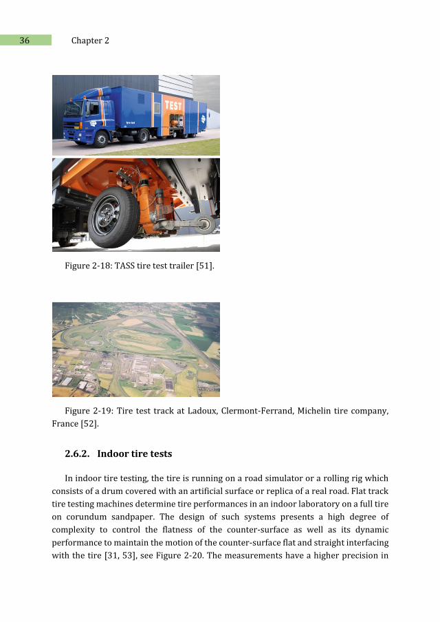
friction principles. There are dedicated fields and test tracks for carrying out outdoor
tire testing, one example is given in Figure 2-19.
Many variables influence the ranking of the tread compounds for the grip properties
in outdoor testing. Under certain test conditions like temperature, car type, and tire
size, the achieved ranking should be repeatable. However, sometimes the non-
reproducibility of grip characterization of tread compounds with another ABS is a
limitation for the tests [26].
36 Chapter 2
Figure 2-18: TASS tire test trailer [51].
Figure 2-19: Tire test track at Ladoux, Clermont-Ferrand, Michelin tire company,
France [52].
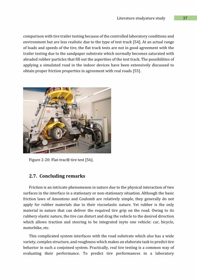
2.6.2. Indoor tire tests
In indoor tire testing, the tire is running on a road simulator or a rolling rig which
consists of a drum covered with an artificial surface or replica of a real road. Flat track
tire testing machines determine tire performances in an indoor laboratory on a full tire
on corundum sandpaper. The design of such systems presents a high degree of
complexity to control the flatness of the counter-surface as well as its dynamic
performance to maintain the motion of the counter-surface flat and straight interfacing
with the tire [31, 53], see Figure 2-20. The measurements have a higher precision in
37 Literature studyature study
comparison with tire trailer testing because of the controlled laboratory conditions and
environment but are less realistic due to the type of test track [54]. At an actual range
of loads and speeds of the tire, the flat track tests are not in good agreement with the
trailer testing due to the sandpaper substrate which normally becomes saturated with
abraded rubber particles that fill out the asperities of the test track. The possibilities of
applying a simulated road in the indoor devices have been extensively discussed to
obtain proper friction properties in agreement with real roads [55].
Figure 2-20: Flat-trac® tire test [56].
2.7. Concluding remarks
Friction is an intricate phenomenon in nature due to the physical interaction of two
surfaces in the interface in a stationary or non-stationary situation. Although the basic
friction laws of Amontons and Coulomb are relatively simple, they generally do not
apply for rubber materials due to their viscoelastic nature. Yet rubber is the only
material in nature that can deliver the required tire grip on the road. Owing to its
rubbery elastic nature, the tire can distort and drag the vehicle to the desired direction
which allows traction and steering to be integrated inyto one vehicle: car, bicycle,
motorbike, etc.
This complicated system interfaces with the road substrate which also has a wide
variety, complex structure, and roughness which makes an elaborate task to predict tire
behavior in such a conjoined system. Practically, real tire testing is a common way of
evaluating their performance. To predict tire performances in a laboratory
38 Chapter 2
environment, a test set-up is required to mimic the tire service condition as close as
possible. This was the basis to launch the task which was formulated as the “leitmotif”
of the present thesis.
2.8. References
1. Ludema, K.C., friction wear lubrication, A textbook in tribology. 1996: CRC Press.
2. Chapter 1 Introduction, in Book 'Tribology and Interface Engineering Series', Z. Si-Wei, Editor. 2004, Elsevier. p. 1-6.
3. Rubber friction, in 2004, Date of access: January 2018; Available from http://insideracingtechnology.com/tirebkexerpt1.htm.
4. Popova, E. and V.L. Popov, The research works of Coulomb and Amontons and generalized laws of friction. Friction, 2015. 3(2): p. 183-190.
5. Moore, D.F., Abrasion and wear, in Book 'The friction and lubrication of elastomers'. 1972, Pergamon press Inc. p. 252-274.
6. Deleau, F., D. Mazuyer, and A. Koenen, Sliding friction at elastomer/glass contact: Influence of the wetting conditions and instability analysis. Tribology International, 2009. 42(1): p. 149-159.
7. Deladi, E.L., Static friction in rubber-metal contacts with application to rubber pad forming processes, in Tribology. 2006, Twente University: Ph.D dissertation.
8. Steen, R.v.d., Tyre/road friction modeling : literature survey DCT rapporten; 2007.072, 2007 Eindhoven.
9. Schallamach, A., friction and abrasion of rubber. wear, 1958. 1: p. 384-417.
10. Grosch, K.A., rubber friction and tire traction, in Book 'The pneumatic tire'. 2006, NHTSA. p. 421-473.
11. Schallamach, A., The Load Dependence of Rubber Friction. Proceedings of the Physical Society. Section B, 1952. 65: p. 657-661.
12. Grosch, K.A. and A. Schallamach, The Load Dependence of Laboratory Abrasion and Tire Wear. Rubber Chemistry and Technology, 1970. 43(4): p. 701-713.
13. Grosch, K.A., rubber abrasion and tire wear, in Book 'The pneumatic tire'. 2006, NHTSA. p. 534-592.
14. Kane, M. and V. Cerezo, A contribution to tire/road friction modeling: From a simplified dynamic frictional contact model to a “Dynamic Friction Tester” model. Wear, 2015. 342-343: p. 163-171.
39 Literature studyature study
15. Persson, B.N.J., Theory of rubber friction and contact mechanics. The Journal of Chemical Physics, 2001. 115(8): p. 3840-3861.
16. Steen, v.d., R., Enhanced friction modeling for steady-state rolling tires. 2010: Technische Universiteit Eindhoven.
17. Fujikawa, T., A. Funazaki, and S. Yamazaki, Tire Tread Temperatures in Actual Contact Areas. Tire Science and Technology, 1994. 22(1): p. 19-41.
18. Lang, A. and M. Klüppel, Temperature and pressure dependence of the friction properties of tire tread compounds on rough granite, in 11th KHK Fall Rubber Colloquium. 2014, Deutsches Institut für Kautschuktechnologie e.V.: Hannover, Germany.
19. Klüppel, M. and G. Heinrich, Rubber Friction on Self-Affine Road Tracks. Rubber Chemistry and Technology, 2000. 73(4): p. 578-606.
20. Fortunato, G., V. Ciaravola, A. Furno, M. Scaraggi, B. Lorenz, and B.N.J. Persson, Dependency of Rubber Friction on Normal Force or Load: Theory and Experiment. Tire Science and Technology, 2017. 45(1): p. 25-54.
21. Malcolm L. Williams, R.F.L., John D. Ferry, The Temperature Dependence of Relaxation Mechanisms in Amorphous Polymers and Other Glass-forming Liquids. Journal of the American Chemical Society, 1955. 77(14): p. 3701-3707.
22. Grosch, K.A., Goodyear Medalist Lecture. Rubber Friction and its Relation to Tire Traction. Rubber Chemistry and Technology, 2007. 80(3): p. 379-411.
23. Grosch, K.A., The Rolling Resistance, Wear and Traction Properties of Tread Compounds. Rubber Chemistry and Technology, 1996. 69(3): p. 495-568.
24. Emami, A. and S. Khaleghian, Investigation of tribological behavior of Styrene-Butadiene Rubber compound on asphalt-like surfaces. Tribology International, 2019. 136: p. 487-495.
25. Afferrante, L., F. Bottiglione, C. Putignano, B.N.J. Persson, and G. Carbone, Elastic Contact Mechanics of Randomly Rough Surfaces: An Assessment of Advanced Asperity Models and Persson’s Theory. Tribology Letters, 2018. 66(2): p. 75.
26. Salehi, M., J.W.M. Noordermeer, L.A.E.M. Reuvekamp, W.K. Dierkes, and A. Blume, Measuring rubber friction using a Laboratory Abrasion Tester (LAT100) to predict car tire dry ABS braking. Tribology International, 2019. 131: p. 191-199.
27. Rajamani, R., Lateral and Longitudinal Tire Forces, in Book 'Vehicle Dynamics and Control'. 2006, Springer US. p. 387-432.
28. Majerus, J.N., your tire's behavior, in Book 'Winning More Safely in Motorsports; the Workbook'. 2007, Racing vehicle Inc. p. 268-283.
40 Chapter 2
29. Miller, S.L., B. Youngberg, A. Millie, P. Schweizer, and J.C. Gerdes. Calculation Longitudinal wheel slip and tire parameters using GPS velocity. in the American control conference. 25-27 Jun 2001. Arlington.
30. Tire behavior, in 2004, Date of access: january 2018; Available from http://insideracingtechnology.com/tirebkexerpt2.htm.
31. Mihajlovic, S., U. Kutscher, B. Wies, and J. Wallaschek, Methods for experimental investigations on tyre-road-grip at arbitrary roads. Internationale Konferenz ESAR "Expertensymposium Accident Research“, 2013.
32. Brown, R., friction and wear, in Book 'Physical testing of rubbers'. 2006, Springer. p. 219-243.
33. Heinz, M. and K.A. Grosch, A Laboratory Method to Comprehensively Evaluate Abrasion, Traction and Rolling Resistance of Tire Tread Compounds. Rubber Chemistry and Technology, 2007. 80(4): p. 580-607.
34. Germann, S., M. Wurtenberger, and A. Daiss. Monitoring of the friction coefficient between tyre and road surface. in 1994 Proceedings of IEEE International Conference on Control and Applications. 24-26 Aug 1994.
35. Najafi, S., Evaluation of Continuous Friction Measuring Equipment (CFME) for Supporting Pavement Friction Management Programs. 2010, Virginia Tech.
36. Bouzid, N. and B. Heimann, Micro Texture Characterization and Prognosis of the Maximum Traction between Grosch Wheel and Asphalt Surfaces under Wet Conditions, in Book 'Elastomere Friction: Theory, Experiment and Simulation', D. Besdo, B. Heimann, M. Klüppel, M. Kröger, P. Wriggers, and U. Nackenhorst, Editors. 2010, Springer Berlin Heidelberg: Berlin, Heidelberg. p. 201-220.
37. Lindner, M., M. Kröger, K. Popp, and H. Blume, EXPERIMENTAL AND ANALYTICAL INVESTIGATION OF RUBBER FRICTION, in ICTAM04 Proceedings. 2004: Warsaw, Poland.
38. Lahayne, O., J. Eberhardsteiner, and R. Reihsner, TRIBOLOGICAL INVESTIGATIONS USING A LINEAR FRICTION TESTER (LFT). Transactions of FAMENA January 2009. 33(2): p. 15-22.
39. Krasmik, V.S., J., Experimental Investigation of the Friction and Wear Behaviour with an Adapted Ball-On-Prism Test Setup. Tribology in Industry, 2015. 37(3): p. 291-298.
40. Pacejka, H.B., Chapter 2 - Basic tyre modelling considerations, in Book 'Tyre and Vehicle Dynamics (Second Edition)'. 2006, Butterworth-Heinemann: Oxford. p. 61-89.
41. Jacob Svendenius, B.W., Review of wheel modeling and friction estimation, in Department of Automatic Control 2003, Lund institute of technology.
42. Steen, R.v.d., Tyre/road friction modeling. 2007,
41 Literature studyature study
43. Bakker, E., L. Nyborg, and H.B. Pacejka, Tyre Modelling for Use in Vehicle Dynamics Studies. 1987, SAE International.
44. Tire Modeling, Lateral and Longitudinal Tire Forces, Erdogan, G., Date of access: July 2020; Available from http://www.menet.umn.edu/~gurkan/Tire%20Modeling%20%20Lecture.pdf.
45. ISO 15113, Rubber, in determination of frictional properties. 2005.
46. ASTM D5963, Standard Test Method for Rubber Property—Abrasion Resistance (Rotary Drum Abrader), in Rubber. re-approved 2001.
47. ASTM D1630, Standard Test Method for Rubber Property—Abrasion Resistance (Footwear Abrader), in Rubber. reapproved 2000.
48. ISO 23794, vulcanized or thermoplastic — Abrasion testing — Guidance, in Rubber. 2010.
49. Appendix 3 - SWIFT parameters A2 - Pacejka, Hans B, in Book 'Tyre and Vehicle Dynamics (Second Edition)'. 2006, Butterworth-Heinemann: Oxford. p. 629-636.
50. Pacejka, H.B., Chapter 12 - Tyre steady-state and dynamic test facilities, in Book 'Tyre and Vehicle Dynamics (Second Edition)'. 2006, Butterworth-Heinemann: Oxford. p. 586-594.
51. Besselink, I.J.M., Tire Characteristics and Modeling, in Book 'Vehicle Dynamics of Modern Passenger Cars', P. Lugner, Editor. 2019, Springer International Publishing: Cham. p. 47-108.
52. The Tyre Grip, Société de Technologie Michelin.,clermont-ferrand, France, Date of access: May 2020; Available from http://www.dimnp.unipi.it/guiggiani-m/Michelin_Tire_Grip.pdf.
53. Cabrera, J., A. Ortiz, A. Simón, F. García, A. Pérez, and A. Perez-Blanca, A Versatile Flat Track Tire Testing Machine Vol. 40. 2003. 271-284.
54. Ludwig, C. Influence of testing surface on tire lateral force characteristics. in Science meets Tires. April 24-25, 2018. Aachen, Germany: ika INSTITUT FÜR KRAFTFAHRZEUGE and RWTH AACHEN UNIVERSITY.
55. Carrillo, C. and C. Bachmann. Can we get the road into the lab? Challenges in tire tesing. in Science meets Tires. April 24-25, 2018. Aachen, Germany: ika INSTITUT FÜR KRAFTFAHRZEUGE and RWTH AACHEN UNIVERSITY.
56. MTS Flat-Trac® IV CT plus tire test bench, in, Date of access: February 2020; Available from https://www.fka.de/.
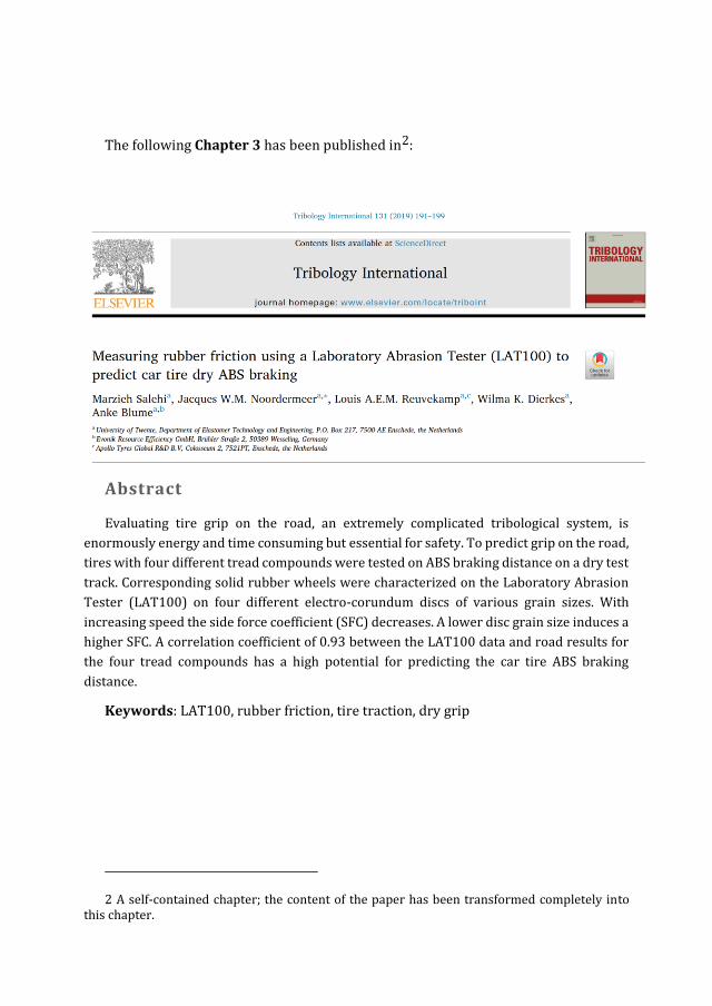
The following Chapter 3 has been published in2:
Abstract
Evaluating tire grip on the road, an extremely complicated tribological system, is
enormously energy and time consuming but essential for safety. To predict grip on the road,
tires with four different tread compounds were tested on ABS braking distance on a dry test
track. Corresponding solid rubber wheels were characterized on the Laboratory Abrasion
Tester (LAT100) on four different electro-corundum discs of various grain sizes. With
increasing speed the side force coefficient (SFC) decreases. A lower disc grain size induces a
higher SFC. A correlation coefficient of 0.93 between the LAT100 data and road results for
the four tread compounds has a high potential for predicting the car tire ABS braking
distance.
Keywords: LAT100, rubber friction, tire traction, dry grip
2 A self-contained chapter; the content of the paper has been transformed completely into this chapter.
3 Prediction of ABS braking distance,
A preliminary study
3.1. Introduction
Tires transmit all types of vehicle loads or forces such as vertical, longitudinal
braking, driving, cornering, and camber thrust to the road. These forces are necessary
for directional control of the vehicle. Tire traction is the result of the generated
frictional forces in various driving states such as cornering, braking, and accelerating.
It is a concept that describes the grip between the tire and the road. A tire with better
grip provides a shorter braking distance wherein the vehicle comes to a full stop. Proper
tire grip provides a good level of handling which is a prerequisite for proper vehicle
steering, braking, accelerating, and cornering [1].
Tires are built up of a multitude of different elements, mostly rubber compounds,
each contributing to the overall performance profile. To improve and develop new tires,
extensive testing is required which is time-consuming and costly. Particularly for new
rubber tire tread compounds, it is very attractive to be able to predict their performance
in a laboratory environment before manufacturing a full tire. To achieve a good
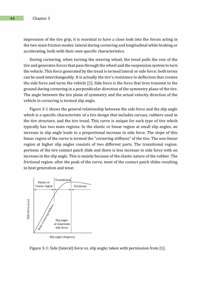
44 Chapter 3
impression of the tire grip, it is essential to have a close look into the forces acting in
the two main friction modes: lateral during cornering and longitudinal while braking or
accelerating, both with their own specific characteristics.
During cornering, when turning the steering wheel, the tread pulls the rest of the
tire and generates forces that pass through the wheel and the suspension system to turn
the vehicle. This force generated by the tread is termed lateral or side force; both terms
can be used interchangeably. It is actually the tire's resistance to deflection that creates
the side force and turns the vehicle [1]. Side force is the force that tires transmit to the
ground during cornering in a perpendicular direction of the symmetry plane of the tire.
The angle between the tire plane of symmetry and the actual velocity direction of the
vehicle in cornering is termed slip angle.
Figure 3-1 shows the general relationship between the side force and the slip angle
which is a specific characteristic of a tire design that includes carcass, rubbers used in
the tire structure, and the tire tread. This curve is unique for each type of tire which
typically has two main regions. In the elastic or linear region at small slip angles, an
increase in slip angle leads to a proportional increase in side force. The slope of this
linear region of the curve is termed the "cornering stiffness" of the tire. The non-linear
region at higher slip angles consists of two different parts. The transitional region:
portions of the tire contact patch slide and there is less increase in side force with an
increase in the slip angle. This is mainly because of the elastic nature of the rubber. The
frictional region: after the peak of the curve, most of the contact patch slides resulting
in heat generation and wear.
Frictional
Slip angle (degrees)
Elastic or Linear region
Transitional
Slip angle at maximum
side force
Sid
e f
orc
e (
a.u
.)
Figure 3-1: Side (lateral) force vs. slip angle; taken with permission from [1].
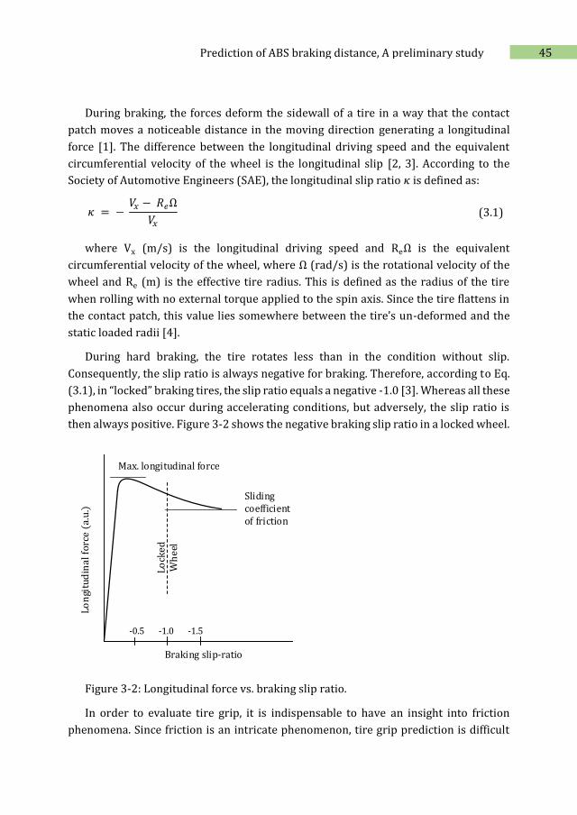
45 Prediction of ABS braking distance, A preliminary study
During braking, the forces deform the sidewall of a tire in a way that the contact
patch moves a noticeable distance in the moving direction generating a longitudinal
force [1]. The difference between the longitudinal driving speed and the equivalent
circumferential velocity of the wheel is the longitudinal slip [2, 3]. According to the
Society of Automotive Engineers (SAE), the longitudinal slip ratio 𝜅 is defined as:
𝜅 = − 𝑉𝑥 − 𝑅𝑒Ω
𝑉𝑥
(3.1)
where Vx (m/s) is the longitudinal driving speed and ReΩ is the equivalent
circumferential velocity of the wheel, where Ω (rad/s) is the rotational velocity of the
wheel and Re (m) is the effective tire radius. This is defined as the radius of the tire
when rolling with no external torque applied to the spin axis. Since the tire flattens in
the contact patch, this value lies somewhere between the tire’s un-deformed and the
static loaded radii [4].
During hard braking, the tire rotates less than in the condition without slip.
Consequently, the slip ratio is always negative for braking. Therefore, according to Eq.
(3.1), in “locked” braking tires, the slip ratio equals a negative -1.0 [3]. Whereas all these
phenomena also occur during accelerating conditions, but adversely, the slip ratio is
then always positive. Figure 3-2 shows the negative braking slip ratio in a locked wheel.
Slidingcoefficientof friction
Braking slip-ratio
Max. longitudinal force
-0.5 -1.0 -1.5
Lo
ngi
tud
ina
l fo
rce
(a.
u.)
Lo
cke
dW
he
el
Figure 3-2: Longitudinal force vs. braking slip ratio.
In order to evaluate tire grip, it is indispensable to have an insight into friction
phenomena. Since friction is an intricate phenomenon, tire grip prediction is difficult
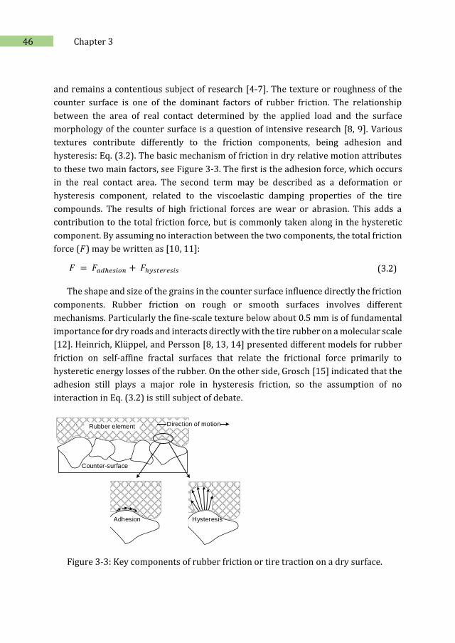
46 Chapter 3
and remains a contentious subject of research [4-7]. The texture or roughness of the
counter surface is one of the dominant factors of rubber friction. The relationship
between the area of real contact determined by the applied load and the surface
morphology of the counter surface is a question of intensive research [8, 9]. Various
textures contribute differently to the friction components, being adhesion and
hysteresis: Eq. (3.2). The basic mechanism of friction in dry relative motion attributes
to these two main factors, see Figure 3-3. The first is the adhesion force, which occurs
in the real contact area. The second term may be described as a deformation or
hysteresis component, related to the viscoelastic damping properties of the tire
compounds. The results of high frictional forces are wear or abrasion. This adds a
contribution to the total friction force, but is commonly taken along in the hysteretic
component. By assuming no interaction between the two components, the total friction
force (𝐹) may be written as [10, 11]:
𝐹 = 𝐹𝑎𝑑ℎ𝑒𝑠𝑖𝑜𝑛 + 𝐹ℎ𝑦𝑠𝑡𝑒𝑟𝑒𝑠𝑖𝑠 (3.2)
The shape and size of the grains in the counter surface influence directly the friction
components. Rubber friction on rough or smooth surfaces involves different
mechanisms. Particularly the fine-scale texture below about 0.5 mm is of fundamental
importance for dry roads and interacts directly with the tire rubber on a molecular scale
[12]. Heinrich, Klüppel, and Persson [8, 13, 14] presented different models for rubber
friction on self-affine fractal surfaces that relate the frictional force primarily to
hysteretic energy losses of the rubber. On the other side, Grosch [15] indicated that the
adhesion still plays a major role in hysteresis friction, so the assumption of no
interaction in Eq. (3.2) is still subject of debate.
Counter-surface
Direction of motion
HysteresisAdhesion
Rubber element
Figure 3-3: Key components of rubber friction or tire traction on a dry surface.
47 Prediction of ABS braking distance, A preliminary study
Grip and wear evaluations of tread compounds suffer from the fact that not only
absolute values but also relative ratings strongly depend on the experimental
conditions under which they are obtained in road tests [16]. Therefore, a meaningful
laboratory evaluation is really needed. Various types of tribometers and testing
machines are available which are able to measure tribological properties. However, to
measure tire tribological properties a tribometer is required that can simulate tire-road
conditions for rubber samples in a laboratory environment.
The so-called Laboratory Abrasion Tester (LAT100) was originally developed by
Grosch [16] to measure the side force and the abrasion loss of a sample in the form of a
solid rubber wheel as a function of various slip angles, loads, speeds and abrasive
surfaces. Afterward, it was further developed to measure wet traction and rolling
resistance. It has been demonstrated before that the results of measuring wet grip with
the LAT100 give a good correlation with ABS braking on the road [16, 17]. Further, good
correlations between tire data and laboratory test results have been obtained for
abrasion and rolling resistance [16, 18-20]. The machine is able to simulate a wide
range of test conditions in a laboratory environment. with a wheel shape sample. This
has been mentioned as a high similarity to a vehicle tire which gives a good correlation
with real tire data [21]. Therefore, it has the potential to be used as an advanced
machine for measuring and predicting tire performance.
In the present manuscript, the rubber friction under dry conditions is evaluated in
detail by using the LAT100 and compared to real tire test results. For this purpose,
various tread compounds were selected and mounted on a standard tire body. The
braking distance of each tire was measured in real tire tests and the resulting ratings
have been calculated. By using the LAT100 in the laboratory environment, the side
forces of the same tread compounds were measured at different test conditions. Finally,
the results of the laboratory measurements are correlated with the real tire data ratings
and the effects of various speeds and LAT100 disc roughness are characterized.
3.2. Experimental
3.2.1. Tire data
Four proprietary passenger tread compounds with various grip properties were
selected for the investigation. Full tires were manufactured with the same construction
process using the same body components together with the four different tread
compound formulations. The ABS braking distances were measured. Table 3-1 shows
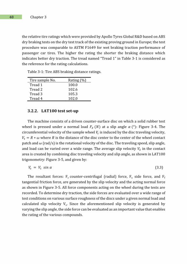
48 Chapter 3
the relative tire ratings which were provided by Apollo Tyres Global R&D based on ABS
dry braking tests on the dry test track of the existing proving ground in Europe; the test
procedure was comparable to ASTM F1649 for wet braking traction performance of
passenger car tires. The higher the rating the shorter the braking distance which
indicates better dry traction. The tread named “Tread 1” in Table 3-1 is considered as
the reference for the rating calculations.
Table 3-1: Tire ABS braking distance ratings.
Tire sample No. Rating (%) Tread 1 100.0 Tread 2 102.6 Tread 3 105.3 Tread 4 102.0
3.2.2. LAT100 test set-up
The machine consists of a driven counter-surface disc on which a solid rubber test
wheel is pressed under a normal load 𝐹𝑍 (𝑁) at a slip angle 𝛼 (°): Figure 3-4. The
circumferential velocity of the sample wheel 𝑉𝑐 is induced by the disc traveling velocity,
𝑉𝑡 = 𝑅 ∗ 𝜔 where 𝑅 is the distance of the disc center to the center of the wheel contact
patch and 𝜔 (rad/s) is the rotational velocity of the disc. The traveling speed, slip angle,
and load can be varied over a wide range. The average slip velocity 𝑉𝑆 in the contact
area is created by combining disc traveling velocity and slip angle, as shown in LAT100
trigonometry: Figure 3-5, and given by:
𝑉𝑠 = 𝑉𝑡 𝑠𝑖𝑛 𝛼 (3.3)
The resultant forces: Fc counter-centrifugal (radial) force, Fs side force, and Ff
tangential friction force, are generated by the slip velocity and the acting normal force
as shown in Figure 3-5. All force components acting on the wheel during the tests are
recorded. To determine dry traction, the side forces are evaluated over a wide range of
test conditions on various surface roughness of the discs under a given normal load and
calculated slip velocity Vs. Since the aforementioned slip velocity is generated by
varying the slip angle, the side force can be evaluated as an important value that enables
the rating of the various compounds.
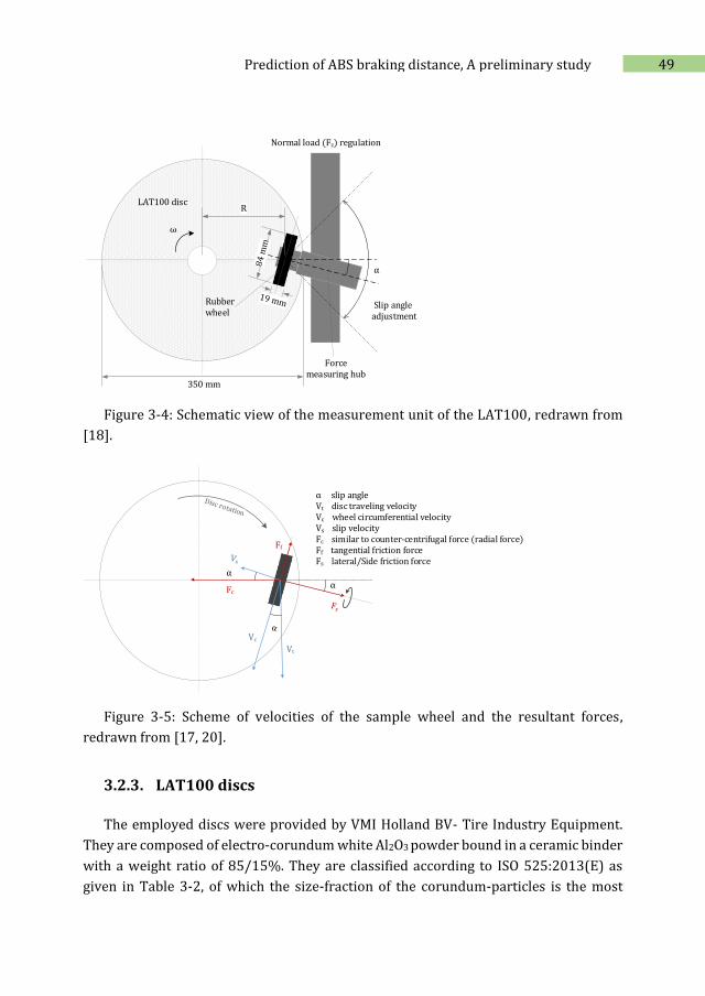
49 Prediction of ABS braking distance, A preliminary study
LAT100 disc
Rubber wheel
R
ω
Normal load (Fz) regulation
Slip angle adjustment
Force measuring hub
α
350 mm
Figure 3-4: Schematic view of the measurement unit of the LAT100, redrawn from
[18].
Vt
Fc
α
α
α slip angleVt disc traveling velocityVc wheel circumferential velocityVs slip velocityFc similar to counter-centrifugal force (radial force) Ff tangential friction forceFs lateral/Side friction force
Vc
Ff
Figure 3-5: Scheme of velocities of the sample wheel and the resultant forces,
redrawn from [17, 20].
3.2.3. LAT100 discs
The employed discs were provided by VMI Holland BV- Tire Industry Equipment.
They are composed of electro-corundum white Al2O3 powder bound in a ceramic binder
with a weight ratio of 85/15%. They are classified according to ISO 525:2013(E) as
given in Table 3-2, of which the size-fraction of the corundum-particles is the most
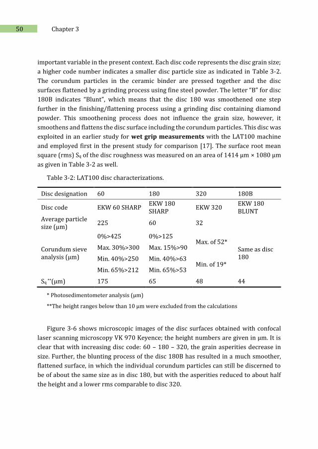
50 Chapter 3
important variable in the present context. Each disc code represents the disc grain size;
a higher code number indicates a smaller disc particle size as indicated in Table 3-2.
The corundum particles in the ceramic binder are pressed together and the disc
surfaces flattened by a grinding process using fine steel powder. The letter “B” for disc
180B indicates “Blunt”, which means that the disc 180 was smoothened one step
further in the finishing/flattening process using a grinding disc containing diamond
powder. This smoothening process does not influence the grain size, however, it
smoothens and flattens the disc surface including the corundum particles. This disc was
exploited in an earlier study for wet grip measurements with the LAT100 machine
and employed first in the present study for comparison [17]. The surface root mean
square (rms) Sq of the disc roughness was measured on an area of 1414 μm × 1080 μm
as given in Table 3-2 as well.
Table 3-2: LAT100 disc characterizations.
Disc designation 60 180 320 180B
Disc code EKW 60 SHARP EKW 180 SHARP
EKW 320 EKW 180 BLUNT
Average particle size (μm)
225 60 32
Same as disc 180
Corundum sieve analysis (μm)
0%>425 0%>125 Max. of 52*
Max. 30%>300 Max. 15%>90
Min. 40%>250 Min. 40%>63 Min. of 19*
Min. 65%>212 Min. 65%>53
Sq **(μm) 175 65 48 44
* Photosedimentometer analysis (μm)
**The height ranges below than 10 μm were excluded from the calculations
Figure 3-6 shows microscopic images of the disc surfaces obtained with confocal
laser scanning microscopy VK 970 Keyence; the height numbers are given in μm. It is
clear that with increasing disc code: 60 – 180 – 320, the grain asperities decrease in
size. Further, the blunting process of the disc 180B has resulted in a much smoother,
flattened surface, in which the individual corundum particles can still be discerned to
be of about the same size as in disc 180, but with the asperities reduced to about half
the height and a lower rms comparable to disc 320.
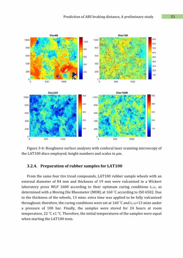
51 Prediction of ABS braking distance, A preliminary study
Figure 3-6: Roughness surface analyses with confocal laser scanning microscopy of
the LAT100 discs employed; height numbers and scales in μm.
3.2.4. Preparation of rubber samples for LAT100
From the same four tire tread compounds, LAT100 rubber sample wheels with an
external diameter of 84 mm and thickness of 19 mm were vulcanized in a Wickert
laboratory press WLP 1600 according to their optimum curing conditions tc,95, as
determined with a Moving Die Rheometer (MDR) at 160 ˚C according to ISO 6502. Due
to the thickness of the wheels, 13 mins. extra time was applied to be fully vulcanized
throughout; therefore, the curing conditions were set at 160 ˚C and tc.95+13 mins under
a pressure of 100 bar. Finally, the samples were stored for 24 hours at room
temperature, 22 ˚C ±1 ˚C. Therefore, the initial temperatures of the samples were equal
when starting the LAT100 tests.
52 Chapter 3
3.2.5. LAT100 tests
First screening was performed at constant normal load, various traveling speeds
over a wide range of slip angles on disc 180B as shown in Table 3-3 row 1. The wide
range of slip angles was selected in a way to cover the potential area of ABS braking for
the experiments. This range of slip angles was in a form of single experiment points.
After the first screening more detailed experiments were executed on various disc
roughness based on the optimized variables, as shown in Table 3-3 row 2.
For realistic and repeatable side force evaluations, it is necessary to remove the
shiny outer vulcanization skin from the LAT100-samples surface before measuring the
side force. For this purpose, a sample run-in was carried out with 75 N normal load, 25
km/h speed, 13° slip angle, over 500 m distance, and repeated for the right and the left
sides of the LAT100-samples on disc 60; according to ISO-23233. Additionally, a disc
run-in is also required to be performed before using a brand-new disc. To prepare a
correct friction curve, it is crucial to collect all the single experimental points at a same
level of surface roughness. Any deviation from the expected surface roughness based
on the disc code interferes with the final results. The disc run-in is a pre-conditioning
and by means of this, sharp asperities are leveled and the sharpness of the asperities
over the disc becomes uniform. After every single test for each slip angle, disc cleaning
was performed using an air pressure nozzle which removed the rubber debris and
particles from the disc surface. All the tests were performed at 75 N normal load which
is equal to the average load in a tire contact patch on the road [16, 18].
Table 3-3: Variables employed in dry grip tests.
Speed (km/h)
Corresponding distance (m)
Slip angle range (˚)
Disc code
0.2, 2.1, 20 2, 17, 120 3 to 35 180B
2.1 2, 17, 120 3 to 35 60, 180, 320, 180B
For all test procedures, the experiments were carried out for the same 4 tread
compounds. For every procedure 5 LAT100-samples were prepared, of which LAT100-
samples 1 and 5 correspond to compound 1. This compound is considered as the
reference to cross-check the experiments in each measuring conditions. To avoid
creating uneven wear or a conical shape on the surface of the LAT100-samples during
the tests, the side force measurements were performed for both sides of the LAT100-
samples. The calculated Side Force Coefficient (SFC) for each data point is an average
53 Prediction of ABS braking distance, A preliminary study
SFC over the right and the left sides of the LAT100-sample. To compare the friction
properties, the SFC was calculated according to:
𝑆𝐹𝐶 =𝐹𝑠 (𝑁)
𝐹𝑧 (𝑁) (3.4)
To correlate the LAT100 results with real road data, the SFCs of the four tread
compounds measured by LAT100 were rated as follows:
𝑆𝐹𝐶 𝑟𝑎𝑡𝑖𝑛𝑔 % = 𝑆𝐹𝐶 𝑆𝑎𝑚𝑝𝑙𝑒
𝑆𝐹𝐶 𝑅𝑒𝑓𝑒𝑟𝑒𝑛𝑐𝑒 × 100 (3.5)
3.3. Results and discussion
The first screening was performed at three different traveling speeds on the disc
180B based on the earlier study on wet grip using the LAT100 [17]. Figure 3-7 shows
the SFC versus slip angle curves for the five LAT100-samples (the four tread
compounds) at various traveling speeds. All the SFC values are normalized by dividing
through the largest SFC value of the reference compound and expressed in percentage.
Therefore, the orders of magnitude of the SFCs are comparable. The expected peak
position of the curves varies with different speeds in this experiment. With increasing
speed the peak position shifts to the left, towards lower slip angle, representing the
LAT100-samples to start sliding at lower slip angles. At the speed of 0.2 km/h, none of
the compounds demonstrates all frictional regions according to Figure 3-1. The
moderate speed, 2.1 km/h, shows all aforementioned friction curve regions. At high
speed, only compound 1 shows all the described regions.
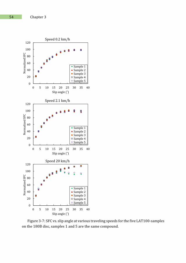
54 Chapter 3
Figure 3-7: SFC vs. slip angle at various traveling speeds for the five LAT100-samples
on the 180B disc, samples 1 and 5 are the same compound.
0
20
40
60
80
100
120
0 5 10 15 20 25 30 35 40
No
rmal
ized
SF
C
Slip angle (˚)
Speed 0.2 km/h
Sample 1Sample 2Sample 3Sample 4Sample 5
0
20
40
60
80
100
120
0 5 10 15 20 25 30 35 40
No
rmal
ized
SF
C
Slip angle (˚)
Speed 2.1 km/h
Sample 1Sample 2Sample 3Sample 4Sample 5
0
20
40
60
80
100
120
0 5 10 15 20 25 30 35 40
No
rmal
ized
SF
C
Slip angle (˚)
Speed 20 km/h
Sample 1Sample 2Sample 3Sample 4Sample 5
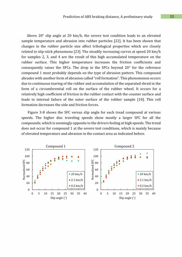
55 Prediction of ABS braking distance, A preliminary study
Above 20° slip angle at 20 km/h, the severe test condition leads to an elevated
sample temperature and abrasion into rubber particles [22]. It has been shown that
changes in the rubber particle size affect tribological properties which are closely
related to slip-stick phenomena [23]. The steadily increasing curves at speed 20 km/h
for samples 2, 3, and 4 are the result of this high accumulated temperature on the
rubber surface. This higher temperature increases the friction coefficients and
consequently raises the SFCs. The drop in the SFCs beyond 20° for the reference
compound 1 most probably depends on the type of abrasion pattern. This compound
abrades with another form of abrasion called “roll formation”. This phenomenon occurs
due to continuous tearing of the rubber and accumulation of the separated shred in the
form of a circumferential roll on the surface of the rubber wheel. It occurs for a
relatively high coefficient of friction in the rubber contact with the counter surface and
leads to internal failure of the outer surface of the rubber sample [10]. This roll
formation decreases the side and friction forces.
Figure 3-8 shows the SFC versus slip angle for each tread compound at various
speeds. The higher disc traveling speeds show mostly a larger SFC for all the
compounds; which is seemingly opposite to the drivers feeling at high speeds. The trend
does not occur for compound 1 at the severe test conditions, which is mainly because
of elevated temperature and abrasion in the contact area as indicated before.
0
20
40
60
80
100
120
0 5 10 15 20 25 30 35 40
No
rmal
ized
SF
C
Slip angle (˚)
Compound 1
20 km/h
2.1 km/h
0.2 km/h
0
20
40
60
80
100
120
0 5 10 15 20 25 30 35 40
No
rmal
ized
SF
C
Slip angle (˚)
Compound 2
20 km/h
2.1 km/h
0.2 km/h
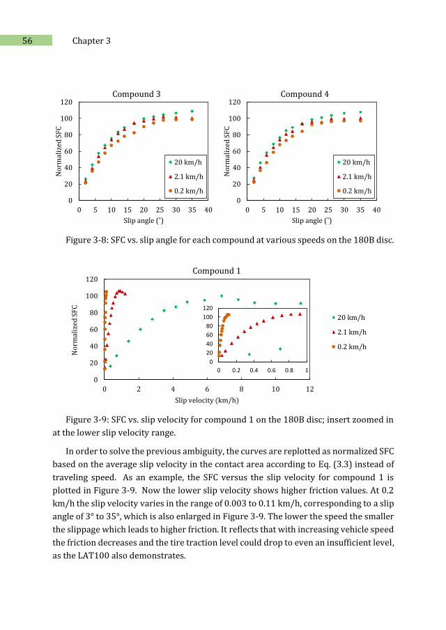
56 Chapter 3
Figure 3-8: SFC vs. slip angle for each compound at various speeds on the 180B disc.
Figure 3-9: SFC vs. slip velocity for compound 1 on the 180B disc; insert zoomed in
at the lower slip velocity range.
In order to solve the previous ambiguity, the curves are replotted as normalized SFC
based on the average slip velocity in the contact area according to Eq. (3.3) instead of
traveling speed. As an example, the SFC versus the slip velocity for compound 1 is
plotted in Figure 3-9. Now the lower slip velocity shows higher friction values. At 0.2
km/h the slip velocity varies in the range of 0.003 to 0.11 km/h, corresponding to a slip
angle of 3° to 35°, which is also enlarged in Figure 3-9. The lower the speed the smaller
the slippage which leads to higher friction. It reflects that with increasing vehicle speed
the friction decreases and the tire traction level could drop to even an insufficient level,
as the LAT100 also demonstrates.
0
20
40
60
80
100
120
0 5 10 15 20 25 30 35 40
No
rmal
ized
SF
C
Slip angle (˚)
Compound 3
20 km/h
2.1 km/h
0.2 km/h
0
20
40
60
80
100
120
0 5 10 15 20 25 30 35 40
No
rmal
ized
SF
CSlip angle (˚)
Compound 4
20 km/h
2.1 km/h
0.2 km/h
0
20
40
60
80
100
120
0 2 4 6 8 10 12
No
rmal
ized
SF
C
Slip velocity (km/h)
Compound 1
20 km/h
2.1 km/h
0.2 km/h
0
20
40
60
80
100
120
0 0.2 0.4 0.6 0.8 1
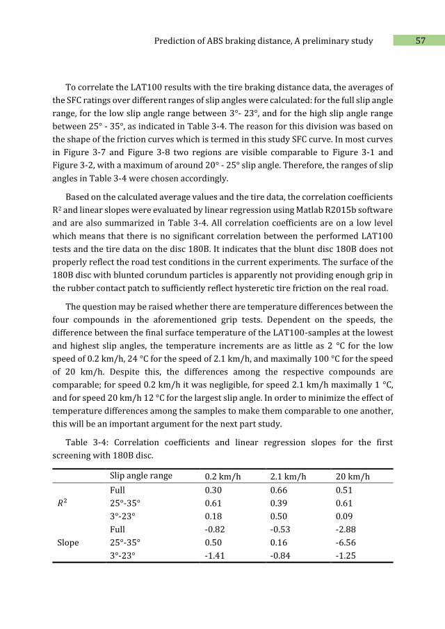
57 Prediction of ABS braking distance, A preliminary study
To correlate the LAT100 results with the tire braking distance data, the averages of
the SFC ratings over different ranges of slip angles were calculated: for the full slip angle
range, for the low slip angle range between 3°- 23°, and for the high slip angle range
between 25° - 35°, as indicated in Table 3-4. The reason for this division was based on
the shape of the friction curves which is termed in this study SFC curve. In most curves
in Figure 3-7 and Figure 3-8 two regions are visible comparable to Figure 3-1 and
Figure 3-2, with a maximum of around 20° - 25° slip angle. Therefore, the ranges of slip
angles in Table 3-4 were chosen accordingly.
Based on the calculated average values and the tire data, the correlation coefficients
R2 and linear slopes were evaluated by linear regression using Matlab R2015b software
and are also summarized in Table 3-4. All correlation coefficients are on a low level
which means that there is no significant correlation between the performed LAT100
tests and the tire data on the disc 180B. It indicates that the blunt disc 180B does not
properly reflect the road test conditions in the current experiments. The surface of the
180B disc with blunted corundum particles is apparently not providing enough grip in
the rubber contact patch to sufficiently reflect hysteretic tire friction on the real road.
The question may be raised whether there are temperature differences between the
four compounds in the aforementioned grip tests. Dependent on the speeds, the
difference between the final surface temperature of the LAT100-samples at the lowest
and highest slip angles, the temperature increments are as little as 2 °C for the low
speed of 0.2 km/h, 24 °C for the speed of 2.1 km/h, and maximally 100 °C for the speed
of 20 km/h. Despite this, the differences among the respective compounds are
comparable; for speed 0.2 km/h it was negligible, for speed 2.1 km/h maximally 1 °C,
and for speed 20 km/h 12 °C for the largest slip angle. In order to minimize the effect of
temperature differences among the samples to make them comparable to one another,
this will be an important argument for the next part study.
Table 3-4: Correlation coefficients and linear regression slopes for the first
screening with 180B disc.
Slip angle range 0.2 km/h 2.1 km/h 20 km/h
𝑅2
Full 0.30 0.66 0.51
25°-35° 0.61 0.39 0.61
3°-23° 0.18 0.50 0.09
Slope
Full -0.82 -0.53 -2.88
25°-35° 0.50 0.16 -6.56
3°-23° -1.41 -0.84 -1.25
58 Chapter 3
Subsequently, to determine which disc predicts the road conditions, a set of
experiments including the three additional surface roughness discs at a constant
moderate speed of 2.1 km/h were performed: Table 3-3, row 2. The constant speed of
2.1 km/h was adopted from the previous measurements, wherefore the SFC curves
covered all regions indicated in Figure 3-1 and the differences between the surface
temperatures among all compounds were comparable.
The results for all compounds are shown in Figure 3-10; the larger the disc grain
size the lower the SFC. A smaller grain size induces a larger real contact area because of
the higher number of asperities within the apparent unit area. This is due to the fact
that the rubber can follow and penetrate into the indentations of the counter-surface,
as determined by the hardness/modulus of the compound. Although a single surface
irregularity induces lower hysteretic friction, the cumulative frequential excitation of
the rubber over all irregularities of the counter surface is higher: Figure 3-3. The higher
the cumulative hysteresis, the higher the SFC which leads to more energy dissipation of
the rubber. This explains the higher hysteretic friction for disc 320 in the range of
surface irregularities according to Table 3-2. On the other side, the disc 60 induces the
lowest SFCs, because it has the biggest particle size and highest rms as a surface
parameter in Figure 3-6.
In spite of the same particle size of discs 180 and 180B, the blunting has reduced the
rms to approximately the same level as disc 320, as indicated by the height order in the
laser microscopic images: Figure 3-6. The disc 320 shows SFC values mostly in the same
order as the 180B disc. Because of the flattening process of the 180B, it may result in a
lower hysteretic component and a higher contribution of an adhesion component. The
contributions of both friction components in dependence of speed and surface micro-
and macro-structure remain a point of debate. Persson in his review article of 2005 [9]
implied that there is almost no adhesion between a rubber ball and a substrate with a
rms larger than 1 μm. The order of magnitude of all employed discs rms is much higher
for all. Grosch and others state that the adhesion component still plays a role and has
an important contribution at low speeds and dry conditions [15, 24-27] which was
extensively discussed based on the area of real contact for dry rubber friction [27].
Wagner even suggested an adhesive part for wet surfaces [25]. The results of the
present study indicate that the lower disc rms and particle size are both involved in
higher friction. Anyhow, the argument here is not to identify which friction component
is responsible for these phenomena. For this purpose, more experiments would be
needed in order to identify the friction components [14, 25, 28, 29]. The current results
are showing that the lateral friction force decreases with increasing the measured rms,
and the LAT100 clearly distinguishes this.
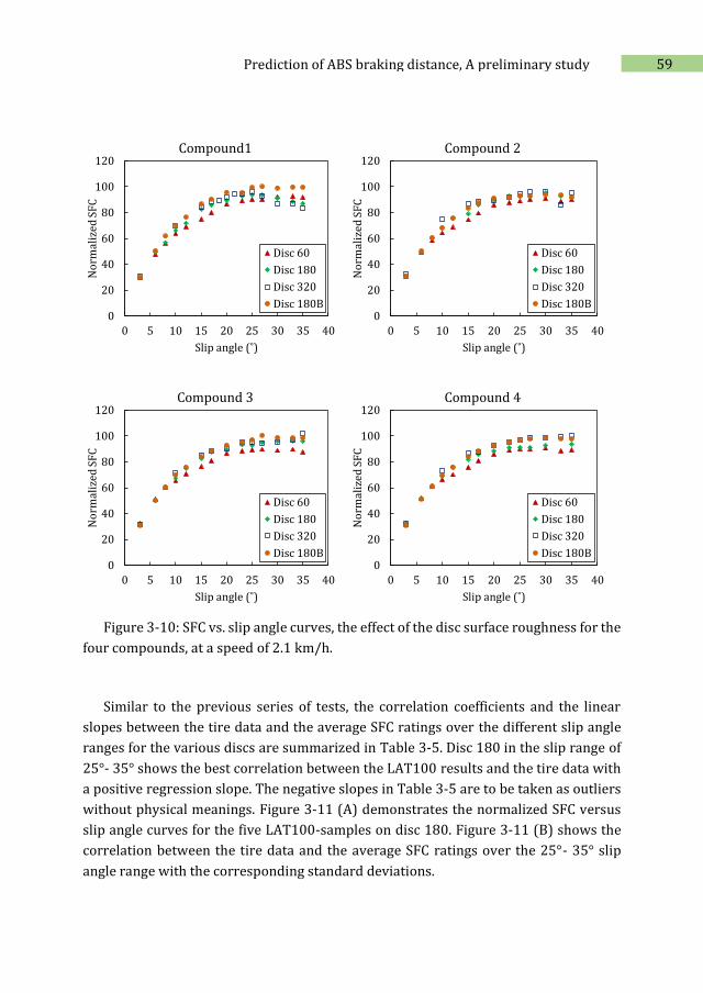
59 Prediction of ABS braking distance, A preliminary study
Figure 3-10: SFC vs. slip angle curves, the effect of the disc surface roughness for the
four compounds, at a speed of 2.1 km/h.
Similar to the previous series of tests, the correlation coefficients and the linear
slopes between the tire data and the average SFC ratings over the different slip angle
ranges for the various discs are summarized in Table 3-5. Disc 180 in the slip range of
25°- 35° shows the best correlation between the LAT100 results and the tire data with
a positive regression slope. The negative slopes in Table 3-5 are to be taken as outliers
without physical meanings. Figure 3-11 (A) demonstrates the normalized SFC versus
slip angle curves for the five LAT100-samples on disc 180. Figure 3-11 (B) shows the
correlation between the tire data and the average SFC ratings over the 25°- 35° slip
angle range with the corresponding standard deviations.
0
20
40
60
80
100
120
0 5 10 15 20 25 30 35 40
No
rmal
ized
SF
C
Slip angle (˚)
Compound1
Disc 60
Disc 180
Disc 320
Disc 180B0
20
40
60
80
100
120
0 5 10 15 20 25 30 35 40
No
rmal
ized
SF
CSlip angle (˚)
Compound 2
Disc 60
Disc 180
Disc 320
Disc 180B
0
20
40
60
80
100
120
0 5 10 15 20 25 30 35 40
No
rmal
ized
SF
C
Slip angle (˚)
Compound 3
Disc 60
Disc 180
Disc 320
Disc 180B0
20
40
60
80
100
120
0 5 10 15 20 25 30 35 40
No
rmal
ized
SF
C
Slip angle (˚)
Compound 4
Disc 60
Disc 180
Disc 320
Disc 180B
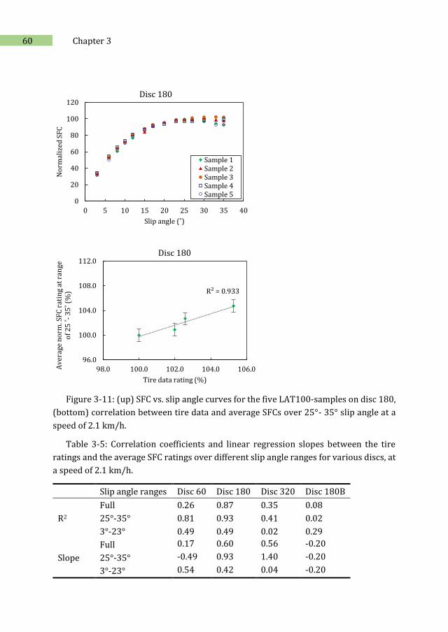
60 Chapter 3
Figure 3-11: (up) SFC vs. slip angle curves for the five LAT100-samples on disc 180,
(bottom) correlation between tire data and average SFCs over 25°- 35° slip angle at a
speed of 2.1 km/h.
Table 3-5: Correlation coefficients and linear regression slopes between the tire
ratings and the average SFC ratings over different slip angle ranges for various discs, at
a speed of 2.1 km/h.
Slip angle ranges Disc 60 Disc 180 Disc 320 Disc 180B
R2
Full 0.26 0.87 0.35 0.08
25°-35° 0.81 0.93 0.41 0.02
3°-23° 0.49 0.49 0.02 0.29
Slope
Full 0.17 0.60 0.56 -0.20
25°-35° -0.49 0.93 1.40 -0.20
3°-23° 0.54 0.42 0.04 -0.20
0
20
40
60
80
100
120
0 5 10 15 20 25 30 35 40
No
rmal
ized
SF
C
Slip angle (˚)
Disc 180
Sample 1Sample 2Sample 3Sample 4Sample 5
R² = 0.933
96.0
100.0
104.0
108.0
112.0
98.0 100.0 102.0 104.0 106.0Av
erag
e n
orm
. SF
C r
atin
g at
ran
ge
of
25
˚-
35
˚ (%
)
Tire data rating (%)
Disc 180
61 Prediction of ABS braking distance, A preliminary study
It does indicate that the disc surface roughness has a significant influence on the
collected SFCs with the LAT100 as discussed. Disc 180 simulates the tire condition on
the road the best and accordingly gives a promising correlation between the lab results
and the current ABS braking distance data, provided the LAT100 data are taken in the
slip angle range between 25° – 35°. The original, non-blunted asperities from the
corundum-particles in the present disc 180 do provide a substantial contribution of
hysteretic friction contact relative to the blunted variant. By comparison of Figure 3-1
and Figure 3-2 with Figure 3-11(A) it is clear that the transitional region observed
within this slip angle range does correspond with the transitional region of the
longitudinal tire friction force, ref. Eq. (3.1), there where ABS-braking is indeed active.
The applied normal load of 75 N on the LAT100-samples corresponds to around
0.34 MPa contact pressure in the LAT100-sample apparent contact area, which is
approximately 2.2 cm2 for a rubber sample with a medium hardness of 65 °Sh A. This
contact pressure is in a similar range like for an average size passenger car tire. The
maximum coefficient of friction for a car tire is expected for a slip rate between 5% and
15% [30]. For example, based on Eq. (3.1) the slip velocity of a car tire traveling at 90
km/h at 10% slip ratio is 2.5 m/s. The correlation presented in Figure 3-11(B) was
made for a traveling speed of 2.1 km/h and in the range of 25° – 35° slip angle.
Therefore, it is possible to estimate the average slip velocity in the contact area of the
LAT100-samples according to Eq. (3.3) which is calculated to be 0.29 m/s for the 5
experimental points for each LAT100-sample in the range of 25° – 35° slip angle in
Figure 3-11(A). This value of 0.29 m/s is around 8 times smaller than the tire slip
velocity which is comparable to the ratio of tire circumference to the LAT100 wheel
circumference. This is still an interesting point to be studied further by modeling and
investigating the difference between the friction mechanisms: the longitudinal friction
for ABS braking and the lateral type friction for the LAT100 wheel.
The question is why the disc 180 offered the best correlation. By comparing the
surface roughness parameter before and after the test procedures: Table 3-6, it is
observed that except for disc 60, there are no large changes of rms. This shows that the
discs except for 60, remain stable during the test procedure. A possible reason for the
strong correlation for disc 180 is similarity of the frequential excitations of the tread
compounds in their respective counter-surface contact areas: between the LAT100-
samples and the disc, the tires on the road. As soon as a LAT100-sample starts slipping
on disc 180, the macro- and micro-roughness of the counter surface causes a frequential
excitation of the rubber. This has to be in a similar range as the penetration of tire
rubber into the indentations of the road surface. This excitation frequency is dependent
on the distance between surface irregularities and the slip velocity of the rubber over
62 Chapter 3
the counter-surface [30]. Provided that the frequency is calculated according to the
surface macro-irregularities with a distance d (m):
Frequency (𝑠−1)= slip velocity ( 𝑚
𝑠⁄ )
d (m) (3.6)
for the average slip velocity of 0.29 m/s of disc 180 with a distance of 200 μm for
hysteresis macro-irregularities (Figure 3-6), the value of this frequential excitation is
1.5*103 s-1. The molecular adhesion frequency range between rubber and a road varies
from 106 s-1 to 109 s-1 and for hysteresis due to road roughness between 102 s-1 to 106 s-
1 [30]. The value of 1.5*103 s-1 is therefore in the range of hysteresis friction or road
indentation. Apparently, adhesion is not playing an important role here. The disc is
composed of a range of particle sizes which are influencing the surface irregularities
distance though. This is an open point for more investigations to estimate the actual
area of contact and the range of frequential excitations. Understanding the grip
mechanism of disc 180 will therefore be the subject of more research.
Table 3-6: surface roughness parameter before and after the test.
Disc designation 60 180 320 180B
Sq* (μm) before 175 65 48 44
Sq* (μm) after 125 50 46 33
*The height ranges below than 10 μm were excluded from the calculations
3.4. Conclusions
To predict the car tire ABS braking distance on dry tracks, friction properties of solid
rubber wheels were measured using the Laboratory Abrasion Tester (LAT100). Tires
with four different tread compounds were rated by measuring ABS braking distances
on the road. The same compounds were characterized on the LAT100 at various
traveling speeds and surface roughness of the counter-discs. At a constant slip velocity
the Side Force Coefficient (SFC) decreased with increasing speed. The LAT100 clearly
distinguishes the effect of disc surface roughness on the SFC. The lower the disc grain
size and rms roughness, the higher the SFC because of the larger real contact area of the
rubbers with the electro-corundum discs. That induces a higher cumulative frequential
excitation of the rubber over the irregularities of the counter surface. The results of
LAT100 were further correlated with the tire data. Disc 180 shows the best correlation
63 Prediction of ABS braking distance, A preliminary study
and the most promising results among the various discs. It reflects the road surface
conditions in the best way between the available tire data and LAT100 test conditions
with a correlation coefficient of 0.93 for the four tread compounds. It has a high
potential for predicting the car tire ABS braking distance.
3.5. References
1. Haney, P., The Racing & High-performance Tire: Using the Tires to Tune for Grip and Balance, in Book. 2003, Co-published by TV MOTORSPORT, Springfield, IL and Society of Automotive Engineers, Inc., Warrendale, PA, USA. p. 5-50.
2. Rajamani, R., Lateral and Longitudinal Tire Forces, in Book 'Vehicle Dynamics and Control'. 2012, Springer US. p. 387-432.
3. Majerus, J.N., your tire's behavior, in Book 'Winning More Safely in Motorsports; the Workbook'. 2007, Racing vehicle Inc. p. 268-283.
4. Miller, S.L., B. Youngberg, A. Millie, P. Schweizer, and J.C. Gerdes. Calculation Longitudinal wheel slip and tire parameters using GPS velocity. in the American control conference. 25-27 Jun 2001. Arlington.
5. Si-Wei, Z., ed. Chapter 1 Introduction. Tribology and Interface Engineering Series, ed. Z. Si-Wei. Vol. Volume 47. 2004, Elsevier. 1-6.
6. Brown, R., friction and wear, in Book 'Physical testing of rubbers'. 2006, Springer. p. 219-243.
7. Grosch, K.A., The Rolling Resistance, Wear and Traction Properties of Tread Compounds. Rubber Chemistry and Technology, 1996. 69(3): p. 495-568.
8. Heinrich, G. and M. Klüppel, Rubber friction, tread deformation and tire traction. Wear, 2008. 265(7–8): p. 1052-1060.
9. Persson, B.N.J., O. Albohr, U. Tartaglino, A.I. Volokitin, and E. Tosatti, On the nature of surface roughness with application to contact mechanics, sealing, rubber friction and adhesion. J Phys Condens Matter, 2005. 17(1): p. R1-r62.
10. Moore, D.F., Abrasion and wear, in Book 'The friction and lubrication of elastomers'. 1972, Pergamon press Inc. p. 252-274.
11. Deleau, F., D. Mazuyer, and A. Koenen, Sliding friction at elastomer/glass contact: Influence of the wetting conditions and instability analysis. Tribology International, 2009. 42(1): p. 149-159.
12. Flintsch, G.W., E.d.L. Izeppi, K.K. McGhee, and S. Najafi, The little book of tire pavement friction. 1.0 ed. 2012: Pavement Surface Properties Consortium, Virginia Tech.
64 Chapter 3
13. Klüppel, M. and G. Heinrich, Rubber Friction on Self-Affine Road Tracks. Rubber Chemistry and Technology, 2000. 73(4): p. 578-606.
14. Persson, B.N.J., Theory of rubber friction and contact mechanics. The Journal of Chemical Physics, 2001. 115(8): p. 3840-3861.
15. Grosch, K.A., Goodyear Medalist Lecture. Rubber Friction and its Relation to Tire Traction. Rubber Chemistry and Technology, 2007. 80(3): p. 379-411.
16. Grosch, K.A., A new way to evaluate traction-and wear properties of tire tread compounds, in Rubber Division, American Chemical Society. 1997: Cleveland, Ohio.
17. Heinz, M., A Universal Method to Predict Wet Traction Behaviour of Tyre Tread Compounds in the Laboratory. Journal of Rubber Research, 2010. 13(2): p. 91-102.
18. Heinz, M. and K.A. Grosch, A Laboratory Method to Comprehensively Evaluate Abrasion, Traction and Rolling Resistance of Tire Tread Compounds. Rubber Chemistry and Technology, 2007. 80(4): p. 580-607.
19. Grosch, K.A., Correlation Between Road Wear of Tires and Computer Road Wear Simulation Using Laboratory Abrasion Data. Rubber Chemistry and Technology, 2004. 77(5): p. 791-814.
20. Grosch, K.A., Rubber Abrasion and Tire Wear. Rubber Chemistry and Technology, 2008. 81(3): p. 470-505.
21. Riehm, P., H.-J. Unrau, and F. Gauterin, A model based method to determine rubber friction data based on rubber sample measurements. Tribology International, 2018.
22. Schallamach, A., The Velocity and Temperature Dependence of Rubber Friction. Proceedings of the Physical Society. Section B, 1953. 66(5): p. 386.
23. Chang, Y.H., B.S. Joo, S.M. Lee, and H. Jang, Size effect of tire rubber particles on tribological properties of brake friction materials. Wear, 2018. 394-395: p. 80-86.
24. Al-Assi, M. and E. Kassem, Evaluation of Adhesion and Hysteresis Friction of Rubber–Pavement System. Applied Sciences, 2017. 7(10): p. 1029.
25. Wagner, P., P. Wriggers, L. Veltmaat, H. Clasen, C. Prange, and B. Wies, Numerical multiscale modelling and experimental validation of low speed rubber friction on rough road surfaces including hysteretic and adhesive effects. Tribology International, 2017. 111: p. 243-253.
26. Lorenz, B., Y.R. Oh, S.K. Nam, S.H. Jeon, and B.N.J. Persson, Rubber friction on road surfaces: Experiment and theory for low sliding speeds. The Journal of Chemical Physics, 2015. 142(19): p. 194701.
65 Prediction of ABS braking distance, A preliminary study
27. Tiwari, A., N. Miyashita, N. Espallargas, and B.N.J. Persson, Rubber friction: The contribution from the area of real contact. The Journal of chemical physics, 2018. 148(22): p. 224701-224701.
28. Feshanjerdi, M., M. Khorrami, A.A. Masoudi, and M. Razzaghi Kashani, The hysteretic contribution of friction for the polished rubber on the concrete surface. Applied Surface Science, 2017. 394: p. 528-533.
29. Mokhtari, M., D.J. Schipper, and T.V. Tolpekina, On the Friction of Carbon Black- and Silica-Reinforced BR and S-SBR Elastomers. Tribol Lett, 2014. 54: p. 297–308.
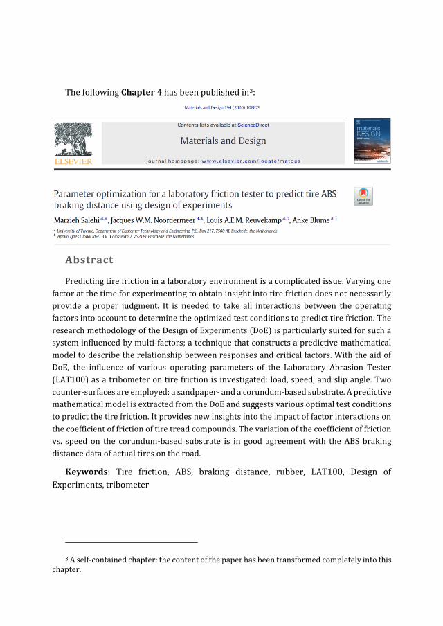
The following Chapter 4 has been published in3:
Abstract
Predicting tire friction in a laboratory environment is a complicated issue. Varying one
factor at the time for experimenting to obtain insight into tire friction does not necessarily
provide a proper judgment. It is needed to take all interactions between the operating
factors into account to determine the optimized test conditions to predict tire friction. The
research methodology of the Design of Experiments (DoE) is particularly suited for such a
system influenced by multi-factors; a technique that constructs a predictive mathematical
model to describe the relationship between responses and critical factors. With the aid of
DoE, the influence of various operating parameters of the Laboratory Abrasion Tester
(LAT100) as a tribometer on tire friction is investigated: load, speed, and slip angle. Two
counter-surfaces are employed: a sandpaper- and a corundum-based substrate. A predictive
mathematical model is extracted from the DoE and suggests various optimal test conditions
to predict the tire friction. It provides new insights into the impact of factor interactions on
the coefficient of friction of tire tread compounds. The variation of the coefficient of friction
vs. speed on the corundum-based substrate is in good agreement with the ABS braking
distance data of actual tires on the road.
Keywords: Tire friction, ABS, braking distance, rubber, LAT100, Design of
Experiments, tribometer
3 A self-contained chapter: the content of the paper has been transformed completely into this chapter.
4 Prediction of ABS braking distance
using design of experiments
4.1. Introduction
Evaluating tire grip on the road as an extremely complicated tribological system,
consumes time and energy but is essential for safety. Proper tire grip provides a good
level of handling which is a prerequisite for vehicle steering during cornering, braking,
and accelerating. The tire grip is the result of the generated frictional forces which are
created by the tire slippage in the contact patch. Commonly, with an Anti-lock Braking
System (ABS), the braking force is optimized based on a specific region of tire slippage,
typically 5 to 15 percent [1, 2], to provide adequate frictional forces and avoid tire
skidding. Numerous factors influence tire friction: the tire construction, tread pattern
and composition; the characteristics, condition, and structure of the counter-surface;
and last the weather and temperature conditions [3]. Overall, the tire tread compound
contributes the largest portion of around 75% of grip on a dry surface [4]. Arrigoni S. et
al. reported that the rubber coefficient of friction has the largest influence on ABS
performance: a 5% increase leads to roughly 2 m reduction of ABS braking distance [2].
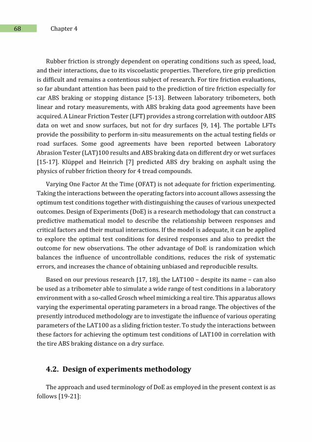
68 Chapter 4
Rubber friction is strongly dependent on operating conditions such as speed, load,
and their interactions, due to its viscoelastic properties. Therefore, tire grip prediction
is difficult and remains a contentious subject of research. For tire friction evaluations,
so far abundant attention has been paid to the prediction of tire friction especially for
car ABS braking or stopping distance [5-13]. Between laboratory tribometers, both
linear and rotary measurements, with ABS braking data good agreements have been
acquired. A Linear Friction Tester (LFT) provides a strong correlation with outdoor ABS
data on wet and snow surfaces, but not for dry surfaces [9, 14]. The portable LFTs
provide the possibility to perform in-situ measurements on the actual testing fields or
road surfaces. Some good agreements have been reported between Laboratory
Abrasion Tester (LAT)100 results and ABS braking data on different dry or wet surfaces
[15-17]. Klüppel and Heinrich [7] predicted ABS dry braking on asphalt using the
physics of rubber friction theory for 4 tread compounds.
Varying One Factor At the Time (OFAT) is not adequate for friction experimenting.
Taking the interactions between the operating factors into account allows assessing the
optimum test conditions together with distinguishing the causes of various unexpected
outcomes. Design of Experiments (DoE) is a research methodology that can construct a
predictive mathematical model to describe the relationship between responses and
critical factors and their mutual interactions. If the model is adequate, it can be applied
to explore the optimal test conditions for desired responses and also to predict the
outcome for new observations. The other advantage of DoE is randomization which
balances the influence of uncontrollable conditions, reduces the risk of systematic
errors, and increases the chance of obtaining unbiased and reproducible results.
Based on our previous research [17, 18], the LAT100 – despite its name – can also
be used as a tribometer able to simulate a wide range of test conditions in a laboratory
environment with a so-called Grosch wheel mimicking a real tire. This apparatus allows
varying the experimental operating parameters in a broad range. The objectives of the
presently introduced methodology are to investigate the influence of various operating
parameters of the LAT100 as a sliding friction tester. To study the interactions between
these factors for achieving the optimum test conditions of LAT100 in correlation with
the tire ABS braking distance on a dry surface.
4.2. Design of experiments methodology
The approach and used terminology of DoE as employed in the present context is as
follows [19-21]:
69 Prediction of ABS braking distance using design of experiments
Factors: can be denoted as input variables that affect the process or the final
outputs. Factors can be continuous (velocity, load, …) or categorical (a type
of surfaces or additives, …).
Responses: the product or process characteristics of interest to the
experimenter and often referred to as output variables, e.g. coefficient of
friction, correlation coefficient, the goodness of a fit. Adequate response
criteria are Specific, Measurable, Attainable, Realistic and Time-limited
(SMART).
Factor levels: the particular values or types of factors. For a continuous
factor such as velocity, the levels could be 1 km/h and 2 km/h, and a
categorical factor, such as type of surface could be type1: sandpaper, type2:
asphalt, etc.
Design: a pre-defined set of experimental runs e.g. two-level full (fractional)
factorial or multi-level central composite design.
Model: a predictive mathematical equation describing the response as a
function of the factors;
Main effect: there is a main effect when different levels of one factor affect
the response differently.
Interaction effect: when the effect of one factor depends on the level of the
other factor. An interaction plot can be used to visualize possible
interactions.
Residuals (or residual error): the difference or the error between the
observed value and the predicted value by the model.
The reader is referred to 4.7.1 for details and elaborations on steps taken for the
DoE and interpretations of the results.
In the present study, experimental designs are defined for load, speed, and slip angle
as influential factors. The initial steps of DoE such as the screening process were
eliminated based on the previous publications and prior knowledge of the LAT100. Two
modeling designs, DoE 1 and 2, are created based on the three factors on two different
experimental tracks of sandpaper P120 and LAT100 disc 180; with large level ranges
to include the extreme test conditions. In the next step, conformation runs were carried
out to compare the results with the predictive mathematical model. Optimization was
carried out by applying a multi-level general factorial DoE 3, which was performed on
the optimal surface. The effect of load and speed was further investigated to explore the
underlying reasons for the correlation and to obtain more insight into the friction
phenomenon.
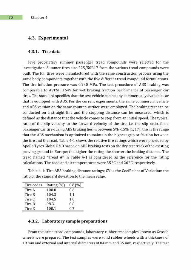
70 Chapter 4
4.3. Experimental
4.3.1. Tire data
Five proprietary summer passenger tread compounds were selected for the
investigation. Summer tires size 225/50R17 from the various tread compounds were
built. The full tires were manufactured with the same construction process using the
same body components together with the five different tread compound formulations.
The tire inflation pressure was 0.230 MPa. The test procedure of ABS braking was
comparable to ASTM F1649 for wet braking traction performance of passenger car
tires. The standard specifies that the test vehicle can be any commercially available car
that is equipped with ABS. For the current experiments, the same commercial vehicle
and ABS version on the same counter-surface were employed. The braking test can be
conducted on a straight line and the stopping distance can be measured, which is
defined as the distance that the vehicle comes to stop from an initial speed. The typical
ratio of the slip velocity to the forward velocity of the tire, i.e. the slip ratio, for a
passenger car tire during ABS braking lies in between 5% -15% [1, 17]; this is the range
that the ABS mechanism is optimized to maintain the highest grip or friction between
the tire and the road. Table 4-1 shows the relative tire ratings which were provided by
Apollo Tyres Global R&D based on ABS braking tests on the dry test track of the existing
proving ground in Europe; the higher the rating the shorter the braking distance. The
tread named “Tread A” in Table 4-1 is considered as the reference for the rating
calculations. The road and air temperatures were 35 °C and 26 °C, respectively.
Table 4-1: Tire ABS braking distance ratings; CV is the Coefficient of Variation: the
ratio of the standard deviation to the mean value.
Tire codes Rating (%) CV (%)
Tire A 100.0 0.6 Tire B 104.3 1.1 Tire C 104.5 1.0 Tire D 98.3 0.8 Tire E 100.1 0.7
4.3.2. Laboratory sample preparations
From the same tread compounds, laboratory rubber test samples known as Grosch
wheels were prepared. The test samples were solid rubber wheels with a thickness of
19 mm and external and internal diameters of 84 mm and 35 mm, respectively. The test
71 Prediction of ABS braking distance using design of experiments
samples were vulcanized in a Wickert laboratory press WLP 1600 for 11 minutes at 170
˚C under a pressure of 160 bar, optimized on basis of tc90 curemeter data. The curing
times of both test laboratory wheels and tire treads were comparable. Finally, the
samples were stored for 24 hours at room temperature, 22 ˚C ±1 ˚C. Therefore, the
initial temperatures of all samples were equal when starting the experiments. After
curing, the samples were pre-conditioned with the LAT100 to remove the vulcanization
skin according to the test conditions which were explained in our previous study [17].
4.3.3. Laboratory test set-up
The LAT100 manufactured by VMI Holland B.V., the Netherlands, is used as the
laboratory tribometer. The details of the test set-up were fully described in our
previous manuscript [17]. The measurement unit consists of a rotary counter-surface
disc with a diameter of 350 mm and a Grosch wheel which is a solid rubber test wheel
fixed to a measuring hub. Using a metal pin the Grosch wheel is locked to the hub so
that it cannot rotate with the counter-surface disc for the current experiments.
Therefore, the sample performs as a locked wheel like a sliding body on the counter-
surface disc, . This differs from our earlier study wherein the rubber wheel was free to
rotate in contact with the disc [17]. The wheel is pressed under a vertical load of 𝐹𝑁 (𝑁)
normal to the driven disc under a specific angle 𝑎. The wheel slides over the counter-
surface as a function of the rotation speed of the disc, however, the sliding speed of the
sample in the contact area is influenced by the disc radius which rises as the slip angle
increases. The resultant frictional forces are generated by means of three input machine
parameters: the disc velocity, the angle known as ‘slip angle’, and the acting normal
force. A schematic view of the measurement unit is depicted in Figure 4-1. The area of
the sliding body in contact with the counter-surface disc is hatched.

72 Chapter 4
R
Metal pin
Vt
Ff
350 mm
3D view
84
mm
35
mm
ɑ
FN
Grosch wheel
front view
ɑCounter-surface disc
angle range
force measuring hub
normal load (FN) regulation
ω
ω
Figure 4-1: Test set-up and rubber wheel under normal load 𝐹𝑁 (N), angle 𝑎 (°),
friction force 𝐹𝑓 (N), and velocity 𝑉𝑡 (km/h).
4.3.4. Set-up of the design of experiments
4.3.4.1. Factors
Table 4-2 shows the input and output parameters of the LAT100 apparatus and the
possible ranges. The selected factors in the current experimental designs were
narrowed to normal load, speed, and (slip) angle. The importance of normal load and
speed is well studied in the rubber tribology field [13, 18, 22-24]. The slip angle
variation not only alters the leading edge of the rubber wheel in contact with the
counter-surface but affects the collected friction and lateral forces in the experimental
set-up as explained due to disc curvature in section 4.3.3. Based on our previous studies,
the distance for each velocity was optimized to the lowest possible amount to obtain a
steady and stable friction coefficient and simultaneously avoid excessive abrasion in
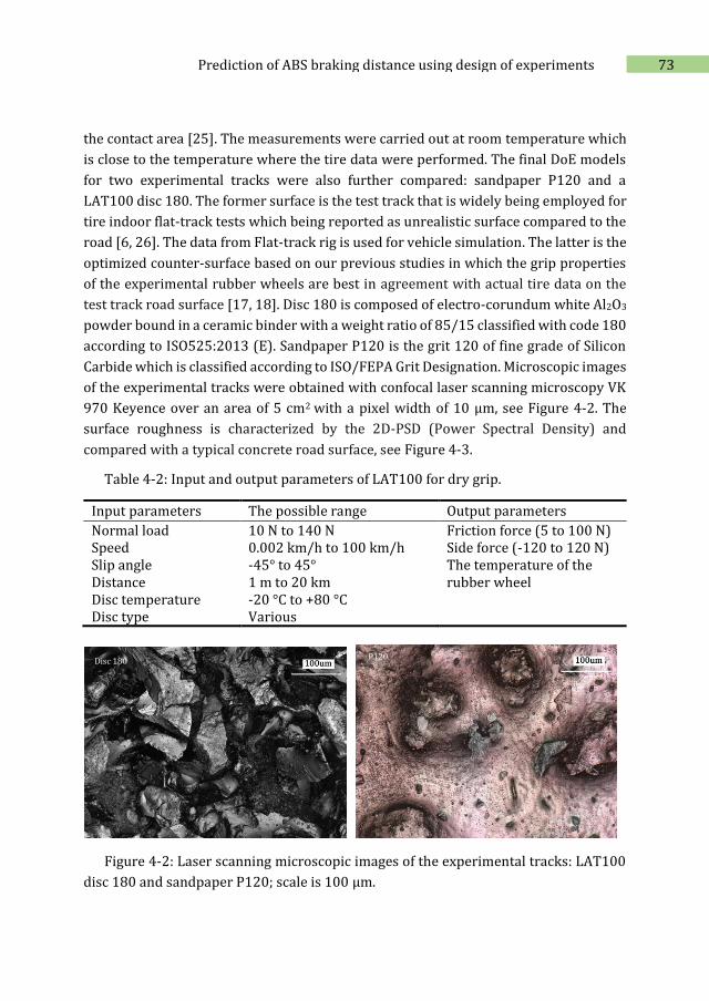
73 Prediction of ABS braking distance using design of experiments
the contact area [25]. The measurements were carried out at room temperature which
is close to the temperature where the tire data were performed. The final DoE models
for two experimental tracks were also further compared: sandpaper P120 and a
LAT100 disc 180. The former surface is the test track that is widely being employed for
tire indoor flat-track tests which being reported as unrealistic surface compared to the
road [6, 26]. The data from Flat-track rig is used for vehicle simulation. The latter is the
optimized counter-surface based on our previous studies in which the grip properties
of the experimental rubber wheels are best in agreement with actual tire data on the
test track road surface [17, 18]. Disc 180 is composed of electro-corundum white Al2O3
powder bound in a ceramic binder with a weight ratio of 85/15 classified with code 180
according to ISO525:2013 (E). Sandpaper P120 is the grit 120 of fine grade of Silicon
Carbide which is classified according to ISO/FEPA Grit Designation. Microscopic images
of the experimental tracks were obtained with confocal laser scanning microscopy VK
970 Keyence over an area of 5 cm2 with a pixel width of 10 μm, see Figure 4-2. The
surface roughness is characterized by the 2D-PSD (Power Spectral Density) and
compared with a typical concrete road surface, see Figure 4-3.
Table 4-2: Input and output parameters of LAT100 for dry grip.
Input parameters The possible range Output parameters
Normal load Speed Slip angle Distance Disc temperature Disc type
10 N to 140 N 0.002 km/h to 100 km/h -45° to 45° 1 m to 20 km -20 °C to +80 °C Various
Friction force (5 to 100 N) Side force (-120 to 120 N) The temperature of the rubber wheel
Disc 180
P120
Figure 4-2: Laser scanning microscopic images of the experimental tracks: LAT100
disc 180 and sandpaper P120; scale is 100 μm.
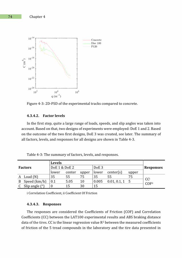
74 Chapter 4
Figure 4-3: 2D-PSD of the experimental tracks compared to concrete.
4.3.4.2. Factor levels
In the first step, quite a large range of loads, speeds, and slip angles was taken into
account. Based on that, two designs of experiments were employed: DoE 1 and 2. Based
on the outcome of the two first designs, DoE 3 was created, see later. The summary of
all factors, levels, and responses for all designs are shown in Table 4-3.
Table 4-3: The summary of factors, levels, and responses.
Factors Levels
Responses DoE 1 & DoE 2 DoE 3 lower center upper lower center(s) upper
A Load (N) 35 55 75 35 55 75 CCi COFii
B Speed (km/h) 0.1 5.05 10 0.005 0.01, 0.1, 1 5 C Slip angle (°) 0 15 30 15
i Correlation Coefficient, ii Coefficient Of Friction
4.3.4.3. Responses
The responses are considered the Coefficients of Friction (COF) and Correlation
Coefficients (CC) between the LAT100 experimental results and ABS braking distance
data of the tires. CC is the linear regression value R2 between the measured coefficients
of friction of the 5 tread compounds in the laboratory and the tire data presented in
75 Prediction of ABS braking distance using design of experiments
Table 4-1. To avoid confusion between R2 of the response value and R-sq of the
predictive mathematical models, the notation of CC is being used for the response.
4.3.4.4. Designs and calculations
Multi-level designs were selected for the present study. The properties of a full
factorial design are an excellent approach for the experimenter to be aware of
confounding4 effects. DoE 1 and 2 were performed with Response Surface Modeling
(RSM, see 4.7.1) using a Face-centered Central Composite (FCC) design for the 3 factors.
DoE 3 was created to optimize the output of the first two designs by exploiting a multi-
level full factorial design with 5 levels for speed and 3 levels for the load. The (cube)
plots of the designs are illustrated in Figure 4-4. One example of 20 test runs of test
conditions according to FCC design is shown in Table 4-4, as carried out for each
compound. The 20 runs were performed for all 5 compounds, a total of 100 experiments
with additional randomization of the wheel specimens A-E. This reduces the effect of
compound type in the sequence of test runs. It should be noted that in Table 4-4 due to
randomization the design order and run order are different, as was employed for all of
the design experiments in the present study.
A novel and effective way of cleaning the counter-surface was developed within the
project, in which the trace of previous rubber compounds was removed from the
experimental tracks. Using a rubber eraser with a unique formulation, the trace and
effect of the previous compound were fully erased before each test run, see Figure 4-5.
The coefficients of friction were calculated by dividing the friction force by the
applied normal load for 100 experiments for DoE 1 and 2. Then, each set of friction
coefficients for the 5 compounds at every test condition of Table 4-4 were correlated
linearly to the ABS braking distance data for the 5 tires. The response CC, the regression
coefficients of the 20 runs of experiments for the 5 compounds, were applied for the
interpretations of the experimental designs and the generation of the predictive models
with statistical analysis. An overview of the whole experimental designs is given in
Table 4-5.
4 Confounding: a situation in which a measure of association or relationship between exposure and outcome is distorted by the presence of another variable [https://online.stat.psu.edu/stat507/node/34/].
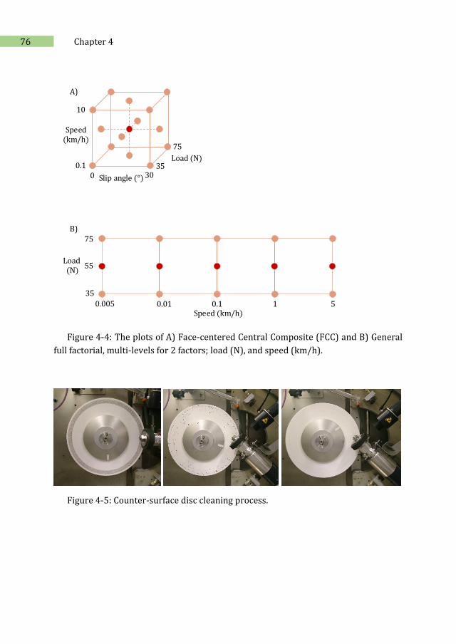
76 Chapter 4
Speed(km/h)
Slip angle (°)
Load (N)
10
0.10 30
35
75
A)
Load (N)
Speed (km/h)0.005
35
0.01 0.1 1 5
75
55
B)
Figure 4-4: The plots of A) Face-centered Central Composite (FCC) and B) General
full factorial, multi-levels for 2 factors; load (N), and speed (km/h).
Figure 4-5: Counter-surface disc cleaning process.
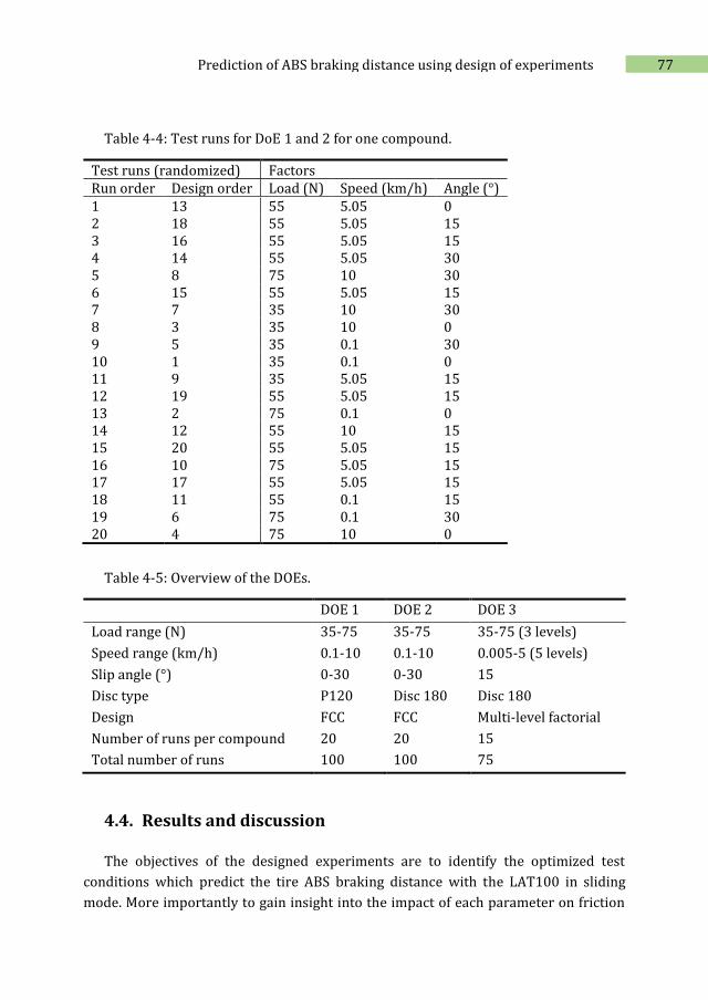
77 Prediction of ABS braking distance using design of experiments
Table 4-4: Test runs for DoE 1 and 2 for one compound.
Test runs (randomized) Factors Run order Design order Load (N) Speed (km/h) Angle (°) 1 13 55 5.05 0 2 18 55 5.05 15 3 16 55 5.05 15 4 14 55 5.05 30 5 8 75 10 30 6 15 55 5.05 15 7 7 35 10 30 8 3 35 10 0 9 5 35 0.1 30 10 1 35 0.1 0 11 9 35 5.05 15 12 19 55 5.05 15 13 2 75 0.1 0 14 12 55 10 15 15 20 55 5.05 15 16 10 75 5.05 15 17 17 55 5.05 15 18 11 55 0.1 15 19 6 75 0.1 30 20 4 75 10 0
Table 4-5: Overview of the DOEs.
DOE 1 DOE 2 DOE 3
Load range (N) 35-75 35-75 35-75 (3 levels)
Speed range (km/h) 0.1-10 0.1-10 0.005-5 (5 levels)
Slip angle (°) 0-30 0-30 15
Disc type P120 Disc 180 Disc 180
Design FCC FCC Multi-level factorial
Number of runs per compound 20 20 15
Total number of runs 100 100 75
4.4. Results and discussion
The objectives of the designed experiments are to identify the optimized test
conditions which predict the tire ABS braking distance with the LAT100 in sliding
mode. More importantly to gain insight into the impact of each parameter on friction
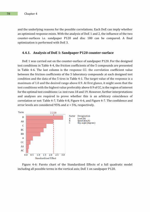
78 Chapter 4
and the underlying reasons for the possible correlations. Each DoE can imply whether
an optimized response exists. With the analysis of DoE 1 and 2, the influence of the two
counter-surfaces i.e. sandpaper P120 and disc 180 can be compared. A final
optimization is performed with DoE 3.
4.4.1. Analysis of DoE 1: Sandpaper P120 counter-surface
DoE 1 was carried out on the counter-surface of sandpaper P120. For the designed
test conditions in Table 4-4, the friction coefficients of the 5 compounds are presented
in Table 4-6. The last column is the response CC: the correlation coefficient value
between the friction coefficients of the 5 laboratory compounds at each designed test
condition and the data of the 5 tires in Table 4-1. The target value of the response is a
maximum of 1.0 and the desired range above 0.9. At first glance, it might seem that the
test conditions with the highest value preferably above 0.9 of CC, is the region of interest
for the optimal test conditions: i.e. test runs 18 and 19. However, further interpretations
and analyses are required to prove whether this is an arbitrary coincidence of
correlation or not: Table 4-7, Table 4-8, Figure 4-6, and Figure 4-7. The confidence and
error levels are considered 95% and 𝛼 = 5%, respectively.
Figure 4-6: Pareto chart of the Standardized Effects of a full quadratic model
including all possible terms in the vertical axis; DoE 1 on sandpaper P120.
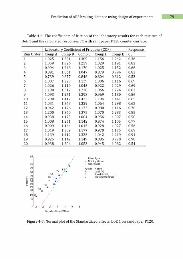
79 Prediction of ABS braking distance using design of experiments
Table 4-6: The coefficients of friction of the laboratory results for each test run of
DoE 1 and the calculated responses CC with sandpaper P120 counter-surface.
Laboratory Coefficient of Frictions (COF) Response Run Order Comp A Comp B Comp C Comp D Comp E CC 1 1.025 1.221 1.309 1.156 1.242 0.36 2 1.059 1.326 1.259 1.029 1.191 0.83 3 0.994 1.248 1.170 1.025 1.152 0.66 4 0.891 1.061 1.047 0.879 0.994 0.82 5 0.739 0.877 0.846 0.804 0.812 0.53 6 1.007 1.229 1.129 1.006 1.116 0.69 7 1.026 1.119 1.045 0.922 1.029 0.69 8 1.190 1.317 1.278 1.066 1.224 0.83 9 1.093 1.251 1.293 0.969 1.180 0.86 10 1.290 1.412 1.473 1.194 1.441 0.65 11 1.031 1.368 1.329 1.064 1.298 0.65 12 0.942 1.176 1.173 0.980 1.116 0.70 13 1.200 1.360 1.375 1.070 1.283 0.85 14 0.938 1.173 1.004 0.956 1.007 0.50 15 1.008 1.261 1.142 0.974 1.105 0.77 16 0.909 1.164 1.015 0.928 1.027 0.56 17 1.019 1.309 1.177 0.970 1.175 0.69 18 1.139 1.412 1.333 1.042 1.219 0.91 19 0.925 1.142 1.149 0.885 0.970 0.98 20 0.938 1.204 1.053 0.945 1.082 0.54
Figure 4-7: Normal plot of the Standardized Effects; DoE 1 on sandpaper P120.
3210-1-2-3
99
95
90
80706050403020
10
5
1
A Load (N)B Speed (km/h)C Slip angle (degrees)
Factor Name
Standardized Effect
Pe
rcen
t
Not SignificantSignificant
Effect Type
BC
AC
AB
CC
BB
AA
C
B
A
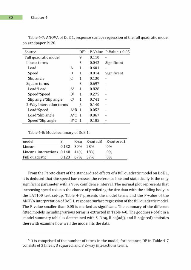
80 Chapter 4
Table 4-7: ANOVA of DoE 1, response surface regression of the full quadratic model
on sandpaper P120.
Source DF5 P-Value P-Value < 0.05
Full quadratic model 9 0.110 -
Linear terms 3 0.042 Significant
Load A 1 0.601 -
Speed B 1 0.014 Significant
Slip angle C 1 0.130 -
Square terms 3 0.697 -
Load*Load A2 1 0.828 -
Speed*Speed B2 1 0.275 -
Slip angle*Slip angle C2 1 0.741 -
2-Way Interaction terms 3 0.140 -
Load*Speed A*B 1 0.052 -
Load*Slip angle A*C 1 0.867 -
Speed*Slip angle B*C 1 0.185 -
Table 4-8: Model summary of DoE 1.
model S R-sq R-sq(adj) R-sq(pred)
Linear 0.132 39% 28% 0%
Linear + interactions 0.140 44% 18% 0%
Full quadratic 0.123 67% 37% 0%
From the Pareto chart of the standardized effects of a full quadratic model on DoE 1,
it is deduced that the speed bar crosses the reference line and statistically is the only
significant parameter with a 95% confidence interval. The normal plot represents that
increasing speed reduces the chance of predicting the tire data with the sliding body in
the LAT100 test set-up. Table 4-7 presents the model terms and the P-value of the
ANOVA interpretation of DoE 1, response surface regression of the full quadratic model.
The P-value smaller than 0.05 is marked as significant. The summary of the different
fitted models including various terms is extracted in Table 4-8. The goodness-of-fit in a
‘model summary table’ is determined with S, R-sq, R-sq(adj), and R-sq(pred) statistics
therewith examine how well the model fits the data.
5 It is comprised of the number of terms in the model; for instance, DF in Table 4-7 consists of 3 linear, 3 squared, and 3 2-way interactions terms.
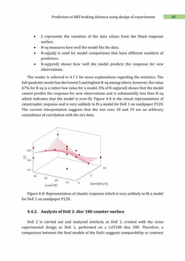
81 Prediction of ABS braking distance using design of experiments
S represents the variation of the data values from the fitted response
surface.
R-sq measures how well the model fits the data.
R-sq(adj) is used for model comparisons that have different numbers of
predictors.
R-sq(pred) shows how well the model predicts the response for new
observations.
The reader is referred to 4.7.1 for more explanations regarding the statistics. The
full quadratic model has the lowest S and highest R-sq among others, however, the value
67% for R-sq is a rather low value for a model. 0% of R-sq(pred) shows that the model
cannot predict the response for new observations and is substantially less than R-sq
which indicates that the model is over-fit. Figure 4-8 is the visual representation of
catastrophic response and is very unlikely to fit a model for DoE 1 on sandpaper P120.
The current interpretation suggests that the test runs 18 and 19 are an arbitrary
coincidence of correlation with the tire data.
Figure 4-8: Representation of chaotic response which is very unlikely to fit a model
for DoE 1 on sandpaper P120.
4.4.2. Analysis of DoE 2: disc 180 counter-surface
DoE 2 is carried out and analyzed similarly as DoE 1, created with the same
experimental design as DoE 1, performed on a LAT100 disc 180. Therefore, a
comparison between the final models of the DoEs suggests comparability or contrast
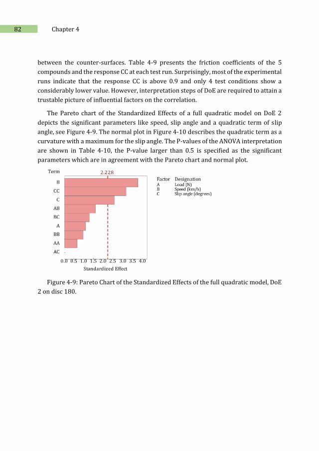
82 Chapter 4
between the counter-surfaces. Table 4-9 presents the friction coefficients of the 5
compounds and the response CC at each test run. Surprisingly, most of the experimental
runs indicate that the response CC is above 0.9 and only 4 test conditions show a
considerably lower value. However, interpretation steps of DoE are required to attain a
trustable picture of influential factors on the correlation.
The Pareto chart of the Standardized Effects of a full quadratic model on DoE 2
depicts the significant parameters like speed, slip angle and a quadratic term of slip
angle, see Figure 4-9. The normal plot in Figure 4-10 describes the quadratic term as a
curvature with a maximum for the slip angle. The P-values of the ANOVA interpretation
are shown in Table 4-10, the P-value larger than 0.5 is specified as the significant
parameters which are in agreement with the Pareto chart and normal plot.
Figure 4-9: Pareto Chart of the Standardized Effects of the full quadratic model, DoE
2 on disc 180.
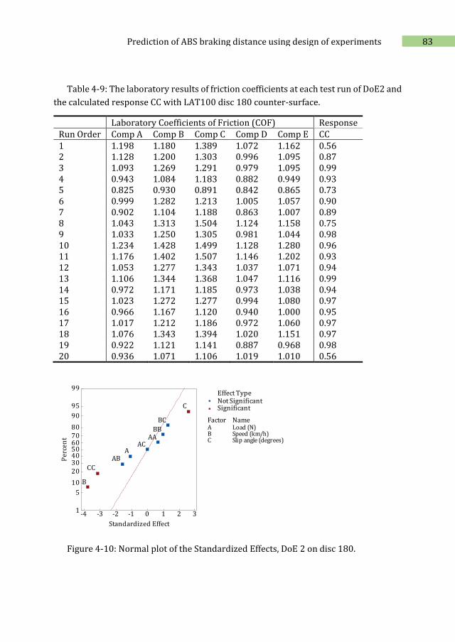
83 Prediction of ABS braking distance using design of experiments
Table 4-9: The laboratory results of friction coefficients at each test run of DoE2 and
the calculated response CC with LAT100 disc 180 counter-surface.
Laboratory Coefficients of Friction (COF) Response Run Order Comp A Comp B Comp C Comp D Comp E CC
1 1.198 1.180 1.389 1.072 1.162 0.56 2 1.128 1.200 1.303 0.996 1.095 0.87 3 1.093 1.269 1.291 0.979 1.095 0.99 4 0.943 1.084 1.183 0.882 0.949 0.93 5 0.825 0.930 0.891 0.842 0.865 0.73 6 0.999 1.282 1.213 1.005 1.057 0.90 7 0.902 1.104 1.188 0.863 1.007 0.89 8 1.043 1.313 1.504 1.124 1.158 0.75 9 1.033 1.250 1.305 0.981 1.044 0.98 10 1.234 1.428 1.499 1.128 1.280 0.96 11 1.176 1.402 1.507 1.146 1.202 0.93 12 1.053 1.277 1.343 1.037 1.071 0.94 13 1.106 1.344 1.368 1.047 1.116 0.99 14 0.972 1.171 1.185 0.973 1.038 0.94 15 1.023 1.272 1.277 0.994 1.080 0.97 16 0.966 1.167 1.120 0.940 1.000 0.95 17 1.017 1.212 1.186 0.972 1.060 0.97 18 1.076 1.343 1.394 1.020 1.151 0.97 19 0.922 1.121 1.141 0.887 0.968 0.98 20 0.936 1.071 1.106 1.019 1.010 0.56
Figure 4-10: Normal plot of the Standardized Effects, DoE 2 on disc 180.
3210-1-2-3-4
99
95
90
80706050403020
10
5
1
A Load (N)B Speed (km/h)C Slip angle (degrees)
Factor Name
Standardized Effect
Pe
rcen
t
Not SignificantSignificant
Effect Type
BC
AC
AB
CC
BBAA
C
B
A
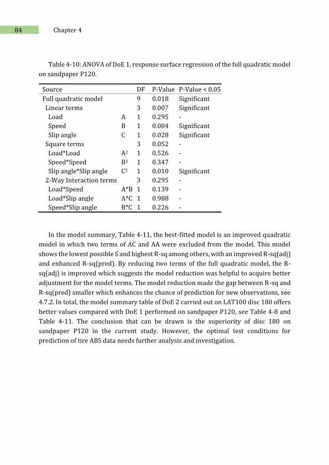
84 Chapter 4
Table 4-10: ANOVA of DoE 1, response surface regression of the full quadratic model
on sandpaper P120.
Source DF P-Value P-Value < 0.05
Full quadratic model 9 0.018 Significant
Linear terms 3 0.007 Significant
Load A 1 0.295 -
Speed B 1 0.004 Significant
Slip angle C 1 0.028 Significant
Square terms 3 0.052 -
Load*Load A2 1 0.526 -
Speed*Speed B2 1 0.347 -
Slip angle*Slip angle C2 1 0.010 Significant
2-Way Interaction terms 3 0.295 -
Load*Speed A*B 1 0.139 -
Load*Slip angle A*C 1 0.988 -
Speed*Slip angle B*C 1 0.226 -
In the model summary, Table 4-11, the best-fitted model is an improved quadratic
model in which two terms of AC and AA were excluded from the model. This model
shows the lowest possible S and highest R-sq among others, with an improved R-sq(adj)
and enhanced R-sq(pred). By reducing two terms of the full quadratic model, the R-
sq(adj) is improved which suggests the model reduction was helpful to acquire better
adjustment for the model terms. The model reduction made the gap between R-sq and
R-sq(pred) smaller which enhances the chance of prediction for new observations, see
4.7.2. In total, the model summary table of DoE 2 carried out on LAT100 disc 180 offers
better values compared with DoE 1 performed on sandpaper P120, see Table 4-8 and
Table 4-11. The conclusion that can be drawn is the superiority of disc 180 on
sandpaper P120 in the current study. However, the optimal test conditions for
prediction of tire ABS data needs further analysis and investigation.
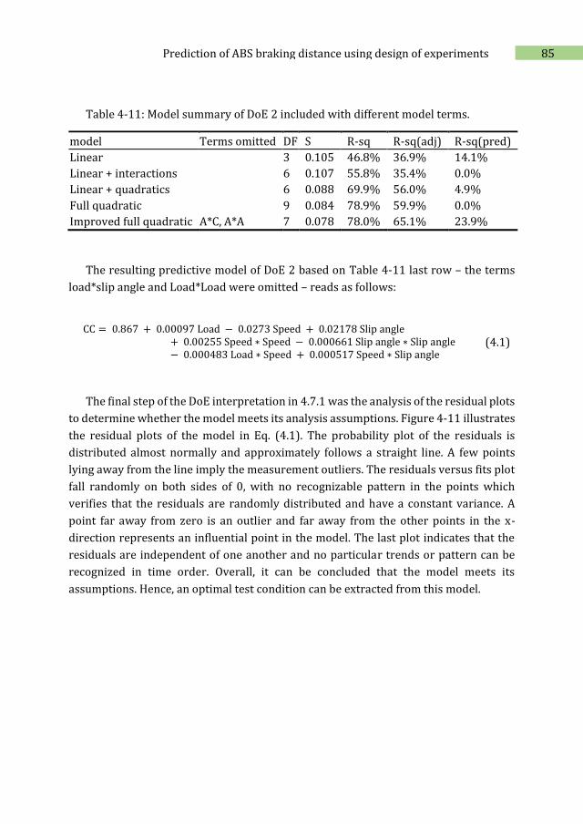
85 Prediction of ABS braking distance using design of experiments
Table 4-11: Model summary of DoE 2 included with different model terms.
model Terms omitted DF S R-sq R-sq(adj) R-sq(pred)
Linear 3 0.105 46.8% 36.9% 14.1%
Linear + interactions 6 0.107 55.8% 35.4% 0.0%
Linear + quadratics 6 0.088 69.9% 56.0% 4.9%
Full quadratic 9 0.084 78.9% 59.9% 0.0%
Improved full quadratic A*C, A*A 7 0.078 78.0% 65.1% 23.9%
The resulting predictive model of DoE 2 based on Table 4-11 last row – the terms
load*slip angle and Load*Load were omitted – reads as follows:
CC = 0.867 + 0.00097 Load − 0.0273 Speed + 0.02178 Slip angle
+ 0.00255 Speed ∗ Speed − 0.000661 Slip angle ∗ Slip angle − 0.000483 Load ∗ Speed + 0.000517 Speed ∗ Slip angle
(4.1)
The final step of the DoE interpretation in 4.7.1 was the analysis of the residual plots
to determine whether the model meets its analysis assumptions. Figure 4-11 illustrates
the residual plots of the model in Eq. (4.1). The probability plot of the residuals is
distributed almost normally and approximately follows a straight line. A few points
lying away from the line imply the measurement outliers. The residuals versus fits plot
fall randomly on both sides of 0, with no recognizable pattern in the points which
verifies that the residuals are randomly distributed and have a constant variance. A
point far away from zero is an outlier and far away from the other points in the x-
direction represents an influential point in the model. The last plot indicates that the
residuals are independent of one another and no particular trends or pattern can be
recognized in time order. Overall, it can be concluded that the model meets its
assumptions. Hence, an optimal test condition can be extracted from this model.
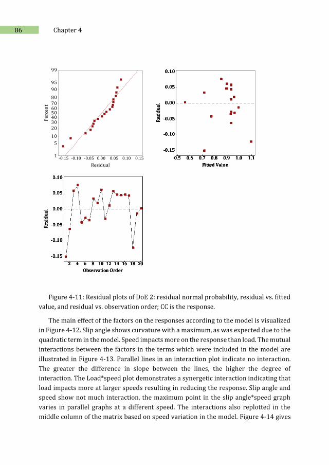
86 Chapter 4
Figure 4-11: Residual plots of DoE 2: residual normal probability, residual vs. fitted
value, and residual vs. observation order; CC is the response.
The main effect of the factors on the responses according to the model is visualized
in Figure 4-12. Slip angle shows curvature with a maximum, as was expected due to the
quadratic term in the model. Speed impacts more on the response than load. The mutual
interactions between the factors in the terms which were included in the model are
illustrated in Figure 4-13. Parallel lines in an interaction plot indicate no interaction.
The greater the difference in slope between the lines, the higher the degree of
interaction. The Load*speed plot demonstrates a synergetic interaction indicating that
load impacts more at larger speeds resulting in reducing the response. Slip angle and
speed show not much interaction, the maximum point in the slip angle*speed graph
varies in parallel graphs at a different speed. The interactions also replotted in the
middle column of the matrix based on speed variation in the model. Figure 4-14 gives
0.150.100.050.00-0.05-0.10-0.15
99
95
90
80706050403020
10
5
1
Residual
Pe
rcen
t
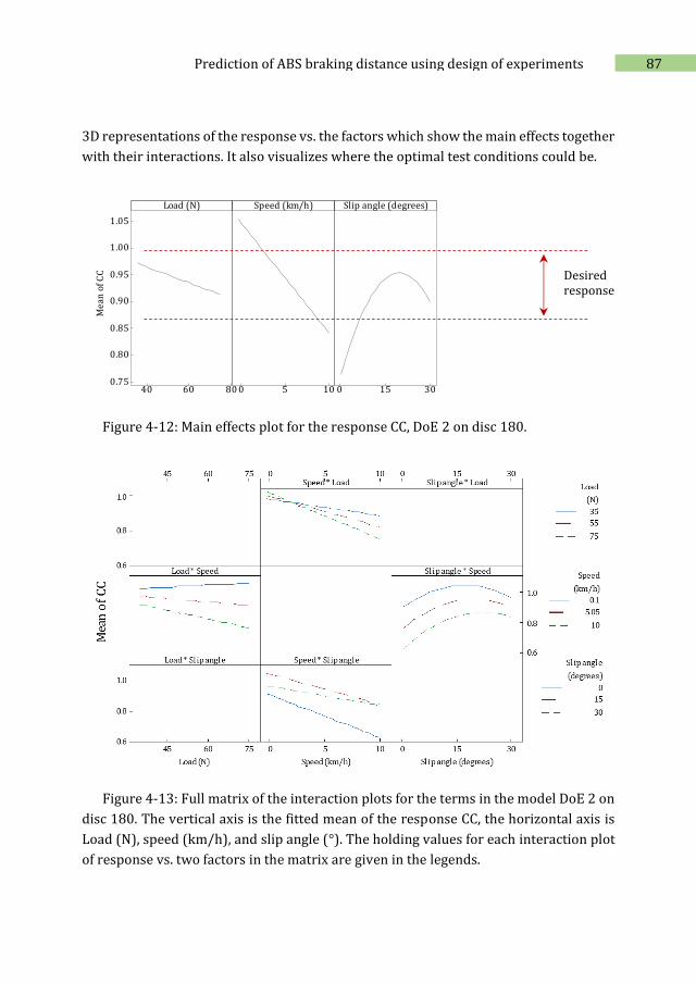
87 Prediction of ABS braking distance using design of experiments
3D representations of the response vs. the factors which show the main effects together
with their interactions. It also visualizes where the optimal test conditions could be.
Figure 4-12: Main effects plot for the response CC, DoE 2 on disc 180.
Figure 4-13: Full matrix of the interaction plots for the terms in the model DoE 2 on
disc 180. The vertical axis is the fitted mean of the response CC, the horizontal axis is
Load (N), speed (km/h), and slip angle (°). The holding values for each interaction plot
of response vs. two factors in the matrix are given in the legends.
806040
1.05
1.00
0.95
0.90
0.85
0.80
0.751050 30150
Load (N)
Me
an o
f CC
Speed (km/h) Slip angle (degrees)
Desired response
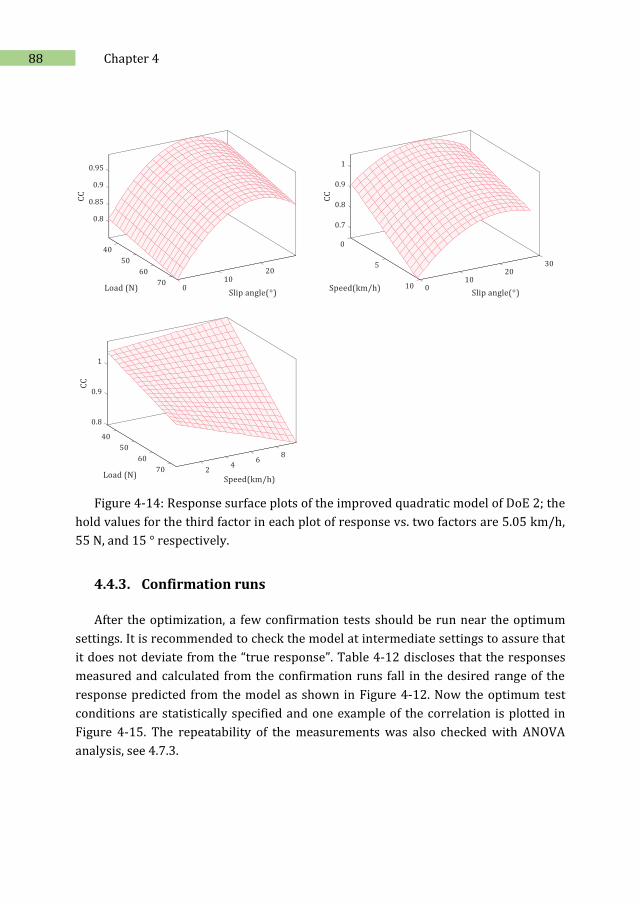
88 Chapter 4
Figure 4-14: Response surface plots of the improved quadratic model of DoE 2; the
hold values for the third factor in each plot of response vs. two factors are 5.05 km/h,
55 N, and 15 ° respectively.
4.4.3. Confirmation runs
After the optimization, a few confirmation tests should be run near the optimum
settings. It is recommended to check the model at intermediate settings to assure that
it does not deviate from the “true response”. Table 4-12 discloses that the responses
measured and calculated from the confirmation runs fall in the desired range of the
response predicted from the model as shown in Figure 4-12. Now the optimum test
conditions are statistically specified and one example of the correlation is plotted in
Figure 4-15. The repeatability of the measurements was also checked with ANOVA
analysis, see 4.7.3.
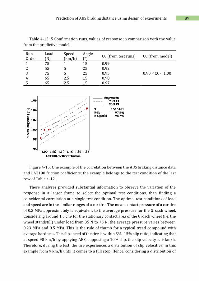
89 Prediction of ABS braking distance using design of experiments
Table 4-12: 5 Confirmation runs, values of response in comparison with the value
from the predictive model.
Run Order
Load (N)
Speed (km/h)
Angle (°)
CC (from test runs) CC (from model)
1 75 1 15 0.99
0.90 < CC < 1.00 2 55 5 25 0.92 3 75 5 25 0.95 4 65 2.5 15 0.98 5 65 2.5 15 0.97
Figure 4-15: One example of the correlation between the ABS braking distance data
and LAT100 friction coefficients; the example belongs to the test condition of the last
row of Table 4-12.
These analyses provided substantial information to observe the variation of the
response in a larger frame to select the optimal test conditions, than finding a
coincidental correlation at a single test condition. The optimal test conditions of load
and speed are in the similar ranges of a car tire. The mean contact pressure of a car tire
of 0.3 MPa approximately is equivalent to the average pressure for the Grosch wheel.
Considering around 1.5 cm2 for the stationary contact area of the Grosch wheel (i.e. the
wheel standstill) under load from 35 N to 75 N, the average pressure varies between
0.23 MPa and 0.5 MPa. This is the rule of thumb for a typical tread compound with
average hardness. The slip speed of the tire is within 5% -15% slip ratio; indicating that
at speed 90 km/h by applying ABS, supposing a 10% slip, the slip velocity is 9 km/h.
Therefore, during the test, the tire experiences a distribution of slip velocities; in this
example from 9 km/h until it comes to a full stop. Hence, considering a distribution of
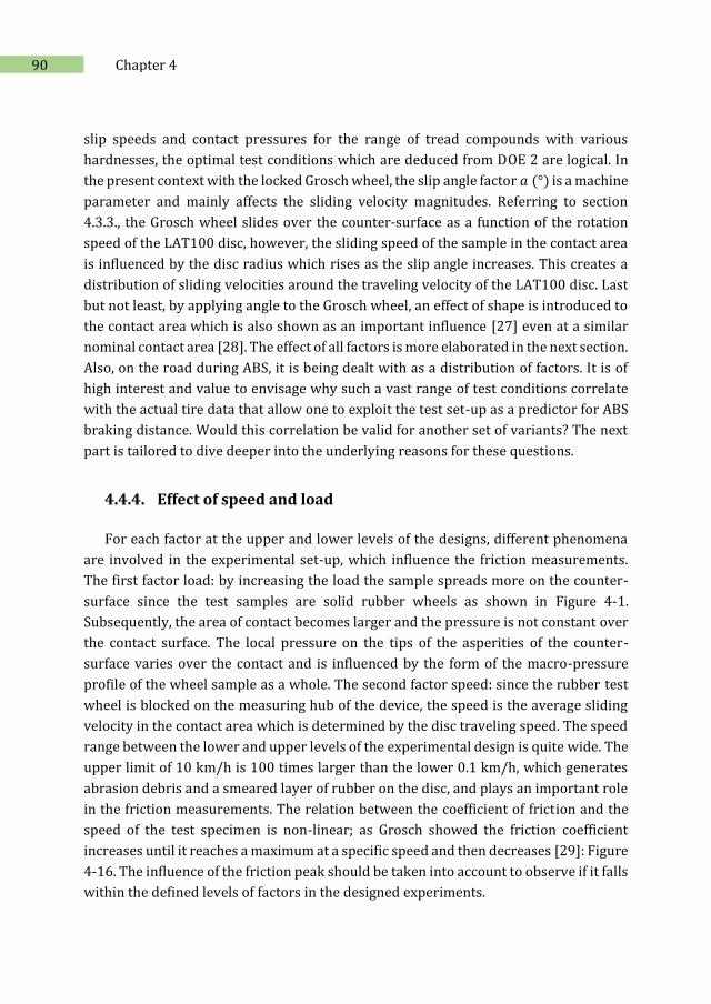
90 Chapter 4
slip speeds and contact pressures for the range of tread compounds with various
hardnesses, the optimal test conditions which are deduced from DOE 2 are logical. In
the present context with the locked Grosch wheel, the slip angle factor 𝑎 (°) is a machine
parameter and mainly affects the sliding velocity magnitudes. Referring to section
4.3.3., the Grosch wheel slides over the counter-surface as a function of the rotation
speed of the LAT100 disc, however, the sliding speed of the sample in the contact area
is influenced by the disc radius which rises as the slip angle increases. This creates a
distribution of sliding velocities around the traveling velocity of the LAT100 disc. Last
but not least, by applying angle to the Grosch wheel, an effect of shape is introduced to
the contact area which is also shown as an important influence [27] even at a similar
nominal contact area [28]. The effect of all factors is more elaborated in the next section.
Also, on the road during ABS, it is being dealt with as a distribution of factors. It is of
high interest and value to envisage why such a vast range of test conditions correlate
with the actual tire data that allow one to exploit the test set-up as a predictor for ABS
braking distance. Would this correlation be valid for another set of variants? The next
part is tailored to dive deeper into the underlying reasons for these questions.
4.4.4. Effect of speed and load
For each factor at the upper and lower levels of the designs, different phenomena
are involved in the experimental set-up, which influence the friction measurements.
The first factor load: by increasing the load the sample spreads more on the counter-
surface since the test samples are solid rubber wheels as shown in Figure 4-1.
Subsequently, the area of contact becomes larger and the pressure is not constant over
the contact surface. The local pressure on the tips of the asperities of the counter-
surface varies over the contact and is influenced by the form of the macro-pressure
profile of the wheel sample as a whole. The second factor speed: since the rubber test
wheel is blocked on the measuring hub of the device, the speed is the average sliding
velocity in the contact area which is determined by the disc traveling speed. The speed
range between the lower and upper levels of the experimental design is quite wide. The
upper limit of 10 km/h is 100 times larger than the lower 0.1 km/h, which generates
abrasion debris and a smeared layer of rubber on the disc, and plays an important role
in the friction measurements. The relation between the coefficient of friction and the
speed of the test specimen is non-linear; as Grosch showed the friction coefficient
increases until it reaches a maximum at a specific speed and then decreases [29]: Figure
4-16. The influence of the friction peak should be taken into account to observe if it falls
within the defined levels of factors in the designed experiments.
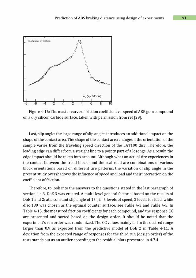
91 Prediction of ABS braking distance using design of experiments
Figure 4-16: The master curve of friction coefficient vs. speed of ABR gum compound
on a dry silicon carbide surface, taken with permission from ref [29].
Last, slip angle: the large range of slip angles introduces an additional impact on the
shape of the contact area. The shape of the contact area changes if the orientation of the
sample varies from the traveling speed direction of the LAT100 disc. Therefore, the
leading edge can differ from a straight line to a pointy part of a lozenge. As a result, the
edge impact should be taken into account. Although what an actual tire experiences in
the contact between the tread blocks and the real road are combinations of various
block orientations based on different tire patterns, the variation of slip angle in the
present study overshadows the influence of speed and load and their interaction on the
coefficient of friction.
Therefore, to look into the answers to the questions stated in the last paragraph of
section 4.4.3, DoE 3 was created. A multi-level general factorial based on the results of
DoE 1 and 2; at a constant slip angle of 15°, in 5 levels of speed, 3 levels for load, while
disc 180 was chosen as the optimal counter surface: see Table 4-3 and Table 4-5. In
Table 4-13, the measured friction coefficients for each compound, and the response CC
are presented and sorted based on the design order. It should be noted that the
experiment's run order was randomized. The CC values mainly fall in the desired range
larger than 0.9 as expected from the predictive model of DoE 2 in Table 4-11. A
deviation from the expected range of responses for the third run (design order) of the
tests stands out as an outlier according to the residual plots presented in 4.7.4.
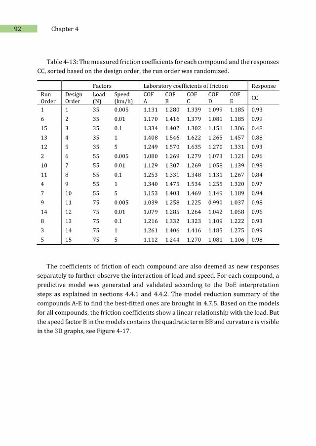
92 Chapter 4
Table 4-13: The measured friction coefficients for each compound and the responses
CC, sorted based on the design order, the run order was randomized.
Factors Laboratory coefficients of friction Response
Run Order
Design Order
Load (N)
Speed (km/h)
COF A
COF B
COF C
COF D
COF E
CC
1 1 35 0.005 1.131 1.280 1.339 1.099 1.185 0.93
6 2 35 0.01 1.170 1.416 1.379 1.081 1.185 0.99
15 3 35 0.1 1.334 1.402 1.302 1.151 1.306 0.48
13 4 35 1 1.408 1.546 1.622 1.265 1.457 0.88
12 5 35 5 1.249 1.570 1.635 1.270 1.331 0.93
2 6 55 0.005 1.080 1.269 1.279 1.073 1.121 0.96
10 7 55 0.01 1.129 1.307 1.269 1.058 1.139 0.98
11 8 55 0.1 1.253 1.331 1.348 1.131 1.267 0.84
4 9 55 1 1.340 1.475 1.534 1.255 1.320 0.97
7 10 55 5 1.153 1.403 1.469 1.149 1.189 0.94
9 11 75 0.005 1.039 1.258 1.225 0.990 1.037 0.98
14 12 75 0.01 1.079 1.285 1.264 1.042 1.058 0.96
8 13 75 0.1 1.216 1.332 1.323 1.109 1.222 0.93
3 14 75 1 1.261 1.406 1.416 1.185 1.275 0.99
5 15 75 5 1.112 1.244 1.270 1.081 1.106 0.98
The coefficients of friction of each compound are also deemed as new responses
separately to further observe the interaction of load and speed. For each compound, a
predictive model was generated and validated according to the DoE interpretation
steps as explained in sections 4.4.1 and 4.4.2. The model reduction summary of the
compounds A-E to find the best-fitted ones are brought in 4.7.5. Based on the models
for all compounds, the friction coefficients show a linear relationship with the load. But
the speed factor B in the models contains the quadratic term BB and curvature is visible
in the 3D graphs, see Figure 4-17.
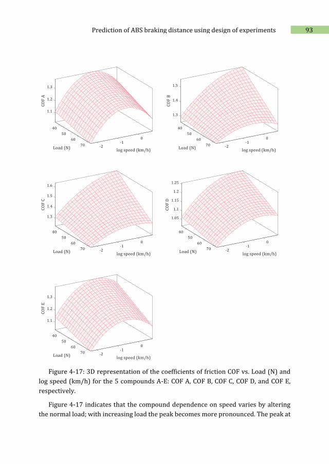
93 Prediction of ABS braking distance using design of experiments
Figure 4-17: 3D representation of the coefficients of friction COF vs. Load (N) and
log speed (km/h) for the 5 compounds A-E: COF A, COF B, COF C, COF D, and COF E,
respectively.
Figure 4-17 indicates that the compound dependence on speed varies by altering
the normal load; with increasing load the peak becomes more pronounced. The peak at
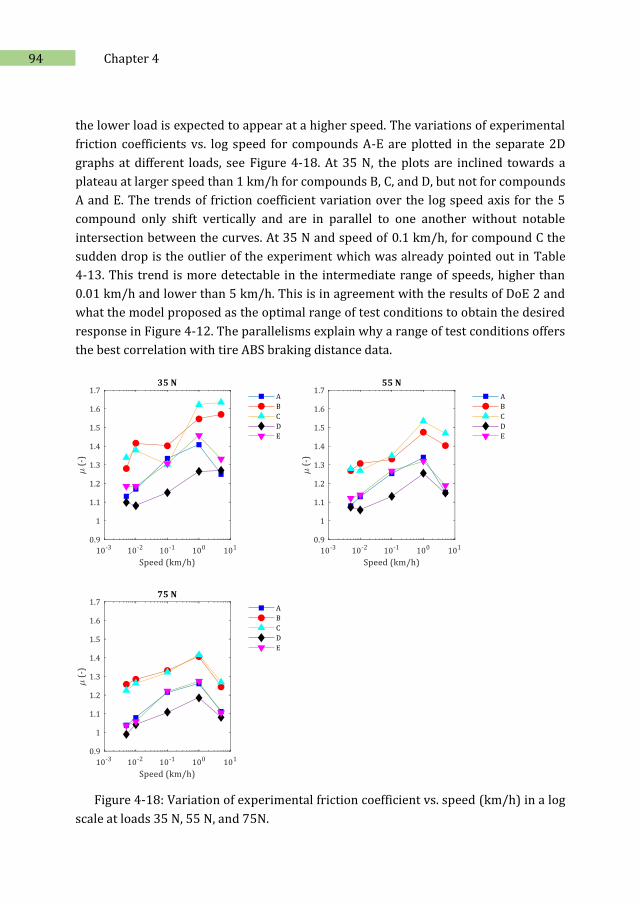
94 Chapter 4
the lower load is expected to appear at a higher speed. The variations of experimental
friction coefficients vs. log speed for compounds A-E are plotted in the separate 2D
graphs at different loads, see Figure 4-18. At 35 N, the plots are inclined towards a
plateau at larger speed than 1 km/h for compounds B, C, and D, but not for compounds
A and E. The trends of friction coefficient variation over the log speed axis for the 5
compound only shift vertically and are in parallel to one another without notable
intersection between the curves. At 35 N and speed of 0.1 km/h, for compound C the
sudden drop is the outlier of the experiment which was already pointed out in Table
4-13. This trend is more detectable in the intermediate range of speeds, higher than
0.01 km/h and lower than 5 km/h. This is in agreement with the results of DoE 2 and
what the model proposed as the optimal range of test conditions to obtain the desired
response in Figure 4-12. The parallelisms explain why a range of test conditions offers
the best correlation with tire ABS braking distance data.
Figure 4-18: Variation of experimental friction coefficient vs. speed (km/h) in a log
scale at loads 35 N, 55 N, and 75N.
95 Prediction of ABS braking distance using design of experiments
4.5. Concluding remarks
To predict tire friction, varying one factor at the time for experimenting does not
necessarily provide a proper judgment. The research methodology of Design of
Experiments (DoE) is implemented in the present study in which a predictive
mathematical model is extracted to describe the relationship between responses and
critical factors. Various operating parameters of the LAT100 as a tribometer on tire
friction are investigated: load, speed, and slip angle. Measurements were performed on
two counter-surfaces of a sandpaper- and a corundum-based substrate. The interaction
of load and speed influences the coefficient of friction of tire tread compounds. The
variation of the coefficient of friction vs. speed on the corundum-based substrate is in
agreement with the ABS braking distance data of actual tires on the road, but not for
the sandpaper substrate. The present study highly emphasized the importance of the
design of experiments in a friction study. It gives guidance by a predictive mathematical
model in selecting optimal test conditions regarding desired responses for present and
also new observations, rather than just choosing arbitrary experimental settings.
4.6. References
1. The Tyre Grip, Société de Technologie Michelin.,clermont-ferrand, France, Date of access: May 2020; Available from http://www.dimnp.unipi.it/guiggiani-m/Michelin_Tire_Grip.pdf.
2. Arrigoni, S., F. Cheli, E. Sabbioni, and P. Gavardi. Influence of tyre characteristics on ABS performance. in Proceedings of the 4th International Tyre Colloquium: Tyre Models for Vehicle Dynamics Analysis. 20-21 April 2015. Guildford, UK: University of Surrey, Guildford, United Kingdom.
3. Grosch, K., Some Factors Influencing the Traction of Radial Ply Tires. Rubber Chemistry and Technology, 1984. 57(5): p. 889-907.
4. Salehi, M., J.W.M. Noordermeer, L.A.E.M. Reuvekamp, and A. Blume. A New Method to Rapidly Predict Tyre Grip In a Laboratory Environment. in International Rubber Conference. 3-5 Sep 2019. London, UK.
5. Gruber, P., R.S. Sharp, and A.D. Crocombe, Normal and shear forces in the contact patch of a braked racing tyre. Part 2: development of a physical tyre model. Vehicle System Dynamics, 2012. 50(3): p. 339-356.
6. O’Neill, A., P. Gruber, J.F. Watts, and J. Prins. Predicting Tyre Behaviour on Different Road Surfaces. Cham: Springer International Publishing.
96 Chapter 4
7. Klüppel, M. and G. Heinrich, Rubber Friction on Self-Affine Road Tracks. Rubber Chemistry and Technology, 2000. 73(4): p. 578-606.
8. Tanaka, H., K. Yoshimura, R. Sekoguchi, J. Aramaki, A. Hatano, S. Izumi, . . . H. Kadowaki, Prediction of the friction coefficient of filled rubber sliding on dry and wet surfaces with self-affine large roughness. Mechanical Engineering Journal, 2016. 3(1): p. 15-00084-15-00084.
9. Ignatyev, P.A., S. Ripka, N. Mueller, S. Torbruegge, and B. Wies, Tire ABS-Braking Prediction with Lab Tests and Friction Simulations. Tire Science and Technology, 2015. 43(4): p. 260-275.
10. Nam, S., Y. Oh, and S. Jeon, The Prediction of Rubber Friction considering Road Characteristics Transactions of the Korean Society of Automotive Engineers 2014. 22(4): p. 105-110.
11. Germann, S., M. Wurtenberger, and A. Daiss. Monitoring of the friction coefficient between tyre and road surface. in 1994 Proceedings of IEEE International Conference on Control and Applications. 24-26 Aug 1994.
12. Grosch, K.A. and G. Maycock, Influence of Test Conditions on Wet Skid Resistance of Tire Tread Compounds. Rubber Chemistry and Technology, 1968. 41(2): p. 477-494.
13. Fortunato, G., V. Ciaravola, A. Furno, M. Scaraggi, B. Lorenz, and B.N.J. Persson, Dependency of Rubber Friction on Normal Force or Load: Theory and Experiment. Tire Science and Technology, 2017. 45(1): p. 25-54.
14. Ella, S., P.-Y. Formagne, V. Koutsos, and J.R. Blackford, Investigation of rubber friction on snow for tyres. Tribology International, 2013. 59: p. 292-301.
15. Heinz, M., A Universal Method to Predict Wet Traction Behaviour of Tyre Tread Compounds in the Laboratory. Journal of Rubber Research, 2010. 13(2): p. 91-102.
16. Heinz, M. and K.A. Grosch, A Laboratory Method to Comprehensively Evaluate Abrasion, Traction and Rolling Resistance of Tire Tread Compounds. Rubber Chemistry and Technology, 2007. 80(4): p. 580-607.
17. Salehi, M., J.W.M. Noordermeer, L.A.E.M. Reuvekamp, W.K. Dierkes, and A. Blume, Measuring rubber friction using a Laboratory Abrasion Tester (LAT100) to predict car tire dry ABS braking. Tribology International, 2019. 131: p. 191-199.
18. Salehi, M., J.W.M. Noordermeer, L.A.E.M. Reuvekamp, T. Tolpekina, and A. Blume, A New Horizon for Evaluating Tire Grip Within a Laboratory Environment. Tribology Letters, 2020. 68(1): p. 37.
19. Minitab® 18.1 software, in 2017, Date of access; Available from https://support.minitab.com/en-us/minitab/18/.
97 Prediction of ABS braking distance using design of experiments
20. Tanco, M., N. Costa, and E. Viles, Experimental design selection: guidelines for practitioners. International Journal of Productivity and Quality Management, 2009. 4(3): p. 283-302.
21. Anderson, M.J. and P.J. Whitcomb., DOE Simplified: Practical Tools for Effective Experimentation. 2015: CRC Press, Taylor & Francis Group.
22. Heinrich, G. and M. Klüppel, Rubber friction, tread deformation and tire traction. Wear, 2008. 265(7–8): p. 1052-1060.
23. Schallamach, A., The Load Dependence of Rubber Friction. Proceedings of the Physical Society. Section B, 1952. 65: p. 657-661.
24. Grosch, K.A. and A. Schallamach, The Load Dependence of Laboratory Abrasion and Tire Wear. Rubber Chemistry and Technology, 1970. 43(4): p. 701-713.
25. Salehi, M., LAT100, Prediction of tire dry grip. 2017, University of Twente: Enschede: Ipskamp Printing.
26. Ludwig, C. Influence of testing surface on tire lateral force characteristics. in Science meets Tires. April 24-25, 2018. Aachen, Germany: ika INSTITUT FÜR KRAFTFAHRZEUGE and RWTH AACHEN UNIVERSITY.
27. Persson, B.N.J., Rubber friction and tire dynamics. Journal of Physics: Condensed Matter, 2010. 23(1): p. 015003.
28. Hale, J., R. Lewis, and M.J. Carré, Rubber friction and the effect of shape. Tribology International, 2020. 141: p. 105911.
29. Grosch, K.A., Goodyear Medalist Lecture. Rubber Friction and its Relation to Tire Traction. Rubber Chemistry and Technology, 2007. 80(3): p. 379-411.
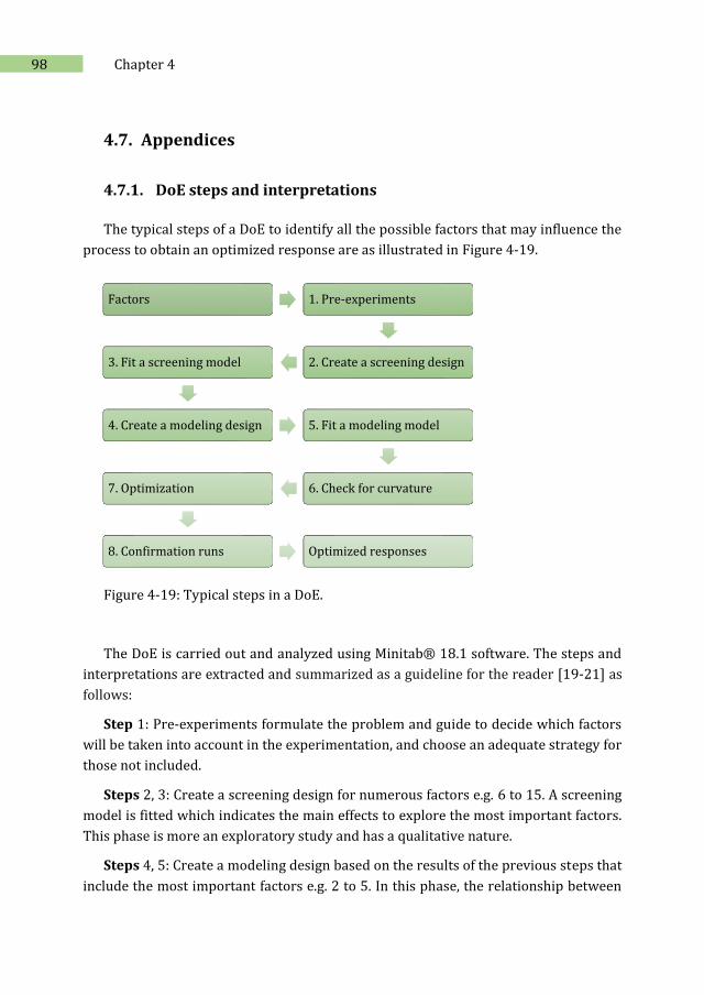
98 Chapter 4
4.7. Appendices
4.7.1. DoE steps and interpretations
The typical steps of a DoE to identify all the possible factors that may influence the
process to obtain an optimized response are as illustrated in Figure 4-19.
Figure 4-19: Typical steps in a DoE.
The DoE is carried out and analyzed using Minitab® 18.1 software. The steps and
interpretations are extracted and summarized as a guideline for the reader [19-21] as
follows:
Step 1: Pre-experiments formulate the problem and guide to decide which factors
will be taken into account in the experimentation, and choose an adequate strategy for
those not included.
Steps 2, 3: Create a screening design for numerous factors e.g. 6 to 15. A screening
model is fitted which indicates the main effects to explore the most important factors.
This phase is more an exploratory study and has a qualitative nature.
Steps 4, 5: Create a modeling design based on the results of the previous steps that
include the most important factors e.g. 2 to 5. In this phase, the relationship between
Factors 1. Pre-experiments
2. Create a screening design3. Fit a screening model
4. Create a modeling design 5. Fit a modeling model
6. Check for curvature7. Optimization
8. Confirmation runs Optimized responses
99 Prediction of ABS braking distance using design of experiments
responses and factors is described in sufficient detail. Fit a linear model that includes
main effects and 2-way interactions and analyze the results and look for evidence of
curvature in the relationship between the factors and the responses.
Steps 6, 7: If no curvature is detected in step 5, use that model to identify factor
settings that optimize the response. If curvature is detected, add points for curvature to
the design. Fit a quadratic model that includes square terms to model the curvature and
analyze the results using Analysis of Variance (ANOVA) and Response Surface Modeling
(RSM). ANOVA is a statistical test used to identify the effects of independent variables
(factors) on the outcomes of an experiment (responses). RSM is a technique that models
responses via polynomial equations and creates a map of responses in 3D surface
graphs or 2D contour-plots. By using the final model, factor settings can be identified
that optimize the response.
An example of the mathematical predictive model tested in ANOVA for 2 factors
including interaction and quadratic terms reads as follows:
𝑌 = 𝛽0 + 𝛽1𝑋1 + 𝛽2𝑋2 + 𝛽12𝑋1𝑋2 + 𝛽11𝑋12+ 𝛽22𝑋2
2 (4.2)
where,
𝑌: the predicted response;
𝑋: input factor;
𝑋𝑋: 2-way interaction term;
𝑋2: a quadratic term;
and 𝛽 are the model coefficients; the subscriptions denote different factors.
Step 8: If an optimum is predicted using RSM, the results should be checked by
confirmation runs. A few confirmation experiments near the anticipated optimum are
recommended.
For Interpretations, four main steps are taken:
Step 1 examines the terms that contribute the most to the variability in the response
using a measure called Pareto bar chart which can be obtained by ANOVA and
diagnostics of the residual errors. This measure can be employed to rank the
importance of the effect of each term in the predictive mathematical model. The Pareto
chart is very useful especially for non-statisticians because it works with standardized
effects; a dimensionless statistical scale that manifests the relative size of the effects for
comparison. The dimensionless statistical scale is the t-value and is defined as the
magnitude of the effect divided by the standard error. The following equations are
employed for the calculations:
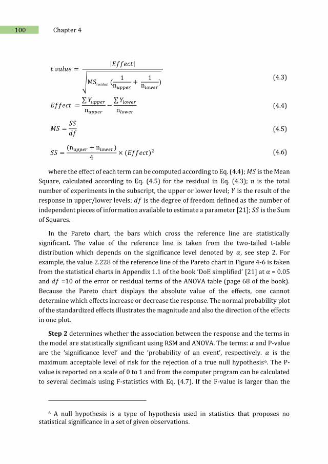
100 Chapter 4
𝑡 𝑣𝑎𝑙𝑢𝑒 =
|𝐸𝑓𝑓𝑒𝑐𝑡|
√MSresidual (1
n𝑢𝑝𝑝𝑒𝑟+
1n𝑙𝑜𝑤𝑒𝑟
)
(4.3)
𝐸𝑓𝑓𝑒𝑐𝑡 =∑ 𝑌𝑢𝑝𝑝𝑒𝑟
n𝑢𝑝𝑝𝑒𝑟
−∑ 𝑌𝑙𝑜𝑤𝑒𝑟
n𝑙𝑜𝑤𝑒𝑟
(4.4)
𝑀𝑆 =𝑆𝑆
𝑑𝑓 (4.5)
𝑆𝑆 =(n𝑢𝑝𝑝𝑒𝑟 + n𝑙𝑜𝑤𝑒𝑟)
4× (𝐸𝑓𝑓𝑒𝑐𝑡)2 (4.6)
where the effect of each term can be computed according to Eq. (4.4); 𝑀𝑆 is the Mean
Square, calculated according to Eq. (4.5) for the residual in Eq. (4.3); 𝑛 is the total
number of experiments in the subscript, the upper or lower level; 𝑌 is the result of the
response in upper/lower levels; 𝑑𝑓 is the degree of freedom defined as the number of
independent pieces of information available to estimate a parameter [21]; 𝑆𝑆 is the Sum
of Squares.
In the Pareto chart, the bars which cross the reference line are statistically
significant. The value of the reference line is taken from the two-tailed t-table
distribution which depends on the significance level denoted by 𝛼, see step 2. For
example, the value 2.228 of the reference line of the Pareto chart in Figure 4-6 is taken
from the statistical charts in Appendix 1.1 of the book ‘DoE simplified’ [21] at α = 0.05
and 𝑑𝑓 =10 of the error or residual terms of the ANOVA table (page 68 of the book).
Because the Pareto chart displays the absolute value of the effects, one cannot
determine which effects increase or decrease the response. The normal probability plot
of the standardized effects illustrates the magnitude and also the direction of the effects
in one plot.
Step 2 determines whether the association between the response and the terms in
the model are statistically significant using RSM and ANOVA. The terms: 𝛼 and P-value
are the ‘significance level’ and the ‘probability of an event’, respectively. 𝛼 is the
maximum acceptable level of risk for the rejection of a true null hypothesis6. The P-
value is reported on a scale of 0 to 1 and from the computer program can be calculated
to several decimals using F-statistics with Eq. (4.7). If the F-value is larger than the
6 A null hypothesis is a type of hypothesis used in statistics that proposes no statistical significance in a set of given observations.
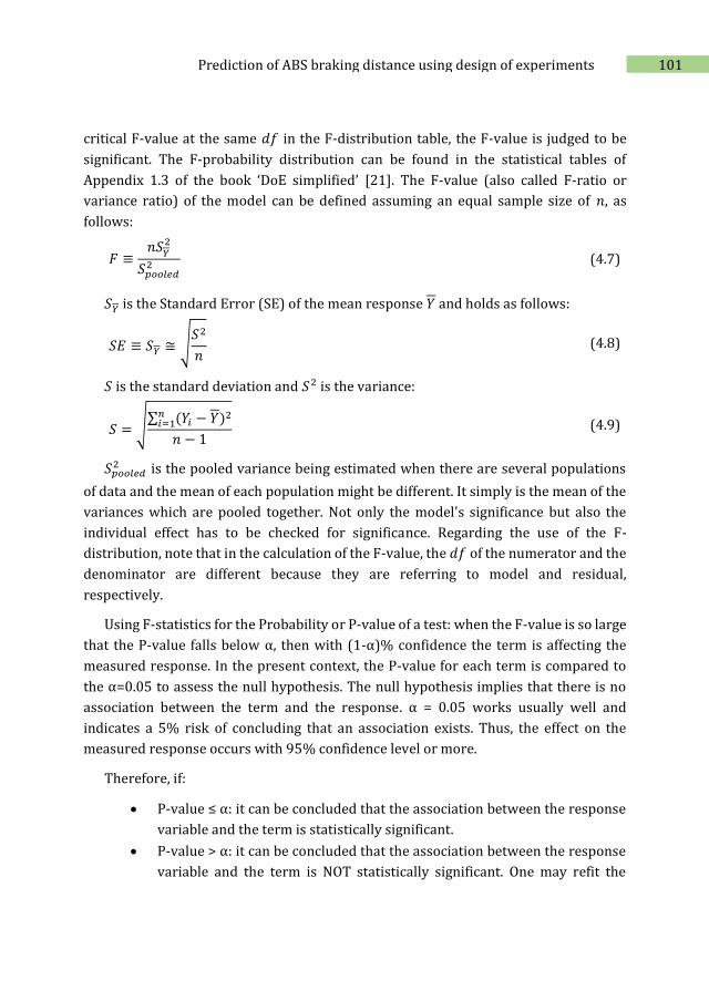
101 Prediction of ABS braking distance using design of experiments
critical F-value at the same 𝑑𝑓 in the F-distribution table, the F-value is judged to be
significant. The F-probability distribution can be found in the statistical tables of
Appendix 1.3 of the book ‘DoE simplified’ [21]. The F-value (also called F-ratio or
variance ratio) of the model can be defined assuming an equal sample size of 𝑛, as
follows:
𝐹 ≡𝑛𝑆𝑌
2
𝑆𝑝𝑜𝑜𝑙𝑒𝑑2 (4.7)
𝑆𝑌 is the Standard Error (SE) of the mean response 𝑌 and holds as follows:
𝑆𝐸 ≡ 𝑆𝑌 ≅ √𝑆2
𝑛 (4.8)
𝑆 is the standard deviation and 𝑆2 is the variance:
𝑆 = √∑ (𝑌𝑖 − 𝑌)2𝑛
𝑖=1
𝑛 − 1 (4.9)
𝑆𝑝𝑜𝑜𝑙𝑒𝑑2 is the pooled variance being estimated when there are several populations
of data and the mean of each population might be different. It simply is the mean of the
variances which are pooled together. Not only the model's significance but also the
individual effect has to be checked for significance. Regarding the use of the F-
distribution, note that in the calculation of the F-value, the 𝑑𝑓 of the numerator and the
denominator are different because they are referring to model and residual,
respectively.
Using F-statistics for the Probability or P-value of a test: when the F-value is so large
that the P-value falls below α, then with (1-α)% confidence the term is affecting the
measured response. In the present context, the P-value for each term is compared to
the α=0.05 to assess the null hypothesis. The null hypothesis implies that there is no
association between the term and the response. α = 0.05 works usually well and
indicates a 5% risk of concluding that an association exists. Thus, the effect on the
measured response occurs with 95% confidence level or more.
Therefore, if:
P-value ≤ α: it can be concluded that the association between the response
variable and the term is statistically significant.
P-value > α: it can be concluded that the association between the response
variable and the term is NOT statistically significant. One may refit the
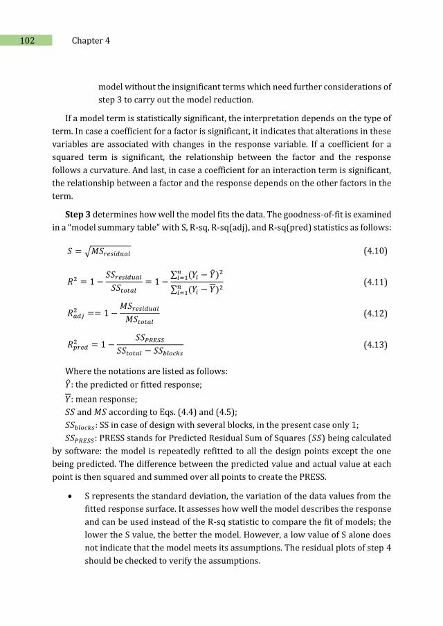
102 Chapter 4
model without the insignificant terms which need further considerations of
step 3 to carry out the model reduction.
If a model term is statistically significant, the interpretation depends on the type of
term. In case a coefficient for a factor is significant, it indicates that alterations in these
variables are associated with changes in the response variable. If a coefficient for a
squared term is significant, the relationship between the factor and the response
follows a curvature. And last, in case a coefficient for an interaction term is significant,
the relationship between a factor and the response depends on the other factors in the
term.
Step 3 determines how well the model fits the data. The goodness-of-fit is examined
in a “model summary table” with S, R-sq, R-sq(adj), and R-sq(pred) statistics as follows:
𝑆 = √𝑀𝑆𝑟𝑒𝑠𝑖𝑑𝑢𝑎𝑙 (4.10)
𝑅2 = 1 −𝑆𝑆𝑟𝑒𝑠𝑖𝑑𝑢𝑎𝑙
𝑆𝑆𝑡𝑜𝑡𝑎𝑙
= 1 −∑ (𝑌𝑖 − �̂�)2𝑛
𝑖=1
∑ (𝑌𝑖 − 𝑌)2𝑛𝑖=1
(4.11)
𝑅𝑎𝑑𝑗2 == 1 −
𝑀𝑆𝑟𝑒𝑠𝑖𝑑𝑢𝑎𝑙
𝑀𝑆𝑡𝑜𝑡𝑎𝑙
(4.12)
𝑅𝑝𝑟𝑒𝑑2 = 1 −
𝑆𝑆𝑃𝑅𝐸𝑆𝑆
𝑆𝑆𝑡𝑜𝑡𝑎𝑙 − 𝑆𝑆𝑏𝑙𝑜𝑐𝑘𝑠
(4.13)
Where the notations are listed as follows:
�̂�: the predicted or fitted response;
𝑌: mean response;
𝑆𝑆 and 𝑀𝑆 according to Eqs. (4.4) and (4.5);
𝑆𝑆𝑏𝑙𝑜𝑐𝑘𝑠: SS in case of design with several blocks, in the present case only 1;
𝑆𝑆𝑃𝑅𝐸𝑆𝑆: PRESS stands for Predicted Residual Sum of Squares (𝑆𝑆) being calculated
by software: the model is repeatedly refitted to all the design points except the one
being predicted. The difference between the predicted value and actual value at each
point is then squared and summed over all points to create the PRESS.
S represents the standard deviation, the variation of the data values from the
fitted response surface. It assesses how well the model describes the response
and can be used instead of the R-sq statistic to compare the fit of models; the
lower the S value, the better the model. However, a low value of S alone does
not indicate that the model meets its assumptions. The residual plots of step 4
should be checked to verify the assumptions.
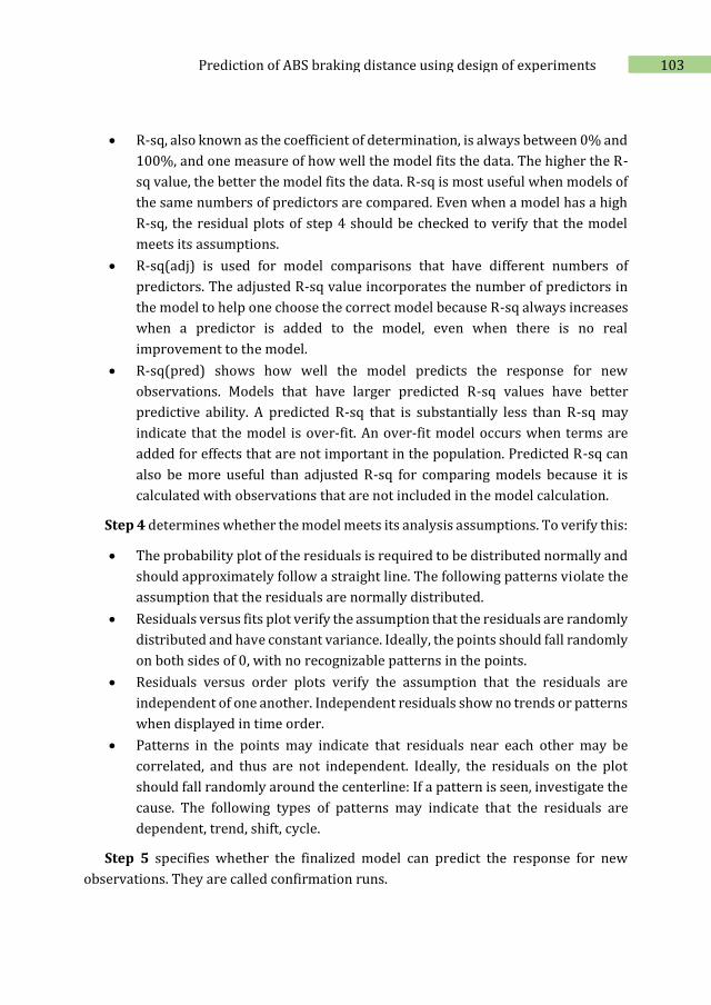
103 Prediction of ABS braking distance using design of experiments
R-sq, also known as the coefficient of determination, is always between 0% and
100%, and one measure of how well the model fits the data. The higher the R-
sq value, the better the model fits the data. R-sq is most useful when models of
the same numbers of predictors are compared. Even when a model has a high
R-sq, the residual plots of step 4 should be checked to verify that the model
meets its assumptions.
R-sq(adj) is used for model comparisons that have different numbers of
predictors. The adjusted R-sq value incorporates the number of predictors in
the model to help one choose the correct model because R-sq always increases
when a predictor is added to the model, even when there is no real
improvement to the model.
R-sq(pred) shows how well the model predicts the response for new
observations. Models that have larger predicted R-sq values have better
predictive ability. A predicted R-sq that is substantially less than R-sq may
indicate that the model is over-fit. An over-fit model occurs when terms are
added for effects that are not important in the population. Predicted R-sq can
also be more useful than adjusted R-sq for comparing models because it is
calculated with observations that are not included in the model calculation.
Step 4 determines whether the model meets its analysis assumptions. To verify this:
The probability plot of the residuals is required to be distributed normally and
should approximately follow a straight line. The following patterns violate the
assumption that the residuals are normally distributed.
Residuals versus fits plot verify the assumption that the residuals are randomly
distributed and have constant variance. Ideally, the points should fall randomly
on both sides of 0, with no recognizable patterns in the points.
Residuals versus order plots verify the assumption that the residuals are
independent of one another. Independent residuals show no trends or patterns
when displayed in time order.
Patterns in the points may indicate that residuals near each other may be
correlated, and thus are not independent. Ideally, the residuals on the plot
should fall randomly around the centerline: If a pattern is seen, investigate the
cause. The following types of patterns may indicate that the residuals are
dependent, trend, shift, cycle.
Step 5 specifies whether the finalized model can predict the response for new
observations. They are called confirmation runs.
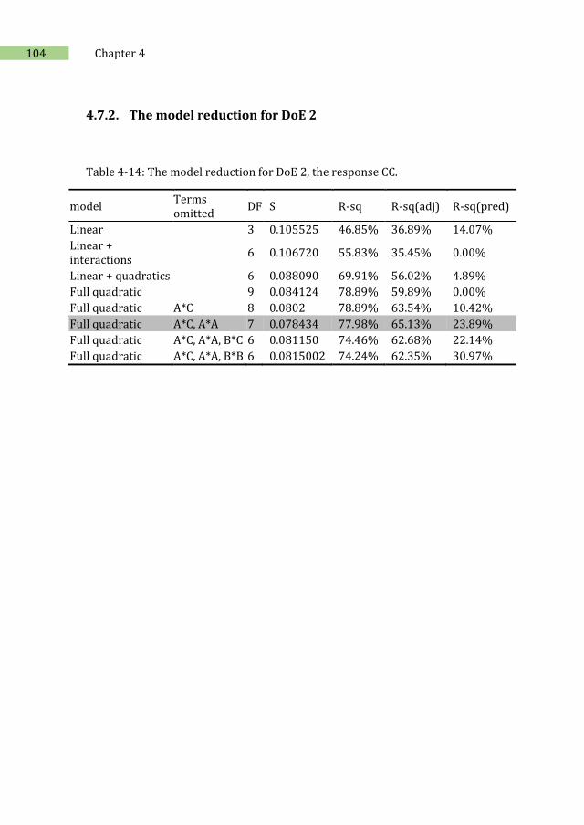
104 Chapter 4
4.7.2. The model reduction for DoE 2
Table 4-14: The model reduction for DoE 2, the response CC.
model Terms omitted
DF S R-sq R-sq(adj) R-sq(pred)
Linear 3 0.105525 46.85% 36.89% 14.07%
Linear + interactions
6 0.106720 55.83% 35.45% 0.00%
Linear + quadratics 6 0.088090 69.91% 56.02% 4.89%
Full quadratic 9 0.084124 78.89% 59.89% 0.00%
Full quadratic A*C 8 0.0802 78.89% 63.54% 10.42%
Full quadratic A*C, A*A 7 0.078434 77.98% 65.13% 23.89%
Full quadratic A*C, A*A, B*C 6 0.081150 74.46% 62.68% 22.14%
Full quadratic A*C, A*A, B*B 6 0.0815002 74.24% 62.35% 30.97%
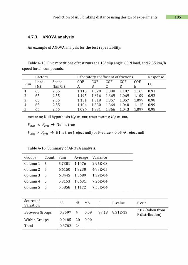
105 Prediction of ABS braking distance using design of experiments
4.7.3. ANOVA analysis
An example of ANOVA analysis for the test repeatability:
Table 4-15: Five repetitions of test runs at a 15° slip angle, 65 N load, and 2.55 km/h
speed for all compounds.
Factors Laboratory coefficient of frictions Response
Run Load (N)
Speed (km/h)
COF A
COF B
COF C
COF D
COF E
CC
1 65 2.55 1.115 1.320 1.388 1.107 1.165 0.93 2 65 2.55 1.195 1.316 1.369 1.069 1.109 0.92 3 65 2.55 1.131 1.318 1.357 1.057 1.099 0.98 4 65 2.55 1.104 1.330 1.364 1.040 1.115 0.99 5 65 2.55 1.094 1.331 1.366 1.043 1.097 0.98
mean: m; Null hypothesis 𝐻0: m1=m2=m3=m4=m5; 𝐻1: m1≠mm
𝐹𝑠𝑡𝑎𝑡 < 𝐹𝑐𝑟𝑖𝑡 Null is true
𝐹𝑠𝑡𝑎𝑡 > 𝐹𝑐𝑟𝑖𝑡 H1 is true (reject null) or P-value < 0.05 reject null
Table 4-16: Summary of ANOVA analysis.
Groups Count Sum Average Variance
Column 1 5 5.7381 1.1476 2.96E-03
Column 2 5 6.6150 1.3230 4.83E-05
Column 3 5 6.8445 1.3689 1.39E-04
Column 4 5 5.3153 1.0631 7.26E-04
Column 5 5 5.5858 1.1172 7.53E-04
Source of Variation
SS df MS F P-value F crit
Between Groups 0.3597 4 0.09 97.13 8.31E-13 2.87 (taken from F distribution)
Within Groups 0.0185 20 0.00
Total 0.3782 24
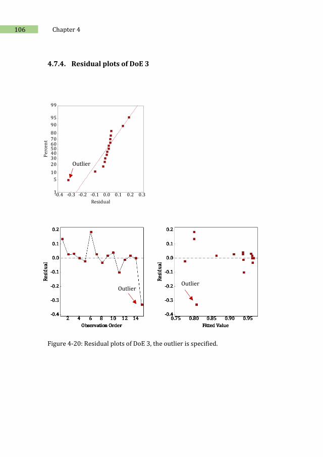
106 Chapter 4
4.7.4. Residual plots of DoE 3
Figure 4-20: Residual plots of DoE 3, the outlier is specified.
0.30.20.10.0-0.1-0.2-0.3-0.4
99
95
90
80706050403020
10
5
1
Residual
Pe
rcen
t
Outlier
Outlier Outlier
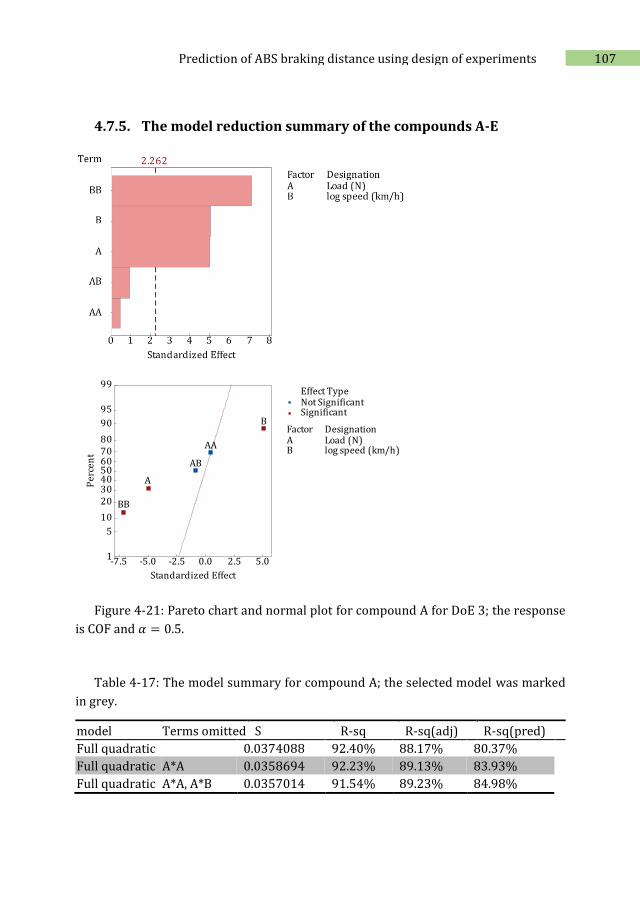
107 Prediction of ABS braking distance using design of experiments
4.7.5. The model reduction summary of the compounds A-E
Figure 4-21: Pareto chart and normal plot for compound A for DoE 3; the response
is COF and 𝛼 = 0.5.
Table 4-17: The model summary for compound A; the selected model was marked
in grey.
model Terms omitted S R-sq R-sq(adj) R-sq(pred)
Full quadratic 0.0374088 92.40% 88.17% 80.37%
Full quadratic A*A 0.0358694 92.23% 89.13% 83.93%
Full quadratic A*A, A*B 0.0357014 91.54% 89.23% 84.98%
5.02.50.0-2.5-5.0-7.5
99
95
90
80706050403020
10
5
1
A Load (N)B log speed (km/h)
Factor Designation
Standardized Effect
Pe
rcen
t
Not SignificantSignificant
Effect Type
AB
BB
AA
B
A
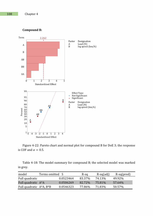
108 Chapter 4
Compound B:
Figure 4-22: Pareto chart and normal plot for compound B for DoE 3; the response
is COF and 𝛼 = 0.5.
Table 4-18: The model summary for compound B; the selected model was marked
in grey.
model Terms omitted S R-sq R-sq(adj) R-sq(pred)
Full quadratic 0.0523464 83.37% 74.13% 49.92%
Full quadratic A*A 0.0506269 82.72% 75.81% 57.64%
Full quadratic A*A, B*B 0.0546323 77.86% 71.83% 50.57%
43210-1-2-3-4-5
99
95
90
80706050403020
10
5
1
A Load (N)B log speed (km/h)
Factor Designation
Standardized Effect
Pe
rcen
t
Not SignificantSignificant
Effect Type
AB
BB
AA
B
A
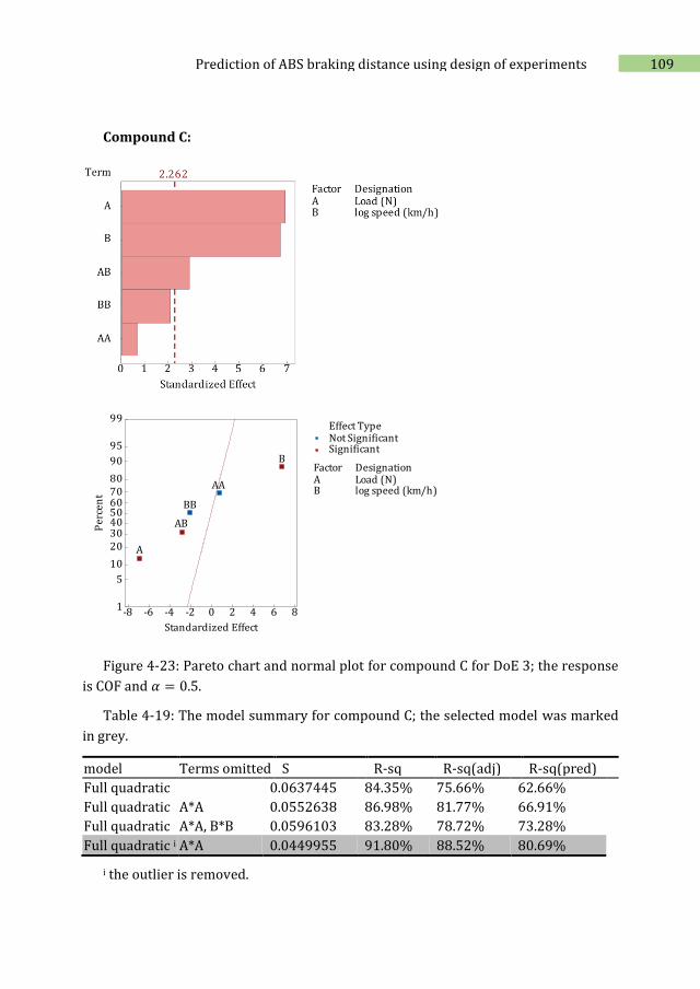
109 Prediction of ABS braking distance using design of experiments
Compound C:
Figure 4-23: Pareto chart and normal plot for compound C for DoE 3; the response
is COF and 𝛼 = 0.5.
Table 4-19: The model summary for compound C; the selected model was marked
in grey.
model Terms omitted S R-sq R-sq(adj) R-sq(pred)
Full quadratic 0.0637445 84.35% 75.66% 62.66%
Full quadratic A*A 0.0552638 86.98% 81.77% 66.91%
Full quadratic A*A, B*B 0.0596103 83.28% 78.72% 73.28%
Full quadratic i A*A 0.0449955 91.80% 88.52% 80.69%
i the outlier is removed.
86420-2-4-6-8
99
95
90
80706050403020
10
5
1
A Load (N)B log speed (km/h)
Factor Designation
Standardized Effect
Pe
rcen
t
Not SignificantSignificant
Effect Type
AB
BB
AA
B
A
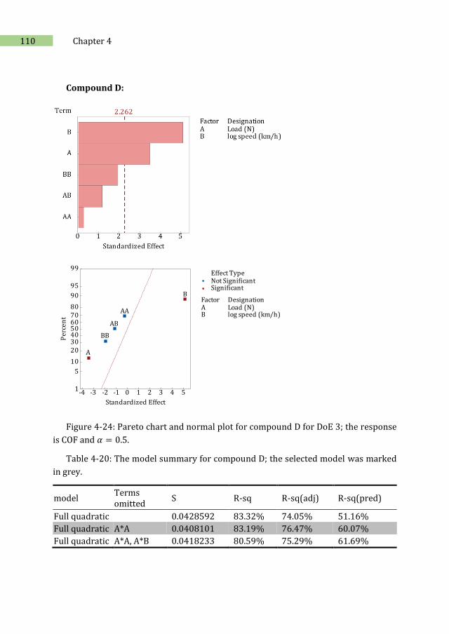
110 Chapter 4
Compound D:
Figure 4-24: Pareto chart and normal plot for compound D for DoE 3; the response
is COF and 𝛼 = 0.5.
Table 4-20: The model summary for compound D; the selected model was marked
in grey.
model Terms omitted
S R-sq R-sq(adj) R-sq(pred)
Full quadratic 0.0428592 83.32% 74.05% 51.16%
Full quadratic A*A 0.0408101 83.19% 76.47% 60.07%
Full quadratic A*A, A*B 0.0418233 80.59% 75.29% 61.69%
543210-1-2-3-4
99
95
90
80706050403020
10
5
1
A Load (N)B log speed (km/h)
Factor Designation
Standardized Effect
Pe
rcen
t
Not SignificantSignificant
Effect Type
AB
BB
AA
B
A
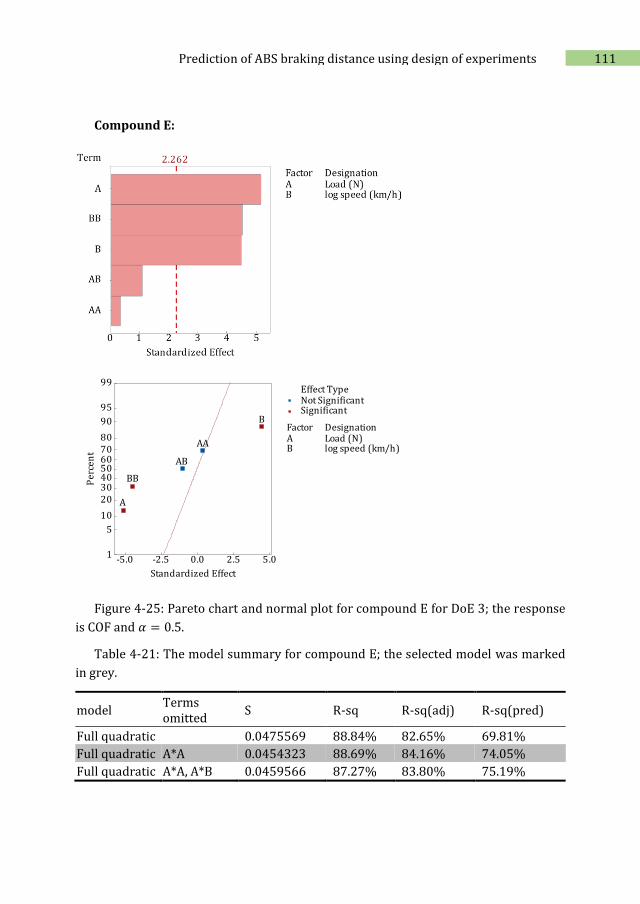
111 Prediction of ABS braking distance using design of experiments
Compound E:
Figure 4-25: Pareto chart and normal plot for compound E for DoE 3; the response
is COF and 𝛼 = 0.5.
Table 4-21: The model summary for compound E; the selected model was marked
in grey.
model Terms omitted
S R-sq R-sq(adj) R-sq(pred)
Full quadratic 0.0475569 88.84% 82.65% 69.81%
Full quadratic A*A 0.0454323 88.69% 84.16% 74.05%
Full quadratic A*A, A*B 0.0459566 87.27% 83.80% 75.19%
5.02.50.0-2.5-5.0
99
95
90
80706050403020
10
5
1
A Load (N)B log speed (km/h)
Factor Designation
Standardized Effect
Pe
rcen
t
Not SignificantSignificant
Effect Type
AB
BB
AA
B
A
The following Chapter 5 has been published in7:
Abstract
The evaluation of tire grip on the road is costly and consumes high energy and time, but
is essential for safety. Prediction of tire grip on a laboratory scale is therefore always of
interest and of utmost importance for research and material developments. It mostly suffers
from lack of comparison with actual tire data. To involve all influencing factors on tire grip
in a laboratory-scale measurement is very complex. Therefore, it has always remained
challenging to obtain a strong correlation between laboratory results and road data.
In the present study, a new test method is developed for a Laboratory Abrasion Tester,
LAT100, which enables to exploit the device as a tribometer. The objective was to develop a
technique on a laboratory device to mimic the common test modalities for evaluating tire
grip on the road with a trailer tester: lateral (α) and longitudinal (κ) sweep tests. The new
method is validated by correlating the laboratory data with the two test modalities of real
tire grip on a dry road using a trailer tester for six different tire tread compositions. For the
LAT100 tests, solid rubber wheels are characterized at three different normal loads. The
effects are comparable with actual tire data. The outcome of the new test method is in good
agreement with actual tire trailer α-sweep tests.
Keywords: Tire dry grip, Tire cornering, Rubber friction, LAT100
7 A self-contained chapter: the content of the paper has been transformed completely into this chapter.
5 New sweep function with LAT100 in
correlation with tire data
5.1. Introduction
Tire grip or traction is a concept that describes the grasp and interaction between
the tire and the road to avoid vehicle skidding or sliding which is crucial for safety. The
terms grip or traction both imply the same meaning and can be used interchangeably
in this context. Proper tire grip provides a good level of handling which is a prerequisite
for vehicle’s steering in various driving states such as cornering, braking, and
accelerating. The tire grip is the result of the generated frictional forces in the
aforementioned driving states which are created by the tire slippage in the contact
patch. When a vehicle brakes, accelerates, or corners, the tire tread elements in the
contact area move a noticeable displacement in relation to the road. This is called
slippage. For instance for an Anti-lock Braking System (ABS), the braking force is
optimized based on a specific region of tire slippage to provide adequate frictional
forces or grip and avoid tire skidding. This has been elaborated in detail in our previous
studies [1, 2]. A tire rolling at a constant speed does not move relative to the road
surface in the contact patch, apart from the shear deformations owing to various forms
114 Chapter 5
of rolling resistance and carcass (the tire internal structural body except for the tread
layer) distortion which creates a very small slippage in the trailing edge. This is beyond
the scope of this paper.
Numerous factors influence tire grip: first, the tire construction, tread formulation
and the pattern of the tire; second, the road surface characteristics, its condition and
structure; and last temperature [3]. The general relationship between the frictional
forces and the slippage is a specific characteristic of a tire design that includes the
carcass, all rubbers used in the tire structure, and most important the tread. The
slippage can be classified in lateral or longitudinal directions based on the driving
states. Accordingly, it creates forces that can be categorized in two main modes: lateral
(side) during cornering and longitudinal while braking or accelerating, both with their
own specific characteristics.
The lateral force is the force that tires transmit to the ground during cornering in
parallel to the rolling axis, see Figure 5-1. The angle between the tire plane of symmetry
and the actual moving direction of the vehicle in cornering is termed slip angle α (°)
which creates lateral slippage. Figure 5-1 (left) shows a typical relationship between
the lateral friction coefficient 𝜇𝑦 and the slip angle. Various lateral forces play a role
during tire service which differ by several orders of magnitude. They encompass
cornering forces, camber thrust, and minor residual influences comprised of two
components - ply steer (pseudo-slip angle) and conicity (pseudo-camber) [4].
The longitudinal friction force is created when the tire contact patch moves a
noticeable displacement in the forward direction during braking or accelerating. The
longitudinal slippage is defined by the difference between the forward driving speed
and the equivalent circumferential velocity of the wheel [5, 6]. According to the Society
of Automotive Engineers (SAE), the longitudinal slip ratio 𝜅 is defined as:
𝜅 = − 𝑉𝑥 − 𝑅𝑒𝜔
𝑉𝑥
(5.1)
where 𝑉𝑥 (𝑚/𝑠) is the longitudinal driving speed and 𝑅𝑒𝜔 is the equivalent
circumferential velocity of the wheel, where 𝜔 (rad/s) is the rotational velocity of the
wheel and 𝑅𝑒 (𝑚) is the effective tire radius. The latter is defined as the radius of the
tire when rolling with no external torque applied to the spin axis. Since the tire flattens
in the contact patch, this value lies somewhere in between the tire’s un-deformed and
the static loaded radii [7]. Figure 5-1 (middle) shows the longitudinal friction coefficient
𝜇𝑥 vs. the negative braking slip ratio according to Eq. (5.1). Whereas all these
phenomena also occur during accelerating conditions, then conversely the slip ratio is
115 New sweep function with LAT100 in correlation with tire data
positive. Each tire is characterized by a specific friction curve based on its carcass, tread
pattern as well as the composition of the various rubber compounds. The typical
important parameters of the friction curves are specified in Figure 5-1. The slope of the
lateral friction at small slip angles, typically smaller than 2° - 3° for a tire where the
friction curve is still linear, represents the cornering stiffness of the tire which
originates from tire carcass and tread stiffness.
Accordingly, there are two common methods for assessing tire dry grip. First, lateral
(α) sweep in which the α is varied over one complete cycle of slip angle at a specific
normal load to the counter-surface at steady speed and a defined camber angle. Second,
longitudinal (κ) sweep which is the variation of κ, while maintaining the α equal to zero.
The degree of κ is continuously varied by applying a braking force to the wheel.
Combined slip is also possible which involves variation of the κ and α simultaneously
[8]. During tire tests the lateral and vertical forces and self-aligning torques are
collected and by employing the Magic Formula (MF) of Pacejka [9] the data are modeled
and presented in the form of the typical graphs as shown in Figure 5-1. It is possible to
perform the measurements at various normal loads and camber angles.
At automotive and tire industrial companies and institutes, indoor and outdoor test
facilities are available for performing full-scale tire measurements to determine tire
performances. The outdoor test installations are built on a truck or trailer that is
equipped with a special wheel suspension and guidance system to which a measuring
hub is attached. Flat track tire testing machines also evaluate tire performances in an
indoor laboratory on a full tire on corundum sandpaper. The design of such systems
presents a high degree of complexity in order to control the flatness of the rolling
surface as well as its dynamic performance to keep it from interfering with the tire [10].
The measurements have a higher precision in comparison with the tire trailer testing
because of controlled laboratory environment and conditions, but less accuracy due to
the type of test track [11]. At an actual range of loads and speeds of the tire, the flat
track tests are not in good agreement with the trailer testing due to the sandpaper
substrate which normally becomes saturated with abraded rubber particles which fill
out the asperities of the test track. The possibilities of applying a simulated road in the
indoor devices have been extensively discussed to obtain proper friction properties
[12].
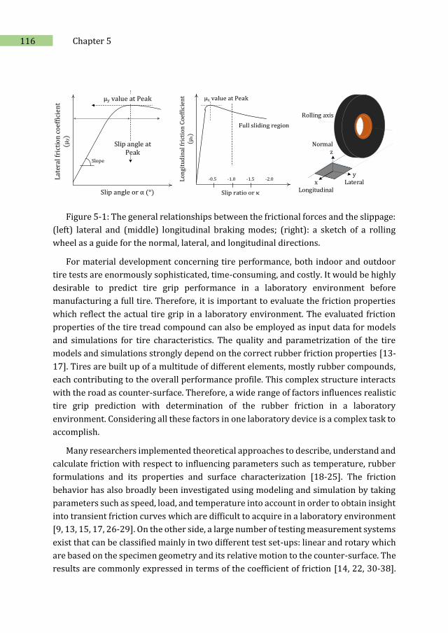
116 Chapter 5
Slip angle or α (°)
Slip angle at Peak
Lat
eral
fri
ctio
n c
oef
fici
ent
(μy)
μy value at Peak
Slope
Slip ratio or κ
Lo
ngi
tud
inal
fri
ctio
n C
oef
fici
ent
(μx)
-0.5 -1.0 -1.5 -2.0
μx value at Peak
Full sliding region
xLongitudinal
yLateral
Normalz
Rolling axis
Figure 5-1: The general relationships between the frictional forces and the slippage:
(left) lateral and (middle) longitudinal braking modes; (right): a sketch of a rolling
wheel as a guide for the normal, lateral, and longitudinal directions.
For material development concerning tire performance, both indoor and outdoor
tire tests are enormously sophisticated, time-consuming, and costly. It would be highly
desirable to predict tire grip performance in a laboratory environment before
manufacturing a full tire. Therefore, it is important to evaluate the friction properties
which reflect the actual tire grip in a laboratory environment. The evaluated friction
properties of the tire tread compound can also be employed as input data for models
and simulations for tire characteristics. The quality and parametrization of the tire
models and simulations strongly depend on the correct rubber friction properties [13-
17]. Tires are built up of a multitude of different elements, mostly rubber compounds,
each contributing to the overall performance profile. This complex structure interacts
with the road as counter-surface. Therefore, a wide range of factors influences realistic
tire grip prediction with determination of the rubber friction in a laboratory
environment. Considering all these factors in one laboratory device is a complex task to
accomplish.
Many researchers implemented theoretical approaches to describe, understand and
calculate friction with respect to influencing parameters such as temperature, rubber
formulations and its properties and surface characterization [18-25]. The friction
behavior has also broadly been investigated using modeling and simulation by taking
parameters such as speed, load, and temperature into account in order to obtain insight
into transient friction curves which are difficult to acquire in a laboratory environment
[9, 13, 15, 17, 26-29]. On the other side, a large number of testing measurement systems
exist that can be classified mainly in two different test set-ups: linear and rotary which
are based on the specimen geometry and its relative motion to the counter-surface. The
results are commonly expressed in terms of the coefficient of friction [14, 22, 30-38].
117 New sweep function with LAT100 in correlation with tire data
ISO 15113 standard [39] for the frictional properties of rubber was first published in
1999 and is probably the most comprehensive of all friction standards. It was developed
from an earlier British standard, BS 903 Part A 61 [40]. The standard methods do not
describe a specific apparatus but emphasize the importance of tight control of the
various parameters and provides guidance on the factors to be considered in measuring
friction. In most mentioned test procedures, the objective is to provide the best
correlation with the service conditions, together with good reproducibility between
laboratories.
Among all available tribometers suitable for measuring tire tread frictional
properties, there is a great interest in measurements with the Grosch wheel [1, 2, 13-
17, 28, 31, 41-48]. The main advantage is the rolling movement in the contact area with
a renewed surface in each revolution. This helps the rubber to relax in a loading
condition similar to a tire which leads to a more realistic temperature profile in the
contact area. Using sliding body measurements does not provide a realistic input for
tire modeling due to poor surface cooling [13]. Some researchers put more emphasize
on the dynamic contact behavior of the rolling wheel because of similarities to the tire
by the aid of modeling [13-17].
The Laboratory Abrasion Tester (LAT100) is one of the machines that is able to
simulate a wide range of test conditions in a laboratory environment with a solid rubber
sample wheel which was originally developed by Grosch in 1996 [46] to measure the
lateral force and the abrasion loss as a function of various slip angles, loads, and speeds
on different counter-surfaces. This apparatus has also been considered for the
evaluation of rubber tribological properties due to its similarity to vehicle tire operating
conditions [1, 28, 31, 41-46, 48].
For tire grip assessments, so far most attention has been paid to car ABS braking
distance data, especially on wet surfaces. Good agreements have been acquired with
laboratory tribometers, both linear and rotary measurements, with ABS braking data.
A Linear Friction Tester (LFT) provides a strong correlation with outdoor ABS data on
wet [49] and snow surfaces [50], but not for dry surfaces primarily because of poor
temperature control in the contact area [49]. The portable LFTs provide the possibility
to perform in-situ measurements on the actual testing fields or road surfaces. Some
good agreements have been reported between LAT100 results and ABS braking data on
different surfaces [1, 31, 48].
In the present study, the prediction of tire grip on a dry surface is investigated in a
laboratory environment with a LAT100, compared with the friction curves acquired
from actual tire grip data in the two driving states of cornering and braking. Basically,
118 Chapter 5
the objective was to apply and simulate α- and κ-sweep tests of the trailer tire testing
in the laboratory device. A new test method is developed for the LAT100 by which the
instrument can be utilized as a tribometer to generate the full friction curve. New
dynamic functions are defined which enable one to work in a semi-automatic mode of
the LAT100 machine. This allows to program the LAT100 parameters: slip angle, load,
and speed with time. The test method is designed in such a way that it needs
substantially shorter test times in comparison with the conventional measuring
method of the LAT100. This method is verified and validated with actual tire data on a
dry road, evaluated with a tire trailer tester with two test modalities of κ and α sweeps
for a wide range of tread compounds. Corresponding solid rubber wheels are
characterized on the modified LAT100 on a specific electro-corundum counter-surface
with a particular grain size based on our earlier study [1], disc 180 of the LAT100 (see
later). The experiments are performed at three different normal loads and the effects
are compared between laboratory and tire samples. The results are in a good agreement
primarily with the actual tire trailer α-sweep tests.
The advantage of the current study is first the comparison and correlation of
laboratory data with the actual tire data on the road, and secondly the design of a unique
method analogous to the tire situation on a laboratory scale for the evaluation of the
rubber properties and the acquisition of full friction curves. This method also reduces
the change of the rubber sample surface during the measurement which stems from the
inherent rubber abrasion during the measurements for acquiring the friction curves.
The test results are comprehensively validated for a large variety of rubber compounds
and test conditions.
5.2. Experimental
5.2.1. Tire data generation
5.2.1.1. Tread compounds
Six passenger tread compounds C1 to C6 were designed comprising various types of
carbon black and silica fillers with different particle sizes; C1 to C3 were pure silica
reinforced, C4 was based on a blend of silica and carbon black and C5 and C6 on pure
carbon black. This was expected to provide a significant difference in tire grip. The
reason for this wide selection was to strengthen the laboratory method validation in
the current study.
119 New sweep function with LAT100 in correlation with tire data
To prepare full tires from experimental compounds for tire trailer testing on the
road, large amounts of such compounds are needed. Each compound needs to be
extruded to the green tread dimension according to its specification. Considering the
different rheological behaviors of the compounds, various die designs would be
required. Consequently, it is not time- and cost-effective to extrude the full treads in a
tire production line. Therefore, experimental tires were prepared via treads which
were prepared in a laboratory environment. To prepare these treads, the rubber
compounds were calendered and rolled into the particular width and assembled
according to the specification of the tire size 235/35R19 slick. Full-size tires were
manufactured with the same construction process using the same body components,
but with the prepared treads. To compare tire data and calculate the rating, an
additional proprietary reference compound was used and considered as the standard
tire.
5.2.1.2. Tire tests
The two types of tire tests that were performed were κ and α sweep tests as
explained in section 5.1, on an asphalt testing field with a test trailer. The tests were
carried out at a constant speed of 60 km/h and at three different normal load settings:
3430 N, 4910 N and 6870 N (corresponding to 350 kg, 500 kg, and 700 kg, respectively).
The slip condition depending on the type of test mechanism differs. The α-sweep tests
were performed from −12° 𝑡𝑜 + 12° slip angle with a slip rate of 2 °/s. The κ-sweep
tests were performed at a constant slip angle α of 0° and the κ varied in a range of 0 to
-0.45 in the braking mode. For α-sweep tests the lateral forces 𝐹𝑦 and for κ-sweep tests
the longitudinal friction forces 𝐹𝑥 were collected. The experiments were executed
randomly for all the tires with the various compounds with 3 times repetition for the
reference tire. The camber or inclination angles in these experiments are less than 0.5°,
which is negligible.
5.2.2. Laboratory data generation
5.2.2.1. Test set-up
The used laboratory set-up is known with the commercial name LAT100
manufactured by VMI Holland B.V., the Netherlands. The details of the test set-up were
fully described in our previous manuscript [1]. The measurement unit consists of a solid
rubber test wheel which is pressed under a vertical load of 𝐹𝑍 (𝑁) normal to a driven
disc as the counter-surface. The circumferential velocity of the test wheel 𝑉𝑐 is induced
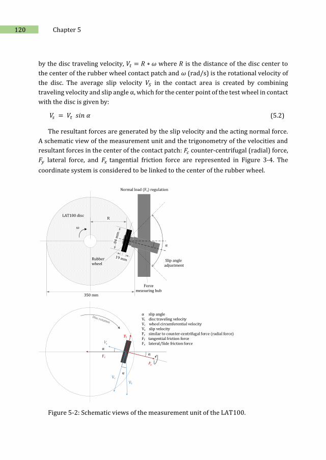
120 Chapter 5
by the disc traveling velocity, 𝑉𝑡 = 𝑅 ∗ 𝜔 where 𝑅 is the distance of the disc center to
the center of the rubber wheel contact patch and 𝜔 (rad/s) is the rotational velocity of
the disc. The average slip velocity 𝑉𝑆 in the contact area is created by combining
traveling velocity and slip angle α, which for the center point of the test wheel in contact
with the disc is given by:
𝑉𝑠 = 𝑉𝑡 𝑠𝑖𝑛 𝛼 (5.2)
The resultant forces are generated by the slip velocity and the acting normal force.
A schematic view of the measurement unit and the trigonometry of the velocities and
resultant forces in the center of the contact patch: 𝐹𝑐 counter-centrifugal (radial) force,
𝐹𝑦 lateral force, and 𝐹𝑥 tangential friction force are represented in Figure 3-4. The
coordinate system is considered to be linked to the center of the rubber wheel.
LAT100 disc
Rubber wheel
R
ω
Normal load (Fz) regulation
Slip angle adjustment
Force measuring hub
α
350 mm
Vt
Fc
α
α
α slip angleVt disc traveling velocityVc wheel circumferential velocityVs slip velocityFc similar to counter-centrifugal force (radial force) Ff tangential friction forceFs lateral/Side friction force
Vc
Ff
Figure 5-2: Schematic views of the measurement unit of the LAT100.
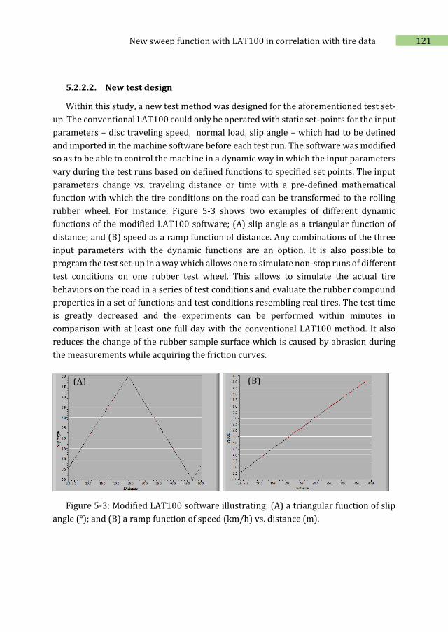
121 New sweep function with LAT100 in correlation with tire data
5.2.2.2. New test design
Within this study, a new test method was designed for the aforementioned test set-
up. The conventional LAT100 could only be operated with static set-points for the input
parameters – disc traveling speed, normal load, slip angle – which had to be defined
and imported in the machine software before each test run. The software was modified
so as to be able to control the machine in a dynamic way in which the input parameters
vary during the test runs based on defined functions to specified set points. The input
parameters change vs. traveling distance or time with a pre-defined mathematical
function with which the tire conditions on the road can be transformed to the rolling
rubber wheel. For instance, Figure 5-3 shows two examples of different dynamic
functions of the modified LAT100 software; (A) slip angle as a triangular function of
distance; and (B) speed as a ramp function of distance. Any combinations of the three
input parameters with the dynamic functions are an option. It is also possible to
program the test set-up in a way which allows one to simulate non-stop runs of different
test conditions on one rubber test wheel. This allows to simulate the actual tire
behaviors on the road in a series of test conditions and evaluate the rubber compound
properties in a set of functions and test conditions resembling real tires. The test time
is greatly decreased and the experiments can be performed within minutes in
comparison with at least one full day with the conventional LAT100 method. It also
reduces the change of the rubber sample surface which is caused by abrasion during
the measurements while acquiring the friction curves.
Figure 5-3: Modified LAT100 software illustrating: (A) a triangular function of slip
angle (°); and (B) a ramp function of speed (km/h) vs. distance (m).
(A) (B)
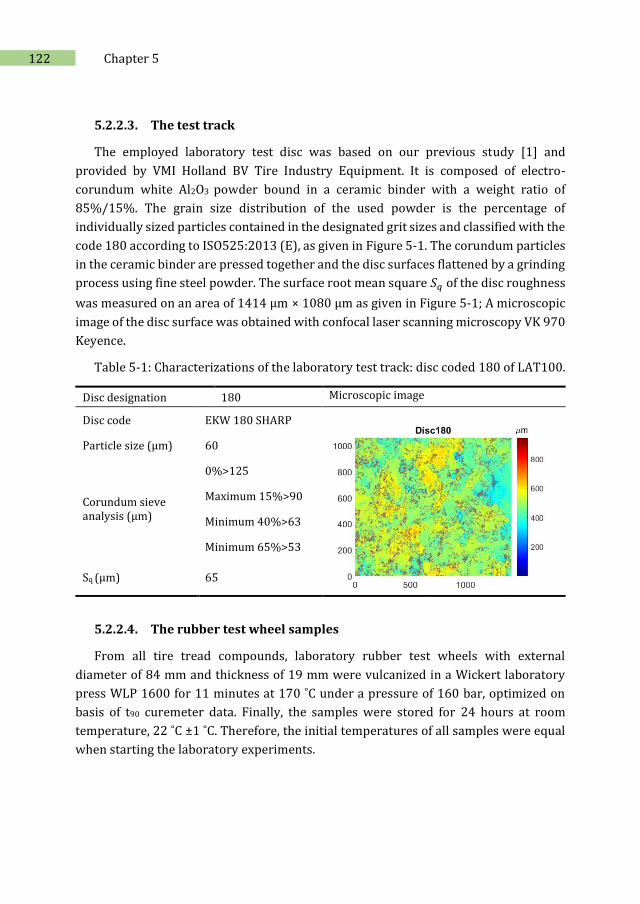
122 Chapter 5
5.2.2.3. The test track
The employed laboratory test disc was based on our previous study [1] and
provided by VMI Holland BV Tire Industry Equipment. It is composed of electro-
corundum white Al2O3 powder bound in a ceramic binder with a weight ratio of
85%/15%. The grain size distribution of the used powder is the percentage of
individually sized particles contained in the designated grit sizes and classified with the
code 180 according to ISO525:2013 (E), as given in Figure 5-1. The corundum particles
in the ceramic binder are pressed together and the disc surfaces flattened by a grinding
process using fine steel powder. The surface root mean square 𝑆𝑞 of the disc roughness
was measured on an area of 1414 μm × 1080 μm as given in Figure 5-1; A microscopic
image of the disc surface was obtained with confocal laser scanning microscopy VK 970
Keyence.
Table 5-1: Characterizations of the laboratory test track: disc coded 180 of LAT100.
Disc designation 180 Microscopic image
Disc code EKW 180 SHARP
Particle size (μm) 60
Corundum sieve analysis (μm)
0%>125
Maximum 15%>90
Minimum 40%>63
Minimum 65%>53
Sq (μm) 65
5.2.2.4. The rubber test wheel samples
From all tire tread compounds, laboratory rubber test wheels with external
diameter of 84 mm and thickness of 19 mm were vulcanized in a Wickert laboratory
press WLP 1600 for 11 minutes at 170 ˚C under a pressure of 160 bar, optimized on
basis of t90 curemeter data. Finally, the samples were stored for 24 hours at room
temperature, 22 ˚C ±1 ˚C. Therefore, the initial temperatures of all samples were equal
when starting the laboratory experiments.
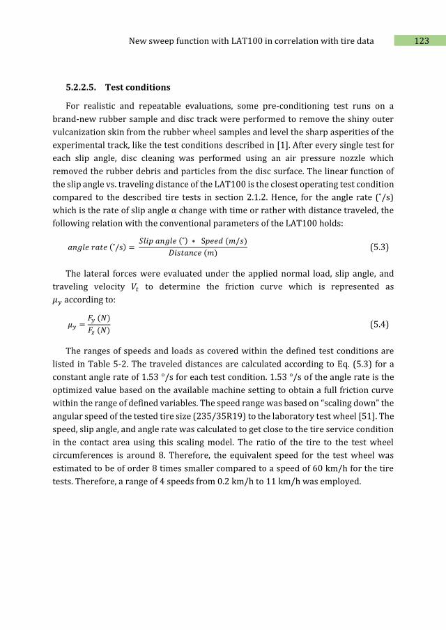
123 New sweep function with LAT100 in correlation with tire data
5.2.2.5. Test conditions
For realistic and repeatable evaluations, some pre-conditioning test runs on a
brand-new rubber sample and disc track were performed to remove the shiny outer
vulcanization skin from the rubber wheel samples and level the sharp asperities of the
experimental track, like the test conditions described in [1]. After every single test for
each slip angle, disc cleaning was performed using an air pressure nozzle which
removed the rubber debris and particles from the disc surface. The linear function of
the slip angle vs. traveling distance of the LAT100 is the closest operating test condition
compared to the described tire tests in section 2.1.2. Hence, for the angle rate (˚/s)
which is the rate of slip angle α change with time or rather with distance traveled, the
following relation with the conventional parameters of the LAT100 holds:
𝑎𝑛𝑔𝑙𝑒 𝑟𝑎𝑡𝑒 (˚/s) = 𝑆𝑙𝑖𝑝 𝑎𝑛𝑔𝑙𝑒 (˚) ∗ S𝑝𝑒𝑒𝑑 (𝑚/𝑠)
𝐷𝑖𝑠𝑡𝑎𝑛𝑐𝑒 (𝑚) (5.3)
The lateral forces were evaluated under the applied normal load, slip angle, and
traveling velocity 𝑉𝑡 to determine the friction curve which is represented as
𝜇𝑦 according to:
𝜇𝑦 =𝐹𝑦 (𝑁)
𝐹𝑧 (𝑁) (5.4)
The ranges of speeds and loads as covered within the defined test conditions are
listed in Table 5-2. The traveled distances are calculated according to Eq. (5.3) for a
constant angle rate of 1.53 °/s for each test condition. 1.53 °/s of the angle rate is the
optimized value based on the available machine setting to obtain a full friction curve
within the range of defined variables. The speed range was based on “scaling down” the
angular speed of the tested tire size (235/35R19) to the laboratory test wheel [51]. The
speed, slip angle, and angle rate was calculated to get close to the tire service condition
in the contact area using this scaling model. The ratio of the tire to the test wheel
circumferences is around 8. Therefore, the equivalent speed for the test wheel was
estimated to be of order 8 times smaller compared to a speed of 60 km/h for the tire
tests. Therefore, a range of 4 speeds from 0.2 km/h to 11 km/h was employed.
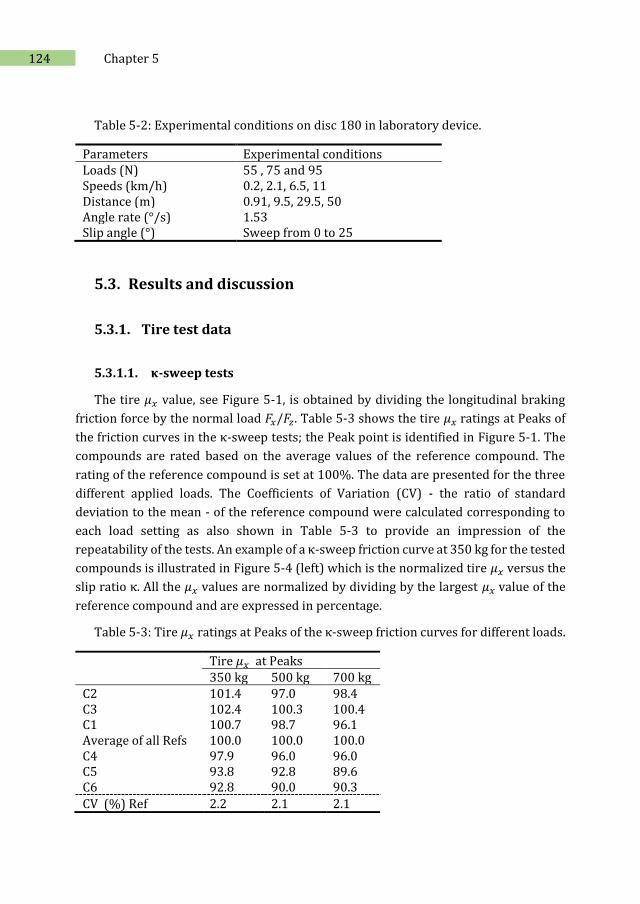
124 Chapter 5
Table 5-2: Experimental conditions on disc 180 in laboratory device.
Parameters Experimental conditions Loads (N) 55 , 75 and 95 Speeds (km/h) 0.2, 2.1, 6.5, 11 Distance (m) 0.91, 9.5, 29.5, 50 Angle rate (°/s) 1.53 Slip angle (°) Sweep from 0 to 25
5.3. Results and discussion
5.3.1. Tire test data
5.3.1.1. κ-sweep tests
The tire 𝜇𝑥 value, see Figure 5-1, is obtained by dividing the longitudinal braking
friction force by the normal load 𝐹𝑥/𝐹𝑧. Table 5-3 shows the tire 𝜇𝑥 ratings at Peaks of
the friction curves in the κ-sweep tests; the Peak point is identified in Figure 5-1. The
compounds are rated based on the average values of the reference compound. The
rating of the reference compound is set at 100%. The data are presented for the three
different applied loads. The Coefficients of Variation (CV) - the ratio of standard
deviation to the mean - of the reference compound were calculated corresponding to
each load setting as also shown in Table 5-3 to provide an impression of the
repeatability of the tests. An example of a κ-sweep friction curve at 350 kg for the tested
compounds is illustrated in Figure 5-4 (left) which is the normalized tire 𝜇𝑥 versus the
slip ratio κ. All the 𝜇𝑥 values are normalized by dividing by the largest 𝜇𝑥 value of the
reference compound and are expressed in percentage.
Table 5-3: Tire 𝜇𝑥 ratings at Peaks of the κ-sweep friction curves for different loads.
Tire 𝜇𝑥 at Peaks 350 kg 500 kg 700 kg C2 101.4 97.0 98.4 C3 102.4 100.3 100.4 C1 100.7 98.7 96.1 Average of all Refs 100.0 100.0 100.0 C4 97.9 96.0 96.0 C5 93.8 92.8 89.6 C6 92.8 90.0 90.3
CV (%) Ref 2.2 2.1 2.1
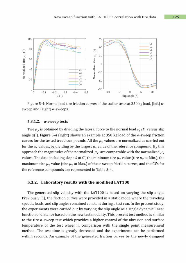
125 New sweep function with LAT100 in correlation with tire data
Figure 5-4: Normalized tire friction curves of the trailer tests at 350 kg load, (left) κ-
sweep and (right) α-sweeps.
5.3.1.2. α-sweep tests
Tire 𝜇𝑦 is obtained by dividing the lateral force to the normal load 𝐹𝑦/𝐹𝑧 versus slip
angle α(˚). Figure 5-4 (right) shows an example at 350 kg load of the α-sweep friction
curves for the tested tread compounds. All the 𝜇𝑦 values are normalized as carried out
for the 𝜇𝑥 values, by dividing by the largest 𝜇𝑥 value of the reference compound. By this
approach the magnitudes of the normalized 𝜇𝑦 are comparable with the normalized 𝜇𝑥
values. The data including slope 𝑆 at 0˚, the minimum tire 𝜇𝑦 value (tire 𝜇𝑦 at Min.), the
maximum tire 𝜇𝑦 value (tire 𝜇𝑦 at Max.) of the α-sweep friction curves, and the CVs for
the reference compounds are represented in Table 5-4.
5.3.2. Laboratory results with the modified LAT100
The generated slip velocity with the LAT100 is based on varying the slip angle.
Previously [1], the friction curves were provided in a static mode where the traveling
speeds, loads, and slip angles remained constant during a test run. In the present study,
the experiments were carried out by varying the slip angle as a single dynamic linear
function of distance based on the new test modality. This present test method is similar
to the tire α-sweep test which provides a higher control of the abrasion and surface
temperature of the test wheel in comparison with the single point measurement
method. The test time is greatly decreased and the experiments can be performed
within seconds. An example of the generated friction curves by the newly designed
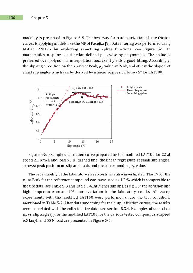
126 Chapter 5
modality is presented in Figure 5-5. The best way for parametrization of the friction
curves is applying models like the MF of Pacejka [9]. Data filtering was performed using
Matlab R2017b by exploiting smoothing spline functions: see Figure 5-5. In
mathematics, a spline is a function defined piecewise by polynomials. The spline is
preferred over polynomial interpolation because it yields a good fitting. Accordingly,
the slip angle position on the x-axis at Peak, 𝜇𝑦 value at Peak, and at last the slope S at
small slip angles which can be derived by a linear regression below 5° for LAT100.
Figure 5-5: Example of a friction curve prepared by the modified LAT100 for C2 at
speed 2.1 km/h and load 55 N; dashed line: the linear regression at small slip angles,
arrows: peak position on slip angle axis and the corresponding 𝜇𝑦 value.
The repeatability of the laboratory sweep tests was also investigated. The CV for the
𝜇𝑦 at Peak for the reference compound was measured as 1.2 % which is comparable to
the tire data: see Table 5-3 and Table 5-4. At higher slip angles e.g. 25° the abrasion and
high temperature create 1% more variation in the laboratory results. All sweep
experiments with the modified LAT100 were performed under the test conditions
mentioned in Table 5-2. After data smoothing for the output friction curves, the results
were correlated with the collected tire data, see section 5.3.4. Examples of smoothed
𝜇𝑦 vs. slip angle (°) for the modified LAT100 for the various tested compounds at speed
6.5 km/h and 55 N load are presented in Figure 5-6.
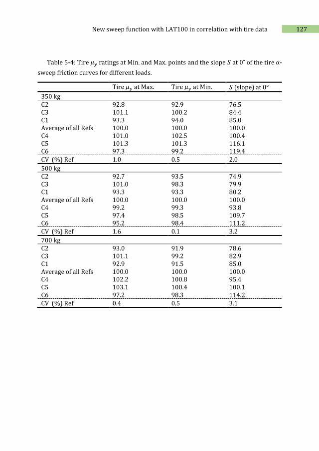
127 New sweep function with LAT100 in correlation with tire data
Table 5-4: Tire 𝜇𝑦 ratings at Min. and Max. points and the slope 𝑆 at 0˚ of the tire α-
sweep friction curves for different loads.
Tire 𝜇𝑦 at Max. Tire 𝜇𝑦 at Min. 𝑆 (slope) at 0°
350 kg C2 92.8 92.9 76.5 C3 101.1 100.2 84.4 C1 93.3 94.0 85.0 Average of all Refs 100.0 100.0 100.0 C4 101.0 102.5 100.4 C5 101.3 101.3 116.1 C6 97.3 99.2 119.4
CV (%) Ref 1.0 0.5 2.0
500 kg C2 92.7 93.5 74.9 C3 101.0 98.3 79.9 C1 93.3 93.3 80.2 Average of all Refs 100.0 100.0 100.0 C4 99.2 99.3 93.8 C5 97.4 98.5 109.7 C6 95.2 98.4 111.2
CV (%) Ref 1.6 0.1 3.2
700 kg C2 93.0 91.9 78.6 C3 101.1 99.2 82.9 C1 92.9 91.5 85.0 Average of all Refs 100.0 100.0 100.0 C4 102.2 100.8 95.4 C5 103.1 100.4 100.1 C6 97.2 98.3 114.2
CV (%) Ref 0.4 0.5 3.1
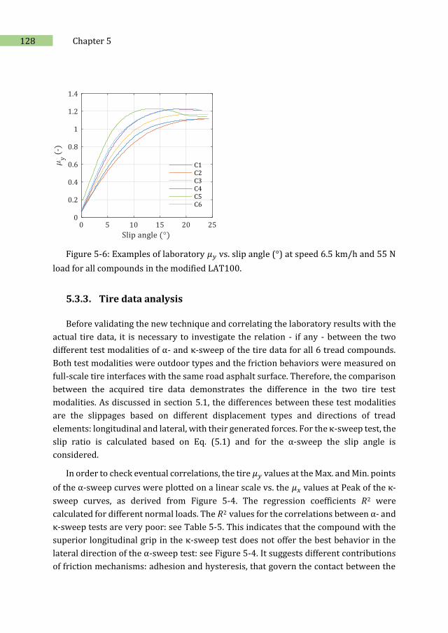
128 Chapter 5
Figure 5-6: Examples of laboratory 𝜇𝑦 vs. slip angle (°) at speed 6.5 km/h and 55 N
load for all compounds in the modified LAT100.
5.3.3. Tire data analysis
Before validating the new technique and correlating the laboratory results with the
actual tire data, it is necessary to investigate the relation - if any - between the two
different test modalities of α- and κ-sweep of the tire data for all 6 tread compounds.
Both test modalities were outdoor types and the friction behaviors were measured on
full-scale tire interfaces with the same road asphalt surface. Therefore, the comparison
between the acquired tire data demonstrates the difference in the two tire test
modalities. As discussed in section 5.1, the differences between these test modalities
are the slippages based on different displacement types and directions of tread
elements: longitudinal and lateral, with their generated forces. For the κ-sweep test, the
slip ratio is calculated based on Eq. (5.1) and for the α-sweep the slip angle is
considered.
In order to check eventual correlations, the tire 𝜇𝑦 values at the Max. and Min. points
of the α-sweep curves were plotted on a linear scale vs. the 𝜇𝑥 values at Peak of the κ-
sweep curves, as derived from Figure 5-4. The regression coefficients 𝑅2 were
calculated for different normal loads. The 𝑅2 values for the correlations between α- and
κ-sweep tests are very poor: see Table 5-5. This indicates that the compound with the
superior longitudinal grip in the κ-sweep test does not offer the best behavior in the
lateral direction of the α-sweep test: see Figure 5-4. It suggests different contributions
of friction mechanisms: adhesion and hysteresis, that govern the contact between the
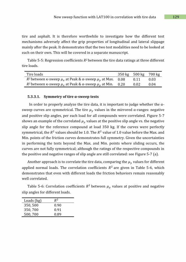
129 New sweep function with LAT100 in correlation with tire data
tire and asphalt. It is therefore worthwhile to investigate how the different test
mechanisms adversely affect the grip properties of longitudinal and lateral slippage
mainly after the peak. It demonstrates that the two test modalities need to be looked at
each on their own. This will be covered in a separate manuscript.
Table 5-5: Regression coefficients 𝑅2 between the tire data ratings at three different
tire loads.
Tire loads 350 kg 500 kg 700 kg
𝑅2 between κ-sweep 𝜇𝑥 at Peak & α-sweep 𝜇𝑦 at Max. 0.08 0.11 0.03 𝑅2 between κ-sweep 𝜇𝑥 at Peak & α-sweep 𝜇𝑦 at Min. 0.20 0.02 0.04
5.3.3.1. Symmetry of tire α-sweep tests
In order to properly analyze the tire data, it is important to judge whether the α-
sweep curves are symmetrical. The tire 𝜇𝑦 values in the mirrored α-ranges: negative
and positive slip angles, per each load for all compounds were correlated. Figure 5-7
shows an example of the correlated 𝜇𝑦 values at the positive slip angle vs. the negative
slip angle for the reference compound at load 350 kg. If the curves were perfectly
symmetrical, the 𝑅2 values should be 1.0. The 𝑅2 value of 1.0 value before the Max. and
Min. points of the friction curves demonstrates full symmetry. Given the uncertainties
in performing the tests beyond the Max. and Min. points where sliding occurs, the
curves are not fully symmetrical; although the ratings of the respective compounds in
the positive and negative ranges of slip angle are still correlated: see Figure 5-7 (a).
Another approach is to correlate the tire data, comparing the 𝜇𝑦 values for different
applied normal loads. The correlation coefficients 𝑅2 are given in Table 5-6, which
demonstrates that even with different loads the friction behaviors remain reasonably
well correlated.
Table 5-6: Correlation coefficients 𝑅2 between 𝜇𝑦 values at positive and negative
slip angles for different loads.
Loads (kg) 𝑅2 350, 500 0.90 350, 700 0.91 500, 700 0.89
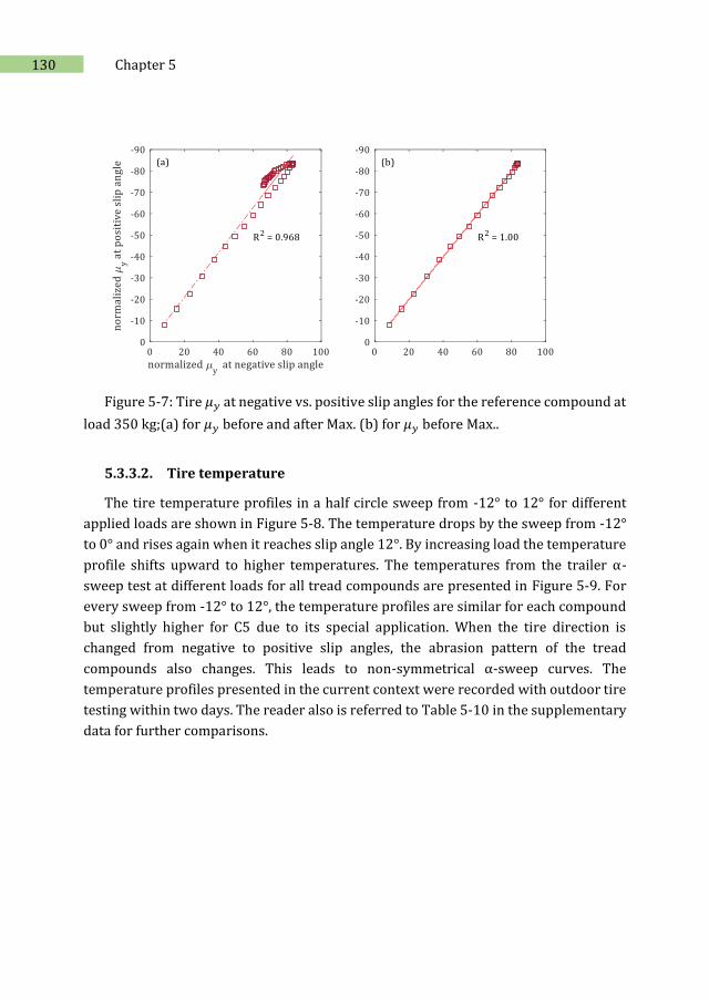
130 Chapter 5
Figure 5-7: Tire 𝜇𝑦 at negative vs. positive slip angles for the reference compound at
load 350 kg;(a) for 𝜇𝑦 before and after Max. (b) for 𝜇𝑦 before Max..
5.3.3.2. Tire temperature
The tire temperature profiles in a half circle sweep from -12° to 12° for different
applied loads are shown in Figure 5-8. The temperature drops by the sweep from -12°
to 0° and rises again when it reaches slip angle 12°. By increasing load the temperature
profile shifts upward to higher temperatures. The temperatures from the trailer α-
sweep test at different loads for all tread compounds are presented in Figure 5-9. For
every sweep from -12° to 12°, the temperature profiles are similar for each compound
but slightly higher for C5 due to its special application. When the tire direction is
changed from negative to positive slip angles, the abrasion pattern of the tread
compounds also changes. This leads to non-symmetrical α-sweep curves. The
temperature profiles presented in the current context were recorded with outdoor tire
testing within two days. The reader also is referred to Table 5-10 in the supplementary
data for further comparisons.
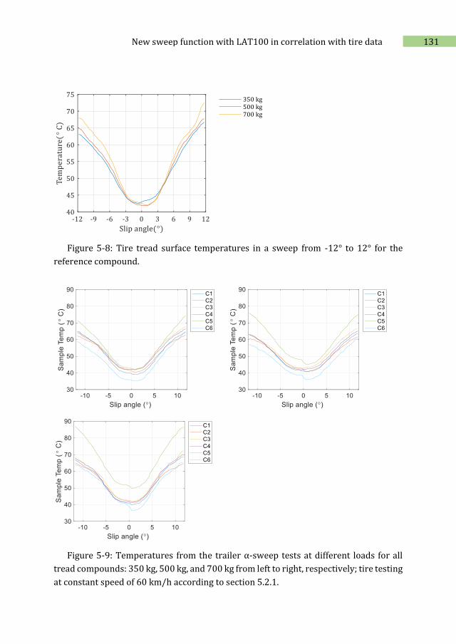
131 New sweep function with LAT100 in correlation with tire data
Figure 5-8: Tire tread surface temperatures in a sweep from -12° to 12° for the
reference compound.
Figure 5-9: Temperatures from the trailer α-sweep tests at different loads for all
tread compounds: 350 kg, 500 kg, and 700 kg from left to right, respectively; tire testing
at constant speed of 60 km/h according to section 5.2.1.
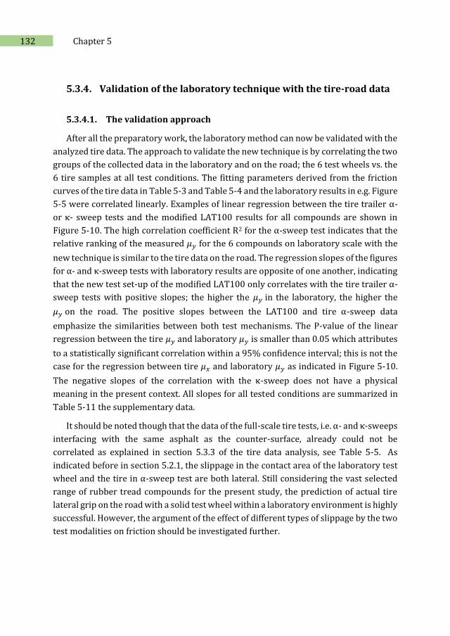
132 Chapter 5
5.3.4. Validation of the laboratory technique with the tire-road data
5.3.4.1. The validation approach
After all the preparatory work, the laboratory method can now be validated with the
analyzed tire data. The approach to validate the new technique is by correlating the two
groups of the collected data in the laboratory and on the road; the 6 test wheels vs. the
6 tire samples at all test conditions. The fitting parameters derived from the friction
curves of the tire data in Table 5-3 and Table 5-4 and the laboratory results in e.g. Figure
5-5 were correlated linearly. Examples of linear regression between the tire trailer α-
or κ- sweep tests and the modified LAT100 results for all compounds are shown in
Figure 5-10. The high correlation coefficient R2 for the α-sweep test indicates that the
relative ranking of the measured 𝜇𝑦 for the 6 compounds on laboratory scale with the
new technique is similar to the tire data on the road. The regression slopes of the figures
for α- and κ-sweep tests with laboratory results are opposite of one another, indicating
that the new test set-up of the modified LAT100 only correlates with the tire trailer α-
sweep tests with positive slopes; the higher the 𝜇𝑦 in the laboratory, the higher the
𝜇𝑦 on the road. The positive slopes between the LAT100 and tire α-sweep data
emphasize the similarities between both test mechanisms. The P-value of the linear
regression between the tire 𝜇𝑦 and laboratory 𝜇𝑦 is smaller than 0.05 which attributes
to a statistically significant correlation within a 95% confidence interval; this is not the
case for the regression between tire 𝜇𝑥 and laboratory 𝜇𝑦 as indicated in Figure 5-10.
The negative slopes of the correlation with the κ-sweep does not have a physical
meaning in the present context. All slopes for all tested conditions are summarized in
Table 5-11 the supplementary data.
It should be noted though that the data of the full-scale tire tests, i.e. α- and κ-sweeps
interfacing with the same asphalt as the counter-surface, already could not be
correlated as explained in section 5.3.3 of the tire data analysis, see Table 5-5. As
indicated before in section 5.2.1, the slippage in the contact area of the laboratory test
wheel and the tire in α-sweep test are both lateral. Still considering the vast selected
range of rubber tread compounds for the present study, the prediction of actual tire
lateral grip on the road with a solid test wheel within a laboratory environment is highly
successful. However, the argument of the effect of different types of slippage by the two
test modalities on friction should be investigated further.
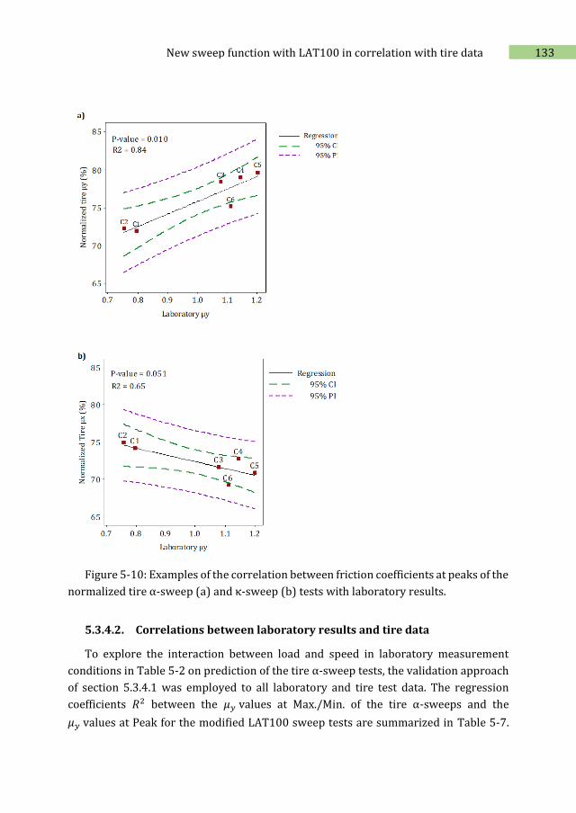
133 New sweep function with LAT100 in correlation with tire data
Figure 5-10: Examples of the correlation between friction coefficients at peaks of the
normalized tire α-sweep (a) and κ-sweep (b) tests with laboratory results.
5.3.4.2. Correlations between laboratory results and tire data
To explore the interaction between load and speed in laboratory measurement
conditions in Table 5-2 on prediction of the tire α-sweep tests, the validation approach
of section 5.3.4.1 was employed to all laboratory and tire test data. The regression
coefficients 𝑅2 between the 𝜇𝑦 values at Max./Min. of the tire α-sweeps and the
𝜇𝑦 values at Peak for the modified LAT100 sweep tests are summarized in Table 5-7.
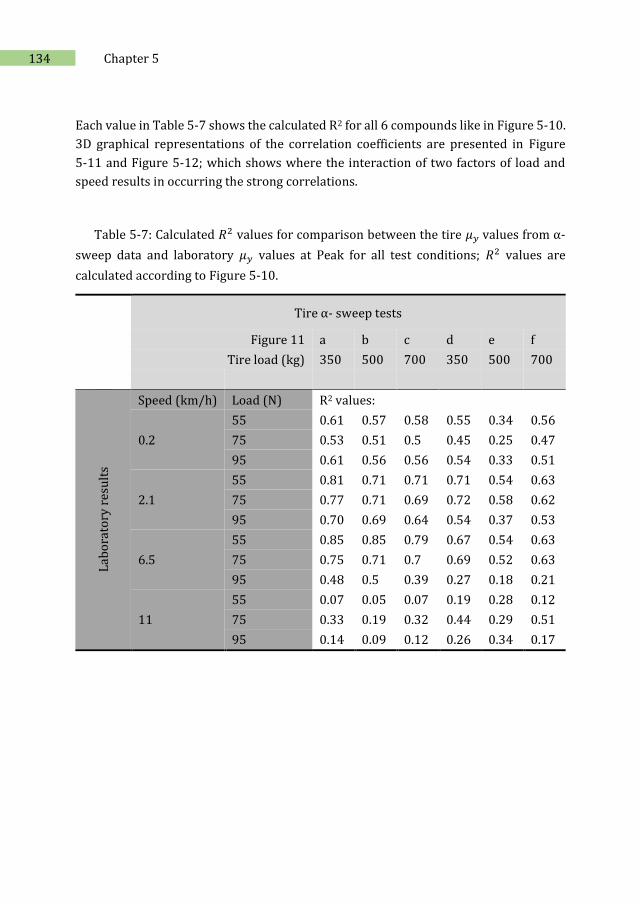
134 Chapter 5
Each value in Table 5-7 shows the calculated R2 for all 6 compounds like in Figure 5-10.
3D graphical representations of the correlation coefficients are presented in Figure
5-11 and Figure 5-12; which shows where the interaction of two factors of load and
speed results in occurring the strong correlations.
Table 5-7: Calculated 𝑅2 values for comparison between the tire 𝜇𝑦 values from α-
sweep data and laboratory 𝜇𝑦 values at Peak for all test conditions; 𝑅2 values are
calculated according to Figure 5-10.
Tire α- sweep tests
Figure 11 a b c d e f Tire load (kg) 350 500 700 350 500 700
Lab
ora
tory
res
ult
s
Speed (km/h) Load (N) R2 values:
0.2
55 0.61 0.57 0.58 0.55 0.34 0.56
75 0.53 0.51 0.5 0.45 0.25 0.47
95 0.61 0.56 0.56 0.54 0.33 0.51
2.1
55 0.81 0.71 0.71 0.71 0.54 0.63
75 0.77 0.71 0.69 0.72 0.58 0.62
95 0.70 0.69 0.64 0.54 0.37 0.53
6.5
55 0.85 0.85 0.79 0.67 0.54 0.63
75 0.75 0.71 0.7 0.69 0.52 0.63
95 0.48 0.5 0.39 0.27 0.18 0.21
11
55 0.07 0.05 0.07 0.19 0.28 0.12
75 0.33 0.19 0.32 0.44 0.29 0.51
95 0.14 0.09 0.12 0.26 0.34 0.17
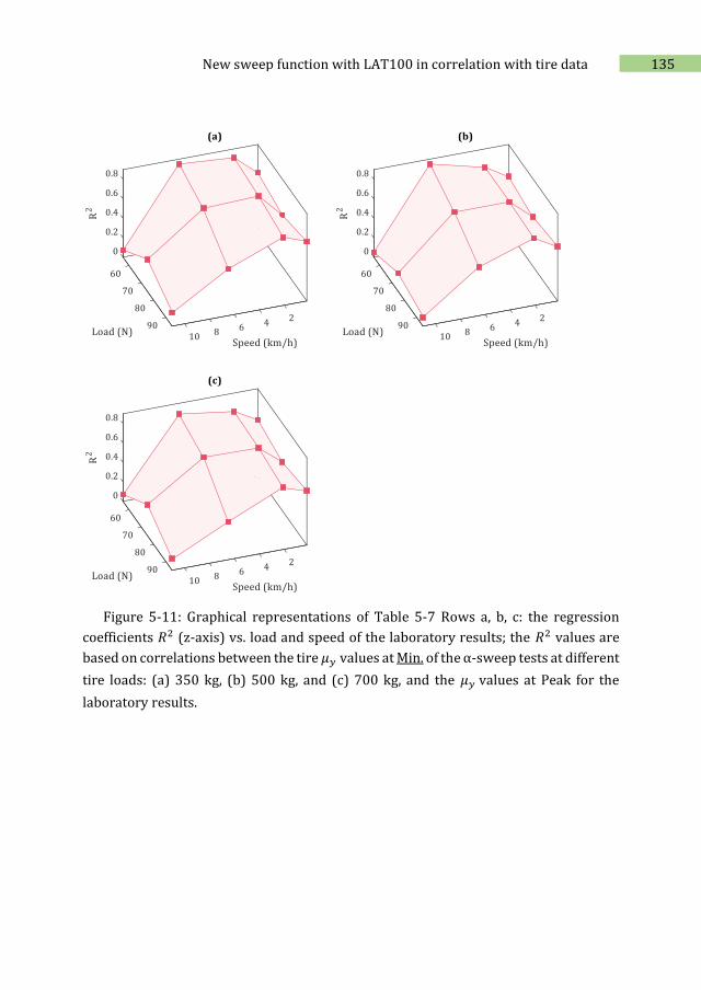
135 New sweep function with LAT100 in correlation with tire data
Figure 5-11: Graphical representations of Table 5-7 Rows a, b, c: the regression
coefficients 𝑅2 (z-axis) vs. load and speed of the laboratory results; the 𝑅2 values are
based on correlations between the tire 𝜇𝑦 values at Min. of the α-sweep tests at different
tire loads: (a) 350 kg, (b) 500 kg, and (c) 700 kg, and the 𝜇𝑦 values at Peak for the
laboratory results.
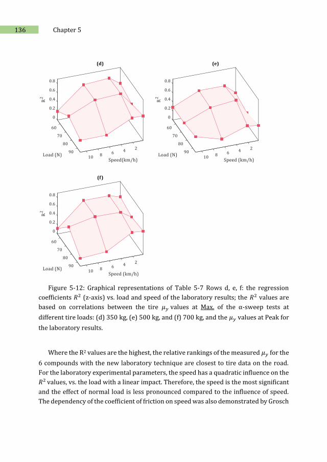
136 Chapter 5
Figure 5-12: Graphical representations of Table 5-7 Rows d, e, f: the regression
coefficients 𝑅2 (z-axis) vs. load and speed of the laboratory results; the 𝑅2 values are
based on correlations between the tire 𝜇𝑦 values at Max. of the α-sweep tests at
different tire loads: (d) 350 kg, (e) 500 kg, and (f) 700 kg, and the 𝜇𝑦 values at Peak for
the laboratory results.
Where the R2 values are the highest, the relative rankings of the measured 𝜇𝑦 for the
6 compounds with the new laboratory technique are closest to tire data on the road.
For the laboratory experimental parameters, the speed has a quadratic influence on the
𝑅2 values, vs. the load with a linear impact. Therefore, the speed is the most significant
and the effect of normal load is less pronounced compared to the influence of speed.
The dependency of the coefficient of friction on speed was also demonstrated by Grosch
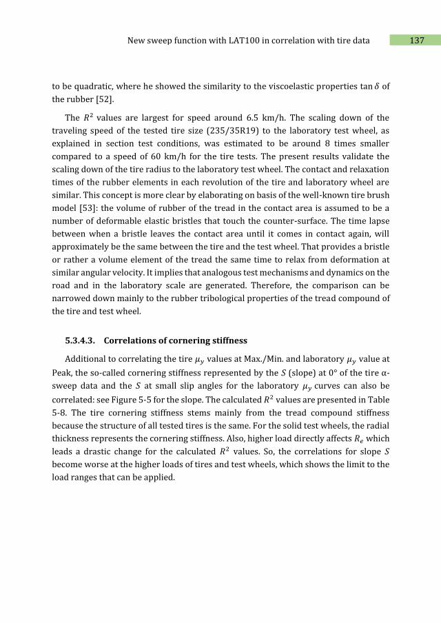
137 New sweep function with LAT100 in correlation with tire data
to be quadratic, where he showed the similarity to the viscoelastic properties tan 𝛿 of
the rubber [52].
The 𝑅2 values are largest for speed around 6.5 km/h. The scaling down of the
traveling speed of the tested tire size (235/35R19) to the laboratory test wheel, as
explained in section test conditions, was estimated to be around 8 times smaller
compared to a speed of 60 km/h for the tire tests. The present results validate the
scaling down of the tire radius to the laboratory test wheel. The contact and relaxation
times of the rubber elements in each revolution of the tire and laboratory wheel are
similar. This concept is more clear by elaborating on basis of the well-known tire brush
model [53]: the volume of rubber of the tread in the contact area is assumed to be a
number of deformable elastic bristles that touch the counter-surface. The time lapse
between when a bristle leaves the contact area until it comes in contact again, will
approximately be the same between the tire and the test wheel. That provides a bristle
or rather a volume element of the tread the same time to relax from deformation at
similar angular velocity. It implies that analogous test mechanisms and dynamics on the
road and in the laboratory scale are generated. Therefore, the comparison can be
narrowed down mainly to the rubber tribological properties of the tread compound of
the tire and test wheel.
5.3.4.3. Correlations of cornering stiffness
Additional to correlating the tire 𝜇𝑦 values at Max./Min. and laboratory 𝜇𝑦 value at
Peak, the so-called cornering stiffness represented by the 𝑆 (slope) at 0° of the tire α-
sweep data and the 𝑆 at small slip angles for the laboratory 𝜇𝑦 curves can also be
correlated: see Figure 5-5 for the slope. The calculated 𝑅2 values are presented in Table
5-8. The tire cornering stiffness stems mainly from the tread compound stiffness
because the structure of all tested tires is the same. For the solid test wheels, the radial
thickness represents the cornering stiffness. Also, higher load directly affects 𝑅𝑒 which
leads a drastic change for the calculated 𝑅2 values. So, the correlations for slope 𝑆
become worse at the higher loads of tires and test wheels, which shows the limit to the
load ranges that can be applied.
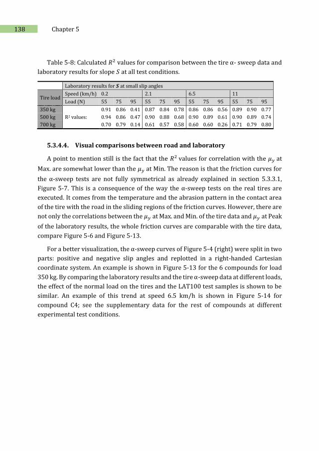
138 Chapter 5
Table 5-8: Calculated 𝑅2 values for comparison between the tire α- sweep data and
laboratory results for slope 𝑆 at all test conditions.
Laboratory results for 𝑺 at small slip angles
Tire load Speed (km/h) 0.2 2.1 6.5 11
Load (N) 55 75 95 55 75 95 55 75 95 55 75 95
350 kg 0.91 0.86 0.41 0.87 0.84 0.78 0.86 0.86 0.56 0.89 0.90 0.77
500 kg R2 values: 0.94 0.86 0.47 0.90 0.88 0.68 0.90 0.89 0.61 0.90 0.89 0.74
700 kg 0.70 0.79 0.14 0.61 0.57 0.58 0.60 0.60 0.26 0.71 0.79 0.80
5.3.4.4. Visual comparisons between road and laboratory
A point to mention still is the fact that the 𝑅2 values for correlation with the 𝜇𝑦 at
Max. are somewhat lower than the 𝜇𝑦 at Min. The reason is that the friction curves for
the α-sweep tests are not fully symmetrical as already explained in section 5.3.3.1,
Figure 5-7. This is a consequence of the way the α-sweep tests on the real tires are
executed. It comes from the temperature and the abrasion pattern in the contact area
of the tire with the road in the sliding regions of the friction curves. However, there are
not only the correlations between the 𝜇𝑦 at Max. and Min. of the tire data and 𝜇𝑦 at Peak
of the laboratory results, the whole friction curves are comparable with the tire data,
compare Figure 5-6 and Figure 5-13.
For a better visualization, the α-sweep curves of Figure 5-4 (right) were split in two
parts: positive and negative slip angles and replotted in a right-handed Cartesian
coordinate system. An example is shown in Figure 5-13 for the 6 compounds for load
350 kg. By comparing the laboratory results and the tire α-sweep data at different loads,
the effect of the normal load on the tires and the LAT100 test samples is shown to be
similar. An example of this trend at speed 6.5 km/h is shown in Figure 5-14 for
compound C4; see the supplementary data for the rest of compounds at different
experimental test conditions.
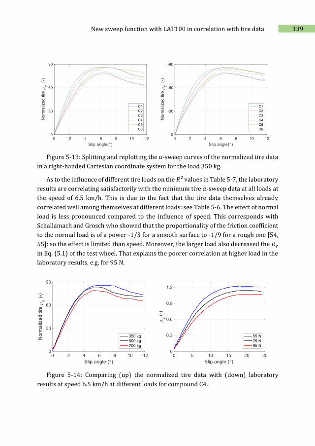
139 New sweep function with LAT100 in correlation with tire data
Figure 5-13: Splitting and replotting the α-sweep curves of the normalized tire data
in a right-handed Cartesian coordinate system for the load 350 kg.
As to the influence of different tire loads on the 𝑅2 values in Table 5-7, the laboratory
results are correlating satisfactorily with the minimum tire α-sweep data at all loads at
the speed of 6.5 km/h. This is due to the fact that the tire data themselves already
correlated well among themselves at different loads: see Table 5-6. The effect of normal
load is less pronounced compared to the influence of speed. This corresponds with
Schallamach and Grosch who showed that the proportionality of the friction coefficient
to the normal load is of a power -1/3 for a smooth surface to -1/9 for a rough one [54,
55]: so the effect is limited than speed. Moreover, the larger load also decreased the 𝑅𝑒
in Eq. (5.1) of the test wheel. That explains the poorer correlation at higher load in the
laboratory results, e.g. for 95 N.
Figure 5-14: Comparing (up) the normalized tire data with (down) laboratory
results at speed 6.5 km/h at different loads for compound C4.
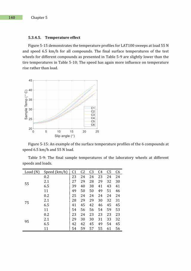
140 Chapter 5
5.3.4.5. Temperature effect
Figure 5-15 demonstrates the temperature profiles for LAT100 sweeps at load 55 N
and speed 6.5 km/h for all compounds. The final surface temperatures of the test
wheels for different compounds as presented in Table 5-9 are slightly lower than the
tire temperatures in Table 5-10; The speed has again more influence on temperature
rise rather than load.
Figure 5-15: An example of the surface temperature profiles of the 6 compounds at
speed 6.5 km/h and 55 N load.
Table 5-9: The final sample temperatures of the laboratory wheels at different
speeds and loads.
Load (N) Speed (km/h) C1 C2 C3 C4 C5 C6
55
0.2 23 24 24 23 24 24 2.1 27 29 28 29 32 30 6.5 39 40 38 41 43 41 11 49 50 50 49 51 46
75
0.2 25 24 24 24 24 24 2.1 28 29 29 30 32 31 6.5 41 45 42 46 45 45 11 54 56 56 54 59 53
95
0.2 23 24 23 23 23 23 2.1 29 30 30 31 33 32 6.5 42 42 45 49 54 45 11 54 59 57 55 61 56
141 New sweep function with LAT100 in correlation with tire data
5.4. Concluding remarks
Above all, the lateral forces measured with the laboratory test method are solely
expected to be the cornering forces; compared to tire α-sweep tests the total collected
lateral forces are comprised of major cornering forces and minor contributions of
camber thrust and residual influences of ply steer and conicity from the tire structure.
Given the large differences between the full-scale tires with air inside and the solid
rubber test wheels in the laboratory, and the many influencing factors involved, the
correlation coefficient of 0.84 in Figure 5-10 (a) for the modified LAT100 test method
on the laboratory track i.e. the disc 180 for this vast range of rubber compounds is a
surprisingly satisfactory correlation and as discussed statistically significant. Provided
the proper experimental conditions are applied based on the scaling down model as
presented here above. This shows the utmost importance of modeling the small solid
rubber wheel in the lab and compare it with the tire load distribution to obtain an
insight into the different ranges of slip angles in x-axes of Figure 5-6 and Figure 5-13.
This will be the subject of a future manuscript.
5.5. Conclusions
Prediction of tire grip on a laboratory scale is always of interest and of high
importance for research and material developments. In the present study, a new test
method was developed for a Laboratory Abrasion Tester (LAT100) in which the device
is exploited as a tribometer with the aim of mimicking the common test modalities of
evaluating the tire grip on the road with a trailer tester: lateral (α) and longitudinal (κ)
sweep tests. For validation, the new test method was compared with tire grip data
collected with the two modalities of a trailer tester on a dry test track for six different
tire tread compositions.
Correlation for the α-sweep tests (lateral slip, i.e. “cornering grip”) were found
to be strong (R2 value > 0.84; P-value < 0.05 and a 95% of confidence interval).
The 𝑅2 values for the correlations between tire α- and κ-sweep tests on the
road are poor. Consequently, the correlations for the κ-sweep tests
(longitudinal slip, i.e. “acceleration and braking grip”) were not found in
agreement with the laboratory test set-up.
Benchtop testing for ranking of lateral slip performance over a range of loads
and speeds can be conducted in only 1 minute, compared with months of
preparation and trailer testing of real tires.
142 Chapter 5
The correlation coefficients are the strongest, based on scaling down of the tire
radius to the laboratory test wheel. The condition of appr. 7 km/h and 55 N
load on the benchtop tester gives the best correlation with 60 km/h and 350
kg load for α-sweep tests on the tire trailer tester.
Given the large differences between the full-scale tires with air inside and the
solid rubber test wheel in the laboratory, the obtained correlations for this vast
range of rubber compounds is surprisingly satisfactory, provided the proper
experimental conditions are applied based on the scaling-down model as
presented.
Additional work is required to better understand the two different modalities
involved in tire slippage in lateral and longitudinal directions on the road, to
be able to also propose new scaling rules for the longitudinal slip on a
laboratory benchtop test.
The approach described to predict actual dry tire grip as a function of speed
and load with this laboratory device offers a positive new horizon to evaluate
tire grip.
5.6. References
1. Salehi, M., J.W.M. Noordermeer, L.A.E.M. Reuvekamp, W.K. Dierkes, and A. Blume, Measuring rubber friction using a Laboratory Abrasion Tester (LAT100) to predict car tire dry ABS braking. Tribology International, 2019. 131: p. 191-199.
2. Salehi, M., LAT100, Prediction of tire dry grip. 2017, University of Twente: Enschede: Ipskamp Printing.
3. Grosch, K., Some Factors Influencing the Traction of Radial Ply Tires. Rubber Chemistry and Technology, 1984. 57(5): p. 889-907.
4. Pacejka, H.B., Chapter 4 - Semi-empirical tyre models, in Book 'Tyre and Vehicle Dynamics (Second Edition)'. 2006, Butterworth-Heinemann: Oxford. p. 156-215.
5. Rajamani, R., Lateral and Longitudinal Tire Forces, in Book 'Vehicle Dynamics and Control'. 2012, Springer US. p. 387-432.
6. Majerus, J.N., your tire's behavior, in Book 'Winning More Safely in Motorsports; the Workbook'. 2007, Racing vehicle Inc. p. 268-283.
7. Miller, S.L., B. Youngberg, A. Millie, P. Schweizer, and J.C. Gerdes. Calculation Longitudinal wheel slip and tire parameters using GPS velocity. in the American control conference. 25-27 Jun 2001. Arlington.
143 New sweep function with LAT100 in correlation with tire data
8. Pacejka, H.B., Chapter 12 - Tyre steady-state and dynamic test facilities, in Book 'Tyre and Vehicle Dynamics (Second Edition)'. 2006, Butterworth-Heinemann: Oxford. p. 586-594.
9. Bakker, E., L. Nyborg, and H.B. Pacejka, Tyre Modelling for Use in Vehicle Dynamics Studies. 1987, SAE International.
10. Cabrera, J., A. Ortiz, A. Simón, F. García, A. Pérez, and A. Perez-Blanca, A Versatile Flat Track Tire Testing Machine A Versatile Flat Track Tire Testing Machine. Vol. 40. 2003. 271-284.
11. Ludwig, C. Influence of testing surface on tire lateral force characteristics. in Science meets Tires. April 24-25, 2018. Aachen, Germany: ika INSTITUT FÜR KRAFTFAHRZEUGE and RWTH AACHEN UNIVERSITY.
12. Carrillo, C. and C. Bachmann. Can we get the road into the lab? Challenges in tire tesing. in Science meets Tires. April 24-25, 2018. Aachen, Germany: ika INSTITUT FÜR KRAFTFAHRZEUGE and RWTH AACHEN UNIVERSITY.
13. Riehm, P., H.-J. Unrau, and F. Gauterin, A model based method to determine rubber friction data based on rubber sample measurements. Tribology International, 2018. 127: p. 37-46.
14. Bouzid, N. and B. Heimann, Micro Texture Characterization and Prognosis of the Maximum Traction between Grosch Wheel and Asphalt Surfaces under Wet Conditions, in Book 'Elastomere Friction: Theory, Experiment and Simulation', D. Besdo, B. Heimann, M. Klüppel, M. Kröger, P. Wriggers, and U. Nackenhorst, Editors. 2010, Springer Berlin Heidelberg: Berlin, Heidelberg. p. 201-220.
15. Bouzid, N., B. Heimann, and A. Trabelsi, Empirical friction coefficient modeling for the Grosch-wheel-road system, in VDI Berichte. 2005. p. 291-307.
16. Gutzeit, F. and M. Kröger, Experimental and Theoretical Investigations on the Dynamic Contact Behavior of Rolling Rubber Wheels, in Book 'Elastomere Friction: Theory, Experiment and Simulation', D. Besdo, B. Heimann, M. Klüppel, M. Kröger, P. Wriggers, and U. Nackenhorst, Editors. 2010, Springer Berlin Heidelberg: Berlin, Heidelberg. p. 221-249.
17. Dorsch, V., A. Becker, and L. Vossen, Enhanced rubber friction model for finite element simulations of rolling tyres. Plastics, Rubber and Composites, 2002. 31(10): p. 458-464.
18. Persson, B.N.J., Theory of rubber friction and contact mechanics. The Journal of Chemical Physics, 2001. 115(8): p. 3840-3861.
19. Lorenz, B., Y.R. Oh, S.K. Nam, S.H. Jeon, and B.N.J. Persson, Rubber friction on road surfaces: Experiment and theory for low sliding speeds. The Journal of Chemical Physics, 2015. 142(19): p. 194701.
144 Chapter 5
20. Mahboob Kanafi, M., A.J. Tuononen, L. Dorogin, and B.N.J. Persson, Rubber friction on 3D-printed randomly rough surfaces at low and high sliding speeds. Wear, 2017. 376-377: p. 1200-1206.
21. Persson, B.N.J., O. Albohr, U. Tartaglino, A.I. Volokitin, and E. Tosatti, On the nature of surface roughness with application to contact mechanics, sealing, rubber friction and adhesion. J Phys Condens Matter, 2005. 17(1): p. R1-r62.
22. Klüppel, M. and G. Heinrich, Rubber Friction on Self-Affine Road Tracks. Rubber Chemistry and Technology, 2000. 73(4): p. 578-606.
23. Heinrich, G. and M. Klüppel, Rubber friction, tread deformation and tire traction. Wear, 2008. 265(7–8): p. 1052-1060.
24. Feshanjerdi, M., M. Khorrami, A.A. Masoudi, and M. Razzaghi Kashani, The hysteretic contribution of friction for the polished rubber on the concrete surface. Applied Surface Science, 2017. 394: p. 528-533.
25. Salehi, M. and M. Razzaghi-Kashani, Comparing styrene butadiene rubber–clay nanocomposites prepared by melt intercalation and latex-coagulation methods. Journal of Applied Polymer Science, 2012. 126(1): p. 253-259.
26. Jacob Svendenius, B.W., Review of wheel modeling and friction estimation, in Department of Automatic Control 2003, Lund institute of technology.
27. Tire Modeling, Lateral and Longitudinal Tire Forces, Erdogan, G., Date of access: July 2020; Available from http://www.menet.umn.edu/~gurkan/Tire%20Modeling%20%20Lecture.pdf.
28. Steen, R.v.d., I. Lopez, and H. Nijmeijer, Experimental and numerical study of friction and .giffness characteristics of small rolling tires. Tire Science and Technology, 2011. 39(1): p. 5-19.
29. Kane, M. and V. Cerezo, A contribution to tire/road friction modeling: From a simplified dynamic frictional contact model to a “Dynamic Friction Tester” model. Wear, 2015. 342-343: p. 163-171.
30. Brown, R., friction and wear, in Book 'Physical testing of rubbers'. 2006, Springer. p. 219-243.
31. Heinz, M. and K.A. Grosch, A Laboratory Method to Comprehensively Evaluate Abrasion, Traction and Rolling Resistance of Tire Tread Compounds. Rubber Chemistry and Technology, 2007. 80(4): p. 580-607.
32. Mihajlovic, S., U. Kutscher, B. Wies, and J. Wallaschek, Methods for experimental investigations on tyre-road-grip at arbitrary roads. Internationale Konferenz ESAR "Expertensymposium Accident Research“, 2013.
145 New sweep function with LAT100 in correlation with tire data
33. Germann, S., M. Wurtenberger, and A. Daiss. Monitoring of the friction coefficient between tyre and road surface. in 1994 Proceedings of IEEE International Conference on Control and Applications. 24-26 Aug 1994.
34. Najafi, S., Evaluation of Continuous Friction Measuring Equipment (CFME) for Supporting Pavement Friction Management Programs. 2010, Virginia Tech.
35. Lindner, M., M. Kröger, K. Popp, and H. Blume, EXPERIMENTAL AND ANALYTICAL INVESTIGATION OF RUBBER FRICTION, in ICTAM04 Proceedings. 2004: Warsaw, Poland.
36. Lahayne, O., J. Eberhardsteiner, and R. Reihsner, TRIBOLOGICAL INVESTIGATIONS USING A LINEAR FRICTION TESTER (LFT). Transactions of FAMENA 2009. 33(2): p. 15-22.
37. Krasmik, V.S., J., Experimental Investigation of the Friction and Wear Behaviour with an Adapted Ball-On-Prism Test Setup. Tribology in Industry, 2015. 37(3): p. 291-298.
38. Pacejka, H.B., Chapter 2 - Basic tyre modelling considerations, in Book 'Tyre and Vehicle Dynamics (Second Edition)'. 2006, Butterworth-Heinemann: Oxford. p. 61-89.
39. ISO 15113, Rubber, in determination of frictional properties. 2005.
40. BS903-A61, PHYSICAL TESTING OF RUBBER - DETERMINATION OF THE FRICTIONAL PROPERTIES OF RUBBER, in Rubber and Plastic industries. 1994, British Standards Institution.
41. Nguyen, V.H., D. Zheng, F. Schmerwitz, and P. Wriggers, An advanced abrasion model for tire wear. Wear, 2018. 396-397: p. 75-85.
42. Wu, J., C. Zhang, Y. Wang, and B. Su, Wear Predicted Model of Tread Rubber Based on Experimental and Numerical Method. Experimental Techniques, 2018. 42(2): p. 191-198.
43. Grosch, K.A., Correlation Between Road Wear of Tires and Computer Road Wear Simulation Using Laboratory Abrasion Data. Rubber Chemistry and Technology, 2004. 77(5): p. 791-814.
44. Grosch, K.A., Goodyear Medalist Lecture. Rubber Friction and its Relation to Tire Traction. Rubber Chemistry and Technology, 2007. 80(3): p. 379-411.
45. Grosch, K.A., Rubber Abrasion and Tire Wear. Rubber Chemistry and Technology, 2008. 81(3): p. 470-505.
46. Grosch, K.A., A new way to evaluate traction-and wear properties of tire tread compounds, in Rubber Division, American Chemical Society. 1997: Cleveland, Ohio.
146 Chapter 5
47. Heinz, M., A laboratory abrasion testing method for use in the development of filler systems. Technical report rubber reinforcement systems, 2015, Evonik Industries GmbH, Essen, Germany.
48. Heinz, M., A Universal Method to Predict Wet Traction Behaviour of Tyre Tread Compounds in the Laboratory. Journal of Rubber Research, 2010. 13(2): p. 91-102.
49. Ignatyev, P.A., S. Ripka, N. Mueller, S. Torbruegge, and B. Wies, Tire ABS-Braking Prediction with Lab Tests and Friction Simulations. Tire Science and Technology, 2015. 43(4): p. 260-275.
50. Ella, S., P.-Y. Formagne, V. Koutsos, and J.R. Blackford, Investigation of rubber friction on snow for tyres. Tribology International, 2013. 59: p. 292-301.
51. Salehi, M., J.W.M. Noordermeer, L.A.E.M. Reuvekamp, and A. Blume. A New Method to Rapidly Predict Tyre Grip In a Laboratory Environment. in International Rubber Conference. 3-5 Sep 2019. London, UK.
52. Grosch, K.A., The Relation between the Friction and Viscoelastic Properties of Rubber. Rubber Chemistry and Technology, 1964. 37(2): p. 386-403.
53. Pacejka, H.B., Chapter 3 - Theory of steady-state slip force and moment generation, in Book 'Tyre and Vehicle Dynamics (Second Edition)'. 2006, Butterworth-Heinemann: Oxford. p. 90-155.
54. Schallamach, A., The Load Dependence of Rubber Friction. Proceedings of the Physical Society. Section B, 1952. 65: p. 657-661.
55. Grosch, K.A. and A. Schallamach, The Load Dependence of Laboratory Abrasion and Tire Wear. Rubber Chemistry and Technology, 1970. 43(4): p. 701-713.

147 New sweep function with LAT100 in correlation with tire data
5.7. Supplementary data
Table 5-10: Tire temperatures from the trailer α-sweep tests at different angles and
loads for all tread compounds; at constant speed of 60 km/h according to section 5.2.1.
Slip angle (º) Tire load (kg) Compound -12 -9 -6 -3 0 3 6 9 12
350
C1 62 58 52 44 41 43 51 58 63 C2 60 57 51 43 39 39 48 56 60 C3 65 59 51 42 40 41 50 59 64 C4 64 59 52 44 42 44 53 61 66 C5 71 64 55 45 43 45 54 64 74 C6 59 53 46 38 36 38 47 56 65
500
C1 61 57 51 45 42 43 49 56 62 C2 60 56 49 43 41 42 49 56 61 C3 63 58 50 43 41 42 49 58 64 C4 63 58 50 44 42 44 51 59 65 C5 76 68 58 50 47 47 55 66 75 C6 57 53 47 40 38 38 45 53 60
700
C1 65 61 54 45 42 44 53 61 64 C2 63 59 51 42 39 42 51 60 65 C3 68 63 54 43 41 42 53 63 69 C4 67 61 54 44 42 44 54 64 70 C5 87 77 65 54 51 52 64 77 87 C6 64 59 53 43 39 39 51 59 65
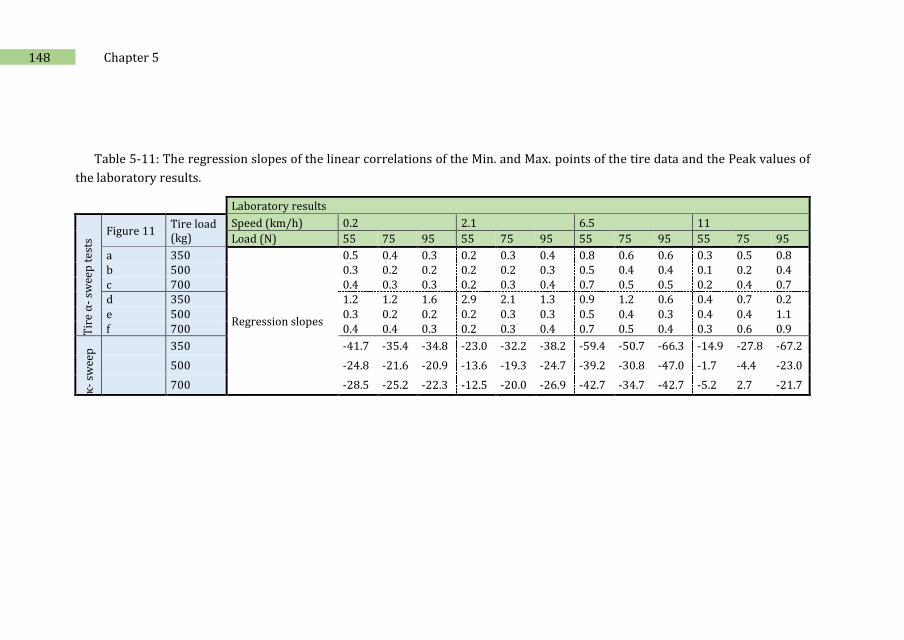
148 Chapter 5
Table 5-11: The regression slopes of the linear correlations of the Min. and Max. points of the tire data and the Peak values of
the laboratory results.
Laboratory results
Tir
e α
- sw
eep
tes
ts Figure 11
Tire load (kg)
Speed (km/h) 0.2 2.1 6.5 11
Load (N) 55 75 95 55 75 95 55 75 95 55 75 95
a 350
Regression slopes
0.5 0.4 0.3 0.2 0.3 0.4 0.8 0.6 0.6 0.3 0.5 0.8 b 500 0.3 0.2 0.2 0.2 0.2 0.3 0.5 0.4 0.4 0.1 0.2 0.4 c 700 0.4 0.3 0.3 0.2 0.3 0.4 0.7 0.5 0.5 0.2 0.4 0.7 d 350 1.2 1.2 1.6 2.9 2.1 1.3 0.9 1.2 0.6 0.4 0.7 0.2 e 500 0.3 0.2 0.2 0.2 0.3 0.3 0.5 0.4 0.3 0.4 0.4 1.1 f 700 0.4 0.4 0.3 0.2 0.3 0.4 0.7 0.5 0.4 0.3 0.6 0.9
κ-
swee
p 350 -41.7 -35.4 -34.8 -23.0 -32.2 -38.2 -59.4 -50.7 -66.3 -14.9 -27.8 -67.2
500 -24.8 -21.6 -20.9 -13.6 -19.3 -24.7 -39.2 -30.8 -47.0 -1.7 -4.4 -23.0
700 -28.5 -25.2 -22.3 -12.5 -20.0 -26.9 -42.7 -34.7 -42.7 -5.2 2.7 -21.7
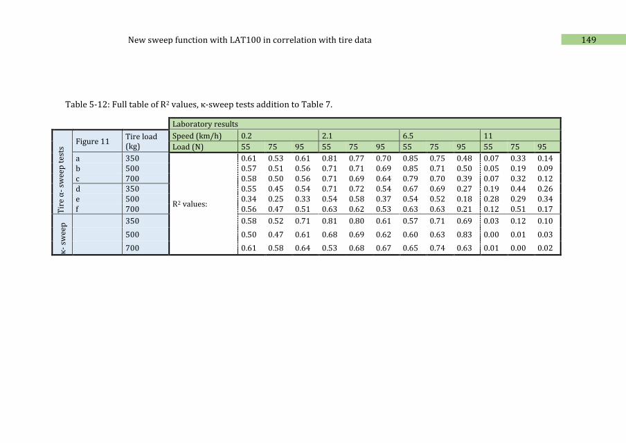
149 New sweep function with LAT100 in correlation with tire data
Table 5-12: Full table of R2 values, κ-sweep tests addition to Table 7.
Laboratory results
Tir
e α
- sw
eep
tes
ts Figure 11
Tire load (kg)
Speed (km/h) 0.2 2.1 6.5 11
Load (N) 55 75 95 55 75 95 55 75 95 55 75 95
a 350
R2 values:
0.61 0.53 0.61 0.81 0.77 0.70 0.85 0.75 0.48 0.07 0.33 0.14 b 500 0.57 0.51 0.56 0.71 0.71 0.69 0.85 0.71 0.50 0.05 0.19 0.09 c 700 0.58 0.50 0.56 0.71 0.69 0.64 0.79 0.70 0.39 0.07 0.32 0.12 d 350 0.55 0.45 0.54 0.71 0.72 0.54 0.67 0.69 0.27 0.19 0.44 0.26 e 500 0.34 0.25 0.33 0.54 0.58 0.37 0.54 0.52 0.18 0.28 0.29 0.34 f 700 0.56 0.47 0.51 0.63 0.62 0.53 0.63 0.63 0.21 0.12 0.51 0.17
κ-
swee
p 350 0.58 0.52 0.71 0.81 0.80 0.61 0.57 0.71 0.69 0.03 0.12 0.10
500 0.50 0.47 0.61 0.68 0.69 0.62 0.60 0.63 0.83 0.00 0.01 0.03
700 0.61 0.58 0.64 0.53 0.68 0.67 0.65 0.74 0.63 0.01 0.00 0.02
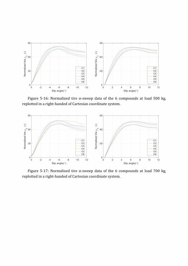
Figure 5-16: Normalized tire α-sweep data of the 6 compounds at load 500 kg,
replotted in a right-handed of Cartesian coordinate system.
Figure 5-17: Normalized tire α-sweep data of the 6 compounds at load 700 kg,
replotted in a right-handed of Cartesian coordinate system.
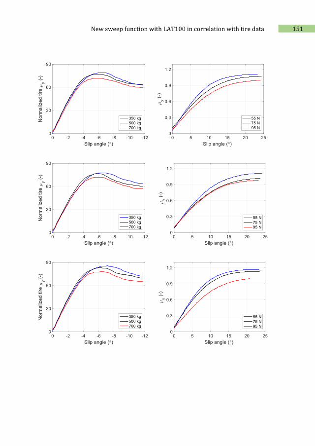
151 New sweep function with LAT100 in correlation with tire data
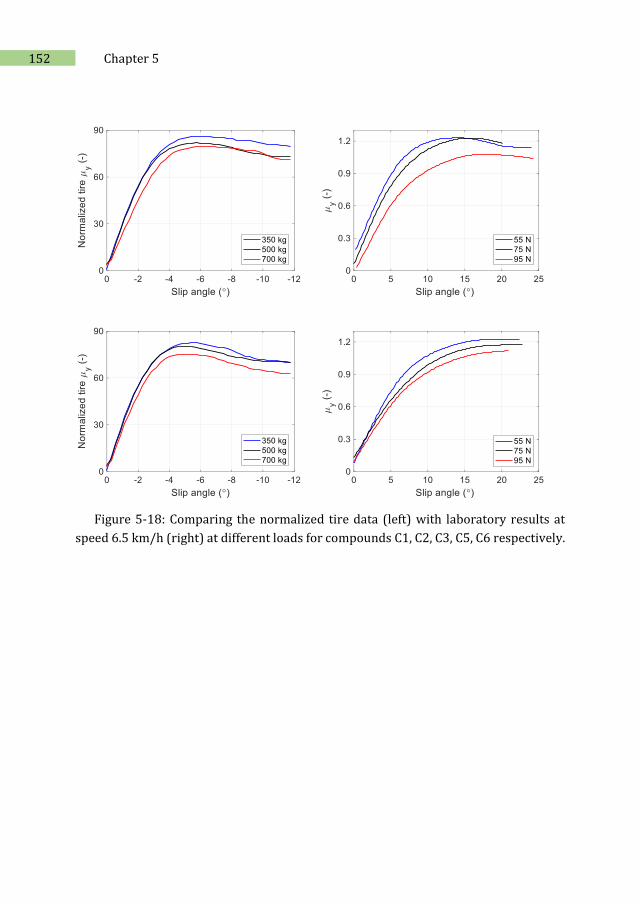
152 Chapter 5
Figure 5-18: Comparing the normalized tire data (left) with laboratory results at
speed 6.5 km/h (right) at different loads for compounds C1, C2, C3, C5, C6 respectively.
6 Characterization of counter-
surfaces
6.1. Introduction
Tire grip is the interaction between the tire and the road as counter-surface. On
studying tire friction, the characteristics of the roads/counter-surfaces are of pivotal
importance as well. The excitations on the tire come from the road asperities. A proper
characterization of the counter-surface texture is, therefore, an absolute necessity. The
present chapter provides the required knowledge over the counter-surfaces employed
in the study throughout this thesis. All surfaces were scanned and characterized by
laser microscopic apparatuses. The surface micro and macro roughness/textures are
evaluated to provide insight into the friction studies.
6.2. Classification of road surface texture
The texture or roughness of the road counter-surface plays a dominant role in tire
friction. Various textures contribute differently to friction components and involve
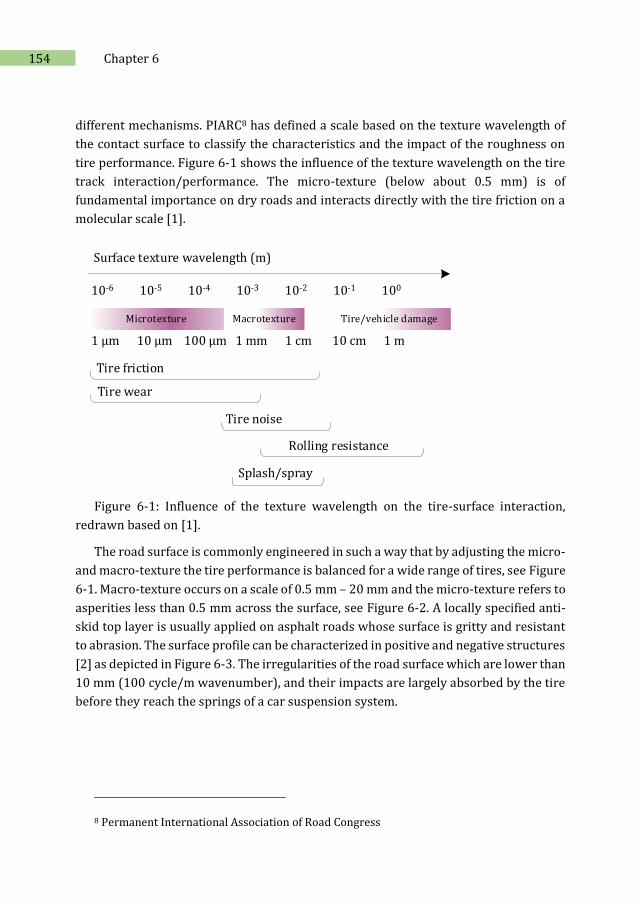
154 Chapter 6
different mechanisms. PIARC8 has defined a scale based on the texture wavelength of
the contact surface to classify the characteristics and the impact of the roughness on
tire performance. Figure 6-1 shows the influence of the texture wavelength on the tire
track interaction/performance. The micro-texture (below about 0.5 mm) is of
fundamental importance on dry roads and interacts directly with the tire friction on a
molecular scale [1].
Surface texture wavelength (m)
10-6 10-5 10-4 10-3 10-2 10-1 100
1 µm 10 µm 100 µm 1 mm 1 cm 10 cm 1 m
Microtexture Macrotexture Tire/vehicle damage
Tire friction
Tire wear
Rolling resistance
Tire noise
Splash/spray
Figure 6-1: Influence of the texture wavelength on the tire-surface interaction,
redrawn based on [1].
The road surface is commonly engineered in such a way that by adjusting the micro-
and macro-texture the tire performance is balanced for a wide range of tires, see Figure
6-1. Macro-texture occurs on a scale of 0.5 mm – 20 mm and the micro-texture refers to
asperities less than 0.5 mm across the surface, see Figure 6-2. A locally specified anti-
skid top layer is usually applied on asphalt roads whose surface is gritty and resistant
to abrasion. The surface profile can be characterized in positive and negative structures
[2] as depicted in Figure 6-3. The irregularities of the road surface which are lower than
10 mm (100 cycle/m wavenumber), and their impacts are largely absorbed by the tire
before they reach the springs of a car suspension system.
8 Permanent International Association of Road Congress
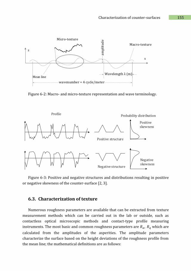
155 Characterization of counter-surfaces
Micro-texture
Wavelength λ (m)
x
z
Mean line
am
pli
tud
e
Macro-texture
wavenumber = 4 cycle/meter
Figure 6-2: Macro- and micro-texture representation and wave terminology.
Positive structure
Negative structure
Negative skewness
Profile Probability distribution
Positive skewness
Figure 6-3: Positive and negative structures and distributions resulting in positive
or negative skewness of the counter-surface [2, 3].
6.3. Characterization of texture
Numerous roughness parameters are available that can be extracted from texture
measurement methods which can be carried out in the lab or outside, such as
contactless optical microscopic methods and contact-type profile measuring
instruments. The most basic and common roughness parameters are 𝑅𝑎, 𝑅𝑞 which are
calculated from the amplitudes of the asperities. The amplitude parameters
characterize the surface based on the height deviations of the roughness profile from
the mean line; the mathematical definitions are as follows:
156 Chapter 6
𝑅𝑎 = 1
𝐿 ∫|𝑧(𝑥)|𝑑𝑥
𝐿
0
(6.1)
𝑅𝑞 = 𝑟𝑚𝑠 = ( 1
𝐿 ∫ 𝑧(𝑥)2𝑑𝑥
𝐿
0
)1/2 (6.2)
where 𝑅𝑎 (𝑚) is an arithmetic average of the absolute values of the height 𝑧 (𝑚) of
the asperities relative to the mean line over a distance 𝑥 (𝑚) on the length of
measurement 𝐿; and 𝑅𝑞(𝑚) is the root mean square (rms) of the surface heights. 𝑅𝑠𝑞 is
another useful parameter for the shape of the asperities: the skewness which can
indicate a positive or negative structure of the counter-surface [4]. Two surfaces with
the same 𝑅𝑞 can have different shapes [3].
𝑅𝑠𝑞 = 1
𝐿𝑅𝑞3
∫ 𝑧(𝑥)3𝑑𝑥
𝐿
0
(6.3)
A surface with a large 𝑅𝑎 value, or a positive 𝑅𝑠𝑞 produces usually high friction and
wears quickly. More parameters should be considered: the form and waviness of both
amplitudes and frequency of the asperities, their slopes and spacing’s. A finite number
of surface parameters to describe the real surface geometry is mainly scale-dependent
and provides only limited information [3].
In 1971, Nayak [5] modeled rough surfaces as two-dimensional isotropic Gaussian
random processes and analyzed them with the aid of random process theory. The
surface statistics such as the distribution and density of heights, and the rms height and
rms slope were related to the power spectral density of the surface profile; it is a
combination of several important surface parameters in one tool. The use of random
process analysis has been reported as a breakthrough in recent years, based on the idea
of the autocorrelation function9 first used in 1946 [6].
The Power Spectral Density (PSD) contains statistical characteristics of the surface
topography regardless of the choice of the particular scan size. It decomposes the
surface into a superposition of numerous sine and cosine signals of different amplitudes
and wavelengths. Using the Fourier transform technique, a wavelength with a specific
9 𝐴(𝜏) =1
𝐿∫ 𝑧(𝑥)𝑧(𝑥 + 𝜏)𝑑𝑥
𝐿
0 : it describes the height similarity of two points on the surface
at a distance 𝜏. At 𝜏 = 0, 𝐴(𝜏) = 𝑅𝑞 2.
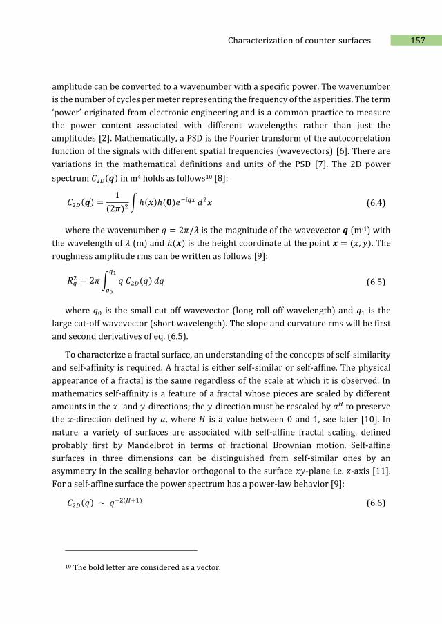
157 Characterization of counter-surfaces
amplitude can be converted to a wavenumber with a specific power. The wavenumber
is the number of cycles per meter representing the frequency of the asperities. The term
‘power’ originated from electronic engineering and is a common practice to measure
the power content associated with different wavelengths rather than just the
amplitudes [2]. Mathematically, a PSD is the Fourier transform of the autocorrelation
function of the signals with different spatial frequencies (wavevectors) [6]. There are
variations in the mathematical definitions and units of the PSD [7]. The 2D power
spectrum 𝐶2𝐷(𝒒) in m4 holds as follows10 [8]:
𝐶2𝐷(𝒒) =1
(2𝜋)2∫ ℎ(𝒙)ℎ(𝟎)𝑒−𝑖𝑞𝑥 𝑑2𝑥 (6.4)
where the wavenumber 𝑞 = 2𝜋/𝜆 is the magnitude of the wavevector 𝒒 (m-1) with
the wavelength of 𝜆 (m) and ℎ(𝒙) is the height coordinate at the point 𝒙 = (𝑥, 𝑦). The
roughness amplitude rms can be written as follows [9]:
𝑅𝑞2 = 2𝜋 ∫ 𝑞 𝐶2𝐷(𝑞)
𝑞1
𝑞0
𝑑𝑞 (6.5)
where 𝑞0 is the small cut-off wavevector (long roll-off wavelength) and 𝑞1 is the
large cut-off wavevector (short wavelength). The slope and curvature rms will be first
and second derivatives of eq. (6.5).
To characterize a fractal surface, an understanding of the concepts of self-similarity
and self-affinity is required. A fractal is either self-similar or self-affine. The physical
appearance of a fractal is the same regardless of the scale at which it is observed. In
mathematics self-affinity is a feature of a fractal whose pieces are scaled by different
amounts in the 𝑥- and 𝑦-directions; the 𝑦-direction must be rescaled by 𝑎𝐻 to preserve
the 𝑥-direction defined by 𝑎, where 𝐻 is a value between 0 and 1, see later [10]. In
nature, a variety of surfaces are associated with self-affine fractal scaling, defined
probably first by Mandelbrot in terms of fractional Brownian motion. Self-affine
surfaces in three dimensions can be distinguished from self-similar ones by an
asymmetry in the scaling behavior orthogonal to the surface 𝑥𝑦-plane i.e. 𝑧-axis [11].
For a self-affine surface the power spectrum has a power-law behavior [9]:
𝐶2𝐷(𝑞) ∼ 𝑞−2(𝐻+1) (6.6)
10 The bold letter are considered as a vector.
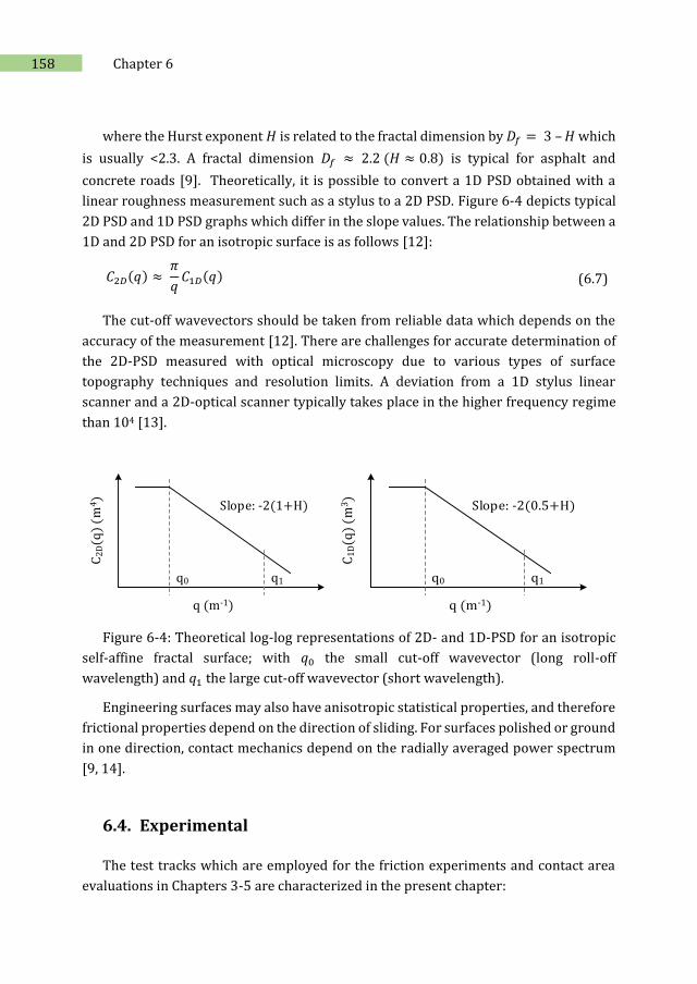
158 Chapter 6
where the Hurst exponent 𝐻 is related to the fractal dimension by 𝐷𝑓 = 3 – 𝐻 which
is usually <2.3. A fractal dimension 𝐷𝑓 ≈ 2.2 (𝐻 ≈ 0.8) is typical for asphalt and
concrete roads [9]. Theoretically, it is possible to convert a 1D PSD obtained with a
linear roughness measurement such as a stylus to a 2D PSD. Figure 6-4 depicts typical
2D PSD and 1D PSD graphs which differ in the slope values. The relationship between a
1D and 2D PSD for an isotropic surface is as follows [12]:
𝐶2𝐷(𝑞) ≈ 𝜋
𝑞𝐶1𝐷(𝑞) (6.7)
The cut-off wavevectors should be taken from reliable data which depends on the
accuracy of the measurement [12]. There are challenges for accurate determination of
the 2D-PSD measured with optical microscopy due to various types of surface
topography techniques and resolution limits. A deviation from a 1D stylus linear
scanner and a 2D-optical scanner typically takes place in the higher frequency regime
than 104 [13].
q (m-1)
C2
D(q
) (m
4)
q0 q1
Slope: -2(1+H)
q (m-1)
C1
D(q
) (m
3)
q0 q1
Slope: -2(0.5+H)
Figure 6-4: Theoretical log-log representations of 2D- and 1D-PSD for an isotropic
self-affine fractal surface; with 𝑞0 the small cut-off wavevector (long roll-off
wavelength) and 𝑞1 the large cut-off wavevector (short wavelength).
Engineering surfaces may also have anisotropic statistical properties, and therefore
frictional properties depend on the direction of sliding. For surfaces polished or ground
in one direction, contact mechanics depend on the radially averaged power spectrum
[9, 14].
6.4. Experimental
The test tracks which are employed for the friction experiments and contact area
evaluations in Chapters 3-5 are characterized in the present chapter:
159 Characterization of counter-surfaces
Road samples: asphalt and concrete;
Sandpaper grade P120;
LAT100 counter-surface discs 60, 180, 320, and 180B;
A comparably smooth surface such as an A4 paper sheet.
The asphalt road sample is a dense asphalt prepared for wet grip tire labeling. A 30
cm2 tile of concrete was selected for the contact area measurements in the laboratory
which is comparable to the asphalt sample. The sandpaper P120 is a fine grade of Silicon
Carbide with an average particle size 125 μm which is classified according to ISO
6344/FEPA Grit Designation. The employed LAT100 counter-surface discs were
provided by VMI Holland B.V. - Tire Industry Equipment. They are composed of electro-
corundum white Al2O3 powder bound in a ceramic binder with a weight ratio of
85/15%. They are classified according to ISO 525:2013(E) as given in Table 6-1, of
which the size-fraction of the corundum-particles is the most important variable in the
present context. Each disc code represents the disc grain size; a higher code number
indicates a smaller corundum particle size. The corundum particles in the ceramic
binder are pressed together and the disc surfaces flattened by a grinding process using
fine steel powder. The letter “B” for disc 180B indicates “Blunt”, which means that the
disc 180 was smoothened one step further in the finishing/flattening process using a
grinding disc containing diamond powder. This smoothening process does not
influence the grain size, however, it affects the surface structure and sharpness of the
asperities as shown in Figure 6-3.
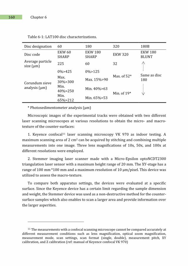
160 Chapter 6
Table 6-1: LAT100 disc characterizations.
Disc designation 60 180 320 180B
Disc code EKW 60 SHARP
EKW 180 SHARP
EKW 320 EKW 180 BLUNT
Average particle size (μm)
225 60 32 Same as disc 180 Corundum sieve
analysis (μm)
0%>425 0%>125 Max. of 52* Max.
30%>300 Max. 15%>90
Min. 40%>250
Min. 40%>63 Min. of 19*
Min. 65%>212
Min. 65%>53
* Photosedimentometer analysis (μm)
Microscopic images of the experimental tracks were obtained with two different
laser scanning microscopes at various resolutions to obtain the micro- and macro-
texture of the counter-surfaces:
1. Keyence confocal11 laser scanning microscopy VK 970 as indoor testing. A
maximum scanning area of 2 cm2 can be acquired by stitching and combining multiple
measurements into one image. Three lens magnifications of 10x, 50x, and 100x at
different resolutions were employed.
2. Stemmer imaging laser scanner made with a Micro-Epsilon optoNCDT2300
triangulation laser sensor with a maximum height range of 20 mm. The XY-stage has a
range of 100 mm *100 mm and a maximum resolution of 10 µm/pixel. This device was
utilized to assess the macro-texture.
To compare both apparatus settings, the devices were evaluated at a specific
surface. Since the Keyence device has a certain limit regarding the sample dimension
and weight, the Stemmer device was used as a non-destructive method for the counter-
surface samples which also enables to scan a larger area and provide information over
the larger asperities.
11 The measurements with a confocal scanning microscope cannot be compared accurately at different measurement conditions such as lens magnification, optical zoom magnification, measurement mode, scan settings, scan format (single, double), measurement pitch, XY calibration, and Z calibration (ref: manual of Keyence confocal VK 970)
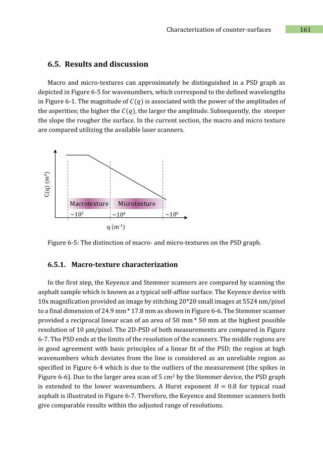
161 Characterization of counter-surfaces
6.5. Results and discussion
Macro and micro-textures can approximately be distinguished in a PSD graph as
depicted in Figure 6-5 for wavenumbers, which correspond to the defined wavelengths
in Figure 6-1. The magnitude of 𝐶(𝑞) is associated with the power of the amplitudes of
the asperities; the higher the 𝐶(𝑞), the larger the amplitude. Subsequently, the steeper
the slope the rougher the surface. In the current section, the macro and micro texture
are compared utilizing the available laser scanners.
MicrotextureMacrotexture
q (m-1)
C(q
) (m
4)
~102 ~104 ~106
Figure 6-5: The distinction of macro- and micro-textures on the PSD graph.
6.5.1. Macro-texture characterization
In the first step, the Keyence and Stemmer scanners are compared by scanning the
asphalt sample which is known as a typical self-affine surface. The Keyence device with
10x magnification provided an image by stitching 20*20 small images at 5524 nm/pixel
to a final dimension of 24.9 mm * 17.8 mm as shown in Figure 6-6. The Stemmer scanner
provided a reciprocal linear scan of an area of 50 mm * 50 mm at the highest possible
resolution of 10 μm/pixel. The 2D-PSD of both measurements are compared in Figure
6-7. The PSD ends at the limits of the resolution of the scanners. The middle regions are
in good agreement with basic principles of a linear fit of the PSD; the region at high
wavenumbers which deviates from the line is considered as an unreliable region as
specified in Figure 6-4 which is due to the outliers of the measurement (the spikes in
Figure 6-6). Due to the larger area scan of 5 cm2 by the Stemmer device, the PSD graph
is extended to the lower wavenumbers. A Hurst exponent 𝐻 = 0.8 for typical road
asphalt is illustrated in Figure 6-7. Therefore, the Keyence and Stemmer scanners both
give comparable results within the adjusted range of resolutions.
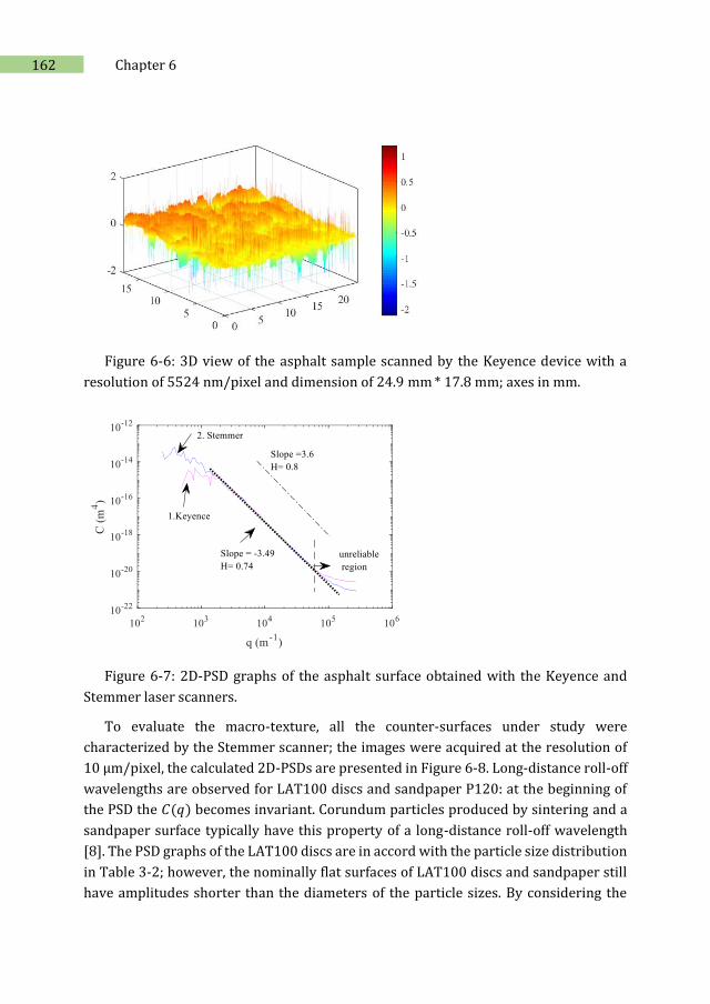
162 Chapter 6
Figure 6-6: 3D view of the asphalt sample scanned by the Keyence device with a
resolution of 5524 nm/pixel and dimension of 24.9 mm * 17.8 mm; axes in mm.
Figure 6-7: 2D-PSD graphs of the asphalt surface obtained with the Keyence and
Stemmer laser scanners.
To evaluate the macro-texture, all the counter-surfaces under study were
characterized by the Stemmer scanner; the images were acquired at the resolution of
10 μm/pixel, the calculated 2D-PSDs are presented in Figure 6-8. Long-distance roll-off
wavelengths are observed for LAT100 discs and sandpaper P120: at the beginning of
the PSD the 𝐶(𝑞) becomes invariant. Corundum particles produced by sintering and a
sandpaper surface typically have this property of a long-distance roll-off wavelength
[8]. The PSD graphs of the LAT100 discs are in accord with the particle size distribution
in Table 3-2; however, the nominally flat surfaces of LAT100 discs and sandpaper still
have amplitudes shorter than the diameters of the particle sizes. By considering the
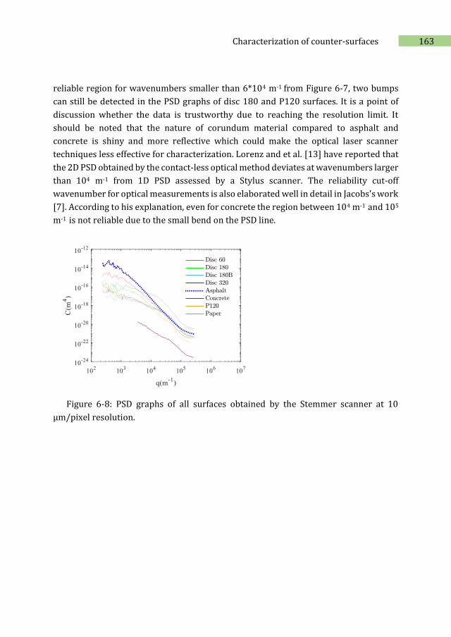
163 Characterization of counter-surfaces
reliable region for wavenumbers smaller than 6*104 m-1 from Figure 6-7, two bumps
can still be detected in the PSD graphs of disc 180 and P120 surfaces. It is a point of
discussion whether the data is trustworthy due to reaching the resolution limit. It
should be noted that the nature of corundum material compared to asphalt and
concrete is shiny and more reflective which could make the optical laser scanner
techniques less effective for characterization. Lorenz and et al. [13] have reported that
the 2D PSD obtained by the contact-less optical method deviates at wavenumbers larger
than 104 m-1 from 1D PSD assessed by a Stylus scanner. The reliability cut-off
wavenumber for optical measurements is also elaborated well in detail in Jacobs's work
[7]. According to his explanation, even for concrete the region between 104 m-1 and 105
m-1 is not reliable due to the small bend on the PSD line.
Figure 6-8: PSD graphs of all surfaces obtained by the Stemmer scanner at 10
μm/pixel resolution.
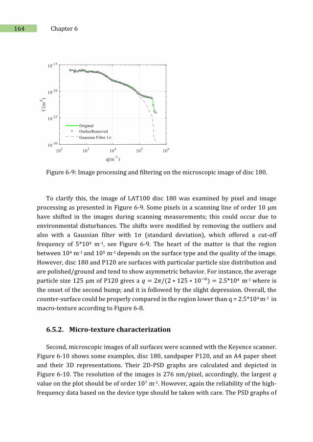
164 Chapter 6
Figure 6-9: Image processing and filtering on the microscopic image of disc 180.
To clarify this, the image of LAT100 disc 180 was examined by pixel and image
processing as presented in Figure 6-9. Some pixels in a scanning line of order 10 μm
have shifted in the images during scanning measurements; this could occur due to
environmental disturbances. The shifts were modified by removing the outliers and
also with a Gaussian filter with 1σ (standard deviation), which offered a cut-off
frequency of 5*104 m-1, see Figure 6-9. The heart of the matter is that the region
between 104 m-1 and 105 m-1 depends on the surface type and the quality of the image.
However, disc 180 and P120 are surfaces with particular particle size distribution and
are polished/ground and tend to show asymmetric behavior. For instance, the average
particle size 125 μm of P120 gives a 𝑞 = 2𝜋/(2 ∗ 125 ∗ 10−6) = 2.5*104 m-1 where is
the onset of the second bump; and it is followed by the slight depression. Overall, the
counter-surface could be properly compared in the region lower than q = 2.5*104 m-1 in
macro-texture according to Figure 6-8.
6.5.2. Micro-texture characterization
Second, microscopic images of all surfaces were scanned with the Keyence scanner.
Figure 6-10 shows some examples, disc 180, sandpaper P120, and an A4 paper sheet
and their 3D representations. Their 2D-PSD graphs are calculated and depicted in
Figure 6-10. The resolution of the images is 276 nm/pixel, accordingly, the largest 𝑞
value on the plot should be of order 107 m-1. However, again the reliability of the high-
frequency data based on the device type should be taken with care. The PSD graphs of
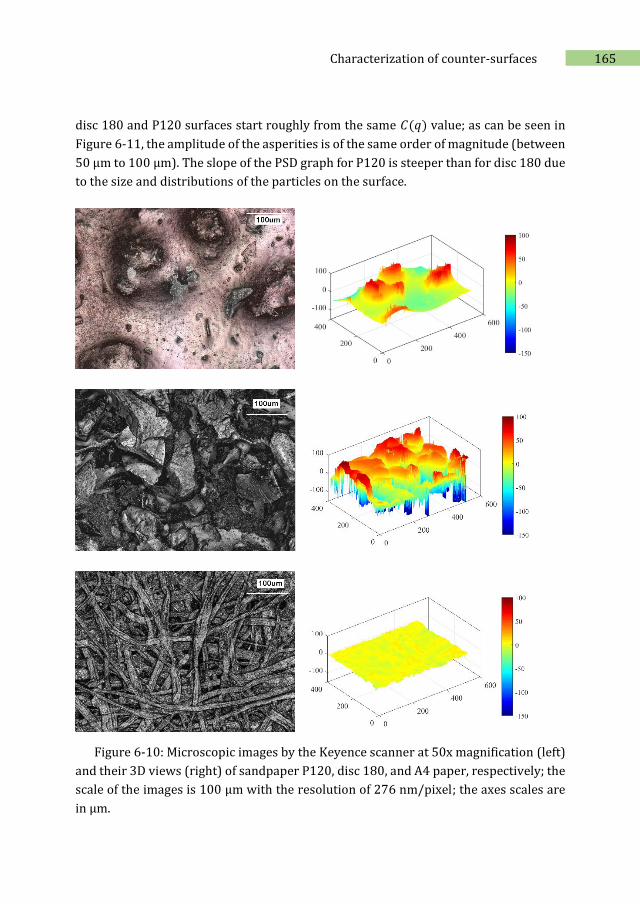
165 Characterization of counter-surfaces
disc 180 and P120 surfaces start roughly from the same 𝐶(𝑞) value; as can be seen in
Figure 6-11, the amplitude of the asperities is of the same order of magnitude (between
50 μm to 100 μm). The slope of the PSD graph for P120 is steeper than for disc 180 due
to the size and distributions of the particles on the surface.
Figure 6-10: Microscopic images by the Keyence scanner at 50x magnification (left)
and their 3D views (right) of sandpaper P120, disc 180, and A4 paper, respectively; the
scale of the images is 100 μm with the resolution of 276 nm/pixel; the axes scales are
in μm.
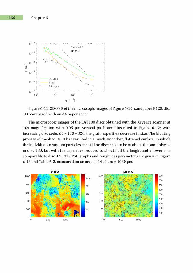
166 Chapter 6
Figure 6-11: 2D-PSD of the microscopic images of Figure 6-10; sandpaper P120, disc
180 compared with an A4 paper sheet.
The microscopic images of the LAT100 discs obtained with the Keyence scanner at
10x magnification with 0.05 μm vertical pitch are illustrated in Figure 6-12; with
increasing disc code: 60 – 180 – 320, the grain asperities decrease in size. The blunting
process of the disc 180B has resulted in a much smoother, flattened surface, in which
the individual corundum particles can still be discerned to be of about the same size as
in disc 180, but with the asperities reduced to about half the height and a lower rms
comparable to disc 320. The PSD graphs and roughness parameters are given in Figure
6-13 and Table 6-2, measured on an area of 1414 μm × 1080 μm.
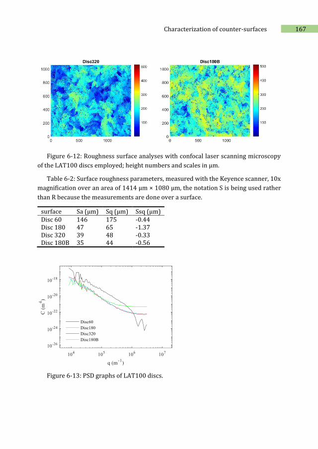
167 Characterization of counter-surfaces
Figure 6-12: Roughness surface analyses with confocal laser scanning microscopy
of the LAT100 discs employed; height numbers and scales in μm.
Table 6-2: Surface roughness parameters, measured with the Keyence scanner, 10x
magnification over an area of 1414 μm × 1080 μm, the notation S is being used rather
than R because the measurements are done over a surface.
surface Sa (μm) Sq (μm) Ssq (μm) Disc 60 146 175 -0.44 Disc 180 47 65 -1.37 Disc 320 39 48 -0.33 Disc 180B 35 44 -0.56
Figure 6-13: PSD graphs of LAT100 discs.
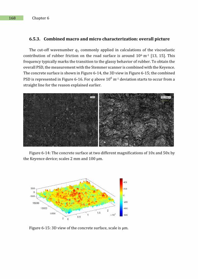
168 Chapter 6
6.5.3. Combined macro and micro characterization: overall picture
The cut-off wavenumber 𝑞1 commonly applied in calculations of the viscoelastic
contribution of rubber friction on the road surface is around 106 m-1 [13, 15]. This
frequency typically marks the transition to the glassy behavior of rubber. To obtain the
overall PSD, the measurement with the Stemmer scanner is combined with the Keyence.
The concrete surface is shown in Figure 6-14, the 3D view in Figure 6-15; the combined
PSD is represented in Figure 6-16. For 𝑞 above 106 m-1 deviation starts to occur from a
straight line for the reason explained earlier.
Figure 6-14: The concrete surface at two different magnifications of 10x and 50x by
the Keyence device; scales 2 mm and 100 μm.
Figure 6-15: 3D view of the concrete surface, scale is μm.
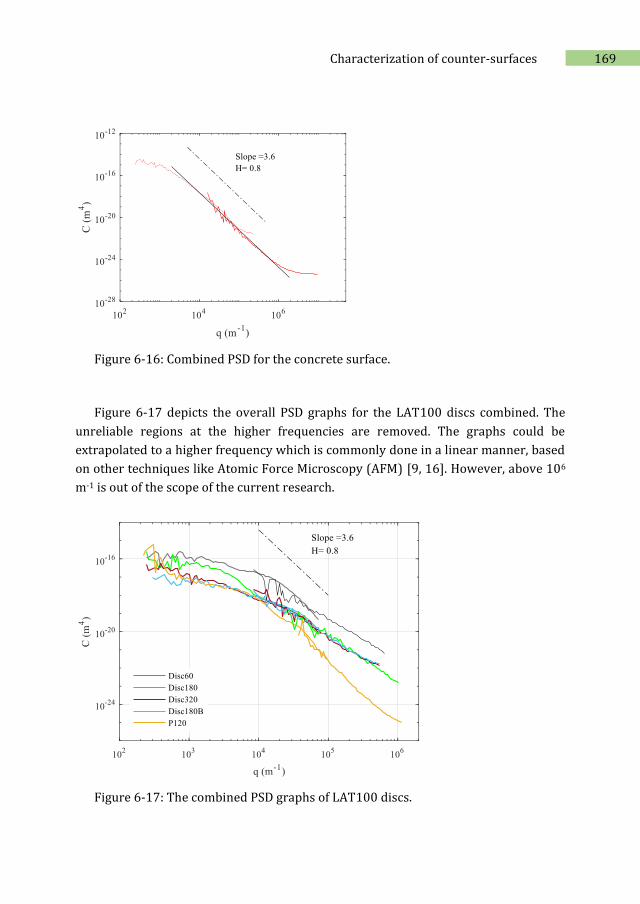
169 Characterization of counter-surfaces
Figure 6-16: Combined PSD for the concrete surface.
Figure 6-17 depicts the overall PSD graphs for the LAT100 discs combined. The
unreliable regions at the higher frequencies are removed. The graphs could be
extrapolated to a higher frequency which is commonly done in a linear manner, based
on other techniques like Atomic Force Microscopy (AFM) [9, 16]. However, above 106
m-1 is out of the scope of the current research.
Figure 6-17: The combined PSD graphs of LAT100 discs.
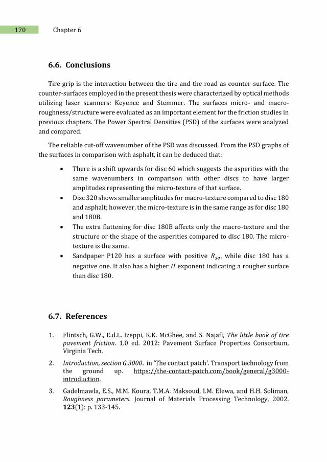
170 Chapter 6
6.6. Conclusions
Tire grip is the interaction between the tire and the road as counter-surface. The
counter-surfaces employed in the present thesis were characterized by optical methods
utilizing laser scanners: Keyence and Stemmer. The surfaces micro- and macro-
roughness/structure were evaluated as an important element for the friction studies in
previous chapters. The Power Spectral Densities (PSD) of the surfaces were analyzed
and compared.
The reliable cut-off wavenumber of the PSD was discussed. From the PSD graphs of
the surfaces in comparison with asphalt, it can be deduced that:
There is a shift upwards for disc 60 which suggests the asperities with the
same wavenumbers in comparison with other discs to have larger
amplitudes representing the micro-texture of that surface.
Disc 320 shows smaller amplitudes for macro-texture compared to disc 180
and asphalt; however, the micro-texture is in the same range as for disc 180
and 180B.
The extra flattening for disc 180B affects only the macro-texture and the
structure or the shape of the asperities compared to disc 180. The micro-
texture is the same.
Sandpaper P120 has a surface with positive 𝑅𝑠𝑞 , while disc 180 has a
negative one. It also has a higher 𝐻 exponent indicating a rougher surface
than disc 180.
6.7. References
1. Flintsch, G.W., E.d.L. Izeppi, K.K. McGhee, and S. Najafi, The little book of tire pavement friction. 1.0 ed. 2012: Pavement Surface Properties Consortium, Virginia Tech.
2. Introduction, section G.3000. in 'The contact patch'. Transport technology from the ground up. https://the-contact-patch.com/book/general/g3000-introduction.
3. Gadelmawla, E.S., M.M. Koura, T.M.A. Maksoud, I.M. Elewa, and H.H. Soliman, Roughness parameters. Journal of Materials Processing Technology, 2002. 123(1): p. 133-145.
171 Characterization of counter-surfaces
4. Chang, W.-R., The effects of surface roughness and contaminants on the dynamic friction between porcelain tile and vulcanized rubber. Safety Science, 2002(40): p. 577-591.
5. Nayak, P.R., Random Process Model of Rough Surfaces. Journal of Lubrication Technology, 1971. 93(3): p. 398-407.
6. Whitehouse, D.J., Surface roughness characterization, in Book 'Handbook of Surface Metrology'. 1994, Institute of Physics Publishing: Bristol UK and Philadelphia USA.
7. Jacobs, T.D.B., T. Junge, and L. Pastewka, Quantitative characterization of surface topography using spectral analysis. Surface Topography: Metrology and Properties, 2017. 5(1, 013001).
8. Persson, B.N.J., O. Albohr, U. Tartaglino, A.I. Volokitin, and E. Tosatti, On the nature of surface roughness with application to contact mechanics, sealing, rubber friction and adhesion. J Phys Condens Matter, 2005. 17(1): p. R1-r62.
9. Persson, B.N.J., On the Fractal Dimension of Rough Surfaces. Tribology Letters, 2014. 54(1): p. 99-106.
10. Carr, J.R., Statistical self-affinity, fractal dimension, and geologic interpretation. Engineering Geology, 1997. 48(3): p. 269-282.
11. Krim, J. and G. Palasantzas, Experimental Observations of Self-affine Scaling and Kinetic Roughening at Sub-microns Lengthscales. International Journal of Modern Physics B, 1995. 09(06): p. 599-632.
12. Tevis, D.B.J., J. Till, and P. Lars, Quantitative characterization of surface topography using spectral analysis. Surface Topography: Metrology and Properties, 2017. 5(1): p. 013001.
13. Lorenz, B., B.N.J. Persson, S. Dieluweit, and T. Tada, Rubber friction: Comparison of theory with experiment. The European Physical Journal E, 2011. 34(12): p. 129.
14. Carbone, G., B. Lorenz, B.N.J. Persson, and A. Wohlers, Contact mechanics and rubber friction for randomly rough surfaces with anisotropic statistical properties. The European Physical Journal E, 2009. 29(3): p. 275-284.
15. Tiwari, A., N. Miyashita, N. Espallargas, and B.N.J. Persson, Rubber friction: The contribution from the area of real contact. J Chem Phys, 2018. 148(22): p. 224701.
16. Persson, J.S., A. Tiwari, E. Valbahs, T.V. Tolpekina, and B.N.J. Persson, On the Use of Silicon Rubber Replica for Surface Topography Studies. Tribology Letters, 2018. 66(4): p. 140.

172 Chapter 6
7 Characterization of contact area
7.1. Introduction
Understanding what a tire experiences in the contact with the counter-surface is a
key to mimic the situation in the laboratory and from there predict tire grip. Tire grip
or friction is an interface phenomenon between two surfaces. Unless the shape and
magnitude of the real contact area between rubber and the counter-surface are fully
understood, it is not possible to calculate or comprehend the tire grip concept. In the
present chapter, the tire contact patch which is the result of the interaction of rubber
material and a counter-surface is being investigated. The real or actual area of contact
depends on the surface characteristics, applied load, tire inflation pressure, tire speed,
and rubber properties. An investigation of the contact area is carried out, measuring
with pressure-sensitive films in a stationary configuration. A calculation method is
applied in which a wide range of pressures is covered to analyze the contact area and
pressure of real tires and the Grosch wheels on different counter-surfaces. The effect of
different surface roughness and normal load for various tread compounds is
considered. The output is compared by applying the Persson friction theory. And finally,
a comparison is carried out between the solid Grosch wheels and the tires.
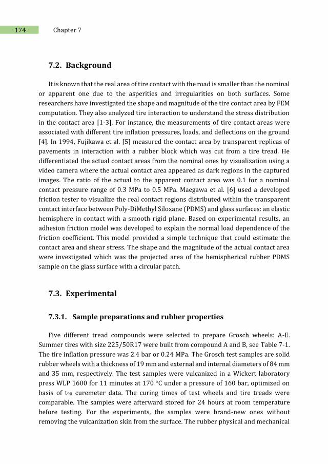
174 Chapter 7
7.2. Background
It is known that the real area of tire contact with the road is smaller than the nominal
or apparent one due to the asperities and irregularities on both surfaces. Some
researchers have investigated the shape and magnitude of the tire contact area by FEM
computation. They also analyzed tire interaction to understand the stress distribution
in the contact area [1-3]. For instance, the measurements of tire contact areas were
associated with different tire inflation pressures, loads, and deflections on the ground
[4]. In 1994, Fujikawa et al. [5] measured the contact area by transparent replicas of
pavements in interaction with a rubber block which was cut from a tire tread. He
differentiated the actual contact areas from the nominal ones by visualization using a
video camera where the actual contact area appeared as dark regions in the captured
images. The ratio of the actual to the apparent contact area was 0.1 for a nominal
contact pressure range of 0.3 MPa to 0.5 MPa. Maegawa et al. [6] used a developed
friction tester to visualize the real contact regions distributed within the transparent
contact interface between Poly-DiMethyl Siloxane (PDMS) and glass surfaces: an elastic
hemisphere in contact with a smooth rigid plane. Based on experimental results, an
adhesion friction model was developed to explain the normal load dependence of the
friction coefficient. This model provided a simple technique that could estimate the
contact area and shear stress. The shape and the magnitude of the actual contact area
were investigated which was the projected area of the hemispherical rubber PDMS
sample on the glass surface with a circular patch.
7.3. Experimental
7.3.1. Sample preparations and rubber properties
Five different tread compounds were selected to prepare Grosch wheels: A-E.
Summer tires with size 225/50R17 were built from compound A and B, see Table 7-1.
The tire inflation pressure was 2.4 bar or 0.24 MPa. The Grosch test samples are solid
rubber wheels with a thickness of 19 mm and external and internal diameters of 84 mm
and 35 mm, respectively. The test samples were vulcanized in a Wickert laboratory
press WLP 1600 for 11 minutes at 170 °C under a pressure of 160 bar, optimized on
basis of t90 curemeter data. The curing times of test wheels and tire treads were
comparable. The samples were afterward stored for 24 hours at room temperature
before testing. For the experiments, the samples were brand-new ones without
removing the vulcanization skin from the surface. The rubber physical and mechanical
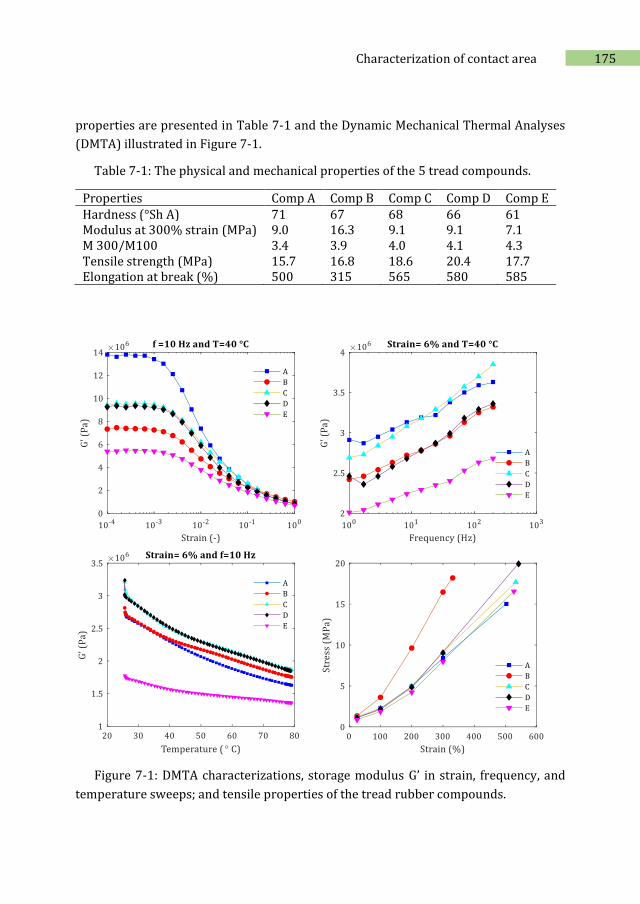
175 Characterization of contact area
properties are presented in Table 7-1 and the Dynamic Mechanical Thermal Analyses
(DMTA) illustrated in Figure 7-1.
Table 7-1: The physical and mechanical properties of the 5 tread compounds.
Properties Comp A Comp B Comp C Comp D Comp E Hardness (°Sh A) 71 67 68 66 61 Modulus at 300% strain (MPa) 9.0 16.3 9.1 9.1 7.1 M 300/M100 3.4 3.9 4.0 4.1 4.3 Tensile strength (MPa) 15.7 16.8 18.6 20.4 17.7 Elongation at break (%) 500 315 565 580 585
Figure 7-1: DMTA characterizations, storage modulus G’ in strain, frequency, and
temperature sweeps; and tensile properties of the tread rubber compounds.
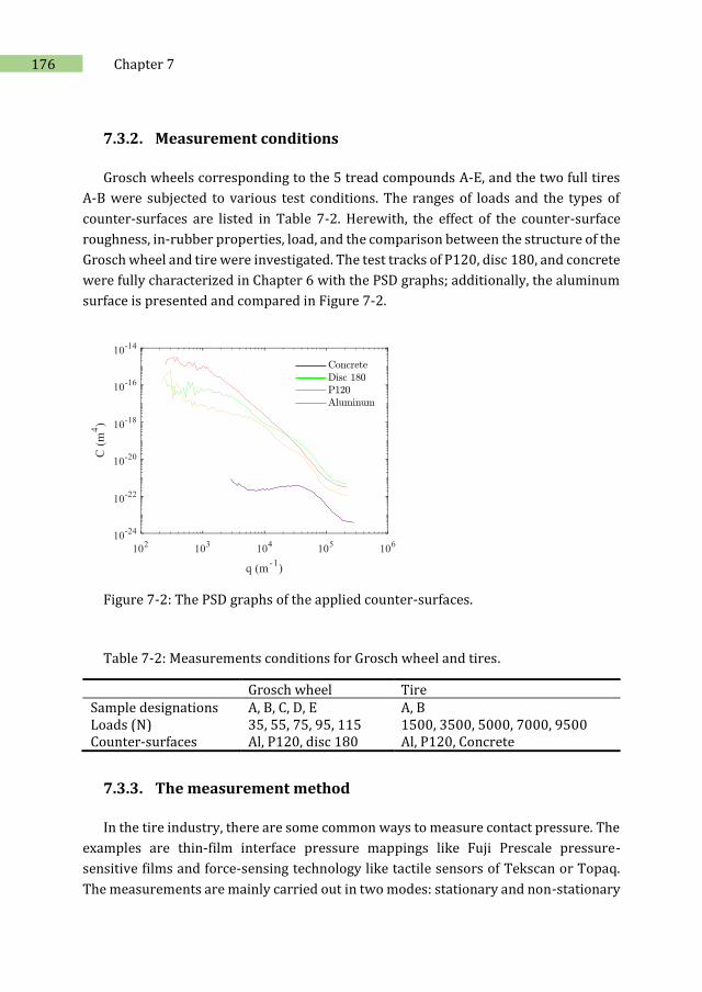
176 Chapter 7
7.3.2. Measurement conditions
Grosch wheels corresponding to the 5 tread compounds A-E, and the two full tires
A-B were subjected to various test conditions. The ranges of loads and the types of
counter-surfaces are listed in Table 7-2. Herewith, the effect of the counter-surface
roughness, in-rubber properties, load, and the comparison between the structure of the
Grosch wheel and tire were investigated. The test tracks of P120, disc 180, and concrete
were fully characterized in Chapter 6 with the PSD graphs; additionally, the aluminum
surface is presented and compared in Figure 7-2.
Figure 7-2: The PSD graphs of the applied counter-surfaces.
Table 7-2: Measurements conditions for Grosch wheel and tires.
Grosch wheel Tire Sample designations A, B, C, D, E A, B Loads (N) 35, 55, 75, 95, 115 1500, 3500, 5000, 7000, 9500 Counter-surfaces Al, P120, disc 180 Al, P120, Concrete
7.3.3. The measurement method
In the tire industry, there are some common ways to measure contact pressure. The
examples are thin-film interface pressure mappings like Fuji Prescale pressure-
sensitive films and force-sensing technology like tactile sensors of Tekscan or Topaq.
The measurements are mainly carried out in two modes: stationary and non-stationary
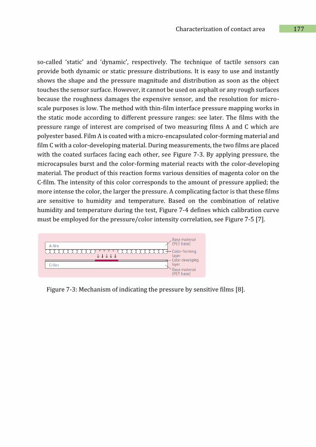
177 Characterization of contact area
so-called ‘static’ and ‘dynamic’, respectively. The technique of tactile sensors can
provide both dynamic or static pressure distributions. It is easy to use and instantly
shows the shape and the pressure magnitude and distribution as soon as the object
touches the sensor surface. However, it cannot be used on asphalt or any rough surfaces
because the roughness damages the expensive sensor, and the resolution for micro-
scale purposes is low. The method with thin-film interface pressure mapping works in
the static mode according to different pressure ranges: see later. The films with the
pressure range of interest are comprised of two measuring films A and C which are
polyester based. Film A is coated with a micro-encapsulated color-forming material and
film C with a color-developing material. During measurements, the two films are placed
with the coated surfaces facing each other, see Figure 7-3. By applying pressure, the
microcapsules burst and the color-forming material reacts with the color-developing
material. The product of this reaction forms various densities of magenta color on the
C-film. The intensity of this color corresponds to the amount of pressure applied; the
more intense the color, the larger the pressure. A complicating factor is that these films
are sensitive to humidity and temperature. Based on the combination of relative
humidity and temperature during the test, Figure 7-4 defines which calibration curve
must be employed for the pressure/color intensity correlation, see Figure 7-5 [7].
Figure 7-3: Mechanism of indicating the pressure by sensitive films [8].
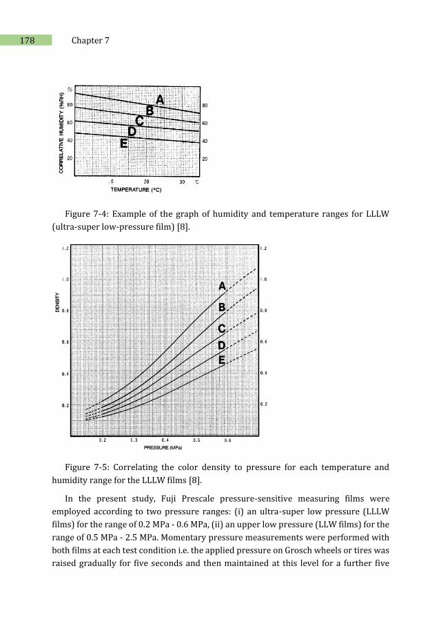
178 Chapter 7
Figure 7-4: Example of the graph of humidity and temperature ranges for LLLW
(ultra-super low-pressure film) [8].
Figure 7-5: Correlating the color density to pressure for each temperature and
humidity range for the LLLW films [8].
In the present study, Fuji Prescale pressure-sensitive measuring films were
employed according to two pressure ranges: (i) an ultra-super low pressure (LLLW
films) for the range of 0.2 MPa - 0.6 MPa, (ii) an upper low pressure (LLW films) for the
range of 0.5 MPa - 2.5 MPa. Momentary pressure measurements were performed with
both films at each test condition i.e. the applied pressure on Grosch wheels or tires was
raised gradually for five seconds and then maintained at this level for a further five
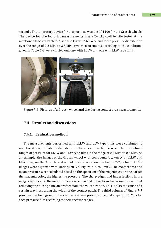
179 Characterization of contact area
seconds. The laboratory device for this purpose was the LAT100 for the Grosch wheels.
The device for tire footprint measurements was a Zwick/Roell tensile tester at the
mentioned loads in Table 7-2, see also Figure 7-6. To calculate the pressure distribution
over the range of 0.2 MPa to 2.5 MPa, two measurements according to the conditions
given in Table 7-2 were carried out, one with LLLW and one with LLW type films.
Figure 7-6: Pictures of a Grosch wheel and tire during contact area measurements.
7.4. Results and discussions
7.4.1. Evaluation method
The measurements performed with LLLW and LLW type films were combined to
map the stress probability distribution. There is an overlap between the pre-defined
ranges of pressure for LLLW and LLW type films in the range of 0.5 MPa to 0.6 MPa. As
an example, the images of the Grosch wheel with compound A taken with LLLW and
LLW films, on the Al surface at a load of 75 N are shown in Figure 7-7, column 1. The
images were digitized with MatlabR2017b, Figure 7-7, column 2. The contact area and
mean pressure were calculated based on the spectrum of the magenta color; the darker
the magenta color, the higher the pressure. The sharp edges and imperfections in the
images are because the measurements were carried out on brand-new samples without
removing the curing skin, an artifact from the vulcanization. This is also the cause of a
certain waviness along the width of the contact patch. The third column of Figure 7-7
provides the histogram of the vertical average pressure in equal steps of 0.1 MPa for
each pressure film according to their specific ranges.
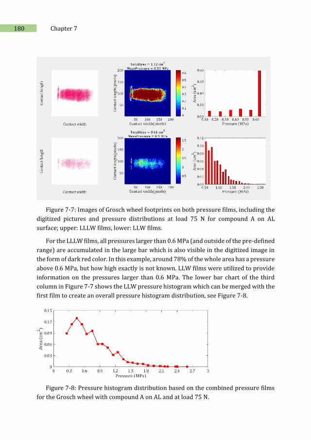
180 Chapter 7
Figure 7-7: Images of Grosch wheel footprints on both pressure films, including the
digitized pictures and pressure distributions at load 75 N for compound A on AL
surface; upper: LLLW films, lower: LLW films.
For the LLLW films, all pressures larger than 0.6 MPa (and outside of the pre-defined
range) are accumulated in the large bar which is also visible in the digitized image in
the form of dark red color. In this example, around 78% of the whole area has a pressure
above 0.6 MPa, but how high exactly is not known. LLW films were utilized to provide
information on the pressures larger than 0.6 MPa. The lower bar chart of the third
column in Figure 7-7 shows the LLW pressure histogram which can be merged with the
first film to create an overall pressure histogram distribution, see Figure 7-8.
Figure 7-8: Pressure histogram distribution based on the combined pressure films
for the Grosch wheel with compound A on AL and at load 75 N.
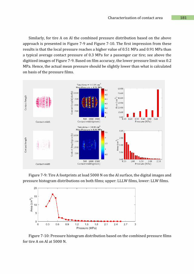
181 Characterization of contact area
Similarly, for tire A on Al the combined pressure distribution based on the above
approach is presented in Figure 7-9 and Figure 7-10. The first impression from these
results is that the local pressure reaches a higher value of 0.51 MPa and 0.91 MPa than
a typical average contact pressure of 0.3 MPa for a passenger car tire; see above the
digitized images of Figure 7-9. Based on film accuracy, the lower pressure limit was 0.2
MPa. Hence, the actual mean pressure should be slightly lower than what is calculated
on basis of the pressure films.
Figure 7-9: Tire A footprints at load 5000 N on the Al surface, the digital images and
pressure histogram distributions on both films; upper: LLLW films, lower: LLW films.
Figure 7-10: Pressure histogram distribution based on the combined pressure films
for tire A on Al at 5000 N.
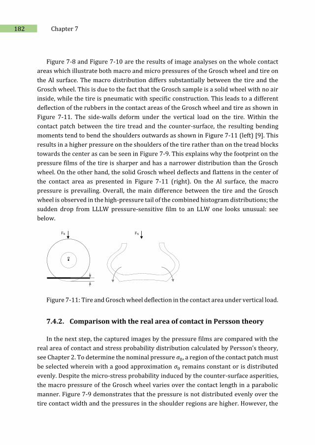
182 Chapter 7
Figure 7-8 and Figure 7-10 are the results of image analyses on the whole contact
areas which illustrate both macro and micro pressures of the Grosch wheel and tire on
the Al surface. The macro distribution differs substantially between the tire and the
Grosch wheel. This is due to the fact that the Grosch sample is a solid wheel with no air
inside, while the tire is pneumatic with specific construction. This leads to a different
deflection of the rubbers in the contact areas of the Grosch wheel and tire as shown in
Figure 7-11. The side-walls deform under the vertical load on the tire. Within the
contact patch between the tire tread and the counter-surface, the resulting bending
moments tend to bend the shoulders outwards as shown in Figure 7-11 (left) [9]. This
results in a higher pressure on the shoulders of the tire rather than on the tread blocks
towards the center as can be seen in Figure 7-9. This explains why the footprint on the
pressure films of the tire is sharper and has a narrower distribution than the Grosch
wheel. On the other hand, the solid Grosch wheel deflects and flattens in the center of
the contact area as presented in Figure 7-11 (right). On the Al surface, the macro
pressure is prevailing. Overall, the main difference between the tire and the Grosch
wheel is observed in the high-pressure tail of the combined histogram distributions; the
sudden drop from LLLW pressure-sensitive film to an LLW one looks unusual: see
below.
FN
o
FN
Figure 7-11: Tire and Grosch wheel deflection in the contact area under vertical load.
7.4.2. Comparison with the real area of contact in Persson theory
In the next step, the captured images by the pressure films are compared with the
real area of contact and stress probability distribution calculated by Persson’s theory,
see Chapter 2. To determine the nominal pressure 𝜎0, a region of the contact patch must
be selected wherein with a good approximation 𝜎0 remains constant or is distributed
evenly. Despite the micro-stress probability induced by the counter-surface asperities,
the macro pressure of the Grosch wheel varies over the contact length in a parabolic
manner. Figure 7-9 demonstrates that the pressure is not distributed evenly over the
tire contact width and the pressures in the shoulder regions are higher. However, the
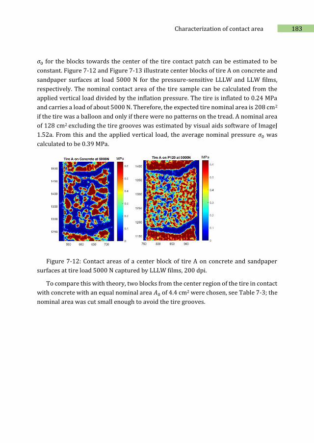
183 Characterization of contact area
𝜎0 for the blocks towards the center of the tire contact patch can be estimated to be
constant. Figure 7-12 and Figure 7-13 illustrate center blocks of tire A on concrete and
sandpaper surfaces at load 5000 N for the pressure-sensitive LLLW and LLW films,
respectively. The nominal contact area of the tire sample can be calculated from the
applied vertical load divided by the inflation pressure. The tire is inflated to 0.24 MPa
and carries a load of about 5000 N. Therefore, the expected tire nominal area is 208 cm2
if the tire was a balloon and only if there were no patterns on the tread. A nominal area
of 128 cm2 excluding the tire grooves was estimated by visual aids software of ImageJ
1.52a. From this and the applied vertical load, the average nominal pressure 𝜎0 was
calculated to be 0.39 MPa.
Figure 7-12: Contact areas of a center block of tire A on concrete and sandpaper
surfaces at tire load 5000 N captured by LLLW films, 200 dpi.
To compare this with theory, two blocks from the center region of the tire in contact
with concrete with an equal nominal area 𝐴0 of 4.4 cm2 were chosen, see Table 7-3; the
nominal area was cut small enough to avoid the tire grooves.
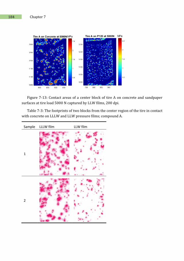
184 Chapter 7
Figure 7-13: Contact areas of a center block of tire A on concrete and sandpaper
surfaces at tire load 5000 N captured by LLW films, 200 dpi.
Table 7-3: The footprints of two blocks from the center region of the tire in contact
with concrete on LLLW and LLW pressure films; compound A.
Sample LLLW film LLW film
1
2
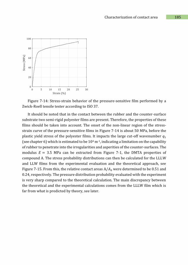
185 Characterization of contact area
Figure 7-14: Stress-strain behavior of the pressure-sensitive film performed by a
Zwick-Roell tensile tester according to ISO 37.
It should be noted that in the contact between the rubber and the counter-surface
substrate two semi-rigid polyester films are present. Therefore, the properties of these
films should be taken into account. The onset of the non-linear region of the stress-
strain curve of the pressure-sensitive films in Figure 7-14 is about 50 MPa, before the
plastic yield stress of the polyester films. It impacts the large cut-off wavenumber 𝑞1
(see chapter 6) which is estimated to be 104 m-1, indicating a limitation on the capability
of rubber to penetrate into the irregularities and asperities of the counter-surfaces. The
modulus 𝐸 = 3.5 MPa can be extracted from Figure 7-1, the DMTA properties of
compound A. The stress probability distributions can then be calculated for the LLLW
and LLW films from the experimental evaluation and the theoretical approach, see
Figure 7-15. From this, the relative contact areas A/𝐴0 were determined to be 0.51 and
0.24, respectively. The pressure distribution probability evaluated with the experiment
is very sharp compared to the theoretical calculation. The main discrepancy between
the theoretical and the experimental calculations comes from the LLLW film which is
far from what is predicted by theory, see later.
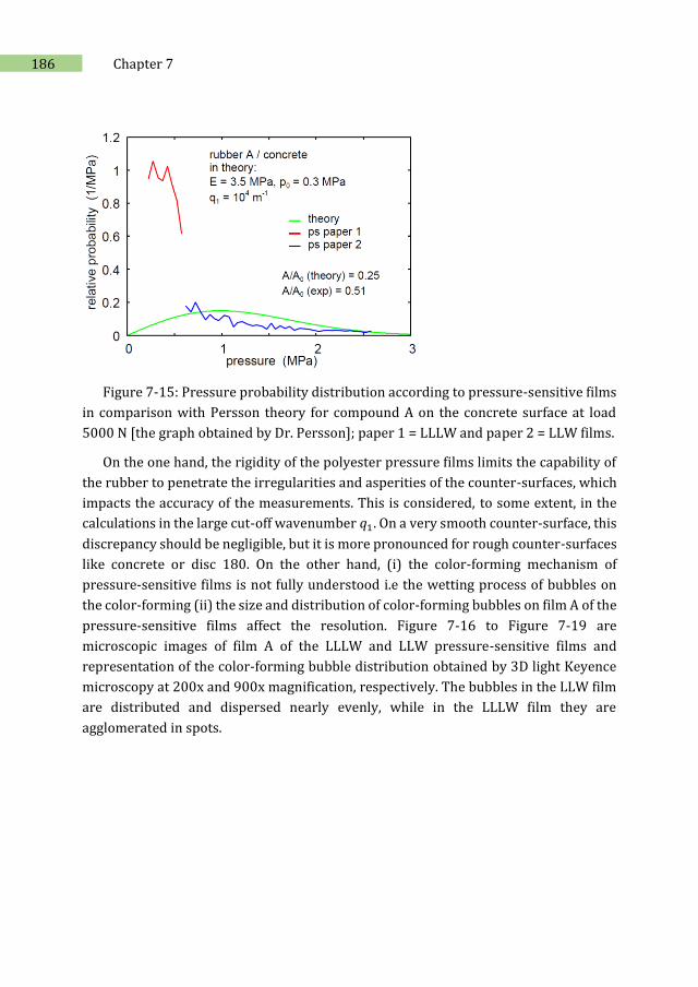
186 Chapter 7
Figure 7-15: Pressure probability distribution according to pressure-sensitive films
in comparison with Persson theory for compound A on the concrete surface at load
5000 N [the graph obtained by Dr. Persson]; paper 1 = LLLW and paper 2 = LLW films.
On the one hand, the rigidity of the polyester pressure films limits the capability of
the rubber to penetrate the irregularities and asperities of the counter-surfaces, which
impacts the accuracy of the measurements. This is considered, to some extent, in the
calculations in the large cut-off wavenumber 𝑞1. On a very smooth counter-surface, this
discrepancy should be negligible, but it is more pronounced for rough counter-surfaces
like concrete or disc 180. On the other hand, (i) the color-forming mechanism of
pressure-sensitive films is not fully understood i.e the wetting process of bubbles on
the color-forming (ii) the size and distribution of color-forming bubbles on film A of the
pressure-sensitive films affect the resolution. Figure 7-16 to Figure 7-19 are
microscopic images of film A of the LLLW and LLW pressure-sensitive films and
representation of the color-forming bubble distribution obtained by 3D light Keyence
microscopy at 200x and 900x magnification, respectively. The bubbles in the LLW film
are distributed and dispersed nearly evenly, while in the LLLW film they are
agglomerated in spots.
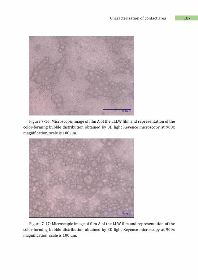
187 Characterization of contact area
Figure 7-16: Microscopic image of film A of the LLLW film and representation of the
color-forming bubble distribution obtained by 3D light Keyence microscopy at 900x
magnification, scale is 100 μm.
Figure 7-17: Microscopic image of film A of the LLW film and representation of the
color-forming bubble distribution obtained by 3D light Keyence microscopy at 900x
magnification, scale is 100 μm.
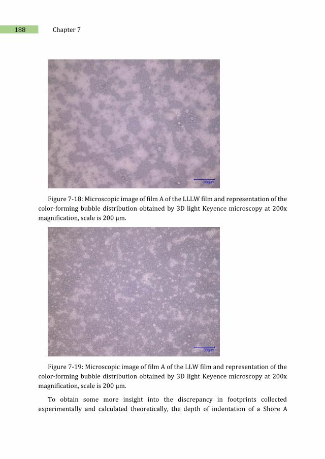
188 Chapter 7
Figure 7-18: Microscopic image of film A of the LLLW film and representation of the
color-forming bubble distribution obtained by 3D light Keyence microscopy at 200x
magnification, scale is 200 μm.
Figure 7-19: Microscopic image of film A of the LLW film and representation of the
color-forming bubble distribution obtained by 3D light Keyence microscopy at 200x
magnification, scale is 200 μm.
To obtain some more insight into the discrepancy in footprints collected
experimentally and calculated theoretically, the depth of indentation of a Shore A
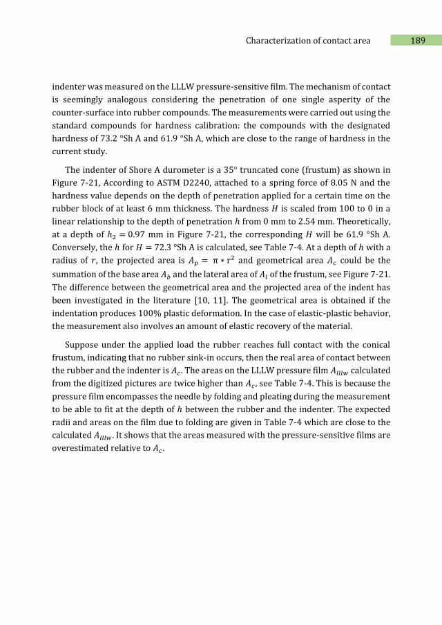
189 Characterization of contact area
indenter was measured on the LLLW pressure-sensitive film. The mechanism of contact
is seemingly analogous considering the penetration of one single asperity of the
counter-surface into rubber compounds. The measurements were carried out using the
standard compounds for hardness calibration: the compounds with the designated
hardness of 73.2 °Sh A and 61.9 °Sh A, which are close to the range of hardness in the
current study.
The indenter of Shore A durometer is a 35° truncated cone (frustum) as shown in
Figure 7-21, According to ASTM D2240, attached to a spring force of 8.05 N and the
hardness value depends on the depth of penetration applied for a certain time on the
rubber block of at least 6 mm thickness. The hardness 𝐻 is scaled from 100 to 0 in a
linear relationship to the depth of penetration ℎ from 0 mm to 2.54 mm. Theoretically,
at a depth of ℎ2 = 0.97 mm in Figure 7-21, the corresponding 𝐻 will be 61.9 °Sh A.
Conversely, the ℎ for 𝐻 = 72.3 °Sh A is calculated, see Table 7-4. At a depth of ℎ with a
radius of 𝑟, the projected area is 𝐴𝑝 = π ∗ r2 and geometrical area 𝐴𝑐 could be the
summation of the base area 𝐴𝑏 and the lateral area of 𝐴𝑙 of the frustum, see Figure 7-21.
The difference between the geometrical area and the projected area of the indent has
been investigated in the literature [10, 11]. The geometrical area is obtained if the
indentation produces 100% plastic deformation. In the case of elastic-plastic behavior,
the measurement also involves an amount of elastic recovery of the material.
Suppose under the applied load the rubber reaches full contact with the conical
frustum, indicating that no rubber sink-in occurs, then the real area of contact between
the rubber and the indenter is 𝐴𝑐 . The areas on the LLLW pressure film 𝐴𝑙𝑙𝑙𝑤 calculated
from the digitized pictures are twice higher than 𝐴𝑐 , see Table 7-4. This is because the
pressure film encompasses the needle by folding and pleating during the measurement
to be able to fit at the depth of ℎ between the rubber and the indenter. The expected
radii and areas on the film due to folding are given in Table 7-4 which are close to the
calculated 𝐴𝑙𝑙𝑙𝑤 . It shows that the areas measured with the pressure-sensitive films are
overestimated relative to 𝐴𝑐 .
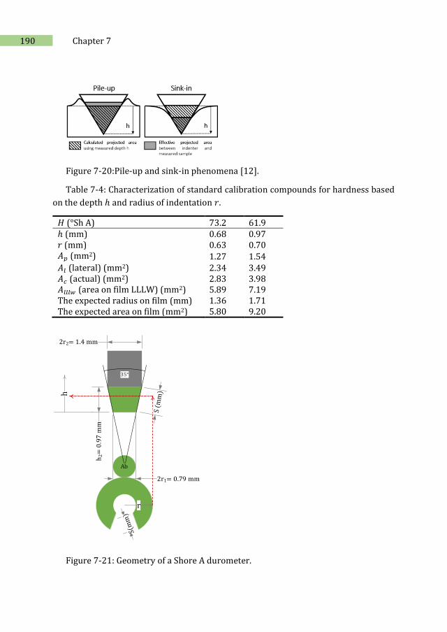
190 Chapter 7
Figure 7-20:Pile-up and sink-in phenomena [12].
Table 7-4: Characterization of standard calibration compounds for hardness based
on the depth ℎ and radius of indentation 𝑟.
𝐻 (°Sh A) 73.2 61.9 ℎ (mm) 0.68 0.97 𝑟 (mm) 0.63 0.70 𝐴𝑝 (mm2) 1.27 1.54 𝐴𝑙 (lateral) (mm2) 2.34 3.49 𝐴𝑐 (actual) (mm2) 2.83 3.98 𝐴𝑙𝑙𝑙𝑤 (area on film LLLW) (mm2) 5.89 7.19 The expected radius on film (mm) 1.36 1.71 The expected area on film (mm2) 5.80 9.20
2r2= 1.4 mm
2r1= 0.79 mm
h2=
0.9
7 m
m
Ab
Al
h
r
Figure 7-21: Geometry of a Shore A durometer.
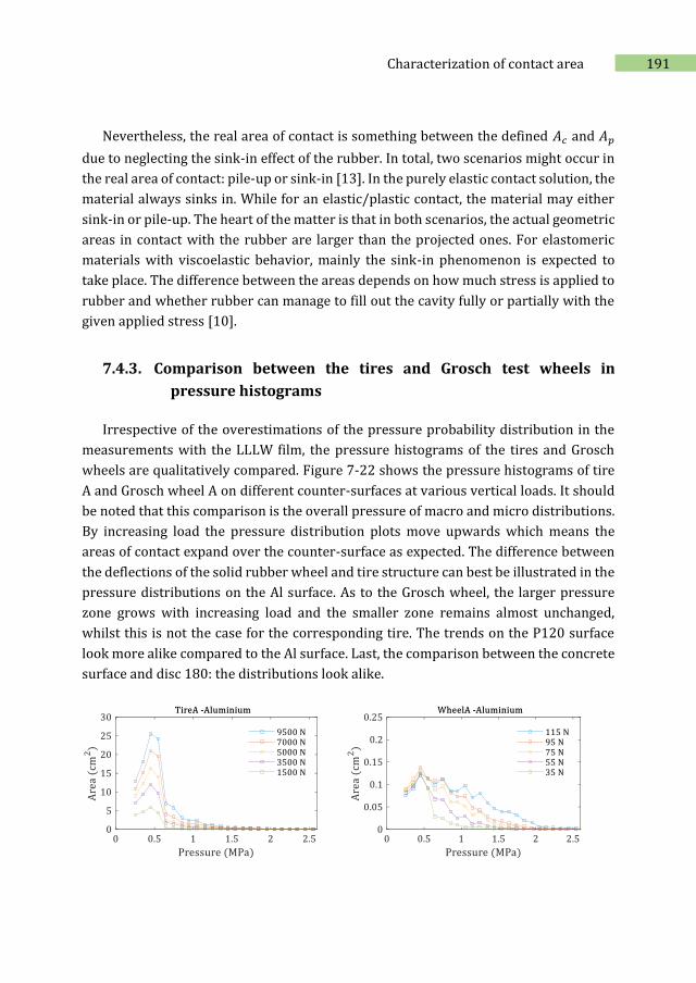
191 Characterization of contact area
Nevertheless, the real area of contact is something between the defined 𝐴𝑐 and 𝐴𝑝
due to neglecting the sink-in effect of the rubber. In total, two scenarios might occur in
the real area of contact: pile-up or sink-in [13]. In the purely elastic contact solution, the
material always sinks in. While for an elastic/plastic contact, the material may either
sink-in or pile-up. The heart of the matter is that in both scenarios, the actual geometric
areas in contact with the rubber are larger than the projected ones. For elastomeric
materials with viscoelastic behavior, mainly the sink-in phenomenon is expected to
take place. The difference between the areas depends on how much stress is applied to
rubber and whether rubber can manage to fill out the cavity fully or partially with the
given applied stress [10].
7.4.3. Comparison between the tires and Grosch test wheels in
pressure histograms
Irrespective of the overestimations of the pressure probability distribution in the
measurements with the LLLW film, the pressure histograms of the tires and Grosch
wheels are qualitatively compared. Figure 7-22 shows the pressure histograms of tire
A and Grosch wheel A on different counter-surfaces at various vertical loads. It should
be noted that this comparison is the overall pressure of macro and micro distributions.
By increasing load the pressure distribution plots move upwards which means the
areas of contact expand over the counter-surface as expected. The difference between
the deflections of the solid rubber wheel and tire structure can best be illustrated in the
pressure distributions on the Al surface. As to the Grosch wheel, the larger pressure
zone grows with increasing load and the smaller zone remains almost unchanged,
whilst this is not the case for the corresponding tire. The trends on the P120 surface
look more alike compared to the Al surface. Last, the comparison between the concrete
surface and disc 180: the distributions look alike.
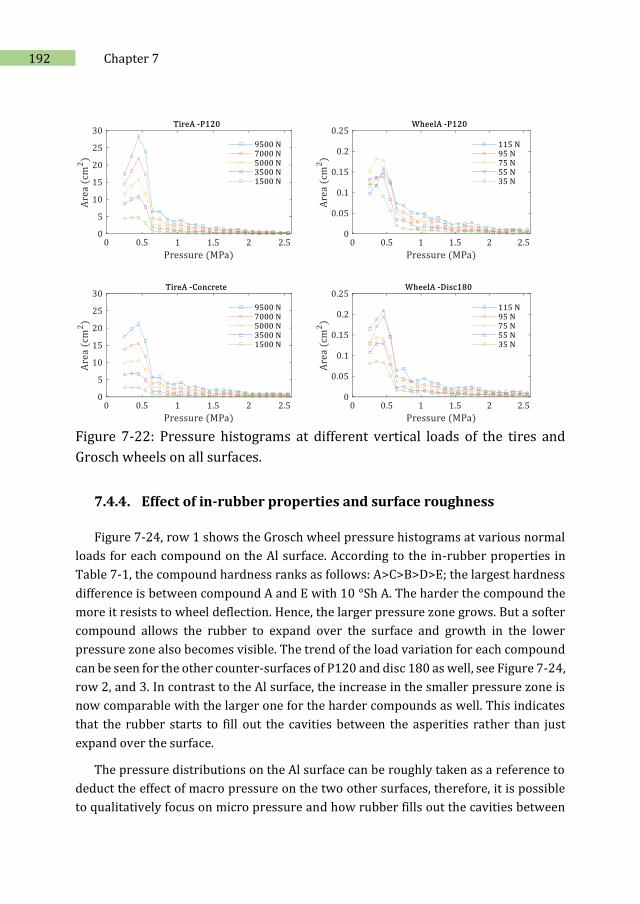
192 Chapter 7
Figure 7-22: Pressure histograms at different vertical loads of the tires and
Grosch wheels on all surfaces.
7.4.4. Effect of in-rubber properties and surface roughness
Figure 7-24, row 1 shows the Grosch wheel pressure histograms at various normal
loads for each compound on the Al surface. According to the in-rubber properties in
Table 7-1, the compound hardness ranks as follows: A>C>B>D>E; the largest hardness
difference is between compound A and E with 10 °Sh A. The harder the compound the
more it resists to wheel deflection. Hence, the larger pressure zone grows. But a softer
compound allows the rubber to expand over the surface and growth in the lower
pressure zone also becomes visible. The trend of the load variation for each compound
can be seen for the other counter-surfaces of P120 and disc 180 as well, see Figure 7-24,
row 2, and 3. In contrast to the Al surface, the increase in the smaller pressure zone is
now comparable with the larger one for the harder compounds as well. This indicates
that the rubber starts to fill out the cavities between the asperities rather than just
expand over the surface.
The pressure distributions on the Al surface can be roughly taken as a reference to
deduct the effect of macro pressure on the two other surfaces, therefore, it is possible
to qualitatively focus on micro pressure and how rubber fills out the cavities between
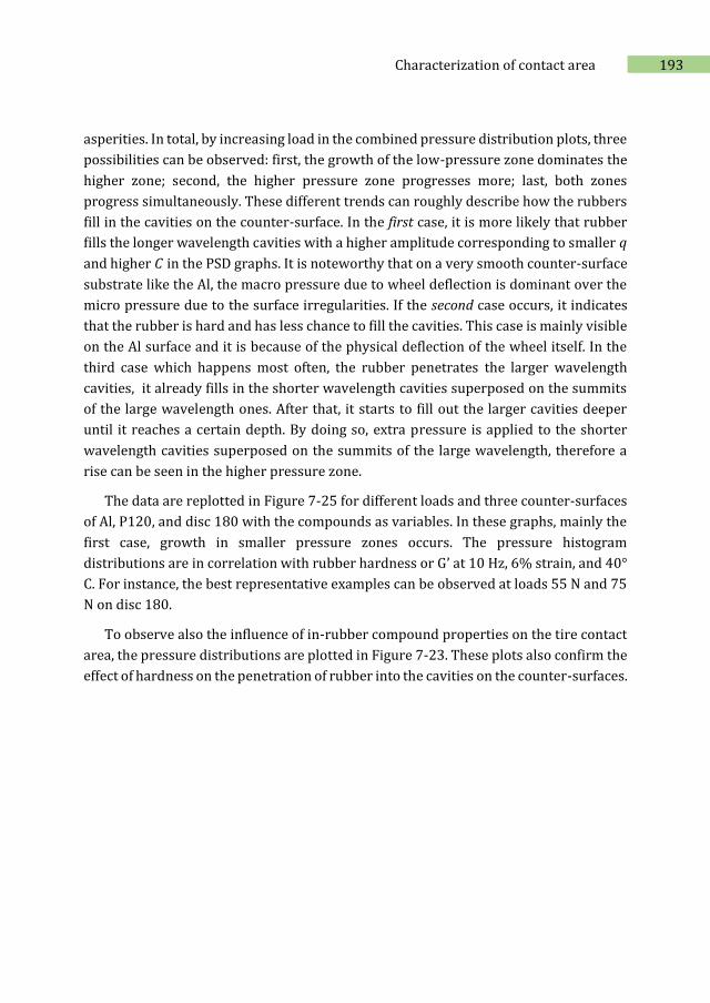
193 Characterization of contact area
asperities. In total, by increasing load in the combined pressure distribution plots, three
possibilities can be observed: first, the growth of the low-pressure zone dominates the
higher zone; second, the higher pressure zone progresses more; last, both zones
progress simultaneously. These different trends can roughly describe how the rubbers
fill in the cavities on the counter-surface. In the first case, it is more likely that rubber
fills the longer wavelength cavities with a higher amplitude corresponding to smaller 𝑞
and higher 𝐶 in the PSD graphs. It is noteworthy that on a very smooth counter-surface
substrate like the Al, the macro pressure due to wheel deflection is dominant over the
micro pressure due to the surface irregularities. If the second case occurs, it indicates
that the rubber is hard and has less chance to fill the cavities. This case is mainly visible
on the Al surface and it is because of the physical deflection of the wheel itself. In the
third case which happens most often, the rubber penetrates the larger wavelength
cavities, it already fills in the shorter wavelength cavities superposed on the summits
of the large wavelength ones. After that, it starts to fill out the larger cavities deeper
until it reaches a certain depth. By doing so, extra pressure is applied to the shorter
wavelength cavities superposed on the summits of the large wavelength, therefore a
rise can be seen in the higher pressure zone.
The data are replotted in Figure 7-25 for different loads and three counter-surfaces
of Al, P120, and disc 180 with the compounds as variables. In these graphs, mainly the
first case, growth in smaller pressure zones occurs. The pressure histogram
distributions are in correlation with rubber hardness or G’ at 10 Hz, 6% strain, and 40°
C. For instance, the best representative examples can be observed at loads 55 N and 75
N on disc 180.
To observe also the influence of in-rubber compound properties on the tire contact
area, the pressure distributions are plotted in Figure 7-23. These plots also confirm the
effect of hardness on the penetration of rubber into the cavities on the counter-surfaces.
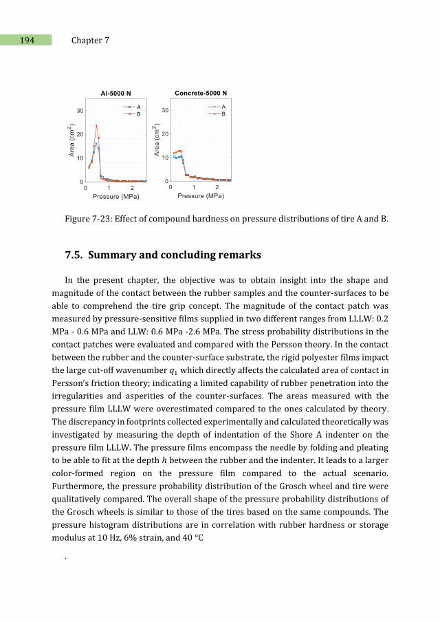
194 Chapter 7
Figure 7-23: Effect of compound hardness on pressure distributions of tire A and B.
7.5. Summary and concluding remarks
In the present chapter, the objective was to obtain insight into the shape and
magnitude of the contact between the rubber samples and the counter-surfaces to be
able to comprehend the tire grip concept. The magnitude of the contact patch was
measured by pressure-sensitive films supplied in two different ranges from LLLW: 0.2
MPa - 0.6 MPa and LLW: 0.6 MPa -2.6 MPa. The stress probability distributions in the
contact patches were evaluated and compared with the Persson theory. In the contact
between the rubber and the counter-surface substrate, the rigid polyester films impact
the large cut-off wavenumber 𝑞1 which directly affects the calculated area of contact in
Persson’s friction theory; indicating a limited capability of rubber penetration into the
irregularities and asperities of the counter-surfaces. The areas measured with the
pressure film LLLW were overestimated compared to the ones calculated by theory.
The discrepancy in footprints collected experimentally and calculated theoretically was
investigated by measuring the depth of indentation of the Shore A indenter on the
pressure film LLLW. The pressure films encompass the needle by folding and pleating
to be able to fit at the depth ℎ between the rubber and the indenter. It leads to a larger
color-formed region on the pressure film compared to the actual scenario.
Furthermore, the pressure probability distribution of the Grosch wheel and tire were
qualitatively compared. The overall shape of the pressure probability distributions of
the Grosch wheels is similar to those of the tires based on the same compounds. The
pressure histogram distributions are in correlation with rubber hardness or storage
modulus at 10 Hz, 6% strain, and 40 °C
.
195 Characterization of contact area
7.6. References
1. Schramm, D., M. Hiller, and R. Bardini, Modeling of the Road-Tire-Contact, in Book 'Vehicle Dynamics: Modeling and Simulation'. 2018, Springer Berlin Heidelberg: Berlin, Heidelberg. p. 145-186.
2. Sabri, M., Computation modelling of tire-road contact. AIP Conference Proceedings, 2018. 1983(1): p. 030018.
3. Farhadi, P., A. Golmohammadi, A. Sharifi, and G. Shahgholi, Potential of three-dimensional footprint mold in investigating the effect of tractor tire contact volume changes on rolling resistance. Journal of Terramechanics, 2018. 78: p. 63-72.
4. Schwanghart, H., Measurement of contact area, contact pressure and compaction under tires in soft soil. Journal of Terramechanics, 1991. 28(4): p. 309-318.
5. Fujikawa, T., A. Funazaki, and S. Yamazaki, Tire Tread Temperatures in Actual Contact Areas. Tire Science and Technology, 1994. 22(1): p. 19-41.
6. Maegawa, S., F. Itoigawa, and T. Nakamura, Effect of normal load on friction coefficient for sliding contact between rough rubber surface and rigid smooth plane. Tribology International, 2015. 92: p. 335-343.
7. Liggins, A.B., W.R. Hardie, and J.B. Finlay, The spatial and pressure resolution of fuji pressure-sensitive film. Experimental Mechanics, 1995. 35(2): p. 166-173.
8. Specifications and Operational Environment, in FujiFilm Prescale, Date of access: 2020 July; Available from https://www.fujifilm.com/products/prescale/prescalefilm/.
9. The contact patch. Transport technology from the ground up. https://the-contact-patch.com/book/general/g3000-introduction.
10. Broitman, E., Indentation Hardness Measurements at Macro-, Micro-, and Nanoscale: A Critical Overview. Tribology Letters, 2016. 65(1): p. 23.
11. Tuck, J.R., A.M. Korsunsky, S.J. Bull, and R.I. Davidson, On the application of the work-of-indentation approach to depth-sensing indentation experiments in coated systems. Surface and Coatings Technology, 2001. 137(2): p. 217-224.
12. Passilly, B. and R. Delannoy, Characterization of the ageing of an epoxy resin using high temperature nanoindentation. Matériaux & Techniques, 2019. 107(2): p. 206.
13. Bolshakov, A. and G.M. Pharr, Influences of pileup on the measurement of mechanical properties by load and depth sensing indentation techniques. Journal of Materials Research, 2011. 13(4): p. 1049-1058.
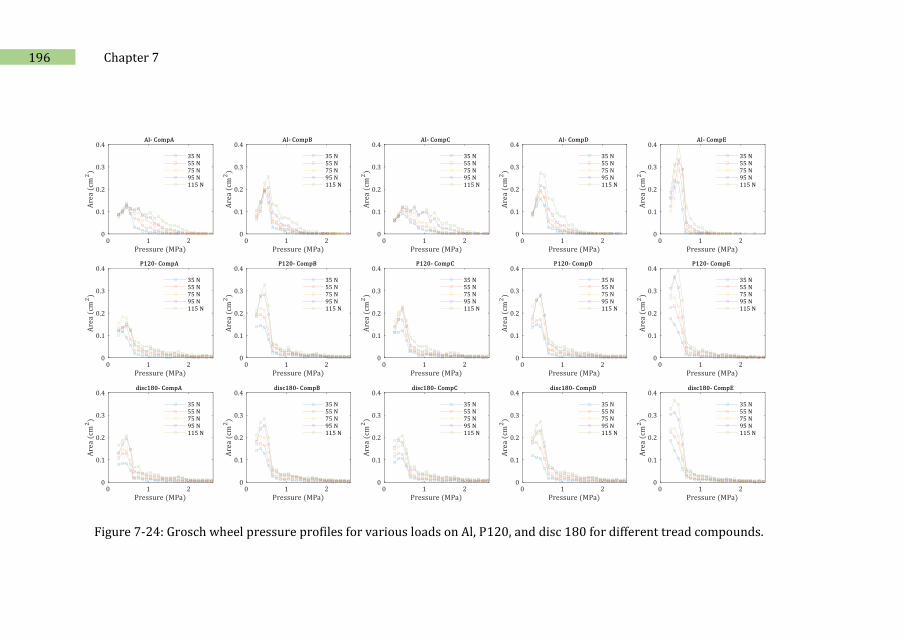
196 Chapter 7
Figure 7-24: Grosch wheel pressure profiles for various loads on Al, P120, and disc 180 for different tread compounds.
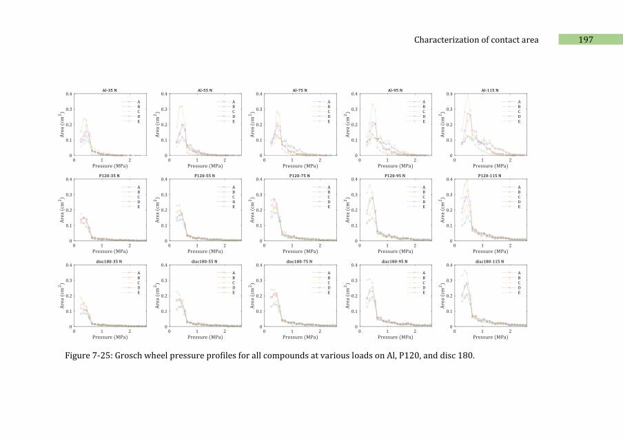
197 Characterization of contact area
Figure 7-25: Grosch wheel pressure profiles for all compounds at various loads on Al, P120, and disc 180.

8 Understanding the LAT100 as a
tribometer for tire friction with
modeling
The LAT100 as the main apparatus used in the present thesis – despite its name –
was re-designed and employed as a laboratory tribometer for prediction of tire friction.
It was demonstrated that the LAT100 can indeed be exploited particularly to simulate
the 𝛼-sweep tire tests, but not the 𝜅-sweep. The correlations were supported and
verified with statistical analyses. Nevertheless, validation was performed for one set of
tread compositions. Obtaining more insight into the wheel rolling dynamics contributes
to the understanding of the involved friction phenomena and mechanisms in the
contact patch. Hence, the conclusion that the LAT100 can be a reliable predictor for tire
grip becomes concrete. Therefore, the present chapter is dedicated to understanding
the dynamics and physics of a rolling rubber wheel on a counter-surface disc of the
LAT100 test step-up utilizing the renowned physical “brush model” for tires. Therewith,
the behavior of the rolling wheel in lateral and longitudinal movements, as opposed to
a real tire, can be investigated. And more comprehension of the intricate differences
between the 𝛼 and 𝜅 sweep test configurations is obtainable.
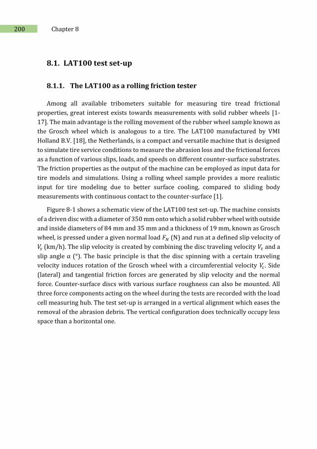
200 Chapter 8
8.1. LAT100 test set-up
8.1.1. The LAT100 as a rolling friction tester
Among all available tribometers suitable for measuring tire tread frictional
properties, great interest exists towards measurements with solid rubber wheels [1-
17]. The main advantage is the rolling movement of the rubber wheel sample known as
the Grosch wheel which is analogous to a tire. The LAT100 manufactured by VMI
Holland B.V. [18], the Netherlands, is a compact and versatile machine that is designed
to simulate tire service conditions to measure the abrasion loss and the frictional forces
as a function of various slips, loads, and speeds on different counter-surface substrates.
The friction properties as the output of the machine can be employed as input data for
tire models and simulations. Using a rolling wheel sample provides a more realistic
input for tire modeling due to better surface cooling, compared to sliding body
measurements with continuous contact to the counter-surface [1].
Figure 8-1 shows a schematic view of the LAT100 test set-up. The machine consists
of a driven disc with a diameter of 350 mm onto which a solid rubber wheel with outside
and inside diameters of 84 mm and 35 mm and a thickness of 19 mm, known as Grosch
wheel, is pressed under a given normal load 𝐹𝑁 (N) and run at a defined slip velocity of
𝑉𝑠 (km/h). The slip velocity is created by combining the disc traveling velocity 𝑉𝑡 and a
slip angle α (°). The basic principle is that the disc spinning with a certain traveling
velocity induces rotation of the Grosch wheel with a circumferential velocity 𝑉𝑐 . Side
(lateral) and tangential friction forces are generated by slip velocity and the normal
force. Counter-surface discs with various surface roughness can also be mounted. All
three force components acting on the wheel during the tests are recorded with the load
cell measuring hub. The test set-up is arranged in a vertical alignment which eases the
removal of the abrasion debris. The vertical configuration does technically occupy less
space than a horizontal one.
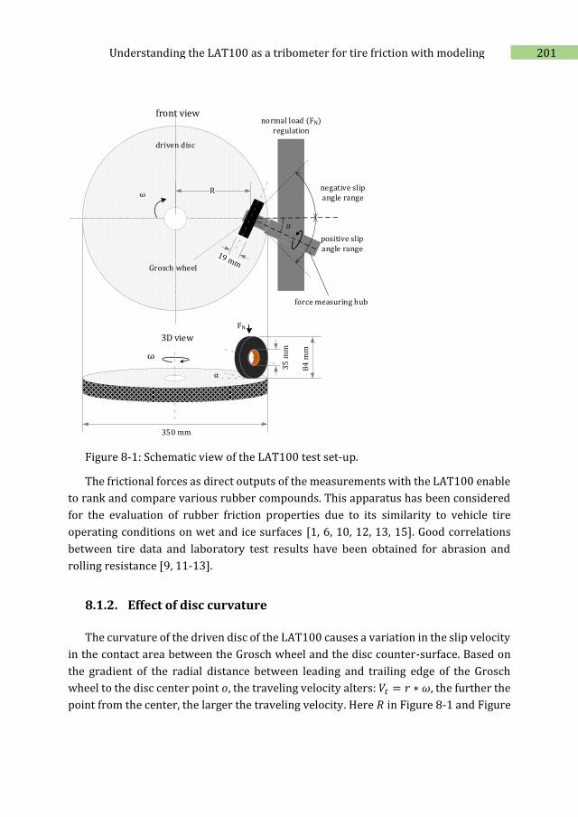
201 Understanding the LAT100 as a tribometer for tire friction with modeling
350 mm
normal load (FN) regulation
R negative slip angle range
force measuring hub
α
driven disc
Grosch wheel
ω
ω
front view
3D view
84
mm
35
mm
α
FN
positive slip angle range
Figure 8-1: Schematic view of the LAT100 test set-up.
The frictional forces as direct outputs of the measurements with the LAT100 enable
to rank and compare various rubber compounds. This apparatus has been considered
for the evaluation of rubber friction properties due to its similarity to vehicle tire
operating conditions on wet and ice surfaces [1, 6, 10, 12, 13, 15]. Good correlations
between tire data and laboratory test results have been obtained for abrasion and
rolling resistance [9, 11-13].
8.1.2. Effect of disc curvature
The curvature of the driven disc of the LAT100 causes a variation in the slip velocity
in the contact area between the Grosch wheel and the disc counter-surface. Based on
the gradient of the radial distance between leading and trailing edge of the Grosch
wheel to the disc center point 𝑜, the traveling velocity alters: 𝑉𝑡 = 𝑟 ∗ 𝜔, the further the
point from the center, the larger the traveling velocity. Here 𝑅 in Figure 8-1 and Figure
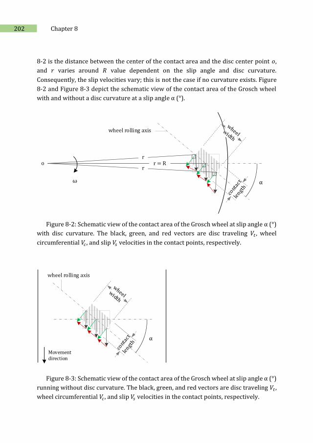
202 Chapter 8
8-2 is the distance between the center of the contact area and the disc center point 𝑜,
and 𝑟 varies around 𝑅 value dependent on the slip angle and disc curvature.
Consequently, the slip velocities vary; this is not the case if no curvature exists. Figure
8-2 and Figure 8-3 depict the schematic view of the contact area of the Grosch wheel
with and without a disc curvature at a slip angle α (°).
o
α
r = R
wheel rolling axis
ω
r
r
Figure 8-2: Schematic view of the contact area of the Grosch wheel at slip angle α (°)
with disc curvature. The black, green, and red vectors are disc traveling 𝑉𝑡 , wheel
circumferential 𝑉𝑐 , and slip 𝑉𝑠 velocities in the contact points, respectively.
α
wheel rolling axis
Movement direction
Figure 8-3: Schematic view of the contact area of the Grosch wheel at slip angle α (°)
running without disc curvature. The black, green, and red vectors are disc traveling 𝑉𝑡 ,
wheel circumferential 𝑉𝑐 , and slip 𝑉𝑠 velocities in the contact points, respectively.
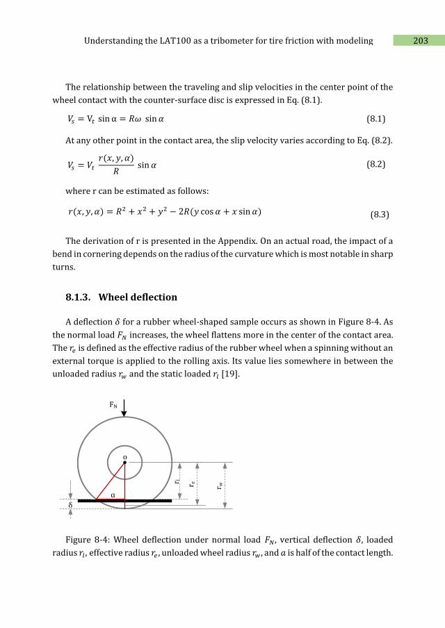
203 Understanding the LAT100 as a tribometer for tire friction with modeling
The relationship between the traveling and slip velocities in the center point of the
wheel contact with the counter-surface disc is expressed in Eq. (8.1).
𝑉𝑠 = V𝑡 sin α = 𝑅𝜔 sin 𝛼 (8.1)
At any other point in the contact area, the slip velocity varies according to Eq. (8.2).
𝑉𝑠 = 𝑉𝑡 𝑟(𝑥, 𝑦, 𝛼)
𝑅 sin 𝛼 (8.2)
where r can be estimated as follows:
𝑟(𝑥, 𝑦, 𝛼) = 𝑅2 + 𝑥2 + 𝑦2 − 2𝑅(𝑦 cos 𝛼 + 𝑥 sin 𝛼) (8.3)
The derivation of r is presented in the Appendix. On an actual road, the impact of a
bend in cornering depends on the radius of the curvature which is most notable in sharp
turns.
8.1.3. Wheel deflection
A deflection 𝛿 for a rubber wheel-shaped sample occurs as shown in Figure 8-4. As
the normal load 𝐹𝑁 increases, the wheel flattens more in the center of the contact area.
The 𝑟𝑒 is defined as the effective radius of the rubber wheel when a spinning without an
external torque is applied to the rolling axis. Its value lies somewhere in between the
unloaded radius 𝑟𝑤 and the static loaded 𝑟𝑙 [19].
FN
o
r wr er l
δ
ɑ
Figure 8-4: Wheel deflection under normal load 𝐹𝑁 , vertical deflection 𝛿, loaded
radius 𝑟𝑙 , effective radius 𝑟𝑒 , unloaded wheel radius 𝑟𝑤 , and 𝑎 is half of the contact length.
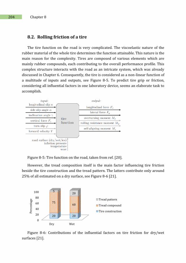
204 Chapter 8
8.2. Rolling friction of a tire
The tire function on the road is very complicated. The viscoelastic nature of the
rubber material of the whole tire determines the function attainable. This nature is the
main reason for the complexity. Tires are composed of various elements which are
mainly rubber compounds, each contributing to the overall performance profile. This
complex structure interacts with the road as an intricate system, which was already
discussed in Chapter 6. Consequently, the tire is considered as a non-linear function of
a multitude of inputs and outputs, see Figure 8-5. To predict tire grip or friction,
considering all influential factors in one laboratory device, seems an elaborate task to
accomplish.
Figure 8-5: Tire function on the road, taken from ref. [20].
However, the tread composition itself is the main factor influencing tire friction
beside the tire construction and the tread pattern. The latters contribute only around
25% of all estimated on a dry surface, see Figure 8-6 [21].
Figure 8-6: Contributions of the influential factors on tire friction for dry/wet
surfaces [21].
0
20
40
60
80
100
Dry Wet
20 20
7560
520
Per
cen
tage Tread pattern
Tread compound
Tire construction
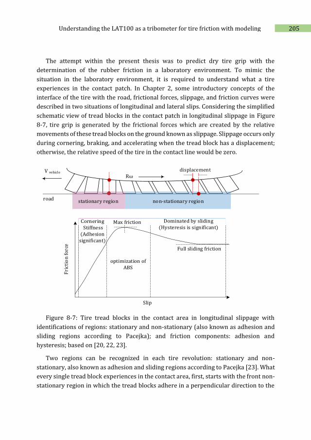
205 Understanding the LAT100 as a tribometer for tire friction with modeling
The attempt within the present thesis was to predict dry tire grip with the
determination of the rubber friction in a laboratory environment. To mimic the
situation in the laboratory environment, it is required to understand what a tire
experiences in the contact patch. In Chapter 2, some introductory concepts of the
interface of the tire with the road, frictional forces, slippage, and friction curves were
described in two situations of longitudinal and lateral slips. Considering the simplified
schematic view of tread blocks in the contact patch in longitudinal slippage in Figure
8-7, tire grip is generated by the frictional forces which are created by the relative
movements of these tread blocks on the ground known as slippage. Slippage occurs only
during cornering, braking, and accelerating when the tread block has a displacement;
otherwise, the relative speed of the tire in the contact line would be zero.
Rω V vehicle
road stationary region non-stationary region
displacement
Slip
Fri
ctio
n f
orc
e
optimization of ABS
Dominated by sliding(Hysteresis is significant)
Cornering Stiffness
(Adhesion significant)
Max friction
Full sliding friction
Figure 8-7: Tire tread blocks in the contact area in longitudinal slippage with
identifications of regions: stationary and non-stationary (also known as adhesion and
sliding regions according to Pacejka); and friction components: adhesion and
hysteresis; based on [20, 22, 23].
Two regions can be recognized in each tire revolution: stationary and non-
stationary, also known as adhesion and sliding regions according to Pacejka [23]. What
every single tread block experiences in the contact area, first, starts with the front non-
stationary region in which the tread blocks adhere in a perpendicular direction to the
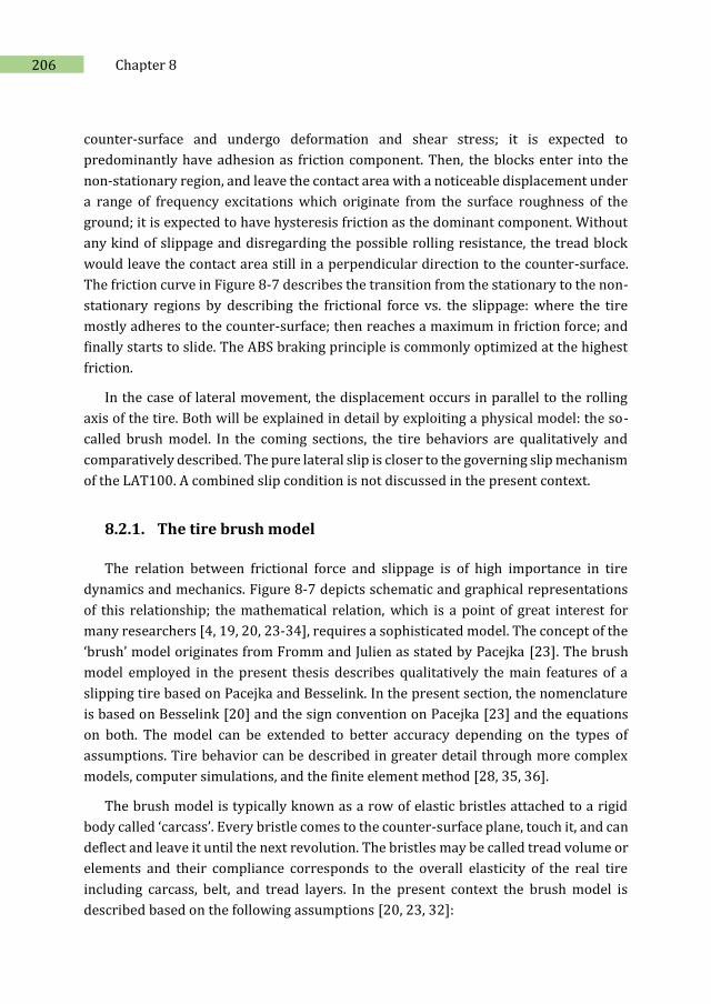
206 Chapter 8
counter-surface and undergo deformation and shear stress; it is expected to
predominantly have adhesion as friction component. Then, the blocks enter into the
non-stationary region, and leave the contact area with a noticeable displacement under
a range of frequency excitations which originate from the surface roughness of the
ground; it is expected to have hysteresis friction as the dominant component. Without
any kind of slippage and disregarding the possible rolling resistance, the tread block
would leave the contact area still in a perpendicular direction to the counter-surface.
The friction curve in Figure 8-7 describes the transition from the stationary to the non-
stationary regions by describing the frictional force vs. the slippage: where the tire
mostly adheres to the counter-surface; then reaches a maximum in friction force; and
finally starts to slide. The ABS braking principle is commonly optimized at the highest
friction.
In the case of lateral movement, the displacement occurs in parallel to the rolling
axis of the tire. Both will be explained in detail by exploiting a physical model: the so-
called brush model. In the coming sections, the tire behaviors are qualitatively and
comparatively described. The pure lateral slip is closer to the governing slip mechanism
of the LAT100. A combined slip condition is not discussed in the present context.
8.2.1. The tire brush model
The relation between frictional force and slippage is of high importance in tire
dynamics and mechanics. Figure 8-7 depicts schematic and graphical representations
of this relationship; the mathematical relation, which is a point of great interest for
many researchers [4, 19, 20, 23-34], requires a sophisticated model. The concept of the
‘brush’ model originates from Fromm and Julien as stated by Pacejka [23]. The brush
model employed in the present thesis describes qualitatively the main features of a
slipping tire based on Pacejka and Besselink. In the present section, the nomenclature
is based on Besselink [20] and the sign convention on Pacejka [23] and the equations
on both. The model can be extended to better accuracy depending on the types of
assumptions. Tire behavior can be described in greater detail through more complex
models, computer simulations, and the finite element method [28, 35, 36].
The brush model is typically known as a row of elastic bristles attached to a rigid
body called ‘carcass’. Every bristle comes to the counter-surface plane, touch it, and can
deflect and leave it until the next revolution. The bristles may be called tread volume or
elements and their compliance corresponds to the overall elasticity of the real tire
including carcass, belt, and tread layers. In the present context the brush model is
described based on the following assumptions [20, 23, 32]:
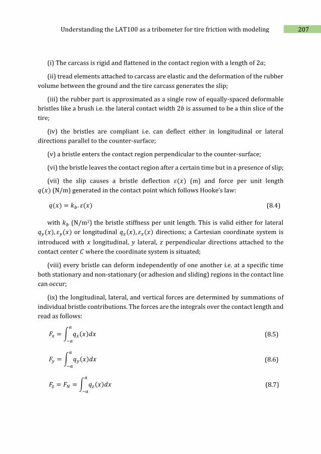
207 Understanding the LAT100 as a tribometer for tire friction with modeling
(i) The carcass is rigid and flattened in the contact region with a length of 2𝑎;
(ii) tread elements attached to carcass are elastic and the deformation of the rubber
volume between the ground and the tire carcass generates the slip;
(iii) the rubber part is approximated as a single row of equally-spaced deformable
bristles like a brush i.e. the lateral contact width 2𝑏 is assumed to be a thin slice of the
tire;
(iv) the bristles are compliant i.e. can deflect either in longitudinal or lateral
directions parallel to the counter-surface;
(v) a bristle enters the contact region perpendicular to the counter-surface;
(vi) the bristle leaves the contact region after a certain time but in a presence of slip;
(vii) the slip causes a bristle deflection 휀(𝑥) (m) and force per unit length
𝑞(𝑥) (N/m) generated in the contact point which follows Hooke’s law:
𝑞(𝑥) = 𝑘𝑏 . 휀(𝑥) (8.4)
with 𝑘𝑏 (N/m2) the bristle stiffness per unit length. This is valid either for lateral
𝑞𝑦(𝑥), 휀𝑦(𝑥) or longitudinal 𝑞𝑥(𝑥), 휀𝑥(𝑥) directions; a Cartesian coordinate system is
introduced with 𝑥 longitudinal, 𝑦 lateral, 𝑧 perpendicular directions attached to the
contact center 𝐶 where the coordinate system is situated;
(viii) every bristle can deform independently of one another i.e. at a specific time
both stationary and non-stationary (or adhesion and sliding) regions in the contact line
can occur;
(ix) the longitudinal, lateral, and vertical forces are determined by summations of
individual bristle contributions. The forces are the integrals over the contact length and
read as follows:
𝐹𝑥 = ∫ 𝑞𝑥(𝑥)𝑑𝑥𝑎
−𝑎
(8.5)
𝐹𝑦 = ∫ 𝑞𝑦(𝑥)𝑑𝑥𝑎
−𝑎
(8.6)
𝐹𝑧 = 𝐹𝑁 = ∫ 𝑞𝑧(𝑥)𝑑𝑥𝑎
−𝑎
(8.7)
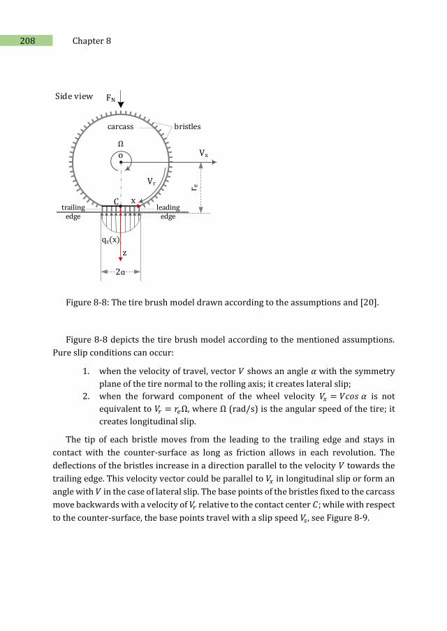
208 Chapter 8
FN
oo
Side view
2ɑ
Ω
r e
Vr
leading edge
trailing edge
C
Vx
z
x
qz(x)
bristlescarcass
Figure 8-8: The tire brush model drawn according to the assumptions and [20].
Figure 8-8 depicts the tire brush model according to the mentioned assumptions.
Pure slip conditions can occur:
1. when the velocity of travel, vector 𝑉 shows an angle 𝛼 with the symmetry
plane of the tire normal to the rolling axis; it creates lateral slip;
2. when the forward component of the wheel velocity 𝑉𝑥 = 𝑉𝑐𝑜𝑠 𝛼 is not
equivalent to 𝑉𝑟 = 𝑟𝑒Ω, where Ω (rad/s) is the angular speed of the tire; it
creates longitudinal slip.
The tip of each bristle moves from the leading to the trailing edge and stays in
contact with the counter-surface as long as friction allows in each revolution. The
deflections of the bristles increase in a direction parallel to the velocity 𝑉 towards the
trailing edge. This velocity vector could be parallel to 𝑉𝑥 in longitudinal slip or form an
angle with 𝑉 in the case of lateral slip. The base points of the bristles fixed to the carcass
move backwards with a velocity of 𝑉𝑟 relative to the contact center 𝐶; while with respect
to the counter-surface, the base points travel with a slip speed 𝑉𝑠, see Figure 8-9.
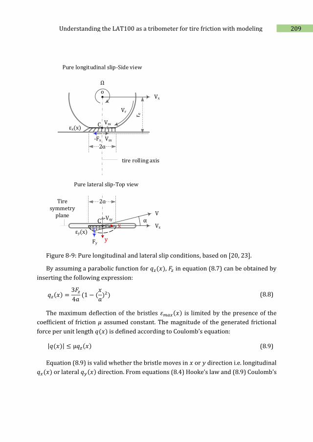
209 Understanding the LAT100 as a tribometer for tire friction with modeling
o
2ɑ
r e
C
Vx
o
Vr
Vsx
Vsx
Pure longitudinal slip-Side view
-Fx
tire rolling axis
Pure lateral slip-Top view
εy(x)
C
y
xα
εx(x)
-Vsy
Fy
Vx
V
Ω
2ɑTire symmetry
plane
Figure 8-9: Pure longitudinal and lateral slip conditions, based on [20, 23].
By assuming a parabolic function for 𝑞𝑧(𝑥), 𝐹𝑧 in equation (8.7) can be obtained by
inserting the following expression:
𝑞𝑧(𝑥) =3𝐹𝑧
4𝑎(1 − (
𝑥
𝑎)2) (8.8)
The maximum deflection of the bristles 휀𝑚𝑎𝑥(𝑥) is limited by the presence of the
coefficient of friction 𝜇 assumed constant. The magnitude of the generated frictional
force per unit length 𝑞(𝑥) is defined according to Coulomb’s equation:
|𝑞(𝑥)| ≤ μ𝑞𝑧(𝑥) (8.9)
Equation (8.9) is valid whether the bristle moves in 𝑥 or 𝑦 direction i.e. longitudinal
𝑞𝑥(𝑥) or lateral 𝑞𝑦(𝑥) direction. From equations (8.4) Hooke’s law and (8.9) Coulomb’s
210 Chapter 8
law, the maximum bristle deflection 휀𝑚𝑎𝑥(𝑥) can be derived in equation (8.10) and has
a parabolic shape as well because it is a function of 𝑞𝑧(𝑥):
|휀𝑚𝑎𝑥(𝑥)| =μ𝑞𝑧(𝑥)
𝑘𝑏
(8.10)
This concept is a good basis for the following discussions of the mathematical
calculations of the frictional forces and ‘break-away’ point which is the transition
between the stationary and non-stationary regions. In the next section, they will be
discussed for two scenarios of pure lateral and longitudinal slips.
8.2.2. Pure lateral (side) slip
In the stationary region, the contact line between the bristles and the counter-
surface is straight, the bristles follow the straight line of contact which is parallel to 𝑉,
the velocity of travel. By applying the slip angle 𝛼, at the moment that the straight line
of contact intersects with the maximum deflection parabola 휀𝑚𝑎𝑥 , the non-stationary
region begins from the intersection or the break-away point in Figure 8-10A. The
bristles coincide with the parabola for the maximum possible deflection. The deflection
is not linear anymore and is curved indicating that available frictional forces become
lower than the forces that would have continued along the straight line, Figure 8-10B.
Due to asymmetry of the deflection, a self-aligning torque or moment 𝑀𝑧 arises. The
moment is the product of multiplying the lateral force 𝐹𝑦 by the moment arm, or the
‘pneumatic trail’ 𝑡𝑝, which is the distance of the lateral force line of action from point 𝐶.
As the slip angle increases, the deformation profile becomes more symmetric. The point
of intersection shifts to the leading edge, the lateral force escalates and 𝑡𝑝 decreases;
until the contact line becomes the tangent to the parabola at the foremost of the leading
edge, Figure 8-10C. The deformation becomes fully symmetric and the stationary
(adhesion) region disappears and full sliding occurs. The friction curve turns flat, the 𝑡𝑝
becomes zero, and the self-aligning moment vanishes. By further increasing the slip
angle, the situation for bristles has to stay theoretically unchanged, see Figure 8-10D.
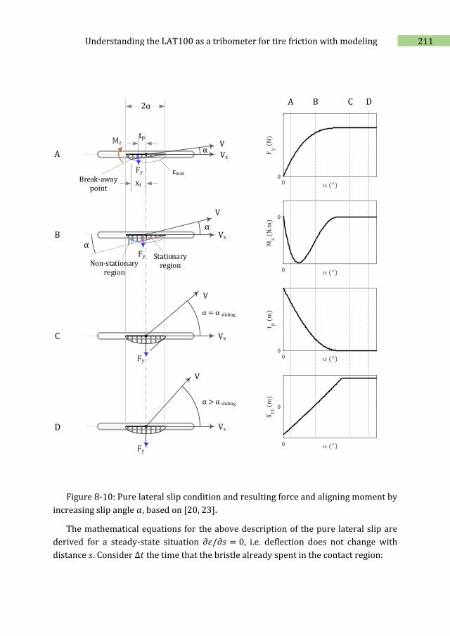
211 Understanding the LAT100 as a tribometer for tire friction with modeling
A
2ɑ
α
Fy
Vx
V
α
Fy
VxB
Fy
Vx
V
C
D
α > α sliding
Fy
Vx
V
V
α = α sliding
εmax
tp
Non-stationary region
Stationary region
xt
α
Mz
Break-away point
A B C D
Figure 8-10: Pure lateral slip condition and resulting force and aligning moment by
increasing slip angle 𝛼, based on [20, 23].
The mathematical equations for the above description of the pure lateral slip are
derived for a steady-state situation 𝜕휀/𝜕𝑠 = 0, i.e. deflection does not change with
distance 𝑠. Consider ∆𝑡 the time that the bristle already spent in the contact region:
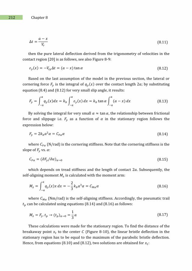
212 Chapter 8
∆𝑡 =𝑎 − 𝑥
𝑉𝑟
(8.11)
then the pure lateral deflection derived from the trigonometry of velocities in the
contact region [20] is as follows, see also Figure 8-9:
휀𝑦(𝑥) = −𝑉𝑠𝑦∆𝑡 = (𝑎 − 𝑥) tan 𝛼 (8.12)
Based on the last assumption of the model in the previous section, the lateral or
cornering force 𝐹𝑦 is the integral of 𝑞𝑦(𝑥) over the contact length 2𝑎; by substituting
equation (8.4) and (8.12) for very small slip angle, it results:
𝐹𝑦 = ∫ 𝑞𝑦(𝑥)𝑑𝑥𝑎
−𝑎
= 𝑘𝑏 ∫ 휀𝑦(𝑥)𝑎
−𝑎
𝑑𝑥 = 𝑘𝑏 tan 𝛼 ∫ (𝑎 − 𝑥)𝑎
−𝑎
𝑑𝑥 (8.13)
By solving the integral for very small 𝛼 ≈ tan 𝛼, the relationship between frictional
force and slippage i.e. 𝐹𝑦 as a function of 𝛼 in the stationary region follows the
expression below:
𝐹𝑦 = 2𝑘𝑏𝑎2𝛼 = 𝐶𝐹𝛼𝛼 (8.14)
where 𝐶𝐹𝛼 (N/rad) is the cornering stiffness. Note that the cornering stiffness is the
slope of 𝐹𝑦 vs. 𝛼:
𝐶𝐹𝛼 = (𝜕𝐹𝑦/𝜕𝛼)𝛼→0 (8.15)
which depends on tread stiffness and the length of contact 2𝑎. Subsequently, the
self-aligning moment 𝑀𝑧 is calculated with the moment arm:
𝑀𝑧 = ∫ 𝑞𝑦(𝑥)𝑥𝑎
−𝑎
𝑑𝑥 = −2
3𝑘𝑏𝑎3𝛼 = 𝐶𝑀𝛼𝛼 (8.16)
where 𝐶𝑀𝛼 (Nm/rad) is the self-aligning stiffness. Accordingly, the pneumatic trail
𝑡𝑝 can be calculated using equations (8.14) and (8.16) as follows:
𝑀𝑧 = 𝐹𝑦 . 𝑡𝑝 → (𝑡𝑝)𝛼→0 =1
3𝑎 (8.17)
These calculations were made for the stationary region. To find the distance of the
breakaway point 𝑥𝑡 to the center 𝐶 (Figure 8-10), the linear bristle deflection in the
stationary region has to be equal to the maximum of the parabolic bristle deflection.
Hence, from equations (8.10) and (8.12), two solutions are obtained for 𝑥𝑡:
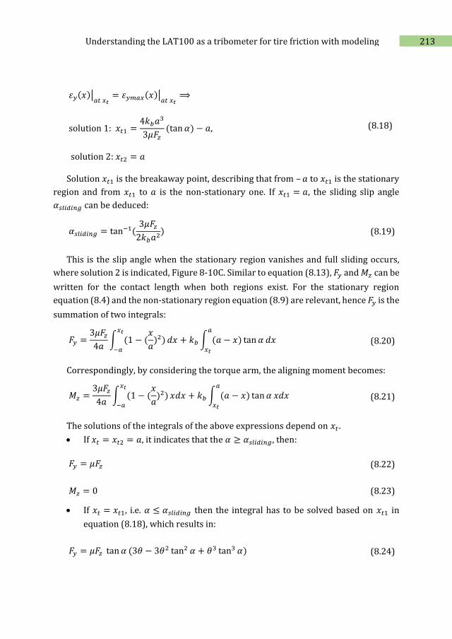
213 Understanding the LAT100 as a tribometer for tire friction with modeling
휀𝑦(𝑥)|𝑎𝑡 𝑥𝑡
= 휀𝑦𝑚𝑎𝑥(𝑥)|𝑎𝑡 𝑥𝑡
⟹
solution 1: 𝑥𝑡1 =4𝑘𝑏𝑎3
3𝜇𝐹𝑧
(tan 𝛼) − 𝑎,
solution 2: 𝑥𝑡2 = 𝑎
(8.18)
Solution 𝑥𝑡1 is the breakaway point, describing that from – 𝑎 to 𝑥𝑡1 is the stationary
region and from 𝑥𝑡1 to 𝑎 is the non-stationary one. If 𝑥𝑡1 = 𝑎, the sliding slip angle
𝛼𝑠𝑙𝑖𝑑𝑖𝑛𝑔 can be deduced:
𝛼𝑠𝑙𝑖𝑑𝑖𝑛𝑔 = tan−1(3𝜇𝐹𝑧
2𝑘𝑏𝑎2) (8.19)
This is the slip angle when the stationary region vanishes and full sliding occurs,
where solution 2 is indicated, Figure 8-10C. Similar to equation (8.13), 𝐹𝑦 and 𝑀𝑧 can be
written for the contact length when both regions exist. For the stationary region
equation (8.4) and the non-stationary region equation (8.9) are relevant, hence 𝐹𝑦 is the
summation of two integrals:
𝐹𝑦 =3𝜇𝐹𝑧
4𝑎∫ (1 − (
𝑥
𝑎)2)
𝑥𝑡
−𝑎
𝑑𝑥 + 𝑘𝑏 ∫ (𝑎 − 𝑥) tan 𝛼𝑎
𝑥𝑡
𝑑𝑥 (8.20)
Correspondingly, by considering the torque arm, the aligning moment becomes:
𝑀𝑧 =3𝜇𝐹𝑧
4𝑎∫ (1 − (
𝑥
𝑎)2)
𝑥𝑡
−𝑎
𝑥𝑑𝑥 + 𝑘𝑏 ∫ (𝑎 − 𝑥) tan 𝛼𝑎
𝑥𝑡
𝑥𝑑𝑥 (8.21)
The solutions of the integrals of the above expressions depend on 𝑥𝑡 .
If 𝑥𝑡 = 𝑥𝑡2 = 𝑎, it indicates that the 𝛼 ≥ 𝛼𝑠𝑙𝑖𝑑𝑖𝑛𝑔, then:
𝐹𝑦 = 𝜇𝐹𝑧 (8.22)
𝑀𝑧 = 0 (8.23)
If 𝑥𝑡 = 𝑥𝑡1, i.e. 𝛼 ≤ 𝛼𝑠𝑙𝑖𝑑𝑖𝑛𝑔 then the integral has to be solved based on 𝑥𝑡1 in
equation (8.18), which results in:
𝐹𝑦 = 𝜇𝐹𝑧 tan 𝛼 (3𝜃 − 3𝜃2 tan2 𝛼 + 𝜃3 tan3 𝛼) (8.24)
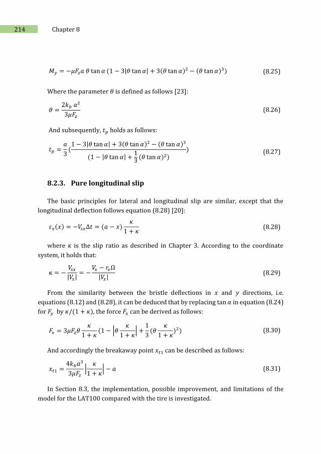
214 Chapter 8
𝑀𝑦 = −𝜇𝐹𝑧𝑎 𝜃 tan 𝛼 (1 − 3|𝜃 tan 𝛼| + 3(𝜃 tan 𝛼)2 − (𝜃 tan 𝛼)3) (8.25)
Where the parameter 𝜃 is defined as follows [23]:
𝜃 =2𝑘𝑏 𝑎2
3𝜇𝐹𝑧
(8.26)
And subsequently, 𝑡𝑝 holds as follows:
𝑡𝑝 =𝑎
3(1 − 3|𝜃 tan 𝛼| + 3(𝜃 tan 𝛼)2 − (𝜃 tan 𝛼)3
(1 − |𝜃 tan 𝛼| +13
(𝜃 tan 𝛼)2)) (8.27)
8.2.3. Pure longitudinal slip
The basic principles for lateral and longitudinal slip are similar, except that the
longitudinal deflection follows equation (8.28) [20]:
휀𝑥(𝑥) = −𝑉𝑠𝑥∆𝑡 = (𝑎 − 𝑥)𝜅
1 + 𝜅 (8.28)
where 𝜅 is the slip ratio as described in Chapter 3. According to the coordinate
system, it holds that:
κ = −𝑉𝑠𝑥
|𝑉𝑥|= −
𝑉𝑥 − 𝑟𝑒Ω
|𝑉𝑥| (8.29)
From the similarity between the bristle deflections in 𝑥 and 𝑦 directions, i.e.
equations (8.12) and (8.28), it can be deduced that by replacing tan 𝛼 in equation (8.24)
for 𝐹𝑦 by 𝜅/(1 + 𝜅), the force 𝐹𝑥 can be derived as follows:
𝐹𝑥 = 3𝜇𝐹𝑧𝜃𝜅
1 + 𝜅(1 − |𝜃
𝜅
1 + 𝜅| +
1
3(𝜃
𝜅
1 + 𝜅)2) (8.30)
And accordingly the breakaway point 𝑥𝑡1 can be described as follows:
𝑥𝑡1 =4𝑘𝑏𝑎3
3𝜇𝐹𝑧
|𝜅
1 + 𝜅| − 𝑎 (8.31)
In Section 8.3, the implementation, possible improvement, and limitations of the
model for the LAT100 compared with the tire is investigated.
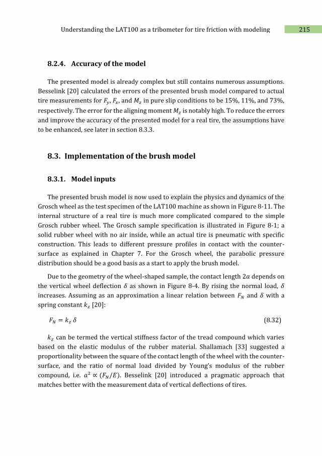
215 Understanding the LAT100 as a tribometer for tire friction with modeling
8.2.4. Accuracy of the model
The presented model is already complex but still contains numerous assumptions.
Besselink [20] calculated the errors of the presented brush model compared to actual
tire measurements for 𝐹𝑦, 𝐹𝑥, and 𝑀𝑧 in pure slip conditions to be 15%, 11%, and 73%,
respectively. The error for the aligning moment 𝑀𝑧 is notably high. To reduce the errors
and improve the accuracy of the presented model for a real tire, the assumptions have
to be enhanced, see later in section 8.3.3.
8.3. Implementation of the brush model
8.3.1. Model inputs
The presented brush model is now used to explain the physics and dynamics of the
Grosch wheel as the test specimen of the LAT100 machine as shown in Figure 8-11. The
internal structure of a real tire is much more complicated compared to the simple
Grosch rubber wheel. The Grosch sample specification is illustrated in Figure 8-1; a
solid rubber wheel with no air inside, while an actual tire is pneumatic with specific
construction. This leads to different pressure profiles in contact with the counter-
surface as explained in Chapter 7. For the Grosch wheel, the parabolic pressure
distribution should be a good basis as a start to apply the brush model.
Due to the geometry of the wheel-shaped sample, the contact length 2𝑎 depends on
the vertical wheel deflection 𝛿 as shown in Figure 8-4. By rising the normal load, 𝛿
increases. Assuming as an approximation a linear relation between 𝐹𝑁 and 𝛿 with a
spring constant 𝑘𝑧 [20]:
𝐹𝑁 = 𝑘𝑧 𝛿 (8.32)
𝑘𝑧 can be termed the vertical stiffness factor of the tread compound which varies
based on the elastic modulus of the rubber material. Shallamach [33] suggested a
proportionality between the square of the contact length of the wheel with the counter-
surface, and the ratio of normal load divided by Young’s modulus of the rubber
compound, i.e. 𝑎2 ∝ (𝐹𝑁/𝐸). Besselink [20] introduced a pragmatic approach that
matches better with the measurement data of vertical deflections of tires.
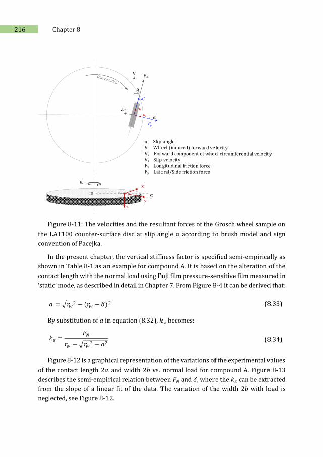
216 Chapter 8
ω
α y
x
z
o
Figure 8-11: The velocities and the resultant forces of the Grosch wheel sample on
the LAT100 counter-surface disc at slip angle α according to brush model and sign
convention of Pacejka.
In the present chapter, the vertical stiffness factor is specified semi-empirically as
shown in Table 8-1 as an example for compound A. It is based on the alteration of the
contact length with the normal load using Fuji film pressure-sensitive film measured in
‘static’ mode, as described in detail in Chapter 7. From Figure 8-4 it can be derived that:
𝑎 = √𝑟𝑤2 − (𝑟𝑤 − 𝛿)2 (8.33)
By substitution of 𝑎 in equation (8.32), 𝑘𝑧 becomes:
𝑘𝑧 =𝐹𝑁
𝑟𝑤 − √𝑟𝑤2 − 𝑎2
(8.34)
Figure 8-12 is a graphical representation of the variations of the experimental values
of the contact length 2𝑎 and width 2𝑏 vs. normal load for compound A. Figure 8-13
describes the semi-empirical relation between 𝐹𝑁 and 𝛿, where the 𝑘𝑧 can be extracted
from the slope of a linear fit of the data. The variation of the width 2𝑏 with load is
neglected, see Figure 8-12.
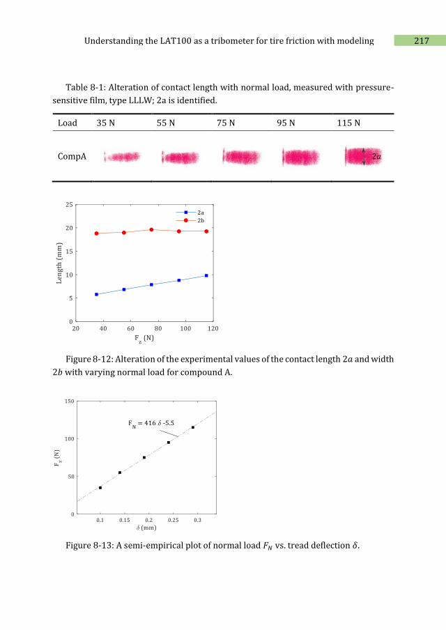
217 Understanding the LAT100 as a tribometer for tire friction with modeling
Table 8-1: Alteration of contact length with normal load, measured with pressure-
sensitive film, type LLLW; 2a is identified.
Load 35 N 55 N 75 N 95 N 115 N
CompA
Figure 8-12: Alteration of the experimental values of the contact length 2𝑎 and width
2𝑏 with varying normal load for compound A.
Figure 8-13: A semi-empirical plot of normal load 𝐹𝑁 vs. tread deflection 𝛿.
2𝑎
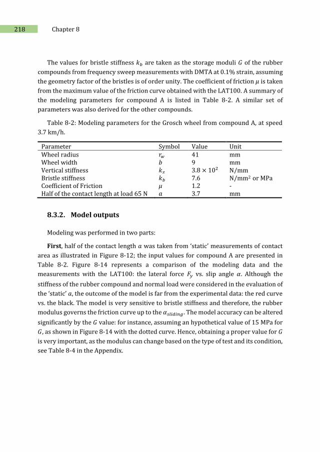
218 Chapter 8
The values for bristle stiffness 𝑘𝑏 are taken as the storage moduli 𝐺 of the rubber
compounds from frequency sweep measurements with DMTA at 0.1% strain, assuming
the geometry factor of the bristles is of order unity. The coefficient of friction 𝜇 is taken
from the maximum value of the friction curve obtained with the LAT100. A summary of
the modeling parameters for compound A is listed in Table 8-2. A similar set of
parameters was also derived for the other compounds.
Table 8-2: Modeling parameters for the Grosch wheel from compound A, at speed
3.7 km/h.
Parameter Symbol Value Unit Wheel radius 𝑟𝑤 41 mm Wheel width 𝑏 9 mm Vertical stiffness 𝑘𝑧 3.8 × 10² N/mm Bristle stiffness 𝑘𝑏 7.6 N/mm2 or MPa Coefficient of Friction μ 1.2 - Half of the contact length at load 65 N 𝑎 3.7 mm
8.3.2. Model outputs
Modeling was performed in two parts:
First, half of the contact length 𝑎 was taken from ‘static’ measurements of contact
area as illustrated in Figure 8-12; the input values for compound A are presented in
Table 8-2. Figure 8-14 represents a comparison of the modeling data and the
measurements with the LAT100: the lateral force 𝐹𝑦 vs. slip angle 𝛼. Although the
stiffness of the rubber compound and normal load were considered in the evaluation of
the ‘static’ 𝑎, the outcome of the model is far from the experimental data: the red curve
vs. the black. The model is very sensitive to bristle stiffness and therefore, the rubber
modulus governs the friction curve up to the 𝛼𝑠𝑙𝑖𝑑𝑖𝑛𝑔 . The model accuracy can be altered
significantly by the 𝐺 value: for instance, assuming an hypothetical value of 15 MPa for
𝐺, as shown in Figure 8-14 with the dotted curve. Hence, obtaining a proper value for 𝐺
is very important, as the modulus can change based on the type of test and its condition,
see Table 8-4 in the Appendix.
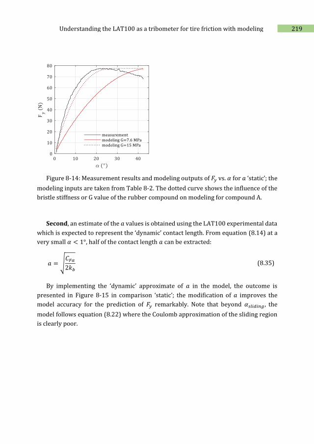
219 Understanding the LAT100 as a tribometer for tire friction with modeling
Figure 8-14: Measurement results and modeling outputs of 𝐹𝑦 vs. 𝛼 for 𝑎 ‘static’; the
modeling inputs are taken from Table 8-2. The dotted curve shows the influence of the
bristle stiffness or G value of the rubber compound on modeling for compound A.
Second, an estimate of the 𝑎 values is obtained using the LAT100 experimental data
which is expected to represent the ‘dynamic’ contact length. From equation (8.14) at a
very small 𝛼 < 1°, half of the contact length 𝑎 can be extracted:
𝑎 = √𝐶𝐹𝛼
2𝑘𝑏
(8.35)
By implementing the ‘dynamic’ approximate of 𝑎 in the model, the outcome is
presented in Figure 8-15 in comparison ‘static’; the modification of 𝑎 improves the
model accuracy for the prediction of 𝐹𝑦 remarkably. Note that beyond 𝛼𝑠𝑙𝑖𝑑𝑖𝑛𝑔 , the
model follows equation (8.22) where the Coulomb approximation of the sliding region
is clearly poor.
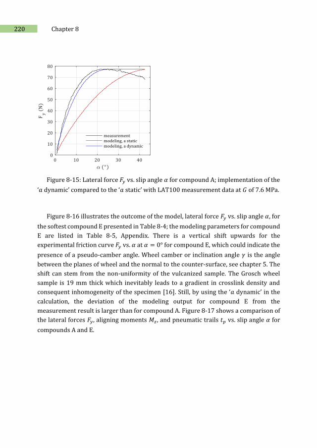
220 Chapter 8
Figure 8-15: Lateral force 𝐹𝑦 vs. slip angle 𝛼 for compound A; implementation of the
‘𝑎 dynamic’ compared to the ‘𝑎 static’ with LAT100 measurement data at 𝐺 of 7.6 MPa.
Figure 8-16 illustrates the outcome of the model, lateral force 𝐹𝑦 vs. slip angle 𝛼, for
the softest compound E presented in Table 8-4; the modeling parameters for compound
E are listed in Table 8-5, Appendix. There is a vertical shift upwards for the
experimental friction curve 𝐹𝑦 vs. 𝛼 at 𝛼 = 0° for compound E, which could indicate the
presence of a pseudo-camber angle. Wheel camber or inclination angle 𝛾 is the angle
between the planes of wheel and the normal to the counter-surface, see chapter 5. The
shift can stem from the non-uniformity of the vulcanized sample. The Grosch wheel
sample is 19 mm thick which inevitably leads to a gradient in crosslink density and
consequent inhomogeneity of the specimen [16]. Still, by using the ‘𝑎 dynamic’ in the
calculation, the deviation of the modeling output for compound E from the
measurement result is larger than for compound A. Figure 8-17 shows a comparison of
the lateral forces 𝐹𝑦, aligning moments 𝑀𝑧 , and pneumatic trails 𝑡𝑝 vs. slip angle 𝛼 for
compounds A and E.
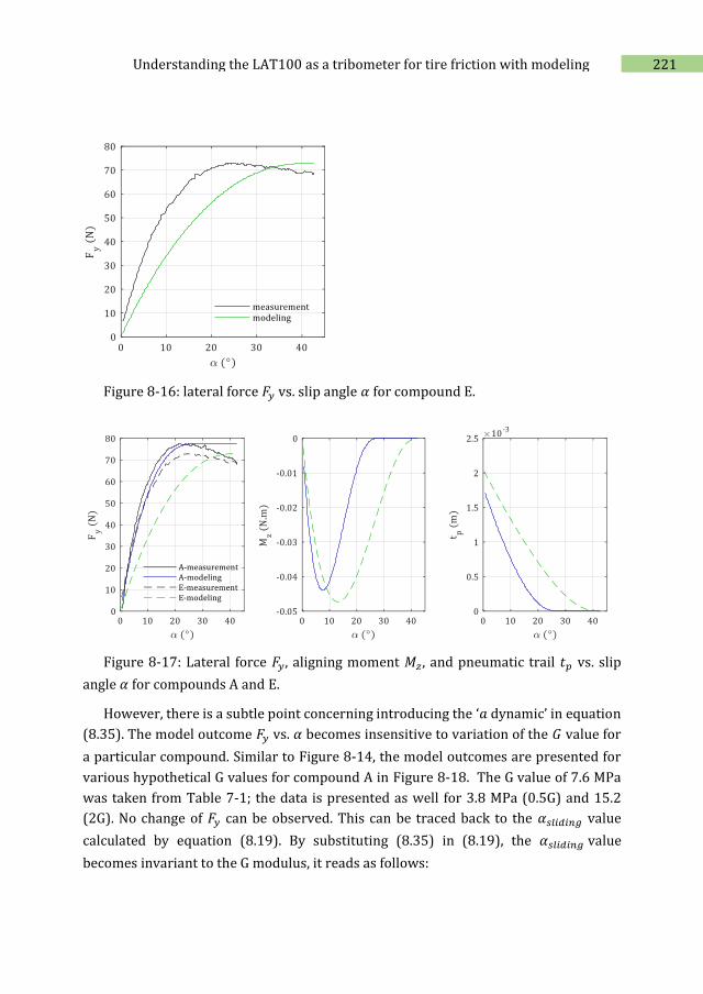
221 Understanding the LAT100 as a tribometer for tire friction with modeling
Figure 8-16: lateral force 𝐹𝑦 vs. slip angle 𝛼 for compound E.
Figure 8-17: Lateral force 𝐹𝑦, aligning moment 𝑀𝑧 , and pneumatic trail 𝑡𝑝 vs. slip
angle 𝛼 for compounds A and E.
However, there is a subtle point concerning introducing the ‘𝑎 dynamic’ in equation
(8.35). The model outcome 𝐹𝑦 vs. 𝛼 becomes insensitive to variation of the 𝐺 value for
a particular compound. Similar to Figure 8-14, the model outcomes are presented for
various hypothetical G values for compound A in Figure 8-18. The G value of 7.6 MPa
was taken from Table 7-1; the data is presented as well for 3.8 MPa (0.5G) and 15.2
(2G). No change of 𝐹𝑦 can be observed. This can be traced back to the 𝛼𝑠𝑙𝑖𝑑𝑖𝑛𝑔 value
calculated by equation (8.19). By substituting (8.35) in (8.19), the 𝛼𝑠𝑙𝑖𝑑𝑖𝑛𝑔 value
becomes invariant to the G modulus, it reads as follows:
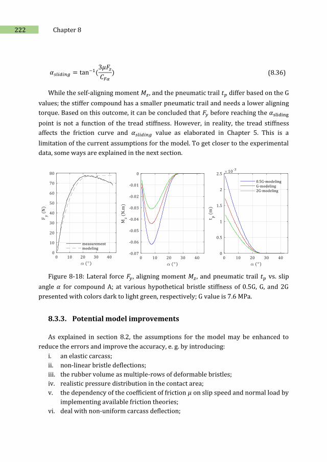
222 Chapter 8
𝛼𝑠𝑙𝑖𝑑𝑖𝑛𝑔 = tan−1(3𝜇𝐹𝑧
𝐶𝐹𝛼
) (8.36)
While the self-aligning moment 𝑀𝑧 , and the pneumatic trail 𝑡𝑝 differ based on the G
values; the stiffer compound has a smaller pneumatic trail and needs a lower aligning
torque. Based on this outcome, it can be concluded that 𝐹𝑦 before reaching the 𝛼sliding
point is not a function of the tread stiffness. However, in reality, the tread stiffness
affects the friction curve and 𝛼𝑠𝑙𝑖𝑑𝑖𝑛𝑔 value as elaborated in Chapter 5. This is a
limitation of the current assumptions for the model. To get closer to the experimental
data, some ways are explained in the next section.
Figure 8-18: Lateral force 𝐹𝑦, aligning moment 𝑀𝑧 , and pneumatic trail 𝑡𝑝 vs. slip
angle 𝛼 for compound A; at various hypothetical bristle stiffness of 0.5G, G, and 2G
presented with colors dark to light green, respectively; G value is 7.6 MPa.
8.3.3. Potential model improvements
As explained in section 8.2, the assumptions for the model may be enhanced to
reduce the errors and improve the accuracy, e. g. by introducing:
i. an elastic carcass;
ii. non-linear bristle deflections;
iii. the rubber volume as multiple-rows of deformable bristles;
iv. realistic pressure distribution in the contact area;
v. the dependency of the coefficient of friction 𝜇 on slip speed and normal load by
implementing available friction theories;
vi. deal with non-uniform carcass deflection;
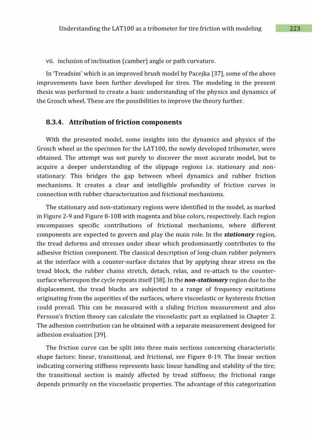
223 Understanding the LAT100 as a tribometer for tire friction with modeling
vii. inclusion of inclination (camber) angle or path curvature.
In ‘Treadsim’ which is an improved brush model by Pacejka [37], some of the above
improvements have been further developed for tires. The modeling in the present
thesis was performed to create a basic understanding of the physics and dynamics of
the Grosch wheel. These are the possibilities to improve the theory further.
8.3.4. Attribution of friction components
With the presented model, some insights into the dynamics and physics of the
Grosch wheel as the specimen for the LAT100, the newly developed tribometer, were
obtained. The attempt was not purely to discover the most accurate model, but to
acquire a deeper understanding of the slippage regions i.e. stationary and non-
stationary. This bridges the gap between wheel dynamics and rubber friction
mechanisms. It creates a clear and intelligible profundity of friction curves in
connection with rubber characterization and frictional mechanisms.
The stationary and non-stationary regions were identified in the model, as marked
in Figure 2-9 and Figure 8-10B with magenta and blue colors, respectively. Each region
encompasses specific contributions of frictional mechanisms, where different
components are expected to govern and play the main role. In the stationary region,
the tread deforms and stresses under shear which predominantly contributes to the
adhesive friction component. The classical description of long-chain rubber polymers
at the interface with a counter-surface dictates that by applying shear stress on the
tread block, the rubber chains stretch, detach, relax, and re-attach to the counter-
surface whereupon the cycle repeats itself [38]. In the non-stationary region due to the
displacement, the tread blocks are subjected to a range of frequency excitations
originating from the asperities of the surfaces, where viscoelastic or hysteresis friction
could prevail. This can be measured with a sliding friction measurement and also
Persson’s friction theory can calculate the viscoelastic part as explained in Chapter 2.
The adhesion contribution can be obtained with a separate measurement designed for
adhesion evaluation [39].
The friction curve can be split into three main sections concerning characteristic
shape factors: linear, transitional, and frictional, see Figure 8-19. The linear section
indicating cornering stiffness represents basic linear handling and stability of the tire;
the transitional section is mainly affected by tread stiffness; the frictional range
depends primarily on the viscoelastic properties. The advantage of this categorization
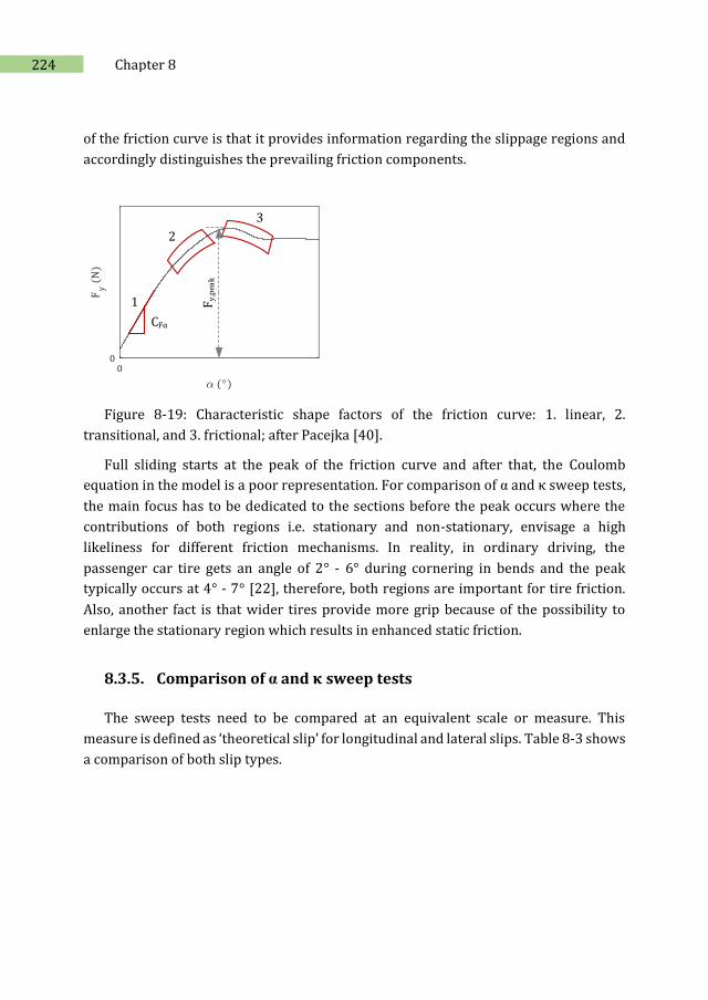
224 Chapter 8
of the friction curve is that it provides information regarding the slippage regions and
accordingly distinguishes the prevailing friction components.
Fy
,pea
k
CFα
1
2
3
Figure 8-19: Characteristic shape factors of the friction curve: 1. linear, 2.
transitional, and 3. frictional; after Pacejka [40].
Full sliding starts at the peak of the friction curve and after that, the Coulomb
equation in the model is a poor representation. For comparison of α and κ sweep tests,
the main focus has to be dedicated to the sections before the peak occurs where the
contributions of both regions i.e. stationary and non-stationary, envisage a high
likeliness for different friction mechanisms. In reality, in ordinary driving, the
passenger car tire gets an angle of 2° - 6° during cornering in bends and the peak
typically occurs at 4° - 7° [22], therefore, both regions are important for tire friction.
Also, another fact is that wider tires provide more grip because of the possibility to
enlarge the stationary region which results in enhanced static friction.
8.3.5. Comparison of α and κ sweep tests
The sweep tests need to be compared at an equivalent scale or measure. This
measure is defined as ‘theoretical slip’ for longitudinal and lateral slips. Table 8-3 shows
a comparison of both slip types.
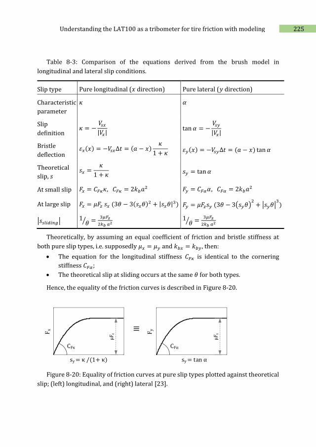
225 Understanding the LAT100 as a tribometer for tire friction with modeling
Table 8-3: Comparison of the equations derived from the brush model in
longitudinal and lateral slip conditions.
Slip type Pure longitudinal (𝑥 direction) Pure lateral (𝑦 direction)
Characteristic
parameter
𝜅 𝛼
Slip
definition 𝜅 = −
𝑉𝑠𝑥
|𝑉𝑥| tan 𝛼 = −
𝑉𝑠𝑦
|𝑉𝑥|
Bristle
deflection 휀𝑥(𝑥) = −𝑉𝑠𝑥∆𝑡 = (𝑎 − 𝑥)
𝜅
1 + 𝜅 휀𝑦(𝑥) = −𝑉𝑠𝑦∆𝑡 = (𝑎 − 𝑥) tan 𝛼
Theoretical
slip, 𝑠 𝑠𝑥 =
𝜅
1 + 𝜅 𝑠𝑦 = tan 𝛼
At small slip 𝐹𝑥 = 𝐶𝐹𝜅𝜅, 𝐶𝐹𝜅 = 2𝑘𝑏𝑎2 𝐹𝑦 = 𝐶𝐹𝛼𝛼, 𝐶𝐹𝛼 = 2𝑘𝑏𝑎2
At large slip 𝐹𝑥 = 𝜇𝐹𝑧 𝑠𝑥 (3𝜃 − 3(𝑠𝑥𝜃)2 + |𝑠𝑥𝜃|3) 𝐹𝑦 = 𝜇𝐹𝑧𝑠𝑦 (3𝜃 − 3(𝑠𝑦𝜃)2
+ |𝑠𝑦𝜃|3
)
|𝑠𝑠𝑙𝑖𝑑𝑖𝑛𝑔| 1𝜃⁄ =
3𝜇𝐹𝑧
2𝑘𝑏 𝑎2 1𝜃⁄ =
3𝜇𝐹𝑧
2𝑘𝑏 𝑎2
Theoretically, by assuming an equal coefficient of friction and bristle stiffness at
both pure slip types, i.e. supposedly 𝜇𝑥 = 𝜇𝑦 and 𝑘𝑏𝑥 = 𝑘𝑏𝑦 , then:
The equation for the longitudinal stiffness 𝐶𝐹𝜅 is identical to the cornering
stiffness 𝐶𝐹𝛼;
The theoretical slip at sliding occurs at the same 𝜃 for both types.
Hence, the equality of the friction curves is described in Figure 8-20.
Fx
Fy
sy = tan α sy = κ /(1+ κ)
CFκ CFα
µF
z
µF
z
Figure 8-20: Equality of friction curves at pure slip types plotted against theoretical
slip; (left) longitudinal, and (right) lateral [23].
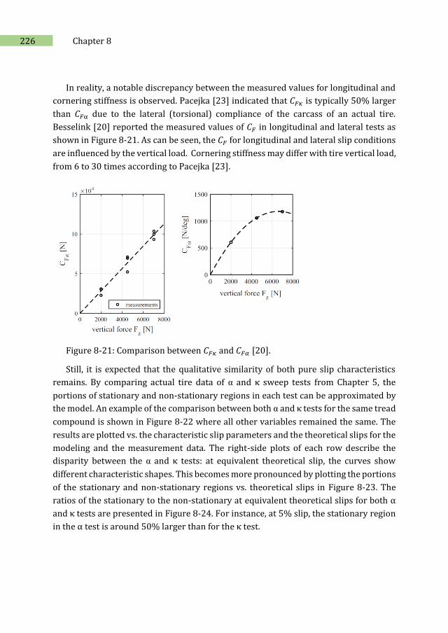
226 Chapter 8
In reality, a notable discrepancy between the measured values for longitudinal and
cornering stiffness is observed. Pacejka [23] indicated that 𝐶𝐹𝜅 is typically 50% larger
than 𝐶𝐹α due to the lateral (torsional) compliance of the carcass of an actual tire.
Besselink [20] reported the measured values of 𝐶𝐹 in longitudinal and lateral tests as
shown in Figure 8-21. As can be seen, the 𝐶𝐹 for longitudinal and lateral slip conditions
are influenced by the vertical load. Cornering stiffness may differ with tire vertical load,
from 6 to 30 times according to Pacejka [23].
Figure 8-21: Comparison between 𝐶𝐹𝜅 and 𝐶𝐹𝛼 [20].
Still, it is expected that the qualitative similarity of both pure slip characteristics
remains. By comparing actual tire data of α and κ sweep tests from Chapter 5, the
portions of stationary and non-stationary regions in each test can be approximated by
the model. An example of the comparison between both α and κ tests for the same tread
compound is shown in Figure 8-22 where all other variables remained the same. The
results are plotted vs. the characteristic slip parameters and the theoretical slips for the
modeling and the measurement data. The right-side plots of each row describe the
disparity between the α and κ tests: at equivalent theoretical slip, the curves show
different characteristic shapes. This becomes more pronounced by plotting the portions
of the stationary and non-stationary regions vs. theoretical slips in Figure 8-23. The
ratios of the stationary to the non-stationary at equivalent theoretical slips for both α
and κ tests are presented in Figure 8-24. For instance, at 5% slip, the stationary region
in the α test is around 50% larger than for the κ test.
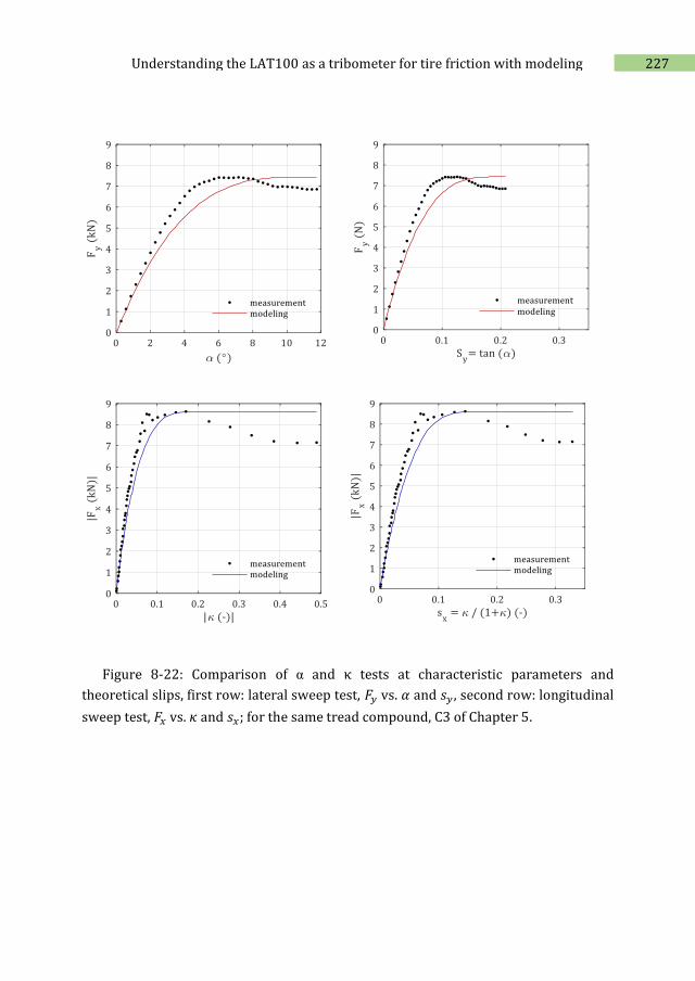
227 Understanding the LAT100 as a tribometer for tire friction with modeling
Figure 8-22: Comparison of α and κ tests at characteristic parameters and
theoretical slips, first row: lateral sweep test, 𝐹𝑦 vs. 𝛼 and 𝑠𝑦 , second row: longitudinal
sweep test, 𝐹𝑥 vs. 𝜅 and 𝑠𝑥; for the same tread compound, C3 of Chapter 5.
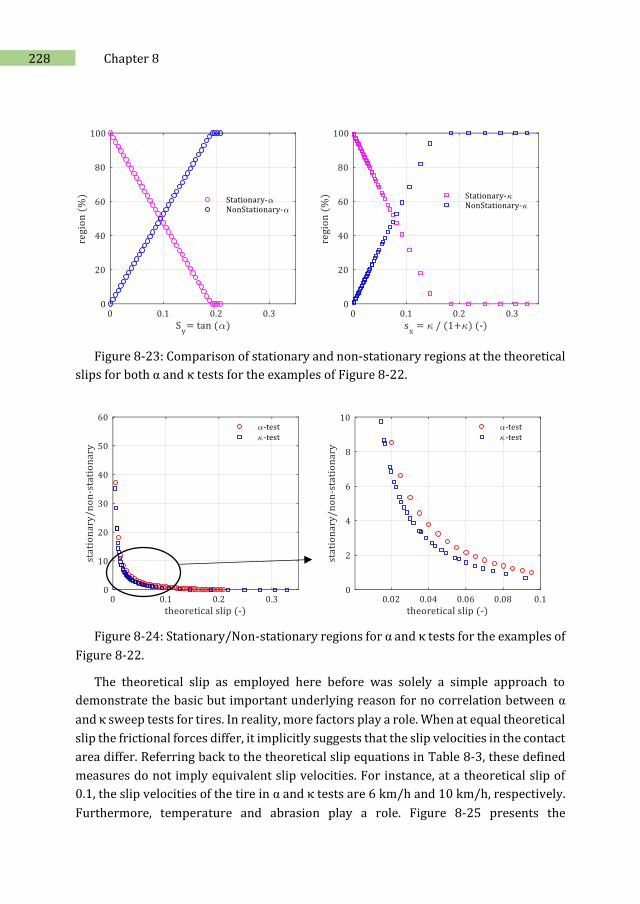
228 Chapter 8
Figure 8-23: Comparison of stationary and non-stationary regions at the theoretical
slips for both α and κ tests for the examples of Figure 8-22.
Figure 8-24: Stationary/Non-stationary regions for α and κ tests for the examples of
Figure 8-22.
The theoretical slip as employed here before was solely a simple approach to
demonstrate the basic but important underlying reason for no correlation between α
and κ sweep tests for tires. In reality, more factors play a role. When at equal theoretical
slip the frictional forces differ, it implicitly suggests that the slip velocities in the contact
area differ. Referring back to the theoretical slip equations in Table 8-3, these defined
measures do not imply equivalent slip velocities. For instance, at a theoretical slip of
0.1, the slip velocities of the tire in α and κ tests are 6 km/h and 10 km/h, respectively.
Furthermore, temperature and abrasion play a role. Figure 8-25 presents the
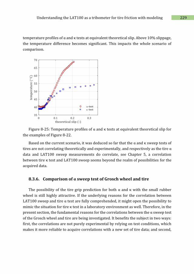
229 Understanding the LAT100 as a tribometer for tire friction with modeling
temperature profiles of α and κ tests at equivalent theoretical slip. Above 10% slippage,
the temperature difference becomes significant. This impacts the whole scenario of
comparison.
Figure 8-25: Temperature profiles of α and κ tests at equivalent theoretical slip for
the examples of Figure 8-22.
Based on the current scenario, it was deduced so far that the α and κ sweep tests of
tires are not correlating theoretically and experimentally, and respectively as the tire α
data and LAT100 sweep measurements do correlate, see Chapter 5, a correlation
between tire κ test and LAT100 sweep seems beyond the realm of possibilities for the
acquired data.
8.3.6. Comparison of α sweep test of Grosch wheel and tire
The possibility of the tire grip prediction for both α and κ with the small rubber
wheel is still highly attractive. If the underlying reasons for the correlation between
LAT100 sweep and tire α test are fully comprehended, it might open the possibility to
mimic the situation for tire κ test in a laboratory environment as well. Therefore, in the
present section, the fundamental reasons for the correlations between the α sweep test
of the Grosch wheel and tire are being investigated. It benefits the subject in two ways:
first, the correlations are not purely experimental by relying on test conditions, which
makes it more reliable to acquire correlations with a new set of tire data; and second,
230 Chapter 8
the advantage of using a wheel shape specimen becomes more concrete to raise the
possibility to also predict κ sweep.
The similarity between the test modalities of lateral sweeps of the tire and LAT100
seems to be the silver lining for the acquired correlations in Chapter 5. In the previous
section, the comparison between tire α and κ tests was elaborated in-depth, the same
approach can now be employed for the α friction curves of the Grosch wheel and the
tire at an equal theoretical measure of 𝑠𝑦 . Referring back to the acquired correlations of
Chapter 5, the slip angle sweep ranges up to the peak points in the measured friction
curves 𝐹𝑦 vs. α of the LAT100 and the tire were different. The α friction curve of LAT100
approaches a plateau roughly above 20°, which can be seen for example in Figure 8-26
for the curves of 𝐹𝑦 vs. α or 𝑠𝑦 for compound C3 at a speed of 6.5 km/h and a normal
load of 55 N. Accordingly, Figure 8-27 shows the stationary and non-stationary regions
resulting from the modeling for the Grosch wheel. For the tire, the α friction curve
reaches full sliding at around 7°, see Figure 8-22: 𝐹𝑦 vs. α. The question is why the sweep
ranges of the tire and LAT100 vary and more particularly with such a large difference,
the α test of the LAT100 and the tire did still correlate.
With the aid of the previously described model, it should be possible to reply to this
question or at least provide some basic understanding, as was implemented for
explaining α and κ sweeps in the previous section. First, the beginning of the measured
friction curve of the Grosch wheel shows a slight upward shift along the y-axis: see
Figure 8-26. This could indicate implicitly the presence of a pseudo-camber angle as
mentioned in section 8.3.2, which could be due to a non-uniformly vulcanized sample
or an induced inclination angle owing to the path curvature. Second, due to this
deviation, the 𝛼𝑠𝑙𝑖𝑑𝑖𝑛𝑔 value for the Grosch wheel can be computed to be 30° (or 𝑠𝑦 =
0.53), but the measurements suggested that full sliding occurred at 20° (or 𝑠𝑦 = 0.45).
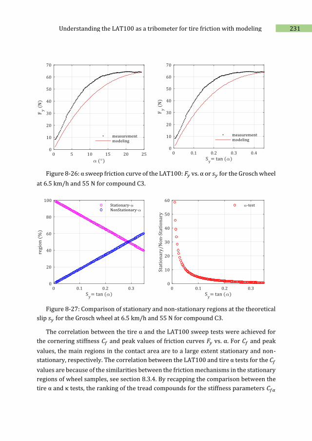
231 Understanding the LAT100 as a tribometer for tire friction with modeling
Figure 8-26: α sweep friction curve of the LAT100: 𝐹𝑦 vs. α or 𝑠𝑦 for the Grosch wheel
at 6.5 km/h and 55 N for compound C3.
Figure 8-27: Comparison of stationary and non-stationary regions at the theoretical
slip 𝑠𝑦 for the Grosch wheel at 6.5 km/h and 55 N for compound C3.
The correlation between the tire α and the LAT100 sweep tests were achieved for
the cornering stiffness 𝐶𝑓 and peak values of friction curves 𝐹𝑦 vs. α. For 𝐶𝑓 and peak
values, the main regions in the contact area are to a large extent stationary and non-
stationary, respectively. The correlation between the LAT100 and tire α tests for the 𝐶𝑓
values are because of the similarities between the friction mechanisms in the stationary
regions of wheel samples, see section 8.3.4. By recapping the comparison between the
tire α and κ tests, the ranking of the tread compounds for the stiffness parameters 𝐶𝑓𝛼
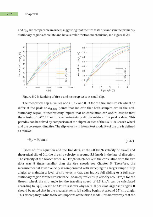
232 Chapter 8
and 𝐶𝑓𝜅 are comparable in order; suggesting that the tire tests of α and κ in the primarily
stationary regions correlate and have similar friction mechanisms, see Figure 8-28.
Figure 8-28: Ranking of tire α and κ sweep tests at small slip.
The theoretical slip 𝑠𝑦 values of c.a. 0.17 and 0.53 for the tire and Grosch wheel do
differ at the peak or 𝛼sliding points that indicate that both samples are in the non-
stationary region; it theoretically implies that no correlation can occur! Despite that,
the α tests of LAT100 and tire experimentally did correlate at the peak values. This
paradox can be solved by comparison of the slip velocities of the LAT100 Grosch wheel
and the corresponding tire. The slip velocity in lateral test modality of the tire is defined
as follows:
−𝑉𝑠𝑦 = 𝑉𝑥 tan 𝛼 (8.37)
Based on this equation and the tire data, at the 60 km/h velocity of travel and
theoretical slip of 0.1, the tire slip velocity is around 5.8 km/h in the lateral direction.
The velocity of the Grosch wheel 6.5 km/h which delivers the correlation with the tire
data was 8 times smaller than the tire speed: see Chapter 5. Therefore, the
measurement at lower velocity is compensated with sweeping to a larger range of slip
angles to maintain a level of slip velocity that can induce full sliding or a full non-
stationary region for the Grosch wheel. At an equivalent slip velocity of 5.8 km/h for the
Grosch wheel, the slip angle for the traveling speed of 6.5 km/h can be calculated
according to Eq. (8.37) to be 41°. This shows why LAT100 peaks at larger slip angles. It
should be noted that in the measurements full sliding begins at around 25° slip angle.
This discrepancy is due to the assumptions of the brush model. It is noteworthy that the
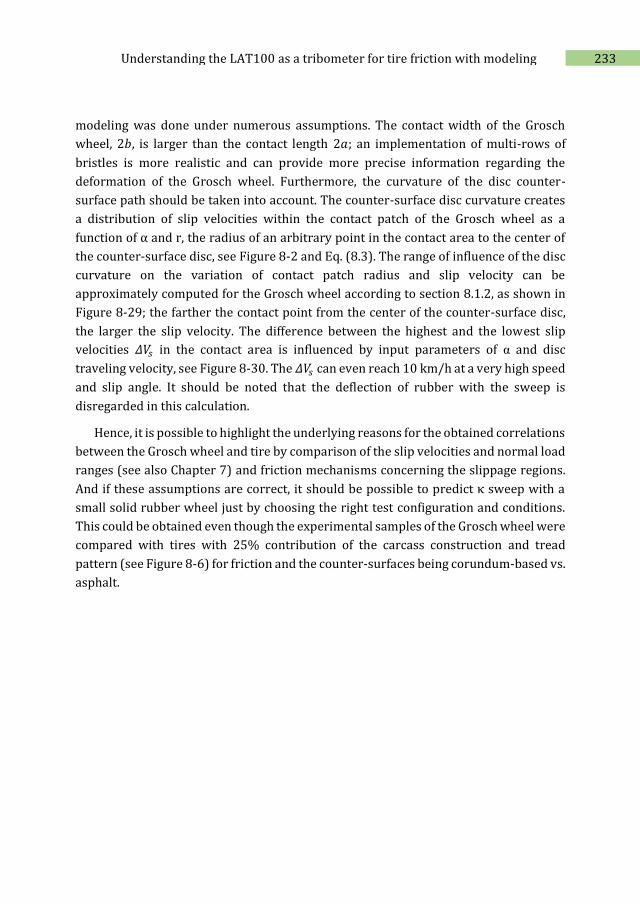
233 Understanding the LAT100 as a tribometer for tire friction with modeling
modeling was done under numerous assumptions. The contact width of the Grosch
wheel, 2𝑏, is larger than the contact length 2𝑎; an implementation of multi-rows of
bristles is more realistic and can provide more precise information regarding the
deformation of the Grosch wheel. Furthermore, the curvature of the disc counter-
surface path should be taken into account. The counter-surface disc curvature creates
a distribution of slip velocities within the contact patch of the Grosch wheel as a
function of α and r, the radius of an arbitrary point in the contact area to the center of
the counter-surface disc, see Figure 8-2 and Eq. (8.3). The range of influence of the disc
curvature on the variation of contact patch radius and slip velocity can be
approximately computed for the Grosch wheel according to section 8.1.2, as shown in
Figure 8-29; the farther the contact point from the center of the counter-surface disc,
the larger the slip velocity. The difference between the highest and the lowest slip
velocities 𝛥𝑉𝑠 in the contact area is influenced by input parameters of α and disc
traveling velocity, see Figure 8-30. The 𝛥𝑉𝑠 can even reach 10 km/h at a very high speed
and slip angle. It should be noted that the deflection of rubber with the sweep is
disregarded in this calculation.
Hence, it is possible to highlight the underlying reasons for the obtained correlations
between the Grosch wheel and tire by comparison of the slip velocities and normal load
ranges (see also Chapter 7) and friction mechanisms concerning the slippage regions.
And if these assumptions are correct, it should be possible to predict κ sweep with a
small solid rubber wheel just by choosing the right test configuration and conditions.
This could be obtained even though the experimental samples of the Grosch wheel were
compared with tires with 25% contribution of the carcass construction and tread
pattern (see Figure 8-6) for friction and the counter-surfaces being corundum-based vs.
asphalt.
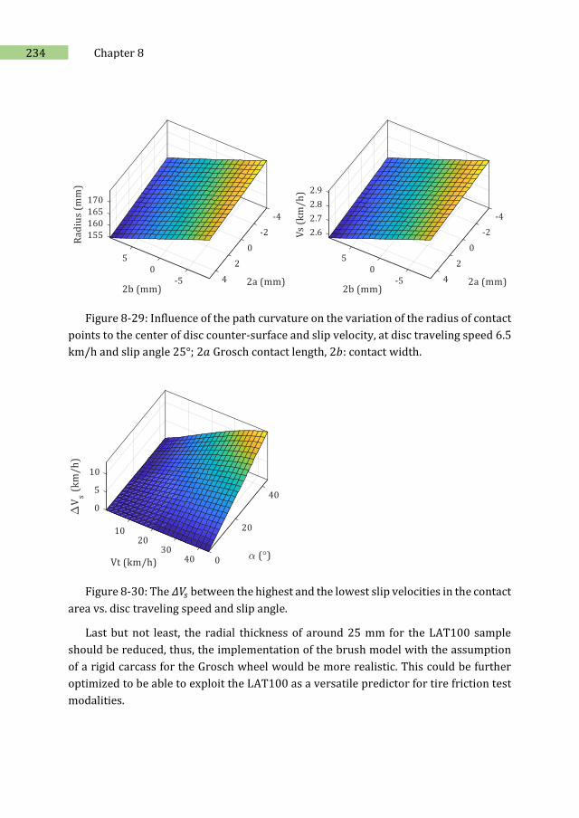
234 Chapter 8
Figure 8-29: Influence of the path curvature on the variation of the radius of contact
points to the center of disc counter-surface and slip velocity, at disc traveling speed 6.5
km/h and slip angle 25°; 2𝑎 Grosch contact length, 2𝑏: contact width.
Figure 8-30: The 𝛥𝑉𝑠 between the highest and the lowest slip velocities in the contact
area vs. disc traveling speed and slip angle.
Last but not least, the radial thickness of around 25 mm for the LAT100 sample
should be reduced, thus, the implementation of the brush model with the assumption
of a rigid carcass for the Grosch wheel would be more realistic. This could be further
optimized to be able to exploit the LAT100 as a versatile predictor for tire friction test
modalities.
235 Understanding the LAT100 as a tribometer for tire friction with modeling
8.4. Conclusions
In the present chapter, by using the renowned physical ‘brush model’, the dynamics
and physics of the Grosch rubber wheel on the LAT100 counter-surface were modeled.
Its behavior in lateral and longitudinal movements, as opposed to a real tire, were
investigated. The differences between the 𝛼 and 𝜅 sweep test modalities were explained
at a defined equivalent measure called theoretical slip. It was deduced that the type of
test modality leads to different friction mechanisms in the contact patch even at similar
test conditions. The underlying reasons for the correlation between LAT100 and tire α
sweep tests were highlighted. The importance of a laboratory wheel sample geometry
compared to a pure sliding body specimen could be substantiated by recognizing the
two regions: a stationary and non-stationary status in the contact area similar to the
tire. This could result in similar friction mechanisms for the Grosch wheel as a rolling
tire. In reality in ordinary driving, the passenger car tire gets an angle of 2° - 6° on the
road and the peak typically occurs at 4° - 7°. This explains the importance of friction
curves studied with the Grosch wheel because it provides insight into the stationary
friction.
It was deduced that the α and κ sweep tests of tires are not correlating theoretically
and experimentally, and respectively as the tire α data and LAT100 sweep
measurements do correlate, a correlation between tire κ test and LAT100 sweep seems
beyond the realm of possibilities. However, the present chapter provided information
that it should be possible to predict κ sweep with a small solid rubber wheel just by
choosing the right test configuration and conditions.
The present chapter suggests that modifications of the Grosch wheel could enhance
the predictability of tire friction on the road, such as improvement of the geometry of
the specimen. The radial thickness and width of the Grosch wheel can be optimized by
utilizing a modified brush model where the assumptions are tailored to be closer to
reality. Therefore, by using such an optimized small rubber wheel, it should be possible
to predict tire grip in the laboratory for material development which is cost and time
effective rather than testing tread compounds by building full-scale tires.
236 Chapter 8
8.5. References
1. Riehm, P., H.-J. Unrau, and F. Gauterin, A model based method to determine rubber friction data based on rubber sample measurements. Tribology International, 2018. 127: p. 37-46.
2. Gutzeit, F. and M. Kröger, Experimental and Theoretical Investigations on the Dynamic Contact Behavior of Rolling Rubber Wheels, in Book 'Elastomere Friction: Theory, Experiment and Simulation', D. Besdo, B. Heimann, M. Klüppel, M. Kröger, P. Wriggers, and U. Nackenhorst, Editors. 2010, Springer Berlin Heidelberg: Berlin, Heidelberg. p. 221-249.
3. Steen, R.v.d., I. Lopez, and H. Nijmeijer, Experimental and numerical study of friction and .giffness characteristics of small rolling tires. Tire Science and Technology, 2011. 39(1): p. 5-19.
4. Dorsch, V., A. Becker, and L. Vossen, Enhanced rubber friction model for finite element simulations of rolling tyres. Plastics, Rubber and Composites, 2002. 31(10): p. 458-464.
5. Bouzid, N. and B. Heimann, Micro Texture Characterization and Prognosis of the Maximum Traction between Grosch Wheel and Asphalt Surfaces under Wet Conditions, in Book 'Elastomere Friction: Theory, Experiment and Simulation', D. Besdo, B. Heimann, M. Klüppel, M. Kröger, P. Wriggers, and U. Nackenhorst, Editors. 2010, Springer Berlin Heidelberg: Berlin, Heidelberg. p. 201-220.
6. Bouzid, N., B. Heimann, and A. Trabelsi, Empirical friction coefficient modeling for the Grosch-wheel-road system, in VDI Berichte. 2005. p. 291-307.
7. Nguyen, V.H., D. Zheng, F. Schmerwitz, and P. Wriggers, An advanced abrasion model for tire wear. Wear, 2018. 396-397: p. 75-85.
8. Wu, J., C. Zhang, Y. Wang, and B. Su, Wear Predicted Model of Tread Rubber Based on Experimental and Numerical Method. Experimental Techniques, 2018. 42(2): p. 191-198.
9. Grosch, K.A., Correlation Between Road Wear of Tires and Computer Road Wear Simulation Using Laboratory Abrasion Data. Rubber Chemistry and Technology, 2004. 77(5): p. 791-814.
10. Grosch, K.A., Goodyear Medalist Lecture. Rubber Friction and its Relation to Tire Traction. Rubber Chemistry and Technology, 2007. 80(3): p. 379-411.
11. Grosch, K.A., Rubber Abrasion and Tire Wear. Rubber Chemistry and Technology, 2008. 81(3): p. 470-505.
12. Heinz, M. and K.A. Grosch, A Laboratory Method to Comprehensively Evaluate Abrasion, Traction and Rolling Resistance of Tire Tread Compounds. Rubber Chemistry and Technology, 2007. 80(4): p. 580-607.
237 Understanding the LAT100 as a tribometer for tire friction with modeling
13. Grosch, K.A., A new way to evaluate traction-and wear properties of tire tread compounds, in Rubber Division, American Chemical Society. 1997: Cleveland, Ohio.
14. Heinz, M., A laboratory abrasion testing method for use in the development of filler systems. Technical report rubber reinforcement systems, 2015, Evonik Industries GmbH, Essen, Germany.
15. Heinz, M., A Universal Method to Predict Wet Traction Behaviour of Tyre Tread Compounds in the Laboratory. Journal of Rubber Research, 2010. 13(2): p. 91-102.
16. Salehi, M., LAT100, Prediction of tire dry grip. 2017, University of Twente: Enschede: Ipskamp Printing.
17. Salehi, M., J.W.M. Noordermeer, L.A.E.M. Reuvekamp, W.K. Dierkes, and A. Blume, Measuring rubber friction using a Laboratory Abrasion Tester (LAT100) to predict car tire dry ABS braking. Tribology International, 2019. 131: p. 191-199.
18. LAT100 tire tread compound testing, VMI Group, in, Date of access: April 2020; Available from https://www.vmi-group.com/specifications/vmi-lat100-tire-tread-compound-tester/.
19. Miller, S.L., B. Youngberg, A. Millie, P. Schweizer, and J.C. Gerdes. Calculation Longitudinal wheel slip and tire parameters using GPS velocity. in the American control conference. 25-27 Jun 2001. Arlington.
20. Besselink, I.J.M., Tire Characteristics and Modeling, in Book 'Vehicle Dynamics of Modern Passenger Cars', P. Lugner, Editor. 2019, Springer International Publishing: Cham. p. 47-108.
21. Engineering Explained YouTube Channel, New Tires vs Worn Tires - What Performs Best?, Date of access; Available from https://www.youtube.com/watch?v=Xa5i0xvmVSg.
22. The Tyre Grip, Société de Technologie Michelin.,clermont-ferrand, France, Date of access: May 2020; Available from http://www.dimnp.unipi.it/guiggiani-m/Michelin_Tire_Grip.pdf.
23. Pacejka, H.B., Chapter 3 - Theory of steady-state slip force and moment generation, in Book 'Tyre and Vehicle Dynamics (Second Edition)'. 2006, Butterworth-Heinemann: Oxford. p. 90-155.
24. Bakker, E., L. Nyborg, and H.B. Pacejka, Tyre Modelling for Use in Vehicle Dynamics Studies. 1987, SAE International.
238 Chapter 8
25. Ossama Mokhiamar, M.A., Simultaneous Optimal Distribution of Lateral and Longitudinal Tire Forces for the Model Following Control. ASME 2004. 126: p. 753-763.
26. Braghin, F., F. Cheli, S. Melzi, and F. Resta, Tyre Wear Model: Validation and Sensitivity Analysis. Meccanica, 2006. 41(2): p. 143-156.
27. Kane, M. and V. Cerezo, A contribution to tire/road friction modeling: From a simplified dynamic frictional contact model to a “Dynamic Friction Tester” model. Wear, 2015. 342-343: p. 163-171.
28. Schramm, D., M. Hiller, and R. Bardini, Modeling of the Road-Tire-Contact, in Book 'Vehicle Dynamics: Modeling and Simulation'. 2018, Springer Berlin Heidelberg: Berlin, Heidelberg. p. 145-186.
29. Tire Modeling, Lateral and Longitudinal Tire Forces, Erdogan, G., Date of access: July 2020; Available from http://www.menet.umn.edu/~gurkan/Tire%20Modeling%20%20Lecture.pdf.
30. Walloch, F. The Impact of Tire Design on Vehicle Braking Performance. in SAE world conference. Continental Tire.
31. Symposium on the Physics of Tire Traction Warren, M., D.F. Hays, A.L. Browne, and L. General Motors Corporation. Research, The physics of tire traction, theory and experiment; proceedings. 1974, New York: Plenum Press.
32. Jacob Svendenius, B.W., Review of wheel modeling and friction estimation, in Department of Automatic Control 2003, Lund institute of technology.
33. Schallamach, A. and D.M. Turner, The wear of slipping wheels. Wear, 1960. 3(1): p. 1-25.
34. Grosch, K.A., rubber friction and tire traction, in Book 'The pneumatic tire'. 2006, NHTSA. p. 421-473.
35. Rosu, I., H. Elias-Birembaux, F. Lebon, H. Lind, and M. Wangenheim, Experimental and Numerical Simulation of the Dynamic Frictional Contact between an Aircraft Tire Rubber and a Rough Surface. Lubricants, 2016. 4(3): p. 29.
36. Ray, L.R., Nonlinear Tire Force Estimation and Road Friction Identification: Simulation and Experiments1,2. Automatica, 1997. 33(10): p. 1819-1833.
37. Appendix 2 - TreadSim A2 - Pacejka, Hans B, in Book 'Tyre and Vehicle Dynamics (Second Edition)'. 2006, Butterworth-Heinemann: Oxford. p. 613-628.
38. Tiwari, A., L. Dorogin, M. Tahir, K.W. Stöckelhuber, G. Heinrich, N. Espallargas, and B.N.J. Persson, Rubber contact mechanics: adhesion, friction and leakage of seals. Soft Matter, 2017. 13(48): p. 9103-9121.
239 Understanding the LAT100 as a tribometer for tire friction with modeling
39. Tolpekina, T.V. and B.N.J. Persson, Adhesion and Friction for Three Tire Tread Compounds. Lubricants, 2019. 7(3): p. 20.
40. Pacejka, H.B., Chapter 1 - Tyre characteristics and vehicle handling and stability, in Book 'Tyre and Vehicle Dynamics (Second Edition)'. 2006, Butterworth-Heinemann: Oxford. p. 1-60.
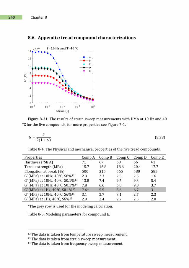
240 Chapter 8
8.6. Appendix: tread compound characterizations
Figure 8-31: The results of strain sweep measurements with DMA at 10 Hz and 40
°C for the five compounds, for more properties see Figure 7-1.
𝐺 =𝐸
2(1 + 𝜈) (8.38)
Table 8-4: The Physical and mechanical properties of the five tread compounds.
Properties Comp A Comp B Comp C Comp D Comp E Hardness (°Sh A) 71 67 68 66 61 Tensile strength (MPa) 15.7 16.8 18.6 20.4 17.7 Elongation at break (%) 500 315 565 580 585 G’ (MPa) at 10Hz, 40°C, S6%12 2.3 2.3 2.5 2.5 1.6 G’ (MPa) at 10Hz, 40°C, S0.1%13 13.8 7.4 9.5 9.3 5.4 G’ (MPa) at 10Hz, 40°C, S0.1%14 7.8 6.6 6.8 9.0 3.7 G’ (MPa) at 1Hz, 40°C, S0.1%15 7.6* 5.5 5.6 6.7 3.1 G’ (MPa) at 10Hz, 40°C, S6%15 3.1 2.7 3.1 2.7 2.3 G’ (MPa) at 1Hz, 40°C, S6%15 2.9 2.4 2.7 2.5 2.0
*The grey row is used for the modeling calculation.
Table 8-5: Modeling parameters for compound E.
12 The data is taken from temperature sweep measurement. 13 The data is taken from strain sweep measurement. 14 The data is taken from frequency sweep measurement.
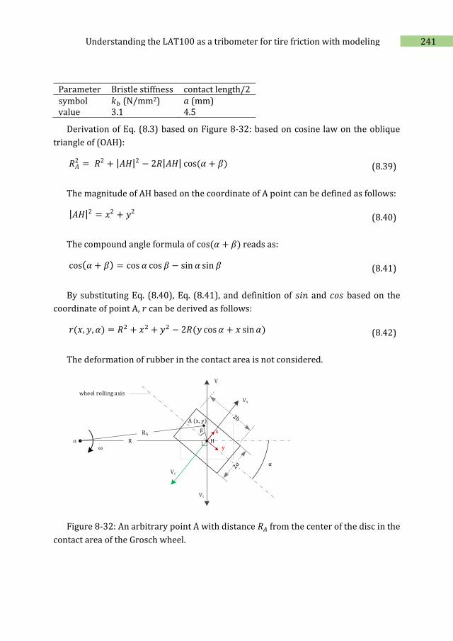
241 Understanding the LAT100 as a tribometer for tire friction with modeling
Parameter Bristle stiffness contact length/2 symbol 𝑘𝑏 (N/mm2) 𝑎 (mm) value 3.1 4.5
Derivation of Eq. (8.3) based on Figure 8-32: based on cosine law on the oblique
triangle of (OAH):
𝑅𝐴2 = 𝑅2 + |𝐴𝐻|2 − 2𝑅|𝐴𝐻| cos(𝛼 + 𝛽) (8.39)
The magnitude of AH based on the coordinate of A point can be defined as follows:
|𝐴𝐻|2 = 𝑥2 + 𝑦2 (8.40)
The compound angle formula of cos(𝛼 + 𝛽) reads as:
cos(𝛼 + 𝛽) = cos 𝛼 cos 𝛽 − sin 𝛼 sin 𝛽 (8.41)
By substituting Eq. (8.40), Eq. (8.41), and definition of 𝑠𝑖𝑛 and 𝑐𝑜𝑠 based on the
coordinate of point A, 𝑟 can be derived as follows:
𝑟(𝑥, 𝑦, 𝛼) = 𝑅2 + 𝑥2 + 𝑦2 − 2𝑅(𝑦 cos 𝛼 + 𝑥 sin 𝛼) (8.42)
The deformation of rubber in the contact area is not considered.
o
α
R
wheel rolling axis
ω
Vc
A (x, y)
H
RAx
y
Vt
β
V
Vx
Figure 8-32: An arbitrary point A with distance 𝑅𝐴 from the center of the disc in the
contact area of the Grosch wheel.

242 Chapter 8
9 Summary
Tire grip is the primary determining factor in transmitting all the forces and
moments originating from the vehicle to the road because tires are the only contact of
a vehicle with the ground and the key consideration for driving safety. The tread
compound is the eventual contact of a full tire with the ground. In order to improve the
frictional properties of these rubber material to optimize tire grip: traction and slip
properties, there is a continuous drive to find methods that allow a better simulation of
the tribological characteristics of the tread compounds in early development stages in
a laboratory environment. Full-scale tire tests are enormously sophisticated, time-
consuming, and costly. It is, therefore, more sustainable and highly desirable to predict
tire performance in a laboratory environment before having to manufacture a full tire,
only for the determination of the frictional properties of the rubber materials used in
the tire.
Considering all the different conditions that a tire may encounter during service,
their simulation in one laboratory apparatus seems an impossible task. Many different
test configurations have been developed over time with varying success. Among the
various available tribometers suitable for assessing rubber frictional properties,
measurements with a solid rubber wheel are most promising. The big advantage is the
244 Chapter 9
rolling motion of the rubber specimen which resembles a tire on the road. This is due
to the physical fact that the relative speed of a wheel’s contact point to the ground is
zero. The Laboratory Abrasion Tester (LAT) 100 is used for the prediction of tire
performance making use of a rolling rubber wheel known as the Grosch wheel. The
equipment was designed to simulate a wide range of tire service conditions to measure
abrasion loss and frictional forces as a function of various tire-road service conditions
such as slip, normal load, and speed on different counter-surfaces. The first purpose for
the LAT100 was to measure rubber abrasion; therefore, its designation “Laboratory
Abrasion Tester”. Gradually it was realized that the apparatus could also be used as a
tribometer to characterize frictional properties. Consequently, there is a steadily
increasing interest to develop this concept further, which was the main purpose of the
research presented in this thesis.
In previous studies, it has been demonstrated that tire performance properties i.e.
wet grip, abrasion, and rolling resistance can be characterized with the LAT100,
provided the right conditions for testing are employed. The question was raised
whether testing of various tire compounds under dry conditions could also be
employed to predict tire frictional properties in longitudinal as well as lateral
conditions. This was taken as the original objective of the present work: various tire
tread formulations, as well as different counter surfaces were included in the study to
fulfill this goal. The results of LAT100 tests were to be correlated with actual tire tests
with the same rubber tread formulations on standardized roads, under ABS-conditions,
and different test modalities for the tires. Later on in the project, a new test
configuration was designed and further developed by introducing a dynamic interface
to the LAT100. This was set as a new objective to understand the machine as a
tribometer because it provided tire service and operating conditions with a wheel-
shaped specimen.
Chapter 1 encompassed a basic introduction to the work performed in this thesis.
Chapter 2 presented a survey of the literature on friction and tire grip concepts and a
short introduction to the Persson’s contact theory. Also, the available laboratory
tribometers and tire testing methods were introduced and compared.
In Chapter 3, preliminary studies were conducted on the LAT100 to characterize the
apparatus possibilities and limitations to be exploited for dry tire friction evaluations.
The frictional forces of four different tread compounds were determined by collecting
individual measurement points at defined test conditions on various counter-surfaces
with different surface roughness properties. The results were correlated with tire ABS
braking distance data. One of the LAT100 counter-surface discs with the designation
245 Summary
code 180 – composed of corundum particles based on sieve analyses according to ISO
525:2013(E) – reflected the present road surface conditions of the tire test in the best
way with good correlation for the four tread compounds. The excitation frequency of
this disk 180 was estimated to be closest to the range of hysteresis friction or road
indentation. The current results showed that the lateral friction force decreases with
increasing measured rms. Disc 180 was therefore chosen as standard counter surface
among other LAT100 disc grades for further experiments.
In Chapter 4, the LAT100 was employed as a sliding friction tester with blocked
wheels for deriving a predictive mathematical model using Design of Experiments for
the input factors. Various operating parameters of the LAT100 as a tribometer on tire
friction were investigated: normal load, speed, and slip angle. Measurements were
performed on sandpaper P120 and LAT100 disc 180 counter-surfaces, using 5 tread
compound formulations with a wide range of grip properties. The former surface is the
test track that is widely employed for tire indoor flat-track tests. The variation of the
coefficient of friction versus speed on the disc 180 was in good agreement with the ABS
braking distance data of actual tires on the road, but not for the sandpaper substrate.
At the specific frequency range, the power spectral density of disc 180 was closer to
asphalt than to sandpaper P120. The optimal test conditions of load and speed were in
similar ranges of a car tire. The mutual interactions of factors on tire friction were
quantified, where the effects of single factors alone could not adequately be identified.
The interaction of normal load and speed influences the coefficient of friction of tire
tread compounds most clearly.
In Chapter 5, the LAT100 was re-designed and a new dynamic interface was
introduced which opens the possibility to perform and mimic tire test modalities in a
laboratory environment with enormously reduced test time duration. Comprehensive
tire testing was performed to provide sufficient data for method validation. Strong
correlations were obtained between the LAT100 results and the lateral tire test
modality called α-sweep, but not for the longitudinal modality or κ-sweep. The
approach described how to predict actual dry tire grip as a function of speed and load
with this laboratory device which offered a positive new horizon to evaluate tire grip.
In Chapters 6 and 7, various counter-surfaces were analyzed using power spectral
density. The real contact area was characterized using Persson’s friction theory
together with some measurements with pressure-sensitive films to obtain insight into
the shape and magnitude of the contact between the rubber samples and the counter-
246 Chapter 9
surfaces. These provided better explanations for the acquired correlations and also
more comprehension of the tire grip concept.
And finally, Chapter 8 was dedicated to understand the dynamics and physics of a
rolling rubber wheel on a counter-surface disc of the LAT100 test step-up utilizing the
physical “brush model” for tires. Therewith, the behavior of the rolling wheel in lateral
and longitudinal movements was modeled in comparison to a real tire. A better
comprehension of the intricate differences between the 𝛼 and 𝜅 sweep test
configurations with respect to slippage distribution in the contact area was obtained in
association with rubber friction components: adhesion vs. hysteresis. It was deduced
that both types of test modalities lead to different friction mechanisms in the contact
patch even at similar test conditions. The underlying reasons for the correlation
between the LAT100 and tire α sweep tests were highlighted. The importance of a
laboratory wheel sample geometry compared to a pure sliding body specimen was
substantiated by recognizing the two regions: a stationary and non-stationary status in
the contact area analogues to the tire which results in similar friction mechanisms for
the Grosch wheel as for a rolling tire.
The present thesis demonstrated that the idea of using a small rubber wheel in a
right test modality smoothens the way to predict tire grip in the laboratory for material
development which is cost and time effective, rather than testing tread compounds by
building full-scale tires.
Samenvatting
Banden grip is de primaire bepalende factor voor de overdracht van alle krachten en
momenten die door het voertuig op de weg worden overgedragen. Banden nemen het enige
contact met de ondergrond voor hun rekening en spelen een hoofdrol bij de veiligheid van het
rijden. Het rubberen loopvlak mengsel vertegenwoordigt het feitelijke contact van een volledige
band met de grond. Teneinde de wrijvings/frictie eigenschappen van deze rubber materialen
voor banden grip te verbeteren: de tractie en slip eigenschappen, is er een voortdurende streven
om methodes te vinden die een betere simulatie mogelijk maken van de tribologische
karakteristieken van loopvlak mengsels in vroege stadia van de ontwikkeling binnen een
laboratorium omgeving. Grootschalige banden testen zijn enorm veelomvattend, tijdverslindend
en kostbaar. Het is daarom meer houdbaar en hogelijk gewenst om het gedrag van een band te
kunnen voorspellen in een laboratorium omgeving, alvorens een volledige band te moeten maken
enkel en alleen voor de bepaling van de frictie-eigenschappen van de rubber materialen gebruikt
in de band.
Vanwege al de verschillende omstandigheden die een band doormaakt tijdens z’n gebruik,
lijkt het simuleren daarvan in één laboratorium apparaat een onmogelijke opgave. Veel
verschillende test configuraties zijn al ontwikkeld in het verleden met wisselend succes. Onder
de verschillende beschikbare tribometers geschikt om de frictie-eigenschappen van rubber te
karakteriseren zijn metingen met solide rubber wielen het meest veelbelovend. Hun grote
voordeel is de rolbeweging van het rubber monster, lijkend op een band op de weg. Dit als gevolg
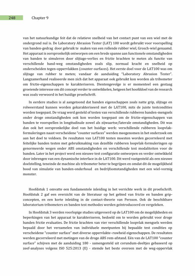
248 Chapter 9
van het natuurkundige feit dat de relatieve snelheid van het contact punt van een wiel met de
ondergrond nul is. De Laboratory Abrasion Tester (LAT) 100 wordt gebruikt voor voorspelling
van banden-gedrag door gebruik te maken van een rollende rubber wiel, Grosch-wiel genaamd.
Het apparaat is oorspronkelijk ontworpen om een brede spanne aan functionele omstandigheden
van banden te simuleren door slijtage-verlies en frictie krachten te meten als functie van
verschillende band-weg omstandigheden zoals slip, normaal kracht en snelheid op
onderscheiden tegen-oppervlakken (counter-surfaces). Het eerste doel voor de LAT100 was om
slijtage van rubber te meten; vandaar de aanduiding “Laboratory Abrasion Tester”.
Langzamerhand realiseerde men zich dat het apparaat ook gebruikt kon worden als tribometer
om frictie-eigenschappen te karakteriseren. Dientengevolge is er momenteel een gestaag
groeiende interesse om dit concept verder te ontwikkelen, hetgeen het hoofddoel van de research
was zoals verwoord in het huidige proefschrift.
In eerdere studies is al aangetoond dat banden eigenschappen zoals natte grip, slijtage en
rolweerstand kunnen worden gekarakteriseerd met de LAT100, mits de juiste testcondities
worden toegepast. De vraag werd gesteld of testen van verschillende rubberen banden-mengsels
onder droge omstandigheden ook kon worden toegepast om de frictie-eigenschappen van
banden te voorspellen in longitudinale zowel als zijwaartse/laterale omstandigheden. Dit was
dan ook het oorspronkelijke doel van het huidige werk: verschillende rubberen loopvlak-
formuleringen naast verscheidene “counter surfaces” werden meegenomen in het onderzoek om
aan het doel te voldoen. De resultaten van LAT100 testen moesten worden gecorreleerd met
feitelijke banden testen met gebruikmaking van dezelfde rubberen loopvlak-formuleringen op
genormeerde wegen onder ABS omstandigheden en verschillende test modaliteiten voor de
banden. Later in het project werd een nieuwe test configuratie ontworpen en verder ontwikkeld
door inbrengen van een dynamische interface in de LAT100. Dit werd vastgesteld als een nieuwe
doelstelling, teneinde de machine als tribometer beter te begrijpen en omdat dit de mogelijkheid
bood van simulatie van banden-onderhoud en bedrijfsomstandigheden met een wiel-vormig
monster.
Hoofdstuk 1 omvatte een fundamentele inleiding in het verrichte werk in dit proefschrift.
Hoofdstuk 2 gaf een overzicht van de literatuur op het gebied van frictie en banden grip-
concepten, en een korte inleiding in de contact-theorie van Persson. Ook de beschikbare
laboratorium tribometers en banden test methodes werden geïntroduceerd en vergeleken.
In Hoofdstuk 3 werden voorlopige studies uitgevoerd op de LAT100 om de mogelijkheden en
beperkingen van het apparaat te karakteriseren, bedoeld om te worden gebruikt voor droge
banden frictie evaluaties. De frictie krachten van vier verschillende loopvlak mengsels werden
bepaald door het verzamelen van individuele meetpunten bij bepaalde test condities op
verscheidene “counter surface” met diverse oppervlakte–ruwheid eigenschappen. De resultaten
werden gecorreleerd met metingen van de droge ABS rem-afstand. Eén van de LAT100 “counter
surface” schijven met de aanduiding 180 - samengesteld uit corundum-deeltjes gebaseerd op
zeef-analyses volgens ISO 525:2013 (E) - stemde het beste overeen met de weg-oppervlak
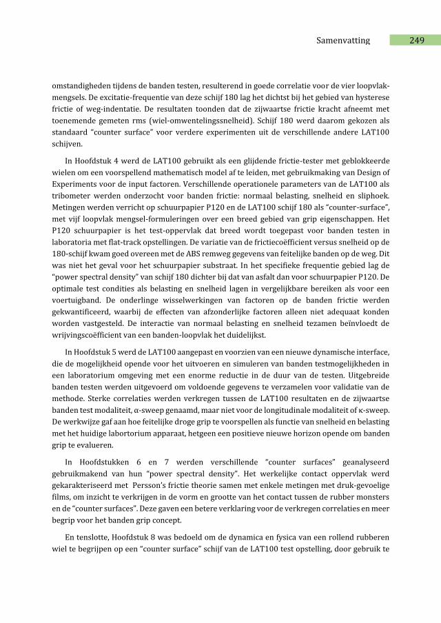
249 Samenvatting
omstandigheden tijdens de banden testen, resulterend in goede correlatie voor de vier loopvlak-
mengsels. De excitatie-frequentie van deze schijf 180 lag het dichtst bij het gebied van hysterese
frictie of weg-indentatie. De resultaten toonden dat de zijwaartse frictie kracht afneemt met
toenemende gemeten rms (wiel-omwentelingssnelheid). Schijf 180 werd daarom gekozen als
standaard “counter surface” voor verdere experimenten uit de verschillende andere LAT100
schijven.
In Hoofdstuk 4 werd de LAT100 gebruikt als een glijdende frictie-tester met geblokkeerde
wielen om een voorspellend mathematisch model af te leiden, met gebruikmaking van Design of
Experiments voor de input factoren. Verschillende operationele parameters van de LAT100 als
tribometer werden onderzocht voor banden frictie: normaal belasting, snelheid en sliphoek.
Metingen werden verricht op schuurpapier P120 en de LAT100 schijf 180 als “counter-surface”,
met vijf loopvlak mengsel-formuleringen over een breed gebied van grip eigenschappen. Het
P120 schuurpapier is het test-oppervlak dat breed wordt toegepast voor banden testen in
laboratoria met flat-track opstellingen. De variatie van de frictiecoëfficient versus snelheid op de
180-schijf kwam goed overeen met de ABS remweg gegevens van feitelijke banden op de weg. Dit
was niet het geval voor het schuurpapier substraat. In het specifieke frequentie gebied lag de
“power spectral density” van schijf 180 dichter bij dat van asfalt dan voor schuurpapier P120. De
optimale test condities als belasting en snelheid lagen in vergelijkbare bereiken als voor een
voertuigband. De onderlinge wisselwerkingen van factoren op de banden frictie werden
gekwantificeerd, waarbij de effecten van afzonderlijke factoren alleen niet adequaat konden
worden vastgesteld. De interactie van normaal belasting en snelheid tezamen beïnvloedt de
wrijvingscoëfficient van een banden-loopvlak het duidelijkst.
In Hoofdstuk 5 werd de LAT100 aangepast en voorzien van een nieuwe dynamische interface,
die de mogelijkheid opende voor het uitvoeren en simuleren van banden testmogelijkheden in
een laboratorium omgeving met een enorme reductie in de duur van de testen. Uitgebreide
banden testen werden uitgevoerd om voldoende gegevens te verzamelen voor validatie van de
methode. Sterke correlaties werden verkregen tussen de LAT100 resultaten en de zijwaartse
banden test modaliteit, α-sweep genaamd, maar niet voor de longitudinale modaliteit of κ-sweep.
De werkwijze gaf aan hoe feitelijke droge grip te voorspellen als functie van snelheid en belasting
met het huidige labortorium apparaat, hetgeen een positieve nieuwe horizon opende om banden
grip te evalueren.
In Hoofdstukken 6 en 7 werden verschillende “counter surfaces” geanalyseerd
gebruikmakend van hun “power spectral density”. Het werkelijke contact oppervlak werd
gekarakteriseerd met Persson’s frictie theorie samen met enkele metingen met druk-gevoelige
films, om inzicht te verkrijgen in de vorm en grootte van het contact tussen de rubber monsters
en de “counter surfaces”. Deze gaven een betere verklaring voor de verkregen correlaties en meer
begrip voor het banden grip concept.
En tenslotte, Hoofdstuk 8 was bedoeld om de dynamica en fysica van een rollend rubberen
wiel te begrijpen op een “counter surface” schijf van de LAT100 test opstelling, door gebruik te
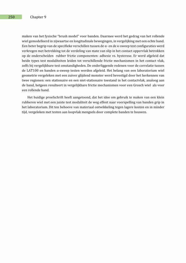
250 Chapter 9
maken van het fysische “brush model” voor banden. Daarmee werd het gedrag van het rollende
wiel gemodelleerd in zijwaartse en longitudinale bewegingen, in vergelijking met een echte band.
Een beter begrip van de specifieke verschillen tussen de α- en de κ-sweep test configuraties werd
verkregen met betrekking tot de verdeling van mate van slip in het contact oppervlak betrokken
op de onderscheiden rubber frictie componenten: adhesie vs. hysterese. Er werd afgeleid dat
beide types test modaliteiten leiden tot verschillende frictie mechanismen in het contact vlak,
zelfs bij vergelijkbare test omstandigheden. De onderliggende redenen voor de correlatie tussen
de LAT100 en banden α-sweep testen werden afgeleid. Het belang van een laboratorium wiel
geometrie vergeleken met een zuiver glijdend monster werd bevestigd door het herkennen van
twee regionen: een stationaire en een niet-stationaire toestand in het contactvlak, analoog aan
de band, hetgeen resulteert in vergelijkbare frictie mechanismen voor een Grosch wiel als voor
een rollende band.
Het huidige proefschrift heeft aangetoond, dat het idee om gebruik te maken van een klein
rubberen wiel met een juiste test modaliteit de weg effent naar voorspelling van banden grip in
het laboratorium. Dit ten behoeve van materiaal ontwikkeling tegen lagere kosten en in minder
tijd, vergeleken met testen aan loopvlak mengsels door complete banden te bouwen.
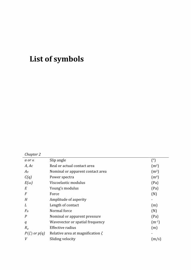
List of symbols
Chapter 2
a or α Slip angle (°)
𝐴, Ac Real or actual contact area (m2)
A0 Nominal or apparent contact area (m2)
C(q) Power spectra (m4)
E(ω) Viscoelastic modulus (Pa)
E Young’s modulus (Pa)
F Force (N)
H Amplitude of asperity -
L Length of contact (m)
FN Normal force (N)
P Nominal or apparent pressure (Pa)
q Wavevector or spatial frequency (m-1)
𝑅𝑒 Effective radius (m)
𝑃(휁) or p(q) Relative area at magnification 휁 -
V Sliding velocity (m/s)
252
𝑉𝑥 Longitudinal driving speed (m/s)
𝛾 Empirical parameter -
𝜅 Longitudinal slip ratio -
λ Wavelength of asperity (m)
𝜇 Coefficient of friction (COF) -
𝜇𝑠 Static coefficient of friction -
𝜇𝑘 Kinetic coefficient of friction -
𝜇𝐴 Adhesion friction coefficient -
𝜇𝐷 Deformation friction coefficient -
𝜇𝐻 Hysteresis friction coefficient -
휁 Magnification parameter -
𝜎0 Mean perpendicular pressure (Pa)
𝜈 Poisson’s ratio -
ω Excitation frequency (s-1)
Ω Wheel rotational velocity (rad/s)
Chapter 3
𝑑 distance (m)
𝐹𝑓 or 𝐹𝑥 Tangential friction force (N)
𝐹𝑠 or 𝐹𝑦 Lateral (Side) force (N)
𝐹𝑐 Counter force to centrifugal force (radial) (N)
𝐹𝑧 Normal force (N)
R Radius (m)
𝑅𝑒 Effective radius (m)
R2 Linear regression coefficient -
SFC Side Force Coefficient -
𝑉𝑐 Circumferential velocity (m/s)
𝑉𝑡 Traveling velocity (m/s)
𝑉𝑥 Longitudinal driving speed (m/s)
𝑉𝑆 Slip velocity (m/s)
α Slip angle (˚)
Ω Wheel rotational velocity (rad/s)
Chapter 4
𝑎 Slip angle (˚)
A Factor A: load (N)
ANOVA Analysis of Variance -
253 List of symbols
B Factor B: speed (km/h)
C Factor C: Slip angle (°)
CC Correlation Coefficient -
COF Coefficient of Friction -
DF or 𝑑𝑓 Degree of Freedom -
𝐹𝑁 Normal force (N)
𝐹𝑓 Friction force (N)
F-ratio Variance ration -
MS Mean Square -
n Number of experiments -
P-Value Probability Value -
RSM Response Surface Modeling -
R-sq R-squared -
R-sq(adj) R-squared adjusted -
R-sq(pred) R-squared predicted -
S Standard deviation -
SS Sum of Squares -
S2 variance -
SE Standard error -
𝑆𝑌 Standard Error of the mean response -
t-value dimensionless statistical scale -
𝑋 Input factor -
𝑋𝑋 2-way interaction term -
𝑋2 Quadratic term -
Y Predicted response -
𝑌 Mean response -
𝑉𝑡 Disc traveling velocity (m/s)
α Significance level -
(1-α) Confidence interval (%)
𝛽 Model coefficient -
μ Coefficient of Friction -
𝜔 Disc rotational velocity (rad/s)
Chapter 5
CV Coefficient of variance or relative standard deviation (%)
𝐹𝑐 Counter force to centrifugal force (radial) (N)
254
𝐹𝑓 or 𝐹𝑥 Tangential friction force (N)
𝐹𝑠 or 𝐹𝑦 Lateral (Side) force (N)
𝐹𝑧 Normal force (N)
R2 Linear regression coefficient -
𝑅𝑒 Effective radius (m)
𝑉𝑐 Circumferential velocity (m/s)
𝑉𝑆 Slip velocity (m/s)
𝑉𝑡 Traveling velocity (m/s)
𝑉𝑥 Longitudinal driving speed (m/s)
α Slip angle (˚)
𝜅 Longitudinal slip ratio -
𝜇𝑥 longitudinal coefficient of friction -
𝜇𝑦 lateral coefficient of friction -
Ω Wheel rotational velocity (rad/s)
Chapter 6
𝐴(𝜏) Auto-correlation function -
𝐶2𝐷(𝒒) 2D power spectrum (m4)
𝐶1𝐷(𝒒) 1D power spectrum (m3)
H Hurst exponent -
L The length of the measurement (m)
PSD power spectral density -
q Wavevector (m-1)
q wavenumber (m-1)
𝑞0 Small cut-off wavevector (long roll-off wavelength) (m-1)
𝑞1 Large cut-off wavevector (short wavelength) (m-1)
𝑅𝑎 The arithmetic average of the absolute values of the
distance of the asperities to the mean line
(μm)
𝑅𝑞 Root mean squared of the distance of the asperities to the
mean line
(μm)
𝑅𝑠𝑞 Skewness -
x Distance in x-direction (m)
z Height of asperities (m)
ΔM Difference between the maximum and minimum torque (dNm)
λ Wavelength (m)
𝜏 Distance defined in the autocorrelation function (m)
255 List of symbols
Chapter 7
𝐴0 Nominal or apparent area of contact (mm2)
𝐴𝑏 The area of the base of frustum (mm2)
𝐴𝑐 Actual area (mm2)
𝐴𝑙 Lateral area (mm2)
𝐴𝑝 Projected area (mm2)
𝐴𝑙𝑙𝑙𝑤 area on film LLLW (mm2)
𝐴/𝐴0 the relative contact areas -
𝐸 modulus (MPa)
𝑓 frequency (Hz)
ℎ Depth of penetration (mm)
ℎ2 Height of the frustum (mm)
𝐻 Hardness (°Sh A)
LLW upper low pressure -
LLLW ultra-super low-pressure film -
𝑃0 Nominal pressure (MPa)
𝑞1 large cut-off wavenumber (m-1)
𝑟 Frustum radius (mm)
S Lateral length of frustum (mm)
𝑇 Temperature (°C)
𝜎0 Nominal pressure (MPa)
Chapter 8
𝑎 Half of contact length (m)
𝑏 Wheel width (m)
𝐶𝐹𝛼 Cornering stiffness (N/rad)
𝐶𝐹𝜅 Longitudinal stiffness (N)
∆𝑡 Time interval (s)
E Young’s modulus (MPa)
𝐹𝑓 or 𝐹𝑥 Tangential friction force (N)
𝐹𝑐 Counterforce to centrifugal force (radial) (N)
𝐹𝑠 or 𝐹𝑦 Lateral (Side) force (N)
𝐹𝑧 or 𝐹𝑁 Normal force (N)
G Shear modulus (MPa)
𝑘𝑏 Bristle stiffness (N/m2)
𝑘𝑧 Vertical tread stiffness (N/m)
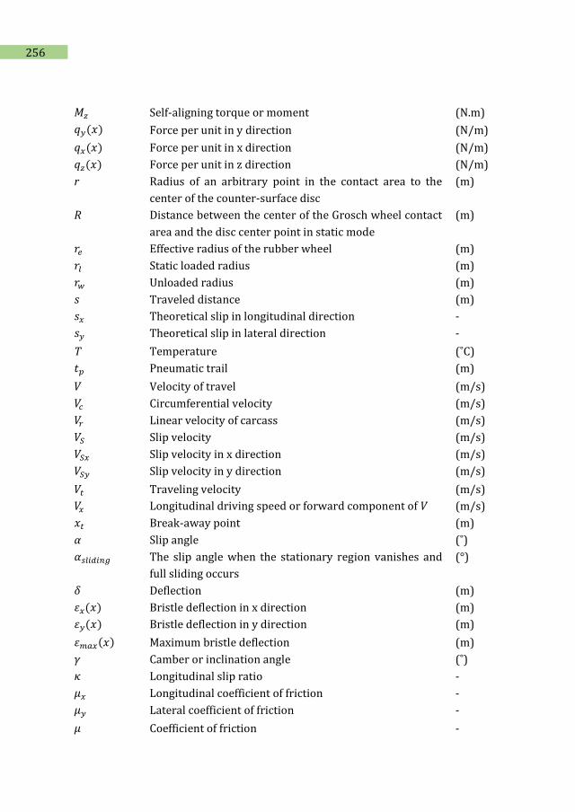
256
𝑀𝑧 Self-aligning torque or moment (N.m)
𝑞𝑦(𝑥) Force per unit in y direction (N/m)
𝑞𝑥(𝑥) Force per unit in x direction (N/m)
𝑞𝑧(𝑥) Force per unit in z direction (N/m)
r Radius of an arbitrary point in the contact area to the
center of the counter-surface disc
(m)
R Distance between the center of the Grosch wheel contact
area and the disc center point in static mode
(m)
𝑟𝑒 Effective radius of the rubber wheel (m)
𝑟𝑙 Static loaded radius (m)
𝑟𝑤 Unloaded radius (m)
𝑠 Traveled distance (m)
𝑠𝑥 Theoretical slip in longitudinal direction -
𝑠𝑦 Theoretical slip in lateral direction -
T Temperature (˚C)
𝑡𝑝 Pneumatic trail (m)
𝑉 Velocity of travel (m/s)
𝑉𝑐 Circumferential velocity (m/s)
𝑉𝑟 Linear velocity of carcass (m/s)
𝑉𝑆 Slip velocity (m/s)
𝑉𝑆𝑥 Slip velocity in x direction (m/s)
𝑉𝑆𝑦 Slip velocity in y direction (m/s)
𝑉𝑡 Traveling velocity (m/s)
𝑉𝑥 Longitudinal driving speed or forward component of 𝑉 (m/s)
𝑥𝑡 Break-away point (m)
α Slip angle (˚)
𝛼𝑠𝑙𝑖𝑑𝑖𝑛𝑔 The slip angle when the stationary region vanishes and
full sliding occurs
(°)
𝛿 Deflection (m)
휀𝑥(𝑥) Bristle deflection in x direction (m)
휀𝑦(𝑥) Bristle deflection in y direction (m)
휀𝑚𝑎𝑥(𝑥) Maximum bristle deflection (m)
𝛾 Camber or inclination angle (˚)
𝜅 Longitudinal slip ratio -
𝜇𝑥 Longitudinal coefficient of friction -
𝜇𝑦 Lateral coefficient of friction -
𝜇 Coefficient of friction -
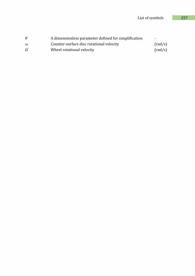
257 List of symbols
𝜃 A dimensionless parameter defined for simplification -
ω Counter-surface disc rotational velocity (rad/s)
Ω Wheel rotational velocity (rad/s)

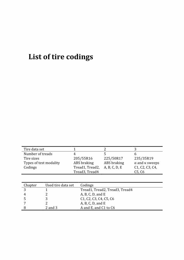
List of tire codings
Tire data set 1 2 3 Number of treads 4 5 6 Tire sizes 205/55R16 225/50R17 235/35R19 Types of test modality ABS braking ABS braking α and κ sweeps Codings Tread1, Tread2,
Tread3, Tread4 A, B, C, D, E C1, C2, C3, C4,
C5, C6
Chapter Used tire data set Codings 3 1 Tread1, Tread2, Tread3, Tread4 4 2 A, B, C, D, and E 5 3 C1, C2, C3, C4, C5, C6 7 2 A, B, C, D, and E 8 2 and 3 A and E, and C1 to C6

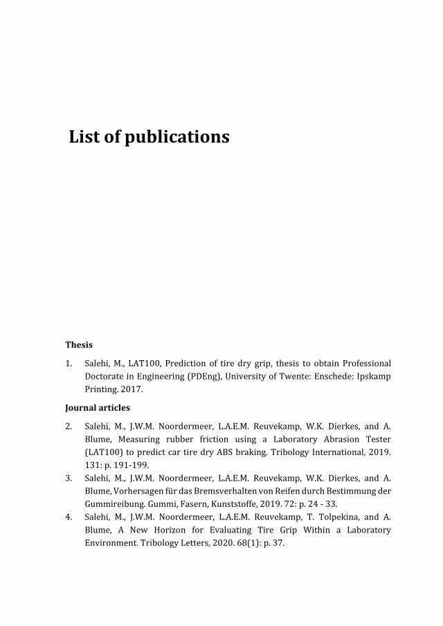
List of publications
Thesis
1. Salehi, M., LAT100, Prediction of tire dry grip, thesis to obtain Professional
Doctorate in Engineering (PDEng), University of Twente: Enschede: Ipskamp
Printing. 2017.
Journal articles
2. Salehi, M., J.W.M. Noordermeer, L.A.E.M. Reuvekamp, W.K. Dierkes, and A.
Blume, Measuring rubber friction using a Laboratory Abrasion Tester
(LAT100) to predict car tire dry ABS braking. Tribology International, 2019.
131: p. 191-199.
3. Salehi, M., J.W.M. Noordermeer, L.A.E.M. Reuvekamp, W.K. Dierkes, and A.
Blume, Vorhersagen für das Bremsverhalten von Reifen durch Bestimmung der
Gummireibung. Gummi, Fasern, Kunststoffe, 2019. 72: p. 24 - 33.
4. Salehi, M., J.W.M. Noordermeer, L.A.E.M. Reuvekamp, T. Tolpekina, and A.
Blume, A New Horizon for Evaluating Tire Grip Within a Laboratory
Environment. Tribology Letters, 2020. 68(1): p. 37.
262
5. Salehi, M., J.W.M. Noordermeer, L.A.E.M. Reuvekamp, and A. Blume, Parameter
optimization for a laboratory friction tester to predict tire ABS braking distance
using design of experiments. Materials & Design, 2020. 194: p. 108879.
6. Salehi, M., J.W.M. Noordermeer, L.A.E.M. Reuvekamp, A. Blume, Measuring
rubber friction using a Laboratory Friction and Abrasion Tester (LAT100) to
predict car tire grip, Part II: characterization of counter-surfaces, submitted to
Tribology International.
7. Salehi, M., J.W.M. Noordermeer, L.A.E.M. Reuvekamp, A. Blume, A new horizon
for evaluating tire grip within a laboratory environment, part II: understanding
the test modalities and correlations with modeling, submitted to Tribology
Letters.
8. Salehi, M., J.W.M. Noordermeer, L.A.E.M. Reuvekamp, A. Blume,
Characterization of the real contact area of solid rubber wheels vs. real tires
with pressure-sensitive films in comparison with Persson theory, under
submission.
Conferences and presentations
9. Salehi M., M. Heinz, T.V. Tolpekina, T.G.G. Teunissen, Louis A.E.M. Reuvekamp,
Wilma K. Dierkes, and A. Blume. Prediction of Tire Dry Grip by Using the
Laboratory Abrasion Tester (LAT100). in 12th Fall Rubber Colloquium 2016.
22-24 Nov., Hannover, Germany.
10. Salehi, M., J.W.M. Noordermeer, L.A.E.M. Reuvekamp, and A. Blume. Correlation
between the tire grip and LAT100 results. in 4th International Conference
Science meets Tires 2018: Perspectives for Tire Technology. 24- 25 April,
Institute for Automotive Engineering (ika) and RWTH Aachen University,
Aachen, Germany.
11. Salehi, M., J.W.M. Noordermeer, L.A.E.M. Reuvekamp, and A. Blume. Prediction
of the Dry Grip, using LAT100. in Tire Technology Expo & Conference 2017. 14-
16 Feb, Hannover, Germany.
12. Salehi, M., J.W.M. Noordermeer, L.A.E.M. Reuvekamp, and A. Blume. A New
Method to Rapidly Predict Tyre Grip In a Laboratory Environment. in
International Rubber Conference (IRC). 3-5 Sep 2019. London, UK.
13. Salehi, M., J.W.M. Noordermeer, L.A.E.M. Reuvekamp, and A. Blume. What
happens in the tire contact area? in Tire Technology Expo 2020, 24-26 Feb.
Hanover, Germany.
14. Salehi, M., J.W.M. Noordermeer, L.A.E.M. Reuvekamp, and A. Blume. Evaluation
of Tire Grip in a Laboratory Environment: Introducing a Rapid Test with
LAT100 in Correlation with Actual Tire Data on Dry Road. in ICTL 2020: 14th
263 List of Publications
International Conference on Tribology and Lubrication. June 11-12, Tokyo,
Japan.
15. Salehi, M., J.W.M. Noordermeer, L.A.E.M. Reuvekamp, and A. Blume. An
investigation into the effect of surface roughness with LAT100 in correlation
with tire data. in Dutch Polymers Days (DPD), 14-15 March 2017. Lunteren,
Netherlands.
16. Salehi, M., J.W.M. Noordermeer, L.A.E.M. Reuvekamp, and A. Blume. Prediction
of the dry grip, using Laboratory Abrasion Tester (LAT100) in DKG West
meeting (Deutsche Kautschuk-Gesellschaft), 3rd April 2017, Bad Neuenahr,
Germany.
17. Salehi, M., J.W.M. Noordermeer, L.A.E.M. Reuvekamp, and A. Blume. A new
method to rapidly predict tire grip in a laboratory environment in 4th Annual
Innovative All-season and Winter Tire Development Forum, 27th – 28th May
2019, Amsterdam, Netherlands.
Collaborations
18. Dirk Schuttel (author), Salehi, M. (interviewee), ‘Advancing abrasion testing’,
Tire Technology International, 2019, The annual review of tire materials and
tire manufacturing technology, pp 88-10.
19. Sekar, P., Salehi, M., Anyszka, R. P., and A. Blume. ‘HydroThermally Carbonized
lignin as sustainable filler for tire-tread application’ in Tire Technology Expo
2020, 24th -26th Feb. Hanover, Germany.
20. Sekar, P., Salehi, M., Anyszka, R. P., and A. Blume. ‘Hydrothermally Carbonized
Lignin as Sustainable Bio-based Filler for Tire-Tread Applications’, under
submission.
Honors and Awards
1. Honored Cum Laude for the PDEng thesis, Professional Doctorate in
Engineering , University of Twente, July 2017.
2. Awarded for the best poster prize in IRC 2019, London, UK.
3. The paper “A New Horizon for Evaluating Tire Grip Within a Laboratory
Environment” was selected as best from the Society of Tribologists and
Lubrication Engineers (STLE) in the July edition of Tribology & Lubrication
Technology magazine in the article Editors’ Selections.

Acknowledgment
I would like to acknowledge professors, companies, colleagues, friends, and
acquaintances who helped me to carry out the present piece of work, without whom the
present dissertation wouldn’t have been accomplished.
My sincere gratitude to my promoter Prof. Anke Blume for continuous support and help.
Dear Anke, I highly appreciate you for providing me this opportunity and trusting me to
establish my own ideas. Thank you for the constant motivation and encouragement to
complete my dissertation especially due to my situation in the last year. My special thanks
to my supervisor and mentor, Prof. Jacque Noordermeer, for the superb guidance, inspiring
discussion, and priceless advice. Dear Jacques, I am privileged for the given chance to learn
from you which impacted highly on my science life and career path. I am grateful for the
inexhaustible time spent on the papers and the thesis with me word by word to find a close
to perfect story. Thanks for the invaluable support like a father and the endless
encouragement for pursuing my goals. I thank you and your wife dear Betty for the warm
and kind visits. I would like to express my gratitude to my company boss, my friend Dr. Louis
Reuvekamp. Dear Louis, I appreciate you for trusting and offering me this position and also
the constant support since we met, particularly for the prompt replies though you were fully
occupied. I would like to also extend my gratefulness to ETE staff members especially Prof.
Wilma Dierkes, dear Ceciel, and Dries for their always openness and great help to support
us.
The present research was sponsored by Apollo Tyres Global R&D B.V., Enschede, the
Netherlands. I acknowledge the support from Apollo particularly the useful discussion and
comments from my project partner Tanya, and also Hans, and Sebastian for the help about
the physics and dynamic aspects of the project. I would like to thank VMI Holland BV, for
sponsoring the project by providing the LAT100 device and the follow-up support within
this period. I appreciate the support of VMI colleagues especially Theo Teunissen, Dirk
Schuttel, and Harald Kroll. This research was also partially sponsored by Evonik Resource
Efficiency GmbH, I extend my gratitude to Dr. Michael Heinz for the insightful discussion and
instructed training regarding the LAT100 device, and also Dr. Jens Kiesewetter, and Dr. Minh
Nguyen; within the first two years of my PDEng study, I enjoyed working with them.
I had the honor to meet Dr. Bo Persson; thanks for such a warm welcome to Jülich. Dear
Bo, I highly learned from you, and many thanks for the insights and expertise in the contact
mechanics that greatly assisted the research. Also, thank Avinash for the help and
interesting discussion during my visit to Jülich. I would like to appreciate dear Erik and Nick
for the help with the measurements of laser microscopy and dear Theo Pünt for the support
and discussion regarding designing new parts for the LAT100 device. Also, I thank dear
Mostafa Jahanifar, an Iranian talented researcher, for the help regarding the image analyses
266
which assisted me in the understanding of the subject. My cousin, Narges, my lovely friend
since childhood, thanks, my dear! for the support and discussion regarding the statistical
analyses. I would like to also thank Dr. Kianoosh Taghizadeh for help with Matlab for data
analysis in the beginning of my project.
Thanks to all my former and current colleagues who made the work environment very
pleasant and lively; special thanks to whom we became good friends over time and made
beautiful memories, particularly my officemates Neven, Carmela, Zuzana, Marcin with
whose company I managed to work sometimes hours till mid-evening in a couple of last
years ago; and Priyanka, I enjoyed working with her and soon became good friends. Several
articles were published within the present thesis, thanks to the anonymous reviewers who
were of great help to enhance the content of the present thesis which incented me to widen
my research from various perspectives.
To my dear friends: Elahe, my energetic and kind friend who stood by me days and nights
when I was in grief; Marie Claire, I am glad to have such a kind, caring, and energetic friend;
Atefeh, Somayeh, Arezoo, and Samira, I have known you already for a long time and these
valuable friendships lasted so long even when we were far away; To my piano teacher Griet,
you work with my soul which kept me calm in life difficulties; To all whoever was there for
me with a great heart especially in last year when I was suffering from a severe trauma of
losing my mother, I couldn’t stand back on my feet without your emotional support; thank
you all!
To my dear Paranymphs: Amir and Ayush who are friends in need. Dear Ayush, you
readily helped and supported me, I was just a call away from you. Thanks! A special Persian
thanks to dear Amir who took care of me in my misery and grief! ‘damet garm k azam
moraghebat karde (boode) boodi Amir jan, mamnoonam vase hame chi’.
Last but not least, to my beautiful mother and my lovely family,
I have a separate letter for you, my mother! You were an admirably strong and untiring
person who dedicated her life to the happiness of the loved ones. The bond that I had with
you, was not only an ordinary mother-daughter relationship, it was my everything! A solid
mountain to lean on! I miss you EVERY SINGLE DAY… this day has come, the day that we
were both looking forwards to it. I know you would be proud of me, whenever I think of not
having another chance to chat with you and hug you, immediately I find myself in endless
misery. I don’t know how I survived the last year, but this is what I promised you, this is for
you and because of you. My sincerest thanks to my lovely family, the greatest gift that I ever
received: not only the immense amount of emotional support that I’ve received since I
moved here, but for standing always next to me particularly my supportive and adorable
sister and my closest friend: you are an angel with a glowing love.
هرگز که من نیهست یاخانواده نیبهتر عاشقتونم. شما یلیدوستتون دارم، خ یلیخ ن،یدلم یزایخانواده گلم، شما عز
.داشته باشم تونستمیم
Proper tire grip provides a good level of handling which is a prerequisite for a vehicle’s steering, braking, accelerating, and cornering. For material development for the acquisition of superior tire performance, full-scale tire testings are enormously sophisticated, time-consuming, and costly. It is sustainable and highly desirable to predict tire grip performance in a laboratory environment before manufacturing a full tire for the determination of rubber friction. However, considering all the influential factors in one laboratory apparatus is a complex task to accomplish, to predict tire tribological properties. In the present thesis, a new way of measurements in a laboratory environment is introduced which is in good agreement with actual tire testing. ISBN 978-90-365-5063-5 UNIVERSITY OF TWENTE.