Embed Size (px)
Citation preview

Louisiana State University Louisiana State University
LSU Digital Commons LSU Digital Commons
LSU Master's Theses Graduate School
2007
Predictive data compression using adaptive arithmetic coding Predictive data compression using adaptive arithmetic coding
Claudio Jose Iombo Louisiana State University and Agricultural and Mechanical College
Follow this and additional works at: https://digitalcommons.lsu.edu/gradschool_theses
Part of the Electrical and Computer Engineering Commons
Recommended Citation Recommended Citation Iombo, Claudio Jose, "Predictive data compression using adaptive arithmetic coding" (2007). LSU Master's Theses. 2717. https://digitalcommons.lsu.edu/gradschool_theses/2717
This Thesis is brought to you for free and open access by the Graduate School at LSU Digital Commons. It has been accepted for inclusion in LSU Master's Theses by an authorized graduate school editor of LSU Digital Commons. For more information, please contact [email protected].

PREDICTIVE DATA COMPRESSION USING ADAPTIVE ARITHMETIC CODING
A Thesis Submitted to the Graduate Faculty of the
Louisiana State University and Agricultural and Mechanical College
in partial fulfillment of the requirements for the degree of
Master of Science in Electrical Engineering in
The Department of Electrical Engineering
by Claudio Iombo
EIT., B.S., Louisiana State University, 2003 August 2007

ii
Table of Contents
Abstract .......................................................................................................................... iv Introduction ...................................................................................................................... 1
Types of Data ............................................................................................................... 1 Data Compression System ........................................................................................... 2 What Is This Thesis About ........................................................................................... 3
Chapter 1 Information Theory ......................................................................................... 6
Information ................................................................................................................... 6 Entropy...................................................................................................................... 6 Joint and Conditional Entropy ................................................................................... 7 Mutual Information .................................................................................................... 8
Chapter 2 Entropy Coding ............................................................................................. 10
Introduction ................................................................................................................ 10 Prefix Codes ............................................................................................................... 10 Kraft’s Inequality ......................................................................................................... 11 Huffman Coding ......................................................................................................... 12
Alternate Implementation ........................................................................................ 13 Adaptive Huffman ................................................................................................... 14
Arithmetic Coding ....................................................................................................... 16 Advantages of Arithmetic Coding ............................................................................ 16 Disadvantages of Arithmetic Coding ....................................................................... 17 Optimality of Arithmetic Coding ............................................................................... 19 Adaptive Arithmetic Coding ..................................................................................... 20
Chapter 3 Data Modeling .............................................................................................. 23
Introduction ................................................................................................................ 23 What Do We Know About The Data ........................................................................ 23 Worst Case Scenario .............................................................................................. 24 Best Case Scenario ................................................................................................ 24 Application to Compression .................................................................................... 24
Sources ...................................................................................................................... 24 Markov Models ........................................................................................................ 25 Adaptive Arithmetic Compression Using Data Models ............................................ 28
Chapter 4 Implementation of Arithmetic Coder ............................................................. 32
Introduction ................................................................................................................ 32 Modeler ...................................................................................................................... 32 Encoder ...................................................................................................................... 33
E1 and E2 Scaling .................................................................................................. 33 E3 Scaling ............................................................................................................... 35
Decoder ...................................................................................................................... 37

iii
Modified Arithmetic Coder .......................................................................................... 39 Modeler ................................................................................................................... 40 Encoder ................................................................................................................... 40 Decoder .................................................................................................................. 42
Chapter 5 Implementation of Huffman Coding.............................................................. 45
Node ........................................................................................................................... 45 Tree ............................................................................................................................ 45
Tree Operations ...................................................................................................... 46 Encode ....................................................................................................................... 51 Decode ....................................................................................................................... 52
Chapter 6 Simulation Results ....................................................................................... 57
Files ............................................................................................................................ 57 Results ....................................................................................................................... 57 Discussion .................................................................................................................. 59
Conclusions and Future Work ....................................................................................... 61 Bibliography ................................................................................................................... 62 Vita ................................................................................................................................ 64

iv
Abstract
The commonly used data compression techniques do not necessarily provide
maximal compression and neither do they define the most efficient framework for
transmission of data. In this thesis we investigate variants of the standard compression
algorithms that use the strategy of partitioning of the data to be compressed. Doing so
not only increases the compression ratio in many instances, it also reduces the
maximum data block size for transmission. The partitioning of the data is made using a
Markov model to predict if doing so would result in increased compression ratio.
Experiments have been performed on text files comparing the new scheme to adaptive
Huffman and arithmetic coding methods. The adaptive Huffman method has been
implemented in a new way by combining the FGK method with Vitter’s implicit ordering
of nodes.
1
Introduction
We deal with information every day. It comes in many forms. We watch
television, use computers, and listen to radio. This information requires a large amount
of storage and bandwidth and it needs to be digitized in order to be processed. Doing
so eases processing of data and reduces errors by making it less susceptible to noise.
Maximum sampling rates are typically used to represent these signals in digital form,
and this does not take into account the periods of inactivity and redundancy that exist in
most messages. For example, 8 bits are used to represent text alphabet symbol,
although has been shown that as few as four bits are enough to convey the same
information [6]. The same can be said about video data which contains regions where
little change occurs from frame to frame. Using this knowledge, the data can be
represented using fewer bits. Data compression is the means developed to minimize
the amount of bits used to represent data. The reduction of storage and bandwidth is
measured against the increase in processing power required to compress the message.
We must keep this tradeoff in mind when designing a system for data compression.
Types of Data
Data to be compressed can be divided into symbolic or diffuse data [6].
Symbolic data is data that can be discerned by the human eye. These are
combinations of symbols, characters or marks. Examples of this type of data are text
and numeric data. Unlike the symbolic data, diffuse data cannot be discerned by the
human eye. The meaning of the data is stored in its structure and cannot be easily
extracted. Examples of this type of data are speech, image, and video data.

2
The approaches taken to compress diffuse and symbolic data are different but
not exclusive. In symbolic data the approach most taken is reduction of redundancy.
This is an approach that uses lossless compression techniques, meaning that the
compression process is reversible with 100 percent accuracy. Lossless compression
algorithms include entropy coding and dictionary based compression. For diffuse data
the approach to compression is the removal of unnecessary information. If a sufficiently
small amount of information is removed from a video segment, most viewers would not
be aware of the change. Therefore, some of this data can be discarded. Lossy data
compression techniques include transform coding. The two approaches for diffuse and
symbolic data can be used together in the same compression system. For example,
both transform data compression techniques and entropy coding is used in H.264 video
compression.
Data Compression System
A data compression system is a combination of data compression techniques
and data modeling. The two parts of the system are the encoder and the decoder. The
encoder consists of input, pre-processing, modeling, and encoding. The decoder
consists of modeling, decoding, and post-processing. The pre-processing transforms
the data into an intermediate form that would facilitate encoding. The post-processing
reverses the data from the intermediate form. The modeling gathers information about
the data that will be used in encoding or decoding. An example of a compression
system is shown in figure 1.
A digital system uses the data compression system to produce an output for the
user: it gathers the data, encodes the data, stores the data, transmits the data, decodes

3
the data, and outputs the data to the end user. The decoding and encoding of this
system is done by the data compression system. An example of a digital system is
shown in figure 2.
Figure 1. Data Compression System
Figure 2. Digital System
What Is This Thesis About
This thesis deals with the construction of a digital compression system for text
data. This compression includes lossless compression using arithmetic coding. We
Encoding
Modeling
Modeling
Post-ProcessingPre-Processing
OutputInput
Encoder Decoder
Decoding
InputE
N
C
O
D
E
R
S
T
O
R
A
G
E
OutputD
E
C
O
D
E
R
TransmissionS
T
O
R
A
G
E

4
discuss the issues and approaches used to maximize the effectiveness of arithmetic
coding. In particular, we address optimization by partitioning the data. Lastly, we
formulate a sequential block partitioning approach that results in higher compression
ratio and/or smaller average block size.
Several papers [4,8,9] have been devoted to optimizing the packet size in a
communication system. This issue helps to maximize efficiency and throughput.
If the packet size is too small there are two pitfalls. In the case of a constant rate
transmitter, the small packets would require more packets to be sent to keep the same
bit rate. This would result in increased packets and congestion in the network. The
second issue is the required overhead in these packets. Small packets would not justify
the amount of overhead needed to encapsulate the packet into the header.
The case of large packet size also results in two unwanted outcomes. First,
large packets tend to be discarded more frequently than smaller packets. This is due to
link and transport layer error checking mechanisms that discard a packet with multiple
errors. The second issue is inefficient fragmentation of the large packets. This occurs in
size-constrained networks such as Ethernet where packets are fragmented into MTUs
(Maximum Transfer Units) of 1500 bytes. These fragmentation operations increase
bandwidth usage and additional delays.
Several procedures have been researched to find the optimum static or variable
network packet size [4]. In our results, we show that we can break up a large message
into significantly smaller packets with very little or no loss in compression. In [14], the
notion of partitioning the file to increase compression was established. The paper left

5
the partition selection for future developments. In this thesis we plan to use prediction
to calculate partition sizes and locations within a file.

6
Chapter 1
Information Theory
Information
The basis for data compression is the mathematical value of information.
Information contained in a symbol x is given by, I(x) =)(
1log2
xp. This value also
describes the number of bits necessary to encode the symbol. This definition reinforces
our notion of information. First, the more probable the occurrence of a symbol, the less
information it provides by its occurrence, and also less bits are used to represent it.
Conversely, the least frequent symbols provide more information by their occurrence.
Secondly, if we have n equally probable messages, we know that log2n bits will be
required to encode each message. This is the information value of each message I=
p
1log2 =log2n. Finally, information of two independent messages should be additive.
Consider two independent messages A and B. Here we have,
I(AB)= )()(
1log2
BpAp=
)(
1log 2
Ap+
)(
1log 2
Bp=I(A)+I(B)
Entropy
Entropy can also be defined as the measure of the average information [7].
According to Shannon, entropy of a discrete source for a finite alphabet X is given by,
∑∈
=Xx xp
xpxH)(
1log)()( 2

7
Properties of Entropy
Theorem 1.1. 0≤H(X)≤log2n where X=x1,x2,….,xn
Proof:
If p(x)=1 for some x, then H(X)=0.
nxp
xpxp
xpXHXx Xx
222 log)(
1)(log
)(
1log)()( =≤=∑ ∑
∈ ∈
If p(x)=1/n for all x, we have
∑ ∑ ∑∑∈ ∈ ∈∈
==−−=−=Xx Xx XxXx
nnn
nnnn
xH 22222 loglog1
log1log11
log1
)( [12]
Joint and Conditional Entropy
The joint entropy H(X,Y) of two discrete random variables X and Y with joint
probability distribution p(x,y) is given as, ∑∑∈ ∈
=Xx Yy yxp
yxpYXH),(
1log),(),( 2 = -
∑∑∈ ∈Xx Yy
yxpyxp ),(log),( 2
The joint H(X,Y) distribution can be seen as the overall average uncertainty of the
information source.
The conditional entropy H(X|Y) is the average information in X after Y has been
defined or revealed. It is given as, ∑∈
=),(),(
2),(
)(log),()|(
YXyx yxp
ypyxpYXH
Properties of Joint and Conditional Entropy
Theorem 1.2. Chain Rule: H(X,Y)=H(X)+X(Y|X)
Proof:
H(X,Y)= ∑∑∈ ∈
−Xx Yy
yxpyxp ),(log),( 2 =∑∑∈ ∈Xx Yy xp
yxpxpyxp
)(
),()(log),( 2

8
= ∑∑∈ ∈
−Xx Yy
xpxypxp )(log)|()( 2 +∑∑∈ ∈Xx Yy yxp
xpyxp
),(
)(log),( 2
= ∑∈
+=+−Xx
XYHXHXYHxpxp )|()()|()(log)( 2 [12]
Theorem 1.3. H(X|Y) where equality holds only if X and Y and independent
Proof:
H(X|Y)-H(X)= log2 log2
= log2
log2
= log2 =
log2
0 if p(x,y)=p(x)p(y) [12]
Mutual Information
The mutual information I(X;Y) is the uncertainty of X that is resolved due to
observing Y. It is defined by I(X;Y)=H(X)-H(X|Y)
Properties of Mutual Information
1. I(X;Y)=I(Y;X)
2. I(X;Y)≥0
3. I(X;Y)=H(Y)-H(Y|X)
4. I(X;Y)=H(X)+H(Y)-H(X,Y)
5. I(X;X)=H(X)

9
The concepts of information and entropy [7] which are summarized above are basic
to the development of data compression techniques. The next chapter discusses
methods that use entropy explicitly.

10
Chapter 2
Entropy Coding
Introduction
Entropy coding is compression algorithms that use the message statistics to
compress the message. There are two basic approaches to entropy coding. The first
approach includes the coding of individual symbols in the message alphabet. This
employs the use of prefix codes. One such example is Huffman code [1]. The second
type is the coding of the message or messages as a whole. This is the approach taken
by Arithmetic coding [1].
Prefix Codes
In compression we can use fixed-length codes to simplify decidability. We find
that for optimal compression variable length codes yield the best results. In variable
length coding the decoder has to be aware when a codeword starts and ends. In order
to be able to effectively decode a message, we must be able to do this without
ambiguity and without having to transfer extra decoding information. Let us suppose
that we have the code (a,1),(b,00),(c,10),(d,0). The message 100 would have multiple
interpretations. It could be decoded as cd or ab. Therefore, one necessary property of
coding is unique decodability.
Prefix code is a type of uniquely decodable code in which no codeword is a prefix
for another codeword. In the context of a binary tree, each message is a leaf of the
tree. This tree is referred to as the prefix-code tree[1].

11
Figure 2.1. Prefix code tree. Codewords are 0,10,11.
Kraft’s Inequality
The average code length of a set of m messages is given by L= xi)ni
where ni =length of symbol i in bits
Theorem 2.1. The codeword lengths for any uniquely decodable code must satisfy
Kraft-McMillan Inequality given as ! -ni [1]
Theorem 2.2. For any alphabet X, a uniquely decodable code follows H(X)L
Proof:
H(X)-L log2 nx= log2
nx log2 log22nx
log2(2-nx/p(x))
log2 !"#$ )
% [1]
Theorem 2.3. For any alphabet X, a uniquely decodable optimal code follows
LH(X)+1
Proof:
Continued on next page
Symbol 1 Symbol 2
Symbol
3
root
0
1
0
1

12
For optimality, we set nx=log2
& ' ()* + , ()* - , +()* - , [1]
Huffman Coding
Huffman coding is the best known form of entropy coding. The premise behind
Huffman coding is that more frequently occurring symbols are coded using longer code
words. To accomplish this, variable length code words are assigned to symbols based
on their frequency of occurrence. Huffman code satisfies two conditions:
1. All code words are uniquely decodable
2. No delimiters or extra information is inserted in the code words to facilitate
decidability
The first condition is accomplished by the use of prefix code. This leads to the second
condition. No markers are needed to separate the code words because of the use of
prefix code.
The coding is performed using a binary tree. First, the symbols are arranged in
order of decreasing probability of occurrence. Then the two least occurring symbols are
combined to form a new node. The result of this node is placed in the tree in a position
that preserves the order. Then the new node is combined with the next least occurring
symbol to create yet another node. This process is repeated until all nodes have been
processed. Afterwards a traversal back to the tree is done to tag one branch as 0 and
the other as 1. Traversal from the final node back to the originating node would give
you the codeword for the symbol. The final node is designated the root.

13
Example 1
d
a
c
b
Prob
0.4
0.3
0.2
0.1
0.3
0.3
0.6
0.4
0
10
01
1
Alphabet
a: 111
b: 01
c: 000
d:1
Figure 2.2. Huffman Code Construction. From this example the message ddccab would be coded as 11000000111101.
Alternate Implementation
A more graphical representation of Huffman coding is often used. This
representation consists of leaves and internal nodes. Leaves are symbols and the
internal nodes are nodes that contain the sum of the weights of its children. Whenever
two leaves are combined, they form an internal node. The internal nodes in turn
combine with other nodes or leaves to form more internal nodes. The leaves and nodes
are ordered in increasing order from left to right.
For the input in example 1, the tree is shown in figure 2.3.
Figure 2.3. (a) Diagram of leaf and nodes.(b) Code tree for example 1. Alphabet: a-110,b-10,c-111,d-0
Weight Weight
LeafInternal Node
(a)
0.4
1
0.3
0.1 0.2
0.3
0.6
01
10
10
a c
b
d
(b)

14
Adaptive Huffman
Scanning of all the data is needed to provide accurate probabilities In order to
perform Huffman coding. In some instances this may be an immense amount of data or
the data may not be available at all. Adaptive Huffman coding schemes were created to
deal with this problem,. In these schemes, the probabilities are updated as more inputs
are processed. Instead of two passes through the data, only one pass is needed. One
of the most famous types of adaptive Huffman algorithms is the FGK algorithm
developed by Faller and Gallager. The algorithm was later improved by Cormack and
Horspool with a final improvement by Knuth [7].
The sibling property is used in the FGK algorithm,. A tree follows the sibling
property if every internal node besides the root has a sibling and all nodes can be
numbered and arranged in nondecreasing probability order. The numbering
corresponds to the order in which the nodes are combined in the algorithm. This tree
has a total of 2n-1 nodes. Another property is lexicographical ordering. A tree is
lexicographically ordered if the probabilities of the nodes at depth d are smaller than the
probabilities of the nodes at depth d-1. If these two properties are employed, it will
ensure that a binary prefix code tree is a Huffman tree[7].
In order for the adaptive Huffman algorithm to work, two trees must be
maintained. One tree is in the encoder and the other is in the decoder. Both encoder
and decoder start with the same tree. When a new symbol is observed, the old symbol
code is send to the decoder and its frequency in the tree is incremented. If the new
incremented value causes the tree to violate the sibling property, exchange the node
with the rightmost node with frequency country lower than the incremented node.

15
When a new value arrives, the update is carried out in two steps. The first step
transforms the tree into another Huffman tree that ensures that the sibling property is
maintained. The second step is incrementing of the leaves.
The first step starts from the leaf of the new symbol as the current node. The
current node and its subtree is swapped with the highest numbered node with the same
weight. The current node becomes the swapped node. Then we move to the swapped
node’s parent. The same swap is repeated here. This step repeats until the root is
reached.
Example 2.2
Consider the dynamically created tree in figure 2.4. Notice that if we get a new
input of “o” and increment the leaf immediately, the tree would no longer satisfy the
sibling property. Therefore, the tree must be updated before incrementing the “o” node.
The current node starts with “o” or node 3. First, node 3 and 4 are swapped. The
current node becomes 8. Then, node 8 and 9 are swapped. The current node becomes
node 12. It does not find any matching nodes, so the next node becomes node 13. The
updating of the tree ends and node 3 is incremented. The final tree satisfies the sibling
property.
Figure 2.4. (a)Initial tree before “o” is observed (b) “o” is swapped with “t”
10
2
2 2
4
6
11
13
109
65
e h
l7
1 1
2
31
a o
4
1 1
2
42
w t
8
12
(a)
10
2
2 2
4
6
11
13
109
65
e o
l
7
1 1
2
31
a t
4
1 1
2
42
w o
8
12
(b)

16
Figure 2.5. Continuation of Figure 2.4. (a) Node 8 is swapped with 9 (b) the “o” is incremented.
Vitter’s algorithm Λ [15] further optimizes the FGK algorithm. In the original FGK
algorithm, it was sufficient for the nodes of a given depth to increase in probability from
left to right. In Vitter’s algorithm all leaves must precede the internal nodes of the same
probability and depth. This change ensures that the dynamic algorithm encodes a
message of length s bits with less than s bits more than with the static Huffman. The
algorithm minimizes ∑wjlj, max lj, and ∑lj. To accomplish this Vitter used implicit
numbering. Nodes where numbered in non-decreasing probability order from left to
right and top to bottom.
Arithmetic Coding
Unlike other types of compression, in Arithmetic coding a sequence of n symbols
is represented by a number between 0 and 1. Arithmetic coding came from Shannon’s
observation that sequences of symbols can be coded by their cumulative probability.
Advantages of Arithmetic Coding
The first advantage of Arithmetic coding is its ability to keep the coding and the
modeler separate. This is its main difference from Huffman coding. This change also
makes adaptive coding is easier because changes in symbol probabilities do not affect
10
2
2 2
4
6
11
13
109
65
e h
l
7
1 0.2
2
31
at
4
1 1
2
42
w o
8
12
(a)
11
2
2 2
4
7
11
13
109
65
e h
l
7
1 0.2
2
31
at
4
1 2
3
42
w o
8
12
(b)

17
the coder. Unlike Huffman coding, no code tree needs to be transmitted to the receiver.
Encoding is done to a group of symbols not symbol by symbol. This leads to higher
compression ratios. The final advantage of Arithmetic coding is its use of fractional
values. In Huffman coding is that there is code waste. It is only optimal for coding
symbols with probabilities that are negative powers of 2. Huffman coding will rarely
reach optimality in real data because H(s) will never be an integer. Therefore, for an
alphabet with entropy H(s), Huffman will use up to 1 unnecessary bit.
Disadvantages of Arithmetic Coding
The first disadvantage of Arithmetic coding is its complex operations. Arithmetic
coding consists of many additions, subtractions, multiplications, and divisions. It is
difficult to create efficient implementations for Arithmetic coding. These operations
make Arithmetic coding significantly slower than Huffman coding. The final
disadvantage of Arithmetic coding is referred to as the precision problem [11].
Arithmetic coding operates by partitioning interval [0,1) into infinitively smaller and
smaller intervals. There are two issues in implementation: there are no infinite precision
structures to store the numbers and the constant division of interval may result in code
overlap. There are many implementations that address these issues.
The main aim of Arithmetic coding is to assign an interval to each potential symbol.
Then a decimal number is assigned to this interval. The algorithm starts from the
interval [0, 1). After each read input, the interval is subdivided into a smaller interval in
proportion to the input symbol’s probability. The symbols in the alphabet are scaled into
the new alphabet.

18
In order to perform the interval reshaping needed for coding cumulative distributions
are needed to keep upper and the lower bound values for the code intervals. Each
rescaling will be based on the current symbol’s range of cumulative probability.
Therefore, each symbol’s rescaling will be different.
For a symbol sk, we have the cumulative probability ./0 /0 where
P(si)=probability of symbol si.
Low bound for symbol sk= /0" .10" High bound for symbol sk = /0 .10" , /0 .10 The low and high values are initially set to 0 and 1 respectively. Whenever a new
symbol sj is received, the low and the high are updated as follows:
range=high-low
Low=()2 , /3" 4 56*5 ()2 ()2 , .713"8 4 91'*:
High=()2 , /3 4 56*5 ()2 ()2 , .7138 4 91'*:
The process runs recursively for all symbols in the input sequence. The final
code value will be between the high and low values.
The decoder is similar to the encoder. The low and high are initially set to 0 and
1. Suppose we have the received code C. Suppose this value falls within symbol k’s
low and upper bound value. Symbol k’s values are used to ensure that low ≤ C ≤ high
values. The range low becomes C(ak-1) and high becomes C(ak)
For all symbols:
Low=()2 , /0" 4 56*5 ()2 ()2 , .10" 4 91'*:
High=()2 , /0 4 56*5 ()2 ()2 , .10 4 91'*:
The next symbol k is such that Low≤ Low + C(ak-1)*range and Low + C(ak)*range ≤ High

19
Example 2.3 Table 2.1 Symbol statistics Symbol Probability Cumulative Distribution low high
A 0.4 0.4 0 0.4
B 0.4 0.8 0.4 0.8
L 0.2 1.0 0.8 1.0
Encoding
Sequence BALL
Encode ‘B’: low=0+0.4*1=0.4 high=0+0.8*1=0.8
Encode ‘A’: low=0.4+(0)*(0.4)=0.4 high=0.4+(0.4)(0.4)=0.56
Encode ‘L’: low=0.4+(0.8)*(0.16)=0.528 high=0.4+(1.0)(0.16)=0.56
Encode ‘L’: low=0.528+(0.8)*(0.032)=0.5536 high=0.528+(1.0)(0.032)=0.56
Decoding
Suppose code is 0.79
Decode ‘B’
Low=0+0.4=0.4 high=0+0.8=0.8
Low=0.4+0*(0.8-0.4)=0.4 high=0.4+(0.4)(0.4)=0.56=>Decode ‘A’
Low=0.4+0.8*(0.56-0.4)=0.528 high=0.4+(1.0)(0.16)=0.56=>Decode ‘L’
Low=0.528+0.8*(0.56-0.528)=0.5536 high=0.528+(1.0)(0.032)=0.56=>Decode ‘L’
Optimality of Arithmetic Coding
From the decoding algorithm, we can see that as the interval is divided, the
number of binary sequence also doubles. Therefore we can say that for an arbitrary
code range, lN, the minimum encoding length, Lmin=-log2 (lN) bits.

20
For an encoding sequence S, the number of bits per symbol is bounded by: LS≤
symbolbitsN
lN /)(log2−σ
Ω where σ is the total compression overhead including bits
required for saving the file, bits representing number of symbols, and information about
the probabilities. Given thatN
k
kN spl1
)(=
∏= , we get LS≤ symbolbitsN
spN
k
k
/
)(log1
2∑=
−σ
The expected number of bits per symbol is
NH
N
mpmp
N
spE
LEL
N
k
M
m
N
k
k
S
σσσ
+Ω≤
−
=
−
≤=
∑∑∑=
−
==−
)(
)]([log)()]([log
][ 1
2
1
01
2
The average number of bits is bounded by the entropy.
NHLH
σ+Ω≤≤Ω
−
)()(
Therefore, as ∞→N , the average number of bits approaches entropy. We can see that
Arithmetic coding achieves optimal performance.
Adaptive Arithmetic Coding
As with Adaptive Huffman, Adaptive Arithmetic coding also reduces the number
of passes through the data from two to one. The difference between the two is that
there is no need to keep a tree for the codewords. The only information that needs to
be synchronized is the frequency of occurrence of the symbols.
Example 2.4
For this example, we will rework example 2.3. Unlike the previous example, the
statistics table will be updated as symbols are encoded. The symbols are also updated
when symbols are decoded.

21
Table 2.2. Initial table symbol frequency probability low high
A 4 0.4 0 0.4
B 4 0.4 0.4 0.8
L 2 0.2 0.8 1
Encode ‘B’: low=0+0.4*1=0.4 high=0+0.8*1=0.8 Table 2.3. Table after ‘B’ is encoded symbol frequency probability low high
A 5 4/11 0 4/11
B 4 5/11 4/11 9/11
L 2 2/11 9/11 1
Encode ‘A’: low=0.4+(0)*(0.4)=0.4 high=0.4+(0.4)(4/11)=6/11
Table 2.4. Table after ‘A’ is encoded symbol frequency probability low high
A 5 5/12 0 5/12
B 5 5/12 5/12 10/12
L 2 2/12 10/12 1
Encode ‘L’: low=0.4+(8/55)*(10/12)=86/165 high=0.4+(1.0)(8/55)=0.56 Table 2.5. Table after ‘L’ is encoded symbol frequency probability low high
A 5 5/13 0 5/13
B 5 5/13 5/13 10/13
L 2 3/13 10/13 1
Encode ‘L’: low=(86/165)+(10/13)*(44/1815)=0.53986
high=(86/165)+(1)(44/1815)=0.54545
Decoding
Input=0.54 Decode ‘B’
low=0+0.4*1=0.4 high=0+0.8*1=0.8 Table 2.6. Table after ‘B’ is decoded symbol frequency probability low high
A 5 4/11 0 4/11
B 4 5/11 4/11 9/11
L 2 2/11 9/11 1

22
low=0.4+(0)*(0.4)=0.4 high=0.4+(0.4)(4/11)=6/11 Decode ‘A’ Table 2.7. Table after ‘B’ is encoded symbol frequency probability low high
A 5 5/12 0 5/12
B 5 5/12 5/12 10/12
L 2 2/12 10/12 1
low=0.4+(8/55)*(10/12)=86/165 high=0.4+(1.0)(8/55)=0.56 Decode ‘L’ Table 2.8. Table after ‘L’ is decoded symbol frequency probability low high
A 5 5/13 0 5/13
B 5 5/13 5/13 10/13
L 2 3/13 10/13 1
low=(86/165)+(10/13)*(44/1815)=0.53986 high=(86/165)+(1.0)(44/1815)=0.54545
Decode ‘L’

23
Chapter 3
Data Modeling
Introduction
Data sources hold certain characteristics that enables for better compression of
the data. For example, consider the statement “Raving mount”. If we were examining
an English text input, there is low probability that the next phrase would be “red suit”.
The modeling of the behavior or characteristics of data enables the compression system
to further compress the data. It would be improbable for one to code a computer to
recognize all possible combinations of phrases. Therefore, we must create a model
describing the structure rather than a phrase dictionary.
In order to examine a model for data, we need to examine the information we
currently hold about it. This includes what we know about the data’s structure and
composition, its worst case scenario for compression, and its best case scenario for
compression.
What Do We Know About the Data
The first step is defining our basic knowledge of the data. For example, in text
data we know that the alphabet consists of the ASCII symbols. If we were to get more
specific, we can define language. Language lets us know about frequencies of words
and letters. For example, Latin languages have more words that start with vowels than
Germanic languages.

24
Worst Case Scenario
In defining the bounds of the data, it would be helpful to know what would be the
worst conditions that would deter compression. This case involves high uncertainty and
complexity in the data. The data in these types of sources have low symbol repetition.
In entropy coding, this is characterized by high source entropy.
Best Case Scenario
The best case scenario is the case where we get the highest compression ratio.
This case involves highly predictable data. A data sequence with highly repetitive data
would be characteristic of these sources. This is characterized by low entropy value in
entropy coding.
Application to Compression
In entropy coding, the statistics of the source data is used in the data
compression. In dictionary algorithms, a table of known words is used in compression
of the data. In video compression there is temporal, spatial, and color space
redundancy in the data.
Another important application of data modeling is in prediction. One can predict future
behavior based on present data or past data. In this paper, we will use this prediction
behavior to predict the information content of future data.
Sources
We need to formulate a mathematical model that describes the data in question
from an information source. In the beginning of the chapter we discussed the entropy
model. This model was based on Shannon’s measure of information. Though helpful in

25
describing the data, it does not fully characterize the relationship between the data
elements in the source. Here we describe the Markov model.
Markov Models
In his famous paper [13] Shannon proposed a statistical structure in which finite
symbols in the alphabet depend on the preceding symbol and nothing else. This type of
process is known as a Markov chain.
Definition: A stochastic process Xn:n=0,1,.. with a finite alphabet S is a Markov chain,
if for any a,b ЄS
P(Xn+1=b|Xn=a,Xn-1=an-1,….,X0=a0)=P(Xn+1=j|Xn=1) [13]
The process is then described using a set of transition probabilities pij=P(Xn+1=j|Xn=i).
These denote the probability of symbol i being followed by symbol j. The probability
transition matrix for 1st order transitions probabilities
3 ; < = > >> >= = ? ==@
This would be sufficient if we were dealing with transitions between two symbols. For
instance, in language we know that often the length of words is two of more letters. We
can reach more words and get a better approximation if our model can reach longer
length of transitions. We can put this in terms Pikj, which is the probability of a letter I
being followed by some k, which in turn is followed by j. This probability is given by:
Pikj= 0∞0 A 03 [13]
Shannon devised source models and showed how they approach language.
General types of approximations as described by Shannon:
1. Zero-order: Symbols are independent and equally probable

26
Example: XFOML RXKHRJFFJUJ ZLPWCFWKCYJ FFJEYVKCQSGHYD
QPAAMKBZAACIBZLHJQD
2. First-order: Symbols independent but with frequencies of English text
Example: OCRO HLI RGWR NMIELWIS EU LL NBNESEBYA TH EEI
ALHENHTTPA OOBTTVA NAH BRL
3. Second-order: digram as in English(second order markov model)
Example: ON IE ANTSOUTINYS ARE T INCTORE ST BE S DEAMY ACHIN D
ILONASIVE TUCOOWE AT TEASONARE FUSO TIZIN ANDY TOBE SEACE
CTISBE
4. Third-order: trigram as in English
Example: IN NO IST LAT WHEY CRATICT FROURE BIRS GROCID
PONDENOME OF DEMONSTRURES OF THE REPTAGIN IS REGOACTIONA
OF CRE
5. First-order word: words independent with frequencies of English text
Example: REPRESENTING AND SPEEDILITY IS AN GOOD APT OR COME
CAN DIFFERENT NATURAL HE THE A IN CAME THE TO OF TO EXPERT
GRAY COME TO FURNISHES THE LINE MESSAGE HAD BE THESE.
6. Second-order word: word transition probabilities used
Example: THE HEAD AND IN FRONTAL ATTACK ON A ENGLISH WRITER
THAT THE CHARACTER OF THIS POINT IS THEREFORE ANOTHER
METHOD FOR THE LETTERS THAT THE TIME OF WHO EVER TOLD THE
PROBLEM FOR AN UNEXPECTED.
27
Models in Compression
There are two types of modeling, static and dynamic. In static modeling, there
are preset values that describe the data in question. Examples would be dictionaries
used in dictionary compression and probabilities in entropy coding. Dynamic modeling
is done as the data is processed. In this section we explore dynamic modeling and how
it will be exploited to optimize Arithmetic coding.
In communication, partitioning of data has many useful advantages. It enables
easier decoding, it helps in minimizing burst errors, and it preserves channel bandwidth.
Theorem 3.1. For any data there can be a partition of size smaller than or equal to the
size of the data to be processed that if employed can yield code smaller than if the total
data was coded.
This is usually the case in data that contains blocks of entropy much smaller than
the total file. Let us look at some examples.
This is usually the case in data that contains blocks of entropy much smaller than
the total file. Let us look at some examples.
Example 3.1
A simple example would be the data sequence “aaaacabc”. Using optimal
coding we get 11 bits for the message (one bit for each “a” and two bits for each b and
c).
If we code the first part “aaaaca” then the second part “bc”, we get six bits for the
first part (one bit for each “a” and one bit for each c) and two bits for the second part
(one bit for each “b” or “c”). It takes a total of eight bits to code these two sequences.
Breaking the total sequence into two parts saves three bits.

28
Example 3.2
Let us look at the sequence “aaaabbbbccccdddd”.
Coding the entire sequence, we get 32 bits (two bits to code each letter). If we break
the file into 4 sequences (aaaa,bbbb,cccc,dddd), we get only 4 bits for each sequence
(one bit for each letter). Here we save 16 bits.
These are small examples, but they highlight our point. If we could recognize
when partitioning the data would help data compression, this would be a useful tool
when dealing with large files.
To employ partitioning in a dynamic compression algorithm, the received input
data has to be analyzed, then the algorithm has to predict if the coding of this portion of
data will yield higher compression than the data combined with the rest of the file. In
order for this prediction to be valid, future values of the data must also be predicted.
This is possible through the use of the entropy and Markov models.
Adaptive Arithmetic Compression Using Data Models
Adaptive Arithmetic coding is most effective on large files. Since we are dealing
with extremely large files, obviously, the amount of data coded before a new value
arrives can also be large. We content that, by using theorem 3.1, we can partition this
portion of data without risking loss of compression ratio. In order for this method to be
effective, all symbol probabilities for a segment must be cleared after each data is sent.
Furthermore, instead of beginning each coding segment with an empty symbol list, we
will initialize all symbols with 1 occurrence. This will keep the program from multiple
transmissions of unobserved symbols for each code block.

29
Partition Conditions
Theorem 3.2. A sequence within a file of n characters with entropy H1 can be
partitioned into its own code if it satisfies:
' , B 'CDE BCDEFEFCG Theorem 3.3. Assuming the worst case where rest of the sequence, H2,approx, has
equally probable symbol distributions, the above condition may be restated as:
' , B 'H B 'I"# ()*B ' BCDEFEFCG
This simplifies to
' , B '()*B ' BCDEFEFCG ' BCDEFEFCG B '()*B '
where N is the size of the total data sequence to be coded, and Happrox,total is the
approximate total entropy if the data was coded together.
Theorem 3.4. Theorem 3 is a strong condition of theorem 3.2, in that if it holds theorem
3.2 also holds.
Proof: Let us examine an arbitrary H2 that satisfies theorem 3.2.
' , B ' BCDEFEFCG We know that BCDEFEFCG B '()*B ' BCDEFEFCG B '
Therefore if ' BCDEFEFCG B '()*B ' then ' BCDEFEFCG B '
We chose to use the strong condition here to compensate for the coding loss due
to repeated transfer of probability data after each coding. The condition had to be
sufficient to justify the premature coding.

30
In order for the test to be effective, the data sequence has to be significantly
large. If the data sequence is significantly smaller than the total sequence, then
B()*B J Happrox,total for the test to pass. This situation would never happen
because the expression B()*B is the upper bound value.
Additionally, we must limit the amount of times the test is administered. If the test
does not pass for n, it is a very low possibility that it will pass for n+1. Therefore, it the
tests are significantly spaced apart, unnecessary tests will be avoided.
Approximation of Symbol Statistics
To approximate the total entropy of the sequence of data, we need to employ the
models discussed earlier. These are entropy and Markov model.
Entropy Model
The entropy model is the simplest. It does not require prediction of symbol
occurrences. The only measure is the total entropy values. Taking into account, the
previous statistical information, we can predict the future statistics. In this case, we will
use previously calculated statistics to calculate entropy. This would require a language
based entropy value.
Markov Model
Markov model will involve the generation of approximate data using 1st order
Markov model. The sequence data would start with the data with the highest frequency
and move from symbol to symbol based on symbol transition probabilities. Like the
entropy model, the static Markov modeling would get its transition probabilities from a
language based table. In the dynamic modeling, the transition probabilities would come
from the data being compressed.

31
To generate the characters, we first recreate the probability matrix so that it
becomes a frequency matrix.
K3 LMMNO O < O=O > >> >O= O= ? O== PQ
QR
First, we start from the first symbol. We then find the highest frequency symbol.
Then the location in the matrix of the corresponding symbol is decremented. The
symbol becomes the current state. The process is repeated until N-n symbols have
been generated. Therefore as N-n goes to infinity the entropy of the generated
sequence will approach the upper bound.
Theorem 3.5. No symbol will experience starvation, a state in which it will never be
visited even though it is reachable from any other symbols(s).
Proof: Let us assume that a state k is only reachable from state r. If the lowest
frequency transition of any symbol greater than k is fk+1, than after fk+1 passes through
the symbol r, fk becomes the highest frequency. Therefore, state r will be visited.

32
Chapter 4
Implementation of Arithmetic Coder
Introduction
The implementation was done using only integer arithmetic. It helped in simplicity
and speed. At the heart of the basic Arithmetic coder is the rescaling of the intervals. In
our implementation, we use scaling techniques employed by Bodden, Clasen, and
Kneis [2]. The coder is broken up into three sections: modeler, encoder, and decoder.
Modeler
Since the model is dynamic, symbol frequencies must be updated after each
symbol is observed. All the values used in the implementation are integers; therefore,
the frequencies instead of probabilities were kept. The properties of each symbol are
frequency, frequency lower bound, frequency upper bound, and cumulative frequency.
The modeler has also contains the global property of total frequency. As mentioned
earlier, all the values are integers. The total frequency and the symbol frequency will be
used to calculate the symbol probabilities. These probabilities will be used in the
rescaling mentioned in chapter three.
Algorithm 4.1. Operation to update the symbol statistics
Model_Update(new_symbol) Increment freq[symbol] Increment total_freq For all symbols i until new_symbol Set low_Freq[i]=cum_Freq[i-1] Set cum_Freq[i]=low_Freq[i] Set high_Freq[i]=cum_Freq[i]+freq[i]

33
Encoder
In the implementation 32 bits were used. The initial low value is zero, and the
initial high value is 0x7FFFFFFFF. The 32th bit was used to store overflows after addition
operations. We add one to the range because High represents the open upper bound
value. The real interval is larger by one. We also subtracted one from the new High
value should be lower than low of next subinterval. We also normalize the cumulative
frequencies into the cumulative probabilities by dividing them by the total frequencies.
Algorithm 4.2 Operation to encode a file
Encoder(file) Start with LOW=0 and HIGH=0x7FFFFFFFF Until end of file Get symbol RANGE = HIGH – LOW + 1
HIGH = HIGH +( RANGE * Cum_Freq[ symbol ] / total_freq )- 1 LOW = LOW + RANGE * Cum_Freq[ symbol-1)]/ total_freq Encoder_Scale()
Model_Update(symbol)
The values of low and high will inevitably converge. Scaling will need to be done
to keep this from happening. This will also allow infinite precision in our coding using
finite precision integers. There are 3 types of scaling: E1, E2, and E3 [2].
E1 and E2 Scaling
Converging happens when either the low value is in the top half of the range or
the high value is in the bottom half of the range. We know that once this happens, the
values will never leave this range. Therefore, we can send the most significant bits of
the low and high values to the output and shift the low and high values. E1 scaling
deals with the situation when the high value is in the bottom half. E2 scaling deals with
the situation when the low value is in the top half. Both of the scaling is performed by

34
doubling the range and shifting. We output a zero if E1 is performed and a one if E2 is
performed.
E1 Scaling
High=2*High+1
Low=2*Low
High=0xxxxx... becomes xxxxx1
Low=0xxxx... becomes xxxxxx0
Figure 4.1. E1 Scaling
E2 Scaling
High=2*(High-Half)+1
Low=2*(Low-Half)
High=1xxxxx... becomes xxxxx1
Low=1xxxx... becomes xxxxxx0
Figure 4.2. E2 Scaling
Max
Half
0
Max
Half
0
E2 SCALING
Ma
x
Hal
f
0
Ma
x
Hal
f
0
E1
SCALING

35
E3 Scaling
E3 scaling deals with situations were low and high are small values around the
halfway point that cannot be represented with our available precision. In this case, E1
and E2 do not apply.
Figure 4.3. E3 Scaling Quarter=!" for m-bit integer
High = (High-Quarter)*2+1
Low = (Low-Quarter)*2
Low = 01xxxxx becomes 0xxxxxx0
High = 10xxxxx becomes 1xxxxxx1
Once E3 Scaling is done, we still will not know which half will contain the result.
This will only be apparent in the next E1 or E2 scaling. Therefore, instead of outputting
a bit, we store the number of E3 scalings and output the corresponding bits in the next
E1 or E2 scaling. We can output the signal for the E3 scalings in the E1 and E2
scalings this is because of the theorem below.
Theorem 4.1. Given the notation S T S3#U n Ej scalings followed by an Ei scaling
We have: S T SV# S# T S1'WS T SV# S# T S Proof: Continued on next page
Max
Half
0
Max
Half
0
E3 SCALING

36
We know that for the interval [a,b)
SX1 Y X!1 !YS#X1 Y X!#1 !#Y SX1 Y X!1 !Y S#X1 Y X!#1 !# , !#Y !# , SVX1 Y !1 !Y -S#X1 Y !#1 !#" , !#Y !#" , -
Therefore,
S T S#X1 Y S Z!#1 !#" , ! !#Y !#" , 
37
High=High*2+1 Low=Low*2 For all E3_Scalings Output 1 if E1 or 0 if E2
Algorithm 4.4. Operation to properly terminate the encoding
Encoder_Termination() If (low<Quarter) Output 01 For all E1 scalings Output 1 Else Output 1
Figure 4.4. Encoding Flowchart
Decoder
The decoder basically reverses the process from the encoder. The decoder
starts by reading the first 31 bits of the output. This is used as a target to get the code
Start
Update model
E1?
Get Symbol
Output 0
Output 1 m
times
Update intervals
Output 1
Output 0 m times
Increment m
End of
file?
E3?E2?
End
yesno
no
yes
no no
yes yes
Is Low <
Quarter
Output 01
Output 1 m
times
Output 1
yes
no

38
values. The code value is used to find the symbol according to symbol low and high
cumulative frequencies. The target is updated using the decoder scalings. For each
scaling, a new bit is shifted into the target. The operation continues until all symbols
have been outputted.
Algorithm 4.5. Operation to decode a file
Decoder(file) LOW=0
HIGH=0x7FFFFFFFF Get target from file
Until end of file RANGE=HIGH-LOW+1 Code=(target-LOW)/(Range/total_freq) Symbol=FindSymbol(Code) Output symbol
HIGH = HIGH +( RANGE * Cum_Freq[ symbol ] / total_freq )- 1 LOW = LOW + RANGE * Cum_Freq[ symbol-1)]/ total_freq Target=Decoder_Scale(target)
Model_Update(symbol)
Algorithm 4.6. Operation to find a symbol base on a code target
FindSymbol(target) For all symbols j If(low_freq[j]<=target and high_freq[j]>target)
symbol=j output symbol
Algorithm 4.7. Operation to rescale the intervals and get bits from the file
Decoder_Scale(target) While E1, E2, or E3 scaling is possible If E3(low>Quarter and high<Half+Quarter) High=(High-Quarter)*2+1; Low=(Low-Quarter)*2 Target=target*2 Target=target+Get_Bit() If E1(High<Half) or E2(Low>Half) High=High*2+1 Low=Low*2 Target=target*2 Target=target+Get_Bit() Output target

39
Figure 4.5. Decoding flowchart
Modified Arithmetic Coder
For the second implementation of the coder, predictive compression was used.
Instead of coding the entire message, the message was broken up into blocks. A
function was created to calculate these blocks. The model changes because now we
have to keep track of the transition frequencies. The transition probabilities are used to
predict the entropy value of the remaining file. The entropy is used predict the final
compression.
Start
Update model
E1?
Get target
Update
intervals and
target
End
of
file?
E3
?
E2
?
End
Find symbol
Output symbol
no no
no
no
yes
yes
yes
yes

40
Modeler
The modeler is updated to keep the symbol transition frequencies. Whenever a
new symbol is observed, the transition frequency from the previous symbol to the
current symbol is updated. The entropy of the alphabet is also kept. The rest of the
values remain the same.
Algorithm 4.8. Operation to update symbol statistics and transitions
Model_Update(new_symbol,previous_symbol) Increment transition(previous_symbol,new_symbol) Increment freq[symbol] Increment total_freq For all symbols i until new_symbol Set low_Freq[i]=cum_Freq[i-1] Set cum_Freq[i]=low_Freq[i] Set high_Freq[i]=cum_Freq[i]+freq[i]
Algorithm 4.9. Operation to calculate model entropy
Entropy(model) Total=0 For all symbols i Total=total+freq[i] Entropy=Total/total_freq
Encoder
Encoder keeps two models, global and local. The global model is kept
throughout the entire file. The local model is restarted whenever a block of data is
coded.
Algorithm 4.10. Operation to encode a file
Encoder(file) Start with LOW=0 and HIGH=0x7FFFFFFFF Until end of file Get symbol RANGE = high_Freq[symbol] – low_Freq_Local[symbol] + 1
HIGH = HIGH +( RANGE * Cum_Freq_Local[ symbol ] / total_steps )- 1 Continued on next page

41
LOW = LOW + RANGE * Cum_Freq_Local[ symbol-1)]/ total_steps Encoder_Scale() local_model=Model_Update(symbol) global_model=Model_Update(symbol) If Can_Partition(n,N, global_model,local_model) Local=Restart _Model()
Output _Termination()
Recall the partition condition '1 'CDEFEFCG B '()*2B ' where N is the
total file size, n is the size of the current segment.
Figure 4.6. File location We will also have some signaling to signify the end and beginning of code blocks. In this
case we will use 128 bits.
Algorithm 4.11. Operation to test if the file can be partitioned
Can_Partition(n,N, global_model,local_model) Happrox=Markov(global,N) Can Partition:
if n*Entropy(Local)<N*Happrox-(N-n)*Log2(N-n)
Algorithm 4.12. Operation to predict symbols based on global model
Markov(global,N) For N characters j=max_symbol(transition(j,k)) temp_Model_Update(j) Entropy=temp_Model_Entropy
n 0 N
Current Segment
N-n Remaining file

42
Figure 4.7. Encoder with block partitioning flowchart
Decoder
The difference between the modified decoder and the normal decoder is that we
now check for termination condition. The termination condition tells the decoder to
restart the model and get another termination coding for the next partition.
Algorithm 4.13. Operation to decode a file
Decoder(file) Start with LOW=0 and HIGH=0x7FFFFFFFF Get encoded block termination signals
Get target from file Until end of file
Continued on next page
Start
Get Symbol
Update local and
global models
Encode Symbol
Partition
?Finish Block
Reset Local
Model
End of
File?
Finish Block
End
yes
yes
no
no
Scale and update
intervals

43
RANGE=HIGH-LOW+1 Code=(target-LOW)/(Range/total_freq) Symbol=FindSymbol(Code) Output symbol
HIGH = HIGH +( RANGE * Cum_Freq[ symbol ] / total_steps )- 1 LOW = LOW + RANGE * Cum_Freq[ symbol-1)]/ total_steps Decoder_Scale(target) Model=Model_Update(symbol) If block termination reached Model=Restart _Model() Get encoded block termination signals
Get target from file
Figure 4.8. Decoder with block partitioning flowchart
Example 4.1 Table 4.1. Encoding table for word HELLO
Input
Symbol low
Symbol High
Total freqs Low High
Scaled High Scaled Low Operations Output
H 72 73 257 609985590 609985590 184248614
3 772922368 E2 E1 E2 E2 E3 E3 E3 100
E 69 70 258 106311408
7 105896849
2 157426687
9 512994304 E2 E1 E1 E1 E1 E1 E1 E2
1111111110
L 78 79 259 836702886 832605310 211637401
5 18414592 E2 E1 E1 E2 E2 E2 E1 E1 E3 1100011
L 78 80 260 663940511 647802364 169000345
5 657161984 E2 E1 E2 E2 E1 E1 110011
O 83 84 261 989570731 985613485 207452057
5 106146534
4 E2 E1 E1 E1 E2 E1 E2 E1 1110101
Start
Get Target
Output Symbol
Find Symbol
Is end
of
block?
Reset Local
Model
End of
File?
End
yes
yes
no
no
Scale and
update intervals
Update Model

44
Table 4.2. Decoding table for word HELLO
Buffer Value Total Symbol
Symbol Lower Bound
Symbol Upper Bound High Low
Operations
Scaled High
Scaled Low
603874150 72 257 H 72 73 609985590 601629624
E2(1) E1(1) E2(1) E2(0) E3(1) E3(0) E3(1)
1842486143
772922368
1060221813 69 258 E 69 70 1063114087
1058968492
E2(1) E1(1) E1(1) E1(1) E1(0) E1(1) E1(1) E2(1)
1574266879
512994304
833844727 78 259 L 78 79 836702886 832605310
E2(0) E1(0) E1(0) E2(0) E2(0) E2(0) E1(0) E1(0) E3(0)
2116374015 18414592
652996096 78 260 L 78 80 663940511 647802364
E2(0) E1(0) E2(0) E2(0) E1(0) E1(0)
1690003455
657161984
989560832 83 261 O 83 84 989570731 985613485
E2(0) E1(0) E1(0) E1(0) E2(0) E1(0) E2(0) E1(0)
2074520575
1061465344

45
Chapter 5
Implementation of Huffman Coding
Two conditions have to be met for implementing the adaptive Huffman program.
First is the sibling property as described in [7], and the second is that every internal
node must proceed any leaf.
Node
The nodes in the tree have several properties: parent, weight, orientation, type,
left, and right. The parent property refers to a node’s parent. The weight property
refers to the frequency value of a node or its children. The node orientation refers to its
position in respect to its parent. The orientation can be left or right. The type property
specifies if the node is an internal node, a leaf, or the root. The left and right properties
refer to left and right children of a node.
Tree
The tree contains a collection of nodes in an ordered list. The Huffman tree
essentially is the code, therefore maintaining the tree is essential. There are three
essential operations on the tree: insert, add, and reorder. The insert operation is called
when a new symbol is observed. The add operation is called when an already
observed symbol is once again encountered. The reorder operation is called whenever
after both the insert or add operations. It ensures that the tree maintains correct
numbering and satisfies the sibling property.

46
Tree Operations
The tree initially is composed of the root and the zero or dummy node. In the first
insertion, the new node is the root’s right child. In subsequence insertions, a new
parent node is created and inserted in the position of the dummy leaf. The dummy leaf
and the leaf for the new symbol are the new parent’s left and right child respectively. To
keep consistent numbering, the new parent is numbered two; the new node is
numbered one, and the dummy node remains number 0. The rest of the nodes are
shifted to accommodate this numbering.
Figure 5.1. (a) Initial tree with the root and dummy leaf (b) Inserting the first symbol k (c) Inserting a symbol j
Algorithm 5.1. Operation to insert a new symbol into the tree Insert_Symbol(newSymbol)
Shift_list() Create_Node(newSymbol)
If only dummy node Continued on next page

47
Right(root)=new_Node Else Create New Parent Left(Parent(zero))=NewParent Parent(zero)=NewParent Parent(newSymbol)=NewParent Right(NewParent)=new_Node Left(NewParent)=zero Update_Immediate_Parents(Parent,old_node,new_node,wt_difference) Update_Distant_Parents(Parent2, node2,node1,Weight_Difference) Reorder_Tree(Number(NewParent))
Algorithm 5.2. Operation that shifts the node list to accommodate the new nodes
Shift_List() For all nodes List(i+2)=List(i)
The add operation serves two purposes. The first is whenever we encounter the
add situation in the encoding operation. Not only do we increment the leaf and its
parent’s weights, but we also output the path to the leaf, with 0 being a move to the left
child and 1 a move to the right child. The second situation happens whenever we
decode a bit sequence until we reach a leaf. Here we simply increment the value in the
decoded leaf and its parents.
Algorithm 5.3. Operation to increment an already observed symbol during encoding
Add_Symbol(symbol) Starting from Current=root If Value(current)=symbol Weight(current)=Weight(current)+1 Update_Immediate_Parents(Parent,invalid,invalid,1) Update_Distant_Parents(Parent2, invalid,invalid,1) Reorder_Tree(Number(current)) Stop If IsChild(Right(current),symbol) Current=Right(current) and Output 1
If IsChild(Left(current),symbol) Current=Left(current) and Output 0
48
Algorithm 5.4. Operation to increment an already observed symbol during decoding
Add_Leaf(current_leaf) Weight(current)=Weight(current_leaf)+1
Update_Immediate_Parents(Parent,invalid,invalid,1) Update_Distant_Parents(Parent, invalid,invalid,1)
Reorder_Tree(ADD)
The reorder operation is the most important operation in the Huffman
implementation. From previous operations, we know that the tree is ordered except
possibly in the position of the node inserted or added. This node is either has a weight
greater than some node(s) higher in the list or it violates Vitter’s condition. The nodes
higher in the list consist of nodes with previously had higher weights. In order to test for
compliance to the conditions we go through the list to find a lower numbered node with
higher weights than the higher numbered node. We store the positions where swapping
is possible. We swap the node with the highest numbered node that violates the
properties. If no swapping is possible, we move to the node’s parent node and continue
comparisons until we reach the root. On a swap, we have to be aware of two situations
for node traversal. If we swap two nodes of the same type, we can make the swapped
node’s parent the next node for comparison. When there are two nodes of a different
type the tree might not comply with the node precedence condition or the sibling
property. Let us look at the situations where this could happen.
Imagine a situation in which we have a leaf for symbol “H” with weight k followed
by N leaves with weight k and an internal node of weight k. If we receive a new “H”,
according to our reorder procedure, the leaf for “H” and the internal node would be
swapped. If we were to move on the internal node’s parent, the node precedence

49
condition would stay unsatisfied. Therefore, in this situation we would have to return to
the swapped node and start the comparisons from that node.
The second situation occurs during the insert operation. When we create a new
node and give it a weight of two. If we have a distant leaf of weight two and we perform
a swap. If we have a node in between these two nodes, the swap would cause the tree
to violate the sibling property. We also have to return to the previous position to
continue the comparisons.
Figure 5.2. Conditions in which swapping would require a return to the swapped position instead of the parent position.
Figure 5.3.(a) Tree after incrementing “e”. Node traversal shown by arrows starting from “e”. Nodes to be swapped are shaded. (b) Tree after leaf 9 and leaf 5 are swapped.(c) Tree after nodes 5 and 6 are swapped
11
3
3 2
5
7
11
13
109
65
e h
l
7
1 1
2
31
DUMMY o
4
1 1
2
42
w t
8
12
(a)
11
3
2
5
7
11
13
109
65
h
l
7
1 1
2
3
1
DUMMY
o
4
1 1
22
w
t
8
12
(b)
3
e
4
11
3
2
5
7
11
13
109
65
h
l
7
1 1
2
3
1
DUMMY
o
4
1 1
2
2
w
t
8
12
(c)
3
e
4
k K K+1 N leaves 2 1 2
(a) (b)

50
Algorithm 5.5. Operation to reorder the tree nodes after an add or insert operation
Reorder_Tree(Start_number) Swap_pos=invalid Until the end of the node list For all nodes i starting from Start_number If(Weight(i)>Weight(i+k)) Swap_pos=i+k Else If swap_pos is valid Swap(i, swap_pos) If nodes are of different types Go to next node i Set node i to parent of swapped position
Algorithm 5.6. Operation to swap two nodes
Swap(node1,node2) Temp=Number(node1) Number(node1)=Number(node2) Number(node2)=Number(node1) Parent1=Parent(node1) Parent2=Parent(node2)
Weight_Difference=Weight(node1)-Weight(node2) Update_Immediate_Parents(Parent1,node1,node2, Weight_Difference) Update_Distant_Parents(Parent1,node1,node2,Weight_Difference) Update_Immediate_Parents(Parent2,node2,node1, Weight_Difference) Update_Distant_Parents(Parent2, node2,node1,Weight_Difference)
Algorithm 5.7. Operation to swap a node’s immediate parents
Update_Immediate_Parents(Parent,old_node,new_node,wt_difference) If(Orientation(old_node)=Right) Right(Parent)=new_node Else Left(Parent)=new_node If old_node and new_node are valid Remove_Child(Parent,old_node) Add_Child(Parent,new_node) Weight(Parent)=Weight(Current)+wt_difference
Algorithm 5.8. Operation to swap a node’s ancestors
Update_Distant_Parents(Parent,old_node,new_node,Weight_Difference) Current=Parent Until current=root Current=Parent(Current) & Weight(Current)=Weight(Current)+Difference If old_node and new_node are valid Remove_Child(Current,old_node) and Add_Child(Current,new_node)

51
Encode
In the encoding of the file, a symbol is encoded as it is observed. If observed for
the first time, we output the code for the dummy leaf followed by the symbol itself. This
will signal to the decoder that it is a first occurrence. For an already observed symbol
its code from the tree is outputted. The code tree is updated after both the insert or the
add operations.
Algorithm 5.9. Operation to encode a file
Encode(file) For all symbols in file
Get symbol If(Is_First_Occurence(symbol))
Output zero occurrence Output symbol Insert_Symbol(symbol)
Else Add_Symbol(symbol) Reorder tree()
Figure 5.4. Encoding flowchart
Is
symbol
new?
Output Path
to symbol’s
leaf
Insert new
symbol
Is end
of file?
Start
End
Output Path
to dummy
nodeAdd to
symbol
Read symbol
Output
symbol
52
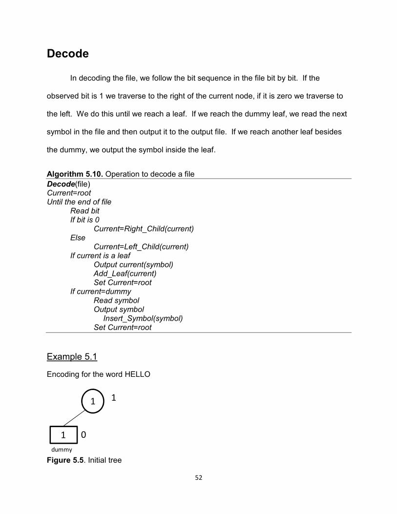
Decode
In decoding the file, we follow the bit sequence in the file bit by bit. If the
observed bit is 1 we traverse to the right of the current node, if it is zero we traverse to
the left. We do this until we reach a leaf. If we reach the dummy leaf, we read the next
symbol in the file and then output it to the output file. If we reach another leaf besides
the dummy, we output the symbol inside the leaf.
Algorithm 5.10. Operation to decode a file
Decode(file) Current=root Until the end of file Read bit If bit is 0 Current=Right_Child(current) Else Current=Left_Child(current) If current is a leaf Output current(symbol) Add_Leaf(current) Set Current=root If current=dummy Read symbol Output symbol Insert_Symbol(symbol) Set Current=root
Example 5.1
Encoding for the word HELLO
Figure 5.5. Initial tree
1 1
1 0
dummy

53
Figure 5.6. Inserting “H”. Operation: output 0, output “H”, insert H
Figure 5.7. Inserting “E”. Operation: output 0, output “E”, insert “E”, reorder tree
Figure 5.8. Inserting “L”. Operation: output 10, output “L”,insert “L”, reorder tree
Figure 5.9. Adding “L”. Operation: output 01,increment “L”, reorder tree
Figure 5.10. Inserting “O”. Operation: output 00, output “O” insert “O”, reorder tree
1 1
1 0
dummy
11
1 0
dummy
1 1
H
2 2
1 0
dummy
root
1 1
H
2 2
1 0
dummy
root
1 3
H
2 4
root
1 1
E
2 2
1 0
dummy
2 4
root
11
E
2 3
1 0
dummy
1 2
H
46
3
1 3
5
E
2 4
root
11
E
2 3
1 0
dummy
1 2
H
4 6
3
1 3
14
H5
E
1 0
dummy
2
1 1
2
L
1 0
dummy
2
1 1
2
L
14
H
46
3
1 3
5
E
1 0
dummy
2
11
2
L
14
H
46
3
1 3
5
E
1 0
dummy
2
21
2
L
14
H
46
3
2 3
5
L1 0
dummy
2
11
2
E
14
H
46
3
2 3
5
L
1 0
dummy
2
11
2
E
14
H
6 8
3 7
1 4
H
3 6
52
L
13
E
1 0
dummy
2 2
1 1
O
6 8
4 72 6
13
E
12
H
1 0
dummy
2 4
1 1
O
52
L

54
Decoding Input buffer: 0H0E10L0100O
Figure 5.11. Initial tree
Figure 5.12. Read 0. Read “H”. Operation: output “H”, insert H
Figure 5.13. Read 0. Read “E”. Operation: output “E”, insert “E”, reorder tree
Figure 5.14. Read 01. Read “L”. Operation: output “L”, insert “L”, reorder tree
Figure 5.15. Read 01. Operation: output “L”, increment “L”, reorder tree
1 1
1 0
dummy
1 1
1 0
dummy
11
1 0
dummy
1 1
H
2 2
1 0
dummy
root
1 1
H
2 2
1 0
dummy
root
1 3
H
2 4
root
1 1
E
2 2
1 0
dummy
2 4
root
11
E
2 3
1 0
dummy
1 2
H
46
3
1 3
5
E
2 4
root
11
E
2 3
1 0
dummy
1 2
H
4 6
3
1 3
14
H5
E
1 0
dummy
2
1 1
2
L
1 0
dummy
2
1 1
2
L
14
H
46
3
1 3
5
E
1 0
dummy
2
11
2
L
14
H
46
3
1 3
5
E
1 0
dummy
2
21
2
L
14
H
46
3
2 3
5
L1 0
dummy
2
11
2
E
14
H

55
Figure 5.16. Read 00. Read “O”. Operation: output “O” insert “O”, reorder tree
Figure 5.17. Decoding flowchart
In this chapter, we implement an adaptive Huffman algorithm that satisfies both
the sibling property and Vitter’s implicit numbering. There are several differences
between this implementation and Vitter and FGK. The first different is that instead of
updating the tree before adding a new symbol to the tree, this implementation updates
after the symbol is added. The second difference is that the dummy node is given a
46
3
2 3
5
L
1 0
dummy
2
11
2
E
14
H
6 8
3 7
1 4
H
3 6
52
L
13
E
1 0
dummy
2 2
1 1
O
6 8
4 72 6
13
E
12
H
1 0
dummy
2 4
1 1
O
52
L
dummy
leaf?
Output
symbol
Insert new
symbol
Is end
of file?
Start
End
Read symbol
Add to
symbol
Read bit
Output
symbol
Bit?Go to right
child
Go to left
child
Is
node a
leaf?
Go to root
node

56
weight of one instead of zero. This changes the updates when a new unobserved
symbol is inserted into the tree. The new parent node moves up the tree quicker in the
beginning of the files.

57
Chapter 6
Simulation Results
For the results we created six files with differing measures of information. The
files were compressed using adaptive Arithmetic coding, Huffman coding, and modified
Arithmetic coding. The main testing parameter is the compression ratios of the various
algorithms.
Files
There were three file types used in the compressions: character file, language
text, and image files. The character files were sequences of characters in no particular
order. The first file, Chars2.txt, was a 108732 byte character file. It was high entropy
and low redundancy. The second file was a 200889 byte character file. The file was
low entropy, high redundancy file. For the language files, two files were used. The first
file was a 152089 byte file of English text, and the second file was a 133754 byte file of
French text. The image files consisted of a 141168 byte simple image, Simple.bmp,
and a 109674 byte complex image, Logo.bmp.
Results
As expected, Arithmetic coding yielded slightly better compression ratios than the
Huffman coding. In complex files the normal Arithmetic coding yielded results slightly
better than the modified version by less than a percent. On the simple files the modified

58
version created two or three partitions. In the instance of the simple image file, it
outperformed the Arithmetic coding.
In the results, the modified coder was able to take advantage of the
characteristics of the files to produce a file with more partitions and satisfactory
compression ratio. In the more complex files, chars2.txt and Logo.bmp, the coder was
conservative. The slight loss of compression arose from the processing overhead. In
the other files, the coder was able to partition into two or more blocks.
(a) (b)
(c) (d)
(f)(e)
Figure 6.1. (a) Chars2.txt (b) Chars.txt (c) English.txt (d) French.txt (e) Logo.bmp (f) Simple.bmp Table 6.1. Compression Results
File Attributes Compression Attributes
File Name File Size Algorithm Size Partitions Ratio
chars2.txt 108732
Adapt. Huffman 84553 1 0.222372439
Normal Adapt. Arithmetic
Coding 82615 1 0.240196078
Modified Arithmetic
Coding 82623 1 0.240122503
Continued on next page
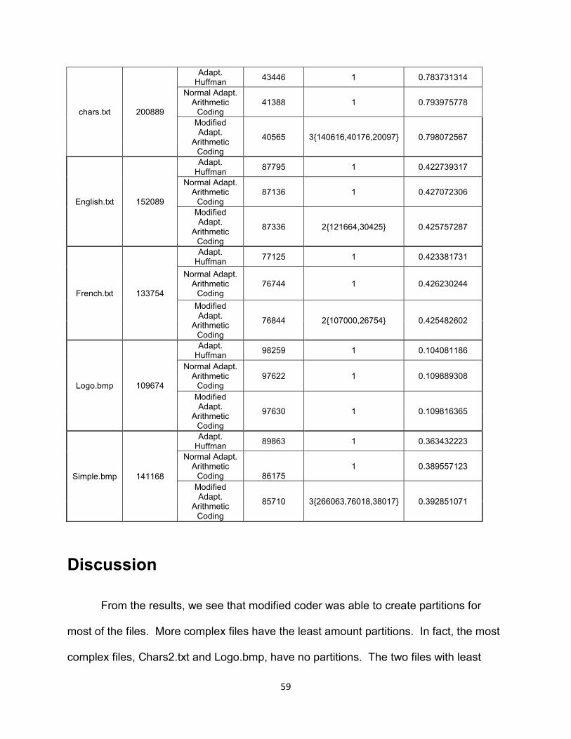
59
chars.txt 200889
Adapt. Huffman
43446 1 0.783731314
Normal Adapt. Arithmetic
Coding 41388 1 0.793975778
Modified Adapt.
Arithmetic Coding
40565 3140616,40176,20097 0.798072567
English.txt 152089
Adapt. Huffman
87795 1 0.422739317
Normal Adapt. Arithmetic
Coding 87136 1 0.427072306
Modified Adapt.
Arithmetic Coding
87336 2121664,30425 0.425757287
French.txt 133754
Adapt. Huffman
77125 1 0.423381731
Normal Adapt. Arithmetic
Coding 76744 1 0.426230244
Modified Adapt.
Arithmetic Coding
76844 2107000,26754 0.425482602
Logo.bmp 109674
Adapt. Huffman
98259 1 0.104081186
Normal Adapt. Arithmetic
Coding 97622 1 0.109889308
Modified Adapt.
Arithmetic Coding
97630 1 0.109816365
Simple.bmp 141168
Adapt. Huffman
89863 1 0.363432223
Normal Adapt. Arithmetic
Coding 86175 1 0.389557123
Modified Adapt.
Arithmetic Coding
85710 3266063,76018,38017 0.392851071
Discussion
From the results, we see that modified coder was able to create partitions for
most of the files. More complex files have the least amount partitions. In fact, the most
complex files, Chars2.txt and Logo.bmp, have no partitions. The two files with least

60
complexity, Chars.txt and Simple.bmp, created three partitions each. The two files with
English and French text created two partitions each.
The files with lower entropy are more likely to be partitioned because the left side
of the equation '1 BCDEFEFCG B '()*2B ' is smaller for those files.
This makes the test for partition more likely to pass.
Taking a close examination of the partitions created by the coder, we see that the
first partition is significantly larger than the subsequent partitions. The reason for this is
in the way that future symbols are predicted. Our Markov model starts by creating
symbols based on the previous occurrences and transitions of the symbols. After all the
symbols have been visited for at least their frequency of occurrence in the files, all the
symbols are equally probable. All subsequent symbol predictions will visit any symbol
with equal frequency. Therefore, the entropy of the generated symbols will approach
maximum entropy. This maximum entropy increases with ratio of remaining file size to
current segment size, N/n. The higher the ratio, the higher that entropy becomes.
Therefore, N≈N-n and Happrox,total≈log2(N-n). Once the test for the partition condition is
administered using '1 BCDEFEFCG B '()*2B ' , the right side will
approach zero. In order for the test to pass, n has to be significantly large and H1 has to
be significantly low.

61
Conclusions and Future Work
In this thesis we covered the theory of data compression. We created
implementations of Huffman and Arithmetic coding. We optimized the compression
ratio of a system using Arithmetic coding and Markov models. We were able to create a
greedy algorithm that partitions the data by predicting compression size. We also
showed in our simulations that our partitions show little loss in compression ratio, and,
at times, it improved the compression ratio.
Next efforts in optimizing the data compression system would be in combining
our technique with data preprocessing techniques. In particular, we can use techniques
such as Run-length encoding, Burrows-Wheeler transform, and Move-To-Front coding
[1]. Each of these techniques changes the complexity of data, therefore, changing the
effect of predictive compression.
Markov prediction models can also be applied to other compression techniques.
We can explore its application to video compression. We compare Markov prediction to
existing variable block size techniques used in video. One of the classical problems in
video and image compression is DCT block size selection. We can study how to apply
prediction to solve this problem.
Now that we have shown its effectiveness in a data compression system, the
next step is to show how the system would help in classical packet optimization
situations. These include wireless systems where noise is high and highly congested
systems with high packet loss. We can next study the effects of constraining the packet
sizes based not only on measures of noise and congestion, but also our reduction of
compression ratio.

62
Bibliography
1. Blellock, Guy E. "Introduction to Data Compression." Carnegie Mellon University. 16 October 2001.
2. Bodden, E., Clasen, M., & Kneis, J. (2002). Arithmetic Coding Revealed: A
guided tour from theory to praxix. Seminar Data Compression . 3. Cleary, John G., Radford M. Neal, and Ian H. Witten. "Arithmetic Coding for Data
Compression." Communications of the ACM 30(1987): 520-540.
4. Eytan, Modiano. "An Adaptive algorithm for optimizing the packet size used in wireless ARQ protocols." Wireless Networks 5(1999): 279-286.
5. Gallager, R. G., 1978. Variations on a theme by Huffman. IEEE Transactions on
Information Theory, Vol. 24, pp. 668-674, November 1978.
6. Hoffman, Roy. Data Compression in Digital Systems. New York: Chapman & Hall, 1997.
7. Khalid, Sayood. Lossless Compression Handbook. San Diego: Academic Press
Series in Communications, Networking, and Multimedia, 2003.
8. Korhonen, Jari, and Wang. "Effect of Packet Size on Loss Rate and Delay in Wireless Links." IEEE Communications Society 3(2005): 1608 - 1613.
9. Massey, Greg, and Jon McClintock. "Packet Size Matters in IP Transport." Radio
World 2006:
10. Moffat, Alistair, Radford M. Neal, and Ian H. Witten. "Arithmetic Coding Revisited." ACM Transactions on Information Systems 16(1998): 256-294.
11. Pu, Ida Mengyi. Fundamental Data Compression. Oxford: Butterworth-
Heinemann, 2006.
12. Roman, Steven. Coding and Information Theory. New Work: Springer-Verlag, 1992.
13. Ross, Sheldon M. Introduction to Probability Models. 8. New Work: Academic
Press, 2003.
14. Saeed, Faisel, Huizhu Lu, and G. E. Hedrick. “Data compression with Huffman coding; an efficient dynamic implementation using file partitioning." Proceedings of the 1990 Symposium on Applied Computing (1990): 348-354.

63
15. Shannon, Claude E., and Warren Weaver. The Mathematical Theory of Communciation. 1. Chicago: The University of Illinois Press, 1969.
16. Vitter, J.S, 1987. Design and analysis of dynamic Huffman codes. Journal of the
ACM, Vol. 34, pp. 823-843, October 1987.

64
Vita
Claudio Iombo is a native of Cabinda, Angola. Angola is a country in the Southwest
coast of the continent of Africa. He is a graduate of Louisiana State University in
electrical and computer engineering in December 2003. He is currently a candidate for
master’s degree in the Department of Electrical and Computer Engineering at Louisiana
State University. His interests include communication and software systems design.


