Embed Size (px)
Citation preview

Efficient and Reliable Solvency II Loss Estimates
With Deep Neural Networks
Zoran NIKOLICDeloitte Germany / Partner
Ning LINDeloitte France / Senior manager
May 11th – May 15th 2020

About the speaker
Zoran NIKOLIĆ
Partner
Deloitte Germany
Zoran is partner in the Actuarial Insurance department of Deloitte German office.
During his 13 years’ experience, Zoran has got a solid background : on modelling insurance (Life and P&C), economics generator scenario, solvency 2, accountings projects and machine-learning.
Zoran is head of the marketing development on machine learning application and industrialization for the insurance company.
Ning LIN
Senior manager
Deloitte France
Ning is senior manager in the Actuarial Insurance department of Deloitte Paris office.
During his 9 years’ experience, Ning has built up a solid modelling background on insurance (Life and P&C) and finance. Ning has also worked a lot around financial performances : reporting, business plan, optimization of French Gap result and Solvency 2 ratio.

Context – Solvency II and Internal Model

Solvency II and SCR (Solvency Capital Requirement)
◼ Solvency II is an EU Directive that codifies and harmonizes the EU insurance regulation.
◼ Solvency Capital Requirement (SCR) is the minimum capital required to ensure that the (re)insurance company will be able to meet its obligations over the next 12 months with a probability of at least 99.5%
◼ SCR can be calculated using:
SCR = VAR 99,5% (loss in one year)
▪ either a standard formula given by the regulators (risks considered, level of stress, correlation matrix etc.)
▪ or an internal model developed by the (re)insurance company
Structure of Standard formula

Nested simulation – the theorical approachHow should the SCR be calculated with an internal
model?
• Project distribution of own funds in 1 year
– For Life liabilities with guarantees, this would
require many thousand real world scenarios with
thousands of market consistent scenarios for
every real world (RW) scenario
• Calculate the difference between simulated own
funds and current own funds to obtain losses in
each scenario
• Order losses to construct a distribution and pick
99.5th percentile to obtain the 1 in 200 loss
Illustrative: nested stochastics
Shocked own funds
Many thousand
one-year RW
stresses
Full run of actuarial/asset
models for each of the
RW one-year out stresses
TNT0 T1
1 in 200 i.e. 99.5th
percentile
Loss distribution
1
2
1 2
What is the challenge?
◼ For insurers with complex organizational structures and portfolios where liabilities have options and guarantees, computational challenges make this approach impossible to achieve
a b
3
3
C

◼ Complex interaction within companies and liabilities have options and guarantees pose computational challenges which make this approach infeasible
LSMC Methodology Design FrameworkLeast Squares Monte Carlo
Fast and business-
effective SCR
computation
Nested simulation LSMC
◼ Each real world scenario is valuated for a very limited number of risk neutral scenarios (e.g. 2)
◼ A function is calibrated based on the these fitting points

◼ Monte Carlo proxy modelling approach combined with least squares regression
◼ Fits a (multi-dimensional) regression surface through approximate Monte Carlo valuations
Approximate Monte Carlo Valuations
Approximate market consistent values
In classical LSMC
polynomials are used
as proxy functions
LSMC Methodology Design FrameworkLeast Squares Monte Carlo

Neural Networksapplication for
approximation of Risk Capital

Introduction to Our Use Case
◼ Core idea: Use the same LSMC approach which is already successfully implemented in the industry, but substitute polynomials with neural networks.
◼ Neural networks can be used to very sophisticated real-life problems, but they can also perform a“normal“ regression through LSMC fitting points.
◼ A neural network consists of:
• A set of nodes (neurons) connected by links
• A set of weights associated with links
• A set of thresholds or levels of activation
◼ A design of a neural network requires:
• The choice of the number and type of units
• The determination of the morphological structure (layers)
• Setting up of other parameters of the training process
• Initialization and training of the weights on the interconnections
through the training set

Settings and Data
15 – 16 inputs describing 1y stresses:
◼ changes in the risk-free yield curves
◼ performance of equity
◼ performance of property
◼ credit risk
◼ Mortality level/trend
◼ Longevity level/trend
◼ expenses
Predict: Best Estimate Liabilities conditional on 1y real
world stresses (1 output)
Outputs
Inputs
Training Set
◼ 6,000 or 25,000 1y real world scenarios
◼ 2 risk neutral simulations
Validation Set
◼ 256 1y real world scenarios
◼ With each 1,000 risk neutral simulations
99.5% Value-at-Risk Set (VaR Set)
◼ 49 real world scenarios
◼ With each 4,000 risk neutral simulations
Base Scenario
◼ 16,000 risk neutral simulations
(The real target is SCR = Base – 99.5% VaR)
Target
Training
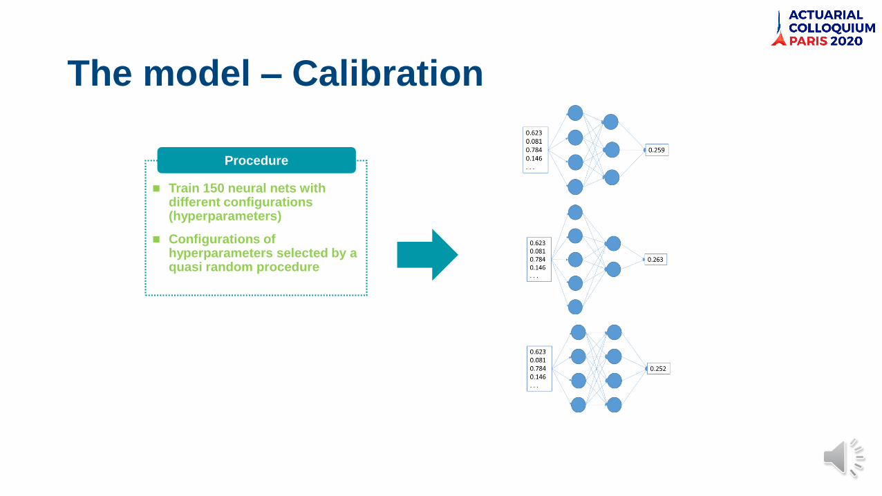
The model – Calibration
◼ Train 150 neural nets with different configurations (hyperparameters)
◼ Configurations of hyperparameters selected by a quasi random procedure
Procedure

The model – Calibration
◼ Train 150 neural nets with different configurations (hyperparameters)
◼ Configurations of hyperparameters selected by a quasi random procedure
◼ Select best 10 models
◼ Based on mean absolute error (MAE) in validation set
Procedure

The model – Calibration
◼ Train 150 neural nets with different configurations (hyperparameters)
◼ Configurations of hyperparameters selected by a quasi random procedure
◼ Select best 10 models
◼ Based on mean absolute error (MAE) in validation set
◼ Build ensemble (by averaging over 10 best models)
Procedure
Avera
ge
0.258
Important: VaR Set & Base Scenario
unseen in Training

The model – Calibration
Hyperparameters
◼ Batch size: 150 – 450
◼ Layers: 3 – 7
◼ Dropout: 0 – 0.4 (constant after each layer)
◼ Nodes: 50 – 200 (constant in each layer)
◼ Initializers: [uniform, glorot, normal]
◼ Learning Rate: 0.0007 – 0.0015
Fixed for all configurations
◼ Optimizer: adam
◼ Activation: sigmoid
Quasi Random Search

Results
◼ Company 1 / Company 2 / Company 3 / Company 4, three life and one health insurer
◼ Run procedure with both 6k and 25k training samples (real world fitting scenarios in the classical LSMC language
◼ Run each procedure twice in order to see whether the results are very unstable
◼ Polynomial regression from classical LSMC as explained above – the current state-of-the-art proxy model in the insurance industry
◼ For the sake of simplicity we have always used 25k training samples (even when comparing with 6k training samples in neural networks)
4 different datasets Benchmark

Results
1 On a laptop with nvidia GeForce 940MX. Only rough reference time - not reproducibly measured as laptop was used
otherwise during training.
For 6k training samples and all four companies - 99.5 % VaR
◼ 6K Training Samples
◼ Runtime: ~3-6h 1
▪ Can be parallelized trivially
◼ Significantly better thanbenchmark
◼ Appears very stable within and across companies
99.5% Value at Risk Set

Results
◼ 6K Training Samples
◼ Similar to benchmark
▪ Except for Company 4
◼ Seems stable within and across companies
Base Scenario
For 6k training samples and all four companies - Base Scenario

Results
1 On a laptop with nvidia GeForce 940MX. Only rough reference time - not reproducibly measured as laptop was used
otherwise during training.
◼ 25k Training Samples
◼ Runtime: ~10-20h ^1
▪ Can be parallelized trivially
◼ Significantly better than benchmark
◼ Seems stable within and across companies
Base Scenario
For 25k training samples and all four companies - 99.5% VaR

Results
◼ 25K Training Samples
◼ Significantly better than benchmark
◼ Seems very stable within and across companies
Base Scenario
For 25k training samples and all four companies - Base Scenario

Summary
87,8
43,5
15,30
20
40
60
80
100
Avera
ge A
bsolu
te E
rror
Base Scenario
Benchmark ANN 6k ANN 25k
0,206
0,066 0,0540
0,05
0,1
0,15
0,2
0,25
Avera
ge A
bsolu
te M
ean
Err
or
[%]
Value-at-Risk 99.5% Set
Benchmark ANN 6k ANN 25k
Average over all tested companies and
ensemblesAverage over all tested companies and
ensembles
◼ Good stability of the procedure
◼ Further tests with other configurations planned (e.g. not only sigmoid)
◼ Significantly better than classical LSMC on both Base Scenario and Value-at-Risk 99.5% set, even when a smaller number of training samples than in the LSMC benchmark used

Thank you for your attention
Contact details :
Zoran NIKOLIĆ
Partner
Deloitte Germany
Phone: + 49 221 9732416
E-Mail: [email protected]
Ning LIN
Senior Manager
Deloitte France
Phone: + 33 01 55 61 68 94
E-Mail: [email protected]
https://www.actuarialcolloquium2020.com/
Deloitte - A leading professional
services firm worldwide

Disclaimer:
The views or opinions expressed in this presentation are those of the authors and do not necessarily reflectofficial policies or positions of the Institut des Actuaires (IA), the International Actuarial Association (IAA) andits Sections.
While every effort has been made to ensure the accuracy and completeness of the material, the IA, IAA andauthors give no warranty in that regard and reject any responsibility or liability for any loss or damageincurred through the use of, or reliance upon, the information contained therein. Reproduction andtranslations are permitted with mention of the source.
Permission is granted to make brief excerpts of the presentation for a published review. Permission is alsogranted to make limited numbers of copies of items in this presentation for personal, internal, classroom orother instructional use, on condition that the foregoing copyright notice is used so as to give reasonablenotice of the author, the IA and the IAA's copyrights. This consent for free limited copying without priorconsent of the author, IA or the IAA does not extend to making copies for general distribution, for advertisingor promotional purposes, for inclusion in new collective works or for resale.


