Embed Size (px)
Citation preview

arX
iv:1
503.
0590
9v2
[m
ath.
ST]
9 M
ar 2
016
PRINCIPAL COMPONENT ANALYSIS FOR SEMIMARTINGALES AND
STOCHASTIC PDE
ALBERTO OHASHI AND ALEXANDRE B. SIMAS
Abstract. In this work, we develop a novel principal component analysis (PCA) for semimartingalesby introducing a suitable spectral analysis for the quadratic variation operator. Motivated by high-dimensional complex systems typically found in interest rate markets, we investigate correlation in
high-dimensional high-frequency data generated by continuous semimartingales. In contrast to thetraditional PCA methodology, the directions of large variations are not deterministic, but ratherthey are bounded variation adapted processes which maximize quadratic variation almost surely.This allows us to reduce dimensionality from high-dimensional semimartingale systems in terms ofquadratic covariation rather than the usual covariance concept.
The proposed methodology allows us to investigate space-time data driven by multi-dimensionallatent semimartingale state processes. The theory is applied to discretely-observed stochastic PDEswhich admit finite-dimensional realizations. In particular, we provide consistent estimators for finite-dimensional invariant manifolds for Heath-Jarrow-Morton models. More importantly, componentsof the invariant manifold associated to volatility and drift dynamics are consistently estimated andidentified. The proposed methodology is illustrated with both simulated and real data sets.
Contents
1. Introduction 21.1. Contributions 21.2. Organization of the paper 52. Assumptions and Preliminary Results 62.1. Notation 62.2. Analysis of quadratic variation matrices 63. Random directions and principal components 94. Bounded variation component and quadratic variation in M 124.1. Correlation in d-dimensional asset prices 124.2. Stochastic PDEs with finite-dimensional realizations 124.3. Noise dimension vs quadratic variation dimension 135. Estimation of (W ,D) 155.1. Identification of the Spaces (W ,D) 155.2. Estimation of the spaces (W ,D) 166. Estimation of Finite-Dimensional Invariant Manifolds 206.1. Splitting the invariant manifold 206.2. Preliminaries on Factor models 246.3. Estimating the underlying dimension 256.4. Main Results 297. Simulation Studies and Applications 37
Date: March 10, 2016.1991 Mathematics Subject Classification. Primary: ; Secondary:Key words and phrases. Principal component analysis, factor models, semimartingales.The first author would like to thank the Mathematics department of ETH Zurich and Forschungsinstitut fur Math-
ematik (FIM) for the very kind hospitality during the first year of this research project. In particular, he would liketo thank Josef Teichmann for inspirational discussions about finite dimensional realizations of stochastic PDEs and forhis encouragement to study their statistical aspects. We also would like to thank M. Laurini for useful discussions onPCA .
1

2 ALBERTO OHASHI AND ALEXANDRE B. SIMAS
7.1. Semimartingale PCA 377.2. Variance versus quadratic variation 387.3. Estimating finite-dimensional realizations from a SPDE 397.4. Application to real data sets 438. Appendix: Estimating dim Q 46References 53
1. Introduction
Dimension reduction techniques have been intensively studied over the last years due to the adventof high-dimensional data in a variety of applied fields. Towards an effective reduction dimension, itis crucial to interpret correctly what kind of lower dimensional manifold one has to find in order torepresent the data properly. For instance, if the second moment structure reasonable describes thedynamics in the data, then the classical Principal Component Analysis (henceforth abbreviated byPCA) and its various extensions are the natural candidates to reduce dimensionality.
There are many cases where correlation in high-dimensional systems may not be accurately de-scribed by covariance structures. An important example is the correlation typically found in high-frequency data which is better described by the so-called quadratic variation matrix
[M ]t := [M i,M j ]t; 1 ≤ i, j ≤ d; 0 ≤ t ≤ T,
where M = (M1, . . . ,Md) is a d-dimensional semimartingale sampled over the time horizon [0, T ] and[M i,M j ] is the quadratic covariation process between M i and M j .
In a financial context, the process [M ]· is called the volatility matrix (sometimes called integratedvolatility). The total amount of volatility in a d-dimensional semimartingale system over [0, t] is fullydescribed by the following quantity
‖[M ]t‖2(2) =d∑
j=1
(λjt )
2,
where λjtdj=1 are the random eigenvalues of [M ]t and ‖ · ‖(2) is the usual Hilbert-Schmidt norm.
Volatility is by far the most important quantity which needs to be estimated for asset pricing, assetallocation and risk management, specially in high-dimensional portfolios. The estimation of high-dimensional quadratic variation matrices has been a topic of great interest in the last years. We referthe reader to the works [10, 50, 51, 39, 52, 18, 23, 21] and other references therein.
Despite all the recent progress on volatility matrix estimation, there has been remarkably littlefundamental theoretical study on dimension reduction techniques based on high-dimensional quadraticvariation matrices. One notorious difficulty is the dynamic interpretation of directions and principalcomponents over the time horizon which in typical cases is formulated in a high-frequency domain.Indeed, [M ]t; 0 ≤ t ≤ T is fully random which makes the analysis more evolved than the standardPCA. More precisely, all the potentially optimal projections will be stochastic processes rather thandeterministic vectors.
In view of the fact many correlation structures in high-dimensional data are fully representedby the quadratic variation concept, it is natural and necessary to construct a dimension reductionmethodology strictly associated to [M ] rather than on classical covariance or conditional distributions.This is the program we start to carry out in this paper.
1.1. Contributions. Let M = (M1, . . . ,Md) be a d-dimensional semimartingale. The starting pointof the analysis is to solve an identification problem related to a possible singularity of the randommatrix [M ]T which can be typically found e.g in large portfolios of financial assets (see e.g Burashi,Porchia and Trojani [16], Ait-Sahalia and Xiu [4] and Fan, Li and Yu [23] and other references therein)

PRINCIPAL COMPONENT ANALYSIS FOR SEMIMARTINGALES AND STOCHASTIC PDE 3
and affine term structure models (see e.g Bjork and Landen [15] and Filipovic [29] and Filipovic andSharef [27]). More precisely, in the presence of non-trivial correlation among semimartingales, one hasrank [M ]T < d a.s and then, under mild assumptions, one can split the set M = span M1, . . . ,Mdinto two complementary linear spaces (W ,D) such that
M = W ⊕Dwhere W and D contains only elements of M with non-zero and zero quadratic variation, respectively.The space W fully describes the volatility structure of M while D is responsible for its hidden puredrift (null quadratic variation) dynamics. At this point, we stress that the potential singularity of thequadratic variation matrix [M ]T introduces non-observable drift components into M which cannot bediscarded in a high-frequency situation. Both spaces are equally important to explain the dynamicsof M in a given physical probability measure. In strong contrast, directions with null variance can befully discarded in the classical PCA. This is the first major difference between the classical PCA andthe theory developed in this article.
We follow the natural and simple idea to seek random variables vt = (v1t , . . . , vdt ) such that
d∑
j=1
vjtMjt
has the largest possible instantaneous quadratic variation over [0, t], where vt is interpreted as a randomcoefficient at time t ∈ [0, T ] rather than a process. By iterating this procedure in an orthogonal way,we shall get a linear transformation of M which under some mild primitive conditions will be afinite-dimensional semimartingale ranked in terms of quadratic variation. Starting with consistent
estimators [M ]T for the quadratic variation matrix [M ]T (see e.g [19, 50, 51, 39, 52, 18, 23, 21] andother references therein), we are able to propose consistent estimators for (W ,D) by means of a
simple eigenvalue analysis of [M ]T based on high-frequency observations of M . This allows us toreduce dimensionality in terms of quadratic variation in a very clear and consistent way. Equallyimportant, the methodology also estimates bounded variation components in D which can not beneglected in multi-dimensional semimartingale systems.
The PCA for semimartingales introduced in the first part of the article is applied to the estimationof principal components of discretely-observed space-time semimartingales which describe stochasticpartial differential equations (henceforth abbreviated by stochastic PDEs) admitting finite-dimensionalrealizations. In particular, in the second part of this article, we illustrate the theory by studying theproblem of the estimation of the so-called finite-dimensional invariant manifolds w.r.t to a stochasticPDE
(1.1) drt =(A(rt) + F (rt)
)dt+
m∑
j=1
σj(rt)dBjt ; r0 = h ∈ E; 0 ≤ t ≤ T,
whereE is a potentially infinite-dimensional Sobolev-type space of continuous functions and (A,F, σi; 1 ≤i ≤ m) satisfy standard assumptions for the existence of solution.
Many space-time phenomena in natural and social sciences can be described by solutions of sto-chastic PDEs like (1.1). However, the intrinsic infinite-dimensionality of space-time data generatedby models like (1.1) creates a big challenge in the statistical analysis of these models. In particularcases, it is well-known that one can reduce dimensionality and still get a very rich class of space-timedata generated by models of type (1.1). For instance, under Lie algebra conditions (see Filipovic andTeichmann [25] and Bjork and Svensson [14]) on the coefficients of (1.1), it is well known that thereexists a family of affine manifolds Gt; 0 ≤ t ≤ T of curves and a d-dimensional semimartingale factorprocess M such that

4 ALBERTO OHASHI AND ALEXANDRE B. SIMAS
(1.2) rt(·) = Gt(·,Mt); r0 = h; 0 ≤ t ≤ T,
where G = Gt(·;x);x ∈ X ⊂ Rd; 0 ≤ t ≤ T ⊂ E is a finite-dimensional parameterized family ofsmooth curves. We shall write it as Gt = φt+V where V is a d-dimensional vector space generated bysmooth curves and φ is an E-valued smooth parametrization which we assume to be a zero quadraticvariation function.
Two central unsolved problems in the stochastic PDE modelling are: (i) the construction of sta-tistical tests to check existence of G and (ii) the development of related estimation methods. Theimportance of this research agenda can be mainly understood in applications to interest rate mod-elling and other term-structure problems in Mathematical Finance. The literature is vast so we referthe reader to e.g [13, 14, 15, 24, 25, 28, 29, 26, 44, 49, 34, 41, 7, 46, 40] and other references therein.In short, under the assumption of existence of G, the estimation of V is essential for a consistentcalibration of potentially infinite-dimensional term-structure models.
Under the assumption that the stochastic PDE (1.1) admits an affine finite-dimensional repre-sentation (1.2), we apply the semimartingale PCA to estimate and identify components of invariantmanifolds G which depicts volatility and drift dynamics in space. More precisely, let us consider thefinite rank random linear operator QT : E → V defined by
QT f := 〈QT (·, ), f〉E ; f ∈ E,
where QT (u, v) := [r(u), r(v)]T ;u, v ≥ R+, 〈·, ·〉E is the inner product of E and we setQ := range QT .We notice the quadratic variation of the stochastic PDE (1.1) is fully generated by QT . In particular,the associated Hilbert-Schmidt norm
‖QT ‖2(2) =dim V∑
j=1
θ2j
fully describes the total amount of energy related to the quadratic variation of (1.1) over [0, T ]. Here,θidim V
i=1 are the eigenvalues of QT arranged in decreasing order.In general, dim Q ≤ dim V a.s, but in typical situations we do have dim Q < dim V 1. Let N be
the complementary subspace of Q in V . Under mild assumptions, we have the following splitting
V = Q⊕N a.s.
In one hand, the pair of subspaces (Q,N ) should be considered as the analogous spaces to (W ,D)but in the spatial variable. On the other hand, we stress that M is not observed and (1.2) is treatedas a factor model
(1.3) rt = φt +
dim V∑
j=1
M jt λj ;V = span λ1, . . . , λd
with dimension d = dim Q + dim N . The present methodology allows us to estimate and identifydirections of the invariant manifold which come from the volatility (represented by Q) and the drift(represented by N ). More importantly, we are able to identify them separately which allows us toestimate null and non-null quadratic variation factors by projecting space-time data of the form (1.3)
onto a pair of estimated vector spaces (Q ⊕ N ). We consider this separation feature as the mostimportant aspect of the second part of this article. As a by-product, our methodology brings two
1The empirical literature on interest rate modelling reports strong evidence of correlation among risk factors (seee.g [3, 43, 17]) which suggest that one can typically find dim Q < dim V in case of affine models. From theoretical side,this phenomena is also related to no-arbitrage restrictions imposed on affine models. See e.g [14, 26, 27, 1, 2] and otherreferences therein.

PRINCIPAL COMPONENT ANALYSIS FOR SEMIMARTINGALES AND STOCHASTIC PDE 5
contributions to the field: It provides a consistent volatility dimension reduction and a method toestimate hidden pure drift components in space-time semimartingale data generating processes.
Our methodology is a combination of classical factor models jointly with suitable random trans-formations over the space of latent semimartingales. More precisely, our approach consists essentiallyin two steps: Firstly, we apply an empirical covariance operator onto the space-time data to obtain afactor decomposition of the form
rt(x) =k∑
j=1
Y kt λk(x), t ∈ Π, x ∈ Π′
in the spirit of discrete-type factor models (see e.g Stock and Watson [47], Bai [9] and Bai and Ng [8]),but in a high-frequency setup as opposed to the usual panel data. In other words, Π×Π′ is a refiningpartition of a two-dimensional set [0, T ] × [a, b]. In linear structures, the covariance operator onlyneglects components of null empirical variance so that, under suitable conditions, our first step doesnot loose information from the invariant manifold V = Q⊕N . The second step consists in using the
semimartingale PCA jointly with suitable random rotations of latent factor estimators Yt to infer theunderlying semimartingale structure of the data. It is not easy to foresee that this two-step procedurewould work. Indeed, to the best of our knowledge it is not known that the covariance operatordecomposition is strong enough to provide a resulting process which is amenable to a consistent
quadratic variation analysis. In fact, the sequence Yt is not even associated to a semimartingale, sothat the quadratic variation analysis based on this two-step procedure must be considered in a broadersense. The proof that this strategy works is the content of the second part of the paper.
It is important to stress the both steps in our methodology are equally important. For instance,the naive application of classical factor models to infer quadratic variation is non-sense when appliedto semimartingale systems. Moreover, a more straightforward strategy based directly on an empiricalquadratic variation does not work in full generality due to a possible singularity of the matrix. Thislast procedure forces the assumptions that dim V = dim Q which may not be optimal (in the mean-square sense) in typical situations when dim N > 0. This is the reason why the two-step procedurein this work is implemented. For instance, Pelger [42] studies principal components directly fromthe empirical quadratic covariation for factors with jumps and discrete loading factors. One crucialassumption in his setup is the non-singularity of the quadratic variation matrix which restricts theapplicability in multivariate systems with non-trivial correlation typically found in large portfoliosand interest rate models.
We should mention that another possible framework is introduced by Ait Sahalia and Xie [5]who interpret principal component analysis by means of the underlying volatility process. The maindrawback of this strategy is the fact that rank of the volatility matrix may be strictly smaller thandim [M ]T (as shown in Proposition 4.1), thus resulting in a substantial underestimation of dim Wand their associated factors. Therefore, similar to Pelger [42], the strategy introduced by [5] does notrecover in full generality the whole semimartingale stricture (M) involved in the optimal decompositiondue to a possible non-negligible dimension (dim D) associated to the drift. In addition, the strongassumption of simple eigenvalues imposed in [5] rules out many finite-dimensional semimartingalesystems typically found in applications.
1.2. Organization of the paper. The remainder of this article is structured as follows. Section 2presents some notation and preliminary results. Section 3 presents the spectral analysis on a genericquadratic variation matrix. Section 4 illustrates the existence of bounded variation components inportfolio management and interest rate models. Section 5 presents the consistency results for theestimators of the dynamic spaces. Section 6 presents the application of semimartingale PCA to theproblem of estimating finite-dimensional invariant manifolds for stochastic PDEs. Section 7 presentsthe numerical results and applications to real data. An Appendix is given in Section 8 which presentsan estimator for dim Q.

6 ALBERTO OHASHI AND ALEXANDRE B. SIMAS
2. Assumptions and Preliminary Results
At first, let us fix notation.
2.1. Notation. Throughout this article, we are going to work with a fixed stochastic basis of the form(Ω,FT ,F,P) where (Ω,FT ,P) is a probability space equipped with a sample space Ω, a sigma-algebraFT , probability measure P and a fixed terminal time 0 < T < ∞. We equip the interval [0, T ] withthe Borel sigma algebra BT and we assume the filtration F := Ft; 0 ≤ t ≤ T satisfies the usualconditions.
All the algebraic setup in this article will be based on the real linear space X d constituted by theset of all Rd-valued BT × FT -measurable processes. In this article, the most important subclass ofX d will be the subspace Sd constituted by the set of all Rd-valued continuous F-semimartingales on
(Ω,FT ,F,P). When d = 1, we set S := S1,X := X 1. We denote L0,kt as the set of all Rk-valued
and Ft-measurable random variables for k ≥ 1 and t ∈ [0, T ]. Throughout this article, we adopt thefollowing convention: If Y ∈ X d, then Yt is interpreted as a column random vector in Rd. Convergence
in probability will be denoted byp→.
In the remainder of this article, Π denotes a deterministic partition 0 = t0 < t1 < . . . < tn = Tand ‖Π‖ := max1≤i≤n|ti − ti−1|. The set Mp×q denotes the space of all p× q-real matrices and M
+p×p
is the subspace of p× p non-negative symmetric real matrices. The norm of linear operators betweenHilbert spaces will be the standard Hilbert-Schmidt norm ‖ · ‖(2) and P⊤ denotes the transpose of amatrix P ∈ Mp×q ; p, q ≥ 1. If A,B are two linear subspaces of X with A ⊂ B, then we denote πA
the usual projection of B onto the quotient space B/A. Throughout this article, we omit the variableω ∈ Ω when no confusion arises.
2.2. Analysis of quadratic variation matrices. In this work, the following bracket will play a keyrole in our analysis
(2.1) [X,Y ]t := lim‖Π‖→0
∑
ti∈Π
(Xti −Xti−1
)(Yti − Yti−1
); 0 ≤ t ≤ T,
in probability.
Definition 2.1. The quadratic covariation [X,Y ]t; 0 ≤ t ≤ T exists for a given pair (X,Y ) ∈ X 2
if the limit (2.1) exists for every sequence of partitions Π such that ‖Π‖ → 0. We say that X ∈ X hasnull quadratic variation if [X,X ]· = 0 a.s
Of course, [X1, X2]t; 0 ≤ t ≤ T is a well-defined bounded variation adapted process for every(X1, X2) ∈ S2. To shorten notation, we sometimes set [Y ] := [Y, Y ] for Y ∈ X . For a given X =(X1, . . . , Xd) ∈ X d and (t, ω) ∈ [0, T ]× Ω, with a slight abuse of notation, we write [X ]t(ω) ∈ M
+d×d
to denote the following random matrix
(2.2) [X ]t(ω) := [X i, Xj]t(ω); i, j = 1, . . . , d; 0 ≤ t ≤ T, ω ∈ Ω,
whenever the right-hand side of (2.2) exists.In the remainder of this section, M = (M1, . . . ,Md) is a given d-dimensional measurable process.
We say that M ∈ X d is truly d-dimensional if its components M1, . . . ,Md are linearly independentover the vector space X . Throughout this paper, we are going to assume the following standingassumptions:
Assumption 2.1. M is a truly d-dimensional measurable process.
Assumption 2.2. The quadratic variation matrix [M ]t; 0 ≤ t ≤ T exists and if there exists i =1, . . . , d such that P[M i,M i]t > 0 > 0 then we have P[M i,M i]t > 0 = 1.

PRINCIPAL COMPONENT ANALYSIS FOR SEMIMARTINGALES AND STOCHASTIC PDE 7
Remark 2.1. We clearly do not loose generality by imposing Assumption 2.1. Assumption 2.2 is verynatural since our theory relies on the study of a realization of the quadratic variation matrix, and thusit is necessary that we do not get a realization of null quadratic variation from a non-null quadraticvariation process.
Example: One typical example of semimartingale which satisfies Assumption 2.2 is given by the2d-Heston model (M i, V i); i = 1, . . . , d with correlation in [−1, 1] where V i denotes the ith square-root-type stochastic volatility component for i = 1, . . . , d. Then, one can easily check that for everyt ∈ (0, T ], we have
[M i,M i]t =
∫ t
0
|M is|2V i
s ds > 0 a.s for every i = 1, . . . , d.
Hence, the classical Heston model satisfies Assumption 2.2.
Let Mt := spanM1, . . . ,Md be the linear space spanned by the 1-dimensional measurable pro-cesses M1, . . . ,Md over [0, t] for 0 ≤ t ≤ T . Assumption 2.1 yields dimMt = d for every t ∈ (0, T ].Let us now split Mt into two orthogonal subspaces. At first, we set
(2.3) Dt := X ∈ Mt; [X ]t = 0 a.s.Observe that Dt is a well-defined linear subspace of Mt for every t ∈ [0, T ]. More importantly, thefollowing remark holds.
Remark 2.2. We recall that any continuous bounded variation local martingale must be constant a.s.Moreover, for every t ∈ (0, T ]
ω; [Y, Y ]t(ω) = 0 = ω ∈ Ω;N·(ω) = 0 over the interval [0, t]where N is the local martingale component of the special semimartingale decomposition of some Y ∈ S.Therefore, Assumption 2.2 allows us to state that if M ∈ Sd is a truly d-dimensional process, then Dt
is a subspace of Mt only constituted by continuous bounded variation adapted processes over [0, t].
Definition 2.2. Let Mt be the span generated by a truly d-dimensional measurable process M ∈ X d
over [0, t]. If dimDt > 0, then we say that Mt has a null quadratic variation component overthe interval [0, t]. In particular, if M ∈ Sd and dimDt > 0, then we say that Mt has a boundedvariation component over [0, t].
Let us give a toy example showing how a non-trivial dimension induced by bounded variationprocesses may appear in a very simple context.
Example: Let B be a one-dimensional Brownian motion and let Mt = (Bt, Bt + t); 0 ≤ t ≤ T.Of course, M is a truly 2-dimensional semimartingale where dim Mt = 2 for every t ∈ (0, T ]. Inparticular, we clearly have dim Dt = 1 for every t ∈ (0, T ].
For a deeper discussion of bounded variation components on semimartingale systems, we refer thereader to Section 4. Let us now provide a natural notion of “quadratic variation dimension” in Mt.To do so, let us consider the following quotient space
(2.4) Mt := Mt/Dt; 0 ≤ t ≤ T.
By definition, Mt can be identified by (Mt,∼) where the equivalence relation is given by
(2.5) X ∼ Y ⇔ X − Y is a null quadratic variation process in Mt over the interval [0, t].
8 ALBERTO OHASHI AND ALEXANDRE B. SIMAS
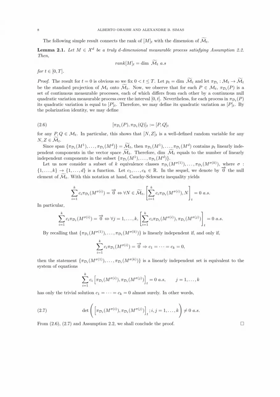
The following simple result connects the rank of [M ]t with the dimension of Mt.
Lemma 2.1. Let M ∈ X d be a truly d-dimensional measurable process satisfying Assumption 2.2.Then,
rank[M ]t = dim Mt a.s
for t ∈ [0, T ].
Proof. The result for t = 0 is obvious so we fix 0 < t ≤ T . Let pt = dim Mt and let πDt : Mt → Mt
be the standard projection of Mt onto Mt. Now, we observe that for each P ∈ Mt, πDt(P ) is aset of continuous measurable processes, each of which differs from each other by a continuous nullquadratic variation measurable process over the interval [0, t]. Nevertheless, for each process in πDt(P )its quadratic variation is equal to [P ]t. Therefore, we may define its quadratic variation as [P ]t. Bythe polarization identity, we may define
(2.6) [πDt(P ), πDt(Q)]t := [P,Q]t
for any P,Q ∈ Mt. In particular, this shows that [N,Z]t is a well-defined random variable for any
N,Z ∈ Mt.
Since span πDt(M1), . . . , πDt(M
d) = Mt, then πDt(M1), . . . , πDt(M
d) contains pt linearly inde-
pendent components in the vector space Mt. Therefore, dim Mt equals to the number of linearlyindependent components in the subset πDt(M
1), . . . , πDt(Md).
Let us now consider a subset of k equivalence classes πDt(Mσ(1)), . . . , πDt(M
σ(k)), where σ :
1, . . . , k → 1, . . . , d is a function. Let c1, . . . , ck ∈ R. In the sequel, we denote by−→0 the null
element of Mt. With this notation at hand, Cauchy-Schwartz inequality yields
k∑
i=1
ciπDt(Mσ(i)) =
−→0 ⇔ ∀N ∈ Mt,
[k∑
i=1
ciπDt(Mσ(i)), N
]
t
= 0 a.s.
In particular,
k∑
i=1
ciπDt(Mσ(i)) =
−→0 ⇔ ∀j = 1, . . . , k,
[k∑
i=1
ciπDt(Mσ(i)), πDt(M
σ(j))
]
t
= 0 a.s.
By recalling that πDt(Mσ(1)), . . . , πDt(M
σ(k)) is linearly independent if, and only if,
k∑
i=1
ciπDt(Mσ(i)) =
−→0 ⇒ c1 = · · · = ck = 0,
then the statement πDt(Mσ(1)), . . . , πDt(M
σ(k)) is a linearly independent set is equivalent to thesystem of equations
k∑
i=1
ci
[πDt(M
σ(i)), πDt(Mσ(j))
]t= 0 a.s, j = 1, . . . , k
has only the trivial solution c1 = · · · = ck = 0 almost surely. In other words,
(2.7) det
([πDt(M
σ(i)), πDt(Mσ(j))
]t; i, j = 1, . . . , k
)6= 0 a.s.
From (2.6), (2.7) and Assumption 2.2, we shall conclude the proof.

PRINCIPAL COMPONENT ANALYSIS FOR SEMIMARTINGALES AND STOCHASTIC PDE 9
Summing up the results of this section, we arrive at the following direct sum
(2.8) Mt = Wt ⊕Dt; 0 ≤ t ≤ T,
where Wt; 0 ≤ t ≤ T is the unique (up to isomorphisms) family of complementary linear subspacesof Mt which realizes (2.8). One should notice that Wt is formed by the null process in X on [0, t] and
of elements V in Mt such that [V, V ]t > 0 a.s. Of course, Wt is isomorphic to Mt for every t ∈ [0, T ].
To shorten notation, in the remainder of this article, we write M := MT ,W := WT , M := MT andD := DT .
3. Random directions and principal components
Let us start with some heuristics related to reduction dimension for a high-dimensional vector ofsemimartingales M = (M1, . . . ,Md) ∈ Sd which we suspect there may be some redundancy in thesense of quadratic variation. Perhaps there may be some way to combine M1, . . . ,Md that capturesmuch of the quadratic variation in a few aggregate semimartingales. In particular, we shall seek
random variables vt = (v1t , . . . , vdt ) ∈ L
0,dt such that
(3.1) St :=
d∑
j=1
vjtMjt
has the largest possible instantaneous quadratic variation over [0, t], where vt = (v1t , . . . , vdt ) in (3.1)
is interpreted as a random coefficient at time t ∈ [0, T ] rather than a process. In other words, we seeka random linear combination of the form (3.1) such that
d∑
i,j=1
vitvjt [M
i,M j ]t
has almost surely the largest possible value over the subset of L0,dt with Euclidean norm 1 for a given
t ∈ [0, T ]. Indeed, we do compute the quadratic variation of the linear combination S at time t byconsidering vt as a random constant over [0, t] which yields
d∑
i,j=1
vitvjt [M
i,M j ]t = [S, S]t.
The random coefficient
vt = argmaxwt∈L
0,dt ,‖wt‖Rd
=1
[d∑
i=1
witM
i,
d∑
i=1
witM
i
]
t
encodes the way to combine M1, . . . ,Md to maximize instantaneous quadratic variation at time t ∈[0, T ]. The new variable - the leading principal component - is
∑di=1 v
itM
it . We shall continue this
strategy by seeking a possible lower dimensional pairwise orthogonal sequence of aggregate variableswhich might explain most of the quadratic variation at each time t ∈ [0, T ].
For simplicity of exposition, we assume that one observes all trajectories of a given truly d-dimensional continuous time semimartingale M satisfying Assumptions 2.1 and 2.2. Let us nowinterpret the eigenvalues and eigenvectors of the quadratic variation matrix in a similar manner ofwhat we interpret in covariance matrices as in classical PCA. In the sequel, we introduce the bracketswhich encode quadratic variation of random linear combinations as described at the beginning of thissection
10 ALBERTO OHASHI AND ALEXANDRE B. SIMAS
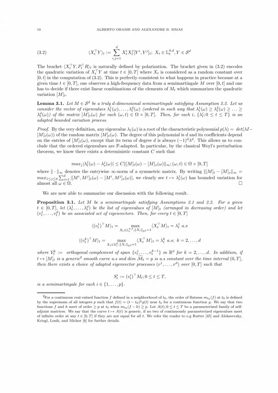
(3.2) 〈X⊤t Y 〉t :=
d∑
i,j=1
X itX
jt [Y
i, Y j ]t; Xt ∈ L0,dt , Y ∈ Sd
The bracket 〈X⊤t Y, P⊤
t R〉t is naturally defined by polarization. The bracket given in (3.2) encodesthe quadratic variation of X⊤
t Y at time t ∈ [0, T ] where Xt is considered as a random constant over[0, t] in the computation of (3.2). This is perfectly consistent to what happens in practice because at agiven time t ∈ [0, T ], one observes a high-frequency data from a semimartingale M over [0, t] and onehas to decide if there exist linear combinations of the elements of Mt which summarizes the quadraticvariation [M ]t.
Lemma 3.1. Let M ∈ Sd be a truly d-dimensional semimartingale satisfying Assumption 2.2. Let usconsider the vector of eigenvalues λ1
t (ω), . . . , λdt (ω) (ordered in such way that λ1
t (ω) ≥ λ2t (ω) ≥ . . . ≥
λdt (ω)) of the matrix [M ]t(ω) for each (ω, t) ∈ Ω × [0, T ]. Then, for each i, λi
t; 0 ≤ t ≤ T is anadapted bounded variation process.
Proof. By the very definition, any eigenvalue λt(ω) is a root of the characteristic polynomial p(λ) = det(λI−[M ]t(ω)) of the random matrix [M ]t(ω). The degree of this polynomial is d and its coefficients dependon the entries of [M ]t(ω), except that its term of degree d is always (−1)dλd. This allows us to con-clude that the ordered eigenvalues are F-adapted. In particular, by the classical Weyl’s perturbationtheorem, we know there exists a deterministic constant C such that
maxj |λjt (ω)− λj
s(ω)| ≤ C‖[M ]t(ω)− [M ]s(ω)‖∞; (ω, t) ∈ Ω× [0, T ]
where ‖ · ‖∞ denotes the entrywise ∞-norm of a symmetric matrix. By writing ‖[M ]t − [M ]s‖∞ =
max1≤j≤d
∑di=1 |[M i,M j]t(ω) − [M i,M j]s(ω)|, we clearly see t 7→ λj
t (ω) has bounded variation foralmost all ω ∈ Ω.
We are now able to summarize our discussion with the following result.
Proposition 3.1. Let M be a semimartingale satisfying Assumptions 2.1 and 2.2. For a givent ∈ [0, T ], let (λ1
t , . . . , λdt ) be the list of eigenvalues of [M ]t (arranged in decreasing order) and let
(v1t , . . . , vdt ) be an associated set of eigenvectors. Then, for every t ∈ [0, T ]
〈(v1t )⊤M〉t = maxXt∈L
0,dt
,‖Xt‖Rd=1
〈X⊤t M〉t = λ1
t a.s
〈(vkt )⊤M〉t = maxXt∈Vk
t ,‖Xt‖Rd=1
〈X⊤t M〉t = λk
t a.s; k = 2, . . . , d
where Vkt := orthogonal complement of span v1t , . . . , vk−1
t in Rd for k = 2, . . . , d. In addition, if
t 7→ [M ]t is a generic2 smooth curve a.s and dim Mt = p is a.s constant over the time interval (0, T ],then there exists a choice of adapted eigenvector processes (v1, . . . , vd) over [0, T ] such that
Sit := (vit)
⊤Mt; 0 ≤ t ≤ T,
is a semimartingale for each i ∈ 1, . . . , p.
2For a continuous real-valued function f defined in a neighborhood of t0, the order of flatness mt0 (f) at t0 is definedby the supremum of all integers p such that f(t) = (t − t0)pg(t) near t0 for a continuous function g. We say that twofunctions f and h meet of order ≥ p at t0 when mt0 (f − h) ≥ p. Let A(t); 0 ≤ t ≤ T be a parameterized family of self-adjoint matrices. We say that the curve t 7→ A(t) is generic, if no two of continuously parameterized eigenvalues meetof infinite order at any t ∈ [0, T ] if they are not equal for all t. We refer the reader to e.g Rutter [45] and Alekseevsky,Kriegl, Losik, and Michor [6] for further details.
PRINCIPAL COMPONENT ANALYSIS FOR SEMIMARTINGALES AND STOCHASTIC PDE 11
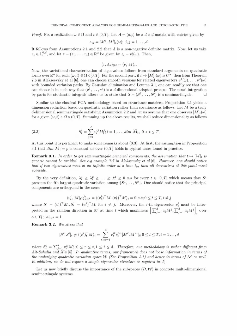
Proof. Fix a realization ω ∈ Ω and t ∈ [0, T ]. Let A = (aij) be a d× d matrix with entries given by
aij = [M i,M j ]t(ω); i, j = 1 . . . , d.
It follows from Assumptions 2.1 and 2.2 that A is a non-negative definite matrix. Now, let us take
vt ∈ L0,dt , and let z = (z1, . . . , zd) ∈ Rd be given by zi = vit(ω). Then,
〈z, Az〉Rd = 〈v⊤t M〉t.Now, the variational characterization of eigenvalues follows from standard arguments on quadraticforms over Rn for each (ω, t) ∈ Ω×[0, T ]. For the second part, if t 7→ [M ]t(ω) is C
∞ then from Theorem7.6 in Alekseevsky et al [6], one can choose smooth versions for related eigenvectors v1(ω), . . . , vd(ω)with bounded variation paths. By Gaussian elimination and Lemma 3.1, one can readily see that onecan choose it in such way that (v1, . . . , vd) is a d-dimensional adapted process. The usual integrationby parts for stochastic integrals allows us to state that S = (S1, . . . , Sp) is a semimartingale.
Similar to the classical PCA methodology based on covariance matrices, Proposition 3.1 yields adimension reduction based on quadratic variation rather than covariance as follows. Let M be a trulyd-dimensional semimartingale satisfying Assumption 2.2 and let us assume that one observes [M ]t(ω)for a given (ω, t) ∈ Ω×(0, T ]. Summing up the above results, we shall reduce dimensionality as follows
(3.3) Sit =
d∑
j=1
vijt M jt ; i = 1, . . . , dim Mt, 0 < t ≤ T.
At this point it is pertinent to make some remarks about (3.3). At first, the assumption in Proposition
3.1 that dim Mt = p is constant a.s over (0, T ] holds in typical cases found in practice.
Remark 3.1. In order to get semimartingale principal components, the assumption that t 7→ [M ]t isgeneric cannot be avoided. See e.g example 7.7 in Alekseevsky et al [6]. However, one should noticethat if two eigenvalues meet at an infinite order at a time t0, then all derivatives at this point mustcoincide.
By the very definition, λ1t ≥ λ2
t ≥ . . . ≥ λdt ≥ 0 a.s for every t ∈ [0, T ] which means that Si
presents the ith largest quadratic variation among S1, . . . , Sp. One should notice that the principalcomponents are orthogonal in the sense
〈vit, [M ]tvjt 〉Rd = 〈(vit)⊤M, (vjt )
⊤M〉t = 0 a.s; 0 ≤ t ≤ T, i 6= j
where Si· = (vi· )
⊤M·, Sj· = (vj· )⊤M· for i 6= j. Moreover, the i-th eigenvector vit must be inter-
preted as the random direction in Rd at time t which maximizes[∑d
j=1 ajMj ,∑d
j=1 ajMj]tover
a ∈ V it ; ‖a‖Rd = 1.
Remark 3.2. We stress that
[Si, Si]t 6= 〈(vi)⊤t M〉t =d∑
ℓ,m=1
viℓt vimt [M ℓ,Mm]t; 0 ≤ t ≤ T, i = 1 . . . , d
where Sir =
∑dj=1 v
ijr M j
r ; 0 ≤ r ≤ t, 1 ≤ i ≤ d. Therefore, our methodology is rather different from
Ait-Sahalia and Xiu [5]. In qualitative terms, our framework does not loose information in terms ofthe underlying quadratic variation space W (See Proposition 4.1) and hence in terms of M as well.In addition, we do not require a simple eigenvalue structure as required in [5].
Let us now briefly discuss the importance of the subspaces (D,W) in concrete multi-dimensionalsemimartingale systems.

12 ALBERTO OHASHI AND ALEXANDRE B. SIMAS
4. Bounded variation component and quadratic variation in MIn this section, we discuss two concrete examples of models which exemplify the importance of
analyzing the principal components of high-dimensional semimartingale systems in terms of (W ,D)rather than covariance matrices.
4.1. Correlation in d-dimensional asset prices. Correlation among asset prices is a well-knownphenomena and it has been studied by many authors in the context of covariance and, more recently,quadratic variation matrices. Let us suppose the asset log-prices form a d-dimensional Ito process
(4.1) M it = M i
0 +
∫ t
0
bisds+
d∑
j=1
∫ t
0
σijs dBj
s ; i = 1, . . . , d; 0 ≤ t ≤ T,
where b : [0, T ] × Ω → Rd and σ : [0, T ] × Ω → Rd×d satisfy usual conditions to get a well-definedd-dimensional semimartingale. For simplicity of exposition, let us assume that d is known.
One typical example of the existence of bounded variation component in M is the occurrence ofcorrelation amongM1, . . . ,Md which can be measured by volatility, i.e., quadratic variation. This typeof phenomena has been recently studied by Ait-Sahalia and Xiu [4] who identify nontrivial correlation
among M i; i = 1, . . . , d by means of suitable estimators [M i,M j ]T ; i, j = 1, . . . , d. In the presenceof correlation among assets as in [4], the subspace D naturally emerges as a non-trivial subspace ofM due to the fact that rank [M ]T < d. See also Buraschi, Porchia and Trojani [16] for a discussionof correlation in the context of optimal portfolio choice.
4.2. Stochastic PDEs with finite-dimensional realizations. Let us describe how (W ,D) arises inthe context of stochastic PDEs. Let us concentrate the discussion in one major research theme relatedto interest rate modelling: The calibration problem of Heath-Jarrow-Morton models [32] (henceforthabbreviated by HJM) based on forward rate curves. We refer the reader to e.g [13, 14, 15, 24] and otherreferences therein for a detailed discussion on this issue. The classical HJM model can be describedby a stochastic PDE of the form
(4.2) drt =(A(rt) + αHJM (rt)
)dt+
m∑
i=1
σi(rt)dBit ; r0 ∈ E,
where A = ddx is the first-order derivative operator acting as an infinitesimal generator of a C0-
semigroup on a separable Hilbert space E which we assume to be a space of functions g : R+ → R.The drift vector field αHJM has great importance for pricing and hedging derivative products and itis fully determined by σ = σ1, . . . , σm under a martingale measure. See e.g [24] for more details.
One central issue in the literature is the use of the stochastic PDE (4.2) in practice. In this case, itis very important to know when (4.2) admits a finite-dimensional subset G where the stochastic PDEnever leaves as long as the initial forward rate curve r0 ∈ G, namely
Prt ∈ G; ∀t ∈ [0, T ] = 1 if r0 ∈ G.The subset G can be interpreted as a finite-dimensional parameterized family of smooth curves G =G(·;x);x ∈ Z ⊂ Rd ⊂ E which can be used to estimate the volatility component of the model (4.2)starting with an initial curve r0 ∈ G. See e.g [7, 14]. Therefore, one central issue in interest ratemodelling is the existence, characterization and estimation of G. See [13, 14, 15, 24, 25, 28, 29, 41,44, 7, 40] and other references therein.
As far as the existence is concerned, Bjork and Svensson [15] and Filipovic and Teichmann [25]have shown that the existence of G is equivalent to
dim µ, σi; i = 1, . . . ,mLA < ∞,

PRINCIPAL COMPONENT ANALYSIS FOR SEMIMARTINGALES AND STOCHASTIC PDE 13
in a neighborhood of r0, where µ is the Stratonovich drift induced by σ and x 7→ µ, σ1, . . . , σmLA(x)is the Lie algebra generated by the vector fields µ, σ1, . . . , σm. In fact, G ⊂ E must be an affinesubmanifold of E. In particular, there exists a parametrization φ : [0, T ] → E, a truly d-dimensionalBrownian semimartimgale M = (M1, . . . ,Md) and a linear subspace V = span λ1, . . . , λd spannedby a basis λidi=1 such that
(4.3) rt(x) = φt(x) +d∑
j=1
M itλi(x) a.s; 0 ≤ t ≤ T ;x ≥ 0.
Under some assumptions (see e.g Duffie and Khan [22]), the semimartingale state process M can begenerically written as an affine process. In contrast to the previous example of sample data from thed-dimensional semimartingale (4.1), M in (4.3) is not observed.
For a given pair (M,V ) as above, one can actually show there exists a unique splitting V = V1⊕V2
which realizes
rt(x) = φt(x) +
p∑
i=1
Y it ϕi(x) +
d∑
j=p+1
Y jt ϕj(x) a.s
for 0 ≤ t ≤ T ;x ≥ 0. Here, Y i; i = 1, . . . , p is a basis for W and Y j ; j = p+1, . . . , d it is basis forD such that
M = W ⊕D.
Moreover, V1 = span ϕ1, . . . , ϕp and V2 = span ϕp+1, . . . , ϕd. The loading factors associated toV2 are related to the risk factors in D which in turn are associated to no-arbitrage restrictions.
Under the assumption that a stochastic PDE (one typical example is (4.2)) admits a finite-dimensional realization (4.3), we are going to present consistent estimators for the minimal invariantsubspace V . More precisely, based on high-frequency data and techniques from factor analysis, wetake advantage of the structure induced by (W ,D) in order to provide consistent estimators (V1, V2)for (V1, V2) related to the minimal invariant subspace V .
4.3. Noise dimension vs quadratic variation dimension. It is convenient to point out that therank of a quadratic variation matrix is not the maximal rank of the underlying volatility processstudied by Jacod and Podolskij [37] and Fissler and Podolskij [30]. See also Sahalia and Xiu [5] for asimilar framework. In fact, let M be a d-dimensional Ito process of the form
Mt = M0 +
∫ t
0
bsds+
∫ t
0
σsdBs; 0 ≤ t ≤ T.
Let Rt := sup0≤s<t rank (cs); 0 < t ≤ T where cs := σsσ⊤s ; 0 ≤ s ≤ T.
Proposition 4.1. If σ has continuous paths, then Rt ≤ rank [M ]t a.s for every t ∈ [0, T ]. Moreover,the inequality may be strict.
Proof. Let us fix a realization ω ∈ Ω in a set of full measure and some t in [0, T ]. Let, also, Rt >0. Then, since ct is a continuous matrix-valued function, and the rank is an integer-valued lower-semicontinuous function, there exists t∗ ∈ [0, t] such that rank ct∗ = Rt.
Since ct∗ is a non-negative definite matrix, we can find a set of Rt linearly independent eigenvectorsfor ct∗ , say, v1, . . . , vRt , with respective eigenvalues λ1, . . . , λRt , such that λi > 0, for i = 1, . . . , Rt.
Now, observe that if c1, . . . , cRt are real numbers such that c21 + · · · + c2Rt> 0, then by putting
w = c1v1 + · · ·+ cRtvRt and using the orthogonality of the eigenvectors, we have
(4.4) 〈w, ct∗w〉Rd = c21λ1 + · · ·+ c2RtλRt > 0.

14 ALBERTO OHASHI AND ALEXANDRE B. SIMAS
Note also that, for any such vector w, the function t 7→ 〈w, ctw〉Rd is continuous, so we can find anopen interval I containing t∗, with length |I| = 2δ (for some δ > 0), satisfying
(4.5) ∀s ∈ I, 〈w, csw〉Rd > 1/2〈w, ct∗w〉Rd .
Furthermore, using the non-negative definiteness of cs, we have that
(4.6) ∀u ∈ [0, T ], 〈w, cuw〉Rd ≥ 0.
Now, suppose, by contradiction, that rank [M ]t < Rt. Then, we can find real numbers c1, . . . , cRt ,with c21 + · · ·+ c2Rt
> 0, such that, for w = c1v1 + · · ·+ cRtvRt , where v1, . . . , vRt are the eigenvectorsof ct∗ given above, we have [M ]tw = 0, and, in particular,
〈w, [M ]tw〉Rd = 0.
Then, using (4.4), (4.5) and (4.6), we obtain
0 = 〈w, [M ]tw〉Rd =
∫ t
0
〈w, csw〉Rdds
≥∫
I
〈w, csw〉Rdds
>
∫
I
1/2〈w, ct∗w〉Rdds
= δ〈w, ct∗w〉Rd > 0.
This contradiction shows that Rt ≤ rank[M ]t.To show that the inequality may be strict, consider the following example: Let us assume that
T ≥ 1 and we take
σs =
(f(s) 00 f(s− 1)
),
where f(t) = t(1− t)11[0,1], with 11A is the indicator function of the set A. Then, clearly,
cs =
(f(s)2 00 f(s− 1)2
),
and Rt = 1, for all t > 0, whereas rank[M ]t = 2 for t > 1.
Remark 4.1. The main message of the above proposition is that if a direction has a non-null quadraticvariation for some time t0 > 0, then this direction has non-null quadratic variation for all times t ≥ t0.This phenomenon does not occur with the volatility matrix cs, as shown above.
We also stress that Assumptions 2.1 and 2.2 yield the study of a statistical test to check theexistence of a null quadratic variation component in M. The full derivation of the statistical test willbe further explored in a future paper.
Corollary 4.1. Let M ∈ X d be a truly d-dimensional process satisfying Assumption 2.2. Letλ1T , . . . , λ
dT be the ordered eigenvalues of the associated quadratic variation matrix [M ]T such that
λ1T ≥ . . . ≥ λd
T . The test H0 : λdT = 0 versus H1 : λd
T > 0, is a well-defined statistical test and it isequivalent to H0 : rank[M ]T < d versus H1 : rank[M ]T = d.
Remark 4.2. It is pertinent to interpret M = W ⊕D from the perspective of semimartingale-basedfactor models. When rank [M ]T < d then
M = W ⊕Dwhere dim D > 0. In applications, one may think M as the space of high-dimensional portfolioscomposed by M which can be depicted into two dynamic spaces. When [M ]T is singular, then thedynamic space has to be filled with zero quadratic variation dynamics which can be neglected onlyif one is solely interested in volatility. We stress that this phenomena is intrinsic to the principalcomponent analysis of high-dimensional semimartingale systems.

PRINCIPAL COMPONENT ANALYSIS FOR SEMIMARTINGALES AND STOCHASTIC PDE 15
5. Estimation of (W ,D)
In this section, we show how to estimate the pair (W ,D) which realizes
M = W ⊕Dfor a given observed processM ∈ X d satisfying Assumptions 2.1 and 2.2. The reader may think (W ,D)as a pair of factor spaces which are not observed. We stress even if one observes all trajectories of M ,the components of D are not visible when dim D > 0.
5.1. Identification of the Spaces (W ,D). Throughout this section, we are going to fix a trulyd-dimensional process M = (M1, . . . ,Md) ∈ X d satisfying Assumption 2.2. Let M = W ⊕D be thesplitting introduced in (2.8). We assume that dim W = p and dim D = d − p, where 1 ≤ p ≤ d. Inorder to clarify the exposition, we first assume that one is able to observe all trajectories of a givenM ∈ X d in continuous time.
Proposition 5.1. Let M = (M1, . . . ,Md) be a d-dimensional process satisfying Assumptions 2.1 and2.2, span M1, . . . ,Md = M and let [M ]T be the quadratic variation matrix of M . Let v1, . . . , vdbe an orthonormal basis formed by eigenvectors associated to the ordered (decreasing order) eigenvaluesof [M ]T . Let V : Ω → Md×d be the random matrix given by
V(ω) := vij(ω); 1 ≤ i, j ≤ d.where vi = (vi1, . . . , vid); 1 ≤ i ≤ d. Then there exists a set Ω∗ of full measure such that for eachrealization ω ∈ Ω∗, (V(ω)M·)i; p+ 1 ≤ i ≤ d is a basis for D and (V(ω)M·)i; 1 ≤ i ≤ p is a basisfor W. Moreover,
(5.1) [(VM)1]T ≥ [(VM)1]T . . . ≥ [(VM)d]T a.s.
Proof. By applying the standard spectral theorem on [M ]T (ω), we can find a set of eigenvectorsvi(ω); 1 ≤ i ≤ d associated to [M ]T (ω) which constitutes an orthonormal basis for Rd, so thatV(ω) is invertible for every ω ∈ Ω. Let p = dim W . If d − p > 0 then Lemma 2.1 yields vi ∈Ker [M ]T a.s; p+ 1 ≤ i ≤ d. Therefore, [M ]T vi is null a.s for every i ∈ p+ 1, . . . , d which impliesthat the last d− p rows of V(ω) [M ]T (ω) are null for every ω ∈ Ω∗ where Ω∗ has full probability. Letus fix ω∗ ∈ Ω∗ and we write V = V(ω∗), vi = vi(ω
∗), (J1, . . . , Jd) ∈ X d, where J i = (VM)i; 1 ≤ i ≤ d.Now, since V is invertible then J1, . . . , Jd is a linearly independent subset of M. Moreover,
d∑
j=1
vij[M ℓ,M j
]T= 0 a.s, ℓ = 1, . . . , d; i = p+ 1, . . . , d
which by linearity implies that
(5.2)[M ℓ,
d∑
j=1
vijMj]T= 0 a.s; ℓ = 1, . . . , d; i = p+ 1, . . . , d.
More importantly, (5.2) yields[∑d
j=1 vijMj]T= 0 a.s; p+1 ≤ i ≤ d. Since span Jp+1, . . . , Jd ⊂ M,
we actually have span Jp+1, . . . , Jd ⊂ D and the linear independence yields span Jp+1, . . . , Jd =D. Therefore,
(5.3) span J1, . . . , Jd = spanJ1, . . . , Jp ⊕ D ⊂ M = W ⊕D.
Since J1 . . . , Jp is a linearly independent subset of M, than (5.3) yields
spanJ1, . . . , Jp = W .

16 ALBERTO OHASHI AND ALEXANDRE B. SIMAS
Lastly, the ordering (5.1) is an immediate consequence of Proposition 3.1.
With the obvious modifications, we stress the result of Proposition 5.1 also holds over [0, t] forevery 0 < t < T .
5.2. Estimation of the spaces (W ,D). Let us suppose that we are in the same setup of the previoussection, but now we have a high-frequency of observations at hand from a truly d-dimensional processM = (M1, . . . ,Md) satisfying Assumption 2.2. In this section, the high-frequency data is assumed tobe observed at common regular times for each M i; i = 1 . . . , d. We leave the case of non-synchronousdata to a future research. Throughout this section, we assume the existence of a consistent estimator
[M ]T for [M ]T which satisfies the following assumption:
Assumption 5.1. [M ]T is a sequence of non-negative definite and self-adjoint matrices such that
[M ]Tp→ [M ]T as ‖Π‖ → 0.
In the sequel, we fix [M ]T satisfying Assumption 5.1 and we choose 3 any consistent estimator pfor rank [M ]T . The goal of this section is to describe a generic estimation methodology based on the
existence of [M ]T satisfying Assumption 5.1. We stress the results of this section do not depend on theestimator of the quadratic variation matrix. We refer the reader to e.g [19, 50, 51, 39, 52, 18, 23, 21]and other references therein for a complete view of the estimation methods for [M ]T .
We need to define a metric notion on the set of finite-dimensional subspaces embedded on a possiblyinfinite-dimensional vector space. For this task, we make use of the same metric between subspacesdefined by Bathia et al. [11]. Let N1 and N2 be two finite-dimensional Hilbert subspaces of aninner product vector space H with dimensions m1 and m2, respectively. Let ζi1, . . . , ζimi be anorthonormal basis of Ni, i = 1, 2. Then, we define
(5.4) D(N1,N2) :=
√√√√1− 1
maxm1,m2
m1∑
k=1
m2∑
j=1
(〈ζ2j , ζ1k〉H)2.
In the sequel, we need to compute distances for finite-dimensional subspaces which are not embeddedin a natural common Hilbert space. For this reason, let A be a finite-dimensional linear space. If A1
and A2 are finite-dimensional subspaces of A, then we define
(5.5) d(A1, A2) := D(Φ(A1),Φ(A2))
where Φ : A → Rm; i = 1, 2 is the canonical isomorphism and dim A = m. One can easily check thatd is indeed a metric over the set of all finite-dimensional subspaces of A. The metric d in (5.5) is veryconvenient to study consistency of subspace estimators.
Before presenting the main result of this section, we need two preliminary lemmas.
Lemma 5.1. Let Cn, C : Ω → Md×d be a sequence of self-adjoint real d × d matrices such that
Cnp→ C as n → ∞. Assume that q = dimKer(C) a.s and let us denote by vn1 , . . . , v
nq a set of
orthonormal eigenvectors associated to the q least eigenvalues of Cn. Let Kn = span vn1 , . . . , vnq andK = Ker(C). Then,
D(Kn,K)p→ 0
as n → ∞.
3For instance, if E‖[M ]T − [M ]T ‖2F
≤ O(rn) than choosing ǫ → 0 in such way that ǫ2(rn)−1 → ∞ as n → ∞ allows
us to take p = the number of non-zero eigenvalues of [M ]T bigger than ǫ as a consistent estimator.

PRINCIPAL COMPONENT ANALYSIS FOR SEMIMARTINGALES AND STOCHASTIC PDE 17
Proof. Letvidi=1 be an orthonormal basis for Rd given by eigenvectors of C. Let v1, . . . , vq bean orthonormal subset of eigenvectors of C associated to eigenvalues α1, . . . , αq and Ker(C) =
span v1, . . . , vq. To shorten notation, in the sequel we denote by 〈·, ·〉 = ‖ · ‖1/2 the inner productover Euclidean spaces. We may assume that 0 < q < d. Let vq+1, . . . , vd be a basis for the orthogo-nal complement K⊥. At first, we notice that since Kn and K have the same dimension, it is sufficient
to prove that D(Kn,K⊥)
p→ 1. This is equivalent to prove that
q∑
j=1
d−q∑
i=1
(〈vnj , vq+i〉)2 p→ 0 as n → ∞.
To do so, let qi,j = 〈vnj , vq+i〉vq+i, and note that ‖qi,j‖ ≤ 1 a.s and Cqi,j = 〈vnj , vq+i〉αq+ivq+i.Therefore,
〈Cqi,j , vnj 〉 = αq+i(〈vnj , vq+i〉)2 ⇒
d∑
i=1
d−q∑
j=1
〈Cqi,j , vnj 〉 =
d∑
i=1
d−q∑
j=1
αq+i(〈vnj , vq+i〉)2,
and since∑
i,j αq+i(〈vnj , vq+i〉)2 ≥ αq+1
∑i,j(〈vnj , vq+i〉)2 a.s we may conclude that
d∑
i=1
d−q∑
j=1
(〈vnj , vq+i〉)2 ≤ 1
αq+1
d∑
i=1
d−q∑
j=1
〈vnj , Cqi,j〉
=1
αq+1
d∑
i=1
d−q∑
j=1
〈qi,j , Cvnj 〉
≤ 1
αq+1
d∑
i=1
d−q∑
j=1
‖qi,j‖ · ‖Cvnj ‖
≤ 1
αq+1
d∑
i=1
d−q∑
j=1
‖Cvnj ‖ a.s ∀n ≥ 1.
We now claim that
(5.6) supv∈Kn
‖v‖=1
‖Cv‖ → 0.
Let αn1 ≥ αn
2 ≥ . . . ≥ αnq be the ordered eigenvalues of Cn related to the q least eigenvalues. Let γn be
the number of non-zero eigenvalues of Cn. We have Pγn = d − q = 1 for every n sufficiently largeso that
supv∈Kn
‖v‖=1
‖Cnv‖ ≤ αn1
p→ 0
as n → ∞.On the other hand, Cn
p→ C as n → ∞ and hence
supv∈R
p
‖v‖=1
‖Cnv − Cv‖ p→ 0
as n → ∞. Therefore, triangle inequality yields
supv∈Kn
‖v‖=1
‖Cv‖ ≤ supv∈Kn
‖v‖=1
‖Cnv − Cv‖+ supv∈Kn
‖v‖=1
‖Cnv‖

18 ALBERTO OHASHI AND ALEXANDRE B. SIMAS
≤ supv∈R
p
‖v‖=1
‖Cnv − Cv‖+ supv∈Kn
‖v‖=1
‖Cnv‖
p→ 0
as n → ∞. This shows (5.6) and we may conclude the proof.
Lemma 5.2. Let M ∈ X d be a truly d-dimensional process satisfying Assumption 2.2. Then, the setker[M ]t is deterministic 4 for every t ∈ [0, T ].
Proof. For t = 0 the statement is obvious, so let us fix t ∈ (0, T ] and let Dt be the subspace of
Mt given by (2.3). Let pt be the dimension of Mt. Let N1, . . . , Nd−pt be a basis of Dt and letR1, . . . , Rpt be a complement basis of Mt in such a way that N1, . . . , Nd−pt , R1, . . . , Rpt is a basisof Mt. Let A be the change of basis from N1, . . . , Nd−pt , R1, . . . , Rpt to M = M1, . . . ,Md withmatrix representation A = (aij)1≤i,j≤d. We set Ω∗ := Ω − O where O :=
ω; rank [M ]t(ω) 6=
pt or [Nℓ]t(ω) > 0 for some ℓ ∈ 1, . . . , d− pt
. From Lemma 2.1 and the definition of Dt, we know
that Ω∗ has full probability. We pick ω ∈ Ω∗. Of course,
a1 := (a11, . . . , ad1), . . . , ad−pt := (a1(d−pt), . . . , ad(d−pt))
constitutes a set of d− pt linearly independent deterministic vectors in Rd and by the every definition
[M ]t(ω)aℓ =
d∑
k=1
akℓ[Mi,Mk]t(ω) = [M i, N ℓ]t(ω) = 0
for 1 ≤ ℓ ≤ d − pt, 1 ≤ i ≤ d. Since ker[M ]t(ω) ⊂ Rd has dimension d − pt for every ω ∈ Ω∗, thenker[M ]t(ω) = span a1, . . . , ad−pt for every ω ∈ Ω∗.
Let V be the orthogonal matrix formed by orthonormal eigenvectors of [M ]T . Of course, we are
not able to prove that VM converges to VM due to the lack of identification of eigenvectors. What istrue is the following notion of convergence. In the sequel, if An, Bn;n ≥ 1 is a sequence of randomvariables, then
An Bn as n → ∞means that, P(An < Bn) → 0 as n → ∞. We similarly define and An ≃ Bn when both An Bn
and An Bn as n → ∞.
Theorem 5.1. Let M = (M1, . . . ,Md) be a process satisfying Assumptions 2.1 and 2.2. Let [M ]Tbe a consistent estimator for [M ]T satisfying Assumption 5.1 and let p be any consistent estimator
for rank [M ]T . Let V be the orthogonal matrix whose rows are formed by eigenvectors of [M ]T . If
(J1· , . . . , J
d· ) := VM·, then let us define W := span J1, . . . , J p and D := span J p+1, . . . , Jd.
Under the above conditions, we have
d(W ,W)p→ 0 and d(D,D)
p→ 0,
as ‖Π‖ → 0. If M := W ⊕ D then d(M,M)p→ 0 as ‖Π‖ → 0. Moreover,
(5.7) [J1]T . . . [J p]T
(5.8) [J i]T ≃ 0; p ≤ i ≤ d as ‖Π‖ → 0.
4A random set A is deterministic if there exists a subset A ⊂ Rd such that A = B a.s.

PRINCIPAL COMPONENT ANALYSIS FOR SEMIMARTINGALES AND STOCHASTIC PDE 19
Proof. Recall the definition of the isomorphism Φ used in (5.5). From Lemma 5.2, we have Φ(D) =
Ker([M ]T ) and by the very definition of D, we also have Φ(D) = Ker([M ]T ). Thus, from Lemma 5.1above, we have
d(D, D)p−→ 0.
Now, notice that
Rd = Φ(D)⊕ Φ(W) = Φ(D)⊕ Φ(W).
Therefore, it follows from the definition of the metric d that
d(W ,W)p−→ 0.
Since p is an integer-valued consistent estimator, we shall assume that p = p. By the very definition,we know that
〈viT , [M ]T viT 〉Rd ≥ 〈vi+1
T , [M ]T vi+1T 〉Rd a.s; 1 ≤ i ≤ d− 1.
and[J i]T = 〈viT , [M ]T v
iT 〉Rd a.s; 1 ≤ i ≤ d.
Let us write
[J i]T − [J i+1]T =([J i]T − 〈viT , [M ]T v
iT 〉Rd
)+(〈viT , [M ]T v
iT 〉Rd − 〈vi+1
T , [M ]T vi+1T 〉Rd
)
+(〈vi+1
T , [M ]T vi+1T 〉Rd − [J i+1]T
); 1 ≤ i ≤ d− 1.
By construction, max1≤i≤d|viT | is bounded in probability and ‖[M ]T − [M ]T ‖F → 0 in probability as
‖Π‖ → 0. Moreover,(〈viT , [M ]T v
iT 〉Rd − 〈vi+1
T , [M ]T vi+1T 〉Rd
)≥ 0 a.s and hence (5.7) holds true. The
proof of (5.8) is similar.
A straightforward consequence is the following result.
Corollary 5.1. Assume that hypotheses in Theorem 5.1 hold and let Y ∈ M be discretely-observed atYtr ; 0 ≤ r ≤ n over [0, T ], where 0 = t0 < t1 . . . < tn = T . Then, there exists α = (α1, . . . , αd) ∈ Rd
such that
(5.9) max0≤r≤n
∣∣∣Ytr −p∑
ℓ=1
αℓJℓtr −
d∑
k=p+1
αkJktr
∣∣∣ p→ 0,
as max1≤i≤n|tr − tr−1| → 0.
Proof. Let us equip X with the topology of the uniform convergence in probability. Let H be thesmallest finite-dimensional subspace of X which contains M1, . . . ,Md; J1, . . . , Jd. Let Φ : H → Rm
be the canonical isomorphism for some m > 0. We notice that Φ is actually an homeomorphism whenH is endowed with the subspace topology. From Theorem 5.1 and the definition of the metric d, weknow that
(5.10) d(M,M) = D(Φ(M),Φ(M)) =√2d sup
‖v‖Rd
=1
‖TΦ(M)v − TΦ(M)
v‖Rdp→ 0
as ‖Π‖ → 0, where TA denotes the projection onto a closed subspace A ⊂ Rd. Then from (5.10) andusing the fact that Φ is an homeomorphism, we get the existence of α = (α1, . . . , αd) ∈ Rd such that
∣∣∣Φ(Y )−p∑
ℓ=1
αℓΦ(Jℓ)−d∑
k=p+1
αkΦ(Jk)∣∣∣ p→ 0

20 ALBERTO OHASHI AND ALEXANDRE B. SIMAS
as ‖Π‖ → 0 which implies assertion in (5.9).
Under the assumptions of Theorem 5.1, if Y ∈ M is a discretely-observed semimartingale atYtk ; 1 ≤ k ≤ n over [0, T ], then we shall use Corollary 5.1 to estimate by OLS
α := argminα∈Rd
n∑
ℓ=1
∣∣∣Ytℓ − VMtℓ · α⊤∣∣∣2
,
the regression coefficients which provide us the precise linear contribution of non-null quadratic varia-tion and pure drift components in W and D, respectively. In this case, the following linear combination
Yk :=
p∑
ℓ=1
αℓJℓtk +
d∑
r=p+1
αrJrtk ; i = 1 . . . , d, k = 0, . . . , n.
depicts Ytr ; 0 ≤ r ≤ n into elements of W ⊕ D over the sample Ytk ; 0 ≤ k ≤ n in [0, T ]. Theestimation of the factor spaces (W ,D) provides a tool to optimal asset allocation/dimension reductionin high-dimensional portfolios composed by semimartingales, a topic which will be further exploredin a future paper.
6. Estimation of Finite-Dimensional Invariant Manifolds
In this section, we apply the theory developed in previous sections to present a methodology for theestimation of finite-dimensional invariant manifolds related to space-time data generated by stochasticPDEs of the form
(6.1) drt =(A(rt) + F (rt)
)dt+
m∑
j=1
σj(rt)dBjt ; t ≥ 0; r0 = h ∈ E,
where A is an infinitesimal generator of a C0-semigroup on a separable Hilbert space E which weassume to be a subspace of absolutely continuous functions g : K → R where for simplicity ofexposition we work with the one-dimensional space5 set K = [a, b] where −∞ < a ≤ x ≤ b < +∞.The vector fields F, σi; i = 1, . . . ,m are assumed to be Lipschitz and the dimension m is fixed.
6.1. Splitting the invariant manifold. Let us now introduce the basic geometric objects relatedto the stochastic PDE (6.1) that we are interested in estimating. We refer the reader to Tappe [48]for a very clear treatment of these objects.
Definition 6.1. A family (Vt)t≥0 of affine manifolds in E is called a foliation generated by a finite-dimensional subspace V ⊂ E if there exists φ ∈ C1(R+;E) such that
Vt = φ(t) + V ; t ≥ 0.
The map φ is a parametrization of (Vt)t≥0.
Remark 6.1. We notice that the parametrizations of (Vt)t≥0 are not unique, but for any distinctparametrizations φ1 and φ2 we have φ1(t)− φ2(t) ∈ V for every t ∈ [0, T ].
In the remainder of this paper, (Vt)t≥0 denotes a foliation generated by a finite-dimensional sub-space.
5Indeed, it is not too difficult to extend the results of this section to the multi-dimensional case where K is a compactsubset of Rn. This type of flexibility is important to treat more complex space-time data such as volatility surfaces inFinancial Engineering.

PRINCIPAL COMPONENT ANALYSIS FOR SEMIMARTINGALES AND STOCHASTIC PDE 21
Definition 6.2. The foliation (Vt)t≥0 of affine manifolds is invariant w.r.t the stochastic PDE (6.1)if for every t0 ∈ R+ and h ∈ Vt0 we have
Prt ∈ Vt0+t, for all t ≥ 0 = 1
for r0 = h.
The above objects lead us to the following definition which is the main object of statistical studyin this section.
Definition 6.3. We say that the stochastic PDE (6.1) has an affine realization generated by a finite-
dimensional subspace V ⊂ E if for each h0 ∈ dom (A) there exists a foliation (Vh0
t )t≥0 generated by
V with h0 ∈ Vh0
0 which is invariant w.r.t (6.1). An affine realization with a generator V is calledminimal, if for another affine realization generated by some subspace W we have V ⊂ W .
Remark 6.2. Suppose that the stochastic PDE (6.1) has an affine realization generated by a subspace
V . We recall that for each h0 ∈ dom (A) the foliation (Vh0
t )t≥0 generated by V is uniquely defined.See e.g [Lemma 2.7 [48]].
See Section 4.2 for a brief discussion on affine realizations in the context of Mathematical Finance.Throughout this paper, we assume that the stochastic PDE data generating process satisfies thefollowing assumption.
Assumption (A1): The stochastic PDE (6.1) has an affine realization generated by a finite-dimensionalsubspace.
Let us now introduce the basic operators which will encode the underlying loading factors ofthe stochastic PDE that we are interested in estimating. We fix once and for all a terminal time0 < T < ∞, r0 ∈ dom (A), the minimal subspace generator V of (6.1) spanned by linearly independentvectors w1, . . . , wd and a parametrization φ ∈ C([0, T ];E) with null quadratic variation [φ(u)]T =0; u ∈ [a, b]. Under Assumption (A1), the stochastic PDE (6.1) has a strong solution. From thereproducing kernel property of E ⊂ C([a, b];R), the evaluation map τu : f 7→ f(u) is a boundedlinear functional and therefore point-wise evaluation of the stochastic PDE is well-defined for everypoint-space and the following representation holds
(6.2) rt(u) = r0(u) +
∫ t
0
(A(rs)(u) + F (rs)(u)
)ds+
m∑
i=1
∫ t
0
σi(rs)(u)dBis,
where we set rt(u) := τurt for 0 ≤ t ≤ T and u ∈ [a, b]. Let us consider the following kernels
σt(u, v) :=
m∑
j=1
σj(rt)(u)σj(rt)(v); 0 ≤ t ≤ T,
QT (u, v) := [r(u), r(v)]T =
∫ T
0
σs(u, v)ds, u, v ∈ [a, b].
The above kernels induce random linear operators QT and σt defined almost everywhere by
(QT f)(·) := 〈QT (·, ), f〉E ; f ∈ E.
σtf(·) := 〈σt(·, ), f〉E ; f ∈ E, 0 ≤ t ≤ T.
By the very definition, the random linear operator QT can be written as
(QT f)(u) =
∫ T
0
(σsf)(u)ds; f ∈ E.

22 ALBERTO OHASHI AND ALEXANDRE B. SIMAS
where we denote Q := Range QT . In the remainder of this article, we denote by N the supplementarysubspace of Q in the minimal subspace V .
From Assumption (A1), we know (see e.g Th. 2.11 and (2.27) in [48]) that there exists a trulyd-dimensional semimartingale Z = (Z1, . . . , Zp) which realizes the strong solution (6.2) as follows
(6.3) rt(u) = φt(u) +
d∑
i=1
Zitwi(u); 0 ≤ t ≤ T, u ∈ [a, b].
Definition 6.4. We say that the stochastic PDE in (6.1) admits a finite-dimensional realization(FDR) if for each h ∈ dom (A) there exists a truly d-dimensional semimartingale Z ∈ Sd, aparametrization φ ∈ C([0, T ];E) and a linearly independent set w1 . . . , wd ⊂ E which realize (6.3).
See e.g [14, 48, 24, 26] for more details on this affine construction of the stochastic PDE. Repre-sentation (6.3) is not unique but it will be the basis for our splitting scheme as follows. At first, inorder to apply the spectral analysis in previous sections, we will assume the following hypothesis onthe stochastic PDE (6.1):
Assumption (A2): For each initial condition h ∈ dom (A), there exists a factor representation Zwhich realizes (6.3) and it satisfies Assumption 2.2.
In the sequel, if L ∈ Md×d and η = (η1, . . . , ηd) is a list of real-valued functions on [a, b], thenη(x) = (η1(x), . . . , ηd(x)) ∈ Md×1 and we set Lη meaning the Rd-valued function x 7→ Lη(x).
Remark 6.3. Let rt(u) = φt(u)+∑d
i=1 Zitwi(u); 0 ≤ t ≤ T, u ∈ [a, b] be a representation of the FDR
of (6.1). Let A ∈ Md×d be a non-singular random matrix. Then
(6.4) rt(x) = φt(x) +d∑
j=1
Y jt ϕj(x); 0 ≤ t ≤ T, x ∈ [a, b]
where ϕ = (A−1)⊤w is a random basis for V and Y· = AZ· ∈ X d.
We can actually write QT in terms of any representation (6.3) as follows
(6.5) (QT f)(u) =
d∑
i,j=1
〈f, wi〉Ewj(u)[Zi, Zj ]T ; f ∈ E;u ∈ [a, b],
and, moreover, the following remark holds.
Remark 6.4. From Lemma 2.1, one can easily see that under Assumption (A2), any truly d-dimensional factor process realizing (6.3) (or (6.4)) will satisfy Assumption 2.2.
In the sequel, we need to introduce new notation. For a given Z ∈ X d satisfying Assumptions
2.1 and 2.2, we denote M(Z) := span Z1, . . . , Zd, M(Z) := M(Z)/D(Z) where D(Z) := X ∈M(Z); [X ]· = 0 a.s on [0, T ] and the quotient space is defined by the equivalence relation (2.5) over
[0, T ]. We stress that M(Z),D(Z) and M(Z) are M,D and M, respectively, which are defined in(2.4) for the specific choice M = Z.
In practice, we are not able to observe any semimartingale factor Z = (Z1, . . . , Zd) of a stochasticPDE admiting a FDR. But it will be very important for our estimation strategy to identify the pair(Q,N ) in terms of the random matrix [Z]T , or more precisely, in terms of the quadratic variation ofrandom rotations of Z. Next, we recall the following result.
Lemma 6.1. Let r be the stochastic PDE (6.1) satisfying Assumptions (A1-A2) and admitting aFDR generated by the minimal foliation Vh
t = φt + V ; 0 ≤ t ≤ T where dim V = d and r0 = h.Then, we shall represent (6.1) as follows

PRINCIPAL COMPONENT ANALYSIS FOR SEMIMARTINGALES AND STOCHASTIC PDE 23
(6.6) rt = φt +
p∑
i=1
Y it ϕi +
d∑
j=p+1
Y jt ϕj ; 0 ≤ t ≤ T,
where Y is a truly d-dimensional semimartingale Y satisfying W(Y ) = spanY 1, . . . , Y p, D(Y ) =spanY p+1, . . . , Y d and V = Q⊕N , where Q = span ϕ1, . . . , ϕp and N = span ϕp+1, . . . , ϕd.Proof. By assumption, there exists a truly d-dimensional semimartingale Z = (Z1, . . . , Zd) satisfyingAssumption 2.2 and a basis w = widi=1 for V such that
rt = φt +
d∑
i=1
Zitwi; 0 ≤ t ≤ T.
From (6.5), we have Q ⊂ V a.s so that we shall consider the random operator QT restricted toV as follows QT : Ω × V → V . Moreover, from (6.5) we readily see that the random matrix of thelinear operator QT is given by [Zi, Zj ]T ; 1 ≤ i, j ≤ d for any pair (Z,w) of latent semimartingale
representation Z and a basis w for V . By Lemma 2.1, we have dim Q = dim M(Z) a.s. LetY = Y 1, . . . , Y d be a truly d-dimensional semimartingale such that Y 1, . . . , Y p is a basis forW(Z) and Y p+1, . . . , Y d is a basis for D(Z) where p = dim Q. Then spanY 1, . . . , Y d = M(Z)and Y satisfies Assumptions 2.1 and 2.2. Let I : M(Z) → M(Z) be the linear isomorphism given bythe change of basis from Z to Y . If [I]ZY = aij ; 1 ≤ i, j ≤ d is the matrix of I, then we shall write
(6.7) rt = φt +d∑
i=1
Y it ϕi; 0 ≤ t ≤ T,
where ϕj :=∑d
i=1 aijwi; 1 ≤ j ≤ d. By writing QT in terms of the basis ϕjdj=1 and using (6.7),
we clearly see that Q = span ϕ1, . . . , ϕp. By taking N = spanϕp+1, . . . , ϕd, we then conclude(6.6).
The main message of Lemma 6.1 is the following. When the stochastic PDE is projected onto Q(N ), then the associated latent factors are non-null quadratic variation (bounded variation) semi-martingales. We remark that the form of the FDRs (6.6) has already been derived in Bjork andLanden [14] and Filipovic and Teichmann [26] in the context of HJM models. Lemma 6.1 provides anexplicit splitting for V by separating the loading factors which generate Q from its complementarysubspace N attached to their associated spaces W(Y ) and D(Y ), respectively.
Summing up the above results, we arrive at the following identification result.
Proposition 6.1. Let r be the stochastic PDE (6.1) satisfying Assumptions (A1-A2). For a givenh ∈ dom (A), let Vh
t = φt + V ; 0 ≤ t ≤ T be the minimal foliation generated by some V such thatr0 = h ∈ Vh
0 . Let
rt = φt +
d∑
i=1
Zitηi; 0 ≤ t ≤ T,
be a factor semimartingale representation, where V = span η1, . . . , ηd and Z satisfies Assumptions2.1 and 2.2. Let A ∈ Md×d be a nonsingular random matrix. Let ϕ(x) = (A−1)⊤η(x);x ≥ 0and Yt = AZt; 0 ≤ t ≤ T . Let L : Ω → Md×d be the random matrix whose rows are given byLi = vi; 1 ≤ i ≤ d where v1, . . . , vd is an orthonormal eigenvector set of [Y ]T associated to theordered eigenvalues q1 ≥ q2 ≥ . . . ≥ qd a.s. Then
(6.8) Q = span(Lϕ)1, . . . , (Lϕ)p
a.s,N = span
(Lϕ)p+1, . . . , (Lϕ)d
a.s,

24 ALBERTO OHASHI AND ALEXANDRE B. SIMAS
and
(6.9) W(Y ) = span(LY )1, . . . , (LY )p
,N (Y ) = span
(LY )p+1, . . . , (LY )d
.
Proof. This is a straightforward consequence of Proposition 5.1, Lemma 6.1 and the identity
〈Zt, η(x)〉Rd = 〈AZt, (A−1)⊤η(x)〉Rd = 〈LAZt,L(A−1)⊤η(x)〉Rd ,
0 ≤ t ≤ T, x ≥ 0 due to the orthogonality of the random matrix L.
6.2. Preliminaries on Factor models. The goal of this section is to describe an estimation method-ology for the pair (Q,N ) which generates invariant foliations for stochastic PDEs of the form (6.1).The methodology will be inspired by the so-called Factor Analysis developed in the Econometricsliterature (see e.g [47], [8], [9], [31]), but with some fundamental differences: (a) Unlike the clas-sical discrete Factor Analysis, we are working with an underlying continuous time process sampledin high-frequency at discrete points in time and space. (b) The spaces (Q,N ) cannot be identifiedby applying standard techniques from Factor Analysis due to the rather distinct behavior betweenquadratic variation and covariance matrices in the high-frequency setup. (c) More importantly, thefactor analysis introduced here allows us to reduce and rank the underlying semimartingale factors interms of quadratic variation rather than covariance, including bounded variation components.
Throughout this section, Assumptions (A1-A2) are in force. We also assume the underlying state-space E is the Sobolev space of absolutely continuous functions f : [a, b] → R such that
‖f‖2E := |f(a)|2 +∫ b
a
|f ′(x)|2µ(dx) < ∞
where µ is absolutely continuous w.r.t Lebesgue measure (see e.g [24]) and we write 〈·, ·〉E to denotethe associated inner product. For simplicity of exposition, we work with the closed subspace of Eformed by functions f(a) = 0 and we set dµ
dx = 1. With a slight abuse of notation we denote it by E.We are going to fix the minimal invariant foliation Vt = φt + V generated by a d-dimensional
subspace V equipped with a basis λ1, . . . , λd and a truly d-dimensional semimartingale (Z1, . . . , Zd)satisfying Assumption 2.2 such that
(6.10) rt = φt +
d∑
j=1
Zjt λj ; 0 ≤ t ≤ T.
In this section, we work in a high-frequency setup as follows. To shorten notation, the points ofpartition in time (tni )
ni=1 and space (xN
j )Nj=1 will be denoted by ti = tni and xj = xNj , respectively,
and we set ρ(n) := sup1≤i≤n−1 |ti+1 − ti| and δ(N) := sup1≤j≤N−1 |xj+1 − xj |. We will assume thesamplings in time and space will be equally spaced and equidistant. For the sake of preciseness, itshould be noted we are dealing with a sequence of refining partitions and we always assume thatρ(n) → 0, δ(N) → 0, n → ∞, N → ∞ as n,N → ∞, where both n and N goes to infinity.
We assume that the observations are generated by a space-time process
(6.11) Xt(x) := rt(x) + εt(x); 0 ≤ t ≤ T, x ∈ [a, b]
where ε represents a space-time error component satisfying some regularity conditions. In this section,we assume that one is able to sample the curves x 7→ Xt(x) in high-frequency in time. For instance,term-structure objects like interpolated forward rate curves are examples of this type of data. Seee.g [38] and other references therein.
In particular, under Assumptions (A1-A2), the (n× N)-matrix Xti(xj) of observations admits anaffine noisy representation

PRINCIPAL COMPONENT ANALYSIS FOR SEMIMARTINGALES AND STOCHASTIC PDE 25
(6.12) Xti(xj) = φti(xj) +d∑
k=1
Zktiλk(xj) + εti(xj)
for i = 1, . . . , n and j = 1, . . . , N . Throughout this section, we assume that φ is known by the observerand with a slight abuse of notation we write X for the difference X −φ. In matrix representation, weshall write
X = ZΛ⊤ + E , Xi = ΛZi + Ei; 1 ≤ i ≤ n
where Λ := λj(xi); 1 ≤ i ≤ N , 1 ≤ j ≤ d, X := Xti(xj); 1 ≤ i ≤ n, 1 ≤ j ≤ N, Z := Zjti ; 1 ≤ i ≤
n, 1 ≤ j ≤ d and E := εti(xj); 1 ≤ i ≤ n, 1 ≤ j ≤ N.
6.3. Estimating the underlying dimension. Obviously, the first step is to estimate the underlyingdimension of the finite-dimensional realization. But this is an almost straightforward application ofBai and Ng [8]. Indeed, we are interested in solving the following optimization problem (for largen,N)
minΛk,Y(k)
ρ(n)δ(N)
n∑
i=1
N∑
j=1
(Xti(xj)− 〈gk(xj), Yti(k)〉Rk
)2,
where the minimum is taken over the set of real matrices with columns
Λk = (g1, . . . , gk) ∈ MN×k ; Y(k) = (Y (1), . . . , Y (k)) ∈ Mn×k,
subject to either δ(N)Λ⊤k Λk = Ik or ρ(n)Y⊤(k)Y(k) = Ik (Identity matrix in Mk×k). Here gi :=
(gi(x1), . . . , gi(xN ))⊤ and Y (i) := (Yt1(i), . . . , Ytn(i))
⊤ for 1 ≤ i ≤ k. The index k encodes theallowance of k factors in the estimation procedure.
Remark 6.5. In order to avoid curse of dimensionality issues, we do assume k < minn, N andn,N → ∞ jointly.
The factor estimator is defined as follows. Let Y (k) ∈ Mn×k be the random matrix defined by
Yti,j(k) := ρ(n)−1/2yjti ; 1 ≤ j ≤ k, 1 ≤ i ≤ n whose the jth column
yj := (yjt1 , . . . , yjtn) ∈ Mn×1
is an eigenvector associated to the j-th largest eigenvalue of XX⊤ ∈ Mn×n subject to ρ(n)Y ⊤(k)Y (k) =
Ik. The loading factor estimator is given by Λk := ρ(n)X⊤Y (k)In the sequel, we denote
V (k, Y (k)) := minΛk
ρ(n)δ(N)
n∑
i=1
N∑
j=1
(Xti(xj)− 〈gk(xj), Yti(k)〉Rk
)2.
The estimation procedure for the underlying dimension of V is due to Bai and Ng [8]. They proposea class of information criteria of the form
(6.13) PC(k) := V (k, Y (k)) + kq(n,N)
for suitable penalty functions q(n,N). One can show the estimation of dim V can be still carry outon the basis of the ideas contained in [8] even in the high-frequency setup, as long as the followingassumptions hold true. The following assumptions are inspired by Bai and Ng [8] and Bai [9] but inthe context of a continuous time setup sampled at discrete times. For the sake of completeness, welist them here. In the sequel, Hq is the space of q-integrable continuous Brownian semimartingales.
(D1) Zj ∈ H4 for each j = 1, . . . , d and

26 ALBERTO OHASHI AND ALEXANDRE B. SIMAS
ρ(n)
n∑
i=1
ZtiZ⊤ti → ΣZ :=
(〈Zi, Zj〉L2([0,T ];R)
)1≤i,j≤d
in probability as n → ∞ and ΣZ is a d× d positive definite matrix a.s
(D2) supj≥1 ‖λ(xj)‖Rd < ∞ and∥∥∥∥∥δ(N)
N∑
j=1
λ⊤(xj)λ(xj)−∫ b
a
λ⊤(x)λ(x)dx
∥∥∥∥∥(2)
→ 0
as δ(N) → 0. Moreover, Σλ :=∫ b
a λ⊤(x)λ(x)dx is a d× d-positive definite matrix.
(D3) The error process ε satisfies assumptions:
• Eεti(xj) = 0, E supi,j |εti(xj)|8 < ∞• If γN (ti, tj) := E〈εti , εtj 〉RN δ(N) then supi γN (ti, ti) < ∞ and the sum ρ(n)
∑ni,j=1 |γN (ti, tj)|
is bounded in n,N .
• supN≥1 δ(N)∑N
ℓ,m=1 supi |Eεti(xm)εti(xℓ)| < ∞.
• supn,N≥1 δ(N)ρ(n)∑n
i,j=1
∑Nℓ,m |Eεti(xℓ)εtj (xm)| < ∞.
• E
∣∣∣δ1/2(N)∑N
ℓ=1[εti(xℓ)εtj (xℓ)− Eεti(xℓ)εtj (xℓ)]∣∣∣4
.
• The error ε and the factors Z are mutually independent.
(D4)
supn,N
supts
E
∥∥∥√ρ(n)δ(N)
n∑
i=1
N∑
j=1
Zti
[εti(xj)εts(xj)− E[εti(xj)εts(xj)
]∥∥∥2
Rd< ∞
supn,N
E
∥∥∥√ρ(n)δ(N)
n∑
i=1
N∑
j=1
Z⊤tiλ(xj)εti(xj)
∥∥∥2
(2)< ∞
Remark 6.6. The assumption Rank ΣZ = d a.s is not strong. Indeed, since ΣZ is a Gramian matrix,then if Z does not satisfy (D1) then we shall reduce the effective dimension without losing information.More importantly, we stress that (D1) implies that factors satisfy Assumption 2.1 but it does not implythat [Z]T has full rank a.s. The fact that Σλ is a positive definite matrix is equivalent to the fact thatλ1, . . . λd is linearly independent on the state space E equipped with the L2([a, b];R)-inner product6.In contrast to the usual factor analysis (see e.g [8, 9]), we stress that ΣZ is random.
In this case, under some mild growth condition on q(n,N),
(6.14) d := argmin1≤k≤kmax PC(k)
will be a consistent estimator for dim V , where kmax is an arbitrary integer such that d ≤ kmax.The proof of this statement will be inspired by the arguments given by Bai and Ng [8] and Bai [9].In one hand, in contrast to [8] and [9], our asymptotic matrix ΣZ is random and the sampling shouldbe in high-frequency. On the other hand, Assumption D1 allows us to prove similar results withoutsignificant extra effort. For the sake of completeness, we give the details here. In the sequel, we denoteCnN := minδ(N)−1/2, ρ(n)−1/2 and
6Since we work with the subspace of functions f ∈ E such that f(a) = 0, then 〈·, ·〉L2 is indeed an inner product
over E.
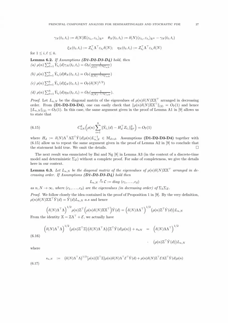
PRINCIPAL COMPONENT ANALYSIS FOR SEMIMARTINGALES AND STOCHASTIC PDE 27
γN (tℓ, ti) := δ(N)E〈εtℓ , εti〉RN θN (tℓ, ti) := δ(N)〈εtℓ , εti〉RN − γN (tℓ, ti)
ξN (tℓ, ti) := Z⊤tiΛ
⊤εtℓδ(N); ηN (tℓ, ti) := Z⊤tℓΛ⊤εtiδ(N)
for 1 ≤ i, ℓ ≤ n.
Lemma 6.2. If Assumptions (D1-D2-D3-D4) hold, then
(a) ρ(n)∑n
ℓ=1 Ytℓ(d)γN (tℓ, ti) = OP(1
ρ(n)−1/2CnN)
(b) ρ(n)∑n
ℓ=1 Ytℓ(d)θN (tℓ, ti) = OP(1
δ(N)−1/2CnN)
(c) ρ(n)∑n
ℓ=1 Ytℓ(d)ξN (tℓ, ti) = OP(δ(N)1/2)
(d) ρ(n)∑n
ℓ=1 Ytℓ(d)ηN (tℓ, ti) = OP(1
δ(N)−1/2CnN).
Proof. Let Ln,N be the diagonal matrix of the eigenvalues of ρ(n)δ(N)XX⊤ arranged in decreasingorder. From (D1-D2-D3-D4), one can easily check that ‖ρ(n)δ(N)XX⊤‖(2) = OP(1) and hence‖Ln,N‖(2) = OP(1). In this case, the same argument given in the proof of Lemma A1 in [9] allows usto state that
(6.15) C2nN
(ρ(n)
n∑
i=1
‖Yti(d)−H⊤d Zti‖2Rd
)= OP(1)
where Hd := δ(N)Λ⊤ΛZ⊤Y (d)ρ(n)L−1n,N ∈ Md×d. Assumptions (D1-D2-D3-D4) together with
(6.15) allow us to repeat the same argument given in the proof of Lemma A2 in [9] to conclude thatthe statement hold true. We omit the details.
The next result was enunciated by Bai and Ng [8] in Lemma A3 (in the context of a discrete-timemodel and deterministic ΣZ) without a complete proof. For sake of completeness, we give the detailshere in our context.
Lemma 6.3. Let Ln,N be the diagonal matrix of the eigenvalues of ρ(n)δ(N)XX⊤ arranged in de-creasing order. If Assumptions (D1-D2-D3-D4) hold then
Ln,Np→ C := diag (c1, . . . , cd)
as n,N → ∞, where (c1, . . . , cd) are the eigenvalues (in decreasing order) of ΣλΣZ .
Proof. We follow closely the idea contained in the proof of Proposition 1 in [9]. By the very definition,
ρ(n)δ(N)XX⊤Y (d) = Y (d)Ln,N a.s and hence
(δ(N)Λ⊤Λ
)1/2ρ(n)Z⊤
(ρ(n)δ(N)XX⊤
)Y (d) =
(δ(N)ΛΛ⊤
)1/2(ρ(n)Z⊤Y (d)
)Ln,N
From the identity X = ZΛ⊤ + E , we actually have
(δ(N)Λ⊤Λ
)1/2(ρ(n)Z⊤
Z)(δ(N)Λ⊤Λ
)(Z⊤Y (d)ρ(n)
)+ snN =
(δ(N)ΛΛ⊤
)1/2
(6.16)
·(ρ(n)Z⊤Y (d)
)Ln,N
where
sn,N :=(
δ(N)Λ⊤Λ)1/2[
ρ(n)(
Z⊤Z)
ρ(n)δ(N)Λ⊤E⊤Y (d) + ρ(n)δ(N)Z⊤EΛZ⊤
Y (d)ρ(n)
(6.17)

28 ALBERTO OHASHI AND ALEXANDRE B. SIMAS
+ ρ(n)δ(N)Z⊤EE⊤Y (d)ρ(n)] = oP(1)
due to Lemma 6.2. Let Un,N :=(δ(N)Λ⊤Λ
)1/2(ρ(n)Z⊤Z
)(δ(N)Λ⊤Λ
)1/2and
En,N :=(δ(N)ΛΛ⊤
)1/2(ρ(n)Z⊤Y (d)
).
We shall write (6.16) as follows
[Un,N + sn,NEn,NE+n,N ]En,N = En,NLn,N
where E+n,N is the pseudoinverse of En,N . Then each column of En,N is an eigenvector of Nn,N +
sn,NEn,NE+n,N . Since En,NE+
n,N = OP(1) then (6.17) and Assumptions (D1, D2) yield
‖Un,N + sn,NEn,NE+n,N − Σ
1/2λ ΣZΣ
1/2λ ‖(2)
p→ 0
as n,N → ∞. By the continuity of the eigenvalues, we do have ‖Ln,N − C‖(2)p→ 0 as n,N → ∞.
Since Σ1/2λ ΣZΣ
1/2λ and ΣλΣZ have the same random eigenvalues, we conclude the proof.
Lemma 6.4. Assume that hypotheses (D1-D2-D3-D4) hold and the eigenvalues of ΣλΣZ ∈ Md×d
are distinct almost surely. Then, for every j = 1, . . . , d, there exists a random vector (G1j , . . . , Gdj)such that
(n∑
ℓ=1
√ρ(n)y1tℓZ
jtℓ , . . . ,
n∑
ℓ=1
√ρ(n)ydtℓZ
jtℓ
)p→(G1j , . . . , Gdj
)
as n,N → ∞. Moreover, the matrix G := (Gij)1≤i,j≤d is invertible a.s and it is given by G =
C1/2Φ⊤Σ−1/2λ and Φ is the eigenvector matrix related to C subject to Φ⊤Φ = Id a.s.
Proof. By using Lemma 6.3, the proof is identical to Proposition 1 in Bai [9] even in the case whenΣZ is random. We refer the reader to the discussion in page 162 in [9].
We are now able to present the following result.
Lemma 6.5. Let us assume that assumptions (D1,D2, D3, D4) hold and let d = arg min1≤k≤kmaxPC(k).
Assume the eigenvalues of ΣλΣZ ∈ Md×d are distinct almost surely. Then, limn,N→∞P[d = d] = 1 if
(i) q(N,n) → 0 and (ii) CnNq(N, T ) → ∞ as n,N → ∞ where CnN = minδ(N)−1/2, ρ(n)−1/2.Proof. The same arguments given in the proof of Theorem 1 in Bai and Ng [8] apply in our context.In particular, Lemmas 2, 3 and 4 in Bai and Ng [8] can be similarly proved in our context as wellby using Assumptions (D1, D2, D3, D4) and the fact that ΣλΣZ has distinct eigenvalues a.s. Inparticular, the fact that ΣZ is not deterministic is not essential for the validity of the analogous resultsof Lemmas 2, 3 and 4 given by [8] in our context, as long as rank ΣZ = d a.s (Assumption D1). In
particular, for k < d let us define J⊤k := Y ⊤(k)Zρ(n)Λ⊤Λδ(N) ∈ Mk×d. In our context, Lemma 3 in
[8] can be written as follows: There exists τk > 0 a.s such that
lim infn,N→∞
V (k,ZJk)− V (d,Z) = tr(Rk.Σλ) =: τk
in probability, where Rk := ΣZ − ΣZHk(H⊤k ΣZHk)
−1H⊤k ΣZ and Hk := limn,N→∞ Jk exists due to
Lemma 6.4. By construction rank Hk = k < d a.s. Assumptions (D1-D2) yield tr(Rk.Σλ) > 0 a.s.By writing
PC(k)− PC(d) = V (k, Y (k)) − V (d, Y (d)) − (d− k)q(n,N)
and splitting
V (k, Y (k)) − V (d, Y (d)) = [V (k, Y (k))− V (k,ZJk)] + [V (k,ZJk)− V (d,ZJd)]

PRINCIPAL COMPONENT ANALYSIS FOR SEMIMARTINGALES AND STOCHASTIC PDE 29
+ [V (d,ZJd)− V (d, Y (d))],
we shall use the same argument in the proof of Th 1 in [8] to conclude that
limn,N→∞
PPC(k) < PC(d) = 0,
for each k < d. If kmax ≥ k ≥ d, then similar to Lemma 4 in [8], Assumptions (D1,D2, D3, D4)and the fact that the eigenvalues of ΣλΣZ ∈ Md×d are distinct almost surely yield
V (k, Y (k)) − V (d, Y (d))) = OP(C−2nN ).
The rest of the proof is identical to the proof of Th 1 in [8], so we omit the details.
6.4. Main Results. Let us now present the main results of this section. The following list of as-sumptions will also be in force throughout this section.
(Q1) The eigenvalues of ΣλΣZ ∈ Md×d are distinct almost surely.
(Q2) We assume
ρ(n)∑
1≤ℓ<s≤n
|yktℓykts |
is bounded in probability for every k ∈ 1, . . . , d.
(Q3)
ρ(n)∑
1≤ℓ<s≤n
yktℓykts〈εtℓ , λr〉RN δ(N)〈εts , λj〉RN δ(N)
p→ 0
as n,N → ∞ for each k, r, j ∈ 1, . . . , d.
(Q4) There exists a sequence of natural numbers γ(n);n ≥ 1 decaying to zero such that
E
n∑
i=1
‖∆εti‖2RN δ(N) = O(γ(n)).
(Q5) sup0≤t≤T ‖εt‖2E is bounded in probability and for each i ∈ 1, . . . , d,
ρ(n)∑
1≤ℓ<s≤n
|yitℓyits |‖εtℓ‖E‖εts‖Ep→ 0
as n → ∞.
Remark 6.7. Assumption (Q1) is essential to our estimation procedure because it yields an asymp-totic Y ∈ X d and a random basis for V which will allow us to construct a consistent pair of estimators(Q, N ) for the splitting V = Q⊕N of the invariant manifold V . The technical conditions (Q2, Q3,Q5) are not strong since they impose a very mild growth condition on the eigenvectors of X⊤X. As-sumption (Q4) is quite natural for error structures arising in space-time data generated by stochasticPDEs. For example, as far as the consistency problem of the HJM model (see section 4.2), assump-tion (Q4) means that the initial fitting method used to interpolate points which generates X cannotintroduce an extrinsic volatility for the market. In other words, (Q4) rules out pure martingale errorstructures.

30 ALBERTO OHASHI AND ALEXANDRE B. SIMAS
The starting point for the estimation of (Q,N ) is to take advantage of the identities (6.8) and(6.9) based on a quadratic variation matrix [Y ]T constructed from an asymptotic Y ∈ X d satisfyingAssumptions 2.1 and 2.2. We define such process as follows: Let Z be a factor representation of (6.1)satisfying Assumption (A2) and the (D1-D2-D3-D4-Q1) and let G be the associated matrix definedin Lemma 6.4. Since G is nonsingular a.s and Σλ is positive definite, then the random matrix matrixA = C−1GΣλ = (Aij)1≤i,j≤d ∈ Md×d given by
(6.18) Aij =
d∑
k=1
c−1i Gik
∫ b
a
λk(x)λj(x)dx; 1 ≤ i, j ≤ d,
is non-singular a.s. Then we shall apply Remark 6.3 to state that AZ ∈ X d is a truly d-dimensionalprocess and it is a factor measurable process realizing (6.4) for the basis (loading factors) (A−1)⊤λ.From Remark 6.4, AZ satisfies Assumptions 2.1 and 2.2.
In the sequel, for a given factor representation Z of (6.1) satisfying Assumption (A2) and the
assumptions in Lemma 6.4, we set Y = AZ. Let [Y ]T := (mℓk)1≤ℓ,k≤d and [Y ]T := (mℓk)1≤ℓ,k≤d be
the matrices given, respectively, by
(6.19) mℓk :=
n−1∑
i=1
(Yti+1,ℓ(d)− Yti,ℓ(d)
)(Yti+1,k(d)− Yti,k(d)
),
for 1 ≤ ℓ, k ≤ d and
msv := [Y s, Y v]T ; 1 ≤ s, v ≤ d.
We stress that Y ∈ X d has a quadratic variation matrix in the sense of Definition 2.1.
Proposition 6.2. If Assumptions (D1, D2, D3, D4) and (Q1, Q2, Q3, Q4) hold true, then
‖[Y ]T − [Y ]T ‖2(2)p→ 0
as n,N → ∞.
Proof. At first, by taking n,N large enough, assumptions (D1, D2, D3, D4, Q1) allow us to use
Lemma 6.5 and we assume that d = d because d is an integer-valued consistent estimator. In thesequel, if P is a real-valued process then we write ∆tiP := Pti+1
− Pti ; 1 ≤ i ≤ n − 1. By using the
definition of Y (d), one can actually write
Yti(d) = H⊤d Zti + L
−1nNρ(n)
n∑
ℓ=1
Ytℓ(d)(
γN(tℓ, ti) + θN(tℓ, ti) + ξN(tℓ, ti) + ηN (tℓ, ti))
=: H⊤d Zti + Rti(n,N),
where H⊤d := L−1
nN Y ⊤(d)Zρ(n)Λ⊤Λδ(N) and LnN is be the diagonal matrix of the eigenvalues ofρ(n)δ(N)XX⊤ arranged in decreasing order (see Lemma 6.3)).
To shorten notation, we set Wti := H⊤d Zti and ϕN (tℓ, ti) := γN (tℓ, ti) + θN (tℓ, ti) + ξN (tℓ, ti) +
ηN (tℓ, ti) for 1 ≤ i, ℓ ≤ n. In the sequel, for r, ℓ = 1, . . . , d we denote OP;(r,ℓ)(ξn) any random variablewhich is O(ξn) in probability, C is a constant which may differ from line to line and let us denote the
d× d-matrix given by W := (wsq) where
wsq :=
n−1∑
i=1
∆Wti(s)∆Wti (q)
for s, q = 1 . . . , d. We claim that
PRINCIPAL COMPONENT ANALYSIS FOR SEMIMARTINGALES AND STOCHASTIC PDE 31
(6.20)d∑
m=1
n−1∑
i=1
(∆Rm
ti (n,N))2 p→ 0
and
(6.21) vec (W )p→ vec ([Y ]T )
as n,N → ∞, where vec is the usual vectorization operator. Let LnN = diag (γ1, . . . , γn). By thevery definition,
(H⊤d )ij =
√ρ(n)δ(N)
d∑
k=1
( n∑
ℓ=1
γ−1i yitℓZ
ktℓ
)( N∑
m=1
λk(xm)λj(xm)); 1 ≤ i, j ≤ d.
By Lemma 6.3, we know that Ln,Np→ diag (c1, . . . , cd) as n,N → ∞, where (c1, . . . , cd) are the
eigenvalues of ΣλΣZ . Then Lemma 6.4 yields
wsq =
d∑
j=1
d∑
r=1
(H⊤d )qj(H
⊤d )sr
n−1∑
i=1
∆Zjti∆Zr
ti
p→d∑
j=1
d∑
r=1
d∑
k=1
d∑
m=1
〈λk, λj〉L2([a,b];R)c−1q Gqk〈λm, λr〉L2([a,b];R)c
−1s Gsm[Zj , Zr]T
= [Y s, Y q]T ; 1 ≤ s, q ≤ d,
as n,N → ∞. This shows that (6.21) holds. By noting that
∆Yti,ℓ(d)∆Yti,k(d) = ∆Wti(k)∆Wti (ℓ) + ∆Wti(k)∆Rℓti (n,N)
(6.22)
+ ∆Rkti(n,N)∆Wti(ℓ) + ∆Rk
ti(n,N)∆Rℓti(n,N); 1 ≤ k, ℓ ≤ d,
we only need to check (6.20) in order to conclude the proof. Let Sti(n,N) := Ln,N Rti(n,N) ∈ Md×1.
From Lemma 6.3, we know that ‖L−1n,N‖(2) = OP(1), so we only need to check that
(6.23)
d∑
m=1
n−1∑
i=1
(∆Sm
ti (n,N))2 p→ 0 as n,N → ∞.
At first, for each k ∈ 1, . . . , d we shall write
n−1∑
i=1
(∆Sk
ti(n,N))2
= ρ(n)n−1∑
i=1
n∑
ℓ=1
|yktℓ |2(∆iϕN (tℓ, ti))2
+ 2ρ(n)n−1∑
i=1
∑
1≤ℓ<s≤n
yktℓ∆iϕN (tℓ, ti)ykts∆iϕN (ts, ti)
=: T1(n,N) + T2(n,N)(6.24)
where ∆iϕN (tℓ, ti) := ϕN (tℓ, ti)−ϕN (tℓ, ti−1); 1 ≤ i ≤ n− 1, 1 ≤ ℓ ≤ n. We divide the argument intotwo steps.
Analysis of T1(n,N). It is sufficient to prove that

32 ALBERTO OHASHI AND ALEXANDRE B. SIMAS
ρ(n)
n−1∑
i=1
n∑
ℓ=1
|yktℓ |2[(∆iγN (tℓ, ti))
2 + (∆iθN (tℓ, ti))2
+ (∆ξN (tℓ, ti))2 + (∆iηN (tℓ, ti))
2]= OP(ρ(n))
for each k ∈ 1, . . . , d. In fact, a simple application of Cauchy-Schwartz inequality and the fact that∑nℓ=1 |yktℓ |2 = 1 yield the following estimates
(6.25) ρ(n)
n−1∑
i=1
n∑
ℓ=1
|yktℓ|2(∆iγN(tℓ, ti))
2 ≤ ρ(n)EN∑
m=1
sups
|εts(xm)|2δ(N)
n−1∑
i=1
N∑
k=1
|∆εti(xk)|2δ(N),
ρ(n)
n−1∑
i=1
n∑
ℓ=1
|yktℓ|2(∆iθN (tℓ, ti))
2 ≤ 2
(
ρ(n)
n−1∑
i=1
n∑
ℓ=1
|yktℓ|2(∆iγN(tℓ, ti))
2
)1/2
×
(
ρ(n)
n−1∑
i=1
n∑
ℓ=1
|δ(N)ε⊤tℓ∆εtiyktℓ|2)1/2
+ ρ(n)
n−1∑
i=1
n∑
ℓ=1
|yktℓ|2(
(∆iγN(tℓ, ti))2 + (δ(N)ε⊤tℓ∆εti)
2)
,(6.26)
(6.27) ρ(n)n−1∑
i=1
n∑
ℓ=1
|yktℓ|2(∆iξN (tℓ, ti))
2 ≤ Cρ(n) supt
‖εt‖2RN δ(N)
d∑
r=1
n−1∑
i=1
|∆Zrti |
2‖λr‖2RN δ(N)
(6.28) ρ(n)
n−1∑
i=1
n∑
ℓ=1
|yktℓ|2(∆iηN (tℓ, ti))
2 ≤ Cρ(n)
n−1∑
i=1
‖∆εti‖2RN δ(N)
d∑
r=1
supt
|Zrt |
2‖λr‖2RN δ(N)
The estimates (6.25),(6.26), (6.27) and (6.28) allow us to conclude that T1(n,N) = OP(ρ(n)).
Analysis of T2(n,N). The estimates for the crossing terms are more involved. Let us split T2(n,N)according to the terms ∆iγN (tℓ, ti), ∆iθN (tℓ, ti), ∆iξN (tℓ, ti) and ∆iηN (tℓ, ti) as follows. To shortennotation, in the sequel we denote J(k, n) = ρ(n)
∑1≤ℓ<s≤n |yktℓykts |. Cauchy-Schwartz inequalities and
routine algebraic manipulations yield the following estimates
ρ(n)
n−1∑
i=1
∑
1≤ℓ<s≤n
|yktℓ∆iγN (tℓ, ti)ykts∆iξN (ts, ti)| ≤ CJ(k, n)
(supt
‖εt‖2RN δ(N))1/2
[(E sup
t‖εt‖2RN δ(N))
n−1∑
i=1
p∑
r=1
|∆Zrti |2‖λr‖2RN δ(N)
]1/2[ n−1∑
i=1
E‖∆εti‖2RN δ(N)
]1/2,
ρ(n)n−1∑
i=1
∑
1≤ℓ<s≤n
|yktℓ∆iξN (tℓ, ti)ykts∆iηN (ts, ti)| ≤ CJ(k, n)
p∑
r,q=1
OP;(r,q)(1)
×[
n−1∑
i=1
‖∆εti‖2RN δ(N)
]1/2,
ρ(n)
n−1∑
i=1
∑
1≤ℓ<s≤n
|yktℓ∆iθN (tℓ, ti)ykts∆iξN (ts, ti)| ≤ CJ(k, n)
p∑
r=1
OP;r(1) supt
‖ε‖RN

PRINCIPAL COMPONENT ANALYSIS FOR SEMIMARTINGALES AND STOCHASTIC PDE 33
×(
n−1∑
i=1
|∆Zrti |2
n−1∑
i=1
‖∆εti‖2RN δ(N)
)1/2
.
We also shall write
ρ(n)
n−1∑
i=1
∑
1≤ℓ<s≤n
yktℓ∆iθN (tℓ, ti)ykts∆iξN (ts, ti) =
p∑
r,j=1
OP;(r,j)(1)ρ(n)∑
1≤ℓ<s≤n
yktℓykts
× 〈εtℓ , λr〉RN δ(N)〈εts , λj〉RN δ(N)
and
ρ(n)
n−1∑
i=1
∑
1≤ℓ<s≤n
|yktℓ∆iγN (tℓ, ti)ykts∆iγN (ts, ti)| ≤ J(k, n)OP(1)
n−1∑
i=1
E‖∆εti‖2RN δ(N),
ρ(n)n−1∑
i=1
∑
1≤ℓ<s≤n
|yktℓ∆iγN (tℓ, ti)ykts∆iηN (ts, ti)| ≤ CJ(k, n)
(n−1∑
i=1
‖∆εti‖2RN δ(N)
)1/2
,
ρ(n)
n−1∑
i=1
∑
1≤ℓ<s≤n
|yktℓ∆iηN (tℓ, ti)ykts∆iηN (ts, ti)| ≤ CJ(k, n)
p∑
q,r=1
OP;(q,r)
(n−1∑
i=1
‖∆εti‖2RN δ(N)
).
The remainder terms in T2(n,N) are analogous. Summing up the above estimates, we conclude thatT2(n,N) → 0 in probability as n,N → ∞. From identities (6.22), (6.23), (6.24) and (6.20), weconclude the proof.
The next step is the analysis of the convergence of the loading factor estimators defined as follows.Let
Λ⊤ := ρ(n)Y ⊤(d)X ∈ Md×N
and
ϕi(x) :=√ρ(n)
n∑
k=1
yitkXtk(x), ξk(x) := ((A−1)⊤λ(x))k
for a ≤ x ≤ b, 1 ≤ i ≤ d, 1 ≤ k ≤ d. Since A ∈ Md×d is non-singular a.s, then ξ1(ω, ·), . . . , ξd(ω, ·) isa basis for V for almost all ω ∈ Ω. More importantly,
rt = φt +
d∑
k=1
Y kt ξk; 0 ≤ t ≤ T.
where Y = AZ ∈ X d.
Proposition 6.3. If Assumptions (D1, D2, D3, D4, Q1, Q5) hold true, then
d∑
j=1
‖ϕj − ξj‖2Ep→ 0
as n,N → ∞.
34 ALBERTO OHASHI AND ALEXANDRE B. SIMAS
Proof. Let us fix i ∈ 1, . . . , d. Since d is an integer-valued consistent estimator for d, then we shall
assume that d = d. Under (D1, D2, D3, D4, Q1), ξi; 1 ≤ i ≤ d is a well-defined random basisfor V . By the very definition,
ϕi(x) =√ρ(n)
n∑
k=1
yitkXtk(x) =
d∑
m=1
( n∑
k=1
√ρ(n)yitkZ
mtk
)λm(x)
+
n∑
k=1
√ρ(n)yitkεtk(x) =: R1,i(x) +R2,i(x), x ∈ [a, b].
Let us recall that for any f ∈ E, we can compute the Sobolev norm as follows ‖f‖2E = supΠ∑
sj∈Π|∆f(sj)|2
∆sj<
∞ where the sup is taken over all partitions Π of [a, b]. See e.g Prop 1.45 in [33] for further details.If Π = sjMj=1 is a partition of [a, b], then
∑
sj∈Π
|∆R2,i(sj)|2∆sj
=∑
sj∈Π
n∑
k=1
ρ(n)|yitk |2|∆εtk(sj)|2
∆sj
+ 2ρ(n)∑
1≤k<m≤n
yitkyitm
∑
sj∈Π
∆εtk(sj)
∆sj
∆εtm(sj)
∆sj
=: I1,i + I2,i
Since ρ(n)Y ⊤(d)Y (d) = Id a.s, then (Q5) yields
|I1,i| ≤n∑
ℓ=1
ρ(n)|yitℓ |2‖εtℓ‖2E ≤ sup0≤t≤T
‖εt‖2Eρ(n)p→ 0
as n → ∞. Cauchy-Schwartz inequality and (Q5) yield
|I2,i| ≤ 2ρ(n)∑
1≤ℓ<s≤n
|yitℓyits |‖εtℓ‖E‖εts‖Ep→ 0
as n → ∞. From Lemma 6.4, we know that (G⊤)−1 = A so that (A−1)⊤ = G. Since λ1, . . . , λd ⊂ E,
then we obviously have ‖R1,i(·)− ξi(·)‖E p→ 0 as n → ∞. This concludes the proof.
In the sequel, p is any consistent estimator for dim Q based on X . See Appendix for details.
Let L ∈ Md×d be the matrix whose rows are given by Li := vi; 1 ≤ i ≤ d, where v1, . . . , vd is
an orthonormal eigenvector set of the matrix [Y ]T (see (6.19)) associated to the ordered eigenvalues
θ1 ≥ θ2 ≥ . . . ≥ θd. Let us define
(6.29) Zjti := j-th component of LYti ; 0 ≤ i ≤ n, 1 ≤ j ≤ d
and
[Zj ]T :=
n∑
i=1
(Zjti − Zj
ti−1
)2
over a sample 0 = t0 < t1 < . . . < tn = T . By the very definition, [Zj ]T = θj ; 1 ≤ j ≤ d.Now we are able to present the main result of this article. Before this, we need an elementary
lemma from linear algebra.

PRINCIPAL COMPONENT ANALYSIS FOR SEMIMARTINGALES AND STOCHASTIC PDE 35
Lemma 6.6. Let v1, . . . , vd be a set of d linearly independent vectors in a real Hilbert space Hwith inner product 〈·, ·〉H and V = spanv1, . . . , vd. Let T : V → V be an orthogonal matrix. Ifτ1, . . . , τd is the Gram-Schmidt orthonormalization of v1, . . . , vd and w1, . . . , wd is the Gram-Schmidtorthonormalization of Tv1, . . . , T vd, then we have
wi = Tτi; i = 1, . . . , d, .
Proof. The proof follows by just observing that for each v ∈ V , ‖Tv‖H = ‖v‖H , and for each u ∈ V ,we have T (Projvu) = ProjTv(Tu), where Projvu = v〈u, v〉H/‖v‖H .
Theorem 6.1. Let r be the stochastic PDE (6.1) satisfying Assumptions (A1-A2). Assume theexistence of a factor representation satisfying Assumption (A2) and (D1, D2, D3, D4, Q1, Q2,Q3, Q4, Q5). For a given h ∈ dom (A), let Vh
t = φt + V ; 0 ≤ t ≤ T be the minimal foliationgenerated by V such that r0 = h ∈ Vh
0 and we set
N := span(Lϕ)p+1, . . . , (Lϕ)d
Q := span
(Lϕ)1, . . . , (Lϕ)p
.
Then, V = Q⊕N a.s and
maxd(N ,N ), d(Q,Q) p→ 0 as n,N → ∞.
Moreover,
(6.30) [Z1]T ≥ . . . ≥ [Z p]T a.s, [Zi]T ≃ 0, p+ 1 ≤ i ≤ d as n,N → ∞,
andd∑
j=1
θ2jp→ ‖QT ‖2(2)
as n,N → ∞.
Proof. From Assumptions (A1-A2), we shall fix a pair (Z, λ) which realizes
rt(x) = φt(x) +
d∑
j=1
Zjt λj(x) = φt(x) +
d∑
j=1
Y jt ξj(x); 0 ≤ t ≤ T
where V = spanλ1, . . . , λd = spanξ1, . . . , ξd, Z is a continuous semimartingale satisfying As-sumption (A2) and (D1, D2, D3, D4), (Q1, Q2, Q3, Q4, Q5). Here, we set Y = AZ andξ(x) = (A−1)⊤λ(x), where A is given by (6.4). From Remark 6.4, Y satisfies Assumption (A2) aswell.
To shorten notation, we abbreviate Gram-Schmidt orthonormalization by GSO. Let
N = span(Lξ)p+1, . . . , (Lξ)d,and
Q = span(Lξ)1, . . . , (Lξ)p.Following the same lines as in the proof of Theorem 5.1 and noting that (see Remark 6.4)
Φ(N ) = Ker([Y ]T ) and Φ(N ) = Ker([Y ]T ),
we obtain
(6.31) d(N ,N )p−→ 0, and d(Q,Q)
p−→ 0,
as n,N → ∞. By using the triangle inequality, we obtain
d(N ,N ) ≤ d(N , N ) + d(N ,N ),
and from equation (6.31), it is enough to prove that d(N , N )p−→ 0. as n,N → ∞.

36 ALBERTO OHASHI AND ALEXANDRE B. SIMAS
Let ϕ1, . . . , ϕd and ξ1, . . . , ξd be as in Proposition 6.3. Let n and N be large enough so that
p = p and d = d. Let τ1, . . . , τd and τ1, . . . , τd be the GSO of ξ1, . . . , ξd and ϕ1, . . . , ϕd,respectively. Lemma 6.6 allows us to state that Lτ1, . . . , Lτd is the GSO of Lξ1, . . . , Lξd and
Lτ1, . . . , Lτd is the GSO of Lϕ1, . . . , Lϕd.From the orthonormalization procedure, for each k ≤ d, we have
spanLϕ1, . . . , Lϕk = spanLτ1, . . . , Lτkand
spanLξ1, . . . , Lξk = spanLτ1, . . . , Lτk.Thus,
N = spanLτ1, . . . , Lτp and N = spanLτ1, . . . , Lτp.Therefore, since Φ is an isometry, we have
d(N , N ) = D(N , N ) = 1− 1
d
∑
i,j
(〈(Lτ )i, (Lτ)j〉)2 a.s.
Let us work with the quantity inside the brackets, and let us introduce some notation: Denote thematrix of L by aij, i.e., for any vector v ∈ Rd,
(Lv)i :=∑
j
aijvj .
Note that since the transformation L is orthogonal, we have∑
k
aik ajk = δij a.s.
Observe that from Proposition 6.3, we have that 〈τi, τj〉 p→ δij as n,N → ∞. Since L is orthogonaland the set of orthogonal matrices is compact, the set ai,j is uniformly bounded in n and N , sothat ∣∣∣∣∣∣
∑
k 6=p
aik ajp〈τk, τp〉
∣∣∣∣∣∣p→ 0,
and ∣∣∣∣∣∑
k
aikajk(〈τk, τk〉 − 1)
∣∣∣∣∣p→ 0
as n,N → ∞.Therefore,
∣∣∣∣∣∣∑
k,p
aikajp〈τk, τp〉 − δij
∣∣∣∣∣∣=
∣∣∣∣∣∣∑
k,p
aik ajp〈τk, τp〉 −∑
k
aikajk
∣∣∣∣∣∣
≤∣∣∣∣∣∑
k
aik ajk(〈τk, τk〉 − 1)
∣∣∣∣∣+
∣∣∣∣∣∣∑
k 6=p
aikajp〈τk, τp〉
∣∣∣∣∣∣p→ 0,
as n,N → ∞, which thus implies that
1
d
∑
i,j
(〈(Lτ)i, (Lτ)j〉)2 =1
d
∑
i,j
∑
k,p
aik ajp〈τk, τp〉
2
p→ 1,

PRINCIPAL COMPONENT ANALYSIS FOR SEMIMARTINGALES AND STOCHASTIC PDE 37
and then,
d(N , N )p−→ 0
as n,N → ∞. The proof for the statement limn,N→∞ d(Q,Q) = 0 in probability follows from the same
reasoning as in the proof of Theorem 5.1. Let us now check the ordering (6.30). Let θ1 ≥ 1 . . . ≥ θd a.s
be the eigenvalues of the self-adjoint non-negative matrix [Y ]T arranged in decreasing order a.s. Bythe very definition,
θi = [Zi]T ; 1 ≤ i ≤ d a.s
Moreover, the eigenvalues are continuous functions of the entries of the matrix and p = p and d = dfor n,N large enough. Then,
maxp+1≤i≤d
θip→ 0
as n.N → ∞. This shows that (6.30) holds. Lastly, by the very definition, the matrix of the randomoperator QT : V → V computed along the basis ξ1, . . . , ξd is given by [Y i, Y j ]T ; 1 ≤ i, j ≤ d ∈Md×d. Therefore, ‖QT‖2(2) = ‖[Y ]T ‖2(2) a.s. Proposition 6.2 yields
‖[Y ]T ‖2(2) =d∑
j=1
θ2j =
d∑
j=1
[Zj ]2Tp→ ‖QT‖2(2)
as n,N → ∞. This concludes the proof.
7. Simulation Studies and Applications
In this section, we present some numerical results to illustrate the methodology developed in thisarticle.
7.1. Semimartingale PCA. In this section, we illustrate the estimation of the factor spaces (W ,D)based on a finite-dimensional semimartingale system sampled in high-frequency. In particular, the goalis to illustrate Proposition 3.1. In the simulation below, we assume that one observes a 4-dimensionalsemimartingale as follows: We consider a Markov diffusion
dMt = µ(Mt)dt+ σ(Mt)dBt
driven by a 3-dimensional Brownian motion B = (B1, B2, B3) and the vector fields µ : R4 → R4 andσ : R4 → M4×3 are given by µ(x1, . . . , x4) = (x2,−2x1 + x3, x4,−x1) and
σ(x1, . . . , x4) =
1 0 x2
0 1 00 0 x2
0 0 x2
One can easily check W = B1, B2,∫M2dB3 and since M is a truly 4-dimensional semimartingale,
then M = W ⊕ D where dim D = 1. The observation times are taken to be equidistant: tnk =2πn−1k; k = 0, . . . , n − 1 where the total number of observations is n = 2000. The estimated factors
in Figure 1 are ranked in terms quadratic variation (see Theorem 5.1) and we clearly observe that
J4 identifies a null quadratic variation factor which generates D. The quadratic variation explained
by the principal components are given by Table 1, where ηi =∑i
j=1θj
∑4r=1
θr, 1 ≤ i ≤ 4 and θi is the i-th
estimated eigenvalue related to i-th estimated principal component J i.

38 ALBERTO OHASHI AND ALEXANDRE B. SIMAS
Table 1. Quadratic variation explained by the principal components
η1 η2 η3 η40.7523 0.9021 0.9996 1.0000
0 1 2 3 4 5 6
−2
02
4
Sample realization of M
t
M
M1 M2 M3 M4
0 1 2 3 4 5 6
−4
02
46
8
Sample realization of the estimated factors J
t
J
J1 J2 J3 J4
Figure 1. Estimation of a basis for W and D
7.2. Variance versus quadratic variation. In this section, the goal is to illustrate that any naiveattempt to implement standard factor models towards dimension reduction in term of quadraticvariation is hopeless. For this purpose, we consider two very simple space-time two-dimensionalsemimartingales driven by a single Brownian motion B.
Xt = Btλ1(x) +(sin(15t)−Bt
)λ2(x)
Ut = Btλ1(x) +(sin(3t)−Bt
)λ2(x)
where B is a one-dimensional Brownian motion, λ1(x) = xcos(x) and λ2(x) = cos(x) − xsin(x); 0 ≤x ≤ 5, 0 ≤ t ≤ 2π. In the sequel, the drift components are denoted by Γ1
t = sin(15t), Γ2t = sin (3t)
and we set H1 = (B,Γ1 −B) and H2 = (B,Γ2 −B). Let M(H1) and M(H2) be the dynamic spacesgenerated by H1 and H2, respectively. We clearly have
M(H1) = spanB ⊕ span Γ1, M(H2) = span B ⊕ span Γ2Here, in the time variable, the observation times are taken to be equidistant: tkn = 2π
n−1k; k = 0, . . . , n−1 where the total number of observations is n = 2000. In the spatial variable, the observation times aretaken to be equidistant: xn
k = 5n−1k; k = 0, . . . , n−1 where the total number of observations is n = 31.
The estimated pair of factors provided by the high-frequency factor model based on variance will be

PRINCIPAL COMPONENT ANALYSIS FOR SEMIMARTINGALES AND STOCHASTIC PDE 39
denoted by (Y 1, Y 2). Here, Y 1 is the estimator of the leading factor component in terms variance. Theestimated pair of factors provided by the high-frequency factor model based on quadratic variation
will be denoted by (Z1, Z2). Here, Z1 is the leading factor component in terms of quadratic variation(see (6.29)).
In Figure 3, we clearly see that the factor analysis based on second moments is not able to identify
(B,Γ1). The leading component estimated factor Y 1 resembles a bounded variation process with large
variance and the second estimated factor Y 2 is essentially the first one distorted by the Brownianpaths in such way that the true pair (B,Γ1) is by no means identified. In strong contrast, Figure
3 clearly reports that the estimated pair (Z1, Z2) identifies the pair (B,Γ1). We stress that in thistwo-dimensional setting, the true factors can be estimated up to multiplicative constants so thatthe results presented in Figures 2 and 3 shows a very consistent estimation of M(H1) by using ourmethodology. More importantly, the correct splitting and ranking in term of quadratic variation isfairly estimated. This numerical example illustrates the use of factor analysis based on variance toinfer volatility (quadratic variation) does not have any sound basis even in a very simple space-timesemimartingale model given by X above.
Figure 4 presents the results for the model U . In this numerical experiment, the goal is to illustratethat null quadratic variation factors with large variance may be the leading component by using
standard factor models in terms of variance. In Figure 4, we report that Y 2 estimates well the
Brownian component B responsible for the quadratic variation subspace of U , Y 1 estimates well thebounded variation component Γ2 responsible for the null quadratic variation subspace of U . However,the correct leading component of the space-time semimartingale U is the Brownian motion and not Γ2.This simple example shows that prioritising components with large variance by using standard factormodels may be completely superfluous in terms of quadratic variation. This shows that dimensionreduction for semimartingale systems can not be accurately performed by using classical dimensionreduction based on variance.
0 1 2 3 4 5 6
−2
24
Sample path realizations of Y1 and Y
2
t
Y1 ,
Y2 Y
1Y
2
0 1 2 3 4 5 6
−2
02
4
Sample path realizations of Z1 and Z
2
t
Z1 ,
Z2 Z
1Z
2
Figure 2. Estimated factors of X .
7.3. Estimating finite-dimensional realizations from a SPDE. Here, we illustrate our method-ology with some applications to space-time semimartingale models. The first example is based on aMarkov diffusion

40 ALBERTO OHASHI AND ALEXANDRE B. SIMAS
0 1 2 3 4 5 6−
22
4
Sample path realizations of Y1 , Z
1 , and B
t
Y1 ,
Z1 ,
B Y1
Z1
B
0 1 2 3 4 5 6
−2
02
4
Sample path realizations of Y2 , Z
2 , and Γ1
t
Y2 ,
Z2 ,
Γ1
Y2
Z2
Γ1
Figure 3. Comparation of the estimated factors of Figure ??
0 1 2 3 4 5 6
−2
24
Sample path realizations of Y1 , Z
1 , and B
t
Y1 ,
Z1 ,
B Y1
Z1
B
0 1 2 3 4 5 6
−2
02
4
Sample path realizations of Y2 , Z
2 , and Γ2
t
Y2 ,
Z2 ,
Γ2
Y2
Z2
Γ2
Figure 4. Specification of the standard factor analysis for a null quadratic variationcomponent as the leading semimartingale component in terms of variance
dMt = µ(Mt)dt+ σ(Mt)dBt
driven by a 3-dimensional Brownian motion B = (B1, B2, B3) and the vector fields µ : R4 → R4 andσ : R4 → M4×3 are given by µ(x1, . . . , x4) = (x2,−2x1 + x3, x4,−x1) and
σ(x1, . . . , x4) =
1 0 00 x2 00 0 x1
0 0 0

PRINCIPAL COMPONENT ANALYSIS FOR SEMIMARTINGALES AND STOCHASTIC PDE 41
where,
(7.1) rt =
4∑
i=1
M itλi,
and λ1 = x cos(x), λ2 = cos(x)−x sin(x), λ3(x) = −2 sin(x)−x cos(x), and λ4(x) = x sin(x)−3 cos(x).In this case, W = span M1,M2,M3, D = span M4, Q = span λ1, λ2, λ3 and N = span λ4.Figure 5 shows the estimated factors of equation (7.1) by using the variance-based factor model Y
and the PCA semimartingale Z developed in this paper. Clearly, the variance-based factor modelis not able to identify the subspace D (and hence N as well), while the PCA semimartingale does.
In addition, Table 2 presents λk :=∑k
j=1 mjj/∑4
j=1 mjj where mjj is the (j, j)-th element of the
matrix [Y ]T (see (6.19)). Table 3 presents the variation explained by PCA semimartingale by means
of ηi =∑i
j=1θj
∑4r=1
θr, 1 ≤ i ≤ 4 where θi is the i-th estimated eigenvalue related to i-th estimated principal
component Zi. One clearly see the use of PCA semimartigale is more efficient than the variance-basedfactor model in identifying quadratic variation dimension.
0 1 2 3 4 5 6
−2
2
Sample realization of Y1
t
Y1
0 1 2 3 4 5 6−
31
Sample realization of Z1
t
Z1
0 1 2 3 4 5 6
−2
1
Sample realization of Y2
t
Y2
0 1 2 3 4 5 6
−3
0
Sample realization of Z2
t
Z2
0 1 2 3 4 5 6
−3
1
Sample realization of Y3
t
Y3
0 1 2 3 4 5 6
−1
2
Sample realization of Z3
t
Z3
0 1 2 3 4 5 6
0.0
2.0 Sample realization of Y
4
t
Y4
0 1 2 3 4 5 6
0.0
2.5 Sample realization of Z
4
t
Z4
Figure 5. Estimated factors for the space-time semimartingale (7.1)
Dynamic distance between manifolds Let us now investigate the robustness of our methodologyin the estimation of the minimal invariant manifold, say V , for a stochastic PDE. For this purpose,
we consider the following objects: Let V = Q⊕ N be the estimator for V based on the entire sample(ti, xj); 0 ≤ i ≤ n, 0 ≤ j ≤ N. Let V−k be the same estimator but computed over the reduced
sample (ti, xj); 1 = 0, . . . , n − k, j = 0, . . . , N where 1 ≤ k ≤ K and K is a fixed integer smaller

42 ALBERTO OHASHI AND ALEXANDRE B. SIMAS
Table 2. Quadratic variation explained by the principal components: Variance-based factor model
λ1 λ2 λ3 λ4
0.4795 0.6912 0.9886 1.0000
Table 3. Quadratic variation explained by the principal components: PCA semimartingale
η1 η2 η3 η40.7805 0.9794 0.9998 1.0000
than n. To compute the distance D between manifolds, we use the following approximation for theSobolev inner product 〈·, ·〉E
〈f, g〉a :=
N∑
i=1
(f(xj)− f(xj−1)
)(g(xj)− g(xj−1)
)
xj − xj−1; f, g ∈ E.
See e.g Prop 1.45 in [33] for more details. Based on this approximation for 〈·, ·〉E , we perform the
Gram Schmidt algorithm to orthonomalize V and V−k. We then use (5.4) computed in terms of 〈·, ·〉a.We repeat the above procedure for k = 1, . . . , K where K is a prescribed integer smaller than n. Theidea is to compute
(7.2) d(V , V−k); k = 5, 10, 15, 20, . . . , 250.
Under existence of a finite-dimensional invariant manifold, k 7→ d(V , V−k) must be null as n,N → ∞.In order to illustrate the invariance aspect of Theorem 6.1, we consider the following stochastic PDE
(7.3) drt =(A(rt) + αHJM (rt)
)dt+
3∑
i=1
λidBit .
where the volatilities curves are λ1 = x cos(x), λ2 = cos(x) − x sin(x), λ3(x) = −2 sin(x) − x cos(x)and λ4(x) = x sin(x) − 3 cos(x), r0 = 0, A = d
dx is the infinitesimal generator of the right-shiftsemigroup (St)t≥0 defined by the action Stϕ(x) := ϕ(t + x). We set α = αHJM as the classicalHeath-Jarrow-Morton drift (see Heath et al [32]). One can easily check that this HJM model admitsa finite-dimensional realization of the form
dZ1t = −Z2
t dt+ dB1t
dZ2t = (−2Z1
t + Z3t )dt+ dB2
t
dZ3t = (Z4
t − Z1t )dt+ dB3
t
dZ4t = −Z1
t dt
and a parametrization
φt(x) = −1
2(x sin(x) + cos(x))
2+
1
2((x+ t) sin(x+ t) + cos(x+ t))
2
− 1
2λ1(x)
2 +1
2λ1(x+ t)2 − 1
2λ2(x)
2 +1
2λ2(x+ t)2,
In this case,

PRINCIPAL COMPONENT ANALYSIS FOR SEMIMARTINGALES AND STOCHASTIC PDE 43
rt = φt +
4∑
i=1
Zitλi
is the strong solution of (7.3). We compute (7.2) for the model (7.3) which shows that it fluctuatesbetween zero and 2.5× 10⁻⁸ so that we prefer do not report this numerical experiment in this section.More interesting than this is to illustrate (7.2) in the presence of noise. For this purpose, we consider
an observational process Xt(x) = rt(x) + εt(x) where εt(x) =√23 utsin (πx) where ut is a standard
Gaussian variable for every t ≥ 0 such that ut is independent form us whenever s 6= t. Figure 6illustrates that the presence of noise may lead to an erroneous analysis for the existence of a finite-dimensional invariant manifold for the stochastic PDE (7.3). As the backward lag increases thedistance between manifolds increases as well with short periods of stability.
0 50 100 150 200 250
0.05
0.10
0.15
Distance between the manifolds
Backward lag
Dis
tanc
e
Figure 6. Dynamic distance (7.2): Finite-dimensional realization with noise
7.4. Application to real data sets. In this section, we illustrate the theoretical results of this articlewith an application to a real data set. We consider the UK nominal spot curve obtained by the Bankof England with maturities .5 to 25 years (50 maturities) and daily data ranging from 27 May 2005 to9 October 2007 summing 601 observations. We postulate an affine structure in the data, for instancefinite-dimensional realizations for a SPDE data generating process. The first task is to estimate theunderlying dimension of the affine manifold. The penalty function used in (6.13) to estimate thenumber of factors is given in page 201 of [8]. Any of these penalty functions produce identical results
for the estimation of the underlying dimension. The statistics d (given by (6.14) estimates sevenfactors for this data. In order to estimate the dimension of the quadratic variation space Q, we makeuse of the Fourier-type estimator introduced by [39]. Under the assumptions of Proposition 8.1 in
Appendix, we take ǫ = n− 13 in Corollary 8.1 in the estimation procedure. The estimation indicates
dim Q = 6, so that dim D = 1. Figures 7 and 8 report the time series of the estimated factors (Y , Z),
where Y denotes the variance-based factor estimator and Z is given by (6.29).
Figure 8 and the estimation dim D = 1 strongly indicate the presence of a non-trivial drift dynamics
in the data. In particular, the estimated factor with smallest variance Y 7 is not able to identify the
drift while Z7 seems to estimate a bounded variation curve subject to small errors due to observationalerrors or microstructure effects.
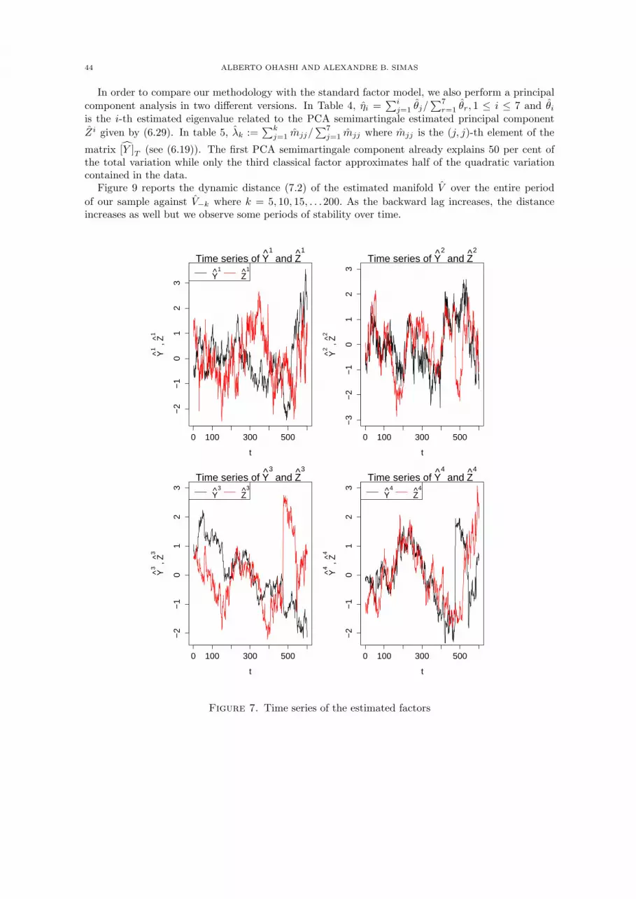
44 ALBERTO OHASHI AND ALEXANDRE B. SIMAS
In order to compare our methodology with the standard factor model, we also perform a principal
component analysis in two different versions. In Table 4, ηi =∑i
j=1 θj/∑7
r=1 θr, 1 ≤ i ≤ 7 and θiis the i-th estimated eigenvalue related to the PCA semimartingale estimated principal component
Zi given by (6.29). In table 5, λk :=∑k
j=1 mjj/∑7
j=1 mjj where mjj is the (j, j)-th element of the
matrix [Y ]T (see (6.19)). The first PCA semimartingale component already explains 50 per cent ofthe total variation while only the third classical factor approximates half of the quadratic variationcontained in the data.
Figure 9 reports the dynamic distance (7.2) of the estimated manifold V over the entire period
of our sample against V−k where k = 5, 10, 15, . . .200. As the backward lag increases, the distanceincreases as well but we observe some periods of stability over time.
0 100 300 500
−2
−1
01
23
Time series of Y1 and Z
1
t
Y1 ,
Z1
Y1
Z1
0 100 300 500
−3
−2
−1
01
23
Time series of Y2 and Z
2
t
Y2 ,
Z2
0 100 300 500
−2
−1
01
23
Time series of Y3 and Z
3
t
Y3 ,
Z3
Y3
Z3
0 100 300 500
−2
−1
01
23
Time series of Y4 and Z
4
t
Y4 ,
Z4
Y4
Z4
Figure 7. Time series of the estimated factors

PRINCIPAL COMPONENT ANALYSIS FOR SEMIMARTINGALES AND STOCHASTIC PDE 45
0 100 300 500
−3
−2
−1
01
23
Time series of Y5 and Z
5
t
Y5 ,
Z5
Y5
Z5
0 100 300 500
−3
−2
−1
01
2
Time series of Y6 and Z
6
t
Y6 ,
Z6
Y6
Z6
0 100 200 300 400 500 600
0.90
0.95
1.00
1.05
1.10
1.15
Time series of Y7 and Z
7
t
Y7 ,
Z7
Y7
Z7
Figure 8. Time series of the estimated factors
Table 4. Quadratic variation explained by the principal components: PCA semimartingale
η1 η2 η3 η4 η5 η6 η70.5010 0.7152 0.8548 0.9471 0.9925 0.9999 1.0000
Table 5. Quadratic variation explained by the principal components: Variance-based factor model
λ1 λ2 λ3 λ4 λ5 λ6 λ7
0.1161 0.4553 0.4911 0.6198 0.8927 0.9996 1.0000

46 ALBERTO OHASHI AND ALEXANDRE B. SIMAS
0 50 100 150 200
0.1
0.2
0.3
0.4
Distance between the manifolds
Backward lag
Dis
tanc
e
Figure 9. Dynamic distance (7.2) of the UK nominal daily spot curve
8. Appendix: Estimating dim QIn this section, we give a concrete alternative for estimating p = dim Q which is an important com-
ponent in Theorem 6.1. From (6.5), we notice that if the stochastic PDE admits a finite-dimensionalrealization, then the matrix of the finite-rank linear operator QT is given by [Z]T whenever
rt = φt +
d∑
j=1
Zjt λj ; 0 ≤ t ≤ T,
for each basis λ1, . . . , λd of a finite-dimensional subspace which generates a finite-dimensional real-ization. Rigorously speaking, we cannot estimate directly dim Q through high-frequency sampling offactors because they are not observed. In this case, one has to work with a high-frequency samplingof observed curves subject to noise. This section provides a feasible estimation procedure for this.
We choose to work with the Fourier-type estimator proposed by Malliavin and Mancino [39] butwe stress that other quadratic variation estimators can be certainly used as well. The strategy is tofind the minimum requirements on the residual process in such way that one can estimate the randomoperator QT via an observed curve process
Xt(x) = rt(x) + εt(x); 0 ≤ t ≤ T, a ≤ x ≤ b.
If ε is negligible in the quadratic variation sense, then the method of the estimation of the kernelQT (u, v) is fully based on any reasonable non-parametric estimator of the integrated volatility. Weassume that X is a well-defined semimartingale random field.
In the sequel, without any loss of generality we assume that [0, T ] = [0, 2π]. Let Π = tni ; i =0, . . . , n be the instant times of observations and ρ(n) = max0≤h≤n−1 |tnh+1 − tnh|. In this section, weassume that ρ(n) → 0 as n → ∞ so we are able to sample the curves x 7→ Xt(x) in high-frequency intime. In the sequel, we make use of the following notation
ϕn(t) := suptnk ; tnk ≤ t
For given positive integers M ≥ 1 and n ≥ 1, we define

PRINCIPAL COMPONENT ANALYSIS FOR SEMIMARTINGALES AND STOCHASTIC PDE 47
QT (u, v) :=1
2M + 1
∑
|s|≤M
∫ T
0
eisϕn(t)dXt(u)
∫ T
0
e−isϕn(t)dXt(v)
=
n−1∑
ℓ,j=0
dM (tnℓ − tnj )∆Xtnℓ+1(u)∆Xtnj+1
(v), u, v ∈ [a, b],
where ∆Xtnℓ+1(u) := Xtnℓ+1
(u)−Xtnℓ(u) and
dM (t) :=1
2M + 1
∑
|s|≤M
eits =
1; t = sT, s ∈ Z
12M+1
sin[(M+1/2)t]sin(t/2) ; t 6= sT
is the normalized Dirichlet kernel. Here M encodes the Bohr convolution product and n the dis-cretization level of the Fourier transform of σt(u, v). See Malliavin and Mancino [39] for more details.
To keep notation simple, from now on we set ti := tni ; 0 ≤ i ≤ n. The kernel QT (u, v) induces a
random linear operator QT on the complexification EC as follows
(QT f)(u) = 〈QT (u, ·), f〉EC
=1
2M + 1
∑
|s|≤M
n−1∑
ℓ=0
n−1∑
k=0
exp(is(tk − tℓ))∆Xtk+1(u)〈∆Xtl+1
, f〉EC,
for f ∈ EC. The reason to consider E on the field C is due to a nice representation as follows. If A andB are two linear operators on Hilbert spaces then AB and BA share the same nonzero eigenvalues.Furthermore, if γ is an eigenvector of BA, Aγ is an eigenvector of AB with the same eigenvalue. Sothe strategy is to write QT = AB in such way that BA : Cp → Cp for some p ≥ 1 and therefore onecan easily relate the eigenvalues of BA to AB. In fact, by the very definition of QT we have
QT = AB
where B : EC → C2M+1 is defined by
B(·) :=(
n−1∑
ℓ=0
exp(−i(−M)tℓ)〈∆Xtℓ+1, · 〉EC
, . . . ,n−1∑
ℓ=0
exp(−i(M)tℓ)〈∆Xtℓ+1, · 〉EC
)
and A : C2M+1 → EC is defined by
(8.1) (Ax)(·) := 1
2M + 1
∑
|s|≤M
xs
n−1∑
k=0
exp(istk)∆Xtk+1(·);x ∈ C
2M+1.
By the very definition, QT := BA : C2M+1 → C2M+1 is given componentwise by
QT y =1
2M + 1
∑
|s|≤M
n−1∑
k,ℓ=1
ys exp(i(stk −mtℓ)
)〈∆Xtℓ+1
,∆Xtk+1〉EC
,
for y ∈ C2M+1, m = −M, . . . ,M. We then arrive at the following elementary result.
Lemma 8.1. The random linear operators QT and QT share the same nonzero eigenvalues in C. Let
p be the number of nonzero eigenvalues θi = 1, . . . , p of QT and let γj = (γj(−M), . . . , γj(M)), j =1, . . . , p be the corresponding eigenvectors in C2M+1. Then

48 ALBERTO OHASHI AND ALEXANDRE B. SIMAS
1
2M + 1
∑
|s|≤M
γj(s)
(n−1∑
k=0
exp(istk)∆Xtk+1
), j = 1, . . . , p
are the p eigenfunctions of QT .
Proof. Let θj ∈ C be a nonzero eigenvalue of QT and let γj ∈ C2M+1 be the corresponding eigenvector.Then
(8.2) QTγj = θjγj and QT (Aγj) = θjAγj a.s,
where A is the operator given by (8.1). By writing (8.2) component by component we have
1
2M + 1
∑
|s|≤M
n−1∑
k,ℓ=0
γj(s) exp(i(stk − rtℓ)
)〈∆Xtℓ+1
,∆Xtk+1〉EC
= θjγj(r) a.s
for r = −M, . . . ,M . On the other hand,
Aγj =1
2M + 1
∑
|s|≤M
γj(s)
(n−1∑
k=0
exp(istk)∆Xtk+1
), j = 1, . . . , p a.s.
This concludes the proof of the Lemma.
Remark 8.1. Let
(8.3)1
2M + 1
∑
|s|≤M
γj(s)
(n−1∑
k=0
exp(istk)∆Xtk+1
), j = 1, . . . , p a.s
be the eigenvectors of QT related to its nonzero eigenvalues θj; j = 1, . . . , p. Since QT is a self-adjoint finite-rank operator then the following spectral decomposition holds a.s
QT f =
p∑
i=1
θi〈f, ϕi〉ECϕi; f ∈ EC,
where p ≤ 2M + 1 a.s for every n,M and ϕi; i = 1, . . . , p is an orthonormal set by applying aGram-Schmidt algorithm to the functions given by (8.3).
Let us now introduce the basic assumptions on the residual process ε. Since the estimation is basedon a high-frequency sampling we need to impose some structure on the continuous-time dynamics.
(B1) The residual process ε is an Ito semimartingale field where the drift component h satisfies
sup0≤t≤T
‖ht‖E ∈ Lp
for every p > 1.
(B2) The quadratic variation of ε(u) at time T satisfies
∫
R
[ε(u), ε(u)]Tµ(du) = 0 a.s.
(B3) The following growth assumption holds
0 < lim infn,M→∞
Mρ(n) ≤ lim supn,M→∞
Mρ(n) < ∞.

PRINCIPAL COMPONENT ANALYSIS FOR SEMIMARTINGALES AND STOCHASTIC PDE 49
(H1) The vector fields F, σi : E → E are globally Lipschitz for each i = 1, . . . ,m.
(H2) Linear growth condition on the vector fields F, σ1; 1 ≤ i ≤ m in (6.1): There exists a constantC > 0 such that
‖F (x)‖2E +
m∑
i=1
‖σi(x)‖2E ≤ C2(1 + ‖x‖2E) for every x ∈ E.
Remark 8.2. As far as the consistency problem of the HJM model (see Section 4.2), Assumption (B2)means that the initial fitting method used to interpolate points which generates X cannot introduce anextrinsic volatility. The interpolation must be chosen in such way that the resulting observed volatilityon the whole curve must be fully dictated by the market and not to the particular choice of fitting.See also Assumption (Q4). The semimartingale decomposition yields the following structure on theresidual process
εt = e+
∫ t
0
hsds
for some F0-measurable random variable e = X0 − r0 and an integrable adapted process h satisfying(B1). Assumption (B3) is a technical assumption in order to get optimal bounds but it is also linkedwith different flavors between the exact Fourier estimator and the usual quadratic variation estimatorfor QT . See Malliavin and Mancino [39] and Clement and Gloter [20] for further details.
Under (H1) and (H2), it is well-known for every initial condition ξ ∈ E, there exists a unique mild
solution rξt of the stochastic PDE. Moreover, the following integrability property holds
E sup0≤t≤T
‖rξt ‖qE < ∞
for every q > 1 and ξ ∈ E.The following result is a functional version of (and almost straightforward consequence) of Propo-
sition 1 and Lemma 3 in [20]. In the sequel, ‖ · ‖(2) is the Hilbert-Schmidt norm operator over EC andto keep notation simple, we write ‖ · ‖ = ‖ · ‖EC
.
Proposition 8.1. Assume that (A1, A2, B1, B2, B3, H1, H2) hold and in addition
(8.4) E1/2 sup
0≤t≤T|∂vσj(rt)(·)|4 ∈ L1(µ)
for each j = 1, . . . ,m. Then
E‖QT − QT ‖2(2) = O(ρ(n)).
Proof. In the sequel, we denote by C a positive constant which may differ from line to line. We alsodecompose
Xt(u) = rt(u) + εt(u),
into
rt(u) :=
m∑
j=1
∫ t
0
σj(rs)(u)dBjs ; 0 ≤ t ≤ T, u ∈ [a, b],
εt(u) =
∫ t
0
ξs(u)ds

50 ALBERTO OHASHI AND ALEXANDRE B. SIMAS
whereξt(u) := Art(u) + F (rt)(u) + ht(u); 0 ≤ t ≤ T, u ∈ [a, b].
For a given (u, v) ∈ [a, b]× [a, b], integration by parts and (B2) yield
QT (u, v)− QT (u, v) =
∫ T
0
(∫ t
0
dM,n(ℓ, t)dXℓ(u))dXt(v)
+
∫ T
0
(∫ t
0
dM,n(ℓ, t)dXℓ(v))dXt(u)
=: Rn,M (u, v)
where
dM,n(ℓ, t) := dM (ϕn(ℓ)− ϕn(t)),
Rn,M (u, v) = Jn,M,1(u, v) + Jn,M,2(u, v) +
3∑
i=1
In,M,i(u, v) +
3∑
i=1
In,M,i(u, v),
and
Jn,M,1(u, v) :=
∫ T
0
(
∫ t
0
dM,n(ℓ, t)drℓ(u))
drt(v),
Jn,M,2(u, v) :=
∫ T
0
(
∫ t
0
dM,n(ℓ, t)drℓ(v))
drt(u),
In,M,1(u, v) :=
∫ T
0
(
∫ t
0
dM,n(ℓ, t)dεℓ(u))
drt(v),
In,M,2(u, v) :=
∫ T
0
(
∫ t
0
dM,n(ℓ, t)drℓ(u))
dεt(v),
In,M,3(u, v) :=
∫ T
0
(
∫ t
0
dM,n(ℓ, t)dεℓ(u))
dεt(v),
where In,M,i are the symmetric quantities w.r.t In,M,i. By the very definition
‖QT − QT‖2(2) = ‖(QT − QT )(0, ·)‖2 +∫
[a,b]
∥∥∥∂u(QT − QT )(u, ·)∥∥∥2
µ(du)
= |QT (0, 0)− QT (0, 0)|2 +∫
[a,b]
|∂vQT (0, v)− ∂vQT (0, v)|2µ(dv)
+
∫
[a,b]
|∂uQT (u, 0)− ∂uQT (u, 0)|2µ(du)
+
∫
[a,b]2|∂2
vuQT (u, v)− ∂2vuQT (u, v)|2µ(du)µ(dv)
=: T1(n,M) + T2(n,M) + T3(n,M) + T4(n,M).
Step 1: The term T1. By the invariance hypothesis (A1), we know that [see [48]; Corollary 2.13]V ⊂ dom (A) so we may consider (dom (A), A) as a bounded operator restricted to V . Moreover, weshall represent
rt = pV ⊥rt + pV rt = pV ⊥Vht + pV rt,

PRINCIPAL COMPONENT ANALYSIS FOR SEMIMARTINGALES AND STOCHASTIC PDE 51
where p is the usual projection and h = r0. From Theorem 2.11 in [48], we also know that t 7→A(πV ⊥Vh
t ) is continuous and therefore there exists a constant C such that ‖Art‖ ≤ C + C‖rt‖ forevery t ∈ [0, T ]. Based on these facts, we may use the linear growth conditions (H1-H2) and (B1)to arrive at the following estimate
(8.5) sup0≤t≤T
‖ξt‖ ≤ C + C sup0≤t≤T
‖rt‖+ C sup0≤t≤T
‖ht‖.
In this case, one can easily check that assumptions in Proposition 1 of [20] hold trivially and all theirestimates as well. In this case, we have
T1(n,M) ≤ C
∫ T
0
∫ t
0
d2M,n(ℓ, t)dℓdt.
Lemma 3 in [20] yields T1(n,M) = O(ρ(n)).
Step 2: The term T2 + T3. Let us now treat T2(n,M) + T3(n,M). For a given (i, j) ∈ 1, . . . ,m2,Burkholder-Davis-Gundy inequality and (H1-H2) yield
E
∫
[a,b]
∣
∣
∣
∫ T
0
∫ t
0
dM,n(ℓ, t)σj(rℓ)(0)dB
jℓ∂vσ
i(rt)(v)dBit
∣
∣
∣
2
µ(dv) ≤ C
∫ T
0
∫ t
0
d2M,n(ℓ, t)dℓdt
This yields∫[a,b] E|∂vJn,M,1(0, v)|2µ(dv) = O(ρ(n)). The same argument also holds for ∂vJn,M,2(0, v)
and we conclude that
∫
[a,b]
E|∂vJn,M,1(0, v) + ∂vJn,M,2(0, v)|2µ(dv) = O(ρ(n))
The drift part is estimated as follows. Cauchy-Schwartz and Burkholder-Davis-Gundy inequalities,the estimate (8.5), (H1-H2), A1, B1 and Lemma 3 in [20] yield
∫
[a,b]
E|∂vIn,M,1(0, v)|2µ(dv) ≤ E
d∑
i=1
∫ T
0
(
∫ t
0
d2M,n(ℓ, t)dℓ×
∫ t
0
‖ξℓ‖2dℓ
× ‖σi(rt)‖2
)
dt
≤ C
∫ T
0
∫ t
0
d2M,n(ℓ, t)dℓdt = O(ρ(n)).
The term ∂vIn,M,2(0, v) is more evolved but we can repeat the same steps as in the proof of Theorem1 in [20] in page 1114 to represent
|In,M,2(u, v)|2 =
∫
[0,T ]2Yn,M (u, t, t)ξt(v)Yn,M (u, t
′
, t′
)ξt′ (v)dtdt′
,
where
Yn,M (u, t, s) :=
∫ s
0
dM,n(ℓ, t)drℓ(u).
We fix η > 0 and we split |In,M,2(0, v)|2 = An,M,1(u, v, η) +An,M,2(u, v, η) so that
∂vAn,M,1(0, v, η) :=
∫ T
0
∫ t
t−η
Yn,M (0, t, t)∂vξt(v)Yn,M (0, t′
, t′
)∂vξt′ (v)dt′
dt
∂vAn,M,2(0, v, η) :=
∫ T
0
∫ t−η
0
Yn,M (0, t, t)∂vξt(v)Yn,M (0, t′
, t′
)∂vξt′ (v)dt′
dt

52 ALBERTO OHASHI AND ALEXANDRE B. SIMAS
By applying the same arguments in the proof of Theorem 1 in [20] with small η > 0 together withCauchy-Schwartz inequalities on E and assumptions (H1-H2), B1, B3, we also have
∫
[a,b]
E|In,M,2(0, v)|2µ(dv) = O(ρ(n)).
Moreover, (B1,B3) and Lemma 3 in [20] yield
∫
[a,b]
E|In,M,3(0, v)|2µ(dv) ≤ C
∫ T
0
∫ t
0
d2M,n(ℓ, t)dℓdt ≤ Cρ(n).
By the symmetry of the other terms, these estimates allow us to conclude that T2(n,M)+T3(n,M) =O(ρ(n)).
Step 3: The term T4. For given (i, j) ∈ 1, . . . ,m2, Burkholder-Davis-Gundy and Cauchy-Schwartzinequalities and (H1-H2) with (8.4) yield
E
∫
[a,b]2|∂2
vuJn,M,1(u, v)|2µ(dv)µ(du) =
∫
[a,b]
E
∫ T
0
(
∫ t
0
dM,n(ℓ, t)∂uσj(rℓ)(u)dB
jℓ
)2
‖σi(rt)‖2dtµ(du)
≤ C
∫ T
0
∫ t
0
d2M,n(ℓ, t)dℓdt
∫
[a,b]
E1/2 sup
0≤t≤T|∂vσ
j(rt)(·)|4µ(du).
Therefore, by the symmetry of the martingale terms and Lemma 3 in [20] we have
∫
R2+
E|∂2vuJn,M,1(u, v) + ∂2
vuJn,M,2(u, v)|2µ(dv)µ(du) = O(ρ(n)).
Similarly, Lemma 3 in [20] and (8.5) yield
∫
R+
E|∂2vuIn,M,1(u, v)|2µ(du)µ(dv) ≤
∫ T
0
∫ t
0
d2M,n(ℓ, t)dℓdt
× E sup0≤t≤T
‖ξt‖2
≤ C
∫ T
0
∫ t
0
d2M,n(ℓ, t)dℓdt = O(ρ(n)).
Summing up all the inequalities for T1, T2, T3 and T4, we conclude the proof.
In the sequel, for each ǫ > 0, we define
pǫ := number of non-zero eigenvalues of QT greater or equal to ǫ a.s
Corollary 8.1. Assume that Assumptions in Proposition 8.1 hold and let Q = Range QT withdimension p. Let ǫ → 0 in such a way that ǫ2ρ(n)−1 → ∞ as n → ∞. Then, P(pǫ 6= p) = O(ǫ−2ρ(n)).
Proof. From Proposition 8.1, we know that E‖QT − QT ‖2(2) = O(ρn). Since we are considering the
ordered eigenvalues, θ1 ≥ θ2 ≥ · · · ≥ 0, we have that pǫ > p = θp+1 > ǫ.A simple calculation on the Hilbert-Schmidt norm together with θp+1 = 0 a.s yield
θp+1 = |θp+1 − θp+1| ≤ ‖QT −QT ‖(2).Therefore,
P(pǫ > p) ≤ ǫ−2E‖QT −QT ‖2(2) = O(ǫ−2ρ(n)).
By noticing that θ < p = θp−1 < ǫ and θp−1 > 0 a.s, we do the same argument to get

PRINCIPAL COMPONENT ANALYSIS FOR SEMIMARTINGALES AND STOCHASTIC PDE 53
Pp < p = (θp+1 − ǫ)2E‖QT −QT ‖2(2) = O(ρ(n))
Since P(pǫ 6= p) = P(pǫ > p) + P(pǫ < p), the result follows.
References
[1] Almeida, C. I. R. (2005). Affine Processes, Arbitrage-Free Term Structures of Legendre Polynomials and Option
Pricing. Int. J. Theor. Appl. Finan., 8, 2, 161-184.[2] Almeida, C. I. R. and Vicente, J. (2008). The Role of No-Arbitrage on Forecasting: Lessons from a Parametric
Term Structure Model. Journal of Banking and Finance, 32, 12, 2695-2705.[3] Alexander, C. Market risk analysis. Volume II. John Willey e Sons. 2008.[4] Ait-Sahalia,Y. and Xiu, D. Increased correlation among asset classes: Are volatility or jumps to Blame, or both ?
Chicago Booth Paper No. 14-11. Preprint.[5] Ait-Sahalia, Y. and Xiu, D. Principal Component Analysis of High Frequency Data. Chicago Booth Paper No.
15-39. Preprint.[6] Alekseevsky, D., Kriegl, A., Losik, M. and Michor, P.W. (1998). Choosing roots of polynomials smoothly. Israel J.
Math, 105, 2013-233.[7] Angeline, F.and Herzel, S. (2002). Consistent Initial Curves for Interest Rate Models. J. Derivatives 9, 4, 8-17.[8] Bai, J. e Ng, S. (2002). Determining the Number of Factors in Approximate Factor Models. Econometrica, 70,
191-221.[9] Bai, J. (2003). Inferential Theory for Factor Models of Large Dimensions. Econometrica, 71, 1, 135-171.
[10] Bandorff-Nielsen, O.E. and Sheppard, N. (2004). Econometric analysis of realized covariation:High-frequency basedcovariance regression, and correlation if financial economics. Econometrica, 72, 3, 885-925.
[11] Bathia, N. Yao, Q. and Ziegelmann, F. (2010). Identifying Finite Dimensionality of Curve Time Series. Ann.
Stat, 38, 3352-3386.[12] Baudoin, F. and Teichmann, J. (2005). Hypoellipticity in infinite dimensions and an application in interest rate
theory. Ann. Appl. Probab, 15, 3, 1765-1777.[13] Bjork, T. and Christensen, B. J. (1999). Interest rate dynamics and consistent forward rate curves. Math. Finance,
9, 323-348.[14] Bjork, T. C. Landen. (2002). On the construction of finite dimensional realizations for nonlinear forward rate
models. Finance Stochast, 6, 303-331.[15] Bjork, T. and Svensson, L. (2001). On the existence of finite-dimensional realizations for nonlinear forward rate
models. Math. Finance, 11, 205-243.[16] Burashi, A., Porchia, P. and Trojani, F. (2010). Correlation Risk and Optimal Portfolio Choice. The J. of Finance,
65, 1, 393-420.[17] Buraschi,A., Cieslak, A. and Trojani, F. Correlation risk and the term structure of interest rates, Working Paper,
University of St. Gallen[18] Bibinger, M., Hautsch, N., Malec, P. and Rei, M. (2014). Estimating the quadratic covariation matrix from noisy
observations: Local method of moments and efficiency. Annals of Stat, 42, 4, 1312-1346.[19] Bibinger, M. and Mikland, P. A. Inference for Multi-Dimensional High-Frequency Data: Equivalence of Methods,
Central Limit Theorems, and an Application to Conditional Independence Testing. arXiv:1301.2074v2.[20] Clement, E. and Gloter, A. (2011). Limit theorems in the Fourier transform method for the estimation of multi-
variate volatility. Stoch. Proc. Appl, 121, 1097-1124.[21] Christensen, K., Podolskij, M. and Vetter, M. (2013): On covariation estimation for multivariate continuous Ito
semimartingales with noise in non-synchronous observation schemes. J. Multivariate Anal, 120, 59-84[22] Duffie, D and Khan, R. (1996). A yield-factor model of interest rate. Math. Finance, 6, 4,379-406.[23] Fan, J., Li, Y. and Yu, K. (2012). Vast volatility matrix estimation using high-frequency data for portfolio selection.
J. Amer. Statist. Assoc,107, 412428.[24] Filipovic, D. (2001). Consistency Problems for Heath–Jarrow–Morton Interest Rate Models. Lecture Notes in Maths
1760. Springer, Berlin.[25] Filipovic, D. and Teichmann, J. (2003). Existence of invariant manifolds for stochastic equations in infinite dimen-
sion. J. Funct. Anal. 197, 398-432.
[26] Filipovic, D. Teichmann, J. (2004). On the Geometry of the Term structure of Interest Rates. Proc. R. Soc. Lond.
Ser. A Math. Phys. Eng. Sci., 460, 129-167.[27] Filipovic, D. and Sharef. (2004). Conditions for consistent expoenential-polynomial forward rate processes with
multiple nontrivial factors. Int. J. Theor. Appl. Finan, 7, 6, 685-700.[28] Filipovic, D. (1999). A note on the Nelson Siegel family. Math. Finance, 9, 349-359.[29] Filipovic, D. (1999). Exponential polynomial families and the term struture of interest rates. Bernoulii, 9, 349-359.[30] Fissler, T. and Podolskij, M. Testing the maximal rank of the volatility process for continuous diffusions observed
with noise. arXiv:1410.6698.

54 ALBERTO OHASHI AND ALEXANDRE B. SIMAS
[31] Forni, M., Hallin, M., Lippi, M; and Reichlin, L. (2000). The Generalized Dynamic Factor Model: Identificationand Estimation. Rev. Econ. Stat, 82, 540-554.
[32] Heath, D., Jarrow, R. and Morton, A. (1992). Bond pricing and the term structure of interest rates: A newmetodology for contingent claims valuation. Econometrica, 60, 77-105.
[33] Friz, P. Victoir, N. Multidimensional stochastic processes as rough paths. Theory and Applications. CambridgeUniversity Press. 2011.
[34] Harms, P., Stefanovits, D., Teichmann, J., and Wuthrich, M. Consistent Recalibration of Yield Curve Models.arXiv:1502.02926.
[35] Henseler, M., Peters, C. and Seydel, R.C. A Tractable Multi-Factor Dynamic Term-Structure Model for RiskManagement. In: Available at SSRN 2225738 (2013).
[36] Heston, S.L (1993). A closed-form solution for options with stochastic volatility with applications to bond andcurrency options. Rev. Financ. Stud, 6, 2, 327-343.
[37] Jacod, J. and Podolskij, M. (2013). A test for the rank of the volatility process: the random perturbation approach.Ann. Statist, 41, 5, 2391-2427.
[38] Laurini, M. and Ohashi, A. (2015). A Noisy Principal Component Analysis for Forward Rate Curves. Eur. J. Oper.
Res, 246, 1, 140-153.[39] Malliavin, P. and Mancino, M.E. (2009). A Fourier transform method for nonparametric estimation of multivariate
volatility. Ann. Statist. 37, 4, 1983-2010.[40] Malliavin, P; Mancino, M. E.; Recchioni, M. C. (2007). A non-parametric calibration of the HJM geometry: an
application of Ito calculus to financial statistics. Japan. J. Math, 2, 1, 55-77.[41] Ohashi, A. (2009). Fractional term structure models: no-arbitrage and consistency. Ann. Appl. Probab, 19, 4,
1553-1580.[42] Pelger, M. Large-dimensional factor modeling based on high-frequency observations. Preprint.[43] Piazzesi, M. (2010). Affine Term-Structure Models. Handbook of Financial Econometrics. Chapter 12, 691 - 766.[44] Richter, A. and Teichmann, J. Discrete Time Term Structure Theory and Consistent Recalibration Models. Preprint
arXiv:/1409.1830.[45] Rutter, J. W. Geometry of Curves, CRC Press, 2009.[46] Slinko, I. (2010). On finite-dimensional realizations of two-country interest rate models. Math. Finance, 20, 1,
117-143.[47] Stock, J. H. and Watson, M. W. (2002). Forecasting Using Principal Components from a Large Number of Predic-
tors. J. Amer. Statist. Assoc, 97, 460, 1167-1179.[48] Tappe, S. (2010). An alternative approach on the existence of affine realizations for HJM term-structure models.
Proc. R. Soc. Lond. Ser. A Math. Phys. Eng. Sci, 466, 2122, 3033-3060.[49] Teichmann, J. and Wthrich, M. Consistent Long-Term Yield Curve Prediction, arXiv/1203.2017, preprint.[50] Wang, Y. and Zou, J. (2010). Vast volatility matrix estimation for high-frequency financial data. Ann. Statist. 38,
2, 943-978.[51] Zeng, X. and Li, Y. (2011). On the estimation of integrated covariance matrices of high dimensional diffusion
processes. Ann. Statist. 39, 6, 3121-3151.
[52] Tao, M., Wang, Y.and Zhou, H.H. (2013). Optimal sparse volatility matrix estimation for high-dimensional Itprocesses with measurement errors. Ann. Statist, 41, 4, 1816-1864.
Departamento de Matematica, Universidade Federal da Paraıba, 13560-970, Joao Pessoa - Paraıba, Brazil
E-mail address: [email protected]; [email protected]
Departamento de Matematica, Universidade Federal da Paraıba, 13560-970, Joao Pessoa - Paraıba, Brazil
E-mail address: [email protected]


