Principal Performance in Texas: Tools for Measuring Effective School Leadership

PRINCIPAL PERFORMANCE IN TEXAS: TOOLS FOR MEASURING EFFECTIVE

SCHOOL LEADERSHIP

KANDYCE FERNANDEZ SANTA FLORES EMILY HUANG CAROLYN IGWE

LESLIE MCDONALD RYAN STROUD

REBECCA WILLIS AMBER DUGAT

FACULTY ADVISOR: DR. LORI TAYLOR

MAY 2007

TABLE OF CONTENTS

EXECUTIVE SUMMARY.........................................................................................................................................1

METHODOLOGY AND INDICATOR ANALYSIS..............................................................................................................1 Student Performance............................................................................................................................................1 Teacher Retention ................................................................................................................................................2 Financial Management ........................................................................................................................................2

CONCLUSION .............................................................................................................................................................3 INTRODUCTION .....................................................................................................................................................5

PRINCIPAL EFFECTIVENESS: A REVIEW OF THE LITERATURE..............................................................6

STUDENT PERFORMANCE...........................................................................................................................................6 Standardized Testing............................................................................................................................................6 Other Measures....................................................................................................................................................7

TEACHER RETENTION ................................................................................................................................................7 FINANCIAL MANAGEMENT ........................................................................................................................................9

Financial Management in Texas Schools.............................................................................................................9 Indicators of School Financial Management .......................................................................................................9

METHODOLOGY AND INDICATOR ANALYSIS.........................................................................................11

STUDENT PERFORMANCE.........................................................................................................................................11 Standardized Tests .............................................................................................................................................11 Accountability ....................................................................................................................................................14 Relevance of Indicators......................................................................................................................................15 Influences of School Characteristics on Student Performance ..........................................................................17 Student Performance Conclusion.......................................................................................................................20

TEACHER RETENTION ..............................................................................................................................................21 Teachers in Texas...............................................................................................................................................21 Measuring Teacher Retention ............................................................................................................................21 Turnover by Category ........................................................................................................................................23 Indicator Adjustment..........................................................................................................................................30 Teacher Turnover Indicators and Demographics ..............................................................................................30

FINANCIAL MANAGEMENT ......................................................................................................................................34 Measuring Campus Level Expenditures.............................................................................................................34 Cost-efficiency Performance and the Cost Function Approach.........................................................................35 Cost Function Model..........................................................................................................................................36 Analysis of Cost Function Model .......................................................................................................................37 School Finance and Attendance Rates ...............................................................................................................39 Instructional Share.............................................................................................................................................40 Conclusions Concerning Financial Management ..............................................................................................43

PRINCIPALS IN TEXAS........................................................................................................................................44

DEMOGRAPHICS.......................................................................................................................................................44 GEOGRAPHIC DISTRIBUTIONS..................................................................................................................................45 EXPERIENCE AND EDUCATION.................................................................................................................................45 PRINCIPAL TENURE..................................................................................................................................................46 CERTIFICATION........................................................................................................................................................46

ANALYSIS OF PRINCIPALS IN TEXAS............................................................................................................48

STUDENT PERFORMANCE.........................................................................................................................................48 Adjusted Gains ...................................................................................................................................................48 Accountability ....................................................................................................................................................49

TEACHER TURNOVER...............................................................................................................................................49 FINANCIAL MANAGEMENT ......................................................................................................................................49

Cost Efficiency ...................................................................................................................................................49 Attendance..........................................................................................................................................................50 Share of Instructional Spending.........................................................................................................................50

CONCLUSION.........................................................................................................................................................51

STUDENT PERFORMANCE.........................................................................................................................................51 TEACHER RETENTION ..............................................................................................................................................51 FINANCIAL MANAGEMENT ......................................................................................................................................52 PRINCIPAL PERFORMANCE.......................................................................................................................................52

NOTES.......................................................................................................................................................................53

WORKS CITED........................................................................................................................................................55

APPENDIX I – STUDENT PERFORMANCE.....................................................................................................61

APPENDIX II – TEACHER RETENTION...........................................................................................................64

APPENDIX III – FINANCIAL MANAGEMENT ..............................................................................................75

APPENDIX IV – PRINCIPAL ANALYSIS..........................................................................................................79

1

EXECUTIVE SUMMARY Since the passage of the No Child Left Behind Act of 2001 (NCLB), federal and state school accountability efforts have intensified. This Act monitors student performance by requiring that schools raise student scores on standardized tests and demonstrate Adequate Yearly Progress, or they risk losing federal funding. In addition to measuring the performance of students, the education system has begun measuring the performance of educators. Some districts, including Houston ISD, have established pay-for-performance systems to promote teacher and administrator effectiveness (Texas Education Agency 2007; Mellon 2007; Houston Independent School District 2007). As incentive-pay programs frequently recognize, principals are integral parts of schools and perform necessary and influential administrative functions. In order to discuss principal performance and introduce accountability into the system, we need a language to describe what it means for a principal to be effective. This analysis, therefore, provides a set of practical tools that educators and policy-makers can use to define and measure the effectiveness of principals. According to the literature, such performance measures should be objective, easily understood, and immune to manipulation (Hatry 1999). We also wanted to provide measures that were easily replicable in Texas and feasible given data, cost, and time constraints. Most studies and current practices primarily use student performance to judge principal effectiveness, but Meier and O’Toole (2002) note in their acclaimed study of Texas superintendents that using a single, simple measure is more likely to produce biased results. We advocate a multi-dimensional approach that includes but is not limited to student performance.

Methodology and Indicator Analysis This analysis provides a set of practical tools that educators and policy-makers can use to define and measure the effectiveness of principals. We focus on three dimensions: student performance, teacher retention, and financial management. Data is derived from the Texas Education Agency (TEA) to develop a total of seven specific indicators to measure success in these three areas for Texas public schools (excluding charter schools). These performance evaluation tools are then applied to principals in Texas and patterns of principal effectiveness are reported on a statewide basis.

Student Performance

For a principal to be labeled effective, the students at his or her school must perform well. Difficulties arise when deciding exactly how to measure student performance, including which indicators to consider. This study measures student performance using standardized

2

tests and school accountability ratings. TEA data is used from 1996-2005 to develop indicators for these two measures. Since our goal was to capture the improvements in student performance attributable to principal effectiveness, we used a value-added measure of changes in TAAS and TAKS passing rates for the same cohort of students from one year to the next. Consideration of gains in passing rates instead of levels of passing rates allow for measurement of the value added by the most recent schools and principals to the existing base of the students’ knowledge and skills. Thus, we can compare the performance of students whether they are already more advanced or are performing at relatively lower levels. Both adjusted gains and accountability ratings are useful for evaluating student performance because the two indicators measure different aspects of performance, and the schools receiving the highest accountability ratings are not always the ones with the highest adjusted gains. Furthermore, interpreting a school’s pattern of adjusted gains is most effective when taking into account the school’s accountability rating group. Because both adjusted gains in standardized passing rates and accountability ratings differ significantly according to levels of student poverty, school size, student ethnicity, and geography, we control for these characteristics in our analysis of principal effectiveness. This finding also indicates that it is both inequitable and inappropriate to compare the effectiveness of principals that are not in the same category in any one of these variables. For example, student performance is generally higher in larger schools. Comparing a principal in a large school to a principal in a small school would be problematic because principal characteristics would be indistinguishable from the characteristics of the school that affect student performance. Thus, any policy aimed at encouraging administrative improvements would be most effective if it took differences among the various groups into account.

Teacher Retention

The second dimension of principal effectiveness we measure is teacher retention. Teacher retention is important because it reflects a principal’s ability to retain teachers and provide adequate support. Teacher retention may also affect student performance and impose costs on a school. Because beginning teacher turnover is systematically higher than the turnover of more experienced teachers, we recommend evaluating principals on beginning and experienced teacher turnover separately. Turnover rates also differ significantly among metropolitan, micropolitan, and rural areas, as well as from one metropolitan area to the next. Thus, principal performance in teacher retention is most appropriately evaluated by comparing beginning and experienced teacher turnover among schools in the same metropolitan area (for metropolitan schools), or in the same education service center (for schools in micropolitan or rural areas).

Financial Management

We used three indicators to measure the financial management dimension of principal performance: cost efficiency, instructional share, and attendance rate. The cost efficiency indicator allows us to compare school district expenditures with the level of expenditures

3

that would be expected given student performance, student demographics, and other cost factors. Arguably, good financial management suggests a balance between instructional, administrative, and other expenditures. As a benchmark, we use the Texas Governor’s 2005 Executive Order, which requires that 65 percent of current expenditures be spent on instruction. In addition, attendance rates are associated with school funding at the district level. As such, a principal may be able to attract more funds to his or her district by promoting high student attendance. Our analysis suggests that on average, schools could spend 11.59 percent less than they do with no decrease in student performance. In particular, high schools could save 13.3 percent, elementary school could save 11.47 percent, and middle schools could save 10.53 percent. This finding shows cost-efficiency is significantly different among elementary schools, middle schools, and high schools, so we recommend comparing elementary school principals to other elementary school principals, middle school principals to other middle school principals, and high school principals to other high school principals. As a final note, we examined the relationship between instructional share and our other indicators and determined there was generally no correlation. This suggests that either instructional share is a poor measure of principal performance or that it picks up an aspect of principal performance unmeasured by our other indicators.

Conclusion

Our last step was to evaluate the effectiveness of Texas principals from 1999 to 2005 using seven indicators (adjusted gains, accountability rating, beginning teacher turnover, experienced teacher turnover, cost-efficiency, instructional share, and attendance). The goal was to determine whether principals with similar effectiveness had any major characteristics in common, such as educational attainment, certification status, or tenure on the job. Because there were a number of significant relationships between the seven principal effectiveness indicators and student and campus characteristics, a comparison was made between principal characteristics and principal effectiveness on our seven indicators while controlling for such influential factors as student demographics (ethnicity, socio-economic status, and mobility), geographic location, campus size, year, and grade level. We find that no observable principal characteristic has a systematic affect on all seven indicators. Principal certification appears to affect attendance rates, but not student performance or teacher retention. Furthermore, we find no differences in principal effectiveness between traditionally certified principals and alternatively certified principals. A principal’s educational attainment influences accountability ratings and attendance rates, but not the other indicators. Principals with more experience in the education system had lower adjusted gains during the TAAS testing period, but not during the TAKS testing period.

4

Principal tenure on the job was the only principal characteristic that significantly affected performance on most of the indicators. Principals in their first year on campus are much less effective than other principals. They have lower adjusted gains, lower accountability ratings, and higher teacher turnover. Students and teachers are negatively affected in the first year that a principal is at a particular campus. Intriguingly, none of the financial indicators are significantly related to a principal’s tenure. Further study is needed to determine whether this phenomenon reflects that a principal learns on the job, that principal volatility itself has a negative effect, or simply that new principals were brought in to help struggling schools. Because lower principal effectiveness occurs during a principal’s first year at a particular school, principal performance evaluations, including pay-for-performance programs, should be applied with caution to principals in their first year at a school.

5

INTRODUCTION Since the passage of the No Child Left Behind Act of 2001 (NCLB), federal and state school accountability efforts have intensified. This Act monitors student performance by requiring that schools raise student scores on standardized tests and demonstrate Adequate Yearly Progress, or they risk losing federal funding. In addition to measuring the performance of students, the education system has begun measuring the performance of educators. Some districts, including Houston ISD, have established pay-for-performance systems to promote teacher and administrator effectiveness (Texas Education Agency 2007; Mellon 2007; Houston Independent School District 2007). As incentive-pay programs frequently recognize, principals are integral parts of schools and perform necessary and influential administrative functions. In order to discuss principal performance and introduce accountability into the system, we need a language to describe what it means for a principal to be effective. This analysis, therefore, provides a set of practical tools that educators and policy-makers can use to define and measure the effectiveness of principals. According to the literature, such performance measures should be objective, easily understood, and immune to manipulation (Hatry 1999). We also wanted to provide measures that were easily replicable in Texas and feasible given data, cost, and time constraints. Most studies and current practices primarily use student performance to judge principal effectiveness, but Meier and O’Toole (2002) note in their acclaimed study of Texas superintendents that using a single, simple measure is more likely to produce biased results. We advocate a multi-dimensional approach that includes but is not limited to student performance. The following report provides a review of the literature describing the areas of principal performance an evaluation should consider. We focus on three dimensions: student performance, teacher retention, and financial management. We then use data from the Texas Education Agency (TEA) to develop a total of seven specific indicators to measure success in these three areas for Texas public schools (excluding charters). Once we develop this set of performance evaluation tools, we apply them to principals in Texas and report patterns of principal effectiveness statewide.

6

PRINCIPAL EFFECTIVENESS: A REVIEW OF THE LITERATURE Our review of education and management literature identified multiple aspects of principal effectiveness. We believe it is of the most value to Texas to focus on indicators which are not only relevant to a school’s success, but are replicable using TEA data. Consequently, our study focuses on student performance, teacher retention, and financial management.

Student Performance Student performance is one of the most common indicators of principal effectiveness (Hallinger et al. 1996; Leithwood and Jantzi 1999; Miller and Rowan 2006). Indeed, because the purpose of schools is to educate, any evaluation of school effectiveness must be concerned with student performance. This priority is already reflected in the Accountability Rating System for Texas Public Schools and Districts, which primarily considers student performance in assigning overall school performance ratings. Additionally, the No Child Left Behind Act of 2001 ties federal education funds to student performance within each state. Student performance at the district level was also found to be a determinant of superintendent salaries, demonstrating concern among both parents and taxpayers regarding the performance of local school children (Ehrenberg, Chaykowski, and Ehrenberg 1998). Because TEA holds districts accountable for student performance, superintendents consider standardized test passing rates and TEA accountability ratings when making decisions at the campus level (TEA 2002). The Commissioner-Recommended Student Performance Domain Worksheet, available through the Region 13 Education Service Center, highlights the importance many administrators place upon such performance measures (ESC13 2006).

Standardized Testing

Many studies focus on standardized testing to measure student performance. Manasse (1985, 440) writes, “While there is no single, commonly agreed upon definition of effective principals, both researchers and practitioners generally identify effective principals partially on the basis of organizational performance (most commonly indicated by student achievement scores).” Hallinger, Bickman and Davis (1996) use statewide reading scores to measure the relationship between principal effectiveness and student performance in Tennessee. Miller and Rowan (2006) designed a reading and math test to use in their study of the relationship between elementary and secondary school management and student performance. Meier and O’Toole (2002), in a study designed to evaluate Texas superintendents, use several variables to measure school performance, most of which are based on standardized testing. Their study provides a useful model for measuring student performance, which we applied to the campus level because of our focus on principals. Hanushek (1997) summarizes previous literature on measuring school performance. His review of 90 publications yields 377 different production functions for education. Seventy-five percent of these studies use standardized testing as their primary or only measure of student performance.

7

Standardized testing is an appropriate indicator for Texas because a well-established accountability system based on standardized testing has been in place in Texas for many years. Gronberg, Jansen, Taylor, & Booker (2004, 1) write, “Texas has been at the forefront of the transition from process or input-based evaluation of schools to outcome- or performance-based assessment. Since 1995, Texas has used the Texas Assessment of Academic Skills (TAAS) test results to establish accountability in the form of school report cards.” The state transitioned to using the Texas Assessment of Knowledge and Skills (TAKS) test results in 2003. Not only is standardized testing data available for Texas, but policymakers and educators are familiar with both exams and accountability systems tied to each. Because all eligible students in Texas take these exams, any effectiveness measures based on TAAS or TAKS test results can be applied to the entire state, compared at the campus level, and replicated. Meier & O’Toole (2002) also use TAAS passing rates as a measure of student performance; however, they acknowledge that using standardized testing as a performance measure is controversial. While standardized testing has limitations, it is the most commonly applied performance measure in the country. More recently, standardized testing has extended to the federal level; No Child Left Behind uses standardized test results to hold states accountable in the allocation of federal education funds (Department of Education 2006).

Other Measures

A review of existing literature reveals a number of indicators of student performance that are not appropriate for statewide analysis, including SAT/ACT scores and dropout rates. SAT and ACT scores are of limited use as a measure of student performance when considering statewide principal effectiveness because they capture only the performance of college-bound high school students (Meier and O’Toole 2002). Furthermore, these exams are not administered uniformly at campuses across the state, and some students may face access barriers based on socioeconomic status or school demographics. Like SAT and ACT scores, dropout rates are also only relevant at the high school level. While dropout rates would be useful as a measure of school completion rates, Gronberg et al. (2004) found dropout reports to be unreliable. Moreover, Meier and O’Toole (2002, 638) note that dropout rates are often underreported since “school districts have few incentives to find out why any given student has not returned for a new academic year.”

Teacher Retention Research indicates that teacher retention is also associated with principal effectiveness. Dissatisfaction with administrative support is frequently highly ranked as one of the reasons teachers leave a school (Graziano 2005; Ingersoll 2001; Darling-Hammond 1997). Results of other surveys showed that teachers left primarily because they were dissatisfied with the way in which principals communicated with parents and other members of the community (Ingersoll 2001; McDiarmid, Larson and Hill 2002).

8

Reflecting on the challenge teacher retention presents for the State of Texas, the Texas Center for Educational Research (TCER) describes high teacher turnover as burdensome and inefficient (2000, 1). Every year a large number of teaching positions have to be filled. While some of these positions are being created to accommodate increased student enrollment, the number of such positions is small compared to those that have to be filled as a result of teacher turnover. In the 1998-1999 school year, for example, more than 63,000 vacancies had to be filled (TCER 2000, 2). Teachers who left the field entirely and those who moved among districts accounted for almost 47,000 of these vacancies. Of the remaining vacancies, 11,000 were attributed to retirement, while 5,700 were new positions created to accommodate increasing student enrollment. While some amount of turnover is both necessary and inevitable, the costs of teacher turnover can be exorbitant. Based on an estimate that turnover costs 25 percent of a teacher’s annual salary plus the cost of benefits, the TCER approximated that turnover during the 2000 school year alone cost the state $329 million (TCER 2000).1 Using a similar estimation strategy, the Texas Comptroller of Public Accounts estimated the cost of turnover for 2004 at $478 million.2 In addition to its financial impact, teacher turnover also affects the school climate. Schools with high teacher turnover rates are reported to experience organizational challenges which affect the planning and implementation of curriculum and the maintenance of positive relationships among teachers (Guin 2004). High turnover rates, according to Guin (2004) result in low levels of trust and cooperation among teachers. One study attributes “high turnover in a school’s teaching staff as one of the most powerful factors in stifling school improvement efforts” (Theobald and Michael 2001, 3). Guin (2004) examined the relationship between teacher turnover rates and five measures of organizational climate, including school climate, teacher climate, principal leadership, teacher influence, and perceptions of teacher respect. The author found all five relationships to be negatively correlated and statistically significant. The literature also indicates a correlation between teacher retention and student performance. McDiarmid, Larson, and Hill (2002) report a positive relationship between low teacher turnover and higher student achievement. Guin (2004) looked at this problem from a slightly different perspective, determining that schools with higher teacher turnover rates experienced lower numbers of students able to meet statewide standards in reading and math. Liu and Meyer (2005) study school staffing problems, which may contribute to high teacher turnover, and determine that such personnel problems are negatively correlated with lower student performance. While additional statistical analysis is necessary to conclude that a causal relationship exists between teacher turnover and student performance, correlations do exist (Guin 2004). In sum, the literature suggests that teacher turnover has negative consequences, including financial costs and instability. In addition, teacher turnover may have direct and negative effects on student performance.

9

Financial Management Numerous texts have listed aspects of financial management as an important indicator of principal performance. Schagen and Weston (1998) consider the “quality of financial management” a core factor in assessing school leaders. Harvey and Sheridan (1995) maintain that one of the major responsibilities of the primary school deputy principal is management of financial resources. The financial situation of a school determines its overall management and operational success.

Financial Management in Texas Schools

Financial management has important implications for the State of Texas because poor financial health and management cause or exacerbate many of the problems schools currently face. Although school policies vary, principals must be the major supervisors and decision-makers in school budgeting, as each activity of a school must begin with budgeting and the appropriation of money. Simmons (2006) posits that many school districts in Texas cannot sustain financial stability at their current levels, as resources are insufficient to achieve their objectives. Simmons argues further that financial problems in school districts in Texas are a result of poor fiscal leadership. This observation can be supported by the Texas Legislature’s recent focus on school financial management and the Executive Order RP47, which requires that 65 percent of a school’s budget be committed to instructional expenditures (Perry 2005). The budgetary authority of school principals varies across Texas. According to the study of nationwide school budgetary authority by Myers and Stonehill (1996), some districts allow the management council to make most school-level decisions, while in other districts the council advises the principal in making budgetary decisions. In either case, the principal has a large role in the decision-making process, either as part of a team or as the final decision maker (Myers and Stonehill 1993). Therefore, financial management is an important dimension of principal effectiveness.

Indicators of School Financial Management

Researchers have adopted numerous indicators to measure financial management with respect to school and leadership effectiveness, including tax rates, educational achievements in correlation with budgets, total school resources, and teacher salary. Each indicator has its benefits and limitations. Ehrenberg and Chaykowski (1988) focused their analysis on the office of the superintendent and found that superintendents perceive fiscal management to be one of the four most important criteria by which school boards evaluate superintendents. More fundamentally, in their study of compensation and mobility of superintendents, the authors found that superintendents were rewarded for keeping tax rates low and maintaining high educational achievement within their districts through salary increases and enhanced opportunities to work at better paying jobs. For the purposes of our study, tax rates will not be a useful measure because our analysis is at the school level, and Texas principals have minimal control over tax rates. However, Texas administrators have influence in maintaining high

10

educational achievement supported by classroom-focused resources. Therefore, we use this study to draw a connection between fiscal management and student performance, both of which are important aspects of principal effectiveness. Studies also suggest that fiscal matters are a major concern and a priority for both school board members and administrators. Samuel Carter (2000), in a study of 21 high-performing yet high-poverty schools, noted one common thread among all high-performing principals in Texas and other states: they manage their money in an effort to improve student performance. Though school districts often make some spending decisions centrally, principals generally have discretion over some amount of funding. Effective principals use this discretionary spending to increase student performance; they often spend remaining discretionary funds on curriculum and teachers (Carter 2000).

Other Indicators In previous research, indicators such as leadership styles and effectiveness in public relations were used to measure principal performance. Many of those indicators are qualitative and evaluated through interview, observation, peer assessment, or survey. For instance, Arrowood (2005) determined which of fifteen traits were the most prevalent among effective and ineffective principals in their schools. Another study in the United Kingdom rated principal quality by peer-assessment on a 68-item survey designed to discern leadership style (Sala 2003). We could have chosen to administer a survey to teachers concerning principal performance, but such data would only be useful this one time for our specific analysis. Also, not only would this be time-consuming and expensive to evaluate principals statewide, but the survey would have to be re-administered each time and in each school that performance evaluation was necessary. Therefore, while qualitative research and data could yield revealing insights concerning principal effectiveness, the results would be susceptible to manipulation (Hatry 1999). The results would also not be replicable. The three indicators we chose are comparatively replicable, more objective and capable of examining changes over time.

11

METHODOLOGY AND INDICATOR ANALYSIS This section describes our methodology for developing indicators for each of the above dimensions of principal performance. We determine which non-principal characteristics may affect our indicators in ways which educators and policy-makers should consider when evaluating principal performance.

Student Performance It is generally accepted that for a principal to be labeled effective, the students at his or her school must perform well. Difficulties arise when deciding exactly how to measure student performance, including which indicators to consider. This study measures student performance using standardized tests and school accountability ratings. We used TEA data from 1996-2005 to develop indicators for these two measures.3

Standardized Tests

We developed our standardized testing indicator for each campus from TAAS passing rates for years 1996–2002 and from TAKS passing rates for years 2004 and 2005.4 A 1998 report from TEA to the Texas Legislature stated that for a testing measure to be used in a performance incentive program, it must indicate either level of achievement or amount of improvement (TEA 1998). Though actual test scores might show more variance or might account for upper- and lower-end improvements, both the current Texas Accountability Rating System and the standards defined by No Child Left Behind use passing rates to indicate acceptable performance. Furthermore, it is most logical to evaluate principals according to the measure for which they are currently held accountable. However, because the accountability system looks only at levels of passing rates instead of changes in passing rates, it is likely that the characteristics of principals identified as successful by this system may differ from principals identified as successful by a value-added test score measure. Therefore, because our goal was to capture the improvements in student performance attributable to principal effectiveness, we used a value-added method to reflect changes in TAAS passing rates. Gronberg et al. (2004) note that the value-added approach makes controlling for historical influences on student performance unnecessary. In other words, consideration of gains in passing rates instead of levels of passing rates allow for measurement of the value added by the most recent schools and principals to the existing base of the students’ knowledge and skills. Thus, gains can be compared whether or not students arrive already more advanced or performing at relatively lower levels. The Adequate Yearly Progress requirement under No Child Left Behind uses a “cross-sectional” methodology (comparing passing rates in one grade to the same grade the previous year). In contrast, our study mirrors the Gronberg et al. (2004) strategy of using a “longitudinal” measure (comparing passing rates this year to the same students the previous year), as this strategy gives a better measure of value-added (TEA 1998b, 11).

12

Our first step was to extract from the TEA data the combined passing rates—the percentage of students passing both the reading and math tests—in each grade at each campus for each year. To construct our value-added measure, we examined the difference in passing rates from any given year compared with the previous year for the exact same students. Because TAAS was administered in grades three through eight at the primary level and in tenth grade at the secondary level, we were able to calculate annual gains in student performance for grades four through eight and ten for those years. In other words, we compared the fourth grade passing rates for year t to third grade passing rates for year t-1, and so on for the rest of the primary grades. We compared passing rates for tenth grade students in year t with the same students’ passing rates in eighth grade, or year t-2. For the later (TAKS) years, we were able to calculate gains for grades four through eleven because TAKS is administered in grades three through eleven. We note that the passing standard for TAKS increased annually throughout this period, making it more difficult to pass the TAKS in 2005 than in 2003. This phase-in resulted in declining passing rates during the first three years of TAKS administration. At that point, we had gains for each grade at each campus in each year. In order to capture improvements in student performance that might be attributable to principals, we wanted to have one combined gain score for each campus for each year. Although a campus’ gain score could be calculated by adding the gains for each grade level in the school and then dividing by the number of grades in the school to get a yearly campus average gain, this approach is problematic. Systematic differences, including variances in the exams administered at different grades and variances in students’ ability to improve at different grade levels, would have the potential to skew any measure of the gain. For example, in averaging the gains by grade across the TAAS years, we found that fifth graders realized gains of 5.9 percentage points per year, on average, while seventh graders realized gains of only 2.7 percentage points. Table 1 summarizes these results. Ignoring these differences, our results could have shown, for example, that middle school principals were systematically worse than elementary school principals, when it could be that students just do not typically gain as much during grades six through eight.

Table 1: Average Increase in TAAS/TAKS Reading and Math Passing Rates by Grade

1995 - 2002

Grade Average Change in TAAS Passing

Rates

Average Change in TAKS Passing

Rates 4 5.75 -12.64 5 5.90 -9.00 6 3.04 -0.20 7 2.69 -10.24 8 3.95 -7.49 9 - -9.39 10 4.69 -14.25 11 - 14.78

13

Due to these concerns, before averaging grade level gain scores into campus level gain scores, we adjusted the gains according to the average statewide gain. That is, we calculated the expected gains – the average statewide change in passing rates for the given year and grade level5. Next, we calculated adjusted gains as the difference between total gains and expected gains. Table 2 explains the calculation of the 2002 adjusted gains for South Knoll Elementary School in College Station, Texas.

Table 2: 2002 (TAAS) Adjusted Gains for South Knoll Elementary, College Station, TX

2001 2002

3rd grade 84.95% -

4th grade - 94.62%

Total Gain 9.67%

Expected Gain 4.73%

Adjusted Gain 4.94%

South Knoll Elementary houses kindergarten through fourth grade only. Because third grade is the first year students take standardize tests, 2002 adjusted gains for this school represent improvements in the passing rate from the third grade to the fourth grade. The passing rate for the fourth grade in 2002 was almost 95 percent. The passing rate of these same students in 2001 was only 85 percent. Thus, this cohort of students had a total gain of almost 10 percentage points from 2001 to 2002. Fourth graders statewide for 2002 gained only about 5 percentage points, which is the expected gain. Subtracting the expected gain from the total gain gives South Knoll Elementary an adjusted gain of 4.9 percentage points for 2002. Table 3 summarizes our calculated adjusted gain scores.6

Table 3: Summary of Adjusted Gains By Year 1996-2005

Year Total Campuses with Adjusted Gains Mean Std. Dev. Min Max

All Years 54,628 1.750 11.489 -117.664 116.2121996 5,722 1.154 11.740 -111.978 88.0221997 5,858 1.358 11.018 -117.664 94.3771998 5,939 1.455 10.927 -113.403 96.9891999 5,999 1.233 10.558 -109.523 98.0842000 6,015 1.322 9.221 -107.542 92.4582001 6,087 1.319 8.589 -105.134 95.5732002 6,122 1.210 7.469 -107.177 47.5192003 - - - - - 2004 6,329 3.664 10.384 -96.274 117.8322005 6,399 3.907 11.130 -91.115 76.869

Note: Adjusted gains were not calculated for 2003

14

Accountability

We also use the school accountability data for school years 1996–2005. The Accountability Rating System for Texas Public Schools and Districts attempts to capture overall school effectiveness using student performance as an essential component. The primary measure of student performance within the Accountability Ratings is passing rates on the TAAS and TAKS standardized tests. The rating system also considers graduation and dropout rates. Based on these criteria, TEA assigns ratings of Exemplary, Recognized, Acceptable, or Unacceptable to indicate the quality of schools (TEA 2005). We used this system as a measure of the quality of school principals because the TEA accountability system is already in place and recognized by many policymakers, educators, and parents as an indicator of school quality. Table 4 shows the number of campuses receiving each accountability rating each year of our analysis. Campuses were not rated in 2003 to allow for the transition between the TAAS and TAKS exams.

Table 4: Total Traditional Campuses Receiving Each Accountability Rating, By Year

Year Exemplary Recognized Acceptable Unacceptable Other1 No Rating Total Campus

All Years 8,815 17,548 29,430 891 7,909 7,502 72,095 1996 394 1,309 4,121 108 687 0 6,619 1997 683 1,617 3,678 67 757 38 6,840 1998 1,048 1,665 3,358 57 885 0 7,013 1999 1,118 1,840 3,138 93 954 0 7,143 2000 1,290 2,003 2,880 125 910 0 7,208 2001 1,566 2,318 2,429 57 936 0 7,306 2002 1,905 2,390 2,036 112 927 0 7,370 20032 0 0 0 0 0 7,463 7,463 2004 510 2,515 3,508 68 927 1 7,529 2005 301 1,891 4,282 204 926 0 7,604

1Category includes any rating not in this table, including all versions of 'Not Rated' and alternative learning special ratings 2Schools were not rated in 2003 due to transition from TAAS to TAKS As Figure 1 illustrates, the number of Exemplary and Recognized schools rose steadily until the transition to the TAKS exam in 2003, while the number of Unacceptable schools remained relatively low and stable. The number of Acceptable schools decreased substantially during this time period, evidently because some of these schools were able to achieve higher rankings. Another explanation for the variation in ratings is that the levels of achievement required for each rating increased every year. That is, while schools had to have a 40 percent TAAS passing rate in 1998 to be labeled Acceptable, a 45 percent passing rate was required to be considered Acceptable in 19997 (see Appendix I).

15

Relevance of Indicators

Next, we compared our calculated adjusted gains with the accountability ratings to see if it was useful to analyze principal performance using both indicators instead of relying only on accountability ratings. Table 5 shows average adjusted gains for each of the accountability rating groups for each year. These numbers indicate that schools demonstrating high performance in terms of adjusted gains in standardized test passing rates are not necessarily the highest performing schools according to the accountability rating system. For example, in 2001, the average adjusted gain for Exemplary schools is 0.14, meaning that most Exemplary schools had close to zero gain above what was expected. However, the passing rates at Unacceptable schools went up by almost 1.5 points the same year. The same pattern holds for 2002.

Table 5: Adjusted Gains by Accountability Rating and Year Adjusted Gains

Accountability Rating 1996 1997 1998 1999 2000 2001 2002 2003 2004 2005Unacceptable -8.52 -2.79 -2.08 -9.14 -2.40 1.42 1.33 -1.87 -6.26Acceptable 1.09 1.57 1.81 1.42 1.81 2.14 2.18 1.08 1.23Recognized 3.94 2.77 2.61 2.63 2.23 1.94 1.76 6.75 9.96Exemplary 3.14 1.54 1.82 1.29 0.64 0.14 -0.01 13.31 17.34Note: Accountability Ratings were not assigned in 2003

Figure 1: Frequencies of Accountability Ratings 1996 - 2005

0

500

1000

1500

2000

2500

3000

3500

4000

4500

5000

1996 1997 1998 1999 2000 2001 2002 2003 2004 2005

Num

ber o

f Cam

puse

s

Unacceptable Acceptable Recognized Exemplary

TAAS TAKS

16

Part of the reason unacceptable campuses gained more than exemplary campuses in the later TAAS years is because many exemplary campuses were already experiencing close to 100 percent passing rates. With the introduction of the new, more challenging TAKS test, the pattern changed. While Figure 2 shows that some unacceptable campuses continue to demonstrate larger gains under the TAKS test than some exemplary campuses, Exemplary campuses as a whole now show the largest gains (see Figure 3). These findings indicate not only the necessity of transitioning to the TAKS test to better capture variations in student performance but also that we should use both accountability ratings and our adjusted gains to describe student achievement.8

Figure 2: Average, Minimum, and Maximum Adjusted Gainsby Accountability Rating

2004 - 2005

ExemplaryRecognizedUnacceptable Acceptable-100

-50

0

50

100

150

17

Influences of School Characteristics on Student Performance

Before analyzing a principal’s effect on student performance as measured by the above two indicators, we wanted to make sure we controlled for campus characteristics that the literature suggests affect student performance. To account for these external factors, we compared performance in each of the indicators between the top 25 percent and bottom 25 percent of campuses for the following four school demographic characteristics:

• school size – a campus-level measure of student enrollment

• district size – a district-level measure of student enrollment

• student poverty – measured by the percentage of students enrolled in the free or reduced lunch program

• student ethnicity – percentage of non-minority students

For example, we compared adjusted gains in the top 25 percent largest schools to adjusted gains in the smallest 25 percent, and so on for the top and bottom quartiles of the other three variables. We also compared the difference in performance between campuses in metropolitan (cities and surrounding counties with at least 50,000 people), micropolitan (counties that contain a town with between 10,000 and 50,000 people), and rural areas (the rest of the state).

Figure 3: Average Adjusted Gains By Accountability 1996 - 2005

-15.00

-10.00

-5.00

0.00

5.00

10.00

15.00

20.00

1996 1997 1998 1999 2000 2001 2002 2003 2004 2005

Ave

rage

Adj

uste

d G

ains

Unacceptable Acceptable Recognized Exemplary

TAAS TAKS

18

We find that performance of schools in the top and bottom quartiles of these four variables is significantly different for TAAS adjusted gains and TAKS adjusted gains, with only one exception (ethnicity during the TAKS period). For example, adjusted gains during the TAAS years were over three percentage points for schools in the 25 percent largest districts, while in the 25 percent smallest districts, adjusted gains were negative. Table 6 summarizes these differences and also shows the correlation between each set of adjusted gains and the school characteristics in general.

Table 6: Average Adjusted Gains By School Characteristics Measures Correlation Characteristic Quartile Mean Quartile Mean

0.281 Student Poverty Lowest Student Poverty

-1.970 Highest Student Poverty

5.405

-0.045 School Size Biggest Schools 0.514 Smallest

Schools -2.448

0.131 District Size Biggest Districts 3.221 Smallest

Districts -0.687

TAAS Adjusted

Gains

-0.212 Student Ethnicity

Highest Percentage

White Students

-0.854

Lowest Percentage

White Students

4.576

-0.035 Student Poverty Lowest Student Poverty

4.849 Highest Student Poverty

4.191

-0.151 School Size Biggest Schools 1.752 Smallest

Schools -0.395

0.051 District Size Biggest Districts 5.138 Smallest

Districts 0.554

TAKS Adjusted

Gains

0.010 Student Ethnicity

Highest Percentage

White Students

3.656

Lowest Percentage

White Students

3.480

Note: All means are significantly different at the 5 percent level except for ethnicity in the TAKS years. Table 7 shows the adjusted gains by geographic area. For both the TAAS and the TAKS standardized tests, adjusted gains varied significantly among the rural, micropolitan, and metropolitan areas.

Table 7: Average Adjusted Gains By Geographic Area Measures Geography Mean

Rural -8.428 Micropolitan 1.208 TAAS

Adjusted Gains Metropolitan 2.648

Rural 0.310 Micropolitan 1.255 TAKS

Adjusted Gains Metropolitan 4.312

Note: All means are significantly different at the 5 percent level

19

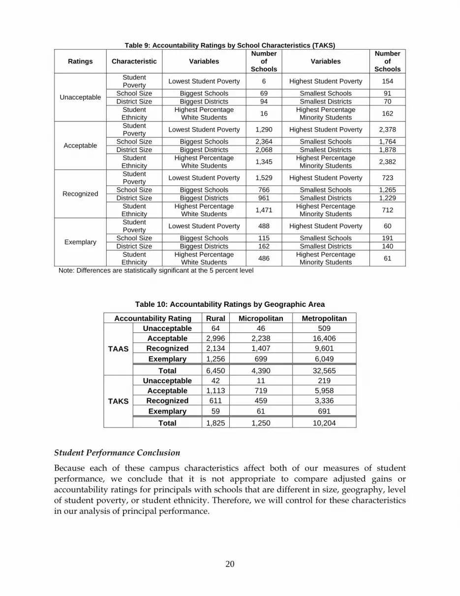
Tables 8 and 9 show the numbers of schools achieving each accountability rating in either the top or bottom quartiles of the school characteristics during either the TAAS or TAKS years. Table 10 shows the accountability ratings for TAAS and TAKS by geographic area. The differences in numbers of schools in each category are also all significantly different.

Table 8: Accountability Ratings by School Characteristics (TAAS)

Ratings Characteristic Variables Number

of Schools

Variables Number

of Schools

Student Poverty Lowest Student Poverty 81 Highest Student

Poverty 258

School Size Biggest Schools 219 Smallest Schools 190 District Size Biggest Districts 265 Smallest Districts 101 Unacceptable

Student Ethnicity Highest

Percentage White Students

23

Highest Percentage

Minority Students

306

Student Poverty Lowest Student Poverty 3,058 Highest Student

Poverty 6,950

School Size Biggest Schools 6,526 Smallest Schools 4,327 District Size Biggest Districts 6,252 Smallest Districts 4,226 Acceptable



2,780

Highest Percentage

Minority Students

6,969


Poverty 2,771

School Size Biggest Schools 2,659 Smallest Schools 3,689 District Size Biggest Districts 2,623 Smallest Districts 3,939 Recognized



3,815

Highest Percentage

Minority Students

2,715


Poverty 848

School Size Biggest Schools 1,429 Smallest Schools 2,629 District Size Biggest Districts 1,526 Smallest Districts 2,574 Exemplary



4,200

Highest Percentage

Minority Students

842

Note: all totals significantly different at the 5 percent level

20

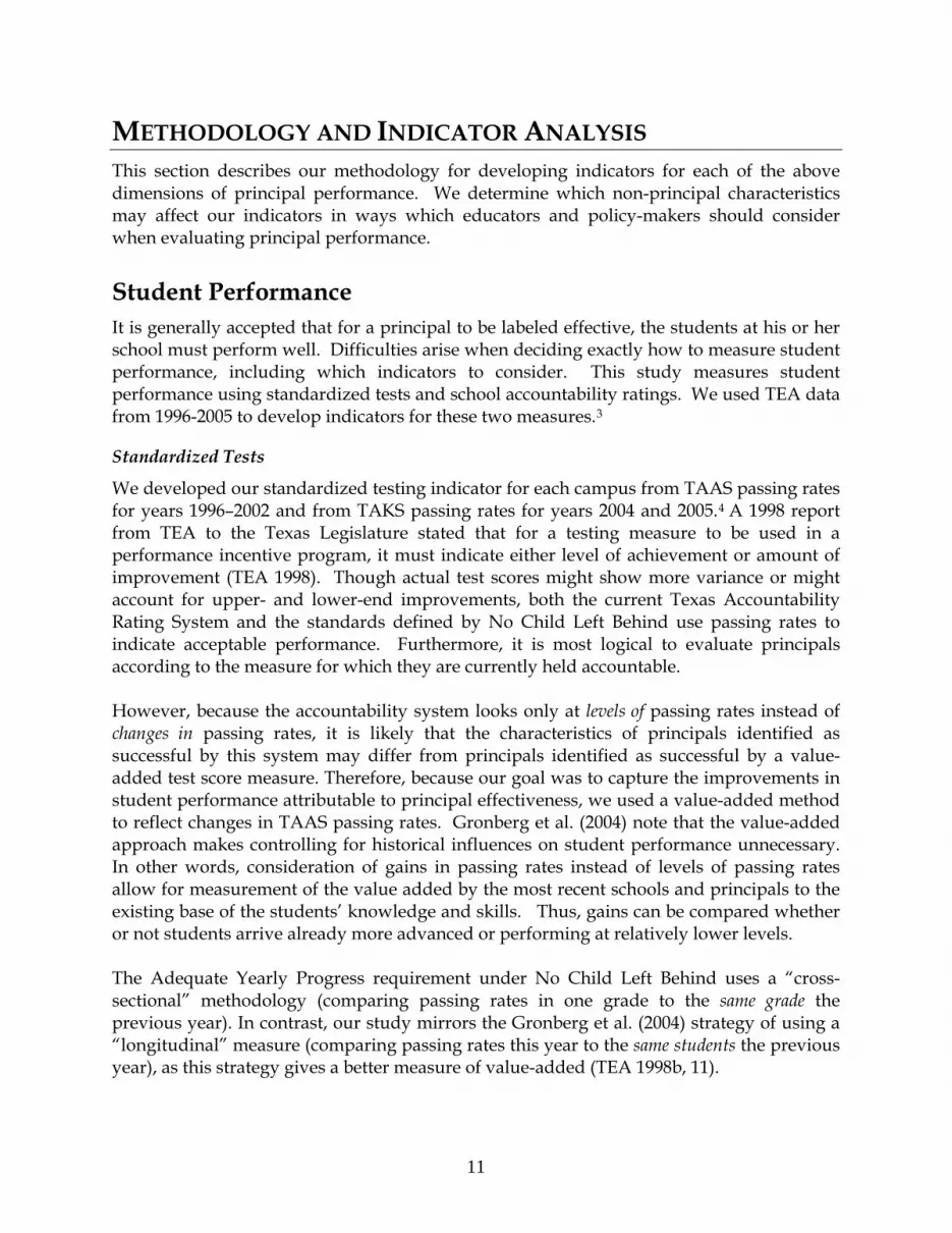
Table 9: Accountability Ratings by School Characteristics (TAKS)

Ratings Characteristic Variables Number

of Schools

Variables Number

of Schools

Student Poverty Lowest Student Poverty 6 Highest Student Poverty 154

School Size Biggest Schools 69 Smallest Schools 91 District Size Biggest Districts 94 Smallest Districts 70 Unacceptable

Student Ethnicity

Highest Percentage White Students 16 Highest Percentage

Minority Students 162

Student Poverty Lowest Student Poverty 1,290 Highest Student Poverty 2,378

School Size Biggest Schools 2,364 Smallest Schools 1,764 District Size Biggest Districts 2,068 Smallest Districts 1,878 Acceptable

Student Ethnicity

Highest Percentage White Students 1,345 Highest Percentage

Minority Students 2,382

Student Poverty Lowest Student Poverty 1,529 Highest Student Poverty 723

School Size Biggest Schools 766 Smallest Schools 1,265 District Size Biggest Districts 961 Smallest Districts 1,229 Recognized

Student Ethnicity

Highest Percentage White Students 1,471 Highest Percentage


Student Poverty Lowest Student Poverty 488 Highest Student Poverty 60

School Size Biggest Schools 115 Smallest Schools 191 District Size Biggest Districts 162 Smallest Districts 140 Exemplary

Student Ethnicity

Highest Percentage White Students 486 Highest Percentage


Note: Differences are statistically significant at the 5 percent level

Table 10: Accountability Ratings by Geographic Area

Accountability Rating Rural Micropolitan Metropolitan Unacceptable 64 46 509

Acceptable 2,996 2,238 16,406 Recognized 2,134 1,407 9,601 Exemplary 1,256 699 6,049

TAAS

Total 6,450 4,390 32,565 Unacceptable 42 11 219

Acceptable 1,113 719 5,958 Recognized 611 459 3,336 Exemplary 59 61 691

TAKS

Total 1,825 1,250 10,204

Student Performance Conclusion

Because each of these campus characteristics affect both of our measures of student performance, we conclude that it is not appropriate to compare adjusted gains or accountability ratings for principals with schools that are different in size, geography, level of student poverty, or student ethnicity. Therefore, we will control for these characteristics in our analysis of principal performance.

21

Teacher Retention The second dimension of principal effectiveness is teacher retention. We measured teacher retention with teacher turnover, which we defined as the percentage of teachers who were not employed as teachers in the same campus the following year. While some researchers use follow-up surveys or longitudinal studies,9 our study analyzed existing data on Texas public schools drawn from information submitted by school districts to TEA’s statewide educational database, Public Education Information Management System (PEIMS). It provided teacher turnover information for the years 1996-2005, as well as detailed annual information on teachers, schools, and students.

Teachers in Texas

During the ten-year period, 1996-2005, more than 617,000 individuals worked as teachers in the State of Texas. As demonstrated below in Figure 4, the number of teachers increased steadily over this period. Appendix II provides an exact breakdown of the number of teachers for each year in this study.

Figure 4: Teachers in Texas1996 - 2005

0

50000

100000

150000

200000

250000

300000

350000

1996 1997 1998 1999 2000 2001 2002 2003 2004 2005

No.

of T

each

ers

Measuring Teacher Retention

We measured teacher retention by distinguishing between categories of teacher turnover. Traditionally, measurement of teacher turnover focused only on those teachers who left the teaching profession (leavers) (Theobald and Michael 2001). However, other researchers have argued that teacher turnover also includes teachers who move from one teaching position to another (movers) (Ingersoll 2001; Theobald and Michael 2001; U.S. Department

22

of Education 2005). While the movers do not decrease the overall supply of teachers, the impact at the campus level is the same as that of leavers because the teachers must be replaced. Liu and Meyer (2005, 996) argue that, “teacher movers disrupt work routines and create vacant positions that must be filled. They, like teacher leavers, may also contribute to school staffing problems because schools cannot easily find replacements.” Our research, therefore, used a broader definition of turnover than TEA typically reports, as we measured campus turnover and not just district turnover. We included in our analysis of teacher retention in Texas the following three categories of teacher turnover:

• leavers - teachers who left teaching10

• internal movers - those who changed campuses but not district or job

• external movers - those who left a district but stayed in teaching

From 1996 to 2005, roughly 55,000 teachers left their positions each year. This includes leavers, internal movers and external movers. As Figure 5 demonstrates, these numbers have fluctuated over the years.

Table 11 displays the annual percentage of teacher turnover for the years 1996–2005. Over this ten year period, the average total teacher turnover by campus was 20 percent. However, if the percentage of teachers who moved within districts was excluded, as TEA reports, the average turnover rate for Texas would have been 15 percent. The 1999-2000 national average of teacher turnover (which includes leavers, internal movers, and external movers) was 16 percent (US Department of Education 2005, 6). The average teacher turnover rate in Texas is, therefore, approximately four percentage points higher than the national average.

Figure 5: Teacher Turnover in Texas1996 - 2005

0

10000

20000

30000

40000

50000

60000

70000

1996 1997 1998 1999 2000 2001 2002 2003 2004 2005

No.

of T

each

ers

23

Table 11: Total Teacher Campus Turnover by Category Percentage of Teacher Turnover

Year Total Left Teaching

Moved Outside District

Moved Within District

1996 0.18 0.08 0.04 0.06 1997 0.19 0.09 0.05 0.05 1998 0.21 0.10 0.05 0.06 1999 0.20 0.09 0.06 0.05 2000 0.22 0.10 0.06 0.06 2001 0.21 0.10 0.06 0.05 2002 0.21 0.10 0.05 0.05 2003 0.19 0.10 0.04 0.05 2004 0.21 0.10 0.05 0.05 2005 0.20 0.09 0.05 0.05

Average 0.20 0.10 0.05 0.05 The breakdown of average teacher turnover is evenly divided between leavers and movers at 10 percent each. This shows that on average, teachers are leaving teaching at the same rate at which they are moving between campuses.

Turnover by Category

The next step in our teacher turnover analysis was to determine whether these combined turnover totals11 were systematically affected in ways beyond a principal’s control. Detailed below are the teacher turnover rates by years of experience, teacher qualifications, and geographic areas. Experience. The literature suggests that teacher turnover is higher among beginning teachers (Theobald and Michael 2001; Ingersoll and Smith 2004; Taylor 2006; Graziano 2005). We wanted to be sure to control for this systematic difference, as well as ascertain whether other patterns also emerge between teacher experience and teacher turnover. To do this, we analyzed teacher turnover according to the following groupings12:

• beginning teachers13 – teachers with less than four years experience

• experienced teachers14 – teachers with 4–19 years experience

• highly experienced teachers – teachers with 20 years or more experience

Figure 6 shows the trends in overall turnover rate among teachers by years of experience over the ten-year period.

24

Beginning Teachers. Beginning teachers account for 30 percent of all Texas teachers. From 1996 to 2005, the average total campus teacher turnover among beginning teachers was 26 percent. While Theobald and Michael’s study (2001) concluded that almost one quarter of all new teachers leave the profession within the first five years of teaching, the rate in Texas is higher. According to PEIMS records, only 61.5 percent of teachers who started teaching in the 1999-2000 school year were still teaching in the Texas public school system in 2004-2005, implying that 38.5 percent leave the profession within the first five years. Graziano (2005, 40) found that as many as 40-50 percent of beginning teachers leave the profession nationwide. Experienced Teachers. Experienced teachers represent approximately 49 percent of all teachers in Texas during the ten-year period examined in our study. The average campus turnover rate for experienced teachers during this time was 18 percent. Highly Experienced Teachers. During the ten-year period covered in this study, highly experienced teachers represented 21 percent of the teaching population. The average campus turnover rate for highly experienced teachers is 16 percent. In comparing teacher turnover by years of experience, the data show that beginning teachers are leaving and moving at higher rates than both experienced and highly experienced teachers. Interestingly, both beginning teachers and experienced teachers moved—both within districts and among districts—at a higher rate than they left the profession. This suggests that a number of campuses are being staffed at the expense of

Figure 6: Turnover Rate By Experience1996 - 2005

0.00

0.05

0.10

0.15

0.20

0.25

0.30

0.35

1996 1997 1998 1999 2000 2001 2002 2003 2004 2005

Perc

ent T

urno

ver

Highly Exp. Experienced Beginning

25

other campuses. Of the three groups, highly experienced teachers are the least likely to leave the profession or change positions. Additionally, highly experienced teachers left the profession at a higher rate than they moved, which is to be expected because of the higher number of teachers within this category who would be retiring from teaching. Table 12 shows the average turnover rates for each year by experience.

Table 12: Average Teacher Turnover By Experience Average Percentage of Teacher Turnover

Year Beginning Experienced Highly Experienced 1996 0.25 0.16 0.14 1997 0.26 0.17 0.14 1998 0.28 0.19 0.16 1999 0.28 0.19 0.14 2000 0.29 0.20 0.17 2001 0.27 0.19 0.16 2002 0.27 0.19 0.18 2003 0.25 0.17 0.17 2004 0.25 0.19 0.20 2005 0.25 0.18 0.15

Average 0.26 0.18 0.16 Because teachers in each experience category have different levels of turnover, we recommend measuring teacher retention as a dimension of principal effectiveness using beginning teacher turnover and experienced teacher turnover as separate indicators. We did not use highly experienced teacher turnover because retirement could bias analysis of highly experienced teachers. Qualifications. The literature suggests that teachers with graduate degrees have lower turnover rates (Theobald and Michael 2001). Accordingly, it could be important to control for the effects of levels of teacher education on overall teacher turnover for each principal. We evaluated turnover rates among teachers with bachelor’s degrees and teachers with master’s or doctoral degrees. Seventy-five percent of the teachers had bachelor’s degrees from 1996 to 2005. As Table 13 demonstrates, the total average turnover rate for teachers with bachelor’s degrees was 20 percent, and total average turnover for teachers with master’s or doctoral degrees was also 20 percent. Because our analysis shows no difference in turnover according to degrees, we do not evaluate teacher retention according to qualifications.

26

Table 13: Average Turnover By Degree Type

Average Percentage of Teacher Turnover Year Bachelor’s Degrees Master’s or Doctoral Degrees 1996 0.19 0.17 1997 0.19 0.18 1998 0.21 0.21 1999 0.21 0.19 2000 0.22 0.22 2001 0.21 0.20 2002 0.21 0.21 2003 0.19 0.20 2004 0.20 0.23 2005 0.19 0.21

Average 0.20 0.20 Geographical Areas. Studies also indicate that teacher retention varies among different geographical locations (Theobald and Michael 2001; Graziano 2005; McDiarmid, Larson and Hill 2002). To account for differences in geography, we analyzed teacher turnover among the TEA’s regional educational service centers, as well as teacher turnover among metropolitan, micropolitan, and rural areas15. Table 14 shows similar overall trends among the three areas.

Table 14: Average Turnover By Geographic Area Average Percentage of Teacher Turnover

Year Rural Micropolitan Metropolitan 1996 0.18 0.15 0.19 1997 0.20 0.18 0.19 1998 0.21 0.21 0.21 1999 0.20 0.19 0.21 2000 0.21 0.19 0.22 2001 0.21 0.19 0.21 2002 0.21 0.19 0.21 2003 0.20 0.18 0.19 2004 0.22 0.21 0.21 2005 0.21 0.18 0.20

Average 0.20 0.19 0.20 Furthermore, average beginning teacher turnover was also the same in all three types of areas, at 26 percent (see Table 15). Turnover among experienced teachers was highest in metropolitan areas (see Table 16). Appendix II shows a detailed breakdown of turnover by rural, micropolitan and metropolitan among the various categories.

27

Table 15: Beginning Teacher Turnover By Geographic Area Average Beginning Teacher Turnover


Average .26 .26 .26

Table 16: Experienced Teacher Turnover By Geographic Area Average Experienced Teacher Turnover


Average 0.18 0.16 0.19

Our analysis shows that turnover is similar between the three types of geography. However, this result is not consistent with previous findings. For example, Theobald and Michael (2001) and Hanushek, Kain, and Rivkin (2002) reported that urban beginning teachers are significantly more likely to move out of their district than are beginning teachers hired by non-urban districts. Our preliminary results show that in the State of Texas, beginning teachers in rural areas are more likely to move out of their districts. Thus, as a more accurate analysis of geography we looked at turnover by labor market. This means that we compared both beginning and experienced teacher turnover among schools in the same metropolitan area and among schools in the same education service center in micropolitan and rural areas. The average teacher turnover rate among beginning teachers in rural areas ranged from a low of 21 percent in the Mount Pleasant and San Angelo service center regions to a high of 32 percent in the Corpus Christi service center region. On the other hand, the turnover rate among experienced teachers in rural areas ranged from a low of 14 percent in the rural areas of the Kilgore and Mount Pleasant service centers to a high of 20 percent in the rural areas of Waco and San Antonio (see Table 17).

28

Table 17: Average Turnover of Beginning and Experienced Teachers In Rural Areas By Education Service Center

Region Name Beginning Teachers

Experienced Teachers

1 Edinburg 0.23 0.17 2 Corpus Christi 0.32 0.18 3 Victoria 0.30 0.16 6 Huntsville 0.30 0.18 7 Kilgore 0.22 0.14 8 Mount Pleasant 0.21 0.14 9 Wichita Falls 0.25 0.15 12 Waco 0.27 0.20 14 Abilene 0.22 0.15 15 San Angelo 0.21 0.17 16 Amarillo 0.23 0.15 17 Lubbock 0.26 0.16 18 Midland 0.28 0.18 20 San Antonio 0.26 0.20

Average 0.25 0.17 The turnover rate among beginning teachers in micropolitan areas ranged from a low of 18 percent in the Mount Pleasant service center region to a high of 29 percent in the Huntsville service center region. On the other hand, the rate among experienced teachers in rural areas ranged from a low of 11 percent in the micropolitan areas of the Wichita Falls service center to a high of 18 percent in the micropolitan areas of Kilgore and Waco (see Table 18).

Table 18: Average Turnover of Beginning and Experienced Teachers In Micropolitan Areas by Education Service Center

Region Name Beginning Teachers


1 Edinburg 0.28 0.16 2 Corpus Christi 0.28 0.16 3 Victoria 0.28 0.14 6 Huntsville 0.29 0.17 7 Kilgore 0.26 0.18 8 Mount Pleasant 0.18 0.15 9 Wichita Falls 0.20 0.11

12 Waco 0.27 0.18 14 Abilene 0.22 0.14 15 San Angelo 0.26 0.16 16 Amarillo 0.25 0.15 17 Lubbock 0.26 0.15 18 Midland 0.27 0.17 20 San Antonio 0.26 0.16

Average 0.26 .16

29

The turnover rate among beginning teachers in metropolitan areas ranged from a low of 21 percent in three areas - Amarillo, Fort Worth-Arlington, and Longview - to a high of 32 percent in College Station-Bryan. On the other hand, the rate among experienced teachers in metropolitan areas ranged from a low of 14 percent in Abilene, Amarillo, and Laredo to a high of 21 percent in Dallas-Plano-Irving (see Table 19). More detailed tables showing turnover rates for rural, micropolitan and metropolitan areas can be found in Appendix II.

Table 19: Average Turnover of Beginning and Experienced Teachers In Metropolitan Areas

ID Name Beginning Teachers


10180 Abilene 0.22 0.14 11100 Amarillo 0.21 0.14 12420 Austin-Round Rock 0.28 0.20 13140 Beaumont-Port Arthur 0.22 0.16 15180 Brownsville 0.22 0.15 17780 College Station-Bryan 0.32 0.18 18580 Corpus Christi 0.24 0.18 19124 Dallas-Plano-Irving 0.29 0.21 21340 El Paso 0.23 0.16 23104 Fort Worth-Arlington 0.21 0.19 26420 Houston-Sugar Land-Baytown 0.25 0.19 28660 Killeen-Temple-Fort Hood 0.31 0.20 29700 Laredo 0.23 0.14 30980 Longview 0.21 0.15 31180 Lubbock 0.27 0.18 32580 McAllen-Edinburg-Mission 0.26 0.16 33260 Midland 0.27 0.19 36220 Odessa 0.30 0.19 41660 San Angelo 0.25 0.18 41700 San Antonio 0.24 0.17 43300 Sherman-Denison 0.24 0.16 45500 Texarkana, TX-Texarkana, AR (part) 0.23 0.16 46340 Tyler 0.25 0.16 47020 Victoria 0.27 0.18 47380 Waco 0.29 0.19 48660 Wichita Falls 0.24 0.14

Average 0.25 .17 In our analysis of beginning and experienced teacher turnover by geographic area and education service center, we discovered that turnover rates differ among labor markets in the same type of geographical area. For example, in Midland, the average turnover is 21 percent, while the average metropolitan turnover is 19 percent. Thus, a school with 21 percent turnover in Midland may be considered to have high turnover when compared to metropolitan areas when in fact it has average turnover compared to other schools in Midland. Table 20 displays a breakdown of Midland’s beginning and experienced teacher turnover to show that grouping turnover by labor market is beneficial.

30

Table 20: Comparative Analysis of Turnover in Midland Beginning Teachers Experienced Teachers

Average turnover among beginning teachers in metro areas

26% Average turnover among experienced teachers in metro areas

17%

Average turnover among beginning teachers in Midland 27%

Average turnover among experienced teachers in Midland

19%

Average turnover among beginning teachers at De Zavala Elementary School in Midland

24% Average turnover among experienced teachers at Lee High School in Midland

14%

This example shows that the average teacher turnover rates in Midland are higher than the average rate in metropolitan areas. Additionally, the turnover rate among beginning teachers in Midland is higher than the average rate among beginning teachers in metro areas. Furthermore, the average turnover rate among experienced teachers in Midland is also higher than the average rate among experienced teachers in metropolitan areas. Despite these higher than average rates, there are schools within Midland with lower than average turnover rates. For example, the beginning teacher turnover rate at De Zavala Elementary School in Midland is 24 percent, which is below the 26 percent average for metropolitan areas. Also, the turnover rate among experienced teachers at Lee High School in Midland is 14 percent, which is five percentage points below the average for metropolitan areas.

Indicator Adjustment

Given the above analysis, we recommend that teacher turnover in metropolitan areas be compared to turnover of other schools in the same metropolitan area. Schools in rural and micropolitan areas should be compared to schools in rural and micropolitan areas in the same educational service center. To control for this variation in teacher turnover by labor market, we adjusted both beginning teacher turnover and experienced teacher turnover for geography to get our final teacher retention indicators. First, we calculated a school’s beginning and experienced teacher turnover. Next, we subtracted from this turnover the turnover that would be expected given the average beginning or experienced turnover in that school’s labor market.

Teacher Turnover Indicators and Demographics

To further control for factors outside a principal’s control, we also examined the relationship between teacher retention and student demographics, including race, special needs, and poverty level. For example, we compared the 25 percent of schools with the most students on free or reduced lunch to the 25 percent of schools with the fewest students on free or reduced lunch. Tables 21 and 22 show the differences in beginning and experienced teacher turnover and correlations between quartiles for all variables tested. Our findings can be summarized as follows:

31

Beginning Teacher Turnover

• As the percentage of white students increases in combined schools and

elementary schools, beginning teacher turnover rates decrease. • As the percentage of black students in combined schools and elementary schools

increases, turnover rates among beginning teachers increases. • As the school size increases, turnover rates among beginning teachers in secondary

schools decreases.

• As student mobility increases, teacher turnover also increases.16 Experienced Teacher Turnover

• As the school size increases, experienced teacher turnover in combined schools, middle schools and secondary schools decreases.

• As the percentage of low income students increases, experienced teacher turnover

increases in elementary schools. • As the percentage of white students increases in elementary schools, experienced

teacher turnover decreases.

• As student mobility increases, teacher turnover also increases.

32

Table 21: Average Turnover For Beginning Teachers By School Characteristic School Type Variables (Low) Mean Variables (High) Mean Correlation

Poverty 4.77% Poverty 7.43% 0.04 Special Ed 1.38% Special Ed 5.82% 0.06 Limited English Proficiency - Limited English Proficiency - -0.01 White 7.51% White 0.14% -0.12 Black 5.76% Black 6.47% 0.11 Hispanic 3.33% Hispanic 6.26% 0.06 Mobility -2.22% Mobility 11.26% 0.09

Combined Schools

(Primary and Secondary)

Small school 2.27% Large school 0.99% -0.06 Poverty 3.98% Poverty 0.62% 0.09 Special ed 0.93% Special ed -1.92% 0.01 Limited English proficiency - Limited English Proficiency - 0.05 White 0.59% White -4.85% -0.11 Black -2.84% Black 1.30% 0.10 Hispanic 3.47% Hispanic -0.90% 0.05 Mobility -4.54% Student Mobility 2.04% 0.09

Elementary Schools

Small school 1.98% Large school -1.26% 0.00 Poverty 1.29% Poverty 5.48% 0.09 Special ed 2.46% Special ed 4.75% 0.07 Limited English proficiency - Limited English proficiency - 0.01 White 4.77% White 2.30% -0.06 Black 3.63% Black 5.04% 0.06 Hispanic 2.35% Hispanic 4.17% 0.03 Mobility 0.67% Mobility 6.93% 0.05

Middle Schools

Small school 3.95% Large school 1.55% -0.08 Poverty 0.32% Poverty 3.23% 0.07 Special ed 0.30% Special ed 4.63% 0.09 Limited English proficiency - Limited English proficiency - 0.00 White 2.20% White 1.59% -0.02 Black 2.56% Black 3.02% 0.02 Hispanic 2.75% Hispanic 2.34% 0.02 Mobility -0.41% Mobility 4.21% 0.01

High Schools

Small school 3.10% Large school -2.28% -0.12

33

Table 22: Average Turnover For Experienced Teachers By School Characteristic

School Type Variables (Low) Mean Variables (High) Mean Correlation Poverty 8.78% Poverty 9.50% 0.00 Special ed 5.58% Special ed 11.60% 0.07 Limited English proficiency - Limited English proficiency - -0.08 White - White - -0.02 Black 9.17% Black 9.20% 0.08 Hispanic 5.82% Hispanic 8.16% 0.05 Mobility 5.76% Mobility 6.47% 0.08

Combined Schools

(Primary and Secondary)

Small school 6.96% Large school 2.91% -0.10 Poverty -1.82% Poverty 1.98% 0.10 Special ed 0.77% Special ed 0.16% 0.03 Limited English proficiency - Limited English proficiency - 0.04 White 1.78% White -2.29% -0.11 Black -0.29% Black 2.16% 0.09 Hispanic 1.57% Hispanic 0.83% 0.05 Mobility -2.84% Mobility 1.30% 0.11

Elementary Schools

Small school -0.24% Large school 0.35% -0.02 Poverty 1.52% Poverty 4.49% 0.07 Special ed 2.54% Special ed 4.29% 0.09 Limited English proficiency - Limited English Proficiency - 0.03 White 4.18% White 1.88% -0.06 Black 3.58% Black 3.78% 0.04 Hispanic 1.96% Hispanic 3.73% 0.04 Mobility 3.63% Mobility 5.04% 0.09

Middle

Schools

Small school 3.29% Large school 1.43% -0.10 Poverty 1.46% Poverty 5.13% 0.08 Special ed 2.48% Special ed 5.50% 0.08 Limited English proficiency - Limited English proficiency - 0.00 White 3.85% White 2.48% -0.03 Black 4.40% Black 3.62% 0.02 Hispanic 2.86% Hispanic 4.16% 0.03 Mobility 2.56% Mobility 3.02% 0.08

High Schools

Small school 4.59% Large school 2.29% -0.18

34

Our findings show both similar and differing results from previous research on the effect of demographics on teacher turnover in Texas. For example, Falch and Strom (2005) report that teachers tend to leave schools that have a high percentage of minority students or a high percentage of students with special needs. They cite earlier research which found that the percentage of black and Hispanic students was positively related to teacher turnover in U.S. schools. Loeb, Darling-Hammond, and Luczak (2005) report that teachers leave schools with higher percentages of low income and minority students. Guin (2004) also reports on the higher turnover as a result of higher percentages of minority students. Our results show that the percentage of black students is positively related to turnover rates in certain types of schools, but they do not show any correlations between the percentage of Hispanics and teacher turnover. Neither do they reveal that the percentage of students with special needs affects teacher turnover. There is a correlation between the percentage of low income students and experienced teacher turnover in elementary schools only.

Financial Management We used three indicators to measure the financial management dimension of principal performance: cost efficiency, attendance rates, and instructional share. The cost efficiency indicator allows us to compare school district expenditures with the level of expenditures that would be expected given student performance, student demographics, and other cost factors. Attendance rates are associated with school funding at the district level. As such, a principal may be able to attract more funds to his or her school by promoting high student attendance. In addition, good financial management suggests a balance between instructional, administrative, and other expenditures. As a benchmark, we use the Texas Governor’s 2005 Executive Order which requires that 65 percent of current expenditures be spent on instruction.

Measuring Campus Level Expenditures

Both the cost function to measure cost efficiency and the analysis of percent of expenditures spent on instruction require calculation of a school’s per pupil expenditures. In addition to the money directly allocated to a particular school, such as the salaries for campus employees, school districts spend their money in a variety of ways. Unallocated expenditures occur at the district level and include central administration costs. Our data shows that on average, allocated costs account for about 77 percent of all school expenditures. The remaining 23 percent is from central administration costs. This shows that schools have significant financial discretion. Although the data shows little difference between allocated funds among different types of schools, the range of the percentage of allocated funds varies widely across campuses. Some schools have only 22 percent allocated costs, while other schools have up to 96 percent allocated costs. This also reveals that the central administration costs vary widely among school districts. Because of these differences, we distributed the unallocated funds to particular schools in order to calculate our per-pupil expenditures. Our strategy for distributing unallocated money is based on school student population; those with more students will receive more unallocated money. An alternative strategy of sharing unallocated money is to make allocations based on schools’ expenditure patterns. This determination is made by how much allocated funds are spent. In other words, if a

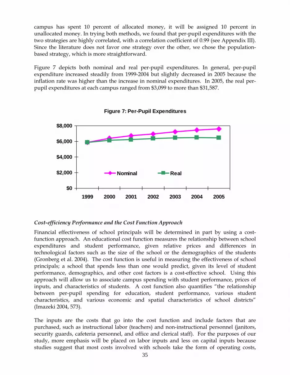
35

campus has spent 10 percent of allocated money, it will be assigned 10 percent in unallocated money. In trying both methods, we found that per-pupil expenditures with the two strategies are highly correlated, with a correlation coefficient of 0.99 (see Appendix III). Since the literature does not favor one strategy over the other, we chose the population-based strategy, which is more straightforward. Figure 7 depicts both nominal and real per-pupil expenditures. In general, per-pupil expenditure increased steadily from 1999-2004 but slightly decreased in 2005 because the inflation rate was higher than the increase in nominal expenditures. In 2005, the real per-pupil expenditures at each campus ranged from $3,099 to more than $31,587.

Cost-efficiency Performance and the Cost Function Approach

Financial effectiveness of school principals will be determined in part by using a cost-function approach. An educational cost function measures the relationship between school expenditures and student performance, given relative prices and differences in technological factors such as the size of the school or the demographics of the students (Gronberg et al. 2004). The cost function is useful in measuring the effectiveness of school principals; a school that spends less than one would predict, given its level of student performance, demographics, and other cost factors is a cost-effective school. Using this approach will allow us to associate campus spending with student performance, prices of inputs, and characteristics of students. A cost function also quantifies “the relationship between per-pupil spending for education, student performance, various student characteristics, and various economic and spatial characteristics of school districts” (Imazeki 2004, 573). The inputs are the costs that go into the cost function and include factors that are purchased, such as instructional labor (teachers) and non-instructional personnel (janitors, security guards, cafeteria personnel, and office and clerical staff). For the purposes of our study, more emphasis will be placed on labor inputs and less on capital inputs because studies suggest that most costs involved with schools take the form of operating costs,

Figure 7: Per-Pupil Expenditures

$0

$2,000

$4,000

$6,000

$8,000

1999 2000 2001 2002 2003 2004 2005

Nominal Real

36

attributed largely to teacher and auxiliary personnel salaries (Imazeki and Reschovsky 2004; Gronberg et al. 2004). Although most studies utilizing the cost function model within an educational context have analyzed the cost function at the district level (Gronberg et al. 2004; Imazeki and Reschovsky 2004), we will consider the cost function at the campus level. The cost function method, however, is not without limitations. For instance, this approach assumes that school districts strive to achieve outcomes at minimum cost. If schools are not doing so, the results of a cost function analysis could be deceptive. Also, the cost function does not provide a prescription for how schools should spend money (Gronberg et al. 2004). Despite these concerns Gronberg et al. (2004) note many advantages to using a cost function to measure the effectiveness of school principals. While there is little research describing the relationship between school funding structure and school accountability, the cost function enables us to forge this link.17 Using a cost function will help us to analyze the factors that influence the costs of education and the output that occurs using a variety of measures of student performance (Imazeki 2004, 573). The cost function will reveal cost efficiency by comparing the actual performance with the predicted spending at the same levels. The dependent variable in the cost function will be per-pupil expenditures for the school year. Following Taylor (2004), we will not include the expenditures for transportation and food from per-pupil spending. Apart from teacher salaries, various operating expenditures are also considered to be costs, including utilities, supplies for maintenance, and rentals on property and equipment.

Cost Function Model

For our cost function, the dependent variable, or the input, is per-pupil expenditure by campus. The independent variables, or the output, are student performance measures—adjusted gain and accountability ratings—previously outlined in this paper (see the Student Performance section in Methodology). Previous research has found that other factors may influence the cost of operating a school (Imazeki and Reschovsky 2004). So following the literature, we also incorporate those as control factors. Our analysis controls for student demographics, campus size18, and teacher wages. In addition, considering the difference between extremely big school districts (Houston and Dallas area) and other districts, we also included a control for district. Table 23 lists all the dependent variables in our cost function model.

37

Table 23: All Variables in the Cost Function

Adjusted TAAS/TAKS passing rates

Square of adjusted TAAS/TAKS passing rate

Accountability rating

Log of district beginning teacher salary

Square of log of district beginning teacher salary

Log of campus enrollment

Square of log of campus enrollment

Log of district enrollment

Square of log of district enrollment

Percentage of students with limited English proficiency

Square of percentage of students with limited English proficiency

Percentage of economically disadvantaged or poor students

Square of percentage of economically disadvantaged or poor students

Percentage of students with special education

Square of percentage of students with special education

Houston independent school district

Dallas independent school district

Year 1999 - 2005 Apart from exploring the relationship between student performance and per-pupil expenditure, we also estimate the efficiency of expenditure in our model. Some schools may have higher per-pupil expenditure, not because of higher costs, but because, “they are not using their resources efficiently” (Imazeki and Reschovsky 2004). To measure efficiency, we adopted a frontier estimation strategy. The frontier regression model, “seeks to explain boundary, frontier or optimal behavior rather than average behavior as in ordinary regression models” (Troutt et al. 2003). In our model, measured efficiency shows how much a school could have spent without decreasing adjusted gains or accountability ratings.19 In other words, the model demonstrates how efficient a school could have operated given their student performance.

Analysis of Cost Function Model

Preliminary analysis found a marked difference between different types of schools, so we construct separate models for elementary schools, middle schools, and high schools. Also, we noticed that the change of standard test from TAAS to TAKS in 2003 may have an impact on student performance measurement and influence other variables. Therefore, to generate more accurate results, we construct a separate model for each type of school before and after 2003. Basic Information. The cost function shows that for all types of schools, higher teacher wages lead to higher per-pupil expenditure. The relationships between school spending and campus size as well as student demographics vary among elementary schools, middle

38

schools, and high schools. The cost function results for all the six models are shown in Appendix III. For elementary schools, extremely high or low student performance is associated with lower per-pupil expenditures. Large campuses spend less than smaller ones. Student demographics have a non-linear relationship with expenditures. For middle schools, on the other hand, better student performance is clearly associated with lower per-pupil expenditure. Also, middle schools with more economically disadvantaged students or more students in special education will spend more than other schools. The relationships between expenditures and school size as well as other student demographics are non-linear. High schools with better student performance usually spend more, but with TAKS test after 2003, the relationship tends to be U-shaped. In addition, the larger a high school or its district is, the less money the school spends. Schools with more economically disadvantaged students or students with limited English proficiency spend more than others. A non-linear relationship exists between the expenditure and the percentage of students in special education. Efficiency Measure. Our analysis reveals that on average, schools could spend 11.59 percent less than they do with no decrease in student performance. In particular, high schools could save 13.3 percent, elementary schools could save 11.47 percent, and middle schools could save 10.53 percent. This finding shows that the efficiency of spending in terms of student performance varies across different types of schools. Comparatively speaking, middle school expenditures are more efficient than the expenditures of the other two types of school; high schools are the least efficient. As shown in Figure 8, about half of the schools could save 10 percent of their expenditures. Nearly 10 percent of all schools could save 20 percent of their expenditures. Only less than 1 percent of all schools spent 40 percent more than they could without decreasing student performance.

39

As previously stated, any efficiency measure, however, is sensitive to the method of measuring school performance. In our models, school performance is mainly indicated by standardized test passing rates, and this is a generally accepted criteria. But we are also aware that expenditures on other school activities, such as sports or arts, may be interpreted as inefficient. This might well be reason for the relative inefficiency in high school expenditures.

School Finance and Attendance Rates

The finance formula of a school district depends on a school’s attendance rates. Attendance rates are thus a fiscal indicator tied to principal performance and overall school effectiveness. By influencing school attendance, a principal influences the financial health of a district. This study uses TEA attendance data for the years 1996-2005. TEA reports attendance for each campus as the number of days students were in attendance each year divided by the number of days students were enrolled in that year. This formula allows for an attendance score of 0-100 for each campus, representing the percent of time that students attended class on average for the year. Attendance rates at elementary, middle, and high schools are slightly different. Attendance rates are 96.7 percent at elementary schools, 95.9 percent in middle schools, and 94.7 percent in high schools. Attendance rates are likely lower in middle and high schools than in elementary schools because it is easier for teenagers to forgo class than it is for children. Attendance rates also fell from year to year. In 2000, attendance rates were 95.5 percent. In 2004, attendance rates were 93.3 percent. Overall, attendance rates have been falling since 2000. There is no relationship between ethnicity and attendance rates, nor is there a relationship between poverty and attendance rates. There is no correlation between the numbers of whites, blacks, Hispanics, Asians, or Native Americans and attendance rates. There is no correlation between attendance rates and the number of economically disadvantaged students in a district.

0500

100015002000250030003500

Sch

ools

0 0.2 0.4 0.6 0.8 100% ormore

School Percent Inefficiency

Figure 8: Frequency of Percentages of Inefficiency

40

Instructional Share

The Governor of Texas recently issued an executive order requiring that 65 percent of a school’s budget be dedicated to instructional expenditure. Though this ruling did not apply during the years in our study, we analyzed instructional shares to see how closely these schools would have come to this benchmark. Although Santiago and Canby (2006) note that there is no research foundation for this indicator, it likely will be part of district evaluation strategies in the future and is therefore included in this study. The Texas definition of instructional expenditure is based in part on the definition provided by the National Center for Education Statistics (NCES). The Texas definition is slightly different from the NCES definition because counseling and technology are not included in the Texas definition of instructional expenditure (Executive Order RP47, 2005). According to this guideline, we calculated the percentage of expenditure that is considered “instructional” using the Texas definition. Our definition of expenditures also varies slightly from the PEIMS definition of instructional expenditure because the executive order issued by Governor Perry does not include counseling or counseling services as a part of instructional expenditures. Analysis of Instructional Share. Our analysis evaluated the impact of using the instructional share criterion for the evaluation of school principals. The data for this measure is derived mostly from the PEIMS data from 1999-2005. The instructional expenditure ratio is a measure required by TEC 44.0071 and indicates the percentage of district total actual expenditures that were used to fund direct instructional activities.20 After analysis of campuses in schools in the State of Texas, we have determined the following:

• Most schools spend less than 65 percent on instruction within the classroom, and most schools spend between 55 and 70 percent on instruction.

• The average instructional share for Texas schools has been remarkably stable over time.

• On average, schools from the elementary to high school level spend nearly 63 percent on instruction.

• Instructional shares in schools in micropolitan, metropolitan, and rural areas are consistently similar.

Most Texas schools spend less than the 65 percent promulgated by the 2005 Executive Order. Figure 9 illustrates the distribution of instructional shares for 2005. This graph demonstrates that 70 percent of campuses in Texas spent less than 65 percent on instruction, and 8 percent of campuses spent less than 55 percent. Most Texas schools spent between 55 and 70 percent of their operating expenditures instruction.

41

The average instructional share for Texas campuses has consistently remained stable during the past few years. Figure 10 illustrates that the average instructional share for Texas schools has been remarkably stable over time. Figure 11 displays the instructional share per-pupil across campus type. All types of campuses from elementary to high school spend, on average, roughly 63 percent on instruction.

Figure 9: Distribution of Instructional Share

0

1,000

2,000

3,000

4,000

0 20 40 60 80 100%Instructional Share

No.

of S

choo

ls

Figure 10: Average Instructional Share

0%20%40%60%80%

1999 2000 2001 2002 2003 2004 2005

Figure 11: Instructional Share by Campus Type

0%

20%

40%

60%

80%

Both Elem Middle HS Total

Type of School

42

Figure 12 displays the instructional share by the per-pupil method across metropolitan, micropolitan, and rural areas. It shows that instructional shares are consistent across geographic areas. Schools with high, medium, and low percentages of students that are economically disadvantaged all spend nearly the same amount on instruction. Figure 13 demonstrates consistency across schools with high, medium, and low percentages of economically disadvantaged students. For example, schools with 75 percent economically disadvantaged students spend on average nearly 63 percent on instruction. Schools with 50 percent economically disadvantaged students spend, on average, 62.4 percent on instruction. Schools with 25 percent economically disadvantaged students spend, on average, nearly 62 percent on instruction. The gap widens very slightly as the percentage of economically disadvantage students decreases. For example, schools with 5 percent economically disadvantaged students spend on average slightly over 64 percent on instruction. However, no matter what the percentage of economically disadvantaged students, only schools with zero percent economically disadvantaged students spend on average over 65 percent on instruction.

Figure 12: Instructional Share by Geographic Area

0%

20%

40%

60%

80%

Metropolitan Micropolitan Rural

Geographic Area

Figure 13: Instructional Share by Percentage of Economically Disadvantaged Students

0%

20%

40%

60%

80%

0% 5% 25% 50% 75%Percent Students Economically Disadvantaged

43

Conclusions Concerning Financial Management

The cost function shows that school types matter in measuring efficiency, and the change in the student performance measure due to the change in standardized tests in 2003 also influenced efficiency. Therefore, using student performance measures as output, school efficiency should be compared among schools of similar type. On average, we also find that schools could spend 11.59 percent less than they do with no decrease in student performance. In particular, high schools could save 13.30 percent, elementary schools could save 11.47 percent, and middle schools could save 10.53 percent. Our analysis indicates that most schools spend less than 65 percent on instruction, with a small number spending less than 55 percent. Furthermore, while instructional shares significantly different across school types and geographic areas, these differences are minor. Given that there is a lack of research regarding instructional share, we wondered if instructional share had any relationship with our other indicators. As Table 24 demonstrates, instructional share is generally not correlated with our other indicators. In particular, campuses with higher instructional shares are not systematically more efficient than those with lower instructional shares. The lack of correlation indicates either that instructional share is a poor measure of principal performance or that it picks up an aspect of principal performance unmeasured by our other indicators.

Table 24: Correlations between Instructional Share and Other Indicators, 2005

School Type Variables Correlation with

Instructional Share21 Adjusted Gains 0.0125 Accountability Ratings 0.2272 Turnover by Beginning Teachers -0.0251 Turnover by Experienced Teachers -0.0518

Combined Schools

(Primary and Secondary

Attendance -0.0891 Adjusted Gains 0.0841 Accountability Ratings 0.0480 Turnover by Beginning Teachers 0.0069 Turnover by Experienced Teachers -0.0092 Inefficiency -0.0137

Elementary Schools

Attendance 0.1003 Adjusted Gains 0.1212 Accountability Ratings 0.0889 Turnover by Beginning Teachers -0.0533 Turnover by Experienced Teachers -0.0715 Inefficiency 0.0653

Middle Schools

Attendance 0.0982 Adjusted Gains 0.0274 Accountability Ratings 0.1237 Turnover by Beginning Teachers -0.0015 Turnover by Experienced Teachers -0.1130 Inefficiency 0.0113

High Schools

Attendance 0.0331

44

PRINCIPALS IN TEXAS We use the seven indicators detailed above to evaluate the effectiveness of principals in Texas from 1999-2005. The seven-year period of analysis examines around 12,500 individual principals in more than 7,600 campuses. We chose this time period because in 1999 Texas undertook several policy changes with regard to education. One of the more significant policy changes for our analysis includes the availability of the alternative certification program for principals. By starting in 1999, our analysis will allow us to compare alternatively certified principals with more traditionally certified principals (standard and out of state certificate holders). In addition, this time period facilitates a comparison of the principals in both the TAAS and TAKS testing periods across all our principal effectiveness indicators. This section provides an overview and comparison of the observable characteristics of principals over the seven-year time period as well as in 2005, highlighting the most recent year of analysis.

Demographics In our seven-year period of analysis, 54 percent of principals were female. The majority of principals worked at elementary schools (58 percent). During the 2005 school year, which included approximately 7,000 principals, 57 percent of principals were female. This reflects a slight increase over time in the number of female principals. Much like the seven-year period, in 2005 the greatest number of principals were found at the elementary level, where nearly 4,000 principals were employed (which accounts for approximately 58 percent of all Texas principals in 2005). Ethnic distribution of principals has remained steady throughout the seven-year period. Nearly 70 percent of principals were white, 18 percent Hispanic, 11 percent black, and close to 1 percent were Asian or Native American/Pacific Islander. At the same time, student demographics reflect a much different ethnic breakdown. As indicated by the charts in Figure 14, Hispanic students made up 42 percent of the student population, while 41 percent of students were white, and 14 percent were black. So while the majority of principals in Texas are white, the majority of students in Texas are either white or Hispanic (see Figure 14).

45

Geographic Distributions An evaluation of geographic differences revealed that in the seven-year period, 78 percent of principals worked in metropolitan areas (which are cities and surrounding counties with 50,000 or more people), 10 percent in micropolitan areas (counties with a town of more than 50,000, but not large enough to be considered metropolitan), and 12 percent in rural areas (the remainder of geographic locations in the state). In 2005, nearly 89 percent of principals worked in a metropolitan or micropolitan area. Of those schools located in either metropolitan or micropolitan areas, students were almost twice as likely to have a principal who was either Hispanic or black.

Experience and Education During the seven-year period, school principals on average maintained 22 years of experience within the school system, which may reflect other experience in the school system. Nevertheless, the difference in average years of experience between principals in metropolitan and micropolitan areas as compared to rural areas was around one year, suggesting that years of experience vary little by geographic area over the seven-year period. Similarly, during the seven-year period, 88 percent of principals in metropolitan and micropolitan areas and 87 percent of principals in rural areas possessed master’s degrees. In 2005, 5 percent of employed principals possessed doctoral degrees, compared to 88 percent with master’s degrees and 8 percent with bachelor’s degrees. However, 88 percent of principals with doctoral degrees were employed in metropolitan areas, while 6 percent worked in micropolitan areas and 6 percent in rural areas. Therefore, years of experience and type of degree vary little by geographic region, with the exception of the doctoral degree (see Table 25 ).

Figure 14: Principal and Student Ethnicity1999 - 2005

Other 3%

Black 14%

Hispanic42%

White41%

Students

Hispanic

Principals Other

1% Black 11%

18%

White 70%

46

Principal Tenure Among principals observed over the seven-year period, around 14 percent were in their first year at a given campus. In 2005, close to 15 percent of principals were in their first year of service at their campus. At the same time, 37 percent of principals in 2005 had served three or more years at their campus, which is about the same percentage of principals during the seven-year period who had served three or more years at a given campus. In either case, more than half of all principals in the seven-year period and in 2005 had served less than three years at a given campus.

Certification Principal certification standards are state-specific. In Texas, prior to 2000, principals were able to obtain the lifetime Mid-Management Administrator Certificate. Since new legislation was enacted in 2000, educators must now receive a five-year renewable principal certificate. In 2005, approximately 84 percent of principals possessed a Mid-Management Administrator Certificate, while 16 percent held a Principal Certificate, demonstrating the transition to the renewable Principal Certification. In Texas, certification in education administration is granted by the Texas State Board for Educator Certification (SBEC) and is earned either by completion of a master’s degree in educational administration from a university or college within Texas (36 credit hours), or by completion of an alternative program through one of the Texas Education Agency’s regional service centers. At the same time, administrators holding out-of-state certificates who are seeking to practice in Texas must have their out-of-state certificate transferred to Texas through the Texas SBEC. Not all out-of-state certificates are considered equivalent, and additional testing may be required for administrative candidates bearing out-of-state certificates. In 2005, 3.2 percent of principals held out-of-state certificates (Texas SBEC Board Meeting 2001). To be considered a principal in Texas, a person must achieve one of the following:

Complete the requirements for the standard administrative certification, in addition to two years of full-time, in-classroom teaching experience and successful completion (passing) of the Texas Examination for Educator Standards (TExES, which began in fall 2002) or ExCET (Examination for the Certification of Educators in Texas).

OR

Complete the requirements for alternative administrative certification plus

additional requirements which typically include three years of leadership experience, a master’s degree bearing a GPA of 3.0 or higher, as well as two years of full-time, classroom experience and successful completion of the TExES or ExCET.

47

Additionally, a probationary administrative certificate exists in Texas. This certificate is offered by SBEC for cohorts in alternative administrative certification programs who wish to practice educational administration during their certification process. The probationary certificate is granted for only one year and was created to allow administrative certificate candidates to earn administrative experience in internship-like settings. In our study, we will classify probationary certificate holders as non-certified so that our analysis evaluates only those holding an actual certificate. Furthermore, standard and alternatively certified principals will be most closely evaluated in terms of our three areas of principal effectiveness. As Table 25 indicates, principals’ skills in Texas are fairly evenly distributed by geographic region, suggesting that students in rural, metropolitan, and micropolitan areas have equally equipped principals.

Table 25: Principal Characteristics by Geographic Region Principal Characteristics

Geographic Areas

Master’s Degrees

Doctoral Degrees

Standard Certificate

Experience in Education

Tenure at Campus

Metropolitan 78% 88% 78% 22.3 years 4.2 years

Micropolitan 10% 6% 10% 21.4 years 4.1 years

Rural 12% 6% 12% 20.5 years 3.8 years

48

ANALYSIS OF PRINCIPALS IN TEXAS Our last step was to evaluate the effectiveness of Texas principals from 1999 to 2005 using the seven indicators addressed in this report (adjusted gains, accountability ratings, beginning teacher turnover, experienced teacher turnover, cost-efficiency, instructional share, and attendance). Our goal was to determine whether principals with similar effectiveness had any major characteristics in common, such as education, certification, and tenure on the job. Because we observed a number of significant relationships between the seven principal effectiveness indicators and student and campus characteristics (see Methodology section), we compared principal characteristics and principal effectiveness on our seven indicators while controlling for such influential factors as student demographics (ethnicity, student socio-economic status, and student mobility), geographic location, campus size, year, and grade level. See Appendix IV for a summary of our regression results.

Student Performance Adjusted Gains

We analyzed adjusted gains for both the TAAS and TAKS periods separately. Over the TAAS and TAKS periods, adjusted gains were not significantly different between principals with different types of certification. Thus, the model suggests that alternatively certified principals had similar gains to traditionally certified principals. Likewise, during both periods, there were no differences between principals with different degrees. Principals with a doctorate did not have systematically higher gains than principals with a bachelor’s degree. We did find differences in adjusted gains based on a principal’s tenure at a campus, however. During the TAAS testing period from 1999-2002, principals in their first year at a campus experienced adjusted gains that were significantly smaller than those experienced by other principals. There was no difference between the gains experienced by principals during their second year at a campus and those experienced by principals with longer tenures. In addition, the number of years of experience a principal had was significantly related to the adjusted gains at the school during the TAAS testing period, but not during the TAKS testing period. It is important to note that principal experience, as measured by TEA, is years of experience in the school system and not necessarily years as a principal. Our analysis indicates that for each year of cumulative experience in education a principal had, adjusted gains at his or her school tended to decrease. Intuitively, it would seem that the opposite would be true, that more experienced principals would have higher adjusted gains scores. However, it may be possible that principals who had more experience in education had less experience in the specific position of principal. The pattern that new principals showed the smallest gains was repeated during the TAKS testing period. This finding may reflect a principal’s ability to learn on the job and demonstrate improvement with each additional year as principal. Alternatively, this result

49

may indicate that principal volatility has a negative effect on student performance, or it may reflect that new principals were brought in to help struggling schools.

Accountability

The other student performance indicator we evaluated was the accountability rating given to each campus.22 In separate analyses of the TAAS and TAKS testing period, accountability ratings were not significantly different between principals with different types of certification. Over the TAAS testing period, all principals with some kind of postsecondary degree had lower accountability ratings than those without any degree. On the other hand, over the TAKS testing period, principals with an advanced degree had significantly higher ratings than those with a bachelor’s degree (see Appendix IV). Much like adjusted gain scores with regard to principal tenure at a campus, we found that principals in their first year as principal at a campus had lower accountability ratings than other principals. We observed this result in both the TAAS and TAKS testing periods. Interestingly, principal experience had no significant relationship with accountability ratings in either the TAAS or TAKS testing periods.

Teacher Turnover Our analysis indicates that neither the type of certification nor the type of degree held by a principal is significantly related to the amount of beginning teacher turnover. Interestingly, our analysis did indicate that as principals gained an additional year of experience in the school system, their beginning teacher turnover rate decreased. Also, the same pattern occurred as with adjusted gains: principals in at least their third year at a school had significantly lower beginning teacher turnover rates than principals in their first year at a campus. The other teacher turnover indicator we used was experienced teacher turnover. Once again, both the type of certificate and degree obtained by a principal had no significant relationship to the amount of experienced teacher turnover. Our evaluation indicates that over the seven-year period, principals who were in their first year at a given campus had higher turnover of experienced teachers than those with more campus tenure.

Financial Management Cost Efficiency

Our analysis included separate evaluations for the TAAS and TAKS testing periods. In general, the type of certificate held by principals had no relationship to their efficiency. However, during the TAKS testing period alternatively certified principals tended to be more inefficient than non-certified principals. During the TAAS period, principals with a master’s degree were more inefficient than principals with a bachelor’s degree, while during the TAKS testing period there were no significant efficiency differences. Interestingly, principals with a doctoral degree also tended to be more inefficient than those with a bachelor’s degree during the TAAS testing period.

50

Finally, both principal experience and tenure have no significant relationship to efficiency ratings. Experienced principals are no more efficient than inexperienced principals. Intriguingly, while student performance is significantly influenced by principal tenure, efficiency is not.

Attendance

Also included in our financial management indicators was an attendance measure. During the seven-year period, principals with a master’s degree had lower attendance rates than those with either a doctorate or a bachelor’s degree. Principals with an out-of-state certificate had higher attendance rates than other principals. There was no significant difference in attendance rates between principals with varying degrees of experience. Furthermore, there was no relationship between principal tenure and attendance rates.

Share of Instructional Spending Our final indicator of financial management was the ratio of instructional spending to non-instructional spending in a school. Our analysis suggests that none of the observable principal characteristics have an independent effect on instructional shares. There was no significant relationship between instructional share and certification, or instructional share and principal tenure, experience or degree. However, these four factors (certification, tenure, experience and educational attainment) are jointly significant, suggesting that principal characteristics do matter for the share of instructional spending.

51

CONCLUSION In this report, we have identified seven indicators that can be used to measure three categories of principal effectiveness in Texas:

Student Performance

1. Adjusted gains in standardized test passing rates

2. Accountability ratings

Teacher Retention

3. Beginning teacher turnover

4. Experienced teacher turnover

Financial Management

5. Cost efficiency

6. Instructional share

7. Attendance rates

Student Performance Both adjusted gains and accountability ratings are useful for evaluating student performance because the two indicators measure different aspects of performance, and the schools receiving the highest accountability ratings are not always the ones with the highest adjusted gains. Furthermore, interpreting a school’s pattern of adjusted gains is most effective when taking into account the school’s accountability rating group. Because both adjusted gains in standardized passing rates and accountability ratings differ significantly according to levels of student poverty, school size, district size, student ethnicity, and geography, we control for these characteristics in our analysis of principal effectiveness. This finding also indicates that it is both inequitable and inappropriate to compare the effectiveness of principals who are not in the same category in any one of these variables. For example, student performance is generally higher in larger schools. Comparing a principal in a large school to a principal in a small school would be problematic because principal characteristics would be indistinguishable from the characteristics of the school that affect student performance. Thus, any policy aimed at encouraging administrative improvements would be most effective if it took differences among the various groups into account.

Teacher Retention Furthermore, because beginning teacher turnover is systematically higher than the turnover of more experienced teachers, we recommend evaluating principals on beginning and experienced teacher turnover separately. Turnover rates also differ significantly among metropolitan, micropolitan, and rural areas, as well as from one metropolitan area to another metropolitan area, and so on. Thus, principal performance in teacher retention is

52

most appropriately evaluated by comparing beginning and experienced teacher turnover among schools in the same metropolitan area (for metropolitan schools), or in the same education service center (for schools in micropolitan or rural areas).

Financial Management Cost-efficiency is significantly different among elementary schools, middle schools, and high schools, so we recommend comparing elementary school principals to other elementary school principals, middle school principals to other middle school principals, and high school principals to other high school principals. Attendance is sensitive to school type but not geography, while instructional shares are consistent across grade levels and geographic areas.

Principal Performance In our judgment, the combination of these seven tools provides a more useful comparison of principals than focusing on a single measure. In comparing Texas principals from 1999 to 2005, we find that no observable principal characteristic has a systematic affect on all seven indicators. Principal certification appears to affect attendance rates, but not student performance or teacher retention. Furthermore, we find no differences in principal effectiveness between traditionally certified principals and alternatively certified principals. A principal’s educational attainment influences accountability ratings and attendance rates, but not the other indicators. Principals with more experience in the education system had lower adjusted gains during the TAAS testing period, but not during the TAKS testing period. Principal tenure on the job was the only principal characteristic that significantly affected performance on most of the indicators. Principals in their first year on campus are much less effective than other principals. They have lower adjusted gains, lower accountability ratings, and higher teacher turnover. Students and teachers are negatively affected in the first year that a principal is at a particular campus. Intriguingly, none of the financial indicators are significantly related to a principal’s tenure. Further study is needed to determine whether this phenomenon reflects that a principal learns on the job, that principal volatility itself has a negative effect, or simply that new principals were brought in to help struggling schools. Because lower principal effectiveness occurs during a principal’s first year at a particular school, principal performance evaluations, including pay-for-performance programs, should be applied with caution to principals in their first year at a school.

53

NOTES 1 The Texas Center for Educational Research utilized various methods to estimate the cost of turnover which are calculated based on “a percentage of annual salary plus the cost of benefits” (2000, 2). The models use an estimate of approximately 25 percent of salary plus the cost of benefit to determine the turnover cost per teacher who leaves. The estimate range was calculated by using “the state base minimum salary for beginning teachers ($24,240) and turnover cost for one teacher making the state average for beginning teachers with no experience ($26,338)” (TCER 2000, 3). Since these figures represent beginning teachers’ salaries, they are described as being very conservative as teachers leave at different points in their careers and most are thus likely to have higher salaries than these two figures. 2 The average teacher’s salary in 2004 was $40,490 and the average benefits were $12,148 (Texas Comptroller of Public Accounts). 3 This range of years is slightly longer than the 1999-2005 range used in other sections of the paper. We decided to include earlier years in the student performance section because of the change in standardized tests in 2003. This way, we have a longer period of time to analyze what was happening with TAAS results before the change to the TAKS test. 4 We did not include 2003 in our analysis since that was the transition year between the two exams. TEA also did not assign Accountability Rates for schools in 2003. 5 Because passing rates calculated with smaller numbers of test takers would have too much influence on the statewide averages relative to passing rates calculated with large numbers of students, we weighted average gain calculations for a particular campus according to the number of students taking the test in each grade. 6 Since adjusted gains represent the increase or decrease in a school’s TAAS/TAKS passing rate compared to what was expected, it is possible to have adjusted gains that are greater than 100 percent. For example, if a school was expected to have an overall five percent decrease in passing rates for a given year and they had a 100 percent increase instead, the adjusted gain would be 105 percent. 7 The benchmark for Exemplary schools has been a consistent 90 percent passing; however, the number of questions a student has needed to get right in order to meet the passing standard has increased. In order for a school to achieve a given Rating, the passing rates must be the required percentage overall and also across all specified subgroups. 8 In addition to changing the levels of passing rates required to achieve the various Accountability Ratings each year, the student scores required to be considered passing were also increasing annually. Therefore, it is possible to have schools with lower gains in 2005 than in 2004. See also Table 5. 9 Several studies have been conducted where researchers utilized different methods to measure teacher turnover. For example, the National Center for Education Statistics has utilized teacher follow-up surveys and school and staffing surveys. Another researcher used a longitudinal approach, where teachers were observed for a selected number of years after certification (Stinebrickner 2002). Some have studied the effect of mentoring programs on teacher turnover (Ingersoll and Smith 2003; Stern 2003; Boyd et al. 2006), while others have studied the effects of teaching conditions and non-pecuniary factors on teacher turnover (Loeb, Darling-Hammond and Luczak 2005; Falch and Strom 2005). Other studies were specifically related to different types of schools—e.g. urban (Guin 2004; Bradley and Loadman 2005). 10 Leavers include one percent of the number of teachers who left teaching who were promoted to other positions. This is considered a positive reason for teacher turnover and should not be confused with negative reasons for turnover when considering principal effectiveness. Negative reasons for turnover include teachers who leave the profession to pursue another career, to pursue a better salary and/or benefits, or because they were frustrated by their lack of influence over school policies. High levels for these reasons could indicate an administrative problem. 11 Because we measure turnover using leavers and both types of movers, we combine all three types into overall turnover from this point forward. A detailed breakdown of each category showing leavers and movers can be found in Appendix II.

54

12 Our research focused on teachers in classrooms because we included student characteristics in this study. Thus, we excluded teachers in the data set who work in administrative centers since these centers do not have students. 13 This is based on the U.S. Department of Education’s definition that teachers who have three or few years of experience are considered beginning teachers (U.S. Department of Education 2005). 14 Experienced teachers were defined in this manner to ensure a more equitable distribution among campuses. A smaller breakdown would have excluded a large number of campuses for certain periods. 15 The breakdown for metropolitan areas in Texas was obtained from the US Census Bureau. The list of Regional Education Service Centers Headquarters was obtained from the Texas State Board for Educator Certification’s website. 16 Student Mobility is defined by the Texas Education Agency as follows:

the number of mobile students divided by

the number of students who were in membership at any time during the school year.

A mobile student has missed six or more weeks during a given year (TEA 2006b). 17 For more information on the cost function, please refer to the paper by Gronberg et al. (2004): School Outcomes and School Costs: The Cost Function Approach. 18 For schools with few enrolled students, the per-pupil cost could be exorbitant. However, these campuses were outliers, and including such data in our analysis would be unreliable. Therefore, in order to make the model more valid using existing data, we dropped schools which had less than 50 students enrolled. 19 Our efficiency measure is technical efficiency, which was estimated as E{exp(-su)|e}(Stata Manual) 20 Instructional Expenditure Ratio (2004-05) (District Profile only): This measure, required by TEC 44.0071, indicates the percentage of the district's total actual expenditures for the 2004-05 fiscal year that were used to fund direct instructional activities. The instructional expenditure ratio is a district-level only measure, and is calculated as follows:

expenditures reported in function codes 11, 12, 13, 31 and object codes 6112 through 6499 divided by

expenditures reported in function codes 11-52, 92,and 95 and object codes 6112 through 6499 Expenditures reported in function codes 11, 12, and 13 and object codes 6112 through 6499 are divided by expenditures reported in function codes 11-52, 92, and 95 and object codes 6112 through 6499 (PEIMS, 2006). To comply with the Executive Order we have decided to eliminate object code 31 within the PEIMS instructional expenditure definition, which includes counseling and counseling services. In other words, the original expenditures definition included function codes 11, 12, 13, and 31. We have decided to eliminate 31 because counseling services are not included in the Executive Order definition. Contact the School Financial Audits Division at (512) 463-9095 for further details on this measure. (Source: PEIMS, March 2006) 21 Accountability ratings are categorical, so this correlation is the square root of the R-squared of an OLS regression of instructional shares on indicator variables for the accountability ratings. 22 Given the nature of the data, we used an ordered probit regression for the accountability analysis.

55

WORKS CITED Alliance for Excellent Education. 2005. “Teacher Attrition: A Costly Loss to the Nation and

to the States.” Accessed: 20 December 2006 <http://www.all4ed.org/publications/TeacherAttrition.pdf>. Arrowood, Derek. 2005. “Principal Effectiveness and the Indiana School Superintendent.”

Ph.D. diss. Purdue University. Ballou, Dale, and Michael Podgursky. 1995. What Makes a Good Principal? How Teachers

Assess the Performance of Principals. Economics of Education Review 14 (3):243-252. Barrios, V. 2004. Factors Influencing the Underrepresentation of Women in the Role of

Superintendency as Perceived by Selected School Board Members and Superintendents of School Districts in Region XX, Education Service Center in Texas. College Station: Texas A&M University.

Boyd, Donald J., Pam Grossman, Hamilton Lankford, Susanna Loeb, Nicholas M. Michelli, and Jim Wyckoff. 2006. “Complex By Design. Investigating Pathways into Teaching in New York City Schools.” Journal of Teacher Education 57(2): 155- 166. Bradley, Kelly D. and William E. Loadman. 2005. “Urban Secondary Educators’ Views of

Teacher Recruitment and Retention.” NASSP Bulletin 89(644):2-27. California School Finance. 2007. EdSource. Accessed: 19 April 2007

<http://www.californiaschoolfinance.org/MoreInformation/SchoolFinanceGlossary/tabid/73/Default.aspx>

Carter, S. C. 2000. No Excuses: Lessons from 21 High Performing, High Poverty Schools.

Washington D.C.: Heritage Foundation. Catano, Nancy and James H. Stronge. 2006. “What Are Principals Expected to Do?

Congruence Between Principal Evaluation and Performance Standards.” NASSP Bulletin 90(3):221-237.

Eby, Beverly J. 2004. “Effective Women Principals: Transformational Leadership.” Diss.

University of Cincinnati. Ehrenburg, Ronald G., Richard P. Chaykowski, & Randy A. Ehrenburg. 1988.

“Determinants of the Compensation and Mobility of School Superintendents.” Industrial and Labor Relations Review 41(3):386-401.

Falch, Torberg and Bjarne Strom. 2005. “Teacher Turnover and Non-Pecuniary Factors.”

Economics of Education Review 24:611-631.

56

Graziano, Claudia. 2005. "School's Out." Edutopia. February/March. Gronberg, Timothy, Dennis Jansen, Lori Taylor, & Kevin Booker. 2004. School Outcomes and

School Costs: The Cost Function Approach: Texas A&M University. Guin, Kacy. 2004. “Chronic Teacher Turnover in Urban Elementary Schools.” Education

Policy Analysis Archives, 12(42):1-30. Hallinger, Philip, Leonard Bickman, and Ken Davis. 1996. “School Context, Principal

Leadership, and Student Reading Achievement.” The Elementary School Journal 96 (5):527-549.

Hanushek, Eric A., John F. Kain and Steven G. Rivkin. 2002. “Why Public Schools Lose

Teachers.” The Journal of Human Resources 35(2):326-354. Hatry, Harry. 1999. Performance Measurement: Getting Results. Washington, D.C.: The Urban Institute. Harvey, Michael and Barry Sheridan. 1995. “Measuring the Perception of the Primary

School Deputy Principal’s Responsibilities.” Journal of Educational Administration 33(4):69-91. Accessed: 31 October 2006 <http://www.emeraldinsight.com/Insight/ViewContentServlet?Filename=Published/EmeraldFullTextArticle/Articles/0740330405.html>.

Hawley, Willis D., Susan Rosenholtz, Henry J. Goodstein, and Ted Hasselbring. 1984.

“Good Schools: What Research Says about Improving Student Achievement.” Peabody Journal of Education 61(4):1-178.

Henninger, Daniel. 2005. “Pay for Performance: How an Arkansas School Found a Way to

Measure Success.” Opinion Journal from the Wall Street Journal Editorial Page. Accessed 31 January 2006 <http://www.opinionjournal.com/columnists/dhenninger/?id=110007406>.

Houston Independent School District. 2007. HISD Connect – General District Information.

Accessed: 2 May 2007 <http://www.houstonisd.org/HISDConnectDS/v/index.jsp?vgnextoid=4ca708f860efc010VgnVCM10000052147fa6RCRD&vgnextchannel=2e2b2f796138c010VgnVCM10000052147fa6RCRD>.

Imazeki, J., & Reschovsky, A. 2004. “Is No Child Left Behind an Un (or Under) funded

Federal Mandate? Evidence from Texas.” National Tax Journal 57(3):571-588. Ingersoll, Richard M. 2001. Teacher Turnover, Teacher Shortages, and the Organization of

Schools. University of Washington - Center for the Study of Teaching and Policy. <http://depts.washington.edu/ctpmail/PDFs/Turnover-Ing-01-2001.pdf>.

57

Ingersoll, Richard M. and Thomas M. Smith. 2004. “Do Teacher Induction and Mentoring Matter?” NASSP Bulletin 88(638):28-40.

Leithwood, Keith, and Doris Jantzi. 1999. “The Relative Effects of Principal and Teacher

Sources of Leadership on Student Engagement with School.” Educational Administration Quarterly 35:679-706.

Leithwood, Kenneth A and Carolyn Riehl. 2003. “What We Know About Successful School

Leadership?” National College for School Leadership. A Report by Division A of AERA. Accessed: 8 September, 2006 <http://www.ncsl.org.uk/mediastore/image2/randd-leithwood-successful-leadership.pdf>.

Liu, Steven Xiaofend and J. Patrick Meyer. 2005. “Teachers’ Perceptions of Their Jobs: A

Multilevel Analysis of the Teacher Follow-Up Survey for 1994-1995.” Teachers College Record 107(5):985-1003.

Loeb, Susanna, Linda Darling-Hammond, and John Luczak. 2005. “How Teaching

Conditions Predict Teacher Turnover in California Schools.” Peabody Journal of Education 80(3):44-70.

Manasse, A. Lorri. 1985. “Improving Conditions for Principal Effectiveness: Policy

Implications of Research.” The Elementary School Journal 85(3):439-463. McDiarmid, G. Williamson, Eric Larson, and Alexandra Hill. 2002. Retaining Quality

Teachers for Alaska. ERIC. University of Alaska. <http://eric.ed.gov/ERICDocs/data/ericdocs2/content_storage_01/0000000b/80/

27/fb/49.pdf>. Meier, Kenneth J, and Laurence J. O’Toole, Jr. 2002. “Public Management and

Organizational Performance: The Effect of Managerial Quality.” Journal of Policy Analysis and Management 21(4):629-643.

Mellon, Ericka. 2007. “Bonuses Bring Smiles, Frowns.” Houston Chronicle. Jan 24.

Accessed: 2 May 2007 <www.chron.com/disp/story.mpl/side2/4494130.html>. Miller, Robert J, and Brian Rowan. 2006. “Effects of Organic Management on Student

Achievement.” American Educational Research Journal 43(2):219-253. Myers, Dorothy and Robert Stonehill. 1993. “School-Based Management.” Consumer Guide.

ED/OERI 92-38. Accessed: October 31, 2006 <http://www.ed.gov/pubs/OR/ConsumerGuides/baseman.html>.

Perry, R. 2005. “Executive Order RP 47--Relating to a comprehensive financial

accountability and reporting system to ensure transparency and fiscal efficiency in school district operations.” Accessed: 24 December 2006

<http://www.governor.state.tx.us/divisions/press/exorders/rp47>.

58

Region 13 Education Service Center. 2006. “Commissioner-Recommended Student Performance Domain Worksheet.” Region 13 Education Service Center.

Accessed: 16 February 2007 <http://www.esc13.net/statewide/admapp/Worksheet.pdf>.

Sala, Fabio. 2003. “Leadership in Education: Effective U.K. College Principals.” Nonprofit

Management & Leadership 14(2): 171-189. Santiago, G., & Canby, T. 2006. “Is the 65% Solution the Silver Bullet for Education?” School

Business Affairs 32-33. Schagen, Ian and Penelope Weston. 1998. “Insights into School Effectiveness from Analysis of

OFSTED’s School Inspection Database.” Oxford Review of Education 24(3). Simmons, D. 2005. School Finance: A Study of School Districts in Texas that Successfully Emerged

from 'Substandard' Fiscal Ratings. Austin: University of Texas. State Board for Educator Certification. 2005. “Approved Programs by Regional Education

Service Center.” Accessed: 28 October 2006 <http://www.sbec.state.tx.us/SBECOnline/approvedprograms.asp>.

Stinebrickner, Todd R. 2002. "An Analysis of Occupational Change and Departure from the

Labor Force: Evidence of the Reasons that Teachers Leave." The Journal of Human Resources 37(1):192-216.

Taylor, Lori. 2004. Adjusting for Geographic Variations in Teacher Compensation: Updating the Texas

Cost-of-Education Index. Austin: Texas School Finance Project. Taylor, Lori. 2006. Teachers and Capital Stocks. Unpublished manuscript. Texas Center for Educational Research. 2000. “The Cost of Teacher Turnover.” Prepared for

the Texas State Board for Educator Certification. Accessed: 20 December 2006 <http://www.sbec.state.tx.us/SBECOnline/txbess/turnoverrpt.pdf>. Texas Comptroller of Public Accounts. 2006. “Special Report: The Cost of Underpaying Texas

Teachers.” March 2006—last update. Texas Comptroller of Public Accounts. Accessed: 15 November 2006 <http://www.window.state.tx.us/specialrpt/teachersalary06/>.

Texas Education Agency. 1995. “Accountability Manual: The 1995 Accountability Rating

System for Texas Public Schools and School Districts and Blueprint for the 1996-2000 Accountability Systems.” Accessed: 14 December 2006 <http://www.tea.state.tx.us/perfreport/account/95/manual.pdf>.

Texas Education Agency. 1996. “The 1996 Accountability Rating System for Texas Public

Schools and Blueprint for the 1998-2000 Accountability Systems.” Accessed: 14 December 2006

<http://www.tea.state.tx.us/perfreport/account/96/manual/contents.html>.

59

Texas Education Agency. 1997. “The 1997 Accountability Rating System for Texas Public Schools and Blueprint for the 1998-2000 Accountability Systems.” Accessed: 14 December 2006

<http://www.tea.state.tx.us/perfreport/account/97/manual97/index.html>. Texas Education Agency. 1998. “The 1998 Accountability Rating System for Texas Public

Schools and Blueprint for the 1999-2000 Accountability Systems.” Accessed: 14 December 2006

<http://www.tea.state.tx.us/perfreport/account/98/MANUAL98.PDF>. Texas Education Agency. 1998b. “Incentive Grant Programs: A Report to the Texas

Legislature from the Texas Education Agency.” Submitted to the Governor, Lieutenant Governor, Speaker of the House, and the Seventy-Sixth Texas Legislature. Austin, TX. Accessed 14 December 2006 <http://www.tea.state.tx.us/reports/incentives.pdf#xml=http://www.tea.state.tx.us/cgi/texis/webinator/search/xml.txt?query=principal+performance&db=db&id=b8a112503051fa7f>.

Texas Education Agency. 1999. “The 1999 Accountability Rating System for Texas Public

Schools and School Districts and Preview for the 2000-2003 Accountability Systems.” ERIC. Accessed: 14 December 2006.


System for Texas Public Schools and School Districts.” Accessed: 14 December 2006 <http://www.tea.state.tx.us/perfreport/account/2000/manual>.


System for Texas Public Schools and School Districts and Blueprint for the 2002 through 2005 Accountability Systems.” Accessed: December 2006

<http://www.tea.state.tx.us/perfreport/account/2001/manual/>. Texas Education Agency. 2002. “Accountability in Texas Public Schools.” Financial

Accountability System Resource Guide. Accessed: 14 December 2006 <http://www.tea.state.tx.us/school.finance/audit/resguide9/account/account-01.html#P70_5126>.

Texas Education Agency. 2004. “2004 Accountability Manual.” Texas Education Agency.

Accessed: 14 December 2006 <http://www.tea.state.tx.us/perfreport/account/2004/manual/>. Texas Education Agency. 2005. “2005 Accountability Manual.” Texas Education Agency. Accessed: 14 December 2006 <http://www.tea.state.tx.us/perfreport/account/2005/manual/>. Texas Education Agency. 2006. “2006 Accountability Manual.” Texas Education Agency.

Accessed: 14 December 2006 <http://www.tea.state.tx.us/perfreport/account/2006/manual/>.

60

Texas Education Agency. 2006b. “Glossary for the Academic Excellence Indicator System 2004-05.“ Accessed: 30 April 2007 <http://www.tea.state.tx.us/perfreport/aeis/2005/glossary.html>. Texas Education Agency. 2007. “Program Evaluation: Teacher Incentive Programs.” Texas

Education Agency. Accessed: 30 April 2007 <http://www.tea.state.tx.us/opge/progeval/TeacherIncentive/background.html>. Theobald, Neil D. and Robert S. Michael. 2001. “Teacher Turnover in the Midwest: Who

Stays, Leaves and Moves?” North Central Regional Educational Laboratory Policy Issues (10):1-8.

U.S. Department of Education, National Center for Education Statistics. 1995. "Which

Types of Schools Have the Highest Teacher Turnover?" Education Statistics Quarterly, August.

U.S. Department of Education, National Center for Education Statistics. 2005. The Condition

of Education 2005 (NCES 2005-094). Washington, DC: U.S. Government Printing Office.

U.S. Department of Education. 2006. “Accountability.” ED.gov. Accessed: 14 December. <http://www.ed.gov/nclb/accountability/index.html?src=ov>. Williams, Henry S. 2000. “Teacher’s Perceptions of Principal Effectiveness in Selected

Secondary Schools in Tennessee.” Education 121(2):264-275. Zellner, A., Kmenta, J., & Dreze, J. 1966. “Specification and Estimation of Cobb-Douglas

Production Function Models.” Econometrica 34(4):784-795

61

APPENDIX I – STUDENT PERFORMANCE

Table A: TEA Accountability Standards by Year Year Base Indicators Exemplary Recognized Acceptable

TAKS Meets 90%

standard for each subject

Meets 70% standard for each

subject OR

Meets 65% floor and Required Improvement

Meets each standard: • Reading/ELA…60% • Writing ……….60% • Social Studies..60% • Mathematics….40% • Science……….35%

OR meets Required Improvement

SDAA II Meets 90% standard

Meets 70% standard

OR meets 65% floor

and Required Improvement

Meets 50% standard OR meets Required

Improvement

Completion Rate I Meets 95.0% standard

Meets 85.0% standard

OR meets 80.0% floor


Meets 75.0% standard OR

meets Required Improvement

2006

Annual Dropout Rate Meets 0.2% standard

Meets 0.7% standard

OR meets 0.9% floor




TAKS Meets 90%



subject OR

meets 65% floor and Required Improvement




Meets 70% standard

Meets 50% standard



OR meets 80.0% floor




2005


Meets 0.7% standard

OR meets 0.9% floor




62

Table A: TEA Accountability Standards by Year (Continued)

TAKS Meets 90%



subject OR

meets 65% floor and Required Improvement




Meets 70% standard

OR meets 65%

standard and Required

Improvement

Meets 50% standard OR






2004


Meets 0.7% standard



TAAS

At least 90% passing each

subject area (all students & each student group)



At least 55% passing each subject area (all students

& each student group) 2002

Annual Dropout Rate 1.0% or less 2.5% or less 5.0% or less

TAAS







Annual Dropout Rate 1.0% or less 3% or less 5.5% or less

TAAS







Annual Dropout Rate At least 94% (grades 1-12)

At least 94% (grades 1-12)

At least 94% (grades 1-12)

TAAS






& each student group)


1999

Attendance Rate At least 94.0% (grades 1-12)

At least 94.0% (grades 1-12)


TAAS


subject area (all groups & each student group)






1998




63

Table A: TEA Accountability Standards by Year (Continued)

TAAS








1997




TAAS








1996




Source: TEA Accountability Manuals 1996 - 2006

64

APPENDIX II – TEACHER RETENTION

Regional Education Service Centers

Source: State Board for Educator Certification, 2006

65

Table A shows the number of teachers in Texas for the period 1995-96 through 2004-2005.

Table A: Teachers in Texas

Year Number of Teachers

1996 241,649 1997 249,126 1998 255,779 1999 259,868 2000 267,629 2001 273,274 2002 281,100 2003 286,365 2004 288,024 2005 293,200

A total of 545,016 teachers left their positions during the ten-year period, 1996 – 2005. Table B shows an annual breakdown.

Table B: Teacher Turnover

Year Number of Teachers

1996 44,153 1997 46,592 1998 54,214 1999 53,283 2000 58,447 2001 57,233 2002 58,699 2003 54,858 2004 59,945 2005 57,592 Total 545,016

66

Beginning Teachers. As Table C demonstrates, beginning teachers left teaching on an average of 12% per annum while they moved at an average of 14% per annum. The table also shows that a slightly higher percentage of beginning teachers moved outside the district than within the same district.

Table C: Total Teacher Campus Turnover – Beginning Teachers Percentage of Teacher Turnover

Year Total Left Teaching Moved Outside District


1996 0.25 0.11 0.08 0.06 1997 0.26 0.12 0.08 0.06 1998 0.28 0.12 0.09 0.06 1999 0.28 0.12 0.09 0.06 2000 0.29 0.13 0.09 0.06 2001 0.27 0.12 0.09 0.06 2002 0.27 0.12 0.08 0.06 2003 0.25 0.12 0.07 0.06 2004 0.25 0.11 0.09 0.06 2005 0.25 0.10 0.08 0.06

Average 0.26 0.12 0.08 0.06 Experienced Teachers. Table D shows that leavers accounted for 8% of experienced teacher turnover. Approximately 5% of experienced teachers moved outside the district, while 6% of experienced teachers moved to other teaching positions within the district.

Table D: Total Teacher Campus Turnover – Experienced Teachers Percentage of Teacher Turnover

Year Total Left Teaching Moved Outside District


1996 0.16 0.07 0.04 0.06 1997 0.17 0.07 0.04 0.05 1998 0.19 0.09 0.05 0.06 1999 0.19 0.08 0.05 0.06 2000 0.20 0.09 0.05 0.06 2001 0.19 0.08 0.05 0.06 2002 0.19 0.08 0.05 0.06 2003 0.17 0.08 0.04 0.05 2004 0.19 0.08 0.05 0.05 2005 0.18 0.08 0.05 0.05

Average 0.18 0.08 0.05 0.06

67

Highly Experienced Teachers. The average campus turnover rate for highly experienced teachers was 16%. Table E demonstrates that leavers account for 10% of the teacher turnover. While approximately 2% of highly experienced teachers moved outside the district, approximately 4% of experienced teachers changed positions within the district.

Table E: Total Teacher Campus Turnover – Highly Experienced Teachers Percentage of Teacher Turnover

Year Total Left Teaching Moved

Outside District


1996 0.14 0.08 0.01 0.04 1997 0.14 0.08 0.01 0.04 1998 0.16 0.10 0.02 0.04 1999 0.14 0.08 0.02 0.04 2000 0.17 0.10 0.02 0.05 2001 0.16 0.10 0.02 0.04 2002 0.18 0.12 0.02 0.04 2003 0.17 0.12 0.01 0.04 2004 0.20 0.15 0.02 0.04 2005 0.15 0.10 0.02 0.04

Average 0.16 0.10 0.02 0.04 Teachers with Bachelor’s Degrees. As Table F demonstrates, approximately 9% of teachers with bachelor’s degrees left teaching altogether. Approximately 6% moved outside the district, while an additional 5% moved to other positions within the district.

Table F: Total Teacher Campus Turnover – Teachers with Bachelors Degrees Percentage of Teacher Turnover


Outside District


1996 0.19 0.08 0.05 0.06 1997 0.19 0.08 0.05 0.05 1998 0.21 0.09 0.06 0.06 1999 0.21 0.09 0.06 0.06 2000 0.22 0.09 0.06 0.06 2001 0.21 0.09 0.06 0.05 2002 0.21 0.09 0.06 0.06 2003 0.19 0.09 0.05 0.05 2004 0.20 0.09 0.06 0.05 2005 0.19 0.08 0.06 0.05

Average 0.20 0.09 0.06 0.05

68

Teachers with Master’s/Doctoral Degrees. As Table G demonstrates, the total average turnover rate for teachers with advanced degrees was 20%, which resembles that of teachers with bachelor’s degrees. An average of 12% of Texas teachers with master’s or doctorate degrees left teaching, which is higher than the rate for teachers with bachelor’s degrees. However, teachers with bachelor’s degrees moved outside the district twice as much as those with master’s degrees. Geographical Areas. Teachers are more likely to move within districts in metropolitan areas while they are more likely to move outside districts in rural areas. The average turnover rates among beginning teachers was the same among rural, micropolitan and metropolitan areas. However, the average turnover among highly experienced teachers and teachers with master’s or doctoral degrees was higher in rural areas. Tables H, I, and J show a detailed breakdown of turnover by rural, micropolitan and metropolitan among the various categories.

Table H: Turnover for Teachers in Metropolitan Areas

Year Turnover Left Teaching



Promoted

1996 0.19 0.09 0.04 0.06 0.01 1997 0.19 0.09 0.04 0.05 0.01 1998 0.21 0.10 0.05 0.06 0.01 1999 0.21 0.10 0.05 0.06 0.01 2000 0.22 0.11 0.05 0.06 0.01 2001 0.21 0.10 0.05 0.06 0.01 2002 0.21 0.10 0.05 0.06 0.01 2003 0.19 0.10 0.04 0.05 0.01 2004 0.21 0.11 0.05 0.05 0.01 2005 0.20 0.09 0.05 0.05 0.01

Average 0.20 0.10 0.05 0.06 0.01

Table G: Total Teacher Campus Turnover – Teachers with Advanced Degrees Percentage of Teacher Turnover


Outside District


1996 0.17 0.09 0.03 0.05 1997 0.18 0.10 0.03 0.05 1998 0.21 0.12 0.03 0.05 1999 0.19 0.11 0.04 0.05 2000 0.22 0.12 0.04 0.06 2001 0.20 0.12 0.04 0.05 2002 0.21 0.13 0.03 0.05 2003 0.20 0.13 0.03 0.05 2004 0.23 0.15 0.04 0.05 2005 0.21 0.12 0.04 0.05

Average 0.20 0.12 0.03 0.05

69

Table I: Turnover for Beginning Teachers in Rural Areas




Promoted

1996 0.25 0.09 0.11 0.05 0.00 1997 0.26 0.10 0.10 0.06 0.00 1998 0.26 0.10 0.12 0.04 0.00 1999 0.26 0.10 0.12 0.04 0.00 2000 0.27 0.10 0.12 0.04 0.00 2001 0.27 0.11 0.12 0.04 0.00 2002 0.27 0.11 0.11 0.04 0.00 2003 0.26 0.12 0.10 0.04 0.00 2004 0.28 0.12 0.12 0.04 0.01 2005 0.28 0.11 0.12 0.04 0.00

Average 0.26 0.11 0.12 0.04 0.00

Table J: Turnover for Beginning Teachers in Micropolitan Areas


Moved Outside the

District

Moved Within the

District Promoted

1996 0.22 0.09 0.09 0.04 0.00 1997 0.24 0.09 0.10 0.05 0.00 1998 0.28 0.10 0.12 0.06 0.00 1999 0.27 0.11 0.11 0.05 0.00 2000 0.28 0.11 0.13 0.04 0.00 2001 0.27 0.11 0.12 0.04 0.00 2002 0.26 0.11 0.10 0.05 0.00 2003 0.24 0.11 0.09 0.04 0.00 2004 0.27 0.11 0.12 0.05 0.00 2005 0.25 0.11 0.10 0.04 0.00

Average 0.26 0.10 0.11 0.05 0.00

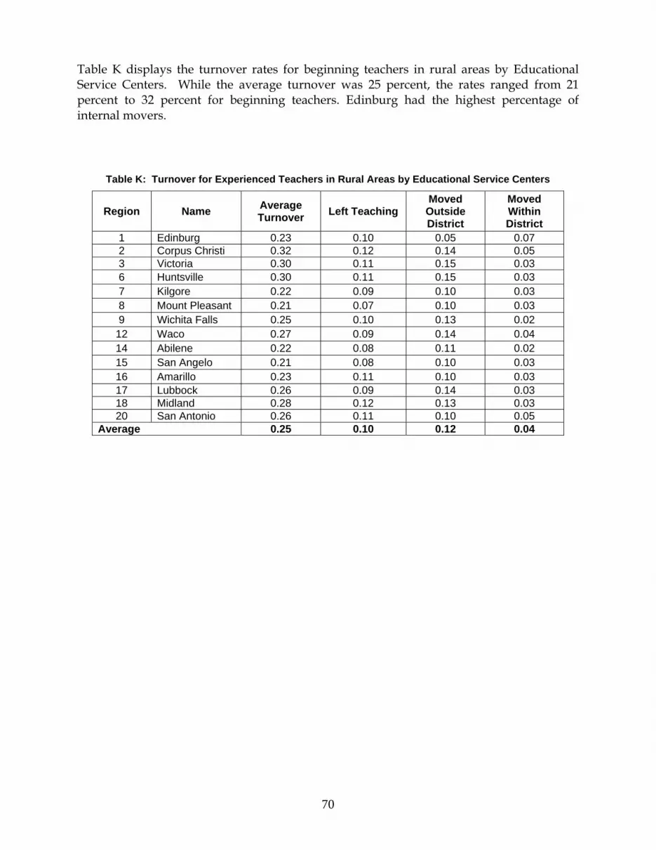
70

Table K displays the turnover rates for beginning teachers in rural areas by Educational Service Centers. While the average turnover was 25 percent, the rates ranged from 21 percent to 32 percent for beginning teachers. Edinburg had the highest percentage of internal movers.

Table K: Turnover for Experienced Teachers in Rural Areas by Educational Service Centers

Region Name Average Turnover Left Teaching



1 Edinburg 0.23 0.10 0.05 0.07 2 Corpus Christi 0.32 0.12 0.14 0.05 3 Victoria 0.30 0.11 0.15 0.03 6 Huntsville 0.30 0.11 0.15 0.03 7 Kilgore 0.22 0.09 0.10 0.03 8 Mount Pleasant 0.21 0.07 0.10 0.03 9 Wichita Falls 0.25 0.10 0.13 0.02

12 Waco 0.27 0.09 0.14 0.04 14 Abilene 0.22 0.08 0.11 0.02 15 San Angelo 0.21 0.08 0.10 0.03 16 Amarillo 0.23 0.11 0.10 0.03 17 Lubbock 0.26 0.09 0.14 0.03 18 Midland 0.28 0.12 0.13 0.03 20 San Antonio 0.26 0.11 0.10 0.05

Average 0.25 0.10 0.12 0.04

71

Table L displays turnover rates for experienced teachers in rural areas by Educational Service Centers. Rates ranged from 14 percent to 20 percent. Edinburg also has the highest percentage of internal movers. Teachers in rural areas moved outside the district more than they left teaching.

Table L: Turnover for Experienced Teachers in Rural Areas by Educational Service Centers.

Region Name Average Turnover Left Teaching



1 Edinburg 0.17 0.06 0.05 0.07 2 Corpus Christi 0.18 0.06 0.07 0.04 3 Victoria 0.16 0.06 0.07 0.03 6 Huntsville 0.18 0.07 0.08 0.03 7 Kilgore 0.14 0.05 0.06 0.03 8 Mount Pleasant 0.14 0.06 0.06 0.03 9 Wichita Falls 0.15 0.05 0.07 0.03 12 Waco 0.20 0.07 0.09 0.03 14 Abilene 0.15 0.06 0.07 0.02 15 San Angelo 0.17 0.06 0.08 0.03 16 Amarillo 0.15 0.07 0.06 0.02 17 Lubbock 0.16 0.06 0.07 0.03 18 Midland 0.18 0.07 0.08 0.03 20 San Antonio 0.20 0.08 0.09 0.04

Average 0.17 0.06 0.07 0.03

72

Table M shows the turnover rates among beginning teachers in micropolitan areas based on the Regional Educational Service Centers breakdown. While the majority of the turnover rates were above 20 percent, the turnover rate in Mount Pleasant was only 18 percent. Edinburg stands out as having the highest percentage of teachers that left teaching while Victoria and Waco had the highest percentage of teachers who were external movers.

Table M: Turnover for Beginning Teachers in Micropolitan Areas by Educational Service Centers

Region Name Turnover Left Teaching



1 Edinburg 0.28 0.13 0.10 0.06 2 Corpus Christi 0.28 0.11 0.13 0.04 3 Victoria 0.28 0.10 0.14 0.03 6 Huntsville 0.29 0.11 0.13 0.05 7 Kilgore 0.26 0.10 0.11 0.05 8 Mount Pleasant 0.18 0.09 0.06 0.04 9 Wichita Falls 0.20 0.09 0.09 0.02 12 Waco 0.27 0.09 0.14 0.05 14 Abilene 0.22 0.08 0.10 0.04 15 San Angelo 0.26 0.11 0.10 0.05 16 Amarillo 0.25 0.10 0.11 0.04 17 Lubbock 0.26 0.10 0.13 0.03 18 Midland 0.27 0.09 0.12 0.07 20 San Antonio 0.26 0.11 0.08 0.07

Average 0.26 0.10 0.11 0.04

73

Table N represents the beginning teacher turnover among metropolitan areas. College Station-Bryan ranks highest at 32 percent while Amarillo, Fort Worth-Arlington and Longview rank lowest at 21 percent. Killeen-Temple-Fort Hood had the highest turnover rate for leavers while College Station-Bryan had the highest rate (14 percent) for external movers.

Table N: Turnover for Beginning Teachers by Metropolitan Areas

ID Metro Area Turnover Left Teaching



10180 Abilene 0.22 0.09 0.08 0.05 11100 Amarillo 0.21 0.10 0.07 0.04 12420 Austin-Round Rock 0.28 0.13 0.08 0.06 13140 Beaumont-Port Arthur 0.22 0.10 0.08 0.04 15180 Brownsville 0.22 0.10 0.06 0.06 17780 College Station-Bryan 0.32 0.14 0.14 0.04 18580 Corpus Christi 0.24 0.10 0.09 0.05 19124 Dallas-Plano-Irving 0.29 0.13 0.09 0.07 21340 El Paso 0.23 0.11 0.05 0.07 23104 Fort Worth-Arlington 0.21 0.10 0.05 0.06 26420 Houston-Sugar Land-Baytown 0.25 0.11 0.08 0.06 28660 Killeen-Temple-Fort Hood 0.31 0.15 0.08 0.08 29700 Laredo 0.23 0.11 0.05 0.06 30980 Longview 0.21 0.09 0.09 0.03 31180 Lubbock 0.27 0.11 0.10 0.06 32580 McAllen-Edinburg-Mission 0.26 0.11 0.08 0.07 33260 Midland 0.27 0.12 0.08 0.06 36220 Odessa 0.30 0.14 0.08 0.08 41660 San Angelo 0.25 0.09 0.09 0.07 41700 San Antonio 0.24 0.10 0.08 0.06 43300 Sherman-Denison 0.24 0.11 0.11 0.03 45500 Texarkana, TX-Texarkana, AR (part) 0.23 0.11 0.08 0.05 46340 Tyler 0.25 0.12 0.09 0.04 47020 Victoria 0.27 0.10 0.10 0.07 47380 Waco 0.29 0.13 0.11 0.04 48660 Wichita Falls 0.24 0.11 0.07 0.06

Average 0.25 0.11 0.08 0.06

74

Table O below represents the experienced teacher turnover among metropolitan areas. Dallas-Plano-Irving ranks highest at 21 percent while Amarillo, Abilene and Laredo rank lowest at 14 percent. Dallas-Plano-Irving also had the highest turnover rate for leavers.

Table O: Turnover for Experienced Teachers by Metropolitan Areas

ID Metro Area Turnover Left Teaching



10180 Abilene 0.14 0.05 0.04 0.04 11100 Amarillo 0.14 0.07 0.03 0.04 12420 Austin-Round Rock 0.20 0.09 0.05 0.06 13140 Beaumont-Port Arthur 0.16 0.07 0.05 0.04 15180 Brownsville 0.15 0.06 0.03 0.05 17780 College Station-Bryan 0.18 0.08 0.06 0.04 18580 Corpus Christi 0.18 0.08 0.05 0.05 19124 Dallas-Plano-Irving 0.21 0.10 0.05 0.06 21340 El Paso 0.16 0.07 0.03 0.06 23104 Fort Worth-Arlington 0.19 0.08 0.05 0.06 26420 Houston-Sugar Land-Baytown 0.19 0.09 0.04 0.06 28660 Killeen-Temple-Fort Hood 0.20 0.09 0.04 0.06 29700 Laredo 0.14 0.07 0.03 0.05 30980 Longview 0.15 0.06 0.06 0.03 31180 Lubbock 0.18 0.08 0.04 0.05 32580 McAllen-Edinburg-Mission 0.16 0.06 0.04 0.06 33260 Midland 0.19 0.08 0.04 0.07 36220 Odessa 0.19 0.08 0.04 0.07 41660 San Angelo 0.18 0.07 0.04 0.07 41700 San Antonio 0.17 0.08 0.04 0.06 43300 Sherman-Denison 0.16 0.07 0.05 0.04 45500 Texarkana, TX-Texarkana, AR (part) 0.16 0.07 0.04 0.05 46340 Tyler 0.16 0.08 0.05 0.03 47020 Victoria 0.18 0.07 0.05 0.07 47380 Waco 0.19 0.08 0.06 0.05 48660 Wichita Falls 0.14 0.06 0.04 0.04

Average 0.17 0.07 0.04 0.05

75

APPENDIX III – FINANCIAL MANAGEMENT

76

Table A: Cost Function Results for Elementary Schools

Before 2003

Dependent variable: Log of per-pupil expenditure Independent variables Coefficient z-statistics

Intercept -22.79 -6.55 Adjusted TAAS/TAKS passing rates 0.10 5.25 Square of adjusted TAAS/TAKS passing rate -0.24 -2.63 Log of district beginning teacher salary 7.72 8.90 Square of log of district beginning teacher salary -0.45 -8.38 Log of campus enrollment -0.20 -5.27 Square of log of campus enrollment 0.00 0.55 Log of district enrollment -0.08 -9.25 Square of log of district enrollment 0.00 8.99 Percentage of students with limited English proficiency 0.00 9.88 Square of percentage of students with limited English proficiency 0.00 -9.85 Percentage of economically disadvantaged or poor students 0.00 -3.34 Square of percentage of economically disadvantaged or poor students 0.00 11.83 Percentage of students with special education 0.01 14.01 Square of percentage of students with special education 0.00 -1.76 Accountability rating as unacceptable -0.01 -0.77 Accountability rating as acceptable -0.01 -3.65 Accountability rating as recognized -0.01 -3.10 Houston independent school district -0.02 -3.72 Dallas independent school district -0.03 -5.01 _Iyear_2000 0.03 9.02 _Iyear_2001 0.07 18.21 _Iyear_2002 0.09 22.78 Log likelihood 9721.01 After 2003


Intercept -71.65 -10.71 Adjusted TAAS/TAKS passing rates 0.00 0.36 Square of adjusted TAAS/TAKS passing rate 0.04 1.09 Log of district beginning teacher salary 19.91 12.04 Square of log of district beginning teacher salary -1.21 -11.83 Log of campus enrollment -0.19 -3.41 Square of log of campus enrollment 0.00 0.30 Log of district enrollment -0.14 -11.31 Square of log of district enrollment 0.01 11.56 Percentage of students with limited English proficiency 0.00 3.56 Square of percentage of students with limited English proficiency 0.00 -2.43 Percentage of economically disadvantaged or poor students 0.00 -2.64 Square of percentage of economically disadvantaged or poor students 0.00 9.53 Percentage of students with special education 0.02 11.58 Square of percentage of students with special education 0.00 -6.46 Accountability rating as unacceptable 0.01 0.59 Accountability rating as acceptable 0.00 -0.26 Accountability rating as recognized 0.00 0.41 Houston independent school district -0.11 -11.83 Dallas independent school district 0.03 3.67 _Iyear_2004 -0.01 -5.21 Log likelihood 5213.14

77

Table B: Cost Function Results for Middle Schools

Before 2003


Intercept -47.82 -7.62 Adjusted TAAS/TAKS passing rates -0.36 -7.01 Square of adjusted TAAS/TAKS passing rate -2.38 -4.03 Log of district beginning teacher salary 13.66 8.69 Square of log of district beginning teacher salary -0.83 -8.45 Log of campus enrollment 0.22 4.15 Square of log of campus enrollment -0.03 -6.42 Log of district enrollment -0.03 -1.07 Square of log of district enrollment 0.00 1.17 Percentage of students with limited English proficiency 0.00 1.89 Square of percentage of students with limited English proficiency 0.00 -2.17 Percentage of economically disadvantaged or poor students 0.00 3.29 Square of percentage of economically disadvantaged or poor students 0.00 2.63 Percentage of students with special education 0.00 -0.17 Square of percentage of students with special education 0.00 2.03 Accountability rating acceptable -0.01 -0.43 Accountability rating as recognized 0.00 -0.18 Accountability rating as exemplary 0.01 0.52 Houston independent school district -0.03 -1.76 Dallas independent school district 0.05 3.17 _Iyear_2000 0.02 3.73 _Iyear_2001 0.06 8.93 _Iyear_2002 0.09 12.27 Log likelihood 3132.67 After 2003


Intercept -77.40 -6.31 Adjusted TAAS/TAKS passing rates -0.02 -0.75 Square of adjusted TAAS/TAKS passing rate -0.03 -0.49 Log of district beginning teacher salary 21.09 6.93 Square of log of district beginning teacher salary -1.29 -6.85 Log of campus enrollment 0.28 3.30 Square of log of campus enrollment -0.03 -4.80 Log of district enrollment -0.13 -3.27 Square of log of district enrollment 0.01 3.53 Percentage of students with limited English proficiency 0.00 0.70 Square of percentage of students with limited English proficiency 0.00 -1.36 Percentage of economically disadvantaged or poor students 0.00 -1.44 Square of percentage of economically disadvantaged or poor students 0.00 5.08 Percentage of students with special education 0.00 1.46 Square of percentage of students with special education 0.00 0.13 Accountability rating as acceptable -0.03 -2.08 Accountability rating as recognized -0.02 -1.44 Accountability rating as exemplary -0.05 -1.71 Houston independent school district -0.10 -3.93 Dallas independent school district 0.09 4.15 _Iyear_2005 0.02 4.17 Log likelihood 1470.15

78

Table C: Cost Function Results for High Schools

Before 2003


Intercept -23.55 -2.98 Adjusted TAAS/TAKS passing rates 0.07 1.82 Square of adjusted TAAS/TAKS passing rate 0.29 2.54 Log of district beginning teacher salary 7.86 3.96 Square of log of district beginning teacher salary -0.46 -3.69 Log of campus enrollment -0.35 -7.42 Square of log of campus enrollment 0.02 5.14 Log of district enrollment 0.07 2.47 Square of log of district enrollment -0.01 -3.68 Percentage of students with limited English proficiency 0.00 1.94 Square of percentage of students with limited English proficiency 0.00 -0.36 Percentage of economically disadvantaged or poor students 0.00 6.05 Square of percentage of economically disadvantaged or poor students 0.00 -2.27 Percentage of students with special education 0.01 6.81 Square of percentage of students with special education 0.00 -8.52 Accountability rating as unacceptable -0.01 -0.76 Accountability rating as acceptable -0.01 -1.26 Accountability rating as recognized -0.01 -2.05 Houston independent school district 0.04 1.81 Dallas independent school district -0.09 -4.55 _Iyear_2000 0.00 0.53 _Iyear_2001 0.04 4.85 _Iyear_2002 0.06 7.32 Log likelihood 2201.01 After 2003


Intercept -63.85 -4.50 Adjusted TAAS/TAKS passing rates 0.03 0.98 Square of adjusted TAAS/TAKS passing rate -0.06 -0.90 Log of district beginning teacher salary 18.27 5.17 Square of log of district beginning teacher salary -1.12 -5.10 Log of campus enrollment -0.49 -7.08 Square of log of campus enrollment 0.03 5.73 Log of district enrollment 0.04 0.80 Square of log of district enrollment 0.00 -1.46 Percentage of students with limited English proficiency 0.00 2.96 Square of percentage of students with limited English proficiency 0.00 -1.81 Percentage of economically disadvantaged or poor students 0.00 1.01 Square of percentage of economically disadvantaged or poor students 0.00 1.54 Percentage of students with special education 0.00 3.69 Square of percentage of students with special education 0.00 -0.32 Accountability rating as acceptable -0.09 -3.90 Accountability rating as recognized -0.09 -3.66 Accountability rating as exemplary -0.12 -2.89 Houston independent school district 0.02 0.56 Dallas independent school district 0.01 0.30 _Iyear_2005 0.01 2.08 Log likelihood 1055.84

79

APPENDIX IV – PRINCIPAL ANALYSIS

Table A: Student Performance Indicators Adjusted Gains Accountability Ratings

Variables TAAS Robust Std. Err. TAKS Robust

Std. Err. TAAS Robust Std. Err. TAKS Robust

Std. Err elementary 0.0491 0.0047 0.1096 0.0069 0.2845 0.0690 0.6319 0.1120 middle -0.0154 0.0049 0.0107 0.0070 -0.2236 0.0704 -0.2962 0.1052 high -0.0261 0.0054 -0.0610 0.0072 0.2139 0.0744 -0.4741 0.1157 alternatively certified 0.0013 0.0056 -0.0151 0.0079 -0.0863 0.1473 -0.3171 0.1409 out of state certification 0.0019 0.0048 0.0028 0.0067 0.0200 0.0976 -0.1118 0.1426 standard certification -0.0030 0.0027 -0.0020 0.0055 0.0676 0.0557 -0.0541 0.1006 docdegree -0.0068 0.0079 -0.0106 0.0129 -0.3311 0.0955 0.4198 0.1867 bachdegree -0.0044 0.0080 -0.0025 0.0126 -0.2311 0.0857 0.2390 0.1839 mastdegree -0.0041 0.0069 -0.0036 0.0125 -0.2430 0.0684 0.3620 0.1712 experience -0.0002 0.0004 -0.0002 0.0004 -0.0088 0.0079 -0.0081 0.0083 experience squared 0.0000 0.0000 0.0000 0.0000 0.0003 0.0002 0.0002 0.0002 first year at campus -0.0040 0.0017 -0.0089 0.0026 -0.1956 0.0286 -0.2174 0.0425 second year at campus 0.0015 0.0018 -0.0032 0.0023 -0.1327 0.0271 -0.0664 0.0447 third year at campus 0.0001 0.0018 0.0003 0.0024 -0.0988 0.0264 -0.0286 0.0417 female 0.0030 0.0013 0.0076 0.0018 0.1415 0.0263 0.1055 0.0295 principal hispanic -0.0011 0.0023 0.0002 0.0026 0.1541 0.0582 0.0518 0.0652 principal black -0.0044 0.0029 -0.0054 0.0028 0.0701 0.0563 0.0180 0.0622 principal asian 0.0143 0.0096 0.0322 0.0161 -0.1924 0.2501 -0.6003 0.4262 enrollment (log) 0.0075 0.0018 -0.0010 0.0021 -0.4529 0.0384 -0.2645 0.0524 mobility percentage -0.0005 0.0002 -0.0008 0.0002 -0.0362 0.0030 -0.0227 0.0041 low ses percentage 0.0007 0.0001 -0.0006 0.0001 -0.0140 0.0018 -0.0150 0.0016 percent black students 0.0002 0.0001 -0.0002 0.0001 -0.0107 0.0022 -0.0111 0.0031 percent hispanic students 0.0000 0.0001 0.0000 0.0001 -0.0010 0.0015 -0.0046 0.0016 metropolitan 0.0016 0.0023 0.0085 0.0034 0.2955 0.0636 0.2616 0.0741 micropolitan -0.0005 0.0024 -0.0045 0.0039 0.0237 0.0725 0.2400 0.0732 yr1999 0.0012 0.0059 (dropped) - -0.0936 0.0285 - - yr2000 (dropped) - (dropped) - - - - - yr2001 -0.0018 0.0025 (dropped) - 0.2271 0.0202 - - yr2002 -0.0027 0.0024 (dropped) - 0.4063 0.0312 - - yr2003 (dropped) - (dropped) - - - - - yr2004 (dropped) - -0.0056 0.0034 - - - - yr2005 (dropped) - (dropped) - - - -0.3892 0.0264 _cons -0.0649 0.0134 0.0510 0.0192 - - - -

80

Table B: Teacher Retention Indicators

Variables Beginning Teacher Turnover

Robust Std. Err

Experienced Teacher Turnover

Robust Std. Err

elementary -0.0257 0.0106 -0.0326 0.0115 middle 0.0312 0.0107 -0.0026 0.0117 high 0.0189 0.0104 -0.0085 0.0115 alternatively certified 0.0058 0.0130 0.0042 0.0091 out of state certification 0.0185 0.0100 0.0101 0.0076 standard certification 0.0016 0.0057 0.0013 0.0045 docdegree 0.0158 0.0081 0.0242 0.0158 bachdegree 0.0206 0.0082 0.0228 0.0136 mastdegree 0.0117 0.0073 0.0170 0.0127 experience 0.0001 0.0006 -0.0007 0.0007 experience squared 0.0000 0.0000 0.0000 0.0000 first year at campus 0.0114 0.0035 0.0125 0.0028 second year at campus 0.0053 0.0032 0.0042 0.0027 third year at campus 0.0019 0.0032 0.0032 0.0024 female 0.0063 0.0023 0.0082 0.0018 principal hispanic 0.0061 0.0035 0.0051 0.0028 principal black 0.0035 0.0063 0.0002 0.0057 principal asian 0.0492 0.0174 0.0138 0.0279 enrollment (log) -0.0071 0.0030 -0.0094 0.0022 student mobility percentage -0.0002 0.0002 0.0003 0.0002 low ses percentage 0.0006 0.0001 0.0002 0.0001 percent black students 0.0005 0.0002 0.0005 0.0002 percent hispanic students -0.0002 0.0001 0.0001 0.0001 metropolitan 0.0026 0.0065 0.0106 0.0046 micropolitan -0.0018 0.0074 0.0034 0.0052 yr1999 0.0046 0.0041 (dropped) - yr2000 (dropped) - -0.0055 0.0033 yr2001 0.0101 0.0040 -0.0045 0.0034 yr2002 -0.0001 0.0042 -0.0063 0.0035 yr2003 -0.0013 0.0048 -0.0059 0.0036 yr2004 0.0012 0.0052 -0.0016 0.0037 yr2005 -0.0068 0.0045 -0.0081 0.0038 _cons -0.0026 0.0213 0.0383 0.0219

81

Table C: Financial Management Indicators

Variables Efficiency - TAAS

Robust Std. Err.

Efficiency - TAKS

Robust Std. Err.

Attendance Robust Std. Err.

Instructional Share

Robust Std. Err.

elementary -0.0130 0.0043 0.0186 0.0024 1.7881 0.5902 0.0301 0.0037

middle -0.0205 0.0032 (dropped) - -0.0586 0.6269 -0.0035 0.0039

high (dropped) - 0.0295 0.0034 -2.6372 0.6068 -0.0205 0.0039

alternatively certified 0.0108 0.0134 0.0215 0.0106 -2.7600 1.3833 -0.0063 0.0038

out of state certification 0.0033 0.0089 -0.0006 0.0089 0.4520 0.7327 0.0028 0.0029

standard certification -0.0016 0.0067 0.0000 0.0069 -0.8797 0.3923 0.0012 0.0017

docdegree -0.0049 0.0059 -0.0074 0.0115 1.8673 0.7207 -0.0050 0.0045

bachdegree -0.0177 0.0053 0.0000 0.0117 1.8420 0.6948 -0.0062 0.0045

mastdegree -0.0074 0.0034 0.0011 0.0104 1.3196 0.6021 -0.0033 0.0040

experience 0.0004 0.0005 0.0002 0.0006 0.0728 0.0589 0.0001 0.0002

experience squared 0.0000 0.0000 0.0000 0.0000 -0.0013 0.0012 0.0000 0.0000

first year at campus -0.0024 0.0022 -0.0027 0.0026 0.1194 0.3132 -0.0023 0.0010

second year at campus -0.0007 0.0020 -0.0027 0.0028 0.2965 0.2658 -0.0021 0.0008

third year at campus 0.0028 0.0024 -0.0005 0.0024 0.0837 0.2892 -0.0014 0.0007

female -0.0047 0.0019 -0.0057 0.0023 0.3156 0.1840 0.0007 0.0009

principal hispanic -0.0020 0.0036 -0.0040 0.0032 -0.2244 0.2896 -0.0065 0.0016

principal black 0.0013 0.0042 -0.0043 0.0036 -0.8526 0.3904 -0.0028 0.0018

principal asian 0.0191 0.0219 0.0167 0.0177 2.2585 1.7122 0.0122 0.0087

enrollment (log) -0.0200 0.0033 -0.0195 0.0043 1.6650 0.1970 0.0051 0.0013

student mobility percentage 0.0002 0.0003 0.0003 0.0003 -0.1338 0.0105 0.0003 0.0001

low ses percentage -0.0006 0.0001 -0.0005 0.0001 -0.0412 0.0092 -0.0001 0.0001

percent black students 0.0006 0.0001 0.0006 0.0002 0.0401 0.0098 0.0000 0.0001

percent hispanic students 0.0005 0.0001 0.0005 0.0001 0.0272 0.0088 0.0000 0.0001

metropolitan -0.0269 0.0064 -0.0298 0.0078 0.0940 0.4193 0.0072 0.0026

micropolitan -0.0267 0.0077 -0.0345 0.0077 -0.8396 0.5295 0.0026 0.0029

yr1999 (dropped) - (dropped) - (dropped) - -0.0075 0.0007

yr2000 0.0004 0.0015 (dropped) - 0.2208 0.0301 (dropped) -

yr2001 -0.0009 0.0023 (dropped) - 0.1232 0.0915 -0.0054 0.0009

yr2002 -0.0027 0.0026 (dropped) - 0.1107 0.0608 -0.0045 0.0010

yr2003 (dropped) - (dropped) - -0.0022 0.0773 (dropped) -

yr2004 (dropped) - 0.0002 0.0015 0.0844 0.0934 -0.0061 0.0021

yr2005 (dropped) - (dropped) - -28.5795 1.1459 -0.0073 0.0021

_cons 1.2905 0.0245 1.2394 0.0298 86.6645 1.6792 0.5834 0.0097

Documents

Principal Performance in Texas: Tools for Measuring Effective School Leadership