Probabilistic and Possibilistic Networksand How To Learn Them from DataChristian Borgelt and Rudolf KruseDept. of Information and Communication Systems,Otto-von-Guericke-University of Magdeburg, 39106 Magdeburg, Germanyborgelt@iik.cs.uni-magdeburg.deAbstract: In this paper we explain in a tutorial manner the technique ofreasoning in probabilistic and possibilistic network structures, which is basedon the idea to decompose a multi-dimensional probability or possibility dis-tribution and to draw inferences using only the parts of the decomposition.Since constructing probabilistic and possibilistic networks by hand can betedious and time-consuming, we also discuss how to learn probabilistic andpossibilistic networks from a data, i.e. how to determine from a database ofsample cases an appropriate decomposition of the underlying probability orpossibility distribution.Keywords: Decomposition, uncertain reasoning, probabilistic networks, pos-sibilistic networks, learning from data.1. IntroductionSince reasoning in multi-dimensional domains tends to be infeasible in thedomains as a whole|and the more so, if uncertainty and/or imprecisionare involved|decomposition techniques, that reduce the reasoning processto computations in lower-dimensional subspaces, have become very popular.For example, decomposition based on dependence and independence relationsbetween variables has been studied extensively in the �eld of graphical mod-eling [17]. Some of the best-known approaches are Bayesian networks [23],Markov networks [20], and the more general valuation-based networks [27].They all led to the development of e�cient implementations, for exampleHUGIN [1], PULCINELLA [26], PATHFINDER [12] and POSSINFER [8].A large part of recent research has been devoted to learning probabilis-tic and possibilistic networks from data [4, 13, 9], i.e. to determine from adatabase of sample cases an appropriate decomposition of the probability orpossibility distribution on the domain under consideration. Such automaticlearning is important, since constructing a network by hand can be tediousand time-consuming. If a database of sample cases is available, as it often is,learning algorithms can take over at least part of the construction task.

In this tutorial paper we survey the basic idea of probabilistic and pos-sibilistic networks and the basic method for learning them from data. InSection 2 we introduce the idea of decomposing multi-dimensional distribu-tions and demonstrate how a decomposition can be used to reason in theunderlying multi-dimensional domain. We do so by inspecting decomposi-tions of relations �rst and then, in Section 3, proceed to decompositions ofprobability distributions. Section 4 considers the graphical representation ofdecompositions. Section 5 discusses the general scheme for inducing decom-positions from data, which is applied to probability distributions in Section 6.With Section 7 we start to transfer the ideas of the preceding sections,where they were presented in the relational and the probabilistic setting, tothe possibilistic setting. To do so, we �rst clarify what we understand bya degree of possibility in Section 7. In Section 8 we look at decompositionof and reasoning in possibility distributions, emphasizing the di�erences tothe probabilistic case. Finally, Section 9 discusses how to induce possibilisticnetworks from data.2. Decomposition and ReasoningThe basic idea underlying probabilistic as well as possibilistic networks is thata probability or possibility distribution D on a multi-dimensional domain canunder certain conditions be decomposed into a set fD1; : : : ; Dng of (over-lapping) distributions on lower-dimensional subspaces. By multi-dimensionaldomain we mean that a state of the universe of discourse can be described bystating the values of a set of attributes. Each attribute|or, more precisely,the set of its possible values|forms a dimension of the domain. Of course, toform a dimension the possible values have to be exhaustive and mutually ex-clusive. Thus each state corresponds to a single point of the multi-dimensionaldomain. A distribution D assigns to each point of the domain a number inthe interval [0; 1], which represents the (prior) probability or the (prior) de-gree of possibility of the corresponding state. By decomposition we mean thatthe distribution D on the domain as a whole can be reconstructed (at leastapproximately) from the distributions fD1; : : : ; Dng on the subspaces.Such a decomposition has several advantages, the most important beingthat a decomposition can usually be stored much more e�ciently and withless redundancy than the whole distribution. These advantages are the mainmotive for studying decompositions of relations (which can be seen as specialpossibility distributions) in database theory [5, 30]. Not surprisingly, databasetheory is closely connected to our subject. The only di�erence is that wefocus on reasoning, while database theory focuses on storing, maintaining,and retrieving data.But just being able to store a distribution more e�ciently would not beof much use for reasoning tasks, were it not for the possibility to draw infer-ences in the underlying multi-dimensional domain using only the distributions

Table 1. The relation RABC stating prior knowledge about the possible combina-tions of attribute values A a1 a1 a2 a2 a2 a2 a3 a4 a4 a4B b1 b1 b1 b1 b3 b3 b2 b2 b3 b3C c1 c2 c1 c2 c2 c3 c2 c2 c2 c3fD1; : : : ; Dng on the subspaces without having to reconstruct the whole dis-tribution D. How this works is perhaps best explained by a simple example,which we present in the relational setting �rst [6, 16, 18]. We consider onlywhether a combination of attribute values is possible or not, thus neglectingits probability or degree of possibility. In other words, we restrict ourselvesto a distribution that assigns to each point of the underlying domain eithera 1 (if the corresponding state is possible) or a 0 (if the corresponding stateis impossible). With this restriction the ideas underlying decomposition andreasoning in decompositions can be demonstrated to the novice reader muchclearer than in the probabilistic setting, where the probabilities can disguisethe very simple structure. Later on we will study the probabilistic and �nallythe possibilistic case.Consider three attributes, A, B, and C, with corresponding domainsdom(A) = fa1; a2; a3; a4g, dom(B) = fb1; b2; b3g, and dom(C) = fc1; c2; c3g.Thus the underlying domain of our example is the Cartesian productdom(A) � dom(B) � dom(C) or, as we will write as an abbreviation, thethree-dimensional space fA;B;Cg.Table 1 states prior knowledge about the possible combinations of at-tribute values in the form of a relation RABC : only the value combinationscontained in RABC are possible. (This relation is to be interpreted under theclosed world assumption, i.e. all value combinations not contained in RABCare impossible.) A graphical representation of RABC is shown in the top leftof Fig. 1: each cube indicates a possible value combination.The relation RABC can be decomposed into two two-dimensional rela-tions, namely the two projections to the subspaces fA;Bg and fB;Cg, bothshown in the right half of Fig. 1. These projections as well as the projectionto the subspace fA;Cg (shown in the bottom left of Fig. 1) are the shadowsthrown by the cubes in the top left of Fig. 1 on the surrounding planes, iflight sources are imagined in front, to the right, and above the relation.Mathematically, a projection of a relation can be de�ned in the follow-ing way. Let X = fA1; : : : ; Amg be a set of attributes. A tuple t over Xis a mapping that assigns to each attribute Ai a value a(i)ji 2 dom(Ai). As-suming an implicit order of the attributes, a tuple t over X can be written�a(1)j1 ; : : : ; a(m)jm �, where each vector element states the value the correspond-

Fig. 1. Graphical representation of the relation RABC and of all three possi-ble projections to two-dimensional subspaces. Since in this relation the equationRABC = �fA;B;CgfA;Bg (RABC) ./ �fA;B;CgfB;Cg (RABC) holds, it can be decomposed intotwo relations on the subspaces fA;Bg and fB;Cg. This is demonstrated in Fig. 2.a1 a2 a3 a4 b1c1 b2c2b3c3" ") )(

) )) ) ( () a1 a2 a3 a4 b1c1 b2c2b3c3" " " "" """ @ @ @ @@ @

a1 a2 a3 a4 b1c1 b2c2b3c3" " " "" """ A AA A A AA A

a1 a2 a3 a4 b1c1 b2c2b3c3" " " "" """ B BBB B

Fig. 2. Cylindrical extensions of two projections of the relation RABC shown inFig. 1. On the left is the cylindrical extension of the projection to fA;Bg, on theright the cylindrical extension of the projection to fB;Cg. Their intersection yieldsthe original relation RABC ." ") )) *** * *a1 a2 a3 a4 b1c1 b2c2

b3c3 ) ((( ) )a1 a2 a3 a4 b1c1 b2c2b3c3

Fig. 3. Propagation of the evidence that attribute A has value a4 in thethree-dimensional relation shown in Fig. 1 using the relations on the subspacesfA;Bg and fB;Cga1 a2 a3 a4@ A� b�fA;BgfAgb1b2b3 a1 a2 a3 a4II@H H HH ��fA;BgfBg @@ B �b�fB;CgfBg c1 c2 c3 b1b2b3I II @H H@@

��fB;CgfCgc1 c2 c3@ @Cing attribute is mapped to. To indicate that X is the domain of de�nition oft, i.e. that t is a tuple over X , we write dom(t) = X . If t is a tuple over Xand Y � X , then tjY denotes the restriction or projection of the tuple t toY , i.e. the mapping tjY assigns values only to the attributes in Y . Hence tjYis a tuple over Y , i.e. dom(tjY ) = Y .A relation R over an attribute set X is a set of tuples over X . If R is arelation over X and Y � X , then the projection �XY (R) of R from X to Yis de�ned as �XY (R) def= fs j dom(s) = Y ^ 9t 2 R : s = tjY g:The two relations RAB = �fA;B;CgfA;Bg (RABC) and RBC = �fA;B;CgfB;Cg (RABC)are a decomposition of the relation RABC , because it can be reconstructedby forming the natural join RAB ./ RBC . In database theory RABC wouldbe called join-decomposable.Forming the natural join of two relations is the same as intersecting theircylindrical extensions to the union of their attribute sets. The cylindrical ex-tensions of RAB and RBC to fA;B;Cg are shown in Fig. 2. They result fromRAB and RBC by simply adding all possible values of the missing dimension.Thus the name \cylindrical extension" is very expressive: since in sketches aset is usually depicted as a circle, adding all values of a perpendicular dimen-sion yields a cylinder. Mathematically, a cylindrical extension can be de�nedin the following way. Let R be a relation over an attribute set X and Y � X .Then the cylindrical extension b�YX (R) of R from X to Y is de�ned asb�YX (R) def= fs j dom(s) = Y ^ 9t 2 R : t = sjY g:

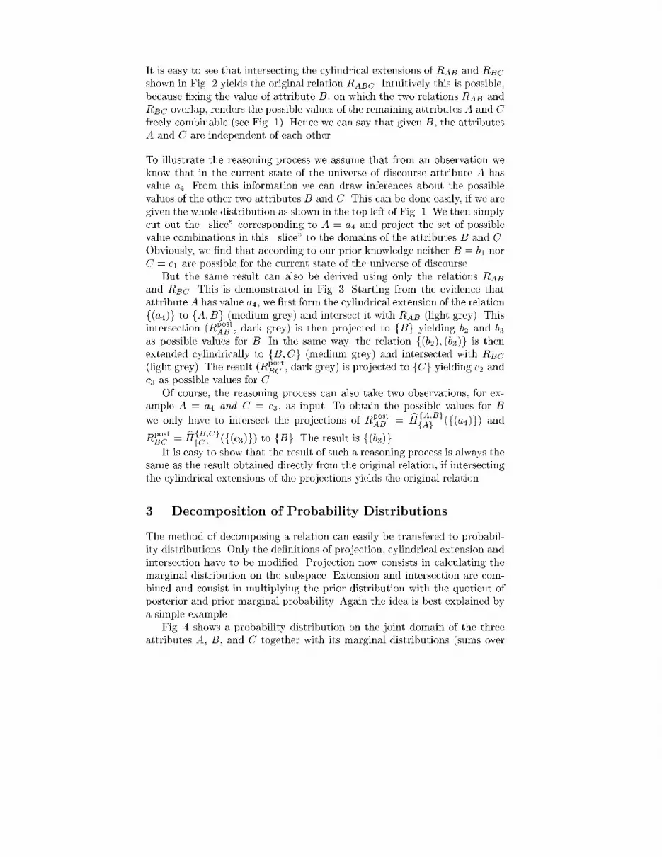
It is easy to see that intersecting the cylindrical extensions of RAB and RBCshown in Fig. 2 yields the original relation RABC . Intuitively this is possible,because �xing the value of attribute B, on which the two relations RAB andRBC overlap, renders the possible values of the remaining attributes A and Cfreely combinable (see Fig. 1). Hence we can say that given B, the attributesA and C are independent of each other.To illustrate the reasoning process we assume that from an observation weknow that in the current state of the universe of discourse attribute A hasvalue a4. From this information we can draw inferences about the possiblevalues of the other two attributes B and C. This can be done easily, if we aregiven the whole distribution as shown in the top left of Fig. 1. We then simplycut out the \slice" corresponding to A = a4 and project the set of possiblevalue combinations in this \slice" to the domains of the attributes B and C.Obviously, we �nd that according to our prior knowledge neither B = b1 norC = c1 are possible for the current state of the universe of discourse.But the same result can also be derived using only the relations RABand RBC . This is demonstrated in Fig. 3. Starting from the evidence thatattribute A has value a4, we �rst form the cylindrical extension of the relationf(a4)g to fA;Bg (medium grey) and intersect it with RAB (light grey). Thisintersection (RpostAB , dark grey) is then projected to fBg yielding b2 and b3as possible values for B. In the same way, the relation f(b2); (b3)g is thenextended cylindrically to fB;Cg (medium grey) and intersected with RBC(light grey). The result (RpostBC , dark grey) is projected to fCg yielding c2 andc3 as possible values for C.Of course, the reasoning process can also take two observations, for ex-ample A = a4 and C = c3, as input. To obtain the possible values for Bwe only have to intersect the projections of RpostAB = b�fA;BgfAg (f(a4)g) andRpostBC = b�fB;CgfCg (f(c3)g) to fBg. The result is f(b3)g.It is easy to show that the result of such a reasoning process is always thesame as the result obtained directly from the original relation, if intersectingthe cylindrical extensions of the projections yields the original relation.3. Decomposition of Probability DistributionsThe method of decomposing a relation can easily be transfered to probabil-ity distributions. Only the de�nitions of projection, cylindrical extension andintersection have to be modi�ed. Projection now consists in calculating themarginal distribution on the subspace. Extension and intersection are com-bined and consist in multiplying the prior distribution with the quotient ofposterior and prior marginal probability. Again the idea is best explained bya simple example.Fig. 4 shows a probability distribution on the joint domain of the threeattributes A, B, and C together with its marginal distributions (sums over

Fig. 4. A three-dimensional probability distribution with its marginal dis-tributions (sums over lines/columns). Since in this distribution the equations8i; j; k : P (ai; bj ; ck) = P (ai; bj)P (bj; ck)P (bj) hold, it can be decomposed into themarginal distributions on the subspaces fA;Bg and fB;Cg. all numbers inparts per 1000$ $# #

# #a1a1

a2a2

a3a3

a4a4

b1b1

b2b2

b3b3

b1 c1b2c2b3

c3b1c1 b2c2 b3c3a1 c1a2 c2a3 c3a4

20 90 10 802 1 20 1728 24 5 318 81 9 728 4 80 6856 48 10 62 9 1 82 1 20 1784 72 15 940 180 20 16012 6 120 102168 144 30 18 50 115 35 10082 133 99 14688 82 36 3420 180 20040 160 40180 120 60

220 330 170 280 400240360240 460 300

Fig. 5. Propagation of the evidence that attribute A has value a4 in thethree-dimensional probability distribution shown in Fig. 4 using the marginal prob-ability distributions on the subspaces fA;Bg and fB;Cga1 a2 a3 a4 newold A�a1b1 a2b2 a3b3 a3 � new oldB � c1 b1c2 b2c3 b3�c1 c2 c3oldnewC0 0 0 1000220 330 170 280�newold%40 0 %1800 %20 0 %160572%12 0 %6 0 %1200 %102364%1680 %1440 %30 0 %1864 Pline 572 400364 24064 360 �newold %2029 %180257 %200286%4061 %160242 %4061%18032 %12021 %6011

Pcolumn240 460 300122 520 358

lines/columns). It is closely related to the example of the preceding section,since in this distribution those value combinations that were contained in therelation RABC (were possible) have a high probability, while those that weremissing (were impossible) have a low probability.Just as the relation RABC can be decomposed into RAB and RBC , theprobability distribution in Fig. 4 can be decomposed into the two marginaldistributions on the subspaces fA;Bg and fB;Cg. This is possible, becausethe three-dimensional distribution can be reconstructed using the formulae8i; j; k : P (ai; bj ; ck) = P (ai; bj)P (bj ; ck)P (bj) ;where P (ai; bj ; ck) is short for P (A = ai; B = bj ; C = ck) etc. These formulaecan be derived from the (generally true) formulae8i; j; k : P (ai; bj ; ck) = P (aijbj ; ck)P (bj ; ck)by noting that in this probability distribution A is conditionally independentof C given B, usually written A ?? C j B. That is8i; j; k : P (aijbj ; ck) = P (aijbj) = P (ai; bj)P (bj) ;i.e. if the value of B is known, the value of A does not depend on the valueof C. Note, that conditional independence is symmetric, i.e. if A ?? C j B,then 8i; j; k : P (ckjbj ; ai) = P (ckjbj) = P (ck; bj)P (bj)also holds. In other words, A ?? C j B entails C ?? A j B.To illustrate the reasoning process, let us assume again that of the currentstate of the universe of discourse we know that A = a4. Obviously the cor-responding probability distributions of B and C can be determined from thethree-dimensional distribution by restricting it to the \slice" that correspondsto A = a4 and computing the marginal distributions of that \slice." But thedistributions on the two-dimensional subspaces are also su�cient to drawthis inference as is demonstrated in Fig. 5. The information that A = a4 isextended to the subspace fA;Bg by multiplying the joint probabilities bythe quotient of posterior and prior probability of A = ai, i = 1; 2; 3; 4. Thenthe marginal distribution on fBg is determined by summing over the lines,which correspond to the di�erent values of B. In the same way the informa-tion of the new probability distribution on B is propagated to C: the jointdistribution on fB;Cg is multiplied with the quotient of prior and posteriorprobability of B = bj , j = 1; 2; 3, and then the marginal distribution on Cis computed by summing over the columns, which correspond to the di�er-ent values of C. This scheme can be derived directly from the decomposition

formulae. It is easy to check that the results obtained are the same as thosethat follow from the computations on the three-dimensional domain.Of course, this scheme is a simpli�cation that does not lend itself todirect implementation, as can be seen when assuming that of the currentstate A = a4 and C = c3 are known. In this case additional computationsare necessary to join the information from A and C arriving at B. We omitthese computations for reasons of simplicity, since our aim is only to illustratethe basic idea.14. Graphical RepresentationThe reasoning scheme suggests the idea to use a graphical structure, i.e. anacyclic hypergraph, to represent the decomposition: the attributes are rep-resented as nodes, the distributions Di of the decomposition as hyperedgesconnecting the attributes of their underlying domains. For the examples ofthe two preceding sections the hypergraph is simplyA | B | Cand hence a normal graph. Of course, in real world applications the resultinghypergraphs can be much more complex, especially the edges can connectmore than two nodes, thus forming real hyperedges.This representation uses undirected edges, since in our example the de-composition consists of joint marginal distributions. If undirected graphs areused in the probabilistic setting, the network is usually called a Markov net-work [23]. But it is also possible to use conditional distributions and directededges (often accompanied by a re�ned hypergraph structure), thus arrivingat so called Bayesian networks [23]. This can be justi�ed by the possibility towrite the decomposition formulae in terms of conditional probabilities. E.g.for the above example we can write8i; j; k : P (ai; bj ; ck) = P (ai; bj)P (bj ; ck)P (bj)= P (ai)P (bj jai)P (ck jbj):These formulae can also be derived from the so called chain rule of probability8i; j; k : P (ai; bj ; ck) = P (ckjai; bj)P (bj jai)P (ai)with the help of the conditional independence A ?? C j B.1 In short: the marginal distributions for B obtained from the two two-dimensionalsubspaces have to be multiplied with each other, divided by the prior distributionof B and normalized to 1. This can easily be derived from the decompositionformulae.

When using conditional probabilities it seems natural to direct the edgesaccording to their inherent direction, i.e. from the conditioning attributes tothe conditioned. In the above example the decomposition would be repre-sented by the directed hypergraphA! B ! CUsually only conditional dependences of one attribute (called the child) givena set of other attributes (called the parents) are used, although in principleit is possible to have joint conditional probabilities of two or more attributesgiven a set of other attributes.The name Bayesian network stems from the fact that, if we want topropagate evidence against the direction of a hyperedge, we now have to useBayes' formula P (yjx) = P (xjy)P (y)P (x)to reverse the conditional probability associated with the hyperedge. (Ofcourse, reasoning in the direction of a hyperedge is simpler now, since we nolonger need to form the quotient of the posterior and prior probability, butcan multiply directly with the posterior probability.)With respect to the class of probability distributions they can represent,the expressive power of Markov networks and Bayesian networks is equiva-lent, since it is always possible to go from joint probabilities to conditionalprobabilities and vice versa (provided the necessary marginal probabilitiesare available). Nevertheless, in some applications Bayesian networks may bepreferable, because the additional degree of freedom consisting in the direc-tion of the hyperedges can be used e.g. to express assumed causal or func-tional dependences. Indeed, when constructing a Bayesian network by hand,one often starts from a supposed causal model and encodes the causal depen-dences as probabilistic conditions. This is the reason why Bayesian networksare sometimes also called probabilistic causal networks.However, in this paper we use mostly undirected graphs and joint dis-tributions and we do so for two reasons. In the �rst place, the direction ofan edge can not be justi�ed from the probabilistic model alone. E.g. in theabove example it is possible to write the decomposition formulae in severaldi�erent ways, i.e.8i; j; k : P (ai; bj ; ck) = P (ai; bj)P (bj ; ck)P (bj)= P (ckjbj)P (bj jai)P (ai) A! B ! C= P (aijbj)P (bj jck)P (ck) A B C= P (aijbj)P (ckjbj)P (bj) A B ! C= P (bj jai)P (bj jck)P (ai)P (ck)P (bj) A! B C

and represent the decomposition by the corresponding graphs. The directionof an edge always comes from an external source, e.g. from assumptions aboutcausal or functional dependences, and even then, this source may justifydirecting only some of the edges. Secondly, restricting to joint distributionsfacilitates the transfer to the possibilistic setting, since it frees us from theneed to de�ne what a conditional possibility distribution is.Note, that the interpretation given here to the structure A ! B Cdi�ers from the interpretation that is usually adopted, which is the generallytrue 8i; j; k : P (ai; bj ; ck) = P (bj jai; ck)P (ai; ck). That is, the conditionalindependence A ?? C j B need not hold in this structure. In our interpretationa situation in which A and C are dependent given B would be representedby one directed hyperedge connecting A and C to B, while two separatedirected edges indicate conditional independence.The problem is that the usual interpretation of edge directions owes alot to causal modeling. As we mentioned above, a Bayesian network is oftenconstructed from a causal model of the universe of discourse. The two separateedges then indicate only that both causes have an in uence on the e�ect: evenif one of the causes (e.g. A) is �xed, a change in the other cause (here C) canstill change the common e�ect (here B). That is, the causes independentlyin uence their common e�ect.Which interpretation to choose may be a matter of taste, but one shouldbe aware of the fact that the interpretation based on independence of causalin uence often contains an implicit assumption. This assumption|which iscontained in the stability assumption [22]|states that given the value of theircommon e�ect causes must be dependent. We will not discuss here whetherthis assumption is reasonable, but only mention that it is easy to come upwith a (mathematical) counterexample2, and that this assumption is a basicpresupposition of the theory of inferred causation [22].5. Learning Networks from DataTo understand the problem of learning networks from data, i.e. of �nding anappropriate decomposition of a multi-dimensional distribution, consider againthe relational example of Section 2. We demonstrated that the relation RABCshown in Fig. 1 can be decomposed into the relations RAB and RBC . It goeswithout saying that we could not have chosen any pair of two-dimensionalsubspaces as a decomposition. Intersecting the projections RAB and RACleads to two, intersecting RAC and RBC to six additional tuples (comparedto RABC). Hence only the pair RAB and RBC forms an exact decomposition.It is also obvious that there need not be an exact decomposition. Imagine,for example, that the tuple (a4; b3; c2) is not possible. Removing the corre-2 Let A, B, and C be variables with dom(A) = dom(B) = dom(C) = f0; 1; 2; 3g.If C = (A mod 2) + 2(B mod 2), then A and B independently in uence C andare independent given C.

sponding cube from Fig. 1 does not change any of the projections, thereforethis cube is present in all possible intersections of cylindrical extensions ofprojections to two-dimensional subspaces. Hence the new relation can not bereconstructed from any projections and thus there is no exact decomposition.In such a situation one either has to work with the relation as a whole or becontented with an approximation that contains some additional tuples. Sincethe former is often impossible in real world applications because of the highnumber of dimensions of the underlying domain, a certain loss of informationis accepted to make reasoning feasible. Often an approximation has to beaccepted even if there is an exact decomposition, because it contains one ormore very large hyperedges (connecting a lot of attributes), that can not bedealt with.Thus the problem of decomposing a relation can be stated in the follow-ing way. Given a relation and a maximal size for hyperedges, �nd an exactdecomposition, or, if there is none, the best approximate decomposition ofthe relation. Unfortunately no direct way to construct such a decompositionhas been found yet. Therefore one has to search the space of all possiblecandidates.It follows that an algorithm for inducing a decomposition consists alwaysof two parts: an evaluation measure and a search method. The evaluationmeasure estimates the quality of a given candidate decomposition (a givenhypergraph) and the search method determines which candidates (which hy-pergraphs) are inspected. Often the search is guided by the value of theevaluation measure, since it is usually the goal to maximize (or to minimize)its value.A desirable property of an evaluation measure is a certain locality ordecomposability, i.e. the possibility to evaluate subgraphs, at best single hy-peredges, separately. This is desirable, not only because it facilitates compu-tation, but also because some search methods can make use of such locality. Inthis paper we only consider local evaluation measures, but global evaluationmeasures are also available. For example, a simple global evaluation measurefor the relational decomposition problem would be the number of additionaltuples in the intersection of the cylindrical extensions of the projections [6].We illustrate the general learning scheme by applying one of the oldestalgorithms for decomposing a multi-dimensional probability distribution, thatwas suggested by Chow and Liu in 1968 [3], to our three-dimensional example.This algorithm can learn only decompositions representable by normal graphs(in which edges connect exactly two nodes) and not hypergraphs (in whichedges can connect more than two nodes). But since our example domain isso small, this restriction does not matter.The idea of Chow and Liu's algorithm is to compute the value of an evalu-ation measure on all possible edges (two-dimensional subspaces) and use theKruskal algorithm to determine a maximum or minimum weight spanningtree. For our relational example we could use as an evaluation measure thenumber of possible value combinations in a subspace relative to the size of this

Table 2. The number of possible combinations relative to the size of the subspaceand the gain in Hartley information for three subspacessubspace relative number of gain inpossible value combinations Hartley informationfA;Bg 63�4 = 12 = 50% log2 3 + log2 4� log2 6 = 1fA;Cg 83�4 = 23 � 67% log2 3 + log2 4� log2 8 � 0:58fB;Cg 53�3 = 59 � 56% log2 3 + log2 3� log2 5 � 0:85subspace (see table 2). Since the overall quality of a decomposition dependson the number of additional tuples in the intersection of the cylindrical ex-tensions of its projections, it is plausible to keep the number of possible valuecombinations in the cylindrical extensions as small as possible. Obviously,this number depends directly on the number of possible value combinationsin the projections. Therefore it seems to be a good heuristic method to selectprojections in which the ratio of the number of possible value combinationsto the size of the subspace is small.This measure is closely connected to the gain in Hartley information [11](see table 2), which we will need again in the possibilistic setting. Intuitively,Hartley information measures the average number of questions necessary todetermine an element within a given set. It does not take into account theprobabilities of the elements and therefore is de�ned as the binary logarithmof the number of elements in the set. Now consider the task of determininga tuple within a two-dimensional relation. Obviously there are two ways todo this: we can determine the values in the two dimensions (the coordinates)separately, or we can determine the tuple directly. For example, to determinea tuple in the relation RAB (shown in the top right of Fig. 1), we can �rstdetermine the value of A (log2 4 bits) and then the value of B (log2 3 bits),or we can determine directly the tuple (log2 6 bits, since there are only sixpossible tuples). When doing the latter instead of the �rst, we gainlog2 4 + log2 3� log2 6 = log2 3�46 = log2 2 = 1 bit:The above calculation shows that the gain in Hartley information is thebinary logarithm of the reciprocal value of the relative number of possiblecombinations.If we interpret the values of table 2 as edge weights, we can apply theKruskal algorithm|to determine a minimum spanning tree for the relativenumber of possible combinations or a maximum spanning tree for the gainin Hartley information|and thus obtain the graphA | B | CHence for our example this algorithm �nds the exact decomposition.

6. Learning Probabilistic NetworksTo apply the ideas of the preceding section to probability distributions weonly have to change the evaluation measure. Chow and Liu [3] originally usedmutual information or cross entropy [19] as edge weight. For two variables Aand B with domains dom(A) = fa1; : : : ; arAg and dom(B) = fb1; : : : ; brBg itis de�ned as Imut(A;B) = rAXi=1 rBXj=1 P (ai; bj) log2 P (ai; bj)P (ai)P (bj)and can be interpreted in several di�erent ways. One of the simplest interpre-tations is to see mutual information as a measure of the di�erence betweenthe joint probability distribution P (A;B) and the distribution P̂ (A;B) thatcan be computed from the marginal distributions P (A) and P (B) under theassumption that A and B are independent, i.e. 8i; j : P̂ (ai; bj) = P (ai)P (bj).3Obviously, the higher the mutual information of two variables, i.e. the moretheir joint distribution deviates from an independent distribution, the morelikely it is that we need their joint distribution to appropriately describe thedistribution on the whole domain.A di�erent interpretation of this measure is connected with the nameinformation gain under which it was used in decision tree induction [25]. Itis then written di�erently,Igain(A;B) = � rBXj=1 P (bj) log2 P (bj)+ rAXi=1 P (ai) rBXj=1 P (bj jai) log2 P (bj jai)= HB �HBjA= HA +HB �HAB ;where H is the Shannon entropy, and thus denotes the expected reduction inentropy or, equivalently, the expected gain in information about the value ofB, if the value of A becomes known. Since mutual information is symmetric,this is also the expected gain in information about the value of A, if thevalue of B becomes known. Because of its apparent similarity to the gain inHartley information, it is plausible that the higher the information gain, themore important it is to have the corresponding edge in the network.Although we do not need this for our example, it should be noted thatinformation gain can easily be extended to more than two attributes:Igain(A1; : : : ; Am) = mXi=1HAi �HA1:::Am :3 It can be shown that Imut is always greater or equal to zero, and equal to zero,if and only if P (ai; bj) = P (ai)P (bj).

Fig. 6. The mutual information of the three attribute pairs of the probability dis-tribution shown in Fig. 4. On the left is the marginal distribution as calculated fromthe whole distribution, on the right the independent distribution, i.e. the distribu-tion calculated by multiplying the marginal distributions on the single attributedomains. Mutual information measures the di�erence of the two.a1 a1a2 a2a3 a3a4 a4b1 b1b2 b2b3 b340 180 20 16012 6 120 102168 144 30 18 88 132 68 11253 79 41 6779 119 61 101Imut(A;B) = 0:43a1 a1a2 a2a3 a3a4 a4c1 c1c2 c2c3 c350 115 35 10082 133 99 14688 82 36 34 66 99 51 84101 152 78 12953 79 41 67Imut(A;C) = 0:05b1 b1b2 b2b3 b3c1 c1c2 c2c3 c320 180 20040 160 40180 120 60 96 184 12058 110 7286 166 108Imut(B;C) = 0:21Note also, that mutual information or information gain is de�ned in termsof probabilities. This is no problem, if we are given the probability distribu-tion on the domain of interest, but in practice this distribution is not directlyaccessible. We are given only a database of sample cases, of which we assumethat it was derived from the underlying distribution by a random experiment.In practice we therefore estimate the true probabilities by the empirical prob-abilities (relative frequencies) found in the database. That is, if n is the totalnumber of tuples in the database and ni the number of tuples in which at-tribute A has value ai, then it is assumed that P (ai) = nin , and the evaluationmeasure is calculated using this value.For the example presented in Section 3 we are given the joint probabilitydistribution in Fig. 4. In Fig. 6 mutual information is used to compute thedi�erence of the three possible two-dimensional marginal distributions of thisexample to the independent distributions calculated from the marginal dis-tributions on the single attribute domains. If we interpret these di�erencesas edge weights, we can again apply the Kruskal algorithm to determine themaximum weight spanning tree. This leads toA | B | Ci.e. the graph already used above to represent the possible decomposition ofthe three-dimensional probability distribution.

A more sophisticated, Bayesian method, the K2 algorithm, was suggested byCooper and Herskovits in 1992 [4]. It is an algorithm for learning directedgraphs and does so by selecting the parents of an attribute.As an evaluation measure Cooper and Herskovits use the g-function,which is de�ned asg(A; par(A)) = c � rpar(A)Yj=1 (rA � 1)!(nj + rA � 1)! rAYi=1 nij !;where A is an attribute and par(A) the set of its parents (this is a measure fordirected hyperedges). rpar(A) is the number of distinct instantiations (valuevectors) of the parent attributes that occur in the database to learn from andrA the number of values of attribute A. nij is the number of cases (tuples)in the database in which attribute A has the ith value and the parent at-tributes are instantiated with the jth value vector, nj the number of cases inwhich the parent attributes are instantiated with the jth value vector, that isnj =PrAi=1 nij . c is a constant prior probability. If it is assumed that all setsof parents have the same prior probability, it can be neglected, since thenonly the relation between the values of the evaluation measure for di�erentsets of parent attributes matters.The g-function estimates (for a certain value of c) the probability of �nd-ing the joint distribution of the variable and its parents that is present in thedatabase. That is, assuming that all network structures are equally likely,and that, given a certain structure, all conditional probability distributionscompatible with this structure are equally likely, K2 uses Bayesian reasoningto compute the probability of the network structure given the database fromthe probability of the database given the network structure.The search method of the K2 algorithm is the following: To narrow thesearch space and to avoid loops in the resulting hypergraph a topological orderof the attributes is de�ned. A topological order is a concept from graph theory.It describes an order of the nodes of a directed graph, such that: if there isa (hyper)edge from an attribute A (and maybe some others) to attributeB, then A precedes B in the order. Fixing a topological order restricts thepermissible graph structures, since the parents of an attribute can only beselected from the attributes preceding it in the order. A topological order caneither be stated by a domain expert or derived automatically [29].The parent attributes are selected using a greedy search. At �rst the evalu-ation measure is calculated for the child attribute alone, or|more precisely|for the hyperedge consisting only of the child attribute. Then in turn each ofthe parent candidates (the attributes preceding the child in the topologicalorder) is temporarily added to the hyperedge and the evaluation measure iscomputed. The parent candidate yielding the highest value of the evaluationmeasure is selected as a �rst parent and permanently added to the hyper-edge. In the third step all remaining candidates are added temporarily as asecond parent and again the evaluation measure is computed for each of the

resulting hyperedges. As before, the parent candidate yielding the highestvalue is permanently added to the hyperedge. The process stops, if either nomore parent candidates are available, a given maximal number of parents isreached or none of the parent candidates, if added to the hyperedge, yieldsa value of the evaluation measure exceeding the best value of the preced-ing step. The resulting hypergraph contains for each attribute a (directed)hyperedge connecting it to its parents (provided parents where added).Of course, the two algorithms examined are only examples. There are severalother search methods (in principle any general heuristic search method isapplicable, like hill climbing, simulated annealing, genetic algorithms etc.)and even more evaluation measures (�2, information gain ratio, measuresbased on the minimum description length principle etc.|see [2] for a survey),which we can not consider here.7. Degrees of PossibilityWe now start to transfer the ideas, that up to now were presented in the rela-tional and the probabilistic setting, to the possibilistic setting. Our discussionrests on a speci�c interpretation of a degree of possibility that is based onthe context model [7, 18]. In this model possibility distributions are inter-preted as information-compressed representations of (not necessarily nested)random sets, a degree of possibility as the one-point coverage of a randomset [21].More intuitively, a degree of possibility is the least upper bound on theprobability of the possibility of a value. We explain this interpretation in threesteps. In the �rst place, the possibility of a value is just what we understandby this term in daily life: whether a value is possible or not. At this point wedo not assume intermediate degrees, i.e. if a value is possible, we can not saymore than that. We can not give a probability for that value. All we know isthat if a value is not possible, its probability must be zero.Secondly, imagine that we can distinguish between certain disjoint con-texts or scenarios, to each of which we can assign a probability and for eachof which we can state whether in it the value under consideration is possibleor not. Then we can assign to the value as a degree of possibility the sum ofthe probabilities of the contexts in which it is possible. Thus we arrive at adegree of possibility as the probability of the possibility of a value.Thirdly, we drop the requirement that the contexts or scenarios must bedisjoint. They can overlap, but we assume that we do not know how. Thisseems to be a sensible assumption, since we should be able to split contexts,if we knew how they overlap. If we now assign to a value as the degree ofpossibility the sum of the probabilities of the contexts in which it is possible,this value may exceed the actual probability, because of the possible overlap.But since we do not know which contexts overlap and how they overlap, thisis the least upper bound consistent with the available information.

Note, that in this interpretation probability distributions are just specialpossibility distributions. If we have disjoint contexts and if in all contexts inwhich a value is possible it has the probability 1, the degree of possibility isidentical to the probability. Note also, that in this interpretation the degreeof possibility can not be less than the probability.8. Decomposition of Possibility DistributionsThe method of decomposing a relation can be transfered to possibility dis-tributions as easily as it could be transfered to probability distributions inSection 3. Again only the de�nitions of projection, cylindrical extension andintersection have to be modi�ed. Projection now consists in computing themaximal degrees of possibility over the dimensions removed by it. Extensionand intersection are combined and consist in calculating the minimum of theprior joint and the posterior marginal possibility degrees.Determining the maximum or minimum of a number of possibility degreesare the usual methods for reasoning in possibility distributions, but it shouldbe noted that projecting multi-dimensional possibility distributions by deter-mining the maximum over the dimensions removed changes the interpretationof the resulting marginal distribution. Unlike marginal probabilities, whichrefer only to value vectors over the attributes of the subspace, maximum-projected possibilities still refer to value vectors over all attributes of theuniverse of discourse. The values of attributes removed by the projection areimplicitly �xed but left unknown.For example, a marginal probability distribution may state: \The proba-bility that attribute A has value a is p." This probability is aggregated overall values of all other attributes and thus refers to single element vectors.A maximum projection states instead: \The degree of possibility of a valuevector with the highest degree of possibility of those value vectors in whichattribute A has value a is p." That is, it always refers to a speci�c value vec-tor over all attributes of the universe of discourse (a speci�c point), althoughonly the value of the attribute A is known for this vector. The reason is thatcomputing the maximum focuses on a speci�c vector and on the contexts inwhich it is possible. But these contexts need not be all in which a value vec-tor with value a for attribute A is possible. Hence the maximum projectionof a possibility distribution will in general be less than the actual marginalpossibility distribution.Why all these complications? Basically they are due to the course of his-tory. There are good reasons for using maximum and minimum when work-ing with one-dimensional possibility distributions, especially if the underly-ing random sets are nested. So it seemed plausible to extend this schemeto multi-dimensional possibility distributions. In addition possibility distri-butions need not be normalized like probability distributions are. The sumover the degrees of possibility of all elements of the universe of discourse can

Fig. 7. A three-dimensional possibility distribution with maximum projec-tions (maximums over lines/columns). Since in this distribution the equations8i; j; k : �(ai; bj ; ck) = minj(maxk �(ai; bj ; ck);maxi �(ai; bj ; ck)) hold, it can bedecomposed into the two projections to the subspaces fA;Bg and fB;Cg.all numbers inparts per 1000$ $# #

# #a1a1

a2a2

a3a3

a4a4

b1b1

b2b2

b3b3

b1 c1b2c2b3

c3b1c1 b2c2 b3c3a1 c1a2 c2a3 c3a4

40 70 10 7020 10 20 2030 30 20 1040 80 10 7030 10 70 6060 60 20 1020 20 10 2030 10 40 4080 90 20 1040 80 10 7030 10 70 6080 90 20 10 40 70 20 7060 80 70 7080 90 40 4020 80 7040 70 2090 60 30

80 90 70 70 80709090 80 70

Fig. 8. Propagation of the evidence that attribute A has value a4 in thethree-dimensional possibility distribution shown in Fig. 7 using the projections tothe subspaces fA;Bg and fB;Cga1 a2 a3 a4 newold A�a1b1 a2b2 a3b3 a3 � new oldB � c1 b1c2 b2c3 b3�c1 c2 c3oldnewC0 0 0 7080 90 70 70minnew%40 0 %80 0 %10 0 %7070%30 0 %10 0 %70 0 %6060%80 0 %90 0 %20 0 %1010 maxline 70 8060 7010 90 minnew %2020 %8070 %7070%4040 %7060 %2020%9010 %6010 %3010

maxcolumn90 80 7040 70 70

exceed one. Therefore, at �rst sight, sum projection seems to be inapplica-ble. But a closer look reveals that it can be used as well (though with someprecaution). Nevertheless we will not discuss this possibility here. Rather weproceed by illustrating the decomposition of possibility distributions with asimple example.Fig. 7 shows a three-dimensional possibility distribution on the joint do-main of the attributes A, B, and C and its maximum projections. Since theequations 8i; j; k : �(ai; bj ; ck) = minj(maxk �(ai; bj ; ck);maxi �(ai; bj ; ck))hold in this distribution, it can be decomposed into projections to the sub-spaces fA;Bg and fB;Cg. Therefore it is possible to propagate the observa-tion that attribute A has value a4 using the scheme shown in Fig. 8. Againthe results obtained are the same as those that can be computed directlyfrom the three-dimensional distribution.9. Learning Possibilistic NetworksLearning possibilistic networks follows the same scheme as learning proba-bilistic ones: we need an evaluation measure and a search method. Since thesearch method is fairly independent of the underlying uncertainty calculus,we can use the same methods as for learning probabilistic networks. Hencewe only have to look for appropriate evaluation measures.One evaluation measure can be derived from the U -uncertainty measureof nonspeci�city of a possibility distribution [15], which is de�ned asnsp(�) = Z sup(�)0 log2 j[�]�jd�and can be justi�ed as a generalization of Hartley information [11] to thepossibilistic setting [14]. nsp(�) re ects the expected amount of information(measured in bits) that has to be added in order to identify the actual valuewithin the set [�]� of alternatives, assuming a uniform distribution on theset [0; sup(�)] of possibilistic con�dence levels � [10].The role nonspeci�city plays in possibility theory is similar to that ofShannon entropy in probability theory. Thus the idea suggests itself to con-struct an evaluation measure from nonspeci�city in the same way as mutualinformation or information gain is constructed from Shannon entropy. Byanalogy we de�ne speci�city gain for two variables A and B asSgain = nsp�maxB (�AB)�+ nsp�maxA (�AB)�� nsp(�AB);or for more than two variablesSgain = mXk=1 nsp�maxX (�A1:::Am)�� nsp(�A1:::Am);

Fig. 9. Illustration of the idea of speci�city gain. A two-dimensional possibilitydistribution is seen as a set of relational cases, one for each �-level. In each relationalcase, determining the allowed coordinates is compared to determining directly theallowed value pairs. Speci�city gain aggregates the gain in Hartley information thatcan be achieved on each �-level by computing the integral over all �-levels.

" " " " "" " " " "" " " " "" " " " "" " " " "A�4 (A AA�3 )A A AA A�2 )A A AA A AA A�1 *A A A AA A A AA A A A�0 *log2 1 + log2 1� log2 1 = 0log2 2 + log2 2� log2 3 � 0:42log2 3 + log2 2� log2 5 � 0:26log2 4 + log2 3� log2 8 � 0:58log2 4 + log2 3� log2 12 = 0

Fig. 10. The speci�city gain of the three attribute pairs of the possibility distri-bution shown in Fig. 7. On the left is the maximum projection as calculated fromthe whole distribution, on the right the independent distribution, i.e. the distribu-tion calculated as the minimum of the maximum projections to the single variabledomains. Speci�city gain measures the di�erence of the two.a1 a1a2 a2a3 a3a4 a4b1 b1b2 b2b3 b340 80 10 7030 10 70 6080 90 20 10 80 80 70 7070 70 70 7080 90 70 70Sgain(A;B) = 0:055a1 a1a2 a2a3 a3a4 a4c1 c1c2 c2c3 c340 70 20 7060 80 70 7080 90 40 40 70 70 70 7080 80 70 7080 90 70 70Sgain(A;C) = 0:026b1 b1b2 b2b3 b3c1 c1c2 c2c3 c320 80 7040 70 2090 60 30 70 70 7080 70 8090 70 80Sgain(B;C) = 0:048

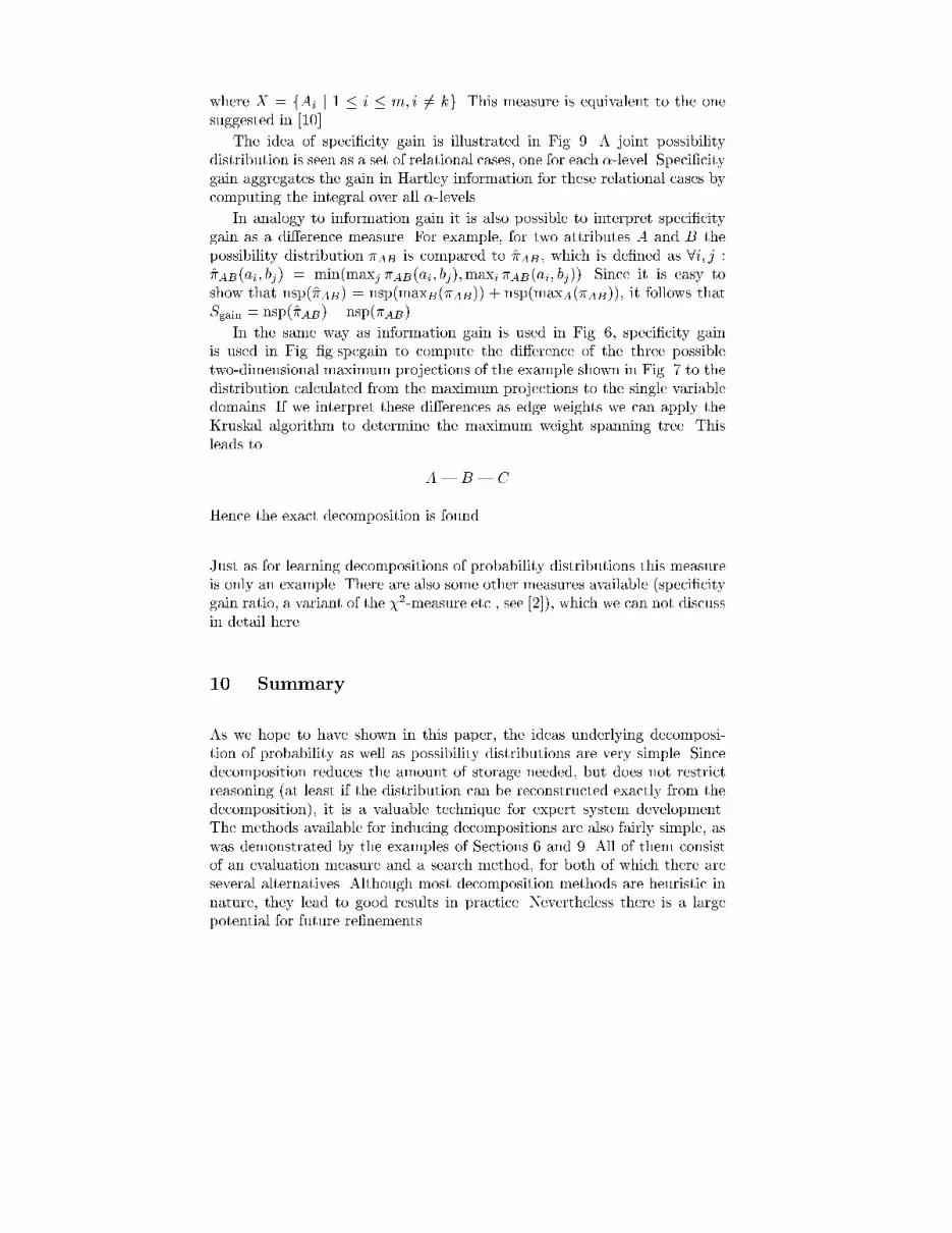
where X = fAi j 1 � i � m; i 6= kg. This measure is equivalent to the onesuggested in [10].The idea of speci�city gain is illustrated in Fig. 9. A joint possibilitydistribution is seen as a set of relational cases, one for each �-level. Speci�citygain aggregates the gain in Hartley information for these relational cases bycomputing the integral over all �-levels.In analogy to information gain it is also possible to interpret speci�citygain as a di�erence measure. For example, for two attributes A and B thepossibility distribution �AB is compared to �̂AB , which is de�ned as 8i; j :�̂AB(ai; bj) = min(maxj �AB(ai; bj);maxi �AB(ai; bj)). Since it is easy toshow that nsp(�̂AB) = nsp(maxB(�AB)) + nsp(maxA(�AB)), it follows thatSgain = nsp(�̂AB)� nsp(�AB).In the same way as information gain is used in Fig. 6, speci�city gainis used in Fig. �g.spcgain to compute the di�erence of the three possibletwo-dimensional maximum projections of the example shown in Fig. 7 to thedistribution calculated from the maximum projections to the single variabledomains. If we interpret these di�erences as edge weights we can apply theKruskal algorithm to determine the maximum weight spanning tree. Thisleads to A | B | CHence the exact decomposition is found.Just as for learning decompositions of probability distributions this measureis only an example. There are also some other measures available (speci�citygain ratio, a variant of the �2-measure etc., see [2]), which we can not discussin detail here.10. SummaryAs we hope to have shown in this paper, the ideas underlying decomposi-tion of probability as well as possibility distributions are very simple. Sincedecomposition reduces the amount of storage needed, but does not restrictreasoning (at least if the distribution can be reconstructed exactly from thedecomposition), it is a valuable technique for expert system development.The methods available for inducing decompositions are also fairly simple, aswas demonstrated by the examples of Sections 6 and 9. All of them consistof an evaluation measure and a search method, for both of which there areseveral alternatives. Although most decomposition methods are heuristic innature, they lead to good results in practice. Nevertheless there is a largepotential for future re�nements.

References1. S.K. Andersen, K.G. Olesen, F.V. Jensen, and F. Jensen. HUGIN | Ashell for building Bayesian belief universes for expert systems. Proc. 11thInt. J. Conf. on Arti�cial Intelligence, 1080{1085, 19892. C. Borgelt and R. Kruse. Evaluation Measures for Learning Probabilisticand Possibilistic Networks. Proc. 6rh IEEE Int. Conf. on Fuzzy Systems(FUZZ-IEEE'97), Vol. 2, 669{676, Barcelona, Spain, 1997.3. C.K. Chow and C.N. Liu. Approximating Discrete Probability Distri-butions with Dependence Trees. IEEE Trans. on Information Theory14(3):462{467, IEEE 19684. G.F. Cooper and E. Herskovits. A Bayesian Method for the Induction ofProbabilistic Networks from Data. Machine Learning 9:309{347, Kluwer19925. C.J. Date. An Introduction to Database Systems, Vol. 1. Addison Wesley,Reading, MA, 19866. R. Dechter. Decomposing a Relation into a Tree of Binary Relations.Journal of Computer and System Sciences 41:2{24, 19907. J. Gebhardt and R. Kruse. A Possibilistic Interpretation of Fuzzy Sets inthe Context Model. Proc. IEEE Int. Conf. on Fuzzy Systems, 1089-1096,San Diego, CA, 1992.8. J. Gebhardt and R. Kruse. POSSINFER | A Software Tool for Possi-bilistic Inference. In: D. Dubois, H. Prade, and R. Yager, eds. Fuzzy SetMethods in Information Engineering: A Guided Tour of Applications,Wiley 19959. J. Gebhardt and R. Kruse. Learning Possibilistic Networks from Data.Proc. 5th Int. Workshop on Arti�cial Intelligence and Statistics, 233{244, Fort Lauderdale, FL, 199510. J. Gebhardt and R. Kruse. Tightest Hypertree Decompositions of Multi-variate Possibility Distributions. Proc. Int. Conf. on Information Process-ing and Management of Uncertainty in Knowledge-based Systems, 199611. R.V.L. Hartley. Transmission of Information. The Bell Systems TechnicalJournal 7:535{563, 192812. D. Heckerman. Probabilistic Similarity Networks. MIT Press, Cambridge,MA, 199113. D. Heckerman, D. Geiger, and D.M. Chickering. Learning Bayesian Net-works: The Combination of Knowledge and Statistical Data. MachineLearning 20:197{243, Kluwer 199514. M. Higashi and G.J. Klir. Measures of Uncertainty and Informationbased on Possibility Distributions. Int. Journal of General Systems 9:43{58, 198215. G.J. Klir and M. Mariano. On the Uniqueness of a Possibility Measure ofUncertainty and Information. Fuzzy Sets and Systems 24:141{160, 198716. R. Kruse and E. Schwecke. Fuzzy Reasoning in a Multidimensional Spaceof Hypotheses. Int. Journal of Approximate Reasoning 4:47{68, 1990

17. R. Kruse, E. Schwecke, and J. Heinsohn. Uncertainty and Vagueness inKnowledge-based Systems: Numerical Methods. Series: Arti�cial Intelli-gence, Springer, Berlin 199118. R. Kruse, J. Gebhardt, and F. Klawonn. Foundations of Fuzzy Systems,John Wiley & Sons, Chichester, England 199419. S. Kullback and R.A. Leibler. On Information and Su�ciency. Ann.Math. Statistics 22:79{86, 195120. S.L. Lauritzen and D.J. Spiegelhalter. Local Computations with Proba-bilities on Graphical Structures and Their Application to Expert Systems.Journal of the Royal Statistical Society, Series B, 2(50):157{224, 198821. H.T. Nguyen. Using Random Sets. Information Science 34:265{274, 198422. J. Pearl and T.S. Verma. A Theory of Inferred Causation. In: J.A. Allen,R. Fikes, and E. Sandewall, eds. Proc. 2nd Int. Conf. on Principles ofKnowledge Representation and Reasoning, Morgan Kaufman, San Mateo,CA, 199123. J. Pearl. Probabilistic Reasoning in Intelligent Systems: Networks ofPlausible Inference (2nd edition). Morgan Kaufman, San Mateo, CA,199224. J.R. Quinlan. Induction of Decision Trees. Machine Learning 1:81{106,198625. J.R. Quinlan. C4.5: Programs for Machine Learning, Morgan Kaufman,San Mateo, CA, 199326. A. Sa�otti and E. Umkehrer. PULCINELLA: A General Tool for Prop-agating Uncertainty in Valuation Networks. Proc. 7th Conf. on Uncer-tainty in AI, 323{331, San Mateo, CA, 199127. G. Shafer and P.P. Shenoy. Local Computations in Hypertrees. WorkingPaper 201, School of Business, University of Kansas, Lawrence, KS, 198828. C.E. Shannon. The Mathematical Theory of Communication. The BellSystems Technical Journal 27:379{423, 194829. M. Singh and M. Valtorta. An Algorithm for the Construction ofBayesian Network Structures from Data. Proc. 9th Conf. on Uncertaintyin AI, 259{265, Morgan Kaufman, San Mateo, CA, 199330. J.D. Ullman. Principles of Database and Knowledge-Base Systems, Vol. 1and 2. Computer Sciences Press, Rockville, MD, 1988/1989This article was processed using the LATEX macro package with LLNCS style