1

Probabilistic seismic slope stability assessment of

geostructures

Yiannis Tsompanakis*1, Nikos D. Lagaros2,

Prodromos N. Psarropoulos1 and Evaggelos C. Georgopoulos1 1Department of Applied Sciences, Technical University of Crete, Greece

2Institute of Structural Analysis and Seismic Research, National Technical University of Athens, Greece

Dates of submission: 11 Nov 2007, revision: 23 June 2008 and acceptance: 10 July 2008

* To whom correspondence should be addressed:

Yiannis Tsompanakis

Department of Applied Sciences, Technical University of Crete,

University Campus, Chania 73100, Greece

e-mail: jt@science.tuc.gr

Tel : +30-28210-37634

Fax : +30-28210-37843

2

Abstract

Typically, seismic analysis of large-scale geostructures, such as embankments, is performed

by means of deterministic pseudostatic slope stability methods where a safety factor based

approach is adopted. However, probabilistic seismic fragility analysis can be a more efficient

and realistic approach for interpreting more accurately the seismic performance and the

vulnerability assessment of an earth structure. There exist two major approaches for

performing vulnerability analysis: either approximately assuming that the demand values

follow the lognormal distribution, or numerically most often via Monte Carlo simulation

(MCS) method, where the probability of exceedance for every limit-state is obtained

performing MCS analyses for various intensity levels. The MCS technique is considered as

the most consistent reliability analysis method, having no limitations regarding its

applicability range. The objective of this work is to present the efficiency of the MCS-based

numerical approach versus the commonly used lognormal empirical approach for developing

fragility curves of embankments.

Keywords: Probabilistic analysis, slope stability, fragility curves, geostructures, Monte Carlo

simulation.

3

1. INTRODUCTION

Deterministic analysis of any structural system requires certain assumptions regarding the

geometry, the material properties and other structural attributes that may affect the overall

capacity of the structure. Moreover, additional simplifying assumptions have to be taken into

account with respect to loads, and especially those related to seismic demand. However, in

real world engineering practice there exist uncertainties associated with both randomness

(aleatory uncertainty) and imperfect knowledge (epistemic uncertainty) of the problems. The

aforementioned uncertainties play a crucial role, especially when they are integrated in the

framework of performance-based earthquake engineering. For instance, the majority of

geotechnical earthquake engineering applications are highly stochastic problems.

Nevertheless, geotechnical seismic design compromises with the use of deterministic

simplifications due to their low computational cost and their minimal complexity, while on

the other hand, probabilistic methods are constantly gaining popularity due to the advances in

computational resources and the significant developments of stochastic analysis methods.

In general, embankments constitute large-scale geostructures of great importance (e.g.,

dams, solid waste landfills), the safety and serviceability of which are directly related to

environmental and social-economical issues. This kind of structures became the subject of

systematic research following the 1989 Loma Prieta (Seed et al. 1990), the 1994 Northridge

(Stewart et al. 1994) and the 1995 Kobe (Bertero et al. 1995) earthquakes, after which

extended investigations took place to examine failures that occurred on embankments due to

seismic actions. In geotechnical engineering practice the slope stability of an embankment is

most frequently evaluated utilizing the deterministic pseudostatic method, in which the

horizontal and vertical pseudostatic inertial forces are included in the safety factor

calculations.

4

Conversely, structural reliability methods have been improved considerably during the

last twenty years, as discussed in several studies (see Schueller 1997, Wen et al. 2003,

Schueller 2005, among others). Structural reliability analysis can be performed either with

simulation methods, such as the Monte Carlo simulation (MCS) method, or with

approximation methods (i.e., first or second order reliability methods (FORM, SORM),

response surface methods (RSM), etc). However, MCS appear to be the only approach

capable of achieving accurate solutions for complex problems that involve nonlinearities, a

great number of random variables, large variations of the uncertain parameters, etc. The major

advantage of MCS is that accurate solutions can be obtained almost for every problem, while

its major deficiency is the increased computational cost which can be substantially reduced

via efficient metamodels (Papadrakakis et al. 1996).

In earthquake engineering applications, any reliability problem can be defined with two

separate sets of variables, representing the demand and the capacity. A popular way of

representing the probabilistic nature of the response of a structural system is via fragility

curves. In this work limit-state probabilities are obtained for a wide range of intensity levels

in order to construct the fragility curves of typical embankments. In order to further exploit

the findings of the study, the fragility curves obtained by MCS are compared to those based

on the assumption that the demand values follow the lognormal distribution, and it is shown

that this assumption may lead to curves that differ considerably from those of the more

rigorous MCS-based methodology. The present investigation involves the consideration of

random variability of the mechanical properties of the soil, the geometry of the geostructure,

as well as the seismic intensity levels (in terms of pseudostatic horizontal acceleration). The

results demonstrate the efficiency of the proposed methodology for treating large-scale

problems in geotechnical earthquake engineering.

5

2. SEISMIC SLOPE STABILITY

Since the failure of embankments is directly related to slope instabilities (either of the

embankment mass or its foundation), seismic slope stability analysis is certainly considered as

a critical component of the geotechnical seismic design process. In engineering practice it is

based on three main categories of methods; namely: stress deformation analysis, permanent

deformation analysis and pseudostatic analysis. Stress deformation analyses are mainly

performed utilizing the finite element method with the application of complicated constitutive

models to describe the potential nonlinear material behaviour. However, the parameters

required for the implementation of the models cannot be easily or accurately quantified in the

laboratory or in situ. It is evident that in the case of waste landfills this deficiency of stress

deformation analysis is critical. In contrast, permanent deformation analyses are based on the

calculation of seismic deformations through the simple sliding block approach proposed by

Newmark (1965).

Due to their complexity or their inherent uncertainties, the two aforementioned methods

are usually excluded from the seismic design of embankments. Most frequently, the

assessment of seismic slope stability is obtained via pseudostatic analyses. Based on the limit

equilibrium methods of static slope stability analysis, and including the horizontal and vertical

inertial forces, the results are provided in terms of the minimum factor of safety (FoS). The

basic limitation of this method is the selection of the proper value of the seismic coefficient,

which controls the inertial forces on the soil masses. Contemporary seismic norms (e.g.,

Eurocode 8 (EC8) Greek Seismic Code (EAK)), suggest the use of pseudostatic slope stability

analysis utilizing a proper value for the related seismic coefficient (the so-called pseudostatic

horizontal acceleration or PHA), equal to a specific portion of the design peak ground

acceleration (PGA) at the site of interest. However, this approach does not take into account

the actual dynamic response of the structure and the corresponding derformations, resulting to

6

incapability of predicting the actual response of the geostructure during a more severe seismic

event. Therefore, in special cases it is advisable to adopt more accurate dynamic analysis

procedures, e.g., for embankments characterized by high non-symmetric geometry or

potentially problematic foundation, and/or when local site conditions (stratigraphy,

topography, geomorphology) may play an important role (Zania et al. 2008a).

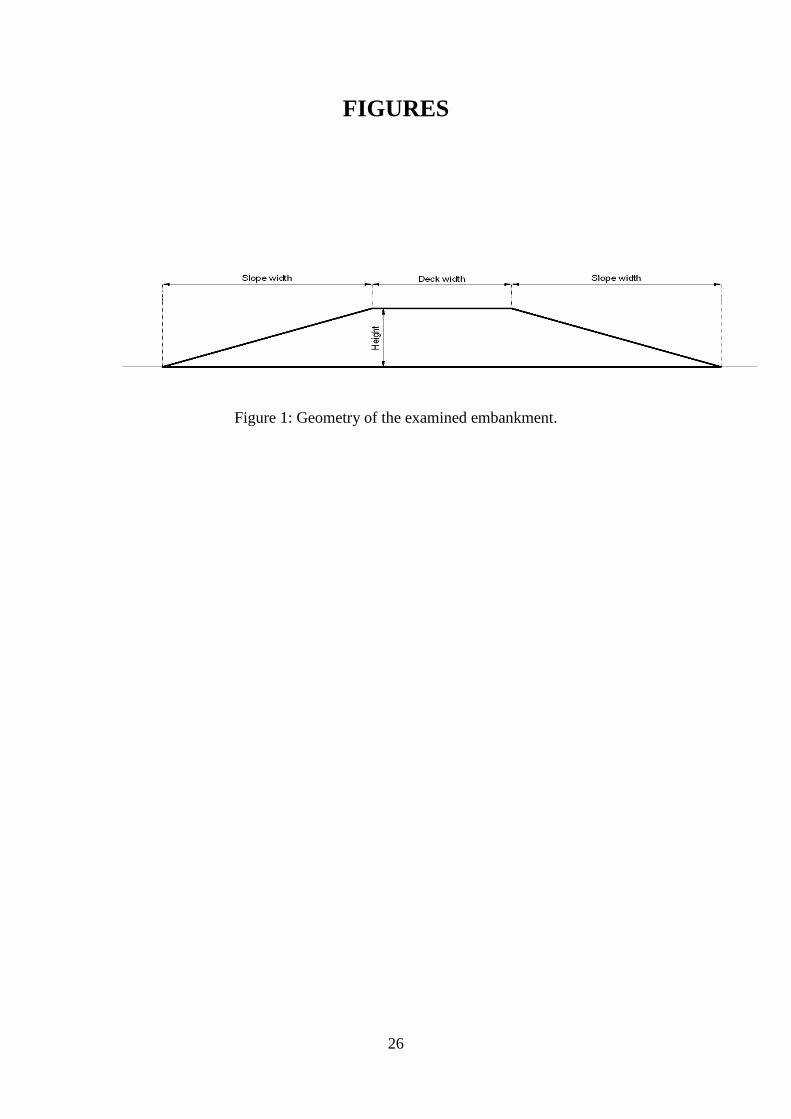
In this study, the typical trapezoid embankment shown in Figure 1 is examined. The

probabilistic calculations involved for the construction of the fragility curves of the

geostructure (especially when dynamic analyses had to be performed) are extremely time-

consuming. Thus, in the current investigation pseudostatic analyses were conducted in which

the required slope stability analyses were performed using a computer code developed by the

authors (Zania et al. 2008b) that utilizes the simplified Bishop’s method for dry conditions

and the assumption of circular failure surfaces within the body of the embankment. In

addition, it is capable of randomly modifying the mechanical and geometrical characteristics

of the model, as well as the acting pseudostatic horizontal acceleration values throughout the

probabilistic analyses via the MCS method.

3. PROBABILISTIC SEISMIC ANALYSIS OF EMBANKMENTS

Despite their very low probabilities of occurrence, severe earthquake events may produce

extensive damages to engineering systems. Therefore, it is essential to establish a reliable

procedure for assessing the seismic risk of real world structures and infrastructures. These

procedures can only be created within the framework of probabilistic safety analysis (PSA),

since it provides a rational framework for taking into account the various sources of

uncertainty that may influence the structural performance. Seismic fragility analysis is

considered as the core of PSA, which provides a measure of the safety margins of every

engineering system under any specified hazard levels.

7

Nowadays, it is possible to predict via deterministic methodologies the level of ground

shaking which is necessary to achieve a target level of response and/or damage state for a

given structure. The material properties and certain other parameters that affect the overall

capacity of the system can be determined in a similar manner. This type of deterministic

assessment requires that certain assumptions should also be made about the ground motion

and local site conditions, since both of them affect seismic demand. Nevertheless, the values

of these parameters are not exact; they undoubtedly posses various types of randomness and

uncertainty. An increasingly popular way of characterizing the probabilistic nature of seismic

phenomena is through the use of the so-called fragility curves. A fragility curve provides the

failure probability of a system as a function of certain seismic intensity measure. In the case

of an embankment, fragility curves can provide the failure probability of the slopes as a

function of the imposed pseudostatic acceleration.

3.1. Seismic fragility analysis of geostructures

Fragility analysis is currently considered as one of the most useful computational tools for

determining the dynamic behavior of any engineering system over a large range of seismic

intensity levels. Specifically, a fragility curve of an earth structure provides the probability

that its slope exceeds a given damage state for a certain seismic hazard level. In general, there

exist two approaches to perform fragility analysis: the first is based on the assumption that the

demand values follow the lognormal distribution, while the second is based on the Monte

Carlo simulation technique performing reliability analysis of the slope for each intensity level

(Tantalla et al. 2001).

The main objective of the present investigation is to perform probabilistic slope stability

analysis of a characteristic geostructure utilizing the pseudostatic method and to develop

fragility curves to assess the vulnerability state of the examined earth structure. In the current

8

study, both the approximate and the numerical approaches have been implemented. The

following general assumption has been made: the empirical fragility curves can be expressed

in the form of the previously described lognormal distribution function and can be developed

as a function of the pseudostatic horizontal acceleration (PHA) in order to represent the

intensity of the seismic ground motion. The use of PHA is reasonable for this purpose, since

this work adopts the pseudostatic slope stability approach, recommended by most of the

modern seismic norms. Similarly, in order to develop fragility curves using reliability

analysis methods (such as MCS), the embankment has to be assessed over a number of

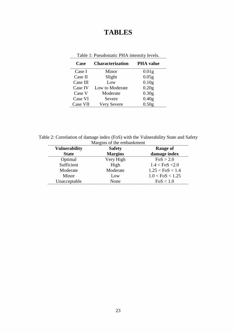
different PHA values. Therefore, seven different hazard levels (see Table 1) ranging from

minor (PHA=0.01g) to very severe (PHA=0.50g) seismic intensity were studied, in an effort

to cover a sufficient range of the seismic demand.

As shown in Table 2, the Damage States (DS) considered are defined in terms of safety

factor for the embankment slope stability and cover the whole range of its potential

Vulnerability States (VS) and the relative Safety Margins (SM). To obtain discrete damage

states, a properly selected range of the geostructural damage index must be specified. Similar

correlation is used for buildings via proper damage indices, such as the interstory drift. The

correlation of specific FoS values with the vulnerability assessment of the slopes is a crucial

factor for the construction of the fragility curves. Therefore, the association presented in Table

2 is used in the present study, which follows the guidelines of the geotechnical design norm

Eurocode 7 ((ΕC7) [18]) and the seismic norms (Eurocode 8 (ΕC8) [7], Greek Seismic Code

(EAK) [11]), where the adopted characteristic damage index (FoS) values are described as:

- FoS = 1.0 is the acceptable factor of safety for the stability of a slope under pseudostatic

conditions (EC8, EAK),

- FoS = 1.25 is the acceptable factor of safety for the stability of a slope for static conditions

when considering the existence of water (EC7),

9

- FoS = 1.4 is the acceptable factor of safety under dry static conditions (EC7).

In addition, a rather extreme upper value of FoS = 2.0 is considered as the indicator for very

high safety margins.

It has to be noted that the present implementation is a preliminary simplifying approach

to deal with this important and complex problem. The above classification of vulnerability

states with the aforementioned values of FoS does not take into account the permanent

seismic deformations of the geostructure, which may be marginal even for the case of

“pseudostatic failure” (for FoS < 1.0). Furthermore, the vulnerability and the corresponding

DS of a geostructure, in terms of deformation and instability, may differ substantially from

the values of Table 2 in the case of “problematic” materials (like soft clay, loose sand, organic

material, waste, etc). In such special cases each vulnerability state should be determined more

elaborately on a case-by-case basis. Nevertheless, there exist cases in which not even

marginal deformations are allowed, and thus FoS should be much greater that unity. It has to

be stressed that even the seismic norms use the “pseudostatic failure” value of FoS = 1.0 only

as a lower bound and not as an absolute limit. Moreover, due to various simplifications used

in the pseudostatic slope stability method, it is realistic to try to have a more clear perception

of the embankment’s safety margins via its fragility curves constructed using values of FoS >

1.0.

The employed procedure for the fragility curves generation that was employed in the

present investigation can be summarized as follows:

a. model the uncertainties of the geostructure

b. use different levels of pseudostatic horizontal acceleration to perform pseudostatic

slope stability analyses

c. construct the fragility curves

10

Brief descriptions regarding the construction of fragility curves, both empirically and

numerically, are presented in the subsequent sections.

3.2. Lognormal assumption

A number of methodologies which are based on the lognormal assumption have been

proposed for developing fragility curves, most of which have been applied to reinforced

concrete framed structures (UTCB 2006, Kappos and Panagopoulos 2008) and bridges

(Mander et. al 2007, Kwon and Elnashai 2008). In the present study, an attempt has been

made to implement a similar methodology for developing approximate fragility curves for

geotechnical earthquake engineering applications. In brief, the empirical approach is based on

the assumption that the probability of reaching or exceeding a given DS can be modeled as a

cumulative lognormal distribution. Recently, new proposals have been presented, in which

other types of functions are used in the empirical approach (Leon and Atanasiu 2007).

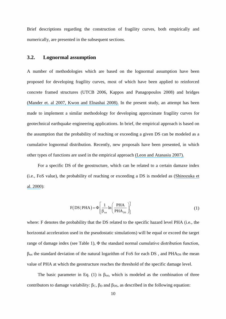
For a specific DS of the geostructure, which can be related to a certain damaxe index

(i.e., FoS value), the probability of reaching or exceeding a DS is modeled as (Shinozuka et

al. 2000):

tot DS

1 PHAF DS| PHA ln

PHA

(1)

where: F denotes the probability that the DS related to the specific hazard level PHA (i.e., the

horizontal acceleration used in the pseudostatic simulations) will be equal or exceed the target

range of damage index (see Table 1), Φ the standard normal cumulative distribution function,

βtot the standard deviation of the natural logarithm of FoS for each DS , and PHADS the mean

value of PHA at which the geostructure reaches the threshold of the specific damage level.

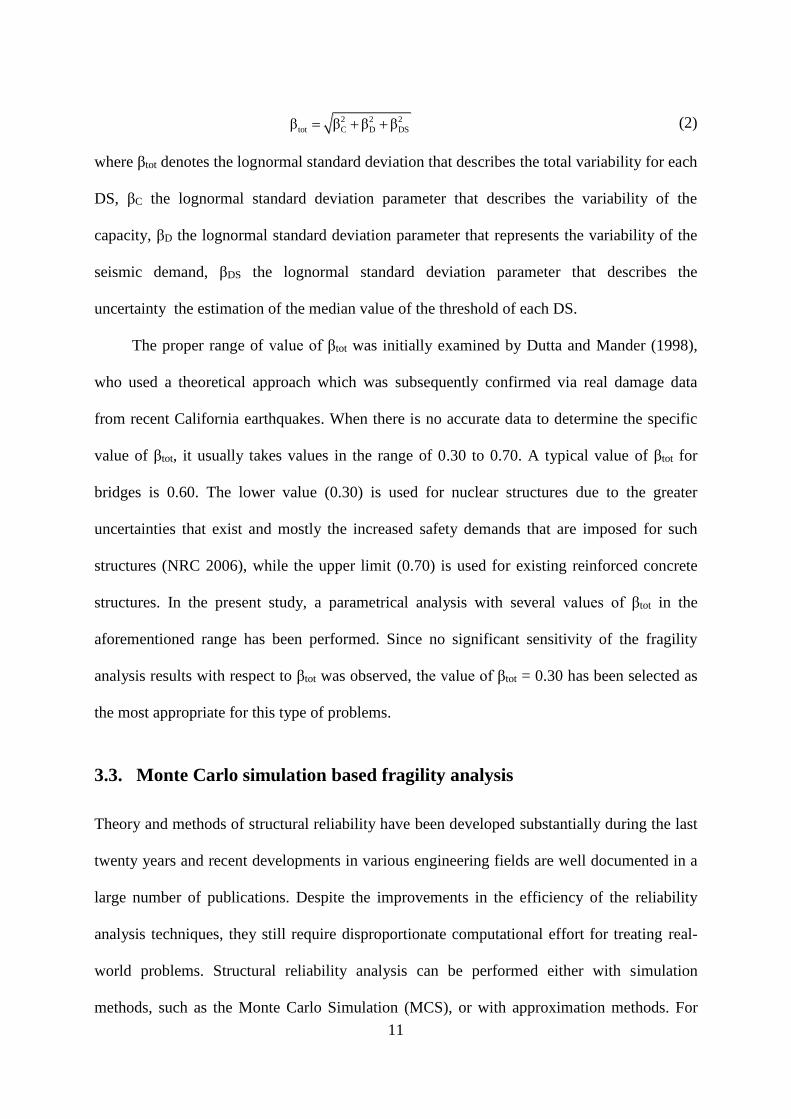
The basic parameter in Eq. (1) is βtot, which is modeled as the combination of three

contributors to damage variability: βC, βD and βDS, as described in the following equation:

11

2 2 2

tot C D DSβ β β β (2)

where βtot denotes the lognormal standard deviation that describes the total variability for each

DS, βC the lognormal standard deviation parameter that describes the variability of the

capacity, βD the lognormal standard deviation parameter that represents the variability of the

seismic demand, βDS the lognormal standard deviation parameter that describes the

uncertainty the estimation of the median value of the threshold of each DS.

The proper range of value of βtot was initially examined by Dutta and Mander (1998),

who used a theoretical approach which was subsequently confirmed via real damage data

from recent California earthquakes. When there is no accurate data to determine the specific

value of βtot, it usually takes values in the range of 0.30 to 0.70. A typical value of βtot for

bridges is 0.60. The lower value (0.30) is used for nuclear structures due to the greater

uncertainties that exist and mostly the increased safety demands that are imposed for such

structures (NRC 2006), while the upper limit (0.70) is used for existing reinforced concrete

structures. In the present study, a parametrical analysis with several values of βtot in the

aforementioned range has been performed. Since no significant sensitivity of the fragility

analysis results with respect to βtot was observed, the value of βtot = 0.30 has been selected as

the most appropriate for this type of problems.

3.3. Monte Carlo simulation based fragility analysis

Theory and methods of structural reliability have been developed substantially during the last

twenty years and recent developments in various engineering fields are well documented in a

large number of publications. Despite the improvements in the efficiency of the reliability

analysis techniques, they still require disproportionate computational effort for treating real-

world problems. Structural reliability analysis can be performed either with simulation

methods, such as the Monte Carlo Simulation (MCS), or with approximation methods. For

12

instance, first and second order approximation methods (FORM and SORM) lead to

formulations that require prior knowledge of the means and variances of the random variables

and the definition of a differentiable failure function. In contrast, MCS appears to be the only

universal method that can provide accurate solutions for problems regardless the complexity

and/or the dimensions of the application. The major advantage of MCS is that accurate

solutions can be obtained for any problem, while the only disadvantage is that it is generally

more time-consuming. Fragility analysis based on MCS technique requires the repeated

solution of the reliability problem for each set of random variables examined. It is obvious

that the computational cost for developing fragility curves via MCS is great, especially when

earthquake loading is considered in a probabilistic manner, since a vast number of analyses

have to be performed for each hazard level.

In this study the MCS method with Latin Hypercube Sampling (LHS) reduction

technique is employed for performing the risk assessment analysis of large-scale

embankments in order to accurately calculate each damage level probability. Typically, MCS

uses a random number generator to select the value of each random variable using its

probability density function. In general, in geotechnical engineering practice there are four

probability density functions that are most commonly used: uniform distribution, triangular

distribution, normal distribution, and lognormal distribution. Other probability density

functions could be used provided that there were test data that matched those functions. More

frequently and also in this study, the normal distribution is used, especially for the basic

parameters encountered in pseudostatic slope stability analyses, such as unit weight (γ),

friction angle (φ), cohesion (c). Details about the most important probabilistic parameters that

are used in geotechnical engineering and the corresponding probability density functions can

by found in Lacasse and Nadim (1996) and USACE (2006).

13

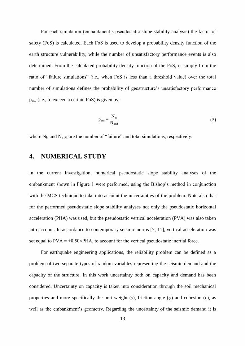
For each simulation (embankment’s pseudostatic slope stability analysis) the factor of

safety (FoS) is calculated. Each FoS is used to develop a probability density function of the

earth structure vulnerability, while the number of unsatisfactory performance events is also

determined. From the calculated probability density function of the FoS, or simply from the

ratio of “failure simulations” (i.e., when FoS is less than a threshold value) over the total

number of simulations defines the probability of geostructure’s unsatisfactory performance

pexc (i.e., to exceed a certain FoS) is given by:

Hexc

SIM

Np

N (3)

where NH and NSIM are the number of “failure” and total simulations, respectively.

4. NUMERICAL STUDY

In the current investigation, numerical pseudostatic slope stability analyses of the

embankment shown in Figure 1 were performed, using the Bishop’s method in conjunction

with the MCS technique to take into account the uncertainties of the problem. Note also that

for the performed pseudostatic slope stability analyses not only the pseudostatic horizontal

acceleration (PHA) was used, but the pseudostatic vertical acceleration (PVA) was also taken

into account. In accordance to contemporary seismic norms [7, 11], vertical acceleration was

set equal to PVA = ±0.50×PHA, to account for the vertical pseudostatic inertial force.

For earthquake engineering applications, the reliability problem can be defined as a

problem of two separate types of random variables representing the seismic demand and the

capacity of the structure. In this work uncertainty both on capacity and demand has been

considered. Uncertainty on capacity is taken into consideration through the soil mechanical

properties and more specifically the unit weight (γ), friction angle (φ) and cohesion (c), as

well as the embankment’s geometry. Regarding the uncertainty of the seismic demand it is

14

imposed through the seismic intensity levels. The geometry of this simple trapezoid example

is determined using three parameters: height, slope width and deck width (see Figure 1). In

this work two distinct cases were examined: in the first the geometry of the geostructure was

considered deterministic (by simply using the mean values of the dimensions given in Table

3), while on the latter the dimensions were also considered as random variables.

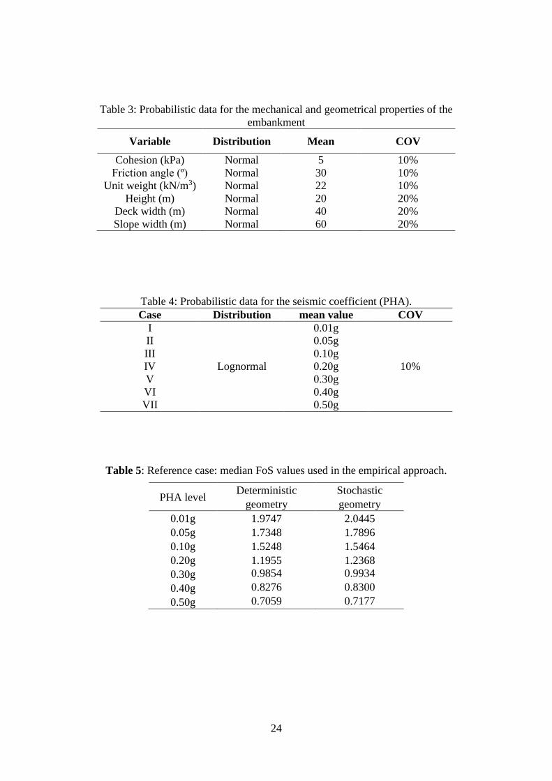
As aforementioned the normal distribution is used for the basic parameters encountered

in pseudostatic slope stability analyses (i.e., geometry, unit weight, friction angle and

cohesion), while the lognormal distribution is used for the seismic coefficient (PHA) levels.

The mean values and the corresponding coefficient of variation (COV) values for the soil

mechanical properties and the geometry are given in Table 3, while for the seismic demand

coefficient are shown in Table 4. Though cohesion may have a greater scattering, thus greater

COV value, than the other mechanical properties of the geostructure, the same COV value

(10%) has been used for all geotechnical parameters for simplicity. In contrast, a greater

variance (20%) has been allowed for the geometrical stochastic variables. Allowing a varying

geometry is performed under the perspective of achieving an improved topology of the

embankment, which is feasible provided that any possible change in the dimensions is not

violating any other constructional and/or functional limitations.

Two cases were examined in the present investigation: In the first, the so-called

reference case, the mechanical properties of which are given in Table 3, the two approaches of

fragility curves generation (empirical and MCS-based) were compared, while the effect of the

randomness of geometrical dimensions was also examined. In the second set of analyses, a

thorough investigation has been performed where the geometry was kept fixed and a

significant number of various combinations of the embankment’s mechanical parameters (c,

φ, γ) was examined, covering a wide range of soil and waste material properties. In all these

analyses both approaches for fragility curves generation were implemented and compared.

15

4.1 Reference case results

Initially, the reference case was examined using the data presented in Tables 2 to 4 examining

both fragility analysis approaches and both types of geometry (deterministic and stochastic) of

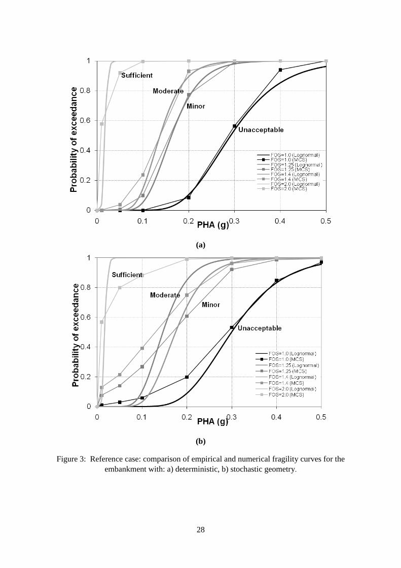
the embankment shown in Figure 1. For the generation of empirical fragility curves (via the

standard lognormal type of Equation (1)), the median value of the FoS of the examined

embankment was calculated for each intensity level. These values, which were used for the

generation of the empirical fragility curves, are presented in Table 5. The comparison of the

standard empirical approach (denoted as Lognormal in the graphs) and the numerical

approach (denoted as MCS) is depicted in Figure 3, where both types of geometry

(deterministic and stochastic) are shown.

By comparing the plot of Figure 3a with the one in Figure 3b, it is obvious that the

empirical fragility curves of the embankment with deterministic and stochastic geometry,

respectively, have very small differences in their lower and upper intervals, and differ

substantially in the region of moderate values of PHA and medium damage levels. More

specifically, at these regions the fragility curves for the deterministic geometry have more

steep inclination than the corresponding ones resulting from the stochastic geometry.

Therefore, for the same PHA value, the probability of reaching a more severe damage level is

bigger in the deterministic case than in the stochastic. A similar trend is observed in the

region of medium PHA and DS when comparing the numerical fragility curves of the

embankment with deterministic and stochastic geometry, also shown in the graphs of Figure

3. Nevertheless, in this case due to the more accurate MCS-based calculations, the trend of

obtaining smoother curves for the stochastic geometry case is also observed, apart from the

medium regions, in the upper and lower intervals of the fragility curves.

The comparison of the empirical and the numerical approaches for the deterministic

geometry types is presented in Figure 3a, where it is verified that there is consistency between

16

the two methods, except for the regions of the upper and lower values. In contrast, the

comparison of the empirical and the numerical approaches for the stochastic geometry, shown

in Figure 3b, reveals that there is a significant variation between the two methods in all the

regions of the curves. The numerical method provides more reliable results in the whole range

of seismic intensity and damage levels. This can be attributed to the fact that the degree of

uncertainty becomes greater, since the number of the probabilistic variables are increased

from four (c, φ, γ, PHA) for the embankment with deterministic geometry, to eight (c, φ, γ,

PHA and the four geometrical parameters) for the earth structure with stochastic geometry.

4.2 Parametric study results

After the investigation of the reference case, a parametric study was performed covering a

significant number of geotechnical parameter combinations of the examined model. The

purpose of this parametric study was twofold: a) to further investigate and compare the two

fragility analysis approaches, and b) to examine how and to what extend the shape of the

fragility curves is affected by the variation of the basic parameters (the soil material

properties) of the problem. As it was previously discussed in the reference case, the empirical

approach has better performance when the geometry of the embankment is considered

deterministic rather than stochastic, thus, the geometry of the geostructure in this set of

analyses was kept fixed, as determined by the values given in Table 3. Therefore, only the soil

material properties and seismic intensity level were considered as stochastic variables. The

stochastic data shown in Table 4 were used for the imposed PHA levels.

The examined soil material properties of the embankment were the following: cohesion

c=5 and 10kPa, friction angle φ=20º and 25º, and unit weight γ=10, 13, 15, 18 and 20 kN/m3.

Concerning stochastic variability of the above data, the same conventions as in the reference

case were used (see Table 3), i.e., the aforementioned values were considered as mean values

17

of the stochastic parameters that follow the normal distribution with 10% standard deviation.

It has to be noted that the lower values of unit weight, which are unrealistic for typical soil

embankments, correspond to special “embankments”, i.e., waste landfills. In such cases, the

existence of stochastic variations of the geostructure’s properties is unavoidable and even

more pronounced.

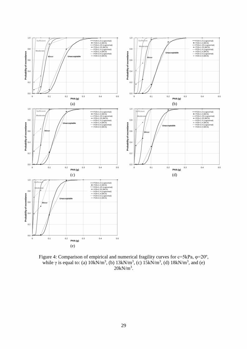
The results that arise from the generation of the empirical fragility curves for the

aforementioned sets of geotechnical parameter combinations, are presented in Figures 4 to 7.

It is obvious that even for this set of runs having deterministic geometry, there are many cases

where there exist great discrepancies between the two methods, not only in the lower and

upper intervals but in the medium regions of the fragility curves as well. Nevertheless, there is

no clear trend with respect to the comparison of the two fragility methods, i.e., to determine

under what circumstances the empirical curves approach more closely the numerical ones.

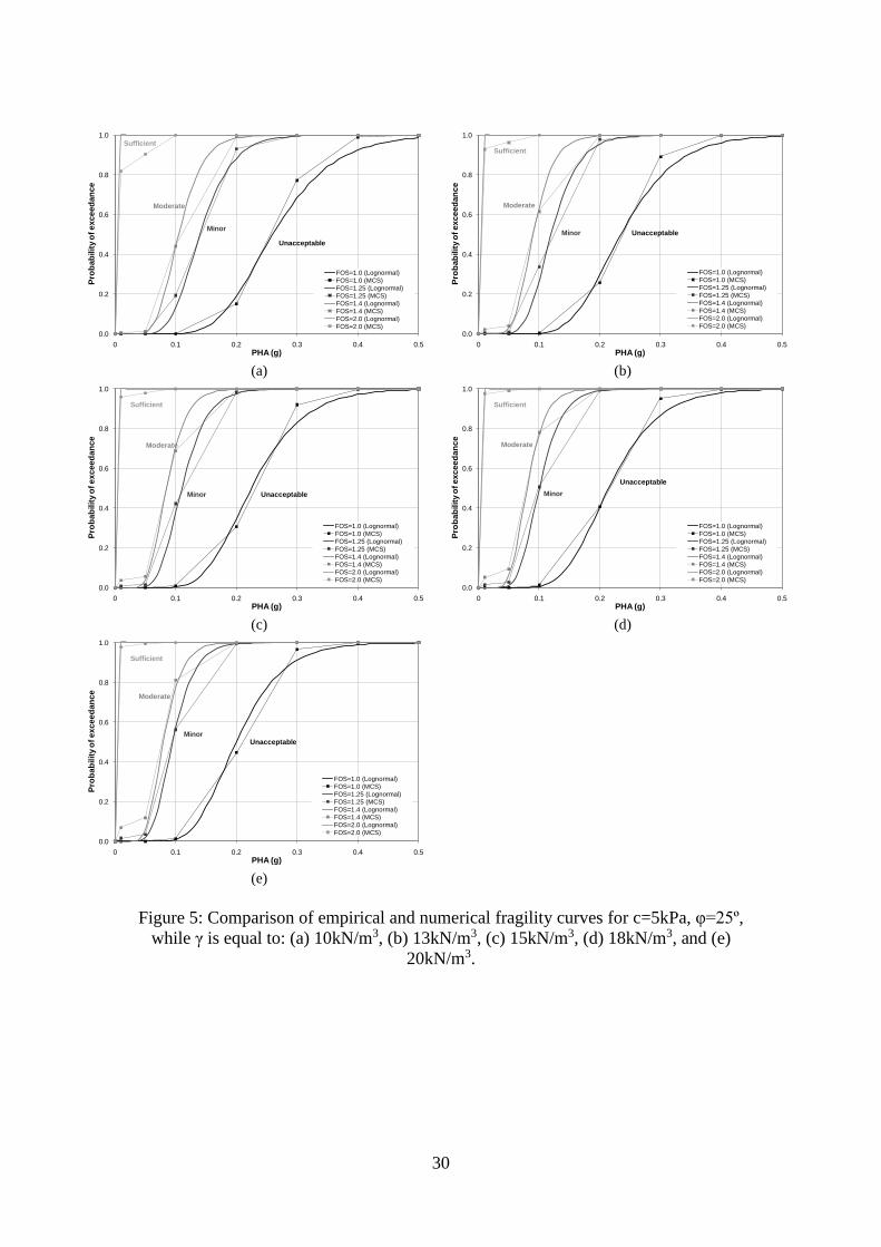
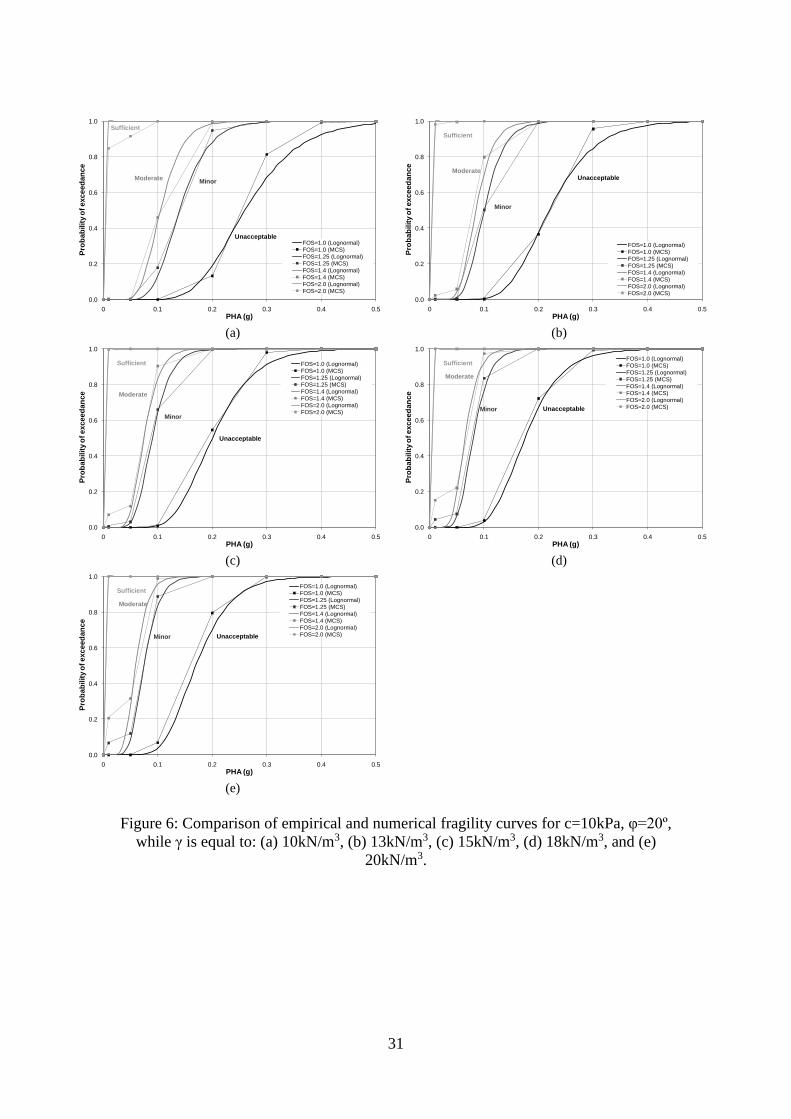
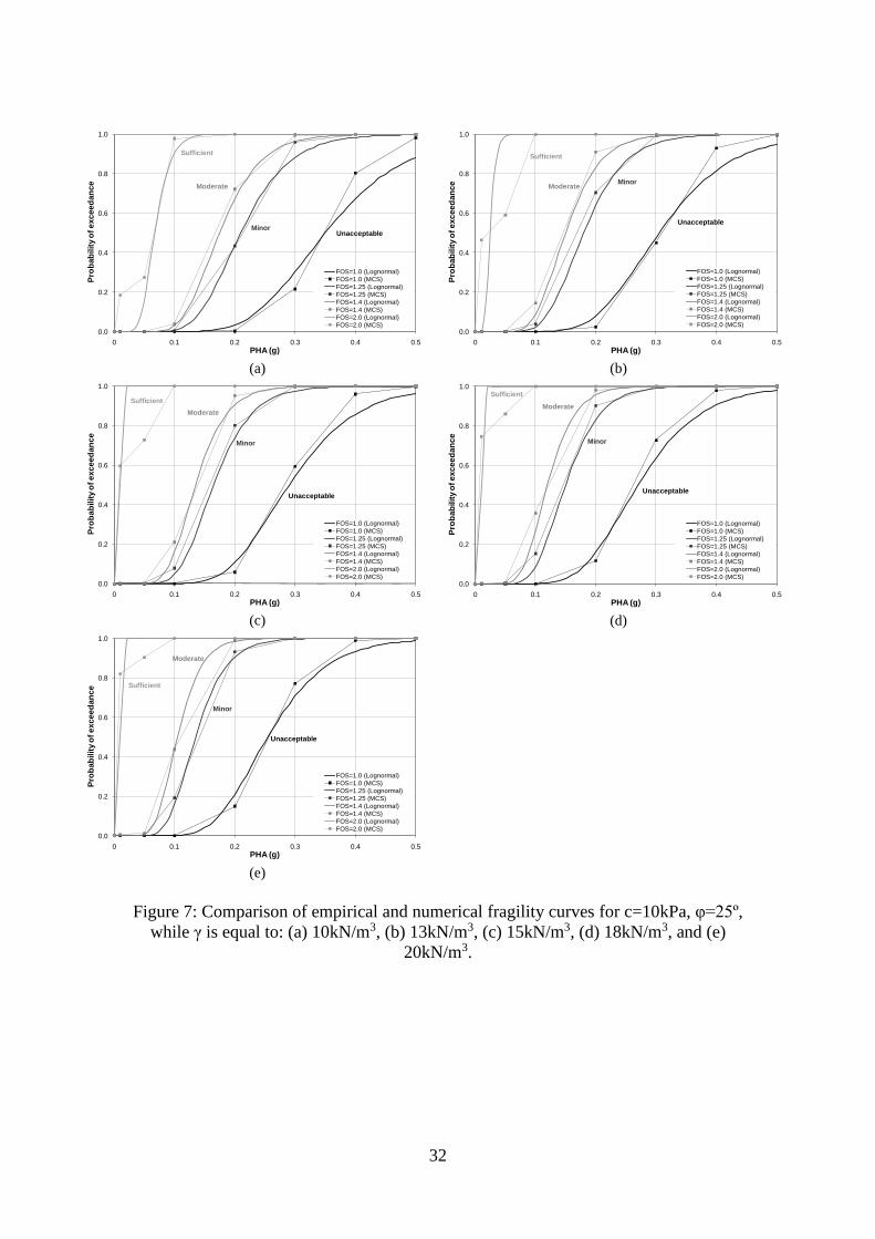
From a geotechnical point of view, there is a great variation with respect to the shape of

the fragility curves. For instance, the impact of cohesion (c) is the following: when it

increases (from 5 to 10 kPa) it shifts the fragility curves to the right. This remark is evident by

comparing the plots of Figures 4 and 6 (with same friction angle φ=20º) and the plots of

Figures 5 and 7 (with equal friction angle φ=25º). In other words, the increase of cohesion

value results to a less vulnerable embankment. In addition, the fragility curves become

slightly smoother as cohesion becomes greater. A similar trend is observed when considering

the impact of the friction angle (φ). By comparing the plots of Figures 4 and 5 (with same

cohesion c=5) and the plots of Figures 6 and 7 (with equal cohesion c=10), it is clear that the

increase of friction angle value results to slightly smoother fragility curves that are also

moved to the right, thus for the same PHA level lead to a less severe damage state. In

contrast, the opposite trend is observed with respect to the unit weight (γ). More specifically,

as γ increases, the fragility curves become much steeper and also are shrunk to the left. For

18

instance, by observing the plots in Figures 4 to 7, it is obvious that the smaller value of unit

weight (γ=10 kN/m3, which is typical for waste landfills) has smoother vulnerability curves

than those obtained for larger unit weight values.

5. CONCLUSIONS

Fragility analysis offer a precise and efficient way to determine a geostructure’s performance

and the evaluation of its seismic vulnerability for multiple hazard levels and multiple damage

states, in the viewpoint of the state-of-the-art Performance-based Earthquake Engineering

(PBEE). Under this perspective, this paper presented the two most commonly used

approaches for establishing fragility curves, as the outcome of the probabilistic pseudostatic

slope stability analysis, of large-scale embankments under pseudostatic seismic loading

conditions.

The proposed implementation involved the consideration of random variability of

geometry, soil mechanical properties as well as the imposed seismic intensity levels on the

geostructure. Both empirical and numerical methodologies were used and compared for the

generation of the fragility curves of a typical embankment for various combinations of soil

material properties and the influence of each parameter (c, φ, γ) was highlighted. The impact

of the geometry type (fixed or random) was also considered, since it also affects substantially

the shape of the curves; regardless of the fragility analysis method, the stochastic geometry

results to smoother curves compared to the deterministic geometry.

When comparing the two approaches it was found that in some occasions there is

consistency between the two types of fragility analysis, usually in the medium regions of the

fragility curves, when the geometry of the embankment is considered constant. However, in

the majority of the deterministic geometry cases examined there are big intervals (especially

in the upper and lower regions) where there are significant variations between numerical and

19

empirical curves. Moreover, this discrepancy between empirical and numerical fragility

curves was more evident when the dimensions of the geostructure were also considered as

random variables.

Conclusively, despite its simplicity and its low computational cost, the application of

empirical fragility curves has questionable accuracy compared to the more accurate (provided

that the MCS sampling size is big enough) and more elaborate numerical approach.

Nevertheless, the generation of the fragility curves using the numerical methodology is a very

computational intensive task, since a much greater number of simulations must be executed.

The implementation of efficient approximation techniques (such as neural networks), which is

the next step of this ongoing research, can alleviate this deficiency of the MCS-based

approach and increase the applicability range and the effectiveness of the numerical

methodology.

6. ACKNOWLEDGEMENTS

This paper is part of the 03ED454 research project, implemented within the framework of the

“Reinforcement Program of Human Research Manpower” (PENED) and co-financed by

National and Community Funds (75% from E.U.-European Social Fund and 25% from the

Greek Ministry of Development-General Secretariat of Research and Technology).

7. REFERENCES

Bertero V.V., Borcherdt R.D., Clark P.W., Dreger D.S., Filippou F.C., Foutch D.A., Gee L.S.,

Higashino M., Kono S., Lu L.-W., Moehle J.P., Murray, M.H., Ramirez J.A.,

Romanowicz B.A., Sitar N., Thewalt C.R., Tobriner S., Whittaker A.S., Wight J.K., Xiao

Y., “Seismological and engineering aspects of the 1995 Hyogoken-Nanbu (Kobe)

earthquake”, Report UCB/EERC-95/10, Earthquake Engineering Research Center,

University of California, Berkeley, 1995

20

Dutta A. and Mander J.B., “Seismic fragility analysis of highway bridges”, in Proc. of

INCEDE-MCEER Workshop on Earthq. Engrg. Frontiers in Transp. Systems, Tokyo

Japan, June 22-23, 1998, pp. 311-325.

EAK, “Greek seismic design code”, Greek Ministry of Public Works, Greece, 2000.

EC8, “Eurocode 8: Design of structures for earthquake resistance, Part 5: Foundations,

retaining structures and geotechnical aspects”, CEN-ENV, Brussels, 2003.

Kappos A.J. and Panagopoulos G., “Fragility curves for R/C buildings in Greece”, In

Tsompanakis Y. (ed.) Special Issue, “Vulnerability assessment of structures and

infrastructures”, Journal of Structure and Infrastructure Engineering (to appear), 2008.

Kwon O.-S. and Elnashai A.S., “Fragility analysis of a highway over-crossing bridge with

consideration of soil-structure-interaction”, In Tsompanakis Y. (ed.) Special Issue,

“Vulnerability assessment of structures and infrastructures”, Journal of Structure and

Infrastructure Engineering (to appear), 2008.

Lacasse S. and Nadim F., “Uncertainties in characterizing soil properties”, In “Uncertainty in

the geologic environment: from theory to practice”, ASCE Geotechnical Special Report

No. 58, Volume 2, American Society of Civil Engineers, New York, 1996.

Leon F. and Atanasiu G.M., “Estimating fragility curves of buildings using genetic

algorithms”, In Topping B.H.V. (ed.), Proceedings of the 9th International Conference on

the Application of Artificial Intelligence to Civil, Structural and Environmental

Engineering, Civil-Comp Press, Stirling, United Kingdom, paper 21, 2007.

Mander J.B., Dhakal R.P., Mashiko N., and Solberg K.M., “Incremental dynamic analysis

applied to seismic financial risk assessment of bridges”, Engineering Structures, 29,

2662–2672, 2007.

Newmark N.M., “Effects of earthquakes on dams and embankments”, Geotechnique, 15(2),

139-160, 1965.

NRC, “Safety Evaluation Report for an early site permit (ESP) at the Exelon generation

company, LLC (EGC) ESP site (NUREG-1844) - Chapter 2.5: Geology, Seismology, and

Geotechnical Engineering”, U.S. Nuclear Regulatory Commission,

http://www.nrc.gov/reading-rm/doc-collections/nuregs/staff/sr1844/sr1844-sec2-5.pdf,

[accessed 15 September 2006].

Papadrakakis M., Papadopoulos V. and Lagaros N.D. “Structural reliability analysis of

elastic-plastic structures using neural networks and Monte Carlo simulation”, Computer

Methods in Applied Mechanics Engineering, 136, 145–163, 1996.

Schueller G.I. (ed.), Special Issue on “A state-of-the-Art report on computational stochastic

mechanics”, Probabilistic Engineering Mechanics, 12(4), 197-321, 1997.

Schueller G.I. (ed.), Special Issue on “Computational methods in stochastic mechanics and

reliability analysis”, Computer Methods in Applied Mechanics Engineering, 194(12-16),

251-1795, 2005.

Seed, R.B., Dickenson, S.E., Riemer, M.F., Bray, J.D., Sitar, N., Mitchell, J.K., Idriss, I.M.,

Kayen, R.E., Kropp, A., Harder, L.F., Jr. and Power, M.S., "Preliminary report on the

principal geotechnical aspects of the October 17, 1989 Loma Prieta Earthquake" , Report

UCB/EERC-90/05, Earthquake Engineering Research Center, University of California,

Berkeley, 1990.

Shinozuka M., Feng M.Q., Kim H.K., Kim H.S., “Nonlinear static procedure for fragility

curve development”, ASCE Journal of Engineering Mechanics, 126(12), 1287-1295,

2000.

21

Stewart, J.P., Bray, J.D., Seed. R.B. and Sitar, N., "Preliminary report on the principal

geotechnical aspects of the January 17, 1994 Northridge Earthquake", Report

UCB/EERC-94/08, Earthquake Engineering Research Center, University of California,

Berkeley, 1994.

Tantalla J.M., Prevost J.H., and Deodatis G., “Spatial variability of soil properties in slope

stability analysis: Fragility curve generation” in Proc. of ICOSSAR ’01: 8th International

Conference on Structural Safety and Reliability, Newport Beach, California, USA, 17–21

June, 2001.

USACE, “Reliability analysis and risk assessment for seepage and slope stability failure

modes for embankment dams”, Publication Number: ETL 1110-2-561, U.S. Army Corps

of Engineers, http://www.usace.army.mil/publications/eng-tech-ltrs/etl1110-2-

561/toc.html, [accessed 15 September 2006].

UTCB, “Study on early earthquake damage evaluation of existing buildings in Bucharest”,

Romania, Technical Report, Technical Univ. of Civil Engineering Bucharest Romania,

http://iisee.kenken.go.jp/net/saito/web_edes_b/ romania3.pdf [accessed 15 September

2006].

Wen, Y.K., Ellingwood, B.R., Veneziano, D., and Bracci, J., “Uncertainty Modeling in

Earthquake Engineering”, Report FD-2, Mid-America Earthquake Center, University of

Illinois at Urbana-Champaign, 2003.

Zania V., Psarropoulos P.N., Karabatsos Y. and Tsompanakis Y., “Estimating the seismically

developed acceleration levels on waste landfills”, Journal of Computers & Structures, 86,

642–651, 2008a.

Zania V., Tsompanakis Y. and Psarropoulos P.N. “Seismic distress and slope instability of

municipal solid waste landfills”, Journal of Earthquake Engineering, 12(2), 312-340,

2008b.

22

TABLE LEGENDS

Table 1: Pseudostatic PHA intensity levels.

Table 2: Correlation of damage index (FoS) with the Vulnerability State and Safety

Margins of the embankment

Table 3: Probabilistic data for the mechanical and geometrical properties of the

embankment.

Table 4: Probabilistic data for the seismic coefficient (PHA).

Table 5: Reference case: median FoS values used in the empirical approach.

23

TABLES

Table 1: Pseudostatic PHA intensity levels.

Case Characterization PHA value

Case I Minor 0.01g

Case II Slight 0.05g

Case III Low 0.10g

Case IV Low to Moderate 0.20g

Case V Moderate 0.30g

Case VI Severe 0.40g

Case VII Very Severe 0.50g

Table 2: Correlation of damage index (FoS) with the Vulnerability State and Safety

Margins of the embankment

Vulnerability

State

Safety

Margins

Range of

damage index

Optimal Very High FoS > 2.0

Sufficient High 1.4 < FoS <2.0

Moderate Moderate 1.25 < FoS < 1.4

Minor Low 1.0 < FoS < 1.25

Unacceptable None FoS < 1.0

24

Table 3: Probabilistic data for the mechanical and geometrical properties of the

embankment

Variable Distribution Mean COV

Cohesion (kPa) Normal 5 10%

Friction angle (º) Normal 30 10%

Unit weight (kN/m3) Normal 22 10%

Height (m) Normal 20 20%

Deck width (m) Normal 40 20%

Slope width (m) Normal 60 20%

Table 4: Probabilistic data for the seismic coefficient (PHA).

Case Distribution mean value COV

I

Lognormal

0.01g

10%

II 0.05g

III 0.10g

IV 0.20g

V 0.30g

VI 0.40g

VII 0.50g

Table 5: Reference case: median FoS values used in the empirical approach.

PHA level Deterministic

geometry

Stochastic

geometry

0.01g 1.9747 2.0445

0.05g 1.7348 1.7896

0.10g 1.5248 1.5464

0.20g 1.1955 1.2368

0.30g 0.9854 0.9934

0.40g 0.8276 0.8300

0.50g 0.7059 0.7177

25

FIGURE LEGENDS

Figure 1: Geometry of the examined embankment.

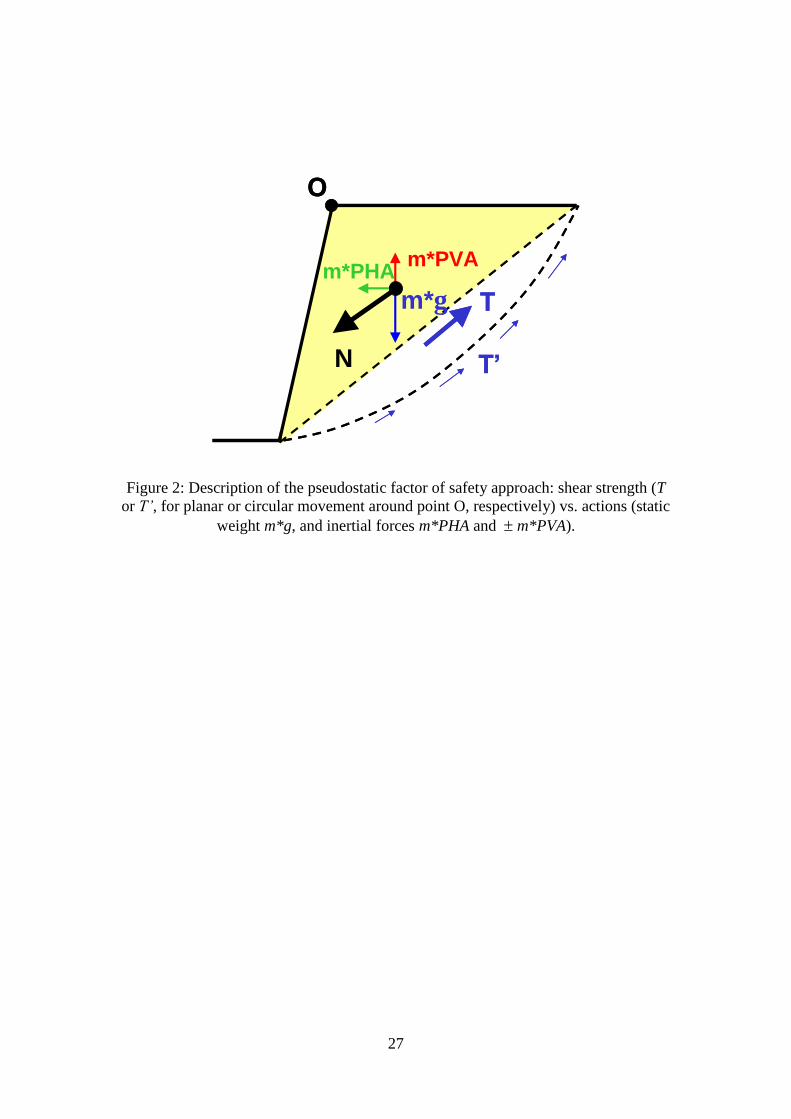
Figure 2: Description of the pseudostatic factor of safety approach: shear strength (T

or T’, for planar or circular movement around point O, respectively) vs. actions (static

weight m*g, and inertial forces m*PHA and m*PVA).

Figure 3: Reference case: comparison of empirical and numerical fragility curves for

the embankment with: a) deterministic, b) stochastic geometry.

Figure 4: Comparison of empirical and numerical fragility curves for c=5kPa, φ=20º,

while γ is equal to: (a) 10kN/m3, (b) 13kN/m3, (c) 15kN/m3, (d) 18kN/m3, and (e)

20kN/m3.

Figure 5: Comparison of empirical and numerical fragility curves for c=5kPa, φ=25º,

while γ is equal to: (a) 10kN/m3, (b) 13kN/m3, (c) 15kN/m3, (d) 18kN/m3, and (e)

20kN/m3.

Figure 6: Comparison of empirical and numerical fragility curves for c=10kPa, φ=20º,

while γ is equal to: (a) 10kN/m3, (b) 13kN/m3, (c) 15kN/m3, (d) 18kN/m3, and (e)

20kN/m3.

Figure 7: Comparison of empirical and numerical fragility curves for c=10kPa, φ=25º,

while γ is equal to: (a) 10kN/m3, (b) 13kN/m3, (c) 15kN/m3, (d) 18kN/m3, and (e)

20kN/m3.

26

FIGURES

Figure 1: Geometry of the examined embankment.

27

m*g

m*PVAm*PHA

Τ

Ο

N Τ’

m*g

m*PVAm*PHA

Τ

Ο

N Τ’

Figure 2: Description of the pseudostatic factor of safety approach: shear strength (T

or T’, for planar or circular movement around point O, respectively) vs. actions (static

weight m*g, and inertial forces m*PHA and m*PVA).

28

(a)

(b)

Figure 3: Reference case: comparison of empirical and numerical fragility curves for the

embankment with: a) deterministic, b) stochastic geometry.

29

0.0

0.2

0.4

0.6

0.8

1.0

0 0.1 0.2 0.3 0.4 0.5

Pro

bab

ilit

y o

f exceed

an

ce

PHA (g)

FOS=1.0 (Lognormal)

FOS=1.0 (MCS)

FOS=1.25 (Lognormal)

FOS=1.25 (MCS)

FOS=1.4 (Lognormal)

FOS=1.4 (MCS)

FOS=2.0 (Lognormal)

FOS=2.0 (MCS)

Sufficient

Moderate

Minor Unacceptable

(a)

0.0

0.2

0.4

0.6

0.8

1.0

0 0.1 0.2 0.3 0.4 0.5

Pro

bab

ilit

y o

f exceed

an

ce

PHA (g)

FOS=1.0 (Lognormal)

FOS=1.0 (MCS)

FOS=1.25 (Lognormal)

FOS=1.25 (MCS)

FOS=1.4 (Lognormal)

FOS=1.4 (MCS)

FOS=2.0 (Lognormal)

FOS=2.0 (MCS)

Sufficient

Moderate

Minor

Unacceptable

(b)

0.0

0.2

0.4

0.6

0.8

1.0

0 0.1 0.2 0.3 0.4 0.5

Pro

bab

ilit

y o

f exceed

an

ce

PHA (g)

FOS=1.0 (Lognormal)

FOS=1.0 (MCS)

FOS=1.25 (Lognormal)

FOS=1.25 (MCS)

FOS=1.4 (Lognormal)

FOS=1.4 (MCS)

FOS=2.0 (Lognormal)

FOS=2.0 (MCS)

Sufficient

Moderate

Minor

Unacceptable

(c)

0.0

0.2

0.4

0.6

0.8

1.0

0 0.1 0.2 0.3 0.4 0.5

Pro

bab

ilit

y o

f exceed

an

ce

PHA (g)

FOS=1.0 (Lognormal)

FOS=1.0 (MCS)

FOS=1.25 (Lognormal)

FOS=1.25 (MCS)

FOS=1.4 (Lognormal)

FOS=1.4 (MCS)

FOS=2.0 (Lognormal)

FOS=2.0 (MCS)

Sufficient

Moderate

Minor

Unacceptable

(d)

0.0

0.2

0.4

0.6

0.8

1.0

0 0.1 0.2 0.3 0.4 0.5

Pro

bab

ilit

y o

f exceed

an

ce

PHA (g)

FOS=1.0 (Lognormal)

FOS=1.0 (MCS)

FOS=1.25 (Lognormal)

FOS=1.25 (MCS)

FOS=1.4 (Lognormal)

FOS=1.4 (MCS)

FOS=2.0 (Lognormal)

FOS=2.0 (MCS)

Sufficient

Moderate

Minor

Unacceptable

(e)

Figure 4: Comparison of empirical and numerical fragility curves for c=5kPa, φ=20º,

while γ is equal to: (a) 10kN/m3, (b) 13kN/m3, (c) 15kN/m3, (d) 18kN/m3, and (e)

20kN/m3.

30

0.0

0.2

0.4

0.6

0.8

1.0

0 0.1 0.2 0.3 0.4 0.5

Pro

bab

ilit

y o

f exceed

an

ce

PHA (g)

FOS=1.0 (Lognormal)

FOS=1.0 (MCS)

FOS=1.25 (Lognormal)

FOS=1.25 (MCS)

FOS=1.4 (Lognormal)

FOS=1.4 (MCS)

FOS=2.0 (Lognormal)

FOS=2.0 (MCS)

Sufficient

Moderate

Minor

Unacceptable

(a)

0.0

0.2

0.4

0.6

0.8

1.0

0 0.1 0.2 0.3 0.4 0.5

Pro

bab

ilit

y o

f exceed

an

ce

PHA (g)

FOS=1.0 (Lognormal)

FOS=1.0 (MCS)

FOS=1.25 (Lognormal)

FOS=1.25 (MCS)

FOS=1.4 (Lognormal)

FOS=1.4 (MCS)

FOS=2.0 (Lognormal)

FOS=2.0 (MCS)

Sufficient

Moderate

Minor Unacceptable

(b)

0.0

0.2

0.4

0.6

0.8

1.0

0 0.1 0.2 0.3 0.4 0.5

Pro

bab

ilit

y o

f exceed

an

ce

PHA (g)

FOS=1.0 (Lognormal)

FOS=1.0 (MCS)

FOS=1.25 (Lognormal)

FOS=1.25 (MCS)

FOS=1.4 (Lognormal)

FOS=1.4 (MCS)

FOS=2.0 (Lognormal)

FOS=2.0 (MCS)

Sufficient

Moderate

Minor Unacceptable

(c)

0.0

0.2

0.4

0.6

0.8

1.0

0 0.1 0.2 0.3 0.4 0.5

Pro

bab

ilit

y o

f exceed

an

ce

PHA (g)

FOS=1.0 (Lognormal)

FOS=1.0 (MCS)

FOS=1.25 (Lognormal)

FOS=1.25 (MCS)

FOS=1.4 (Lognormal)

FOS=1.4 (MCS)

FOS=2.0 (Lognormal)

FOS=2.0 (MCS)

Sufficient

Moderate

Minor

Unacceptable

(d)

0.0

0.2

0.4

0.6

0.8

1.0

0 0.1 0.2 0.3 0.4 0.5

Pro

bab

ilit

y o

f exceed

an

ce

PHA (g)

FOS=1.0 (Lognormal)

FOS=1.0 (MCS)

FOS=1.25 (Lognormal)

FOS=1.25 (MCS)

FOS=1.4 (Lognormal)

FOS=1.4 (MCS)

FOS=2.0 (Lognormal)

FOS=2.0 (MCS)

Sufficient

Moderate

MinorUnacceptable

(e)

Figure 5: Comparison of empirical and numerical fragility curves for c=5kPa, φ=25º,

while γ is equal to: (a) 10kN/m3, (b) 13kN/m3, (c) 15kN/m3, (d) 18kN/m3, and (e)

20kN/m3.

31

0.0

0.2

0.4

0.6

0.8

1.0

0 0.1 0.2 0.3 0.4 0.5

Pro

bab

ilit

y o

f exceed

an

ce

PHA (g)

FOS=1.0 (Lognormal)

FOS=1.0 (MCS)

FOS=1.25 (Lognormal)

FOS=1.25 (MCS)

FOS=1.4 (Lognormal)

FOS=1.4 (MCS)

FOS=2.0 (Lognormal)

FOS=2.0 (MCS)

Sufficient

ModerateMinor

Unacceptable

(a)

0.0

0.2

0.4

0.6

0.8

1.0

0 0.1 0.2 0.3 0.4 0.5

Pro

bab

ilit

y o

f exceed

an

ce

PHA (g)

FOS=1.0 (Lognormal)

FOS=1.0 (MCS)

FOS=1.25 (Lognormal)

FOS=1.25 (MCS)

FOS=1.4 (Lognormal)

FOS=1.4 (MCS)

FOS=2.0 (Lognormal)

FOS=2.0 (MCS)

Sufficient

Moderate

Minor

Unacceptable

(b)

0.0

0.2

0.4

0.6

0.8

1.0

0 0.1 0.2 0.3 0.4 0.5

Pro

bab

ilit

y o

f exceed

an

ce

PHA (g)

FOS=1.0 (Lognormal)

FOS=1.0 (MCS)

FOS=1.25 (Lognormal)

FOS=1.25 (MCS)

FOS=1.4 (Lognormal)

FOS=1.4 (MCS)

FOS=2.0 (Lognormal)

FOS=2.0 (MCS)

Sufficient

Moderate

Minor

Unacceptable

(c)

0.0

0.2

0.4

0.6

0.8

1.0

0 0.1 0.2 0.3 0.4 0.5

Pro

bab

ilit

y o

f exceed

an

ce

PHA (g)

FOS=1.0 (Lognormal)

FOS=1.0 (MCS)

FOS=1.25 (Lognormal)

FOS=1.25 (MCS)

FOS=1.4 (Lognormal)

FOS=1.4 (MCS)

FOS=2.0 (Lognormal)

FOS=2.0 (MCS)

Sufficient

Moderate

Minor Unacceptable

(d)

0.0

0.2

0.4

0.6

0.8

1.0

0 0.1 0.2 0.3 0.4 0.5

Pro

ba

bilit

y o

f e

xc

ee

da

nc

e

PHA (g)

FOS=1.0 (Lognormal)

FOS=1.0 (MCS)

FOS=1.25 (Lognormal)

FOS=1.25 (MCS)

FOS=1.4 (Lognormal)

FOS=1.4 (MCS)

FOS=2.0 (Lognormal)

FOS=2.0 (MCS)

Sufficient

Moderate

Minor Unacceptable

(e)

Figure 6: Comparison of empirical and numerical fragility curves for c=10kPa, φ=20º,

while γ is equal to: (a) 10kN/m3, (b) 13kN/m3, (c) 15kN/m3, (d) 18kN/m3, and (e)

20kN/m3.

32

0.0

0.2

0.4

0.6

0.8

1.0

0 0.1 0.2 0.3 0.4 0.5

Pro

bab

ilit

y o

f exceed

an

ce

PHA (g)

FOS=1.0 (Lognormal)

FOS=1.0 (MCS)

FOS=1.25 (Lognormal)

FOS=1.25 (MCS)

FOS=1.4 (Lognormal)

FOS=1.4 (MCS)

FOS=2.0 (Lognormal)

FOS=2.0 (MCS)

Sufficient

Moderate

MinorUnacceptable

(a)

0.0

0.2

0.4

0.6

0.8

1.0

0 0.1 0.2 0.3 0.4 0.5

Pro

bab

ilit

y o

f exceed

an

ce

PHA (g)

FOS=1.0 (Lognormal)

FOS=1.0 (MCS)

FOS=1.25 (Lognormal)

FOS=1.25 (MCS)

FOS=1.4 (Lognormal)

FOS=1.4 (MCS)

FOS=2.0 (Lognormal)

FOS=2.0 (MCS)

Sufficient

ModerateMinor

Unacceptable

(b)

0.0

0.2

0.4

0.6

0.8

1.0

0 0.1 0.2 0.3 0.4 0.5

Pro

ba

bilit

y o

f e

xc

ee

da

nc

e

PHA (g)

FOS=1.0 (Lognormal)

FOS=1.0 (MCS)

FOS=1.25 (Lognormal)

FOS=1.25 (MCS)

FOS=1.4 (Lognormal)

FOS=1.4 (MCS)

FOS=2.0 (Lognormal)

FOS=2.0 (MCS)

Sufficient

Moderate

Minor

Unacceptable

(c)

0.0

0.2

0.4

0.6

0.8

1.0

0 0.1 0.2 0.3 0.4 0.5

Pro

bab

ilit

y o

f exceed

an

ce

PHA (g)

FOS=1.0 (Lognormal)

FOS=1.0 (MCS)

FOS=1.25 (Lognormal)

FOS=1.25 (MCS)

FOS=1.4 (Lognormal)

FOS=1.4 (MCS)

FOS=2.0 (Lognormal)

FOS=2.0 (MCS)

Sufficient

Moderate

Minor

Unacceptable

(d)

0.0

0.2

0.4

0.6

0.8

1.0

0 0.1 0.2 0.3 0.4 0.5

Pro

ba

bilit

y o

f e

xce

ed

an

ce

PHA (g)

FOS=1.0 (Lognormal)

FOS=1.0 (MCS)

FOS=1.25 (Lognormal)

FOS=1.25 (MCS)

FOS=1.4 (Lognormal)

FOS=1.4 (MCS)

FOS=2.0 (Lognormal)

FOS=2.0 (MCS)

Sufficient

Moderate

Minor

Unacceptable

(e)

Figure 7: Comparison of empirical and numerical fragility curves for c=10kPa, φ=25º,

while γ is equal to: (a) 10kN/m3, (b) 13kN/m3, (c) 15kN/m3, (d) 18kN/m3, and (e)

20kN/m3.