Embed Size (px)
Citation preview


Probing the Interstellar Medium
and Dark Matter with Pulsars
Dissertation
zur
Erlangung des Doktorgrades (Dr. rer. nat.)
der
Mathematisch-Naturwissenschaftlichen Fakultät
der
Rheinischen FriedrichWilhelmsUniversität, Bonn
vorgelegt von
Nataliya Konstantinovna Poraykoaus
Moskau, Russland
Bonn 2020

Angefertigt mit Genehmigung der Mathematisch-Naturwissenschaftlichen Fakultätder Rheinischen FriedrichWilhelmsUniversität Bonn
1. Referent: Prof. Dr. Michael Kramer2. Referent: Prof. Dr. Frank BertoldiTag der Promotion: 28.10.2019Erscheinungsjahr: 2020
Diese Dissertation ist auf dem Hochschulschriftenserver der ULB Bonn unterhttp://nbn-resolving.de/urn:nbn:de:hbz:5n-56982 elektronisch publiziert

Abstractby Nataliya K. Porayko
for the degree of
Doctor rerum naturalium
Pulsars are rapidly rotating, highly magnetised neutron stars which emit elec-tromagnetic radiation from their magnetic poles in the form of highly collimatedbeams. Their extreme properties, such as strong gravitational elds and supra-nuclear densities in their interiors, along with their high rotational stabilities,make them not only fascinating objects, but also unique laboratories for a widevariety of physical experiments. Pulsars are also known as a powerful tool toprobe the interstellar medium (ISM) and its constituents in the Miky Way. Be-fore reaching Earth, pulsar radiation propagates through the matter which llsthe space between the source and observer. This matter leaves a distinct imprintin the registered signals from pulsars. In this thesis we focus on investigatingthese propagation eects in order to probe the non-baryonic entities in the MilkyWay, namely interstellar magnetic elds and dark matter.
The rst part of the thesis is dedicated to the investigation of Galactic mag-netic elds, which are a major agent in the dynamics and energy balance ofthe ISM, and general evolution of the Galaxy. Small-scale turbulent magneticelds in the Milky Way can be probed by monitoring variations in the Faradayrotation of linearly polarised radiation of pulsars. Following this idea, we usehigh-cadence, low-frequency observations from a set of selected pulsars carriedout with German LOw-Frequency ARray (LOFAR) stations. The method thatis used to determine the Faraday rotation measures (RMs) of pulsar signals is theBayesian generalised Lomb-Scargle periodogram technique, developed in this the-sis. We nd that measured RMs are strongly aected by the highly time-variableterrestrial ionosphere. The observed ionospheric RM variations are ve to six or-ders of magnitude larger than the astrophysical signal from a magnetised plasma.We have mitigated the ionospheric contribution assuming a thin-layer model ofthe ionosphere. Within this approximation, the electron densities are recon-structed from GPS-derived ionospheric maps, and magnetic elds are obtainedfrom semi-empirical geomagnetic models. We show the comparison of dierentionospheric maps and investigate the systematics and correlated noise generatedby the residual ionospheric Faraday rotation using several-month-long pulsar ob-servations. We conclude that for the best ionospheric maps the ionospheric RMcorrections are accurate to ∼ 0.06 0.07 radm−2, which denes our sensitivitytowards long-term astrophysical RM variations. Following these results, we in-vestigate the sensitivity to the turbulence in the magnetised ISM between thepulsar and observer. For this purpose, we have used three-year-long LOFARpulsar observations. No astrophysically credible signal has been detected. We

discuss implications of the non-detection and analyse the possibilities for futureinvestigations.
The second part of this thesis deals with dark matter a matter which ac-counts for about a quarter of the energy density of the Universe, and the na-ture of which is still under debate. The ultralight scalar eld dark matter (alsoknown as fuzzy dark matter), consisting of bosons with extremely low masses ofm ∼ 10−22 eV and is one of the compelling dark matter candidates, which solvessome of the problems of the conventional cold dark matter hypothesis. It wasshown by Khmelnitsky and Rubakov that fuzzy dark matter in the Milky Wayinduces oscillating gravitational potentials, leaving characteristic imprints in thetimes of arrival of radio pulses from pulsars. We search for traces of ultralightscalar-eld dark matter in the Galaxy using the latest Parkes Pulsar Timing Ar-ray dataset that contains the times of arrival of 26 pulsars regularly monitoredfor more than a decade. No statistically signicant signal has been detected.Therefore, we set an upper limit on the local dark matter density assuming thefuzzy dark matter hypothesis. Our stringent upper limits are obtained in thelow-boson-mass regime: for boson masses m < 10−23 eV, our upper limits arebelow 6GeV cm−3, which is one order of magnitude above the local dark-matterdensity inferred from kinematics of stars in the Milky Way. We conclude bydiscussing the prospects of detecting the fuzzy dark matter with future radioastronomical facilities.

To my ancestors and ospring


Acknowledgements
This PhD thesis is not only my personal achievement, but it was rather supported andmotivated by many people.
In the beginning, I would like to thank my scientic advisers, who had direct in-uence on the work presented here. Many thanks to Dr. Aristeidis Noutsos, who hassupervised me on a regular basis, for his wise compromise between ruling me with aniron st and giving me full scientic freedom. I would like to thank my scientic adviserDr. P.W. Verbiest for showing me practical scientic hacks and highlighting pitfalls ofthe scientic world, which are to be avoided. Special thanks to my adviser Dr. CaterinaTiburzi, who was ready to help 24 hours/7 days a week. Caterina, I appreciate yourcareful supervision and motivation, especially during periods of frustration and hope-lessness. I am very thankful that I had a chance to be supervised by one of the iconsof pulsar astronomy Prof. Dr. Michael Kramer. Due to his status, it was challengingto get a hold of him at the oce, however, he was always available in virtual space andwas able to solve critical issues in a microsecond (no exaggeration here!).
Big thanks to post-docs and sta members at the MPIfR and Bielefeld University.It was a great pleasure to work shoulder to shoulder with these outstanding experts. Iwould like to highlight Julian Dönner, Olaf Wucknitz and Jörn Künsemöller for theirhelp with LOFAR data and software. Many thanks to David Champion, GregoryDesvignes, Ann Mao and Dominic Schnitzeler for their scientic assistance.
I would like to acknowledge the excellent work of our secretaries and administration:Frau Kira Kühn, Frau Barbara Menten and Frau Tuyet-Le Tran, who were alwayshelpful in clarifying the subtlety of German laws and trying to protect us from directinteraction with the German bureaucracy. Special thanks goes to Frau Schneider forspreading positive vibes to everyone who passes by the reception desk of the MPIfR.
I would like to acknowledge my friends from the MPIfR for an absolutely uniqueatmosphere which gave birth to many interesting discussions and ideas (and potentialstart-ups). In particular, Mary Cruses, Alessandro Ridol, Vika Yankelevich, HansNguyen, Marina Beresina, Joey Martinez, James McKee, Nicolas Caballero and PatrickLazarus. Many thanks to Eleni Graikou, my long-term ocemate. Although, we hadour ups and downs, I still think tandem Eleni-Natasha was quite successful. I wouldlike to thank Tilemachos Athanasiadis and Ralph Eatough, who have brought out themusician in me. And of course, I would like to thank my boyfriend Henning Hilmarsson,for his ∞+ 1 patience and kindness.
I would like to acknowledge my external collaborators. Thanks to Yuri Levin,Xingjiang Zhu and George Hobbs, who oered me an interesting project with theAustralian PPTA group (which eventually became one of the chapters of this thesis)and were of great assistance throughout the project. I would like to thank my colleaguesand friends from SAI and ITEP. In particular my former scientic advisers Prof. Dr.Valentin Rudenko and Dr. Dmitry Litvinov, my colleagues Prof. Dr. KonstantinPostnov and Prof. Dr. Sergei Blinnikov with whom I have continued exciting scientic
ii
collaboration and who have always impressed me by the breadth of their knowledgeand their scientic intuition.
I would also like to thank Aristeidis Noutsos, Joris Verbiest, Michael Kramer, Cate-rina Tiburzi, Henning Hilmarsson, Dominic Schnitzeler, Sergei Blinnikov, Ann Mao,James McKee for reading all or parts of my thesis. Your comments helped me toimprove both the stylistics and content of the text.
Thanks to many people outside of work. A special mention is for my friend NastiaNaumenko for sharing with me her highly peculiar view of life. I would also like tothank her for drawing the cover picture of this thesis. My university friends (my uglycousins), especially Elena Kyzingasheva and Anna Sinitovish, who encouraged me tostay in academia. I would like to acknowledge Tim Keshelava, Bulat Nizamov, ValeraVasiliev, Misha Ivanov and Sasha Zhamkov for their up-to-date scientic news andenlightening discussions. I would also like to thank my atmate Katharina Rotté, whoshowed me many sides of German culture.
Finally, I would like to thank my family, who was far away physically, but alwaysclose mentally. To my cousin Julia for cheering us up. Many thanks to my grandparents,my mom and dad, who were triggering my interest in science since childhood, and whohave taught me to handle so, dass du die Menschheit sowohl in deiner Person, als inder Person eines jeden anderen jederzeit zugleich als Zweck, niemals bloÿ als Mittelbrauchst.

Contents
1 Introduction 3
1.1 Historical overview . . . . . . . . . . . . . . . . . . . . . . . . . . . . . . 41.2 Birth of a neutron star . . . . . . . . . . . . . . . . . . . . . . . . . . . . 41.3 Fundamental properties of NSs and pulsars . . . . . . . . . . . . . . . . 5
1.3.1 Emission properties of pulsars . . . . . . . . . . . . . . . . . . . . 61.3.2 Spin-down, braking index and pulsar ages . . . . . . . . . . . . . 91.3.3 Pulsar evolution . . . . . . . . . . . . . . . . . . . . . . . . . . . 12
1.4 Propagation of pulsar signals through the media . . . . . . . . . . . . . . 131.4.1 Dispersion . . . . . . . . . . . . . . . . . . . . . . . . . . . . . . . 131.4.2 Scattering and Scintillation . . . . . . . . . . . . . . . . . . . . . 151.4.3 Faraday rotation . . . . . . . . . . . . . . . . . . . . . . . . . . . 16
1.5 Scientic applications of pulsars . . . . . . . . . . . . . . . . . . . . . . . 181.6 Pulsars as probes of the interstellar medium and dark matter . . . . . . 20
1.6.1 The interstellar medium . . . . . . . . . . . . . . . . . . . . . . . 201.6.2 Dark matter . . . . . . . . . . . . . . . . . . . . . . . . . . . . . . 22
1.7 Thesis outline . . . . . . . . . . . . . . . . . . . . . . . . . . . . . . . . . 24
2 Practical aspects of pulsar observations 27
2.1 Radio observations of pulsars . . . . . . . . . . . . . . . . . . . . . . . . 272.2 Low-frequency pulsar observations with phased arrays . . . . . . . . . . 29
2.2.1 German LOFAR stations. German long-wavelength consortium. . 312.3 Pulsar timing . . . . . . . . . . . . . . . . . . . . . . . . . . . . . . . . . 342.4 On probing pulsar polarisation . . . . . . . . . . . . . . . . . . . . . . . 40
2.4.1 Stokes parameters . . . . . . . . . . . . . . . . . . . . . . . . . . 402.4.2 Modelling the Faraday eect: RM measurement techniques . . . 42
3 Bayesian Generalised Lomb-Scargle Periodogram 49
3.1 Basic denitions . . . . . . . . . . . . . . . . . . . . . . . . . . . . . . . 493.2 Derivation of the marginalised posterior probability . . . . . . . . . . . . 513.3 Limitations of the method and ways for further improvement . . . . . . 53
4 Testing the ionospheric Faraday rotation with LOFAR 57
4.1 Introduction . . . . . . . . . . . . . . . . . . . . . . . . . . . . . . . . . . 584.2 Observations and Data Reduction . . . . . . . . . . . . . . . . . . . . . . 60
4.2.1 On modelling the ionospheric RM variations: thin layer iono-spheric model . . . . . . . . . . . . . . . . . . . . . . . . . . . . . 62
4.3 Systematics in the RM residuals . . . . . . . . . . . . . . . . . . . . . . . 674.3.1 Analysis of RM residuals on timescales up to one year . . . . . . 694.3.2 Analyis of RM residuals on timescales beyond one year . . . . . . 72
4.4 Discussions and Conclusions . . . . . . . . . . . . . . . . . . . . . . . . . 74

iv Contents
5 Investigation of interstellar turbulence with pulsars 81
5.1 Introduction . . . . . . . . . . . . . . . . . . . . . . . . . . . . . . . . . . 825.2 Observations . . . . . . . . . . . . . . . . . . . . . . . . . . . . . . . . . 835.3 RM variations from the turbulent ISM: mathematical description . . . . 84
5.3.1 Theoretical structure function of RM variations . . . . . . . . . . 865.3.2 Theoretical covariance function of RM variations . . . . . . . . . 87
5.4 Comparison with observations: parameter estimation and upper limits . 885.4.1 Structure function analysis . . . . . . . . . . . . . . . . . . . . . 885.4.2 Covariance function analysis . . . . . . . . . . . . . . . . . . . . . 89
5.5 Conclusions . . . . . . . . . . . . . . . . . . . . . . . . . . . . . . . . . . 96
6 PPTA constraints on ultralight scalar-eld dark matter 99
6.1 Introduction . . . . . . . . . . . . . . . . . . . . . . . . . . . . . . . . . . 1006.2 The pulsar timing residuals from fuzzy dark matter . . . . . . . . . . . . 1046.3 PPTA data and noise properties . . . . . . . . . . . . . . . . . . . . . . 105
6.3.1 Observations and timing analysis . . . . . . . . . . . . . . . . . . 1056.3.2 The likelihood function . . . . . . . . . . . . . . . . . . . . . . . 1066.3.3 Noise modeling . . . . . . . . . . . . . . . . . . . . . . . . . . . . 108
6.4 Search techniques and Results . . . . . . . . . . . . . . . . . . . . . . . . 1136.4.1 Bayesian analysis . . . . . . . . . . . . . . . . . . . . . . . . . . . 1136.4.2 Frequentist analysis . . . . . . . . . . . . . . . . . . . . . . . . . 1176.4.3 Upper limits . . . . . . . . . . . . . . . . . . . . . . . . . . . . . 118
6.5 Future prospects . . . . . . . . . . . . . . . . . . . . . . . . . . . . . . . 1206.6 Conclusions . . . . . . . . . . . . . . . . . . . . . . . . . . . . . . . . . . 123
7 Concluding remarks and future plans 125
7.1 Studying the magnetised ISM with pulsars . . . . . . . . . . . . . . . . . 1257.1.1 Future plans . . . . . . . . . . . . . . . . . . . . . . . . . . . . . 126
7.2 Studying dark matter with pulsars . . . . . . . . . . . . . . . . . . . . . 1277.2.1 Future plans . . . . . . . . . . . . . . . . . . . . . . . . . . . . . 128
A Earth-term limits and eects of SSE 131
B Noise properties for six PPTA pulsars 133
Bibliography 135

Nomenclature
Astronomical and Physical Constants
Speed of light c = 2.9979× 1010 cm s−1
Gravitational constant G = 6.670× 10⁻⁸ dynes cm2 gr−1
Planck's constant h = 6.626× 10⁻²⁷ erg s
Electron mass me = 9.110× 10⁻²⁸ gr
Proton mass mp = 1.673× 10⁻²⁴ gr
Astronomical unit 1AU= 1.496× 1013 cm
Parcec 1 pc= 3.086× 1018 cm
Solar mass 1M = 1.989× 1027 gr
Solar radius 1R = 6.960× 1010 cm
Solar luminosity 1 L = 3.9× 1033 erg s−1
Frequently Used Acronyms
ADC Analogue-to-digital converter MRP Mildly recycled pulsar
BGLSP Bayesian generalised MSP Millisecond pulsar
Lomb-Scargle periodogram NFW Navarro-Frenk-White
CDM Cold dark matter NS Neutron star
CME Coronal mass ejection PSR Pulsar
CPU Central processing unit PFB Polyphase lterbank
DFT Discrete fourier transform PPTA Parkes pulsar timing array
DM Dispersion measure PPA Polarisation position angle
EoS Equation of state PTA Pulsar timing array
ESE Extreme scattering event QCD Quantum chromodynamics
FDM Fuzzy" dark matter RFI Radio frequency interference
FFT Fast Fourier transform RM Rotation measure
FT Fourier transform rms Root-mean square
GLOW German Long-Wavelength consortium SF Structure function
GPS Global Positioning System S/N Signal-to-noise ratio
GPU Graphical processing unit SMBHB Super-massive black hole binary
GW Gravitational wave SKA Square Kilometer Array
HBA High-band antenna SSB Solar System barycenter
IRI International Reference Ionosphere SSE Solar System ephemerides
ISM Interstellar medium TEC Total electron content
LBA Low-band antenna TOA Time of arrival
LOFAR LOw-Frequency ARray TT Terrestrial Time
LoS Line of sight WN White noise


Chapter 1
Introduction
Contents
1.1 Historical overview . . . . . . . . . . . . . . . . . . . . . . . . . . 4
1.2 Birth of a neutron star . . . . . . . . . . . . . . . . . . . . . . . . 4
1.3 Fundamental properties of NSs and pulsars . . . . . . . . . . . . 5
1.3.1 Emission properties of pulsars . . . . . . . . . . . . . . . . . . . . 6
1.3.2 Spin-down, braking index and pulsar ages . . . . . . . . . . . . . 9
1.3.3 Pulsar evolution . . . . . . . . . . . . . . . . . . . . . . . . . . . 12
1.4 Propagation of pulsar signals through the media . . . . . . . . 13
1.4.1 Dispersion . . . . . . . . . . . . . . . . . . . . . . . . . . . . . . . 13
1.4.2 Scattering and Scintillation . . . . . . . . . . . . . . . . . . . . . 15
1.4.3 Faraday rotation . . . . . . . . . . . . . . . . . . . . . . . . . . . 16
1.5 Scientic applications of pulsars . . . . . . . . . . . . . . . . . . . 18
1.6 Pulsars as probes of the interstellar medium and dark matter 20
1.6.1 The interstellar medium . . . . . . . . . . . . . . . . . . . . . . . 20
1.6.2 Dark matter . . . . . . . . . . . . . . . . . . . . . . . . . . . . . 22
1.7 Thesis outline . . . . . . . . . . . . . . . . . . . . . . . . . . . . . . 24
First discovered in 1967 by J. Bell and A. Hewish (Hewish et al., 1968), pulsars arerapidly rotating, highly-magnetised neutrons stars (NSs) which emit electromagneticradiation in the form of highly collimated beams. As they rotate, the emission beamssweep across the surrounding space in a similar fashion to a lighthouse. For this reasona distant observer registers the signal in the form of regular pulses of electromagneticemission.
Pulsars are believed to be formed during the nal gravitational collapse of massivestars and, therefore, they are characterised by extreme properties, e.g. super-nucleardensities and strong magnetic elds. Pulsars have stimulated research in many dier-ent branches of physics from magneto-hydrodynamics to general relativity, includingthe strong-eld regime of relativistic gravity, and established themselves as powerfulphysical tools of probing a wide variety of astrophysical problems.
This chapter provides a brief introduction to the subject of pulsars, aspects of theirformation, characteristics and observed phenomenology. The scientic application ofpulsars with a particular emphasis on probing the interstellar medium (ISM) and darkmatter is presented as well.

4 Chapter 1. Introduction
1.1 Historical overview
The concept of a NS started to develop in the early 1930s. While working on the evo-lution of stars, S. Chandrasekhar discovered the stellar mass limit1, known today asthe Chandrasekhar limit, above which an electron-degenerate stellar core cannot holditself up against its own gravitational self-attraction, and is subject to further gravita-tional collapse (Chandrasekhar, 1931). Basing on the works of S. Chandrasekhar, L.Landau further speculated on the existence of stars with masses exceeding the Chan-drasekhar limit, which eventually leads to extremly high densities of the stellar matter,such that "nuclei come into contact resulting in one gigantic nucleus" (Landau, 1932).The actual theoretical discovery of a star composed entirely of neutrons was made byW. Baade and F. Zwicky (Baade & Zwicky, 1934), shortly after the discovery of theneutron (Chadwick, 1932). In their work they have as well pondered the possible for-mation scenario of NSs via supernova explosions. A few years later R.Oppenheimerand G.Volko led the pioneering work on the structure of NSs and calculated the NSmass upper limit (Oppenheimer & Volko, 1939). Despite some interest in the topic inthe following decades (e.g. Gamow & Schoenberg, 1941; Migdal, 1959; Ambartsumyan& Saakyan, 1960), NSs remained purely theoretical until the year 1967, when J. Bell, agraduate student at Cambridge University in England, detected a pulsar, an extrater-restrial source producing strictly periodic intensity uctuations at radio frequencies(Hewish et al., 1968). During the rst year after the discovery, the nature of pulsarswas under debate: it was proposed that the pulsations could be produced by hot spotson surfaces of rotating white dwarfs (Ostriker, 1968), or could be due to the orbitalmotion of close binaries (Saslaw, 1968). However, the observed short pulse periods ofthe newly found Vela and Crab pulsars (Large et al., 1968; Staelin & Reifenstein, 1968)and the gradual spin-down in the pulsation rate of pulsars (Davies et al., 1969) did notsupport those models. Eventually, the link between pulsars and rotating NSs was sug-gested by T.Gold (Gold, 1968, 1969), basing on theoretical ideas by Pacini (1967), whohad predicted just a few months before the discovery of pulsars the magnetic dipoleemission of highly spinning magnetised NSs. High-precision mass measurements ofpulsars (e.g. Taylor & Weisberg, 1989) and their association with supernovae remnants(e.g. Large et al., 1968; Staelin & Reifenstein, 1968; Frail & Kulkarni, 1991), along withother observational properties, left no room for doubt that pulsars are indeed rotatingNSs.
1.2 Birth of a neutron star
NSs are thought to be the nal stage of the evolution of massive (& 8M) main-sequence stars2. During its life, a star supports itself against self-gravity by nuclear
1Due to unrealistic assumptions on the electron/nucleon ratio originally the limit calculated in
Chandrasekhar (1931) was 0.91M. This number was reconsidered later in e.g. Landau (1932).2The link between the main-sequence mass of the star and the compact remnant is still under
debate. According to current thinking, main-sequence stars with masses in the approximate range
8 − 20M leave NSs (Woosley et al., 2002, and reference therein). It is believed that a black hole is

1.3. Fundamental properties of NSs and pulsars 5
fusion. For stars with low masses, the temperature and pressure in their cores is nothigh enough to ignite elements heavier than carbon. As a consequence, those stars endup as CO or He white dwarfs, supported by electron degenerate pressure. In contrast,the central temperature in the cores of more massive stars exceeds 3×10⁹ K, whichis sucient to start silicon burning and to develop an iron core. The fusion of 56Feis an endothermic process, meaning that energy needs to be contributed in order toconvert iron to heavier elements. Therefore, the iron core rapidly becomes unstable.Being unable to provide enough energy pressure to sustain its self-gravity, it startsto collapse, giving rise to a core-collapse supernova. This process is accompanied bythe neutronisation of the core matter via inverse β-decay and photo-disentagration of56Fe into α-particles and neutrons. Consequently, the contracted core predominantlyconsists of cold degenerate neutrons with a small admixture of electrons and protons.At nuclear densities (∼1014g cm−3), when interaction between nucleons is far frombeing negligible, the neutron gas becomes incompressible. The sudden `stiness' ofthe Equation of State (EoS) terminates the collapse of the core. At the same timethe outer layers of the star are bounced outwards, forming a supernova explosion. Thelatter process signies the birth of a NS3. For details on the evolution of massive starssee Arnett (1996); Woosley et al. (2002); Nadyozhin & Imshennik (2005) and referencetherein. The resultant NS is not homogenous (e.g. Shapiro & Teukolsky, 1983; Chamel& Haensel, 2008). The atmosphere is formed by very hot (106 K) non-degeneratematter, which encapsulates the iron crust. Probing deeper into the star the densitygradually increases, and the iron lattice dissolves into superuid neutron gas with asmall portion of superconductive protons. The composition of the inner core is poorlyknown and strongly depends on the EoS of the matter at super-nuclear densities (seeBecker, 2009, for a review).
1.3 Fundamental properties of NSs and pulsars
Due to the conservation of the magnetic eld ux and angular momentum, the resultantcompact ball, which is ∼ 10− 20 km in diameter, possesses a strong magnetic eld (upto 5 × 10¹² G) and a high spin period ranging from a few milliseconds to seconds(Lorimer & Kramer, 2004). The formed magnetic eld of a NS is dipolar to rstorder. The fast rotation of the magnetic dipole reinforces the generation of an electriceld (Deutsch, 1955), whose magnitude then exceeds the gravitational force of the NS.Under this condition, charged particles are pulled o from the surface and they ll thespace around the NS, forming a `cocoon' called magnetosphere. The magnetospherecan co-rotate with a pulsar only up to a distance, called the light cylinder radius, RL,at which the speed of a co-rotating reference frame equals the speed of light (see Figure1.1). Up to the radius of the light cylinder, the magnetic eld lines of the NS are
formed, if a star has a larger mass. However, stars with masses around 50M, due to their strong
stellar winds and consequent stellar mass loss, can also in some cases end their lives as NSs (e.g. Spera
et al., 2015; Ertl et al., 2016).3Although the vast majority of NSs are formed via core-collapse supernovae, some alternative
formation channels have been considered. See Heger et al. (2003) and Dessart et al. (2006) for details.

6 Chapter 1. Introduction
closed. In this region, the electrostatic eld of charged particles in the magnetosphereshields the electric eld generated by the rotating dipole. Beyond the light cylinderradius, the magnetic eld lines of the NS are open. In this region, the plasma whichis leaving the magnetosphere in the form of a relativistic wind must be continuouslyreplenished by the pair production and charged particles lifted from the stellar surface(Spitkovsky, 2004), so the charge density of the open magnetosphere tends to restorethe Goldreich-Julian density (Kramer et al., 2006a). It is the open magnetosphere thatis subject to charged particle acceleration and consequent radiation generation in theform of highly collimated radio beams. Therefore, the size of the emission beam ismainly determined by the size of the open-eld-line region. If the magnetic dipole isinclined by some angle αm from the rotation axis, the radiation beam co-rotating withthe pulsar can sweep past an observer. As a consequence, the NS is observed as a pulsar.The period of repetition of the radio pulses coincides with the rotational period of thepulsar. Described above is a simplied model of the radio emission formation, whichwas developed in the works of Goldreich & Julian (1969); Radhakrishnan & Cooke(1969) and Komesaro (1970). Within this thesis we will refer to it as the standard
model of pulsar emission.
1.3.1 Emission properties of pulsars
Flux density spectra Pulsar emission is broadband. However, it is mainly visibleat radio wavelengths. Within the standard model, the pulsar radio emission isformed in the following manner. As it was discussed before, in the active part ofthe magnetosphere the charged particles (electrons and positrons) are acceleratedto very high energies by the strong electric eld, induced by the time-variablemagnetic ux. The relativistic particles moving along the open magnetic eldlines will produce photons through the curvature radiation mechanism. Thesephotons can eventually produce electron-positron pairs, which will undergo tofurther acceleration and hence they will emit even more energetic electromagneticradiation. This secondary plasma generates the radiation in dierent spectralbands, depending on the part of the magnetosphere in which the radiation wasactually formed. It is generally accepted that the observed radio emission isformed by the secondary plasma in a so-called polar cap in the vicinity to themagnetic poles of the pulsar at approximately ≤10 % of the light cylinder radiusfrom the pulsar surface (see Figure 1.1). The spectrum of the resultant curvatureemission, produced by the ensemble of charged particles with a range of energies,follows the power-law:
P (ν) ∼ νκ, (1.1)
where κ is the spectral index of the pulsar. This power-law spectrum has beenconrmed by a number of observations. The measured mean spectral index isaround −1.6 (e.g. Lorimer et al., 1995; Kramer et al., 1998; Bates et al., 2013).However, some of the pulsars show a more complex behaviour, namely atteningor turning over at lower frequencies (Izvekova et al., 1981; Maron et al., 2000).

1.3. Fundamental properties of NSs and pulsars 7
Figure 1.1: A) A schematic model of a pulsar. The NS is spinning around the spin axess. The corresponding light cylinder (the imaginary surface at which the corotationspeed equals to speed of light) is shown with a grey thick line. The closed magneticeld lines encapsulated within the light cylinder, are shown in blue. The open mag-netosphere and pulsar wind are shown in pink. The pulsar radiation beam shown inyellow, is aligned with the magnetic moment, m. The angle between the spin axis sand magnetic moment m is αm. B) The zoomed-in region where the pulsar radiationoriginates. The plane of linear polarisation of the ordinary mode is shown with blackarrows. The plane of polarisation of the extraordinary mode is perpendicular to theplane of the gure. C) The pole-on view of the emission beam of the pulsar. The pro-jections of the magnetic eld lines are shown with thin black lines. The plane of linearpolarisation of the received signal is shown with black arrows (only the ordinary modeis considered). As the LoS (thick red and black arrows) cuts the beam, the observersees the typical S-shape swing in the PPA vs pulse phase diagram (sub-plot D). Notethat the shape of the S-swing can change depending on the geometry of the beam.

8 Chapter 1. Introduction
The deviations from the simple power-law spectrum can be due to plasma insta-bilities, which are thought to take place in pulsar magnetosphere (Malofeev &Malov, 1980). The observed turnovers at GHz frequencies (Kijak et al., 2017),which exhibit some of the pulsars, could be caused by free-free absorption in thesurrounding material (Rajwade et al., 2016).
Polarisation Soon after their discovery, pulsars established themselves as stronglylinearly polarised radio sources. The degree of linear polarization is on average40−60% but has been measured as 100% in some cases (Lyne & Smith, 1968). Theorigin of a large fraction of linear polarisation can be successfully explained withinthe standard model of pulsar emission as the consequence of curvature radiationof relativistic charged particles in the magnetosphere. The generated emission iselliptically polarised. The electric eld of the radiation oscillates perpendicular tothe magnetic eld lines mainly in the plane of the orbit (ordinary mode). Besidesthe ordinary waves, there is a second component oscillating perpendicular tothe orbit (extraordinary mode). Due to the dierent refractive indices, ordinaryand extraordinary waves have dierent trajectories in the pulsar magnetosphere(Ginzburg, 1970). Therefore, two modes are expected to be beamed in dierentdirections, after exciting the magnetosphere. Assuming that only one of themodes is visible, the polarisation position angle (PPA), which characterises theorientation of the plane of polarisation with respect to the line of sight (LoS) (seeSection 2.4.1), changes gradually across the beam. As the pulsar rotates, the LoScrosses the beam, creating the typical S-swing in the PPA vs pulse-phase diagram(Radhakrishnan & Cooke, 1969, see Figure 1.1). These S-shape swings have beenobserved for some pulsars, which rearms the validity of the standard model (e.g.Johnston et al., 2008b). However, the majority of pulsars exhibit drastic changesof the PPA by 90, which is commonly referred to as orthogonal jumps (Xilouriset al., 1998; Everett & Weisberg, 2001; Johnston et al., 2008b; Noutsos et al.,2015). It is speculated that these jumps may mark the transition between theordinary and extraordinary modes (see e.g. Cordes et al., 1978; Petrova, 2001;Beskin & Philippov, 2012).
Pulsars also exhibit a small fraction of circular polarisation (typically less than10%, Gould & Lyne, 1998). This can be due to the Faraday conversion of thelinearly polarised component to circularly polarised light, taking place in the rel-ativistic plasma of pulsar magnetospheres (Sazonov, 1969; Pacholczyk & Swihart,1970; Kennett & Melrose, 1998; Ilie et al., 2019).
Individual and integrated pulse proles Pulsar emission is not a stationary pro-cess which produces the radiation uniformly across the beam. In fact, short-terminstabilities in the outowing plasma can be the origin of the observed complexbehaviour of individual pulses from a pulsar (see Figure 1.2). These individualpulses can exhibit a large variety of morphological characteristics, including gi-ant pulses (Heiles & Campbell, 1970), nulling (Backer, 1970), drifting subpulses(Drake & Craft, 1968), and jitter (Helfand et al., 1975; Jenet et al., 1998). At the

1.3. Fundamental properties of NSs and pulsars 9
same time, the integrated pulse proles, which are formed by summing togetherhundreds or thousands of individual pulses, are remarkably stable in a given fre-quency band (Helfand et al., 1975; Rathnasree & Rankin, 1995). According tothe simplied standard model of pulsar emission, the intensity of emitted radiowaves decreases with increasing curvature radius of the magnetic eld lines. Inthis case the radiation beam is shaped as a hollow cone (Komesaro, 1970). Asthe LoS crosses the radiation cone, a one- or two-component prole should beobserved. For the majority of sources, integrated pulse proles have a more com-plex structure exhibiting multiple components, which can suggest the existenceof unevenly distributed long-lived emitting patches in the open magnetosphere(Lyne & Manchester, 1988; Karastergiou & Johnston, 2007). Alternatively, thevariety of pulse morphology can also be explained within the double-core-cone(Rankin, 1993) or the fan shaped beam models (Wang et al., 2014).
Despite many attempts to create a consistent model of pulsar emission which accountsfor all observational data accumulated since the discovery of the rst pulsar, there arestill numerous theoretical aspects of the emission mechanism that are under debate.The scientic community is still in active search of a consistent solution (see e.g. Beskinet al., 1988; Asseo et al., 1990; Timokhin & Arons, 2013; Philippov et al., 2019)
1.3.2 Spin-down, braking index and pulsar ages
Long-term pulsar observations have shown that the pulsar spin frequency ν tends todecrease with time (Davies et al., 1969). Magnetic dipole radiation, gamma-ray emis-sion and high-energy particle outow are commonly considered to be the processesresponsible for the gradual reduction of the rotational energy of pulsars. The generalexpression used to describe the spin-down rate of pulsars is a power-law (Lorimer &Kramer, 2004):
ν = −Kνn, (1.2)
where K is a constant and n is the braking index, which can be further expressed as afunction of the rst and second spin frequency time derivatives:
n =νν
ν2. (1.3)
The braking index is an important quantity, which can shed light on the possiblemechanisms responsible for the pulsar energy losses. Under the assumption that allpulsar rotational energy Erot is lost through magnetic dipolar emission Edp, the pulsarspin-down rate is:
Erot︷︸︸︷Jνν =
Edp︷ ︸︸ ︷2
3
|m|2ν4 sin2 αmc3
⇒ ν = −2|m|2 sin2 αm3Jc3
ν3,(1.4)
where m is the magnetic moment of the dipole and J is the NS moment of iner-tia. Comparing Equations (1.2) and (1.4) yields n = 3 for magnetic dipole radiation.

10 Chapter 1. Introduction
Figure 1.2: Individual pulses (top panel) andthe integrated prole (bottom panel) of PSRB1133+16. The individual pulses vary in in-tensity and shape, while the averaged proleis impressively stable. The plot also exhibitspulse nulling. These data were taken with theEelsberg telescope at 1.41 GHz. The plot isadapted from Kramer (1995).
The braking indices can only bederived for pulsars for which ν, ν,and ν are known. The ν decreasesrapidly with pulsar age, therefore thebraking index has only been mea-sured for young pulsars. Recentworks (Archibald et al., 2016; Es-pinoza et al., 2017) estimate the brak-ing indices to be in the range 0.9 <
n < 3.15, suggesting that dipole radi-ation is not the only process responsi-ble for the observed pulsar spin-down.Moreover, in Johnston & Karaster-giou (2017) it was shown that the ob-served braking index can change withtime due to the decay of the inclina-tion angle between the magnetic androtation axes or due to a decay of themagnetic eld itself.
Another useful characteristic thatcan be assessed by measuring ν andν is the characteristic age of a pulsar.From Equation (1.2) one gets:
τn =ν
(n− 1)ν
[1−
(ν
ν0
)n−1], (1.5)
where ν0 is the initial spin frequency of the pulsar. Assuming again pure magneticdipole braking (n = 3) and ν ν0 this expression simplies to:
τc =ν
2ν. (1.6)
For the vast majority of pulsars their age cannot be measured directly, unless throughassociations with supernova remnants, or, in even rarer cases, through association withan observed supernova explosion. τc gives an order-of-magnitude estimate of the ageof slow pulsars. However, this value should be taken with caution, as Equation (1.6)is based on the simplied assumption of pure magnetic dipole braking, which doesn'tseem to hold in reality (see discussions above). This is especially true for pulsars inbinary systems, undergoing dierent evolutionary scenarios, which includes accretionand consequent spin-up of the pulsar4.

1.3. Fundamental properties of NSs and pulsars 11
Death
Line
Young pulsars
Ordinary pulsars
MSPs
Figure 1.3: Period-Period derivative (P -P ) diagram of the currently known 2703 pulsarsaccording to the ATNF catalogue (version 1.60, Manchester et al., 2005). The thin greydashed lines show constant characteristic ages (Equation (1.6)) and constant magneticeld strengths (see Lorimer & Kramer, 2004). The ellipses show the most importantsubclasses of pulsars: young, ordinary and MSPs. The grey thick line represents theconventional death line model (Chen & Ruderman, 1993). The position of the deathline depends on the mechanisms which drive the pulsar radio emission. The fact thatthere are few pulsars below the death line suggests that the physics of pulsar emissionis not yet fully understood. The pink arrow shows the approximate path of an isolatedpulsar during its rotation-powered phase assuming no magnetic decay (n=3). Mildlyrecycled pulsars are located in the `transition' zone between the ordinary pulsars andMSPs.
12 Chapter 1. Introduction
1.3.3 Pulsar evolution
Isolated pulsars Many of the younger pulsars (i.e., observed close to their birth)are associated with their corresponding supernova remnants5. This evolutionarystage is characterised by short rotational periods (0.01 − 1 s) and large periodderivatives (> 10−15 s s−1), implying small characteristic ages (< 100 kyr). Iso-lated pulsars are destined to reduce their spin frequency, due to the energy lossprocesses discussed in the previous section. Young pulsars will eventually turninto regular pulsars with periods of ∼ 0.5−1 s. In turn, ordinary pulsars continueto spin down until they reach a point where their accelerating electric eld po-tential is not high enough to eject charged particles in the magnetosphere. As aresult, the pulsar radio emission ceases. At this stage, a NS becomes undetectableat almost all wavelengths6.
A convenient way of tracing pulsar evolution is by using the so-called period-period derivative (P -P ) diagram (see Figure 1.3). During its lifetime, an isolatedpulsar moves towards the bottom-right of the plot; the `death line' marks thebeginning of the `radio-quiet' evolutionary stage.
Pulsars in binary systems For a pulsar in a binary system, its evolution is morecomplex than of an isolated pulsar due to the possible mass transfer from itsstellar companion (e.g. Bhattacharya & van den Heuvel, 1991; Tauris & van denHeuvel, 2006). The accretion process starts when the companion star turns intoa giant or supergiant and lls its Roche lobe. During this stage the Alfvén ra-
dius, RA =(|m|4
2GMM2
)1/7, becomes smaller than the light cylinder radius RL
and the corotation radius, Rc =(GM
4π2ν2
)1/3, where M is the mass of the NS
(Lipunov, 1992). The mass exchange circularises the orbit and recycles the pul-sar to millisecond periods (Radhakrishnan & Srinivasan, 1982). The accretionalso increases the mass of the pulsar and suppresses its magnetic elds, whichleads to orders of magnitude lower energy loss rates than in regular pulsars (e.g.Cumming et al., 2001). During the mass transfer the system is observed as an X-ray binary. After the mass transfer is terminated, the recycled pulsar returns tothe rotationally-powered state. It is generally accepted that millisecond pulsars
(MSPs), which are located at the bottom-left of the P -P diagram, are formedexactly through this scenario. Mildly recycled pulsars (MRPs) are believed tobe formed from binary systems with more massive companion stars (Tauris &van den Heuvel, 2006), resulting in the faster evolution of the stellar companionand a shortened accretion stage. Being only partially spun up, MRPs have pe-riods in the range 10 − 200 ms and are located in the `transition' zone between
4Moreover, the resultant spin frequencies of spin-up pulsars are so high that the assumption ν ν0breaks down.
5The Crab and Vela pulsars are the most famous examples (Staelin & Reifenstein, 1968; Large
et al., 1968)6 These pulsars emit only thermal optical or UV emission (Pavlov et al., 2017), which is extremely
hard to detect due to their tiny radii.

1.4. Propagation of pulsar signals through the media 13
regular pulsars and MSPs. In contrast to young and regular pulsars, recycledpulsars show remarkable rotational stability, which makes them a valuable toolfor astrophysics and fundamental science, as discussed in the Section 1.5.
1.4 Propagation of pulsar signals through the media
Before being registered on Earth, pulsar emission is propagating through three distinctmagnetoionic media: the ISM in our Galaxy, the interplanetary medium (Solar wind)and the terrestrial ionosphere. Although the ISM is a very dilute ionised gas, it aectsthe pulsar radiation the most in comparison to the other two, as the electromagneticwaves from pulsars must travel substantial distances of the order of hundreds of pcthrough the ISM. With constantly increasing precision of astronomical observations, forsome sorts of astronomical problems, e.g. pulsar observations near the Solar conjunction(Tiburzi et al., 2019), the propagation eects of the other two media become noticeableand should be taken into account along with the ISM eects.
On its way through magnetoionic media, beamed pulsar radiation at radio frequen-cies is aected in several ways, primarily by dispersion and Faraday rotation. On topof that, if the intervening plasma contains inhomogeneities, e.g. in the form of tur-bulence or laments, two other propagation eects, scintillation and scattering takeplace. All these four eects have strong dependencies with the inverse of the radia-tion frequency, and can signicantly corrupt the broad-band signal, particularly at lowobserving frequencies.
1.4.1 Dispersion
It can be shown from Maxwell's equations that the group velocity vg of electromagneticwaves propagating through plasmas depends on the wave's frequency: vg(f) = cn(f),where c is the speed of light and n is the refractive index. This phenomenon is knownin optics as dispersion. For a non-relativistic cold magnetised ionised medium, thedispersive delay (when compared to propagation time in vacuum) of a pulse is givenby (Suresh & Cordes, 2019):
∆t =
∫dr
cn(f)− L
c'
e2
2πmec
DM︷ ︸︸ ︷∫nedr
1
f2± c2
2π
RM︷ ︸︸ ︷e3
2π(mec2)2
∫neBdr
1
f3+
3e4
8π2m2ec
EM︷ ︸︸ ︷∫n2edr
1
f4,
(1.7)
where ne is the electron density, me is the mass of the electron, B is the magnetic eldvector, L is the distance to the pulsar, and dr is an innitesimal distance interval alongthe LoS from the source to the observer. The ± sign in the second term corresponds toleft- and right-hand polarised waves respectively. The integration runs along the opticalpath from the source to the observer. The above expression for the propagation timecan be rewritten in terms of LoS-integrated observables, known as dispersion measure

14 Chapter 1. Introduction
120
130
140
150
160
170
180
Freq
uenc
y,M
Hz
0.0 0.2 0.4 0.6 0.8 1.0
Pulse phase
Flux
120
130
140
150
160
170
180
Freq
uenc
y,M
Hz
0.0 0.2 0.4 0.6 0.8 1.0
Pulse phase
Flux
Figure 1.4: The eect of dispersion on timing data of PSR J0837+0610 (DM=12.89 radm2). This observation was taken with the German LOFAR HBA. Left : the pulsar signalshows a characteristic quadratic sweep due to the dispersion eect across the frequencyband. The integrated ux prole shown in the bottom panel is fully smeared. Right :the same pulsar observation, but de-dispersed. The bottom panel shows the restoredux prole.
(DM), rotation measure (RM)7 and emission measure (EM):
∆t = 4.15msDMf2± 2.86× 10⁻⁹ ms
RMf3
+ 0.25× 10⁻⁹ msEMf4
, (1.8)
where we have used the standard units for DM (pc cm−3), RM (rad m−2), EM (pccm−6), and f (GHz). With current instrumentation we are only sensitive to the DMterm, which is nine to ten orders of magnitude greater than the other two. To a highaccuracy the dierence in the arrival time of a pulsar signal received at two observingfrequencies f1 and f2 is therefore:
δt ' 4.15×msDM
pc cm−3
[(f1
GHz
)−2
−(
f2
GHz
)−2]. (1.9)
Even for relatively nearby pulsars with DM=30 pc cm−3 observed at central frequencyof 150 MHz, the dispersive delay across a bandwidth of 100 MHz is ∼10 s, whichexceeds the periods of the vast majority of pulsars (see Figure 1.3), rendering them un-detectable. The process of compensation for this eect is called de-dispersion (Lorimer& Kramer, 2004) and is described in Section 2.1.
For the majority of pulsars DM changes with time. The main contribution to thesechanges comes from the turbulent ISM as the pulsar moves relative to the Earth, andthe LoS intersects dierent parts of the ionised media. The induced variations aretypically of order 10−3 pc cm−3 on a several year timescale (Keith et al., 2013; Joneset al., 2017). As we will see in Chapter 6 the DM variations from the ISM, if not
7See Section 1.4.3.

1.4. Propagation of pulsar signals through the media 15
Figure 1.5: The DM time series of PSR J0034−0534, which exhibits obvious variationsdue to the Solar wind. Multiple colours indicate dierent German LOFAR stations.The grey lines show a Solar angle of 50. The plot is taken from Tiburzi et al. (2019).
properly taken into account, induce stochastic irregularities in the times-of-arrival ofradio pulses from pulsars, and strongly degrade the sensitivity of the pulsar timing (seeSection 2.3) to gravitational wave (GW) detection (see also Lentati et al., 2016).
The next largest contribution comes from the Solar wind. For the pulsars observednear the Solar conjunction the induced DM uctuations are up to 5 × 10⁻⁴ pc cm−3
(Tiburzi et al., 2019, see Figure 1.5). The proper modelling of DM variations inducedby the Solar heliosphere will be of great importance for the next generation of high-precision pulsar timing experiments. The non-stationary terrestrial ionosphere createsDM uctuations of order 10−5 pc cm−3, which have not yet been resolved by currentinstruments.
1.4.2 Scattering and Scintillation
In addition to temporal variations in DM, electron density homogeneities in the mediumbetween the pulsar and the observer are the cause of two other observed eects, namelyscattering and scintillation.
The wavefront of an electromagnetic wave, propagating through an inhomoge-neous plasma, becomes crinkled: the phase varies randomly along the wavefront.In other words, dierent rays are bent by various degrees and, thus, take multiplepaths from the source to the observer. Due to longer propagation paths, a geomet-rical time delay occurs, which depends on the relative conguration of the source,observer and scattering medium (Williamson, 1972). The pulse prole will thereforebe broadened. The broadening is commonly modelled by the convolution of the intrin-

16 Chapter 1. Introduction
sic pulse shape with a one-sided exponential function with a characteristic scatteringtimescale τs. In the case where the scattering medium is represented by a thin slab,placed approximately between the source and the observer, the time constant will beτs = L(L − ∆)θ2/2∆c ' Lθ2/2c, where ∆ is the distance from the observer to thescattering scree and θ is the scattering angle (Williamson, 1972)8. The time constantτs scales with observing frequency as θ2 ∼ (∆Φ/k)2 ∼ f−4 when electron density ir-regularities are all assumed to have the same size, where ∆Φ is the cumulative phaseshift and k is the wavenumber. If electron density irregularities follow the Kolmogorovlaw, τs scales with frequency as ∼ f−4.4.
As the eect of pulse broadening cannot be adequately removed, pulsar surveys arestrongly limited by scattering, making it dicult to detect pulsars with τs larger thanthe pulse period. Scattering is one of the main challenges when searching for shortperiod pulsars in regions with high plasma density, e.g. in the vicinity of the Galacticcenter (e.g. Spitler et al., 2014).
Another phenomenon, closely related to scattering, is called scintillation. Let usassume that the turbulent medium between the source and the observer is replaced byan eective thin slab. As before, immediately beyond the thin screen there are phasemodulations, but no amplitude modulations. At some distance ∆ from the screen,the phase modulations are converted to amplitude variations through the interferencebetween the rays coming from dierent parts of the crinkled wavefront. As a result, aninterference pattern is formed in the plane of the observer. In other words, the plasmascreen acts as an irregular diraction grating. Depending on the relative velocity of thesource, observer and plasma screen, the intensity registered at Earth changes. Whenthe distance ∆ is substantial, i.e. the observer is in the far eld, Frauhnofer diractionis observed, referred to in pulsar astronomy as strong scintillation, in contrast to weak
scintillation, described by the Fresnel diraction equations (see reviews in Rickett, 1990;Narayan, 1992). Scintillation can only happen if the phases of the interacting waves arebelow ∼1 radian, i.e. 2πδντs 1, where δν is known as the decorellation bandwidth.That is to say, the waves with frequencies outside of the decorrelation bandwidth willnot contribute to the interference pattern.
The ISM screens induce strong scintillation for most of the pulsars at distancesmore than about 100 pc and at frequencies higher than 1.4 GHz (e.g. Lyne & Rickett,1968; Roberts & Ables, 1982). Scintillation caused by the ionosphere, which is locatedmuch closer to the observer than the ISM screens, falls in the regime of weak scatteringwhen observed at 1.4 GHz. Strong scintillation due to the ionosphere can be observedat much larger wavelengths (e.g. Fallows et al., 2014). Ionospheric scintillation has notyet been observed directly in pulsar data as it is challenging to separate them fromscintillation induced by the ISM and the Solar wind.
1.4.3 Faraday rotation
When pulsar radiation propagates through the ionised magnetised medium with a non-zero magnetic-eld component along the LoS, Faraday rotation of the signal takes
8When the scattering medium is extended over the whole LoS τs = 3Lθ2/2π2c.
1.4. Propagation of pulsar signals through the media 17
place, which is a rotation of the plane of linearly polarised pulsar emission. Linearlypolarised waves can be represented as the superposition of left- and right-hand circularlypolarised waves of equal amplitude. The origin of the Faraday rotation phenomenon liesin the dierence of the phase velocities of these waves, which occurs in the magnetisedmedium and is equivalent to a rotation of the plane of linear polarization.
Analogous to Equation (1.8), the phase shift of an electromagnetic wave propa-gating in the cold ionised magnetised medium (when compared to the phase of anelectromagnetic wave propagating in vacuum) is (Lorimer & Kramer, 2004):
∆Φ =2πfL
c−∫
2πf
vphdr ' 2π
[e2
2πmec
DM
f± c2
2π
RM
f2+
3e4
8π2m2ec
EM
f3
], (1.10)
where vph is the phase velocity. The expression for dierential phase rotation betweenthe right- and left-hand polarised waves immediately follows from the equation above,and is given by:
δΨF(f) = ΦR − ΦL = 2c2
f2RM, (1.11)
with
RM =e3
2π(mec2)2
∫neBdr, (1.12)
ne is in cm−3, |B| is in µG, |dr| is in pc. Conventionally, RM is positive if the magneticeld is directed towards the observer, and negative in the opposite direction. As onecan see from the above expressions, the eect is stronger at lower observing frequencies.The RM is an informative quantity on the magnetic elds and electron densities in theISM. Moreover, by measuring RM and DM of a pulsar simultaneously, one can inferthe average magnetic eld strength along the LoS 〈B||〉 (e.g. Mitra et al., 2003):
〈B||〉 =
∫neBdr∫nedr
= 1.23µG
(RM
rad m−2
)(DM
cm−3pc
). (1.13)
The above expression should be taken with caution, as DM and RM can be dominatedby very dierent scales. For more robust constraints on the magnetic eld, the extrainformation about the gas distribution along the LoS must be used (see e.g. Eatoughet al., 2013).
Due to the intrinsic time variability of intervening media and the relative motionbetween the pulsar and the observer, the RM of pulsars is not immutable. In contrastto DM variations the major contribution to changes in RM comes from the terrestrialionosphere 9. Being driven by Solar activity, the ionospheric RM varies on diurnal, sea-sonal and Solar-cycle timescales. Fluid instabilities and gravity waves induce variabilityon smaller timescales with coherence lengths of ∼ 10 − 100 km (see e.g. Hoogeveen &Jacobson, 1997; Helmboldt et al., 2012; Buhari et al., 2014; Loi et al., 2015). RM vari-ations arise both due to intrinsic ionospheric variability and geometrical eects, which
9This is true for the majority of pulsars. Although there are a few examples where RM variatons
are caused predominantly by extreme environments such as the magnetised environment around a
Be-star (Johnston et al., 2005) and the Galactic center magnetar (Desvignes et al., 2018).

18 Chapter 1. Introduction
involve diering LoS paths through the ionosphere and varying angles between the ge-omagnetic eld and the LoS. The resultant ionospheric RM varies from 1 to 4 radm−2
(positive in northern hemisphere and negative in southern hemisphere).The contribution from the turbulent ISM is expected to be ve to six orders of
magnitude smaller than the ionospheric variations on a year timescale. As the pulsarmoves in the tangent plane, the turbulent ISM induces time-correlated noise with anexcess in power at low frequencies in the RM time series of a pulsar
Observations of pulsars close to the Solar conjuction can potentially be used to probethe heliospheric magnetic eld and electron density. The heliospheric RM is expectedto be comparable to the ionospheric contribution, being ∼ 6 radm−2 at an elongationof 2.5, dropping below 0.5 radm−2 at 5 from the Sun (Oberoi & Lonsdale, 2012, andreferences therein). Coronal mass ejections (CMEs), which are violent expulsions ofmagnetised plasma in the corona and the Solar wind, induce additional signatures inRM datasets of background sources. CMEs with favourable geometries can result instrong RM variability, up to 0.05 radm−2 (Jensen et al., 2010). The Faraday rotationdue to CMEs and the Solar corona have been observed with linearly polarised beaconsnear the Sun (Bird et al., 1985; Levy et al., 1969). These signatures have not yet beenprobed with pulsars as it is extremely challenging to disentangle these eects fromionospheric RMs.
1.5 Scientic applications of pulsars
According to the ATNF catalogue (Manchester et al., 2005), there are over 2700 knownpulsars, and new pulsar searching campaigns are undertaken with great enthusiasmfrom the community. The constantly growing interest in pulsar astronomy is reinforcedby the wealth of scientic highlights in the past, as well as by potential for futurediscoveries. Due to their unique properties, pulsars serve as laboratories for probingextreme physics, which is not possible to do on Earth. Moreover, their high rotationalstability, which is the basis of the high-precision pulsar timing technique (see Section2.3), essentially makes them very precise `celestial clocks', reinforcing the usefulness ofpulsars.
One of the greatest successes in pulsar astronomy is testing the relativistic theoriesof gravity in the strong-eld regime, by means of high-precision timing of pulsars inbinary systems. PSR B1913+16 was the rst binary pulsar discovered (by R. Hulseand J. Taylor at the Arecibo radio telescope, Puerto Rico: Hulse & Taylor, 1975). Onlya few years after the discovery of PSR B1913+16, timing data enabled the detectionof three relativistic eects. This includes the orbital decay due to GW emission, whichprovided the rst indirect conrmation of the existence of GWs (Taylor et al., 1979).For this discovery R. Hulse and J. Taylor were awarded the Nobel prize in physics in1993.
Six relativistic parameters have been resolved by timing the Double Pulsar systemPSR J0737−3039A/B, an even more spectacular binary system than B1913+16, inwhich both members were detectable pulsars (Burgay et al., 2003; Lyne et al., 2004).
1.5. Scientic applications of pulsars 19
Kramer et al. (2006b) showed that General Relativity (GR) correctly describes thesystem at the 99.95 % level, which makes it the most stringent test of GR in strong-eld conditions. The precise measurements of relativistic eects allowed to measurethe masses of the two NSs with an accuracy of 10−4 M. The recent discovery ofthe triple system J0337+1715 (Ransom et al., 2014) provides the opportunity for evenmore stringent tests of GR validity in the strong-eld regime (Archibald et al., 2018).Other MSP-white dwarf binary systems are also extensively used to put constraints ondierent classes of alternative theories of gravity (see e.g. Freire et al., 2012).
High-precision mass measurements of pulsars in binary systems can reveal the na-ture of the very dense NS interiors. The maximum possible mass of a NS stronglydepends on the EoS of matter at supra-nuclear densities. Those densities cannot bereproduced in terrestrial laboratories, which makes high-mass pulsars an importantand unique tool for probing the EoS of high-density matter. The highest pulsar massesmeasured to date are 2.01(4)M for PSR J0348+0432 (Antoniadis et al., 2013) and2.1(1)M for PSR J0740+6620 (Cromartie et al., 2019). These measurements alreadyrule out some of the `softest' EoSs10. By simultaneously measuring the masses and radiiof NSs one can make the current constraints on EoSs even more powerful. However,due to pulsars' small sizes, there is no straightforward way to directly determine thepulsar radii (Özel & Freire, 2016). A future measurement of the spin-orbit coupling ina highly relativistic binary, such as the Double Pulsar system, will allow the momentof inertia of a NS to be determined for the rst time (Lyne et al., 2004), which willenable the radius of a NS to be determined.
Another ambitious project, which became possible due to the high rotational sta-bility of pulsars, is the detection of GWs in the nHz regime between 10−9 and 10−7 Hz.Sazhin (1978) and Detweiler (1979a) were the rst to realise that the passage of a con-tinuous low-frequency GW will perturb the regular propagation of pulses from pulsars.The primary sources of such low-frequency GWs can be inspiraling super-massive blackhole binaries (SMBHB) believed to be located in the centers of galaxies (e.g. Koushi-appas & Zentner, 2006; Malbon et al., 2007). The GW background, created by theassociation of SMBHBs, will induce stochastic correlated signatures in the timing sig-nals of dierent pulsars (Phinney, 2001). For an isotropic stochastic GW background,the correlations depend only on the angular separation of pulsars, following the Hellingsand Downs correlation pattern (Hellings & Downs, 1983). Both continuous GWs anda GW background are nowadays probed with a network of MSPs with extremely highrotational stabilities, known as Pulsar Timing Arrays (PTAs, Foster & Backer, 1990).There are three separate PTA projects underway: the European Pulsar Timing Ar-ray (EPTA, Desvignes et al., 2016), the North American Nanohertz Observatory forGravitational Waves (NANOGrav, Arzoumanian et al., 2018a) and the Parkes PulsarTiming Array (PPTA, Manchester et al., 2013), which are cooperating under the Inter-national Pulsar Timing Array (IPTA), boosting the sensitivity of the resultant dataset(Verbiest et al., 2016). The recent upper limits on the amplitudes of GW sources setwith above-mentioned PTAs can be found in e.g. Shannon et al. (2015); Lentati et al.
10See https://www3.mpifr-bonn.mpg.de/staff/pfreire/NS_masses.html

20 Chapter 1. Introduction
(2015); Babak et al. (2016); Aggarwal et al. (2018) and Arzoumanian et al. (2018b).On top of that, other correlated signals can be present in the timing data of PTAs.
For instance, one of the essential requirements of high-precision pulsar timing is rmknowledge of the planetary masses and orbits in the Solar System. The errors in theSolar System ephemerides (SSE) will create a recognisable pattern in the timing data.The current PTA sensitivity allows us to verify and rene the planetary ephemerides,estimated with alternative methods (Champion et al., 2010; Arzoumanian et al., 2018b;Caballero et al., 2018).
Another very interesting practical application of pulsars is deep-space navigation(Chester & Butman, 1981; Sheikh et al., 2006; Becker et al., 2013). A set of knownpulsars can form a kind of `Galactic Global Positioning System' (GPS). The positionof a space vessel is triangulated by comparing the received pulsar signals with a knowndatabase of pulsar parameters. For spacecraft navigation it is more convenient touse X-ray rather than radio pulsars, due to the vastly less demanding collecting arearequirements of X-ray telescopes. The accuracy in spacecraft position that can beachieved with current data is better than 20 km (Deng et al., 2013).
1.6 Pulsars as probes of the interstellar medium and dark
matter
This section presents a brief overview of the ISM with an emphasis on the ISM turbu-lence and dark matter. Here we also introduce scalar eld dark matter, which is one ofthe viable alternatives to cold dark matter. Finally, we briey review the methods ofprobing the ISM and dark matter with pulsars.
1.6.1 The interstellar medium
Despite what it may look like at rst glance, the space between stars is not empty, butlled with material, known as the ISM. This includes interstellar gas and dust grains,bathed in cosmic rays, magnetic elds and electromagnetic radiation, generated bymany sources including the cosmic microwave background. Although the ISM is verydilute, it plays an important role in astrophysics, being a reservoir of material for starsand planets. During their lives, stars return the material back in the form of stellarwinds or, more dramatically, via supernova explosions, thereby enriching the ISM withthe products of nuclear burning in their interiors. Thus, the ISM actively participatesin the chemical evolution and contains information on the chemical history of galaxies.
The major part of the baryonic ISM (around 99% by mass, Hildebrand, 1983) is ina gas phase. The interstellar gas is mostly hydrogen, which makes up 70% of the mass.Another 28% is in the form of helium, and 2% are heavier elements. The interstellar gasexists in dierent phases with dierent physical properties (temperature, density andionisation state). Those are molecular H2, atomic HI (warm and cold), and ionised HII(warm and hot) hydrogen. Molecular hydrogen is found in the form of dense molecularclouds, observed as dark opaque blobs in the Milky Way. These cold molecular clouds
1.6. Pulsars as probes of the interstellar medium and dark matter 21
are of great importance, as they are strongly associated with star forming regions(Stahler & Palla, 2005). Although, a substantial part of the ISM mass is tied to thesecompact clouds, the ISM volume is mostly lled with hot HII (∼50%) and some mixtureof warm HII and HI (∼50%) (Draine, 2011).
The dynamics of the ISM is governed by turbulence. To sustain the turbulentcascade, kinetic energy should be regularly pumped into the system. In the case ofthe ISM, there are multiple physical processes responsible for the energy injection,including supernova explosions, expanding ionising shells (e.g. McKee, 1989; Krumholzet al., 2006; Lee et al., 2012), galactic compression in the spiral arms (e.g. Dobbset al., 2008), and magneto-rotational instabilities (e.g. Piontek & Ostriker, 2007). Onsmaller scales the turbulence is driven by stellar winds and protostellar jets (Norman &Silk, 1980; Banerjee et al., 2007; Tamburro et al., 2009). The injected energy cascadesdown through a sequence of downsizing eddies. When the size of the eddies becomescomparable to the mean free path, the kinetic energy dissipates into random thermalmotion.
The density uctuation spectrum of classical incompressible subsonic turbulence(Kolmogorov, 1941), i.e. the speed of turbulent ows is smaller than the speed ofsound in the medium, is a power-law with P (k) ∼ k−11/3. Multiple studies haveshown that density uctuations in the warm ionised medium follow the Kolmogorovspectrum (Gaensler et al., 2011; Burkhart et al., 2012), which implies subsonic regimeof the turbulence. In other colder and denser phases of the ISM, such as HI and H2,the turbulence is supersonic. In this case the Kolmogorov description is not suitable.Due to its complexity and 3D-structure, the properties of the supersonic turbulenceare mainly investigated via computer simulations. Recent theoretical works (Kritsuket al., 2007; Federrath et al., 2010) along with observations (Lazarian, 2009; Hennebelle& Falgarone, 2012) suggest that in the supersonic turbulence regime, the measureddensity spectra are much shallower than in the case of Kolmogorov turbulence.
The overall picture of turbulence is further complicated by the presence of interstel-lar magnetic elds. Due to the high electric conductivity of the ISM, the magnetic eldsare closely coupled to the matter. Therefore, the interstellar magnetic elds activelyparticipate in the turbulent ow and, in turn, aect the dynamics of the turbulence.For instance, the magnetic elds lead to anisotropy of the turbulence, i.e. energy cas-cades dierently in the directions parallel and perpendicular to the eld lines (see e.g.Lazarian et al., 2015). Moreover, it is thought that small-scale dynamos taking placein the ISM, initiate an inverse cascade, which brings the magnetic energy up to theinjection scales (Cho & Lazarian, 2009; Beresnyak, 2012; Zrake, 2014). It is gener-ally accepted that such small-scale dynamos are responsible for the amplication ofthe primordial 'seed' magnetic elds towards the present µG values (Kazantsev, 1968;Brandenburg & Subramanian, 2005), thus, playing an important role in the formationof large-scale turbulent isotropic magnetic elds. Despite all the complications, thepower-law description of the turbulence in magnetised interstellar plasmas still seemsto be valid (see e.g. Maron & Goldreich, 2001).
Pulsar observations can signicantly increase our knowledge of the ionised ISMand physical processes taking place between its constituents. The large number of

22 Chapter 1. Introduction
known pulsars in the Galaxy provides sucient sampling of the ISM by a multitudeof LoSs. The interstellar dispersion of pulsar signals allows us to probe the integratedelectron densities between the pulsar and observer (see Section 1.4.1). By measuringthe DM of an ensemble of pulsars, the electron density distribution in the Galaxy canbe reconstructed as has been attempted by Cordes et al. (1991); Cordes & Lazio (2003);Yao et al. (2017) amongst others. In the same manner the Faraday rotation of highlylinearly polarised pulsar signals (see Section 1.4.3) enables the large-scale structure ofthe Galactic magnetic elds to be probed (e.g. Han et al., 2006; Noutsos et al., 2008).Pulsars can also signicantly enlarge our knowledge of the ISM turbulence. Electron-density uctuations can be probed on multiple scales from 10−5 AU up to 100 pcthrough scintillation and scattering (see Section 1.4.2), as well as through monitoringof time-variable DM of pulsars (e.g. Armstrong et al., 1995). The variations of the RMof a pulsar, as it propagates in the plane orthogonal to the LoS, and the LoS crossesdierent parts of the turbulent ISM, can shed light on the physics of the turbulentmagnetic elds. The attempt to measure the latter variations has been undertaken inthis thesis.
1.6.2 Dark matter
The most recent estimate of the total mass of the Galaxy encapsulated within a radiusof 20 kpc, gives 1.91(17)×1011M (Posti & Helmi, 2019). However, only a small fractionof this mass is contained in stars and the ISM, while a substantial part (to be specic1.37(17)×1011M) is in the form of non-luminous matter of yet unknown nature, knownas dark matter. The striking proof of the existence of dark matter at galactic scalesis rotation curves of galaxies, which show the relation between the circular velocitiesof stars and gas and their distance around the Galactic center. The typical rotationcurve exhibits attening even far beyond the visible disk, which in strong tension withthe observed galactic surface brightness. The discrepency can be explained by thepresence of extended non-visible dark matter halos. Measuring the rotation curve ofour own Galaxy is less straightforward. Nevertheless, the presence of dark matter inthe Galaxy can be inferred via accurate reconstruction of the gravitational potentialusing observed velocity dispersion of globular clusters (Posti & Helmi, 2019) or a largesample of stars (Bienaymé et al., 2014). The observational evidence of dark matter onlarger scales is also compelling. The dierence between the luminous and dynamicallyinferred mass observed in galaxy clusters, conrms the presence of dark matter in theintergalactic medium (Zwicky, 1933; Diaferio et al., 2008). On cosmological scalesthe observational features in the power spectrum of the cosmic microwave background(Planck Collaboration et al., 2016) suggest the presence of a uid interacting withitself and with other baryonic matter almost only gravitationally. Despite much moreobservational evidence of dark matter at dierent astronomical scales, it has not yetbeen found in direct-detection experiments on Earth (Tanabashi et al., 2018).
Currently, the most commonly accepted dark matter candidate is cold dark matter,which is impressively successful in matching theoretical predictions to observationaldata at large cosmological scales (see Bertone et al., 2005; Primack, 2012, for a review).

1.6. Pulsars as probes of the interstellar medium and dark matter 23
On the contrary, at kpc to Mpc scales, the cold dark matter hypothesis has been poorlytested and in most cases is inconsistent with observations (see e.g. Del Popolo & LeDelliou, 2017, reference therein).
Figure 1.6: Dark matter density proles obtained from rotation curves of seven lowsurface brightness galaxies. The black dotted lines show the family of cold dark matterpredictions (Navarro et al., 1996a). The red lines show the family of best-t pseudo-isothermal halo models (e.g. Begeman et al., 1991). The plot was adapted from (Ohet al., 2011)
One of the diculties, for example, is associated with the small number of satellitegalaxies observed around larger galaxies, in contrast to the abundance of sub-galactichalos predicted by cold dark matter simulations (Klypin et al., 1999) Another issueis the 'cuspy' cores seen in simulations (Navarro et al., 1996a), while the majority ofobserved galaxy rotation curves suggest shallower density proles Oh et al. (e.g. 2011);McGaugh et al. (e.g. 2016, see Figure 1.6). Some of these problems can be possiblysolved within the cold dark matter paradigm by including baryonic physics in N-bodysimulations to account for photoionisation of intergalactic gas, supernova explosions,star formation, and other related processes (Navarro et al., 1996a; Somerville, 2002;Macciò et al., 2010; Governato et al., 2012). However, the nuances of baryonic feedbackinclusion are still under debate (e.g. Klypin et al. (2015); Schneider et al. (2017)).On the other hand, in order to nd solutions to the cusp-core and missing-satelliteproblems, part of the scientic community questions the cold dark matter hypothesis

24 Chapter 1. Introduction
itself. Among the promising alternatives, usually involving a small-scale suppressionin the matter power spectrum, are warm dark matter (Colín et al., 2000; Bode et al.,2001), self-interacting dark matter (Spergel & Steinhardt, 2000), self-annihilating darkmatter (Kaplinghat et al., 2000) and fuzzy dark matter (FDM) (Turner, 1983; Hu et al.,2000; Goodman, 2000; Hui et al., 2017).
Pulsars are instrumental in understanding the nature of dark matter. Timing ofthe Double Pulsar and eccentric binaries have provided stringent constraints on thefamily of tensor-vector-scalar theories, one of the dark matter alternatives constitutingthe modication of Newtonian gravity in the weak-eld regime (Freire et al., 2012).Dark matter in the form of ultracompact minihalos (Clark et al., 2016; Kashiyama &Oguri, 2018), or primordial black holes (Seto & Cooray, 2007; Blinnikov et al., 2016;Clesse & García-Bellido, 2017) can also be probed with pulsars. In this thesis we focusspecically on testing the FDM hypothesis in which dark matter is composed of spin-0extremely light bosons. For suciently light (10−23 − 10−20 eV) bosons, the ∼ pc-kpcde Broglie wavelength smooths the inhomogeneities at sub-galactic scales, whereas oncosmological scales it is indistinguishable from cold dark matter (Sarkar et al., 2016;Hloºek et al., 2018). As these bosons are extremely light and interact very weakly withbaryonic matter, their detection in a laboratory is extremely challenging (Arvanitakiet al., 2010). In the boson mass range 3×10⁻²¹−3×10⁻²⁰ eV the FDM can be probedvia resonant binary pulsars (Blas et al., 2017, Heusgen et al, in prep.). In Chapter 6we explore the possibility of detection of FDM with PTAs in an even more low-massregime, from ∼ 10−23 to 10−22 eV.
1.7 Thesis outline
This thesis deals with the investigation of the turbulent ISM, namely magnetic elds,and dark matter in our Galaxy. The thesis is organised as follows:
• In Chapter 2 we provide an overview of general aspects of pulsar observations.The specications of data acquisition in radio band are discussed. Nuances ofpulsar polarimetry including propagation of polarised pulsar emission throughthe ionised magnetised plasma are revised. Multiple commonly used methods,which allow to estimate the RM of Faraday-rotated pulsar signals are describedin detail.
• In Chapter 3 we present a new application of the Bayesian Lomb-Scargle Peri-odogram for rotation-measure estimation.
• In Chapter 4 we discuss the Faraday rotation caused by the terrestrial iono-sphere. We describe ways to eliminate the ionospheric contribution and carefullyinvestigate the systematics, caused by improper ionospheric modelling. We con-clude that currently the imperfections of the ionospheric modelling are the mainlimiting factor of interstellar magnetic-eld investigation with pulsars.

1.7. Thesis outline 25
• In Chapter 5, after subtracting the ionospheric contribution, we attempt to mea-sure the interstellar turbulent magnetic elds, and set an upper limit on theamplitude of any magnetic-eld uctuations.
• In Chapter 6 we discuss one of the viable dark matter candidates, FDM. Weinvestigate the prospects of FDM detection with PTAs, and set an upper limiton the density of dark matter with PPTA Data Release 2.
• Finally, in Chapter 7 we summarise our results and discuss future prospects forISM and dark-matter investigation with pulsars.


Chapter 2
Practical aspects of pulsar
observations: from observables to
fundamental results
Contents
2.1 Radio observations of pulsars . . . . . . . . . . . . . . . . . . . . 27
2.2 Low-frequency pulsar observations with phased arrays . . . . . 29
2.2.1 German LOFAR stations. German long-wavelength consortium. 31
2.3 Pulsar timing . . . . . . . . . . . . . . . . . . . . . . . . . . . . . . 34
2.4 On probing pulsar polarisation . . . . . . . . . . . . . . . . . . . 40
2.4.1 Stokes parameters . . . . . . . . . . . . . . . . . . . . . . . . . . 40
2.4.2 Modelling the Faraday eect: RM measurement techniques . . . 42
Since their discovery in the radio band, pulsars have been observed over a wide rangeof the electromagnetic spectrum, starting at low radio frequencies (10 MHz) up to veryhigh-energy γ-rays (100 TeV). Although the means of data acquisition are dierentin dierent parts of the spectrum, there are several things in common: e.g. weakpulsar signals require huge collecting areas and long integration times; tiny periods ofpulsations can be resolved with high time resolution instruments. The most fruitfultype of observations, which have signicantly expanded our understanding of pulsars,have been carried out at radio frequencies.
2.1 Radio observations of pulsars
The traditional way of studying pulsars is by observing them with radio telescopes.The principal scheme of a modern telescope involves two main components: a frontendand a backend. The frontend is the initial receiving system of the telescope, whichcollects and amplies the signal. For typical single-dish radio telescopes the collectingarea is formed by a reecting surface, which usually has the shape of a paraboloid.The largest steerable parabolic reectors extensively used for pulsar observations arethe 100-m Eelsberg radio telescope in Germany, the 76-m Lovell Telescope in theUK, the 105-m Robert C. Byrd Green Bank Telescope in the USA, the 64-m Parkesradio telescope in Australia, and the 64-m Sardinia radio telescope. The largest non-steerable reectors, such as the 300-m Arecibo radio telescope in Puerto Rico and the

28 Chapter 2. Practical aspects of pulsar observations
brand-new 500-m FAST radio telescope in China, are designed as spherical caps. Insome modern observing systems based on phased arrays, the collecting reectors arecompletely removed from the scheme (see Section 2.2).
The reectors coherently sum the signal in the focus of the antenna, where it isgathered by the receiver feed horn, which converts the incoming radiation into a seriesof electric voltages. Afterwards, the analogue voltages are driven through a chain ofampliers and bandpass lters. The latter attenuate all the frequencies outside of theband of interest. Commonly, the signal received at radio frequency f is down-convertedto lower frequencies by modulating the original signal with a monochromatic signalof xed frequency fLO by a Local Oscillator. As a result, two new signals with twonew intermediate frequencies are produced, fIM = f ±fLO, from which the lower one ischosen with a bandpass lter. The main reasons for down-conversion are to facilitate theprocess of transmission through the hardware and to avoid negative feedback, causedby the amplied signals that can possibly escape from the hardware system.
While the frontend is a general-purpose system developed for a broad variety of ra-dio astronomical applications, the backend is a more special purpose equipment, whichis responsible for further digitisation and processing of the data. The digitisation is han-dled by Analogue-to-digital converters (ADCs), which must sample the analogue signalwith a sampling frequency two times higher than the resultant bandwidth, followingthe Nyquist theorem (Nyquist, 1928; Kotelnikov, 1933; Shannon, 1949). Afterwards,the data are channelised with polyphase lter bank (PFB) technique. A PFB producesa power spectrum of the signal, signicantly suppressing the eects of spectral leakageand scalloping loss, which are inherent to classic discrete fourier transforms (DFT).
In order to compensate for the frequency-dependent dispersion of pulsar signals,which was discussed in Section 1.4.1, the data are de-dispersed. The backend appliesa proper dispersive delay given by Equation (1.9), corresponding to the best availableDM, to each frequency channel, making the signal aligned across the whole band. Thismethod is known as incoherent de-dispersion, and is easy to apply, as well as beingcomputationally inexpensive. Although it is limited by the dispersive smearing withineach individual frequency channel.
One can overcome this issue by using another method, called coherent de-dispersion
(Hankins & Rickett, 1975). Within this approach the dispersive delay is expressed interms of the phase shift ∆Ψ (see Equation (1.9)). In the frequency domain this eectcan be described by the transfer function H, which is to rst order1:
H = e−i∆Φ ' e− e2
mecDMfi. (2.1)
In order to correct for the dispersion, the raw voltages are Fourier transformed with thefast Fourier transform (FFT). The phase of each Fourier component is derotated by anamount that is proportional to the best-known DM of the pulsar, by applying the inverseof the transfer function, H−1. The coherent de-dispersion is very computationally
1The expression can be further expanded as a Taylor series around the central frequency f0:1f'
1f0− f−f0
f20+ (f−f0)2
f30.

2.2. Low-frequency pulsar observations with phased arrays 29
expensive, as the method implies several FFTs and matrix-matrix multiplication ofthe full-time-resolution data. Nowadays, modern observing systems make ecient useof both central processing units (CPUs) and graphical processing units (GPUs), andare able to perform real-time coherent de-dispersion of pulsar observations (e.g. De &Gupta, 2016).
Finally, the signal is converted to a suitable format, corresponding to the observingmode that has been chosen. There are three main data formats, which are extensivelyused in radio pulsar astronomy:
baseband data are essentialy the raw voltages sampled at Nyquist frequency. Al-though this data format provides the maximum exibility in terms of further pro-cessing, the baseband data are demanding in terms of storage space. Therefore,this data format is used for special radioastronomical studies such as observationof the Galactic center magnetar (e.g. Desvignes et al., 2018), construction of theLarge European Array for Pulsars (LEAP) (Bassa et al., 2016) or investigationsof giant radio pulses (e.g. Karuppusamy et al., 2010).
lterbank data are baseband data channelised with PFB. Commonly the frequencyand time resolution of lterbank format are reduced to more manageable values,in order to simplify further processing and storage of the data. Filterbank dataare extensively used for pulsar searches (see e.g Ransom, 2001), as well as fastradio burst searches (see e.g. Farah et al., 2018).
folded data are used to observe pulsars with known characteristics. The size of thedata is signicantly reduced via a procedure known as folding. From a few hun-dreds to a few thousands of single pulses are summed up coherently modulo thepulse period with the pulsar ephemerides taken into account (see Section 2.3).The nal folded archive is the collection of the integrated proles and has theformat of a time-frequency-pulse-phase and polarisation data cube.
2.2 Low-frequency pulsar observations with phased arrays
Although the rst steps of pulsar astronomy have been taken at long wavelengths(< 300 MHz, Cole, 1969; Staelin & Reifenstein, 1968; Rankin et al., 1970), the eldfairly quickly shifted towards higher frequencies (300-2000 MHz). Partially, this shiftwas motivated by the growing quantity of radio astronomical facilities sensitive tohigher frequencies, due to the discovery of 21-cm line of hydrogen at 1420 MHz (Ewen& Purcell, 1951), and the strong demand for higher angular resolution observations.Specically for pulsar observations, the main reason was associated with propagationeects in the ISM and the terrestrial ionospheric plasma, and the lack of adequatetechnologies to deal with them. For almost 40 years there was a dearth of pulsar ob-servations below 200 MHz. The majority of those have been conducted sporadically bythe rst era of low-frequency interferometers: the Large Phased Array (LPA) in Russia(Malofeev et al., 2000), the Clark Lane TPT synthesis telescope (Mahoney & Erickson,1985) in the USA, the Ukraine T-shaped Radio telescope (Novikov et al., 1984) and

30 Chapter 2. Practical aspects of pulsar observations
d
(N−1)ϕN ϕ ϕ 0
θ
Wave Front
Wave Front
Power CombinerPower CombinerPower CombinerPower Combiner
ϕ=2πNdco
s (θ)
λ
Receiving elements
Figure 2.1: The scheme of phased arrays formed by the inverted-V antennas, xedabove the reecting grid. Left : the phased array composed of one receiving element.The antenna beam pattern, shown in light grey, is omnidirectional. Right : the phasedarray composed of N elements, equally spaced by a distance d. The times of arrivalof the signal from the source at dierent antenna elements are dierent, thus, timedelays need to be incorporated at each signal path before summing in the output. Theresultant antenna beam pattern is shown in light grey.
the Gauribidanur Radio Telescope in India (Asgekar & Deshpande, 1999). In the lasttwo decades, the astronomical community has taken steps towards more sensitive andadvanced instruments, which are capable of patching up the low-frequency gap. Insa-tiable interest in the HI line at cosmological distances, the origin of cosmic magnetism,the detection of steep-spectrum pulsars (Conway et al., 1963), and high-redshift radiogalaxies were the main motivations for the ambitious international Square KilometerArray (SKA) (Lazio & Gaensler, 2007). Naturally, there has been a growing demandfor the construction of low-frequency digital telescopes, which are smaller and moreaordable SKA pathnders and at the same time can be used as sensitive observatorieson their own. At low frequencies a dish-based design would be impractical2, while a setof multiple stationary antennas, so-called phased arrays, would provide the requiredsensitivity.
The concept of phased arrays was rst introduced by the German physicist KarlFerdinand Braun in 1905, who was awarded the Nobel prize in 1909 "in recognition of
2The full-width half-maximum of the main lobe is proportional to the observational wavelength
λ and inversely proportional to the diameter of a telescope D: FWHM=1.02λ/D. Thus, in order to
achieve the given angular resolution in low-frequencies, the diameter of a telescope should be increased
respectively.

2.2. Low-frequency pulsar observations with phased arrays 31
their [Guglielmo Marconi and Karl Braun] contributions to the development of wirelesstelegraphy". For more than six decades phased arrays have been extensively utilised fora variety of purposes, such as wireless communication, meteorology and radio astron-omy. The basic principles of a typical phased array, formed by a set of equally-spacedelements, is demonstrated in Figure 2.1. The huge collecting area of a usual radio re-ector is replaced with a set of receivers. If the front of electromagnetic waves emittedby an astronomical source does not arrive directly from the zenith, the signal arrivesat the elements out of phase. The separate time delays between dierent receivers arexed, so the signals from multiple receivers are combined coherently at the output. Asa result the antenna is steered electronically, eliminating the need for any mechanicalrotation of the array. In the older schemes the dierence in optical paths of the signalsreceived by dierent antenna elements was compensated by the use of variable circuits3
before the digitization stage. Nowadays, the signals from multiple antenna elements arerst digitised and then handled by the adding electronics, which sums up the signals'in-phase'. The advantages of digital phased arrays are:
• Agile beam redirection as the beam is redirected electronically;
• Multifunctional capability such as multibeaming: ability to track multiple targetssimultaneously.
Among the most striking disadvantages are:
• Relatively high power consumption;
• High demand for powerful data processing facilities and storage infrastructure.
Due to revolutionary advances in digital electronics, high performance comput-ing and storage capacity in recent decades, the concept of digital phased arrays hasnowadays been successfully implemented in a number of next-generation instruments,namely the Long Wavelength Array (LWA) in the USA (Ellingson et al., 2009), theMurchison Wideeld Array (MWA) and the Australian SKA Pathnder (ASKAP) inAustralia (Tingay et al., 2013; Johnston et al., 2008a), the Precision Array to Probe theEpoch of Reionization (PAPER) and MeerKat in South Africa (Parsons et al., 2010;Booth & Jonas, 2012) and the Low Frequency Array (LOFAR) in Europe (van Haarlemet al., 2013).
2.2.1 German LOFAR stations. German long-wavelength consor-
tium.
LOFAR is a set of phased-array telescopes operating at very low frequencies from theionospheric cut-o (which is around 10 MHz) up to 270 MHz. Each LOFAR stationexploits two types of antennas: low-band antennas (LBA) and high-band antennas
3The concept of beam forming has originally been reported by Friis & Feldman (1937), where they
have introduced the rst multiple steerable antenna (MUSA). Interestingly, before the era of electronic
control, in order to form multiple independent beams the early types of scanned arrays were using
mechanically rotated phase shifters.

32 Chapter 2. Practical aspects of pulsar observations
1.4
m
1.7 m
0.5
m
Receiving elements
Coax cables
Isolator
Reflecting wired grid
LBA HBA
Figure 2.2: The principal scheme of inverted-V LBA (left panel) and bow-tie HBA(right panel). Credit: A.R. Oringa, M. Soida
(HBA), which are sensitive to the frequency ranges 8-80 MHz and 110-270 MHz, re-spectively. Both LBA and HBA elements consist of two crossed omnidirectional dipoles(see Figure 2.2), which makes each element sensitive to two orthogonal linear polariza-tions. Due to the design specications, the HBA antennas are laid in a uniform grid,which causes strong sidelobes. At the same time the quasi-random distribution of theLBAs provides optimal uv coverage and reduces the sidelobes of the beam.
The telescope is composed of 24 core and 14 remote stations in the Netherlands,and 13 international stations, distributed all around Europe (see Table 2.1). Six ofthe stations are located in Germany: DE601 in Eelsberg, DE602 in Unterweilenbach,DE603 in Tautenburg, DE604 in Bornim, DE605 in Jülich and DE609 in Norderstedt.Most of the observing time the German stations operate in conjunction with the corestations as a part of the long-baseline interferometer. Additionally, the German stationsare used individually as stand-alone telescopes within the GLOW (the German Long-Wavelength) consortium, to perform an observations of pulsars at low frequencies (from∼110 to 200 MHz) using the HBAs. The GLOW consortium is an association of Germanuniversities and research institutes, which promotes the use of the meter-wavelengthspectral window for astrophysical purposes. GLOW members operate the GermanLOFAR stations and the GLOW consortium is further involved in the planned SKAproject. More details can be found at https://www.glowconsortium.de.
Pulsar observations are recorded in the so-called beam-formed mode, which, incontrast to imaging mode, can provide sub-millisecond time resolution. The simpliedscheme of data ow in a single German HBA station in beam-formed mode is displayedin Figure 2.3. In order to increase the eciency of the system, the HBAs of each stationare grouped into tiles of 4×4 elements that involves the initial analog beamforming andsignal amplication for each polarization. At this stage the beam size of one tile is 20.

2.2. Low-frequency pulsar observations with phased arrays 33
Table 2.1: The LOFAR stations in Europe. See details in van Haarlem et al. (2013).
# of stations Type Site
24 Core stations 2× 24 HBA tiles 96 LBAs The Netherlands
14 Remote stations 48 HBA tiles 96 LBAs The Netherlands
6 International stations 96 HBA tiles 96 LBAs Germany
3 International stations 96 HBA tiles 96 LBAs Poland
1×4 International stations 96 HBA tiles 96 LBAs France, Ireland,
Sweden, the UK
1×2 International stations 96 HBA tiles 96 LBAs Latvia, Italy
(under construction/planned)
96 tiles96 tiles
16 pairs of 16 pairs of dipole antennasdipole antennas
Polyphase Polyphase FilterbankFilterbank
100 MHz in 512 ch.
BeamformerBeamformer(8-bit down-sampled)(8-bit down-sampled)
95 MHz in 488 ch. 71 MHz in 366 ch.
LuMPLuMP366/488 ch.
dspsrdspsre.g. PSRdefault
5.12μ sGLOWGLOW
VLANVLAN&
RCUsRCUs
Ban
dp
ass
flt
ers
5 n
s 1
2-b
it A
/DC
s
Baseband
Filterbank
Timing m
ode
Figure 2.3: The scheme of the data ow in German LOFAR stations: from raw voltages,recorded at the station, to psrfits archives in timing format (PSRdefault observingmode).
After initial ltering and amplication the signal from each tile arrives via coax cables atthe RCU (ReCeiver Unit), where it is digitised with a 12-bit ADC. The time resolutionof the digitised data is 5 ns, provided by a 200-MHz Rubidium clock, which yields 100MHz of bandwidth. The need for a mixing stage is precluded as the LOFAR ADCs usethe wide-band direct-conversion architecture (van Haarlem et al., 2013). The requiredfrequency band is selected with a bandpass lter, which is placed just before the ADC.Specically for GLOW pulsar observations the second Nyquist zone from 100 to 200MHz (RCU-mode 5) is used. The whole list of possible observing frequencies, clockrates and RCU outputs is given in McKay-Bukowski et al. (2015). Afterwards, thedigitised signal arrives at the remote signal processing boards (RSPs), where it is splitin 1024×5 ns chunks and channelised in 512 frequency bins of 195 kHz with the PFBtechnique. The subsequent beamforming stage is done via a phase-gradient technique inthe frequency domain. Due to the limited capacity of the electronics, the beamformingsupports only 488 out of 512 frequency channels, thus, the bandwidth is reduced to 95MHz. All 488 channels are used only for DE601 observations, while for the other ve

34 Chapter 2. Practical aspects of pulsar observations
GLOW stations the bandwidth is further reduced to 71 MHz (366 channels), by pickingthe frequency range with the highest sensitivity of the LOFAR HBA band. Finally,the beamformed and channelised data are recorded on machines at the Max-Planck-Institut für Radioastronomie in Bonn and at the Jülich Supercomputing Centre usingthe LuMP (LOFAR und MPIfR Pulsare) Software4. The datasets are then coherentlyde-dispersed and converted to more manageable psrfits archives (Hotan et al., 2004)with the dspsr software5 (van Straten & Bailes, 2011). There are three main processingmodes, which are run on the recording machines:
• PSRdefault The standard processing mode, which is used for the majority ofGLOW observations. The data are folded modulo the pulse period (timing mode)and stored as psrfits archives. The time resolution is 10 sec; the pulse prole issplit in 1024 phase bins; the bandwidth is split in 366 or 488 channels dependingon the station; the required disk space for a 1-hour observation is ∼ 1 GB.
• PSRsinglepulse Processing mode created for single-pulses studies. The data arestored in the form of a set of psrfits archives; the timespan of a single archivecorresponds to the duration of one pulse; the pulse prole is split in 1024 phasebins; the size of a single archive is ∼ 1 MB.
• PSRextrahighfreqres The frequency resolution of the data can be increased.The data are folded modulo the pulse period as in the PSRdefault mode; storedas a set of psrfits archives; the time resolution is 10 sec; the pulse prole is splitin 1024 phase bins; the bandpass is split in 14724 or 19032 frequency channels(depending on the station) of 0.005 MHz; the occupied disk space is ∼ 20 GB for1 hour of data.
2.3 Pulsar timing
Pulsar timing is one of the main techniques which astronomers use for further inves-tigation of pulsars, following their initial detection. Pulsar timing strongly relies onthe rotational stability of pulsars, which is in some cases comparable to the stabilityof atomic clocks (Taylor, 1991; Hobbs et al., 2012). Therefore, the observed periodicsignals from some pulsars can be treated as very stable celestial frequency standards.In brief, the basic idea of pulsar timing consists of high-precision measurements oftimes-of-arrival (TOAs) of pulses, which are later tted to a physical model capable ofcorrectly describing the pulsar rotation and motion, as well as any propagation eects.This model, which is often referred to as ephemerides, includes a necessary minimumset of parameters that can adequately describe the propagation time of the signal be-tween the pulsar and the observer. The parameters that are commonly included inthe model are astrometric (e.g. the position and proper motion of the pulsar), propa-gation (the dispersion measure, see Section 1.4.1), and intrinsic parameters describing
4https://github.com/AHorneffer/lump-lofar-und-mpifr-pulsare5http://dspsr.sourceforge.net/

2.3. Pulsar timing 35
the spin evolution of the pulsar. For pulsars in binary systems this list should be fur-ther extended to include parameters which describe the motion of the pulsar in thebinary orbit along with any relativistic eects of the orbital motion. Pulsar timing isan iterative procedure, in which any new TOAs are compared to the model, and thelatter is repeatedly improved. Long-term campaigns aimed at precise TOA registrationenables determination of timing ephemerides with high precision, which can be of usefor a variety of astrophysical applications. In this section we will further expand onthe theoretical and practical principles of pulsar timing: from TOA computation to thedetermination of timing parameters.
Generating the TOAs Although individual pulses dier signicantly in both inten-sity and shape (see Chapter 1), the pulse prole averaged over a few hundredrotations is generally quite stable (Helfand et al., 1975; Rathnasree & Rankin,1995). Therefore, the TOAs are computed from integrated proles P (t), whichare obtained by folding the pulsar observations modulo the pulse period6. TheTOA of the folded archive is computed with respect to an epoch ti, related tosome reference point, which is usually associated with the single pulse closestto the middle of the sub-integration. The integrated archives P (t) are cross-correlated7 with the pulse template T (t), which is a high signal-to-noise (S/N)prole computed by adding multiple observations together, or by tting the realprole with the sum of analytic components (e.g. Kramer, 1994). It is impliedthat P (t) is (e.g. Taylor, 1992):
P (t) = a+ bT (t− τ) + n(t), (2.2)
where a is a ux density oset, b is a scaling factor, n(t) is the instrumental andsky noise, and τ is a phase shift. Therefore, the measured TOA=τ + ti. Theapproximate precision of obtained TOAs can be expressed as the ratio of thepulse width W to its S/N (e.g Lorimer & Kramer, 2004):
σTOA 'W
S/N=
W32
Smean
√P −W
Tsys√np∆t∆ν
, (2.3)
where Smean is the mean ux density, P is the pulse period, np is the num-ber of polarisations. From Equation (2.3) one can see that observational setupswith lower system temperatures Tsys and longer integration times ∆t and largerbandwidths ∆ν provide more precise TOAs.
The timing model In order to model the observed TOAs registered at the telescope,they should be rst recalculated to the times of pulse emission at the pulsar'scomoving reference frame. This transformation includes a set of geometric, rel-ativistic and propagation time delays which are briey introduced below (seeFigure 2.4, Edwards et al., 2006):
6The initial set of parameters that is commonly known for a newly discovered pulsar is the approx-
imate position, the spin period and the dispersion measure.7The cross-correlation procedure is commonly carried out in the Fourier domain (Taylor, 1992),
which yields higher precision than traditional tting in the time domain.

36 Chapter 2. Practical aspects of pulsar observations
SSB
BB
A
B
C
Figure 2.4: Left : The geometry of pulsar timing with highlighted time correctionsrelated to corresponding reference frame transformations. Right : Real timing residualsof PPTA pulsars, which will be described in Chapter 6. From top to bottom: A) Whitetiming residuals of PSR J0613−0200 with χ2
red = 1.5; B) the timing data of PSRJ0437−4715 with characteristic systematics caused by an incorrect proper motion; C)the timing residuals of PSR J0437−4715 perturbed by a strong unmodelled intrinsicnoise.

2.3. Pulsar timing 37
tpsr = tobs + ∆clk − (∆R + ∆E + ∆S + ∆π)︸ ︷︷ ︸Barycentric corrections
+
+ (∆VP∗ + ∆D∗ + ∆E∗)︸ ︷︷ ︸Interstellar corrections
+(∆BR + ∆B
E + ∆BS + ∆B
A)︸ ︷︷ ︸Binary corrections
.(2.4)
• ∆clk The TOAs are measured with observatory atomic clocks (e.g. Hydrogentime standard), which are very precise only on the time-scales of severalweeks. This is not sucient for the purposes of long-term timing. Thecorrection term ∆clk adjusts the TOAs measured with local clocks to a muchmore stable time standard, Terrestrial Time (TT), referred to Earth's geoid(Hobbs et al., 2012). The most precise TT available is the one producedby the Bureau International des Poids et Mesures, which is the averageover hundreds of atomic clocks located at multiple time laboratories acrossthe globe. This organisation annually publishes a version of the terrestrialtimescale, referred to as TT(BIPMXX), where XX is the year of the release(Petit, 2004).
• ∆R,∆E,∆S The reference frame of the telescope, used for TOA regis-tration, is non-inertial: the telescope is located on a spinning Earth whichrevolves around the Sun. ∆R, ∆E and ∆S are used to recalculate thetopocentric TOAs to the barycentric TOAs, measured at the Solar Systembarycenter (SSB), which is an inertial reference frame to a good approx-imation. The Solar System Rømer delay ∆R is essentially the classicalgeometrical delay equal to the light travel time in vacuum between the tele-scope site and the SSB. ∆S is a relativistic Shapiro delay (Shapiro, 1964),which incorporates the excess path that the light has to travel in the curvedspace-time in the vicinity to Solar System bodies. In practice, only the inu-ence of the most massive objects, namely the Sun, Jupiter, Saturn, Uranusand Neptune, is taken into account. ∆E is the Einstein delay, which isassociated with special and general relativistic time dilation between thereference frame of the telescope and the SSB: the clock, which is movingrelative to the observer and/or is under the inuence of a stronger gravi-tational eld than the observer goes slower than the observer's clock. Thiseect is time-varying due to the changing gravitational eld of in the vicin-ity of Earth, as it moves around the Sun on an elliptical orbit (e.g. Irwin &Fukushima, 1999).
• ∆π is an optional timing parallax delay, which arises due to the actual cur-vature of the wavefront emitted from the pulsar. In contrast to a planewavefront approximation, the spherical wavefront induces a delay in theTOAs with a half-year periodic modulation, as the Earth orbits the Sun(Backer & Hellings, 1986). The magnitude of this eect decreases inverselyproportional to the pulsar distance, thus the timing parallax is measurablefor a very limited number of nearby pulsars.
In order to compute the barycentric terms ∆R ,∆E ,∆S ,∆π one needs to

38 Chapter 2. Practical aspects of pulsar observations
have precise knowledge of the SSE, i.e. the positions and the masses of the SolarSystem objects, especially the Sun and the massive planets. The most accu-rate SSE are regularly published by the Jet Propulsion Laboratory (JPL) andNumérique Planétaire de l'Observatoire de Paris (INPOP) . The most up-to-date versions are DE436 and INPOP17A. Recent papers have shown that currentpulsar-timing experiments are sensitive to the choice of SSE (Tiburzi et al., 2016;Arzoumanian et al., 2018b) and can be used to rene the masses of Solar Systembodies (Champion et al., 2010; Caballero et al., 2018).
• ∆VP∗ is the vacuum propagation delay, which is the light travel time invacuum between the SSB and the pulsar's barycenter. In pulsar timing ex-periments it is assumed that the distance between the SSB and the pulsar'sbarycenter does not change considerably. Therefore, the vacuum propaga-tion delay is a assumed to be constant oset.
• ∆D∗ is the dispersion delay, which arises due to the frequency-dependenceof the group velocity of electromagnetic waves. For the ISM the dispersiondelay is inversely proportional to the square of the radiation frequency atthe SSB, fSSB:
∆D∗ ∼DM
f2SSB
. (2.5)
This eect was discussed in detail in Section 1.4.1.
• ∆E∗ is the Einstein delay, which in this case describes the time dilationbetween the SSB and the pulsar's co-moving reference frame. As the pulsarmass is assumed to be unchanging, ∆E∗ is simply a constant oset8.
In the case of an isolated pulsar the above set of corrections is enough to recal-culate the topocentric TOAs to the pulse emission times. If the pulsar is part ofa binary system, an additional set of parameters should be introduced. For widenon-relativistic systems those are seven Keplerian parameters9. If the pulsar ismoving in a strong gravitational eld of a companion, e.g. another NS, relativis-tic orbital eects need to be taken into account. These eects are explained byadditional seven parameters10, known as post-Keplerian parameters (Damour &Deruelle, 1986; Damour & Taylor, 1992). In order to account for the motion ofthe pulsar in its orbit, the TOAs measured at the binary system barycenter arerecalculated to the pulsar's comoving reference frame.
• ∆BR, ∆B
E, ∆BS are the orbital Rømer, orbital Shapiro and orbital Einstein de-
lays, associated with the coordinate transformation from the binary system
8Some other time delays were precluded from the list due to their negligibility.9These are the orbital inclination i, longitude of the ascending node Ωasc
p , longitude of periastron
ωp, semi-major axis ap, eccentricity e, orbital period Pb and the epoch of passage at periastron T0.10These are the rate of advance of periastron ω, time dilation and gravitational redshift γ, orbital
decay Pb, range r and shape s of the Shapiro delay, and orbital deformation parameters δθ and δr.
The last two are particularly challenging to detect due to their strong covariance with other orbital
and spin parameters.

2.3. Pulsar timing 39
barycenter to the pulsar's comoving frame. These terms are analogous tothose used to correct topocentric TOAs to the SSB reference frame.
• ∆BA is the additional abberation term, caused by the pulsar's rotation and
transverse motion with respect to the observer.
Once the topocentric TOAs, tobs, are recalculated to the pulse emission times tpsr
via Equation (2.4), one needs to describe the pulsar's rotational evolution in thereference frame co-moving with the pulsar's center of mass. As was discussed inChapter 1, pulsars mainly spin down due to electromagnetic wave emission. Thecurrent rotational phase at epoch t is given by (Lorimer & Kramer, 2004)11:
φ(t)
2π=φ0
2π+ ν(t− t0) +
1
2ν(t− t0)2 + ..., (2.6)
where φ0 is the rotational phase measured at epoch t0. Within the lighthousemodel approximation, each single rotation of the pulsar counts as 2π towards therotational phase φ. The pulsar's spin frequency ν[Hz] and spin-down rate ν[Hzs−1] are the nal parameters in our timing model.
The process of tting for timing parameters is commonly conducted via linearisedχ2-minimization evaluated with the tempo/tempo2 software (Taylor & Weis-berg, 1989; Hobbs et al., 2006)12. The reduced χ2 is dened as:
χ2red =
1
nDoF
nTOA∑i=1
(φ(ti)− φ0
σi
)2
, (2.7)
where the number of degrees of freedom is the dierence between the numberof TOAs and the number of timing parameters, nDoF = nTOA − npar. Thetiming uncertainties σi of the i-th TOA are estimated within a template-matchingtechnique described above. The value φ(ti)−φ0 is usually referred to as a timing
residual. The minimum χ2red of the converged solution provides information on
the predictive power of a timing model. If a timing model fully describes thedata, the χ2
red is close to unity. Recognisable patterns in the timing residualsand large values of χ2
red indicate the presence of unmodelled processes, or thatsome eects were not adequately taken into account (see Figure 2.4) or thatuncertainties determined through template matching were underestimated. Forinstance, the majority of pulsars, especially the young ones, experience so-calledintrinsic timing noise, which shows itself as correlated structures in the timingresiduals with an excess of power at lower frequencies. This intrinsic noise is ofan unknown nature and cannot be adequately mitigated, thus can signicantlydegrade the sensitivity of a timing dataset.
Although the least-square linear t carried out in tempo/tempo2 is broadlyused in pulsar timing it relies on a number of assumptions, which do not hold
11The rst two terms (ν and ν) are usually enough to describe the rotational evolution of stable
pulsars.12http://tempo.sourceforge.net/, https://bitbucket.org/psrsoft/tempo2

40 Chapter 2. Practical aspects of pulsar observations
in reality. Covariances between timing parameters, as well as the presence ofcorrelated noise such as intrinsic timing noise, can bias the timing solution. Inorder to account for these issues, more advanced methods have been developedthat exploit Bayesian parameter sampling (Lentati et al., 2014) and χ2-mapping(Lazarus et al., 2014).
Pulsar timing provides a number of unique applications in physics and astrophysics,ranging from strong tests of gravity and condensed matter physics to establishing apulsar timescale. Some of the examples of how pulsar timing has contributed to sciencehave already been given in Chapter 1. Specically for this thesis we will apply high-precision timing observations of stable MSPs visible from the southern hemisphere(PPTA data) to put constraints on fuzzy dark matter. The details and the results ofthis study are presented in Chapter 6.
2.4 On probing pulsar polarisation
In this section we introduce a mathematical framework within which polarisation prop-erties of pulsars are studied. We discuss how the polarisation properties are aectedby the ISM. Lastly, we review the techniques which are used to estimate the RM withpulsar data.
2.4.1 Stokes parameters
As was discussed in Chapter 1, pulsar radiation is commonly substantially polarised,both linearly and circularly. In order to recover the full polarisation information of thepulsar signal E(t), the receiver of the radio telescope has two receptors, which sampletwo orthogonal polarisation states of the incoming light, Ex(t) and Ey(t):
E(t) = Ex(t) · i+ Ey(t) · j, (2.8)
where i and j are the unit vectors in the directions of the x- and y-axis respectively,and the components of the electric eld are:
Ex(t) = Ex cos(2πft+ φx),
Ey(t) = Ey cos(2πft+ φy).(2.9)
Equations (2.9) can be reformulated into an elliptical equation in rotated Cartesiancoordinates: (
ExEx
)2
+
(EyEy
)2
− 2
(ExEx
)(EyEy
)cos(∆φ) = sin2(∆φ), (2.10)
where ∆φ = φx − φy. In the special case of ∆φ = 0 or π, the ellipse reduces to a line:Ey = ±ExEyEx. When ∆φ = ±π
2 and Ex = Ey, the ellipse degenerates into circle.The above expressions are only valid for monochromatic waves with time-constant
values for Ex, Ey and ∆φ. In reality, the emission of celestial radio sources can be

2.4. On probing pulsar polarisation 41
North
West Left polarised
Right polarised
Figure 2.5: Polarisation ellipse. The angle χ denes the polarisation state, while theangle ΨPPA denes the position of the polarisation ellipse in Cartesian coordinates.The directions of the x- and y-axes, as well as the left- and right-handed circularpolarisations have been chosen according to IAU/IEEE convention.

42 Chapter 2. Practical aspects of pulsar observations
represented as the superposition of statistically independent waves with a variety ofpolarisations. In order to study such signals radio astronomers use so-called Stokesparameters (Stokes, 1851), which are related to the time-averaged components of theelectric eld:
I = 〈E2x + E2
y 〉,Q = 〈E2
x − E2y 〉 = Ip cos(2χ) cos(2ΨPPA),
U = 〈2ExEy cos(∆φ)〉 = Ip cos(2χ) sin(2ΨPPA),
V = 〈2ExEy sin(∆φ)〉 = Ip sin(2χ),
(2.11)
where χ and the polarisation position angle (PPA) ΨPPA dene the orientation of thepolarisation ellipse in the Cartesian coordinate system (see Figure 2.5). The Stokes pa-rameter I is the measure of the total intensity, Q and U represent the linearly polarisedcomponents, while V is related to the circularly polarised counterpart of the radiation.The linearly polarised intensity is given by L =
√Q2 + U2. Generally, an astrophysical
signal can be regarded as the sum of two components: completely polarised and ran-domly polarised. The ratio between the completely polarised component and the total
ux is characterised by the polarisation fraction p, which is dened as p =
√Q2+U2+V 2
I .In case of fully polarised radiation p = 1.
Alternatively, the Stokes parameters can be expressed as the function of cross-correlation intensities, XX, Y Y , Re(XY ) and Im(Y X), which is the common outputof multiplying polarimeters:
I = XX + Y Y,
Q = XX − Y Y,U = 2Re(XY ),
V = 2Im(Y X).
(2.12)
The set of four Stokes parameters I,Q, U, V are the main observables, which areextensively used to investigate the polarisation properties of pulsars.
2.4.2 Modelling the Faraday eect: RM measurement techniques
While propagating through the ISM, the intrinsic polarisation properties of a pulsarare altered. Namely the polarisation ellipse shown in Figure 2.5 starts to rotate due tothe Faraday eect described in Section 1.4.3. For a point source13, the observed PPArotation is proportional to the square of observational wavelength λ, where RM is a
13The trivial λ2 dependency for the point source turns into a more sophisticated form in the case
of extended objects with angular sizes greater than the typical size of turbulent cells in the ISM (e.g.
Burn, 1966; Tribble, 1991; Sokolo et al., 1998; O'Sullivan et al., 2012). This is not the case for pulsars,
the angular size of which is negligibly small in comparison to the typical turbulent cell scales in the
Milky Way (Haverkorn et al., 2006).

2.4. On probing pulsar polarisation 43
coecient of proportionality:
ΨPPA = Ψ0 + ΨF/2 = Ψ0 + λ2RM,
RM = 0.81 rad m−2
∫neBdr,
(2.13)
where ne is in cm−3, |B| is in µG, |dr| is in pc, and Ψ0 is the initial PPA at the pulsar.Proper modelling and estimation of Faraday rotation is necessary if one wants to re-cover the intrinsic properties of pulsar radiation, or if one is interested in the magneticcharacteristics of the intervening medium itself: magnetic elds, and magnetic prop-erties of turbulence. The broadband capabilities of modern radio facilities operatingat longer wavelengths with narrow frequency channels across the band, enables us tomeasure RM with higher precision. The set of tools that astronomers are using toderive RMs of polarised sources from the full-Stokes data are outlined below.
PPA tting The traditional way of computing the RM of a polarised source is toperform a linear t to the PPA determined at multiple observing frequenciesagainst λ2 (Cooper & Price, 1962). The PPA can be expressed as a function ofdirect observables: Stokes Q and U . By dividing U by Q, from Equations (2.11)one gets:
ΨPPA(f) = Ψ0 + λ2RM =1
2tan−1
(U(f)
Q(f)
), (2.14)
Hereafter, Q and U imply the Stokes parameters summed across the phase binsof the on-pulse region:
U =∑ON
Ui, Q =∑ON
Qi.
The upper panel of Figure 2.6 demonstrates the linear trend in PPA as a functionof λ2 and the best-t solution. The uncertainties on the resultant RM can bedetermined via the Fisher information matrix.
The major disadvantage of the method is the so-called nπ-ambiguity problem(e.g. Brentjens & de Bruyn, 2005). Eect arises because the measured ΨPPA hasperiodicity of π. For high RM values the nπ-ambiguity causes multiple jumpson PPA plots, which signicantly complicates the tting procedure (e.g. Noutsoset al., 2008). In the case the frequency band is signicantly undersampled, aninnite number of equally valid RM solutions arise, corresponding to the PPAmodulo nπ. The eect is demonstrated in the lower panel of Figure 2.6. The redline shows the true signal, while the grey line indicates an alternative solution.
Strictly speaking, PA tting is only valid for Faraday simple sources, i.e. pointsources, such as pulsars, which have negligible intrinsic Faraday rotation (e.g.Wang et al., 2011) and do not suer from depolarisation eects (Sokolo et al.,1998). For unresolved extended foreground sources, the radiation of which takesmultiple paths from the source to the observer and, thus, is Faraday rotatedby varying degrees, the simple linear PPA dependency is no longer applicable.Furthemore, depolarization occurs when both synchrotron-emitting and Faradayrotating sources are present in the beam volume (dierential Faraday rotation).
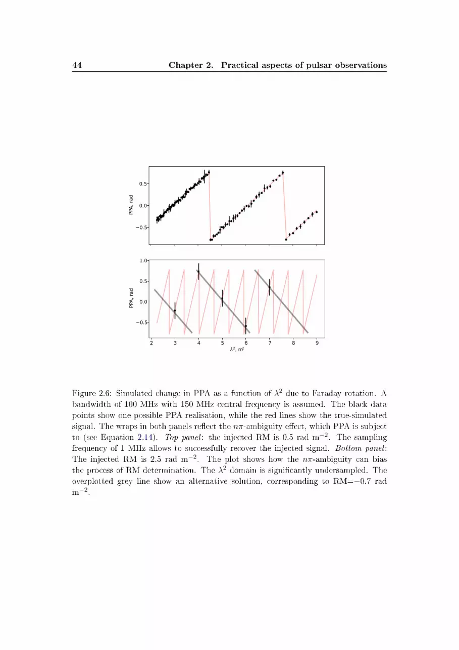
44 Chapter 2. Practical aspects of pulsar observations
2 3 4 5 6 7 8 9λ, m2
−0.5
0.0
0.5
PPA
, ra
d
2 3 4 5 6 7 8 9λ2, m2
−0.5
0.0
0.5
1.0
PPA
, ra
d
Figure 2.6: Simulated change in PPA as a function of λ2 due to Faraday rotation. Abandwidth of 100 MHz with 150 MHz central frequency is assumed. The black datapoints show one possible PPA realisation, while the red lines show the true-simulatedsignal. The wraps in both panels reect the nπ-ambiguity eect, which PPA is subjectto (see Equation 2.14). Top panel : the injected RM is 0.5 rad m−2. The samplingfrequency of 1 MHz allows to successfully recover the injected signal. Bottom panel :The injected RM is 2.5 rad m−2. The plot shows how the nπ-ambiguity can biasthe process of RM determination. The λ2 domain is signicantly undersampled. Theoverplotted grey line show an alternative solution, corresponding to RM=−0.7 radm−2.

2.4. On probing pulsar polarisation 45
These problems can be eradicated when other, more general, methods for RMdetermination, such as QU-tting and RM synthesis, are applied.
RM synthesis RM synthesis, a technique that was initially proposed by Burn (1966),and then further developed by Brentjens & de Bruyn (2005), is nowadays broadlyused in the eld (e.g. Mao et al., 2010; Noutsos et al., 2015). It can be shownthat a non-zero RM gives rise to harmonic signals in both of the Stokes Q and U ,which are shifted by π/2 with respect to each other (see the Equations (2.11)).The theoretically predicted Stokes Qmod and Umod are given by:
Qmod(λ2) = Ipcos(2χ)cos(2ΨPPA) = Ipcos(2χ)cos(2RMλ2 + 2Ψ0),
Umod(λ2) = Ipcos(2χ)sin(2ΨPPA) = Ipcos(2χ)sin(2RMλ2 + 2Ψ0).(2.15)
In order to not only estimate the absolute value of RM, but also determine itssign, one needs to perform an FFT on the measured complex linear polaristionPPP = Q+ iU , also known as the polarisation vector:
F (RM) =
∫ +∞
−∞PPP (λ2)e−2iRMλ2dλ. (2.16)
The peak in the power spectrum will correspond to the sought RM. Faradaythick structures, probed with extended sources, will be shown in the spectrumas extensive patterns with multiple peak. RM synthesis implements this simpleidea, but with some nuances.
The main problem that arises in reality, is that PPP is dened for a nite numberof frequency channels Nch. The situation is further exacerbated by irregularsampling in the λ2 domain, as well as due to the excision of frequency channelsbecause of RFI. The more incomplete the coverage of λ2 is the stronger the side-lobes in the power spectrum, which can bias the RM determination process. Fora realistic case the observed polarised ux can be expressed as:
PPP (λ2) = W (λ2)PPP (λ2). (2.17)
W (λ2) is the windowing function, which is nonzero, where measurements weretaken, and zero elsewhere. The windowing function W (λ2) can be generalisedfor the case of unequal performance of dierent frequency channels, by weightingW (λ2) with (S/N)2 for each frequency channel. Then, by making use of theconvolution theorem, the Fourier transform (FT) of the unevenly sampled PPP (λ2)
is:
F (RM) =
∫ +∞
−∞PPP (λ2)e−2iRMλ2dλ = F (RM) ∗ W (RM), (2.18)
where W (RM) is the FT of the window function. In practice, if RM(δλ2) 1,where δλ is the average bandwidth of the channels, the integrals can be rewritten

46 Chapter 2. Practical aspects of pulsar observations
as sums:
F (RM) =
Nch∑j=1
PPP (λ2j )e−2iRM(λ2j−λ20),
W (RM) =
Nch∑j=1
W (λ2j )e−2iRM(λ2j−λ20),
(2.19)
where λ0 is the central wavelength, which is introduced in the equations to sta-bilise the rapidly oscillating behaviour of the real and imaginary parts of the FTof PPP (λ2) (Brentjens & de Bruyn, 2005; Heald, 2009). In order to recover thepower spectrum of the original polarised ux, F (RM), one needs to perform adeconvolution routine, for example one analogous to the clean algorithm de-signed for the purposes of aperture synthesis (Högbom, 1974). More completecoverage in the λ2-domain increases the quality of the reconstructed F (RM).
The uncertainties on the measured RM are dened by the following semi-empiricalexpression14:
σRM =δφ
2× (S/N)L=
3.8
2×∆λ2(S/N)L. (2.20)
Larger bandwidths ∆λ2 decrease the width of the peak in the Faraday spectra δφand, thus, increase the accuracy of the determined RM. The application of RMsynthesis on example data of PSR J0953+0755 is demonstrated in the right-handpanel of Figure 2.7 C.
QU-tting The Equations (2.15) can be utilised directly without any further manip-ulations, and a simultaneous t of both Q(λ2) and U(λ2) can be performed. Tond the best-t RM one can minimise the sum of the squares of the residuals (ormore generally a maximumise the likelihood):
Nch∑i=1
(Qobs,i −Qmod)
σ2Q,i
+(Uobs,i − Umod)
σ2U,i
, (2.21)
where σQ and σU are the uncertainties of the observed Stokes Qobs and Uobs,respectively, measured as the root-mean-square of Q and U in the o-pulse regionin each frequency channel. Qmod and Umod are the theoretically predicted Stokesparameters, which in case of a point source are described by Equations (2.15).Within frequentist inference the RM uncertainty can be calculated via the Fisherinformation matrix.
QU-tting has been extensively investigated and developed in Schnitzeler & Lee(2017), where authors have taken into account specitaions of broad-band pulsarobservations, e.g. the observed power-law polarised ux density spectrum of pul-sars. The QU-tting has been also successfully enhanced and implemented for
14The factor 3.8 was empirically derived in Schnitzeler et al. (2009)

2.4. On probing pulsar polarisation 47
RM determination of extended sources (e.g. O'Sullivan et al., 2012; Schnitzeleret al., 2015; Ma et al., 2017). An example application of the method to pulsardata is demonstrated in the right-hand panel of Figure 2.7 A. This method wasfurther developed within this thesis (see Chapter 3).
RMFIT is a brute-force method for the RM determination of pulsars, which is asubroutine of the psrchive package. The presumed RM range is split into steps.A given psrfits pulsar archive is derotated with user-dened trial RMs, in orderto nd the RM value that maximises the frequency-averaged linearly polarisedintensity:
L(RM) =
Nch∑i=1
√Q2
RM,i + U2RM,i.
The peak in the resultant RM spectrum is tted with a Gaussian, the centroid ofwhich determines the best-t RM. The RM uncertainty is estimated as the widthof the Gausssian divided by the (S/N)L. Figure 2.7 B shows rmfit applied tothe example data of PSR J0953+0755.
Bayesian Generalised Lomb-Scargle Periodogram is a method that is aimed atsearching for periodicities in the data series. Within this thesis the method wasadapted and applied for the rst time to RM determination. The details ofthis technique are described in Chapter 3. The application of the method isdemonstrated in Figure 2.7 D.

48 Chapter 2. Practical aspects of pulsar observations
RM synthesis
rmfit
BGLSP
A
B
C
D
E
F
Figure 2.7: Faraday rotation of PSR J0953+0755 in the example data taken withLOFAR HBA. A) Normalised Q/I and U/I intensities as a function of observing fre-quency. The observed values for Q/I and U/I are shown with grey dots, while thered lines show the best-t solution: RM=2.96±0.003 radm−2. B) Application of thermfit routine. The black line shows the linear intensity L, the best-t Gaussian t-ted to the peak of the RM spectrum is shown with the red line. The inferred valueis RM=2.95±0.02 radm−2. C) Black line shows the RM spectrum constructed withthe RM synthesis technique. The inferred value is RM=2.97±0.001 radm−2. D) Theapplication of the BGLSP method. The black line shows the logarithm of the RMposterior probability. The inferred value is RM=2.96±0.003 radm−2. E) Stokes Q asa function of pulse phase and observing frequency. The top plot shows uctuations inStokes Q caused by the Faraday eect. The bottom plot shows the integrated StokesQ prole, which is misrepresented due to a nonzero RM. F) The same as E), but afterthe signal was de-rotated with RM=2.96 radm−2. The shape of the integrated Q iscorrectly restored.

Chapter 3
Bayesian Generalised Lomb-Scargle
Periodogram
The work presented in this section is based on Appendices A, B and C of the following
article:
• N. K. Porayko, A. Noutsos, C. Tiburzi, J.P.W. Verbiest, A. Horneer, J.Künsemöller, S. Osªowski, M. Kramer, D.H.F.M. Schnitzeler, J.M. Anderson,M. Brüggen, J.-M. Grieÿemeier, M. Hoeft, D.J. Schwarz, M. Serylak, O. Wuck-nitz; "Testing the accuracy of the ionospheric Faraday rotation corrections through
LOFAR observations of bright northern pulsars", 2019, MNRAS, 483, 4100
In this part of the publication, I have adapted the Bayesian Generalised Lomb-ScarglePeriodogram technique and further develop it for the RM determination problem.
Contents
3.1 Basic denitions . . . . . . . . . . . . . . . . . . . . . . . . . . . . 49
3.2 Derivation of the marginalised posterior probability . . . . . . 51
3.3 Limitations of the method and ways for further improvement 53
As it was shown in Chapter 2, the eect of Faraday rotation induces harmonic signalsin the observed Stokes Q and U with period equal to π/RM as a function of the squareof the observational wavelength. Here we develop an algorithm, based on Bayesiangeneralised Lomb-Scargle periodogram, which incorporates Stokes I, Q and U in orderto estimate the RM of a polarised radio point source. The algorithm also quantiesuncertainties of the tted RM, assuming the noise of Stokes I, Q and U follow aGaussian distribution. We also discuss limitations of the algorithm as well as prospectsof future improvements.
3.1 Basic denitions
Building on the QU-tting technique, described in Section 1.4.3, and taking into ac-count the specics of the observational setup, we further develop the method of RMdetermination for the case of point sources. As mentioned in Section 1.4.3, if thedata are not inuenced by the eects of multibeam propagation such as dierential

50 Chapter 3. Bayesian Generalised Lomb-Scargle Periodogram
Faraday rotation and wavelength-dependent polarization (Sokolo et al., 1998), theinduced variation in the polarization angle is simply proportional to the square of theobservational wavelength λ.
Mathematically, the problem of RM determination can be described in the followingway. The modelled Stokes Qmod and Umod can be expressed as (from Equation (2.15)):
Qmod(λ2) = Imodp cos(2χ) cos(2RMλ2 + 2ψ0),
Umod(λ2) = Imodp cos(2χ) sin(2RMλ2 + 2ψ0).(3.1)
In practice, we can only access measured Stokes parameters Iobs, Qobs, Uobs, corruptedby noise. For the sake of simplicity, as we do not know the intrinsic intensity of thesource if we do not perform ux calibration, we use Qobs/Iobs and Uobs/Iobs, denoted asq and u, respectively. In this method, we assume that q and u are distributed normallyaround their mean values with variances:
σq =Q
I
√(σQQ
)2
+(σII
)2,
σu =U
I
√(σUU
)2+(σII
)2,
(3.2)
where σI , σQ and σU are the standard deviations of the observed Stokes parameters inthe o-pulse region.
To recover the RM, we have adapted the method of the Bayesian GeneralisedLomb-Scargle Periodogram (BGLSP), described in Bretthorst (2001) and Mortier et al.(2015). Although we kept the spirit of the original BGLSP method, some modicationshad to be introduced in order to make the method applicable to the problem of RMsearching. To be more specic, we have synthesised the ideas from both Bretthorst(2001) and Mortier et al. (2015), and created an algorithm which recovers the period ofa complex signal Q+ iU with the two constant osets γq and γu, which are associatedwith the instrumental peak. This resultant algorithm can recover the harmonic signalin RM ranges from π/[λ2
max−λ2min] up to approximately the average Nyquist boundary
π/2δ(λ2), where δ(λ2) is average bandwidth of the channels, determined by the sizeof the frequency channel, and λmin and λmax are the lowest and highest observationalwavelengths, respectively. In case of LOFAR HBAs, the range of available RMs is0.5− 120 radm−2.
By writing ci = cos(2RMλ2i − θ) and si = sin(2RMλ2
i − θ), the normalised Stokesqobs and uobs can be expressed as
qobs,i = Aci +Bsi + γq + εq,i, and
uobs,i = −Asi +Bci + γu + εu,i,(3.3)
where A and B are the amplitudes of the oscillation, and θ is an arbitrary phasereference point, which does not aect the RM and is dened in Section 3.2. Thenoise contributions εq,i and εu,i are assumed to be normally distributed, with standarddeviations σq,i and σu,i and to vary independently across frequency channels.

3.2. Derivation of the marginalised posterior probability 51
As the integration time of our observations is not innitely small, the rate of changeof the ionospheric RM during the integration time will introduce an additional ambi-guity to the measured RMs, which we have taken into account here by introducing theparameter η (see also Schnitzeler & Lee, 2017). It acts eectively as a multiplier for allthe Q and U error bars (see Section 3.2) and is correlated with the reduced χ2 value.
According to Bayes' theorem, the posterior probability Ppst can be written as
Ppst(parameters|data) =Ppr(parameters)P (data|parameters)
P (data), (3.4)
where Ppr(parameters) is the prior distribution of the unknown parameters,P (data|parameters) is the likelihood function, P (data) is the so-called Bayesian ev-idence, which is a normalization factor in our case and plays an important role in theproblem of model selection. Assuming uniform prior distributions of the parameters,the posterior probability is proportional to a likelihood :
Pposterior(A,B, γq, γu,RM, η|qobs,i, uobs,i)
∝ ΠNch
i=1
1√2πσq,iη
exp
(−(qobs,i −Aci −Bsi − γq)2
2(σq,iη)2
)×ΠNch
i=1
1√2πσu,iη
exp
(−(uobs,i +Asi −Bci − γu)2
2(σu,iη)2
).
(3.5)
The resultant form for the posterior probability is analytically marginalised over thenuisance parameters [A, B, γq, γu] (see Equation (3.9)) and is provided in the nextsection. The parameter η was estimated separately, using Equation (3.11), and xedto its maximum likelihood value.
3.2 Derivation of the marginalised posterior probability
Here we provide the derivation of the marginalised posterior probability Pposterior fromEquation (3.5). Using similar notations to Mortier et al. (2015), we can determinethe part of the expression for the posterior probability which depends on unknownparameters (called Sucient Statistics) as1:
lnPposterior (A,B, γq, γu,RM|qobs,i, uobs,i)
∝ −1
2
Nch∑i=1
[(qobs,i −Aci −Bsi − γq)2
σ2q,i
+(uobs,i +Asi −Bci − γu)2
σ2u,i
]
=1
2(− ˆY Y + 2A ˆY C + 2BY S + 2γqYq + 2γuYu −A2CC −B2SS − γ2
qWq
− γ2uWu − 2AγqCq − 2AγuCu − 2BγqSq − 2BγuSu).
(3.6)
The cross term AB∑Nch
i=1 (ωq,i − ωu,i) cisi can be suppressed by assuming thattan(2θ) =
∑Nch
i=1 (ωq,i − ωu,i) sin(4RMλ2
)/∑Nch
i=1 (ωq,i − ωu,i) cos(4RMλ2
). In the
1Parameter η will be introcuduced later in this chapter
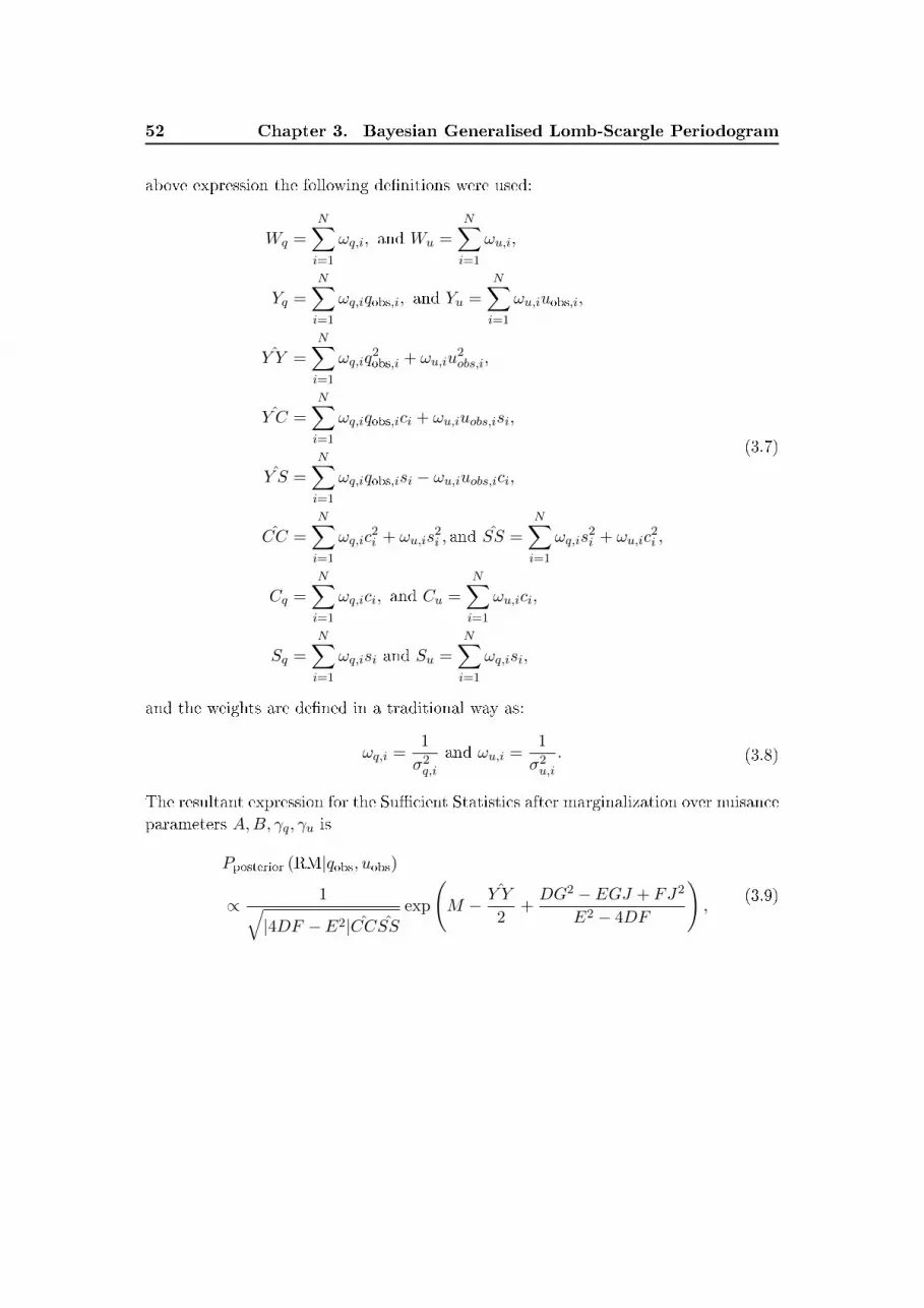
52 Chapter 3. Bayesian Generalised Lomb-Scargle Periodogram
above expression the following denitions were used:
Wq =
N∑i=1
ωq,i, and Wu =
N∑i=1
ωu,i,
Yq =N∑i=1
ωq,iqobs,i, and Yu =N∑i=1
ωu,iuobs,i,
ˆY Y =N∑i=1
ωq,iq2obs,i + ωu,iu
2obs,i,
ˆY C =
N∑i=1
ωq,iqobs,ici + ωu,iuobs,isi,
Y S =N∑i=1
ωq,iqobs,isi − ωu,iuobs,ici,
CC =N∑i=1
ωq,ic2i + ωu,is
2i , and SS =
N∑i=1
ωq,is2i + ωu,ic
2i ,
Cq =
N∑i=1
ωq,ici, and Cu =
N∑i=1
ωu,ici,
Sq =N∑i=1
ωq,isi and Su =N∑i=1
ωq,isi,
(3.7)
and the weights are dened in a traditional way as:
ωq,i =1
σ2q,i
and ωu,i =1
σ2u,i
. (3.8)
The resultant expression for the Sucient Statistics after marginalization over nuisanceparameters A,B, γq, γu is
Pposterior (RM|qobs, uobs)
∝ 1√|4DF − E2|CCSS
exp
(M −
ˆY Y
2+DG2 − EGJ + FJ2
E2 − 4DF
),
(3.9)

3.3. Limitations of the method and ways for further improvement 53
where
D =C2q SS + S2
q CC −WqCCSS
2CCSS,
F =C2uSS + S2
uCC −WuCCSS
2CCSS,
E =CuCqSS + SuSqCC
CCSS,
J =Cq ˆY CSS + SqY SCC − YqCCSS
CCSS,
G =Cu ˆY CSS + SuY SCC − YuCCSS
CCSSand
M =ˆY C
2SS + Y S
2CC
2CCSS.
(3.10)
The resultant expression can be easily generalised for the case of underestimated uncer-tainties in StokesQ and U by including an extra free parameter η, such that ωq → η−2ωqand ωu → η−2ωu. In this case the resultant marginalised posterior probability will bea function of two parameters: Pposterior (RM, η|qobs, uobs).
In order to determine the unknown parameters within the Bayesian framework, oneneeds to numerically reconstruct the 2D posterior probability, which can be eectivelymanaged by Markov Chain Monte Carlo. In the frequentist approach, which is lesscomputationally expensive and was used in this work, we are interested in the maximumlikelihood estimation of the unknown parameters, which for η can be found analytically:
η2 = − 2
2Nch − 4
[M −
ˆY Y
2+DG2 − EGJ + FJ2
E2 − 4DF
]. (3.11)
By performing a 1D grid search in the RM parameter space, we can successfullyrecover the RM posterior probability distribution (see Figure 2.6, 4.1). The uncertaintyin the RM value is determined as the variance of the normal Gaussian distribution, tto the resultant shape of the posterior probability.
3.3 Limitations of the method and ways for further im-
provement
By postulating that the observed Stokes Iobs, Qobs and Uobs are normally distributed,one can derive that q and u will actually follow a Cauchy-like distribution. InSchnitzeler & Lee (2017) it was shown that the non-Gaussianity of q and u can bias theuncertainty of measured RMs in the low S/N regime. However, in the case of high S/N(i.e., σI/I < 0.1, see Hayya et al. (1975); Kuethe et al. (2000)), the resultant Cauchydistribution can be reasonably well approximated by the normal distribution. By select-ing frequency channels above the threshold, and simulating the normally-distributed

54 Chapter 3. Bayesian Generalised Lomb-Scargle Periodogram
6.17 6.18 6.19 6.20 6.21 6.22 6.23 6.24
RM, rad m−2
0
20
40
60
80
100
120
140
Nr.
of
occ
ure
nce
s
Figure 3.1: Distribution of the reconstructed RMs for simulated data of PSRJ1136+1551 (grey line) and posterior probability of RM as predicted with the BGLSPmethod (black line). The vertical dashed lines show the quantiles of the reconstructeddistribution Q16% and Q84%. Half of the interquartile range of the RM distribution, re-constructed from the simulations, is (Q84%−Q16%)/2 = 0.009 radm−2, while the 1σ un-certainty, determined with the BGLSP is 0.0092 radm−2. The S/N of PSR J1136+1551in linear intensity is '50.
Stokes parameters in each of them, we have reconstructed the RM posterior distribu-tion determined with the BGLSP method. For the two pulsars that we have includedin the test (PSRs J0332+5434 and J1136+1551 observed with the LOFAR HBAs), wehave found that the distribution of the resultant RMs can be well approximated by anormal one and its parameters (variance and mean) are in good agreement with thosedetermined with the BGLSP. In Figure 3.1 we display the RM distribution for PSRJ1136+1551. The properties of the reconstructed distribution are given in the caption.
Schnitzeler & Lee (2017) demonstrated that this problem can be avoided by intro-ducing Nch (number of frequency channels) nuisance parameters Imod,i, and found theanalytic expression for the likelihood, marginalised over these parameters, in the caseof weakly polarised sources (Lmod Imod). The further analysis of non-Gaussianity ofq and u and its inuence on the distribution of the resultant RMs will be addressed infuture work.
Another potential weakness of the method is so-called channel depolarisation, whicharises due to the nite size of the frequency channels (Schnitzeler & Lee, 2015). Whenconsidering the channel depolarisation, the measured polarisation vector PPP at the chan-

3.3. Limitations of the method and ways for further improvement 55
nels central frequency fc is:
PPP (fc, j) ∼∫ fj+1
fjω(f)PPP (f)e2iRM(c/f)2df∫ fj+1
fjω(f)df
, (3.12)
where ω(f) is the response function of the frequency channel. For the simplest case,when frequency channels have a top-hat response function in the λ2 domain, the ob-served Stokes parameters are depolarised by a factor sinc(RMδλ2), which marginallydepends on λ2. For relatively small RMs and high frequency resolution, such thatRMδλ2 1, the sinc factor approaches 1. In the real datasets we expect to observethe top-hat response in the frequency rather than in the λ2 domain, which causesthe measured amplitude of the polarisation vector P (and, thus, Q and U) to have acomplex dependency on frequency. The channel depolarisation can severely modulatethe signal at the low-frequency part of the band, and possibly bias the resultant RM.However, in Schnitzeler & Lee (2015) it was shown that the eect becomes noticeablewhen the probed RM is larger than
RMboundary ' 1.44× 10⁴ rad m−2
(flow
GHz
) 52(fhigh
GHz
) 12(δf
GHz
)−1
, (3.13)
when a the large part of the observing band is aected by channel depolarisation. In theabove expression, flow, fhigh are the low- and high-ends of the observing band, and δfis the size of the frequency channel. For the LOFAR HBAs RMboundary ' 100 radm−2,signicantly exeeding the RMs considered in this thesis (< 70 radm−2).


Chapter 4
Testing the accuracy of the
ionospheric Faraday rotation
corrections through LOFAR
observations of bright northern
pulsars
The work presented in this section is based on the main text of the following article:
• N. K. Porayko, A. Noutsos, C. Tiburzi, J.P.W. Verbiest, A. Horneer, J.Künsemöller, S. Osªowski, M. Kramer, D.H.F.M. Schnitzeler, J.M. Anderson,M. Brüggen, J.-M. Grieÿemeier, M. Hoeft, D.J. Schwarz, M. Serylak, O. Wuck-nitz; "Testing the accuracy of the ionospheric Faraday rotation corrections through
LOFAR observations of bright northern pulsars", 2019, MNRAS, 483, 4100
For this part of the publication, I have partially performed the observations andreduction of the radio data. I have determined RMs of the pulsars with the BGLSPmethod. Further, I have devised and performed the analysis of the residual systematicand noises after mitigation of the ionospheric Faraday rotation.
Contents
4.1 Introduction . . . . . . . . . . . . . . . . . . . . . . . . . . . . . . 58
4.2 Observations and Data Reduction . . . . . . . . . . . . . . . . . 60
4.2.1 On modelling the ionospheric RM variations: thin layer iono-
spheric model . . . . . . . . . . . . . . . . . . . . . . . . . . . . . 62
4.3 Systematics in the RM residuals . . . . . . . . . . . . . . . . . . 67
4.3.1 Analysis of RM residuals on timescales up to one year . . . . . . 69
4.3.2 Analyis of RM residuals on timescales beyond one year . . . . . 72
4.4 Discussions and Conclusions . . . . . . . . . . . . . . . . . . . . . 74
Faraday rotation of polarized emission from pulsars measured at radio frequencies pro-vides a powerful tool to investigate the interstellar and interplanetary magnetic elds.However, besides being sensitive to the astrophysical media, pulsar observations in ra-dio are aected by the highly time-variable ionosphere. In this article, the amount of

58 Chapter 4. Testing the ionospheric Faraday rotation with LOFAR
ionospheric Faraday rotation has been computed by assuming a thin layer model. Forthis aim, ionospheric maps of the free electron density (based on Global PositioningSystem data) and semi-empirical geomagnetic models are needed. Through the dataof ve highly polarized pulsars observed with the individual German LOw-FrequencyARray stations, we investigate the performances of the ionospheric modelling. In addi-tion, we estimate the parameters of the systematics and the correlated noise generatedby the residual unmodelled ionospheric eects, and show the comparison of the dif-ferent free-electron density maps. For the best ionospheric maps, we have found thatthe rotation measure corrections on one-year timescales after subtraction of diurnalperiodicity are accurate to ∼ 0.06− 0.07 radm−2.
4.1 Introduction
Since their discovery (Hewish et al., 1968), pulsars have been a powerful tool to probethe magnetoionic plasma. Due to frequency-dependent dispersion delay and scatteringof their signals, pulsars can be used to study, e.g., turbulence in the ionised interstellarmedium (ISM) on many orders of magnitude (e.g. Rickett, 1977; Armstrong et al.,1995; You et al., 2007a), the distribution of free electrons in the Milky Way and theLocal Bubble (e.g. Cordes & Lazio, 2002; Bhat et al., 1998), and the electron contentof the Solar wind (e.g. You et al., 2007b; Howard et al., 2016). Magnetised plasmaalso induces Faraday rotation in linearly polarised radiation, that is, a rotation of thepolarization angle Ψ depending on the radiation wavelength λ (see Section 2.4.2),
ΨPPA = Ψ0 + RM λ2, (4.1)
From the above expression one can see that more accurate RM estimations can beachieved with broad-band instruments operating at longer wavelengths.
Due to the high percentage of linear polarisation, and low levels of magnetosphericFaraday rotation (e.g. Wang et al., 2011), pulsars are useful objects to measure RMinduced by the ionised ISM, and hence the Galactic magnetic elds (e.g. Han et al.,2018).
Because the propagation eects strongly depend on λ, low frequencies are favouredfor studies of these eects in pulsars1. Moreover, the steep spectra of pulsars (e.g. Bateset al., 2013) and the reduction of the linear polarisation fractions at high frequencies inpulsar emission (e.g. Johnston et al., 2008b), make the low-frequency band even morepreferable for Faraday rotation studies.
Nevertheless, polarisation studies at low frequencies are challenging. Besides theeects of the magnetised ionised ISM, linearly polarised radiation can be noticeablyrotated by the highly variable terrestial ionosphere. Moreover, it can signicantlydepolarise observations when averaging over several hours. For a review on the propa-gation of radio waves through the ionosphere, see e.g. Wilson et al. (2013) or Thompsonet al. (2001).
1For strongly Faraday rotated sources, such as pulsars in the dense regions(e.g. magnetar in the
Galactic center) and distant active galactic nuclei, RMs can be as well eectively probed with instru-
ments, operating at 1− 2 GHz and higher frequencies.

4.1. Introduction 59
In order to mitigate the ionospheric contribution to Faraday rotation, numeroustechniques have been developed. One very promising approach is based on provid-ing quasi-simultaneous observations of a known background source (e.g. the diusepolarised background), located within the ionospheric correlation spatial scale with re-spect to the source of interest, to recover the ionospheric Faraday rotation (Lenc et al.,2016).
Alternatively, the ionospheric Faraday rotation can be estimated by combining mod-els of the ionospheric electron density and of the geomagnetic eld. In the majorityof the studies that aimed to measure the interstellar Faraday rotation in astronomicalsources (e.g. Weisberg et al., 2004; Han et al., 2006; Yan et al., 2011b), the iono-spheric electron density was computed through the semi-empirical International Ref-erence Ionosphere (IRI) model (Bilitza et al., 2014), which provides monthly-averagedionospheric electron density proles up to 2000 km, as a function of time and loca-tion. However, due to the sparsely distributed ground and space observatories thatcontribute to the IRI model, and the large averaging time, the modelled values of elec-tron densities can signicantly deviate from the real ones (Mosert et al., 2007). Higheraccuracies can be reached by a technique described in Erickson et al. (2001), wherethe ionospheric electron densities are obtained through raw dual-frequency GPS data,recorded with a set of local GPS receivers. When applied to PSR J1932+1059, thevariance of the dierences between the observed RM as obtained at the VLA, and thepredicted ionospheric RM as computed with the AIPS APGPS routine2, was found tobe 0.2 rad m−2.
A handier and less computationally expensive alternative to this approach consistsin using global ionospheric maps of electron column densities in the ionosphere, whichare based on the available data from all the GPS stations spread around Earth. Thistechnique was implemented and tested on a set of pulsars by Sotomayor-Beltran et al.(2013), showing a qualitatively good agreement between the expected and the observedvalues of Faraday rotation. However, Sotomayor-Beltran et al. (2013) have restrictedtheir analysis to probing only two global ionospheric maps (ROBR and CODG), and theresearch was carried out on a set of observations with timespans of only several hours.The standard deviations of the residuals between the RMs, observed and modelled withCODG and ROBR, varied for dierent datasets in the ranges 0.12− 0.20 radm−2 and0.07− 0.20 radm−2, respectively.
In this thesis, we aim to compare the performance, and estimate the accuracyof dierent publicly available global ionospheric maps, when applied to correct forionospheric Faraday rotation in several months of pulsar data. For these goals, weused pulsar observations obtained with the international LOFAR stations in Germany.In Section 4.2 we describe the instrumental and observational setup and our datareduction, including a rst application of a simple ionospheric modelling. In Section 4.3we attempt to model the ionospheric Faraday rotation in our dataset and we analyse thesystematics left in the RM residuals after ionospheric mitigation. In Sections 4.3.1, 4.3.2
2A similar approach is implemented in the ALBUS software https://github.com/twillis449/
ALBUS_ionosphere

60 Chapter 4. Testing the ionospheric Faraday rotation with LOFAR
Table 4.1: Details of the observations used for the white noise plateau investigation(see Section 4.3.1) and for the long-term systematics (see Section 4.3.2)
Short-term
Jname Site Tobs
J0332+5434 DE609 2015-12-19 − 2016-06-13J0814+7429 DE605 2016-01-08 − 2017-04-30J1136+1551 DE601 2016-01-09 − 2016-10-09
Long-term
Jname Site Tobs
J0332+5434 DE605 2014-03-09 − 2017-02-11J0826+2637 DE603 2015-02-22 − 2017-02-03J1136+1551 DE601 2013-09-06 − 2016-12-31J1921+2153 DE605 2014-03-08 − 2017-02-11
we focus on how to correct for the systematics, and show the results obtained after theimplementation of our additional corrections and the comparison of dierent globalionospheric maps. In Section 4.4 we then summarise our ndings.
4.2 Observations and Data Reduction
All the obsevations were conducted with German LOFAR HBAs in stand-alone mode(see Section 2.2.1). Commonly the integration time per pulsar is ∼2-hours. Thespecics for the dataset used in the presented analysis are summarised in Table 4.1. Asit will be shown in the next sections, we focus our analysis on the characterization ofpotential short- and long-term trends in the residuals between the ionospheric modelsand the data. All the selected pulsars have high signal-to-noise ratio (S/N), whichvaries from ∼800 up to ∼2000, and a signicant fraction of linear polarization (at least10%), which allows us to measure the RM with high accuracy and precision. Besidesthis, for the purposes of the short-term analysis, we chose pulsars with a signicantfraction of long, continuous observations (from a few hours to entire days). This al-lows us to properly identify also high-frequency systematics. For the purposes of thelong-term analysis, this last requirement is not strictly necessary, and we thus selectedpulsars with a long observing baselines.
After digitizing and beamforming, the data is recorded on machines at the Max-Planck-Institut für Radioastronomie in Bonn and at the Jülich Supercomputing Centreusing the LuMP (LOFAR und MPIfR Pulsare) Software3. The datasets are then, coher-ently de-dispersed, folded modulo the pulse period and reduced to more manageable10-second sub-integrations with the DSPSR software4 (van Straten & Bailes, 2011), andstored as PSRFITS archives (Hotan et al., 2004). We then excise the radio-frequencyinterference with the COASTGUARD's clean.py surgical algorithm (Lazarus et al., 2016).
In contrast to steerable radio telescopes, the LOFAR antennas are xed on theground, which causes a distortion of the polarisation signal, as well as decrease of the
3https://github.com/AHorneffer/lump-lofar-und-mpifr-pulsare4http://dspsr.sourceforge.net/

4.2. Observations and Data Reduction 61
intrinsic signal intensity, towards low elevations, due to the projection eects (Noutsoset al., 2015). For instance, such an instrumental response is responsible for the so-calledinstrumental peak at 0 radm−2 in the RM spectrum while performing the RM synthesisanalysis (Burn, 1966; Brentjens & de Bruyn, 2005). We mitigate these instrumentaleects by applying a Jones calibration matrix based on the Hamaker measurementequations (see Hamaker et al., 1996; Smirnov, 2011). However, Noutsos et al. (2015)showed that across several hours of observations taken with the Superterp, the intrinsicsignal intensity of the LOFAR antennas signicantly degrades at low elevations (. 30)even after the calibration procedure has been applied.
Due to the fact that radio observations in the LOFAR frequency band are quitesensitive to the highly variable ionospheric layer (van Weeren et al., 2016), we split pul-sar archives into 15-minute subintegrations with the PSRCHIVE software package5 (vanStraten et al., 2012), which corresponds to the minimum time-sampling of ionosphericmaps that we have tested (see Section 4.2.1). This reduces the unresolved contributionof ionospheric RM, while still providing a reasonable S/N.
After this, we estimate the RM for each of the 15-minute subintegrations, buildingan RM time series for each of the analysed datasets. For this, we use an optimisedversion of the classical RM synthesis technique, BGLSP, described in Chapter 3.
In Figure 4.1 we demonstrate the example of the BGLSP application to one of the15-min observation of PSR J1136+1551. We clearly see systematic deviation from themodelled Q and U , which is reected in the spectrum as a low-frequency excess ofpower around 0 radm−2. The origin of these systematics is not known for certain, butit is highly likely that it is associated with instrumental properties, e.g. non-linearityin the instrumental setup. Because the spurious peak aects a small range of valuesaround 0 radm−2, we expect sources with signicant larger RMs to be uneected,suggesting little or no inuence on our results. However, we point out that the resultscan be biased when dealing with astronomical sources with low RM values. In order toprove these considerations, we have performed two tests. Firstly, we tested the basicassumption that any discrepancies between the models and the data are induced byan eect that is strongly frequency dependent. Therefore, we have split data into twosub-bands and measured RM values separately for the bottom and upper half of thebandwidth. The results show that both RM values are in excellent agreement withinthe uncertainties. This suggests that the eect is not strongly depending on frequency.Still, we also tested whether a systematic eect could conspire to mimic a wrong RMvalue. As a worst case scenario, we have investigated the impact of systematics, in casethey had a quadratic dependency on frequency, which would mimic the λ2 dependencyintroduced by the physical eect of Faraday rotation. The simulated Stokes Q andU were evenly sampled in frequency with a realistic 20% of data loss due to radio-frequency interference. We run a Monte Carlo simulation with 103 realizations of thisset-up, for increasing values of RMs from 0 to 20 radm−2. A range of the systematicamplitudes were tested with reduced χ2 of up to 10, as the reduced χ2 detected inthe data did not exceed this value. We found that, starting from an RM value of
5http://psrchive.sourceforge.net/

62 Chapter 4. Testing the ionospheric Faraday rotation with LOFAR
−15 −10 −5 0 5 10 15
RM, rad m−2
0.0
0.2
0.4
0.6
0.8
1.0
Pow
er
0.4
0.2
0.0
0.2
Q/I
110 120 130 140 150 160 170 180 190
f, MHz
0.4
0.2
0.0
0.2
0.4
U/I
Figure 4.1: Top panel : A comparison between the RM spectrum obtained with theclassical RM synthesis (grey line) and the logarithm of the RM posterior probability(black line) given by Equation (3.9) for a 15-minute observation of PSR J1136+1551.All the curves are normalised to the maximum values. The maximum peak correspondsto the observed pulsar RM=9.076 radm−2. Bottom panel : Harmonic variations of theStokes parameters Q and U across the observed bandwidth (grey points). The blacklines show the expected harmonic trend, given the pulsar's RM.
∼ 6 radm−2, the mean and variance of the distribution of the recovered RMs are ina good agreement with the results from BGLSP (see Figure 4.2). This behaviour isexpected, since as soon as the source RM is larger than the width of the systematicfeature, the two signals can be separated reliably.
With the reliability of our RM measurements established by these tests, we proceedto do a rst attempt to mitigate the Faraday rotation ionospheric contribution.
4.2.1 On modelling the ionospheric RM variations: thin layer iono-
spheric model
If not taken into account, the ionosphere introduces noise in the measured RM values.This makes it impossible, for instance, to investigate RM variations caused by the

4.2. Observations and Data Reduction 63
0.000
0.005
0.010
0.015
0.020
0.025
0.030
σ, rad m
−2 BGLSP
Monte Carlo
0 5 10 15 20
RM, rad m−2−0.0005−0.0004−0.0003−0.0002−0.00010.00000.00010.00020.00030.0004
∆ RM, rad m
−2
Figure 4.2: Top panel : The uncertainties on the RM values detected with BGLSP (blackcircles), overplotted with the variance of the distribution of the detected RMs obtainedfrom Monte Carlo simulations (grey stars). The plot demonstrates that BGLSP uncer-tainties are underestimated for |RM|<6 radm−2. Lower panel : The dierence betweenthe injected RMs and the mean values of the Monte Carlo distributions. No systematicdeviations between BGLSP and Monte Carlo can be seen. For both panels the reducedχ2 of the u and q t was 10.
turbulent ionised ISM, which are expected to be ∼ 3−4 orders of magnitude lower thanthe root-mean-square (rms) of the ionospheric RM uctuations (see Equation (4.10)).We now briey recap the ionospheric RM behavior and the ways to model it.
The ionospheric layer, partially consisting of free electrons and positively chargedionised molecules and atoms, extends from 50 km to beyond 2000 km above the Earth'ssurface (Rishbeth & Garriott, 1969). The ionospheric contribution to RM can beestimated to be of the order of 1 − 4 radm−2, however, the essential complexity intreating the ionospheric RM comes from its strong variability, which typically changesduring the day up to 80%. The ionization fraction of the ionospheric shell, mostlycaused by photoionization processes involving the Sun's extreme ultra-violet and X-rayemission, varies signicantly over timescales of minutes (due to Solar ares) up to years(11-year Solar cycle). Besides this, the ionosphere shows diurnal (caused by the relativemotion of the Sun on the celestial sphere) and 27-day periodicities (due to the Solarrotation). As the Earth's atmosphere is not homogeneous and dierent molecules aredominating at dierent heights, the ionospheric shell, does not have a homogeneouselectron density distribution, and achieves its maximum during the day time in theso-called F sublayer, which implies ∼ 50 − 60% of all the electrons in the ionosphere(Bilitza et al., 2017). Because of this, the ionosphere can be reasonably well modelledby a thin shell located at the eective ionospheric height, which is usually estimatedto be between 300 and 600 km above the Earth's surface.
As the projected thickness of the non-uniform ionospheric layer increases out from

64 Chapter 4. Testing the ionospheric Faraday rotation with LOFAR
0.5
1.0
1.5
2.0
RM
,rad
m−
2
PSR J0332+5434
2016/05/13 −2016/05/30 HH:MM, UTC
−64.4
−64.2
−64.0
RM
obs-
RM
iono
,rad
m−
2
May 13 2016
May 15 2016
May 17 2016
May 19 2016
May 21 2016
May 23 2016
May 25 2016
May 27 2016
May 29 2016
May 31 2016
2016/05/13 −2016/05/30 HH:MM, UTC
−64.4
−64.2
−64.0
RM
obs-
RM
iono
-RM
1day
,rad
m−
2
Figure 4.3: Example of application of JPLG ionospheric maps and POMME10 geo-magnetic model to real data of PSR J0332+5434 observed by DE609. Upper panel :modelled ionospheric RM computed with RMextract using JPLG ionospheric maps (ingrey), applied to measured RMs shifted by a constant value RMISM (black dots). Theuncertainties on the modelled RM are smaller than the symbol used. Middle panel :residuals between observed and modelled RM (black dots) before subtraction of 1-daysinusoid. Lower panel : residuals between observed and modelled RM (black dots) aftersubtraction of 1-day sinusoid. The grey dashed line shows the constant value RMISM.The uncertainties on the measured RMs are modied by the values determined throughthe analysis described in Section 4.3.1. Only the observations above ∼ 30 in elevationwere used.

4.2. Observations and Data Reduction 65
the zenith, it is common practice to discard data at low elevations. For this work wehave used a 30 elevation cut-o6. In the case of the ionosphere, and with the mentionedassumptions, Equation (2.13) is reduced to (Sotomayor-Beltran et al., 2013):
RMiono = 2.6× 10⁻¹⁷STEC× Biono radm−2, (4.2)
where STEC (Slant TEC, where TEC stands for `Total Electron Content') is equal tothe column density of electrons [m−2] at the cross-section between the LoS and theionospheric shell and Biono is the projection of the magnetic eld [G] in the F-layer onthe LoS. The thin layer approximation has already been implemented in several codesaimed at the estimation of the ionospheric RM (e.g. in Sotomayor-Beltran et al., 2013).In particular, for the work presented here we use the publicly available RMextract
software7, that estimates the ionospheric RM along a certain LoS and at a certainpoint in time making use of a geomagnetic eld model and a global ionospheric map.An example of ionospheric RM calibration with RMextract, applied to the RM sequenceof PSR J0332+5434, is demonstrated on Figure 4.3 (upper panel). From here on inthis paper for demonstration purposes we have used JPLG maps, which have showedthe second best result in our analysis and are commonly available for the majority ofour observing epochs.
The geomagnetic eld models are conventionally represented as spherical harmoni-cal expansions of a scalar magnetic potential. Several geomagnetic models are publiclyavailable, among which are the Enhanced Magnetic Model (EMM)8, the InternationalGeomagnetic Reference Field (IGRF) (Thébault et al., 2015), the World MagneticModel9, and POMME1010. The lower panel of Figure 4.4 shows a comparison of theionospheric magnetic eld given by EMM, POMME10 and IGRF12, for the years 2013through 2018 for lines of sight from Germany in the direction of 30 in elevation (min-imum elevation used in our work). The plot demonstrates clear systematic behaviour,although, on average between 2013 and 2018, there is less than 0.1% dierence betweendierent geomagnetic models. The discrepancy seems to be increasing with time. Thus,for the future datasets taken around 2020 geomagnetic models with non-evolving withtime geomagnetic parameters will reach few per cent level dierence between them andshould be used with care. Figure 4.5 demonstrates that for low elevation observationsthis dierence can hit 1% from the absolute value.
We have conducted a full analysis by making use of all three geomagnetic models.In order to be concise, we present only the results of POMME10 (Maus et al., 2006)here (see Table 4.2). In the case one of the other two geomagnetic models the resultson parameter estimation and the presence of various systematics in the data remainunchanged.
6This number is partially motivated by the limitations of the polarization calibration method used
in this work7https://github.com/lofar-astron/RMextract8https://www.ngdc.noaa.gov/geomag/EMM/9https://www.ngdc.noaa.gov/geomag/WMM/DoDWMM.shtml10http://geomag.org/models/pomme10.html

66 Chapter 4. Testing the ionospheric Faraday rotation with LOFAR
0.0
0.5
1.0
1.5
2.0
2.5
RM
ion
,ra
dm−
2
IGSG
UQRG
JPLG
CODG
ESAG
EHRG
UPCG
0.5
1.0
1.5
2.0
RM
ion
,ra
dm−
2
EMM+JPLG
POMME10+JPLG
IGRF+JPLG
20142015
20162017
2018
Date
−0.001
0.000
0.001
∆R
Mio
n,
rad
m−
2
POMME-EMM
IGRF-EMM
Figure 4.4: Upper panel : Comparison between ionospheric RMs in the direction ofPSR J0332+5434 observed at constant 30 elevation, as modelled by dierent iono-spheric maps (+POMME10 geomagnetic model). Middle panel : Comparison betweenionospheric RMs in the direction of PSR J0332+5434 observed at constant 30 el-evation, as modelled by POMME10, EMM and IGRF12 (+JPLG ionospheric map).Bottom panel : Dierence between ionospheric RMs in the direction of PSR J0332+5434observed at constant 30 elevation, as modelled by POMME10, EMM and IGRF12(+JPLG ionospheric map). The empty circles show the dierence between IGRF12and EMM. The black stars show the dierence between EMM and POMME10, whichis on average less than 0.001 radm−2 for observations above 30 in elevation.

4.3. Systematics in the RM residuals 67
06:00:00
09:00:00
12:00:00
15:00:00
18:00:00
21:00:00
00:00:00
03:00:00
Time, hh:mm:ss
−0.010
−0.005
0.000
0.005
∆R
M,r
adm−
2
POMME-EMMIGRF-EMM
10
20
30
40
50
60
70
80
90
Ele
v.an
gle
(deg
)
Figure 4.5: Dierence between ionospheric RMs in the direction of PSR J0332+5434observed at multiple elevations along the day, as modelled by POMME10, EMM andIGRF12. The empty circles show the dierence between IGRF12 and EMM. The blackstars show the dierence between EMM and POMME10, which is on average less than0.001 radm−2 for observations above 30 in elevation. The thick gray line shows thechange in PSR J0332+5434 elevation angle.
The global ionospheric maps (publicly available11,12) in IONEX13 format, provideestimates of the vertical TEC. Several global ionospheric maps are available: CODG(from the University of Bern), ESAG and EHRG (European Space Agency), JPLG(Jet Propulsion Laboratory), UPCG and UQRG (Technical University of Catalonia,see Orús et al. (2005)), IGSG (International GNSS Service). Although the maps canbe based on the same GPS data, the published TEC values can vary from group to groupbecause of dierent interpolation schemes and dierent spatial and temporal resolution.In practice, the maps we have used, all have a spatial resolution of 2.5×5(latitude ×longitude). CODG and EHRG have a time resolution of 1 hour, UQRG of 0.25 hoursand the remaining maps (ESAG, IGSG, JPLG and UPCG) have a time resolution of 2hours.
4.3 Systematics in the RM residuals
The residual RM series, after subtraction of the ionospheric model from the observedRM values, show the presence of correlated structures and strong colored noise. Forinstance, Figure 4.6 shows the residual RMs for three dierent pulsars across about
11ftp://cddis.gsfc.nasa.gov/gnss/products/12ftp://igs.ensg.ign.fr/13https://igscb.jpl.nasa.gov/igscb/data/format/ionex1.pdf

68 Chapter 4. Testing the ionospheric Faraday rotation with LOFAR
a 2-month long timespan. As mentioned in the previous section, the ionospheric RMwas corrected by using the RMextract software package, the POMME10 geomagneticeld model, and the CODG/JPLG maps. The CODG time series show similar trend(e.g. the jump of the RM around the 15th of May 2016) despite the pulsars beingsignicantly separated on the sky. The magnitude of these RM variations signicantlyexceeds those expected from astrophysical sources (see Section 4.4 for details). Thisimplies that the origin of the correlations is not interstellar, but an insucient mod-elling of the ionosphere. Moreover, if these maps provide unreliable information aboutthe uncertainties of the TEC values, this will aect the uncertainties of the modelledionospheric RM and, in turn, our ability to determine the signicance of astrophysicalRM variations.
−64.4
−64.2
−64.0
−63.8 PSR J0332+5434
−14.0
−13.8
−13.6
−13.4
RM
obs-R
Mio
no,
rad
m−
2 PSR J0814+7429
2016-04-17
2016-04-24
2016-05-01
2016-05-08
2016-05-15
2016-05-22
2016-05-29
Date
3.75
4.00
4.25
4.50
4.75PSR J1136+1551
Figure 4.6: Residuals (RMobs−RMmod), while applying the CODG+POMME10 (blackdots) and JPLG+POMME10 (red dots) models for three dierent pulsars observed withthree dierent GLOW stations. From top to bottom: PSRs J0332+5434 (with DE609),J0814+7429 (with DE605), J1136+1551 (with DE601).
In order to solve for these issues, we conduct an independent search of the system-atics in the modelled ionospheric RMs, with the aim of obtaining good estimates of thewhite-noise level and the uncertainties for the ionospheric RM time series.

4.3. Systematics in the RM residuals 69
Some of the observed structures in the residuals can be well explained by a diurnalsinusoid with amplitude Ad, the eect of which is demonstrated in Figure 4.7 andFigure 4.3 B,C. Besides being responsible for a 1-day peak in the power spectrum ofthe RM residuals, it also creates a 1-year pseudo-periodicity in the data, as the transittime of the source shifts gradually during the day across the year.
After subtracting the 1-day sinusoid, the spectrum shows obvious evidence of rednoise at high frequencies, and evolves into a white noise plateau at low frequencies (seeFigure 4.8). Such a spectrum is described in our model by a Lorentzian function, alsoknown as an Ornstein-Uhlenbeck process (Uhlenbeck & Ornstein, 1930). In the nexttwo paragraphs we provide the reader with the mathematical description of the foundsystematics and introduce the criteria for the comparison of dierent ionospheric maps.
4.3.1 Analysis of RM residuals on timescales up to one year
The observational evidences, discussed in Section 4.3 allow us to dene a mathematicalmodel to describe the contributions to the observed RM time series with timescaleshorter than a year. As will be pointed out in Section 4.4, the interstellar contributionRMISM is very small, and typically only visible on timescales of order of several years(Yan et al., 2011a). We have restricted the dataset considered in this section to onlyseveral months (Table 4.1), so we can assume this parameter to be constant and, thus,the contribution RMISM will not bias the estimates of the parameters of the systematics.
The vector RMobs = [RMt1 ,RMt2 , ...,RMtN ] that contains the RM time series ofa certain pulsar observed at N epochs ti can be seen as a combination of deterministicand stochastic contributions:
RMobs = RMiono +RM1day + RMISM︸ ︷︷ ︸deterministic
+RMnoise + n︸ ︷︷ ︸stochastic
. (4.3)
RMiono stands for the semi-empirical ionospheric thin layer model of RM variationsdescribed in Section 4.2.1. RM1day is the harmonic signal with 1-day period, that canbe parametrised as RM1day = Ad sin(2πt/1day + φ). RMnoise and n are stochasticnoise contributions. RMnoise is given by the plateau of the Lorentzian spectrum, whoseone-sided spectral density is described as:
S(f) =A2L
f0
[1 +
(ff0
)2] , (4.4)
with AL [rad m−2] being the already mentioned amplitude of the stochastic signal andf0 [day−1] the turnover frequency. From this expression it can be easily shown that,while behaving like red noise on a short time scales, RMnoise reduces to white noisefor f f0 with a constant variance A2
L. By applying the Wiener-Khinchin theorem,the variance-covariance matrix of this process is then given by:
CL = A2L exp(−f0τ), (4.5)
where τ = 2π|ti − tj | with ti and tj are two dierent epochs.

70 Chapter 4. Testing the ionospheric Faraday rotation with LOFAR
−64.5
−64.4
−64.3
−64.2
−64.1
−64.0
RM
obs-
RM
iono
,rad
m−
2
0 5 10 15 20
Time of a Day, hours−64.5
−64.4
−64.3
−64.2
−64.1
−64.0
RM
obs-
RM
iono
-RM
1day
,rad
m−
2
3.8
4.0
4.2
4.4
4.6
RM
obs-
RM
iono
,rad
m−
2
0 5 10 15 20
Time of a Day, hours3.8
4.0
4.2
4.4
4.6
RM
obs-
RM
iono
-RM
1day
,rad
m−
2
Figure 4.7: Top gure: Correlation pattern of the RM residuals after correcting forthe ionosphere with respect to the time in a day of observations for PSR J0332+5434,while using JPLG+POMME10 model. Upper panel : before the subtraction of a 1-daysinusoid. Lower panel : after the subtraction of a 1-day sinusoid. The black thick lineon both plots shows the result of data smoothing. Bottom gure: The same as in theupper gure for PSR J1136+1551 with UQRG+POMME10 model.

4.3. Systematics in the RM residuals 71
10 7 10 6 10 5 10 4
f, Hz10 14
10 12
10 10
10 8
10 6
10 4
Powe
r, ra
d2 m4 y
r
J0332+5434
10 7 10 6 10 5 10 4
f, Hz10 14
10 12
10 10
10 8
10 6
10 4
Powe
r, ra
d2 m4 y
r
J0814+7429
10 7 10 6 10 5 10 4
f, Hz10 14
10 12
10 10
10 8
10 6
10 4
Powe
r, ra
d2 m4 y
r
J1136+1551
Figure 4.8: Power spectrum of the residuals (RMobs − RMmod − RM1day), shown with grey line, whileapplying JPLG+POMME10 model to a 6-month datasets of the circumpolar PSRs J0332+5434 (upperplot), J0814+7429 (middle plot) and J1136+1551 (lower plot). The solid black line shows the theoreticalshape of a Lorentzian spectrum with AL and f0, dened in Table 4.2. The thick dashed line shows thelevel of the uncorrelated noise, as given by RM measurement uncertainties. The thin dot-dashed lineshows the theoretically predicted power spectrum of ionised ISM turbulence (see Equation (4.10)).

72 Chapter 4. Testing the ionospheric Faraday rotation with LOFAR
The uncorrelated white noise component n in Equation (4.3), coming from themeasurement noise of Stokes parameters (see Figure 3.1), has a at power spectraldensity with variance-covariance of the form:
CWN = σ2i δij , (4.6)
with δij being a Kronecker delta and σ the vector of the formal uncertainties of theobserved RMs14, determined via the Bayesian Lomb-Scargle Periodogram described atthe end of Chapter 3.
In order to investigate the properties of the stochastic and deterministic signalsthat emerge in the RM residuals after the ionospheric correction, we use Bayesianinference in the time domain. Given the model in Equation (4.3), and assuming that thestochastic parts are drawn from random Gaussian processes, the posterior probabilityfor the unknown parameters Θ = [AL, f0, Ad, φ,RMISM] is written as:
logPpst(Θ) ∼ logPpr(Θ)
= −N∑i=1
1
2(RMobs −RMiono −RM1day − RMISM)
× C−1 × (RMobs −RMiono −RM1day − RMISM)− 1
2ln(2πdetC),
(4.7)
where C = CL + CWN.We have applied the model discussed in this paragraph to pulsar datasets that span
less than a year (outlined in Table 4.1). The high S/Ns of our pulsars make us moresensitive to the signals generated by the imperfections of ionospheric RM modelling,described by Equation (4.8). The factor fB was xed to 1.11, as found in Section 4.3.2,and, thus, was excluded from the set of free parameters of the model.
In order to explore the 5-dimensional parameter space Θ of Equation (4.3), we rana Markov Chain Monte Carlo simulation, using the Bayesian inference tool MultiNest(Feroz et al., 2009). The priors of the parameters Ppr(Θ) were chosen to be uninfor-mative (see Caballero et al., 2016): uniform for AL, f0, φ, and RMISM and log-uniformfor Ad. A representative example of the obtained 2-dimensional posterior probabilityplot is shown in Figure 4.11.
Because we only used data from a limited group of pulsars, and probed a statisticallynot signicant sample of LoS, the values given in Table 4.2 should not be treated asdenitive solutions. However, our results give a qualitative estimation of the accuracyof dierent ionospheric maps.
4.3.2 Analyis of RM residuals on timescales beyond one year
After subtractingRMiono andRM1day from the observed RM time series, the long termdatasets still show a deterministic linear trends. The trend is not visible on a timescaleof months, but it becomes obvious across several years (see Figure 4.9). We nd that
14The uncertainties are modied by a factor η, see Equation (3.11)

4.3. Systematics in the RM residuals 73
Jan 2014
May 2014
Sep 2014
Jan 2015
May 2015
Sep 2015
Jan 2016
May 2016
Sep 2016
Jan 2017
May 2017
−64.6
−64.4
−64.2
−64.0
RM
obs-
RM
iono
-RM
1day
,rad
m−
2
J0332+5434
fB = 1.11
fB = 1.0
Jan 2015
Apr 2015
Jul 2015
Oct 2015
Jan 2016
Apr 2016
Jul 2016
Oct 2016
Jan 2017
Apr 2017
5.0
5.5
RM
obs-
RM
iono
-RM
1day
,rad
m−
2
J0826+2637
fB = 1.11
fB = 1.0
Oct 2013
Apr 2014
Oct 2014
Apr 2015
Oct 2015
Apr 2016
Oct 2016
Apr 2017
3.5
4.0
4.5
RM
obs-
RM
iono
-RM
1day
,rad
m−
2
J1136+1551
fB = 1.11
fB = 1.0
Jan 2014
May 2014
Sep 2014
Jan 2015
May 2015
Sep 2015
Jan 2016
May 2016
Sep 2016
Jan 2017
May 2017
−17.5
−17.0
−16.5
RM
obs-
RM
iono
-RM
1day
,rad
m−
2
J1921+2153
fB = 1.11
fB = 1.0
Figure 4.9: Absorption of the linear trend due to the application of the fB factor. Thegrey circles correspond to the fB = 1, black dots to fB = 1.11. We here use threeyears of data for (from top to bottom) PSRs J0332+5434, J0826+2637, J1136+1551,J1921+2153. The ionospheric contribution is modelled with JPLG maps combinedwith POMME10 geomagnetic model.

74 Chapter 4. Testing the ionospheric Faraday rotation with LOFAR
such linear trend can be suppressed by scaling the RMiono time series (resulting froma thin layer model) by a constant factor fB. In other words, Equation (4.3) is modiedas
RMobs =RMiono
fB+RM1day + RMISM +RMnoise + n. (4.8)
A positive trend of the order of 1 − 2 × 10⁻⁴ rad m−2 day−1 was noticed in fourpulsars observed with three GLOW stations. Removal of the linear trend, by applyingthe factor fB, is demonstrated in Figure 4.9.
Making use of pulsar datasets that span more than one year (outlined in Table4.1) and all six global ionospheric maps, considered in this paper, the least square testimate was found to be fB = 1.11+0.04
−0.04. The decrease in root-mean-square (rms),mostly due to the elimination of the linear trend, is illustrated in Figure 4.10. Theresults for all three geomagnetic models are identical.
There are several physical interpretations possible for the factor fB. Among themis the possible overestimation of the geomagnetic strength, BLoS, and/or the underesti-mation of the ionospheric eective height (Birch et al., 2002) due to the poor knowledgeof the electron density in Earth's plasmasphere. For instance, fB = 1.11 is equivalentto an increase of the eective height from 450 km up to ∼ 700 km. An explanationto the trend might be searched in the complex dynamical behavior of the ionosphericeective height. As a matter of fact, it has been shown in multiple investigations (e.g.Hernández-Pajares et al., 2011; Arora et al., 2016), that the ionospheric eective heightcan vary from 300 up to 800 km, depending on the time of day, season, and level of So-lar activity. For instance, the 11-year sunspot cycle, the last maximum of which was in2014, can cause signicant ionization in the ionospheric layer, thus both increasing theionospheric thickness and ionospheric eective height (Liu et al., 2007). One promisingway to improve the model is by using the eective heights determined via the IRI-Plassoftware (Gulyaeva et al., 2013), which takes into account plasmasphere contribution(Arora et al., 2016).
The nature of the factor fB is still under investigation and is planned to be testedon a larger sample of pulsars in the future.
4.4 Discussions and Conclusions
In this paper, we have characterised and investigated the deterministic and stochasticRM variations generated by the ionospheric layer through pulsar observations takenwith the German LOFAR stations. The main day-to-day variability was modelledby assuming a thin-layer ionosphere, located at 450 km above the Earth's surface.For this model, the magnetic eld was taken from the publicly available geomagneticmaps (POMME10, EMM, IGRF), while the information about electron densities wasextracted from the selection of dierent global ionospheric maps. Besides that, an ad-ditional signal peaked at a frequency of 1 day−1 in the power spectrum, which wassignicant in almost all processed datasets, and was removed by including in the model

4.4. Discussions and Conclusions 75
0.0
0.5
1.0
1.5
2.0
∆rm
s<
∆rm
s>
J0332+5434 with DE605J0826+2637 with DE603J1136+1551 with DE601J1921+2153 with DE605
1.00 1.05 1.10 1.15 1.20 1.25 1.30
fB
0.0
0.5
1.0
1.5
2.0
∆rm
s<
∆rm
s>
uqrgjplgcodgigsgupcg
Figure 4.10: Upper panel : Rms of the RM residuals obtained by using the JPLGmap (and normalised with respect to the minimum value for each case), vs the fBfactor. We here use 3 years of data for PSRs J0332+5434, J0826+2637, J1136+1551,J1921+2153 (see Table 4.1). Lower panel : Rms of the RM residuals obtained byusing UQRG, JPLG, CODG, IGSG, and UPCG maps (and normalised with respectto the minimum value for each case) vs the fB factor. We here use 3 years of datafor PSR J0332+5434 observed with DE605 (see the text for more details). The trendsshow clear improvements of the modelling when using fB ' 1.10− 1.14
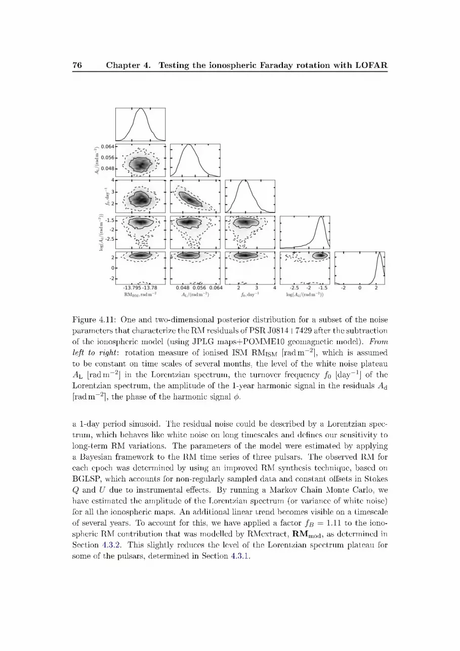
76 Chapter 4. Testing the ionospheric Faraday rotation with LOFAR
0.048
0.056
0.064
AL/(radm−2)
2
3
4
f 0,day−1
-2.5
-2
-1.5
log(A
d/(rad
m−2))
-13.795 -13.78RMISM, radm
−2
-2
0
2
φ
0.048 0.056 0.064AL/(radm
−2)2 3 4f0, day
−1-2.5 -2 -1.5
log(Ad/(radm−2))
-2 0 2φ
Figure 4.11: One and two-dimensional posterior distribution for a subset of the noiseparameters that characterize the RM residuals of PSR J0814+7429 after the subtractionof the ionospheric model (using JPLG maps+POMME10 geomagnetic model). From
left to right : rotation measure of ionised ISM RMISM [radm−2], which is assumedto be constant on time scales of several months, the level of the white noise plateauAL [radm−2] in the Lorentzian spectrum, the turnover frequency f0 [day−1] of theLorentzian spectrum, the amplitude of the 1-year harmonic signal in the residuals Ad
[radm−2], the phase of the harmonic signal φ.
a 1-day period sinusoid. The residual noise could be described by a Lorentzian spec-trum, which behaves like white noise on long timescales and denes our sensitivity tolong-term RM variations. The parameters of the model were estimated by applyinga Bayesian framework to the RM time series of three pulsars. The observed RM foreach epoch was determined by using an improved RM synthesis technique, based onBGLSP, which accounts for non-regularly sampled data and constant osets in StokesQ and U due to instrumental eects. By running a Markov Chain Monte Carlo, wehave estimated the amplitude of the Lorentzian spectrum (or variance of white noise)for all the ionospheric maps. An additional linear trend becomes visible on a timescaleof several years. To account for this, we have applied a factor fB = 1.11 to the iono-spheric RM contribution that was modelled by RMextract, RMmod, as determined inSection 4.3.2. This slightly reduces the level of the Lorentzian spectrum plateau forsome of the pulsars, determined in Section 4.3.1.
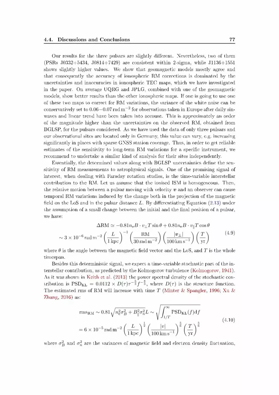
4.4. Discussions and Conclusions 77
Our results for the three pulsars are slightly dierent. Nevertheless, two of them(PSRs J0332+5434, J0814+7429) are consistent within 2-sigma, while J1136+1551shows slightly higher values. We show that geomagnetic models mostly agree andthat consequently the accuracy of ionospheric RM corrections is dominated by theuncertainties and inaccuracies in ionospheric TEC maps, which we have investigatedin the paper. On average UQRG and JPLG, combined with one of the geomagneticmodels, show better results than the other ionospheric maps. If one is going to use oneof these two maps to correct for RM variations, the variance of the white noise can beconservatively set to 0.06−0.07 radm−2 for observations taken in Europe after daily sin-waves and linear trend have been taken into account. This is approximately an orderof the magnitude higher than the uncertainties on the observed RM, obtained fromBGLSP, for the pulsars considered. As we have used the data of only three pulsars andour observational sites are located only in Germany, this value can vary, e.g. increasingsignicantly in places with sparse GNSS station coverage. Thus, in order to get reliableestimates of the sensitivity to long-term RM variations for a specic instrument, werecommend to undertake a similar kind of analysis for their sites independently.
Essentially, the determined values along with BGLSP uncertainties dene the sen-sitivity of RM measurements to astrophysical signals. One of the promising signal ofinterest, when dealing with Faraday rotation studies, is the time-variable interstellarcontribution to the RM. Let us assume that the ionised ISM is homogeneous. Then,the relative motion between a pulsar moving with velocity v and an observer can causetemporal RM variations induced by the change both in the projection of the magneticeld on the LoS and in the pulsar distance L. By dierentiating Equation (2.13) underthe assumption of a small change between the initial and the nal position of a pulsar,we have:
∆RM ' −0.81neB · v⊥T sin θ + 0.81neB · v‖T cos θ
∼ 3× 10⁻⁶ radm−2
(L
1 kpc
)−1( RM
30 radm−2
)( |v⊥|100 km s−1
)(T
yr
) (4.9)
where θ is the angle between the magnetic eld vector and the LoS, and T is the wholetimespan.
Besides this deterministic signal, we expect a time-variable stochastic part of the in-terstellar contribution, as predicted by the Kolmogorov turbulence (Kolmogorov, 1941).As it was shown in Keith et al. (2013) the power spectral density of the stochastic con-tribution is PSDKL = 0.0112 × D(τ)τ−
53 f−
83 , where D(τ) is the structure function.
The estimated rms of RM will increase with time T (Minter & Spangler, 1996; Xu &Zhang, 2016) as:
rmsRM ∼ 0.81√n2eσ
2B +B2
‖σ2nL ∼
√∫ ∞1/T
PSDKL(f)df
= 6× 10⁻⁵ radm−2
(L
1 kpc
) 12( |v|
100 km s−1
) 56(T
yr
) 56
(4.10)
where σ2B and σ2
n are the variances of magnetic eld and electron density uctuation,

78 Chapter 4. Testing the ionospheric Faraday rotation with LOFAR
respectively.These calculations show that the signals of interest are characterised by a very
small amplitudes, of the order of 10−5 − 10−4 radm−2 , which is several orders ofmagnitude lower than the observed RM variations in this work. From the comparisonof the power spectral densities15 we can conclude that we need several decades ofobservations with the current sensitivity (mostly limited by the imperfections of theionospheric modelling) for this kind of signals to become signicant.
More promising signals of astrophysical nature could be registered thanks to ex-treme scattering events (ESEs, Coles et al., 2015), associated with the passage of ablob of high density plasma through the LoS, extreme magneto-ionic environment ofthe source (Desvignes et al., 2018), and coronal mass ejections Howard et al. (2016),which may cause more prominent RM perturbations.
A deeper understanding of the physics of ionospheric behaviour and instrumentalGPS biases, along with the development of more regular GPS station arrays in thedirect vicinity to the radio telescopes will improve the quality of the estimates of TECin the ionospheric layer, which will, in turn, increase our sensitivity to the astrophysicalRM variations.
15PSDKL ' PSDWN = σ2/fNy, where PSDWN is the power spectral density of the white noise and
fNy is the Nyquist frequency of our dataset.

4.4. Discussions and Conclusions 79
PSR J0332+5434
Model AmedL fmed
0 Amedd RMML
ISM
UQRG 0.045+0.003−0.002 1.5+0.2
−0.2 0.012+0.007−0.006 −64.16
JPLG 0.050+0.002−0.002 1.7+0.2
−0.2 0.025+0.007−0.005 −64.21
EHRG 0.054+0.003−0.003 1.2+0.1
−0.1 0.012+0.007−0.008 −64.05
IGSG 0.060+0.003−0.003 1.2+0.1
−0.1 0.02+0.005−0.007 −64.08
ESAG 0.068+0.005−0.004 1.1+0.1
−0.1 0.025+0.007−0.009 −64.05
UPCG 0.073+0.003−0.004 0.9+0.1
−0.1 0.025+0.008−0.014 −64.17
CODG 0.12+0.01−0.01 0.29+0.06
−0.06 0.063+0.009−0.009 −63.95
PSR J1136+1551
Model AmedL fmed
0 Amedd RMML
ISM
UQRG 0.061+0.005−0.004 2.1+0.3
−0.3 0.079+0.01−0.009 4.16
JPLG 0.073+0.004−0.004 1.9+0.6
−0.5 − 4.02
EHRG 0.082+0.005−0.004 1.3+0.2
−0.2 0.03+0.01−0.02 4.22
IGSG 0.142+0.008−0.01 0.6+0.1
−0.1 0.04+0.02−0.02 4.19
ESAG 0.110+0.008−0.007 1.0+0.1
−0.1 0.03+0.02−0.01 4.26
UPCG 0.123+0.010−0.008 0.9+0.2
−0.1 0.08+0.02−0.02 4.18
CODG 0.21+0.02−0.02 0.14+0.03
−0.03 0.08+0.02−0.02 4.18
PSR J0814+7429
Model AmedL fmed
0 Amedd RMML
ISM
UQRG 0.053+0.004−0.003 2.7+0.5
−0.5 0.049+0.006−0.007 −13.75
JPLG 0.051+0.004−0.003 2.3+0.4
−0.4 0.024+0.006−0.008 −13.79
EHRG 0.054+0.003−0.003 2.1+0.3
−0.3 0.033+0.01−0.02 −13.66
IGSG 0.064+0.005−0.004 1.4+0.3
−0.3 0.047+0.01−0.008 −13.69
ESAG 0.067+0.005−0.005 1.5+0.3
−0.3 0.03+0.01−0.01 −13.65
UPCG 0.069+0.005−0.005 1.4+0.3
−0.3 0.045+0.01−0.01 −13.74
CODG 0.10+0.01−0.01 0.7+0.1
−0.1 0.07+0.02−0.01 −13.62
Table 4.2: Estimation of the noise parameters based on the Bayesian analysis of RMresiduals using POMME10 geomagnetic model and dierent ionospheric maps. Theresults for other two considered in this paper geomagnetic models (EMM and IGRF) areindistinguishable within the uncertainties. The used noise model is the one describedin Equation (4.8). The factor fB = 1.11 was applied.


Chapter 5
Investigation of magnetised
interstellar turbulence with pulsars
Contents
5.1 Introduction . . . . . . . . . . . . . . . . . . . . . . . . . . . . . . 82
5.2 Observations . . . . . . . . . . . . . . . . . . . . . . . . . . . . . . 83
5.3 RM variations from the turbulent ISM: mathematical descrip-
tion . . . . . . . . . . . . . . . . . . . . . . . . . . . . . . . . . . . . 84
5.3.1 Theoretical structure function of RM variations . . . . . . . . . . 86
5.3.2 Theoretical covariance function of RM variations . . . . . . . . . 87
5.4 Comparison with observations: parameter estimation and up-
per limits . . . . . . . . . . . . . . . . . . . . . . . . . . . . . . . . 88
5.4.1 Structure function analysis . . . . . . . . . . . . . . . . . . . . . 88
5.4.2 Covariance function analysis . . . . . . . . . . . . . . . . . . . . 89
5.5 Conclusions . . . . . . . . . . . . . . . . . . . . . . . . . . . . . . . 96
The study of magnetic-eld turbulence is crucial for understanding various physicalprocesses taking place in the magnetised plasma of the ISM such as cosmic-ray scatter-ing, magnetic eld reconnection and overall hydrostatic balance of the ISM. Achievingthe detection of RM variations in pulsar emission due to the ionised ISM can shedlight on the properties of the small-scale turbulent magnetic elds. Here, we attemptto measure these variations by using three-year-long datasets of four pulsars: PRSsJ0332+5434, J0826+2637, J1136+1551 and J1921+2153, observed with German LO-FAR stations. After mitigation of the ionospheric Faraday rotation, the datasets oftwo of these pulsars, PSRs J1136+1551 and J1921+2153, exhibit correlated noise, inthe same fashion as expected from ISM turbulence. We speculate that these variationscan be caused by the residual ionospheric Faraday rotation or instrumental noise, asno convincing evidence of astrophysical origin of these variations has been found. Weset an upper limit on the power of the magnetic eld uctuations. Our most stringentconstraints obtained with the datasets of PSRs J0332+5434 and J0826+2637 lie be-low magnetic-eld amplitudes derived in Haverkorn et al. (2008), however, are still 4to 16 times higher than the expected conservative value predicted in Minter & Span-gler (1996) with 95% condence. Finally, we analyse the prospects of detecting of the

82 Chapter 5. Investigation of interstellar turbulence with pulsars
magnetic eld turbulence and conservatively conclude that, assuming the current sen-sitivity, we would need about 20 years of observing timespan to condently detect thesignal as predicted in Minter & Spangler (1996).
5.1 Introduction
Turbulence in the Milky Way is systemic. Among the most striking evidence is the `BigPower Law' of electron density uctuations (Armstrong et al., 1995), fractal structure ofmolecular clouds (Stutzki et al., 1998) and structures in HI data cubes (see e.g. Crovisier& Dickey, 1983; Green, 1991; Stanimirovic et al., 1999). Interstellar turbulent plasmahas been investigated extensively over a wide range of scales from 10−11 to severalpc (Spangler & Gwinn, 1990; Armstrong et al., 1995; Stinebring et al., 2000; Wanget al., 2005; Chepurnov & Lazarian, 2010), however there is a dearth of observationalinformation on turbulent magnetic elds. Magnetic elds have a crucial role in variousastrophysical processes, such as star formation (McKee & Ostriker, 2007) and cosmic-ray propagation (Kóta & Jokipii, 2000), and can signicantly alter the properties ofturbulence. Astrophysical magnetic elds cannot be probed directly: observables whichencapsulate information on these elds, typically depend on other quantities, which onetries to disentangle in order to study these elds directly. One of the tools to prove themagnetised turbulence in the ISM is the RM of background polarised sources, which isthe integrated magnetic eld parallel to the LoS, weighted by the electron density (seeSection 1.4.3). On scales of ∼ 10−100 pc, magnetic-eld statistics have been mainlyinferred from studies of RMs of an ensemble of extragalactic sources (Simonetti &Cordes, 1986; Minter & Spangler, 1996; Clegg et al., 1992; Haverkorn et al., 2008;Oppermann et al., 2012). Structure functions (SFs) of extragalactic RM maps1 derivedin the aforementioned works, all exhibit similar behaviour. It was found that the SFshave shallower slopes than expected from Kolmogorov turbulence and tend to attenon larger scales. The scale at which the SFs saturate is commonly associated withthe injection scale of turbulence, and varies substantailly across the Galaxy (see e.g.Haverkorn et al., 2008).
In this chapter, we discuss which additional information can be inferred about themagnetised ionised phases of the ISM from time-dependent RM measurements of pul-sars. The astrophysical variations in RM are caused by the intrinsic motion of pulsars,which changes both the direction and length of the LoS. We have mostly focused ouranalyses on RM variations caused by the transverse pulsar motion. Due to this motionthe LoS samples dierent parts of the turbulent ISM, which induces a stochasticallychanging, epoch-dependent RM estimate. Through the investigation of these varia-tions, we can gain insights about the turbulent components of the electron densityand magnetic elds on 10−4−10−3 pc-scales2. Moreover, by simultaneously measuringRMs and DMs of a pulsar, the electron-density and magnetic-eld components can be
1SFs measure the mean value of the measurement variance as a function of time dierence of two
observations or angular separation on the sky.2Assuming a typical pulsar velocity of 200 km s−1, the distance that a pulsar travels through the
medium within a year is of order 10−4 pc.

5.2. Observations 83
disentangled and one can estimate the pure contribution of the interstellar magneticelds to the RM variations.
The RM variations induced by astrophysical (non-terrestrial) plasmas have beenobserved for only a few pulsars. Perhaps, the most remarkable example is the Galactic-centre magnetar PSR J1745−2900, which exhibits strong RM variations and up to3500 rad m−2 (Desvignes et al., 2018). The origin of these large RM variations are,most likely, local magnetic phenomena in the Galactic-centre neighbourhood. Johnstonet al. (2005) observed RM variations of 1000 rad m−2 for PSR B1259-63, which is partof a binary system. These observations are consistent with the interpretation that thepulsar emission passes through the dense magnetised disk (ne > 108−1010 cm−3) of itsBe star companion. The Vela and Crab pulsars also show changes in RM (>4 radm−2)and DM (Hamilton et al., 1977; Rankin et al., 1988), which are associated with thelamentary structure of their corresponding supernova remnants observed by the Hub-ble Space Telescope3. Additionally, the abrupt changes in RM and DM can arise dueto ionised shells with a much ner structure than the aforementioned laments. Thesene structures were traced via observations of discrete moving echoes from the Crabpulsar (Lyne et al., 2001).
While all the above sources are associated with extreme local environments, therehas been no clear evidence of RM variations along LoSs probing the diuse ISM (Yanet al., 2011b). In this chapter, we investigate the prospects of detecting RM variationscaused by ordinary ISM turbulence using LOFAR pulsar observations. In Section5.2, we report the details of the observations and data processing. The mathematicalformalism for expected stochastic RM variations is developed in Section 5.3. In Section5.4 we analyse the observed RM time series and set upper limits on the turbulentcomponent of interstellar magnetic eld. In Section 5.5 we summarise our results.
5.2 Observations
The data that are used in this chapter were taken with the LOFAR HBAs and are de-scribed in detail in Chapter 4. In order to investigate the prospects of detecting inter-stellar magnetic uctuations, which are expected to aect the RM time series at longertime scales (e.g. Lazarian & Pogosyan, 2016), we have chosen a long-term dataset,composed of ∼ 3-year observations of four pulsars: PSRs J0332+5434, J0826+2637,J1136+1551 and J1921+21534. The specications of the dataset are given in Table4.1. The pre-processing routines, including folding, implementation of the beam modeland RFI mitigation are described in detail in Section 4.2. The ionospheric mitigationwas performed with the software RMextract5. The geomagnetic eld was modelledwith POMME106 and the electron density in the ionosphere was reconstructed usingUQRG maps (Orús et al., 2005), which on average perform better than other maps,as detailed in Chapter 4. The additional systematics, namely the annual sinusoid and
3https://archive.stsci.edu/4PSRs B0329+54, B0823+26, B1133+16 and B1919+21 when original B1950 coordinates are used.5https://github.com/lofar-astron/RMextract6http://geomag.org/models/pomme10.html
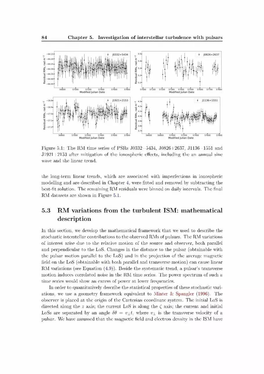
84 Chapter 5. Investigation of interstellar turbulence with pulsars
56800 57000 57200 57400 57600 57800Modified Julian Date
64.45
64.40
64.35
64.30
64.25
64.20
64.15
Resid
ual R
Ms,
rad
m2 J0332+5434
57000 57100 57200 57300 57400 57500 57600 57700 57800Modified Julian Date
5.1
5.2
5.3
5.4
5.5
Resid
ual R
Ms,
rad
m2 J0826+2637
56800 57000 57200 57400 57600 57800Modified Julian Date
17.2
17.1
17.0
16.9
16.8
Resid
ual R
Ms,
rad
m2 J1921+2153
56600 56800 57000 57200 57400 57600 57800Modified Julian Date
3.7
3.8
3.9
4.0
4.1
4.2
4.3
Resid
ual R
Ms,
rad
m2 J1136+1551
Figure 5.1: The RM time series of PSRs J0332+5434, J0826+2637, J1136+1551 andJ1921+2153 after mitigation of the ionospheric eects, including the an annual sinewave and the linear trend.
the long-term linear trends, which are associated with imperfections in ionosphericmodelling and are described in Chapter 4, were tted and removed by subtracting thebest-t solution. The remaining RM residuals were binned on daily intervals. The nalRM datasets are shown in Figure 5.1.
5.3 RM variations from the turbulent ISM: mathematical
description
In this section, we develop the mathematical framework that we used to describe thestochastic interstellar contributions to the observed RMs of pulsars. The RM variationsof interest arise due to the relative motion of the source and observer, both paralleland perpendicular to the LoS. Changes in the distance to the pulsar (obtainable withthe pulsar motion parallel to the LoS) and in the projection of the average magneticeld on the LoS (obtainable with both parallel and transverse motion) can cause linearRM variations (see Equation (4.9)). Beside the systematic trend, a pulsar's transversemotion induces correlated noise in the RM time series. The power spectrum of such atime series would show an excess of power at lower frequencies.
In order to quantitatively describe the statistical properties of these stochastic vari-ations, we use a geometry framework equivalent to Minter & Spangler (1996). Theobserver is placed at the origin of the Cartesian coordinate system. The initial LoS isdirected along the z axis; the current LoS is along the ζ axis; the current and initialLoSs are separated by an angle δθ = v⊥t, where v⊥ is the transverse velocity of apulsar. We have assumed that the magnetic eld and electron density in the ISM have

5.3. RM variations from the turbulent ISM: mathematical description 85
z ζ
L L'
δθ
v ⊥
Figure 5.2: The geometry that is used to derive the SFISM(δθ) and CISM(δθ). Theobserver is at the origin of the coordinate system. The pulsar is moving perpendicularto the z axis with transverse velocity equal to v⊥. The initial and nal directionstowards the pulsar are along z and ζ axis, respectively. The angle between the initialand nal LoSs is δθ = v⊥t. The background picture of turbulence is adapted fromFederrath et al. (2010).
the following form:
n = n0 + δn ,
B = B0 + δB ,(5.1)
where n0 and B0 are the mean components. The random uctuating terms, δn andδB, are assumed to be zero-mean and follow Gaussian statistics. Additionally, it wasassumed that uctuations in the magnetic eld and electron density are independent7.
To describe both electron-density and magnetic-eld uctuations we used a power-law wavenumber spectrum, given by:
Pn(q) = C2n
(q2 + q2
0
pc−2
)−αn/2, PB(q) = C2
B
(q2 + q2
0
pc−2
)−αB/2, (5.2)
where q is the wavenumber. In the above expressions C2n and C2
B are the spectral coe-cients and αn and αB are the spectral indices of the electron-density and magnetic-elductuations, respectively. For homogeneous and incompressible turbulence, the spec-tral index is 11/3; this is commonly referred to as Kolmogorov turbulence. The outerscale of uctuations l0 = 2π/q0 indicates at which wavenumber the power spectrum
7This condition may not hold under certain conditions (Beck, 2001). The relaxation of this condition
will be considered in future work.

86 Chapter 5. Investigation of interstellar turbulence with pulsars
attens and is assumed to be the same for both electron-density and magnetic-eld uc-tuations. From the above expressions, the spatial correlation relations for the electrondensity and magnetic eld are respectively given by:
〈δn(r1)δn(r2)〉 =
∫d3qPn(q)e−iq|r1−r2|,
〈δBj(r1)δBj(r2)〉 =
∫d3qPB(q)e−iq|r1−r2|,
(5.3)
where the angle brackets denote the ensemble average, δBj is the component of δBalong the j-axis, and r1 and r2 denote the vectors towards the source at two dierentarbitrary epochs.
5.3.1 Theoretical structure function of RM variations
A powerful statistical tool which is widely used to study turbulence is the SF. The SFof RM measurements towards dierent LoSs separated by an angle δθ on the sky, isgiven by:
SF(δθ) = 〈[RM(θ)− RM(θ + δθ)]2〉
= 〈[∫ L
0n(z, 0)Bz(z, 0)dz −
∫ L′
0n(ζ cos δθ, ζ sin δθ)Bζ(ζ cos δθ, ζ sin δθ)dζ]2〉,
(5.4)where L and L
′are the length of the LoSs, and Bz = B0z + δBz is the magnetic eld
component along the z axis. For a power-law wavenumber spectrum with 2 < αn,B < 4,given by Equation (5.2), under the assumptions that L ' L′ , Lδθ l0 and l0 < L, thetheoretical SFISM of RM variability produced by the motion of a pulsar is expressed as(Minter, 1995; Minter & Spangler, 1996):
SFISM(δθ) = (0.81)2[f(ρn)B20zC2
nL2ρn+1(δθ)2ρn + f(ρB)n2
0C2BL
2ρB+1(δθ)2ρB+
C2nC2
Bk(ρn, ρB)q1−ρn−ρB0 Lρn+ρB+1
(δθ)2ρnΓ(1− ρn)
2Γ(ρn + 1)+
(δθ)2ρBΓ(1− ρB)
2Γ(ρB + 1)
], (5.5)
where Γ is the gamma function, and
ρ = α/2− 1,
f(ρ) =4π2Γ(1− ρ)
22ρ(2ρ+ 1)ρΓ(1 + ρ),
k(ρn, ρB) =π3Γ(0.5ρn + 0.5ρB − 0.5)2
ρnρB(ρn + ρB + 1)Γ(ρn + ρB − 1).
(5.6)
For a purely Kolmogorov spectrum (ρn = ρB = 5/6) the SFISM behaves as a power lawwith a slope of 5/3. For δθL & l0, SFISM becomes at, i.e. the RM variations becomeless correlated.

5.3. RM variations from the turbulent ISM: mathematical description 87
By comparing the theoretical and observed SFs, one can infer the properties of theISM turbulence, e.g. turning points and slopes of the power spectra. However, as wasshown in Emmanoulopoulos et al. (2010), model parameters estimated via SF analysisshould be interpreted with caution. The major problem is that statistical routines(least-square minimisation, maximum-likelihood estimation) which are commonly usedfor tting the observed SF to the model, assume that tted SF measurements arestatistically independent and follow a Gaussian distribution. Both of these assumptionsare not valid in reality. Non-Gaussianity and lack of statistical independence of SFmeasurements can reinforce underestimation of uncertainties in the model parameters.Additionally, the irregular sampling and nite length of a dataset introduce furtherbiases in the derived quantities.
5.3.2 Theoretical covariance function of RM variations
Alternatively, in order to quantify the RM variability of pulsars, one can use the auto-covariance function C(δθ):
C(δθ) = 〈RM(θ)RM(θ + δθ)〉. (5.7)
For a given geometry applying the conditions in equations (5.2) and (5.3) and assumingagain L ' L
′, Ll−1
0 δθ < 1 and l0 < L, we have parameterised the covariance functionas8:
CISM(δθ) = 〈∫ L
0n(z, 0)Bz(z, 0)dz
∫ L′
0n(ζ cos δθ, ζ sin δθ)Bζ(ζ cos δθ, ζ sin δθ)dζ〉
= C0 −1
2SFISM(δθ),
C0 = (0.81)2Lπ2
(B2
0z
2C2n
ρnq2ρn0
+ n20
2C2B
ρBq2ρB0
+ πC2nC2
Bq0−2ρn−2ρB+1 4ρn+ρBΓ(ρn + ρB − 0.5)2
2ρnρBΓ(2ρn + 2ρB − 1)
)(5.8)
In contrast to the SF formalism, within the formalism used in the covariance function,one directly `ts' observed RMs, which are assumed to be statistically independent, tothe theoretical model (see Equation 5.9). Therefore, the covariance function analysisis expected to recover the true underlying variability with greater robustness. Due toaforementioned reasons, our quantitative results are primarily based on the covariancefunction approach, while the SF analysis was used only for qualitative tests. The tech-nical details of the comparison of theoretical models to the real data and its applicationare demonstrated below.
8The form of the theoretical covariance function was derived within this thesis and was based on
calculations performed in Minter (1995).

88 Chapter 5. Investigation of interstellar turbulence with pulsars
5.4 Comparison with observations: parameter estimation
and upper limits
5.4.1 Structure function analysis
Although the parameters inferred from tting the SFs can be biased, the SF is a usefulillustrative tool for inspecting the evidence of turbulence in the RM and DM of pulsars.As discussed in Section 5.3.1, in the regime where the data are dominated by ISMturbulence, the SFs follow power laws, while in the noise-dominated regime the SFs areexpected to be at. We have calculated the RM SFs using Equation (5.4) for all fourpulsars. Because the considered time series are all irregularly sampled, we have appliedlogarithmic binning of the SFs such that the shortest time lag is the mean samplingtime of the dataset (∼ 7 days). The SF uncertainties were estimated with Monte-Carlo simulations by varying the RM time series within the corresponding measurementuncertainties; the resultant uncertainties were calculated as 1-σ condence intervals ofthe SF distribution over 1000 iterations. Figure 5.3 shows the estimated SFs for eachpulsar. We nd that SFs of PSRs J0332+5434 and J0826+2637 are at within theuncertainties and consistent with SFs of purely white noise, while PRSs J1136+1551and J1921+2153 marginally exhibit a positive power-law scaling in a manner similarto that expected from Kolmogorov turbulence.
101 102
τ , mjd
2× 10⁻³
3× 10⁻³
4× 10⁻³
SF
,ra
d2
m−
4
J0332+5434
102
τ , mjd
10−2
3× 10⁻³
4× 10⁻³
6× 10⁻³
2× 10⁻²
SF
,ra
d2
m−
4
J0826+2637
101 102 103
τ , mjd
10−2
6× 10⁻³
2× 10⁻²
SF
,ra
d2
m−
4
J1136+1551
101 102
τ , mjd
10−2
4× 10⁻³
6× 10⁻³
SF
,ra
d2
m−
4
J1921+2153
Figure 5.3: SFs of the RM time series from Figure 5.1.

5.4. Comparison with observations: parameter estimation and upper
limits 89
5.4.2 Covariance function analysis
In this section we describe how to model the data within the covariance function for-malism using Bayesian statistics. Within the Bayesian framework the data are xedand the model parameters are treated as random variables. The multivariate posteriorprobability of model parameters is then given by:
Ppost(Cn, CB, αn, αB, q0, n0, BLoS,κ,Σ|RMobs) =
1√(2π)n detC
× exp
[−1
2(RMobs −RMmod(κ))TC−1(RMobs −RMmod(κ))
],
C = CWN + CISM,(5.9)
where RMobs is the vector which contains the RM time series of a pulsar observed fora range of δθ. RMmod, which depends on the parameter vector κ, contains all deter-ministic systematics. Specically in our case, the parameters characterising the lineartrend are expected to be signicantly covariant with CB and αB and were thereforeincluded in the model in order to increase the robustness of the results. Therefore,RMmod = κ1 +κ2t, where t is the vector of observational epochs. CWN = (σ2
i + Σ2)δijis the covariance of the uncorrelated white-noise component, where σi are the formaluncertainties of measured RMs, and Σ is the variance of a common white-noise process,associated with the limited accuracy of the modelled ionospheric RMs9. To estimatethe parameters of interest, namely CB and αB, one needs to reconstruct the posteriorprobability Ppost while simultaneously marginalising (numerically or analytically) overunwanted parameters. In our case, the vast majority of model parameters have beenxed to their a priori known values adapted from the literature, implying that theirprior distributions are Dirac delta functions10. Specically, the distances L were takenfrom the ATNF catalogue (Manchester et al., 2005), estimated using the combinedparallax and HI methods (Verbiest et al., 2012). The proper motions measured withradio interferometric and timing measurements were also obtained from the ATNF cat-alogue. The average LoS electron densities were inferred from DM measurements(Bilous et al., 2016), such that n0=〈DM〉/L (see Section 1.4.1). The average magneticeld strength towards the pulsars was estimated using Equation (1.13). LoS dependentparameters are given in Table 5.1.
Building upon previous studies (e.g. Cordes et al., 1985; Armstrong et al., 1995;Donner et al., 2019), electron-density uctuations were assumed to be purely Kol-mogorov with a power-law index αn = 11/3 and spectral coecient C2
n = 10−4
cm−6 pc3. Analyses of the RM of polarised extragalactic sources have shown thatthe outer scale of turbulence diers signicantly across the Galaxy (Haverkorn et al.,2008, and references therein). The inferred outer scale is smaller than about 10 pc for
9As shown in Chapter 4, the noise associated with the imperfectness of ionospheric modelling on
longer time scales can be modelled as an additional white component with variance of ∼0.06 radm−2.10The uncertainties in the distances and proper motions have not been taken into account. For
PSRs J0332+5434, J0826+2637 and J1136+1551 we expect less than 20% change in the upper limits.
However, due to the large uncertainty in the distance towards J1921+2153, the inferred CB can be
signicantly biased. Nevertheless, our overall results and conclusions won't change.

90 Chapter 5. Investigation of interstellar turbulence with pulsars
Jname Bname L, µ, 〈DM〉, 〈RM〉, n0, BLOS,
kpc mas yr−1 cm−3 pc radm−2 cm−3 µG
J0332+5434 B0329+54 1.0+0.1−0.1 19.5(4) 26.2 −64.29 0.03 −3.0
J0826+2637 B0823+26 0.32+0.08−0.05 108(3) 19.5 5.30 0.06 0.3
J1136+1551 B1133+16 0.35+0.02−0.02 375.5(4) 4.8 3.97 0.01 1.0
J1921+2153 B1919+21 0.3+0.8−0.2 36(6) 12.4 −17.03 0.04 −1.7
Table 5.1: The pulsar parameters that have been xed in the analysis. The DMs areadapted from (Bilous et al., 2016), the distances and proper motions are obtained fromthe ATNF catalogue (see text for details). The RMs are obtained in this work.
the spiral arms, while it is around 100 pc for the interarm regions. Two extreme valuesof 5 and 100 pc are considered in the current analysis. When all aforementioned param-eters are xed, the resultant posterior probability is Ppost(CB, αB,κ,Σ|RMobs). Thesampling of Ppost(CB, αB,κ,Σ|RMobs) was performed using the MultiNest software(Feroz et al., 2009). The prior distribution of the non-xed parameters was chosen tobe uninformative, i.e. log-uniform for CB and uniform for other parameters. The fulllist of all the parameters (xed and non-xed) is given in Table 5.2.
Parameter estimation. The reconstructed posterior probabilities for PSRsJ0332+5434 and J0826+2637 (see Figure 5.4) do not show any evidence of the sig-nal described by Equation (5.8). The posterior probabilities for PSRs J1136+1551 andJ1921+2153 are non-uniform, implying the presence of correlated noise, and are shownin Figure 5.5. The inferred CB and αB are in good agreement with the results obtainedwith the SFs, which are demonstrated in the lower panel of Figure 5.5. The obtainedpower spectral indices (αB ∼2.2−2.5) are much shallower than what we expect fromKolmogorov turbulence.
The origin of these signals is still under scrutiny. Beside being caused by theKolmogorov-type turbulence in the ISM, the observed signals could be of terrestrialnature, e.g. unmodelled long-term ionospheric Faraday rotation. As astrophysical RMvariations are thought to be mainly guided by uctuations in electron density (Minter& Spangler, 1996; Haverkorn et al., 2004), a strong conrmation of the astrophysi-cal nature of the observed changes in RM would be covariance with simultaneouslymeasured DMs. The DM measurements were obtained via timing with a frequency-resolved template-matching technique described in e.g. Donner et al. (2019); Tiburziet al. (2019). This method was applied to the same pulsar datasets, with the DM mea-surements provided by J.Donner (private communication). The top panel of Figure5.6 demonstrates the scatter plot of RM vs DM measurements for PSRs J1136+1551and J1921+2153. The Pearson correlation coecients for PSRs J1136+1551 andJ1921+2153 are −0.09 ± 0.05 and −0.05 ± 0.08, respectively, implying no signicant

5.4.Compariso
nwith
observatio
ns:parameterestim
atio
nandupper
limits
91
Table
5.2:List
ofparam
etersused
forthe
Bayesian
analysis.Parameter Value Description References
n0 See Table 5.1 LoS average electron density, cm−3 n0 = 〈DM〉/L
BLoS See Table 5.1 LoS average magnetic eld, µG BLoS = 1.23〈RM〉/〈DM〉
L See Table 5.1 Pulsar distance, pc Manchester et al. (2005)
µ See Table 5.1 Proper motion, mas yr−1 Manchester et al. (2005)
q0 5, 100 Outer scale of turbulence, pc Haverkorn et al. (2008)
Cn 10−2 Electron-density power-law amplitude, cm−3 pc3/2 Armstrong et al. (1995)
αn 11/3 Electron-density power-law index Armstrong et al. (1995)
CB [10−5; 102] Magnetic-eld power-law amplitude, µGpc3/2 Minter & Spangler (1996)
Haverkorn et al. (2008)
αB [2; 4] Magnetic-eld power-law spectral index Minter & Spangler (1996)
κ κ1: [-10; 10] Linear trend parameters:
κ2: [-1; 1] κ1[rad m−2] + κ2[rad m−2 day−1]t
Σ [0; 1] Common white-noise variance, rad m−2

92 Chapter 5. Investigation of interstellar turbulence with pulsars
−7.5−6.0−4.5−3.0−1.5
Log[CB/µG/pc2/3]
2.1
2.4
2.7
3.0
3.3
Pow
er-l
awin
dexαB
2.1
2.4
2.7
3.0
3.3
Power-law index αB−7.5−6.0−4.5−3.0−1.5
Log[CB/µG/pc2/3]
2.1
2.4
2.7
3.0
3.3
Pow
er-l
awin
dexαB
2.1
2.4
2.7
3.0
3.3
Power-law index αB
Figure 5.4: One- and two-dimensional posterior distributions for CB and αB of PSRsJ0332+5434 (left) and J0826+2637 (right). The posterior probabilities are at, there-fore, the RM time series of these two pulsars do not display correlated noise of thefunctional form described by Equation (5.8).
correlation between pulsar RMs and DMs. We have additionally carried out a morerobust correlation test, where we have explored the statistical relation of detrendedRM and DM time series. For detrending we have used non-parametric rst dier-
ences technique, within which we have regressed ∆RM = RM(tj+1) − RM(tj) and∆DM = DM(tj+1)−DM(tj) against each other. The results are shown in the bottompanel of Figure 5.6; the inferred Pearson correlation coecients for PSRs J1136+1551and J1921+2153 are −0.01 ± 0.08 and −0.03 ± 0.1, respectively. Neither of the twocorrelation tests have shown statistical relation between RM and DM for either pulsar.Therefore, there is insucient evidence to claim the astrophysical nature of the signal.
Upper limits. As no astrophysically signicant signal has been found, we insteadplace an upper limit on the amplitude of the turbulent magnetic-eld uctuations.Within the Bayesian framework, the calculation of an upper limit on CB is a matterof parameter estimation. In this framework, it is assumed that a signal is present inthe data, and its amplitude is less than C∗B, with 95%-probability, which is the 95%-Bayesian upper limit. In order to set an upper limit on CB as a function of αB, we dividethe range of αB in small bins, in which we separately reconstruct the joint posteriorprobability of non-xed parameters. In order to obtain robust upper limits, the priordistribution of CB was chosen to be non-informative and conservative, e.g uniform. TheBayesian upper limit C∗B was chosen as the 95%-quantile of the reconstructed posteriordistribution of CB numerically marginalised over all other parameters.
Figure 5.7 (left) shows the upper limits on the spectral coecient C2B as a function

5.4. Comparison with observations: parameter estimation and upper
limits 93
−3.0−2.5−2.0−1.5−1.0
Log[CB/µG/pc2/3]
2.1
2.4
2.7
3.0
3.3
Pow
er-l
awin
dexαB
2.1
2.4
2.7
3.0
3.3
Power-law index αB−2.5−2.0−1.5−1.0−0.5
Log[CB/µG/pc2/3]
2.1
2.4
2.7
3.0
3.3
Pow
er-l
awin
dexαB
2.1
2.4
2.7
3.0
3.3
Power-law index αB
101 102 103
τ , mjd
10−2
6× 10⁻³
2× 10⁻²
SF
,ra
d2
m−
4
J1136+1551
101 102
τ , mjd
10−2
4× 10⁻³
6× 10⁻³SF
,ra
d2
m−
4
J1921+2153
Figure 5.5: Top: One- and two-dimensional posterior distributions for CB andαB of PSRs J1136+1551 (left) and J1921+2153 (right). The black and grey re-gions indicate the 68% and 95% condence intervals. The inferred parametersare log(CB/(µG pc3/2)) = −1.9+0.4
−0.4 and αB = 2.57+0.1−0.07 for PSR J1921+2153;
log(CB/(µG pc3/2)) = −2.2+0.4−0.4 and αB = 2.46+0.1
−0.07 for PSR J1136+1551. Bottom:The observed SFs (black points) overplotted with the theoretically predicted SFs (greylines). The theoretically predicted SFs were calculated as 2Σ2 + SFISM (see Equation(5.5)), where we have used the median value of CB and αB from the covariance functionanalysis.
of the magnetic-eld index αB obtained from the analysis of ∼ 3-year RM time-seriesof PSRs J0332+5434, J0826+2637, J1136+1551 and J1921+2153. Due to the lackof direct measurements of C2
B and αB at the considered scales of 10−4 pc, we havecompared our upper limits to the values adopted from Minter & Spangler (1996) andHaverkorn et al. (2008). In both works, parameters of the magnetic-eld turbulencewere inferred from the investigation of SFs of extragalactic RMs. By analysing theproperties of turbulence in the region at high Galactic latitudes, Minter & Spangler
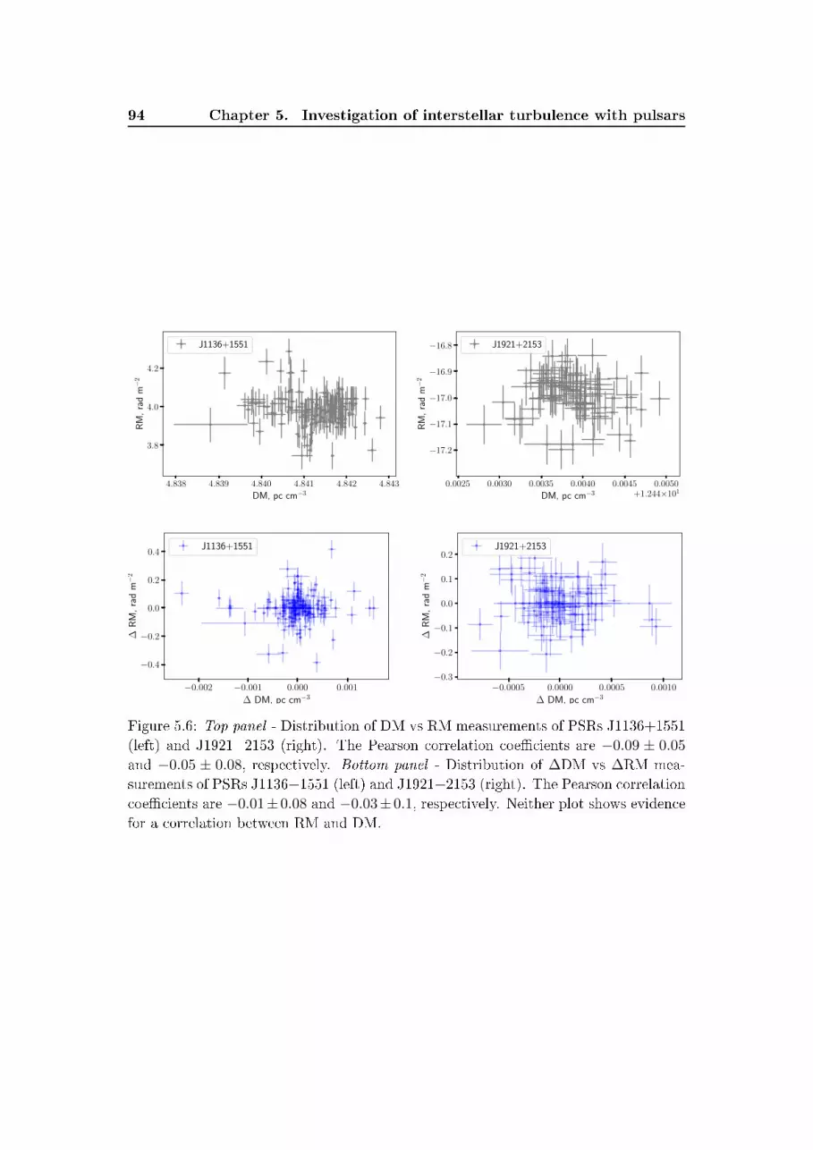
94 Chapter 5. Investigation of interstellar turbulence with pulsars
4.838 4.839 4.840 4.841 4.842 4.843
DM, pc cm−3
3.8
4.0
4.2
RM
,ra
dm−
2
J1136+1551
0.0025 0.0030 0.0035 0.0040 0.0045 0.0050
DM, pc cm−3 +1.244×101
−17.2
−17.1
−17.0
−16.9
−16.8
RM
,ra
dm−
2
J1921+2153
−0.002 −0.001 0.000 0.001
∆ DM, pc cm−3
−0.4
−0.2
0.0
0.2
0.4
∆R
M,
rad
m−
2
J1136+1551
−0.0005 0.0000 0.0005 0.0010
∆ DM, pc cm−3
−0.3
−0.2
−0.1
0.0
0.1
0.2
∆R
M,
rad
m−
2
J1921+2153
Figure 5.6: Top panel - Distribution of DM vs RM measurements of PSRs J1136+1551(left) and J1921+2153 (right). The Pearson correlation coecients are −0.09 ± 0.05
and −0.05 ± 0.08, respectively. Bottom panel - Distribution of ∆DM vs ∆RM mea-surements of PSRs J1136+1551 (left) and J1921+2153 (right). The Pearson correlationcoecients are −0.01±0.08 and −0.03±0.1, respectively. Neither plot shows evidencefor a correlation between RM and DM.

5.4. Comparison with observations: parameter estimation and upper
limits 95
(1996) have inferred C2B = 2.2 × 10⁻² µG2 pc3 for αB = 11/3. In Haverkorn et al.
(2008), authors used a set of extragalactic sources behind the inner Galactic plane.Under the assumption of pure Kolmogorov turbulence (αB = 11/3), the inferred C2
B ∼0.6− 4µG2 pc3. Results of both works are shown in Figure 5.7 with dashed grey lines.
However, it is worth mentioning that the values inferred from studies of extragalac-tic sources should be compared to the results of our analysis with caution. To startwith, the scales probed in this thesis are v⊥t ' 10−6 − 10−3 pc, with the lower limitdened by the cadence of our observations and the upper limit by the timespan of thedataset. The inquired scales in Minter & Spangler (1996) and Haverkorn et al. (2008)are several orders of magnitude larger: from 1 to 103 pc, limited by the range of probedangular separations of used sources. Secondly, the radiation from extragalactic sourcespropagates through the entire column of the Galactic medium, while pulsars used inthis chapter are only probing a small fraction of it. And lastly, in Minter & Spangler(1996); Haverkorn et al. (2008) the RMs of extragalactic sources were not corrected forthe intrinsic and extragalactic Faraday rotation, therefore, the results of these studiescan be biased.
Because of the high proper motion and large average electron density along theLoS, the most stringent constraints on C2
B are set with the RM time series of PSRJ0826+2637. The upper limits obtained with PSRs J0332+5434 and J0826+2637 arealready astrophysically interesting as they lie below C2
B = 0.6µG2 pc3 predicted inHaverkorn et al. (2008), implying that magnetic-eld uctuations with this amplitudeshould have been detected already. However, the aforementioned upper limits are stilla factor of 4 16 higher than the values derived in Minter & Spangler (1996). Theupper limits obtained with PSRs J1136+1551 and J1921+2153 are less constrainingdue to the presence of correlated noise.
We additionally analysed how our upper limits will improve with time. Figure 5.7(right) shows the upper limits on the spectral coecient C2
B as a function of themagnetic-eld index, obtained with the simulated datasets, assuming the RMs aremeasured at the 0.06 rad m−2 accuracy level (see Chapter 4). The proper motion of asource placed 1 kpc from Earth was set to 200 km s−1 (the average two-dimensional pul-sar velocity from Hobbs et al., 2005). The average electron density and magnetic eldtowards the pulsar were assumed to be n0 = 0.01 cm−3 and BLoS =µG, respectively.We have considered three dierent setups: a) a data span of 5 years and observingcadence of 7 days are assumed, while the outer scale of turbulence is xed to q0 =
100 pc; b) a data span of 5 years and observing cadence of 7 days are assumed, whilethe outer scale of turbulence is xed to q0 = 5 pc; c) a data span of 20 years andobserving cadence of 14 days are assumed, while the outer scale of turbulence is xedto q0 = 100 pc. Assuming the current sensitivity, we would be sensitive to magneticeld turbulence in ∼ 20 years (assuming the predictions by Minter & Spangler, 1996).
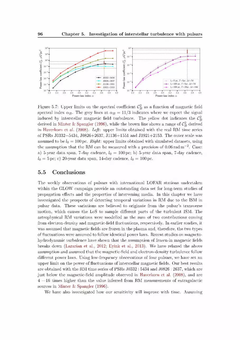
96 Chapter 5. Investigation of interstellar turbulence with pulsars
2.2 2.4 2.6 2.8 3.0 3.2 3.4 3.6 3.8 4.0
Power-law index α
10−9
10−7
10−5
10−3
10−1
101
103
105
Pow
er-l
awco
effici
entC2 B
,µ
G2p
c3
J0332+5434
J0826+2637
J1136+1551
J1921+2153
2.2 2.4 2.6 2.8 3.0 3.2 3.4 3.6 3.8 4.0
Power-law index α
10−9
10−7
10−5
10−3
10−1
101
Pow
er-l
awco
effici
entC2 B
,µ
G2p
c3
l0=5 pc, T=5yr, ∆t=7d
l0=100 pc, T=5yr, ∆t=7d
l0=100 pc, T=20yr, ∆t=14d
Figure 5.7: Upper limits on the spectral coecient C2B as a function of magnetic eld
spectral index αB. The grey lines at αB = 11/3 indicates where we expect the signalinduced by interstellar magnetic eld turbulence. The yellow dot indicates the C2
B
derived in Minter & Spangler (1996), while the brown line shows a range of C2B derived
in Haverkorn et al. (2008). Left : upper limits obtained with the real RM time seriesof PSRs J0332+5434, J0826+2637, J1136+1551 and J1921+2153. The outer scale wasassumed to be l0 = 100 pc. Right : upper limits obtained with simulated datasets, usingthe assumption that the RM can be measured with a precision of 0.06 rad m−2. Case:a) 5-year data span, 7-day cadence, l0 = 100 pc; b) 5-year data span, 7-day cadence,l0 = 5 pc; c) 20-year data span, 14-day cadence, l0 = 100 pc.
5.5 Conclusions
The weekly observations of pulsars with international LOFAR stations undertakenwithin the GLOW campaign provide an outstanding data set for long-term studies ofpropagation eects and the properties of intervening media. In this chapter we haveinvestigated the prospects of detecting temporal variations in RM due to the ISM inpulsar data. These variations are believed to originate from the pulsar's transversemotion, which causes the LoS to sample dierent parts of the turbulent ISM. Theastrophysical RM variations were modelled as the sum of two contributions comingfrom electron-density and magnetic-eld uctuations, respectively. In earlier studies, itwas assumed that magnetic elds are frozen in the plasma and, therefore, the two typesof uctuations were assumed to follow identical power laws. Recent studies on magneto-hydrodynamic turbulence have shown that the assumption of frozen-in magnetic eldsbreaks down (Lazarian et al., 2012; Eyink et al., 2013). We have relaxed the aboveassumption and assumed that the magnetic-eld and electron-density turbulence followdierent power laws. Using low-frequency observations of four pulsars, we have set anupper limit on the power of uctuations of interstellar magnetic elds. Our best resultsare obtained with the RM time series of PSRs J0332+5434 and J0826+2637, which arejust below the magnetic-eld amplitude observed in Haverkorn et al. (2008), and are4 16 times higher than the value inferred from RM measurements of extragalacticsources in Minter & Spangler (1996).
We have also investigated how our sensitivity will improve with time. Assuming
5.5. Conclusions 97
typical characteristics of the ISM towards the pulsar and a realistic noise level whichis mostly dened by the imperfections in the ionospheric modelling, we conservativelyfound that our dataset becomes sensitive to interstellar RM uctuations in ∼ 20 years.This number can be reduced by choosing pulsars with larger apparent velocities andhigher average electron densities along the LoSs as well as by improving the quality ofionospheric modelling.
Two pulsars in our sample, PSRs J1136+1551 and J1921+2153, exhibit correlatednoise in the RM time series, across about three years of data. The origin of the cor-related signal is still not ascertained. Among the possible sources are the inaccuratelymitigated ionospheric Faraday rotation or instrumental biases. If these eects are notthe cause of the observed signal, then it is likely that our observations of those twopulsars have indeed detected magnetic-eld turbulence in the ISM. The inferred power-law indices are much shallower than what we expect from 3D Kolmogorov turbulence.However, the observed signals are in good agreement with two-dimensional turbulence,which predicts a power-law index of 8/3. 2D Kolmogorov turbulence can be observedif one probes turbulent matter within a thin sheet or lament, when the angular sepa-ration is greater than the thickness of the screen (Minter & Spangler, 1996). Moreover,recent simulations have shown that shallower power-law indices are also expected inthe supersonic regime of turbulence (see e.g. Federrath, 2013; Lazarian & Pogosyan,2016, and reference therein). In order to investigate the possible astrophysical natureof the signal, we have additionally tested the covariance between the RM and DMmeasurements. No correlation between the DM and RM of the pulsars measured at thesame epochs has been found. The astrophysical nature of these signals are still underdebate and will be explored further in future work.


Chapter 6
Parkes Pulsar Timing Array
constraints on ultralight scalar-eld
dark matter
The work presented in this section is based on the following article:
• N. K. Porayko, X.-J. Zhu, Y. Levin, L. Hui, G. Hobbs, A. Grudskaya, K. Postnov,M. Bailes, R.N.D. Bhat, W. Coles, S. Dai, J. Dempsey, M.J. Keith, M. Kerr, M.Kramer, P.D. Lasky, R.N. Manchester, S. Osªowski, A. Parthasarathy, V. Ravi,D.J. Reardon, P.R. Rosado, C.J. Russell, R.M. Shannon, R. Spiewak, W. vanStraten, L. Toomey, J. Wang, L. Wen, X. You, PPTA Collaboration; "ParkesPulsar Timing Array constraints on ultralight scalar-eld dark matter", 2018,Phys.Rev.D, 98, 102002
The text, gures, and tables have only been modied to match the style, spelling andformat of the rest of this thesis. X.-J. Zhu and I are the main authors of the paper.For this publication, I have used the newest PPTA dataset to analyse properties of thetiming data within Bayesian framework, and to set Bayesian upper limits on theultralight scalar-eld dark matter density in the Galaxy. Further, I have investigatedhow our sensitivity will increase with future upcoming radio facilities.
Contents
6.1 Introduction . . . . . . . . . . . . . . . . . . . . . . . . . . . . . . 100
6.2 The pulsar timing residuals from fuzzy dark matter . . . . . . 104
6.3 PPTA data and noise properties . . . . . . . . . . . . . . . . . . 105
6.3.1 Observations and timing analysis . . . . . . . . . . . . . . . . . . 105
6.3.2 The likelihood function . . . . . . . . . . . . . . . . . . . . . . . 106
6.3.3 Noise modeling . . . . . . . . . . . . . . . . . . . . . . . . . . . . 108
6.4 Search techniques and Results . . . . . . . . . . . . . . . . . . . . 113
6.4.1 Bayesian analysis . . . . . . . . . . . . . . . . . . . . . . . . . . . 113
6.4.2 Frequentist analysis . . . . . . . . . . . . . . . . . . . . . . . . . 117
6.4.3 Upper limits . . . . . . . . . . . . . . . . . . . . . . . . . . . . . 118
6.5 Future prospects . . . . . . . . . . . . . . . . . . . . . . . . . . . . 120
6.6 Conclusions . . . . . . . . . . . . . . . . . . . . . . . . . . . . . . . 123

100 Chapter 6. PPTA constraints on ultralight scalar-eld dark matter
It is widely accepted that dark matter contributes about a quarter of the critical mass-energy density in our Universe. The nature of dark matter is currently unknown,with the mass of possible constituents spanning nearly one hundred orders of magni-tude. The ultralight scalar eld dark matter, consisting of extremely light bosons withm ∼ 10−22 eV and often called fuzzy dark matter, provides intriguing solutions tosome challenges at sub-Galactic scales for the standard cold dark matter model. Asshown by Khmelnitsky and Rubakov, such a scalar eld in the Galaxy would producean oscillating gravitational potential with nanohertz frequencies, resulting in periodicvariations in the times of arrival of radio pulses from pulsars. The Parkes Pulsar Tim-ing Array (PPTA) has been monitoring 20 millisecond pulsars at two to three weeksintervals for more than a decade. In addition to the detection of nanohertz gravita-tional waves, PPTA oers the opportunity for direct searches for fuzzy dark matterin an astrophysically feasible range of masses. We analyze the latest PPTA data setwhich includes timing observations for 26 pulsars made between 2004 and 2016. Weperform a search in this data set for evidence of ultralight dark matter in the Galaxyusing Bayesian and Frequentist methods. No statistically signicant detection has beenmade. We, therefore, place upper limits on the local dark matter density. Our limits,improving on previous searches by a factor of 2 to 5, constrain the dark matter densityof ultralight bosons with m ≤ 10−23 eV to be below 6GeVcm−3 with 95% condence inthe Earth neighborhood. Finally, we discuss the prospect of probing the astrophysicallyfavored mass range m & 10−22 eV with next-generation pulsar timing facilities.
6.1 Introduction
Dark matter, a concept established in the early 1930s for the purpose of explaining theobserved enigmatic dynamics of disk galaxies and motion of galaxies in clusters (Zwicky,1933, 1937; Smith, 1936), is nowadays considered to be an essential ingredient of theUniverse. It is instrumental in explaining a wide range of astrophysical phenomena,such as strong gravitational lensing of elliptical galaxies (Koopmans & Treu, 2003), thedynamics of interacting clusters (Clowe et al., 2004) and the large-scale structure of theUniverse (Tegmark et al., 2004). The latest analysis of temperature and polarizationanisotropies of the cosmic microwave background (Planck Collaboration et al., 2016)suggested that the Universe contains 26% dark matter, which is ve times more thanordinary baryonic matter such as stars and galaxies.
The most popular dark matter candidates are weakly interacting massive particles(WIMPs) and quantum chromodynamics (QCD) axions. We refer to both as standardcold dark matter, or simply CDM. The CDM paradigm has met with impressive successin matching observational data on large cosmological scales (see Bertone et al., 2005;Primack, 2012, for reviews). Recently, there has been an increased number of ideasabout dark matter that go beyond the standard paradigm, building on old ideas insome cases (see e.g. Battaglieri et al., 2017, for an overview).
One such idea an ultralight axion or axion-like particle can be thought ofas a generalization of the QCD axion. An axion is an angular eld, i.e. the eld

6.1. Introduction 101
range is nite and periodic with a periodicity 2πFaxion with Faxion often referred toas the axion decay constant. A simple axion Lagrangian has a standard kinetic term,and a self-interaction potential V generated by non-perturbative eects (that can beapproximated by instanton potential),
V (φ) = m2F 2axion[1− cos(φ/Faxion)] , (6.1)
where m is the mass of the axion φ. The non-perturbative eects are typically highlysuppressed (e.g. exponentially suppressed by an instanton action), leading to a fairly lowenergy scale
√mFaxion. In the early Universe, the scalar eld is frozen at its primordial
value, generically expected to be order of Faxion. When the Hubble expansion rate dropsbelow the mass scale m, the scalar eld oscillates with an amplitude that redshifts withthe expansion of the Universe. Averaging over oscillation cycles, φ behaves like CDMwith a relic density of (see e.g. Arvanitaki et al., 2010; Hui et al., 2017)1
Ωaxion ∼ 0.1( m
10−22 eV
)1/2(
Faxion
1017 GeV
)2
. (6.2)
String theory contains many axion candidates with Faxion somewhere in the range1016 − 1018 GeV (Svrcek & Witten, 2006). Equation (6.2) tells us that a very low m
is preferred if the axion were to account for dark matter. It should be emphasizedthough that there is a fairly large possible range for m; in fact, the relic abundance ismore sensitive to Faxion than to m. A lighter mass, e.g., m ∼ 10−23 eV, can be easilyaccommodated by a slightly higher Faxion, though it is disfavored by astrophysicalobservations such as the existence and structure of dwarf galaxies2.
Such an ultralight axion has a macroscopic de Broglie wavelength λdB, given by
λdB2π
=~mv≈ 60 pc
(10−22eV
m
)(10−3c
v
), (6.3)
where v is the velocity, implying wave-like phenomena on astronomically accessiblescales, unlike standard CDM. In linear perturbation theory, the wave-like propertyleads to a suppression of power on small scales (small compared to the Jeans scale,which is a geometric mean of the Compton and Hubble scale). It is this propertythat motivated Hu et al. (2000) to propose an ultralight boson as an alternative tostandard CDM, and to coin the term fuzzy dark matter (FDM). The term FDMrefers generally to a scalar dark matter particle with a very small mass, such that itsde Broglie wavelength is macroscopic. An ultralight axion is a particularly compellingrealization. Our constraints derived in this paper apply to the ultralight axion, as wellas the broader class of FDM.
The thinking was that the suppression of power on small scales would help resolvecertain small-scale problems of CDM, which generally have to do with CDM predicting
1The relic density computation follows the classic arguments of Preskill et al. (1983); Abbott &
Sikivie (1983); Dine & Fischler (1983), which were developed for the QCD axion.2Note that the requisite
√mFaxion is much less than the QCD scale; hence this is not the QCD
axion.

102 Chapter 6. PPTA constraints on ultralight scalar-eld dark matter
too much small-scale structure compared to that observed. There is a vast literature onthis subject, but it remains a matter of debate as to whether the perceived small-scalestructure problems of CDM are in fact amenable to astrophysical solutions (such asfeedback processes modifying the mass distribution within Galactic halos; see Bullock& Boylan-Kolchin, 2017, for a review).
There exist several dierent bounds on the FDM model. One class of bounds comesfrom measurements of the linear power spectrum at high redshifts, such as from themicrowave background (e.g. Hloºek et al., 2018), and from the Lyman-alpha forest(Ir²i£ et al., 2017; Kobayashi et al., 2017). In particular, the Lyman-alpha forest dataappear to disfavor a FDM mass lighter than about 10−21 eV. Another example of abound of this kind come from 21-cm observations the recent detection of a global 21-cm absorption signal at redshift around 18 (Bowman et al., 2018) puts a lower limit onthe FDM mass similar to the Lyman-alpha forest bound (Schneider, 2018; Lidz & Hui,2018; Sullivan et al., 2018). Yet another class of bounds comes from dynamical data onthe density proles of galaxies (e.g. Calabrese & Spergel, 2016; Deng et al., 2018; Baret al., 2018). Many of these bounds are subject to their own astrophysical uncertainties.For instance, the Lyman-alpha forest bound is predicated upon the correct modelingof uctuations from such as the ionizing background, the temperature and feedbackprocesses. The 21-cm bound relies on assumptions about star formation (that it tracksthe halo formation and that the fraction of baryons that form stars is less than about5%), and of course, assumes the validity of the detection. Constraints from rotationcurve measurements generally make assumptions about how feedback processes, suchas from stellar explosions, aect (or do not aect) density proles.
Recently, a number of authors, based on numerical simulations and analytical argu-ments, pointed out additional testable astrophysical implications of FDM, especially inthe nonlinear regime (Schive et al., 2014; Mocz & Succi, 2015; Veltmaat & Niemeyer,2016; Hui et al., 2017; Nori & Baldi, 2018; Veltmaat et al., 2018). A particularly in-teresting probe of ultralight dark matter using PTAs was pointed out by Khmelnitsky& Rubakov (2014). Through purely gravitational coupling, scalar eld dark matterinduces periodic oscillations in gravitational potentials with frequency twice the eldmass f ∼ 2m ∼ 5 × 10⁻⁸ Hz (m/10−22 eV). The oscillating gravitational potentialsalong the line of sight of pulsars cause sinusoidal variations in the ToAs of radio pulses.The frequency of such variations lies right in the sensitivity band of PTAs. This wayof detecting or constraining FDM is completely independent of other methods (andtheir assumptions), and provides a useful check. As shown in Khmelnitsky & Rubakov(2014); Porayko & Postnov (2014); De Martino et al. (2017); Blas et al. (2017) andlater in this paper, the current PTA data can only be sensitive to very low-mass FDM(m < 10−23 eV). We will discuss what would be required to probe the higher andcosmologically more favorable masses.
The concept of a PTA is to regularly monitor ToAs of pulses from an array of themost rotationally stable millisecond pulsars (Sazhin, 1978; Detweiler, 1979b; Hellings& Downs, 1983; Foster & Backer, 1990). Measured ToAs are tted with a deterministictiming model that accounts for the pulsar spin behavior and for the geometrical eectsdue to the motion of the pulsar and the Earth. The dierence between the observed

6.1. Introduction 103
ToAs and those predicted by the best-t timing model are called timing residuals (seeSection 2.3 for more details). By analyzing the pulsar timing residuals, we can obtainthe information about other physical processes that aect the propagation of radiopulses through the Galaxy, for instance, the presence of ultralight scalar eld darkmatter in the Galaxy.
The Parkes Pulsar Timing Array (PPTA, Manchester et al., 2013) uses the 64-mParkes radio telescope in Australia. Building on earlier pulsar timing observations atParkes, it started in 2005 to time 20 millisecond pulsars at a regular interval of two tothree weeks. PPTA and its counterparts in North America (NANOGrav, McLaughlin,2013) and Europe (EPTA, Kramer & Champion, 2013) have joined together to form theInternational Pulsar Timing Array (IPTA, Hobbs et al., 2010a; Verbiest et al., 2016),aiming for a more sensitive data set. The IPTA currently observes around 70 pulsarsusing the world's most powerful radio telescopes.
The rst PPTA data release was published in 2013 (Manchester et al., 2013). Itincluded six years of observations for 20 pulsars. This data set was used to searchfor a stochastic GW background (Shannon et al., 2013), continuous GWs (Zhu et al.,2014) and GW bursts with memory (Wang et al., 2015a). The second data release isstill being actively developed, but for this paper, we have made use of a data set thatcontains observations made between 2004 and 2016 with ve new pulsars added since2010. An early subset of this data was used to place the most constraining limit todate on the amplitude of a stochastic GW background in the nHz regime (Shannonet al., 2015).
In this work we search for evidence of ultralight scalar eld dark matter in theGalaxy using the PPTA data. A similar study was carried out through Bayesiananalysis by Porayko & Postnov (2014), using the NANOGrav 5-yr 17-pulsar data setpublished in Demorest et al. (2013). Our work improves on that of Porayko & Postnov(2014) in several ways. First, we make use of an independent data set with muchlonger data span and smaller errors in the timing residuals. Second, we use an up-to-date Bayesian inference packages for PTA data analysis, PAL2 (Ellis & van Haasteren,2017) and NX01 (Taylor & Baker, 2017), and include proper treatment of the noiseprocesses. Re-analyzing the NANOGrav data with the improved analysis, we nd thatthe sensitivity was overestimated by a factor of ten in Porayko & Postnov (2014).Third, we also adopt a standard Frequentist searching method and obtain consistentresults with Bayesian analysis.
Our paper is organized as follows. In Section 6.2, we describe pulsar timing resid-uals expected in the presence of ultralight scalar eld dark matter in the Galaxy. InSection 6.3, we introduce our data set, the likelihood function and our Bayesian andFrequentist methods to model the noise properties of PPTA data. We also present re-sults of our noise analysis. In Section 6.4, we describe our search techniques and applythem to the PPTA data set. As we nd no signicant signals, we set upper limits onthe local density of FDM in the Galaxy. In Section 6.5, we discuss how the sensitivitywill be improved in the future. Finally, we provide concluding remarks in Section 6.6.

104 Chapter 6. PPTA constraints on ultralight scalar-eld dark matter
6.2 The pulsar timing residuals from fuzzy dark matter
In this section we briey describe the magnitude and time dependence of timing resid-uals induced by the scalar eld dark matter in the Galaxy. A detailed derivation canbe found in Khmelnitsky & Rubakov (2014).
Because of the huge occupation number, the collection of ultralight dark matterparticles behaves like a classical scalar eld φ. To a very good approximation, here weignore quartic self-interaction and coupling of ultralight dark matter particles to otherelds3 (Krnjaic et al., 2018; Brdar et al., 2018). The scalar action in this case can bewritten as
Sφ =
∫d4x√−g
[1
2gµνDνφDµφ−
1
2m2φ2
], (6.4)
to which the standard Einstein-Hilbert action for the metric should be added. The φequation of motion is the Klein-Gordon-Fock Equation: (g + m2)φ(x) = 0. We areinterested in a computation of φ and the metric gµν inside the Galaxy. The metric isapproximately Minkowski plus corrections at the level of 10−6. To good approximation,φ everywhere in the Galaxy oscillates at an angular frequency mc2/~ (corrections dueto the momentum of the particles and the gravitational potential are small). Theenergy-momentum tensor to the leading order diagonal and its spatial components(pressure) oscillate at twice the eld particle mass. This produces time-dependentgravitational potentials g00 = 1 + 2Φ(t) and gij = −1 − 2Ψ(t)δij in the metric tensor(in the Newtonian covariant form) with leading oscillating contributions at a frequency
f =2mc2
h≈ 4.8× 10⁻⁸
( m
10−22 eV
)Hz . (6.5)
The amplitude of oscillating parts of the potentials Ψ and Φ are a factor of (v/c)2
smaller than the time-independent parts Φ0 = −Ψ0 ∼ GρFDMλ2dB, where ρFDM is
the local scalar eld dark matter density. For cosmologically favored boson masses∼ 10−22 eV, the frequency is fortuitously located in the sensitivity range of PTAs.
As in the case of GWs (Detweiler, 1979b), pulsar photons propagating in a time-dependent metric undergo a frequency shift δν, which is related to timing residuals(Khmelnitsky & Rubakov, 2014)
s(t) =
∫ t
0
δν
νdt =
Ψc(xe)
2πfsin[2πft+ 2α(xe)]
−Ψc(xp)
2πfsin
[2πf
(t− L
c
)+ 2α(xp)
]+
(Ψ + Φ
2πf
)O(vc
), (6.6)
where L is the distance to the pulsar and Ψc is the amplitude of cosine component ofthe oscillating part of the energy-momentum tensor. The subsequent terms in Equa-tion (6.6) are suppressed with respect to Ψc by a factor v/c ' 10−3, and to the leadingorder the signal s(t) does not depend on the oscillating part of the potential Φ.
3In the axion context, the oscillation amplitude of φ gradually diminishes due to the expansion of the
universe, making the quadratic m2φ2/2 an excellent approximation to the potential in Equation (6.1).

6.3. PPTA data and noise properties 105
As one can see in Equation (6.6), the dark matter signal also has `Earth' and `pulsar'terms. Oscillation frequencies at the Earth and at the pulsar are identical, which makesit analogous to the case of nonevolving continuous GWs (Zhu et al., 2016). The scalar-eld oscillation phases on the Earth α(xe) and pulsar α(xp) generally take dierentvalues; but they become correlated when the Earth and a pulsar are located within thecoherence de Broglie wavelength λdB.
The amplitude Ψc, which can be eectively probed in pulsar timing experiments,depends on the local density of dark matter ρFDM,
Ψc =GρFDMπf2
≈ 6.1× 10⁻¹⁸( m
10−22 eV
)−2(ρFDMρ0
), (6.7)
where ρ0 = 0.4GeV cm−3 is the measured local dark matter density (Bovy & Tremaine,2012; Read, 2014; Sivertsson et al., 2018). The rms amplitude of induced pulsar-timingresiduals is
δt ≈ 0.02 ns( m
10−22 eV
)−3(
ρFDM
0.4GeVcm−3
). (6.8)
The expected signal amplitude scales strongly with the boson mass. At 10−22 eV andabove, the signal is negligibly small. For mass below 10−23 eV, the induced rms residuals(& 20 ns) are comparable to current timing precision for the best pulsars, as we discussin Section 6.3.1.
In this work, we assume the Earth term and pulsar terms have the same amplitudeΨc. This is a reasonable approximation since most PPTA pulsars are relatively close(. 1 kpc) to the Earth (see Table 6.1). We discuss eects of the dark matter densityvariability in Section 6.5. Under this assumption, Equation (6.6) can be written into amore compact form,
s(t) =Ψc
πfsin(αe − θp) cos(2πft+ αe + θp) , (6.9)
where we have dened αe = α(xe) and θp = αp − πfL/c with αp = α(xp). Dening θpthis way allows us searching for a single phase parameter per pulsar. One should note,however, that the parameter pair (αe, θp) is indistinguishable from (αe ± π, θp ± π).
6.3 PPTA data and noise properties
6.3.1 Observations and timing analysis
Here we provide a brief overview of the data set used in this work. The data set is avail-able from the CSIRO pulsar data archive4. The observing systems and data processingtechniques are similar to the rst data release (DR1) as described in Manchester et al.(2013). Table 6.1 summarizes key characteristics of the PPTA data set, including themedian ToA uncertainties, weighted rms values of timing residuals, data spans and thenumber of observations.
4https://doi.org/10.4225/08/5afff8174e9b3

106 Chapter 6. PPTA constraints on ultralight scalar-eld dark matter
Our data set consists of observations for 26 pulsars collected between 2004, Febru-ary 5 and January 31, 2016 using the Parkes telescope. It includes DR1 data thatwere acquired between March 2005 and March 2011 for 20 pulsars, along with someearlier data for some pulsars that were observed in the 20-cm observing band priorto the ocial start of the PPTA project. Currently, the PPTA observes 25 pulsars,with PSR J1732−5049 having been removed from the pulsar sample in 2011 becausewe were unable to obtain high quality data sets for this pulsar. The observing cadenceis normally once every two to three weeks. In each session, every pulsar was observedin three radio bands (10, 20 and 50 cm) with a typical integration time of one hour.Twenty of these pulsars were monitored for more than ten years up to twelve years;only ve pulsars have data spans less than ve years. For this data set, the median ToAuncertainties vary from 149 ns (PSR J0437−4715) to 4.67µs (PSR J2124−3358); theweighted rms residuals in this data set vary from 152 ns (PSR J0437−4715) to 16.53µs(PSR J1824−2452A). PSRs J1939+2134 and J1824−2452A were excluded from thesearch analysis, as they show strong evidence for a large unmodeled red-noise com-ponent5. For our purpose, we nd these two pulsars make little contribution to thesensitivity.
During pulsar timing observations, ToAs are rst referred to a local hydrogen maserfrequency standard at the observatory. These ToAs are further transformed to Coordi-nated Universal Time (UTC) and then to a TT as published by the Bureau Internationaldes Poids et Mesures. For the current data set, we used TT(BIPM2015) and adoptedthe JPL DE418 (Folkner et al., 2007) SSE model to project ToAs to the solar-systembarycenter. Potential errors in SSE models are accounted for in our Bayesian analysis(Section 6.4.1).
Before performing the search for dark matter signals, we t pulsar ToAs with a tim-ing model using the standard TEMPO2 software package (Hobbs et al., 2006; Edwardset al., 2006). Typical parameters included in this t are the pulsar sky location (RAJand DecJ), spin frequency and spin-down rate, dispersion measure, proper motion, par-allax and (when applicable) binary orbital parameters. Additionally, constant osetsor jumps were tted among ToAs collected with dierent receiver/backend systems.Below we describe our methods to estimate the noise properties of the PPTA data.
6.3.2 The likelihood function
The likelihood function for pulsar timing residuals, marginalized over the m timingmodel parameters, can be written as (van Haasteren et al., 2009; van Haasteren &Levin, 2013),
L(ϑ,ψ|δt) =
√det(MTC−1M)−1√
(2π)n−m detC
× exp
[−1
2(δt− s′)TC ′(δt− s′)
],
(6.10)
5This is evident as their rms residuals are much larger than the median ToA uncertainties given
in Table 6.1. This may be accounted for using system- and band-specic noise terms (Lentati et al.,
2016).

6.3. PPTA data and noise properties 107
Jnameσ rms Tobs Range Nobs
L
(µs) (µs) (yr) (kpc)
J0437−4715 0.15 0.15 11.98 2004.02−2016.01 3820 0.16J0613−0200 1.20 1.38 11.98 2004.02−2016.01 969 0.78J0711−6830 3.29 1.58 11.98 2004.02−2016.01 1017 0.11J1017−7156 0.97 0.76 5.54 2010.07−2016.01 524 0.26J1022+1001 2.23 2.11 11.98 2004.02−2016.01 1008 1.13J1024−0719 3.39 3.61 11.87 2004.02−2015.12 679 1.22J1045−4509 3.82 3.35 11.98 2004.02−2016.01 854 0.34J1125−6014 1.59 1.29 10.12 2005.12−2016.01 203 0.99J1446−4701 1.81 1.47 5.19 2010.11−2016.01 161 1.57J1545−4550 1.08 1.01 4.74 2011.05−2016.01 215 2.25J1600−3053 0.91 0.71 11.98 2004.02−2016.01 969 1.80J1603−7202 2.13 1.43 11.98 2004.02−2016.01 747 0.53J1643−1224 1.75 2.96 11.98 2004.02−2016.01 713 0.74J1713+0747 0.38 0.24 11.98 2004.02−2016.01 880 1.18J1730−2304 2.01 1.48 11.98 2004.02−2016.02 655 0.62J1732−5049 2.55 2.75 7.23 2004.03−2011.12 144 1.87J1744−1134 0.68 0.61 11.98 2004.02−2016.01 855 0.40J1824−2452A 2.67 16.5 10.36 2005.05−2015.10 339 5.50J1832−0836 0.53 0.25 2.86 2012.11−2015.10 68 0.81J1857+0943 2.00 1.93 11.98 2004.02−2016.01 580 1.20J1909−3744 0.25 0.16 11.98 2004.02−2016.01 1670 1.14J1939+2134 0.36 1.43 11.87 2004.03−2016.01 591 3.50J2124−3358 4.67 2.52 11.98 2004.02−2016.01 889 0.41J2129−5721 1.82 1.19 11.65 2004.06−2016.01 540 3.20J2145−0750 1.71 1.16 11.86 2004.03−2016.01 881 0.53J2241−5236 0.44 0.28 5.98 2010.02−2016.01 615 0.96
Table 6.1: Key characteristics of the PPTA data set: σ median ToA uncertainty, rms weighted root-mean-square of timing residuals, Tobs data span and its start andend months, Nobs number of observations, L pulsar distance taken from the ATNFPulsar catalogue (Manchester et al., 2005).

108 Chapter 6. PPTA constraints on ultralight scalar-eld dark matter
where δt is a vector of timing residuals with length n, s′ is the deterministic signalvector, including the dark matter signal as described in Section 6.2 and deterministicsystematics, M is the (n ×m) design matrix or regression matrix of the linear model(Press et al., 1996) that describes how ToAs depend on timing model parameters6. Thenoise covariance matrix C = CWN+CSN+CDM includes contributions from uncorrelatedwhite noise (CWN), time-correlated spin noise (CSN) and dispersion measure variations(CDM). In Equation (6.10), we have dened C ′ = C−1−C−1M(MTC−1M)−1MTC−1.The covariance matrix C depends on the set of noise parameters ϑ, and ψ denotesdeterministic signal parameters so that s′ = s′(ψ). As a result, this form of thelikelihood, which was rst implemented in van Haasteren et al. (2009), depends bothon ϑ and ψ, and provides the possibility of proper treatment of the signal in thepresence of correlated noise and systematics. The likelihood in Equation (6.10) can befurther reduced to a more compact form (see van Haasteren & Levin, 2013, for details):
L(ϑ,ψ|δt) =1√
(2π)n−m det(GTCG)
× exp
[−1
2(δt− s′)TG(GTCG)−1GT (δt− s′)
],
(6.11)
where the n × (n − m) dimension matrix G is obtained through the singular-valuedecomposition of the design matrix M . Specically, M = USV ∗ where U and V areunitary matrices with n × n and m × m dimension respectively, and S is an n × mdiagonal matrix containing singular values of M . The G matrix is obtained such thatU = (U1G) with U1 and G consisting of the rst m and the remaining n−m columnsof U respectively.
In this work, we assume that only the dark matter signal, noise processes (that willbe described in the next subsection) and deterministic systematics, associated withSSE errors, contribute to the data. We neglect errors in terrestrial time standards andother common noise processes (such as a stochastic GW background). Therefore, thelikelihood function for the full PTA can be expressed as a product:
L(ϑ,ψ|δt) =
Np∏i=1
L(ϑi,ψi|δti) , (6.12)
where Np is the number of pulsars in the timing array.
6.3.3 Noise modeling
For each pulsar in the PPTA data set, we estimate its noise properties using bothBayesian and Frequentist approaches. We present a general description of possiblenoise sources here.
Stochastic noise processes can be divided into the time-correlated and uncorrelatedcomponents. The uncorrelated (white) noise is represented by the uncertainties ofthe measured ToAs derived through cross-correlation of the pulsar template and the
6It can be obtained with the TEMPO2 designmatrix plugin.

6.3. PPTA data and noise properties 109
integrated prole. However, it is common that ToA uncertainties underestimate thewhite noise present in pulsar timing data. This might be caused by, e.g. radio frequencyinterference, pulse prole changes or instrumental artifacts. Two parameters, namely,EFAC (Error FACtor) and EQUAD (Error added in QUADrature), are included to accountfor excess white noise. They are introduced for each observing system used in the dataset. Following standard conventions, dierent parameterizations are used for EFAC andEQUAD. In TEMPO2 and for our Frequentist analysis, the re-scaled ToA uncertainties (σs)are related to their original values (σ) by
σ2s = T2EFAC2(σ2 + T2EQUAD2). (6.13)
In Bayesian analysis, we use the following relation
σ2s = (EFACσ)2 + EQUAD2. (6.14)
Numerous studies (Boynton et al., 1972; Blandford et al., 1984; Hobbs et al., 2010b)have found evidence for additional low-frequency noise in pulsar timing data. This time-correlated stochastic process is dominated by two components: achromatic (i.e indepen-dent of radio frequency) spin noise and chromatic (i.e dependent on radio frequency)such as DM variations. The former is intrinsic to the pulsar and might be relatedto pulsar rotational instabilities. The latter is associated with the interstellar mediumwhich introduces time delays in pulsar ToAs. As pulsar travels in the tangent plane, theline of sight intersects spatially variable interstellar medium characterized by dierentcolumn electron densities. For current receivers, the bandpass is generally not broadenough to resolve these kind of variations in each individual observation. Therefore,a typical strategy is to observe pulsars at widely separated radio bands, allowing thecorrection of DM variations.
Below we discuss details of noise modeling in the Bayesian and Frequentist frame-works.
6.3.3.1 Bayesian framework
The Bayesian framework provides a consistent approach to the estimation of a set ofparameters Θ by updating the initial distribution of those parameters Ppr(Θ) as moreinformation becomes available. Bayes' theorem states:
Ppst(Θ|D) =L(Θ|D)Ppr(Θ)
Z, (6.15)
where Ppst(Θ|D) stands for the posterior (or updated) distribution of the parametersΘ, given the data (or external information) D, L(Θ|D) is the likelihood function, andZ is known as Bayesian evidence and dened as:
Z =
∫L(Θ|D)Ppr(Θ)dn(Θ) (6.16)
The Bayesian evidence is a normalizing factor for parameter estimation problem andis a key criterion for model selection and decision making. Here Z does not depend

110 Chapter 6. PPTA constraints on ultralight scalar-eld dark matter
on Θ and it holds that Ppst(Θ|D) ∝ L(Θ|D)Ppr(Θ). When applied for the case ofPTAs, data D includes an array of pulsar timing ToAs δt, Θ includes [ϑ,ψ] and thelikelihood L(Θ|D) is given by Equation (6.10). The set of parameters, used for theBayesian analysis, and the corresponding priors are described in Table 6.2.
For computational purposes, the noise covariance matrix C from Equation (6.10)can be split as a sum of a diagonal matrix CWN and a large dense matrix K = CSN +
CDM = FΦF T , where Φ = ΦSN+ΦDM is the diagonal matrix (2k×2k), k << n, wherek is the number of terms in the approximation sum. By using the Woodbury matrixlemma7 (William, 1989), the computationally heavy inversion of covariance matrix C,involving O(n3) operations, is reduced to lower rank diagonal matrix inversion Φ−1.More details on this technique can be found in (Arzoumanian et al., 2014; van Haasteren& Vallisneri, 2015).
In this work we have used the so-called Fourier-sum prescription (or time-frequency method), introduced in Lentati et al. (2013). In this case, the Fouriertransform matrix F for achromatic processes can be written as:
F = (F sF c),
F sji = sin(2πνitj), Fcji = cos(2πνitj) ,
(6.17)
where νi = i/T , where T is the whole timespan of the PPTA data set, 11.98 years. Thedimensionality of the Fourier matrix F is (n × 2k), where k is number of frequencycomponents, which in our case is 30. The noise vector for a specic noise process canbe expressed as τj =
∑iFjiai =
∑iasi sin 2πνitj + aci cos 2πνitj , where a = (as,ac) is
the vector of Fourier coecients.The covariance matrix of Fourier coecients Φ can be derived from the covariance
matrix of the theoretical power spectrum of a specic type of noise. Within Bayesianframework, we use the following parametrization for power-law noise:
P (f) =A2
12π2yr3(
f
yr−1
)−γ. (6.18)
Therefore, the elements of the matrix Φ, which are identical for both spin and DMnoises, are expressed as:
Φij =A2
12π2
ν−γiT
yr3δij , (6.19)
where i, j iterates over dierent Fourier frequencies and δij is a Kronecker delta. Ifmultiband observations are available, the degeneracy between the spin noise and DMcontributions can be broken, because of the dependency of the amplitude of the DMvariations on the observational frequency fo. This dependency enters in the Fouriertransform matrix as:
FDM = (F sDMF
cDM),
F sDM,ji =sin(2πνitj)
Kf2o,j
, F cDM,ji =cos(2πνitj)
Kf2o,j
,(6.20)
7(N + FΦFT )−1 = N−1 −N−1F (Φ−1 + FTN−1F )−1FTN−1

6.3.PPTAdata
andnoise
propertie
s111
Table
6.2:List
ofparam
etersand
priordistributions
usedfor
theBayesian
analysis.U
andlog-U
standfor
uniformand
log-uniformpriors,
respectively.
Parameter Description Prior Comments
Noise parameters (ϑ)EFAC White-noise modier per backend U[0, 10] xed for setting limitsEQUAD Additive white noise per backend log-U[−10, −4] xed for setting limitsASN Spin-noise amplitude log-U[−20, −11] (search) one parameter per pulsar
U[10−20, 10−11] (limit)γSN Spin-noise spectral index U[0, 7] one parameter per pulsarADM DM-noise amplitude log-U[−20, −6.5] (search) one parameter per pulsar
U[10−20, 10−6.5] (limit)γDM DM-noise spectral index U[0, 7] one parameter per pulsar
Signal parameters (ψ)Ψc Oscillation amplitude log-U[−20, −12] (search) one parameter per PTA
U[10−20, 10−12] (limit)αe Oscillation phase on Earth U[0, 2π] one parameter per PTAθp θp = αp − πfL/c U[0, 2π] one parameter per pulsarf (Hz) Oscillation frequency log-U[−9, −7] delta function for setting limits
BayesEphem parameters (ψsys)zdrift Drift-rate of Earth's orbit about ecliptic z-axis U[−10−9, 10−9] rad yr−1 one parameter per PTA∆Mjupiter Perturbation of Jupiter's mass N (0, 1.5× 10⁻¹¹)M one parameter per PTA∆Msaturn Perturbation of Saturn's mass N (0, 8.2× 10⁻¹²)M one parameter per PTA∆Muranus Perturbation of Uranus' mass N (0, 5.7× 10⁻¹¹)M one parameter per PTA∆Mneptune Perturbation of Neptune's mass N (0, 7.9× 10⁻¹¹)M one parameter per PTAPCAi Principal components of Jupiter's orbit U[−0.05, 0.05] six parameters per PTA
112 Chapter 6. PPTA constraints on ultralight scalar-eld dark matter
where K = 2.41 × 10⁻¹⁶ Hz−2 cm−3 pc s−1 and fo,j is the radio observing frequencyat time tj . Using this terminology, the time delay δt between signal received at radiofrequency f0 and one received at f → ∞ is given by δt = K−1f−2
0 DM = 4.15 ×10⁶f−2
0 DMms. Note that the linear and quadratic trends in DM variations get absorbedby timing model parameters DM1 and DM2, which are included in the Bayesian timingmodel. The inclusion of the DM derivatives in our analysis absolves us from the spectralleakage problem (Lentati et al., 2014).
The formalism, described in this subsection, was implemented in a range of publiclyavailable codes. For the single pulsar analysis we have used PAL2 Software − a packagefor the Bayesian processing of the pulsar timing data. Ecient sampling from theposteriors is performed by the Bayesian inference tool MULTINEST (Feroz et al., 2009),running in constant eciency mode, a computational technique that allows one tomaintain the user-dened sampling eciency for high-dimensional problems (see Ferozet al., 2013, for more details). For each PPTA pulsar we perform separately a fullnoise modeling analysis, simultaneously including all stochastic components discussedabove. The noise parameters ϑ, estimated within single pulsar analysis, are given inTable 6.3. The marginalized posterior probabilities for the six most sensitive pulsarsin PPTA (see Section 6.4.1) are presented in Appendix B.
As was shown in Keith et al. (2013) and Coles et al. (2015), and later conrmed inLentati et al. (2016), data for PSR J1603−7202 and PSR J1713+0747 show signicantevidence for non-stationary ESEs, which are usually associated with the passage ofhigh density plasma blobs along the line of sight of a pulsar. ESEs are modeled asdeterministic signals tESE,i (Lentati et al., 2016):
tESE,i =S(ti,AESE,W)
Kf2o,i
, (6.21)
by making use of shapelet basis function expansion:
S(t,AESE,W) =
jmax∑j=0
AESE,jBj(t,W) ,
Bj(t,W) = [2jj!W√π]−1/2Hj
(t− t0W
)exp
[−(t− t0)2
2W2
],
(6.22)
where t0 is the epoch of ESE, W stands for the characteristic length scale of ESE, Hj
is the j-th Hermitian polynomial, jmax is the number of terms used in the expansion,which is 3 in our case, AESE is a vector of shapelet amplitudes. The inclusion ofnon-stationary ESEs in the noise model (see Table 6.3) leads to smaller DM spectralamplitudes ADM and slightly steeper slopes, characterised by γDM, which is consistentwith results presented in Lentati et al. (2016).
6.3.3.2 Frequentist methods
In the Frequentist framework, we use the method that was originally introduced in Youet al. (2007a) and further improved in Keith et al. (2013) for correcting DM variations.
6.4. Search techniques and Results 113
The basic idea works as follows. Timing residuals are separated into two components,one dependent on the radio wavelength, namely, dispersion measure variations DM(t),and the other independent of the radio wavelength. The latter could contain red noise,GWs or dark matter signals. Since pulsar timing data are irregularly sampled, we usea linear interpolation scheme to estimate DM(t) at regular intervals. For the PPTAdata, we estimate one DM(t) every 60-180 days using observations taken at three bands(10, 20, 50 cm). The time epochs and the estimated DM osets are stored as DMOFFparameters in the TEMPO2 .par les. We model the red spin noise on data that havebeen corrected for DM variations, in which case, the noise covariance matrix containsonly the white noise and spin noise terms.
Following the TEMPO2 convention, for our Frequentist analysis the intrinsic spinnoise is parameterized using the following power-law spectrum
P (f) =P0[
1 +(ffc
)2]α/2 , (6.23)
where P0 is an overall amplitude (normally expressed in yr3), fc is the so-called cornerfrequency, α is the power-law exponent. The covariance matrix for such a red noiseprocess is given by
C(τ) =
∫ ∞0
P (f) cos τfdf (6.24)
=2(1−α)/2
f−(1+α)/2c
P0√πτ (α−1)/2J 1−α
2(fcτ)
Γ(α2
) ,
where τ = 2π|ti − tj | with ti and tj being the ToA at the i-th and j-th observationrespectively, J is the modied Bessel function of second kind and Γ is the Gammafunction.
We follow the method described in Coles et al. (2011) to estimate red noise proper-ties iteratively. We t a power-law model of the form given by Equation (6.23) to thepower spectrum of timing residuals, leading to an initial estimate of the noise covari-ance matrix. We then use the Cholesky decomposition of this matrix to transform thedata. The power spectrum of the transformed residuals should be white. We repeat theabove procedure to obtain improved estimates of the spectrum. The iteration is con-sidered converged if the whitened data show a suciently at spectrum for which thespectral leakage is not dominant. The results are usually validated with simulations.We list our best estimates of red noise parameters in Table 6.3.
6.4 Search techniques and Results
6.4.1 Bayesian analysis
Within a Bayesian framework, the signal detection problem is addressed through modelselection. Given the observational data, we wish to choose between two mutually ex-clusive hypotheses: the null hypothesis H0 that the signal is absent and the alternative

114 Chapter 6. PPTA constraints on ultralight scalar-eld dark matter
Table 6.3: Noise properties of PPTA pulsars, determined through Bayesian and Fre-quentist analyses. The comparison of the results for intrinsic spin noise determined viatwo methods, can be performed when fcT 1, such as P0 → A2
SN/(12π2f2c ). Dashed
lines indicate either that noise parameters are not constrained, i.e., at posterior prob-abilities (Bayesian) or that no spin noise is detected (Frequentist). In the two notecolumns, C is for constrained" distributions, whereas SC stands for `semiconstrained'distributions which exhibit long tails and signicant deviation from Gaussianity (pos-sibly due to correlation with other parameters); See Figure B.1 in Appendix B forillustrations. The last two rows list results when parameters for non-stationary ESEsare included. Only pulsars with a † symbol next to their names are used for settingBayesian upper limits.
PulsarName
Bayesian
Frequentist
log
10(A
SN
)γSN
note
log
10(A
DM
)γDM
note
αf c
(yr−
1)
P0(yr3
)
J0437−4715†
−13.9
6+0.05
−0.05
2.0+0.2
−0.2
C−
10.9
0+0.04
−0.04
3.2
+0.2
−0.2
C3.5
0.08
2.3
7×
10−27
J0613−0200
−16.8
9+1.9
−1.9
3.4+2.0
−2.0
SC
−10.6
2+0.05
−0.05
2.1
+0.3
−0.3
C2.5
0.08
1.3
0×
10−26
J0711−6830
−14.1
+0.5
−0.4
4.2+
1.2
−1.1
C−
12.1
+0.8
−1.7
3.9+1.6
−1.7
SC
4.0
0.08
3.98×
10−
26
J1017−7156
−13.5
+0.3
−0.6
3.6+
1.9
−1.5
C−
10.1
2+0.06
−0.06
3.2+0.4
−0.4
C6.0
1.0
9.54×
10−
28
J1022+1001
−16.9
+2.4
−1.7
2.9+
2.1
−2.0
SC
−11.3
+0.3
−0.4
3.2+1.2
−0.8
C2.0
0.08
3.04×
10−
26
J1024−0719
−14.6
+0.4
−0.5
6.1+
0.6
−0.9
SC
−11.6
+0.4
−0.6
4.2+
1.3
−1.2
C3.0
0.08
4.30×
10−
25
J1045−4509
−12.8
5+0.2
−0.5
2.0+
1.1
−0.6
C−
9.73
+0.04
−0.04
2.8+
0.3
−0.3
C3.0
0.3
7.44×
10−
27
J1125−6014
−14.5
+0.4
−0.4
6.0+
0.7
−0.7
C−
11.6
+0.5
−0.5
4.3+
1.1
−1.2
C3.0
0.2
5.79×
10−
27
J1446−4701
···
···
···
···
···
···
···
J1545−4550
···
···
−10.8
+0.3
−0.4
4.6+
1.3
−1.3
C3.0
0.1
1.66×
10−26
J1600−3053†
−16.8
+1.7
−1.9
3.3
+2.1
−1.9
SC
−10.6
+0.08
−0.09
2.7+
0.3
−0.3
C2.0
0.08
1.05×
10−27
J1603−7202
−13.3
+0.2
−0.5
2.4
+1.2
−0.7
C−
10.2
0+0.05
−0.05
2.5+
0.3
−0.3
C3.0
0.08
8.39×
10−26
J1643−1224
−12.4
0+0.05
−0.05
1.5
+0.4
−0.3
C−
9.81
+0.04
−0.04
1.6+
0.3
−0.3
C1.5
0.08
3.43×
10−26
J1713+0747
−13.5
+0.1
−0.1
2.4
+0.3
−0.3
C−
10.7
9+0.07
−0.06
1.7+
0.3
−0.3
C···
···
···
J1730−2304
−17.2
+1.7
−1.7
3.2
+2.0
−2.0
C−
11.2
+0.3
−0.4
3.6+
0.9
−0.7
C2.0
0.08
2.17×
10−26
J1732−5049
−16.1
+2.3
−2.3
3.3
+2.1
−1.9
SC
−10.6
+0.6
−5.7
3.2
+1.7
−1.3
SC
···
···
···
J1744−1134†
−13.3
3+0.06
−0.06
1.2
+0.3
−0.3
SC
−11.5
+0.3
−0.5
3.3
+1.2
−0.7
SC
6.0
1.0
2.5
5×
10−28
J1824−2452A
−12.6
0+0.07
−0.12
3.7
+1.4
−0.4
SC
−9.7
4+0.07
−0.06
2.5
+0.4
−0.4
C4.0
0.1
1.2
2×
10−23
J1832−0836
···
···
···
···
···
···
···
J1857+0943
−15.1
+1.1
−2.4
4.0+1.7
−2.0
SC
−10.6
+0.1
−0.2
2.3
+0.5
−0.5
C···
···
···
J1909−3744†
−14.5
+0.5
−0.7
2.4+1.1
−0.8
C−
11.0
9+0.04
−0.04
1.6
+0.3
−0.2
C2.5
0.07
7.5
4×
10−28
J1939+2134
−13.3
4+0.1
−0.2
3.2+0.6
−0.4
C−
10.2
5+0.04
−0.04
3.1
+1.8
−1.5
C4.0
0.08
2.5
0×
10−25
J2124−3358
···
···
−11.9
+0.9
−4.5
2.8
+0.9
−0.9
SC
5.0
1.0
5.6
4×
10−27
J2129−5721
−16.9
+1.8
−1.8
3.2+
2.0
−2.0
SC
−10.9
+0.1
−0.1
2.3+0.5
−0.5
C2
0.08
1.37×
10−26
J2145−0750
−13.0
4+0.06
−0.06
1.4+
0.2
−0.2
C−
11.1
+0.2
−0.2
2.9+0.6
−0.6
C1.0
0.08
5.13×
10−27
J2241−5236†
−13.4
8+0.08
−0.1
1.4+
0.6
−0.5
C−
12.8
+1.0
−4.8
3.9+2.1
−2.4
SC
···
···
···
Includingextrem
escatteringevents
J1603−7202
−13.3
+0.2
−0.2
2.3+0.5
−0.6
C−
10.5
5+0.08
−0.08
2.6
+0.3
−0.3
C
J1713+0747†
−13.5
0+0.08
−0.08
2.3+0.3
−0.3
C−
11.2
+0.1
−0.1
2.5
+0.4
−0.4
C

6.4. Search techniques and Results 115
hypothesis H1 that the signal is present. We compute the evidences Z, dened inEquation (6.16), of the two hypotheses, H0 and H1. Assuming a priori equal probabil-ity for both hypotheses, the following evidence ratio (commonly called Bayes factor)quanties the support of H1 against H0
B =Z1
Z0=
∫L(ϑ,ψ,ψsys|δt)Ppr(ϑ,ψ,ψsys)dϑdψsysdψ∫L(ϑ,ψsys|δt)Ppr(ϑ,ψsys)dϑdψsys , (6.25)
where ψsys are the parameters of the deterministic systematics, SSE errors in our case,which should be distinguished from dark matter signal parameters ψ. In order to obtainaccurate evidence estimates, we carry out numerical integration via MULTINEST withenabled importance nested sampling in constant eciency mode. With the currentPPTA data, we nd a log Bayes factor lnB of 2.1 in the frequency range [10−9, 8 ×10⁻⁸] Hz, implying that our data are consistent with containing only noise. When weextend the search frequency to 10−7 Hz, the signal hypothesis is favored against the nullhypothesis with lnB = 70. We suspect this is caused by the unmodeled perturbationsof the mass and orbital elements of Mercury, for which the synodic period is ∼ 116 days,corresponding to a frequency of 10−7 Hz. We defer the investigation of this feature toa future work.
In order to set an upper limit on the signal amplitude within the Bayesian frame-work, we perform the parameter estimation routine. By sampling from the posteriorprobabilities of model parameters, we can numerically marginalize over nuisance pa-rameters, and get the posterior distribution for the amplitude Ψc. We dene the 95%
Bayesian upper limit Ψc, such that 95% of the samples from the posterior probabilitylie within the range [0, Ψc]:
0.95 =
∫ Ψc
0dΨc
∫dψ′dϑL(Ψc,ψ
′,ϑ|δt)Ppr(Ψc)
Ppr(ψ′)Ppr(ϑ). (6.26)
We split the frequency range between 10−9 and 10−7 Hz into a number of small binsand nd Ψc for each bin separately.
To reduce the computational costs of numerical marginalization, a common practiceis to x the noise model parameters to their maximum likelihood values (Babak et al.,2016; Arzoumanian et al., 2014), determined from single pulsar analysis. However sucha procedure can possibly lead to upper limits biased by a factor of . 2 (Arzoumanianet al., 2014). In this work we allow both signal and correlated noise parameters to varysimultaneously. The white noise EFACs and EQUADs, which should have little or nocorrelation with dark matter parameters, are xed to the maximum-likelihood valuesobtained from single pulsar analysis.
Recently, it was shown that the search for a stochastic GW background can beseriously aected by the uncertainties in the SSE (Arzoumanian et al., 2018b; Tiburziet al., 2016). We employ a physical model BayesEphem to account for the SSE un-certainties that are most relevant for pulsar timing. The BayesEphem model has 11parameters, including 4 parameters which describe the perturbations in the masses of
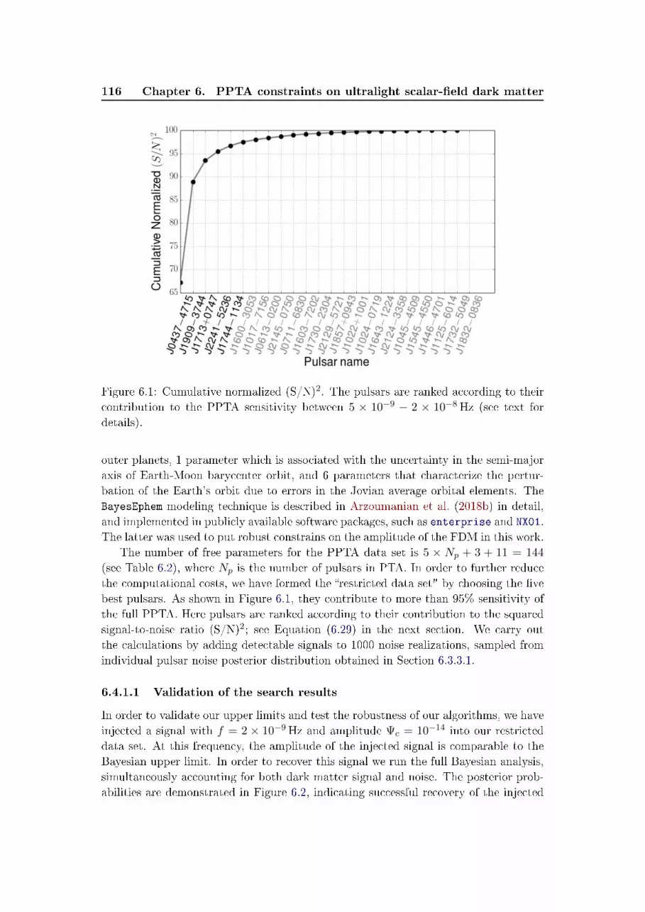
116 Chapter 6. PPTA constraints on ultralight scalar-eld dark matter
Figure 6.1: Cumulative normalized (S/N)2. The pulsars are ranked according to theircontribution to the PPTA sensitivity between 5 × 10⁻⁹ − 2 × 10⁻⁸ Hz (see text fordetails).
outer planets, 1 parameter which is associated with the uncertainty in the semi-majoraxis of Earth-Moon barycenter orbit, and 6 parameters that characterize the pertur-bation of the Earth's orbit due to errors in the Jovian average orbital elements. TheBayesEphem modeling technique is described in Arzoumanian et al. (2018b) in detail,and implemented in publicly available software packages, such as enterprise and NX01.The latter was used to put robust constrains on the amplitude of the FDM in this work.
The number of free parameters for the PPTA data set is 5 × Np + 3 + 11 = 144
(see Table 6.2), where Np is the number of pulsars in PTA. In order to further reducethe computational costs, we have formed the restricted data set" by choosing the vebest pulsars. As shown in Figure 6.1, they contribute to more than 95% sensitivity ofthe full PPTA. Here pulsars are ranked according to their contribution to the squaredsignal-to-noise ratio (S/N)2; see Equation (6.29) in the next section. We carry outthe calculations by adding detectable signals to 1000 noise realizations, sampled fromindividual pulsar noise posterior distribution obtained in Section 6.3.3.1.
6.4.1.1 Validation of the search results
In order to validate our upper limits and test the robustness of our algorithms, we haveinjected a signal with f = 2 × 10⁻⁹ Hz and amplitude Ψc = 10−14 into our restricteddata set. At this frequency, the amplitude of the injected signal is comparable to theBayesian upper limit. In order to recover this signal we run the full Bayesian analysis,simultaneously accounting for both dark matter signal and noise. The posterior prob-abilities are demonstrated in Figure 6.2, indicating successful recovery of the injected

6.4. Search techniques and Results 117
signal.
-14.2 -14 -13.8log Ψc
-8.85
-8.7
-8.55
logf
-8.85 -8.7 -8.55log f
Figure 6.2: The marginalized posterior distributions for the amplitude Ψc and frequencyf for a signal injection in the actual PPTA data. The thick black lines mark the injectedvalues and the contours are 1- and 2-σ credible regions.
6.4.2 Frequentist analysis
In a Frequentist framework, signal detection is essentially a statistical hypothesis testingproblem; we wish to choose between the null hypothesis H0 and the signal hypothesisH1 based on the observations. The task is to nd an optimal statistic that maxi-mizes the signal detection probability at a xed false alarm probability. Following theNeyman-Pearson criterion, the log-likelihood ratio is an optimal statistic
ln Λ ≡ lnL(H1|δt)
L(H0|δt)=
Np∑i=1
[(δti|si)−
1
2(si|si)
], (6.27)
where we have used Equations (6.11)-(6.12) to derive the second equality above, andthe inner product between two time series x and y is dened as
(x|y) = xTG(GTCG)−1GTy . (6.28)
It is useful to dene the signal-to-noise ratio in the following form
S/N =√
2〈ln Λ〉 =
Np∑i=1
(si|si)
1/2
, (6.29)

118 Chapter 6. PPTA constraints on ultralight scalar-eld dark matter
where 〈...〉 stands for the expectation value over a large number of noise realizations. Inthis work, we adopt 2 ln Λ as our detection statistic. For our Frequentist analysis, noisemodel parameters are xed at their maximum likelihood values. The signal parametersin question are: the amplitude of dark matter induced gravitational-potential oscilla-tions Ψc, oscillation frequency f , phase parameters αe and θp; see Equation (6.9). Itturns out that the statistic can be analytically maximized over Ψc and thus the param-eter space that needs to be numerically searched over is Np + 2 dimensional. For ourdata this corresponds to 28 dimensions, making a grid-based search unfeasible. We em-ploy the Particle Swarm Optimization technique (Eberhart & Kennedy, 1995), whichhas been demonstrated to be very eective for searches for continuous GWs with PTAs(Wang et al., 2015b; Zhu et al., 2016). The detection statistic follows a χ2 distributionwith one degree of freedom for noise-only data.
Since we nd no evidence for statistically signicant signals in the data, which isconsistent with results from the Bayesian analysis as described in the previous subsec-tion, we set upper limits on the dimensionless amplitude Ψc. We compute the 95%condence upper limits for a number of frequency bins between 10−9 and 10−7 Hz.At each frequency, we compute the S/N for 103 simulated signals with random phaseparameters and a xed Ψc. The 95% condence upper limit on Ψc corresponds to theamplitude at which 95% of signals result in S/N ≥ 2.4. Here the S/N threshold ischosen such that the expectation value for our detection statistic in the presence ofsignals, given by 1 + (S/N)2, is greater than the detection threshold that correspondsto 1% false alarm probability. It implies that: if there was a signal with an amplitudehigher than Ψc present in the data, it would have been detectable with more than 95%probability.
6.4.3 Upper limits
Figure 6.3 shows the 95% upper limits on the amplitude Ψc, calculated within Bayesian(black solid line) and frequentist frameworks (purple solid line). As one can see,Bayesian upper limits are a factor of 2−3 worse than frequentist upper limits in thelow-frequency regime, while in the mid-to-high frequency range both methods producecomparable results. The dierence might be predominantly attributed to the covari-ance between signal and noise (especially the red spin noise). Frequentist upper limitswere calculated by xing noise parameters at their maximum likelihood values, whereaswe search simultaneously over signal and noise parameters in the Bayesian analysis.
The Bayesian upper limits, obtained with 5-year NANOGrav data set (Demorestet al., 2013), are also plotted as the thin dash-dotted (taken from Porayko & Postnov,2014) and dashed (recalculated in this paper) lines. We note that upper limits presentedin Porayko & Postnov (2014) were underestimated by a factor of 10 due to the lessconservative8 choice of prior (log-uniform) probability of the amplitude Ψc, as well asthe noninclusion of DM variations and additional white noise terms (EFAC and EQUAD).From Figure 6.3, one can see that our data set is a factor of 5 more sensitive to the dark
8We note that uniform priors result in upper limits that are a factor of ∼ 5 higher than log-uniform
priors.

6.5. Future prospects 119
matter signal than NANOGrav 5-year data at low frequencies, corresponding to bosonmasses m . 10−23 eV. In the intermediate regime, the improvement is about a factorof 2. This is expected because of our much longer data span and higher observingcadence. It is interesting to note that the upper limit curves in Figure 6.3 exhibitsimilar frequency dependencies to the sky-averaged upper limits for continuous GWs(see e.g. Zhu et al., 2014). In Appendix A, we present Frequentist upper limits obtainedby including in the analysis only Earth terms. We also show how Bayesian upper limitsare modied if dierent xed SSE models are used.
10−9 10−8 10−7
Frequency (Hz)
10−16
10−15
10−14
10−13
10−12
10−11
10−10
Dim
ensi
onle
ssΨ
c
PPTA BayesPPTA freqNANOGrav newNANOGrav PP2014Eq. (7)
10−23 10−22Boson mass (eV)
Figure 6.3: Upper limits on the signal amplitude Ψc, generated by the scalar eld darkmatter in the Galaxy, as a function of frequency (boson mass). The purple solid lineshows results from Frequentist analysis of the full data set of 24 pulsars, while theblack solid line demonstrates the upper limits derived within a Bayesian framework(only the ve best pulsars were used). These are compared with previous studies usingthe NANOGrav 5-yr data set: dash-dotted orange − upper limits set in Porayko &Postnov (2014), dashed red − upper limits recalculated in this work. The thick blackdashed line shows the model amplitude Ψc, assuming ρFDM = 0.4GeVcm−3, given byEquation (6.7).

120 Chapter 6. PPTA constraints on ultralight scalar-eld dark matter
10−9 10−8 10−7
Frequency (Hz)
10−3
10−2
10−1
100
101
102
103
104ρ
FD
M(G
eVcm−
3)
PPTA current
SKA/FAST 10p for 10y
SKA/FAST 100p for 10y
SKA/FAST 100p for 10y (turbo)
10−23 10−22Boson mass (eV)
8 kpc
2 kpc
Figure 6.4: Upper limits on the dark matter density ρ in the Galaxy. The currentPPTA upper limits (black solid line) are shown along with projected limits in theFAST/SKA era (purple lines, all assuming 10-yr data span): a) 10 pulsars, 14-daycadence, 30-min integration, b) 100 pulsars, 14-day cadence, 30-min integration, andc) 100 pulsars, 1-day cadence, 2-hours integration (turbo). The black dashed linesshow the dark matter density in the Halo at 8 kpc (ρFDM = 0.4GeVcm−3) and 2kpc (ρFDM = 3.4GeVcm−3) from the Galactic Center, assuming NFW prole. The8 kpc line demonstrates the predicted dark matter density, applicable to current PPTApulsars and the Earth, while the 2 kpc line applies to pulsars located at 2 kpc distancefrom the Galactic Center. For boson masses m . 4× 10⁻²³ eV the size of the solitoniccore becomes larger than 2 kpc (Schive et al., 2014), and the dark matter density willdeviate from the NFW prediction towards higher values (see text for details).
6.5 Future prospects
In this section we discuss the future improvement in sensitivity of PTAs to the darkmatter signal. In particular, the FAST radio telescope (Nan et al., 2011) in China,MeerKAT (Bailes et al., 2018) − a precursor for the planned Square Kilometre Array(SKA, Lazio, 2013) − and ultimately the SKA, are expected to signicantly increasethe sensitivities of PTAs. With broad frequency bands and massive collecting areas, theradiometer noise for some of the brightest pulsars can be reduced from current 100 nslevel down to below 10 ns (Hobbs et al., 2014). However, it might be too optimistic toassume a white noise level of 10 ns because of the so-called jitter noise, which is thought
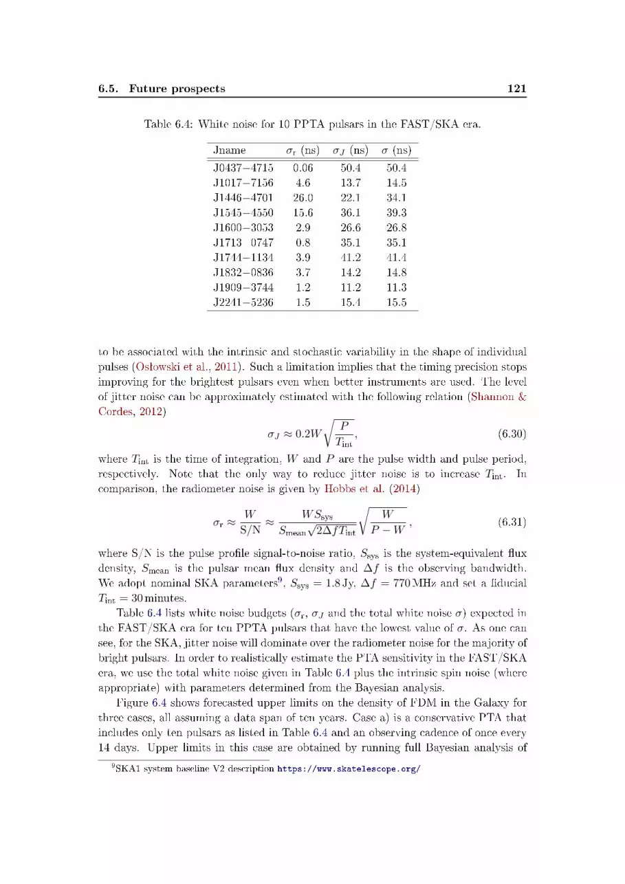
6.5. Future prospects 121
Table 6.4: White noise for 10 PPTA pulsars in the FAST/SKA era.
Jname σr (ns) σJ (ns) σ (ns)
J0437−4715 0.06 50.4 50.4J1017−7156 4.6 13.7 14.5J1446−4701 26.0 22.1 34.1J1545−4550 15.6 36.1 39.3J1600−3053 2.9 26.6 26.8J1713+0747 0.8 35.1 35.1J1744−1134 3.9 41.2 41.4J1832−0836 3.7 14.2 14.8J1909−3744 1.2 11.2 11.3J2241−5236 1.5 15.4 15.5
to be associated with the intrinsic and stochastic variability in the shape of individualpulses (Osªowski et al., 2011). Such a limitation implies that the timing precision stopsimproving for the brightest pulsars even when better instruments are used. The levelof jitter noise can be approximately estimated with the following relation (Shannon &Cordes, 2012)
σJ ≈ 0.2W
√P
Tint, (6.30)
where Tint is the time of integration, W and P are the pulse width and pulse period,respectively. Note that the only way to reduce jitter noise is to increase Tint. Incomparison, the radiometer noise is given by Hobbs et al. (2014)
σr ≈W
S/N≈ WSsys
Smean
√2∆fTint
√W
P −W , (6.31)
where S/N is the pulse prole signal-to-noise ratio, Ssys is the system-equivalent uxdensity, Smean is the pulsar mean ux density and ∆f is the observing bandwidth.We adopt nominal SKA parameters9, Ssys = 1.8 Jy, ∆f = 770MHz and set a ducialTint = 30minutes.
Table 6.4 lists white noise budgets (σr, σJ and the total white noise σ) expected inthe FAST/SKA era for ten PPTA pulsars that have the lowest value of σ. As one cansee, for the SKA, jitter noise will dominate over the radiometer noise for the majority ofbright pulsars. In order to realistically estimate the PTA sensitivity in the FAST/SKAera, we use the total white noise given in Table 6.4 plus the intrinsic spin noise (whereappropriate) with parameters determined from the Bayesian analysis.
Figure 6.4 shows forecasted upper limits on the density of FDM in the Galaxy forthree cases, all assuming a data span of ten years. Case a) is a conservative PTA thatincludes only ten pulsars as listed in Table 6.4 and an observing cadence of once every14 days. Upper limits in this case are obtained by running full Bayesian analysis of
9SKA1 system baseline V2 description https://www.skatelescope.org/

122 Chapter 6. PPTA constraints on ultralight scalar-eld dark matter
simulated data. We analytically scale this limit curve to two more ambitious cases10.We increase the number of pulsars to 100 in case b), leading to a factor of
√10 improve-
ment. For case c), we further increase the cadence to once every day and adopt anintegration time of two hours, providing another factor of
√4× 14 improvement. Case
c) might be an interesting option in the SKA era since small radio telescopes (comparedto SKA/FAST) such as Parkes, can be dedicated for high-cadence and long integrationobservations of the brighter pulsars.
As one can see from Figure 6.4, we will be able to constrain the contribution ofFDM to the local dark matter density below 10% for m . 10−23 eV in ten years underthe conservative assumption for SKA sensitivity. However, it is more challenging forboson masses above 10−22 eV; we estimate that decade-long observations of hundredsof pulsars timed at nearly daily cadence with precision . 20 ns are necessary to placeinteresting limits.
There are a couple of ways to improve our analysis. First, the coherence betweenpulsar terms and Earth terms can be used to enhance the sensitivity. When a pulsarand the Earth are located within a de Broglie wavelength λdB, the oscillation phases,which have been assumed to be independent in the current analysis, are correlated.However, for m & 10−22 eV, this eect will have no impact on the current results, sinceλdB = 60 pc (10−22 eV/m) and no pulsars have been found within 60 pc to the Earth.Another interesting point is that pulsars that are close to each other within λdB alsoexperience phase-coherent oscillations (De Martino et al., 2017). We plan to explorethese features in a future work.
Second, the oscillation amplitude Ψc is proportional to the local dark matter density.Thus, in contrast to the amplitude of the Earth term, the amplitude of the pulsar termvaries from pulsar to pulsar; see Equation (6.7). In Λ-FDM cosmological simulations(De Martino et al., 2017; Schive et al., 2014), it was shown that due to wave interferencethe dark matter forms gritty pattern with typical granule size of around λdB. Whenaveraged over λdB scales, the periphery (> 1 kpc) density prole is similar to theclassical Navarro-Frenk-White (NFW) prole, whereas a distinct density peak is seenin the central regions (usually called solitonic core, see Schive et al., 2014, for details).
Figure 6.5 shows the expected signal amplitude for PPTA pulsars assuming theNFW dark matter density prole (Navarro et al., 1996b) with parameters from Sofue(2012). As one can see, pulsars closer to the Galactic Center provide better sensitivityto the dark matter signal. The amplitude of the dark matter signal becomes evenlarger than NFW prediction within the central solitonic core (. 1 kpc, De Martinoet al., 2017). For the current PPTA sample, PSR J1824−2452A is expected to havethe largest signal amplitude, a factor of ∼ 5 larger than other pulsars11. However,this pulsar is nearly the worst timer in PPTA (see Table 6.1 and Figure 6.1). Existing
10Note that the scaling factor should be a good approximation at high frequencies where red noise
plays a less important role.11The density of the scalar eld dark matter in globular clusters is not expected to deviate sig-
nicantly from the general trend as λdB is larger than typical sizes of globular clusters. Thus, the
amplitude of the oscillation at J1824−2452A, located in a globular cluster, is expected to follow the
NFW prediction.

6.6. Conclusions 123
2 3 4 5 6 7 8 9 10
Distance to the Galactic Center (kpc)
0.0
0.2
0.4
0.6
0.8
1.0
1.2
Dim
ensi
onle
ssΨ
c
×10−15
J1824−2452A
Earth
Figure 6.5: The amplitude of the expected dark matter signal for dierent pulsars, as-suming NFW dark matter density prole. The mass of the scalar dark matter particlesis assumed to be 2× 10⁻²³ eV.
and future pulsar surveys might help nd high quality millisecond pulsars close to theGalactic Center and thus provide better sensitivity to the dark matter searches (Krameret al., 2004).
6.6 Conclusions
Pulsar timing is a powerful tool to study a wide variety of astrophysical phenomena. Byexploiting precision timing observations from an array of the most stable millisecondpulsars, PTAs allow us to measure minute correlations in the ToAs of dierent pulsars.Like continuous GWs from individual supermassive binary black holes, FDM in theGalaxy produces periodic variations in pulsar ToAs. We perform a search for evidenceof ultralight dark matter in the latest PPTA data set. Finding no statistically signicantsignals, we place upper limits on the dark matter density: for boson massm . 10−23 eV,our analysis constrains the density below 6GeVcm−3 with 95% condence; at m ≈10−22 eV, our upper limits remain 3 orders of magnitude above the local dark matterdensity 0.4GeVcm−3 inferred from kinematics measurements of stars in the Galaxy(Sivertsson et al., 2018).
We derived the noise properties of PPTA data and obtain dark matter constraintsusing both Bayesian and Frequentist methods. Our upper limits from the two methodsare broadly consistent. We reanalyzed the NANOGrav 5-yr data set and found thatthe PPTA data result in a factor of 2 to 5 improvement in dark matter constraints.We studied potential systematics due to SSE errors in our analysis and found that thesearch for ultralight dark matter is insensitive to such errors. We have ignored eectsfrom instabilities in terrestrial time standards; such clock errors produce a monopolarbroad-band noise (Hobbs et al., 2012). Whereas this eect should be distinguishable

124 Chapter 6. PPTA constraints on ultralight scalar-eld dark matter
from the sinusoidal ToA variations due to ultralight dark matter, one needs to includeit in a future study to quantitatively assess the impact.
We forecasted the PTA sensitivity in the FAST/SKA era while accounting for re-alistic noise levels. We found that observing the ten best PPTA pulsars for ten yearswould constrain the density of FDM below 0.05GeVcm−3 for m . 10−23 eV, about10% of measured total dark matter density. At m ≈ 2× 10⁻²³ eV, our projected limitis around 0.4GeVcm−3; for higher boson masses, the upper limits increase as ∼ m3.Above m ≈ 10−22 eV, the projected limits are more than one order of magnitude abovethe local dark matter density. To place interesting limits in this mass range, an am-bitious timing program in which hundreds of pulsars timed with daily cadence andhigh precision (. 20 ns) for more than a decade is required. Finally, we point out thathigh-quality pulsars in the vicinity of the Galactic Center will be ideal tools to test thefuzzy dark matter hypothesis.

Chapter 7
Concluding remarks and future
plans
Contents
7.1 Studying the magnetised ISM with pulsars . . . . . . . . . . . . 125
7.1.1 Future plans . . . . . . . . . . . . . . . . . . . . . . . . . . . . . 126
7.2 Studying dark matter with pulsars . . . . . . . . . . . . . . . . . 127
7.2.1 Future plans . . . . . . . . . . . . . . . . . . . . . . . . . . . . . 128
The primary scientic motivation of this thesis is the investigation of eects whichinuence the propagation of pulsar signals, in order to probe the properties of theintervening medium and its constituents. We mainly focus our analysis on probing theturbulence in the magnetised ionised ISM using Faraday rotation of pulsars, and darkmatter in the Galaxy using a high-precision pulsar timing technique. We investigatehow the recent, highly sensitive data can constrain (or measure!) the aforementionedpropagation eects that haven't been studied extensively before. The most signicantaccomplishments of the work in this thesis as well as potential improvements and futureplans are summarised below.
7.1 Studying the magnetised ISM with pulsars
Pulsars are known to be a powerful probe of the magnetoionic phase of the ISM in theMilky Way. Specically in this thesis we used Faraday rotation of linearly polarisedradiation from pulsars to study the diuse magnetic eld in the Milky Way. SinceISM eects are more prominent at longer wavelengths, we have conducted the pulsarobservations with the low-frequency radio interferometer LOFAR. The RMs of pulsarswere obtained with the novel BGLSP technique, which provides reliable estimates ofthe uncertainties on the observed RMs, and is described in Chapter 3. It was foundthat detected RM variations are dominated by the Faraday rotation taking place inthe Earth's ionosphere, which is ve to six orders of magnitude greater than what weexpect from the ISM. In order to compensate for the ionospheric RM we have useda conventional thin-layer ionospheric approximation. The Earth's magnetic eld wasreconstructed with so-called geomagnetic eld models produced using magnetic eldmeasurements from satellites and approximately 200 operating magnetic observatories
126 Chapter 7. Concluding remarks and future plans
around the globe. The electron density in the ionosphere was modelled using a se-lection of global free-electron density maps, produced by dierent scientic groups viavarious numerical techniques using GPS data. In Chapter 4 we compared dierent ge-omagnetic models and free-electron density maps, and investigated the reconstructionquality of ionospheric Faraday rotation using several months of LOFAR observationsof selected pulsars. We found that on average the UQRG and JPLG maps performbetter than other ionospheric maps, while the performance of dierent geomagneticmodels is indistinguishable with our current sensitivity. After subtraction of the de-terministic systematics that left residual unmodelled ionospheric eects, the correctedRM measurements have a precision of ∼ 0.06−0.07 radm−2. This number is approx-imately an order of magnitude higher than the uncertainties of the observed RMs forthe considered pulsars and therefore denes our sensitivity to any sort of astrophysicalRM variation.
One of the promising signals of interest are RM variations caused by turbulent ISMstructures between the pulsar and the observer. In Chapter 5 we made an eortto measure these RM variations using ∼3-year long LOFAR observations of pulsars.However, no astrophysically reliable signal has been found. We set an upper limiton the amplitude of any magnetic eld uctuations. Our best result, obtained withJ0826+2637, is already below the value derived in Haverkorn et al. (2008), howeverstill four times higher that the expected value observed in Minter & Spangler (1996).With a set of simulations we have shown that for a reliable detection we need ∼ 20years of regular monitoring of pulsars with LOFAR.
7.1.1 Future plans
In this section we summarise which steps should be undertaken in order to improve oursensitivity to RM variations of pulsars. These ideas are important for future initiativesas well as for current actions.
Regular monitoring of pulsars with low-frequency interferometers
Searching for RM variations in pulsar signals is an on-going study. Ger-man LOFAR stations are now observing more than 100 pulsars bi-weekly at150MHz. Such continuing monitoring campaigns of pulsars at low frequenciesprovide a valuable basis for investigating long-term RM changes. Besides theRM variations caused by the turbulent ISM, the same data set can be usedto probe other RM signals of interest, such as those caused by the Solar wind(Oberoi & Lonsdale, 2012), ESEs (Fiedler et al., 1987; Cognard et al., 1993)and reconnection sheets in the ISM (Pen & Levin, 2014). Along with the RMs,the DMs of pulsars can be used to determine the electron density towards thepulsar, providing additional insight into the physical structures and processestaking place between the source and the observer. By simultaneously measuringthe RMs and DMs of pulsars, one can probe the possible correlations of thesequantities and increase the reliability of the results.
Improving ionospheric modelling As mentioned, the inuence of the ionosphere

7.2. Studying dark matter with pulsars 127
can be the main obstacle towards detecting astrophysical RM variations. There-fore, a conspicuous way of increasing the sensitivity towards signals of interestis by improving the quality of the ionospheric modelling. In this thesis we haveused a simplied model within which the ionosphere is a thin single layer xedat an altitude of 450 km. However in reality, the ionosphere is highly dynamic.In multiple studies it has been shown that the peak electron density height (andtherefore the eective ionospheric height) varies signicantly as a function of thetime of day, season, and solar activity (Rama Rao et al., 2006; Gulyaeva et al.,2013; Wang et al., 2016). Therefore, a more realistic representation of the single-layer model would be taking into account variations of the eective ionosphericheight. This can be carried out by combining the GPS-derived electron-densityvalues with semi-empirical ionospheric proles like the IRI (Bilitza et al., 2017)or the IRI-Plas (Arikan et al., 2015). An even more sophisticated analysis canbe performed with multi-layer or 3D models of the ionosphere, created using theGPS data combined with electron-density measurements from on-site ionoson-des (e.g. Ma et al., 2005). Alternatively, non-parametric routines can be usedto account for the ionospheric contribution. An intriguing solution is to use adiuse polarised background or a set of linearly polarised sources as calibratorsto track the ionospheric Faraday rotation (Lenc et al., 2016). By analysing mul-tiple observing snapshots made at dierent epochs, one can estimate the RM ofthe source of interest puried from the ionospheric contribution. However, thesource and the calibrators should be located close enough on the sky, i.e withinthe coherence length of the ionosphere (<10, Loi et al., 2015).
7.2 Studying dark matter with pulsars
Recent studies suggest that about 70% of the mass of the Milky Way comes from darkmatter (Posti & Helmi, 2019). In astrophysical systems with sizes ranging from galac-tic to cosmological scales the dark-matter hypothesis is supported by various lines ofobservational evidence. Among the most striking proofs are rotation curves of galaxies,the angular power spectrum of the cosmic microwave background and enigmatic dy-namics of galaxy clusters. The standard ΛCDM model has been remarkably successfulin explaining many of these observational features, given that 27% of the critical mass-energy density consists of dark matter. However, on scales similar to those of galaxies,the ΛCDM model has been poorly tested and in most cases it is in tension with ob-servational data. One of the viable alternatives is FDM, consisting of extremely lightbosons with mass m ∼ 10−22 eV. As was shown in Khmelnitsky & Rubakov (2014),such FDM will produce oscillations of gravitational potentials at nHz frequencies. Thistime-dependent space-time will cause variations in ToAs of pulsar signals, which arecorrelated between dierent pulsars. In Chapter 6 we attempt to measure these vari-ations using the ∼12-year PPTA dataset. We performed a search for an FDM signalin the Milky Way using both frequentist and Bayesian approaches. As no statisticallysignicant signal has been found, we put an upper limit on the dark matter density in

128 Chapter 7. Concluding remarks and future plans
the Galaxy. Our best results at m < 10−23 eV are below 6GeV cm−3, while our upperlimit at m = 10−22 eV is still three orders of magnitude higher than the expected darkmatter density of 0.4GeV cm−3, obtained from kinematic studies of stars in the Galaxy.
7.2.1 Future plans
Investigation of the dark matter problem is of great importance in cosmology. Thework presented in this thesis provides our modest contribution towards revealing thenature of dark matter. Additional methods to improve the data analysis and increaseour sensitivity to FDM are proposed below.
Mitigation of correlated noise and systematics in the PTA data The pres-ence of various noise processes signicantly increases the complexity of theanalysis and, what is more important, degrades the sensitivity of PTAs (seeVerbiest & Shaifullah, 2018, and reference therein).
One of the bottlenecks for high precision PTAs is DM variations caused by theionised ISM (see e.g. Chapter 6) and Solar wind (Tiburzi et al., 2019). As weare more sensitive to propagation eects at lower frequencies, one of the promis-ing techniques to correcting DM variations is to use low-frequency observations(Janssen et al., 2015). However, due to DM chromaticity (Cordes et al., 2016;Donner et al., 2019) the eect can be removed only partially.
It has already been shown in multiple works that even with our current sensitivitypulsar timing is sensitive to errors in the SSEs and time standard (Tiburzi et al.,2016; Caballero et al., 2018). These two types of errors are the source of correlatednoise with monopolar and dipolar spatial correlations, respectively. As was shownin Tiburzi et al. (2016), the presence of this correlated noise increases the false-alarm probability of GW detection with PTAs. In the case of a signal coming fromFDM we would be especially aected by the correlated noise from clocks, due tothe monopolar nature of the FDM signal. Some techniques, such as includingthe SSEs in the timing model (Champion et al., 2010; Caballero et al., 2018;Arzoumanian et al., 2018b), have already been successfully adopted in PTAs.Another viable method is non-parametric suppression of correlated noise fromterrestrial clock standards and SSEs (Taylor et al., 2017).
In the era of more sensitive instruments the problem of correlated noises andsystematics will be further exacerbated. Therefore, mitigation of these eects forcurrent and especially future PTA analysis is of great importance.
New and upcoming radio facilities A new generation of radio telescopes will soonbe available at full capacity and will assist the PTA campaigns. Two of these arethe 500-meter-FAST radio telescope (Nan et al., 2011) in the Northern hemisphereand MeerKAT (Booth & Jonas, 2012), a phased array formed by 64 13.5-meter-dishes, in the Southern hemisphere. Both of these saw the `rst light' in 2016.The even more ambitious SKA radio telescope (Bull et al., 2018), which will beformed by thousands of small antennas located on two continents in the Southern

7.2. Studying dark matter with pulsars 129
hemisphere, will become operational in the next decade. Huge collecting areas ofthe aforementioned telescopes combined with their low system temperatures willincrease the S/N of already detected pulsars, and therefore signicantly improvethe sensitivity of PTAs as a whole. In Chapter 6 we have investigated how thePTA sensitivity to an FDM signal will increase with upcoming radio facilities.We found that stringent constraints below 0.05GeV cm−3 can be put for m <
10−23 eV, when observing the ten best PPTA pulsars for ten years with futurefacilities. For putting astrophysically interesting upper limits for m > 10−22
eV a more ambitious observing programme in which hundreds of pulsars areobserved daily, is required. Moreover, the higher sensitivity of the upcoming radiotelescopes is expected to signicantly increase the number of known pulsars, andmay populate PTA family with more stable MSPs. As the density of dark matterincreases towards the central regions of our Galaxy, pulsars detected closer to theGalactic Centre will provide better sensitivity to an FDM signal.


Appendix A
Earth-term limits and eects of SSE
When searching for continuous GWs in PTA data, it is common to use only the Earthterms. Similarly, for the case of scalar eld dark matter, we can include in the analysisonly Earth terms in Equation (6.6). Although pulsar and Earth terms lie in the samefrequency bin, we expect that for a suciently large set of pulsars, pulsar terms willbe averaged out, as they all have dierent phases. In the left panel of Figure A.1,we compare the Frequentist upper limits on the density of scalar eld dark matterρSF when only Earth terms are considered (black dashed) and when the full signalis used (purple solid). We nd that both limits are comparable to each other. Thenoisy features in the (purple) solid curve are due to the amplitude modulation of pulsarterms; see Equation (6.9).
We also demonstrate the eects of SSE errors. In the right panel of Figure A.1,we show the upper limits obtained when DE418 and DE435 planetary ephemeris areused. The results with xed ephemeris are overplotted with upper limits obtained withBayesEphem model, which accounts for uncertainties in the SSE. We see that the resultsare comparable, indicating the search for FDM signal, or continuous waves in general,is insensitive to SSE errors.
10−9 10−8 10−7
Frequency (Hz)
10−1
100
101
102
103
ρS
F(G
eVcm−
3)
Freq E+PFreq E
10−23 10−22Boson mass (eV)
10−9 10−8 10−7
Frequency (Hz)
10−1
100
101
102
103
ρS
F(G
eVcm−
3)
DE418 BayesEphemDE418DE435
10−23 10−22Boson mass (eV)
Figure A.1: Upper limits on the density of fuzzy dark matter ρSF in the Galaxy, asa function of frequency (boson mass). Left : results from Frequentist analysis whenonly the Earth term is included (Freq E) or both terms are used (Freq E+P). Right :Bayesian upper limits when SSE parameters are included in the search (BayesEphem),or using xed DE418 and DE435 planet ephemerids. The horizontal black dashed linemarks the measured local dark matter density 0.4GeVcm−3 (Sivertsson et al., 2018).


Appendix B
Noise properties for six PPTA
pulsars
Figure B.1 shows results of the Bayesian noise parameter estimation, described inSection 6.3.3.1, for the six most sensitive pulsars in the current PPTA data set.
J0437-4715 J1600-3053
J1713+0747 J1744-1134
J1909-3744 J2241-5236
Figure B.1: The one- and two-dimensional marginalized posterior distributions for thelog-amplitude and slope of the DM and spin noises for the six best pulsars in the currentPPTA data set.


Bibliography
Abbott L. F., Sikivie P., 1983, Phys. Lett. B, 120, 133 (Cited on page 101.)
Aggarwal K., et al., 2018, arXiv e-prints, (Cited on page 20.)
Ambartsumyan V. A., Saakyan G. S., 1960, Soviet Ast., 4, 187 (Cited on page 4.)
Antoniadis J., et al., 2013, Science, 340, 448 (Cited on page 19.)
Archibald R. F., et al., 2016, ApJ, 819, L16 (Cited on page 10.)
Archibald A. M., et al., 2018, Nature, 559, 73 (Cited on page 19.)
Arikan F., Sezen U., Gulyaeva T. L., Cilibas O., 2015, Advances in Space Research,55, 2106 (Cited on page 127.)
Armstrong J. W., Rickett B. J., Spangler S. R., 1995, ApJ, 443, 209 (Cited on pages 22,58, 82, 89 and 91.)
Arnett D., 1996, Supernovae and Nucleosynthesis: An Investigation of the History ofMatter from the Big Bang to the Present (Cited on page 5.)
Arora B. S., et al., 2016, PASA, 33, e031 (Cited on page 74.)
Arvanitaki A., Dimopoulos S., Dubovsky S., Kaloper N., March-Russell J., 2010,Phys. Rev. D, 81, 123530 (Cited on pages 24 and 101.)
Arzoumanian Z., et al., 2014, ApJ, 794, 141 (Cited on pages 110 and 115.)
Arzoumanian Z., et al., 2018a, ApJS, 235, 37 (Cited on page 19.)
Arzoumanian Z., et al., 2018b, ApJ, 859, 47 (Cited on pages 20, 38, 115, 116 and 128.)
Asgekar A., Deshpande A. A., 1999, Bulletin of the Astronomical Society of India, 27,209 (Cited on page 30.)
Asseo E., Pelletier G., Sol H., 1990, MNRAS, 247, 529 (Cited on page 9.)
Baade W., Zwicky F., 1934, Proceedings of the National Academy of Science, 20, 254(Cited on page 4.)
Babak S., et al., 2016, MNRAS, 455, 1665 (Cited on pages 20 and 115.)
Backer D. C., 1970, Nature, 228, 42 (Cited on page 8.)
Backer D. C., Hellings R. W., 1986, ARA&A, 24, 537 (Cited on page 37.)
Bailes M., et al., 2018, in Proceedings of MeerKAT Science2016. p. 11(arXiv:1803.07424) (Cited on page 120.)

136 Bibliography
Banerjee R., Klessen R. S., Fendt C., 2007, ApJ, 668, 1028 (Cited on page 21.)
Bar N., Blas D., Blum K., Sibiryakov S., 2018, preprint, (arXiv:1805.00122) (Citedon page 102.)
Bassa C. G., et al., 2016, MNRAS, 456, 2196 (Cited on page 29.)
Bates S. D., Lorimer D. R., Verbiest J. P. W., 2013, MNRAS, 431, 1352 (Cited onpages 6 and 58.)
Battaglieri M., et al., 2017, arXiv e-prints, (Cited on page 100.)
Beck R., 2001, Space Sci. Rev., 99, 243 (Cited on page 85.)
Becker W., ed. 2009, Neutron Stars and Pulsars Astrophysics and Space Science LibraryVol. 357, doi:10.1007/978-3-540-76965-1. (Cited on page 5.)
Becker W., Bernhardt M. G., Jessner A., 2013, Acta Futura, Issue 7, p. 11-28, 7, 11(Cited on page 20.)
Begeman K. G., Broeils A. H., Sanders R. H., 1991, MNRAS, 249, 523 (Cited onpage 23.)
Beresnyak A., 2012, Phys. Rev. Lett., 108, 035002 (Cited on page 21.)
Bertone G., Hooper D., Silk J., 2005, Phys. Rep., 405, 279 (Cited on pages 22 and 100.)
Beskin V. S., Philippov A. A., 2012, MNRAS, 425, 814 (Cited on page 8.)
Beskin V. S., Gurevich A. V., Istomin I. N., 1988, Ap&SS, 146, 205 (Cited on page 9.)
Bhat N. D. R., Gupta Y., Rao A. P., 1998, ApJ, 500, 262 (Cited on page 58.)
Bhattacharya D., van den Heuvel E. P. J., 1991, Phys. Rep., 203, 1 (Cited on page 12.)
Bienaymé O., et al., 2014, A&A, 571, A92 (Cited on page 22.)
Bilitza D., Altadill D., Zhang Y., Mertens C., Truhlik V., Richards P., McKinnell L.-A.,Reinisch B., 2014, Journal of Space Weather and Space Climate, 4, A07 (Cited onpage 59.)
Bilitza D., Altadill D., Truhlik V., Shubin V., Galkin I., Reinisch B., Huang X., 2017,Space Weather, 15, 418 (Cited on pages 63 and 127.)
Bilous A. V., et al., 2016, A&A, 591, A134 (Cited on pages 89 and 90.)
Birch M. J., Hargreaves J. K., Bailey G. J., 2002, Radio Science, 37, 15 (Cited onpage 74.)
Bird M. K., et al., 1985, Sol. Phys., 98, 341 (Cited on page 18.)

Bibliography 137
Blandford R., Narayan R., Romani R. W., 1984, Journal of Astrophysics and Astron-omy, 5, 369 (Cited on page 109.)
Blas D., Nacir D. L., Sibiryakov S., 2017, Phys. Rev. Lett., 118, 261102 (Cited onpages 24 and 102.)
Blinnikov S., Dolgov A., Porayko N. K., Postnov K., 2016, J. Cosmology Astropart.Phys., 11, 036 (Cited on page 24.)
Bode P., Ostriker J. P., Turok N., 2001, ApJ, 556, 93 (Cited on page 24.)
Booth R. S., Jonas J. L., 2012, African Skies, 16, 101 (Cited on pages 31 and 128.)
Bovy J., Tremaine S., 2012, ApJ, 756, 89 (Cited on page 105.)
Bowman J. D., Rogers A. E. E., Monsalve R. A., Mozdzen T. J., Mahesh N., 2018,Nature, 555, 67 (Cited on page 102.)
Boynton P. E., Groth E. J., Hutchinson D. P., Nanos Jr. G. P., Partridge R. B.,Wilkinson D. T., 1972, ApJ, 175, 217 (Cited on page 109.)
Brandenburg A., Subramanian K., 2005, Phys. Rep., 417, 1 (Cited on page 21.)
Brdar V., Kopp J., Liu J., Prass P., Wang X.-P., 2018, Phys. Rev. D, 97, 043001 (Citedon page 104.)
Brentjens M. A., de Bruyn A. G., 2005, A&A, 441, 1217 (Cited on pages 43, 45, 46and 61.)
Bretthorst G. L., 2001, in Mohammad-Djafari A., ed., American Institute of PhysicsConference Series Vol. 568, Bayesian Inference and Maximum Entropy Methods inScience and Engineering. pp 241245, doi:10.1063/1.1381888 (Cited on page 50.)
Buhari S. M., Abdullah M., Hasbi A. M., Otsuka Y., Yokoyama T., Nishioka M.,Tsugawa T., 2014, J. of Geophysical Research (Space Physics), 119, 10 (Cited onpage 17.)
Bull P., et al., 2018, arXiv e-prints, (Cited on page 128.)
Bullock J. S., Boylan-Kolchin M., 2017, Annu. Rev. Astron. Astrophys., 55, 343 (Citedon page 102.)
Burgay M., et al., 2003, Nature, 426, 531 (Cited on page 18.)
Burkhart B., Lazarian A., Gaensler B. M., 2012, ApJ, 749, 145 (Cited on page 21.)
Burn B. J., 1966, MNRAS, 133, 67 (Cited on pages 42, 45 and 61.)
Caballero R. N., et al., 2016, MNRAS, 457, 4421 (Cited on page 72.)
Caballero R. N., et al., 2018, MNRAS, 481, 5501 (Cited on pages 20, 38 and 128.)
138 Bibliography
Calabrese E., Spergel D. N., 2016, MNRAS, 460, 4397 (Cited on page 102.)
Chadwick J., 1932, Nature, 129, 312 (Cited on page 4.)
Chamel N., Haensel P., 2008, Living Reviews in Relativity, 11, 10 (Cited on page 5.)
Champion D. J., et al., 2010, ApJ, 720, L201 (Cited on pages 20, 38 and 128.)
Chandrasekhar S., 1931, ApJ, 74, 81 (Cited on page 4.)
Chen K., Ruderman M., 1993, ApJ, 402, 264 (Cited on page 11.)
Chepurnov A., Lazarian A., 2010, ApJ, 710, 853 (Cited on page 82.)
Chester T. J., Butman S. A., 1981, Telecommunications and Data Acquisition ProgressReport, 63, 22 (Cited on page 20.)
Cho J., Lazarian A., 2009, ApJ, 701, 236 (Cited on page 21.)
Clark H. A., Lewis G. F., Scott P., 2016, MNRAS, 456, 1402 (Cited on page 24.)
Clegg A. W., Cordes J. M., Simonetti J. M., Kulkarni S. R., 1992, ApJ, 386, 143 (Citedon page 82.)
Clesse S., García-Bellido J., 2017, Physics of the Dark Universe, 18, 105 (Cited onpage 24.)
Clowe D., Gonzalez A., Markevitch M., 2004, ApJ, 604, 596 (Cited on page 100.)
Cognard I., Bourgois G., Lestrade J.-F., Biraud F., Aubry D., Darchy B., DrouhinJ.-P., 1993, Nature, 366, 320 (Cited on page 126.)
Cole T. W., 1969, Nature, 221, 29 (Cited on page 29.)
Coles W., Hobbs G., Champion D. J., Manchester R. N., Verbiest J. P. W., 2011,MNRAS, 418, 561 (Cited on page 113.)
Coles W. A., et al., 2015, ApJ, 808, 113 (Cited on pages 78 and 112.)
Colín P., Avila-Reese V., Valenzuela O., 2000, ApJ, 542, 622 (Cited on page 24.)
Conway R. G., Kellermann K. I., Long R. J., 1963, MNRAS, 125, 261 (Cited onpage 30.)
Cooper B. F. C., Price R. M., 1962, Nature, 195, 1084 (Cited on page 43.)
Cordes J. M., Lazio T. J. W., 2002, ArXiv Astrophysics e-prints, (Cited on page 58.)
Cordes J. M., Lazio T. J. W., 2003, arXiv Astrophysics e-prints, (Cited on page 22.)
Cordes J. M., Rankin J., Backer D. C., 1978, ApJ, 223, 961 (Cited on page 8.)
Cordes J. M., Weisberg J. M., Boriako V., 1985, ApJ, 288, 221 (Cited on page 89.)

Bibliography 139
Cordes J. M., Weisberg J. M., Frail D. A., Spangler S. R., Ryan M., 1991, Nature, 354,121 (Cited on page 22.)
Cordes J. M., Shannon R. M., Stinebring D. R., 2016, ApJ, 817, 16 (Cited on page 128.)
Cromartie H., et al., 2019, arXiv e-prints, (Cited on page 19.)
Crovisier J., Dickey J. M., 1983, A&A, 122, 282 (Cited on page 82.)
Cumming A., Zweibel E., Bildsten L., 2001, ApJ, 557, 958 (Cited on page 12.)
Damour T., Deruelle N., 1986, Ann. Inst. Henri Poincaré Phys. Théor., Vol. 44, No. 3,p. 263 - 292, 44, 263 (Cited on page 38.)
Damour T., Taylor J. H., 1992, Phys. Rev. D, 45, 1840 (Cited on page 38.)
Davies J. G., Hunt G. C., Smith F. G., 1969, Nature, 221, 27 (Cited on pages 4 and 9.)
De K., Gupta Y., 2016, Experimental Astronomy, 41, 67 (Cited on page 29.)
De Martino I., Broadhurst T., Tye S.-H. H., Chiueh T., Schive H.-Y., Lazkoz R., 2017,Phys. Rev. Lett., 119, 221103 (Cited on pages 102 and 122.)
Del Popolo A., Le Delliou M., 2017, Galaxies, 5, 17 (Cited on page 23.)
Demorest P. B., et al., 2013, ApJ, 762, 94 (Cited on pages 103 and 118.)
Deng X. P., et al., 2013, Advances in Space Research, 52, 1602 (Cited on page 20.)
Deng H., Hertzberg M. P., Namjoo M. H., Masoumi A., 2018, Phys. Rev. D, 98, 023513(Cited on page 102.)
Dessart L., Burrows A., Ott C. D., Livne E., Yoon S.-C., Langer N., 2006, ApJ, 644,1063 (Cited on page 5.)
Desvignes G., et al., 2016, MNRAS, 458, 3341 (Cited on page 19.)
Desvignes G., et al., 2018, ApJ, 852, L12 (Cited on pages 17, 29, 78 and 83.)
Detweiler S., 1979a, ApJ, 234, 1100 (Cited on page 19.)
Detweiler S., 1979b, ApJ, 234, 1100 (Cited on pages 102 and 104.)
Deutsch A. J., 1955, Annales d'Astrophysique, 18, 1 (Cited on page 5.)
Diaferio A., Schindler S., Dolag K., 2008, Space Sci. Rev., 134, 7 (Cited on page 22.)
Dine M., Fischler W., 1983, Phys. Lett. B, 120, 137 (Cited on page 101.)
Dobbs C. L., Glover S. C. O., Clark P. C., Klessen R. S., 2008, MNRAS, 389, 1097(Cited on page 21.)
Donner J. Y., et al., 2019, A&A, 624, A22 (Cited on pages 89, 90 and 128.)

140 Bibliography
Draine B. T., 2011, Physics of the Interstellar and Intergalactic Medium (Cited onpage 21.)
Drake F. D., Craft H. D., 1968, Nature, 220, 231 (Cited on page 8.)
Eatough R. P., et al., 2013, Nature, 501, 391 (Cited on page 17.)
Eberhart R. C., Kennedy J., 1995, in Proceedings of the sixth international symposiumon micro machine and human science. IEEE, pp 3943 (Cited on page 118.)
Edwards R. T., Hobbs G. B., Manchester R. N., 2006, MNRAS, 372, 1549 (Cited onpages 35 and 106.)
Ellingson S. W., Clarke T. E., Cohen A., Craig J., Kassim N. E., Pihlstrom Y., RickardL. J., Taylor G. B., 2009, IEEE Proceedings, 97, 1421 (Cited on page 31.)
Ellis J., van Haasteren R., 2017, jellis18/PAL2: PAL2, doi:10.5281/zenodo.251456,https://doi.org/10.5281/zenodo.251456 (Cited on page 103.)
Emmanoulopoulos D., McHardy I. M., Uttley P., 2010, MNRAS, 404, 931 (Cited onpage 87.)
Erickson W. C., Perley R. A., Flatters C., Kassim N. E., 2001, A&A, 366, 1071 (Citedon page 59.)
Ertl T., Janka H.-T., Woosley S. E., Sukhbold T., Ugliano M., 2016, ApJ, 818, 124(Cited on page 5.)
Espinoza C. M., Lyne A. G., Stappers B. W., 2017, MNRAS, 466, 147 (Cited onpage 10.)
Everett J. E., Weisberg J. M., 2001, ApJ, 553, 341 (Cited on page 8.)
Ewen H. I., Purcell E. M., 1951, Nature, 168, 356 (Cited on page 29.)
Eyink G., et al., 2013, Nature, 497, 466 (Cited on page 96.)
Fallows R. A., et al., 2014, Journal of Geophysical Research (Space Physics), 119, 10(Cited on page 16.)
Farah W., et al., 2018, MNRAS, 478, 1209 (Cited on page 29.)
Federrath C., 2013, MNRAS, 436, 1245 (Cited on page 97.)
Federrath C., Roman-Duval J., Klessen R. S., Schmidt W., Mac Low M.-M., 2010,A&A, 512, A81 (Cited on pages 21 and 85.)
Feroz F., Hobson M. P., Bridges M., 2009, MNRAS, 398, 1601 (Cited on pages 72, 90and 112.)

Bibliography 141
Feroz F., Hobson M. P., Cameron E., Pettitt A. N., 2013, preprint, (arXiv:1306.2144)(Cited on page 112.)
Fiedler R. L., Dennison B., Johnston K. J., Hewish A., 1987, Nature, 326, 675 (Citedon page 126.)
Folkner W., Standish E., Williams J., Boggs D., 2007, Jet Propulsion Laboratory,Memorandum IOM 343R-08-003 (Cited on page 106.)
Foster R. S., Backer D. C., 1990, ApJ, 361, 300 (Cited on pages 19 and 102.)
Frail D. A., Kulkarni S. R., 1991, Nature, 352, 785 (Cited on page 4.)
Freire P. C. C., et al., 2012, MNRAS, 423, 3328 (Cited on pages 19 and 24.)
Friis H. T., Feldman C. B., 1937, The Bell System Technical Journal, 16, 337 (Citedon page 31.)
Gaensler B. M., et al., 2011, Nature, 478, 214 (Cited on page 21.)
Gamow G., Schoenberg M., 1941, Physical Review, 59, 539 (Cited on page 4.)
Ginzburg V. L., 1970, The propagation of electromagnetic waves in plasmas (Cited onpage 8.)
Gold T., 1968, Nature, 218, 731 (Cited on page 4.)
Gold T., 1969, Nature, 221, 25 (Cited on page 4.)
Goldreich P., Julian W. H., 1969, ApJ, 157, 869 (Cited on page 6.)
Goodman J., 2000, New Astronomy, 5, 103 (Cited on page 24.)
Gould D. M., Lyne A. G., 1998, MNRAS, 301, 235 (Cited on page 8.)
Governato F., et al., 2012, MNRAS, 422, 1231 (Cited on page 23.)
Green D. A., 1991, MNRAS, 253, 350 (Cited on page 82.)
Gulyaeva T. L., Arikan F., Hernandez-Pajares M., Stanislawska I., 2013, Journal ofAtmospheric and Solar-Terrestrial Physics, 102, 329 (Cited on pages 74 and 127.)
Hamaker J. P., Bregman J. D., Sault R. J., 1996, Astronomy and Astrophysics Sup-plement, 117, 137 (Cited on page 61.)
Hamilton P. A., McCulloch P. M., Manchester R. N., Ables J. G., Komesaro M. M.,1977, Nature, 265, 224 (Cited on page 83.)
Han J. L., Manchester R. N., Lyne A. G., Qiao G. J., van Straten W., 2006, ApJ, 642,868 (Cited on pages 22 and 59.)

142 Bibliography
Han J. L., Manchester R. N., van Straten W., Demorest P., 2018, ApJS, 234, 11 (Citedon page 58.)
Hankins T. H., Rickett B. J., 1975, Methods in Computational Physics, 14, 55 (Citedon page 28.)
Haverkorn M., Gaensler B. M., McClure-Griths N. M., Dickey J. M., Green A. J.,2004, ApJ, 609, 776 (Cited on page 90.)
Haverkorn M., Gaensler B. M., McClure-Griths N. M., Dickey J. M., Green A. J.,2006, ApJS, 167, 230 (Cited on page 42.)
Haverkorn M., Brown J. C., Gaensler B. M., McClure-Griths N. M., 2008, ApJ, 680,362 (Cited on pages 81, 82, 89, 91, 93, 95, 96 and 126.)
Hayya J., Armstrong D., N. G., 1975, Management Science, 21, 1338 (Cited on page 53.)
Heald G., 2009, in Strassmeier K. G., Kosovichev A. G., Beckman J. E., eds, IAUSymposium Vol. 259, Cosmic Magnetic Fields: From Planets, to Stars and Galaxies.pp 591602, doi:10.1017/S1743921309031421 (Cited on page 46.)
Heger A., Fryer C. L., Woosley S. E., Langer N., Hartmann D. H., 2003, ApJ, 591, 288(Cited on page 5.)
Heiles C., Campbell D. B., 1970, Nature, 226, 529 (Cited on page 8.)
Helfand D. J., Manchester R. N., Taylor J. H., 1975, ApJ, 198, 661 (Cited on pages 8,9 and 35.)
Hellings R. W., Downs G. S., 1983, ApJ, 265, L39 (Cited on pages 19 and 102.)
Helmboldt J. F., Lazio T. J. W., Intema H. T., Dymond K. F., 2012, Radio Science,47, RS0L02 (Cited on page 17.)
Hennebelle P., Falgarone E., 2012, A&A Rev., 20, 55 (Cited on page 21.)
Hernández-Pajares M., Juan J. M., Sanz J., Aragón-Àngel À., García-Rigo A., SalazarD., Escudero M., 2011, Journal of Geodesy, 85, 887 (Cited on page 74.)
Hewish A., Bell S. J., Pilkington J. D. H., Scott P. F., Collins R. A., 1968, Nature,217, 709 (Cited on pages 3, 4 and 58.)
Hildebrand R. H., 1983, QJRAS, 24, 267 (Cited on page 20.)
Hloºek R., Marsh D. J. E., Grin D., 2018, MNRAS, 476, 3063 (Cited on pages 24and 102.)
Hobbs G., Lorimer D. R., Lyne A. G., Kramer M., 2005, MNRAS, 360, 974 (Cited onpage 95.)

Bibliography 143
Hobbs G. B., Edwards R. T., Manchester R. N., 2006, MNRAS, 369, 655 (Cited onpages 39 and 106.)
Hobbs G., et al., 2010a, Classical and Quantum Gravity, 27, 084013 (Cited onpage 103.)
Hobbs G., Lyne A. G., Kramer M., 2010b, MNRAS, 402, 1027 (Cited on page 109.)
Hobbs G., et al., 2012, MNRAS, 427, 2780 (Cited on pages 34, 37 and 123.)
Hobbs G., Dai S., Manchester R. N., Shannon R. M., Kerr M., Lee K. J., Xu R., 2014,preprint, (arXiv:1407.0435) (Cited on pages 120 and 121.)
Högbom J. A., 1974, A&ASuppl., 15, 417 (Cited on page 46.)
Hoogeveen G. W., Jacobson A. R., 1997, Annales Geophysicae, 15, 236 (Cited onpage 17.)
Hotan A. W., van Straten W., Manchester R. N., 2004, PASA, 21, 302 (Cited onpages 34 and 60.)
Howard T. A., Stovall K., Dowell J., Taylor G. B., White S. M., 2016, ApJ, 831, 208(Cited on pages 58 and 78.)
Hu W., Barkana R., Gruzinov A., 2000, Phys. Rev. Lett., 85, 1158 (Cited on pages 24and 101.)
Hui L., Ostriker J. P., Tremaine S., Witten E., 2017, Phys. Rev. D, 95, 043541 (Citedon pages 24, 101 and 102.)
Hulse R. A., Taylor J. H., 1975, ApJ, 195, L51 (Cited on page 18.)
Ilie C. D., Johnston S., Weltevrede P., 2019, MNRAS, 483, 2778 (Cited on page 8.)
Ir²i£ V., Viel M., Haehnelt M. G., Bolton J. S., Becker G. D., 2017, Phys. Rev. Lett.,119, 031302 (Cited on page 102.)
Irwin A. W., Fukushima T., 1999, A&A, 348, 642 (Cited on page 37.)
Izvekova V. A., Kuzmin A. D., Malofeev V. M., Shitov I. P., 1981, Ap&SS, 78, 45(Cited on page 6.)
Janssen G., et al., 2015, Advancing Astrophysics with the Square Kilometre Array(AASKA14), p. 37 (Cited on page 128.)
Jenet F. A., Anderson S. B., Kaspi V. M., Prince T. A., Unwin S. C., 1998, ApJ, 498,365 (Cited on page 8.)
Jensen E. A., Hick P. P., Bisi M. M., Jackson B. V., Clover J., Mulligan T., 2010,Sol. Phys., 265, 31 (Cited on page 18.)

144 Bibliography
Johnston S., Karastergiou A., 2017, MNRAS, 467, 3493 (Cited on page 10.)
Johnston S., Ball L., Wang N., Manchester R. N., 2005, MNRAS, 358, 1069 (Cited onpages 17 and 83.)
Johnston S., et al., 2008a, Experimental Astronomy, 22, 151 (Cited on page 31.)
Johnston S., Karastergiou A., Mitra D., Gupta Y., 2008b, MNRAS, 388, 261 (Citedon pages 8 and 58.)
Jones M. L., et al., 2017, ApJ, 841, 125 (Cited on page 14.)
Kaplinghat M., Knox L., Turner M. S., 2000, Phys. Rev. Lett., 85, 3335 (Cited onpage 24.)
Karastergiou A., Johnston S., 2007, MNRAS, 380, 1678 (Cited on page 9.)
Karuppusamy R., Stappers B. W., van Straten W., 2010, A&A, 515, A36 (Cited onpage 29.)
Kashiyama K., Oguri M., 2018, arXiv e-prints, (Cited on page 24.)
Kazantsev A. P., 1968, Soviet Journal of Experimental and Theoretical Physics, 26,1031 (Cited on page 21.)
Keith M. J., et al., 2013, MNRAS, 429, 2161 (Cited on pages 14, 77 and 112.)
Kennett M., Melrose D., 1998, PASA, 15, 211 (Cited on page 8.)
Khmelnitsky A., Rubakov V., 2014, JCAP, 2, 019 (Cited on pages 102, 104 and 127.)
Kijak J., Basu R., Lewandowski W., Ro»ko K., Dembska M., 2017, ApJ, 840, 108(Cited on page 8.)
Klypin A., Kravtsov A. V., Valenzuela O., Prada F., 1999, ApJ, 522, 82 (Cited onpage 23.)
Klypin A., Karachentsev I., Makarov D., Nasonova O., 2015, MNRAS, 454, 1798 (Citedon page 23.)
Kobayashi T., Murgia R., De Simone A., Ir²i£ V., Viel M., 2017, Phys. Rev. D, 96,123514 (Cited on page 102.)
Kolmogorov A. N., 1941, Akademiia Nauk SSSR Doklady, 32, 16 (Cited on pages 21and 77.)
Komesaro M. M., 1970, Nature, 225, 612 (Cited on pages 6 and 9.)
Koopmans L. V. E., Treu T., 2003, ApJ, 583, 606 (Cited on page 100.)
Kóta J., Jokipii J. R., 2000, ApJ, 531, 1067 (Cited on page 82.)

Bibliography 145
Kotelnikov V. A., 1933, Procs. of the rst All-Union Conference on the technologicalreconstruction of the communications sector and low-current engineering (Cited onpage 28.)
Koushiappas S. M., Zentner A. R., 2006, ApJ, 639, 7 (Cited on page 19.)
Kramer M., 1994, A&ASuppl., 107, 527 (Cited on page 35.)
Kramer M., 1995, PhD thesis, University of Bonn (Cited on page 10.)
Kramer M., Champion D. J., 2013, Classical and Quantum Gravity, 30, 224009 (Citedon page 103.)
Kramer M., Xilouris K. M., Lorimer D. R., Doroshenko O., Jessner A., Wielebinski R.,Wolszczan A., Camilo F., 1998, ApJ, 501, 270 (Cited on page 6.)
Kramer M., Backer D. C., Cordes J. M., Lazio T. J. W., Stappers B. W., Johnston S.,2004, New Astr. Rev., 48, 993 (Cited on page 123.)
Kramer M., Lyne A. G., O'Brien J. T., Jordan C. A., Lorimer D. R., 2006a, Science,312, 549 (Cited on page 6.)
Kramer M., et al., 2006b, Science, 314, 97 (Cited on page 19.)
Kritsuk A. G., Norman M. L., Padoan P., Wagner R., 2007, ApJ, 665, 416 (Cited onpage 21.)
Krnjaic G., Machado P. A. N., Necib L., 2018, Phys. Rev. D, 97, 075017 (Cited onpage 104.)
Krumholz M. R., Matzner C. D., McKee C. F., 2006, ApJ, 653, 361 (Cited on page 21.)
Kuethe D. O., Caprihan A., Gach H. M., Lowe I. J., Fukushima E., 2000, Journal ofApplied Physiology, 88, 2279 (Cited on page 53.)
Landau L. D., 1932, Phys. Zs. Sowjet., vol.1, p.285, 1932 (English and German), 1, 285(Cited on page 4.)
Large M. I., Vaughan A. E., Mills B. Y., 1968, Nature, 220, 340 (Cited on pages 4and 12.)
Lazarian A., 2009, Space Sci. Rev., 143, 357 (Cited on page 21.)
Lazarian A., Pogosyan D., 2016, ApJ, 818, 178 (Cited on pages 83 and 97.)
Lazarian A., Eyink G. L., Vishniac E. T., 2012, Physics of Plasmas, 19, 012105 (Citedon page 96.)
Lazarian A., de Gouveia Dal Pino E. M., Melioli C., eds, 2015, Magnetic Fields inDiuse Media Astrophysics and Space Science Library Vol. 407, doi:10.1007/978-3-662-44625-6. (Cited on page 21.)
146 Bibliography
Lazarus P., et al., 2014, MNRAS, 437, 1485 (Cited on page 40.)
Lazarus P., Karuppusamy R., Graikou E., Caballero R. N., Champion D. J., Lee K. J.,Verbiest J. P. W., Kramer M., 2016, MNRAS, 458, 868 (Cited on page 60.)
Lazio T. J. W., 2013, Classical and Quantum Gravity, 30, 224011 (Cited on page 120.)
Lazio T. J. W., Gaensler B. M., 2007, Highlights of Astronomy, 14, 390 (Cited onpage 30.)
Lee E. J., Murray N., Rahman M., 2012, ApJ, 752, 146 (Cited on page 21.)
Lenc E., et al., 2016, ApJ, 830, 38 (Cited on pages 59 and 127.)
Lentati L., Alexander P., Hobson M. P., Taylor S., Gair J., Balan S. T., van HaasterenR., 2013, Phys. Rev. D, 87, 104021 (Cited on page 110.)
Lentati L., Alexander P., Hobson M. P., Feroz F., van Haasteren R., Lee K. J., ShannonR. M., 2014, MNRAS, 437, 3004 (Cited on pages 40 and 112.)
Lentati L., et al., 2015, MNRAS, 453, 2576 (Cited on page 19.)
Lentati L., et al., 2016, MNRAS, 458, 2161 (Cited on pages 15, 106 and 112.)
Levy G. S., Sato T., Seidel B. L., Stelzried C. T., Ohlson J. E., Rusch W. V. T., 1969,Science, 166, 596 (Cited on page 18.)
Lidz A., Hui L., 2018, Phys. Rev. D, 98, 023011 (Cited on page 102.)
Lipunov V. M., 1992, Astrophysics of Neutron Stars (Cited on page 12.)
Liu H., Stolle C., FöRster M., Watanabe S., 2007, Journal of Geophysical Research(Space Physics), 112, A11311 (Cited on page 74.)
Loi S. T., et al., 2015, Geoph. Research Lett., 42, 3707 (Cited on pages 17 and 127.)
Lorimer D. R., Kramer M., 2004, Handbook of Pulsar Astronomy (Cited on pages 5,9, 11, 14, 17, 35 and 39.)
Lorimer D. R., Yates J. A., Lyne A. G., Gould D. M., 1995, MNRAS, 273, 411 (Citedon page 6.)
Lyne A. G., Manchester R. N., 1988, MNRAS, 234, 477 (Cited on page 9.)
Lyne A. G., Rickett B. J., 1968, Nature, 219, 1339 (Cited on page 16.)
Lyne A. G., Smith F. G., 1968, Nature, 218, 124 (Cited on page 8.)
Lyne A. G., Pritchard R. S., Graham-Smith F., 2001, MNRAS, 321, 67 (Cited onpage 83.)
Lyne A. G., et al., 2004, Science, 303, 1153 (Cited on pages 18 and 19.)

Bibliography 147
Ma X. F., Maruyama T., Ma G., Takeda T., 2005, Journal of Geophysical Research(Space Physics), 110, A05308 (Cited on page 127.)
Ma Y. K., Mao S. A., Basu A., Heiles C., West J., 2017, Galaxies, 5, 66 (Cited onpage 47.)
Macciò A. V., Kang X., Fontanot F., Somerville R. S., Koposov S., Monaco P., 2010,MNRAS, 402, 1995 (Cited on page 23.)
Mahoney M. J., Erickson W. C., 1985, Nature, 317, 154 (Cited on page 29.)
Malbon R. K., Baugh C. M., Frenk C. S., Lacey C. G., 2007, MNRAS, 382, 1394 (Citedon page 19.)
Malofeev V. M., Malov I. F., 1980, Soviet Ast., 24, 90 (Cited on page 8.)
Malofeev V. M., Malov O. I., Shchegoleva N. V., 2000, Astronomy Reports, 44, 436(Cited on page 29.)
Manchester R. N., Hobbs G. B., Teoh A., Hobbs M., 2005, VizieR Online Data Catalog,7245 (Cited on pages 11, 18, 89, 91 and 107.)
Manchester R. N., et al., 2013, PASA, 30, e017 (Cited on pages 19, 103 and 105.)
Mao S. A., Gaensler B. M., Haverkorn M., Zweibel E. G., Madsen G. J., McClure-Griths N. M., Shukurov A., Kronberg P. P., 2010, ApJ, 714, 1170 (Cited onpage 45.)
Maron J., Goldreich P., 2001, ApJ, 554, 1175 (Cited on page 21.)
Maron O., Kijak J., Kramer M., Wielebinski R., 2000, A&ASuppl., 147, 195 (Cited onpage 6.)
Maus S., Rother M., Stolle C., Mai W., Choi S., Lühr H., Cooke D., Roth C., 2006,Geochemistry, Geophysics, Geosystems, 7, Q07008 (Cited on page 65.)
McGaugh S. S., Lelli F., Schombert J. M., 2016, Phys. Rev. Lett., 117, 201101 (Citedon page 23.)
McKay-Bukowski D., et al., 2015, IEEE Transactions on Geoscience and Remote Sens-ing, 53, 1440 (Cited on page 33.)
McKee C. F., 1989, ApJ, 345, 782 (Cited on page 21.)
McKee C. F., Ostriker E. C., 2007, ARA&A, 45, 565 (Cited on page 82.)
McLaughlin M. A., 2013, Classical and Quantum Gravity, 30, 224008 (Cited onpage 103.)
Migdal A. B., 1959, Nucl. Phys. A, 13, 655 (Cited on page 4.)

148 Bibliography
Minter A. H., 1995, PhD thesis, THE UNIVERSITY OF IOWA. (Cited on pages 86and 87.)
Minter A. H., Spangler S. R., 1996, ApJ, 458, 194 (Cited on pages 77, 81, 82, 84, 86,90, 91, 93, 95, 96, 97 and 126.)
Mitra D., Wielebinski R., Kramer M., Jessner A., 2003, A&A, 398, 993 (Cited onpage 17.)
Mocz P., Succi S., 2015, Phys. Rev. E, 91, 053304 (Cited on page 102.)
Mortier A., Faria J. P., Correia C. M., Santerne A., Santos N. C., 2015, A&A, 573,A101 (Cited on pages 50 and 51.)
Mosert M., Gende M., Brunini C., Ezquer R., Altadill D., 2007, Advances in SpaceResearch, 39, 841 (Cited on page 59.)
Nadyozhin D. K., Imshennik V. S., 2005, International Journal of Modern Physics A,20, 6597 (Cited on page 5.)
Nan R., et al., 2011, International Journal of Modern Physics D, 20, 989 (Cited onpages 120 and 128.)
Narayan R., 1992, Philosophical Transactions of the Royal Society of London Series A,341, 151 (Cited on page 16.)
Navarro J. F., Eke V. R., Frenk C. S., 1996a, MNRAS, 283, L72 (Cited on page 23.)
Navarro J. F., Frenk C. S., White S. D. M., 1996b, ApJ, 462, 563 (Cited on page 122.)
Nori M., Baldi M., 2018, MNRAS, 478, 3935 (Cited on page 102.)
Norman C., Silk J., 1980, ApJ, 238, 158 (Cited on page 21.)
Noutsos A., Johnston S., Kramer M., Karastergiou A., 2008, MNRAS, 386, 1881 (Citedon pages 22 and 43.)
Noutsos A., et al., 2015, A&A, 576, A62 (Cited on pages 8, 45 and 61.)
Novikov A. Y., Popov M. V., Soglasnov V. A., Bruk Y. M., Ustimenko B. Y., 1984,AZh, 61, 343 (Cited on page 29.)
Nyquist H., 1928, Transactions of the American Institute of Electrical Engineers, Vol-ume 47, Issue 2, pp. 617-624, 47, 617 (Cited on page 28.)
O'Sullivan S. P., et al., 2012, MNRAS, 421, 3300 (Cited on pages 42 and 47.)
Oberoi D., Lonsdale C. J., 2012, Radio Science, 47, RS0K08 (Cited on pages 18and 126.)

Bibliography 149
Oh S.-H., de Blok W. J. G., Brinks E., Walter F., Kennicutt Jr. R. C., 2011, AJ, 141,193 (Cited on page 23.)
Oppenheimer J. R., Volko G. M., 1939, Phys. Rev., 55, 374 (Cited on page 4.)
Oppermann N., et al., 2012, A&A, 542, A93 (Cited on page 82.)
Orús R., Hernández-Pajares M., Juan J. M., Sanz J., 2005, Journal of Atmosphericand Solar-Terrestrial Physics, 67, 1598 (Cited on pages 67 and 83.)
Osªowski S., van Straten W., Hobbs G. B., Bailes M., Demorest P., 2011, MNRAS,418, 1258 (Cited on page 121.)
Ostriker J., 1968, Nature, 217, 1227 (Cited on page 4.)
Özel F., Freire P., 2016, ARA&A, 54, 401 (Cited on page 19.)
Pacholczyk A. G., Swihart T. L., 1970, ApJ, 161, 415 (Cited on page 8.)
Pacini F., 1967, Nature, 216, 567 (Cited on page 4.)
Parsons A. R., et al., 2010, AJ, 139, 1468 (Cited on page 31.)
Pavlov G. G., Rangelov B., Kargaltsev O., Reisenegger A., Guillot S., Reyes C., 2017,ApJ, 850, 79 (Cited on page 12.)
Pen U.-L., Levin Y., 2014, MNRAS, 442, 3338 (Cited on page 126.)
Petit G., 2004, in Finkelstein A., Capitaine N., eds, Proceedings of the Journées 2003Systèmes deréférence spatio-temporels: Astrometry, Geodynamics and Solar Sys-tem Dynamics: from milliarcseconds to microarcseconds. pp 314317 (Cited onpage 37.)
Petrova S. A., 2001, A&A, 378, 883 (Cited on page 8.)
Philippov A., Uzdensky D. A., Spitkovsky A., Cerutti B., 2019, arXiv e-prints, (Citedon page 9.)
Phinney E. S., 2001, arXiv Astrophysics e-prints, (Cited on page 19.)
Piontek R. A., Ostriker E. C., 2007, ApJ, 663, 183 (Cited on page 21.)
Planck Collaboration et al., 2016, A&A, 594, A13 (Cited on pages 22 and 100.)
Porayko N. K., Postnov K. A., 2014, Phys. Rev. D, 90, 062008 (Cited on pages 102,103, 118 and 119.)
Posti L., Helmi A., 2019, A&A, 621, A56 (Cited on pages 22 and 127.)
Preskill J., Wise M. B., Wilczek F., 1983, Phys. Lett. B, 120, 127 (Cited on page 101.)

150 Bibliography
Press W. H., Teukolsky S. A., Vetterling W. T., Flannery B. P., 1996, NumericalRecipes in C. Vol. 2, Cambridge university press Cambridge (Cited on page 108.)
Primack J. R., 2012, Annalen der Physik, 524, 535 (Cited on pages 22 and 100.)
Radhakrishnan V., Cooke D. J., 1969, Astrophys. Lett., 3, 225 (Cited on pages 6and 8.)
Radhakrishnan V., Srinivasan G., 1982, Current Science, 51, 1096 (Cited on page 12.)
Rajwade K., Lorimer D. R., Anderson L. D., 2016, MNRAS, 455, 493 (Cited on page 8.)
Rama Rao P. V. S., Niranjan K., Prasad D. S. V. V. D., Gopi Krishna S., Uma G.,2006, Annales Geophysicae, 24, 2159 (Cited on page 127.)
Rankin J. M., 1993, ApJ, 405, 285 (Cited on page 9.)
Rankin J. M., Comella J. M., Craft Jr. H. D., Richards D. W., Campbell D. B.,Counselman III C. C., 1970, ApJ, 162, 707 (Cited on page 29.)
Rankin J. M., Campbell D. B., Isaacman R. B., Payne R. R., 1988, A&A, 202, 166(Cited on page 83.)
Ransom S. M., 2001, PhD thesis, Harvard University (Cited on page 29.)
Ransom S. M., et al., 2014, Nature, 505, 520 (Cited on page 19.)
Rathnasree N., Rankin J. M., 1995, ApJ, 452, 814 (Cited on pages 9 and 35.)
Read J. I., 2014, Journal of Phys. G Nuclear Physics, 41, 063101 (Cited on page 105.)
Rickett B. J., 1977, ARA&A, 15, 479 (Cited on page 58.)
Rickett B. J., 1990, ARA&A, 28, 561 (Cited on page 16.)
Rishbeth H., Garriott O. K., 1969, Introduction to ionospheric physics (Cited onpage 63.)
Roberts J. A., Ables J. G., 1982, MNRAS, 201, 1119 (Cited on page 16.)
Sarkar A., Mondal R., Das S., Sethi S. K., Bharadwaj S., Marsh D. J. E., 2016, JCAP,4, 012 (Cited on page 24.)
Saslaw W. C., 1968, Nature, 217, 1222 (Cited on page 4.)
Sazhin M. V., 1978, Soviet Ast., 22, 36 (Cited on pages 19 and 102.)
Sazonov V. N., 1969, Soviet Ast., 13, 396 (Cited on page 8.)
Schive H.-Y., Chiueh T., Broadhurst T., 2014, Nature Phys., 10, 496 (Cited onpages 102, 120 and 122.)

Bibliography 151
Schneider A., 2018, Phys. Rev. D, 98, 063021 (Cited on page 102.)
Schneider A., Trujillo-Gomez S., Papastergis E., Reed D. S., Lake G., 2017, MNRAS,470, 1542 (Cited on page 23.)
Schnitzeler D. H. F. M., Lee K. J., 2015, MNRAS, 447, L26 (Cited on pages 54 and 55.)
Schnitzeler D. H. F. M., Lee K. J., 2017, MNRAS, 466, 378 (Cited on pages 46, 51, 53and 54.)
Schnitzeler D. H. F. M., Katgert P., de Bruyn A. G., 2009, A&A, 494, 611 (Cited onpage 46.)
Schnitzeler D. H. F. M., Baneld J. K., Lee K. J., 2015, MNRAS, 450, 3579 (Cited onpage 47.)
Seto N., Cooray A., 2007, ApJ, 659, L33 (Cited on page 24.)
Shannon C. E., 1949, IEEE Proceedings, 37, 10 (Cited on page 28.)
Shannon R. M., Cordes J. M., 2012, ApJ, 761, 64 (Cited on page 121.)
Shannon R. M., et al., 2013, Science, 342, 334 (Cited on page 103.)
Shannon R. M., et al., 2015, Science, 349, 1522 (Cited on pages 19 and 103.)
Shapiro I. I., 1964, Phys. Rev. Lett., 13, 789 (Cited on page 37.)
Shapiro S. L., Teukolsky S. A., 1983, Black holes, white dwarfs, and neutron stars: Thephysics of compact objects (Cited on page 5.)
Sheikh S. I., Pines D. J., Ray P. S., Wood K. S., Lovellette M. N., Wol M. T., 2006,Journal of Guidance Control Dynamics, 29, 49 (Cited on page 20.)
Simonetti J. H., Cordes J. M., 1986, ApJ, 310, 160 (Cited on page 82.)
Sivertsson S., Silverwood H., Read J. I., Bertone G., Steger P., 2018, MNRAS, 478,1677 (Cited on pages 105, 123 and 131.)
Smirnov O. M., 2011, A&A, 527, A106 (Cited on page 61.)
Smith S., 1936, ApJ, 83, 23 (Cited on page 100.)
Sofue Y., 2012, Pub. of the Astr. Soc. of Jap., 64, 75 (Cited on page 122.)
Sokolo D. D., Bykov A. A., Shukurov A., Berkhuijsen E. M., Beck R., Poezd A. D.,1998, MNRAS, 299, 189 (Cited on pages 42, 43 and 50.)
Somerville R. S., 2002, ApJ, 572, L23 (Cited on page 23.)
Sotomayor-Beltran C., et al., 2013, A&A, 552, A58 (Cited on pages 59 and 65.)

152 Bibliography
Spangler S. R., Gwinn C. R., 1990, ApJ, 353, L29 (Cited on page 82.)
Spera M., Mapelli M., Bressan A., 2015, MNRAS, 451, 4086 (Cited on page 5.)
Spergel D. N., Steinhardt P. J., 2000, Phys. Rev. Lett., 84, 3760 (Cited on page 24.)
Spitkovsky A., 2004, in Camilo F., Gaensler B. M., eds, IAU Symposium Vol. 218,Young Neutron Stars and Their Environments. p. 357 (arXiv:astro-ph/0310731)(Cited on page 6.)
Spitler L. G., et al., 2014, ApJ, 780, L3 (Cited on page 16.)
Staelin D. H., Reifenstein III E. C., 1968, Science, 162, 1481 (Cited on pages 4, 12and 29.)
Stahler S. W., Palla F., 2005, The Formation of Stars (Cited on page 21.)
Stanimirovic S., Staveley-Smith L., Dickey J. M., Sault R. J., Snowden S. L., 1999,MNRAS, 302, 417 (Cited on page 82.)
Stinebring D. R., Smirnova T. V., Hankins T. H., Hovis J. S., Kaspi V. M., KempnerJ. C., Myers E., Nice D. J., 2000, ApJ, 539, 300 (Cited on page 82.)
Stokes G. G., 1851, Transactions of the Cambridge Philosophical Society, 9, 399 (Citedon page 42.)
Stutzki J., Bensch F., Heithausen A., Ossenkopf V., Zielinsky M., 1998, A&A, 336, 697(Cited on page 82.)
Sullivan J. M., Hirano S., Bromm V., 2018, MNRAS, 481, L69 (Cited on page 102.)
Suresh A., Cordes J. M., 2019, ApJ, 870, 29 (Cited on page 13.)
Svrcek P., Witten E., 2006, JHEP, 06, 051 (Cited on page 101.)
Tamburro D., Rix H.-W., Leroy A. K., Mac Low M.-M., Walter F., Kennicutt R. C.,Brinks E., de Blok W. J. G., 2009, AJ, 137, 4424 (Cited on page 21.)
Tanabashi M., et al., 2018, Phys. Rev. D, 98, 030001 (Cited on page 22.)
Tauris T. M., van den Heuvel E. P. J., 2006, Formation and evolution of compact stellarX-ray sources. pp 623665 (Cited on page 12.)
Taylor Jr. J. H., 1991, IEEE Proceedings, 79, 1054 (Cited on page 34.)
Taylor J. H., 1992, Philosophical Transactions of the Royal Society of London SeriesA, 341, 117 (Cited on page 35.)
Taylor S., Baker P. T., 2017, stevertaylor/NX01 1.2, doi:10.5281/zenodo.250258,https://doi.org/10.5281/zenodo.250258 (Cited on page 103.)
Taylor J. H., Weisberg J. M., 1989, ApJ, 345, 434 (Cited on pages 4 and 39.)

Bibliography 153
Taylor J. H., Fowler L. A., McCulloch P. M., 1979, Nature, 277, 437 (Cited on page 18.)
Taylor S. R., Lentati L., Babak S., Brem P., Gair J. R., Sesana A., Vecchio A., 2017,Phys. Rev. D, 95, 042002 (Cited on page 128.)
Tegmark M., et al., 2004, ApJ, 606, 702 (Cited on page 100.)
Thébault E., et al., 2015, Earth, Planets, and Space, 67, 79 (Cited on page 65.)
Thompson A. R., Moran J. M., Swenson Jr. G. W., 2001, Interferometry and Synthesisin Radio Astronomy, 2nd Edition (Cited on page 58.)
Tiburzi C., et al., 2016, MNRAS, 455, 4339 (Cited on pages 38, 115 and 128.)
Tiburzi C., et al., 2019, arXiv e-prints, (Cited on pages 13, 15, 90 and 128.)
Timokhin A. N., Arons J., 2013, MNRAS, 429, 20 (Cited on page 9.)
Tingay S. J., et al., 2013, PASA, 30, e007 (Cited on page 31.)
Tribble P. C., 1991, MNRAS, 250, 726 (Cited on page 42.)
Turner M. S., 1983, Phys. Rev. D, 28, 1243 (Cited on page 24.)
Uhlenbeck G. E., Ornstein L. S., 1930, Phys. Rev., 36, 823 (Cited on page 69.)
Veltmaat J., Niemeyer J. C., 2016, Phys. Rev. D, 94, 123523 (Cited on page 102.)
Veltmaat J., Niemeyer J. C., Schwabe B., 2018, Phys. Rev. D, 98, 043509 (Cited onpage 102.)
Verbiest J. P. W., Shaifullah G. M., 2018, Classical and Quantum Gravity, 35, 133001(Cited on page 128.)
Verbiest J. P. W., Weisberg J. M., Chael A. A., Lee K. J., Lorimer D. R., 2012, ApJ,755, 39 (Cited on page 89.)
Verbiest J. P. W., et al., 2016, MNRAS, 458, 1267 (Cited on pages 19 and 103.)
Wang N., Manchester R. N., Johnston S., Rickett B., Zhang J., Yusup A., Chen M.,2005, MNRAS, 358, 270 (Cited on page 82.)
Wang C., Han J. L., Lai D., 2011, MNRAS, 417, 1183 (Cited on pages 43 and 58.)
Wang H. G., et al., 2014, ApJ, 789, 73 (Cited on page 9.)
Wang J. B., et al., 2015a, MNRAS, 446, 1657 (Cited on page 103.)
Wang Y., Mohanty S. D., Jenet F. A., 2015b, ApJ, 815, 125 (Cited on page 118.)
Wang X.-L., Wan Q.-T., Ma G.-Y., Li J.-H., Fan J.-T., 2016, Research in Astronomyand Astrophysics, 16, 116 (Cited on page 127.)

154 Bibliography
Weisberg J. M., Cordes J. M., Kuan B., Devine K. E., Green J. T., Backer D. C., 2004,ApJS, 150, 317 (Cited on page 59.)
William H. W., 1989, SIAM Revew, 31, 221 (Cited on page 110.)
Williamson I. P., 1972, MNRAS, 157, 55 (Cited on pages 15 and 16.)
Wilson T. L., Rohlfs K., Hüttemeister S., 2013, Tools of Radio Astronomy,doi:10.1007/978-3-642-39950-3. (Cited on page 58.)
Woosley S. E., Heger A., Weaver T. A., 2002, Reviews of Modern Physics, 74, 1015(Cited on pages 4 and 5.)
Xilouris K. M., Kramer M., Jessner A., von Hoensbroech A., Lorimer D. R., WielebinskiR., Wolszczan A., Camilo F., 1998, ApJ, 501, 286 (Cited on page 8.)
Xu S., Zhang B., 2016, ApJ, 824, 113 (Cited on page 77.)
Yan W. M., et al., 2011a, Ap&SS, 335, 485 (Cited on page 69.)
Yan W. M., et al., 2011b, MNRAS, 414, 2087 (Cited on pages 59 and 83.)
Yao J. M., Manchester R. N., Wang N., 2017, ApJ, 835, 29 (Cited on page 22.)
You X. P., et al., 2007a, MNRAS, 378, 493 (Cited on pages 58 and 112.)
You X. P., Hobbs G. B., Coles W. A., Manchester R. N., Han J. L., 2007b, ApJ, 671,907 (Cited on page 58.)
Zhu X.-J., et al., 2014, MNRAS, 444, 3709 (Cited on pages 103 and 119.)
Zhu X.-J., Wen L., Xiong J., Xu Y., Wang Y., Mohanty S. D., Hobbs G., ManchesterR. N., 2016, MNRAS, 461, 1317 (Cited on pages 105 and 118.)
Zrake J., 2014, ApJ, 794, L26 (Cited on page 21.)
Zwicky F., 1933, Helvetica Physica Acta, 6, 110 (Cited on pages 22 and 100.)
Zwicky F., 1937, ApJ, 86, 217 (Cited on page 100.)
van Haarlem M. P., et al., 2013, A&A, 556, A2 (Cited on pages 31 and 33.)
van Haasteren R., Levin Y., 2013, MNRAS, 428, 1147 (Cited on pages 106 and 108.)
van Haasteren R., Vallisneri M., 2015, MNRAS, 446, 1170 (Cited on page 110.)
van Haasteren R., Levin Y., McDonald P., Lu T., 2009, MNRAS, 395, 1005 (Cited onpages 106 and 108.)
van Straten W., Bailes M., 2011, PASA, 28, 1 (Cited on pages 34 and 60.)
van Straten W., Demorest P., Oslowski S., 2012, Astronomical Research and Technol-ogy, 9, 237 (Cited on page 61.)
van Weeren R. J., et al., 2016, ApJS, 223, 2 (Cited on page 61.)

List of Figures
1.1 A schematic model of a pulsar . . . . . . . . . . . . . . . . . . . . . . . . 71.2 Individual pulses and the integrated prole of PSR B1133+16 . . . . . . 101.3 Period-Period derivative (P -P ) diagram . . . . . . . . . . . . . . . . . . 111.4 The eect of dispersion on timing data of PSR J0837+0610 . . . . . . . 141.5 The DM time series of PSR J0034−0534 . . . . . . . . . . . . . . . . . . 151.6 Dark matter density proles obtained from rotation curves of seven low
surface brightness galaxies . . . . . . . . . . . . . . . . . . . . . . . . . . 23
2.1 The scheme of phased arrays antenna . . . . . . . . . . . . . . . . . . . . 302.2 The principal scheme of inverted-V LBA and bow-tie HBA . . . . . . . . 322.3 The scheme of the data ow in German LOFAR stations . . . . . . . . . 332.4 The geometry of pulsar timing and pulsar timing residuals . . . . . . . . 362.5 Polarisation ellipse . . . . . . . . . . . . . . . . . . . . . . . . . . . . . . 412.6 Illustration of PPA tting technique . . . . . . . . . . . . . . . . . . . . 442.7 Faraday rotation of PSR J0953+0755. Application of dierent RM mea-
surement techniques . . . . . . . . . . . . . . . . . . . . . . . . . . . . . 48
3.1 Distribution of the reconstructed RMs for simulated data of PSRJ1136+1551 . . . . . . . . . . . . . . . . . . . . . . . . . . . . . . . . . . 54
4.1 Top panel : A comparison between classical RM synthesis and BGLSPmethods. Bottom panel : Harmonic variations in Stokes Q and U acrossthe observed bandwidth . . . . . . . . . . . . . . . . . . . . . . . . . . . 62
4.2 Top panel : The uncertainties on the RM values detected with BGLSP(black circles), overplotted with the variance of the distribution of thedetected RMs obtained from Monte Carlo simulations. Lower panel Thedierence between the injected RMs and the mean values of the MonteCarlo distributions . . . . . . . . . . . . . . . . . . . . . . . . . . . . . . 63
4.3 Example of application of JPLG ionospheric maps and POMME10 geo-magnetic model to real data of PSR J0332+5434 observed by DE609 . . 64
4.4 Upper panel : Comparison between ionospheric RMs in the direction ofPSR J0332+5434 observed at constant 30 elevation, as modelled by dif-ferent ionospheric maps and dierent geomagnetic models: POMME10,EMM and IGRF12 . . . . . . . . . . . . . . . . . . . . . . . . . . . . . . 66
4.5 Dierence between ionospheric RMs in the direction of PSR J0332+5434observed at multiple elevations along the day as modelled by as modelledby POMME10, EMM and IGRF12 . . . . . . . . . . . . . . . . . . . . . 67
4.6 Residuals (RMobs − RMmod), while applying the CODG+POMME10and JPLG+POMME10 models for three dierent pulsars observed withthree dierent GLOW stations . . . . . . . . . . . . . . . . . . . . . . . 68

156 List of Figures
4.7 Correlation pattern of the RM residuals after correcting for theionosphere with respect to the time in a day of observations forPSRs J0332+5434 and J1136+1551, while using JPLG+POMME10 model 70
4.8 Power spectrum of the RM residuals while applying JPLG+POMME10model to a 6-month datasets of the circumpolar PSRs J0332+5434,J0814+7429 and J1136+1551 . . . . . . . . . . . . . . . . . . . . . . . . 71
4.9 Absorption of the linear trend due to the application of the fB factor inthe long-term datasets of three pulsars . . . . . . . . . . . . . . . . . . . 73
4.10 Upper panel : Rms of the RM residuals obtained by using the JPLG mapand long-term datasets of four pulsars vs the fB factor. Lower panel :Rms of the RM residuals obtained by using UQRG, JPLG, CODG,IGSG, and UPCG maps vs the fB factor . . . . . . . . . . . . . . . . . . 75
4.11 One and two-dimensional posterior distribution for a subset of the noiseparameters that characterize the RM residuals of PSR J0814+7429 afterthe subtraction of the ionospheric model . . . . . . . . . . . . . . . . . . 76
5.1 The long-term RM time series of PSRs J0332+5434, J0826+2637,J1136+1551, J1921+2153 . . . . . . . . . . . . . . . . . . . . . . . . . . 84
5.2 The geometry that is used to derive the SFISM(δθ) and CISM(δθ) . . . . 855.3 SFs of the RM time series from Figure 5.1. . . . . . . . . . . . . . . . . . 885.4 One- and two-dimensional posterior distributions for CB and αB of PSRs
J0332+5434 and J0826+2637 . . . . . . . . . . . . . . . . . . . . . . . . 925.5 Posterior distributions and SFs for CB and αB of PSRs J1136+1551 and
J1921+2153 . . . . . . . . . . . . . . . . . . . . . . . . . . . . . . . . . . 935.6 Correlation of DM vs RM measurements of PSRs J1136+1551 and
J1921+2153 . . . . . . . . . . . . . . . . . . . . . . . . . . . . . . . . . . 945.7 95%-upper limits on the spectral coecient C2
B as a function of magneticeld spectral index αB . . . . . . . . . . . . . . . . . . . . . . . . . . . . 96
6.1 Cumulative normalized (S/N)2 of PPTA pulsars . . . . . . . . . . . . . . 1166.2 The marginalized posterior distributions for the amplitude Ψc and fre-
quency f for a signal injection in the actual PPTA data . . . . . . . . . 1176.3 Upper limits on the signal amplitude Ψc, generated by the scalar eld
dark matter in the Galaxy, as a function of boson mass . . . . . . . . . . 1196.4 Upper limits on the dark matter density ρ in the Galaxy . . . . . . . . . 1206.5 The amplitude of the expected dark matter signal for dierent pulsars,
assuming NFW dark matter density prole . . . . . . . . . . . . . . . . 123
A.1 Upper limits on the density of fuzzy dark matter ρSF in the Galaxy, as afunction of frequency (boson mass): probing dierent statistics and SSEmodels . . . . . . . . . . . . . . . . . . . . . . . . . . . . . . . . . . . . . 131
B.1 The one- and two-dimensional marginalized posterior distributions forthe log-amplitude and slope of the DM and spin noises for the six bestpulsars in the current PPTA data set . . . . . . . . . . . . . . . . . . . . 133

List of Tables
2.1 The LOFAR stations in Europe . . . . . . . . . . . . . . . . . . . . . . . 33
4.1 Details of the observations used for the short-term and long-term analysis 604.2 Estimation of the noise parameters based on the model described in
Equation (4.8) . . . . . . . . . . . . . . . . . . . . . . . . . . . . . . . . 79
5.1 The pulsar parameters − L, µ, DM, RM, n0, BLOS− used for upper limitanalysis . . . . . . . . . . . . . . . . . . . . . . . . . . . . . . . . . . . . 90
5.2 List of parameters used for the Bayesian analysis . . . . . . . . . . . . . 91
6.1 Key characteristics of the PPTA pulsars . . . . . . . . . . . . . . . . . . 1076.2 List of parameters and prior distributions used for the Bayesian analysis 1116.3 Noise properties of PPTA pulsars, determined through Bayesian and
Frequentist analyses . . . . . . . . . . . . . . . . . . . . . . . . . . . . . 1146.4 White noise for 10 PPTA pulsars in the FAST/SKA era . . . . . . . . . 121


![EXAM WITH SOLUTIONS [ Pulsars and Supernovae ] Part II](https://img.pdfslide.net/doc/110x75/633b3750b04c9ea6d00227a9/exam-with-solutions-pulsars-and-supernovae-part-ii.jpg)


