Embed Size (px)
Citation preview
This content has been downloaded from IOPscience. Please scroll down to see the full text.
Download details:
IP Address: 129.79.13.20
This content was downloaded on 28/06/2014 at 21:49
Please note that terms and conditions apply.
Probing the statistical properties of Anderson localization with quantum emitters
View the table of contents for this issue, or go to the journal homepage for more
2011 New J. Phys. 13 063044
(http://iopscience.iop.org/1367-2630/13/6/063044)
Home Search Collections Journals About Contact us My IOPscience
T h e o p e n – a c c e s s j o u r n a l f o r p h y s i c s
New Journal of Physics
Probing the statistical properties of Andersonlocalization with quantum emitters
Stephan Smolka1,3,4, Henri Thyrrestrup1, Luca Sapienza1,5,Tau B Lehmann1, Kristian R Rix1, Luis S Froufe-Pérez2,Pedro D García1 and Peter Lodahl1,3
1 DTU Fotonik, Department of Photonics Engineering, Technical University ofDenmark, Building 345V, 2800 Kongens Lyngby, Denmark2 Departamento de Física de la Materia Condensada, Universidad Autónoma deMadrid, E-28049 Madrid, SpainE-mail: [email protected] and [email protected]
New Journal of Physics 13 (2011) 063044 (13pp)Received 30 March 2011Published 28 June 2011Online at http://www.njp.org/doi:10.1088/1367-2630/13/6/063044
Abstract. Wave propagation in disordered media can be strongly modified bymultiple scattering and wave interference. Ultimately, the so-called Anderson-localized regime is reached when the waves become strongly confined inspace. So far, Anderson localization of light has been probed in transmissionexperiments by measuring the intensity of an external light source afterpropagation through a disordered medium. However, discriminating betweenAnderson localization and losses in these experiments remains a majorchallenge. In this paper, we present an alternative approach where we usequantum emitters embedded in disordered photonic crystal waveguides as lightsources. Anderson-localized modes are efficiently excited and the analysis ofthe photoluminescence spectra allows us to explore their statistical properties,for example the localization length and average loss length. With increasing theamount of disorder induced in the photonic crystal, we observe a pronouncedincrease in the localization length that is attributed to changes in the local densityof states, a behavior that is in stark contrast to entirely random systems. Theanalysis may pave the way for accurate models and the control of Andersonlocalization in disordered photonic crystals.
3 Authors to whom any correspondence should be addressed.4 Present address: Institute of Quantum Electronics, ETH Zürich, 8093 Zürich, Switzerland.5 Present address: Center for Nanoscale Science and Technology, National Institute of Standards and Technology,Gaithersburg, MD 20899, USA.
New Journal of Physics 13 (2011) 0630441367-2630/11/063044+13$33.00 © IOP Publishing Ltd and Deutsche Physikalische Gesellschaft
2
Contents
1. Introduction 22. Experimental method 23. Quality factor distribution of Anderson-localized modes 44. Intensity probability distribution in the Anderson-localized regime 105. Conclusion 12Acknowledgments 12References 12
1. Introduction
Wave propagation through a disordered system is usually described as a random walk [1] whereinterference effects can be ignored after performing an ensemble average over all configurationsof disorder. However, if multiple scattering is very pronounced, this approximation fails andwave interference may survive the ensemble averaging, leading to a very different regime wherethe wave becomes localized in space [2], as experimentally demonstrated with light [3–5],matter [6, 7] and acoustic waves [8]. In this so-called Anderson-localized regime, the intensity ofa light wave for a single realization of disorder exhibits very large spatial fluctuations, whereasthe ensemble-averaged intensity decays exponentially from the light source on a characteristiclength scale called the localization length, ξ . Confirming Anderson localization experimentallyremains a major challenge because any optical loss in the system, for example absorption orscattering out of the structure, also results in an exponential decay of the intensity profile withan average loss length, l. In most experimental situations, both effects are present at the sametime, and this problem can be circumvented by analyzing the fluctuations in the transmitted lightintensity [3, 8]. A drawback of this approach, however, is that in transmission experiments onlya fraction of the confined modes are excited, namely those that have non-vanishing amplitudes atthe sample surface [9], thus imposing a limitation on a detailed statistical analysis of Andersonlocalization.
In this paper, we present a new approach to excite Anderson-localized modes efficientlyby employing the light emission from quantum dots (QDs) embedded in disordered photoniccrystal waveguides. We record the spatial and spectral intensity fluctuations of the Anderson-localized modes, and by analyzing the quality (Q) factor distributions of the modes we extractimportant information on the localization length and average loss length. Based on this analysis,we demonstrate that the localization length can be tuned by controlling the degree of disorderof the sample. In an extension of the theory, we show that losses in disordered photonic crystalwaveguides are also distributed. The use of embedded light sources to characterize Andersonlocalization is expected to open a new avenue of research within multiple scattering, withpossible applications in random lasers [10], and for enhancing light–matter interaction [11].
2. Experimental method
We investigate photonic crystals consisting of a triangular periodic lattice of air holes etched ina GaAs membrane containing a layer of self-assembled InAs QDs in the center with a density
New Journal of Physics 13 (2011) 063044 (http://www.njp.org/)
3
(b)(a)
zl
1
030
4050z ( m) 969
970
971
(nm)
Inte
nsity
zm
(c)
0
1
Inte
nsity
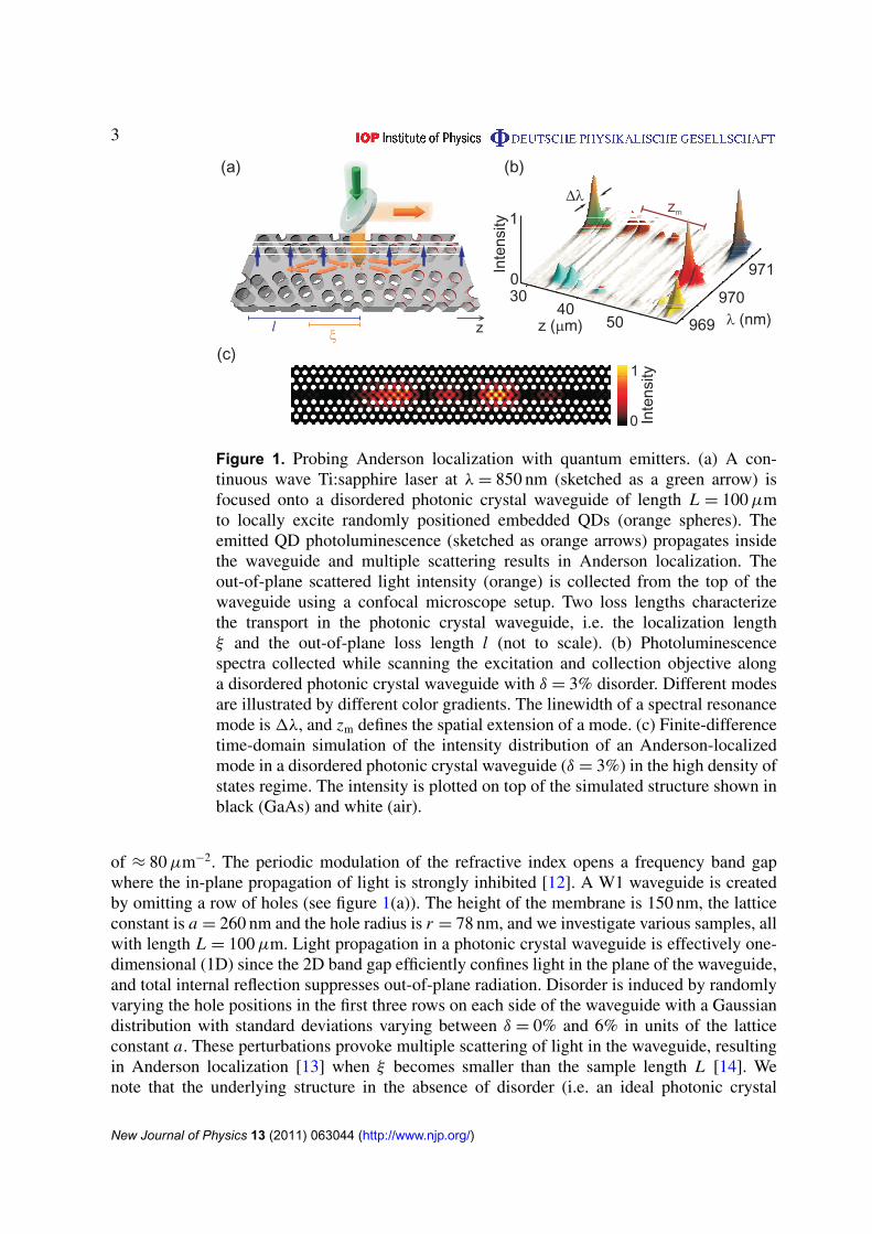
Figure 1. Probing Anderson localization with quantum emitters. (a) A con-tinuous wave Ti:sapphire laser at λ = 850 nm (sketched as a green arrow) isfocused onto a disordered photonic crystal waveguide of length L = 100 µmto locally excite randomly positioned embedded QDs (orange spheres). Theemitted QD photoluminescence (sketched as orange arrows) propagates insidethe waveguide and multiple scattering results in Anderson localization. Theout-of-plane scattered light intensity (orange) is collected from the top of thewaveguide using a confocal microscope setup. Two loss lengths characterizethe transport in the photonic crystal waveguide, i.e. the localization lengthξ and the out-of-plane loss length l (not to scale). (b) Photoluminescencespectra collected while scanning the excitation and collection objective alonga disordered photonic crystal waveguide with δ = 3% disorder. Different modesare illustrated by different color gradients. The linewidth of a spectral resonancemode is 1λ, and zm defines the spatial extension of a mode. (c) Finite-differencetime-domain simulation of the intensity distribution of an Anderson-localizedmode in a disordered photonic crystal waveguide (δ = 3%) in the high density ofstates regime. The intensity is plotted on top of the simulated structure shown inblack (GaAs) and white (air).
of ≈ 80 µm−2. The periodic modulation of the refractive index opens a frequency band gapwhere the in-plane propagation of light is strongly inhibited [12]. A W1 waveguide is createdby omitting a row of holes (see figure 1(a)). The height of the membrane is 150 nm, the latticeconstant is a = 260 nm and the hole radius is r = 78 nm, and we investigate various samples, allwith length L = 100 µm. Light propagation in a photonic crystal waveguide is effectively one-dimensional (1D) since the 2D band gap efficiently confines light in the plane of the waveguide,and total internal reflection suppresses out-of-plane radiation. Disorder is induced by randomlyvarying the hole positions in the first three rows on each side of the waveguide with a Gaussiandistribution with standard deviations varying between δ = 0% and 6% in units of the latticeconstant a. These perturbations provoke multiple scattering of light in the waveguide, resultingin Anderson localization [13] when ξ becomes smaller than the sample length L [14]. Wenote that the underlying structure in the absence of disorder (i.e. an ideal photonic crystal
New Journal of Physics 13 (2011) 063044 (http://www.njp.org/)
4
waveguide) is strongly dispersive, giving rise to a modified local density of optical states(DOS); it has been employed as an efficient single-photon source [15]. This modified DOS,however, prevails in the presence of a moderate amount of disorder, which is the situationin the present experiment. This allows us to study an interesting interplay between order anddisorder where Anderson localization may occur close to the photonic band edge of disorderedphotonic crystals, as proposed theoretically in a pioneering work on photonic bandgapmaterials [16]. As a consequence, a disorder parameter such as the localization length can becontrolled to a certain degree by exploiting the underlying dispersion of the photonic bandstructure.
The samples are probed using a confocal micro-photoluminescence setup for exciting anensemble of QDs within a diffraction-limited region along the waveguide; see figure 1(a). Theemitted light is collected with a microscope objective with a numerical aperture of 0.65. Thesamples are placed in a helium flow cryostat and cooled to a temperature of T = 10 K. Byusing a high excitation power density of P = 2 kW cm−2 the QD emission is saturated, enablingefficient excitation of Anderson-localized modes over a spectral range of λ = 950 ± 50 nm.The photoluminescence is sent to a spectrometer with 50 pm resolution and measured on aCCD camera. The sample position is controlled with stages providing a spatial resolutionof 0.3 µm. Spatially confined and spectrally separated resonances are clearly visible in thephotoluminescence spectra collected at different positions z along the waveguide (figure 1(b)).Neighboring peaks appearing along the waveguide and characterized by the sample centralwavelength, λ, and linewidth, 1λ, are attributed to the same Anderson-localized mode andplotted in figure 1(b) with the same color. Finite-difference time-domain simulations support theexistence of localized modes. Figure 1(c) displays the calculated intensity at a fixed wavelength,showing that light is strongly confined along the waveguide owing to the process of multiplescattering. A thorough numerical investigation of Anderson-localized modes in disorderedphotonic crystal waveguides can be found in [17].
3. Quality factor distribution of Anderson-localized modes
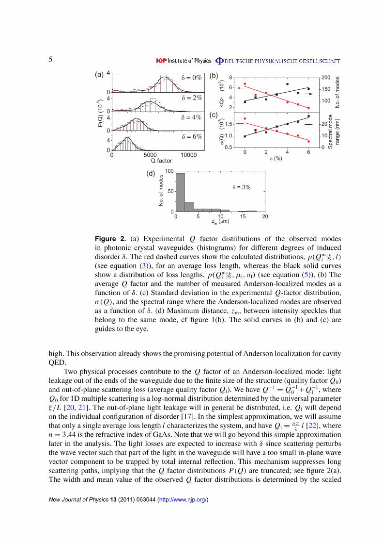
Multiple scattering of light is described by a statistical process. As a consequence, allcharacteristic parameters of Anderson-localized modes, i.e. the Q factor or the spatial extent, aredistributed and only statistical parameters such as the average or the variance can be predicted.In this section, we analyze the distributions of Q factors of the Anderson-localized modes andrelate them to the underlying characteristic parameters, i.e. the localization length and the loss-length distributions. We observe more than 100 spatially and spectrally distributed Anderson-localized modes in each photonic crystal waveguide (figure 2(b)) at wavelengths in the regionof a high DOS, where the extinction length is the shortest [9]. The Q factor of the modes,Q = λ/1λ, is extracted from the intensity spectra collected along the waveguide by fitting theresonances with Lorentzians [18]. Since the narrowest Q factors are influenced by the resolutionof the spectrometer, all experimental spectra are first deconvoluted with the measured instrumentresponse function. The Q factors that are attributed to the same mode are only counted once.We observe in figure 2(a) that Anderson localization gives rise to a very broad distributionof Q factors ranging from Q = 200 to Q = 10 000 and notably that the average Q decreaseswith the amount of introduced disorder. Interestingly, the highest Q factors we observe in theAnderson-localized cavities are not far from the values obtained with state-of-the-art engineerednano-cavities with low density of QDs [19], despite the fact that our QD density is relatively
New Journal of Physics 13 (2011) 063044 (http://www.njp.org/)
5
(b)(a)
(c)2
4
6
8
<Q
>(1
03 )
100
150
200
No.
ofm
odes
0 2 4 60.5
1.0
1.5
(Q)
(103 )
(%)
0
10
20
Spe
ctra
lmod
era
nge
(nm
)
(d)
0 5 10 15 200
50
100
No.
ofm
odes
zm
( m)
= 3%
0
4
= 2%
= 4%
= 6%
= 0%
0
4
P(Q
)(1
0-4)
0 5000 100000
4
Q factor
0
4
Figure 2. (a) Experimental Q factor distributions of the observed modesin photonic crystal waveguides (histograms) for different degrees of induceddisorder δ. The red dashed curves show the calculated distributions, p(Qm
i |ξ, l)(see equation (3)), for an average loss length, whereas the black solid curvesshow a distribution of loss lengths, p(Qm
i |ξ, µl, σl) (see equation (5)). (b) Theaverage Q factor and the number of measured Anderson-localized modes as afunction of δ. (c) Standard deviation in the experimental Q-factor distribution,σ(Q), and the spectral range where the Anderson-localized modes are observedas a function of δ. (d) Maximum distance, zm, between intensity speckles thatbelong to the same mode, cf figure 1(b). The solid curves in (b) and (c) areguides to the eye.
high. This observation already shows the promising potential of Anderson localization for cavityQED.
Two physical processes contribute to the Q factor of an Anderson-localized mode: lightleakage out of the ends of the waveguide due to the finite size of the structure (quality factor Q0)and out-of-plane scattering loss (average quality factor Ql). We have Q−1
= Q−10 + Q−1
l , whereQ0 for 1D multiple scattering is a log-normal distribution determined by the universal parameterξ/L [20, 21]. The out-of-plane light leakage will in general be distributed, i.e. Ql will dependon the individual configuration of disorder [17]. In the simplest approximation, we will assumethat only a single average loss length l characterizes the system, and have Ql =
n π
λl [22], where
n = 3.44 is the refractive index of GaAs. Note that we will go beyond this simple approximationlater in the analysis. The light losses are expected to increase with δ since scattering perturbsthe wave vector such that part of the light in the waveguide will have a too small in-plane wavevector component to be trapped by total internal reflection. This mechanism suppresses longscattering paths, implying that the Q factor distributions P(Q) are truncated; see figure 2(a).The width and mean value of the observed Q factor distributions is determined by the scaled
New Journal of Physics 13 (2011) 063044 (http://www.njp.org/)
6
localization length ξ/L , and a wide distribution means a small localization length and viceversa. Furthermore, the highest achievable Q is limited by the loss length l.
In the following, a detailed analysis of the experimental Q factor distributions is presented,allowing us to estimate ξ and l. We can express P(Q) by the log-normal probability distributionof the in-plane Q factors P(Q0) [21] that is modified due to the presence of out-of-planescattering:
P(Q) = 2(Ql − Q)
∫∞
0dQ0 P(Q0)δ
[Q − (Q−1
0 + Q−1l )−1
], (1)
where the Heaviside step function, 2, imposes an upper limit, Ql, on the distribution. Afterevaluating equation (1) we obtain the conditional likelihood that a 1D disordered medium witha certain localization length ξ and average loss length l supports an Anderson-localized modewith quality factor Qi :
p1(Qi |ξ, l) = exp
(−
(µ − log( Qi QlQl−Qi
))2
2s2
)Ql2(Ql − Qi)
Qi (Qi − Ql)√
2π s, (2)
where µ = (5.9 ± 0.3) (ξ/L)−0.22±0.01 and s = (0.4 ± 0.2) (ξ/L)−0.59±0.01. Equation (2) is a log-normal distribution characterized by the parameters s and µ that are related to the localizationlength via a power law. The explicit expressions for s and µ were obtained by calculating thein-plane Q factors of Anderson-localized modes in a 1D disordered medium that is composedof a stack of layers with randomly varying real parts of the refractive index. We note that allphysical observables in a lossy 1D random medium are determined by the universal parametersξ/L and l/λ, i.e. the microscopic details of the medium are indifferent. Therefore, since lightpropagation in a photonic crystal waveguide is 1D, the stack of randomly varying dieletriclayers is an adequate model that is parameterized by the two universal quantities. This modelcan subsequently be employed to extract the two universal parameters from the experimentaldata, as will be explained in detail below. We stress that calculations of the actual values ofξ/L and l/λ would require full 3D numerical simulations including an appropriate ensembleaverage over configurations of disorder [23]. We obtain the distribution P(Q0) by ensembleaveraging over eight million different realizations of disorder using an average refractive indexof each layer of n = 3.44 (refractive index of GaAs), a thickness of L p = 10 nm and the samplelength of L = 100 µm. The refractive index is randomly varied by applying a flat distributionwithin n ± 1n, where 1n = (0.22 ± 0.03)(ξ/L)−0.55±0.01. This functional form is obtained aftercalculating the ensemble-averaged transmission through the stacked layers depending on thesample length, i.e. 〈ln T (L)〉 = −L/ξ , and for different 1n. It is evident from equation (2)that the localization length and the loss length contribute differently to the distribution ofQ factors. Experimentally recording the distribution of Q factors therefore enables one todistinguish the localization from loss, which is not a priori possible for standard transmissionmeasurements. Since the measured Q factors, Qm
i , have experimental uncertainty, the resultantprobability distribution will not be abruptly truncated at Ql and we account for this uncertaintyby convoluting p1(Qi |ξ, l) with a normal distribution, p2(Qm
i − Qi), that is centered aroundQm
i , i.e.
p(Qmi |ξ, l) =
∫∞
0dQi p1(Qi |ξ, l) p2(Qm
i − Qi). (3)
New Journal of Physics 13 (2011) 063044 (http://www.njp.org/)
7
(a)
(c)
(b)
0.4
l(m
m) 0.6
0.8
10 20( m)
0
max
P(
,)
l | {
Q}
30
0
10
20
30
(m
)
0 2 4 60.25
0.50
0.75
l(m
m)
(%)
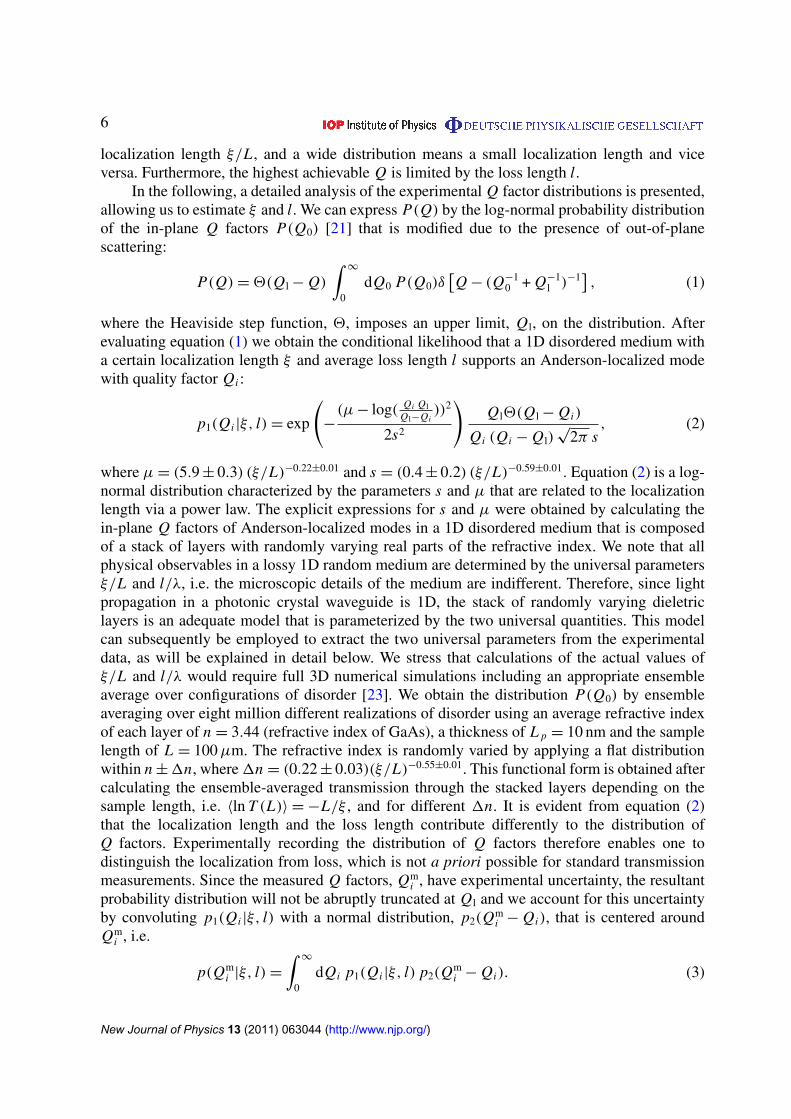
Figure 3. (a) Conditional probability P(ξ, l|{Q}) that a disordered 1D mediumwith a localization length ξ and average loss length l can be described by themeasured Q factor distributions, plotted as a function of ξ and l and for variousdegrees of disorder. (b) Localization length versus degree of disorder. The redcircles are obtained from the data in panel (a) by locating the value wherethe probability P(ξ, l|{Q}) is largest. The black triangles are obtained fromP(ξ, µl, σl|{Q}) where a distribution of loss lengths were included. Inset: sketchof the light scattering processes (red arrows) and out-of-plane scattering (bluearrows). (c) Blue circles (black triangles) are the average loss lengths extractedfrom P(ξ, l|{Q}) (P(ξ, µl, σl|{Q})). The solid curves in (b) and (c) are guidesto the eye.
Assuming that the individual probabilities p(Qmi |ξ, l) are independent, the combined
probability of measuring a set of N individual Q factors, {Q} = {Qm1 , . . . , Qm
N}, isP({Q}|ξ, l) =
∏Ni=1 p(Qm
i |ξ, l). In order to estimate the localization length and loss lengthfor a specific set {Q}, we calculate the inverted conditional probability using the Bayesiantheorem [24]
P(ξ, l|{Q}) =P({Q}|ξ, l)
P({Q}), (4)
where P({Q}) is a normalization factor. These expressions can be compared to our experimentaldata on the distribution of Q factors. In figure 2(a), the theoretical Q factor distributions ofthe form in equation (3) that give rise to the largest probability P(ξ, l|{Q}) are plotted and,in general, good agreement between experiment and theory is observed for all degrees ofdisorder.
Equation (4) is a very useful relation since it can be used to extract the localizationlength and average loss length from the measured Q factor distributions. The dependenceof the conditional probability on ξ and l is shown in figure 3(a). We only observe largevalues of P(ξ, l|{Q}) in a very restricted range that is strongly dependent on disorder. Thisenables us to extract the localization length and the loss length. The corresponding data areplotted in figure 3(b); these were obtained by averaging over the full spectral range whereAnderson-localized modes were observed, cf figure 2(c). We extract a localization length thatincreases with disorder from ξ = 6 µm to ξ = 24 µm, which is shorter than the sample length(L = 100 µm), thus confirming that the 1D criterion for Anderson localization is fulfilled. We
New Journal of Physics 13 (2011) 063044 (http://www.njp.org/)
8
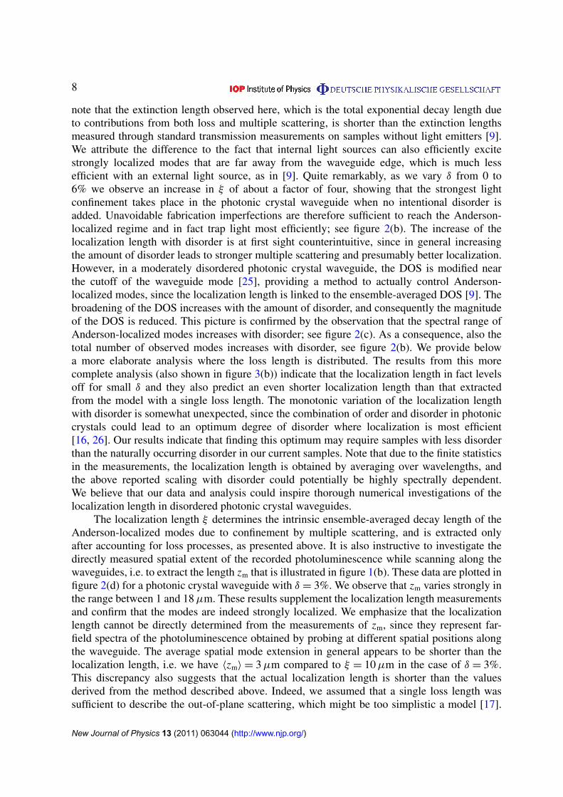
note that the extinction length observed here, which is the total exponential decay length dueto contributions from both loss and multiple scattering, is shorter than the extinction lengthsmeasured through standard transmission measurements on samples without light emitters [9].We attribute the difference to the fact that internal light sources can also efficiently excitestrongly localized modes that are far away from the waveguide edge, which is much lessefficient with an external light source, as in [9]. Quite remarkably, as we vary δ from 0 to6% we observe an increase in ξ of about a factor of four, showing that the strongest lightconfinement takes place in the photonic crystal waveguide when no intentional disorder isadded. Unavoidable fabrication imperfections are therefore sufficient to reach the Anderson-localized regime and in fact trap light most efficiently; see figure 2(b). The increase of thelocalization length with disorder is at first sight counterintuitive, since in general increasingthe amount of disorder leads to stronger multiple scattering and presumably better localization.However, in a moderately disordered photonic crystal waveguide, the DOS is modified nearthe cutoff of the waveguide mode [25], providing a method to actually control Anderson-localized modes, since the localization length is linked to the ensemble-averaged DOS [9]. Thebroadening of the DOS increases with the amount of disorder, and consequently the magnitudeof the DOS is reduced. This picture is confirmed by the observation that the spectral range ofAnderson-localized modes increases with disorder; see figure 2(c). As a consequence, also thetotal number of observed modes increases with disorder, see figure 2(b). We provide belowa more elaborate analysis where the loss length is distributed. The results from this morecomplete analysis (also shown in figure 3(b)) indicate that the localization length in fact levelsoff for small δ and they also predict an even shorter localization length than that extractedfrom the model with a single loss length. The monotonic variation of the localization lengthwith disorder is somewhat unexpected, since the combination of order and disorder in photoniccrystals could lead to an optimum degree of disorder where localization is most efficient[16, 26]. Our results indicate that finding this optimum may require samples with less disorderthan the naturally occurring disorder in our current samples. Note that due to the finite statisticsin the measurements, the localization length is obtained by averaging over wavelengths, andthe above reported scaling with disorder could potentially be highly spectrally dependent.We believe that our data and analysis could inspire thorough numerical investigations of thelocalization length in disordered photonic crystal waveguides.
The localization length ξ determines the intrinsic ensemble-averaged decay length of theAnderson-localized modes due to confinement by multiple scattering, and is extracted onlyafter accounting for loss processes, as presented above. It is also instructive to investigate thedirectly measured spatial extent of the recorded photoluminescence while scanning along thewaveguides, i.e. to extract the length zm that is illustrated in figure 1(b). These data are plotted infigure 2(d) for a photonic crystal waveguide with δ = 3%. We observe that zm varies strongly inthe range between 1 and 18 µm. These results supplement the localization length measurementsand confirm that the modes are indeed strongly localized. We emphasize that the localizationlength cannot be directly determined from the measurements of zm, since they represent far-field spectra of the photoluminescence obtained by probing at different spatial positions alongthe waveguide. The average spatial mode extension in general appears to be shorter than thelocalization length, i.e. we have 〈zm〉 = 3 µm compared to ξ = 10 µm in the case of δ = 3%.This discrepancy also suggests that the actual localization length is shorter than the valuesderived from the method described above. Indeed, we assumed that a single loss length wassufficient to describe the out-of-plane scattering, which might be too simplistic a model [17].
New Journal of Physics 13 (2011) 063044 (http://www.njp.org/)
9
Below we go beyond this assumption by introducing a distribution of loss lengths, and indeedin this case a shorter localization length is found.
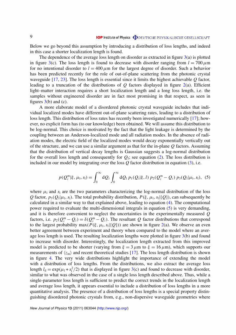
The dependence of the average loss length on disorder as extracted in figure 3(a) is plottedin figure 3(c). The loss length is found to decrease with disorder ranging from l = 700 µmfor no intentional disorder to l = 400 µm for the largest degree of disorder. Such a behaviorhas been predicted recently for the role of out-of-plane scattering from the photonic crystalwaveguide [17, 23]. The loss length is essential since it limits the highest achievable Q factor,leading to a truncation of the distributions of Q factors displayed in figure 2(a). Efficientlight–matter interaction requires a short localization length and a long loss length, i.e. thesamples without engineered disorder are in fact most promising in that respect, as seen infigures 3(b) and (c).
A more elaborate model of a disordered photonic crystal waveguide includes that indi-vidual localized modes have different out-of-plane scattering rates, leading to a distribution ofloss length. This distribution of loss rates has recently been investigated numerically [17]; how-ever, no explicit form has (to our knowledge) been obtained. We will assume this distribution tobe log-normal. This choice is motivated by the fact that the light leakage is determined by thecoupling between an Anderson-localized mode and all radiation modes. In the absence of radi-ation modes, the electric field of the localized modes would decay exponentially vertically outof the structure, and we can use a similar argument as that for the in-plane Q factors. Assumingthat the distribution of vertical decay lengths is Gaussian suggests a log-normal distributionfor the overall loss length and consequently for Ql; see equation (2). The loss distribution isincluded in our model by integrating over the loss Q factor distribution in equation (3), i.e.
p(Qmi |ξ, µl, sl) =
∫∞
0dQi
∫∞
0dQl p1(Qi|ξ, l) p2(Qm
i − Qi) p3(Ql|µl, sl), (5)
where µl and sl are the two parameters characterizing the log-normal distribution of the lossQ factor, p3(Ql|µl, sl). The total probability distribution, P(ξ, µl, sl|{Q}), can subsequently becalculated in a similar way to that explained above, leading to equation (4). The computationalpower required to evaluate the multi-dimensional integrals in equation (5) is very demanding,and it is therefore convenient to neglect the uncertainties in the experimentally measured Qfactors, i.e. p2(Qm
i − Qi) = δ(Qmi − Qi). The resultant Q factor distributions that correspond
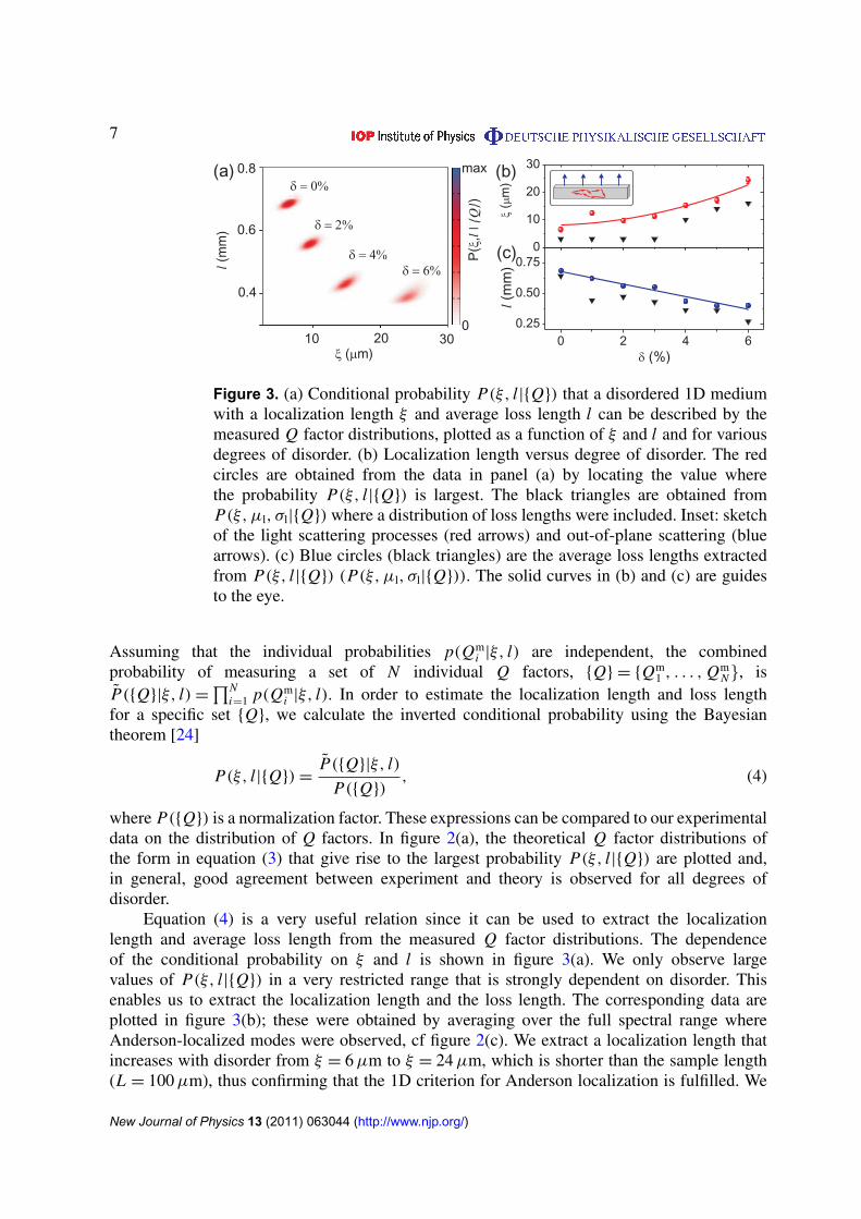
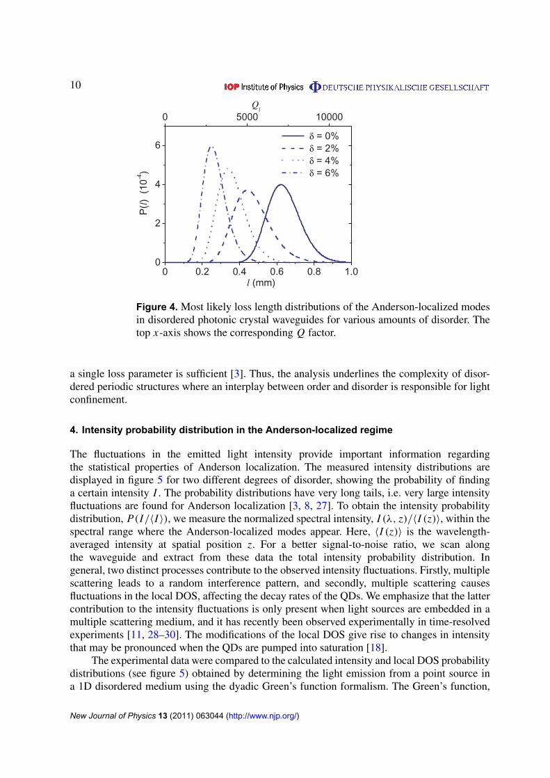
to the largest probability max(P(ξ, µl, sl|{Q})) are shown in figure 2(a). We observe an evenbetter agreement between experiment and theory when compared to the model where an aver-age loss length is used. The resulting localization lengths were plotted in figure 3(b) and foundto increase with disorder. Interestingly, the localization length extracted from this improvedmodel is predicted to be shorter (varying from ξ = 3 µm to ξ = 16 µm), which supports ourmeasurements of 〈zm〉 and recent theoretical studies [17]. The loss length distribution is shownin figure 4. The very wide distributions highlight the importance of extending the modelwith a distribution of loss lengths. From the distributions, we also extract the average losslength ld = exp(µl + s2
l /2) that is displayed in figure 3(c) and found to decrease with disorder,similar to what was observed in the case of a single loss length described above. Thus, while asingle-parameter loss length is sufficient to predict the correct trends in the localization lengthand average loss length, it appears essential to include a distribution of loss lengths in a morequantitative analysis. The presence of a distribution of loss lengths is a special property distin-guishing disordered photonic crystals from, e.g., non-dispersive waveguide geometries where
New Journal of Physics 13 (2011) 063044 (http://www.njp.org/)
10
0 0.2 0.4 0.6 0.8 1.00
2
4
6δ = 0%δ = 2%δ = 4%δ = 6%
P(l
)(1
0-4)
l (mm)
0 5000 10000Q
l
Figure 4. Most likely loss length distributions of the Anderson-localized modesin disordered photonic crystal waveguides for various amounts of disorder. Thetop x-axis shows the corresponding Q factor.
a single loss parameter is sufficient [3]. Thus, the analysis underlines the complexity of disor-dered periodic structures where an interplay between order and disorder is responsible for lightconfinement.
4. Intensity probability distribution in the Anderson-localized regime
The fluctuations in the emitted light intensity provide important information regardingthe statistical properties of Anderson localization. The measured intensity distributions aredisplayed in figure 5 for two different degrees of disorder, showing the probability of findinga certain intensity I . The probability distributions have very long tails, i.e. very large intensityfluctuations are found for Anderson localization [3, 8, 27]. To obtain the intensity probabilitydistribution, P(I/〈I 〉), we measure the normalized spectral intensity, I (λ, z)/〈I (z)〉, within thespectral range where the Anderson-localized modes appear. Here, 〈I (z)〉 is the wavelength-averaged intensity at spatial position z. For a better signal-to-noise ratio, we scan alongthe waveguide and extract from these data the total intensity probability distribution. Ingeneral, two distinct processes contribute to the observed intensity fluctuations. Firstly, multiplescattering leads to a random interference pattern, and secondly, multiple scattering causesfluctuations in the local DOS, affecting the decay rates of the QDs. We emphasize that the lattercontribution to the intensity fluctuations is only present when light sources are embedded in amultiple scattering medium, and it has recently been observed experimentally in time-resolvedexperiments [11, 28–30]. The modifications of the local DOS give rise to changes in intensitythat may be pronounced when the QDs are pumped into saturation [18].
The experimental data were compared to the calculated intensity and local DOS probabilitydistributions (see figure 5) obtained by determining the light emission from a point source ina 1D disordered medium using the dyadic Green’s function formalism. The Green’s function,
New Journal of Physics 13 (2011) 063044 (http://www.njp.org/)
11
0 5 10 15 20 251E-5
1E-4
1E-3
0.01
0.1
1
10
100
1000= 1%= 6%
P(I/<I>)P(LDOS/<LDOS>)
P(I
/<I>
)
I/<I>
x 100
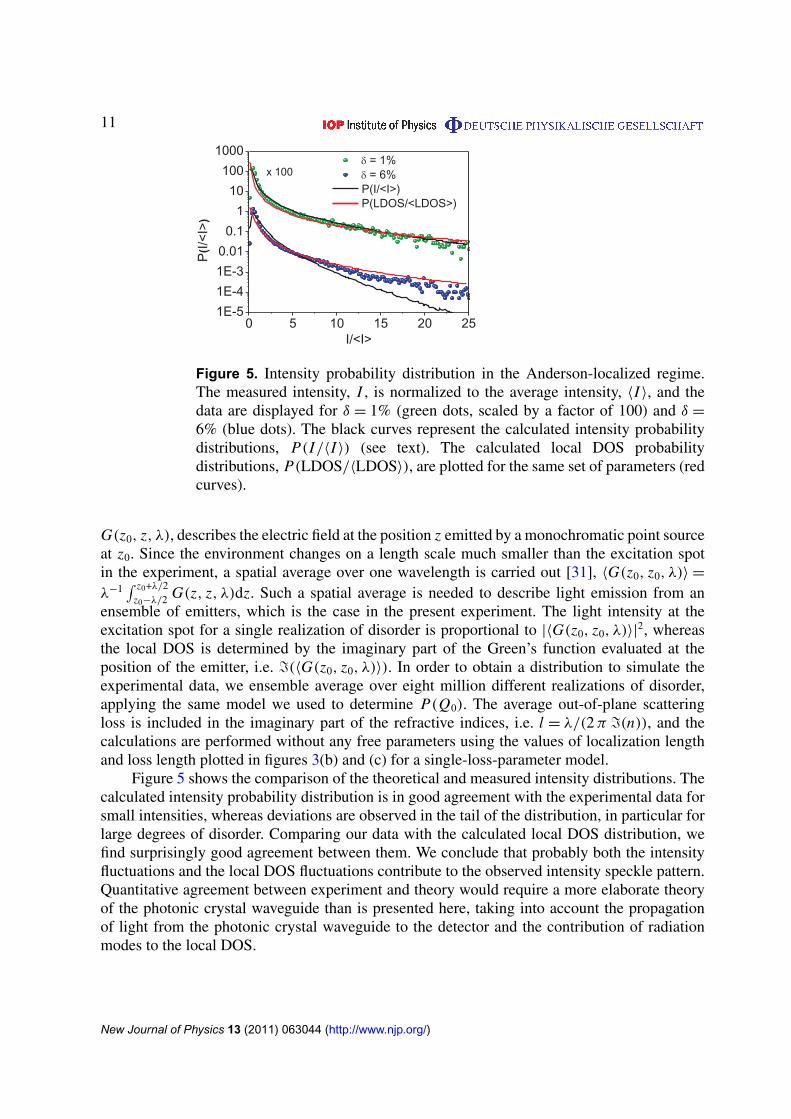
Figure 5. Intensity probability distribution in the Anderson-localized regime.The measured intensity, I , is normalized to the average intensity, 〈I 〉, and thedata are displayed for δ = 1% (green dots, scaled by a factor of 100) and δ =
6% (blue dots). The black curves represent the calculated intensity probabilitydistributions, P(I/〈I 〉) (see text). The calculated local DOS probabilitydistributions, P(LDOS/〈LDOS〉), are plotted for the same set of parameters (redcurves).
G(z0, z, λ), describes the electric field at the position z emitted by a monochromatic point sourceat z0. Since the environment changes on a length scale much smaller than the excitation spotin the experiment, a spatial average over one wavelength is carried out [31], 〈G(z0, z0, λ)〉 =
λ−1∫ z0+λ/2
z0−λ/2 G(z, z, λ)dz. Such a spatial average is needed to describe light emission from anensemble of emitters, which is the case in the present experiment. The light intensity at theexcitation spot for a single realization of disorder is proportional to |〈G(z0, z0, λ)〉|2, whereasthe local DOS is determined by the imaginary part of the Green’s function evaluated at theposition of the emitter, i.e. =(〈G(z0, z0, λ)〉). In order to obtain a distribution to simulate theexperimental data, we ensemble average over eight million different realizations of disorder,applying the same model we used to determine P(Q0). The average out-of-plane scatteringloss is included in the imaginary part of the refractive indices, i.e. l = λ/(2 π =(n)), and thecalculations are performed without any free parameters using the values of localization lengthand loss length plotted in figures 3(b) and (c) for a single-loss-parameter model.
Figure 5 shows the comparison of the theoretical and measured intensity distributions. Thecalculated intensity probability distribution is in good agreement with the experimental data forsmall intensities, whereas deviations are observed in the tail of the distribution, in particular forlarge degrees of disorder. Comparing our data with the calculated local DOS distribution, wefind surprisingly good agreement between them. We conclude that probably both the intensityfluctuations and the local DOS fluctuations contribute to the observed intensity speckle pattern.Quantitative agreement between experiment and theory would require a more elaborate theoryof the photonic crystal waveguide than is presented here, taking into account the propagationof light from the photonic crystal waveguide to the detector and the contribution of radiationmodes to the local DOS.
New Journal of Physics 13 (2011) 063044 (http://www.njp.org/)
12
5. Conclusion
In conclusion, we have presented a novel approach to probe the statistical properties ofAnderson localization in a disordered photonic crystal waveguide. Using ensembles of QDemitters distributed along the waveguide, Anderson-localized modes are very efficiently excited,allowing us to study the Q factor distributions and the intensity fluctuations. By analyzingthe QD photoluminescence, we recorded a broad distribution of Q factors that was stronglydependent on the induced disorder, and which can be explained by changes in the localizationand loss lengths. Comparing the experimental data with a 1D model for Anderson localization,we determined the localization length and found a counterintuitive increase with the amount ofdisorder, which we attribute to the modified DOS of a photonic crystal waveguide prevailingin the presence of a moderate amount of disorder. The observed monotonic increase in thelocalization length showed that Anderson localization in disordered photonic crystals behavesfundamentally differently than in uncorrelated disordered systems, where the localization lengthdecreases with the amount of disorder. We furthermore conclude that the loss in a disorderedphotonic crystal waveguide is also distributed, which significantly increases the complexity ofthe multiple scattering model used for extracting universal parameters from the experimentaldata. These results may open a route to the engineering of Anderson-localized modes bycontrolling the amount and type of disorder, which could significantly improve the performanceof quantum electrodynamic experiments in random media [11]. Finally, we recorded theintensity fluctuations in the photoluminescence signal and observed good agreement with ourtheoretical model using the parameters extracted from the Q factor distribution analysis. Theconsistency between the two independent sets of measurements is an important check of thevalidity of the applied approach, proving that a 1D multiple scattering model very successfullydescribes the behavior of light transport in disordered photonic crystal waveguides.
Acknowledgments
We thank P T Kristensen and N A Mortensen for fruitful discussions on the simulations andtheoretical model and gratefully acknowledge financial support from the Villum Foundation,the Danish Council for Independent Research (Natural Sciences and Technology and ProductionSciences) and the European Research Council (ERC consolidator grant). LSFP acknowledgesfinancial support from the Spanish MICINN Consolider Nanolight project (CSD2007-00046).
References
[1] van Rossum M C W and Nieuwenhuizen Th M 1999 Rev. Mod. Phys. 71 313[2] Anderson P W 1958 Phys. Rev. 109 1492[3] Chabanov A A, Stoytchev M and Genack A Z 2000 Nature 404 850[4] Wiersma D S, Bartolini P, Lagendijk A and Righini R 1997 Nature 390 671[5] Störzer M, Gross P, Aegerter C M and Maret G 2006 Phys. Rev. Lett. 96 063904[6] Billy J, Josse V, Zuo Z, Bernard A, Hambrecht B, Lugan P, Clément D, Sanchez-Palencia L, Bouyer P and
Aspect A 2008 Nature 453 891[7] Roati G, D’Errico C, Fallani L, Fattori M, Fort C, Zaccanti M, Modugno G, Modugno M and Inguscio M
2008 Nature 453 895[8] Hu H, Strybulevych A, Page J H, Skipetrov S E and van Tiggelen B A 2008 Nat. Phys. 4 945
New Journal of Physics 13 (2011) 063044 (http://www.njp.org/)
13
[9] García P D, Smolka S, Stobbe S and Lodahl P 2010 Phys. Rev. B 82 165103[10] Tureci H E, Ge L, Rotter S and Stone A D 2008 Science 320 643[11] Sapienza L, Thyrrestrup H, Stobbe S, García P D, Smolka S and Lodahl P 2010 Science 327 1352[12] Julsgaard B, Johansen J, Stobbe S, Stolberg-Rohr T, Sünner T, Kamp M, Forchel A and Lodahl P 2008 Appl.
Phys. Lett. 93 094102[13] Topolancik J, Ilic B and Vollmer F 2007 Phys. Rev. Lett. 99 253901[14] Sheng P 1995 Introduction to Wave Scattering, Localization and Mesoscopic Phenomena (New York:
Academic)[15] Lund-Hansen T, Stobbe S, Julsgaard B, Thyrrestrup H, Sünner T, Kamp M, Forchel A and Lodahl P 2008
Phys. Rev. Lett. 101 113903[16] John S 1987 Phys. Rev. Lett. 58 2486[17] Savona V 2011 Phys. Rev. B 83 085301[18] Gayral B and Gérard J M 2008 Phys. Rev. B 78 235306[19] Hennessy K, Badolato A, Winger M, Gerace D, Atatüre M, Gulde S, Fält S, Hu E L and Imamoglu A 2008
Nature 445 896[20] Kottos T 2005 J. Phys. A: Math. Gen. 38 10761[21] Pinheiro F A 2008 Phys. Rev. A 78 023812[22] Joannopoulos J D, Johnson S G, Winn J N and Meade R D 2008 Photonic Crystals: Molding the Flow of
Light (Princeton, NJ: Princeton University Press)[23] Mazoyer S, Hugonin J P and Lalanne P 2009 Phys. Rev. Lett. 103 063903[24] Gregory P 2005 Bayesian Logical Data Analysis for the Physical Sciences (Cambridge: Cambridge University
Press)[25] Thyrrestrup H, Sapienza L and Lodahl P 2010 Appl. Phys. Lett. 96 231106[26] Conti C and Fratalocchi A 2008 Nat. Phys. 4 794[27] Bertolotti J, Gottardo S, Wiersma D S, Ghulinyan M and Pavesi L 2005 Phys. Rev. Lett. 94 113903[28] Birowosuto M D, Skipetrov S E, Vos W L and Mosk A P 2010 Phys. Rev. Lett. 105 013904[29] Ruijgrok P V, Wüest R, Rebane A A, Renn A and Sandoghdar V 2010 Opt. Express 18 6360[30] Krachmalnicoff V, Castanie E, De Wilde Y and Carminati R 2010 Phys. Rev. Lett. 105 183901[31] Schomerus H, Titov M, Brouwer P W and Beenakker C W J 2002 Phys. Rev. B 65 121101
New Journal of Physics 13 (2011) 063044 (http://www.njp.org/)


