Pro-cyclical Solow Residuals Without

Technology Shocks ?

Andrew J. Clarke

Department of Economics, University of Melbourne, VIC, 3010, Australia

Alok Johri ∗

Department of Economics, McMaster University, 1280 Main St West, HamiltonON L8S 4M4, Canada

Abstract

Most Real Business Cycle models have a hard time jointly explaining the twinfacts of strongly pro-cyclical Solow residuals and extremely low correlations betweenwages and hours. We present a model that delivers both these results without us-ing exogenous variation in total factor productivity (technology shocks). The keyinnovation of the paper is to add learning-by-doing to firms technology. As a resultfirms optimally vary their prices to control the amount of learning which in turninfluences future productivity. We show that exogenous variation in labour wedges(preference shocks) measured from aggregate data deliver around fifty percent ofthe standard deviation in the efficiency wedge (Solow residual) as well as realisticsecond moments for key aggregate variables which is in sharp contrast to the modelwithout learning-by-doing.

Key words: Business cycles; Learning-by-Doing; ProductivityJEL classification: E32

? 29 June 2007∗ Corresponding author. Tel +1-905-525-9140 Ext 23830; Fax +1-905-521-8232

Email addresses: andrew.clarke@unimelb.edu.au (Andrew J. Clarke),johria@mcmaster.ca (Alok Johri).

1 Introduction

While the neoclassical growth model has proved to be an extremely effective tool for cap-

turing the basic features of business cycles, two major areas of weakness have been identified in

the literature, in terms of the ability of the model to capture the dynamics of the aggregate data.

These problems have been elegantly re-interpreted in terms of “wedges” in the equations of the

model in a recent paper by Chari et al. (2007). In an accounting exercise, the authors show that

the wedges embedded in the hours first order condition and in the production technology, are es-

sential for “explaining” the bulk of the movement seen in aggregate US data. In the business cycle

literature, these wedges have been interpreted in the past as exogenous “shocks” which are the

source of fluctuations. These interpretations of the two wedges as preference shocks and technology

shocks respectively have been controversial, not least because they assume rather than explain a

large fraction of the variation in the aggregate data. In this context, a number of authors have

attempted to develop models that produce fluctuations in the labour wedge and account for a part

of the movement in the efficiency wedge1. However much more work remains to be done in this

area. As pointed out by Chari et al. (2007), “. . . our results suggest that future theoretical work

should focus on developing models which lead to fluctuations in efficiency and labor wedges. Many

existing models produce fluctuations in labor wedges. The challenging task is to develop detailed

models in which primitive shocks lead to fluctuations in efficiency wedges as well.”2. The goal of

this paper is to take a step in this direction.

Unlike most business cycle models, there are no exogenous movements in technology in our

model. Instead, we rely on movements in the labour wedge to induce fluctuations in aggregate

variables, and the general equilibrium structure of the model to generate dynamic correlations

between these variables. We show that when fluctuations in the labour wedge are fed into a

prototypical real business cycle model, it is unable to account for many of the key features of the

data. However, when they are fed into our model it does quite well. In particular, the model does a

good job of explaining fluctuations in the efficiency wedge (essentially the Solow residual) whereas

1 See the discussion and references in King & Rebelo (1999).2 See Chari et al. (2007), p 828.

2

the prototypical model would generate no endogenous fluctuations. These results are achieved with

a simple modification to a standard real business cycle model: the presence of learning-by-doing

effects in firm’s technology which act as an endogenous propagation mechanism, converting shocks

to the labour wedge into persistent movements in total factor productivity and output.

There is a large empirical literature documenting the pervasive influence of learning-by-

doing in productive activities. Recent studies include Bahk & Gort (1993), Irwin & Klenow (1994),

Jarmin (1994), Benkard (2000), Thompson (2001), Thornton & Thompson (2001), Cooper & Johri

(2002), and Clarke (2006b). These studies find that agents and organizations appear to become

more productive as they gain experience at producing a particular product or service. A number

of these studies also report spillover effects in learning across similar products, both within and

across firms. Since there is evidence in favour of both internal and external learning-by-doing, and

there is some controversy around which one is empirically more important, we look at both types

of learning models and find that the results are not only qualitatively similar, the quantitative

differences are quite small at the aggregate level.

There exist a small number of papers that introduce learning-by-doing into dynamic general

equilibrium business cycle models. Both Cooper & Johri (2002) and Chang et al. (2002) empha-

size the ability of learning-by-doing to propagate shocks. In the former study, a representative

consumer has access to a production technology with learning effects. The latter offers a specific

decentralization in which workers learn and accumulate human capital. Our model offers a dif-

ferent decentralization in which firms accumulate production related knowledge but workers do

not3. Firms in our model operate in a market with monopolistic competition and therefore have

the power to set prices. None the less, our model is quite close Cooper & Johri (2002) in that it

directly borrows the way in which learning effects are introduced into the production technology4.

As shall be clear later, these changes have a number of novel implications. The pricing decision

facing these firms becomes dynamic because raising current prices lowers current production and

3 There is considerable evidence that organizations accumulate intangible capital which is specific to the organization.Some (though not all) aspects of this are related to learning-by-doing. Recent attempts to quantify different aspectsof organizational capital under varying names can be found in Brynjolfsson & Hitt (2000), Hall (2000), Lev &Radharkrishnan (2003), and Atkeson & Kehoe (2005) and the references therein.

4 This paper also differs in that business cycles are not generated by technology shocks.

3

learning which lead to future productivity decreases. Moreover, when firms are aware that they

can learn and build up knowledge, price-cost markups can vary endogenously in an environment

where they would be constant in the absence of learning-by-doing. In this sense, the model may be

viewed as a new theory of time varying markups. These features are absent in the earlier papers.

In contrast to our model, those models imply that labour supply is dynamic. The implications of

dynamic labour supply are discussed more fully in Johri & Letendre (2006). While we believe that

learning by workers is an important phenomenon, we choose to ignore it in this study in order to

focus on the new implications of incorporating firm level learning in business cycle models.

Simulations from a linearized version of the model calibrated to US data show that sub-

stantial improvements to the existing literature can be achieved in terms of matching the usual set

of “key” second moments. For example, the model can deliver a small positive correlation between

average labour productivity and hours which has eluded most current business cycle models, either

real or monetary. Moreover, the model generates a highly volatile and persistent efficiency wedge

(Solow residual). Depending on the specification, we can account for around forty to fifty percent

of the actual volatility in the efficiency wedge and over eighty percent of the movement in aggre-

gate output, hours, consumption and investment. These results are obtained with fairly modest

learning effects. In sharp contrast the results from the model without learning-by-doing are quite

unrealistic: average labour productivity is negatively correlated with both output and hours5. In

addition, investment and hours are too volatile relative to output. Moreover the model explains

none of the volatility in the efficiency wedge and only sixty seven percent of the volatility in output.

Unfortunately, while the simulated markups are time varying, the volatility is quantitatively too

small to account for actual markup variations over the business cycle.

The next two sections of the paper presents the two models of learning-by-doing in order

of decreasing complexity starting with the internal learning model. Section four presents results

from simulating linearized versions of the model calibrated to the U.S. economy. The final section

concludes.

5 This counter-cyclical (and counter-factual) movement in average labour productivity has long troubled models of thebusiness cycle driven by aggregate demand disturbances. See Rotemberg & Woodford (1991, 1999) for a discussionof the various attempts to overcome these problems.

4

2 A Decentralization of the Internal Learning Model

The model presented below offers a decentralization of the Cooper & Johri (2002) model.

A common feature of both models is that learning occurs as a by-product of production. The key

difference occurs in who gets to learn. In Cooper & Johri (2002), learning occurs at the household

level while in the current model it is intermediate goods firms which learn by accumulating pro-

duction related knowledge which we will refer to as organizational capital. These firms operate in

a market with monopolistic competition which gives them the power to choose prices6. The firms

control how much they wish to learn by varying the markup of price over marginal cost to maximize

the present discounted value of profits. Since the behaviour of consumers is standard, we discuss

firms first.

Final and Intermediate Goods Producers

There are a large number of producers operating in a competitive industry that produce

a final good Yt using the following technology that converts intermediate goods Qt(i) indexed by

i ∈ [0, 1] into final goods:

Yt ={ ∫ 1

0[Qt(i) ]1/µ di

}µ

(1)

Each period these firms choose inputs Qt(i) for all i ∈ [0, 1], and output Yt to maximize profits.

The conditional demand for each intermediate input Qt(i) that emerge from this exercise are:

f (vt(i), Yt) = vt(i)µ

1−µ Yt (2)

where vt(i) is the relative price charged by the ith intermediate goods producer. The price elasticity

of demand, faced by intermediate goods producer i, will be given by µ/(1 − µ). A zero profit

condition ties down the price charged by the final goods producer Pt as a function of intermediate

good prices.

There is a continuum of intermediate goods producers, indexed by the letter i that operate in

6 The model outlined below takes the standard Blanchard & Kiyotaki (1987) model of monopolistic competition,commonly used in aggregate general equilibrium models, modified to allow for the accumulation of organizationalcapital. Neither Cooper & Johri (2002) nor Chang et al. (2002) include this feature.

5

a monopolistically competitive economy. Each such producer produces a differentiated intermediate

good Q(i) according to the following production technology:

Qt(i) = F [Kt(i), Zt(i),Ht(i)] = Kt(i)θ Ht(i)α Zt(i)ε 0 < α, θ, ε < 1 (3)

where organizational capital Z(i) is combined with physical capital K(i) and labour H(i) to produce

output Q(i). The technology differs from a standard neo-classical production function because

the firm carries a stock of organizational capital which is an input in the production technology.

Organizational capital refers to the information accumulated by the firm, through the process of

past production, regarding how best to organize its production activities and deploy its inputs7.

As a result, the higher the level of organizational capital, the more productive the firm8. Note

that there are diminishing returns to accumulating organizational capital, a feature often found in

empirical studies of learning-by-doing.

While learning-by-doing is often associated with workers and modeled as the accumulation

of human capital, a number of economists have argued that firms are also store-houses of knowledge.

Atkeson & Kehoe (2005) note “At least as far back as Marshall (1930, bk.iv, chap. 13.I), economists

have argued that organizations store and accumulate knowledge that affects their technology of

production. This accumulated knowledge is a type of unmeasured capital distinct from the concepts

of physical or human capital in the standard growth model.” Similarly Lev & Radharkrishnan (2003)

write, “Organization capital is thus an agglomeration of technologies—business practices, processes

and designs, including incentive and compensation systems—that enable some firms to consistently

extract out of a given level of resources a higher level of product and at lower cost than other

firms.” There are at least two ways to think about what constitutes organizational capital. Some,

like Rosen (1972), think of it as a firm specific capital good while others focus on specific knowledge

embodied in the matches between workers and tasks within the firm. While these differences are

important, especially when trying to measure the payments associated with various inputs, we

7 Atkeson & Kehoe (2005) model and estimate the size of organizational capital for the US manufacturing sector andfind that it has a value of roughly 66 percent of physical capital. Although their broad interpretation of organizationalcapital is similar to ours, they do not allow for depreciation of past learning.

8 Since we are focusing on movements at the business cycle frequency we ignore technical progress of any form.

6

believe they are not crucial to the issues at hand. As a result we do not distinguish between the

two.

Learning at the firm level is modeled through an accumulation equation for organizational

capital which is closely related to the empirical learning-by-doing literature in which each cumulative

unit of past production contributes equally to the creation of knowledge. Our specification differs

in that the contribution of production in any period to the current level of organizational capital is

decreasing over time. Following Cooper & Johri (2002), who provide evidence on this specification,

we write the accumulation technology as

Zt+1(i) = Zt(i)η Qt(i)γ (4)

or

lnZt(i) = ηt lnZ0(i) + γt−2∑k=0

ηk lnQt−1−k(i)

where Zt(i) denotes the stock of organizational capital available to the production unit at time t,

Z0(i) denotes the initial endowment of organizational capital and Qt(i) denotes the current level of

output. This initial stock of organizational capital constitutes the inherited knowledge of the orga-

nization which might include a common component reflecting the prevailing best practice systems,

structures, and procedures, and an idiosyncratic component reflecting more specific knowledge

imparted by the organization’s founders that becomes a durable feature of the organization.

This modification of the traditional specification of learning has a number of advantages.

First, it allows for the sensible idea that production knowledge may become less and less relevant

over time as new techniques of production, new product lines and new markets emerge. Second, it

allows in a general way for the idea that some match specific knowledge may be lost to the firm as

workers leave or get reassigned to new tasks or teams within the firm. In addition, the knowledge

accumulated through production experience will be a function of the current vintage of physical

capital. The decision to replace physical capital will imply that the existing stock of organizational

capital will be less relevant. Third, it allows for the existence of a steady state in which the stock

of organizational capital is constant. In contrast, the traditional specification in the empirical

7

learning-by-doing literature allows the stock of organizational capital to grow unboundedly. An

alternative way to bound learning is to assume that productivity increases due to learning occur

for a fixed number of periods. While this may be appropriate for any one task or worker within

the firm, we think of the internal context of firms as an environment with an ever changing set

of tasks, workers, teams, machines and information. In this context it may be better to model

organizational capital as continually accumulating and depreciating.

The restriction η < 1 is consistent with the empirical evidence supporting the hypothesis of

depreciation of organizational capital often referred to as organizational forgetting. Argote et al.

(1990) provide empirical evidence for this hypothesis of organizational forgetting associated with the

construction of Liberty Ships during World War II. Similarly, Darr et al. (1995) provide evidence

for this hypothesis for pizza franchises and Benkard (2000) provides evidence for organizational

forgetting associated with the production of commercial aircraft. One difference between these

studies and and this paper is that the accumulation technology is log-linear rather than linear.

Clarke (2006a) shows that the additional curvature in this log-linear technology is unlikely to

produce predictions for aggregate variables, in response to a technology shock, considerably different

to those associated with a linear technology. It is the implied dynamic structure associated with

the accumulation of organizational capital, rather than any functional form assumptions that drives

the results in Cooper & Johri (2002). We expect similar results to follow in the current context9.

It is useful to dissect the problem faced by an intermediate goods producer into two stages.

In the first stage, the producer chooses the cost minimizing quantities of labour and physical capital,

for a given stock of organizational capital, to solve the following static cost minimization problem:

C[wt, rt, Qt(i), Zt(i)] = minHt(i) ,Kt(i)

{wtHt(i) + rtKt(i) | Kt(i)θ Ht(i)α Zt(i)ε ≥ Qt(i)

}(5)

Each intermediate goods producer is assumed to operate within perfectly competitive input markets

such that the real rental price of physical capital rt and the real wage wt are taken as given. This

9 Another seemingly crucial feature of our model is that organizational capital is accumulated as a by-product ofproduction. This ignores the considerable intentional investments made by firms in raising productivity. Hou & Johri(2007) show that allowing for intentional investments in organizational capital result in only small differences fromthe Cooper & Johri (2002) model.

8

cost minimization problem produces conditional factor demands that are a function of factor prices,

the required level of output (Qt) and the stock of organizational capital (Zt). The cost function

(5) will be a non-increasing function of the (given) stock of organizational capital.

In the second stage, the intermediate goods producer will solve a dynamic problem that

selects the time path of output supply Qt(i), or the relative price vt(i), and the time path of

organizational capital Zt(i) that maximizes the real expected discounted present value of profits,

subject to the demand function (2), the accumulation technology for organizational capital (4), and

the initial stock of organizational capital Z0(i).

Each intermediate goods’ producer solves the following maximization problem:

maxvt(i),Zt+1(i)

E0

∞∑t=0

Dt [vt(i) · f (vt(i), Yt) − C {wt, rt, f (vt(i), Yt) , Zt(i)} ]

subject to

Zt(i)η [f (vt(i), Yt)]γ = Zt+1(i)

given some initial stock of organizational capital Z0(i) and subject to an appropriate transversality

condition on the stock of organizational capital. Since firms are owned by households, Dt is the

appropriate endogenous discount rate for the firms.

The solution to the (profit) maximization problem will satisfy the following first order

conditions:

vt(i)f ′ (vt(i)) + f (vt(i)) − mct(i) f ′ (vt(i)) = −λft (i)

∂Zt+1(i)∂Qt(i)

f ′ (vt(i)) (6)

and

λft (i) = Et

[Dt+1

Dt

{λf

t+1(i)∂Zt+2(i)∂Zt+1(i)

− ∂Ct+1(i)∂Zt+1(i)

}](7)

where mct(i) denotes the marginal cost of producing output Q(i). The term λft (i) denotes the

Lagrange multiplier associated with the maximization problem defined above and represents the

discounted value of an additional unit of organizational capital, in terms of marginal real profits.

The first order condition (6) captures the nature of the dynamic tradeoff that arises when

9

intermediate goods producers face a downward sloping demand curve. Fundamentally, these pro-

ducers face a tradeoff between maximizing current period profits and losing future productivity

increases. The first order condition (6) determines the optimal relative price vt to be set by the

producer of the intermediate input i. Since the intermediate goods producer faces a downward

sloping demand curve for their product, raising the output price by one unit causes demand for

their product to fall. The first two terms in (6) captures the impact on current revenue of raising the

relative price of output vt. The third term represents the reduction in current period costs resulting

from this corresponding lower level of output. The accumulation technology for organizational cap-

ital implies that a reduction in current output will lead to a reduction in the stock of organizational

capital available in the next period. The term on the right hand side of (6) represents the value of

this reduced (future) stock of organizational capital. The term f ′ (vt(i)) measures the reduction in

current output due to the higher relative price and the term ∂Zt+1/∂Qt represents the reduction in

the stock of organizational capital resulting from the reduction in current period output, evaluated

at the marginal value of organizational capital to the intermediate goods producer. The first order

condition implies that the firm will set its optimal price by equating the current period benefit

of increasing its relative price by one unit to the discounted future costs. This tradeoff, captured

by the (dynamic) term on the right hand side of (6), will not appear in the standard model of

monopolistic competition, without the accumulation of organizational capital

The first order condition (7) determines the value of an additional unit of organizational

capital for use by the producer in period t + 1. This additional unit of organizational capital has a

(marginal) value, in terms of profits, of λft to the producer. Since the cost function is decreasing in

the stock of organizational capital, an additional unit of organizational capital reduces the cost of

producing output level Qt+1. The accumulation equation for organizational capital implies that an

additional unit of organizational capital will increase the stock of organizational capital available

in period t + 2. This higher stock of organizational capital has a value of λft+1 to the producer.

The condition (7) implies that organizational capital will be accumulated up to the point where

the value of an additional unit of organizational capital today is equal to the discounted value of

this organizational capital next period.

10

Households

The economy is populated by a continuum of identical, infinitely lived households. At time

t, the representative household has preferences over consumption of final goods Ct and leisure

(T − Ht) where T represents the total time endowment. The representative household maximizes

the expected discounted present value of utility by choosing consumption Ct, labour supply Ht,

and investment in physical capital It, taking as given the real wage wt and the real interest rate rt.

Consumers sell labour services and rent physical capital to the intermediate goods producers. As

owners of the intermediate goods producers, they also receive the current profits of these producers.

Physical capital is stored and accumulated by consumers according to a standard accumulation

technology. The flow utility of the representative household is given by:

U(Ct, T − Ht) = lnCt + Bt V(T − Ht) (8)

where:

V(T − Ht) =

11 − ν

(T − Ht)1−ν for ν ≥ 0 and ν 6= 1

ln (T − Ht) for ν = 1

and the term Bt evolves according to:

lnBt = (1 − ρb) ln B̄ + ρb lnBt−1 + υbt

where υbt is an iid random variable with mean zero and standard deviation σb. Bt is the only

exogenous source of fluctuations in our model. It represents the idea of the “labour wedge” explored

in Chari et al. (2007). We chose this formulation of the labour wedge over representing it as a labour

income tax because it is also consistent with the idea of preference shocks which are increasingly

being used in business cycle models. Early references include Parkin (1988) and Baxter & King

(1991). More recently they can be found in Chang et al. (2002) which is a business cycle model

11

with only real shocks and Ireland (2004a,b) which have both preference and money shocks10.

An obvious question that arises in this context is what does the labour wedge represent?

Our interpretation is that this is anything that exogenously shifts the aggregate labour supply

at business cycle frequencies. Some possible sources of such shifts have been explored in the

literature. For example, if the marginal utility of leisure is a function of omitted variables such

as money balances or government spending, then variations in these might directly account for

these shifts. See Parkin (1988) for an early discussion of this point. At a deeper level one might

imagine these may be caused by changes in the amount of distortions in the economy caused by

taxation and transfer payments, unionization and other shifts in market power. See, for example,

Mulligan (2002) and Chari et al. (2002) or Cole & Ohanian (2002, 2004) for a model in which shifts

in government policy towards monopolies in a model with unions can account for these preference

shifts in the context of the Great Depression. Rotemberg & Woodford (1991, 1999) consider models

of imperfect competition in which distortions vary over the business cycle. Alternatively a model

with monetary shocks and sticky wages might account for them. Finally Hall (1997) has suggested

that these shifts might be accounted for in a labour search model where the amount of aggregate

hours spent searching for jobs varies with the cycle11.

Households own the imperfectly competitive firms and receive all (real) profits earned by

firms. The household budget constraint then becomes:

Ct + Kt+1 − (1 − δ) Kt = wt Ht + rt Kt +∫ 1

0πt(i) di (9)

The households problem may be represented by:

maxCt,Ht,Kt+1

E0

∞∑t=0

βt [lnCt + Bt V(T − Ht)]

subject to the budget constraint and the usual transversality condition given an initial stock of

10 See Uhlig (2004) for the use of preference shocks in the context of an interesting model of labour hoarding involvingworkplace leisure.

11 There is also a literature that suggests these shifts arise as a result of ‘aggregation error’ in a model with heterogenousagents. See Maliar & Maliar (2004), Chang & Kim (2004)

12

physical capital K0. The first order conditions associated with this problem are:

BtV′(T − Ht) =wt

Ct(10)

and1Ct

= βEt

{1

Ct+1[rt+1 + (1 − δ)]

}(11)

where δ represents the depreciation rate for physical capital. The interpretation of these first

order conditions is quite standard. Condition (10) requires per-capita consumption and hours be

chosen so that the marginal rate of substitution between consumption and leisure, for all t, is

equal to the real wage rate. Condition (11) is the standard Euler equation for the accumulation of

physical capital which requires that, at the optimal solution, the utility cost of giving up one unit

of consumption must be equal to the present value (in terms of utility) of this unit of consumption

tomorrow.

Equilibrium Prices and Quantities

A competitive equilibrium consists of:

1. allocations Ct, Ht, Kt+1 that solve the consumer’s problem, taking prices as given

2. allocations Kit, Hit, Zi,t+1 for i ∈ [0, 1] that solve the firm’s problem, taking all prices but

their own output price as given

3. allocations Yt, Qit that solve the final goods producer’s problem, taking prices as given

4. prices wt, rt, vit for i ∈ [0, 1]

In addition, these allocations must satisfy the factor market clearing conditions and the

aggregate resource constraint. Since the technology of the economy is assumed symmetric with

respect to all intermediate goods producers, attention may be restricted to the symmetric equilib-

rium where all producers in the intermediate goods sector charge the same price and produce the

13

same output. In this case:

Yt ={ ∫ 1

0[Qt(i) ]1/µ di

}µ

= Qt

so that symmetry requires the relative price vt = 1 for all firms. Since all intermediate goods

producers have the same level of technology and have the same initial endowment of organizational

capital, it will be true that Ht(i) = Ht; Kt(i) = Kt; and Zt(i) = Zt. In this case, the total demand

for hours and the total demand for physical capital will be given by:

HDt =

∫ 1

0Ht(i) di = Ht and KD

t =∫ 1

0Kt(i) di = Kt

with the aggregate stock of organizational capital given by:

Zt =∫ 1

0Zt(i) di = Zt

Using the factor market clearing conditions, the household’s budget constraint in the symmetric

equilibrium will be given by:

Ct + Kt+1 − (1 − δ)Kt = Yt

3 An Aggregate Model with Learning Externalities

The most direct way to discuss the impact of learning externalities is to retain all features of

the previous model except that firms no longer realize that production leads to the accumulation of

organizational capital. Instead they take as given the economy-wide stock of organizational capital

as an input in their production technologies. The obvious implication of this change in specification

is that (7) is no longer part of the system of equations associated with equilibrium in the external

model. Secondly (6), the pricing equation, simplifies to the standard condition found in models of

monopolistic competition—price is set as a fixed markup over marginal cost. In other words the

term on the right hand side of equation (6) equals zero.

An alternative way to proceed is to abandon the decentralization involving monopolistic

competition and solve a representative agent model economy with external learning effects built

14

directly into the technology. An advantage of this approach is that the model can be directly

compared to some earlier work especially the closely related model presented in Cooper & Johri

(2002). The two models then will differ in only two ways. First while the agent in Cooper & Johri

(2002) internalizes the learning effects built into the technology, here they will not. Second, the

source of fluctuations in Cooper & Johri (2002) were technology shocks whereas here they will be

preference shocks.

The agent has preferences over consumption and leisure and has access to a Cobb-Douglas

technology that produces a consumption\investment good (Y) using three inputs: hours (H), phys-

ical capital (K) and organizational capital (Z)

Yt = Kθt Hα

t Ztε (12)

The agent can use this good for consumption or to invest in physical capital. The specification for

the accumulation of physical capital is

Kt+1 = (1 − δ)Kt + It (13)

where δ is the depreciation rate. The stock of organizational capital depends on past production

as well as past organizational capital as follows:

Zt+1 = Zγt Y η

t (14)

The maximization problem of the representative agent is given by:

maxCt,Ht,Kt+1

E0

∞∑t=0

βt [lnCt + Bt V(T − Ht)]

subject to the aggregate resource constraint, the accumulation technology (14), the transversality

condition limt→∞ Λht Kt = 0 and an initial stock of physical capital K0

15

4 Solution Method and Calibration

An approximate linear solution, to the models outlined above, is obtained using the method outlined

in King & Watson (2002). This solution is derived by linearizing the equations characterizing the

competitive equilibrium in the neighbourhood of the steady state. It is necessary to specify values

for the discount rate β, the depreciation rate of physical capital δ, the production technology

parameters α, θ, and ε, the accumulation technology parameters γ and η, the preference parameter

ν, the persistence ρb and the volatility σb of the preference shock. In addition, for the internal

learning model, the demand parameter µ needs to be specified.

The following values for key parameters were used : δ = 0.02, β = 0.9926 and θ = 0.34.

These values imply a steady state share of investment in output of 21.57 percent and a steady state

(physical) capital to output ratio of 10.78. Previous attempts to measure the degree of returns to

scale in the aggregate production function using instrumental variable techniques have yielded quite

a range of estimates often with large standard errors. Despite this, the consensus view (see the work

of Basu (1996) and Basu & Fernald (1997)) is that the scale elasticity measured by (α+θ) is close to

unity. Consequently, given θ = 0.34, the model is calibrated with α = (1− θ) = 0.6612. Turning to

the parameters associated with learning-by-doing, we draw on the results of Cooper & Johri (2002).

To illustrate the impact of varying the parameters associated with learning we report results for

two different specifications of the learning technology that Cooper & Johri (2002) focussed on. For

our baseline case, we set the elasticity of output with respect to organizational capital, ε = 0.264.

This value is close to manufacturing industry estimates reported in Cooper & Johri (2002) and

corresponds to a learning rate of twenty percent, commonly estimated in microeconomic studies of

learning-by-doing that do not allow past experience to become less valuable to the firm13.

12 Papers in the organizational capital literature often work with decreasing returns in labour and capital. Typicallythe implied capital output ratios are much lower than found in aggregate US data. Our results are not very sensitiveto this assumption.

13 This value is also (broadly) consistent with industry-level and plant-level estimates in Clarke (2006b), based uponstructural estimation of the firm side of the internal learning model outlined above. Note that Benkard (2000) hasargued that allowing for “organizational forgetting” leads to higher estimates of the learning rate. For example inhis work on aircraft production, the estimated learning rate rises to 39 percent once forgetting is allowed. Keepingthis in mind, and the even higher estimate of ε = .49 for the aggregate economy in Cooper & Johri (2002), it wouldnot be unreasonable to allow for an ε = 0.4 which corresponds to a learning rate of roughly 32 percent. Results forthis case were reported in an earlier version of the paper and are available from the authors.

16

Two alternative values for the parameters of the accumulation technology are considered.

The first set (γ = 0.5 and η = 0.5) correspond to manufacturing level estimates reported in Cooper

& Johri (2002). Sensitivity analysis is conducted with a second set ( γ = 0.2 and η = 0.8 ) of values

which are based on economy-wide estimates reported in Cooper & Johri (2002). Our value for µ

varies across specifications to deliver a constant capital output ratio and a steady state markup

of fifteen per cent. We also report results for a much lower learning rate of ten percent. This

specification sets (γ = 1 and η = 0.5) as in Cooper & Johri (2002).

While the calibration of the learning by doing parameters is based on estimates obtained in

earlier studies, it may be useful to shed further light on the importance of organizational capital in

the economy implied by these parameters. The level of organizational capital relative to output in

the economy is governed by the accumulation equation (4). Since we have assumed (for the baseline

case) constant returns to scale in this function, we end up with a steady state level of Z/Q = 1. By

contrast, the ratio of physical capital to output is around 10 and Atkeson & Kehoe (2005) report

that organizational capital is roughly 2/3 the size of physical capital, implying a Z/Q of roughly

six. Our justification for a lower Z/Q is that we choose to focus on only one type of organizational

capital, that which is accumulated as a by-product of production through learning-by-doing. The

literature on organizational capital also emphasizes that firms intentionally invest conventional

inputs in the creation of knowledge which may be captured in estimates of organizational capital.

Finally organizational capital may also include intangibles such as “work-culture” which may have

an effect on productivity. To the extent that these features do not vary over the business cycle,

their exclusion from the model should not strongly influence the results. In this context note that if

other aspects of organizational capital are not varying over the business cycle then the accumulation

equation can be modified to include a constant term:

Zt+1(i) = Z0Zt(i)η Qt(i)γ . (15)

In steady state this implies Z(i) = Z0(i)1/(1−γ) Q(i). In the current model Z0 = 1. Given

an estimate of the steady state ratio of organizational capital to output, Z0 could be calibrated

to deliver that number. However, the interesting thing to note about the level of steady state

17

organizational capital is that it has little, if any, influence on the short run dynamics of the model.

A simple (albeit incomplete) way to see this is to examine the linearized version of the accumulation

equation where all lowercase variables are in deviations from steady state.

zt+1 = γzt + (1 − γ)yt (16)

Note that the level of organizational capital plays no role in it’s short run dynamics and that Z0

drops out of the equation.

An alternative way to evaluate the impact of organizational capital on the economy is to

compare the implied value for Tobin’s q in the model with the data. Empirical estimates of average

q vary quite widely. For example Barnett & Sakellaris (1999) provide an estimate of q=1.77 on

average for the manufacturing sector. This accords well with the average estimate of q=1.7 reported

in Summers et al. (1981). A much lower estimate of q=1.11 can be found in Lang & Schultz (1994).

In our model for the baseline calibration Tobin’s q is equal to 1.643 which is in between the above

estimates14.

One can also ask to what extent do firms invest in organizational capital in steady state?

The model provides an indirect answer to this question since there are no direct investments in

organizational capital by firms. However, since firms realize that producing more output yields

additional future organizational capital, they choose to produce more than they would in the ab-

sence of learning-by-doing and more also than if they did not internalize the learning technology.

How should we evaluate this additional “investment” in organizational capital? One way would be

to calculate the costs associated with the extra output produced by firms that internalize learning

effects. Recall, however, that the additional output also yields revenue, albeit at a lower price.

Therefore it would appear that the best way to calculate the value of the investments in organiza-

tional capital is to calculate the difference in the steady state flow of profits between the internal

and external learning models. Steady-state profits are 68% larger in the external learning model

as compared to the internal learning model. Attributing this difference in steady-state profits to

14 Business cycle models are typically calibrated to a markup of 11.11 %. The implied q is greater than 2 for a typicalcalibration.

18

investments in learning, the steady-investment to output ratio for organizational capital is approx-

imately 0.0359. This number may be compared to the income share of investments in intangible

capital that are broadly similar to organizational capital. Corrado et al. (2006) refer to these

as investments in firm-specific resources. Their estimates suggest that such investments account

for approximately one third of all investments in intangible capital providing an income share of

investments in intangible firm-specific resources of 5%.

For the data under consideration, the average per-capita total hours worked per quarter is

given by approximately 300 hours per quarter15. With a calibrated total time endowment of 1369

hours per quarter, this provides average per-capita total hours, as a proportion of the total time

endowment H/T , of 21%16.

The preferences of the representative household, given by (8), imply the following inter-

temporal elasticity of labour supply (iels):

iels =1ν

T − Ht

Ht

The value of ν = 2.7226 was picked to deliver an inter-temporal labour supply elasticity of 1.3088 as

estimated in Chang et al. (2002)17. which is close to the upper end of estimates of the inter-temporal

labour supply elasticity using microeconomic data18.

The first order conditions from the household’s maximization problem imply the following

relationship for the labour wedge:

lnBt = − ln Ct + ν (T − Ht) + ln (Wt)

Consequently, an (implied) series for the exogenous process may be determined using data on

consumption Ct, hours Ht, and wages Wt. This series Bt can then be used to estimate the second

15 We use aggregate US data at the quarterly frequency covering the period 1955:Q1–1992:Q4. We thank MichelleAlexopoulos for providing this data to us.

16 See Christiano & Eichenbaum (1992), Burnside et al. (1993), or Burnside & Eichenbaum (1996)17 We also explored the impact of setting ν = 1 which, together with the steady state h/T implies an inter-temporal

labour supply elasticity of 3.563. This value is commonly used in the business cycle literature. The results weresimilar and are available from the authors upon request.

18 See Browning et al. (1999) for a review of this literature

19

moments of the process according to:

lnBt = (1 − ρb) ln B̄ + ρb lnBt−1 + υbt

Obviously, these moments will depend upon the value of the preference parameter ν. Based upon

the data, the model with ν = 2.7226 is calibrated with ρb = 0.9536 and σb = 0.0107.

5 Simulation Results

Response to movements in labour wedge

This section presents quantitative results from simulating the calibrated linearized versions

of the learning models along with a baseline real business cycle model without learning effects. We

begin with a discussion of the implications for productivity and then briefly discuss the implied

second moments usually presented in the business cycle literature.

σsr ρsr ρh,alp ρh,w ρw,y

US data 0.0208 0.9457 0.0828 0.1900 0.7034No Learning 0 n/a -0.4316 -0.4316 -0.121720 % Learning 1 (η = 0.5) 0.0094 0.9951 0.2453 0.2487 0.673020 % Learning 2 (η = 0.8) 0.0084 0.9981 0.1416 0.1273 0.603910 % Learning (η = 0.5) 0.0103 0.9954 0.2695 0.2752 0.7042

Table 1: Productivity and Wages

Table 1 presents some key results for productivity and wages. The first two columns contain

the standard deviation and first order autocorrelation coefficient of the Solow residual while the next

two columns present the contemporaneous correlations of hours with average labour productivity

and wages. The final column presents the contemporaneous correlation between output and wages.

Comparing row two of Table 1 with row one, it is clear that the baseline business cycle model,

without learning, generates results that are incompatible with US data on wages and productivity.

Not only is there no mechanism for endogenously generating movements in the Solow residual

(efficiency wedge), average labour productivity and wages are both highly negatively correlated

20

with hours while the correlations in US data are weakly positive. Similarly wages are negatively

correlated with output while they are highly positively correlated in the data.

The next three rows present results for three variants of the model with internal learning-

by-doing. Rows 3 and 4 correspond to a 20 percent learning rate (ε = 0.26) while the learning rate

in row 5 is ten percent with γ = 1 as is typical in the learning literature. Examination of these

rows reveals that all three specifications generate considerable movement in the Solow residual.

Depending on the specification, the model can account for 40 to 50 per cent of the volatility of the

Solow residual seen in the US data19. The model with learning also does quite well in replicating

the low positive correlation of hours with wages and average labour productivity as well as the

high positive correlation between output and wages. The results from the external learning model

are quite similar except that in general the model generates a little more endogenous movement

in the Solow residual and slightly higher correlations of productivity and wages with hours and

output.These results are presented in an appendix with no discussion.

To understand why the learning models generate a small correlation between wages (average

labour productivity) and hours it is useful to think in terms of a labour demand-labour supply

diagram. The shock causes agents to shift their labour supply curves outwards leading to an

increase in hours worked. Absent the learning channel, this would cause a movement down the

labour demand curve leading to a sharp fall in wages and labour productivity, as in the model

without learning. Once firms are allowed to learn from production, we get an offsetting second

shift of the labour demand curve to the right induced by the increase in future productivity due

to the accumulation of organizational capital. The net result of the two shifts is a large movement

in hours, even if the supply curve is not very responsive to movements in the real wage, and a

small movement in labour productivity. This analysis is reminiscent of Christiano & Eichenbaum

(1992) but recall that in that model the two shifts occurred in response to two separate shocks:

a government spending shock and a technology shock whereas here the only exogenous shift is in

labour supply.

19 Obviously the amount of variation in the Solow residual will depend on how productive organizational capital is inoutput production. In an earlier version of the paper we showed that even with a moderate learning rate of 32 % themodel could account for 80% of the variation in the Solow residual.

21

The analysis is also reminiscent of the discussion in Cooper & Johri (2002) of how the

representative agent responds to a technology shock. There, as is usual, the technology shock causes

a rightward shift in labour demand while the wealth effect of the accumulation of organizational

capital is to shift the labour supply curve to the left. Once again the model delivers a lower

correlation of hours and average labour productivity than the baseline model but it also delivers

a lower movement in hours which is counter-factual. This occurs because the labour supply curve

shifts left, countering some of the rightward movement of labour demand.

Given this analysis, it is useful to compare the moments reported in Table 1 with similar

moments generated by total factor productivity (tfp) shocks instead of preference shocks. These

are reported in Table 5. As expected, the no learning model generates too high correlations of

wages (and productivity) with hours and output. The actual values are .54 and .97 respectively.

As discussed above, the internal learning by doing models are able to lower the correlation of

wages with hours but the quantitative impact of this is small. As a result we conclude that the

performance of the learning-by-doing model with preference shocks is superior to its performance

with technology shocks.

Figure 1 presents impulse response plots for the high learning model (stars) as well as the

baseline model without learning effects (solid lines). The impact of learning-by-doing on endogenous

productivity movements is clearly visible in the strong hump-shaped response of the Solow residual.

As expected, absent any learning mechanism, average labour productivity falls sharply when hours

rise in the impact period and remain below steady state levels for four years. With learning,

organizational capital is built up due to above steady state output. On its own this effect increases

productivity thus counteracting the negative influence of the increase in hours worked. As a result

labour productivity is below steady state for only six quarters as opposed to fourteen quarters.

Table 2 presents selected second moments for the four models discussed above as well as

for linearly de-trended aggregate U.S. data. Each row of the table is set up as before with the first

three columns reporting standard deviations relative to output. The next three columns report

contemporaneous correlations with output while the last two report the first order autocorrelation

and standard deviation of output respectively. A glance at Table 2 suggests that all the models do

22

σC/Y

σI/Y

σH/Y

ρC,Y ρI,Y ρH,Y ρY σY

US Data 0.79 1.76 0.72 0.92 0.83 0.78 0.97 0.0399No Learning 0.78 2.79 1.10 0.94 0.86 0.95 0.97 0.026720 % Learning 1 (η = 0.5) 0.79 2.15 0.77 0.94 0.89 0.88 0.99 0.035820 % Low Learning 2 (η = 0.8) 0.81 2.05 0.80 0.95 0.89 0.87 0.99 0.033010 % Learning (η = 0.5) 0.80 2.12 0.74 0.94 0.89 0.88 0.99 0.0371

Table 2: Selected Second Moments

a reasonable job of capturing the basic features of consumption and investment over the business

cycle. As in the data, consumption, investment and hours are positively correlated with output

and consumption is less volatile than output while investment is more volatile. Looking down

the second column one notices that learning tends to temper the relative volatility of investment

which is too high compared to the data in the baseline model without learning. This moderating

influence is clearly evident in figure 1 where we see that investment rises by just over 2.5 percent

in the impact period without learning while the rise is just under 1.5 percent in the model with

learning. A small hump-shaped pattern is also evident in this case.

The impact of learning-by-doing shows up more starkly when we study the behaviour of

aggregate hours. The baseline model generates a very high correlation between hours and output

(0.95) which is reduced in all three specifications of the internal learning model. Similarly hours

are too volatile in the baseline model. Without learning effects, the relative volatility of hours with

respect to output is 1.1 whereas this falls to around .7 with learning. This is much closer to the

US data which exhibits a relative volatility of 0.72. The last two columns of Table 2 display the

effectiveness of learning-by-doing as a propagation mechanism. Not only does learning-by-doing

increase the persistence of output, it also magnifies the effect of shocks as is evident in the increase

in the volatility of output from 0.0267 in the baseline model to roughly 0.0358 in the 20 percent

learning specification which is about 90% of the volatility of output seen in aggregate US data. The

extra propagation effect of learning-by-doing can also be seen in the strong hump-shaped response

of output in Figure 1.

The external learning model produces results that are very similar to those reported above

both qualitatively and quantitatively. Tables 3 and 4 in the appendix provides the details. Here

23

we quickly summarize the key differences. In general, given our specification for the learning

parameters, the external model tends to magnify and propagate shocks more strongly. As a result,

the volatility of productivity measures, output and investment tends to be higher. For the same

reason the correlation of labour productivity and hours is somewhat higher as well.

Turning to the behaviour of the internal learning by doing model in the presence of tech-

nology shocks. We see from Table 6 in the Appendix that the moments largely mirror the results

reported above. As widely documented in the literature, the key area of under-performance for

both the models with and without learning effects is the volatility of hours. With persistent tfp

shocks, hours do not move enough.

6 Conclusions

This paper presents two business cycle models with learning-by-doing that are quite success-

ful in explaining the broad features of the US business cycle. The only shock to the economy comes

from exogenous movement in the labour wedge which we interpret as an unmodeled fluctuation in

labour supply. Our models endogenously generate pro-cyclical movements in labour productivity,

wages and the Solow residual which are highly persistent and volatile. The learning-by-doing mod-

els also do well in generating a realistically small correlation between average labour productivity

(wages) and hours, an elusive goal for most business cycle models. We show that the learning

effects built into these models are key aspects of this success. Absent learning, the baseline model

performs quite poorly: as expected, labour productivity is strongly counter-cyclical and there is

no movement in the Solow residual. Moreover hours and investment are too volatile relative to

output. Learning-by-doing is able to temper this excessive volatility. While the benchmark no-

learning model can account for around 67 percent of the volatility of aggregate output seen in US

data, the learning models can account for virtually all of it.

Chari et al. (2007) argue that wedges in the hours first order condition (labour wedge)

and in the production function (efficiency wedge) of a prototypical real business cycle model are

key ingredients in accounting for modern business cycle fluctuations. In this paper we show that

learning-by-doing can be an effective ingredient in developing an explanation of the efficiency wedge.

24

Specifically we show that exogenous movements in the labour wedge can lead to endogenous move-

ments in the efficiency wedge. The model can account for about fifty percent of the observed

movement in the wedge.

25

References

Argote, L., Beckman, S. L., & Epple, D. (1990). The Persistence and Transfer of Learning inIndustrial Settings. Management Science, 36(2), 140–154.

Atkeson, A. & Kehoe, P. J. (2005). Modeling and Measuring Organization Capital. Journal ofPolitical Economy, 113(5), 1026–1053.

Bahk, B.-H. & Gort, M. (1993). Decomposing Learning by Doing in New Plants. Journal ofPolitical Economy, 101(4), 561–583.

Barnett, S. A. & Sakellaris, P. (1999). A New Look at Firm Market Value, Investment, andAdjustment Costs. Review of Economics and Statistics, 81(2).

Basu, S. (1996). Procyclical Productivity: Increasing Returns or Cyclical Utlilization? QuarterlyJournal of Economics, 111(3), 719–751.

Basu, S. & Fernald, J. G. (1997). Returns to Scale in U.S Production: Estimates and Implications.Journal of Political Economy, 105(2), 249–283.

Baxter, M. & King, R. G. (1991). Productive Externalities and Business Cycles. Institute forEmpirical Macroeconomics, Federal Reserve Bank of Minneapolis Discussion Paper, 53.

Benkard, C. L. (2000). Learning and Forgetting: The Dynamics of Aircraft Production. AmericanEconomic Review, 90(4), 1034–1054.

Blanchard, O. & Kiyotaki, N. (1987). Monopolistic Competition and Aggregate Demand Distur-bances. American Economic Review, 77(4), 647–666.

Browning, M., Hansen, L. P., & Heckman, J. (1999). Micro Data and General Equilibrium Models.In J. B Taylor & M. Woodford (Eds.). Handbook of Macroeconomics Volume IA, (pp.543—633). Elsevier Science B.V.

Brynjolfsson, E. & Hitt, L. M. (2000). Beyond Computation: Information Technology, Organiza-tional Transformation and Business Performance. Journal of Economic Perspectives, 14(4),23–48.

Burnside, C. & Eichenbaum, M. (1996). Factor-Hoarding and the Propagation of Business-CycleShocks. American Economic Review, 86(5), 1154–1174.

Burnside, C., Eichenbaum, M., & Rebelo, S. (1993). Labor Hoarding and the Business Cycle.Journal of Political Economy, 101, 245–273.

Chang, Y., Gomes, J. F., & Schorfheide, F. (2002). Learning-by-Doing as a Propagation Mechanism.American Economic Review, 92(5), 1498–1520.

Chang, Y. & Kim, S.-B. (2004). Heterogeneity and Aggregation in the Labor Market: Implicationsfor Aggregate Preference Shifts. Manuscript.

Chari, V. V., Kehoe, P. J., & McGrattan, E. R. (2002). Accounting for the Great Depression.American Economic Review, 92(2), 22—27.

26

Chari, V. V., Kehoe, P. J., & McGrattan, E. R. (2007). Business Cycle Accounting. Econometrica,75(3), 781–836.

Christiano, L. J. & Eichenbaum, M. (1992). Current Real-Business-Cycle Theories and AggregateLabor-Market Fluctuations. American Economic Review, 82(3), 430–450.

Clarke, A. (2006a). Learning-by-Doing and Aggregate Fluctuations: Does the Form of the Accu-mulation Technology Matter? Economics Letters, 92, 434–439.

Clarke, A. (2006b). Learning-by-Doing in Manufacturing Establishments: An Euler EquationApproach. Manuscript, University of Melbourne.

Cole, H. L. & Ohanian, L. E. (2002). The U.S. and U.K. Great Depressions Through the Lens ofNeoclassical Growth Theory. American Economic Review, 92(2), 28—32.

Cole, H. L. & Ohanian, L. E. (2004). New Deal Policies and the Persistence of the Great Depression:A General Equilibrium Analysis. Journal of Political Economy, 112(4), 779—816.

Cooper, R. W. & Johri, A. (2002). Learning-by-Doing and Aggregate Fluctuations. Journal ofMonetary Economics, 49, 1539–1566.

Corrado, C. A., Hulten, C. R., & Sichel, D. E. (2006). Intangible Capital and Economic Growth.NBER Working Paper, 11948.

Darr, E. D., Argote, L., & Epple, D. (1995). The Acquisition, Transfer, and Depreciation ofKnowledge in Service Organizations: Productivity in Franchises. Management Science,41(11), 1750–1762.

Hall, R. E. (1997). Macroeconomic Fluctuations and the Allocation of Time. Journal of LaborEconomics, 15(2), S223–S250.

Hall, R. E. (2000). E-Capital: The Link between the Stock Market and the Labor Market in the1990’s. Brookings Papers on Economic Activity, 2, 73–102.

Hou, K. & Johri, A. (2007). Costly Investments in Organizational Capital and Learning-by-Doing.Manuscript, McMaster University.

Ireland, P. N. (2004a). Money’s Role in the Monetary Business Cycle. Journal of Money, Creditand Banking, 36(6), 969—983.

Ireland, P. N. (2004b). Technology Shocks in the New Keynesian Model. NBER Working Paper,10309.

Irwin, D. A. & Klenow, P. J. (1994). Learning-by-Doing Spillovers in the Semiconductor Industry.Journal of Political Economy, 102(6), 1200–1227.

Jarmin, R. S. (1994). Learning by Doing and Competition in the Early Rayon Industry. RANDJournal of Economics, 25(3), 441–454.

Johri, A. & Letendre, M.-A. (2006). What Do ‘Residuals’ from First-Order Conditons RevealAbout DGE Models? Journal of Economic Dynamics and Control, (forthcoming).

27

King, R. G. & Rebelo, S. T. (1999). Resuscitating Real Business Cycles. In J. B Taylor & M.Woodford (Eds.). Handbook of Macroeconomics Volume IB, (pp. 927–1007). Elsevier ScienceB.V.

King, R. G. & Watson, M. W. (2002). System Reduction and Solution Algorithms for SingularLinear Difference Systems under Rational Expectations. Computational Economics, 20,57—86.

Lang, L. H. P. & Schultz, R. M. (1994). Tobin’s q: Corporate Diversification and Firm Performance.Journal of Political Economy, 6, 1248–1280.

Lev, B. & Radharkrishnan, S. (2003). The Measurement of Firm-Specific Organizational Captial.NBER Working Paper, 9581.

Maliar, L. & Maliar, S. (2004). Preference Shocks from Aggregation: Time Series Evidence. Cana-dian Journal of Economics, (pp. 768—781).

Mulligan, C. B. (2002). A Century of Labor-Leisure Distortions. NBER Working Paper, 8774.

Parkin, M. (1988). A Method for Determining Whether Parameters in Aggregative Models areStructural. Carnegie-Rochester Conference Sreies on Public Policy, 29, 215—252.

Rosen, S. (1972). Learning by Experience as Joint Production. Quarterly Journal of Economics,86(3), 366–382.

Rotemberg, J. J. & Woodford, M. (1991). Markups and the Business Cycle. NBER MacroeconomicsAnnual, (pp. 63—129). Elsevier Science B.V.

Rotemberg, J. J. & Woodford, M. (1999). The Cyclical Behaviour of Prices and Costs. In J. BTaylor & M. Woodford (Eds.). Handbook of Macroeconomics Volume IA, (pp. 1051—1135).Elsevier Science B.V.

Summers, L. H., Bosworth, B. P., Tobin, J., & White, P. M. (1981). Taxation and CorporateInvestment: A q-Theory Approach. Brookings Papers on Economic Activity, 1, 67–140.

Thompson, P. (2001). How Much Did the Liberty Shipbuilders Learn?: New Evidence for an OldCase Study. Journal of Political Economy, 109(1), 103–137.

Thornton, R. A. & Thompson, P. (2001). Learning from Experience and Learning from Others:An Exploration of Learning and Spillovers in Wartime Shipbuilding. American EconomicReview, 91(5), 1350–1369.

Uhlig, H. (2004). Do Technology Shocks Lead to a Fall in Total Hours Worked? Journal of theEuropean Economics Association, 2, 361—371.

28

Simulation Results—External Learning-by-Doing

σsr ρsr ρh,alp ρh,w ρw,y

US data 0.0208 0.9457 0.0828 0.1900 0.7034No Learning 0 n/a -0.4316 -0.5782 -0.121720 % Learning 1 (η = 0.5) 0.0114 0.9960 0.2886 0.2886 0.725820 % Learning 2 (η = 0.8) 0.0103 0.9984 0.1967 0.1967 0.681410 % Learning (η = 0.5) 0.0126 0.9963 0.3104 0.3104 0.7530

Table 3: External Model: Productivity and Wages

σC/Y

σI/Y

σH/Y

ρC,Y ρI,Y ρH,Y ρY σY

US Data 0.79 1.76 0.72 0.92 0.83 0.78 0.97 0.0399No Learning 0.78 2.79 1.10 0.94 0.86 0.95 0.97 0.026720 % Learning 1 (η = 0.5) 0.84 2.31 0.72 0.97 0.87 0.87 0.99 0.043420 % Learning 2 (η = 0.8) 0.85 2.18 0.75 0.97 0.88 0.85 0.99 0.034310 % Learning (η = 0.5) 0.84 2.28 0.69 0.97 0.87 0.86 1.00 0.0384

Table 4: External Model: Selected Second Moments

29

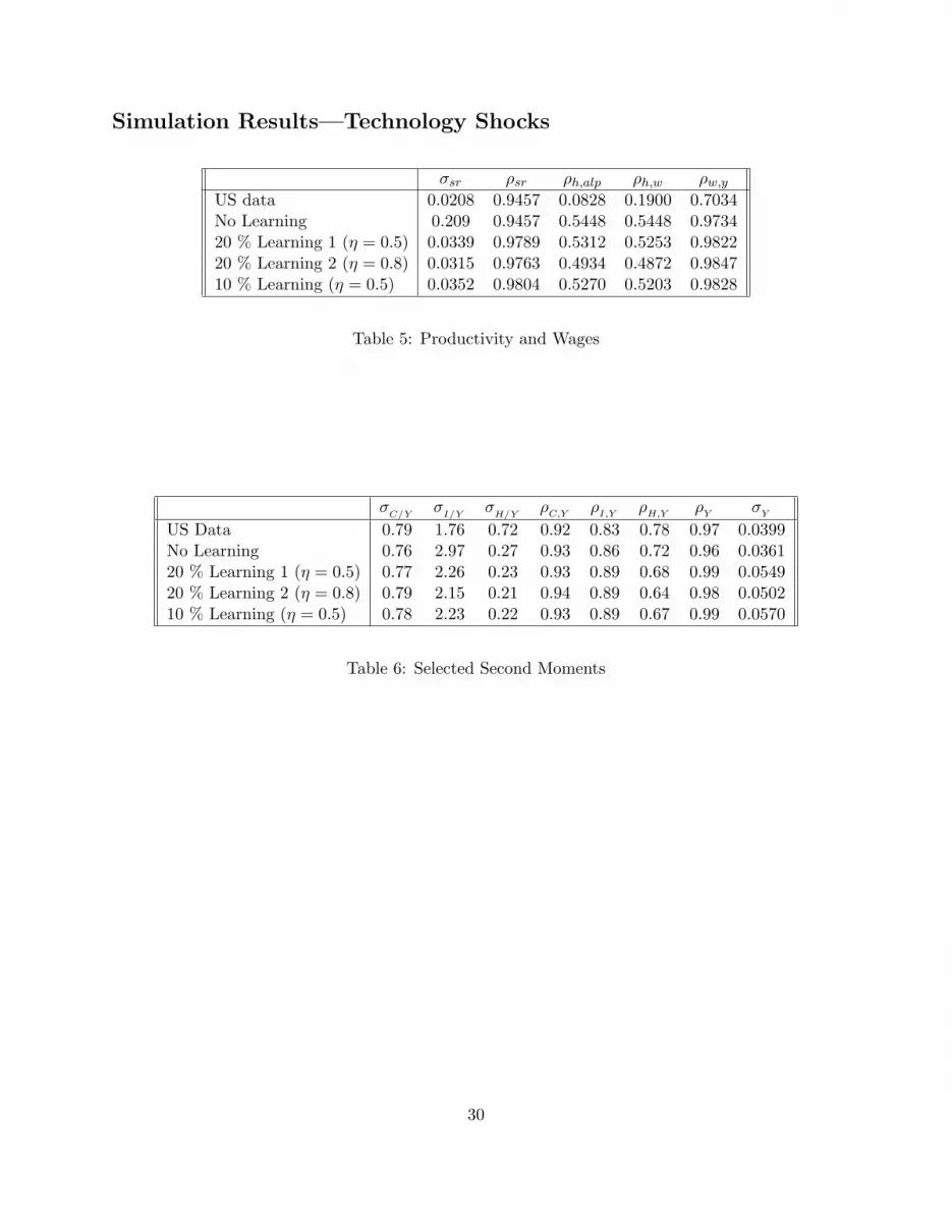
Simulation Results—Technology Shocks

σsr ρsr ρh,alp ρh,w ρw,y

US data 0.0208 0.9457 0.0828 0.1900 0.7034No Learning 0.209 0.9457 0.5448 0.5448 0.973420 % Learning 1 (η = 0.5) 0.0339 0.9789 0.5312 0.5253 0.982220 % Learning 2 (η = 0.8) 0.0315 0.9763 0.4934 0.4872 0.984710 % Learning (η = 0.5) 0.0352 0.9804 0.5270 0.5203 0.9828

Table 5: Productivity and Wages

σC/Y

σI/Y

σH/Y

ρC,Y ρI,Y ρH,Y ρY σY

US Data 0.79 1.76 0.72 0.92 0.83 0.78 0.97 0.0399No Learning 0.76 2.97 0.27 0.93 0.86 0.72 0.96 0.036120 % Learning 1 (η = 0.5) 0.77 2.26 0.23 0.93 0.89 0.68 0.99 0.054920 % Learning 2 (η = 0.8) 0.79 2.15 0.21 0.94 0.89 0.64 0.98 0.050210 % Learning (η = 0.5) 0.78 2.23 0.22 0.93 0.89 0.67 0.99 0.0570

Table 6: Selected Second Moments

30

0 10 20 30 40 50 60 70 80 90 100

0

0.05

0.1

0.15

0.2

0.25

0.3

0.35

0.4

Periods

% D

evia

tion

from

Ste

ady

Stat

e

Consumption

0 10 20 30 40 50 60 70 80 90 100

-0.5

0

0.5

1

1.5

2

2.5

3

Periods

% D

evia

tion

from

Ste

ady

Stat

e

Investment

No LearningLearning

0 10 20 30 40 50 60 70 80 90 100

0

0.1

0.2

0.3

0.4

0.5

0.6

0.7

Periods

% D

evia

tion

from

Ste

ady

Stat

e

Output

0 10 20 30 40 50 60 70 80 90 100

0

0.1

0.2

0.3

0.4

0.5

0.6

0.7

Periods

% D

evia

tion

from

Ste

ady

Stat

e

Organizational Capital

0 10 20 30 40 50 60 70 80 90 100

-0.4

-0.3

-0.2

-0.1

0

0.1

0.2

0.3

Periods

% D

evia

tion

from

Ste

ady

Stat

e

Real Wages

0 10 20 30 40 50 60 70 80 90 100

-0.2

0

0.2

0.4

0.6

0.8

1

1.2

Periods

% D

evia

tion

from

Ste

ady

Stat

e

Hours

No LearningLearning

0 10 20 30 40 50 60 70 80 90 100

-0.4

-0.3

-0.2

-0.1

0

0.1

0.2

0.3

Periods

% D

evia

tion

from

Ste

ady

Stat

e

Average Labour Productivity

0 10 20 30 40 50 60 70 80 90 100

-0.05

0

0.05

0.1

0.15

0.2

Periods

% D

evia

tion

from

Ste

ady

Stat

e

Solow Residual

Figure 1: Internal Learning-by-Doing: Selected Impulse Responses to a 1% Shock to the LabourWedge

31