Embed Size (px)
Citation preview
Propagation of Ocean Swell across the PacificAuthor(s): F. E. Snodgrass, G. W. Groves, K. F. Hasselmann, G. R. Miller, W. H. Munk, W. H.PowersReviewed work(s):Source: Philosophical Transactions of the Royal Society of London. Series A, Mathematical andPhysical Sciences, Vol. 259, No. 1103 (May 5, 1966), pp. 431-497Published by: The Royal SocietyStable URL: http://www.jstor.org/stable/73313 .Accessed: 01/05/2012 14:19
Your use of the JSTOR archive indicates your acceptance of the Terms & Conditions of Use, available at .http://www.jstor.org/page/info/about/policies/terms.jsp
JSTOR is a not-for-profit service that helps scholars, researchers, and students discover, use, and build upon a wide range ofcontent in a trusted digital archive. We use information technology and tools to increase productivity and facilitate new formsof scholarship. For more information about JSTOR, please contact [email protected].
The Royal Society is collaborating with JSTOR to digitize, preserve and extend access to PhilosophicalTransactions of the Royal Society of London. Series A, Mathematical and Physical Sciences.
http://www.jstor.org
[ 431 ]
PROPAGATION OF OCEAN SWELL ACROSS THE PACIFIC
BY F. E. SNODGRASS, G. W. GROVES,, K. F. HASSELMANN, G. R. MILLER, W. H. MUNK AND W. H. POWERS
Institute of Geophysics and Planetary Physics, University of California, La Jolla
(Communicated by G. E. R. Deacon, F.R.S.--Received 3 February 1965)
[Plate 6]
CONTENTS
PAGE PAGE
1. INTRODUCTION 432 (f) The intense cyclone of 9 to 15 August 468
2. WAVE STATIONS 432 August (a) The 'reference great-circle' 434 (g) Otherevents 468
(b) Cape Palliser, New Zealand 435 6. TEE MEAN WAVE FIELD 471 (c) Tutuila, Samoa 436 (d) Palmyra 437 7. DISCUSSION OF OBSERVATIONS 473
(e) Honolulu, Hawaii 438 (a) Attenuation 473 (f) Flip 439 (b) Afterglow 475 (g) Yakutat, Alaska 440 (c) Forward scattering 475
(d) Summary 479 3. SPECTRAL ANALYSIS 440
(a) Honolulu dual station 440 8. WAVE-WAVE INTERACTIONS 481 (b) Flip pressure transducers 441 (a) Interaction rules 481 (c) Flip accelerometers 444 (b) Scattering in and near the generating
region 482 4. PROPAGATION 45(C) Scattering of a narrow beam 485
(a) Invariance of spectrum 445 (d) Wave breaking 487 (b) 'Visible apertures' of storms 446 (e) Surfbeat 489 (c) Refraction 447 (d) Oblateness 450 9. MICROSEISMS 489
5. THE PRINCIPAL EVENTS 451 10. CONCLUSIONS 491 (a) Identification of events 451 (b) The great-circle event of 1 9 August 454 APPENDIX 493
Wave propagation on an oblate (c) The Tasman Sea event of 232 July 461 sphero id 493
(d) The Ross Sea storm of 28-7 August 463 spheroid
(e) The Madagascar event of 300 August 466 REFERENCES 497
Six wave stations were occupied for 2- months along a great circle between New Zealand and Alaska. Twice-daily wave records were analysed to yield energy spectra Ei(f, t) for station i as functions of frequency and time. Events from major storms appear as slanting ridges in the Es(f, t) field; the ridge linesf = (g/4ir) (t - to) /Ai determine source t;ime, to, and source distance, A,; rough estimates of direction Oi(f) were made at two stations. Twelve major events, including several from antipodal storms (A z 180?) in the Indian Ocean, could be clearly tracked from station to station. Source parameters are found to be mutually consistent, and usually in accord with weather information.
Cuts in Ei (f, t) along the ridges give spectra firom which the effect of dispersion is removed. These were corrected for geometric spreading and island shadowing. Comparison of the corrected ridge
VOL. 259. A. 1103. (Price fi. vs., U.S. $4.05) 53 [Published 5 May Ig66
432 F. E. SNODGRASS AND OTHERS
spectra between stations indicate negligible attenuation for frequencies below 70 mc/s (less than 0-02 dB/deg between New Zealand and Alaska), and 0415 dB/deg at 80 mc/s, with a considerable scatter from event to event. At higher frequencies the events disappear into a background spectrum which is remarkably uniform over the Pacific, and presumably the result of global high winds along the entire storm belt of the South Pacific. The attenuation in the near zone of the storm (within a distance comparable to the storm diameter) is estimated at 0-2 dB/deg at 70 mc/s and 0 4 dB/deg at 80 mc/s.
Wave-wave interactions have been derived from a perturbation expansion of the Navier-Stokes equations. The computed attenuation due to interaction between wave groups from a storm is not inconsistent with observations in both the near and far zones. The observed super-exponential decay is attributed to the decrease in interaction efficiency with diminishing wave energy along the path and dispersive narrowing of the spectral peak. Interaction with background (such as the trade wind sea) is unimportant. The conclusion is that the observed propagation could be accounted for by the effects of Stokes interaction (? 8b,c, figure 38) between wave groups from a single storm.
1. INTRODUCTION
The transmission of ocean waves over very large distances became apparent with the earliest spectral analyses of ocean waves (Barber & Ursell I948). These analyses showed the arrival at Cornwall, England, of waves generated off Cape Horn at a distance of 10o0
(10 60 nautical miles). The source distance could be inferred from the successive shift of
spectral peaks towards higher frequencies. Subsequent observations have confirmed the
global nature of swell propagation. Munk & Snodgrass (I957) observed swell at Guadalupe
Island generated at an inferred distance of 130?. The Pacific Ocean is too small to permit
such distant sources, and it was thought that the swell came from a storm in the Indian
Ocean and entered the Pacific along a great-circle route between Antarctica and Australia.
This was subsequently confirmed with a three-station array at San Clemente Island off
California (Munk, Miller, Snodgrass & Barber I963) which permitted the directional
recordings of swell. In some instances the generation turned out to be antipodal (ca. 1800).
The present paper is an account of measurements of swell propagation at stations along
a great-circle route. Simultaneous measurements of microseisms on the Island of Maui,
Hawaii (Haubrich & Mackenzie I965) and at various locations on the deep sea bottom
(Bradner, Dodds & Foulks I965) show the relation between the release of dispersive swell
trains from the major storms and micro-tremors of the Earth.
2. WAVE STATIONS
Vibrotron pressure gauges (Snodgrass I958, I964) mounted on the sea bottom in 20 m of
water converted pressure fluctuations into a frequency-modulated voltage which was
transmitted to shore by underwater cable. Once every 2 sec a digital frequency meter
punched a reading on perforated paper tape. This reading gives the number of microseconds
in 20 000 Vibrotron oscillations and provides a measurement to a precision of 0-01 cm of
water pressure. At each station a 3 h record was obtained twice daily for 21 months during
the 1963 southern winter. The data tapes were airmailed to California for immediate analysis. A total of 1 O data points were collected; yet the analysis could be kept reasonably up to date to serve as a running check of the instruments and to monitor the progress of the experimenlt.
At the remote sites the recording equipmnent was operated from automobile batteries charged by petrol-powered generators. When reliable commercial power was available,
PROPAGATION OF OCEAN SWELL ACROSS THE PACIFIC 433
~~~~~~~~~~~~~~~~.
0 9 10
74X~~~~~~~~~~~~~~~~0
\ \ \C : ' hX t 0 ~~~~~~~~0 1.9 tj \~~~~~~~ ~~~~~ w Ze a - l I d
(J27.4 means 27 July, 96 h G.M.T.).~27-4- 40
*Al3-7 ~ ~ ~ ~ ~ 5-
\~~~~~1 .2 . ..
_ 1 8 0~~~~6
(J27-4 means 2~A7 Jul,.9t hG.,..)
A3 -0 0~~~~~~~~~~~~3
434 F. E. SNODGRASS AND OTHERS
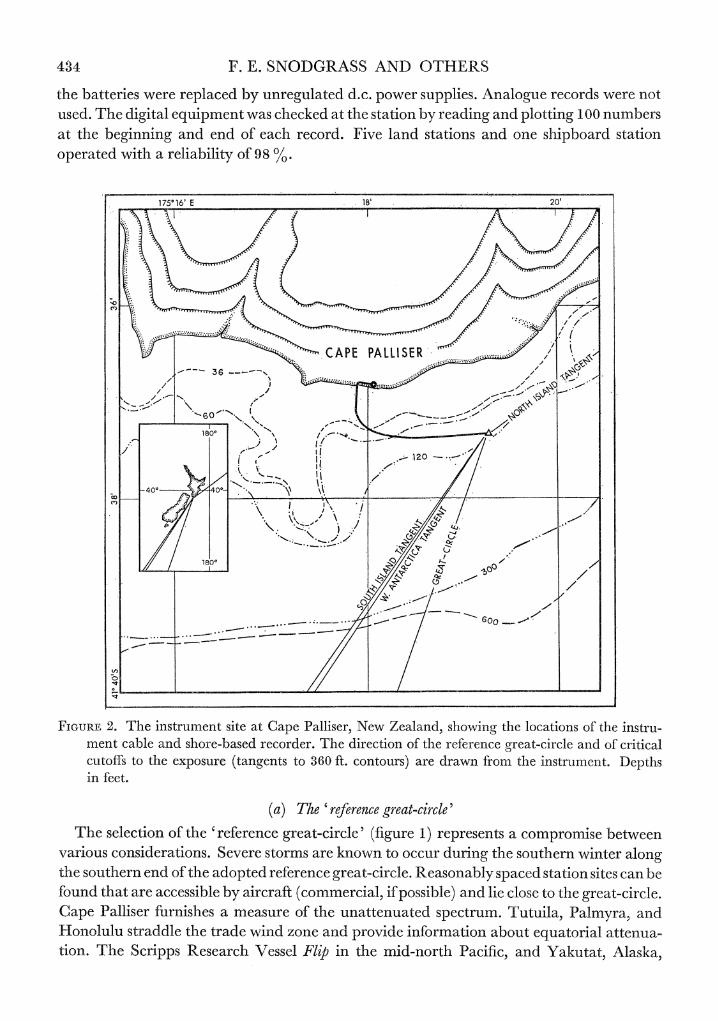
the batteries were replaced by unregulated d.c. power supplies. Analogue records were not used. The digital equipment was checked at the station by reading and plotting 100 numbers at the beginning and end of each record. Five land stations and one shipboard station operated with a reliability of 98 00.
175?16' E . 18' . 20'
l | \/ ,--- 36 X CAPE PALl LISSE,AR
N~~~~~~~~~~~~~~~~~~~~~~~~~~~~~~~~
40 40- 4oI
FIGUR:E 2. The instrument site at Cape Palliser, New Zealand, showing the locations of the instru- ment cable and shore-based recorder. The direction of the reference great-circle and of critical cutoffs to the exposure (tangents to 360 ft. contours) are drawn from the instrument, Depths in feet.
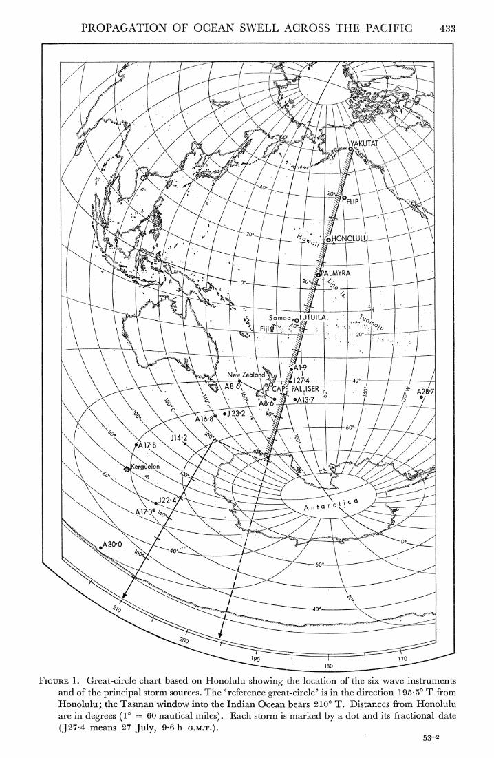
(a) The ' reference great-circle '
The selection of the 'reference great-circle' (figure 1) represents a compromise between various considerations. Severe storms are known to occur during the southern winter along the southern end of the adopted reference great- circle. Reasonably spaced station sites can be foundl that are accessible by aircraft (commercial, if possible) and lie close to the great-circle. Cape Palliser furnishes a measure of the unattenuated spectrum. Tutuila, Palmyra, and Honolulu straddle the trade wind zone and provide information about equatorial attenua- tion. The Scripps Research Vessel Flip in the mid-north Pacific, and Yakultat, Alaska,
PROPAGATION OF OC'EAN SWELL ACROSS THE PACIFIC 435
provide information at very long distances. The separation between Antarctica and Yakutat is 1380, or 25 000 typical wavelengths.
Before the experiment it was not clear whether the renowned Honolulu breakers were associated with waves from west or east of New Zea]Land. The western route (through the Tasman Sea) is partially obstructed by the Fiji and Lau Islands. Accordingly a great-circle to the east of New Zealand was chosen, yet lying close enough to the western passage to permit rough estimates of the attenuation of waves firom the Indian Ocean.
177O 50' W 48' 461
! 1...Xf
C4 0T 0 ________ _______________ 0WA
______ _____ _____ ____ Leone Bazy : 1706
_ _ _ _ _ _ _ _ _ _ _ _ _ _ _ A~~~~~~~'V V ailo a T o i *150
1700 __ __ -
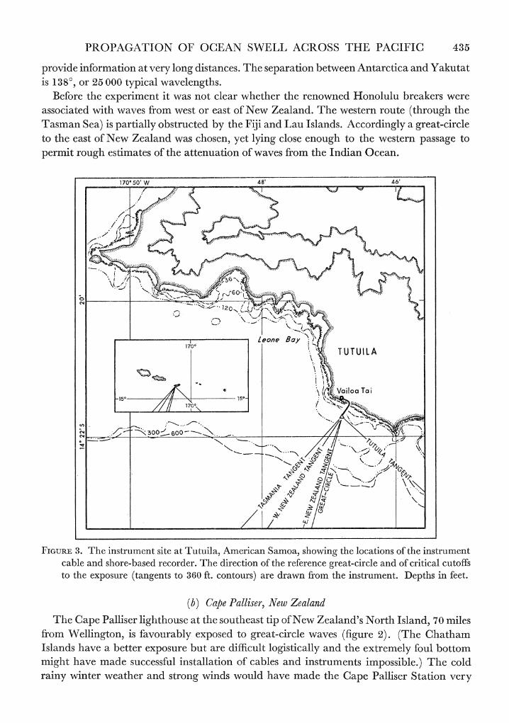
FIGURE 3. The instrument site at Tutuila, American Samoa, showing the locations of the instrument cable and shore-based recorder. The direction of the reference great-circle and of critical cutoffis to the exposure (tangents to 360 ft. contours) are drawn from the instrument. Depths in feet.
(b) Capve Palliser, New ,Zealand The Cape Palliser lighlthouse at the southeast tip of New Zealand's North Island, 70 miles
from Wellington, is favourably exposed to great-circle waves (figure 2). (The Chatham Islands have a better exposure but are difficult logist;ically and the extremely foul bottom might have made successfull installation of cables and instruments impossible.) The cold rainy winter weather and strong winds would have made thle Cape Palliser Station very
436 F. E. SNODGRASS AND OTHERS
unpleasant if it had not been for the kind hospitality of Mr and Mrs Midtgard of the New Zealand Lighthouse Service. Periodically the lighthouse was completely isolated by swollen streams that could normally be forded by Land Rover.
The station was operated by Frank Peterson, who assisted also with the installation of the
Honolulu station. Peterson accomplished the difficult Cape Palliser cable installation under
162?8' W 6' 41
6o.1\ and 1
z
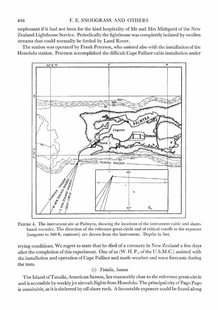
FIGURE, 4. The instrument site at Palmyra, showing the locations of the instr-ument cable and shore- based recorder. The direction of the reference great-circle and of critical cutoffis to the exposiure (tangents to 360 ft. contours) are drawn from the instrument. Depths inz feet.
trying cond'itilons. We regret to state that he died of a coronary in New Zealand a few days after the completion of this experiment. One of uls (W. H. P., of the U.S.M.C.) assisted wilth the installation and operation of Cape Palliser and made weather and wave forecasts during the tests.
~~~~~~O ~ ~ ~ C TuraaNSao
The~~~~ N Isan 0fTtia mrcnSma israoal ls oterfrnegetcrl
and is*accsil9y ekyjeKicafflg<_foiooll.Te/rnialct/f aoPg
isusiabe siti hltrdb ffsoeref.Afa4rbeexouecol efon ln
PROPAGATION OF OCEAN SWELL ACROSS THE PACIFIC 437
the remote southwestern shore (figure 3), which was without electricity, running water, and other conveniences. High Chief Satele provided a Samnoan Fale for the observer (W. H. M.) and his family in the village of Vailoa Tai, and this served as laboratory-living quarters. During the last 2 weeks of measurements the instrument was successfully tended by High Chief Satele.
157?52'W 50'
C4~~~~C
t \\ H N r L
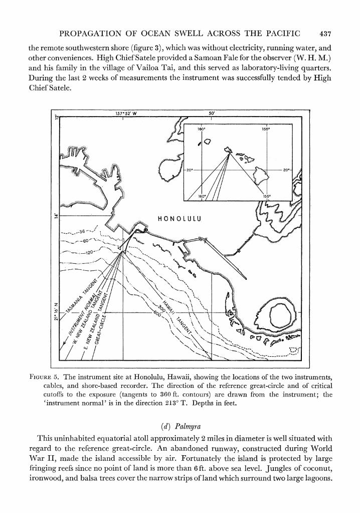
FIGURE 5. The instrument site at Honolulu, Hawaii, showing the locations of the two instruments, cables, and shore-based recorder. The direction of the reference great-circle and of critical cutoffis to the exposure (tangents to 360 ft. contours) are drawn from the instrument; the 'instrument normal' is in the direction 2130 T. Depths in feet.
(d ) Palmyra This uninhabited equatorial atoll approximately 2 miles in diameter is well situated with
regard to the reference great-circle. An abandoned runway, constructed during World War II, made the island accessible by air. Fortunately the island is protected by large fringing reefs since no point of land is more than 6 ft. above sea level. Jungles of coconut, ironwood, and balsa trees cover the narrow strips of land which surround two large lagoons.
438 F. E. SNODGRASS AND OTHERS
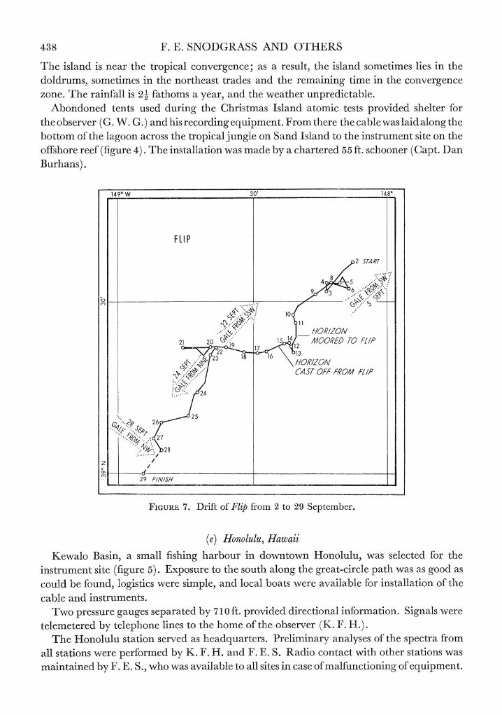
The island is near the tropical convergence; as a result, the island sometimes lies in the doldrums, sometimes in the northeast trades and the remaining time in the convergence zone. The rainfall is 2- fathoms a year, and the weather unpredictable.
Abondoned tents used during the Christmas Island atomic tests provided shelter for the observer (G. W. G.) and his recording equipment. From there the cable was laid along the bottom of the lagoon across the tropical jungle on Sand Island to the instrument site on the offshore reef (figure 4). The installation was made by a chartered 55 ft. schooner (Capt. Dan Burhans).
1490 W 30 1480
2 STA RT
_ 48 5
HORIZON 21 20 '19
15 1 4400259 TO F//P
CAS OFF FROM F// P
. J~~~~~~24
26
28
z
2 9 FINISH
FIGURE 7. Drift of Flip from 2 to 29 September.
(e) Honolulu, Hawaii
Kewalo Basin, a small fishing harbour in downtown Honolulu, was selected for the instrument site (figure 5). Exposure to the south along the great-circle path was as good as could be found, logistics were simple, and local boats were available for installation of the cable and instruments.
Two pressure gauges separated by 710 ft. provided directional information. Signals were telemetered by telephonle lines to the home of the observ7er (K. FS. H[.) .
The Honolulu station served as headquarters. Prelimninary analyses of the spectra from all stations were performned by K<. F. H. and F. E. S. Radio contact with other stations was
mnaintained by F. E. S., who was av7ailable to all sites in case of mnalfunctioninlg of equipment.
Snodgrass et al. Phil. Trans. A, volume 259, plate 6
/~~~ ~ ~ ~~~~~~~ 1.
'Si -
~~~~s- I -
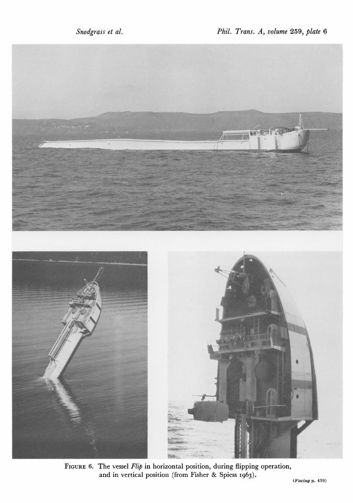
FIGURE 6. The vessel Flip in horizontal position, during flipping operation, and in vertical position (from Fisher & Spiess 1963).
(F'acinQ p. 43}9)
PROPAGATION OF OCEAN SWELL ACROSS THE PACIFIC 439
(f) Flip The Scripps Research Vessel Flip (floating instrument platform) completed sea trials just
before the expedition and was able to occupy a site halfway between Honolulu and Yakutat. Flip is essentially a long, slender, tubular hull that terminates abruptly where it joins the somewhat conventional 40 ft. bow (figure 6, plate 6). Flip is designed to be towed in a horizontal attitude ballasted so as to float at approximately half its diameter. Upon arrival
139? 50'W 48'
"'K~~~~~~
F ' ' \-__-..S'\. ''
I 1
180, 1400
YAKUTAT 60
> _ _, . 40 >60_
0o,,
1600~~~~~~~~~~~~~~~180 10
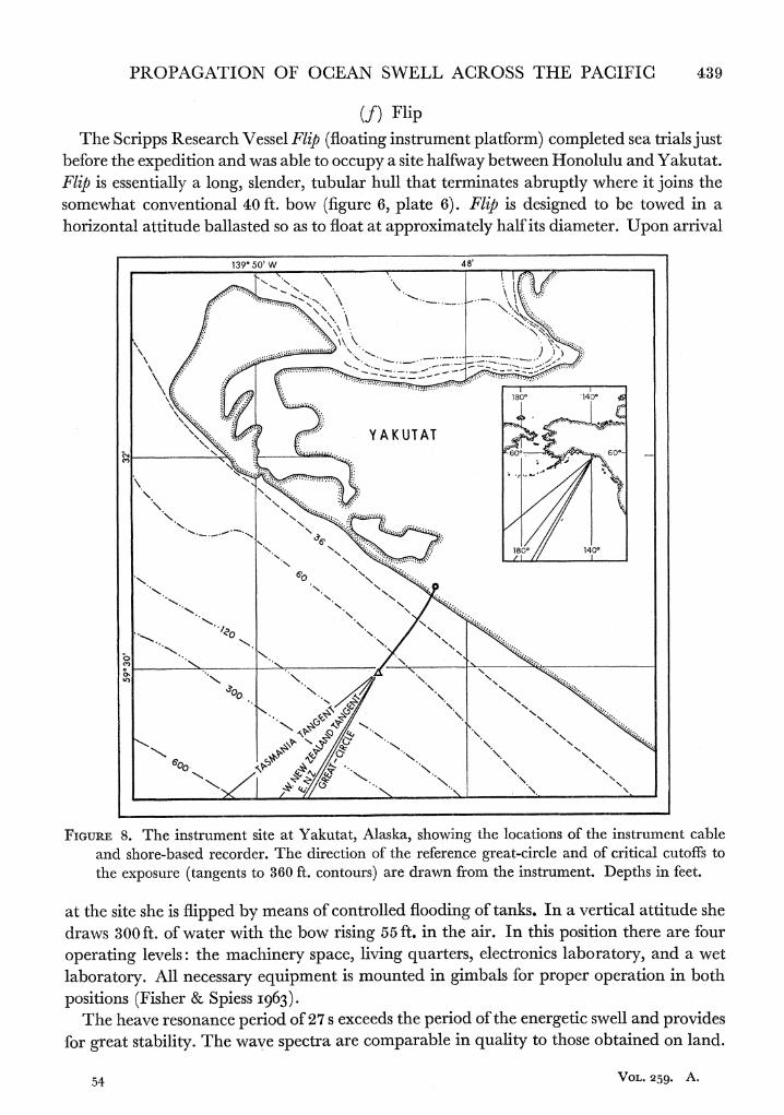
FIGURE 8. The instrument site at Yakutat, Alaska, showing the locations of the instrument cable and shore-based recorder. The direction of the reference great-circle and of critical cutoffs to the exposure (tangents to 360 ft. contours) are drawn from the 'instrument. Depths in feet.
at the site she is flipped by means of controlled flooding fof tanks. In avertical attitude she draws 300 ft. of water with the bow rising 55 ft. in the ailr. In this position there are four operating levels: the machinery space, Iliving quarters, electronics laboratory, and a wet
laboratory. ~ ~ 1neesreqim nt;i one ngmasfrpoe prto nbt
postins Fse pesI6)
Nh hevNeoac eidoE2 xed h eido h nrei wl n rrie
fo get tbiiy.Th av peta recmprbl n uaiy oths otand nlad
54 vOL. 259. A.
440 F. E. SNODGRASS AND OTHERS
Two pressure gauges were installed on the hull; one at 31 m and the other at 88 m below the surface with Flip in the vertical position. By using two instruments, the vertical displace- ment of Flip and of the sea surface could be independently determined (? 3 b).
John Northrop and David Holloway of the Marine Physical Laboratory, Scripps Institu- tion of Oceanography, operated the wave recorders, measured temperature with a ther- mistor chain, recorded earthquake T-phases and transient underwater acoustic signals. Hydrographic casts, bathythermographs, cores, and soundings were obtained aboard the tender Horizon which remained within sight of the platform (Northrop, I964). Flip was maintained in a vertical position for 28 days, drifting along the irregular path shown in figure 7. The vessel performed well during several gales which occurred during the towing period and while on station. Men aboard the platform found the quarters to be somewhat cramped and noisy but they never suffered from motion sickness.
(g) Yakutat, Alaska
There are very few coastal towns along the Gulf of Alaska, and Yakutat was the only reasonable choice. The local harbour provided fishing boats for the cable installation. A U.S. Coast Guard Loran Station, located a few hundred feet from a straight sand beach with a gradual offshore slope, provided an ideal site for the cable terminus and the recording equipment (figure 8); reliable 110 V power at the station eliminated the inconvenience of batteries and petrol-powered generators. The observer (G. R. M.) and his family lived in a housetrailer and commuted by motor scooter to the Loran Station (experiencing an occasional encounter with a moose or bear).
3. SPECTRAL ANALYSIS
Each data cycle consists of a pressure value and a data number. The computing program initially checks for data gaps and searches for errors, filling gaps, and correcting values if necessary. (The vast majority of runs required no corrections.) Subsequently the tides are removed by numerical high-pass filtering, and the autocorrelation and cosine transforms computed according to the method of Tukey. The 'Parzen fader' was used (Parzen I96I) which avoids negative side bands at the expense of reducing the resolution somewhat. An isolated line of unit strength centred in a given band has its energy distributed in neigh- bouring bands as follows: 0 0030, 00617, 0-2471, 0-3762, 0-2471, 0-0617, 0 0030.
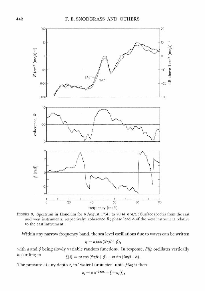
Spectral values were computed at intervals of 1 mc/s (millicycle per second) between 0 and 250 mc/s. The degrees of freedom for a typical record of 5400 values is 43, and this implies 15 % r.m.s. errors. A sample spectrum* is shown in the top panel of figure 9, with a parti- cularlywelldefinedspectralpeakat 50mc/s extending 15 dBabove the adjoining background.
Dual transducers were installed at Honolulu for directional information, and on Flip to separate wave motion from ship motion. These two stations require special consideration.
(a) Honolulu dual station Let x.(t) (&- 1,92) designate the departures from the mean of the east and west records,
respectively. We have computed the covariance
* All spectra have been corrected for water depth and represenst surfalce wave spectra.
PROPAGATION OF OCEAN SWELL ACROSS THE PACIFIC 441
and its Fourier transforms
Cij (f) s (r) pij (T) cos 2irfTr dr, -00 (3.2)
Qij(f) j ' s(r) pij (r) sin 2iffr d'r,
where s(r) is an appropriate fading function. C1I(f) and C22(f) are the power spectra ofthe two records, C12(f) is called the cospectrum and Ql2(f) the quadrature spectrum. The coherence, R(f), and the relative phase, 0(f), are defined by
R2 C122+ 2 tan Q12 (3.3)
A sample spectrum (out of a total of 152 Ionolulu spectra) is shown in figure 9, consisting of the four* functions C1 (f), C22 (f) R(f) and 0 (jy). The coherence is very high at the spectral peak of 50 mc/s. This implies that the incoming energy is concentrated in a narrow beam. For the simplest case of straight parallel contours with two elementary incoherent wave trains of amplitude a and frequencyf, coming from directions 0' and 0', respectively, relative to the normal of the pair of instruments, we have (Munk et al. I963, ? 5 d)
R-cosIAO, AOS l' -q$, AXS-1 0(' - O), (3.4)
where 2' =2rkD sin 0', qY' 2-,rkD sin 0", k = 1/wavelength (not 217/wavelength), and D the instrument separation. When the sources are close together,
AO -of _ V/ ,(1 J?2) sin 0 - 0 O+0.35a
7rD cost9' sn=2-ffkD' = 2(?40(.a
Atf=- 50mc/s, we have R 094, -= -1 rad, k 1/850ft, and A= 011 rad. In the case of a narrow beam extending uniformly from 0' to 0" the results are
AO = J12 (Il-R2) sinz =-- (3.5b) 5 fkD cos0' 2itfkD'(.b so that AOS- O17 rad.t
At the peak frequency the west instrument leads the east instrument by -1 rad, thus indicating that the incoming waves corne from the east relative to the instrument normal (figures 5 and 9). The direction in deep water can be inferred by allowing for refraction
(?4(c)). Reflexion from shore is neglected. For furtlher discussion of directional wave recording, we refer to Munk et al. (I963).
(b) Flip pressure transducers
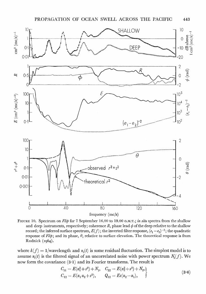
Vibrotron pressure transducers were mounted at depths of 30-6 and 88d1 m. The depth of the shallow instrument is governed by the need of greatly attenuating waves at and beyond the Nyquist (or 'folding') frequency. The deep instrument was placed as near the bottom of the hull as is practical. Let xl (t), x2(t) designate departures from the mean at the shallow and deep instruments, respectively, and define C,>(f), Qi(f), R(f) and 05(f ) as in (3.1) to (3.3) . Figure 10 shows a typical plot of C11, C22, RandqS.
* At stations with a single instrument, the output consists of one function only, C11 (f). j This result neglects the bias in the observed values of coherence in finite records, and implies a beam
width somewhat too narrow. 54-2
442 F. E. SNODGRASS AND OTHERS
100 - 20
10 -0
Q
01 -10 0.1 >~~~~~~~~~~~~~~~ EAST
WEST 001 -20 _0
0mom1 -30
0.
Q
0
0
2-
0-2
0 20 40 60 80 100
frequency (mc/s)
FIGURE 9. Spectrum in Honolulu for 6 August 17.41 to 20.41 G.M.T.: Surface spectra from the east and west instruments, respectively; coherence R; phase lead q5 of the west instrument relative to the east instrument.
Withini any narrow frequency band, the sea level oscillations due to waves can be written
g = a cos (21Tft+ 0),
with a and 0 being slowly variable random functions. In response, Flip oscillates vertically according to
6(t) -racos (2irft+0S) +sa sin (2irft+q$).
The pressure at any depth zi in 'water barometer' units p/pg is then
PROPAGATION OF OCEAN SWELL ACROSS THE PACIFIC 443
10- SALW10
1 0 _ z
0']~~~~~~~~~~~~~~~~~~~~~~~~~~~~~~~~~~~~~~~~0 cq 0.1 DEE P -10 5
001 420
2
"'*(e1...)~2,,, .......".... 0~~~~~~~~~~5 .. .. ~ ~ ~ ~ ~ ........ ... ..-
10 lo, -2 ~~~~~~ 100 ~ ~ ~ ~ ~ ~ ~ ~ ~ ~ ~ ~ ~~~~~~~1
ki 0?-1 (e e2b):V 2zi 2
10 2 0~~~~~~1
_
................
00 2 10 ..8010 6
frequency (mc/s)
FIGURE 10. Spectrum on Flip for 7 September 16.00 to 19.00 G.M.T.; in situ spectra from the shallow and deep instruments, respectively; coherence R, phase lead 95 of the deep relat'ive to the shlallow record; the inferred surface spectrum, E(f' ); the inverted filter response, (e - e2) -2 9 the quadratic response of Fli.p; and its phase, 0, relative to surface e'levation. The theoretical response is from Rudnick (I964)
where k(f ) I /lwavelength and ni(t) is some residual fluctuation. The silmplest model is to assume -- -- I P /nhoeia is th f s of - uncorreae n we c N )
(72 E06a2-5)9 Q1-80 (6 ?120 16
444 F. E. SNODGRASS AND OTHERS
where (a2'> E(f) Sf is the energy of the sea surface in the narrow band 5f, and where
eci -eir, e2 e-2nkzi.
The four equations (3.6) relate the four observed functions Cij(f) to the five unknown functions E(f), r(f), s(f), Nj(f), and N2(f). The following combinations of observed functions have been evaluated:
C11+C22-2Cl2E M +k (3-72
Cl+ C22-212- s+function (Ni), (3*8)
el -,/I(ClIE)- s2}--- r+function (Ni). (3.9)
In the absence of noise, the left-hand side of (3.7) equals the wave spectrum E(f) (and is labelled accordingly on the figure). We may expect the noise to predominate at extreme frequencies, and the plotted curve to approach (N1 + N2) (el- e}-2; if the noise spectrum is fairly flat, the curve then becomes proportional to (el - e2)-2, as shown. Apparently this is the case below 20 mc/s. The remaining curves give
r2 + s2, 0 arctan (s/r)
evaluated from (3.8) and (3.9) under the assumption that noise can be neglected. r2 + s2 is the quadratic response of Flip, and 0 its lag relative to surface elevation. Rudnick's (I964) calculated response of Flip is shown for comparison.
We may now attempt to interpret the six peaks in the raw spectra. The enhanced activity between 0 and 5 mc/s is probably associated with temperature effects on the pressure transducer. Internal waves of 3 m amplitude produce 1 degC temperature fluctuations at the depth of the shallow instrument, and this produces a signal equivalent to 5 cm of water pressure because of the sensitivity of Vibrotrons to temperature. Observed variations in temperature and in Vibrotron output are very roughly in accord with this description. The peak at 22 mc/s corresponds to the natural roll of Flip (oscillation about a horizontal axis), yet the observed in-phase coherence between the instruments suggests a heaving motion coupled to the roll. The peak at 37 mc/s is the resonant heave response, and properly absent in the E(f) spectrum. The peak at 60 mc/s is due to a storm in the Ross Sea on 28-7 August (? 5 (d)); that at 67 mc/s from a storm in the Tasman Sea on 26-0 August. Finally, the broad maximum at 85 mc/s is the result of high winds in the North Pacific. The peaks in the wave spectrum at 60, 67 and 85 mc/s are properly absent in the response function. It appears that E(f) is meaningfully determined above 40 mc/s. The lowest point in the computed spectrumn is at 42 mc/s where it is nearly 30 dB below the swell peak and 40 dB below the sea peak. The precision of the Flip measurements above 40 mc/s is comparable to that on shore!
(c) Flip accelerometers
The acceleration was measured in three components aboard Flip. The records were of relatively short duration, and the resolution correspondingly poor, so that these records do not contribute further information concerning the power spectra. But the records are useful in providing some directional information, particularly since the uncertainties from refrac- tion are avoided.
PROPAGATION OF OCEAN SWELL ACROSS THE PACIFIC 445
Measurements of directional wave spectra using a floating buoy have been described by Longuet-Higgins, Cartwright & Smith (I963). Let xl (t), x2(t) represent horizontal com- ponents of acceleration, and consider two elementary wave trains of frequencyf', amplitude a from direction O' and 8", respectively, re:lative to the xl axis. We form the cross spectra as defined in ? 3 (a):
Cll(f) = (2irkga)2 (cos2 8' + cos2 0") S(f-f'),
C22(f) = l(2irkga)2 (sin28'+ sin2 0") S(f-f'), C12(f) 2(2irkga)2 (cos O' sin 8' +cos O" sin O") S(f-f'),
Q12(f) o.
When the sources are close together,
AO8- sin (20) j(1-R2), tan28 C22/C11, 8-2(8'+8"). (3.10)
The beam width varies as /(1-R2), similar to the case of two recorders (equations (3.5)).
4. PROPAGATION
(a) Invariance of spectrum
The wave energy between frequenciesf andf+ dfa:nd directions 81 and 81 + dO8 in a small element of surface area do-, centred at a point V,u at time t1 is given by
F(ff f01, tLj tl) dfdO, do-, (dimension L4). F(f, ,) j1) tl) is the two-dimensional space and time dependent energy density (dimension L2 T). 8 is the bearing relative to some reference direction (arbitrary at each point). The energy of the waves of any given frequency is propagated at group velocity along a great-circle. At a later time t2 all the 'wave packets' originally occupying the phase element dfdO8 do-, at position V,u in direction 81 will occupy the new phase element dfdO2 do2 at position R2 and in direction 2. Let K be a factor which multiplies the energy density at point 1 to give that at point 2. K(f, 81) is specified by the coordinates of either one of the points (say V.,), and by the time difference At t2 - tl; thus
F(f, 02) 2) t2) =7 K(f,8 1, -1, At) F(f,8 1, -1, tl). (4.1)
Conservation of energy in a wave packet requires that
F(Jf 02, -2 t2) dfd2 do-2 - F(f, 80, 1,5tj) dfd8, do
and we may refer to K(ff81, -, At) =d(8, o-) ' a ~~~d(82,o'-2) as the 'propagation Jacobian'.
Because of the reversibility of the propagation paths, waves travelling from V.2 to l have directions 02 +Xi at the point 2' 01 + Xf at V. and the phase element ratio is reciprocal to waves travelling from Ft to R2 K(f, 8l, >, At) K (f, 82+., )2 At) 1.
If the propagation depends only on the separation between the two points (as on a uniform sphere), K-IK(f,At),
so that the above relation becomes K2 _1.
446 F. E. SNODGRASS AND OTHERS
Hence F(f, 02, ,2' t2) F(f, 01, , tl), (4.2)
where 02, I2 are functions off, 01, V., and At in a manner appropriate to spherical geometry and the dispersive properties of the waves.*
If refraction occurs equation (4.2) no longer holds. It has been shown in this case by more general dynamical arguments that the invariance of the spectrum remains valid for the spectral density function containing the wave number as an argument rather thanf and 0 (Longuet-Higgins 1957; Dorrestein i960; Backus i962).
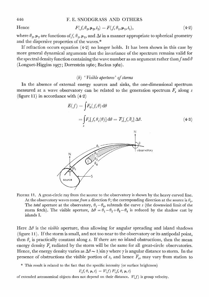
(b) ' Visible apertures' of storms In the absence of external energy sources and sinks, the one-dimensional spectrum
measured at a wave observatory can be related to the generation spectrum F, along s (figure 11) in accordance with (4 2)
E(f) FoF(f, 0) dO
zzFs[F) fs(0)] da F=jff, Os] A. (4.3) s
N
observatory
FIGURE 11. A great-circle ray firom the source to the observatory is shown by the heavy curved line. At the observatory waves comefrom a direction 0; the corresponding direction at the source is ?s.
The total aperture at the observatory, 01 -04, subtends the curve s (the downwind limit of the storm fetch). The visible aperture, A0S-01-02?03-04 iS reduced by the shadow cast by
S~~~ ~~ 2
Here AS is the visible aperture, thus allowing for angular spreading and island shadows (figure 11). If the storm is small, and not too near to the observatory or its antipodal point, then At is practically constant along s. If there are no island obstructions, then the mean e hergy density Fa radiated by the storm will be the same for all great-circle observatories. Hence, the energy density e aries as AS 1/sin y where y is angular distance to storm. In the presence of obstructions the visible portion of s, and hence K. may vary from station to
* This result is related to the fact that the specific intensity (or surface brightness)
I(f, 0, ~, t) = VF(f) F(f7, 0, >, t)
of extended astronomical objects does not depend on their distance. V(f) is group velocity.
PROPAGATION OF OCEAN SWELL ACROSS THE PACIFIC 447
station. But the ratio of E(f) at different observatories will be independent of frequency, provided F(fJ, f9) can be factorized into X(f) and Y(Os).
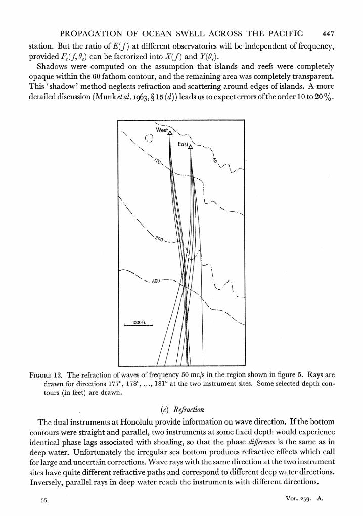
Shadows were computed on the assumption that islands and reefs were completely opaque within the 60 fathom contour, and the remaining area was completely transparent. This 'shadow' method neglects refraction and scattering around edges of islands. A more detailed discussion (Munk et al. I963, ? 15 (d)) leads us to expect errors of the order 10 to 20 %.
*> ~~~West %\
East '-
N>
~-600 7
1000 ft K
FIGURE 12. The refraction of waves of frequency 50 mc/s in the region shown in figure 5. Rays are drawn for directions 1770, 1780, ...) 1810 at the two instrument sites. Some selected depth con- tours (in feet) are drawn.
(c) Refraction
The dual instruments at Honolulu provide information on wave direction. If the bottom contours were straight and parallel, two instruments at some fixed depth would experience identical phase lags associated with shoaling, so that the phase difference is the same as in deep water. Unfortunately the irregular sea bottom produces refractive effects which call for large and uncertain corrections. Wave rays with the same direction at the two instrument sites have quite different refractive paths and correspond to different deep water directions. Inversely, parallel rays in deep water reach the instruments with different directions.
55 ~~~~~~~~~~~~~~~~~~VOL. 259. A.
448 F. E. SNODGRASS AND OTHERS
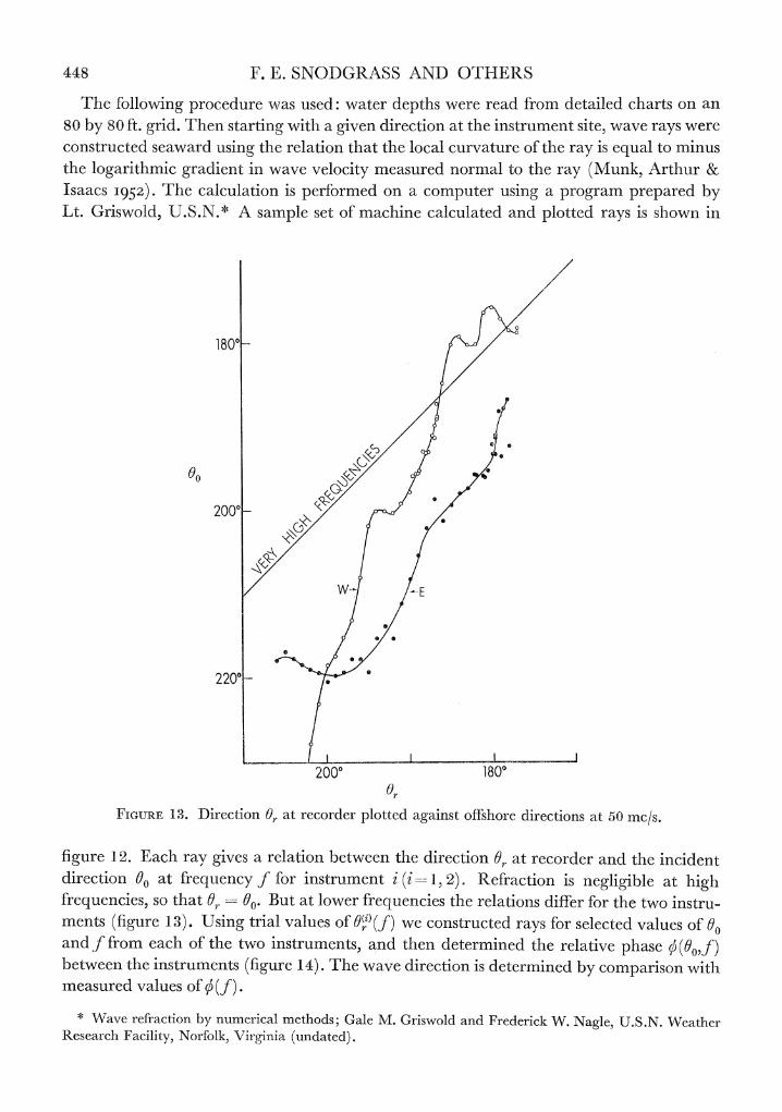
The following procedure was used: water depths were read from detailed charts on an 80 by 80 ft. grid. Then starting with a given direction at the instrument site, wave rays were constructed seaward using the relation that the local curvature of the ray is equal to minus the logarithmic gradient in wave velocity measured normal to the ray (Munk, Arthur & Isaacs 1952). The calculation is performed on a computer using a program prepared by Lt. Griswold, U.S.N.* A sample set of machine calculated and plotted rays is shown in
1800-
00~ ~ ~ ~ ~~~~~~
00
? 2000gU
2200
2000 1800 Or
FIGURE 13. Direction 0r at recorder plotted against offshore directions at 50 mc/s.
figure 12. Each ray gives a relation between the direction 0r at recorder and the incident direction 00 at frequency f for instrument i (i 1, 2). Refraction is negligible at high frequencies, so that or == 0. But at lower frequencies the relations differ for the two instru- ments (figure 1 3) . Using trial values of O(i)(f) we constructed rays for selected values of 00 and f from each of the two instruments, and then determined the relative phase 0 (0jf) between the instruments (figure 14). The wave direction is determined by comparison with measured values of qS(f) .
* Wave refraction by numerical methods; Gale M. Griswold and Frederick W. Nagle, U.S.N. Weather GResearch Facility, :Norfiolk, Virginia (undated).
PROPAGATION OF OCEAN SWELL ACROSS THE PACIFIC 449
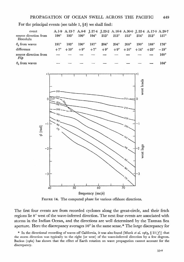
For the principal events (see table 1, ? 5) we shall find:
event A.1*9 A.13.7 A.8'6 J.27-4 J.23-2 A.16.8 A.30.0 J.224 A.170 A.28-7 source direction from 1980 1930 1990 1940 2130 2130 2150 2140 2130 1570
Honolulu
O0 fromwaves 1910 1830 1900 1870 2040 2040 2050 1900 1880 1760
difference +70 +100 + 90 + 70 + 9 +90 +100 +140 +250 -190
source direction from - - - 1600 Flip
O0 from waves - - - - 164?
+ ......... + 1
215
2~1,0 25-::
2N_ 0- 1 0
4 20 506070
40~~~~~~~~~~~~~~~1 200
-2 - 1T0 -2
-3 -3
40 50 60 70
frequency (mc/s) FIGURE 14. The computed phase for various offshore directions.
The first four events are from recorded cyclones along the great-circle, and their fetch regions lie 80 west of the wave-inferred direction. The next four events are associated with storms in the Indian Ocean, and the directions are well determined by the Tasman Sea aperture. Here the discrepancy averages 1O' in the same sense.* The large discrepancy for
* In the directional recording of waves off California, it was also found (Munk et al. I963, ? 11 (f)) that the storm direction was typically to the right (or west) of the wave-inferred direction by a few degrees. Backus (I962) has shown that the effect of Earth rotation on wave propagation cannot account for the discrepancy.
55-2
450 F. E. SNODGRASS AND OTHERS
the event of 17-0 August (also through the Tasman Sea) is probably related to poor direction finding at Honolulu due to an unfavourable signal background ratio. The last event is further to the east, and the discrepancy is 190 in the opposite sense. This event was also recorded on FliP and the accelerometer direction (? 3 (c)) agrees with the source direction. It appears as if the refractive corrections are too small so that the inferred incident direction is too near to the shore normal.
The results in direction finding are disappointing. The instruments should have been placed into deeper water to reduce the troublesome refractive corrections. An error in the assumed position of one instrument by 5 ft. may vary the computed 00 by a few degrees. There are some features in the Griswold-Nagle computer program which may lead to systematic errors of the same order (personal communication from Dr Wyman Harrison). But the recorded directions are of some use in sorting the great-circle from the Tasman events, and in supporting the identification of the event of 28'7 August as a Ross Sea storm.
So far we have dealt with the effect of refraction on direction finding. There is an addi- tional effect on energy density. The ratio of energy densities at the recorder to that in deep water is given by Er VO cos00
Eo Vr cos Or
where 00 is the angle between the incident ray and the offshore normal. The following table gives a few selected values for an instrument at 60 ft. depth:
f (mc/s) 50 60 70 100
V0/Vr 1P22 1.10 1P00 0.82 Cos 00/cos Or 00 = 30' 0.88 0 89 090 0.92
00 = 150 0*98 0.99 1'00 1*00
Stations were selected for exposures in the direction of the reference great-circle, so that 00 is small. It follows that the enhancement in shallow water at the five shore-based stations may be as large as 20 % (0.8 dB) at 50 mc/s, and less at higher frequencies. The difference between shore-based stations is even smaller. On the other hand, a glance at figure 13 shows that anamolous values of doria0O may be expected for certain combinations of 00 and f. This explains the differences of the power spectra of the east and west instruments at Honolulu (figure 9). We have made no attempt to correct for these.
(d) Oblateness
Here we are concerned as to whether discrepancies in the measured wave directions could be accounted for by the oblateness of the ocean surface. The assumption of a spherical surface introduces also small errors in the computed distances (i.e. arrival times). A calculation of these effects is given in the Appendix.
The maximum error in wave direction that can be incurred by neglect of oblateness is equal to the ellipticity e 1/297 0.20 (A 13). The error in distance between two given points is given by (A 14). The corrections are smaller than the uncertainty in the positions of fetch areas. For example, if the two points are 45 S 00 E and 45 N 90 E, the wave direction is 550 T at each point and the error in distance is
-1.15ae - -25km or -0Ax5ae-z-10km
PROPAGATION OF OCEAN SWELL ACROSS THE PACIFIC 451
depending on whether the equatorial radius or the mean radius of the Earth was used. In either case the distance is shorter than on a spherical Earth, and the arrival earlier than expected.
The energy density is not affected by oblateness, and the discrepancy in ray paths appears to be completely negligible in this paper.
5. THE PRINCIPAL EVENTS
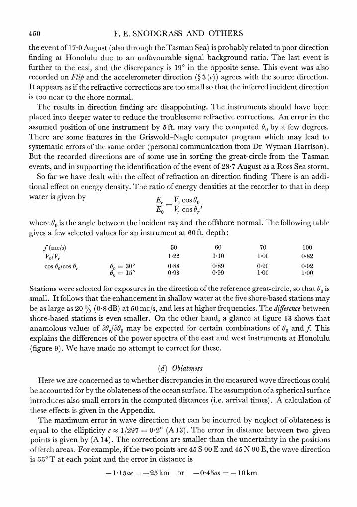
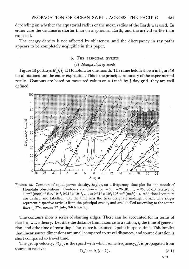
(a) Identification o!f events Figure 15 portrays E(f, t) at Honolulu for one month. The same field is shown in figure 16
for all stations and the entire expedition. This is the principal summary of the experimental results. Contours are based on measured values on a 1 mc/s by . day grid; they are well defined.
100 B.n
............... ..... . . . , .,,....... - -5 . ......... ........... ,-i....
.'X''
''.::::::' . X",?-,.
.................................. ........ . . . ,,,., ............ ..
90 g
10~~~~ i .
~26- 28 30 I2 4 6 8 tO 12 14 16 18 20 22
August
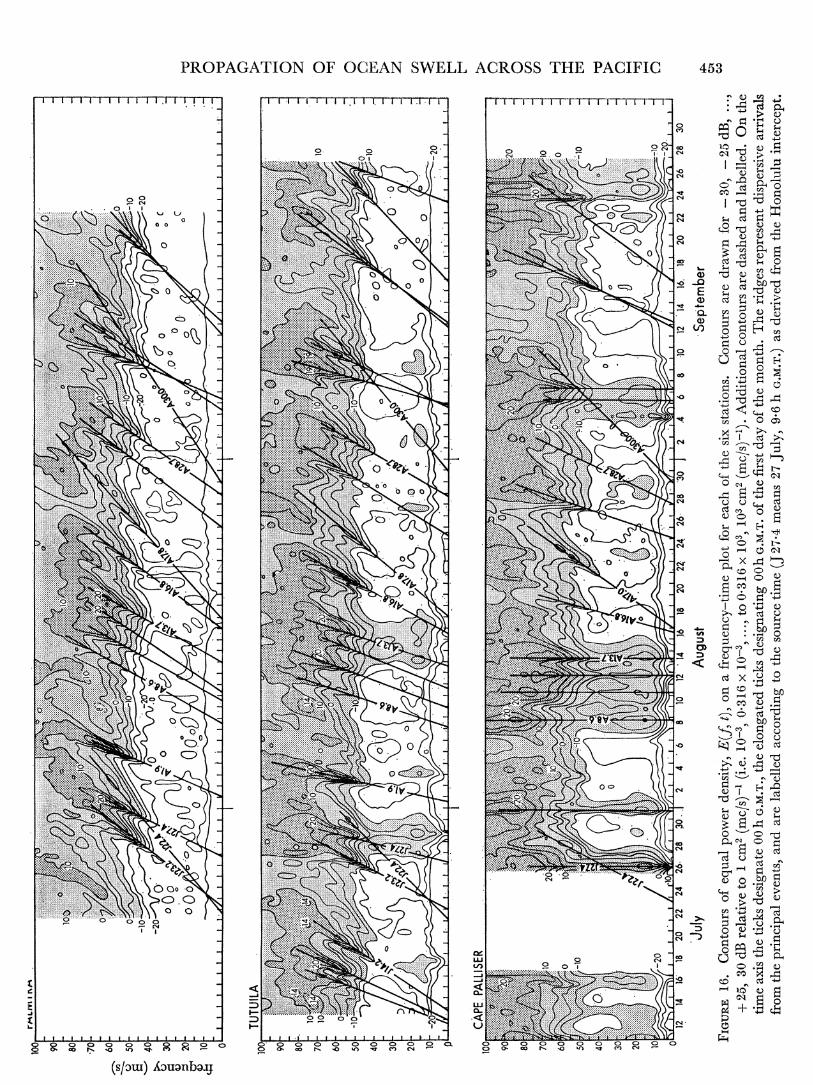
FIGURE 15. Conltours of equal power density, E(f, t), on a frequency-time plot for one month of HIonolulu observations. Contours are drawn fo:r -30, -25 dB, ..., + 25, 30 dB relative to 1 cm2 (mc/s1 (i.e. 10-3, 0-316 x 1O ..., to 0316 x 103, 103 cm.2 (mc/s).). Additional contours are dashed and labelled. On the time axis the ticks designate mnidnight G.M.T. The ridges represent dispersive arrivals from the principal events, and are labelled according to the source timne (J 27I4 means 27 July, 9I6 h G.M.T.).
The contours show a series of slanting ridges. These can be accounted for in terms of classical wave theory. Let A\ be the distance -from a source to a station, to the time of genera- tion, and t the time of recording. The source is assumed a point in space-time. This implies that linear source dimensions are small compared to travel distances, and source duration is short compared to travel time.
The group velocity, V(f ), is the speed with which some frequency,f, is propagated from source to receiver V(f ) = A/ (t- t0o (5.1)
55-3
452 F. E. SNODGRASS AND OTHERS
o ., . ... . ... . ... ',.,. SS~~~~~~~~~~~~~~~~~~~~~~~~~~~~~~~~~~~~~~~~~~~~~~~~~~. . . . . .
.. v.-.... . ....
...,...-...,.,...,..,''.'.,,"''', ' "'''''tAP\E ~ ~ ~ ~ ~ ~ ~ ~~~~~~~~~~~~~~~.. .....
0~~~~~~~~~
CN~
j ES, , . i I t . ,.> X.S i, ..... E! iS,,,.t (, R \o~~~~~~~~~~~~~~~~~~~~~~~~~~~~~~~~~~~~~~~~~~~~~~~~~~~~~~~~~~~~~. . . .... . . . . . .
t .N@dr8........... .... WBt<
0
^ L&t.. . ... .. .. .. ... . . ... X. .. s. . . . .ss.\ ). . .
C,.,S,,,,,W,,,w.,,.,<\ Ar)- - . ,, ,,...,0
C".~~~~~~~~~~~ S $ e A - < ,1 :1 I F | g g S Q62
130000000A't000miA02\e eW \l I ] 'BSc'EB-'. -e <e0
BiSi40iB0SW <\\ ? 4 flB 0%? ea-
PROPAGATION' OF OCEAN SWELL ACROSS THE PACIFIC 453
4) rl
0 ~ ~ ~ ~ ~~~~~~~~1
0 K~~~~~~~~~~~~~~~~~~~~~~~~~~~~~~~1 ~~~~~~~~~~~~ 0~ ~ ~ ~ ~ ~ ~ ~ ~ ~~~~~~~~~~~C I I~~~~~~~~~~~~~~~~~~~~~~~~~~~~~~~~~~~~~~~~~~~~~~~~~~~~~~~~~~~~~~~~~~~~~~l
0 0
4. a~~~~~~~~~~~~~~~~~~~~~~~~~~~~~~~~~~~~~~~~~~~~~~~~~~~~~~1
* . 0 V2~~~~~~~~~~~~~~~~~~ 414,0 4) -.-~~~~~~~~~~~~~~~~~~~~~l)'
C=~~~~~~~~~~~~~ ~~ ~ ~4 )J
Q C)
C14
0 C',~~~~~~~~~~~~~0
~~~~~~~~~~~ c~~~~~~~~~~~~~~~~~~~~~~~~~~~c
0~~~~~~~~~~~~~~~~~~~~~~~~~~~~~~~~~1 0 0.~~~~~~~~~~~~~~~~~~~~~~~~~~~~~~~~~0
o0 ~~~~~~~~~~~~~~~
0 ~ ~ ~ ~ ~~~ ~~~ ~~~~~~~~~~~~~~~~~~~~~~~0
OOo 0~~~~~~~~~~~~~~~~~~~~~~~~~~~~~~~~~~~. ...c L
N '0 _ N ~~~~~~~~~~~~~~~~~~~~~~~~~0 ~~~~~~~~o '~~~~~~~~~~~ C') ~~~~~ ~ c i
454 F. E. SNODGRASS AND OTHERS
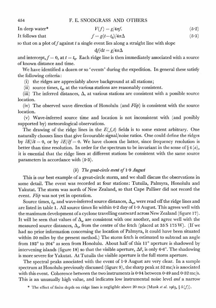
In deep water* V(f) = g/4igf. (5.2)
It follows that fz g(t-to)/47rfA (5.3)
so that on a plot off against t a single event lies along a straight line with slope
df/dt - g/47A
and intercept,J- 0, at t = to. Each ridge line is then immediately associated with a source of known distance and time.
We have identified a dozen or so 'events' during the expedition. In general these satisfy the following criteria:
(i) the ridges are appreciably above background at all stations; (ii) source times, t0, at the various stations are reasonably consistent. (iii) The inferred distances, A, at various stations are consistent with a possible source
location. (iv) The observed wave direction of Honolulu (and Fli is consistent with the source
location. (v) Wave-inferred source time and location is not inconsistent with (and possibly
supported by) meteorological observations. The drawing of the ridge lines in the E(f, t) fields is to some extent arbitrary. One
naturally chooses lines that give favourable signal/noise ratios. One could define the ridges by dE/lt- 0, or by dE/df = 0. We have chosen the latter, since frequency resolution is better than time resolution. In order for the spectrum to be invariant in the sense of ? 4 (a), it is essential that the ridge lines at different stations be consistent with the same source parameters in accordance with (5.3).
(b) The great-circle event of 1-9 August
This is our best example of a great-circle storm, and we shall discuss the observations in some detail. The event was recorded at four stations: Tutuila, Palmyra, Honolulu and Yakutat. The storm was north of New Zealand, so that Cape Palliser did not record the event. Flip was not yet in operation.
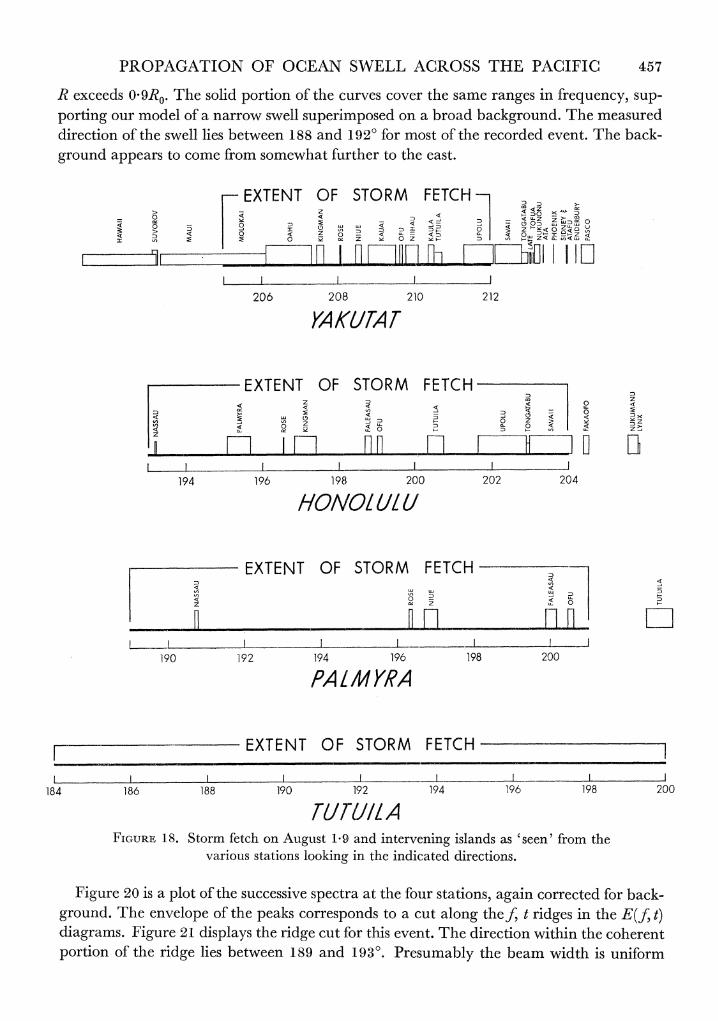
Source times, to, and wave-inferred source distances, A., were read off the ridge lines and are listed in table 1. All source times lie within 0-2 day of 1'9 August. This agrees well with the maximum development of a cyclone travelling eastward across New Zealand (figure 17). It will be seen that values of A\ are consistent with one another, and agree well with the measured source distances, A., from the centre of the fetch (placed at 35S 175 W). (If we had no prior information concerning the location of Palmyra, it could have been situated within 50 miles by the present method.) The storm fetch is estimated to subtend an angle from 1930 to 204? as seen from Honolulu. About half of this 110 aperture is shadowed by intervening islands (figure 18) so that the visible aperture, AO, is only 6060. The shadowing is more severe for Yakutat. At Tutuila the visible aperture is the full storm aperture.
The spectral peaks associated with the event of 1P9 August are very clear. In a sample spectrum at Honolulu previously discussed (figure 9), the sharp peak at 52 mc/s is associated with this event. Coherence between the two instruments is 094 between 0-49 and 0-52 mc/s. This is an unusually high value, and indicates low instrumental noise level and a narrow
* The effect of finite depth on ridge lines is negligible above 20 mc/s (Munk et al. I963, ? 5 (f)).
PROPAGATION OF OCEAN SWELL ACROSS THE PACIFIC 455
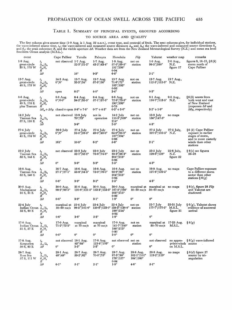
TABLE 1. SUMMARY OF PRINCIPAL EVENTS, GROUPED ACCORDING
TO SOURCE AREA AND QUALITY
The first column gives source time (1.9 Aug. is 1 Aug. 22 G.C.T.), event type, and centroid of fetch. The next columns give, for individual stations, the wave-inferred source time, to; the wave-inferred and measured source distances A,,, and A,; the wave-inferred and measured source directions ,w and 0,; the peak coherence R, and the visible aperture AO. Weather data are from the New Zealand Meteorological Survey (N.Z.) and mean sea level Southern Ocean analysis (M.S.L.).
event Cape Palliser Tutuila Palmyra Honolulu Flip Yakutat weather map remarks 1-9 Aug. to not observed 1-7 Aug. 1-7 Aug. 1*9 Aug. not on 1 9 Aug. 2J0 Aug., figures 9, 18-21, ?6(b) great-circle AAl/s 22.30121-20 43.20143.80 57.50/59.50 station 98-50/1000 N.Z. storm north of 35 S, 175 W 6w/6s 1910/1980 figure 17 Cape Palliser
R 0*94 AO 160 9.30 6.60 2.10
13-7 Aug. to 14-3 Aug. 13-7 Aug. 13-7 Aug. 13-7 Aug. not on 13-7 Aug. 13-7 Aug., great-circle Al/As 00/00 33.30/340 57.50/560 71-60/720 station 112.50/112.50 N.Z. 48 S, 175 W Ow/G, 1830/1930
R 0-93 AO open 6.20 4.00 3.40 0.30
8-6 Aug. to 8-8 Aug. 8-4 Aug. 8-4 Aug. 8-6 Aug. not on 8-1 Aug. 9 5 Aug., ?6(b) waves from great-circle Al/As 00/6.00 34.20/35.50 57.10/57.50 72.90/73.50 station 116.70/113.50 N.Z. both west and east 48 S, 175 E W/0'S 1900/1990 of New Zealand plus Tasman R 0 75 (responses AO and
AOW + AGE closed+open 5.80+7.80 0.70+4.30 0.30+ 3.60 3-20+ 1.90 AE, respectively)
14 2 July to not observed 13-9 July not in 14-2 July not on 13-9 July no maps Tasman Sea Aw/As 7001730 operation 110-5011090 station 1500/147-50 57 S, 110 E 0Ow 2140
AO 3.90 2-50 4-30
27-4 July to 26.9 July 27-4 July 27-4 July 27-4 July not on 27-5 July 27-5 July, ?6 (b) Cape Palliser great-circle AWIAS 00/00 25.00/26.50 49.00/49.00 65.00/65.00 station 107.20/105.50 N.Z. exposed to earlier 41 S, 175W 6w46, 1870/1940 stages of storm,
R 0 96 and to more easterly AG 1610 10.50 6.20 5.60 2.10 winds than other
stations
23-2 July to not observed 23-2 July 23-0 July 23-2 July not on 23-2 July 22-8 July, ? 6(c) see figures Tasman Sea AW/As 52.10/52.20 76.60/74.60 88.30/88.30 station 129.60/1280 N.Z. 23-28 52 S, 145 E /wlGs 2040/2130 figure 22
R 0-96 AG 00 3-90 3.30 2.50 4.30
16-8 Aug. to 16-7 Aug. 16-6 Aug. 16-8 Aug. 16-8 Aug. not on 16-9 Aug. no maps Cape Palliser exposure Tasman Sea AW/As 27-10/27-10 55.80/54.50 75.00/76.00 92.90/920 station 127.80/129.50 to a different storm 52 S, 140 E OW/Os 2040/2130 sector than other
R 0 95 stations ? 6 (g) AG 0.60 3.90 3.10 2.50 4.30
30-0 Aug. to 30 0 Aug. 31-0 Aug. 30-0 Aug. 30 0 Aug. marginal at marginal at no maps ? 6 (e), figure 28 Flip Madagascar AW/A, 99.20/99.50 120-80/121-50 153-30/153.50 167.5011680 50-60 mc/s 50-60 mc/s and Yakutat are 31 S, 31 E GW/G- 2050/2150 shadowed
R 0-89 AG 0.60 3.90 3.10 1.90 00 00
22-4 July to marginal at 22-4 July 22-4 July 22.4 July not on 22-7 July 22-25 July ? 6 (g), Yakutat shows Indian Ocean AW/AO 50-60 mc/s 98.50/101.00 120.80/123-00 138.30/138.80 station 177.70/177.50 M.S.L. evidence of scattered 52 S, 60 E GW/Gs 1900/2140 figure 31 arrival
R 0*95 AG 0.60 3.60 2.30 1.90 00
17-0 Aug. to 17-0 Aug. marginal marginal 17-0 Aug. not on marginal at 17-25 Aug. ? 6(g) Indian Ocean AW/Al 71-20172-50 at 70 mc/s at 70 mc/s 141-70/1400 station 50-70 mc/s M.S.L. 51 S, 57 E G,,,/G, 1880/2130
R 0 90 AO 0.60 00 00 2-00 00 00
17-8 Aug. to not observed 18-1 Aug. 17-8 Aug. not observed not on not observed no appro- ? 6 (g) wave-inferred Kerguelen A.0A, 850/880 113-80/1090 station priate winds source 50 S, 85 E AG 00 3.50 2.30 00 00 on M.S.L.
28-7 Aug. to 28-1 Aug. 28-7 Aug. 28-7 Aug. 28-7 Aug. 28-8 Aug. 28-8 Aug. no maps ? 6 (d) figure 27 Ross Sea A,,,/A, 480/480 59.20/620 70.00/750 87.50/880 102.10/1010 119.20/1190 source by tri- 57 5, 111 W 6w/GO 1760/1570 1640/1600 anglation
R 0584 AG 6.01 5.10 2*1' 1.90 4.60 5.10
456 F. E. SNODGRASS AND OTHERS
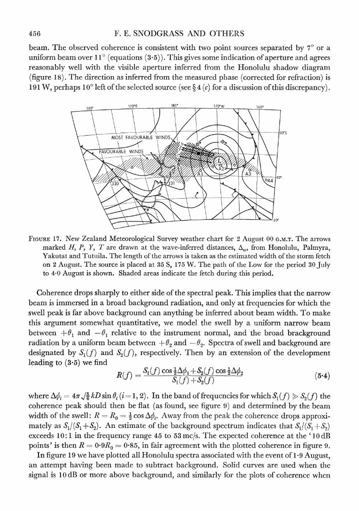
beam. The observed coherence is consistent with two point sources separated by 70 or a uniform beam over 110 (equations (3.5)). This gives some indication of aperture and agrees reasonably well with the visible aperture inferred from the Honolulu shadow diagram (figure 18). The direction as inferred from the measured phase (corrected for refraction) is 191 W, perhaps 10o left of the selected source (see ? 4 (c) for a discussion of this discrepancy).
160' 1~~~70'E 1800 170'W 10
\ - ~~MOST FAVOURABLE WINDu
FIGURE 17. New Zealand Meteorological Survey weather chart for 2 August 00 G.M.T. The arrows marked H, P, Y, T are drawn at the wave-inferred distances, AfW from Honolulu, Palmyra, Yakutat and Tutuila. The length of the arrows is taken as the estimated width of the storm fetch on 2 August. The source is placed at 35 S, 175 W. The path of the Low for the period 30 July to 4 0 August is shown. Shaded areas indicate the fetch during this period.
Coherence drops sharply to either side of the spectral peak. This implies that the narrow beam is immersed in a broad background radiation, and only at frequencies for which the swell peak is far above background can anything be inferred about beam width. To make this argument somewhat quantitative, we model the swell by a uniform narrow beam between + 01 and -01 relative to the instrument normal, and the broad brackground radiation by a uniform beam between + 02 and -02. Spectra of swell and background are designated by SI(f) and S2(f), respectively. Then by an extension of the development leading to (3.5) we find
R(f) = Sl (f) COS Aq51-S2 (f) COS 2Aq2 (5.4)
where Ai= 4ffr /6 kD sin 0i (i= 1, 2). In the band of frequencies for which S1 (f) > S2(f) the coherence peak should then be flat (as found, see figure 9) and determined by the beam width of the swell: R oRs - COS Aoi. Away from the peak the coherence drops approxi- mately as S1/(S1 +S2). An estimate of the background spectrum indicates that 51I(S, +S2) exceeds 10: 1 in the frequency range 45 to 53 mc/s. The expected coherence at the '10 dB points' is then R-0 T9R-0 085, in fair agreement with the plotted coherence in figure 9.
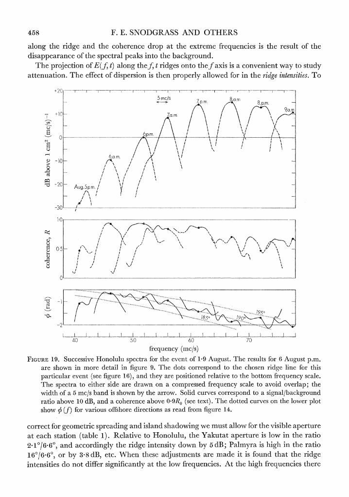
In figure 1 9 we have plotted all Honolulu spectra associated with the event of 1 *9 August, an attempt having been made to subtract background. Solid curves are used when the signal is 10 dB or more above background, and similarly for the plots of coherence when
PROPAGATION OF OCEAN SWELL ACROSS THE PACIFIC 457
R exceeds 0-9Ro. The solid portion of the curves cover the same ranges in frequency, sup- porting our model of a narrow swell superimposed on a broad background. The measured direction of the swell lies between 188 and 1920 for mnost of the recorded event. The back- ground appears to come from somewhat further to the east.
EXTENT OF STORM FETCH 0 z <
206 208 210 212
KAKUTAT
EXTENT OF STORM FETCH <( 0 E2 < , U0 ?
0 0~~~0z !. 0zZ
I I _ i ?. ____ _ _
194 196 198 200 202 204
HONOL UIl U
EXTENT OF STORM FETCH
z ~ ~ ~ t z z z > n;
!~~~~~~~~~~~~~~~~~~~ 0
L! I I I
~~~~~~_ I _
190 19 00
z ~ ~ ~ ~ ~ ~ ~ ~ ~ ~ ~ ~ '
190 192 194 196 198 200
PAH O /RA
EXTENT OF STORM FETCH t _ i . _ I I _ _ I _i_ L I __. I . LI
184 186 188 190 192 194 196 198 200
,7YTUIL A FIGURE 1.8. Storm fetch on August 1 9 and intervening islands as 'seen' from the
various stations looking in the indicated directions.
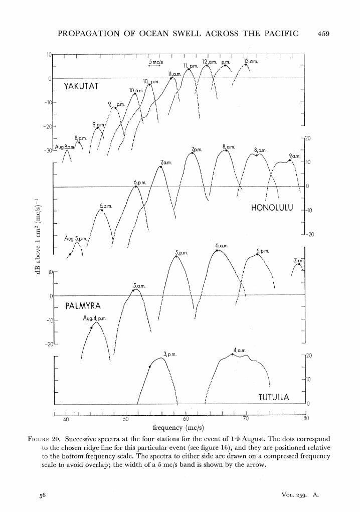
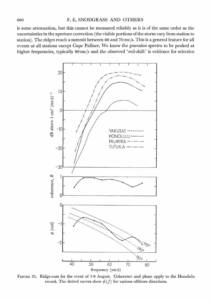
Figure 20 is a plot of the successive spectra at the four stations, again corrected for back- ground. The envelope of the peaks corresponds to a cut along thef, t ridges in the E(f, t) diagrams. Figure 21 displays the ridge cut for this evenlt. The direction within the coherent portion of the ridge lies between 189 and 1 93?. Presumably the beam width is uniform
458 F. E. SNODGRASS AND OTHERS
along the ridge and the coherence drop at the extreme frequencies is the result of the disappearance of the spectral peaks into the background.
The projection of E(f, t) along thef, t ridges onto thef axis is a convenient way to study attenuation. The effect of dispersion is then properly allowed for in the ridge intensities. To
+ 20iT F TT T F T T F~
5 mc/s 8,a.m 7P.M. 3,pm.
+10- I rn. T aTM
:- CI'o,\X
0
F a a 6a' / / M
~ 20 - Aug.5,.pm./
-30 ,
' ~ ~ ~ ~ . I -1
- 3 L _ ._ _ _ _ _ _ _ _ _ _ _ _ _ _ _ _ _ _ _ _ _ . _ _ _ _ _ _ _ _ . _ _ _
1.0
1 1 \\ -........
.............. ~ ~ ~ ~ ~ I ~ / ../
40 50 60 70 firequency (mc/s)
FIGURE 19. Successive Honolulu spectra for the evenlt of 19 August. The results for 6 August p.m. are shown in more detail in figure 9. The dots correspond to the chosen ridge line for this particular event (see figure 16), and they are positioned relative tzo the bottom frequency scale. The spectra to either side are drawn on a comnpressed frequency scale to avoid overlap; the width of a 5 mc/s band is shown by the arrow. Solid curves correspond to a signal/background ratio above 10 dB, and a coherence above 0 I9Ro (see text). The dotted curves on the lower plot show ()for various offishore directions as read from figure 14.
correct for geometric spreading and island shadowing we must allow for the visible aperture
at i eac staio (tbe1.Rltv oEoouu h Ykttaetr slwih ai
2*1?/6-6?,~~ /n acodnl'h.ideitniydw b -B\amr s ihi h ai
16?16*6?,~~~~~~~ or by 3-d,ec hnteeajsmnsar aei sfudta h ig
inestisd no dife signfcnl at th o rqece.A h ihfeuniethr
PROPAGATION OF OCEAN SWELL ACROSS THE PACIFIC 459
o0 -- r II? - r-- rE -1 - -- ~ 5 mc/s 12a.m. p.m. 13,a.m.
YAK TAT 0 pm , ' '
-IO 98 p.m. |
9am I /\
luz | 6, a . m .~~~~I / ivX \\IHONOl
-20- 1am \ / /
8.,m./ / / Y 20 -30 Aug.8,a/ p / a.m.
-30 7PM , p.m.
9/a.m.
6a.m. V10
L~~~~~~~~~~~~~~~~~~~~ I l I
6,pam / \ I 6a.m. I~~~~~~~~~~~~~I ~~HONOLULU -10
Aug . 6m.a..
> 5 p.m. 70 p80
56 EIOL. 259. A.~~~~~~~~~~~~~~~~~7
'e 10
5,a.m. /
PALMYRA -Aug.4, p.m. /\ /
-20/ I
I ~~~~~~~~~~~3, Pm. 4a.. 2 0
I I ~~~TUTU ILA
to ~~~~~~~frequency (mc/s)
FIGURE 20. Successive spectra at the four stations for the event of 1P9 August. The dots correspond
460 F. E. SNODGRASS AND OTHERS
is some attenuation, but this cannot be measured reliably as it is of the same order as the uncertainties in the aperture correction (the visible portions of the storm vary from station to station). The ridges reach a summit between 60 and 70 mc/s. This is a general feature for all events at all stations except Cape Palliser. We know the generation spectra to be peaked at higher frequencies, typically 80 mc/s and the observed 'red-shift' is evidence for selective
I I I- - I XI T
20
10
C-1 0
; -lo - / / YAKUTAT / - .X1 / HONOLULU X / , PALMYRA- -
-20 / TUTUILA ---
,,/ -30 /
C. I
L
-2
1 . I . . . ..
40 50 60 70 80 firequency (mc/s)
FIGURE 21. Ridge-cuts for the event of 1@9 August. Coherence and phase apply to the Honolulu record. The dotted curves show q5 (f) for various offshore directions.
PROPAGATION OF OCEAN SWELL ACROSS THE PACIFIC 461
attenuation of the higher frequencies. But the red shift is small between Tutuila and Yakutat, and we surmise that most of the selective attenuation takes place in the first 1000 miles beyond the storm.
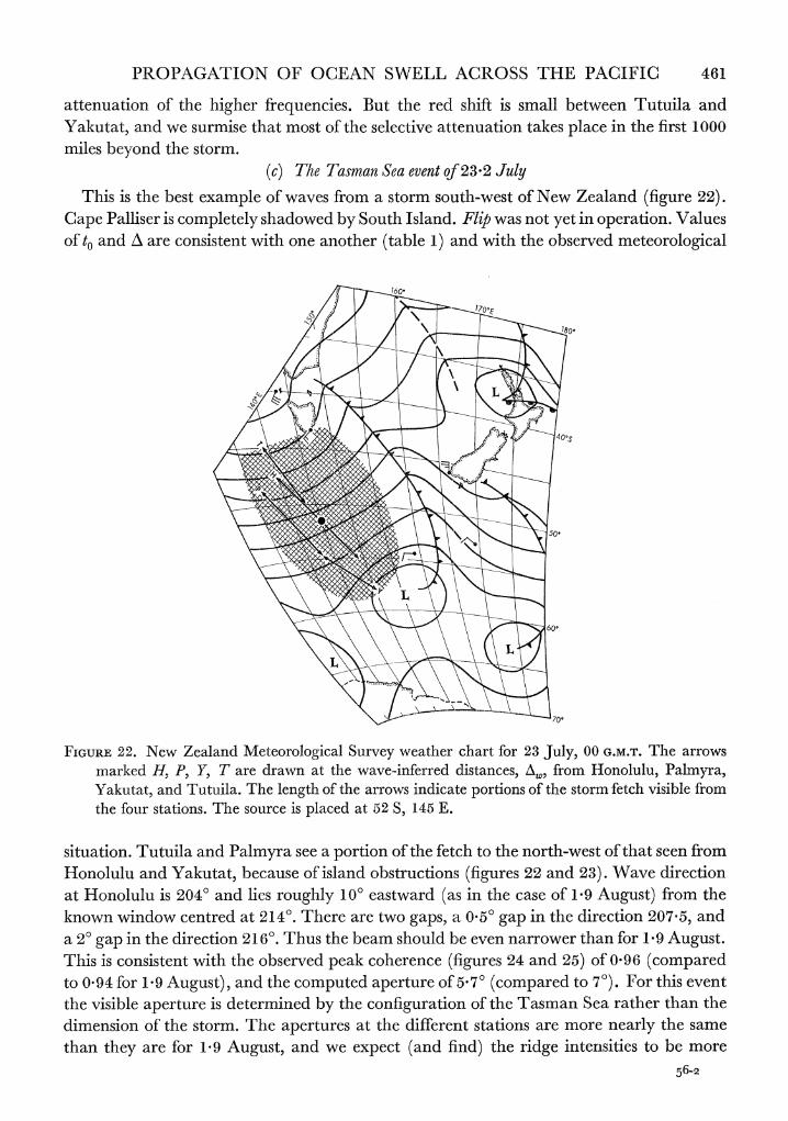
(c) The Tasman Sea event qf 23.2 July
This is the best example of waves from a storm south-west of New Zealand (figure 22). Cape Palliser is completely shadowed by South Island. Flip was not yet in operation. Values ofto and A are consistent with one another (table 1) and with the observed meteorological
FIGURE 22. New Zealand Meteorological Survey weather chart for 23 July, 00 G.M.T. The arrows marked H, P, Y, T are drawn at the wave-inferred distances, Aw, from Honolulu, Palmyra, Yakutat, and Tutuila. The length of the arrows indicate portions of the storm fetch visible from the four stations. The source is placed at 52 S, 145 E.
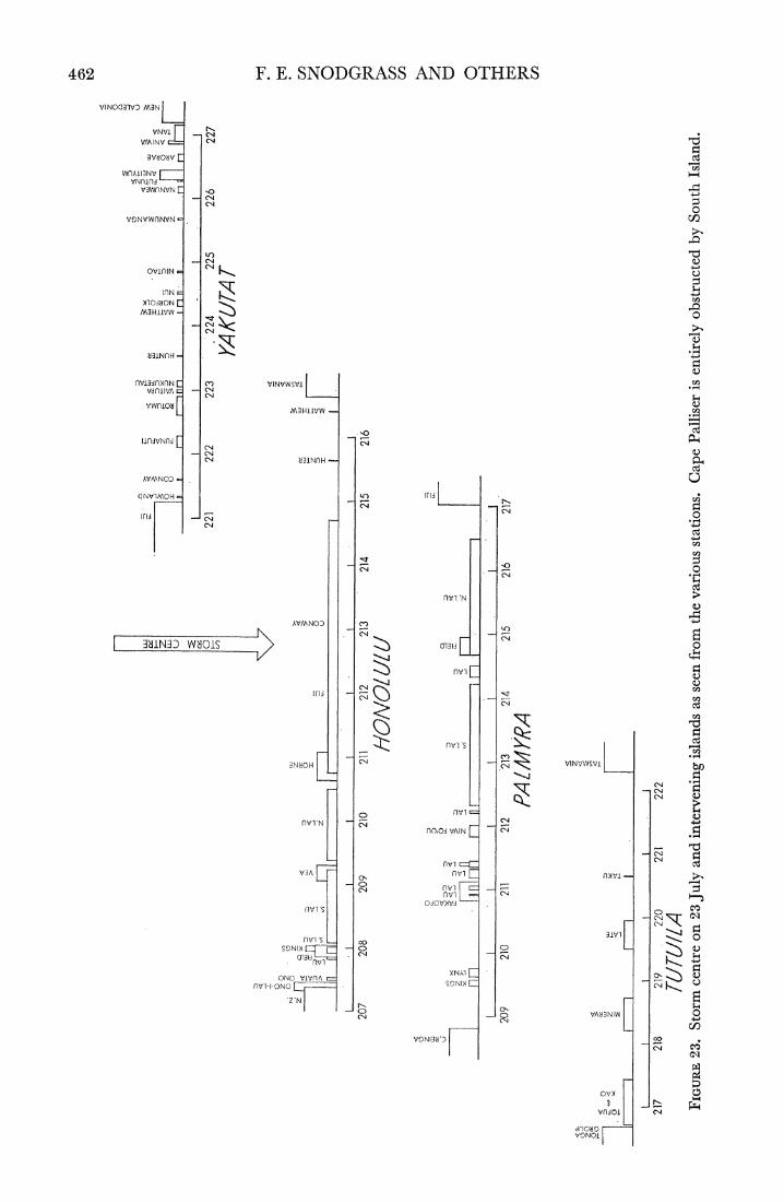
situation. Tutuila and Palmyra see a portion of the fetch to the north-west of that seen from Honolulu and Yakutat, because of island obstructions (figures 22 and 23) . Wave direction at Honolulu is 204? and lies roughly 100 eastward (as in the case of 1m9 August) from the known window centred at 214?. There are two gaps, a 0.50 gap in the direction 207m5, and a 2? gap in the direction 21 6?. Thus the beam should be even narrower than for 1 9 August. This is consistent with the observed peak coherence (figures 24 and 25) of 0-96 (compared to 0 94forl*~9August), and the computed aperture of 5.70 (compared to 7?). For this event the visible aperture is determined by the configurationl of the Tasman Sea rather than the dimension of the storm. The apertures at the different stations are more nearly the same than thley are for Pt9 August, and we expect (and find) the ridge intensities to be more
56-2
462 F. E. SNODGRASS AND OTHERS
VIN0311VD MA3N
VNVI r VMINV _
VNnllfnl V3WnNVN 0
CN
VONVWONVN NVN
.N 4 U) r~~~~~~~~~~~~~~~~~~~~~~~~~~~~~~~~~~~~~~~~~~~~~~~~~~. OV_flN
Q .~~ InN
)lowoIN C .j) M3HiiVW - zz1
nlVignfnN C") VINVWSVI '-4 VdlIIVA CN.
VWlnl0U PAM3HIIVW
(ljnn N U (N IJnNflNH p.4
AVAVNOD
(ONV1AOH L EZi
,,_. . .-. . _ \. CN_-,_W
(Nlj 0 > g nX _ S
no,jVAIN >
(N~~~~~~~~~~~~~~~~~~~L
0 O r~~~~v i N >
AVIANOD M LO
4*0
C14~~~~~~~~~~~~C (N
nvi
HA~~~~~~~~~~~~~~~~no _e ( A2
31N1OH1-1 VINVWSVI
nvl'N C14 ~ ~ ~ ~ ~ ~ ~ N
nlooi VAIN (N4
VIA fr niVEinv
IlVi S Q~~~~~~~~vi C
S!DNI>i C' C)
nvi
PROPAGATION OF OCEAN SWELL ACROSS THE PACIFIC 463
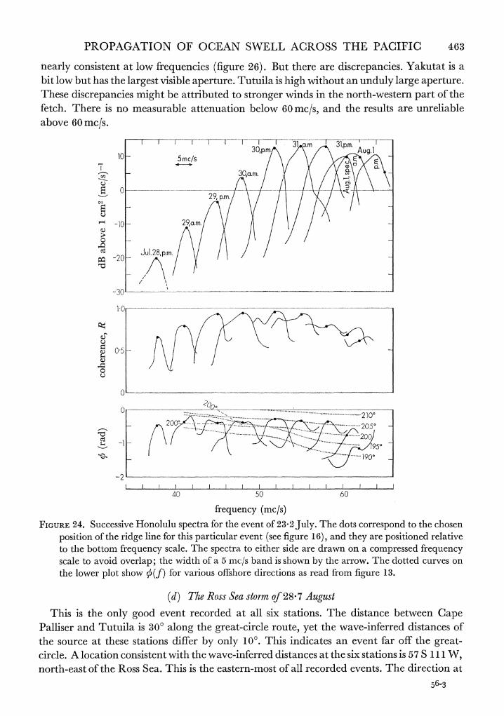
nearly consistent at low frequencies (figure 26). But there are discrepancies. Yakutat is a bit low but has the largest visible aperture. Tutuila is hIigh without an unduly large aperture. These discrepancies might be attributed to stronger winds in the north-western part of the fetch. There is no measurable attenuation below 60 mc/s, and the results are unreliable above 60 mcls.
L 1 1~~~~~~~~3 pm 31 a m 31PM A_
S f 5mc/s
--0
Jl ul.28,p.m. -20-
-30 --- - - -____________
1 0 - - - - - - _ _ _ _ _ _ _ _ _ _ _
Q
05
0
.. ~~~~~~~~~2100
2OO2~~~~~~~ . - .~~~ ... ....... crs
... ........
~~.. . 200
40 50 60
frequency (mc/s)
FIGURE 24. Successive Honolulu spectra for the event of 23-2July. The dots correspond to the chosen position of the ridge line for this particular event (see figure 16), and they are positioned relative to the bottom frequency scale. The spectra to either sidle are drawn on a compressed frequency scale to avoid overlap; the width of a 5 mc/s band is shown by the arrow. The dotted curves on the lower plot show 0(f) for various offshore directions as read from figure 13.
(d) The Ross Sea storm of 28-7 August
This is the only good event recorded at all six stations. The distance between Cape Palliser and Tutuila is 30? along the great-circle route, yet the wave-inferred distances of the source at these stations differ by only 10?. This indicates an event far off the great- circle. A location consistent with the wave-inferred distanlces at the six stations is 57 S 111 W, north-east of the Ross Sea. This is the eastern-most of all recorded events. The direction at
56-3
464 F. E. SNODGRASS AND OTHERS
10 I T I I I -I I - I I I - I - -I ' 1- - - -
2 P-M. am 4
0
YAKUTAT 1 p.m. Aug.l,aim. 5mc/s
-10 /
-20- 31a.m./ 31,a.m. 31,p.m. Aug. 1,
3030,p0,pm i28,.mm a.m 2
2Zp.m. 28, ~~~p.m.
10
-3o 30,~~~~~~2 a.m.
< /0
Jul228,p.m. 20
pq oAuMRAg.1,\\/ j
J~~~~~~~~~~~~~~~~~~~~~~1am a.m.-m
I I . I
10 -~~~~_
40 50 60 70
frequency (mc/s)
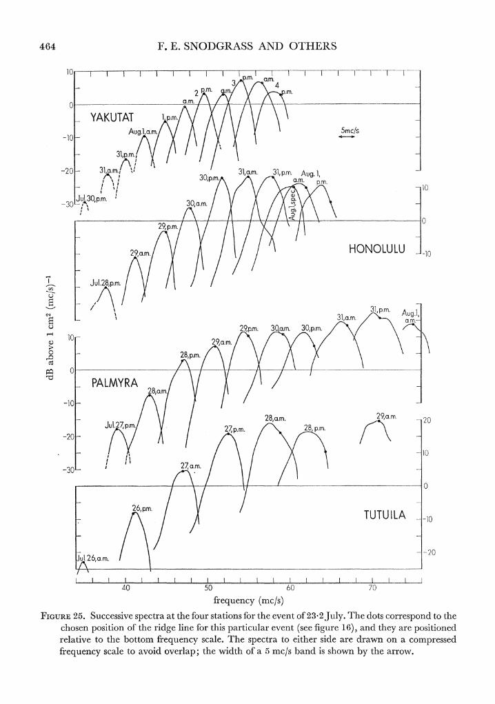
FIGURE 25. Successive spectra at the four stations for the event of 23-2Juy. The dots correspond to the chosen position of the ridge line for this particular event (see figure 16), and they are positioned relative to the bottom frequency scale. The spectra to either side are drawn on a compressed frequency scale to avoid overlap; the width of a 5 inc/s band is shown by the arrow.
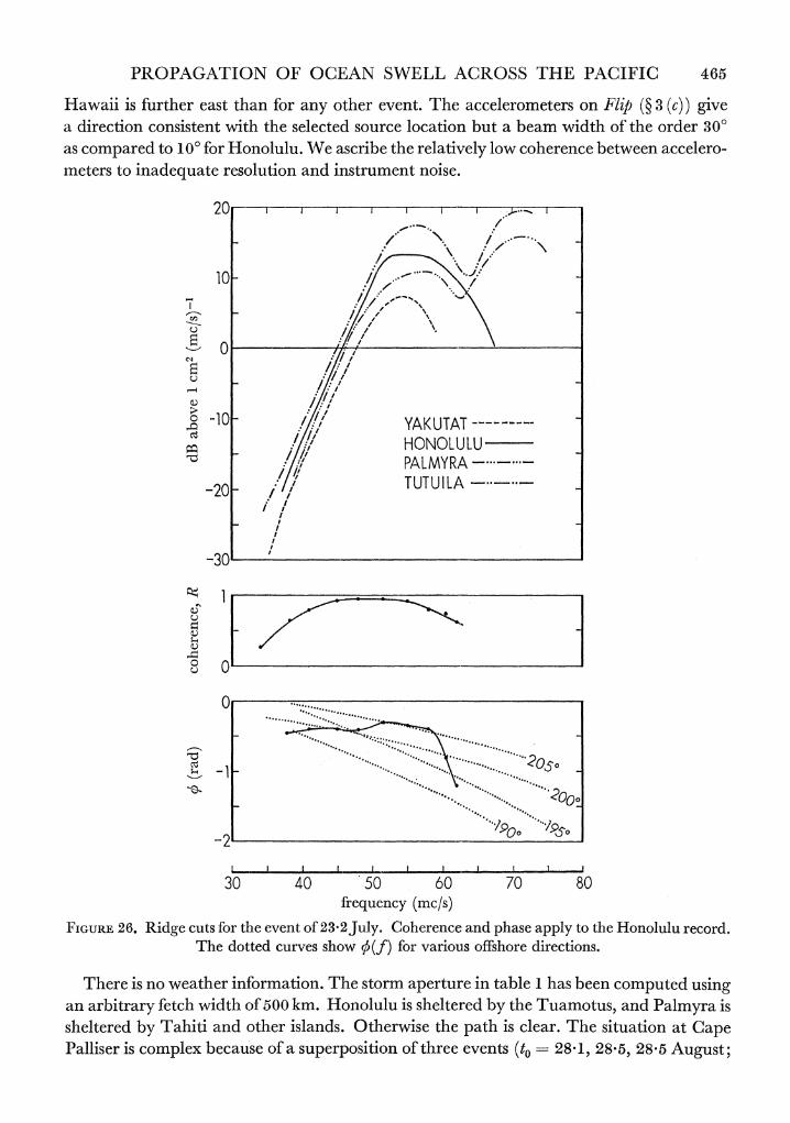
PROPAGATION OF OCEAN SWELL ACROSS THE PACIFIC 465
Hawaii is further east than for any other event. The accelerometers on Flip (? 3 (c)) give a direction consistent with the selected source location but a beam width of the order 30? as compared to IO' for Honolulu. We ascribe the relatively low coherence between accelero- meters to inadequate resolution and instrument noise.
20 -r--r----- I _
N,42~ ~ ~ 4-> \\ 4X
10 i
L/~~~ /1
30
8I 0I- ~~ -10 / / ~~ YAKUTAT------ HONOLUJLU
/ '~~ PALMYRA -20 ~~~~TUTUILA-~-~
( / -20-
-30
Xi
Cf I
anabirryftc idhof50 mHnluuisseleedb the0 'saotu,adPlyai
FIGUtre26 byTaidgctsndorthereislnto232sl. Coherwientheanphatiscear.pTelstuathionoatuCapeod Pallier iscompex dottuedo curverposhtow of fore var ents offsor =directions. *Augst
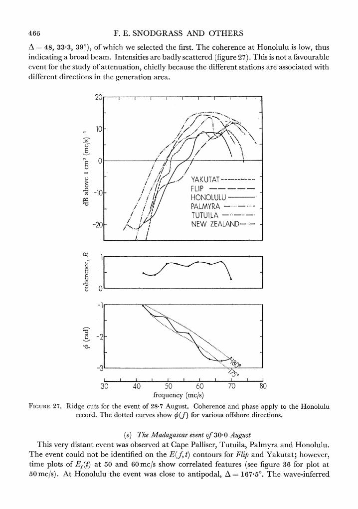
466 F. E. SNODGRASS AND OTHERS
Ai 48, 33*3, 390), of which we selected the first. The coherence at Honolulu is low, thus indicating a broad beam. Intensities are badly scattered (figure 27). This is not a favourable event for the study of attenuation, chiefly because the different stations are associated with different directions in the generation area.
20 - - - -
'10
, p ,< ./ YAKUTAT - ~~ -10 1 ~~~~FLIP
I ~HONOLULU PALMYRA- - TUTUILA
-20 - ,/ _,,>7NEW ZEALAND--
=n0 g~~~ /
-2-
-3 I I
30 40 50 60 70 80 frequency (mc/s)
FIGURE 27. Ridge cuts for the event of 28*7 August. Coherence and phase apply to the Honolulu record. The dotted curves show s(f) for various offshore directions.
(e) The Madagascar event of 30 0 August This very distant event was observed at Cape Palliser, Tutuila, Palmyra and Honolulu.
The event could not be identified on the E(f, t) contours for Flip and Yakutat; however, time plots of Ef(t) at 50 and 60 ic/s show correlated features (see figure 36 for plot at 50 mc/s). At Honolulu the event was close to antipodal, A= 1 67A5?. The wave-inferred
PROPAGATION OF OCEAN SWELL ACROSS THE PACIFIC 467
20
C z HONOLULU
-10.' PALMYRA-+-*S-- j7sl 1 TUTUILA *-- -
- i v ~~NEW ZE-.ALAND----E-
-20
1
. 7
10 420 50.60.7
........... .: _ _ _ _ __ _ _ _ I ....................
-20
-3~~~~~~~~~~~~~~~~~~~~-
30- 40 50 60 70
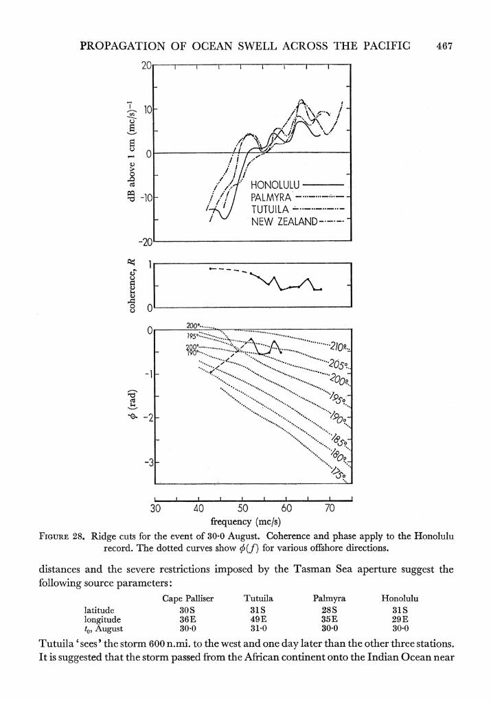
frequency (mc/s) FIGURE 28. Ridge cuts for the event of 30'0 August. Coherence and phase apply to the Honolulu
record. The dotted curves show 0(f) for various offshore directions.
distances and the severe restrictions imposed by the Tasman Sea aperture suggest the following source parameters:
Cape Palliser Tutuila Palmyra Honolulu latitude 30S 31S 28S 31S longitude 36E 49E 35E 29E to) August 30 0 310 3Q'0 300
Tutuila 'sees' the storm 600 n.mi. to the west and one day later than the other three stations. It is suggested that the storm passed from the African continent onto the Indian Ocean near
468 F. E. SNODGRASS AND OTHERS
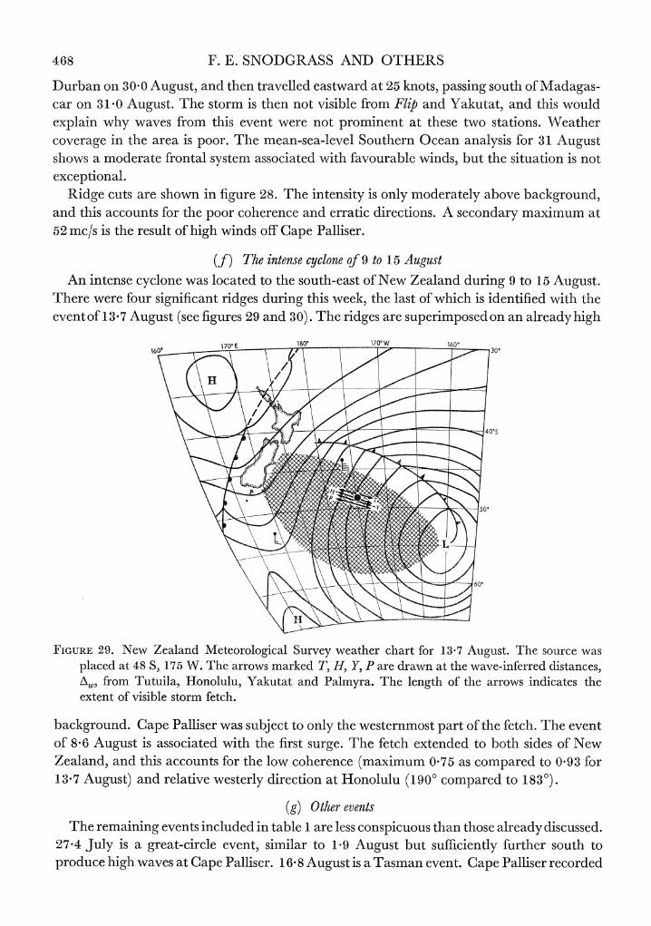
Durban on 30 0 August, and then travelled eastward at 25 knots, passing south of Madagas- car on 31F0 August. The storm is then not visible from Flip and Yakutat, and this would explain why waves from this event were not prominent at these two stations. Weather coverage in the area is poor. The mean-sea-level Southern Ocean analysis for 31 August shows a moderate frontal system associated with favourable winds, but the situation is not exceptional.
Ridge cuts are shown in figure 28. The intensity is only moderately above background, and this accounts for the poor coherence and erratic directions. A secondary maximum at 52 mcls is the result of high winds off Cape Palliser.
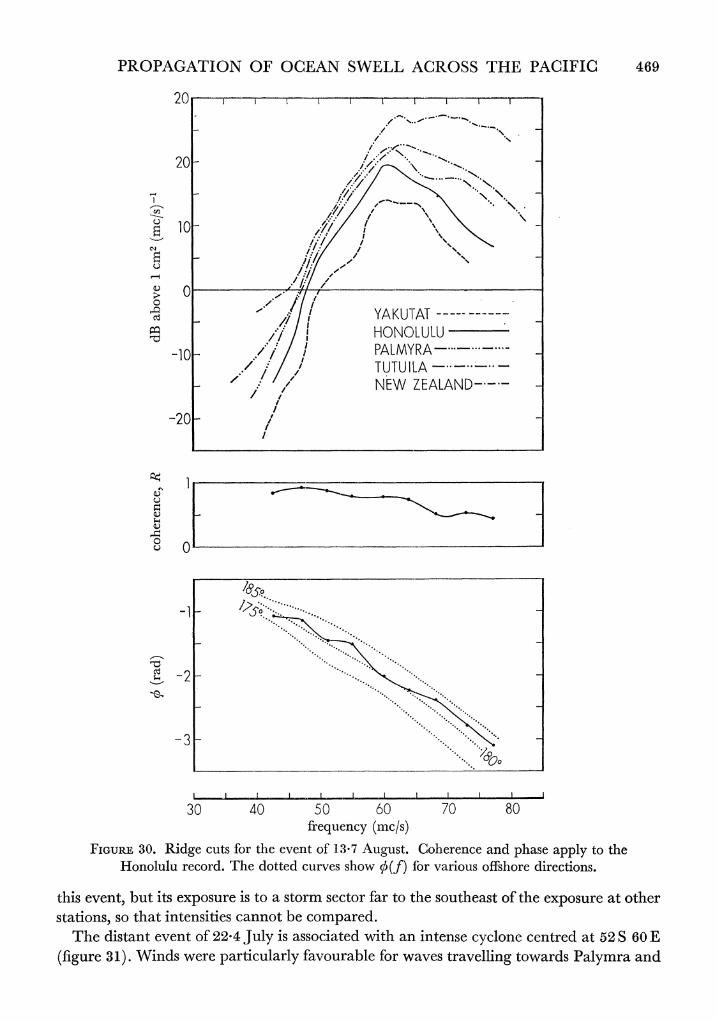
(f ) The intense cyclone of 9 to 15 August An intense cyclone was located to the south-east of New Zealand during 9 to 15 August.
There were four significant ridges during this week, the last of which is identified with the event of 137 August (see figures 29 and 30). The ridges are superimposed on an already high
160*170' E 180? . 170?W 160?
4W'S~~~~~~~~~~~~~~~~~~~~~0
FIGURE 29. New Zealand Meteorological Survey weather chart for 13-7 August. The source was placed at 48 S, 175 W. The arrows marked T,-H, Y, P are drawn at the wave-inferred distances, Aw, from Tutuila, Honolulu, Yakutat and Palmyra. The length of the arrows indicates the extent of visible storm fetch.
background. Cape Palliser was subject to only the westernmost part of the fetch. The event of 8'6 August is associated with the first surge. The fetch extended to both sides of New Zealand, and this accounts for the low coherence (maximum 0 75 as compared to 0-93 for 13-7 August) and relative westerly direction at Honolulu (1900 compared to 1830).
(g) Other events The remaining events included in table 1 are less conspicuous than those already discussed.
27@4 July is a great-circle event, similar to 1 9 August but sufficienltly further south to produce high waves at Cape Palliser. 1 6 8 August is a Tasman event. Cape Palliser recorded
PROPAGATION OF OCEAN SWELL ACROSS THE PACIFIC 469
20 - IT I I 1- I' -I lT -r
20 ---------r
n _ ' i// YAKU1AT'
C/I~~~~~~~~~~~~~
-10 _ / / PAlMYRA --
- ' / /1 NE ZEl ND
01
-20L ~ ~ ~ A /
> 10 ..
1. /
_ -/// _____ _____
0
-' / / ~YAKUlTAT /1 HONOLULU
-10! PALMYRA----------
/ ~~NEW ZEALAND-----
-20 /
Q 0
U-2
-3
30 40 50 60 70 80 frequency (mc/s)
FIGURE 30. Ridge cuts for the event of 13-7 August. Coherence and phase apply to the Honolulu record. The dotted curves show 0(f) for various offshore directions.
this event, but its exposure is to a storm sector far to t:he southeast of the exposure at other
stations, so that intensities cannot be compared.
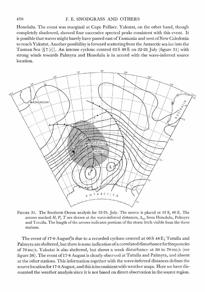
The distant event of 22t4 July is associated with an intense cyclone centred at 52 S 60 E
(figure 31). Winds were particularly favourable for waves travelling towards Palymra and
470 F. E. SNODGRASS AND OTHERS
Honolulu. The event was marginal at Cape Palliser. Yakutat, on the other hand, though completely shadowed, showed four successive spectral peaks consistent with this event. It is possible that waves might barely have passed east of Tasmania and west of New Caledonia to reach Yakutat. Another possibility is forward scattering from the Antarctic sea ice into the Tasman Sea (? 7 (c)). An intense cyclone centred 63 S 69 E on 22-25 July (figure 31) with strong winds towards Palmyra and Honolulu is in accord with the wave-inferred source location.
FIGURE 31. The Southern Ocean analysis for 22*25. July. The source is placed at 52 5, 60 E. The arrows marked H, P, T arc drawn at the wave-inferred distances, Aw, from Honolul-u, Palmyra and Tutuila. The length of the arrows indlicates portions of the stormr fetch visible -from the three stations.
T he event of 1 7*0 Augustfis due to a recorded cyclone centred at 60 S 48 E; Tutuila and Palmyra are sheltered, but there is some indication of a correlaLted disturbance for frequencies of 70mnc/s. Yakutat is also sheltered, but shows a weak disturbance at 50 to 70 nc/s (see figure 36) . The event of 17-8 August is clearly observed at T utuila and Palxnyra, and absent at the other stations. This information together with the wave-inferred distances dlefines the source location for 17-8 August, and this is inconsistent with wweather maps. Here we have dis- counted the weather analysis since it is not based on direct observation in the source region.
PROPAGATION OF OCEAN SWELL ACROSS THE PACIFIC 471
Among the unidentified event lines on figure 15 is a well defined Flip ridge with intercept to = 1P7 September and A - 42 degrees; Flip accelerometers yield 0 = 290? and R = 0'89. This indicates a North Pacific storm from which other stations are sheltered.
6. THE MEAN WAVE FIELD
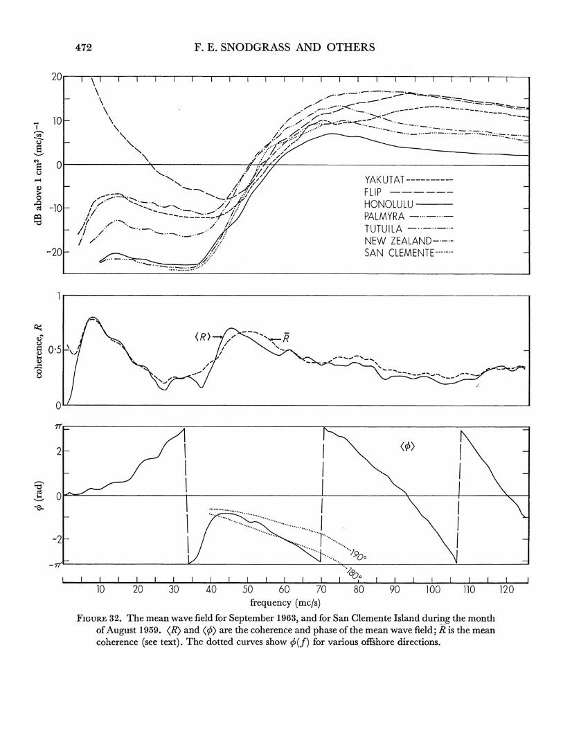
The upper display of figure 32 shows the mean wave spectra during September 1963 (while Flip was on station). For comparison we have included the mean wave spectrum measured at San Clemente Island, California, during August 1959 (Munk et al. I963). The mean spectra are closely bunched near 50 mc/s, where the scatter is presumably the result of differential shadowing. Below 45 mc/s Flip measuremnents are not significant (? 3 (b)); the other stations exhibit flat spectra roughly proportional to their peak energies. This is the 'surfbeat'phenomenon due to non-linear interaction of neighbouring frequencies (? 8 (e)).
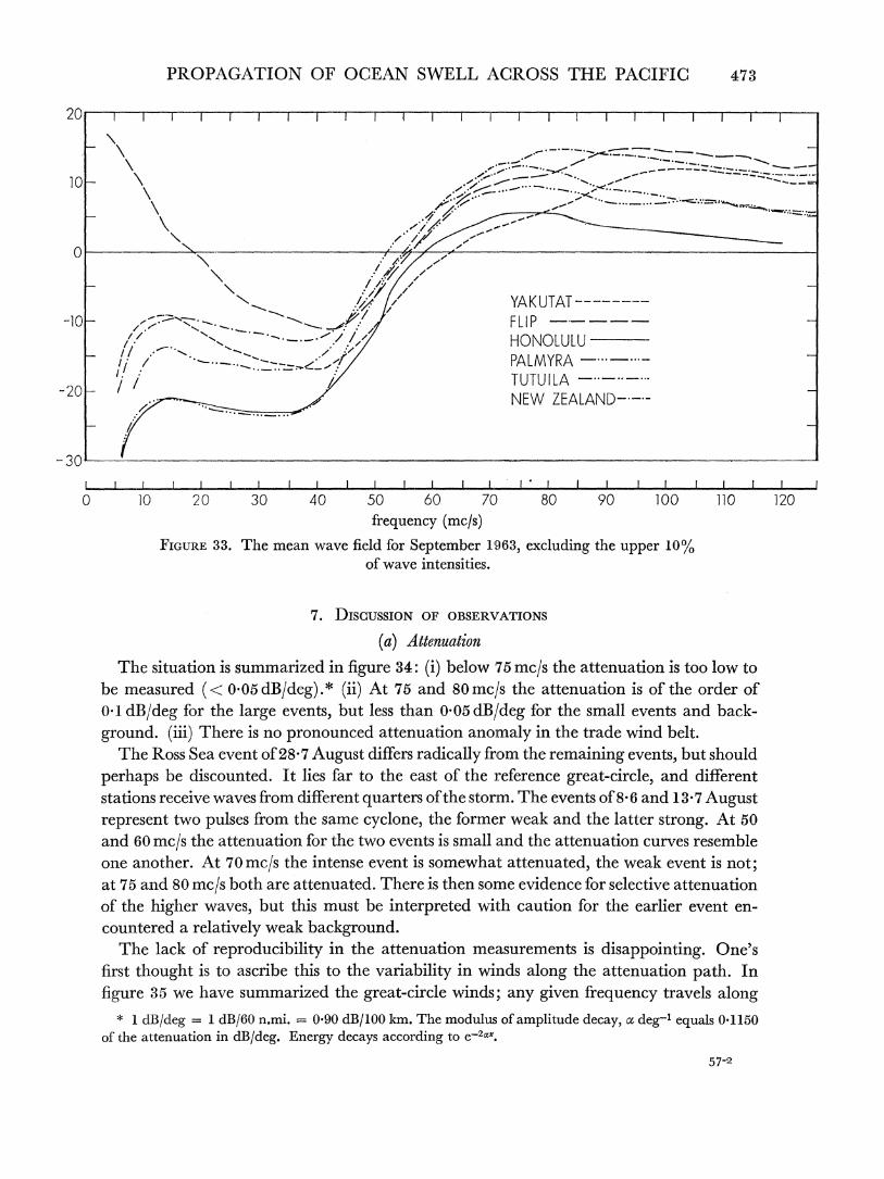
We attribute the rise above 75 mc/s at Yakutat and Flip to local high winds. An attempt to suppress the effects of local storms and of the most energetic events has been made by removing from the average for each station and for each frequency band the most intense 10 0 of the cases (figure 33).
The lower displays in figure 32 give certain means of coherence and phase. Let Cij(f), Qij(f), and R(f) designate as usual the cross spectra and coherence measured twice daily at Honolulu. Vj(f), Qij(f), R(f) are the September averages of these functions, whereas <R(f)> and <0(f)> are computed from 0(.f), Qij(f) according to (3.3).
The distinction between R and <R> can be illustrated as follows. Suppose the wave field at any given time is contained in a single pencil bearn (R - 1), but at different times the beam is from different directions. Then R % 1, whereas <R> is smaller because it measures the width of the smeared pencil beams. On the other hand, if the typical background at any given time comes from a broad beam, then R, R and <R> will all be relatively small. The second alternative fits better. We conclude that the background radiation subtends a wide angle.
For a very rough estimate we consider a uniform (and not too wide) beam between 00 relative to the instrument normal. For a straight beach and straight parallel contours k sin 8 is independent ofdepth and equals ko sin 00, whereko = 2img If' is the deep water wave- number, and 80 the offshore direction. Replace sin 8 by 8. According to (3 5 b)
R 1-_ t -302D2k202 1-7- ,Ug2D202p4
so that R diminishes with increasingf, as observed. AtJf = 45 mc/s we find R = 0 7, and this yields a subtended angle 2O= 44?. At higher frequencies the computed coherence diminishes at a rate higher than the observed rate, thus indicating an even broader beam width.
Similar results are found from Flip accelerometer records.* The coherences associated with the principal events can be as high as 0 90; similar values are found for local seas above 100 inc/s. The background radiation is associated with coherences of less than 0-25, too low to be significant, and comes from a southerly quarter.
In sumnmary, the evidence points towards generation of the wave background by high winds along the entire storm belt of the South Pacific.
* We are inldebted to Dr P. Rudnick for the analyses of these records.
57 ~~~~~~~~~~~~~~~~~~VOL. 259. A.
472 F. E. SNODGRASS AND OTHERS
20
1. -
0
i~ -10 - ,, L .X- X~' F PLMYRPA- YTUTULAT
j z - /.': ~~~~~~NEW ZEALAND--- -20 _ .// ~~~~~~~SAN CLEMENTE.
0
10
~~~~~~~~~~0-~ ~ ~~~~~~~~~~~AMR - --p---
? I I I I C X\ Ii\
21 ~ ~~~~~~~~~~~~~~~~~~~~~~~~~~~~~~~~~~~~~~~~~~~~~~~~~~~~~~~ II<>rzo \\I
10 20 30 40 50 60 70 80 90 100 110 120 frequency (mc/s)
FIGURE 32. The mean wave field for September 1963, and for San Clemente Island during the month of August 1959. KR> and (q0> are the coherence and phase of the mean wave field; R is the mean coherence (see text). The dotted curves show 0b(f) for various offshore directions.
PROPAGATION OF OCEAN SWELL ACROSS THE PACIFIC 473
2 0 1 I I I I I I I I I I I I I
\0 I
YAKUTAT- - -10 ,-fs---. FLIP
HONOLULU PALMYRA
-20L i Y TUTUILA NEW ZEALAND----
-30 ,,, I , , I , 1 , . I, L ,1 I I , 1,_ ,1, L....1..,..1,JI.t........ 1 , , 1,, 1, . I I I I I
0 10 20 30 40 50 60 70 80 90 100 110 120 frequency (mc/s)
FIGURE 33. The mean wave field for September 1963, excluding the upper 10% of wave intensities.
7. DisCUSSION OF OBSERVATIONS
(a) Attenuation
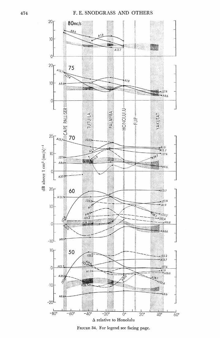
The situation is summarized in figure 34: (i) below '75 mc/s the attenuation is too low to be measured (< 0o05 dB/deg) . * (ii) At 75 and 80 mc/s the attenuation is of the order of 0 1 dB/deg for the large events, but less than 0 05 dB/deg for the small events and back- ground. (iii) There is no pronounced attenuation anomaly in the trade wind belt.
The Ross Sea event of 28.7 August differs radically from the remaining events, but should perhaps be discounted. It lies far to the east of the reference great-circle, and different stations receive waves from different quarters of the storm. The events of 8 6 and 13 7 August represent two pulses from the same cyclone, the former weak and the latter strong. At 50 and 60 mc/s the attenuation for the two events is small and the attenuation curves resemble one another. At 70 mc/s the intense event is somewhat attenuated, the weak event is not; at 75 and 80 mc/s both are attenuated. There is then some evidence for selective attenuation of the higher waves, but this must be interpreted with caution for the earlier event en- countered a relatively weak background.
The lack of reproducibility in the attenuation measurements is disappointing. One's first thought is to ascribe this to the variability in winds along the attenuation path. In figure 35 we have summarized the great-circle winds; any given frequency travels along
* 1 dB/deg = 1 dB/60 n.mi. = 0 90 dB/100 km. The modulus of amplitude decay, aG deg1 equals 0.1150 of the attenuation in dB/deg. Energy decays according to e~2ax.
57-2
474
- _-. I- .- 1 20 I. --
II---., w_-_1 . '.1-11".. _ 111- --. - - -
. . ;.....'- .. - A - 11. .-.1.111-.- -.1. ..... . ... ._ _- - .. ..... w o, ..... . - , - .. - 1- -1 -_--l- I ..... Z__4-? -...... __ ... ... ..-.= -l..--,.:,:- 1-1- _ ,. ...... :;... ::: ... .il- . "
, ,
, 7 W. .-. .... - 07-----4_4L I _ - .. . 11 ..., ................. _. - ... -_% ..,.. - .1 .1 . - - . - ,. .%,..-.- ._ . l I.... q- - . .. p.... - 1"...... _ ,._ I I_ . .... -- - - 1 .11 11 1-1. . I - , -.1. __ - 10 - - _- --.1 - _. ,-1 " , I- 1. ., -
",.-,., I - .- I ... I 1: 1. ', . I , .., - - _111114 ; . I , .' 11 .11.. - 1- ,I .. 1-
, .- I ,- - .- . - . 1: 11- . - -.1- ,..-_- . - , I .. ' ' . . .
w - 1; , _- .._.-.- -'l,._%, .. ". .... q ; , , - , ,
p-.1 =-:11- 1 p ..... - . ". - 1I
.. I 14 - .I 1% .L 1.1b :... .,-.-. .1 _. - p., ::..
- . . . I I I I - I.-
%W_11-11.. l -- - -_ ,_- -- I-
1:14,111".'.... . 11: -%-. - ... , , ,%. --- .. -- l"... 2 0 %...... ... q.- ,I ...- - I.. - - ... -. -, W- ....,-. .... .. . ._ ..."... -_ . ..- _.- '_-.- ,., :. ... .. . --l.. 7 5 ----11- I. .11 . 1% ... -- i-I..... -!.. 1 . I . ... - 73 -- ".." I - . ,Il I _ . 11 - ".. .1 -,...... _% _.! ,11. 1. 1- -- - _- `- - - ,_ .
-__....:__._. .1 ....
...
!*
11, - - I - I..", -1 11- . , - I I - ... . - - , . .. _%. ... - . I., I.I, - - ;;_ __. .
-11 - N.'. 1-1 1".. I I I , I... I. 4.. : 1- 1 I .'.'. '. . , I. I - ...
10
- A8--:_.--.i I :-.1 , l ...... .....".,.""'',ll,",...',.lI `w
--.... .. . 1. ---- ,:,. I -
- ,, I ____l , I
I % _ 11 I II.
- 11.1 1 I I,-1, . -p; I j - 1111 - -1-11%.. 1_. . ..... .. - --, .... W ..... .11--d.. , --l".- .1 ; %%,
__ ._.-. .-..-.
N _ W., . q - %_.-_ I'--- I , 1% 11 ...... .. 1.111, .....
- 1. .. - - .. .:,: I- I...... :- 7.l ,10- 1 .
,.. - " -- ....::........ , : --....... .-..- :c - ... I :- % .... I ..... -. . - ..I.. '.'.'. '-.- .. ..."%,:...-......,.... . .... ..... ....., I
; .1 -.... . - - 1 - ,. - -. - . - I.. ... -_%%%_.%...:_ , %_ _- r'le, I .',, ,I - . .. ,_ -, .--.--- -. - ol II.. -..... I.... -11. -<.... I : ..,--- ...., '.-.l _ - 4- , ....... ".1-11,".. ...., __ .. 2:.,. %. "...., v..,..,.:, -.%.. ...... .1. . - :1. ;"..l. %': _... I ,., ... - --- - " (./')
-1 -- ZD :.,...% . -.11 ... .- __j ,-:- 1. _.. -1. ... ...
-_ :. -q. q. .. , ___j .1.
__j 1W."I'll.-W ... 1. .... I%% C L _ l .- 1. - .
`
-1-111 ." --N-.. _5.,, < ,- N,-L_ .-_-. .....I ....i -, - I ...-.% .-.-% .. .- z - - ...... ..-I. , . I-1 F = )` -,.. ,... S."., t... , --. t: "..... _ . LU .. - n ---- ____-l-%_, %- ... ,..:,__l- ,., ._ _ ,._ .. ................ .:, ...... -1- .. -_-- - ... . .... -.- ---1-1-1- 11 m ,". .,qw " , - _Y... %.- ..' --.11111.-- _ .... ., .. . -I .1 -, .;,;. .. ..,..,.,. "...'" ....:, .,.,. .... 1. ' '.. _ ., . ...
< '_:,--_- .... -_ -- .. I .,..% ` ..",..........,.%-2::",.":.,.,.,.- .,_-,-_-_ l ... ..... .. ......- : ,-- , -1-1.1'.."ll- , ... .: ... %_.. . ...,___.,_..,. :_ .% . ... ... O. " . . ..... "I - .... .-.1-- ... ..% .. ..... - - . ........ --,., - _ .I .- ...-..... u o.,:.. I ...p.. %- ... .. ... _ -.1--l... " .- ... 1: ... %:.-__ .... _ _ ". - , . , - - 20 -_. ,.11-1-.. :... . i .- -111. 0,,., - _ ,"', -.-. `- ... __ _ -- .
.. I- ...I 11- 1.1 ... 7.3. - ':'I' 7 0 I -1
" ...- 2..
__ ... q.-.- .,
,, .......
-4 `__. - -11-11.1 ..... I ,_-.1--A ,, __- . .. ... ,__.., 1-11 q._-_ .." I'l ... cn .... =%. :Fll-:.i --- .... 10 v_-..I.. 11.11, *-__ lb
1.
' - I ''.." - :- . - - - I ,... . 11-1 I .,---Ii - b -, ,..., '..__.- . _.__', . ''Ill'. 1,4 '... J2
I ,....... . - " ..... '* u , _ - m m z -,"'.-I...
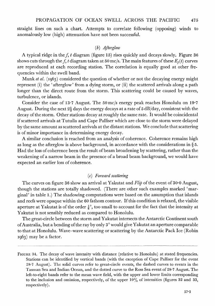
PROPAGATION OF OCEAN SWELL ACROSS THE PACIFIC 475
straight lines on such a chart. Attempts to correlate following (opposing) winds to anomalously low (high) attenuation have not been successful.
(b) Afterglow
A typical ridge in thef, t diagram (figure 15) rises quickly and decays slowly. Figure 36 shows cuts through the f, t diagram taken at 50 mc/s. T'he main features of these Ef (t) curves are reproduced at each recording station. The correlation is equally good at other fre- quencies within the swell band.
Munk et al. (I963) considered the question of whether or not the decaying energy might represent (i) the 'afterglow' from a dying storm, or (ii) the scattered arrivals along a path longer than the direct route from the storm. This scattering could be caused by waves, turbulence, or islands.
Consider the case of 13-7 August. The 50mc/s energy peak reaches Honolulu on 19-7 August. During the next 2-2 days the energy decays at a rate of 5 dB/day, consistent with the decay of the storm. Other stations decay at roughly the same rate. It would be coincidental if scattered arrivals at Tutuila and Cape Palliser which are close to the storm were delayed by the same amount as scattered arrivals at the distant stations. We conclude that scattering is of minor importance in determining energy decay.
A similar conclusion is reached from an analysis of coherence. Coherence remains high as long as the afterglow is above background, in accordance with the considerations in ? 5. Had the loss of coherence been the result of beam broadening by scattering, rather than the weakening of a narrow beam in the presence of a broad beam background, we would have expected an earlier loss of coherence.
(c) Forward scattering
The curves on figure 36 show an arrival at Yakutat and Flip of the event of 30 0 August, though the stations are totally shadowed. (There are other such examples marked 'mar- ginal' in table 1.) The shadowing computations were based on the assumption that islands and reefs were opaque within the 60 fathom contour. If this condition is relaxed, the visible aperture at Yakutat is of the order w?, too small to account for the fact that the intensity at Yakutat is not sensibly reduced as compared to Honolulu.
The great-circle between the storm and Yakutat intersects the Antarctic Continent south of Australia, but a bending of the ray by only 30 would give Yakutat an aperture comparable to that at Honolulu. Wave-wave scattering or scattering by the Antarctic Pack Ice (Robin I963) may be a factor.
FIGURE 34. The decay of wave intensity with distance (relative to Honolulu) at stated frequencies. Stations can be identified by vertical bands (with the exception of Cape Palliser for the event 28.7 August). The solid curves refer to great-circle events, the dashed curves to events in the Tasman Sea and Indian Ocean, and the dotted curve to the Ross Sea event of 28*7 August. The left-to-right bands refer to the mean wave field, with the upper anld lower limits corresponding to the inclusion and omission, respectively, of the upper 10%/ of intensities (figures 32 and 33, respectively).
57-3
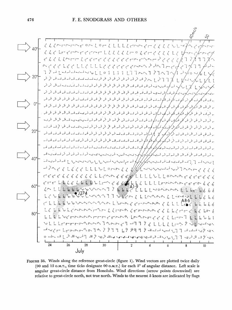
476 F. E. SNODGRASS AND OTHERS
_~~~~~~~~~~~~~
4>/, Ft-r-r~'>? 0 L 0 L L L P~<'rW V
- i -, . . .
ts dd d d <L Ld L L L< <<>sm9)X -4<l( S X ol 1 2 L JlS~/<L L? 1 0 L1 A1 2 u1_ >o/
/ 20 r > > > > > > ) 2 L 2 /L L/<>L L
200
~ LL~LLLrA\ L LJ L
600 -9 L~
L( VL .)-V1slJ )1 S) LLrL)A JA 1 /7iSLL1 /L4U
> 2 >4 S 26 > >> S>S>/28a> 30`2 47 8
L L L/ s F- torJ /11Jr /01 /0Xjt - JSs |~~~~~~~~~~~~~~L L 2z d<L- <L?r34 4wL StA tr-<d i
July~~~~~~~~~~~~~~~~~~~Lv
60 L /r- f? A g L-/7 -t 3t
FIUE 5 Wid aLon \wtherfrneget-crl (fgr 1) Win vectors ar pLotted twice dail
0- < nTW-"'+- v~/^ '4LLL>0kLt
(00nd G.M L ticks di ter 00 G T frr ec 50 f an L ft L is angu L g -L drstnef Honoulu Win dei (arrow point d o i are relativeto great-cirl nort t te north s t ne a L Lk L Lrt b fas
| S wdrr L o -, =1 qb jY -Y es JS> 1nSS
24 26 28 30 2 4 6 8 10 July
FTIGUlD.RE 5. Wincds alonng tlhe reference great-circle (fimire 1). Windi vectors- are plottedc twire tlailv
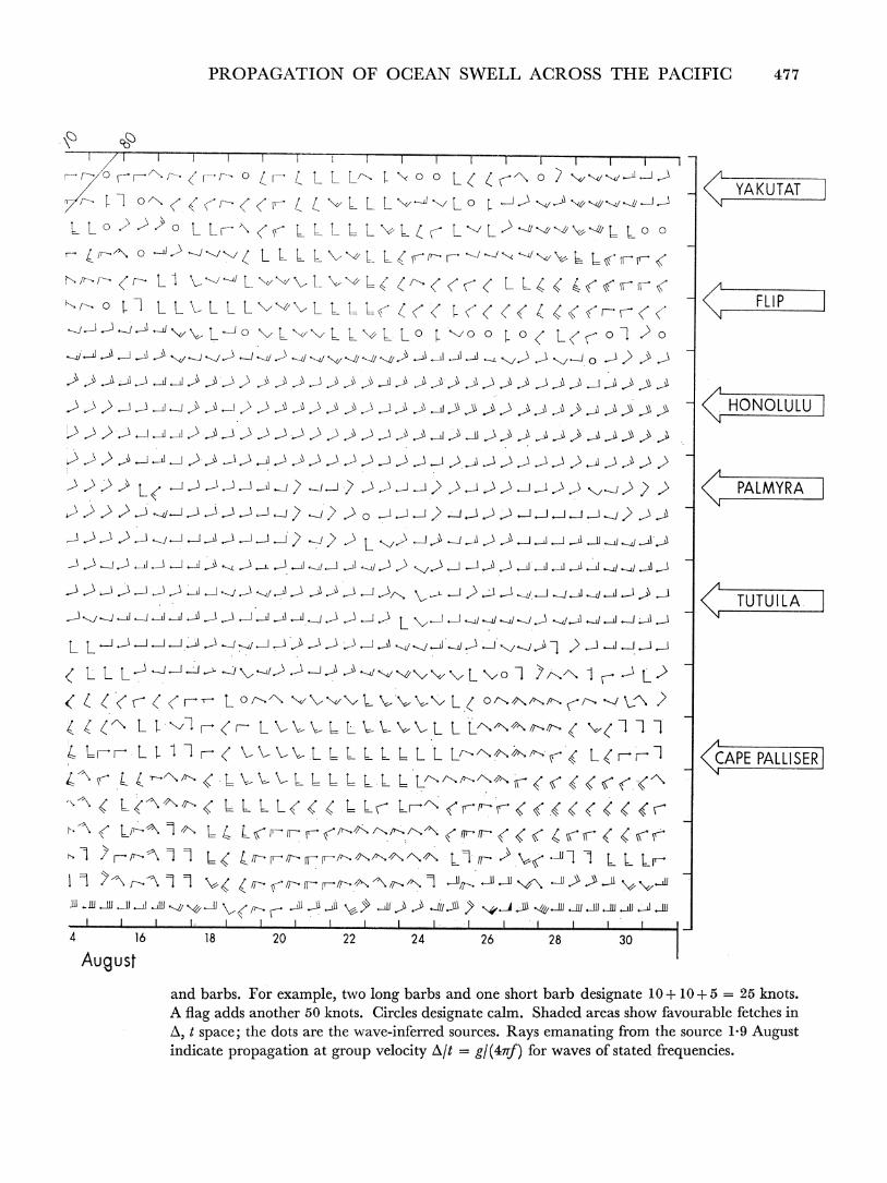
PROPAGATION OF OCEAN SWELL ACROSS THE PACIFIC 477
I I I I ~ ~ ~~~~~~~~~~I I I I
LLOT >>?>LLv-< LL 0LLLVLtLL>"94@4V -LO r 0 t/ U ? >v< L L L LWW-L Ld'+''V9 L6r,r->
KftzOt71LL LLL>ss< LL< <<'<< <>d L L t<nfrzd FP L < o7'1 L L L L< LVVL L VV<L FLIP
L. L wL-L > ? L ?L L L L <L L ?? N |
I I I I I I I I I I I I o
4 16 18 'S 20 22 ) 242*)S> 2 26 28 30MYA
SS S'n-i>lS 2 So JS>2S>>S>S__t -j -
g 9Aj --J- --j -j -Sj 2 L w >l*
)
'9/SS )>L)' LS J>SS <S4St>S) 2<: T~UTUILA
'L L SJ-S/s )A S lSv JS |
L L L4 >'')A's9w < /m1r>L
d d d d d < r
L 0' \/wt L'<\Ld?soN<oXt 4 X dt L Lord L L1 Lt >WL L L/"-- d 411 Lr-r- -L L : dLLL L- L -L L- L L L L/-- rf- L rr- 2<C PALLISER| r\f t/ L 4 L L L- L L -L L- L/---, ^ X<f< t0 < L LX> L L Ld L L r Lr--- <r<
st<L< L L fp- a -S<,cXNX <<<4f r<<f
O1 ;>r
r~~~~t. 1 t 4,nrrAm t -A A A -lu 11t. M
4 1 6 1 8 2 0 2 2 2 4 2 6 2 8 3 0
August
and barbs. For example, two long barbs and one short barb designate 10 +10 + =-25 knots. A flag adds another 50 knots. Circles designate calm. Shaded areas show favourable fetches in AS, t space; the dots are the wave-inferred sources. Rays emanating from the source 1 9 August indicate propagation at group velocity A/t = g/(4lTf) for waves of stated frequencies.
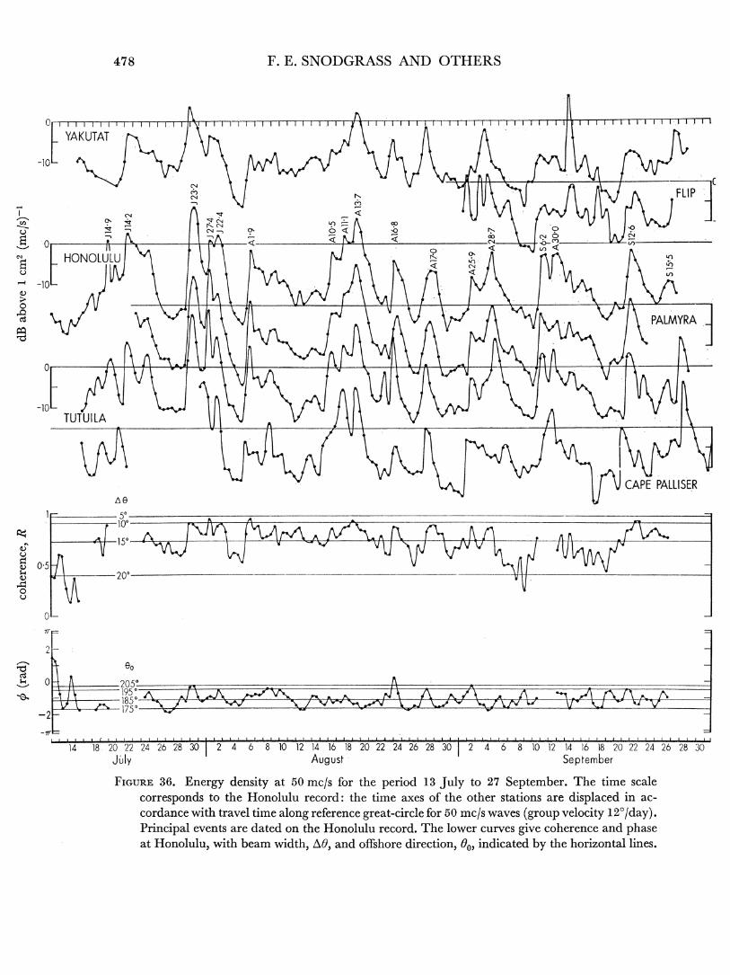
478 F. E. SNODGRASS AND OTHERS
A~~~~~~~~~~~~~~~~~~~~~~~~~~~
01 1 1 1 1 1 I t. I I I I I I I 1 1 1 1 - I I I I I I I I I I I I I I I I I I I I I I I I I I I I ' I I I I I I I ! I I I I I 'I I I I I
co~~~~~~ F L'IP
4f 64 00~~~~~~~~~~~~~~~~~~~0 (O(
CN 0.~~~~~~~
-~~~~~~~~~~~~~~~~~~~~~~~~~~~~~~~~~~~~~0 ;- 1
,<~~~~~~~~~~~~~~~~~~~~~~~~~~~~~~~~~~~ < 2
HONOLULU R 9
0
o~~~~~~~~~~~~~~~~~~~~~~~~~~~~~~~~~~~~~~~~~~~~~~~~~~~ Itt
Cd '~~~~~~~~~~~~~~~~~~~~~~~PALMYRA
AG
0
-0L
0~~~~~~~5 0~~~~1
2FL 2
0 205-0 I I19.So w E _ A\1950
-2 _ 1750
-IT~~~~~~~~~~~~~~~~~~~~~~~~~~~~~~~~~~~~~~~~~- l t ~ ~ ~ ~ ~ 1- - t I I I I.-A A I I .. - -4 t I I I t t I t I t I I 1-- I I I I t t t I I I I I I t
14 18 20 22 24 26 28 301 2 4 6 8 10 12 14 16 18 20 22 24 26 28 30' 2 4 6 8 10 12 14 16 18 20 22 24 26 28 30 July August September
FIGURE 36. Energy density at 50 mc/s for the period 13 July to 27 September. The time scale corresponds to the Honolulu record: the time axes of the other stations are displaced in ac- cordance with travel time along reference great-circle for 50 inc/s waves (group velocity 1 20/day) . Principal events are dated on the Honolulu record. The lower curves give coherence and phase at Honolulu, with beam width, AO, and offshore direction, G0, indicated by the horizontal lines.
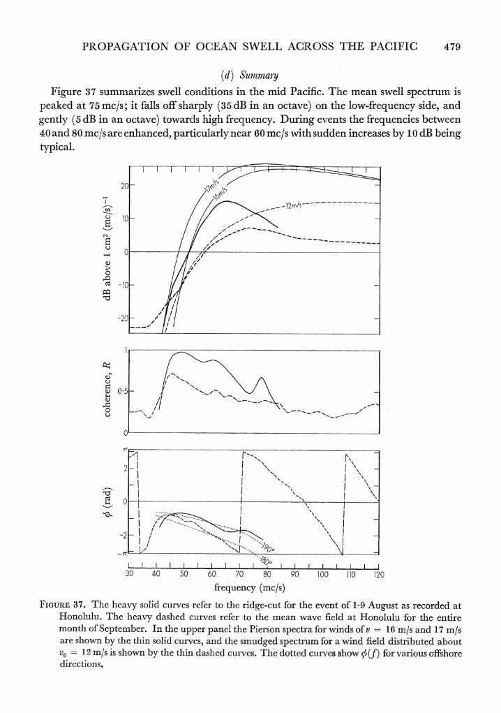
PROPAGATION OF OCEAN SWELL ACROSS THE PACIFIC 479
(d) Summary
Figure 37 summarizes swell conditions in the mid Pacific. The mean swell spectrum is peaked at 75 mc/s; it falls off sharply (35 dB in an octave) on the low-frequency side, and gently (5 dB in an octave) towards high frequency. During events the frequencies between 40 and 80 mc/s are enhanced, particularly near 60 mc/s with sudden increases by 1 0 dB being typical.
20
10 - ~ ~ ~ ~ ~ ~ ,--
M e _ _ _ _ _
- C-- "I,.<-o
1_1
o ~ ~_ II- gI
/10
320 ,' 50 6 0 8 0 0 1 2
2-1
21 1
-2 -
30 40 50 60 /0 80 90 100 110 120
frequency (mc/s)
FIGURE 37. The heavy solid curves refer to the ridge-cut for the event of 1-9 August as recorded at Honolulu. The heavy dashed curves refer to the mean wave field at Honolulu for the entire month of September. In the upper panel the Pierson spectra for winds of v-16 rn/s and 17 rn/s are shown by the thin solid curves, and the smudged spectrum for a wind field distributed about
vO= 1.2 rn/s is shown by the thin dash.ed curves. The dotted curves show 56(f) for various offshore directions.
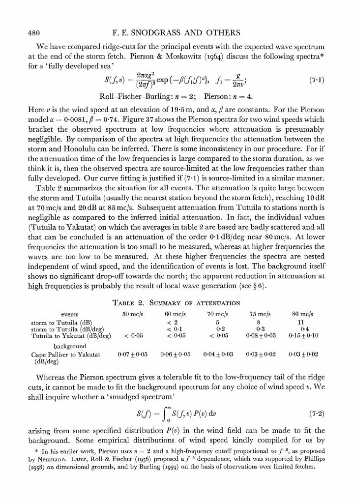
480 F. E. SNODGRASS AND OTHERS
We have compared ridge-cuts for the principal events with the expected wave spectrum at the end of the storm fetch. Pierson & Moskowitz (i964) discuss the following spectra* for a 'fully developed sea'
2rnx og2g(71 S(f, v) (2f5exp{ (fi/f)} 2gv (7.1)
Roll-Fischer-Burling: n = 2; Pierson: n 4.
Here v is the wind speed at an elevation of 19 5 m, and a, fi are constants. For the Pierson model a --- 0'0081, fi- 074. Figure 37 shows the Pierson spectra for two wind speeds which bracket the observed spectrum at low frequencies where attenuation is presumably negligible. By comparison of the spectra at high frequencies the attenuation between the storm and Honolulu can be inferred. There is some inconsistency in our procedure. For if the attenuation time of the low frequencies is large compared to the storm duration, as we think it is, then the observed spectra are source-limited at the low frequencies rather than fully developed. Our curve fitting is justified if (7-1) is source-limited in a similar manner.
Table 2 summarizes the situation for all events. The attenuation is quite large between the storm and Tutuila (usually the nearest station beyond the storm fetch), reaching 10 dB at 70 mc/s and 20 dB at 85 mc/s. Subsequent attenuation from Tutuila to stations north is negligible as compared to the inferred initial attenuation. In fact, the individual values (Tutuila to Yakutat) on which the averages in table 2 are based are badly scattered and all that can be concluded is an attenuation of the order 0-1 dB/deg near 80 mc/s. At lower frequencies the attenuation is too small to be measured, whereas at higher frequencies the waves are too low to be measured. At these higher frequencies the spectra are nested independent of wind speed, and the identification of events is lost. The background itself shows no significant drop-off towards the north; the apparent reduction in attenuation at high frequencies is probably the result of local wave generation (see ? 6).
TABLE 2. SUMMARY OF ATTENUATION
events 50 mc/s 60 mc/s 70 mc/s 75 mc/s 80 mics storm to Tutuila (dB) < 2 5 8 11 storm to Tutuila (dB/deg) < 041 0.2 03 0 4 Tutuila to Yakutat (dB/deg) < 0 05 < 0 05 < 0 05 0 08 + 0 05 0.15 + 0.10
background Cape Palliser to Yakutat 0'07 + 0'05 0.06 + 0 05 0 04 + 0'03 0 03 + 0.02 0^03 + 0.02
(dB/deg)
Whereas the Pierson spectrum gives a tolerable fit to the low-frequency tail of the ridge cuts, it cannot be made to fit the background spectrum for any choice of wind speed v. We shall inquire whether a 'smudged spectrum'
S(f) f S(f,v) P(v) dv (7.2)
arising from some specified distribution P(v) in the wind field can be made to fit the background. Some empirical distributions of wind speed kindly compiled for us by
* In his earlier work, Pierson uses n = 2 and a high-frequency cutoff proportional to f-6, as proposed by Neumann. Later, Roll & Fischer (I956) proposed a f- dependence, which was supported by Phillips (I958) on dimensional grounds, and by Burling (I959) on the basis of observations over limited fetches.
PROPAGATION OF OCEAN SWELL ACROSS THE PACIFIC 481
Col. A. R. Gordon,Jr ofthe U.S. Naval Oceanographic Office suggest distribution of the type v e-vm with peak probability between 5 and 10 m/s. The Rayleigh distribution, m = 1, does not discriminate sufficiently against high wind speeds. We chose m = 4, because it leads to a simple integration P(v) = 47T-i v 2v exp {- (v/vO)4} (7.3)
which is peaked at v = 2-v0 and has a mean wind speed 2-4vo. Substituting in (7.2) and carrying out the integration leads to
(2fr)exp{ 2flI (folf) 2}' fo = (7.4)
which turns out to be a Roll-Fischer-Burling distribution. Raw and smudged spectra are nested against the samef-5 curve (the Phillips 'saturation' function) at high frequencies. The low-frequency cutoff has been softened in the smuidged spectrum, from exp (-f-4) to exp (f-2), and the background can be tolerably fittedi by a choice v0 12 m/s. The wind distribution is then peaked at 2-1 12 = 8-5 rnms, which is a reasonable value.
The conclusion is that the background spectrum is t:he result of global high winds in the storm belt of the South Pacific (the 'roaring forties' and 'fighting fifties'). The drop in the observed background spectrum with respect to 3(f) at frequencies exceeding 70 mc/s is attributed to attenuation immediately after the waves leave the storm belt. The model is consistent with the lower coherence and a mean direction from further left (as seen at Honolulu) of the background as compared to most individual events.
The disappearance of individual events into the background at frequencies above 80 mc/s may be interpreted as follows: lower frequencies are the result of severe storms which occur intermittently at intervals large as compared to the storm duration, and thus have a pro- nounced effect on the spectral densities. The higher frequencies are maintained at steady levels and are the result of moderate storms which occur at frequent intervals, and perhaps simultaneously at a number of locations.
8. WAVE-WAVE INTERACTIONS
The fact that most of the swell energy is lost immediately beyond the generating area suggests that the dissipation is primarily non-linear. Within the generating area itself the growth of the spectrum is ultimately limited by the non-linear processes of wave breaking (Phillips I958) and wave-wave scattering (Phillips I96o; Hasselmann I960, I962, I963 a, b). These processes continue to be effective immediately after the generation has ceased, but rapidly become weak as the energy of the waves is reduced. It is possible to give some quantitative assessment of the role of wave-wave scattering in our propagation study. The effects of wave breaking can be discussed only in qualitative terms.
(a) Interaction rules
The energy transfer due to non-linear interactions between random wave fields may conveniently be interpreted as collision processes between waves and 'antiwaves', (or particles and ' antiparticles ') . Each wave train w is anaLlogous to a particle whose energy is proportional to the wave frequency co, and whose momzentum is proportional to the wave number k. Antiwaves w have negative energy (ca. -) and negative momentum (ca. -k),
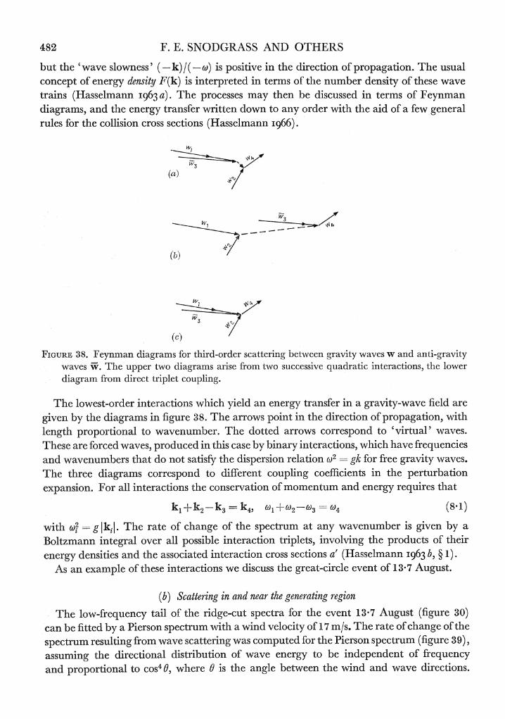
482 F. E. SNODGRASS AND OTHERS
but the 'wave slowness' (- k) / ( - o) is positive in the direction of propagation. The usual concept of energy density F(k) is interpreted in terms of the number density of these wave trains (Hasselmann I963 a). The processes may then be discussed in terms of Feynman diagrams, and the energy transfer written down to any order with the aid of a few general rules for the collision cross sections (Hasselmann I966).
w
(a) /
FIGURE 38. Feynman diagrams for third-order scattering between gravity waves w and anti-gravity waves W. The upper two diagrams arise from two successive quadratic interactions, the lower diagram from direct triplet coupling.
The lowest-order interactions which yield an en ergyv transfer 'in a gravity-wave field are
given by the diagrams in figure 38. The arrows point in the direction of propagation, with
length -proportional to wavenumber. The dotted arrows correspond to 'virtual' waves.
These are forced waves, produced in this case by binary interactions, which have frequencies and wavenumbers that do not satisfy the d'ispersion relation o)2 gk for free gravity waves. The three diagrams correspond to different coupling coefficients in the perturbation expansion. For all interactions the conservation of momentum and energy requires that
kl+k -k3= k ()+4(8.1)
2 3 if +)203 _6
with 38.g IFki. The rate of change of the spectrum at any wavenumber is given by a
Boltzmann integral over all possible interaction triplets, involving the products of their
energy densities and the associated interaction cross sections a' (Hasselmann 1963 b, ? 1). As an example of these interactions we discuss the great-circle event of 13f7 August.
(b) Scattering in and near the generating region
can be I Itted by e aerseon spectrum wit a wn veloiAty of 17 in/s. The rate of chnen of t spectrum ~ ~~(b rsligfowaeScattering wnasd computhed fonratheg Piersonspcrm(iue3)
assuming the directional distribution of wave energy to be independent of frequency and proportional to cos4 0, where 0 is the angle between the wind and wave directions.
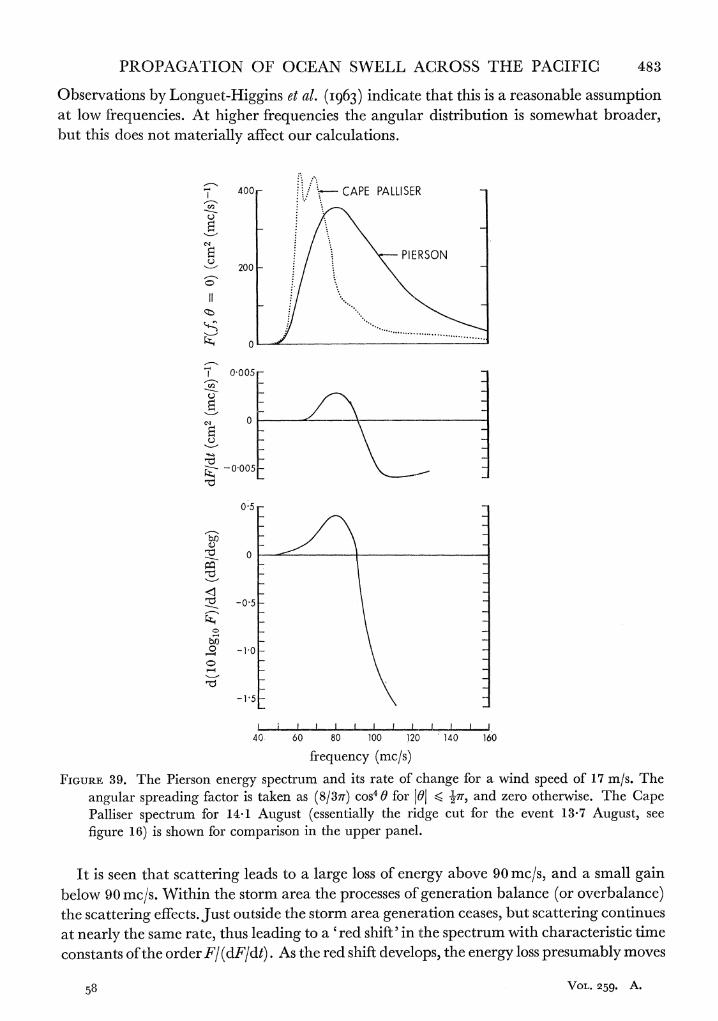
PROPAGATION OF OCEAN SWELL ACROSS THE PACIFIC 483
Observations by Longuet-Higgins et al. (I963) indicaltle that this is a reasonable assumption at low frequencies. At higher frequencies the angular distribution is somewhat broader, but this does not materially affect our calculations.
-7 400 ' .CAPE PALLISER
PIERSON ,- 200
1 0005
0
- 0 005
0 5
O - 5 0
bD 0 -1P0
-15 -
40 60 80 100 120 140 160
frequency (mc/s)
FIGURE 39. The Pierson energy spectrum and its rate of change for a wind speed of 17 m/s. The angular spreading factor is taken as (8137T) cos4 0 for 0J < 27, and zero otherwise. The Cape Palliser spectrum for 14 1 August (essentially the ridge cut for the event 13-7 August, see figure 16) is shown for comparison in the upper panel.
It is seen that scattering leads to a large loss of energy above 90 mc/s, and a small gain below 90 me/s. Within the storm area the processes of generation balance (or overbalance) the scattering effects. Just outside the storm area generation ceases, but scattering continues at nearly the same rate, thus leading to a ' red shift ' in the spectrum with characteristic time constants of the order F/ (dF/dt) . As the red shift develops, the energy loss presumably moves
58 VOL. 259. A.
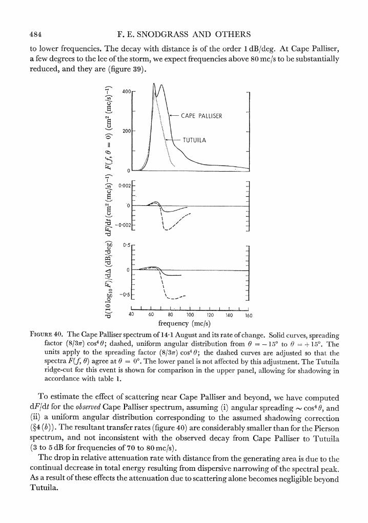
484 F. E. SNODGRASS AND OTHERS
to lower frequencies. The decay with distance is of the order 1 dB/deg. At Cape Palliser, a few degrees to the lee of the storm, we expect frequencies above 80 mc/s to be substantially reduced, and they are (figure 39).
400
CAPE PALLISER
200-
TUTU ILA
0
0 002F
F_____ ____.
ci 0- <i o
F I 0
6f) -0-5-1 0~~~~~~~~~~~~~~~~6
40tr(/ar o40 dased unior angla ditrbuio from
10
-5 o0+ h FIGURE 40. The Cape Palliser spectrum of 14 1 August and its rate of change. Solid curves, spreading
factor (8/31T) cos4 0; dashed, uniform angular distribution from 0 = - 150 to 0 -= + 150. The units apply to the spreading factor (8/3ir) cos4 0; the dashed curves are adjusted so that the spectra F(f, 0) agree at 0 00. The lower panel is not affected by this adjustment. The lutuila ridge-cut for this event is shown for comparison in the upper panel, allowing for shadowing in accordance with table 1.
To estimate the effect of scattering near Cape Palliser and beyond, we have computed dF/dt for the observed Cape Palliser spectrum, assuming (i) angular spreading_ cos4 0, and (ii) a uniform angular distribution corresponding to the assumed shadowing correction (?4 (b)). The resultant transfer rates (figure 40) are considerably smaller than for the Pierson spectrum, and not inconsistent with the observed decay from Cape Palliser to Tutuila (3 to 5 dB for frequencies of 70 to 80 mc/s).
The drop in relative attenuation rate with distance from the generating area is due to the continual decrease in total energy resulting from dispersive narrowing of the spectral peak. As a result of these effects the attenuation due to scattering alone becomes negligible beyond Tutuila.
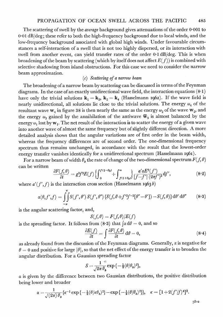
PROPAGATION OF OCEAN SWELL ACROSS THE PACIFIC 485
The scattering of swell by the average background gives attenuations of the order 0'001 to 0.01 dB/deg; these refer to both the high-frequency background due to local winds, and the low-frequency background associated with global high winds. Under favourable circum- stances a self-interaction of a swell that is not too highly dispersed, or its interaction with swell from another event, can yield transfer rates of the order 041 dB/deg. This is when broadening of the beam by scattering (which by itself does not affect E(f)) is combined with selective shadowing from island obstructions. For this case we need to consider the narrow beam approximation.
(c) Scattering of a narrow beam
The broadening of a narrow beam by scattering can be discussed in terms of the Feynman diagrams. In the case of an exactly unidirectional wave field, the interaction equations (8) 1) have only the trivial solutions k, k3, k2 = k4 (Hasselmann i962). If the wave field is nearly unidirectional, all solutions lie close to the trivial solutions. The energy )4 of the resultant wave w4 in figure 38 is then nearly the same as the energy )2 of the wave w2, and the energy w03 gained by the annihilation of the antiwave W3 iS almost balanced by the energy (w, lost by wl. The net result of the interaction is to scatter the energy of a given wave into another wave of almost the same frequency but of slightly different direction. A more detailed analysis shows that the angular variations are of first order in the beam width, whereas the frequency differences are of second order. The one-dimensional frequency spectrum thus remains unchanged, in accordance with the result that the lowest-order energy transfer vanishes identically for a unidirectional spectrum (Hasselmann I96I).
For a narrow beam of width Ob the rate of change of the two-dimensional spectrum F(f, 0) can be written
dF(f~ 0) g33() f(-Ob)? }a'cxE2()(s) aF(A?) =g3y3E(f)
f 'b + df l+) f ftl(7> (8 2) at 0 (1+01') If-fj (2af')5df
where a' (f',f) is the interaction cross section (Hasselmann i963 b)
a (O,f',f) ffS(f', 0') S(f',O0") {S(f, +f'2f-2[0" -0']) -S(f, O)} dO' dO" (8.3) -T
is the angular scattering factor, and, S(f; O) F(f, 0)/E(f)
is the spreading factor. It follows from (8.3) that fa dO = 0, and so
ME(f) _ aF(f ?) dO 0 (8.4) at J at
as already found from the discussion of the Feynman diagrams. Generally, az is negative for 0 = 0 and positive for large I01, so that the net effect of the energy transfer is to broaden the angular distribution. For a Gaussian spreading factor
S - 0 exp { - I(010b) 2},
a is given by the difference between two Gaussian distributions, the positive distribution being lower and broader
a = ,(2 ~) } Kb exp{ 2(0IK0b)2}exp{ _2(O!Ob)2}}, K = [1 +2(f'/f)4]k.
58-2
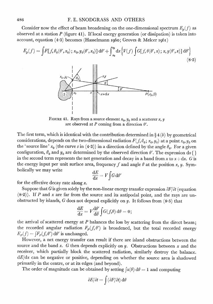
486 F. E. SNODGRASS AND OTHERS
Consider now the effect of beam broadening on the one-dimensional spectrum EXp(f) as observed at a station P (figure 41). If local energy generation (or dissipation) is taken into account, equation (4.3) becomes (Hasselmann I960; Groves & Melcer I96I)
Ep(f) JF[f, 0O(0', xo); xo, yo(0', xo)] dO' + dx { V(f) {G[f, 0(0', x); x, y(O', x)] d0'
(8.5)
Xo,Y0NI Oo
00~~~~~~~~0
Sxp I0x?d,x P(X,,O)
FIGURE 41. Rays from a source element x0, yo and a scatterer x, y are observed at P coming from a direction 0'.
The first term, which is identical with the contribution determined in ? 4 (b) by geometrical considerations, depends on the two-dimensional radiation F(f, So; xo, yo) at a point x0) Yo on the 'source line' x0 (the curve s in (4 3)) in a direction defined by the angle 00. For a given configuration, 00 and yo are determined by the observed direction 0'. The expression dx { } in the second term represents the net generation and decay in a band from x to x + dx. G is the energy input per unit surface area, frequency f and angle 0 at the position x, y. Sym- bolically we may write d
-I -- V [GMd' dx for the effective decay rate along x.
Suppose that G is given solely by the non-linear energy transfer expression dF/dt (equation (8 2)). If P and x are far from the source and its antipodal point, and the rays are un- obstructed by islands, G does not depend explicitly on y. It follows from (8 5) that
dE VdO' G(f,) dO0-?; dx - dO
the arrival of scattered energy at P balances the loss by scattering from the direct beam; the recorded angular radiation Fp(f, 0') is broadened, but the total recorded energy Ep(f) f JFP(f, 0') dO' is unchanged.
However, a net energy transfer can result if there are island obstructions between the source and the band x. G then depends explicitly on y. Obstructions between x and the receiver, which partially block the scattered radiation, similarly destroy the balance. dE/dx can be negative or positive, depending on whether the source area is shadowed primarily in the centre, or at its edges (and beyond).
The order of magnitude can be obtained by setting fJ(0) dO 1 and computing
dEXt= j(dF/dt) dO
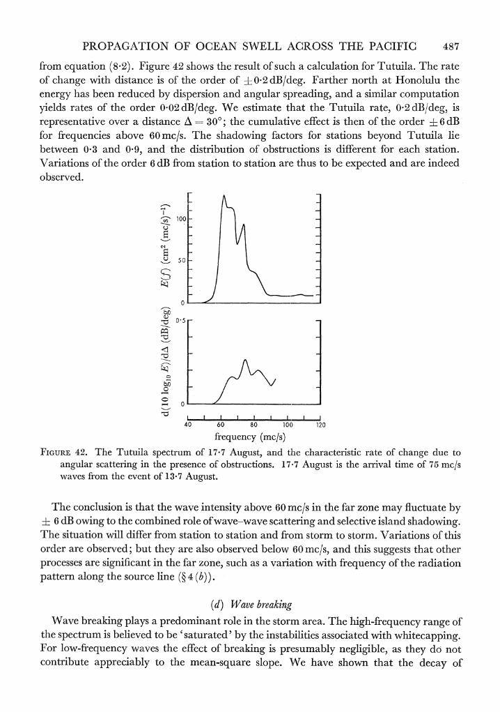
PROPAGATION OF OCEAN SWELL ACROSS THE PACIFIC 487
from equation (8 2). Figure 42 shows the result of such a calculation for Tutuila. The rate of change with distance is of the order of ? 0 2 dB/cleg. Farther north at Honolulu the energy has been reduced by dispersion and angular spreading, and a similar computation yields rates of the order 0-02 dB/deg. We estimate that the Tutuila rate, 02 dB/deg, is representative over a distance A = 30?; the cumulative effect is then of the order { 6 dB for frequencies above 60 mc/s. The shadowing factors for stations beyond Tutuila lie between 0-3 and 0 9, and the distribution of obstructions is different for each station. Variations of the order 6 dB from station to station are thus to be expected and are indeed observed.
9 100 _
50
50
0 -
0
4 05 _
40 60 80 10() 120
frequency (mc/s) FIGURE 42. The Tutuila spectrum of 17-7 Autgust, and the characteristic rate of change due to
angular scattering in the presence of obstructions. 17-7 August is the arrival time of 75 mc/s waves from the event of 13-7 August.
The conclusion is that the wave intensity above 60 mnc/s in the far zone may fluctuate by ? 6 dB owing to the combined role of wave--wave scattering and selective island shadowing. The situation will differ from station to station and from storm to storm. Variations of this order are observed; but they are also observed below 60 mc/s, and this suggests that other processes are significant in the far zone, such as a variation with frequency of the radiation pattern along the source line (? 4 (b)).
(d) Wave breaking Wave breaking plays a predominant role in the storm area. The high-frequency range of
the spectrum is believed to be ' saturated ' by the instabilities associated with whitecapping. For low-frequency waves the effect of breaking is presumably negligible, as they do not contribute appreciably to the mean-square slope. We have shown that the decay of
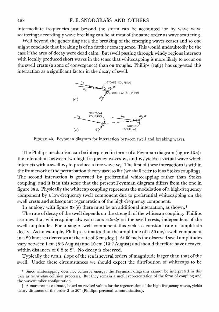
488 F. E. SNODGRASS AND OTHERS
intermediate frequencies just beyond the storm can be accounted for by wave-wave scattering; accordingly wave breaking can be at most of the same order as wave scattering.
Well beyond the generating area the breaking of the emerging waves ceases and so one might conclude that breaking is of no further consequence. This would undoubtedly be the case if the area of decay were dead calm. But swell passing through windy regions interacts with locally produced short waves in the sense that whitecapping is more likely to occur on the swell crests (a zone of convergence) than on troughs. Phillips (I963) has suggested this interaction as a significant factor in the decay of swell.
4__ //STOKES COUPLING
'-WHITECAP COUPLING
(a)
WHITECAP WI COUPLINGS W
_L-9 STOKES)
(b) COUPLING
FIGURE 43. Feynman diagram for interaction between swell and breaking waves.
The Phillips mechanism can be interpreted in terms of a Feynman diagram (figure 43 a): the interaction between two high-frequency waves w1 and W3 yields a virtual wave which interacts with a swell w2 to produce a free wave W4. The first of these interactions is within the framework of the perturbation theory used so far (we shall refer to it as Stokes coupling). The second interaction is governed by preferential whitecapping rather than Stokes coupling, and it is in this sense that the present Feynman diagram differs from the one in figure 38 a. Physically the whitecap coupling represents the modulation of a high-frequency component by a low-frequency swell component due to preferential whitecapping on the swell crests and subsequent regeneration of the high-frequency component.
In analogy with figure 38 (b) there must be an additional interaction, as shown.* The rate of decay of the swell depends on the strength of the whitecap coupling. Phillips
assumes that whitecapping always occurs entirely on the swell crests, independent of the swell amplitude. For a single swell component this yields a constant rate of amplitude decay. As an example, Phillips estimates that the amplitude of a 50 mc/s swell component in a 20 knot sea decreases at the rate of 5 cm/deg.t At 50 mc/s the observed swell amplitudes vary between 1 cm (8.6 August) and 10 cm (13.7 August) and should therefore have decayed within distances of 0-2 to 2?. No decay is observed.
Typically the r.m.s. slope of the sea is several orders of magnitude larger than that of the swell. Under these circumstances we should expect the distribution of whitecaps to be
* Since whitecapping does not conserve energy, the Feynman diagrams cannot be interpreted in this case as conservative collision processes. But they remain a useful representation of the form of coupling and the wavenumber configuration.
t A more recent estimate, based on revised values for the regeneration of the high-frequency waves, yields decay distances of the order 2 to 200 (Phillips, personal communication).
PROPAGATION OF OCEAN SWELL ACROSS THE PACIFIC 489
slightly modified by the swell rather than to be concentrated entirely on the swell crests. The degree of modification remains an unsolved problem. In all events we should then expect a strong dependence of attenuation on the local wind field. It is perhaps significant that no such dependence has been found (? 7 (a)).
(e) Surfbeat In the discussion of the mean wave field (? 6) we have briefly referred to the flat spectra
below 45 mc/s. We attribute these low-frequency waves to non-linear interaction between neighbouring frequencies in the main spectral peak; hence the term 'surfbeat'. During local storms the surface beat is clearly discernible on theJ, t diagrams as a tongue extending downward into the otherwise featureless low frequencies (see figure 16, 26 and 31 July at Cape Palliser, 18 September at Yakutat) .
The appropriate wave-wave interaction can be represented on a Feynman diagram by two almost equal vectors w- and w2 (the sea) producing a short difference vector w. By taking -w1 nearly equal to ?2 one obtains oscillations of very low frequency @ = 2=01-
w represents a virtual wave, confined in space and time to the space-time configuration of the envelope of the irregular incoming waves. Accordingly, it does not have the relation 4o(k) appropriate to free (or propagating) waves.
In the presence of an irregular bottom, w interacts with that particular Fourier com- ponent of the bottom (the bottom 'wave' W3) which yields W4 with a relation (ok) appro- priate to gravity wave theory. Some of the low-frequency energy is radiated seaward, most is trapped in the continental wave guide (Munk, Snodgrass & Gilbert I964). Attenuation is very slow, and the entire ocean basin is filled with low-frequency energy that expresses a radiative balance of the non-linear processes along the world's coast lines.
The bispectral analysis of Hasselmann, Munk & MacDonald (I963) is an experimental test of the W1, w2- w interaction; there has not yet been a direct test of the triplet interaction W, W2, W3 + W4-
9. MICROSEISMS
At continental stations certain peaks in the spectra of microseisms can definitely be associated with peaks in the spectra of swell (Haubrich, Munk & Snodgrass I963). To take advantage of the present effort to monitor swell on an oceanwide scale, Haubrich installed seismic instruments on the island of Maui, Hawaii, an(d Bradner recorded seismic noise on the bottom of the deep sea along the reference great-circle. We shall sketch the results in so far as they relate to our study; full accounts of the seismic work will be published separately (Haubrich & Mackenzie I965; Bradner et al. i965).
Haubrich operated a three-station, nine-componenlt array from 15 June to 15 August. At times the seismic spectra show peaks in the frequency interval 40 to 70 mc/s, and simul- taneously peaks at twice this frequency. The double frequencies are generally 20 to 30 dB above the primary frequencies. In figure 44 we have superimposed the seismic spectral peaks upon ridge lines determined from the Honolulu wave spectra, and upon lines of twice the ridge frequency. Onl 1, 2 and 3 August; the seismic peaks closely follow the observed dispersive increase in swell frequency for the event of 27 4 July at both primary and double frequencies (see also 22 to 24 July for the event of 14?2 July). These results bear out the present views concerning the generation of mnicroseisms by ocean waves (Longuet-Higgins
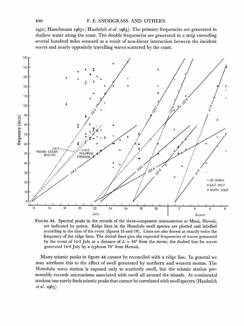
490 F. E. SNODGRASS AND OTHERS
I950; Hasselmann I963 C; Haubrich et al. I963). The primary frequencies are generated in shallow water along the coast. The double frequencies are generated in a strip extending several hundred miles seaward as a result of non-linear interaction between the incident waves and nearly oppositely travelling waves scattered by the coast.
/50 /
140
130 0
120 0
~~~~~~~~~~~~80~~~~~~~~~~~~~~~~~~~~
90 , '
70-
60//
J 14 2 /J J14-0
50 INDIAN OCEANPHLPIE4
BEACHES ~TYPHOON
40
30 - AA
according to th dateof te evet (fgures15 ad 16). Lins ar alsodraw at eactl o UP-DOWN 20 /-
/ / ~~~~~~~~~~~~~~~~~~~~~~~~~~EAST -WEST / *~~~~~~~~~~~~~~~~~~~~~~~~~~~~~~~ NORTH - SOUTI- 10 /
14 16 18 20 22 24 26 28 30 2 4 6 8
July August
FIGURE 44. Spectral peaks in the records of the three-component seismometers at Maui, Hawaii, are indicated by points. Ridge lines in the Honolulu swell spectra are plotted and labelled according to the date of the event (figures 15 and 16). Lines are also drawn at exactly twice the frequency of the ridge lines. The dotted lines give the expected frequencies of waves generated by the event of 14*2 July at a distance of A = 650 from the storm; the dashed line for waves generated 14-0 July by a typhoon 700 from Hawaii.
Many seismic peaks in figure 44 cannot be reconciled with a ridge line. In general we may attribute this to the effect of swell generated by northern and western storms. The Honolulu wave station is exposed only to southerly swell, but the seismic station pre- sumably records microseisms associated with swell all around the islands. At continental -stations one rarely finds seismic peaks that cannot be correlated with swrell spectra (Haubrich et al. I963) .
PROPAGATION OF OCEAN SWELL ACROSS THE PACIFIC 491
The largest group of seismic peaks not related to ridge lines occurs between 60 and 80 mc/s during 20 to 24 July. These peaks appear to have a linear trend and a double-frequency counterpart. One possible source is swell from the west generated by a 135-knot typhoon in the Philippine Sea on 14July. A second lhypothesis is that the microseisms are associated with the same Tasman Sea event of 14-2July for which the ridge line is plotted, but generated at beaches much nearer to the storm. If a line is cdrawn through these points and the 14-2 July zero intercept (see figure), the inferred distance of the microscismic generations is 60 to 70? from the storm (Honolulu is 109"), presumably on beaches of the Indian Ocean along the west coast of Africa and south coast of Asia. A previous occasion is known (Oliver I962) where microseisms could be attributed to large waves on very distant beaches. If the second hypothesis were to hold, we can conclude that microseisms may be associated with wave activity on beaches near the storm as well as on beaches near the station.
The sea-bottom seismometers were sensitive only to frequencies above 100 mc/s, and comparison with ocean wave spectra is limited to the double-frequency effect. On days with large ocean swell at Cape Palliser, Bradner found peaks in the microseismic spectra at twice the frequency of the Cape Palliser swell. The best results were obtained for drops off Samoa on 9 and 11 August, and a drop on Chatham Rise east of New Zealand on 6 September. However, this interpretation is in question for the August drops. Most of the seismic energy was in the form of Rayleigh waves coming from the direction of open-sea disturbances rather than from New Zealatnd. Bradner has not been able to establish the relative contribution of shore reflexion against open-sea disturbances.
10 . CONCLUSIONS
Figure 45 shows a highly idealized synthesis ofthe observational findings. The background spectrum rises by 30 dB between 30 and 75 mc/s, and then remains fairly constant up to 100 mc/s. At higher frequencies the background may rise again because of the effect of local winds. We attribute the July to September background between 30 and 100 mc/s to global high winds in the storm belt of the South Pacific (the ' roaring forties' and 'fighting fifties').
Once or twice a week a wave train associated with a severe southern storm leads to an identifiable 'event' that can be traced across the entire ocean. The event shows up as a slanting ridge in af, t contour presentation of the power spectrum. The three-dimensional field E(f, t, A) at a distance A along the great circle appears to have been adequately sampled on a 1 mc/s by 2 day by 200 grid. It would have been feasible to predict swell for the North Pacific stations based on the observations in the South Pacific (and vice versa for the northern winter). A typical event begins at 30 mc/s and ends at 80 mc/s, lasting for 2 days at Tutuila and for a week at Yakutat, the progressive lengthening being attributable to dispersive stretching of the wave train. The 'ridge spectra' in figure 45 are a composite of successive spectra from which the effect of dispersion has been removed.
The events are most conspicuous at 50 to 60 mc/s, where the event spectra rise 10 to 20 dB above background, and attenuation is negligible (less than 2 dB3 between New Zealand and Alaska). Attenuation at 70 ic/s and the resulting red shift at distant stations is barely observable. At frequencies above 80 mtc/s, for which the initial attenuation must be severe, the event spectra disappear in the background even at the southern stations. Thus at low
59 V~~~~~~~~~~~~~~~~~~~AOL. 259. A.
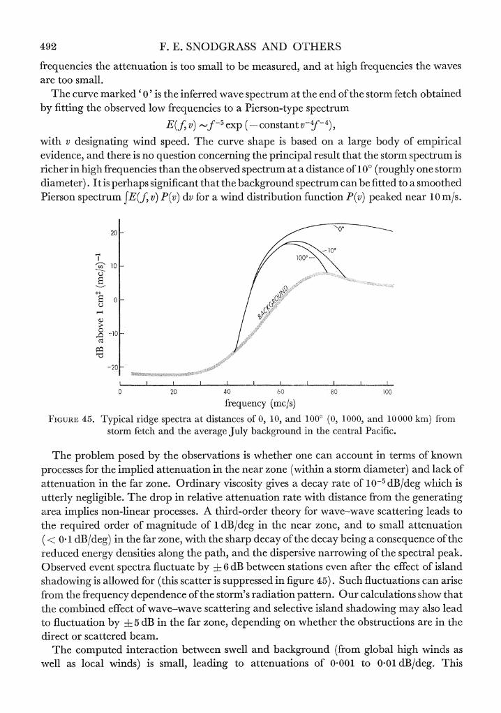
492 F. E. SNODGRASS AND OTHERS
frequencies the attenuation is too small to be measured, and at high frequencies the waves are too small.
The curve marked 'O' is the inferred wave spectrum at the end of the storm fetch obtained by fitting the observed low frequencies to a Pierson-type spectrum
E(f, v) _f-5 exp (- constant v-f-4),
with v designating wind speed. The curve shape is based on a large body of empirical evidence, and there is no question concerning the principal result that the storm spectrum is richer in high frequencies than the observed spectrum at a distance of 100 (roughly one storm diameter). It is perhaps significant that the background spectrum can be fitted to a smoothed Pierson spectrum fE(f, v) P(v) dv for a wind distribution function P(v) peaked near 10 m/s.
20p
-~~~~~~~~~~10 ~ ~ ~ ~ ~ ~~~1
Q~~~~~~~~~~~~~
~-10
-20
0 20 40 60 80 100
frequency (mc/s) FIGURE 45. Typical ridge spectra at distances of 0, 10, and 100? (0, 1000, and 10000 km) fromn
storm fetch and the average July background in the central Pacific.
The problem posed by the observations is whether one can account in terms of known processes for the implied attenuation in the near zone (within a storm diameter) and lack of attenuation in the far zone. Ordinary viscosity gives a decay rate of 10-5 dB/deg which is utterly negligible. The drop in relative attenuation rate with distance from the generating area implies non-linear processes. A third-order theory for wave-wave scattering leads to the required order of magnitude of 1 dB/deg in the near zone, and to small attenuation ( < 0 1 dB/deg) in the far zone, with the sharp decay of the decay being a consequence of the reduced energy densities along the path, and the dispersive narrowing of the spectral peak. Observed event spectra fluctuate by ? 6 dB between stations even after the effect of island shadowing is allowed for (this scatter is suppressed in figure 45). Such fluctuations can arise from the frequency dependence of the storm's radiation pattern. Our calculations show that the combined effect of wave-wave scattering and selective island shadowing may also lead to fluctuation by i 5 dB in the far zone, depending on whether the obstructions are in the direct or scattered beam.
The computed interaction between swell and background (from global high winds as well as local winds) is small, leading to attenuations of 0 001 to 0 01 dB/deg. This
PROPAGATION OF OCEAN SWELL ACROSS THE PACIFIC 493
calculation, in agreement with the observed attenuation (see figure 34), disposes of the suggestion by Munk et al. (I963) that scattering by the trade wind sea may prevent swell frequencies above 80 mc/s from crossing the equator. Interaction of swell with locally gener- ated white-caps (as suggested by Phillips) implies a correlation between attenuation and winds, and this is not found. As far as our observations go, the propagation of swell across the Pacific is not inconsistent with considerations involving only wave-wave scattering and island absorption.
The simplicity of figure 45 is in a sense misleading, for individual events do not fit easily into a generalized pattern. For this reason our expedition, though experimentally successful, has not led to the definitive results we had hoped for. In part this may be attributed to the station locations. We would have done better if the reference great-circle had been chosen to avoid some of the dense island groups. The spacing of stations was too much conditioned by the faulty notions of exponential decay and possibly anomalous scattering in the equa- torial wind belt. But the essential reason is quite different: in studies involving the linear wave approximation much could be learned from limited measurements, such as observa- tions of the one-dimensional spectrum at one point. In the consideration of non-linear processes everything depends on everything else, and mieasurements of the one-dimensional spectrum along a line are not really adequate. The basic problem is one in radiative transfer involving the time variations of a four-dimensional energy distribution
F(f, ; t,x,y) dfdOdxdy
due to winds and wave-wave interactions, and this calls for serial measurements of the two-dimensional spectrum F(f, 0; t) over a two-dimensional grid.
The Office of Naval Research, U.S. Navy, has generously supported this programme. We are grateful to Jay Carr (W 6 FAY, KP 6 AZ), Edward Naylor (WA 6 FXO), Ken Schissman (KH 6 DUV), Paul Hodges (KS 6 BA), Ern-ie Edwards (W 6JUT), and to the entire amateur radio fraternity for maintaining communications. J. Ardern has carried out the very extensive computational work almiost single-handed. We are grateful to Miss F. Oglebay for her assistance with the computing programs, and Mrs R. Sidowski and H. Taylor for the preparation of the manuscript.
APPENDIX. WAVE PROPAGATION ON AN OBLATE SPHEROID
It is assumed that wave rays coincide with geodesics (geometric optics, no diffraction). Neglect of oblateness of the earth introduces errors whose magnitudes are of the first order in ellipticity e 1/297. Thus the square and higher powers of e are neglected in the follow- ing discussion.
The ocean surface is given by
x -UcosA, y UsinT , z J( U),
where U == a sirixo(1+ue cos2z),
f(U)-==(1-e)V$(a2-U2). 59-2
494 F. E. SNODGRASS AND OTHERS
Here a is the equatorial radius of the earth, x, y, z are cartesian coordinates, A is east longitude and a is geographic (not geocentric) colatitude. Geodesics on a surface of revolution obey the following relations:
Usin 0 - constant along geodesic, ds2- U2dA2+ (I +f'f) dU2, (A 1)
where ds is arc length along the geodesic, and 0 is the true bearing of the forward direction along the geodesic measured clockwise from north. By means of the above relations it can be shown that doads -- -a-'[i-e(1-3sin2a)] cosO,)
dA/ds a-'(I -ecos2 a) cosecasin 0, (A 2) dO/ds a-'(I -ecos2x) cotanasin 0,
along the geodesic. There is a double family of geodesic rays on the ocean surface, and let us assume that each member is characterized by two invariants
u(, A,0) u = 0+eeuj, (A 3a) v(a, A, 0) = v0+evl, j
which are constant along any given ray. Let us also consider a third invariant which depends on arc length s along the ray
w(x,iA,0,s) = wo+ewi (A3b)
for use in computing distances. Invariance requires that
au da audA du dO au 7:0
~~~~(A 4) Y30 Ts + AA ds + Yo as- + a3s _= ?'(A4 and similarly for v and w. For the functions u0 and ul we can take the first of the expressions (A 1) u0 = sin a sin 0, u1 =sin a cos2a sin 0. (A 5)
For v0 and w0 we can take the functions
voA + arctan (sec a cotan 0), (A 6)
wo =a- s-arctan (cotanocsec 0) (A 7)
as given by Groves & Melcer (I96I) for a spherical ocean. It should be noted that the argument of the multiple-valued arctangent in (A 6) passes through oo each time the ray crosses the equator. Each time an eastward ray crosses the equator the next lower branch of the arctangent function in (A 6) should be taken (the next higher branch for a westward ray). The argument of the arctangent in (A 7) passes through co each time the ray becomes tangent to a latitude circle. On these occasions the next higher branch of the arctangent function should be taken for either an eastward or a westward ray.
If the expressions (A 6) and (A 7) are taken for v0 and w0, then equations (A 4) and (A 2) require that 2 4c sn os r1-sin24sin26 (A8)
and L(w1) +1i2 l . 2so20-9cos2azsina =0, (A9)
PROPAGATION OF OCEAN SWELL ACROSS THE PACIFIC 495
a a a . a where L _ sina cos a --sin8 --cos a sin O- -asin a dx as, d
Particular solutions of (A 8) and (A 9) are
sin2' acosc asinO cos0 C i [ r 1osX 1 VI 1 -sin 2cx sin' sini2 a siln arci J(n '-sin2cX sin2 0) (A 10)
I /3-sin2oa sin2U9 . *2*2 *r Cosa ( W =-52 i2 0 cosi sinaX cos80+ (1 +sin2 a sin2 ) arcsin[J(1 2 i 20)lw
(All)
An increasing branch of the multiple-valued arcsin functions in (A 10) and (A 1 1) must be taken wherever the ray proceeds northward (a decreasing branch wherever the ray proceeds southward) in order that (A10) and (All.) satisfy (A 8) and (A 9). Their arguments are identical and become + 1 in the Northern Hlemisphere at the point where the ray becomes tangent to a latitude circle, and -1 under the same circumstances in the Southern Hemi- sphere. It is therefore evident that at such points the arcsin function in both (A 10) and (A 1 1) must move onto the next higher branch; that is, both arcsin functions monotonically increase as one moves along in the forward direction of the ray, for either an eastward or a westward ray.
Consider a ray having parameters aAa Oasa at point a. After a complete circuit of the earth the ray will cross the parallel x c xa at; point b. Here the ray direction will again be Oa because of invariance of u. The longitude Ab at point b is determined by invariance of v as given by (A 3), (A 6) and (A 10). The only change in v between the two points arises from the A term, the arctangent function and the arcsin function, all of which change by the amount 2ir. We obtain
AA = Ab Aa?27 -2re sin aa sin a = -2u
where the minus sign is taken for an eastward ray (plus sign for a westward ray). Thus the ray is a closed curve only if it passes through a pole. Otherwise it 'undershoots' its starting point because AA is negative for an eastward ray, positive for a westward ray. The maximum possible undershoot is about a degree. The distance traversed between points a and b is calculated in the same way by considering the invariaint w. The result is
27a [I -le (I +u2)]
Consider any two successive points a and b on a ray. Let the wave directions 0a and Ob be determined by neglecting oblateness. Thus
UOa UOb
VOa VOb,
where uOa is written for uO (aa Aa Oa), etc. Let the 'true' wave directions be Oa + doa and Ob + dOb, where dOa and dO4b are small quantities of the same order as e. Thus
Z4a dOaUob dOb -e(ula ulb):}| (A 12)
V0 ?-O a e(v1a -V1b)
496 F. E. SNODGRASS AND OTHERS
from which the error in direction due to neglect of oblateness can be evaluated. The primes denote derivatives with respect to 0, so that
f * , cos a U0 sino coS0a Vo 1-sin2 C sin2, O
It is noted that the determinant of (A 12) can be zero only in case points a and b coincide. The maximum error in wave direction can be determined by taking points a and b on the
same northward segment of a ray circling the earth in an eastward direction. Because of symmetry there is no loss of generality if we take
06b - T 06aa
Equation (A 12) then becomes dOa = dOb Viae/VOa.
To find an extreme value it is convenient to first substitute the variables
Cos xa Y=a(1-sin2x sin20) V/(1- Sin2zXa sin20O) 'a a
obtaining dOa = Y(1 - 2) {V/(1 _ 2)+ X- I arcsin X} e.
rrhe extreme value within the domain of interest is found to be
max. (d0a) e) (A 13)
corresponding to the values X 0, Y = 2/2,
or (Xa =2!ffl Oa = a 7
Thus, the maximum error in determination of wave direction is not greater than between two points near the equator bearing northeast-southwest from each other. In this case the error is related to the fact that a degree of latitude is not the same length as a degree of longitude at the equator of an oblate spheroid.
To find the true distance between any two points a and b on a ray, let us take Sa 0 O and determine Sb by neglecting oblateness. Thus
W0a W0b,
wlhere wOa = w0 (aa, AwaO Sa) S etc. If the true distance is Sb + ds where ds is of order e, then
ds -(Wla-Wlb) e!wob ae(wla-wlb)
is the error incurred by assuming spherical geometry, where the prime indicates a derivative with respect to s. However, a large part of this error can be eliminated by taking for the radius of the sphere the mean radius of the spheroid -a (radius of sphere having same volume as spheroid) rather than its equatorial radius a. The relation between the two radii is
-a( -le).
If s'b is the distance computed by spherical geometry using the mean radius, and ds' the error incurred by this procedure, then
ds'z-ds 3eSb =e[a(wla-wlb) +3Sb]b (A 14)
If we assume that ?Cb -- z,-j, thenl
ds' ae[wla-wlb-+ iw].
PROPAGATION OF OCEAN SWELL ACROSS THE PACIFIC 497
It has been shown (Groves & Backus I966) that the wave vector density is invariant for a wave packet on an arbitrary surface. In the absence of refraction the frequency- direction spectrum is invariant also. Thus, oblateness does not introduce any discrepancy in the wave spectrum.
REFERENCES
Backus, G. E. i962 Deep Sea Res. 9, 185-197. Barber, B. F. & Ursell, F. I948 Phil. Trans. A, 240, 527-560. Bradner, H., Dodds J. & Fouiks, R I965 J. Geophys. Res. (in the Press). Burling, R. W. I959 Dtsch. Hydrogr. Zr. 12, 45-64 and 96-117. Dorrestein, R. I960 J. Geophys. Res. 65, 637-642. Fisher, F. H. & Spiess, F. N. I963 J. Acoust. Soc. Amer. 35, 1633-1644. Groves, G. W. & Backus, G. E., I966 (in preparation.) Groves, G. W. & Melcer, J. I96I Geofis. Intern. 1, 77-93. Hasselmann, K. F. I960 Schifstechnik, 7, 191-195. Hasselmann, K. F. i962 J. Fluid Mech. 12, 481-500. Hasselmann, K. F. 1963 a J. Fluid Mech. 15, 273-281. Hasselmann, K. F. i963 b J. Fluid Mech. 15, 385-398. Hasselmann, K. F. I963C Rev. Geoph. 1, 177-210. Hasselmann, K. F. I966 Rev. Geoph. (in the Press). Hasselmann K. F., Munk, W. H. & MacDonald, G. J. F. I963 Chapter 8 of Time series analysis.
New York: Wiley. Haubrich, R. A. & Mackenzie, G. S. I965 J. Geoph. Res. 70, no. 6, 1429-1440. Haubrich, R. A., Munk, W. H. & Snodgrass, F. E. I963 Bull. Seism. Soc. Amer. 53, 27-37. Longuet-Higgins, M. S. I950 Phil. Trans. A, 243, 1-35. Longuet-Higgins, M. S. I957 Proc. Camb. Phil. Soc. 53, 226-229. Longuet-Higgins, M. S., Cartwright, D. E. & Smith, N. ). I963 Ocean wave spectra. Maryland:
Prentice-Hall. Munk, W. H., Arthur, R. S. & Isaacs, J. D. 1952 Trans. Amer. Geoph. Un. 33, 855-865. Munk, W. H., Miller, G. R., Snodgrass, F. E. & Barber, N. F. I963 Phil. Trans. A, 255, 505-584. Munk, W. H. & Snodgrass, F. E. I957 Deep. Sea Res. 4, 272-286.
Munk, W. H., Snodgrass, F. E. & Gilbert, F. i964 J. Fluid Mech. 20, Pt. 4, 529-554.
Northrop, J. I964 Trans. Amer. Geophys. Un. 45, no. 1, 165. Oliver, J. I962 Bull. Seism. Soc. Amer. 52, no. 3, 507-517. Parzen, E. I96I Technometrics, 3, 167-190. Phillips, 0. M. I958 J. Fluid Mech. 4, 426-433. Phillips, 0. M. I959 J. Fluid Mech. 5, pt, II, 177-192 Phillips, 0. M. I960 J. Fluid Mech. 9, 193-217. Phillips, 0. M. I963 J. Fluid Mech. 16, 321-332. Pierson, W. J. & Moskowitz, L. i964 J. Geophys. Res. 69, no. 24, 5181-5190. Robin, G. de Q. I963 Phil. Trans. A, 255, 313-339. Roll, H. U. & Fischer, G. I956 Dtsch. Hydrogr. Z. 9, 9-14. Rudnick, P. I964 Science, 146, 1268-1273. Snodgrass, F. E. I958 Trans. Amer. Geophys. Un. 39, 109-113. Snodgrass, F. E. I964 Science, 146, 198-208.


