Airport2030_TN_Propeller-Efficiency_13-08-12

Aircraft Design and Systems Group (AERO) Department of Automotive and Aeronautical Engineering

Hamburg University of Applied Sciences (HAW) Berliner Tor 9

D - 20099 Hamburg

Propeller Efficiency Calculation in Conceptual Aircraft Design

Andreas Johanning Dieter Scholz

2013-08-12

Technical Note

Table of Contents

1 Introduction ......................................................................................................................... 4 1.1 Basics of Efficiency, Power and Thrust ................................................................................ 4 1.2 Main Parameters Influencing Propulsive Efficiency ............................................................. 6 1.3 Importance of an Accurate Estimation of the Propeller Efficiency in Conceptual

Aircraft Design ...................................................................................................................... 8

2 Propeller Efficiency ............................................................................................................. 9 2.1 Propeller Basics ..................................................................................................................... 9

3 Methods for the Calculation of Propeller Efficiency ..................................................... 13 3.1 Simple Methods to Estimate Propeller Efficiency .............................................................. 13 3.2 Calculating Propeller Efficiency with Diagrams ................................................................. 14 3.3 Simplified Physical Approach for the Calculation of the Propeller Efficiency .................. 17 3.4 Optimum Propeller Design and Propeller Efficiency .......................................................... 20

List of Figures Figure 1.1 Fluid flow through a propulsive device (Anderson 1999) .......................................... 5 Figure 2.1 Airflow at the propeller blade tip and root ................................................................... 9 Figure 2.2 Airflow at a propeller blade with different incidence angle at root and tip ............... 10 Figure 2.3 Airflow at a propeller blade tip and root at an increased cruise speed ...................... 10 Figure 2.4 Airflow at a variable pitch propeller blade tip and root at an increased cruise

speed .......................................................................................................................... 11 Figure 2.5 Anderson 1999, p.158 ................................................................................................ 12 Figure 3.1 Relationship between propeller efficiency and cruise Mach number for a

maximum propeller efficiency of 0.85 (based on the equations of Mattingly 1987) .......................................................................................................................... 14

Figure 3.2 Propeller efficiency over design true airspeed according to Stinton 1983 ............... 15 Figure 3.3 Propeller efficiency over speed according to Marckwardt 1998 ............................. 17 Figure 3.4 Speeds and forces at a propeller blade (Truckenbrodt 1999) .................................. 18 Figure 3.5 Propeller efficiency over speed for several disc loadings using the Truckenbrodt

equation ...................................................................................................................... 19 Figure 3.6 Comparison of the Marckwardt diagram and the Truckenbrodt equation ................. 20 Figure 3.7 Airflow at the propeller blade .................................................................................... 21

1 Introduction This report is intended to provide an overview about the calculation of the propeller efficiency of turboprop aircraft and to evaluate the methods concerning their suitability for conceptual aircraft design.

1.1 Basics of Efficiency, Power and Thrust The basics of efficiency, power and thrust are part of many books related to aircraft. In this Sec-tion, some of the fundamental relations will be presented based on the explanations of Anderson 1999. This reference is also suggested if the reader is interested in a more detailed discussion of the equations. The efficiency η of a propulsive device can be calculated as the ratio of the provided useful power (called available power PA) divided by the total generated power PT

T

A

PP

=η (1.1)

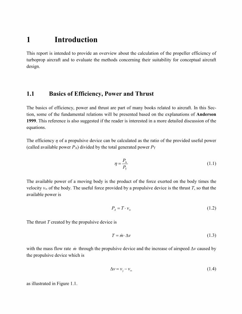
The available power of a moving body is the product of the force exerted on the body times the velocity v∞ of the body. The useful force provided by a propulsive device is the thrust T, so that the available power is ∞⋅= vTPA (1.2) The thrust T created by the propulsive device is vmT ∆⋅= (1.3) with the mass flow rate m through the propulsive device and the increase of airspeed Δv caused by the propulsive device which is ∞−=∆ vvv j (1.4)

as illustrated in Figure 1.1.

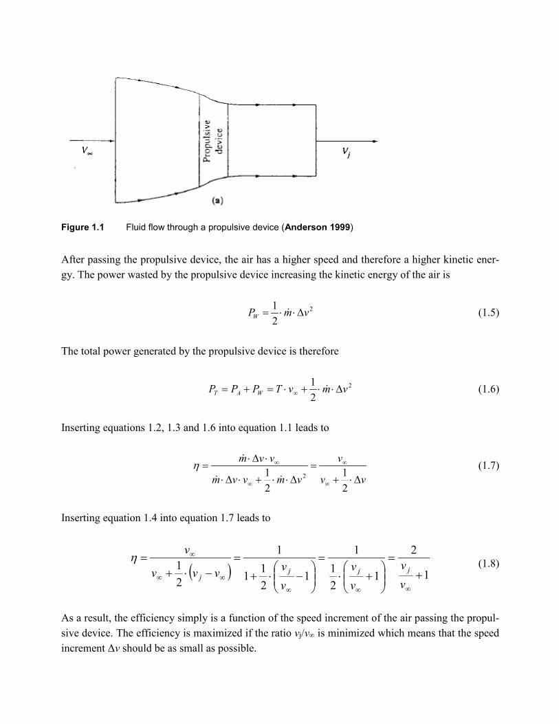
Figure 1.1 Fluid flow through a propulsive device (Anderson 1999)

After passing the propulsive device, the air has a higher speed and therefore a higher kinetic ener-gy. The power wasted by the propulsive device increasing the kinetic energy of the air is

2

21 vmPW ∆⋅⋅= (1.5)

The total power generated by the propulsive device is therefore

2

21 vmvTPPP WAT ∆⋅⋅+⋅=+= ∞ (1.6)

Inserting equations 1.2, 1.3 and 1.6 into equation 1.1 leads to

vv

v

vmvvm

vvm

∆⋅+=

∆⋅⋅+⋅∆⋅

⋅∆⋅=

∞

∞

∞

∞

21

21 2

η (1.7)

Inserting equation 1.4 into equation 1.7 leads to

( ) 1

2

121

1

1211

1

21

+=

+⋅

=

−⋅+

=−⋅+

=

∞∞∞

∞∞

∞

vv

vv

vvvvv

vjjj

j

η (1.8)

As a result, the efficiency simply is a function of the speed increment of the air passing the propul-sive device. The efficiency is maximized if the ratio vj/v∞ is minimized which means that the speed increment Δv should be as small as possible.

As shown in Equation 1.3, the thrust of a propulsive device is the product of mass flow rate and speed increment Δv. As Δv should be minimized to achieve maximum efficiency, the mass flow rate should be as high as possible to achieve a given required thrust. The mass flow rate can be calculated by Avm ⋅⋅= ∞ρ (1.9) where ρ is the density, and A the cross-sectional area of the mass flow. For a high mass flow rate leading to a high efficiency, a propulsive device should be operated in a dense (high ρ) and fast (high v∞) fluid and have a big cross-sectional area. These basic rules can easily be transferred to propeller driven aircraft. For high propeller efficien-cy, propeller driven aircraft should fly in low altitudes (high ρ) at high cruise speeds (high v∞) and have a large propeller area which can be achieved by a large propeller diameter or a high number of engines. However, just flying extremely low and fast, or having an extremely large propeller diameter does not lead to the optimum aircraft. There are other influences leading to advantages and disad-vantages of these parameters on the overall aircraft level which will be discussed in the next sec-tion.

1.2 Main Parameters Influencing Propulsive Efficiency As shown in the last Section, the three parameters density, speed and propeller area directly influ-ence the propeller efficiency. This Section is intended to discuss the advantages and disadvantages of manipulating these parameters to achieve high propeller efficiencies. On the one hand, high density and therefore low flight altitudes lead to high propeller efficiencies. Therefore, just considering the propeller efficiency, propeller driven aircraft should fly as low as possible. But on the other hand, just considering the aircraft design process, there is another opti-mum altitude which is far above the optimum altitude for the propeller efficiency. For commercial aircraft, this altitude reaches from about 7000 m … 12000 m. Deviating from this optimum altitude impairs the performance of the aircraft. The next parameter directly influencing propeller efficiency is the aircraft speed. As shown above, a high aircraft speed leads to a high propeller efficiency. Secondly, a high aircraft speed leads to a

short trip duration and therefore allows a high number of trips per year lowering the operating costs per seat-mile. Just considering these two aspects, an aircraft should fly as fast as possible. But on the other hand, high cruise speeds cause, amongst others, high airspeeds at the propeller blade tips. As soon as these speeds reach the speed of sound, shock waves are produced. The shock waves lead to a serious drag increase causing a torque increase at the engine. The rotational speed of the engine decreases and therefore the power obtained from the engine which reduces the thrust. The shock waves also reduce the lift coefficient of the airfoil section which also leads to a thrust reduction. (Anderson 1999, p.150) This effect causes a decrease in propeller efficiency increasing the fuel consumption and therefore leading to higher costs. Though the airspeeds at the blade tips can be kept below critical speeds by lowering the rotational speed of the propeller, this measure also leads to an impairment of the propeller efficiency. Again, there is obviously an optimum trade-off between high cruise speeds and high propeller efficiencies in aircraft design. The third parameter directly influencing propeller efficiency is the propeller area. As already men-tioned, the propeller area can be increased by increasing the propeller diameter or by using a higher number of propellers. Both measures will lead to an improvement of the propeller efficiency. However, a higher number of engines will increase maintenance costs and might also increase the overall mass of the aircraft. A higher propeller diameter causes the same problems as the high cruise speed, as the airspeed near the propeller blade tips reaches the speed of sound finally result-ing in an impaired propeller efficiency. Again, by lowering the rotational speed of the propeller, the airspeed at the blade tip can be kept below critical speed but again, this measure leads to an im-pairment of the propeller efficiency. Obviously, there is a trade-off for the optimum flight altitude, cruise speed, propeller area and the number of propellers. The objective of the aircraft design process is to find this optimum trade-off. The next Section will discuss the influence of the propeller efficiency on the overall aircraft design and explain why it is important to have an accurate prediction of the propeller efficiency.

1.3 Importance of an Accurate Estimation of the Propeller Effi-ciency in Conceptual Aircraft Design

The fuel mass mF consumed by an aircraft on a certain range R assuming a constant speed v and a constant lift coefficient CL is

−⋅=

−BR

F emm 10 (1.10)

with the take-off mass m0 and the Breguet factor B. The higher B, the lower mF, which means that a high Breguet factor is important for low fuel consumption. For a Turboprop Aircraft (TA), B can be calculated as

gPSFC

EB⋅

⋅=

η (1.11)

with the propeller efficiency η, the glide ratio E, the power specific fuel consumption PSFC and the gravitational acceleration g. The higher the propeller efficiency, the higher the Breguet factor and therefore the lower the consumed fuel mass. Obviously, the propeller efficiency has an important influence on the overall performance of a TA. A bad prediction of η leads to a bad prediction of the required fuel mass and therefore of the maximum take-off mass of the aircraft. An accurate predic-tion of the achievable propeller efficiency is therefore crucial for the correct evaluation of a TA design.

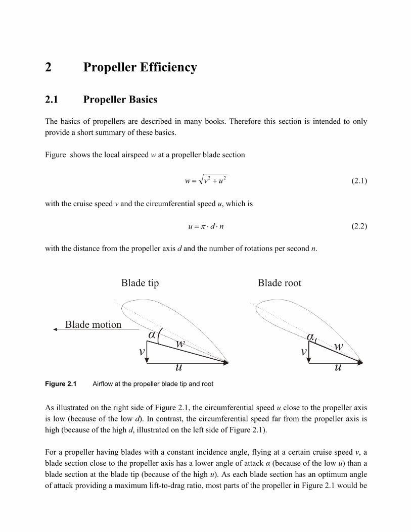
2 Propeller Efficiency 2.1 Propeller Basics The basics of propellers are described in many books. Therefore this section is intended to only provide a short summary of these basics. Figure shows the local airspeed w at a propeller blade section

22 uvw += (2.1) with the cruise speed v and the circumferential speed u, which is ndu ⋅⋅= π (2.2) with the distance from the propeller axis d and the number of rotations per second n.

Figure 2.1 Airflow at the propeller blade tip and root

As illustrated on the right side of Figure 2.1, the circumferential speed u close to the propeller axis is low (because of the low d). In contrast, the circumferential speed far from the propeller axis is high (because of the high d, illustrated on the left side of Figure 2.1). For a propeller having blades with a constant incidence angle, flying at a certain cruise speed v, a blade section close to the propeller axis has a lower angle of attack α (because of the low u) than a blade section at the blade tip (because of the high u). As each blade section has an optimum angle of attack providing a maximum lift-to-drag ratio, most parts of the propeller in Figure 2.1 would be

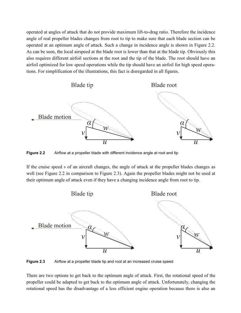
operated at angles of attack that do not provide maximum lift-to-drag ratio. Therefore the incidence angle of real propeller blades changes from root to tip to make sure that each blade section can be operated at an optimum angle of attack. Such a change in incidence angle is shown in Figure 2.2. As can be seen, the local airspeed at the blade root is lower than that at the blade tip. Obviously this also requires different airfoil sections at the root and the tip of the blade. The root should have an airfoil optimized for low speed operations while the tip should have an airfoil for high speed opera-tions. For simplification of the illustrations, this fact is disregarded in all figures.

Figure 2.2 Airflow at a propeller blade with different incidence angle at root and tip

If the cruise speed v of an aircraft changes, the angle of attack at the propeller blades changes as well (see Figure 2.2 in comparison to Figure 2.3). Again the propeller blades might not be used at their optimum angle of attack even if they have a changing incidence angle from root to tip.

Figure 2.3 Airflow at a propeller blade tip and root at an increased cruise speed

There are two options to get back to the optimum angle of attack. First, the rotational speed of the propeller could be adapted to get back to the optimum angle of attack. Unfortunately, changing the rotational speed has the disadvantage of a less efficient engine operation because there is also an

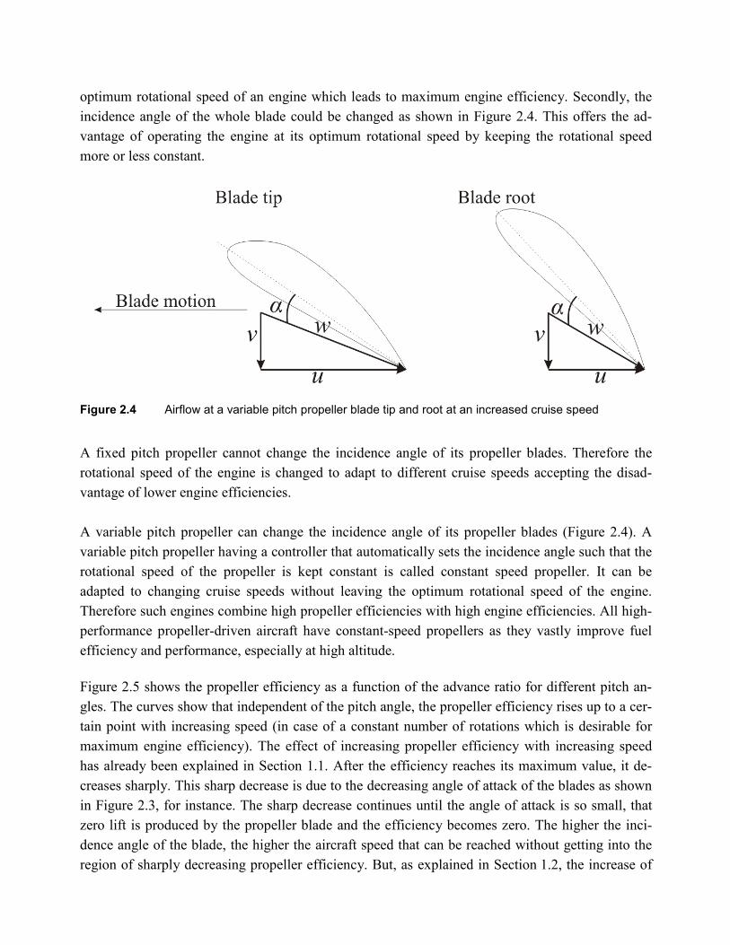
optimum rotational speed of an engine which leads to maximum engine efficiency. Secondly, the incidence angle of the whole blade could be changed as shown in Figure 2.4. This offers the ad-vantage of operating the engine at its optimum rotational speed by keeping the rotational speed more or less constant.

Figure 2.4 Airflow at a variable pitch propeller blade tip and root at an increased cruise speed

A fixed pitch propeller cannot change the incidence angle of its propeller blades. Therefore the rotational speed of the engine is changed to adapt to different cruise speeds accepting the disad-vantage of lower engine efficiencies. A variable pitch propeller can change the incidence angle of its propeller blades (Figure 2.4). A variable pitch propeller having a controller that automatically sets the incidence angle such that the rotational speed of the propeller is kept constant is called constant speed propeller. It can be adapted to changing cruise speeds without leaving the optimum rotational speed of the engine. Therefore such engines combine high propeller efficiencies with high engine efficiencies. All high-performance propeller-driven aircraft have constant-speed propellers as they vastly improve fuel efficiency and performance, especially at high altitude. Figure 2.5 shows the propeller efficiency as a function of the advance ratio for different pitch an-gles. The curves show that independent of the pitch angle, the propeller efficiency rises up to a cer-tain point with increasing speed (in case of a constant number of rotations which is desirable for maximum engine efficiency). The effect of increasing propeller efficiency with increasing speed has already been explained in Section 1.1. After the efficiency reaches its maximum value, it de-creases sharply. This sharp decrease is due to the decreasing angle of attack of the blades as shown in Figure 2.3, for instance. The sharp decrease continues until the angle of attack is so small, that zero lift is produced by the propeller blade and the efficiency becomes zero. The higher the inci-dence angle of the blade, the higher the aircraft speed that can be reached without getting into the region of sharply decreasing propeller efficiency. But, as explained in Section 1.2, the increase of

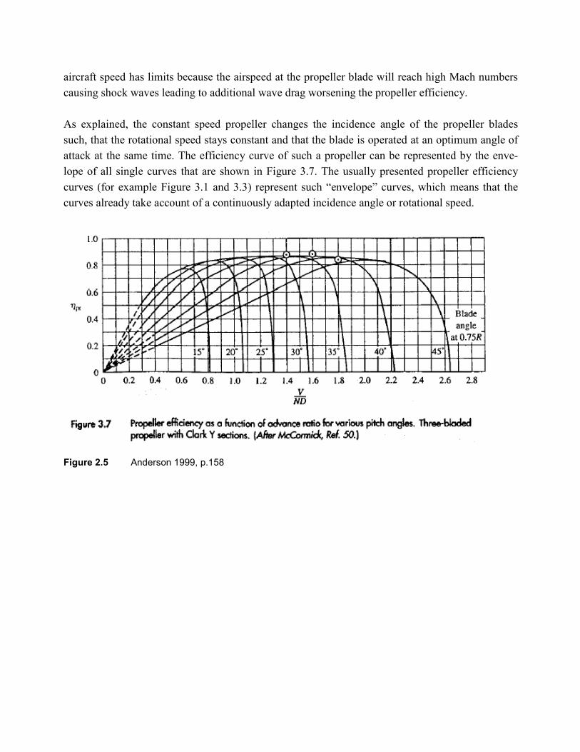
aircraft speed has limits because the airspeed at the propeller blade will reach high Mach numbers causing shock waves leading to additional wave drag worsening the propeller efficiency. As explained, the constant speed propeller changes the incidence angle of the propeller blades such, that the rotational speed stays constant and that the blade is operated at an optimum angle of attack at the same time. The efficiency curve of such a propeller can be represented by the enve-lope of all single curves that are shown in Figure 3.7. The usually presented propeller efficiency curves (for example Figure 3.1 and 3.3) represent such “envelope” curves, which means that the curves already take account of a continuously adapted incidence angle or rotational speed.

Figure 2.5 Anderson 1999, p.158

3 Methods for the Calculation of Propeller Efficiency

3.1 Simple Methods to Estimate Propeller Efficiency Several authors suggest to simply considering the propeller efficiency as a constant value in the first sizing steps. Raymer 2006 suggests that a value of 0.8 can be used for rough initial sizing. Bräunling 2001 suggests that a maximum propeller efficiency of 0.85 is a good mean for the cur-rent state of the art (obviously in the year 2001). Bräunling 2001 also states that efficiencies up to 0.9 can be found in the literature. Using a constant value for the propeller efficiency causes certain problems in conceptual aircraft design. As explained in Section 1.2, there is an optimum cruise speed leading to maximum propel-ler efficiency. If the propeller efficiency is considered as a constant, no matter how fast the aircraft flies, the optimum turboprop aircraft would probably fly at unrealistic high speeds. Mattingly 1987 proposes an easy method to consider the decreasing efficiency of TA with increas-ing cruise Mach numbers: For Ma0 ≤ 0.1: ( )

max010 propprop Ma ηη ⋅⋅= (3.1)

0.1 < Ma0 ≤ 0.7: ( )

maxpropprop ηη = (3.2)

0.7 < Ma0 < 0.85:

( )

−−⋅⋅⋅=

37.0110 0

max0MaMa propprop ηη (3.3)

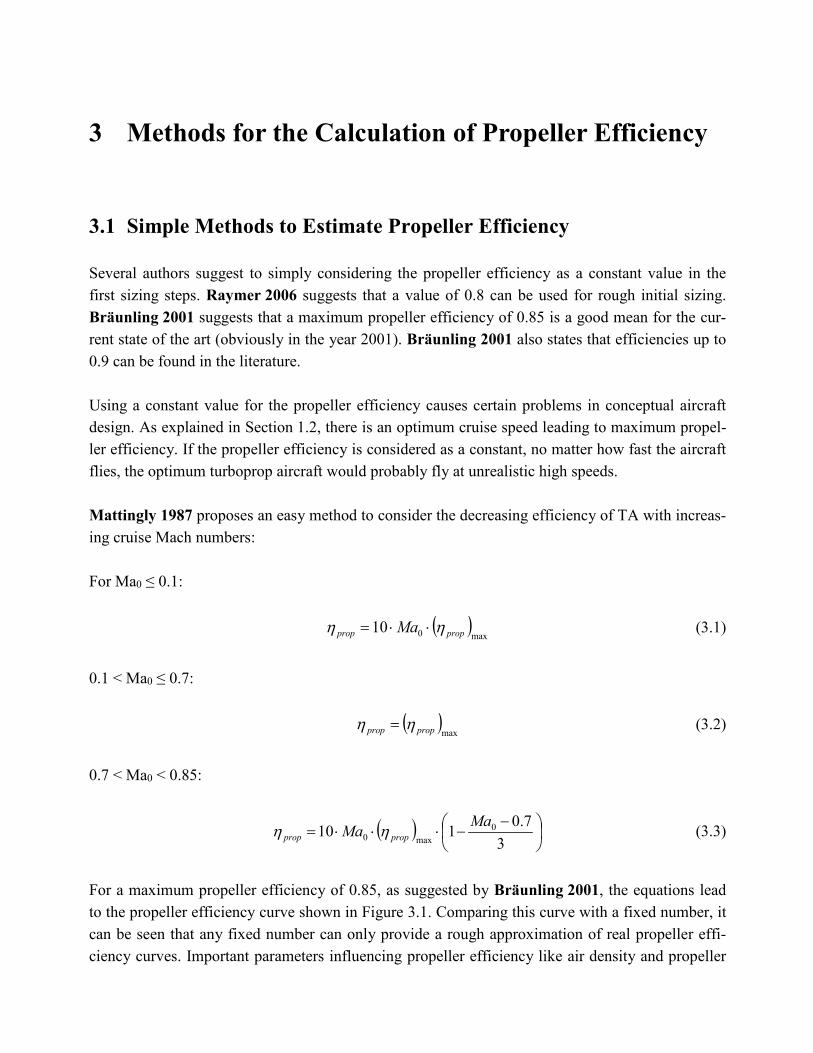
For a maximum propeller efficiency of 0.85, as suggested by Bräunling 2001, the equations lead to the propeller efficiency curve shown in Figure 3.1. Comparing this curve with a fixed number, it can be seen that any fixed number can only provide a rough approximation of real propeller effi-ciency curves. Important parameters influencing propeller efficiency like air density and propeller

area are not considered. Also, if equations like (3.3) (Fig. 3.1) would be used to determine propeller efficiency in aircraft design, there would be no advantage of having a higher number of engines or a large propeller diameter but only disadvantages concerning maintenance costs or landing gear length, for instance. Therefore the resulting number of propellers of an optimum aircraft would be as low as possible and the resulting propeller diameter would be small (so that it does not dimen-sion the landing gear length). As an accurate calculation of propeller efficiency is of high im-portance in conceptual aircraft design (as explained in Section 1.3), a better method should be used.

Figure 3.1 Relationship between propeller efficiency and cruise Mach number for a maximum propeller

efficiency of 0.85 (based on the equations of Mattingly 1987)

3.2 Calculating Propeller Efficiency with Diagrams Another simple approach for the calculation of the propeller efficiency in conceptual aircraft design is by using one of the many graphs presented in books about aircraft and aircraft engines. Up to now, the graph in Figure 3.3 has been used to calculate propeller efficiencies in the design tools of the Aircraft Design and Systems Group (AERO). This section is intended to analyze the advantages and disadvantages of the use of such graphs. The biggest advantage of this approach is its simplicity. To be able to determine the efficiency of propellers, a function simply has to be determined representing the curve/curves of the propeller efficiency diagram in the best possible way. After that, this function can be used to determine the propeller efficiency of any propeller, based on few input parameters. Nevertheless, the method has important disadvantages that will be explained in the following paragraphs using Figure 3.2 and Figure 3.3 as example.

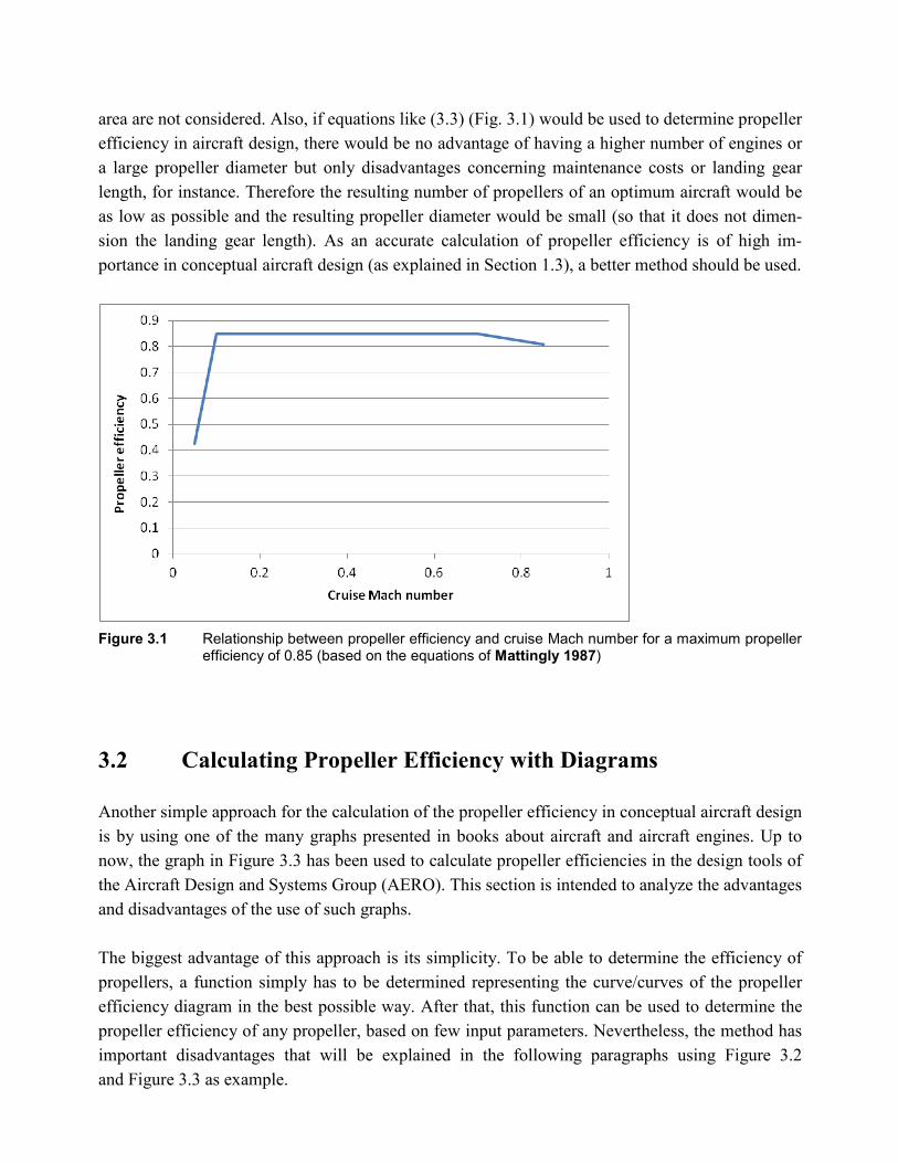
According to Figure 3.2, maximum propeller efficiency can be achieved at a true airspeed of about 230 kt (118 m/s). Above that speed, there is a sharp drop of the propeller efficiency. At 389 kt (200 m/s), the propeller efficiency is only around 40 %. The Figure could be used to determine propeller efficiency in a very simple way, only depending on design true airspeed. But, as ex-plained in Sections 1.1 and 1.2, the propeller efficiency is not only influenced by aircraft speed, but also by propeller area, air density and other factors that are obviously not considered. The negative effects of not considering these parameters are the same as those already described at the end of the previous section. Additionally, the optimum aircraft speed would probably be around 230 kt (118 m/s) because maximum propeller efficiency is achieved at this speed. As this speed is very low compared to the cruise speeds of turbofan aircraft (for instance, the Airbus A320-200 is flying at a cruise speed of about 224 m/s), the possible number of flights in a given time period would be much lower, probably leading to higher costs per passenger-kilometer compared to a tur-bofan aircraft. Obviously, the use of such a diagram could not only lead to a badly chosen value for a design parameters like propeller diameter, but also to a wrong evaluation of the overall aircraft design.

Figure 3.2 Propeller efficiency over design true airspeed according to Stinton 1983

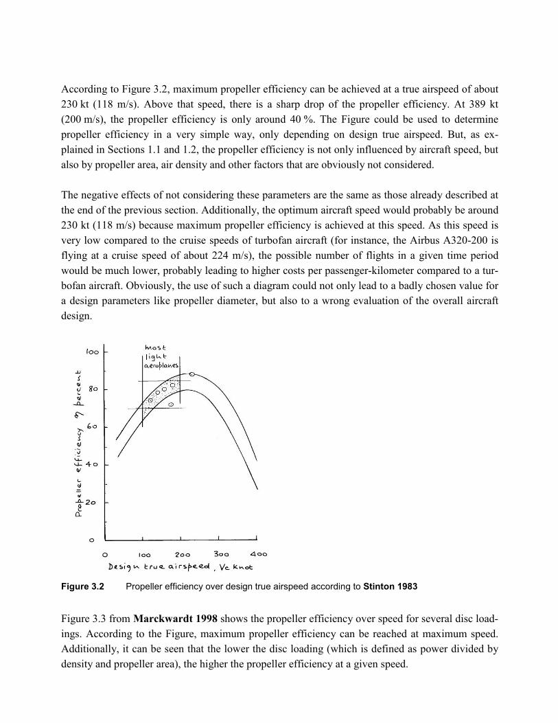
Figure 3.3 from Marckwardt 1998 shows the propeller efficiency over speed for several disc load-ings. According to the Figure, maximum propeller efficiency can be reached at maximum speed. Additionally, it can be seen that the lower the disc loading (which is defined as power divided by density and propeller area), the higher the propeller efficiency at a given speed.

According to Figure 3.3, the propeller efficiency at 200 m/s is around 85 … 90 %, while Figure 3.2 led to a propeller efficiency of around 40 % at this speed. This difference would cause completely different results for an entire aircraft design and therefore gives a good example of a general prob-lem of the use of such diagrams. In most cases, it is not clear which database or method has been used to create the propeller efficiency diagrams. Therefore, the limitations for the use of the dia-grams are unknown and it is not possible to decide which one is the “correct” diagram. Nevertheless, the diagram considers that propeller efficiency increases with increasing speed, den-sity and propeller area and therefore represents the same trends as explained in Section 1.1. Obvi-ously, the diagram considers the most important parameters influencing propeller efficiency and, as further justified in the next Section, could therefore be used for a simplified estimation of propeller efficiencies at low Mach numbers. Unfortunately, the diagram does not consider the sharp drop of propeller efficiency caused by shock waves at high Mach numbers. Propeller driven aircraft designed with this diagram would therefore probably have a very high optimum cruise speed. As one of the main disadvantages of the use of propellers is not considered, the diagram should not be used for the calculation of propeller efficiencies at high Mach numbers. Otherwise a fair comparison with a turbofan aircraft, for in-stance, would not be possible.

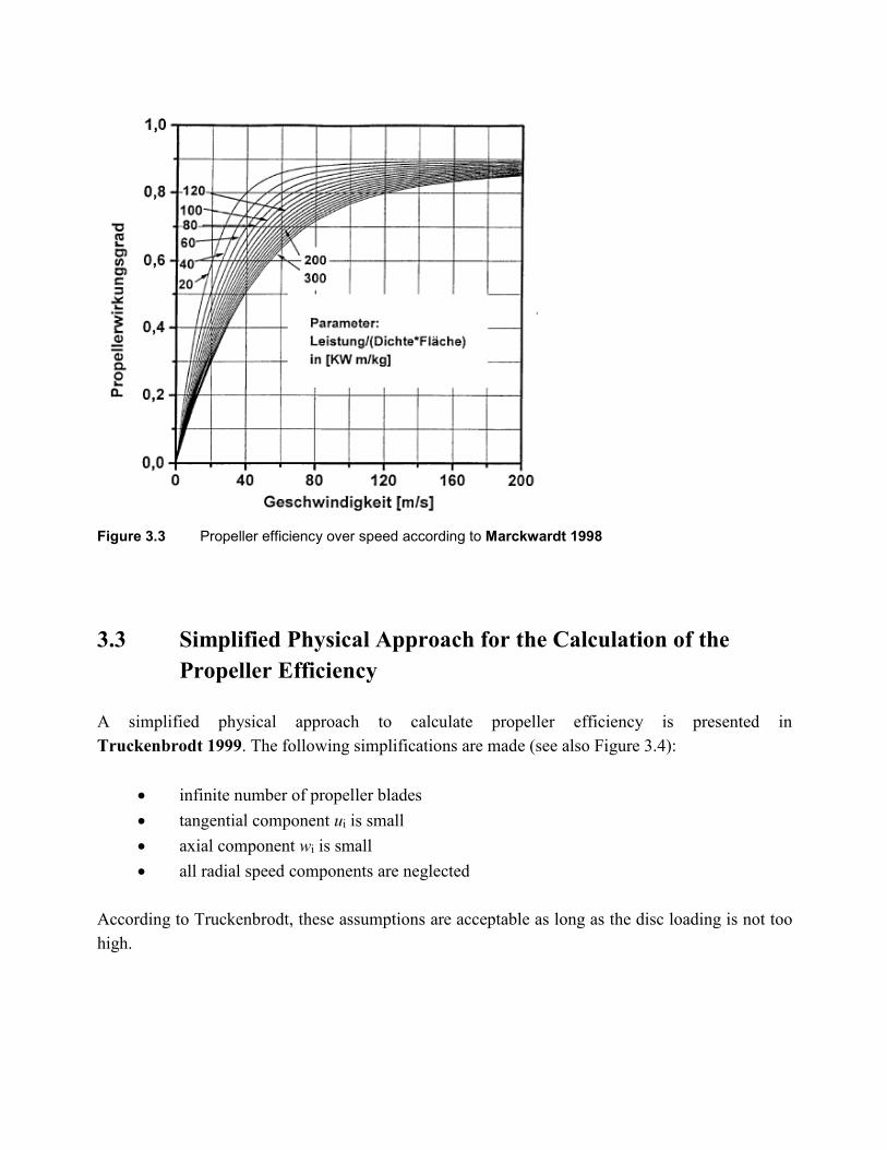
Figure 3.3 Propeller efficiency over speed according to Marckwardt 1998

3.3 Simplified Physical Approach for the Calculation of the Propeller Efficiency A simplified physical approach to calculate propeller efficiency is presented in Truckenbrodt 1999. The following simplifications are made (see also Figure 3.4):

• infinite number of propeller blades • tangential component ui is small • axial component wi is small • all radial speed components are neglected

According to Truckenbrodt, these assumptions are acceptable as long as the disc loading is not too high.

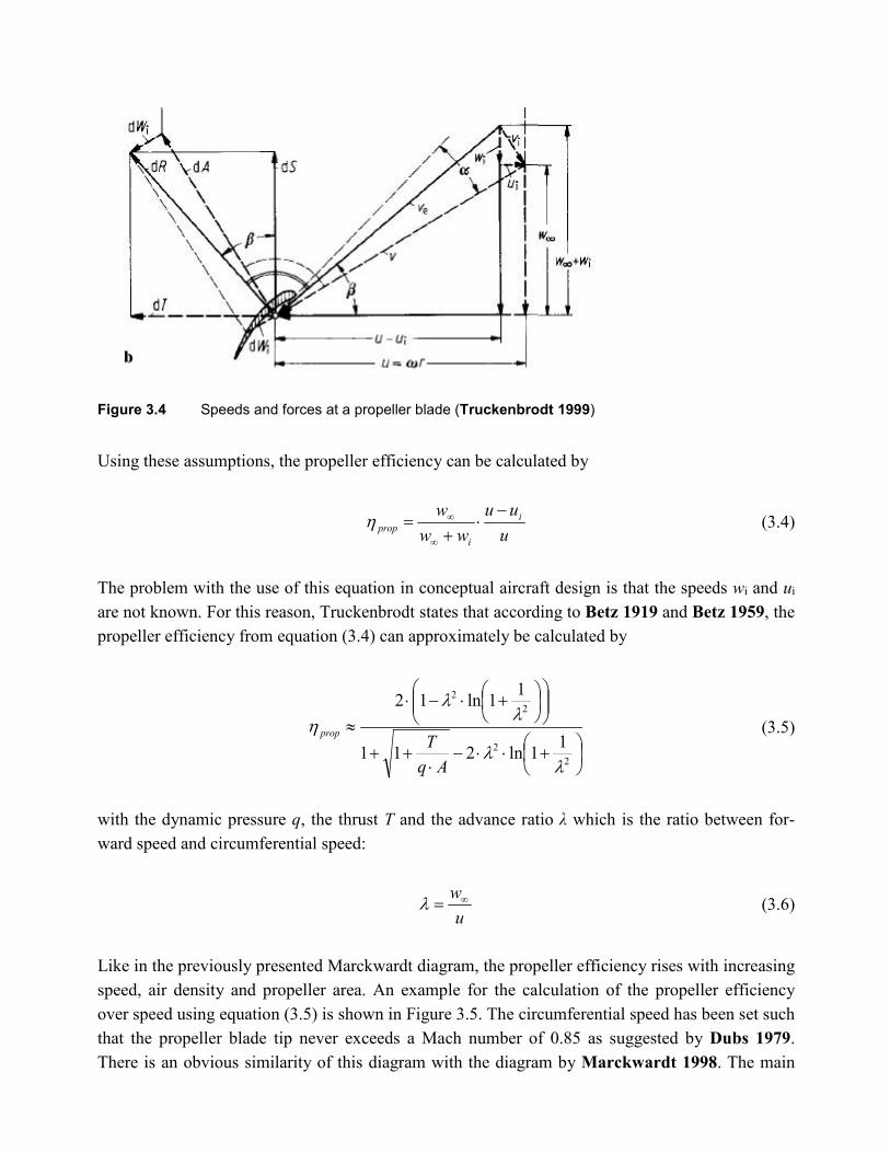
Figure 3.4 Speeds and forces at a propeller blade (Truckenbrodt 1999)

Using these assumptions, the propeller efficiency can be calculated by

u

uuww

w i

iprop

−⋅

+=

∞

∞η (3.4)

The problem with the use of this equation in conceptual aircraft design is that the speeds wi and ui are not known. For this reason, Truckenbrodt states that according to Betz 1919 and Betz 1959, the propeller efficiency from equation (3.4) can approximately be calculated by

+⋅⋅−

⋅++

+⋅−⋅

≈

22

22

11ln211

11ln12

λλ

λλ

η

AqTprop (3.5)

with the dynamic pressure q, the thrust T and the advance ratio λ which is the ratio between for-ward speed and circumferential speed:

u

w∞=λ (3.6)

Like in the previously presented Marckwardt diagram, the propeller efficiency rises with increasing speed, air density and propeller area. An example for the calculation of the propeller efficiency over speed using equation (3.5) is shown in Figure 3.5. The circumferential speed has been set such that the propeller blade tip never exceeds a Mach number of 0.85 as suggested by Dubs 1979. There is an obvious similarity of this diagram with the diagram by Marckwardt 1998. The main

difference between the two diagrams is that Truckenbrodt's equation approaches an efficiency of 1, while the Marckwardt's diagram only approaches efficiencies of 0.9.

0.0

0.1

0.2

0.3

0.4

0.5

0.6

0.7

0.8

0.9

1.0

0 50 100 150 200

Prop

elle

r effi

cienc

y

Speed [m/s]

20

40

60

80

100

120

300

Disc loading:

Figure 3.5 Propeller efficiency over speed for several disc loadings using the Truckenbrodt equation

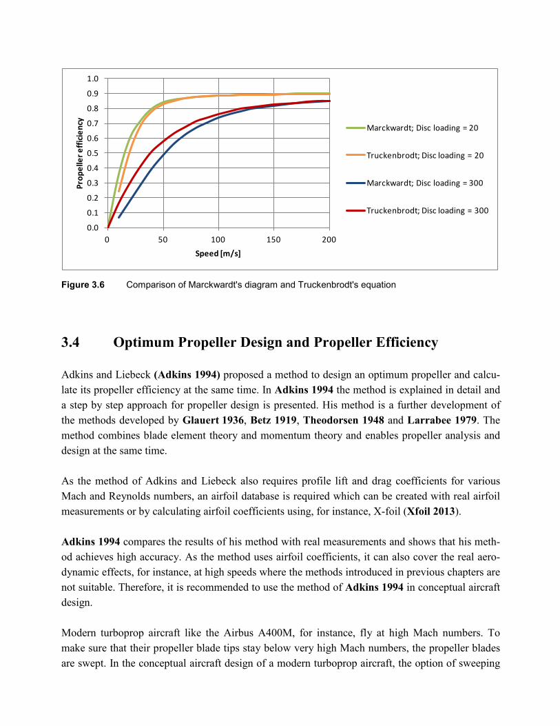
For a better comparison of the two diagrams, the equation was multiplied by a maximum achieva-ble propeller efficiency of 0.9. After that, the propeller efficiency curves of Marckwardt and Truckenbrodt for a disc loading of 20 and 300 have been plotted in the same diagram, as shown in Figure 3.6. As can be seen, the curves of both authors are very similar. It is likely that Marck-wardt 1998 used the equation of Truckenbrodt 1999 to create his diagram. The difference be-tween the curves could come from the fact, that the values of Marckwardt's diagram, as they are presented here, have been measured by hand and because Marckwardt might have used a slightly different value for the circumferential speed. The formation of shock waves is not considered in this equation. Therefore, it should not be used for the calculation of propeller efficiencies at higher speeds. Nevertheless, the equation can be used for a first estimation of the propeller efficiency at lower speeds.

0.0

0.1

0.2

0.3

0.4

0.5

0.6

0.7

0.8

0.9

1.0

0 50 100 150 200

Prop

elle

r effi

cienc

y

Speed [m/s]

Marckwardt; Disc loading = 20

Truckenbrodt; Disc loading = 20

Marckwardt; Disc loading = 300

Truckenbrodt; Disc loading = 300

Figure 3.6 Comparison of Marckwardt's diagram and Truckenbrodt's equation

3.4 Optimum Propeller Design and Propeller Efficiency Adkins and Liebeck (Adkins 1994) proposed a method to design an optimum propeller and calcu-late its propeller efficiency at the same time. In Adkins 1994 the method is explained in detail and a step by step approach for propeller design is presented. His method is a further development of the methods developed by Glauert 1936, Betz 1919, Theodorsen 1948 and Larrabee 1979. The method combines blade element theory and momentum theory and enables propeller analysis and design at the same time. As the method of Adkins and Liebeck also requires profile lift and drag coefficients for various Mach and Reynolds numbers, an airfoil database is required which can be created with real airfoil measurements or by calculating airfoil coefficients using, for instance, X-foil (Xfoil 2013). Adkins 1994 compares the results of his method with real measurements and shows that his meth-od achieves high accuracy. As the method uses airfoil coefficients, it can also cover the real aero-dynamic effects, for instance, at high speeds where the methods introduced in previous chapters are not suitable. Therefore, it is recommended to use the method of Adkins 1994 in conceptual aircraft design. Modern turboprop aircraft like the Airbus A400M, for instance, fly at high Mach numbers. To make sure that their propeller blade tips stay below very high Mach numbers, the propeller blades are swept. In the conceptual aircraft design of a modern turboprop aircraft, the option of sweeping

the propeller blades should be included. Unfortunately, swept propeller blades are not considered by the method of Adkins and Liebeck. Therefore the method has been extended to be able to take account of the effects of sweep The extension of the Adkins method for the consideration of sweep is explained in the following paragraphs (it has also already been explained in ICAS 2012). For the method of Adkins, please refer to Adkins 1994. As already mentioned, Dubs 1979 suggests to limit the Mach number at the propeller blade tip to 0.85 to keep noise in acceptable levels. This requirement for a maximum Mach number at the blade determines the rotational speed of the propeller as shown in the following paragraphs. According to Torenbeek 1988, a sweep angle leads to a reduced effective Mach number of 25cosϕ⋅= MM eff

(3.7)

which gives us an equation for the maximum possible Mach number at the blade for a given Meff and φ25

25cosϕ

effMM = (3.8)

Setting Meff to 0.85 and the sweep angle φ25 at the propeller tip to 55° (which is the approximate sweep angle at the blade tip of the Ratier-Figeac FH386 propellers used for the military transport aircraft Airbus A400M), leads to a maximum allowed local Mach number M of 1.12 at the blade tip. At the same time a swept blade has a reduced maximum lift coefficient (Raymer 2006). 25max,,max,, cosϕ⋅= unsweptLsweptL CC (3.9)

Blade motion

vu

w

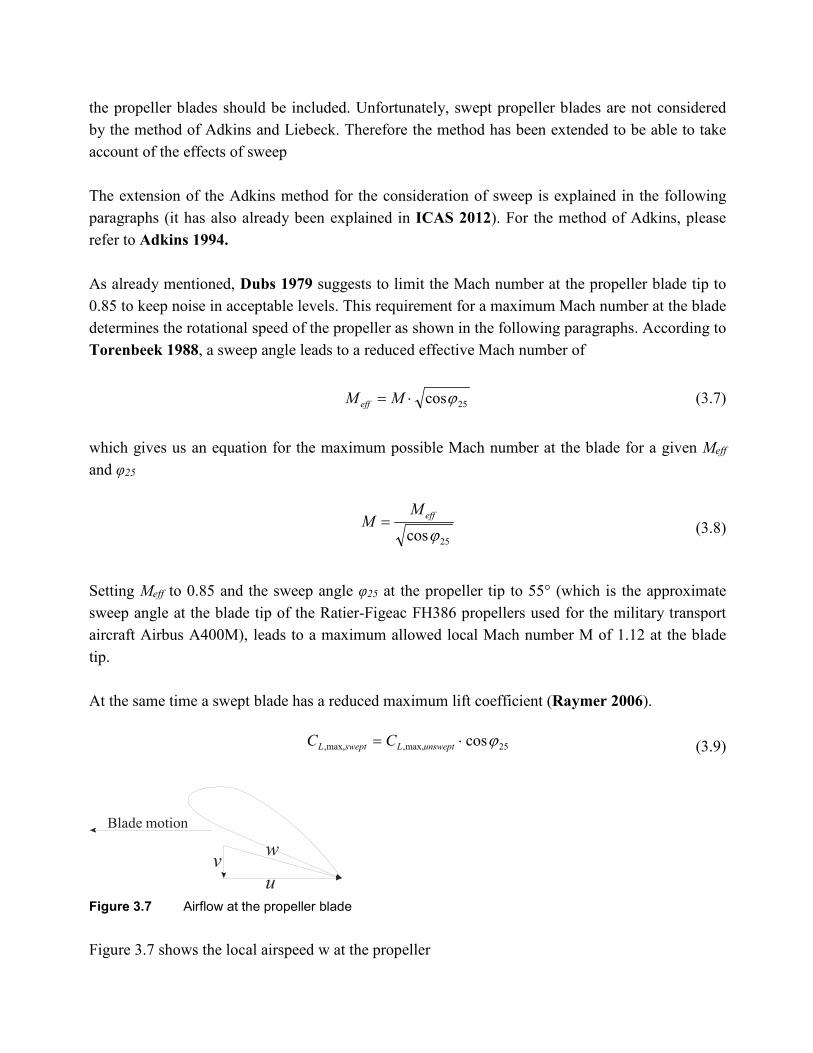
Figure 3.7 Airflow at the propeller blade

Figure 3.7 shows the local airspeed w at the propeller

22 uvw += (3.10) where the circumferential speed u is nDu ⋅⋅= π (3.11) with the propeller diameter D and the number of rotations per second n. The freestream velocity v is aMv ⋅= (3.12) with the speed of sound a. The calculated maximum Mach number of 1.12 together with D, a and the design cruise speed vCR can be used to determine the rotational speed of the propeller that leads to a maximum effective Mach number at the blade tip of 0.85.

( )

Dva

n CR

⋅−⋅

=π

2212.1 (3.13)

Setting Meff to 0.85 and M to 1.12 also allows to calculate the sweep angle of all other blade sec-tions using Equation 3.7 and Adkins 1994. The propeller design method finally leads to the optimum chord length, incidence angle and sweep angle at all considered blade sections and the overall propeller efficiency which has been used in the further aircraft design process.

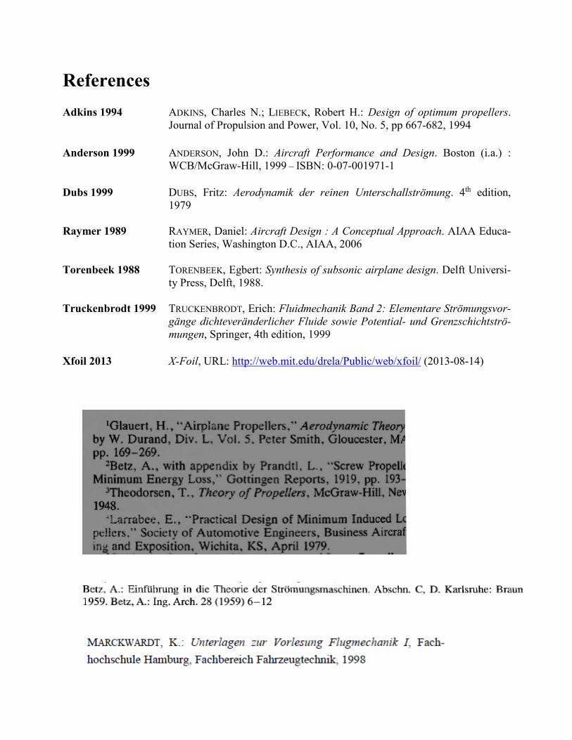
References Adkins 1994 ADKINS, Charles N.; LIEBECK, Robert H.: Design of optimum propellers.

Journal of Propulsion and Power, Vol. 10, No. 5, pp 667-682, 1994 Anderson 1999 ANDERSON, John D.: Aircraft Performance and Design. Boston (i.a.) :

WCB/McGraw-Hill, 1999 – ISBN: 0-07-001971-1 Dubs 1999 DUBS, Fritz: Aerodynamik der reinen Unterschallströmung. 4th edition,

1979 Raymer 1989 RAYMER, Daniel: Aircraft Design : A Conceptual Approach. AIAA Educa-

tion Series, Washington D.C., AIAA, 2006 Torenbeek 1988 TORENBEEK, Egbert: Synthesis of subsonic airplane design. Delft Universi-

ty Press, Delft, 1988. Truckenbrodt 1999 TRUCKENBRODT, Erich: Fluidmechanik Band 2: Elementare Strömungsvor-

gänge dichteveränderlicher Fluide sowie Potential- und Grenzschichtströ-mungen, Springer, 4th edition, 1999

Xfoil 2013 X-Foil, URL: http://web.mit.edu/drela/Public/web/xfoil/ (2013-08-14)