Embed Size (px)
Citation preview

Topics in Geometry, Coding Theory and Cryptography

Algebra and Applications
Volume 6
Managing Editor:
Alain VerschorenRUCA, Belgium
Series Editors:
Christoph SchweigertHamburg University, Germany
Ieke MoerdijkUtrecht University, The Netherlands
John GreenleesSheffield University, UK
Mina TeicherBar-llan University, Israel
Eric FriedlanderNorthwestern University, USA
Idun ReitenNorwegian University of Science and Technology, Norway
Algebra and Applications aims to publish well written and carefully refereedmonographs with up-to-date information about progress in all fields of algebra, itsclassical impact on commutative and noncommutative algebraic and differentialgeometry, K-theory and algebraic topology, as well as applications in relateddomains, such as number theory, homotopy and (co)homology theory, physics anddiscrete mathematics.Particular emphasis will be put on state-of-the-art topics such as rings of differentialoperators, Lie algebras and super-algebras, group rings and algebras, C*algebras,Kac-Moody theory, arithmetic algebraic geometry, Hopf algebras and quantumgroups, as well as their applications. In addition, Algebra and Applications will alsopublish monographs dedicated to computational aspects of these topics as well asalgebraic and geometric methods in computer science.

Topics in Geometry, CodingTheory and Cryptography
Edited by
Arnaldo GarciaInstituto de Matematica Pura e Aplicada (IMPA),
Rio de Janeiro, Brazil
and
Henning StichtenothUniversity of Duisburg-Essen, Germany and
Sabanci University, Istanbul, Turkey

A C.I.P. Catalogue record for this book is available from the Library of Congress.
ISBN-10 1-4020-5333-9 (HB)ISBN-13 978-1-4020-5333-7 (HB)ISBN-10 (e-book)
Published by Springer,P.O. Box 17, 3300 AA Dordrecht, The Netherlands.
www.springer.com
Printed on acid-free paper
All Rights Reserved
No part of this work may be reproduced, stored in a retrieval system, or transmittedin any form or by any means, electronic, mechanical, photocopying, microfilming, recording
or otherwise, without written permission from the Publisher, with the exceptionof any material supplied specifically for the purpose of being entered
and executed on a computer system, for exclusive use by the purchaser of the work.
1-4020-5334-4 ISBN-13 978-1 - 4 0 2 0 - 5 3 3 4 - (e-book)4
© 2007 Springer

Contents
Foreword vii
1.1
1 Introduction 1
2 Towers and Codes 5
3 Genus and Splitting Rate of a Tower 16
4 Explicit Tame Towers 24
5 Explicit Wild Towers 31
6 Miscellaneous Results 47
References 55
2. Function Fields over Finite Fields and Their Applications59
1 Introduction 59
2 Applications to Combinatorial Cryptography 60
3 Applications to Stream Ciphers and Linear Complexity 89
References 99
3. Artin-Schreier Extensions and Their Applicationsby C. Guneri and F. Ozbudak 105
1 Introduction 105
2 Artin-Schreier Extensions 107
3 Cyclic Codes and Their Weights 111
4 Trace Codes 120
5 Maximal Function Fields 126
References 130
v
¨ ¨
by A. Garcia and H. StichtenothExplicit Towers of Function Fields over Finite Fields
to Cryptography by H. Niederreiter, H. Wang and C. Xing
vi Contents
4. Pseudorandom Sequences by A. Topuzoglu and A. Winterhof 135
1 Introduction 135
2 Linear Complexity and Linear Complexity Profile 137
3 Autocorrelation and Related Distribution Measures for BinarySequences 154
4 Discrepancy and Uniform Distribution 157
References 162
5. Group Structure of Elliptic Curves over Finite Fields andApplications by R. Murty and I. Shparlinski 167
1 Introduction 167
2 Group Structure 171
3 Applications to Cryptography 180
References 187
195Algebraic Function Fields
About the Authors 199
Appendix:
˘

Foreword
The theory of algebraic function fields has a long history. Its origins are innumber theory, and there are close interrelations with other branches of puremathematics such as algebraic geometry or compact Riemann surfaces. In fact,the study of algebraic function fields is essentially equivalent to the study ofalgebraic curves. These relations have been well-known for a long time.
Around 1980 V. D. Goppa came up with a brilliant idea of constructing error-correcting codes by means of algebraic function fields over finite fields. Thesecodes are now known as geometric Goppa codes or algebraic geometry codes(AG codes). The key point of Goppa’s construction is that one gets informationabout the code parameters (length, dimension, minimum distance of the code)in terms of geometric and arithmetic data of the function field (number of ratio-nal places, genus). Goppa’s method can be seen as a “simple” generalizationof the construction of Reed-Solomon codes: one just replaces the evaluation ofpolynomials in one variable at elements of a finite field (which is used for thedefinition of Reed-Solomon codes) by evaluating functions of a function fieldat some of its rational places. A basic role is then played by the Riemann-Rochtheorem.
Soon after Goppa’s discovery, M. A. Tsfasman, S. G. Vladut and T. Zinkconstructed families of AG codes of increasing length whose asymptotic pa-rameters are better than those of all previously known infinite sequences ofcodes and which beat the Gilbert-Varshamov bound - a bound which is well-known in coding theory and which is a classical measure for the performanceof long codes. The proof of the Tsfasman-Vladut-Zink result uses two maintools: Goppa’s construction of AG codes and the existence of curves or func-tion fields (more specifically: classical or Drinfeld modular curves) over a finitefield having large genus and many rational places.
vii

viii Foreword
Cyclic codes have a natural representation as trace codes, and one can asso-ciate with each codeword of a trace code an Artin-Schreier function field. Prop-erties of this function field (specifically the number of rational places) reflectproperties of the corresponding cyclic code (namely the weights of codewordsand subcodes). In this way one gets another link between codes and functionfields which is entirely different from Goppa’s.
In 1985, N. Koblitz invented cryptosystems which are based on elliptic curves(or elliptic function fields) over a finite field. These cryptosystems are very pow-erful and attracted much attention; they created a new and very lively area ofresearch (elliptic curve cryptography) and brought together researchers frompure mathematics (number theory, arithmetic geometry) and applied mathemat-ics and engineering (cryptography). Similar as in the case of coding theory, thisinteraction proved fruitful for both sides, posing new problems and leading tomany interesting practical and theoretical results.
The above-mentioned applications of function fields in constructing goodlong codes (due to Goppa and to Tsfasman-Vladut-Zink) and in constructingpowerful cryptosystems via elliptic or hyperelliptic curves are now well-known.However, most mathematicians and engineers are not so familiar with manyother, entirely different applications of function fields. To mention some ofthem: dense sphere packings in high-dimensional spaces; sequences with lowdiscrepancy; multiplication algorithms in finite fields; the construction of non-linear codes whose asymptotic parameters are even better than the Tsfasman-Vladut-Zink bound; the construction of good hash families. In all these casesthe use of function fields leads to better results than those of classical approaches.
In this book we present five survey articles on some of these new devel-opments. Most of the material is directly related to the interactions betweenfunction fields and their various applications; in particular the structure and thenumber of rational places of function fields are always of great significance.When choosing the topics, we also tried to focus on material which has notyet been presented in books or review articles. So, for instance, we did not in-clude chapters about elliptic curve cryptography or about AG codes. There arenumerous interconnections between the individual articles. Wherever applica-tions are pointed out, a special effort has been made to present some backgroundconcerning their use. For the convenience of the reader, we have included anappendix which summarizes the basic definitions and results from the theoryof algebraic function fields.

Foreword ix
We give now a brief summary of the five chapters. More detailed descrip-tions are given in the introduction of each chapter.
Chapter 1. Towers of Algebraic Function Fields over Finite Fields, by Ar-naldo Garcia and Henning Stichtenoth. In this chapter, the authors give a com-prehensive survey of their work on explicit towers of algebraic function fieldshaving many rational places. This concept provides a more elementary and ex-plicit approach than class field towers and towers from modular curves. Towerswith many rational places play a crucial role in many “asymptotic” construc-tions, such as error-correcting codes (Tsfasman-Vladut-Zink), low-discrepancysequences (Niederreiter-Xing), and other applications of function fields in cryp-tography (see Chapter 2). Several examples of asymptotically good recursivetowers are presented in detail. The proofs for the behaviour of the genus inwild towers are considerably simplified, compared to the proofs in the originalpapers.
Chapter 2. Function Fields over Finite Fields and Their Applications toCryptography, by Harald Niederreiter, Huaxiong Wang and Chaoping Xing.This survey article focuses on several recent, less well-known applications offunction fields – specifically, function fields with many rational places – in cryp-tography and combinatorics. Many of these applications are due to the authors.Among the topics are constructions of authentication codes, frameproof codes,perfect hash families, cover-free families and pseudorandom sequences of highlinear complexity.
Chapter 3. Artin-Schreier Extensions and Their Applications, by Cem Guneriand Ferruh Ozbudak. Extensions of function fields of Artin-Schreier type pro-vide many examples of function fields having many rational places; this makesthem very interesting for coding theory. In this chapter, several other appli-cations of Artin-Schreier extensions are discussed, among them to the famousWeil bound for character sums, to weights of trace codes and to generalizationsof cyclic codes.
Chapter 4. Pseudorandom Sequences, by Alev Topuzoglu and Arne Winter-hof. Various constructions of pseudorandom sequences are based on functionfields, see Chapters 2 and 5. Therefore, some background material on the the-ory of pseudorandom sequences is presented in Chapter 4. In particular, theimportant concept of linear complexity and some related measures for the per-formance of pseudorandom sequences are discussed in this chapter.
Chapter 5. Group Structure of Elliptic Curves over Finite Fields and Ap-plications, by Ram Murty and Igor Shparlinski. Motivated by applications of

x Foreword
elliptic curves to cryptography, the structure of the group of Fq-rational pointsof an elliptic curve has attracted much attention. In particular it is an importantfeature for cryptographic applications if this group is cyclic or if it contains alarge cyclic subgroup. The authors give a survey of recent results on this topic.Techniques from many branches of number theory and algebraic geometry areused in this chapter.
Each chapter begins with a detailed introduction, giving an overview of itscontents and also giving some applications and motivation. It is clear that we donot want to present all proofs here. However, whenever possible, some typicalproofs are provided. Our aim is to stimulate further research on some promisingtopics at the border line between pure and applied mathematics; therefore eachchapter contains also an extensive list of references of recent research papers.
Some of the authors (A. Garcia, H. Niederreiter, I. Shparlinski, H. Stichtenoth,A. Winterhof and C. Xing) visited Sabancı University in Istanbul (Turkey) dur-ing the years 2002-2005, where they presented part of the material of thisvolume. It is our pleasure to thank our hosts at Sabancı University for theirsupport and hospitality.
January 2006
Arnaldo Garcia, Henning Stichtenoth
Chapter 1
EXPLICIT TOWERS OF FUNCTION FIELDSOVER FINITE FIELDS
Arnaldo Garcia and Henning Stichtenoth
1. IntroductionThe purpose of this review article is to serve as an introduction and at the same
time, as an invitation to the theory of towers of function fields over finite fields.More specifically, we treat here the case of explicit towers; i.e., towers wherethe function fields are given by explicit equations. The asymptotic behaviour ofthe genus and of the number of rational places in towers are important featuresfor applications to coding theory and to cryptography (cf. Chapter 2).
The interest in solutions of algebraic equations over finite fields has a longhistory in mathematics, especially when the equations define a one-dimensionalobject (a curve or, equivalently, a function field). The major result of thistheory is the Hasse-Weil theorem which gives in particular an upper bound forthe number of rational points in terms of the genus of the curve and of thecardinality of the finite field.
The Hasse-Weil theorem is equivalent to the validity of Riemann’s Hypoth-esis for the Zeta function associated to the curve by E. Artin, in analogy withthe classical situation in Number Theory. This upper bound of Hasse-Weil issharp, and the curves attaining this bound are called maximal curves. Y. Iharawas the first to notice that the Hasse-Weil bound can be improved for curves ofhigh genus, and he gave in particular an upper bound for the genus of maximalcurves in terms of the cardinality of the finite field.
We will use here the language of function fields; i.e., we will be closer toNumber Theory than to Algebraic Geometry. Hence the concepts we will dealwith are function fields, field extensions, traces, norms, valuations, places, ratio-
1
A. Garcia and H. Stichtenoth (eds.), Topics in Geometry, Coding Theory and Cryptography, 1–58.C© 2007 Springer.

2 Towers of Function Fields
nal places, ramification indices and inertia degrees, tame and wild ramification,etc.
Denote by Fq the finite field of cardinality q. For a function field F over Fq
we denote by N(F ) its number of Fq-rational places and by g(F ) its genus.The upper bound of Hasse-Weil is
N(F ) ≤ 1 + q + 2√q · g(F ),
and Ihara showed that if the equality holds above then 2g(F ) ≤ q(q − 1).The following real number
A(q) := lim supg(F )→∞
N(F )/g(F ),
where F runs over all function fields over the field Fq, was introduced by Ihara.It is of fundamental importance for the theory of function fields over a finitefield, since it gives information about how many rational places a function fieldF/Fq of large genus can have.
In order to investigate the quantity A(q), it is natural to study towers offunction fields over Fq; i.e., one considers sequences F = (F0, F1, F2, . . .)of function fields Fi over Fq with F0 ⊆ F1 ⊆ F2 ⊆ . . . with the propertyg(Fi) →∞. It can be seen easily that the limit of the tower
λ(F) := limn→∞
N(Fn)/g(Fn)
always exists (see Section 3), and it is clear that the estimate below holds:
0 ≤ λ(F) ≤ A(q).
As follows from the Hasse-Weil bound, we have that A(q) ≤ 2√q. Based on
Ihara’s ideas, this bound was improved by Drinfeld-Vladut who showed that
A(q) ≤ √q − 1.
But even before this bound of Drinfeld-Vladut was obtained, Ihara (and indepen-dently Tsfasman-Vladut-Zink) proved that if q is a square thenA(q) ≥ √q−1.We thus have the equality
A(q) =√q − 1, if q is a square.
The proofs given by Ihara and Tsfasman-Vladut-Zink use the fact that certainmodular curves have many rational points. However these curves are in generalnot easy to describe by explicit equations. Another approach due to J.-P. Serreuses class field theory in order to prove the existence of curves of arbitraryhigh genus with sufficiently many rational points. Also this construction is not

A. Garcia and H. Stichtenoth 3
explicit. Our purpose here is to stimulate the investigation of explicit towersof function fields over finite fields; i.e., the function fields of the towers shouldbe given explicitly by algebraic equations. The concept of explicit towers wasfirst introduced in 1995 in the paper [20].
These notes are organized as follows:
Section 2 contains basic concepts such as towers of function fields and theirlimits; recursive towers and the corresponding pyramids; tame and wildramification in towers; linear codes and their parameters. In Section 2 onealso finds:
- The statement of the fundamental Hasse-Weil theorem (Theorem 2.3).
- Serre’s “explicit formulae” for bounding the number of rational placesin a function field (Proposition 2.4).
- The Drinfeld-Vladut bound (Theorem 2.5).
- The Tsfasman-Vladut-Zink theorem connecting the asymptotics of func-tion fields with the asymptotics of linear codes (Theorem 2.7).
- Abhyankar’s lemma which is an important tool to study the behaviourof the genus in recursive towers (Theorem 2.11).
Section 3 is devoted to the investigation of the behaviour of the genus andof the number of rational places in towers of function fields over finitefields. It contains the following notions: the genus and the splitting rate of atower; subtowers; asymptotically good and asymptotically optimal towers;ramification locus and splitting locus of a tower. In Section 2 one also finds:
- A proof that the limit of a tower exists (Definition 3.4).
- The limit of a subtower is at least as big as the limit of the tower (Propo-sition 3.6).
- A sufficient condition which ensures that the genus of a tower is finite(Theorem 3.8 and Corollary 3.9).
- A sufficient condition which ensures that a tower has finite ramificationlocus (Proposition 3.10).
- A sufficient condition which ensures the existence of completely split-ting places (Proposition 3.13).
- A sufficient condition which ensures that a polynomial f(X,Y ) doesdefine a recursive tower (Proposition 3.14).
In Section 4 we investigate some interesting recursive tame towers, in whichevery step Fn+1/Fn is a Kummer extension. It contains the followingsubsections:

4 Towers of Function Fields
- Section 4.1: The optimal tower T1 over F4 which is given recursivelyby the equation Y 3 = X3/(X2 +X + 1).
- Section 4.2: For r ≥ 2 and q = r, the tower T2 over Fq which isdefined recursively by the equation
Y m = (X + 1)m − 1 with m = (q − 1)/(− 1).
This tower gives a very simple proof that A(q) > 0 if q is not a primenumber.
- Section 4.3: For q = p2 and p an odd prime number, the optimal towerT3 over Fq given recursively by the equation
Y 2 = (X2 + 1)/2X.
This tower corresponds to the modular curves X0(2n) and it revealssome remarkable properties of Deuring’s polynomial.
We also mention in Section 4 some other interesting towers from the papers[3, 14, 24, 33, 37].
Section 5 is devoted to recursive wild towers. Especially interesting are wildtowers where every stepFn+1/Fn is an Artin-Schreier extension, since someof the best towers known in the literature are of this type. We present here asimple method which allows a unified treatment of the genus behaviour ofseveral towers of Artin-Schreier type (Lemma 5.1). Section 5 contains thefollowing subsections:
- Section 5.1: The optimal tower W1 over Fq with q = 2, which isdefined recursively by the equation
Y + Y = X/(X−1 + 1).
A complete proof for the optimality of the tower W1 is given and thisproof is much simpler than the original one in [21].
- Section 5.2: The optimal tower W2 over Fq with q = 2, which isthe first explicit example in the literature attaining the Drinfeld-Vladutbound [20].
- Section 5.3: The optimal towerW3 over Fq with q = 2, which is givenrecursively by the equation
(Y − 1)/Y = (X − 1)/X.
- Section 5.4: The towerW4 over the field with eight elements, which isrecursively given by
Y 2 + Y = X + 1 + 1/X.

A. Garcia and H. Stichtenoth 5
This tower was first introduced in [30], and we give here a much simplerproof for its asymptotic behaviour.
- Section 5.5: The tower W5 over the cubic field Fq with q = 3 whichis defined recursively by the equation
Y − Y −1 = 1−X −X−(−1).
The tower W5 generalizes the tower W4 of Section 5.4, and its limitλ(W5) ≥ 2(2 − 1)/( + 2) gives the best known lower bound forIhara’s quantity A(3).
Section 6 contains some miscellaneous results on towers, among them acouple of conditions which easily show sometimes that a given tower isasymptotically bad (Theorem 6.2, Theorem 6.3 and Theorem 6.6). Thissection has the following subsections:
- Section 6.1: In a tower (F0, F1, F2, . . .) of function fields, the growthof the genus g(Fn) depends on the behaviour of the different degrees ofthe extensions Fn/Fn−1. This interrelation is explored in Theorem 6.1and Theorem 6.2 where sufficient conditions are given for the tower tohave finite or infinite genus.
- Section 6.2: Skew towers are asymptotically bad. This means: if theequation f(X,Y ) = 0 which defines a recursive tower has unequaldegrees in the variables X and Y , then the tower is asymptotically bad(Theorem 6.3).
- Section 6.3: Here the concept of the dual tower of a recursive tower isintroduced; if the ramification loci of the tower and of its dual tower aredistinct, then the tower is bad (Theorem 6.6).
- Section 6.4: This subsection contains a classification result on recursivetowers defined by an Artin-Schreier equation of prime degree p of theform
Y p + aY = ψ(X),
with a ∈ F×q and with a rational function ψ(X) ∈ Fq(X). If such a
tower is asymptotically good, then the function ψ(X) must have a veryspecific form (Theorem 6.8).
2. Towers and CodesThroughout this Chapter we denote by Fq the finite field with q elements and
by p = char(Fq) its characteristic. We are interested in function fields overFq (briefly, Fq-function fields) having many rational places with respect to thegenus. For basic concepts and facts about algebraic function fields (such as the

6 Towers of Function Fields
definitions of function fields, places, divisors, rational places, genus, ramifica-tion, and Riemann-Roch theorem, Hurwitz genus formula, etc.) we refer to theAppendix or to [48]. For an Fq-function field F we always assume through-out that Fq is the full constant field ofF ; i.e., that Fq is algebraically closed inF .
We denote by N(F ) the number of rational places and by g(F ) the genusof an Fq-function field F , and we will be mainly interested in the behaviourof the ratio N(F )/g(F ) for function fields of large genus. To investigate thisbehaviour, Ihara [31] introduced the following quantity A(q):
A(q) = lim supg(F )→∞
N(F )/g(F ),
where F runs over all function fields over Fq. To deal with this quantity A(q)one is naturally led to towers of function fields.
Definition 2.1. A tower F over Fq (or an Fq-tower) is an infinite sequenceF = (F0, F1, F2, ...) of function fields Fi/Fq such that
i) F0 F1 F2 . . . Fn . . .;
ii) each extension Fn+1/Fn is finite and separable;
iii) the genera satisfy g(Fn) →∞ as n→∞.
For an Fq-tower F the following limit does exist (see Section 3):
λ(F) = limn→∞
N(Fn)/g(Fn).
It is clear from the definitions that one has
0 ≤ λ(F) ≤ A(q).
Definition 2.2. The real number λ(F) is called the limit of the Fq-tower F .The tower F is called asymptotically good if it has a positive limit λ(F) > 0.If λ(F) = 0 then F is said to be asymptotically bad.
It is not easy in general to construct asymptotically good towers, and it is aneven harder task to construct towers over finite fields with large limits. Theseare the main concerns of this Chapter.
We start by deriving an upper bound forA(q), the so-called Drinfeld-Vladutbound. It states that
A(q) ≤ √q − 1. (2.1)
This bound is then also an upper bound for the limit of towers; i.e., the followinginequality holds for all Fq-towers F :
λ(F) ≤ √q − 1.

A. Garcia and H. Stichtenoth 7
In order to prove the upper bound in (2.1) for A(q) we will need the followingtheorem due to Hasse and Weil, which is the central result of the theory offunction fields over finite fields. It is equivalent to the validity of the RiemannHypothesis in this context, cf. [48, p.169]. Hasse [29] proved it for ellipticfunction fields (i.e., for g(F ) = 1), and Weil [61] proved it in the general case.For other proofs of the Hasse-Weil theorem we refer to [10] and [47].
We need some notation: for a function field F/Fq, let F (r) := F · Fqr bethe constant field extension of F of degree r, and let Nr(F ) := N(F (r)) bethe number of Fqr -rational places of the function field F (r) over Fqr . TheHasse-Weil theorem can be stated in the following form:
Theorem 2.3. (Hasse-Weil) Let F be an Fq-function field of genus g(F ) = g.Then there exist complex numbers α1, α2, . . . , α2g ∈ C with the followingproperties:
i) They can be ordered in such a way that
αg+i = αi for i = 1, . . . , g.
ii) The polynomial L(t) :=∏2g
i=1(1− αit) has integer coefficients. It followsin particular that each αi is an algebraic integer.
iii) For all r ≥ 1 we have
Nr(F ) = qr + 1−2g∑
i=1
αri .
iv) The absolute value of αi is
|αi| =√q for i = 1, . . . , 2g.
The elements α−1i ∈ C are the roots of the Zeta function associated to the
function field F/Fq. From item iv) and item iii) with r = 1, one gets theso-called Hasse-Weil bound
N(F ) ≤ q + 1 + 2√q · g(F ).
This bound implies immediately that A(q) ≤ 2√q. For the proof of the
Drinfeld-Vladut bound (2.1) we make use of Serre’s “explicit formulae”:
Proposition 2.4. (Serre) (see [49]). Let 0 = h(X) ∈ R[X] be a polynomialwith non-negative coefficients and with h(0) = 0. Suppose that the associatedrational function H(X), which is defined as
H(X) = 1 + h(X) + h(X−1),

8 Towers of Function Fields
satisfies the condition
H(β) ≥ 0 for all β ∈ C with |β| = 1.
Then for any function field F/Fq we have
N(F ) ≤ 1 +h(q1/2)h(q−1/2)
+g(F )
h(q−1/2).
Proof. LetF be a function field over Fq with g(F ) = g, and letα1, α2, . . . , α2g
be the associated complex numbers, ordered as in item i) of Theorem 2.3. Forsimplicity we set Nr(F ) = Nr and in particular N(F ) = N1. Write
h(X) =m∑
r=1
crXr,
with cr ∈ R and cr ≥ 0 for all r. Then we have
Nr = 1 + qr −g∑
i=1
(αri + αr
i ),
by item iii) of Theorem 2.3; hence
Nr · q−r/2 = q−r/2 + qr/2 −g∑
i=1
((αiq−1/2)r + (αiq
−1/2)r)
(2.2)
= q−r/2 + qr/2 −g∑
i=1
(βri + βr
i ),
with βi = αiq−1/2. By item iv) of Theorem 2.3, the complex numbers βi have
absolute value |βi| = 1, so βi = β−1i . We now multiply Equation (2.2) by the
coefficient cr of h(X) and we sum up for r = 1, . . . ,m, to obtain
m∑
r=1
Nr · cr · q−r/2 = h(q−1/2) + h(q1/2) + g −g∑
i=1
H(βi), (2.3)
as follows from the definition of the rational function H(X). We then rewriteEquation (2.3) as follows
N1 · h(q−1/2) = h(q−1/2) + h(q1/2) + g −R,
with
R =g∑
i=1
H(βi) +m∑
r=1
(Nr −N1)crq−r/2.

A. Garcia and H. Stichtenoth 9
Since Nr ≥ N1, cr ≥ 0 and H(βi) ≥ 0, it follows that R ≥ 0 and hence
N1 · h(q−1/2) ≤ h(q−1/2) + h(q1/2) + g.
Now we can prove:
Theorem 2.5. (Drinfeld-Vladut bound) (see [12]). The following boundholds:
A(q) ≤ √q − 1.
In particular we have for any tower F over Fq:
λ(F) ≤ √q − 1.
Proof. For each m ∈ N with m ≥ 2 we consider the polynomial hm(X) ∈R[X] which is given by
hm(X) =m∑
r=1
(1− r
m
)·Xr. (2.4)
The key point of the proof of Theorem 2.5 is the following equality
hm(X) =X
(X − 1)2·(Xm − 1m
+ 1−X)
, (2.5)
which we prove in Lemma 2.6 below. For the associated rational functionHm(X) we then get
Hm(X) = 1 + hm(X) + hm(X−1)
= 1 +X
(X − 1)2
(Xm − 1m
+ 1−X)
+X−1
(X−1 − 1)2
(X−m − 1
m+ 1−X−1
)
(2.6)
=X
(X − 1)2· X
m +X−m − 2m
=2− (Xm +X−m)m(X − 1)(X−1 − 1)
.
For any complex number β = 1 with |β| = 1, the numbers (β−1)(β−1−1)and 2 − (βm + β−m) are positive real numbers. Hence the hypothesis inProposition 2.4 is satisfied; i.e., we have Hm(β) ≥ 0 for all β ∈ C with

10 Towers of Function Fields
|β| = 1. It follows from Proposition 2.4 that for any function field F over Fq
with genus g(F ) > 0 the following inequality holds for all m ≥ 2
N(F )g(F )
≤ 1hm(q−1/2)
+1
g(F )·(
1 +hm(q1/2)hm(q−1/2)
)
. (2.7)
Using again Equation (2.5) we see that
limm→∞
1hm(q−1/2)
=√q − 1.
Let ε > 0 be a real number and choose n = n(ε) such that
1hn(q−1/2)
≤ √q − 1 + ε/2.
Choose g0 = g0(ε, n) such that
1g0·(
1 +hn(q1/2)hn(q−1/2)
)
< ε/2.
Then we conclude from (2.7) with m = n = n(ε) that for all function fieldsF/Fq with g(F ) ≥ g0,
N(F )g(F )
≤ (√q − 1 + ε/2) + ε/2 =
√q − 1 + ε.
We still have to prove Equation (2.5):
Lemma 2.6. For all m ≥ 2 the following identity holds:
m∑
r=1
(1− r
m
)·Xr =
X
(X − 1)2·(Xm − 1m
+ 1−X)
.
Proof. We set
f(X) :=m∑
r=1
Xr =Xm+1 −XX − 1
;
then we haveX · f ′(X)
m=
m∑
r=1
r
m·Xr,

A. Garcia and H. Stichtenoth 11
and thereforem∑
r=1
(1− r
m
)·Xr = f(X)− X · f ′(X)
m
=X
X − 1· (Xm − 1)− X
m· (X − 1)((m+ 1)Xm − 1)− (Xm+1 −X)
(X − 1)2
=X
(X − 1)2·(Xm − 1m
+ 1−X)
.
The interest in the quantity A(q) also arose from applications of functionfields to coding theory, cf. [48, 54]. The Tsfasman-Vladut-Zink theoremestablishes a close connection between the asymptotics of Fq-function fields(represented by the quantityA(q)) and the asymptotics of codes over Fq. Someconnections to cryptography are discussed in Chapter 2. For further connec-tions to other areas we refer to [2, 40, 41, 44, 50, 52, 59].
Let us briefly recall the connection to coding theory. A linear code C overFq of length n = n(C) is a linear subspace of F
nq . The dimension k = k(C)
of C is its dimension as a vector space over Fq. An important parameter of alinear code C = 0 is its minimum distance d = d(C), which is defined by
d = min wt(c) | c ∈ C and c = 0,
where for a nonzero vector c = (c1, . . . , cn) ∈ Fnq its weight wt(c) is given by
wt(c) = #i | 1 ≤ i ≤ n and ci = 0.
A linear code C over Fq of length n = n(C), dimension k = k(C) andminimum distance d = d(C) is briefly called an [n, k, d]-code, and the integersn, k and d are called the parameters of the code. In order to compare codesof different lengths, one also introduces relative parameters of the code C asfollows:
- the transmission rate R(C), given by R(C) = k(C)/n(C).
- the relative minimum distance δ(C), given by δ(C) = d(C)/n(C).
We then get a map ϕ : Fq-linear codes → [0, 1]× [0, 1] by setting
Cϕ−→ (δ(C), R(C)).
For a real number δ ∈ [0, 1] we consider the accumulation points of the imageof the map ϕ on the vertical line X = δ. The largest second coordinate of

12 Towers of Function Fields
such accumulation points on the line X = δ is denoted by αq(δ). We can nowstate the connection of the asymptotics of codes (represented by αq(δ)) withthe quantity A(q) that represents the asymptotics of Fq-function fields:
Theorem 2.7. (Tsfasman-Vladut-Zink) (see [54], [48, p.207] ). Let q be aprime power such that A(q) > 1. Then
αq(δ) ≥ 1−A(q)−1 − δ.
This result ensures the existence of arbitrary long codes (i.e., codes of arbi-trary large length) having good parameters. For many values of q, Theorem 2.7improves on the so-called Gilbert-Varshamov bound, which is a bound knownfrom elementary coding theory, see [36].
Theorem 2.7 asks for good lower bounds forA(q). For arbitrary q one knowsthat A(q) > c · log q > 0 with a real constant c > 0, see [47]. The actual valueof A(q) is only known when q = 2 is a square. In this case we have thefollowing result (see [31, 54] and Sections 4 and 5 below):
A(2) = − 1, for any prime power .
This shows that the Drinfeld-Vladut bound given in Theorem 2.5 is sharp forfinite fields of square cardinality. If q = 3 is a cube, then we have the followinggood lower bound (see [8, 61] and also Section 4):
A(3) ≥ 2(2 − 1)+ 2
, for any prime power .
Much less is known about the quantity A(r) for prime exponents r ≥ 5.
Usually one gets information about the quantity A(q) through the limits oftowers of function fields over Fq. The towers which appear in the literature areof the following three types:
class field towers, cf. [43, 47];
modular towers, cf. [14, 16, 31, 54];
explicit towers, cf. [14, 21, 24].
By an explicit tower we mean a tower F = (F0, F1, F2, . . .) where each of thefunction fields Fi is given by explicit polynomial equations. For practical ap-plications in coding theory and cryptography one needs an explicit descriptionof the underlying function fields and of their Fq-rational places.

A. Garcia and H. Stichtenoth 13
Here we will mainly deal with explicit towers. Even more, the explicitdescription of the function fields F0, F1, F2, . . . in the tower F will often havethe following very simple shape:
Definition 2.8. Let F = (F0, F1, F2, . . .) be a tower of function fields overFq, where F0 = Fq(x0) is the rational function field. We say that the towerF is recursive if there exist a polynomial f(X,Y ) ∈ Fq[X,Y ] and functionsxn ∈ Fn such that:
i) f(X,Y ) is separable in both variables X and Y ;
ii) Fn+1 = Fn(xn+1) with f(xn, xn+1) = 0, for all n ≥ 0;
iii) [Fn+1 : Fn] = degY f(X,Y ), for all n ≥ 0.
We also say that the tower F is given by the equation f(X,Y ) = 0 or thatF is defined recursively by the polynomial f(X,Y ). Sometimes a tower isrecursively given by an equation of the form
g(X,Y ) = h(X,Y ) (2.8)
with rational functions g(X,Y ) and h(X,Y ) ∈ Fq(X,Y ). It is obvious that,after clearing denominators, Equation (2.8) can be transformed into the formf(X,Y ) = 0 with a polynomial f(X,Y ) ∈ Fq[X,Y ]. For example, thedefining equation
Y − Y = X/(X−1 + 1)
can be transformed into the polynomial equation
f(X,Y ) = (X−1 + 1) · (Y − Y )−X = 0,
cf. Section 5.1 below.
For a recursive tower F = (F0, F1, F2, . . .), much information about it isalready contained in the field F1 = Fq(x0, x1). So we define:
Definition 2.9. Let F be a recursive tower over Fq given by the polynomialequation f(X,Y ) = 0. Then its basic function field is defined as
F = Fq(x, y), with the relation f(x, y) = 0.
It will be shown in Section 6.2 that for a recursive tower F with positivelimit λ(F) > 0 one has
degX f(X,Y ) = degY f(X,Y ).

14 Towers of Function Fields
For the corresponding basic function field F = Fq(x, y) this condition meansthat
[F : Fq(x)] = [F : Fq(y)] if λ(F) > 0.
We recall the concepts of tame and wild ramification (see [48, p. 94]).
Definition 2.10. Let E/F be a function field extension. A place Q of the fieldE is tamely ramified (or tame) in the extensionE/F , if the characteristic p doesnot divide the ramification index e(Q|P ), where P is the restriction ofQ to thefield F . Otherwise we say that Q is wild in the extension E/F . The extensionE/F is called tame if all places of E are tame in E/F .
For example, a Galois extension E/F whose degree is relatively prime tothe characteristic is a tame extension. This is the case for Kummer extensions(see Section 4). On the contrary, in the case of Artin-Schreier extensions (seeSection 5) we have that all ramified places are wild.
The most convenient way to work with recursive towers is to think of themas pyramids; i.e., one considers in the same picture the fields
Fq(xn, xn+1, . . . , xm), for all natural numbers n ≤ m.
We illustrate this way of thinking of a recursive tower with Figure 2.1 (see nextpage) that reaches the 8th step of the tower. The tower itself appears on the leftedge of the pyramid.
For instance, the fields E and H in Figure 2.1 are E = Fq(x1, x2, x3, x4)and H = Fq(x2, x3, x4, x5, x6). All fields on the same horizontal line are iso-morphic to each other (for example, F3 E E′ and F4 H).
Let Q be a place of the field F8, just for reasoning in the concrete situationof Figure 2.1. For the determination of the genus g(F8) one is led, by Hurwitzgenus formula, to consider the ramification indices of (the restrictions of) Q inthe various field extensions in Figure 2.1; i.e., in the extensions F8/F7, F8/F0,G/E,G/H , etc. One starts from the extensions at the base of the pyramid; i.e.,from the extensions
Fq(xn, xn+1)/Fq(xn) and Fq(xn, xn+1)/Fq(xn+1),
with 0 ≤ n ≤ 7. Knowing ramification indices in the extensions F/Fq(x) andF/Fq(y), where F = Fq(x, y) is the corresponding basic function field, onegets the ramification indices of the place Q at the base of the pyramid from thevalues x0(Q), x1(Q), . . . , x8(Q). Then one tries to climb up the pyramid tothe right and to the left by using repeatedly the following fundamental tool:

A. Garcia and H. Stichtenoth 15
Theorem 2.11. (Abhyankar’s lemma) (see [48, p.125]). Let E/F be afunction field extension and let E1, E2 be two intermediate fields with E =E1 ·E2 (i.e., E is the composite field ofE1 andE2). LetQ be a place ofE anddenote by Q1, Q2 and P its restrictions to E1, E2 and F . If Q1|P or Q2|P istame, then
e(Q|P ) = lcm(e(Q1|P ), e(Q2|P )),
where lcm stands for the least common multiple.
Let us consider again the situation as in Figure 2.1. Suppose that all ramifica-tions at the base of the pyramid are tame. It is then obvious that one gets easilyall ramification indices in the pyramid by using Abhyankar’s lemma repeatedly.
The situation is more difficult if wild ramification occurs at the base of thepyramid. This is in fact one of the major problems in dealing with the so-calledwild towers (see Section 5): all known examples of explicit wild towersF withλ(F) > 0 are such that the corresponding pyramids have infinitely many timesthe phenomenon illustrated in the following picture, where is a power of the

16 Towers of Function Fields
characteristic and moreover e(Q1|P ) = e(Q2|P ) = (with notations as inTheorem 2.11).
Abhyankar’s lemma does not apply in this situation, and it is in general ahard task to determine the ramification index e(Q|Q1) = ?. Even harder is ingeneral the determination of the different exponent d(Q|Q1) ofQ|Q1. We willdiscuss some special cases of this situation in Section 5.
3. Genus and Splitting Rate of a TowerAs before letF = (F0, F1, F2, . . .) be a tower of function fields over Fq. We
want to investigate the limit λ(F) = limn→∞N(Fn)/g(Fn) of the tower (thislimit does exist, see Proposition 3.2 and Definition 3.4). It will be convenientto treat the number of rational places and the genus separately.
Lemma 3.1. Let F0 ⊆ F ⊆ E be finite separable extensions of algebraicfunction fields over Fq. Then we have
N(F )[F : F0]
≥ N(E)[E : F0]
andg(F )− 1[F : F0]
≤ g(E)− 1[E : F0]
.
In particular, if g(F ) ≥ 2 then
N(F )g(F )− 1
≥ N(E)g(E)− 1
.
Proof. It is clear that N(E) ≤ [E : F ] ·N(F ). Dividing this inequality by thedegree [E : F0] = [E : F ] · [F : F0] we get
N(E)[E : F0]
≤ N(F )[F : F0]
.

A. Garcia and H. Stichtenoth 17
Since the extension E/F is separable, the Hurwitz genus formula gives that
2g(E)− 2 = [E : F ] · (2g(F )− 2) + deg Diff(E/F )
≥ [E : F ] · (2g(F )− 2).
We divide by 2[E : F0] to obtain the desired result.
Proposition 3.2. Given a tower F = (F0, F1, F2, . . .) over Fq, the followinglimits do exist:
ν(F) := limn→∞
N(Fn)/[Fn : F0] and γ(F) := limn→∞
g(Fn)/[Fn : F0].
Proof. By Lemma 3.1, the sequence (N(Fn)/[Fn : F0])n≥0 is monotonouslydecreasing, hence convergent in R. On the other hand, we have that the sequence((g(Fn) − 1)/[Fn : F0]) is monotonously increasing, hence convergent inR ∪ ∞. Since
limn→∞
(g(Fn)− 1)/[Fn : F0] = limn→∞
g(Fn)/[Fn : F0],
Proposition 3.2 follows.
Definition 3.3. The quantities ν(F) and γ(F) in Proposition 3.2 are called thesplitting rate and the genus of the tower F , respectively.
One has that0 ≤ ν(F) ≤ N(F0) and 0 < γ(F) ≤ ∞.
If γ(F) <∞, we say that the tower has finite genus.
It follows from Proposition 3.2 that the sequence N(Fn)/g(Fn) is conver-gent, since we have
N(Fn)g(Fn)
=N(Fn)/[Fn : F0]g(Fn)/[Fn : F0]
→ ν(F)γ(F)
, as n→∞.
This leads us to the following definition which is crucial for the theory of towers.
Definition 3.4. For any tower F = (F0, F1, F2, . . .) over Fq, the limit
λ(F) := limn→∞
N(Fn)/g(Fn)
is called the limit of the tower.
We know from Section 2 that 0 ≤ λ(F) ≤ A(q) ≤ √q − 1 (the last
inequality is the Drinfeld-Vladut bound). Recall that the tower F is said to be

18 Towers of Function Fields
asymptotically good if λ(F) > 0; it is asymptotically optimal if λ(F) = A(q).We clearly have:
Corollary 3.5. For a tower F over Fq one has that
λ(F) = ν(F)/γ(F).
Moreover, the following statements are equivalent:
i) The tower F is asymptotically good.
ii) The genus γ(F) is finite and the splitting rate ν(F) is strictly positive.
Let E = (E0, E1, E2, . . .) and F = (F0, F1, F2, . . .) be two towers overFq. We call E a subtower of F , if for any En there exists some Fm such thatEn ⊆ Fm.
Proposition 3.6. If E is a subtower of F , then λ(E) ≥ λ(F). In particular, ifthe tower F is asymptotically good (resp. optimal), then any subtower E of Fis also asymptotically good (resp. optimal).
Proof. LetEn ⊆ Fm, and suppose that g(En) ≥ 2 (which holds for sufficientlylarge n, since E is a tower). By Lemma 3.1 we have
N(En)g(En)− 1
≥ N(Fm)g(Fm)− 1
,
and hence λ(E) ≥ λ(F).
In order to study the limit λ(F) of a towerF , it is often suitable to investigateseparately the genus and the splitting rate of F . We start with the investigationof the genus.
Definition 3.7. Let F = (F0, F1, F2, . . .) be a tower over Fq, and let P bea place of F0. We say that P is ramified in the tower F if for some n ≥ 1there exists a place Q of Fn lying above P such that Q|P is ramified; i.e., theramification index satisfies e(Q|P ) > 1. If there exists an index n ≥ 1 and aplaceQ of Fn above P such thatQ|P is wildly ramified (i.e., the characteristicof Fq divides the ramification index e(Q|P )), thenP is said to be wildly ramifiedin the tower F . Otherwise, the place P is said to be tame in F . The set
V (F) := P | P is a place of F0 which is ramified in F
is called the ramification locus of F .
All asymptotically good towers which are known at present have a finiteramification locus. However, there are examples of non-recursive towers Fover Fq such that the ramification locus V (F) is infinite and the genus γ(F)

A. Garcia and H. Stichtenoth 19
is finite, see [13]. A tower F with finite ramification locus V (F) may haveinfinite genus γ(F) = ∞, but in many cases one can use the next theorem toensure the finiteness of γ(F).
Recall the following notations: Let E/F be a finite separable extension offunction fields, P a place of F and Q a place of E lying above P , then e(Q|P )(resp. d(Q|P )) denotes the ramification index (resp. the different exponent) ofthe place Q over P .
Theorem 3.8. Let F = (F0, F1, F2, . . .) be a tower with a finite ramificationlocus V (F). Suppose that for each placeP ∈ V (F) there exists a real constantcP > 0 such that, for all n ≥ 1 and for all places Q of Fn lying above P , wehave
d(Q|P ) ≤ cP · e(Q|P ).
Then the genus of the tower is finite and it satisfies
γ(F) ≤ g(F0)− 1 +12·∑
P∈V (F)
cP · degP <∞.
Proof. The Hurwitz genus formula for the extension Fn/F0 gives
2g(Fn)− 2 = (2g(F0)− 2) · [Fn : F0] + deg Diff(Fn|F0)
= (2g(F0)− 2)[Fn : F0] +∑
P∈V (F)
∑
Q|Pd(Q|P ) · degQ
≤ (2g(F0)− 2) · [Fn : F0] +∑
P∈V (F)
cP ·∑
Q|Pe(Q|P ) · degQ
= [Fn : F0] ·
2g(F0)− 2 +∑
P∈V (F)
cP · degP
,
where the last equality follows from the “fundamental equality”∑
Q|Pe(Q|P ) · f(Q|P ) = [Fn : F0],
see [48, p.64]. Dividing the inequality above by 2·[Fn : F0] and lettingn→∞,we obtain the desired result.
An important special case of Theorem 3.8 is the case of tame towers:
Corollary 3.9. Let F = (F0, F1, F2, . . .) be a tower with a finite ramificationlocus V (F), and suppose that all places P ∈ V (F) are tame in F . Then
γ(F) ≤ g(F0)− 1 +12·∑
P∈V (F)
degP.

20 Towers of Function Fields
Proof. By Dedekind’s different theorem, the different exponent of a tamelyramified place Q|P satisfies d(Q|P ) = e(Q|P )− 1, and hence we can choosecP := 1 for each place P ∈ V (F).
In Section 5 we will see that Theorem 3.8 can also be applied to some inter-esting wild towers.
How can one check if the ramification locus V (F) is finite? We discuss thisproblem in a particular case. Assume that the tower F = (F0, F1, F2, . . .) isrecursively defined by the equation
ϕ(Y ) = ψ(X), (3.1)
where ϕ(T ), ψ(T ) ∈ Fq(T ) are rational functions (see Definition 2.8). Asbefore, let F = Fq(x, y) be the corresponding basic function field which isgiven by the equation ϕ(y) = ψ(x), and define
V0 := P | P is a place of Fq(x) which ramifies in F/Fq(x).
The set V0 is finite, since the extension F/Fq(x) is separable. We also define
R0 := x(P ) | P ∈ V0. (3.2)
Clearly, this set R0 is a finite subset of Fq ∪ ∞.
Proposition 3.10. Let F = (F0, F1, F2, . . .) be a tower over Fq which isrecursively defined by Equation (3.1). Assume that there exists a finite subsetR ⊆ Fq ∪ ∞ such that the following two conditions hold:
a) The set R contains R0, with R0 as in Equation (3.2).
b) If β ∈ R and α ∈ Fq∪∞ satisfy the equationϕ(β) = ψ(α), then α ∈ R.
Then the ramification locus of the tower F satisfies
V (F) ⊆ P | P is a place of F0 with x0(P ) ∈ R;
in particular , V (F) is finite and moreover
∑
P∈V (F)
degP ≤ #R. (3.3)
Proof. Let P ∈ V (F). There is some n ≥ 0 and a place Q of Fn lying aboveP such that Q is ramified in the extension Fn+1/Fn. Let P ′ := Q ∩ Fq(xn)denote the place of Fq(xn) lying belowQ, and consider the following diagram:

A. Garcia and H. Stichtenoth 21
Since Q is ramified in Fn+1/Fn, the place P ′ is ramified in the extensionFq(xn, xn+1) over Fq(xn). Hence β := xn(P ′) ∈ R0. For i = 0, . . . , n weset αi := xi(Q); then (by Condition a)) we have that αn = β ∈ R. Since
ϕ(αi) = ψ(αi−1) for each i = 1, . . . , n,
it follows from Condition b) that αn−1, αn−2, . . . , α0 ∈ R, and in particularwe have x0(P ) = x0(Q) = α0 ∈ R. We have thus shown that P ∈ V (F)implies x0(P ) ∈ R. In order to prove Inequality (3.3) one just notes that∑
P∈V (F) degP is invariant under constant field extensions.
Now we start the investigation of the splitting rate. In particular we wantto establish a criterion analogous to Proposition 3.10 which implies a positivesplitting rate ν(F) > 0, for a particular class of recursive towers.
Definition 3.11. Let F = (F0, F1, F2, . . .) be a tower over Fq, and let P be arational place of F0 (i.e., degP = 1). We say that P splits completely in thetower F if P splits completely in all extensions Fn/F0; i.e., there are exactly[Fn : F0] places of Fn above the place P (and they are rational places of Fn).The set
Z(F) := P | P is a rational place of F0 which splits completely in F
is called the splitting locus of the tower F . It is obvious thatZ(F)∩V (F) = ∅.
Lemma 3.12. Let F be a tower over Fq. Then we have
ν(F) ≥ #Z(F).
Proof. The assertion is trivial since for alln, any placeP ∈ Z(F) has [Fn : F0]distinct extensions in the field Fn, all of them being rational places of Fn.
For a rational function field Fq(z) and an element α ∈ Fq, we denote by(z = α) the place which is the zero of the function z − α in Fq(z). Similarly,

22 Towers of Function Fields
(z = ∞) denotes the pole of the function z in Fq(z). We consider again a towerF over Fq which is defined recursively by the equation
ϕ(Y ) = ψ(X). (3.4)
Proposition 3.13. Let F = (F0, F1, F2, . . .) be a tower over Fq defined re-cursively by Equation (3.4), and let F = Fq(x, y) be the corresponding basicfunction field with the relation ϕ(y) = ψ(x). Assume that there exists a non-empty subset S of Fq ∪ ∞ which satisfies the following two conditions:
a) For all α ∈ S, the place (x = α) of Fq(x) splits completely in the extensionF/Fq(x).
b) If α ∈ S and if Q is a place of F lying above the place (x = α), theny(Q) ∈ S.
Then for all α ∈ S, the place (x0 = α) of F0 = Fq(x0) splits completely inthe tower F; i.e., we have (x0 = α) ∈ Z(F). In particular, the splitting ratesatisfies
ν(F) ≥ #S.
Proof. By induction: Letα ∈ S and letQ be a place ofFn lying above the place(x0 = α). Then xn(Q) =: β ∈ S, by Condition b). The place (xn = β) splitscompletely in the extension Fq(xn, xn+1)/Fq(xn), by Condition a). Thereforethe placeQ splits completely in the extension Fn+1/Fn. The inequality for thesplitting rate follows from Lemma 3.12.
Note that both conditions a) and b) in Proposition 3.13 follow from thestronger condition below:
Condition c) For all α ∈ S, the equation ϕ(T ) = ψ(α) has m = degϕdistinct roots in the set S.
For an absolutely irreducible polynomial f(X,Y ) ∈ Fq[X,Y ], it is ingeneral not true that the equation f(X,Y ) = 0 defines a recursive towerF = (F0, F1, F2, . . .); i.e., F0 = Fq(x0) is a rational function field andFn+1 = Fn(xn+1) with the relation f(xn, xn+1) = 0. It may happen, forinstance, that the fields defined in this way satisfy Fr = Fr+1 = Fr+2 = . . .,for some index r ≥ 1. However in many cases, the following proposition showsthat the equation f(X,Y ) = 0 defines indeed a recursive tower.
Proposition 3.14. Let f(X,Y ) ∈ Fq[X,Y ] be a polynomial which satisfiesthe condition degY f(X,Y ) = m ≥ 2, and let F0 ⊆ F1 ⊆ F2 ⊆ . . . be asequence of function fields over Fq, recursively defined by F0 = Fq(x0) andFn+1 = Fn(xn+1) with f(xn, xn+1) = 0. Suppose that for each n ≥ 0 thereexists a placeQn of Fn such that the following two conditions hold (see Figure3.2 below):

A. Garcia and H. Stichtenoth 23
a) There is a placeRn of the function field Fq(xn, xn+1) lying above the placePn := Qn ∩ Fq(xn), such that the ramification index of Rn|Pn satisfiese(Rn|Pn) = m.
b) The ramification index e(Qn|Pn) is relatively prime to m.
Then [Fn+1 : Fn] = m for all n ≥ 0, and the equation f(X,Y ) = 0 defines arecursive tower F over Fq.
Proof. We proceed by induction: Suppose that the field Fq is algebraicallyclosed inFn and consider the field extensionFn+1/Fn, withFn+1 = Fn(xn+1)and f(xn, xn+1) = 0. We have the following situation, where Pn is the re-striction of the placeQn to Fq(xn) andRn is the unique place of Fq(xn, xn+1)above Pn:
It follows from Abhyankar’s lemma, that the placeQn is ramified inFn+1/Fn
with ramification indexm. In particular we have that [Fn+1 : Fn] ≥ m. On theother hand, the element xn+1 satisfies the equation f(xn, xn+1) = 0 over Fn
and therefore [Fn+1 : Fn] = [Fn(xn+1) : Fn] ≤ m. Hence [Fn+1 : Fn] = m,the place Qn is totally ramified in Fn+1/Fn and Fq is also algebraically closedin Fn+1.
Remark 3.15. In many interesting cases (see Section 4 and Section 5), thepolynomial f(X,Y ) guarantees a very special ramification behaviour at thebase of the pyramid, which implies immediately that the equation f(X,Y ) = 0indeed defines a recursive tower. As before we set m := degY f(X,Y ) ≥ 2,and we assume that there exists a place P0 of Fq(x0) = F0 which leads to theramification picture in Figure 3.3.

24 Towers of Function Fields
This picture means: the place P0 of Fq(x0) is ramified in the extensionFq(x0, x1) over Fq(x0) with ramification index e = m. Hence there is just oneplaceQ1 of Fq(x0, x1) lying aboveP0, and this placeQ1 is totally ramified overP0. The place P1 := Q1∩Fq(x1) of Fq(x1) also has ramification index e = min the extension Fq(x1, x2)/Fq(x1), and we denote by Q2 the unique place ofFq(x1, x2) lying above P1, etc. Moreover we make the crucial assumption thatthe ramification indices e1 := e(Q1|P1), e2 := e(Q2|P2), e3 := e(Q3|P3), . . .are all relatively prime to m. Using Abhyankar’s lemma repeatedly as in theproof of Proposition 3.14 one concludes that [Fn : F0] = mn, that P0 is totallyramified inFn/F0 and that the equation f(X,Y ) = 0 indeed defines a recursivetower over Fq.
Remark 3.16. There are recursive towers which do not satisfy the assumptionsof Proposition 3.14. In such a case it seems to be more difficult to decide if thecorresponding equation f(X,Y ) = 0 defines indeed a tower (see [57, 58]).
4. Explicit Tame TowersBefore presenting some explicit asymptotically good tame towers of function
fields, we make the following general remark: Let F = (F0, F1, F2, . . .) be arecursive Fq-tower, given by a polynomial f(X,Y ) ∈ Fq[X,Y ]. Let h(Z) ∈Fq(Z) be a fractional linear transformation; i.e., h(Z) = (aZ + b)/(cZ + d)with a, b, c, d ∈ Fq and ad = bc. Then the tower F can also be defined by theequation
g(X,Y ) := f(h(X), h(Y )) = 0.
A. Garcia and H. Stichtenoth 25
Performing such a fractional linear transformation can sometimes transformthe defining equation to a nicer form, or it can make it easier to describe theramification locus or the splitting locus of the tower.
All towers T that we consider in this section are recursive tame towers,which satisfy the hypothesis of Proposition 3.10 and hence they have a finiteramification locus. Moreover they have a non-empty splitting locus Z(T ).Then we get from Section 3 the following lower bound for the limit λ(T ) ofthe tower T :
Lemma 4.1. Assume that T is a recursive tame tower defined by Equation (3.4)and satisfying the hypothesis of Proposition 3.10. Then its limit λ(T ) satisfiesthe estimate
λ(T ) ≥ 2 ·#Z(T )#R− 2
,
whereR is the finite set whose existence is the main assumption made in Propo-sition 3.10.
Proof. We have the inequalities ν(T ) ≥ #Z(T ) (see Lemma 3.12) and alsoγ(T ) ≤ (−2+#R)/2 (see Corollary 3.9 and Proposition 3.10). The assertionfollows then immediately since λ(T ) = ν(T )/γ(T ) (see Corollary 3.5).
The defining equations that we will consider in this section do give rise totowers of function fields T = (F0, F1, F2, . . .), since it will always be the casethat in all extensions Fn+1/Fn arising from our equations, there exist places ofthe field Fn that are totally ramified in Fn+1 (see Proposition 3.14 and Remark3.15).
4.1 The Tower T1
Consider the tower T1 over the field F4 with four elements, which is givenrecursively by the equation
Y 3 = X3/(X2 +X + 1). (4.1)
Let P = (x0 = ∞) denote the place at infinity of the rational function fieldF0 = F4(x0) and let Q denote a place of the field F1 = F0(x1) above P .The place P is a simple pole of the right hand side of the defining equationx3
1 = x30/(x
20 + x0 + 1), and we get
vQ(x31) = −e(Q|P ); hence e(Q|P ) = 3 and vQ(x1) = −1.

26 Towers of Function Fields
Here vQ denotes the valuation corresponding to the placeQ, and e(Q|P ) is theramification index of Q|P . This shows that the place P is totally ramified inthe field F1, and in particular that Q is the unique place of F1 above P . Also,since vQ(x1) = −1, the place Q is a simple pole for the right hand side of thedefining equation x3
2 = x31/(x
21 + x1 + 1), and we conclude as before that the
place Q is totally ramified in the field extension F2/F1, and so on. In this waywe see that the defining equation (4.1) really leads to a tower, since the placeP is totally ramified in all extensions.
Now we show that the place P0 = (x0 = 0) of F0 splits completely inthe tower. Let Q0 be a place of F1 above P0. From the defining equationx3
1 = x30/(x
20 + x0 + 1), we see that x1(Q0) = 0. We have that
F1 = F0(x1/x0), with (x1/x0)3 = 1/(x20 + x0 + 1).
Since x0(P0) = 0, it follows from the last equation above that P0 splits com-pletely in the extension F1/F0. Again we have that
F2 = F1(x2/x1), with (x2/x1)3 = 1/(x21 + x1 + 1).
Since x1(Q0) = 0, it follows from the last equation above that each of the threeplaces Q0 of F1 above P0 splits completely in the extension F2/F1, and so on.Thus the splitting locus of the tower T1 has cardinality #Z(T1) ≥ 1.
>From the theory of Kummer extensions (see [48, p.110 ff.]), or with argu-ments similar to the ones used above for the place P , one obtains that the setR0
in Proposition 3.10 (see Equation (3.2)) is given byR0 = (F4 \F2)∪∞; i.e.,the elements of R0 are the poles of the function X3/(X2 +X + 1), and theyare simple poles. We show now that the setR = F
×4 ∪∞ satisfies Condition
b) in Proposition 3.10. In fact if β = ∞ and α3/(α2 + α + 1) = β3, thenα =∞ or α2 + α+ 1 = 0, hence α ∈ R0. If β ∈ F
×4 then
α3/(α2 + α+ 1) = β3 = 1,
and hence α3 = α2 + α + 1. Since the characteristic is p = 2, we get(α+ 1)3 = α3 + α2 + α+ 1 = 0, therefore α = 1 ∈ R. From Lemma 4.1 weconclude now that the limit λ(T1) satisfies
λ(T1) ≥2 · 14− 2
= 1 =√
4− 1.
So the tower T1 over the field F4 attains the Drinfeld-Vladut bound; i.e., it isasymptotically optimal over F4.

A. Garcia and H. Stichtenoth 27
Performing the fractional linear transformation h(Z) = 1/Z, we see that thetower T1 can also be defined by the nicer equation Y 3 = (X + 1)3 − 1. Thetower T1 is therefore the very particular case = r = 2 of the following towerT2.
4.2 The Tower T2
Let be any prime power and let q = r , where r ∈ N and r ≥ 2. Considerthe tower T2 over Fq which is given recursively by the equation
Y m = (X + 1)m − 1, with m = (q − 1)/(− 1). (4.2)
Similarly as for the tower T1 one shows that the place P0 = (x0 = 0) of thefunction field F0 = Fq(x0) is totally ramified in all extensions Fn/F0, so thatEquation (4.2) does define a recursive tower T2 = (F0, F1, F2, . . .). One canalso argue as in Remark 3.15 as follows: In the ramification picture of Figure3.3 for the place P0 = (x0 = 0) one has that Pi is the zero of the function xi inFq(xi) for all i ≥ 0, and the ramification indices ei in Figure 3.3 are all equalto ei = 1 (as follows from the equation xm
i = (xi−1 + 1)m − 1). ThereforeEquation (4.2) does define a tower, and the place P0 is totally ramified in allextensions Fn/F0.
Let F = Fq(x, y) with ym = (x + 1)m − 1 be the basic function fieldcorresponding to the tower T2 and let V0 be the set of places of Fq(x) whichramify in F/Fq(x). The setR0 = x(P ) | P ∈ V0 (as defined in (3.2)) is heregiven by
R0 = β ∈ Fq | (β + 1)m = 1,as follows from the theory of Kummer extensions of function fields. We claimthat the set R := Fq satisfies the conditions in Proposition 3.10. In fact, wehaveR0 ⊆ Fq (sincem = (q−1)/(−1) is the norm exponent of the extensionFq/F), and for β ∈ Fq and α ∈ Fq with βm = (α + 1)m − 1 it follows that(α+1)m = 1+βm ∈ F, hence α ∈ Fq. By Proposition 3.10, the ramificationlocus V (T2) is finite and it satisfies
V (T2) ⊆ P | P is a place of F0 with x0(P ) ∈ Fq.
Next we show that the place P∞ = (x0 = ∞) of the rational function fieldF0 = Fq(x0) splits completely in the tower T2. We have
F1 = F0
(x1
x0 + 1
)
and
(x1
x0 + 1
)m
= 1−(
1x0 + 1
)m
.
The right hand side of the last equality above takes the value 1 at the place P∞,and since the exponent m = (q − 1)/( − 1) is the norm exponent of Fq/F

28 Towers of Function Fields
we conclude that P∞ splits completely in the extension F1/F0. Let Q∞ be aplace of F1 above P∞. Then we have from the equation xm
1 = (x0 + 1)m − 1that vQ∞(x1) = vQ∞(x0) = −1. Since
F2 = F1
(x2
x1 + 1
)
and
(x2
x1 + 1
)m
= 1−(
1x1 + 1
)m
,
it follows as above that the placeQ∞ splits completely in the extension F2/F1.Repeating this argument we find that P∞ splits completely in the tower T2, thus#Z(T2) ≥ 1. From Lemma 3.1, we then get a positive limit
λ(T2) ≥ 2/(q − 2) > 0;
i.e., the tower T2 over Fq is asymptotically good.
Using class field theory, J.-P. Serre [49] proved in particular thatA(q) > 0 forall prime powers q. The tower T2 above gives a very simple proof of this resultof Serre, when q is not a prime number. No asymptotically good explicit towerover a finite field of prime order is known at present, and it is one of the mainchallenges to construct an explicit asymptotically good tower over a prime field.
The tower T2 above is a special case of the so-called towers of Fermat type;these are defined as follows: Let a, b, c ∈ F
×q and letm ≥ 2 be a natural number
which is not divisible by p = char Fq. Then the equation
Y m = a(X + b)m + c
does define a tower over Fq, see [58]. Some of these towers of Fermat type canbe shown to be asymptotically good, with similar arguments as in Section 4.2above (see [24, 28]). For example, let be any prime power with ≥ 3 and letq = 2. Take m = − 1, choose any b ∈ F
× and consider the tower T over Fq
which is given recursively by the equation
Y −1 = −(X + b)−1 + 1.
Its limit satisfies λ(T ) ≥ 2/(− 2). In particular for = 3, we obtain a towerover the field F9 attaining the Drinfeld-Vladut bound. Using the transformationh(Z) = b · Z, we see that all these towers (for distinct values of b ∈ F
× ) are
equal to each other.
4.3 The Tower T3
In this subsection we discuss another interesting tame tower that was intro-duced in [24]. Let p be an odd prime number and let q = p2. Consider the

A. Garcia and H. Stichtenoth 29
equation
Y 2 =X2 + 1
2X(4.3)
over the field Fq. Similarly to the case of the tower T1 in Section 4.1, one seesthat Equation 4.3 does define recursively a tower T3 = (F0, F1, F2, . . .) over Fq,and that the place P∞ = (x0 = ∞) of the rational function field F0 = Fq(x0)is totally ramified in all extensions Fn/F0.
Let a ∈ Fq be such that a2 = −1 (note that such an element exists in Fq sinceq = p2). The set R0 in Proposition 3.10 is here given by R0 = 0,∞,±a.We claim that the set
R = 0,∞,±a,±1satisfies Condition b) in Proposition 3.10. This follows from the followingassertions, which are all easily verified:
- if β = 0 and β2 = (α2 + 1)/2α, then α = ±a.
- if β =∞ and β2 = (α2 + 1)/2α, then α ∈ 0,∞.
- if β = ±a and β2 = (α2 + 1)/2α, then α = −1.
- if β = ±1 and β2 = (α2 + 1)/2α, then α = 1.
Much harder is here the determination of a single rational place of F0 thatsplits completely over Fp2 in this tower T3. In fact, there are at least 2(p − 1)such places; i.e., #Z(T3) ≥ 2(p− 1). From this and from Lemma 4.1 we thenget
λ(T3) ≥2 · 2(p− 1)
6− 2= p− 1;
i.e., the tower T3 over Fp2 attains the Drinfeld-Vladut bound. In particular, oneconcludes that #Z(T3) = 2(p− 1).
For the description of the completely splitting places in the tower T3 thefollowing polynomial H(X) ∈ Fp[X] plays a crucial role:
H(X) =(p−1)/2∑
m=0
((p− 1)/2
m
)2
·Xm,
where((p−1)/2
m
)denotes the binomial coefficient. The polynomial H(X) is
the so-called Deuring polynomial; its roots parametrize supersingular elliptic

30 Towers of Function Fields
curves in Legendre normal form (see [5]). It is well-known (but non-trivial)that H(X) is a separable polynomial having all roots in the field Fp2 . The keypoint here is to prove the following polynomial identity (see [24]):
H(X4) = Xp−1 ·H((
X2 + 12X
)2)
. (4.4)
A nice remark by M. Zieve is that it follows from Equation (4.4) that the rootsof H(X) are in fact 4-th powers in the field Fp2 ; i.e., we have the followinginclusion
S := α ∈ Fp|H(α4) = 0 ⊆ Fp2 . (4.5)
Zieve’s argument is as follows: If H(α4) = 0 then H(((α2 + 1)/2α)2) = 0by Equation (4.4). Since all roots of H(X) are in Fp2 , it follows that α4 ∈ Fp2
and that ((α2 + 1)/2α)2 ∈ Fp2 , and then α2 ∈ Fp2 . We have thus shown
H(β2) = 0 ⇒ β ∈ Fp2 .
In particular, sinceH(((α2+1)/2α)2) = 0, we obtain that (α2+1)/2α ∈ Fp2 .Since also α2 ∈ Fp2 we see that the element α itself is in Fp2 . This provesthat the set S in (4.5) is contained in Fp2 (for another proof see H. G. Ruck’sappendix to [24]). The cardinality of S is #S = 2(p− 1), sinceH(0) = 0 andH(X) is a separable polynomial.
It is now a simple matter to check (using Equation (4.4)) that the set S in(4.5) above satisfies Condition c) just after Proposition 3.13, and hence it fol-lows from Proposition 3.13 that #Z(T3) ≥ #S = 2(p− 1).
It follows from the work of N. Elkies [14] that the tower T3 is in fact themodular tower X0(2n), see also [24, p.75 ff.].
The key identity Equation (4.4) satisfied by Deuring’s polynomial is provedby using Gauss’ hypergeometric differential equation. This idea of using certaindifferential equations to control rational places in tame towers was taken againby Beelen-Bouw, providing a more systematic technique for the search forasymptotically good tame towers. We just illustrate an application of theirtechnique: If p is a prime number and p ≡ ±1 mod 8, then the tower T overFp2 which is defined recursively by the equation
Y 2 =X(1−X)X + 1
attains the Drinfeld-Vladut bound, see Proposition 4.6 in [3] and Example 4.5in [24].

A. Garcia and H. Stichtenoth 31
All tame towers considered here so far have "separated variables"; i.e., theyare all defined recursively by an equation ϕ(Y ) = ψ(X) with two rationalfunctions ϕ(Y ) ∈ Fq(Y ) and ψ(X) ∈ Fq(X). There are also very interestingtame towers with non-separated variables (see [33, 37]). For example, thefour recursive towers over Fp2 (for p = 2, 3, 5 and 7) given by the followingpolynomials f(X,Y ) are asymptotically optimal:
- Case p = 2 and f(X,Y ) = X2Y 3 + (X3 +X2 +X)Y 2 + (X + 1)Y +X3 +X .
- Case p = 3 and f(X,Y ) = 2XY 2 + (X2 +X + 1)Y +X2 +X + 2.
- Case p = 5 and f(X,Y ) = (4X + 1)Y 2 + (X2 +X + 2)Y +X + 3.
- Case p = 7 and f(X,Y ) = (X2 + 6)Y 2 +XY +X2 + 4.
All four towers above were shown to be elliptic modular by Elkies (see theappendix in [33]).
We finish this section with the remark that all optimal recursive towers pre-sented here support the “modularity conjecture” for such towers; a conjecturewhich was proposed by N. Elkies in [14].
5. Explicit Wild Towers
In this section we discuss wild towers F over Fq; i.e., towers such that thereexist places which are wildly ramified inF . As was pointed out at the end of Sec-tion 2, the calculation of the genus γ(F) for wild towers is more difficult than inthe case of tame towers, since Abhyankar’s lemma does not apply in general (seeFigure 2.2). Typical examples of wild towers are the so-called Artin-Schreiertowers F = (F0, F1, F2, . . .). Here F0 is the rational function field over Fq,and all extensions Fn+1/Fn are Galois of degree [Fn+1 : Fn] = p = char(Fq).As follows from Galois theory, there then exist elements xn+1 ∈ Fn+1 andzn ∈ Fn such that Fn+1 = Fn(xn+1) and xp
n+1 − xn+1 = zn, for all n ≥ 0.
In some cases of wild ramification, Lemma 5.1 below replaces Abhyankar’slemma. It will be very useful in order to estimate the genus γ(F) of somespecific wild towers (see Theorem 5.7 and Theorem 5.17 below). First werecall some notations and facts: Let E/F be a finite separable extension offunction fields, let P be a place of F and Q a place of E lying above P . Thene(Q|P ) and d(Q|P ) denote the ramification index and the different exponentof Q|P , respectively. If the extensions E/F is Galois of degree p = char(Fq),

32 Towers of Function Fields
it is well-known that d(Q|P ) = s · (e(Q|P ) − 1) for some s ≥ 2 (see [48, p.124]). The next result deals with the case when s = 2.
Lemma 5.1. Let F/Fq be a function field and let E1/F and E2/F be distinctGalois extensions ofF such that [E1 : F ] = [E2 : F ] = p = char(Fq). Denoteby E = E1 · E2 the composite field of E1 and E2. Let Q be a place of E anddenote byQ1, Q2 and P its restrictions to the subfieldsE1, E2 and F . Supposethat we have d(Qi|P ) = 2 · (e(Qi|P )− 1) for i = 1, 2. Then we also have
d(Q|Qi) = 2 · (e(Q|Qi)− 1) for i = 1, 2.
Proof. Denote by vP the discrete valuation of F corresponding to the place P(and by vQ, vQi the valuations ofE,Ei accordingly). The only non-trivial caseof Lemma 5.1 is when d(Q1|P ) = d(Q2|P ) = 2 · (p − 1). By the theory ofArtin-Schreier extensions (see [48, p. 115]) we can find elements x1 ∈ E1 andx2 ∈ E2 such that E1 = F (x1), E2 = F (x2) and moreover
xp1 − x1 = z1 and xp
2 − x2 = z2,
where z1 and z2 are functions in F with vP (z1) = vP (z2) = −1. It followsfrom the equation xp
1 − x1 = z1 that vQ1(x1) = −1. Since the residue classfield of F at the place P is perfect, there are elements u and w in F satisfying
z2z1
= up + w, vP (u) = 0 and vP (w) ≥ 1.
It follows that
xp2−x2 = z1u
p+z1w = (xp1−x1)up+z1w = ((x1u)p−x1u)+x1(u−up)+z1w.
Setting x3 := x2 − x1u, we obtain that E = E1(x3) and
xp3 − x3 = ux1 + w =: z3,
with vQ1(u) ≥ 0, vQ1(w) ≥ 0 and vQ1(x1) = −1. Hence we have vQ1(z3) =−1 or vQ1(z3) ≥ 0. If vQ1(z3) = −1, then e(Q|Q1) = p and d(Q|Q1) =2(p − 1); if vQ1(z3) ≥ 0, then e(Q|Q1) = 1 and d(Q|Q1) = 0. This showsthat we have d(Q|Q1) = 2(e(Q|Q1)− 1).
In the subsequent subsections 5.1 - 5.5 we shall investigate wild towersthat were introduced in the papers [8, 9, 20, 21, 30]. Using Theorem 3.8and Lemma 5.1, we will give simpler and less computational proofs of theasymptotic behaviour of the genus of the towers in [20, 21, 30].

A. Garcia and H. Stichtenoth 33
5.1 The Tower W1
This is an asymptotically optimal wild tower over a finite field with squarecardinality (see [21]). Let q = 2 where is a power of a prime number p. Weconsider the towerW1 over Fq which is recursively given by the equation
Y + Y =X
X−1 + 1. (5.1)
First we have to show that Equation (5.1) actually defines a tower.
Lemma 5.2. Let W1 = (F0, F1, F2, . . .) where F0 = Fq(x0) is the ratio-nal function field and Fn+1 = Fn(xn+1) with the relation x
n+1 + xn+1 =x
n/(x−1n + 1), for each n ≥ 0. Then the following holds:
i) For each n ≥ 0, the extension Fn+1/Fn has degree [Fn+1 : Fn] = , andthe field Fq is algebraically closed in Fn+1.
ii) The pole P∞ of x0 in F0 is totally ramified in all extensions Fn+1/F0. IfQn+1 denotes the unique place of Fn+1 above P∞, then Qn+1 is a simplepole of the function xn+1.
Proof. We proceed by induction. LetQn be the unique place of Fn above P∞,and let vQn denote the corresponding valuation ofFn. By induction hypothesis,we have vQn(xn) = −1. Let Qn+1 be a place of Fn+1 above Qn. It followsfrom Equation (5.1) that
vQn+1(xn+1 +xn+1) = e(Qn+1|Qn) ·vQn(x
n/(x−1n +1)) = −e(Qn+1|Qn).
Therefore the place Qn+1 is a pole of the function xn+1, and
−e(Qn+1|Qn) = vQn+1(xn+1 + xn+1) = · vQn+1(xn+1).
We then conclude that e(Qn+1|Qn) = and that vQn+1(xn+1) = −1. Allassertions of Lemma 5.2 follow now immediately.
Next we determine the ramification locus V (W1) of the tower W1. Recallthat (x0 = α) denotes the place of the rational function field F0 which is thezero of the function x0 − α.
Lemma 5.3. The ramification locus V (W1) of the towerW1 is given by
V (W1) = P∞ ∪ (x0 = α) | α + α = 0.
Proof. LetF = Fq(x, y) with y+y = x/(x−1+1) be the basic function fieldof the tower W1. It is clear from the theory of Artin-Schreier extensions (see[48, p.115]) that exactly the places (x = α), with α−1 + 1 = 0, and the pole

34 Towers of Function Fields
of x are ramified in the extension F/Fq(x). With notations as in Proposition3.10, we thus have
R0 = ∞ ∪ α | α−1 + 1 = 0.
Consider now the set
R := ∞ ∪ α | α + α = 0.
We want to apply Proposition 3.10 and therefore we have to show: if β ∈ Rand α ∈ Fq ∪ ∞ satisfy the equation
β + β = α/(α−1 + 1), (5.2)
then α ∈ R. First consider the case β = ∞. It follows from Equation (5.2)that α = ∞ or α−1 + 1 = 0, hence α ∈ R. In case β ∈ R \ ∞, Equation(5.2) gives
α/(α−1 + 1) = β + β = 0,
and it follows thatα = 0 ∈ R. So the hypothesis of Proposition 3.10 is satisfied,and we conclude that
V (W1) ⊆ P | P is a place of F0 with x0(P ) ∈ R= P∞ ∪ (x0 = α) | α + α = 0.
The places P∞ and (x0 = α) with α−1 + 1 = 0 are ramified in the extensionF1/F0, and it is easily verified that the place (x0 = 0) ramifies in the extensionF2/F0. This finishes the proof of Lemma 5.3.
The splitting locus Z(W1) of the tower W1 can be easily determined byusing Proposition 3.13.
Lemma 5.4. The splitting locus Z(W1) of the towerW1 is given by
Z(W1) = (x0 = α) | α ∈ Fq and α + α = 0.
In particular, the splitting rate ν(W1) satisfies the inequality ν(W1) ≥ 2 − .
Proof. Observe that the map γ → γ +γ (resp. the map γ → γ+1) is the trace(resp. the norm) map from Fq = F2 to the subfield F. Using notations as inProposition 3.13 we consider the set
S := α ∈ Fq | α + α = 0.
For α ∈ S, the equation
β + β = α/(α−1 + 1) = α+1/(α + α) ∈ F \ 0

A. Garcia and H. Stichtenoth 35
has distinct roots β in S. Thus Condition c) (just after the proof of Proposition3.13) is satisfied, and it follows from Proposition 3.13 that
Z(W1) ⊇ (x0 = α) | α ∈ Fq and α + α = 0. (5.3)
As V (W1) = P∞∪ (x0 = α) | α +α = 0 (by Lemma 5.3) and since wehave V (W1) ∩ Z(W1) = ∅, we conclude that equality holds in (5.3).
The previous lemmas show that the towerW1 has a finite ramification locusand a positive splitting rate, so it is a promising candidate for being asymptot-ically good. In the next lemmas we determine the different exponents of theramified places in the tower.
Lemma 5.5. Let F = Fq(x, y) with y + y = x/(x−1 + 1) be the basicfunction field of the towerW1. Then the following holds:
i) Both extensions F/Fq(x) and F/Fq(y) are abelian extensions with degrees[F : Fq(x)] = [F : Fq(y)] = .
ii) Let P be a place of Fq(x) (or of Fq(y)) which is ramified in F . Then Pis totally ramified in F . If Q is the place of F above P , then the differentexponent of Q|P is d(Q|P ) = 2(− 1) = 2(e(Q|P )− 1).
iii) Let = pa where p = char(Fq) and a ≥ 1. Then there exist intermediatefields in the extensions F/Fq(x) and F/Fq(y)
Fq(x) = M0 ⊆ . . . ⊆Ma = F and Fq(y) = L0 ⊆ . . . ⊆ La = F
with the following properties:
a) All extensions Mi+1/Mi and Li+1/Li are Galois of degree p.
b) If Pi is any place of the field Mi (resp. of Li) and Pi+1 is a place ofMi+1 (resp. of Li+1) above Pi, then the different exponent of Pi+1|Pi
is given by d(Pi+1|Pi) = 2 · (e(Pi+1|Pi)− 1).
Proof. i) All solutions of the equation γ + γ = 0 are in Fq, and the mapsy → y+γ yield distinct automorphisms ofF over Fq(x). Hence the extensionF/Fq(x) is Galois of degree , and the Galois group is abelian. The irreducibleequation between x and y can be rewritten as
(1x
)
+1x
=1
y + y(5.4)
and the same argument as above shows that the extension F/Fq(y) is alsoabelian of degree .ii) For the extension F/Fq(x), the assertion follows from the theory of Artin-Schreier extensions [48] and from the defining equation y+y = x/(x−1+1);

36 Towers of Function Fields
for the extension F/Fq(y) one considers Equation (5.4).iii) The existence of intermediate fields Mi (resp. Li) with Property a) is clear,from Galois theory. Property b) follows by induction from item ii) and fromthe following claim:Claim: LetN/L be an abelian extension of function fields over Fq with degreesatisfying [N : L] = pc, where p = char(Fq) and c ≥ 1, and let Q be a placeof N . Let M be an intermediate field and set P := Q ∩ L and R := Q ∩M .Suppose that d(Q|P ) = 2 · (e(Q|P )− 1). Then it follows that
d(Q|R) = 2 · (e(Q|R)− 1) and d(R|P ) = 2 · (e(R|P )− 1).
Proof of the Claim: Hilbert’s different formula (see [48, p. 124]) implies that
d(Q|R) ≥ 2 · (e(Q|R)− 1) and d(R|P ) ≥ 2 · (e(R|P )− 1).
The transitivity of different exponents then yields
d(Q|P ) = e(Q|R) · d(R|P ) + d(Q|R)≥ e(Q|R) · 2 · (e(R|P )− 1) + 2 · (e(Q|R)− 1) (5.5)
= 2 · (e(Q|P )− 1) = d(Q|P ).
Hence the inequality in (5.5) must be an equality, and the claim is proved. Thisfinishes also the proof of Lemma 5.5.
Lemma 5.6. Let W1 = (F0, F1, F2, . . .) be the tower over Fq which is recur-sively defined by Equation (5.1). For n ≥ 1, let Q be a place of Fn and setP = Q ∩ F0. Then
d(Q|P ) = 2 · (e(Q|P )− 1).
Proof. We refine the pyramid associated to the tower W1 with intermediatefields of degree p, according to Lemma 5.5 iii). Figure 5.1 below illustrates thisrefinement process:
For each extension of degree p on the bottom edges Fq(xn, xn+1)/Fq(xn)or Fq(xn, xn+1)/Fq(xn+1) of this pyramid, the different exponents are either2p − 2 or 0, as follows from Lemma 5.5. Climbing up the refined pyramid(using Lemma 5.1 repeatedly) it follows that for any subextension of degree pin the refined pyramid, the different exponents are either 2p−2 or 0. This holdsin particular along the left edge of the pyramid which represents the towerW1.By the transitivity of different exponents, Lemma 5.6 now follows.

A. Garcia and H. Stichtenoth 37
Theorem 5.7. Let q = 2 be a square, and let W1 = (F0, F1, F2, . . .) bethe tower over Fq which is recursively defined by the equation Y + Y =X/(X−1 + 1). Then we have:
γ(W1) = , ν(W1) = 2 − and λ(W1) = − 1.
In particular, the towerW1 attains the Drinfeld-Vladut bound and it is thereforeasymptotically optimal over Fq.
Proof. By Lemma 5.3, the ramification locus of the tower W1 has cardinality#V (W1) = +1. From Lemma 5.6 we have that for all placesP ∈ V (W1), alln ≥ 1 and all places Q of Fn above P , the different exponent of Q|P satisfiesd(Q|P ) ≤ 2e(Q|P ). Now Theorem 3.8 gives the following upper bound forthe genus γ(W1) of the towerW1:
γ(W1) ≤ −1 +12· 2 · (+ 1) = .
The splitting rate ν(W1) satisfies ν(W1) ≥ 2 − , by Lemma 4.4. Therefore
λ(W1) = ν(W1)/γ(W1) ≥ (2 − )/ = − 1.
On the other hand, we have λ(W1) ≤ − 1 by the Drinfeld-Vladut bound (seeTheorem 2.5). Hence λ(W1) = − 1, γ(W1) = and ν(W1) = 2 − .
Remark 5.8. i) It follows from the Drinfeld-Vladut bound and from Theorem5.7 that A(q) =
√q − 1 if q is a square.

38 Towers of Function Fields
ii) A detailed analysis of the ramification behaviour of the places P ∈ V (W1)in the towerW1 yields a precise formula for the genus g(Fn) as follows:
g(Fn) =
(q(n+1)/2 − 1)2 for n ≡ 1 mod 2;(qn/2 − 1)(q(n+2)/2 − 1) for n ≡ 0 mod 2.
(5.6)
The proof of Equation (5.6) is very technical and it requires subtle “pole orderreductions”, see [21]. If one just settles for the asymptotic result (i.e., forthe genus γ(W1) = of the tower W1), the proof of Theorem 5.7 given here(following the paper [26]) is much easier and shorter than the original one givenin [21].
5.2 The Tower W2
As in Section 5.1 let q = 2 be a square. For each divisor m ≥ 1 of (+ 1),we will construct here an asymptotically optimal tower W2 over Fq. In thespecial case m = + 1, the towerW2 coincides with the first explicit examplein the literature attaining the Drinfeld-Vladut bound, which is the content ofthe paper [20].
We start with the tower E = (E0, E1, E2, . . .) over Fq which is defined asfollows:
E0 = Fq(z0) is the rational function field,
E1 = E0(z1) = Fq(z1) with z1 + z1 = z0, and (5.7)
En+1 = En(zn+1) with zn+1 + zn+1 = z
n/(z−1n + 1), for all n ≥ 1.
It is clear that the tower (E1, E2, E3, . . .) is just the towerW1 that was discussedin Section 5.1, and thatE0 ⊆ E1 is the subfieldE0 = Fq(z
1 + z1) ⊆ Fq(z1) =E1. The place (z0 = 0) of E0 splits completely in E1/E0 into the places(z1 = α) of E1 with α + α = 0. The place (z0 = ∞) is the only ramifiedplace in the extension E1/E0; its extension to E1 is the pole (z1 = ∞) ofz1, and the different exponent d of (z1 = ∞) over (z0 = ∞) is given byd = 2( − 1). Therefore the ramification locus of the tower E is (see Lemma5.3)
V (E) = (z0 = 0), (z0 =∞).
For a place P0 ∈ V (E), an integer n ≥ 1 and a place Q0 of the field En lyingabove P0, we have
d(Q0|P0) = 2(e(Q0|P0)− 1). (5.8)
Equation (5.8) follows from Lemma 5.6 and the transitivity of different expo-nents applied to the extensions E0 ⊆ E1 ⊆ En. Now we fix an integer m ≥ 1

A. Garcia and H. Stichtenoth 39
which is a divisor of (+ 1) and we consider the fields
F0 := Fq(x0) with xm0 = z0, and
(5.9)
Fn := F0 · En for all n ≥ 1.
It is obvious that we thus obtain a tower
W2 := (F0, F1, F2, . . .) over Fq.
Figure 5.2 illustrates the towers E andW2:
For all i ≥ 0, the degrees of the field extensions in Figure 5.2 are
[Fi+1 : Fi] = [Ei+1 : Ei] = and [Fi : Ei] = m.
Theorem 5.9. Let q = 2 be a square and let m ≥ 1 be a divisor of ( + 1).Then the towerW2 over Fq which is defined by (5.7) and (5.9) is asymptoticallyoptimal; i.e., its limit is λ(W2) = − 1, and it attains therefore the Drinfeld-Vladut bound.
Proof. We consider the two towers E andW2 as illustrated in Figure 5.2. Fromthe equation xm
0 = z0 it follows that in the extension F0/E0 just the two places(z0 = 0) and (z0 = ∞) are (totally and tamely) ramified; the places of F0

40 Towers of Function Fields
above them are the places (x0 = 0) and (x0 = ∞), respectively. All otherplaces of E0 are unramified in F0/E0. Since the tower E has the ramificationlocus V (E) = (z0 = 0), (z0 = ∞), we conclude that the tower W2 hasramification locus
V (W2) = (x0 = 0), (x0 = ∞).
Let P ∈ V (W2) and let Q be a place of Fn lying above P . Set P0 = P ∩ E0,Q0 = Q ∩ En and e = e(Q0|P0). Since the ramification index e(Q0|P0) is apower of the characteristic p and sincem is a divisor of (+1), it follows fromAbhyankar’s lemma that we have the following situation:
We now calculate the different exponent d(Q|P0) in two different ways,using the transitivity of different exponents:
d(Q|P0) = e · d(P |P0) + d(Q|P ) = e · (m− 1) + d(Q|P ),
d(Q|P0) = m · d(Q0|P0) + d(Q|Q0) = m · (2e− 2) + (m− 1).
In the last equality above we have used Equation (5.8). Hence
d(Q|P ) = m · (2e− 2) + (m− 1)− e(m− 1) = (m+ 1)(e− 1). (5.10)
Now using Theorem 3.8 with cP = m + 1 (see Equation (5.10)) one gets anupper bound for the genus of the towerW2 as follows:
γ(W2) ≤ −1 +12· 2 · (m+ 1) = m. (5.11)
Next we determine the splitting locus Z(W2) of the tower W2. From Lemma5.4 and from the equation z
1 + z1 = z0, it is obvious that the splitting locus ofthe tower E is
Z(E) = (z0 = α) | α ∈ F and α = 0 = (z0 = α) | α−1 = 1.

A. Garcia and H. Stichtenoth 41
For α ∈ F \ 0, the equation βm = α has m distinct roots β ∈ Fq, since mis a divisor of (+ 1). Therefore all places in Z(E) split completely in F0/E0
and hence we have
Z(W2) ⊇ (x0 = β) | βm(−1) = 1.
This implies that the splitting rate ν(W2) satisfies the inequality
ν(W2) ≥ m · (− 1). (5.12)
We conclude from (5.11) and (5.12) that
λ(W2) = ν(W2)/γ(W2) ≥ m · (− 1)/m = − 1,
hence λ(W2) = − 1 and the towerW2 is asymptotically optimal.
Remark 5.10. We consider the special casem = +1 and we define for n ≥ 1the elements xn ∈ Fn recursively by
xn := zn/xn−1. (5.13)
It follows from the defining equations (5.7) and (5.9) of the tower W2 that thefollowing relation holds:
zn+1 + zn+1 = x+1
n , for all n ≥ 0. (5.14)
Equations (5.13) and (5.14) are just the defining equations of the asymp-totically optimal tower in the paper [20]. We have thus obtained a new (andmuch simpler) proof of the main result of [20], which states that γ(W2) =+ 1 in the case m = + 1.
5.3 The Tower W3
We describe now another wild tower which was investigated in detail in thepaper [9]. As before, let q = 2 be a square. Our starting point is the towerW1 from Section 5.1 which is given recursively by Y +Y = X/(X−1 +1).So W1 = (L0, L1, L2, . . .) where L0 = Fq(t0) and for each n ≥ 0, Ln+1 =Ln(tn+1) with the relation
tn+1 + tn+1 = tn/(t−1n + 1). (5.15)
Defining the function xn ∈ Ln by xn := (t−1n + 1)−1, a straightforward
calculation shows that the equation below holds (for all n ≥ 0):
xn+1 − 1x
n+1
=x
n − 1xn
. (5.16)

42 Towers of Function Fields
We setFn := Fq(x0, x1, . . . , xn) and thus obtain a subtowerW3 = (F0, F1, . . .)of the towerW1. As follows from Proposition 3.6, the towerW3 is also an as-ymptotically optimal tower over Fq. We summarize these results in the nexttheorem:
Theorem 5.11. Let q = 2 be a square. Then the equation
Y − 1Y
=X − 1X
(5.17)
defines recursively a towerW3 = (F0, F1, F2, . . .) over Fq withλ(W3) = −1;i.e., the towerW3 attains the Drinfeld-Vladut bound.
Remark 5.12. i) The tower W3 has some interesting features. While in thetowers W1 and W2 all steps Fi+1/Fi are Galois, this is not true for the towerW3 (if = 2). Also, if = 2 there occurs both wild and tame ramification inthe tower W3. As before (see Remark 5.8) an explicit formula for the genusg(Fn) requires subtle “pole order reductions” (see [9] for details).ii) One can show that the tower W3 is the same as the tower in [16, Equation(25)], where it is proved that the towers W1,W2 and W3 above are Drinfeldmodular.
5.4 The Tower W4
It seems to be more difficult to exhibit asymptotically good wild towers overfinite fields with non-square cardinalities. The first explicit example was foundby van der Geer - van der Vlugt [30]; it is a tower over the field with eightelements. We present now their example, giving a simplified proof for the limitof the tower. The van der Geer - van der Vlugt tower W4 = (F0, F1, F2, . . .)over the field F8 is recursively defined by the equation
Y 2 + Y = X + 1 + 1/X. (5.18)
Lemma 5.13. Equation (5.18) defines a tower W4 over the field F8. We have[Fn : F0] = 2n for all n ≥ 0, and the pole P∞ of the function x0 is totallyramified in all extensions Fn/F0.
Proof. Similar to the proof of Lemma 5.2.
We want to apply Proposition 3.13 to determine the splitting locus Z(W4)of the towerW4.
Lemma 5.14. We have Z(W4) ⊇ (x0 = α) | α ∈ F8 \ F2. Hence thesplitting rate satisfies ν(W4) ≥ 6.
Proof. Consider the basic function fieldF = F8(x, y) with y2+y = x+1+1/xand the set
S := F8 \ F2 = α ∈ F8 | α6 + α5 + α4 + α3 + α2 + α+ 1 = 0.

A. Garcia and H. Stichtenoth 43
Let α ∈ S and consider the solutions β ∈ F8 of the equation β2 + β =α+ 1 + α−1. Then one has
β2 +β = α+1+α−1, β4 +β2 = α2 +1+α−2 and β8 +β4 = α4 +1+α−4.
Adding these equations we obtain
β8 + β = α4 + α2 + α+ 1 + α−1 + α−2 + α−4
= α−4(α8 + α6 + α5 + α4 + α3 + α2 + 1)= α−4(α6 + α5 + α4 + α3 + α2 + α+ 1) = 0.
Hence β ∈ F8, so Condition a) of Proposition 3.13 is satisfied. It is also clearthat β = 0, 1, since otherwise α + 1 + α−1 = 0 and then α ∈ F8. So wehave β ∈ S and also Condition b) of Proposition 3.13 holds. Now Lemma 5.14follows from Proposition 3.13.
Next we determine the ramification locus V (W4) of the towerW4.
Lemma 5.15. We have V (W4) ⊆ (x0 = α) | α ∈ F4 or α =∞.
Proof. We use here Proposition 3.10. Let F = F8(x, y) be the basic functionfield of the tower W4 with y2 + y = x + 1 + 1/x. Only the places (x = 0)and (x = ∞) are ramified in the extension F/F8(x), so the set R0 as definedin (3.2) is R0 = 0,∞. Let β ∈ R := F4 ∪ ∞, and let α ∈ F8 ∪ ∞ be asolution of the equation
β2 + β = α+ 1 + α−1.
If β = ∞, then α = 0 or α = ∞. If β ∈ F4, then β2 + β ∈ F2 and α satisfiesan equation of degree 2 over F2, hence α ∈ F4. In all cases we have proved thatα ∈ R. Now the assertion of Lemma 5.15 follows from Proposition 3.10.
In fact it is an easy exercise to prove that the ramification locus V (W4) isequal to the set (x0 = α) | α ∈ F4 or α = ∞: for example, there is a placeP of F2 such that x0(P ) = 1, x1(P ) ∈ F4 \ F2 and x2(P ) = 0; this place isthen ramified in the extension F3/F2.
We also have an analogue to Lemma 5.5 for the basic function field associatedto the towerW4:
Lemma 5.16. Let F = F8(x, y) with y2 + y = x + 1 + 1/x be the basicfunction field of the tower W4. Then both extensions F/F8(x) and F/F8(y)are Galois of degree 2. If P is a place of F8(x) (or of F8(y)) which is ramifiedin F , and if Q is the place of F lying above P , then the different exponent ofQ|P is d(Q|P ) = 2.

44 Towers of Function Fields
Proof. This follows immediately from the two equations below (see [48, p.115]):
y2 + y = x+ 1 + 1/x and
(x
x+ 1
)2
+(
x
x+ 1
)
=1
y2 + y + 1.
Theorem 5.17. The tower W4 over F8, which is recursively defined by theequation Y 2 + Y = X + 1 + 1/X , is asymptotically good. Its limit λ(W4)satisfies
λ(W4) ≥ 3/2.
It follows in particular that Ihara’s quantity A(q) for q = 8 satisfies the in-equality A(8) ≥ 3/2.
Proof. LetW4 = (F0, F1, F2, . . .), let Q be a place of Fn and let P = Q∩F0
be the place of F0 belowQ. As in Lemma 5.6, it follows from Lemma 5.16 thatthe different exponent ofQ|P is d(Q|P ) = 2(e(Q|P )− 1). Now Theorem 3.8with cP = 2 and Lemma 5.15 yield
γ(W4) ≤ −1 +12· 5 · 2 = 4.
By Lemma 4.14 we have ν(W4) ≥ 6 and hence
λ(W4) = ν(W4)/γ(W4) ≥ 6/4 = 3/2.
Remark 5.18. i) One can calculate precisely the genus of all fields Fn inthe tower W4. These calculations are long and very technical, see [30]. Forinstance, one obtains the formula
g(Fn) = 2n+1 + 1− (n+ 2 · [n/4] + 15) · 2(n−3)/2
for n ≡ 1 mod 2.ii) For p a prime number, one has the following lower bound for the quantityA(p3) which is due to Zink (see [61]):
A(p3) ≥ 2(p2 − 1)/(p+ 2).
So the towerW4 gives a proof of this bound in the particular case p = 2.

A. Garcia and H. Stichtenoth 45
5.5 The Tower W5
Our last example of an asymptotically good wild tower is a generalization ofthe van der Geer - van der Vlugt tower presented in Section 5.4. It was studiedin detail in [8]. The constant field Fq has now cubic cardinality; i.e.,
q = 3 for some prime power .
We define the towerW5 over Fq recursively by the equation
Y − Y −1 = 1−X +X−(−1). (5.19)
For = 2 this equation is the same as the defining equation (see Equation(5.18)) of the towerW4. The tower in [8] is given recursively by
1− VV
=U + U − 1
U. (5.20)
The change of variables X = U−1 and Y = V −1 shows that Equation (5.19)and Equation (5.20) define in fact the same tower.
It is easily seen that Equation (5.19) defines a tower; the proof is similar tothe proof of Lemma 5.2. In order to determine the splitting locus Z(W5) werewrite Equation (5.19) as follows:
f(Y ) = 1− 1
f
(X
X − 1
) with f(T ) := T − T −1. (5.21)
One verifies easily that the polynomial f(T ) satisfies the equation
T · (f(T )+1 − f(T ) + 1) = (T − 1)2++1 + 1. (5.22)
We are going to use Proposition 3.13 and therefore we consider the set
S := α ∈ Fq | (α− 1)2++1 = −1 \ 0. (5.23)
Since q = 3, it is clear that S ⊆ Fq. From Equation (5.22) it follows that
S = α ∈ Fq | f(α)+1 − f(α) + 1 = 0. (5.24)
Using (5.23) one checks that
α ∈ S =⇒ α
α− 1∈ S. (5.25)
Take now an element α ∈ S and let β ∈ Fq be such that
β − β−1 = 1− α+ α−(−1).

46 Towers of Function Fields
Setting δ := α/(α− 1) we then have
f(β) = 1− 1f(δ)
with δ ∈ S,
by (5.21) and (5.25). Therefore from Equation (5.24) we have
f(β)+1 − f(β) + 1 =(
1− 1f(δ)
)+1
+1
f(δ)
=1
f(δ)+1(f(δ)+1 − f(δ) + 1) = 0.
It follows that β ∈ S, and we conclude from Proposition 3.13:
Lemma 5.19. All places (x0 = α) with (α − 1)2++1 = −1 and α = 0split completely in the tower W5. In particular we have that the splitting ratesatisfies
ν(W5) ≥ 2 + .
It is much more difficult to determine the genus γ(W5) of the towerW5. Forthe proof of the following result we refer to [8].
Theorem 5.20. Let q = 3 where is any prime power, and letW5 be the towerover Fq which is recursively defined by the equation
Y − Y −1 = 1−X +X−(−1).
Then we have
γ(W5) =2 + 22(− 1)
, ν(W5) ≥ 2 + and λ(W5) ≥2(2 − 1)+ 2
.
Corollary 5.21. For any cubic prime power q = 3 one has
A(3) ≥ 2(2 − 1)+ 2
.
Remark 5.22. i) If = p is a prime number, Corollary 5.21 is Zink’s lowerbound for A(p3) which was first obtained by considering degenerations of cer-tain modular surfaces, see [61].
ii) The ramification behaviour of the towerW5 is rather complicated, see [8] and[30]. For the case = 2, all stepsFn+1/Fn in the towerW5 = (F0, F1, F2, . . .)are non-Galois. In this case, some places are wildly ramified and some othersare tamely ramified. Again here the detailed analysis of the different exponentsof the ramified places gives an exact formula for the genus g(Fn) of all functionfields Fn in the towerW5.

A. Garcia and H. Stichtenoth 47
6. Miscellaneous ResultsIn this section we discuss some specific aspects of towers, and in particular
6.1 Genus and Different Degree
Let F = (F0, F1, F2, . . .) be a tower of function fields over Fq. Then thefield extensions Fn+1/Fn are separable of degree [Fn+1 : Fn] > 1, for all
n) is related to the degree of the different Diff(Fn/F0)by the Hurwitz genus formula. We want to explore this relation in detail. For all
n the degree of the different of the extension Fn/Fn−1:
Dn := deg Diff(Fn/Fn−1).
Theorem 6.1. Let F = (F0, F1, F2, . . .) be a tower of function fields overFq. Suppose that there exists a constant ε ∈ R with 0 ≤ ε < 1 such that thefollowing inequality holds:
Dn ≤ ε · [Fn : Fn−1] ·Dn−1 , for all n ≥ 2. (6.1)
Then the genus γ(F) of the tower F is finite and the estimate below holds:
γ(F) ≤ g(F0)− 1 +D1
2(1− ε) · [F1 : F0].
Proof. It follows immediately from (6.1) and from the transitivity of the dif-ferent that the following inequality
deg Diff(Fn/F0) ≤
n−1∑
j=0
ε j
·D1 · [Fn : F1]
holds, for all n ≥ 1. Using Hurwitz genus formula, we then have:
2g(Fn)− 2 = [Fn : F0](2g(F0)− 2) + deg Diff(Fn/F0)
≤ [Fn : F0] ·
2g(F0)− 2 +D1
[F1 : F0]·
n−1∑
j=0
ε j
≤ [Fn : F0] ·(
2g(F0)− 2 +D1
(1− ε)[F1 : F0]
)
.
the asymptotic behaviour of the genus of a tower. The results of Sections 6.1-
n ≥ 0. The genus g(F
Section 6.4 we present some classification results for Artin-Schreier towers.
n ≥ 1, we denote by D
6.3 often lead to a quick decision about asymptotical badness of a tower. In

48 Towers of Function Fields
Hence we obtain the desired estimate:
γ(F) = limn→∞
g(Fn)[Fn : F0]
≤ g(F0)− 1 +D1
2(1− ε) · [F1 : F0].
A counterpart to Theorem 6.1 is the following result.
Theorem 6.2. Let F = (F0, F1, F2, . . .) be a tower over Fq. Suppose thatthere exist positive real numbers ρ1, ρ2, . . . with the following properties:
a) ρn ≤ Dn = deg Diff(Fn/Fn−1), for all n ≥ 1.
b) ρn ≥ [Fn : Fn−1] · ρn−1 , for all n ≥ 2.
Then the genus of the tower is infinite. In particular the tower is asymptoticallybad; i.e., its limit satisfies λ(F) = 0.
Proof. Using again the transitivity of the different, one shows by induction that
deg Diff(Fn/F0) ≥ [Fn : F1] · n · ρ1, for all n ≥ 1.
Therefore from Hurwitz genus formula, we have that
2g(Fn)− 2 ≥ [Fn : F0](2g(F0)− 2) + [Fn : F1] · n · ρ1.
Dividing this inequality by [Fn : F0] and letting n→∞, we see that the genusof the tower satisfies γ(F) = limn→∞ g(Fn)/[Fn : F0] = ∞.
6.2 Skew Towers are Bad
LetF be a recursive tower with defining equation f(X,Y ) = 0. Consideringthe examples of asymptotically good towers in Section 4 and Section 5 one notesin all cases that degX f(X,Y ) = degY f(X,Y ). This is in fact a necessarycondition for the tower to be asymptotically good:
Theorem 6.3. (see [23]). Let F = (F0, F1, F2, . . .) be a recursive tower overFq defined by the equation f(X,Y ) = 0. If degX f(X,Y ) = degY f(X,Y ),then λ(F) = 0; i.e., the tower F is asymptotically bad.
Proof. We set a := degY f and b := degX f . It follows from the definition ofa recursive tower (see Definition 2.8) that [Fn+1 : Fn] = a and hence we have(for all n ≥ 1):
[Fn : F0] = an and [Fn : Fq(xn)] = bn. (6.2)
This means that the pyramid (see Figure 2.1) attached to the towerF is “skew”.Now we distinguish the cases a > b and a < b.

A. Garcia and H. Stichtenoth 49
Case 1: a > b. Considering the extension Fn/Fq(xn), we see from (6.2) thatN(Fn) ≤ bn(q + 1). Therefore the splitting rate ν(F) satisfies
ν(F) = limn→∞
N(Fn)/[Fn : F0] ≤ limn→∞
(q + 1) · (b/a)n = 0.
By Corollary 3.5, the tower is then asymptotically bad.
Case 2: a < b. Fix an index r ≥ 0 such that g(Fr) ≥ 2. For n ≥ r weconsider the fieldEr := Fq(xn, xn−1, . . . , xn−r) ⊆ Fn which is isomorphic toFr. The Hurwitz genus formula for the extension Fn/Er gives
2g(Fn)− 2 ≥ (2g(Er)− 2) · [Fn : Er] ≥ 2bn−r,
hence g(Fn) ≥ bn−r. It follows that the genus γ(F) satisfies
γ(F) = limn→∞
g(Fn)/[Fn : F0] ≥ limn→∞
bn−r/an =∞.
By Corollary 3.5, the tower F is asymptotically bad.
Example 6.4. As an application of Theorem 6.3 we investigate a generalizationof the tower W1 which was discussed in Section 5.1. Let q = s where is aprime power and s ≥ 2. Let
τ(T ) := T + T + . . .+ T s−1and µ(T ) := T 1++...+s−1
.
The polynomial τ(T ) (resp. µ(T )) represents the trace map (resp. the normmap) from Fq to its subfield F. We then consider the tower F over Fq whichis defined recursively by the equation
τ(Y ) =µ(X)τ(X)
. (6.3)
Observe that Equation (6.3) coincides with Equation (5.1) in the particular caseq = 2. As in Section 5.1 one can easily show that Equation (6.3) indeed definesa recursive tower F = (F0, F1, F2, . . .) over the field Fq with the followingproperties:
i) For all n ≥ 0, the extension Fn+1/Fn is Galois of degree [Fn+1 : Fn] =s−1 (cf. Lemma 5.2).
ii) All places (x0 = α) with α ∈ Fq and τ(α) = 0 are completely splitting inthe tower F (cf. Lemma 5.4).
For s = 2, the tower is asymptotically optimal over Fq (see Theorem 5.7). Fors ≥ 3 however, the tower is asymptotically bad. This follows from Theorem6.3, since the degree of the left hand side of Equation (6.3) is deg τ(Y ) = s−1,and the right hand side ψ(X) = µ(X)/τ(X) of Equation (6.3) has degree
degψ(X) = s−1 + s−2 + . . .+ = deg τ(Y ).
The last inequality above follows since s ≥ 3.

50 Towers of Function Fields
6.3 The Dual Tower
In this section we consider recursive towers. To such a tower F we shallassociate another tower G (called the dual tower of F), and we shall studyrelationships between F and G. The results of this section are from [6].
Definition 6.5. Let F be a recursive tower over Fq which is defined by thepolynomial f(X,Y ) ∈ Fq[X,Y ]. Then its dual tower G is the tower which isdefined recursively by the polynomial f(Y,X).
Definition 6.5 means that F = (F0, F1, F2, . . .) and G = (G0, G1, G2, . . .)where
Fn = Fq(x0, x1, . . . , xn) with f(xi, xi+1) = 0,
Gn = Fq(y0, y1, . . . , yn) with f(yi+1, yi) = 0,
for all n ≥ 1 and all indices i with 0 ≤ i ≤ n − 1. We identify the rationalfunction fields F0 = Fq(x0) and G0 = Fq(y0) by setting x0 = y0, and then wehave the following picture:
It is clear that the function fields Fn and Gn are isomorphic, for all n ≥ 0 ;henceN(Fn) = N(Gn) and g(Fn) = g(Gn). It follows that the towersF andGhave the same limit λ(F) = λ(G). Moreover, assuming that degX f(X,Y ) =degY f(X,Y ), which is a natural assumption (see Theorem 6.3), then one alsohas
γ(F) = γ(G) and ν(F) = ν(G).
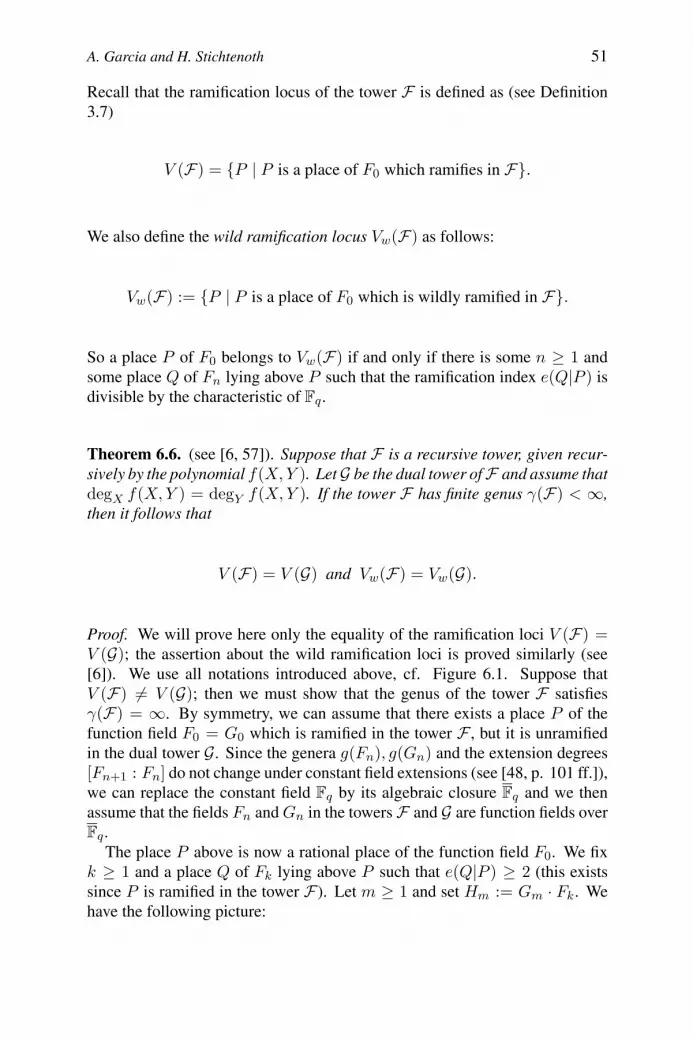
A. Garcia and H. Stichtenoth 51
Recall that the ramification locus of the tower F is defined as (see Definition3.7)
V (F) = P | P is a place of F0 which ramifies in F.
We also define the wild ramification locus Vw(F) as follows:
Vw(F) := P | P is a place of F0 which is wildly ramified in F.
So a place P of F0 belongs to Vw(F) if and only if there is some n ≥ 1 andsome place Q of Fn lying above P such that the ramification index e(Q|P ) isdivisible by the characteristic of Fq.
Theorem 6.6. (see [6, 57]). Suppose that F is a recursive tower, given recur-sively by the polynomial f(X,Y ). LetG be the dual tower ofF and assume thatdegX f(X,Y ) = degY f(X,Y ). If the tower F has finite genus γ(F) < ∞,then it follows that
V (F) = V (G) and Vw(F) = Vw(G).
Proof. We will prove here only the equality of the ramification loci V (F) =V (G); the assertion about the wild ramification loci is proved similarly (see[6]). We use all notations introduced above, cf. Figure 6.1. Suppose thatV (F) = V (G); then we must show that the genus of the tower F satisfiesγ(F) = ∞. By symmetry, we can assume that there exists a place P of thefunction field F0 = G0 which is ramified in the tower F , but it is unramifiedin the dual tower G. Since the genera g(Fn), g(Gn) and the extension degrees[Fn+1 : Fn] do not change under constant field extensions (see [48, p. 101 ff.]),we can replace the constant field Fq by its algebraic closure Fq and we thenassume that the fields Fn andGn in the towers F and G are function fields overFq.
The place P above is now a rational place of the function field F0. We fixk ≥ 1 and a place Q of Fk lying above P such that e(Q|P ) ≥ 2 (this existssince P is ramified in the tower F). Let m ≥ 1 and set Hm := Gm · Fk. Wehave the following picture:
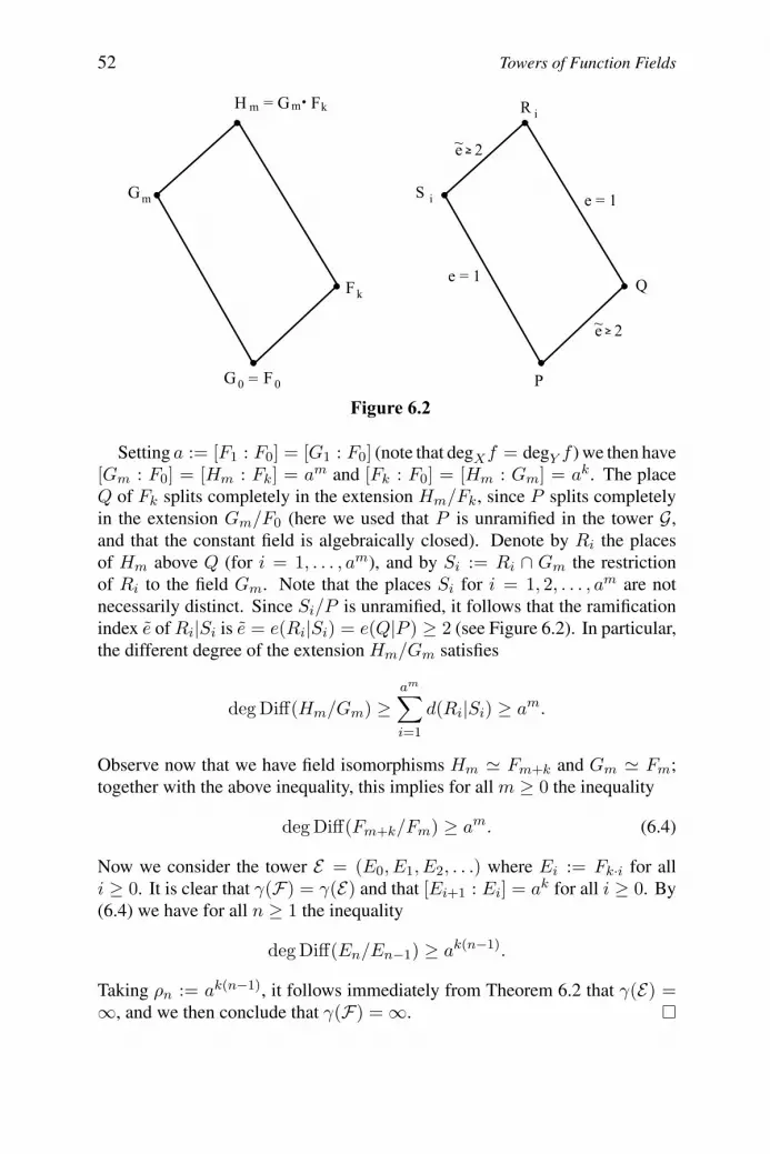
52 Towers of Function Fields
Setting a := [F1 : F0] = [G1 : F0] (note that degXf = degY f ) we then have[Gm : F0] = [Hm : Fk] = am and [Fk : F0] = [Hm : Gm] = ak. The placeQ of Fk splits completely in the extension Hm/Fk, since P splits completelyin the extension Gm/F0 (here we used that P is unramified in the tower G,and that the constant field is algebraically closed). Denote by Ri the placesof Hm above Q (for i = 1, . . . , am), and by Si := Ri ∩ Gm the restrictionof Ri to the field Gm. Note that the places Si for i = 1, 2, . . . , am are notnecessarily distinct. Since Si/P is unramified, it follows that the ramificationindex e ofRi|Si is e = e(Ri|Si) = e(Q|P ) ≥ 2 (see Figure 6.2). In particular,the different degree of the extension Hm/Gm satisfies
deg Diff(Hm/Gm) ≥am∑
i=1
d(Ri|Si) ≥ am.
Observe now that we have field isomorphisms Hm Fm+k and Gm Fm;together with the above inequality, this implies for all m ≥ 0 the inequality
deg Diff(Fm+k/Fm) ≥ am. (6.4)
Now we consider the tower E = (E0, E1, E2, . . .) where Ei := Fk·i for alli ≥ 0. It is clear that γ(F) = γ(E) and that [Ei+1 : Ei] = ak for all i ≥ 0. By(6.4) we have for all n ≥ 1 the inequality
deg Diff(En/En−1) ≥ ak(n−1).
Taking ρn := ak(n−1), it follows immediately from Theorem 6.2 that γ(E) =∞, and we then conclude that γ(F) = ∞.

A. Garcia and H. Stichtenoth 53
We illustrate the use of Theorem 6.6 with the following example.
Example 6.7. Let q = p3 and consider the tower F = (F0, F1, F2, . . .) overFq which is defined recursively by the equation
Y p+1 − Y + 1 =Xp+1 −X + 1
Xp. (6.5)
One can easily show that Equation (6.5) defines indeed a recursive tower. LetG denote the dual tower of F . The following properties of the towers F and Gare easily checked:
a) V (F) = V (G) = (x0 = 0), (x0 = 1), (x0 = ∞).
b) All places (x0 = α) of F0 with αp+1 − α + 1 = 0 split completely in thetower F (note here that all roots of Xp+1 −X + 1 = 0 are in Fq).
By Property b), the splitting rate ν(F) is at least p + 1, and by Property a)the ramification locus of the tower F is finite. So the tower F is a promisingcandidate for being asymptotically good over the cubic field Fq with q = p3.However, the place (x0 = ∞) of F0 = G0 is tame in F and it is wild in thedual tower G. Now it follows from Theorem 6.6 that the genus of F satisfiesγ(F) = ∞, and hence the tower F is asymptotically bad.
6.4 Classification of Recursive Artin-Schreier Towers
Let p = char(Fq). A polynomial ϕ(T ) = T pk+ ak−1T
pk−1+ . . .+ a0T ∈
Fq[T ] is called an additive polynomial; it is separable if and only if a0 = 0.We say that a tower F = (F0, F1, F2, . . .) over Fq is a recursive Artin-Schreiertower of degree pk if F is defined recursively by an equation ϕ(Y ) = ψ(X),with ϕ(Y ) ∈ Fq[Y ] a separable monic additive polynomial of degree pk andwith ψ(X) ∈ Fq(X). Assuming that all roots of the polynomial ϕ(T ) belongto Fq, then all steps Fn/Fn−1 of the above tower are Galois extensions ofdegree pk, each step having an elementary abelian Galois group of exponent p.Note that some of the asymptotically good wild towers which were presentedin Section 5 are recursive Artin-Schreier towers.
Here we restrict our attention to recursive Artin-Schreier towers F over Fq
of prime degree p. So F is defined recursively by an equation of the form
ϕ(Y ) = Y p + aY = ψ(X), (6.6)
with 0 = a ∈ Fq and with a rational function ψ(X) ∈ Fq(X). The followingtheorem shows that ifF is asymptotically good, then the rational functionψ(X)must be of a very special form.

54 Towers of Function Fields
Theorem 6.8. Suppose that F is an asymptotically good Artin-Schreier towerover Fq which is recursively defined by Equation (6.6). Then the rationalfunction ψ(X) is of one of the following three types:
i) ψ(X) = (X−b)p/ψ1(X)+c, with elements b, c ∈ Fq and with a polynomialψ1(X) ∈ Fq[X] \ Fq[Xp] of degree degψ1(X) ≤ p satisfying ψ1(b) = 0.
ii) ψ(X) = ψ0(X)/(X − b)p, with an element b ∈ Fq and with a polynomialψ0(X) ∈ Fq[X] \ Fq[Xp] of degree degψ0(X) ≤ p satisfying ψ0(b) = 0.
iii) ψ(X) = 1/ψ1(X) + c, with an element c ∈ Fq and with a polynomialψ1(X) ∈ Fq[X] \ Fq[Xp] of degree degψ1(X) = p.
For the proof of Theorem 6.8 we refer to [4]. Note that the examples inSection 5 of asymptotically good recursive Artin-Schreier towers are all ofType i). We do not know any example of an asymptotically good tower of Typeii) or Type iii).
6.5 h-Towers
We finish this review on towers of algebraic function fields over finite fieldswith another observation about recursive towers: many of the asymptoticallygood recursive towers known in the literature are so-called h-towers. Thismeans that there exist a rational function h(T ) and two fractional linear trans-formations A and B in Fq(T ) such that the tower is defined recursively by theequation
h(Y ) = Ah(BX). (6.7)
For instance, the towers T1, T2 and T3 in Section 3 and the towersW1,W3,W4
andW5 in Section 5 are h-towers for an appropriate choice of functions h(T ) ∈Fq(T ).
In [7] some conditions for a tower to be anh-tower are investigated, especiallyfor towers of Kummer or Artin-Schreier type. The transformation of a recursivetower (whenever possible) to a form as in Equation (6.7) is often desirable sinceit may facilitate both the consideration of the genus and of the splitting rate ofthe tower.
A. Garcia and H. Stichtenoth 55
References
[1] P. Beelen, “Graphs and recursively defined towers of function fields”, J. Number Theory,Vol. 108 , 217-240 (2004).
[2] S. Ballet, “Curves with many points and multiplication complexity in any extension of Fq”,Finite Fields Appl., Vol. 5, 364-377 (1999).
[3] P. Beelen and I. Bouw, “Asymptotically good towers and differential equations”, CompositioMathematica, Vol. 141, 1405-1424 (2005).
[4] P. Beelen, A. Garcia and H. Stichtenoth, “On towers of function fields of Artin-Schreiertype”, Bull. Braz. Math. Soc., Vol. 35, 151-164 (2004).
[5] P. Beelen, A. Garcia and H. Stichtenoth, “On towers of function fields over finite fields”,Arithmetic, Geometry and Coding Theory (AGCT 2003) (eds. Y. Aubry, G. Lachaud),Seminaires et Congres 11, Societe Mathematique de France, 1-20 (2005).
[6] P. Beelen, A. Garcia and H. Stichtenoth, “On ramification and genus of recursive towers”,Portugal. Math., Vol. 62, 231-243 (2005).
[7] P. Beelen, A. Garcia and H. Stichtenoth, “Towards a classification of recursive towers offunction fields over finite fields”, Finite Fields Appl., Vol. 12, 56-77 (2006).
[8] J. Bezerra, A. Garcia, H. Stichtenoth, “An explicit tower of function fields over cubic finitefields and Zink’s lower bound”, J. Reine Angew. Math., Vol. 589, 159-199 (2005).
[9] J. Bezerra and A. Garcia, “A tower with non-Galois steps which attains the Drinfeld-Vladutbound”, J. Number Theory, Vol. 106, 142-154 (2004).
[10] E. Bombieri, “Counting points on curves over finite fields”, Sém. Bourbaki, Exp. No. 430,(1972/73).
[11] M. Deuring, “Die Typen der Multiplikatorenringe elliptischer Funktionenkorper”, Abh.Math. Sem. Hamburg, Vol. 14, 197 - 272 (1941).
[12] V. G. Drinfeld and S. G. Vladut, “The number of points of an algebraic curve”, Funktsional.Anal. i Prilozhen, Vol. 17, 68-69 (1983). [Funct. Anal. Appl., Vol. 17, 53-54 (1983).]
[13] I. Duursma, B. Poonen and M. Zieve, “Everywhere ramified towers of global functionfields”, Proceedings of the 7th International Conference on Finite Fields and ApplicationsFq7, Toulouse (eds. G. Mullen et al.), LNCS, Vol. 2948, 148-153 (2004).
[14] N. Elkies, “Explicit modular towers”, Proceedings of the 35th Annual Allerton Conferenceon Communication, Control and Computing (eds. T. Basar et al.) Urbana, IL, 23-32 (1997).
[15] N. Elkies, “Excellent nonlinear codes from modular curves”, STOC’ 01: Proceedings of the33rd Annual ACM Symp. on Theory of Computing, Hersonissos, Crete, Greece, 200-208.
[16] N. Elkies, “Explicit towers of Drinfeld modular curves”, European Congress of Mathe-matics, vol.II (eds. C.Casacuberta et al.), Birkhauser, Basel, 189-198 (2001).
[17] N. Elkies, “Still better nonlinear codes from modular curves”, preprint, 2003.

56 Towers of Function Fields
[18] N. Elkies, E. Howe, A. Kresch, B. Poonen, J. Wetherell and M. Zieve, “Curves of everygenus with many points, II: Asymptotically good families”, Duke Mat. J., Vol. 122, 399-422(2004).
[19] G. Frey, M. Perret and H. Stichtenoth, “On the different of abelian extensions of globalfields”, Coding Theory and Algebraic Geometry. Proceedings, Luminy, 1991 (eds. H.Stichtenoth et al.), Springer LNM, Vol. 1518, 26 - 32 (1992).
[20] A. Garcia and H. Stichtenoth, “A tower of Artin-Schreier extensions of function fieldsattaining the Drinfeld-Vladut bound”, Invent. Math., Vol. 121, 211-222 (1995).
[21] A. Garcia and H. Stichtenoth, “On the asymptotic behaviour of some towers of functionfields over finite fields”, J. Number Theory, Vol. 61, 248-273 (1996).
[22] A. Garcia, H. Stichtenoth, “Asymptotically good towers of function fields over finite fields”,C. R. Acad. Sci. Paris, t. 322, Sèr. I, 1067-1070 (1996).
[23] A. Garcia, H. Stichtenoth, “Skew pyramids of function fields are asymptotically bad”, Cod-ing Theory, Cryptography and Related Topics, Proceedings of a Conference in Guanajuato,1998 (eds. J. Buchmann et al.), Springer-Verlag, Berlin, 111 - 113 (2000).
[24] A. Garcia and H. Stichtenoth, “On tame towers over finite fields”, J. Reine Angew. Math.,Vol. 557, 53-80 (2003).
[25] A. Garcia and H. Stichtenoth, “Asymptotics for the genus and the number of rational placesin towers of function fields over a finite field”, Finite Fields Appl., Vol. 11, 434-450 (2005).
[26] A.Garcia and H. Stichtenoth, “Some Artin-Schreier towers are easy”, Moscow Math. J.,to appear.
[27] A. Garcia and H. Stichtenoth, “On the Galois closure of towers”, preprint, 2005.
[28] A. Garcia, H. Stichtenoth and M. Thomas, “On towers and composita of towers of functionfields over finite fields”, Finite Fields Appl., Vol. 3, 257-274 (1997).
[29] G. van der Geer, “Curves over finite fields and codes”, European Congress of Mathematics,vol.II (eds. C.Casacuberta et al.), Birkhauser, Basel, 189-198 (2001).
[30] G. van der Geer and M. van der Vlugt, “An asymptotically good tower of curves over thefield with eight elements”, Bull. London Math. Soc., Vol. 34, 291-300 (2002).
[31] H. Hasse, “Zur Theorie der abstrakten elliptischen Funktionenkorper III”, J. Reine Angew.Math., Vol. 175, 193 - 208 (1936).
[32] Y. Ihara, “Some remarks on the number of rational points of algebraic curves over finitefields”, J. Fac. Sci. Tokyo, Vol. 28, 721 - 724 (1981).
[33] W.-C. W. Li, H. Maharaj and H. Stichtenoth, “New optimal towers of function fields oversmall finite fields”, with an appendix by N.D. Elkies. Proceedings of the 5th Int. Symp. onAlgorithmic Number Theory, ANTS-5 (eds. C. Fieker and D. R. Kohel), LNCS, Vol. 2369,372-389 (2002).
[34] S. Ling, H. Stichtenoth and S. Yang, “A class of Artin-Schreier towers with finite genus”,Bull. Braz. Math. Soc., Vol. 36, 393-401 (2005).

A. Garcia and H. Stichtenoth 57
[35] J. H. van Lint, Introduction to Coding Theory, Springer-Verlag, New York, 1982.
[36] H. W. Lenstra Jr., “On a problem of Garcia, Stichtenoth and Thomas”, Finite Fields Appl.,Vol. 8, 1-5 (2001).
[37] H. Maharaj and J. Wulftange, “On the construction of tame towers over finite fields”, J.Pure Appl. Alg., Vol. 199, 197-218 (2005).
[38] Y. J. Manin, “What is the maximal number of points on a curve over F2?”, J. Fac. Sci.Univ. Tokyo, Vol. 28, 715-720 (1981).
[39] R. Matsumoto, “Improvement of the Ashikmin-Litsyn-Tsfasman bound for quantumcodes”, IEEE Trans. Inform. Theory, Vol. 48, 2122-2124 (2002).
[40] H. Niederreiter and F. Ozbudak, “Constructive asymptotic codes with an improvementon the Tsfasman-Vladut-Zink and Xing bound”, Coding, Cryptography and Combina-torics (eds. K. Q. Feng et al.), Progress in Computer Science and Applied Logic, Vol. 23,Birkhauser, Basel, 259-275 (2004).
[41] H. Niederreiter and F. Ozbudak, “Further improvements on asymptotic bounds for codesusing distinguished divisors”, Finite Fields Appl., to appear.
[42] H. Niederreiter and C. P. Xing, “Curve sequences with asymptotically many rationalpoints”, Contemporary Mathematics, Vol. 245, 3 - 14 (1999).
[43] H. Niederreiter and C. P. Xing, Rational points of curves over finite fields, Cambridge Univ.Press, Cambridge, 2001.
[44] H. Niederreiter and C. P. Xing, “Quasirandom points and global function fields”, FiniteFields and Applications, Cambridge University Press, Cambridge, London Math. Soc. Lec-ture Notes Series, Vol. 233, 269-296 (1996).
[45] R. Pellikaan, H. Stichtenoth and F. Torres, “Weierstrass semigroups in an asymptoticallygood tower of function fields”, Finite Fields Appl., Vol. 4, 381-392 (1998).
[46] J.-P. Serre, “Sur le nombre des points rationelles d’une courbe algebrique sur une corpsfini”, C. R. Acad. Sci. Paris, Vol. 296, 397 - 402 (1983).
[47] J.-P. Serre, “Rational points on curves over finite fields”, unpublished lecture notes by F.Q.Gouvea, Harvard University, 1985.
[48] H. Stichtenoth, Algebraic function fields and codes, Springer Verlag, Berlin 1993.
[49] H. Stichtenoth, “Explicit constructions of towers of function fields with many rationalplaces”, European Congress of Mathematics, Vol. II (eds. C.Casacuberta et al.), Birkhauser,Basel, 219-224 (2001).
[50] H. Stichtenoth, “Transitive and self-dual codes attaining the Tsfasman-Vladut-Zinkbound”, IEEE Trans. Inform. Theory, Vol. 52, 2218-2214 (2006).
[51] H. Stichtenoth and C. P. Xing, “Excellent non-linear codes from algebraic function fields”,IEEE Trans. Inform. Theory, Vol. 51, 4044-4046 (2005).
[52] K. O. Stohr and J. F. Voloch, “Weierstrass points and curves over finite fields”, Proc.London Math. Soc., Vol. 52, 1 - 19 (1986).

58 Towers of Function Fields
[53] A. Temkine, “Hilbert class field towers of function fields over finite fields and lower boundson A(q)”, J. Number Theory, Vol. 87, 189-210 (2001).
[54] M. A. Tsfasman, S. G. Vladut and T. Zink, “Modular curves, Shimura curves and Goppacodes better than the Varshamov-Gilbert bound”, Math. Nachr., Vol. 109, 21-28 (1982).
[55] M. A. Tsfasman and S. G. Vladut, Algebraic-geometric codes, Kluwer Acad. Publ., Dor-drecht/Boston/London, 1991.
[56] A. Weil, Sur les courbes algebriques et les varietes qui s’en deduisent, Act. Sc. et Indus-trielles, Vol. 1041. Hermann, Paris, 1948.
[57] J. Wulftange, Zahme Turme algebraischer Funktionenkorper, Ph.D. thesis, Essen, 2003.
[58] J. Wulftange, “On the construction of some towers over finite fields”, Proceedings of the 7th
International Conference on Finite Fields and Applications Fq7, Toulouse, (eds. G.Mullenet al.), LNCS, Vol. 2948, 154-165 (2004).
[59] C. P. Xing, “Nonlinear codes from algebraic curves improving the Tsfasman-Vladut-Zinkbound”, IEEE Trans. on Information Theory, Vol. 49, 1653-1657 (2003).
[60] A. Zaytsev, “The Galois closure of the Garcia-Stichtenoth tower”, preprint, 2005.
[61] T. Zink, “Degeneration of Shimura surfaces and a problem in coding theory”, Fundamentalsof Computation Theory, (ed. L. Budach), LNCS, Vol. 199, 503-511(1985).

Chapter 2
FUNCTION FIELDS OVER FINITE FIELDSAND THEIR APPLICATIONS TO CRYPTOGRAPHY
Harald Niederreiter, Huaxiong Wang and Chaoping Xing
1. Introduction
It is well known that algebraic function fields over finite fields have manyapplications in coding theory, and the latter is closely related to cryptography.This has led researchers in a natural way to consider methods based on somespecified function fields in order to construct cryptographic schemes, such asschemes for unconditionally secure authentication, traitor tracing, secret shar-ing, broadcast encryption and secure multicast, just to mention a few.
There is no doubt that the sophisticated techniques of function fields and theircryptographic applications have become a new, promising research direction.Over the past few years, a lot of research in this new direction has been carriedout and the results are fruitful.
This paper surveys some initial efforts in this new emerging direction. Wedescribe several interesting links among function fields, cryptography and com-binatorics. As examples we show that constructions based on function fields forauthentication codes, frameproof codes, perfect hash families, cover-free fami-lies and sequences with high linear complexity outperform the previously exist-ing results, thus yielding in turn, directly or indirectly, cryptographic schemeswith better performance.
It should be noted that this paper is far from exhaustive, as it presents onlya portion of results that appeared in the literature. We hope that the paper willnevertheless stimulate further research in this new and promising direction ofapplying function fields to cryptography.
59
A. Garcia and H. Stichtenoth (eds.), Topics in Geometry, Coding Theory and Cryptography, 59–104.C© 2007 Springer.

60 Applications to Cryptography
2. Applications to Combinatorial CryptographyIn this section, we will present several interesting applications of function
fields over finite fields to the construction of unconditionally secure authenti-cation codes, frameproof codes, perfect hash families and cover-free families.
2.1 Constructions of Authentication CodesOne fundamental goal in cryptography is to ensure integrity of sensitive data,
which simply means providing assurance about the content and origin of thecommunicated and/or stored data. Data integrity is accomplished by meanssuch as digital signature schemes and message authentication codes. In a digi-tal signature scheme the signature is generated using the secret key of the signer,and the authenticity is verified by a public verification algorithm. The secu-rity of signature schemes relies on some assumed computational complexity ofproblems such as the discrete logarithm and factorisation problems. A messageauthentication code (or MAC), on the other hand, is a private-key based cryp-tosystem, requiring to share a secret key between a sender and a receiver aheadof the communication. A typical example of a MAC is constructed by usingblock ciphers (e.g., DES or AES) in the cipher block chaining (CBC) mode. TheMACs based on block ciphers are generally much faster than digital signatureschemes, but there is no known proof of security, not even one based on a plau-sible computational assumption. However, it is possible to construct MACs thatcan be proved secure, without any computational assumptions. Such MACs areusually called unconditionally secure authentication codes, or authenticationcodes, or simply A-codes for short.
Unconditionally secure A-codes were invented by Gilbert, MacWilliams andSloane [27]. The general theory of unconditional authentication was developedby Simmons ([59, 60]) and has been extensively studied in the past 25 years.
In the model for unconditional authentication, there are three participants: atransmitter, a receiver and an opponent. The transmitter wants to communicatesome information to the receiver using a public channel which is subject toactive attack. That is, the opponent can create a forged message and insert itinto the channel. To protect against this threat, the transmitter and the receivershare a secret key which is then used in an authentication code.
A systematic A-code (or A-code without secrecy) is a code where the sourcestate (i.e. plaintext) is concatenated with an authenticator (or a tag) to obtain amessage which is sent through the channel. Such a code is a triple (S, E , T ) ofnonempty finite sets together with an authentication mapping f : S × E → T .Here S is the set of source states, E is the set of keys and T is the set ofauthenticators. When the transmitter wants to send the information s ∈ Susing a key e ∈ E , which is secretly shared with the receiver, he transmits themessage m = (s, t), where s ∈ S and t = f(s, e) ∈ T . When the receiver

H. Niederreiter, H. Wang and C. Xing 61
gets a message m = (s, t), she checks the authenticity by verifying whethert = f(s, e) or not, using the secret key e ∈ E .
The security of an A-code is measured by an opponent’s deception probabil-ity. Suppose an opponent sees a sequence of i ≥ 0 authenticated messages, allof which are authenticated using the same key. Then the opponent creates a newforged message, which he hopes is accepted by the receiver as authentic. Forsimplicity we only consider two typical attacks in the unconditionally secureauthentication model. Suppose the opponent has the ability to insert messagesinto the channel and/or to modify existing messages. When the opponent in-serts a new message m′ = (s′, t′) into the channel, this is called impersonationattack. When the opponent sees a message m = (s, t) and changes it to amessage m′ = (s′, t′) where s = s′, this is called substitution attack. We saya message (s, t) is valid if there exists a key e ∈ E such that t = f(s, e).
We assume that there is a probability distribution on the source states whichis known to all the participants. Given the probability distribution on the sourcestates, the receiver and the transmitter will choose a probability distributionfor E . Denote the probability of success for the opponent when trying imper-sonation attack and substitution attack by PI and PS , respectively, and P (·)and P (·|·) specify probability and conditional probability distribution on themessage spaceM. Then we have
PI = maxs,t
P (m = (s, t) valid ),
PS = maxs,t
maxs′ =s
t′P (m′ = (s′, t′) valid |m = (s, t) observed ).
If we further assume that the keys and the source states are uniformly dis-tributed, then the deception probabilities can be expressed as
PI = maxs,t
|e ∈ E : t = f(s, e)||E| ,
PS = maxs,t
maxs′ =s
t′
|e ∈ E : t = f(s, e), t′ = f(s′, e)||e ∈ E : t = f(s, e)| .
For the sake of simplicity, we will always assume that the keys and the sourcestates are uniformly distributed.
For an A-code (S, E , T ), where S is a set of k source states and T is a setof authenticators, it is known [63] that PI ≥ 1/ and PS ≥ 1/. Codes withPI = PS = 1/ have been known to be equivalent to orthogonal arrays. Thatis, we have the following result.
Lemma 2.1 ([63]). Suppose we have an A-code (S, E , T ) without secrecy fork source states and having authenticators in which PI = PS = 1/. Then

62 Applications to Cryptography
|E| ≥ k(− 1)+1 and equality occurs if and only if there exists an orthogonalarray OA(, k, λ), where λ = (k(− 1) + 1)/2.
The goal of authentication theory is to derive bounds for various parametersin A-codes and to construct A-codes with desired properties. For reviews ofdifferent bounds and constructions for A-codes, we refer to [31, 32, 63].
One of the most powerful tools to construct A-codes is universal hash fami-lies introduced by Carter and Wegman [12] in 1979. It is worth mentioning thatuniversal hash families have also found numerous applications in computer sci-ence, such as in complexity theory, search algorithms and information retrieval,to mention a few. We refer to [65] for a good account of the development inthis field.
Consider a hash familyH, which is a set ofN functions such that h : A→ Bfor each h ∈ H, where |A| = k and |B| = . There will be no loss in generalityin assuming k ≥ and we callH an (N ; k, ) hash family. We first review therelevant definitions and results as follows.
Definition 2.2. An (N ; k, ) hash familyH is called ε-almost universal (ε-AUfor short) if for any two distinct elements a1, a2 ∈ A, there are at most εNfunctions h ∈ H such that h(a1) = h(a2).
The following lemma, due to Bierbrauer, Johansson, Kabatianskii and Smeets[4], establishes the equivalence between ε-AU hash families and error-correctingcodes.
Lemma 2.3. If there exists a q-ary code with codeword length N , cardinalityM , and minimum Hamming distance d, then there exists an ε-AU (N ;M, q)hash family, where ε = 1−d/N . Conversely, if there exists an ε-AU (N ;M, q)hash family, then there exists a code with parameters as above.
Definition 2.4. An (N ; k, ) hash familyH is called ε-almost strongly universal(ε-ASU for short) if:
1 for any element a ∈ A and any element b ∈ B, there exist exactly N/functions h ∈ H such that h(a) = b;
2 for any two distinct elements a1, a2 ∈ A and for any two (not necessarilydistinct) elements b1, b2 ∈ B, there exist at most εN/ functions h ∈ Hsuch that h(ai) = bi, i = 1, 2.
There is a strong relationship between ε-ASU hash families and A-codes.Given an A-code (S, E , T ) with authentication mapping f : S × E → T andwith PI = 1/|T | and PS , each key e ∈ E corresponds to a unique functionhe from S to T defined by he(s) = f(s, e). It is straightforward to verify thatH = he : e ∈ E is an ε-ASU hash family from S to T , where ε = PS .Conversely, given an ε-ASU (N ; k, ) hash family H from A to B, we can
H. Niederreiter, H. Wang and C. Xing 63
associate an A-code (S, E , T ), where S = A, T = B and |E| = |H|, and eachkey e ∈ E corresponds to a unique hash function he ∈ H indexed by e. Theauthentication mapping f : S × E → T is defined by f(s, e) = he(s). Thenthe resulting A-code has PI = 1/ and PS ≤ ε. In summary, we have thefollowing result.
Lemma 2.5 ([4, 64]). If there exists an A-code (S, E , T ) with PI = 1/|T |and PS , then there exists an ε-ASU (N ; k, ) hash family, where ε = PS ,N = |E|, k = |S| and = |T |. Conversely, if there exists an ε-ASU (N ; k, )hash family, then there exists an A-code with the above parameters such thatPI = 1/|T | and PS ≤ ε.
Earlier research on A-codes had generally been devoted to constructionswhich ensure that the opponent’s deception probabilities are bounded by 1/.In terms of ε-ASU hash families, this amounts to ε = 1/. Such codes wereshown to be equivalent to an orthogonal array, and from Lemma 2.1 we knowthat |E| ≥ k(− 1) + 1. This means that for a fixed security (i.e. 1/), the keysize increases linearly as a function of the size of possible source states — asimilar situation as for the “one-time pad”. Thus, for a large size of the set ofsource states, it requires many bits of keys to store and “secretly” exchange.
The significance of ε-ASU hash families in the construction of A-codes, asobserved by Wegman and Carter [76], is that by not requiring the deceptionprobability to be the theoretical minimum, that is ε > 1/, we can expectto reduce the key size significantly. As shown in [4, 65, 76], by allowingPS > PI (i.e. ε > 1/), it is possible that the size of the set of source statesgrows exponentially in the key size. This observation is very important from theviewpoint of practice, as we may deal with scenarios where we are satisfied withdeception probabilities slightly larger than 1/, but where we have a limitationon the key storage.
A very useful method of constructing an ε-ASU hash family is to composean AU hash family and an ASU hash family with appropriate parameters. Thefollowing lemma is due to Stinson [64] and independently to Bierbrauer, Jo-hansson, Kabatianskii and Smeets [4].
Lemma 2.6 (Composition). Let H1 be an ε1-AU hash family from A1 to B1
and letH2 be an ε2-ASU hash family from B1 to B2. ThenH = h2h1 : h1 ∈H1, h2 ∈ H2 is an ε-ASU hash family from A1 to B2 with ε = ε1 + ε2.
It turns out that many constructions of ε-ASU hash families with large |A|are based on the above composition principle. The constructions giving goodperformance use Reed-Solomon codes [4, 64], or more general geometric codes[3], as the ε-AU hash family in the above composition construction. Hellesethand Johansson [29] gave a direct construction of ε-ASU hash families withoutusing the above composition principle, rather by using exponential sums. Forlarge |A|, it results in ε-ASU hash families with better performance.

64 Applications to Cryptography
In [88], Xing, Wang and Lam gave another direct construction (without usingcomposition) of ε-ASU hash families from function fields over finite fields. Theconstruction results in new classes of A-codes with better performance thanthose previously known. In the following, we describe the construction givenin [88].
Let F/Fq be a global function field of genus g with N(F ) ≥ 1 and let T bea nonempty set of rational places of F . Let D be a positive divisor of F withT ∩ Supp(D) = ∅. Choose a rational place R in T and put G = D−R. Thendeg(G) = deg(D) − 1, L(G) ⊆ L(D) and Fq ∩ L(G) = 0. Let each pair(P, α) ∈ T × Fq be associated with a map h(P,α) from L(G) to Fq defined byh(P,α)(f) = f(P ) + α.
Lemma 2.7. LetH = h(P,α) : (P, α) ∈ T × Fq. If deg(D) ≥ 2g + 1, thenthe cardinality ofH is equal to q|T |.
Proof. It is sufficient to prove that h(P,α)(P,α)∈T×Fqare pairwise distinct.
Assume that h(P,α) = h(Q,β) for (P, α) and (Q, β) in T × Fq, i.e.,
h(P,α)(f) = h(Q,β)(f) (2.1)
for all f ∈ L(G). In particular,
α = h(P,α)(0) = h(Q,β)(0) = β. (2.2)
It follows from (2.1) and (2.2) that
f(P ) = f(Q)
for all f ∈ L(G). This implies that
e(P ) = e(Q) (2.3)
for all e ∈ L(D) since L(D) = Fq ⊕ L(G).Suppose that P is different fromQ. As deg(D−P ) > deg(D−P −Q) ≥
2g − 1, we obtain by the Riemann-Roch theorem
(D − P ) = deg(D)− g, (D − P −Q) = deg(D)− g − 1,
where (G) = dim(L(G)) for a divisor G.By the above results on dimensions, we can choose a function u from the set
L(D − P ) \ L(D − P − Q). Then it is clear that u(P ) = 0 and u(Q) = 0.This contradicts (2.3). Hence P = Q. The proof is complete.
Theorem 2.8 ([88]). Let F/Fq be a global function field of genus g withN(F ) ≥ 1 and let T be a nonempty set of rational places of F . Suppose

H. Niederreiter, H. Wang and C. Xing 65
thatD is a positive divisor of F with deg(D) ≥ 2g+1 and T ∩Supp(D) = ∅.Then there exists an ε-ASU (N ; k, q) hash family with
N = q|T |, k = qdeg(D)−g, ε =deg(D)|T | .
Proof. Let R ∈ T be a rational place of F and put G = D −R. Define
A := L(G), B := Fq
andH := h(P,α) : (P, α) ∈ T × Fq.
Then |H| = q|T | by Lemma 2.7. It is easy to verify that for any elementa ∈ A = L(G) and b ∈ B = Fq, there exist exactly |T | = N/q pairs(P, α) ∈ T × Fq such that
h(P,α)(a) = a(P ) + α = b,
i.e., there exist exactly N/q functions h(P,α) ∈ H such that h(P,α)(a) = b.Now let a1, a2 be two distinct elements of A and b1, b2 two elements of B.
We consider
m := maxa1 = a2 ∈ A
b1, b2 ∈ B
|h(P,α) ∈ H : h(P,α)(a1) = b1;h(P,α)(a2) = b2
|
= maxa1 = a2 ∈ A
b1, b2 ∈ B
| (P, α) ∈ T × Fq : a1(P ) + α = b1; a2(P ) + α = b2 |
= maxa1 = a2 ∈ A
b1, b2 ∈ B
∣∣∣∣
(P, α) ∈ T × Fq : (a1 − a2 − b1 + b2)(P ) = 0;a2(P ) + α = b2
∣∣∣∣ .
As a1−a2 ∈ L(G)\0 and b1−b2 ∈ Fq, we know that 0 = a1−a2−b1+b2 ∈L(D). Thus, there are at most deg(D) distinct zeros of a1 − a2 − b1 + b2 inT . Since α is uniquely determined by P from the equality a2(P )+α = b2, wehave that at most deg(D) pairs (P, α) ∈ T × Fq satisfy
(a1 − a2 − b1 + b2)(P ) = 0 and a2(P ) + α = b2,
i.e.,
m ≤ deg(D) =deg(D)|T | · N
q.
Hence we can take ε = deg(D)/|T |. This completes the proof.
Example 2.9. Consider the rational function field F/Fq. Then g = g(F ) = 0.
(a) Let d be an integer between 1 and q and P a rational place of F . PutD = dP and let T be the set of all rational places of F except P . Then

66 Applications to Cryptography
deg(D) = d ≥ 2g + 1, |T | = q and T ∩ Supp(D) = ∅. By Theorem 2.8,we obtain an ε-ASU (N ; k, q) hash family with
N = q2, k = qd, ε =d
q.
The ε-ASU hash family with the above parameters can also be found in [4].
(b) Let d be an integer between 2 and q and let T be the set of all rationalplaces of F . As there always exists an irreducible polynomial of degreed over Fq, we can find a positive divisor D such that deg(D) = d andT ∩ Supp(D) = ∅. Then deg(D) = d ≥ 2g + 1 and |T | = q + 1. ByTheorem 2.8, we obtain an ε-ASU (N ; k, q) hash family with
N = q(q + 1), k = qd, ε =d
q + 1.
Example 2.10. Let the prime power q be a square and put r =√q. Consider
a sequence of function fields Fm/Fq given in [24] as follows (see also Chapter1, Section 5.1). Let F1 be the rational function field F1 = Fq(x1). For m ≥ 2let Fm = Fm−1(xm) with
xrm + xm =
xrm−1
xr−1m−1 + 1
.
Then the number of rational places of Fm is more than (r − 1)rm and thegenus gm of Fm is less than rm for all m ≥ 1. Choose an integer c between2 and
√q − 1 (c is independent of m) and a rational place Pm of Fm and put
Dm = cqm/2Pm. Let Tm be a subset of Fm(Fq) \ Pm with
|Tm| = (r − 1)rm = qm/2(√q − 1),
where Fm(Fq) denotes the set of rational places of Fm. By Theorem 2.8, weobtain a sequence of ε-ASU (Nm; km, q) hash families with
Nm = qm/2(q√q − q), km = qcqm/2−gm > q(c−1)qm/2
, ε =c
√q − 1
.
By phrasing the construction in the above example in terms of A-codes, weobtain the following result.
Corollary 2.11. The construction in Example 2.10 results in an A-code C =(S, E , T ) with the parameters
|S| = q(c−1)qm/2, |E| = qm/2(q
√q − q), |T | = q,

H. Niederreiter, H. Wang and C. Xing 67
and with deception probabilities
PI =1q, PS ≤
c√q − 1
,
where q is a prime power and a square, whereas c andm are integers satisfying2 ≤ c ≤ √q − 1 and m ≥ 1.
It has been shown in [88] that the above A-codes outperform some bestknown A-codes for several parameter sets.
2.2 Constructions of Frameproof CodesIn order to protect copyrighted material (such as digital data, computer soft-
ware, etc.), a distributor endows each copy with some codeword that allowshim/her to detect any unauthorised copy and trace it back to the user who cre-ated it. Such codes can offer protection by providing some form of traceabilityfor pirated data. Frameproof codes are such codes first introduced by Bonehand Shaw [10] in the context of digital fingerprinting.
We begin with an example to motivate the topic. In the broadcast encryptionscheme suggested by Chor, Fiat and Naor in [13], a sender (such as a distributioncentre or a company) wishes to broadcast an encrypted message to a set of userswho use their individual decoder to decrypt the broadcast message. A decoderbox consists of N keys, where each key takes on one of q possible values.A decoder box a can typically be represented as an N -tuple (a1, . . . , aN ),where 1 ≤ ai ≤ q for 1 ≤ i ≤ N . A user can redistribute the key of hisdecoder box without altering it. If an unauthorised copy of the decoder boxis found containing the keys of user u’s decoder box, we can accuse u ofproducing a pirate decoder box. However, u could claim that he was framed bya coalition which created a decoder box containing his keys. Thus, it is desirableto construct decoder boxes that satisfy the following property: no coalition cancollude to frame a user not in the coalition. Codes that satisfy this property arethen called frameproof codes, or c-frameproof codes if the condition is relaxedby limiting the size of the coalition to at most c users.
We will use a slightly different definition from the one in the literature, byusing the restriction that the keys are chosen from a finite field.
Let Fq denote again the finite field with q elements and let N be a positiveinteger. Define the i-th projection
πi : FNq → Fq, (a1, . . . , aN ) → ai.
For a subset A ⊆ FNq , we define the descendants of A, desc(A), to be the set
of all x ∈ FNq such that for each 1 ≤ i ≤ N there exists a ∈ A satisfying
πi(x− a) = 0.

68 Applications to Cryptography
Definition 2.12. Let c ≥ 2 be an integer. A q-ary c-frameproof code of lengthN is a subset C ⊆ F
Nq such that for all A ⊆ C with |A| ≤ c we have
desc(A) ∩ C = A.
From this definition it is clear that a q-ary c-frameproof code C is a q-aryc1-frameproof code for any 2 ≤ c1 ≤ c.
We denote a q-ary c-frameproof code in FNq of size M by c-FPC(N,M).
Since each codeword can be “fingerprinted” into a copy of the distributed doc-uments, we would like the value of M as large as possible. This leads to thefollowing definition.
Definition 2.13. For a fixed prime power q and integers c ≥ 2 and N ≥ 2, letMq(N, c) denote the maximal size of q-ary c-frameproof codes of length N ,i.e.,
Mq(N, c) := maxM : there exists a q-ary c-FPC(N,M) .
In [61] Staddon, Stinson and Wei proved that Mq(N, c) ≤ c(qN/c − 1
),
which was improved by Blackburn in [7] where the following was shown.
Theorem 2.14. Let c ≥ 2 and N ≥ 2 be integers and q a prime power. Then
Mq(N, c) ≤ maxqN/c, r
(qN/c − 1
)+ (c− r)
(qN/c − 1
),
where r is the unique integer in 0, 1, . . . , c− 1 such that r ≡ N (mod c).
Consider the following construction in [7]. LetC be the set of all codewordsof lengthN and weight exactly 1. ThenC is a c-frameproof code of cardinalityN(q − 1). Indeed, let a ∈ C with its ith component nonzero. Now, any setA ⊆ C such that a ∈ desc(A) must contain a codeword b such that ai = bi.Since a codeword of weight 1 is uniquely determined by its nonzero component,it follows that a = b. Hence C is a c-frameproof code. Combining Theorem2.14 and this construction, we obtain that for any integers 2 ≤ N ≤ c and forany prime power q we haveMq(N, c) = N(q−1). Thus, we shall be interestedonly in the case where N > c.
We consider now the asymptotic behaviour of Mq(N, c). From Theorem2.14, we have Mq(N, c) = θ(qN/c), and the hidden constants in the approx-imation notation may depend on N, c and q. This suggests the ratio Dq(c)defined as follows. For fixed q and c, define the asymptotic quantity
Dq(c) = lim supN→∞
logq Mq(N, c)N
.
The following upper bound on Dq(c) can be derived from [7].
H. Niederreiter, H. Wang and C. Xing 69
Theorem 2.15. We always have
Dq(c) ≤1c.
It has been suggested by many authors that frameproof codes can be con-structed from error-correcting codes. We review the construction based onlinear error-correcting codes proposed by Cohen and Encheva [14], as theconstructions from function fields can be viewed as a generalisation of thisconstruction.
Proposition 2.16. Let q be a prime power. Then a q-ary [N, k, d]-linear codeC is a q-ary c-FPC(N, qk) with c = (N − 1)/(N − d).
Proof. Let A be a subset of C with |A| ≤ c. Suppose that desc(A) ∩ C = A.Choose x ∈ (desc(A) ∩ C) \ A. Since there are at most c elements in A, itfollows from x ∈ desc(A) that there is a codeword y ∈ A such that y agreeswith x in at least N/c positions, i.e., the Hamming weight of y− x satisfies
wt(y − x) ≤ N − Nc ≤ N − N
c.
As x = y, we get
d ≤ wt(y − x) ≤ N − N
c,
which implies c ≥ N/(N − d). This contradicts c = (N − 1)/(N − d).
We remark that in this construction, as well as other constructions fromerror-correcting codes, the crucial parameter c is determined by the minimumdistance of C if the length is given. Xing [82] showed that this feature canbe relaxed based on global function fields, and consequently the results fromerror-correcting codes can be improved.
From the above relationship between linear codes and frameproof codes,we immediately obtain a lower bound on Dq(c) using the Gilbert-Varshamovbound.
Theorem 2.17. Let q be a prime power and c ≥ 2 an integer. Then
Dq(c) ≥ 1−Hq(1−1c),
where
Hq(δ) = δ logq(q − 1)− δ logq δ − (1− δ) logq(1− δ)
is the q-ary entropy function.

70 Applications to Cryptography
Note that the bound in Theorem 2.17 is only an existence result as the Gilbert-Varshamov bound is not constructive.
Xing [82] gave two new lower bounds on Dq(c) from algebraic-geometrycodes. One bound can be obtained by directly applying Proposition 2.16 andthe Tsfasman-Vladut-Zink bound, while the other bound relies on the Jacobiangroup structure of global function fields.
From the theory of algebraic-geometry codes, we have the following lemma(see Chapter 1 and [46, Theorem 6.2.6]).
Lemma 2.18. For any prime power q and any 0 ≤ δ < 1, there exists asequence of q-ary (Ni,Mi, di)-codes such that Ni →∞ as i→∞ and
limi→∞
di
Ni= δ, lim
i→∞
logq Mi
Ni≥ 1− δ − 1
A(q).
Here and in the following, A(q) is the well-known quantity
A(q) := lim supg→∞
1g
maxF/Fq
g(F/Fq)=g
N(F/Fq) (2.4)
from the asymptotic theory of rational places of global function fields (seeChapter 1 and [46, Chapter 5]).
A direct consequence of the above lemma leads to an improved new lowerbound on Dq(c).
Theorem 2.19. For any prime power q and any integer c ≥ 2, we have
Dq(c) ≥1c− 1A(q)
.
Note that (i) the bound in Theorem 2.19 is constructive since the algebraic-geometry codes in Lemma 2.18 are constructive as long as the sequences ofglobal function fields are explicit (see Chapter 1, Sections 4 and 5); (ii) com-paring with the upper bound in Theorem 2.15, we find that
1c− 1A(q)
≤ Dq(c) ≤1c.
As we can see from the following corollary, 1/A(q) → 0 as q →∞, i.e.,Dq(c)is getting closer to 1/c as q →∞.
Corollary 2.20. (i) If q is a prime power square, then for any c ≥ 2,
Dq(c) ≥1c− 1√q − 1
.

H. Niederreiter, H. Wang and C. Xing 71
(ii) If q is a prime power cube, then for any c ≥ 2,
Dq(c) ≥1c− q1/3 + 2
2(q2/3 − 1).
(iii) If q is any prime power, then for any c ≥ 2,
Dq(c) ≥1c− 96
log2 q.
Another improved lower bound onDq(c) is obtained by applying algebraic-geometry codes based on the Jacobian group structure of global function fields.
Let P1, P2, . . . , PN beN distinct rational places of F/Fq. Choose a positivedivisor D of F such that L(D −
∑Ni=1 Pi) = 0. Let νPi(D) = vi ≥ 0 and
ti be a local parameter at Pi for each i = 1, 2, . . . , N .Consider the map
φ : L(D) −→ FNq , f → ((tv1
1 f)(P1), (tv22 f)(P2), . . . , (t
vNN f)(PN )).
Then the image of φ forms a subspace of FNq that is defined as an algebraic-
geometry code. The image of φ is denoted by C(P1, P2, . . . , PN ;D)L, orsimplyC(
∑Ni=1 Pi, D)L. The mapφ is an embedding sinceL(D−
∑Ni=1 Pi) =
0. Thus, the dimension of C(P1, P2, . . . , PN ;D)L is equal to (D) :=dim(L(D)).
Note that the above construction is a modified version of algebraic-geometrycodes defined by Goppa. The advantage of this construction is to make it pos-sible to get rid of the condition Supp(D)∩P1, P2, . . . , PN = ∅. This is cru-cial for this construction of frameproof codes. When the condition Supp(D)∩P1, P2, . . . , PN = ∅ is satisfied, i.e., vi = 0 for all i = 1, 2, . . . , N , then theabove construction of algebraic-geometry codes agrees with Goppa’s construc-tion.
Proposition 2.21. LetF/Fq be a function field and letP1, P2, . . . , PN beN dis-tinct rational places of F . LetD be a positive divisor of F such that deg(D) <N . Let c ≥ 2 satisfy L(cD −
∑Ni=1 Pi) = 0. Then C(
∑Ni=1 Pi, D)L is a
c-FPC(N, q(D)).
Proof. Denote by cf the codeword
φ(f) = ((tv11 f)(P1), (tv2
2 f)(P2), . . . , (tvNN f)(PN )) for all f ∈ L(D).
Let A = cf1 , . . . , cfr be a subset of C := C(P1, P2, . . . , PN ;D)L with|A| = r ≤ c. Let ch ∈ desc(A) ∩ C for some h ∈ L(D). Then by thedefinition of descendant, for each 1 ≤ i ≤ N we have
r∏
j=1
πi(cfj − ch) = 0,

72 Applications to Cryptography
where πi(cfj − ch) stands for ith coordinate of cfj − ch. This implies that
r∏
j=1
(tvii fj − tvi
i h)(Pi) = 0,
i.e.,
νPi(r∏
j=1
(tvii fj − tvi
i h)) ≥ 1.
This is equivalent to
νPi(r∏
j=1
(fj − h)) ≥ −rvi + 1.
Hence
r∏
j=1
(fj − h) ∈ L(rD −N∑
i=1
Pi) ⊆ L(cD −N∑
i=1
Pi) = 0.
Thus, the function∏r
j=1(fj −h) is the zero function. So, fj −h = 0 for some1 ≤ j ≤ r. Hence ch = cfj ∈ A.
We remark that in the above proposition the minimum distance of the algebraic-geometry code does not play an important role, in contrast to the general con-struction based on error-correcting codes. However, the result in Proposition2.21 is not constructive.
From Proposition 2.21, we see that it is crucial to find a positive divisor Dsuch that L(cD −
∑ni=1 Pi) = 0. We will show some sufficient conditions
for the existence of such divisors D. But first let us introduce some notation.For a function field F/Fq of genus g, let Ai(F ) (or simply denoted by Ai in
the case of no confusion) be the number of all positive divisors of F of fixeddegree i ≥ 0. It is clear that A0 = 1 and A1 is the number of rational places ofF/Fq. The zeta-function of F/Fq is defined as the power series
Z(T ) :=∞∑
i=0
AiTi.
The zeta-function can be written as a rational function
Z(T ) =L(T )
(1− T )(1− qT ),
where L(T ) is a polynomial of degree 2g with integral coefficients. All rootsof T 2gL(1/T ) have absolute value
√q. The polynomial L(T ) is called the
L-polynomial of F/Fq.

H. Niederreiter, H. Wang and C. Xing 73
Let J(F/Fq) denote the zero divisor class group of F/Fq. It is a finiteabelian group. The order of J(F/Fq) is L(1), where L(T ) is the L-polynomialof F/Fq. Suppose that F/Fq has a rational place P0. For a divisor D of F ,we denote by [D − deg(D)P0] the class of the zero divisor D − deg(D)P0 inJ(F/Fq).
Lemma 2.22. Let F/Fq be a function field of genus g with a rational placeP0. Then for an integer c ≥ 2 and any fixed integer m ≥ g, the subgroup ofJ(F/Fq) given by
c[D − deg(D)P0] : D ≥ 0,deg(D) = m
has order at least h/c2g, where h denotes the zero divisor class number|J(F/Fq)| = L(1).
Proof. It is a well-known fact that the set
[D − deg(D)P0] : D ≥ 0,deg(D) = m
is the whole group J(F/Fq) for m ≥ g (e.g. see [80, proof of Lemma 2.2]).Therefore,
c[D − deg(D)P0] : D ≥ 0,deg(D) = m = cJ(F/Fq).
Since the p-rank of J(F/Fq) is at most 2g for any prime p (see [41, p. 39]), thedesired result follows.
Lemma 2.23. Let F/Fq be a function field of genus g with at least one rationalplace P0. Let c,m, n be three integers satisfying c ≥ 2 and g ≤ m ≤ n < cmand G a fixed positive divisor of F of degree n. Then there exists a positivedivisorD ofF of degreem such thatL(cD−G) = 0 provided thatAcm−n <h/c2g.
Proof. By Lemma 2.22, we have
|[cH − cdeg(H)P0] : H ≥ 0,deg(H) = m| = |cJ(F/Fq)| ≥h
c2g.
Moreover,
|[K +G− deg(K +G)P0] : K ≥ 0,deg(K) = cm− n| ≤ Acm−n.
Thus, [cH − cdeg(H)P0] : H ≥ 0,deg(H) = m \ [K +G − deg(K +G)P0] : K ≥ 0,deg(K) = cm− n is not empty. Choose an element [cD −c deg(D)P0] from the above nonempty set for some positive divisor D of F .We claim thatL(cD−G) = 0. Otherwise, there would be a nonzero functionf ∈ L(cD−G). Therefore, the divisor div(f) + cD−G is a positive divisor.

74 Applications to Cryptography
Put K = div(f) + cD − G. Then deg(K) = cm − n and cD is equivalentto K +G, i.e., [cD − cdeg(D)P0] is the same as [K +G− deg(K +G)P0].This contradicts the choice of [cD − cdeg(D)P0].
Lemma 2.24. Let F/Fq be a function field of genus g ≥ 2 with zero divisorclass number h. Then the number Ar of positive divisors of F/Fq of degree rsatisfies
Ar <(3√q − 1)qr+1−ggh
(q − 1)(√q − 1)
for 0 ≤ r ≤ g − 1.
Proof. It was shown in [44, Lemma 3(ii)] that in the field C(z) of rationalfunctions over the complex numbers we have the identity
g−2∑
n=0
Anzn +
g−1∑
n=0
qg−1−nAnz2g−2−n =
L(z)− hzg
(1− z)(1− qz) ,
where L(z) is the L-polynomial of F/Fq. Letting z → 1 we get
g−2∑
n=0
An +g−1∑
n=0
qg−1−nAn = limz→1
L(z)− hzg
(1− z)(1− qz)
= limz→1
L′(z)− ghzg−1
−(1− qz)− q(1− z)
=L′(1)− ghq − 1
.
Now L(z) =∏2g
i=1(1 − ωiz) with |ωi| =√q for 1 ≤ i ≤ 2g by Weil’s
proof of the Riemann hypothesis for global function fields. By logarithmicdifferentiation,
L′(z)L(z)
=2g∑
i=1
−ωi
1− ωiz.
Putting z = 1 and using L(1) = h, we obtain
|L′(1)| ≤ h
2g∑
i=1
|ωi||1− ωi|
≤ 2gh√q
√q − 1
,
and so ∣∣∣∣L′(1)− ghq − 1
∣∣∣∣ ≤
(3√q − 1)gh
(q − 1)(√q − 1)
.
Thus, by noting that
qg−1−rAr <
g−2∑
n=0
An +g−1∑
n=0
qg−1−nAn ≤(3√q − 1)gh
(q − 1)(√q − 1)

H. Niederreiter, H. Wang and C. Xing 75
for 0 ≤ r ≤ g − 1, we complete the proof.
Lemma 2.25. Let F/Fq be a function field of genus g ≥ q with at least onerational place. Let c,m, n be three integers satisfying c ≥ 2 and g ≤ m ≤n < cm and
cm− n ≤ g(1− 2 logq c)− 1− logq
(3√q − 1)g
(q − 1)(√q − 1)
. (2.5)
Let G be a fixed positive divisor of F of degree n. Then there exists a positivedivisor D of F of degree m such that L(cD −G) = 0.
Proof. By rewriting the inequality (2.5), we have
(3√q − 1)gq(cm−n)+1−gh
(q − 1)(√q − 1)
≤ h
c2g.
The desired result follows now from Lemmas 2.23 and 2.24.
Theorem 2.26. For any prime power q and any integer 2 ≤ c <√q, we have
Dq(c) ≥1c− 1A(q)
+(1− 2 logq c)
c· 1A(q)
.
Proof. Choose a family of function fields Fi/Fq with growing genus such thatlimi→∞N(Fi)/g(Fi) = A(q). Put ni = N(Fi) and gi = g(Fi). Let Pi be theset of all rational places of Fi and put
Gi =∑
P∈Pi
P.
For any fixed ε > 0, put
mi =⌊ni
c+
(1− 2 logq c)gi
c− εgi
c
⌋
.
Then
limi→∞
cmi − ni − (1− 2 logq c)gi
gi= −ε < 0.
Therefore, for all sufficiently large i we have
cmi − ni ≤ gi(1− 2 logq c)− 1− logq
(3√q − 1)gi
(q − 1)(√q − 1)
.

76 Applications to Cryptography
By Lemma 2.25, there exists a positive divisor Di of Fi of degree mi such thatL(cDi−Gi) = 0 for each sufficiently large i. Thus, by Proposition 2.21 thecode C(Gi, Di)L is a c-FPC(ni, q
(Di)). Hence
Dq(c) ≥ lim supi→∞
logq q(Di)
ni
≥ limi→∞
mi − gi + 1ni
=1c− 1A(q)
+(1− 2 logq c)
c· 1A(q)
− ε
cA(q).
Since the above inequality holds for any ε > 0, we get
Dq(c) ≥1c− 1A(q)
+(1− 2 logq c)
c· 1A(q)
by letting ε tend to 0. This completes the proof.
Note that for c <√q the above theorem improves the lower bound in The-
orem 2.19 by the term(1− 2 logq c)
c· 1A(q)
.
We remark that codes providing various forms of traceability such as trace-ability codes, c-secure frameproof codes and identifiable parent property codes,etc., have been studied by numerous authors (see, for example, [7, 10, 13, 14,21, 61, 68]).
2.3 Constructions of Perfect Hash FamiliesLet n and m be integers such that 2 ≤ m ≤ n. Let A be a set of size n
and let B be a set of size m. A hash function is a function h from A to B.We say a hash function h : A → B is perfect on a subset X ⊆ A if h isinjective when restricted to X . Let w be an integer such that 2 ≤ w ≤ m andletH ⊆ h : A→ B.
Definition 2.27. We sayH is an (n,m,w)-perfect hash family if for anyX ⊆ Awith |X| = w there exists at least one function h ∈ H such that h is perfecton X . We use PHF (N ;n,m,w) to denote an (n,m,w)-perfect hash familywith |H| = N
The terminology of “perfect hash family” is motivated by the fact that wehave a family of hash functions with the property that if at most w elements areto be hashed, then at least one function in the family yields no collisions whenapplied to the given w inputs.

H. Niederreiter, H. Wang and C. Xing 77
Obviously, one can take all functions from A to B which yields a perfecthash family with |H| = mn. What makes perfect hash families interesting andchallenging are the following questions: (i) how can we construct perfect hashfamilies for which |H| is as small as possible (constructions)?; and (ii) howsmall can we have |H| (bounds)?
There have been different definitions and representations of perfect hashfamilies in the literature. For example, a PHF (N ;n,m,w) can be depicted asan N × n array of m symbols, where each row of the array corresponds to oneof the functions in the family. This array has the property that, for any subsetof w columns, there exists at least one row such that the entries in the w givencolumns of that row are distinct. A PHF (N ;n,m,w) can also be treated as afamily of N partitions of an n-set A such that each partition π has at most mparts and such that for all X ⊆ A with |X| = w, there exists a partition π forwhich the elements in X are in distinct parts of π.
Example 2.28 ([2]). The following array gives rise to a PHF (4; 9, 3, 3) whichis constructed from a resolvable (9, 12, 4, 3, 1)-BIBD (balanced incompleteblock design).
1 1 1 2 2 2 3 3 31 2 3 1 2 3 1 2 31 2 3 3 1 2 2 3 11 2 3 2 3 1 3 1 2
Example 2.29 ([6]). Let R be a set of size r ≥ 2. Set A = R3 and B = R2.We define functions φ1, φ2, φ3 : A −→ B by
φ1((a, b, c)) = (a, b)φ2((a, b, c)) = (b, c) and
φ3((a, b, c)) = (a, c),
for all a, b, c ∈ R. Then φ1, φ2, φ3 forms a PHF (3; r3, r2, 3).
Perfect hash families originally arose as part of compiler design; see Mehl-horn [39] for a summary of the early results in this area. They have applicationsto operating systems, language translation systems, hypertext, hypermedia, filemanagers and information retrieval systems; see the survey article of Czech,Havas and Majewski [15]. More recently, they have found numerous applica-tions to cryptography.
Consider the following example of an application of perfect hash families inthreshold cryptography. The main goal of threshold cryptography is to replacea system entity, such as a signer in a classical digital signature scheme, with agroup of entities sharing the same power. In a (w, n) threshold signature scheme[16], signature generation requires collaboration of at leastwmembers of a set of
78 Applications to Cryptography
n signers. Although construction of threshold signature schemes generally usesa combination of secret sharing schemes and signature schemes, a simplisticcombination of the two primitives could result in a completely insecure systemthat allows the members of an authorised group to recover the secret key ofthe signature scheme. In a secure threshold signature scheme, the power ofsignature generation must be shared among n signers in such a way that wparticipants can collaborate to produce a valid signature for any given message,whilst no subset of fewer than w signers can forge a signature even if manysignatures on different messages are known.
For example, a major problem in the construction of threshold RSA signatureschemes is that the secret exponent (key) of RSA, which must be shared amongthe participants, is an element of Zφ(P ), which is an abelian group and not afield, where P is the public modulus of RSA and φ is Euler’s function. Thismeans that the majority of classical secret sharing schemes, such as Shamir’sscheme [58], cannot be used directly. A simple and early solution to thresholdRSA signature is as follows: a trusted dealer shares the signature key d (the RSAexponent) amongn signersu1, . . . , un such thatui holdsdi andd = d1+· · ·+dn
(mod φ(P )). To sign a message s, each signer ui produces a partial signaturesdi (mod P ). The resulting desired signature is then obtained by multiplicationof n partial signatures, as sd = sd1 · · · · · sdn (mod P ) for the normal RSAsignature on s. This is an (n, n) signature scheme and requires collaboration ofevery single member of the group for generating a signature. To implement asystem with a thresholdw, w < n, one can generalise the above (n, n) scheme,adopting a protocol such as the one below. The dealer generates the shares of(
nw
)independent runs of a (w,w) additive secret sharing scheme for the same
secret, the signing key d in this case, that is for each run i, 1 ≤ i ≤(
nw
), we
have
d = d(i)1 + · · ·+ d(i)
n (mod φ(P )).
Then the dealer gives appropriate shares to each signer. Now any w-subset ofthe group has the complete set of shares for one run of the secret sharing schemeand can sign a message. The main drawback of schemes such as this is theirinefficiency, in the sense that each signer has to store shares which are in total(
n−1w−1
)times the size of the RSA signing key. In the following, we show how
to apply perfect hash families to improve the above threshold RSA signaturescheme.
Let H = h1, h2, . . . , hN be a PHF (N ;n,w,w) from 1, 2, . . . , n to1, 2, . . . , w. Let d be the RSA secret key which is chosen by the dealer andkept secret. The dealer generates shares ofN independent runs of (w,w) secretsharing to share the same secret d, that is,
d(i) =(d
(i)1 , . . . , d(i)
w
),

H. Niederreiter, H. Wang and C. Xing 79
where d = d(i)1 + · · · + d
(i)w (mod φ(P )) for all 1 ≤ i ≤ N . The dealer then
distributes the secret keys to the n signers u1, . . . , un in such a way that u,1 ≤ ≤ n, holds the keys
d =(d
(1)h1(), d
(2)h2(), . . . , d
(N)hN ()
).
Next, generation of the signature is by using the perfect hash family andis reduced to the underlying (w,w) threshold signature scheme. Assume wsigners ui : i ∈ X, whereX ⊆ 1, 2, . . . , n and |X| = w, wish to generatea signature for a message s. From the property of the perfect hash family itfollows that there exists a function hk from H such that hk restricted to Xis one-to-one. That means, the signers ui : i ∈ X know all the w shares
(d(k)1 , . . . , d
(k)w ) of the kth runs and so can generate a valid signature using the
(w,w) RSA signature as we already explained. On the other hand, each signerholds exactly one share from each run of secret sharing and so for any up tow−1signers, they will have at mostw−1 shares for each run and so cannot generatea valid signature, and hence it results in a (w, n) threshold RSA signature.
Now each signer has to store N shares of the RSA signing key, which isN times the size of the underlying RSA secret key. Thus, the complexity ofthe key storage is dependent on the value of N , the number of functions inH. As we will show, in its optimal form we have perfect hash families with|H| = O(logn), which yields a significant improvement on
(n−1w−1
)times the
size of the underlying RSA secret key from the trivial solution.Let N(n,m,w) denote the minimum N for which a PHF (N ;n,m,w)
exists. We are interested in determining these values. In particular, we areinterested in the asymptotic behaviour of N(n,m,w) as a function of n whenm and w are fixed.
We first review some bounds for N(n,m,w). All logarithms throughoutthis subsection are to the base 2. The first result is due to Fredman and Komlos[22].
Theorem 2.30. We have
N(n,m,w) ≥(
n−1w−2
)mw−2 log(n− w + 2)
(m−1w−2
)nw−2 log(m− w + 2)
.
As noted in [5], this lower bound is approximately equal to
mw−2
m(m− 1)(m− 2) · · · (m− (w − 1))· lognlog(m− w + 2)
as n→∞ with w and m fixed.A weaker bound, due to Mehlhorn [39], is as follows.

80 Applications to Cryptography
Theorem 2.31. N(n,m,w) ≥ log nlog m .
This bound can be met when w = 2. Indeed, we know that an N × n arrayof m symbols is a PHF (N ;n,m, 2) if and only if no columns of the arrayare identical. It follows that there exists an PHF (N ;n,m, 2) if and only ifn ≤ mN . Therefore we obtain explicit constructions such that N(n,m, 2) = log n
log m for any integers n ≥ m ≥ 2.Using an elementary probabilistic argument, the following non-constructive
upper bound for N(n,m,w) was proved by Mehlhorn [39].
Theorem 2.32. We have
N(n,m,w) ≤⌈
log(
nw
)
log(mw)− log(mw − w!(mw
))
⌉
.
Straightforward approximations using Theorem 2.32 yield the followingcorollary.
Corollary 2.33 ([39]). N(n,m,w) ≤ wew2/m log n.
From Theorem 2.31 and Corollary 2.33, it follows that for fixed m andw, N(n,m,w) as a function of n is Θ(logn). However, the above existenceresults are non-constructive, and it was believed that it is difficult to give explicitconstructions that are asymptotically as good as Corollary 2.33.
Efforts have been made to provide explicit constructions which are muchmore efficient compared to the trivial solutions or quite reasonable compared tothe asymptotically optimal bounds. Most known explicit perfect hash familiesare constructed from error-correcting codes by Alon [1], resolvable balancedincomplete block designs by Brickell [11] and various inductive techniques byAtici, Magliveras, Stinson and Wei [2]. For a good survey of this subject werefer readers to Blackburn [5].
In [74], Wang and Xing gave a construction of perfect hash families basedon function fields over finite fields. The construction proceeds as follows.
Let T be a nonempty set of rational places of F/Fq. Let G be a divisor of Fwith T ∩ Supp(G) = ∅. As usual, let L(G) be the vector space formed by
L(G) = f ∈ F \ 0 : div(f) +G ≥ 0 ∪ 0.
Let each place P ∈ T be associated with a map hP from L(G) to Fq definedby hP (f) = f(P ). Put H = hP : P ∈ T. It is shown as in the proof ofLemma 2.7 that if deg(G) ≥ 2g(F ) + 1, then the cardinality of H is equal to|T |.
Theorem 2.34 ([74]). Let F/Fq be a global function field and T a nonemptyset of rational places of F . Suppose that G is a divisor of F with deg(G) ≥

H. Niederreiter, H. Wang and C. Xing 81
2g(F )+1 andT∩Supp(G) = ∅. ThenH is aPHF (|T |; qdeg(G)−g(F )+1, q, w)provided that 2 ≤ w ≤ q and |T | > deg(G) ·
(w2
).
Proof. Let H be as the above. For a subset X of L(G) with w elements,consider the set
SX := (u− v)2 : u, v ∈ X,u = v.
Then SX has at most(w2
)elements and the number of zeros of an element
(u − v)2 is equal to the number of zeros of u − v. The number of zeros ofu− v from the set T is at most deg(G) since u− v is an element of L(G) andT ∩ Supp(G) = ∅. Therefore, the number of zeros from T of all functions inSX is at most
deg(G) · |SX | ≤ deg(G) ·(w
2
)
.
By the condition |T | > deg(G) ·(w2
), we can find a place R ∈ T such that R
is not a zero for any element of SX .We claim that the functionhR is one-to-one on the subsetX . Indeed, suppose
u and v are two different elements of X . Then (u − v)2 ∈ SX , thus R is nota zero of (u − v)2, i.e., u(R) = v(R). This is equivalent to hR(u) = hR(v).The proof is complete.
Theorem 2.34 gives a construction of perfect hash families based on generalglobal function fields. Applying Theorem 2.34 to the function fields due toGarcia and Stichenoth (see Chapter 1), we obtain perfect hash families withnice parameters:
Let q be a square and put r =√q. Consider a sequence of function fields
Fi/Fq as follows (see Chapter 1, Section 5.1). Let F1 be the rational functionfield F1 = Fq(x1). For i ≥ 2 let Fi = Fi−1(xi) with
xri + xi =
xri−1
xr−1i−1 + 1
.
Then the number of rational places of Fi is more than (r − 1)ri and the genusgi of Fi is less than ri for all i ≥ 1.
Put
Ni = (√q − 1)qi/2, ti = (c+ 1)qi/2, w =
√2
c+ 1q1/4,
where 1 ≤ c ≤ (√q − 2)/2 is a real constant independent of i. Then
Ni > ti
(w
2
)
for all i ≥ 1,

82 Applications to Cryptography
and there exist a subsetTi of rational places ofFi with |Ti| = Ni and a divisorGi
ofFi of degree ti such that Ti∩Supp(Gi) = ∅. Applying Theorem 2.34 gives aPHF (Ni; qti+1−gi , q, w) for all i ≥ 1. Since ti+1−gi > (c+1)ri+1−ri >cqi/2, we obtain the following result.
Theorem 2.35. Let the prime power q ≥ 16 be a square and let c be a realnumber with 1 ≤ c ≤ (
√q − 2)/2. Then there exists a
PHF
(
(√q − 1)qi/2; qcq
i/2, q,
⌊√2
c+ 1q1/4
⌋)
for each i ≥ 1. In particular, taking c = 1, we obtain a
PHF((√q − 1)qi/2; qqi/2
, q, q1/4)
for each i ≥ 1.
Before describing the next result, we first recall a simple composition con-struction of perfect hash families, due to Blackburn, Burmester, Desmedt andWild [8, 5]. Assume that H1 is a PHF (N ;n, n0, w) from A1 to B1 andH2 is a PHF (N0;n0,m,w) from A2 to B2 such that B1 = A2. Then it isfairly straightforward to verify that H = h2h1 : h1 ∈ H1, h2 ∈ H2 is aPHF (NN0;n,m,w) from A1 to B2. That is, we have the following result.
Lemma 2.36 ([5]). Suppose there exist explicit hash familiesPHF (N ;n, n0, w)and PHF (N0; n0, m, w). Then there exists an explicit PHF (NN0;n,m,w).
Combining the above composition method with Theorem 2.35, we arrive atthe following result from [74].
Theorem 2.37 ([74]). For any integers m ≥ w ≥ 2, there exist explicit con-structions of PHF (N ; n, m,w) such thatN ≤ C log n, whereC is a constantindependent of n and n can go to∞.
Proof. Let q be the least square prime power such that q ≥ m and q1/4 ≥ w.
Since g(x) =√
2x+1q
1/4 is continuous on [1,∞), it follows that we may choose
a c0 ∈ [1,∞) such that√
2c0+1q
1/4 = w. Then 1 ≤ c0 ≤ (√q − 2)/2 as
required in Theorem 2.35. By Theorem 2.35, we know that there is an explicitPHF ((
√q − 1)qi/2; qc0qi/2, q, w) for all i ≥ 1. Since q ≥ m, there exists
an explicit PHF (N0; q,m,w), where the parameter N0 can be effectivelydetermined by m because of the previous choice of q. From Lemma 2.36, itfollows that there exist constructions for
PHF (N0(√q − 1)qi/2; qc0qi/2,m,w)

H. Niederreiter, H. Wang and C. Xing 83
for all i ≥ 1. We thus obtain PHF (N ;n,m,w) with N ≤ C logn, where
C ≈ N0(√q − 1)
c0 log q
in which all the parameters on the right-hand side depend only on m and w,but n can go to ∞ as n = qc0qi/2 for all i = 1, 2, . . . . The desired resultfollows.
Finally we remark that in recent years perfect hash families have found nu-merous applications to cryptography, for example, to broadcast encryption [20],secret sharing [8], key distribution patterns [67], anti-jamming radio networks[17], distributing the encryption and decryption of block ciphers [38], securemulticasting [53] and frameproof codes [61, 68].
On the other hand, a great deal of research efforts on constructing perfecthash families with good parameters and deriving bounds on N(n,m,w) havebeen carried out. In [2], Atici, Magliveras, Stinson and Wei provided variousrecursive methods resulting in explicit constructions of PHF (N ;n,m,w) inwhichN is a polynomial function of logn for fixedm andw. Stinson, Wei andZhu [69] employed some combinatorial techniques to generalise and improveresults from [2]. For given m and w, they constructed PHF (N ;n,m,w) inwhich N is O(C log∗(n) log n), where C is a constant depending only on w andlog∗ is the function from Z
+ to Z+ recursively defined as follows:
log∗(1) = 1, log∗(n) = log∗(log n) + 1 for n > 1.
Blackburn and Wild [9] introduced and studied linear perfect hash families andshowed that there exist explicit constructions for PHF (N ;n,m,w) in whichN = (w− 1)(log n)/ logm, wherem is a prime power and n is a power ofm.
2.4 Constructions of Cover-Free FamiliesDefinition 2.38. A set system (X,B) with X = x1, . . . , xt and B = Bi ⊆X : i = 1, . . . , n is called an (n, t, r)-cover-free family (or (n, t, r)-CFF forshort) if for any subset ∆ ⊆ 1, . . . , nwith |∆| = r and any i ∈ 1, . . . , n\∆we have ∣
∣∣∣∣∣Bi \⋃
j∈∆
Bj
∣∣∣∣∣∣≥ 1.
We say (X,B) is k-uniform if |Bi| = k for all 1 ≤ i ≤ n.
Note that an (n, t, 1)-CFF is exactly a Sperner system. Another trivial cover-free family is the family consisting of single-element subsets, in which n = t.We will be interested in (n, t, r)-CFF for which n > t, in particular, for givent and r, we want the value of n to be as large as possible.

84 Applications to Cryptography
Cover-free families were first studied in terms of superimposed binary codesby Kautz and Singleton [33] in 1964. These codes are related to files re-trieval, data communication and magnetic memories. In 1985 Erdos, Frankland Furedi [19] studied cover-free families as combinatorial objects, general-ising the Sperner systems. Since then, they have been discussed by numerousresearchers in the subjects of information theory, combinatorics, communica-tion and cryptography.
Let us start with an example of an application of cover-free families in multi-receiver authentication systems. Conventional authentication systems, as dis-cussed in Section 2.1, deal with point-to-point message authentication in whichthe sender and the receiver share a secret key and are both assumed honest.Multi-receiver authentication systems are an extension of the point-to-pointauthentication model in which there are multiple receivers who cannot all betrusted. The sender broadcasts a message to all the receivers who can individu-ally verify authenticity of the message using their secret key information. Thereare malicious groups of receivers who use their secret keys and all the previouscommunications in the system to construct fraudulent messages. They succeedin their attack as soon as a single receiver accepts the message as being authen-tic. In an (r, n) multi-receiver authentication system there are n receivers suchthat the coalition of any r receivers cannot cheat other receivers.
Obviously, a multi-receiver authentication system can be constructed from aconventional authentication code by allowing the sender to use n authenticationkeys for the n receivers and broadcast a codeword that is simply a concatenationof the codewords for each receiver. The length of the combined authenticationtag is n times the length of the individual receivers’ authentication tags, and thesender’s key is n times the size of a receiver’s key. This is a very uneconomicalmethod of authenticating a message as such a system can prevent attacks byeven n−1 colluding receivers, while it is reasonably realistic to assume that an(r, n) multi-receiver authentication system is sufficient to satisfy the securityrequirements and r is a system parameter independent of n. That is, we assumethat in every group of r + 1 receivers there is at least one honest receiver. Inthe following we show that cover-free families can play a role to improve theabove trivial construction.
Assume that (X,B) is an (n, t, r)-CFF and (S, E , T ), together with the au-thentication mapping f : S×E → T , is an authentication code 1. We constructan (r, n) multi-receiver authentication system with n receivers R1, . . . , Rn asfollows. The sender randomly chooses a t-tuple of keys (e1, . . . , et) ∈ E t andprivately sends ei to every receiver Rj for all j with xi ∈ Bj , 1 ≤ i ≤ t.To authenticate a source message s ∈ S, the sender computes ai = f(s, ei)
1(S, E, T ) can be either an unconditionally secure A-code or a computationally secure MAC.

H. Niederreiter, H. Wang and C. Xing 85
for all 1 ≤ i ≤ t and broadcasts (s, a1, . . . , at) to all the receivers. Since thereceiverRj holds the keys ei for all i with xi ∈ Bj , Rj accepts (s, a1, . . . , am)as authentic if ai = f(s, ei) for all i satisfying xi ∈ Bj .
It has been proved in [51] that this construction gives rise to an (r, n) multi-receiver authentication system where both the sizes of key for the sender andof the broadcasting message are t times increased from the underlying point-to-point authentication codes, in contrast to the n times increase in the trivialconstruction.
It is clear from the above example that we want to maximise the value of nwhen t and r are fixed, or equivalently, to minimise the value of t while n andr are given. It is also easy to see that there is a trade-off between the values ofn and t in a cover-free family.
As we mentioned before, a Sperner system is an (n, t, 1)-CFF in which fromSperner’s Theorem we know that n ≤
(t
t2)
and the bound is tight.
In [19], Erdos, Frankl and Furedi gave an upper bound on n for uniformcover-free families.
Theorem 2.39 ([19]). In a k-uniform (n, t, r)-CFF we have
n ≤(
t
kr
)/(k
kr − 1
)
.
As pointed out by Wei [77], the above bound can be reached for some specialcases. For example, there exists a probabilistic construction in [19] for a 2r-uniform (n, t, r)-CFF with n = (t2/(4r)) − o(t2). However, it remains openwhether or not the bound in Theorem 2.39 is the best possible bound for theuniform case.
In the general case, the best lower bound on t is given in [70]. Proofs ofvariants of the following theorem can be found in [18, 23, 50].
Theorem 2.40. For any (n, t, r)-CFF with r ≥ 2, we have
t ≥ cr2
log rlog n
for some constant c ≈ 1/2.
On the other hand, using a probabilistic method, Erdos, Frankl and Furedi[19] proved the existence of (n, t, r)-CFF with t = O(r2 log n) and |Bi| =O(r logn) for any r ≥ 2. Explicit constructions to achieve this bound asymp-totically are of high interest.
We first give two constructions of cover-free families from perfect hash fam-ilies.

86 Applications to Cryptography
Construction from PHF I: This gives a direct construction of cover-free familiesfrom perfect hash families. Assume that H is a PHF (N ;n,m,w) from A toB. Let A = 1, 2, . . . , n and B = 1, 2, . . . ,m. We define
X = H×B = (h, j) : h ∈ H, j ∈ B.
For each 1 ≤ i ≤ n, we define a subset (block) Bi of X by
Bi = (h, h(i)) : h ∈ H,
and B = Bi : 1 ≤ i ≤ n. Then (X,B) is an (n,Nm,w − 1)-CFF.Clearly, |X| = Nm and |B| = n. For any w blocks Bi1 , . . . , Biw , since H isa PHF (N ;n,m,w), there exists a perfect hash function h ∈ H such that hrestricted to i1, . . . , iw is one-to-one. It follows that h(i1), . . . , h(iw) are wdistinct elements inB, which also implies that (h, h(i1)), . . . , (h, h(iw)) are wdistinct elements inBi1 , . . . , Biw , respectively. So the union of anyw−1 blocksin B cannot cover any remaining block. Thus, we have shown the followingresult.
Theorem 2.41. If there exists aPHF (N ;n,m,w), then there exists an (n,Nm,w − 1)-CFF.
Applying Theorem 2.37 and its proof, we immediately obtain the followingresult.
Corollary 2.42. For any integer r ≥ 2, there exists an explicit construction for(n, t, r)-CFF in which t is O(r4 logn).
Construction from PHF II: This construction provides a method of buildingnew cover-free families from old ones, using perfect hash families. The con-struction works as follows. Let (X0,B0) be an (n0, t0, w − 1)-CFF and letH = h1, . . . , hN be a PHF (N ;n, n0, w). Consider N copies of (X0,B0),denoted by (X1,B1), . . . , (XN ,BN ), where Xi and Xj are disjoint sets, i.e.
Xi∩Xj = ∅, for all i = j. For each 1 ≤ j ≤ N , letXj = x(j)1 , . . . , x
(j)t0 and
Bj = B(j)1 , . . . , B
(j)n0 . Then (Xj ,Bj) is an (n0, t0, w−1)-CFF. We construct
a pair (X,B) with
X = X1 ∪ · · · ∪XN and B = B1, . . . , Bn,
where Bi = B(1)h1(i) ∪ · · · ∪ B
(N)hN (i) = ∪N
j=1B(j)hj(i)
for 1 ≤ i ≤ n. That is, anelement of B is a union of elements of Bj , 1 ≤ j ≤ N , chosen through theapplication of a perfect hash family. We show that (X,B) is an (n,Nt0, w −1)-CFF. Clearly, |X| = Nt0 and |B| = n. Now for any given w blocksBi, Bj1 , . . . , Bjw−1 ⊆ B, there exists at least one hash function hk ∈ Hwhich is one-to-one on i, j1, . . . , jw−1. For each 1 ≤ j ≤ N , consider the
H. Niederreiter, H. Wang and C. Xing 87
set system (Xj ,Bj), which may be regarded as a subsystem of (X,B). Since(Xk,Bk) is an (n0, t0, w − 1)-CFF, we have
|Bi \ (Bj1 ∪ · · · ∪Bjw−1)| ≥ |B(k)hk(i) \ (B(k)
hk(j1) ∪ · · · ∪B(k)hk(jw−1))|
≥ 1,
which proves the desired result. Thus, we have shown the following theorem.
Theorem 2.43. Suppose that there exists an (n0, t0, w−1)-CFF and aPHF (N ;n, n0, w). Then there exists an (n,Nt0, w − 1)-CFF.
Construction from error-correcting codes: Another nice construction of cover-free families is through error-correcting codes. Let Y be an alphabet of qelements. Recall that an (N,M, d, q) code is a set C of M vectors in Y N suchthat the Hamming distance between any two distinct vectors in C is at least d.
Consider an (N,M, d, q) code C. We write each codeword as ci = (ci1, . . . ,ciN ) with cij ∈ Y , where 1 ≤ i ≤ M, 1 ≤ j ≤ N . Set X = 1, . . . , N × Yand B = Bi : 1 ≤ i ≤ M, where for each 1 ≤ i ≤ M we define Bi =(j, cij) : 1 ≤ j ≤ N. It is easy to see that |X| = Nq, |B| = M and|Bi| = N . For each choice of i = k, we have |Bi ∩Bk| = |(j, cij) : 1 ≤ j ≤N ∩ (j, ckj) : 1 ≤ j ≤ N| = |j : cij = ckj| ≤ N − d.
It is straightforward to show that (X,B) is an (M,Nq, r)-CFF if the conditionr < N
N−d holds. We thus obtain the following theorem.
Theorem 2.44. If there is an (N,M, d, q) code, then there exists an (M,Nq, r)-CFF provided that r < N
N−d .
Now if we apply the above code construction to algebraic-geometry codes,we immediately obtain the following corollary.
Corollary 2.45 ([48]). Let F/Fq be a global function field of genus g withN +1 rational places. Then for any integer ≥ 1 with g ≤ < N , there existsa (q−g+1, Nq, (N − 1)/)-CFF.
We are interested in the asymptotic behaviour of cover-free families in Corol-lary 2.45. We use the quantity A(q) introduced in (2.4). By Ihara [30] andVladut and Drinfeld [73], we know that A(q) =
√q − 1 if q is a square prime
power (see also Chapter 1). Thus, we have the following asymptotic result.
Corollary 2.46. For a fixed r ≥ 1 and a square prime power q with r <√q−1,
there exists a sequence of CFFs with parameters
(qi−g+1, Niq, r)
such that
limi→∞
log qi−g+1
Niq=
log qq· (1r− 1√q − 1
). (2.6)

88 Applications to Cryptography
Corollary 2.46 shows that for any fixed r there are infinite families of (n, t, r)-CFFs in which t = O(logn) and the constructions are explicit.
Next, we improve the asymptotic result in Corollary 2.46 by applying thefunction field construction directly.
LetF/Fq be a global function field of genus g with at leastm+g+1 rationalplaces. By using an argument similar to that in the proof of [62, PropositionI.6.10], we can show that there exist m+ 1 rational places P∞, P1, . . . , Pm ofF such that
L(rP∞ −m∑
i=1
Pi) = 0,
provided that r−m ≤ g − 1.For each f ∈ L(P∞), we denote Bf = (Pi, f(Pi)) : i = 1, 2, . . . ,m.
For any r + 1 distinct f1, f2, . . . , fr, f ∈ L(P∞), we have∏r
i=1(f − fi) ∈L(P∞) as f = fi for any i = 1, . . . , r. On the other hand, since
∏ri=1(f −
fi) = 0, we have∏r
i=1(f−fi) ∈ L(rP∞−∑m
i=1 Pi). Therefore, there existsa Pj such that
∏ri=1(f − fi)(Pj) = 0, i.e., f(Pj) = fi(Pj), ∀i = 1, 2, . . . , r.
We then conclude (Pj , f(Pj)) ∈ Bf and (Pj , f(Pj)) ∈ ∪ri=1Bfi . That is,
|Bf \ ∪ri=1Bfi | ≥ 1.
This shows that there exists a (ql−g+1,mq, r)-CFF. Moreover, if we let r =g − 1 +m/, then we obtain a
(q−g+1,mq, g − 1 +m/l)-CFF.
Thus, we obtain the following result.
Corollary 2.47 ([48]). If q is a square prime power, then for a fixed r ≥ 1 weobtain a sequence of CFFs with parameters
(qi−g+1, Niq, r)
such that
limi→∞
log qi−g+1
Niq=
log qq·(
1r− (1− 1
r)
1√q − 2
)
. (2.7)
Obviously, the bound (2.7) improves the bound (2.6) for r <√q − 1. We
note that Corollaries 2.46 and 2.47 show that the existence bounds for CFFs in[19, 70] can be asymptotically met by the explicit constructions.
We conclude this section by mentioning a generalisation of cover-free fam-ilies, called (s, r)-cover-free families, defined below.

H. Niederreiter, H. Wang and C. Xing 89
Definition 2.48. Let X be a set of t elements (points) and let B be a set ofn subsets (blocks) of X . Then (X,B) is called an (s, r)-cover-free familyprovided that, for any s blocks B1, . . . , Bs in B and r other blocks B′
1, . . . , B′r
in B, one has∩s
i=1Bi ⊆ ∪rj=1B
′j .
In words, no intersection of up to s blocks is contained in the union ofr other blocks. For s = 1, a (1, r)-cover-free family is exactly the one westudied earlier in this subsection. For s = 2, a (2, w)-cover-free family wasintroduced, under the name of key distribution pattern, by Mitchell and Piper[40] to provide a mechanism for distributing a secret key to each pair of usersin a network. For general s, they are relevant to conference key distribution andbroadcast encryption [20, 66].
Cover-free families and their generalisations have been used for many othercryptographic problems such as frameproof codes and traceability schemes[21, 61, 68], authentication for group communication [51, 53], broadcast anti-jamming systems [17], multiple time signature schemes [48] and blacklistingproblems [35], to just mention a few.
3. Applications to Stream Ciphers and Linear Complexity3.1 Background
A cryptosystem protects sensitive data by transforming the original data (i.e.,the plaintext) into encrypted data (i.e., the ciphertext) and allowing uniquerecovery of the plaintext from the ciphertext by decryption. The encryptionand decryption algorithms depend on the choice of parameters called keys,with the provision that the number of possible keys is so large that it inhibitsexhaustive key search by an attacker.
A stream cipher is a symmetric (or private-key) cryptosystem since it uses thesame key for encryption and decryption. This common key has to be kept secret.In practical implementations, a stream cipher will be a bit-based cryptosystem.The plaintext, the ciphertext and the key are all bit strings of the same length, butthis length can be arbitrary (as opposed to a block cipher where the lengths arefixed). Encryption proceeds by taking the plaintext string and bitwise XORingit with the key string (or, in other words, adding the two strings bit by bit inthe finite field F2). It is clear that the plaintext is recovered by bitwise XORingthe ciphertext string and the key string. Thus, in a bit-based stream cipherthe encryption and decryption algorithms are identical, which has the practicaladvantage that the same hardware can be used for both operations.
From the theoretical point of view, it does not make any difference whetherwe consider stream ciphers over F2 or over an arbitrary finite field Fq. Thereforewe consider the general case where plaintext and ciphertext are strings (or, inother words, finite sequences) of elements of Fq and encryption and decryption

90 Applications to Cryptography
proceed by termwise addition, respectively subtraction, of the same key stringof elements of Fq. The key string is commonly called the keystream and knownonly to authorised users. It is convenient from now on to speak of strings,respectively sequences, over Fq when we mean strings, respectively sequences,of elements of Fq.
In an ideal situation, the keystream would be a “truly random” string over Fq.In this case, the stream cipher would be perfectly secure since the ciphertextswill carry absolutely no information, and so there will be no basis for an attackon the cryptosystem. In practice, sources of true randomness are hard to comeby, and so keystreams are taken to be pseudorandom strings that are obtainedfrom certain secret seed data by a (perhaps even publicly available) algorithm.A central issue in the security analysis of stream ciphers is then the qualityassessment of these pseudorandom keystreams. In other words, we need toknow how close a given keystream is to true randomness. We focus here onthe complexity-theoretic aspects of this assessment where global function fieldshave played some methodological role. There are also statistical techniques forthis assessment which will not concern us here. For general background onstream ciphers we refer to Chapter 4 and to the survey article of Rueppel [49].
3.2 Linear ComplexityMost practical keystreams are built up from linear recurring sequences, that
is, sequences generated by linear recurrence relations. Hence it is a naturalidea to look for the linear recurrence relation of lowest order that can generatethe keystream. Clearly, if a keystream can be generated by a low-order linearrecurrence relation, then it is easily predictable, hence distinctly nonrandom,and thus has to be discarded as unsuitable. This viewpoint leads to the followingnotions of complexity.
Definition 3.1. Let n be a positive integer and let S be a sequence over Fq.Then the nth linear complexity Ln(S) of S is the least k such that the first nterms of S can be generated by a linear recurrence relation over Fq of order k.The linear complexity L(S) of the sequence S is defined by
L(S) = supn≥1
Ln(S).
It is clear that we always have 0 ≤ Ln(S) ≤ n and Ln(S) ≤ Ln+1(S).The extreme values of Ln(S) correspond to highly nonrandom behaviour, forif s1, . . . , sn are the first n terms of S, then Ln(S) = 0 if and only if si = 0 for1 ≤ i ≤ n, whereas Ln(S) = n if and only if si = 0 for 1 ≤ i ≤ n − 1 andsn = 0. Note also that if S is ultimately periodic, then we have L(S) < ∞.For arbitrary sequences over Fq we have the following concept.

H. Niederreiter, H. Wang and C. Xing 91
Definition 3.2. For a sequence S over Fq, letLn(S) denote again the nth linearcomplexity of S. Then the sequence L1(S), L2(S), . . . is called the linearcomplexity profile of S.
The linear complexity profile of S is a nondecreasing sequence of nonnega-tive integers. Thus, the linear complexity profile is fully determined if we knowwhere and how large its jumps are. These data can be conveniently describedin terms of the continued fraction expansion of the generating function of S. Ifs1, s2, . . . are the terms of S, then the generating function of S is given by
G :=∞∑
i=1
six−i ∈ Fq((x−1)).
Here Fq((x−1)) is the field of formal Laurent series over Fq in the variable x−1,or equivalently Fq((x−1)) is the completion of the rational function field Fq(x)with respect to its infinite place. The continued fraction expansion ofG has theform
G = 1/(A1 + 1/(A2 + · · · )),where the partial quotients A1, A2, . . . are polynomials over Fq of positivedegree. This expansion is finite if G is rational, i.e., if G ∈ Fq(x), and infiniteif G is irrational, i.e., if G /∈ Fq(x). It can be shown that the jumps in thelinear complexity profile of S are exactly the degrees deg(A1),deg(A2), . . .of the partial quotients and that the locations of the jumps are also uniquelydetermined by these degrees (see [46, Section 7.1]).
Let µq be the uniform probability measure on Fq which assigns the measure1/q to each element of Fq. Let F
∞q denote the sequence space over Fq and let
µ∞q be the complete product probability measure on F∞q induced by µq. Then,
except on a set of sequences S with µ∞q -measure 0, we have
limn→∞
Ln(S)n
=12. (3.1)
We refer to [46, Section 7.1] for an elementary proof of this fact. This resultsuggests to study the deviations of Ln(S) from n/2. There has been a stronginterest in sequences S for which these deviations are bounded.
Definition 3.3. Let d be a positive integer. Then a sequence S over Fq is calledd-perfect if
|2Ln(S)− n| ≤ d for all n ≥ 1.
A 1-perfect sequence is also called perfect. A sequence is called almost perfectif it is d-perfect for some d.
An alternative characterisation of d-perfect sequences can be based on con-tinued fractions (see [46, Theorem 7.2.2]).

92 Applications to Cryptography
Proposition 3.4. A sequence S over Fq is d-perfect if and only if the generatingfunction G of S is irrational and the partial quotients Aj in the continuedfraction expansion of G satisfy deg(Aj) ≤ d for all j ≥ 1.
Example 3.5. Let q = 2 and let S be the sequence s1, s2, . . . over F2 definedby si = 1 if i = 2h− 1 for some integer h ≥ 1 and si = 0 otherwise. Then thegenerating function G of S satisfies the identity G2 = xG + 1 in F2((x−1)),hence G = x + G−1. This leads to a continued fraction expansion of G withpartial quotients Aj = x for all j ≥ 1. Therefore the sequence S is perfect byProposition 3.4.
The following convenient sufficient condition for a sequence to be d-perfectcan be obtained from [46, Remark 7.2.3].
Proposition 3.6. Let S be a sequence over Fq and let d be a positive integer. If
Ln(S) ≥ n+ 1− d2
for all n ≥ 1,
then S is d-perfect.
3.3 Constructions of Almost Perfect SequencesThe idea of using global function fields for the construction of almost perfect
sequences is due to Xing and Lam [84]. Throughout this subsection, we letF/Fq be a global function field, P a rational place of F , and t a local parameterat P with deg((t)∞) = 2.
We first describe the construction of Xing and Lam [84]. Let f ∈ F withf /∈ Fq(t) and νP (f) ≥ 0. Then the local expansion of f at P has the form
f =∞∑
i=0
siti
with all si ∈ Fq. From this expansion we read off the sequenceS1 of coefficientss1, s2, . . . .
Theorem 3.7. If the integer d is such that d ≥ deg((f)∞), then the sequenceS1 constructed above is d-perfect.
Proof. We proceed by Proposition 3.6. Fix n ≥ 1, put k = Ln(S1) and write alinear recurrence relation over Fq of order k satisfied by s1, . . . , sn in the form
k∑
h=0
ahsi+h = 0 for 1 ≤ i ≤ n− k, (3.2)

H. Niederreiter, H. Wang and C. Xing 93
where ah ∈ Fq for 0 ≤ h ≤ k and ak = 1. Consider
b := f
k∑
h=0
ak−hth −
k∑
j=0
(j∑
i=0
ak−j+isi
)
tj .
Note that b is a nonzero element of F since ak = 0 and f /∈ Fq(t). By applyingthe linear recurrence relation (3.2) and considering the local expansion of b atP , we obtain νP (b) ≥ n+ 1. On the other hand, the pole divisor of b satisfies
(b)∞ ≤ (f)∞ + (tk)∞.
Therefore
n+ 1 ≤ νP (b) ≤ deg((b)0) = deg((b)∞) ≤ d+ 2k,
and so
k ≥ n+ 1− d2
.
Thus, S1 is d-perfect by Proposition 3.6.
Example 3.8. Let q = 2, let F be the rational function field F2(x), and let Pbe the zero of x. We choose t = x2 + x and f = x/(x + 1). Then at P wehave the local expansion
f =x2
t=
∞∑
h=1
t2h−1.
The sequence S1 of coefficients 1, 0, 1, 0, 0, 0, 1, . . . is perfect by Theorem 3.7.Note that this is the same sequence as in Example 3.5.
The case where f ∈ F with f /∈ Fq(t) and νP (f) < 0 can be reduced tothat in Theorem 3.7, as was pointed out by Xing et al. [87]. Indeed, if we putw = −νP (f) > 0, then νP (twf) = 0 and we have a local expansion at P ofthe form
twf =∞∑
i=0
siti
with all si ∈ Fq. From this expansion we read off the sequenceS′1 of coefficients
s1, s2, . . . .
Corollary 3.9. If νP (f) = −w < 0 and the integer d is such that d ≥deg((f)∞), then the sequence S′
1 constructed above is (d+ w)-perfect.
Proof. We have
deg((twf)∞) ≤ deg((f)∞) + deg((tw)∞)− deg(wP ) ≤ d+ w,

94 Applications to Cryptography
and so Theorem 3.7 yields the desired result.
Two variants of this construction of almost perfect sequences were introducedby Xing et al. [87]. For the first variant, let again f ∈ F with f /∈ Fq(t) andlet v = νP (f) be arbitrary. Then the local expansion of f at P has the form
f = tv∞∑
i=0
siti
with all si ∈ Fq. From this expansion we read off the sequenceS2 of coefficientss0, s1, . . . .
Theorem 3.10. If v = νP (f) and the integer d is such that d ≥ deg((f)∞),then the sequence S2 constructed above is (d + v − 1)-perfect if v > 0 and(d− v + 1)-perfect if v ≤ 0.
Proof. First let v > 0. Then
t1−vf =∞∑
i=1
si−1ti.
Furthermore, by using νP (t) = 1 and deg((t)∞) = 2, we obtain
deg((t1−vf)∞) ≤ deg((f)∞) + v − 1 ≤ d+ v − 1.
Thus, by applying Theorem 3.7 with f replaced by t1−vf , we get the first partof the theorem. The second part follows by adapting the argument in the proofof Theorem 3.7.
Example 3.11. Let q = 3, let F be the rational function field F3(x), and let Pbe the zero of x. We choose t = x2 − x and f = x. Then at P we have thelocal expansion
f = −t+ t2 + t3 − t4 + t5 + 0 · t6 + · · · .
The sequence S2 of coefficients −1, 1, 1,−1, 1, 0, . . . is perfect by Theorem3.10.
The second construction variant from [87] is obtained as follows. Let f ∈ Fwith f /∈ Fq(t) and νP (f) ≤ 0. Put w = −νP (f) ≥ 0. Then the localexpansion of f at P can be written in the form
f =w∑
j=1
rjtj−w−1 +
∞∑
i=0
siti

H. Niederreiter, H. Wang and C. Xing 95
with all rj ∈ Fq and si ∈ Fq. From this expansion we read off the sequence S3
of coefficients s1, s2, . . . . The following result is shown by the same methodas Theorem 3.7.
Theorem 3.12. If νP (f) ≤ 0 and the integer d is such that d ≥ deg((f)∞),then the sequence S3 constructed above is d-perfect.
Further examples of almost perfect sequences that are obtained from the threetheorems in this subsection can be found in Kohel, Ling and Xing [34], Xing[79], [81], and Xing and Niederreiter [86]. The paper of Kohel, Ling and Xing[34] also discusses the efficient computation of local expansions by means ofan effective form of Hensel’s lemma.
3.4 Generalisation to MultisequencesA multisequence is a parallel stream of finitely many sequences. We will
denote an m-fold multisequence consisting of m parallel streams of sequencesS1, . . . , Sm over Fq by S = (S1, . . . , Sm). In the framework of linear complex-ity theory, the appropriate complexity measure for multisequences is obtainedby looking at the linear recurrence relations that initial segments of S1, . . . , Sm
satisfy simultaneously.
Definition 3.13. Let n be a positive integer and let S = (S1, . . . , Sm) be an
m-fold multisequence over Fq. Then the nth joint linear complexity L(m)n (S)
of S is the least order of a linear recurrence relation over Fq that simultaneouslygenerates the first n terms of each sequence Sj , 1 ≤ j ≤ m. The sequence
L(m)1 (S), L(m)
2 (S), . . . is called the joint linear complexity profile of S.
As in the case of single sequences, we again have 0 ≤ L(m)n (S) ≤ n and
L(m)n (S) ≤ L
(m)n+1(S). The analysis of the joint linear complexity profile is
considerably more complicated than for the linear complexity profile. Notethat for single sequences we have the limit relation (3.1) outside of a set ofsequences S with µ∞q -measure 0. Let µ∞q,m be the corresponding probabilitymeasure on the space of m-fold multisequences over Fq. Then, according to afolklore conjecture (see e.g. [75] and [78]), we have
limn→∞
L(m)n (S)n
=m
m+ 1(3.3)
except on a set ofm-fold multisequences S with µ∞q,m-measure 0. This conjec-ture was shown in [75] for m = 2. Recently, the conjecture was proved for allm by Niederreiter and Wang [42].
The limit relation (3.3) and Proposition 3.6 suggest the following extensionof the definition of a d-perfect sequence.

96 Applications to Cryptography
Definition 3.14. Let d be a positive integer. Then an m-fold multisequence Sover Fq is called d-perfect if
L(m)n (S) ≥ m(n+ 1)− d
m+ 1for all n ≥ 1.
A multisequence is called almost perfect if it is d-perfect for some d.
Xing [78] showed that if an m-fold multisequence over Fq is d-perfect, thend must be at least m. In the same paper, the following construction of almostperfect m-fold multisequences over Fq based on global function fields wasintroduced.
Let F/Fq be a global function field and let Q be a place of F of degree m.Let t be a local parameter at Q with deg((t)∞) = m + 1. Since the residueclass field FQ of Q satisfies [FQ : Fq] = m, we can choose x1, . . . , xm ∈ Fwith νQ(xj) ≥ 0 for 1 ≤ j ≤ m such that the residues x1(Q), . . . , xm(Q)form an Fq-basis of FQ. Finally, we choose y ∈ F with νQ(y) ≥ 0 such thaty /∈ ⊕m
i=1Fq(t)xi. The local expansion of y at Q has the form
y =∞∑
i=0
m∑
j=1
si,jxj
ti
with all si,j ∈ Fq. Then for 1 ≤ j ≤ m, let Sj be the sequence over Fq withterms s1,j , s2,j , s3,j , . . . .
Theorem 3.15. Let S = (S1, . . . , Sm) be the m-fold multisequence over Fq
obtained from the above construction. Then S is d-perfect with
d = deg((y)∞ ∨ (x1)∞ ∨ · · · ∨ (xm)∞).
Here∨denotes the maximum operation for divisors, i.e., ifD1, D2, . . . , Dm+1
are arbitrary divisors of F with
Dk =∑
P
n(k)P P for 1 ≤ k ≤ m+ 1,
then
D1 ∨D2 ∨ · · · ∨Dm+1 =∑
P
max(n(1)P , n
(2)P , . . . , n
(m+1)P )P.
The proof of Theorem 3.15 proceeds by generalising the argument in the proofof Theorem 3.7.
Xing [78] gave several examples for this construction. Further examplesin which the m-fold multisequence is d-perfect with the least possible valued = m were presented by Xing, Lam and Wei [85].

H. Niederreiter, H. Wang and C. Xing 97
3.5 Sequences with Low Correlation and Large LinearComplexity
Global function fields can also be used for the construction of periodic se-quences with low correlation and large linear complexity. A construction ofthis type was given by Xing, Kumar and Ding [83] for the binary case. Werecall the definition of correlation for binary sequences.
Definition 3.16. Let S = si∞i=1 and T = ti∞i=1 be two binary sequencesof period r (it is allowed that S and T are the same). Then their correlation atshift w ∈ Z is given by
cS,T (w) =r∑
i=1
(−1)si+ti+w .
The construction in [83] proceeds as follows. Let q be a power of 2 andlet F/Fq be a global function field. Choose a rational place P of F and anFq-automorphism σ of F . Note that σ(P ) is again a rational place of F . PutPi = σi(P ) for all integers i ≥ 1. For an element z ∈ F with νPi(z) ≥ 0 forall i ≥ 1, define the binary sequence
Sz = Tr(z(Pi))∞i=1. (3.4)
Here Tr denotes the trace function from Fq to F2 and z(Pi) is, as usual, theresidue of z in the residue class field of Pi.
If r is the least positive integer satisfying σr(P ) = P , then it is clear that thesequence Sz in (3.4) is periodic with period r. As shown in [83], the followingis a sufficient condition for r to be the least period of Sz: suppose that thereexists a unique poleQ of z with νQ(z) odd, thatQ, σ(Q), σ2(Q), . . . , σr−1(Q)are distinct, and that d = deg((z)∞) satisfies
q + 1 + 2(2g(F ) + 2d− 1)√q < 2r.
Under these conditions we also have the following lower bound on the linearcomplexity.
Theorem 3.17. With the above notation and conditions, the linear complexityof the sequence Sz satisfies
L(Sz) ≥2r − q − 1− 2(2g(F ) + d− 1)
√q
2d√q
.
Theorem 3.17 indicates that the linear complexity of Sz is large if the leastperiod r is relatively large compared with q and 2g(F )
√q.
We recall that in the case of characteristic 2, an element z ∈ F is callednondegenerate if it cannot be written in the form a+ h2 + h for some a ∈ Fq

98 Applications to Cryptography
and h ∈ F . A sufficient condition for z to be nondegenerate is that there exists apoleQ of z with νQ(z) odd. The following is an upper bound on the correlationof two sequences of the type (3.4).
Theorem 3.18. Let z1, z2 ∈ F with νPi(zj) ≥ 0 for j = 1, 2 and all i ≥ 1.Suppose that z1 + σ−w(z2) is nondegenerate for some w ∈ Z. Then we have
|cSz1 ,Sz2(w)| ≤ 2(2g(F ) + b− 1)
√q + |q + 1− r|+ 2(N(F )− r),
where b is the degree of the pole divisor of z1 + σ−w(z2).
Examples for this construction of sequences with low correlation and largelinear complexity are given in the papers of Xing [79], [81] and Xing, Kumarand Ding [83].

H. Niederreiter, H. Wang and C. Xing 99
References
[1] N. Alon, “Explicit construction of exponential sized families of k-independent sets”, Dis-crete Math., Vol. 58, 191–193 (1986).
[2] M. Atici, S. S. Magliveras, D. R. Stinson and W. D. Wei, “Some recursive constructionsfor perfect hash families”, J. Combinatorial Designs, Vol. 4, 353–363 (1996).
[3] J. Bierbrauer, “Universal hashing and geometric codes”, Designs, Codes and Cryptography,Vol. 11, 207–221 (1997).
[4] J. Bierbrauer, T. Johansson, G. Kabatianskii and B. Smeets, “On families of hash functionsvia geometric codes and concatenation”, Advances in Cryptology – CRYPTO ’93, LNCS,Vol. 773, 331–342 (1994).
[5] S. R. Blackburn, “Combinatorics and threshold cryptology”, Combinatorial Designs andTheir Applications, Chapman and Hall/CRC Research Notes in Mathematics, CRC Press,London, 49–70 (1999).
[6] S. R. Blackburn, “Perfect hash families: probabilistic methods and explicit constructions”,J. Combinatorial Theory Series A, Vol. 92, 54–60 (2000).
[7] S. R. Blackburn, “Frameproof codes”, SIAM J. Discrete Math., Vol. 16, 499–510 (2003).
[8] S. R. Blackburn, M. Burmester, Y. Desmedt and P. R. Wild, “Efficient multiplicative sharingschemes”, Advances in Cryptology – EUROCRYPT ’96, LNCS, Vol. 1070, 107–118 (1996).
[9] S. R. Blackburn and P. R. Wild, “Optimal linear perfect hash families”, J. CombinatorialTheory Series A, Vol. 83, 233–250 (1998).
[10] D. Boneh and J. Shaw, “Collision-secure fingerprinting for digital data”, IEEE Trans.Inform. Theory, Vol. 44, 1897–1905 (1998).
[11] E. F. Brickell, “A problem in broadcast encryption”, 5th Vermont Summer Workshop onCombinatorics and Graph Theory, June 1991.
[12] J. L. Carter and M. N. Wegman, “Universal classes of hash functions”, J. Computer andSystem Sciences, Vol. 18, 143–154 (1979).
[13] B. Chor, A. Fiat and M. Naor, “Tracing traitors”, Advances in Cryptology – CRYPTO ’94,LNCS, Vol. 839, 257–270 (1994).
[14] G. Cohen and S. Encheva, “Efficient constructions of frameproof codes”, Electronics Let-ters, Vol. 36, 1840–1842 (2000).
[15] Z. J. Czech, G. Havas and B. S. Majewski, “Perfect hashing”, Theoretical Computer Sci-ence, Vol. 182, 1–143 (1997).
[16] Y. Desmedt, “Threshold cryptography”, European Trans. on Telecommunications, Vol.5(4), 449–457 (1994).
[17] Y. Desmedt, R. Safavi-Naini, H. Wang, L. M. Batten, C. Charnes and J. Pieprzyk, “Broad-cast anti-jamming systems”, Computer Networks, Vol. 35 (2-3), 223–236 (2001).

100 Applications to Cryptography
[18] A.G. Dyachkov and V.V. Rykov, “Bounds on the length of disjunctive codes” (in Russian),Problemy Peredachi Informatsii, Vol. 18, 7–13 (1982).
[19] P. Erdos, P. Frankl and Z. Furedi, “Families of finite sets in which no set is covered by theunion of r others”, Israel J. Math., Vol. 51, 79–89 (1985).
[20] A. Fiat and M. Naor, “Broadcast encryption”, Advances in Cryptology – CRYPTO ’93,LNCS, Vol. 773, 480–491 (1994).
[21] A. Fiat and T. Tassa, “Dynamic traitor tracing”, Advances in Cryptology – CRYPTO ’99,LNCS, Vol. 1666, 354–371 (1999).
[22] M. L. Fredman and J. Komlos, “On the size of separating systems and families of perfecthash functions”, SIAM J. Alg. Discrete Methods, Vol. 5, 61–68 (1984).
[23] Z. Furedi, “On r-cover-free families”, J. Combinatorial Theory Series A, Vol. 73, 172–173(1996).
[24] A. Garcia and H. Stichtenoth, “A tower of Artin-Schreier extensions of function fieldsattaining the Drinfeld-Vladut bound”, Invent. Math., Vol. 121, 211–222 (1995).
[25] A. Garcia and H. Stichtenoth, “On the asymptotic behaviour of some towers of functionfields over finite fields”, J. Number Theory, Vol. 61, 248–273 (1996).
[26] A. Garcia, H. Stichtenoth and C. P. Xing, “On subfields of the Hermitian function field”,Compositio Math., Vol. 120, 137–170 (2000).
[27] E. N. Gilbert, F. J. MacWilliams and N. J. A. Sloane, “Codes which detect deception”, TheBell System Technical Journal, Vol. 33 (3), 405–424 (1974).
[28] R. Hartshorne, Algebraic Geometry, Springer, New York, 1977.
[29] T. Helleseth and T. Johansson, “Universal hash functions from exponential sums over finitefields and Galois rings”, Advances in Cryptology – CRYPTO ’96, LNCS, Vol. 1109, 31–44(1996).
[30] Y. Ihara, “Some remarks on the number of rational points of algebraic curves over finitefields”, J. Fac. Sci. Univ. Tokyo Sect. IA Math., Vol. 28, 721–724 (1981).
[31] T. Johansson, Contributions to unconditionally secure authentication, Ph.D. thesis, Lund,1994.
[32] G. Kabatianskii, B. Smeets and T. Johansson, “On the cardinality of systematic authen-tication codes via error-correcting codes”, IEEE Trans. Inform. Theory, Vol. 42, 566–578(1996).
[33] W. H. Kautz and R. C. Singleton, “Nonrandom binary superimposed codes”, IEEE Trans.Inform. Theory, Vol. 10, 363–377 (1964).
[34] D. Kohel, S. Ling and C. P. Xing, “Explicit sequence expansions”, Sequences and TheirApplications (C. S. Ding, T. Helleseth and H. Niederreiter, eds.), Springer, London, 308–317(1999).
[35] R. Kumar, S. Rajagopalan and A. Sahai, “Coding constructions for blacklisting problemswithout computational assumptions”, Advances in Cryptology – CRYPTO ’99, LNCS, Vol.1666, 609–623 (1999).

H. Niederreiter, H. Wang and C. Xing 101
[36] Yu. I. Manin, “What is the maximum number of points on a curve over F2?”, J. Fac. Sci.Univ. Tokyo Sect. IA Math., Vol. 28, 715–720 (1981).
[37] K. Martin, J. Pieprzyk, R. Safavi-Naini, H. Wang and P. Wild, “Threshold MACs”, 5thInternational Conference on Information Security and Cryptology (ICISC ’02), LNCS,Vol. 2587, 237–252 (2003).
[38] K. Martin, R. Safavi-Naini, H. Wang and P. Wild, “Distributing the encryption and decryp-tion of a block cipher”, Designs, Codes and Cryptography, Vol. 36, 263–287 (2005).
[39] K. Mehlhorn, Data Structures and Algorithms, Volume 1, Springer, Berlin, 1984.
[40] C. J. Mitchell and F. C. Piper, “Key storage in secure networks”, Discrete Applied Math.,Vol. 21, 215–228 (1988).
[41] D. Mumford, Abelian Varieties, Oxford University Press, Oxford, 1970.
[42] H. Niederreiter and L.-P. Wang, “Proof of a conjecture on the joint linear complexity profileof multisequences”, Progress in Cryptology – INDOCRYPT 2005, LNCS, Vol. 3797, 13–22(2005).
[43] H. Niederreiter and C. P. Xing, “Explicit global function fields over the binary field withmany rational places”, Acta Arith., Vol. 75, 383–396 (1996).
[44] H. Niederreiter and C. P. Xing, “Low-discrepancy sequences and global function fieldswith many rational places”, Finite Fields Appl., Vol. 2, 241–273 (1996).
[45] H. Niederreiter and C. P. Xing, “Towers of global function fields with asymptotically manyrational places and an improvement on the Gilbert-Varshamov bound”, Math. Nachr., Vol.195, 171–186 (1998).
[46] H. Niederreiter and C. P. Xing, Rational Points on Curves over Finite Fields: Theory andApplications, Cambridge University Press, Cambridge, 2001.
[47] H. Niederreiter and C. P. Xing, “Constructions of digital nets”, Acta Arith., Vol. 102,189–197 (2002).
[48] J. Pieprzyk, H. Wang and C. P. Xing, “Multiple-time signature schemes secure againstadaptive chosen message attacks”, 10th Workshop on Selected Areas in Cryptography (SAC’03), LNCS, Vol. 3006, 88–100 (2004).
[49] R. A. Rueppel, Stream ciphers, Contemporary Cryptology: The Science of InformationIntegrity (G. J. Simmons, ed.), IEEE Press, New York, 65–134 (1992).
[50] M. Ruszinko, On the upper bound of the size of the r-cover-free families, J. CombinatorialTheory Series A, Vol. 66, 302–310 (1994).
[51] R. Safavi-Naini and H. Wang, “New results on multireceiver authentication codes”, Ad-vances in Cryptology – EUROCRYPT ’98, LNCS, Vol. 1403, 527–541 (1998).
[52] R. Safavi-Naini and H. Wang, “New constructions of secure multicast re-keying schemesusing perfect hash families”, 7th ACM Conference on Computer and Communication Se-curity, ACM Press, 228–234 (2000).

102 Applications to Cryptography
[53] R. Safavi-Naini and H. Wang, “Efficient authentication for group communication”, Theo-retical Computer Science, Vol. 269, 1–21 (2001).
[54] R. Schoof, “Algebraic curves over F2 with many rational points”, J. Number Theory, Vol.41, 6–14 (1992).
[55] J. P. Serre, “Sur le nombre des points rationnels d’une courbe algebrique sur un corps fini”,C. R. Acad. Sci. Paris Ser. I Math., Vol. 296, 397–402 (1983).
[56] J. P. Serre, “Nombres de points des courbes algebriques surFq”, Sem. Theorie des Nombres1982-1983, Exp. 22, Universite de Bordeaux I, Talence, 1983.
[57] J. P. Serre, Rational Points on Curves over Finite Fields, Lecture Notes, Harvard University,1985.
[58] A. Shamir, “How to share a secret”, Communications of the ACM, Vol. 22, 612–613 (1979).
[59] G. J. Simmons, “Authentication theory/coding theory”, Advances in Cryptology – CRYPTO’84, LNCS, Vol. 196, 411–431 (1984).
[60] G. J. Simmons, “A survey of information authentication”, Contemporary Cryptology: TheScience of Information Integrity (G. J. Simmons, ed.), IEEE Press, New York, 379–419(1992).
[61] J. N. Staddon, D. R. Stinson and R. Wei, “Combinatorial properties of frameproof andtraceability codes”, IEEE Trans. Inform. Theory, Vol. 47, 1042–1049 (2001).
[62] H. Stichtenoth, Algebraic Function Fields and Codes, Springer, Berlin, 1993.
[63] D. R. Stinson, “Combinatorial characterization of authentication codes”, Designs, Codesand Cryptography, Vol. 2, 175–187 (1992).
[64] D. R. Stinson, “Universal hashing and authentication codes”, Designs, Codes and Cryp-tography, Vol. 4, 369–380 (1994); also Advances in Cryptology – CRYPTO ’91, LNCS, Vol.576, 74–85 (1992).
[65] D. R. Stinson, “On the connection between universal hashing, combinatorial designs anderror-correcting codes”, Congressus Numerantium, Vol. 114, 7–27 (1996).
[66] D. R. Stinson, “On some methods for unconditionally secure key distribution and broadcastencryption”, Designs, Codes and Cryptography, Vol. 12, 215–243 (1997).
[67] D. R. Stinson, T. van Trung and R. Wei, “Secure frameproof codes, key distribution patterns,group testing algorithms and related structures”, J. Statist. Plan. Infer., Vol. 86, 595–617(2000).
[68] D. R. Stinson and R. Wei, “Combinatorial properties and constructions of traceabilityschemes and frameproof codes”, SIAM J. Discrete Math., Vol. 11, 41–53 (1998).
[69] D. R. Stinson, R. Wei and L. Zhu, “New constructions for perfect hash families and relatedstructures using combinatorial designs and codes”, J. Combinatorial Designs, Vol. 8, 189–200 (2000).
[70] D. R. Stinson, R. Wei and L. Zhu. “Some new bounds for cover-free families”, J. Combi-natorial Theory Series A, Vol. 90, 224–234 (2000).

H. Niederreiter, H. Wang and C. Xing 103
[71] M. A. Tsfasman, S. G. Vladut and T. Zink, “Modular curves, Shimura curves, and Goppacodes, better than Varshamov-Gilbert bound”, Math. Nachr., Vol. 109, 21–28 (1982).
[72] G. van der Geer and M. van der Vlugt, “Tables of curves with many points”, Math. Comp.,Vol. 69, 797–810 (2000).
[73] S. G. Vladut and V. G. Drinfeld, “Number of points of an algebraic curve”, Funct. Anal.Appl., Vol. 17, 53–54 (1983).
[74] H. Wang and C. P. Xing, “Explicit constructions of perfect hash families from algebraiccurves over finite fields”, J. Combinatorial Theory Series A, Vol. 93, 112–124 (2001).
[75] L.-P. Wang and H. Niederreiter, “Enumeration results on the joint linear complexity ofmultisequences”, Finite Fields Appl., to appear.
[76] M. N. Wegman and J. L. Carter, “New hash functions and their use in authentication andset equality”, J. Computer and System Sciences, Vol. 22, 265–279 (1981).
[77] R. Wei, “On cover-free families”, Discrete Math., to appear.
[78] C. P. Xing, “Multi-sequences with almost perfect linear complexity profile and functionfields over finite fields”, J. Complexity, Vol. 16, 661–675 (2000).
[79] C. P. Xing, “Applications of algebraic curves to constructions of sequences”, Cryptographyand Computational Number Theory (K.-Y. Lam et al., eds.), Birkhauser, Basel, 137–146(2001).
[80] C. P. Xing, “Algebraic-geometry codes with asymptotic parameters better than the Gilbert-Varshamov and the Tsfasman-Vladut-Zink bounds”, IEEE Trans. Inform. Theory, Vol. 47,347–352 (2001).
[81] C. P. Xing, “Constructions of sequences from algebraic curves over finitefields”, Sequencesand Their Applications – SETA ’01 (T. Helleseth, P. V. Kumar and K. Yang, eds.), Springer,London, 88–100 (2002).
[82] C. P. Xing, “Asymptotic bounds on frameproof codes”, IEEE Trans. Inform. Theory, Vol.48, 2991–2995 (2002).
[83] C. P. Xing, P. V. Kumar and C. S. Ding, “Low-correlation, large linear span sequences fromfunction fields”, IEEE Trans. Inform. Theory, Vol. 49, 1439–1446 (2003).
[84] C. P. Xing and K. Y. Lam, “Sequences with almost perfect linear complexity profiles andcurves over finite fields”, IEEE Trans. Inform. Theory, Vol. 45, 1267–1270 (1999).
[85]in Cryptology – ASIACRYPT ’99 (K. Y. Lam, E. Okamoto and C. P. Xing, eds.), LNCS,Vol. 1716, 299–305 (1999).
[86] C. P. Xing and H. Niederreiter, “Applications of algebraic curves to constructions of codes
reiter, eds.), Springer, Berlin, 475–489 (2001).
[87] C. P. Xing, H. Niederreiter, K. Y. Lam and C. S. Ding, “Constructions of sequences withalmost perfect linear complexity profile from curves over finite fields”, Finite Fields Appl.,Vol. 5, 301–313 (1999).
and almost perfect sequences”, Finite Fields and Applications (D. Jungnickel and H.Nieder-
C. P. Xing, K. Y. Lam and Z. H. Wei, “A class of explicit perfect multi-sequences”, Advances

104 Applications to Cryptography
[88] C. P. Xing, H. Wang and K. Y. Lam, “Constructions of authentication codes from algebraiccurves over finite fields”, IEEE Trans. Inform. Theory, Vol. 46, 886–892 (2000).

Chapter 3
ARTIN-SCHREIER EXTENSIONS ANDTHEIR APPLICATIONS
Cem Guneri and Ferruh Ozbudak
1. IntroductionA Galois extension E/F of fields is called a cyclic extension if the Galois
group is cyclic. Assume that p > 0 is the characteristic of our fields and n isthe degree of the field extension E/F . If n is relatively prime to p, and thereis a primitive nth root of unity in F , then E/F is a Kummer extension, i.e.E = F (y) with yn ∈ F . If n = p, then E/F is an Artin-Schreier extension,i.e. E = F (y) with yp − y ∈ F . Finally, if n = pa for a > 1, then theextension E/F can be described in terms of Witt vectors. For these facts, see[34, Section VI.7].
In this survey, we are interested in Artin-Schreier extensions of functionfields and their generalizations. Namely, we will have a Galois extension E/Fof function fields of degree q = pe (e ≥ 1) whose Galois group is isomorphicto the direct sum of e copies of Z/pZ. When e = 1 this is an Artin-Schreierextension as mentioned above. When e > 1 such an extension is called anelementary abelian p-extension due to the structure of its Galois group. Wewill in general refer to all such extensions as Artin-Schreier type extensions.
Besides introducing some basic properties of Artin-Schreier type extensions,the second purpose of this chapter is to explain some applications of suchfunction field extensions to coding theory. We remind the reader that since theintroduction of algebraic geometry codes by Goppa in [23], interaction betweencoding theory and algebraic function fields (curves) over finite fields has beenexplored by many researchers, both mathematicians and engineers. Our focuswill be on another well-established relation between these two topics, which
105
A. Garcia and H. Stichtenoth (eds.), Topics in Geometry, Coding Theory and Cryptography, 105–133.C© 2007 Springer.

106 Artin-Schreier Extensions and Applications
arises via the trace map between finite fields. By Hilbert’s Theorem 90 andDelsarte’s theorem, weights (and higher weights) of the so-called trace codesare intimately related to Artin-Schreier function fields.
Let us give a short summary. In Section 2, we introduce Artin-Schreier typeextensions and specifically address the genus and irreducibility issues. In thesame section, a relation between the number of solutions of defining equationsof Artin-Schreier type extensions and certain character sums is established. Itis shown that the Hasse-Weil bound for Artin-Schreier function fields can beused to obtain the Weil bound for character sums.
Section 3 is devoted to applications of Artin-Schreier type extensions toweight analysis of cyclic codes. After reviewing basic material on cyclic codes,we prove their trace representation and state Wolfmann’s bound on the weightsof cyclic codes using the Hasse-Weil theorem. We also illustrate an extensionof Wolfmann’s bound to a larger class of cyclic codes and describe how similarmethods can be adapted to multidimensional cyclic codes.
In general, a code over Fq which can be described as the image under thetrace map of another code over an extension of Fq is called a trace code. In thissense, cyclic codes are also trace codes. Section 4 deals with trace codes and theapplication of Artin-Schreier type extensions to their “ordinary” weights andhigher weights. We explore this relation when q = p is a prime and mentionthe complications in the case q = pe with e > 1.
In the last section we summarize some of the developments in the explicitconstruction of function fields over finite fields with many rational places. Artin-Schreier type extensions yield many “good” examples in this respect. We notethat although the topic addressed in this section is purely mathematical, theinterest in recent times on this topic was motivated by applications to codingtheory. We finish by recalling a theorem of Frey-Perret-Stichtenoth which statesthat although one can find a lot of examples of Artin-Schreier type function fieldswith many rational places, this class is “asymptotically bad”.
As is the case with most publications in this area, one has to make a choicebetween the language of curves and function fields. We will mostly use ter-minology and notation from function fields, for which a reader can consult theappendix of this volume or [50]. Yet, we remind the fact that the two approachesare equivalent and we will feel free to use the geometric language as well.
Unless otherwise stated the following notation will be valid throughout thischapter.
Fq is a finite field with q = pe elements, where p is a prime number.
F is a function field over Fq.
m ≥ 2 is an integer.
TrFqm/Fqand TrFqm/Fp
are the trace maps from Fqm onto Fq and Fp.

C. Guneri and F. Ozbudak 107
2. Artin-Schreier ExtensionsIn this section we introduce a class of abelian extensions of algebraic function
fields in positive characteristic. Namely, given a function field F of character-istic p > 0, we are interested in Galois extensions E of F such that the GaloisgroupGal(E/F ) is either Z/pZ or a direct sum of a finite number of copies ofZ/pZ. Although we will refer to this kind of extensions as Artin-Schreier (orArtin-Schreier type), due to the structure of Galois group, they are also calledelementary abelian p-extensions. The rest of the chapter will be mainly basedon the results stated in this section. At the end of the section, we discuss arelation between the number of rational places of Artin-Schreier function fieldsand certain character sums.
We start with the simplest case:
Definition 2.1. For f ∈ F , assume that T p−T − f ∈ F [T ] is irreducible. LetE = F (y) with yp − y = f . Then E/F is called an Artin-Schreier extension.
An Artin-Schreier extension E/F is a Galois extension with Galois groupGal(E/F ) = σi : y → y+i, i ∈ Fp, which is isomorphic to Z/pZ. A placeP of F is either unramified or totally ramified inE/F . In particular if vP (f) ≥0, then P is unramified. If there exists a ramified place in the extension, thenEand F have the same constant field (see [50, Proposition III.7.8] for the proofsof these assertions). Let us also remark that in characteristic p > 0, any Galoisextension of degree p is an Artin-Schreier extension ([34, Theorem 6.4]).
The genus ofE can be computed using the genus ofF and Riemann-Hurwitzformula ([50, Proposition III.4.12]). In particular if F = Fq(x) is the rationalfunction field and f is a polynomial in Fq[x] with gcd(deg f, p) = 1, thenT p − T − f defines an Artin-Schreier extension over F . In this extension theplace at infinity is the only ramified place and the genus g(E) of E is
g(E) =(p− 1)(deg f − 1)
2. (2.1)
Next, we introduce a class of elementary abelian extensions, which includesthe class of Artin-Schreier extensions.
Definition 2.2. Let F be a function field with Fq ⊂ F . Assume that thepolynomial T q−T −f ∈ F [T ] is irreducible. LetE = F (y) with yq−y = f .We call E/F an Artin-Schreier type extension.
The following result, and more on Artin-Schreier type extensions, can befound in [11].
Theorem 2.3. Let F be a function field with Fq ⊂ F .(i) If E/F is an elementary abelian extension of degree q, then there exists
an element y ∈ E with E = F (y) whose minimal polynomial over F has theform T q − T − f for some f ∈ F .

108 Artin-Schreier Extensions and Applications
(ii) Conversely, ifT q−T−f ∈ F [T ] is irreducible overF , then the extensionF (y)/F with yq−y = f is an elementary abelian extension of degree q. Thereare (q − 1)/(p − 1) intermediate fields F ⊂ Ea ⊂ F (y) with [Ea : F ] = p.These are defined by Ea = F (ya), where a ∈ F
∗q and
ya = (ay)pe−1+ (ay)pe−2
+ · · ·+ (ay)p + (ay).
The element ya satisfies the equation ypa − ya = az.
(iii) T q − T − z ∈ F [T ] is irreducible over F if and only if T p − T − az isirreducible over F for all a ∈ F
∗q .
(iv) Assume that F is the rational function field whose constant field is finiteand contains Fq. If E is an elementary abelian extension of F of degree qwith the same constant field, and E1, . . . , Ev denote the intermediate fieldsF ⊂ Ei ⊂ E with [Ei : F ] = p for all i = 1, . . . , v = (q − 1)/(p − 1), thenthe genus g(E) of E is
g(E) =v∑
i=1
g(Ei).
Example 2.4. Assume that F = Fqm(x), f ∈ Fqm [x] and gcd(deg f, p) = 1.Then T q − T − f ∈ F [T ] is irreducible. Let E = F (y) with yq − y = f .Using Theorem 2.3 (iv) and Equation (2.1), for the genus g(E) of E we obtainthat
g(E) =(q − 1)(deg f − 1)
2. (2.2)
For applications and also due to its theoretical appeal, the number of rationalplaces of Artin-Schreier extensions is of great interest. Although we have aseparate section (Section 5) on this issue, we start the discussion of the topichere. This will also enable us to explain a relation with character sums.
Recall that Hilbert’s Theorem 90 states that for m ≥ 1 and α ∈ Fqm ,
TrFqm/Fq(α) = 0⇐⇒ α = βq − β for some β ∈ Fqm . (2.3)
Note that if there exists an element β ∈ Fqm with βq − β = α, then for anyc ∈ Fq, the element β + c also satisfies the same equation. Combining thisobservation with the ramification structure of Artin-Schreier type extensionsand Kummer’s theorem ([50, Theorem III.3.7]), we obtain the following:
Proposition 2.5. Let F be a function field whose constant field is Fqm . Assumethat T q − T − f ∈ F [T ] is irreducible and E = F (y) with yq − y = f . Forany rational place P of F with vP (f) ≥ 0 we have:
i) if TrFqm/Fq(f(P )) = 0, then there are q rational places of E over P ,
ii) if TrFqm/Fq(f(P )) = 0, then there is no rational place of E over P ,

C. Guneri and F. Ozbudak 109
where f(P ) ∈ Fqm denotes the evaluation (residue class) of f at P .
Another consequence of Hilbert’s Theorem 90 is the following.
Proposition 2.6. Let f(x) ∈ Fqm [x] be a polynomial. Then, the number ofsolutions of the equation yq − y = f(x) in Fqm × Fqm is divisible by q and itis bounded by qm+1.
We refer the reader to [24, Theorem 2.5] for a characterization of the poly-nomials f(x) that yield the maximum possible number of solutions in thisProposition.
Assume that f(x) ∈ Fqm [x] and gcd(deg f, p) = 1. Let Nf denote thenumber solutions of the equation
yq − y = f(x),
where (x, y) ∈ Fqm × Fqm . Let E = Fqm(x, y) be the function field definedby this equation and N(E) denote the number of rational places of E. Then Ehas just one rational place at infinity and Nf affine rational places, i.e.
N(E) = 1 +Nf . (2.4)
By the Hasse-Weil bound ([50, Theorem V.2.3]) and (2.2) we obtain that
|N(E)− (qm + 1)| ≤ 2g(E)qm/2 = (q − 1)(deg f − 1)qm/2. (2.5)
In the rest of this section we want to show that the bound (2.5) for the rationalplaces of certain Artin-Schreier type function fields can be used to prove Weil’sTheorem on additive character sums. Before stating this theorem we need somepreparation.
Definition 2.7. An additive character ψ of Fqm is a homomorphism from theadditive group of Fqm into the multiplicative group of C, i.e.
ψ(x+ y) = ψ(x)ψ(y) for x, y ∈ Fqm .
For a ∈ Fqm , the map ψa : Fqm → C∗ defined by
ψa(x) = e2πip
TrFqm/Fp (ax),
where Fp is identified with the set 0, 1, . . . , p − 1, is an additive character.Moreover any additive character of Fqm is of this form for some a ∈ Fqm (cf.[86, Theorem 5.7]). The character ψ0 is called the trivial additive character ofFqm . Note that the image of an additive character lies in the unit circle |z| = 1in C.
We recall Weil’s Theorem on additive character sums (cf. [86, Theorem5.38]).

110 Artin-Schreier Extensions and Applications
Theorem 2.8. If f(x) ∈ Fqm [x] is a polynomial with gcd(deg f, p) = 1 and ψis a nontrivial additive character of Fqm , then we have
∣∣∣∑
x∈Fqm
ψ(f(x))∣∣∣≤ (deg f − 1)qm/2.
Remark 2.9. It is possible to prove Theorem 2.8 using only “elementary meth-ods”, the so-called Stepanov-Schmidt method instead of the Hasse-Weil bound.We refer the reader to [86, Chapter 6] for details.
For a nontrivial additive characterψ of Fqm and s ≥ 1, letψ(s) be the additivecharacter of Fqms defined by
ψ(s)(x) = ψ(TrFqms/Fqm (x)
).
We will need the following results for the proof of Theorem 2.8. For theirproofs, we refer to [86, Theorem 5.36, Lemma 6.55].
Theorem 2.10. For f ∈ Fqm [x] with deg f ≥ 2, gcd(deg f, p) = 1 and anontrivial additive character ψ of Fqm , there exist nonzero complex numbersw1, . . . , wdeg f−1 such that for each s ≥ 1 we have
∑
x∈Fqms
ψ(s)(f(x)) = −ws1 − · · · − ws
deg f−1.
Lemma 2.11. Letw1, . . . , wn be nonzero complex numbers andB > 0,C > 0be constants. Assume that for each s ≥ 1 we have
|ws1 + · · ·+ ws
n| ≤ CBs.
Then |wi| ≤ B for each 1 ≤ i ≤ n.
We are ready to prove Theorem 2.8. For s ≥ 1 and a ∈ Fqm , letNs(a) denotethe number of x ∈ Fqms such that TrFqms/Fqm (f(x)) = a. Using Proposition2.5 we note that the number of rational places of the function field Fqms(x, y),where
yqm − y = f(x)− a, (2.6)
is qmNs(a) + 1. Using the Hasse-Weil bound (2.5), we have
|Ns(a)− qm(s−1)| ≤ qm − 1qm
(deg f − 1)qms/2. (2.7)

C. Guneri and F. Ozbudak 111
Let Rs(a) = Ns(a)− qm(s−1). For s ≥ 1 we have∑
x∈Fqms
ψ(s)(f(x)) =∑
a∈Fqm
ψ(Ns(a)a)
=∑
a∈Fqm
Ns(a)ψ(a)
=∑
a∈Fqm
(Rs(a) + qm(s−1)
)ψ(a).
Since ψ is a nontrivial caharacter of Fqm , there exists b ∈ Fqm with ψ(b) = 0.Then
ψ(b)∑
a∈Fqm
ψ(a) =∑
a∈Fqm
ψ(a+ b) =∑
a∈Fqm
ψ(a),
and hence∑
a∈Fqmψ(a) = 0. Then for s ≥ 1,
∑
x∈Fqms
ψ(s)(f(x)) =∑
a∈Fqm
Rs(a)ψ(a),
and using (2.7) we get∣∣∣∑
x∈Fqms
ψ(s)(f(x))∣∣∣≤∑
a∈Fqm
|Rs(a)| ≤ (qm − 1)(deg f − 1)qms/2. (2.8)
Assume that w1, . . . , wdeg f−1 are nonzero complex numbers such that∣∣∣∑
x∈Fqms
ψ(s)(f(x))∣∣∣=∣∣ws
1 + · · ·wsdeg f−1
∣∣
for all s ≥ 1 (cf. Theorem 2.10). Then by (2.8) and Lemma 2.11 we have|wi| ≤ qm/2 for each i = 1, . . . ,deg f − 1. Hence we have
∣∣∣∑
x∈Fqm
ψ(f(x))∣∣∣=
∣∣∣∣∣
deg f−1∑
i=1
wi
∣∣∣∣∣≤
deg f−1∑
i=1
|wi| ≤ (deg f − 1)qm/2,
which proves Theorem 2.8.
3. Cyclic Codes and Their WeightsDetermining the minimum distance of a code is one of the most fundamental
problems in coding theory. This is a difficult problem in general. Therefore,finding effective bounds for the minimum distance of a code is of great interest.The main goal in this section is to obtain a general bound on the minimum

112 Artin-Schreier Extensions and Applications
distance of a large class of cyclic codes (due to J. Wolfmann, see [61]), whichis, in particular, valid for any p-ary cyclic code (cf. Remark 3.6). Our tools willbe Artin-Schreier type extensions of algebraic function fields and the Hasse-Weil bound.
For more information on cyclic codes, and algebraic coding theory in general,we refer to [36, 40, 43]. A good survey of cyclic codes and some open problemson the subject are provided in [2].
We start with defining basic notions about codes. A q-ary code of lengthn is simply a subset C of F
nq . If C is a linear subspace of F
nq , then we call it
a linear code. In this Chapter, the term “code” is only used for linear codes.If C is a k-dimensional subspace of F
nq , then it is called a code of length n
and dimension k. An element of a code is called a codeword. The minimumdistance of a code is defined as the minimum nonzero codeword weight, wherethe weight of a codeword is the number of nonzero coordinates in it. A linearcode with length n, dimension k, and minimum distance d is called an [n, k, d]code. These three parameters of a code are related via the Singleton bound ([36,page 67]), which states that k + d ≤ n + 1. If the parameters of a code yieldequality in the Singleton bound, then such a code is called maximum distanceseparable (MDS).
Definition 3.1. A linear code C with the property that if (c0, c1, . . . , cn−1) isin C, then (cn−1, c0, . . . , cn−2) is also in C is called a cyclic code.
The set of n-tuples that are orthogonal to all members of the code C, withrespect to the usual inner product on F
nq , is called the dual code and is denoted
by C⊥. Observe that the dual of a cyclic code is also cyclic.One of the most important features of cyclic codes is that they can be repre-
sented as ideals in certain rings. For this, observe the Fq-isomorphism betweenF
nq and Fq[t]/(tn − 1):
(a0, a1, . . . , an−1) ∈ Fnq ←→ a(t) =
n−1∑
i=0
aiti ∈ Fq[t]/(tn − 1) (3.1)
Under this identification a codeword c ∈ C can now be viewed as a polynomialc(t) and in this way we can think of a cyclic code as a subset of Fq[t]/(tn− 1).It is easy to see that a linear code C in F
nq is cyclic if and only if C is an ideal
in Fq[t]/(tn − 1).Since a cyclic code is an ideal in the principal ideal ring Fq[t]/(tn − 1),
it is generated by a unique monic polynomial g(t) of lowest degree in Fq[t]which divides tn − 1. This polynomial is called the generator polynomialof the cyclic code. Besides other uses, the generator polynomial gives usa simple way to compute the dimension of a cyclic code. Namely, the setg(t), tg(t), . . . , tn−k−1g(t) forms a basis for C, where k = deg g. Hence,dimC = n− deg g.

C. Guneri and F. Ozbudak 113
We will assume throughout that (n, p) = 1. The roots of g(t) in an algebraicclosure Fq of Fq are called zeros of the cyclic code C. Obviously the zeros of acyclic code are the common roots of all the codewords in C. Since g(t) dividestn − 1 and the latter polynomial does not have multiple roots, the number ofzeros of C is equal to the degree of g(t). Hence the dimension of a cyclic codeC of length n is n− k, where k is the number of zeros of C.
Assume that tn − 1 = g1(t) · · · gs(t) is the factorization into irreduciblepolynomials over Fq. Since the generator polynomial g(t) ∈ Fq[t] of a cycliccode C divides tn − 1, it is a product of some combination of the factorsg1, . . . , gs. In particular, zeros of C are roots of the irreducible factors of g(t).If αi is a root of the irreducible polynomial gi in some extension of Fq, thenthe other roots of gi are obtained by consecutive qth powers of αi, i.e. Fq-conjugates. In order to describe a cyclic code over Fq, it is enough to tell theirreducible factors of its generating polynomial. An irreducible polynomial isuniquely determined by its roots, or just one of its roots, as explained above.Hence, a q-ary cyclic code C is uniquely described by a subset of its zeros;namely a subset consisting of exactly one root of each irreducible factor of thegenerator polynomial g(t). We call such a subset a basic zero set of C. Notethat the choice of a basic zero set is in general not unique.
Example 3.2. Let C be a cyclic code of length n over Fq, m be the order ofq mod n, and α be a primitive nth root of unity in Fqm . We call C a BCHcode of designed distance d if the generator polynomial of C is the productof all distinct minimal polynomials over Fq of the d − 1 consecutive powersαl, αl+1, . . . , αl+d−2. When l = 1, we call such a code a narrow-sense BCHcode and if n = qm − 1, i.e. α is a primitive element of Fqm , then the BCHcode is called primitive.
An important example of a BCH code is obtained in the simplest case whenn = q − 1. Then all zeros of the code lie in Fq or equivalently, all irreduciblefactors of the generating polynomial are linear. Namely, a Reed-Solomon (RS)code is a primitive BCH code of length n = q − 1. In this case, the generatingpolynomial has the form
∏d−1i=1 (t− αi), where α is a primitive element of Fq.
RS codes are commonly used in practice.
A well-known bound on the minimum distance of a cyclic code is the so-called BCH bound ([43, page 116]). It states that if the zero set of a cycliccode contains β, β2, . . . , βd−1, where β is in some extension of Fq (e.g. a BCHcode), then d(C) ≥ d. This bound is valid for any cyclic code but it is in generalweak. Still, it enables us to compute the minimum distance of RS codes and toprove that these codes are MDS as follows: Let CRS be a RS code of length nwith d− 1 consecutive zeros. Then, from the discussion above, we have
d(CRS) ≥ d and k(CRS) = n− (d− 1).

114 Artin-Schreier Extensions and Applications
Hence, d(CRS)+k(CRS) ≥ n+1 which implies, by the Singleton bound, thatd(CRS) = d.
In the following, we denote by Tr the trace mapping from Fqm to Fq. Wealso use the same symbol to denote the Fq-linear map from (Fqm)n to F
nq , which
is defined by applying Tr componentwise.Our aim is to state a minimum distance bound for cyclic codes which is much
more effective than the BCH bound in general. One of the main ingredients inobtaining this result will be the following coding theoretic fact.
Theorem 3.3 (Delsarte). For any code C over Fqm , we have
(C|Fq)⊥ = Tr(C⊥),
where C|Fq denotes the restriction of C to Fq, i.e. C|Fq = C ∩ Fnq .
Proof. See [5] or [50, Theorem VIII.1.2].
Let g(x) ∈ Fqm [x] be a polynomial, α be a primitive element of Fqm andn = qm − 1. We will use the following notation:(Tr(g(x)))
x∈F∗qm
=(Tr(g(α)),Tr
(g(α2)
), . . . ,Tr
(g(αn)
)). (3.2)
For polynomials f1(x), . . . , ft(x) ∈ Fqm [x], the Fqm-linear space spanned bythe set f1, . . . , ft will be denoted by 〈f1, . . . , ft〉Fqm
.The following is the key result which relates cyclic codes to Artin-Schreier
type equations.
Theorem 3.4 (Wolfmann [61]). Let m > 1 and C be a q-ary cyclic code oflength n = qm−1. Letα be a primitive element of Fqm and αi1 , αi2 , . . . , αisbe a basic zero set of the dual code C⊥. Then
C =(
Tr(f(x)))
x∈F∗qm
; f(x) ∈⟨xi1 , . . . , xis
⟩Fqm
. (3.3)
Proof. Viewing C⊥ as an ideal in Fq[t]/(tn − 1), note that
C⊥ =(fαi1 (t)fαi2 (t) · · · fαis (t)
),
where fαij (t) is the minimal polynomial of αij over Fq, for all j. Let C be the
code over Fqm of the same length whose dual has the zero setαi1 , αi2 , . . . , αis,i.e.
C⊥ =((t− αi1)(t− αi2) · · · (t− αis)
)⊂ Fqm [t]/(tn − 1).
Then C⊥ is the restriction of C⊥ to Fq and hence we have C = Tr(C) byDelsarte’s theorem.

C. Guneri and F. Ozbudak 115
Observe that for any codeword b(t) =∑n−1
i=0 biti in C⊥, we have b(αij ) = 0,
for all j = 1, 2, . . . , s. These equalities can also be written using the usual innerproduct in n-space as follows:
(b0, b1, . . . , bn−1) · (1, (αi1)1, . . . , (αi1)n−1) = 0,(b0, b1, . . . , bn−1) · (1, (αi2)1, . . . , (αi2)n−1) = 0,
...(b0, b1, . . . , bn−1) · (1, (αis)1, . . . , (αis)n−1) = 0.
Remembering the vector representation of cyclic codes, the above equalitiesmean that the following vectors are codewords in C:
v1 = (1, (α1)i1 , . . . , (αn−1)i1) = (xi1)x∈F∗qm
v2 = (1, (α1)i2 , . . . , (αn−1)i2) = (xi2)x∈F∗qm
...vs = (1, (α1)is , . . . , (αn−1)is) = (xis)x∈F
∗qm
∈ C.
The generator polynomial of C⊥ reveals that the Fqm-dimension of C is s.It is not difficult to show that v1, . . . , vs is a linearly independent set overFqm . Hence, it forms an Fqm-basis for C. This implies that any codeword inC = Tr(C) can be written as Tr(λ1v1 + · · ·+ λsvs) for some λj in Fqm .
Corollary 3.5 (Wolfmann [61]). Let m > 1 and C be a q-ary cyclic code oflength n = qm−1. Letα be a primitive element of Fqm and αi1 , αi2 , . . . , αisbe a basic zero set of the dual code C⊥, where 0 < i1 < · · · < is. If
gcd(ij , p) = 1, for all j = 1, . . . , s (3.4)
then the nonzero weights w of C satisfy∣∣w − (qm − qm−1)
∣∣ ≤ (q − 1)(is − 1)q
m2−1. (3.5)
Proof. Let c be a nonzero codeword in C with a trace representation as inTheorem 3.4 with some (λ1, . . . , λs) ∈ F
sqm . By Hilbert’s Theorem 90 (cf.
(2.3)), the weight of c is
w(c) = qm − N
q, (3.6)
where N is the number of solutions of the following equation in Fqm × Fqm :
yq − y = λ1xi1 + λ2x
i2 + · · ·+ λsxis (3.7)
By assumption (3.4) and Example 2.4, this equation is irreducible over therational function field Fqm(x). Hence it defines a degree q extension of Fqm(x)

116 Artin-Schreier Extensions and Applications
with genus g = (q−1)(deg f −1)/2 (cf. Equation (2.2)), where f denotes thepolynomial on the right hand side of Equation (3.7). Using Hasse-Weil boundfor the largest possible genus, i.e. deg f = is, the result follows.
Remark 3.6. Assumption (3.4), which is required to guarantee irreducibility ofEquation (3.7) over Fqm(x), need not hold for every q-ary cyclic code. Howeverif q = p, then there is a choice of a basic zero set for C⊥ which necessarilysatisfies this condition. Note that if a and b are in the same p-cyclotomic cosetmodulo n = pm−1, i.e. a ≡ bpu (mod n) for some u, then αa and αb are rootsof the same irreducible polynomial in Fp[t]. If each ij is chosen as the minimalelement of its cyclotomic coset, then it is necessarily relatively prime to p.
Note that in any case one should choose a basic zero set consisting of smallestpossible numbers, satisfying (3.4), in order to lower the genus term in the boundand hence obtain the strongest result.
Remark 3.7. Let n be a proper divisor of qm − 1, ω be a primitive nth root ofunity, and D be a cyclic code of length n whose dual D⊥ has ωi1 , . . . , ωisas a basic zero set. Then the above proof also works forD and every codewordcan be represented as (Tr(f(ω0)),Tr(f(ω1)), . . . ,Tr(f(ωn−1))) with somef(x) = λ1x
i1 + · · · + λsxis in Fqm [x]. Here, we denote again the trace
map TrFqm/Fqby Tr for simplicity. Now, let α be a primitive (qm − 1)th
root of unity and C be a cyclic code of length qm − 1 with the basic zeroset αri1 , . . . , αris for its dual C⊥, where r = (qm − 1)/n. In this case acodeword in C has the form (Tr(f(α0)),Tr(f(α1)), . . . ,Tr(f(αqm−2))) withsome f(x) = λ1x
ri1 + · · · + λsxris in Fqm [x]. Then it is easy to see that
d(D) = nqm−1d(C). This shows that one can, without loss of generality, study
only the weights of cyclic codes of “full length” qm − 1.
Let i1, . . . , is be nonnegative integers, r1, . . . , rs be positive integers whichare not divisible by p and λ1, . . . , λs ∈ Fqm . Consider the equation
yq − y = λ1xr1pi1 + · · ·+ λsx
rspis. (3.8)
By Theorem 2.3 (iii), this equation is reducible over Fqm(x) if and only if thereexists a ∈ F
∗q such that
yp − y = aλ1xr1pi1 + · · ·+ aλsx
rspis(3.9)
is reducible over Fqm(x). Note that for any 1 ≤ j ≤ s, the change of variable
y ↔ (y− (aλj)p−1xrjpij−1
) in (3.9) does not change the function field definedby this equation. However, if it is applied for all j = 1, . . . , s as many times asnecessary, it reduces (3.9) to
yp − y = (aλ1)p−i1xr1 + · · ·+ (aλs)p−is
xrs . (3.10)

C. Guneri and F. Ozbudak 117
If there exists rj which is different than all the other rj′’s, then for any a ∈ F∗q
the term xrj in (3.10) will be isolated and it will have a nonzero coefficient.Hence, by (2.1) and Theorem 2.3 (iii,iv), we have the following:
Proposition 3.8. Consider
yq − y = λ1xr1pi1 + · · ·+ λsx
rspis,
where λj ∈ Fqm and p rj for all j = 1, 2, . . . , s. If there exists rj suchthat rj = rj′ for any j′ = j, then the equation defines an Artin-Schreiertype extension of Fqm(x). In this case the genus of the extension satisfiesg ≤ (q − 1)(r − 1)/2, where r = maxr1, . . . , rs. If r1, . . . , rs are pairwisedistinct, then g = (q − 1)(r − 1)/2.
Note that this proposition extends the conclusions in Example 2.4 to moregeneral Artin-Schreier type equations. Hence, we can relax the condition (3.4)in Corollary 3.5 and obtain an immediate extension of Wolfmann’s result to aclass of cyclic codes for which the dual’s basic zero set is of the form
αr1pi1, . . . , αrspis, (3.11)
where r1, . . . , rs are pairwise distinct.In [27], the following Hasse-Weil type bound is obtained for the number of
solutions in Fqm × Fqm of a reducible Artin-Schreier type equation.
Theorem 3.9. Let q = pe and r1, . . . , rk be pairwise distinct positive integerswhich are not divisible by p. Let 0 ≤ it,1 < it,2 and jt = it,2 − it,1 fort = 1, . . . , k. Consider a reducible equation
yq−y =(λ1x
r1pi1,1 + β1xr1pi1,2
)+· · ·+
(λkx
rkpik,1 + βkx
rkpik,2), (3.12)
where λ1, . . . , λk, β1, . . . , βk ∈ Fqm . Assume that r = maxr1, . . . , rk,l = gcd(e, j1, . . . , jk) and N denotes the number of solutions of (3.12) inFqm × Fqm . Then we have
|N − pem+l| ≤ (pe − pl)(r − 1)√pem.
The consequence of this theorem for cyclic codes is clear: it allows us toextend Corollary 3.5 further. Namely, one can allow pairs of equal ri’s to appearin the dual’s basic zero set in (3.11). Details and the bound for the weights ofcyclic codes can be found in [27]. Naturally, finding results similar to Theorem3.9 for the number of solutions of more general reducible equations wouldextend Wolfmann’s approach and his bound to even wider classes of cycliccodes.

118 Artin-Schreier Extensions and Applications
Example 3.10. Let q = 2m for some m > 2, α be a primitive element in Fq,and consider the binary BCH codeBm of length n = q− 1 with the generatingpolynomial g(t) = fα(t)fα3(t) ∈ Fq[t], i.e. α, α3 is a basic zero set. Thecode Bm is also referred to as double-error-correcting binary BCH code anddenoted as BCH(2). For anym > 2, the zero set of Bm contains α, α2, α3, α4.Hence, d(Bm) ≥ 5 by the BCH bound. In fact, this is the exact minimumdistance and we can say more about the weights of Bm.
Note that the dual code can be represented as
B⊥m =(
Tr(f(x))x∈F∗
q; f(x) ∈
⟨x, x3⟩
Fq
.
Hence, weights inB⊥m are related to the familyF = y2−y = λx+µx3; λ, µ ∈
Fq. If µ = 0, then the resulting function field is rational and the definingequation has exactly q solutions in Fq × Fq. When µ = 0, we have a genus1 (elliptic) function field (cf. Example 2.4). In this case, the possible numberof Fq-rational points and their frequencies in F are known (see [45]). Hence,we have the list of all the weights and their frequencies for the code B⊥
m, i.e.the so-called weight enumerator of the code. Then the weight enumerator ofthe BCH code Bm can be obtained using the MacWilliams identity in codingtheory ([36, Page 41]), which gives a relation between the weight enumeratorsof dual codes (see [46] for details).
We have demonstrated two research directions related to the problem in hand.Wolfmann’s work, together with Theorem 3.9, covers a large class of cycliccodes whereas Example 3.10 studies a specific family of codes. Althoughone naturally obtains stronger results in special cases, e.g. complete weightenumerator as opposed to a minimum distance bound, this approach requiresa more in-depth study of the related family of curves. The problem becomesparticularly difficult when the genus is large. We will refer to some works inthe literature that utilize the method described here, i.e. algebraic curves viatrace representation.
Binary Melas codes and their duals are studied in [47]. The ternary casefor these codes is considered in [14, 21]. In both cases, complete weightenumerators are obtained. Related families of curves for the dual Melascodes are
binary : Fb = y2 − y = ax+ b/x; a, b ∈ F2mternary : Ft = y3 − y = ax+ b/x; a, b ∈ F3m
In other words, a basic zero set for the Melas code Mm of length 2m − 1(resp. 3m − 1) is α, α−1, where α is a primitive element of F2m (resp.F3m).

C. Guneri and F. Ozbudak 119
In [37], the intersection of the binary Melas codeMm and the binary double-error-correcting BCH code Bm (cf. Example 3.10) is studied for m > 2.In other words, if α is a primitive element of F2m , then the generatingpolynomial of the code C is fα(x)fα−1(x)fα3(x) and the related family ofcurves for C⊥ is F = y2 − y = ax+ b/x+ cx3; a, b, c ∈ F2m. The setof possible weights for C⊥ (not the weight enumerator) is obtained exactlyfor the case m even. For m odd, a less complete but similar result is found.
LetC be the binary, narrow-sense, primitive BCH code of length 2m−1 withdesigned distance d = 2t+1, i.e. the generating polynomial ofC is the leastcommon multiple of fα(x), fα2(x), . . . , fαd−1(x), where α is a primitiveelement of F2m . Note that for any element αj , there is an odd number jsuch thatαj andαj share the same minimal polynomial over F2, i.e. they areF2-conjugate. Hence, the generating polynomial of C is the least commonmultiple of the minimal polynomials fα(x), fα3(x), . . . , fα2t−1(x) over F2.This also shows that choosing d = 2t + 1 rather than d = 2t does notcause a lack of generality since these codes coincide. Since a basic zero setconsisting only of odd powers of α can be chosen, Corollary 3.5 can be usedforC⊥. In fact, it yields |w−2m−1| ≤ (t−1)
√2m for the nonzero weights
w of the dual BCH code C⊥ (q = 2 and is = 2t− 1 in (3.5)). Note that thisbound is nontrivial for t − 1 < 2m/2−1. In [59], the author improves theHasse-Weil bound on the related family of curves for C⊥ using a variant ofthe method in [53]. This way, he obtains an effective bound for the weightsof C⊥ in an extended range of t values.
Remark 3.11. Let n1, . . . , nl be positive integers which are relatively primeto p. By definition, an l − D cyclic code over Fq of volume n1 × · · · × nl
is an ideal of the ring R = Fq[x1, . . . , xl]/(xn11 − 1, . . . , xnl
l − 1). Analogywith cyclic codes is clear but it can be made more transparent in the case ofl = 2. Denote the Fq-linear space of dimension n1n2 by F
n1×n2q and represent
the vectors in this space as n1 × n2 arrays. As in the case of cyclic codes, wehave the following isomorphism:
Fn1×n2q ←→ Fq[x, y]/(xn1 − 1, yn2 − 1)
(ai,j
)←→
n1−1∑
i=0
n2−1∑
j=0
ai,jxiyj
Note that under this identification a 2 − D cyclic code is an Fq-subspace ofF
n1×n2q which is closed under row and column shifts of codewords (arrays).As in the case of cyclic codes, one can start with a “basic zero set” of the
dual l−D cyclic code C⊥ to obtain a trace representation for the code C. Thedifference with cyclic codes is that the trace expressions involve polynomials

120 Artin-Schreier Extensions and Applications
in l indeterminates. Hence, the weight of a codeword is determined by thenumber of rational points of a higher dimensional geometric object; namely anArtin-Schreier hypersurface of the form yq − y = f(x1, . . . , xl). In this case,one can again use the Hasse-Weil bound for curves or a bound on charactersums in several variables due to Deligne (see [4, Proposition 3.8]). The resultsand further information can be found in [24, 26].
For an interesting application of the above-mentioned bound of Deligne tominimum distance analysis of certain cyclic codes, we refer to [38].
4. Trace CodesIn this section we will introduce the general class of codes that can be repre-
sented by means of the trace map. These codes are called trace codes. We sawin the previous section that any cyclic code has a trace representation (Theorem3.4). Hence, cyclic codes will be a special case of the type of codes to be inves-tigated in this section (cf. Remark 4.3). Our main interest will be the weights,particularly the so-called higher weights (generalized Hamming weights), of aclass of trace codes obtained from function fields.
As in the previous section, Tr will denote the trace map from Fqm to Fq aswell as the induced Fq-linear map from (Fqm)n to (Fq)n. When q = p, we willdenote both maps by tr.
Definition 4.1. Let C be a code of length n over Fqm . The trace code Tr(C)of C is defined by Tr(C) = Tr(c) : c ∈ C.
Note that Tr(C) is an Fq-linear code and it is dual to the restriction code(or the subfield subcode) (C⊥)|Fq of C⊥, by Delsarte’s Theorem. For an Fqm-linear code C of length n, the following estimates on the dimensions of itssubfield subcode and its trace code follow from the definitions and Delsarte’stheorem (see [50, Lemma VIII.1.3]).
dimC−(m−1)(n−dimC) ≤ dimC|Fq ≤ dimC ≤ dim Tr(C) ≤ mdimC.(4.1)
We note that the dimensions above represent dimensions over different fields,depending on the alphabets of the codes considered, e.g. dimC is consideredover Fqm whereas dim Tr(C) is considered over Fq. We refer the interestedreader to [49, 56–58] for improvements on these general dimension bounds forsome special classes of codes.
Example 4.2. We are interested in trace codes obtained from algebraic functionfields. Namely, let F be a function field with full constant field Fqm and V ⊂ Fbe a finite dimensional Fqm-subspace. For distinct rational places P1, . . . , Pn
of F , let D = P1 + · · ·+ Pn and assume that vPi(f) ≥ 0 for all f ∈ V . Thenwe define
CD(V ) = (f(P1), . . . , f(Pn)) : f ∈ V ⊂ (Fqm)n (4.2)

C. Guneri and F. Ozbudak 121
and
TrD(V ) = Tr(CD(V )) = (Tr(f(P1)), . . . ,Tr(f(Pn))) : f ∈ V ⊂ (Fq)n
(4.3)
Remark 4.3. Note that if F = Fqm(x) is the rational function field, the setP1, . . . , Pn consists of the set of all rational places of F except the the zeroand the pole of x, and V is the Fqm-linear space spanned by the set of functionsxi1 , . . . , xis in F , then we obtain the cyclic code in Equation (3.3).
We also note that the codes in (4.2) are generalizations of algebraic geometry(AG) codes. Namely, if V = L(G) is the Riemann-Roch space of a divisorG whose support does not contain any of the Pi’s, then the resulting codeCD(L(G)) is an AG code. We refer to [50, Chapters 2,7] for background onAG codes.
It is clear that as in the case of cyclic codes, the weights of codewords inTrD(V ) are related to Artin-Schreier type equations via Hilbert’s Theorem 90(see [50, Chapter 8]). Our aim is to extend this relation to the so-called higherweights of the code. For this we need some definitions.
Definition 4.4. Let F be a finite field. For a subset S of Fn, we define the
support and weight of S by
Supp(S) = i : ∃ (s1, . . . , sn) ∈ S with si = 0, w(S) = |Supp(S)|.
Definition 4.5. Let C be an [n, k] code over the finite field F. For 1 ≤ r ≤ k,we define the rth generalized Hamming weight of C by
dr(C) = minw(S) : S is an r-dimensional subcode of C.
We call the set d1(C), . . . , dk(C) the (higher) weight hierarchy ofC. Notethat d1(C) is nothing but the minimum distance of C. It is also clear that theweight hierarchy is a nondecreasing positive sequence. In fact more is true.
Proposition 4.6. For an [n, k] code C over F, we have(i) 0 < d1(C) < d2(C) < · · · < dk(C) ≤ n.(ii) (Generalized Singleton Bound) r ≤ dr(C) ≤ r + (n− k), for all r.
Proof. (i) We want to show that the strict inequality dr−1(C) < dr(C) holds forany 2 ≤ r ≤ k. Let S ⊆ C be an r-dimensional subcode with w(S) = dr(C).Let i be an element in Supp(S) and consider the projection pi : S → F sending(s1, . . . , sn) to si. This is an F-linear map which is onto, since i ∈ Supp(S).Therefore the kernel S is an (r−1)-dimensional subcode ofC and i /∈ Supp(S).This implies that dr−1(C) ≤ w(S) < w(S) = dr(C).
(ii) The monotonicity result obtained in part (i) immediately yields r ≤dr(C). Again by part (i) we have (k−r) ≤ (dk(C)−dr(C)). Since dk(C) ≤ n

122 Artin-Schreier Extensions and Applications
the second inequality, which yields the Singleton bound for the case r = 1,follows.
Generalized Hamming weights were introduced by Wei in [60]. Besidesproving the results in Proposition 4.6, he computed weight hierarchies of cer-tain well-known codes and proved a “duality theorem” between the weighthierarchies of C and C⊥:
dr(C) : 1 ≤ r ≤ k = 1, 2, . . . , n \ n+ 1− dr(C⊥) : 1 ≤ r ≤ n− k.
Later, further relations between the generalized Hamming weights of dual codeswere obtained. For 1 ≤ i ≤ n and 1 ≤ r ≤ k, define
Ari (C) = |S : S is a linear subspace of C with dimS = r and w(S) = i| .
The set Ari (C) : 1 ≤ i ≤ n, 1 ≤ r ≤ k is called the support (effective
length) distribution of C. This set is also referred to as the higher weightspectrum of C. Note that this is a generalization of the weight enumerator (cf.Example 3.10). The MacWilliams identity states that the weight enumeratorsof dual codes completely determine each other. The same is also true forsupport weight distributions of dual codes. MacWilliams-type identitites forgeneralized Hamming weights were found by Kløve in [32] and Simonis in[48].
After Wei’s article, the subject developed in two directions: investigation ofgeneral properties of higher weights and generalized weight studies of particularfamilies of codes. We tried to mention some of the general results above. Formore information, we refer to [30, 55]. At the end of this section we willmention some of the works that use function field theoretic approach in thehigher weights study of specific classes of codes.
The main aim in this section is to find a relation between generalized weightsof trace codes obtained from function fields and the number of rational placesof certain algebraic function fields. This relation was established in [51] and[16]. We will give a proof of this result for p-ary trace codes (see the commentson the q-ary case in Remark 4.11). Therefore, we replace q by p in Example4.2 and consider a function field F whose full constant field is Fpm . The rest ofthe ingredients of Example 4.2, i.e. V and D, are also considered accordingly.Hence, the trace code obtained in (4.3) is a p-ary code and, following ournotational convention, it is denoted as follows:
C = trD(V ) = tr(CD(V )) = (tr(f(P1)), . . . , tr(f(Pn))) : f ∈ V ⊂ (Fp)n
(4.4)
Definition 4.7. We call a subspace U of V an r-dimensional D-regular sub-space of V if dimFp U = r and trD(f) is not equal to (0, . . . , 0) or (1, . . . , 1),for any nonzero f ∈ U .

C. Guneri and F. Ozbudak 123
Proposition 4.8. Let f ∈ F be an element such that trD(f) = (0, . . . , 0).Then ψf (T ) = T p − T − f is irreducible over F .
Proof. Let us start by observing a well-known fact which is true without theassumptions we made on f . The polynomial ψf is either irreducible over F orit splits into linear factors in F [T ]. Note that if α is a root of ψf , then the rootsof ψf are α + c, where c ∈ Fp. Hence, if one root lies in F , which containsFp, all the roots lie in F . Assume that ψf does not split into linear factors overF and it is not irreducible over F . Write ψf (T ) = β(T )µ(T ) for β, µ ∈ F [T ]with 0 < d = deg β < p. We know that ψf splits into linear factors, with rootsα+ c : c ∈ Fp, in some extension of F . Therefore the coefficient of T d−1 inβ is of the form dα+ k for some positive integer k. Since β has coefficients inF and d = 0, we conclude α ∈ F , which is a contradiction. Hence, ψf mustbe irreducible over F .
Now, assume that ψf is reducible over F . Then, by the above fact, thereexists a root z ∈ F , i.e. zp − z = f . Since vPi(f) ≥ 0 for all 1 ≤ i ≤ n, wealso have vPi(z) ≥ 0 for all 1 ≤ i ≤ n (using the triangle inequality). Hencez(Pi) makes sense and we have
trD(f) =(tr(f(P1)), . . . , tr(f(Pn))
)
=(tr(z(P1)p − z(P1)), . . . , tr(z(Pn)p − z(Pn)))
)
= (0, . . . , 0).
This contradicts the assumption.
For an r-dimensional D-regular subspace U of V , let EU be the splittingfield of all the irreducible polynomials ψf (as f runs through U ) over F . Notethat EU/F is a Galois extension since ψf is separable for all f ∈ U . In fact,EU/F is an elementary abelian extension of degree pr (see [11, Section 1] or[51, Proposition 1]). If f1, . . . , fr is an Fp-basis of U and ψfi(yi) = 0 for1 ≤ i ≤ r, then it can be seen that EU = F (y1, . . . , yr). Furthermore, thefull constant field of the extension EU is also Fpm . We note that the validity ofthese assertions rely on the regularity assumption on U .
Proposition 4.9. Let P(1)F denote the set of rational places of F/Fpm and R =
P(1)F \ P1, . . . , Pn. For an r-dimensional D-regular subspace U ⊂ V , letEU be the extension of F as defined above and define the set
Supp(U) = Pi : 1 ≤ i ≤ n and tr(f(Pi)) = 0 for some f ∈ U,
whose cardinality is denoted by w(U). Let RU = Q ∈ P(1)EU
: Q ∩ F ∈ R.Then the number of rational places N(EU ) of EU satisfies
N(EU ) = pr(n− w(U)) + |RU |. (4.5)

124 Artin-Schreier Extensions and Applications
Proof. A rational place of EU lies over a rational place of F . Since the setRU collects those rational places lying overR, we need to check the extensionsof the places P1, . . . , Pn. If Pi ∈ Supp(U), then there exists f ∈ U withtr(f(Pi)) = 0. Consider the irreducible polynomial ψf (T ) = T p−T −f overF and the Artin-Schreier intermediate field F ⊂ F (yf ) ⊂ EU that it definesfor some yf ∈ EU with ψf (yf ) = 0. Since tr(f(Pi)) = 0, the reduction ofψf mod Pi is irreducible over Fpm which implies, by Kummer’s Theorem (see[50, Theorem III.3.7]), that Pi has a unique extension of degree p in F (yf ).Therefore, for those Pi that lie in Supp(U), there is no rational extension inEU . If Pi ∈ Supp(U), then tr(f(Pi)) = 0 for all f ∈ U . Hence, again byKummer’s Theorem, Pi has p rational extensions in each intermediate fieldF (yf ) (as f runs through U ). Since EU is the splitting field of F (yf )’s, using[50, Corollary III.8.4], Pi has pr rational extensions in EU . Hence, Equation(4.5) follows.
LetS be an r-dimensional subcode of the codeC in (4.4) and (1, . . . , 1) /∈ S.If s1, . . . , sr is an Fp-basis of S, let fi ∈ V such that trD(fi) = si, fori = 1, . . . , r. Consider US = 〈f1, . . . , fr〉Fp
⊂ V . It is easy to see that US isan r-dimensional D-regular subspace of V such that trD(US) = S. Also notethat, with the notation of Proposition 4.9, we have w(S) = w(US). Hence, weget the following:
Theorem 4.10. With the notation as above assume that (1, . . . , 1) /∈ C =trD(V ). Then for the rth generalized Hamming weight of C we have
dr(C) = n− 1pr
max(N(EUS
)−∣∣RUS
∣∣), (4.6)
where the maximum is taken over all r-dimensional subcodes S of C.
Remark 4.11. A natural thing to do is to obtain estimates on dr by boundingthe term max
(N(EUS
)−∣∣RUS
∣∣). If one attempts to use the Hasse-Weil bound
for this purpose, then the genus computation (or estimation) ofEUSis required.
If F is the rational function field Fpm(x), then this can be done by Theorem2.3(iv). Otherwise, one needs to use a more general genus formula which isgood for elementary abelian extensions of arbitrary function fields (see [11,Theorem 2.1]).
We refer to [25] for the study of q-ary trace codes (q = p). This case requiresa new notion, called strongly linearly independent subspace, that plays the roleof a regular subspace in the p-ary case.
Finally, both in the weight analysis in this section (Theorem 4.10) and inSection 3 (Corollary 3.5 and Theorem 3.9), one could use an improvementof the Hasse-Weil bound due to Serre ([50, Theorem V.3.1]) to estimate thenumber of rational places of function fields. Serre’s improvement replaces the

C. Guneri and F. Ozbudak 125
part 2g√q in the Hasse-Weil bound by 2√qg. In [39], an improvement of
Serre’s bound for elementary abelian extensions of the rational function field isemployed to improve the generalized weight estimate on the dual of a p-ary BCHcode, which is obtained in [51] (see Example 4.12). In [25], the technique usedby Moreno et al in [39], called “p-divisibility”, is extended to “q-divisibility”,and it is combined with other methods to obtain further improvements of Serre’sbound for elementary abelian extensions. This is then applied to a large class ofq-ary trace codes. We do not include these estimates on the number of rationalplaces since they are rather technical.
Example 4.12. Let C = BCH(t) be the binary, narrow-sense, primitive BCHcode of length n = 2m − 1 with designed distance d = 2t + 1. We saw inSection 3 that the generating polynomial of C is the least common multiple ofthe minimal polynomials fα(x), fα3(x), . . . , fα2t−1(x) over F2, where α is aprimitive element of F2m . We want to analyze generalized weights of the dualcode C⊥. For an estimate on dr of cyclic codes, in general, we refer to [51,Theorem 10].
Since (1, . . . , 1) ∈ C and n is odd, (1, . . . , 1) /∈ C⊥. Note that, withthe notation of Example 4.2 and Remark 4.3, C⊥ = trD(V ), where D =P1 + · · · + Pn is the sum of all rational places of F = F2m(x) except thezero P0 and the pole P∞ of x, and V =
⟨x, x3, . . . , x2t−1
⟩F2m
⊂ F . For
an r-dimensional subcode S of C⊥, consider the extension EUS/F . Since an
element f ∈ US is of the form f = c1x + c2x3 + · · · + ctx
2t−1 for someci ∈ F2m , the genus of the intermediate field Ef = F (yf ) of EUS
/F , definedby yp
f − yf = f , is at most (t− 1) (see Equation (2.1)). Then, Theorem 2.3(iv)gives g(EUS
) ≤ (t− 1)(2r − 1), which implies by Serre’s bound that
|N(EUS)− (2m + 1)| ≤ 2(m+2)/2(t− 1)(2r − 1). (4.7)
Since f(P0) = 0, P0 has 2 rational extensions in Ef (cf. Proposition 2.5).The place P∞, on the other hand, is totally ramified in Ef/F and has a uniquerational extension in Ef . Since these observations are valid for any f ∈ US ⊂V , and using [50, Theorem III.8.4], P0 has 2r rational extensions in EUS
andP∞ has only one. Therefore,
∣∣RUS
∣∣ = 2r + 1. Hence we have
∣∣w(S)− 2m(1− 2−r)
∣∣ ≤ (t− 1)(1− 2−r)2(m+2)/2. (4.8)
Since the above discussion holds for any r-dimensional subcode, we also obtain
dr(C⊥) ≥ (1− 2−r)(2m − (t− 1)2(m+2)/2
). (4.9)
In [6, Theorem 4.2 and 4.3], the authors show that the above bounds aretight in some cases by exhibiting function fields which are maximal/minimal(cf. Section 5).

126 Artin-Schreier Extensions and Applications
G. van der Geer and M. van der Vlugt have extensively studied trace codes andtheir generalized Hamming weights. Although there are also other contributionsto the subject, we will cite some of their works since the methods used areparallel to the one described in this section.
In [17], the following exact result on d2 of the binary code BCH(2)⊥ oflength q − 1 = 2m − 1 is obtained for m ≥ 5.
d2(BCH(2)⊥) =32d1(BCH(2)⊥) =
3(q −
√2q)/4, m odd
3(q − 2√q)/4, m even
Note that this result implies that the bound in Equation (4.9) is tight forr = t = 2 and m even.
In [15], the authors compute the second and third generalized Hammingweights of binary Melas codes using properties of elliptic curves. They alsoobtain results on the second generalized weight of the dual code.
We have seen that low weight codewords and low weight subcodes in tracecodes correspond to Artin-Schreier and composita of Artin-Schreier func-tion fields, respectively, with many rational places (cf. Equations (3.6) and(4.5)). In Sections 3 and 4, we used our knowledge on the number of rationalplaces of function fields to estimate weights (higher weights) of trace codes.However, constructing function fields with many rational places is also aninteresting problem (see the next section). In [20], the authors construct lowweight codewords and subcodes of the generalized Reed-Muller codes toshow the existence of function fields with many rational places. The sameidea for other classes of codes can also be found in [18, 19].
5. Maximal Function FieldsLet F/Fq2 be a function field with Fq2 as its full constant field. Using the
Hasse-Weil bound for the number N(F ) of degree one places of F , we have
N(F ) ≤ q2 + 1 + 2g(F )q,
where g(F ) is the genus of F . We call F/Fq2 maximal if
N(F ) = q2 + 1 + 2g(F )q.
There are many examples of maximal function fields of Artin-Schreier type.The most famous is the Hermitian function fieldH = Fq2(x, y) which is definedby yq +y = xq+1. We can turn the defining equation of the Hermitian functionfield into the form in Definition 2.2. For this, letα ∈ Fq2 \0withαq +α = 0,y1 = y/α and x1 = x/α. Then
H = Fq2(x1, y1) with yq1 − y1 = αxq+1
1 . (5.1)

C. Guneri and F. Ozbudak 127
Using the affine model of H in (5.1), it is easy to determine the number ofrational places of H . For each t ∈ Fq2 we have
TrFq2/Fq(αtq+1) = αtq+1 + αqtq+1 = 0
and hence the number of rational places of H is q3 + 1. Using Equation (2.2)we obtain that the genus of H is (q− 1)q/2, which implies that H is maximal.
For each m ≥ 2 with m|(q + 1), the function field F = Fq2(x, y) withyq + y = xm is a subfield of H and hence is also maximal ([33]). For α ∈Fq2 \ 0 with αq + α = 0, y1 = y/α and x1 = x/α we have
F = Fq2(x1, y1) with yq1 − y1 = αm−qxm
1 .
Hence, F is also of Artin-Schreier type. Note that the genus of this functionfield is (q − 1)(m− 1)/2.
It is interesting to determine possible genera of maximal function fields, theirexplicit equations and to classify maximal function fields of a given genus [10].We address these issues now.
A large class of maximum function fields are obtained using the Hermitian,Suzuki and Ree function fields, whose definitions we recall below.
Hermitian function field: Fq2(x, y) with
yq + y = xq+1.
Suzuki function field: F22s+1(x, y) with s ≥ 1 and
y22s+1+ y = x2s
(x22s+1+ x).
Ree function field: F32s+1(x, y, z) with s ≥ 1 and
y32s+1 − y = x3s(x32s+1 − x), z32s+1 − z = y2·3s
(y2s+1 − y).
All Hermitian function fields are maximal. For m ≥ 1, the constant fieldextension FF2(2s+1)m of a Suzuki function field F is maximal if and only ifm ≡ 4 mod 8. Similarly for m ≥ 1, the constant field extension FF3(2s+1)·mof a Ree function field F/F32s+1 is maximal if and only if m ≡ 6 mod 12([28], [42, Section 3]). We also note that new maximal function fields areobtained using subfields of maximal function fields [33], [12], [22], [3].
We have some restrictions on the genera of maximal function fields. It isknown that for the genus g of a maximal function field over Fq2 we have [31]
g ≤ q(q − 1)/2.
128 Artin-Schreier Extensions and Applications
Moreover there are also some gaps in the set 0, 1, . . . , q(q− 1)/2 of nonneg-ative integers for the possible genera of maximal function fields over Fq2 . Forexample it has been proved in [9, 52] that there is no maximal function fieldover Fq2 with
⌊(q − 1)2
2
⌋
+ 1 ≤ g ≤ q(q − 1)2
− 1.
We would like to state one of the first results in the classification of maximalfunction fields. In [44] it has been proved that the Hermitian function field overFq2 is the unique maximal function field, up to isomorphism, over Fq2 withgenus q(q − 1)/2. There are further results in the classification of maximalfunction fields (cf. [8], [1])).
We denote the maximum number of degree one places among the functionfields with full constant field Fq of genus g by Nq(g). The Hasse-Weil boundimmediately implies that Nq(g) ≤ q + 1 + 2g
√q. There are further improve-
ments on Nq(g) and we know the exact value of Nq(g) only in some specialcases, e.g. g = 1 [13]. We call that a function field of genus g with full con-stant field Fq is optimal if its number of degree one places isNq(g). From boththeoretical and application point of view, it is of interest to construct functionfields with as many rational places as possible (cf. [54], [50], [41]). We referto [41] for various methods of such constructions. Applications also requireexplicit equations of such function fields. Let us give an example of an explicitfunction field which is constructed using Artin-Schreier extensions. We notethat this is Example 4.4.7 in [41]. Let F = F2(x, y1, y2) with
y21 + y1 =
x(x1)x3 + x+ 1
, y22 + y2 =
x(x+ 1)x3 + x2 + 1
.
The genus of F is 9 and its number of degree one places is 12. This functionfield over F2 is optimal.
For applications of function fields in the asymptotic theory of codes, it isimportant to find sequences of function fields Ei∞i=1 with full constant field
Fq such that g(Ei) → ∞ andN(Ei)g(Ei)
→ λ > 0 as i → ∞, where N(Ei) and
g(Ei) are the number of rational places and the genus of Ei respectively (seealso Chapter 1). The following result suggests that it may not be easy to findsuch a sequence of function fields.
Theorem 5.1 (Frey-Perret-Stichtenoth [7]). Let F/Fq be an algebraic functionfield with Fq as its full constant field. Assume that Ei∞i=1 is a sequence ofabelian extensions of F such that Fq is the full constant field of Ei for i ≥ 1.If N(Ei) and g(Ei) are the number of degree one places and the genus of Ei,

C. Guneri and F. Ozbudak 129
for all i, and limi→∞g(Ei) = ∞, then
limi→∞
N(Ei)g(Ei)
= 0.
In particular Theorem 5.1 implies that if Ei is an Artin-Schreier type exten-
sion over F for each i ≥ 1 and g(Ei) →∞ as i→∞, thenN(Ei)g(Ei)
→ 0.
130 Artin-Schreier Extensions and Applications
References
[1] M. Abdon and F. Torres, “On maximal curves in characteristic two”, Manuscripta Math.,Vol. 99, 39-53 (1999).
[2] P. Charpin, “Open problems on cyclic codes”, Handbook of Coding Theory, North-Holland,963-1063 (1998).
[3] E. Cakcak and F. Ozbudak, “Subfields of the function field of the Deligne-Luszting curveof Ree type”, Acta Arith., Vol. 115, 133-180 (2004).
[4] P. Deligne, “Applications de la formule des traces aux sommes trigonometriques”, SGA 4 12
Cohomologie Etale, Lecture Notes in Mathematics, Vol. 569, 168-232 (1978).
[5] P. Delsarte, “On Subfield Subcodes of Reed-Solomon Codes”, IEEE Trans. Inform. Theory,Vol. 21, 575-576 (1975).
[6] I. Duursma, H. Stichtenoth and C. Voss, “Generalized Hamming weights for duals of BCHcodes and maximal algebraic function fields”, Arithmetic, geometry and coding theory(Luminy, 1993), 53-65 (1996).
[7] G. Frey, M. Perret and H. Stichtenoth, “On the different of abelian extensions of globalfields”, Coding Theory and Algebraic Geometry (Luminy 1991), Lecture Notes in Mathe-matics, Vol. 1518, 26-32 (1992).
[8] R. Fuhrman, A. Garcia and F. Torres, “On maximal curves”, J. Number Theory, Vol. 67,29-51 (1997).
[9] R. Fuhrman and F. Torres, “The genus of curves over finite fields with many rational points”,Manuscripta Math., Vol. 89, 103-106 (1996).
[10] A. Garcia, “Curves over finite fields attaining the Hasse-Weil upper bound”, EuropeanCongress of Mathematics, Vol. II (Barcelona, 2000), Progr. Math., Vol. 202, 199-205 (2001).
[11] A. Garcia and H. Stichtenoth, “Elementary abelian p-extensions of algebraic functionfields”, Manuscripta Math., Vol. 72, 67-79 (1991).
[12] A. Garcia, H. Stichtenoth and C. P. Xing, “On subfields of the Hermitian function field”,Compositio Math., Vol. 120, 137-170 (2000).
[13] G. van der Geer and M. van der Vlugt, Tables of curves with many points, available athttp://www.science.uva.nl/~geer/tables-mathcomp15.ps.
[14] G. van der Geer and M. van der Vlugt, “Artin-Schreier curves and codes”, J. Algebra, Vol.139, 256-272 (1991).
[15] G. van der Geer and M. van der Vlugt, “Generalized Hamming weights of Melas codesand dual Melas codes”, SIAM J. Discrete Math., Vol. 7, 554-559 (1994).
[16] G. van der Geer and M. van der Vlugt, “Fibre products of Artin-Schreier curves andgeneralized Hamming weights of codes”, J. Combin. Theory Ser. A, Vol. 70, 337-348(1995).

C. Guneri and F. Ozbudak 131
[17] G. van der Geer and M. van der Vlugt, “The second generalized Hamming weight of thedual codes of double-error correcting binary BCH codes”, Bull. London Math. Soc., Vol.27, 82-86 (1995).
[18] G. van der Geer and M. van der Vlugt, “Generalized Hamming weights of codes andcurves over finite fields with many points”, Proceedings of the Hirzebruch 65 Conferenceon Algebraic Geometry (Ramat Gan, 1993), Israel Math. Conf. Proc., Vol. 9, 417-432(1996).
[19] G. van der Geer and M. van der Vlugt, “Quadratic forms, generalized Hamming weightsof codes and curves with many points”, J. Number Theory, Vol. 59, 20-36 (1996).
[20] G. van der Geer and M. van der Vlugt, “Generalized Reed-Muller codes and curves withmany points”, J. Number Theory, Vol. 72, 257-268 (1998).
[21] G. van der Geer, R. Schoof and M. van der Vlugt, “Weight formulas for ternary Melascodes”, Math. Comp., Vol. 58, 781-792 (1992).
[22] M. Giulietti, G. Korchmaros and F. Torres, “Quotient curves of the Deligne-Lusztig curveof Suzuki type”, available at arXiv:math.AG/0206311, preprint, 2002.
[23] V.D. Goppa, “Codes on algebraic curves”, Soviet Math. Dokl., Vol. 24, 170-172 (1981).
[24] C. Guneri, “Artin-Schreier curves and weights of two-dimensional cyclic codes”, FiniteFields Appl., Vol. 10, 481-505 (2004).
[25] C. Guneri and F. Ozbudak, “Improvements on generalized Hamming weights of some tracecodes”, Des. Codes Cryptogr, Vol. 39, 215-231 (2006).
[26] C. Guneri and F. Ozbudak, “Multidimensional cyclic codes and Artin-Schreier hypersur-faces”, preprint, 2006.
[27] C. Guneri and F. Ozbudak, “Cyclic codes and reducible additive equations”, preprint, 2006.
[28] J. P. Hansen and J. P. Pedersen, “Automorphism groups of Ree type, Deligne-Lusztig curvesand function fields”, J. Reine Angew. Math., Vol. 440, 99-109 (1993).
[29] H. Hasse, “Theorie der relativ zyklischen algebraischen Funktionenkorper”, J. ReineAngew. Math., Vol. 172, 37-54 (1934).
[30] T. Helleseth, T. Kløve and Ø. Ytrehus “Generalized Hamming weights of linear codes”,IEEE Trans. Inform. Theory, Vol. 38, 1133-1140 (1992).
[31] Y. Ihara, “Some remarks on the number of rational points of algebraic curves over finitefields”, J. Fac. Sci. Tokio, Vol. 28, 721-724 (1981).
[32] T. Kløve, “Support weight distribution of linear codes”, Discrete Math., Vol. 106/107,311-316 (1992).
[33] G. Lachaud, “Sommes d’Eisenstein et nombre de points de certaines courbes algebriquessur les corps finis”, C.R. Acad. Sci. Paris, Vol. 305, 729-732 (1987).
[34] S. Lang, Algebra, Addison-Wesley, 3rd ed., 1999.
[35] R. Lidl and H. Niederreieter, Finite Fields, Cambridge University Press, Cambridge, 1997.

132 Artin-Schreier Extensions and Applications
[36] J.H. van Lint, Introduction to Coding Theory, Springer-Verlag, 1999.
[37] G. McGuire and J.F. Voloch, “Weights in codes and genus 2 curves”, Proc. Amer. Math.Soc., Vol. 133, 2429-2437 (2005).
[38] O. Moreno and P.V. Kumar, “Minimum distance bounds for cyclic codes and Deligne’stheorem”, IEEE Trans. Inform. Theory, Vol. 39, 1524-1534 (1993).
[39] O. Moreno, J.P. Pedersen and D. Polemi, “An improved Serre bound for elementary abelianextensions of Fq(x) and the generalized Hamming weights of duals of BCH codes”, IEEETrans. Inform. Theory, Vol. 44, 1291-1293 (1998).
[40] F.J. MacWilliams and N.J.A. Sloane, The theory of error-correcting codes, North-Holland,10th Ed., 1998.
[41] H. Niederreiter and C. Xing, Rational Points on Curves over Finite Fields, CambridgeUniversity Press, Cambridge, 2001.
[42] J. P. Pedersen, “A function field related to the Ree group”, Coding Theory and AlgebraicGeometry (Luminy 1991), Lecture Notes in Mathematics, Vol. 1518, 122-131 (1992).
[43] V. Pless, Introduction to the Theory of Error-Correcting Codes, Wiley, 1998.
[44] H. G. Ruck and H. Stichtenoth, “A characterization of Hermitian function fields over finitefields”, J. Reine Angew. Math., Vol. 457, 185-188 (1994).
[45] R. Schoof, “Nonsingular plane cubic curves over finite fields”, J. Combin. Theory Ser. A,Vol. 46, 183-211 (1987).
[46] R. Schoof, “Families of curves and weight distributions of codes”, Bull. Amer. Math. Soc.,Vol. 32, 171-183 (1995).
[47] R. Schoof and M. van der Vlugt, “Hecke operators and the weight distributions of certaincodes”, J. Combin. Theory Ser. A, Vol. 57, 163-186 (1991).
[48] J. Simonis, “The effective length of subcodes”, Appl. Algebra Engrg. Comm. Comput.,Vol. 5, 371-377 (1994).
[49] H. Stichtenoth “On the dimension of subfield subcodes”, IEEE Trans. Inform. Theory, Vol.36, 90-93 (1990).
[50] H. Stichtenoth, Algebraic Function Fields and Codes, Springer-Verlag, Berlin, 1993.
[51] H. Stichtenoth and C. Voss, “Generalized Hamming weights of trace codes”, IEEE Trans.Infrom. Theory, Vol. 40, 554-558 (1994).
[52] H. Stichtenoth and C. P. Xing, “The genus of maximal function fields over finite fields”,Manuscripta Math., Vol. 86, 217-224 (1995).
[53] K-O. Stohr and J.F. Voloch, “Weierstrass points and curves over finite fields”, Proc. LondonMath. Soc., Vol. 52, 1-19 (1986).
[54] M. A. Tsfasman and S. G. Vladut, Algebraic-Geometric Codes, Kluwer, Dordrecht, 1991.
[55] M. A. Tsfasman and S. G. Vladut, “Geometric approach to higher weights”, IEEE Trans.Inform. Theory, Vol. 41, 1564-1588 (1995).

C. Guneri and F. Ozbudak 133
[56] M. van der Vlugt, “The true dimension of certain binary Goppa codes”, IEEE Trans. Inform.Theory, Vol. 36, 397-398 (1990).
[57] M. van der Vlugt, “On the dimension of trace codes”, IEEE Trans. Inform. Theory, Vol.37, 196-199 (1991).
[58] M. van der Vlugt, “A new upper bound for the dimension of trace codes”, Bull. LondonMath. Soc., Vol. 23, 395-400 (1991).
[59] J.F. Voloch, “On the duals of binary BCH codes”, IEEE Trans. Inform. Theory, Vol. 47,2050-2051 (2001).
[60] V.K. Wei, “Generalized Hamming weights for linear codes”, IEEE Trans. Inform. Theory,Vol. 37, 1412-1418 (1991).
[61] J. Wolfmann, “New bounds on cyclic codes from algebraic curves”, Lecture Notes inComputer Science, Vol. 388, 47-62 (1989).

Chapter 4
PSEUDORANDOM SEQUENCES
Alev Topuzoglu and Arne Winterhof
1. IntroductionSequences, which are generated by deterministic algorithms so as to simulate
truly random sequences are said to be pseudorandom (PR). A pseudorandomsequence in the unit interval [0, 1) is called a sequence of pseudorandom num-bers (PRNs). In particular, for a prime p we represent the elements of the finitefield Fp of p elements by the set 0, 1, ..., p − 1, and arrive at a sequence ofPRNs, say (yn), through a sequence (xn) over Fp satisfying yn = xn/p. Thesequence (xn) in this case is usually called a pseudorandom number generator.
Our main aim here is to elucidate the motivation for constructing PR se-quences with some specific properties that foster their use in cryptography andin quasi-Monte Carlo methods. Our exposition focuses on some particularmeasures of “randomness” with respect to which “good” sequences have beenconstructed recently by the use of geometric methods. Some of these construc-tions are given in Chapter 2 of this book.
We also illustrate some typical methods that are used in the classical analysisof randomness of PRNs and briefly describe some recent approaches in order tofamiliarise the reader with basic notions and problems in this area of research.An extensive list of references is provided for the interested reader.
Various quality measures for randomness of PR sequences are in use. Oneshould note here that the hierarchy among them varies according to the typeof problem where PR sequences are needed. For example, if one wishes toemploy a quasi-Monte Carlo method to approximate π by choosing N pairs(xn, xn+1) ∈ [0, 1)2, n = 0, 1, . . . , N−1, of PRNs, counting the numberK of
135
A. Garcia and H. Stichtenoth (eds.), Topics in Geometry, Coding Theory and Cryptography, 135–166.C© 2007 Springer.

136 Pseudorandom Sequences
pairs (xn, xn+1) in the unit circle and taking π ≈ 4K/N , one should make surethat the PRNs in use are “distributed uniformly” in the unit square. On the otherhand “unpredictability” is often the most desirable property for cryptographicapplications, as it is described in Chapter 2, Section 3.
This chapter is structured as follows. We start with an outline of some basicfacts regarding “linear complexity” and “linear complexity profile”, which arepotent measures of unpredictability (or, at least of predictability). Results onlower bounds for linear complexity and linear complexity profile for various PRsequences of wide interest are given in Section 2.1. We consider explicit and re-cursive nonlinear generators, in particular a new class of PR sequences, definedvia Dickson polynomials and Redei functions, and a generalisation of the wellknown inversive generator. Section 2.1 also deals with Legendre sequences andtheir variants, and the elliptic curve generators which have attracted consider-able attention recently. In Section 2.2, we describe other measures related tolinear complexity, with particular emphasis on the lattice test. In Sections 3and 4 we turn our attention to measures of distribution; in particular we fo-cus on autocorrelation and related concepts for binary sequences in Section 3.This may provide further background for Section 3 of Chapter 2. We concludewith Section 4 where we concentrate on discrepancy as a measure for uni-form distribution of PRNs. Some recent results are presented which illustratethe well known relation of discrepancy to exponential sums. The significanceof recent geometric constructions of low-discrepancy point sets is described.With the intention of keeping this chapter concise, we present primarily shortor elementary proofs which are sufficiently indicative of some standard tools.
In the sequel we shall be concerned with PR sequences over a finite field Fq
of q = pr elements with a positive integer r and a prime p. Note that asequence (yn) of PRNs in the unit interval can be obtained from a sequence(ξn) over Fq by yn = (kr +kr−1p+ . . .+k1p
r−1)/q if ξn = k1β1 + . . .+krβr
for some fixed ordered basis β1, . . . , βr of Fq over Fp. A sequence over F2 iscalled a bit sequence. We shall restrict ourselves to (purely) periodic sequences,i.e., to those (ξn) satisfying ξn+t = ξn for some positive integer t, for all n ≥ 0.
We should note here that the term “pseudorandom number generator” iscommonly used in the literature on pseudorandom sequences. In particular forsequences over Fp (identified with Zp = 0, 1, ..., p− 1) or the ring Zm, onerefers to congruential generators. The “generator” here is sometimes used tomean the “(recurrence) relation” producing the sequence over Fp (or Zm), whichin return gives rise to a PRN in the unit interval. In this Chapter we generallyuse the expression PR sequences. However the term congruential generator (orgenerator) will also appear when referring to some specific sequences over Fp
(or Fq), that are widely known as such.

A. Topuzoglu and A. Winterhof 137
2. Linear Complexity and Linear Complexity ProfileLinear complexity and linear complexity profile are defined in Chapter 2.
We restate their definitions here for the convenience of the reader.Let us first recall that a sequence (sn)n≥0 of elements of a ring R is called
a (homogeneous) linear recurring sequence of order k if there exist elementsa0, a1, . . . , ak−1 in R, satisfying the linear recurrence of order k over R;
sn+k = ak−1sn+k−1 + ak−2sn+k−2 + . . .+ a0sn, n = 0, 1, . . .
Now let (sn) be a sequence over a ring R. One can associate to it a non-decreasing sequence L(sn, N) of non-negative integers as follows:
The linear complexity profile of a sequence (sn) over the ring R is the se-quence L(sn, N), N ≥ 1, where its N th term is defined to be the smallest Lsuch that a linear recurrence of order L over R can generate the first N termsof (sn).
We use the convention that L(sn, N) = 0 if the first N elements of (sn) areall zero and L(sn, N) = N if the first N − 1 elements of (sn) are zero andsN−1 = 0.
The valueL(sn) = sup
N≥1L(sn, N)
is called the linear complexity of the sequence (sn). For the linear complexityof any periodic sequence of period t one easily verifies that
L(sn) = L(sn, 2t) ≤ t.
Linear complexity and linear complexity profile of a given sequence (as wellas the linear recurrence defining it) can be determined by using the well knownBerlekamp-Massey algorithm (see e.g. [35]). The algorithm is efficient forsequences with low linear complexity and hence such sequences can easily bepredicted. One typical example is the so-called “linear generator”
sn+1 = asn + b, (2.1)
for a, b ∈ Fp, a = 0, with L(sn) ≤ 2. Faster algorithms are known forsequences of particular periods [26, 78, 79]. PR sequences with low linearcomplexity are shown to be unsuitable also for some applications using quasi-Monte Carlo methods (see [53, 55, 59]).
The expected values of linear complexity and linear complexity profile showthat a “random” sequence should have L(sn, N) to be close to minN/2, tfor all N ≥ 1, see Chapter 2.
Two types of problems concerning linear complexity and linear complexityprofile are of interest. One would like to construct sequences with high linear

138 Pseudorandom Sequences
complexity (and possibly with other favourable properties). Chapter 2 illus-trates such constructions. One would also like to find lower bounds for widelyused PR sequences in order to judge whether it is reasonable to use them forcryptographic purposes. The present section focuses on this problem.
2.1 Lower Bounds for Linear Complexity and LinearComplexity Profile
Explicit Nonlinear Pseudorandom Sequences
It is possible to express linear complexity in connection with various invari-ants of the PR sequences at hand. The linear complexity profile of a sequence,for instance, can be determined utilising its generating function as described inChapter 2.
In case of a q-periodic sequence (ξn) over Fq, linear complexity is relatedto the degree of the polynomial g ∈ Fq[X] representing the sequence (ξn). Werecall that the polynomial g can be uniquely determined as follows: Consider afixed ordered basis β1, . . . , βr of Fq over Fp, and for n = n1 + n2p+ . . .+nrp
r−1 with 0 ≤ nk < p, 1 ≤ k ≤ r, order the elements of Fq as
ζn = n1β1 + n2β2 + . . .+ nrβr.
Then g is the polynomial which satisfies deg g ≤ q − 1 and
ξn = g(ζn), 0 ≤ n ≤ q − 1. (2.2)
When deg g ≥ 2, q = p (and β1 = 1) these sequences are called explicitnonlinear congruential generators and we have
L(ξn) = deg g + 1 (2.3)
(for a proof, see Blackburn et al [5, Theorem 8]). For a prime power q theyare named explicit nonlinear digital generators. In general (2.3) is not validfor r ≥ 2. Meidl and Winterhof [47] showed however that the followinginequalities hold:
(deg(g) + 1 + p− q)qp≤ L(ξn) ≤ (deg(g) + 1)
p
q+ q − p.
For lower bounds on the linear complexity profile of (ξn) see Meidl and Win-terhof [48].
A similar relation is valid for t-periodic sequences over Fq where t dividesq − 1. For a t-periodic sequence (ωn) one considers the unique polynomialf ∈ Fq[x] of degree at most t− 1, satisfying
ωn = f(γn), n ≥ 0,

A. Topuzoglu and A. Winterhof 139
for an element γ ∈ Fq of order t. In this case, L(ωn) is equal to the number ofnonzero coefficients of f (see [35]). Lower bounds for the linear complexityprofile in some special cases are given by Meidl and Winterhof in [49]. For ageneral study of sequences with arbitrary periods see Massey and Serconek [42].
The following sequences exhibit a particularly nice behaviour with respect tothe linear complexity profile. The explicit inversive congruential generator (zn)was introduced by Eichenauer-Herrmann in [19]. The sequence (zn) in this caseis produced by the relation
zn = (an+ b)p−2, n = 0, . . . , p− 1, zn+p = zn, n ≥ 0, (2.4)
with a, b ∈ Fp, a = 0, and p ≥ 5. It is shown in [48] that
L(zn, N) ≥
(N − 1)/3, 1 ≤ N ≤ (3p− 7)/2,N − p+ 2, (3p− 5)/2 ≤ N ≤ 2p− 3,p− 1, N ≥ 2p− 2.
(2.5)
We provide the proof of a slightly weaker result.
Theorem 2.1. Let (zn) be as in (2.4), then
L(zn, N) ≥ minN − 1
3,p− 1
2
, N ≥ 1.
Proof. Suppose (zn) satisfies a linear recurrence relation of length L,
zn+L = cL−1zn+L−1 + . . .+ c0zn, 0 ≤ n ≤ N − L− 1, (2.6)
with c0, . . . , cL−1 ∈ Fp. We may assume L ≤ p− 1. Put
CL(N) = n; 0 ≤ n ≤ minN − L, p − 1, a(n+ l) + b = 0, 0 ≤ l ≤ L
Note that #CL(N) ≥ minp,N − L − (L+ 1).
For n ∈ CL(N) the recurrence (2.6) is equivalent to
(a(n+ L) + b)−1 = cL−1(a(n+ L− 1) + b)−1 + . . .+ c0(an+ b)−1.
Multiplication withL∏
j=0
(a(n+ j) + b)
yieldsL−1∏
j=0
(a(n+ j) + b) =L−1∑
l=0
cl
L∏
j=0j =l
(a(n+ j) + b)

140 Pseudorandom Sequences
for all n ∈ CL(N). Hence the polynomial
F (X) = −L−1∏
j=0
(a(X + j) + b) +L−1∑
l=0
cl
L∏
j=0j =l
(a(X + j) + b)
is of degree at most L and has at least minp,N −L− (L+ 1) zeros. On theother hand
F (−a−1b− L) = −aLL−1∏
j=0
(j − L) = 0,
hence F (X) is not the zero polynomial and we get
L ≥ deg(F ) ≥ minp,N − L − (L+ 1),
which implies the desired result.
Analogues of (2.5) for digital inversive generators, i.e., for r ≥ 2, are alsogiven in [48]. For t-periodic inversive generators, where t is a divisor of q− 1,see [49].
We mention one more explicit nonlinear generator, namely the quadraticexponential generator, introduced by Gutierrez et al [32]. Given an elementϑ ∈ F
∗q we consider the sequence (qn) where
qn = ϑn2, n = 0, 1, . . . .
The lower bound
L(qn, N) ≥ min N, t2
, N ≥ 1,
is obtained in [32]. Here t is at least τ/2 where τ is the multiplicative orderof ϑ.
Recursive Nonlinear Pseudorandom Sequences
Given a polynomial f(X) ∈ Fp[X] of degree d ≥ 2, the nonlinear con-gruential pseudorandom number generator (un) is defined by the recurrencerelation
un+1 = f(un), n ≥ 0, (2.7)
with some initial value u0 ∈ Fp. Obviously, the sequence (un) is eventuallyperiodic with some period t ≤ p. As usual, we assume it to be purely periodic.
The following lower bound on the linear complexity profile of a nonlinearcongruential generator is given in [32].
A. Topuzoglu and A. Winterhof 141
Theorem 2.2. Let (un) be as in (2.7), where f(X) ∈ Fp[X] is of degree d ≥ 2,then
L(un, N) ≥ min logd(N − logdN), logd t , N ≥ 1.
Proof. Let us consider the following sequence of polynomials over Fp:
F0(X) = X, Fi(X) = Fi−1(f(X)), i = 1, 2, . . . .
It is clear that deg(Fi) = di for every i = 1, 2, . . . . Moreover un+j = Fj(un)for any integers n, j ≥ 0. Put L = L(un, N) so that we have
un+L =L−1∑
l=0
clun+l, 0 ≤ n ≤ N − L− 1,
for some c0, . . . , cL−1 ∈ Fp. Therefore the polynomial
F (X) = −FL(X) +L−1∑
l=0
clFl(X)
has degree dL and at least min N − L, t zeros. Thus dL ≥ min N − L, t.Since otherwise the result is trivial, we may suppose L ≤ logdN and getdL ≥ min N − logdN, t, which yields the assertion.
For some special classes of polynomials much better results are available,see [30, 32, 65]. For instance, in case of the largest possible period t = p wehave
L(un, N) ≥ minN − p+ 1, p/d, N ≥ 1.
The inversive (congruential) generator (yn) defined by
yn+1 = ayp−2n + b =
ay−1
n + b if yn = 0,b otherwise,
n ≥ 0, (2.8)
with a, b, y0 ∈ Fp, a = 0, has linear complexity profile
L(yn, N) ≥ minN − 1
3,t− 1
2
, N ≥ 1. (2.9)
This sequence, introduced by Eichenauer and Lehn [18], has succeeded indrawing significant attention due to some of its enchanting properties. In termsof the linear complexity profile the lower bound (2.9) shows that the inversivegenerator is almost optimal. This aspect will be reconsidered in Section 2.2.The sequence (yn) attains the largest possible period t = p if, for instance,X2−aX−b is a primitive polynomial over Fp. See Flahive and Niederreiter [21]for a refinement of this result.

142 Pseudorandom Sequences
The power generator (pn), defined as
pn+1 = pen, n ≥ 0,
with some integer e ≥ 2 and initial value 0 = p0 ∈ Fp satisfies
L(pn, N) ≥ min
N2
4(p− 1),t2
p− 1
, N ≥ 1.
Results about the period length of (pn) can be found in Friedlander et al [23, 24].The family of Dickson polynomials De(X, a) ∈ Fp[X] is defined by the
recurrence relation
De(X, a) = XDe−1(X, a)− aDe−2(X, a), e = 2, 3, . . . ,
with initial values D0(X, a) = 2, D1(X, a) = X, where a ∈ Fp. Obviously,the degree of De is e. It is easy to see that De(X, 0) = Xe, e ≥ 2, whichcorresponds to the case of the power generator. In the special case that a = 1the lower bound
L(un, N) ≥ minN2, 4t216(p+ 1)
− (p+ 1)1/2, N ≥ 1,
for a new class of nonlinear congruential generators where f(X) = De(X, 1)is proven by Aly and Winterhof [1]. Here t is a divisor of p− 1 or p+ 1.
Another class of nonlinear congruential pseudorandom number generators,where f(X) is a Redei function, is analysed by Meidl and Winterhof [52].Suppose that
r(X) = X2 − αX − β ∈ Fp[X]
is an irreducible quadratic polynomial with the two different roots ξ and ζ = ξp
in Fp2 . We consider the polynomials ge(X) and he(X) ∈ Fp[X], which areuniquely defined by the equation
(X + ξ)e = ge(X) + he(X)ξ.
The Redei function fe(X) of degree e is then given by
fe(X) =ge(X)he(X)
.
The function fe(X) is a permutation of Fp if and only if gcd(e, p+1) = 1, seeNobauer [63]. For further background on Redei functions we refer to [41, 63].We consider generators (rn) defined by
rn+1 = fe(rn), n ≥ 0,

A. Topuzoglu and A. Winterhof 143
with a Redei permutation fe(X) and some initial element u0 ∈ Fp. The se-quence (rn) is periodic with period t, where t is a divisor of ϕ(p + 1) and ϕis the Euler ϕ-function. As any mapping over Fp, the Redei permutation canbe uniquely represented by a polynomial of degree at most p− 1 and thereforethe sequence (rn) belongs to the class of nonlinear congruential pseudoran-dom number generators (2.7). In [52] the following lower bound on the linearcomplexity profile of the sequence (rn) is obtained:
L(rn, N) ≥ minN2, 4t220(p+ 1)3/2
, N ≥ 2,
provided that t ≥ 2.The linear complexity profile of pseudorandom number generators over Fp,
defined by a recurrence relation of order m ≥ 1 is studied in Topuzoglu andWinterhof [71];
un+1 = f(un, un−1, . . . , un−m+1), n = m− 1,m, . . . . (2.10)
Here initial valuesu0, . . . , um−1 are in Fp andf ∈ Fp(X1, . . . , Xm) is a rationalfunction in m variables over Fp. The sequence (2.10) eventually becomesperiodic with least period t ≤ pm. The fact that t can actually attain thevalue pm gains nonlinear generators of higher orders a particular interest. Incase of a polynomial f , lower bounds for the linear complexity and linearcomplexity profile of higher order generators are given in [71].
A particular rational function f in (2.10) gives rise to a generalisation of theinversive generator (2.8), as described below. Let (xn) be the sequence overFp, defined by the linear recurrence relation of order m+ 1;
xn+1 = a0xn + a1xn−1 + . . .+ amxn−m, n ≥ m,
with a0, a1, . . . , am ∈ Fp and initial values x0, . . . , xm ∈ Fp. An increasingfunction N(n) is defined by
N(0) = minn ≥ 0 : xn = 0,N(n) = minl ≥ N(n− 1) + 1 : xl = 0,
and the nonlinear generator (zn) is produced by
zn = xN(n)+1x−1N(n), n ≥ 0
(see Eichenauer et.al. [17]). It is easy to see that (zn) satisfies
zn+1 = f(zn, . . . , zn−m+1), n ≥ m− 1,
whenever zn · · · zn−m+1 = 0 for the rational function
f(X1, . . . , Xm) = a0 + a1X−11 + a2X
−11 X−1
2 + . . .+ amX−11 X−1
2 · · ·X−1m .

144 Pseudorandom Sequences
A sufficient condition for (zn) to attain the maximal period length pm isgiven in [17]. It is shown in [71] that the linear complexity profile L(zn, N) of(zn) with the least period pm satisfies
L(zn, N) ≥ min(⌈p−m
m+ 1
⌉pm−1 + 1, N − pm + 1
)
, N ≥ 1.
This result is in accordance with (2.9), i.e., the case m = 1.
Legendre Sequence and Related Bit Sequences
Let p > 2 be a prime. The Legendre-sequence (ln) is defined by
ln =
1,(
np
)= −1,
0, otherwise,n ≥ 0,
where(
·p
)is the Legendre-symbol. Obviously, (ln) is p-periodic. Results on
the linear complexity of (ln) can be found in [13, 73]. We give the proof heresince the method is illustrative.
Theorem 2.3. The linear complexity of the Legendre sequence is
L(ln) =
(p− 1)/2, p ≡ 1 mod 8,p, p ≡ 3 mod 8,
p− 1, p ≡ 5 mod 8,(p+ 1)/2, p ≡ 7 mod 8.
Proof. We start with the well known relation
L(ln) = p− deg(gcd(S(X), Xp − 1))
where
S(X) =p−1∑
n=0
lnXn,
(see for example [66, Lemma 8.2.1]), i.e., in order to determine the linearcomplexity it is sufficient to count the number of common zeros of S(X) andXp − 1 in the splitting field F of Xp − 1 over F2. Let 1 = β ∈ F be a root of
Xp − 1. For q with(
qp
)= 1 we have
S(βq) =p−1∑
n=0
lnβnq =
∑
(np
)=−1
βnq =∑
(np
)=−1
βn = S(β)

A. Topuzoglu and A. Winterhof 145
and for m with(
mp
)= −1,
S(βm) =∑
(np
)=−1
βnm =∑
(np
)=1
βn
=p−1∑
n=1
(1 + ln)βn =βp − ββ − 1
+ S(β) = 1 + S(β).
Moreover, we have S(β) ∈ F2 if and only if S(β)2 = S(β2) = S(β), i.e.,(2p
)= 1 which is equivalent to p ≡ ±1 mod 8. Next we have
S(1) =∑
(np
)=−1
1 =p− 1
2=
0 if p ≡ 1 mod 4,1 if p ≡ 3 mod 4.
Let Q and N denote the sets of quadratic residues and nonresidues modulop, respectively. If p ≡ ±1 mod 8 then we have one of the following twocases: Either S(βq) = S(βm) + 1 = 0 for all q ∈ Q and m ∈ N , orS(βm) = S(βq) + 1 = 0 for all q ∈ Q and m ∈ N . Now the assertion is clearsince |Q| = |N | = (p− 1)/2.
The profile can be estimated by using bounds on incomplete sums of Legen-dre symbols. The proof below essentially follows that of [66, Theorem 9.2].
Theorem 2.4. The linear complexity profile of the Legendre sequence satisfies
L(ln, N) >minN, p
1 + p1/2(1 + log p)− 1, N ≥ 1.
Proof. Since L(ln, N) ≥ L(ln, p) for N > p we may assume N ≤ p. Asusual, put L = L(ln, N) so that
ln+L = cL−1ln+L−1 + . . .+ c0ln, 0 ≤ n ≤ N − L− 1,
for some c0, . . . , cL−1 ∈ F2. Since (−1)ln =(
np
), 1 ≤ n ≤ p−1, with cL = 1
we have
1 = (−1)∑L
j=0 cj ln+j =
(∏Lj=0(n+ j)cj
p
)
, 1 ≤ n ≤ N − L− 1,
and thus
N − L− 1 =N−L−1∑
n=1
(∏Lj=0(n+ j)cj
p
)
.

146 Pseudorandom Sequences
The following bound for the right hand side of this equation∣∣∣∣∣
N−L−1∑
n=1
(∏Lj=0(n+ j)cj
p
)∣∣∣∣∣< (L+ 1)p1/2(1 + log p) (2.11)
yieldsN − (L+ 1) < (L+ 1)p1/2(1 + log p)
from which the assertion follows. The bound (2.11) can be proved as follows:For an integer k ≥ 2 put ek(x) = exp(2πix/k). The relations below can befound in [74];
k−1∑
a=0
ek(au) =
0, u ≡ 0 mod k,k, u ≡ 0 mod k, (2.12)
k−1∑
a=1
∣∣∣∣∣
K−1∑
x=0
ek(ax)
∣∣∣∣∣≤ k log k, 1 ≤ K ≤ k. (2.13)
The Weil bound, which we present in the following form (see [64, Theorems 2Cand 2G]),
∣∣∣∣∣
p−1∑
a=0
χ(f(a))ep(ax)
∣∣∣∣∣≤p1/2 deg f, 1 ≤ x < p,
p1/2(deg f − 1), x = 0,(2.14)
where χ denotes a nontrivial multiplicative character of Fp and f ∈ Fp[X],enables us to handle the complete hybrid character sum below. Application ofVinogradov’s method (see [70]) with (2.12) and
f(X) =L∏
j=0
(X + j)cj
gives
∣∣∣∣∣
N−L−1∑
n=1
(f(n)p
)∣∣∣∣∣
=1p
∣∣∣∣∣∣
∑
x∈Fp
∑
m∈Fp
(f(m)p
)N−L−1∑
n=1
ep(x(n−m))
∣∣∣∣∣∣
≤ 1p
∑
x∈Fp
∣∣∣∣∣∣
∑
m∈Fp
(f(m)ep(−xm)
p
)∣∣∣∣∣∣
∣∣∣∣∣
N−L−1∑
n=1
ep(xn))
∣∣∣∣∣
< (L+ 1)p1/2(1 + log p),
where we used that f is not a square (since cL = 1) to apply (2.14) in the casex = 0.
A. Topuzoglu and A. Winterhof 147
For similar sequences, that are defined by the use of the quadratic characterof arbitrary finite fields and the study of their linear complexity profiles, see [39,46, 76].
Let γ be a primitive element and η be the quadratic character of the finitefield Fq of odd characteristic. The Sidelnikov sequence (σn) is defined by
σn =
1, if η(γn + 1) = −1,0, otherwise,
n ≥ 0.
In many cases one is able to determine the linear complexity L(σn) over F2
exactly, see Meidl and Winterhof [51]. For example, if (q − 1)/2 is an oddprime such that 2 is a primitive root modulo (q − 1)/2, then (sn) attains thelargest possible linear complexity L(σn) = q−1. Moreover we have the lowerbound, see [51],
L(σn, N) = Ω(
minN, qq1/2 log q
)
, N ≥ 1.
The linear complexity over Fp of this sequence has been estimated in Garaev etal [27] by using bounds of character sums with middle binomial coefficients.For small values of p the linear complexity can be evaluated explicitly.
Let p and q be two distinct odd primes. Put
Q = q, 2q, . . . , (p− 1)q, Q0 = Q ∪ 0,
and
P = p, 2p, . . . , (q − 1)p.
The pq-periodic sequence (tn) over F2, defined by
tn =
0, if (n mod pq) ∈ Q0,1, if (n mod pq) ∈ P,(1−(
np
)(nq
))/2, otherwise
is called the two-prime generator (or generalised cyclotomic sequence of order2) (see [10], and [13, Chapter 8.2]). Under the restriction gcd(p−1, q−1) = 2

148 Pseudorandom Sequences
it satisfies
L(tn) =
pq − 1, p ≡ 1 mod 8 and q ≡ 3 mod 8or p ≡ 5 mod 8 and q ≡ 7 mod 8,
(p− 1)q, p ≡ 7 mod 8 and q ≡ 3 mod 8or p ≡ 3 mod 8 and q ≡ 7 mod 8,
pq − p− q + 1, p ≡ 7 mod 8 and q ≡ 5 mod 8or p ≡ 3 mod 8 and q ≡ 1 mod 8,
(pq + p+ q − 3)/2, p ≡ 1 mod 8 and q ≡ 7 mod 8or p ≡ 5 mod 8 and q ≡ 3 mod 8,
(p− 1)(q − 1)/2, p ≡ 7 mod 8 and q ≡ 1 mod 8or p ≡ 3 mod 8 and q ≡ 5 mod 8,
(p− 1)(q + 1)/2, p ≡ 7 mod 8 and q ≡ 7 mod 8or p ≡ 3 mod 8 and q ≡ 3 mod 8.
In the most important case when |p− q| is small we have a lower bound on thelinear complexity profile of order of magnitude
O(N1/2(pq)−1/4 log−1/2(pq))
for 2 ≤ N < pq.
Elliptic Curve Generators
We recall some definitions and basic facts about elliptic curves (see [37] orChapter 5).
Let p > 3 be a prime and E be an elliptic curve over Fp of the form
Y 2 = X3 + aX + b
where the coefficients a, b are in Fp and 4a3 + 27b2 = 0. The set E(Fp) of allFp -rational points onE forms an abelian group where we denote addition by⊕.The point O at infinity is the zero element of E(Fp). We recall the Hasse-Weilbound
|#E(Fp)− p− 1| ≤ 2p1/2,
where #E(Fp) is the number of Fp-rational points, including O. For a giveninitial value W0 ∈ E(Fp), a fixed point G ∈ E(Fp) of order t and a rationalfunction f ∈ Fp(E) the elliptic curve congruential generator (with respectto f ) is defined by wn = f(Wn), n ≥ 0, where
Wn = G⊕Wn−1 = nG⊕W0, n ≥ 1.
Obviously, (wn) is t-periodic. See [3, 34] and references therein for results onthe properties of elliptic curve generators. For example, choosing the function

A. Topuzoglu and A. Winterhof 149
f(x, y) = x, the work of Hess and Shparlinski [34] gives the following lowerbound for the linear complexity profile:
L(wn, N) ≥ minN/3, t/2, N ≥ 2.
Here we present an elementary proof of a slightly weaker result. Let x(Q)denote the first coordinate x of the point Q = (x, y) ∈ E.Theorem 2.5. Let (wn) be the t-periodic sequence defined by
wn = x(nG), 1 ≤ n ≤ t− 1, (2.15)
with some w0 ∈ Fp and G ∈ E of order t. Then we have
L(wn, N) ≥ minN, t/2 − 34
, N ≥ 2.
Proof. We may assume N ≤ t/2 and L(wn, N) < t/2. Put nG = (xn, yn),1 ≤ n ≤ t − 1. Note that xk = xm if and only if k = m or k = t − m,1 ≤ k ≤ t− 1, and yk = 0 if and only if t is even and k = t/2. Put cL = −1and assume that
L∑
l=0
clwn+l = 0, L+ 1 ≤ n ≤ N − L− 1,
or equivalently
L∑
l=0
clwt−n−l = 0, L+ 1 ≤ n ≤ N − L− 1.
Hence,
L∑
l=0
clwn+l + wt−n−l
2= 0, L+ 1 ≤ n ≤ N − L− 1.
By the addition formulas for points on elliptic curves we have
xn+l =(yn − yl
xn − xl
)2
− (xn + xl)
=xlx
2n + (x2
l + a)xn + axl + 2b− 2ylyn
(xn − xl)2, l + 1 ≤ n ≤ t− l − 1,
where we used y2n = x3
n + axn + b. Similarly we get
xt−n−l =xlx
2n + (x2
l + a)xn + axl + 2b+ 2ylyn
(xn − xl)2, l + 1 ≤ n ≤ t− l − 1,
150 Pseudorandom Sequences
and hence
xn+l + xt−n−l
2=xlx
2n + (x2
l + a)xn + axl + 2b(xn − xl)2
, l + 1 ≤ n ≤ t− l − 1.
So we get
L∑
l=0
clxlx
2n + (x2
l + a)xn + axl + 2b(xn − xl)2
= 0, L+ 1 ≤ n ≤ N − L− 1.
Clearing denominators we get
L∑
l=0
cl(xlx2n+(x2
l +a)xn+axl+2b)L∏
j=0j =l
(xn−xj)2 = 0, L+1 ≤ n ≤ N−L−1.
So the polynomial
F (X) =L∑
l=0
cl(xlX2 + (x2
l + a)X + axl + 2b)L∏
j=0j =l
(X − xj)2
of degree at most 2(L+ 1) has at least N − 2L− 1 different zeros. Moreover,we have
F (xL) = −2(x3L + axL + b)
L−1∏
j=0
(xL − xj)2 = −2y2L
L−1∏
j=0
(xL − xj)2 = 0.
Hence we get 2(L+ 1) ≥ N − 2L− 1 and the result follows.
2.2 Related Measures
Lattice Test
In order to study the structural properties of a given periodic sequence (sn)over Fq, it is natural to consider the subspacesL(sn, s) of F
sq for s ≥ 1, spanned
by the vectors sn − s0, n = 1, 2, . . . where
sn = (sn, sn+1, . . . , sn+s−1), n = 0, 1, . . . .
We recall that (sn) is said to pass the s-dimensional lattice test for someinteger s ≥ 1, if L(sn, s) = F
sq. It is obvious for example that the linear
generator (2.1) can pass the s-dimensional lattice test at most for s = 1. Onthe other hand for q = p, the nonlinear generator (2.2) passes the test for alls ≤ deg g (see [53]). However this test is well known to be unreliable since

A. Topuzoglu and A. Winterhof 151
sequences, which pass the lattice test for large dimensions, yet having badstatistical properties are known [53].
Accordingly the notion of lattice profile is introduced by Dorfer and Winter-hof [16]. For given s ≥ 1 andN ≥ 2 we say that (sn) passes the s-dimensionalN -lattice test if the subspace spanned by the vectors sn − s0, 1 ≤ n ≤ N − s,is F
sq. The largest s for which (sn) passes the s-dimensional N -lattice test is
called the lattice profile at N , and is denoted by S(sn, N).The lattice profile is closely related to the linear complexity profile, as the
following result in [16] shows:We have either
S(sn, N) = minL(sn, N), N + 1− L(sn, N)
or
S(sn, N) = minL(sn, N), N + 1− L(sn, N) − 1.
The results of Dorfer et al [15] on the expected value of the lattice profile showthat a “random” sequence should have S(sn, N) to be close to minN/2, t.
k-Error Linear Complexity
We have remarked that a cryptographically strong sequence necessarily hasa high linear complexity. It is also clear that the linear complexity of such asequence should not decrease significantly when a small number of its termsare altered. The error linear complexity is introduced in connection with thisobservation [14, 69].
Let (sn) be a sequence over Fq, with period t. The k-error linear complex-ity Lk(sn) of (sn) is defined as
Lk(sn) = min(yn)
L(yn),
where the minimum is taken over all t-periodic sequences (yn) over Fq, forwhich the Hamming distance of the vectors (s0, . . . , st−1) and (y0, . . . , yt−1)is at most k.
One problem of interest here is to determine the minimum value k, for whichLk(sn) < L(sn). This problem is tackled by Meidl [44], in case (sn) is a bitsequence with period length pn, where p is an odd prime and 2 is a primitiveroot modulo p2. Meidl [44] also describes an algorithm to determine the k-errorlinear complexity that is based on an algorithm of [79]. Stronger results forpn-periodic sequences over Fp have been recently obtained in Meidl [45].
Here we give the proof of the following recent result on the k-error linearcomplexity over Fp of Legendre sequences, obtained by Aly and Winterhofin [2].

152 Pseudorandom Sequences
Theorem 2.6. Let Lk(ln) denote the k-error linear complexity over Fp of theLegendre sequence (ln). Then,
Lk(ln) =
p, k = 0,(p+ 1)/2, 1 ≤ k ≤ (p− 3)/2,
0, k ≥ (p− 1)/2.
Proof. Put
g1(X) =12
(Xp−1 −X(p−1)/2
)and g2(X) =
12
(1−X(p−1)/2
).
Since ln = g1(n) for n ≥ 0 we get that the Legendre sequence (ln) over Fp
has linear complexity L(ln) = p by (2.3).Consider now the p-periodic sequence (l′n) defined by l′n = g2(n), n ≥ 0.
Note thatg1(n) = g2(n), 1 ≤ n ≤ p− 1,
and
Lk(ln) ≤ L(l′n) =p+ 1
2, k ≥ 1.
Assume now that 1 ≤ k ≤ (p − 3)/2. Let (sn) be any sequence obtainedfrom (ln) by changing at most (p − 3)/2 elements. Suppose that g is thepolynomial in Fp[x] of degree at most p−1, which represents the sequence (sn),i.e., sn = g(n), n ≥ 0.
It is obvious that the sequences (sn) and (l′n) coincide for at least p − 1 −k ≥ (p + 1)/2 elements in a period. Hence, the polynomial g(X) − g2(X)has at least (p + 1)/2 zeros, which implies that either g(X) = g2(X) ordeg g ≥ (p+ 1)/2. Therefore Lk(ln) = L(l′n) = (p+ 1)/2.
Finally we remark that Lk(ln) = 0 for k ≥ (p − 1)/2, since we haveexactly (p − 1)/2 nonzero elements in a period of (ln) and the zero sequenceof linear complexity 0 can be obtained by (p− 1)/2 changes.
Aly and Winterhof also give a lower bound for the k-error linear complexityover Fp of Sidelnikov sequences in the same paper ,
Lk(σn) ≥ min((
p+ 12
)r
− 1,q − 1k + 1
−(p+ 1
2
)r
+ 1)
.
For k ≥ (q−1)/2 we haveLk(σn) = 0. The 1-error linear complexity over Fp
L1(σn) =(p+ 1
2
)r
− 1, q > 3.
of Sidelnikov sequences has recently be determined by Eun et al. in [20] to be

A. Topuzoglu and A. Winterhof 153
Other Measures Related to Linear Complexity
The Kolmogorov complexity of a binary sequence is, roughly speaking, thelength of the shortest computer program that generates the sequence. The re-lationship between linear complexity and Kolmogorov complexity was studiedin [4, 75].
We recall that the nonlinear complexity profile NLm(sn, N) of an infinitesequence (sn) over Fq is the function, which is defined for every integerN ≥ 2,as the smallest k such that a polynomial recurrence relation
sn+k = Ψ(sn+k−1, . . . , sn), 0 ≤ n ≤ N − k − 1,
with a polynomial Ψ(λ1, . . . , λk) over Fq of total degree at most m can gen-erate the first N terms of (sn). Note that generally speaking NL1(sn, N) =L(sn, N) because in the definition of L(sn, N) one can use only homogeneouslinear polynomials. Obviously, we have
L(sn, N) ≥ NL1(sn, N) ≥ NL2(sn, N) ≥ . . . .
See [32] for the presentation of results on the linear complexity profile of non-linear, inversive and quadratic exponential generators in a more general form,namely in terms of lower bounds on the nonlinear complexity profile.
Linear Complexity and Predictability
It is clear that sequences with low linear complexity have to be avoidedfor cryptographic applications. One should note that sequences which showfavourable behaviour with respect to linear complexity and related quality mea-sures should also be used with care. Rigorous results, demonstrating this fact,have been recently obtained by Blackburn et al [6, 7], which we briefly describebelow.
As we have remarked earlier, the inversive generator (2.8) stands out as asequence with almost best possible linear complexity. Nevertheless it turns outthat it is polynomial time predictable if sufficiently many bits of its consecutiveterms are known, except for some very limited special cases.
Recall that the inversive generator (yn) is defined as
yn+1 = ayp−2n + b =
ay−1
n + b if yn = 0,b otherwise,
n ≥ 0,
with a, b, y0 ∈ Fp (regarded as integers in 0, 1, . . . , p− 1), a = 0.The elements a, b and y0 are assumed to be the secret key in the cryptographic
setting. Since it is easy to recover the secret key in case several consecutive termsof the sequence are known, it is assumed that only the most significant bits ofthem are revealed. When approximationsx0, x1, x2, x3 to yn, yn+1, yn+2, yn+3
are known for some n, [6] shows that a, b, yn, . . . , yn+3 can be recovered in

154 Pseudorandom Sequences
polynomial (in log p) time, if the approximations are sufficiently good and asmall set of values of a, b is excluded.
It is shown in [7] that the knowledge of b, and approximations x0, x1, x2 toyn, yn+1, yn+2 is sufficient to recovera and the consecutive termsyn, yn+1, yn+2,in polynomial time, provided that the approximations are good enough and theinitial value y0 is not in a certain small set. Although the assumption that bis public is not realistic in the cryptographic setting, it is not unlikely that theresult can be extended to the case when b is unknown (see [7]).
References to the earlier work on the predictability of linear congruentialgenerators can also be found in [6, 7]. A weaker attack is discussed in Klap-per [36], where the idea is to decrease the linear complexity of a given sequenceby considering it over a ring which is different from the ring where the sequenceis naturally defined (and its high linear complexity is guaranteed). The resultin Shparlinski and Winterhof [67] shows that this approach has very limitedchance to succeed.
3. Autocorrelation and Related Distribution Measures forBinary Sequences
3.1 AutocorrelationOne would expect that a periodic random sequence and a shift of it would
have a low correlation. Autocorrelation measures the similarity between asequence (sn) of period t and its shifts by k positions, for 1 ≤ k ≤ t− 1.
The (periodic) autocorrelation of a t-periodic binary sequence (sn) is thefunction defined by
A(sn, k) =t−1∑
n=0
(−1)sn+k+sn , 1 ≤ k ≤ t− 1.
Note that Section 3 of Chapter 2 is concerned with the correlation of twosequences (sn) and (tn).
Obviously a low autocorrelation is a desirable feature for pseudorandomsequences that are used in cryptographic systems. Local randomness of periodicsequences is also of importance cryptographically, since only small parts of theperiod are used for the generation of stream ciphers.
The aperiodic autocorrelation reflects local randomness and is defined by
AA(sn, k, u, v) =v∑
n=u
(−1)sn+k+sn , 1 ≤ k ≤ t− 1, 0 ≤ u < v ≤ p− 1.

A. Topuzoglu and A. Winterhof 155
For the Legendre sequences, for example, A(ln, k) can be immediately de-rived from the well-known formula, see e.g. [35],
p−1∑
n=0
(n
p
)(n+ k
p
)
= −1, 1 ≤ k ≤ p− 1,
and the following bound on the aperiodic autocorrelation of Legendre sequencesfollows immediately from (2.11).
Theorem 3.1. The (aperiodic) autocorrelation of the Legendre sequence sat-isfies
A(ln, k) =(k
p
)(1 + (−1)(p−1)/2
)− 1, 1 ≤ k ≤ p− 1,
|AA(ln, k, u, v)| ≤ 2p1/2(1+ log p)+2, 1 ≤ k ≤ p− 1, 0 ≤ u ≤ v ≤ p− 1.
For bounds on the aperiodic autocorrelation of extended Legendre sequencessee [50]. For the aperiodic autocorrelation of Sidelnikov sequences and two-prime generators see [68] and [10], respectively.
3.2 Related Distribution Measures
Higher Order Correlation
In Mauduit and Sarkozy [43] the correlation measure of order k of a binarysequence (sn) is introduced as
Ck(sn) = maxM,D
∣∣∣∣∣
M∑
n=1
(−1)sn+d1 · · · (−1)sn+dk
∣∣∣∣∣, k ≥ 1,
where the maximum is taken over all D = (d1, d2, . . . , dk) with non-negativeintegers d1 < d2 < . . . < dk and M such that M − 1 + dk ≤ T − 1.C2(sn) is obviously bounded by the maximal absolute value of the aperiodicautocorrelation of (sn). It is also shown in [43] that the Legendre sequence hassmall correlation measure up to rather high orders.
The following family of pseudorandom binary sequences is introduced inGyarmati [33]: Let p be an odd prime and g be a primitive root modulo p.Denote by ind n the discrete logarithm of n to the base g, i.e., ind n = j ifn = gj with 1 ≤ j ≤ p− 1. Let f(X) be a polynomial of degree k modulo p.Then the finite sequence (en) is defined by
en =
1 if 1 ≤ ind f(n) ≤ (p− 1)/2,−1 if (p+ 1)/2 ≤ ind f(n) ≤ p− 1 or p | f(n), 1 ≤ n ≤ p− 1.
156 Pseudorandom Sequences
The correlation measure of the sequence (en) is also analysed in [33].The sequence (kn) of signs of Kloosterman sums is defined as follows;
kn =
1 if
∑p−1j=1 exp(2πi(j + nj−1)/p) > 0,
−1 if∑p−1
j=1 exp(2πi(j + nj−1)/p) < 0,1 ≤ n ≤ p− 1,
where j−1 is the inverse of j modulo p. Bounds on the correlation measure oforder k of (kn) are given in Fouvry et al [22].
Recently Brandstatter and Winterhof [12] have shown that the linear com-plexity profile of a given t-periodic sequence can be estimated in terms of itscorrelation measure;
L(sn, N) ≥ N − max1≤k≤L(sn,N)+1
Ck(sn), 2 ≤ N ≤ t− 1.
Hence, a lower bound on L(sn, N) can be obtained whenever an appropriatebound on maxCk(sn) is known. The proof is similar to that of Theorem 2.4.
Nonlinearity
Each binary sequence (sn) of period t over the field F2 can naturally beassociated with a Boolean function B. More precisely, we define an integer mby 2m ≤ t < 2m+1 and denote by Bm the set of m-bit integers
Bm = n ∈ Z : 0 ≤ n ≤ 2m − 1.
We do not distinguish between m-bit integers n ∈ Bm and their binary ex-pansion. So Bm can be considered as the m-dimensional Boolean cube Bm =0, 1m. The Boolean function B : Bm → F2 associated to the sequence (sn)is given by
B(n) = sn, n ∈ Bm. (3.1)
For n, r ∈ Bm, 〈n, r〉 denotes the inner product of n and r considered asbinary vectors. That is
〈n, r〉 = n1r1 + . . .+ nmrm,
where n = (n1, . . . , nm) and r = (r1, . . . , rm) are the binary representationsof n and r.
The Fourier coefficients of a Boolean functionB : Bm → 0, 1 are definedas
B(r) = 2−m∑
n∈Bm
(−1)B(n)+〈n,r〉, r ∈ Bm,
and the nonlinearity NL(B) is defined as
NL(B) = 2m−1 − 2m−1 maxr∈Bm
∣∣∣B(r)
∣∣∣ .

A. Topuzoglu and A. Winterhof 157
The nonlinearity corresponds to the smallest possible Hamming distance be-tween the vector of values ofB and the vector of values of a linear function inmvariables over F2. For the cryptographic significance of this notion see [11] andreferences therein. In particular, a high nonlinearity is necessary for achievingconfusion and avoiding differential attacks.
In Brandstatter and Winterhof [11] the nonlinearity of the Boolean func-tion B, defined by (3.1) is estimated in terms of the correlation measure oforder 2 of the sequence (sn). It is shown that
NL(B) > 2m−1(1− 81/42−m/4C2(sn)1/4).
This result can be applied to any binary sequence for which a bound on thecorrelation measure of order 2 or the aperiodic autocorrelation is known. Forexample, consider the Boolean function
B(n) =
0 if(
np
)= 1 or n = 0,
1 if(
np
)= −1,
0 ≤ n ≤ 2m − 1,
corresponding to the Legendre sequence, where 2m ≤ p < 2m+1. The bound
NL(B) = 2m−1(1 +O(2−m/8m1/4))
follows immediately from [66, Theorem 10.1] or [43].Note that the Legendre sequence describes the least significant bit of the
discrete logarithm. An analogue result on the nonlinearity of the Booleanfunction corresponding to the sequence of least significant bits of the discretelogarithm in the finite field F2r ¨
4. Discrepancy and Uniform DistributionA quantitative measure of uniformity of distribution of a sequence, the so-
called discrepancy has a long history. Originated from a classical problem inDiophantine approximations, namely distribution of fractional parts of integermultiples of an irrational in the unit interval, this concept has found applicationsin various areas like combinatorics, probability theory, mathematical finance,to name a few. It is apparent that it can be used in the analysis of PR sequences;it also emerges as a valuable tool in quasi-Monte Carlo methods where theso-called quasi-random sequences are often utilised.
LetP be a point set (finite sequence) x0,x1, . . . ,xN−1 ∈ [0, 1)s with s ≥ 1.
The discrepancy D(s)N of P is defined as
D(s)N (P ) = D
(s)N (x0,x1, . . . ,xN−1) = sup
J
∣∣∣∣AN (J)N
− V (J)∣∣∣∣ ,
is given in Brandstatter et al. [9].

158 Pseudorandom Numbers
where the supremum is taken over all subboxes J ⊆ [0, 1)s, AN (J) is thenumber of points x0,x1, . . . ,xN−1 in J and V (J) is the volume of J . We put
DN (P ) = D(1)N (P ). For an infinite sequence (sn) ∈ [0, 1)s, the discrepancy
of (sn) is defined as
D(s)N (sn) = D
(s)N (s0, s1, . . . , sN−1).
It is evident from the well-known Erdos-Turan inequality, (4.1) below, thatthe main tool in estimating discrepancy is the use of bounds on exponentialsums. Let P be a point set x0, x1, . . . , xN−1 in [0, 1). There exists an absoluteconstant C such that for any integer H ≥ 1,
DN (P ) < C
(1H
+1N
H∑
h=1
1h|SN (h)|
)
, (4.1)
where SN (h) =∑N−1
n=0 exp (2πihxn).For the case s ≥ 2 the generalised version of (4.1), namely the Erdos-Turan-
Koksma inequality is used.The law of the iterated logarithm asserts that the order of magnitude of
discrepancy ofN points in [0, 1)s should be aroundN−1/2(log logN)1/2. Ac-cordingly, as a measure of randomness of a PRN sequence, one investigates thediscrepancy of s-tuples of consecutive terms.
Consider, for example, the inversive congruential PRNs, produced by (2.5),with least period p. For a fixed dimension s ≥ 1, put
xn = (yn/p, yn+1/p, . . . , yn+s−1/p) ∈ [0, 1)s, n = 0, . . . , p− 1.
Depending on the parameters a, b ∈ Fp, and in particular on the average,
D(s)p (x0, . . . ,xp−1)has an order of magnitude betweenp−1/2 andp−1/2(log p)s
for every s ≥ 2. Similar favourable results are available, for instance, for non-linear, quadratic exponential and elliptic curve generators.
As we have remarked earlier, only parts of the period of a PR sequence areused in applications. Therefore bounds on the discrepancy of sequences in partsof the period are of great interest.
The following theorem of Niederreiter and Shparlinski [57] gives an upperbound for the discrepancy of nonlinear congruential PRNs for parts of theperiod. We present a slightly imroved version.
Theorem 4.1. Let (un) be a nonlinear congruential generator (2.7) with pe-riod t. For any positive integer r we have
DN (un/p) = O(N−1/(2r)p1/(2r)(log p)−1/2 log log p), 1 ≤ N ≤ t,
where the implied constant depends on r and the degree of f .

A. Topuzoglu and A. Winterhof 159
Proof. First we prove that, for gcd(h, p) = 1,
SN (h) = O(N1−1/(2r)p1/(2r)(log p)−1/2), 1 ≤ N ≤ t. (4.2)
Select any h ∈ Z with gcd(h, p) = 1. It is obvious that for any integer k ≥ 0we have ∣
∣∣∣∣SN (h)−
N−1∑
n=0
ep(un+k)
∣∣∣∣∣≤ 2k.
Therefore, for any integer K ≥ 1,
K|SN (H)| ≤W +K(K − 1),
where
W =N−1∑
n=0
∣∣∣∣∣
K−1∑
k=0
ep(un+k)
∣∣∣∣∣.
We consider again the sequence of polynomials Fk(X) defined in the proof ofTheorem 2.2. By the Holder inequality and using un+k = Fk(un) we obtain
W 2r ≤ N2r−1N−1∑
n=0
∣∣∣∣∣
K−1∑
k=0
ep(Fk(un))
∣∣∣∣∣
2r
≤ N2r−1∑
x∈Fp
∣∣∣∣∣
K−1∑
k=0
ep(Fk(x))
∣∣∣∣∣
2r
≤ N2r−1K−1∑
k1,...,k2r
∣∣∣∣∣∣
∑
x∈Fp
ep(F (x))
∣∣∣∣∣∣,
where F (X) = Fk1(X) + . . . + Fkr(X) − Fkr+1(X) − . . . − Fk2r(X). Ifk1, . . . , kr = kr+1, . . . , k2r, then F (X) is constant and the inner sum istrivially equal to p. There are at most r!Kr such sums. Otherwise we canapply Weil’s bound to the inner sum using degF ≤ dK−1, to get the upperbound dK−1p1/2 for at most K2r sums. Hence,
W 2r ≤ r!KrN2r−1p+ dK−1K2rN2r−1p1/2.
Choose
K =⌈
0.4log plog d
⌉
.
Then it is easy to see that the first term dominates the second one and weget (4.2) after simple calculations. Choosing
H =⌈N1/(2r)p−1/(2r)(log p)1/2
⌉

160 Pseudorandom Numbers
in (4.1), we obtain the discrepancy bound.
Note that the known upper bounds obtained for full period are often the bestpossible, as the corresponding lower bounds demonstrate (see [53]). Howeverfor parts of the period, the bound in Theorem 4.1 is rather weak and improve-ments are sought for. One should note on the other hand that the method usedin [57] for estimating SN (h), is the first to give nontrivial bounds for parts ofthe period. This method also applies in case s ≥ 2.
As to bounds on discrepancy of some special nonlinear generators for parts ofthe period, much better results can be obtained. For the inversive congruentialgenerators (yn) of period t, Niederreiter and Shparlinski showed in [58] that
DN (yn/p) = O(N−1/2p1/4 log p), 1 ≤ N ≤ t.
For an average discrepancy bound over all initial values of a fixed inversivecongruential generator see Niederreiter and Shparlinski [60].
Results about the distribution of the power generator follow from the boundsof exponential sums in Friedlander and Shparlinski [25] and in Bourgain [8].Exponential sums of nonlinear generators with Dickson polynomials have beenestimated in Gomez-Perez et al [28]. Discrepancy bounds for nonlinear con-gruential generators of higher order can be found in [29, 31, 72].
For the distribution of explicit nonlinear generators see the series of pa-pers [61, 62, 77]. In particular for the explicit inversive generator (2.4) wehave the discrepancy bound
DN (zn/p) = O(minN−1/2p1/4 log p,N−1p1/2(log p)2), 1 ≤ N ≤ p.
The order of magnitude of discrepancy of the PRNs produced by the ellipticcurve generator of period t with f(x, y) = x or f(x, y) = y is t−1p1/2 log p,by Hess and Shparlinski [34]. This result can be easily extended to parts of theperiod. We present the proof of the following special version.
Theorem 4.2. The sequence (wn) defined by (2.15), having period t satisfies
DN (wn/p) = O(t−1p1/2 log p log t), 1 ≤ N < t.
Proof. First we estimate the exponential sums
SN =N−1∑
n=1
ep(wn) =N−1∑
n=1
ep(x(nG)), 1 ≤ N < t.
Using the Vinogradov method again we get by (2.12)
|SN | ≤1t
t−1∑
a=0
∣∣∣∣∣
t−1∑
n=1
ep(x(nG))et(an)
∣∣∣∣∣
∣∣∣∣∣
N−1∑
m=0
et(am)
∣∣∣∣∣= O(p1/2 log t)

A. Topuzoglu and A. Winterhof 161
by (2.13) and [38, Corollary 1]. The discrepancy bound follows from (4.1).
The distribution of an elliptic curve analogue of the power generator has beenanalysed in Lange and Shparlinski [40].
We should remark that the linear congruential generator, unlike other gen-erators we mentioned above, is distributed too evenly. In case a in (2.1) is aprimitive root mod p, b = 0 and s0 = 0, the sequence has period length p− 1,and for most choices of a,
D(s)p−1(sn/p) = O(p−1(log p)s(log log(p+ 1))).
Although such low-discrepancy sequences need to be avoided as PR se-quences, they are needed for use in quasi-Monte Carlo methods (see [53]). Thestudy of irregularities of distribution suggests that for anyN -element point setPand any sequence (sn) in [0, 1)s, s ≥ 1, the least order of magnitude ofD(s)
N (P )and D(s)
N (sn) can be N−1(log n)s−1 and N−1(log n)s, respectively.The construction of point sets and sequences with these least possible bounds
has been a challenging problem; both for theoretical interest and for applica-tions. Recent results of Xing, Niederreiter and Ozbudak show that geometricmethods are particularly fruitful for such constructions. We refer the reader tothe surveys by Niederreiter [54, 56] for an extensive description of this study,illustrating yet another application of global function fields.

162 Pseudorandom Sequences
References
[1] H. Aly and A. Winterhof, “On the linear complexity profile of nonlinear congruentialpseudorandom number generators with Dickson polynomials”, Des. Codes Cryptogr., toappear.
[2] H. Aly and A. Winterhof, “On the k-error linear complexity over Fp of Legendre andSidelnikov sequences”, preprint 2005.
[3] P. Beelen and J.M. Doumen, “Pseudorandom sequences from elliptic curves”, Finitefields with applications to coding theory, cryptography and related areas (Oaxaca, 2001),Springer, Berlin, 37–52 (2002).
[4] T. Beth and Z.D. Dai, “On the complexity of pseudo-random sequences—or: If you candescribe a sequence it can’t be random”, Advances in cryptology—EUROCRYPT ’89(Houthalen, 1989), Lecture Notes in Comput. Sci., Vol. 434, 533–543 (1990).
[5] S.R. Blackburn, T. Etzion and K.G. Paterson, “Permutation polynomials, de Bruijn se-quences, and linear complexity”, J. Combin. Theory Ser. A, Vol. 76, 55–82 (1996).
[6] S.R. Blackburn, D. Gomez-Perez, J. Gutierrez and I. Shparlinski, “Predicting the inversivegenerator”, Lecture Notes in Comput. Sci., Vol. 2898, 264–275 (2003).
[7] S.R. Blackburn, D. Gomez-Perez, J. Gutierrez and I. Shparlinski, “Predicting nonlinearpseudorandom number generators”, Math. Comp., Vol. 74, 1471–1494 (2005).
[8] J. Bourgain, “Mordell’s exponential sum estimate revisited”, J. Amer. Math. Soc., Vol. 18,477-499 (2005).
[9] N. Brandstatter, T. Lange and A. Winterhof, “On the non-linearity and sparsity of Booleanfunctions related to the discrete logarithm”, preprint 2005.
[10] N. Brandstatter and A. Winterhof, “Some notes on the two-prime generator”, IEEE Trans.Inform. Theory, Vol. 51, 3654–3657 (2005).
[11] N. Brandstatter and A. Winterhof, “Nonlinearity of binary sequences with small autocor-relation”, Proceedings of the Second International Workshop on Sequence Design and itsApplications in Communications (IWSDA’05), to appear.
[12] N. Brandstatter and A. Winterhof, “Linear complexity profile of binary sequences withsmall correlation measure”, preprint 2005.
[13] T.W. Cusick, C. Ding and A. Renvall, Stream ciphers and number theory, Revised edition.North-Holland Mathematical Library, 66. Elsevier Science B.V., Amsterdam, 2004.
[14] C. Ding, G. Xiao and W. Shan, The stability theory of stream ciphers, Lecture Notes inComputer Science, Vol. 561, Springer-Verlag, Berlin 1991.
[15] G. Dorfer, W. Meidl and A. Winterhof, “Counting functions and expected values for thelattice profile at n”, Finite Fields Appl., Vol. 10, 636–652 (2004).
[16] G. Dorfer and A. Winterhof, “Lattice structure and linear complexity profile of nonlinearpseudorandom number generators”, Appl. Algebra Engrg. Comm. Comput., Vol. 13, 499–508 (2003).

A. Topuzoglu and A. Winterhof 163
[17] J. Eichenauer, H. Grothe, J. Lehn and A. Topuzoglu, “A multiple recursive nonlinearcongruential pseudo random number generator”, Manuscripta Math., Vol. 59, 331–346(1987).
[18] J. Eichenauer and J. Lehn, “A nonlinear congruential pseudorandom number generator”,Statist. Hefte, Vol. 27, 315–326 (1986).
[19] J. Eichenauer-Herrmann, “Statistical independence of a new class of inversive congruentialpseudorandom numbers”, Math. Comp., Vol. 60, 375–384 (1993).
[20] Y.-C. Eun, H.-Y. Song and M.G. Kyureghyan, “One-error linear complexity over Fp ofSidelnikov sequences”, Sequences and Their Applications SETA 2004, Lecture Notes inComput. Sci., Vol. 3486, 154–165 (2005).
[21] M. Flahive and H. Niederreiter, “On inversive congruential generators for pseudorandomnumbers”, Finite fields, coding theory, and advances in communications and computing(Las Vegas, NV, 1991), Lecture Notes in Pure and Appl. Math., Vol. 141, 75–80 (1993).
[22] E. Fouvry, P. Michel, J. Rivat and A. Sarkozy, “On the pseudorandomness of the signs ofKloosterman sums”, J. Aust. Math. Soc., Vol. 77, 425–436 (2004).
[23] J.B. Friedlander, C. Pomerance and I. Shparlinski, “Period of the power generator andsmall values of Carmichael’s function”, Math. Comp., Vol. 70, 1591–1605 (2001).
[24] J.B. Friedlander, C. Pomerance and I. Shparlinski, “Corrigendum to: Period of the powergenerator and small values of Carmichael’s function”, Math. Comp., Vol. 71, 1803–1806(2002).
[25] J.B. Friedlander and I. Shparlinski, “On the distribution of the power generator”, Math.Comp., Vol. 70, 1575–1589 (2001).
[26] R.A. Games and A.H. Chan, “A fast algorithm for determining the complexity of a binarysequence with period 2n”, IEEE Trans. Inform. Theory, Vol. 29, 144–146 (1983).
[27] M.Z. Garaev, F. Luca, I. Shparlinski and A. Winterhof, “On the lower bound of the linearcomplexity over Fp of Sidelnikov sequences”, preprint 2005.
[28] D. Gomez-Perez, J. Gutierrez and I. Shparlinski, “Exponential sums with Dickson poly-nomials”, Finite Fields Appl., Vol. 12, 16-25 (2006).
[29] F. Griffin, H. Niederreiter and I. Shparlinski, “On the distribution of nonlinear recursivecongruential pseudorandom numbers of higher orders”, Applied algebra, algebraic algo-rithms and error-correcting codes (Honolulu, HI, 1999), Lecture Notes in Comput. Sci.,Vol. 1719, 87–93 (1999).
[30] F. Griffin and I. Shparlinski,“On the linear complexity profile of the power generator”,IEEE Trans. Inform. Theory, Vol. 46, 2159–2162 (2000).
[31] J. Gutierrez and D. Gomez-Perez, “Iterations of multivariate polynomials and discrepancyof pseudorandom numbers”, Applied algebra, algebraic algorithms and error-correctingcodes (Melbourne, 2001), Lecture Notes in Comput. Sci., Vol. 2227, 192–199 (2001).
[32] J. Gutierrez, I. Shparlinski and A. Winterhof, “On the linear and nonlinear complexityprofile of nonlinear pseudorandom number-generators”, IEEE Trans. Inform. Theory, Vol.49, 60–64 (2003).

164 Pseudorandom Sequences
[33] K. Gyarmati, “On a family of pseudorandom binary sequences”, Period. Math. Hungar.,Vol. 49, 45–63 (2004).
[34] F. Hess and I. Shparlinski, “On the linear complexity and multidimensional distribution ofcongruential generators over elliptic curves”, Des. Codes and Cryptogr., Vol. 35, 111–117(2005).
[35] D. Jungnickel, Finite fields. Structure and arithmetics, Bibliographisches Institut,Mannheim, 1993.
[36] A. Klapper, “The vulnerability of geometric sequences based on fields of odd characteris-tic”, J. Cryptology, Vol. 7, 33–51 (1994).
[37] N. Koblitz, Algebraic Aspects of Cryptography, Springer-Verlag, Berlin Heidelberg, 1998.
[38] D.R. Kohel and I. Shparlinski, “On exponential sums and group generators for ellipticcurves over finite fields”, Algorithmic number theory (Leiden, 2000), Lecture Notes inComput. Sci., Vol. 1838, 395–404 (2000).
[39] S. Konyagin, T. Lange and I. Shparlinski, “Linear complexity of the discrete logarithm”,Des. Codes Cryptogr., Vol. 28, 135–146 (2003).
[40] T. Lange and I. Shparlinski, “Certain exponential sums and random walks on ellipticcurves”, Canad. J. Math., Vol. 57, 338–350 (2005).
[41] R. Lidl, G.L. Mullen and G. Turnwald, Dickson polynomials, Pitman Monographs andSurveys in Pure and Applied Mathematics, 65. Longman Scientific & Technical, Harlow;copublished in the United States with John Wiley & Sons, Inc., New York, 1993.
[42] J.L. Massey and S. Serconek, “Linear complexity of periodic sequences: a general theory”,Advances in cryptology—CRYPTO ’96 (Santa Barbara, CA), Lecture Notes in Comput. Sci.,Vol. 1109, 358–371 1996.
[43] C. Mauduit and A. Sarkozy, “On finite pseudorandom binary sequences. I. Measure ofpseudorandomness, the Legendre symbol”, Acta Arith., Vol. 82, 365–377 (1997).
[44] W. Meidl, “How many bits have to be changed to decrease the linear complexity?”, Des.Codes Cryptogr., Vol. 33, 109–122 (2004).
[45] W. Meidl, “Linear complexity and k-error linear complexity for pn-periodic sequences”,Coding, cryptography and combinatorics, Progr. Comput. Sci. Appl. Logic, Vol. 23, 227–235 (2004).
[46] W. Meidl and A. Winterhof, “Lower bounds on the linear complexity of the discrete loga-rithm in finite fields”, IEEE Trans. Inform. Theory, Vol. 47, 2807–2811 (2001).
[47] W. Meidl and A. Winterhof, “Linear complexity and polynomial degree of a function overa finite field”, Finite fields with applications to coding theory, cryptography and relatedareas (Oaxaca, 2001), Springer, Berlin, 229–238 (2002).
[48] W. Meidl and A. Winterhof, “On the linear complexity profile of explicit nonlinear pseudo-random numbers”, Inform. Process. Lett., Vol. 85, 13–18 (2003).
[49] W. Meidl and A. Winterhof, “On the linear complexity profile of some new explicit inversivepseudorandom numbers”, J. Complexity, Vol. 20, 350–355 (2004).

A. Topuzoglu and A. Winterhof 165
[50] W. Meidl and A. Winterhof, “On the autocorrelation of cyclotomic generators”, Finitefields and applications, Lecture Notes in Comput. Sci., Vol. 2948, 1–11 (2004).
[51] W. Meidl and A. Winterhof, “Some notes on the linear complexity of Sidelnikov-Lempel-Cohn-Eastman sequences”, Designs, Codes and Cryptography, to appear.
[52] W. Meidl and A. Winterhof, “On the linear complexity profile of nonlinear pseudorandomnumber generators with Redei functions”, Finite Fields Appl., to appear.
[53] H. Niederreiter, Random number generation and quasi-Monte Carlo methods, CBMS-NSFRegional Conference Series in Applied Mathematics, Vol. 63. Society for Industrial andApplied Mathematics (SIAM), Philadelphia, PA, 1992.
[54] H. Niederreiter, “Constructions of (t, m, s)-nets”, Monte Carlo and quasi-Monte Carlomethods 1998 (Claremont, CA), Springer, Berlin, 70–85 (2000).
[55] H. Niederreiter, “Linear complexity and related complexity measures for sequences”,Progress in cryptology—INDOCRYPT 2003, Lecture Notes in Comput. Sci., Vol. 2904,1–17 (2003).
[56] H. Niederreiter, “Constructions of (t, m, s)-nets and (t, s)-sequences”, Finite Fields Appl.,Vol. 11, 578–600 (2005).
[57] H. Niederreiter and I. Shparlinski, “On the distribution and lattice structure of nonlinearcongruential pseudorandom numbers”, Finite Fields Appl., Vol. 5, 246–253 (1999).
[58] H. Niederreiter and I. Shparlinski, “On the distribution of inversive congruential pseudo-random numbers in parts of the period”, Math. Comp., Vol. 70, 1569–1574 (2001).
[59] H. Niederreiter and I. Shparlinski, “Recent advances in the theory of nonlinear pseudo-random number generators”, Monte Carlo and quasi-Monte Carlo methods, 2000 (HongKong), Springer, Berlin, 86–102 (2002).
[60] H. Niederreiter and I. Shparlinski, “On the average distribution of inversive pseudorandomnumbers”, Finite Fields Appl., Vol. 8, 491–503 (2002).
[61] H. Niederreiter and A. Winterhof, “Incomplete exponential sums over finite fields andtheir applications to new inversive pseudorandom number generators”, Acta Arith., Vol.93, 387–399 (2000).
[62] H. Niederreiter and A. Winterhof, “On the distribution of some new explicit nonlinear con-gruential pseudorandom numbers”, Sequences and Their Applications SETA 2004, LectureNotes in Comput. Sci., Vol. 3486, 266–274, (2005).
[63] R. Nobauer, “Redei-Permutationen endlicher Korper”, Contributions to general algebra,5 (Salzburg, 1986), Holder-Pichler-Tempsky, Vienna, 235–246 (1987).
[64] W.M. Schmidt, Equations over finite fields. An elementary approach, Lecture Notes inMathematics, Vol. 536, 1976.
[65] I. Shparlinski, “On the linear complexity of the power generator”, Des. Codes Cryptogr.,Vol. 23, 5–10 (2001).

166 Pseudorandom Sequences
[66] I. Shparlinski, Cryptographic applications of analytic number theory. Complexity lowerbounds and pseudorandomness, Progress in Computer Science and Applied Logic, 22.Birkhauser Verlag, Basel, 2003.
[67] I. Shparlinski and A. Winterhof, “On the linear complexity of bounded integer sequencesover different moduli”, Inform. Process. Lett., Vol. 96, 175-177 (2005).
[68] V.M. Sidel’nikov, “Some k-valued pseudo-random sequences and nearly equidistantcodes”, Problems of Information Transmission, Vol. 5, 12–16 (1969); translated from Prob-lemy Peredaci Informacii, Vol. 5, 16–22 (1969), (Russian).
[69] M. Stamp and C.F. Martin, “An algorithm for the k-error linear complexity of binarysequences with period 2n”, IEEE Trans. Inform. Theory, Vol. 39, 1398–1401 (1993).
[70] A. Tietavainen, “Vinogradov’s method and some applications”, Number theory and itsapplications (Ankara, 1996), Lecture Notes in Pure and Appl. Math., Vol. 204, 261–282(1999).
[71] A. Topuzoglu and A. Winterhof, “On the linear complexity profile of nonlinear congru-ential pseudorandom number generators of higher orders”, Appl. Algebra Engrg. Comm.Comput., Vol. 16, 219–228 (2005).
[72] A. Topuzoglu and A. Winterhof, “On the distribution of inversive congruential pseudoran-dom number generators of higher orders with largest possible period", preprint 2006.
[73] R.J. Turyn, “The linear generation of Legendre sequence”, J. Soc. Indust. Appl. Math.,Vol. 12, 115–116 (1964).
[74] I.M. Vinogradov, Elements of number theory, Dover Publications, Inc., New York, 1954.
[75] Y. Wang, “Linear complexity versus pseudorandomness: on Beth and Dai’s result”, Ad-vances in cryptology—ASIACRYPT’99 (Singapore), Lecture Notes in Comput. Sci., Vol.1716, 288–298 (1999).
[76] A. Winterhof, “A note on the linear complexity profile of the discrete logarithm in finitefields”, Coding, cryptography and combinatorics, Progr. Comput. Sci. Appl. Logic, Vol.23, 359–367 (2004).
[77] A. Winterhof, “On the distribution of some new explicit inversive pseudorandom numbersand vectors”, Proceedings MC2QMC 2004, to appear.
[78] G. Xiao and S. Wei, “Fast algorithms for determining the linear complexity of periodsequences”, Progress in cryptology - INDOCRYPT 2002. Third international conferenceon cryptology in India, Hyderabad, India, December 16-18, 2002, Lect. Notes in Comput.Sci., Vol. 2551, 12-21, (2002).
[79] G. Xiao, S. Wei, K.Y. Lam and K. Imamura, “A fast algorithm for determining the linearcomplexity of a sequence with period pn over GF(q)”, IEEE Trans. Inform. Theory, Vol.46, 2203–2206 (2000).

Chapter 5
GROUP STRUCTURE OF ELLIPTIC CURVESOVER FINITE FIELDS AND APPLICATIONS
Ram Murty and Igor Shparlinski
1. Introduction1.1 Motivation and General Outline
Let E be an elliptic curve defined over Fq, the finite field of q elements. Itis known that the set of Fq-rational points of E has a structure of an abeliangroup. This fact, since the works of Koblitz [68] and Miller [98], underlies allknown applications of elliptic curves to cryptography, see [3, 15, 16, 50, 73]and references therein. We give a survey of recent results about the structureof this group as well as techniques used.
In particular, we discuss how often this group is cyclic or has a massivecyclic component. The famous Lang–Trotter conjecture [77], which in turn ismotivated by Artin’s conjecture, is a typical example of what kind of questionwe consider. We recall, that Artin’s conjecture, in a quantitative form, claimsthat for any integer g = −1, which is not a perfect square, there is a constantA(g) > 0 such that g is a primitive root for Ng(x) ∼ A(g)π(x) primes p ≤ x,where as usual, π(x) is the total number of primes p ≤ x. Under the ExtendedRiemann Hypothesis (ERH), this conjecture has been proved by Hooley [61].There are also several unconditional results on Artin’s conjecture “on average”over g, see Chapter 2 in [110] and a more recent survey [84]. There is alsoa series of results, originated by the work of Murty [103], and then furtherdeveloped in [55, 59, 109], which show that the multiplicative structure ofpossible exceptional values of g is very restrictive.
Nowadays a great variety of modifications, generalizations and applicationsof Artin’s conjecture is known, see [65, 85, 104, 112], among which one can
167
A. Garcia and H. Stichtenoth (eds.), Topics in Geometry, Coding Theory and Cryptography, 167–198.C© 2007 Springer.

168 Group Structure of Elliptic Curves and Applications
consider elliptic curve analogues of Artin’s conjecture, see [105]. In particular,one can ask for how many primes p ≤ x, the reduction modulo p of a fixedpoint G of infinite order on a given elliptic curve E defined over Q generatesthe whole group of points on the reduction of E modulo p. The Lang–Trotterconjecture predicts an asymptotic formula for this quantity. A related questionis the question of Serre [123] about counting for how many primes p ≤ x, thisreduction of E modulo p forms a cyclic group. We discuss these questions inSection 2.1.
An associated question is the question about the largest cyclic component ofthe group of points on an elliptic curve over a finite field. This and some otherrelated questions are addressed in Section 2.2.
We also describe several recent results about the arithmetic structure of thecardinality of this group (which is ultimately related to the group structure), seeSection 2.3.
These questions are of intrinsic interest and also have very important appli-cations to cryptography which we outline too. We do not discuss the discretelogarithm problem on elliptic curves and various attacks on this problem butrather refer to [3, 15, 16, 50, 73] where the reader can find exhaustive treat-ments of this topic. Instead, we concentrate on less known questions aboutrelevance of the results on the group structure of the set of Fq-rational pointson an elliptic curve and the arithmetic properties of the cardinality of this setfor several recently emerged applications to cryptography and pose some openquestions for further research. For instance, we describe some recent resultscharacterising the probability of success of the so-called MOV attack on thediscrete logarithm problem on elliptic curves, see Section 3.1. Very often, suchquestions are extremely hard. For example, the question about the primality ofthe number of Fq-rational points on an elliptic curve is of great cryptographicsignificance but appears to be out of reach at the present time.
The wealth of various techniques which have been used to treat these ques-tions is truly remarkable. They use tools from essentially all areas of numbertheory and include, but are not limited to:
ERH
Chebotarev Density Theorem
Bounds of character and exponential sums
L-functions
Subspace Theorem
Linear forms in p-adic logarithms
Distribution of prime numbers

R. Murty and I. Shparlinski 169
and many others.Unfortunately, we are not able to provide complete or even abbreviated proofs
of the results we discuss, which are typically quite technically involved andlengthy (and as we have mentioned require rather extensive background fromother areas of number theory). However sometimes we try to explain the mainideas behind these proofs and refer the reader to the original publications forfurther details.
Neither do we give a systematic introduction to elliptic curves, but ratherrefer to some standard sources such as [127]. We however give a self-containedoutline of the basic facts on elliptic curves which are used here.
We would like to use this survey as an opportunity to attract more attentionof the cryptographic community to a great variety of readily available numbertheoretic results and techniques which can be of great significance for cryptog-raphy. On the other hand, we hope that more number theorists can be motivatedto use their skills for solving problems of cryptographic significance. There aremany problems which are important for cryptography and for which heuristicapproaches are not immediately clear and thus rigorous analysis is necessaryand appears to be rather feasible.
Throughout the paper, any implied constants in the symbols “O”, “ ! ”and “ " ” may occasionally depend (where obvious) on the elliptic curve Ewhen it is fixed and some other parameters vary and are absolute otherwise. Werecall that the statements A! B and B " A are equivalent to A = O(B) forpositive functions A and B.
1.2 Background on Elliptic CurvesLet E be an elliptic curve defined over Fq, defined by an affine Weierstrass
equation
Y 2 + a1XY + a3Y = X3 + a2X2 + a4X + a6
with the discriminantDE = 0 (an explicit, but rather lengthy, expression forDE
can be found in many standard texts on elliptic curves, for example, see [127]).Sometimes it is more convenient to consider the projective model, but here
we prefer the affine representation.Two elliptic curves E1 and E2 defined over Fq are called isomorphic if
there exist two morphisms (that is, two rational maps, regular at any point)ϕ : E1 → E2 and ψ : E2 → E1 such that their compositions ψϕ and ϕψ arethe identity maps on E1 and E2, respectively.
Let NE(q) denote the number of Fq-rational points on an elliptic curve Edefined over Fq, including one more special point which is called the point atinfinityO (which cannot be described in affine coordinates, but has a projectiverepresentation).

170 Group Structure of Elliptic Curves and Applications
Two elliptic curves E1 and E2 defined over Fq are called isogenous ifNE1(q) = NE2(q).
If the characteristic of Fq is p > 3 then each curve E has an isomorphicversion which can be described by a Weierstrass equation of the form
Y 2 = X3 +AX +B. (1.1)
In this case DE = −16(4A3 + 27B2).In particular we see that the set of all possible elliptic curves E(q) defined
by all possible equations (1.1) over Fq contains
#E(q) = q2 +O(q)
curves (note that here we count the number of distinct Weierstrass equationsrather than the number of isomorphism classes of elliptic curves). However,each curve has approximately the same number of isomorphic copies in this setdefined by the twists of the original equation
Y 2 = X3 +At4X +Bt6,
(the number of isomorphic twists depends on gcd(q−1, 12) and whetherAB =0 or not).
We also consider extensions Fqn of Fq and, accordingly, we consider the setsE(Fqn) of Fqn-rational points on E (including the point at infinity O).
On the other hand, given an elliptic curve E defined over Q we consider setsof Fp-rational points on the reduction of this curve modulo p.
We recall that E(Fqn) forms an abelian group (with O as the identity ele-ment). The cardinality NE(qn) = #E(Fqn) of this group satisfies the Hasse–Weil inequality
|NE(qn)− qn − 1| ≤ 2qn/2 (1.2)
(see [15, 127, 128] for this, and other general properties of elliptic curves).We remark that two isomorphic curves are also isomorphic as abelian groups,
but the converse statement is not true.It is well-known that the group of Fqn-rational points E(Fqn) is of the form
E(Fqn) ∼= Z/LZ× Z/MZ, (1.3)
where the integersL andM are uniquely determined withM | L. In particular,NE(qn) = LM . The number E(qn) = L is called the exponent of E(Fqn),and is the largest possible order of points P ∈ E(Fqn).
In this paper we give a survey of recent results on the group structure ofE(Fqn).
Trivially, from the definition (1.3), and from (1.2), we see that the inequality
E(qn) ≥ (NE(qn))1/2 ≥ (qn + 1− 2qn/2)1/2 = qn/2 − 1

R. Murty and I. Shparlinski 171
holds for all q and n. It is not hard to show that this bound can be attained.The difference
aE(qn) = NE(qn)− qn − 1
plays a prominent role in determining the properties of E. In particular, werecall that an elliptic curve E ∈ E(q) is called supersingular if and only ifaE(q) ≡ 0 (mod p) (this is one of many alternative definitions, see [15, 127]).Otherwise, E is called non-supersingular or ordinary.
If E is an elliptic curve over an algebraic number field K, the endomorphismring of E over K, denoted EndK(E), contains a copy of the integers corre-sponding to the morphisms x → nx for each n ∈ Z. If this ring is strictlybigger than Z, we say E has complex multiplication (CM) for in that case, itis a classical theorem that the ring is isomorphic to an order in an imaginaryquadratic field. Otherwise, we say E is a non-CM curve. In the case K is afinite field, the ring of endomorphisms is always larger than Z and two cases canarise. Either the ring is isomorphic to an order in an imaginary quadratic fieldor it is an order in a quaternion algebra. In the latter case, this is equivalent toE having supersingular reduction. Many of the questions about elliptic curvesfall naturally into these two categories, the CM case and the non-CM case. Inmany instances, the CM case is the easier one to deal with since we can thenexploit the presence of additional structure.
Although generally the group structure of elliptic curves over finite fields,described by (1.3) is reasonably well understood, still there are many delicateaspects and challenging open questions. For instance, we describe severalknown results about the size and arithmetic structure of the integers M and Lwhich appear in (1.3). Here, we are mainly interested in a better lower boundof the size of the exponent E(qn) when at least one of the parameters E, q andn varies. In particular, the case of cyclicity E(qn) = NE(qn) is of primaryinterest.
2. Group Structure2.1 Cyclicity
Here we concentrate on the question of cyclicity, that is, whether E(qn) =NE(qn), which essentially dates back to work of Borosh, Moreno and Porta [20]as well as Serre [123].
In the situation where E is defined over Q, the question about the cyclicityof the reduction E(Fp) when p runs over the primes has been addressed in aseries of recent works [24, 25, 29, 30] due to Cojocaru, Fouvry and Murty, seealso a recent survey [26]. In particular, this problem is closely related to thefamous Lang–Trotter conjecture, see [77].
One can show that E(Fp) is cyclic if and only if p does not split completelyin each of the fields K = Q(E[]) obtained from Q by adjoining to it the

172 Group Structure of Elliptic Curves and Applications
co-ordinates of the -division points of E, as varies over the primes. Thus, anapplication of the inclusion-exclusion principle along with the effective Cheb-otarev Density Theorem with the error term implied by the ERH allows one toeasily derive an asymptotic formula for the number of such primes (see [103]).Structurally, this problem is similar to Artin’s primitive root conjecture in thatthe same method carries over. However, there are some major differences ashas been noted in [57]. The most notable is the observation that K containsthe -th cyclotomic field generated over Q by a primitive -th root of unityζ = exp(2πi/). Thus, if p splits completely in K, then it splits completelyin Q(ζ). Primes that split completely in the latter field are necessarily con-gruent to 1 modulo . This implies that if we can restrict the number of primedivisors of p− 1 then there are fewer cases to check in the inclusion-exclusionprocedure. Restricting the number of prime divisors of p−1 can be achieved byan application of the lower bound sieve and this strategy has been successfullycarried out by Gupta and Murty in [57], where they have shown that if E hasan irrational 2-division point, then there are at least
πE(X) " x
(log x)2
primes p ≤ x for which E(Fp) is cyclic, where the implied constant dependsonly on the curve E.
Another feature different from the setting of the Artin primitive root ques-tion is highlighted in the paper of Cojocaru and Murty [30] where they prove,assuming the ERH, that
πE(X) = cElix+O(x5/6 log2/3 x)
with cE > 0 whenever E has an irrational 2-division point. It is unclear ifsuch error terms can be derived in the Artin primitive root conjecture settingassuming only the ERH.
The elliptic curve analog of the primitive root conjecture predicts in thegeneric case an infinitude of primes for which E(Fp) is generated by the modulop reduction of a fixed global rational point. This is still unresolved even underthe assumption of the ERH. However, in the CM case, Gupta and Murty [56]have been able to prove the conjecture under the ERH by exploiting the factthat K is abelian over the CM field of E in this situation.
For curves in extension fields, this question appears to be somewhat easierand has been satisfactorily answered by Vladut [134]. For example given acurve E over Fq, and a large real x > 0 one can define the set
CE(x) = n ≤ x | E(Fqn) is cyclic.Then we can define the upper and lower densities
D(E) = lim supx→∞
#CE(x)/x and d(E) = lim infx→∞
#CE(x)/x

R. Murty and I. Shparlinski 173
Clearly D(E) = d(E) = 0 unless E(Fq) is cyclic itself. We now put
∆(q) = maxD(E) | E ∈ E(q), E(Fq) is cyclicδ(q) = mind(E) | E ∈ E(q), E(Fq) is cyclic.
It is shown in [134] that ∆(q) ≤ 7/8 if q is even, and ∆(q) ∈ 1/2, 2/3 if qis odd (in fact each case ∆(q) = 1/2 and ∆(q) = 2/3 is fully characterised).Yet another result of [134] asserts that
lim infp→∞
δ(p) = 0
when p→∞ runs through the set of primes. Similar quantities are also studiedseparately for the families of ordinary and supersingular curves.
Vladut [133] has also considered the dual question when the field Fq is fixedbut the curveEvaries overE(q) (as well as over all ordinary and all supersingularcurves from E(q)). In particular, a complete characterisation of prime powersq for which all curves from E(q) are cyclic is given in Theorem 4.1 of [133].Such prime powers include, but are not limited to, all Mersenne primes. Itdoes not follow immediately from the characterisation given in [133] that thereare infinitely many such prime powers, but it looks quite promising that suchan unconditional result can be obtained for the prime powers described in thecases (ii) and (iii) of Theorem 4.1 of [133].
Furthermore, Theorem 6.1 of [133] gives an asymptotic formula
c(q) =∏
|q−1
(
1− 1(2 − 1)
)
+O(q−1/2+o(1)
)
for the proportion c(q) of the isomorphism classes of curves from E(q) whichcontain cyclic curves.
2.2 The Size of the ExponentFor a fixed non-CM elliptic curve E which is defined over Q, it has been
shown by Schoof [121] that
the inequality
E(p) " p1/2 log plog log p
holds for all sufficiently large primes p;
under the ERH, for infinitely many primes,
E(p) ! p7/8 log p.

174 Group Structure of Elliptic Curves and Applications
It is also remarked in [121] that for CM curves the exponent can apparentlybe small infinitely often. For example, if E is given by Y 2 = X3 −X , thus Ehas complex multiplication over Z[i], then E(p) = k ∼ p1/2 for every primep of the form p = k2 + 1.
Duke [38] has recently shown, unconditionally for CM elliptic curves andunder the ERH for non-CM elliptic curves, that for any function f(x) →∞ forx → ∞, the lower bound E(p) ≥ p/f(p) holds for almost all primes p. Fornon-CM elliptic curves, the only unconditional result available is also in [38],and asserts that the weaker inequality E(p) ≥ p3/4/ log p holds for almost allprimes p. Moreover, it follows from the proof of that result that in fact for almostall primes p we have E(p) ≥ p3/4/ log p for all elliptic curves E ∈ E(p). Inthis form, the bound is tight. Indeed, using the Bombieri-Vinogradov theoremone can show that for any fixed ε there is a positive proportion of primes p suchthat p− 1 has a prime divisor r with p1/4−ε ≤ r ≤ p1/4−ε/2. Thus there is aninteger N ∈ [p− 2p1/2 + 1, p+ 2p1/2 + 1] with r2|N . Then by [62, 115, 131,135] there exists an elliptic curve E ∈ E(p) with
E(Fp) ∼= Z/LZ× Z/MZ,
where M = r, L = N/r and thus
E(p) = L! p3/4+ε,
see [45] for more details.It is useful to note that many of the above results are analogues (albeit some-
what weaker) of the results of [42, 63, 108, 111] on the size of the multiplicativeorder of a given integer a > 1 modulo p, when p varies.
It has also been shown in [121], that, under the ERH, for any curve E overQ,
lim infp→∞
E(p)p7/8 log p
<∞ (2.1)
where p runs through all prime numbers. This bound rests on an explicit formof the Chebotarev Density Theorem. Accordingly, unconditional results of [75]lead to an unconditional, albeit much weaker, upper bound on E(p).
In extension fields of Fq, with E defined over Fq, stronger lower bounds onE(qn) can be obtained. For example, it has recently been shown by Luca andShparlinski [93] that for any ε > 0, the inequality
E(qn) ≥ qn(1−ε) (2.2)
holds for all but at most 2ϑε−6+O(ε−5) values of n, where ϑ = 372−10 =2.135 . . .. It also implies that
E(qn) > qn(1−η(log n)−1/6)

R. Murty and I. Shparlinski 175
for almost all positive integers n, for any fixed constant
η > (372−10 log 2)1/6 = 1.067 . . . .
The proof of the bound (2.2) is based on recently emerged applications ofthe celebrated Subspace Theorem (see [43, 44] for most recent achievements)as well as on an upper bound due to van der Poorten and Schlickewei [113], onthe number of zeros of linear recurrence sequences. It also uses several ideasfrom [31]. Because the proof of (2.2) is based on the Subspace Theorem the setof exceptional values cannot be effectively determined. Using very differentarguments, Luca and Shparlinski [93] have also derived a much weaker buteffective bound
E(qn) ≥ qn/2+ϑ(q)n/ log n
which holds for all positive integers n, where ϑ(q) > 0 is an effectively com-putable constant.
We note that the bound (2.2) means that no result of the same strength as (2.1)is possible for elliptic curves in extension fields.
Accordingly, Luca, McKee and Shparlinski [91] give a more modest boundwhich asserts that for some absolute constant η > 0
lim infn→∞
E(qn)qn exp
(−nη/ log log n
) <∞.
The proof is based on studying the degree of the field extension of Fq containingall k-torsion points, that is, the points P ∈ E(Fq) on E in the algebraic closureFq of Fq with kP = O. It is known that for gcd(k, q) = 1 these points form agroup
E[k] ∼= Z/kZ× Z/kZ
of cardinality k2. Let d(k) denote the degree of the field of definition of E[k](that is, the field generated by the coordinates of all the k-torsion points, overFq). It is shown in [91] that if r is a prime with
gcd(r, q(aE(qn)2 − 4qn
))= 1
and such that aE(qn)2−4qn is a quadratic residue modulo r, then d(r) | (r−1).Then a modification of a result of [1] is shown which asserts that infinitely manyintegers n have exponentially many divisors of the form r − 1, where r is oneof the above primes. For each such n one can easily conclude that E(Fqn)contains the corresponding torsion subgroups E[r] which forces E(qn) to besufficiently small compared to qn.
Most of the proofs are based on the reduction of the original question to acertain number theoretic question about the arithmetic structure of some integersof special form. This reduction is based on one or both of the following twofacts:

176 Group Structure of Elliptic Curves and Applications
By a result of Lenstra [83], for any prime p and any integer N ,
#E ∈ E(p) | NE(p) = N = O(p3/2 log p(log log p)2). (2.3)
By the Weil pairing, for any prime power e and E ∈ E(q)
mE(q)|q − 1, (2.4)
wheremE(q) = NE(q)/E(q) (2.5)
Finally, one can also study an apparently easier question about the distribu-tion of E(q) “on average” over various families of elliptic curves from E(q),see [125, 133]. For example, it is shown in [125] that “on average” over thecurves E ∈ E(p), the value of mE(p), given by (2.5) is of order at mostlog p(log log p)3. Indeed, using (2.3) and (2.4), we deduce∑
E∈E(p)
mE(p) ≤∑
m|p−1
m≤p1/2+1
m∑
|N−p−1|≤2p1/2
N≡0 (mod m2)
p3/2 log p(log log p)2
≤ p3/2 log p(log log p)2∑
m|p−1
m≤p1/2+1
m
(4p1/2
m2+ 1
)
! p2 log p(log log p)2∑
m|p−1
1m! p2 log p(log log p)3.
A related question about the size of the Tate-Shafarevich group is consideredin [26, 28] which is closely related to the question on the distribution of thelargest integer square dividing aE(p)2 − 4p where E is defined over Q and theprime p varies.
Luca and Shparlinski [94] have studied the dual case where p is fixed andE runs through the set of all elliptic curves from E(p) and have shown that foralmost all curves the largest square factor of aE(p)2 − 4p is logarithmicallysmall.
2.3 Arithmetic Properties of NE(qn)
It is natural to ask whether NE(q) can take all values satisfying the inequal-ity (1.2) when E runs through the set E(q). This question is fully answered bythe classical results of Deuring [36], see also [13, 120, 136]. Namely, for anyt with |t| ≤ 2q1/2, there is a curve E ∈ E(q) with NE(q) = q + 1 − t if andonly if one of the following conditions is satisfied
gcd(t, p) = 1;

R. Murty and I. Shparlinski 177
q = p2m+1 is an odd power of p and
t = 0;
t = ±(pq)1/2 for p = 2 and p = 3;
q = p2m is an even power of p and
t = 0, for p = 2 and p ≡ 3 (mod 4);
t = ±q1/2 for p = 3 and p ≡ 2 (mod 3);
t = ±2q1/2.
Lenstra [83] has made it more precise and has shown that for a prime q = peach integer a with |a| ≤ 2p1/2 is taken by aE(p) for E ∈ E(p) no morethan some logarithmic factor of the expected value, namely no more thanO(p3/2 log p(log log p)2) times, see (2.3). Moreover in the smaller interval|a| ≤ p1/2, each integer is taken by aE(q) no less than some logarithmic frac-tion of the expected value, namely no less than Cp3/2/ log p times, for someabsolute constant C > 0. Thus, all isogeny classes of elliptic curves containabout the same number of classes of isomorphic curves. These results can alsobe extended to arbitrary finite fields.
In particular, using the above results, one can immediately find the numberof isogeny classes of elliptic curves over Fq. The number I(q) of isomorphismclasses of curves from E(q) is also known:
if q is odd then
I(q) = 2q + 3 +(−1q
)
+ 2(−3q
)
,
where (a/b) is the Jacobi symbol,
if q is even thenI(q) = 2q + 1,
see [120].Possible group structures which can be realised by E ∈ E(q) are also known,
for example, see [62, 115, 131, 135]. Roughly speaking, with only few fullydescribed exceptions, for any integers L and M with M | L and such thatML can be realised as a cardinality of an elliptic curve over Fq, there is alsoE ∈ E(q) for which
E(Fq) ∼= Z/LZ× Z/MZ.
The dual problem is to study πE(a, x), which is the number of primes forwhich aE(p) = a for a given curve E defined over Q and a given integer a.

178 Group Structure of Elliptic Curves and Applications
In the case that E does not have CM or a = 0, Lang and Trotter [76]conjecture that
πE(a, x) ∼ cE,a
√x
log xfor some constant cE,a. In [107], it is shown that
πE(a, x) ! x4/5(log x)−1/5
assuming the ERH for Dedekind zeta functions. For a = 0, in [107], onecan find a stronger estimate of O(x3/4), but this has also been establishedunconditionally by Elkies [41] using a remark of Murty (see [40]).
Concerning lower bounds, Fouvry and Murty [46] have shown that
πE(0, x) " log log log x(log log log log x)δ
for any δ > 0. Assuming the ERH for classical Dirichlet L-functions, Elkiesand Murty (see [40]) have shown that
πE(0, x) " log log x.
Fouvry and Murty [46] have also considered πE(a, x) on average over thefamily of curves E(U, V ) described by all possible Weierstrass equations of theform (1.1) with |A| ≤ U , |B| ≤ V . Theorem 6 of [46] gives the expectedaverage order of πE(a, x) whenever minU, V ≥ x1/2+ε and UV ≥ x3/2+ε
for some fixed ε > 0. This result is based, among other tools, on the Weilbound for exponential sums, see Chapter 3 or [86, Chapter 5]. Average valuesof higher powers of πE(a, x) are estimated by David and Pappalardi [34].
The joint distribution for several curves has been studied by Akbary, Davidand Juricevic [2], see also [11, 35, 64]. Several more relevant results haverecently been obtained by Gekeler [51].
David, Kisilevsky and Pappalardi [33] give a certain characterisation of thepairs (E, a) of elliptic curves E over Q and integers a such that there are noprimes p with ap(E) = a.
It is also relevant to recall that according to the famous Sato–Tate conjecture,for every non-CM elliptic curve E over Q, the ratios aE(p)/p1/2, when pruns through all sufficiently large primes, are distributed in the interval [−2, 2]according to the Sato–Tate measure
dµST (x) =1π
√
1− x2
4dx.
Studying how often NE(q) is prime is of great interest, although it appearsto be very hard. In both situations when E is a fixed curve over Q and p varies

R. Murty and I. Shparlinski 179
and when p is fixed prime and E runs through E(p), the question of primalityof NE(p) appears to be out of reach, even if heuristically the situation is wellunderstood (which is quite sufficient for cryptographic applications) thanks toworks of Galbraith and McKee [48], Koblitz [69, 72] and Weng [137]. In factstudying primality of NE(qn)/NE(q) when E is a fixed curve over Fq andn varies is probably even harder. Clearly, this question is no easier than thequestion of primality of Mersenne numbers.
The only scenario in which rigorous results have been obtained is whenboth p varies and E runs through E(p). In this case Koblitz [70] shows thatNE(p) is prime for the set of pairs (p,E) of the right order of magnitude. Theresult of [70] follows from the prime number theorem and the aforementionedresult of Lenstra [83], which asserts that every integer value, in the interval[p+ 1− 2p1/2, p+ 1 + 2p1/2], except maybe for at most two such integers, istaken by NE(p) about the same number of times when E runs through E(p).Moreover, under the ERH there are no exceptions.
We also remark that it follows immediately from the result of Liu and Wu [87]that for a prime power q there is a positive proportion of integers n in themiddle part of the Hasse–Weil interval n ∈ [q + 1 − q1/2, q + 1 + q1/2] withP (n) ≥ n0.738, where P (n) denotes the greatest prime factor of n. Clearly,each prime number ≥ n0.738 occurs at most once as = P (n) for n ∈[q+1−q1/2, q+1+q1/2] (provided q is large enough). In fact, the recent resultof Harman [58] allows to replace 0.738 with 0.74. LetK =
⌈q1/4(log q)−1/2
⌉.
Then removing
O
(K∑
k=1
log(qk − 1)log log(qk − 1)
)
= O
(
K2 log qlog log q
)
= o(q1/2)
such integers n with
P (n)
∣∣∣∣∣
K∏
k=1
(qk − 1)
we see that for the other n (which still form a set of positive density) thecardinality of an elliptic curve E with NE(q) = n contains a very large primedivisor and also the MOV attack [97] (see Section 3.1) has no chance to succeedeven if a polynomial time algorithm for the ordinary discrete logarithm problemis discovered.
As a certain “approximation” to the primality question, one may study thevalues of ω(NE(q)) and Ω(NE(q)), where as usual ω(m) and Ω(m) are thenumber of distinct prime factors and the number of prime divisors counted withmultiplicity of a positive integer m > 1.

180 Group Structure of Elliptic Curves and Applications
Miri and Murty [100] have proved that under the ERH, for any non-CMelliptic curve E over Q, one has an analogue of the Turan–Kubilius inequality:
∑
p≤x
(ω (NE(p))− log log p)2 = O(π(x) log log x)
where, as usual, π(x) is the number of primes p ≤ x (see also [27] where thesame result is obtained under a weaker hypothesis). For CM curves, a similarresult is obtained by Liu [88], see also [89, 90]. In a more general framework,similar questions are considered in [106].
Steuding and Weng [130], improving some previous results of Miri andMurty [100], have shown, under the ERH, that there are at leastC(E)x/(log x)2
primes p ≤ x such that Ω(NE(p)) ≤ 9, if E is a non-CM curve, Ω(NE(p)) ≤ 4,if E is a CM curve, where the constant C(E) > 0 depends only on E. In thenon-CM case, they have also proved that ω(NE(p)) ≤ 6 for the same numberof primes p ≤ x. Note that the above results are actually quoted from theErratum to [130] rather than from the original version claiming slightly strongerestimates. Finally, Cojocaru [27] has obtained an unconditional result, showingthat if E is a CM curve then ω(NE(p)) ≤ 5 for at leastC(E)x/(log x)2 primesp ≤ x.
A number of other results about the arithmetic structure of NE(p) (such asdivisibility, primality, squarefreeness) and several others associated withNE(p)quantities are conveniently summarised by Cojocaru [26].
Several more questions on the smoothness of the values ofNE(p), which arealso relevant to elliptic curve factorisation [83], have been raised by McKee [96].
3. Applications to Cryptography3.1 Menezes-Okamoto-Vanstone Algorithm
The best known general discrete logarithm algorithms in the group E(Fq)run in timeQ1/2(log q)1+o(1) whereQ is the largest prime divisor ofNE(q) (asfor any other abelian group of the same order).
A different algorithm that has been developed for the elliptic curve discretelogarithm is the well-known Menezes-Okamoto-Vanstone algorithm, MOV,see [97]. This algorithm constructs an embedding of a fixed cyclic subgroup oforder L of E(Fp) into the multiplicative group F
∗pk of a suitable extension of
Fp, namely such that L | pk − 1.Heuristically, discrete logarithms in F
∗pk can be found in running time
Lpk
(1/3, (64/9)1/3
)by the number field sieve algorithm (see [32, 117, 118]),
where, as usual, Lm(α, β) denotes any quantity of the form
Lm(α, β) = exp((β + o(1))(logm)α(log logm)1−α
).

R. Murty and I. Shparlinski 181
In particular, it follows that in order for the running time for MOV (combinedwith the number field sieve) to be subexponential one needs k ≤ (log p)2.
Balasubramanian and Koblitz [4] give an upper bound on the probabilitythat a random pair (p,E) consisting of a prime number p in the interval [x/2, x]and an elliptic curve E ∈ E(p) and having a prime number of points (thus,NE(p) = Q), satisfies the condition that NE(p) | (pk − 1) for some k ≤(log p)2. They show that for a sufficiently large x the above probability isO(x−1(log x)9(log log x)2
). This means that for a random elliptic curve with
a prime number of points, MOV succeeds only with negligible probability.Luca, Mireles and Shparlinski [92] obtain various extensions of this result.
In particular, they do not use the assumption of primality ofNE(p) and thus donot need averaging over primes p in [x/2, x].
Given a curve E ∈ E(q), it would also be interesting to estimate for howmany n ≤ xMOV can be used for the discrete logarithm problem in the groupsE(Fqn). The arguments of [93] can be used to get some results in this directionbut they are rather weak.
3.2 Elliptic Curves with Low Embedding DegreeAs we have seen in Section 3.1, it is very unlikely for random curve to have
a low embedding degree.On the other hand, since the pioneering works [18, 19, 66, 67, 114, 116, 132]
which have introduced several other cryptographic applications of the Tate orWeil pairing on elliptic curves (see, for example, [3, 16]), there has been activeinterest in constructing such rare curves.
In particular, for these applications, the following problem is of primal in-terest: Find an efficient algorithm to construct an elliptic curve E ∈ E(q), suchthat #E(Fq) has a sufficiently large prime divisor | NE(q) which also satis-fies | qk − 1 for a reasonably small value of the positive integer k, see [8–10,22, 39, 49, 101, 122].
Let
Φk(X) =k∏
j=0gcd(j,k)=1
(X − exp(2πιj/k))
be the kth cyclotomic polynomial, where ι =√−1. Typically, the above
mentioned constructions work in two steps:
Step 1 Choose a prime , integers k ≥ 2 and t, and a prime power q such that
|t| ≤ 2q1/2, t = 0, 1, 2, | q + 1− t, | Φk(q). (3.1)
Step 2 Construct an elliptic curve E ∈ E(q) with NE(q) = q + 1 − t (thuswith aE(q) = t).

182 Group Structure of Elliptic Curves and Applications
In the above construction, k should be reasonably small (for example k =2, 3, 4, 6 are typical values), while the ratio log / log q should be as large aspossible, preferably close to 1.
Unfortunately, there is no efficient algorithm for Step 2, except for the casewhen t2 − 4q has a very small square-free part; that is, when
t2 − 4q = −r2s (3.2)
with some integers r and s, where s is a small square-free positive integer. Inthis case either s or 4s is the fundamental discriminant of the CM field of thecorresponding elliptic curve. As we have mentioned in Section 2.2, the resultof [94] shows that for every finite field there are very few curves for which theCM discriminant is small. However we now have an additional condition (3.1),which further reduces the number of possible curves. In fact, it has been shownin [95] that there are very few fields for which a suitable elliptic curve mayexist.
More precisely, for positive real numbers x, y and z, let us denote byQk(x, y, z) the number of prime powers q ≤ x for which there exist a prime ≥ y and an integer t satisfying (3.1) and (3.2) with a square-free positiveinteger s ≤ z. For any fixed integer k, this quantity has been estimated in [95]as
Qk(x, y, z) ≤ x3/2+o(1)y−1z, x→∞.In particular, if z = xo(1), which is the only practically interesting case, weconclude that unless y ≤ x1/2 there are very few finite fields suitable forpairing based cryptography. In other words, unless the request of the primalityof NE(Fq) is relaxed to the request for NE(Fq) to have a large prime divisor(that is, a prime divisor with log / log q ≥ 1/2), the suitable fields are veryrare.
One can also find in [95] a heuristic analysis of one of the first constructionsof pairing friendly curves, known as MNT curves, see [101], which suggeststhat this algorithm may produce only finitely many curves over all possiblefinite fields. On the other hand, it is argued in [95] that the same algorithm mayproduce infinitely many fields Fq and curves E ∈ E(q) for which NE(q) has aprime divisor |NE(q) of size = q1+o(1).
3.3 Distribution of Points and Pseudorandom NumberGenerators
Given a curve E ∈ E(p) it is natural to ask how (visually) the set of pointsof E(Fp) looks like, that is, if one plots all finite points P ∈ E(Fp) inside ofthe square [0, p− 1]× [0, p− 1], how does this picture look like?
We start with an observation that the traditional picture, which occurs inalmost all books on elliptic curves, illustrating an elliptic curve as an oval and a

R. Murty and I. Shparlinski 183
line has nothing to do with how elliptic curves over finite fields look like. In fact,the bound of Bombieri [17] immediately implies that the points P ∈ E(Fp)are uniformly distributed in [0, p − 1] × [0, p − 1], thus the picture is a ratherunexciting uniformly grey square.
Kohel and Shparlinski [74] have proved that this picture does not changemuch even if one considers only points from an arbitrary sufficiently largesubgroup H of E(Fp), namely of any subgroup of size #H ≥ p1/2+ε, wherep is a sufficiently large prime. This result is based on the following estimate ofexponential sums
∑
P∈H
exp (2πif(P )/p) = O(p1/2), (3.3)
which holds for any subgroup H ∈ E(Fp) and any function f which is notconstant on E (and a similar bound for additive character sums in extensionfields). Beelen and Doumen [12] give some analogues of the results of [74],including bounds of sums of multiplicative characters over points of ellipticcurves.
Hess and Shparlinski [60] have used (3.3) to study the uniformity of dis-tribution properties of the elliptic curve analogue of the linear congruentialgenerator which is a sequence of points Qn ∈ E(Fq) satisfying the relation
Qn = Qn−1 +G = nG+Q0, n = 1, 2, . . . .
whereQ0 ∈ E(Fq) is initial value andG ∈ E(Fq) is a fixed point of sufficientlylarge order.
Lange and Shparlinski [80] have estimated exponential sums along the se-quence of points Pn ∈ E(Fq) satisfying the relation
Pn = ePn−1 = enG, n = 1, 2, . . . .
for some fixed integer e and the initial valueP0 = G (see also Chapter 4, Section2.1). In fact this sequence gives an elliptic curve analogue of the so-called powergenerator of pseudorandom numbers.
The bound (3.3) has also been applied in [124] to study the distribution of theNaor-Reingold generator on elliptic curves, which for a given pointG ∈ E(Fp)and a k-dimensional integer vector a = (a1, . . . ak), is defined as the sequence:
Fa(n) = aν11 . . . aνk
k G, n = 1, 2, . . . ,
where n = ν1 . . . νk is the bit representation of n, 0 ≤ n ≤ 2k − 1.Hess and Shparlinski [60], Lange and Shparlinski [80], Shparlinski and Sil-
verman [126] study some structural properties of various sequences of pointson elliptic curves which are relevant to applications to pseudorandom numbers.

184 Group Structure of Elliptic Curves and Applications
In particular, establishing these properties is of independent interest and relatedto the notion of linear complexity (see Chapter 4). However, they are also cru-cial in order to be able to apply the bound of [74] and prove correspondinguniformity of distribution results in [60, 80, 124].
Recently, Banks, Friedlander, Garaev and Shparlinski [6], have shown thatfor any prime p and E ∈ E(p)
maxa∈F∗
p
∣∣∣∣∣
∑
u∈U
∑
v∈Vαuβv exp(2πiax(uvG)/p)
∣∣∣∣∣! ABt5/6(#U#V)1/2p1/12+ε,
where G ∈ E(Fp) is of order t, x(Q) denotes the x-coordinate of Q =(x(Q),y(Q)) ∈ E(Fp), U and V are arbitrary subsets of Z/tZ, αu and βv
are arbitrary real numbers with
A = maxu∈U
|αu|, B = maxv∈V
|βv|,
and the implied constant depends only on arbitrary ε > 0. Such bounds canbe used to study the distribution of the Diffie-Hellman triples (uG, vG, uvG)over elliptic curves and also have many other applications. For example, theycan be applied to estimate the distribution of points rG, where r runs through asequence of prime numbers or a sequence of smooth numbers, see [6] for moredetails.
3.4 Fast Generation of PointsGiven a curve E ∈ E(q) and a point P = (x, y) ∈ E(Fqn) one can im-
mediately obtain n more (usually distinct) points by applying the Frobeniusendomorphism ϕ, which operates on the points by raising each coordinate tothe power of q:
ϕi(P ) = (xqi, yqi
), i = 0, . . . , n− 1.
One can now consider linear combinations
n−1∑
i=0
miϕi(P ), (m0, . . . ,mn−1) ∈M, (3.4)
where the setM is such that the above linear combinations are easy to compute.A natural example would be a set of binary vectors. However, a cryptograph-ically more interesting example is given by the set M of non-adjacent 0,±1vectors. That is, the set of vectors having only 0,±1 as components and nothaving two consecutive nonzero components. It also follows from Proposition 4of [21] that for n ≥ 2 we have #M = 2n+2/3 +O(1).

R. Murty and I. Shparlinski 185
Solinas [129] gives a detailed study of the above set of points in the case ofthe Koblitz curves [71]
Y 2 +XY = X3 + aX2 + 1, a = 0, 1,
defined over F2. Various generalisations, including generalisations to hyper-elliptic curves have been proposed by Gunther, Lange and Stein [54] andLange [78, 79].
It is certainly not guaranteed that points (3.4) are pairwise distinct (and infact this is generally not true). However, Lange and Shparlinski [81] haveobtained a tight upper bound on the number of repetitions in some interestingand practically important cases, such as the Koblitz curves with the above setof non-adjacent vectors. Several results about the uniformity of distribution ofsuch and similar points have recently been obtained in [82].
3.5 Compact Weierstrass EquationsAssume that E is given by a Weierstrass equation (1.1) over Fp (with p ≥ 5).
It is certainly natural to ask what is the smallest valueHE(p) for which one canfind a possibly different pair of coefficients A and B with 0 ≤ A,B ≤ HE(p)for which the corresponding equation defines an elliptic curve isomorphic to E.
The question has been introduced by Ciet, Quisquater and Sica in [23], wherethe bound HE(p) = O(p3/4) is given. It has also been shown by Banks andShparlinski [7] that for almost all curves from E(p), one hasHE(p) = O(p2/3).These results are based on using exponential sums to show that the residues ofAt4 and Bt6 modulo p can be made simultaneously small for some integert ∈ F
∗p. This is required for all pairs (A,B) ∈ F
2p for the purposes of [23], and
for almost all pairs (A,B) ∈ F2p for the purposes of [7].
In fact the method of proof used in [23] is almost identical to that used in [46].So it is natural to try to combine the arguments of [46] with those of [7] andimprove the result of [46]. However this, if possible at all, seems to requirebringing in some new ideas.
3.6 Computation of the Group StructureThe algorithm of R. Schoof [119] computes NE(q) in deterministic polyno-
mial time, see also [3, 15, 16, 50] for more recent improvements (both theoreticand practical). However, computing the group structure (1.3) seems to be muchmore complicated.
The deterministic algorithm of [74] computes the group structure of anyelliptic curve E ∈ E(q) in exponential time O(q1/2+o(1)) which is too slow forpractical applications.
A more efficient but probabilistic algorithm of Miller [99] runs in expectedpolynomial time plus the time needed to factor gcd(NE(q), q−1), see also [14].Friedlander, Pomerance and Shparlinski [47] have shown that for a sufficiently

186 Group Structure of Elliptic Curves and Applications
large p and for almost all elliptic curves E ∈ E(p), the factorisation part of thealgorithm is in fact less time consuming than the rest of the computation (sincegcd(NE(p), p− 1) tends to be rather small).
3.7 Primality TestingIt is well known that elliptic curves play an important role in modern factori-
sation and primality proving algorithms, see [32]. It is probably less known thatthey can be used to design an analogue of the Fermat primality test. Namelygiven a pointP on a CM curve E over Q, one can verify that for any sufficientlylarge prime p ≡ 3 (mod 4) the point (p + 1)P is the point at infinity on thereduction of E modulo p. Accordingly, a composite n ≡ 3 (mod 4) is called anelliptic pseudoprime (with respect to the curve E and the point P ) if a similarproperty holds modulo n. It has been shown in [5, 52, 53, 102] that ellipticpseudoprimes form a sparse set, so this test may supplement other primalitytests.

R. Murty and I. Shparlinski 187
References
[1] L. M. Adleman, C. Pomerance and R. S. Rumely, “On distinguishing prime numbers fromcomposite numbers”, Annals Math, Vol. 117, 173–206 (1983).
[2] A. Akbary, C. David and R. Juricevic, “Average distributions and product of L-series”,Acta Arith., Vol. 111, 239–268 (2004).
[3] R. Avanzi, H. Cohen, C. Doche, G. Frey, T. Lange and K. Nguyen, Elliptic and hyperellipticcurve crytography: Theory and practice, CRC Press, 2005.
[4] R. Balasubramanian and N. Koblitz, “The improbability that an elliptic curve has subexpo-nential discrete log problem under the Menezes-Okamoto-Vanstone algorithm”, J. Cryp-tology, Vol. 11, 141–145 (1998).
[5] R. Balasubramanian and M. R. Murty, “Elliptic pseudoprimes”, Semin. Theor. Nombres,Paris 1988-89, Birkhauser, Boston, MA, Prog. Math., Vol. 91, 13–25 (1990).
[6] W. D. Banks, J. B. Friedlander, M. Garaev and I. E. Shparlinski, “Double character sumsover elliptic curves and finite fields”, Pure and Appl. Math. Quart., Vol. 2., 179–197(2006).
[7] W. Banks and I. E. Shparlinski, “Average normalizations of elliptic curves”, Bull. Austral.Math. Soc., Vol. 66, 353–358 (2002).
[8] P. S. L. M. Barreto, B. Lynn and M. Scott, “Elliptic curves with prescribed embeddingdegrees”, Lect. Notes in Comp. Sci., Vol. 3006, 17–25 (2003).
[9] P. S. L. M. Barreto, B. Lynn and M. Scott, ‘ ‘Efficient implementation of pairing-basedcryptosystems”, J. Cryptology, Vol. 17, 297–319 (2004).
[10] P. S. L. M. Barreto and M. Naehrig, “Pairing-friendly elliptic curves of prime order”, Lect.Notes in Comp. Sci., Vol. 3897, 319–331 (2006).
[11] J. Battista, J. Bayless, D. Ivanov and K. James, “Average Frobenius distributions for ellipticcurves with nontrivial rational torsion”, Acta Arith., Vol. 119, 81–91 (2005).
[12] P. Beelen and J. Doumen, “Pseudorandom sequences from elliptic curves”, Finite Fieldswith Applications to Coding Theory, Cryptography and Related Areas, Springer-Verlag,Berlin, 37–52 (2002).
[13] B. J. Birch, “How the number of points of an elliptic curve over a fixed prime field varies”,J. Lond. Math. Soc., Vol. 43, 57–60 (1968).
[14] I. F. Blake, V. K. Murty and G. Xu, “Refinements of Miller’s algorithm for computing theWeil/Tate pairing”, J. Algorithms, Vol. 58, 134–149 (2006).
[15] I. F. Blake, G. Seroussi and N. Smart, Elliptic curves in cryptography, London Math. Soc.,Lecture Note Series, Vol. 265, Cambridge Univ. Press, 1999.
[16] I. F. Blake, G. Seroussi and N. Smart, Advances in elliptic curves in cryptography, LondonMath. Soc., Lecture Note Series, Vol. 317, Cambridge Univ. Press, 2005.

188 Group Structure of Elliptic Curves and Applications
[17] E. Bombieri, “On exponential sums in finite fields”, Amer. J. Math., Vol. 88, 71–105(1966).
[18] D. Boneh and M. Franklin, “Identity-based encryption from the Weil pairing”, SIAM J.Comp., Vol. 32, 586–615 (2003).
[19] D. Boneh, B. Lynn and H. Shacham, “Short signatures from the Weil pairing”, J. Cryp-tology, Vol. 17, 297–319 (2004).
[20] I. Borosh, C.J. Moreno and H. Porta, “Elliptic curves over finite fields, II”, Math. Comp.,Vol. 29, 951-964 (1975).
[21] W. Bosma, “Signed bits and fast exponentiation”, J. Theorie des Nombres Bordeaux, Vol.13, 27–41 (2001).
[22] F. Brezing and A. Weng, “Elliptic curves suitable for pairing based cryptography”, De-signs, Codes and Cryptography, Vol. 37, 133–141 (2005).
[23] M. Ciet, J.-J. Quisquater and F. Sica, “Elliptic curve normalization”, Crypto Group Tech-nical Report Series CG-2001/2, Univ. Catholique de Louvain, Belgium, 1–13 (2001).
[24] A. Cojocaru, “On the cyclicity of the group of Fp-rational points of non-CM ellipticcurves”, J. Number Theory, Vol. 96, 335–350 (2002).
[25] A. Cojocaru, “Cyclicity of CM elliptic curves modulo p”, Trans. Amer. Math. Soc., Vol.355, 2651–2662 (2003).
[26] A. Cojocaru, “Questions about the reductions modulo primes of an elliptic curve”, Proc.7th Meeting of the Canadian Number Theory Association (Montreal, 2002), CRM Pro-ceedings and Lecture Notes, Vol. 36, Amer. Math. Soc., 61–79 (2004).
[27] A. Cojocaru, “Reductions of an elliptic curve with almost prime orders”, Acta Arith., Vol.119, 265–289 (2005).
[28] A. Cojocaru and W. Duke, “Reductions of an elliptic curve and their Tate-Shafarevichgroups”, Math. Annalen, Vol. 329, 513–534 (2004).
[29] A. Cojocaru, E. Fouvry and M. R. Murty, “The square sieve and the Lang–Trotter con-jecture”, Canadian J. Math., Vol 57, 1155-1177, (2005).
[30] A. Cojocaru and M. R. Murty, “Cyclicity of elliptic curves modulo p and elliptic curveanalogues of Linnik’s problem”, Math. Annalen, Vol. 330, 601–625 (2004).
[31] P. Corvaja and U. Zannier, “A lower bound for the height of a rational function at S-unitpoints”, Monatsh. Math., Vol. 144, 203–224 (2005).
[32] R. Crandall and C. Pomerance, Prime numbers: A computational perspective, Springer-Verlag, New York, 2005.
[33] C. David, H. Kisilevsky and F. Pappalardi, “Galois representations with non-surjectivetraces”, Canad. J. Math., Vol. 51, 936–951 (1999).
[34] C. David and F. Pappalardi, “Average Frobenius distribution of elliptic curves”, Internat.Math. Res. Notices, Vol. 4, 165–183 (1999).

R. Murty and I. Shparlinski 189
[35] C. David and F. Pappalardi, “Average Frobenius Distribution for inerts in Q(i)”, J. Ra-manujan Math. Soc., Vol. 19, 1–21 (2004).
[36] M. Deuring, “Die Typen der Multiplikatorenringe elliptischer Funktionenkorper”, Abh.Math. Sem. Hansischen Univ., Vol. 14, 197–272 (1941).
[37] C. Doche, K. Ford and I. E. Shparlinski, “On finite fields with Jacobians of small expo-nent”, preprint, 2005.
[38] W. Duke, “Almost all reductions modulo p of an elliptic curve have a large exponent”,Comptes Rendus Mathematique, Vol. 337, 689–692 (2003).
[39] R. Dupont, A. Enge and A. Morain, “Building curves with arbitrary small MOV degreeover finite prime fields”, J. Cryptology, Vol. 18, 79–89 (2005).
[40] N. Elkies, Supersingular primes of a given elliptic curve over a number field, PhD thesis,Harvard University, 1987.
[41] N. Elkies, “Distribution of supersingular primes”, Asterisque, No. 198-200, 127–132(1991).
[42] P. Erdos and R. Murty, “On the order of a (mod p)”, Proc. 5th Canadian Number TheoryAssociation Conf., Amer. Math. Soc., Providence, RI, 87–97 (1999).
[43] J.-H. Evertse, “An improvement of the quantitative subspace theorem”, Compos. Math.,Vol. 101, 225–311 (1996).
[44] J.-H. Evertse and H. P. Schlickewei, “A quantitative version of the absolute subspacetheorem”, J. Reine Angew. Math., Vol. 548, 21–127 (2002).
[45] K. Ford and I. E. Shparlinski, “On finite fields with Jacobians of small exponent”, preprint,2005.
[46] E. Fouvry and M. R. Murty, “On the distribution of supersingular primes”, Canad. J.Math., Vol. 48, 81–104 (1996).
[47] J. B. Friedlander, C. Pomerance and I. E. Shparlinski, “Finding the group structure ofelliptic curves over finite fields”, Bull. Aust. Math. Soc., Vol. 72, 251–263 (2005).
[48] S. D. Galbraith and J. McKee, “The probability that the number of points on an ellipticcurve over a finite field is prime”, J. London Math. Soc., Vol. 62, 671–684 (2000).
[49] S. D. Galbraith, J. McKee and P. Valenca, “Ordinary abelian varieties having small embed-ding degree”, Proc. Workshop on Math. Problems and Techniques in Cryptology, CRM,Barcelona, 29–45 (2005).
[50] S. D. Galbraith and A. Menezes, “Algebraic curves and cryptography”, Finite Fields andTheir Appl., Vol. 11, 544–577 (2005).
[51] E.-U. Gekeler, “Frobenius distributions of elliptic curves over finite prime fields”, Int.Math. Res. Notes, Vol. 2003, 1999–2018 (2003).
[52] D. M. Gordon, “On the number of elliptic pseudoprimes”, Math. Comp., Vol. 52, 231–245(1989).

190 Group Structure of Elliptic Curves and Applications
[53] D. Gordon and C. Pomerance, “The distribution of Lucas and elliptic pseudoprimes”,Math. Comp., Vol. 57, 825–838 (1991).
[54] C. Gunther, T. Lange and A. Stein, “Speeding up the arithmetic on Koblitz curves of genustwo”, Lect. Notes in Comp. Sci., Vol. 2012, 106–117 (2001).
[55] R. Gupta and M. R. Murty, “A remark on Artin’s conjecture”, Invent. Math., Vol. 78,127–130 (1984).
[56] R. Gupta and M. R. Murty, “Primitive points on elliptic curves”, Compos. Math. Vol. 58,13–44 (1986).
[57] R. Gupta and M. R. Murty, “Cyclicity and generation of points mod p on elliptic curves”,Invent. Math., Vol. 101, 225–235 (1990).
[58] G. Harman, Prime-detecting sieves, Princeton Univ. Press, Princeton, NY, to appear.
[59] D. R. Heath-Brown, “Artin’s conjecture for primitive roots”, Quart. J. Math. Vol. 37,27–38 (1986).
[60] F. Hess and I. E. Shparlinski, “On the linear complexity and multidimensional distributionof congruential generators over elliptic curves”, Designs, Codes and Cryptography, Vol.35, 111–117 (2005).
[61] C. Hooley, “On Artin’s conjecture”, J. Reine Angew. Math., Vol. 225, 209–220 (1967).
[62] E. W. Howe, “On the group orders of elliptic curves over finite fields”, Compositio Math.,Vol. 85, 229–247 (1993).
[63] H.-K. Indlekofer and N. M. Timofeev, “Divisors of shifted primes”, Publ. Math. Debrecen,Vol. 60, 307–345 (2002).
[64] K. James, “Average Frobenius distributions for elliptic curves with 3-torsion”, J. NumberTheory, Vol. 109, 278–298 (2004).
[65] E. Jensen and M. R. Murty, “Artin’s conjecture for polynomials over finite fields”, NumberTheory, Birkhauser, Basel, 167–181 (2000).
[66] A. Joux, “A one round protocol for tripartite Diffie–Hellman”, Lect. Notes in Comp. Sci.,Vol. 1838, 385–393 (2000).
[67] A. Joux, “The Weil and Tate pairings as building blocks for public key cryptosystems”,Lect. Notes in Comp. Sci., Vol. 2369, 20–32 (2002).
[68] N. Koblitz, “Elliptic curve cryptosystems”, Math. Comp., Vol. 48, 203–209 (1987).
[69] N. Koblitz, “Primality of the number of points on an elliptic curve over a finite field”,Pacific J. Math., Vol. 131, 157–166 (1988).
[70] N. Koblitz, “Elliptic curve implementation of zero-knowledge blobs”, J. Cryptology, Vol.4, 207–213 (1991).
[71] N. Koblitz, “CM curves with good cryptographic properties”, Lect. Notes in Comp. Sci.,Vol. 576, 279–287 (1992).

R. Murty and I. Shparlinski 191
[72] N. Koblitz, “Almost primality of group orders of elliptic curves defined over small finitefields”, Experiment. Math., Vol. 10, 553–558 (2001).
[73] N. Koblitz, “Good and bad uses of elliptic curves in cryptography”, Moscow Math. J.,Vol. 2, 693–715 (2002).
[74] D. R. Kohel and I. E. Shparlinski, “Exponential sums and group generators for ellipticcurves over finite fields”, Lect. Notes in Comp. Sci., Vol. 1838, 395–404 (2000).
[75] J. C. Lagarias, H. L. Montgomery and A. M. Odlyzko, “A bound for the least prime idealin the Chebotarev density theorem”, Invent. Math., Vol. 54, 271–296 (1979).
[76] S. Lang and H. Trotter, Frobenius distributions in GL2 extensions, Lecture Notes inMathematics, Vol. 504, 1976.
[77] S. Lang and H. Trotter, “Primitive points on elliptic curves”, Bull. Amer. Math. Soc., Vol.83, 289–292 (1977).
[78] T. Lange, Efficient arithmetic on hyperelliptic curves, PhD thesis, UniversitatGesamthochschule Essen, 2001.
[79] T. Lange, “Koblitz curve cryptosystems”, Finite Fields and Their Appl., Vol. 11, 200–229(2005).
[80] T. Lange and I. E. Shparlinski, “Certain exponential sums and random walks on ellipticcurves”, Canad. J. Math., Vol. 57, 338–350 (2005).
[81] T. Lange and I. E. Shparlinski, “Collisions in fast generation of ideal classes and pointson hyperelliptic and elliptic curves”, Appl. Algebra in Engin., Commun. and Computing,Vol. 15, 329–337 (2005).
[82] T. Lange and I. E. Shparlinski, “Distribution of some sequences of points on ellipticcurves”, preprint, 2006.
[83] H. W. Lenstra, “Factoring integers with elliptic curves”, Ann. Math., Vol. 126, 649–673(1987).
[84] S. Li and C. Pomerance, “Primitive roots: A survey”, Number Theoretic Methods (Iizuka,2001), Kluwer Acad. Publ., Dordrecht, 219–231 (2002).
[85] S. Li and C. Pomerance, “On generalizing Artin’s conjecture on primitive roots to com-posite moduli”, J. Reine Angew. Math., Vol. 556, 205–224 (2003).
[86] R. Lidl and H. Niederreiter, Finite fields, Cambridge University Press, Cambridge, 1997.
[87] H.-Q. Liu and J. Wu, “Numbers with a large prime factor”, Acta Arith., Vol. 89, 163–187(1999).
[88] Y.-R. Liu, “Prime divisors of the number of rational points on elliptic curves with complexmultiplication”, Bull. London Math. Soc., Vol. 37, 658–664 (2005).
[89] Y.-R. Liu, “A prime analogue to Erdos-Pomerance’s conjecture for elliptic curves”, Com-ment. Math. Helv., Vol. 80, 755–769 (2005).

192 Group Structure of Elliptic Curves and Applications
[90] Y.-R. Liu, “Prime analogues of the Erdos-Kac theorem for elliptic curves”, J. NumberTheory, to appear.
[91] F. Luca, J. McKee and I. E. Shparlinski, “Small exponent point groups on elliptic curves”,J. Theorie des Nombres Bordeaux, to appear.
[92] F. Luca, D. J. Mireles and I. E. Shparlinski, “MOV attack in various subgroups on ellipticcurves”, Illinois J. Math., Vol. 48, 1041–1052 (2004).
[93] F. Luca and I. E. Shparlinski, “On the exponent of the group of points on elliptic curvesin extension fields”, Intern. Math. Research Notices, Vol. 2005, 1391–1409 (2005).
[94] F. Luca and I. E. Shparlinski, “Discriminants of complex multiplication fields of ellipticcurves over finite fields”, preprint, 2005.
[95] F. Luca and I. E. Shparlinski, “Elliptic curves with low embedding degree”, preprint, 2005.
[96] J. McKee, “Subtleties in the distribution of the numbers of points on elliptic curves overa finite prime field”, J. London Math. Soc., Vol. 59, 448–460 (1999).
[97] A. Menezes, T. Okamoto and S. A. Vanstone, “Reducing elliptic curve logarithms tologarithms in a finite field”, IEEE Transactions on Information Theory, Vol. 39, 1639–1646 (1993).
[98] V. S. Miller, “Uses of elliptic curves in cryptography”, Lect. Notes in Comp. Sci., Vol.218, 417–426 (1986).
[99] V. S. Miller, “The Weil pairing and its efficient calculation”, J. Cryptology, Vol. 17, 235–261 (2004).
[100] S. A. Miri and V. K. Murty, “An application of sieve methods to elliptic curves”, Lect.Notes in Comp. Sci., Vol. 2247, 91–98 (2001).
[101] A. Miyaji, M. Nakabayashi and S. Takano, “New explicit conditions of elliptic curvetraces for FR-reduction”, IEICE Trans. Fundamentals, Vol. E84-A, 1234–1243 (2001).
[102] I. Miyamoto and M. R. Murty, “Elliptic pseudoprimes”, Math. Comp., Vol. 53, 415–430(1989).
[103] M. R. Murty, “On Artin’s conjecture”, J. Number Theory, Vol. 16, 147–168 (1983).
[104] M. R. Murty, “An analogue of Artin’s conjecture for abelian extensions”, J. NumberTheory, Vol. 18, 241–248 (1984).
[105] M. R. Murty, “Artin’s conjecture and elliptic analogues”, Sieve Methods, ExponentialSums, and their Applications in Number Theory, Cambridge Univ. Press., 325–344 (1996).
[106] M. R. Murty and V. K. Murty, “Prime divisors of Fourier coefficients of modular forms”,Duke Math. J., Vol. 51, 57–76 (1984).
[107] M. R. Murty, V. K. Murty and N. Saradha, “Modular forms and the Chebotarev densitytheorem”, American J. Math., Vol. 110, 253-281 (1988).
[108] M. R. Murty, M. Rosen and J. H. Silverman, “Variations on a theme of Romanoff”, Intern.J. Math. Soc., Vol. 7, 373–391 (1996).

R. Murty and I. Shparlinski 193
[109] M. R. Murty and S. Srinivasan, “Some remarks on Artin’s conjecture”, Canad. Math.Bull., Vol. 30, 80–85 (1987).
[110] W. Narkiewicz, Classical problems in number theory, Polish Sci. Publ., Warszawa, 1986.
[111] F. Pappalardi, “On the order of finitely generated subgroups of Q∗ (mod p) and divisors
of p − 1”, J. Number Theory, Vol. 57, 207–222 (1996).
[112] F. Pappalardi and I. E. Shparlinski, “On Artin’s conjecture over function fields”, FiniteFields and Their Appl., Vol. 1, 399–404 (1995).
[113] A. J. van der Poorten and H. P. Schlickewei, “Zeros of recurrence sequences”, Bull.Austral Math. Soc., Vol. 44, 215–223 (1991).
[114] K. Rubin and A. Silverberg, “Supersingular abelian varieties in cryptology”, Lect. Notesin Comp. Sci., Vol. 2442, 336–353 (2002).
[115] H.-G. Ruck, “A note on elliptic curves over finite fields”, Math. Comp., Vol. 49, 301–304(1987).
[116] R. Sakai, K. Ohgishi and M. Kasahara, “Cryptosystems based on pairing”, Proc. ofSCIS’2000, Okinawa, Japan, 2000.
[117] O. Schirokauer, “Discrete logarithms and local units”, Philos. Trans. Roy. Soc. London,Ser. A, Vol. 345, 409–423 (1993).
[118] O. Schirokauer, D. Weber and T. Denny, “Discrete logarithms: The effectiveness of theindex calculus method”, Lect. Notes in Comp. Sci., Vol. 1122, 337–362 (1996).
[119] R. Schoof, “Elliptic curves over finite fields and the computation of square rootsmod p”, Math. of Comp., Vol. 44, 483–494 (1985).
[120] R. Schoof, “Nonsingular plane cubic curves over finite fields”, J. Combin. Theory, Ser.A, Vol. 47, 183–211 (1987).
[121] R. Schoof, “The exponents of the group of points on the reduction of an elliptic curve”,Arithmetic Algebraic Geometry, Progr. Math., Vol. 89, Birkhauser, Boston, MA, 325–335(1991).
[122] M. Scott and P. S. L. M. Barreto, “Generating more MNT elliptic curves”, Designs, Codesand Cryptography, to appear.
[123] J.-P. Serre, “Resume des cours de 1977-1978”, Collected Papers, Vol. III, Springer Verlag,Berlin, 465–468 (1986).
[124] I. E. Shparlinski, “On the Naor–Reingold pseudo-random function from elliptic curves”,Appl. Algebra in Engin., Commun. and Computing, Vol. 11, 27–34 (2000).
[125] I. E. Shparlinski, “Orders of points on elliptic curves”, Affine Algebraic Geometry, Amer.Math. Soc., 245–252 (2005).
[126] I. E. Shparlinski and J. H. Silverman, “On the linear complexity of the Naor–Reingoldpseudo-random function from elliptic curves”, Designs, Codes and Cryptography, Vol.24, 279–289 (2001).

194 Group Structure of Elliptic Curves and Applications
[127] J. H. Silverman, The arithmetic of elliptic curves, Springer-Verlag, Berlin, 1995.
[128] J. H. Silverman and J. Tate, Rational points on elliptic curves, Springer-Verlag, Berlin,1992.
[129] J. Solinas, “Efficient arithmetic on Koblitz curves”, Designs, Codes and Cryptography,Vol. 19, 195–249 (2000).
[130] J. Steuding and A. Weng, “On the number of prime divisors of the order of elliptic curvesmodulo p”, Acta Arith., Vol. 117, 341–352 (2005).
[131] M. Tsfasman and S. Vladut, Algebraic-Geometric Codes, Kluwer Acad. Pres, Dordrecht,1991.
[132] E. R. Verheul, “Evidence that XTR is more secure than supersingular elliptic curve cryp-tosystems”, Lect. Notes in Comp. Sci., Vol. 2045, 195–210 (2001).
[133] S. G. Vladut, “Cyclicity statistics for elliptic curves over finite fields”, Finite Fields andTheir Appl., Vol. 5, 13–25 (1999).
[134] S. G. Vladut, “On the cyclicity of elliptic curves over finite field extensions”, Finite Fieldsand Their Appl., Vol. 5, 354–363 (1999).
[135] J.F. Voloch, “A note on elliptic curves over finite fields”, Bull. Soc. Math. Franc., Vol.116, 455–458 (1988).
[136] W. C. Waterhouse, “Abelian varieties over finite fields”, Ann. Sci. Ecole Norm. Sup., Vol.2, 521–560 (1969).
[137] A. Weng, “On group orders of rational points of elliptic curves”, Quaest. Math., Vol. 25,513–525 (2002).

Algebraic Function Fields
In large parts of this book, the basic theory of algebraic function fields isassumed. In this appendix we collect the main definitions, notations and resultsof this theory. For a detailed exposition the reader is referred to the books “Al-gebraic Function Fields and Codes” by H. Stichtenoth (Springer Universitext,1993) and “Rational Points on Curves over Finite Fields” by H. Niederreiterand C. P. Xing (London Math. Soc. Lecture Notes Ser. 285, 2001).
(1) An algebraic function field F/K is a finite field extension of the rationalfunction field K(x) where K is a perfect field. We always assume implicitelythat the field K is algebraically closed in F (i.e.; every element z ∈ F whichis algebraic over K is already in K). The field K is called the constant fieldof F . We consider in this book mostly function fields F/Fq where Fq is thefinite field with q elements. Such function fields are also called global functionfields.
(2) A place of F is, by definition, the maximal ideal of some valuation ringO of F/K. To every place P there corresponds a unique normalized discretevaluation, denoted vP or νP , which is a surjective map from F to Z ∪ ∞satisfying the following properties:
(i) vP (x) = ∞ if and only if x = 0.(ii) vP (xy) = vP (x) + vP (y) for all x, y ∈ F .(iii) vP (x+ y) ≥ min(vP (x), vP (y)) for all x, y ∈ F .(iv) vP (a) = 0 for all a ∈ K×.
In terms of the valuation vP , the corresponding valuation ring O = OP of theplace P is then given as OP = x ∈ F | vP (x) ≥ 0, and the place P isgiven as P = x ∈ F | vP (x) > 0. The residue class field OP /P is a finiteextension of the constant field K, and the degree of the place P is defined as
degP = [OP /P : K].
195
Appendix:

196
The place P is said to be a rational place if degP = 1. In this case we havethe residue class map at P as follows:
OP → K , f → f(P ) ,
where f(P ) ∈ K is the residue class of f in K = OP /P .
(3) A divisor D of F/K is a formal sum D =∑
P aPP of places P withinteger coefficients aP , and aP = 0 for only finitely many P . One aften writesvP (D) for the coefficient aP , hence
D =∑
P
vP (D)P.
The support of the divisor D is the finite set of places
Supp(D) = P | vP (D) = 0,
and the degree of D is defined as
deg(D) =∑
P
vP (D) degP.
Let P be a place of F and x a nonzero element of F . The place P is called azero of x if vP (x) > 0 and a pole of x if vP (x) < 0. The zero divisor of theelement x is defined as
(x)0 =∑
vP (x)>0
vP (x)P,
and the pole divisor of x is defined as
(x)∞ = (x−1)0 = −∑
vP (x)<0
vP (x)P.
The principal divisor of x is given by
div(x) = (x)0 − (x)∞.
All principal divisors have degree zero.
(4) With a divisor D of F one associates its Riemann-Roch space
L(D) = x ∈ F× | div(x) ≥ −D ∪ 0.
This is a finite-dimensional vector space over K, its dimension is denoted by(D). One of the main results in the theory of function fields is the followingtheorem which gives a formula for the dimension of Riemann-Roch spaces:
Appendix: Algebraic Function Fields

197
(5) (Riemann-Roch theorem) Let F/K be a function field. Then there is anon-negative integer g = g(F ) such that:
(i) (D) ≥ deg(D) + 1− g for all divisors D of F/K.(ii) For all divisorsDwith degD > 2g−2 we have (D) = deg(D)+1−g.
The integer g is uniquely determined by the conditions in (i) and (ii), and it iscalled the genus of the function field F . The rational function field K(x) hasgenus g(K(x)) = 0.
(6) Let F/K and E/K be function fields with F ⊆ E. Then the extensionE/F is a finite field extension. Let P be a place of F and let Q be a place ofE. We say that Q lies above P (and write then Q|P ), if the valuation ring ofthe place Q contains the valuation ring of P . We have the following facts:
(i) For all places P of F , the set of places Q of E which lie above P is finiteand non-empty.
(ii) Let Q be a place of E. Then there exists exactly one place P of F suchthat Q|P , namely P = Q ∩ F .Now letQ|P be places as above. Then there is a unique integer e = e(Q|P ) ≥ 1such that vQ(z) = e · vP (z) for all elements z ∈ F . The number e is calledthe ramification index of Q|P . The place Q is said to be ramified over P ife(Q|P ) > 1, otherwise Q|P is unramified.Also, there is an integer f = f(Q|P ) ≥ 1 such that deg(Q) = f(Q|P ) ·deg(P ), and we call f(Q|P ) the relative degree ofQ|P . The following formula(“fundamental equality”) holds for any place P of the function field F :
∑
Q|Pe(Q|P ) · f(Q|P ) = [E : F ].
(7) Let F/K and E/K be function fields such that E ⊇ F is a finite andseparable extension. Then almost all (i.e., all but finitely many) places of Eare unramified in E/F . Let P be a place of F and let Q be a place of E lyingaboveP . Then one defines the different exponent d(Q|P ); this is a non-negativeinteger which has the following property :
d(Q|P ) ≥ e(Q|P )− 1 ,with equality if and only if e(Q|P ) is not divisible by the characteristic of K.The divisor
Diff(E/F ) =∑
Q
d(Q|P )Q
is called the different ofE/F . Note that the different ofE/F is a divisor of thefunction field E/K, and we have Diff(E/F ) ≥ 0. The support of Diff(E/F )contains exactly the places of E which are ramified in E/F .
Appendix: Algebraic Function Fields

198
(8) Consider again a separable extension E/F of function fields as in (7), andlet P and Q be places of F and E with Q|P . We say that Q|P is wildlyramified if the ramification index e(Q|P ) is divisible by the characteristic ofK. Otherwise, Q|P is said to be tame. By (7) we have that
d(Q|P ) = e(Q|P )− 1, if Q|P is tame,
andd(Q|P ) ≥ e(Q|P ), if Q|P is wild.
(9) LetE/F be a separable extension of function fields having the same constantfield K. Then one has the following “Hurwitz genus formula” which relatesthe genera of F and E:
2g(E)− 2 = [E : F ](2g(F )− 2) + deg Diff(E/F ).
This formula is crucial in order to determine the genus of a function field, sincea function field F/K is often represented as a finite separable extension of arational subfield K(x). Then the Hurwitz genus formula becomes
2g(F )− 2 = −2[F : K(x)] + deg Diff(F/K(x)).
Appendix: Algebraic Function Fields

About the Authors
Arnaldo Garcia; Instituto de Matematica Pura e Aplicada (IMPA), Rio deJaneiro RJ, Brazil; E-mail: [email protected]
Cem Guneri; Faculty of Engineering and Natural Sciences, Sabancı University,Istanbul, Turkey; E-mail: [email protected]
Ram Murty1 2; Department of Mathematics, Queen’s University, Ontario,Canada ; E-mail: [email protected]
Harald Niederreiter3; Department of Mathematics, National University ofSingapore, Singapore; E-mail: [email protected]
Ferruh Ozbudak4; Department of Mathematics, Middle East Technical Uni-versity, Ankara, Turkey; E-mail: [email protected]
Igor Shparlinski1 5; Department of Computing, Macquarie University, Sydney,Australia; E-mail: [email protected]
Henning Stichtenoth; Department of Mathematics, University of Duisburg-Essen, Essen, Germany and Faculty of Engineering and Natural Sciences,Sabancı University, Istanbul, Turkey; E-mail: [email protected] [email protected]
Alev Topuzoglu; Faculty of Engineering and Natural Sciences, Sabancı Uni-versity, Istanbul, Turkey; E-mail: [email protected]
1Thanks to Florian Luca and Francesco Pappalardi for a careful reading of the manuscript and many valuablecomments.2The author was supported in part by an NSERC grant.3The author was supported by Australian Research Council Discovery Grants and by the MOE-ARF researchgrant R-146-000-066-112.4The author was supported in part by the Turkish Academy of Sciences in the framework of Young ScientistsAward Programme (F.O./TUBA-GEBIP/2003-13).5The author was supported in part by an ARC grant.
199
A. Garcia and H. Stichtenoth (eds.), Topics in Geometry, Coding Theory and Cryptography, 199–198.C© 2007 Springer.

200
Huaxiong Wang3; Department of Computing, Macquarie University, Sydney,Australia ; E-mail: [email protected]
Arne Winterhof6; Johann Radon Institute for Computational and Ap-plied Mathematics, Austrian Academy of Sciences, Linz, Austria; E-mail:[email protected]
Chaoping Xing3; Department of Mathematics, National University of Singa-pore, Singapore; E-mail: [email protected]
6The author was supported in part by Austrian Science Fund (FWF), grant S8313
About the Authors

Algebras and Applications
1. C.P. Millies and S.K. Sehgal: An Introduction to Group Rings. 2002
ISBN Hb 1-4020-0238-6; Pb 1-4020-0239-4 2. P.A. Krylov, A.V. Mikhalev and A.A. Tuganbaev: Endomorphism Rings of Abelian
Groups. 2003 ISBN 1-4020-1438-4 3. J.F. Carlson, L. Townsley, L. Valero-Elizondo and M. Zhang: Cohomology Rings
of Finite Groups. Calculations of Cohomology Rings of Groups of Order Dividing 64. 2003 ISBN 1-4020-1525-9
4. K. Kiyek and J.L. Vicente: Resolution of Curve and Surface Singularities. In Characteristic Zero. 2004 ISBN 1-4020-2028-7
5. U. Ray: Automorphic Forms and Lie Superalgebras. 2006 ISBN 1-4020-5009-7
6. A. Garcia and H. Stichtenoth: Topics in Geometry, Coding Theory and Cryptography. 2006 ISBN 1-4020-5333-9
www.springer.com