Quality of group judgment

Psychological Bulletin1977, Vol. 84, No. 1, 158-172

Quality of Group Judgment

Hillel J. Einhorn Robin M. HogarthGraduate School of Business Institut Europeen d'Administration des Affaires

University of Chicago Fontainebleau, France

Eric KlempnerGraduate School of Business

University of Chicago

The quality of group judgment is examined in situations in which groups haveto express an opinion in quantitative form. To provide a yardstick for evaluat-ing the quality of group performance (which is itself defined as the absolutevalue of the discrepancy between the judgment and the true value), four base-line models are considered. These models provide a standard for evaluatinghow well groups perform. The four models are: (a) randomly picking a singleindividual; (b) weighting the judgments of the individual group membersequally (the group mean); (c) weighting the "best" group member (i.e., theone closest to the true value) totally where the best is known, a priori, withcertainty; (d) weighting the best member totally where there is a given prob-ability of misidentifying the best and getting the second, third, etc., best mem-ber. These four models are examined under varying conditions of group sizeand "bias." Bias is denned as the degree to which the expectation of the pop-ulation of individual judgments does not equal the true value (i.e., there issystematic bias in individual judgments). A method is then developed to eval-uate the accuracy of group judgment in terms of the four models. The methoduses a Bayesian approach by estimating the probability that the accuracy ofactual group judgment could have come from distributions generated by thefour models. Implications for the study of group processes and improving groupjudgment are discussed.

Consider a group of size N that has to arriveat some quantitative judgment, for example, asales forecast, a prediction of next year's grossnational product, the number of bushels ofwheat expected in the next quarter, and thelike. Given the prevalence of such predictiveactivity in the real world, it is clearly im-portant to consider how well groups can anddo perform such tasks, as well as to considerstrategies that may be used to improve per-formance. In this paper we address the issueof defining the quality of group judgment andassess the effects and limitations on judgmentalquality of different strategies for combiningopinions under a variety of circumstances.

This research was supported by a grant from theSpencer Foundation.

We would like to thank Sarah Lichtenstein for herinsightful comments on an earlier draft of this paperand Ken Friend for making his data available to us.

Requests for reprints should be sent to Hillel J.Einhorn, Graduate School of Business, University ofChicago, Chicago, Illinois 60637.

First, we define quality of performance interms of how close the group judgment is tothe true (actual) value being predicted once itis known. We then consider the differentialexpected quality of performance of differentbaseline models, that is, how well would groupsperform if they formed their judgments ac-cording to a number of different assumptions.However, it is shown that in many circum-stances the baseline performances expected ofthe different models are quite similar. Wetherefore present, and illustrate, a statisticalprocedure for considering which baselines areappropriate for evaluating the quality ofgroup judgment in empirical studies. Theconceptualization and procedures presentedhere do, we believe, have considerable potentialfor illuminating the often seemingly contra-dictory results in the literature on the accuracyof group judgment, as well as for setting upstandards for comparing quality of groupjudgment both within and between differentpopulations of groups.

158

QUALITY OF GROUP JUDGMENT 159

The earliest standard used in comparinggroup judgment was the individual; that is,given a group judgment and N individualjudgments, the accuracy of the group judgmentwas compared with the various individualjudgments. One could then determine if thegroup was performing at the level of its best,second best, etc., member (cf. Taylor, 1954;Steiner & Rajaratnam, 1961). The results ofsuch studies have been summarized by Lorge,Fox, Davitz, and Brenner (1958): "At bestgroup judgment equals the best individualjudgment but usually is somewhat inferior tothe best judgment" (p. 348). Although groupsdo not seem to perform at the level of theirbest member (which is, after all, denned afterthe true value is known), the question remainsas to how well groups can identify and weighttheir better members before the true valuebecomes known.

A second and related line of research, usingjudgments made in simple laboratory tasks(such as estimating the number of beans in ajar), has dealt with staticized groups. Staticizedrefers simply to an average of a number ofindividual judgments (or even one person'sjudgment given many times). Those averageshave been compared to individual judgmentsin terms of accuracy (Gordon, 1923; Stroop,1932; Zajonc, 1962). Results have shown thatthe average judgment is more accurate thanmost individual judgments (there have beenexceptions, see Klugman, 1947). However,comparisons have rarely been made betweenstaticized groups and actual groups becausethe emphasis of this line of research has beenon groups versus individuals.

A third line of research, developed outsidethe field of psychology, deals with the potentialadvantages that can result from the pooling ofindividual judgments by a systematic statisti-cal procedure. The method used has beencalled the "Delphi" technique (Dalkey, 1969b;Dalkey & Helmer, 1963). The general idea isto try to produce a consensus of opinionthrough statistical feedback (usually themedian of the individual judgments). Further-more, the group does not meet in a face-to-faceformat, since it is contended that social inter-action causes biases that adversely affect groupperformance. Although more experimental evi-dence is needed on this point (Dalkey, 1969a;

Sackman, 1974), the Delphi technique ex-plicitly recognizes the possibility that actualgroups may be performing below some sta-tistical standard.

A Baseline Approach

In conceptualizing how well groups performspecific tasks, Steiner (1966, 1972) has identi-fied three critical factors: (a) the type of taskwith which the group is faced, (b) the resourcesat the group's disposal (i.e., the expertise ofthe different group members), and (c) theprocess used by the group. In the kinds ofjudgmental tasks considered here, we con-ceptualize the group judgment as a weightingand combining of the judgments of the in-dividual members. Thus, one crucial issue isthe process used by the group to allocateweights to the opinions of the different mem-bers and the extent to which various strategiesfor weighting opinions have important effectson the quality of judgment in differentcircumstances.

Steiner (1972) listed four reasons why groupsmay not, in fact, weight their individualmembers appropriately:

(a) failure of status differences to parallel the qualityof the contributions offered by participatingmembers;

(b) the low level of confidence proficient memberssometimes have in their own ability to performthe task;

(c) the social pressures that an incompetent majoritymay exert on a competent minority;

(d) the fact that the quality of individual contributionsis often very difficult to evaluate, (pp. 38-39)

Whether groups do misweight in actuality,and with what frequency, is an empiricalmatter. However, before one can concludethat a group is misweighting, there must besome standard against which to compare itsperformance. The approach taken here is todevelop baseline models founded on assump-tions made about group processes. Thesemodels are not meant to describe what groupsactually do, they simply say that if groupswere to do such and such, then a certain levelof performance would result. Although the fourmodels considered differ greatly in what theyassume about group process, it is instructiveto compare them under a wide variety ofcircumstances.

160 H. J. EINHORN, R. M. HOGARTH, AND E. KLEMPNER

The first model consists in assuming thatthe group picks one member at random anduses that judgment as the group judgment.Intuitively we would expect such a model toyield a low level of performance because itassumes that the group lacks any ability toidentify and weight its better members ap-propriately. However, it is possible that actualgroup judgment may be no better than thisstrategy. The random model is discussed atgreater length when considering our secondmodel.

The second baseline model involves weight-ing each individual judgment equally, that is,by \/N. This model is equivalent to using theaverage of the individual judgments as a com-parison for actual group judgment. It must, ofcourse, be remembered that we are not in-terested in whether the group average is agood representation of the group judgment butrather whether the group average is as accurateas the group judgment. This is a crucial dis-tinction that must be kept in mind in discussingall of our models.

There are several reasons for considering theequal weight model: (a) The equal weightmodel can be thought of as representing in-dividual members' weights before discussiontakes place; that is, before information con-cerning perceived expertise is obtained, thegroup treats each member equally. Therefore,equal weighting provides an interesting base-line with which to compare groups' abilities toallocate weights on a differential basis, (b)Recent research (cf. Dawes & Corrigan, 1974;Einhorn & Hogarth, 1975) has shown that anequal weight model can outpredict differentialweight models under a wide variety of circum-stances. Part of the reason for this is that equalweights cannot reverse the relative weightingof the variables. For example, it is better toweight all group members equally than toassign high weights to those with poor judg-ment. Therefore, if groups reverse the relativeweights (due to nonvalid social cues thatinfluence perceived expertise), an equal weightmodel can be expected to perform better. Ifgroups actually perform worse than would beexpected on the basis of an equal weight model,it may suggest that group discussion is dysfunc-tional with respect to the assignment ofweights, (c) The mean of a random variable

has certain desirable statistical qualities. Forexample, consider that each individual judg-ment contains the true value of the phe-nomenon to be predicted plus a random errorcomponent. If this is the case, the expectationof the individual scores will be the true score.Furthermore, the expectation of the means ofgroups of size N drawn from the distributionof individual scores will be equal to the truescore and the variance of this distribution willbe less than the distribution of individualscores. Therefore, using the group mean willresult in a "tighter" distribution around thetrue value—a situation that is most beneficialand of great practical importance.

The merits of the preceding argument de-pend on the assumption that each individualjudgment can be divided into a true value plusa random error component. However, whendealing with human judgment in complex tasks(such as predicting sales, judging guilt orinnocence, etc.), we feel that systematic biasesmay enter into judgment in ways differentfrom laboratory tasks. The former situationsdiffer from the latter in at least two respects:(a) The definition of the stimulus is moreambiguous and subject to diverse influences.This means that the information on whichjudgments are based may differ among in-dividuals. Furthermore, in such conditions ofstimulus ambiguity, there is much researchthat indicates that individual judgments arebiased by social pressures (Deutsch & Gerard,1955). (b) Because a large and diverse set ofinformation has to be processed, it is quitelikely that erroneous assumptions, biases, andother constant errors will be made. Recent psy-chological work (e.g., Slovic, 1972a; Tversky& Kahneman, 1974) has shown that thehuman's limited information processing abilityleads him to make systematic errors in judg-ment. Moreover, these biases seem to be wide-spread and applicable to "experts" as well asto novices (Kidd, 1970; Slovic, 1972b). Giventhe questionable assumption of random errorin individual judgments, we examine each ofour baseline models under varying amounts ofbias (this is defined formally in the nextsection).

The third model we consider is the following:Assume that through group discussion, thegroup is able to identify its best member with


distance between xt and M, that is,

b = (xt—n). (1)

x.-N(M,o)

x -N(u,oAN)N

/. Distribution of individual judgments andgroup means.

certainty (i.e., the group can determine whichmember's judgment will be closest to the truevalue). In such a situation, a sensible strategywould clearly be to give all the weight to the"best" judgment and none to the remainingN — 1 members. Although it is possible forthe actual group judgment, or the group mean,to be closer to the true value on any trial, thisis unlikely to be the case on average. There-fore, we compare the random and mean modelswith the best model.

Our final model takes cognizance of thefact that groups will find it extremely difficultto identify their best member with certainty.That is, what happens if the group can bemistaken as to the identity of the best mem-ber? In other words, how well will the groupperform if it only has a certain probability ofpicking the best person? We denote this modelas the "proportional" model and compare it tothe three models discussed above. We nowturn to a formal development of the models.

The Models

We begin by considering a population distri-bution of individual judgments. Let Xj be thejudgment of the j'th person and assume thatjudgments are normally distributed withE(XJ) = n and varfe) = a-2. The true value tobe predicted is denoted by xt. The distributionis shown in Figure 1, in which we have drawnxt so that it does not coincide with the mean ofthe individual judgments. We now define twomeasures of bias. The first is simply the

We call the second the standardized biasbecause it is the distance between xt and nmeasured in terms of the population standarddeviation, that is,

B = (*, - M)A . (2)

Now consider that we sample N individualsfrom the Xj distribution and calculate theirmean (Xn/). The result can be considered as adrawing from the sampling distribution of themean with mean of /x and standard deviationof a/-\N. This is shown in the lower half ofFigure 1. The important point to note is thatxt is further out in the tail of the distributionof means than in the original distribution.Moreover, as group size increases, the varianceof the distribution of means decreases; there-fore, xt will be even further out in the tail area.The implication here is that the probability ofbeing close to xt would then decrease.1 It isclear that the standardized bias (B), as well asgroup size (N), will affect the quality of per-formance of both the mean and randommodels (the latter being, of course, equivalentto sampling a single observation from the x,-distribution). We now turn to a more completeconsideration of these models under varyingamounts of B and N.

We first need to define the quality of anyparticular judgment. We do this by definingquality as being synonymous with accuracy.2

If we wish to be as close to xt as possible andfeel that it makes no difference whether weare above or below xt, then an appropriatemeasure of accuracy is given by

d = \XK-xt\ . (3)

Note that when N = 1, Equation 3 expressesthe accuracy of any individual judgment.3 In

1 However, the probability of being very far from xtalso decreases.

2 We realize that certain writers (cf. Maier, 1967)have denned the effectiveness of group problem solvingas a function of both the quality of the solution and itsacceptability by the group members. We do not dealwith the acceptability issue in this paper.

3 A more general form for Equation 3 would bed = ct\Xn — xt for a > 0. However, because we are


order not to confuse these meanings of d, wedenote di as being the case when N = 1 and dfor all other values of N. Clearly, the smallerd is, the greater the accuracy. The absolutevalue operator is used because we assume thatbeing above or below xt incurs the same cost(symmetric loss function).

In order to evaluate the effects of group sizeand standardized bias on d, we examine theexpected value and variance of d under varyingcombinations of B and N. Therefore, we lookat d "on average" as well as its dispersion. Inorder to calculate E(d\ B, N) and var(d\ B, N),we must examine the distribution of d. By wayof illustration, we assume N = 1. ConsiderFigure 1 again. To obtain the distribution ofd, assume that we can "fold" the Xj distributionat xt so that the area previously lying to theleft of xt now lies to its right. This procedureyields the distribution that results when xt issubtracted from Xj and the absolute value istaken (e.g., when xt = n, we get "half" of anormal distribution). Note that it does notmatter whether x, is below or above the meanbecause the same d distribution will result.Figure 2 shows the distribution of d when xt isat the value shown in Figure 1 . The upper partof Figure 2, (a) , shows the effect of folding overthe Xj distribution from left to right at xt. Theshaded area refers to the tail area that was tothe right of xt. This tail will begin at d = 0(where Xj = xt). The lower part of Figure2, (b), shows the distribution of d when thetail area is added to the distribution truncatedat xt.

Before deriving E(d) and var(rf), however,we deal with a standardized distribution ofindividual judgments, which will simplify ourdiscussion. However, in order to distinguishbetween results on the basis of standardizedand original units, we use primes to denotethat the variables have been standardized interms of the population of individual scores.Therefore,

X'N = (XN -

x't = (*, - it) B ,

only interested in the relative differences between themodels, we may conveniently work with the specialcase of a = 1 without loss of generality.

f(d)

oo

f(d)

03

Figure 2. (a) "Folded" distribution of Xj at x>. (b)Distribution of d for given xt.

and

'= X'N-x't\

It is important to note that d = ad'. Thismeans that any results using d' can be con-verted to original units by multiplying by thepopulation standard deviation.

We first wish to find the unconditional ex-pectation of d'. This is given by

E(d') = f+X | X'N - x't | f(X'N)dx . (4)

It is shown in Appendix A that this is

E(d') =(5)

where F = cumulative normal distribution andfN = ordinate of normal distribution. We canalso determine the variance of d', namely,

var(rf') = E(\X'N - B\? - \_E(d')J. (6)

It is shown in Appendix A that this is

var(d') = (1/AO + W- lE(d')J. (7)

In order to examine the effects of B and Non Equations 5 and 7, we have calculatedE(d' B, N) and va.r(d' B, N) for the followingvalues of B and N: B = 0, .5, 1, 1.5, 2, 2.5,


Table 1E(d') and var(&') for Varying Levels of B and N

N

B 10 12 16

0

.5

1.0

l.S

2.0

2.5

3.0

.798(.364).896

(.448)1.167(.607)1.559(.821)2.017(.931)2.504(.980)3.001(.996)

.564(.181).700

(.260)1.050(.397)1.509(.475)2.001(.496)2.500(.500)3.000(.500)

.461(.121).623

(.194)1.020(.294)1.502(.328)2.000(.333)2.500(.333)3.000(.333)

.399(.091).583

(.160)1.008(.233)1.500(.249)2.000(.250)2.500(.250)3.000(.250)

.357(.073).559

(.138)1.004(.192)1.500(.200)2.000(.200)2.500(.200)3.000(.200)

.326(.061).544

(.121)1.002(.163)1.500(.166)2.000(.166)2.500(.166)3.000(.166)

.282(.045).525

(.099)1.000(.124)1.500(.125)2.000(.125)2.500(.125)3.000(.125)

.252(.036).515

(.085)1.000(.010)1.500(.010)2.000(.010)2.500(.010)3.000(.010)

.230(.030).510

(.073)1.000(.084)1.500(.084)2.000(.084)2.500(.084)3.000(.084)

.199(.023).504

(.058)1.000(.063)1.500(.063)2.000(.063)2.500(.063)3.000(.063)

Note. N — 1 is the random model. The numbers in parentheses represent var(d').

and 3; N = 1, 2, 3, 4, 5, 6, 8, 10, 12, and 16.4

These results are shown in Table 1.There are four main results in Table 1: (a)

as B (i.e., x't) increases, for any given N, E(d')and var(d') increase. As would be expected,the greater the standardized bias in the popu-lation, the poorer the mean model does; (b)as N increases, E(d') decreases, but whenB ^ 1.0, the decrease is small. Note that al-though E(d') does not decrease much underthese conditions, var(d') does; (c) when N — 1(the random model), both E(d'i) and var(rf'0are higher than any other group size. Therefore,the random model will do worse than the meanmodel on average. However, when B ^ 1.0,the expected value of d' is similar for these twomodels;6 (d) as N increases, E(d') approachesB.

We now turn to the models for the best andproportional strategies. Consider the d\ dis-tribution for a given B. Furthermore, let usrandomly sample N individuals from thisdistribution and order their d\ scores (fromlowest to highest). To make use of this order-ing, we can use the following result from orderstatistics: If groups of size N are randomlyassembled from the d'\ distribution and themembers are ordered according to their d'iscores, on average, the members will divide thepopulation distribution into N + 1 equal parts(cf. Hogg & Craig, 1965; Steiner & Rajarat-nam, 1961). This means, for example, that

four-person groups will, on average, havemembers that fall at the 20th, 40th, 60th, and80th fractiles of the d'\ distribution. There-fore, on average, the best member of a four-person group will perform better than 80% ofthe population (i.e., will be at the 20th fractileof the d\ distribution).

Let us denote the ith best score in a groupof size N as </',-,#. Therefore, d'\,± would be thebest score in a group of size four. We wish todetermine the expectation of d'i,n for variouscombinations of B and N. We use an approxi-mation here to calculate this expected value.The sampling distribution of the ith bestperson is asymptotically normal with mean atthe fractile corresponding to the ith best(Crame'r, 1951). For example, the mean of thebest person in a group of size four will fall atapproximately the 20th fractile of the d\ dis-tribution (note that because smaller d\ valuesare more desirable, we use the 20th fractile

4 Although we only use positive values of B, it is thecase that negative values of B yield identical results.Therefore, the absolute value of B is the importantdeterminant of E(d').

'Under the loss function, "a miss is as good as amile," the random model actually has a lower E(d')than the mean model. This occurs because the proba-bility of being at x, for the mean model is smaller ifxt 7* 0. The fact that the mean model has a lowerprobability of being further away from xt is immaterialunder this loss function.


Figure 3. Distribution of x'j and folded distribution ofd'i around B showing d' distance.

rather than the 80th). Therefore, if we can findthe d\ score that corresponds to the appro-priate fractile, we can find E(d'i^).

Consider Figure 3, which shows the parentdistribution of x'j. A distance of d' (correspond-ing to x\ and x'2) is shown around B. Whenthe distribution is folded at B, the resulting

Table 2E(d'i,N) and Ep(d') for Values of B and N

d\ distribution will have a distance of d' fromthe origin. Therefore, to determine the valueof d' that corresponds to any given fractile ofthe d'i distribution, one needs the area that d'cuts off. This can be found using the normaldistribution by noting that

d'% = F(B + d') - F(B - d') , (8)

where d'% = fractile of the d\ distribution andF = cumulative normal distribution. An itera-tive computer program has been written thatyields appropriate values of d1 for any givenfractile of the d\ distribution. Conversely, forany given d' value, one can obtain the fractileof the d'i distribution.

Before presenting the results of E(d'\1x) forvarious values of B and N, we consider ourfourth model, the proportional model. In orderto formally deal with this model, it is necessaryto introduce a new variable, pi.tf- This is theprobability of identifying the ith best personin a group of size N as the best. Therefore,pi,4 would denote the probability of correctlyidentifying the best person in a group of sizefour as the best. It seems likely that pi,ti willbe affected by the size of the group (i.e., itwould seem to be easier to correctly identifythe best person in a group of size 4 than in agroup of size 16). In order to incorporate thisinto our model, we assume here that p{,x isinversely proportional to each member's rank

N

10 12 16

0

.5

1.0

1.5

2.0

2.5

3.0

.798(.798).895

(.895)1.166

(1.166)1.557

(1.557)2.016

(2.016)2.503

(2.503)3.000

(3.000)

.467(.687).527

(.772).719

(1.017)1.044

(1.386)1.469

(1.834)1.944

(2.317)2.438

(2.813)

.335(.632).379

(.711).527

(.942).806

(1.301)1.202

(1.742)1.666

(2.224)2.157

(2.719)

.262(.599).297

(.674).418

(.898).662

(1,250)1.033

(1.688)1.487

(2.168)1,976

(2.663)

.216(.577).244

(.650).347

(.868).564

(1.215).914

(1.651)1.357

(2.130)1.843

(2.626)

.183(.562).208

(.632).296

(.846).492

(1.191).823

(1.625)1.257

(2.104)1.740

(2.599)

.141(.541).160

(.609).230

(.818).393

(1.158).691

(1.590)1.108

(2.068)1.586

(2.563)

.115(.527).131

(.594).188

(.800).328

(1.138).599

(1.568)1.000

(2.046)1.474

(2.540)

.097(.518).110

(.584).159

(.788).281

(1.123).501

(1.553).917

(2.030)1.386

(2.525)

.074(.506).084

(.571).122

(.771).219

(1.105).433

(1.533).794

(2.010)1.254

(2.504)

Note. The numbers in parentheses represent Ef(d').


E(d')1.0

.75

.50

.25

0

B = 0

Random

Proportional

1 2 3 4 5 6 8 10

SAMPLE SIZE (N)

Figure 4. E(d') for the models at B = 0

12

in the group. For example, in a four-persongroup, one can consider that there are tenweights to be allocated ( 4 + 3 + 2 + 1 ) . Thebest person will receive four, the second bestthree, and so on. Subsequently, the weightsmust be divided by their sum in order tonormalize them. The probabilities allocatedunder such a scheme are given by

pi.N=2(N+l-i)/(N+l)N. (9)

For example, in a four-person group, the prob-ability of correctly identifying the best personis .4, whereas the probability of identifying thesecond best as the best is .3, third best as bestis .2, and worst as best is .I.6 Of course, thescheme presented is arbitrary. We do not knowhow well groups actually do identify their"better" members. However, we feel that re-sults from such a model provide a useful bench-mark to contrast with the best model, whichappears unrealistic.

The expected level of performance using theproportional model is

EP(d') = L pitNE(d'i,lf) . (10)t-i

Table 2 shows the values for £(^'I,AT) andEp(d') for various levels of B and N.

In order to compare the four models, we haveplotted E(d') for each model as a function ofboth standardized bias and group size. Theseresults can be seen in Figures 4, 5, 6, and 7.

Consider Figure 4, in which there is nostandardized bias. The most important resultis that the mean strategy is quite close to thebest model. Note further that the proportionalmodel is clearly inferior to the mean, whereas

the random model is poorest. Furthermore,when the group size is greater than three, theE(d') values for the models decrease veryslowly. This indicates that increasing groupsize after three does not reduce E(d') greatly.

As bias increases, in Figures 5, 6, and 7, thebest model begins to improve relative to theothers. However, the closeness of the meanand proportional models is particularly in-teresting. It is not until the standardized biasis around .7 that the proportional model beginsto perform better than the mean. Again, theeffect of group size is small except for the beststrategy.

Using the Models

The theoretical results shown in Figures 4through 7 indicate that depending upon B andN, the baseline performance of the variousmodels as represented by E(d') may be quiteclose. Furthermore, because there is dispersionaround the expected levels of baseline perform-ance, in empirical situations it would often bequite difficult to determine the level of per-formance (i.e., baseline of a particular groupor groups). This, in turn, would of course leadto difficulty in judging the quality of groupperformance.

For example, consider the situation inwhich we have observed a number of groupjudgments (xg) and can measure the accuracy

'' This model should not be confused with a modelin which each Xj is given a weight and the weightedXj& are combined into a group judgment. The propor-tional model says that only one judgment is to be usedas the group judgment.


B=.5

E(d')1.0

.75

.50

.25

Random

Porportional

2 3 4 5 126 8 10

SAMPLE SIZE <N)

Figure 5. E(d') for the models at B = .5.

16

of such judgments by

da = \xt — xt\ .

At what level of performance are these groupsperforming? We consider that a reasonablemanner in which to answer this question is toassess the probability of each of the baselinemodels given the observed data and any otherinformation we deem relevant. These questionscan be answered by treating the problem withinthe framework of Bayesian statistical inference.

Specifically, we need to determine theposterior probability favoring each model, k,given the data, that is, p (model k \ d g ) . Thisprobability can be obtained through Bayes'Theorem as

/•(model k \ d a )/>(<£„ | model k)p (model k)

£ p(dg\model k)p(model k) 'k

where the term p (dg \ model k} is the likelihoodof observing dg given the kih model and/•(model k) is the prior probability that thekth model is correct.7

If the investigator has prior knowledge con-cerning the probability of the different models(based on, for example, theoretical or empiricalconsiderations), then he may assign differentprior probabilities to the different models. Onthe other hand, he may wish to proceed as ifhe had no prior knowledge and assign equalprior probability to each of the models (i.e.,.25). For illustrative purposes, we do thisbelow. However, we note that it is a restrictiveprior distribution in that it assumes that onlyfour models are possible. A way around thisdifficulty is to use the posterior odds form ofreporting results and to consider the odds of

one model versus another, or all the others. Forexample, for two models i and j, the posteriorodds favoring model i are given by

p (model i \ dg)/•(model j \ d g )

p (dg | model i) p (model i}p(dg\ model j) p (model j)

(12)

which breaks down into the likelihood andprior odds ratios. In this form, the investigatorneed only consider the relative prior prob-ability of one model against another, or theothers.

We now develop the likelihood functions forthe four models. For the random model, con-sider Figure 3 again. The values x\ and x'%are equidistant from B. Therefore, when thex'j distribution is folded over, the density ofd'i will be the sum of the densities of x'\ andx\ in the nonfolded distribution, that is,

f(d\) = M*'x) + M*'2) . (13)

(14)

However, note that

x\ = B + d'and

x\ = B - d'.

Therefore

f(d'i) = MB + d') + fN(B - d') . (15)

7 For those not familiar with the Bayesian approach,the interpretation of the terms in Equation 11 is asfollows: p (model k\da) = probability that the kthmodel could have generated results as good as the givenda; />(<*„ | model k) = probability of getting a d, per-formance level given that d, was generated by the £thmodel; p (model k) = probability that the &th modelgenerates all dg values.


E(d")

1.25

1.0

.75

.50

.25

0

Random Mean

Best

2 3 5 6 8 1 0

SAMPLE SIZE (N)

Figure 6. E(d') for the models at B

12

1.0.

16

Similarly, for the mean model the density func-tion of d' is given by

f(d') = *jN(fN^N(B+d/)l

+ fN^N(B - d')]} • (16)The density function for d'i,N when i — 1 canbe found in Hogg and Craig (1965, p. 173). Inour notation, this is

= N(\ - (17)

where d'% = fractile that d' cuts off in the d!\distribution. The density function for theproportional strategy is more complicated andis derived in Appendix B. It is

[N-(N- 1K%] - (is)

Equations 15 through 18 provide the condi-tional probability of any d' value given theparticular model. These can then be sub-

stituted into Equation 11 to yield the posteriorprobability of each model given the data.

To illustrate the above procedures, considerthe data from an experiment performed at theUniversity of Chicago. Twenty groups of sizethree were formed randomly using MBA(master of business administration) students.The subjects were asked to estimate themetropolitan population (as of the 1970 census)of several cities. Here we only consider Wash-ington, D. C. The subjects first estimated thepopulation individually and then met in groupsto come to a consensus answer. Therefore, wehave 60 individual judgments (x,), 20 groupjudgments (xa), and the true value (xt = .75million). In our example, we consider one groupanswer of .55 million and ask what is the prob-ability that an answer as good as .55 could havecome from each of the baseline models.

Because the results depend on knowing B,it must be estimated. This involves estimating

B-3.0

EW)

3.0

2.75

2.50

2.25

2.0

1.75

1.50

1.25

Random and Mean

Beat

1 2 3 4 5 6 7 8 1 0 1 2

SAMPLE SIZE (N)

•Figure 7. E(d'~) for the models at B =• 3.0.

16


Table 3Posterior Probabilities for Models X Groups

Model

GroupPropor-

Best Mean tional Random

1234S67891011121314IS1617181920

.406*

.249

.406*

.328*

.354*

.431*

.354*

.406*

.381*

.301*

.085

.015

.354*

.301*

.406*

.301*

.200

.200

.406*

.301*

.221

.287*

.221

.257

.245

.209

.245

.221

.233

.268

.271

.115

.245

.268

.221

.268

.299*

.299*

.221

.268

.220

.245

.220

.232

.228

.216

.228

.220

.224

.237

.282

.325

.228

.237

.220

.237

.253

.253

.220

.237

.152

.219

.152

.182

.172

.144

.172

.152

.162

.194

.362*

.545*

.172

.194

.152

.194

.249

.249

.152

.194All groups .796* .114 .088 .002

Note. The asterisk indicates the highest probabilityin each row.

both n and a, since it is known that xt = .75.Using the total sample of 60 individual judg-ments, we can estimate M and a by the samplemean (X) and unbiased sample standarddeviation (SD). For our data, X — 1.02 andSD = .638. Therefore, our best estimate of Bis .42. We now convert the group consensus tod'g because our results are all in terms of astandardized distribution:

d',= xg-x,\/SD.

For our data, d'g = .31. Because we know Nto be 3 and B to be .42, we can substitute d'ainto Equations 15-18 to obtain the likelihoods.When this is done, the results can be put intoEquation 11 to obtain the posterior probabilityof each model given the group d'0 value. Forour example, we have done this assuming thatthe prior probability of each model is .25 (seeabove discussion); thus, the posterior prob-abilities are .328, .257, .232, and .182 for thebest, mean, proportional, and random models,respectively. Therefore, for a group consensusof .55 million, the probability that a result thisgood could come from the best model is highest,although there is substantial probability that

this result could have come from the othermodels. In Table 3 we present the posteriorprobabilities for the 20 groups individually. Wealso present the posterior probability over the20 groups, that is, because the groups inter-acted independently of the others, we canassume independence and multiply the in-dividual likelihoods to obtain the joint likeli-hood over all groups :

Lk= .! model*),

where Lj, — likelihood of &th model over allgroups and g = 1,2 ..... M. These values canthen be substituted into Equation 1 1 to obtainthe overall probability of the £th model giventhe data.8

Examination of Table 3 reveals that theposterior probability for the best model ishighest for 15 of the 20 groups. This result isperhaps surprising in that the best model couldbe considered a kind of upper limit on groupperformance. In order to check this result, welooked at the raw data and did indeed findthat for nine groups the group consensus wasat least as good as the best person in the group(for three groups the consensus was better thanthe best person). However, note that for twogroups, Numbers 11 and 12, the model thatseems to best describe the quality of thejudgment is the random model. Overall, theposterior probability of the best model isconsiderably higher than the other models (theposterior odds of the best to the mean arealmost 7:1, best to proportional 9:1, best torandom 398:1). Although we realize that pre-dicting the population of cities is not a taskfrom which one can generalize, the data doillustrate how the theory and method can beused to analyze actual group data in terms ofthe four baseline models.

DiscussionWe discuss our results in terms of four

general areas.

1. We began this paper by discussing theresearch on groups versus individuals and

8 A computer program has been written (in BASIC)that will print out the posterior probabilities for eachgroup and the posterior probability over all groups. Theinput needed for the program is simply xa, X,, xt, andSD. A listing of the program is available from theauthors.


staticized groups. Our theoretical analysisoffers insight into why the experimental liter-ature in these two areas has led to conflictingresults. Because previous researchers did notexplicitly consider the effects of standardizedbias and group size, exceptions to "generalrules" were always found. Our results indicatethat B and N are crucial determinants inconsidering whether individuals perform betterthan actual groups or staticized groups. There-fore, at the very least, our models make itclear that these issues will not be settled ex-perimentally. What is amenable to experi-mental study are the variables that affect B,whether they are task and/or individualfactors. We know very little about this,although work dealing with the biases ofjudges in probabilistic situations is potentiallyrelevant (Tversky & Kahneman, 1974). Fur-thermore, it is important to know the empiricaldistribution of B over varying tasks becausethis has great practical importance. For ex-ample, if B is large, use of the proportionalstrategy, where the group decides to follow theopinion of one member, is to be preferred tothe group mean.

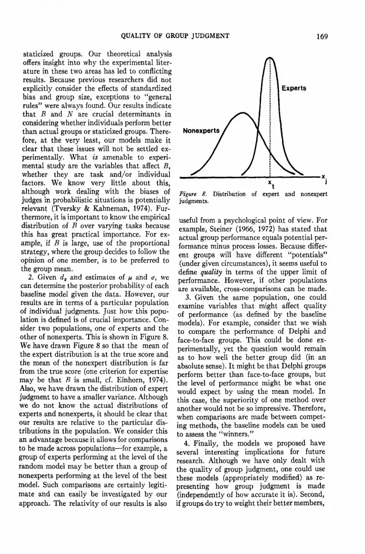
2. Given dg and estimates of /* and <r, wecan determine the posterior probability of eachbaseline model given the data. However, ourresults are in terms of a particular populationof individual judgments. Just how this popu-lation is defined is of crucial importance. Con-sider two populations, one of experts and theother of nonexperts. This is shown in Figure 8.We have drawn Figure 8 so that the mean ofthe expert distribution is at the true score andthe mean of the nonexpert distribution is farfrom the true score (one criterion for expertisemay be that B is small, cf. Einhorn, 1974).Also, we have drawn the distribution of expertjudgment to have a smaller variance. Althoughwe do not know the actual distributions ofexperts and nonexperts, it should be clear thatour results are relative to the particular dis-tributions in the population. We consider thisan advantage because it allows for comparisonsto be made across populations—for example, agroup of experts performing at the level of therandom model may be better than a group ofnonexperts performing at the level of the bestmodel. Such comparisons are certainly legiti-mate and can easily be investigated by ourapproach. The relativity of our results is also

Experts

Nonexperts

Figure 8. Distribution of expert and nonexpertjudgments.

useful from a psychological point of view. Forexample, Steiner (1966, 1972) has stated thatactual group performance equals potential per-formance minus process losses. Because differ-ent groups will have different "potentials"(under given circumstances), it seems useful todefine quality in terms of the upper limit ofperformance. However, if other populationsare available, cross-comparisons can be made.

3. Given the same population, one couldexamine variables that might affect qualityof performance (as defined by the baselinemodels). For example, consider that we wishto compare the performance of Delphi andface-to-face groups. This could be done ex-perimentally, yet the question would remainas to how well the better group did (in anabsolute sense). It might be that Delphi groupsperform better than face-to-face groups, butthe level of performance might be what onewould expect by using the mean model. Inthis case, the superiority of one method overanother would not be so impressive. Therefore,when comparisons are made between compet-ing methods, the baseline models can be usedto assess the "winners."

4. Finally, the models we proposed haveseveral interesting implications for futureresearch. Although we have only dealt withthe quality of group judgment, one could usethese models (appropriately modified) as re-presenting how group judgment is made(independently of how accurate it is). Second,if groups do try to weight their better members,


it is an interesting empirical question as to therelationship of pi,x and group size. Third, ourresults have potential use in a normative sense.For example, consider that in a particulargroup, one member gives a judgment that isvery discrepant from the judgments of theother members. The tendency of the majoritymay be to ignore the discrepant opinion(weight it zero). However, if the majorityopinions were too high relative to xt, the in-clusion of the discrepant opinion (if it wasbelow xt) might improve the accuracy of thegroup judgment. In fact, there is the realpossibility that equally weighting N "wrong"judgments could lead to the correct answer.Whether groups have any ability to make useof the statistical properties of their judgmentsis an interesting and important question thatawaits further research.9 If groups are not ableto make use of this information, mechanicallycombining individual judgments might becalled for in order to improve judgmentalaccuracy.

Our hope is that the above theoretical andmethodological results will help to stimulatemore research in the area of group judgment.Although psychologists have traditionally beenmainly interested in how groups behave, wefeel that more concern with the quality ofjudgment should lead to both theoretical andmethodological insights that will bear on boththe descriptive and normative aspects ofjudgment.

9 It is interesting to speculate whether groups areable to apply negative weights to individual judgments.It seems to us that this would be very difficult for agroup to do. The possibility that groups only applyzero or positive weights makes the use of equal weight-ing strategies even more effective (see Einhorn &Hogarth, 1975).

References

Cramer, H. Mathematical methods of statistics. Princeton,N. J.: Princeton University Press, 1951.

Dalkey, N. C. The Delphi method: An experimentalstudy of group opinion (RM-5888-PR). Santa Monica,Calif.: The Rand Corporation, 1969. (a)

Ualkey, N. An experimental study of group opinion:The Delphi method. Futures, 1969, 1, 408-426. (b)

Dalkey, N., & Helmer, O. An experimental applicationof the Delphi method to the use of experts. Manage-ment Sciences, 1963, 9, 458^67.

Dawes, R. M., & Corrigan, B. Linear models in decisionmaking. Psychological Bulletin, 1974, 81, 95-106.

Deutsch, M., & Gerard, H. B. A study of normative andinformational social influences upon individual judg-ment. Journal of Abnormal and Social Psychology,1955, 51, 629-636.

Einhorn, H. J. Expert judgment: Some necessary con-ditions and an example. Journal of Applied Psychol-ogy, 1974, 59, 562-571.

Einhorn, H. J., & Hogarth, R. M. Unit weightingschemes for decision making. Organizational Be-havior and Human Performance, 1975, 13, 171-192.

Gordon, K. A study of esthetic judgments. Journal ofExperimental Psychology, 1923, 6, 36-43.

Hogg, R. V., & Craig, A. T. Introduction to mathe-matical statistics (2nd ed.). New York: Macmillan1965.

Kidd, J. B. The utilization of subjective probabilitiesin production planning. Acta Psychologica, 1970, 34,338-347.

Klguman, S. F. Group and individual judgments foranticipated events. Journal of Social Psychology,1947,2(5,21-28.

Lorge, L, Fox, D., Davitz, J., & Brenner, M. A surveyof studies contrasting the quality of group perform-ance and individual performance, 1920-1957. Psy-chological Bulletin, 1958, 55, 337-372.

Maier, N. R. F. Assets and liabilities in group problemsolving: The need for an integrative function.Psychological Review, 1967, 74, 239-249.

Sackman, H. Delphi assessment: Expert opinion, fore-casting, and group process (R-1283-PR). SantaMonica, Calif.: The Rand Corporation, 1974.

Schlaifer, R. Probability and statistics for businessdecisions. New York: McGraw-Hill, 1959.

Slovic, P. From Shakespeare to Simon: Speculation—•and some evidence—about man's ability to processinformation. Oregon Research Institute Bulletin, 1972,12 (12), 1-29. (a)

Slovic, P. Psychological study of human judgment:Implications for investment decision-making. Journalof Finance, 1972, 27, 779-799. (b)

Steiner, I. D. Models for inferring relationships betweengroup size and potential group productivity. Be-havioral Science, 1966, 11, 273-283.

Steiner, I. D. Group process and productivity. New York:Academic Press, 1972.

Steiner, I. D., & Rajaratnam, N. A model for thecomparison of individual and group performancescores. Behavioral Science, 1961, 6, 142-147.

Stroop, J. B. Is the judgment of the group better thanthat of the average member of the group? Journalof Experimental Psychology, 1932, 15, 550-560.

Taylor, D. W. Problem solving by groups. Proceedingsof the 14th International Congress of Psychology, 1954.Amsterdam: North-Holland Publishing, 1954.

Tversky, A., & Kahneman, D. Judgment under un-certainty: Heuristics and biases. Science, 1974, 185,1124-1131.

Zajonc, R. B. A note on group judgments and groupsize. Human Relations, 1962, 15, 177-180.

QUALITY OF GROUP JUDGMENT

Appendix A

We wish to derive E(d') and var(d')-+

/

«>\X'N- B\f(X'N)dX'N. (Al)

This can be divided into two parts without theabsolute operator (viz., when X'K < B andX'N > B).

171

(A4)

r-^ / f(u)du .JVNB

E(d') = rJ-«

(B - X'N)f(X'N)dX'N

(A2,

/

g

f(X'lf')dX'N-00

- IB X'Nf(X'N)dX'N

Terms a and d are expressed in terms ofcumulative normal distributions, that is,

and d =

Terms b and c are the partial expectations ofa normal distribution. For a unit normal dis-tribution, they are (see Schlaifer, 1959, p. 300)

-B (A3)

and

Combining all terms yields

+_ _

V]V

/—

^ '

. . . _Because X tf is normally distributed with _H = 0, (7 = 1/Vtf, we consider the variable u, E(d") = B[_2F(^NB) - 1]

where « = ^NX'N and du = -\lNdX' y.^Since« is XV multiplied by a constant (V^V), itwill be distributed normally with n = 0 and<r = 1 (i.e., VA/VJV). Therefore, the distri- The variance of rf/ is 8iven bVbution of u is unit normal. Multiplying the endpoints of the integrals by ^N, Equation (A3) var(d') = E(d')* - [E(<2')]2 (A6)becomes, by variable transformation, .

E(d') = B f(u)du

N

Therefore,

var(<0 = ^ -

(A7)

(A8)

(Appendix B on next page)


Appendix B

We wish to derive the probability density Substituting Equation B4 into Equation B3function for the proportional model, fp(d'). yields

N M T / 2M — 2 ? -I- 2/P(«O = E pi,N!(d'i,N) , (Bi) fp(dr) = E ( M_l,

»-i j=o L\ M + 2

where X/60'|MX%)/(rf'i) (BS)

and

d' = _ ^ _ - E JMJ I tf, <*'

3—0X Ijt \ » 1/4 if \N—j//j/ \ I /DO\\A%) (1 — "•%) ](."' l) • \"A)

J and

Let j = i — 1 and M = N — 1. Then Equa- M, . .. , _ ,tion B2 becomes £, JJ6" I M' d %> ~ Md%.

fd') = E \2(M~ j+ 1] (M)l Therefore,

X (W(l - *)-</<*>. (B3)

X+ E/»WI^ , r f '%) ] . (B6)

(see Hogg & Craig, 1965, p. 173). Therefore, >'-»

However,

. (B7)

The binomial distribution of j successes in M ~ f/ji \trials, with probability of success, d'%, is fp(d') — [TV — (TV — l)rf'%] . (B8)given by TV + 1

X (rf'%)J'(l — d'%)M->. (B4) Received October 29, 197S

Documents

Quality of group judgment