QUANTILE SELECTION METHOD IN SEQUENTIAL INSPECTION PROBLEMS

Rev. Mat. Estat., São Paulo, v. 23, n.1, p.7-17, 2005 7

QUANTILE SELECTION METHOD IN SEQUENTIAL INSPECTION PROBLEMS

Carla Regina Guimarães BRIGHENTI1 Lucas Monteiro CHAVES2

��ABSTRACT: A strategy of sequential inspection in which the characteristic of an object follows a known distribution is presented. From the n-th and (n-1)-th order statistics, a quantile ξp was defined, where p = (n-1)/n. The strategy is to sequentially inspect the objects of an n size sample and interrupt the process at the first object with a characteristic value higher than the quantile (n-1)/n. If this does not occur the n-th object will be accepted automatically. Quantile (n-1)/n is obtained from order statistics. The probability of winning, of really taking the best object, is greater than that obtained by the strategy based upon relative ranks and smaller than the optimum strategy based on only one decision number. The expectation of the whole inspection time is asymptotically n(e-1)/e and the variance is n2(e2- 2e-1)/e2. The quantile proposed is equal or close to the mode of the distribution of the n-th order statistic, for exponential, logistic, Gumbel and uniform distribution.

��KEYWORDS: Order statistics; secretary problem; optimal strategy.

1 Introduction

A known number of items is to be presented one by one in random order, all n! possible orders being equally likely. The observer is able at any time to rank the items that have so far been presented in order of desirability. As each item is presented he must either accept it, in which case the process stops, or reject it, when the next item in the sequence is presented and the observer faces the same choice as before. If the last item in the sequence is presented, it must be accepted. The observer’s aim is to maximize the probability that the item he chooses is, in fact, the best of the n items available. We shall abbreviate this outcome to the single word ‘win’ or ‘success’ (Freeman, 1983).

One of the classical problems in this area is the Secretary Problem. Assume we want to hire a new secretary, and we know that n candidates have applied for the job. The candidates are interviewed in a random order. At each moment, the interviewer knows the relative rank of the already interviewed candidates, from the best to the worst. After each interview the candidate is accepted or rejected. In the former, all the others are rejected; in

1 Departamento de Ensino, Escola Preparatória de Cadetes do Ar - EPCAR, CEP 36200-000, Barbacena, MG,

Brasil. E-mail: [email protected] 2 Departamento de Ciências Exatas, Universidade Federal de Lavras - UFLA, CEP 37200-000, Lavras, MG,

Brasil. E-mail: [email protected]


the latter, she cannot be hired anymore. In particular, after rejecting all the other (n-1) first candidates, candidate n is accepted without any interviews (Ferguson, 1989).

The classical Secretary Problem is extended in several directions. The inspection can be the a full-information problem with (Dhariyal and Dudewicz, 1981; Ferenstein and Enns, 1988) or without cost (Gilbert and Mosteller, 1966). The no-information problem can be found with (Rose, 1984) or without cost (Lindley, 1961). In the same way, the partial-information problem (Enns, 1975) or utilizing bayesian inference (Stewart, 1978). The inspection can have one or several choices (Dynkin and Yushkevick, 1969; Samuels, 1985), unknown number of candidates (Bruss, 1984) or inspection by groups of candidates (Hsiau and Yang, 2000).

The history of this problem probably started with Cayley (1875)3 addressed by Ferguson (1989). The first published solution of the classical problem was given by Lindley (1961) using dynamic programming and decision theory. Dynkin (1963) presented another solution by utilizing the concept of optimum stop time for Markov chains. The strategy is based upon the attribution of relative ranks to the already interviewed candidates (no-information problem). One candidate has the possibility of being chosen if she is the best up to the moment. In this case we have a point of local maximum in the sequence of relative ranks. A strategy based upon relative ranks will be successful if it stops at the last point of maximum.

The optimum strategy corresponds to observing the kn first candidates without interrupting the process and stopping it as soon as candidate appears better than all the previous ones, where kn is the number which verifies the ratio (Landim, 1993):

1 1 1 1... 1 ...

1 1 1n nk n k n+ + < < + +

+ − −.

The optimum strategy consists of waiting for approximately n/e candidates and choosing the first better than all the previous (Lindley, 1961; Dynkin, 1963) ones.

The probability of the optimum strategy to select the best candidate is given by

( )

1 1.

n

nn

wink k

kP

n k

−

=

= � (1)

When n� ∞, P(win) � 1/e(Lindley, 1961). Another aspect to be considered is the time spent during the process. If each

inspection is performed in one unit of time, random variable T (spent time), is equal to the number of inspections.

The expectation is,

2 1( )

1n

n

nk k

nE T k

k n

−

=

� �� = +� �−� �� (2)

and the variance

3CAYLEY, A. Mathematical questions with their solutions. The Educational Times, Cambridge, v.23,

p.18-19,1875

https://www.researchgate.net/publication/254286765_Optimal_Sequential_Selection_From_a_Known_Distribution_With_Holding_Costs?el=1_x_8&enrichId=rgreq-7c2c8129e6b4faeeb7175b24806f5794-XXX&enrichSource=Y292ZXJQYWdlOzI1MzYzODAyMjtBUzoxNjQ1MDYyOTAzNjg1MTNAMTQxNjIzMjc2NDgxMg==



222 21 1

( ) 11 1

n n

n n

n n nk k k k

n nV T k n k k

k n k n

− −

= =

� � � � � �� = + − − + − +

� � � �− − �� (3)

The asymptotic results are: E(T) ≈ 2n/e and V(T) ≈ n2(2e – 5)/e2 (Quine and Law, 1996).

Gilbert and Mosteller (1966) presented the optimum strategy for the full-information problem using the uniform distribution U(0,1). The strategy is based on the choice of the optimum decision numbers di, i = 1, 2, ..., n, where each di depends only on the number of remaining candidates (a number in [0,1] is associated with each candidate). The i-th candidate will be chosen if her number is greater than di. The decision numbers decrease as inspection goes on.

The probability of the optimum strategy to select the best candidate at inspection (r +1) is given by

1(1) (1 ) /nP d n= − ,

1

1 1( 1) ,

( ) ( )

r n nr ri i r

i i

d d dP r n-1 r 1.

r n r n n r n+

= =+ = − − ≥ ≥

− −� �

(4)

When n� ∞, P(win) � 0.58012(Gilbert and Mosteller, 1966). Using the class of sequential inspection strategies based on only one decision

number, that is, d1 = d2 = … = dn-1 = d and dn = 0, the optimum value of d in this class tends to 1 when n increases, but in such a manner that n(1- d) tends to a constant µ

2 3( )lim

2!2 3!3nP win e e eµ µ µµ µµ− − −

→∞= + + + ⋅⋅⋅ (Gilbert and Mosteller, 1966) (5)

The optimum asymptotic value of µ ≈ 1.503, which gives a limiting probability of winning about 0.51735.

In this paper we propose a quantile used as a decision number. The performance of this strategy was compared with the strategy based Relative Ranks (RR) in no-information problem and Optimum Strategy (OS) using only one decision number in full-information problem.

2 Methodology

Consider the following variation of the Secretary Problem. Suppose that the characteristic to be evaluated may be quantified and that this characteristic follows a probability distribution f(x). The n candidates (or objects) x1, x2,..., xn are presented for inspection in a random sequence. At each inspection the value of the characteristic of the object is verified and it is rejected or accepted. All rejected objects cannot be reconsidered and once one of the objects is accepted, the process is stopped.

The criterion to choose the object, stopping the process, is to compare value xi with an appropriate quantile ξp of f(x), xi > ξp accepted, rejected otherwise. In the case that the choice is note made until the (n-1)-th object, the last one will be accepted. This procedure will be called Quantile Sequential Inspection Strategy (QSIS).

https://www.researchgate.net/publication/2647259_Exact_Results_For_A_Secretary_Problem?el=1_x_8&enrichId=rgreq-7c2c8129e6b4faeeb7175b24806f5794-XXX&enrichSource=Y292ZXJQYWdlOzI1MzYzODAyMjtBUzoxNjQ1MDYyOTAzNjg1MTNAMTQxNjIzMjc2NDgxMg==



3 Quantile sequential inspection strategy

The value of ξp which will define the strategy is obtained from the order statistics Yn and Yn-1. The strategy will always be successful when Yn-1 � ξp < Yn. There are other situations where the strategy may be successful too, for example, Yn-2 � ξp < Yn-1 < Yn and the best Yn object is inspected before object Yn-1. To calculate the probability that the random interval (Yi, Yj), i < j includes a quantile ξp, we must observe that the event Yi � �p occurs if and only if Yi � �p < Yj or �p > Yj, and these two events are mutually exclusive, then,

P (Yi � �p ) = P (Yi � �p < Yj ) + P (�p >Yj). As P (Yi � �p ) = FYi(�p), where

iYF is the cumulative distribution of Yi

( ) [ ( )] [1 ( )] [ ( )] [1 ( )]n n

m n m m n mi p j p p p p

m i m j

n nP Y Y F F F F

m mξ ξ ξ ξ ξ− −

= =

� � � �≤ < = − − −� � � ��

� � ,

( ) ( )1

1j n mm

i p jm i

nP Y Y p p

mξ

− −

=

� �≤ < = −� �

� ��

then )1()( 11 pnpYYP n

npn −=<≤ −− ξ .

Maximizing the probability that the random interval (Yn-1;Yn) contains quantile ξp, the derivative should be equal to zero, so the value of p is: p = (n-1)/n.In spite of the parametric approach, only n defines quantile ξp.

3.1 Probability of winning

The probability of winning (or success) using quantile ξp with p = (n-1)/n will be:

( ) ( )( )1

11

nn n i i pwin p p

i

nP

ii n

ξξ ξ

−

=

� �= − +� ��

� (6)

Each summation term is the probability of i objects being greater than the quantile times the probability of the best in i being inspected first. The last term of the right hand side in (6) is regarded to the case where all the values are less than the quantile, and the greater value’s object is the last one to be inspected.

In the case of uniform distribution, U(0,1), gives n(1-ξp) = n(1-(n-1)/n) = 1 for the optimum strategy ( )lim 1

nn d µ

→∞− = � 1,503 (Gilbert and Mosteller, 1966).

The asymptotic result utilizing the Poisson theory in this case is:

( )1 1 1 1

lim2!2 3!3 4!4win

nP

e→∞

� �= + + ⋅⋅⋅� ��

(7)

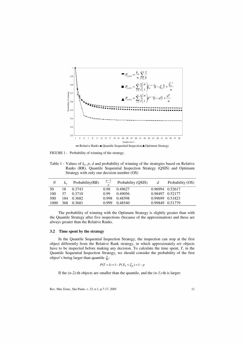
The asymptotic value is about 0.48483. Figure 1 and Table 1 compare the probability of winning obtained in each one of the

strategies, using the approximate value of d given by expression n(1-d) = 1,503 as the optimum strategy.


0,2

0,3

0,4

0,5

0,6

0,7

0,8

0,9

1

1 3 5 7 9 11 13 15 17 19 21 23 25 27 29 31 33 35 37 39 41 43 45 47 49

Sample size n

Prob

abili

ty o

f win

ning

� Relative Ranks � Quantile Sequential Inspection�Optimum Strategy

FIGURE 1 - Probability of winning of the strategy.

Table 1 - Values of kn, p, d and probability of winning of the strategies based on Relative Ranks (RR), Quantile Sequential Inspection Strategy (QSIS) and Optimum Strategy with only one decision number (OS)

N kn Probability(RR) n

n 1− Probability (QSIS) d Probability (OS)

50 18 0.3743 0.98 0.49627 0.96994 0.52617 100 37 0.3710 0.99 0.49056 0.98497 0.52177 500 184 0.3682 0.998 0.48598 0.99699 0.51823 1000 368 0.3681 0.999 0.48540 0.99849 0.51779

The probability of winning with the Optimum Strategy is slightly greater than with

the Quantile Strategy after five inspections (because of the approximation) and these are always greater than the Relative Ranks.

3.2 Time spent by the strategy

In the Quantile Sequential Inspection Strategy, the inspection can stop at the first object differently from the Relative Rank strategy, in which approximately n/e objects have to be inspected before making any decision. To calculate the time spent, T, in the Quantile Sequential Inspection Strategy, we should consider the probability of the first object’s being larger than quantile ξp:

1( 1) 1 ( ) 1pP T P X pξ= = − < = −

If the (n-2)-th objects are smaller than the quantile, and the (n-1)-th is larger:

( )

( )n

ddd

i

n

iP

ni

n

iP

knk

P

niin

n

iwin

npi

pin

p

n

iwin

n

kk

nwin

n

+−��

��

�=

+−��

��

�=

=

−

=

−

=

−

=

�

�

�

11

11

1

1][

1][

1

][

ξξξ


21 2 1( 1) ( )... ( ) ( ) (1 )n

p n p n pP T n P X P X P X p pξ ξ ξ −− −= − = < < > = −

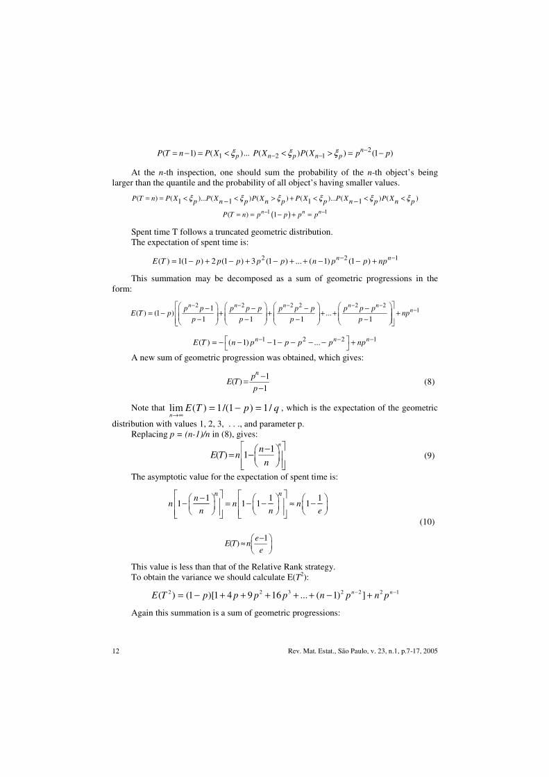
At the n-th inspection, one should sum the probability of the n-th object’s being larger than the quantile and the probability of all object’s having smaller values.

( ) ( )... ( ) ( ) ( )... ( ) ( )1 1 1 1P T n P X P X P X P X P X P Xp n p n p p n p n pξ ξ ξ ξ ξ ξ= = < < > + < < <− −

( )1 1( ) 1n n nP T n p p p p− −= = − + =

Spent time T follows a truncated geometric distribution. The expectation of spent time is:

2 2 1( ) 1(1 ) 2 (1 ) 3 (1 ) ... ( 1) (1 )n nE T p p p p p n p p np− −= − + − + − + + − − +

This summation may be decomposed as a sum of geometric progressions in the form:

2 2 2 2 2 211

( ) (1 ) ...1 1 1 1

n n n n nnp p p p p p p p p p p

E T p npp p p p

− − − − −−� � � � � � � � �− − − −= − + + + + + ��

� � � � � � � �− − − − ��

1 2 2 1( ) ( 1) 1 ...n n nE T n p p p p np− − −� = − − − − − − − +�

A new sum of geometric progression was obtained, which gives:

1( )

1

npE T

p−=−

(8)

Note that lim ( ) 1/(1 ) 1/n

E T p q→∞

= − = , which is the expectation of the geometric

distribution with values 1, 2, 3, . . ., and parameter p. Replacing p = (n-1)/n in (8), gives:

1( ) 1

nnE T n

n

� −� �= − ��

(9)

The asymptotic value for the expectation of spent time is:

1 1 11 1 1 1

n nnn n n

n n e

� � −� � � � � � − � = − − � ≈ −� � � � � �

� � � � � � � ��

1( )

eE T n

e−� �≈ � �

� �

(10)

This value is less than that of the Relative Rank strategy. To obtain the variance we should calculate E(T2):

1222322 ])1(...16941)[1()( −− +−+++++−= nn pnpnppppTE

Again this summation is a sum of geometric progressions:


1222222

22222

)}]()2()1[()(5

)(3)1){(1()(−−−

−−

+−−−+++++

+++++++++−=nnn

nn

pnpnnpp

pppppppTE

��

��

2 2 2 22 2 11

( ) (1 ) 1 3 ... [2 3]1 1 1

n n n nnp p p p p p p p

E T p n n pp p p

− − − −−� � � � � � �− − −= − + + + − + �� − − − ��

( ) ( )[ ] 122111

122 ...1

211

)1()( −−−−−

− +��

��

��

��

−++−��

��

�

−+��

��

�

−−+−−= nnnn

nn pnpppp

ppp

pnTE

( )( )( )2

11

112122

12

1)2(

211

)1()(−

−−

−−

+��

��

�

−−

+−−=−

−−

−−

p

ppp

pn

pp

pnpnTEn

nn

nn

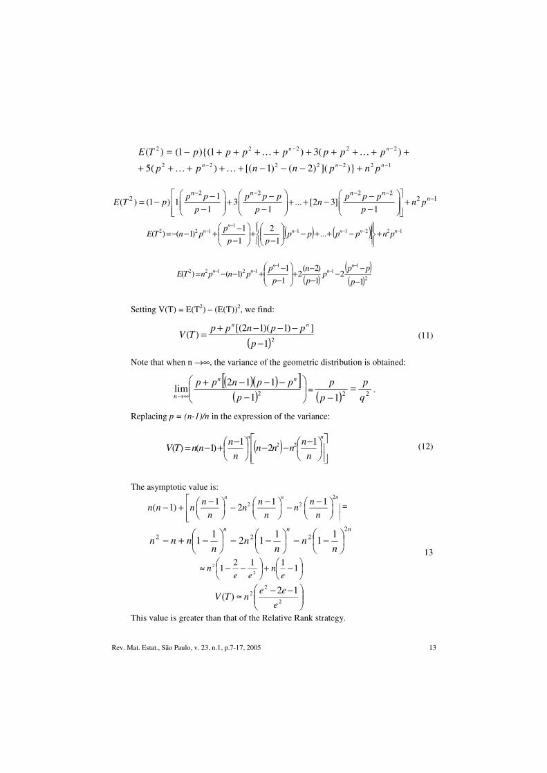
Setting V(T) = E(T2) – (E(T))2, we find:

( )21

])1)(12[()(

−−−−+

=p

ppnppTV

nn

(11)

Note that when n →∞, the variance of the geometric distribution is obtained:

( )( )[ ]( ) �

��

��

�

−−−−+

∞→ 21112

limp

ppnpp nn

n= ( ) 221 q

p

p

p =−

.

Replacing p = (n-1)/n in the expression of the variance:

( )��

�

��

��

� −−−��

��

� −+−=nn

nn

nnnn

nnnTV

12

1)1()( 22 (12)

The asymptotic value is:

22 21 1 1

( 1) 2n n n

n n nn n n n n

n n n

� − − −� � � � � �− + − − = ��

=

��

��

� −−��

��

� −−��

��

� −+−nnn

nn

nn

nnnn

2222 1

11

121

1

��

��

� −+��

��

� −−≈ 1112

12

2

en

een

��

��

� −−≈2

22 12

)(e

eenTV

13

This value is greater than that of the Relative Rank strategy.


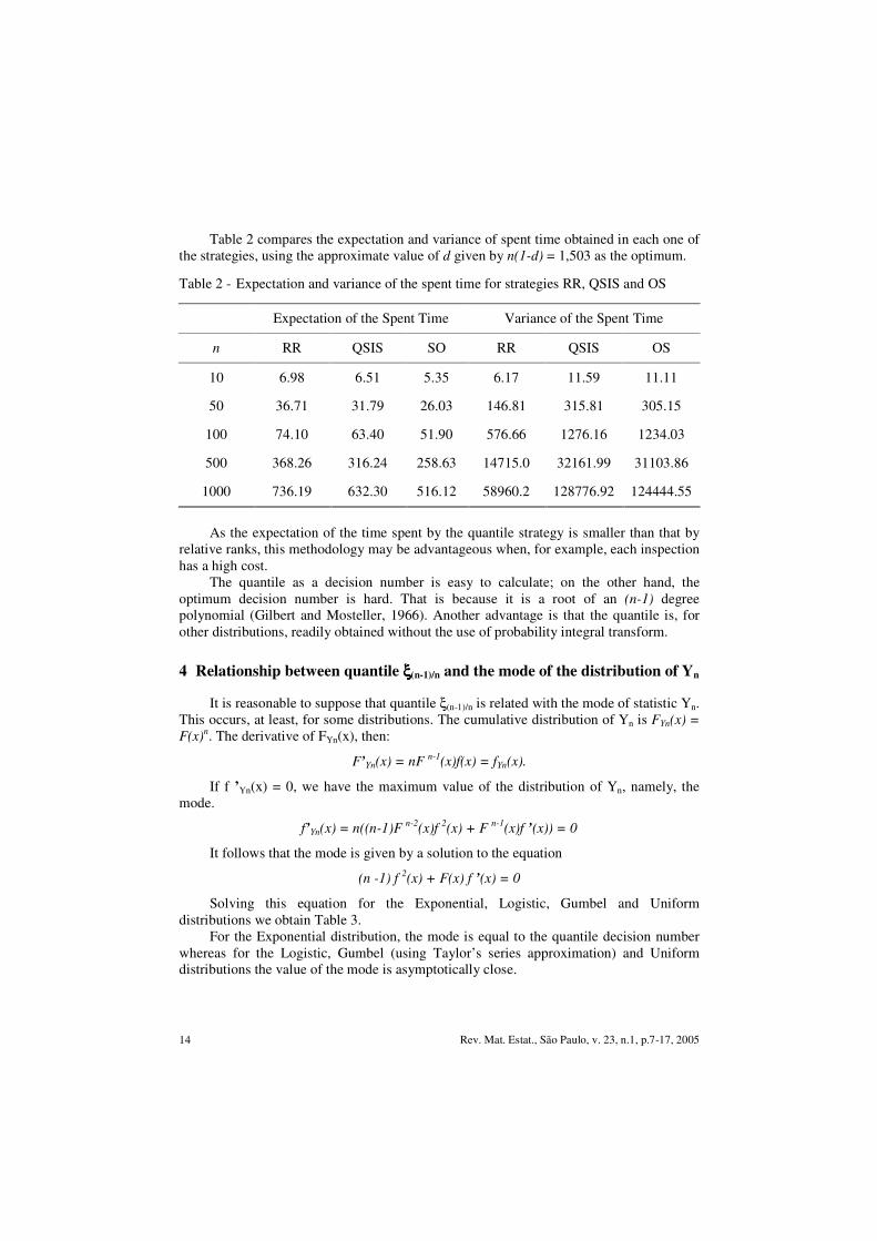
Table 2 compares the expectation and variance of spent time obtained in each one of the strategies, using the approximate value of d given by n(1-d) = 1,503 as the optimum.

Table 2 - Expectation and variance of the spent time for strategies RR, QSIS and OS

Expectation of the Spent Time Variance of the Spent Time

n RR QSIS SO RR QSIS OS

10 6.98 6.51 5.35 6.17 11.59 11.11

50 36.71 31.79 26.03 146.81 315.81 305.15

100 74.10 63.40 51.90 576.66 1276.16 1234.03

500 368.26 316.24 258.63 14715.0 32161.99 31103.86

1000 736.19 632.30 516.12 58960.2 128776.92 124444.55

As the expectation of the time spent by the quantile strategy is smaller than that by

relative ranks, this methodology may be advantageous when, for example, each inspection has a high cost.

The quantile as a decision number is easy to calculate; on the other hand, the optimum decision number is hard. That is because it is a root of an (n-1) degree polynomial (Gilbert and Mosteller, 1966). Another advantage is that the quantile is, for other distributions, readily obtained without the use of probability integral transform.

4 Relationship between quantile ξξξξ(n-1)/n and the mode of the distribution of Yn

It is reasonable to suppose that quantile ξ(n-1)/n is related with the mode of statistic Yn. This occurs, at least, for some distributions. The cumulative distribution of Yn is FYn(x) = F(x)n. The derivative of FYn(x), then:

F’Yn(x) = nF n-1(x)f(x) = fYn(x).

If f ’Yn(x) = 0, we have the maximum value of the distribution of Yn, namely, the mode.

f’Yn(x) = n((n-1)F n-2(x)f 2(x) + F n-1(x)f ’(x)) = 0

It follows that the mode is given by a solution to the equation

(n -1) f 2(x) + F(x) f ’(x) = 0

Solving this equation for the Exponential, Logistic, Gumbel and Uniform distributions we obtain Table 3.

For the Exponential distribution, the mode is equal to the quantile decision number whereas for the Logistic, Gumbel (using Taylor’s series approximation) and Uniform distributions the value of the mode is asymptotically close.


Table 3 - Relationship between quantile ξ(n-1)/n, and the mode of Yn

Continuous Distribution F(x) ξ(n-1)/n Mode of Yn

Exponential 1-e-λx λ

)ln(n

λ)ln(n

Logistic (x )

1

1 e−α−β+

α + β ln (n -1) α + β ln (n)

Gumbel ( x )

ee−α−β− ��

�

��

��

��

�

−−

1lnln

nnβα α + β ln (n)

Uniform x ab a

−−

( )a b

bn−+ b

5 An application of quantile sequential inspection strategy

A possible simple application of QSIS is the following. Table 4 contains coffee prices during ten months of year 2004 in Brazil.

Table 4 - Coffee’s price in Brazil (2004)

Month 1 2 3 4 5 6 7 8 9 10 Price (R$) 196,00 195,00 204,00 195,00 208,00 213,00 202,00 190,00 217,00 210,00

Source: www.cccmg.com.br Assuming that the price is normally distributed with estimated parameters

µ = 203.00 and σ = 8.93, suppose that a farmer has to sell his coffee and he has to decide to sell, or not, at the beginning of each month, that is, he has 12 opportunities. Quantile ξ(n-1)/n = ξ11/12 = ξ0.9167, witch corresponds to R$ 215,35. Then he must sell his coffee in the first month when the price is greater than that value. The probability of selling for the best price is 0.5363.

Conclusions

The proposed strategy of Quantile Sequential Inspection (QSIS) using quantile ξ(n-1)/n

has probability of winning which is very close to of that the Optimum Strategy based on just one decision number, and greater than that of the optimum strategy based on Relative Ranks. The expectation of the time spent by QSIS is asymptotic to n(e-1)/e, which is shorter than 2n/e, spent by the strategy based on Relative Ranks. However, the variance of the QSIS’s time is asymptotic to n2(e2-2e-1)/e2, which is larger than n2(2e-5)/e2, the variance of the strategy based on Relative Ranks. Another advantage is that the quantile decision number is easy to calculate and can be used directly for many distributions.

Quantile ξ(n-1)/n is equal or close to the mode of the distribution of Yn for the Exponential, Logistic, Gumbel and Uniform distributions.


BRIGHENTI, C. R. G., CHAVES, L. M. Método de seleção por quantil em problemas de inspeção seqüencial. Rev. Mat. Estat., São Paulo, v.23, n.1, p.7-17, 2005.

�� RESUMO: Uma estratégia de inspeção seqüencial em que a característica avaliada do objeto

segue uma distribuição de probabilidade conhecida é apresentada. A partir das n-ésima e (n-1)-ésima estatísticas de ordem, definiu-se um quantil ξp, em que p = (n-1)/n, que fornece uma probabilidade de sucesso próxima à alcançada pela estratégia ótima. A estratégia é inspecionar seqüencialmente os objetos da amostra de tamanho n e interromper o processo no primeiro objeto com valor maior que o quantil (n-1)/n; caso isto não ocorra, o n-ésimo objeto será aceito automaticamente. O quantil (n-1)/n é obtido por meio das estatísticas de ordem. A probabilidade de sucesso é maior que a obtida pela estratégia de postos relativos e menor que a estratégia ótima baseada em somente um número de decisão. A esperança do tempo de execução da estratégia de inspeção é assintoticamente igual a n(e-1)/e e a variância n2(e2- 2e-1)/e2. O quantil proposto nesta estratégia é igual ou próximo à moda da distribuição da n-ésima estatística de ordem para as distribuições exponencial, logística, Gumbel e uniforme.

��PALAVRAS-CHAVE: Estatística de order; problema da secretária; estratégia ótima.

References

BRUSS, F. T. A unified approach to a class of best choice problems with an unknown number of options. Ann. Prob., Hayward, v.12, p. 882-889, 1984.

DHARIYAL, I. D.; DUDEWICZ, E. J. Optimal selection from a finite sequence with sampling cost. J. Am. Stat. Assoc., New York, v.76, n.376, p.952-959, 1981.

DYNKIN, E. B. The optimum choice of the instant for stopping a Markov processes. Sov. Math. Dokl., Providence, v.4, p.627-629, 1963.

ENNS, E. G. Selecting the maximum of a sequence with imperfect information. J. Am. Stat. Assoc., New York, v.70, n.351, p.640-643, 1975.

FERENSTEIN, E. A.; ENNS, E.G. Optimal sequential selection from a known distribution with holding costs. J. Am. Stat. Assoc., New York, v.83, n.402, p.382-386, 1988.

FERGUSON, T. S. Who solved the secretary problem? Stat.. Sci., Hayward, v.4, n.3, p.282-289, 1989.

FREEMAN, P. R. The secretary problem and its extensions: a review. Int. Stat. Rev., Voorburg, v.51, n.2, p.189-206, 1983.

GILBERT, J.; MOSTELLER, F. Recognizing the maximum of a sequence. J. Am. Stat. Assoc., New York, v.61, n.313, p.35-73, 1966.

HSIAU, S.R.; YANG, J. R. A natural variation of the standard secretary problem. Stat. Sinica, Taipei, v.10, n.2, p.639-646, 2000.

LANDIM, C. Otimização estocástica. In: COLÓQUIO BRASILEIRO DE MATEMÁTICA, 18., 1993, Rio de Janeiro. Anais... Rio de Janeiro: IMPA, 1993. p.38-61.

LINDLEY, D. V. Dynamic programming and decision theory. J. R. Stat. Soc.: Serie C – Appl. Stat., London, v.10, n.1, p.39-51, 1961.





QUINE, M. P.; LAW, J. S. Exact results for a secretary problem. J. Appl. Probab., Sheffield, v.33, n.3, p.630-639, 1996.

REICHL, P. Contraception Management by STORCH: the sequential test for ovulation reckoning and contraception handling. Aschen, 1995. 18p. Disponível em: <http://userver.ftw.at/~reichl/publications/STORCH.pdf>. Acesso em: 4 jan. 2003.

ROSE, J. S. Optimal sequential selection based on relative ranks with renewable call options. J. Am. Stat. Assoc., New York, v.79, n.386, p.430-435, 1984.

SAMUELS, S. M. A best-choice problem with linear travel cost. J. Am. Stat. Assoc., New York, v.80, n.390, p.461-464, 1985.

STEWART, T. J. Optimal selection from a random sequence with learning of the underlying distribution. J. Am. Stat. Assoc., New York, v.73, n.364, p.775-780, 1978.

Received 09.06.2004.

Received in revised form 25.01.2005.



Documents

QUANTILE SELECTION METHOD IN SEQUENTIAL INSPECTION PROBLEMS