Quantitative Assessment of Land Cover Change Using Landsat Time Series Data: Case of Chunati Wildlife Sanctuary (CWS), Bangladesh

International Journal of Environment and Geoinformatics 3 (2), 45-55 (2016)

Quantitative Assessment of Land Cover Change Using Landsat Time

Series Data: Case of Chunati Wildlife Sanctuary (CWS), Bangladesh

Kamrul Islam*1, Mohammed Jasimuddin1, Biswajit Nath2, Tapan Kumar Nath1, 3

1University of Chittagong, Institute of Forestry and Environmental Sciences, CHITTAGONG-BD 2University of Chittagong, Department of Geography and Environmental Studies, CHITTAGONG-BD 3University of Nottingham Malaysia Campus, School of Biosciences, SEMENYIH-MY

Corresponding author* Tel: +08801836763416 Received 13 April 2016

E-mail: [email protected] Accepted 27 June 2016

Abstract

Due to inappropriate management and absence of land use planning, land cover change of developing country

like Bangladesh is a common phenomenon. This land cover change phenomenon will have its tremendous effect

if found at a greater extent on natural habitat area for numerous animal and tree species. In this study, land cover

change of Chunati Wildlife Sanctuary (CWS) was assessed from (2005-2015) using Landsat TM (Thematic

Mapper) and Landsat 8 OLI/TIRS (Operational Land Imager/Thermal Infrared Sensor). ArcGIS v10.1 and

ERDAS Imagine v14 were used to process satellite derived imageries and assess other quantitative data for land

cover change assessment of this study area. Land cover change of the area was identified using Normalized

Difference Vegetation Index (NDVI) technique. Highest NDVI value was found in 2005 (0.71) which denotes

presence of moderate-high vegetation cover at that time period. After 2005, highest NDVI value was found

following a decreasing trend (0.56 in 2010 and 0.4 in 2015) which clearly represents the rapid vegetation cover

change in the study area. Almost 7608 hectares of moderate to high density natural forest cover dominated the

area during 2005 but was totally absent in 2015 which may be considered as a great threat regarding proper

ecosystem functioning of CWS. From the findings of this research, it can be easily concluded that the sanctuary

area has lost its valuable land cover both qualitatively and quantitatively.

Keywords: Land Cover Change, Remote Sensing, NDVI, Chunati Wildlife Sanctuary, Landsat Satellite

Imagery

Introduction

The physical entity in terms of topography,

spatial nature which is associated with economic

value is land (FAO, 1995). Land use/land cover

change (LULCC) or simply land change is the

term for the modification of earth’s terrestrial

surface by human being (Ellis, 2013) and it is so

pervasive that if aggregated globally can

significantly affect the earth’s system proper

functioning (Lambin et al., 2001). Land use is

defined as series of operations on land by

humans whether land cover is commonly the

vegetation cover both natural and planted,

building constructions, and water bodies that

cover the earth surface of the earth (Coffey,

2013). Alterations in land cover affect the

sustainability of ecosystem (Vescovi et al.,

2002) and human actions most of the cases

accelerate the process (Agarwal et al., 2001).

Though land cover change is sometimes natural

phenomenon but the vast growing population of

the world is contributing enough for further

change of it (López et al., 2001) considering the

bio-physical and socio-economic attributes of

regions (Aspinall, 2004; Zeng et al., 2008). The

reasons behind natural land cover changes are

many ( Veldkamp, 1997; Agarwal et al., 2001;

Geist, 2005; Lambin, 1997; Veldkamp &

Lambin, 2001; Zeng et al., 2008); but amongst

them tropical deforestation, rangeland

modification, agricultural intensification,

urbanization and globalization are the prime

causes and factors for global, regional land

use/land cover changes (Lambin et al., 2001).

In order to prevent forest degradation and to

protect the wildlife, mainly of Asian elephant,

Chunati reserve forest was declared as the

Chunati Wildlife Sanctuary (CWS) in 1986

which represents a fragile forest landscape near

the Bay of Bengal. If the sanctuary is not

45

Islam, K. et al., / IJEGEO 3 (2), 45-55 (2016)

46

conserved soon, may be lost for the future

generation which is a matter of serious concern

considering the value of this unique ecosystem.

Anthropogenic pressures such as increased

commercial extraction of forest produce,

brought by manifold increase in human

population that ultimately led to widespread

shrinkage and deforestation of hill forests which

in turn ultimately converts the natural land cover

into different land uses. Conversion of land

cover into human induced land uses have

tremendous effect on the natural habitats of

plant and animal species of this area which is a

threat for the sustaining of this fragile ecosystem

(NSP, 2004). Change in land cover due to due to

human induced activities or others may have a

tremendous effect on the surrounding

environment. In order to take proper steps

considering this, top most priority is given on

the information relating to the quantitative

assessment of change from a base time period.

Remote sensing can be a great tool in this aspect

as used worldwide due to its cost-effectiveness.

Change detection is the temporal effects as

variation in spectral response which involves

situations where the spectral characteristics of

the vegetation or other types of cover in a

location change over time (Hoffer, 1978). Singh

(1989) described this technique as a process

which observes the differences of phenomenon

or objects at different times. A number of

techniques is available for studying the seasonal

changes in vegetation using satellite imageries,

among them vegetation indices quantify the

range of greenness (Chuvieco, 1998). Change in

vegetation can be evaluated using the vegetation

indices. One of the prominent and widely used

such indices is Normalized Difference

Vegetation Index (NDVI) which measures

balance between energy received and energy

emitted by objects on earth. When this thing is

applied on plant community, the index

establishes a value range to represent the

greenness of that particular area and this is the

indirect quantification of vigor of growth of

plants (Tovar, 2012). NDVI approach is based

on the fact that dense or healthy vegetation has

a low acceptance in the visible portion of

electromagnetic spectrum due to chlorophyll

absorption and high acceptance in the near

infrared band because of the internal reflectance

from the mesophyll tissue of green leaf of plants.

This is also the reason behind the use of red and

near infrared band of images while NDVI

processing (Campbell, 1987). The range of

NDVI value is from -1 to +1; due to the reason

of high acceptance in the near infrared portion

of electromagnetic spectrum, dense or healthy

vegetation is represented by high value between

0.1 and 1. Reverse to this, water bodies, bare

rock etc. land cover or commonly non-vegetated

surfaces yield negative to close to zero values of

NDVI because the absorption of

electromagnetic spectrum (Lillesand and Kiefer,

1979, 1994 and 2000).

This paper discusses the change in land cover of

the CWS from 2005 – 2015 using Landsat time

series data (i.e. 2005, 2010, and 2015). While

reviewing literature it is found that massive

destruction of forest was done during this period

of time so that this time period is considered for

the study. The overall objectives of this piece of

research is to assess and quantify the change in

vegetation cover of CWS within this 15 years of

study period.

Materials and Methods

Background Information of the Study Area

The CWS is a tropical semi-evergreen forest in

Bangladesh, situated at about 70 km south of

Chittagong city on the west side of Chittagong –

Cox’s Bazar Highway. The area lies between

21º 40′ N 92º 07′ E (Figure 1). Different

literature shows that he Wildlife Sanctuary

covers an area of 7763.94 ha. But in this piece

of research the area considered for CWS is

10822.77 hectares. This 3058.83 ha or 39.37%

area increased due to the reason that there were

irregularities in the map boundaries which is

very difficult to maintain in this present map;

another important thing is that still there are

some privately acquired land inside the

sanctuary area which is also included in this map

thus increased the overall area of the CWS area.

Removal of this area will certainly decrease the

present area that is used in this study, but due to

the difficulties it can’t be done in this study.

Regarding all these issues, the Area of Interest

(AOI) for CWS is considered 10822.77

hectares. The sanctuary embraces partly 7

unions (namely Chunuti, Adhunagar, Harbang,

Puichari, Banskhali, Borohatia, Toitong) of


47

Banskhali and LohagaraUpazila of Chittagong

District and ChokoriaUpazila of Cox’s Bazar

District. Chunati WS was formally established

through a Gazette Notification in 1986

under the provision of Wildlife preservation

Act. There are 7 mouzas, divided into 15

villages and further divided into about 70

settlements (locally called para). Of the paras,

about 48% is located inside and at the edge of

the forest and the rest are located outside, but

adjacent and nearby the forest.

Figure 1: Location Map of the Study Area

Data Used:

Base map of the study area was prepared

using satellite imageries from Google Earth

7.0v. Printed subset images from Google

Earth were combined manually and used to

recognize different features in the study

area. The latest high resolution satellite

imagery provided by Google Earth and

NASA-GLCF Global Land Cover Facility

Archive (freely downloadable worldwide)

for Landsat TM and USGS for Landsat 8

OLI-TIRS satellite imagery (2005-2015)

were used for visual image interpretation,

land use identification and land use

classification (Figure 2). All of these


48

Landsat TM and Landsat 8 OLI-TIRS

sensors have spatial resolution of 30m.

Characteristics of Landsat data are shown in

Table 1.

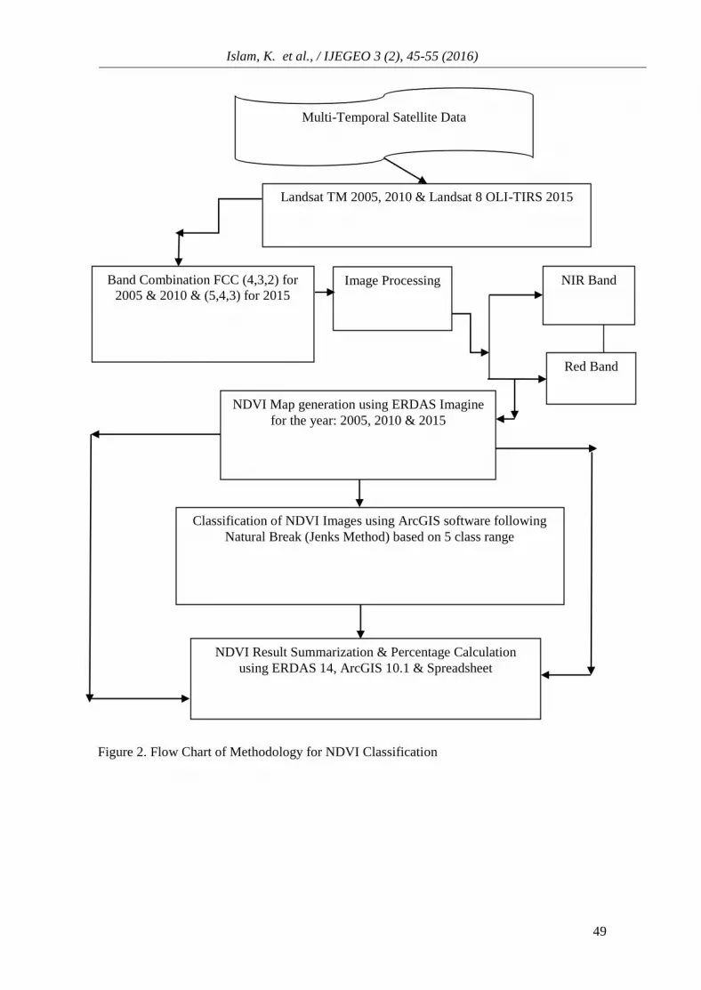
Methodology

Landsat TM and Landsat 8 OLI-TIRS data

were used in this study. Normalized

Difference Vegetation Index (NDVI) and

Land use change assessment of the study

area were performed from the satellite

imageries using ArcGIS 10.1 & ERDAS

Imagine 14. Both ArcGIS 10.1 & ERDAS

Imagine 14 were used for image processing,

classification, its final analysis, NDVI and

Land use map generation respectively to

achieve the objectives of the study. Excel

spreadsheet 2010 was also used for

analyzing the results.

Table 1: Data Characteristics of Satellite Imageries (Source: NASA-Global Land Cover Facility (GLCF) and USGS Landsat 8 OLI-TIRS Series Archive)

ERDAS Imagine was used to generate the

false color composite, by combining near

infrared, red and green which were bands

4,3,2 together for the two (2) imageries of

2005, 2010 & 5,4, 3 band combinations of

Landsat 8/OLI TIRS Image of 2015. This

false color composite was used for

vegetation recognition; its range wise index

classification, because chlorophyll in plants

reflects very well in the near infrared rather

than visible band. Then three individual

NDVI maps (2005-2015) were prepared.

The use of the Normalized Difference

Vegetation Index (NDVI) was applied to

detect areas of vegetation cover change of

Chunati Wildlife Sanctuary (CWS) and

different year wise NDVI derived

quantitative data were generated and

summarized using remote sensing and GIS

software. The method which was followed

for this present research is shown in the

following flow chart model (Figure 2.2).

NDVI from reflectance images is obtained

by mean of channels 3 (0.63-0.69 µm) and 4

(0.78-0.90 µm) for Landsat TM Data and for

Landsat 8 OLI-TIRS Imagery channel 4

(0.64-0.67) and 5 (0.85-0.88). The formula

for NDVI calculation for Landsat TM of

2005 and 2010 is shown in equation 1 and

for Landsat 8 OLI-TIRS of 2015

respectively are shown in equation 2.

NDVI= Band 4−Band 3

Band 4+Band 3 …………… (Eq. 1)

NDVI= Band 5−Band 4

Band 5+Band 4 …………… (Eq. 2)

Satellite Sensor Band

Combinations

Date of Acquisition Spatial

Resolution

Landsat

Landsat

Landsat 8

TM

TM

OLI-TIRS

NIR, R, G (4,3,2)

NIR, R, G (4,3,2)

NIR, R, G (5,4,3)

25 November 2005

08 February 2010

26 March 2015

30m

30m

30m


49

Figure 2. Flow Chart of Methodology for NDVI Classification

Red Band

Multi-Temporal Satellite Data

Landsat TM 2005, 2010 & Landsat 8 OLI-TIRS 2015

Image Processing Band Combination FCC (4,3,2) for

2005 & 2010 & (5,4,3) for 2015 NIR Band

NDVI Result Summarization & Percentage Calculation

using ERDAS 14, ArcGIS 10.1 & Spreadsheet

Classification of NDVI Images using ArcGIS software following

Natural Break (Jenks Method) based on 5 class range

NDVI Map generation using ERDAS Imagine

for the year: 2005, 2010 & 2015


50

Results and Discussion

Normalized Difference Vegetation Index

(NDVI) calculations using Landsat TM

and Landsat 8 OLI-TIRS satellite

imageries (2005-2015)

Vegetation indices have long been used in

remote sensing to monitor temporal changes

associated with vegetation. NDVI value

ranges from -1 to +1. Rock and bare soil

have a very much similar reflectance giving

NDVI value close to ‘0’. Value a little

higher than zero in NDVI indicates presence

of little vegetation class; while moderate

and high values indicate stressed vegetation

and healthy vegetation respectively;

whereas near zero and negative values

indicate non-vegetation like water, snow,

built-up areas and barren land.

Using the formula given in methodology

section along with the following algorithm,

NDVI of CWS calculated:

i. Computation of NDVI values for

the entire study areas by

conversion of spectral reflectance

values into NDVI values.

ii. Conversion of these NDVI values

to a scaled channel values by using

density-slicing method that

measures apparent reflectance to

sensor values.

iii. Display of image with NDVI and

creation of a legend keeping the

threshold values (Figure 3.1(A, B,

and C)

The greenness range is divided into discrete

classes by slicing the range of NDVI values

into five ranges by fixing the thresholds for

NDVI classification and the method used is

Natural Breaks (Jenks). Similar step was

followed for all the three (3) different years’

image classification. A cursory examination

of pseudo color image of NDVI and

classified output of NDVI image reveals

that along the water bodies, built up lands

yield negative values, their reflectance

being more visible rather than near IR

wavelengths. This technique is applied for

comparison of vegetation cover change

from multiple dates of Landsat TM and

Landsat 8 OLI/TIRS derived NDVI

imageries. Figure 3 (A, B and C) shows

resultant maps generated from NDVI

classification. It shows that high reflectance

of vegetation in 2005 image, with an

increase in NDVI values but the vegetation

reflectance is low in 2015 and rather than

moderate reflectance was found in 2010,

which shows decreasing scenario. In

parallel with these decreasing condition,

Forest Plantation is also noticed at ground

level investigation period which is the

resultant form initiative to regenerate forest

in the earlier degraded areas. NDVI image

derived statistics for the three different

years are shown in Table 2.

The NDVI analysis shows that in 2005,

CWS was dominated by medium to high

density forest cover (70 % area in 0.500-

0.710 category) mostly concentrated at the

core zone of all the beats especially in

Chambal, Napura and Puichari beats

(Figure 3.1A; Table 3.1). Besides this

category, there was also significant amount

of forest cover under medium density (25 %

area in 0.300-0.500 category) was found

everywhere of CWS areas in close

attachment with moderate-high density

patches and its concentration are

prominently visible in the western margin of

Jaldi, Chambal, Napura and Puichari beat,

whereas this category is mostly dominant in

the north, eastern and southern margin of

the remaining forest beats i.e., Chunati,

Aziznagar and Harbang Forest beats. Low-

moderate density forest areas (value of

0.150 - 0.300) are found all over CWS areas

with dispersed condition highlighted with

pink color (3.72 % area) (Figure 3A).


51

Table 2: NDVI derived change statistics of CWS Areas during 2005-2015

NDVI

value

based category

NDVI

value

2005

Area

(Ha) (%)

NDVI value

2010

Area

(Ha)

(%) NDVI

value

2015

Area (Ha) (%)

WB & BL - 0.2 -0.0 4.05 0.03

-0.19- (-) 0.0001

18.54 0.17

0 55.66 0.51

LD 0.0 -0.15 47.6 0.44

-0.001 -0.15 584.28 5.4 0 -0.15 878.74 8.11

L-MD 0.15 -0.3 402.12 3.7

2

0.15 -0.3 4655.07 43.

01

0.15-0.3 9280.73 85.76

MD 0.3 -0.5 2760.25 25.

51

0.3 -0.5 5555.16 51.

33

0.3 -0.4 607.64 5.62

M-HD 0.5 -0.71 7608.2 70.3

0.5 -0.562 9.72 0.09

NA NA NA

Total 10822.77 10822.77 10822.77

(Note that: WB & BL = Water bodies & barren land, LD = Low Density, L-MD = Low-Moderate

Density, MD = Moderate Density, M-HD = Moderate-High Density, NA = Not Available)

Density of forest cover showed degrading

trend. In 2005, moderate-high density forest

was found dominating having an area of

7608.2 hectares (70.30 % of overall area)

but this was found totally absent in 2015

(Table 2. Figure 3A). The year 2010,

showed a threatening situation where only

9.72 hectares of moderate-high density

vegetation cover was found and most of the

forest was found under moderate density

(51% area in 0.300-0.500 category) and

low–moderate density (43% area in 0.150-

0.300 category) covers (Table 2; Figure 3B)

. Following the trend of losing scenario of

moderate-high density vegetation, lower-

moderate density vegetation cover

dominates the CWS in 2015 (86% area in

0.150-0.300 category) (Table 2; Figure 3C).

The degradation of moderate-high density

vegetation cover is a clear indicator of

quantitative and qualitative deterioration of

land cover in CWS. Only 47.6 hectares

lower density vegetation cover was found in

2005, but this class increased in 2015 with

an area of 878.74 hectares. The CWS thus

showing a pattern of losing moderate-high

quality vegetation cover which if not

recovered in near future will bear

catastrophic situation. The continuously

degrading vegetation cover scenario is

shown in Figure 4 for better understanding.


52

Figure 3A NDVI map of CWS -2005

CWS areas faced severe hill forest

degradation due to illegal encroachment and

different anthropogenic activities. Large

scale timber extraction and massive

dependencies of the local people on forest

products at regular interval in all seasons

had put pressure on forest resources in CWS

areas which were clearly identified at this

stage. Very high density forest was not

observed in the year 2005. The value of ((-)

0.200–0.000) indicate water bodies and

barren areas which was found in very

negligible amount in CWS areas.

Due to illegal encroachment, forest

clearance and high dependence of local

people on CWS areas, the forest

densification was reduced further in 2010.

The derived NDVI values of 2010 sharply

indicate decreasing scenarios of forest cover

in comparison to 2005. The highest NDVI

value of the year 2010 ends with 0.500-

0.562 value representing as moderate-high

forest density whereas it was higher (0.500-

0.710) in 2005 (Figure 3B)

After 2005, the satellite derived data gave

us a better clue of the forest destruction of

CWS areas which shows negative attitude

towards forest conservation and it’s only

happened due to different anthropogenic

activities with support of the local

influential people, where forest

dependency was highly observed by

getting this interpretation result. Due to low

forest coverage water bodies and barren

areas are also in shrinking condition rather

than its earlier scenarios. Value ranges

0.299-0.500 (moderate density) and 0.150-

0.299 (low-moderate density) shows more

dominant category (2nd highest share and

3rd highest share respectively) which are

found all over CWS areas along with

moderate density areas (Table 2; Figure

3B). The vacant land and massive water

bodies indicate no vegetation category

which is represented by negative NDVI

values in the year 2005 and 2010. On the

other hand, due to dry season image of 26

March, 2015 have no minus value

representing dry up condition of water

bodies which was also noticed during field

investigation.

The data of NDVI in 2015 starts with 0.000

which is categorized as barren land and

value (0.000-0.150) indicate low density

forest which are mainly found in

concentrated way in Chambal, Napura,

Puichari, and north-south alignment of the

Jaldi beat highlighted as brick red color

respectively (Table 2 & Figure 3C).The

CWS areas had faced massive human

intervention which started after the year

1991 where severe cyclonic storm was

damaged in the surrounding regions of it, so

people had no choice at that time to move

anywhere. They found shelter in the nearby

safer place which is inside the CWS and its

close proximity areas. People were very

much dependent on the Chunati forest

resources for their livelihood because it was

easily accessible from their shelter areas.


53

Figure: 3B: NDVI map of CWS-2010

Due to their dependencies, seven forest

beats are extensively damaged at higher rate

for different purposes i.e., establishment of

settlements, extraction of timber and other

resources. Recent survey shows that due to

social awareness, alternative activities

provided by the different NGO’s and

people’s willingness to change their

profession rather than forest destruction and

plantation in the degraded areas is

improving the scenarios of the CWS areas

but the current scenarios till 26 March 2015,

the NDVI result shows the situation is not

improving. In 2015 image, moderate to high

density and high density forest classes were

found absent in the CWS areas. The value

of 0.150-0.299 represents low-moderate

density forest coverage of CWS areas which

are found in every single forest beat with

high concentration highlighted with pink

color and moderate density (NDVI value

0.299-0.404) represents with blue color

(Figure 3C).

Figure 3C: NDVI map of CWS-2015

Conclusion

Remote sensing & GIS along with satellite

derived images are some powerful tools that

are widely used in natural resource

management sectors. Using these tools

along human intelligence is thus a better

option to take management decision in

natural resource management. In this study

satellite imageries of 2005, 2010, and 2015

of CWS were used to detect land cover

change and was done using NDVI. The

results derived from the experiment is

highly satisfactory. Although there are

some other tools that are also used in land

use/land cover change assessment, but most

of them are costly. There lies the scope of

this research as very simple technique was

used and the cost needed for this kind of

research was minimal. It is hoped that this

research along with generating new

knowledge in the field of land use/cover

management, will also help in local, regional, and national scale land use policy decision.


54

Figure 4: Temporal Change of Land Cover in CWS

Results of this research showed that, natural

forest cover of CWS was following a decreasing

trend which may be considered as a threat.

Although there was an increase in land area for

forested category from (2005-2015), field

observation along with NDVI derived classified

maps of the different temporal scale, it was clear

that the CWS area was losing forest cover both

quantitatively and qualitatively. Thus deep

forest patches were only present in some areas

in a very scattered mode. From this study, it is

found that moderate-high density forest was

only present in 2005 (NDVI value 0.71). After

that due to anthropogenic disturbances or other

related reasons, this area started to lose the

forest cover. Thus, the highest NDVI value

found was only 0.5 for 2010 and 0.4 for 2015

respectively. This clearly shows the conversion

scenarios of moderate-deep forest cover to low

or low – moderate forest cover from 2005-2015

time period in CWS.

References

Agarwal, C., Green, G. M., Grove, J. M., Evans,

T. P., & Schweik, C. M. (2001). A Review

and Assessment of Land-Use Change

Models Dynamics of Space, Time, and

Human Choice. CIPEC Collaborative

Report Series No. 1, Center for the Study

of Institutions Population, and

Environmental Change Indiana

University.

Aspinall, R. (2004). Modelling land use change

with generalized linear models - A multi-

model analysis of change between 1860

and 2000 in Gallatin Valley, Montana.

Journal of Environmental Management,

72, 91–103.

Campbell, J. B., Introduction to Remote

Sensing, The Guilford Press, New York,

1987.

Chuvieco, E., “El factor temporal

enteledeteccioń: evolutioń

fenomenolo´gica y ana´lisis de cambio,

Revista de Teledeteccioń, 10. 1 -9. 1998.

0

2000

4000

6000

8000

10000

12

34

5

4,0547,6 402,12

2760,25

7608,2

18,54 584,28

4655,075555,16

9,72

55,66878,74

9280,73

607,64

Are

a (

Hec

tare

s)

NDVI Value Based Category

Temporal Change in Land Cover

2005

2010

2015

1 = Water bodies &

Barren Land

2 = Lower density

3 = Lower-Moderate

density


55

Coffey, R., 2013. The difference between “land

use” and “land cover” [www Document].

URL The difference between “land use”

and “land cover”

Ellis, E. (2013). Land-use and land-cover

change. The Encyclopedia of Earth.

FAO. (1995). Planning for sustainable use of

land resources Towards a new approach.

FAO Land and Water Bulletin 2, Rome.

Geist, H. J. (2005). The Land-Use And Cover

Change (Lulc) Project. Land Use, Land

Cover And Soıl Sciences, I. Retrieved

from http://www.eolss.net/sample-

chapters/c19/E1-05.pdf

Hoffer, R. M., Biological and Physical

considerations in Applying Computer-

aided analysis techniques to Remote

sensor data, In Remote Sensing: The

quantitative approach, edited by P. H.

Swamand S.M. Davis Mc Graw-Hill.;

U.S.A., 1978.

Lambin, E. F. (1997). Modelling and

monitoring land-cover change processes

in tropical regions. Progress in Physical

Geography, 21(3), 375–393.

Lambin, E. F., Turner, B. L., Geist, H. J.,

Agbola, S. B., Angelsen, A., Folke, C.,

Veldkamp, T. A. (2001). The causes of

land-use and land-cover change : moving

beyond the myths. Global Envıronmental

Change, 11, 261–269. Retrieved from

www.elsevier.com/locate/gloenvcha.

Lillesand, T. M., and Keifer, R. W., Remote

Sensing and Image Interpretation; John

Wiley and Sons, New York, 1979, 1994

and 2000.

López, E., Bocco, G., Mendoza, M., & Duhau,

E. (2001). Predicting land-cover and

land-use change in the urban fringe.

Landscape and Urban Planning, 55(4),

271–285.

NSP. (2004). Site-Level Field Appraisal for

Protected Area Co-Management:

Chunati Wildlife Sanctuary. International

Resources Group (IRG).

Singh, A., “Review Article: Digital Change

Detection Techniques using Remotely

Sensed Data,” International Journal of

Remote Sensing, 10. 989-1003. 1989.

Tovar, C. L. Meneses., “NDVI as indicator of

Degradation,” Unasylva, 62. 238. 2012.

Veldkamp, A, and Lambin, E. . (2001).

Predicting land-use change. Agriculture,

Ecosystems & Environment, 85, 1–6.

Veldkamp, A., L, F., 1997. Exploring land use

scenarios, an alternative approach based

on actual land use. Agric. Syst. 1–17.

Vescovi, F. D., Park, S. J., and Vlek, P. L.

(2002, September). Detection of human-

induced land cover changes in a savannah

landscape in Ghana: I. Change detection

and quantification. In 2nd Workshop of

the EARSeL Special Interest Group on

Remote Sensing for Developing

Countries. Bonn, Germany.

Zeng, Y.N., Wu, G.P., Zhan, F.B., Zhang, H.

H. (2008). Modeling spatial land use

pattern using autologistic regression. The

International Archives of the

Photogrammetry, Remote Sensing and

Spatial Information Sciences, XXXVII,

115–118.

Documents

Quantitative Assessment of Land Cover Change Using Landsat Time Series Data: Case of Chunati Wildlife Sanctuary (CWS), Bangladesh