arX

iv:1

206.

4700

v1 [

hep-

th]

20

Jun

2012

SISSA 17/2012/EP

IPMU-12-0128

UT-12-15

UCHEP-12-09

Quantum Higgs branches of isolated

N = 2 superconformal field theories

Philip C. Argyresα, Kazunobu Maruyoshiβ , and Yuji Tachikawaγ

α Physics Department, University of Cincinnati, Cincinnati OH 45221-0011, USAβ SISSA and INFN, Sezione di Trieste, via Bonomea 265, 34136 Trieste, Italyγ Department of Physics, University of Tokyo, Hongo, Tokyo 113-0033, Japan

and Kavli IPMU, University of Tokyo, Kashiwa, Chiba 277-8583, Japan

Abstract

We study the Higgs branches of the superconformal points of four-dimensional N=2 super

Yang-Mills (SYM) which appear due to the occurrence of mutually local monopoles having

appropriate charges. We show, for example, that the maximal superconformal point of

SU(2n) SYM has a Higgs branch of the form C2/Zn. These Higgs branches are intrinsic to

the superconformal field theory (SCFT) at the superconformal point, but do not appear in

the SYM theory in which it is embedded. This is because the embedding is a UV extension of

the SCFT in which some global symmetry acting on the Higgs branch is gauged irrelevantly.

Higgs branches deduced from earlier direct studies of these isolated SCFTs using BPS wall-

crossing or 3-d mirror symmetry agree with the ones we find here using just the Seiberg-

Witten data for the SYM theories.

1 Introduction and Summary

On the Coulomb branch of a four-dimensional N=2 supersymmetric gauge theory, there

are often points where electric and magnetic particles become simultaneously massless. The

infrared limit of the theory at those points then becomes a superconformal theory, possibly

with additional decoupled sectors [1, 2, 3, 4, 5]. It is often the case that starting from

different ultraviolet gauge theories, we end up with the same superconformal theory in

the infrared limit. For example, the equivalence of the superconformal point of the SU(3)

SYM theory and the superconformal point of the SU(2) theory with one flavor was already

noted in [2]. Additional examples of such equivalences were noted recently in [6, 7, 8]. In

particular, in [7] it was pointed out that the maximal superconformal point of the SO(2n)

SYM theory is equivalent to the maximal superconformal point of the SU(n − 1) theory

with two flavors: their Seiberg-Witten curves and differentials are identical.

This equivalence presents a puzzle: the SU(n − 1) theory with two flavors has a Higgs

branch of the form C2/Z2 which is rooted at the superconformal point [9], while the SO(2n)

SYM has no Higgs branch at all. Thus the maximal superconformal point of SO(2n) SYM

theory should have a nontrivial Higgs branch, although the original theory in the ultraviolet

does not have any hypermultiplets at all.

The aim of this short note is to explain how a nontrivial “quantum” Higgs branch can

appear in the pure Yang-Mills gauge theory. We will summarize the mechanism by which a

quantum Higgs branch can appear immediately below; detailed examples are discussed in

later sections.

Consider, then, an N=2 SYM theory with a simply-laced gauge group G of rank r. In

the ultraviolet, we have Coulomb branch operators of the form ui = trΦdi , where d1,...,r are

the degrees of the independent adjoint invariants of G, constructed from the scalar Φ in

the vector multiplet. At its superconformal point, suitable redefinitions of ui have scaling

dimensions ∆(ui) = ei/(h+ 2) [4]. We distinguish three cases:

• ∆(ui) > 1. Denote them by vi = ui, i = 1, . . . , r0.

• ∆(ui) < 1. Denote them by ci = ur−i, i = 1, . . . , r0, so that ∆(ci) + ∆(vi) = 2.

• ∆(ui) = 1. Denote them by ma, a = 1, . . . , f = r − 2r0.

As discussed in [2], the superconformal point has r0 operators Ui with vevs vi = 〈Ui〉parameterizing the Coulomb branch of the IR SCFT. The ci are parameters for the relevant

deformations

δS =

∫d4xd4θ ciUi, (1.1)

1

where the integral is over the chiral N=2 superspace. The remaining f U(1) multiplets on

the Coulomb branch of the UV theory we denote by Ma, with vevs ma = 〈Ma〉. In the

IR since they have scaling dimension one at the superconformal point, they must decouple

from the SCFT. Their vevs are mass parameters in the SCFT which explicitly break the

rank-f global flavor symmetry of the SCFT to its U(1)f subgroup.

At the superconformal point, there are mutually non-local massless BPS states. Among

them there may be h mutually local hypermultiplets, which are related to monopoles in the

weakly-coupled regime. If it happens that h > r0, then they can give rise to a nontrivial

Higgs branch H. In these cases, it turns out that the Higgs branch H has flavor symmetries,

to which the U(1) multiplets Ma couple. Therefore, there are (N=2)-invariant couplings

given by an N=1 superpotential term

∫d2θMa(QQ)a, (1.2)

where (QQ)a schematically stands for the moment map for the a-th U(1) flavor symmetry.

When the multiplets Ma are dynamical — i.e., when the SCFT is embedded as an IR fixed

point in the UV SYM theory — this translates to the potential on the space H given by

V = (g2)ab(QQ)ai(QQ)bi + terms proportional to MaMb (1.3)

where i is the index for the SU(2)R triplet, and (g2)ab is the matrix of coupling constants

of the U(1) multiplets Ma. This potential term lifts the Higgs branch when g2 is nonzero.

Therefore, we have the space H as the true Higgs branch only in the strict infrared limit

where the U(1) multiplets Ma are completely decoupled.

The ci parameters (1.1) enter the superconformal fixed point theory in the same way as

do vevs of vectormultiplet fields. In fact, in the examples under discussion here where the

UV theory is N=2 SYM in which all the elementary fields are in vector multiplets, the ciare literally vector multiplet vevs. Then a standard non-renormalization theorem [9] implies

that any Higgs branch which exists for non-vanishing ci will be independent of the ci, and so

will persist for any and all values of the ci. Indeed, below we will demonstrate the existence

of Higgs branches by deforming away from the superconformal point by turning on generic

ci.

It is less clear whether, in principle, there could be an additional component of the Higgs

branch which occurs at the superconformal point only when the ci = 0. If the standard

coupling (1.2) were the only coupling preserving N=2 supersymmetry at the superconformal

point, then the potential could not depend on any parameters other than the ma and the

Higgs branch at the superconformal point should persist even when we turn on the couplings

2

ci. But it is unclear to us how to show that (1.2) is the only allowed coupling between a

(non-Lagrangian) SCFT and U(1) multiplets.

In the rest of the paper, we study individual SYM theories in detail. In section 2, we

study the Seiberg-Witten curves of SU(n+ 1) and SO(2n) SYM, and deduce the spectrum

of mutually-local monopoles at the superconformal points. We will find that

• the superconformal point of SU(2k) SYM has the Higgs branch C2/Zk;

• the superconformal point of SU(2k + 1) SYM doesn’t have any Higgs branch;

• the superconformal point of SO(4k + 2) SYM has the Higgs branch C2/Z2; and

• the superconformal point of SO(4k) SYM has a two-dimensional Higgs branch, which

generically has SU(2) × U(1) flavor symmetry, which enhances to SU(3) only when

k = 2.

In section 3, we study the SO(2n) SYM further. Namely, we determine the one-loop

beta function of the gauge coupling of the U(1) vector multiplet M , which decouples at the

superconformal point, directly from the Seiberg-Witten curve. The beta function should

give the central charge of the SU(2) flavor symmetry of the superconformal point. We will

see that the central charge computed in this way indeed agrees with the one of the maximal

superconformal point of the SU(n− 1) theory with two flavors in [5].

In section 4, we compare our findings with the properties of isolated SCFTs observed in

works on the BPS spectra [6, 10, 11] and 3d mirror symmetry [12]. These allow two indepen-

dent determinations of Higgs branches associated with large classes of isolated SCFTs. For

the SCFTs studied here, we find they agree with each other and with the Higgs branches we

compute. In addition, we will see that the BPS quiver method [6, 10, 11] predicts that the

superconformal point of the E7 theory will have a one-dimensional Higgs branch, but that

those for E6 and E8 are empty. We have not tried to verify this using the Seiberg-Witten

curves for the maximal superconformal points of the En SYM theories.

One limitation of our method, mentioned above, is that it only determines those Higgs

branches which persist under deformations of the SCFT by the ci parameters, but fails to

rule in or out an additional Higgs branch component at ci = 0. This limitation is shared

by the BPS quiver method. Indeed, our computations in the next section are a pedestrian

approach to obtaining BPS spectra and should be subsumed by the more powerful machinery

of the BPS quiver method. The 3d mirror symmetry method, on the other hand, seems to

be sensitive to data beyond the BPS spectrum. In particular, for our examples it predicts

no additional component of the Higgs branch at ci = 0.

3

2 Higgs branches from Seiberg-Witten curves

In this section, we consider the Higgs branches of the maximally conformal points of N = 2

SU(n + 1) and SO(2n) SYM theories, which we call, respectively, the An and Dn theories.

By analyzing the Seiberg-Witten curve, we explicitly show that a Higgs branch does exists

exactly at these points, but disappears (is lifted) in the total SU and SO SYM theories. We

note that the BPS spectrum of the An superconformal points had already been studied in

[13] in a similar manner; see also a recent work [14].

2.1 An theory

First of all, we consider N = 2 SU(n+1) SYM theory. The Seiberg-Witten curve is [15, 16]

y2 = Pn+1(x)2 − Λ2(n+1), (2.1)

where

Pn+1(x) = xn+1 + u2xn−1 + . . .+ unx+ un+1, (2.2)

and ui are the Coulomb moduli parameters and Λ is the dynamical scale. The Seiberg-

Witten differential is given by

λSW = xP ′n+1

dx

y, (2.3)

where P ′ is the derivative with respect to x.

When n ≥ 2, at a special locus of the Coulomb branch, mutually nonlocal massless par-

ticles could appear, which implies the superconformal invariance of the theory [1]. In terms

of the Seiberg-Witten curve this occurs at a point where the curve strongly degenerates.

The maximally degenerate point of the above curve [1, 3] is at ui = Λn+1δi,n+1, where the

curve is

y2 ∼ xn+1(xn+1 + 2Λn+1

). (2.4)

This indicates that n + 1 branch points collide at x = 0 and the other n + 1 points are

at x ∼ O(Λ). The relevant deformations from this point, after taking the decoupling limit

Λ → ∞ and scaling to the region near x = 0, is described by

y2 = xn+1 + u2xn−1 + . . .+ un+1, (2.5)

with the Seiberg-Witten differential

λSW ∼ ydx, (2.6)

4

where we have redefined un+1 → Λn+1 + un+1. The n + 1 branch points at x ∼ O(Λ) of

(2.4) are effectively sent to x = ∞ by this procedure.

Note that the differential has a pole at x = ∞ of degree (n + 5)/2 if n is odd, which

originates from the decoupled cuts. Related to this fact, the properties of the An theories

are different depending on whether n is even or odd. Thus, in the following, we consider

them separately and show that when n = 2k − 1 the Higgs branch is C2/Zk, while there is

no Higgs branch when n = 2k.

2.1.1 A2k−1 theory

Let us first consider the n = 2k − 1 case (k > 1). The curve can be written as

y2 = x2k + c2x2k−2 + . . .+ ckx

k + ck+1xk−1 + vkx

k−2 + . . .+ v2. (2.7)

The scaling dimensions of the parameters are given, by demanding the dimension of the

Seiberg-Witten differential is one, as

∆(ci) =2i

n+ 3, ∆(vi) =

2(n+ 3− i)

n+ 3, ∆(ck+1) = 1, (2.8)

for i = 2, . . . , k. Due to the fact that ∆(vi) + ∆(ci) = 2 and ∆(vi) > 1, we can interpret viand ci as the vevs of the relevant operators and their corresponding couplings as in (1.1),

respectively. The Coulomb branch is k − 1 dimensional, which is equal to the genus of the

curve (2.7). Also, the dimension-one parameter ck+1 is related to the mass parameter of a

U(1) flavor symmetry. Indeed, the residue at the Seiberg-Witten differential is 12ck+1+f(ci),

where f(ci) is a polynomial in the ci with i ≤ k and homogeneous of scaling dimension one.

In order to see the Higgs branch, let us set this residue to zero. Then, for any given

values of the ci parameters (i = 2, . . . , k), by appropriately tuning the Coulomb moduli to

a special point

vi = v⋆i (cj), (2.9)

we can obtain the degenerate curve

y2 = Qk(x)2, (2.10)

where Qk(x) is a polynomial of degree k. For generic (non-vanishing) ci, Qk(x) will itself be

non-degenerate. Let xi (i = 1, . . . , k) be the distinct roots of this polynomial. Denote by Ai

the k degenerating cycles each of which encircles a single xi. Only k− 1 of these, say Ai for

i = 1, . . . , k − 1, are independent homology cycles. We take these k − 1 A-cycles to define

a basis for the (mutually local) charge lattice of the low energy U(1)k−1 gauge symmetry.

5

x1 x2 x3 x4

A1 A2 A3 A4

B1 B2 B3

Figure 1: Branch points xi ± bi√δ, denoted by filled blobs, and cycles Ai, Bi of the A2k−1

theory; k = 4 in the picture. The dotted arrows show the movements of the branch points

under δ → e2πiδ.

Any integer linear combination of the Ai cycles is a vanishing cycle of the degenerate

curve (2.10). To determine for which of these (infinitely many) cycles there exists a BPS

state in the spectrum, it is sufficient to determine the monodromy of a basis of homology

cycles as one encircles v⋆i on the Coulomb branch. This is because we are working at a

generic ci where all the vanishing cycles of the degenerate curve (2.10) are mutually local,

and there is a standard relation [1] between these monodromies and charges of mutually

local massless BPS states.

Consider a small deformation from v⋆i which deforms (2.10) to

y2 = Qk(x)2 + δ. (2.11)

The branch points now are at xi± bi√δ, where bi are constants and we have ignored higher-

order terms in δ. Let Bi (i = 1, . . . , k − 1) be the cycles which go through xi to xi+1

crossing the two cuts, as depicted in figure 1. Let also the corresponding Ai and Bi periods

be ai and aDi respectively. By the monodromy transformation δ → e2πiδ, we can check

that aDi → aDi + ai − ai+1. Thus, the charges of the massless particles qi in a particular

normalization of the charge lattice are obtained as in table 1. Here qi is an N = 1 chiral

superfield (or its scalar component) and the BPS state is in an N = 2 hypermultiplet

consisting of qi and q†i , where qi is another N = 1 chiral superfield with the opposite gauge

charges to qi. (The charges of the qi are not shown in table 1.)

We can now see that the Higgs branch is C2/Zk [17]. Let us quickly recall how this works.

Holomorphic gauge invariant operators are constructed as Mi = qiqi, N = q1q2q3q4 · · · , andN = q1q2q3q4 · · · , which satisfy the constraint

∏ki=1Mi = NN . The F-term equations

further give the constraints Mi +Mi+1 = 0 for i = 1, . . . , k− 1. Therefore, the independent

invariants are reduced only to (M1, N, N) ∈ C3 with the constraint

(−1)[k/2]Mk1 = NN, (2.12)

6

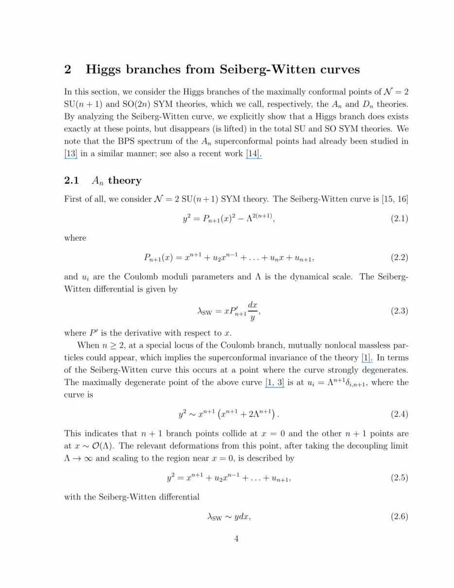
U(1)1 U(2)2 . . . U(1)k−2 U(1)k−1

q1 1 0 . . . 0 0

q2 1 1 . . . 0 0...

.... . .

. . ....

...

qk−1 0 0 . . . 1 1

qk 0 0 . . . 0 1

Table 1: U(1) charges of massless BPS particles of the A2k−1 theory.

where [s] is the integer part of s. This is the orbifold singularity C2/Zk. Thus, we have

found a C2/Zk Higgs branch at the special point of the Coulomb branch for arbitrary values

of ci. Note that when k = 2 the orbifold C2/Z2 has an SU(2) isometry. Thus, the flavor

symmetry is enhanced from U(1) to SU(2) in this case.

This Higgs branch does not exist if we go back to the original SU(2k) description. In

particular, the U(1) flavor symmetry of the A2k−1 theory is gauged, which can be seen from

the fact that the residue at x = ∞ comes from decoupled cuts. In the case of k = 2 the

U(1) subgroup of SU(2) is gauged. Indeed, we can check that the gauge charges of q1 and

q2 with respect to this gauged U(1) are 1 and −1 respectively.

2.1.2 A2k theory

Let us next see that no Higgs branch exists in the n = 2k case. The Seiberg-Witten curve

is

y2 = x2k+1 + c2x2k−1 + . . .+ ck+1x

k + vk+1xk−1 + . . .+ v2, (2.13)

and the Seiberg-Witten differential is λSW = ydx. Note that there is no residue at x = ∞in this case. The scaling dimensions of the parameters are given as (2.8) for i = 2, . . . , k+1

without any dimension-one parameter. The Coulomb branch is k-dimensional.

We see that there is a locus in the Coulomb branch where k mutually local cycles

degenerate to points at generic ci. At this point, the curve is written as

y2 = (x− x0)Qk(x)2, (2.14)

where Qk(x) is a polynomial of degree k and x0 is a constant. A similar argument to the

one in the n = 2k − 1 case shows that the charge assignment of massless BPS particles qiat this locus to be as in table 2.

A basis of holomorphic gauge invariant operators are Mi = qiqi, N , and N as before.

But the F-term equations give Mi = 0, meaning that there is no Higgs branch.

7

U(1)1 U(2)2 . . . U(1)k−1 U(1)k

q1 1 0 . . . 0 0

q2 1 1 . . . 0 0...

.... . .

. . ....

...

qk−1 0 0 . . . 1 0

qk 0 0 . . . 1 1

Table 2: U(1) charges of massless BPS particles of the A2k theory

2.2 Dn theory

Our second example is the Dn theory, which is the maximally conformal point of SO(2n)

SYM theory. We will show that this theory has SU(2) flavor symmetry in the case of odd

n with C2/Z2 Higgs branch, and SU(2)×U(1) (SU(3) for n = 4) in the case of even n. For

n even the Higgs branch has (quaternionic) dimension two (or real dimension eight).

The Seiberg-Witten curve of SO(2n) SYM theory is [18, 19, 20]

y2 = xPn(x)2 − Λ4(n−1)x3, (2.15)

where

Pn(x) = xn +

n−1∑

i=1

s2ixn−i + s2n, (2.16)

and the Seiberg-Witten differential is

λSW = (Pn − xP ′n)

dx

y. (2.17)

The branch points are at the 2n + 1 roots of the right hand side of (2.15) and at x = ∞.

The curve is of genus n.

The maximal degeneration of the curve occurs at s2i = Λ2(n−1)δi,n−1 and sn = 0 [3], at

which point the curve has the form

y2 ∼(xn + 2Λ2(n−1)x

)xn+1. (2.18)

Thus, n + 2 branch points collapse to x ∼ 0 and the other n − 1 branch points are at

x ∼ O(Λ2). It is convenient to redefine s2(n−1) → Λ2(n−1)+ s2(n−1), so {s2j , sn} now measure

the deviation from the singular point. Then, by taking a decoupling limit Λ → ∞ and

scaling to the maximal singular point on the Coulomb branch, we get the curve of the Dn

maximal superconformal theory. Since this decoupling plus scaling procedure is less straight

forward than in the An case, we now give a few details.

8

Keeping only terms which control the leading positions of the zeros of y2 near x = 0 as

all sj , sn → 0, gives

y2 = 2x2Pn + xs4n, (2.19)

where Pn is still given by (2.16) even though we have shifted the definition of s2(n−1). This

is equivalent to taking the Λ → ∞ decoupling limit. Note that at this stage the xs4n term

is kept even though it will later turn out to scale to zero much faster than the x2s2n term

because it nevertheless controls the position of one of the roots of y2. Note also that (2.19)

describes a genus [(n+ 1)/2] curve.

Now demand a scaling symmetry to x = y = s2j = sn = 0 in the curve. There is only

one consistent scaling,1 with ∆(x) = (2/n)∆(sn) = (1/j)∆(s2j), which makes the xs4n term

in (2.19) irrelevant. The curve then becomes y2 = 2x2Pn, which is singular at x = 0 where

one handle is always pinched, reducing the genus by one to [(n− 1)/2]. This can be made

explicit by defining a new coordinate y = y/x so that the curve becomes

y2 = 2Pn. (2.20)

The pinched handle is no longer apparent, but will show up as a pair of poles in the Seiberg-

Witten differential at x = 0. Replacing y → xy in (2.17) gives, up to a total derivative, the

differential

λSW =y

xdx (2.21)

on the part of the curve in the vicinity of the singularity. Demanding that ∆(λSW) = 1 then

gives

∆(s2j) =2j

nand ∆(sn) = 1. (2.22)

λSW has a pole at x = 0 with residue ∼ sn, which identifies sn as a mass parameter. The

s2j with 2j > n have dimensions greater than one, so are identified with Coulomb branch

vevs, while those with 2j < n have dimensions less than one, so are relevant couplings like

the ci in (1.1).

Note that for n even, sn has dimension one, and λSW also has a pole at x = ∞ with

residue ∼ s′n := sn + f(s2j) where f is a polynomial in the s2j with 2j < n which is

homogeneous of scaling dimension one. This identifies s′n as a second mass parameter in the

theory for n even. As in the An theory, let us consider the odd and even n cases separately.

1Thus the possibility of multiple consistent scalings, discussed in [5], does not arise in this case.

9

0 x1 x2

∞A0 A1 A2

B0 B1 B2

Figure 2: Branch points and cycles of the D2k+1 theory when m = 0; k = 3 in the picture.

The dotted arrows show the movements of the branch points under δ → e2πiδ.

2.2.1 D2k+1 theory

We first consider the n = 2k + 1 case. The curve (2.21) is (after rescaling y by√2 and

renaming the {s2j , sn} parameters)

y2 = x2k+1 + c1x2k + . . .+ ckx

k+1 + vkxk + . . .+ v1x+m2. (2.23)

As in the An case, the vi are the Coulomb moduli and ci are the associated deformation

parameters. Their scaling dimensions (2.22) are thus ∆(ci) = (2i/n), ∆(vi) = 2(n − i)/n,

and ∆(m) = 1, for i = 1, . . . , k. Note that this curve is the same as that of (the relevant

deformation from) the maximal superconformal point of the SU(2k) theory with two flavors

[7]. So, it might be natural to expect that the flavor symmetry is SU(2). Let us check this

here.

As in the An theory, we set the mass parameter to zero and choose the special locus

of vi = v⋆i (cj) where k non-intersecting cycles degenerate. Note that this locus satisfies

v⋆1 = 0. We can see that at this locus there are k + 1 mutually local massless BPS particles

by examining a monodromy around the locus in the Coulomb branch. Indeed, by setting

vi = v⋆i for arbitrary fixed ci, the Seiberg-Witten curve degenerates to

y2 = x2(x− xk)Qk−1(x)2, (2.24)

where Qk−1(x) is a degree-(k−1) polynomial whose roots we denote as xi (i = 1, . . . , k−1)

and xk is a constant depending on the ci. A small deformation from this locus (still fixing

m = 0) is

y2 = x(x(x− xk)Qk−1(x)

2 − δ). (2.25)

The branch points are at x = 0, δ, xi ± bi√δ and xk + bkδ where bi are some constants. Let

A0 and Ai (i = 1, . . . , k − 1) be the cycles around x = 0, δ and x = xi ± bi√δ, respectively.

10

U(1)1 U(2)2 . . . U(1)k−1 U(1)k

q1 1 0 . . . 0 0

q2 1 0 . . . 0 0

q3 1 1 . . . 0 0...

.... . .

. . .. . .

...

qk+1 0 0 . . . 1 1

Table 3: U(1) charges of massless particles of the D2k+1 theory.

Let also B0 and Bi (i = 1, . . . , k− 1) be the cycles from 0 to x1 and from xi to xi+1 passing

through two cuts, respectively; see figure 2.

The monodromy under δ → e2πiδ is aD0 → aD0 + 2a0 − a1, aDi → aDi + ai − ai+1

and aDk−1 → aDk−1 + ak−1, while the ai periods stay fixed. Therefore the charges of the

k + 1 massless BPS particles are assigned as in table 3. Note that the coefficient 2 in

aD0 → aD0 +2a0 − · · · signifies the existence of two hypermultiplets with charge 1, because

in general we have aD → aD + ka where k =∑

s qs2 where qs are the charges of the

hypermultiplets charged under the U(1) corresponding to a.

This charge assignment shows that the Higgs branch is simply C2/Z2. Indeed, the gauge

invariant operators constructed from qi are Mi = qiqi (i = 1, . . . , k + 1) and N = q1q2and N = q2q1, with one constraint M1M2 = NN . The F-term equations set Mi = 0 for

i = 3, . . . , k + 1 and M1 = −M2. Thus, M21 + NN = 0, implying C2/Z2. The flavor

symmetry is SU(2) under which the BPS particles q1 and q2 transform as a doublet.

Next, in order to see how this SU(2) flavor symmetry is broken in the total SO(4k + 2)

SYM theory, we analyze the spectrum of light BPS particles with a small mass parameter

m. While it could be possible to do this for general k, we consider only k = 1 for illustration.

In this case, the curve is y2 = x3 + c1x2 + v1x+m2 and its discriminant is

∆ = −4

(v31 −

c214v21 −

9c1m2

2v1 + c31m

2 +27

4m4

). (2.26)

The roots of the discriminant are v1 = w0 and w± where

w0 =c214+

2

c1m2 +O(m3), w± = ±2

√c1m− 1

c1m2 +O(m3). (2.27)

The last two roots are related by the sign flip of m. Let us focus on the point v1 = w+ where

the three roots of the right-hand side of the curve are at x ∼ O(m), O(m) and O(1). The

A0 cycle collapses at this value of v1 and this indicates a massless BPS particle with central

charge −m − a, where a is the period of the cycle along the other cut (from x ∼ O(m)

to ∞). It is easy to see that the point v1 = w− corresponds to the massless particle with

11

central charge m− a since this is obtained by the sign flip of the above case. (When m = 0

these two BPS particles become the doublet of the SU(2) flavor symmetry.) Thus, these

two BPS particles have charge +1 and −1 under the U(1) subgroup of SU(2).

As we saw above, the pole of λSW at x = 0 comes from a degenerating cut of the original

Seiberg-Witten curve (2.19) or (2.15). Thus, the U(1) subgroup of SU(2) at the maximally

conformal point is gauged in the total SO(6) theory. This argument can be applied to the

general SO(4k + 2) case (and also to the SO(4k) case which will be discussed in the next

subsection): the U(1) subgroup of SU(2) is gauged and there is no Higgs branch.

2.2.2 D2k theory

We now turn to the D2k theory. The curve is

y2 = x2k + c1x2k−1 + . . .+ ck−1x

k+1 + ckxk + vk−1x

k−1 + . . .+ v1x+m2. (2.28)

The Seiberg-Witten differential is again λSW = (y/x)dx with m the residue of the pole at

x = 0. The enhancement of the U(1) flavor symmetry associated to m to an SU(2) flavor

symmetry follows by repeating the argument in the previous subsection.

The new feature here is the existence of the additional pole at x = ∞. Its residue can

be written in terms of ck plus a polynomial in the other ci<k parameters, and has scaling

dimension one. This means that, up to a shift, ck is a mass parameter with an associated

U(1) flavor symmetry. Thus the total flavor symmetry of the D2k superconformal point is

at least SU(2)×U(1).

By setting m = 0, we can find the locus of the Coulomb moduli where the Seiberg-Witten

curve degenerates to

y2 = x2Qk−1(x)2, (2.29)

where Qk−1(x) is again a degree-(k−1) polynomial. This represents the appearance of k+1

mutually local massless particles qi. This can be seen in the same way as in the n = 2k + 1

case, and their charge assignments are given in table 4.

Note that the flavor symmetry is enhanced to SU(3) in the k = 2 case, that is the D4

theory. In this case, the Weyl group of the SU(3) flavor symmetry can be identified with

the S3 outer automorphism group of the original D4 = SO(8) theory. In the other theories,

the flavor symmetry is SU(2)×U(1). The Higgs branch is two-(quaternionic-)dimensional

(or, 8-real-dimensional). In the total SO(4k) theory, the U(1)2 ⊂ SU(2)× U(1) (or SU(3))

is gauged and there is no Higgs branch.

12

U(1)1 U(2)2 . . . U(1)k−2 U(1)k−1

q1 1 0 . . . 0 0

q2 1 0 . . . 0 0

q3 1 1 . . . 0 0...

.... . .

. . .. . . 0

qk 0 0 . . . 1 1

qk+1 0 0 . . . 0 1

Table 4: U(1) charges of massless particles of the D2k theory.

3 Flavor central charge

We will consider in this section the central charge of the SU(2) flavor symmetry of the Dn

theory by embedding it into the SO(2n) SYM theory where the U(1) subgroup of the SU(2)

is gauged and by analyzing the Seiberg-Witten curve.

Let us suppose that we have a flavor symmetry H . The flavor central charge is defined

by the OPE of the currents Jaµ as

Jaµ(x)J

bν(0) =

3kH4π4

δabx2gµν − 2xµxν

x8+ . . . . (3.1)

We normalize the flavor central charge such that n free chiral multiplets give kU(n) = 1. If

there is a weakly gauged group G which is a subgroup of the flavor symmetry H , the central

charge is given by

kG⊂H = IG→HkH , (3.2)

where IG→H is the embedding index, see e.g. [21]. Then, the one-loop beta function of the

gauge group G is given in terms of the central charge:

b0 = 2T2(adj)−kG⊂H

2. (3.3)

where we defined b0 =∂

∂ lnQ(8π2/g2(Q)). When G = U(1) and H = SU(2) which is the case

we will see below, we have kU(1)⊂SU(2) = IU(1)→SU(2)kSU(2) = kSU(2). Thus, the beta function

coefficient of the U(1) gauge group is b0 = −kSU(2)

2. In other words, the effective coupling

constant of the U(1) should be written as

τ =b02πi

ln Λ = −kSU(2)

4πiln Λ. (3.4)

Now let us consider the Dn theory which has SU(2)(×U(1)) flavor symmetry (when

n = 2k). As we discussed in detail in subsection 2.2, the U(1) subgroup of the SU(2)

13

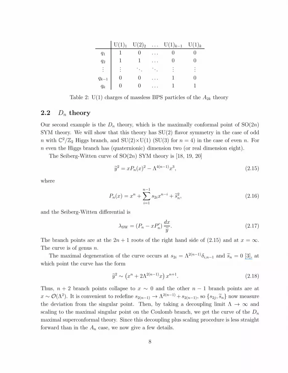
0 x0 x1 x2

∞A A0 A1 A2

B B0 B1 B2

Figure 3: Branch points and cycles of the curve (3.6) for n = 7, for m 6= 0. The A cycle

degenerates in the limit Λ → ∞ corresponding to that the U(1) gauge group is decoupled.

is gauged in the IR effective theory of the SO(2n) SYM theory where the Dn theory is

embedded. This U(1) gauge symmetry corresponds to the degenerating cut (or the pinched

handle) in the decoupling limit Λ → ∞. In order to see this more clearly, let us go back to

the curve (2.19) and keep the dynamical scale dependence explicit:

y2 ∼ x(2Λ2(n−1)Pn + s4n

)∼ 2Λ2(n−1)x

(x+

s2n2Λ2(n−1)

)Pn. (3.5)

By scaling x and the parameters appropriately, we get

y2 = x

(x+

m2Λ−2(n−1)/n

2

)Pn, (3.6)

with the differential λSW = yx2dx, where Pn is the RHS of (2.23) for odd n or (2.28) for even

n. The degenerating cut is from x = 0 to x = −m2Λ−2(n−1)/n/2. Denote by A and B the

cycles encircling this cut and from x = −m2Λ−2(n−1)/n/2 to x = x0 going through two cuts,

as depicted in figure 3. The period integrals in the limit where Λ → ∞ can be evaluated as

follows: ∮

A

λSW = 2πim,

∮

B

λSW ∼∫ −m2Λ−2(n−1)/n/2

mdx

x∼ −2(n− 1)

nm ln Λ. (3.7)

The coupling constant of the decoupling U(1) is then given by

τ = − 1

4πi

4(n− 1)

nlnΛ + . . . . (3.8)

It follows from this and (3.4) that the central charge of the flavor symmetry is

kSU(2) =4(n− 1)

n. (3.9)

which agrees with the result in [5].

14

A3 D4 E6

A4 D5 E7

A5 D6 E8

Figure 4: BPS quivers of the superconformal points of the A-D-E SYM theories.

4 Comparisons to other recent results

The properties of the Higgs branch of the superconformal points of N=2 SYM theories can

also be determined from more modern methods.

4.1 Using BPS quivers

In [6], it was stated that the BPS spectrum in a certain chamber on the Coulomb branch of

the superconformal point of the SYM theory with simply-laced gauge group G is given by a

BPS quiver of the form of the Dynkin diagram of type G; see figure 4. Namely, each node

stands for a hypermultiplet, and two nodes are connected by n = |〈q1, q2〉| arrows, where q1,2are electromagnetic charges of two particles, and 〈·, ·〉 is the Dirac quantization pairing; the

arrow is oriented by the sign of 〈q1, q2〉. For G = SU(N) this was already known in [13]; our

analysis in section 2.2 can be thought of as an elementary confirmation of this statement

for G = SO(2n).

Any simply-laced Dynkin diagram is bipartite; let us color the nodes accordingly with

white and black. Then the particles corresponding to the white nodes are mutually local,

and similarly for the particles corresponding to the black nodes. Let us say that the number

of black nodes is not larger than the number of white nodes. Let us then take the basis of

U(1) charges such that the i-th black node has the magnetic charge δij under the j-th U(1)

and no electric charges. Then the i-th white node has the electric charge +1 under j-th

U(1) charge if the i-th white node and the j-th black node are connected, and neutral under

the j-th U(1) otherwise. This procedure easily reproduces the tables of charges in tables 1,

2, 3, and 4. This also makes it manifest that the enhancement of the flavor symmetry to

SU(3) is only possible when G = D4.

The only thing that our analysis in section 2 adds to this picture is the direct construction

from the Seiberg-Witten curve that of a locus on the Coulomb branch where the BPS states

corresponding to the white modes are massless while those corresponding to the black nodes

are massive. To do this it was crucial that we could deform away from the superconformal

15

A3 A5 A7 D4 D6 D8

Figure 5: 3d mirrors of the A2k−1 and D2k theories.

point by turning on the relevant ci couplings (1.1).

Assuming that the BPS spectrum of the superconformal points of En SYM theory, first

studied in [4], is given by the Dynkin diagram, we can immediately find the table of U(1)

charges of mutually local particles. We do not have Higgs branches for E6 and E8, while

we have a one-dimensional Higgs branch for E7. This also is in accord with the spectrum

of scaling dimensions of these theories, because there is no dimension-one operator when

G = E6,8, while there is one dimension-one operator when G = E7.

4.2 Using the 3d mirror

In the mathematical works [22, 23], it was shown that the 3d Coulomb branch of a wild

quiver gauge theory (in the sense of [7]) compactified on S1 of radius R is given, in the limit

R → 0, by the Higgs branch of another non-wild quiver gauge theory. In section 6 of [12],

this non-wild quiver gauge theory was interpreted as the 3d mirror of the S1 compactification

of the wild quiver gauge theory. Then, some properties of the Higgs branches of the original

theory are visible using the Coulomb branch of the 3d mirror, see figure 5. In the figure,

a gray node stands for a U(1) gauge group, and a line between two nodes corresponds to

a bifundamental hypermultiplet; the overall U(1) is decoupled and to be removed. We see

that there is a one-dimensional Higgs branch when G = A2k−1, and a two-dimensional Higgs

branch when G = D2k.

The flavor symmetry enhancement on the Coulomb branch side of a quiver was studied

in [24]; the rule of thumb is that the set of nodes corresponding to a U(N) group coupled

to precisely 2n fundamentals, together with the edges among them, forms a finite or affine

Dynkin diagram Γ. Then the flavor symmetry enhancement is given by the type of Γ. In

our case all the nodes correspond to U(1) groups, so N = 1. We then easily see that for

G = A3 we have SU(2) flavor symmetry, while for other G = A2k−1 we just have U(1)

flavor symmetry. We also see that G = D4 we have SU(3) flavor symmetry, while for other

G = D2k we just have SU(2)× U(1) flavor symmetry. Note that this method explains only

the flavor symmetry enhancement, and we have supplied a U(1) to the generic A2k−1 and

D2k cases because the ranks of the flavor symmetries are always one and two respectively.

16

Acknowledgments

The authors would like to thank G. Bonelli, S. Cecotti, T. Eguchi, A. Shapere, A. Tanzini,

and D. Xie for useful comments. PCA is partially supported by DOE grant FG02-84-

ER40153. KM is partially supported by the INFN project TV12. YT is partially supported

by World Premier International Research Center Initiative (WPI Initiative), MEXT, Japan.

References

[1] P. C. Argyres and M. R. Douglas, “New Phenomena in SU(3) Supersymmetric Gauge

Theory,” Nucl. Phys. B448 (1995) 93–126, arXiv:hep-th/9505062.

[2] P. C. Argyres, M. R. Plesser, N. Seiberg, and E. Witten, “New N = 2 Superconformal Field

Theories in Four Dimensions,” Nucl. Phys. B461 (1996) 71–84, arXiv:hep-th/9511154.

[3] T. Eguchi, K. Hori, K. Ito, and S.-K. Yang, “Study of N = 2 Superconformal Field Theories

in 4 Dimensions,” Nucl. Phys. B471 (1996) 430–444, arXiv:hep-th/9603002.

[4] T. Eguchi and K. Hori, “N = 2 Superconformal Field Theories in Four-Dimensions and

A-D-E Classification,” in The Mathematical Beauty of Physics: A Memorial Volume for

Claude Itzykson, J. Drouffe and J. Zuber, eds., vol. 24 of Advanced Series in Mathematical

Physics, pp. 67–82. World Scientific, 1997. arXiv:hep-th/9607125 [hep-th].

[5] D. Gaiotto, N. Seiberg, and Y. Tachikawa, “Comments on Scaling Limits of 4D N = 2

Theories,” JHEP 1101 (2011) 078, arXiv:1011.4568 [hep-th].

[6] S. Cecotti, A. Neitzke, and C. Vafa, “R-Twisting and 4D/2D Correspondences,”

arXiv:1006.3435 [hep-th].

[7] G. Bonelli, K. Maruyoshi, and A. Tanzini, “Wild Quiver Gauge Theories,”

JHEP 1202 (2012) 031, arXiv:1112.1691 [hep-th].

[8] D. Xie, “General Argyres-Douglas Theory,” arXiv:1204.2270 [hep-th].

[9] P. C. Argyres, M. R. Plesser, and N. Seiberg, “The Moduli Space of N = 2 SUSY QCD and

Duality in N = 1 SUSY QCD,” Nucl. Phys. B471 (1996) 159–194, arXiv:hep-th/9603042.

[10] S. Cecotti and C. Vafa, “Classification of complete N=2 supersymmetric theories in 4

dimensions,” arXiv:1103.5832 [hep-th].

[11] M. Alim, S. Cecotti, C. Cordova, S. Espahbodi, A. Rastogi, et al., “BPS Quivers and

Spectra of Complete N = 2 Quantum Field Theories,” arXiv:1109.4941 [hep-th].

[12] D. Nanopoulos and D. Xie, “More Three Dimensional Mirror Pairs,”

JHEP 1105 (2011) 071, arXiv:1011.1911 [hep-th].

17

[13] A. D. Shapere and C. Vafa, “BPS Structure of Argyres-Douglas Superconformal Theories,”

arXiv:hep-th/9910182.

[14] J. Seo and K. Dasgupta, “Argyres-Douglas Loci, Singularity Structures and Wall-Crossings

in Pure N = 2 Gauge Theories with Classical Gauge Groups,” JHEP 1205 (2012) 072,

arXiv:1203.6357 [hep-th].

[15] P. C. Argyres and A. E. Faraggi, “The Vacuum Structure and Spectrum of N = 2

Supersymmetric SU(n) Gauge Theory,” Phys. Rev. Lett. 74 (1995) 3931–3934,

arXiv:hep-th/9411057.

[16] A. Klemm, W. Lerche, S. Yankielowicz, and S. Theisen, “Simple Singularities and N = 2

Supersymmetric Yang-Mills Theory,” Phys. Lett. B344 (1995) 169–175,

arXiv:hep-th/9411048.

[17] M. R. Douglas and G. W. Moore, “D-Branes, Quivers, and ALE Instantons,”

arXiv:hep-th/9603167 [hep-th].

[18] A. Brandhuber and K. Landsteiner, “On the Monodromies of N = 2 Supersymmetric

Yang-Mills Theory with Gauge Group SO(2n),” Phys. Lett. B358 (1995) 73–80,

arXiv:hep-th/9507008.

[19] P. C. Argyres and A. D. Shapere, “The Vacuum Structure of N = 2 Superqcd with Classical

Gauge Groups,” Nucl. Phys. B461 (1996) 437–459, arXiv:hep-th/9509175.

[20] A. Hanany, “On the Quantum Moduli Space of N = 2 Supersymmetric Gauge Theories,”

Nucl. Phys. B466 (1996) 85–100, arXiv:hep-th/9509176.

[21] P. C. Argyres and N. Seiberg, “S-Duality in N = 2 Supersymmetric Gauge Theories,”

JHEP 0712 (2007) 088, arXiv:0711.0054 [hep-th].

[22] P. Boalch, “Irregular connections and Kac-Moody root systems,”

arXiv:0806.1050 [math.DG].

[23] P. Boalch, “Hyperkahler manifolds and nonabelian Hodge theory of (irregular) curves,”

arXiv:1203.6607 [math.AG].

[24] D. Gaiotto and E. Witten, “S-Duality of Boundary Conditions in N = 4 Super Yang-Mills

Theory,” arXiv:0807.3720 [hep-th].

18