ρ-adic L-functions, ρ-adic Gross-Zagier formulas and plectic points

Víctor Hernández Barrios

ADVERTIMENT La consulta d’aquesta tesi queda condicionada a l’acceptació de les següents condicions d'ús: La difusió d’aquesta tesi per mitjà del repositori institucional UPCommons (http://upcommons.upc.edu/tesis) i el repositori cooperatiu TDX ( h t t p : / / w w w . t d x . c a t / ) ha estat autoritzada pels titulars dels drets de propietat intel·lectual únicament per a usos privats emmarcats en activitats d’investigació i docència. No s’autoritza la seva reproducció amb finalitats de lucre ni la seva difusió i posada a disposició des d’un lloc aliè al servei UPCommons o TDX. No s’autoritza la presentació del seu contingut en una finestra o marc aliè a UPCommons (framing). Aquesta reserva de drets afecta tant al resum de presentació de la tesi com als seus continguts. En la utilització o cita de parts de la tesi és obligat indicar el nom de la persona autora. ADVERTENCIA La consulta de esta tesis queda condicionada a la aceptación de las siguientes condiciones de uso: La difusión de esta tesis por medio del repositorio institucional UPCommons (http://upcommons.upc.edu/tesis) y el repositorio cooperativo TDR (http://www.tdx.cat/?locale- attribute=es) ha sido autorizada por los titulares de los derechos de propiedad intelectual únicamente para usos privados enmarcados en actividades de investigación y docencia. No se autoriza su reproducción con finalidades de lucro ni su difusión y puesta a disposición desde un sitio ajeno al servicio UPCommons No se autoriza la presentación de su contenido en una ventana o marco ajeno a UPCommons (framing). Esta reserva de derechos afecta tanto al resumen de presentación de la tesis como a sus contenidos. En la utilización o cita de partes de la tesis es obligado indicar el nombre de la persona autora. WARNING On having consulted this thesis you’re accepting the following use conditions: Spreading this thesis by the institutional repository UPCommons (http://upcommons.upc.edu/tesis) and the cooperative repository TDX (http://www.tdx.cat/?locale- attribute=en) has been authorized by the titular of the intellectual property rights only for private uses placed in investigation and teaching activities. Reproduction with lucrative aims is not authorized neither its spreading nor availability from a site foreign to the UPCommons service. Introducing its content in a window or frame foreign to the UPCommons service is not authorized (framing). These rights affect to the presentation summary of the thesis as well as to its contents. In the using or citation of parts of the thesis it’s obliged to indicate the name of the author.

Facultat de Matemàtiques i EstadísticaPrograma de doctorat de Matemàtica Aplicada

Departament de Matemàtiques

PhD Thesis in Mathematics

?-adic !-functions, ?-adic Gross-Zagierformulas and plectic points

Author: Víctor Hernández Barrios

Advisors: Dr. Santiago Molina Blanco, Dr. Victor Rotger Cerdà

Barcelona, 2022

AgraïmentsEstic profundament agraït als meus directors de tesi, en Santiago Molina i en VictorRotger, per la seva dedicació, guia i suport al llarg de tot aquest treball.

Li dono les gràcies a l’Albert Jiménez per la seva amistat, i als meus companys dedoctorat, Armando Gutiérrez, Daniel Gil, Francesca Gatti, Guillem Sala, Marc Felipe iÓscar Rivero, per la seva companyonia i suport.

Finalment dono les gràcies a la meva família i al Sobi per la seva estima, ajut, ipaciència incondicionals.

Aquesta tesi ha rebut finançament de l’European Research Council (ERC): Consolida-tor Grant Euler systems and the conjectures of Birch and Swinnerton-Dyer, Bloch andKato, PI: Victor Rotger, (grant agreement No 682152).

Per a la meva germana, na Irene.

AbstractIn this work we generalize the construction of ?-adic anticyclotomic !-functions associatedto an elliptic curve �/� and a quadratic extension /�, by defining a measure �)?�

attachedto /� and an automorphic form. In the case of parallel 2, the automorphic form isassociated with an elliptic curve �/�.

The first main result is a ?-adic Gross-Zagier formula: if � has split multiplicativereduction at p and p does not split at /�, we compute the first derivative of the ?-adic!-function by relating it with the conjugate difference of a Darmon point twisted by acharacter �. The proof uses the reciprocity map provided by class field theory as a naturalway to interpret conjugate differences of points in �( p) as elements in the augmentationideal for the evaluation at the character �. This generalizes a result of Bertolini andDarmon. With a similar argument, after discovering the work of Fornea and Gehrmannon plectic points, we prove an exceptional zero formula which relates a higher orderderivative of �)(� with plectic points.

We find an interpolating measure �Φ?

�for �)?�

attached to an interpolating Hida familyΦ?

� for )?

�. Here �Φ?� can be regarded as a two variable ?-adic !-function, which now includesthe weight as a variable. Then we define the Hida-Rankin ?-adic !-function !?()?� , �, :)as the restriction of �

Φ?

�to the weight space. Finally, we prove a formula which relates

the weight-leading term of !?()?� , �, :) with plectic points. In short, the leading term is anexplicit constant times Euler factors times the logarithm of the trace of a plectic point.This formula is a generalization of a result of Longo, Kimball and Hu, which has beenused to prove the rationality of a Darmon point under some hypotheses.

MSC2020 classification: 11F67, 11F75, 11G05, 11F70, 11G40.

ResumEn aquesta tesi generalitzem la construcció de funcions ! ?-àdiques anticiclotòmiquesassociades a una corba el·líptica �/� i una extensió quadràtica /�, definint una mesura�)?�

associada a /� i una forma automorfa. En el cas de pes paral·lel 2, la forma automorfas’associa a una corba el·líptica �/�.

El primer resultat és una fórmula ?-àdica de Gross-Zagier: si � té reducció multiplica-tiva split a p i p descomposa a /�, calculem la primera derivada de la funció ! ?-àdicarelacionant-la amb la diferència conjugada d’un punt de Darmon twistat per un caràc-ter �. La demostració utilitza l’aplicació de reciprocitat de la teoria de cossos com unamanera natural d’interpretar les diferències conjugades de punts de �( p) com elementsen l’ideal d’augmentació de l’avaluació en el caràcter �. Això generalitza un resultatde Bertolini i Darmon. Amb un argument semblant, després de descobrir el treball deFornea i Gehrmann sobre els punts plèctics, demostrem una fórmula de zero excepcionalque relaciona una derivada d’ordre superior de �)(�

amb punts plèctics.Trobem una mesura d’interpolació �

Φ?

�per a �)?�

associada a la família Hida Φ?

� quepassa per )

?

�. Aquí �Φ?

�es pot considerar com una funció ! de dues variables, que ara

inclou el pes com a variable. Aleshores definim una funció ! de Hida-Rankin ?-àdica!?()?� , �, :) com la restricció de �

Φ?

�a l’espai de pesos. Finalment, demostrem una fórmula

que relaciona el terme principal de !?()?� , �, :) respecte al pes amb punts plèctics. Enresum, el terme principal és una constant explícita multiplicada per factors d’Euler i pellogaritme de la traça d’un punt plèctic. Aquesta fórmula és una generalització d’un re-sultat de Longo, Kimball i Hu, que s’ha utilitzat per demostrar la racionalitat d’un puntde Darmon sota certes hipòtesis.

MSC2020 classification: 11F67, 11F75, 11G05, 11F70, 11G40.

Contents

List of symbols xiii

1 Introduction 11.1 The BSD conjecture . . . . . . . . . . . . . . . . . . . . . . . . . . . . . . 11.2 ?-adic !-functions . . . . . . . . . . . . . . . . . . . . . . . . . . . . . . . . 21.3 Heegner points . . . . . . . . . . . . . . . . . . . . . . . . . . . . . . . . . 41.4 Overview of the main results . . . . . . . . . . . . . . . . . . . . . . . . . . 9

2 Automorphic forms 132.1 The ring of adèles . . . . . . . . . . . . . . . . . . . . . . . . . . . . . . . . 132.2 Some algebraic groups associated to quaternion algebras . . . . . . . . . . 142.3 Results from Class Field Theory . . . . . . . . . . . . . . . . . . . . . . . . 142.4 Automorphic forms and representations for GL2 . . . . . . . . . . . . . . . 152.5 Automorphic forms as cohomology classes . . . . . . . . . . . . . . . . . . 202.6 Eichler-Shimura for automorphic forms . . . . . . . . . . . . . . . . . . . . 212.7 Waldspurger’s formula in higher cohomology . . . . . . . . . . . . . . . . . 222.8 Automorphic cohomology classes . . . . . . . . . . . . . . . . . . . . . . . 24

3 The fundamental class 253.1 Fundamental classes of tori . . . . . . . . . . . . . . . . . . . . . . . . . . . 253.2 Pairings . . . . . . . . . . . . . . . . . . . . . . . . . . . . . . . . . . . . . 30

4 Darmon and plectic points 334.1 Construction of Darmon points . . . . . . . . . . . . . . . . . . . . . . . . 334.2 Fornea-Gehrmann plectic points . . . . . . . . . . . . . . . . . . . . . . . . 36

5 ?-adic !-functions 415.1 Anticyclotomic ?-adic L-functions . . . . . . . . . . . . . . . . . . . . . . . 415.2 ?-adic !-functions attached to modular elliptic curves . . . . . . . . . . . . 545.3 Overconvergent modular symbols . . . . . . . . . . . . . . . . . . . . . . . 545.4 Hida families . . . . . . . . . . . . . . . . . . . . . . . . . . . . . . . . . . 60

6 Main results 756.1 A ?-adic Gross-Zagier formula . . . . . . . . . . . . . . . . . . . . . . . . . 756.2 Exceptional zero formulas . . . . . . . . . . . . . . . . . . . . . . . . . . . 786.3 The Hida-Rankin ?-adic L-function . . . . . . . . . . . . . . . . . . . . . . 83

xi

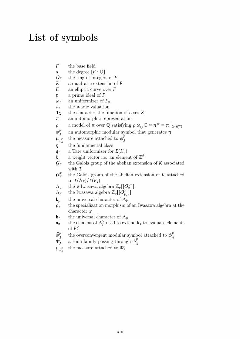
List of symbols

� the base field3 the degree [� : Q]O� the ring of integers of � a quadratic extension of �� an elliptic curve over �p a prime ideal of �+p an uniformizer of �pEp the p-adic valuation1- the characteristic function of a set -� an automorphic representation� a model of � over Q satisfying � ⊗Q C ' �∞ = � |�(A∞

�)

)?

� an automorphic modular symbol that generates ��)?�

the measure attached to )?

�

� the fundamental class@p a Tate uniformizer for �( p): a weight vector i.e. an element of Z3G) the Galois group of the abelian extension of associated

with )Gp)

the Galois group of the abelian extension of attachedto )(A�)/)(�p)

Λp the p-Iwasawa algebra Z?[[O×p ]]Λ� the Iwasawa algebra Z?[[O×�? ]]k? the universal character of Λ��" the specialization morphism of an Iwasawa algebra at the

character "kp the universal character of Λpap the element of Λ×

�used to extend kp to evaluate elements

of �×p)?

� the overconvergent modular symbol attached to )?

�Φ?

� a Hida family passing through )?

��Φ?

�the measure attached to Φ?�

xiii

xiv

Chapter 1

Introduction

Some first examplesHistorically, there are some reasons to believe that !-series or zeta functions link arith-metic with analysis, linking local and global behaviour. The Riemann zeta function �(B)is defined by the series �(B) = ∑∞

==1 =−B which converge for B ∈ C with <B > 1. Rie-

mann showed that �(B) extends to a meromorphic function of C and proved its functionalequation. Euler gave another expression for �(B), its Euler product

�(B) =∏?

(1 − ?−B

) −1where ? runs over the primes of Z. It follows from the fundamental theorem of arithmetic.Using the Euler product, Riemann linked the prime counting function �(G) with the zeroesof �(B), and formulated the Riemann hypothesis, still open. Given a number field �/Q,its Dedekind zeta function is defined similarly and also has an Euler product

��(B) =∑a⊂O�

(Na)−B =∏p

(1 − (Np)−B

) −1where a runs over the ideals of O� and p over the prime ideals. The class number formulalinks several invariants of � with the behaviour of ��(B) at B = 1,

limB→1(B − 1)��(B) =

2AR · (2�)AC · Reg ·ℎ F ·

√|3 |

(1.1)

where AR is the number of real embeddings of � into C, AR + 2AC = [� : Q], Reg is theregulator of , F the number of roots of unity in , ℎ the class number of and 3 its discriminant.

The conjectures of Beilinson and Bloch-Kato, out of the scope of this text, are one ofthe first general attempts to link the special values of !-functions with arithmetic, fromwhich the BSD conjecture can be regarded as an special case.

1.1 The BSD conjectureGiven an elliptic curve �/� of conductor N ⊂ O�, we have a natural geometric group law,giving rise to its abelian group of �-rational points �(�). Mordell proved �(�) is finitelygenerated and thus has finite Z-rank, this is the algebraic rank Aalg(�/�) of �. We canalso form its Hasse-Weil !-function with the following Euler product

!(�/�, B) =∏p-N

(1 − 0p@−Bp + @1−2Bp

) −1 ·∏p|N

(1 − 0p@−Bp

)(1.2)

1

where each 0p = 0p,� is given explicitly in terms the reduction type and the number ofrational points of � over �p. The product converges absolutely on <(B) > 3/2 becausethe 0p have a controlled behaviour: they satisfy Hasse’s inequality.

In few words, automorphic representations are generated by automorphic forms, whichare a generalization of modular forms. We say � is modular if there exists an automorphicrepresentation � for PGL2/� of parallel weight 2 such that

!(�, B − 1

2

)•= !(�/�, B)

where •= denotes that we ignore the archimedean factors. It is a classic result of Hecke thatthe !-series !( 5 , B) associated to a modular form 5 ∈ (:(Γ0(#)) of level # has an analyticcontinuation to C, and that its normalized !-function Λ( 5 , B) = # B/2(2�)−BΓ(B)!( 5 , B)satisfies the functional equation

Λ( 5 , B) = � · Λ( 5 , : − B) (1.3)

Similar results (functional equation and analytic continuation) hold for automorphic rep-resentations. The existence of the automorphic representation associated with � is nowknown when � = Q by the modularity theorem, and also for most elliptic curves when �is a totally real field, thus in these cases !(�/�, B) extends to an entire function.

However, in the 60s Birch and Swinnerton-Dyer formulated a conjecture based oncomputational evidence, a prediction about the behaviour of !(�/Q, B) at B = 1, yet therewas no modularity, no Langlands programme to support whether the !-function is definedat B = 1. The BSD conjecture can be stated by means of an equality which involves severalinvariants of the elliptic curve as in (1.1), together with the claim that

Aalg(�/�) = ordB=1!(�/�, B) (1.4)

That is, the algebraic rank is a computable number equal to the analytic rank, the orderof vanishing of !(�/ , B) at B = 1. The weak version of BSD conjecture only claimsequation 1.4 and the finiteness of the Tate-Shafarevich group, an invariant of �.

From (1.4) we observe that if the !-function vanishes then �( ) should be infinite,and at least a -rational point of infinite order should exist. Some of the progress inproving partial versions of (1.4) use a set of special points, called Heegner points, thatemerge when is a totally imaginary quadratic extension of a totally real field � and �is modular and defined over �. In fact, for now the cases of rank 0 and 1 are the mostunderstood due to the results of Gross, Zagier and Kolyvagin and their use of Heegnerpoints.

1.2 ?-adic !-functionsAn automorphic form has an associated !-function, which as we have seen above con-jecturally holds a lot of arithmetic information, but is inaccessible by current methods.Much of the recent progress on this problem comes from proving results about ?-adic!-functions, rather than working with the !-function directly. These objects, which areconstructed in many different ways, in some sense interpolate the classic !-function. Wewill later focus on one possible automorphic construction of a ?-adic !-function, by re-garding the twists of the !-function as the integral of the character " over a certainmeasure.

2

In this approach the measure � determines the ?-adic !-function, and to find its :-thTaylor coefficient amounts to compute the image of � in � :/� :+1 when it has a zero oforder : (see [MT87]), where � is an ideal called the augmentation ideal. To illustrate thisidea, consider the following example. In the polynomial ring C[-] we can consider themorphism C[-] → C given by - ↦→ 0, inducing the sequence

0 � C[-] C 0

where � = ker (- ↦→ 0). Then an element 5 ∈ C[-] has a zero of order : at - = 0when 5 ∈ � : and the coefficient of - : in 5 can be identified with its image in � :/� :+1.

One usual way to construct ?-adic !-functions is through measures of Z?-extensions ofthe base field �. There is a unique Z?-extension of Q, namely QΔ∞,? where Q∞,? = Q(�?∞)is the field generated by the ?= roots of unity for all = ≥ 1 and

Gal(Q∞,?/Q) ' Z×? = Δ × Σ, Δ = Z/(? − 1)Z, Σ = Z?

For a general number field this does no longer hold (see [Sha19]). Apart from the cyclo-tomic extension, an imaginary quadratic field has an abelian Z?-extension ! of whichis anticyclotomic: !/Q is Galois and Gal( /Q) acts on Gal(!/ ) by −1. For now, therehave been constructions of both cyclotomic and anticyclotomic ?-adic measures.

Cyclotomic case

The Mazur and Swinnerton-Dyer ?-adic !-function !?( 5 , B) is defined through a measure�? of the cyclotomic Z?-extension of Q. Given a cusp form 5 ∈ (2(#), it can be definedas the ?-adic Mellin transform

!?( 5 , B) =∫Z×?

exp?(B log? �)3�?(�) : C? → C? .

Since the ?-adic exponential and logarithm are ?-adic analytic, so is !?( 5 , B). Its inter-polation property shows !?( 5 , B) is related with the classical !-function: given a finitecharacter " : Z×? → C× one has∫

Z×?

"(�)3�?(�) = �?(", 5 ) · !( 5 , ", 1),

where !( 5 , ", 1) is the classical !-function twisted by this character and �?(", 5 ) someEuler factor.

Later, Mazur, Tate and Teitelbaum formulated the ?-adic version of the BSD conjec-ture. One consequence of this conjecture is the exceptional zero conjecture: !?(�, B) =!?( 5 , B) has exactly one more extra zero at the critical point than !(�, B), when 5 isattached to an elliptic curve � with split multiplicative reduction at ?. In rank zerosituations it is now a theorem by Greenberg and Stevens and it states that in this case

!′?(�, 1) = ℒ(�) ·!(�, 1)Ω+�

, (1.5)

where ℒ(�) = log?(@�)/ord?(@�) is the ℒ-invariant and Ω+� the real period of �.Note that since !?( 5 , 0) =

∫Z×?3�?, when !?( 5 , B) has a zero of order A at B = 0 its

Taylor coefficient can be found by computing the image of �? in �A/�A+1 where � is the

3

augmentation ideal, the kernel of integrating the constant function 1. More generally, if' is a ring the '-valued measures of a topological space X form a ring Meas(X , ') and �fits into the exact sequence

0 � Meas(X , ') ' 0

�∫X 3�

Anticyclotomic case

Let be a quadratic imaginary field over Q. In [BD96; BD98; BD99], Bertolini and Dar-mon constructed the anticyclotomic ?-adic !-function !?(�/ ) associated to an ellipticcurve �/ with split multiplicative reduction at ? and the anticyclotomic extension of .They proved an analogous Greenberg-Stevens exceptional zero formula if /� splits, byrelating the derivative !′?(�/ ) at the critical point with the classical !-function and theℒ-invariant similarly as in (1.5). Instead of using Hida families as Greenberg and Stevens,the proof uses ?-adic integration on Shimura curves. Also, they showed that when /�is inert the derivative !′?(�/ ) can be used to obtain a -rational point in �( ). In fact,the image ΦTate(!′?(�/ )) by the Tate uniformization is a difference of conjugate Heegnerpoints ;

ΦTate(!′?(�/ )) = − . (1.6)

In the papers [Ber+02; BD07] these results were generalized for higher weights.

1.3 Heegner pointsThe classical way to construct Heegner points on an (modular) elliptic curve �/Q ofconductor # is essentially to take the image of CM points of the modular curve -0(#) oflevel # using its modular parametrization !. The modular curve -0(#) can be regardedas the solution of the moduli problem (i.e. the corresponding functor is representable) ofclassifying pairs (�′, �′) where �′ is an elliptic curve and �′ a cyclic subgroup of order #modulo isomorphism. If ℌ = {I ∈ C : =I > 0} is the upper half plane and ℌ∗ = ℌ∪Q∪{∞}the extended upper half-plane, each � ∈ ℌ has an associated elliptic curve �� = C/〈1, �〉over C with endomorphism ring O�. From this it can be shown that

-0(#)(C) ' ℌ∗/Γ0(#).

The ring O� is either Z or an order of a quadratic imaginary field /Q. In the last case � issaid to be a CM point ; the theory of complex multiplication shows there is a finite numberof isomorphism classes of elliptic curves �� with O� = O for a fixed order O of a quadraticimaginary field , and that their 9-invariants must be algebraic integers that generateabelian extensions of . This is a remarkable property; by evaluating transcendentalfunctions on certain arguments we obtain values that generate class fields in a systematicway, an instance of a realization of Kronecker’s Jugendtraum.

Elliptic curves have a uniformization over C because �(C) can be regarded as a torusC/Λ for some lattice Λ ⊂ C. There is an explicit parametrization !: if C/Λ ' �(C) (and2 is Manin’s constant) then ! is given by

! : -0(#)(C) ' ℌ/Γ0(#) C/Λ� 2

∫ �

8∞ 2�8 5 (I)3I(1.7)

4

where 5 = 5� is a weight 2 modular form attached to � by modularity. The image ofa CM point lies in fact in the group of rational points �(�), where � is the ring classfield associated to O. The construction can be carried out under certain conditions on and O, the Heegner hypothesis : the conductor of O ⊂ is prime to # and the primes ℓdividing # split in /Q. For instance if the conductor of O is 1 then the point belongsto �(�1) where �1 is the Hilbert class field of .

This gives a quite general construction of algebraic points on �. The link between the !-function of � and Heegner points was found by Gross and Zagier in the 80s. Their formularelates the Néron-Tate pairing with the first derivative of !(�/ , B); if % = Tr�1/ %1 isthe trace of a Heegner point of conductor 1 then

〈% , % 〉 = !′(�/ , 1)

where the equality is up to some explicit non-zero factor. In particular, % is non torsionif and only if !′(�/ , 1) ≠ 0. This connection was strengthened by Kolyvagin’s results; heproved that if % is non torsion then the Mordeil-Weil group of -rational points �( ) hasrank 1. Altogether their results show that if �/Q has analytic rank ≤ 1 then � satisfiesthe weak BSD conjecture.

If one wants to relax the Heegner hypothesis, one must parametrize the elliptic curvewith a certain Shimura curve -#+ ,#− instead, otherwise % cannot be constructed. That isone of the reasons for which we will work with algebraic groups associated to a quaternionalgebra, that we define in the next section. Here #+, #− is an admissible factorizationof # . The complex points of -#+ ,#− can be identified with a quotient of the upper halfplane ℌ by a discrete subgroup Γ#+ ,#− of a quaternion algebra. The curve is also definedover Q as -0(#) and is the solution to another moduli problem. In this setting, Zhanggeneralized the Gross-Zagier formula for Heegner points obtained from the Shimura curves-#+ ,#− .

?-adic Heegner points

To obtain similar results to those of Gross, Zagier and Kolyvagin in other settings, for ex-ample when is not imaginary, one should first generalize Heegner points. Note howeverthat the algebraicity of Heegner points was provided by the theory of complex multipli-cation, which is either absent or conjectural in the real setting; there are some intriguingresults for special cases and conjectures in this direction though, see [DPV21].

One first step is to phrase the construction of Heegner points differently, by usingmodular symbols. Recall the modular parametrization ! : -0(#) → � and denote byΔ the free abelian group of divisors of ℌ. Then there is a natural map 8( 5 ) attached to5 = 5� from the degree zero divisors Δ0 on ℌ to C, namely

8 : (2(#) HomΓ0(#)(Δ0,C)

5 8( 5 ) :(�′ − � ↦→

∫ �′

�5 (I)3I

)Since 8( 5 ) is Γ0(#)-equivariant, we have 8( 5 ) ∈ HomΓ0(#)(Δ0,C) = �0(Γ0(#),Hom(Δ0,C))

and to evaluate an any point of ℌ rather than only at Δ0, we should try to lift 8( 5 ) toHomΓ0(#)(Δ,C). Consider the short exact sequence associated to the degree map

0 Δ0 Δ Z 0deg

5

TheHom(•,C) functor is contravariant, and exact in this case because C is an injectiveZ-module, and we obtain

0 Hom(Z,C) ' C Hom(Δ,C) Hom(Δ0,C) 0

Taking the long exact sequence of Γ0(#)-cohomology we obtain

· · · HomΓ0(#)(Δ,C) HomΓ0(#)(Δ0,C) �1(Γ0(#),C) · · ·�

The connecting morphism here is �(ℎ) =∫ ��

�ℎ(I)3I and its cohomology class does

not depend on the choice of �. It turns out the image of 8( 5 ) is a lattice Λ 5 ⊂ C suchthat � is isogeneous to C/Λ 5 . Rewriting the long exact sequence above but now applyingHomΓ(•,C/Λ 5 ) we obtain by construction 8( 5 ) ∈ ker 2, so there exists a lift � 5 of 8( 5 ) toΔ. Historically, an element in HomΓ0(#)(Δ0, ") = �0(Γ0(#),Hom(Δ0), ")) or rather isrestriction to the cuspidal degree zero divisors, was understood as a modular symbol. Inthis work, we will call modular symbol to any cohomology class in �A(Γ0(#),Hom(#, "))for any Γ0(#)-modules # and ". In §2.8 we will see automorphic analogues of thesecohomology classes.

This argument can be translated to the ?-adic setting, by using the ?-adic uni-formizations of the elliptic curve and the modular curve. If p is a prime of � of splitmultiplicative reduction for � then the Tate uniformization provides an isomorphismΦTate : C×?/@Z

'→ �(C×? ) for some @ ∈ �×p with |@ |p < 1. The C?-points of -0(#) can beidentified as a quotient of the ?-adic upper half plane ℌ? = P1(C?) − P1(Q?)

-0(#)(C?) ' ℌ?/Γ

for some subgroup Γ of the units of a definite quaternion algebra �/Q split at ? i.e. thereis an isomorphism of algebras "2(Q?) ' �? = � ⊗Q Q?. It can be shown that 5 = 5�has a naturally attached element # 5 of HomΓ(St(Q?),Z), where St(Q?) is the Steinbergrepresentation 1 that we introduce in §2.4.1 and §4.1.1. Now we only need to use themultiplicative integral instead, to account for the multiplicative nature of C×?/@Z. Asbefore, we first define the modular symbol for a degree zero divisor � − �′ ∈ Δ0

? of ℌ?:

×∫P1(Q?)

G − �G − �′3� 5 (G) = lim

U

∏*∈U

(G* − �G* − �′

)# 5 (1* )∈ C×?

where the limit is taken along coverings U of P1(Q?) ordered by refinement and G* ∈ *.This defines a morphism 8 : HomΓ(St(Q?),Z) → HomΓ(Δ0

? ,C×?/@Z). Repeating the same

diagram above with these changes we obtain

HomΓ(St(Q?),Z)

· · · HomΓ(Δ? ,C×?/@Z) HomΓ(Δ0? ,C

×?/@Z) �1(Γ,C×?/@Z) · · ·

8�◦8

�

1By the Jacquet-Langlands correspondence, 5� has an attached quaternionic analytic modular form6�. In turn, 6� has an attached harmonic cocycle 2 5 , a function of the edges of the Bruhat-Tits treeof PSL2(Q?), which can be regarded as a Z-valued measure of P1(Q?). For a complete exposition see[Dar04].

6

By construction 8# 5 ∈ ker�, so there exists a lift � 5 to arbitrary divisors Δ?. × actson ℌ? by fractional linear transformations, and the points of ℌ? fixed by = Q( ) arethose fixed by , because Q acts trivially. If the image of in "2(Q) is � =

(0 12 3

)then

a point � fixed by corresponds to an eigenvector of � because(0 1

2 3

) (�1

)= (2� + 3)

(��1

)The characteristic polynomial of � is the same as that of , and so the eigenvalue 2� + 3and � lies in the quadratic extension . If we assume without loss of generality that = 2� + 3, modulo isogenies we can regard H = � 5 (� ) ∈ C×?/@Z as a point in �(C?),and we say H is a ?-adic Heegner point of �. In fact it lies in ×? /@Z ' �( ?), and itcoincides with the algebraic point constructed previously; H is the image of the Heegnerpoint under the natural inclusion �(�) ⊆ �( ?).

The natural analogue of Heegner points in the case � = Q and real quadratic areDarmon’s Stark-Heegner points. Darmon took the analytical construction of Heegnerpoints and translated it to a local setting, by using the analytic uniformization of �( �)as we have just explained, and obtained points of �( �) for some non archimedean place�.

These elements have been progressively defined in other settings over the years byDasgupta, Greenberg, Sengun, Masdeu, Guitart and Molina for an arbitrary quadraticextension /� and an elliptic curve � over �. We will refer to the points constructed in[GMM17] as Darmon points. In the archimedean case the uniformization always exists,and in the non archimedean case one imposes that � has split multiplicative reductionat � to use the Tate uniformization. Conjecturally, these should be global points definedover ab and satisfy a Shimura reciprocity law. Together with plectic points, which are yetanother generalization, they will be constructed in §4.1 with a similar diagram chasing.

Plectic points

As we will see in chapter 6, Gross-Zagier formulas for Darmon points consistent withthe rank 1 case of the BSD conjecture can be obtained, but until recently not much wasknown in the case of rank > 2. In this direction, M. Fornea and L. Gehrmann came in[FG21] with a novel and interesting construction which provides elements - plectic points- in certain completed tensor products of elliptic curves, and stated ?-adic Gross-Zagierformulas for these elements. Their construction generalizes that of Darmon points in§4.1.3, and requires the use of tensor products in both the local representations at ?, thelocal uniformizations �( p) of the elliptic curve for a subset ( of primes p of � above ?,and the groups of divisors.

Hida theoryIn few words, this theory provides a framework to make sense of interpolating automorphicor modular forms continuously. For introductions on this topic see [BD07; Maz12].

Introduction

Historically, one of the first examples of ?-adically interpolated objects are the Eisenstein

7

series. Bernoulli numbers �: can be defined by the equality -4-−1 =

∑=≥0 �=

-=

=! . TheKummer congruences assert that under some conditions on : and ℓ(

1 − ?2:−1)�2:2:≡

(1 − ?2ℓ−1

)�2ℓ

2ℓmod ?0+1

Let �2:(@) be the weight 2: Eisenstein series, �∗2:(@) = �2:(@) − ?2:−1�2:(@?) and define

the weight space as

, = Homcont

(Z×? ,Z

×?

)' HomZ?−alg(Λ,Z?)

Here, is endowed the topology of uniform convergence and Λ = Z?[[Z×? ]] is the Iwasawaalgebra of Z×? . By regarding ℎ ∈ Z as the map I ↦→ Iℎ we can embed Z ⊂ , , and forℎ ∈ , write Iℎ := ℎ(I). Similarly, for � ∈ Λ we write �(ℎ) for the image of � throughthe corresponding specialization morphism ℎ ∈ HomZ?-alg(Λ,Z?).

Serre noticed that the Fourier coefficients of �∗ℎ(@), regarded now as a formal power

series in @, are continuous Z?-valued functions when ℎ varies in the even weights ℎ ∈ ,i.e. those ℎ with (−1)ℎ = 1. In particular, the constant term of �2:(@) is a rationalmultiple of �2: . This led him to the notion of ?-adic modular forms, formal power series

5 =∑=

0=@= ∈ Q?[[@]]

which are limits in the �?-metric of rational modular forms 5< =∑= 0=,<@

= of SL2(Z).That is, lim< inf= �? (0= − 0=,<) = 0.

Using these objects, Serre gave an alternative proof of the Kummer congruences. Nev-ertheless, it can be shown that the spaces of ?-adic modular forms are infinite dimensionalBanach spaces where the Hecke operators are not compact in general, so one cannot applythe spectral theorem to obtain a basis of eigenforms as in the classical case. One firstidea to account for these obstructions is to focus on the ordinary subspace instead, as inHida’s work.

Hida families

Suppose that ? is an odd prime and �?(#) = 1. An eigenform 5 ∈ (:(Γ0(#)) is ?-ordinarywhen its Hecke eigenvalue �? by *? is in Z×? . In particular, the *? Hecke operator isinvertible when restricted to the ?-ordinary subspace. One also says that 5 has slope <when �?(�?) = <.

Then we have the identification

, ' (Z/?Z)× × Z? ' Z/(? − 1)Z × Z?

For each open * ⊂ , we define �(*) to be the set of analytic functions 5 on * i.e. if+ = * ∩

({0} × Z?

)and 0 ∈ (Z/?Z)×, 5 |+ is a power series. A Λ-adic form is then a

formal @-expansion 5∞ =∑= 0=@

= for which there exists a neighborhood of : in , suchthat its weight : specialization 5: =

∑= 0=(:)@= is a weight :, ?-ordinary, normalized

eigenform. This is a first example of a Hida family, a formal @-expansion with coefficientsin a convenient Iwasawa algebra specializing to classical modular forms.

Iwasawa algebras come equipped with an universal character k that has an universalproperty. As an example, for the group � = Z×? with Iwasawa algebra Λ = Z?[[Z×? ]], the

8

universal property of Λ and k is that for any character " : Z×? → C? the specializationmorphism �" fits in the following commutative diagram

Z×? Λ

C?

"

k

�" (1.8)

One of Hida’s main results is that ?-ordinary eigenforms are always in some Hida family.

Overconvergent modular forms and the eigencurve

Coleman, by rephrasing Katz’s geometric definition of modular forms, showed that mostoverconvergent modular forms of finite slope are in a ?-adic family, generalizing Hida’sresult.

Although in our approach we do not seek a geometric interpretation of Hida familiesbut rather use them as interpolating objects, there is a nice geometric picture behind this;the eigencurve defined by Coleman and Mazur. It is a rigid analytic curve with still manyunknown properties. This object was further generalized by Buzzard to eigenvarieties,which deal with overconvergent quaternionic automorphic forms over totally real fields.

1.4 Overview of the main resultsIn this work we generalize the construction of ?-adic anticyclotomic !-functions associatedto an elliptic curve �/� and a quadratic extension /�, by defining in §5.1.1 a measure�)?�

attached to /� and an automorphic form of even weight vector

: + 2 = (:1 + 2, · · · , :3 + 2) ∈ 2Z3≥2where 3 = [� : Q]. In the case of parallel 2, the automorphic form is associated with anelliptic curve �/�. Given a set of places ( above ? we will recall the construction of theFornea-Gehrmann plectic point %(� ∈

⊗p∈( �( p) attached to a finite order character �.

When ( = {p} is a single place %p� is a Darmon point. In this parallel weight 2 setting,we can define a measure �)(�

depending on ( that can be regarded as the restriction of�)?�

. Write �� for the augmentation ideal attached to the evaluation at �. The first mainresult is a ?-adic Gross-Zagier formula, namely

Theorem 6.1.1. Assume that � has split multiplicative reduction at p and p does notsplit at /�. Then �)p�

∈ ��. Moreover,

�)p�≡ [Op+ : O+]−1 · ! ◦ recp

(%p

� − %p�)

mod �2�

where O+ and Op+ are the groups of totally positive units and p-units, respectively.

In this result, the morphism ! ◦ recp provided by class field theory is a natural wayto interpret conjugate differences of points in �( p) as elements in ��. This relates thedifference of conjugate (twisted by �) Darmon points %p� with the first derivative of the?-adic !-function, which generalizes result (1.6) of Bertolini and Darmon. With a similar

9

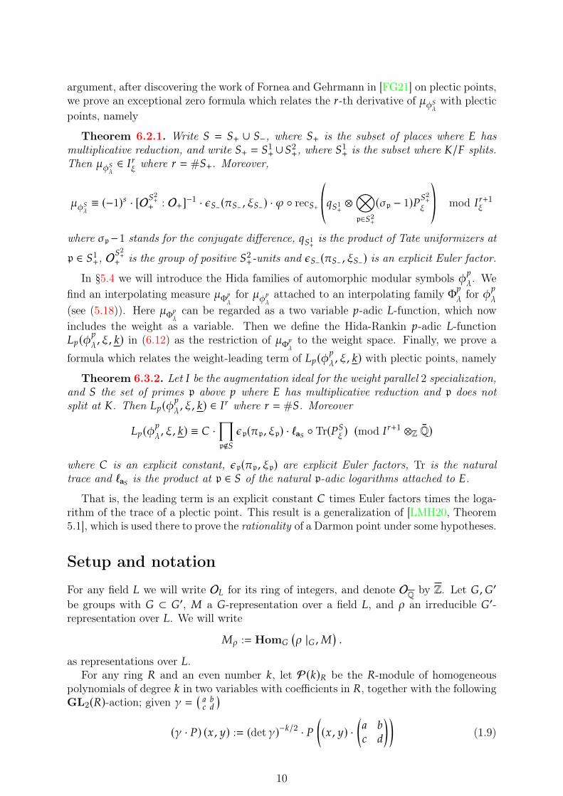
argument, after discovering the work of Fornea and Gehrmann in [FG21] on plectic points,we prove an exceptional zero formula which relates the A-th derivative of �)(� with plecticpoints, namely

Theorem 6.2.1. Write ( = (+ ∪ (−, where (+ is the subset of places where � hasmultiplicative reduction, and write (+ = (1+∪(2+, where (1+ is the subset where /� splits.Then �)(�

∈ �A� where A = #(+. Moreover,

�)(�≡ (−1)B · [O(

2++ : O+]−1 · &(−(�(− , �(−) · ! ◦ rec(+

©­«@(1+ ⊗⊗p∈(2+

(�p − 1)%(2+

�ª®¬ mod �A+1�

where �p−1 stands for the conjugate difference, @(1+ is the product of Tate uniformizers at

p ∈ (1+, O(2++ is the group of positive (2+-units and &(−(�(− , �(−) is an explicit Euler factor.

In §5.4 we will introduce the Hida families of automorphic modular symbols )?�. Wefind an interpolating measure �

Φ?

�for �)?� attached to an interpolating family Φ?� for )?�

(see (5.18)). Here �Φ?

�can be regarded as a two variable ?-adic !-function, which now

includes the weight as a variable. Then we define the Hida-Rankin ?-adic !-function!?()?� , �, :) in (6.12) as the restriction of �

Φ?

�to the weight space. Finally, we prove a

formula which relates the weight-leading term of !?()?� , �, :) with plectic points, namely

Theorem 6.3.2. Let � be the augmentation ideal for the weight parallel 2 specialization,and ( the set of primes p above ? where � has multiplicative reduction and p does notsplit at . Then !?()?� , �, :) ∈ �A where A = #(. Moreover

!?()?� , �, :) ≡ � ·∏p∉(

&p(�p, �p) · ℓa( ◦ Tr(%(� ) (mod �A+1 ⊗Z Q)

where � is an explicit constant, &p(�p, �p) are explicit Euler factors, Tr is the naturaltrace and ℓa( is the product at p ∈ ( of the natural p-adic logarithms attached to �.

That is, the leading term is an explicit constant � times Euler factors times the loga-rithm of the trace of a plectic point. This result is a generalization of [LMH20, Theorem5.1], which is used there to prove the rationality of a Darmon point under some hypotheses.

Setup and notation

For any field ! we will write O! for its ring of integers, and denote OQ by Z. Let �, �′

be groups with � ⊂ �′, " a �-representation over a field !, and � an irreducible �′-representation over !. We will write

"� := Hom�

(� |� , "

).

as representations over !.For any ring ' and an even number :, let P(:)' be the '-module of homogeneous

polynomials of degree : in two variables with coefficients in ', together with the followingGL2(')-action; given � =

(0 12 3

)(� · %) (G, H) := (det �)−:/2 · %

((G, H) ·

(0 1

2 3

))(1.9)

10

Note that the factor (det �)−:/2 makes the central action trivial.Denote by +(:)' the dual space Hom'(P(:)' , '). In the case ' = C we set +(:) :=

+(:)C. Given a vector : = (:8) ∈ (2N)= we define

+(:)':=

=⊗8=1

+(:8)'

Note that, if = = 3 = [� : Q] and : = (:�) ∈ (2N)3 is indexed by the embeddings� : ↩→ C of �, then +(:) := +(:)C has a natural action of �(�∞). The subspace +(:)Qis fixed by the action of the subgroup �(�) ⊆ �(�∞).

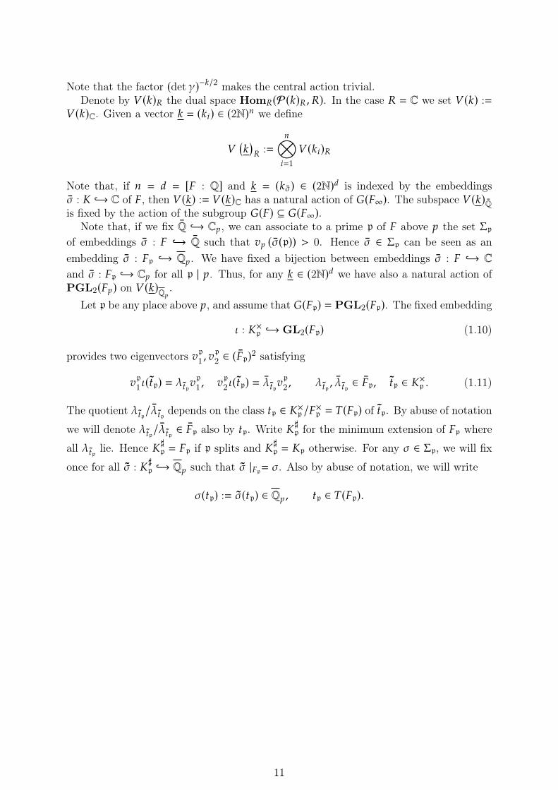
Note that, if we fix Q ↩→ C?, we can associate to a prime p of � above ? the set Σpof embeddings � : � ↩→ Q such that E? (�(p)) > 0. Hence � ∈ Σp can be seen as anembedding � : �p ↩→ Q?. We have fixed a bijection between embeddings � : � ↩→ Cand � : �p ↩→ C? for all p | ?. Thus, for any : ∈ (2N)3 we have also a natural action ofPGL2(�?) on +(:)Q? .

Let p be any place above ?, and assume that �(�p) = PGL2(�p). The fixed embedding

� : ×p ↩→ GL2(�p) (1.10)

provides two eigenvectors Ep1 , Ep

2 ∈ (�p)2 satisfying

Ep

1 �(Cp) = �CpEp

1 , Ep

2 �(Cp) = �CpEp

2 , �Cp , �Cp ∈ �p, Cp ∈ ×p . (1.11)

The quotient �Cp/�Cp depends on the class Cp ∈ ×p /�×p = )(�p) of Cp. By abuse of notation

we will denote �Cp/�Cp ∈ �p also by Cp. Write ♯p for the minimum extension of �p where

all �Cp lie. Hence ♯p = �p if p splits and ♯

p = p otherwise. For any � ∈ Σp, we will fix

once for all � : ♯p ↩→ Q? such that � |�p= �. Also by abuse of notation, we will write

�(Cp) := �(Cp) ∈ Q? , Cp ∈ )(�p).

11

12

Chapter 2

Automorphic forms

2.1 The ring of adèlesSince automorphic forms are functions on adèlic points of an algebraic group, in our caseGL2 or the group of units of a quaternion algebra, we introduce the necessary notationand define of the ring of the adèles. The adèles will also be used to describe Galois groupsusing class field theory.

Let � be a number field of degree 3 over Q and O� its ring of integers. We will denoteby either ∞ or Σ� the set of archimedean or infinite places of � i.e. classes of embeddings� : �→ C of � into C modulo complex conjugation, the non trivial element of Gal(C/R).Furthermore, sometimes ? will denote the set of places of � above a rational prime ?.Note that the complex embeddings are paired up into one place, since either im � ⊂ R ornot. Given a place � let �� be the completion of � at �. The non archimedean or finiteplaces are the classes associated to the prime ideals p ⊂ O� i.e. those for which �� isneither R nor C. For a finite place p denote by Ep : �×p → Q its associated valuation, $pa fixed uniformizer with Ep(+p) = 1 and @p the cardinality of the residue field O�,p/p. IfA� , B� are the number of real and complex places then A� + 2B� = 3. If a place � ∈ ∞ isgiven by the class of an embedding � : � ↩→ C, we write � | �.

For a set of places ( write

�( :=∏�∈(

�� and �( :=∏�∉(

��

The ring of adèles is defined as the following restricted product

A� = �∞ ×∏

p�p

where the · imposes that elements have a finite number of p-components which arenot in O�,p. The diagonal embedding provides a way to regard � as a subset of A�,

� A�

( , , · · · )For a set ( of places define A(

�:= A� ∩ �(. Since A×

�is a locally compact Hausdorff

topological group, we can use its associated Haar measure to integrate functions ) ofthe idèles A×

�. The defining properties of this measure are its inner and outer regularity,

invariance by left multiplication i.e.

�(6 · -) = �(-), for any 6 ∈ A×� and Borel subset -

and uniqueness up to a constant. In particular, we have∫A×

)(C)3×C =∫A×

)(�C)3×C , ∀� ∈ A×

13

2.2 Some algebraic groups associated to quaternion al-gebras

Let /� be a quadratic extension and Σun( /�) be the set of archimedean places � of �that split at . Then

Σun( /�) = ΣRR( /�) t ΣCC( /�)

where ΣRR( /�) is the set of real places of � which remain real in and ΣCC( /�) the set

of complex places of �. We will denote by D, A /�,R and B� the cardinality of these threesets so that D = A /�,R + B�. Analogously, we write ΣCR( /�) for Σ�\Σun( /�).

A quaternion algebra �/� is a central simple algebra of dimension 4 over �. Let �/�be a quaternion algebra for which there exists an embedding ↩→ �, that we fix now.Let Σ� be the set of archimedean places � of � for which the quaternion algebra � splitsi.e. such that

� ⊗� �� ' "2(��)We can define � an algebraic group associated to �×/�× as follows: � represents thefunctor that sends any O�-algebra ' to

�(') = (O� ⊗O� ')×/'×,

where O� is a maximal order in � that we fix once and for all. Similarly, we define thealgebraic group ) associated to ×/�× by

)(') = (O2 ⊗O� ')×/'×,

where O2 := O� ∩ is an order of conductor 2 in O . Note that ) ⊂ �. We denoteby �(�∞)+ and )(�∞)+ the connected component of the identity of �(�∞) and )(�∞),respectively. We also define )(�)+ := )(�) ∩ )(�∞)+ and �(�)+ := �(�) ∩ �(�∞)+.

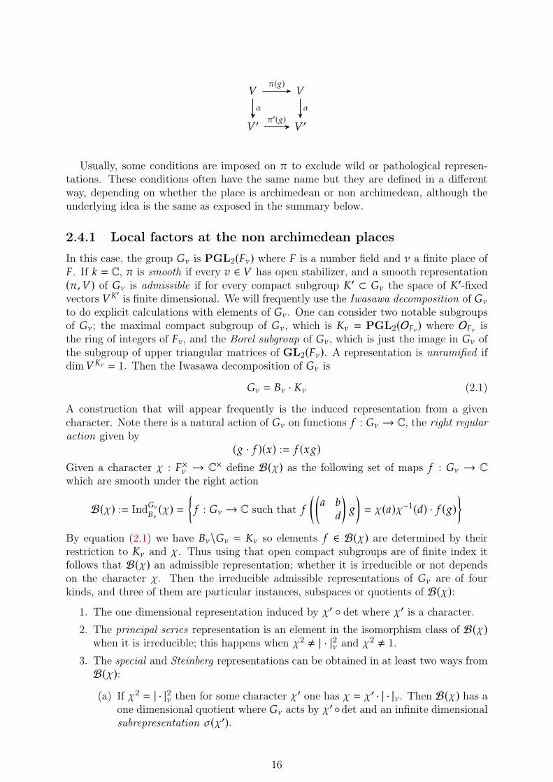
Given � ∈ Σ� note that )(��) = (O2 ⊗O� ,� ��)×/�×� is either C×/R×,R× or C×. Define)(��)0 to be the intersection of all the connected subgroups # of 1 in )(��) for whichthe quotient )(��)/# is compact. Note that )(��)/)(��)0 ' lim←−# )/# is then compact.The set )(��)0 depends on the ramification type of �, as is described in the followingtable

ramificationtype )(��) )(��)0 )(��)/)(��)0

ΣCR( /�) C×/R× 1 C×/R× ' (1

ΣRR( /�) R× R+ ±1ΣCC( /�) C× R+ (1

If � ∈ Σun( /�), then only the second and third of the ramification types on the tableactually occur. For any set of infinite places Σ, we write )(�Σ)0 =

∏� )(��)0.

2.3 Results from Class Field TheoryClass field theory describes the abelian extensions of a local (e.g. a finite extension of Q?)or global fields (e.g. a number field) in terms of their arithmetic. Essentially, if � is aglobal field it provides a surjective morphism from the idèles of � to the maximal abelianextension of �. For a complete exposition on this topic see [Mil20].

14

Let F be a place of " above a place E of �. Recall that given a finite abelian extension"/� of number fields we can consider the Galois action of Gal("/�) on the places F of"; if F is archimedean then the action �F := � ◦ F is composition and if F = p is nonarchimedean then the action is �p = �(p). Then the decomposition group of F is definedas the Galois subgroup which fixes F

�(F) = {� ∈ Gal("/�) such that �F = F}

Local class field theory shows that this group is isomorphic to the local Galois group as-sociated to F i.e. �(F) ' Gal("F/�E). The local reciprocity law induces an isomorphism�!/ : �E/Nm"F/�E ("×F) → Gal("F/�E).

Then it turns out that one can glue the maps �!/ - they form an inverse system andthus we can take the projective limit - to construct a surjective group morphism to theabsolute Galois group of the abelian closure of �, known as the Artin map

� : A×�/�×→ Gal(�ab/�)

This result allows one to regard Galois groups as a certain quotient of an adèlic group.Note that given a Galois character " : Gal(�/�) −→ C of � we can construct a

character of A�, since by the above it can be regarded as a character of GL1(A�) = A� .

" : A×�/�× �−→ Gal

(�ab/�

)"−→ C

This is an automorphic character, which generates a one dimensional irreducible repre-sentation. They were first studied in depth by Tate, who essentially tackled the GL1 caseof automorphic forms in his thesis by using Fourier analysis on the adèles. It can be seenas a reformulation of Hecke’s work on the analytic continuation of the !-series associatedto a Grossencharakter and its functional equation.

2.4 Automorphic forms and representations for GL2

The theory of classical modular forms can be generalized in several directions: automor-phic forms, Katz and overconvergent modular forms, Hida families, etc. One possiblemotivation to do so was explained in §2.3.

We will work with automorphic representations of a quaternion algebra or GL2, andregard them as group cohomology classes in the formalism Michael Spiess introduced inhis study of automorphic ℒ-invariants (see [Spi13]). This approach does not rely on ageometric picture, but rather uses group representation theory and allows one to changethe base field freely.

We remark that automorphic representations are not "representations" in the classicalsense, but rather an infinite (restricted) tensor product of local representations for eachplace as we recall now below. For a complete exposition on this topic see [Bum98].

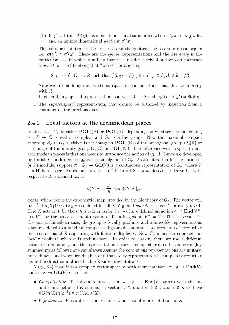
Let : be a field. A group representation of � is a group morphism � : � → Aut(+)where + is a :-vector space, and an irreducible representation has no proper invariant sub-spaces. An intertwining map : + → +′ between two representations (�, +), (�′, +′) isa :-linear map that commutes with the group action i.e. the following diagram commutesfor every 6 ∈ �

15

+ +

+′ +′

�(6)

�′(6)

Usually, some conditions are imposed on � to exclude wild or pathological represen-tations. These conditions often have the same name but they are defined in a differentway, depending on whether the place is archimedean or non archimedean, although theunderlying idea is the same as exposed in the summary below.

2.4.1 Local factors at the non archimedean places

In this case, the group �� is PGL2(��) where � is a number field and � a finite place of�. If : = C, � is smooth if every E ∈ + has open stabilizer, and a smooth representation(�, +) of �� is admissible if for every compact subgroup ′ ⊂ �� the space of ′-fixedvectors + ′ is finite dimensional. We will frequently use the Iwasawa decomposition of ��

to do explicit calculations with elements of ��. One can consider two notable subgroupsof ��; the maximal compact subgroup of ��, which is � = PGL2(O��) where O�� isthe ring of integers of ��, and the Borel subgroup of ��, which is just the image in �� ofthe subgroup of upper triangular matrices of GL2(��). A representation is unramified ifdim+ � = 1. Then the Iwasawa decomposition of �� is

�� = �� · � (2.1)

A construction that will appear frequently is the induced representation from a givencharacter. Note there is a natural action of �� on functions 5 : �� → C, the right regularaction given by

(6 · 5 )(G) := 5 (G6)Given a character " : �×� → C× define ℬ(") as the following set of maps 5 : �� → Cwhich are smooth under the right action

ℬ(") := Ind��

��(") =

{5 : �� → C such that 5

((0 1

3

)6

)= "(0)"−1(3) · 5 (6)

}By equation (2.1) we have ��\�� = � so elements 5 ∈ ℬ(") are determined by theirrestriction to � and ". Thus using that open compact subgroups are of finite index itfollows that ℬ(") an admissible representation; whether it is irreducible or not dependson the character ". Then the irreducible admissible representations of �� are of fourkinds, and three of them are particular instances, subspaces or quotients of ℬ("):

1. The one dimensional representation induced by "′ ◦ det where "′ is a character.

2. The principal series representation is an element in the isomorphism class of ℬ(")when it is irreducible; this happens when "2 ≠ | · |2� and "2 ≠ 1.

3. The special and Steinberg representations can be obtained in at least two ways fromℬ("):

(a) If "2 = | · |2� then for some character "′ one has " = "′ · | · |�. Then ℬ(") has aone dimensional quotient where �� acts by "′◦det and an infinite dimensionalsubrepresentation �("′).

16

(b) If "2 = 1 then ℬ(") has a one dimensional submodule where �� acts by "◦detand an infinite dimensional quotient �′(").

The subrepresentation in the first case and the quotient the second are isomorphici.e. �("′) ' �′("). These are the special representations and the Steinberg is theparticular case in which " = 1; in that case " ◦ det is trivial and we can constructa model for the Steinberg that "works" for any ring

St' :={5 : �� → ' such that 5 (16) = 5 (6) for all 6 ∈ �� , 1 ∈ ��

}/'

Note we are modding out by the subspace of constant functions, that we identifywith '.In general, any special representation is a twist of the Steinberg i.e. �("′) ' St⊗ "′.

4. The supercuspidal representation, that cannot be obtained by induction from acharacter as the previous ones.

2.4.2 Local factors at the archimedean places

In this case, �� is either PGL2(R) or PGL2(C) depending on whether the embedding� : � → C is real or complex, and �� is a Lie group. Now the maximal compactsubgroup � ⊂ �� is either is the image in PGL2(R) of the orthogonal group $2(R) orthe image of the unitary group *2(C) in PGL2(C). The difference with respect to nonarchimedean places is that one needs to introduce the notion of (g� , �)-module developedby Harish-Chandra, where g� is the Lie algebra of ��. As a motivation for the notion of(g, )-module, suppose � : �� → GL(+) is a continuous representation of ��, where +is a Hilbert space. An element E ∈ + is �1 if for all - ∈ g = Lie(�) the derivative withrespect to - is defined i.e. if

�(-)E :=3

3C�(exp(C-)E)|C=0

exists, where exp is the exponential map provided by the Lie theory of ��. The vector willbe �: if �(-1) · · ·�(-:)E is defined for all -8 ∈ g, and smooth if it is �: for every : ≥ 1.Here - acts on E by the infinitesimal action i.e. we have defined an action g→ End+∞.Let +∞ be the space of smooth vectors. Then in general +∞ ≠ + . This is because inthe non archimedean case, the group is locally profinite and admissible representationswhen restricted to a maximal compact subgroup decompose as a direct sum of irreduciblerepresentations of appearing with finite multiplicity. Now �� is neither compact norlocally profinite when � is archimedean. In order to classify them we use a differentnotion of admissibility and the representation theory of compact groups. It can be roughlysummed up as follows: one can always assume the continuous representations are unitary,finite dimensional when irreducible, and that every representation is completely reduciblei.e. is the direct sum of irreducible -subrepresentations.

A (g� , �)-module is a complex vector space + with representations � : g→ End(+)and � : → GL(+) such that :

• Compatibility : The given representation � : g → End(+) agrees with the in-finitesimal action of on smooth vectors +∞, and for - ∈ g and : ∈ we have�(:)�(-)�(:−1) = � ((Ad :)-).

• -finiteness : + is a direct sum of finite dimensional representations of

17

In addition, it will be admissible if every isomorphism class of -subrepresentationappears with finite multiplicity.

There is a complete classification of irreducible admissible (g, )-modules in the case�� = PGL2(R). Since = SO2(R) ' R/2�Z, + =

⊕: +[:] where

(cos C − sin Csin C cos C

)acts by

the character 4 8:C on each +[:], which are the -isotypic components of + . It turns outthat one can find an explicit basis, usually denoted by ', !, �, /, for gC = g⊗RC, so that'+[:] ⊂ +[: + 2] and !+[:] ⊂ +[: − 2] i.e. ', ! raise or lower : respectively, and the+[:] have dimension one at most. Similar results hold for PGL2(C), see [Mol22, §3].

After some considerations one shows there are at most three possibilities for + . Eachpossibility is then constructed explicitly: the principal series, the discrete series, and thefinite-dimensional irreducible representations of PGL2(R). These last are a twist by a1-dimensional character of the space of homogeneous polynomials in two variables, withthe action described in (1.9).

2.4.3 Local factors at ramified places

The above accounts for almost all places, but a quaternion algebra � over � is ramified(i.e. �� ≠ "2(��)) in an even finite number of places of �. In this case the classification issimple. There are only finite dimensional representations: for the non archimedean placesone dimensional representations induced by a character composed with the reduced normof � (similar to the non archimedean kind 1 of §2.4.1), and for the archimedean placeshomogeneous polynomials in two variables with the GL2(C)-action given by (1.9). Here�×� acts through the morphism �×� ↩→ (�� ⊗R C)× = GL2(C).

2.4.4 Definition of automorphic representation

Let � be a set and +8 vector spaces indexed by 8 ∈ �. Choose E0,8 ∈ +8 for almost every8 ∈ �. Then the restricted tensor product of the +8 with respect to the E0,8 is the space

′⊗8∈�

+8 := {⊗8∈�E8 such that E8 = E0,8 for almost every 8}

An irreducible admissible �(A�)-module is a restricted tensor product

� =′⊗�

��

where � runs over the places of � such that

• (�∞, +∞) is an irreducible admissible (g∞, ∞)-module

• For a finite place �, (�� , +�) is an irreducible admissible representation of �(��).• For almost every �, �� is unramified, and the vectors �0,� are in + �

� .

An (irreducible) automorphic representation is an irreducible admissible �(A�)-moduleisomorphic to a subquotient of !2(�(�)\�(A�)), the space of square-integrable functionsin �(�)\�(A�).

18

Classical modular forms as automorphic formsClassical modular forms are defined as certain functions on the complex upper half planeℌ. Recall that ℌ = {I ∈ C with =(I) > 0} and that GL2(R)+ acts on ℌ by fractionallineal transformations (

0 1

2 3

)I :=

0I + 12I + 3

In fact, it is its isometry group with respect to the Poincaré metric 3B2 = 3G2+3H2H2

. Asa semisimple Lie group, GL2(R)+ has an Iwasawa decomposition GL2(R)+ = �#

where ={(

cos� − sin�sin� cos�

)}is the stabilizer of 8, � =

{( AA−1

)with A > 0

}and # ={(

1 G1

)where G ∈ R

}. Modular forms are defined usually by satisfying a relation by ele-

ments of the discrete subgroup SL2(Z) ⊂ GL2(R)+, which tessellates ℌ by ideal triangles,or Γ0(#) ⊂ SL2(Z), the congruence subgroup of upper triangular matrices modulo # .

Let " be a Dirichlet character modulo # , a morphism (Z/#Z)× → C×. It can beextended to Z by setting "(=) = 0 when (=, #) ≠ 1, and it induces a character on Γ0(#)by evaluating upper left entries i.e. "(�) = "(0) where � =

(0 12 3

). A modular form of

weight : of level # and nebentypus " is an holomorphic function 5 : ℌ → C that isholomorphic at infinity (i.e. having a Fourier expansion

5 (I) =∑=≥0

0=@=

where @ = exp(2�8I)) satisfying

5 (�I) = "(�) · 9(�, I): 5 (I) for all � ∈ Γ0(#)

where 9(�, I) = 2I + 3 if � =(0 12 3

). Note that 9(�, I) satisfies the cocycle relation

9(��′, I) = 9(�, �′I)9(�′, I)

A modular form is cuspidal if 00 = 0. The set of cuspidal modular forms of weight : andlevel # form a finite dimensional C-vector space (:(#, ").

One can regard classical modular forms as automorphic forms, by translating some theabove objects to the adèles. The character " has an associated idèlic character $" ofA×Q/Q×. We can define 0(#) as the subgroup of GL2(Z) of elements which are upper

triangular modulo #Z, where Z =∏

? Z?. Then by the strong approximation theorem wecan write any element 6 ∈ GL2(AQ) as 6 = �ℎ∞:, with � ∈ GL2(Q), ℎ∞ ∈ GL2(R)+, : ∈ 0(#), and the adelization of an element 5 ∈ (:(#, ") can be defined as a function! 5 : GL2

(AQ

)→ C given by

! 5 (6) = 9 (ℎ∞, 8)−: 5 (ℎ∞ · 8)$"(:)

It can be checked that ! 5 is an automorphic form of GL2 with central character $".Later on we will work with the automorphic representation � associated to an elliptic

curve �; the local representation �� at the archimedean places is a discrete series of weight2, and at the non archimedean places is the principal series or the (possibly twisted)Steinberg representation depending on whether � has good or multiplicative reduction at�. The supercuspidal representation corresponds to the case of additive reduction.

19

2.5 Automorphic forms as cohomology classesThus in few words, an automorphic form of � is a function �(A�) → C which is �(�)-invariant and has good properties. More precisely, let A(C) be the set of functions

5 : �(A�) → C (2.2)

which are

• right-* 5 -invariant for some open subgroup * 5 ⊂ �(A∞� )• �∞ when restricted to �(�∞)• right-/�-finite and right- �-finite for all � ∈ Σ�

where /� is the center of the universal enveloping algebra of �(��) and � is themaximal compact subgroup of �(��).

We can obtain an admissible representation of �(A�) by letting �(A�) act by righttranslation on A(C), and if �(�) acts by left translation instead then automorphic formsare just �(�)-invariant elements of A(C).

If we only want to work with forms which generate a fixed local representation or a fixed(g∞, ∞)-module at infinity, we can proceed as follows. Recall that a (g∞, ∞)-module isa tensor product

V =

⊗�

V�

where V� is a (g� , �)-module or a finite-dimensional �(��)-representation, dependingon whether � ∈ Σ� or � ∈ Σ� − Σ�. Then given a (g∞, ∞)-module V we define

A∞(V ,C) := Hom(g∞ , ∞)(V ,A(C))

This notion can be further generalized, to fix representations at several places or changethe coefficients of the forms. Let � ⊂ �(�) be a subgroup, ' a topological ring, and (a finite set of places of � above ?. The subgroup � will usually be �(�), �(�)+, )(�) or)(�)+. For any '[�]-modules ", # let

A(∪∞(", #) :=) : �(A(∪∞� ) → Hom'(", #),

there exists an open compactsubgroup * ⊂ �(A(∪∞� )

with )(·*) = )(·)

,(2.3)

and let also A(∪∞(#) := A(∪∞(', #). Then A(∪∞(", #) has a natural action of � and�(A(∪∞

�), namely

(ℎ))(G) := ℎ · )(ℎ−1G), (H))(G) := )(GH),

where ℎ ∈ � and G, H ∈ �(A(∪∞�).

As an example, let : ∈ 2Z3 be a weight vector and consider the (g∞, ∞)-module�(:) =

⊗� ��(:�) where ��(:�) is the discrete series of weight :� or+(:�−2), depending

on whether � ∈ Σ� or � ∈ Σ� − Σ� (see §3 of [Mol22]). Then an automorphic form ofweight : defines a �(�)-invariant element of A∞(�(:),C) that maps a generator of �(:)to the automorphic form

Φ ∈ �0(�(�),A∞(�(:),C)) (2.4)

20

Conversely, any such Φ defines an automorphic form of weight :. If + is a finite-dimensional �(�∞)-representation then by lemma 2.3 of [GMM17]

A∞(+,C) = A∞(V ,C)

where V is the (g∞, ∞)-module associated with + .

2.6 Eichler-Shimura for automorphic forms

Overview

The Eichler-Shimura morphism can be seen as a method to regard automorphic forms ascohomological elements or cohomological modular symbols. Its first version establishes acorrespondence between Γ-modular forms and the first cohomology group of Γ, where Γis an arithmetic subgroup of SL2(Z). In other words, the sheaf of (holomorphic) differ-ential forms on -(Γ) when regarded as a Riemann surface is isomorphic to the singularcohomology of .(Γ), since -(Γ) is the compactification of .(Γ) = ℌ/Γ.

The classical argument is geometric, based on a careful study of the canonical structureof the modular curve -0(#) as a moduli space, its Jacobian and the Hecke algebra of(2(#). Moreover,

"2(Γ) ⊕ (2(Γ) ' �1(Γ,C)For higher weight there is a natural generalization

(:(#) �1(Γ, +(:))

5(� ↦→

(% ↦→

∫ �I0I0

%(1,−I) 5 (I)3I))

since +(0) = HomC(P(0)C,C) ' C.This classical vision can be generalized to the automorphic case using group cohomol-

ogy, as is done in [Mol17a] without relying on a moduli or geometric description. If � = Qthe discrete series of weight : fits into the exact sequences

0 �(:) �(:)± +(: − 2)± 0

where �(:)± is an appropriate induced representation and ± is a choice of sign. By(2.4), an automorphic form can be regarded as a �(�)-invariant element of A∞(�(:),C)i.e.

�0 (�(�),A∞(�(:),C))Thus, the connecting morphism from the long exact sequence of group cohomology givesan element of �1(�(�)+,A∞(+(:−2)))±. For arbitrary � something similar happens, thediscrete series of weight : ∈ Z3 are the kernel of a sequence,

0 �(:) �1(:)� �2(:)� · · · �B(:)� +(: − 2)� 0

where +(: − 2) =⊗

�+(:� − 2), B = #Σ�, �8(:)� are appropriate induced repre-sentations, and � : �(�)/�(�)+ → ±1 is a character. The Eichler-Shimura morphismis regarded as the composition of connecting morphism of the underlying short exactsequences.

ES� : �0(�(�),A∞(�(:),C)) → �B(�(�)+,A∞(+(: − 2)))�.

21

2.7 Waldspurger’s formula in higher cohomologyWe will first recall Waldspurger’s formula in its classic form. It can be regarded equiva-lently as providing an expression for the leading term of the !-function of an elliptic curveor an explicit relation between a toric period and local data. Although it has severalmodern counterparts, as the proposed generalization in Gan-Gross-Prasad conjectures,we use the one presented in [Mol22] for higher cohomology in the next sections.

Classic results and motivation

In equation 1.3 of the introduction, � is called the sign of the functional equation. Notethat � = ±1 since applying (1.3) twice gives �2 = 1. Suppose now � = Q and that /� isan imaginary quadratic field. Let �/Q be a modular elliptic curve of conductor # .

By considering the base change of � to we obtain another sign � = �(� ) of thecorresponding functional equation. Under general Heegner hypothesis on the conductor# = #+#−, that #+ is a product of primes split in and #− is a product of primesinert in and squarefree, we have

� (� ) = −(−1)#{? |#−}

and for each case there are two well-known formulas that express the first non-trivialcoefficient of the !-series of �.

• If � = −1, the even terms of the Taylor series are 0 thus the first non-trivialcoefficient is the value of !′(� , 1). By considering the Shimura curve -(#+, #−)associated to the quaternion algebra that ramifies precisely at #−, a product ofan even number of primes inert in , the Yuan-Zhang-Zhang generalization of theGross-Zagier formula shows !′(� , 1) is related to Néron-Tate height of a CM pointin a Shimura curve,

!′ (� , 1) =( 5 , 5 )

|3 |12��O×

/{±1}

��2 ·⟨!H , !H

⟩NT

deg !

where ! : -(#+, #−) → � is a modular parametrization and H is the Gal(� / )-trace of a CM point of -(#+, #−). Recall that !H is the trace of a Heegnerpoint

• If � = +1, Waldspurger showed that !(� , 1) is related very explicitly to CMpoints in a Shimura set, which in this case is associated to a quaternion algebrawhich ramifies precisely at #− and ∞, as follows

! (� , 1) =( 5 , 5 )

|3 |12��O×

/{±1}

��2 · P2

where now P is Waldspurger’s toric period.

Automorphic analogues

In the automorphic side, Waldspurger’s formula relates certain periods with the criticalvalue of an automorphic !-function. Recall our setup: a number field �, a quadratic

22

extension /�, a quaternion algebra �/� with ↩→ � and an irreducible automorphicrepresentation � on � = �×/�×. Given a character " on )(�) = ×/�×, for any ) ∈ �we can consider the following toric period

P(), ") :=∫)(A�)/)(�)

"(C))(C)3×C

Note that since ) is a function of �(A�) it can be restricted to the idèles of , and thatthe integral does not depend on the choice of a fundamental domain since "(C))(C) is ×-invariant. Note that we have a linear functional

P ∈ Hom)(A�)(� ⊗ ",C) =′∏�

Hom)(��)(�� ⊗ "� ,C)

The following results of Tunnel and Saito provide key information on the local spacesHom)(��)(�� ⊗ "� ,C):

Theorem 2.7.1. We have multiplicity one

dimCHom)(��)(�� ⊗ "� ,C) ≤ 1

and if for any �0� irreducible representation of PGL2(��), �1

� is its Jacquet-Langlandstransfer to �� /�� then

dimCHom)(��)(�0� ⊗ "� ,C) + dimCHom)(��)(�1

� ⊗ "� ,C) = 1

Suppose now " is trivial. If � comes from an elliptic curve �/Q of conductor #then it can be shown that �1

� = 0 when � - # , and if � |# then dimCHom)(��)(�0� ⊗

"� ,C) = 1 if � |#+ and dimCHom)(��)(�1� ⊗ "� ,C) = 1 if � |#−. Together these imply

that dimHom)(A�)(�⊗",C) = 1. Waldspurger formula then provides explicit expressionfor the "ratio" of two elements in a one dimensional space: for an appropriate choice ofthe Haar measure it asserts

Theorem 2.7.2 (Waldspurger). For some explicit constant �,

P(), ")2 = � · !(�, ", 1/2) ·∏�

�()� , "�

)This relates P2 with a critical value of the classical !-function associated to the auto-

morphic representation � twisted by " and the local factors �,

�()� , "�) :=∫)(��)〈��(ℎ))� , )�〉"�(ℎ)3ℎ (2.5)

which are 1 for almost every �. Note that in some cases, depending on whether the centralcharacter of � and " coincide, we may obtain a trivial equality 0 = 0. Again when " = 1and � = Q, the value !(�, ", 1/2) coincides with !(� , 1). In fact

Corollary 2.7.3.

P(), ") ≠ 0 if and only if Hom)(A�)(� ⊗ ") ≠ 0 and !(� ⊗ ", 1/2) ≠ 0

23

2.8 Automorphic cohomology classesLet �/� be a modular elliptic curve. Hence, attached to �, we have an automorphicform for PGL2/� of parallel weight 2. Let us assume that such form admits a Jacquet-Langlands lift to �, and denote by � the corresponding automorphic representation.Let B := #Σ�. As shown in [Mol17b] and overviewed in §2.6, once fixed a character� : �(�)/�(�)+ → ±1, the image through the Eichler-Shimura isomorphism of suchJacquet-Langlands lift provides a cohomology class in �B(�(�)+,A∞(C))�, where thesuper-index � stands for the subspace where the natural action of �(�)/�(�)+ on thecohomology groups is given by the character �. Moreover, since the coefficient ring of theautomorphic forms is Z, such a class is the extension of scalars of a class

)� ∈ �B(�(�)+,A∞(Z))�.

Indeed, �B(�(�)+,A∞(Z))⊗ZC = �B(�(�)+,A∞(C)) (see for example [Spi14, Proposition4.6]). For general automorphic forms of arbitrary even weight (:+2) ∈ (2N)3, the Eichler-Shimura morphism provides a class

)� ∈ �B(�(�)+,A∞(+(:)Q))�.

The �(A∞�)-representation � over Q generated by )� satisfies � ⊗Q C ' �∞ := � |�(A∞

�).

This implies that )� defines an element

Φ� ∈ �B(�(�)+,A∞(+(:)))��∞ .

For any set ( of places above ?, write +( := � |�(�(), with +( =⊗

p∈(+p, and for anyring ' we denote by +'

(=

⊗+'p the '-module generated by )�. By [GMM17, Remark

2.1] we have that

Φ� ∈ �B(�(�)+,A∞(+(:)))��∞ = �B(�(�)+,A(∪∞(+( , +(:)))��∞ . (2.6)

For any G( ∈ �( := � |�(A(∪∞�), the image Φ�(G() defines an element

)(� ∈ �B(�(�)+,A(∪∞(+( , +(:)Q))

�.

We will usually treat )(� as an element of the cohomology group �B(�(�)+,A(∪∞(+( , +(:)))�since

�B(�(�)+,A(∪∞(+Z( , +(:)Q)) ⊗Q C = �B(�(�)+,A(∪∞(+( , +(:))),

again by [Spi14, Proposition 4.6]. The classes )(� are essential in our construction ofanti-cyclotomic ?-adic L-functions, and plectic points.

If )� is associated with an elliptic curve as above and G( ∈ �( is now an element ofZ-module generated by the translations of )�, we can think )(� as an element

)(� ∈ �B(�(�)+,A(∪∞(+Z( ,Z))

� ,

since the coefficient ring of � is Z. Similarly, we will sometimes regard � as a Q-representation.

24

Chapter 3

The fundamental class

3.1 Fundamental classes of toriIn this section we define certain fundamental classes associated with the torus ). Theirdefinition is a generalization to the one defined in [GMM17]; in the case of Darmon pointsonly one E-uniformization is needed, but for plectic points we will need to account forseveral places p above one fixed prime ?.

3.1.1 The fundamental class � of the torus

Let * =∏q )(O�q) and denote by O := )(�) ∩* the group of relative units. Similarly,

we define O+ := O ∩ )(�∞)+ to be the group of totally positive relative units. By anstraightforward argument using Dirichlet Units Theorem

rankZO = rankZO+ = (2A /�,R + A /�,C + 2B� − 1) − (A� + B� − 1) = A /�,R + B� = D.

We also define the class group

Cl())+ := )(A�)/()(�) ·* · )(�∞)+) ' )(A∞� )/()(�)+ ·*) .

Note that the subgroup

)(�Σun( /�))0 = RD+ = (R+)#ΣRR( /�)×(R+)#Σ

CC( /�) ⊂ )(�Σun( /�)) = (R×)#Σ

RR( /�)×(C×)#ΣCC( /�)

is isomorphic to RD by means of the homomorphism )(�∞)+ → RD given by I ↦→(log |�I |)�∈Σun( /�). Moreover, under this isomorphism the image of O+ is a Z-latticeΛ ⊂ RD, as in the proof of Dirichlet’s Unit Theorem.

We can identify Λ with its preimage in )(�Σun( /�))0. Then )(�Σun( /�))0/Λ is a D-dimensional real torus. The fundamental class � is a generator of �D()(�Σun( /�))0/Λ,Z) 'Z. We can give a better description of �: let " := )(�Σun( /�))0 ' RD. The de Rhamcomplex Ω•

"is a resolution for R. This implies that we have an edge morphism of the

corresponding spectral sequence

4 : �0(Λ,ΩD") → �D(Λ,R).

We identify any 2 ∈ �D("/Λ,Z) with 2 ∈ �D(Λ,Z) by means of the relation∫2

$ = 4($) ∩ 2, where $ ∈ �0(Λ,ΩD") = Ω

D"/Λ.

We can think of � ∈ �D(Λ,Z) as such that:

4($) ∩ � =∫)(�∞)/Λ

$, for all $ ∈ �0(Λ,ΩD"). (3.1)

25

Note that

)(�∞)+ = T × )(�Σun( /�))0, T := ((1)#ΣCR( /�)+#ΣCC( /�). (3.2)

Let O+,T = O+ ∩ T. Since O+ is discrete and T is compact, O+,T is finite.

Lemma 3.1.1. We have that O+ ' Λ × O+,T. In particular,

)(�∞)+/O+ ' )(�Σun( /�))0/Λ × T/O+,T (3.3)

Proof. The image of the morphism �|O+ : O+ ↩→ )(�∞)+�→ )(�Σun( /�))0 is Λ by

definition. Since T = ker�, ker�|O+ = T ∩ O+ = O+,T and we deduce the following exactsequence

0 O+,T O+ Λ 0.�|O+

Since Λ is a free Z-module, such sequence splits and the result follows. �

The group Cl())+ fits in the following exact sequence

0 )(�)+/O+→ )(A∞�)/* Cl())+ 0.

?

We fix preimages C 8 ∈ )(A∞� ) for every element C8 ∈ Cl())+ and we consider the compactset

ℱ =

⋃8

C8* ⊂ )(A∞� )

It is compact because Cl())+ is finite and * compact.

Lemma 3.1.2. For any C ∈ )(A�) there exists a unique �C ∈ )(�)/O+ such that�C−1C ∈ )(�∞)+ × ℱ .

Proof. Since )(�∞)/)(�∞)+ = )(�)/)(�)+, given C = (C∞, C∞) ∈ )(A�) there exists� ∈ )(�) such that �C∞ ∈ )(�∞)+. On the other hand, ?(�C∞*) = C8 for some 8. By thedefinition of Cl())+, there exists � ∈ )(�)+ such that ��C∞* = C8*. Hence

��C = (��C∞, ��C∞) ∈ )(�∞)+ × C8* ⊂ )(�∞)+ × ℱ .

By considering the image of �−1�−1 in )(�)/O+, we deduce the existence of �C .For the unicity, suppose there exist �, �′ ∈ )(�) with

(�C∞, �C∞) = �C ∈ )(�∞)+ × ℱ 3 �′C = (�′C∞, �′C∞)

Then �−1�′ = (�C∞)−1(�′C∞) ∈ )(�∞)+. On the other hand, �C∞ = C 8D for some C 8 andD ∈ *, and �′C∞ = C 9D

′ for some C 9 and D′ ∈ *. So �−1�′ = (C 8)−1C 9D−1D′. This impliesC8 = ?(C 8*) = ?(C 9*) = C 9. By the construction of ℱ , we must have C 8 = C 9. Then�−1�′ ∈ * ∩ )(�) ∩ )(�∞)+ = O+. �

The set of continuous functions �(ℱ ,Z) has a natural action of O+ given by translation.The characteristic function 1ℱ is O+-invariant. Consider the cap product

� = 1ℱ ∩ � ∈ �D(O+, �(ℱ ,Z)), (3.4)

26

where 1ℱ ∈ �0(O+, �(ℱ ,Z)) is the indicator function and � ∈ �D(O+,Z) is the image of� through the corestriction morphism.

For any ring ' and any '-module ", write �02 ()(A�), ") for the set of locally constant

"-valued functions of )(A�) that are compactly supported when restricted to )(A∞�). If

" is endowed with a natural )(�)-action, then we have a natural action of )(�) on�02 ()(A�), ").

Lemma 3.1.3. There is an isomorphism of )(�)-modules

Ind)(�)O+ (�(ℱ ,Z)) ' �02 ()(A�),Z).

Proof. Since ℱ ⊂ )(A�) is compact there is an O+-equivariant embedding

� : �(ℱ ,Z) �02 ()(A�),Z)

) (�))(C∞, C∞) = 1)(�∞)+(C∞) · )(C∞) · 1ℱ (C∞).

By definition, an element Φ ∈ Ind)(�)O+ (�(ℱ ,Z)) is a function Φ : )(�) → �(ℱ ,Z)finitely supported in )(�)/O+, and satisfying the compatibility condition Φ(C�) = �−1 ·Φ(C) for all � ∈ O+.

We define the morphism

! : Ind)(�)O+ (�(ℱ ,Z)) �02 ()(A�),Z)

Φ !(Φ) = ∑C∈)(�)/O+ C · �(Φ(C)).

The sum is finite because Φ is finitely supported, and from the O+-equivariance of �and the O+-compatibility it follows that it is well-defined and )(�)-equivariant.

By lemma 3.1.2, for all G ∈ )(A�) there exists a unique �G ∈ )(�)/O+ such that�G−1G ∈ )(�∞)+ × ℱ . Hence

!(Φ)(G) = �(Φ(�G))(�G−1G) (3.5)

Then ! is bijective because

• It is injective: Suppose !(Φ) = 0. Since �G = �GH for all H ∈ )(�∞)+ × ℱ , by (3.5)

!())(GH) = �(Φ(�GH))(�GH−1GH) = �(Φ(�G))(�G−1GH) = 0

Thus �(Φ(�G)) = 0 is identically zero for all G ∈ )(A�). Then Φ(C) = 0 for allC ∈ )(�) because � is injective and �C = C for all C ∈ )(�).

• It is surjective: Let ) ∈ �∅2 ()(A�),Z). By lemma 3.1.2

)(A�) =⊔

C∈)(�)/O+

C()(�∞)+ × ℱ )

LetΦ(C)(G∞) := )(C , CG∞) = (C−1 · ))(1, G∞) ∈ �(ℱ ,Z)

where C ∈ )(�). There are finitely many C()(�∞)+ × ℱ ) in the support of ), bylemma 3.1.2 and because ) has compact support. Thus Φ(C) = 0 except for finitely

27

many C. Note ) is )(�∞)+-invariant since it is Z-valued and )(�∞)0-invariant. ForG ∈ )(A�)

!(Φ)(G) =∑

C∈)(�)/O+

C · �(Φ(C))(G) =∑

C∈)(�)/O+

1)(�∞)+(C−1G∞) · Φ(C)(C−1G∞) · 1ℱ (C−1G∞)

=

∑C∈)(�)/O+

)(C , G∞) · 1C()(�∞)+×ℱ )(G) = )(G)

Since ! is bijective the result follows. �

Thus, by Shapiro’s lemma one may regard

� ∈ �D()(�), �02 ()(A�),Z)).

The (-fundamental classes �(

In 3.1.1 we have defined a fundamental class �. As shown in [Mol22], by means of � wecan compute certain periods related with certain critical values of classical L-functions.Nevertheless in [GMM17] different fundamental classes �p are defined in order to constructDarmon points. We devote this section to slightly generalize the definition of �p in[GMM17] and we will relate � and �p in the next section.

Let ( be a set of places p of � above ?. Write ( := (1 ∪ (2, being (1 the set of placesp in ( where ) splits, )(�p) = �×p , and (2 the set of places where ) does not split. Weconsider:

ℱ ( =⊔8 B 8*

( , *( = )(O(�), O(

�=

∏q∉( O�q , (3.6)

where B 8 ∈ )(A(∪∞�) are representatives of the elements of Cl())(+ and

Cl())(+ = )(A(∪∞� )/(*()(�)+

). (3.7)

Let us consider also the set of totally positive relative (-units O(+ := *( ∩ )(�)+. Notethat we have an exact sequence

0 )(�()/O(+)(O�,() Cl())+ Cl())(+ 0 (3.8)

where O�,( :=∏p∈( O�p .

It is clear that Z-rank of the quotient )(�()/)(O�,() is A = #(1. Moreover, we havethe natural exact sequence

0 O+ O(+ )(�()/)(O�,() (3.9)

Note that (3.9) and (3.8) imply that we have an exact sequence

0 O+ O(+ )(�()/)(O�,() Cl())+ Cl())(+ 0

(3.10)This implies that the Z-rank of O(+ is A + D, since Cl())+ is finite. Write �( := O(+/O+.The free part Λ(

�of �( provides a fundamental class 2( ∈ �A(�( ,Z). Indeed, the map

(Ep)p∈(1 : �( −→ RA

28

given by the ?-adic valuations identifies Λ(�

as a lattice in RA , hence we can proceed asin the previous section to define 2(. We can consider the image �( ∈ �D+A(O(+ ,Z) of 2(through the composition

2( ∈ �A(�( ,Z) 1 ↦→�−→ �A(�( , �D(O+,Z)) −→ �D+A(O(+ ,Z),

where � ∈ �D(O+,Z) is the fundamental class defined previously, and the last arrow is theedge morphism of the Lyndon–Hochschild–Serre spectral sequence �?(�( , �@(O+,Z)) ⇒�?+@(O(+ ,Z). We have, similarly as in Lemma 3.1.3,

�02 ()(A(∪∞� ),Z) = Ind)(�)+O(+

�(ℱ ( ,Z),

where �02 ()(A(∪∞�

), ") is the set of "-valued locally constant and compactly supportedfunctions of )(A(∪∞

�). Thus, the cap product 1ℱ ( ∩ �( provides an element

�( := 1ℱ ( ∩ �( ∈ �D+A(O(+ , �(ℱ ( ,Z))(a)= �D+A()(�)+, �0

2 ()(A(∪∞� ),Z)), (3.11)

where (a) follows from Shapiro’s Lemma.

Relation between fundamental classes

Since )(�∞)/)(�∞)+ ' )(�)/)(�)+, there is a )(�)-equivariant isomorphism

! : �02 ()(A�), ") → Ind)(�)

)(�)+�02 ()(A∞� ), ") := �

02 ()(A∞� ), ") ⊗'[)(�)+] '[)(�)] (3.12)

given by !( 5 ) := ∑C∈)(�)/)(�)+

((C−1 · 5 )|)(A∞) ⊗ C

). Moreover, for any ring '

�02 ()(A∞� ), ') ' �

02 ()(A(∪∞� ), ') ⊗' �0

2 ()(�(), ') ' �02 ()(A(∪∞� ), �0

2 ()(�(), ')), (3.13)

where �02 ()(�(), ') is the set of '-valued locally constant and compactly supported func-

tions on )(�(), seen as )(�)-module by means of the diagonal embedding )(�) ↩→ )(�().Putting these two identities together we obtain

�02 ()(A�),Z) = Ind)(�)

)(�)+

(�02 ()(A(∪∞� ),Z) ⊗Z �0

2 ()(�(),Z)).

The following result relates the previously defined fundamental classes (see also [BG18,Lemma 1.4]):

Lemma 3.1.4. We have that

#(�(tor) · � = �( ∩

⋃p∈(

res)(�p))(�)+Ip

in �D

()(�)+, �0

2 ()(A(∪∞�),Z) ⊗Z �0

2 ()(�(),Z))= �D()(�), �0

2 ()(A�),Z)), where �(tor

for the torsion subgroup of �(,

Ip = 1)(�p) ∈ �0()(�p), �02 ()(�p),Z)), if p ∈ (2,

and Ip ∈ �1()(�p), �02 ()(�(),Z)) is the class associated with the exact sequence

0 −→ �02 ()(�p),Z)) −→ �0

2 (�p,Z))5 ↦→ 5 (0)−→ Z −→ 0,

if p ∈ (1.

29

Proof. Note that on the one hand that, if p ∈ (1, the class Ip has representative Ip(C) =1O�,p − C1O�,p . Hence Ip(C) is characterized to be the function such that

∑=∈Z C

=Ip(C) =1)(�p), for all C ∈ )(�p) with Ep(C) > 0. Thus,

(⊗p∈( Ip

)(2() is characterized so that

∑�∈Λ(

�

�

(⊗p∈(

Ip

)(2() = 1)(�().

On the other hand, the exact sequence (3.8) implies

0 �( )(�()/)(O�,() , 0

where , := ker(Cl())+→ Cl())(+

), and note that

ℱ =

⊔B 8∈Cl())+

B8* =

⊔C 9∈,

⊔B:∈Cl())(+

B:*( × C 9)(O�,() =

⊔C 9∈,

ℱ ( × C 9)(O�,().

Hence∑�∈Λ(

�

�∑

�∈�(tor

� · 1ℱ =∑ ∈�(

·©­­«

∑C 9∈)(�p)/)(O�,()O(+

1ℱ ( ⊗ C 91)(O�,()ª®®¬ = 1ℱ ( ⊗ 1)(�(),

and so∑

�∈�(tor

� · 1ℱ = 1ℱ ( ⊗(⊗

p∈( Ip)(2() implying that

�( ∩⋂p∈(

res)(�p))(�)+Ip =

(1ℱ ( ∩

⋂p∈(

res)(�p))(�)+Ip

)∩ �( = ©­«

∑�∈�(

tor

�1ℱª®¬ ∩ �

= #(�(tor) · (1ℱ ∩ �) = #(�(

tor) · �,and the result follows. �

For ( = {p} = (2, we recover the definition �p given in [GMM17], and the previouslemma relates it with �.

3.2 PairingsIn order to relate the ?-arithmetic cohomology groups defined in §2.8 and the homologygroups defined in §3.1, we will define certain pairings that will allow us to perform capproducts. For this purpose, we assume for the rest of this work the following hypothesis:

Hypothesis 3.2.1. Assume that Σ� = Σun( /�). Hence, in particular, D = B and�(�)/�(�)+ = )(�)/)(�)+.

As above, let ( be a set of primes p above ?. For any )(�)-modules " and # , let usconsider the )(�)+-equivariant pairing

〈·, ·〉+ : �02 ()(A(∪∞�

), ") × A(∪∞(", #) #,

( 5 , )) 〈 5 , )〉+ :=∫)(A(∪∞

�) )(C)( 5 (C))3

×C ,(3.14)

30

where 3×C is the corresponding Haar measure. This implies that, once fixed a character� : �(�)/�(�)+ = )(�)/)(�)+→ ±1, it induces a well-defined )(�)-equivariant pairing

〈·, ·〉 : Ind)(�))(�)+�

02 ()(A(∪∞�

), ") × A(∪∞(", #)(�) −→ #,⟨∑C∈)(�)/)(�)+ 5C ⊗ C , )

⟩:= [)(�) : )(�)+]−1

∑C∈)(�)/)(�)+ C · 〈 5C , C

−1)〉+,(3.15)

where A(∪∞(", #)(�) is the twist of the )(�)-representation A?∪∞(", #) by the char-acter �.

Assume that " = �02 ()(�(), ') ⊗' + , for a finite rank '-module + ,

Ind)(�))(�)+�

02 ()(A(∪∞� ), ") = �0

2 ()(A�), ') ⊗' +.

This implies that (3.15) provides a final )(�)-equivariant pairing

〈·|·〉 : �02 ()(A�), ') ⊗' + ×A(∪∞(�0

2 ()(�(), ') ⊗' +, #)(�) −→ #,

〈 5( ⊗ 5 ( ⊗ E |)〉 = [)(�) : )(�)+]−1∑G∈)(�)/)(�)+ �(G)−1

∫)(A(∪∞) 5

((G, C) · )(C)( 5( ⊗ E)3×C.(3.16)

All the pairings above induce cap products in �-(co)homology by their �-equivariance.Now denote by 5� the projection of 5 to the subspace

�02 ()(A�), ')� :=

{5 ∈ �0

2 ()(A�), ') with 5 |)(�∞) = �}.

One easily computes that for E ∈ +, 5 ∈ �02 ()(A�), ') and ) ∈ A(∪∞(�0

2 ()(�(), '), #)(�)

〈 5 ⊗ E |)〉 = 〈 5� ⊗ E |)〉 = 〈 5� |)(A∞) ⊗E, )〉+.

Since we can identify �D(�(�)+, •)� ' �D(�(�), •(�)), we deduce that for all 5 ⊗ E ∈�D()(�), �0

2 ()(A�), ') ⊗' +) and ) ∈ �D()(�)+,A(∪∞(�02 ()(�(), ') ⊗' +, #))�,

( 5 ⊗ E) ∩ ) = ( 5� ⊗ E) ∩ ) = ( 5� |)(A∞�) ⊗E) ∩ res)(�)

)(�)+) ∈ #, (3.17)

where res)(�))(�)+ is the restriction morphism and the cap products are the induced by

(3.14),(3.16), respectively.

31

32

Chapter 4

Darmon and plectic points

4.1 Construction of Darmon pointsIn this section we expose the construction of non-archimedean Darmon points given in[GMM17]. Throughout this section we will assume that ( = {p}, )(�p) is non-split and+Z(= StZ(�p). We will write

)p� := )(� ∈ �D(�(�)+,A{p}∪∞(StZ(�p),Z))� ,

the class associated with the elliptic curve �/� where D = Σ) = Σ�. Since � has splitmultiplicative reduction at p, it admits a ?-adic Tate’s uniformization at p.

4.1.1 Extensions of the Steinberg representation

Let ℌp = p \ �p be the p-adic upper half plane and

-p :=

{ℌp, if ) does not split at p,P1(�p), if splits at p.

In any case, -p is endowed with a natural action of �(�p) given by fractional lineartransformations, (

0 1

2 3

)∗ G = 0G + 1

2G + 3 (4.1)

Let �p, �p ∈ -p be the two fixed points by �()(�p)), where � is the embedding fixed in(1.10). We will assume that �( ×p ) ∩ % = �×p , hence in the split case �p, �p ≠ ∞ (see alsohypothesis 5.1.5). In fact, �p and �p correspond to the two simultaneous eigenvectors ofall matrices �(C) because of the following identity.

�(C)(�p1

)=

(0 1

2 3

) (�p1

)= (2�p + 3)

(�(C) · �p

1

)= �C

(�p1

), �(C)

(�p1

)= �C

(�p1

). (4.2)

being C ↦→ C and C ↦→ C the two embeddings p ↩→ C?.Assume that the local representation �p is Steinberg. Thus �p is the quotient of the

induced representation Ind�% 1 modulo the constant functions. Let �0(P1(�p),Z) be the setof locally constant Z-valued functions of the projective line with the action (4.1). Since�(�p)/% ' P1(�p), we can give a simple description of +Zp = StZ(�p),

StZ(�p) = �0(P1(�p),Z)/Z.

Denote by Cov(-) the poset of open coverings of a topological space - ordered byrefinement. Let

Δp := Div(ℌp) and Δ0p := Div0(ℌp) ⊂ Δp

33

the set of divisors and degree zero divisors. The multiplicative integral 8 is defined by

8 : Hom(StZ(�p),Z) Hom(Δ0p,

×p )

#(I2 − I1 ↦→ ×

∫P1(�p)

G−I2G−I1 3�#(G)

) (4.3)

where

×∫P1(�p)

G − I2G − I1

3�#(G) = limU∈Cov(P1(�p))

∏*∈U

(G* − I2G* − I1

)#(1* )Here each G* ∈ * and 1* is the characteristic function of *.

In [GMM17] the multiplicative integral is described alternatively: for any topologicalgroup ", write St" := �(P1(�p), ")/". Then we have a natural morphism

!unv : Hom(StZ(�p),Z) −→ Hom(St�×p , �×p ), !unv(#)( 5 ) := lim

U∈Cov(P1(�p))

∏*∈U

5 (G*)#(1* )

(4.4)For any multiplicative top. group " and any continuous character ℓ : �×p → " let

ℰ(ℓ ) :={(), H) ∈ �(GL2(�p), ") × Z : )

((B G

C

)6

)= ℓ (C)H · )(6)

}/(", 0). (4.5)

Then the universal extension of St�×p is ℰ�×p = ℰ(id) in the sense that, for any ℓ as above,the morphism (H, )) ↦→ (H, ℓ)) provides a morphism ℓ : ℰ�×p → ℰ(ℓ ). If we define

ev(I) := ()I , 1), )I

(0 1

2 3

):= 2I + 3 ∈ ×p . (4.6)

then we have a natural morphism ev : Δp→ ℰ ×p and a commutative diagram

0 Δ0p Δp Z 0

0 St ×p ℰ ×p Z 0

ev ev Id

ySt

(4.7)

The morphism (4.3) is then the composition ev∗ ◦ !unv, where ev∗ is the associated pull-back.

4.1.2 ?-adic uniformization

The morphism in (4.3) induces a �(�)+-equivariant morphism

8 : A{p}∪∞(StZ(�p),Z) → A{p}∪∞(Δ0p,

×p )

which induces morphisms in �(�)+-cohomology. The degree map short exact sequence0 → Δ0

p → Δp → Z → 0 and its associated long exact sequence in �(�)+-cohomology,provides a commutative diagram

�D(�(�)+,A{p}∪∞(StZ(�p),Z))�

· · · → �D(�(�)+,A{p}∪∞(Δp, ×p ))� �D(�(�)+,A{p}∪∞(Δ0p,

×p ))� �D+1(�(�)+,A{p}∪∞( ×p ))� → · · ·

82

34

One can show that there exists @p ∈ �×p such that 2)p� ∈ �D+1(�(�)+,Ap,∞(@Zp )). Anisogeny ×p /@Zp ∼ �( p) is expected (see [GMM17, Conjecture 3.8]): this has been verifiedin many situations, see [GR21] and [Spi21]. Recall that the map �{p} 3 Gp ↦→ )p� definesan element

Φ� ∈ �D(�(�)+,A{p}∪∞(StZ(�p),Q))�� . (4.8)

Hence, if we write �Q( p) := �( p) ⊗ Q, we can consider instead the diagram

�D(�(�)+,A{p}∪∞(StZ(�p),Q))��

· · · → �D(�(�)+,A{p}∪∞(Δp, �Q( p)))�� �D(�(�)+,A{p}∪∞(Δ0p, �Q( p)))�� �D+1(�(�)+,A{p}∪∞(�Q( p)))�� → · · ·

82

obtained reducing modulo @Zp , and by definition Φ� ∈ ker 2. This implies that thereexists an element

Ψ� ∈ �D(�(�)+,A{p}∪∞(Δp, �Q( p)))�� (4.9)which maps to 8Φ�. It is unique by [GMM17, Lemma 3.6 ]. By [Spi13]

�((�(�)+,A{p}∪∞(Δp, �Q( p)))� = �((�(�)+,A{p}∪∞(Δp, �( p)))� ⊗Z Q.so we can write

#p� ∈ �D(�(�)+,A{p}∪∞(Δp, �( p)))� ,

for the image of Gp ∈ �{p} once we get rid of denominators.

4.1.3 Darmon points

Let �p ∈ ℌp be the point fixed by )(�) as in §4.1.1. Consider the following morphism of�(�)+-modules

·|�p : Z[�(�)+/)(�)+] Δp

= · 6)(�)+ = · 6(�p)(4.10)

It is well-defined because �p is )(�)-invariant. Then composing by ·|�p induces a �(�)+-equivariant morphism

·|�p : A{p}∪∞(Δp, �( p)) −→ A{p}∪∞(Z[�(�)+/)(�)+], �( p))which in turn induces morphisms in the �(�)+-cohomology. By [GMM17, Lemma 4.1]

A{p}∪∞(Z[�(�)+/)(�)+], �( p)) ' coInd�(�)+)(�)+

(A{p}∪∞(�( p))

).

Hence we obtain an element

#p� |�p ∈ �D()(�)+,A{p}∪∞(�( p)))� ,

by Shapiro’s lemma. Here we regard � as a character of )(�)/)(�)+ since we have anisomorphism �(�)/�(�)+ ' )(�)/)(�)+ induced by the natural embedding ) ↩→ � andthe determinant.

Let Gp)be the Galois group of the abelian extension of attached to )(A�)/)(�p).

Note )(�p) is compact because p does not split in . Then the Artin map factors throughthe following map

A× / × )(�∞)/)(�∞)+ × )(A∞� )/)(�p))(�)+ = )(�)/)(�)+ × )(A

{p}∪∞�

)/)(�)+.(4.11)

35

and hence we have a decomposition into �-eigenspaces

�(Gp),Q) =

⊕�:)(�)/)(�)+→{±1}

�0()(�)+, �0()(A{p}∪∞

�),Q)

). (4.12)

If � ∈ �(Gp),Z) is a locally constant character with � |)(�∞)= � then we can consider its

�-component �� ∈ �0()(�)+, �0()(A{p}∪∞

�,Z))

). We can define a twisted Darmon point

%p

� =(�p ∩ ��

)∩ #p� |�p ∈ �( p) ⊗Z Z,

where the ∩ are with respect to 〈·, ·〉+ of (3.14).These points are conjectured to be defined over abelian extensions of (see [GMM17,

Conjecture 4.3]). Moreover, in the special case � is totally real and is totally imaginary,this construction fits with the ?-adic construction of classical Heegner points. For a moredetailed description of these facts see §5 in [GMM17].

4.2 Fornea-Gehrmann plectic pointsA plectic point will be defined as an element of the (completed) tensor product ⊗p�( p),and they owe their name to the plectic conjectures made by Nekovár and Scholl, see[NS16].

In the case of Darmon points one had to assume that the local representation at ? isthe special representation, which corresponds to the case of split multiplicative reductionat p, while in the plectic approach of Fornea and Gehrmann we can allow the non splitreduction case. This is done by choosing an appropriate uniformization, as in (4.15).

Moreover, they are conjectured to be non-zero in rank A ≤ [� : Q] situations, hencethey open the door to important progress towards the understanding of the Birch andSwinnerton-Dyer conjecture in rank A ≥ 2 situations, although we are restricted to thecase A ≤ [� : Q]. In this direction, they prove in [FG21, Theorem 5.13] the analogous ofTheorem 6.1.1 with Darmon points replaced by plectic points. Our aim in the followingsections is to generalize their result adapting our proof of Theorem 6.1.1.

Let )(� ∈ �D(�(�)+,A(∪∞(+Z(,Z))� be the modular symbol associated with an elliptic

curve �/� as in §2.8, and ( a set of finite places above ? such that ) does not split atany p ∈ (. We will assume that

�(�() = PGL2(�() and +Z( =⊗p∈(

StZ(�p)(�p), (4.13)

where �p : �(�p) → ±1 is given by 6 ↦→ (±1)Ep det 6.

4.2.1 (-adic uniformization

This section is analogous to §4.1.2 but for several primes, which requires an induction step.For all p ∈ (, the �(�p)-invariant morphism (4.3) induces the �(�p)-invariant morphism

8p : Hom(StZ(�p)(�p),Z) −→ Hom(Δ0p,

×p )(�p), (4.14)

36

where (�p) denotes again the twist by the character �p. The restriction �p : )(�p) → ±1is non trivial only if �p ≠ 1 and ) ramifies at p. Moreover, if ��p/ p is the extension cutout by �p, by [Sil94, Corollary 5.4]

�( p) ={D ∈ �×�p/@

Zp : D−�p(�)D� ∈ @Zp

}, 1 ≠ � ∈ Gal(��p/ p). (4.15)

Hence, we no longer have a Tate uniformization ×p /@Zp ∼ �( p) but an isomorphism

×p /@Zp ∼ �( p)�p := {% ∈ �(��p); %� = �p(�) · %}.

Thus, applying the same construction given in §4.1.2 one obtains

Ψ� ∈ �D(�(�)+,A{p}∪∞(Δp, �Q( p)�p)(�p))�� ,

as in (4.9), where �p is now seen as a character of �(�) by means of the composition

�(�) ↩→ �(�p)�p−→ ±1.

If we consider another q ∈ (, we can apply again [GMM17, Remark 2.1] to obtain

Ψ� ∈ �D(�(�)+,A{p}∪∞(Δp, �( p)�p)(�p) ⊗ Q)��

= �D(�(�)+,A{p,q}∪∞(StZ(�q)(�q) ⊗ Δp, �( p)�p)(�p) ⊗ Q)�� .

After evaluating at certain Gpq ∈ �{p,q} and clearing denominators, we obtain

#p� ∈ �D(�(�)+,A{p,q}∪∞(StZ(�q)(�q) ⊗ Δp, �( p)�p)(�p))�.

From the definition given in (4.3), we deduce that (4.14) provides a �(�)-equivariantmorphism

8p : A{p,q}∪∞(StZ(�q)(�q)⊗Δp, �( p)�p)(�p)(�) −→ A{p,q}∪∞(Δ0q⊗Δp, ×q ⊗Z? �( p)�p)(�p,q)(�),

where (·) stands for the ?-adic completion of the torsion free part and �p,q := �p · �q.Thus we can consider 8p#

p

� ∈ �D(�(�)+,A{p,q}∪∞(Δ0q ⊗ Δp, ×q ⊗Z? �( p)�p)(�p,q))�. Let

" := ×q ⊗Z? �( p)�p(�p,q) and consider the commutative diagram given by the degreelong exact sequences

�D(�(�)+,A{p,q}∪∞(Δq ⊗ Δp, "))� �D(�(�)+,A{p,q}∪∞(Δ0q ⊗ Δp, "))� �D+1(�(�)+,A{p,q}∪∞(Δp, "))�

�D(�(�)+,A{p,q}∪∞(Δq ⊗ Δ0p, "))� �D(�(�)+,A{p,q}∪∞(Δ0

q ⊗ Δ0p, "))� �D+1(�(�)+,A{p,q}∪∞(Δ0

p, "))�

�D+1(�(�)+,A{p,q}∪∞(Δq, "))� �D+1(�(�)+,A{p,q}∪∞(Δ0q , "))� �D+2(�(�)+,A{p,q}∪∞("))�

!2 21

!1

22

Clearly 8p#p

� is a preimage through !1 of 8p,q)p,q� ∈ �D(�(�)+,A{p,q}∪∞(Δ0

q⊗Δ0p,

×q ⊗Z?

×p ))� modulo ×q ⊗ @Z?p , where 8p,q = 8p ◦ 8q and

)p,q� = Φ�(Gpq) ∈ �D(�(�)+,A{p,q}∪∞(StZ(�p)(�p) ⊗Z StZ(�q)(�q),Z))�

37

once we have the identification

Φ� ∈ �D(�(�)+,A{p}∪∞(StZ(�p)(�p),Q))�� = �D(�(�)+,A{p,q}∪∞(StZ(�p)(�p)⊗ZStZ(�q)(�q),Q))��

of (4.8). Conjecture [GMM17, Conjecture 3.8] implies that 228p,q)p,q� lies in the line

@Z?q ⊗Z? �( p)�p(�p,q) ⊆ ", hence without loss of generality, we can assume that 218p#

p

�

lies in @Z?q ⊗Z? �( p)�p(�p,q). The preimage of 8p#

p

� through !2 modulo @Z?q ⊗Z? �( p)�p(�p,q)

provides, after taking �-isotypical components, a unique

Ψ� ∈ �D(�(�)+,A{p,q}∪∞(Δp ⊗ Δq, �( q)�q ⊗Z? �( p)�p ⊗Z? Q?)(�p,q))�� .

Repeating this construction for all places in (, one obtains

Ψ� ∈ �D(�(�)+,A(∪∞(Δ( , �( ()�( ⊗Z? Q?)(�())�� ,

Here Δ( :=⊗

p∈( Δp where the tensor product is taken over Z, �( ()�( :=⊗

p∈( �( p)�pwhere the tensor product is taken over Z?, and �( :=

∏p∈( �p. After getting rid of

denominators, the image of G( ∈ �( corresponding to )(� provides a class

#(� ∈ �D(�(�)+,A(∪∞(Δ( , �( ()�()(�())�.

By construction, the restriction of #(� at Δ0(:=

⊗p∈( Δ

0p is the projection modulo

∑p∈(

©­«@Z?p ⊗⊗q∈(\{p}

×qª®¬

of8()

(� ∈ �

D(�(�)+,A(∪∞(Δ0( ,

×( )(�())

� , ×( :=⊗p∈(

×p ,

where 8( =∏p∈( 8p is the morphism induced by (4.14) and the tensor product is taken

over Z?.

4.2.2 Plectic points

For all p ∈ (, let �p ∈ ℌp be the point fixed by )(�) as in §4.1.3. The morphism of�(�)+-modules

Z[�(�)+/)(�)+] −→ Δ(; = · 6)(�)+ ↦−→ =

(⊗p∈(

6�p

). (4.16)

is well-defined and it induces a �(�)+-equivariant morphism

A(∪∞(Δ( , �( ()�()(�() −→ A(∪∞(Z[�(�)+/)(�)+], �( ()�()(�(), # ↦→ # |(�p)p .

Since we have (see [GMM17, Lemma 4.1])

A(∪∞(Z[�(�)+/)(�)+], �( ()�()(�() ' coInd�(�)+)(�)+

(A(∪∞(�( ()�()(�()

),

38

we obtain by Shapiro’s lemma

#(� |(�p)p∈ �D()(�)+,A(∪∞(�( ()�()(�())�.

Consider the subspace of functions

�(G) ,Q)�( :={5 ∈ �(G) ,Q), �∗ 5 |)(�()= �(

},

where �( : )(�() → ±1 is now the product of the local �p. This is consistent with theconstruction given in §4.1.3, since if ( = {p} and �p = 1 then �(G) ,Q)�( = �(Gp) ,Q). Inthis situation, the Artin map provides a decomposition:

�(G) ,Q)�( =⊕

�:)(�)/)(�)+→{±1}�0

()(�)+, �0()(A(∪∞� ),Q)(�()

). (4.17)

Given a locally constant character � ∈ �(G) ,Z)�( we can consider

�� ∈ �0()(�)+, �0()(A(∪∞� ,Z)(�())

)its �-component, and define the twisted plectic point

%(� =(�( ∩ ��

)∩ #(� |(�p)p∈ �( ()�( ⊗Z Z,

where again the cap product is with respect to the pairing 〈·, ·〉+ of (3.14) twisted by &(.

4.2.3 Conjectures

As with Darmon points in [GMM17, Conjecture 4.3], it is conjectured that plectic pointscome from certain rational points of the elliptic curve �. The corresponding conjecturesthat can be found in [FG21, §1.4].

Let � ∈ �(G) ,Q)�( be a locally constant character such that � |)(�∞)= � (namely,�� ≠ 0). Let ��/ the abelian extension cut out by �. Since �∗� |)(�()= �(, we canembed �� ⊂ ��( . Moreover, if we consider

�( )� = {% ∈ �(��) ⊗Z Z; %� = �(�) · %},

clearly �( )� ⊂ �( p)�p . Fornea and Gehrmann consider the natural morphism

yp : �( )� ↩→ �( p)�p ⊗Z Z −→ �( p)�p ⊗Z Z,

and, if we write A := #(, we define

det :

A∧�( )� ↦−→ �( ()�( ; det(%1 ∧ · · · ∧ %A) := det

©­«yp1(%1) · · · ypA (%1)

· · ·yp1(%A) · · · ypA (%A)

ª®¬ .Recall that our construction of %(� depends on the choice of a vector G( =

⊗′�∉(∪∞ G

(� ∈ �(

corresponding to the modular symbol )(�. The following conjecture is analogous to thoseof [FG21, §1.4]. Let �E : )(�E) → C× be the local characters corresponding to � via classfield theory.

39

Conjecture 4.2.1. We have that %(�=0 unless∏

�∉(∪∞ E(G(� , �E) ≠ 0, where E ∈Hom)(�E)(�E ⊗ �E ,C) is the morphism of (2.5). In this case:

• Algebraicity and reciprocity law: There exists '� ∈∧A �( )� such that

det'� = %(� .

• Connection with BSD: Assume that rank(�( )�) ≥ A. If %(� ≠ 0, we have that

rank(�( )�) = A

40

Chapter 5

?-adic !-functions

5.1 Anticyclotomic ?-adic L-functionsIn this chapter we will define the anticyclotomic ?-adic L-functions associated with ?, )and the automorphic cohomology class

)?

� ∈ �D(�(�)+,A∞,?(+? , +(:))

for an even weight : ∈ 2N3 (here we choose ( = ?).

5.1.1 Defining the distribution

Let �:()(�?),Q?) be the space of Q?-valued locally polynomial functions of )(�?) ofdegree less than :. These correspond to the set of functions 5 : )(�?) → Q? such that inan small neighbourhood * of C? = (Cp)p|? ∈ )(�?)

5 (B?) =∑|<� |≤ :�2

0<(*)∏p|?

∏�∈Σp

�(Bp)<�

where < = (<�) ∈ Z3, 0<(*) ∈ Q? and B? ∈ *. If we denote by �0 the set of locallyconstant functions, there is an isomorphism

y : �0()(�?),Q) ⊗Q P(:)Q ⊗ Q? −→ �:()(�?),Q?) (5.1)

defined by

ℎ ⊗⊗�

%� ↦−→©­«C? = (Cp)p|? ↦→ ℎ(C?)

∏p|?

∏�∈Σp

%�(�

(Ep

1 + CpEp

2

) )�(Cp)

−:�2

ª®¬ .It is )(�?)-equivariant, indeed for any G? = (Gp) ∈ )(�?),

G? · y(ℎ ⊗

⊗�

%�

)(C?) = y

(ℎ ⊗

⊗�

%�

)(G−1? C?)

= ℎ(G−1? C?)∏p|?

∏�∈Σp

%�

(�

(Ep

1 +�Gp�Gp

CpEp

2

))�

(�Gp�Gp

Cp

) −:�2

41

= ℎ(G−1? C?)∏p|?

∏�∈Σp

%�(�

(�GpE

p

1 + Cp�GpEp

2

) )�

(�Gp�GpCp

) −:�2

= (G? · ℎ)(C?)∏p|?

∏�∈Σp

%�(�

(Ep

1 �(Gp) + CpEp

2 �(Gp)) )�

(det(�(Gp))Cp

) −:�2

= (G? · ℎ)(C?)∏p|?

∏�∈Σp((��(Gp) · %�)

(�

(Ep

1 + CpEp

2

) )�

(Cp

) −:�2

= y

((G? · ℎ) ⊗

(G? ·

(⊗�

%�

)))(C?).

Let G) be the Galois group of the abelian extension of associated with ). By classfield theory, there is a continuous morphism

� :()(�∞)/)(�∞)+ × )(A∞� )

)/)(�) → G) . (5.2)

Let us consider the subset of �()(A�),Q?):

�:()(A�),Q?) := { 5 : )(A?

�) → �:()(�?),Q?), locally constant},

and write also �:(G) ,Q?) for the subspace of continuous functions 5 : G) → Q? suchthat �∗( 5 ) ∈ �:()(A�),Q?). The pullback of � together with the cap product by � givethe following morphism

� : �:(G) ,Q?) �0()(�), �:()(A�),Q?)) �D()(�), �:,2()(A�),Q?)).�∗ ∩�

(5.3)where �:,2()(A�),Q?)) is the subspace of functions in �:()(A�),Q?)) which are compactlysupported when restricted to )(A∞

�). Note that y of (5.1) provides an isomorphism

�:,2()(A∞� ),Q?)) = �02 ()(A∞� ),Q) ⊗Q P(:)Q ⊗ Q? . (5.4)

In order to define the distribution we need to construct a )(�?)-equivariant morphism:

�? = (�p)p|? : �02 ()(�?),Q) −→ +? , �p : �

02 ()(�p),Q) −→ +p. (5.5)

Given such a �? we can directly define the distribution associated with

)?

� ∈ �D(�(�)+,A?∪∞(+? , +(:)Q)

)�as follows: ∫

G)63�)?�

:= �(6) ∩ �∗?)?

� , for all 6 ∈ �:(G) ,Q?) (5.6)

where the cap product is induced by the pairing (3.16) and

�∗? : A?∪∞(+? , +(:)Q) −→ A?∪∞

(�02 ()(�?),Q) ⊗Q P(:)Q,Q?

)is the corresponding )(�)-equivariant pullback.

42

5.1.2 Admissibility

A continuous function 5 ∈ �()(�?),C?) is locally analytic if, for any G? = (Gp)p|? ∈ )(�?)there exists a neighbourhood * of C? and 0=(*) ∈ Q? such that

5 |* (B?) =∑=∈N3

0=(*)∏p|?

∏�∈Σp(�(Bp) − �(Gp))=� , for all B? = (Bp)p|? ∈ * ⊂ )(�?).

Write �an()(�?),C?) for the subspace of locally analytic functions. Note that �:()(�?),C?) ⊂�an()(�?),C?). Indeed, it is clear that �(Cp)<� ∈ �an()(�?),C?) when <� is positive, butwhen <� < 0,

�(Cp)<� =

∑8≥0

(<�

8

)�(Gp)<�−8(�(Cp) − �(Gp))8 ∈ �an()(�?),C?).

Similarly as above, we consider

�an()(A�),C?) := { 5 : )(A?�) → �an()(�?),C?), locally constant} ⊂ �()(A�),C?),

and �an(G) ,C?) := (�∗)−1�an()(A�),C?).In the previous section we have constructed a locally polynomial distribution

�)?�∈ Dist:(G) ,Q?) := Hom(�:(G) ,Q?),Q?).

In this section we aim to extend it to a locally analytic distribution

�)?�∈ Distan(G) ,C?) := Homcnt(�an(G) ,C?),C?).

Write also

Dist:()(�?),Q?) :=Hom(�:,2()(�?),Q?),Q?),Distan()(�?),C?) :=Homcnt(�an,2()(�?),C?),C?).

Consider the open compact subsets

*p(0, =) := 0((O�,? + +=−Ep(0)

p O ,?)×/O×�,?

)⊂ ×? /�×? = )(�?),

for any 0 ∈ )(�p), where 0 is regarded as an element 0 = �0/�0 ∈ �p as in (1.11). Notethat for all p | ?, the *p(0, =) generate a basis for the topology of )(�?). Moreover, itcan be described as

*p(0, =) = {C ∈ )(�p); +=p | (C − 0)}.

We will assume that = ∈ N if )(�p) does not ramify. If )(�p) ramifies we will choose by

convenience that = ∈ 12 + N, understanding that +

12p is the uniformizer of p

12 , the unique

prime ideal of p above p.

Definition 5.1.1. For any p | ?, a locally polynomial distribution � ∈ Dist:()(�?),Q?)is ℎp-admissible at p if for every 0 ∈ )(�p) there exists a fixed constant �p ∈ C? onlydepending on p, ) and a neighbourhood of 0 such that∫

*p(0,=)63� ∈ �p?−=ℎpOC? ,

for any = ∈ N and 6 ∈ �:()(�?),OQ? ).

43

Proposition 5.1.2. Let 4p be the ramification index of p. If 4pℎp < min{:� + 1, � ∈Σp}, a distribution � ∈ Dist:()(�?),Q?) that is ℎp-admissible at every p | ? can beextended to a unique locally analytic measure in Distan()(�?),C?) such that∫

*p(0,=)63� ∈ �p · ?−=ℎpOC? ,

for any 6 ∈ �an()(�?),OC? ) which is analytic in *p(0, =).

Proof. Any locally analytic function is topologically generated by functions of the form

%0,#< (G) := 1*p(0,#)(G) ·(Gp − 0+#p

)<G− :2p , 0 ∈ )(�p),

where < ∈ NΣp and (Gp − 0+#p

)<G− :2p :=

∏�∈Σp

�

(Gp − 0+#p

)<�

�(Gp)−:�2 .

By definition, we have the values �(%0,#< ) for every <� ≤ :�. If there exist � ∈ Σp suchthat <� > 4pℎp, we define �(%0,#< ) = lim=→∞ 0=, where

0= =∑

1 mod +=p1 ≡ 0 mod +#p

∑9�≤4pℎp

(1 − 0+#p

)<−9 (<

9

)+9(=−#)p �(%1,=

9),

and (<

9

)=

∏�∈Σp

(<�

9�

), +

9(=−#)p :=

∏�∈Σp

�(+p)9�(=−#)

The definition agrees with � when there exist � ∈ Σp such that 4pℎp < <� ≤ :� because

+9(=−#)p �(%1,=

9) =→ 0 when 9� > 4pℎp.

It can be checked similarly as in [Mol21, Proposition 2] that the sequence 0= is Cauchy,hence the limit exists. It is clear by the definition that �(%0,#< ) ∈ �p · ?−#ℎpOC? for all <and # . Hence, it extends to a locally analytic measure as described. �

Let ") =

(Ep

1Ep

2

)∈ GL2(Q?) be the matrix given by the eigenvectors Ep

8. Recall that

") ∈ GL2( ♯p) acts also on P(:)Q? and +(:)Q? since we have fixed embeddings � :

♯p ↩→

Q? extending each �. In the non-split situation, we will fix Ep1 = (1,−�p) and Ep

2 = (−1, �p),where �p, �p ∈ ×p are the points fixed by the action of y( ×p ) on P1( p) given by linearfractional transformations. Note that, "−1

)· Cp ∈ P1(�p), for all Cp ∈ )(�p). Indeed,

")−1 · Cp =

1

�p − �p

(�p �p1 1

)· Cp =

�pCp + �pCp + 1

.

44

Since Cp = Cp−1 where (·) stands for the non-trivial automorphism of Gal( p/�p), we obtain

")−1 · Cp =

�pCp−1 + �pCp−1 + 1

= ")−1 · Cp.

which is in P1(�p) as claimed.Write E? : C? → Q for the ?-adic valuation satisfying E?(?) = 1.

Proposition 5.1.3. Assume that �(�p) = PGL2(�p) for all p | ? and there exists p ∈ C×? such that the )(�?)-equivariant morphism �? = (�p)p|? of (5.5) satisfies for =big enough

(1 0

+=p

)")�p(1*p(0,=)) = 1

=p2(0, =)+, )(�p) splits,(

+�p B+

�p

+=+<−�p

)�p(1*p(0,=)) = 1

=p2(0, =)+, )(�p) is non-split, B = −")

−1(−0) ∈ O�p ,(B−1+

�p +

�p

−+=+<−�p

)�p(1*p(0,=)) = 1

=p2(0, =)+, )(�p) is non-split, B−1 =

(−")

−1(−0)) −1 ∈ p,

(5.7)where < is the p-valuation of �p− �p, � = bEp(1− 0)c, if B ∈ O�p, and � = bEp(0�p− �p)c,if B−1 ∈ p. Moreover, + ∈ +p do not depend neither 0 nor =, and 2(0, =) has ?-adicvaluation only depending on a neighbourhood of 0. If

4pE?( ∗p) < min{:� + 1, � ∈ Σp}, where ∗ = p+:

2p ,

then the distribution �)?�extends to a unique locally analytic ?-adic distribution.

Remark 5.1.4. Note that

�p − �p = (B + �p)(1 − 0) = (1 + �pB−1)(0�p − �p).

This implies that |� | is bounded. Indeed, it is easy to show that � ≤ max{<, < − Ep(�p)}.

Proof. Let �? = (�p)p ⊂ �(O�? ) be finite index subgroup such that + ∈ +�pp for all

p | ?. We have a well defined �(�?)-equivariant morphism

�+ : Hom(+? , +(:)Q

)−→ coInd

�(�?)�?(+(:)Q)

where �+(!)(6)(%) := !(6+)(6%) and

coInd�(�?)�?(+(:)Q) =

{5 : �(�?) → +(:)Q; 5 (62) = 2

−1 5 (6), 2 ∈ �?}.

Thus, we have a �(�)+-equivariant morphism

�+ : A?∪∞(+? , +(:)Q? ))� −→ A?∪∞

(coInd

�(�?)�?(+(:)Q? )

)' A∞

(+(:)Q?

)�?.

By [Spi14, Proposition 4.6] we have that

�D(�(�)+,A∞(+(:)Q? )

)�,�?' �D

(�(�)+,A∞(+(:)Z? )

)�,�?⊗Z? Q?

45

hence up to a constant we can assume that

�+)?

� ∈ �D(�(�)+,A∞(+(:)Z? )

)�,�?= �D

(�(�)+,A?∪∞

(coInd

�(�?)�?(+(:)Z? )

))�(+(:)Z? admits an action of �? ⊆ �(O�? )).

On the other hand, let ! ∈ Hom(+? , +(:)Q?

)such that �+(!) ∈ coInd

�(�?)�?(+(:)Z? ).

We compute for all < ∈ NΣp with <� ≤ :�,∫*p(0,=)

(Dp − 0+=p

)<D− :2p 3�∗?!(Dp) = !(�p1*p(0,=))

©­«"−1)⊗�∈Σp

(H� − �(0)G��(+p)=

)<�

G:�−<��

ª®¬·det("))−:

2

= !(�p1*p(0,=))©­«"−1)

(1 0

+=p

)−1

⊗�∈Σp

H<�� G

:�−<��

ª®¬ · det("))−:

2 · +−=:

2p

If )(�p) splits, we have �0,= =(1 0

+=p

)") ∈ GL2(�p), hence

∫*p(0,=)

(Dp − 0+=p

)<D− :2p 3�∗?!(Dp) =

2(0, =)( ∗p)= · det("))

:

2

·!(�0,=

−1+) ©­«�0,=−1

⊗�∈Σp

H<�� G

:�−<��

ª®¬=

2(0, =)( ∗p)= · det("))

:

2

· �+(!) (�0,=

−1) ©­«⊗�∈Σp

H<�� G

:�−<��

ª®¬ ∈ �p

?=E?( ∗p)OC? ,

where �p =2(0,=)

det(") ):2

. Since all such(Dp−0+=p

)<D− :2p 1*p(0,=)(Dp) generate the space �:()(�?),OQ? ),

we obtain that �∗?! is E?( ∗p)-admissible for all p | ?.If )(�p) does not split, we write B = −"−1

)· (−0) = 0�p−�p

1−0 . Assume that = > �, thenwe have decompositions (

1 0

+=p

)") = �(0, =)�B,= ,

where�B,= :=

(+�p B+

�p

+=+<−�p

)∈ GL2(�p), �(0, =) :=

(1−0+�p

−+=−�p

�p−�p1−0 +

�−<p

), if B ∈ O�p ,

�B,= :=

(B−1+

�p +

�p

−+=+<−�p

)∈ GL2(�p), �(0, =) := ©­«

0�p−�p+�p

−+=−�p

�p−�p0�p−�p+

�−<p

ª®¬ , if B−1 ∈ p.

The matrices �(0, =)−1 have bounded denominators. Indeed, the determinant is in O× p

by the definition of <, and the coefficients have valuation not less than &/2, where & = 0,if )(�p) inert, and & = 1, if )(�p) ramifies. We obtain that∫*p(0,=)

(Dp − 0+=p

)<D− :2p 3�∗?!(Dp) =

2(0, =)( ∗p)= · det("))

:

2

·!(�B,=

−1+) ©­«�B,=−1�(0, =)−1

⊗�∈Σp

H<�� G

:�−<��

ª®¬46

=2(0, =)

( ∗p)= · det(")):

2

�+(!) (�0,=

−1) ©­«�(0, =)−1⊗�∈Σp

H<�� G

:�−<��

ª®¬ ∈ �p

?=E?( ∗p)OC? ,

where �p are similarly as above with an extra control of the bounded denominators of�(0, =)−1

⊗�∈Σp H

<�� G

:�−<�� . The same argument as above shows that the distribution is

E?( ∗p)-admissible for all p | ? in this setting.

In summary, since �+)?

� ∈ �D(�(�)+,A?∪∞

(coInd

�(�?)�?(+(:)Z? )

))�, we deduce that

�∗?)?

� ∈ �D()(�)+,A?∪∞

(Dist:()(�?),Q?)ℎ?

))�, ℎ? = (E?( ∗p)),

where superindex ℎ? means E?( ∗p)-admissible for all p | ?. The result follows by Propo-sition 5.1.2. �

5.1.3 The morphism �?

Assume that �(�?) = PGL2(�?). As seen in the previous §, we want to construct amorphism

�? = (�p)p|? : �02 ()(�?),Q) −→ +? , �p : �

02 ()(�p),Q) −→ +p.

satisfying relation (5.7).Let us fix a place p | ?, and let �p be the local representation. From now on we will

do the following assumptions:

Hypothesis 5.1.5. Let % be the subgroup of upper triangular matrices, then we assumethat % ∩ y( ×p ) = �×p . Moreover we will assume that �p is either principal series ℬ("p) orSteinberg �′("p) (see §2.4.1).

By the previous assumption, +p is a quotient of

Ind�% ("p)0 =

{5 ∈ GL2(�p) → Q, locally constant 5

((G1 H

G2

)6

)= "p

(G1

G2

)· 5 (6)

},

for a locally constant character "p. We construct

�p : �02 ()(�p),Q) Ind�

%("p)0

5 �p( 5 )(6):=

{"p

(G1G2

)· 5 (C−1), 6 =

( G1 HG2

)y(C) ∈ %�( ×p )

0, 6 ∉ %�( ×p )

(5.8)

where � is the embedding fixed in (1.10). It is clearly )(�p)-equivariant. Moreover, itinduces the wanted )(�p)-equivariant morphism

�p : �02 ()(�p),Q) −→ +p.

The following result is a generalization of [BM21, Lemma 5.2] for more general inducedrepresentations:

47

Lemma 5.1.6. The morphism �p is given by

�p : �2()(�p),Q) −→ Ind�% ("p)0; �p( 5 )

(0 12 3

)= "p

(03 − 12

(2�p + 3)(2�p + 3)

)· 5

(2�p + 32�p + 3

).

In particular, if )(�p) does not split then �p is bijective.

Proof. From the relations

�(C)(�p1

)= �C

(�p1

), �(C)

(�p1

)= �C

(�p1

);

we deduce

y(C) = 1

�p − �p

(�C�p − �C�p �p�p(�C − �C)�C − �C �C�p − �C�p

).

Hence, if we have(0 1

2 3

)=

(G1 H

G2

)y(C) = �C

�p − �p

(G1 H

G2

) (C�p − �p �p�p(1 − C)C − 1 �p − C�p

)where C = �C/�C ∈ )(�p), we obtain the identities

−32=C−1�p − �pC−1 − 1 , 03−12 = G1G2�C�C , C−1 =

�p + 32

�p + 32

=2�p + 32�p + 3

, 2 =G2(C − 1)�C�p − �p

.

Thus, we obtain

�p( 5 )(0 1

2 3

)= "p

((03 − 12)

22(C − 1)2

C(�p − �p)2

)· 5

(2�p + 32�p + 3

)= "p

©­­«(03 − 12)

22

(2�p+32�p+3 − 1

) (1 − 2�p+3

2�p+3

)(�p − �p)2

ª®®¬ · 5(2�p + 32�p + 3

),

and the result follows. �

Let us check that it satisfies the relations (5.7): We aim to compute for = big enough:

�0,=�p(1*p(0,=)

),

�0,= =

(1 0

+=p

)") , if )(�p) splits,

�0,= =

(+�p B+

�p

+=+<−�p

), if )(�p) is non-split and B = −")(−0) ∈ O�p ,

�0,= :=

(B−1+

�p +

�p

−+=+<−�p

), if )(�p) is non-split and B = −")(−0) ∉ O�p .

48

Split case

Assuming that )(�p) splits, we can choose ") =( 1 −�p−1 �p

). Thus, we have

�0,=�p(1*p(0,=)

)(y(C)")

−1) = �p(1*p(0,=))(

1

(�p − �p)2( �C�p−�C�p �p�p(�C−�C)

�C−�C �C�p−�C�p

) ( �p �p1 1

) ( 1 0+=p

) ( 1 −�p−1 �p

) )= �p(1*p(0,=))

(�C

(�p − �p)

(�p(1 − 0) − +=

p C−1�p 0�2p + �p�p(+=

p C−1 − 1)

1 − 0 − +=p C−1 0�p − �p + +=

p C−1�p

))= "p

(+=p

C(0 + +=p C−1)

)· 1*p(0,=)

(0 + +=

p C−1) = "p(+p)=

"p(0)· "p(C−1) · 1O�p (C

−1),

if = is bigger then the conductor of "p. We obtain that �p satisfies (5.7) with p ="p(+p)−1 and + = ")+0 where

+0(y(C)) = "p(C−1) · 1O�p (C−1).

Non-split case with B = −")(−0) ∈ O�pWrite the bijective map

! : )(�p) −→ P1(�p); C ↦→ y(C) · ∞ =C�p − �pC − 1 .

We compute for = − � bigger than the conductor of "( +�p B+

�p

+=+<−�p

)�p

(1*p(0,=)

)(y(C)) = �p

(1*p(0,=)

) (1

�p − �p( �C�p−�C�p �p�p(�C−�C)

�C−�C �C�p−�C�p

) ( +�p B+

�p

+=+<−�p

) )= �p

(1*p(0,=)

) (�C(C − 1)�p − �p

( !(C) −�p�p1 −!(C−1)

) ( +�p B+

�p

+=+<−�p

) )

= "p

©­­­­«+=+<−2�p

(1−0)20

C(C−1)2

N /�

(1 − !(C−1)+<+=−2�p

(1−0)−1(�p−�p)

) ª®®®®¬· 1*p(0,=)

©­«0 + +=p

!(C−1)(1 − 0)2+−2�p

!(C−1)+=−2�p (1 − 0) + �p−�p

+<p

ª®¬= "p

(+=+<−2�p

(1 − 0)20

C

(C − 1)2

)· 1O p

©­­«(1 − 0)+−�p

+=−�p − B+�p

+<−�p

!(C−1)−1ª®®¬

= "p(+p)=+< · "p

((0 − 1)2

+2�p 0

)· "p

(C

(C − 1)2

)· 1!−1(p−&)

(C−1

),

where & = 0 if )(�p) is inert and & = 1 if it ramifies. Since Ep

((0−1)2

+2�p 0

)= &, we obtain

that �p satisfies (5.7) with p = "p(+p)−1 and

+(y(C)) = "p

(C

(C − 1)2

)· 1!−1(p−&)

(C−1

).

49

Non-split case with B = −")(−0) ∉ O�pWe compute for max{= − �, = − � + Ep(�)} bigger than the conductor of "p( B−1+

�p +

�p

−+=+<−�p

)�p

(1*p(0,=)

)(y(C)) = �p

(1*p(0,=)

) (�C(C − 1)�p − �p

( !(C) −�p�p1 −!(C−1)

) ( B−1+�p +

�p

−+=+<−�p

) )

= "p

©­­­­«+=+<−2�p

(0�p−�p)20

C(C−1)2

N /�

(1 − !(C−1)�p+<+=−2�p

(0�p−�p)−1(�p−�p)

) ª®®®®¬· 1*p(0,=)

©­­«0 + +=p

(�p − 0�p)+−�p !(C−1)

+=−�p �p!(C−1) + 1+�pB−1

+<−�p

ª®®¬= "p

(+=+<−2�p

(0�p − �p)20

C

(C − 1)2

)· 1O p

©­­«(�p − 0�p)+−�p

+=−�p �p + 1+�pB−1

+<−�p

!(C−1)−1ª®®¬

= "p(+p)=+< · "p

((0�p − �p)2

+2�p 0

)· "p

(C

(C − 1)2

)· 1!−1(p−&)

(C−1

).

Again since Ep

((�p0−�p)2

+2�p B

)= &, we obtain that �p satisfies (5.7) with p and + as above.

Remark 5.1.7. By Proposition 5.1.3, using the above �? the ?-adic distribution ex-

tends to a locally analytic measure if 4pE?( ∗p) < min�∈Σp(:�+1) where ∗p = "p(+p)−1+:

2p .

If this is the case we say that )?� has non-critical slope.

5.1.4 Local integrals

Given the morphism �p defined in §5.1.3, we aim to calculate in this section the followingintegrals ∫

)(�p)�p(C)〈C�p(1�), �p(1�)〉3×C , (5.9)

where �p is a locally constant character, � ⊂ )(O�p) is an open and compact subgroupsmall enough so that �p is �-invariant, 3× is a Haar measure of )(�p), and 〈·, ·〉 is thenatural �(�p)-equivariant pairing on +p.

Since �p is unitary, by [Bum98, Proposition 4.6.11] the character "p | · |−12 is either uni-

tary or real. In our setting, the second case corresponds to the Steinberg representations,namely "p = ±1.

If "p | · |−12 is unitary, by [Bum98, Proposition 4.5.5] and [Bla19, Corollary 8.2] we have

a �(�p)-invariant pairing

〈·, ·〉 : Ind�% ("p)0 × Ind�% ("p)

0 −→ C; 〈 51, 52〉"p =∫)(�p)

51(y(�)) · 52(y(�))3×�.

We deduce〈C�p(1�), �p(1�)〉 =

∫)(�p)

�p(1C�)(y(�)) · �p(1�)(y(�))3×�

50

=

∫)(�p)

1C�(�−1) · 1�(�−1)3×� = vol(�) · 1�(C).

Thus we obtain∫)(�p)

�p(C)〈C�p(1�), �p(1�)〉3×C = vol(�)∫�

�p(C)3×C = vol(�)2.

If "p = ±1 the computation is much more complicated but it can be found in [Bla19,§3.5]. Up to a constant depending on ), we have∫)(�p)

�p(C)〈C�p(1�), �p(1�)〉3×C ={vol(�)2 · !(12 ,�p, �p) · !(−1

2 ,�p, �p)−1, cond(�p) = 0,vol(�)2 · @=�p , cond(�p) = =�p ,

where, if we write p = "p(+p) = ±1

!(B,�p, �p) =

(1 − p�p(+p)@−B−

12 )−1(1 − p�p(+p)−1@−B−

12 )−1, )(�p) splits,

(1 − @−1−2B)−1, )(�p) inert,(1 − p�p(+

12p )@−B−

12 )−1, )(�p) ramifies.

(5.10)

Recall that in the ramified case +12p denotes the uniformizer of p.

Let � ∈ �(�) such that � · y(C) = y(C) · � for all C ∈ )(�). We write � =( �1 G

�2

)· y(C�) for

some C� ∈ )(�p) and �8 ∈ �×p . We compute

��p( 5 )(y(C)) = �p( 5 )(y(C)·�) = �p( 5 )(� ·y(C)) = "p

(�1

�2

)·�p( 5 )(y(C� ·C−1)) = "p

(�1

�2

)·�p( 5 ∗)(y(C)),

where 5 ∗(C) = 5 (C−1C�). Since �2 ∈ �×, we deduce that "p(�1�2

)= ±1. We aim to compute

as well the integral ∫)(�p)

�p(C)〈C�p(1�), ��p(1�)〉3×C ,

Using the above computation∫)(�p)

�p(C)〈C�p(1�), ��p(1�)〉3×C = ±∫)(�p)

�p(C)〈C�p(1�), �p(1C��)〉3×C

= ±∫)(�p)

�p(C)〈C�p(1�), C��p(1�)〉3×C

= ±�p(C�) ·∫)(�p)

�p(C)〈C�p(1�), �p(1�)〉3×C.

Thus, we obtain

∫)(�p)

�p(C)〈C�p(1�), ��p(1�)〉3×C ={±�p(C�) · vol(�)2 · !(12 ,�p, �p) · !(−1

2 ,�p, �p)−1, cond(�p) = 0,±�p(C�) · vol(�)2 · @=�p , cond(�p) = =�p .

51

5.1.5 Interpolation properties

As we have previously emphasized, we have to think of �)?� as a generalization of Bertolini-Darmon anticyclotomic ?-adic L-function. Hence it needs to have a link with the classicalL-function, namely, an interpolation property.

Definition 5.1.8. Let � ∈ �:(G) ,C?) be a locally polynomial character. Thus, in aneighbourhood * of 1 in )(�p)

�∗� |* (C?) =∏p|?

∏�∈Σp

�(Cp)<� , < = (<�); −:

2≤ < ≤

:

2.

We define the archimedean avatar of �:

� : )(A�)/)(�) −→ C×; �(C) = �∗�(C) ·∏p|?

∏�∈Σp

�(Cp)−<� ·∏�∈∞

∏� |�

�(C�)<� ,

once identified the set of embeddings � : � ↩→ C with⋃pΣp.

We will write �∗� =∏

E �E and �? =∏

E-? �E. The following results provides theinterpolation property of the distribution �)?�

:

Theorem 5.1.9. Given a locally polynomial character � ∈ �:(G) ,C?), we have that∫G)

�3�)?�=

{ (G? , �?) ·

( :

:−<)−1 · �(:) · &?(�? , �?) · !(1/2,�, �) 12 , �∗� |)(�∞)= �,

0, �∗� |)(�∞)≠ �,

where (:

: − <

)=

∏�

(:�

:� − <�

); �(:) =

∏�∈∞

(∑� |�(:� + 1)

)!∏

� |� :�!,

(G? , �?) is an explicit constant depending on �? and the image of )?� in �?∪∞,

&?(�? , �?) =∏p|?

�p(�p, �p); &p(�p, �p)2 =!(1/2,�p, �p)−1, �p ≠ StC(�p)(±),!(−1/2,�p, �p)−1, �p ' StC(�p)(±), cond�p = 0,@="!(1/2,�p, �p)−1, �p ' StC(�p)(±), cond�p = =� ,

and StC(�p)(±) denotes the Steinberg representation twisted by the character 6 ↦→(±1)Ep det(6).

Proof. Let us consider the )(�)-equivariant morphism

! : (�0()(A�),C) ⊗ P(:)) ⊗ A∞(+(:))(�) −→ �0()(A�),C);!(( 5 ⊗ %) ⊗ ))(I, C) := 5 (I, C) · �(I)−1 · )(C) (%) ,

for all I ∈ )(�∞) and C ∈ )(A∞�), and the natural pairing 〈·, ·〉) : �0()(A�),C) ×

�02 ()(A�),C) → C given by the Haar measure

〈 51, 52〉) :=1

=

∑G∈��

∫)(A∞

�)51(G, C)· 52(G, C)3×C , = := [)(�) : )(�)+], �� := )(�∞)/)(�∞)+.

52

For any 5 ∈ �0()(A�),C) and 52 ∈ �02 ()(A�),C), write 5 · 52 = 5? ⊗ 5 ? and let � ⊆ )(�?)

be a small enough open compact subgroup so that 5? is �-invariant, namely, 5? =∑C?∈)(�?)/� 5?(C?)1C?� . If we consider the �(�)-equivariant morphism � : A?∪∞(+? , +(:))(�) →A∞(+(:))(�) defined by

�())(6? , 6?) := )(6?)(6?�?(1�)); 6? ∈ �(�?), 6? ∈ �(A?∪∞�),

we compute using the concrete description of 〈·|·〉 given in (3.16):

〈!( 5 ⊗ %, �)), 52〉) =1

=

∑I∈��

∫)(A∞

�)5 (I, C) · �(I)−1 · 52(I, C) · �)(C) (%) 3×C

=1

=

∑I∈��

�(I)−1 ·∫)(A?∪∞

�)

∫)(�?)

5 ?(I, C?) · 5?(C?) · )(C?)(�?(1C?�)) (%) 3×C?3×C?

=vol(�)=

∑I∈��

�(I)−1 ·∫)(A?∪∞

�)5 ?(I, C?) · �∗?)(C?)( 5?)(%)3×C?

= vol(�) · 〈 5 · 52 ⊗ % |�∗?)〉,

for all ) ∈ A?∪∞(+? ,C),C)(�). Hence, we obtain by definition∫G)

�3�)?�= (�∗� ∩ �) ∩ �∗?)

?

� =1

vol(�)(� ∪ �)?

�) ∩ �,

where the cap and cup products in the third identity correspond to the pairings 〈·, ·〉)and !. In [Mol22, Theorem 4.25] an expression for (� ∪ �)?�) ∩ � is obtained in terms ofthe classical L-function:

(� ∪ �)?�) ∩ � ={ ·

( :

:−<)−1 · �(:) · !(1/2,�, �) 12 ·∏�-∞ (G�)

12 , �∗� |)(�∞)= �,

0, �∗� |)(�∞)≠ �,(5.11)

where ∈ C is a non-zero explicit constant only depending on ) and �, GE ∈ �E is theimage of �)?� in the corresponding local representation, and

(G�) =!(1,#�)

��(1) · !(1/2,�� , ��)

∫)(��)

��(C)〈��(C)G� ,��(��)G�〉�3×C , (5.12)

are usual local factors appearing in classical Waldspurger formulas (see [Wal85] and [Hsi14]for more details).

The product (G? , �?) = ·∏�∉?∪∞ (G?� )12 is a constant only depending on G? and

�?. We can apply the formulas obtained in §5.1.4 to compute that, up to a constant factordepending on )(�p),

(�p(1�p))vol(�p)2

=

!(1/2,�p, �p)−1, �p ≠ StC(�p)(±),!(−1/2,�p, �p)−1, �p ' StC(�p)(±), cond"p = 0,@="!(1/2,�p, �p)−1, �p ' StC(�p)(±), cond"p = =" ,

and the result follows. �

Remark 5.1.10. If �p ' StC(�p)(±) and �p is unramified, we observe in (5.10) thatif �p(+p) = p = ±1 we obtain that !(−1/2,�p, �p)−1 = 0. This phenomena is knownas exceptional zero and the aim of the following chapters is to relate this exceptionalzeroes with points in the extended Mordell-Weil group.

53

5.2 ?-adic !-functions attached to modular elliptic curvesWe have constructed an admissible distribution �)?�

of G) attached to an automorphic

modular symbol )?�. In case of parallel weight 2, we can also consider a modular symbol

)(� ∈ �D(�(�)+,A∞∪((+( ,Q))� ,

where ( is any non-empty set of places p above ?. Hence, the same formalism as aboveapplies to construct an admissible distribution associated with )(�:∫

G)6�)(�

= �(6) ∩ �∗()(� , 6 ∈ �0(G) ,Q?)

where

� : �0(G) ,Q?) �0()(�), �0()(A�),Q?)) �D()(�), �02 ()(A�),Q?)),

�∗ ∩�

and�( : �0

2 ()(�(),Q) → +(; �( =∏p∈(

�p.

We can also study the admissibility in this setting, obtaining analogously as in Remark5.1.7, that if 4pE?( p) = 4pE?("p(+p)−1) < 1 where +p is a quotient of Ind�

%"p, then �)(�

extends to a distribution that is locally analytic at places p ∈ (.

5.3 Overconvergent modular symbolsIn this section we extend non-critical modular symbols to overconvergent modular sym-bols. We will describe our admissible distributions in terms of the corresponding over-convergent modular symbols.

5.3.1 Distributions

Let us consider

ℒp :={(G, H) ∈ O�p × O�p ; (G, H) ∉ p × p

}, ℒ? :=

∏p

ℒp.

For any complete Z?-algebra ', and any continuous character "? : O×�?→ '×, let us

consider the space of homogeneous functions

�"? (ℒ? , ') ={5 : ℒ? → ', continuous s.t. 5 (0G, 0H) = "?(0) · 5 (G, H), for 0 ∈ O×�?

}.

We write D"? (') for the '-dual space of �"? (ℒ? , '), namely,

D"(') := Hom(�"? (ℒ? , '), ').

For any continuous extension "? : �×? → '× of "?, we can consider the inducedrepresentation

Ind�% ("?) ={5 : �(�?) → ', continuous , 5

((G1 H

G2

)6

)= "?

(G1

G2

)· 5 (6)

},

54

A choice of the extension "? provides a natural �(�?)-action on �"−2?(ℒ? , ') since we

have an isomorphism!? : �"−2?

(ℒ? , ') → Ind�% ("?) (5.13)

given by

!?( 5 )((G1 H

G2

):

)= "?

(G1

G2

)· 5 (2, 3) · "?(det(:)), : =

(0 1

2 3

)∈ GL2(O�? ).

This provides a well defined �(�?)-action on D"−2?(') depending on the extension "?.

Definition 5.3.1. To provide an extension "? : �×? → '× it suffices to choose a tuple ∗ = ( ∗p)p|?, where ∗p ∈ '×. Indeed, the extension depends on a choice ∗p = "?(+p)−1 ∈'×, for the fixed uniformizers +p. We will denote by D"−2?

(') ∗ the space D"−2?(') with

the action of �(�) provided by the corresponding extension.

Remark 5.3.2. Given the extension "? : �×? → '×, we can directly describe the actionof 6 ∈ �(�?) on 5 ∈ �"−2?

(ℒ? , ') compatible with !∗?. Indeed, for (2, 3) ∈ ℒ?,

(6 5 )(2, 3) = "?(G)−2 · "?(det 6) · 5 (G−1(2, 3)6), (5.14)

where G ∈ �×? is such that G−1(2, 3)6 ∈ ℒ?.

Assume that ' ⊆ C? and "? is locally analytic. We can define the subspace �an"−2?(ℒ? , ')

of locally analytic functions. If we also assume that "?(0) = 0−:

2"0?(0), for some : ∈ 2N3

and some locally constant character "0?, then we can consider the subspace �:

"−2?(ℒ? , ')

of locally polynomial functions of homogeneous degree :. If "? = "0? then the subspace

is �0"−2?(ℒ? , ') the set of locally constant functions. For any extension "? as above, we

define

Ind�% ("?)∗ := !?

(�∗"−2?(ℒ? , ')

), where ∗ = 0, an, :.

We also write D∗"−2?(') for the dual space of �∗

"−2?(ℒ? , '), where ∗ = :, 0, and write Dan

"−2?(')

for the continuous dual of �an"−2?(ℒ? , '). If we write "?(0) = 0−

:

2 "0?(0) for some locally

constant character "0?, we have �(�?)-equivariant isomorphisms

� : Ind�% ("0?)0 ⊗' P(:)'

'−→ Ind�% ("?): ,

where �(5 ⊗ %

) (0 1

2 3

)= 5

(0 1

2 3

)· %(2, 3) · (03 − 12)−

:

2 , and

�∗ : D:

"−2?(') ∗

'−→ Hom(Ind�% ("

0?)0, +(:)'

),

where ∗ = ( ∗p)p with ∗p = "0?(+p)−1+

:

2p .

55

5.3.2 Admissibility

As above, we fix a locally polynomial character "? = ("p)p : O×�?→ C? where "?(0) =

0−:

2"0?(0), for some : ∈ 2N3 and some locally constant character "0

? = ("0p)p. For any

1 ∈ O�p , < ∈ N3, and = ∈ N, let us consider the homogeneous locally analytic functions5<

1,=, 6

<

1,=∈ �an

"−2p(ℒp,OC? ):

5<

1,=(G, H) =

(H − 1G+=p

)<G:−< · "0

p(G)−2 · 1*p(1,=)(G, H),

6<

1,=(G, H) =

(G − 1H+=p

) :−<H< · "0

p(H)−2 · 1+p(1,=)(G, H),

where*p(1, =) = {(G, H) ∈ ℒp; G ∈ O×�p , HG

−1 ≡ 1 mod +=p },

+p(1, =) = {(G, H) ∈ ℒp; H ∈ O×�p , GH−1 ≡ 1 mod +=

p }.

It is clear that if < ≤ : the functions 5 <1,=

and 6<1,=

form a basis of �:"−2p(ℒp,C?). Moreover,

any locally analytic function in �an"−2p(ℒp,C?) with support in *p(1, =) (resp. +p(1, =))

can be written as a series∑< 0< 5

<

1,=(resp.

∑< 0<6

<

1,=), where the coefficients 0< tend to

0.

Definition 5.3.3. A distribution � ∈ D:"−2?(C?) is ℎp-admissible at p if for every

1 ∈ O�p there exists a fixed constant �p ∈ C? only depending on p such that∫*p(1,=)

5 3� ∈ �p?−=ℎpOC? ,∫+p(1,=)

5 3� ∈ �p?−=ℎpOC? ,

for any = ∈ N and 5 ∈ �:"−2p(ℒp,OC? ).

We choose ∗ = ( ∗p)p, with ∗p ∈ C×? , and we consider the �(�?)-representationD:

"−2?(C?) ∗ .

Lemma 5.3.4. Let ℎ? = (ℎp)p where ℎp = E?( ∗p). We write D:"−2?(C?)

ℎ? ∗ ⊆ D

:

"−2?(C?) ∗

for the subspace of ℎp-admissible distributions at every p | ?. Then D:"−2?(C?)

ℎ? ∗ is �(�?)-

invariant.

Proof. By (5.14) the action of �(O�p) on �:

"−2p(ℒp,C?) fixes �

:

"−2p(ℒp,OC? ) (notice that

"?(O�p) ∈ O×C?). Moreover,(0 1

2 3

)1*(�,=) =

1*

(0�−13−�2 ,=

) , 3 − �2 ∉ p

1+

(3−2��0−1 ,=

) , 0� − 1 ∉ p ,

(0 1

2 3

)∈ �(O�p).

Together, this implies that �(O�? ) · D:

"−2?(C?)

ℎ? ∗ ⊆ D

:

"−2?(C?)

ℎ? ∗ .

56

Again by equation (5.14),(+p

1

)<�(G, H) =

{"?(+p)−< · �(G, +−<p H); Ep(H) = A ≥ <,"?(+p)<−2A · �(+<−A

p G, +−Ap H); Ep(H) = A < <.

Thus, if we write

�* =

(+p

1

)< (5 · 1*(�,=)

)(G, H), �+ =

(+p

1

)< (5 · 1+(�,=)

)(G, H)

we obtain for every 5 ∈ �:"−2p(ℒp,OC? ),

�* = ( ∗p)< · 5 (G, +−<p H) · 1*(�+<p ,=+<)(G, H)

�+ =

{( ∗p)<−2Ep(�) · 5 (+

Ep(�)p G, +

Ep(�)−<p H) · 1*(�−1+<p ,=+<−2Ep(�))(G, H); Ep(�) ≤ <,

( ∗p)−< · 5 (+<p G, H) · 1+(�+−<p ,=−<)(G, H); Ep(�) > <.

Hence if we write A = Ep(�) and

�* =

∫*p(�,=)

5 3( +p

1

)−<�, �+ =

∫+p(�,=)

5 3( +p

1

)−<�

then for any � ∈ D:"−2?(C?)

ℎ? ∗ ,

�* = ( ∗p)<(∫

*(�+<p ,=+<)5 (G, +−<p H)3�

)∈ ( ∗p)<�p?−(=+<)ℎpOC? = �p?−=ℎpOC? ,

�+ =

(∫*(�−1+<p ,=+<−2A)

5 (+ApG,+A−<p H)3�)

( ∗p)2A−<∈ ( ∗p)<−2A�p?−(=+<−2A)ℎpOC? = �p?−=ℎpOC? ; A ≤ <,(∫

+(�+−<p ,=−<) 5 (+<p G,H)3�

)( ∗p)<

∈ ( ∗p)−<�p?−(=−<)ℎpOC? = �p?−=ℎpOC? ; A > <.

We conclude that( +p

1

)−< · D:"−2?(C?)

ℎ? ∗ ⊆ D

:

"−2?(C?)

ℎ? ∗ . By Cartan decomposition

�(�p) =⊔<∈N

�(O�p)(+p

1

)−<�(O�p).

Hence, the result follows. �

Lemma 5.3.5. If we assume that 4pℎp < min{:� + 1, � ∈ Σp} for all p | ?, then any� ∈ D:

"−2?(C?)

ℎ? ∗ lifts to a unique locally analytic distribution � ∈ Dan

"−2?(C?) ∗.

Proof. The proof is completely analogous to that of Proposition 5.1.2. By definition,the values �( 5 <

0,#) and �(6<

0,#) are given for every < ≤ :. We proceed to define �( 5 <

0,#)

when there exist � ∈ Σp such that <� > 4pℎp, and the rest of values �(6<0,#) can be

defined analogously: we write �( 5 <0,#) = lim=→∞ 0=, where

0= =∑

1 mod +=p1 ≡ 0 mod +#p

∑9�≤4pℎp

(1 − 0+#p

)<−9 (<

9

)+9(=−#)p �( 5

9

1,=).

57

The definition agrees with � when there exist � ∈ Σp such that 4pℎp < <� ≤ :� because

+9(=−#)p �( 5

9

1,=) =→ 0 when 9� > 4pℎp. The usual computations show that the sequence 0=

is Cauchy, hence the limit exists. Since the functions 5 <0,#

and 6<0,#

topologically generate�an"−2p(ℒp,C?), this defines a locally analytic measure extending the locally polynomial

distribution �. �

5.3.3 Lifting the modular symbol

Assume that �p is principal series or special for all p | ?. Thus, we have a projection

A : Ind�% ("0?)0→ +

C?? =

⊗p|?

+C?p , "0

? =

∏p|?

"0p ,

as �(�?)-representations for some locally constant character "0? : �×? → C×? . Write "0

?

for the restriction of "0? to O×

�?. Moreover, we consider the locally polynomial character

"? = I−:

2 "0? : �

×? → C×? and "? its restriction to O×

�?.

Under the above assumptions, the modular symbol

)?

� ∈ �D(�(�)+,A?∪∞(+? , +(:)C? )

)�satisfies

A∗)?

� ∈ �D(�(�)+,A?∪∞

(Ind�% ("

0?)0, +(:)C?

))� �∗' �D

(�(�)+,A?∪∞

(D:

"−2?(C?) ∗

))�where ∗ = ( ∗p)p with ∗p = "0

p(+p)−1+:

2p = "p(+p)−1.

Proposition 5.3.6. Assume that for all p | ? we have 4p · E?( ∗p) < min{:� + 1, � ∈

Σp}, then any cohomology class )?� ∈ �D(�(�)+,A?∪∞(+? , +(:)C? )

)�extends to a unique

)?

� ∈ �D

(�(�)+,A?∪∞(Dan

"−2?(C?) ∗)

)�.

Namely,

�∗)?

� = A∗)

?

� ∈ �D(�(�)+,A?∪∞(Ind�% ("

0?)0, +(:)C? )

)�.

Proof. We write "0? =

∏p "

0p. If + = "0

p(G)−2 · 1O×�p×O�p (G, H) ∈ �0("0p )−2(ℒp,C?), by

equation (5.14)

"p(+p)−= · 5<

1,==

(1 1

+=p

)−1 (+ · H<G:−<

), "p(+p)−= ·6

<

1,==

(1 1+=p

)−1 (+ · H<G:−<

).

As in the proof of Proposition 5.1.3, let us consider the �(�?)-equivariant morphism

�+ : D:

"−2?(C?) ∗ ' Hom

(Ind�% ("0

?)0, +(:)C?)−→ coInd

�(�?)�?(+(:)C? ),

�+(!)(6)(%) := !(6+)(6%),

58

where �? ⊆ �(O�? ) is a small enough subgroup of classes of matrices upper triangular

modulo ?. We compute, for any � ∈ D:"−2?(C?) ∗ such that �+(�) ∈ coInd

�(�?)�?(+(:)OC? ),∫

*p(1,=)5<

1,=3� =

(1

∗p

)= ∫ℒp

(1 1

+=p

)−1 (+ · H<G:−<

)3�

=

(1

∗p

)=�+(�)

((1 1

+=p

)−1)(H<G:−<) ∈ ?−=ℎpOC? ;∫

+p(1,=)6<

1,=3� =

(1

∗p

)= ∫ℒp

(1 1+=p

)−1 (+ · H<G:−<

)3�

=

(1

∗p

)=�+(�)

((1 1+=p

)−1)(H<G:−<) ∈ ?−=ℎpOC? ,

where ℎp = E?( ∗p). Since 5<

1,=and 6

<

1,=generate the functions in �"−2p

(ℒp,OC? ) withsupport in *p(1, =) and +p(1, =) respectively, we deduce � ∈ D

:

"−2?(C?)

ℎ? ∗ , with ℎ? = (ℎp)p.

By [Spi14, Proposition 4.6] we have that

�D(�(�)+,A∞(+(:)C? )

)�,�?' �D

(�(�)+,A∞(+(:)OC? )

)�,�?⊗OC? C? ,

hence up to a constant we can assume that

�+ A∗)

?

� ∈ �D(�(�)+,A∞(+(:)OC? )

)�,�?= �D

(�(�)+,A?∪∞

(coInd

�(�?)�?(+(:)OC? )

))�By the above computation, this implies that

A∗)?

� ∈ �D

(�(�)+,A?∪∞

(D:

"−2?(')ℎ? ∗

))�.

Hence, the result follows from Lemma 5.3.5. �

5.3.4 Relation with ?-adic L-functions

Attached to the modular symbol )?�, we have a unique overconvergent cohomology class

)?

� ∈ �D

(�(�)+,A?∪∞(Dan

"−2?(C?) ∗)

)�On the other side, we have a fundamental class

� ∈ �D()(�), �2()(A�),Z))

The formula used to define �p in (5.8) extends to

�? : �an,2()(�?),C?) −→ Ind�% ("?)an

!∗?' �an

"−2?(ℒ? ,C?).

59

Hence, for any 5 ∈ �an(G) ,C?), we can define the cap-product with respect to the pairingsof §3.2 (

(�∗ 5 ) ∩ �)∩ �∗?()

?

�),where

�∗ 5 ∈ �0()(�), �an()(A�),C?)),

�∗?()?

�) ∈ �D(�(�)+,A?∪∞(Distan()(�?),C?))

)�,

�∗ 5∩� ∈ �D()(�), �an,2()(A�),C?)) = �D

()(�), Ind)(�)

)(�)+�02

()(A?∪∞

�), �an,2()(�?),C?)

)).

The following result follows directly from the definitions:

Theorem 5.3.7. Assume that for all p | ? we have

4p · E?( ∗p) = 4p · E?("p(+p)−1) < min{:� + 1, � ∈ Σp},

and let )?� ∈ �D

(�(�)+,A?∪∞(Dan

I:"−2?(C?))

)�be the extension of )?� provided by Propo-

sition 5.3.6. Then we have that∫G)5 3�)?�

=((�∗ 5 ) ∩ �

)∩ �∗?()

?

�),

for any locally analytic function 5 ∈ �an(G) ,C?).

5.4 Hida familiesFrom now on we will assume that the modular symbol )?� ∈ �D(�(�)+,A?∪∞(+? , +(:)))�is ordinary, namely, the attached distribution is 0-admissible. By Proposition 5.1.3 thisis to state that the valuations of ∗p = "p(+p)−1 = +

:/2p "0

?(+p)−1 are zero for all p | ?. Weare convinced that our work can be generalized to the finite slope situation by workingwith locally analytic distributions. From now on we will work with continuous functionsand measures, namely bounded distributions, instead of locally analytic functions andadmissible distributions.

Let Λ� be the Iwasawa algebra associated with O×�?, and let

k? : O×�? −→ Λ×� ,

be the universal character. Recall that k? is characterized by the following property: Forany complete Z?-algebra ', and any continuous character "? : O×�? → '×, there exists amorphism �"? : Λ� → ' such that "? = �"? ◦ k?.

Let a = (ap)p, where ap ∈ Λ×� . Note that Dk−2?(Λ�)a satisfies that, for any such a pair

(', "?), we have a natural �(�?)-equivariant morphism

Dk−2?(Λ�)a ⊗�"? ' −→ D"−2?

(') ∗ , (5.15)

where ∗ = �"? (a).

60

5.4.1 Lifting the form to a family

In this ordinary setting, Proposition 5.3.6 states that the modular symbol )?� lifts to an

overconvergent modular symbol )?� ∈ �D(�(�)+,A?∪∞(D"−2?

(OC? ) ∗))�. Assume that

there exists a = (ap)p, with ap ∈ Λ×� such that �"? (ap) = ∗p. This defines an extension k?of the universal character k?. Hence, the specialization map �"? provides a morphism

�D(�(�)+,A?∪∞(Dk−2?

(Λ�)a))�

//

�"?

++

�D(�(�)+,A?∪∞(Dk−2?

(Λ�)a))�⊗�"? OC?

��

�D(�(�)+,A?∪∞(D"−2?

(OC? ) ∗)�.

(5.16)

In this section we will discuss the existence of both a that specializes ∗ and a class

Φ?

� ∈ �D(�(�)+,A?∪∞(Dk−2?

(Λ�)a))�

lifting the overconvergent modular symbol )?�.

Local systems and group cohomology

Given a compact subgroup � ⊆ �(A∞�), we can construct the locally symmetric space

.� := �(�)+\�(�∞)+ × �(A∞� )/�∞�,where �∞ is the maximal compact subgroup of �(�∞)+. When � is totally real and � issmall enough, .� is in correspondence with the set of complex points of a Shimura variety.

Let �? := � ∩ �(�?). Given a �?-module + , we can define the local system

V := �(�)+\(�(�∞)+ × �(A∞� ) ×+

)/�∞� −→ .� ,

where the left �(�)+-action and right �∞�-action on �(A�) ×+ is given by

�(6∞, 6∞, E)(2∞, 2) = (�6∞2∞, �6∞2, 2?−1E),being 2? ∈ �? the ?-component of 2 ∈ �.

A locally constant section of the local systemV amounts to a function B : �(A∞�) → +

such that B(6∞) = 2?B(�6∞2), for all � ∈ �(�)+ and 2 ∈ �. Indeed, such a functionprovides the well defined section

.� −→ V; 6 ↦−→ (6∞, 6∞, B(6∞)).Let us consider the coinduced representation

coInd�(�?)�?

+ = { 5 : �(�?) → + ; 5 (6?2?) = 2?−1 5 (6?), 6? ∈ �(�?), 2? ∈ �?},

with �(�?)-action (ℎ? 5 )(6?) = 5 (ℎ?−16?), ℎ? ∈ �(�?). Thus, to provide such an B isequivalent to provide an element

B ∈ �0(�(�)+,A?∪∞(coInd�(�?)

�?+)

)�?, B(6?)(6?) := B(6? , 6?),

where �? := �∩�(A?∪∞�). Hence, we can identify the cohomology of the sheaf of local sec-

tions ofV with the �?-invariant subgroup of the group cohomology ofA?∪∞(coInd�(�?)�?

+),namely,

� :(.� ,V) = � :(�(�)+,A?∪∞(coInd�(�?)

�?+)

)�?. (5.17)

61

Families and the eigencurve

Given a Z?-algebra ', write �(O�? , ') and �(O�? , ') for the set of '-valued continuousfunctions and its continuous dual, respectively. Write ℐ? ⊂ �(�?) the usual Iwahorisubgroup

ℐ? =∏p|?ℐp, ℐp := PGL2(O�p) ∩

(O�p

O�p+pO�p O�p

)/O�? .

Given a continuous character "? : O×�? → '×, one can define a ℐ?-action on �(O�? , ') bymeans of the formula

(8? 5 )(G) = 5

(1 + 3G0 + 2G

)· "?(det 8?) · "−2? (0 + 2G), 8? =

(0 12 3

)∈ ℐ? , 5 ∈ �(O�? , ').

This provides the usual action on �(O�? , ') given by (8?�)( 5 ) = �(8?−1 5 ). We write�"? (O�? , ') for the space endowed with the above action of ℐ?. Such an action can beextended to the semigroup Σ?−1 of inverses of

Σ? :=∏p|?Σp, Σp := PGL2(O�p) ∩

( O�p

O�p+pO�p O�p

)/O�? .

Indeed, if we write 〈 〉 = ∏p|? +

Ep( )p

∈ O×? for any ∈ �×? , the action is defined by

(6? 5 )(G) = 5

(1 + 3G0 + 2G

)· "?

(〈det 6?〉

)· "−2? (0 + 2G), 6? =

(0 12 3

)∈ Σ? .

Hence it makes sense to consider the action of the matrices( +p 8

1

), 8 ∈ O�p/p, defining

Hecke operators *p.

Remark 5.4.1. We have a morphism

�(O�? , ') −→ �"−2?(ℒ? , '); 5 ↦−→ 5 (G, H) = "?(G)−2 · 5

( HG

)· 1O×

�?×O�? (G, H),

satisfying for all : =(0 12 3

)∈ �(O�? )

(: 5 )(G, H) = "?(det :)· 5 ((G, H):) = 5

(1G + 3H0G + 2H

)·"?(det :)·"−2? (0G+2H)·1(O×�?×O�? ):−1(G, H).

In particular it is ℐ?-equivariant with respect to the above action. More generally, given6 =

(0 12 3

)∈ Σ?

6−1 6 5 (G, H) = "?( )−2 · "?−1(det 6) · 6 5 ( −1(G, H)6−1)

= "?( )−2 · "?−1(det 6) · 6 5(

1

det(6)(3G − 2H, 0H − 1G)),

by (5.14), where ∈ �×? is such that −1(G, H)6−1 ∈ ℒ?. Since 0 ∈ O×�?

and 2 ∈ ∏p +p,

a necessary condition for (3G − 2H, 0H − 1G) being in �×? (O×�? ×O�? ) is G ∈ O×�?. Since the

support of 6 5 is precisely O×�?× O�? , we conclude that G ∈ O×

�?and

Ep

(H

G− 10

)= Ep(0H − 1G) ≥ Ep(3G − 2H) = Ep

(3 − 2

H

G

)= Ep

(det(6)0+ 2

(1

0−H

G

)).

62

Thus, H

G ∈ 10 + det(6)O�? and = 1. Hence, if we write *(6) := 1

0 + det(6)O�? , wecompute,

6−1 6 5 (G, H) = "?−1(det 6) · "−2?

(3G − 2Hdet(6)

)· (6 5 )

(0H − 1G3G − 2H

)· 1*(6)

( HG

)= 5

( HG

)·"?

(〈det 6〉

)"?(det 6)

· "−2? (G) · 1*(6)( HG

)="?

(〈det 6〉

)"?(det 6)

· �5 · 1*(6)(G, H).The classical strategy to construct the eigenvariety is to consider finite slope subspaces

for the action of *p of the locally analytic analogues of cohomology spaces

� :(.� ,Dk? (O�? ,Λ�)),

where Dk? (O�? ,Λ�) is the local system associated with �k? (O�? ,Λ�) and � ⊂ �(A?∪∞�) is

a compact open subgroup such that �? = ℐ?. Since our setting is ordinary, it is enough forus to consider �k? (O�? ,Λ�). A connected component of the eigenvariety passing through� provides a system of eigenvalues for the Hecke operators in Λ�.

Once we have a system of eigenvalues, in particular eigenvalues ap for the*p-operators,a different and challenging problem is to provide eigenvectors living in the space of coho-mology �D(.� ,Dk? (O�? ,Λ�))�. If � is totally real, then one can make use of the étalenessof the eigenvariety to prove the existence of such families in middle degree : = D (see[BDJ21, Theorem 2.14] for the case � = PGL2, and notice that techniques of [BDJ21,§2.5] can be extended to general �). For arbitrary number fields � the situation is morecomplicated (see [GR21] or [BW21]). Since these questions are beyond the scope of thiswork, we will directly assume the existence of a family Φ?� ∈ �D(.� ,Dk? (O�? ,Λ�))�,*p=apand we will address the reader to the previous references for details in each concretesituation. By Equation (5.17)

�D(.� ,Dk? (O�? ,Λ�))�,*p=ap = �D(�(�)+,A?∪∞(coInd�(�?)ℐ? �k? (O�? ,Λ�)*p=ap)

)�,�?,

where the action of *p on ) ∈ Ind�(�?)ℐ? �k? (O�? ,Λ�) is given by

*p)(6?) =∑

8∈O�p/p

(1 8

+p

)−1)

(6?

(1 8

+p

)−1).

Remark 5.4.2. Given 0 ∈ O�p/p= write 60 =( 1 0

+=p

). For any

) ∈ coInd�(�?)ℐ? �k? (O�? ,Λ�)*p=ap)

it is clear that ∫8+pO�?

3)(6) = 1

p

∫O�?

3)(668−1),

by the definition of *p. Applying this fact inductively, we deduce∫0+p=O�?

3)(6) = 1

=p

∫O�?

3)(660−1),

for all 0 ∈ O�p/p=. This implies that the integrals∫O�?

3)(6) characterize the element ).

63

Proposition 5.4.3. We have a �(�?)-equivariant isomorphism.

Dk−2?(Λ�)a

'−→ coInd�(�?)ℐ? �k? (O�? ,Λ�)*p=ap ,

where a = (ap)p.

Proof. By Remark 5.4.1, we have a ℐ?-equivariant morphism

res : Dk−2?(Λ�)a −→ �k? (O�? ,Λ�);

∫O�?

5 (I)3(res�)(I) :=∫O×�?×O�?

5 (G, H)3�(G, H).

Hence it provides a well defined �(�?)-equivariant morphism

! : Dk−2?(Λ�)a −→ coInd

�(�?)ℐ? �k? (O�? ,Λ�), !(�)(6?) := res(6?−1�).

Let us check that the image lies in the subspace where *p acts like ap: If we write68 =

(1 8+p

), then by Remark 5.4.1,∫

O�?5 (I)3*p(!(�))(6?)(I) =

∑8∈O�p/p

∫O�?

5 3(6−18 !(�)

(6?6

−18

) )=

∑8∈O�p/p

∫O�?

68 5 3(686?

−1�)

=

∑8∈O�p/p

∫O�?

68−1 68 5 3

(6?−1�

)= k(+p)−1 ·

∑8∈O�p/p

∫O�?

�5 · 18+p3 (6?−1�

)= ap ·

∫O�?

5 3(6?−1�

)= ap ·

∫O�?

5 (I)3!(�)(6?)(I).

Thus *p(!(�)) = ap · !(�). This implies that we have a well defined �(�)-equivariantmorphism

! : Dk−2?(Λ�)a −→ coInd

�(�?)ℐ? �k? (O�? ,Λ�)*p=ap .

It is clearly injective since the vanishing of !(�) in particular implies that the distribution� vanishes when restricted to (O×

�?× O�? )�(O�? ) = ℒ?.

Let us consider the function 50 ∈ �k−2?(ℒ? ,Λ�), defined by 50(G, H) = k−2? (G) · 1O×�? (G).

Note that 1O�? = 50. Then it is clear that the translates 6? 50, where 6? ∈ �(�?),topologically generate �k−2?

(ℒ? ,Λ�). Thus, we can define

# : coInd�(�?)ℐ? �k? (O�? ,Λ�)*p=ap −→ Dk−2?

(Λ�)a,∫ℒ?(6? 50)3#()) =

∫O�?

3)(6?).

It is easy to check that the morphism # is �(�?)-equivariant, indeed, for ℎ? ∈ �(�?)∫ℒ?(6? 50)3#(ℎ?)) =

∫O�?

3)(ℎ?−16?) =∫ℒ?(ℎ?−16? 50)3#()) =

∫ℒ?(6? 50)3

(ℎ?#())

).

64

We also have to check that it is well defined, namely, given any linear relation∑8 28ℎ8 50 =∑

9 ℎ 9 50 we have that ∑8

28

∫ℒ?ℎ8 503#()) =

∑9

2 9

∫ℒ?ℎ 9 503#()).

But such relations are �(�?)-generated by

50 =1

p

∑8∈O�p/p

(+p 8

1

)50 =

1

p

∑8∈O�p/p

68−1 50,

Hence, by Remark 5.4.2, the morphism # is well defined since∫ℒ?503#()) =

∫O�?

3)(1) =∑

8∈O�p/p

∫8+pO?

3)(1)

=1

p

∑8∈O�p/p

∫O�?

3)(68−1) =1

p

∑8∈O�p/p

∫ℒ?(68−1 50)3#()).

We compute∫ℒ?(6? 50)3

(# ◦ !(�)

)=

∫O�?

3!(�)(6?) =∫O×�?×O�?

1O�? 3(6?−1�

)=

∫ℒ?(6? 50)3�,

hence # ◦ !(�) = �. Moreover, for all 6? ∈ �(�?),∫0+p=O�?

3! ◦ #())(6?) =1

=p

∫O�?

3! ◦ #())(6?60−1) =1

=p

∫ℒ?

1O�? 3(606?−1#()))

=1

=p

∫ℒ?(6?60−1 50)3#()) =

1

=p

∫O�?

3)(6?60−1)

=

∫0+p=O�?

3)(6?),

by Remark 5.4.2. Hence ! ◦ #()) = ) and the result follows.�

The above result together with equation (5.17) implies that we have an isomorphism

�D(�(�)+,A?∪∞(Dk−2?

(Λ�)a))� '−→ �D(.� ,Dk? (O�? ,Λ�))�,*p=ap .

Thus, the assumption on the existence of a classical familyΦ?� ∈ �D(.� ,Dk? (O�? ,Λ�))�,*p=apensures the existence of the lift

Φ?

� ∈ �D(�(�)+,A?∪∞(Dk−2?

(Λ�)a))�

(5.18)

65

5.4.2 p-Iwasawa algebras

Let Λp := Z?[[O×�p]] the p-Iwasawa algebra with universal character kp. For any continu-ous character "p : O×�p → '×, we consider the space of homogeneous measures

D"p(') = Homcnt(�"p(ℒp, '), '), Dkp(Λp)0 = {� ∈ Dkp(Λp) : (�1�)(1) = 0},

where the specializations �"p : Dkp(Λp) → D"p(') are defined analogously as in (5.15).Recall that any extension kp : �×p → Λ×p of the universal character provides an isomor-

phism �k−2p(ℒp,Λp)

!p' Ind�% (kp) as in (5.13), and this provides an action of �(�p) onDk−2p(Λp). If we write ap = kp(+p)−1 as usual, then we denote the space with such an

action by Dk−2p(Λp)ap .

Lemma 5.4.4. If �1(ap) = 1, then the subspace Dk−2p(Λp)0 is �(�p)-invariant. We will

denote the subspace with the corresponding action by Dk−2p(Λp)0ap.

Proof. Given � ∈ Dkp(Λp)0 we have to check that 6� ∈ Dkp(Λp)0 for all 6 ∈ �(�p). By�(�p)-equivariance

(�16�)(1) = (6�1�)(1) = (�1�)(6−11).

But if �1(ap) = 1 we have �1�kp(ℒp,Λp)!p' Ind�

%(1), and !p(1) is �(�p)-invariant. Hence

6−11 = 1 and the result follows. �

Throughout the rest of this section we will assume that �1(ap) = 1, hence we are inthe setting of the above Lemma. Write �p for the augmentation ideal

�p := ker(Λp

�1−→ Z?). (5.19)

There is a natural isomorphism

O×�p ⊗Z Z? =: O×�p

'−→ �p/�2p ; ↦→ (kp( ) − 1) + �2p .

Since �1(ap) = 1, the above isomorphism can be extended to a character

ℓap : ×p −→ �p/�2p ; ↦→ (kp( ) − 1) + �2p .

Remark 5.4.5. For any H ∈ Z, 5 ∈ �kHp(ℒp,O×�p) ⊂ �k

Hp(ℒp,Λp) and any � ∈

Dkp(Λp)0, ∫ℒp5 3�kHp� ∈ �p ⊂ Λp.

Indeed, since 5 has values in O�p, we have that �1 5 = 1. Hence

�1

(∫ℒp5 3�kHp�

)=

∫ℒp

13�1� = 0,

by the definition of Dkp(Λp)0.

66

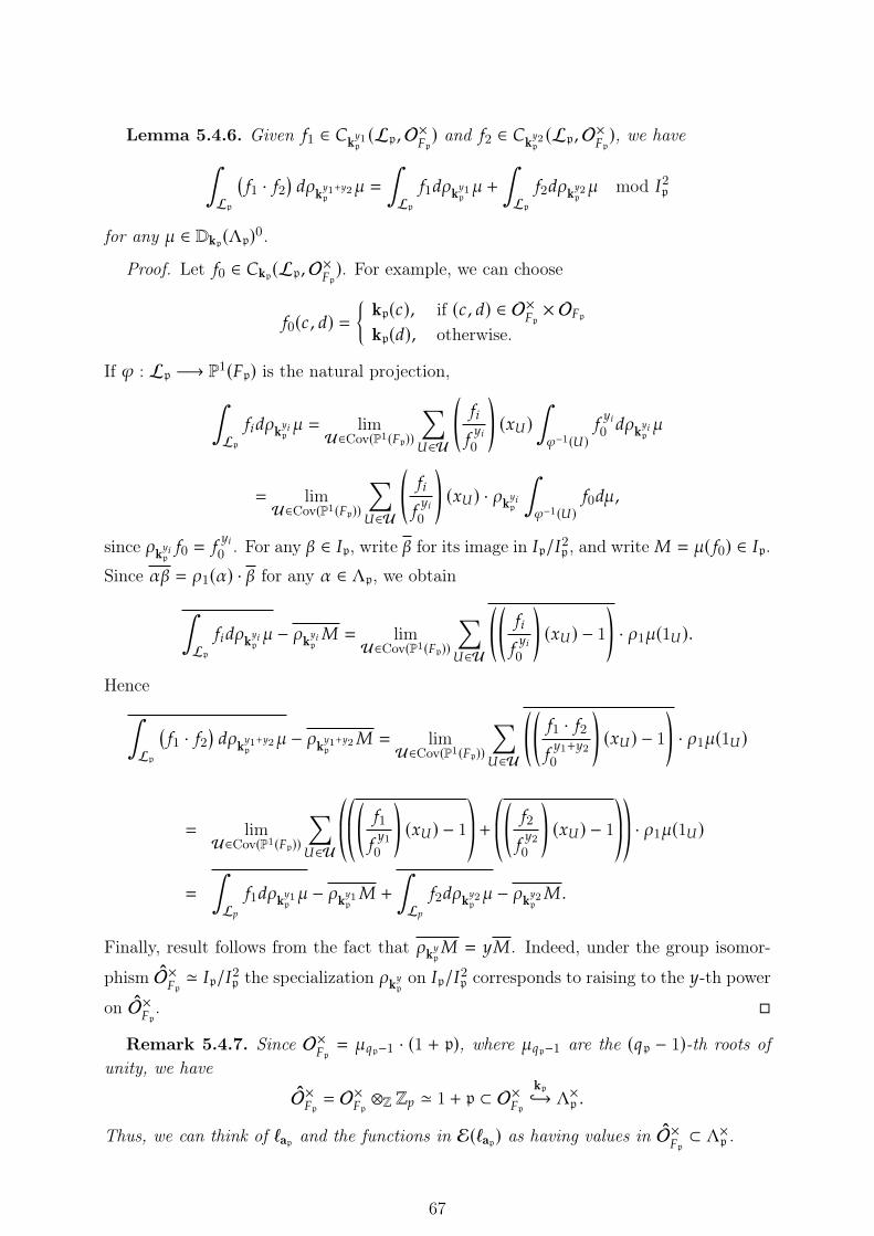
Lemma 5.4.6. Given 51 ∈ �kH1p(ℒp,O×�p) and 52 ∈ �k

H2p(ℒp,O×�p), we have∫

ℒp

(51 · 52

)3�kH1+H2p

� =

∫ℒp513�kH1p � +

∫ℒp523�kH2p � mod �2p

for any � ∈ Dkp(Λp)0.

Proof. Let 50 ∈ �kp(ℒp,O×�p). For example, we can choose

50(2, 3) ={kp(2), if (2, 3) ∈ O×

�p× O�p

kp(3), otherwise.

If ! : ℒp −→ P1(�p) is the natural projection,∫ℒp583�kH8p � = lim

U∈Cov(P1(�p))

∑*∈U

(58

5H80

)(G*)

∫!−1(*)

5H80 3�kH8p �

= limU∈Cov(P1(�p))

∑*∈U

(58

5H80

)(G*) · �kH8p

∫!−1(*)

503�,

since �kH8p 50 = 5H80 . For any � ∈ �p, write � for its image in �p/�2p , and write " = �( 50) ∈ �p.

Since � = �1( ) · � for any ∈ Λp, we obtain∫ℒp583�kH8p � − �kH8p " = lim

U∈Cov(P1(�p))

∑*∈U

((58

5H80

)(G*) − 1

)· �1�(1*).

Hence∫ℒp

(51 · 52

)3�kH1+H2p

� − �kH1+H2p" = lim

U∈Cov(P1(�p))

∑*∈U

((51 · 525H1+H20

)(G*) − 1

)· �1�(1*)

= limU∈Cov(P1(�p))

∑*∈U

©­«©­«(51

5H10

)(G*) − 1

ª®¬ + ©­«(52

5H20

)(G*) − 1

ª®¬ª®¬ · �1�(1*)=

∫ℒ?513�kH1p � − �kH1p " +

∫ℒ?523�kH2p � − �kH2p ".

Finally, result follows from the fact that �kHp" = H". Indeed, under the group isomor-

phism O�p' �p/�2p the specialization �kHp on �p/�

2p corresponds to raising to the H-th power

on O�p. �

Remark 5.4.7. Since O×�p= �@p−1 · (1 + p), where �@p−1 are the (@p − 1)-th roots of

unity, we have

O×�p = O×�p⊗Z Z? ' 1 + p ⊂ O×�p

kp↩→ Λ×p .

Thus, we can think of ℓap and the functions in ℰ(ℓap) as having values in O×�p⊂ Λ×p .

67

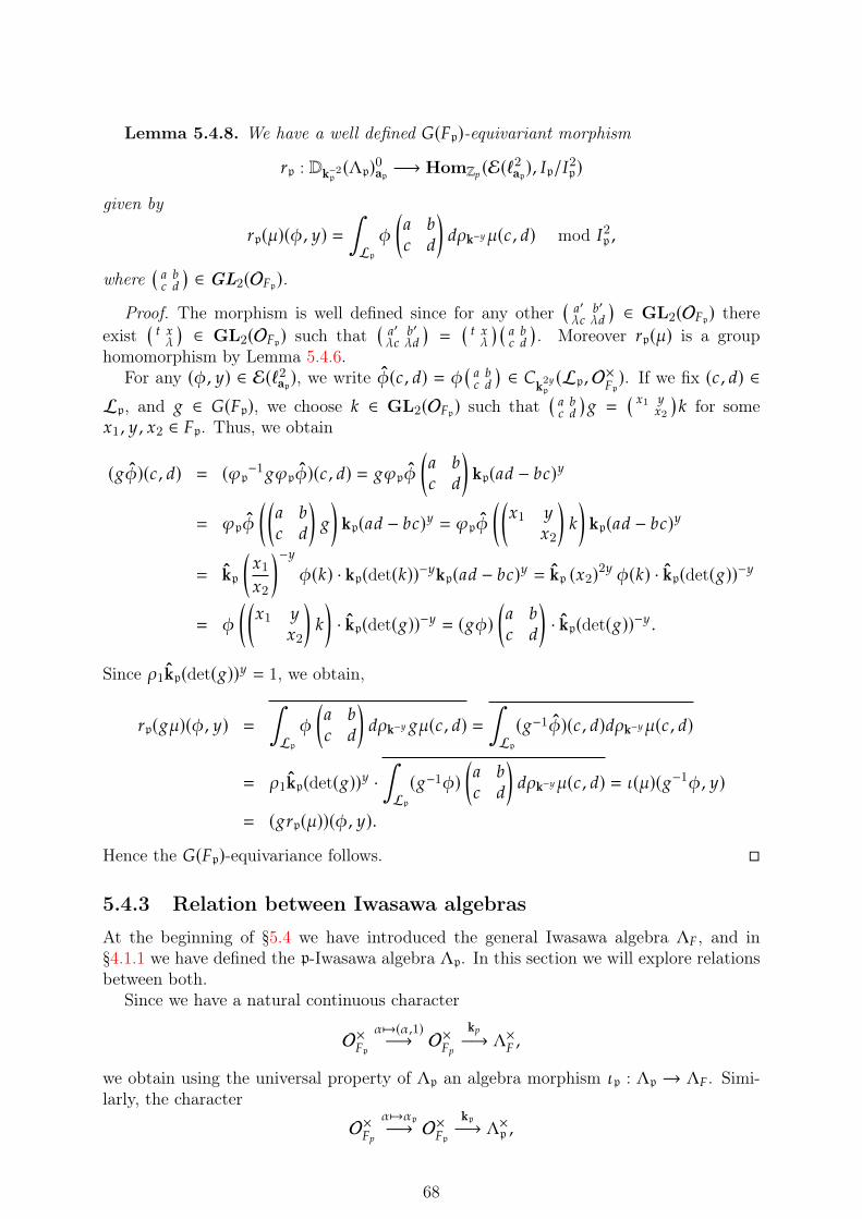
Lemma 5.4.8. We have a well defined �(�p)-equivariant morphism

Ap : Dk−2p(Λp)0ap −→ HomZ? (ℰ(ℓ2ap), �p/�

2p)

given by

Ap(�)(), H) =∫ℒp

)

(0 1

2 3

)3�k−H�(2, 3) mod �2p ,

where(0 12 3

)∈ GL2(O�p).

Proof. The morphism is well defined since for any other(0′ 1′�2 �3

)∈ GL2(O�p) there

exist(C G�

)∈ GL2(O�p) such that

(0′ 1′�2 �3

)=

(C G�

) (0 12 3

). Moreover Ap(�) is a group

homomorphism by Lemma 5.4.6.For any (), H) ∈ ℰ(ℓ2ap), we write )(2, 3) = )

(0 12 3

)∈ �

k2Hp

(ℒp,O×�p). If we fix (2, 3) ∈ℒp, and 6 ∈ �(�p), we choose : ∈ GL2(O�p) such that

(0 12 3

)6 =

( G1 HG2

): for some

G1, H, G2 ∈ �p. Thus, we obtain

(6))(2, 3) = (!p−16!p))(2, 3) = 6!p)

(0 1

2 3

)kp(03 − 12)H

= !p)

((0 1

2 3

)6

)kp(03 − 12)H = !p)

((G1 H

G2

):

)kp(03 − 12)H

= kp

(G1

G2

)−H)(:) · kp(det(:))−Hkp(03 − 12)H = kp (G2)2H )(:) · kp(det(6))−H

= )

((G1 H

G2

):

)· kp(det(6))−H = (6))

(0 1

2 3

)· kp(det(6))−H .

Since �1kp(det(6))H = 1, we obtain,

Ap(6�)(), H) =

∫ℒp

)

(0 1

2 3

)3�k−H 6�(2, 3) =

∫ℒp(6−1))(2, 3)3�k−H�(2, 3)

= �1kp(det(6))H ·∫ℒp(6−1))

(0 1

2 3

)3�k−H�(2, 3) = �(�)(6−1), H)

= (6Ap(�))(), H).

Hence the �(�p)-equivariance follows. �

5.4.3 Relation between Iwasawa algebras

At the beginning of §5.4 we have introduced the general Iwasawa algebra Λ�, and in§4.1.1 we have defined the p-Iwasawa algebra Λp. In this section we will explore relationsbetween both.

Since we have a natural continuous character

O×�p ↦→( ,1)−→ O×�?

k?−→ Λ×� ,

we obtain using the universal property of Λp an algebra morphism �p : Λp → Λ�. Simi-larly, the character

O×�? ↦→ p−→ O×�p

kp−→ Λ×p ,

68

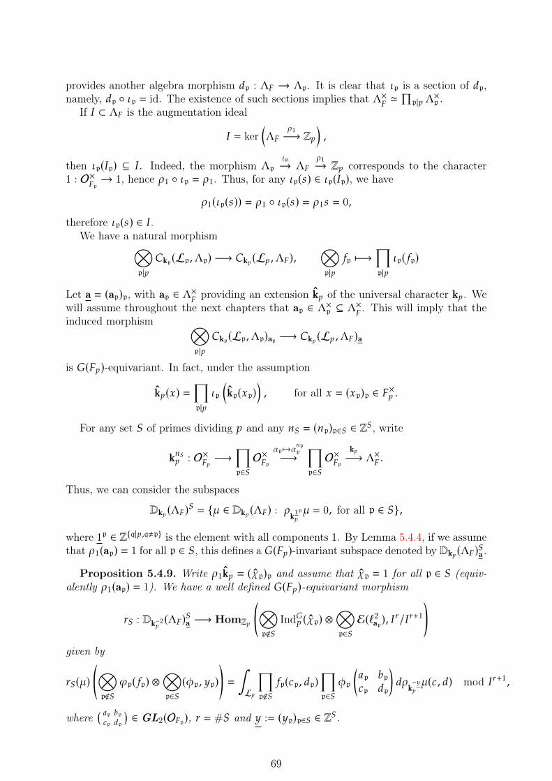
provides another algebra morphism 3p : Λ� → Λp. It is clear that �p is a section of 3p,namely, 3p ◦ �p = id. The existence of such sections implies that Λ×

�'∏

p|? Λ×p .

If � ⊂ Λ� is the augmentation ideal

� = ker(Λ�

�1−→ Z?),

then �p(�p) ⊆ �. Indeed, the morphism Λp�p→ Λ�

�1→ Z? corresponds to the character1 : O×

�p→ 1, hence �1 ◦ �p = �1. Thus, for any �p(B) ∈ �p(�p), we have

�1(�p(B)) = �1 ◦ �p(B) = �1B = 0,

therefore �p(B) ∈ �.We have a natural morphism⊗

p|?�kp(ℒp,Λp) −→ �k? (ℒ? ,Λ�),

⊗p|?

5p ↦−→∏p|?

�p( 5p)

Let a = (ap)p, with ap ∈ Λ×� providing an extension k? of the universal character k?. Wewill assume throughout the next chapters that ap ∈ Λ×p ⊆ Λ×� . This will imply that theinduced morphism ⊗

p|?�kp(ℒp,Λp)ap −→ �k? (ℒ? ,Λ�)a

is �(�?)-equivariant. In fact, under the assumption

k?(G) =∏p|?

�p(kp(Gp)

), for all G = (Gp)p ∈ �×? .

For any set ( of primes dividing ? and any =( = (=p)p∈( ∈ Z(, write

k=(? : O×�? −→∏p∈(O×�p

p ↦→ =pp−→

∏p∈(O×�p

k?−→ Λ×� .

Thus, we can consider the subspaces

Dk? (Λ�)( = {� ∈ Dk? (Λ�) : �k1p

?

� = 0, for all p ∈ (},

where 1p ∈ Z{q|?,q≠p} is the element with all components 1. By Lemma 5.4.4, if we assumethat �1(ap) = 1 for all p ∈ (, this defines a �(�?)-invariant subspace denoted by Dk? (Λ�)(a .

Proposition 5.4.9. Write �1k? = ("p)p and assume that "p = 1 for all p ∈ ( (equiv-alently �1(ap) = 1). We have a well defined �(�?)-equivariant morphism

A( : Dk−2?(Λ�)(a −→ HomZ?

(⊗p∉(

Ind�% ("p) ⊗⊗p∈(ℰ(ℓ2ap), �

A/�A+1)

given by

A((�)(⊗p∉(

!p( 5p) ⊗⊗p∈(()p, Hp)

)=

∫ℒ?

∏p∉(

5p(2p, 3p)∏p∈(

)p

(0p 1p2p 3p

)3�

k−H?�(2, 3) mod �A+1,

where( 0p 1p2p 3p

)∈ GL2(O�p), A = #( and H := (Hp)p∈( ∈ Z(.

69

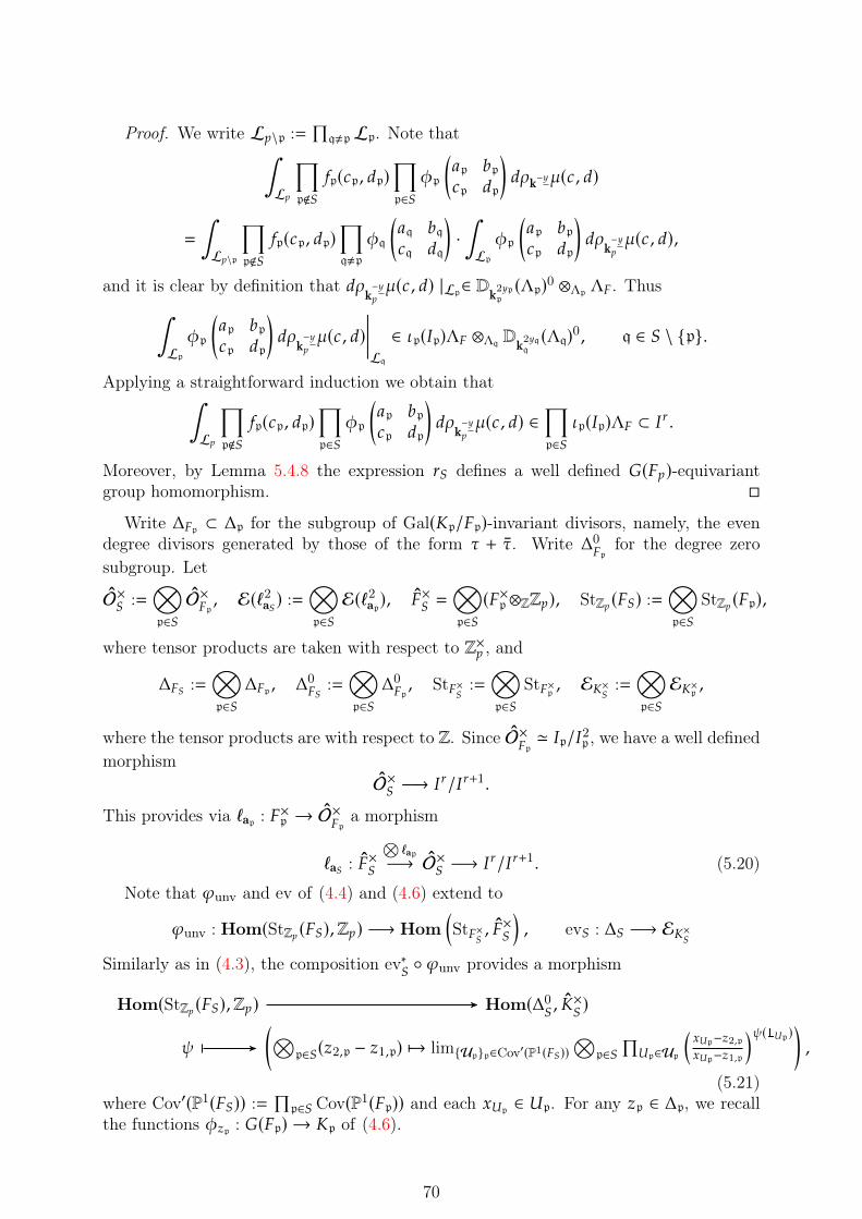
Proof. We write ℒ?\p :=∏q≠pℒp. Note that∫

ℒ?

∏p∉(

5p(2p, 3p)∏p∈(

)p

(0p 1p2p 3p

)3�k−H�(2, 3)

=

∫ℒ?\p

∏p∉(

5p(2p, 3p)∏q≠p

)q

(0q 1q2q 3q

)·∫ℒp

)p

(0p 1p2p 3p

)3�

k−H?�(2, 3),

and it is clear by definition that 3�k−H?�(2, 3) |ℒp∈ Dk

2Hpp

(Λp)0 ⊗Λp Λ�. Thus∫ℒp

)p

(0p 1p2p 3p

)3�

k−H?�(2, 3)

����ℒq∈ �p(�p)Λ� ⊗Λq Dk

2Hqq

(Λq)0, q ∈ ( \ {p}.

Applying a straightforward induction we obtain that∫ℒ?

∏p∉(

5p(2p, 3p)∏p∈(

)p

(0p 1p2p 3p

)3�

k−H?�(2, 3) ∈

∏p∈(

�p(�p)Λ� ⊂ �A .

Moreover, by Lemma 5.4.8 the expression A( defines a well defined �(�?)-equivariantgroup homomorphism. �

Write Δ�p ⊂ Δp for the subgroup of Gal( p/�p)-invariant divisors, namely, the evendegree divisors generated by those of the form � + �. Write Δ0

�pfor the degree zero

subgroup. Let

O×( :=⊗p∈(O×�p , ℰ(ℓ

2a() :=

⊗p∈(ℰ(ℓ2ap), �×( =

⊗p∈((�×p ⊗ZZ?), StZ? (�() :=

⊗p∈(

StZ? (�p),

where tensor products are taken with respect to Z×? , and

Δ�( :=⊗p∈(

Δ�p , Δ0�(

:=⊗p∈(

Δ0�p, St�×

(:=

⊗p∈(

St�×p , ℰ ×( :=⊗p∈(ℰ ×p ,

where the tensor products are with respect to Z. Since O�p' �p/�2p , we have a well defined

morphismO×( −→ �A/�A+1.

This provides via ℓap : �×p → O×�p a morphism

ℓa( : �×(

⊗ℓap−→ O×( −→ �A/�A+1. (5.20)

Note that !unv and ev of (4.4) and (4.6) extend to

!unv : Hom(StZ? (�(),Z?) −→ Hom(St�×

(, �×(

), ev( : Δ( −→ ℰ ×

(

Similarly as in (4.3), the composition ev∗(◦ !unv provides a morphism

Hom(StZ? (�(),Z?) Hom(Δ0(, ×

()

#

(⊗p∈((I2,p − I1,p) ↦→ lim{Up}p∈Cov′(P1(�())

⊗p∈(

∏*p∈Up

(G*p−I2,pG*p−I1,p

)#(1*p )),

(5.21)where Cov′(P1(�()) :=

∏p∈( Cov(P1(�p)) and each G*p ∈ *p. For any Ip ∈ Δp, we recall

the functions )Ip : �(�p) → p of (4.6).

70

Proposition 5.4.10. Write �1k? = ("p)p, +( =⊗

p∉( Ind�%("p), and assume that

"p = 1 for all p ∈ (. We have �(�?)-equivariant morphisms

ev( : Hom(+( ⊗ ℰ(ℓ2a(), �

A/�A+1)−→ Hom

(+( ⊗ Δ�( , �A/�A+1

),

! ↦−→(E( ⊗

⊗p∈((Ip + Ip) ↦→ !

(E( ⊗

⊗p∈((ℓap()Ip · )Ip), 1)

)),

making the following diagram commutative

Hom(+( ⊗ Δ�( , �A/�A+1) Hom(+( ⊗ Δ0�(, �A/�A+1)

Dk−2?(Λ�)(a

HomZ? (+( ⊗ StZ? (�(),Z?) Hom(+( ⊗ Δ0�(, �×

()

ev(◦A(

�1

ev∗(◦!unv

ℓa(

Proof. The �(�?)-equivariance of ev( is clear by the definitions. Given � ∈ Dk−2?(Λ�)(a ,

we compute

ℓa(

((ev∗( ◦ !unv ◦ �1

)(�)

(E( ⊗

⊗p∈((Ip,1 − Ip,2 + Ip,1 − Ip,2)

))=

= lim{Up}p∈Cov′(P1(�())

ℓa(©­«⊗p∈(

∏*p∈Up

()Ip,1)Ip,1)Ip,2)Ip,2

)(G*p)�1(�)(E

(⊗1*p )ª®¬= lim{Up}p∈Cov′(P1(�())

∏p∈(

�pℓap©­«

∏*p∈Up

()Ip,1)Ip,1)Ip,2)Ip,2

)(G*p)�1(�)(E

(⊗1*p )ª®¬ mod �A+1

=

∫P1(�()

∏p∈(

ℓap

()Ip,1)Ip,1)Ip,2)Ip,2

)3�1(�)(E() mod �A+1

= A((�)(E( ⊗

⊗p∈(

(ℓap

()Ip,1)Ip,1)Ip,2)Ip,2

), 0

))= ev( ◦ A((�)

(E( ⊗

⊗p∈((Ip,1 − Ip,2 + Ip,1 − Ip,2)

).

Hence, we obtain the required commutativity of the diagram. �

5.4.4 ?-adic periods and L-invariants

Fix a prime p | ? and let )p� ∈ �D(�(�)+,Ap∪∞(StZ(�p),Z))� be a modular symbolassociated with an elliptic curve �/� with multiplicative reduction at p. The short exactsequence

0 −→ Δ0p −→ Δp −→ Z −→ 0,

provides a connection morphism

�D(�(�)+,Ap∪∞(Δ0p,

×p ))�

2−→ �D+1(�(�)+,Ap∪∞( ×p ))�.

Moreover, the commutative diagram (4.7) shows that

2(ev∗ ◦ !unv))p� ∈ �D+1(�(�)+,Ap∪∞(@Zp ))� ⊂ �D+1(�(�)+,Ap∪∞(�×p ))� ,

71

for some @p ∈ �×p . The generalized Oda’s conjecture ([GMM17, Conjecture 3.8]) assertsthat, in fact, the elliptic curve �/�p is isogenous to the Tate curve defined by the quotient�p/@Zp .

Theorem 5.4.11. Let Φp� ∈ �D(�(�)+,Ap∪∞(Dk−2p(Λp))ap)� be a family lifting )p�.

Thenℓap(@p) = 1 ∈ O×�p .

Proof. Since Φp� specializes to the Steinberg representation, we have in fact

Φp

� ∈ �D(�(�)+,Ap∪∞(Dk−2p

(Λp))0ap)�.

If we consider the exact sequence

�D(�(�)+,Ap∪∞(Δ�p , �×p ))�res−→ �D(�(�)+,Ap∪∞(Δ0

�p, �×p ))�

2−→ �D+1(�(�)+,Ap∪∞(�×p ))� ,

by Proposition 5.4.10,

res(ev ◦ Ap)Φp� = ℓap(ev∗ ◦ !unv))p� |Δ0

�p.

This implies thatℓap2(ev∗ ◦ !unv))p� |Δ0

�p= 0.

Since 2(ev∗ ◦ !unv))p� |Δ0�p

lies in �D+1(�(�)+,Ap∪∞(@2Zp ))�, we deduce ℓap(@p) = 1 from

the fact that O�p

is torsion free. �

Remark 5.4.12. As showed in §5.4.1, the elements ap ∈ Λ� are the eigenvalues of the*p-operators acting on the Hida family. By definition

ℓap(+p) = ap−1 − 1 ∈ �p/�2p .

Thus, the relation ℓap(@p) = 1 implies

ordp(@p)(ap−1 − 1

)+ logp(@p) ≡ 0 mod �2p .

We obtain that the image of ap−1 in �p/�2p is given by the L-invariant ℒp = logp(@p)/ordp(@p).With the formalism previously described, we have showed that the derivative of ap−1 withrespect to the weight variable is given by the L-invariant ℒp. In the classical setting,this is a key result due to Greenberg-Stevens towards the exceptional zero conjecture (see[GS93]).

5.4.5 2 variable ?-adic L-functions

Let )?

� ∈ �D(�(�)+,A?∪∞(+? , +(:)C? )

)�be an ordinary cohomology class generating

an automorphic representation �. By Proposition 5.3.6, )?� provides an overconvergentcohomology class

)?

� ∈ �D(�(�)+,A?∪∞(D"−2?

(C?) ∗))�,

72

for some locally polynomial character "?−1. Assume that we have the extension k? of theuniversal character k? and an element

Φ?

� ∈ �D(�(�)+,A?∪∞(Dk−2?

(Λ�)a))�

mapping to )?

� through the morphism �"? of (5.16). Similarly as in Theorem 5.3.7, wecan define the distribution �

Φ?

�as∫

G)5 3�

Φ?

�=

((�∗ 5 ) ∩ �

)∩ �∗?(Φ

?

�), 5 ∈ �(G) ,Λ�)

where �? is defined as in (5.8):

�? : �2()(�?),Λ�) −→ Ind�% (k?)!?' �k−2?

(ℒ? ,Λ�).

Indeed, we can think �∗?(Φ?

�) and �∗ 5 ∩ � as elements

�∗?(Φ?

�) ∈ �D(�(�)+,A?∪∞(Meas()(�?),Λ�))

)�,

�∗ 5 ∩ � ∈ �D()(�), �2()(A�),Λ�)) = �D

()(�), Ind)(�)

)(�)+�02

()(A?∪∞

�), �2()(�?),Λ�)

)),

hence the pairing (3.15) applies and the cap-product is well defined. The measure �Φ?

�is

considered as the 2-variable ?-adic L-function since its specialization at different weights�? : O×�? → C? provides different measures ��? (�Φ?�) of G) . In particular

�"? (�Φ?�) = �)?�,

by Theorem 5.3.7. Thus �Φ?

�interpolates �)?� as the weight varies.

73

74

Chapter 6

Main results

Throughout this chapter we will assume that the automorphic representation is attachedto an elliptic curve �/�.

6.1 A ?-adic Gross-Zagier formula

As in §4.1, let us assume that ( = {p} and �(�p) = PGL2(�p), +Zp = StZ(�p) and ) doesnot split at p. We have seen in §5.2 that we can construct a measure �)p� attached to amodular symbol )p�. In this setting the distribution is 0-admissible, hence bounded.

Let � ∈ �(G) ,C) be as above with �∗�|)(�∞) = �. If we also assume that �p = 1, wehave by Remark 5.1.10 ∫

G)�3�)p�

= 0.

Write Meas(G) ,C?) for the space of measures of �(G) ,C?), i.e. bounded distributionsof G endowed with the natural group law∫

G)5 3(�1 ★�2) =

∫G)

∫G)5 ( · �)3�1( )3�2(�). (6.1)

Thus, �)p� lies in the kernel �� of the algebra morphism &� given by integration, definedby the exact sequence

0 �� Meas(G) ,C?) C? 0&�

� ↦→∫G)

�3�(6.2)

Since �p = 1 the character � descends to a character of Gp), denoted the same way. In

4.1.3 we have constructed Darmon points %�� ∈ �( p) ⊗Z Z associated with �. We aim torelate the image of �)p� in ��/�2� with %�� . In order to do that, we introduce the followingwell-defined morphism

! : G) ⊗Z Z ��/�2�;∫G) 5 3!(�) = �(�)−1 · 5 (�) − 5 (1), � ∈ G) .

(6.3)Denote by (G ↦→ G) the nontrivial element of Gal( p/�p). Since @ ∈ �p we can regard thedifference %

p

� − %p� as

%p

� − %p� ∈ )(�p) ⊗Z Z, )(�p) = ×p /�×p ' {G ∈ ×p ; G · G = 1} ⊂ ×p , (6.4)

and we can consider its image through the natural morphism provided by the Artin map

recp : )(�p) ⊗Z Z G) ⊗Z Z. (6.5)

75

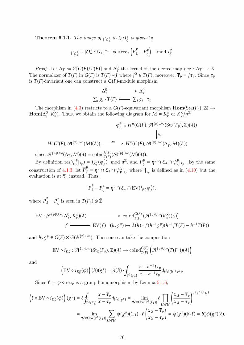
Theorem 6.1.1. The image of �)p� in ��/�2� is given by

�)p�≡ [Op+ : O+]−1 · ! ◦ recp

(%p

� − %p�)

mod �2� .

Proof. Let Δ) := Z[�(�)/)(�)] and Δ0)the kernel of the degree map deg : Δ) → Z.

The normalizer of )(�) in �(�) is )(�)o � where �2 ∈ )(�), moreover, �p = ��p. Since �pis )(�)-invariant one can construct a �(�)-module morphism

Δ0)

Δ0p∑

8 68 · )(�)∑8 68 · �p

The morphism in (4.3) restricts to a �(�)-equivariant morphism Hom(StZ(�p),Z) →Hom(Δ0

), ×p ). Thus, we obtain the following diagram for " = ×p or ×p /@Z

)p� ∈ �D(�(�),A{p}∪∞(StZ(�p),Z)(�))

�D()(�),A{p}∪∞(")(�)) �D(�(�),A{p}∪∞(Δ0), ")(�))

8"

res

since A{p}∪∞(Δ) , ")(�) = coInd�(�))(�) (A

{p}∪∞(")(�)).By definition res(#p� |�? ) = 8 ×p ()

p

�) mod @Z, and %p� = �p ∩ �� ∩ #p� |�? . By the same

construction of 4.1.3, let %p

� = �p ∩ �� ∩ #�p |�? where ·|�? is defined as in (4.10) but the

evaluation is at �p instead. Thus,

%p

� − %p� = �p ∩ �� ∩ EV(8 ×p )p

�),

where %p

� − %p� is seen in )(�p) ⊗ Z,

EV : A{p}∪∞(Δ0), ×p )(�) coInd�(�)

)(�)(A{p}∪∞( ×p )(�)

)5 EV( 5 ) : (ℎ, 6p) ↦→ �(ℎ) · 5 (ℎ−16p)(ℎ−1�)(�) − ℎ−1)(�))

and ℎ, 6p ∈ �(�) × �(A{p}∪∞). Then one can take the composition

EV ◦ 8 ×p : A{p}∪∞(StZ(�p),Z)(�) → coInd�(�))(�)

(A{p}∪∞()(�p))(�)

)and (

EV ◦ 8 ×p ()))(ℎ)(6p) = �(ℎ) · ×

∫P1(�p)

G − ℎ−1��pG − ℎ−1�p

3�)(ℎ−16p).

Since ℓ := ! ◦ recp is a group homomorphism, by Lemma 5.1.6,(ℓ ◦ EV ◦ 8 ×p ())

)(6p) = ℓ ×

∫P1(�p)

G − �pG − �p

3�)(6p) = limU∈Cov(P1(�p))

ℓ∏*∈U

(G* − �pG* − �p

))(6p)(1* )= limU∈Cov(P1(�p))

∑*∈U

)(6p)(1*) · ℓ(G* − �pG* − �p

)= )(6p)(�pℓ ) = �∗p)(6p)(ℓ ),

76

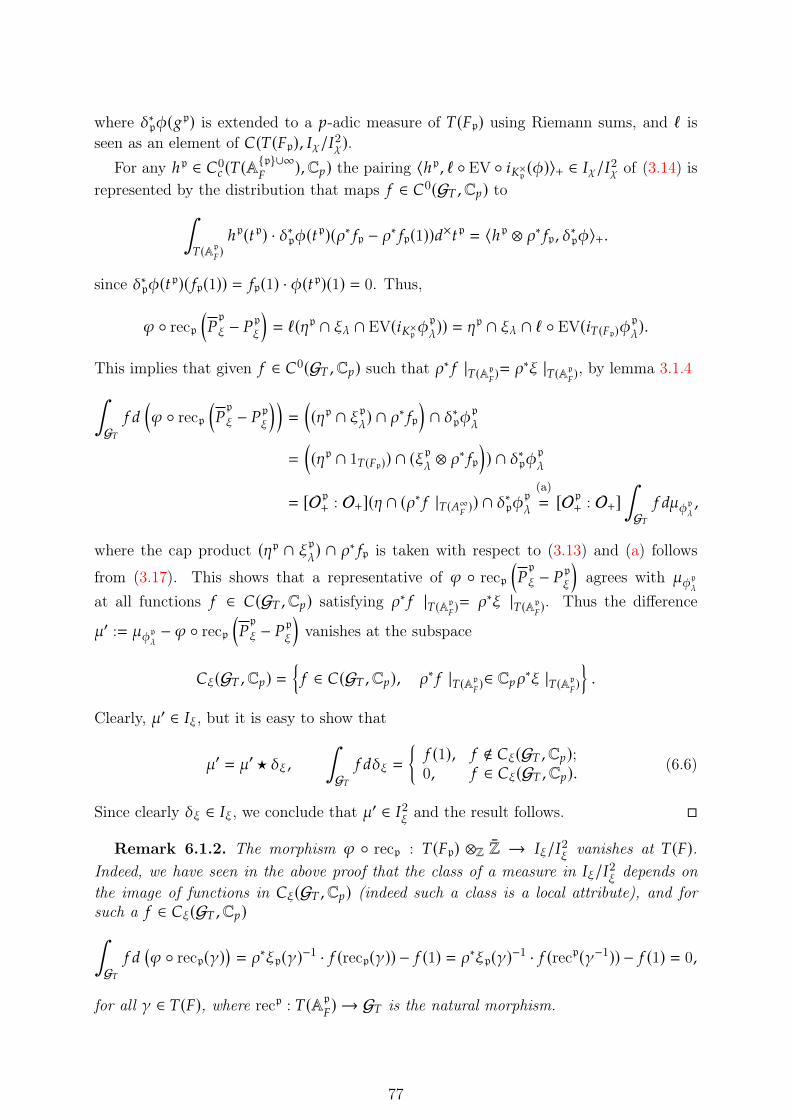
where �∗p)(6p) is extended to a ?-adic measure of )(�p) using Riemann sums, and ℓ isseen as an element of �()(�p), �"/�2").

For any ℎp ∈ �02 ()(A

{p}∪∞�

),C?) the pairing 〈ℎp, ℓ ◦ EV ◦ 8 ×p ())〉+ ∈ �"/�2" of (3.14) isrepresented by the distribution that maps 5 ∈ �0(G) ,C?) to∫

)(Ap�)ℎp(Cp) · �∗p)(Cp)(�∗ 5p − �∗ 5p(1))3×Cp = 〈ℎp ⊗ �∗ 5p, �∗p)〉+.

since �∗p)(Cp)( 5p(1)) = 5p(1) · )(Cp)(1) = 0. Thus,

! ◦ recp(%p

� − %p�)= ℓ (�p ∩ �� ∩ EV(8 ×p )

p

�)) = �p ∩ �� ∩ ℓ ◦ EV(8)(�p))p

�).

This implies that given 5 ∈ �0(G) ,C?) such that �∗ 5 |)(Ap�)= �∗� |)(Ap

�), by lemma 3.1.4∫

G)5 3

(! ◦ recp

(%p

� − %p�))=

((�p ∩ �p�) ∩ �

∗ 5p)∩ �∗p)p�

=

((�p ∩ 1)(�p)) ∩ (�

p

� ⊗ �∗ 5p

)) ∩ �∗p)p�

= [Op+ : O+](� ∩ (�∗ 5 |)(�∞� )) ∩ �∗p)

p

�

(a)= [Op+ : O+]

∫G)5 3�)p�

,

where the cap product (�p ∩ �p�) ∩ �∗ 5p is taken with respect to (3.13) and (a) follows

from (3.17). This shows that a representative of ! ◦ recp(%p

� − %p�)agrees with �)p�

at all functions 5 ∈ �(G) ,C?) satisfying �∗ 5 |)(Ap�)= �∗� |)(Ap

�). Thus the difference

�′ := �)p�− ! ◦ recp

(%p

� − %p�)vanishes at the subspace

��(G) ,C?) ={5 ∈ �(G) ,C?), �∗ 5 |)(Ap

�)∈ C?�∗� |)(Ap

�)

}.

Clearly, �′ ∈ ��, but it is easy to show that

�′ = �′★ �� ,

∫G)5 3�� =

{5 (1), 5 ∉ ��(G) ,C?);0, 5 ∈ ��(G) ,C?). (6.6)

Since clearly �� ∈ ��, we conclude that �′ ∈ �2� and the result follows. �

Remark 6.1.2. The morphism ! ◦ recp : )(�p) ⊗Z Z → ��/�2� vanishes at )(�).Indeed, we have seen in the above proof that the class of a measure in ��/�2� depends onthe image of functions in ��(G) ,C?) (indeed such a class is a local attribute), and forsuch a 5 ∈ ��(G) ,C?)∫G)5 3

(! ◦ recp(�)

)= �∗�p(�)−1 · 5 (recp(�)) − 5 (1) = �∗�p(�)−1 · 5 (recp(�−1)) − 5 (1) = 0,

for all � ∈ )(�), where recp : )(Ap�) → G) is the natural morphism.

77

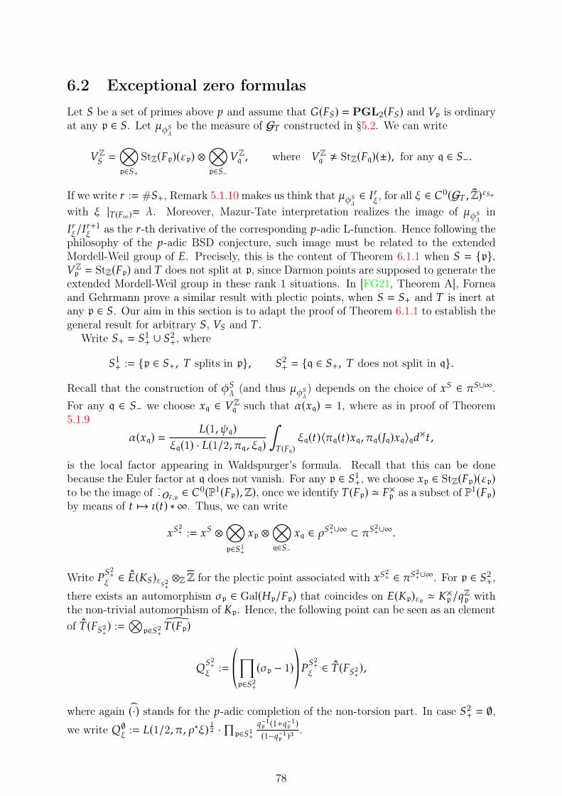
6.2 Exceptional zero formulasLet ( be a set of primes above ? and assume that �(�() = PGL2(�() and +p is ordinaryat any p ∈ (. Let �)(� be the measure of G) constructed in §5.2. We can write

+Z( =⊗p∈(+

StZ(�p)(�p) ⊗⊗p∈(−

+Zq , where +Zq ; StZ(�q)(±), for any q ∈ (−.

If we write A := #(+, Remark 5.1.10 makes us think that �)(� ∈ �A�, for all � ∈ �0(G) , Z)�(+

with � |)(�∞)= �. Moreover, Mazur-Tate interpretation realizes the image of �)(� in�A�/�

A+1� as the A-th derivative of the corresponding ?-adic L-function. Hence following the

philosophy of the ?-adic BSD conjecture, such image must be related to the extendedMordell-Weil group of �. Precisely, this is the content of Theorem 6.1.1 when ( = {p},+Zp = StZ(�p) and ) does not split at p, since Darmon points are supposed to generate theextended Mordell-Weil group in these rank 1 situations. In [FG21, Theorem A], Forneaand Gehrmann prove a similar result with plectic points, when ( = (+ and ) is inert atany p ∈ (. Our aim in this section is to adapt the proof of Theorem 6.1.1 to establish thegeneral result for arbitrary (, +( and ).

Write (+ = (1+ ∪ (2+, where

(1+ := {p ∈ (+, ) splits in p}, (2+ = {q ∈ (+, ) does not split in q}.

Recall that the construction of )(� (and thus �)(�) depends on the choice of G( ∈ �(∪∞.For any q ∈ (− we choose Gq ∈ +Zq such that (Gq) = 1, where as in proof of Theorem5.1.9

(Gq) =!(1,#q)

�q(1) · !(1/2,�q, �q)

∫)(�q)

�q(C)〈�q(C)Gq,�q(�q)Gq〉q3×C ,

is the local factor appearing in Waldspurger’s formula. Recall that this can be donebecause the Euler factor at q does not vanish. For any p ∈ (1+, we choose Gp ∈ StZ(�p)(�p)to be the image of 1O�,p ∈ �0(P1(�p),Z), once we identify )(�p) ' �×p as a subset of P1(�p)by means of C ↦→ y(C) ∗ ∞. Thus, we can write

G(2+ := G( ⊗

⊗p∈(1+

Gp ⊗⊗q∈(−

Gq ∈ �(2+∪∞ ⊂ �(

2+∪∞.

Write %(2+

� ∈ �( ()�(2+ ⊗Z Z for the plectic point associated with G(2+ ∈ �(2+∪∞. For p ∈ (2+,

there exists an automorphism �p ∈ Gal(�p/�p) that coincides on �( p)�p ' ×p /@Zp withthe non-trivial automorphism of p. Hence, the following point can be seen as an elementof )(�(2+) :=

⊗p∈(2+

�)(�p)&(2+� :=

©­«∏p∈(2+

(�p − 1)ª®¬%(

2+

� ∈ )(�(2+),

where again (·) stands for the ?-adic completion of the non-torsion part. In case (2+ = ∅,we write &∅� := !(1/2,�, �∗�) 12 ·∏p∈(1+

@−1p (1+@−1p )(1−@−1p )3

.

78

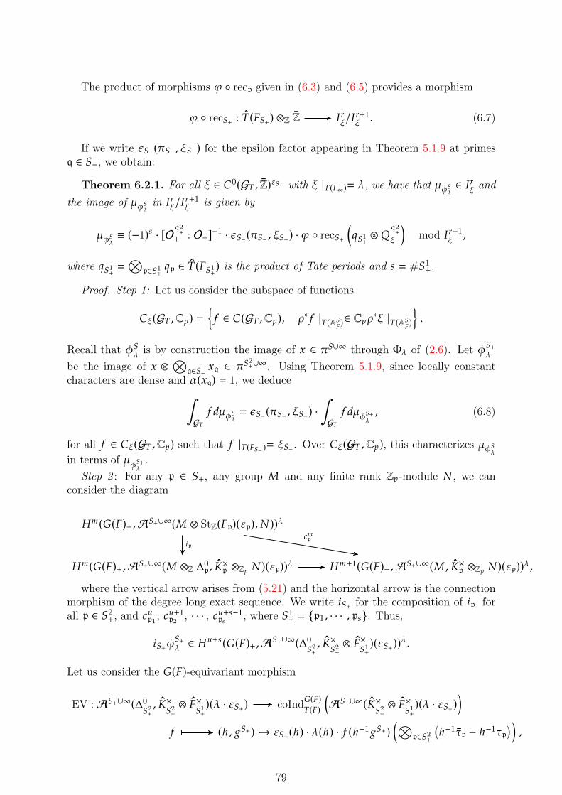
The product of morphisms ! ◦ recp given in (6.3) and (6.5) provides a morphism

! ◦ rec(+ : )(�(+) ⊗Z Z �A�/�A+1� . (6.7)

If we write &(−(�(− , �(−) for the epsilon factor appearing in Theorem 5.1.9 at primesq ∈ (−, we obtain:

Theorem 6.2.1. For all � ∈ �0(G) , Z)�(+ with � |)(�∞)= �, we have that �)(� ∈ �A� and

the image of �)(� in �A�/�A+1� is given by

�)(�≡ (−1)B · [O(

2++ : O+]−1 · &(−(�(− , �(−) · ! ◦ rec(+

(@(1+ ⊗ &

(2+�

)mod �A+1� ,

where @(1+ =⊗

p∈(1+ @p ∈ )(�(1+) is the product of Tate periods and B = #(1+.

Proof. Step 1: Let us consider the subspace of functions

��(G) ,C?) ={5 ∈ �(G) ,C?), �∗ 5 |)(A(

�)∈ C?�∗� |)(A(

�)

}.

Recall that )(� is by construction the image of G ∈ �(∪∞ through Φ� of (2.6). Let )(+�be the image of G ⊗

⊗q∈(− Gq ∈ �(

2+∪∞. Using Theorem 5.1.9, since locally constant

characters are dense and (Gq) = 1, we deduce∫G)5 3�)(�

= &(−(�(− , �(−) ·∫G)5 3�)(+�

, (6.8)

for all 5 ∈ ��(G) ,C?) such that 5 |)(�(− )= �(− . Over ��(G) ,C?), this characterizes �)(�in terms of �)(+�

.Step 2 : For any p ∈ (+, any group " and any finite rank Z?-module # , we can

consider the diagram

�<(�(�)+,A(+∪∞(" ⊗ StZ(�p)(�p), #))�

�<(�(�)+,A(+∪∞(" ⊗Z Δ0p,

×p ⊗Z? #)(�p))� �<+1(�(�)+,A(+∪∞(", ×p ⊗Z? #)(�p))� ,

8p2<p

where the vertical arrow arises from (5.21) and the horizontal arrow is the connectionmorphism of the degree long exact sequence. We write 8(+ for the composition of 8p, forall p ∈ (2+, and 2Dp1 , 2D+1p2

, · · · , 2D+B−1pB, where (1+ = {p1, · · · , pB}. Thus,

8(+)(+� ∈ �

D+B(�(�)+,A(+∪∞(Δ0(2+, ×

(2+⊗ �×

(1+)(�(+))�.

Let us consider the �(�)-equivariant morphism

EV : A(+∪∞(Δ0(2+, ×

(2+⊗ �×

(1+)(� · �(+) coInd�(�)

)(�)

(A(+∪∞( ×

(2+⊗ �×

(1+)(� · �(+)

)5 (ℎ, 6(+) ↦→ �(+(ℎ) · �(ℎ) · 5 (ℎ−16(+)

(⊗p∈(2+

(ℎ−1�p − ℎ−1�p

) ),

79

where ℎ, 6(+ ∈ �(�) ×�(A(+∪∞). Since we are evaluating at divisors of the form ℎ−1�p −ℎ−1�p it is easy to show that the image of )(+� lies in )(�(+). Thus, by Shapiro,

EV8(+)(+� ∈ �

D+B()(�)+,A(+∪∞()(�(+))(�(+))�.

We claim that

@(1+ ⊗ &(2+� = #

(O(++ /O

(2++

)−1tor· (�(+ ∩ ��) ∩ EV8(+)

(+� ∈ )(�(+) ⊗Z Z. (6.9)

Indeed, by functoriality and the description of the multiplicative integral given in §4.1.1,we have that

EV8(+)(+� = EV8(2+!unv)

(+� ∪

⋃p∈(1+

res�(�)+)(�)+ 2p,

where !unv is the morphism of (4.4), 2p ∈ �1(�(�), St�×p ) is the class associated with theextension ℰ�×p of (4.5), and

!unv)(+

� ∈ �D(�(�)+,A(+∪∞(+Z

(2+⊗ St�×

(1+, �×

(1+(�(1+)))

� , St�×(1+

:=⊗p∈(1+

St�×p

is the corresponding push-forward. In fact, [GMM17, Conjecture 3.8] can be interpretedas

!unv)(+� ∪

⋃p∈(1+

2p = @(1+ ⊗©­«)(+� ∪

⋃p∈(1+

2ordp

ª®¬ ,where 2ord

p ∈ �1(�(�), StZ(�p)) is the class associated with the extension (see [Bla19,§6.1])

StZ(�p) ℰZ(�p)5 ( 5 (6−1 ∗ ∞), 0)

and

ℰZ(�p) :={(), H) ∈ �(GL2(�p),Z) × Z : )

((B G

C

)6

)= H · Ep(C) + )(6)

}/(Z, 0).

For p ∈ (1+, write �p and �p for the points in P1(�p) fixed by )(�p) as in §4.1.1. Thus, ifwe write

)1

(0 1

2 3

)= Ep(3 + �p · 2) −

((Ep + 1) · 1O�,p

) (3 + �p · 23 + �p · 2

), (6.10)

the element ()1, 1) ∈ ℰZ(�p) is a generator mapping to 1 under the natural �(�)-morphismℰZ(�p) → Z. Hence the cocycle res�(�)

)(�) 2ordp has representative

2ordp (C)(G) = (1 − C))1(G) = (1 − C)

((Ep + 1) · 1O�,p

) (G − �pG − �p

)=

(∫)(�p)

1O�,p(�)(�1O�,p − C�1O�,p

)3�

) (G − �pG − �p

),

80

for all C ∈ )(�). We compute, recalling the definition of Ip of Lemma 3.1.4,

(�(+ ∩ ��) ∩ EV8(+)(+� = @(1+ ⊗ (�

(+ ∩ ��) ∩©­«EV8(2+)(+� ∪

⋃p∈(1+

res�(�)+)(�)+ 2

ordp

ª®¬= @(1+ ⊗

©­«�(+ ∩⋃p∈(1+

res)(�p))(�)+Ip ∩ ��

ª®¬ ∩ EV8(2+)(2+�

= #(O(++ /O

(2++

)tor· @(1+ ⊗

(�(

2+ ∩ ��

)∩ EV8(2+)

(2+� ,

where the third equality follows from Lemma 3.1.4 and the second from the fact that

Φ(G(∪p)(2ordp (C)) =

∫)(�p)

1O�,p(�) · Φ(G(∪p)(�1O�,p − C�1O�,p

)3�

=

∫)(�p)

(1O�,p(�) − C1O�,p(�)

)· Φ(G(∪p)

(�1O�,p

)3�

=

∫)(�p)

Ip(C)(�) · Φ(G(∪p ⊗ 1O�,p)(�)3×�,

for any Φ ∈ A{p}∪(∪∞(StZ(�p), ")� = A(∪∞(")� and G(∪p ∈ �(∪{p}. If (2+ = ∅, the samearguments used in the interpolation formula (Theorem 5.1.9) together with the fact that

(1O�,p) =@−1p (1+@−1p )(1−@−1p )3

(as seen in the proof of [Bla19, Theorem 7.5]) proves the claim (6.9)

in this case. If (2+ ≠ ∅, we apply the same arguments used in the proof of Theorem 6.1.1to obtain

(�(

2+ ∩ ��

)∩ EV8(2+)

(2+� = &

(2+� , and to deduce the claim (6.9).

Step 3: Similarly as in (6.10), if p ∈ (1+ and we write

)1

(0 1

2 3

)= (3 + �p · 2) ·

(3 + �p · 23 + �p · 2

)1O�,p ( 3+�p ·23+�p ·2

), (6.11)

the element ()1, 1) ∈ ℰ�×p is a generator mapping to 1 under the natural �(�)-morphism

ℰ�×p → Z. Hence the cocycle res�(�))(�) 2p has representative

2p(C)(G) = (1 − C))1(G) = (1 − C)©­«(G − �pG − �p

)1O�,p ( G−�pG−�p

)ª®¬= C

1CO�,p

(G−�pG−�p

)·(G − �pG − �p

) Ip(C)( G−�pG−�p

)∈ )(�) ·

(G − �pG − �p

) Ip(C)( G−�pG−�p

),

for all C ∈ )(�). Therefore, we can consider the composition

EV ◦ 8 ×p : A(+∪∞(+Z(+ ,Z)(�) → coInd�(�))(�)

(A(+∪∞(St�×

(1+, )(�(2+)(�(+))(�)

),

and the cocycle 2(1+ =⊗

p∈(1+ 2p : )(�)B → St�×

(1+, obtaining

(EV ◦ 8 ×p ())

)(1)(6(+)

(2(1+(�)

)= limU∈Cov(P1(�(+ ))

∏*∈U

⊗p∈(+

p

(G* − �pG* − �p

) B(p)·Ip(�p)( G*−�pG*−�p

)·)(6(+ )(1* )

,

81

where � = (�p)p∈(1+ ∈ )(�)B , p ∈ )(�); and B(p) = −1 if p ∈ (1+ and 1 otherwise (recall

that Ip = 1)(�p) for p ∈ (2+). Since ℓ =∏p∈(+ ℓp := ! ◦ rec(+ is a product of group

morphisms ℓp that vanish at )(�) by Remark 6.1.2,

ℓ◦EV◦8 ×p ())(6(+)

(2(1+(�)

)= limU∈Cov(P1(�(+ ))

(−1)B∑*∈U

)(6(+)(1*)·∏p∈(+

(Ip(�p) · ℓp

) (G* − �pG* − �p

)

= (−1)B)(6(+)(⊗p∈(+

�p(ℓp ∩ Ip)(�p))= (−1)B�∗(+)(6

(+)(∏p∈(+(ℓp ∩ Ip)(�p)

),

where �∗(+)(6p) is extended to a ?-adic measure of the compactly supported functions in

)(�p) using Riemann sums, and ℓ is seen as an element of �0()(�), �()(�p), ��/�2�)) byRemark 6.1.2. Since ! is a group homomorphism, we have that∫

G)5 3

(∏p∈(+

ℓp(Cp))= �∗�(C(+)−1 · �∗ 5 (C(+) − 5 (1) = �(+(C(+)−1 · �∗ 5 (C(+) − 5 (1),

where C(+ = (Cp)p ∈ )(�(+). Thus, for any ℎ(+ ∈ �02 ()(A(+∪∞�

),C?) the element

(−1)B⟨ℎ(+ , ℓ ◦ EV ◦ 8 ×p ())

(2(1+(�)

)⟩+∈ �A�/�

A+1�

obtained by means of (3.14) is represented by the distribution that maps 5 ∈ �0(G) ,C?)to ∫

)(A(+�)ℎ(+(C(+) · �∗(+)(C

(+)(⊗p∈(+

Ip(�)(�(+−1�∗ 5(+ − 5 (1)))3×Cp

=

⟨ℎ(+ ⊗ (�(+−1�∗ 5(+ − 5 (1))

⊗p∈(+

Ip(�), �∗(+)⟩+

.

This implies that, for any 5 ∈ �(+� (G) ,C?) := { 5 ∈ ��(G) ,C?), �∗ 5 |)(�(− )= �∗� |)(�(− )},∫G)5 3

(! ◦ rec(+

(@(1+ ⊗ &

(2+�

))= #

(O(++ /O

(2++

)−1tor·∫G)5 3

((�(+ ∩ ��) ∩ ℓ ◦ !univ ◦ EV

(8(2+)

(+� ∩ 2(1+

))=

(−1)B

#(O(++ /O

(2++

)tor

·(((�(+ ∩ ��)

)∩

(⊗p∈(+

Ip ∩ (�(+−1�∗ 5(+ − 5 (1))))∩ �∗(+)

(+�

= (−1)B · [O(2++ : O+] ·

((� ∩ �∗ 5 ) ∩ �∗(+)

(+� − 5 (1) · (� ∩ �

∗�) ∩ �∗(+)(+�

)= (−1)B · [O(

2++ : O+] ·

∫G)5 3�)(+�

,

82

by Lemma 3.1.4 and (3.17), since (� ∩ �∗�) ∩ �∗(+)(+� =

∫G) �3�)(+�

= 0.Step 4 : Analogously as in Theorem 6.1.1, combining the previous calculation with

(6.8), we deduce that �′ := �)(�−(−1)B · [O(

2++ : O+]−1 · &(−(�(− , �(−) ·!◦ rec(+

(@(1+ ⊗ &

(2+�

)vanishes at ��(G) ,C?). Clearly, �′ ∈ �� and �′ = �′★ ��, where∫

G)5 3�� =

{5 (1), 5 ∉ ��(G) ,C?);0, 5 ∈ ��(G) ,C?). .

Since clearly �� ∈ ��, we conclude that �′ ∈ �A+1� and the result follows. �

6.3 The Hida-Rankin ?-adic L-function

Let � : G) → Z× be a locally constant character such that �∗� |)(�∞)= �. Using thenatural ring homomorphism Z ⊂ Λ� ⊗ Z, it can be seen as a function in �(G) ,Λ� ⊗ Z).We consider

!?()?� , �, :) :=∫G)

�3�Φ?

�∈ Λ� ⊗Z Z. (6.12)

For any weight �? ∈ Λ�(C?) = Hom(Λ� ,C?), we write

!?()?� , �, �?) := ��? (!?()?

� , �, :)) ∈ C? .

We can think of !?()?� , �, :) as a restriction of the two variable ?-adic L-function �Φ?

�to

the weight variable.Assume as in the above section that )

?

� is ordinary (where ( = ?), and let )?

� beits associated overconvergent modular symbol. We will also assume that there exists afamily Φ?� passing through )

?

�, hence we can construct the Hida-Rankin ?-adic !-function!?()?� , �, :) associated with Φ?�. Recall the augmentation ideals � , �p fitting in the exactsequences0 � Λ� Z? 0 and 0 �p Λp Z? 0

�1 �1

Let ( be a set of primes p above ? such that:

• ) does not split at any p ∈ (.• The representation +Zp is StZ(�p)(�p) for all p ∈ (.• We have that �∗� |)(�()= �( |)(�().As discussed in §5.4.4, for any p ∈ ( one can identify �( p)�p with ×p /@Zp . For any

point % ∈ �( p)�p , we can think its trace % + % ∈ �(�p)�p as an element

% + % ∈ �×p /@2Zp ⊂ �(�p)�p := {% ∈ �(��p); %� = �p(�) · %, % = %},

where ��p/ p is the extension cut out by �p. Hence, by Theorem 5.4.11 it makes senseto consider

ℓap ◦ Tr(%) := ℓap(% + %) ∈ �p/�2p .This implies that, given a plectic point %(� ∈ �( ()�( ⊗Z Z, we can consider

ℓa ◦ Tr(%(� ) :=(∏p∈(

ℓap ◦ Tr)(%(� ) ∈ �

A/�A+1 ⊗Z Z.

83

where A := #(.

Remark 6.3.1. Recall that )?� ∈ �D(�(�),A?∪∞(+( ⊗Z?+Z?(,Z?)(�)), where +

Z?(

is a

product of twisted Steinberg representations and +( =⊗

q∉(+Z?q . Since for any E( ∈ +(

we have a �(�)-equivariant morphism

A?∪∞(+( ⊗Z? +Z?(,Z?) −→ A(∪∞(+Z?

(,Z?); ) ↦−→ )(E(),

with

)(E()(6()(E() := )(6?)(6?\(E( ⊗ E(), E( ∈ +( , 6( = (6?\( , 6?) ∈ �(A(∪∞),

we can consider )?�(E() ∈ �D(�(�),A(∪∞(+( ,Z?)(�)). By means of )?�(E() and a char-acter � we can construct the corresponding plectic point (depending on E()

%(� (E() ∈ �( ()�( ⊗Z Z.

Let %(� = %(� (E

(0 ) be the plectic point corresponding to E(0 ∈ +( such that (E(0,q) = 1

for all q ∈ ?\(, where the pairing is that of (5.12). Recall the Euler factors &p(�p, �p)introduced in §5.1.5. The following theorem is a ?-adic Gross-Zagier formula for theHida-Rankin ?-adic !-function:

Theorem 6.3.2. Assume that A = #( ≠ 0. Then we have that

!?()?� , �, :) ∈ �A ⊗Z Q.

Moreover,

!?()?� , �, :) ≡(−1)A

[O(+ : O+]·∏p∉(

&p(�p, �p) · ℓa( ◦ Tr(%(� ) (mod �A+1 ⊗Z Q). (6.13)

Proof. Since Φ?� ∈ �D(�(�),A?∪∞(Dk−2?(Λ�)a)(�)) is such that

�1(Φ?�) ∈ �D(�(�),A?∪∞(+( ⊗Z? StZ? (�()(�(),Z?)(�)); +( =

⊗q∉(

+q,

the family lies in fact in

Φ?

� ∈ �D(�(�),A?∪∞(Dk−2?

(Λ�)(a∗(�())(�)), a∗ =(�p

( +p1

)· ap

)p.

Hence we can apply A( and ev( of Propositions 5.4.9 and 5.4.10 and we obtain

ev( ◦ A((Φ?

�

)∈ �D(�(�),A?∪∞(+( ⊗Z? Δ�( , �A/�A+1)(�()(�))

Let Δ) := Z[�(�)/)(�)]. Since �p and �p are )(�)-invariant, one can construct a�(�)-module morphism

Δ) Δ�( =⊗

p∈( Δ�p ⊂ Δ( =⊗

p∈( Δp∑8 68 · )(�)

∑8

⊗p∈( 68 · (�p + �p)

84

The morphism ev∗(◦!unv restricts to a �(�)-equivariant morphismHom(StZ? (�()(�(),Z?) →

Hom(Δ0), �×

()(�(), where Δ0

)is the set of degree zero divisors in Δ) . Thus, for all E( ∈ +(

we obtain the following diagram for " = �×(or " =

⊗p∈( �

×p /@2Zp ⊆

⊗p∈( �(�p)�p =:

�(�()�(

)?

�(E() ∈ �D(�(�),A(∪∞(StZ? (�()(�(),Z?)(�))

�D(�(�),A(∪∞(ℰ�×(, ")(�()(�)) �D(�(�),A(∪∞(St�×

(, ")(�()(�))

�D()(�),A(∪∞(")(�()(�)) �D(�(�),A(∪∞(Δ0), ")(�()(�))

!univ

ev|Δ)res

since A(∪∞(Δ) , ")(�) = coInd�(�))(�) (A

(∪∞(")(�)). If " =⊗

p∈( �×p /@2Zp , we have

that !univ)?

�(E() extends to an element )?�(E() ∈ �D(�(�),A(∪∞(ℰ�×(, ")(�()(�)). It is

clear thatTr

(%(� (E

())= �( ∩ �� ∩ ev |Δ) )

?

�(E() ∈ �(�()�( ⊗ Z.

If we apply the logarithm ℓa( : " → �A/�A+1, by Proposition 5.4.10 we have that

ℓa( ◦ Tr(%(� (E

())= �( ∩ �� ∩ ℓa(ev |Δ) )

?

�(E() = �( ∩ �� ∩ ev |Δ) A(Φ

?

�(E().

where ev |Δ) A(Φ?

�(E() ∈ �D()(�),A(∪∞(�A/�A+1)(�()(�)) is defined as in Remark 6.3.1.Write (·) for the reduction modulo �A+1. Let Φ ∈ A?∪∞(Dk−2?

(Λ�)(a? ) and let 5 ( =

5?\( ⊗ 5 ? ∈ �02 ()(A(∪∞�

), Z), where 5?\( ∈ �02 ()(�?\(), Z) and 5 ? ∈ �0

2 ()(A?∪∞�), Z).

Moreover, assume that � ⊆ )(�?\() is a compact subgroup small enough so that 5?\( =∑G 5?\((G) · 1G� . If we write �(? :=

⊗p∈?\( �p, we compute the pairing (3.14):

〈 5 ( , ev |Δ) A(Φ(�(?(1�))〉+ =∫)(A(∪∞

�)

(5?\( ⊗ 5 ?

)(C) · ev |Δ) A(Φ(�(?(1�))(C)3×C

=

∫)(A?∪∞

�)5 ?(I)

∫)(�?\()

5?\((G) · (ev( ◦ A() (Φ)(I)(G�(?(1�) ⊗

⊗p∈((�p + �p)

)3×G3×I

= vol(�)∫)(A?∪∞

�)5 ?(I) · A(Φ(I)

(�(?( 5?\() ⊗

⊗p∈(

(ℓap()�p)�p), 1

))3×I

= vol(�)∫)(A?∪∞

�)5 ?(I) ·

∫ℒ?

�(?( 5?\() ·∏p∈(

ℓap((2�p + 3)(2�p + 3)

)3�

k−1(?Φ(I)3×I

(a)=

vol(�)(−1)#(

∫)(A?∪∞

�)5 ?(I) ·

∫ℒ?

�(?( 5?\() ·∏p∈(

ℓap−1 ((2�p + 3)(2�p + 3)

)3�

k1(?Φ(I)3×I

85

(b)=

vol(�)(−1)A

∫)(A?∪∞

�)5 ?(I) ·

∫ℒ?

�(?( 5?\() ·∏p∈(

kp−1((2�p + 3)(2�p + 3)

)3�

k1(?Φ(I)3×I

(c)=

vol(�)(−1)A

∫)(A?∪∞

�)5 ?(I) · Φ(I)

(�?

(5?\( ⊗ 1)(�()

))3×I =

vol(�)(−1)A 〈 5

( ⊗ 1)(�(), �∗?Φ〉+,

where (a) follows from Corollary 5.4.6, (b) follows from the fact that kap(G)−ℓap(G) ∈ �2p bydefinition of ℓap , and (c) follows from Lemma 5.1.6. Hence by Lemma 3.1.4 and relation(3.17), we obtain

!?()?� , �, :) =((�∗�) ∩ �

)∩ �∗?(Φ

?

�) = [O(+ : O+]−1

((�∗�( ⊗ �() ∩ (�( ∩ 1)(�())

)∩ �∗?(Φ

?

�)

=(−1)A

[O(+ : O+] · vol(�)·�(∩��∩ev |Δ) A(Φ

?

�(�(?(1�)) =

(−1)A

[O(+ : O+] · vol(�)·ℓa(◦Tr

(%(� (�

(?(1�))

).

Since )?�(CE() = C)?

�(E(), for all C ∈ )(�?\(), the morphism

#( : +( −→ �A/�A+1 ⊗Z Q, E( ↦−→ ℓa( ◦ Tr(%(� (E

()),

satisfies #((CE() = �∗�(C)−1 ·#((E() for all C ∈ )(�?\(). By the results of Saito and Tunnel(Theorem 2.7.1, see also [Sai93],[Tun83]), the space

Hom)(�?\()(+( ⊗ �∗�, �A/�A+1 ⊗Z Q)

is at most one dimensional. Moreover, in §5.1.5 we have introduced the pairing

(E1, E2) =∫)(�?\()

�∗�(C)〈CE1, �E2〉3×C ∈ Hom)(�?\()(+( ⊗ �∗�, Q)⊗2 ' Q.

By Saito-Tunnel, we have that

#((�(?(1�)) = #((E(0 ) · (�(?(1�), E(0 ).

Moreover, also by Saito-Tunnel,

(E( , �(?(1�)) = (E(0 , �(?(1�)) · (E( , E(0 ).

From the symmetry of , we deduce (�(?(1�), E(0 ) = (�(?(1�), �(?(1�))12 , and the result

follows from the computations of §5.1.4. �

86

Bibliography

[BD07] Massimo Bertolini and Henri Darmon. “Hida families and rational points onelliptic curves”. In: Inventiones mathematicae 168.2 (2007), pp. 371–431.

[BD96] Massimo Bertolini and Henri Darmon. “Heegner points on Mumford-Tatecurves”. In: Inventiones mathematicae 126.3 (1996), pp. 413–456.

[BD98] Massimo Bertolini and Henri Darmon. “Heegner points, p-adic L-functions,and the Cerednik-Drinfeld uniformization”. In: Inventiones mathematicae 131.3(1998), pp. 453–491.

[BD99] Massimo Bertolini and Henri Darmon. “p-adic periods, p-adic L-functions, andthe p-adic uniformization of Shimura curves”. In: Duke mathematical journal98.2 (1999), pp. 305–334.

[BDJ21] Daniel Barrera, Mladen Dimitrov, and Andrei Jorza. “?-adic L-functions ofHilbert cusp forms and the trivial zero conjecture”. In: J. Eur. Math. Soc.(2021), published online first. doi: DOI10.4171/JEMS/1165.

[Ber+02] Massimo Bertolini et al. “Teitelbaum’s exceptional zero conjecture in the an-ticyclotomic setting”. In: American Journal of Mathematics 124.2 (2002), pp.411–449.

[BG18] Felix Bergunde and Lennart Gehrmann. “Leading terms of anticyclotomicStickelberger elements and ?-adic periods”. In: Transactions of the Amer-ican Mathematical Society 370.9 (2018), 6297–6329. issn: 1088-6850. doi:10.1090/tran/7120. url: http://dx.doi.org/10.1090/tran/7120.

[Bla19] Santiago Molina Blanco. “Anticyclotomic p-adic l-functions and the excep-tional zero phenomenon”. In: Transactions of the American Mathematical So-ciety 372 (2019), pp. 2659–2714. issn: 1088-6850. doi: 10.1090/tran/7646.url: https://doi.org/10.1090/tran/7646.

[BM21] Víctor Hernández Barrios and Santiago Molina. Exceptional zero formulas foranticyclotomic p-adic L-functions. 2021. arXiv: 2107.01838 [math.NT].

[Bum98] D. Bump. Automorphic Forms and Representations. Automorphic Forms andRepresentations. Cambridge University Press, 1998. isbn: 9780521658188.

[BW21] Daniel Barrera and Chris Williams. “Families of Bianchi modular symbols:critical base-change ?-adic L-functions and p-adic Artin formalism”. In: Se-lecta Mathematica Ser. 27, 82 (2021). doi: https://doi.org/10.1007/s00029-021-00693-8.

[Dar04] Henri Darmon. Rational points on modular elliptic curves. 101. AmericanMathematical Soc., 2004.

[DPV21] Henri Darmon, Alice Pozzi, and Jan Vonk. The values of the Dedekind-Rademachercocycle at real multiplication points. 2021. arXiv: 2103.02490 [math.NT].

[FG21] Michele Fornea and Lennart Gehrmann. “Plectic Stark-Heegner points”. In:preprint (2021). url: https://arxiv.org/abs/2104.12575.

87

[GMM17] Xavier Guitart, Marc Masdeu, and Santiago Molina. “An automorphic ap-proach to Darmon points”. In: Indiana University Mathematics Journal 69.4(2017). doi: 10.1512/iumj.2020.69.7949. url: https://doi.org/10.1512/iumj.2020.69.7949.

[GR21] Lennart Gehrmann and Giovanni Rosso. “Big principal series, p-adic familiesand L-invariants”. In: preprint (2021). url: https://arxiv.org/abs/2005.12799.

[GS93] Ralph Greenberg and Glenn Stevens. “p-adic L-functions and p-adic periodsof modular forms”. In: Invent. math 111.2 (1993), pp. 407–447.

[Hsi14] Ming-Lun Hsieh. “Special values of anticyclcotomic Rankin-Selberg L-functions”.In: Documenta Mathematica 19 (2014), pp. 709–767.

[LMH20] Matteo Longo, Kimball Martin, and Yan Hu. Rationality of Darmon pointsover genus fields of non-maximal orders. 2020. arXiv: 1801.05779 [math.NT].

[Maz12] Barry Mazur. A brief introduction to the work of Haruzo Hida. 2012.

[Mil20] J.S. Milne. Class Field Theory (v4.03). 2020. url: https://www.jmilne.org/math/CourseNotes/cft.html.

[Mol17a] S. Molina. “Eichler–Shimura isomorphism and group cohomology on arith-metic groups”. In: 180 (2017), 280–296. doi: 10.1016/j.jnt.2017.04.007.url: http://hdl.handle.net/2117/343981.

[Mol17b] Santiago Molina. “Eichler–Shimura isomorphism and group cohomology onarithmetic groups”. In: Journal of Number Theory 180 (2017), pp. 280–296.issn: 0022-314X. doi: 10.1016/j.jnt.2017.04.007. url: https://doi.org/10.1016/j.jnt.2017.04.007.

[Mol21] Santiago Molina. “Extremal p-Adic L-Functions”. In: Mathematics 9.3 (2021).issn: 2227-7390. doi: 10.3390/math9030234. url: https://www.mdpi.com/2227-7390/9/3/234.

[Mol22] Santiago Molina. Waldspurger formulas in higher cohomology. 2022. arXiv:2201.00524 [math.NT].

[MT87] B. Mazur and J. Tate. “Refined conjectures of the “Birch and Swinnerton-Dyer type””. In: Duke Mathematical Journal 54.2 (1987), pp. 711 –750. doi:10.1215/S0012-7094-87-05431-7. url: https://doi.org/10.1215/S0012-7094-87-05431-7.

[NS16] Jan Nekovar and AJ Scholl. “Introduction to plectic cohomology”. In: Ad-vances in the theory of automorphic forms and their L-functions 664 (2016),pp. 321–337.

[Sai93] Hiroshi Saito. “On Tunnell’s formula for characters of �!(2)”. eng. In: Com-positio Mathematica 85.1 (1993), pp. 99–108. url: http://eudml.org/doc/90193.

[Sha19] Romyar Sharifi. “Iwasawa theory: a climb up the tower”. In: Notices of theAmerican Mathematical Society 66.1 (2019).

[Sil94] Joseph H. Silverman. Advanced Topics in the Arithmetic of Elliptic Curves.Springer-Verlag, 1994.

88

[Spi13] Michael Spiess. On special zeros of ?-adic !-functions of Hilbert modularforms. 2013. arXiv: 1207.2289 [math.NT].

[Spi14] Michael Spiess. “On special zeros of p-adic L-functions of Hilbert modularforms”. In: Invent. math. 196 (2014), 69–138. doi: 10.1007/s00222-013-0465-0. url: https://doi.org/10.1007/s00222-013-0465-0.

[Spi21] Michael Spiess. “On L-invariants associated to Hilbert modular forms”. In:preprint (2021). url: https://arxiv.org/abs/2005.11892.

[Tun83] Jerrold B. Tunnell. “Local -Factors and Characters of GL(2)”. In: Ameri-can Journal of Mathematics 105.6 (1983), pp. 1277–1307. issn: 00029327,10806377. url: http://www.jstor.org/stable/2374441.

[Wal85] Jean-Loup Waldspurger. “Sur les valeurs de certaines fonctions L automorphesen leur centre de symetrie”. fr. In: Compositio Mathematica 54.2 (1985), pp.173–242. url: http://www.numdam.org/item/CM_1985__54_2_173_0/.

89

90